Embed Size (px)
Citation preview
The London School of Economics and Political Science
Integer and Constraint Programming methods for Mutually Orthogonal Latin Squares
PhD Thesis
by
Ioannis Mourtos
London, 2003

UMI Number: U615464
All rights reserved
INFORMATION TO ALL USERS The quality of this reproduction is dependent upon the quality of the copy submitted.
In the unlikely event that the author did not send a complete manuscript and there are missing pages, these will be noted. Also, if material had to be removed,
a note will indicate the deletion.
Dissertation Publishing
UMI U615464Published by ProQuest LLC 2014. Copyright in the Dissertation held by the Author.
Microform Edition © ProQuest LLC.All rights reserved. This work is protected against
unauthorized copying under Title 17, United States Code.
ProQuest LLC 789 East Eisenhower Parkway
P.O. Box 1346 Ann Arbor, Ml 48106-1346

OFPOLITICAL
AND u ,
' ‘'T. ' '
I H t S E S
FSI Of
A bstract
This thesis examines the Orthogonal Latin Squares (OLS) problem from the viewpoint of Integer and Constraint programming. An Integer Programming (IP) model is proposed and the associated polytope is analysed. We identify several families of strong valid inequalities, namely inequalities arising from cliques, odd holes, antiwebs and wheels of the associated intersection graph. The dimension of the OLS polytope is established and it is proved that certain valid inequalities are facet-inducing. This analysis reveals also a new family of facet-defining inequalities for the polytope associated with the Latin square problem. Separation algorithms of the lowest complexity are presented for particular families of valid inequalities.
We illustrate a method for reducing problem’s symmetry, which extends previously known results. This allows us to devise an alternative proof for the non-existence of an OLS structure for n = 6, based solely on Linear Programming. Moreover, we present a more general Branch & Cut algorithm for the OLS problem. The algorithm exploits problem structure via integer preprocessing and a specialised branching mechanism. It also incorporates families of strong valid inequalities. Computational analysis is conducted in order to illustrate the significant improvements over simple Branch & Bound.
Next, the Constraint Programming (CP) paradigm is examined. Im portant aspects of designing an efficient CP solver, such as branching strategies and constraint propagation procedures, are evaluated by comprehensive, problem-specific, experiments. The CP algorithms lead to computationally favourable results. In particular, the infeasible case of n = 6, which requires enumerating the entire solution space, is solved in a few seconds.
A broader aim of our research is to successfully integrate IP and CP. Hence, we present ideas concerning the unification of IP and CP methods in the form of hybrid algorithms. Two such algorithms are presented and their behaviour is analysed via experimentation. The main finding is that hybrid algorithms are clearly more efficient, as problem size grows, and exhibit a more robust performance than traditional IP and CP algorithms. A hybrid algorithm is also designed for the problem of finding triples of Mutually Orthogonal Latin Squares (MOLS).
Given th a t the OLS problem is a special form of an assignment problem, the last part of the thesis considers multidimensional assignment problems. It introduces a model encompassing all assignment structures, including the case of MOLS. A necessary condition for the existence of an assignment structure is revealed. Relations among assignment problems are also examined, leading to a proposed hierarchy. Further, the polyhedral analysis presented unifies and generalises previous results.

Acknowledgm ents
I would like to thank Dr. Gautam M. Appa for being a creative and patient supervisor for the last three years. Apart from being a source of interesting ideas, Dr. Appa has provided vital personal support. Most im portant, his example of an intellectual has had strong influence on my perception of academic attitude.
The Operational Research Department of the London School of Economics has been an excellent academic environment for conducting research and a place full of affable people. My special thanks to Brenda Mowlam, whose support and sense of humour always made things look much simpler. I should also mention Dr. Susan Powell’s motivation in starting my PhD and her continuing support thereafter. I feel also fortunate for having had as fellow PhD students my friends Balazs Kotnyek and Monica Oliveira.
Dr. Dimitris Magos has been a valuable colleague, who soon became a close friend. Working with him has been equally stimulating and enjoyable. I would also like to thank Dr. Hugues Marchand, Dr. Jeanette Janssen, Professor A.D. Keedwell and Professor H.P. Williams for their advisory role in various stages of my study.
This research has been accomplished under scholarhips awarded by the Bodossaki Foundation and the Institu te of State Scholarships in Greece. I should also acknowledge the financial support of the London School of Economics and the Discrete Optimization Network of the European Union.
Preface
This thesis considers the problem of Mutually Orthogonal Latin Squares (MOLS) from the perspectives of Integer Programming (IP) and Constraint Programming (CP). In Chapter 1, we present basic definitions and facts from the theory of Latin squares, emphasising the results related to our research. A number of related fields and applications are discussed in order to illustrate the problem’s importance and to motivate the following analysis. We also devise and compare two IP formulations for the problem of Orthogonal Latin Squares (OLS). Finally, we provide a description of the convex- hull of a relaxed problem for n = 2, in the form of families of valid inequalities. This final section anticipates the forthcoming analysis.
The convex hull of integer vectors, which are feasible with respect to the IP model, defines the OLS polytope. Integer points in this polytope have a one-to-one correspondence to OLS structures of order n. Moreover, it is shown that the OLS problem is equivalent to the planar 4-index assignment problem. To sufficiently characterise this combinatorial object, we need to obtain families of, polyhedrally strong, valid inequalities. This is the aim of Chapter 2. The main method for obtaining valid inequalities is the analysis of the intersection graph associated w ith the IP model. We identify certain subgraphs of the intersection graph, study the form of induced inequalities and strengthen these inequalities via sequential lifting. Specifically, we describe and count all clique inequalities, all inequalities arising from wheels of a particular type, a family of antiweb inequalities, a family of composite cliques and two families of odd-hole inequalities. We also prove th a t no odd anti-hole subgraphs exist.
Chapter 3 applies the tools of polyhedral combinatorics to the OLS polytope. This polytope exhibits certain irregularities, which can be handled only by exploiting the problem’s structure. For example, it is difficult to illustrate a trivial integer vector, i.e. an OLS structure, for every value of n. After identifying the rank of the constraint matrix, we are able to establish the dimension of the OLS polytope. The next step is to identify facets of this polytope. We show which of the linear constraints defining the problem’s LP-relaxation give rise to trivial facets. Most im portant, we examine the polyhedral properties of the inequalities presented in Chapter 2, in terms of their dimension and their Chvatal rank. It is shown th a t two families of clique inequalities and the family of composite clique inequalities induce facets of the OLS polytope. In this context, we also identify a new family of facets for the polytope associated with the Latin square problem. Further, we provide separation algorithms for clique, lifted antiweb and lifted odd-hole inequalities. These algorithms determine whether a given fractional LP-solution violates any of these inequalities. Their complexity is linear in the number of variables.
Separation procedures are a prerequisite for the design of a Branch &; Cut algorithm. This is precisely the topic addressed in Chapter 4. At this point, our focus is transferred to algorithmic aspects and remains as such until Chapter 7. We should note th a t the OLS problem is basically treated as a feasibility problem. Hence, Chapter 4 begins with an alternative proof, solely based on
vii
PREFACE viii
Linear Programming, for the non-existence of OLS for n = 6. This instance was the first studied by L. Euler in the 18th century. To achieve this result, we propose a method for eliminating symmetries. Afterwards, we present the components of our IP algorithm, namely a problem-specific preprocessor, a specialised branching rule based on Special Ordered Sets and a cut generator, which utilises the results of Chapter 3. Computational results reveal the extent to which each of these components improves over a Branch & Bound algorithm. Overall, the Branch & Cut algorithm accelerates the solution time approximately by a factor of 2.
The Constraint Programming approach is illustrated in Chapter 5. After providing a logic proof for the infeasibility of OLS for n = 2, we review the related literature. Next, we design a CP algorithm for the OLS problem. This algorithm incorporates various procedures for constraint propagation within a Forward Checking algorithmic framework. Essentially, it provides an enumerative approach analogous to our IP algorithm, without solving the LP-relaxation. Problem-specific features allow this approach to produce favourable computational results and, in particular, to prove infeasibility for n = 6 much more rapidly.
Chapter 6 is the culmination of the previous two chapters in terms of comparing and integrating IP and CP methods. First, we discuss theoretical links between logic and optimisation, along with algorithmic ideas concerning the integration of IP and CP. Afterwards, we implement these ideas in the form of two hybrid algorithm for the OLS problem. The computational analysis shows that hybrid methods exhibit a more balanced performance. Especially one hybrid algorithm performs better for higher orders, a fact th a t allows more general conclusions to be drawn. The final sections of this chapter present algorithms for identifying a triple of MOLS. The algorithm solves the problem efficiently for up to n = 9 but returns no solution for n = 10. The existence of an MOLS triple for n = 10 is probably the most famous unsolved instance of MOLS. We show th a t our hybrid algorithm is more efficient, compared to traditional IP and CP methods. We also provide an estimate of the time required to enumerate the entire solution space, in case the problem is infeasible.
It has been said th a t the inclination of lawyers towards prosecuting is exceeded only by the propensity of mathematicians to generalise. Hence, Chapter 7 is mainly devoted to generalising our polyhedral analysis to multidimensional assignment problems. We introduce an IP model, provide a necessary condition for the existence of an integer feasible vector and propose a hierarchy among assignment problems. Establishing the dimension of classes of assignment polytopes unifies and generalises previously known results. Apart from identifying trivial facets, we also prove th a t a certain family of clique inequalities induces facets of the axial assignment polytope. The last section introduces CP models and discusses methods for extending the hybrid algorithms of Chapter 6 to multidimensional assignment problems.
Contents
A b stract iii
A cknow ledgm ents v
P reface vii
1 T he P rob lem o f M utually O rthogonal L atin Squares 11.1 Definitions........................................................................................................................................ 11.2 Theory of Latin Squares .......................................................................................................... 3
1.2.1 Single Latin S q u a re s ....................................................................................................... 31.2.2 M utually Orthogonal Latin S q u a r e s .......................................................................... 5
1.3 Related a r e a s .................................................................................................................................. 61.4 Applications of Orthogonal Latin S q u a re s ............................................................................. 71.5 IP models for the OLS p ro b lem ................................................................................................. 81.6 The convex hull of the OLS polytope for n = 2 ...................................................................... 10
2 T he in tersection graph o f th e OLS problem 132.1 The OLS p o ly to p e ........................................................................................................................ 142.2 The intersection g r a p h ................................................................................................................. 152.3 The cliques of G a ........................................................................................................................ 162.4 A family of Antiwebs of Ga ....................................................................................................... 182.5 The Wheels of Ga ........................................................................................................................ 20
2.5.1 Properties of w h e e ls ....................................................................................................... 212.5.2 Lifted wheel inequalities ................................................................................................. 26
2.6 A family of composite cliques of Ga.... ...................................................................................... 292.7 The Odd holes of G a ................................................................................................................... 30
2.7.1 Odd holes of type I .......................................................................................................... 322.7.2 Odd holes of type I I ....................................................................................................... 33
2.8 Odd an tih o le s .................................................................................................................................. 362.9 Concluding r e m a r k s .................................................................................................................... 42
3 P olyhedral characterisation o f th e OLS p o ly to p e 433.1 Introduction and preliminaries ............................................................................................... 433.2 The dimension of P j ................................................................................................................... 453.3 Dimension of the inequalities defining Pl ............................................................................ 553.4 Clique in e q u a li t ie s ........................................................................................................................ 56
3.4.1 Dimension and Chvatal rank of clique in e q u a li t ie s ............................................... 573.4.2 Separation algorithms for clique inequalities . 61
3.5 Antiweb in e q u a litie s .................................................................................................................... 643.6 Composite clique in e q u a li t ie s .................................................................................................... 663.7 Odd cycle in e q u a lit ie s ................................................................................................................. 73
3.7.1 Separation algorithms for odd cycles of type I ......................................................... 743.7.2 The dimension of odd cycles of type I I ...................................................................... 76
3.8 Concluding r e m a r k s .................................................................................................................... 87
ix
CONTENTS x
4 In te g e r P ro g ra m m in g a lg o rith m s 894.1 Two Integer Programming models for OLS .......................................................................... 904.2 Reducing the solution s p a c e ....................................................................................................... 924.3 Proving in fe a s ib il i ty ..................................................................................................................... 944.4 A Branch & Cut algorithm for OLS ....................................................................................... 97
4.4.1 P reprocessing ..................................................................................................................... 1004.4.2 The branching m echanism .............................................................................................. 1014.4.3 Cutting p l a n e s .................................................................................................................. 1064.4.4 Solving the L P -re la x a tio n .............................................................................................. 108
4.5 Implementation of the Branch & Cut a lg o rith m ................................................................... 1094.5.1 M atrix operations ........................................................................................................... 1094.5.2 Control p a ram eters........................................................................................................... 1094.5.3 “Callback” s u b ro u tin e s .................................................................................................. 1104.5.4 Cut m anagem en t............................................................................................................... 110
4.6 Computational a n a ly s i s .............................................................................................................. 1104.6.1 Methods for solving L P s ................................................................................................. I l l4.6.2 Branching rules & objective fu n c tio n s ....................................................................... I l l4.6.3 P reprocessing ..................................................................................................................... 1124.6.4 Quality of cutting planes .............................................................................................. 1134.6.5 Cut s tra teg ie s ..................................................................................................................... 116
4.7 Concluding r e m a r k s ..................................................................................................................... 118
5 C o n s tra in t P ro g ra m m in g a lg o rith m s 1195.1 The Constraint Programming p a r a d ig m ................................................................................. 119
5.1.1 Logic Programming applied to OLS for n = 2 .......................................................... 1195.1.2 Definitions ........................................................................................................................ 1245.1.3 The constraint g ra p h ........................................................................................................ 1255.1.4 Arc-consistency and its generalisations....................................................................... 126
5.2 Methods for solving a CSP ........................................................................................................ 1295.2.1 Generate &; T e s t ............................................................................................................... 1295.2.2 Chronological B ack track in g ........................................................................................... 1295.2.3 Forward C h e c k in g ........................................................................................................... 1315.2.4 Forward sch e m e s ............................................................................................................... 1325.2.5 Backward sc h e m e s ........................................................................................................... 1335.2.6 Hybrid methods .............................................................................................................. 1345.2.7 Variable and value o rd e r in g ........................................................................................... 134
5.3 CP algorithms for the OLS p r o b le m ....................................................................................... 1355.3.1 Problem fo rm u la tio n ........................................................................................................ 1355.3.2 Branching s t ra te g ie s ........................................................................................................ 1375.3.3 Algorithms &; Constraint P ro p a g a tio n ....................................................................... 1385.3.4 Implementation d e ta ils ..................................................................................................... 141
5.4 Computational ex p e rien ce ........................................................................................................... 1425.4.1 Branching s tra te g ie s ........................................................................................................ 1425.4.2 Procedures for Constraint P ropaga tion ....................................................................... 144
5.5 Concluding r e m a r k s ..................................................................................................................... 145
6 In te g ra t in g C o n s tra in t a n d In te g e r P ro g ra m m in g 1476.1 Theoretical connections between CP & I P ............................................................................. 1476.2 Algorithmic approaches combining CP & I P .......................................................................... 1496.3 Design of hybrid a lg o rith m s........................................................................................................ 151
6.3.1 Algorithm I P C .................................................................................................................. 1526.3.2 Algorithm C P I .................................................................................................................. 154
6.4 Computational ex p e rien ce ........................................................................................................... 1556.4.1 Algorithm I P C .................................................................................................................. 1556.4.2 Algorithm C P I .................................................................................................................. 1566.4.3 The benefits of integrating IP and C P ....................................................................... 156
CONTENTS xi
6.5 An algorithm for triples of M O L S............................................................................................ 1596.5.1 IP and CP models for the 3-MOLS p ro b lem ............................................................... 1606.5.2 Algorithms for the 3-MOLS p ro b le m ............................................................................ 1616.5.3 Computational R esu lts ..................................................................................................... 163
6.6 Concluding r e m a r k s ................................................................................................................... 164
7 M ultid im ensional A ssignm ent Problem s 1657.1 M athematical fo rm u la tio n ......................................................................................................... 1667.2 Assignment polytopes and related structures ..................................................................... 168
7.2.1 General c o n c e p ts .............................................................................................................. 1687.2.2 Two special c a se s .............................................................................................................. 169
7.3 The (k ,s ) linear assignment po ly tope..................................................................................... 1697.4 The (k , s ) assignment p o ly to p e ............................................................................................... 1767.5 The axial assignment p o ly to p es ............................................................................................... 1797.6 A family of facets for the axial assignment p o ly to p e s ........................................................ 1837.7 The planar assignment p o ly to p e s ............................................................................................ 1857.8 Constraint Programming fo rm u la tio n s .................................................................................. 1927.9 Concluding r e m a r k s ................................................................................................................... 195

CONTENTS xii
Chapter 1
The Problem of M utually Orthogonal Latin Squares
It is natural for a thesis focused on M utually Orthogonal Latin Squares to initiate the discussion by presenting the problem itself. Latin Squares and their extensions define an entire field of finite algebra, having cross-links to multiple areas of mathematics. Therefore, the related literature is enormous. An extensive discussion of the subject, involving old and more recent developments can be found in [34, 35, 60]. We restrict ourselves to review only the aspects, which are relevant to this work and act as a motivation for the following chapters.
Section 1.1 provides a number of introductory definitions, which will be used throughout the thesis. Im portant facts concerning the theory of Latin squares are presented in Section 1.2. Section 1.3 reveals the strong connection of Latin squares to certain areas of discrete mathematics, while Section1.4 presents a series of applications. In Section 1.5, we provide and compare two IP formulations for the OLS problem. Finally, Section 1.6 demonstrates the convex hull of all feasible solutions to the OLS problem for n = 2, thus anticipating the developments of forthcoming chapters.
1.1 Definitions
The following definitions are obtained from [34], unless otherwise stated.
D e fin itio n 1.1 A Latin square of order n is a square matrix of order n, where each value 0,.., (n — 1) appears exactly once in each row and column.
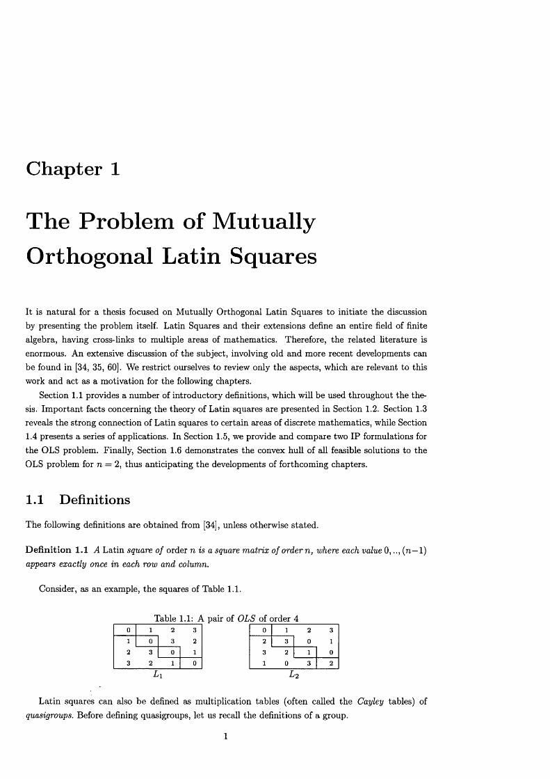
Consider, as an example, the squares of Table 1.1.
_________Table 1.1: A pair of OLS of order_4_________0 1 2 3
1 0 3 2
2 3 0 1
3 2 1 0
0 1 2 3
2 3 0 1
3 2 1 0
1 0 3 2
L i L 2
Latin squares can also be defined as multiplication tables (often called the Cayley tables) of quasigroups. Before defining quasigroups, let us recall the definitions of a group.
1
CHAPTER 1. The Problem of Mutually Orthogonal Latin Squares 2
D efin ition 1.2 A finite group, denoted as a tuple (S',*), is defined as a non-empty finite set S together with a binary operation (*), having the following properties:
( i) a * (6 * c) = (a * b) * c, for all a, b, c G S, i.e. operation * is associative-,
( ii) there is an identity element e G S', such that a * e = e * a = a, for all a G 5;
( ii i) for each a G S , there is an inverse element a -1 G S, such th a t a * a -1 = a -1 * a = e.
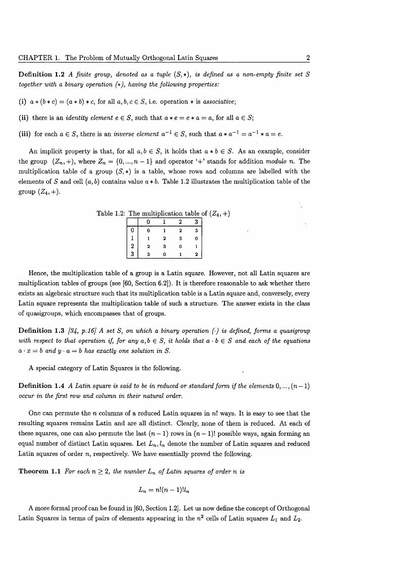
An implicit property is that, for all a,b G S, it holds th a t a * b G S. As an example, considerthe group (Zn ,+ ) , where Z n = {0, ...,n — 1} and operator ‘+ ’ stands for addition modulo n. The multiplication table of a group (S', *) is a table, whose rows and columns are labelled with the elements of S and cell (a,b) contains value a * b. Table 1.2 illustrates the multiplication table of the group {Z4,+ ).
Table 1.2: The multiplication table of (Z4, + )0 1 2 3
0 0 1 2 3
1 1 2 3 0
2 2 3 0 1
3 3 0 1 2
Hence, the multiplication table of a group is a Latin square. However, not all Latin squares are multiplication tables of groups (see [60, Section 6.2]). It is therefore reasonable to ask whether there exists an algebraic structure such that its multiplication table is a Latin square and, conversely, every Latin square represents the multiplication table of such a structure. The answer exists in the class of quasigroups, which encompasses th a t of groups.
D e fin itio n 1.3 [34, P-16] A set S, on which a binary operation (■) is defined, forms a quasigroup with respect to that operation if, for any a,b G S, it holds that a • b G S and each o f the equations a • x = b and y ■ a = b has exactly one solution in S.
A special category of Latin Squares is the following.
D e fin itio n 1.4 A Latin square is said to be in reduced or standard form i f the elements 0 ,..., (n — 1) occur in the first row and column in their natural order.
One can permute the n columns of a reduced Latin squares in n! ways. It is easy to see th a t the resulting squares remains Latin and are all distinct. Clearly, none of them is reduced. At each of these squares, one can also permute the last (n — 1) rows in (n — 1)! possible ways, again forming an equal number of distinct Latin squares. Let L n , ln denote the number of Latin squares and reduced Latin squares of order n, respectively. We have essentially proved the following.
T h e o re m 1.1 For each n > 2 , the number L n of Latin squares o f order n is
L n — n\(jn 1)!£ji
A more formal proof can be found in [60, Section 1.2]. Let us now define the concept of Orthogonal Latin Squares in terms of pairs of elements appearing in the n 2 cells of Latin squares L \ and L 2.
1.2. Theory of Latin Squares 3
D e fin itio n 1.5 Two Latin squares of order n are called orthogonal (OLS) i f and only i f each of the n2 ordered pairs (0, 0),..., (n — l ,n — 1) appears exactly once in the two squares.
A pair of OLS of order 4 appears in Table 1.1. This definition is naturally extended to sets of k > 2 Latin squares, which are called Mutually Orthogonal (MOLS) if they axe pairwise orthogonal. Extending the idea of a reduced Latin square, we call a set of k MOLS reduced or standardised if elements 0 ,.., (n — 1) appear at the first row of all squares and a t the first column of exactly one square in natural order. A concept related to OLS is th a t of a transversal.
D efin itio n 1.6 A transversal of a Latin square is a set o fn cells, each in a different row and column, which contain n pairwise different values.
Denote the squares of Table 1.1 as L\ and L 2 . For each set of 4 cells in square L 2 th a t contain the same value, observe th a t the corresponding cells of square L \ form a transversal. An easy to prove but quite significant property of OLS is the following.
T h e o re m 1.2 [34, Theorem 5.1.1] A Latin square of order n has an orthogonal mate i f and only if it can be decomposed into n disjoint transversals.
OLS were introduced by Euler via his famous problem of the 36 army officers [36]. These officers should belong to 6 distinct ranks, 6 to each one, and are collected from 6 different regiments (6 officers from each regiment). The 36 officers can be arranged into a 6 x 6 grid such th a t exactly one officer of each rank appears in each row and column. By definition, this is a Latin square L \ . Similarly, the officers can be arranged into another square L 2 according to their regiment, i.e. exactly one officer from each regiment appears in each row and column. The number of reduced Latin squares of order 6 is known to be 9408. Hence, these arrangements can be devised in 6!5! x 9408 ~ 109 ways, which is the number of Latin squares of order 6. The question is whether there exist squares L \ and L 2
such th a t all 36 rank-regiment combinations appear exactly once, i.e. whether there is a pair of OLS of order 6. Euler’s belief about the non-existence of such a pair was formally proved by Tarry ([81]), essentially by exhaustive enumeration. Shorter proofs have also been proposed, for example in [80].
It is trivial to show th a t there can exist no pair of OLS for n = 2. Motivated by the non-existence of OLS for n = 2,6, Euler stated a conjecture th a t no pair of OLS exists if n is an odd multiple of 2. The falsity of this conjecture was shown in 1959 ([19]) by constructing a pair of OLS for n = 22. This celebrated result revived the interest in Orthogonal Latin squares and their properties.
1.2 Theory of Latin Squares
In this section, we state certain theorems regarding Latin squares and OLS, without their proofs. The related theory is much broader and is still being augmented. Hence, only results relevant to our research are illustrated.
1.2.1 Single Latin Squares
Recall the simple observation that a square remains Latin after perm uting its columns. In fact, a Latin square embodies three entities, conventionally corresponding to the n-sets of rows, columns and values. Apparently, any of these sets can be permuted w ithout violating the fact th a t each value must exist exactly once in each row and column. The following statem ent provides a formal definition in term s of quasigroups.
CHAPTER 1. The Problem of Mutually Orthogonal Latin Squares 4
D e fin itio n 1.7 Let (G , •) and (H , *) be two quasigroups. An ordered triple (9 ,(f,if) of 1 — 1 mappings 9, (f>, if o f the set G onto the set H is called an isotopism of (G , •) upon (H , *) if (x9 ) * (y</>) = (x •/o r all x ,y £ G. The quasigroups are then said to be isotopic. I f 9 = (f — if such a transformation is called an isomorphism.
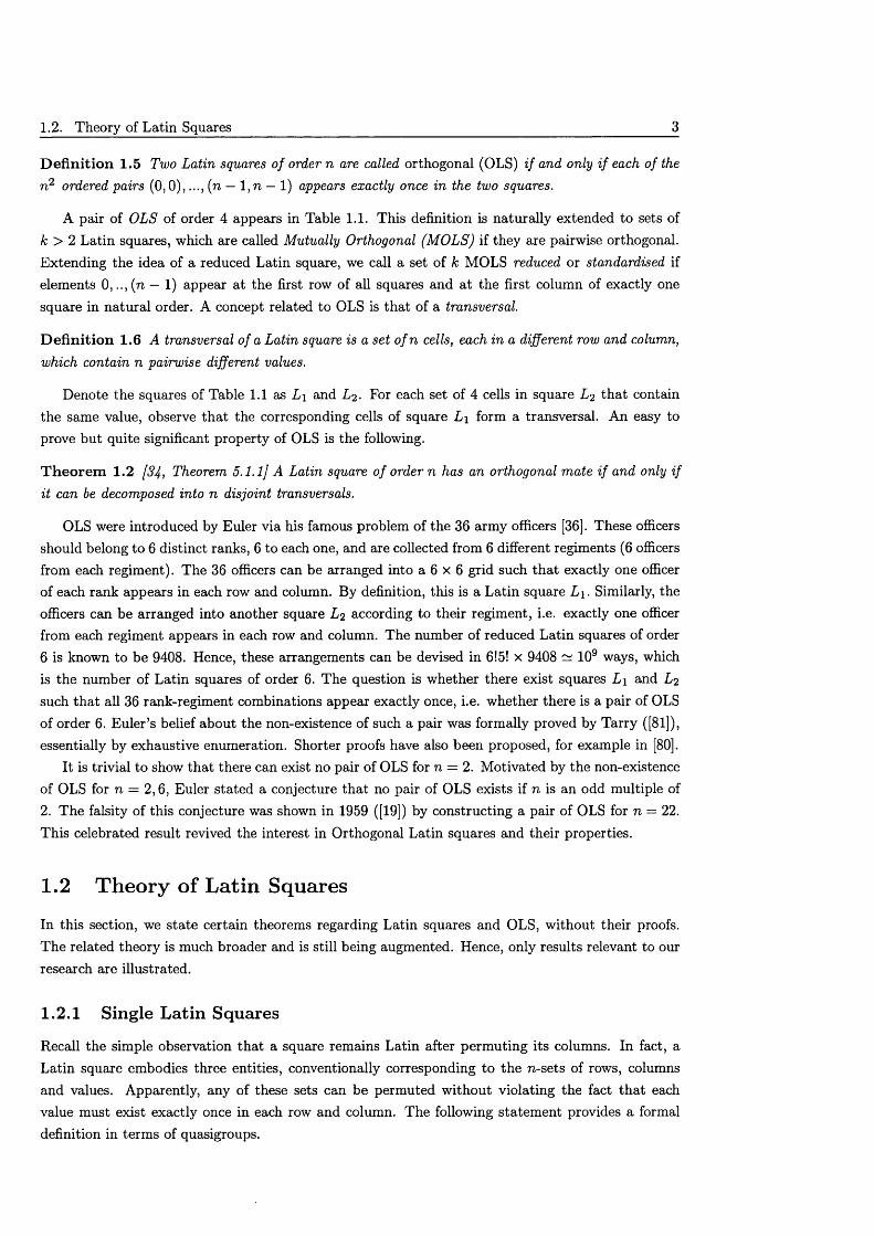
The definitions of isotopism and isomorphism are obtained from [34]. To avoid confusion, we have to remark th a t numerous textbooks in graph theory and combinatorics (e.g. [17]) assign to isomorphism the properties of what is defined here as isotopism. Clearly, two Latin squares are called isotopic if they define the multiplication tables of isotopic quasigroups. As an example, consider square L \ of Table 1.1. In order to derive an isotopic square L \, we need to define three different permutations for the sets of rows, columns and elements of L \. If we apply the permutations
^ = (2 3 1 o )> ^ = (o 3 1 2) and V’ = (0 1 2 3) rows> columns and elements of L \, we obtain the isotopic square L \ of Table 1.3. For example, notice th a t cell (2,3) of L \, containing value 1, is mapped to (1,2) in L \, also containing value 1. Similarly, to derive the square L \ of Table 1.3, which is isomorphic to L \ , we apply the same permutation 9 = (f = if = (° 3 \ q) to rows, columns and elements of L \.
Table 1.3: Isotopic and isomorphic squares of L \3 1 0 2
2 0 1 3
0 2 3 1
1 3 2 0
2 3 0 1
3 2 1 0
0 1 2 3
1 0 3 2
L 1 Lj
Hence, isotopy is a property encompassing the inherent symmetry of Latin squares. A less obvious form of symmetry is obtained if we observe th a t the roles of rows, columns and values are interchangeable. For example, by interchanging the roles of rows and columns of a Latin square L, we derive its transpose L T , which is also a Latin square. Since there exist 3! permutations of the three entities, each Latin square may be used to obtain up to 5 other Latin squares L '. Any such square L' is said to be conjugate to L. Notice th a t the conjugate squares of a Latin square L are not necessarily distinct.
T h e o re m 1.3 [34, Section I . 4 J The number of distinct conjugates o f a Latin square L is always 1,2,3 or 6.
Isotopy and isomorphy are associative and commutative properties. In this sense, they define equivalence relations among Latin squares of the same order. Let Qn denote the set of Latin squares of order n. Define as isotopy (isomorphism) class the subset of Vtn formed by a particular Latin square and all its isotopic (isomorphic) ones. The following theorems concern the classification of members of Qn .
T h e o re m 1.4 Each isotopy class o fQ n splits into disjoint isomorphism classes.
D e fin itio n 1.8 A set of Latin squares, which comprises all the members of an isotopy class together with their conjugates is called a main class of Latin squares.
T h e o re m 1.5 Qn splits into disjoint main classes and each main class is a union of isotopy classes.
An equivalent statem ent is the following.
1.2. Theory of Latin Squares 5
C orollary 1.6 Each main class of Qn , and therefore Qn itself\ splits into disjoint isomorphism classes.
1.2.2 M utually Orthogonal Latin Squares
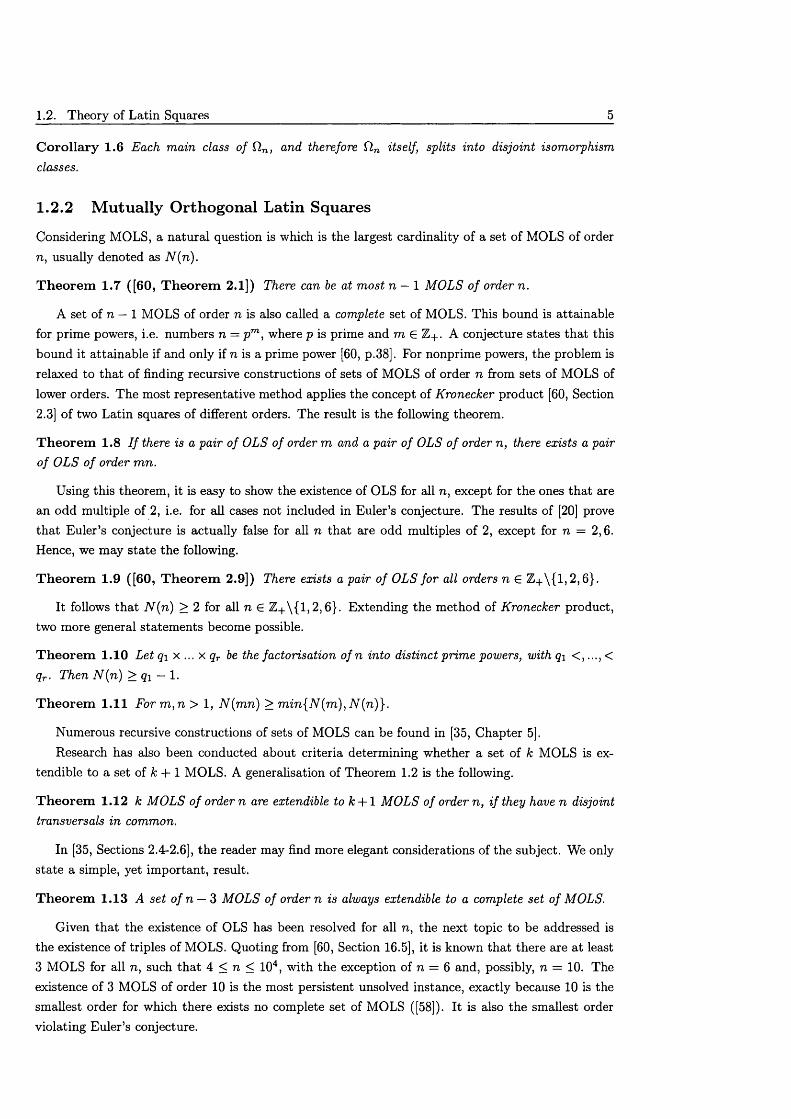
Considering MOLS, a natural question is which is the largest cardinality of a set of MOLS of order n, usually denoted as N (n).
T heorem 1.7 ([60, T heorem 2.1]) There can be at most n — 1 M OLS o f order n.
A set of n — 1 MOLS of order n is also called a complete set of MOLS. This bound is attainable for prime powers, i.e. numbers n — pm , where p is prime and m € Z+. A conjecture states that this bound it attainable if and only if n is a prime power [60, p.38]. For nonprime powers, the problem is relaxed to th a t of finding recursive constructions of sets of MOLS of order n from sets of MOLS of lower orders. The most representative method applies the concept of Kronecker product [60, Section 2.3] of two Latin squares of different orders. The result is the following theorem.
T heorem 1.8 I f there is a pair of OLS of order m and a pair of OLS o f order n, there exists a pair of OLS o f order m n.
Using this theorem, it is easy to show the existence of OLS for all n, except for the ones th a t are an odd multiple of 2, i.e. for all cases not included in Euler’s conjecture. The results of [20] prove th a t Euler’s conjecture is actually false for all n that are odd multiples of 2, except for n = 2,6. Hence, we may state the following.
T heorem 1.9 ([60, T heorem 2.9]) There exists a pair of OLS for all orders n € Z + \{1,2 ,6}.
It follows th a t N (n ) > 2 for all n € Z + \{ 1 ,2 ,6}. Extending the method of Kronecker product, two more general statem ents become possible.
T heorem 1.10 Let q\ x ... x qr be the factorisation of n into distinct prime powers, with q\ < ,..., < qr . Then N (n ) > <?i — 1.
T heorem 1.11 F o r m ,n > 1, N (m n ) > m in {N (m ), N (n )} .
Numerous recursive constructions of sets of MOLS can be found in [35, Chapter 5].Research has also been conducted about criteria determining whether a set of k MOLS is ex
tendible to a set of k + 1 MOLS. A generalisation of Theorem 1.2 is the following.
T heorem 1.12 k M O LS o f order n are extendible to k + 1 M OLS o f order n, i f they have n disjoint transversals in common.
In [35, Sections 2.4-2.6], the reader may find more elegant considerations of the subject. We only state a simple, yet im portant, result.
T heorem 1.13 A set of n — 3 M OLS of order n is always extendible to a complete set o f MOLS.
Given th a t the existence of OLS has been resolved for all n, the next topic to be addressed is the existence of triples of MOLS. Quoting from [60, Section 16.5], it is known th a t there are a t least 3 MOLS for all n, such th a t 4 < n < 104, with the exception of n = 6 and, possibly, n = 10. The existence of 3 MOLS of order 10 is the most persistent unsolved instance, exactly because 10 is the smallest order for which there exists no complete set of MOLS ([58]). I t is also the smallest order violating Euler’s conjecture.

CHAPTER 1. The Problem of Mutually Orthogonal Latin Squares 6
1.3 R elated areas
Research on Latin squares is intensive not only because these structures give rise to interesting puzzles, but mainly because of their relevance to core areas of discrete mathematics and finite algebra. This section presents equivalences between complete sets of MOLS and certain combinatorial objects.
To begin our discussion, let us present the definition of an affine plane.
D e fin itio n 1.9 An affine plane is a geometric system of points and lines, satisfying the following axioms
A 1 There is a unique line joining any two points.
A 2 For a certain point P and a line I not containing P, there is a unique line containing P and not intersecting I.
A 3 There are four points, no three of which are on the same line.
Two im portant corollaries are the following.
C o ro lla ry 1.14 In any finite affine plane, there exists a positive integer n, such that every line contains exactly n points and every point is on exactly n + 1 lines. Number n is said to be the order of the affine plane
C o ro lla ry 1.15 A finite affine plane o f order n contains n 2 points.
The fundamental link between finite affine planes and sets of MOLS is revealed by the next theorem.
T h e o re m 1.16 A complete set o f M OLS of order n exists i f and only i f a finite affine plane of order n exists.
Hence, it follows directly th a t an affine plane of order 6 does not exist. A related concept is that of a projective plane.
D e fin itio n 1.10 A projective plane is a geometric system o f points and lines, satisfying the following axioms
P I There is a unique line joining any two points.
P 2 Any two lines intersect at a unique point.
P 3 There are four points, no three of which are on the same line.
We omit the counterparts of Corollaries 1.14 and 1.15 for projective planes and state directly the main result.
T h e o re m 1.17 A finite affine plane o f order n exists i f and only i f a finite projective plane o f order n exists.
C o ro lla ry 1.18 A complete set of M OLS o f order n exists i f and only i f a finite projective plane of order n exists.
1.4. Applications of Orthogonal Latin Squares 7
Hence, a problem regarding a complete set of MOLS can be tackled by any of its equivalents (see [58]) and vice versa.
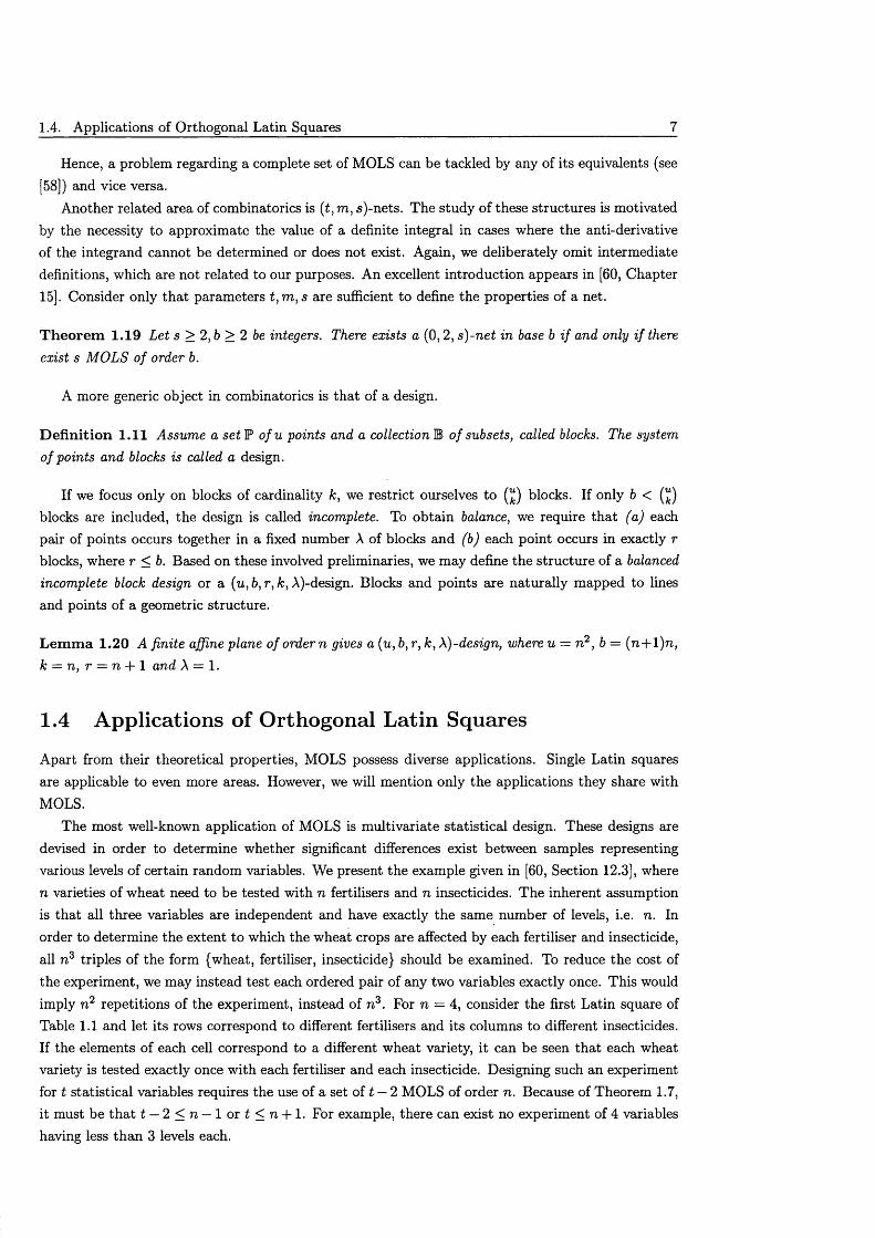
Another related area of combinatorics is (£, m, s)-nets. The study of these structures is motivated by the necessity to approximate the value of a definite integral in cases where the anti-derivative of the integrand cannot be determined or does not exist. Again, we deliberately omit intermediate definitions, which are not related to our purposes. An excellent introduction appears in [60, Chapter 15]. Consider only th a t parameters t ,m ,s are sufficient to define the properties of a net.
T heorem 1.19 Let s > 2, b > 2 be integers. There exists a (0,2, s)-net in base b i f and only i f there exist s M OLS of order b.
A more generic object in combinatorics is that of a design.
D efin ition 1.11 Assume a set P o fu points and a collection B of subsets, called blocks. The system of points and blocks is called a design.
If we focus only on blocks of cardinality k , we restrict ourselves to (£) blocks. If only b < (£) blocks are included, the design is called incomplete. To obtain balance, we require that (a) each pair of points occurs together in a fixed number X of blocks and (b) each point occurs in exactly r blocks, where r < b. Baaed on these involved preliminaries, we may define the structure of a balanced incomplete block design or a (u,b, r, k, A)-design. Blocks and points are naturally mapped to lines and points of a geometric structure.
Lem m a 1.20 A finite affine plane of order n gives a (u , b, r, k, X)-design, where u = n 2, b = (n + l)n , k = n, r = n + 1 and X = 1.
1.4 Applications of Orthogonal Latin Squares
Apart from their theoretical properties, MOLS possess diverse applications. Single Latin squares are applicable to even more areas. However, we will mention only the applications they share with MOLS.
The most well-known application of MOLS is multivariate statistical design. These designs are devised in order to determine whether significant differences exist between samples representing various levels of certain random variables. We present the example given in [60, Section 12.3], where n varieties of wheat need to be tested with n fertilisers and n insecticides. The inherent assumption is that all three variables are independent and have exactly the same number of levels, i.e. n. In order to determine the extent to which the wheat crops are affected by each fertiliser and insecticide, all n 3 triples of the form {wheat, fertiliser, insecticide} should be examined. To reduce the cost of the experiment, we may instead test each ordered pair of any two variables exactly once. This would imply n 2 repetitions of the experiment, instead of n 3. For n = 4, consider the first Latin square of Table 1.1 and let its rows correspond to different fertilisers and its columns to different insecticides. If the elements of each cell correspond to a different wheat variety, it can be seen that each wheat variety is tested exactly once with each fertiliser and each insecticide. Designing such an experiment for t statistical variables requires the use of a set of t — 2 MOLS of order n. Because of Theorem 1.7, it must be th a t t — 2 < n — 1 or t < n + 1. For example, there can exist no experiment of 4 variables having less than 3 levels each.
CHAPTER 1. The Problem of Mutually Orthogonal Latin Squares 8
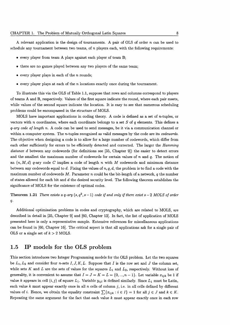
A relevant application is the design of tournaments. A pair of OLS of order n can be used to schedule any tournam ent between two teams, of n players each, with the following requirements:
• every player from team A plays against each player of team B;
• there are no games played between any two players of the same team;
• every player plays in each of the n rounds;
• every player plays at each of the n locations exactly once during the tournament.
To illustrate this via the OLS of Table 1.1, suppose th a t rows and columns correspond to players of teams A and B, respectively. Values of the first square indicate the round, where each pair meets, while values of the second square indicate the location. It is easy to see th a t numerous scheduling problems could be encompassed in the structure of MOLS.
MOLS have im portant applications in coding theory. A code is defined as a set of n-tuples, or vectors with n coordinates, where each coordinate belongs to a set S of q elements. This defines a q-ary code o f length n. A code can be used to send messages, be it via a communication channel or within a computer system. The n-tuples recognised as valid messages by the code are its codewords. The objective when designing a code is to allow for a large number of codewords, which differ from each other sufficiently for errors to be efficiently detected and corrected. The larger the Hamming distance d between any codewords (for definitions see [35, Chapter 9]) the easier to detect errors and the smallest the maximum number of codewords for certain values of n and q. The notion of an (n, M , d) q-axy code C implies a code of length n with M codewords and minimum distance between any codewords equal to d. Fixing the values of n, q, d, the problem is to find a code with the maximum number of codewords M . Parameter n could be the bit-length of a network, q the number of states allowed for each bit and d the desired security level. The following theorem establishes the significance of MOLS for the existence of optimal codes.
T heorem 1.21 There exists a q-ary (s, q2,s — 1) code i f and only i f there exist s — 2 M OLS of order
q-
Additional optimisation problems in codes and cryptography, which are related to MOLS, are described in detail in [35, Chapter 9] and [60, Chapter 13]. In fact, the list of application of MOLS presented here is only a representative sample. Extensive references for miscellaneous applications can be found in [60, Chapter 16]. The critical aspect is th a t all applications ask for a single pair of OLS or a single set of k > 2 MOLS.
1.5 IP models for the OLS problem
This section introduces two Integer Programming models for the OLS problem. Let the two squares be L u L 2 and consider four n-sets / , J, K , L. Suppose th a t I is the row set and J the column set, while sets K and L are the sets of values for the squares L \ and L 2, respectively. W ithout loss of generality, it is convenient to assume that I = J = K = L = {0, ...,n — 1}. Let variable Xijk be 1 if value k appears in cell ( i , j) of square L \. Variable is defined similarly. Since L \ must be Latin, each value k must appear exactly once in all n cells of column j , i.e. in all cells defined by different values of i. Hence, we obtain the equality constraint i G /} = 1 for all j G J and k G K .Repeating the same argument for the fact th a t each value k must appear exactly once in each row
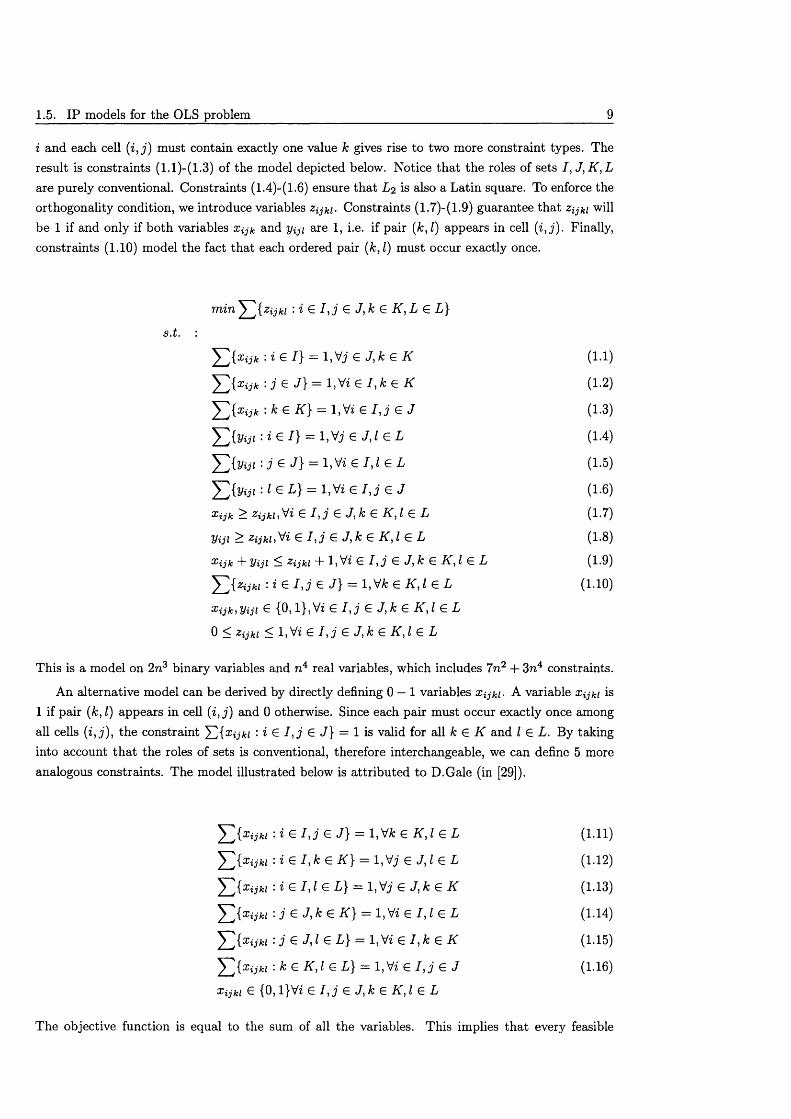
1.5. IP models for the OLS problem 9
i and each cell ( i , j) must contain exactly one value k gives rise to two more constraint types. The result is constraints (1.1)-(1.3) of the model depicted below. Notice th a t the roles of sets I , J ,K ,L are purely conventional. Constraints (1.4)-(1.6) ensure th a t L 2 is also a Latin square. To enforce the orthogonality condition, we introduce variables z^ki- Constraints (1.7)-(1.9) guarantee th a t z^ki will be 1 if and only if both variables x ^k and yiji are 1, i.e. if pair (k , l ) appears in cell (i, j) . Finally, constraints (1.10) model the fact th a t each ordered pair (k , l ) must occur exactly once.
m min : i e / , j £ J, k £ K , L £ L}
s.t.
J 2 { ^ i j k - - i e l } = i y j e J , k e K (1.1)
£ { * « * : i 6 = 1-V« 6 I , k € K (1.2)
: k € K } = 1 ,Vi e I , j S J (1.3)
£ ]{ y y I : i e 1} = 1, V) e J, I e L (1.4)
'■ j s J} = 1>V» e 1,1 € L (1.5)
^ { y y , : l e ! } = i , V i e / , j e J (1.6)
Xijk > Zijku'ii £ l , j e J ,k £ K ,l e L (1.7)
Viji > Zijki, Vi € I , j £ J ,k e K , l £ L (1.8)
Xijk + Viji Zijki “b 1,Vi £ I ) j £ J t k G K ,l G L (1.9)
^ \ zjjki '• i £ I , j £ J } = 1, VA; G K , I G L (1.10)
Xijk} Viji ^ {0, lj-, Vi £ I , j £ J ,k £ K , I £ L
0 < z^ki < 1 ,Vi £ I , j £ J ,k £ K J £ L
This is a model on 2n 3 binary variables and n 4 real variables, which includes 7n 2 + 3n4 constraints.
An alternative model can be derived by directly defining 0 — 1 variables Xijki. A variable Xijki is1 if pair (k , I) appears in cell ( i , j) and 0 otherwise. Since each pair must occur exactly once amongall cells (i, j ) , the constraint J 2 ix ijki : i £ I , j £ J } = 1 is valid for all k £ K and I £ L. By takinginto account th a t the roles of sets is conventional, therefore interchangeable, we can define 5 more analogous constraints. The model illustrated below is attributed to D.Gale (in [29]).
^^{X ijk l i £ I , j £ J } = l ,\ fk e K ,l £ L (1.11)
^^{X ijk l i £ I , k £ K } = 1, V? G J ,l £ L (1.12)
T A x ijk i i £ 1,1 £ L ] = 1, V? G J ,k £ K (1.13)
j £ J ,k £ K } = 1, Vz G 1,1 £ L (1.14)
J^ iX ijk l j £ J, I £ L} = 1, Vz G I , k G K (1.15)
E ^ k i k £ K ,l £ L} = l,Vz G I , j £ J (1.16)
Xijki ^ {0, l}Vi G I , j G J, k G K , I £ L
The objective function is equal to the sum of all the variables. This implies th a t every feasible
CHAPTER 1. The Problem of Mutually Orthogonal Latin Squares 10
solution is also optimal. Minimising or maximising this objective function is not really important, since our research treats OLS as a feasibility problem. This second model involves n 4 binary variables and 6n 2 constraints.
Comparing the two models, it is clear th a t the first model is larger in terms of both variables and constraints. It follows th a t the associated linear programming relaxation would take longer to solve. Moreover, constraints of a form similar to th a t of (1.7) are known to produce very weak relaxations, as argued in [68, 1.1]. However, the first model has far fewer integer variables, i.e. n 3 against n 4 of the second model. Thinking in terms of a Branch & Bound algorithm, it is reasonable to suggest that the second model is more impractical. However, this is not the case. Roughly speaking, the reason is simply that every integer feasible solution to the first model would require 2n 2 integer variables to be set to 1, in contrast to the n2 variables required to be 1 by the second model.
Another advantage of the second model i / its simplicity and symmetry. This symmetry reflects more accurately the inherent symmetry of the OLS problem, in term s of the fact th a t all four entities are indistinguishable. Hence, the second model is the one used throughout the remainder of this thesis.
1.6 The convex hull of the OLS polytope for n — 2
The convex hull of a set of vectors x i , . . . ,x m is defined as the set of all real points x, for which there exists non-negative scalars Ai, ...Am, such that x = A*£* and A* = 1. Consider the second IP model of the previous paragraph and recall that the integer vectors satisfying constraints (1.11)-(1.16) have a 1 — 1 correspondence to all pairs of OLS of order n. If we replace '= ’ by '< ’ in all constraints, we obtain a model, whose solutions are all incomplete OLS of order n. Notice that the zero vector, i.e. an “empty” pair of OLS, is also a solution to this model. This section illustrates all inequalities defining the convex hull of the vectors corresponding to incomplete OLS structures of n = 2. A pair of incomplete OLS of order 2 is illustrated at Table 1.4.
Table 1.4: A pair of incomplete OLS of order 20 1
To derive this convex hull we use the PORTA software ([24]), which accepts as input a set of integer vectors. The output is a minimal representation of the convex hull of the input vectors in terms of inequalities, which are facet-defining. The inequalities illustrated for this simple example anticipate the results of Chapter 2 and could also serve the purposes of an introduction to that chapter. Any terminology used to characterise each set of inequalities, e.g. cliques of type II, will be formally defined in Chapter 2.
Let A denote the constraint matrix of equalities (1.11)-(1.16). The convex hull of incomplete pairs of OLS is the polytope P j = conv{x G {0 ,1}”4 : A x < e}. Let R = (K x L) U • • • U ( I x K ) and C = I x J x K x L be the row and column sets of A, respectively. The facet-defining inequalities of Pi for n = 2 are categorised as follows.
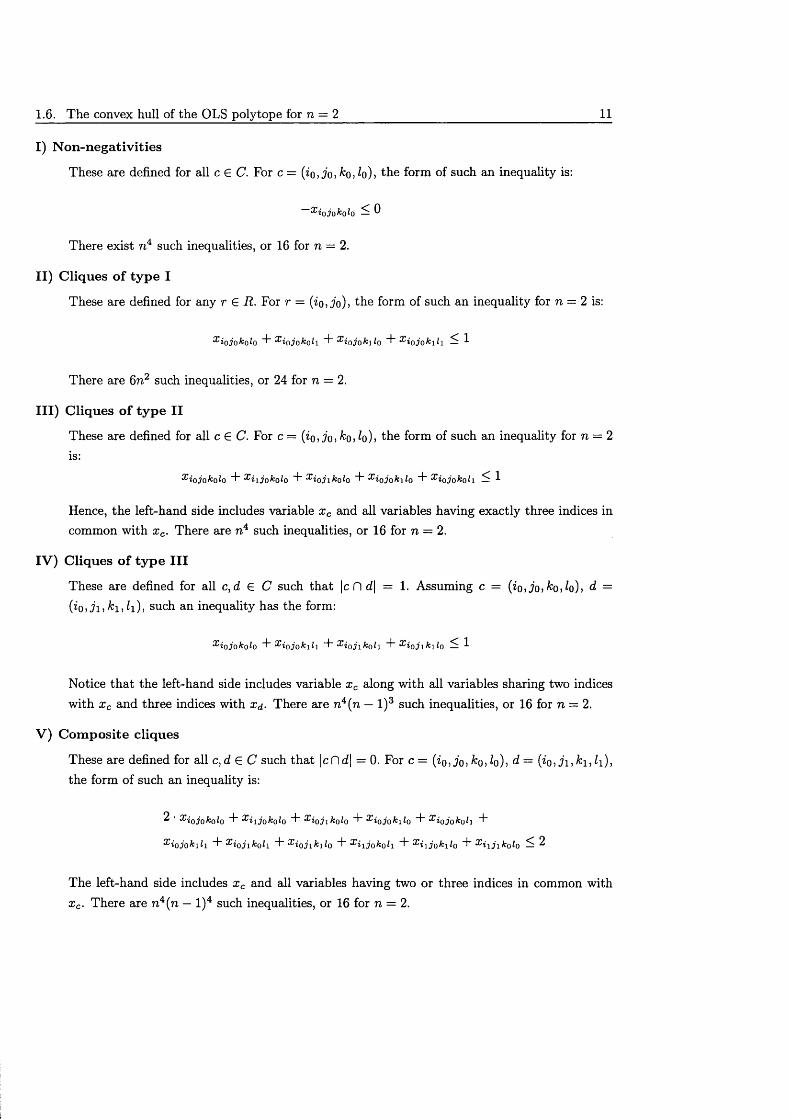
1.6. The convex hull of the OLS polytope for n = 2 11
I) N on -n egativ ities
These are defined for all c £ C. For c = &o, lo), the form of such an inequality is:
~~x iojokolo ^ 0
There exist n4 such inequalities, or 16 for n — 2.
II) C liques o f ty p e I
These are defined for any r £ R. For r = (io,jo), the form of such an inequality for n = 2 is:
x iojokolo "F x iojokoh "F x iojokilo “I” x iojokil\ — 1
There are 6n 2 such inequalities, or 24 for n = 2.
III) C liques o f ty p e II
These are defined for all c £ C. For c = {io,jo,ko,lo), the form of such an inequality for n = 2 is:
x iojokolo “I” x iijokolo ~F x ioj\kolo "F x iojokilo “I” x iojokal\ — 1
Hence, the left-hand side includes variable x c and all variables having exactly three indices in common with x c. There are n 4 such inequalities, or 16 for n — 2.
IV ) C liques o f ty p e III
These are defined for all c,d £ C such that |c fl d\ = 1. Assuming c = (io,jo,ko,lo), d =( io , j i ,k i ,h ) , such an inequality has the form:
x iojokoh "F x iojok\h "F x iojikoli "F x ioj\k\lo — 1
Notice th a t the left-hand side includes variable x c along with all variables sharing two indices with x c and three indices with x j. There are n 4(n — l )3 such inequalities, or 16 for n = 2.
V ) C om p osite cliques
These are defined for all c,d £ C such th a t |c fld | = 0. For c = (i0, jo, koJo), d = («o, j i , k i, Zi), the form of such an inequality is:
^ ‘ x iojokolo 4” x iijokolo ~F x ioji kolo F- x iojok\lo x iojokoh
x iojok\li "F x iojikoli *F x iojik\lo 4“ x iijokoh "F x i\jok\lo "F x i\j\kolo ^ 2
The left-hand side includes x c and all variables having two or three indices in common with x c. There are n 4(n — l )4 such inequalities, or 16 for n = 2.
CHAPTER 1. The Problem of Mutually Orthogonal Latin Squares 12
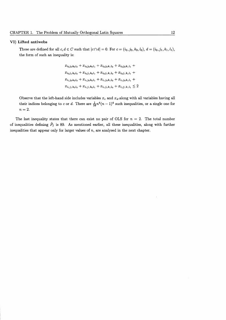
VI) L ifted antiw ebs
These are defined for all c,d € C such that |c fld | = 0. For c = (io, joi &o, fo)> d = (io ,ji, &i, l\), the form of such an inequality is:
x iojokolo "P 3' io jokol i "P x i o j o k i l o P' x i o j o k \ h "P
x i o j i k o l o ”P 3 ' i o j i k o h "P^ioJikdo ~P x i o j i k i h "P
• t ' i i jokolo “I” x i \ j o k o h "P x i i j o k i lo "P x i \ j a k \ l i P
x i i j i k 0 l0 + x i i j i k 0 l\ "P x i i j i k i l0 P^MJifciii 5: 2
Observe th a t the left-hand side includes variables x c and xa-along with all variables having all their indices belonging to c or d. There are ^ n 4(n — l )4 such inequalities, or a single one for n = 2.
The last inequality states that there can exist no pair of OLS for n = 2. The total number of inequalities defining Pj is 89. As mentioned earlier, all these inequalities, along with further inequalities th a t appear only for larger values of n, are analysed in the next chapter.
Chapter 2
The intersection graph o f the OLS problem
This chapter presents a framework for characterising the OLS problem from an Integer Programming (IP) perspective. A first step towards this direction is the formulation of an IP model for the problem, i.e. a linear model on integer variables. Such a model was presented in Section 1.5. A relaxation of this model is derived by requiring the variables to be simply non-negative. This is the problem’s linear programming (LP) relaxation. The convex hull of the feasible solutions of the original model defines a polytope P j, within the polytope Pl defined by the problem’s LP relaxation. Although the feasible points are located within P j , we initially know only the set of linear inequalities defining Pl .
In order to efficiently characterise and solve the OLS problem using IP, at least a partial knowledge of polytope Pi is required. This knowledge is usually provided in the form of inequalities, which are valid for polytope P j but not for the polytope Pl - In other words, these inequalities are derived by enforcing the requirement th a t certain variables must be integer. Among these inequalities, it is reasonable to identify the ones, which are not dominated by any other valid inequality. These valid inequalities are called maximal. Any maximal valid inequality defines a non-empty face of Pj and the set of maximal valid inequalities contains all of the facet-defining inequalities for P j ([68, p.207]).
Amongst a number of methods for identifying families of valid inequalities, one with a considerable record, especially in problems involving a 0 — 1 constraint m atrix, is th a t of studying a graph associated with the IP model. This is the intersection graph, introduced in Section 2.2 (see also [26, 69]). Subgraphs of this graph exhibiting a particular structure give rise to strong valid inequalities for the set-packing and set-partitioning polytopes (see [8, 18] for a review). In this chapter, a number of such subgraphs, along with the induced inequalities, are identified and analysed for the intersection graph of our IP model. In particular, cliques, antiwebs, wheels, composite cliques and odd holes are presented in sections 2.3-2.7, respectively. Finally, Section 2.8 examines the existence of odd antiholes and proves th a t such structures do not exist for this particular problem.
13
CH APTER 2. The intersection graph of the OLS problem 14
2.1 The OLS polytope
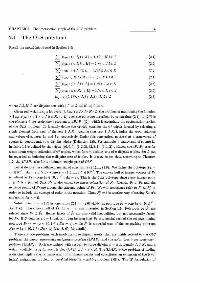
Recall the model introduced in Section 1.5:
^2 {x ijk i : i e I , j £ J } = 1 ,Vfc £ K ,l £ L (2.1)
'Y ^{x ijki : i € I , k £ K ] = l,V j £ J ,l £ L (2.2)
^ i j k i - i e 1,1 e L} = l ,V j £ J ,k £ K (2.3)
^ { x i j k i : j e J, k £ K } = 1, Vz € I , I £ L (2.4)
^ ^{xjjki • j € J)l € L} = 1 ,Vi £ I , k £ K (2.5)
$ > « « : k £ K ,l £ L} = 1, Vi £ I , j £ J (2.6)
Xijki e {0 ,l}Vi £ I , j £ J ,k £ K ,l £ L (2.7)
where I , J, A", L are disjoint sets with | I |= | J |= | K |= | L |= n.
Given real weights Cijki for every (i, j , k , l ) £ I x J x K x L , the problem of minimizing the function J 2 icijkiXijki - i £ I , j € J ,k £ K , I £ L} over the polytope described by constraints (2.1),..., (2.7) is the planar 4-index assignment problem or 4P A P n ([2]), which is essentially the optimisation version of the OLS problem. To formally define the 4P A P n consider the n 3 triples formed by selecting a single element from each of the sets I , J, K . Assume th a t sets / , J, AT, L index the rows, columns and values of squares L \ and L 2 , respectively. Under this convention, notice th a t a transversal of square L \ corresponds to n disjoint triples (Definition 1.6). For example, a transversal of square L\ in Table 1.1 is defined by the triples {(0,0,0), (1,2,3), (2 ,3 ,1), (3,1,2)}. Hence, the 4P A P n asks for a minimum weight collection of n 2 triples, which form n disjoint sets of n disjoint triples. Set L can be regarded as indexing the n disjoint sets of triples. It is easy to see that, according to Theorem 1.2, the 4P A P n asks for a minimum weight pair of OLS.
Let A denote the coefficient matrix of constraints (2.1),..., (2.6). We define the polytope P l = {x £ Rn : A x = e, x > 0} where e = {1,1,..., 1}T £ R6”2. The convex hull of integer vectors of P l is defined as P i = conv{x £ {0, l} n : A x = e}. This is the OLS polytope since every integer point x £ Pi is a pair of OLS. P l is also called the linear relaxation of P j. Clearly, P j C P l and the extreme points of P / are among the extreme points of P l. We will sometimes refer to P j as P f in order to include the concept of order in the notation. Thus, P f — 0 is another way of stating Euler’s conjecture for n = 6 .
Substituting (=) by (<) in constraints (2.1),..., (2.6) yields the polytope Pi = conv{x £ {0, I }™4 : A x < e}. The convex hull of P j, for n = 2, was presented in Section 1.6. Polytopes Pi, Pi are related since Pi C P /. Hence, facets of Pi are also valid inequalities, but not necessarily facets, for Pi. If D denotes a 0 — 1 matrix, it can be seen that Pi is a special case of the set-partitioning polytope P spp = {x £ {0, l }9 : D x = e}, while Pi is a special case of the set-packing polytope P sp = {x £ {0, l }9 : D x < e} (see [8, 69] for details).
There are two problems, each involving three disjoint n-sets, th a t are highly related to the OLS problem: the planar three-index assignment problem (3P A P n) and the axial three-index assignment problem (3A A P n). Both are defined with respect to three disjoint n — sets, namely I , J , K , and a weight coefficient for each triplet ( i , j ,k ) £ I x J x K. The 3A A P n is the problem of finding n disjoint triplets (i.e. a transversal) of minimum weight and constitutes an extension of the (two- index) assignment problem or weighted bipartite matching problem ([68]). The IP formulation of
2.2. The intersection graph 15
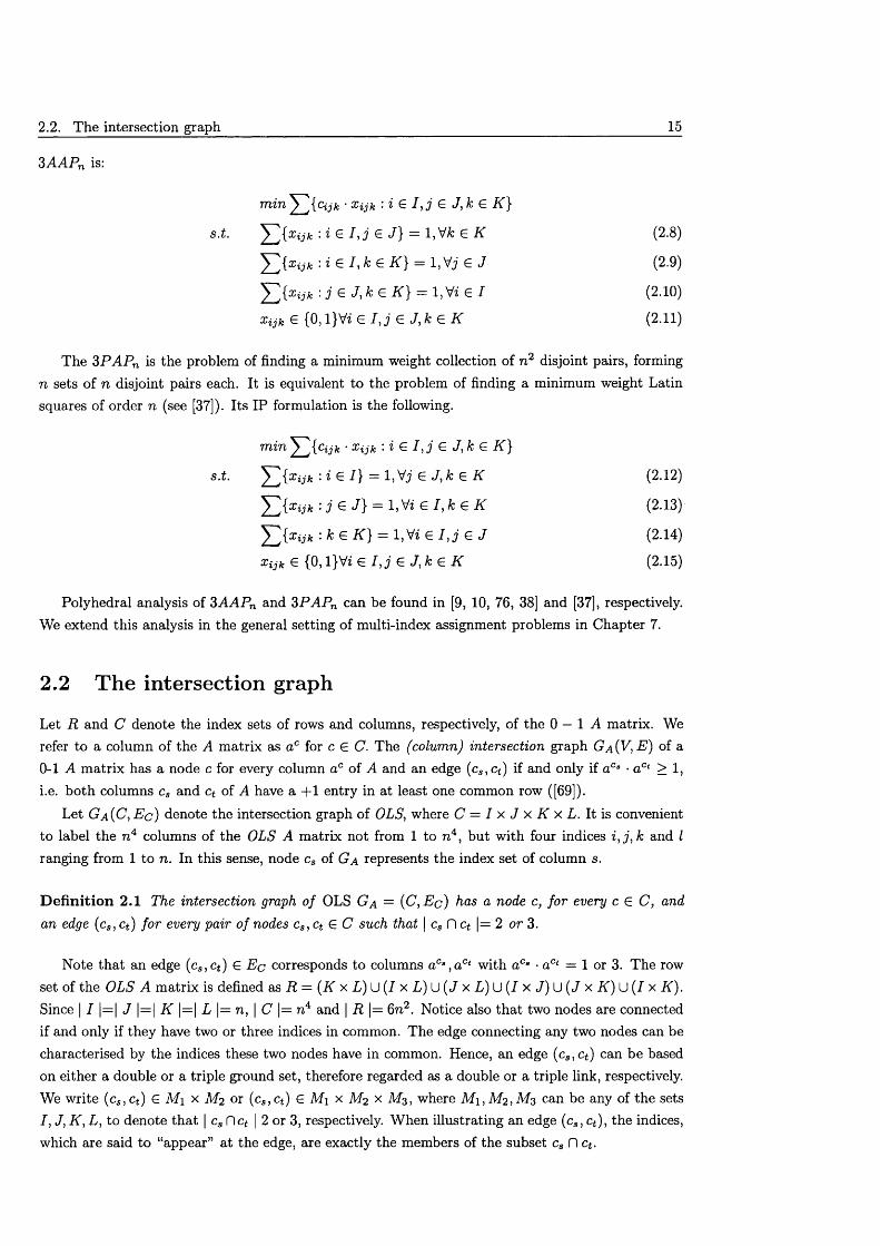
3A AP n is:
m in Y ^ { c ijk • Xijk : i £ I , j £ J ,k £ K }
'^ 2 { x ijk : i £ I , j £ J } = 1,VA: £ K (2.8)
^ ~2{xijk : i £ I , k £ K } = 1,Vj £ J (2.9)
SjTJ{x ijk : j € J, k £ K } = 1, Vz £ I (2.10)
x ijk e {0, l}Vi £ I , j £ J ,k £ K (2.11)
The 3P A P n is the problem of finding a minimum weight collection of n 2 disjoint pairs, forming n sets of n disjoint pairs each. It is equivalent to the problem of finding a minimum weight Latin squares of order n (see [37]). Its IP formulation is the following.
m in Y ^ { c ijk ■ x ijk : i £ I , j £ J ,k £ K }
s.t. Y ,{ x i jk : £ -0 = 1 ,V j € J ,k £ K (2.12)
Y ,{ x i jh : j € J } = 1, Vi £ I , k £ K (2.13)
: k £ K } = l,Vz £ I , j £ J (2.14)
x ijk e {0 ,l}Vi £ I , j £ J ,k £ K (2.15)
Polyhedral analysis of 3A A P n and 3P A P n can be found in [9, 10, 76, 38] and [37], respectively.We extend this analysis in the general setting of multi-index assignment problems in Chapter 7.
2.2 The intersection graph
Let R and C denote the index sets of rows and columns, respectively, of the 0 — 1 A matrix. We refer to a column of the A m atrix as ac for c £ C. The (column) intersection graph G a ( V , E ) of a 0-1 A m atrix has a node c for every column ac of A and an edge (cs ,c t ) if and only if aCs • aCt > 1, i.e. both columns cs and ct of A have a +1 entry in at least one common row ([69]).
Let G a (C ,E c ) denote the intersection graph of OLS, where C = I x J x K x L. It is convenient to label the n 4 columns of the OLS A matrix not from 1 to n4, but with four indices i , j , k and I ranging from 1 to n. In this sense, node cs of Ga represents the index set of column s.
D e fin itio n 2.1 The intersection graph o f OLS G a = (C ,E c ) has a node c, for every c £ C, and an edge (cs ,c t ) fo r every pair o f nodes cs ,ct £ C such that \ cs D c% |= 2 or 3.
Note th a t an edge (cs ,ct ) £ E c corresponds to columns aCs ,a Ct with ac° ■ aCt = 1 or 3. The rowset of the OLS A m atrix is defined as R = (K x L) U (I x L) U (J x L) U ( / x J ) U (J x K ) U ( I x K ). Since | I |= | J |= | K |= | L |= n, | C |= n 4 and | R |= 6n 2. Notice also th a t two nodes are connected if and only if they have two or three indices in common. The edge connecting any two nodes can be characterised by the indices these two nodes have in common. Hence, an edge (ca,c t) can be based on either a double or a triple ground set, therefore regarded as a double or a triple link, respectively. We write (cs ,c t ) £ M i x M 2 or (cs ,c t) £ M \ x M2 x M3, where M i, M 2 , M 3 can be any of the sets I , J, K , L, to denote th a t | cs Dct | 2 or 3, respectively. W hen illustrating an edge (cs , c*), the indices, which are said to “appear” at the edge, are exactly the members of the subset cs fl ct .
CHAPTER 2. The intersection graph of the OLS problem 16
P ro p o s itio n 2.1 The graph G a (C, E c ) is regular of degree 2(3n — l) (n — 1).
P ro o f. Consider any c G C. There are (n — l ) 4 elements of C, which have no index in common with c. For each of the four indices of c there are (n —l ) 3 elements of C, which share the same value for this index but have different values for the other three. Therefore, there are 4(n — l ) 3 elements of C which have exactly one index in common with c. By Definition 2.1, c is connected only to nodes that have two or three indices in common with it, so it is connected to all but (n — l ) 4 + 4(n — l ) 3 nodes. Therefore the degree of each c G C is n 4 — 1 — ((n — l ) 4 + 4(n — l ) 3) = 6n2 — 8n + 2 = 2(3n —l)(n —1). ■
C o ro lla ry 2.2 | E c |= n 4(3n — l)(n — 1).
P ro o f. Since the number of edges of a graph equals the sum of the degrees of its nodes divided by 2, it follows that | E c |= 0.5 x n 4 x 2(3n — l)(n — 1) = n 4(3n — l) (n — 1). ■
2.3 The cliques of G a
A maximal complete subgraph of a graph G (V ,E ) is called a clique ([9, 69]). Let Q C V denote the node set of a clique. The cardinality of a clique is the cardinality of its node set Q , denoted | Q |.
Let a£ denote the entry of the A matrix a t row r and column c. Then we define the set R (r) = {c G C : = 1}. So R (r) denotes the set of columns with a non-zero entry in row r.
P ro p o s itio n 2.3 For each r G R, the node set R (r) induces a clique o f cardinality n 2 in G a (C, E c )-
There are 6n2 cliques of this type.
P ro o f. The subgraph induced by the node set R (r) is complete since all its elements have two indices in common. To prove that it is also maximal assume w.l.o.g. th a t r = ( i i , i i ) G / x J and consider Co = (io, jo, &o> lo) £ G \ R (r) where io ^ i\ and jo ^ j \ . Since R (r) contains all n2 elements of C, whose first two indices are i\ and j i, it contains an element c\ = ( i i , i i , &i, h ) with | co n c i j= 0 . Next consider Co = (i\,jo ,ko , lo) G C \R ( r ) . But then there exists c\ G C (for example
ci = (*i> ii> k i ,h ) ) so th a t | cq Pi c\ |= 1. The same happens if c0 = (io ,ii , &o> fo)- Therefore there is no co such th a t the subgraph induced by R (r) U {co} is complete. Consequently, the subgraph having R(r) as its node set is maximal. There are as many cliques of this type as the number of rows of the A matrix, i.e. 6n2. ■
P ro p o s itio n 2.4 For each c G C the set Q(c) = {c} U {s G C :| c fl s |= 3} induces a clique of cardinality 4n — 3 in G a { C , E c ). There are n 4 cliques o f this type.
P ro o f. W.l.o.g. consider c = cq = { i o , j o , k o , l o ) G C. Let ci,C2 G Q(co) with ci ^ C2 ^ cq ^ c \ . Since Ci,C2 have three indices in common with Co, at least two of their indices coincide. Therefore, (ci,C2) G E c for any ci,C2 G Q(co), i.e. Q(co) is complete. To show th a t Q ( cq) is also maximal consider C3 = (13, J3, ^3, Z3) G C \ Q { cq). Then C3 has exactly two indices in common with Co, by definition. If | co fl C3 |= 2, w.l.o.g. consider io = 23, j o = j z and ko ^ k%, Iq ^ 1%. By definition, Q(co) contains two elements, namely cs = { is , j o , k o , l o ) and ct = {io ,jt,ko ,lo ) such th a t io 7 i s and j o 7 j t . But then | C3 fl cs |= | C3 fl ct |= 1, i.e. the subgraph Q ( cq) U {03} is not complete. Hence, Q ( cq) is also maximal.
The set Q(cq) includes node co = (io,io, ko, Iq) and all nodes w ith exactly one index different from cq, hence | Q(co) \= 4 (n — 1) + 1 = 4n — 3. There are n 4 elements belonging to the set C and each one can play the role of Cq . Therefore, there are n 4 distinct cliques of this type. ■
2.3. The cliques of G a 17
P ro p o s i tio n 2.5 Let c ,s G C such that \ c fl s |= 1. Then the set Q(c, s) = {c} U {t G C :| c D t |= 2, | s fl t |= 3} induces a 4-clique in Ga (C ,E c )-
P ro o f. W.l.o.g. let c = cq = (io,jo,ko,lo) and s = (io, j i , ki, h ). We can uniquely define three elements ti = (io, jo, 12 = (io, j i , ko, h ) , t 3 = (i0, j i , ki, l0), satisfying | c H t i |= 2 and| s n t i |= 3 for i = 1,2,3. It is obvious that the node set {c, t \ , V ,£3} induces a complete subgraph of G a { C , E c ). To show th a t this subgraph is also maximal, consider C2 = {i2, J2, ^2, 2} G C \ Q{c,s). If i 2 io then for an edge (c, C2) to exist in G a (C, E c ) we must have | cflC2 |> 2, which implies that | C2 fl ti |= 1 for i = 1,2,3. Therefore, Q (c ,s ) cannot be extended to include C2, since the resulting graph is not complete. If i<i = io either C2 has another element common with c and the remaining two with s, in which case it coincides with one of the V s, or it has one more element in common with c and with s. In the latter case, w.l.o.g. let j'2 = jo and k 2 = k \. Then we have | C2 fl £2 |= 1- Hence, Q (c,s) cannot again be extended. The results follows. ■
Concerning the cardinality of the set of cliques of this type, every ordered pair (c, s ) such that | c fl s |= 1 can be used to create a clique of this type. Considering th a t | C |= n 4 and that for each c G C there are 4(n — l ) 3 possible s such th a t | c fl s \= 1, the number of such ordered pairs is 4n4(n — l ) 3. Note, however, th a t the 4-clique Q (c,s) = (c, is als° generated as Q (ci,Si) fori = 1 ,2 ,3 where
ci = ti = (io,jo ,k i , l i ) and si = (io ,ji,ko ,lo ),
C2 = t 2 = (io, ji,& o ,h ) and S2 = (io,Jo,& i,Iq),C3 = £3 = ( io , j i ,k i , l0) and S3 = (io, jo, ko, li).
P ro p o s itio n 2.6 Q (c,s) = Q(ci,Si), i = 1,2,3
It is also obvious th a t the 4-clique Q(c, s) = (c, t i , ^2, ^3) cannot arise from any other choice of c and s.
C o ro lla ry 2.7 The number o f distinct 4-cliques is n 4(n — l ) 3.
P ro o f. Each 4-clique arises from four different ordered pairs of C and there exist 4n4(n — l ) 3 such pairs. ■
Cliques described in Propositions 2.3, 2.4 and 2.5 will be called cliques of type I, II and III respectively. Each clique Q of the intersection graph Ga (V ,E ) defines an inequality of the form
J2 {xq - q ^ Q } < 1. In particular, cliques of type II, for c = (io, Jo, ko, 0), define an inequality of the form:
x i o j o k o l o ~b ^ x i j o k o l o ”b ^ ] x i o j k o l o "b ^ x i o j o k l o “b ^ X i 0j 0 k o l — 1i^io j^jo k^ko i/io
while cliques of type III, for c = (io ,jo ,kQ,lo) and s = (io, j i , k \ , l i ) define the inequality:
x iojokolo “b^iojifciZo x ioj\kol\ “b x iojokih — ^
Inequalities arising from cliques of type I, taken as equalities, define the original formulation. Examples of these inequalities, for n = 2, were given in Section 1.6
T h e o re m 2.8 The cliques of type I, I I and II I are the only cliques in Ga (C, E c).
P ro o f. Let Q be the node set of a clique in Ga (C, E c ). Let c = (io, Jo, ^0, 0) £ Q- Every otherq G Q must have at least two indices in common with c. If | c fl q |= 3 for all q G Q, Q is a node
CHAPTER 2. The intersection graph of the OLS problem 18
set o f a clique o f typ e II. O therw ise, there m ust ex is t q s £ Q , such th a t | c f l ^ |= 2. W .l.o .g . let
Qs — (io , jo , If every other elem ent o f Q has th e sam e values io , jo f ° r the first tw o indices, Q
is a n ode set o f a clique o f ty p e I. If not, there m ust ex ist q t = ( i t , j t , k t , h ) £ Q , w hich satisfies all
of th e follow ing conditions:
(i) E ither i t = io or j t = jo- If b o th i t 7 io and j t 7 jo th en it m ust b e k t = k o and l t = Iq in
order for q t to be connected to c. B u t then | q s C \ q t |= 0, i.e. Q does not induce a clique.
(ii) E ither (k t , l t ) = { k o , l \ ) or (k t , l t ) = { k i , l o ) - If b o th k t 7 k o and I t 7 lo then , together w ith
condition (i), we have \ c f ) q t |= 1; if k t = k o and l t = Iq th en | q s D q t |= 1. In b oth cases, Q
does not induce a clique.
W .l.o .g . assum e th a t q t = (io , j i , &o, ii) - If (io , j i , fci, h ) € Q then Q = Q (c , (io , j i , h , h ) ) , i.e.
Q is th e node set o f a clique o f typ e III. If (io, j i , k \ , Iq) £ Q , there m ust ex ist q r £ Q , such that
I Qr H (io , j i , k i , l o ) |< 1, | q r Cl c |> 2, | q r fl q s |> 2 and | q r D q t |> 2. E very such q r m ust have at
least three indices in com m on w ith (io, jo , &o, h ) , in w hich case Q = Q ( i o , j o , k o , l \ ) , i.e. Q induces a
clique o f typ e II. ■
C oro llary 2.9 T h e t o t a l n u m b e r o f c l i q u e s i n G a { C , E c ) i s n 4 ((n — l )3 + 1) + 6 n 2 .
P roof. A s show n above, there are 6 n 2, n 4 , and n 4(n — l )3 cliques o f ty p e I, II and III respectively.
■It is easy to see th at an inequality arising from a clique o f G a cann ot be augm ented by adding
more variables w ith non-zero coefficients to its l.h .s . w ith ou t raising its r.h .s. ([69]). It follows
th at every other inequality w ith a l.h .s. o f 1 and p ositive coefficients at th e l.h .s. is bound to be
dom inated by a clique inequality. Under th is v iew , clique inequalities are th e stron gest inequalities
w ith r.h.s. o f 1 .
2.4 A fam ily o f A ntiw ebs o f G a
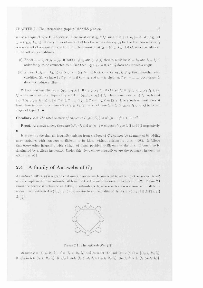
An antiweb A W (x ,y ) is a graph containing x nodes, each connected to all but y other nodes. A web is the complement of an antiweb. Web and antiweb structures were introduced in [82]. Figure 2.1 shows the generic structure of an A W (8,3) antiweb graph, where each node is connected to all but 3 nodes. Each antiweb A W (x ,y ) , y < x, gives rise to an inequality of the form J2 i x i '■ * ^ M (x , j / ) }< s.
Figure 2.1: The antiweb AW(8,3)
Assume c = (i0, jo,&o4o), d = (*1, ji ,& i,ii) and consider the node set A ( c , d ) = {(io, jo ,k0 , lo),
( i i ,jo ,^0, io), ( i i , j i , k o , l o ) , (ii,ji,fc i,/o ), (*1, ji,& i,ii)> (io ,ji,& i,h ) , (io,jo,&i>h ) , (io,jo,&o,h ) } -
2.4. A family of Antiwebs of Ga 19
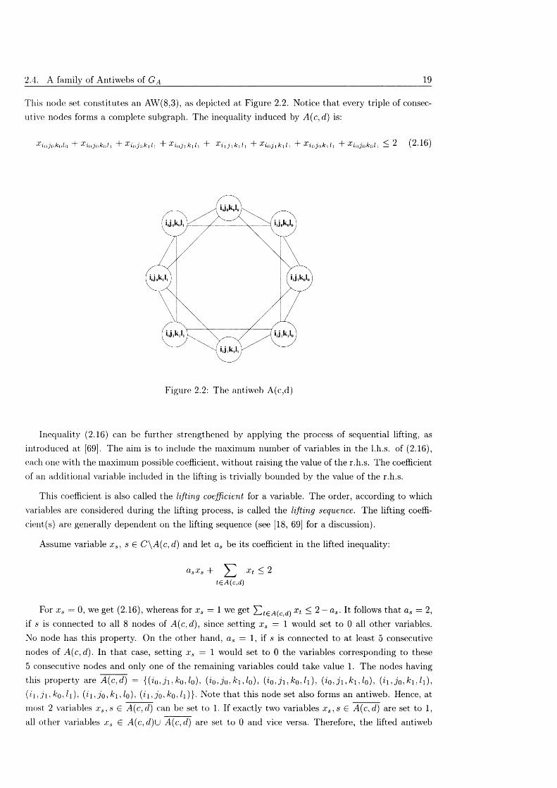
T h is n od e se t c o n st itu te s an A W (8 ,3 ), as d ep icted at F igu re 2 .2 . N o tice th a t every trip le o f consec
u tive n od es form s a co m p lete subgraph. T h e in eq u ality induced by A ( c , d ) is:
x iiiJ o k o lo + x io j( )k o l] T x i 0j o k i l \ + x i 0j \M i A M j i M i + x i o j i k l l 1 + x i o j o k \ l \ + M ijoM i ^ 2 (2 .16)
F igure 2.2: T h e an tiw eb A (c ,d )
In eq u a lity (2 .16 ) can be further stren gth en ed by ap p ly in g th e p rocess o f seq u en tia l lifting, as
in trod uced at [69]. T h e aim is to inclu de th e m axim um num ber o f variab les in th e l.h .s . o f (2 .16 ),
each o n e w ith th e m axim u m p ossib le coefficient, w ith o u t raising th e va lu e o f th e r.h .s. T h e coefficient
o f an a d d itio n a l variab le included in th e liftin g is tr iv ia lly b ou n d ed by th e value o f th e r.h .s.
T h is coeffic ien t is a lso ca lled th e l i f t i n g c o e f f i c i e n t for a variable. T h e order, accord ing to w hich
variab les are considered du ring th e liftin g process, is called th e l i f t i n g s e q u e n c e . T h e liftin g coeffi
c ie n t s ) are gen era lly d ep en d en t on th e liftin g sequ en ce (see [18, 69] for a d iscu ssion ).
A ssu m e variab le x s , s € C \ A ( c , d ) and let a s b e its coeffic ien t in th e lifted inequality:
a3x s + Y 2 -r ' - ~t £A(c ,d)
For x s = 0 , w e get (2 .1 6 ), w hereas for x s = 1 w e get Y l t e A ( c d ) x t — 2 — a s - It fo llow s th a t a s = 2 ,
if s is co n n ected to all 8 n od es o f A ( c , d ) , sin ce se tt in g .r>s = 1 w ou ld se t to 0 all o ther variables.
N o n od e h as th is property. O n th e other hand , a s = 1 , if s is con n ected to at lea st 5 con secu tive
n odes o f A ( c , d ) . In th a t case, se ttin g x s = 1 w ould se t to 0 th e variab les corresp ond in g to th ese
5 con secu tive n od es and on ly on e o f th e rem ain ing variab les cou ld tak e va lu e 1. T h e nod es having
th is p roperty are A ( c , d ) = { { i 0 ) j i f f i o J o ) , ( i 0 , j g f f i i J o ) , { i o J i , k o , h ) , ( i o J u h G o ) , ( i u j o f f i i G i ) ,
( i \ , j i , k o , l \ ), ( i i , j o , k i , l o ) , ( i i G o ^ k o G i ) } . N o te th a t th is nod e se t a lso form s an antiw eb . H ence, at
m ost 2 variab les x s , s € A ( c , d ) can be set to 1 . If ex a c tly tw o variab les .r*. .s £ A ( c , d ) are set to 1 ,
all o th er variab les x s € A ( c , d ) U A ( c , d ) are se t to 0 and v ice versa. T herefore, th e lifted antiw eb
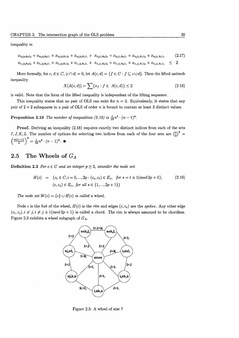
CHAPTER 2. The intersection graph of the OLS problem 20
inequality is:
x iojokolo "b x iojokol\ ”1" x iojok\lo "I- x iojok\l\ “b x iojikolo "b x ioj\kol\ "b x iojikilo "b x ioj\k\l\ (2.17)
x i\jokolo "b x iijok0li "b x iijokil0 "b x iijokih "b x iij\kolo “b x i\j\k0li "b x i\j\k il0 ^ x i\3\kih — 2
More formally, for c, d € C , \c fl d\ = 0, let A(c, d) = { / G C : f C cUd}. Then the lifted antiweb inequality
X (A (c,d)) = : / e A(c,d)} < 2 (2.18)
is valid. Note th a t the form of the lifted inequality is independent of the lifting sequence.This inequality states th a t no pair of OLS can exist for n = 2. Equivalently, it states that any
pair of 2 x 2 subsquares in a pair of OLS of order n is bound to contain at least 3 distinct values.
P ro p o s itio n 2.10 The number of inequalities (2.18) is jgri4 • (n — l ) 4.
P ro o f. Deriving an inequality (2.18) requires exactly two distinct indices from each of the sets / , J, K , L. The number of options for selecting two indices from each of the four sets are (£)4 = ( n l ^ l l ) 4 = i n 4 . ( „ _ ! ) « . .
2.5 The W heels of G a
D efin itio n 2.2 For c € C and an integer p > 2, consider the node set:
H (c) = {ci G C ,i = 0, ...,2p : (cs ,c t ) £ E c, for s = t ± l(m od2p + 1}, (2.19)
(c, cs) G E c, for all s e {1,..., 2p + 1}}
The node set W{c) = {c} U H(c) is called a wheel.
Node c is the hub of the wheel, H (c) is the rim and edges (c, cs) are the spokes. Any other edge (c i,c j) ,i ^ j , i 7 j ± l(m od2p + 1} is called a chord. The rim is always assumed to be chordless. Figure 2.3 exhibits a wheel subgraph of Ga -
nnnn
Ixj
Kx JxL
Figure 2.3: A wheel of size 7
2.5. The Wheels of Ga 21
For i , j G {1,...,2p + 1}, the spokes (c, C{), (c, C j), i ^ j , will be called rim adjacent, if they are incident to adjacent nodes of the rim, i.e. if (Ci,Cj) G E c- For example, spokes ( (n ,n ,n ,n ) , (n ,n ,k o ,l i) ) and ( (n ,n ,n ,n ) , ( io ,n ,n ,li) ) in Figure 2.3 are rim adjacent. Two nodes of the rim, whose spokes are based on the same double ground set, will be called conjugate. An example of such a pair is nodes (n ,n ,k o ,lo ) and (n ,n ,k o , l \ ) in Figure 2.3. The rim edges can be either double or triple links, i.e. |cs , ct \ > 2 for cs ,ct G H (c ) and s ^ t.We assume, however, th a t the spokes can only be double links, i.e. |c f lcs | = 2 for all cs G H{c).Throughout the rest of this section, we also assume, w.l.o.g., th a t c = (n, n, n, n) and p > 2.
Each wheel induces an inequality of the form:
p ■ x c + ^ 2 x d < P (2.20)d£H(c)
The validity of this inequality is justified as follows: setting x c= l implies 2 = 0 for all d G H(c)\ if x c = 0, a t most p of the variables xd, d G H (c) can be set to 1. In both cases, (2.20) is satisfied as equality. As an example, the inequality induced by the 7— wheel of Figure 2.3 is:
3 ' X n n n n - |- X n n ]iQiQ K n n k o l i “t- i o n n l i &i o n k i n ^ i i n k ^ n ”1“ - ^ n j o k i n ”1“ %n j o n l o ^ 3
The wheels of Ga can be categorised with respect to three characteristics: the size p, the number of pairs of conjugate nodes Dp and the number of triple links on the rim Tp. These aspects affect both the configuration of the wheel subgraph and the form of the resulting (lifted) inequality. The following section examines the structural properties of the wheels of Ga -
2.5.1 Properties of wheels
P ro p o s itio n 2.11 Let cs ,c t G H(c), such that (c, cs), (c, ct ) G M i x M 2, M i, M2 = / , J , K , L. Then c f ) c s = c fl ct .
P ro o f. This proposition states th a t at most one member of each double ground set can appear on the spokes. Let Mi = I , M 2 = J and cs = {n ,n ,ko ,lo), ko,lo ^ n, i.e. c fl cs = (n ,n ) G I x J. Assume ct G H(c), such th a t c fl ct G / x J. It is obvious th a t c D ct = (n, n), i.e. c D cs = c fl ct . ■
P ro p o s itio n 2.12 There can be at most two spokes based on the same double ground set. I f exactly two spokes are based on the same double ground set, these spokes have to be rim adjacent.
P ro o f. Assume w.l.o.g. th a t cs = (n ,n ,ko ,lo ),c t = ( n ,n ,k \ , l i ) , k o ,lo ,k i,li ^ n. Then the spokes (c, cs), (c, ct ) are based on the double ground set I x J and (cs ,c t ) G E c- Unless nodes Ci,C2 are rim adjacent, the edge (01, 02) is a chord. If there exists another cu G H{c), such that (c,Cu) € I x J, then one of the edges (c i,cu), (c2,cu), (01, 02) will again be a chord. ■
T h e o re m 2.13 p < 5.
P ro o f. There exist six distinct double ground sets and, according to Prop. 2.12, at most two spokes can be based on each one. Therefore, the largest odd number of nodes in the rim is 11. ■
P ro p o s itio n 2.14 Let cs ,c t G H(c), s ^ t and assume (c,cs) G M i x M2, (c ,ct ) G M3 x M4, M i, M2, M3, M4 = I , J ,K ,L . I f (cs ,ct ) G E c, then, at least one o f M i, M 2 must coincide to either M3 or M 4.
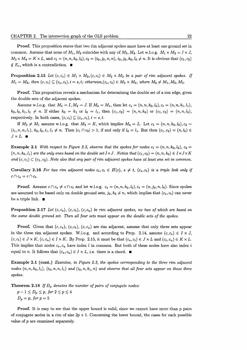
CH APTER 2. The intersection graph of the OLS problem 22
P ro o f . This proposition states th a t two rim adjacent spokes must have a t least one ground set in common. Assume th a t none of M i, M2 coincides with any of M 3, M4. Let w.l.o.g. Mi x M2 = I x J, M3 x M4 = K x L, and ci = (n, n, ko, Iq) , = (io ,jo ,n ,n ), io ,jo ,ko ,lo ^ n. It is obvious th a t (01, 02) ^ E C 1 which is a contradiction. ■
P ro p o s i t io n 2.15 Let (c, cs) E M i x M 2 ,(c ,c t ) E M 2 x M3 6e a pair of rim adjacent spokes. I f M i = M3, £/ien (c, c*) C (cs ,c t ) , i = s ,t; otherwise,(cs ,c t ) E M 2 x M4, w/iere M4 ^ M i, M2, M3.
P ro o f. This proposition reveals a mechanism for determining the double set of a rim edge, given the double sets of the adjacent spokes.
Assume w.l.o.g. th a t M i = I , M2 = J. If M3 = M i, then let cs = ( n , n , k Q , l o ) , c t = ( n , n , k \ , l i ) ,
k 0 , l 0 , k 1 , l 1 7 n - ^ either ko = k i or Iq = Zi, then (01, 02) = (n,n,&o) or (ci>c2) = ( n , n , l o ) ,
respectively. In both cases, (c, c*) C (cs ,ct ) , i = s ,t.If M 3 7 M i assume w.l.o.g. th a t M 3 = K , which implies M 4 = L. Let ci = {n,n,ko,lo),C 2 =
( i i ,n ,n , l i ) , k 0 , l o , i i , l i ^ n. Then |ci fl C2I > 1, if and only if Iq = l i . But then (01, 02) = (n ,l 0 ) E
J x L. m
E x a m p le 2.1 With respect to Figure 2.3, observe that the spokes fo r nodes ci = (n,n,kQ ,lo), C2 = (n ,n ,k o ,l i) are the only ones based on the double set I x J . Notice that (c\ , C2) = (n ,n , Ao) E I x J x K and (c, ci) c (ci, C2). Note also that any pair of rim adjacent spokes have at least one set in common.
C o ro lla ry 2.16 For two rim adjacent nodes cs ,c t E H ( c ) , s 7 £, (cs ,ct) is a triple link only if c fl c3 = c fl ct .
P ro o f. Assume c fl cs ^ c fl ct and let w.l.o.g. cs = (n ,n , k 0 ,lQ),ct = (n ,jQ ,n,lo). Since spokes are assumed to be based only on double ground sets, jo,kQ ^ n, which implies th a t (cs ,c t ) can never be a triple link. ■
P ro p o s itio n 2.17 Let (c,cs), (c, ct ), (c,cu) be rim adjacent spokes, no two o f which are based on the same double ground set. Then all four sets must appear on the double sets o f the spokes.
P ro o f. Given th a t (c, cs), (c, ct), (c , c u ) are rim adjacent, assume th a t only three sets appear in the three rim adjacent spokes. W.l.o.g. and according to Prop. 2.14, assume (c, cs) E I x J, (c, ct ) E J x K , (c, c u ) E I x K . By Prop. 2.15, it must be th a t (cs , c t ) E J x L and (c t , c u ) E K x L. This implies th a t nodes c s , cu have index I in common. But both of these nodes have also index i
equal to n. It follows th a t (c s , c u ) E I x L, i.e. there is a chord. ■
E x am p le 2.1 (co n t.) Examine, in Figure 2.3, the spokes corresponding to the three rim adjacent nodes (n ,n , Aq, Zi), ( io ,n ,n ,li) and (iQ ,n ,k i,n ) and observe that all four sets appear on these three spokes.
T h e o re m 2.18 I f Dp denotes the number o f pairs of conjugate nodes: p — 1 < Dp < p, for 2 < p < 4 Dp = p , fo r p = 5
P ro o f. It is easy to see th a t the upper bound is valid, since we cannot have more than p pairsof conjugate nodes in a rim of size 2p + 1. Concerning the lower bound, the cases for each possiblevalue of p are examined separately.
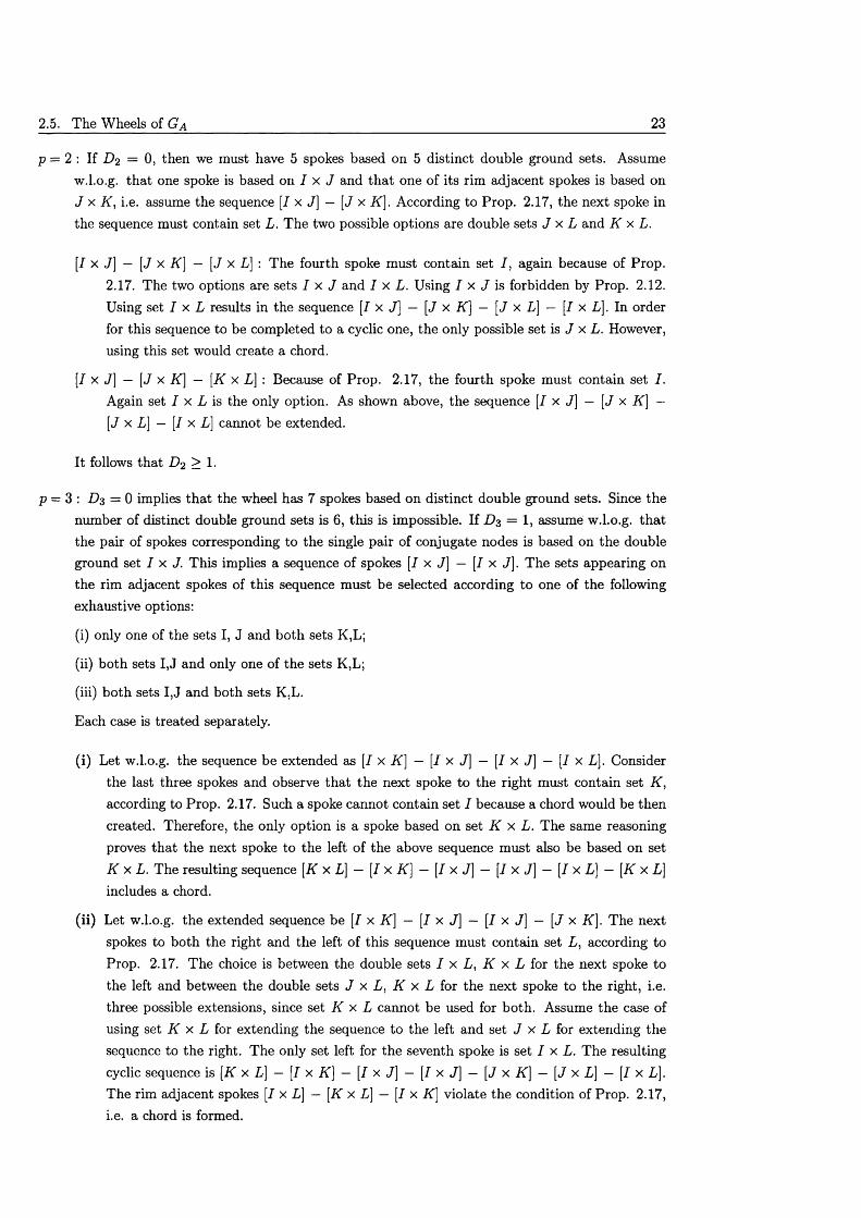
2.5. The Wheels of Ga 23
p = 2 : If D 2 = 0, then we must have 5 spokes based on 5 distinct double ground sets. Assume w.l.o.g. th a t one spoke is based on I x J and th a t one of its rim adjacent spokes is based on J x K, i.e. assume the sequence [I x J] — [J x K]. According to Prop. 2.17, the next spoke in the sequence must contain set L. The two possible options are double sets J x L and K x L.
[I x J] — [J x K] — [J x L\ : The fourth spoke must contain set / , again because of Prop. 2.17. The two options are sets I x J and I x L. Using I x J is forbidden by Prop. 2.12. Using set I x L results in the sequence [I x J] — [J x K) — [J x L] — [I x L]. In order for this sequence to be completed to a cyclic one, the only possible set is J x L. However, using this set would create a chord.
[I x J] — [J x K] — [K x L] : Because of Prop. 2.17, the fourth spoke must contain set I. Again set I x L is the only option. As shown above, the sequence [I x J] — [J x K] — [J x L\ — [I x L] cannot be extended.
It follows that D 2 > 1.
p — 3 : D 3 = 0 implies th a t the wheel has 7 spokes based on distinct double ground sets. Since the number of distinct double ground sets is 6, this is impossible. If D% = 1, assume w.l.o.g. th a t the pair of spokes corresponding to the single pair of conjugate nodes is based on the double ground set I x J. This implies a sequence of spokes [I x J] — [I x J]. The sets appearing on the rim adjacent spokes of this sequence must be selected according to one of the following exhaustive options:
(i) only one of the sets I, J and both sets K,L;
(ii) both sets I,J and only one of the sets K,L;
(iii) both sets I,J and both sets K,L.
Each case is treated separately.
(i) Let w.l.o.g. the sequence be extended as [I x K] — [I x J] — [I x J] — [I x L}. Considerthe last three spokes and observe that the next spoke to the right must contain set K , according to Prop. 2.17. Such a spoke cannot contain set I because a chord would be then created. Therefore, the only option is a spoke based on set K x L. The same reasoning proves th a t the next spoke to the left of the above sequence must also be based on set K x L. The resulting sequence [K x L] — [I x K] — [I x J] — [I x J] — [I x L] — [K x L] includes a chord.
( ii) Let w.l.o.g. the extended sequence be [I x K] — [I x J] — [I x J] — [J x K]. The next spokes to both the right and the left of this sequence must contain set L, according to Prop. 2.17. The choice is between the double sets I x L, K x L for the next spoke to the left and between the double sets J x L, K x L for the next spoke to the right, i.e. three possible extensions, since set K x L cannot be used for both. Assume the case of using set K x L for extending the sequence to the left and set J x L for extending the sequence to the right. The only set left for the seventh spoke is set I x L. The resulting cyclic sequence is [K x L] — [I x K] — [I x J] — [I x J] — [J x K] — [J x L] — [I x L\. The rim adjacent spokes [I x L] — [K x L\ — [I x K] violate the condition of Prop. 2.17, i.e. a chord is formed.
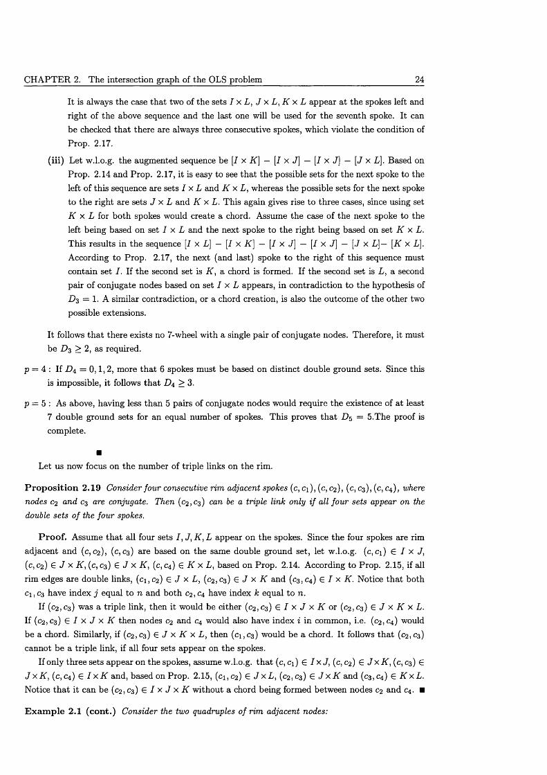
CHAPTER 2. The intersection graph of the OLS problem 24
It is always the case that two of the sets I x L, J x L, K x L appear a t the spokes left and right of the above sequence and the last one will be used for the seventh spoke. It can be checked th a t there are always three consecutive spokes, which violate the condition of Prop. 2 .17 .
(iii) Let w.l.o.g. the augmented sequence be [I x K] — [I x J] — [I x J] — [J x L\. Based on Prop. 2.14 and Prop. 2 .17 , it is easy to see th a t the possible sets for the next spoke to the left of this sequence are sets I x L and K x L, whereas the possible sets for the next spoke to the right are sets J x L and K x L. This again gives rise to three cases, since using set K x L for both spokes would create a chord. Assume the case of the next spoke to the left being based on set I x L and the next spoke to the right being based on set K x L. This results in the sequence [I x L\ — [I x K] — [I x J] — [I x J] — [J x L \— [K x L\. According to Prop. 2 .17, the next (and last) spoke to the right of this sequence must contain set I. If the second set is K , a chord is formed. If the second set is L , a second pair of conjugate nodes based on set I x L appears, in contradiction to the hypothesis of I>3 = 1. A similar contradiction, or a chord creation, is also the outcome of the other two possible extensions.
It follows th a t there exists no 7-wheel with a single pair of conjugate nodes. Therefore, it must be £ 3 > 2, as required.
p = 4 : If £)4 = 0 ,1 , 2 , more th a t 6 spokes must be based on distinct double ground sets. Since this is impossible, it follows th a t £ 4 > 3 .
p = 5 : As above, having less than 5 pairs of conjugate nodes would require the existence of at least 7 double ground sets for an equal number of spokes. This proves th a t £5 = 5 .The proof is complete.
■Let us now focus on the number of triple links on the rim.
P rop osition 2.19 Consider four consecutive rim adjacent spokes (c, Ci), (c, C2), (c, C3), (c, C 4 ) , where nodes c2 and C3 are conjugate. Then (02,03) can be a triple link only i f all four sets appear on the double sets o f the four spokes.
Proof. Assume th a t all four sets / , J, A, L appear on the spokes. Since the four spokes are rim adjacent and (0,02), (0,03) are based on the same double ground set, let w.l.o.g. (c ,c\) E I x J, (0,02) E J x K , (0,03) e J x K , (0,04) E K x L, based on Prop. 2 .14 . According to Prop. 2 .15 , if all rim edges are double links, (01,02) E J x L, (02,03) E J x K and (03,04) E I x K. Notice th a t both Ci, c3 have index j equal to n and both C2, C4 have index k equal to n.
If (02,03) was a triple link, then it would be either (02,03) E I x J x K or (02,03) E J x K x L. If (c2> 03) E I x J x K then nodes 02 and 04 would also have index i in common, i.e. (02,04) would be a chord. Similarly, if (02,03) E J x K x L, then (01,03) would be a chord. It follows th a t (02,03) cannot be a triple link, if all four sets appear on the spokes.
If only three sets appear on the spokes, assume w.l.o.g. th a t (c, ci) E I x J , (c, 02) E J x K, (c, 03) E
J x K , (c, c4) E I x K and, based on Prop. 2 .15, (ci, 02) E J x L, (02,03) E J x K and (03,04) E K x L. Notice th a t it can be (02,03) E I x J x K w ithout a chord being formed between nodes 02 and c4. ■
E xam ple 2.1 (cont.) Consider the two quadruples of rim adjacent nodes:
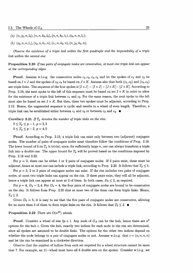
2.5. The Wheels of Ga 25
(a) (n, j 0, n, l0), (n, to, k0,l0), (n, n, kQ, h ), (i0, n, n, Zi);
(b) { io ,n ,n ,h ) ,( io ,n ,k i ,n ) , { i \ ,n ,k 2,n ) ,{ n ,jo ,k 2,n)\
Observe the existence o f a triple link within the first quadruple and the impossibility of a triple link within the second one.
P ro p o s i t io n 2.20 I f two pairs of conjugate nodes are consecutive, at most one triple link can appear at the corresponding edges.
P ro o f . Assume w.l.o.g. the consecutive nodes Ci,02, 03,04 and let the spokes of c\ and 02 be based on I x J and the spokes of 0 3 , 0 4 be based on J x K . Assume also th a t both (c i, c2) and ( 0 3 , C 4)
are triple links. The sequence of the four spokes is [Jx J] — [Jx J] — [ J x K ] — [ J x K ] . According to Prop. 2.19, the next spoke to the left of this sequence must be based on set I x K in order to allow for the existence of a triple link between c\ and 02. For the same reason, the next spoke to the left must also be based on set I x K. But then, these two spokes must be adjacent, according to Prop.2.12. Hence, the augmented sequence is cyclic and results in a wheel of even length. Therefore, a triple link can be established either between c\ and C2 or between C3 and C 4. ■
C o ro lla ry 2.21 I f T p denotes the number o f triple links on the rim:0 < Tp < p - 1, p = 2,3 0 < T p < p - 2 , p = 4,5
P ro o f. According to Prop. 2.15, a triple link can exist only between two (adjacent) conjugate nodes. The number of pairs of conjugate nodes must therefore follow the conditions of Prop. 2.18. The lower bound of 0 on Tp is trivial, since, for sufficiently large n, one can always transform a triple link into a double one. The upper bound for Tp will be proved based on the conditions imposed by Prop. 2.18 and 2.20.
For p = 2, there can be either 1 or 2 pairs of conjugate nodes. If 2 pairs exist, these must be adjacent, hence a t most one can include a triple link, according to Prop. 2.20. It follows th a t T2 < 1.
For p = 3, 2 or 3 pairs of conjugate nodes can exist. If the rim includes two pairs of conjugate nodes, a t most two triple links can appear on the rim. If three pairs exist, they will all be adjacent, hence a triple link can appear at most a t 2 of them. In both cases, < 2, as required.
For p = 4, = 3,4. For D 4 = 4, the four pairs of conjugate nodes are bound to be consecutiveon the rim. It follows from Prop. 2.20 th a t at most two of the them can form triple links. Hence, T4 < 2.
Given D$ = 5, it is easy to see th a t the five pairs of conjugate nodes are consecutive, allowing for no more than 3 of them to form triple links on the rim. It follows th a t T5 < 3. ■
P ro p o s i tio n 2.22 There are 0 (n 2°) wheels.
P ro o f. Consider a wheel of size 2p -f 1. Any node of Ga can be the hub, hence there axe n 4 options for the hub c. Given the hub, exactly two indices for each node in the rim are determined, since all spokes are assumed to be double links. The options for the other two indices depend on whether the node belongs to a pair of conjugate nodes or not. Assume w.l.o.g. th a t c = (n ,n ,n ,n ) and let the rim be examined in a clockwise direction.
Observe th a t the number of indices from each set required for a wheel structure cannot be more th a t 7. For example, an 11—wheel must have all 6 double sets on the spokes. Consider w.l.o.g. set
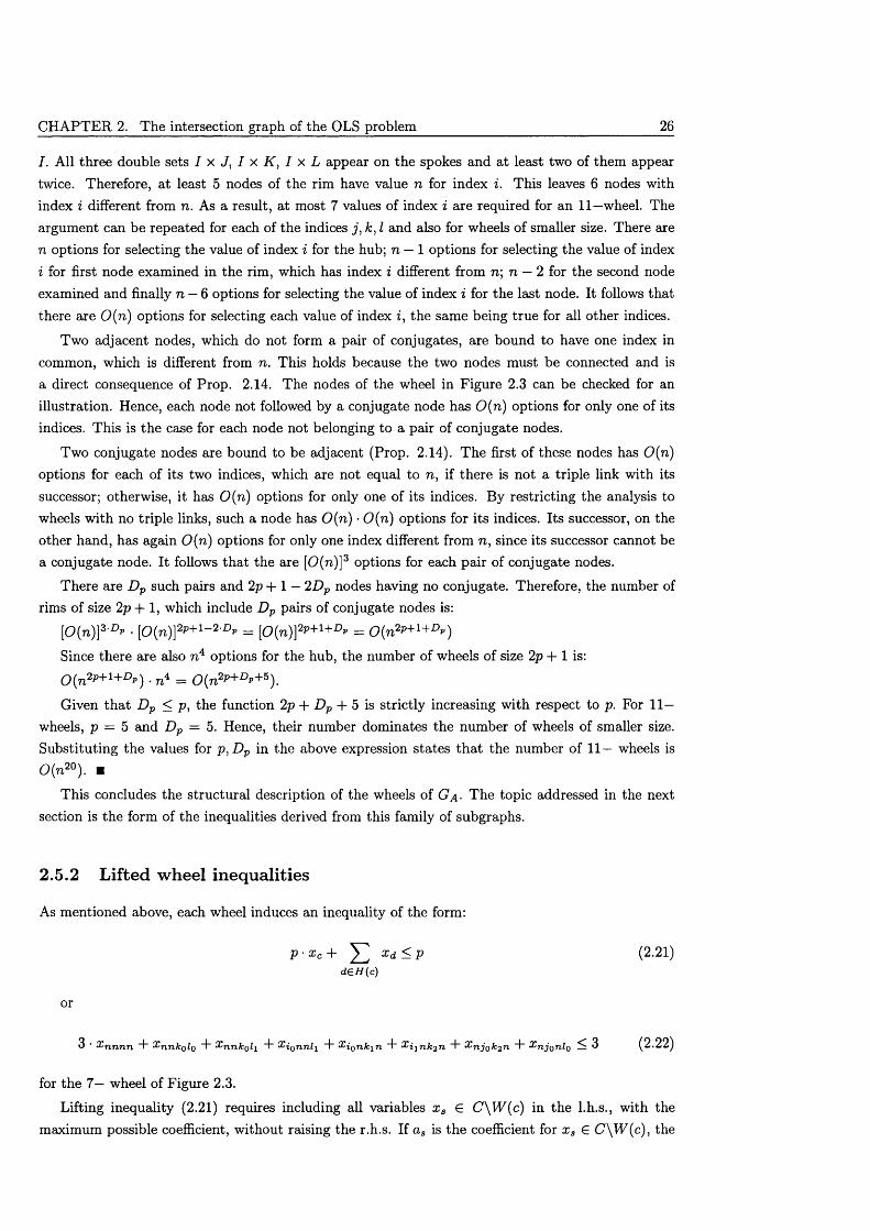
CHAPTER 2. The intersection graph of the OLS problem 26
I. All three double sets I x J, I x K , I x L appear on the spokes and at least two of them appear twice. Therefore, at least 5 nodes of the rim have value n for index i. This leaves 6 nodes with index i different from n. As a result, at most 7 values of index i are required for an 11—wheel. The argument can be repeated for each of the indices j , k, I and also for wheels of smaller size. There are n options for selecting the value of index i for the hub; n — 1 options for selecting the value of index i for first node examined in the rim, which has index i different from n; n — 2 for the second node examined and finally n — 6 options for selecting the value of index i for the last node. It follows that there are 0 ( n ) options for selecting each value of index i, the same being true for all other indices.
Two adjacent nodes, which do not form a pair of conjugates, are bound to have one index in common, which is different from n. This holds because the two nodes must be connected and is a direct consequence of Prop. 2.14. The nodes of the wheel in Figure 2.3 can be checked for an illustration. Hence, each node not followed by a conjugate node has 0 ( n ) options for only one of its indices. This is the case for each node not belonging to a pair of conjugate nodes.
Two conjugate nodes are bound to be adjacent (Prop. 2.14). The first of these nodes has 0 (n ) options for each of its two indices, which are not equal to n, if there is not a triple link with its successor; otherwise, it has 0 (n ) options for only one of its indices. By restricting the analysis to wheels with no triple links, such a node has 0 (n ) ■ 0 ( n ) options for its indices. Its successor, on the other hand, has again 0 ( n ) options for only one index different from n, since its successor cannot be a conjugate node. It follows th a t the are [O(n)]3 options for each pair of conjugate nodes.
There are Dp such pairs and 2 p + l — 2Dp nodes having no conjugate. Therefore, the number ofrims of size 2p F 1, which include Dp pairs of conjugate nodes is:
[0{n)}3 Dp • [0{n)]2P+1~2 Dp = [0{n)]2P+1+Dp = 0 ( n 2P+1+D”)
Since there are also n 4 options for the hub, the number of wheels of size 2p + 1 is:0 (n2p+l+DP) . n 4 = 0 ( n 2P+ D p+ 5 )
Given th a t Dp < P, the function 2p + D p + 5 is strictly increasing with respect to p. For 1 1 - wheels, p = 5 and Dp = 5. Hence, their number dominates the number of wheels of smaller size. Substituting the values for p ,D p in the above expression states th a t the number of 11— wheels is 0 (n2°). ■
This concludes the structural description of the wheels of Ga - The topic addressed in the nextsection is the form of the inequalities derived from this family of subgraphs.
2.5.2 Lifted w heel inequalities
As mentioned above, each wheel induces an inequality of the form:
P ' x c + X / Xd - P (2.21)d e H ( c )
or
3 • Xnnnn F %nnkolo F Xnnko?i F ^ionnii F -ionfcin F Xi-i nk2 'n F Xnj Qk2n F xnjoni0 < 3 (2 .22)
for the 7— wheel of Figure 2 .3 .
Lifting inequality (2 .21) requires including all variables x s G C \kF(c) in the l.h.s., with themaximum possible coefficient, without raising the r.h.s. If as is the coefficient for xs G C\W(c) , the
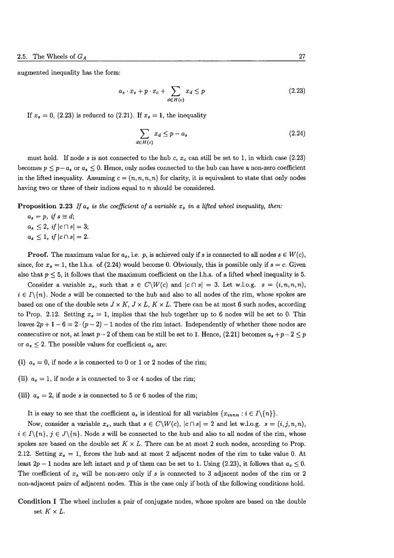
2.5. The Wheels of Ga 27
augmented inequality has the form:
as ■ x s + p ■ x c + ^2, x d < P d e H ( c )
(2.23)
If x s = 0, (2.23) is reduced to (2.21). If x s = 1, the inequality
^ 2 x d < P ~ a s d £ H (c )
(2.24)
must hold. If node s is not connected to the hub c, x c can still be set to 1, in which case (2.23) becomes p < p — as or as < 0 . Hence, only nodes connected to the hub can have a non-zero coefficient in the lifted inequality. Assuming c = (n, n, n, n) for clarity, it is equivalent to state that only nodes having two or three of their indices equal to n should be considered.
P ro p o s itio n 2.23 I f as is the coefficient o f a variable x a in a lifted wheel inequality, then:as = p, i f s = d]
as < 2, i f |c fl s\ = 3;as < 1, i f \c fl s| = 2.
P ro o f. The maximum value for a s , i.e. p, is achieved only if s is connected to all nodes s G W (c), since, for x s = 1, the l.h.s. of (2.24) would become 0. Obviously, this is possible only if s = c. Given also th a t p < 5, it follows th a t the maximum coefficient on the l.h.s. of a lifted wheel inequality is 5.
Consider a variable x s , such th a t s G C \W (c) and |c fl s| = 3. Let w.l.o.g. s = (i ,n ,n ,n ), i G / \ { n }- Node s will be connected to the hub and also to all nodes of the rim, whose spokes are based on one of the double sets J x K, J x L, K x L. There can be a t most 6 such nodes, according to Prop. 2 .12 . Setting x 8 = 1, implies that the hub together up to 6 nodes will be set to 0. This leaves 2p + \ — 6 = 2 • (p — 2) — 1 nodes of the rim intact. Independently of whether these nodes are consecutive or not, at least p — 2 of them can be still be set to 1 . Hence, (2 .21) becomes as + p — 2 < p or as < 2 . The possible values for coefficient as are:
(i) as = 0, if node s is connected to 0 or 1 or 2 nodes of the rim;
(ii) as = 1, if node s is connected to 3 or 4 nodes of the rim;
(iii) as = 2, if node s is connected to 5 or 6 nodes of the rim;
It is easy to see th a t the coefficient as is identical for all variables {Xinnn : i G 7\{n}}.Now, consider a variable x s , such th a t s G C \W (c), |c f l s | = 2 and let w.l.o.g. s = (i , j , n , n ),
i G I \ { n ] , j £ J \{ n } . Node s will be connected to the hub and also to all nodes of the rim, whose spokes are based on the double set K x L. There can be a t most 2 such nodes, according to Prop.2.12. Setting x s = 1, forces the hub and at most 2 adjacent nodes of the rim to take value 0. At least 2p — 1 nodes are left intact and p of them can be set to 1. Using (2.23), it follows th a t as < 0. The coefficient of x s will be non-zero only if s is connected to 3 adjacent nodes of the rim or 2 non-adjacent pairs of adjacent nodes. This is the case only if both of the following conditions hold.
C o n d itio n I The wheel includes a pair of conjugate nodes, whose spokes are based on the double set K x L.
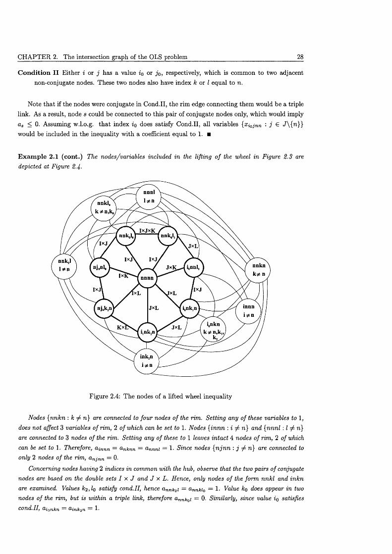
CHAPTER 2. The intersection graph of the OLS problem 28
C o n d itio n I I Either i or j has a value io or jo, respectively, which is common to two adjacent non-conjugate nodes. These two nodes also have index k or I equal to n.
Note th a t if the nodes were conjugate in Cond.II, the rim edge connecting them would be a triple link. As a result, node s could be connected to this pair of conjugate nodes only, which would imply as < 0. Assuming w.l.o.g. th a t index io does satisfy Cond.II, all variables {Xi0j nn : j e A { n }} would be included in the inequality with a coefficient equal to 1. ■
E x am p le 2.1 (con t.) The nodes/variables included in the lifting o f the wheel in Figure 2.3 are depicted at Figure 2.f.
IxJnnkn k * n
nnnn
IxJ'
Figure 2.4: The nodes of a lifted wheel inequality
Nodes {nnkn : k ^ n} are connected to four nodes o f the rim. Setting any of these variables to 1, does not affect 3 variables o f rim, 2 of which can be set to 1. Nodes { in n n : i ^ n} and {nnnl \ I ^ n } are connected to 3 nodes o f the rim. Setting any of these to 1 leaves intact 4 nodes of rim, 2 of which can be set to 1. Therefore, ainnn = anknn — o,nnni = 1. Since nodes {n jn n : j ^ n] are connected to only 2 nodes o f the rim, a nj nn = 0.
Concerning nodes having 2 indices in common with the hub, observe that the two pairs o f conjugate nodes are based on the double sets I x J and J x L. Hence, only nodes o f the form nnkl and inkn are examined. Values k2 ,lo satisfy cond.II, hence annk2i = annkiQ = 1. Value ko does appear in two nodes o f the rim, but is within a triple link, therefore annk0i = 0. Similarly, since value io satisfies cond.II, aionkn — a,ink2n = 1.
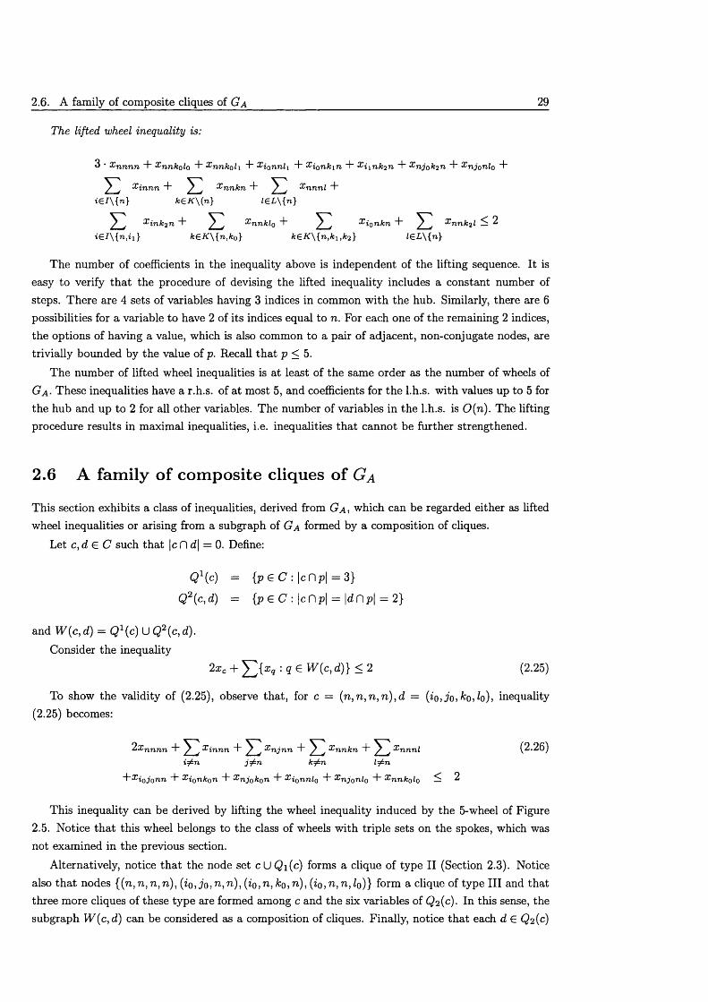
2.6. A family of composite cliques of Ga 29
The lifted wheel inequality is:
3 • X n n n n T X n n k o l o T X n n k o l i "I” ^ io n n Z i “I- X i Qnk i n + X i lTi k “I” -^n jo k iT i "I” X n j Qni0 +
^ Xinnn "b ^ S 'n n fc n "I- ^ Xnnnl "bi G / \ { n } f c G / f \ ( n } l&L\{n}
E **■*«+ E *""«o+ E **.«*«+ E ^ < 2i € / \ { n , i i } k £ K \ { n , k o } A :€ K \{ n ,A :1 ,A:2} l £ L \ { n }
The number of coefficients in the inequality above is independent of the lifting sequence. It is easy to verify th a t the procedure of devising the lifted inequality includes a constant number of steps. There are 4 sets of variables having 3 indices in common with the hub. Similarly, there are 6 possibilities for a variable to have 2 of its indices equal to n. For each one of the remaining 2 indices, the options of having a value, which is also common to a pair of adjacent, non-conjugate nodes, are trivially bounded by the value of p. Recall that p < 5.
The number of lifted wheel inequalities is at least of the same order as the number of wheels of Ga - These inequalities have a r.h.s. of at most 5, and coefficients for the l.h.s. with values up to 5 for the hub and up to 2 for all other variables. The number of variables in the l.h.s. is 0 (n ). The lifting procedure results in maximal inequalities, i.e. inequalities th a t cannot be further strengthened.
2.6 A family of com posite cliques of G a
This section exhibits a class of inequalities, derived from Ga , which can be regarded either as lifted wheel inequalities or arising from a subgraph of Ga formed by a composition of cliques.
Let c,d G C such th a t |c fl d\ = 0. Define:
Q l {c) = {p G C : |c n p | = 3}
Q2(c,d) = {p G C : \c H p | = \d flp | = 2}
and W ( c } d) = Q 1(c) U Q2(c, d).
Consider the inequality2xc + : q G W(c,d) } < 2 (2.25)
To show the validity of (2.25), observe that, for c = (n ,n ,n ,n ) ,d = (io, j o , k o , l o) , inequality (2.25) becomes:
2%nnnn ‘X’innn E %njnn E Knnkn T E Xnnnl (2.26)i^n k^n l^n
~ ~-Eiojonn T - ionkon "b "b XionniQ -f- XnjQniQ -(- Xnnk0l0 ^ 2
This inequality can be derived by lifting the wheel inequality induced by the 5-wheel of Figure 2.5. Notice th a t this wheel belongs to the class of wheels w ith triple sets on the spokes, which was not examined in the previous section.
Alternatively, notice th a t the node set c U Qi{c) forms a clique of type II (Section 2.3). Notice also th a t nodes { (n ,n ,n ,n ) , ( i o , j o , n , n ) , (zo,n, &o,n), { i o , n , n , l o ) } form a clique of type III and that three more cliques of these type are formed among c and the six variables of Qz{c). In this sense, the subgraph W(c, d) can be considered as a composition of cliques. Finally, notice th a t each d G Q2(c)
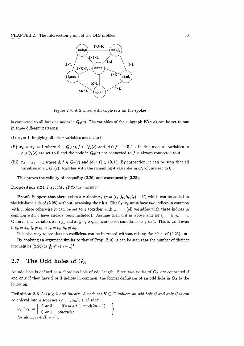
CHAPTER 2. The intersection graph of the OLS problem 30
IxJ
nnnn
Figure 2.5: A 5-wheel with triple sets on the spokes
is connected to all but one nodes in Q 2 (c). The variables of the subgraph W(c,d) can be set to one in three different patterns:
(i) x c = 1, implying all other variables are set to 0
( ii) Xd = Xf = 1 where d G Qi ( c ) , f G Q 2 {c) and \d fl / | G {0 ,1} . In this case, all variables inc U Qi{c) are set to 0 and the node in Q2(c) not connected to / is always connected to d.
( iii) Xd = Xf — 1 where d, / G Q 2 (c) and \d fl / | G {0 ,1}. By inspection, it can be seen that all variables in cU Q i(c), together with the remaining 4 variables in Q 2 (c), are set to 0.
This proves the validity of inequality (2.26) and consequently (2.25).
P ro p o s itio n 2.24 Inequality (2.25) is maximal.
P ro o f. Suppose th a t there exists a variable xp (p = (ip, j p, kp,lp) G C) which can be added to the left-hand side of (2.25) without increasing the r.h.s. Clearly, x p must have two indices in common with c, since otherwise it can be set to 1 together with x nnnn (all variables with three indices in common with c have already been included). Assume then c, d as above and let ip = n, j p = n. Observe th a t variables x nnkpip and x njon[Q, Xionnn can be set simultaneously to 1. This is valid even if kp = Hq , lp ^ Iq or lp = Iq , kp ^ A:q .
It is also easy to see th a t no coefficient can be increased without raising the r.h.s. of (2.25). ■ By applying an argument similar to th a t of Prop. 2.10, it can be seen th a t the number of distinct
inequalities (2.25) is ^ n 4 • (n — l ) 4.
2.7 The Odd holes of G a
An odd hole is defined as a chordless hole of odd length. Since two nodes of Ga are connected if and only if they have 2 or 3 indices in common, the formal definition of an odd hole in G a is the following.
D efin itio n 2.3 Let p > 2 and integer. A node set H Q C induces an odd hole i f and only if it can be ordered into a sequence {co, ...,C2P}, such that:
2 or 3, i f t = s ± 1 mod(2p + 1)0 or 1, otherwise
for all cs ,ct G H, s ^ t.
2.7. The Odd holes of Ga 31
Each odd hole H induces an inequality of the form:
5 > j < P (2.27)d e H
Note th a t wheels are essentially special cases of odd holes, w ith an extra node (hub) connected to all 2p + 1 nodes.
This section exhibits a number of properties regarding the odd holes of Ga • Two classes of odd holes are also presented. The first of them, called odd holes of type I, is derived from the odd holes of the 3A A P n problem, introduced in [9]. The second, called odd holes of type II, is derived from a new class of odd holes for the 3P A P n problem. Each class is further analysed and the form of lifted odd hole inequalities is also presented.
Recall first th a t the edge between two adjacent nodes in the odd hole can be either double or triple, as defined in Section 2 .2 .
P rop osition 2.25 Two adjacent edges of an odd hole cannot be based on the same double ground set.
Proof. Assume w.l.o.g. edges (c i,c2), (02, 03). Let (c i,c2) G I x J and c\ = ( i i , j i , k i , l i ) , 02 = (ii) j i , £2,^2), &i 7 &2, h 7 h- If (02, 03) is also based also on I x J or on a triple ground set, which contains single sets I and J, node 03 will have the form 03 = k$, Z3), k\ ^ /c2 or h 7= h-This implies th a t (01, 03) will be a chord, a fact th a t contradicts to the definition of an odd hole. ■
P rop osition 2.26 Two adjacent edges cannot both be triple links.
Proof. Assume w.l.o.g. an edge (c i,c2) G I x J x K. An adjacent edge, which is also based on a triple ground set, is bound to contain two of the three sets I , J , K. This would imply the creation of a chord, which is a contradiction. ■
The following proposition is based on [9, Prop.5.3].
P rop osition 2.27 The number t o f triple links in an odd hole o f length 2p + 1 must satisfy
'5max < 0, ^ ( 2 p + l ) - 3 n 2 < t < p (2 .28)
Proof. The number of positive components of the vector a r = aCl + ... + aC2p+1 is 5 • {2p+ 1) — 21. This number cannot exceed the number of rows of m atrix A, i.e. 6n 2. The inequality 5 ■ (2p +1) — 21 < 6n2 gives the lower bound of (2.28). To prove the validity of the upper bound, assume an odd hole with p + 1 triple links. This hole should have two triple links incident to the same node. This contradicts to Prop. 2.26. ■
P rop osition 2.28 The maximum coefficient in the l.h.s. of a lifted odd hole inequality is 5.
Proof. Consider a variable x s , s G C \H , and let as be its coefficient in a lifted odd hole inequality. The form of the inequality will be the following:
asx s + x d < p (2.29)d e H
There can be at most 2 nodes of the hole, which have exactly the same indices in common with node s and, if there are exactly 2 , they must also be adjacent. The argument supporting this point
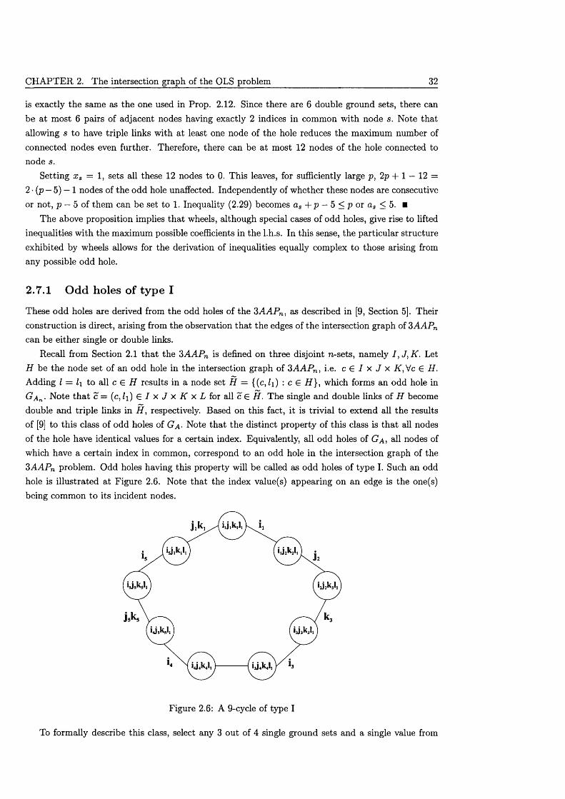
CHAPTER 2. The intersection graph of the OLS problem 32
is exactly the same as the one used in Prop. 2.12. Since there are 6 double ground sets, there can be at most 6 pairs of adjacent nodes having exactly 2 indices in common with node s. Note that allowing s to have triple links with at least one node of the hole reduces the maximum number of connected nodes even further. Therefore, there can be at most 12 nodes of the hole connected to node s.
Setting x s = 1, sets all these 12 nodes to 0. This leaves, for sufficiently large p, 2p + 1 — 12 = 2 • (p — 5) — 1 nodes of the odd hole unaffected. Independently of whether these nodes are consecutive or not, p — 5 of them can be set to 1. Inequality (2.29) becomes as + p — 5 < p or as < 5. ■
The above proposition implies th a t wheels, although special cases of odd holes, give rise to lifted inequalities w ith the maximum possible coefficients in the l.h.s. In this sense, the particular structure exhibited by wheels allows for the derivation of inequalities equally complex to those arising from any possible odd hole.
2.7.1 Odd holes of type I
These odd holes are derived from the odd holes of the 3A A P n , as described in [9, Section 5]. Their construction is direct, arising from the observation that the edges of the intersection graph of 3A A P n can be either single or double links.
Recall from Section 2.1 th a t the 3AAPn is defined on three disjoint n-sets, namely J, J, K. Let H be the node set of an odd hole in the intersection graph of 3A A P n , i.e. c £ I x J x K ,V c £ H. Adding I = l\ to all c £ H results in a node set H = {(c, Zi) : c £ H }, which forms an odd hole in GAn- Note th a t c = £ I x J x K x L for all c £ H . The single and double links of H becomedouble and triple links in H , respectively. Based on this fact, it is trivial to extend all the results of [9] to this class of odd holes of G a - Note that the distinct property of this class is th a t all nodes of the hole have identical values for a certain index. Equivalently, all odd holes of Ga-, all nodes of which have a certain index in common, correspond to an odd hole in the intersection graph of the 3A A P n problem. Odd holes having this property will be called as odd holes of type I. Such an odd hole is illustrated at Figure 2.6. Note that the index value(s) appearing on an edge is the one(s) being common to its incident nodes.
Figure 2.6: A 9-cycle of type I
To formally describe this class, select any 3 out of 4 single ground sets and a single value from
2.7. The Odd holes of Ga 33
the fourth set. Assume w.l.o.g. sets I , J , K and value lj G L. Select subsets Q j C I, Q j C J, Q k C K, satisfying |Q /| + \Qj\ + \Q k\ — 2p + 1, 1 < \Qm\ < p for M = I , J , K . Define the set Q = Qi U Q j U Q/c, |Q| = 2p + l.T he associated odd hole H is the one where all nodes have index I equal to l\ and edges are labelled by the members of set Q. Note th a t set Q, together with value Zi, defines also a row subset of matrix A, namely the rows indexed by R H = {(q, l i) : q G Q } . The matrix formed by this row subset and the columns c G H is identical to the circulant m atrix Cfp+i > up to row and column permutations ([9, P rop.5.5]).
As an extension of the properties exhibited in [9], odd holes of type I, with length 2 p + 1, exist for p < n —1. The number of triple links t must satisfy the inequality max {0,2(2p + 1) — 3n} < t < p —1. Note th a t these bounds are tighter than the ones of inequality (2.28).
Consider the inequality:
: | . n ( Q u { J , } ) | > 3 } < p (2.30)
For p < n — 1, this inequality can be regarded as a lifted odd hole inequality. Its Chvatal rank is 1, since it can be derived by adding all rows {(g, l\) : q G Q}, dividing the resulting inequality by 2, replacing = by < and rounding down both sides. If |Q /| = r, |Q j | = s, \Qk \ — t, the number of variables in the l.h.s. of (2.30) is n • (rs + rt + s t) — 2rs t ([9]).
The number of distinct lifted odd hole inequalities for the 3A A P n is 0 (2 3n). Since each such inequality can be extended to an inequality of the 4P A P n by considering any of the n values for the fourth index, it follows th a t the number of lifted odd holes inequalities of type I is 0 (n • 23n).
2.7.2 Odd holes of type II
This class of odd holes appears both in the 3P A P n and the 4P A P n problem. Therefore, it can be better exhibited by examining first its appearance in 3P A P n .
Recall from Section 2.1 th a t the 3P A P n is defined on three disjoint n-sets, namely / , J, K. Consider subsets of the three ground sets Q': C / , Q'j C J, Q'K C K } such th a t |Q j| = |Q j| = |Q ^ | = m.Assume any perm utation of the elements of the three subsets Q'j = {ii, Q'j = { j i,
Q'k ~ {&i» —»km}, 3 < m < n .
P ro p o s itio n 2.29 The node seth j i k i , zij’2^2, Z2j 2fc2>--->im jmkm , imj lkl , Z72 odd
Q = .............................................h j l h , h j\k,2 , Zij'2^2> Z2J2&2) •••,
i'mjm km, imjqkm, Zm jqkl, Zmjf'ifci, 771 even, q 1,771 1,772 Jinduces an odd hole in the intersection graph o f3 P A P n .
P ro o f . Recall th a t in the intersection graph of both the 3P A P n and the 4P A P n two nodes are connected if they have at least two indices in common([37]). Considering the order of members of Q to be cyclic, each node is connected only to its predecessor and its successor according to this order.
The number of nodes is 3m for m odd and 3m + 1, if m is even. In both cases the length of the hole is odd. ■
For the purpose of illustrating this odd hole in the form of a Latin square, assume w.l.o.g. that Q i = Q'j = Q'k = {1,2, ...,77i}. The odd hole includes the nodes depicted at Table 2.1. Note that q can be equal to 2,3,. ., m — 2.
The inequality induced by such an odd cycle has the form:
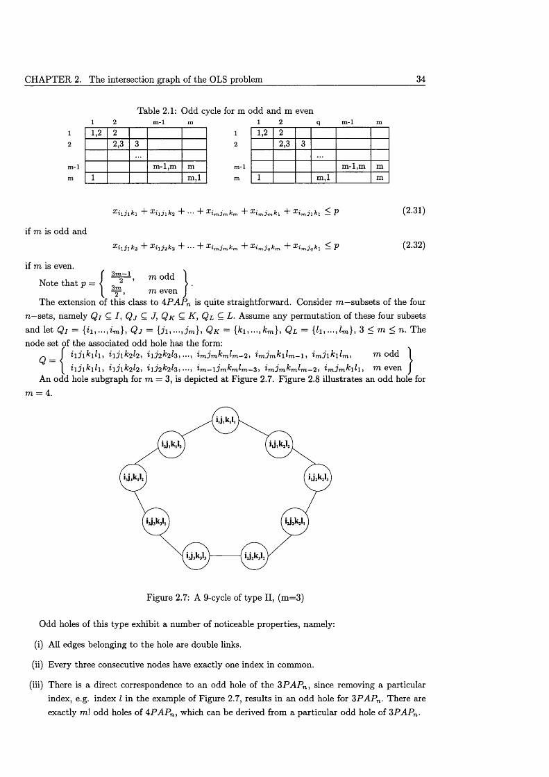
CHAPTER 2. The intersection graph of the OLS problem 34
Table 2.1: Odd cycle for m odd and m even1 2 m -l m 1 2 q m-1 m
1 1,2 2 1 1,2 22 2,3 3 2 2,3 3
m -l m-l,m m m -l m-l,m mm 1 m ,l m 1 m ,l m
if m is odd and
if m is even.
Note th a t p =
Xiljlk\ Xiljlk2 Ximjmkrn T Ximjmk 1 “I- Ximj\ki — P
x i\jik2 + x ii32k2 + •■• + x imjmkm + x iTnjqkm d" x imjqk\ 5: P
3r7 ~1, m odd ^3 m
2 ’
(2.31)
(2.32)
m even JThe extension of this class to 4P A P n is quite straightforward. Consider m —subsets of the four
n —sets, namely Qi C I, Q j C J, QK C K, Q l C L. Assume any perm utation of these four subsets
and let Qj = im\ , Q j = { j i > •• • > j m \ , Q k = {^1 > •• • > }> Q l = O i, ••• > ) 3 ^ ttl 5; 7i. Thenode set of the associated odd hole has the form:
'ljl '2 2') *lj2^2^3) •••> imim^m^m-2] 771 odd 1
i l j l k l h > h j l f a h , *lj2^2 3) •••, i'm.Jmkl^i) ^ even JAn odd hole subgraph for m = 3, is depicted at Figure 2.7. Figure 2.8 illustrates an odd hole for
777 = 4 .
Q =
Figure 2.7: A 9-cycle of type II, (m=3)
Odd holes of this type exhibit a number of noticeable properties, namely:
(i) All edges belonging to the hole are double links.
(ii) Every three consecutive nodes have exactly one index in common.
(iii) There is a direct correspondence to an odd hole of the 3P A P n , since removing a particular index, e.g. index I in the example of Figure 2.7, results in an odd hole for 3P A P n . There are exactly 771! odd holes of 4P A P n , which can be derived from a particular odd hole of 3P A P n .
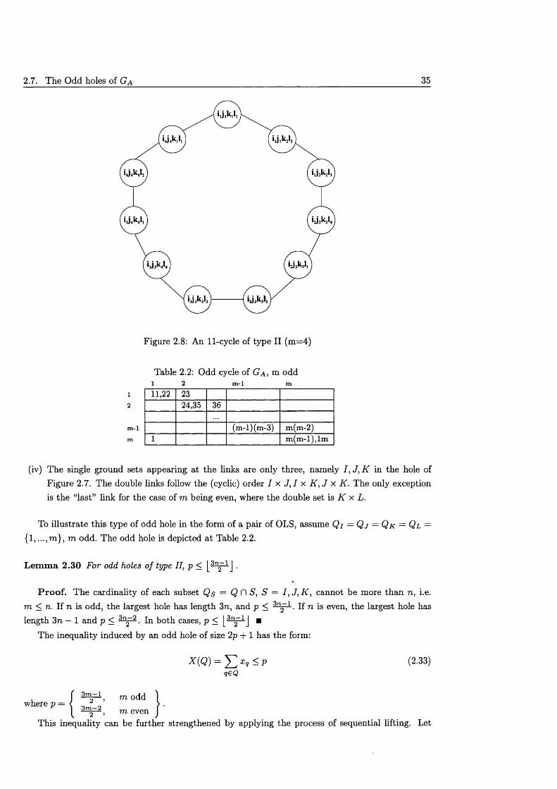
2.7. The Odd holes of Ga 35
Figure 2.8: An 11-cycle of type II (m=4)
Table 2.2: Odd cycle of Ga , ni odd1 2 m -l m
1 11,22 232 24,35 36
m -l
nii-H1JS, m(m-2)m 1 m (m -l) , lm
(iv) The single ground sets appearing at the links are only three, namely I , J ,K in the hole of Figure 2.7. The double links follow the (cyclic) order I x J , I x K ,J x K. The only exception is the “last” link for the case of m being even, where the double set is K x L.
To illustrate this type of odd hole in the form of a pair of OLS, assume Q j — Q j — Qk = Ql — {1, ...,m }, m odd. The odd hole is depicted a t Table 2.2.
L em m a 2.30 For odd holes o f type II, p < .
P ro o f. The cardinality of each subset Q s = Q f l S, S — / , J , K , cannot be more than n, i.e.m < n. If n is odd, the largest hole has length 3n, and p < 3n2~1. If n is even, the largest hole haslength 3n — 1 and p < 3n~- . In both cases, p < [ 3n~1 j ■
The inequality induced by an odd hole of size 2p + 1 has the form:
X ( Q ) = J 2 ^ < P (2-33)
3 m —1where p = ' 2
m odd3m 2 m evenk 2
This inequality can be further strengthened by applying the process of sequential lifting. Let
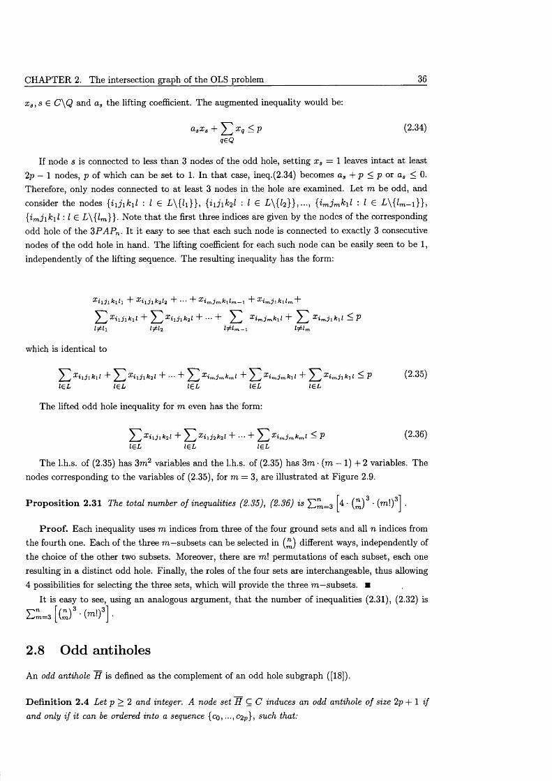
CHAPTER 2. The intersection graph of the OLS problem 36
x 3,s G C \Q and a3 the lifting coefficient. The augmented inequality would be:
asx s + x q < p (2-34)geQ
If node s is connected to less than 3 nodes of the odd hole, setting x s = 1 leaves intact at least 2p — 1 nodes, p of which can be set to 1. In that case, ineq.(2.34) becomes as + p < p or as < 0 . Therefore, only nodes connected to at least 3 nodes in the hole are examined. Let m be odd, and consider the nodes { i \ j \ k \ l : I G L\{Zi}}, { i i j iM : I £ L \{ /2}}, •••, {im3mk\l : I G L \{ /m_i}},
: I G L \{ lm }}- Note th a t the first three indices are given by the nodes of the corresponding odd hole of the 3P A P n . It it easy to see th a t each such node is connected to exactly 3 consecutive nodes of the odd hole in hand. The lifting coefficient for each such node can be easily seen to be 1, independently of the lifting sequence. The resulting inequality has the form:
X i \ j \ k i l \ 4" X i \ j l k 2l 2 4” 4“ X i m j m k l l m — l 4" X i m j l k i l m A ’
^ 1 4" ^ x h j i k 2 l 4" + y 4“ ^ ] x i m j i k i l < P
which is identical to
T . 1 x i\i\k2l 4" ••• 4- ^ x imjrnkml 4- ^ < V (2.35)l£L 1&L l£Lt
The lifted odd hole inequality for ra even has the form:
y>2x iijik2l + ^ 2 ,x n j2k2l 4- ... + ^ 2 x imjmkml < P (2.36)l£L l£L l£L
The l.h.s. of (2.35) has 3m2 variables and the l.h.s. of (2.35) has 3m • (m — 1) + 2 variables. Thenodes corresponding to the variables of (2.35), for m = 3, are illustrated at Figure 2.9.
P ro p o s itio n 2.31 The total number of inequalities (2.35), (2.36) is Ylm=3 (m) 3 ' (m -)"
P ro o f. Each inequality uses m indices from three of the four ground sets and all n indices from the fourth one. Each of the three m —subsets can be selected in (^ ) different ways, independently of the choice of the other two subsets. Moreover, there are m! permutations of each subset, each one resulting in a distinct odd hole. Finally, the roles of the four sets are interchangeable, thus allowing 4 possibilities for selecting the three sets, which will provide the three m —subsets. ■
It is easy to see, using an analogous argument, th a t the number of inequalities (2.31), (2.32) is
E"=3fD 3-(>n!)r
2.8 Odd antiholes
An odd antihole H is defined as the complement of an odd hole subgraph ([18]).
D efin itio n 2.4 Let p > 2 and integer. A node set H C C induces an odd antihole of size 2p + 1 if and only if it can be ordered into a sequence { c q , . . . , C 2 P } , such that:
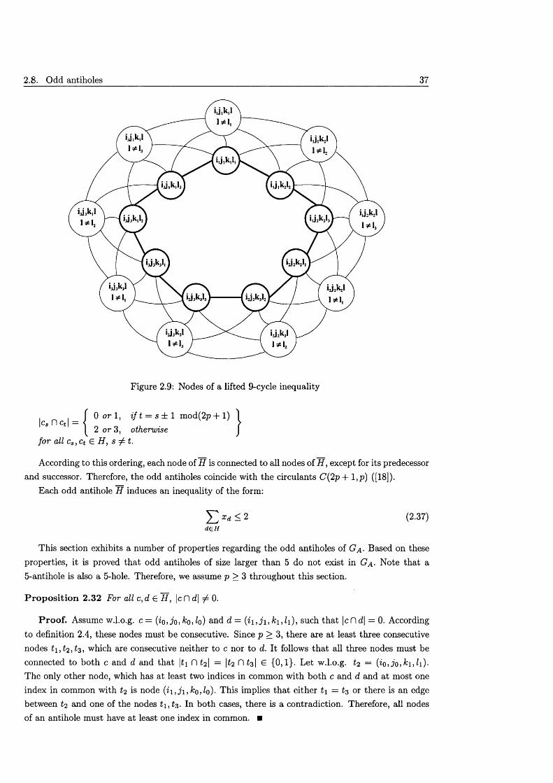
2.8. Odd antiholes 37
Figure 2.9: Nodes of a lifted 9-cycle inequality
\ca riCtl =O o r l , i f t = s ± 1 mod(2p + 1) 2 or 3, otherwise
for all cs ,ct G H, s ^ t.
According to this ordering, each node of H is connected to all nodes of H , except for its predecessor and successor. Therefore, the odd antiholes coincide with the circulants C{2p + 1 ,p) ([18]).
Each odd antihole H induces an inequality of the form:
^ Zd < 2 deH
(2.37)
This section exhibits a number of properties regarding the odd antiholes of G a - Based on these properties, it is proved th a t odd antiholes of size larger than 5 do not exist in G a - Note that a 5-antihole is also a 5-hole. Therefore, we assume p > 3 throughout this section.
P ro p o s itio n 2.32 For all c, d € H , \cf]d\ ^ 0.
P ro o f. Assume w.l.o.g. c = (io,jo> &(bfo) and d — { i i , j i , k i , l i ) } such th a t |cDd| = 0. According to definition 2.4, these nodes must be consecutive. Since p > 3, there are a t least three consecutive nodes which are consecutive neither to c nor to d. It follows th a t all three nodes must beconnected to both c and d and th a t |ti fl ^1 = 1 2 O 31 € {0,1}. Let w.l.o.g. t 2 = {io, jo,ki , l i ) . The only other node, which has at least two indices in common with both c and d and a t most one index in common with t 2 is node («i, j i , ko, lo). This implies th a t either t \ = £3 or there is an edge between £2 and one of the nodes £1, £3. In both cases, there is a contradiction. Therefore, all nodes of an antihole must have at least one index in common. ■
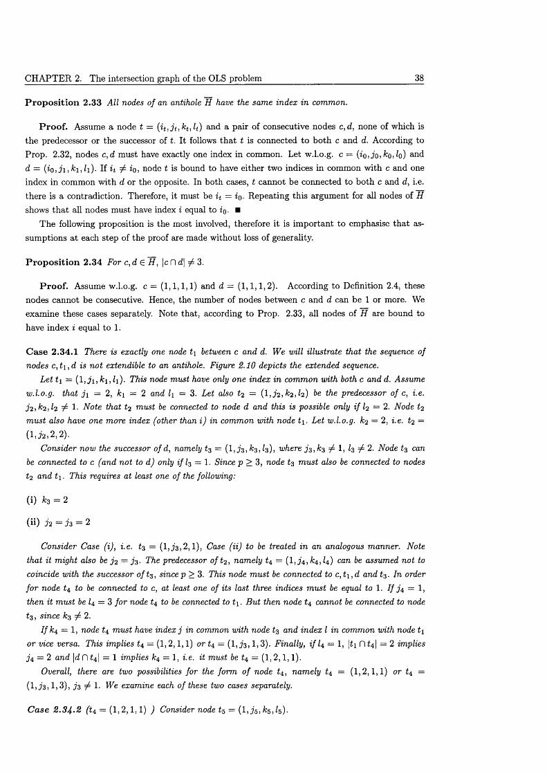
CHAPTER 2. The intersection graph of the OLS problem 38
P ro p o s i t io n 2.33 All nodes of an antihole H have the same index in common.
P ro o f . Assume a node t = ( i t , j t , k t ,h) and a pair of consecutive nodes c,d, none of which is the predecessor or the successor of t. It follows th a t t is connected to both c and d. According to Prop. 2.32, nodes c,d must have exactly one index in common. Let w.l.o.g. c = (io, jo, ko, lo) and d = ( io , j i , k i , l i ) . If i t 7 io, node t is bound to have either two indices in common with c and one index in common with d or the opposite. In both cases, t cannot be connected to both c and d, i.e. there is a contradiction. Therefore, it must be it = io- Repeating this argument for all nodes of H shows th a t all nodes must have index i equal to io- ■
The following proposition is the most involved, therefore it is im portant to emphasise th a t assumptions a t each step of the proof are made without loss of generality.
P ro p o s i t io n 2.34 For c,d G H, \c n d\ ^ 3.
P ro o f . Assume w.l.o.g. c = (1,1,1,1) and d = (1 ,1 ,1 ,2). According to Definition 2.4, these nodes cannot be consecutive. Hence, the number of nodes between c and d can be 1 or more. We examine these cases separately. Note that, according to Prop. 2.33, all nodes of H are bound to have index i equal to 1.
C ase 2.34.1 There is exactly one node t\ between c and d. We will illustrate that the sequence of nodes c, £i ,d is not extendible to an antihole. Figure 2.10 depicts the extended sequence.
Let t\ = This node must have only one index in common with both c and d. Assumew.l.o.g. that j \ = 2, ki = 2 and li = 3. Let also £2 = (1,.72, &2, k ) be the predecessor of c, i.e. j 2 >k2 , h 7 1- Note that £2 must be connected to node d and this is possible only i f I2 = 2. Node £2 must also have one more index (other than i) in common with node t\ . Let w.l.o.g. ^2 = 2, i.e. £2 =(1,J2, 2, 2).
Consider now the successor of d, namely £3 = ( l , j z , £3, £3), where j 3 ,kz ^ 1 , I3 ^ 2. Node £3 can be connected to c (and not to d) only i f lz = 1. Since p > 3, node £3 m ust also be connected to nodes £2 and £1. This requires at least one of the following:
(i) k3 = 2
(ii) h = h = 2
Consider Case (i), i.e. £3 = (1,.7*3 , 2,1), Case (ii) to be treated in an analogous manner. Note that it might also be j 2 = jz- The predecessor o f t 2 , namely £4 = (1, j 4, £ 4 , l4) can be assumed not to coincide with the successor of tz, since p > 3. This node m ust be connected to c , t i , d and £3. In order for node £4 to be connected to c, at least one of its last three indices m ust be equal to 1. I f j 4 — 1, then it must be l4 = 3 for node £4 to be connected to t \ . But then node £ 4 cannot be connected to node £3, since kz ^ 2.
I f k 4 = 1, node £4 must have index j in common with node £3 and index I in common with node t\ or vice versa. This implies £4 = (1 ,2 ,1 ,1) or £4 = (1, jz , 1,3). Finally, i f l4 = 1, |£i D £4! = 2 implies j 4 = 2 and \d fl £4! = 1 implies k4 = 1, i.e. it must be £4 = (1, 2, 1, 1).
Overall, there are two possibilities for the form o f node £ 4 , namely £4 = (1 ,2 ,1, 1) or t 4 = (1,J3, 1,3), jz 7 1- We examine each of these two cases separately.
Case 2.34-2 (t4 = (1,2,1,1) ) Consider node £5 = (1, , A:s, Z5).
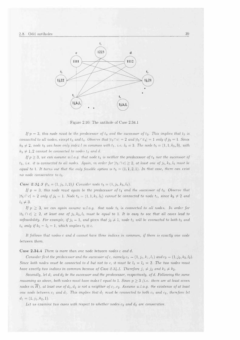
2.8. Odd antiholes 39
t,1223
11121111
Figure 2 .10: The antihole of Case 2 .34.1
I f p = 3 , t h i s n o d e m u s t b e t h e p r e d e c e s s o r o f £4 a n d t h e s u c c e s s o r o f £3. T h i s i m p l i e s t h a t £5 i s
c o n n e c t e d t o a l l n o d e s , e x c e p t £3 and £4. O b s e r v e t h a t |^ 5 flc | = 2 a n d |£s D£41 = 1 o n l y i f = 1 . S i n c e
k 5 ^ 2 , n o d e £5 c a n h a v e o n l y i n d e x I i n c o m m o n w i t h t \ , i . e . £5 = 3 . T h e n o d e £5 = (1, 1, ^ 5 ,3 ) , w i t h
& 5 ^ 1 , 2 c a n n o t b e c o n n e c t e d t o n o d e s £ 2 a n d d .
I f P > 3 , w e c a n a s s u m e w . l . o . g . t h a t n o d e £5 i s n e i t h e r t h e p r e d e c e s s o r o f £4 n o r t h e s u c c e s s o r o f
£3, i . e . i t i s c o n n e c t e d t o a l l n o d e s . A g a i n , i n o r d e r f o r |£s Dc| > 2 , a t l e a s t o n e o f js, ^ ,£5 m u s t b e
e q u a l t o 1. I t t u r n s o u t t h a t t h e o n l y f e a s i b l e o p t i o n i s £5 = (1, 1 , 2 , 1). I n t h a t c a s e , t h e r e c a n e x i s t
n o n o d e c o n s e c u t i v e t o £5.
C a s e 2 . 3 4 - 3 ( t $ = (1 , J3 , 1,3)^ C o n s i d e r n o d e £5 = (1, j& , £ 5 , £5).I f p = 3 , t h i s n o d e m u s t a g a i n b e t h e p r e d e c e s s o r o f £4 a n d t h e s u c c e s s o r o f £3. O b s e r v e t h a t
(£5 H c| = 2 o n l y i f = 1. N o d e £5 = (1, l , k ^ , £5) c a n n o t b e c o n n e c t e d t o n o d e t \ , s i n c e 7 2 a n d
* 5 ^ 3 .
I f p > 3, w e c a n a g a i n a s s u m e w . l . o . g . t h a t n o d e £5 i s c o n n e c t e d t o a l l n o d e s . I n o r d e r f o r
|£5 fl c| > 2 , a t l e a s t o n e o f ^5,^5, £5 m u s t b e e q u a l t o 1. I t i s e a s y t o s e e t h a t a l l c a s e s l e a d t o
i n f e a s i b i l i t y . F o r e x a m p l e , i f j’5 = 1, a n d g i v e n t h a t j 3 ^ 1, n o d e £5 w i l l b e c o n n e c t e d t o b o t h £3 a n d
£4 o n l y i f k $ = £5 = 1, w h i c h i m p l i e s £5 = c.
I t f o l l o w s t h a t n o d e s c a n d d c a n n o t h a v e t h r e e i n d i c e s i n c o m m o n , i f t h e r e i s e x a c t l y o n e n o d e
b e t w e e n t h e m .
C ase 2.34.4 T h e r e i s m o r e t h a n o n e n o d e b e t w e e n n o d e s c a n d d .
C o n s i d e r f i r s t t h e p r e d e c e s s o r a n d t h e s u c c e s s o r o f c , n a m e l y c \ = (1, j \ , k \ , l\) a n d c 2 = (1,J2> ^2 ^ 2 )-
S i n c e b o t h n o d e s m u s t b e c o n n e c t e d t o d b u t n o t t o c , i t m u s t b e l \ = I2 = 2 . T h e t w o n o d e s m u s t
h a v e e x a c t l y t w o i n d i c e s i n c o m m o n b e c a u s e o f C a s e 2 . 3 4 - 1 • T h e r e f o r e j i ^ j ’2 a n d k \ ^ /C2 •
S e c o n d l y , l e t d \ a n d c?2 b e t h e s u c c e s s o r a n d t h e p r e d e c e s s o r , r e s p e c t i v e l y , o f d . F o l l o w i n g t h e s a m e
r e a s o n i n g a s a b o v e , b o t h n o d e s m u s t h a v e i n d e x I e q u a l t o 1 . S i n c e p > 3 ( i . e . t h e r e a r e a t l e a s t s e v e n
n o d e s i n H ), a t l e a s t o n e o f d \ , d 2 i s n o t a n e i g h b o r o f C \ ,C 2 - A s s u m e w . l . o . g . t h e e x i s t e n c e o f a t l e a s t
o n e n o d e b e t w e e n c \ a n d d \ . T h i s i m p l i e s t h a t d \ m u s t b e c o n n e c t e d t o b o t h c \ a n d C2 , t h e r e f o r e l e t
d \ = { l , j i , k 2 , l ) .
L e t u s e x a m i n e t w o c a s e s w i t h r e s p e c t t o w h e t h e r n o d e s C2 a n d d 2 a r e c o n s e c u t i v e .
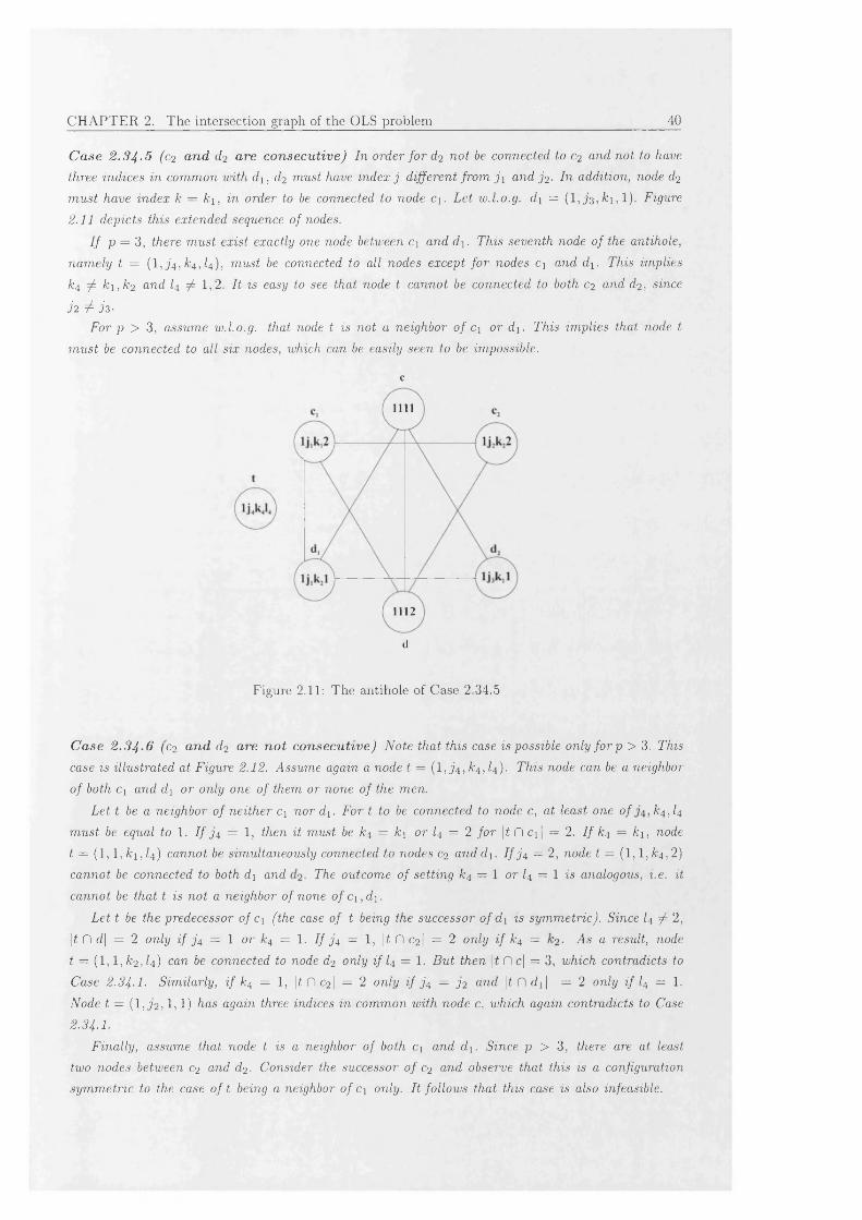
CHAPTER 2. The intersection graph of the OLS problem 40
C ase 2 .34-5 (c 2 and d2 ore consecutive) I n o r d e r f o r <i2 n o t b e c o n n e c t e d t o C2 a n d n o t t o h a v e
t h r e e i n d i c e s i n c o m m o n w i t h d \ , d2 m u s t h a v e i n d e x j d i f f e r e n t f r o m j \ a n d jf2 . l a a d d i t i o n , n o d e d2
m ust h a v e i n d e x k = k \ , i n o r d e r t o b e c o n n e c t e d t o n o d e c \ . L e t w . l . o . g . d \ = (1 , J3 , fci, 1). F i g u r e
2.11 d e p i c t s t h i s e x t e n d e d s e q u e n c e o f n o d e s .
I f p = 3 , t h e r e m u s t e x i s t e x a c t l y o n e n o d e b e t w e e n c \ a n d d \ . T h i s s e v e n t h n o d e o f t h e a n t i h o l e ,
n a m e l y t = ( l , j -4 , k $ , I4), m u s t b e c o n n e c t e d t o a l l n o d e s e x c e p t f o r n o d e s c \ a n d d \ . T h i s i m p l i e s
^ 4 7 k i , k 2 a n d I4 ^ 1 ,2 . I t i s e a s y t o s e e t h a t n o d e t c a n n o t b e c o n n e c t e d t o b o t h c2 a n d d2 , s i n c e
h ± h -F o r p > 3, a s s u m e w . l . o . g . t h a t n o d e t i s n o t a n e i g h b o r o f C\ o r d \ . T h i s i m p l i e s t h a t n o d e t
m u s t b e c o n n e c t e d t o a l l s i x n o d e s , w h i c h c a n b e e a s i l y s e e n t o b e i m p o s s i b l e .
c
1111
1112
d
Figure 2.11: T he antihole o f C ase 2.34.5
C ase 2 .34-6 (c2 and d2 are n o t consecutive) N o t e t h a t t h i s c a s e i s p o s s i b l e o n l y f o r p > 3. T h i s
c a s e i s i l l u s t r a t e d a t F i g u r e 2 . 1 2 . A s s u m e a g a i n a n o d e t = (1, j'4 , £ 4 , £4 ). T h i s n o d e c a n b e a n e i g h b o r
o f b o t h C \ a n d d \ o r o n l y o n e o f t h e m o r n o n e o f t h e m e n .
L e t t b e a n e i g h b o r o f n e i t h e r c \ n o r d \ . F o r t t o b e c o n n e c t e d t o n o d e c, a t l e a s t o n e o f k4 J 4
m u s t b e e q u a l t o 1 . I f 34 = 1, t h e n i t m u s t b e /C4 = k\ o r I4 = 2 f o r \ t Pi c i | = 2. I f k 4 = k \ , n o d e
t = ( 1 , 1 , fc j ,£4 ) c a n n o t b e s i m u l t a n e o u s l y c o n n e c t e d t o n o d e s c2 a n d d \ . / / j '4 = 2 , n o d e t = ( 1 , 1 , £ 4 , 2 )
c a n n o t b e c o n n e c t e d t o b o t h d \ a n d T h e o u t c o m e o f s e t t i n g ^ 4 = 1 o r I4 = 1 i s a n a l o g o u s , i . e . i t
c a n n o t b e t h a t t i s n o t a n e i g h b o r o f n o n e o f c \ , d \ .
Let t be the predecessor of c\ (the case of t being the successor of d\ is symmetric). Since I4 ^ 2,
\t n d\ = 2 only if j 4 = 1 or /C4 = 1. I f 3 4 = 1, \t fl c2| = 2 only i f /C4 = As a result, node t = (1,1, k 2 , 1 4 ) can be connected to node d2 only if I4 = 1. But then \t fl c| = 3, which contradicts to Case 2 . 3 4 . 1 • Similarly, if ^4 = 1, |£ fl c2| = 2 only i/jf'4 = 3 2 and |£nc?i| = 2 only if I4 = 1. Node t = ( l , j 2) 1) 1) has again three indices in common with node c, which again contradicts to Case2 . 3 4 . 1 .
F i n a l l y , a s s u m e t h a t n o d e t i s a n e i g h b o r o f b o t h Ci a n d d \ . S i n c e p > 3, t h e r e a r e a t l e a s t
t w o n o d e s b e t w e e n c2 a n d d2 ■ C o n s i d e r t h e s u c c e s s o r o f c2 a n d o b s e r v e t h a t t h i s i s a c o n f i g u r a t i o n
s y m m e t r i c t o t h e c a s e o f t b e i n g a n e i g h b o r o f c \ o n l y . I t f o l l o w s t h a t t h i s c a s e i s a l s o i n f e a s i b l e .
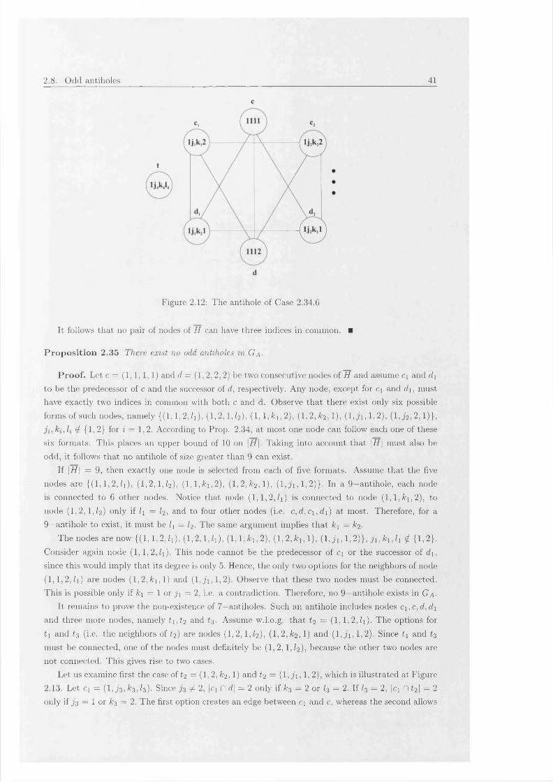
2.8. Odd antiholes 41
Figure 2.12: T he antihole o f C ase 2 .34 .6
It follow s th at no pair o f nodes of H can have three indices in com m on. ■
P ro p o s itio n 2.35 T h e r e e x i s t n o o d d a n t i h o l e s i n G a -
P ro o f. Let c = ( 1 ,1 ,1 ,1 ) and d = (1 ,2 ,2 ,2 ) be tw o con secu tive nodes o f H and assum e c \ and d \
to b e th e predecessor o f c and the successor o f d , respectively . A ny n ode, excep t for c \ and d \ , m ust
have ex a c tly tw o ind ices in com m on w ith both c and d. O bserve th a t there ex ist on ly six possib le
form s o f such nodes, nam ely { ( l , l , 2 ,Z i ) , ( 1 , 2 , 1 , Z2), ( l , l , f c i , 2 ) , ( l ,2 , f c 2 , l ) , ( 1 , j i , 1 , 2 ), (1 , j 2 , 2 , 1 ) } ,
& { 1 )2 } for i = 1 ,2 . A ccording to Prop. 2.34, a t m ost on e n ode can follow each one o f these
six form ats. T h is p laces an upper bound of 10 on \H\. T aking in to accou nt th a t \H\ m ust also be
odd , it follow s th a t no antihole o f size greater than 9 can ex ist.
If \ H \ = 9 , th en ex a ctly one node is selected from each o f five form ats. A ssum e th a t th e five
nod es are { ( 1 ,1 ,2 , Zi), ( 1 ,2 ,1 ,Z2), ( l , l , f c i , 2 ) , (1 ,2 , A:2,1 ) , ( l , j i , l , 2 ) } . In a 9 —antihole, each node
is connected to 6 o ther nodes. N otice th at node ( 1 ,1 ,2 , l i ) is conn ected to n ode ( 1 ,1 , A i,2 ) , to
node (1 ,2 ,1 , Z2) only if l \ = Z2, and to four other n odes (i.e. c, d , c \ , d i ) a t m ost. Therefore, for a
9 —antihole to ex ist, it m ust be l i = l 2 . T he sam e argum ent im plies th a t k i = k 2 .
T h e nodes are now { ( 1 , 1 , 2 ^ ) , ( 1 ,2 ,1 , Zi), (1 ,1 , A*, 2), ( l , 2 , f c i , l ) , (1 , j u 1 ,2 ) } , j lt kit h £ { 1 ,2 } .
C onsider again n od e ( 1 , 1 , 2 , Zi). T h is node cannot b e th e predecessor o f c \ or th e successor o f d \ ,
since th is w ould im ply th a t its degree is only 5. H ence, th e on ly tw o op tion s for th e neighbors o f node
( 1 , 1 , 2 ,Zi) are nodes ( l , 2 ,& i , l ) and ( l , j i , 1 ,2 ). O bserve th a t th ese tw o nodes m ust be connected .
T h is is p ossib le on ly if k \ = 1 or j \ = 2, i.e. a contrad iction . T herefore, no 9 —antihole ex ists in G a -
It rem ains to prove th e non-existence o f 7 —antiholes. Such an antihole includes nodes c i ,c , d , d \
and three m ore nodes, nam ely t \ , t 2 and £3 . A ssum e w .l.o .g . th a t £ 2 = (1 , l ,2 ,Z i) . T h e op tion s for
t \ and £ 3 (i.e. th e neighbors of £2) are nodes (1 ,2 , l , / 2), ( 1 ,2 , A2 , 1 ) and ( l , j i , 1 ,2 ) . S ince £ 1 and £ 3
m ust b e connected , one o f th e nodes m ust defin itely b e ( 1 , 2 , 1 , l 2 ) , b ecau se th e other tw o nodes are
not connected . T h is gives rise to two cases.
Let us exam ine first th e case o f £2 = (1 ,2 , A:2 ,1 ) and t 2 = (1, j \ , 1 ,2 ) , w hich is illu strated at F igure
2.13. L et c \ = ( 1 ,^3 , fc3 ,Z3). Since ± 2, |c i f ld | = 2 on ly if k 3 = 2 or Z3 = 2. If Z3 = 2, \ c \ f l£ 2 | = 2
on ly if j 3 = 1 or k ^ = 2. T h e first option creates an ed ge b etw een c \ and c, w hereas the second allow s
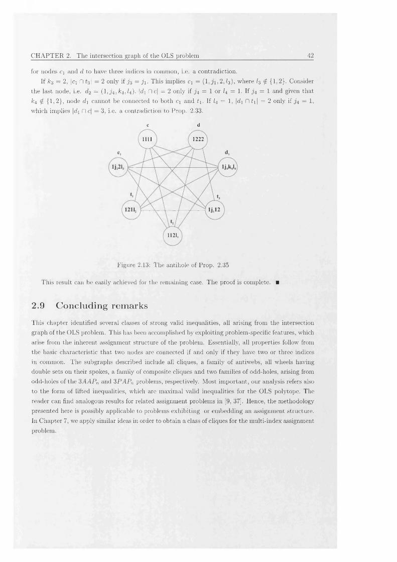
CHAPTER 2. The intersection graph of the OLS problem 42
for n od es c \ and d to have three indices in com m on, i.e. a contrad iction .
If & 3 = 2, |c i f l t 3 | = 2 on ly if jr'3 = j \ . T his im plies c\ = ( 1 , , 2 , Z3 ) , w here Z3 £ {1,2}. Consider
th e la st node, i.e. = ( 1 ,^ 4 , ^4 , 4 )- Mi fl c| = 2 on ly if j '4 = 1 or I4 = 1. If jf'4 = 1 and given that
k 4 {1 ,2} , node d \ can not b e connected to b oth c \ and t \ . If Z4 = 1, |d i f l t i | = 2 on ly if = 1,
w hich im plies \ d i fl c\ = 3, i.e. a contradiction to Prop. 2.33.
c d
12221111
1121,
F igure 2.13: T h e antihole o f Prop. 2 .35
T h is result can be easily achieved for th e rem aining case. T h e proof is com plete. ■
2.9 C oncluding remarks
T h is chapter identified several classes o f strong valid inequalities, a ll arising from th e in tersection
graph o f th e OLS problem . T h is has been accom plished by exp lo itin g problem -specific features, which
arise from th e inherent assignm ent structure o f the problem . E ssentia lly , all properties follow from
th e basic ch aracteristic th a t tw o nodes are con nected if and on ly if th ey have tw o or three indices
in com m on. T h e subgraphs described include all cliques, a fam ily o f antiw ebs, all w heels having
double se ts on their spokes, a fam ily of com posite cliques and tw o fam ilies o f odd-holes, arising from
od d -holes o f th e 3 A A P n and 3 P A P n problem s, respectively. M ost im p ortant, our analysis refers also
to th e form o f lifted inequalities, w hich are m axim al valid in eq u a lities for th e OLS p olytop e. T he
reader can find analogous resu lts for related assignm ent problem s in [9, 37]. H ence, th e m ethodology
presented here is p ossib ly applicable to problem s ex h ib itin g or em bedd in g an assignm ent structure.
In C hapter 7, we apply sim ilar ideas in order to ob ta in a class o f cliques for th e m ulti-index assignm ent
problem .
Chapter 3
Polyhedral characterisation o f the OLS polytope
3.1 Introduction and preliminaries
This chapter presents a polyhedral characterisation of the OLS problem. The dimension of the associated polytope P j is established and families of valid inequalities presented in the previous chapter are further analysed from a polyhedral perspective. This amounts to examining which of these inequalities are facets of P j, identifying their Chvatal rank and providing separation algorithms of low complexity.
We briefly summarize some basic concepts and definitions of polyhedral theory ([47, 74, 68]). A polyhedron is the intersection of a finite number of half spaces. A polytope is a bounded polyhedron. A polytope P is of dimension n, denoted as dim (P) = n, if it contains n + 1 affinely independent points. By convention, if P — 0 then dim (P) = —1. If P = {x G Rn : P x = b ,B ~ x < b~ } then
dim(P) = n — ra n k(B ) (3.1)
where B and B ~ denote the matrix of coefficients of equality and “less-than-or-equal-to” type inequality constraints respectively, while b and b ~ denote the corresponding right-hand side vectors for the linear system defining P . An inequality ax < Oq is called valid for P, if it is satisfied by all x G P . It is called supporting, if it is valid and there exist x G P satisfying ax = ao- The set of points, which satisfy ax < ao as equality (F = {x G P : ax = ao}), is called a face of P . A face F of a polytope P is said to be improper, if ax = ao for all x G P . A proper, non-empty face F of P is called a facet, if dim (P) = dim (P) — 1. Facets are im portant, since they provide a minimal inequality representation of a polyhedron. Our main interest in this chapter is in the facets of the convex hull P / of integer points in P l , defined in Section 2.1. Conditions (c) and (d) of the following theorem usually provide the two basic tools for proving th a t a given inequality ax < oq defines a facet.
T h e o re m 3.1 (see [74, Theorem 3.16J)Let P C ]Rn be a polyhedron and assume that B is a real valued r a x n matrix and b G Rm such that P = {x G Rn : B x = b , B ~ x < b ~ } where B = (B , B ~ ) t and b = {b , b~) T . Let F be a non-empty face o f P , then the following statements are equivalent:
(a) F is a facet o f P .
43
CH APTER 3. Polyhedral characterisation of the OLS poly tope 44
(b) F is a maximal proper face of P.
(c) dim(F) — dim(P) — 1.
(d) There exists an inequality ax < ao valid with respect to P with the following three properties:
(i) F = {x £ P : ax = ao}.
(ii) There exists x E P with ax < ao, i.e. the inequality is proper
I f any other inequality dx < do, valid with respect to P satisfies F = {x £ P : dx = do}, then (d,do) can be expressed as a linear (affine) combination o f (B = ,b=) and (a,ao).
Condition (d) has been used in [2] to prove th a t cliques of type II and III (Section 2.3) inducefacets of Pj. In this chapter, we apply the same approach to prove that composite clique inequalitiesalso define facets of Pi (Section 2.6). We also apply condition (d) to prove th a t odd cycles of type II (Section 2.7.2) induce facets of the Latin square polytope or 3P A P n ([37]). The dimension of Pj is also established in a similar manner. A similar approach has been used for establishing the dimension and facet-defining inequalities of the 3A A P n , and 3P A P n polytopes in [9] and [37], respectively (Section 2.1).
Recall the IP model for the OLS problem and the definitions of polytopes P i , Pi and Pj, from Section 2.1. The following remark will be used for establishing the dimension of Pj, and P j.
R e m a rk 3.1 Constraints (2.1), (2.2), (2.3), for a given value o f the I index, are equivalent to the constraints of a 3A A P n .
Let us first discuss some properties of Pj. Since the OLS packing polytope P j is a special case of Ps p , Pi shares the following properties of Psp ([18]):
(i) Pi is full-dimensional, i.e. dim (P i) = n 4. The n 4 + 1 independent points of P j are the zerovector and all the n 4 unit vectors.
(ii) Pj is down monotone, i.e. x E Pi => y E Pi for all y such th a t 0 < y < x.
(iii) The non-negativity constraints Xijki > 0 define facets of P j.
Although we know quite a few things about the facial structure of P j, the same cannot be said with respect to P j. Since P j is a face of P, we know th a t dim(Pj ) < dim (P i). However, the structure of Pi presents irregularities th a t do not appear in P j. For example, we know th a t P j = 0 for n = 2 and n = 6. P f = 0 can be easily verified, since there are only two Latin squares for n = 2. As stated previously, P f = 0 was proven in [81]. Fortunately, P f ^ 0 for n ^ 2,6 as shown in [20] (see also [60, Theorem 2.9]).
Moreover, a complete characterisation of all the facets defining a polytope arising from a 0 — 1 IP is possible only if M V —CoMV, as analysed in [68, p. 139-141]. Hence, the complexity of the problem restricts any attem pt to achieve a complete description of the convex hull of integer points. A partial polyhedral description of the OLS polytope appears to be the only reasonable aim. Even such a result, however, can be sufficient in order to solve the problem with a cutting plane algorithm incorporated within a Branch & Cut algorithmic framework.
The remainder of this chapter proceeds as follows. Section 3.2 identifies the dimension of both Pj, and P j. Section 3.3 examines which of the constraints defining Pj, define facets of Pj. The following
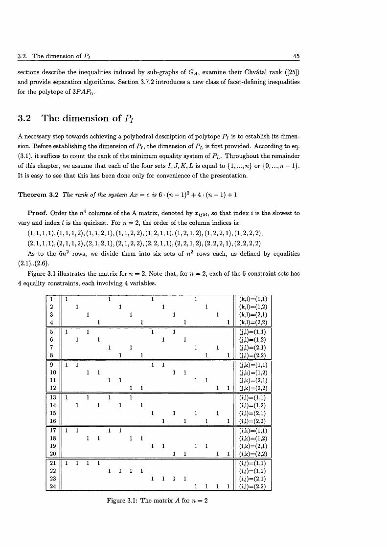
3.2. The dimension of Pj 45
sections describe the inequalities induced by sub-graphs of G a , examine their Chvatal rank ([25]) and provide separation algorithms. Section 3.7.2 introduces a new class of facet-defining inequalities for the polytope of 3P A P n .
3.2 The dimension of Pj
A necessary step towards achieving a polyhedral description of polytope Pj is to establish its dimension. Before establishing the dimension of P j, the dimension of Pl is first provided. According to eq.(3.1), it suffices to count the rank of the minimum equality system of Pl . Throughout the remainder of this chapter, we assume th a t each of the four sets / , J, K , L is equal to {1,..., n} or {0,..., n — 1}. It is easy to see th a t this has been done only for convenience of the presentation.
T h eo rem 3.2 The rank of the system A x = e is 6 • (n — l )2 + 4 • (n — 1) + 1
P ro o f. Order the n4 columns of the A matrix, denoted by Xijki, so th a t index i is the slowest to vary and index I is the quickest. For n = 2, the order of the column indices is:
( 1, 1 , 1 , 1), ( 1 , 1 , 1 , 2), ( 1 , 1 , 2 , 1), ( 1 , 1 , 2 , 2), ( 1 , 2 , 1 , 1), ( 1 , 2 , 1 , 2 ), ( 1 , 2 , 2 , 1), ( 1 , 2 , 2 , 2),
(2 , 1 , 1 , 1), (2 , 1 , 1 , 2), (2 , 1 , 2 , 1), (2 , 1 , 2 , 2 ), (2 , 2 , 1 , 1), (2 , 2 , 1 , 2 ), (2 , 2 , 2 , 1), ( 2 , 2 , 2 , 2)
As to the 6n 2 rows, we divide them into six sets of n 2 rows each, as defined by equalities(2.1)..(2.6).
Figure 3.1 illustrates the matrix for n — 2. Note that, for n — 2, each of the 6 constraint sets has 4 equality constraints, each involving 4 variables.
1 1 1 1 1 (k ,l)= ( l , l )2 1 1 1 1 (k,l)=(l,2)3 1 1 1 1 (k,l)=(2,l)4 1 1 1 1 (k,l)=(2,2)
5 1 1 1 1 (j , l)= ( l , l )6 1 1 1 1 G,i)=(i,2)7 1 1 1 1 G,l)=(2,l)8 1 1 1 1 (j>l)=(2,2)9 1 1 1 1 (j ,k )= (l ,l)10 1 1 1 1 (j)k)=(l,2)11 1 1 1 1 (j>k)=(2,l)12 1 1 1 1 G,k)=(2,2)
13 1 1 1 1 (i>l)=(l>l)14 1 1 1 1 (i,l)=(l,2)15 1 1 1 1 (i,l)=(2,l)16 1 1 1 1 (i,l)=(2,2)17 1 1 1 1 ( i ,k )= (l , l)18 1 1 1 1 (i,k)=(l,2)19 1 1 1 1 (i,k)=(2,l)20 1 1 1 1 (i,k)=(2,2)
21 1 1 1 1 ( i j ) = ( l , l )22 1 1 1 1 ( i j )= ( l ,2 )23 1 1 1 1 (i,j)=(2,l)24 1 1 1 1 (iJ)=(2,2)
Figure 3.1: The m atrix A for n = 2
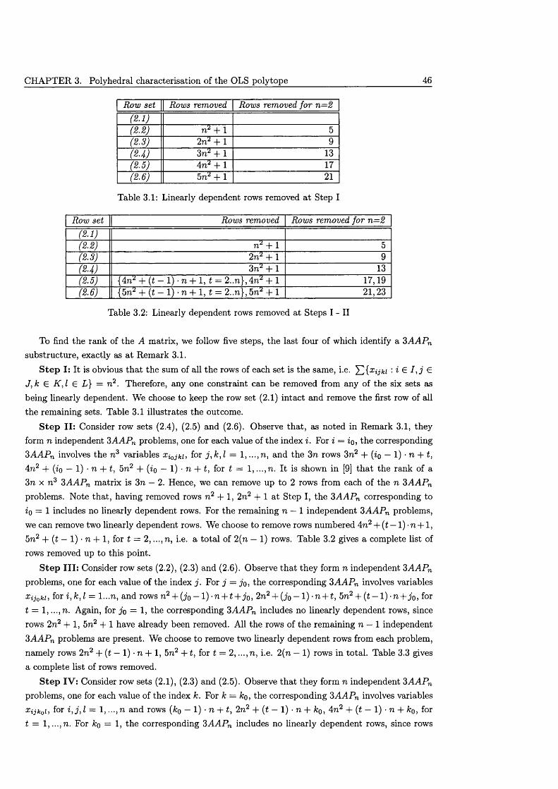
CHAPTER 3. Polyhedral characterisation of the OLS polytope 46
Row set Rows removed Rows removed for n=2(2 . 1 )(2 .2 ) 712 + 1 5(2 .S) 2ti2 + 1 9( U ) 3n2 + 1 13(2.5) 4712 + 1 17(2 . 6 ) 5712 + 1 21
Table 3.1: Linearly dependent rows removed a t Step I
Row set Rows removed Rows removed for n=2(2 . 1 )(2 .2 ) 712 + 1 5(2.3) 2 n 2 + l 9(24) 3712 + 1 13(2.5) {4712 + (t — 1) • 71 + 1, t = 2..7l}, 4ti2 + 1 17,19(2 . 6 ) {5712 + (t — 1) • 71 + 1, t = 2..7l}, 5712 + 1 21 ,23
Table 3.2: Linearly dependent rows removed at Steps I - II
To find the rank of the A matrix, we follow five steps, the last four of which identify a 3A A P n substructure, exactly as a t Remark 3.1.
S tep I: It is obvious th a t the sum of all the rows of each set is the same, i.e. ^2{xijki : i G I , j G
J , k G K, I G L} = n 2. Therefore, any one constraint can be removed from any of the six sets as being linearly dependent. We choose to keep the row set (2.1) intact and remove the first row of all the remaining sets. Table 3.1 illustrates the outcome.
S te p II : Consider row sets (2.4), (2.5) and (2.6). Observe that, as noted in Remark 3.1, they form n independent 3A A P n problems, one for each value of the index i. For i = io, the corresponding 3 A A P n involves the n 3 variables x iojki, for j , k , l = 1, ...,n , and the 3n rows 3n2 + (io — 1) • n + t, 4n 2 + (io — 1) • n + t, 5n 2 + (io — 1) • n + t, for t = 1, ...,7i. It is shown in [9] th a t the rank of a 3n x n 3 3A A P n matrix is 3n — 2. Hence, we can remove up to 2 rows from each of the n 3A A P n problems. Note that, having removed rows n 2 + 1, 2n2 + 1 at Step I, the 3A A P n corresponding to io = 1 includes no linearly dependent rows. For the remaining n — 1 independent 3A A P n problems, we can remove two linearly dependent rows. We choose to remove rows numbered 4n2 + (t — 1) • n + 1 , 5n 2 + (t — 1) • n + 1, for t = 2 ,..., n, i.e. a total of 2(n — 1) rows. Table 3.2 gives a complete list of rows removed up to this point.
S te p I I I : Consider row sets (2.2), (2.3) and (2.6). Observe th a t they form n independent 3A A P n problems, one for each value of the index j . For j = jo, the corresponding 3A A P n involves variables Xijoki, for i , k , l = l...n , and rows n 2 + (j 0 - 1) -n + t + jo, 2n2 + ( j o ~ l ) -n + t, 5n2 + ( t - 1) -n + jo, for t = 1, . . . , n. Again, for jo = 1, the corresponding 3A A P n includes no linearly dependent rows, since rows 27i2 + 1, 5n2 + 1 have already been removed. All the rows of the remaining n — 1 independent 3A A P n problems are present. We choose to remove two linearly dependent rows from each problem, namely rows 2n 2 + {t — 1) • n + 1, 57i2 + 1 , for t = 2,..., n, i.e. 2(71 — 1) rows in total. Table 3.3 gives a complete list of rows removed.
Step IV : Consider row sets (2.1), (2.3) and (2.5). Observe th a t they form n independent 3A A P n problems, one for each value of the index k. For k = ko, the corresponding 3A A P n involves variables Xijk0 i , f°r h = 1) and rows (k0 — 1) • n + t , 2n2 + (t — 1) • n + &o, 47i2 + (t — 1) • n + ko, for t = 1,..., 71. For ko = 1, the corresponding 3A A P n includes no linearly dependent rows, since rows
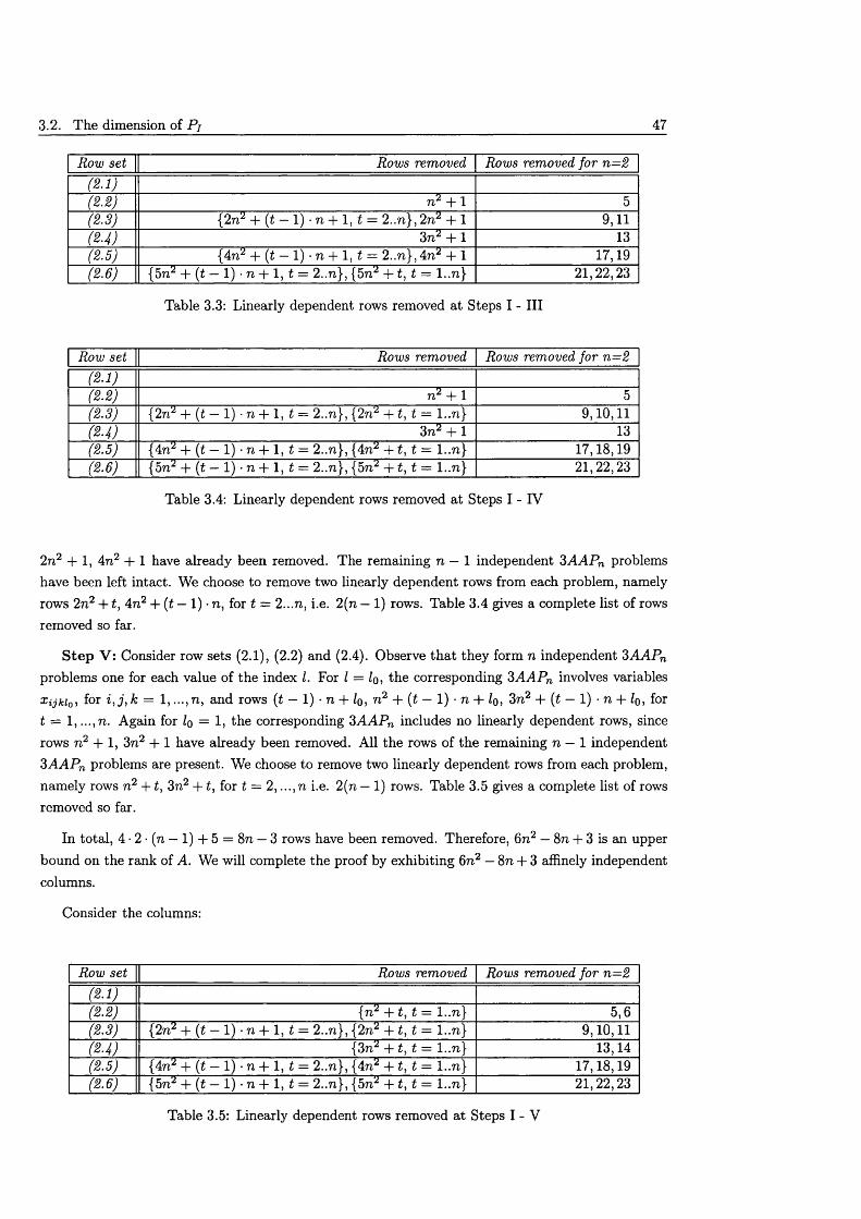
3.2. The dimension of Pi 47
Row set Rows removed Rows removed for n=2(2 .1 )(2 .2 ) n 2 + 1 5(2.3) {2n2 + (t — 1) ■ n + 1, t = 2..n}, 2n 2 + 1 9,11( U ) 3n2 + 1 13(2.5) {4n2 + {t — 1) ■ n + 1, t = 2 ..n},4n2 + 1 17,19(2 .6 ) {5n2 + (t — 1) • n + 1, t = 2..n}, {5n2 + 1, t = l..n} 21,22,23
Table 3.3: Linearly dependent rows removed at Steps I - III
Row set Rows removed Rows removed for n=2(2 .1 )(2 .2 ) n 2 + 1 5(2.3) {2n2 + (t — 1) • n + 1, t = 2..n}, {2n2 + t, t = l ..n} 9,10,11(2-4) 3 n 2 + 1 13(2.5) {4n2 + (£ — 1) ■ n 4 - 1, £ = 2..n}, (4n2 + £, £ = l..n} 17,18,19(2.6) {5n2 + (£ — 1) • n + 1, £ = 2..n}, {5n^+ £, £ = l..n} 21,22,23
Table 3.4: Linearly dependent rows removed at Steps I - IV
2n 2 + 1, 4n2 + 1 have already been removed. The remaining n — 1 independent 3AAPn problems have been left intact. We choose to remove two linearly dependent rows from each problem, namely rows 2n2 +£, 4n 2 + (£ — 1) • n, for £ = 2...n, i.e. 2(n — 1) rows. Table 3.4 gives a complete list of rows removed so far.
S te p V : Consider row sets (2.1), (2.2) and (2.4). Observe th a t they form n independent 3A A P n problems one for each value of the index I. For I = Iq, the corresponding 3AAP n involves variables Xijkio, f°r = 1) and rows (£ — 1) • n + Iq , n 2 + (£ — 1) • n + lo, 3n 2 + (£ — 1) • n + Iq , for £ = 1, ...,n . Again for Iq = 1, the corresponding 3A A P n includes no linearly dependent rows, since rows n2 + 1, 3n2 + 1 have already been removed. All the rows of the remaining n — 1 independent 3A A P n problems are present. We choose to remove two linearly dependent rows from each problem, namely rows n 2 +£, 3n2 + £, for £ = 2,..., n i.e. 2(n — 1) rows. Table 3.5 gives a complete list of rows removed so far.
In total, 4 • 2 • (n — 1) + 5 = 8n — 3 rows have been removed. Therefore, 6n 2 — 8n + 3 is an upper bound on the rank of A. We will complete the proof by exhibiting 6n 2 — 8n + 3 affinely independent columns.
Consider the columns:
Row set Rows removed Rows removed for n —2(2 .1 )(2 .2 ) [n 2 + £, £ = l..n} 5,6(2.3) {2n2 + (£ — 1) • n + 1, £ = 2..n}, {2n2 + £, £ = l..n} 9,10,11(2-4) {3n2 + £, £ = l..n} 13,14(2.5) {4n2 + (£ — 1) • n + 1, £ = 2..n}, {4n2 + £, £ = l..n} 17,18,19(2 .6 ) {5n2 + (£ — 1) • n + 1, £ = 2..n}, {5n2 + £, £ = l..n} 21,22,23
Table 3.5: Linearly dependent rows removed at Steps I - V
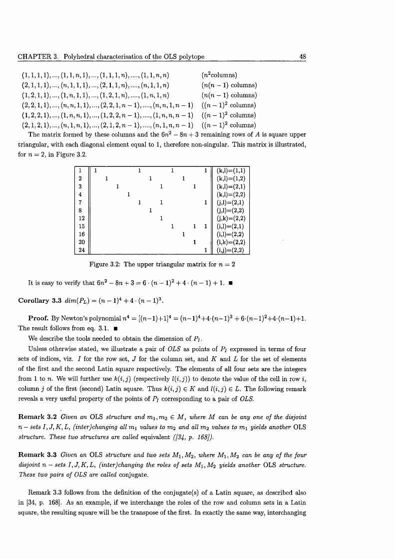
CHAPTER 3. Polyhedral characterisation of the OLS polytope 48
. , ( l , l , n , l ) , . . . , ( l , l , l , n ) , . . . . , ( l , l , n , n )
(2, 1 ,1 ,1 ),..., (71,1,1,1),..., (2,1,1,71),....,(71,1,1,71)(1 .2 .1 .1 ) ,.. . , ( l , n , l , l ) , ...,(1 ,2 , l ,n ) , . . . . , ( l ,n , l , n )(2 .2 .1. 1),..., (n, n, 1, 1),..., (2 ,2 ,1, n - 1) , (n, n, l ,n - 1)( 1. 2. 2. 1),..., (1, n ,n , 1),..., (1, 2, 2, n — 1) , ( 1, n ,n , n — 1)(2 .1 .2 .1 ),..., (n, 1, n, 1),..., (2 ,1 ,2 ,n — 1 ) , (n, 1, n, n - 1)
The matrix formed by these columns and the 6n2 — 8n + 3 remaining rows of A is square uppertriangular, with each diagonal element equal to 1, therefore non-singular. This m atrix is illustrated, for n — 2, in Figure 3.2.
(n2columns)(n(n — 1) columns) (n(n — 1) columns) ((n — l ) 2 columns) ((n — l ) 2 columns) ((n — l ) 2 columns)
1 1 1 1 1 (k, l)=( l , l )2 1 1 1 (k, l)=(l,2)3 1 1 1 (kjl)=(2,l)4 1 (k,l)=(2,2)7 1 1 1 (j, l)=(2,l)8 1 (j)l)=(2,2)12 1 (j,k)=(2,2)15 1 1 1 (M)=(2, l)16 1 (i,l)=(2,2)20 1 (i,k)=(2,2)24 1 (ij)=(2,2)
Figure 3.2: The upper triangular m atrix for n = 2
It is easy to verify th a t 6n2 — 8n + 3 = 6 • (n — l ) 2 + 4 • (n — 1) + 1. ■
C o ro lla ry 3.3 dim{Pi) = (n — l ) 4 + 4 ■ (n — l ) 3.
P ro o f. By Newton’s polynomial n 4 = [(n—1)+1]4 = (n—l ) 4+ 4 -(n —l ) 3 + 6-(n—l) 2+4-(n—1)+1. The result follows from eq. 3.1. ■
We describe the tools needed to obtain the dimension of P j.
Unless otherwise stated, we illustrate a pair of OLS as points of Pi expressed in terms of four sets of indices, viz. I for the row set, J for the column set, and K and L for the set of elementsof the first and the second Latin square respectively. The elements of all four sets are the integersfrom 1 to n. We will further use k{ i , j ) (respectively l{i , j)) to denote the value of the cell in row i , column j of the first (second) Latin square. Thus k { i , j ) G K and l ( i , j ) G L. The following remark reveals a very useful property of the points of Pi corresponding to a pair of OLS.
R e m a rk 3.2 Given an OLS structure and m i , m 2 G M , where M can be any one of the disjoint n — sets I, J, K , L, (inter)changing all m i values to m 2 and all m 2 values to m i yields another OLS structure. These two structures are called equivalent ([34, p. 168]).
R e m a rk 3.3 Given an OLS structure and two sets Mi , M 2 , where M i , M 2 can be any of the four disjoint n — sets I , J , K , L , (inter)changing the roles of sets Mi , M 2 yields another OLS structure. These two pairs of OLS are called conjugate.
Remark 3.3 follows from the definition of the conjugate(s) of a Latin square, as described also in [34, p. 168]. As an example, if we interchange the roles of the row and column sets in a Latin square, the resulting square will be the transpose of the first. In exactly the same way, interchanging
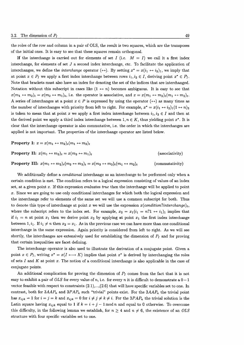
3.2. The dimension of Pi 49
the roles of the row and column in a pair of OLS, the result is two squares, which are the transposes of the initial ones. It is easy to see th a t these squares remain orthogonal.
If the interchange is carried out for elements of set I (i.e. M = I) we call it a first index interchange, for elements of set J a second index interchange, etc. To facilitate the application of interchanges, we define the interchange operator (<->). By setting x * = x( i \ «-» i2) i , we imply that a t point x e Pi we apply a first index interchange between rows 21,22 G / , deriving point x* G Pi. Note th a t brackets must also have an index for denoting the set of the indices th a t are interchanged. Notation without this subscript in cases like (1 n) becomes ambiguous. It is easy to see th a t x ( m i «-> 7722)4 = x ( m 2 772i)t, i-e- the operator is associative, and x = x{m\ 7722)4(2721 <-» 7722)4. A series of interchanges at a point x G P is expressed by using the operator (<->) as many times as the number of interchanges with priority from left to right. For example, x* — x(i \ <-> 22)1(1 72)3is taken to mean that a t point x we apply a first index interchange between 21,22 G I and then at the derived point we apply a third index interchange between 1,77 G K, thus yielding point x*. It is clear th a t the interchange operator is also commutative, i.e. the order in which the interchanges are applied is not important. The properties of the interchange operator are listed below.
P rop erty I: x = x(m\ 7 7 2 2 )4 ( 7 7 2 1 <-*■ 7 7 2 2 ) 4
P rop erty II: x(mi <-> 7722)4 = x ( m 2 7721)4 (associativity)
P rop erty III: x( m i <-> 7 7 2 2 ) 4 ( 7 7 2 2 <-» 7 7 7 3 ) 4 = £ ( 7 7 2 2 <-> 7 7 2 3 )4 ( 7 7 2 1 *-> 7 7 2 2 ) 4 (commutativity)
We additionally define a conditional interchange as an interchange to be performed only when a certain condition is met. The condition refers to a logical expression consisting of values of an index set, at a given point x. If this expression evaluates true then the interchange will be applied to point x. Since we are going to use only conditional interchanges for which both the logical expression and the interchange refer to elements of the same set we will use a common subscript for both. Thus to denote this type of interchange at point x we will use the expression x(condition?interchange)t , where the subscript refers to the index set. For example, x 2 = X\ (21 = 77?1 <->21)1 implies th a t if 2i = 7 7 a t point X\ then we derive point x 2 by applying a t point X\ the first index interchange between 1, 23. If 21 ^ n then x 2 = x \ . As in the previous case we can have more than one conditional interchange in the same expression. Again priority is considered from left to right. As we will see shortly, the interchanges are extensively used for establishing the dimension of Pi and for proving th a t certain inequalities are facet defining.
The interchange operator is also used to illustrate the derivation of a conjugate point. Given a point x £ Pi, writing x* = x ( I <— > K ) implies th a t point x* is derived by interchanging the roles of sets I and K at point x. The notion of a conditional interchange is also applicable in the case of conjugate points.
An additional complication for proving the dimension of Pi comes from the fact th a t it is not easy to exhibit a pair of OLS for every value of 7 7 , i.e. for every n it is difficult to demonstrate a 0 — 1 vector feasible with respect to constraints (2.1),...,(2.6) th a t will have specific variables set to one. In contrast, both for 3A A P n and 3P A P n such “trivial” points exist. For the 3A A P n the trivial point has Xijk = 1 for i = j = k and Xijk = 0 for 2 7 j 7 k 7 2. For the 3P A P n the trivial solution is the Latin square having x ^ k equal to 1 if k = i + j — 1 mod n and equal to 0 otherwise. To overcome this difficulty, in the following lemma we establish, for n > 4 and 77 7 6 , the existence of an OLS structure with four specific variables set to one.
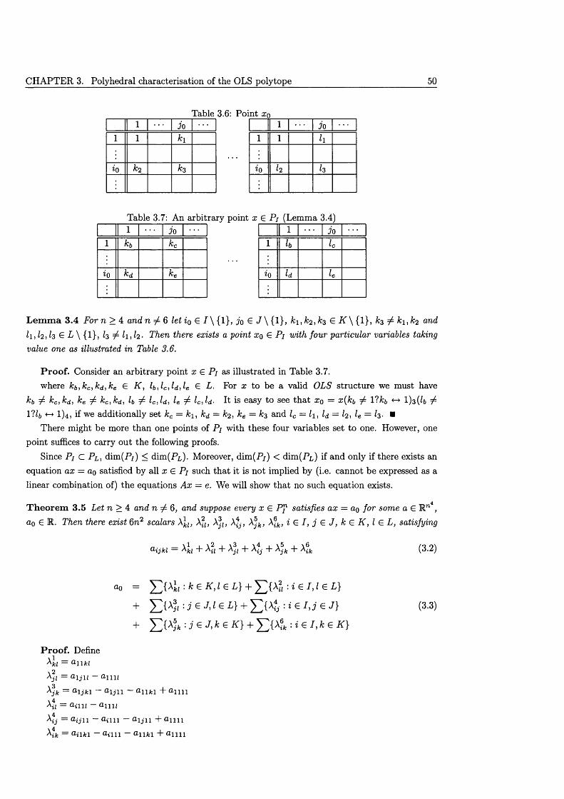
CHAPTER 3. Polyhedral characterisation of the OLS polytope 50
Table 3.6: Point xp1 jo
1 1 h
*0 h h
1 3o1 1 ki
io k 2 kz
Table 3.7: An arbitrary point x £ P / (Lemma 3.4)1 3o
1 k k
*0 k le
1 jo1 kb kc
0 kd ke
Lem m a 3.4 For n > 4 and n ^ 6 l e t i 0 £ 7 \ {1}, jo £ J \ {1}, k\, /c2, fc3 £ K \ {1}, andh , h , h £ L \ {1}, k ^ h , h - Then there exists a point xq £ Pi with four particular variables taking value one as illustrated in Table 3.6.
Proof. Consider an arbitrary point x £ Pi as illustrated in Table 3.7.
where kb,kc, k d, k e £ K , k , k J d , k £ L. For x to be a valid OLS structure we must have kb 7 kc, k d, ke ± kc, kd, lb ^ lc,ld, k ± k , k - It is easy to see th a t x 0 = x(kb ± Y!kb «-» 1)3(lb ± 1 ?lb *-+ 1 ) 4 , if we additionally set kc = k\, kd = &2, ke = fc3 and lc = li, ld = I2 , le = h- ■
There might be more than one points of Pi with these four variables set to one. However, one point suffices to carry out the following proofs.
Since Pi C Pl , dim (Pi) < dim(Pi,). Moreover, dim (Pj) < dim(Px,) if and only if there exists an equation ax = ao satisfied by all x £ Pi such that it is not implied by (i.e. cannot be expressed as a linear combination of) the equations A x = e. We will show th a t no such equation exists.
4
T heorem 3.5 Let n > 4 and n / 6, and suppose every x £ P f satisfies ax = ao for some a £ Rn , ao £ R. Then there exist 6 n 2 scalars X2t, A^, A^, Xjk, A®fc, i £ l , j £ j , k £ K , l £ L , satisfying
a i j k i = X lkl + X 2U + A^ + A i j + X 5j k + X i k (3.2)
“0 = k e K . i e L ) + ' £ { > & - . i e 1,1 e L ]
+ £ ( Ai ' ■ j e J , l e L } + £ { A * , - . i e l j e J ] (3.3)
+ £ { A , V i 6 J , f c 6 J i r } + 5>i: i £ l , k £ K }
Proof. DefineA ki = a u k i
^ji = aijii ~ a m i^ j k = a i j k i ~ a i j n — anfci 4- a. 1 1 1 1\ 4 = am i — a m i\ 4\ j = a i j i i ~ O iin — a i j n + a i m \ 4 A i k = a n k i — a m i — a n k i + a i m
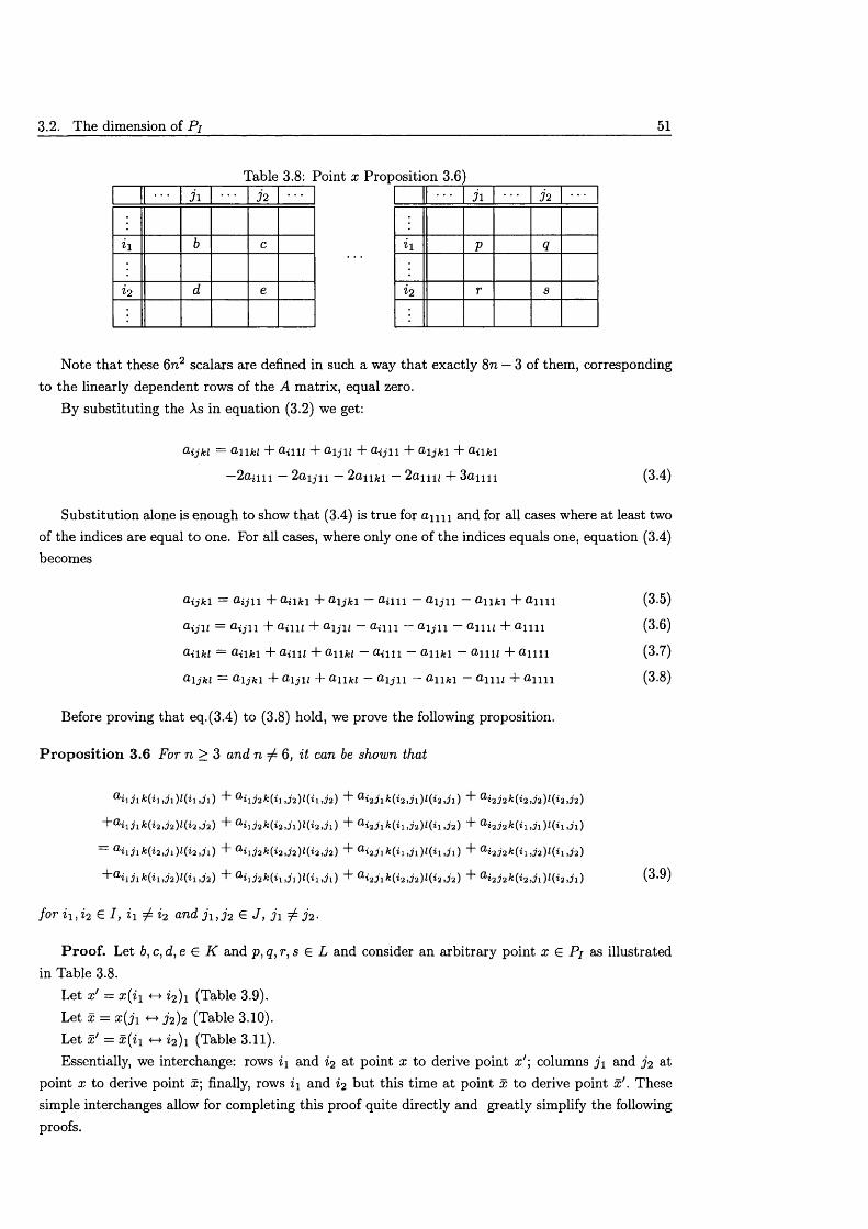
3.2. The dimension of Pj 51
Table 3.8: Point x Proposition 3.6)j i 32
h V q
*2 r s
3 i 32
k b c
*2 d e
Note th a t these 6n2 scalars are defined in such a way th a t exactly 8n — 3 of them, corresponding to the linearly dependent rows of the A matrix, equal zero.
By substituting the As in equation (3.2) we get:
o ijki = anki + ami + aiju + a ^ n + aij^i + a m i
—2 a u n — 2a i ju — 2 a m i — 2 a im + 3 a m i (3.4)
Substitution alone is enough to show that (3.4) is true for a im and for all cases where at least twoof the indices are equal to one. For all cases, where only one of the indices equals one, equation (3.4) becomes
a i j k i = a i j i i + a m i + a \ j k i — a m i — a i j u — a n k i + a m i (3.5)
a i j i t = a ^ u + a n u + a ijiz ~ a m i — a i j i i — a n i i + a i m (3.6)
a n k i = a n k i + a n i l + a n k i — a m i — a m i — Q ini + a m i (3.7)
a i j k i = a i j k i + a ijiz + a iu ; — a \ j \ \ — a i m — “ m i + a i m (3.8)
Before proving that eq.(3.4) to (3.8) hold, we prove the following proposition.
P ro p o s itio n 3.6 For n > 3 and n ^ 6 , it can be shown that
a h j i k ( i u j i ) l ( i 1 , j i ) + a*ij2A;(*i,j2)i(*i,Ja) + a i 2 3 i k ( t 2 , j i ) l ( i 2 , j i ) + a i 232k( i 2 , j 2) l ( i 2 ,32)
+ a i i 3 i k ( i 2 , h ) l ( i 2 ,32) + a i i 3 2 k ( i 2 , j i ) l ( i 2 , j i ) + a i23i k ( i i ,j2 )Z(ii ,3 2 ) a i 2 3 2 k ( i i , j i ) l ( i i , j i )
= a i i j i H i 2 , j i ) l ( i 2 , j i ) + a i i j2k(i2,32)l(i2,32) + a i2 j i *:(«i,ii)l(n,ii) + a i 2 3 2 k( i i ,32)l(ii ,3 2 )
+aiijik(i1,j2)l(ii,32) + aiihk(ii,ji)l(h,ji) + ai23ik(i2,32)l(i2,32) + ai232k(i2,3i)l(i2,ji) (3-9)
for i i , i 2 £ I , h ± i2 and j u j 2 e J, j i ± j 2.
P ro o f. Let b,c,d,e £ K and p ,q ,r , s G L and consider an arbitrary point i 6 P ; as illustratedin Table 3.8.
Let x' = x( i\ <-> *2)1 (Table 3.9).Let x = x( j i <-* j 2 ) 2 (Table 3.10).Let x' = x{i\ <-> 12)1 (Table 3.11).Essentially, we interchange: rows i\ and i 2 at point x to derive point x'\ columns j \ and j 2 at
point x to derive point x; finally, rows i\ and i 2 but this time at point x to derive point x ' . These simple interchanges allow for completing this proof quite directly and greatly simplify the following proofs.
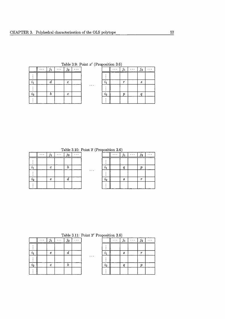
CHAPTER 3. Polyhedral characterisation of the OLS poly tope 52
Table 3.9: Point x ' (Proposition 3.6)h h
h r s
h P q
J i 32
h d e
12 b c
Table 3.10: Point x (Proposition 3.6)3 \ 32
h q p
*2 s r
3 \ 32
c b
12 e d
Table 3.11: Point x ' Proposition 3.6)h 32
h e d
h c b
h 32
h s r
12 q P
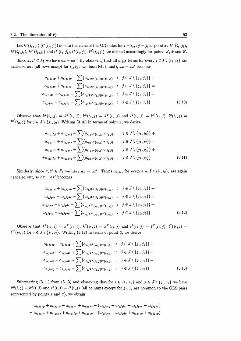
3.2. The dimension of P j 53
Let k x(is , j t ) (lx {is , j t )) denote the value of the k(l) index for i = zs , : j = j t at point x. k x' (iS)jt), k£(is , jt) , k x' ( i s , j t ) and lx'{is , j t ), lx {is , j t ), lx' { h , 3 t) are defined accordingly for points x ', x and x'.
Since x, x' G Pi we have ax = ax '. By observing th a t all a ^ terms for every i G / \ { i i , 2} are canceled out (all rows except for i i , i 2 have been left intact), ax = ax' becomes
a i i j i b p 4“ a i i j 2cq 4“ ^ j k x ( i i , j ) l x ( i i , j )
a i 2j \ d r + 0‘i 2j 2es + ^ a i 2j k x ( i 2 , j ) l x ( i2 , j )
0‘i 1j 1d r + 0‘i 1j 2es + ^ ^ { a i i j k x' { i i , j ) l x '
a i 2j i b p + a i 2j 2cq + ^ 2 i a i 2j k x> ( i2 , j ) l x ' ( i 2 , j )
j G J \ { j i J 2}} +
j G J \ { j i , j 2}} =
j G J \ { j i , j 2 }} +
j G J \ { j i , j 2}} (3.10)
Observe th a t k x (i2 , j ) = k x' ( i i , j ) , k x { i i j ) = kx' (i 2 , j ) and lx (i2 , j ) = lx { h , j ) =lx { h , j ) for j G J \ { j i , J 2 }- Writing (3.10) in terms of point x, we derive
a i i j i b p + a i i j 2cq 4” ^ ^ { a i i j k x ( i i , j ) l x ( i i , j )
a i 2j i d r 4" a i 2j 2es 4" ^ '] { a i 2j k x ( i 2 , j ) l x ( i 2 , j )
a h j i d r + a i i j 2es + ^ ]{a ii j k x ( i 2 , j ) l x ( i 2 , j )
P < i 2 3 \ b p 4" 0-i2j 2cq 4" ^ ^ { a i 2j k x ( i i , j ) l x ( i i , j )
j e J \ { j l j 2 }} +
j G J \ { j l j 2}} =
j e J \ 0 ‘i , J 2}} +
j e J \ {j i , j 2}} (3.11)
Similarly, since x ,x ' G P j we have ax = ax'. Terms a ^ , for every i G I \ {^1, 2}> are again canceled out, so ax = ax ' becomes
a i i j i cq + 0,i i j 2bp + , j ) Z * ( * i , j )
a i 2j i e s 4* a i 2j 2dr + ^ ^ { a i 2j k x ( i 2 , j ) l x ( i 2 , j )
0>ixj i e s 4" & i i j 2dr + j k x> ( i i , j ) l x ' ( i j , j )
a i 2j i c q + a i 2j 2bp + 5 3 { a i 2jA:i / ( i 2 , j ) Z 5 ' ( i 2 j )
j G J \ { j l , i 2}} +
j G J \ { jl, J 2}} =
3 € « 7 \ 0 ‘l> J 2 > } +
j G J \ { j l , j 2}} (3.12)
Observe th a t k x (i2 , j ) = k x' { i i , j ), k x {iu j ) = k x' (i 2 , j ) and lx (i2 , j ) = lx' { i i , j ), Is ( i i tj ) = (i2 ,j) for 3 € J \ { j 1,^2}- Writing (3.12) in terms of point x, we derive
a i i j i c q 4- 0>i i j2bp 4“ ^ : 3 ^ ^ \ O'lj 3 2 ^ } 4"
a i 2j i e s + &i 2j 2d r 4“ ^ { a i2 jfei (i2 ,j)Zs (i2 ij) : 3 ^ J \ {j?"l j ^2} } =
"b 0 > i i j 2 d r "b
ai2jicq 4“ ai2 j 2bp + ^ y{a 2jfea(ti,j)Za(z] ,j) • 3 ^ J \ { j l ) 3 2 } } (3.13)
Subtracting (3.11) from (3.13) and observing th a t for i G { i i , i 2} and j G J \ { j i , j 2} we havek x{hj ) = k x{ h j ) and lx ( i , j ) = lx { i , j ) (all columns except for j i , j 2 are common to the OLS pairsrepresented by points x and x), we obtain
®i i j i b p 4“ Q'i i j2cq 4" &i 2j i d r 4“ a i 2j 2es { ® i i j i c q 4“ Ui1j2bp 4“ Ui2j'ies 4“ &i 2j 2d r )
= Q“i \ j \ d r 4“ & i i j 2es 4“ O ' ^ j i b p 4“ 0>i2j 2cq (^ iijies 4" Q*iij2d r 4“ Q>i2j \ c q 4“ &i2j 2bp)
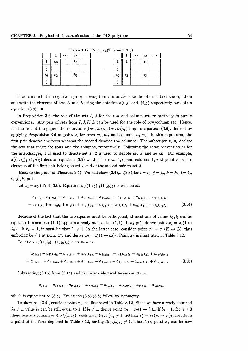
CHAPTER 3. Polyhedral characterisation of the OLS polytope 54
Table 3.12: Point ^ (T h eo rem 3.5)1 Jo
1 1 h
i o h h
1 Jo1 ko ki
0 k 2 k3
If we eliminate the negative sign by moving terms in brackets to the other side of the equation and write the elements of sets K and L using the notation k ( i , j ) and respectively, we obtain equation (3.9). ■
In Proposition 3.6, the role of the sets I, J for the row and column set, respectively, is purely conventional. Any pair of sets from I , J , K , L can be used for the role of row/column set. Hence, for the rest of the paper, the notation x ( ( m i , m 2 )ti ; { n \ ,n 2 )t2) implies equation (3.9), derived by applying Proposition 3.6 at point x, for rows m i , m 2 and columns 711, 712. In this expression, the first pair denotes the rows whereas the second denotes the columns. The subscripts t \ , t 2 declare the sets that index the rows and the columns, respectively. Following the same convention as for the interchanges, 1 is used to denote set I, 2 is used to denote set J and so on. For example, rc ((l,ii)i; (1, 71)2) denotes equation (3.9) w ritten for rows l , i i and columns l , n a t point x , where elements of the first pair belong to set I and of the second pair to set J .
(Back to the proof of Theorem 3.5). We will show (3.4),...,(3.8) for i = i0, j = jo, k = ko, I = Z0,
io,jo, k0 1.
Let X\ = x q (Table 3.6). Equation £ i( ( l ,io ) i; (1,.70)2) is w ritten as:
“ 1111 + a llfc3Z3 + a i0lM i + a*olfc2«2 + aljokili + aljok2 l2 + aiojoll + aiojok3 l3
= O, ilfej/i + 0 >llk2 l2 + a iolll + a iolfc3/3 + a l7'oll + aljok3 l3 + aiojokili + ai0 j 0 k2 l2 (3-14)
Because of the fact th a t the two squares must be orthogonal, at most one of values A3, lo can be equal to 1, since pair (1,1) appears already at position (1,1). If ko 7 1, derive point X2 = x i { l <-> ko)o- If ko = 1, it must be th a t lo 7 1. In the latter case, consider point x\ — x \ ( K *-> L), thus enforcing A3 7 1 at point x\ , and derive X2 = x \ ( l ko)o- Point X2 is illustrated in Table 3.12.
Equation X2 {(l,io)i', ( l,.7o)2) is w ritten as:
a llA :ol + a llA:3 l3 + a i 0 l k i h “1“ a i o l k 2 l 2 + a l j o k i h + a l j o k 2 l 2 "b a i o j o k 0 \ + a i o j o k 3 l 3
= ailk^h + aUk2 l2 + Giolfcol + a iolA:3l3 + alj 0 k0l + aljok3 l3 + ai0jokih + aiojok2 l2 (3.15)
Subtracting (3.15) from (3.14) and cancelling identical terms results in
^1111 — a i i / c 0 l + a i o j o l l — a i o j o k 0 l = O - i o l l l ~ a i 0 l k 0 l + a - l j Q\ \ ~ ^ ljo fe o l
which is equivalent to (3.5). Equations (3.6)-(3.8) follow by symmetry.
To show eq. (3.4), consider point X2 , as illustrated in Table 3.12. Since we have already assumed ko 1, value lo can be still equal to 1. If lo 7 1, derive point xo = £2(1 0)4- If h = 1, for n > 3there exists a column j 1 € J \ { l , j o } , such th a t l ( io , j i ) X 2 7 1- Setting £3 — x 2 {jo j 1)2) results in a point of the form depicted in Table 3.12, having l{io,jo)x* 7 1. Therefore, point xo can be now
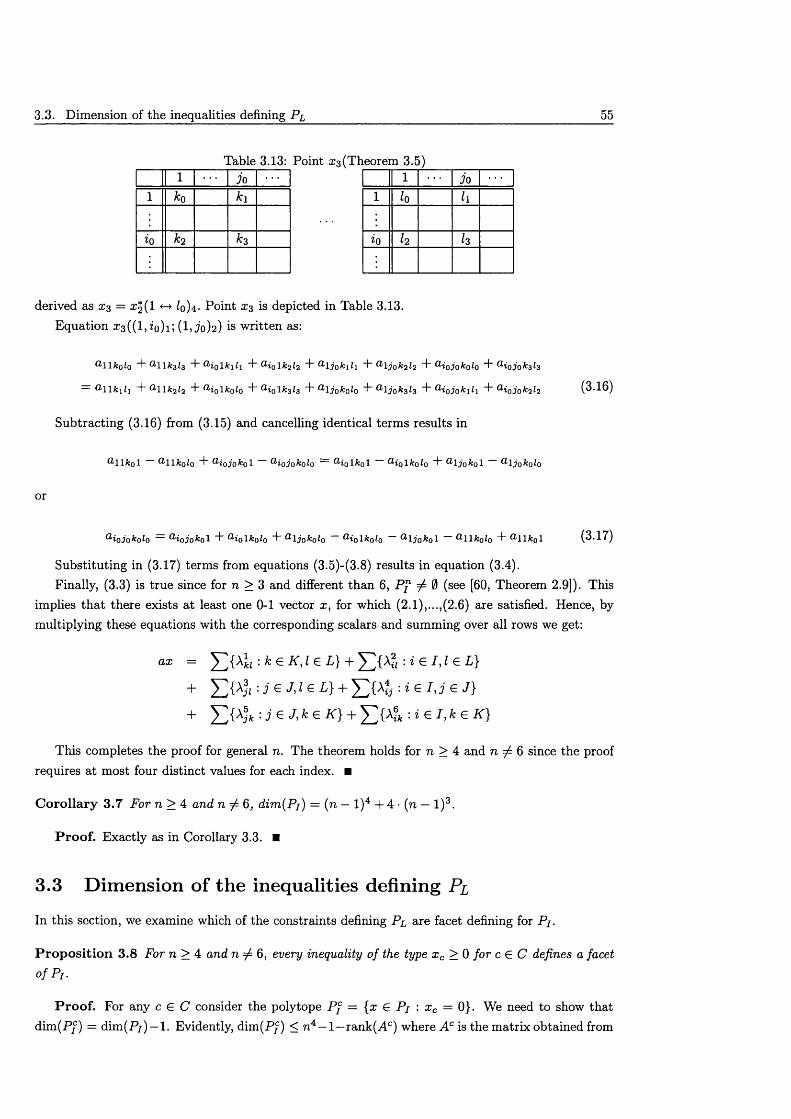
3.3. Dimension of the inequalities defining Pl 55
Table 3.13: Point £3(Theorem 3.5)1 jo
1 k0 ki
io k2 k 3
1 jo1 lo h
*0 h h
derived as £3 = ££(1 *-* Iq)^. Point £3 is depicted in Table 3.13.
Equation £3((M o )i; (1>^0)2) is written as:
a llfc0/0 “b 1 A:3Z3 + a i0lA:iJi “b O’i 0 l k 2 h "b a l j o k i h "b a l j o k 2 l2 “b a i o j o k o l o "b a i o j o k 3 l3
= allkili "b ^ 11 2/2 “I” a iol^o^o aiolk3 l3 "b alj 0 k0lo "b a ljok3 l3 "b aiojokih "b a ioJo&2*2 (3.16)
Subtracting (3.16) from (3.15) and cancelling identical terms results in
a llf c 0 l allk 0 l0 "b O'iojokol ^iojokolo ^ io lA o l @ iolkolo ~b O, l j o k o l ® ljok o lo
or
® i o j o k o l o Q ' i o j o k o l ^ io l^ o io "b ^ l j o k o l o O i o l k o l o ^ lj 'o ^ o l ^ llfc o io ~b Q.llfc0 l (^■^■'^)
Substituting in (3.17) terms from equations (3.5)-(3.8) results in equation (3.4).Finally, (3.3) is true since for n > 3 and different than 6, P f ^ 0 (see [60, Theorem 2.9]). This
implies th a t there exists a t least one 0-1 vector x, for which (2.1),...,(2.6) are satisfied. Hence, bymultiplying these equations with the corresponding scalars and summing over all rows we get:
a® = £ ( A« : * e i r , l e L } + £ { A S : i e J , i e L }
+ '■ j £ J, I € L} + : i £ / , j € J}
+ y^{Ajfc : j € J, k e K } + y^{A ffc : i e I , k 6 K }
This completes the proof for general n. The theorem holds for n > 4 and n ^ 6 since the proof requires at most four distinct values for each index. ■
C o ro lla ry 3 .7 For n > 4 and n ^ 6, dim(Pi) = (n — l ) 4 + 4 • (n — l ) 3.
P ro o f. Exactly as in Corollary 3.3. ■
3.3 D im ension of the inequalities defining Pl
In this section, we examine which of the constraints defining Pl are facet defining for P /.
P ro p o s i tio n 3.8 For n > 4 and n 6, every inequality of the type x c > 0 for c G C defines a facet of Pi.
P ro o f. For any c G C consider the polytope P f = {x ^ Pj : x c — 0}. We need to show that d im (P /) = dim (P/) —1. Evidently, dim (P j) < n4 —1—rank(Ac) where A c is the m atrix obtained from
CHAPTER 3. Polyhedral characterisation of the OLS polytope 56
A if we remove column ac. It is not hard to see th a t the rank of A c is equal to the rank of A. This is immediate, if the column ac is not among the columns of the upper triangular m atrix described in Theorem 3.2; otherwise it follows by symmetry. Therefore, dim (P7) < n 4 — 6n 2 + 8n — 4. To prove that this bound is attained, we use the same approach as in the proof of Theorem 3.5, i.e. show th a t any equation ax = ao (different than x c = 0) satisfied for every x G P f is a linear combination of A cx = e. The proof goes through essentially unchanged. ■
P ro p o s itio n 3.9 For n > 4 and n ^ 6, every inequality x c < 1 for c G C does not define a facet of
Pi
P ro o f. For any c G C consider the polytope P f = {x e Pi : x c — 1}. We will show th a t dim(P7c) < dim (P/) — 1. We know that dim (P7) < dim(P£) where P f is the linear relaxation of Pf . Setting x c to one is equivalent to setting the variables belonging to the common constraints with x c to zero. The number of these variables is 2(3n — l) (n — 1) (Prop. 2.1). Thus, dim(P£) = n 4 — 2(3n — l)(n — 1) — rank(A^) where A £ is the m atrix obtained from A by removing the columns corresponding to the variables set to zero. Obviously rank(An_ i) < rank(A^) where A n- \ is the constraint matrix of the OLS of order n — 1. By Theorem 3.2 rank(An_ i) = 6(n — l )2 — 8(n — 1) + 3 so
dim(P7) < dim(P£) < n 4 — 2(3n — l)(n — 1) — (6(n — l ) 2 — 8(n — 1) + 3)
= n4 — 12n2 4- 28n — 19
which is less than dim (P/) — 1 = n4 — 6n2 + 8n — 4 for n > 3. ■It is easy to see th a t cliques of type I do not induce facets of P /. For each of these cliques, the
coefficient vector of the corresponding inequality is identical to a row of the A matrix. Thus, each of this inequalities is satisfied as equality by all x e Pi, therefore defining an improper face of P /.
3.4 Clique inequalities
If Q C C, is the node set of a clique in the graph Ga = (C , E c ), then the complete sub-graph K\q \ induces the inequality
: d G Q] < 1 (3.18)
Inequalities (3.18) define facets of the general set-packing polytope P s p p ■ Therefore, they alsoinduce facets of the OLS packing polytope P /. The proof is trivial and can be found, among others, in([69]). However, no similar result has been proven for general set-partitioning polytope P s p , whichis itself a face of Ps p p - In particular, no trivial argument has been found, proving th a t inequalities(3.18) are facet-defining for the OLS polytope P /, which is a face of P /.
Cliques of type II give rise to inequalities of the form:
: d e Q{c)} < 1 (3.19)
for every c G C.Cliques of type III give rise to inequalities of the form:
: d G Q (c,s)} < 1 (3.20)
3.4. Clique inequalities 57
for every c , s G C such th a t | c fl s |= 1.
3.4.1 D im ension and Chvatal rank o f clique inequalities
In [2], it has been proved th a t the inequalities induced by cliques of both types II &; III define facets of P j. We reproduce here the main results.
T h e o re m 3.10 ([2, Theorem 4-11]) Let Q(c) denote the node set of a clique of type II. Then, for n > 5 and n ^ 6 the inequality
^ 2 { x q : q G Q(c)} < 1 (3.21)
defines a facet of Pj for every c G C.
T h e o re m 3.11 ([2, Theorem 4-13]) Let Q(c ,s ) denote the node set of a clique of type III. Then, for n > 5 and n ^ 6 the inequality
: Q(c, s)} < 1 (3.22)
defines a facet of Pj for every c,s G C such that \ c fl s |= 1.
Let us now examine the Chvatal rank of clique inequalities.
P ro p o s itio n 3.12 The inequalities (3.19) are of Chvatal rank 2.
P ro o f. We will first derive a lower bound for the rank of (3.19), by showing th a t the inequality cannot be of rank 1. We will proceed by illustrating how the inequality can be derived within two steps of the Chvatal-Gomory procedure. This will provide an upper bound of 2 on its rank.
Assume w.l.o.g. c = ( io, j o , ko, l0 ). The node set of the clique is Q(c) = { ( i o , j o , k o , l o ) , { ( i , j o , k o , l o )
i G A IM h {(i o J , k 0 , l o ) : j € J \ { j o } } , { ( i o , j o , k , l 0 ) : k € K \ { k 0 } } , { ( i o , j o , k 0 , l ) : I G P\IM}}- The induced inequality is:
Xiojokolo d- ^ 3'ijokolo “I- ^ Xi0jkolo “h ^ Xi0 j 0 ki0 ~|- E x iojokol — 1 (3.23)i€l\{i0} jeJ\{jo} keK\{k0} l£L\{l0}
If the inequality (3.23) is of Chvatal rank 1, there exists 0 < e < 1, such th a t every solution to the LP-relaxation of OLS, i.e. A x = e , x > 0, satisfies:
Xiojokolo Xij0 kQl0 “I" Xi0 jk0 l0 "h ] Xi0 jQki0 + E Xiojokol ^ 2 £ (3.24)i£l\{io} j£J\{jo} keK\{k0} l£L\{l0}
A solution having Xij0 kQio Xi0 jk0 i0 XiQj 0 ki0 = %i0 j0koi = 2(n—i) > ® ^ AI®o}> J € •Alio}, k G K \ { k o}, L G L \IM > and x ioj 0 k0 i0 = 0, violates (3.24), since the its l.h.s. has 4(n — 1) variables equal to 2 (n - i ) » therefore becomes equal to 2. Such a solution also has:
• Xijk0 i0 = Xij0 ki0 = Xij0 k0l = %i0jklo = x i0 jk0l = Xi0 j0kl — 0,
2n—3• XiQjkl — Xijokl = x ijk0l — Xijki0 = 2(n—l)3 >
(n-2)2• Xijkl — (n_i)4
for all i G AIM , 3 € A lio } , k G K \ { k 0 } , L G AIM-To see th a t x G Pj,, assume row ( m \ , m 2) G M\ x M2, M \ , M 2 — I , J , K , L , M\ ^ M 2 and
c = (i o , j o , k 0 , l o )• Then:
CHAPTER 3. Polyhedral characterisation of the OLS polytope 58
C ase 3.12.1 I f m i , m 2 C c, the row has 2(n — 1) variables equal to 2 (n-i) and 2 n — l variables equalto 0 .
C ase 3 .12.2 I f m \ C c, m 2 £ c or m \ £ c, m 2 C c, the row has 1 variable equal to 2(n - i)» (n — I)2variables equal to an^ ^(n ~ 1) variables equal to 0.
C ase 3 .12.3 I f m i , m 2 £ c, the row has 2 (n — 1) variables equal to 22Ti_ 135 > (n — I)2 variables equal
t° (n-i)-* and 1 variable equal to 0.
Therefore, inequality (3.23) is of Chvatal rank at least 2.
On the other hand, adding rows ( i o J o ) , { j o J o ) , ( k o j o ) , dividing the resulting inequality by 2 and rounding down both sides gives:
Adding rows (i o , k o ), ( j o , ho) , ( k o , l Q), dividing the resulting inequality by 2 and rounding down both sides gives:
Adding rows ( i o , j o ) , ( i o , k o ), ( i o J o ) , dividing the resulting inequality by 2 and rounding down both sides gives:
Dividing inequality (3.29) by 3 and rounding down both sides gives inequality (3.23). Therefore, inequality (3.23) is of rank a t most 2. The proof is complete. ■
P ro p o s itio n 3.13 The inequalities (3.20) are of Chvatal rank 2.
P ro o f. The proof will essentially proceed in the same way as the proof of Proposition 3.12.
Assume w.l.o.g. c = ( i o , j o , k o , l o ) and s = ( i o , j i , k i , l i ) . The node set of the clique is Q(c,s ) = { J o , j o , k 0 J o ) , ( i o , j o , k i , h ) , ( i o , j i , k o J i ) , J o , j i , k i J o ) } , the induced inequality being:
iojokolo "b ^ x ijokoh "P ^ ] x iojkolo "P ^ ] x iojoklo — i€l\{io} j£J\{jo} k€K\{k0}
x iojokolo "P ^ j x ijokolo "P ^ iojkolo "P ^ x iojokol ^ 1i € / \ { i o } jeJ\{jo} l£L\{l0}
Adding rows ( io, j o ) , ( j o , ko) , (jo Jo), dividing the resulting inequality by 2 and rounding down both sides gives:
x i o j okolo "P ^ y x i jokolo "P ^ x i o j ok l o "P E x io j oko l 5; 1 (3.27)ieAPo} k€K\{k0} ieL\{i0}
x iojokolo “b ^ x iojkolo “b ^ x iojoklo "P ^ x iojokol — 1jeAD'o} f c G K \{ f c 0 } ieL\{i0y
Finally, adding rank 1 inequalities (3.25)-(3.28) gives the following inequality:
^ x i o j o k o l o "P 3 x i j o k o l o "P 3 ^ x iojkolo "P 3 ' x iojoklo "P 3 E x i o j o k o l 1 (3.29)f c G K \{ f c 0 }
x iojokolo ~b "Aojofciii “b-^ioJifcob “b-AojifciJo — 1- (3.30)
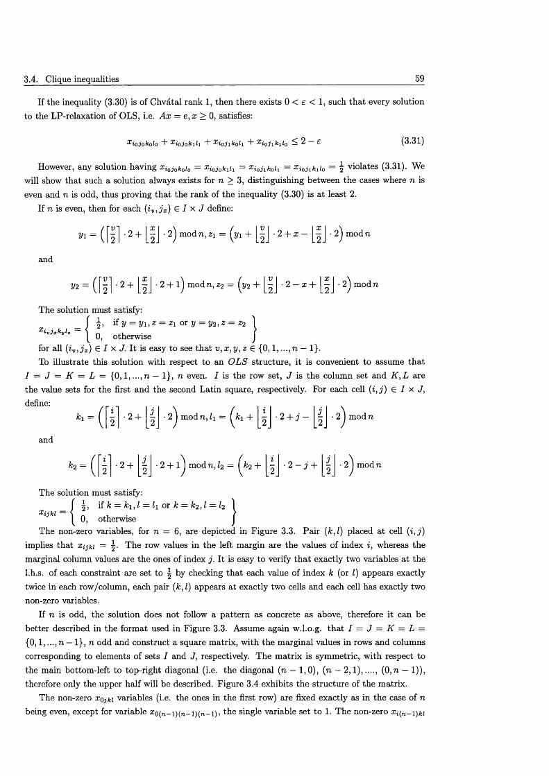
3.4. Clique inequalities 59
If the inequality (3.30) is of Chvatal rank 1, then there exists 0 < e < 1, such th a t every solution to the LP-relaxation of OLS, i.e. A x = e , x > 0, satisfies:
•Eiojokolo “I" S'iojokih "P ^ioji koli %iojikilo ^ 2 E (3.31)
However, any solution having x laJukuiu = x KKklh = = x iojlkii0 = 5 violates (3.31). Wewill show that such a solution always exists for n > 3, distinguishing between the cases where n is even and n is odd, thus proving th a t the rank of the inequality (3.30) is at least 2.
If n is even, then for each {iv, jx) £ 7 x J define:
V l - (’V
•2 +X
2 . 2 .2 m odn, z\ = (yi +
vL2J
2 + x —x
L2J
and
V2 -(' V
•2 +X
2 . 2 .2 + l ) mod n, z 2 = (y 2 +
V X— • 2 — x + —
. 2 . .2 J
• 2 ) mod n
2 ) mod n
The solution must satisfy:if y = y i , z = zi or y = y2, z = z 2 )
0, otherwise Jfor all (iv , j x) € / x <7. It is easy to see th a t v , x , y , z € {0, 1, ...,n — 1}.To illustrate this solution with respect to an O L S structure, it is convenient to assume that
I = J = K = L = {0 ,1 ,...,n — 1}, n even. I is the row set, J is the column set and K, L arethe value sets for the first and the second Latin square, respectively. For each cell ( i , j ) G I x J,define:
ki = (i
•2 + 1
V 2 2• 2 J m o d n , l\ = ( k\ + 2 + j ~ ■ 2 I mod n
and
k 2 =i
■ 2 + j2 _2 _
2 + 1 I mod n , l 2 = ( k 2 + 2 - 3 + ■ 2 I mod n
The solution must satisfy:if k — ki, I = li or k = k2, 1 = l2 1
0, otherwise JThe non-zero variables, for n = 6, are depicted in Figure 3.3. Pair (k,l) placed at cell (i , j )
implies that Xijki = The row values in the left margin are the values of index i, whereas the marginal column values are the ones of index j. It is easy to verify th a t exactly two variables a t the l.h.s. of each constraint are set to ^ by checking th a t each value of index k (or I) appears exactly twice in each row/column, each pair (k,l) appears at exactly two cells and each cell has exactly two non-zero variables.
If n is odd, the solution does not follow a pattern as concrete as above, therefore it can bebetter described in the format used in Figure 3.3. Assume again w.l.o.g. th a t I — J = K = L ={0,1,..., n — 1}, n odd and construct a square matrix, w ith the marginal values in rows and columns corresponding to elements of sets I and J, respectively. The m atrix is symmetric, with respect to the main bottom-left to top-right diagonal (i.e. the diagonal (n — 1,0), (n — 2 ,1),...., (0 ,n — 1)), therefore only the upper half will be described. Figure 3.4 exhibits the structure of the matrix.
The non-zero Xojki variables (i.e. the ones in the first row) are fixed exactly as in the case of n
being even, except for variable z 0(n_i)(n_i)(n_i), single variable set to 1. The non-zero x ^ n_i
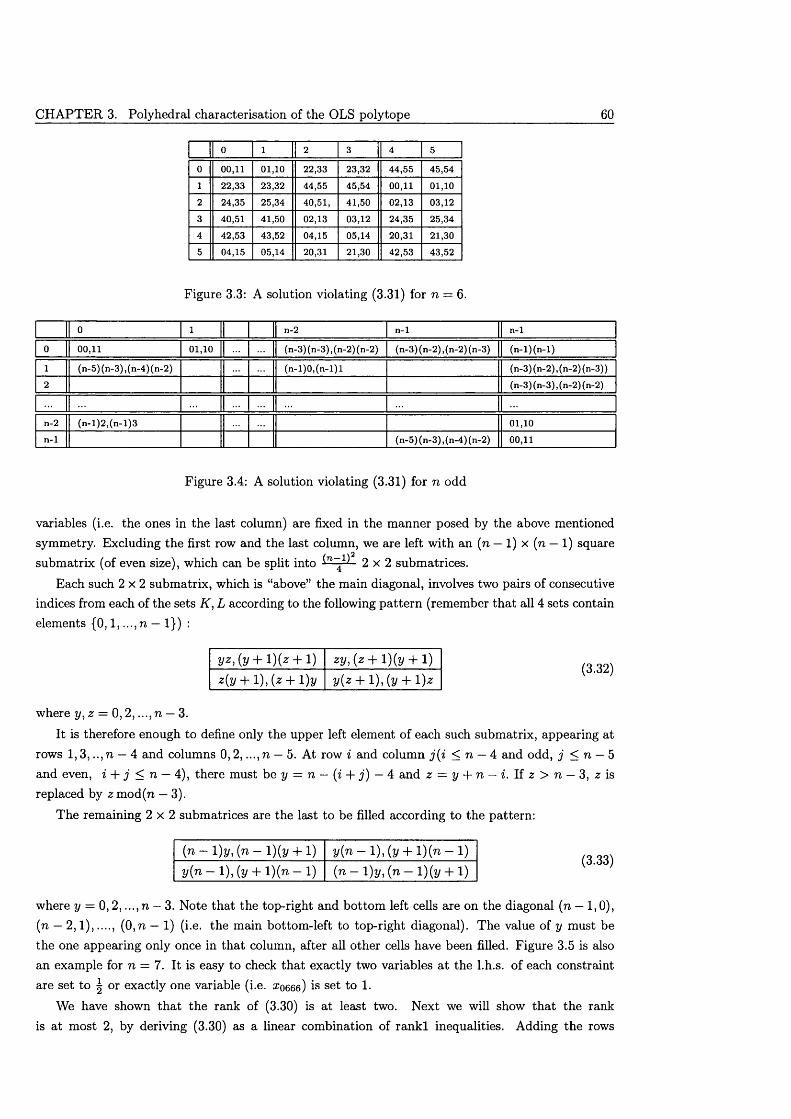
CH APTER 3. Polyhedral characterisation of the OLS polytope 60
0 1 2 3 4 5
0 00,11 01,10 22,33 23,32 44,55 45,541 22,33 23,32 44,55 45,54 00,11 01,102 24,35 25,34 40,51, 41,50 02,13 03,123 40,51 41,50 02,13 03,12 24,35 25,34
4 42,53 43,52 04,15 05,14 20,31 21,30
5 04,15 05,14 20,31 21,30 42,53 43,52
Figure 3.3: A solution violating (3.31) for n = 6.
0 1 n-2 n-1 n-1
0 00,11 01,10 (n-3)(n-3),(n-2)(n-2) (n-3) (n-2), (n-2) (n-3) (n-l)(n-l)
1 (n-5)(n-3),(n-4)(n-2) (n-l)0 ,(n -l)l (n-3)(n-2), (n-2)(n-3))2 (n-3) (n-3), (n-2) (n-2)
n-2 (n-l)2,(n -l)3 01,10n-1 (n-5)(n-3),(n-4)(n-2) 00,11
Figure 3.4: A solution violating (3.31) for n odd
variables (i.e. the ones in the last column) are fixed in the manner posed by the above mentioned symmetry. Excluding the first row and the last column, we axe left w ith an (n — 1) x (n — 1) square subm atrix (of even size), which can be split into 2 x 2 submatrices.
Each such 2 x 2 submatrix, which is “above” the main diagonal, involves two pairs of consecutive indices from each of the sets K, L according to the following pattern (remember th a t all 4 sets contain elements {0,1,..., n — 1}) :
(3.32)
where y , z = 0,2, ...,n — 3.
It is therefore enough to define only the upper left element of each such submatrix, appearing at rows 1 ,3 ,.., n — 4 and columns 0 ,2,..., n — 5. At row i and column j ( i < n — 4 and odd, j < n — 5 and even, i + j < n — 4), there must be y = n — ( i + j ) — 4 and z — y + n — i. l i z > n — 3, 2 is replaced by 2 mod(n — 3).
The remaining 2 x 2 submatrices are the last to be filled according to the pattern:
(3.33)
where y = 0 ,2 ,..., n — 3. Note that the top-right and bottom left cells are on the diagonal (n — 1,0), (n — 2 ,1 ),...., (0 ,n — 1) (i.e. the main bottom-left to top-right diagonal). The value of y must be the one appearing only once in that column, after all other cells have been filled. Figure 3.5 is also an example for n = 7. It is easy to check th a t exactly two variables a t the l.h.s. of each constraint are set to | or exactly one variable (i.e. xo666) is set to 1.
We have shown th a t the rank of (3.30) is at least two. Next we will show th a t the rank is at most 2, by deriving (3.30) as a linear combination of ran k l inequalities. Adding the rows
( n - l ) y , (n — l )(y + 1) y ( n - l ) , ( y + l ) ( n - l )y ( n - l ) , { y + l ) { n - l ) ( n - l ) y , ( n - l)(y + l)
yz , ( y + l ) (z + l) z y , ( z + l){y + 1)z(y + l ) , ( z + l )y y(z + l ) , ( y + l ) z
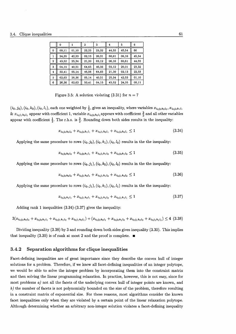
3.4. Clique inequalities 61
0 1 2 3 4 5 6
0 00,11 01,10 22,33 23,32 44,55 45,54 66
1 24,35 42,53 02,13 20,31 60,61 06,16 45,54
2 43,52 25,34 21,30 03,12 06,16 60,61 44,55
3 04,15 40,51 64,65 46,56 03,12 20,31 23,32
4 50,41 05,14 46,56 64,65 21,30 02,13 22,33
5 62,63 26,36 05,14 40,51 25,34 42,53 01,10
6 26,36 62,63 50,41 04,15 43,52 24,35 00,11
Figure 3.5: A solution violating (3.31) for n = 7
(io, jo), (io, k0), (i0, h) , each one weighted by \ , gives an inequality, where variables Xi0 jokoiQ, x iQjoklh & XiQj lkoi1 appear with coefficient 1, variable appears w ith coefficient | and all other variablesappear with coefficient The r.h.s. is Rounding down both sides results in the inequality:
x iojokolo d~ ‘ ioJo^ih d" x io3 i^oh d“ ^iojokoh — (3.34)
Applying the same procedure to rows (io, jo), (io ,^i), (io, ^o) results in the the inequality:
x iojokolo d- x iojokih + Xi0 j lk-l iQ + X{0 jQkli0 < 1 (3.35)
Applying the same procedure to rows (io, j i ) , (io, ^o), (io, io) results in the the inequality:
x io j oko l o d" x i o j i k o h d~ X { 0j 1 k l l0 + X i Qj l k o iQ < 1 (3.36)
Applying the same procedure to rows (io, j i ) , (io, &i), (io, h ) results in the the inequality:
x iojokih d" XiQj lkoi1 + x i0 j ikli0 + X{0 j lkli1 < 1 (3.37)
Adding rank 1 inequalities (3.34)-(3.37) gives the inequality:
d" x iojokih d- XiQj 1 kll0 d- XiQj lkoi1) + (XiQjokol} d- XiQjokliQ + XiQj lkoiQ + Xi0 j lkli1) ^ 4 (3.38)
Dividing inequality (3.38) by 3 and rounding down both sides gives inequality (3.30). This implies th a t inequality (3.30) is of rank at most 2 and the proof is complete. ■
3.4.2 Separation algorithm s for clique inequalities
Facet-defining inequalities are of great importance since they describe the convex hull of integer solutions for a problem. Therefore, if we knew all facet-defining inequalities of an integer polytope, we would be able to solve the integer problem by incorporating them into the constraint matrix and then solving the linear programming relaxation. In practice, however, this is not easy, since for most problems a) not all the facets of the underlying convex hull of integer points are known, andb) the number of facets is not polynomially bounded on the size of the problem, therefore resultingin a constraint m atrix of exponential size. For these reasons, most algorithms consider the known facet inequalities only when they axe violated by a certain point of the linear relaxation polytope. Although determining whether an arbitrary non-integer solution violates a facet-defining inequality
CHAPTER 3. Polyhedral characterisation of the OLS poly tope 62
of the convex hull of integer solutions for an M V -hard problem is generally also HV ~hard, it is sometimes possible to do th a t efficiently for certain classes of facets. In particular, with respect to the OLS, we propose two polynomial procedures, one for each class of facet defining cliques, that deal w ith the problem of detecting a violated clique inequality.
The separation algorithms of this paragraph have been motivated by the ones in [9]. First, we provide an algorithm th a t detects a violated facet-defining inequality induced by cliques of type II.
A lg o rith m 3.14 (S e p a ra tio n o f C liques o f ty p e II ) Let x G Pl \P i and v G N such that v > 5.
S te p I Set dc = 0, for all c G C.
S te p 2 : For all s G C check x s . I f x s > set dc = dc + x s for all c G Q{s). I f dc > 1 stop: the
inequality XX^g '• Q ^ Q (c)} — 1 violated; otherwise, continue.
S te p 3 : For all c G C if dc > check whether the inequality XX^g : # £ Q (c)} < 1 ^ violated. I f yes stop; otherwise continue.
In order to prove the correctness and complexity of the algorithm we need a number of intermediate results.
L em m a 3.15 For a point x G Pl and a positive integer v, the number o f components of x with 2
value > v is < — .— — V
P ro o f. The value of the linear program L = max{ex : x G Pl } can be easily shown to be n 2since the vectors x G M”4 and u G R6n2 defined by x c = ^r,Vc G C and ur = ^,Vr G R are feasible
2solutions to L and its dual, respectively. Therefore, they are optimal. If more than ^ components of x have values greater than or equal to v, the value of ex would be greater than n 2 contradicting the above. ■
L em m a 3.16 For any x G P l and any positive integer v , the number of c G C, such that XX^g : q G Q{c)} > v is < - ■
P ro o f . ConsiderG Q(c)} : c G C} (3.39)
Recall th a t | Q(c) |= 4n — 3 for all c G C which implies th a t each x c appears 4n — 3 times in (3.39). Hence:
E < 5 > : q G Q(c)} : c G C] = (4n — 3) E { * . : c G C} < (4n - 3)n2
If there were more than n X^i^g : Q ^ Q(c)} with a value greater than or equal to v then itwould be : q G Q(c)} : c G C } > n 2(4n — 3) contradicting the above. ■
T h e o re m 3.17 Algorithm 3.14 determines in 0 ( n 4) steps whether a given x G P l violates a facet- defining inequality of type II.
P ro o f. Let us first prove th a t the algorithm is correct. Assume th a t the inequality XX^g : 9 £ Q{c)} 5; 1 is violated for some c G C. Then
dc = y ^ { x g : q G Q(c) ,xq > ^ - } > 1 - y ^ { x q : q G Q(c) , xq < ^ - }
^ 4n — 3 ^ u — 4 — vn ~~ v
3.4. Clique inequalities 63
Hence, violation is detected a t Step 3 of the algorithm. Therefore the algorithm is correct.
Let us now examine the complexity of the algorithm. At Step 1, we initialize n 4 counters. At Step 2, there can be at most un3 components of a fractional point x, which are examined (Lemma 3.15). For each of those, 4n — 3 counters are updated since there axe 4n — 3 nodes in the node set of a clique of type II. Hence, in the worst case the complexity of Step 2 is vn 3 (4n — 3). At Step 3, the
number of c £ C for which XX^g : 9 ^ Q(c)} > is most vn (Lemma 3.16). For eachsuch c we need 4n — 3 extra steps to check whether the corresponding inequality is indeed violated. Hence, the complexity of Step 3 is . The overall complexity of the algorithm is
f ( v , n) = n 4 + vn 3 (4n - 3) + vn2(4 n ~ 3 ) 2 (3>40)v — 4
which is 0 (n4).The value of v th a t minimizes f (v , n) is found by setting the first derivative with respect to v to
zero:
= n{v 4)4 4(4n - 3 ) = 0 = * u = 4 + J 1 6 - —dv V n
which for large n produces v = 8. For this value of v eq. (3.40) becomes f ( n ) = n 4 + 8n3(4n — 3) + 2n2(4n — 3)2. ■
Note th a t the complexity of the above algorithm remains linear with respect to the number of variables, therefore it is the lowest possible (see also [9]). A separation algorithm for cliques of type III follows.
A lg o rith m 3.18 (S e p a ra tio n o f C liques o f ty p e I I I ) Let x E Pl \ P i •
S te p 1: For all c £ C, i f \ < x c < 1;
S te p 2: Then for all t G C with \ c fl t |= 2, if x t > —ff*
S te p 3: Then for all s G C, such that \ c fl s |= 1 and \ s D t \= 3, i f XX^g : Q £ Q{ci s )} > 1 stop: a violated inequality has been found; otherwise continue.
T h e o re m 3.19 Algorithm 3.18 determines in 0 ( n 4) steps whether a given x G P l violates a facet defining inequality of type III.
P ro o f. Let us examine the correctness of the algorithm. Q(c, s) is a node set of a 4-clique thus if a non-integer point x violates XXxg : ? G Q(c,s)} < 1 at least one component of x must be > W.l.o.g. assume th a t x c > ^ for c = ( io, jo, ko, Iq). Since x G P l , variable x c appears in the following constraints:
pip : * € I J e j } = 1 (3.41)
x iojkl0 : j G J , k G K } = 1 (3.42)
y ' { xijoMo : i G I, k G K ) = 1 (3.43)
^ ^ { x iojokl : k G K, I G L} = 1 (3.44)
Xiiok0l : i e 1,1 e L} = 1 (3.45)
^ 'Xa'*oJ*(W : j G J, I G L } = 1 (3.46)
CH APTER 3. Polyhedral characterisation of the OLS polytope 64
If x c = 1 then for all £ G C such that | c fl £ |= 2 we have x t = 0. Hence, the inequality : 9 ^Q(c, s)} < 1 is satisfied as equality for all s G C such th a t | c fl s |= 1. Therefore, if x violates such an inequality, it must be th a t | < x c < 1. Since | Q(c,s) |= 4, the condition x t > must hold for at least one £ G Q(c, s)\{c}. Consequently, Algorithm 3.18 is correct.
Concerning the complexity of the algorithm, we note th a t the comparison in Step 1 is executed in the worst case n 4 times, once for each variable. The number of variables with value > ^ is at most 4n2 (Lemma 3.15). For each such variable, there are 6(n — l )2 £ G C such th a t | c n £ |= 2, as indicated by constraints (3.41),...,(3.46). Hence, we need 24n2(n — l )2 comparisons to identify all such ordered pairs (c, £), yielding a complexity of 0 ( n 4). For each such c, the number of £ cannot be more than 3 in each of (3.41),...,(3.46), since otherwise one of these inequalities would be violated. Thus the to tal number of £ given c, for which x t > is satisfied, is 18. For c, £ given, there are at most n - 1 s E C such th a t | c fl s |= 1. Thus, Step 3 will be executed 4n2 x 18 x (n — 1) times, i.e. its complexity is of the order 0 ( n 3). The total complexity is 0 (n 4). ■
C o ro lla ry 3.20 Whether there exists a violated clique inequality can be detected in linear time with respect to the number of variables, i.e. in 0 (n4) steps.
3.5 Antiweb inequalities
For c, d G C, \c Pl d\ = 0, let A(c , d) = { / G C : / C c U d}. It has been proved th a t the inequality
X(A(c , of)) = ■ f 6 A(c, d ) } < 2 (3.47)
can be regarded as lifted from an (8,3) antiweb. Recall also its form for c = (io,jo,ko,lo), d =
( i i iJ i.fc i.f i) :
'f'iojokolo "P 'iojohoh "P iojo^ih "P "^iojo^ih "P "P *P "P (3.48)
x iijokolo + x iijokoh "P x i\3ok\lo + x i\jokili + x i\j\kolo "P x i\jikoh + x i\j\k],lo "P Si 2
Both the Chvatal rank and the dimension of this inequality remain unknown. The fact th a t this inequality cannot be further lifted, i.e. it cannot be made stronger, suggests th a t this inequality cannot be dominated. This implies th a t the face defined by inequality (3.47) is maximal with respect to set inclusion, i.e. is not included in any other face defining polytope P j. A beneficial feature, however, is th a t inequalities (3.47) can also be separated in linear time with respect to the number of variables, i.e. in 0 ( n 4) steps, although their number is 0 (n 8). The following separation algorithm achieves this result. We may assume th a t the previously exhibited separation algorithms for clique inequalities have already been executed for a specific point x € Pl \ P i and that no violated clique inequality of type II has been identified. This assumption is possible without loss of generality and is also im portant for the correctness and complexity of the following algorithm.
A lg o rith m 3.21 Let x G P l \ P i , which violates no clique inequality.
Step I For all c G C, i f \ < x c < 1, then:
Step I I For all d G C, such that \c fl d\ = 2 i f Xd> -~[qg then:
Step III For all p G C , such that |cfl <?| = 0, |d n p | = 2, check whether the inequality X ( A ( c ,g )) < 2 is violated. I f yes, stop; otherwise, continue.
3.5. Antiweb inequalities 65
Step I V For all d G C, such that |cfl d\ = 3, i f Xd > then:
Step V For all f G C, such that |cfl / | = 2, |cfl f \ = 3, i f Xj > 1 ~xc - x<i then:
Step VI For all g e C, such that \c fl g\ = 0, \ f D g\ = 2, check whether the inequality X ( A ( c ,g )) < 2 is violated. I f yes, stop; otherwise, continue.
P ro p o s i t io n 3.22 Algorithm 3.21 determines in 0 ( n 4) steps whether a given x € P l \ P i violates an inequality (3.4,7).
P ro o f. We first prove the correctness of the algorithm, assuming th a t no clique inequality has been found to be violated by the particular fractional point. Since the number of variables in the inequality is 16 and the r.h.s. is 2, at least one variable must possess a value greater than If this variable, namely x c, is equal to 1, then 10 other variables having at least 2 indices in common with x c will be set to 0. The remaining 5 variables, which have 0 or 1 index in common with x c, belong to a clique of type II, therefore cannot sum up to a value greater than 1. Therefore, variable x c being 1 implies th a t inequality (3.48) cannot be violated. This proves the validity of the bounds a t Step I.
As an example, let c = {io,jo, ko,lo) and consider inequality (3.48). The 5 variables not set to 0
if x c 1 are %iiji kilo i ji ki i\ } 9>nd all belong to the node set of theclique of type II Q(d), for d = ( i i , j i , k i , l i ) .
Since 5 variables belong to a clique of type II and no such inequality is violated, the sum of these 5 variables will be no more than 1. Therefore, the antiweb inequality will be violated only if the sum of remaining 11 variables is greater than 1. Since one of those variables is already greater than | (variable x c of the algorithm), at least one of the remaining 10 must be greater than 1Yqc • This can be a variable having either 2 or 3 indices in common with x c. The remaining steps attem pt to find such a variable.
Concerning the complexity of the algorithm, Step I is performed up to n 4 times. Step I I will be performed at most 8 n 2 times (see Lemma 3.15). For a particular x c, the variables xj , such th a t |cD d | = 2, are 6(n — l ) 2, as shown in the proof of Theorem 3.19. Therefore, it takes up to 8n2 • 6(n — l ) 2, i.e. 0 ( n 4), steps to identify all such ordered pairs (c, d). This is the complexity of Step II.
Taking into account th a t a particular c appears at exactly six constraints, the number of d's such th a t Xd > --^qc cannot be more than 10 in each constraint, or 60 in total. This implies that Step I I I will be performed at most 60 x 8n2 times. For c,d given, the number of g's such that |c fl g\ = 0, \d fl #| = 2 is exactly (n — l ) 2. Checking whether the inequality X ( A ( c , g)) < 2 is violated involves a constant number of steps. Overall, the complexity of Step I I I is 60 -8n2 • (n — l ) 2, i.e.O(n4).
Similarly, Step I V is implemented up to 8n2 • 4(n — 1) times in order to identify all ordered pairs (c, d), therefore the complexity of this step is 0 ( n 3). Following the same reasoning as before, the number of d's such th a t |c f ld | = 3, Xd > c , cannot be more th a t 60. For c,d fixed, finding all f ' s of Step V involves 3(n — 1) steps. As a result, Step V will be performed 8n2 • 60 • 3(n — 1), i.e. 0 ( n 3) times.
Finally, the number of f ' s can be up to 54. For a particular pair of (c, / ) , the number of g's examined a t Step VI are exactly (n — l ) 2. Overall, Step VI is implemented 8n2 • 60 • 54 • (n — l ) 2, i.e. 0 ( n 4). The complexity of each step of the algorithm being at most 0 ( n 4) implies th a t the algorithm is also of linear complexity with respect to the number of variables. ■
CHAPTER 3. Polyhedral characterisation of the OLS polytope 66
3.6 Com posite clique inequalities
Composite clique inequalities were introduced in Section 2.6. This section proves that they induce facets of Pj. The proof is based on condition (d) of Theorem 3.1, exactly as the proofs in [2]. Let uspresent again the form of the inequality, for cn = (n , n , n , n ), Co = {io,jo,ko,lo)'-
2Xnnnn E innn E %njnn E %nnkn ^ Xnnnl (3.49)i^n j ^ 71 ky^n l^n
iojonn ionkon "h Xnjokon "h ionnlo “I- Znjonlo "I- XnnkolQ — 2
T h e o re m 3.23 For n > 7, (3.49) defines a facet of Pi.
P ro o f . Since (3.49) is induced by a wheel, its validity for all x E Pi arises from the intersection graph. Let P i(W (cn , Co)) = {x : x E Pi, : 9 e ^ ( cn>Co)} = 2}. Denote as x a point of Picorresponding to a standardised pair of OLS, i.e. x titt = 1,V£ G { 1 ,... ,n}
Let x = x ( l <r-> n )2. Point x G P/(W (cn , Co)), since x nnnn — 1; hence, P i(W (cn , Co)) / 0.To show th a t P / \ Pi ( W ( cu, cq)) ^ 0, we consider again the point x We consider two cases, viz
Xnnkolo = Ij^nnfcoZo L
C ase (i): If x nnkoiQ = 1, there exists j i G J \ { l,n } such th a t (k(i0, j i ) , l(i0, j i ) ) ± {k0 , n ) }(n, l0). Let x = x( j i <-+ 71)2- Clearly, x G P / \ P /(W (cn , co)).
C ase (ii): For xnnfcoi0 ^ 1, if x ionkon = 0 and x ionni0 = 0 it follows th a t x G Pj \ P /(W (cn , c0)). Otherwise, assume w.l.o.g. that x ionkon = 1. Observe th a t there must exist a column j \ G
J \ {1,n}, such th a t {k(i 0 , j i ) , l ( i 0 , j i ) ) ± {nJo) and {k(n , j{) , l(n , j i ) ) 7 (fco>fo)- Let x = x (ji n )2. Clearly, x G P / \ P /(W (cn , Co)).
4
Let a G Rn , a0 G M such th a t ax = ao, for every x G P i(W (cn , cq)). The proof established that (a, ao) is bound to be a linear combination of the rows of A and inequality (2.26). This implies that there exist scalars Afcz> A^, A^, ^ j k> ^fkj 'Tr ^ JR., Vi G I , j G J , k G K , l G L, such that:
& i j k l
AL + + Aji + Kj + Ajk + A®fc, G C \ W (cn ,co)A*z + A?i + A^ + A?-+ A®fc + Affc + 7r, (i, j , k, l) G W (cn ,co) \ {cn} (3.50)
„ Ann + A^n + A^n + X^n + A^n + A®n + 2 n ( i , j , k , l ) = ( n , n ,n , n )
ao — X ^ + X ! ^ + X ^ + X ^ X ^ + X / ^ + 27r (3.51)keK,ieL iei,ieL jeJ,ieL iei , jeJ jeJ,keK iei ,keK
Define the scalars )}kl, ..., Affc as in Theorem 3.5.To study the case of (i , j , k, l) G C \ W(cn , co), we need a number of intermediate results.
Lem m a 3.24 For n > 7, i q, i i G I \ { l ,n } , j q, j i G J \ {1 , n}, A:2 , ^ 3 £ K \ { l , k o , n } where
ko G K \ {1, n) , li G L \ { l , l o , n } , I2 G L \ {1, Z0}, I3 E L \ {1} where Iq G L \ {1, n} , there exists
x G P i as illustrated in Table 3.14
P ro o f. At point x, let i\ G I \ { l,n } , j \ G J \ {1} be such th a t k ( i i , j i ) = 1, l { h , j i ) = n. W.l.o.g. assume th a t there exists iq G I \ { l , i i ,n } , such that k( iq, 1) = k\. Let also «2 E I \ { i \ ,n } , h € I \ { j i , n } be such th a t x i2 j2kin = 1. By denoting 23, J3 the row and column at which the pair (fc2,n ) appears (xi3j3fc2n = 1,23 G / \ { i i , i 2 , ^ } , h ^ «•}) and by performing the interchanges
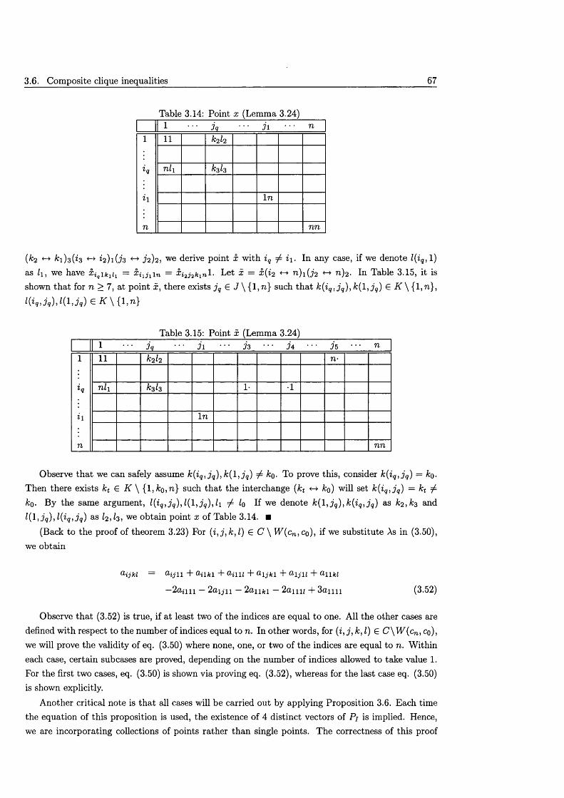
3.6. Composite clique inequalities 67
Table 3.14: Point x (Lemma 3.24)1 •■• jq ■■■ 3\ • • • n
1
iq
h
n
11 k2l2
Till k$l 3
In
nn
(k2 *-* 2)10*3 3 2 )2 > we derive point x with iq ^ i\ . In any case, if we denote l(iq, 1)as li, we have x iqiklh = x ^ j ^ n = Xi2j2kin 1. Let x = x( i 2 *-> n ) i ( j 2 «-> n)2. In Table 3.15, it is shown th a t for n > 7, at point x, there exists j q G J \ { l,n } such th a t k(iq, j q), k ( l , j q) € i f \ { l,n} ,
3q) 3q) £ i f \ {!>
Table 3.15: Point x (Lemma 3.24)1 • • • jq • • ■ j \ • • ■ 3 3 • • • j4 • • ■ h • • • n
1
iq
i\
n
11 k2h n-
nli k zh 1- •1
In
nn
Observe th a t we can safely assume k ( i q , j q) , k ( l , j q) ^ ko. To prove this, consider k ( i q , j q) = ko.
Then there exists k t G i f \ {1, k o , n } such that the interchange ( k t <-> ko) will set k ( i q , j q) = k t ^ k 0 . By the same argument, l { i q , j q) , l { l , j q) , h 7 0 I f we denote k ( l , j q) , k ( i q, j q) as k 2 , ko and l ( l , j q) , l { i q , j q) as l2 ,l%, we obtain point x of Table 3.14. ■
(Back to the proof of theorem 3.23) For (i , j , k , l ) E C \ W (cn ,co), if we substitute As in (3.50), we obtain
a i j k l ~ O ' i j 11 + f l i lfc l + O - i l l l + a l j k l + a l j l l +
—2 a m i — 2 a i j n — 2anfci — 2 a m ; + 3 a im (3.52)
Observe th a t (3.52) is true, if at least two of the indices are equal to one. All the other cases are defined with respect to the number of indices equal to n. In other words, for (i , j , k , I) 6 C \ W ( c n , cq), we will prove the validity of eq. (3.50) where none, one, or two of the indices are equal to n. W ithin each case, certain subcases are proved, depending on the number of indices allowed to take value 1. For the first two cases, eq. (3.50) is shown via proving eq. (3.52), whereas for the last case eq. (3.50) is shown explicitly.
Another critical note is th a t all cases will be carried out by applying Proposition 3.6. Each time the equation of this proposition is used, the existence of 4 distinct vectors of P j is implied. Hence, we are incorporating collections of points rather than single points. The correctness of this proof
CHAPTER 3. Polyhedral characterisation of the OLS poly tope 68
requires th a t all these points belong also to the face P /(W (cn , Co)).
C ase 1: Let (i , j , k , l ) = (i q, j q, k q,lq), where iq ± n j q ± n , k q ^ n , l q ± n.Let also x 1 denote point x of Lemma 3.24. For n > 5, there exists kq E K \ ,n}such th a t x 2 = x*(l kq)3. For n > 6, there exists lq E L \ { l , h , l 2 , h , n } such that x 3 = x 2(l <-> lq)4, x 4 = x 4(l lq)4. Let A i , X2, A 3, X4 denote the collections of points for each variable. Notice th a t X \ , X 2 , A 3, X 4 E P i i W (cn , cq)), since at all points of these collections have (k ( n ,n ) , l ( n ,n )) = (7 2 , 7 2 ).Subtracting equation x2(( l,z g)i; (1, ^ ) 2) from x 1 ( ( l , i q)\) (1, )2) yields eq. (3.52) for the coefficient aiqjqkqi. The correctness of eq. (3.52) for aljqkqiq,a iqlkqiq,aiqjqllq follows by symmetry.
Similarly, subtracting equation x4(( l,zg)i; (1, ^ ) 2) from x 3(( l,z g)i; (1, ^ ) 2) results in
a i q j q k q l q = { O ' i q j q l l q + ^ i q l k q l q + j q k q l q ) ~ ^ l l Z , ~ ~ « 1 1 k q l q + ^ 1 1 1 * ,
Substituting terms in brackets from eq. (3.52) for a,\jqkqiq,aiqikqiq,aiqjqu q, we obtain, after arithm etic operations, eq. (3.52) for caqjqkqiq-
C ase 2: Let (i , j , k , l ) = (iq, j q, n , l q), where iq ± n , j q =£n,lq ^ n.As in the previous case, at point x of Lemma 3.24, let kq E K \ {1, &2> ^3, 72} and lq G L \ { l , h , l 2 , h , n } - Derive points x 1 = x{l\ <-> lq)4 and x2 = x : ( l <-> 72)3(11 <-> 72)1 (ji <-> 72)2. Again, X \ , X 2 E P/(VF(cn , co)), since at all points of these collections (k(n ,n) , l (n ,n)) = (72, 72). Subtracting equation x2(( l,z g)i; (1, ^ ) 2) from x 1(( l,zg)i; (1, ^ ) 2) results in:
a l l l l + al jqnl + Cliqlnl + aiqjqll — (aiqjqnl + CLiqiu + CL\jq\\ + a iin i)
= aiqjqnlq + diqlllq + ^ljgllq + «lln(, ~ {.aiqjq\lq + O-iqlfllq + aljqnlq + 0111/,) (3.53)
Let x 1 = x l (l\ <-> ig)4 and x2 = x2(/i <-> lq)4. Notice X i,X 2 £ -P/(VF(cn ,co)), since (k (n ,n ) , l (n ,n )) = (72, 72) at all points of these collections. Adding the difference x 1((l, zg)i; (1, ^ ) 2) — x2(( l,z g)!; (1, ^ ) 2) to (3.53) yields:
2 ( ^ 1 1 1 1 + O - l j q U l + a i q l n l + a i q j q l l ~ ( a i q j q T l 1 + <2 ^ 11 1 + ^ 1 ^ 1 1 + O l l n l ) )
= ^ {aiqjqnl "F aiqlll "F <2ljglZ + CL\\nl (aiqjqll ~F aiqlnl "F aljqnl “F Allll)} (3.54)l£{l 1 ,lq}
Let x3 = x2(l <-» Zg)4(1 <-> Zi)4, x4 = x ( l lq)4. Again X 3,X i G P/(VF(cn , Co)). The difference x3(( l,z g)i; (1, j q)2) — x4(( l,zg)i; (1, j q)2) shows th a t the right-hand side of (3.54) is 0, therefore proving (3.52) for the coefficient aiqjq U The correctness of eq. (3.52) for coefficients aiqiniq,a ljqriiq follow by symmetry.Because of (3.52), taken for aiqjq7li, the right-hand side of (3.53) is equal to 0, hence:
aiqjqnlq + Uiqlllq + CLljqllq + O-llnlq ~ (o>iqjqllq + &iq lnlq + aljqnlq) - ai ll lq
Substituting terms in brackets from (3.52)for aiqjqu q,aiqiniq,a i j qniq, we obtain (3.52) for aiqjqniq ■ By reversing the roles of the sets, and following the same procedure, we can derive
eq. (3.52)for 0 'iqjgnlq y aiqjqkqn) aiqnkqlq ■
C ase 3: Let (i , j , k , l ) = ( n , n , k q,lq), where kq ^ n , l q ^ lo,n.
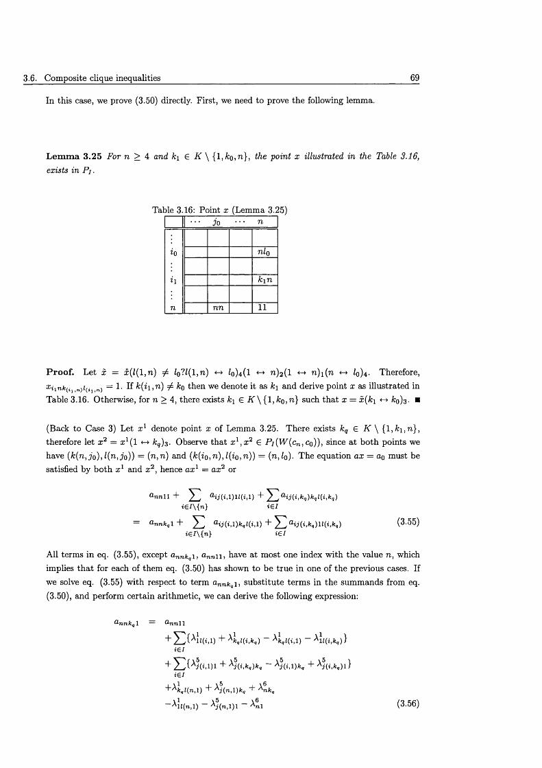
3.6. Composite clique inequalities 69
In this case, we prove (3.50) directly. First, we need to prove the following lemma.
L em m a 3.25 For n > 4 and k\ G K \ {l,A:o,n}, the point x illustrated in the Table 3.16, exists in Pj.
Table 3.16: Point x (Lemma 3.25). . . j Q . . . n
io
h
n
nl 0
k \ n
nn 11
P ro o f. Let x = x(£(l,n ) ^ £o?£(l,n) <-> £0)4(1 <-> 72)2(1 <-* 72)1(72 <-> £0)4- Therefore, Xiink(il n)i(i n) = 1- If k ( i \ , n ) 7 ko then we denote it as ki and derive point x as illustrated in Table 3.16. Otherwise, for n > 4, there exists k\ € K \ {1, ko, n} such th a t x = x(k \ «-» £0)3- ■
(Back to Case 3) Let x 1 denote point x of Lemma 3.25. There exists k q E K \ { l,fci,n} , therefore let x 2 = x : ( l «-> kq)3. Observe that x l , x 2 G P /(W (cn ,Co)), since a t both points we have ( k ( n , j o ) , l ( n , j o ) ) = (n , n ) and ( k ( i o , n ) , l ( i o , n ) ) = (n,£o). The equation a x = ao must be satisfied by both x 1 and x2, hence a x 1 = ax2 or
G n n l l + ) * , * ( » , * , )
i£l\{n} i£l
= annkq 1 4” E aij(i,l)kql(i,l) + ^ ^ / aij(i,kg)ll(i,kq) (3.55)iG/\{n} i€l
All terms in eq. (3.55), except a n n kq 1, a n n n , have at most one index with the value n, which implies th a t for each of them eq. (3.50) has shown to be true in one of the previous cases. If we solve eq. (3.55) with respect to term annkq i, substitute term s in the summands from eq. (3.50), and perform certain arithmetic, we can derive the following expression:
ttnnkg 1 = Q“nnl 1
~b ^ ^kql(i,kq) ^kql(i, 1) ^1 l(i,kq)}<€/
~b ^ j(i,kq)kq ~ ^j(i,l)kq +i£l
~b fcgZ(n,l) “I- ^j(n,l)kq "b ^nkq
~ ^j(n,l)l ~ -^nl (3.56)
CHAPTER 3. Polyhedral characterisation of the OLS polytope 70
The critical observation is that:
Also observe th a t we can substitute term a nn i i from (3 .5 0 ) , because it has two indices equal to one (3 .5 2 ) . Eq. (3 .5 6 ) becomes:
P AfcqJ(n,l) P Aj ( n , l ) k q P An k q
— X 1 — X 5 — X6H (n,l) j ( n , l ) l ^ n l
Since Z(n, 1) = 1 , j (n , 1) = n (Table 3.16), the above equation becomes:
a n n k ql = P + A ^ + A*n + \ bnkq + \ Gnkq
which is identical to (3 .5 0 ) for term annkq\.
Let x 3 = x 2(l <-> lq ) 4 where lq G L \ { l , l o , l i , n } , x 3 G P i i W ^ , c q ) ) . From ax2 = ax 3 we
transformations similar to those performed on eq. (3 .5 5 ) , we obtain eq. (3 .5 0 ) for annkqiq. By reversing the roles of the sets, we can illustrate the correctness of eq. (3 .5 0 ) for all other cases where two of the indices of ( i ,j , k,l) G C \ W{cn , Co) are equal to n.
Our proof concerning all (i , j , k, l) G C \ W(cn , c q ) is now complete.
For (i , j , k , l ) G VF(cn ,c0) \ { (n ,n ,n ,n )} define:
To show (3 .5 0 ) , for (i , j , k , l ) G W (cn ,co) \ { (n ,n ,n ,n )} , it is sufficient to prove th a t all 'Kijki are equal. We proceed in a series of steps.
S te p l: For (za, j lt k it h) , (i2 , j 2 , k 2 , l2) e VF(cn ,c0) such th a t \(ii, j i , k lt h ) n cn \ = 2,
\(i i , 3 i , k i , l i ) n c0| = 2 and \(i2, j 2, k 2 , l2) n cn | = 2, |(z2, j 2, k2 , l2) D c0| = 2, we prove that
= ^ 1232^2 = 7r<
derive
(3 .5 7 )
where the value of the k index, for given i , l is denoted as k(i, l). If we apply to eq. (3.57)
(3 .5 8 )
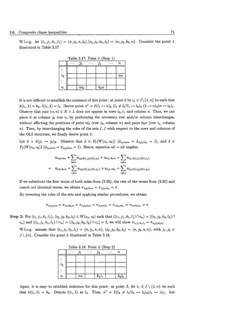
3.6. Composite clique inequalities 71
W.l.o.g. let = {n, jo, n , l 0), (i2, 72, k 2 , h ) = ( n J o , k 0 ,n ). Consider the point xillustrated in Table 3.17
Table 3.17: Point x (Step 1). . . j Q . . . j 1 . . . n
20
n
nn
nlo kon
It is not difficult to establish the existence of this point: at point x let i\ G 7\{1, n} be such th a t , 1) = fco, l(i i , l ) = h- Derive point x 1 = x{l\ <-> 72)4 (l\ 7 Iq11\ <-> 0)4 (1 22)2(n 20)1 •
Observe that pair (72, 72) G K x L does not appear in rows io,i i and column n. Thus, we canplace it in column 7o row n, by performing the necessary row and/or column interchanges, without affecting the positions of pairs nlo (row z0, column n) and pairs k0n (row i \ , column n). Then, by interchanging the roles of the sets 7, J w ith respect to the rows and columns of the OLS structure, we finally derive point x.
Let x = x( j i «-> 70)2• Observe that x G Pi (W (cn ,c0)) (x<0„nn = x njoniQ = 1), and x G
Pi(W(cn ,co)) (x ionnn = x njokon = 1). Hence, equation ax = ax implies
0 >njQnlo + y"! aijok(i,jo)l(i,jo) + anjik0n + ^ ' aijik(i,ji)l(i,j\) i^n i^n
— Xnjokon “I" Ei^n i^n
If we substitute the first terms of both sides from (3.58), the rest of the terms from (3.50) and
cancel out identical terms, we obtain 7rnjQk0n — ^nj 0 ni0 = tt*
By reversing the roles of the sets and applying similar procedures, we obtain
Tfiojonn = ^ionkon ~ ^njokon = ^ionnlo ~ ^njonlo = '^nnkolo = ^
S te p 2: For (21,71, *1. *i), (12,72,^ 2^ 2) € W (cn ,c0) such th a t (( ii,7 i, k ly h ) Dcn) = ((22,72,^ 2, 72)0cn) and |( ii,7 i,fc i,/i) O cn | = |(i2,72, *2, h) 0 cn \ = 3, we will show 7rilJlfclZl = 7riaja*aza.
W.l.o.g. assume th a t (ii,7 i, ki, h) = (n ,7 i,n ,n ) , (12,72,^ 2^ 2) = (n ,72 ,n ,n ), with 7 i,72 € J \ {n}. Consider the point x illustrated in Table 3.18.
Table 3.18: Point x (Step 2). . . . . . j 2 . . . n
2(3
n nn k \ h OO
Again, it is easy to establish existence for this point: at point x, let i\ G 7 \ {1,72} be such that fc(zi,l) = ko. Denote Z(zi, 1) as I2 . Then, x 1 = x f a 7 lo^h *-* 0)4(21 *-* 22)1- Let
CHAPTER 3. Polyhedral characterisation of the OLS poly tope 72
i2 E I \ { l,n } be such th a t k(i2, 1) = k\. We denote l(i2, 1) as li and perform the interchange (1 7 1 )2 . At the derived point we reverse the roles of the sets I, J, thus obtaining point x of
Table 3.18. Let x = x ( j i j 2)2 • Observe th a t x G P i (W (c n ,co)) (x nj inn = x nnk0i0 = !) and x G P i (W ( cn ,c0)) (x nj2nn = x nnkoi0 = 1). Thus, ax = ax implies
O ' n j y T i n + + a n j 2 k i l i + ^ ^ a i j 2 k ( i , j 2 ) l ( i , j 2 )
= an j 2n n "I- a i j 2 k ( i , j i ) l ( i , j i ) d” a n j i k i l l + a i j \ k ( i , j 2) l{ i ,32)i^n i^n
If we substitute the first terms of both sides from (3.58), the rest of the terms from (3.50) and cancel out identical terms, we obtain itn j i n n = 7rnj2nn = tt2, Vfr, j 2 G J \ {n}.
Reversing the roles of the sets is enough to prove:
7Ti in n n = ^ i 2nnn ~ ^ > W j , i 2 G I \ {A }
n n k \n = n n k 2n ~ ^ i V fci, &2 G A \ { n }
' Rnnnl i = n n n l 2 = ^ > ^ 1 > 2 € L \ {vi}
S te p 3: We will show that n 1 = 7r2 = n 3 = 7r4.
Let 5 = x (ji n )2 where x is the point illustrated in Table 3.17 Let x = x(io *-* n)\ . Note
that X G P i ( W ( c n , Co)) ([^njonlo = ^ n nk o n — 1) Mid X G P l( h V ( C n > Q))) (X n j^ nn X iQnkon !)• Thus, ax = ax implies
G n n k o n d- &n j on l o d- ^ a n j k ( n , j ) l ( n , j ) d~ & i o j i n n d- ^ ^ i o j k ( i o , j ) l ( i o t j ) j ^ j o , n j ^ j i
= Q' t i j inn d“ X i o n k o n d“ E a n j k ( i 0 , j ) l ( i 0 , j ) d" a i o j o n l 0 d" ^ a i o j k ( n , j ) l ( n , j )
31^31 3 7^30,n
Substituting the first two terms of both sides from eq. (3.58), the rest of the terms fromeq. (3.50) and taking into account the results obtained in the previous two steps we obtainK n n k 0 n = ^ n j j n n 7T3 = 7r2. As in the previous steps, by reversing the roles of the sets andfollowing the same procedure, we obtain
-1 — J* _ .3 _ v* _ „7T =7T =7T = 7T = K,
S tep 4: We will prove th a t k = it.
Consider the point x illustrated in Table 3.19.
It is easy to see th a t this point exists. At an arbitrary point x G Pi pairs ( n l o ) , (nn) cannot lie a t the same row or column. Thus we can easily derive a point x such th a t x njoniQ =
% i in n n = 1- Also let x ipjpkon = 1. Clearly, j p ^ n , i p ^ i x. If ip ± n and j p ± j 0 then x — x( ip ^ i o l i p <-> i o ) \ ( j p 7 j i ' t j p +-* j 1)2- Otherwise assume w.l.o.g. th a t i p = n. There exist i 2 G I \ {zi,n}, j 2 G J \ {j o , j p , n }, k i G K \ {&o,™} such th a t x i2 j 2kin = 1. Derive point
x = x( i 2 ^ z0?Z2 <-» io ) i( j2 7 J i?J2 <-* j i h ( k i k 0 ) 3 .
Now, let x = x( j i *-> n) 2. Note th a t x G Pi(W(cn,co)) (xnj 0 ni0 = n innn = 1) and x G
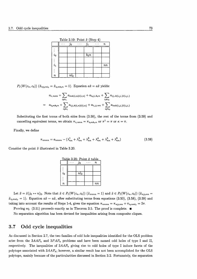
3.7. Odd cycle inequalities 73
Table 3.19: Point x (Step 4). . . j Q . . . j l . . . n
k
h
n
kon
nn
nl 0
Pi {W (cn ,cQ)) (Xnjonio = x ionk0n = 1)- Equation ax = ax yields:
a i i n n n + + £ ' «H* *(« J. W Wi
= Xionkon “I- ^ &ijik{i , i i ) l(i ,r i) “b O-iij^nn £ i^i\ i^io
Substituting the first terms of both sides from (3.58), the rest of the terms from (3.50) and cancelling equivalent terms, we obtain iViinnn = K^nkon or 7T1 = 7r or k = 7r.
Finally, we define
7Tnnnn = a nnnn — (^ nn “b ^ n n “b ^ n n "b \ m “b ^ n n "b \ i n )
Consider the point x illustrated in Table 3.20.
Table 3.20: Point x table
(3.59)
. . . j Q . . . n
k
n
nlQ
nn
Let x = x ( j 0 «-> n)2. Note th a t x e P i(W (cn ,co)) (x nnnn = 1) and x e P i(W (cn , Co)) (xnjonn = Xi0 nni0 = 1)- Equation ax = arc, after substituting terms from equations (3.50), (3.58), (3.59) and taking into account the results of Steps 1-4, gives the equation n nnnn = 7rnj 0nn + ^ i 0n n i0 = 2n.
Proving eq. (3.51) proceeds exactly as in Theorem 3.5. The proof is complete. ■No separation algorithm has been devised for inequalities arising from composite cliques.
3.7 Odd cycle inequalities
As discussed in Section 2.7, the two families of odd hole inequalities identified for the OLS problem arise from the 3A A P n and 3P A P n problems and have been named odd holes of type I and II, respectively. The inequalities of 3A A P n giving rise to odd holes of type I induce facets of the polytope associated with 3A A P n ; however, a similar result has not been accomplished for the OLS polytope, mainly because of the particularities discussed in Section 3.2. Fortunately, the separation
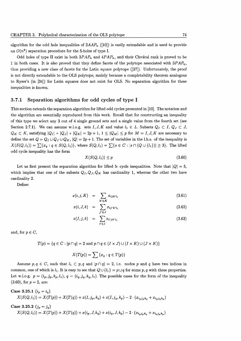
CHAPTER 3. Polyhedral characterisation of the OLS polytope 74
algorithm for the odd hole inequalities of 3A A P n ([10]) is easily extendable and is used to provide an 0 ( n 4) separation procedure for the 5-holes of type I.
Odd holes of type II exist in both 3P A P n and 4P A P n , and their Chvatal rank is proved to be 1 in both cases. It is also proved th a t they define facets of the polytope associated with 3P A P n , thus providing a new class of facets for the Latin square polytope ([37]). Unfortunately, the proof is not directly extendable to the OLS polytope, mainly because a completability theorem analogous to Ryser’s (in [34]) for Latin squares does not exist for OLS. No separation algorithm for these inequalities is known.
3.7.1 Separation algorithm s for odd cycles of typ e I
This section extends the separation algorithm for lifted odd cycles presented in [10]. The notation and the algorithm are essentially reproduced from this work. Recall th a t for constructing an inequality of this type we select any 3 out of 4 single ground sets and a single value from the fourth set (see Section 2.7.1). We can assume w.l.o.g. sets I , J , K and value l\ € L. Subsets Qj C I, Q j C J, Q k C K , satisfying \Qi\ + \Qj\ + \Qk\ = 2p + 1, 1 < \Qm\ < p for M = / , J, A” are necessary to define the set Q = Qi U Q j U Q k , \Q\ = 2p + 1 . The set of variables in the l.h.s. of the inequality is X { S { Q, h ) ) = ■ Q e S ( Q , h ) } , where S{ Q, h ) = |s n ( Q u { h } ) | > 3}. The liftedodd cycle inequality has the form
X ( S ( Q , h ) ) < p (3.60)
Let us first present the separation algorithm for lifted 5- cycle inequalities. Note th a t \Q\ = 5, which implies that one of the subsets Q i , Q j , Q k has cardinality 1, whereas the other two have cardinality 2.
Define:
x ( i J , K) — x i j k ' l i
k ’ e K
(3.61)
x ( i } J, k ) = X / X i 3 ’k ' h j ' € J
(3.62)
x { I , j , k ) = 'y X j ' j k ' i i
i ' e i
(3.63)
and, for p G C,
T(p ) = {q e C : |p fl q\ = 2 and p n q G ( I x J ) U ( / x K ) U (J x K )}
*(?>)) = 9 e r(p)}Assume p, q e C, such th a t l\ C p, q and |p fl q\ = 2, i.e. nodes p and q have two indices in
common, one of which is l\. It is easy to see that Q u { ii} = pUq for some p, q with these properties.Let w.l.o.g. p = (ip, jp, kp,li), q = (iq, j q, k q,li). The possible cases for the form of the inequality (3.60), for p = 2, are:
Case 3.25.1 (ip — iq)X(S( Q, l \ )) = X ( T ( p )) + X(T(q) ) + x ( I , j p, kq) -I- a :( / ,jg, kp) — 2 • {xipj pkq + x ipjqkp)
Case 3.25.2 (j p = j q)X(S( Q, l\)) = X(T(p) ) + X(T(q) ) + x(ip , J, kq) + x( iq, J, kp) — 2 • (Xipjpkq + x iqjpkp)
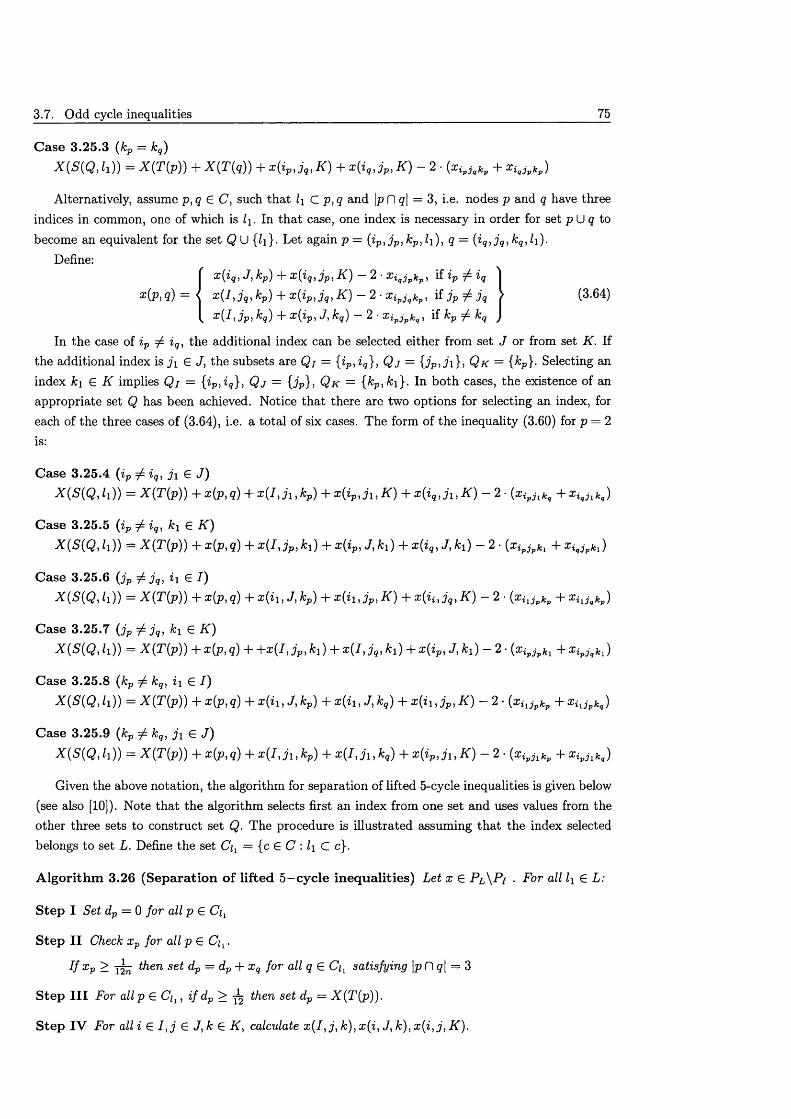
3.7. Odd cycle inequalities 75
C ase 3 .25.3 (kp = kq)X (S ( Q , l \ ) ) — X (T ( p )) + X { T ( q ) ) + x( i p , jq, K ) + x { i q , j p , K ) — 2 • {xipj qkp + x iqj Pkp)
Alternatively, assume p,q £ C, such th a t l\ C p, q and \p Pi q\ = 3, i.e. nodes p and q have three indices in common, one of which is l\. In th a t case, one index is necessary in order for set p U q to become an equivalent for the set Q U {7i}. Let again p = {ip, j p, kp ,li), q = (iq, j q , kq,li).
Define:x( iq, J , kp) + x{iq, j p, K ) — 2 ■ Xigjpkp > if ip 7 iq
x {.PiQ) — < 1 jq> kp) + x( ip, j q, K) 2 • Xipj qkp, if j P ^ jq > (3.64), X(I > Jpi kq) + x{ip, J, kq) — 2 • Xipj pkq, if kp ^ kq t
In the case of ip ^ i q, the additional index can be selected either from set J or from set K. If the additional index is j i £ J, the subsets are Qj = {ip, i q}, Q j = {jp , j i}, Q k = {kp}- Selecting an index k\ £ K implies Qi = {ip, i q}, Q j = { jP}, Q k = {kp,ki } . In both cases, the existence of an appropriate set Q has been achieved. Notice that there are two options for selecting an index, foreach of the three cases of (3.64), i.e. a total of six cases. The form of the inequality (3.60) for p = 2
is:
C ase 3 .25.4 (ip ^ iq, j \ £ J )X ( S ( Q , h )
Case 3.25.5X ( S ( Q , h )
Case 3.25.6X ( S ( Q , h )
Case 3.25.7X ( S ( Q , h )
Case 3.25.8X ( S ( Q , h )
Case 3.25.9X ( S ( Q , h )
= X(T(p) ) + x(p, q) + x { I , j 1, kp) + x(ip, j U K) + x{iq, j i , K ) - 2 • (x ipjlkq + x igjlkq)
ip 7 iqi ^ X )= X(T(p) ) + x(p,q) + x ( I , j p , fci) + x(ip, J , k i ) + x{iq, J, h ) - 2 - (x ipjpkl + x iqjpkl)
j p 7 j q t i \ £ -0= X(T(p) ) +x(p ,q) + x{ii , J,kp) + x ( i i , j p , K ) + x ( i i , j q, K ) - 2- (xiljpkp + x iljqkp)
jp 7 j q ) ^1 ^ X )= X(T(p) ) + x(p, q) + +x(I , j p , k x) + x{I, j q, fci) + x( ip, J , k l ) - 2 - (x ipjpkl + x ipjqkl)
kp 7 kq, i\ £ 7)= X(T(p) ) + x{p,q) + x (ii, J , kp) + x( i1, J , k q) + x ( i i , j p , K) - 2 ■ (x iljpkp + x iljpkq)
kp 7 kq, j \ £ ,7)= X{T{p)) + x(p,q) + x{ I , j i , kp) + x ( I , j 1,kq) + x{ ip, j 1, K ) - 2 - (xipjlkp + x ipjlkq)
Given the above notation, the algorithm for separation of lifted 5-cycle inequalities is given below (see also [10]). Note th a t the algorithm selects first an index from one set and uses values from the other three sets to construct set Q. The procedure is illustrated assuming th a t the index selected belongs to set L. Define the set Cix = {c £ C \ l\ C. c}.
A lgorithm 3.26 (Separation o f lifted 5—cycle inequalities) Let x £ P l \ P i • For all li £ L:
Step I Set dp = 0 for all p £ Cix
Step II Check xp for all p £ .
U xp > then set dp = dp + x q for all q £ Ci, satisfying \p D q\ = 3
Step III For al lp £ C^ , i f dp > ^ then set dp = X(T(p)) .
Step IV For al i i £ I , j £ J , k £ K, calculate x ( I , j , k ) , x ( i , J , k ) , x ( i , j , K ) .
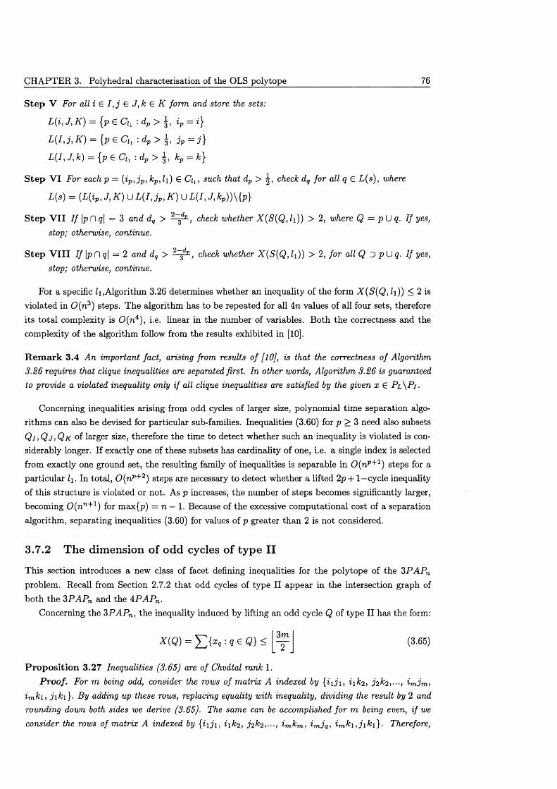
CHAPTER 3. Polyhedral characterisation of the OLS polytope 76
S tep V For all i G I , j G J , k G K form and store the sets:
L(i, J, K'j — |p G Ci . dp g, ip — i ^
L ( I , j , K) = { p e Ch :dp > \ , jp = j }
L(I , J, k) = {p G Ch : dp > kp = k}
S tep V I For each p = (ip, j p, kp , l\) G Cj, , such that dp > check dq for all q G L(s), where
L(s) = ( L ( i p , J , K ) u L ( I J p, K ) U L ( I , J , k p ) ) \ { p }
Step V I I I f \p n q\ = 3 and dq > check whether X ( S ( Q, h) ) > 2, where Q — p U q. I f yes,stop; otherwise, continue.
Step V I I I I f \p fl g| = 2 and dq > check whether X{S{Q, l \ )) > 2, /o r all Q D p Uq . I f yes,stop; otherwise, continue.
For a specific Algorithm 3.26 determines whether an inequality of the form X( S ( Q, l\)) < 2 is violated in 0 ( n 3) steps. The algorithm has to be repeated for all 4n values of all four sets, therefore its to tal complexity is 0 ( n 4), i.e. linear in the number of variables. Both the correctness and the complexity of the algorithm follow from the results exhibited in [10].
R em ark 3.4 An important fact, arising from results of [10], is that the correctness o f Algorithm 3.26 requires that clique inequalities are separated first. In other words, Algorithm 3.26 is guaranteed to provide a violated inequality only i f all clique inequalities are satisfied by the given x G P l \ P i -
Concerning inequalities arising from odd cycles of larger size, polynomial time separation algorithm s can also be devised for particular sub-families. Inequalities (3.60) for p > 3 need also subsets Q i i Q j , Q k of larger size, therefore the time to detect whether such an inequality is violated is considerably longer. If exactly one of these subsets has cardinality of one, i.e. a single index is selected from exactly one ground set, the resulting family of inequalities is separable in 0 ( n p+1) steps for a particular li. In total, 0 (n p+2) steps are necessary to detect whether a lifted 2p + 1—cycle inequality of this structure is violated or not. As p increases, the number of steps becomes significantly larger, becoming 0 (n n+1) for max{p) = n — 1. Because of the excessive com putational cost of a separation algorithm, separating inequalities (3.60) for values of p greater than 2 is not considered.
3.7.2 The dim ension o f odd cycles of type II
This section introduces a new class of facet defining inequalities for the polytope of the 3P A P n problem. Recall from Section 2.7.2 th a t odd cycles of type II appear in the intersection graph of both the 3P A P n and the 4P A P n .
Concerning the 3P A P n , the inequality induced by lifting an odd cycle Q of type II has the form:
P ro p o s itio n 3.27 Inequalities (3.65) are of Chvatal rank 1.P roof. F o r m being odd, consider the rows of matrix A indexed by { i \ j \ , i \ k 2 , 3 2 ^ 2 ,•••,
consider the rows o f matrix A indexed by {i \ j \ , i-mkm, imjq, i mk i , j i k i } . Therefore,
3m(3.65)
2
imki, j i k \ } . By adding up these rows, replacing equality with inequality, dividing the result by 2 and rounding down both sides we derive (3.65). The same can be accomplished fo r m being even, i f we
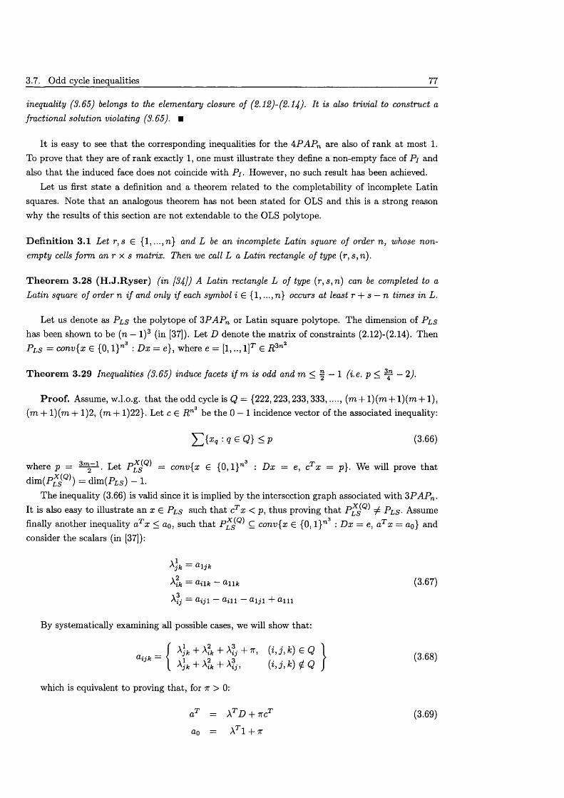
3.7. Odd cycle inequalities 77
inequality (3.65) belongs to the elementary closure of (2.12)-(2. I f ) . It is also trivial to construct a fractional solution violating (3.65). ■
I t is easy to see th a t the corresponding inequalities for the 4P A P n are also of rank a t most 1. To prove th a t they are of rank exactly 1, one must illustrate they define a non-empty face of Pj and also th a t the induced face does not coincide with Pj. However, no such result has been achieved.
Let us first state a definition and a theorem related to the completability of incomplete Latin squares. Note that an analogous theorem has not been stated for OLS and this is a strong reason why the results of this section are not extendable to the OLS polytope.
D e fin itio n 3.1 Let r ,s G { l,...,n } and L be an incomplete Latin square o f order n, whose nonempty cells form an r x s matrix. Then we call L a Latin rectangle o f type (r, s ,n ).
T h e o re m 3.28 (H .J .R y se r ) (in [34]) A Latin rectangle L of type (r, s ,n ) can be completed to a Latin square of order n i f and only i f each symbol i G {1,..., n ) occurs at least r + s — n times in L.
Let us denote as P is the polytope of 3PAPn or Latin square polytope. The dimension of P l s
has been shown to be (n — l ) 3 (in [37]). Let D denote the m atrix of constraints (2.12)-(2.14). Then P l s = conv{x G {0,1}”3 : D x = e}, where e = [1,.., 1]T G P 3n2
T h e o re m 3.29 Inequalities (3.65) induce facets i f m is odd and m < j — 1 (i.e. p < ^ — 2).
P ro o f. Assume, w.l.o.g. that the odd cycle is Q = {222,223,233,333,...., (m + l)(m + l)(m -|-1), (m + l)(m + 1)2 , (m +1)22}. Let c G R n3 be the 0 — 1 incidence vector of the associated inequality:
: q £ Q } < p (3.66)
where p = 3rT ~1. Let P ^ s ^ = conv{x € {0, l} n3 : D x = e, cT x = p}. We will prove th a t dim (P*5(g)) = dim (PLS) - 1.
The inequality (3.66) is valid since it is implied by the intersection graph associated with 3P A P n . It is also easy to illustrate an x G P l s such th a t cTx < p , thus proving th a t P l s ^ 7^ P l s - Assume finally another inequality aTx < a0, such that P * ^ ^ conv{x G {0, l} n3 : D x = e, aTx = a 0 } and consider the scalars (in [37]):
= a l j k
^ ik = ®ilfc ®11 k (3 .6 7 )
= a i j l — a i l l — a l j l + a l l l
(3 .6 8 )
which is equivalent to proving that, for n > 0:
By systematically examining all possible cases, we will show that:
_ f ^jk + ^Hk + ^Hj + tt, { i , j , k ) e Q
aT = AT D + 7rcT
ao = Ar l -f 7r
(3.69)
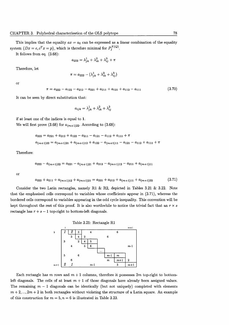
CHAPTER 3. Polyhedral characterisation of the OLS polytope 78
This implies that the equality ax = ao can be expressed as a linear combination of the equality system { Dx = e, cTx = p}, which is therefore minimal for
It follows from eq. (3.68):
^222 = ^jk + ^ik + + 7r
Therefore, let
7T = a222 - (A*fc + A + A? )
or7r = a2 22 — «122 — a212 — a22i + a2n + a i2i + a n 2 — a m (3.70)
It can be seen by direct substitution that:
c i i j k = A]fc + \ ? k + A ?■
if at least one of the indices is equal to 1.We will first prove (3.68) for a(m+1)22. According to (3.68):
0-222 = 0 2 21 + 0 2 1 2 + « i 2 2 — ^211 — a m — a n 2 + a m + 7r
a (m +l)22 = a (m +l)21 + a (m +l)12 + a 122 “ « ( m + l ) l l — a 121 — a 112 + ^111 + ^
Therefore:
0222 — a (m + l)2 2 = a 221 — ^(m +l)21 + a 212 ~ <Rm+1)12 ~ a 211 + f l (m + l) ll
or
0222 + O2 1 1 + 0 (m + l)1 2 + 0(m+1)21 = a 221 + ^212 + + G(m+1)22 (3-71)
Consider the two Latin rectangles, namely R1 & R2, depicted in Tables 3.21 h 3.22. Note th a t the emphasised cells correspond to variables whose coefficients appear in (3.71), whereas the bordered cells correspond to variables appearing in the odd cycle inequality. This convention will be kept throughout the rest of this proof. It is also worthwhile to notice the trivial fact th a t an r x s rectangle has r + s — 1 top-right to bottom-left diagonals.
m + l
Each rectangle has m rows and m + l columns, therefore it possesses 2m top-right to bottom- left diagonals. The cells of a t least m + 1 of those diagonals have already been assigned values. The remaining m — 1 diagonals can be identically (but not uniquely) completed with elements m + 2, ...,2m + 2 in both rectangles without violating the structure of a Latin squaxe. An example of this construction for m = 5, n = 6 is illustrated in Table 3.23.
Table 3.21: Rectangle R1
m-l
5 66
2 1 m-l
m-lm + l
m+l
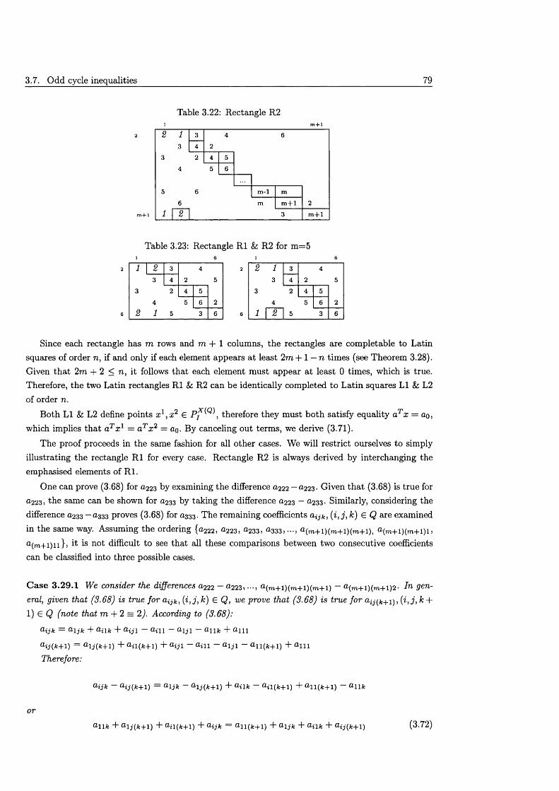
3.7. Odd cycle inequalities 79
Table 3.22: Rectangle R21 m + l
2 2 1 3 4 6
3 4 2
3 2 4 5
5
4
6
5 6
m-l m6 m m + l 2
m + l 1 2 3 m + l
Table 3.23: Rectangle R1 & R2 for m =51 6 1 6
1 2 3 4 2 2 1 3 4
3 4 2 5 3 4 2 5
3 2 4 5 3 2 4 5
4 5 6 2 4 5 6 2
2 1 5 3 6 6 1 2 5 3 6
Since each rectangle has m rows and m + l columns, the rectangles are completable to Latin squares of order n, if and only if each element appears a t least 2m + 1 — n times (see Theorem 3.28). Given that 2m + 2 < n, it follows that each element must appear at least 0 times, which is true. Therefore, the two Latin rectangles R1 & R2 can be identically completed to Latin squares LI & L2 of order n.
Both LI Sz L2 define points x 1,# 2 £ therefore they must both satisfy equality aTx = ao,which implies that aTx 1 = aTx 2 = ao. By canceling out terms, we derive (3.71).
The proof proceeds in the same fashion for all other cases. We will restrict ourselves to simply illustrating the rectangle R1 for every case. Rectangle R2 is always derived by interchanging the emphasised elements of R l.
One can prove (3.68) for <2223 by examining the difference £2222 — &223- Given th a t (3.68) is true for £1223) the same can be shown for (2233 by taking the difference £2223 — a 233- Similarly, considering the difference £1233 — <2333 proves (3.68) for £1333. The remaining coefficients (i , j , k) £ Q are examined
in the same way. Assuming the ordering { a 222 , <*223, ^ 233, ^ 3 3 3 , •••, a ( m + i ) ( m + i ) ( m + i ) , a ( m + i ) ( m + i ) i ,
a ( m + i ) n } ) it is not difficult to see that all these comparisons between two consecutive coefficients can be classified into three possible cases.
C a s e 3 . 29.1 We consider the differences £2222 ®223) •••> ® ( m + i ) ( m + i ) ( m + i ) ® ( m + i ) ( m + i ) 2 ' 9 &n-eral, given that (3.68) is true for aijk, (i , j , k) £ Q, we prove that (3.68) is true for £2ij(*.+1), (i , j , k + 1) £ Q (note that m + 2 = 2). According to (3.68):
O ' i j k = O ' l j k “I" & i \ k "I” & i j 1 ® i l l ^ I j l ®11A; d" £ 2 ll l
aij(k+1) = alj(k+l) + a il(fc+l) + aij 1 — aill — a lj l — a ll(fc+l) + a ll lTherefore:
a-ijk — o-ij{fc+i) = a-ijk — a ij(fc+i) + a nk — an(k+i ) + a n(fc+i) ~ a iifc
or
ail k + £2ij(fc+i) + £2ii(fc+l) + Oijk = Ull(fc+1) + aljk + a-iik + a ij(A:+l) (3.72)
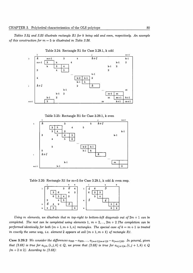
CHAPTER 3. Polyhedral characterisation of the OLS polytope 80
Tables 3.24 and 3.25 illustrate rectangle R1 for k being odd and even, respectively. A n example o f this construction for m = 5 is illustrated in Table 3.26.
Table 3.24: Rectangle R1 for Case 3.29.1, k odd1 j m + l
k+1m + l k-1lm + l k-1
k-1
k-1k-2 k-1k-1
k+1k-1
k-1 m-lk-1 k+1m + l
k+1 m + lm + l
Table 3.25: Rectangle R1 for Case 3.29.1, k even1 j m + l
k+1
k-1k-1
k-2 k-1k-1
k+1
k-1k-1m + l
Table 3.26: Rectangle R1 for m =5 for Case 3.29.1, k odd & even resp.1 5 6 1 4 6
5 3 6 4 1 4 6 53 6 4 2 6 2 3
6 3 4 2 3 4
3 4 5 4 5 46 4 2 5 5 6
4 2 6 6 6 2
Using m elements, we illustrate that m top-right to bottom-left diagonals out of 2m + 1 can be completed. The rest can be completed using elements 1, m + 2 ,..., 2m + 2 .The completion can be performed identically for both (m + 1, m + 1, n) rectangles. The special case o f k — m + l is treated in exactly the same way, i.e. element 2 appears at cell (m + l ,m + 1) of rectangle R l.
C a s e 3 . 29.2 We consider the differences 0 2 2 3 — a 2 3 3 5 •••) a ( m + i ) ( m + i ) 2 — a ( m + i) 2 2 - I n general, given that (3.68) is true for a i j k , { i , j , k ) € Q, we prove that (3.68) is true for (i, j + l , k ) e Q(m + 2 = 2). According to (3.68):
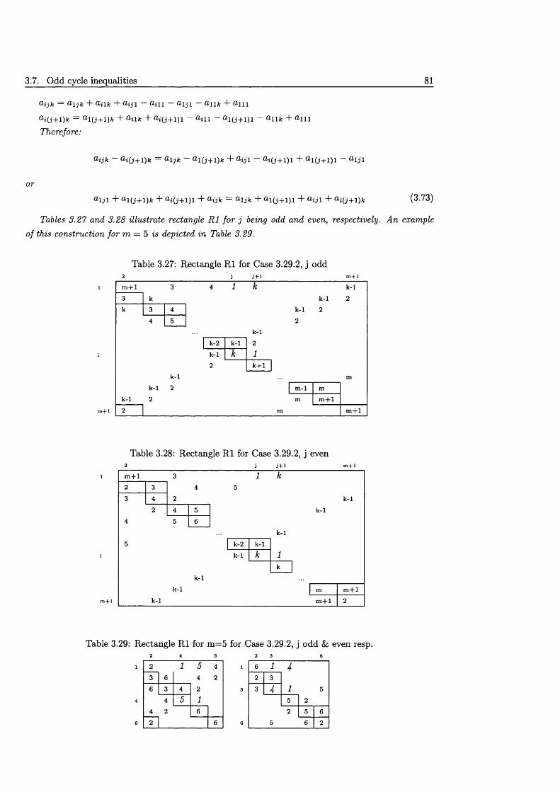
3.7. Odd cycle inequalities 81
or
d i j k — O' l j k “I” O' i lk d~ &i j 1 ^ i l l ^ l j l ^ 1 1 k d - & 111
a i ( j + l ) k = a l ( j + l ) k d " CLilk d " a i ( j + l ) l — a i \ \ ~~ a l ( j + l ) l — a m d " A l i i
Therefore:
a i j k a i ( j + l ) k ~ a l j k ~ a l ( j '+ l ) f c d " a i j 1 — a i ( j + 1)1 d" a l ( j + l ) l — a l j l
d i j i d - a i ( j + i ) f c d - a , i ( j + i ) i d - a , i j k = a i j k + a i ( j + i ) i d - d i j i d - a q J + 1 ) fc (3.73)
Tobies 3.27 dnd 3.28 illustmte rectangle R1 for j being odd and even, respectively. An example of this construction for m = 5 is depicted in Table 3.29.
Table 3.27: Rectangle R1 for Case 3.29.2, j oddj j+i
m + l
k-1k-1
2
k-12
k
k-1
k-2 k-1 2k-1 k 12 k + 1
k-1
2
m - l
k-1
2
m + l
k-1
2
m + l
Table 3.28: Rectangle R1 for Case 3.29.2, j evenj j+i
m + l
m + lk-1
k-1
k -1
1 k
k-1
k -2 k-1
1k-1 k
k
k-1
k-1
m + l
m + l
Table 3.29: Rectangle R1 for ra=5 for Case 3.29.2, j odd & even resp.2 4 6 2 3 6
2 1 5 4 l 6 1 43 6 4 2 2 3
6 3 4 2 3 3 4 l 5
4 5 1 5 2
4 2 6 2 5 6
2 6 6 5 6 2
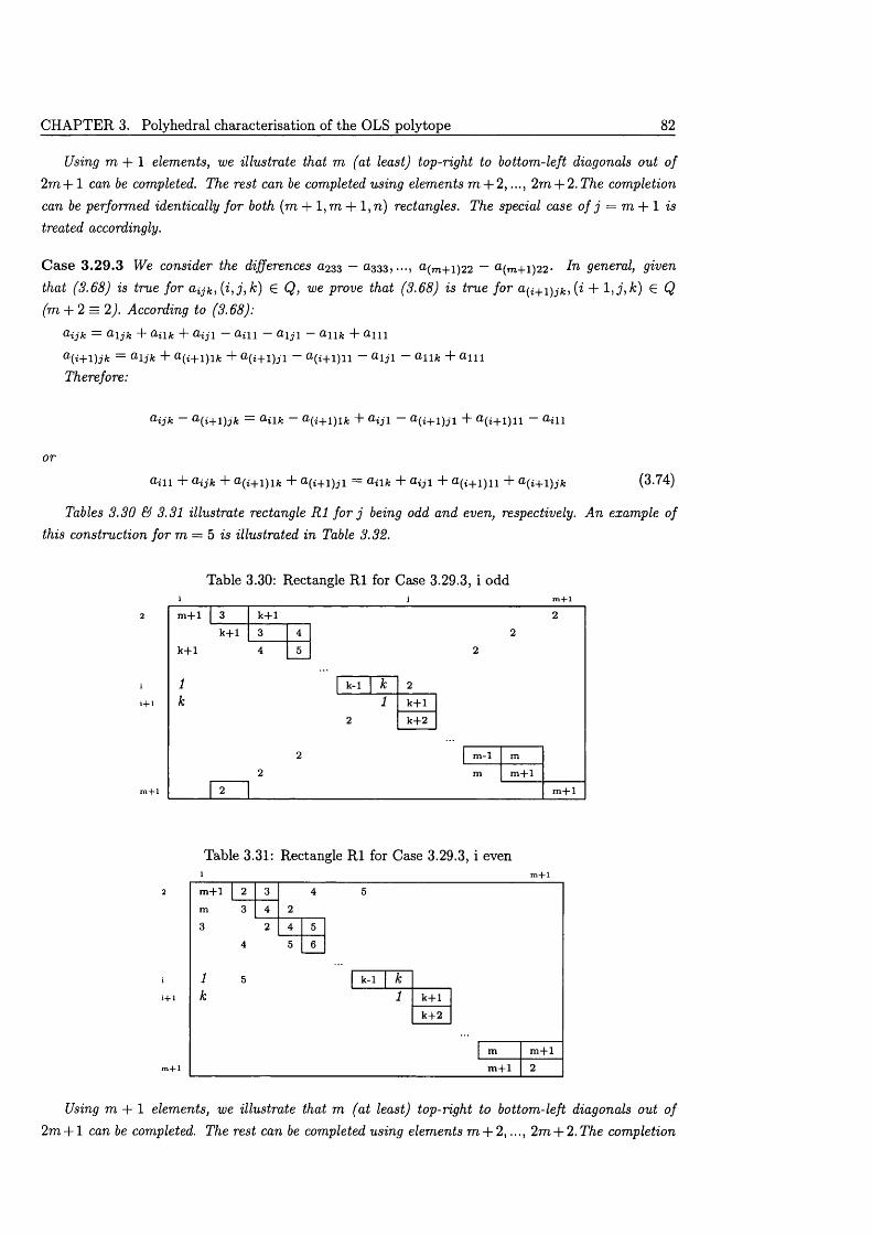
CHAPTER 3. Polyhedral characterisation of the OLS polytope 82
Using m + l elements, we illustrate that m (at least) top-right to bottom-left diagonals out of 2m + 1 can be completed. The rest can be completed using elements m + 2 , ..., 2m + 2.The completion can be performed identically for both (m + l ,m + l ,n ) rectangles. The special case o f j = m + 1 is treated accordingly.
C ase 3 .29.3 We consider the differences 0 2 3 3 — < 2 3 3 3 , fl(m+1)22 — a(m+1)22- In general, given that (3.68) is true for ai j k , { i , j , k ) G Q, we prove that (3.68) is true for a^i+i^jk ,(i + l , j , k ) G Q (m + 2 = 2). According to (3.68):
& i j k = Q*ljk + <+lfc + < + ,jl <+11 * + j l < + lfc + < + 1 1
a ( i + i ) j k = a i j k + & ( i + i ) i k + a ( i + 1 )j-! — a ( i + 1 ) n — a i j i — a n * + a m
Therefore:
& i j k ~ a ( i + l ) j k = a i l k ~ a ( i + l ) l f c + a i j 1 — a ( i + l ) j l + a ( i + l ) l l — a i l l
or
*+11 + a i j k + 0-(i+l)lA: + a ( i + l ) j l — °>i\k + <+jl + < l ( i + l ) l l + <+ i+ l) jf t (3.74)
Tables 3.30 & 3.31 illustrate rectangle R1 for j being odd and even, respectively. An example of this construction for m = 5 is illustrated in Table 3.32.
Table 3.30: Rectangle R1 for Case 3.29.3, i odd
m + l
k+1
1k
k+1
k+1
k-1 k 21
2k+1
k+2
m -l
m + l
m + l
Table 3.31: Rectangle R1 for Case 3.29.3, i even
m + l
k-1 k1 k+1
k+2
m + l
m + l
Using m + l elements, we illustrate that m (at least) top-right to bottom-left diagonals out of 2m + 1 can be completed. The rest can be completed using elements m + 2,..., 2m + 2. The completion
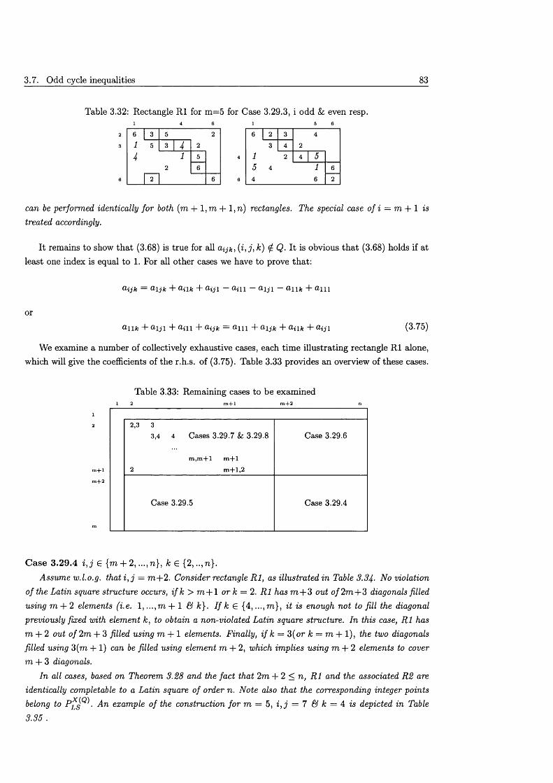
3.7. Odd cycle inequalities 83
Table 3.32: Rectangle R1 for m =5 for Case 3.29.3, i odd & even resp.1 4 6 1 5 6
6 3 5 2 6 2 3 4
1 5 3 4 2 3 4 2
4 l 5 4 1 2 4 52 6 5 4 1 6
2 6 6 4 6 2
can be performed identically for both (m + l ,m + l ,n ) rectangles. The special case of i = m + 1 is treated accordingly.
It remains to show th a t (3.68) is true for all a^k, (i , j , k ) ^ Q. It is obvious th a t (3.68) holds if at least one index is equal to 1. For all other cases we have to prove that:
®ijk = O'ljk T &ilk T O'ijl ^ill ®ljl ^l lk T ®111
or
Gil* + a \ j i + d in -T a ^ k = + o-ijk + a n k + <Rji (3.75)
We examine a number of collectively exhaustive cases, each time illustrating rectangle R1 alone, which will give the coefficients of the r.h.s. of (3.75). Table 3.33 provides an overview of these cases.
Table 3.33: Remaining cases to be examined1 2 m + l m + 2 n
12
Cases 3 .29.7 & 3 .29.: Case 3 .29.6
m ,m + l m + l
m + l , 2m + l
m + 2
Case 3 .29.5 Case 3 .29.4
m
C ase 3.29.4 i , j e {m + 2 ,..., n}, k e {2,.., n).Assume w.l.o.g. t ha t i , j — m +2. Consider rectangle R l, as illustrated in Table 3.34- No violation
of the Latin square structure occurs, i f k > m + l or k = 2. R l has m + 3 out o /2 m + 3 diagonals filled using m + 2 elements (i.e. 1 ,.. .,m + 1 & A;}. I f k G {4, ...,m }, it is enough not to fill the diagonal previously fixed with element k, to obtain a non-violated Latin square structure. In this case, R l has m + 2 out o f 2m + 3 filled using m + l elements. Finally, i f k = 3(or k = m + 1), the two diagonals filled using 3(m + 1) can be filled using element m + 2, which implies using m + 2 elements to cover m + 3 diagonals.
In all cases, based on Theorem 3.28 and the fact that 2m + 2 < n, R l and the associated R2 are identically completable to a Latin square of order n. Note also that the corresponding integer points belong to • A n example o f the construction for m = 5, i, j = 7 & k = 4 is depicted in Table3.35 .
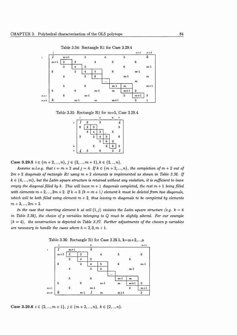
CHAPTER 3. Polyhedral characterisation of the OLS polytope 84
Table 3.34: Rectangle R l for Case 3.29.41 m + l m + 2
m + lm + l
m-lm-l
m-l
m + lm -lm-l m + l
m-l m + lm +lm-li + 2
Table 3.35: Rectangle R l for m=5, Case 3.29.41 4 6 7
1 1 6 3 46 2 3 5
3 4 2 5
3 2 4 5 6
5 6 2
6 5 2 6 3
7 4 5 6 3 1
C ase 3.29.5 i E {m + 2, . . . ,n}, j E {2, ...,m + 1}, k E {2,.., n}.Assume w.l.o.g. that i = m + 2 and j = 4. I f k E {m + 2,..., n}, the completion o f m + 2 out of
2m + 2 diagonals of rectangle R l using m + 2 elements is implemented as shown in Table 3.36. I f k E {4, ...,ra}, but the Latin square structure is retained without any violation, it is sufficient to leave empty the diagonal filled by k. This will leave m + l diagonals completed, the rest m + l being filled with elements m + 2, ...,2m + 2. I f k = 3 (k = m + l ) element k m ust be deleted from two diagonals, which will be both filled using element m + 2, thus leaving m diagonals to be completed by elements m + 3, ...,2m + 2.
In the case that inserting element k at cell (1 , j ) violates the Latin square structure (e.g. k = 4 in Table 3.36), the choice of p variables belonging to Q must be slightly altered. For our example (k = 4), the construction is depicted in Table 3.37. Further adjustments o f the chosen p variables are necessary to handle the cases where k = 2 ,3 ,m + 1.
Table 3.36: Rectangle R l for Case 3.29.5, k=m +2,...,n
m + l
m + 2
C ase 3.29.6 i E {2, ...,m + 1}, j E {m + 2, ...,n}, k E {2, ..,n}.
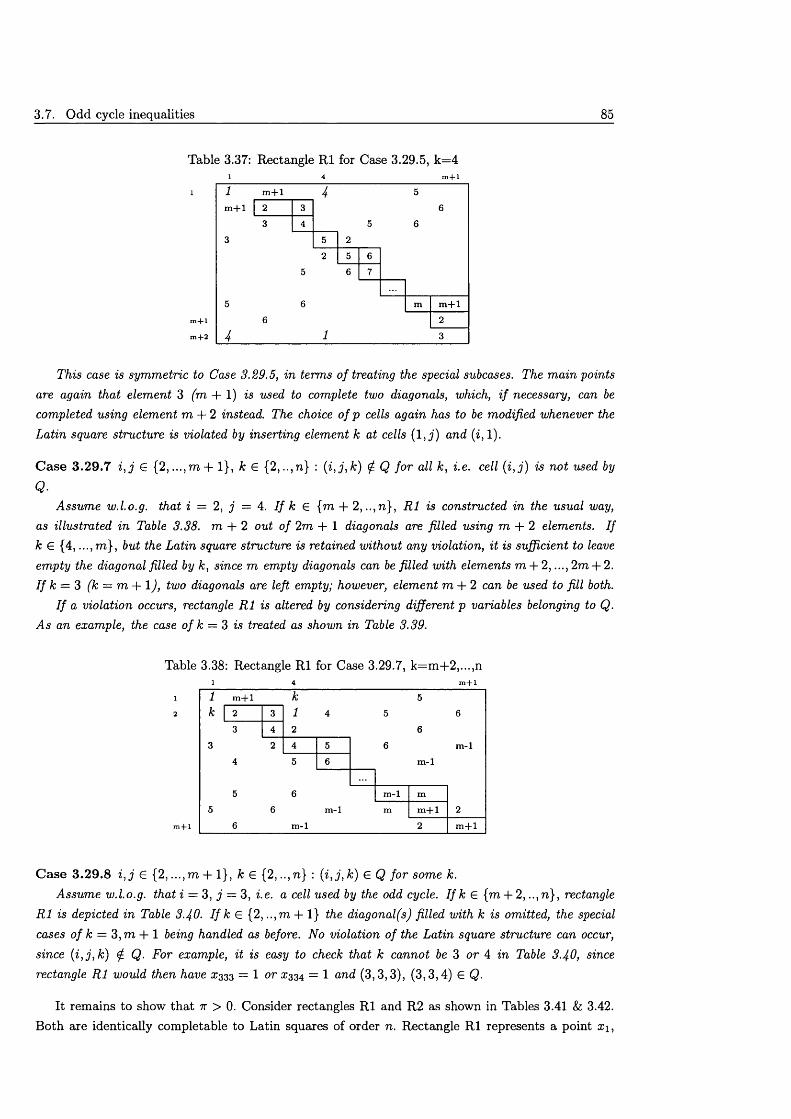
3.7. Odd cycle inequalities 85
Table 3.37: Rectangle R l for Case 3.29.5, k=4
m + l
m + 2
This case is symmetric to Case 3.29.5, in terms of treating the special subcases. The main points are again that element 3 (m + l) is used to complete two diagonals, which, i f necessary, can be completed using element m + 2 instead. The choice o f p cells again has to be modified whenever the Latin square structure is violated by inserting element k at cells (1 , j ) and (i , 1).
C ase 3 .29 .7 i , j G {2 ,...,m + l}, k G {2,..,n} : (i , j , k ) ^ Q fo r all k , i.e. cell (i , j ) is not used by
Q ■Assume w.l.o.g. that i = 2, j = 4. I f k G [m + 2 ,..,n } , R l is constructed in the usual way,
as illustrated in Table 3.38. m + 2 out o f 2m + 1 diagonals are filled using m + 2 elements. I f k G {4, ...,m }, but the Latin square structure is retained without any violation, it is sufficient to leave empty the diagonal filled by k , since m empty diagonals can be filled with elements m + 2, ...,2m + 2. I f k = 3 (k = m + l) , two diagonals are left empty; however, element m + 2 can be used to fill both.
I f a violation occurs, rectangle R l is altered by considering different p variables belonging to Q. As an example, the case of k = 3 is treated as shown in Table 3.39.
Table
1 2
C ase 3 . 29.8 i , j G {2, ...,m + 1}, k G {2, ..,n} : (i , j , k ) G Q for some k.Assume w.l.o.g. that i = 3, j = 3, i.e. a cell used by the odd cycle. I f k € {m + 2,.., n}, rectangle
R l is depicted in Table 3.40. I f k G {2, ..,m + 1} the diagonal(s) filled with k is omitted, the special cases o f k = 3 ,m + 1 being handled as before. No violation of the Latin square structure can occur, since (i , j , k ) ^ Q. For example, it is easy to check that k cannot be 3 or A in Table 3-40, since rectangle R l would then have £333 = 1 or £334 = 1 and (3 ,3,3), (3 ,3 ,4) G Q.
It remains to show th a t 7r > 0. Consider rectangles R l and R2 as shown in Tables 3.41 & 3.42. Both are identically completable to Latin squares of order n. Rectangle R l represents a point £ 1,
3.38: Rectangle R l for Case 3.29.7, k=m +2,...,n1 4 m + l
m + l
5 66 m-l
6 m-l
5 6 6
6 m-l m -l
m-lm + l
m + l
1 4 m + l
1 m + l 4 5m + l 2 3 6
3 4 5 63 5 2
2 5 6
5
5
6
6 7
m m + l6 2
4 1 3
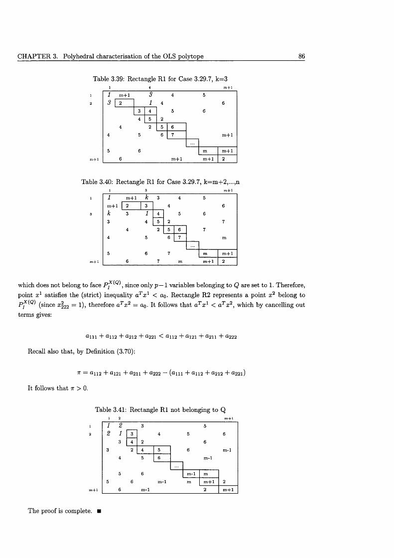
CHAPTER 3. Polyhedral characterisation of the OLS polytope 86
Table 3.39: Rectangle R l for Case 3.29.7, k=3
1 2
m + 1
Table 3.40: Rectangle R l for Case 3.29.7, k=m +2,...,n
3
m -j-1
which does not belong to face ; since only p — 1 variables belonging to Q are set to 1. Therefore,point x 1 satisfies the (strict) inequality aTx 1 < ao. Rectangle R2 represents a point x 2 belong to pMQ) (sjnce x 2 2 2 = l)j therefore aT x2 = ao. It follows th a t aTx 1 < aTx 2, which by cancelling out terms gives:
U n i + U ll2 + a 212 + a 221 < a 112 + a 121 + a 2 l \ + a 222
Recall also that, by Definition (3.70):
7T = a n 2 + ^121 + a 211 + a 222 — (a l l l + a n 2 + 0212 + <3.221)
It follows that 7r > 0.
Table 3.41: Rectangle R l not belonging to Q
12
m-lm-l
5 66 m -l
6 m-l
m -l mm + l
m + l
1m + lk3
1+1 k 3 44
5
6 77
m + lm + l
1 m + ls r ~
3 41 4
52
m + l
m + l m + lm + l
The proof is complete. ■
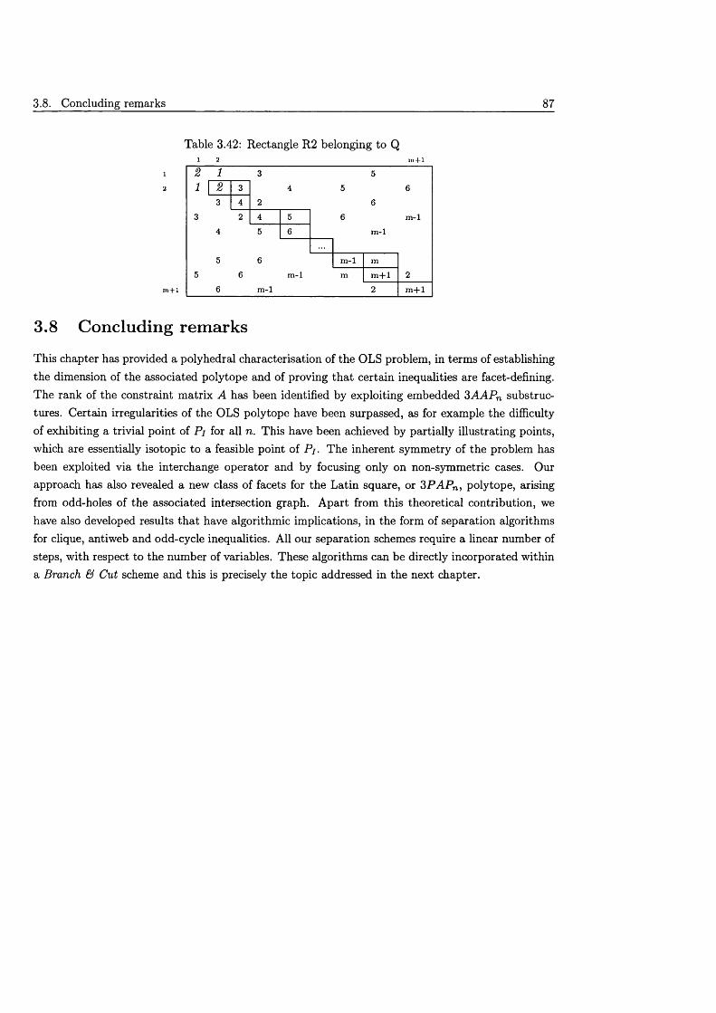
3.8. Concluding remarks 87
Table 3.42: Rectangle R2 belonging to Q1 2 m + l
2 1 1
3 2
4
m-lm-l
m-l
m-l
m-l
m + lm + l
3.8 Concluding remarks
This chapter has provided a polyhedral characterisation of the OLS problem, in terms of establishing the dimension of the associated polytope and of proving th a t certain inequalities are facet-defining. The rank of the constraint matrix A has been identified by exploiting embedded 3AAPn substructures. Certain irregularities of the OLS polytope have been surpassed, as for example the difficulty of exhibiting a trivial point of Pi for all n. This have been achieved by partially illustrating points, which are essentially isotopic to a feasible point of Pj. The inherent symmetry of the problem has been exploited via the interchange operator and by focusing only on non-symmetric cases. Our approach has also revealed a new class of facets for the Latin square, or 3PAPn , polytope, arising from odd-holes of the associated intersection graph. Apart from this theoretical contribution, we have also developed results th a t have algorithmic implications, in the form of separation algorithms for clique, antiweb and odd-cycle inequalities. All our separation schemes require a linear number of steps, with respect to the number of variables. These algorithms can be directly incorporated within a Branch & Cut scheme and this is precisely the topic addressed in the next chapter.

CHAPTER 3. Polyhedral characterisation of the OLS poly tope
Chapter 4
Integer Program m ing algorithm s
This chapter presents algorithms for solving the OLS problem using Linear and Integer Programming. The most motivating instance of the OLS problem is the infeasible case of n = 6. Proving infeasibility for this instance via Integer Programming, apart from being one of the aims of our research, demonstrates the benefits of using IP to solve this particular problem. Infeasibility was formally proved for the first time by Taxry ([81]), essentially by exhaustive enumeration. Shorter proofs have also been proposed, for example in [80]. This chapter presents an alternative proof, based solely on Linear Programming. The proof reduces the solution space of the original problem by incorporating a method for eliminating symmetries.
Computer-based methods have been successfully applied to answer open questions in finite algebra, the most characteristic example being the proof of the non-existence of a finite projective plane, or equivalently of a set of 9 MOLS, of order 10 ([58]). This work also explores the potential of algorithmic methods to answer theoretical questions related to Latin Squares. The innovative aspect of our approach is th a t this is implemented via m athematical programming. In particular, the non-existence of an OLS structure of order 6 is shown by solving exactly 12 linear programs. This IP model is presented in Section 4.1. A symmetry breaking mechanism, resulting in a reduction of the solution space, is described in Section 4.2. The actual proof of infeasibility for n = 6 is given in Section 4.3, where it is shown th a t 12 integer programming problems are infeasible because of the infeasibility of the corresponding linear programming problems. The infeasibility of each LP is demonstrated by exhibiting dual values, which in conjunction with Farkas’ lemma ([68, Theorem 2.7]), illustrate the result.
The OLS problem for general n can be viewed as a feasibility problem, i.e. as the problem of identifying a pair of OLS of order n. Our work adopts exactly this perspective instead of treating OLS as an optimization problem. This conforms also to the applications of OLS (Section 1.4), which normally ask for a single, rather than an optimal, solution. In order to solve this problem, a “Branch & Cut” algorithm has been devised and is presented in this chapter.
Integer programming is simply the extension of linear programming to problems, where a subset of the variable set is required to be integer. Pure integer programs define the class of integer programs, where all problem variables must be integer. A special case of integer programs are the binary or 0 — 1 integer programs (BIP), which involve only 0 — 1 variables. Clearly, the OLS problem falls within this last category.
The study of integer programs was motivated by the success of the simplex method in solving linear programs. Extending this method to 0 — 1 integer programs essentially partitions the original
89
CHAPTER 4. Integer Programming algorithms 90
problem into subproblems, formed recursively by setting variables to 0 or 1. This is apparently an enumeration scheme, usually named “Divide & Conquer” or 11 Branch & Bound”. The first term emanates from the computer science literature, whereas the second has been introduced by the mathematical programming community. As noted in [68, Chapter II.4], the first Branch & Bound algorithm for general integer programs was presented in [59], although the approach was broadly adopted after the first such algorithm appeared for the Travelling Salesman Problem (TSP) in [61]. Another version of the enumerative approach, specifically for 0 — 1 programs, is the implicit enumeration algorithm ([7]).
A Branch & Bound algorithm can be improved by strengthening the LP formulation of the problem. This amounts to adding extra inequalities, generated by enforcing the fact th a t certain variables must be integer. A systematic procedure for generating all valid inequalities for an integer program is presented in [45] (see also [68, Section II. 1-2]). This celebrated result initiated the theory of valid inequalities and motivated the development of the “Branch & Cut” algorithmic approach for solving integer programs. This generic scheme adds valid inequalities to the LP of each subproblem in Branch &; Bound. These inequalities are also called “cuts” because they are normally added only if violated by the current fractional solution of the LP-relaxation. Again, the TSP has been the problem where one of the first Branch & Cut codes was applied ([66]). Because of the number of valid inequalities being enormous, a criterion for selecting the most prominent ones is required. Polyhedral theory has provided a natural characterisation of the strongest possible valid inequalities or facets (see also Section 3.1). Hence, several Branch & Cut codes incorporating families of, general purpose or problem specific, valid inequalities have been developed in the last decades. Numerous successful applications of this approach to both industrial and theoretical problems can be found in the mathematical programming literature (e.g. [68]). Especially set-packing and set-partitioning problems have attracted considerable attention, exactly because of their generic structure. The literature for set-partitioning includes algorithms for crew scheduling ([50]), and for the axial 3- index assignment problem ([11]). These algorithms use valid inequalities induced by cliques and odd-holes of the problem’s intersection graph.
Section 4.4 presents the components of the Branch & Cut algorithm for the OLS problem. These components include a problem-specific preprocessor, a specialised branching mechanism, which uses Special Ordered Sets of type /, and separation algorithms for families of valid inequalities. The implementation details are analysed in Section 4.5. The computer code uses advanced features provided by the XPRESS-MP software ([31]) for branching, LP-solving and cut management. Finally, computational results are discussed in Section 4.6. These results measure different branching rules, certain strategies for cut addition and the quality of various families of cutting planes. The test problems used are the instances of the OLS problem for orders up to 12. Nevertheless, the case of n = 6 remains the most significant benchmark, since the entire solution space must be searched in order for infeasibility to be proved.
4.1 Two Integer Programming models for OLS
We illustrate again the IP model for OLS used in the previous chapters. The only difference is th a t the objective function is simply the sum of all the variables. This objective function results in every feasible solution being also optimal and relates to the fact th a t the OLS problem is treated as a
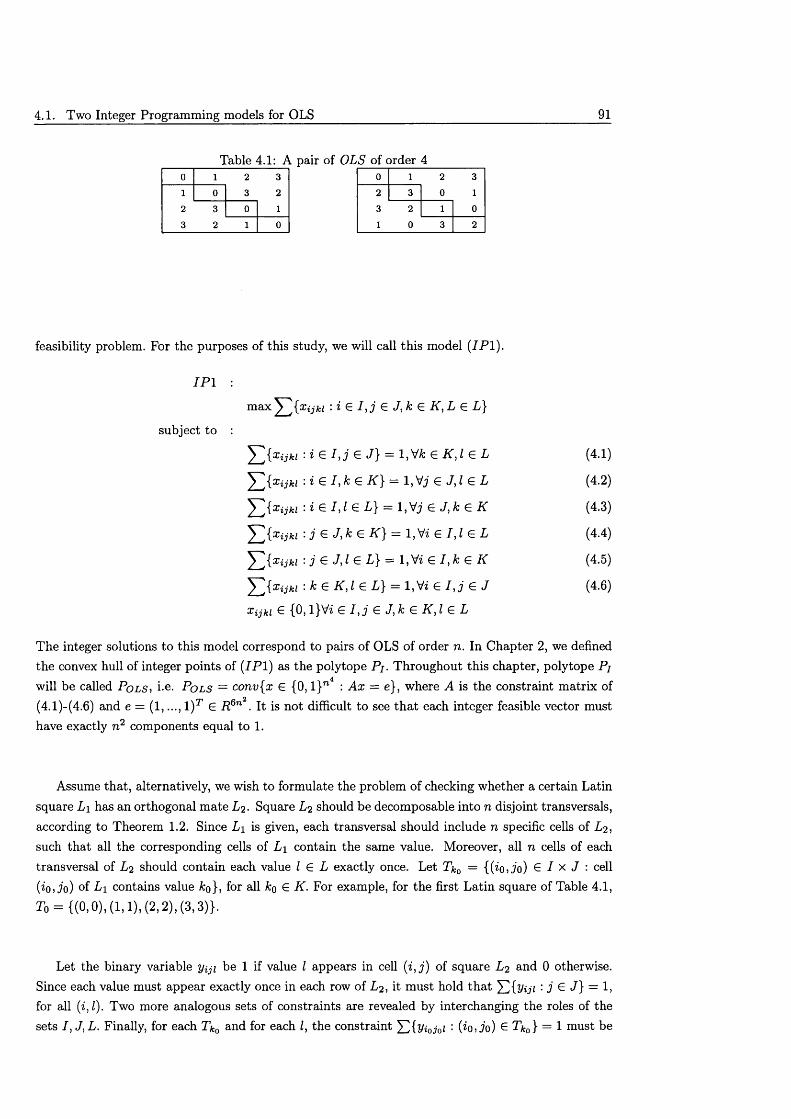
4.1. Two Integer Programming models for OLS 91
Table 4.1: A pair of OLS of order 40 1 2 3
1 0 3 2
2 3 0 1
3 2 1 0
0 1 2 3
2 3 0 1
3 2 1 0
1 0 3 2
feasibility problem. For the purposes of this study, we will call this model ( IP 1).
IP 1 :
subject to
m a x .^^{x ijk i : i e l , j e J , k e K , L e L }
x ijkl • i G I , j G J} = 1 y k G K , l G L (4.1)
x ijkl • i G I , k G K } = 1, Vj G J, l G L (4.2)
^ ^{Xijkl : i G 1,1 G L} = 1, Vj G J , k G K (4.3)
^ ^{x ijkl ’• j G J , k G K } = l,V i G 1,1 G L (4.4)
^ ' yj{x ijkl '■j G J ,l G L} = 1, Vz G I , k G K (4.5)
$ > « « ' k G K ,l G L} = l,Vz G / , j G J (4.6)
x ijkl ^ {0, l}Vz G I , j G J , k G K , l G L
The integer solutions to this model correspond to pairs of OLS of order n. In Chapter 2, we defined the convex hull of integer points of ( I P 1) as the polytope Pj. Throughout this chapter, polytope Pj
4will be called P o l s > i - e - P o l s = conv{x G {0, l} n : A x = e}, where A is the constraint m atrix of (4.1)-(4.6) and e = (1,..., 1)T G R 6n2. It is not difficult to see th a t each integer feasible vector must have exactly n 2 components equal to 1.
Assume that, alternatively, we wish to formulate the problem of checking whether a certain Latin square L\ has an orthogonal m ate Z^- Square L 2 should be decomposable into n disjoint transversals, according to Theorem 1.2. Since L \ is given, each transversal should include n specific cells of L 2 , such that all the corresponding cells of L \ contain the same value. Moreover, all n cells of each transversal of L 2 should contain each value I G L exactly once. Let Tk0 = {(^o, jo) e I x J : cell (i0Jo) of Li contains value /cq}, for all k0 G K. For example, for the first Latin square of Table 4.1, To = {(0,0), (1,1), (2,2), (3,3)}.
Let the binary variable yiji be 1 if value I appears in cell ( i , j ) of square L 2 and 0 otherwise. Since each value must appear exactly once in each row of L 2 , it must hold th a t YUViji : j G ^} = h for all (i,l). Two more analogous sets of constraints are revealed by interchanging the roles of the
sets / , J, L. Finally, for each Tk0 and for each I, the constraint YUViojoi ’• (io,jo) £ Tk0} = 1 must be
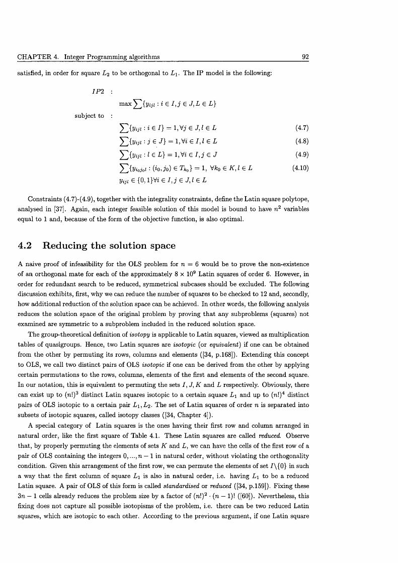
CH APTER 4. Integer Programming algorithms 92
satisfied, in order for square L 2 to be orthogonal to L \ . The IP model is the following:
I P2 :
subject to
m a x y ' {yi j i : i G I , j G J , L G L}
Viji : i € 1} = 1, Y? G J, I G L (4.7)
5 3 {Viji : j e J } = 1, Vi e l , l e L (4.8)
: G L} = 1, Vi G I, j G J (4.9)
E w * ' (^O)Jo) € Tk0} — 1, Vfco € K , l G L (4.10)
Viji G {0, l}Vi G / j ' G J , / g I
Constraints (4.7)-(4.9), together with the integrality constraints, define the Latin square polytope, analysed in [37]. Again, each integer feasible solution of this model is bound to have n 2 variables equal to 1 and, because of the form of the objective function, is also optimal.
4.2 Reducing the solution space
A naive proof of infeasibility for the OLS problem for n = 6 would be to prove the non-existence of an orthogonal mate for each of the approximately 8 x 10⁹ Latin squares of order 6. However, in order for redundant search to be reduced, symmetrical subcases should be excluded. The following discussion exhibits, first, why we can reduce the number of squares to be checked to 12 and, secondly, how additional reduction of the solution space can be achieved. In other words, the following analysis reduces the solution space of the original problem by proving th a t any subproblems (squares) not examined are symmetric to a subproblem included in the reduced solution space.
The group-theoretical definition of isotopy is applicable to Latin squares, viewed as multiplication tables of quasigroups. Hence, two Latin squares are isotopic (or equivalent) if one can be obtained from the other by permuting its rows, columns and elements ([34, p. 168]). Extending this concept to OLS, we call two distinct pairs of OLS isotopic if one can be derived from the other by applying certain permutations to the rows, columns, elements of the first and elements of the second square. In our notation, this is equivalent to permuting the sets I , J, K and L respectively. Obviously, there can exist up to (n!)3 distinct Latin squares isotopic to a certain square L \ and up to (n!)4 distinct pairs of OLS isotopic to a certain pair L \, L 2 . The set of Latin squares of order n is separated into subsets of isotopic squares, called isotopy classes ([34, Chapter 4]).
A special category of Latin squares is the ones having their first row and column arranged in natural order, like the first square of Table 4.1. These Latin squares are called reduced. Observe that, by properly permuting the elements of sets K and L, we can have the cells of the first row of a pair of OLS containing the integers 0, ...,n — 1 in natural order, w ithout violating the orthogonality condition. Given this arrangement of the first row, we can perm ute the elements of set /\{0 } in such a way th a t the first column of square L\ is also in natural order, i.e. having L \ to be a reduced Latin square. A pair of OLS of this form is called standardised or reduced ([34, p. 159]). Fixing these 3n — 1 cells already reduces the problem size by a factor of (n!)2 • (n — 1)! ([60]). Nevertheless, this fixing does not capture all possible isotopisms of the problem, i.e. there can be two reduced Latin squares, which are isotopic to each other. According to the previous argument, if one Latin square
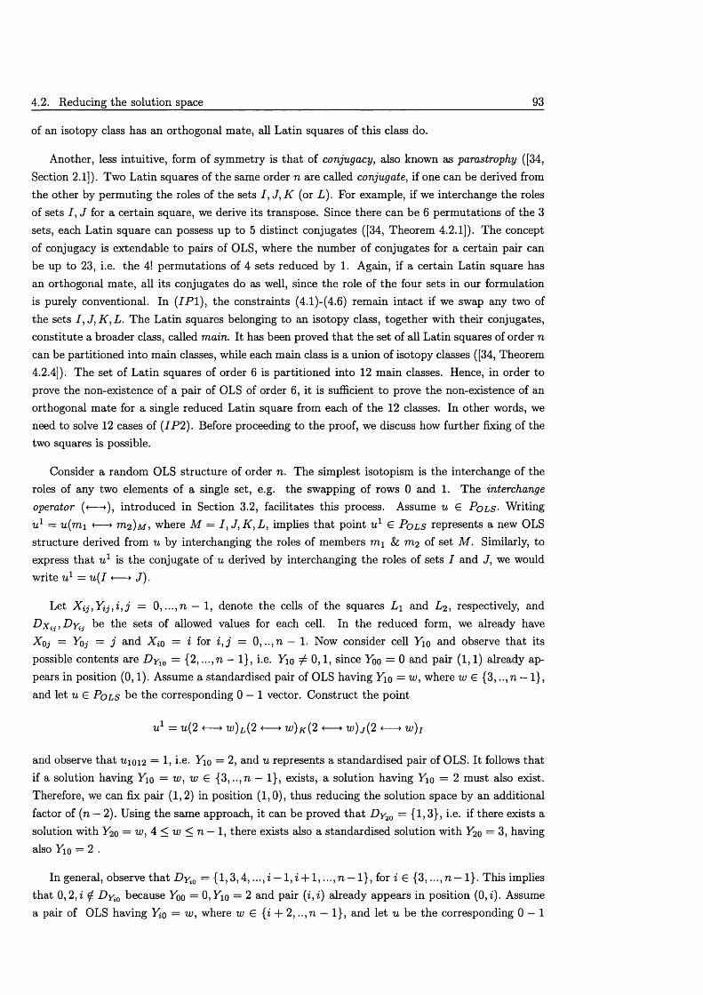
4.2. Reducing the solution space 93
of an isotopy class has an orthogonal mate, all Latin squares of this class do.
Another, less intuitive, form of symmetry is th a t of conjugacy, also known as parastrophy ([34, Section 2.1]). Two Latin squares of the same order n are called conjugate, if one can be derived from the other by permuting the roles of the sets I , J, K (or L). For example, if we interchange the roles of sets 7, J for a certain square, we derive its transpose. Since there can be 6 permutations of the 3 sets, each Latin square can possess up to 5 distinct conjugates ([34, Theorem 4.2.1]). The concept of conjugacy is extendable to pairs of OLS, where the number of conjugates for a certain pair can be up to 23, i.e. the 4! permutations of 4 sets reduced by 1. Again, if a certain Latin square has an orthogonal mate, all its conjugates do as well, since the role of the four sets in our formulation is purely conventional. In ( IP 1), the constraints (4.1)-(4.6) remain intact if we swap any two of the sets / , J, K , L. The Latin squares belonging to an isotopy class, together w ith their conjugates, constitute a broader class, called main. It has been proved th a t the set of all Latin squares of order n can be partitioned into main classes, while each main class is a union of isotopy classes ([34, Theorem 4.2.4]). The set of Latin squares of order 6 is partitioned into 12 main classes. Hence, in order to prove the non-existence of a pair of OLS of order 6, it is sufficient to prove the non-existence of an orthogonal mate for a single reduced Latin square from each of the 12 classes. In other words, we need to solve 12 cases of (IP 2 ). Before proceeding to the proof, we discuss how further fixing of the two squares is possible.
Consider a random OLS structure of order n. The simplest isotopism is the interchange of the roles of any two elements of a single set, e.g. the swapping of rows 0 and 1. The interchange operator (<— >), introduced in Section 3.2, facilitates this process. Assume u G P o l s • Writing u 1 = u(m i <— > m 2 )M , where M = I , J , K , L , implies th a t point u 1 G P o l s represents a new OLS structure derived from u by interchanging the roles of members m\ h m 2 of set M. Similarly, to express that u 1 is the conjugate of u derived by interchanging the roles of sets I and J, we would write u 1 = u( I <— ► J).
Let X i j , Y i j , i , j = 0, ...,n — 1, denote the cells of the squares L \ and L 2 , respectively, and D x i:j, D Yij be the sets of allowed values for each cell. In the reduced form, we already have Xqj = Yqj = j and Xio = i for i , j = 0, ..,n — 1. Now consider cell Yio and observe th a t its possible contents are D y 10 = {2, ...,n — 1}, i.e. Yio 7 0,1, since Foo = 0 and pair (1,1) already appears in position (0,1). Assume a standardised pair of OLS having Yio = w, where w G {3,.., n — 1}, and let u G P o ls be the corresponding 0 — 1 vector. Construct the point
u 1 = u (2 <— > w )L(2 <— > lu)k (2 <— ► w ) j (2 <— > w)i
and observe that U1012 = 1, he. Yio = 2, and u represents a standardised pair of OLS. It follows that if a solution having Yio = w, w € {3, ..,n — 1}, exists, a solution having Yio = 2 must also exist. Therefore, we can fix pair (1,2) in position (1,0), thus reducing the solution space by an additional factor of (n — 2). Using the same approach, it can be proved th a t D y 2Q = {1,3}, i.e. if there exists a solution with Y20 = w, 4 < w < n — 1, there exists also a standardised solution with Y20 = 3, having also Yio = 2 .
In general, observe th a t D y i0 = {1,3,4, ...,i — 1, i + 1 , . . . , n — 1}, for i G {3, ...,n — 1}. This implies that 0 ,2 , i £ D y i0 because Yoo = 0,Yio = 2 and pair (i , i ) already appears in position (0,i). Assume a pair of OLS having Y*o = uj, where w G {i + 2, . . ,n — 1}, and let u be the corresponding 0 — 1
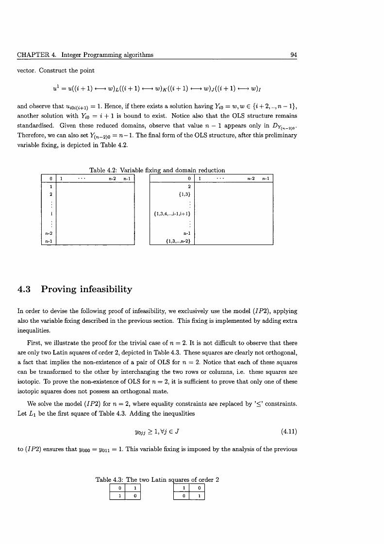
CHAPTER 4. Integer Programming algorithms 94
vector. Construct the point
u 1 = u((i + 1) <— ► w)L((i + 1) *— > w)K ((i + 1) *— ► w)j ( ( i + 1) <— ► w)i
and observe that Uioi(i+i) = 1. Hence, if there exists a solution having Yio = w , w G {i + 2 , n — 1}, another solution with Yio = * + 1 is bound to exist. Notice also th a t the OLS structure remains standardised. Given these reduced domains, observe th a t value n — 1 appears only in Z)y(ri 2)0. Therefore, we can also set Y"(n_2)o = n —1. The final form of the OLS structure, after this preliminary variable fixing, is depicted in Table 4.2.
Table 4.2: Variable fixing and domain reductionn-2 n-1
n-2n-1
0 1 • • • n-2 n-1
2
{1.3}
{ l ,3 ,4 , . . , i - l , i+ l }
n-1
{1,3,.. ,n-2}
4.3 Proving infeasibility
In order to devise the following proof of infeasibility, we exclusively use the model (/P 2 ), applying also the variable fixing described in the previous section. This fixing is implemented by adding extra inequalities.
First, we illustrate the proof for the trivial case of n = 2. It is not difficult to observe that there are only two Latin squares of order 2, depicted in Table 4.3. These squares are clearly not orthogonal, a fact that implies the non-existence of a pair of OLS for n — 2. Notice th a t each of these squares can be transformed to the other by interchanging the two rows or columns, i.e. these squares are iso topic. To prove the non-existence of OLS for n = 2, it is sufficient to prove th a t only one of these isotopic squares does not possess an orthogonal mate.
We solve the model (I P 2 ) for n = 2, where equality constraints are replaced by ’< ’ constraints. Let L\ be the first square of Table 4.3. Adding the inequalities
z / o j j > i , V j e J (4.11)
to (I P 2 ) ensures that ?/ooo = Von = 1- This variable fixing is imposed by the analysis of the previous
Table 4.3: The two Latin squares of order 20 11 0
1 00 1
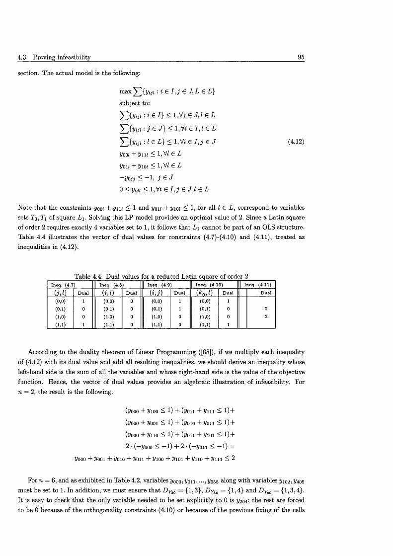
4.3. Proving infeasibility 95
section. The actual model is the following:
max y ^{yiji : i G I , j G J , L G L}
subject to:
^ 2 { y i j i - i e l } < i y j e J t l e L
V i j i : j e J } < i , V i e l , l e L
£ { y « i : l e L } < 1, Vz G 1 ,3 G J (4.12)
yooi + y i u < l , V/ g L
y o u + y io i < l , V/ g L
yojj — j 0 < yiji < 1,Vi G I , j G J , l e L
Note th a t the constraints yooz + y i u < 1 and you + yioz < 1, for all I G L, correspond to variables sets To,Xi of square L\ . Solving this LP model provides an optimal value of 2. Since a Latin square of order 2 requires exactly 4 variables set to 1, it follows th a t L\ cannot be part of an OLS structure. Table 4.4 illustrates the vector of dual values for constraints (4.7)-(4.10) and (4.11), treated as inequalities in (4.12).
Table 4.4: Dual values or a reduced Latin square of order 2Ineq. (4.7) Ineq. (4.8) Ineq. (4.9) Ineq. (4.10) Ineq. (4.11)
U,1) Dual ( i , 0 Dual ( i J ) Dual ( * o , 0 Dual Dual
(0,0) 1 (0,0) 0 (0,0) 1 (0,0) 1
(0,1) 0 (0,1) 0 (0,1) 1 (0,1) 0 2
(1,0) 0 (1,0) 0 (1,0) 0 (1,0) 0 2
(1,1) 1 (1,1) 0 ( i , i ) 0 (1,1) 1
According to the duality theorem of Linear Programming ([68]), if we multiply each inequality of (4.12) with its dual value and add all resulting inequalities, we should derive an inequality whose left-hand side is the sum of all the variables and whose right-hand side is the value of the objective function. Hence, the vector of dual values provides an algebraic illustration of infeasibility. For n = 2, the result is the following.
(yooo + y ioo < 1) + (you + y i u < 1 ) +
(yooo + yooi < 1) + (yo io + y o n < 1 ) +
(yooo + y n o < l ) + (y o n + y io i < l ) +
2 ■ ( —yooo < —1) + 2 • ( —y o n < —1) =
yooo + yooi + yoio + y o u + y ioo + y io i + y n o + y m < 2
For n = 6, and as exhibited in Table 4.2, variables yooo>y o n > •••,yoss along with variables yio2>y405 must be set to 1. In addition, we must ensure th a t P y 20 = {1,3}, Dy30 = {1,4} and Hy50 = {1,3,4}. It is easy to check th a t the only variable needed to be set explicitly to 0 is y 204 ! the rest are forced to be 0 because of the orthogonality constraints (4.10) or because of the previous fixing of the cells
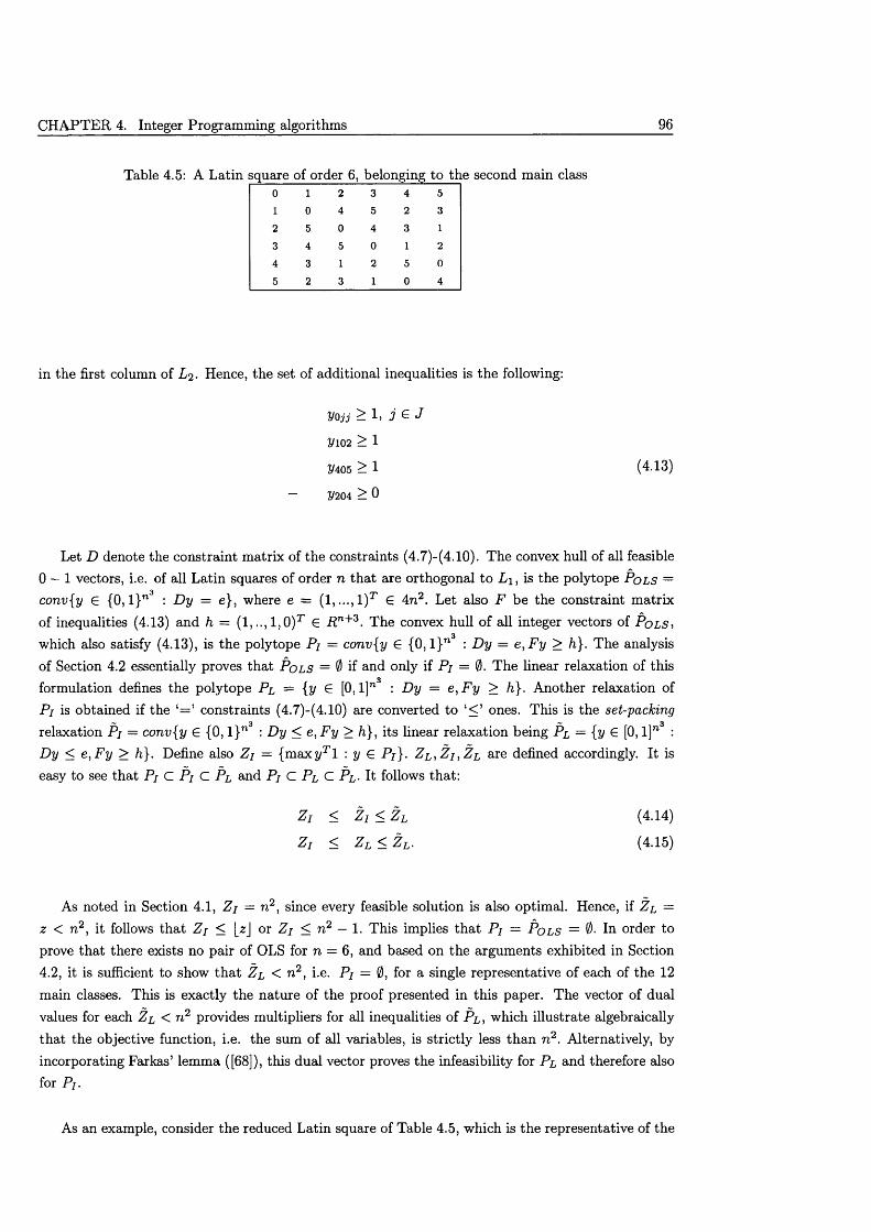
CHAPTER 4. Integer Programming algorithms 96
Table 4.5: A Latin square of order 6, belonging to the second main class0 1 2 3 4 5
1 0 4 5 2 3
2 5 0 4 3 13 4 5 0 1 24 3 1 2 5 05 2 3 1 0 4
in the first column of Hence, the set of additional inequalities is the following:
Vojj ^ 1 ) j £ J
2/102 > l
2 /4 0 5 > 1 (4-13)
— y 2 0 4 > 0
Let D denote the constraint matrix of the constraints (4.7)-(4.10). The convex hull of all feasible 0 — 1 vectors, i.e. of all Latin squares of order n that are orthogonal to L i, is the polytope P o ls — conv{y G {0 ,1}”3 : D y = e}, where e = (1 ,...,1 )T G 4n2. Let also F b e the constraint matrix of inequalities (4.13) and h = (1 ,..,1 ,0 )T G R n+3. The convex hull of all integer vectors of P o l s >
3
which also satisfy (4.13), is the polytope P j = conv{y G {0, l} n : D y = e , F y > h}. The analysis of Section 4.2 essentially proves that P o ls — 0 if and only if P / = 0. The linear relaxation of this
3
formulation defines the polytope Pl = {y £ [0, l]n : D y = e , F y > h}. Another relaxation ofP j is obtained if the ‘= ’ constraints (4.7)-(4.10) are converted to l< ’ ones. This is the set-packing
~ 3 -w 3
relaxation P / = conv{y G {0, l} n : D y < e, F y > h}, its linear relaxation being P l = {y G [0, l]n : Dy < e, F y > h}. Define also Zj = {m axyTl : y G P/}. Z l , Z j , Z l are defined accordingly. It is easy to see th a t P / C P / C P l and Pj C P l C Pl- It follows that:
Zi < Zj < Z l (4.14)
Zj < Z L < Z L. (4.15)
As noted in Section 4.1, Z j = n 2, since every feasible solution is also optimal. Hence, if Zi, = 2 < n2, it follows th a t Zj < [ z \ or Zi < n 2 — 1. This implies th a t Pi = P o l s = 0- In order to prove that there exists no pair of OLS for n = 6, and based on the arguments exhibited in Section 4.2, it is sufficient to show th a t Z l < n 2 , i.e. P / = 0, for a single representative of each of the 12 main classes. This is exactly the nature of the proof presented in this paper. The vector of dual values for each Z l < n 2 provides multipliers for all inequalities of P l , which illustrate algebraically th a t the objective function, i.e. the sum of all variables, is strictly less than n 2. Alternatively, by incorporating Farkas’ lemma ([68]), this dual vector proves the infeasibility for P l and therefore also for P 7.
As an example, consider the reduced Latin square of Table 4.5, which is the representative of the
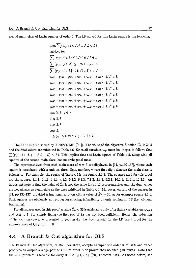
4.4. A Branch &; Cut algorithm for OLS 97
second main class of Latin squares of order 6. The LP solved for this Latin square is the following:
m&xy^{y i j i : i e I , j e J , L e L}
subject to:
: i e 1 } < 1, Vj e J, l g L
- j e J } < l , Vi g / ,Z g L
^ { y i j i : l e L} < l , V i € I , j € J
Vooi + 2 /ii2 + 2/221 + 2/332 + 2/451 + 2/541 < 1 , VZ G L
2/012 + 2/102 + 2/252 + 2/342 + 2/422 + 2/532 < 1 , VZ G L
2/022 + 2/142 + 2/202 + 2/352 + 2/432 + 2/512 < 1 , VZ G L
2/032 + 2/152 + 2/242 + 2/302 + 2/412 + 2/522 < 1 , VZ G L
2/042 + 2/122 + 2/232 + 2/312 + 2/402 + 2/552 < 1 , VZ G L
2/052 + 2/132 + 2/212 + 2/322 + 2/442 + 2/502 < 1 , VZ G 1 /
yojj j J 2/102 > 1
2 /4 0 5 > 1
2 /2 0 4 < 0
0 < V i j i < 1, Vi G 1,3 G J,Z G L
This LP has been solved by XPRESS-MP ([31]). The value of the objective function Z l is 34.5 and the dual values are exhibited in Table 4.6. Since all variables y i j i must be integer, it follows that Y,{yiji : i £ I , j € J ,L £ L} < 34. This implies th a t the Latin square of Table 4.5, along with all squares of the second main class, has no orthogonal mate.
The representatives from each main class of n = 6 are displayed in [34, p. 130-137], where each square is associated with a unique, three digit, number, whose first digit denotes the main class it belongs to. For example, the square of Table 4.5 is the square 2.1.1. The squares used for this proof are the squares 1.1.1, 2.1.1, 3.1.1, 4.1.2, 5.1.2, 6.1.3, 7.1.3, 8.3.1, 9.2.1, 10.2.1, 11.2.1, 12.3.1. An im portant note is th a t the value of Z l is not the same for all 12 representatives and the dual values are not always as symmetric as the ones exhibited in Table 4.6. Moreover, certain of the squares in [34, pp.130-137] provided a fractional solution with a value of Z l = 36, as for example square 8.1.1. Such squares are obviously not proper for showing infeasibility by only solving an LP (i.e. without branching).
For all squares used in this proof, a value Z l < 36 is achievable only after fixing variables 2/102 > 2/405
and 1/204 to 1, i.e. simply fixing the first row of L 2 has not been sufficient. Hence, the reduction of the solution space, as presented in Section 4.2, has been crucial for the LP-based proof for the non-existence of OLS for n — 6.
4.4 A Branch & Cut algorithm for OLS
The Branch & Cut algorithm, or B&C for short, accepts as input the order n of OLS and either produces as output a singe pair of OLS of order n or proves th a t no such pair exists. Note that the OLS problem is feasible for every n G Z +\{1 ,2 ,6} ([60, Theorem 2.9]). As noted before, the
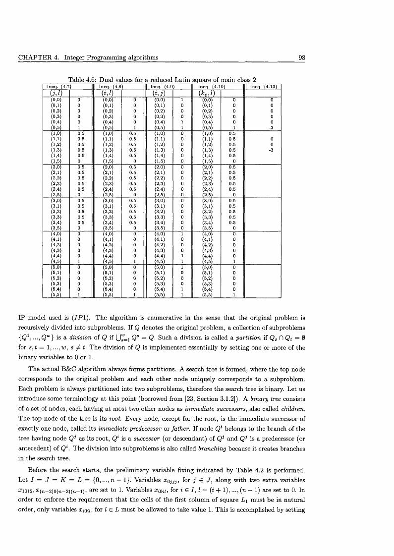
CHA PTER 4. Integer Programming algorithms 98
Table 4.6: Dual values for a reduced Latin square of main class 2Ineq. (4.7) | Ineq. (4.8) | Ineq. (4.9) | Ineq. (4.10) | Ineq. (4.13)
( M ) ( h j ) ( k n , l)(0,0) 0 (0,0) 0 (0,0) 1 (0,0) 0 0(0,1) 0 (0,1) 0 (0,1) 0 (0,1) 0 0(0,2) 0 (0,2) 0 (0,2) 0 (0,2) 0 0(0,3) 0 (0,3) 0 (0,3) 0 (0,3) 0 0(0,4) 0 (0,4) 0 (0,4) 1 (0,4) 0 0(0,5) 1 (0,5) 1 (0,5) 1 (0,5) 1 -3(1,0) 0.5 (1,0) 0.5 (1,0) 0 (1,0) 0.5(1,1) 0.5 (1,1) 0.5 (1,1) 0 (1,1) 0.5 0(1,2) 0.5 (1,2) 0.5 (1,2) 0 (1,2) 0.5 0(1,3) 0.5 (1,3) 0.5 (1,3) 0 (1,3) 0.5 -3(1,4) 0.5 (1,4) 0.5 (1,4) 0 (1,4) 0.5(1,5) 0 (1,5) 0 (1,5) 0 (1,5) 0(2,0) 0.5 (2,0) 0.5 (2,0) 0 (2,0) 0.5(2,1) 0.5 (2,1) 0.5 (2,1) 0 (2,1) 0.5(2,2) 0.5 (2,2) 0.5 (2,2) 0 (2,2) 0.5(2,3) 0.5 (2,3) 0.5 (2,3) 0 (2,3) 0.5(2,4) 0.5 (2,4) 0.5 (2,4) 0 (2,4) 0.5(2,5) 0 (2,5) 0 (2,5) 0 (2,5) 0(3,0) 0.5 (3,0) 0.5 (3,0) 0 (3,0) 0.5(3,1) 0.5 (3,1) 0.5 (3,1) 0 (3,1) 0.5(3,2) 0.5 (3,2) 0.5 (3,2) 0 (3,2) 0.5(3,3) 0.5 (3,3) 0.5 (3,3) 0 (3,3) 0.5(3,4) 0.5 (3,4) 0.5 (3,4) 0 (3,4) 0.5(3,5) 0 (3,5) 0 (3,5) 0 (3,5) 0(4,0) 0 (4,0) 0 (4,0) 1 (4,0) 0(4,1) 0 (4,1) 0 (4,1) 0 (4,1) 0(4,2) 0 (4,2) 0 (4,2) 0 (4,2) 0(4,3) 0 (4,3) 0 (4,3) 0 (4,3) 0(4,4) 0 (4,4) 0 (4,4) 1 (4,4) 0(4,5) 1 (4,5) 1 (4,5) 1 (4,5) 1(5,0) 0 (5,0) 0 (5,0) 1 (5,0) 0(5,1) 0 (5,1) 0 (5,1) 0 (5,1) 0(5,2) 0 (5,2) 0 (5,2) 0 (5,2) 0(5,3) 0 (5,3) 0 (5,3) 0 (5,3) 0(5,4) 0 (5,4) 0 (5,4) 1 (5,4) 0(5,5) 1 (5,5) 1 (5,5) 1 (5,5) 1
IP model used is ( IP 1). The algorithm is enumerative in the sense th a t the original problem is recursively divided into subproblems. If Q denotes the original problem, a collection of subproblems {Q1,..., Qw} is a division of Q if U™=i Qs = Q- Such a division is called a partition if Qs fl Qt = 0 for s , t = 1, ...,w , s ^ t. The division of Q is implemented essentially by setting one or more of the binary variables to 0 or 1.
The actual B&C algorithm always forms partitions. A search tree is formed, where the top node corresponds to the original problem and each other node uniquely corresponds to a subproblem. Each problem is always partitioned into two subproblems, therefore the search tree is binary. Let us introduce some terminology at this point (borrowed from [23, Section 3.1.2]). A binary tree consists of a set of nodes, each having at most two other nodes as immediate successors, also called children. The top node of the tree is its root. Every node, except for the root, is the immediate successor of exactly one node, called its immediate predecessor or father. If node Q l belongs to the branch of the tree having node Qi as its root, Q1 is a successor (or descendant) of and QJ is a predecessor (or antecedent) of Ql . The division into subproblems is also called branching because it creates branches in the search tree.
Before the search starts, the preliminary variable fixing indicated by Table 4.2 is performed. Let I — J = K = L = {0, . .. ,n — 1}. Variables xojjj, for j € J , along with two extra variables £ 1012, £(n—2)o(n—2)(n—1)> are set to 1. Variables xiqu, for i G I, I = (i + 1),..., (n — 1) are set to 0. In order to enforce the requirement th a t the cells of the first column of square L\ must be in natural order, only variables Xiou, for I G L must be allowed to take value 1. This is accomplished by setting
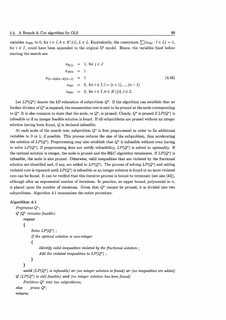
4.4. A Branch Sz Cut algorithm for OLS 99
variables Xioki to 0, for i G / , k G K \ { i } , L G L. Equivalently, the constraints : I E L} = 1,for i G / , could have been appended to the original IP model. Hence, the variables fixed before starting the search are:
x 0jjj = 1, for ;i € J
x 1012 = 1
( n - 2 ) 0 ( n - 2 ) ( n - l ) = 1
XiOil = 0, for 'ii G 1,1 = (i + l ) , . . . , ( n
XiOkI = 0, for ii e I , k e K \ { i } , l e L
Let L P ( Q S) denote the LP-relaxation of subproblem Q s . If the algorithm can establish th a t no further division of Qs is required, the enumeration tree is said to be pruned a t the node corresponding to Qs. It is also common to state th a t the node, or Qs, is pruned. Clearly, Q s is pruned if L P ( Q S) is infeasible or if an integer feasible solution is found. If all subproblems are pruned without an integer solution having been found, Q is declared infeasible.
At each node of the search tree, subproblem Qs is first preprocessed in order to fix additional variables to 0 or 1, if possible. This process reduces the size of the subproblem, thus accelerating the solution of L P ( Q S). Preprocessing may also establish th a t Q9 is infeasible without even having to solve L P ( Q S). If preprocessing does not certify infeasibility, L P ( Q S) is solved to optimality. If the optimal solution is integer, the node is pruned and the B&C algorithm terminates. If L P{ QS) is infeasible, the node is also pruned. Otherwise, valid inequalities th a t are violated by the fractional solution are identified and, if any, are added to L P ( Q S). The process of solving L P ( Q S) and adding violated cuts is repeated until L P ( Q S) is infeasible or an integer solution is found or no more violated cuts can be found. It can be verified th a t this iterative process is bound to term inate (see also [45]), although after an exponential number of iterations. In practice, an upper bound, polynomial in n, is placed upon the number of iterations. Given th a t Qs cannot be pruned, it is divided into two subproblems. Algorithm 4.1 summarises the entire procedure.
A lgorithm 4.1Preprocess Q s; i f (Qs remains feasible)
repeat
{Solve L P ( Q S) ;I f the optimal solution is non-integer
{Identify valid inequalities violated by the fractional solution ;Add the violated inequalities to L P ( Q S) ;
}}u n ti l (L P ( Q S) is infeasible) o r (an integer solution is found) o r (no inequalities are added)
i f (LP(QS) is still feasible) and (no integer solution has been found)Partition Qs into two subproblems;
else prune Qs; return ;
CHAPTER 4. Integer Programming algorithms 100
The components of the B&C algorithm to be further analysed are the preprocessor, the branching mechanism, the approach for identifying violated cuts and the m ethods for solving L P ( Q S).
4.4.1 Preprocessing
The aim of preprocessing each subproblem is to reduce the problem size by excluding variables because other variables have already been set to 0 or 1. During the search, variables are being explicitly set to 0 or 1 because of branching. This is implemented either by adding an extra equality constraint or, most commonly, by altering the variable bounds. Initially, all variables have a lower bound of 0 and an upper bound of 1. Setting the upper bound of a variable to 0 is equivalent to setting this variable to 0. Similarly, setting the lower bound of a variable to 1, fixes this variable to value 1. Hence, at each node/subproblem, certain variables have been explicitly fixed. Preprocessing uses this information to fix even more variables (see also [6, 78]).
Recall from Section 2.2 th a t the row set of the constraint m atrix A is R = (K x L) U (I x L) U
( J x L) U (I x J) U ( J x K) U (I x K) , while its column set is C = I x J x K x L. Each column appears, i.e. contains a non-zero entry, in exactly 6 rows. For example, column (io,jo, ko,lo) appears in the rows (io,jo), {io,ko), (io,lo), {jo,ko), (jo,lo), {ko,lo). It is not difficult to see th a t column c G C appears in row r G R if and only if r C c. Notice th a t we trea t members of sets R and C as subsets of indices, therefore the expression r C c is valid.
Whenever a variable x c is set to 1, all variables having 2 or 3 indices in common with c are automatically forced to 0 in any feasible solution, i.e. a total of 6(n — l ) 2 + 4(n — 1) variables. The matrix columns associated with these variables, along with the column c, can be removed from the matrix without losing any information. For the same reason, all rows where column c appears, i.e. { r £ R : r C c}, can be also removed. Similarly, whenever a variable x c is set to 0, column c can be removed from A. Another possibility is that there has remained a single variable x c not set to 0 in a row r. Clearly, x c will be 1 in any feasible solution, therefore x c can be explicitly set to 1 and the above mentioned rows and columns can be deleted. If all rows have a single variable not set to 0, it is obvious th a t an integer feasible solution has been found. If a certain row has all its variables set to 0, the subproblem is infeasible. Note th a t setting a variable to 0 or 1 might have further repercussions, therefore this process is repeated until matrix A is no longer reducible. We emphasise th a t this variable fixing would have been implicitly implemented whenever the LP is solved. The main reason for explicitly deleting rows and columns of A is to reduce its size, therefore accelerating the solution of L P ( Q S) . It is also possible that infeasibility, or an integer solution, is detected without having to solve L P ( Q S).
Any deletions of rows and columns at a certain node are inherited in all descendant nodes. Therefore, we denote as A s the matrix at the node associated w ith subproblem Qs. R s and Cs are defined accordingly. For each Qs , the lists Ffi, F* of variables already fixed to 0 and 1 at its predecessors, i.e. deleted, are also retained. Obviously, Fq U F f = C \C 3. Algorithm 4.2 describes the preprocessing steps in pseudo-code. All rows and columns are repetitively checked until no more changes are possible. Each iteration includes 0 ( n 4) steps, since each remaining row and column must be examined. Let t denote the iteration counter.
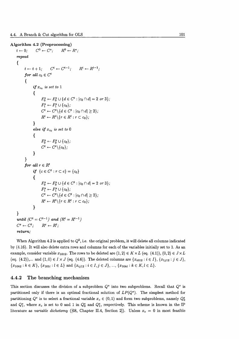
4.4. A Branch & Cut algorithm for OLS 101
A lgorith m 4.2 (P reprocessing)* 4 - 0 ; F ° <— R s;repeat
{t ^ t + 1; C 4 <— C 4-1; R * * - # - 1;f o r all Co G C 4
{i f x Co is set to 1
{Fq <— Fq U {d e C 1 : Ic0 D d| = 2 or 3};F{ 4- F{ U { c o } ;
C 4 <— C 4\{d G C 4 : | c 0 D d| > 2};F 4 4 - F 4\{ r G F 4 : r c c0};
}eZse i / rrC0 is set to 0
{F 0S ♦ - F 0* U { c o } ;
C 4 4- C 4\{c0};
}}/ o r all r G F 4
i / { c G C 4 : r C c } = { c q }
{Fq 4- Fq U {d G C 4 : I Co n d\ = 2 or 3};F f 4- F{ U { c 0 } ;
C4 * - C 4\{d G C 4 : | c o n d \ > 2};F 4 4- R t \{ r G F 4 : r C c0};
}}u n til (C l = C 4" 1; a n d (R l = F 4" VCs 4- C l; R 3 4- F 4;re tu rn ;
When Algorithm 4.2 is applied to Q°, i.e. the original problem, it will delete all columns indicated by (4.16). It will also delete extra rows and columns for each of the variables initially set to 1. As an example, consider variable £ 1012- The rows to be deleted are (1,2) G K x L (eq. (4.1)), (0,2) G J x L
(eq. (4.2)),... and (1,0) G I x J (eq. (4.6)). The deleted columns are {xioi2 : « G /} , {%ij \ 2 '• j £ J}, {x\ok2 : k G K } , {zioit : I G L } and {x ijl2 : i G I , j G J}, ..., { x 10m : k e K ,l e L}.
4.4.2 The branching m echanism
This section discusses the division of a subproblem Qs into two subproblems. Recall th a t Qs is partitioned only if there is an optimal fractional solution of L P ( Q S). The simplest method for partitioning Qs is to select a fractional variable x c G (0,1) and form two subproblems, namely Qq and Qf, where x c is set to 0 and 1 in Qq and Q\, respectively. This scheme is known in the IP literature as variable dichotomy ([68, Chapter II.4, Section 2]). Unless x c = 0 in most feasible
CH APTER 4. Integer Programming algorithms 102
solutions, Q\ will contain significantly fewer feasible solutions than Q q. In other words, setting x c
to 0 achieves no real progress and the set of feasible solutions in Q q is almost identical to that of Qs . Because of the extensive symmetries existing in the OLS problem, no variable can be signalled as unlikely to be 1 in a feasible solution. Therefore, variable dichotomy appears to be a mediocre choice for branching.
It seems better to perform branching in a way th a t approximately halves the solution space of Qs. A method achieving this is commonly referred to as Generalised Upper Bound (GUB) dichotomy.
Each constraint of the form X)cec0 Xc = or ^ ^ *s ca^e< a GUB constraint. Notice th a t (IP 1) contains exclusively GUB constraints. The variable set of such a constraint is also said to form a Special Ordered Set of type /, or SOS-I for short ([13]). Formulation ( IP 1) contains 6n2 SOS-I, each of cardinality n 2. Let S represent the set of variables appearing on the left-hand side of a particular equality. Exactly one variable in 5 will be 1 at any feasible 0 — 1 vector. It follows that, for S\ C S, the single variable of S set to 1 will be either in S \ or in S \S \ . I t is easy to see th a t the problem can be partitioned into two subproblems, each defined by setting the variables of either S\ or S \S \ to 0. Formally, Qs is partitioned into QSl and Qs\ s\ where variables {x c : c E S \} are set to 0 in QSl and variables { x c : c G S \S \ } are set to 0 in Q s\ S l . Notice th a t variable dichotomy is a special case of GUB dichotomy, where <Si = {xc}. In order to ensure th a t the sets of feasible solutions of QSl andQ S \ Sl are almost equally large, sets S\ and S \S i should be of approximately the same cardinality.
By recursively partitioning sets S\ and S \ S \ , eventually a subproblem will be left with a single variable of S not set to 0, which is bound to be 1. If |Si | = |S\<Si | = 2j-, a variable is set to 1 at most after = \2 iog2 n] or 0 (log2 n ) partitions (levels of the tree), since each equality constraintinvolves n 2 variables. Whenever a variable is set to 1, the partition proceeds by selecting another SOS-I, meaning another equality, whose left-hand side has at least one variable still not set to 0. It is not difficult to prove that, GUB dichotomy, compared to variable dichotomy, drastically reduces the depth of the search tree (see also [63, 68]). W hat remains to be clarified is how to select the SOS-I among the 6n2 ones available.
To facilitate the following discussion, let us examine the OLS problem independently of the actual formulation. As in Section 4.2, let X i j ,Y i j , i , j = 0,..., n —1, denote the cells of the squares L \ and L 2
(also referred to as squares X , Y ). Let D x i:j, D y^ be the sets of allowed values (domains) for each cell (i, j ) . Suppose also th a t certain cells are initially fixed as indicated by Table 4.2. The search should select a certain cell and then select a pair to be assigned to this cell. It seems reasonable to initiate the search by fixing the remaining (n — 3) cells in the first column of Y , i.e. cells Y2 0 , ..., V(n_ 3)o, T(n_i)0. Once this have been done, the cells of the remaining (n — 1) x (n — 1) subsquare must be fixed.
There are two systematic methods for selecting the next cell to be examined. One is to examine all cells in a certain row (or column). Since the cells of the first row and column are already fixed, cell (1,1) is selected first, followed by cell (1,2) and so on, until cell ( l ,n — 1) is also assigned a pair. Once the first row of OLS is complete, the algorithm switches to the next row, i.e. cell (2,1) is selected and a pair (2 ,1), I G Dy2l, is assigned to it. The last cell to be assigned a pair is (n — 1, n — 1). Equivalently, we could proceed by fixing all elements in the first column, then in the second one and so on.
The alternative method is, having assigned a pair to cell (i, j ) , to switch to a pair ( i ' , j ') such that i' ^ i and j ' ^ j . This implies that we always select a cell in a different row and column. Roughly speaking, this method constructs the squares in a “diagonal” fashion. Notice that, since the first method fixes rows of the squares, it has to select each time a different value for a cell in the current row of both X and Y . This second method does not need to select a different value for X each time,
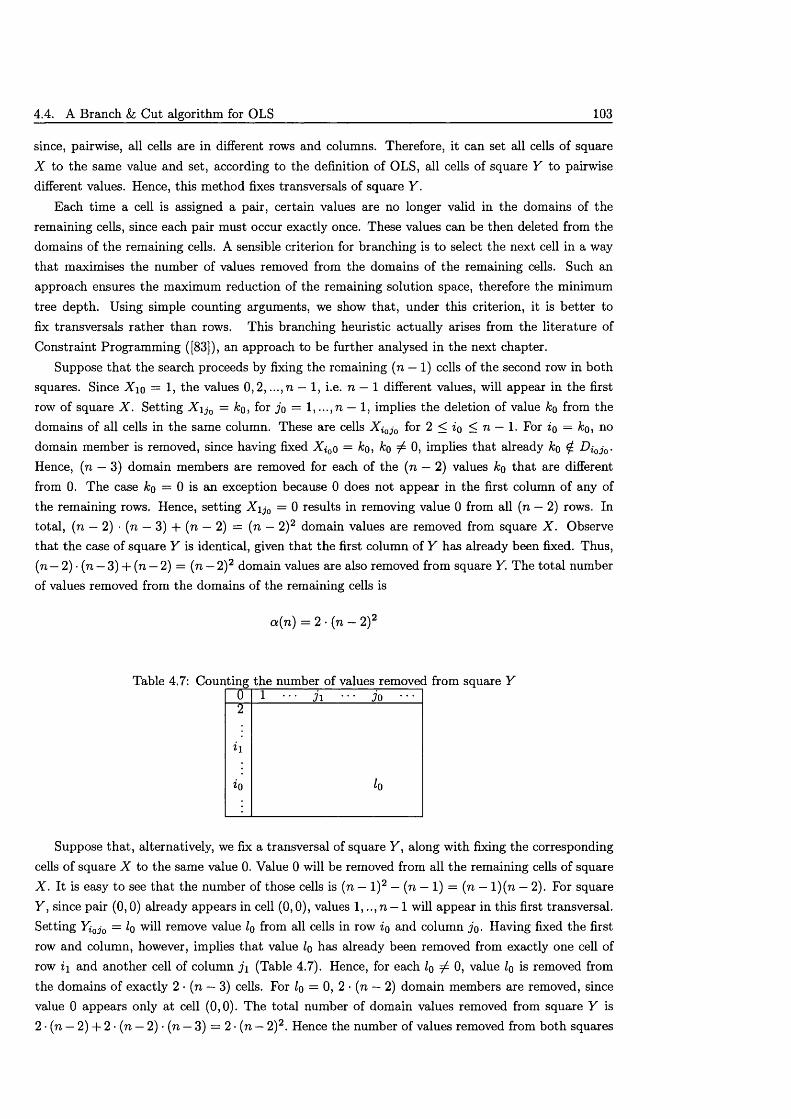
4.4. A Branch k, Cut algorithm for OLS 103
since, pairwise, all cells axe in different rows and columns. Therefore, it can set all cells of square X to the same value and set, according to the definition of OLS, all cells of square Y to pairwise different values. Hence, this method fixes transversals of square Y .
Each time a cell is assigned a pair, certain values are no longer valid in the domains of the remaining cells, since each pair must occur exactly once. These values can be then deleted from the domains of the remaining cells. A sensible criterion for branching is to select the next cell in a way th a t maximises the number of values removed from the domains of the remaining cells. Such an approach ensures the maximum reduction of the remaining solution space, therefore the minimum tree depth. Using simple counting arguments, we show that, under this criterion, it is better to fix transversals rather than rows. This branching heuristic actually arises from the literature of Constraint Programming ([83]), an approach to be further analysed in the next chapter.
Suppose th a t the search proceeds by fixing the remaining (n — 1) cells of the second row in both squares. Since Xio = 1, the values 0,2, ...,n — 1, i.e. n — 1 different values, will appear in the first row of square X . Setting X \ j0 = ko, for jo — 1, ...,n — 1, implies the deletion of value ko from the domains of all cells in the same column. These are cells X i0j0 for 2 < io < n — 1. For io — ko, no domain member is removed, since having fixed X i0o = ko, ko ^ 0, implies th a t already ko ^ Di0j0. Hence, (n — 3) domain members are removed for each of the (n — 2) values ko th a t are different from 0. The case ko = 0 is an exception because 0 does not appear in the first column of any of the remaining rows. Hence, setting X \jQ = 0 results in removing value 0 from all (n — 2) rows. In total, (n — 2) • (n — 3) + (n — 2) = (n — 2)2 domain values are removed from square X . Observe that the case of square Y is identical, given th a t the first column of Y has already been fixed. Thus, (n — 2) • (n — 3) + (n — 2) = (n — 2)2 domain values are also removed from square Y. The to tal number of values removed from the domains of the remaining cells is
a(n) = 2 • (n — 2)2
Table 4.7: Counting the number of values removed from square Y0 1 • • 3 i • • • Jo • ••2
h
io io
Suppose that, alternatively, we fix a transversal of square Y , along with fixing the corresponding cells of square X to the same value 0. Value 0 will be removed from all the remaining cells of square X . It is easy to see th a t the number of those cells is (n — l ) 2 — (n — 1) = (n — l) (n — 2). For square Y , since pair (0,0) already appears in cell (0,0), values 1, . . , n — 1 will appear in this first transversal. Setting Yi0j0 = Iq will remove value Iq from all cells in row iq and column jo. Having fixed the first row and column, however, implies th a t value lo has already been removed from exactly one cell of row i\ and another cell of column j i (Table 4.7). Hence, for each lo ^ 0> value Iq is removed from the domains of exactly 2 • (n — 3) cells. For lo = 0, 2 • (n — 2) domain members are removed, since value 0 appears only at cell (0,0). The total number of domain values removed from square Y is 2 • (n — 2) + 2 • (n — 2) • (n — 3) = 2 • (n — 2)2. Hence the number of values removed from both squares
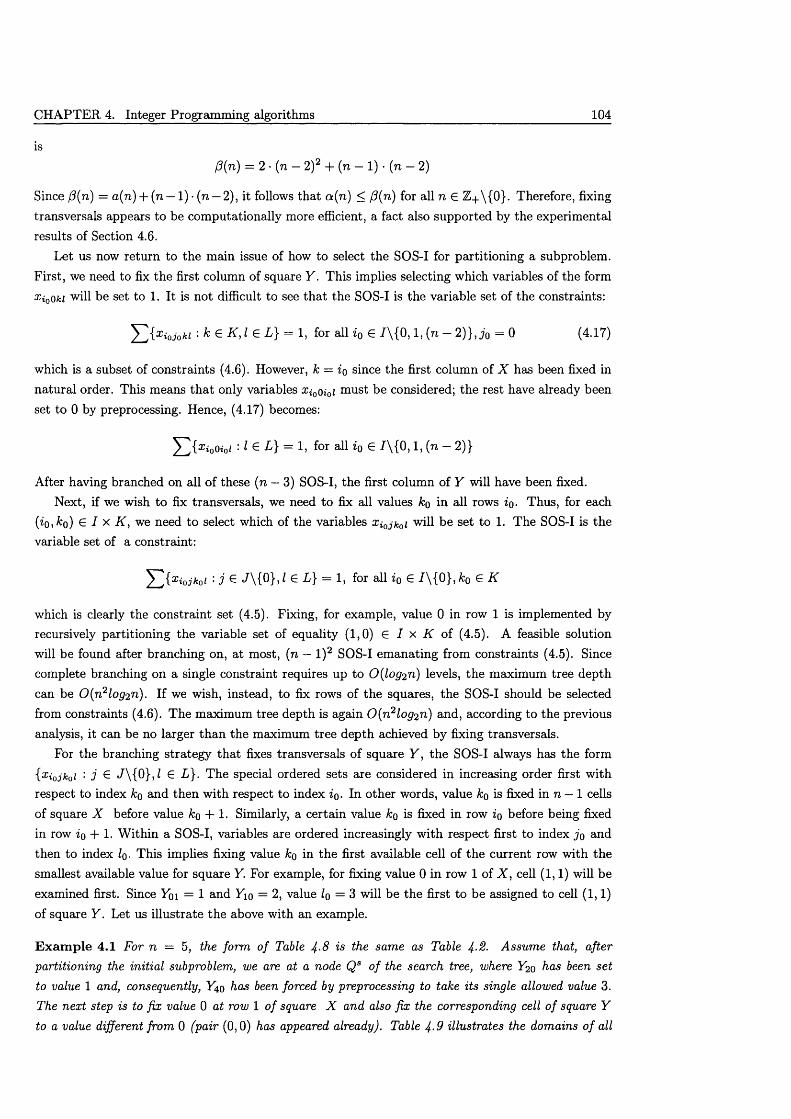
CHAPTER 4. Integer Programming algorithms 104
isP(n) = 2 • (n — 2)2 + (n — 1) • (n — 2)
Since (3(n) = a(n ) + (n — 1) • (n —2), it follows that a(n) < (3(n) for all n G Z+ \{0}. Therefore, fixing transversals appears to be computationally more efficient, a fact also supported by the experimental results of Section 4.6.
Let us now return to the main issue of how to select the SOS-I for partitioning a subproblem. First, we need to fix the first column of square Y. This implies selecting which variables of the form x io0 ki will be set to 1. It is not difficult to see th a t the SOS-I is the variable set of the constraints:
Y ^ { Xioioki : k G K ,l G L} = 1, for all z0 G 7 \{ 0 ,1, (n - 2)}, j 0 = 0 (4.17)
which is a subset of constraints (4.6). However, k = io since the first column of X has been fixed in natural order. This means th a t only variables Xi0 oi0i must be considered; the rest have already been set to 0 by preprocessing. Hence, (4.17) becomes:
^{zioO io/ : l e L} = 1, for all z0 G I \ { 0,1, (n - 2)}
After having branched on all of these (n — 3) SOS-I, the first column of Y will have been fixed.Next, if we wish to fix transversals, we need to fix all values ko in all rows zo. Thus, for each
(iQ,k 0) G I x K , we need to select which of the variables Xi0 jk0i will be set to 1. The SOS-I is the variable set of a constraint:
X ^o jA o Z : 3 € c/\{0}, Z GL} = 1, for all z0 G I \ { 0 } ,k o G K
which is clearly the constraint set (4.5). Fixing, for example, value 0 in row 1 is implemented by recursively partitioning the variable set of equality (1,0) G I x K of (4.5). A feasible solution will be found after branching on, at most, (n — l ) 2 SOS-I em anating from constraints (4.5). Since complete branching on a single constraint requires up to 0(Zop2n) levels, the maximum tree depth can be 0 (n 2 log2 n). If we wish, instead, to fix rows of the squares, the SOS-I should be selected from constraints (4.6). The maximum tree depth is again 0 (n 2 log2 n) and, according to the previous analysis, it can be no larger than the maximum tree depth achieved by fixing transversals.
For the branching strategy that fixes transversals of square Y, the SOS-I always has the form {x i0 jk0i '■ j £ */\{0}, Z G L}. The special ordered sets are considered in increasing order first with respect to index ko and then with respect to index zo- In other words, value ko is fixed in n — 1 cells of square X before value ko + 1. Similarly, a certain value ko is fixed in row zo before being fixed in row Zo + 1. W ithin a SOS-I, variables are ordered increasingly w ith respect first to index jo and then to index lo- This implies fixing value ko in the first available cell of the current row with the smallest available value for square Y. For example, for fixing value 0 in row 1 of X , cell (1,1) will be examined first. Since Y q\ = 1 and Yio = 2, value lo = 3 will be the first to be assigned to cell (1,1) of square Y. Let us illustrate the above with an example.
E x am p le 4.1 For n = 5, the form of Table 4-8 is the same as Table 4-2- Assume that, after partitioning the initial subproblem, we are at a node Qs of the search tree, where Y2o has been set to value 1 and, consequently, Y4 0 has been forced by preprocessing to take its single allowed value 3. The next step is to fix value 0 at row 1 of square X and also fix the corresponding cell of square Y to a value different from 0 (pair (0,0) has appeared already). Table 4-9 illustrates the domains o f all
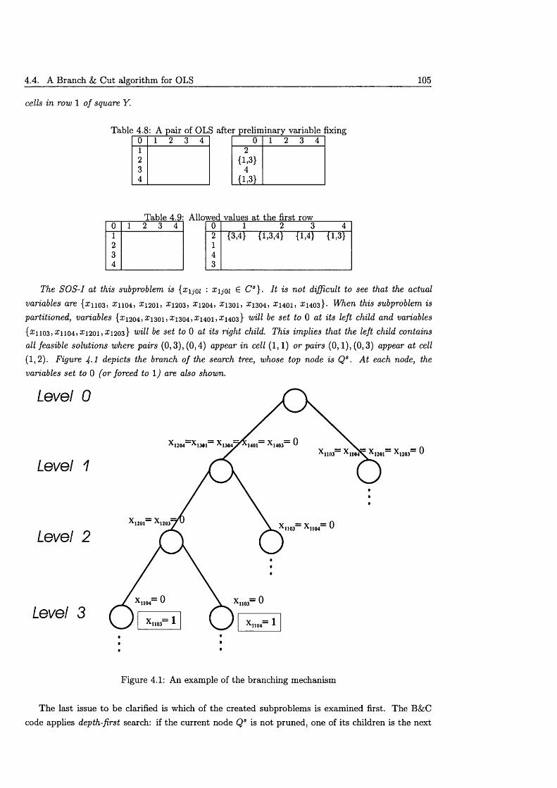
4.4. A Branch & Cut algorithm for OLS 105
cells in row 1 of square Y.
Table 4.8: A pair of OLS after preliminary variable fixing0 1 2 3 4
2{1,3}
4{1.3}
0 1 2 3 41234
Table 4.9: Allowed values at the first row0 1 2 3 41234
0 1 2 3 42 {3,4} {1,3,4} {1,4} {1,3}143
The SO S-I at this subproblem is {xijoz : x ijOi £ C s}. It is not difficult to see that the actual variables are { x n o 3 , Z i i 0 4 , £ 1201, ^ 1203 , ^ 1204 , ^ 1301 , ^ 1304 , x i a o i , ^ 1403}- When this subproblem is partitioned, variables {£1204, £1301 ,£ 1304, #1401 >^1403} be set to 0 at its left child and variables {^1103)^ 1104)^ 1201)^ 1203} will be set to 0 at its right child. This implies that the left child contains all feasible solutions where pairs (0,3), (0,4) appear in cell (1,1) or pairs (0,1), (0,3) appear at cell (1,2). Figure 4-1 depicts the branch of the search tree, whose top node is Qs . A t each node, the variables set to 0 (or forced to 1) are also shown.
Level 0
14011103 X 1 1 0 4 ^ X 1201 X 1203-
Level
Level
Levelt
Figure 4.1: An example of the branching mechanism
The last issue to be clarified is which of the created subproblems is examined first. The B&C code applies depth-first search: if the current node Qs is not pruned, one of its children is the next
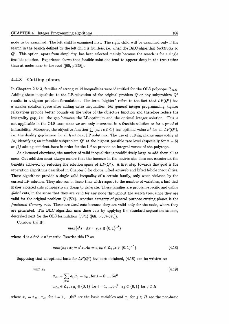
CHAPTER 4. Integer Programming algorithms 106
node to be examined. The left child is examined first. The right child will be examined only if the search in the branch defined by the left child is fruitless, i.e. when the B&C algorithm backtracks to Q s. This option, apart from simplicity, has been selected mainly because the search is for a single feasible solution. Experience shows that feasible solutions tend to appear deep in the tree rather than a t nodes near to the root ([68, p.358]).
4.4.3 C utting planes
In Chapters 2 & 3, families of strong valid inequalities were identified for the OLS polytope P o l s -
Adding these inequalities to the LP-relaxation of the original problem Q or any subproblem Qs results in a tighter problem formulation. The term “tighter” refers to the fact th a t L P (Q S) has a smaller solution space after adding extra inequalities. For general integer programming, tighter relaxations provide better bounds on the value of the objective function and therefore reduce the integrality gap, i.e. the gap between the LP-optimum and the optimal integer solution. This is not applicable in the OLS case, since we are only interested in a feasible solution or for a proof of infeasibility. Moreover, the objective function ^ { x c : c E C} has optimal value n 2 for all L P (Q S), i.e. the duality gap is zero for all fractional LP solutions. The use of cutting planes aims solely at (a) identifying an infeasible subproblem Q3 at the highest possible tree level (especially for n = 6) or (b) adding sufficient faces in order for the LP to provide an integral vertex of the polytope.
As discussed elsewhere, the number of valid inequalities is prohibitively large to add them all at once. Cut addition must always ensure th a t the increase in the m atrix size does not counteract the benefits achieved by reducing the solution space of L P (Q S). A first step towards this goal is the separation algorithms described in Chapter 3 for clique, lifted antiweb and lifted 5-hole inequalities. These algorithms provide a single valid inequality of a certain family, only when violated by the current LP-solution. They also run in linear time with respect to the number of variables, a fact that makes violated cuts comparatively cheap to generate. These families are problem-specific and define global cuts, in the sense th a t they are valid for any node throughout the search tree, since they are valid for the original problem Q ([50]). Another category of general purpose cutting planes is the fractional Gomory cuts. These are local cuts because they are valid only for the node, where they are generated. The B&;C algorithm uses these cuts by applying the standard separation scheme, described next for the OLS formulation ( /P l ) ([68, p.367-370]).
Consider the IP:, 4
m ax { e x : A x = e, x E (0, l} n }
where A is a 6n2 x n 4 matrix. Rewrite this IP as
. 4m a x{xo : x Q = e x, A x = e, xo E Z +,x E {0, l} n } (4-18)
Supposing th a t an optimal basis for L P (Q S) has been obtained, (4.18) can be w ritten as:
m ax xo (4-19)
XBi + &ijXj = Gio, for i = 0 , ..., 6n2 jeH
x Bo E Z +,x Bi G {0,1} for i = l , . . . ,6 n 2, Xj E {0,1} for j E H
where xq = x Bo, x Bi for i = 1 ,...,6 n 2 are the basic variables and Xj for j E H are the non-basic
4.4. A Branch & Cut algorithm for OLS 107
ones. Since the basis is primal and dual feasible, it holds th a t a*o > 0 for z = 1,..., 6n2 and a,Qj > 0 for j G H . Suppose th a t there exists an z such th a t a;o ^ (0,1), i.e. variable Xbz is fractional. The following proposition identifies the Gomory fractional cut associated with this variable.
P rop osition 4.3 (G om ory fractional cut) IfdiQ e (0,1) then
^ f i j x j 5; f i O (4.20)j € H
where f y = f y — [ f y \ , f y = a^o — |_UioJ> is a valid inequality for (4-18).
Observe th a t inequality (4.20) is violated by the current LP-solution. It is easy to see th a t (4.20) can be w ritten with respect to the basic variables, using the simplex tableau. Notice also that a Gomory fractional cut can be obtained for each fractional variable.
Further technical details of the cut addition process must be analysed. Notice first that the computational effort imposed by cut addition refers to generating the cut and, mainly, to re-optimising L P (Q S) in order to derive a new feasible solution, or prove th a t the amended L P (Q S) is infeasible.
F irst, the separation algorithms, in the form given in Chapter 3, add only one cut at a time. This approach might require numerous iterations of cut addition and re-optimisation before a viable outcome is achieved. A greedier approach of adding more the one violated inequality from each family sounds more appropriate. The natural question is what should be the maximum number of inequalities added from each family. Clearly, this upper bound should be a polynomial of n of rather small degree, e.g. a multiple of n or n 2, The number of cuts added at each iteration, in conjunction with the maximum number of iterations at each node, determines the “aggressiveness” of the cut strategy. Recall th a t the number of iterations should also be polynomial in n in order to ensure a polynomial time procedure for solving each subproblem. It follows th a t a B&C algorithm faces an obvious trade-off between adding more violated cuts at each node, hence reducing the number of subproblems, and posing more computational effort at each node. There is no unequivocal answer to this question. Normally, the answer is problem specific and requires computational experimentation. We discuss this topic further in Section 4.6.
A second aspect is the order in which families of valid inequalities are examined. As discussed in Sections 3.5 and 3.7.1, the separation algorithms for lifted antiweb and lifted 5-hole inequalities are correct only if no violated clique inequalities have been found. Correctness refers to the algorithms’ ability to provide a violated cut, if such exists. This implies th a t inequalities induced by cliques of type II and III should be separated first and lifted antiweb and lifted 5-hole inequalities should be examined only if no violated clique inequalities arise. Notice, however, th a t separation of, say, lifted antiweb inequalities can still provide a violated cut, even though clique inequalities have not been examined. In practice, one should separate first the inequalities which are (a) more effective in pruning a node and (b) on average cheaper to generate. For example, if lifted 5-hole inequalities happen to be stronger in this sense, they should be the first to be added to the matrix, the rest of the families to be examined afterwards. Hence, regardless of the algorithmic correctness, one must still experiment with the order in which families of valid inequalities are separated. It is expected, however, th a t Gomory fractional cuts will be the weakest ones, exactly because they are local and encompass no knowledge about problem’s structure.
Another critical aspect is the frequency of cutting planes addition. On the one hand, cutting planes can be added at every single node of the tree, as in [50]. This approach, apart from being
CHAPTER 4. Integer Programming algorithms 108
computationally more expensive, does not guarantee more successful pruning, since the problem is not significantly different in each node. If, for example, a single variable is set to 0 for creating a subproblem (e.g. the nodes of Level 3 in Figure 4.1), this subproblem will be almost identical to its father. The other extreme is to add cutting planes only at the top node of the tree and simply retain them in all other nodes. The reasonable option lies between these two extremes ([6, 68]). Hence, cuts are added at the top node of the tree and then whenever a variable is forced to become 1 by preprocessing. A variable becoming 1 offers a practical criterion for detecting th a t the current subproblem is sufficiently different from its ancestors. Recall that, by branching on SOS-I, a variable is forced to value 1 at most every [2 • log2 n] levels of the tree. Another, more conservative, approach is to add cuts once after the first column is fixed and then every time a transversal is fixed, i.e. whenever (n — 1) variables are set to 1. Clearly, this takes place at most every \2 • (n — l)log 2 n~\ tree levels.
Normally, all cutting planes added at a node are retained in all descendant nodes. This might eventually cause a drastic increase in the matrix size. Moreover, cuts added early in the tree are not necessarily useful in subsequent nodes. Therefore, a method for determining which cuts to retain must be devised. Dropping all cuts of a node is not practical either, because the LP-relaxation of its children must be tightened again from the beginning. An intermediate option, extensively used in recent B&C codes (see for example [5]), is to retain at descendant nodes only the cutting planes which are satisfied as equalities in the last (fractional) LP-solution. These are also called binding cuts. This approach is also followed by our B&C algorithm.
4.4.4 Solving the LP-relaxation
Throughout this section we use the standard terminology of Linear Programming, without actually defining every single term. The formal description of technical terms, e.g. primal feasible solution, can be found in any LP textbook (see for example [68, Chapter 1.2])
At each node Qs , L P (Q S) can be solved by any method for solving linear programs. The standard method is the primal or dual simplex algorithm. Recall th a t m atrix A has significantly more columns than rows. It is usually preferable to have less columns (variables) for the simplex method. In this sense, the dual simplex appears as the most favourable option, although this has to be supported by computational results. Therefore, both the primal and the dual simplex algorithms are tested in Section 4.6. Interior-point or Newton-Barrier methods have been recently shown to be much more efficient, especially for large LPs ([91]). They are also embedded in commercial solvers ([31]), a fact th a t allows us to test them as well.
Once L P (Q S) is solved to optimality, violated inequalities are identified. After adding violated inequalities, the previously optimal solution becomes primal infeasible. The dual solution, however, remains feasible and can be used as the initial solution for the dual simplex algorithm. Hence, it is natural to re-optimise L P (Q S) via the dual simplex algorithm. In contrast, the primal simplex and the Newton-Barrier method have to reconstruct a primal feasible solution from scratch. Actually, re-optimising with the dual simplex is the default setting in all commercial codes. There exists another, similar, advantage when using dual simplex for initially solving L P (Q S). Each node has the same matrix rows as its father, unless a row corresponding to a basic variable of the dual solution is deleted during preprocessing. If this is not the case, the optimal solution of the father remains dual feasible in the child. Hence, it may be used again as the initial solution when solving L P (Q S) with dual simplex.
4.5. Implementation of the Branch & Cut algorithm 109
O ur last note concerns the form of the objective function. Since we deal with a feasibility problem, the actual objective function is of no real importance. Notice th a t the original objective function of ( IP 1) has a coefficient of 1 for every variable. This implies th a t the right-hand side of all dual constraints will be identical, thus allowing the appearance of degeneracy. An objective function with different coefficients for each variable could easily resolve this problem. Therefore, the coefficients of the objective function used when solving LPs are randomly generated. Any integer in the interval [ l ,n 4] is randomly allocated to a single variable.
4.5 Im plem entation of the Branch &: Cut algorithm
The B&C algorithm has been implemented by using the commercial package XPRESS-MP ([31]). A part from being a mixed integer programming solver, XPRESS-MP provides full flexibility in terms of allowing the user to intervene in various aspects of the solver. This is possible mainly via the Optimiser Subroutine Library XOSL. This library contains all the parameters controlling the solver, along with numerous subroutines, which can be called from a main computer program. Complete documentation of these subroutines is provided in [31]. The main program, including the procedures for preprocessing, branching and cut separation, has been written in the Microsoft C + + programming environment.
XPRESS-MP requires an IP model to be written in an algebraic language, which is essentially ( IP 1), except for differences in the syntax. The output of the XPRESS modeller is a model in the standard MPS format. Once this MPS format is created, the model can be solved as either an LP or an IP. In the latter case, the Branch and Bound solver is invoked. To clarify matters, we briefly present certain technical details concerning the functionality of the solver.
4.5.1 M atrix operations
The constraint m atrix is fully controllable by the user. This aspect allows all characteristics to be read and possibly edited. For example, the coefficients of the objective function can be replaced by randomly generated ones.
The preprocessing mechanism can identify the bounds of the 0 — 1 variables and subsequently alter them in order to fix variables to 0 or 1. It may also delete rows and columns of the matrix a t a particular node Qs , without affecting the m atrix used in other nodes. Similarly, the branching mechanism can set variables to 0 in order to define new subproblems.
Moreover, the user is allowed to intervene with the simplex algorithm by defining the basis or the pivots. The simplex tableau is available at each point. Once L P (Q 3) is optimised, the simplex tableau is used for detecting the fractional variables and constructing the Gomory fractional cuts. Any cutting plane can be added to the m atrix in the form of additional rows.
4.5.2 Control param eters
Numerous control parameters can be handled in order to tune the behaviour of the solver. The first param eter is the algorithm used for solving L P (Q S), the options being the primal or dual simplex and the Newton-Barrier. The user can switch to any of those algorithms a t any point. For example, the initial subproblem can be solved by primal simplex and every linear program thereafter can be solved exclusively by the dual simplex.
CHAPTER 4. Integer Programming algorithms 110
XPRESS-MP provides its own preprocessing routine, which can be controlled to perform reduced cost fixing, logical preprocessing, probing or any combination of those three methods (see [78] for details). The solver also incorporates general purpose cutting planes which can be either used or not. Also, node selection can follow various strategies, e.g. depth-first. Finally, technical aspects of numerical precision, like zero tolerance, can be manipulated.
4.5.3 “Callback” subroutines
Perhaps the main strength of XPRESS-MP lies in the set of routines, which can be called a t various points of the solution process in order for the user to specify the B&C algorithm. The relatively complex branching mechanism for the OLS problem is implementable only via these routines. These functions are named callbacks, exactly because they can be called at each node. A fist of all nodes th a t have not been pruned is maintained by XPRESS-MP. Any of these nodes can be accessed at any point.
At each node of the tree, we are allowed to preprocess and possibly prune the subproblem, before solving L P (Q S). If the subproblem has to be partitioned, the user can define the bounds applied in the two descendant nodes, the next subproblem to be solved and the information printed as output. The node can be pruned, if infeasible, and the entire solver can term inate if an integer solution is found.
4.5.4 Cut m anagem ent
A designated set of callback routines handles the cutting planes. As noted above, cutting planes can be simply added as rows of the m atrix at each Q s. However, since certain cuts added at a node are retained at descendant nodes, the same cuts will appear in multiple matrices. For large problem instances, this process occupies unnecessary memory for storing duplicate information. XPRESS-MP overcomes this drawback by maintaining a pool of cutting planes. Hence, additional constraints are no longer added at m atrix rows, but explicitly as cuts. Cuts are retained at the “cut pool” only if they have been used in nodes th a t have not been pruned. Each cutting plane is accompanied by a list of the nodes it appears at. Before a node is solved, all the relevant cuts are added to its matrix. Note th a t this process takes place automatically, w ithout the user having to intervene.
Specifically, there exists routines for adding cuts even before the original problem is solved. At each node a cut-handling routine is called. W ithin this routine, the user-provided code can identify violated cuts, add them to the cut pool or to the m atrix, and indicate when the iterative procedure of Algorithm 4.1 will terminate. The user can also specify a param eter delta, controlling the minimum violation necessary for a cut to be added. Hence, only cuts violated by more than delta are considered. This aspect is related to issues of numerical precision. Typical values for delta lie in the interval [10~4,10-2 ]. Another routine is used to identify the cuts to be deleted from both the m atrix and the cut pool, i.e. the non-binding cuts.
4.6 Com putational analysis
The discussion of the previous section indicates th a t the B&C algorithm consists of a number of components and each of those includes various parameters. The exact form of the algorithm is difficult to be devised unless we experiment with these parameters. This is exactly the aim of this
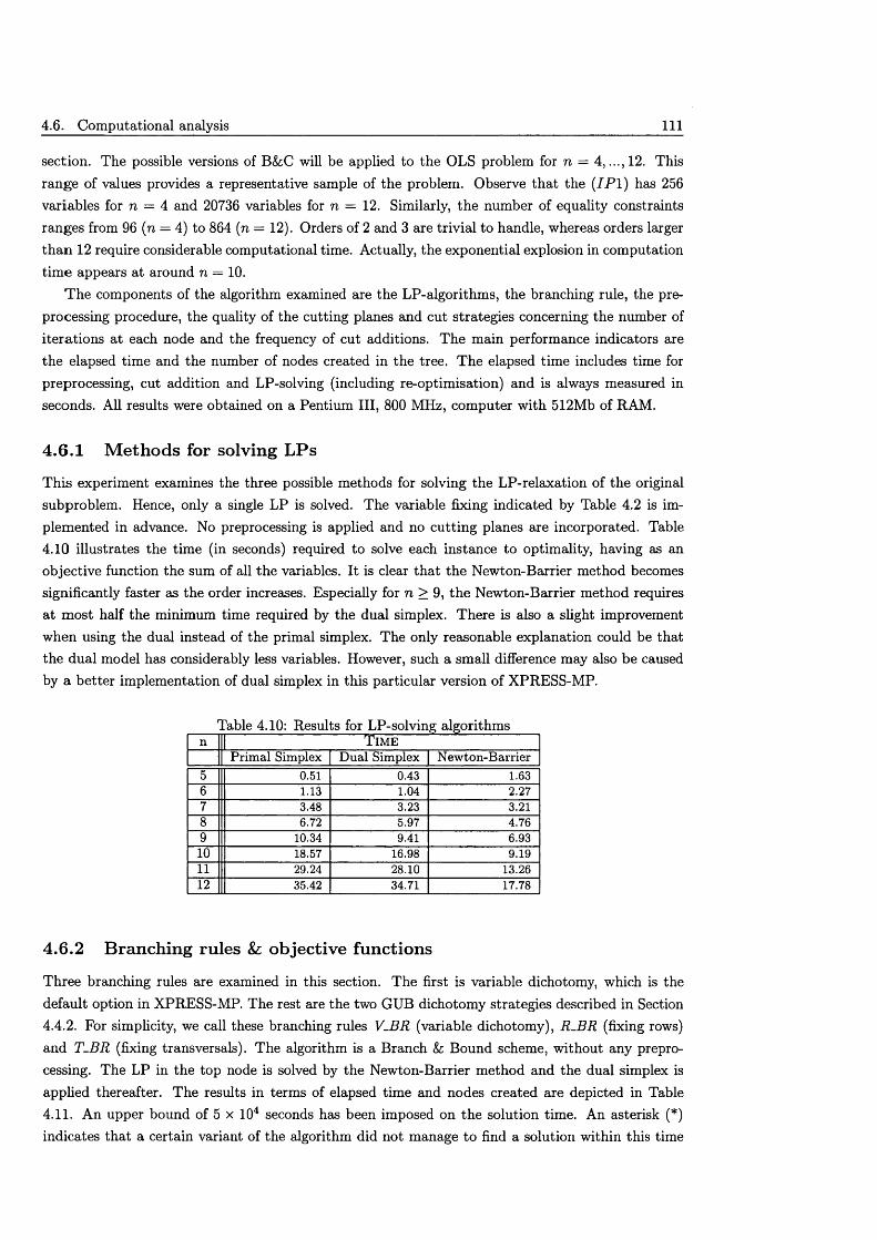
4.6. Computational analysis 111
section. The possible versions of B&C will be applied to the OLS problem for n = 4 ,..., 12. This range of values provides a representative sample of the problem. Observe th a t the ( IP 1) has 256 variables for n = 4 and 20736 variables for n = 12. Similarly, the number of equality constraints ranges from 96 (n = 4) to 864 (n = 12). Orders of 2 and 3 are trivial to handle, whereas orders larger th an 12 require considerable computational time. Actually, the exponential explosion in computation tim e appears at around n — 10.
T he components of the algorithm examined are the LP-algorithms, the branching rule, the preprocessing procedure, the quality of the cutting planes and cut strategies concerning the number of iterations at each node and the frequency of cut additions. The main performance indicators are the elapsed time and the number of nodes created in the tree. The elapsed time includes time for preprocessing, cut addition and LP-solving (including re-optimisation) and is always measured in seconds. All results were obtained on a Pentium III, 800 MHz, computer w ith 512Mb of RAM.
4.6 .1 M ethods for solving LPs
This experiment examines the three possible methods for solving the LP-relaxation of the original subproblem. Hence, only a single LP is solved. The variable fixing indicated by Table 4.2 is implemented in advance. No preprocessing is applied and no cutting planes are incorporated. Table 4.10 illustrates the time (in seconds) required to solve each instance to optimality, having as an objective function the sum of all the variables. It is clear th a t the Newton-Barrier method becomes significantly faster as the order increases. Especially for n > 9, the Newton-Barrier method requires a t most half the minimum time required by the dual simplex. There is also a slight improvement when using the dual instead of the primal simplex. The only reasonable explanation could be that the dual model has considerably less variables. However, such a small difference may also be caused by a better implementation of dual simplex in this particular version of XPRESS-MP.
Table 4.10: Results for LP-solving algorithmsn 1 T i m e
Primal Simplex Dual Simplex Newton-Barrier5 0.51 0.43 1.636 1.13 1.04 2.277 3.48 3.23 3.218 6.72 5.97 4.769 10.34 9.41 6.93
10 18.57 16.98 9.1911 29.24 28.10 13.2612 35.42 34.71 17.78
4.6.2 Branching rules &; objective functions
Three branching rules are examined in this section. The first is variable dichotomy, which is the default option in XPRESS-MP. The rest are the two GUB dichotomy strategies described in Section 4.4.2. For simplicity, we call these branching rules V-BR (variable dichotomy), R -B R (fixing rows) and T-BR (fixing transversals). The algorithm is a Branch & Bound scheme, without any preprocessing. The LP in the top node is solved by the Newton-Barrier method and the dual simplex is applied thereafter. The results in terms of elapsed time and nodes created are depicted in Table 4.11. An upper bound of 5 x 10⁴ seconds has been imposed on the solution time. An asterisk (*) indicates th a t a certain variant of the algorithm did not manage to find a solution within this time
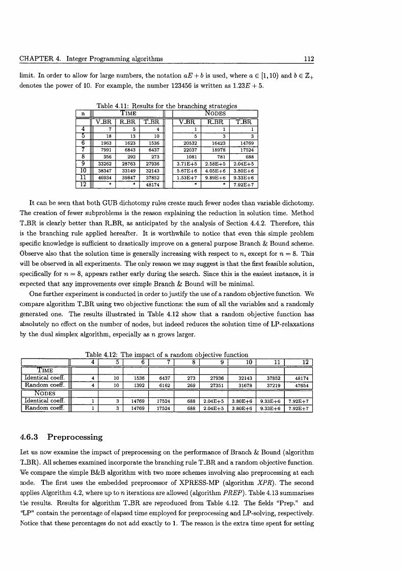
CHAPTER 4. Integer Programming algorithms 112
limit. In order to allow for large numbers, the notation aE + b is used, where a € [1,10) and b £ Z+ denotes the power of 10. For example, the number 123456 is w ritten as 1.23E + 5.
Table 4.11: Results for the branching strategiesn | T im e N o d e s
V-BR R_BR T_BR V-BR R_BR T.BR4 7 5 4 i l l5 18 13 10 5 3 36 1963 1623 1536 20532 16423 147697 7991 6843 6437 22037 18978 175248 356 292 273 1081 781 6889 33262 28763 27936 3.71E+5 2.58E+5 2.04E+510 38347 33149 32143 5.67E+6 4.05E+6 3.80E+611 46934 39847 37852 1.53E+7 9.89E+6 9.33E+612 * * 48174 * ★ 7.92E+7
It can be seen th a t both GUB dichotomy rules create much fewer nodes than variable dichotomy. The creation of fewer subproblems is the reason explaining the reduction in solution time. Method T_BR is clearly better than RJBR, as anticipated by the analysis of Section 4.4.2. Therefore, this is the branching rule applied hereafter. It is worthwhile to notice th a t even this simple problem specific knowledge is sufficient to drastically improve on a general purpose Branch &; Bound scheme. Observe also th a t the solution time is generally increasing with respect to n, except for n = 8. This will be observed in all experiments. The only reason we may suggest is th a t the first feasible solution, specifically for n = 8, appears rather early during the search. Since this is the easiest instance, it is expected th a t any improvements over simple Branch h Bound will be minimal.
One further experiment is conducted in order to justify the use of a random objective function. We compare algorithm T_BR using two objective functions: the sum of all the variables and a randomly generated one. The results illustrated in Table 4.12 show th a t a random objective function has absolutely no effect on the number of nodes, but indeed reduces the solution time of LP-relaxations fcy the dual simplex algorithm, especially as n grows larger.
Table 4.12: The impact of a random objective function4 5 6 7 8 9 10 11 12
T imeIdentical coeff. 4 10 1536 6437 273 27936 32143 37852 48174Random coeff. 4 10 1392 6162 269 27351 31678 37219 47654
N o d e sIdentical coeff. 1 3 14769 17524 688 2.04E+5 3.80E+6 9.33E+6 7.92E+7Random coeff. 1 3 14769 17524 688 2.04E+5 3.80E+6 9.33E+6 7.92E+7
4.6.3 Preprocessing
Let us now examine the impact of preprocessing on the performance of Branch & Bound (algorithm T_BR). All schemes examined incorporate the branching rule T_BR and a random objective function. We compare the simple B&B algorithm with two more schemes involving also preprocessing at each node. The first uses the embedded preprocessor of XPRESS-MP (algorithm X P R ). The second applies Algorithm 4.2, where up to n iterations are allowed (algorithm PREP). Table 4.13 summarises tie results. Results for algorithm T_BR are reproduced from Table 4.12. The fields “Prep.” and ‘L P” contain the percentage of elapsed time employed for preprocessing and LP-solving, respectively, botice th a t these percentages do not add exactly to 1. The reason is the extra time spent for setting
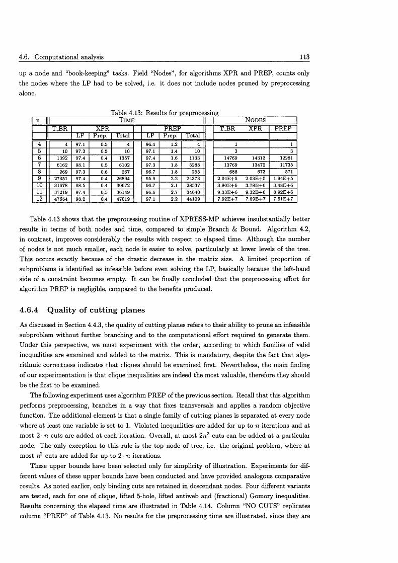
4.6. Com putational analysis 113
up a node and “book-keeping” tasks. Field “Nodes” , for algorithms XPR and PREP, counts only the nodes where the LP had to be solved, i.e. it does not include nodes pruned by preprocessing alone.
Table 4.13: Results for preprocessingn | T im e N o d e s
T_BR XPR PREP T_BR XPR PREPLP Prep. Total LP Prep. Total
4 4 97.1 0.5 4 96.4 1.2 4 l l5 10 97.3 0.5 10 97.1 1.4 10 3 36 1392 97.4 0.4 1357 97.4 1.6 1133 14769 14313 122817 6162 98.1 0.5 6102 97.3 1.8 5288 13769 13472 117358 269 97.3 0.6 267 96.7 1.8 255 688 673 5719 27351 97.4 0.4 26894 95.9 2.2 24373 2.04E+5 2.03E+5 1.94E+510 31678 98.5 0.4 30672 96.7 2.1 28537 3.80E+6 3.78E+6 3.48E+611 37219 97.4 0.5 36149 96.6 2.7 34640 9.33E+6 9.32E+6 8.92E+612 47654 98.2 0.4 47019 97.1 2.2 44109 7.92E+7 7.89E+7 7.51E+7
Table 4.13 shows th a t the preprocessing routine of XPRESS-MP achieves insubstantially better results in terms of both nodes and time, compared to simple Branch &; Bound. Algorithm 4.2, in contrast, improves considerably the results with respect to elapsed time. Although the number of nodes is not much smaller, each node is easier to solve, particularly at lower levels of the tree. This occurs exactly because of the drastic decrease in the m atrix size. A limited proportion of subproblems is identified as infeasible before even solving the LP, basically because the left-hand side of a constraint becomes empty. It can be finally concluded th a t the preprocessing effort for algorithm PREP is negligible, compared to the benefits produced.
4.6 .4 Q uality of cutting planes
As discussed in Section 4.4.3, the quality of cutting planes refers to their ability to prune an infeasible subproblem without further branching and to the computational effort required to generate them. Under this perspective, we must experiment with the order, according to which families of valid inequalities are examined and added to the matrix. This is mandatory, despite the fact th a t algorithmic correctness indicates th a t cliques should be examined first. Nevertheless, the main finding of our experimentation is that clique inequalities are indeed the most valuable, therefore they should be the first to be examined.
The following experiment uses algorithm PREP of the previous section. Recall th a t this algorithm performs preprocessing, branches in a way that fixes transversals and applies a random objective function. The additional element is th a t a single family of cutting planes is separated at every node where at least one variable is set to 1. Violated inequalities are added for up to n iterations and at most 2 • n cuts are added a t each iteration. Overall, at most 2n 2 cuts can be added at a particular node. The only exception to this rule is the top node of tree, i.e. the original problem, where at most n2 cuts are added for up to 2 • n iterations.
These upper bounds have been selected only for simplicity of illustration. Experiments for different values of these upper bounds have been conducted and have provided analogous comparative results. As noted earlier, only binding cuts are retained in descendant nodes. Four different variants are tested, each for one of clique, lifted 5-hole, lifted antiweb and (fractional) Gomory inequalities. Results concerning the elapsed time are illustrated in Table 4.14. Column “NO CUTS” replicates column “PR E P ” of Table 4.13. No results for the preprocessing time are illustrated, since they are
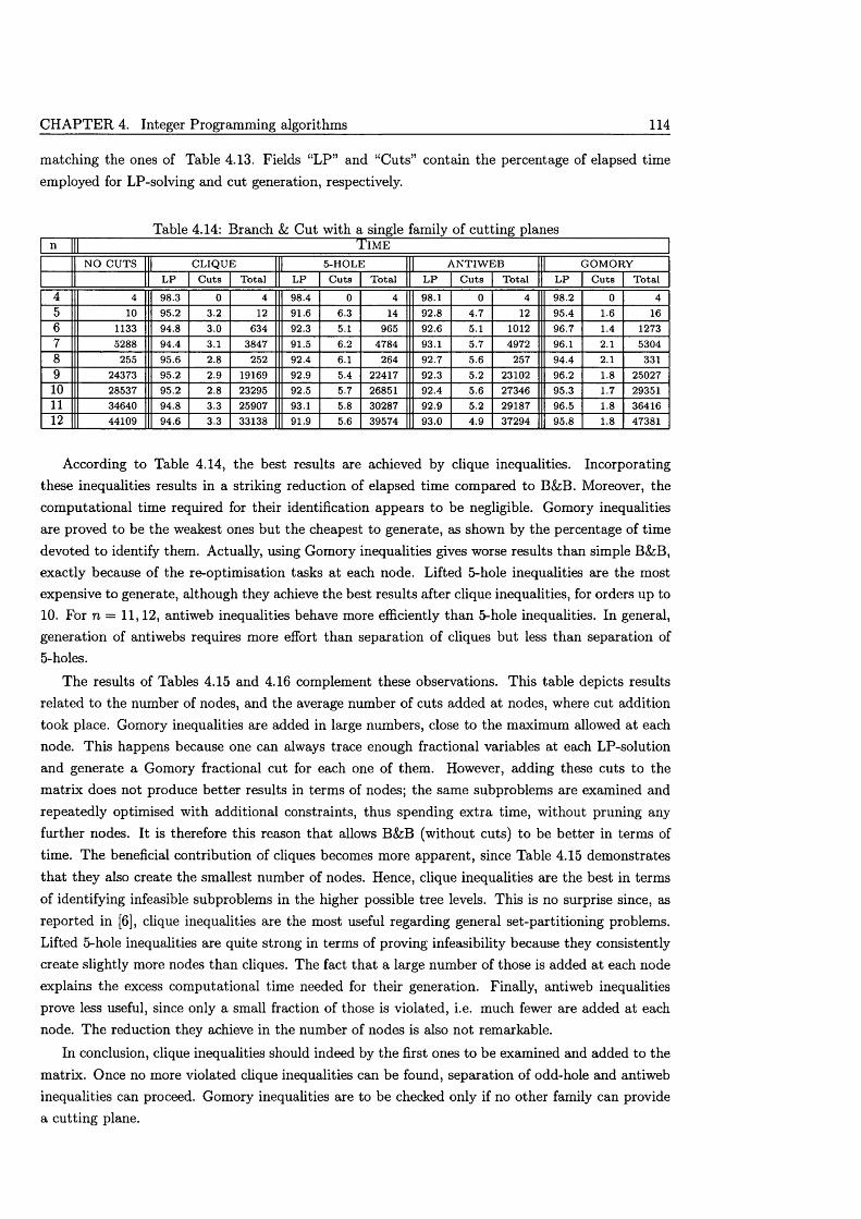
CH APTER 4. Integer Programming algorithms 114
matching the ones of Table 4.13. Fields “LP” and “Cuts” contain the percentage of elapsed time employed for LP-solving and cut generation, respectively.
Table 4.14: Branch fc Cut with a single family of cutting planesn | T im e
NO CUTS | CLIQUE | 5-HOLE | ANTIWEB | GOMORYLP Cuts Total LP Cuts Total LP Cuts Total LP Cuts Total
4 4 98.3 0 4 98.4 0 4 98.1 0 4 98.2 0 45 10 95.2 3.2 12 91.6 6.3 14 92.8 4.7 12 95.4 1.6 166 1133 94.8 3.0 634 92.3 5.1 965 92.6 5.1 1012 96.7 1.4 12737 5288 94.4 3.1 3847 91.5 6.2 4784 93.1 5.7 4972 96.1 2.1 53048 255 95.6 2.8 252 92.4 6.1 264 92.7 5.6 257 94.4 2.1 3319 24373 95.2 2.9 19169 92.9 5.4 22417 92.3 5.2 23102 96.2 1.8 2502710 28537 95.2 2.8 23295 92.5 5.7 26851 92.4 5.6 27346 95.3 1.7 2935111 34640 94.8 3.3 25907 93.1 5.8 30287 92.9 5.2 29187 96.5 1.8 3641612 44109 94.6 3.3 33138 91.9 5.6 39574 93.0 4.9 37294 95.8 1.8 47381
According to Table 4.14, the best results are achieved by clique inequalities. Incorporating these inequalities results in a striking reduction of elapsed time compared to B&B. Moreover, the com putational time required for their identification appears to be negligible. Gomory inequalities are proved to be the weakest ones but the cheapest to generate, as shown by the percentage of time devoted to identify them. Actually, using Gomory inequalities gives worse results than simple B&B, exactly because of the re-optimisation tasks at each node. Lifted 5-hole inequalities are the most expensive to generate, although they achieve the best results after clique inequalities, for orders up to 10. For n = 11,12, antiweb inequalities behave more efficiently than 5-hole inequalities. In general, generation of antiwebs requires more effort than separation of cliques but less than separation of 5-holes.
The results of Tables 4.15 and 4.16 complement these observations. This table depicts results related to the number of nodes, and the average number of cuts added at nodes, where cut addition took place. Gomory inequalities are added in large numbers, close to the maximum allowed at each node. This happens because one can always trace enough fractional variables at each LP-solution and generate a Gomory fractional cut for each one of them. However, adding these cuts to the m atrix does not produce better results in terms of nodes; the same subproblems are examined and repeatedly optimised with additional constraints, thus spending extra time, without pruning any further nodes. It is therefore this reason th a t allows B&B (without cuts) to be better in terms of time. The beneficial contribution of cliques becomes more apparent, since Table 4.15 demonstrates th a t they also create the smallest number of nodes. Hence, clique inequalities are the best in terms of identifying infeasible subproblems in the higher possible tree levels. This is no surprise since, as reported in [6], clique inequalities are the most useful regarding general set-partitioning problems. Lifted 5-hole inequalities are quite strong in terms of proving infeasibility because they consistently create slightly more nodes than cliques. The fact th a t a large number of those is added at each node explains the excess computational time needed for their generation. Finally, antiweb inequalities prove less useful, since only a small fraction of those is violated, i.e. much fewer are added at each node. The reduction they achieve in the number of nodes is also not remarkable.
In conclusion, clique inequalities should indeed by the first ones to be examined and added to the matrix. Once no more violated clique inequalities can be found, separation of odd-hole and antiweb inequalities can proceed. Gomory inequalities are to be checked only if no other family can provide a cutting plane.
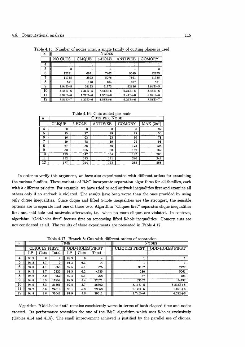
4.6. Com putational analysis 115
Table 4.15: Number of nodes when a single family of cutting planes is usedn | N o d e s
NO CUTS CLIQUE 5-HOLE ANTIWEB GOMORY4 l l l l l5 3 l l l 36 12281 6871 7462 9649 122737 11735 3593 5076 7861 117358 571 178 184 407 5719 1.94E+5 58123 61773 92136 1.94E+510 3.48E+6 7.31E+5 7.44E+5 9.31E+5 3.48E+611 8.92E+6 1.27E+6 1.35E+6 3.47E+6 8.92E+612 7.51E+7 4.23E+6 4.58E+6 6.23E+6 7.51E+7
Table 4.16: Cuts added per noden | C u t s p e r N o d e
CLIQUE 5-HOLE ANTIWEB GOMORY MAX (2na)4 0 0 0 0 325 25 27 29 49 506 46 62 32 70 787 59 78 39 95 988 67 86 56 123 1289 83 105 68 162 16210 129 147 104 197 20011 152 193 121 240 24212 177 214 163 288 288
In order to verify this argument, we have also experimented with different orders for examining the various families. These variants of B&C incorporate separation algorithms for all families, each w ith a different priority. For example, we have tried to add antiweb inequalities first and examine all others only if no antiweb is violated. The results have been worse than the ones provided by using only clique inequalities. Since clique and lifted 5-hole inequalities are the strongest, the sensible options are to separate first one of these two. Algorithm “Cliques first” separates clique inequalities first and odd-hole and antiwebs afterwards, i.e. when no more cliques are violated. In contrast, algorithm “Odd-holes first” focuses first on separating lifted 5-hole inequalities. Gomory cuts are not considered at all. The results of these experiments are presented in Table 4.17.
Table 4.17: Branch &; Cut with different orders of separationn | T i m e | N o d e s
| CLIQUES FIRST | ODD-HOLES FIRST CLIQUES FIRST ODD-HOLES FIRSTLP Cuts Total LP Cuts Total
4 98.3 0 4 98.3 0 4 l l5 94.8 3.7 9 91.3 6.3 14 l l6 94.3 4.1 553 92.5 5.1 975 3167 71277 94.5 3.7 2325 91.5 6.2 4735 280 50618 95.2 3.2 252 92.4 6.1 268 57 1849 94.8 3.5 17854 92.9 5.4 22371 33102 5479210 94.9 3.3 21561 92.5 5.7 26792 5.11E+5 6.834E+511 94.7 3.6 24813 93.1 5.8 29858 9.12E+5 1.02E+612 94.8 3.6 31642 91.9 5.6 39611 2.74E+6 4.22E+6
Algorithm “Odd-holes first” remains consistently worse in terms of both elapsed time and nodes created. Its performance resembles the one of the B&C algorithm which uses 5-holes exclusively (Tables 4.14 and 4.15). The small improvement achieved is justified by the parallel use of cliques.
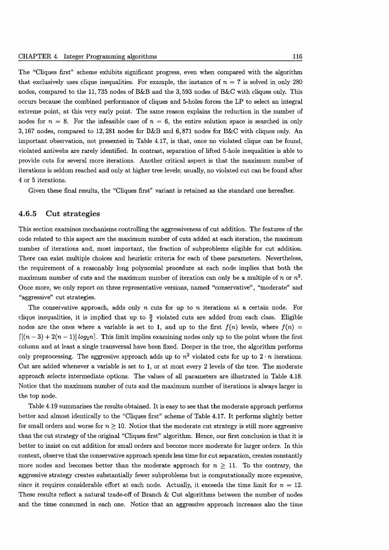
CHAPTER 4. Integer Programming algorithms 116
The “Cliques first” scheme exhibits significant progress, even when compared with the algorithm th a t exclusively uses clique inequalities. For example, the instance of n = 7 is solved in only 280 nodes, compared to the 11, 735 nodes of B&B and the 3,593 nodes of B&C with cliques only. This occurs because the combined performance of cliques and 5-holes forces the LP to select an integral extreme point, a t this very early point. The same reason explains the reduction in the number of nodes for n = 8. For the infeasible case of n = 6, the entire solution space is searched in only 3,167 nodes, compared to 12,281 nodes for B&B and 6,871 nodes for B&C with cliques only. An im portant observation, not presented in Table 4.17, is that, once no violated clique can be found, violated antiwebs are rarely identified. In contrast, separation of lifted 5-hole inequalities is able to provide cuts for several more iterations. Another critical aspect is th a t the maximum number of iterations is seldom reached and only at higher tree levels; usually, no violated cut can be found after 4 or 5 iterations.
Given these final results, the “Cliques first” variant is retained as the standard one hereafter.
4.6.5 Cut strategies
This section examines mechanisms controlling the aggressiveness of cut addition. The features of the code related to this aspect are the maximum number of cuts added a t each iteration, the maximum number of iterations and, most important, the fraction of subproblems eligible for cut addition. There can exist multiple choices and heuristic criteria for each of these parameters. Nevertheless, the requirement of a reasonably long polynomial procedure at each node implies th a t both the maximum number of cuts and the maximum number of iteration can only be a multiple of n or n 2. Once more, we only report on three representative versions, named “conservative” , “moderate” and “aggressive” cut strategies.
The conservative approach, adds only n cuts for up to n iterations at a certain node. For clique inequalities, it is implied th a t up to | violated cuts are added from each class. Eligible nodes are the ones where a variable is set to 1, and up to the first f ( n ) levels, where f ( n ) = [[(n — 3) + 2(n — 1)] log2 n \ . This limit implies examining nodes only up to the point where the first column and at least a single transversal have been fixed. Deeper in the tree, the algorithm performs only preprocessing. The aggressive approach adds up to n 2 violated cuts for up to 2 • n iterations. Cut axe added whenever a variable is set to 1, or at most every 2 levels of the tree. The moderate approach selects intermediate options. The values of all parameters are illustrated in Table 4.18. Notice th a t the maximum number of cuts and the maximum number of iterations is always larger in the top node.
Table 4.19 summarises the results obtained. It is easy to see th a t the m oderate approach performs better and almost identically to the “Cliques first” scheme of Table 4.17. It performs slightly better for small orders and worse for n > 10. Notice that the moderate cut strategy is still more aggressive than the cut strategy of the original “Cliques first” algorithm. Hence, our first conclusion is th a t it is better to insist on cut addition for small orders and become more moderate for laxger oxders. In this context, observe th a t the conservative approach spends less time for cut separation, creates constantly more nodes and becomes better than the moderate approach for n > 11. To the contrary, the aggressive strategy creates substantially fewer subproblems but is computationally more expensive, since it requires considerable effort at each node. Actually, it exceeds the time limit for n = 12. These results reflect a natural trade-off of Branch & Cut algorithms between the number of nodes and the time consumed in each one. Notice that an aggressive approach increases also the time
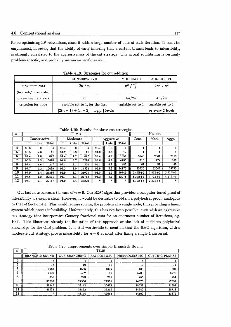
4.6. Com putational analysis 117
for re-optimising LP-relaxations, since it adds a large number of cuts at each iteration. It must be emphasised, however, th a t the ability of early inferring th a t a certain branch leads to infeasibility, is strongly correlated to the aggressiveness of the cut strategy. The actual equilibrium is certainly problem-specific, and probably instance-specific as well.
Table 4.18: Strategies for cut additionCONSERVATIVE MODERATE AGGRESSIVE
maximum cuts(top node/ other nodes)
2 n / n n 2 / ^ 2n 2 / n2
maximum iterations n 4n/2n 4n /2n
criterion for node variable set to 1, for the first [[2(n — 1) + (n — 3)] • log2n] levels
variable set to 1 variable set to 1
or every 2 levels
Table 4.19: Results for three cut strategiesn | T ime | N o d e s
| Conservative | Moderate | Aggressive Cons. Mod. Aggr.LP Cuts Total LP Cuts Total LP Cuts Total
4 98.6 0 4 98.4 0 4 98.4 0 4 l 1 15 96.5 2.6 11 94.7 3.3 11 94.8 3.6 12 1 1 16 97.4 1.8 892 94.4 4.2 527 93.4 4.7 1851 3243 2861 21597 96.5 1.9 3870 94.6 3.7 3278 93.6 4.9 4153 316 274 1858 97.4 1.6 247 95.1 3.1 254 94.1 4.8 482 61 57 499 97.7 1.2 19639 95.2 3.0 17592 92.9 5.3 24176 35726 32542 2873510 97.9 1.4 24816 94.9 3.3 21903 93.5 4.6 29749 5.42E+5 3.86E+5 2.73E+511 97.6 1.2 22531 94.7 3.1 25713 93.2 5.1 32978 8.24E+5 7.71E+5 4.17E+512 97.7 1.1 32187 94.9 3.4 33872 * * * 4.12E+5 2.37E+6 ♦
Our last note concerns the case of n = 6. Our B&C algorithm provides a computer-based proof of infeasibility via enumeration. However, it would be desirable to obtain a polyhedral proof, analogous to th a t of Section 4.3. This would require solving the problem at a single node, thus providing a linear system which proves infeasibility. Unfortunately, this has not been possible, even with an aggressive cut strategy that incorporates Gomory fractional cuts for an enormous number of iterations, e.g. 1000. This illustrates already the limitation of this approach or the lack of sufficient polyhedral knowledge for the OLS problem. It is still worthwhile to mention th a t the B&C algorithm, with a moderate cut strategy, proves infeasibility for n = 6 at most after fixing a single transversal.
Table 4.20: Improvements over simple Branch & Boundn | T ime
BRANCH & BOUND GUB BRANCHING RANDOM O.F. PREPROCESSING CUTTING PLANES
4 7 4 4 4 45 18 10 10 10 116 1963 1536 1392 1133 5277 7991 6437 6162 5288 32788 356 273 269 255 2549 33262 27936 27351 24373 1759210 38347 32143 30678 28537 2190311 46934 37852 37219 34640 2571312 * 48174 47654 44109 33872
CH APTER 4. Integer Programming algorithms 118
4.7 Concluding remarks
In this chapter, we have reported on computational work, related to the application of IP to solve the OLS problem. For the infeasible case of n = 6, we have proposed an alternative, LP-based, proof. The proof is accomplished only after preliminary variable fixing, which arises from a certain method for reducing problem’s symmetry. We have also presented a Branch & Cut algorithm for the OLS problem. This algorithm uses the polyhedral developments of the previous chapters and exploits the structure of the problem to devise efficient preprocessing and branching mechanisms. The actual form of the algorithm is determined via experimenting with several parameters. Computational results show that the algorithm improves significantly over a commercial solver and th a t strong valid inequalities constitute, apart from a theoretical description, a powerful solution tool. As a summary of all previous results, Table 4.20 shows the performance of B&B with variable dichotomy and the improved performance after incorporating, one by one, the branching mechanism, the randomised objective function, the preprocessing procedure and the moderate cut strategy of the previous section. This table shows th a t the most drastic reduction in solution time appears after applying the cutting planes.
On the other hand, our results show that at least 95% of com putation time is devoted to solving and re-optimising linear programming relaxations. Hence, limitations on the B&C approach are imposed by a large m atrix size, at least in the higher tree levels, along with the absence of faster re-optimisation methods. Next chapter introduces an enumeration paradigm, whose performance is not restricted by the necessity to solve linear programs.
Chapter 5
Constraint Program m ing algorithm s
This chapter presents the application of Constraint Programming (CP) to the OLS problem. Its first part serves the purposes of a review of the CP approach. Hence, Section 5.1 defines Constraint Satisfaction Problems (CSP) and presents the notions of constraint graph and arc-consistency. Examples involving Latin squares are used to illustrate these concepts. Methods developed to solve CSPs are presented in Section 5.2, where their performance is also analysed. There exists a broad spectrum of such methods, from the naive Generate & Test scheme to more sophisticated ones, like Conflict-Directed Backjumping. The critical aspects concerning the design of a CP algorithm are extensively discussed. The actual application of CP methods to the OLS problem is exhibited in Section 5.3. Several branching strategies and solution schemes, which exploit the problem structure in different ways, are proposed. Computational results are presented in Section 5.4.
5.1 The Constraint Programming paradigm
Constraint logic programming or Constraint Programming (CP) is a method for solving a large variety of problems. The origins of the method are located within the Artificial Intelligence (AI) community. Its main area of application has been feasibility problems arising from the computer science literature, although recent developments ([40]) suggest th a t CP could serve as a method for general combinatorial optimisation problems. Examples include machine vision, belief maintenance and scheduling ([57]), along with the generic satisfiability problem (SAT). The latter is defined on a number of logical sentences on Utrue — fa lse ” (binary) variables, and asks for an assignment that makes all sentences simultaneously true. The research field focusing on SAT problems is referred to as Logic Programming. In a sense, Constraint Logic Programming can be regarded as the extension of Logic Programming to problems involving variables w ith domains of cardinality greater than 2. Before presenting a number of formal definitions of CP, we apply Logic Programming to the OLS problem for n = 2.
5.1.1 Logic Program m ing applied to OLS for n = 2
This section illustrates a proof of the non-existence of a pair of OLS for n = 2. It acts as an example for the use of logic methods for inference. We first formulate the OLS problem for n = 2 in the form
119
CHAPTER 5. Constraint Programming algorithms 120
of logical sentences. Assume Latin squares X and Y and let variables X{j, yij £ {0,1}, i , j = 0,1, denote the value contained in cell ( i , j ) of square X and Y, respectively.
We briefly review the elementary concepts of Logic Programming. An atomic proposition is simply a binary variable, e.g. xoo- A literal is an atomic proposition or its negation, e.g. xoo or -ixoo- A formula or proposition is a sentence of atomic propositions, using the symbols {V, A}. Any subformula which is a pure disjunction of literals, i.e. uses only operator V, is called a clause. It is common to express a formula as a conjunction of clauses or, formally, in conjunctive normal form (CNF). Finally, a model is an assignment of values to literals, such th a t all clauses are simultaneously satisfied.
There exists an alternative representation of formulas in the form of rules. For example, if pair (0,0) appears in cell (0,0), both variables xqo and yoo must be 0, i.e. variables -ixoo and —<j/oo must be 1. As a consequence, pair (0,0) cannot appear in position (0,1), therefore variables xoi and yoi should be 1. The rule for expressing this fact is
-ixoo A ->yoo —> ^oi V yoi (5.1)
where symbol stands for “implies” , xoo,yoo are antecedents and £oi,2/oi form the consequent of the rule ([23, Section 2.1.3]). It is easy to see th a t rule (5.1) is equivalent to the clause:
(zoo V y0o V xoi V y0i)
All rules ensuring that, if the pair (0,0) appear at the cells (0,0), it should not appear in any other cell, are:
- ’Zoo A ->yoo —> xoi V yoi
-'Zoo A ->yoo —* xio V yio (5.2)
-'Zoo A -'yoo —► z n V yn
Rules (5.2) are equivalent to the clauses:
(zoo V yoo V x o i V y o i )
(zoo V y00 V xio V y i0) (5.3)
(zoo Vy00 V x n V yn )
Three more sets of clauses can be constructed by assuming th a t pair (0,0) appears in
cell (0,1):
(zoi V y0i V x0o V y0o)
(z0i V y0i V x 10 V yio)
(zoi V y0i V x n V y n )
(5.4)
5.1. The Constraint Programming paradigm 121
cell (1,0):
( z io V y io V x 00 V y 00)
( z io V y io V z o i V y 0i ) (5 .5 )
( ^ 1 0 V y i o V X u V y n )
cell (1,1):
( z n V y n V x 00 V y 0o)
( x n V y n V x q i V y 0i ) (5 .6 )
( z n V y n V x i o V y i 0 )
After removing any duplications, the set of clauses enforcing th a t pair (0,0) must occur exactly once are:
(zoo V yoo V x 0i V y o i)
( z o o V y 00 V x i o V y 1 0 )
(a^oo V yoo V x n V y n )
(* o i V y 0i V x io V y io ) (5 .7 )
(a?oi V y 0 i V x n V y n )
(® io Vyio V x n V yn )
Three more sets of 6 clauses each represent the fact th a t each of the remaining three pairs must also appear exactly once.
For pair (0,1) the constraints are:
For pair (1,0) the constraints are:
(xoo V -iyoo V x o i V - .y o i)
( z 0o V -^yoo V x io V ->yi0 )
( x 00 V -iyoo V x n V - - y n )
( x 0i V --yo i V x io V - -y io ) (5 .8 )
( x 0i V - . y o i V x n V - . y n )
( x i o V - -y io V x n V - - y n )
(--xoo V yoo V —<x0i V yoi)
(--xoo V yoo V —-xio V yio)
(-.x00 Vy00 V -.x n V y n )
( —-Xoi v yoi V —-Xio V yio) (5 .9 )
( i x 0i Vyoi V -.Xn Vy n )
(-.xio Vyio V - . i n V y n )
CHAPTER 5. Constraint Programming algorithms 122
For pair (1,1) the constraints are:
( - ' Z o o V J *£ o o V - z 0 i V “ '2/ o i )
( - ' Z o o V - ' y o o V ^ Z i o V - ^ i o )
( - ' Z o o V - 2 / 0 0 V - a n V - 2/ 11)
( - ’Z o i V “ 1/01 V ^ z 10 V - 2/ i o )
( - ’Z o i V -'Z/oi V - , z 1 i V - 2 / 1 1 )
( - 'Z l O V “ 'S/io V - - Z i i V - 2/ i i )
Additional clauses are required to model the fact th a t each square is Latin. For example, if zoo is 0, both xq\ and ziq must be 1. The associated rules are:
—zoo Zoi
—zoo xio
These are equivalent to the clauses:
zoo V x0i
zoo V Xio
Repeating the procedure for all cells and both values, and after deleting duplicate clauses, yields the set:
(z00 Vxoi)
(zoo V Xio)
(zoi V i n )
(z io V x n )
(-iz00 V -iz0i) (5.11)
{ - ' X o o v -iXio)
(-ixoi V —>xn)
(—'Z10 V - a n )
The set of clauses for square Y are analogous. The number of clauses can be reduced by erasing clauses th a t are dominated. It is said th a t a clause Cs absorbs a clause Ct if all literals of Cs appear in Ct- A clause Ct is implied by a clause Cs if Ct is a tautology or if Cs absorbs Ct- Observe that the first two and the last two of clauses (5.7)-(5.10) are implied by one of the clauses (5.11) and by one of the corresponding clauses for square Y . For example the clause (zoo Vyoo V zoi V yoi) of (5.7) is absorbed by both clauses (z0o V Zoi) and (yoo V yoi). Table 5.1 illustrates the set of non-implied clauses for the OLS problem for n = 2.
Algorithms for solving models in logic (formulas) are based on the principle of resolution ([23, Section 2.1.2]):
In any CNF formula, suppose there are two clauses Cs , Ct with exactly one atomic proposition p appearing negated in Cs and posited in Ct- It is then possible to resolve Cs and
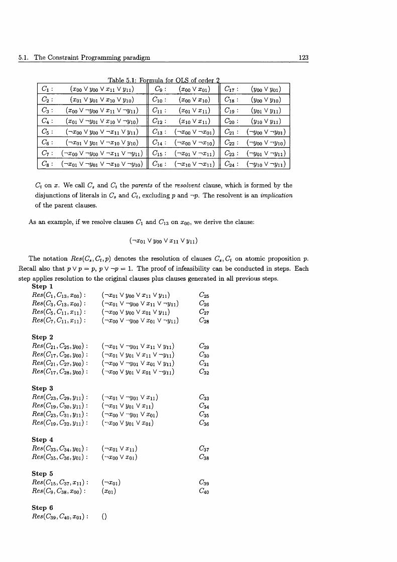
5.1. The Constraint Programming paradigm 123
Cl ( ^ 0 0 v yoo v Xn V yn) c 9 (x00 V Xoi) C\7 ( y o o V yoi)C2 (zoi V y0i V xio V yio) C10 (x00 v Xio) Cis ( y o o V yio)C3 (x00 V ->y0o V x n V ->yn) C 11 (xoi V x n ) C19 (yoi Vy n)c 4 (x0i V ->y0i V xio V -.yio) C12 (xio V x n ) C20 (yio Vyn)c 5 (^x00 Vy00 v - i x n Vyn) C13 ( —-xoo V —-Xoi) C21 (“’yoo V --yoi)C6 (1 x01 V y0i V - 1x 10 V yio) C14 ( - -X00 v - 1X1 0 ) C22 (“'yoo V --yio)c v ( 'Xoo V -iyoo V i x n V ->yn) C15 (--xoi V -ix n ) C 23 (“’yoi V -.yn)C 8 (~'X0i V --yoi V —-Xio V iy io ) C l 6 (--xio V -.x n ) C 24 ( - ’yio V -.yn )
C t on x. We call C s and C t the p a r e n t s of the r e s o l v e n t clause, which is formed by the disjunctions of literals in C s and C t , excluding p and - > p . The resolvent is an i m p l i c a t i o n
of the parent clauses.
As an example, if we resolve clauses C \ and C13 on Xoo, we derive the clause:
(-'*01 V y0o V x \ \ V y n )
The notation R e s ( C s , C t , p ) denotes the resolution of clauses C s , C t on atomic proposition p .
Recall also th a t p V p = p, p v ->p = 1. The proof of infeasibility can be conducted in steps. Each step applies resolution to the original clauses plus clauses generated in all previous steps.
Step 1R e s ( C i , C 1 3 , xoo) : ( ^ o i V yoo V i n V p n ) C 2 5
R e s { C $ , C 1 3 , xoo) : (“’ oi V - > y o o V x n V - .y n ) C 26
R e s ( C 5 , C \ \ , x n ) : ( _i^oo V yoo V x o i V y n ) C 27
R e s ( C 7 , C \ \ , x n ) : ( _|Xoo V -iyoo V xo i V ~ < y n ) C 28
Step 2R e s ( C 2 i , C 2 5 , y o o ) ■ (_l oi V ->yoi V x n V y n ) C29R e s ( C 17, C 2 6 , y 00) ' • ( - * 2:01 V y0i V x n V -.yn ) C 3 0
Res(C2i,C27,yoo) ' (~'^oo V -.yoi V xoi V y n ) C31R e s ( C w , C 2 8 , yoo) : ( ^ o o V yoi V xoi V ~-yn) C 32
Step 3R e s ( C 2 3 , C 2 9 , yn ) : ( ^ o i V ->yoi V x n ) C 33
R e s ( C i Q , C3o,yn) : (“^oi V yoi V x n ) C 3 4
Res{C23 , C 3 i , y n ) ■ (-l^oo V —>yoi V xoi) C 3 5
Res(C7i9 , C3 2 , yn ) : (“'Zoo V yoi V xoi) C36
Step 4R e s ( C 3 3 , C 3 4 , y o i ) : (-nioi V x n ) C 37
R e s ( C 3 5 , C 3 6 , y o i ) : ( “ ' Z o o V x o i ) C 3 3
Step 5R e s (C i 5 ,C ,3 7 , x n ) : (“.x o i) C 3 9
Res{C9, C 38,xoo) : ( ^ 0 1 ) C 40
Step 6Res(C39,C40, x 0i ) : ( )
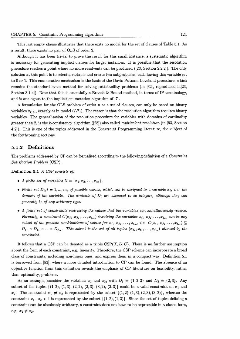
CHAPTER 5. Constraint Programming algorithms 124
This last empty clause illustrates th a t there exits no model for the set of clauses of Table 5.1. As a result, there exists no pair of OLS of order 2.
Although it has been trivial to prove the result for this small instance, a systematic algorithm is necessary for generating implied clauses for larger instances. It is possible th a t the resolution procedure reaches a point where no more resolvents can be produced ([23, Section 2.2.2]). The only solution at this point is to select a variable and create two subproblems, each having this variable set to 0 or 1. This enumerative mechanism is the basis of the Davis-Putnam-Loveland procedure, which remains the standard exact method for solving satisfiability problems (in [32], reproduced in[23, Section 3.1.4]). Note th a t this is essentially a Branch &; Bound method, in terms of IP terminology, and is analogous to the implicit enumeration algorithm of [7].
A formulation for the OLS problem of order n as a set of clauses, can only be based on binary variables Xijki, exactly as in model ( I P 1). The reason is th a t the resolution algorithm requires binary variables. The generalisation of the resolution procedure for variables with domains of cardinality greater than 2, is the ^-consistency algorithm ([28]) also called multivalent resolution (in [53, Section 4.2]). This is one of the topics addressed in the Constraint Programming literature, the subject of the forthcoming sections.
5.1.2 D efinitions
The problems addressed by CP can be formalised according to the following definition of a Constraint Satisfaction Problem (CSP).
D e fin itio n 5.1 A CSP consists of:
• A finite set o f variables X = {x\ , X2 , . . . , x m }.
• Finite set D i,i = l , . . . ,m, of possible values, which can be assigned to a variable X{, i.e. the domain of the variable. The contents o f Di are assumed to be integers, although they can generally be of any arbitrary type.
• A finite set of constraints restricting the values that the variables can simultaneously receive. Formally, a constraint C ( x j 1 , X j 2 , . . . , X j m ) involving the variables X j 1 , X j 2 , . . . , X j m can be any subset of the possible combinations o f values for X j l , X j 2 , . . . , X j m , i.e. C ( x j i , X j 2 , . . . , X j m ) C D j i x D j 2 x ... x D j m . This subset is the set of all tuples ( x j x , X j 2 , . . . , X j m ) allowed by the constraint.
It follows th a t a CSP can be denoted as a triple CSP(X, D, C). There is no further assumption about the form of each constraint, e.g. linearity. Therefore, the CSP scheme can incorporate a broad class of constraints, including non-linear ones, and express them in a compact way. Definition 5.1 is borrowed from [83], where a more detailed introduction to CP can be found. The absence of an objective function from this definition reveals the emphasis of CP literature on feasibility, rather than optimality, problems.
As an example, consider the variables x \ and x2, with D i = {1,2,3} and D 2 = {2,3}. Any subset of the tuples {(1,2), (1,3), (2,2), (2,3), (3,2), (3,3)} could be a valid constraint on x \ and x 2. The constraint x i ^ x 2 is represented by the subset {(1,2), (1,3), (2,3), (3,2)}, whereas the constraint x \ • x 2 < 4 is represented by the subset {(1,2), (1,3)}. Since the set of tuples defining a constraint can be absolutely arbitrary, a constraint does not have to be expressible in a closed form, e.g. x i ± x 2.
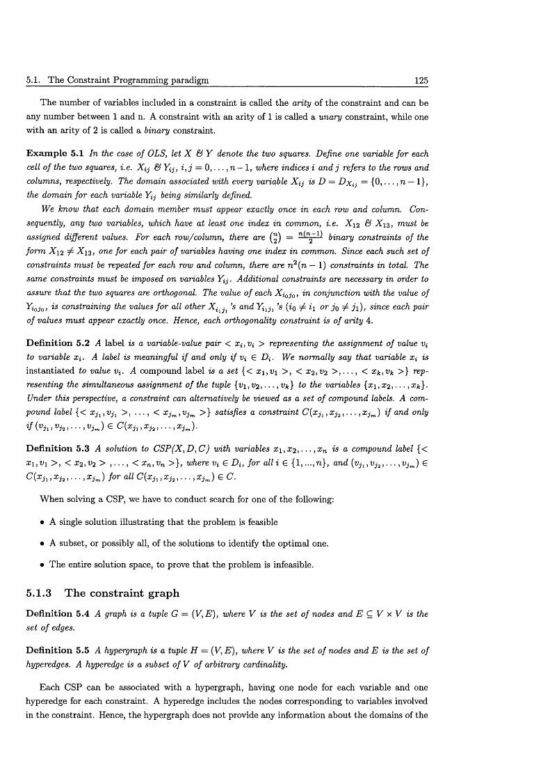
5.1. The Constraint Programming paradigm 125
The number of variables included in a constraint is called the arity of the constraint and can be any number between 1 and n. A constraint with an arity of 1 is called a unary constraint, while one w ith an arity of 2 is called a binary constraint.
E x a m p le 5.1 In the case of OLS, let X & Y denote the two squares. Define one variable for each cell o f the two squares, i.e. X ij & Yij, i , j = 0 , . . . , n — 1, where indices i and j refers to the rows and columns, respectively. The domain associated with every variable X ij is D — D x i:j = {0, . . . , n — 1}, the domain for each variable Yij being similarly defined.
We know that each domain member must appear exactly once in each row and column. Consequently, any two variables, which have at least one index in common, i.e. X \ 2 & A 13, must be assigned different values. For each row/column, there are Q) = n(n~1) binary constraints of the form X 1 2 7 A 13, one for each pair o f variables having one index in common. Since each such set of constraints m ust be repeated for each row and column, there are n 2(n — 1) constraints in total. The same constraints m ust be imposed on variables Y\ j . Additional constraints are necessary in order to assure that the two squares are orthogonal. The value o f each X i 0j 0, in conjunction with the value of Yi0j0, is constraining the values for all other X ilj 1 ’s and Yi1j 1 ’s {iq ^ i\ or jq ^ j i ) , since each pair of values must appear exactly once. Hence, each orthogonality constraint is of arity 4.
D e fin itio n 5.2 A label is a variable-value pair < Xi,Vi > representing the assignment of value v to variable X{. A label is meaningful i f and only i f Vi G Di. We normally say that variable Xi is instantiated to value Vi. A compound label is a set {< x \ ,v \ > , < X2 ,V2 > , . . . , < Xk,Vk >} representing the simultaneous assignment of the tuple {v \,V 2 , ■ ■ ■, Vk) to the variables {xi, X2 , . . . , x*}. Under this perspective, a constraint can alternatively be viewed as a set of compound labels. A compound label {< Xj1 ,Vj1 > , . . . , < Xjm,Vjm >} satisfies a constraint C(x j 1 ,Xj2, . . . ,Xjm) i f and only
i f iVh > v 3 2 > • • • > vjm) e C{xjl , x j2, . . . , x jm).
D e fin itio n 5.3 A solution to C S P ( X , D , C ) with variables x \ , X2, . . . , xn is a compound label {< ^ 1,^1 >, < x2, v2 > , . . . , < x n ,v n >}, where v G Di, for all i G {1, ...,n } , and {vjl ,Vj2, . .. ,Vjm) G C{xjl , x j2, . . . , x jm) for all C(x j} , x j2, . . . , x jm) G C.
W hen solving a CSP, we have to conduct search for one of the following:
• A single solution illustrating th a t the problem is feasible
• A subset, or possibly all, of the solutions to identify the optimal one.
• The entire solution space, to prove th a t the problem is infeasible.
5.1.3 The constraint graph
D efin itio n 5.4 A graph is a tuple G = (V,E), where V is the set o f nodes and E C V x V is the set o f edges.
D e fin itio n 5.5 A hypergraph is a tuple H = (V,E) , where V is the set o f nodes and E is the set of hyperedges. A hyperedge is a subset of V o f arbitrary cardinality.
Each CSP can be associated with a hypergraph, having one node for each variable and one hyperedge for each constraint. A hyperedge includes the nodes corresponding to variables involved in the constraint. Hence, the hypergraph does not provide any information about the domains of the
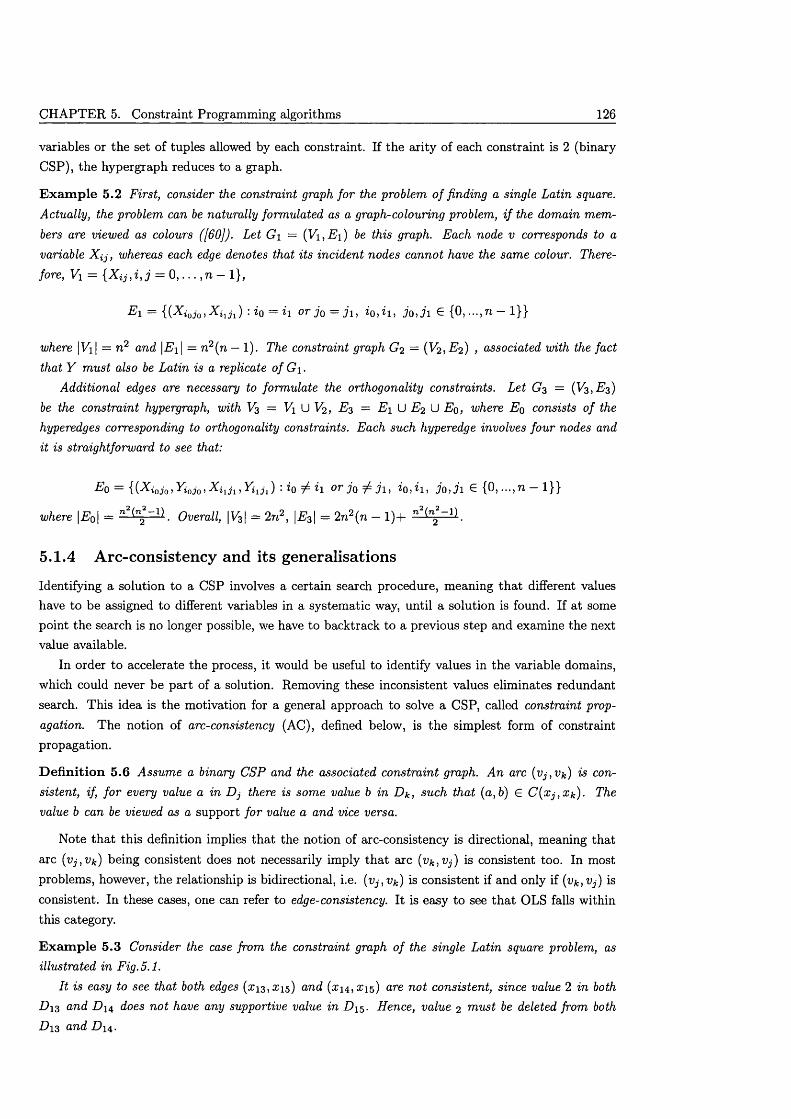
CHAPTER 5. Constraint Programming algorithms 126
variables or the set of tuples allowed by each constraint. If the arity of each constraint is 2 (binary CSP), the hypergraph reduces to a graph.
E x am p le 5.2 First, consider the constraint graph for the problem o f finding a single Latin square. Actually, the problem can be naturally formulated as a graph-colouring problem, i f the domain members are viewed as colours ([60]). Let G i = (V\ ,Ei ) be this graph. Each node v corresponds to a variable X ^ , whereas each edge denotes that its incident nodes cannot have the same colour. Therefore, Vi = { X i j , i , j = 0 , . . . , n - 1},
E-i = {(XiQj0, X i d l ) : i Q = ii or j Q = j i, z0,zi, j 0, j i G {0, . . . ,n - 1}}
where |Vi| = n 2 and |£ i | = n2(n — 1). The constraint graph G i = (V2 , E 2 ) , associated with the fact that Y must also be Latin is a replicate of G 1.
Additional edges are necessary to formulate the orthogonality constraints. Let G3 = (V^jE^) be the constraint hypergraph, with V3 = Vi U V2 , £3 = £1 U £2 U Eq, where Eq consists of the hyperedges corresponding to orthogonality constraints. Each such hyperedge involves four nodes and it is straightforward to see that:
£ 0 = {(Ariojo)^ioj0) ^ i h > yi in) l i o ^ h o r 3o¥z 3~Li ‘loAij 30i j i £ {0, ...,n — 1}}
where |£ 0| = Overall, |V3| = 2n 2, |£ 3| = 2n 2(n - 1)+ I .
5.1.4 A rc-consistency and its generalisations
Identifying a solution to a CSP involves a certain search procedure, meaning th a t different values have to be assigned to different variables in a systematic way, until a solution is found. If at some point the search is no longer possible, we have to backtrack to a previous step and examine the next value available.
In order to accelerate the process, it would be useful to identify values in the variable domains, which could never be part of a solution. Removing these inconsistent values eliminates redundant search. This idea is the motivation for a general approach to solve a CSP, called constraint propagation. The notion of arc-consistency (AC), defined below, is the simplest form of constraint propagation.
D e fin itio n 5.6 Assume a binary CSP and the associated constraint graph. A n arc (vj,Vk) is consistent, if, fo r every value a in Dj there is some value b in Dk, such that (a,b) 6 C(xj ,Xk) . The value b can be viewed as a support for value a and vice versa.
Note th a t this definition implies th a t the notion of arc-consistency is directional, meaning that arc (vj ,Vk) being consistent does not necessarily imply th a t arc (Vk,Vj) is consistent too. In most problems, however, the relationship is bidirectional, i.e. (vj,Vk) is consistent if and only if (v^,Vj) is consistent. In these cases, one can refer to edge-consistency. It is easy to see th a t OLS falls within this category.
E x am p le 5.3 Consider the case from the constraint graph of the single Latin square problem, as illustrated in Fig. 5.1.
It is easy to see that both edges (£13, £ 15) and (£14, 0:15) are not consistent, since value 2 in both D 13 and D 14 does not have any supportive value in £ 15. Hence, value 2 m ust be deleted from both D 13 and -D14.
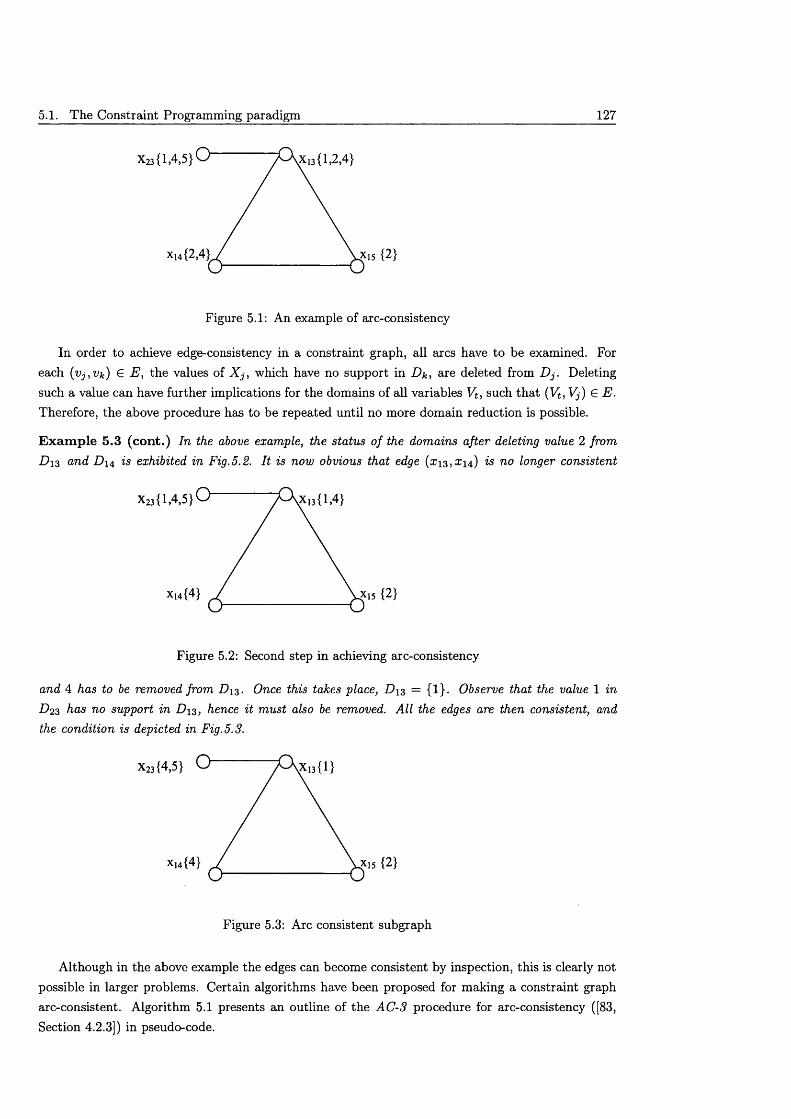
5.1. The Constraint Programming paradigm 127
,X,3 {1,2,4}
Figure 5.1: An example of arc-consistency
In order to achieve edge-consistency in a constraint graph, all arcs have to be examined. For each (Vj , Vk) E E, the values of X j , which have no support in Dk, are deleted from D j . Deleting such a value can have further implications for the domains of all variables Vt, such th a t (Vt , V j ) E E.
Therefore, the above procedure has to be repeated until no more domain reduction is possible.
E x am p le 5.3 (co n t.) In the above example, the status of the domains after deleting value 2 from D 13 and D\± is exhibited in Fig.5.2. It is now obvious that edge (£13,£ 14) is no longer consistent
Figure 5.2: Second step in achieving arc-consistency
and 4 has to be removed from D 13. Once this takes place, D \z = {1}. Observe that the value 1 in D 2 3 has no support in D 1 3 , hence it must also be removed. All the edges are then consistent, and the condition is depicted in Fig. 5.3.
Figure 5.3: Arc consistent subgraph
Although in the above example the edges can become consistent by inspection, this is clearly not possible in larger problems. Certain algorithms have been proposed for making a constraint graph arc-consistent. Algorithm 5.1 presents an outline of the AC-3 procedure for arc-consistency ([83, Section 4.2.3]) in pseudo-code.
CHAPTER 5. Constraint Programming algorithms 128
A lg o rith m 5.1 (A lg o rith m A C -3)
Q = { > vk) £ E , i ^ j }repeat
{CHANGE <- false; f o r each (vj,Vk) 6 Q do
{f o r each a G D j do / / D j is th e d o m a in o f va r ia b le j
{D ELETE <— false;if, for each b G D fa, (<2, 6 ) ^ C{Xj , X]f) / / N o s u p p o r t va lu e is le ft f o r a
{Delete a from D j;D ELETE <— true;
}CHANGE «- CHANGE V DELETE;
}}
u n til (CHANGE =false) / / U n tu n o m o re va lu e s c a n be de le ted
re tu rn ;
Note th a t Algorithm 5.1 assumes directionality. The authors of [14] present a variant of AC-3, which takes bidirectionality into account, hence reducing the com putation needed for maintaining arc-consistency. More efficient algorithms, namely AC-4 & AC-5, are presented in [67] and [49], respectively. These schemes can maintain arc-consistency in 0(ed?) steps in the worst case, where d is an upper bound on the size of each domain and e is the number of constraints.
The question, which naturally arises, is whether, after making the constraint graph arc-consistent, no search is required to advance to a solution. If this is indeed the case, the constraint graph is said to have become backtrack-free. This could occur only if:
• Every variable is left with a single value in its domain, hence indicating a unique solution.
• The domain of a variable is left empty, therefore the CSP is infeasible.
• All the values left in the domains can be part of a solution, therefore any combination of these remaining values can be used to construct a solution. Such a case is illustrated in Fig.5.3.
Unfortunately, the above conditions rarely occur and only in special problem instances. A more formal argument is provided by the notion of k- consistency, which generalises th a t of arc-consistency
D efin itio n 5.7 A graph is k-consistent, if, whenever a partial instantiation o f any k — 1 variables violates none o f the constraints involving those variables, there exists a value for any other kth variable, which violates none o f the constraints involving all k variables. A graph is strongly k- consistent i f it is j-consistent for all j < k.
Hence, arc-consistency is equivalent to 2-consistency. Path-consistency is an extension of arc- consistency, equivalent to 3-consistency. In path-consistency, any two binary constraints with one variable in common are also examined. For example, assume the existence of constraints C{xj ,Xk)
5.2. Methods for solving a CSP 129
and C(xk,xi ) . The domains of Xj Sz xi are indirectly interrelated, and this implicit information can be used to exclude values from both Dj & Di. Although only binary constraints are included in the original problem, path-consistency can induce implicit constraints of arity 3, in the form of triples of (Xj ,Xk , x i ) th a t can be part of a solution.
Clearly, no search is necessary if a graph can be made strongly |F [-consistent, since no constraint can involve more than |V| variables. An optimal algorithm for achieving th a t is proposed in [28]. However, achieving strong |P (-consistency can be computationally more expensive than the most naive search procedure. There are specific problem classes, for which the constraint graph can become backtrack-free, if it is made ^-consistent for a certain k < \V\. As it is usually the case, the methods achieving this are problem-specific and therefore difficult to generalise ([57]).
5.2 M ethods for solving a CSP
This section examines a number of representative algorithms for solving CSPs. The algorithms axe presented in ascending order with respect to their level of sophistication. An excellent survey of CSP algorithms can be found in [57]. The authors of [56] provide a theoretical framework for assessing the performance of most of the schemes presented here.
5.2.1 G enerate &; Test
Generate & Test (GT) is the simplest method for solving a CSP. All possible assignments of values to variables are generated in a systematic way. After a complete assignment (compound label) is generated, it is tested against all problem constraints. If none of those is violated, the assignment is a feasible solution and the algorithm terminates. If a violation occurs, the next assignment is generated. The problem is declared infeasible, if all possible assignments fail to give a solution.
If the problem is defined on m variables, each with a domain of size p, m p assignments have to be generated if (i) no solution exists or (ii) all solutions are required or (iii) the best solution is required. Assume a binary constraint C ( x j , X k ) not allowing the compound label (< X j , a > , < >). Alln m~2 assignments containing this label will be generated, although this is obviously fruitless.
E x am p le 5.4 Suppose that we wish to solve the Latin square problem with GT. There can be no Latin square o f order n having two CPs in the first column, therefore no assignment of the form (< Xoo,0 > , < Xio,0 > , . . . ) can be a solution. There exist, however, n "2-2 such assignments, which will be generated and tested. The amount o f redundant search becomes more significant, if all such cases are taken into account.
5.2.2 C hronological B ackt racking
A normal extension of the above technique is to proceed incrementally with variable instantiation. This means that, at each step, only one variable is assigned a value and all the constraints are checked with respect to the variables instantiated so far. If a violation occurs, the most recently instantiated variable, which has still values not considered, is re-instantiated to its next available value. Thus, partial instantiation is sufficient to prune larger subsets of the solution space. This constitutes the Chronological Backtracking (BT) paradigm.
The search performed by BT can be represented by a search tree. Each level in this tree corresponds to a variable and nodes a t the same level correspond to different values assigned to the
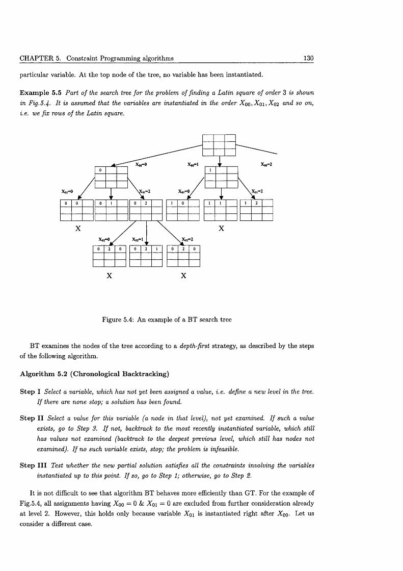
CHAPTER 5. Constraint Programming algorithms 130
particular variable. At the top node of the tree, no variable has been instantiated.
E x am p le 5.5 Part o f the search tree for the problem of finding a Latin square of order 3 is shown in Fig.5-4- It is assumed that the variables are instantiated in the order Xoo,Xoi,Xo2 and so on, i.e. we fix rows o f the Latin square.
X X
Figure 5.4: An example of a BT search tree
BT examines the nodes of the tree according to a depth-first strategy, as described by the steps of the following algorithm.
A lg o rith m 5.2 (C h ro n o lo g ica l B ack track in g )
S te p I Select a variable, which has not yet been assigned a value, i.e. define a new level in the tree. I f there are none stop; a solution has been found.
S te p I I Select a value for this variable (a node in that level), not yet examined. I f such a value exists, go to Step 3. I f not, backtrack to the most recently instantiated variable, which still has values not examined (backtrack to the deepest previous level, which still has nodes not examined). I f no such variable exists, stop; the problem is infeasible.
S te p I I I Test whether the new partial solution satisfies all the constraints involving the variables instantiated up to this point. I f so, go to Step 1; otherwise, go to Step 2.
It is not difficult to see that algorithm BT behaves more efficiently than GT. For the example of Fig.5.4, all assignments having Xoo = 0 & Xoi = 0 are excluded from further consideration already at level 2. However, this holds only because variable X qi is instantiated right after Xoo- Let us consider a different case.
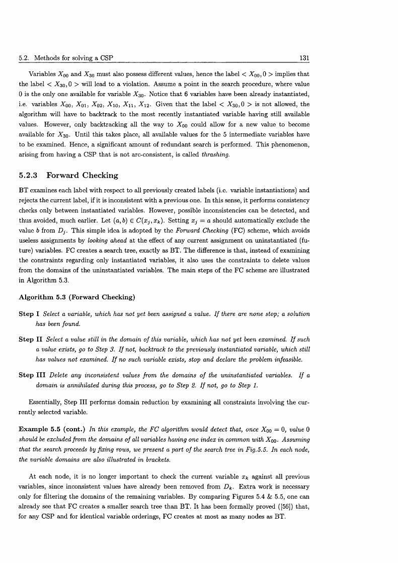
5.2. Methods for solving a CSP 131
Variables Xqo and X 30 must also possess different values, hence the label < Xoo , 0 > implies that the label < X 30, 0 > will lead to a violation. Assume a point in the search procedure, where value 0 is the only one available for variable X 30. Notice th a t 6 variables have been already instantiated,
i.e. variables Xoo, ^ 01, -^02, -X'io, -^11, -^12- Given th a t the label < X 3o,0 > is not allowed, the algorithm will have to backtrack to the most recently instantiated variable having still available values. However, only backtracking all the way to Xoo could allow for a new value to become available for X 30. Until this takes place, all available values for the 5 intermediate variables have to be examined. Hence, a significant amount of redundant search is performed. This phenomenon, arising from having a CSP that is not arc-consistent, is called thrashing.
5.2.3 Forward Checking
BT examines each label with respect to all previously created labels (i.e. variable instantiations) and rejects the current label, if it is inconsistent with a previous one. In this sense, it performs consistency checks only between instantiated variables. However, possible inconsistencies can be detected, and thus avoided, much earlier. Let (a, 6) E C (xj,X k). Setting Xj = a should automatically exclude the value b from D j . This simple idea is adopted by the Forward Checking (FC) scheme, which avoids useless assignments by looking ahead at the effect of any current assignment on uninstantiated (future) variables. FC creates a search tree, exactly as BT. The difference is that, instead of examining the constraints regarding only instantiated variables, it also uses the constraints to delete values from the domains of the uninstantiated variables. The main steps of the FC scheme are illustrated in Algorithm 5.3.
A lg o rith m 5.3 (F o rw ard C heck ing)
S te p I Select a variable, which has not yet been assigned a value. I f there are none stop; a solution has been found.
S te p I I Select a value still in the domain of this variable, which has not yet been examined. I f such a value exists, go to Step 3. I f not, backtrack to the previously instantiated variable, which still has values not examined. I f no such variable exists, stop and declare the problem infeasible.
S te p I I I Delete any inconsistent values from the domains o f the uninstantiated variables. I f a domain is annihilated during this process, go to Step 2. I f not, go to Step 1.
Essentially, Step III performs domain reduction by examining all constraints involving the currently selected variable.
E x am p le 5.5 (co n t.) In this example, the FC algorithm would detect that, once Xoo = 0, value 0 should be excluded from the domains of all variables having one index in common with Xoo- Assuming that the search proceeds by fixing rows, we present a part o f the search tree in Fig. 5.5. In each node, the variable domains are also illustrated in brackets.
At each node, it is no longer im portant to check the current variable Xk against all previous variables, since inconsistent values have already been removed from D k • E xtra work is necessary only for filtering the domains of the remaining variables. By comparing Figures 5.4 &; 5.5, one can already see th a t FC creates a smaller search tree than BT. It has been formally proved ([56]) that, for any CSP and for identical variable orderings, FC creates at most as many nodes as BT.
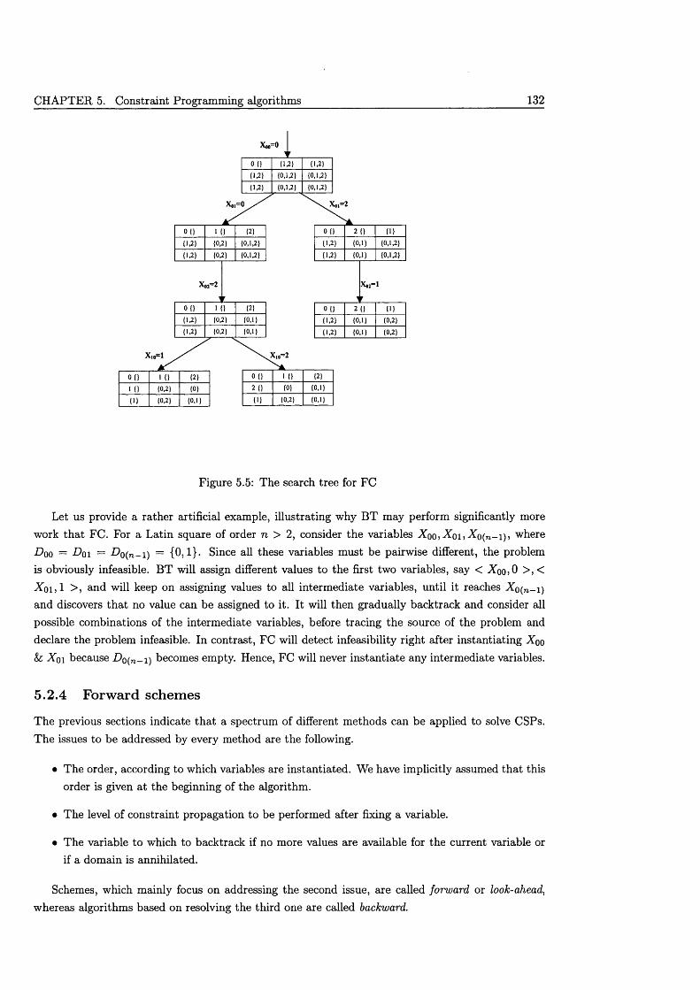
CHAPTER 5. Constraint Programming algorithms 132
Figure 5.5: The search tree for FC
Let us provide a rather artificial example, illustrating why BT may perform significantly more work th a t FC. For a Latin square of order n > 2, consider the variables Xoo, Xoi, Xo(n_i), where D qq = Dqi = £>0(n_i) = {0,1}. Since all these variables must be pairwise different, the problem is obviously infeasible. BT will assign different values to the first two variables, say < Xoo,0 >, < X o i , 1 > , and will keep on assigning values to all intermediate variables, until it reaches Xo(n_i) and discovers th a t no value can be assigned to it. It will then gradually backtrack and consider all possible combinations of the intermediate variables, before tracing the source of the problem and declare the problem infeasible. In contrast, FC will detect infeasibility right after instantiating Xoo & Xoi because L>o(n_i) becomes empty. Hence, FC will never instantiate any intermediate variables.
5.2.4 Forward schemes
The previous sections indicate th a t a spectrum of different methods can be applied to solve CSPs. The issues to be addressed by every method are the following.
• The order, according to which variables are instantiated. We have implicitly assumed that this order is given at the beginning of the algorithm.
• The level of constraint propagation to be performed after fixing a variable.
• The variable to which to backtrack if no more values are available for the current variable or if a domain is annihilated.
Schemes, which mainly focus on addressing the second issue, are called forward or look-ahead, whereas algorithms based on resolving the third one are called backward.
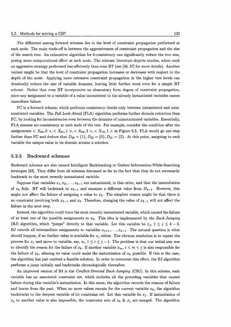
5.2. M ethods for solving a CSP 133
The difference among forward schemes lies in the level of constraint propagation performed at each node. The main trade-off is between the aggressiveness of constraint propagation and the size of the search tree. An exhaustive algorithm for ^-consistency can significantly reduce the tree size, posing more computational effort at each node. The relevant literature depicts studies, where such an aggressive strategy performed less efficiently than even BT (see [56, 57] for more details). Another variant might be th a t the level of constraint propagation increases or decreases with respect to the depth of the node. Applying more extensive constraint propagation in the higher tree levels can drastically reduce the size of variable domains, leaving little further work even for a simple BT scheme. Notice th a t even BT incorporates an elementary form degree of constraint propagation, since any assignment to a variable of a value inconsistent to the already instantiated variables causes immediate failure.
FC is a forward scheme, which performs consistency checks only between instantiated and uninstantiated variables. The Full Look-Ahead (FLA) algorithm performs further domain reduction than FC, by looking for inconsistencies even between the domains of uninstantiated variables. Essentially, FLA ensures arc-consistency at each node of the tree. For example, consider the condition after the assignments < Aoo,0 > , < Aoi, 1 > , < Ao2,2 > , < Aio, 1 > in Figure 5.5. FLA would go one step further than FC and deduce th a t D 2 0 = {1}, £>22 = {0},L^2i = {2}. At this point, assigning to each variable the unique value in its domain attains a solution.
5.2.5 Backward schemes
Backward schemes are also named Intelligent Backtracking or Gather-Information-While-Searching strategies [83]. They differ from all schemes discussed so far in the fact th a t they do not necessarily backtrack to the most recently instantiated variable.
Suppose th a t variables x i, X2 , . . . , % k - \ are instantiated, in this order, and th a t the instantiation of Xk fails. BT will backtrack to X k-i and examine a different value from D k -i. However, this might not affect the failure of assigning a value to x*,. The simplest reason might be th a t there is no constraint involving both X k - i and x*. Therefore, changing the value of X k - i will not affect the failure in the next step.
Instead, the algorithm could trace the most recently instantiated variable, which caused the failure of at least one of the possible assignments to x*,. This idea is implemented by the Back-Jumping (BJ) algorithm, which “jum ps” directly to that variable. Let this variable be Xj, 1 < j < k — 2. B J cancels all intermediate assignments to variables Xj+i , . . . , X k ~ \ . The natural question is what should happen, if no further value is available for Xj either. The obvious resolution is to repeat the process for Xj and move to variable, say, x;, 1 < i < j — 1. The problem is th a t our initial aim was to identify the reason for the failure of x&. If another variable xm, i < m < j is also responsible for the failure of x*,, altering its value could make the instantiation of x* possible. If this is the case, the algorithm has just omitted a feasible solution. In order to overcome this effect, the BJ algorithm performs a jum p initially and backtracks chronologically thereafter.
An improved version of BJ is the Conflict-Directed Back-Jumping (CBJ). In this scheme, each variable has an associated constraint set, which includes all the preceding variables that caused failure during this variable’s instantiation. In this sense, the algorithm records the reasons of failure and learns from the past. When no more values remain for the current variable x*,, the algorithm backtracks to the deepest variable of its constraint set. Let this variable be X j . If instantiation of X j to another value is also impossible, the constraint sets of X k Sz X j are merged. The algorithm
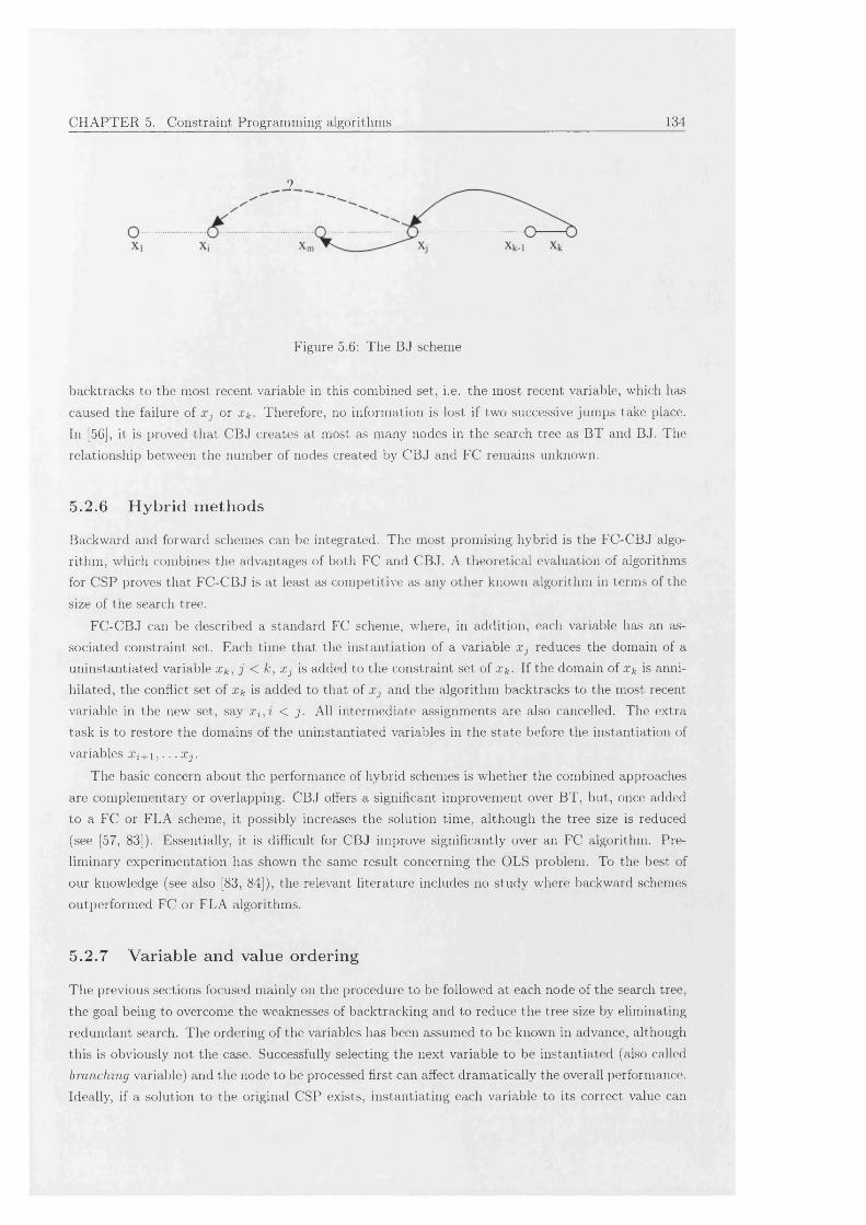
CHAPTER 5. Constraint Programming algorithms 134
Figure 5.6: T h e B J schem e
backtracks to th e m ost recent variable in th is com bined set, i.e . th e m ost recent variable, w hich has
caused th e failure o f X j or X k - T herefore, no inform ation is lost if tw o su ccessive jum ps take place.
In [56], it is proved th a t C B J creates at m ost as m any nodes in th e search tree as B T and BJ. T he
relationsh ip betw een the num ber o f nodes created by C B J and FC rem ains unknown.
5.2.6 H ybrid m ethods
Backward and forward schem es can be in tegrated . T h e m ost prom ising hybrid is th e F C -C B J algo
rithm , w hich com bines th e advantages o f b oth FC and C B J. A th eoretica l eva lu ation o f algorithm s
for C SP proves th a t F C -C B J is at least as com p etitive as any other know n algorithm in term s o f the
size o f th e search tree.
F C -C B J can b e described a standard FC schem e, w here, in ad d ition , each variable has an as
socia ted constra in t set. E ach tim e th a t the in stan tia tion o f a variable X j reduces th e dom ain o f a
u n in stan tia ted variable X k , j < k , X j is added to th e constraint se t o f x k . I f the dom ain o f X k is anni
h ila ted , th e conflict se t o f x k is added to th at o f x j and th e a lgorithm backtracks to th e m ost recent
variable in th e new set, say X i , i < j . A ll in term ed iate assignm ents are also cancelled . T he extra
task is to restore th e dom ains o f th e un instan tiated variables in th e sta te before th e in stan tiation of
variables X i + 1 , . . . X j .
T h e basic concern ab ou t the perform ance o f hybrid schem es is w h eth er the com bined approaches
are com plem en tary or overlapping. C BJ offers a significant im provem ent over B T , but, once added
to a FC or F L A schem e, it p ossib ly increases th e so lu tion tim e, a lth ou gh th e tree size is reduced
(see [57, 83]). E ssentially , it is difficult for C B J im prove sign ifican tly over an FC algorithm . Pre
lim inary exp erim en tation has show n th e sam e resu lt concern ing th e OLS problem . To the best of
our know ledge (see also [83, 84]), th e relevant literature includes no stu d y w here backward schem es
outperform ed FC or F L A algorithm s.
5.2 .7 Variable and value ordering
T h e previous section s focused m ain ly on the procedure to be follow ed at each n ode o f th e search tree,
th e goal b ein g to overcom e th e w eaknesses o f backtracking and to reduce th e tree size by elim inating
redundant search. T h e ordering o f th e variables has b een assum ed to b e know n in advance, although
th is is ob viously n ot th e case. Successfu lly se lecting th e n ext variable to b e in stan tia ted (also called
b r a n c h i n g variable) and th e node to be processed first can affect d ram atica lly th e overall perform ance.
Ideally, if a so lu tion to th e original C SP ex ists, in stan tia tin g each variable to its correct value can
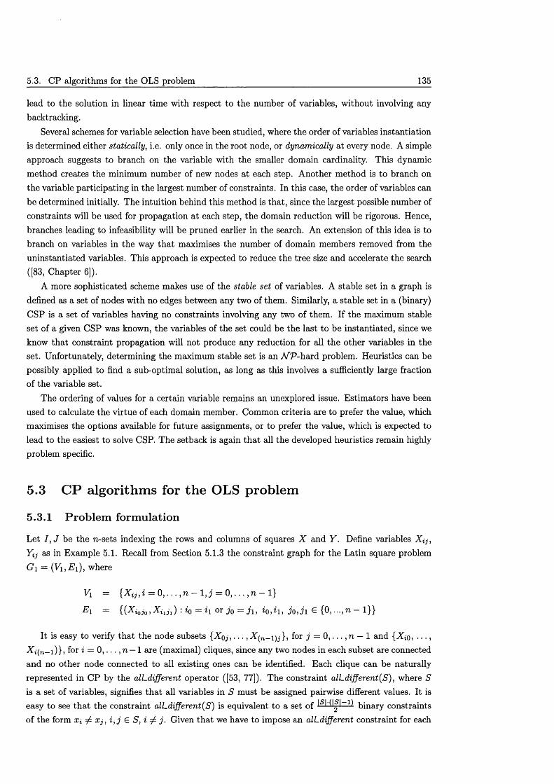
5.3. CP algorithms for the OLS problem 135
lead to the solution in linear time with respect to the number of variables, without involving any backtracking.
Several schemes for variable selection have been studied, where the order of variables instantiation is determined either statically, i.e. only once in the root node, or dynamically at every node. A simple approach suggests to branch on the variable with the smaller domain cardinality. This dynamic method creates the minimum number of new nodes at each step. Another method is to branch on the variable participating in the largest number of constraints. In this case, the order of variables can be determined initially. The intuition behind this method is that, since the largest possible number of constraints will be used for propagation a t each step, the domain reduction will be rigorous. Hence, branches leading to infeasibility will be pruned earlier in the search. An extension of this idea is to branch on variables in the way th a t maximises the number of domain members removed from the uninstantiated variables. This approach is expected to reduce the tree size and accelerate the search ([83, Chapter 6]).
A more sophisticated scheme makes use of the stable set of variables. A stable set in a graph is defined as a set of nodes with no edges between any two of them. Similarly, a stable set in a (binary) CSP is a set of variables having no constraints involving any two of them. If the maximum stable set of a given CSP was known, the variables of the set could be the last to be instantiated, since we know th a t constraint propagation will not produce any reduction for all the other variables in the set. Unfortunately, determining the maximum stable set is an M V-hard problem. Heuristics can be possibly applied to find a sub-optimal solution, as long as this involves a sufficiently large fraction of the variable set.
The ordering of values for a certain variable remains an unexplored issue. Estimators have been used to calculate the virtue of each domain member. Common criteria are to prefer the value, which maximises the options available for future assignments, or to prefer the value, which is expected to lead to the easiest to solve CSP. The setback is again th a t all the developed heuristics remain highly problem specific.
5.3 CP algorithms for the OLS problem
5.3.1 Problem formulation
Let I , J be the n-sets indexing the rows and columns of squares X and Y . Define variables X i j ,
as in Example 5.1. Recall from Section 5.1.3 the constraint graph for the Latin square problem G\ = (V i,E i) , where
Vi = { X i j , i = 0, . . . , n - l , j = 0, . . . , n — l}
E i = : = h or j 0 = j i , iQ,h , j Q, j x € {0, . . . ,n — 1}}
It is easy to verify that the node subsets { X o j , . . . , for j = 0 , . . . , n — 1 and { X i o , . . . ,X;(n_i)} , for i = 0 , . . . , n — 1 are (maximal) cliques, since any two nodes in each subset are connected and no other node connected to all existing ones can be identified. Each clique can be naturally represented in CP by the all-different operator ([53, 77]). The constraint all-different(S), where S is a set of variables, signifies th a t all variables in S must be assigned pairwise different values. It is easy to see th a t the constraint all-different(S) is equivalent to a set of binary constraintsof the form Xi ^ X j , i , j G S, i ^ j . Given th a t we have to impose an all-different constraint for each
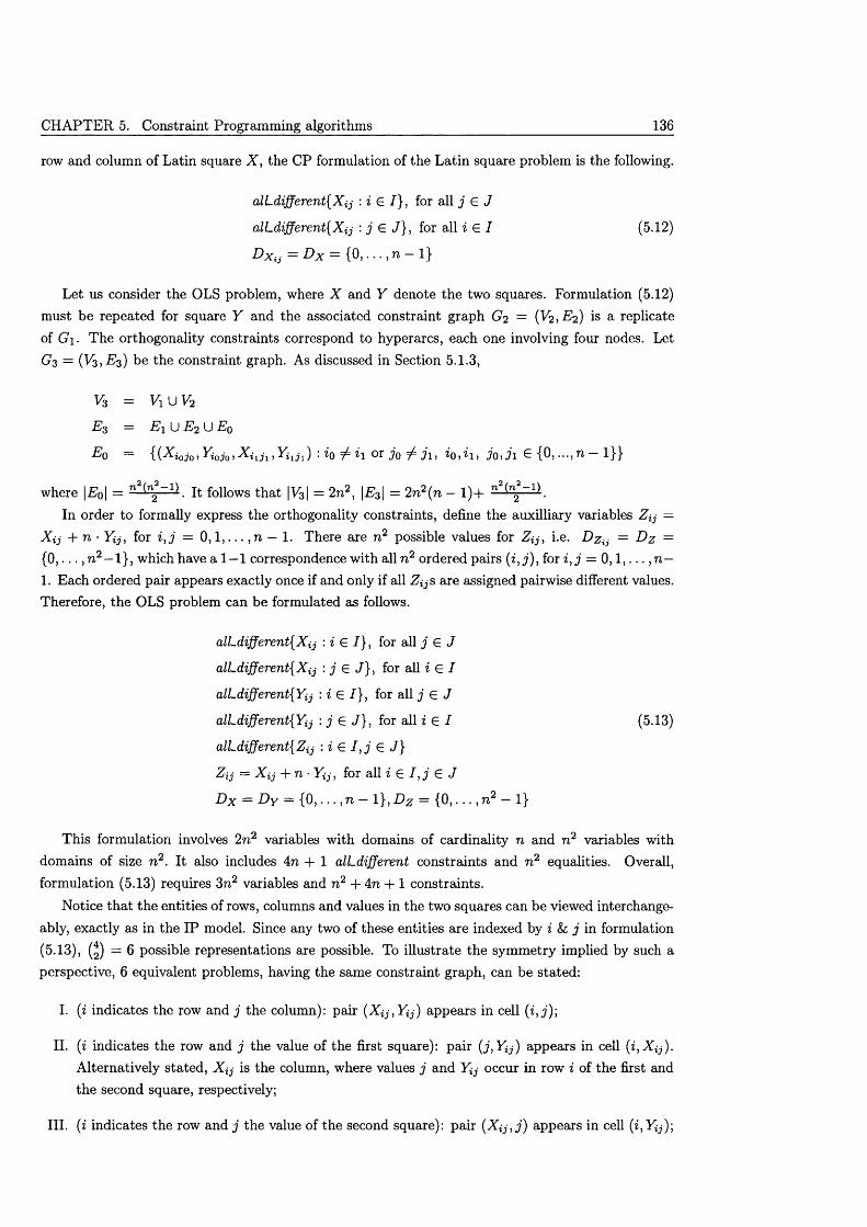
CHAPTER 5. Constraint Programming algorithms 136
row and column of Latin square X , the CP formulation of the Latin square problem is the following.
alLdifferent{Xij : i G I} , for all j G J
alLdifferent{Xij : j G J} , for al lz G I (5-12)
D Xij = D x = {0, . . . , n - 1}
Let us consider the OLS problem, where X and Y denote the two squares. Formulation (5.12) must be repeated for square Y and the associated constraint graph G2 = {V2 ,E 2) is a replicateof G \. The orthogonality constraints correspond to hyperarcs, each one involving four nodes. LetG3 = (V3, E 3) be the constraint graph. As discussed in Section 5.1.3,
p3 = v1uv2E% = E \ U E 2 U Eq
Eq = {(Ai0j0, Yi0 j 0 , X i 1j 1, Yijj 1) io ^ i\ ot jo ^ j \ , io ,ii , jo , j i G {0,..., 71 — 1}}
where |£ 01 = ■- • It follows th a t |V31 = 2n 2, |f?3| = 2n2(n — 1)+ nIn order to formally express the orthogonality constraints, define the auxilliary variables Zij —
X ij + n • Yij, for i , j = 0 , 1 , . . . , n — 1. There are n 2 possible values for Zij, i.e. D z = D z = {0 , . . . , n 2 — 1}, which have a 1 — 1 correspondence with all n 2 ordered pairs ( i , j) , for i , j = 0 , 1 , . . . , n — 1. Each ordered pair appears exactly once if and only if all ZijS are assigned pairwise different values. Therefore, the OLS problem can be formulated as follows.
alLdifferent{Xij : i G I} , for all j £ J
alLdifferent{Xij : j G J} , for alH G I
alLdifferent{Yij : i G I} , for all j G J
alLdifferent{Yij : j G J} , for alH G I (5.13)
alLdifferent{Zij : i G I , j G J}
Zij = X ij + n • Yij, for all i G I , j G J
D x = D y = {0, . . . , n — 1 } ,D z = {0, . . . , n 2 — 1}
This formulation involves 2n 2 variables with domains of cardinality n and n 2 variables with domains of size n 2. It also includes 4n + 1 alLdifferent constraints and n 2 equalities. Overall, formulation (5.13) requires 3n2 variables and n 2 + 4n + 1 constraints.
Notice th a t the entities of rows, columns and values in the two squares can be viewed interchangeably, exactly as in the IP model. Since any two of these entities are indexed by i & j in formulation(5.13), (2) = 6 possible representations are possible. To illustrate the symmetry implied by such a perspective, 6 equivalent problems, having the same constraint graph, can be stated:
I. (i indicates the row and j the column): pair (X ij ,Y i j ) appears in cell (i, j);
II. (i indicates the row and j the value of the first square): pair (j ,Y i j ) appears in cell ( i,X ij) . Alternatively stated, X ij is the column, where values j and Y\j occur in row i of the first and the second square, respectively;
III. (i indicates the row and j the value of the second square): pair (X i j , j ) appears in cell (z, Y^);
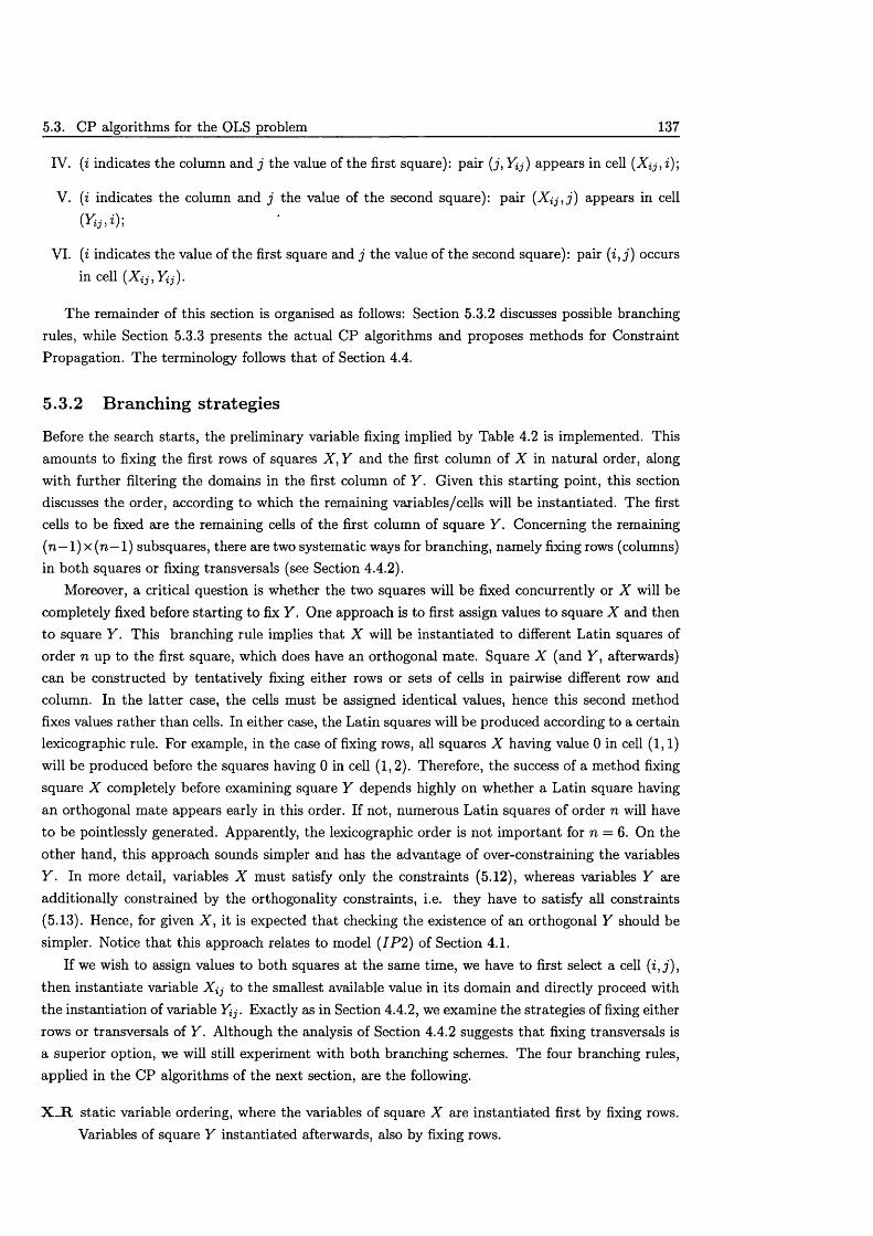
5.3. CP algorithms for the OLS problem 137
IV. (i indicates the column and j the value of the first square): pair (j , Yij) appears in cell (X ij, i)\
V. (i indicates the column and j the value of the second square): pair (X i j , j ) appears in cell (Yij, i );
VI. (i indicates the value of the first square and j the value of the second square): pair ( i , j) occurs in cell (X ^ , Yij).
The remainder of this section is organised as follows: Section 5.3.2 discusses possible branching rules, while Section 5.3.3 presents the actual CP algorithms and proposes methods for Constraint Propagation. The terminology follows th a t of Section 4.4.
5.3.2 Branching strategies
Before the search starts, the preliminary variable fixing implied by Table 4.2 is implemented. This amounts to fixing the first rows of squares X , Y and the first column of X in natural order, along with further filtering the domains in the first column of Y . Given this starting point, this section discusses the order, according to which the remaining variables/cells will be instantiated. The first cells to be fixed are the remaining cells of the first column of square Y . Concerning the remaining (n —1) x (n —1) subsquares, there are two systematic ways for branching, namely fixing rows (columns) in both squares or fixing transversals (see Section 4.4.2).
Moreover, a critical question is whether the two squares will be fixed concurrently or X will be completely fixed before starting to fix Y . One approach is to first assign values to square X and then to square Y . This branching rule implies that X will be instantiated to different Latin squares of order n up to the first square, which does have an orthogonal mate. Square X (and Y , afterwards) can be constructed by tentatively fixing either rows or sets of cells in pairwise different row and column. In the latter case, the cells must be assigned identical values, hence this second method fixes values rather than cells. In either case, the Latin squares will be produced according to a certain lexicographic rule. For example, in the case of fixing rows, all squares X having value 0 in cell (1, 1) will be produced before the squares having 0 in cell (1,2). Therefore, the success of a method fixing square X completely before examining square Y depends highly on whether a Latin square having an orthogonal m ate appears early in this order. If not, numerous Latin squares of order n will have to be pointlessly generated. Apparently, the lexicographic order is not im portant for n = 6. On the other hand, this approach sounds simpler and has the advantage of over-constraining the variables Y . In more detail, variables X must satisfy only the constraints (5.12), whereas variables Y are additionally constrained by the orthogonality constraints, i.e. they have to satisfy all constraints(5.13). Hence, for given X , it is expected th a t checking the existence of an orthogonal Y should be simpler. Notice th a t this approach relates to model (IP 2) of Section 4.1.
If we wish to assign values to both squares at the same time, we have to first select a cell ( i ,j) , then instantiate variable X ij to the smallest available value in its domain and directly proceed with the instantiation of variable Y ^. Exactly as in Section 4.4.2, we examine the strategies of fixing either rows or transversals of Y . Although the analysis of Section 4.4.2 suggests th a t fixing transversals is a superior option, we will still experiment with both branching schemes. The four branching rules, applied in the CP algorithms of the next section, are the following.
X _R static variable ordering, where the variables of square X are instantiated first by fixing rows. Variables of square Y instantiated afterwards, also by fixing rows.
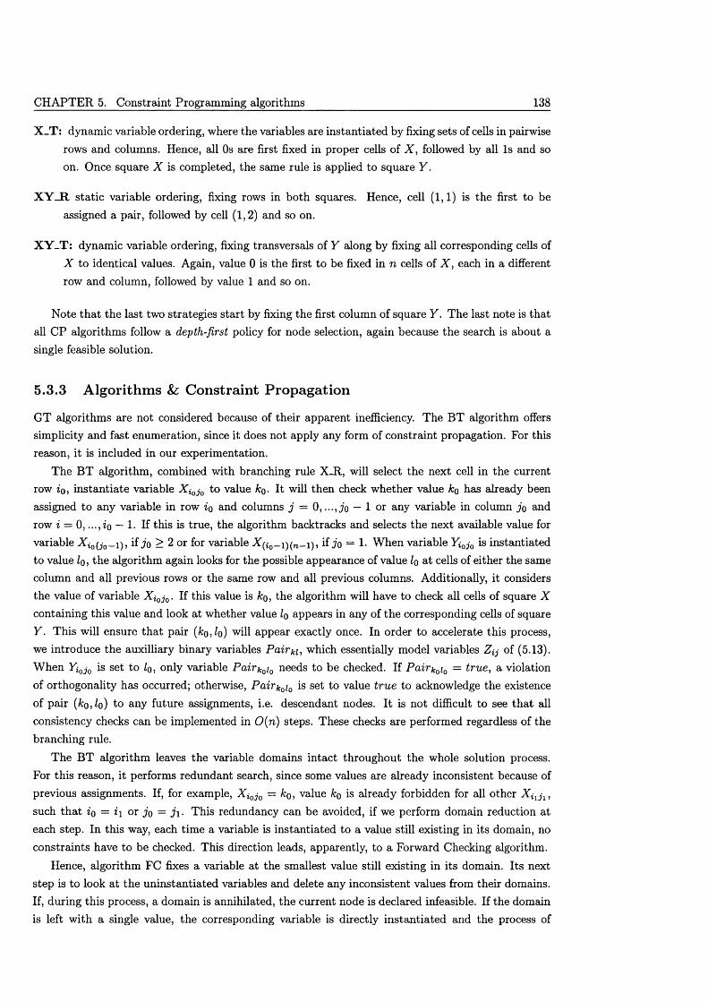
CHAPTER 5. Constraint Programming algorithms 138
X_T: dynamic variable ordering, where the variables are instantiated by fixing sets of cells in pairwise rows and columns. Hence, all Os are first fixed in proper cells of X , followed by all Is and so on. Once square X is completed, the same rule is applied to square Y .
X Y _R static variable ordering, fixing rows in both squares. Hence, cell (1,1) is the first to be assigned a pair, followed by cell (1, 2) and so on.
X Y_T: dynamic variable ordering, fixing transversals of Y along by fixing all corresponding cells of X to identical values. Again, value 0 is the first to be fixed in n cells of X , each in a different row and column, followed by value 1 and so on.
Note th a t the last two strategies start by fixing the first column of square Y . The last note is that all CP algorithms follow a depth-first policy for node selection, again because the search is about a single feasible solution.
5.3.3 A lgorithm s Constraint Propagation
GT algorithms are not considered because of their apparent inefficiency. The BT algorithm offers simplicity and fast enumeration, since it does not apply any form of constraint propagation. For this reason, it is included in our experimentation.
The BT algorithm, combined with branching rule X_R, will select the next cell in the current row io, instantiate variable X i 0 j 0 to value ho- It will then check whether value ko has already been assigned to any variable in row zo and columns j = 0 ,..., jo — 1 or any variable in column jo and row z = 0 ,. . . ,Zo — 1. If this is true, the algorithm backtracks and selects the next available value for variable X iQ 0 _ i^ if jo > 2 or for variable if jo = 1. W hen variable Yi0 j 0 is instantiatedto value Zq, the algorithm again looks for the possible appearance of value Zo at cells of either the same column and all previous rows or the same row and all previous columns. Additionally, it considers the value of variable X i 0 j0. If this value is &o, the algorithm will have to check all cells of square X containing this value and look at whether value Zq appears in any of the corresponding cells of square Y . This will ensure th a t pair [kofio] will appear exactly once. In order to accelerate this process, we introduce the auxilliary binary variables Pairki, which essentially model variables of (5.13). W hen Yi0 j 0 is set to Zo, only variable Pairk 0 i0 needs to be checked. If Pairk 0 i0 = tru e , a violation of orthogonality has occurred; otherwise, Pairk 0 i0 is set to value true to acknowledge the existence of pair (Zco,Zo) to any future assignments, i.e. descendant nodes. I t is not difficult to see th a t all consistency checks can be implemented in 0 (n ) steps. These checks are performed regardless of the branching rule.
The BT algorithm leaves the variable domains intact throughout the whole solution process. For this reason, it performs redundant search, since some values are already inconsistent because of previous assignments. If, for example, X i 0 j 0 = /c0, value ko is already forbidden for all other X {lj l , such th a t zo = zi or jo = j \ . This redundancy can be avoided, if we perform domain reduction at each step. In this way, each time a variable is instantiated to a value still existing in its domain, no constraints have to be checked. This direction leads, apparently, to a Forward Checking algorithm.
Hence, algorithm FC fixes a variable at the smallest value still existing in its domain. Its next step is to look at the uninstantiated variables and delete any inconsistent values from their domains. If, during this process, a domain is annihilated, the current node is declared infeasible. If the domain is left with a single value, the corresponding variable is directly instantiated and the process of
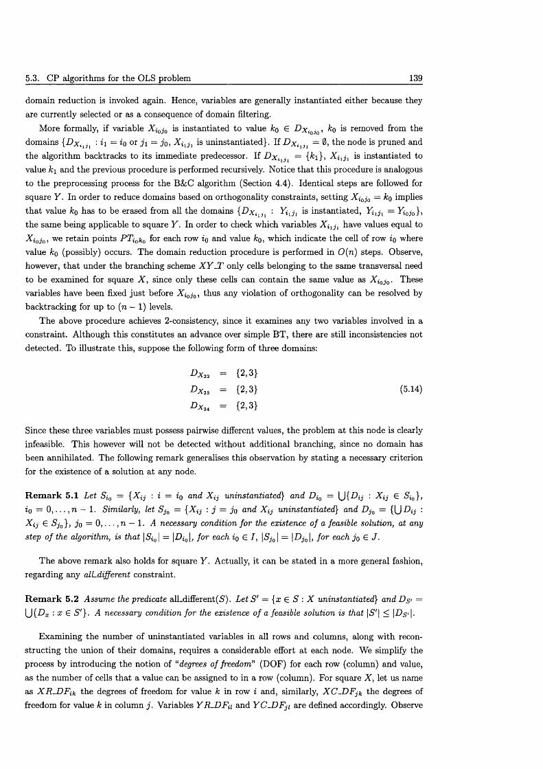
5.3. CP algorithms for the OLS problem 139
domain reduction is invoked again. Hence, variables are generally instantiated either because they are currently selected or as a consequence of domain filtering.
More formally, if variable X{0j0 is instantiated to value ko 6 D x iQjQ, ko is removed from the domains {D x i2J1 : i\ = io or j \ = jo, X i1j 1 is uninstantiated}. If D x iljl = 0, the node is pruned and the algorithm backtracks to its immediate predecessor. If D x ii:il — j^ i} , X{ij i is instantiated to value k\ and the previous procedure is performed recursively. Notice th a t this procedure is analogous to the preprocessing process for the B&C algorithm (Section 4.4). Identical steps are followed for square Y . In order to reduce domains based on orthogonality constraints, setting X{0j0 — ko implies th a t value ko has to be erased from all the domains {D xi j : Yhji is instantiated, Yi1j l = Yi0j0}, the same being applicable to square Y . In order to check which variables X ^ j , have values equal toX iQj0, we retain points PTi0k0 for each row io and value ko, which indicate the cell of row io wherevalue ko (possibly) occurs. The domain reduction procedure is performed in 0 (n ) steps. Observe, however, th a t under the branching scheme X Y - T only cells belonging to the same transversal need to be examined for square X , since only these cells can contain the same value as X i0j0. These variables have been fixed ju st before X i0j0, thus any violation of orthogonality can be resolved by backtracking for up to (n — 1) levels.
The above procedure achieves 2-consistency, since it examines any two variables involved in a constraint. Although this constitutes an advance over simple BT, there are still inconsistencies not detected. To illustrate this, suppose the following form of three domains:
Dx„ = {2,3}
D x „ = {2,3} (5.14)
= {2,3}
Since these three variables must possess pairwise different values, the problem at this node is clearly infeasible. This however will not be detected without additional branching, since no domain has been annihilated. The following remark generalises this observation by stating a necessary criterion for the existence of a solution at any node.
R e m a rk 5.1 Let Si0 = {X ij : i = io and X ^ uninstantiated} and Di0 = U [Dij : X ^ G Si0}, io = 0 , . . . , n — 1. Similarly, let S j0 = {X ij : j = jo and X ij uninstantiated} and D j0 = {(JDij : X ij € 5,0 }, jo = 0 , . . . , n — 1. A necessary condition for the existence o f a feasible solution, at any step o f the algorithm, is that | 5 i 0 | = \Di0\, for each io G 7, \Sj0 \ = \Dj0\, for each jo G J .
The above remark also holds for square Y . Actually, it can be stated in a more general fashion, regarding any alLdifferent constraint.
R e m a rk 5.2 Assume the predicate alLdifferent( 5 ) . Let S ' = {x G S : X uninstantiated} and Ds> = U P * : x G S '} . A necessary condition for the existence o f a feasible solution is that |5"| < |T)s'|.
Examining the number of uninstantiated variables in all rows and columns, along with reconstructing the union of their domains, requires a considerable effort at each node. We simplify the process by introducing the notion of “degrees of freedom” (DOF) for each row (column) and value, as the number of cells th a t a value can be assigned to in a row (column). For square X , let us name as X R -D F ik the degrees of freedom for value k in row i and, similarly, X C -D F jk the degrees of freedom for value k in column j . Variables Y R -D F u and Y C -D F ji are defined accordingly. Observe
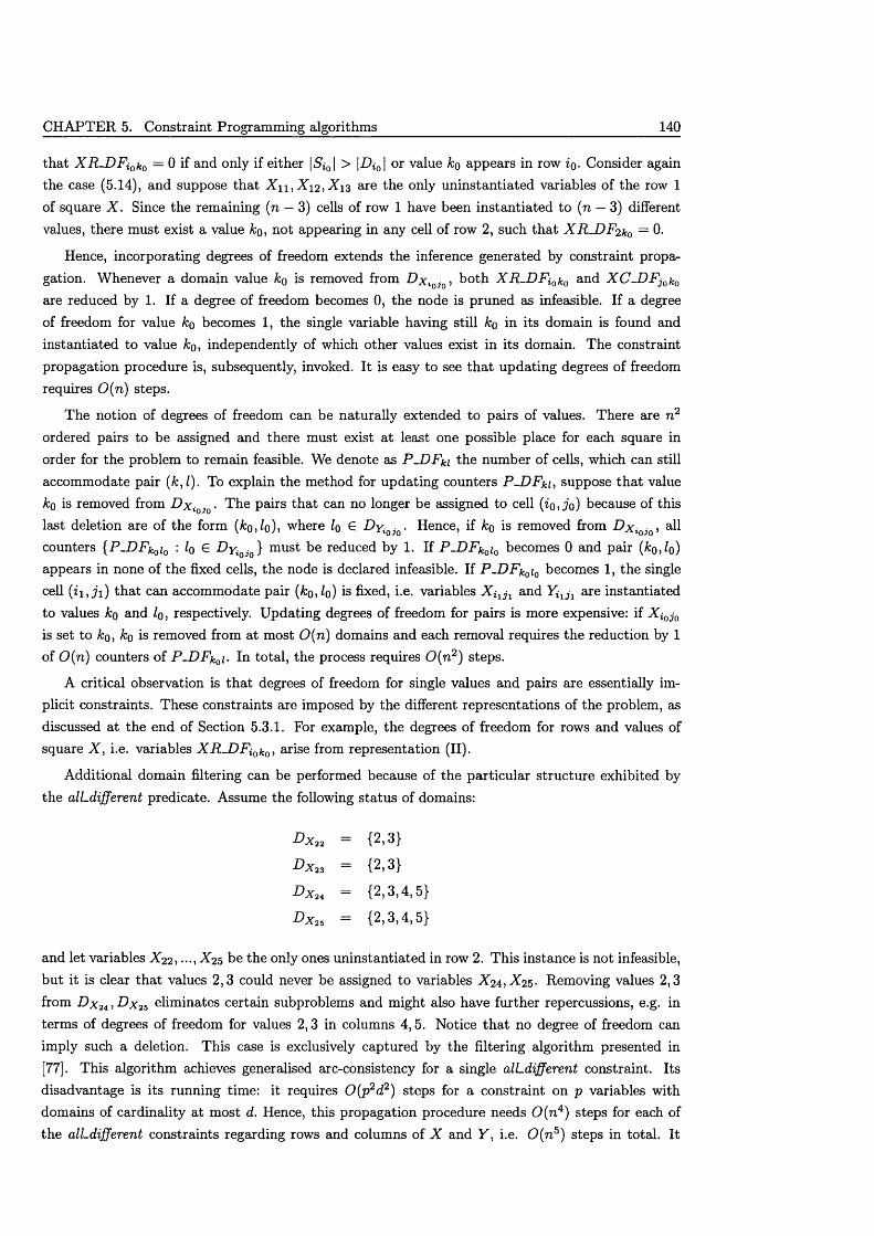
CHAPTER 5. Constraint Programming algorithms 140
that X R J D F i 0 k 0 = 0 if and only if either \ S i 0 \ > \ D i 0 \ or value ko appears in row i$. Consider again the case (5.14), and suppose that X u , X i 2 , X i o are the only uninstantiated variables of the row 1 of square X . Since the remaining (n — 3) cells of row 1 have been instantiated to (n — 3) different values, there must exist a value ko, not appearing in any cell of row 2, such th a t X R -D F 2 k0 = 0.
Hence, incorporating degrees of freedom extends the inference generated by constraint propagation. Whenever a domain value ko is removed from D x i Q j Q , both X R - D F i 0 k 0 and X C - D F J 0 k 0
are reduced by 1. If a degree of freedom becomes 0, the node is pruned as infeasible. If a degree of freedom for value ko becomes 1, the single variable having still ko in its domain is found and instantiated to value ko, independently of which other values exist in its domain. The constraint propagation procedure is, subsequently, invoked. It is easy to see th a t updating degrees of freedom requires 0 ( n ) steps.
The notion of degrees of freedom can be naturally extended to pairs of values. There are n 2 ordered pairs to be assigned and there must exist at least one possible place for each square in order for the problem to remain feasible. We denote as P-DFki the number of cells, which can still accommodate pair (k ,l). To explain the method for updating counters P-DFki, suppose th a t value ko is removed from D x iQjQ ■ The pairs th a t can no longer be assigned to cell (io,jo) because of this last deletion are of the form (ko,lo), where Iq G DyiQjQ ■ Hence, if ko is removed from D x iQjQ, all counters {P .D F k 0 i0 : Iq G DyioJo } must be reduced by 1. If P-D Fk 0 i0 becomes 0 and pair (ko,lo) appears in none of the fixed cells, the node is declared infeasible. If P-D Fk 0 i0 becomes 1, the single cell th a t can accommodate pair (ko, lo) is fixed, i.e. variables X i 1j 1 and Y i 1j 1 are instantiatedto values ko and Iq , respectively. Updating degrees of freedom for pairs is more expensive: if X i 0j Q
is set to A:o, ko is removed from at most 0 (n ) domains and each removal requires the reduction by 1 of 0 (n ) counters of P-D Fk 0 i. In total, the process requires 0 ( n 2) steps.
A critical observation is th a t degrees of freedom for single values and pairs are essentially implicit constraints. These constraints are imposed by the different representations of the problem, as discussed at the end of Section 5.3.1. For example, the degrees of freedom for rows and values of square X , i.e. variables X R - D F i 0 k 0 , arise from representation (II).
Additional domain filtering can be performed because of the particular structure exhibited by the all-different predicate. Assume the following status of domains:
D x 22 = {2.3}D x k = {2,3}
D x , t = {2,3,4,5}
D x 3, = {2, 3 ,4 , 5}
and let variables X 2 2 , •••, X 25 be the only ones uninstantiated in row 2. This instance is not infeasible, but it is clear th a t values 2,3 could never be assigned to variables X 24, X 25. Removing values 2,3 from D X 2 4 j D x 25 eliminates certain subproblems and might also have further repercussions, e.g. in terms of degrees of freedom for values 2,3 in columns 4,5. Notice th a t no degree of freedom can imply such a deletion. This case is exclusively captured by the filtering algorithm presented in [77]. This algorithm achieves generalised arc-consistency for a single all-different constraint. Its disadvantage is its running time: it requires 0 (p 2d2) steps for a constraint on p variables with domains of cardinality at most d. Hence, this propagation procedure needs 0 ( n 4) steps for each of the all-different constraints regarding rows and columns of X and Y , i.e. 0 ( n 5) steps in total. It

5.3. CP algorithms for the OLS problem 141
also requires 0 ( n 8) steps for the alLdifferent constraint on the Zij variables in (5.13).Note that, whenever the filtering is applied to an alLdifferent constraint, only uninstantiated
variables are considered. This implies that, in contrast to all previous propagation procedures, this scheme performs consistency checks also among uninstantiated variables. Actually, this algorithm accomplishes hyperarc consistency for the variable set of an alLdifferent constraint ([53, Section11.3]). A constraint is hyperarc consistent when any value remaining in the domain of any variable can be part of a feasible solution. Notice that this does not imply th a t simply selecting a value from each domain can construct a feasible solution ([53, Section 11.1]).
Each time the algorithm is called for a row/column or for the Zij variables, certain domain members are deleted. This obviously has further effects, even if a single value is removed, therefore the process must be iteratively called. An upper bound on the number of iterations is mandatory, in order to avoid calling this elaborate scheme only for an unsubstantial amount of domain reduction. A practical option is to set this bound as a multiple of n. The steps of the CP algorithm at each node Qs are summarised in the following procedure.
A lg o rith m 5.4repeat
{(I) Perform
i f (Qs(W
i f (Qs(III)
i f (Q9(IV)
i f (Qs(V)
Update degrees of freedom for rows/columns; s feasible)
Update degrees of freedom for pairs; s feasible)
Apply the filtering algorithm to alLdifferent constraints for variables X ij, Y ij; s feasible)Apply the filtering algorithm to alLdifferent constraint for variables Z{j ;
}until (Qs is infeasible) or (a solution is found) or (no more domain values are removed) i f (Qs is still feasible) and (no solution has been found)
Partition Qs into subproblems;else
prune Qs; return;
Notice the analogy between Algorithm 5.4 and Algorithm 4.1 of Section 4.4.Being significantly more expensive than any other propagation procedure, this filtering scheme
should better be applied in a subset of nodes. The trade-off is obviously between more nodes in the tree and more rigorous domain reduction in each node. Section 5.4 examines this question and provides computational evidence assessing the performance of all propagation schemes. Table 5.2 summarises the various m ethods for constraint propagation, along w ith their complexity.
5.3.4 Im plem entation details
All computer codes have been implemented in the programming environment of Microsoft C + + . Although the code is problem-specific, it incorporates all the routines of a typical CP application. In
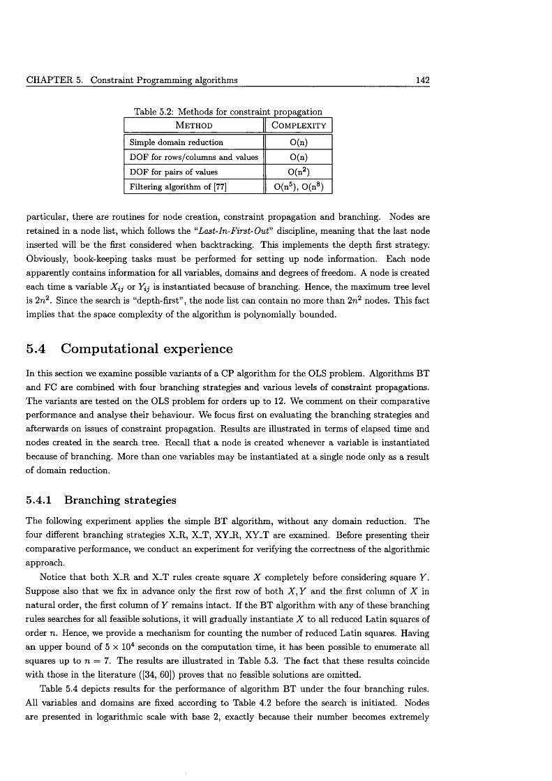
CHAPTER 5. Constraint Programming algorithms 142
Table 5.2: Methods for constraint propagationM e th o d C o m p l e x it y
Simple domain reduction O(n)
DOF for rows/columns and values O(n)
DOF for pairs of values 0 (n 2)
Filtering algorithm of [77] 0 (n 5), 0 ( n 8)
particular, there are routines for node creation, constraint propagation and branching. Nodes are retained in a node list, which follows the 11 Last-In-First-Out” discipline, meaning that the last node inserted will be the first considered when backtracking. This implements the depth first strategy. Obviously, book-keeping tasks must be performed for setting up node information. Each node apparently contains information for all variables, domains and degrees of freedom. A node is created each time a variable X ij or Yij is instantiated because of branching. Hence, the maximum tree level is 2n 2. Since the search is “depth-first” , the node list can contain no more than 2n 2 nodes. This fact implies th a t the space complexity of the algorithm is polynomially bounded.
5.4 Com putational experience
In this section we examine possible variants of a CP algorithm for the OLS problem. Algorithms BT and FC are combined with four branching strategies and various levels of constraint propagations. The variants are tested on the OLS problem for orders up to 12. We comment on their comparative performance and analyse their behaviour. We focus first on evaluating the branching strategies and afterwards on issues of constraint propagation. Results are illustrated in terms of elapsed time and nodes created in the search tree. Recall th a t a node is created whenever a variable is instantiated because of branching. More than one variables may be instantiated a t a single node only as a result of domain reduction.
5.4.1 Branching strategies
The following experiment applies the simple BT algorithm, without any domain reduction. The four different branching strategies X_R, X_T, XY_R, XY_T are examined. Before presenting their comparative performance, we conduct an experiment for verifying the correctness of the algorithmic approach.
Notice th a t both X_R and X_T rules create square X completely before considering square Y . Suppose also th a t we fix in advance only the first row of both X , Y and the first column of X in natural order, the first column of Y remains intact. If the BT algorithm with any of these branching rules searches for all feasible solutions, it will gradually instantiate X to all reduced Latin squares of order n. Hence, we provide a mechanism for counting the number of reduced Latin squares. Having an upper bound of 5 x 10⁴ seconds on the computation time, it has been possible to enumerate all squares up to n = 7. The results are illustrated in Table 5.3. The fact th a t these results coincide w ith those in the literature ([34, 60]) proves that no feasible solutions are omitted.
Table 5.4 depicts results for the performance of algorithm BT under the four branching rules. All variables and domains are fixed according to Table 4.2 before the search is initiated. Nodes are presented in logarithmic scale with base 2, exactly because their number becomes extremely
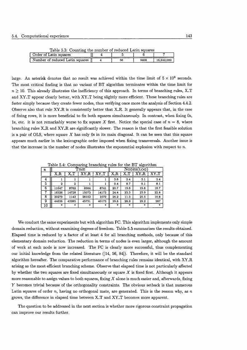
5.4. Computational experience 143
Table 5.3: Counting the number of reduced Latin squares| Order of Latin squares I I I 4 | 5 | 6 1 7 1| Number of reduced Latin squares I I 4 | 56 | 9408 | 16,942,080 |
large. An asterisk denotes th a t no result was achieved within the time limit of 5 x 10⁴ seconds. The most critical finding is th a t no variant of BT algorithm term inates within the time limit for n > 10. This already illustrates the inefficiency of this approach. In terms of branching rules, X_T and XY_T appear clearly better, with XY_T being slightly more efficient. These branching rules are faster simply because they create fewer nodes, thus verifying once more the analysis of Section 4.4.2. Observe also th a t rule XY_R is consistently better th a t X_R. It generally appears that, in the case of fixing rows, it is more beneficial to fix both squares simultaneously. In contrast, when fixing Os, Is, etc. it is not remarkably worse to fix square X first. Notice the special case of n = 8, where branching rules X_R and XY_R are significantly slower. The reason is th a t the first feasible solution is a pair of OLS, where square X has only Os in its main diagonal. It can be seen th a t this square appears much earlier in the lexicographic order imposed when fixing transversals. Another issue is that the increase in the number of nodes illustrates the exponential explosion with respect to n.
Table 5.4: Comparing branching rules for the BT algorithmn | T i m e N o d e s ( l o g )
X_R X_T XY.R XY_TJ X_R X_T XY_R XY_T4 l l l l 3.6 2.4 3.1 2.45 2 2 l l 9.4 8.7 9.1 8.16 11647 8762 8984 8741 20.7 19.6 19.8 18.77 16326 14728 15073 14173 24.4 23.3 23.9 22.88 30279 1143 28152 1079 26.2 11.3 25.5 10.89 44638 42285 45731 40173 29.8 28.9 29.2 28710 * * * * * * 3*c *
We conduct the same experiments but with algorithm FC. This algorithm implements only simple domain reduction, without examining degrees of freedom. Table 5.5 summarises the results obtained. Elapsed time is reduced by a factor of at least 4 for all branching methods, only because of this elementary domain reduction. The reduction in terms of nodes is even larger, although the amount of work at each node is now increased. The FC is clearly more successful, thus complementing our initial knowledge from the related literature ([14, 56, 84]). Therefore, it will be the standard algorithm hereafter. The comparative performance of branching rules remains identical, with XY_R arising as the most efficient branching scheme. Observe th a t elapsed time is not particularly affected by whether the two squares are fixed simultaneously or square X is fixed first. Although it appears more reasonable to assign values to both squares, fixing X alone is much easier and, afterwards, fixing Y becomes trivial because of the orthogonality constraints. The obvious setback is th a t numerous Latin squares of order n, having no orthogonal mate, are generated. This is the reason why, as n grows, the difference in elapsed time between X_T and XY_T becomes more apparent.
The question to be addressed in the next section is whether more rigorous constraint propagation can improve our results further.
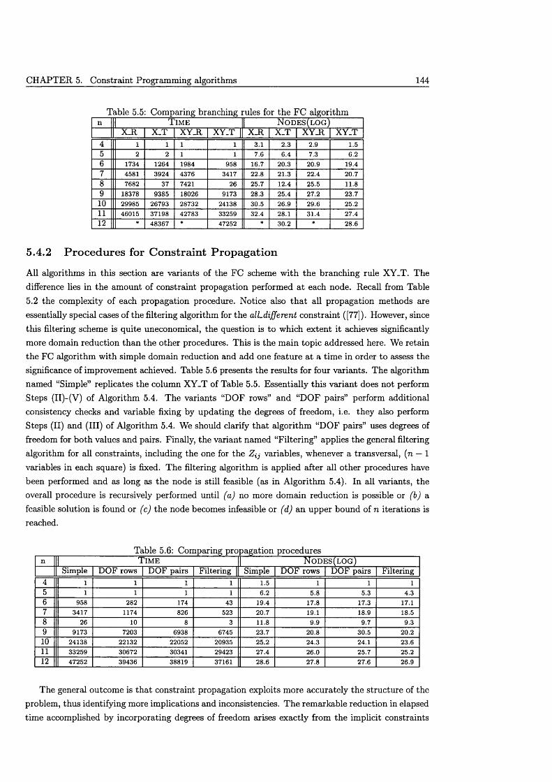
CHAPTER 5. Constraint Programming algorithms 144
Table 5.5: Comparing branching rules for the FC algorithmn T ime | N o d e s ( l o g )
X_R X .T XY_R XY_T ] X_R X_T XY_R XY_T4 l l l l 3.1 2.3 2.9 1.55 2 2 l l 7.6 6.4 7.3 6.26 1734 1264 1984 958 16.7 20.3 20.9 19.47 4581 3924 4376 3417 22.8 21.3 22.4 20.78 7682 37 7421 26 25.7 12.4 25.5 11.89 18378 9385 18026 9173 28.3 25.4 27.2 23.710 29985 26793 28732 24138 30.5 26.9 29.6 25.211 46015 37198 42783 33259 32.4 28.1 31.4 27.412 * 48367 * 47252 * 30.2 * 28.6
5.4.2 Procedures for Constraint Propagation
All algorithms in this section are variants of the FC scheme with the branching rule XY_T. The difference lies in the amount of constraint propagation performed a t each node. Recall from Table5.2 the complexity of each propagation procedure. Notice also th a t all propagation methods are essentially special cases of the filtering algorithm for the alLdifferent constraint ([77]). However, since this filtering scheme is quite uneconomical, the question is to which extent it achieves significantly more domain reduction than the other procedures. This is the main topic addressed here. We retain the FC algorithm with simple domain reduction and add one feature at a time in order to assess the significance of improvement achieved. Table 5.6 presents the results for four variants. The algorithm named “Simple” replicates the column XY_T of Table 5.5. Essentially this variant does not perform Steps (II)-(V) of Algorithm 5.4. The variants “DOF rows” and “DOF pairs” perform additional consistency checks and variable fixing by updating the degrees of freedom, i.e. they also perform Steps (II) and (III) of Algorithm 5.4. We should clarify th a t algorithm “DOF pairs” uses degrees of freedom for both values and pairs. Finally, the variant named “Filtering” applies the general filtering algorithm for all constraints, including the one for the Zij variables, whenever a transversal, (n — 1 variables in each square) is fixed. The filtering algorithm is applied after all other procedures have been performed and as long as the node is still feasible (as in Algorithm 5.4). In all variants, the overall procedure is recursively performed until (a) no more domain reduction is possible or (b) a feasible solution is found or (c) the node becomes infeasible or (d) an upper bound of n iterations is reached.
Table 5.6: Comparing propagation proceduresn rriME | N o d e s ( l o g )
Simple DOF rows DOF pairs Filtering | Simple DOF rows DOF pairs Filtering4 1 l 1 1 1.5 l l 15 1 l 1 1 6.2 5.8 5.3 4.36 958 282 174 43 19.4 17.8 17.3 17.17 3417 1174 826 523 20.7 19.1 18.9 18.58 26 10 8 3 11.8 9.9 9.7 9.39 9173 7203 6938 6745 23.7 20.8 30.5 20.210 24138 22132 22052 20935 25.2 24.3 24.1 23.611 33259 30672 30341 29423 27.4 26.0 25.7 25.212 47252 39436 38819 37161 28.6 27.8 27.6 26.9
The general outcome is th a t constraint propagation exploits more accurately the structure of the problem, thus identifying more implications and inconsistencies. The remarkable reduction in elapsed time accomplished by incorporating degrees of freedom arises exactly from the implicit constraints
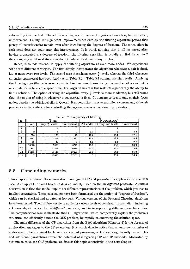
5.5. Concluding remarks 145
enforced by this method. The addition of degrees of freedom for pairs achieves less, but still clear, improvement. Finally, the significant improvement achieved by the filtering algorithm proves that plenty of inconsistencies remain even after introducing the degrees of freedom. The extra effort in each node does not counteract this improvement. It is worth noticing th a t in all instances, after having propagated via degrees of freedom, the filtering algorithm is usually applied for up to 2 iterations; any additional iterations do not reduce the domains any further.
Hence, it sounds rational to apply the filtering algorithm at even more nodes. We experiment with three different strategies. The first simply incorporates the algorithm whenever a pair is fixed, i.e. at most every two levels. The second uses this scheme every ^ levels, whereas the third whenever an entire transversal has been fixed (as in Table 5.6). Table 5.7 summarises the results. Applying the filtering algorithm whenever a pair is fixed reduces dramatically the number of nodes but is much inferior in terms of elapsed time. For larger values of n this restricts significantly the ability to find a solution. The option of using the algorithm every ^ levels is more moderate, but still worse than the option of using it whenever a transversal is fixed. It appears to create only slightly fewer nodes, despite the additional effort. Overall, it appears th a t transversals offer a convenient, although problem-specific, criterion for controlling the aggressiveness of constraint propagation.
Table 5.7: Frequency of filteringn T ime | N o d e s ( l o g )
Pair Every ^ levels Transversal | All nodes Every two levels Transversal4 1 l l l l 15 2 l l 2.1 3 4.36 614 153 43 13.2 16.7 17.17 2287 1279 523 15.6 18.1 18.58 68 42 3 6.9 8.8 9.39 13873 7930 6745 17.3 18.9 20.210 27831 22473 20935 21.7 22.4 23.611 36165 31138 29423 23.1 24.6 25.212 * 42823 37161 * 26.1 26.9
5.5 Concluding remarks
This chapter introduced the enumeration paradigm of CP and presented its application to the OLS case. A compact CP model has been devised, mainly based on the alLdifferent predicate. A critical observation is th a t this model implies six different representations of the problem, which give rise to implicit constraints. These constraints have been formalised via the notion of “degrees of freedom” , which can be checked and updated at low cost. Various versions of the Forward Checking algorithm have been tested. Their differences lie in applying various levels of constraint propagation, including a known algorithm for the alLdifferent predicate, and in incorporating different branching rules. The computational results illustrate that CP algorithms, which competently exploit the problem’s structure, can efficiently handle the OLS problem, by rapidly enumerating the solution space.
The main difference of the CP algorithms from the B&C algorithm (Chapter 4) is the absence of a relaxation analogous to the LP-relaxation. It is worthwhile to notice th a t an enormous number of nodes need to be examined for large instances but processing each node is significantly faster. This and additional parallelisms reveal the potential of integrating CP and IP methods. Motivated by our aim to solve the OLS problem, we discuss this topic extensively in the next chapter.

CHAPTER 5. Constraint Programming algorithms T46
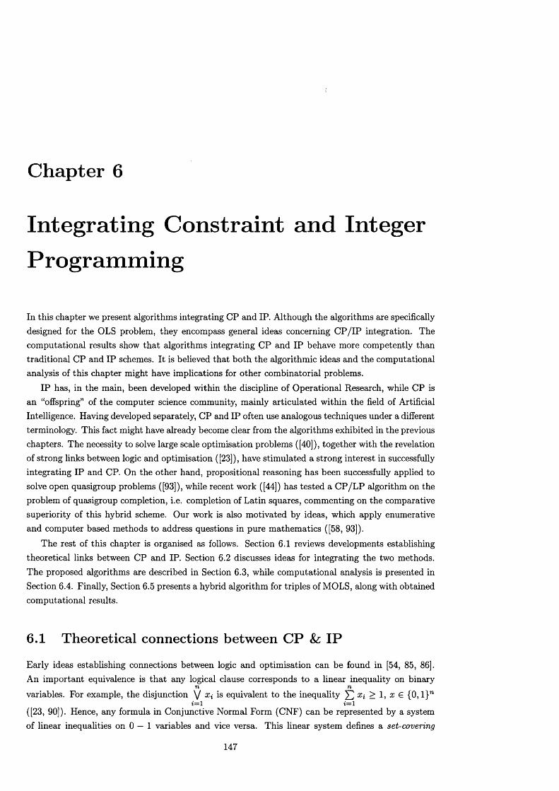
Chapter 6
Integrating Constraint and Integer P r ogr amming
In this chapter we present algorithms integrating CP and IP. Although the algorithms are specifically designed for the OLS problem, they encompass general ideas concerning C P /IP integration. The computational results show th a t algorithms integrating CP and IP behave more competently than traditional CP and IP schemes. It is believed that both the algorithmic ideas and the computational analysis of this chapter might have implications for other combinatorial problems.
IP has, in the main, been developed within the discipline of Operational Research, while CP is an “offspring” of the computer science community, mainly articulated within the field of Artificial Intelligence. Having developed separately, CP and IP often use analogous techniques under a different terminology. This fact might have already become clear from the algorithms exhibited in the previous chapters. The necessity to solve large scale optimisation problems ([40]), together with the revelation of strong links between logic and optimisation ([23]), have stimulated a strong interest in successfully integrating IP and CP. On the other hand, propositional reasoning has been successfully applied to solve open quasigroup problems ([93]), while recent work ([44]) has tested a C P /L P algorithm on the problem of quasigroup completion, i.e. completion of Latin squares, commenting on the comparative superiority of this hybrid scheme. Our work is also motivated by ideas, which apply enumerative and computer based methods to address questions in pure m athematics ([58, 93]).
The rest of this chapter is organised as follows. Section 6.1 reviews developments establishing theoretical links between CP and IP. Section 6.2 discusses ideas for integrating the two methods. The proposed algorithms are described in Section 6.3, while com putational analysis is presented in Section 6.4. Finally, Section 6.5 presents a hybrid algorithm for triples of MOLS, along with obtained computational results.
6.1 Theoretical connections between CP &; IP
Early ideas establishing connections between logic and optimisation can be found in [54, 85, 86]. An im portant equivalence is th a t any logical clause corresponds to a linear inequality on binary
n nvariables. For example, the disjunction \J Xi is equivalent to the inequality > 1, r G {0, l} n
i=i i=i([23, 90]). Hence, any formula in Conjunctive Normal Form (CNF) can be represented by a system of linear inequalities on 0 — 1 variables and vice versa. This linear system defines a set-covering
147
CHAPTER 6. Integrating Constraint and Integer Programming 148
problem, i.e. an integer program of the form {A x > e ,x E {0, l} m}, where m is the number of atomic propositions. A CNF formula can be solved by employing a form of resolution called unit resolution. This procedure selects a clause with a single literal p (if such exists) and deletes all clauses containing p and all appearances of ->p. In other words, unit resolution simply observes that p must be true in any feasible solution. A famous theorem (in [15]) states that unit resolution can prove unsatisfiability for a CNF formula if and only if the LP-relaxation of the corresponding set of linear inequalities is infeasible. This result already indicates th a t LP-based methods can be applied to problems arising from logic. The inverse is also possible: the resolution algorithm can be applied to the CNF formula arising from a linear constraint set in order to generate resolvent inequalities, also called logic cuts ([46, 51, 53]).
Furthermore, the set of feasible solutions to a logical formula has a minimal representation in terms of the strongest possible clauses. These are the prime implications, derived from the original set of clauses by repetitively applying the resolution procedure. A clause is a prime implication if it is not absorbed by any other resolvent clause. Hence, prime implications are maximal with respect to set inclusion, i.e. not dominated. The equivalent concept for IP is th a t of maximal valid inequalities (see Chapter 2 and [68, p.207]). Exactly as prime implications are derived via resolution after a finite number of steps, maximal valid inequalities are generated after a finite number of steps of the Chvatal-Gomory procedure ([45]). This parallelism is exploited in [23, Section 3.7], where SAT is formulated as a set-covering problem and facets of the associated polyhedron are examined. For infeasible problems, resolution will produce the empty clause as a prime implication (as in Section 5.1.1), whereas the Chvatal-Gomory procedure will produce an inequality of the form Ox < —1. An im portant statem ent is the following (in [27]):
There exists a polynomial p{N, M ) such th a t for any unsatisfiable set S of clauses containing M literals, if the unsatisfiability of S has a cutting plane proof of length N , then it has an extended resolution proof of length p{N, M ).
For the notion of extended resolution see [23, Section 3.5.5].
Another pioneering result is the observation th a t the resolution procedure is closely related to the Fourier-Motzkin algorithm for polyhedral projection (in [85]). Resolution eliminates an atomic proposition and appends additional clauses to the initial representation in a way analogous to that of eliminating variables in the Fourier-Motzkin method. A relevant development concerns the rep- resentability of mixed integer linear programming problems (MILP) ([54]). As noted in [23, Section4.4.3], this work essentially proves that any set representable as an MILP can be also represented in a disjunctive form, i.e. w ith either/or constraints. It also provides a significant characterisation result for integer programming. The actual theorem states that:
A set in n-space is MILP representable if and only if it is the union of finitely many polyhedra having the same set of recession directions.
A rather recent direction of research examines constraints of special structure, like the alLdifferent predicate, and proposes equivalent representations in the form of linear inequalities. The convex hull of all feasible solutions to the alLdifferent predicate is described in [89], while analogous results for cardinality rules are presented in [92].
6.2. Algorithmic approaches combining CP & IP 149
6.2 Algorithm ic approaches combining CP & IP
The combinatorial optimisation problems (COP) targeted by both CP and IP are of the following generic form, hereafter called C O P (x , / , C, D):
m in { f(x ) : x E C, x E I?} (6.1)
In this formulation, x is the vector of variables, / the objective function, D the external product of variables’ domains and C a set of constraints, restricting the possible values th a t the variables can take simultaneously. The variable domains can be integers, symbols or intervals of real numbers. A relaxation of (6.1), called R E L (x , f ,C ',D ') , is defined as:
m in { f ( x ) : x E C ',x E D '} (6.2)
where C' C C and D ' D D, i.e. (6.2) is derived by dropping a t least one constraint or by enlarging the domain of at least one variable. This implies th a t the set of feasible solutions of (6.2) includes th a t of (6.1). Hence, a solution to (6.2) is not necessarily a solution to (6.1). If, however, (6.2) has no solution, neither does (6.1).
Every algorithmic method for (6.1) adopts further assumptions about the form of / , C and D. In particular, IP requires both the objective function and the set of constraints to be linear. This fact highly restricts its declarative power, but allows it to produce efficient problem relaxations. In theory, the form of the constraints in CP is of arbitrary type. However, there is a broadening menu of specific, well-defined, constraint types, which are extensively used in the CP literature, e.g. the alLdifferent predicate. CP has been mainly focused on feasibility problems, meaning problems where the set of feasible solutions is relatively small. However, the notion of an objective function can be naturally introduced; hence, CP is adequate also for COP. In general, IP can be efficiently used to solve problems in propositional logic ([23]). Logic, on the other hand, is possible to embed within a classic optimisation framework (see [53]). Both methods have been applied separately to various problems (see [30, 88]). Nonetheless, the integration of the two approaches poses a different task, viz. th a t of using the tools of both CP and IP for modelling and solving COP of general form. The necessity of this direction becomes more apparent as problem types diversify and problem sizes grows.
Chapters 4 &; 5 have illustrated that IP & CP models are solved using analogous algorithmic schemes. Both IP and CP use the “Divide & Conquer” principle, i.e. they recursively divide the original problem into subproblems and form a search tree. Both methods are exact, in the sense that they guarantee a complete search. The prospect of integration will be discussed with respect to the generic algorithm shown below. Notice th a t Algorithms 4.1 and 5.4 are special cases of this scheme.
A lg o rith m 6.1 A t each node/subproblem:(I) Preprocess C O P (x, / , C , D);
i f (feasible) repeat
{(II) Solve R E L {x , / , C", D');(III) Infer additional constraints;
}
CHAPTER 6. Integrating Constraint and Integer Programming 150
u n til (x G D ) o r (infeasible) o r (no inference) i f (no inference) a n d (x £ D ) a n d (R E L (x , f ,C ' ,D ') remains feasible))
( IV ) Create subproblems; else
prune this node;re tu rn ;
Concerning IP, Step I involves variable preprocessing ([78]). Using simple logical connections and information from the variables already fixed, additional variable fixing is attem pted. Although not mentioned explicitly in Algorithm 6.1, preprocessing is iteratively applied until no more variables can be fixed (see also Algorithm 4.2). Step II implies solving a continuous relaxation of the problem, derived by dropping the integrality constraints. The L P relaxation can be solved efficiently using interior point or simplex-based algorithms. Its main advantage is th a t it provides an assignment of values to all variables and, if infeasible, it implies infeasibility for the original (sub)problem. If, however, a feasible but non-integer solution is derived, IP proceeds by introducing additional inequalities, which cut-off this fractional solution and restrict further the feasible region D ' of the relaxation. This is Step III. The process of solving the relaxation and extracting further inference in the form of cutting planes is repeated until the problem becomes infeasible or an integer solution is found or no additional constraints can be produced. Identifying families of efficient cutting planes normally requires a polyhedral analysis of the problem.
For CP, Steps I Sz III are essentially the same process. Constraint propagation removes inconsistent values from the domains of the uninstantiated variables. Although domain reduction can be efficiently performed to achieve 1 & 2-consistency, higher consistency levels require considerable computational effort. Exceptions occur in the case of structured constraints, like the alLdifferent constraint. Step II is not performed by CP, since it lacks a proper relaxation, although recent work ([53, Chapter 21]) explores the potential of defining useful discrete relaxations. Constraint propagation is repetitively applied until no more domain filtering is possible. The more intense the propagation performed at each node, the larger the computational effort required and the smaller the number of nodes created. This behaviour was observed in Section 5.4 with respect to the OLS problem. The leverage point cannot be theoretically justified and is probably located in moderate options, which apply constraint propagation periodically. The counterpart for IP algorithms is the persistence in generating violated cuts. The number of cuts added to each problem and the frequency of cut addition must balance between efficient solution of subproblems and early pruning of infeasible branches (see Section 4.6). For both methods, the question is identical and is concerned with the effort devoted to infer additional constraints at Step III.
Step IV is conducted in analogous ways by both methods. The standard method is to select a variable and split its domain to create two or more subproblems. Heuristic criteria for this choice are common to both methods. Examples are to select the variable with the smallest domain, or the variable, which participates in most constraints, or the one, which is expected to improve the objective function most. It has been argued ([13]) th a t branching on Special Ordered Sets is a valuable option for IP. The corresponding branching method for CP is to simply split the domain of the branching variable recursively until a single value remains available. Equivalently, the CP algorithm can directly create a number of nodes equal to the cardinality of the domain and set the branching variable to a different value in each node. Recall th a t this is exactly the branching mechanism used for the OLS problem.
6.3. Design of hybrid algorithms 151
It follows th a t CP & IP can be integrated in an algorithmic sense. For Step I, logical preprocessing conducted by IP is a subset of the sophisticated tools available for CP. The crucial contribution of IP is the powerful relaxation lacking from CP. The inference Step (III) can still be performed by both methods. The complementarity exists in the fact th a t CP directly reduces the solution space of the original problem in contrast to IP, which reduces the solution space of the relaxation. Finally, one of the two, or both, methods can be applied at Step IV to determine the partition of the subproblem.
An im portant aspect of complementarity is that CP forms only partial assignments of values to variables, except for the point where a feasible solution is identified. In contrast, IP constantly constructs complete assignments for the relaxed problem, which can possibly be feasible solutions for the original problem. Moreover, from a more abstract viewpoint, both methods depend on an interplay between search and inference. Exhaustive search enumerates the possible options for a subproblem, whereas inference accelerates the search by reducing the solution space and by providing certificates of optimality or infeasibility. This fundamental feature is observed and discussed in [52].
Substantial ideas regarding the integration of CP and IP are exhibited in [16], where it is proposed th a t the constraint set C is partitioned into primitive and non-primitive constraints. A constraint is characterised as primitive, if an efficient solver is available, which can provide a complete assignment of values to all variables without any further search. The best example is linear constraints on real variables. All other constraints are classified as non-primitive. For example, the only nonprimitive constraint in an IP model is an integrality constraint. This work also proposes an interesting algorithmic framework, named “Branch &; Infer” : at each node of the search tree, both methods infer primitive constraints, e.g. cutting planes, which axe added to problem’s relaxation. Independently of whether the modelling framework allows for both CP Sz IP constraints to be inserted, the immediate requirement is for a proper decomposition of the problem. Such a decomposition should allow for an IP and CP solver to be used in parallel, without the overhead of maintaining and updating two models and two search trees becoming overwhelming.
The theoretical connections and equivalences between CP & IP do not guarantee a beneficial integration; they primarily illustrate the feasibility of the project. The virtue of integration can be properly justified only if the inference generated by the two m ethods can be viewed as complementary. In other words, it has to be concluded th a t one approach succeeds in cases where the other fails. So far, evidence for this fact remains mostly empirical. In theory, CP is much faster in searching the solution space, since it does not have to solve a relaxation. However, it is exactly the LP-relaxation, which gives IP its global perspective and allows for a solution to be found without extensive branching ([52]). Next section examines, in more detail, algorithms integrating the two methods.
6.3 Design of hybrid algorithms
We propose two algorithms for the OLS problem th a t incorporate both CP and IP methods. A critical issue concerning the design of these algorithms is whether the problem will be decomposed into two components to be handled by either CP or IP. We select to perform no decomposition, i.e. both CP and IP representations are retained. The first reason is th a t the cost of maintaining both models is negligible. Most im portant, we wish to extract the best possible implicit information from both models and also assess the quality of inference achieved by each of the two methods. This will hopefully lead to valuable insights about whether CP and IP complement each other.
According to the above discussion, Steps I-III of Algorithm 6.1 can be performed by CP and IP w ithout any overlap. At each subproblem, Step IV is the only one th a t has to be determined by a
CHAPTER 6. Integrating Constraint and Integer Programming 152
single method. The selected method determines the form of the search tree, since branching via IP always creates two branches, whereas branching on a CP variable results in a number of subproblems equal to the cardinality of its domain. Hence, partition into subproblems can be decided by:
A . IP alone, which implies embedding IP within a CP search tree;
B . CP alone, which implies embedding CP within an IP search tree;
C. both IP and CP, which implies interchanging between the IP and CP search trees according toa certain criterion.
In case (A), Step I is implemented by both IP & CP repetitively. Each method operates on its own model and, if a variable is fixed or a domain is filtered, the information is passed to its counterpart. Steps II-IV are implemented only by IP. Concerning case (B), Steps I & IV are performed by CP alone. IP solver is called at certain nodes and performs the “loop” of steps (II) & (III). The inference achieved by CP in Step (I) is passed to the relaxation in the form of bounds on the (continuous) variables. Finally, case (C) is a combination of the previous two. Both search trees remain active and, whenever the search procedure is transferred from one to the other, all the inference produced is also conveyed. The roles of IP and CP in cases (A) & (B) are reproduced when the search is implemented at the IP or CP tree, respectively.
These cases encompass all options for hybridisation, with case (C) integrating the two methods more closely. The algorithms proposed for the OLS problem adopt options (A) and (B). Option (C) is incorporated in an algorithm for triples of MOLS, to be presented in Section 6.5.
6.3.1 A lgorithm IPC
Algorithm IPC is the B&C algorithm, described in Chapter 4, incorporating also constraint propagation as an additional preprocessing step. At each node of the search tree, IP preprocessing is applied first, exactly as illustrated at Algorithm 4.2. If this procedure term inates without proving infeasibility, the CP preprocessor is called, thus attem pting to fix additional variables to 0. The aim is not only to enhance the preprocessing of each node, but also to reveal the extent to which CP can be beneficial in terms of detecting infeasible nodes before the LP is solved.
Observe th a t there exists an alLdifferent constraint associated w ith each of the 6 constraint sets of model (IP 1). For example, consider constraint set (4.6):
: k G K ,l G L} = 1, Vi G I , j G J
which states th a t exactly one pair (k,l) can be assigned to any cell (i , j) . Assume variables Wij, having domains D w i:j — {0, ... ,n 2 — 1}. There is a 1 — 1 correspondence between any ordered pair (k , l ) and a value in D w ir Hence, the constraint is:
alLdifferent{Wij : i E I , j £ J}
Note th a t this is exactly the constraint on the variables of the CP model (in Section 5.3.1). The alLdifferent predicates for the remaining constraint sets (4.1)-(4.5) are similarly defined. Again, observe th a t each of these predicates corresponds to one of the 6 representations discussed in Section 5.3.1.
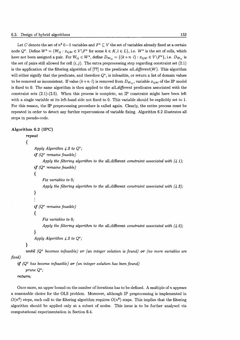
6.3. Design of hybrid algorithms 153
Let C denote the set of n4 0 — 1 variables and F s C V the set of variables already fixed at a certain node Qs . Define W s = {Wij : Xijki G V \F S for some k E K , I E L}, i.e. W s is the set of cells, which have not been assigned a pair. For Wij E W s, define = {(k + n- l ) : Xijki G V \ F S}, i.e. is the set of pairs still allowed for cell (i, j ) . The extra preprocessing step regarding constraint set (2.1) is the application of the filtering algorithm of [77] to the predicate alLdifferent(W ). This algorithm will either signify th a t the predicate, and therefore Qs , is infeasible, or return a list of domain values to be removed as inconsistent. If value (k + n - l) is removed from 1 ) ^ , variable x^ki of the IP model is fixed to 0. The same algorithm is then applied to the alLdifferent predicates associated with the constraint sets (2.1)-(2.5). W hen this process is complete, an IP constraint might have been left w ith a single variable at its left-hand side not fixed to 0. This variable should be explicitly set to 1. For this reason, the IP preprocessing procedure is called again. Clearly, the entire process must be repeated in order to detect any further repercussions of variable fixing. Algorithm 6.2 illustrates all steps in pseudo-code.
A lg o rith m 6.2 (IP C ) repeat
{Apply Algorithm 4-2 to Qs;
i f (Qs remains feasible)Apply the filtering algorithm to the alLdifferent constraint associated with (4-1)',
i f (Qs remains feasible)
{Fix variables to 0;
Apply the filtering algorithm to the alLdifferent constraint associated with (4-2);
}
i f (Qs remains feasible)
{Fix variables to 0;
Apply the filtering algorithm to the alLdifferent constraint associated with (4-6);
}Apply Algorithm 4-2 to Qs;
}u n til (Qs becomes infeasible) o r (an integer solution is found) o r (no more variables are
fixed)
i f (Qs has become infeasible) o r (an integer solution has been found) prune Qs;
re tu rn ;
Once more, an upper bound on the number of iterations has to be defined. A multiple of n appears a reasonable choice for the OLS problem. Moreover, although IP preprocessing is implemented in 0 ( n 4) steps, each call to the filtering algorithm requires 0 ( n 8) steps. This implies th a t the filtering algorithm should be applied only at a subset of nodes. This issue is to be further analysed via com putational experimentation in Section 6.4.
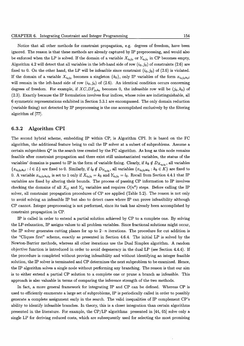
CHAPTER 6. Integrating Constraint and Integer Programming 154
Notice th a t all other methods for constraint propagation, e.g. degrees of freedom, have been ignored. The reason is th a t these methods are already captured by IP preprocessing, and would also be enforced when the LP is solved. If the domain of a variable X i0j0 or Yi0j0 in CP becomes empty, Algorithm 4.2 will detect that all variables in the left-hand side of row ( i o , j o ) of constraints (2.6) are fixed to 0. On the other hand, the LP will be infeasible since constraint ( i o , j o ) of (2.6) is violated. If the domain of a variable X i0j0 becomes a singleton {ko}, only IP variables of the form Xi0j0k0i will remain in the left-hand side of row ( i o , j o ) of (2.6). An identical condition occurs concerning degrees of freedom. For example, if X C - D F j 0k0 becomes 0, the infeasible row will be ( j o , k o ) of (2.3). Exactly because the IP formulation involves four indices, whose roles are indistinguishable, all 6 symmetric representations exhibited in Section 5.3.1 are encompassed. The only domain reduction (variable fixing) not detected by IP preprocessing is the one accomplished exclusively by the filtering algorithm of [77].
6.3.2 A lgorithm CPI
The second hybrid scheme, embedding IP within CP, is Algorithm CPI. It is based on the FC algorithm, the additional feature being to call the IP solver a t a subset of subproblems. Assume a certain subproblem Q s in the search tree created by the FC algorithm. As long as this node remains feasible after constraint propagation and there exist still uninstantiated variables, the status of the variables’ domains is passed to IP in the form of variable fixing. Clearly, if ko ^ D x lQjQ, all variables {xiojokoi ’■ I £ L} are fixed to 0. Similarly, if Iq ^ D yiojQ, all variables {xi0j0ki0 ' ko G K } are fixed to 0. A variable X i 0j 0 k 0 i0 is set to 1 only if X i 0j 0 = k o and Y i 0j 0 = I q . Recall from Section 4.4.1 th a t IP variables are fixed by altering their bounds. The process of passing CP information to IP involves checking the domains of all and Yij variables and requires 0 (n 4) steps. Before calling the IP solver, all constraint propagation procedures of CP are applied (Table 5.2). The reason is not only to avoid solving an infeasible IP but also to detect cases where IP can prove infeasibility although CP cannot. Integer preprocessing is not performed, since its task has already been accomplished by constraint propagation in CP.
IP is called in order to extend a partial solution achieved by CP to a complete one. By solving the LP-relaxation, IP assigns values to all problem variables. Since fractional solutions might occur, the IP solver generates cutting planes for up to 2 • n iterations. The procedure for cut addition is the “Cliques first” scheme, exactly as presented in Section 4.6.4. The initial LP is solved by the Newton-Barrier methods, whereas all other iterations use the Dual Simplex algorithm. A random objective function is introduced in order to avoid degeneracy in the dual LP (see Section 4.4.4). If the procedure is completed without proving infeasibility and without identifying an integer feasible solution, the IP solver is term inated and CP determines the next subproblem to be examined. Hence, the IP algorithm solves a single node without performing any branching. The reason is th a t our aim is to either extend a partial CP solution to a complete one or prune a branch as infeasible. This approach is also valuable in terms of comparing the inference strength of the two methods.
In fact, a more general framework for integrating IP and CP can be defined. Whereas CP is used to efficiently enumerate a large set of subproblems, IP is periodically called in order to possibly generate a complete assignment early in the search. The valid inequalities of IP complement C P ’s ability to identify infeasible branches. In theory, this is a closer integration than certain algorithms presented in the literature. For example, the C P /L P algorithms presented in [44, 65] solve only a single LP for deriving reduced costs, which are subsequently used for selecting the most promising
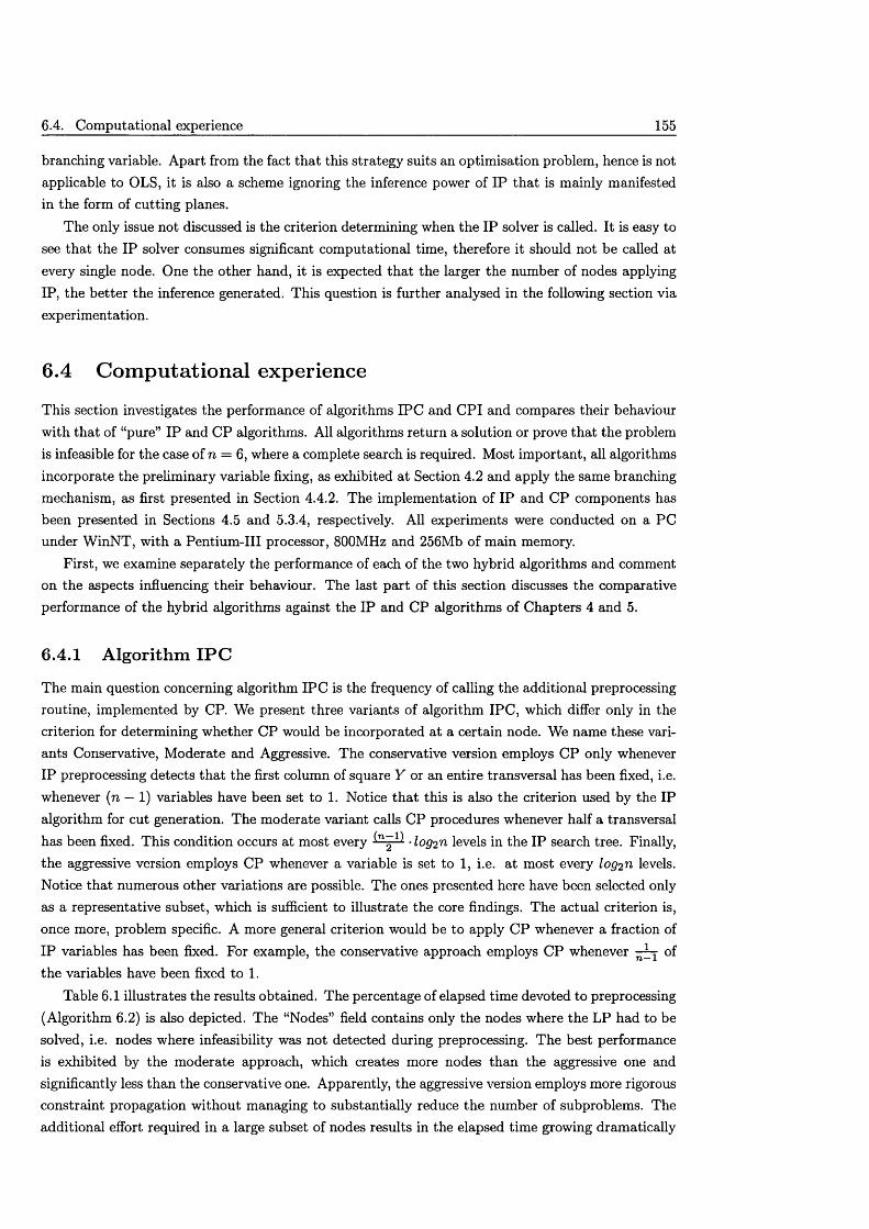
6.4. Computational experience 155
branching variable. Apart from the fact th a t this strategy suits an optimisation problem, hence is not applicable to OLS, it is also a scheme ignoring the inference power of IP th a t is mainly manifested in the form of cutting planes.
The only issue not discussed is the criterion determining when the IP solver is called. It is easy to see th a t the IP solver consumes significant computational time, therefore it should not be called at every single node. One the other hand, it is expected th a t the larger the number of nodes applying IP, the better the inference generated. This question is further analysed in the following section via experimentation.
6.4 Com putational experience
This section investigates the performance of algorithms IPC and CPI and compares their behaviour with th a t of “pure” IP and CP algorithms. All algorithms return a solution or prove th a t the problem is infeasible for the case of n = 6, where a complete search is required. Most im portant, all algorithms incorporate the preliminary variable fixing, as exhibited at Section 4.2 and apply the same branching mechanism, as first presented in Section 4.4.2. The implementation of IP and CP components has been presented in Sections 4.5 and 5.3.4, respectively. All experiments were conducted on a PC under WinNT, with a Pentium -Ill processor, 800MHz and 256Mb of main memory.
First, we examine separately the performance of each of the two hybrid algorithms and comment on the aspects influencing their behaviour. The last part of this section discusses the comparative performance of the hybrid algorithms against the IP and CP algorithms of Chapters 4 and 5.
6.4.1 A lgorithm IPC
The main question concerning algorithm IPC is the frequency of calling the additional preprocessing routine, implemented by CP. We present three variants of algorithm IPC, which differ only in the criterion for determining whether CP would be incorporated at a certain node. We name these variants Conservative, M oderate and Aggressive. The conservative version employs CP only whenever IP preprocessing detects th a t the first column of square Y or an entire transversal has been fixed, i.e. whenever (n — 1) variables have been set to 1. Notice th a t this is also the criterion used by the IP algorithm for cut generation. The moderate variant calls CP procedures whenever half a transversal has been fixed. This condition occurs at most every • log2 n levels in the IP search tree. Finally, the aggressive version employs CP whenever a variable is set to 1, i.e. at most every log2 n levels. Notice th a t numerous other variations are possible. The ones presented here have been selected only as a representative subset, which is sufficient to illustrate the core findings. The actual criterion is, once more, problem specific. A more general criterion would be to apply CP whenever a fraction of IP variables has been fixed. For example, the conservative approach employs CP whenever of the variables have been fixed to 1.
Table 6.1 illustrates the results obtained. The percentage of elapsed time devoted to preprocessing (Algorithm 6.2) is also depicted. The “Nodes” field contains only the nodes where the LP had to be solved, i.e. nodes where infeasibility was not detected during preprocessing. The best performance is exhibited by the moderate approach, which creates more nodes than the aggressive one and significantly less than the conservative one. Apparently, the aggressive version employs more rigorous constraint propagation without managing to substantially reduce the number of subproblems. The additional effort required in a large subset of nodes results in the elapsed time growing dramatically
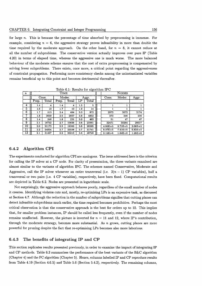
CHAPTER 6. Integrating Constraint and Integer Programming 156
for large n. This is because the percentage of time absorbed by preprocessing is immense. For example, considering n = 6, the aggressive strategy proves infeasibility in more than double the time required by the moderate approach. On the other hand, for n = 8, it cannot reduce at all the number of subproblems. The conservative version actually improves over pure IP (Table 4.20) in terms of elapsed time, whereas the aggressive one is much worse. The more balanced behaviour of the moderate scheme ensures th a t the cost of ex tra preprocessing is compensated by solving fewer subproblems. There exists, once more, a critical point regarding the aggressiveness of constraint propagation. Performing more consistency checks among the uninstantiated variables remains beneficial up to this point and becomes detrimental thereafter.
Table 6.1: Results for algorithm IPCn | T ime N o d e s
| Cons. Moder. Aggr. Cons. Moder. Aggr.Prep. Total Prep. Total LP Total
4 1 .4 4 1 .4 4 1 .5 5 1 1 15 1.6 10 1 .7 10 1 .9 1 4 1 1 16 1 .7 5 1 3 2 .4 4 8 4 3 .3 9 7 2 2 9 7 3 2 6 7 2 2 1 7 4
7 1.8 3 0 5 9 2 .5 2 9 3 7 3 .8 4 8 5 2 2 7 3 2 4 6 2 1 6
8 1 .4 2 4 6 1.8 2 3 1 3 .2 4 8 3 5 1 4 7 4 7
9 2.1 1 6 7 3 2 2 .7 1 5 8 2 6 3 .6 2 2 5 6 1 3 2 4 7 1 3 0 2 8 4 2 9 5 1 7
10 2.0 2 1 1 7 3 2 .5 1 9 3 0 6 3 .8 2 6 2 8 5 4 . 9 3 E + 5 3 . 7 1 E + 5 3 . 0 8 E + 5
11 2.2 2 4 8 3 4 2 .7 2 3 5 3 8 3 .7 3 1 7 4 1 8 . 3 7 E + 5 7 . 4 1 E + 5 6 . 8 3 E + 5
12 2.1 3 1 4 9 7 2 .9 2 9 2 1 3 3 .6 4 8 7 4 9 2 . 1 2 E + 6 1 .8 4 E + 6 1 . 2 8 E + 6
6.4.2 A lgorithm CPI
The experiments conducted for algorithm CPI are analogous. The issue addressed here is the criterion for calling the IP solver at a CP node. For clarity of presentation, the three variants examined are almost similar to the variants of algorithm IPC. The schemes named Conservative, Moderate and Aggressive, call the IP solver whenever an entire transversal (i.e. 2(n — 1) CP variables), half a transversal or two pairs (i.e. 4 CP variables), respectively, have been fixed. Computational results are depicted in Table 6.2. Nodes are presented in logarithmic scale.
Not surprisingly, the aggressive approach behaves poorly, regardless of the small number of nodes it creates. Identifying violates cuts and, mostly, re-optimising LPs is an expensive task, as discussed a t Section 4.7. Although the reduction in the number of subproblems signifies th a t cutting planes can detect infeasible subproblems much earlier, the time required becomes prohibitive. Perhaps the most critical observation is th a t the conservative approach is the best for orders up to 10. This implies that, for smaller problem instances, IP should be called less frequently, even if the number of nodes remains unaffected. However, the picture is inverted for n = 11 and 12, where IP ’s contribution, through the moderate strategy, becomes more substantial. As n grows, cutting planes are more powerful for pruning despite the fact that re-optimising LPs becomes also more laborious.
6.4.3 The benefits o f integrating IP and CP
This section replicates results presented previously, in order to examine the impact of integrating IP and CP methods. Table 6.3 summarises the performance of the best variants of the B&C algorithm (Chapter 4) and the FC algorithm (Chapter 5). Hence, columns labelled IP and CP reproduce results from Table 4.19 (Section 4.6.5) and Table 5.6 (Section 5.4.2), respectively. The remaining columns,
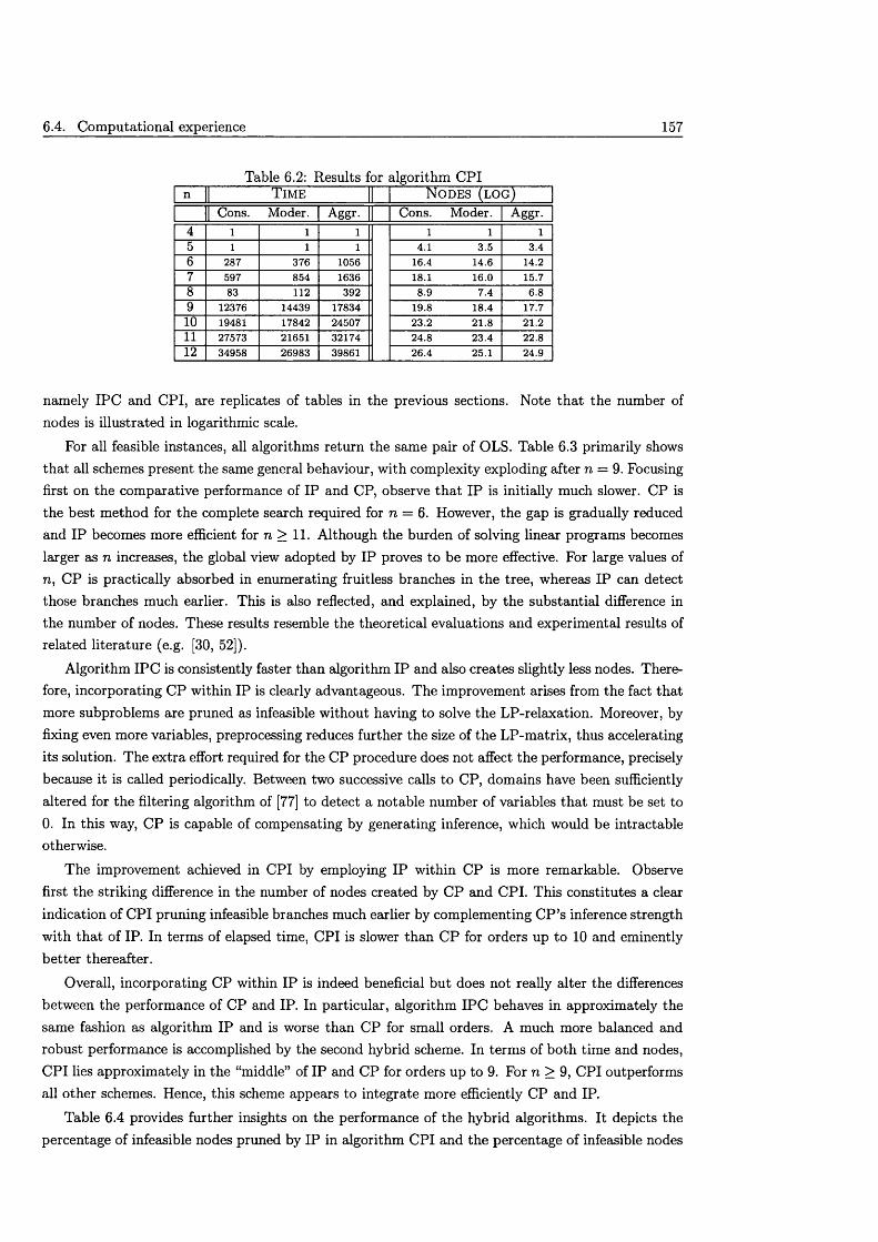
6.4. Computational experience 157
Table 6.2: Results for algorithm CPIn T im e N o d e s ( l o g )
| Cons. Moder. Aggr. Cons. Moder. Aggr.4 l 1 1 l l 15 l 1 1 4 .1 3 .5 3 .4
6 2 8 7 3 7 6 1 0 5 6 1 6 .4 1 4 .6 1 4 .2
7 5 9 7 8 5 4 1 6 3 6 1 8 .1 1 6 .0 1 5 .7
8 8 3 112 3 9 2 8 .9 7 .4 6.89 1 2 3 7 6 1 4 4 3 9 1 7 8 3 4 1 9 .8 1 8 .4 1 7 .7
10 1 9 4 8 1 1 7 8 4 2 2 4 5 0 7 2 3 .2 21.8 21.211 2 7 5 7 3 2 1 6 5 1 3 2 1 7 4 2 4 .8 2 3 .4 22.812 3 4 9 5 8 2 6 9 8 3 3 9 8 6 1 2 6 .4 2 5 .1 2 4 .9
namely IPC and CPI, are replicates of tables in the previous sections. Note th a t the number of nodes is illustrated in logarithmic scale.
For all feasible instances, all algorithms return the same pair of OLS. Table 6.3 primarily shows th a t all schemes present the same general behaviour, with complexity exploding after n = 9. Focusing first on the comparative performance of IP and CP, observe th a t IP is initially much slower. CP is the best method for the complete search required for n = 6. However, the gap is gradually reduced and IP becomes more efficient for n > 11. Although the burden of solving linear programs becomes larger as n increases, the global view adopted by IP proves to be more effective. For large values of n, CP is practically absorbed in enumerating fruitless branches in the tree, whereas IP can detect those branches much earlier. This is also reflected, and explained, by the substantial difference in the number of nodes. These results resemble the theoretical evaluations and experimental results of related literature (e.g. [30, 52]).
Algorithm IPC is consistently faster than algorithm IP and also creates slightly less nodes. Therefore, incorporating CP within IP is clearly advantageous. The improvement arises from the fact that more subproblems are pruned as infeasible without having to solve the LP-relaxation. Moreover, by fixing even more variables, preprocessing reduces further the size of the LP-matrix, thus accelerating its solution. The extra effort required for the CP procedure does not affect the performance, precisely because it is called periodically. Between two successive calls to CP, domains have been sufficiently altered for the filtering algorithm of [77] to detect a notable number of variables th a t must be set to 0. In this way, CP is capable of compensating by generating inference, which would be intractable otherwise.
The improvement achieved in CPI by employing IP within CP is more remarkable. Observe first the striking difference in the number of nodes created by CP and CPI. This constitutes a clear indication of CPI pruning infeasible branches much earlier by complementing C P ’s inference strength with th a t of IP. In terms of elapsed time, CPI is slower than CP for orders up to 10 and eminently better thereafter.
Overall, incorporating CP within IP is indeed beneficial but does not really alter the differences between the performance of CP and IP. In particular, algorithm IPC behaves in approximately the same fashion as algorithm IP and is worse than CP for small orders. A much more balanced and robust performance is accomplished by the second hybrid scheme. In terms of both time and nodes, CPI lies approximately in the “middle” of IP and CP for orders up to 9. For n > 9, CPI outperforms all other schemes. Hence, this scheme appears to integrate more efficiently CP and IP.
Table 6.4 provides further insights on the performance of the hybrid algorithms. It depicts the percentage of infeasible nodes pruned by IP in algorithm CPI and the percentage of infeasible nodes
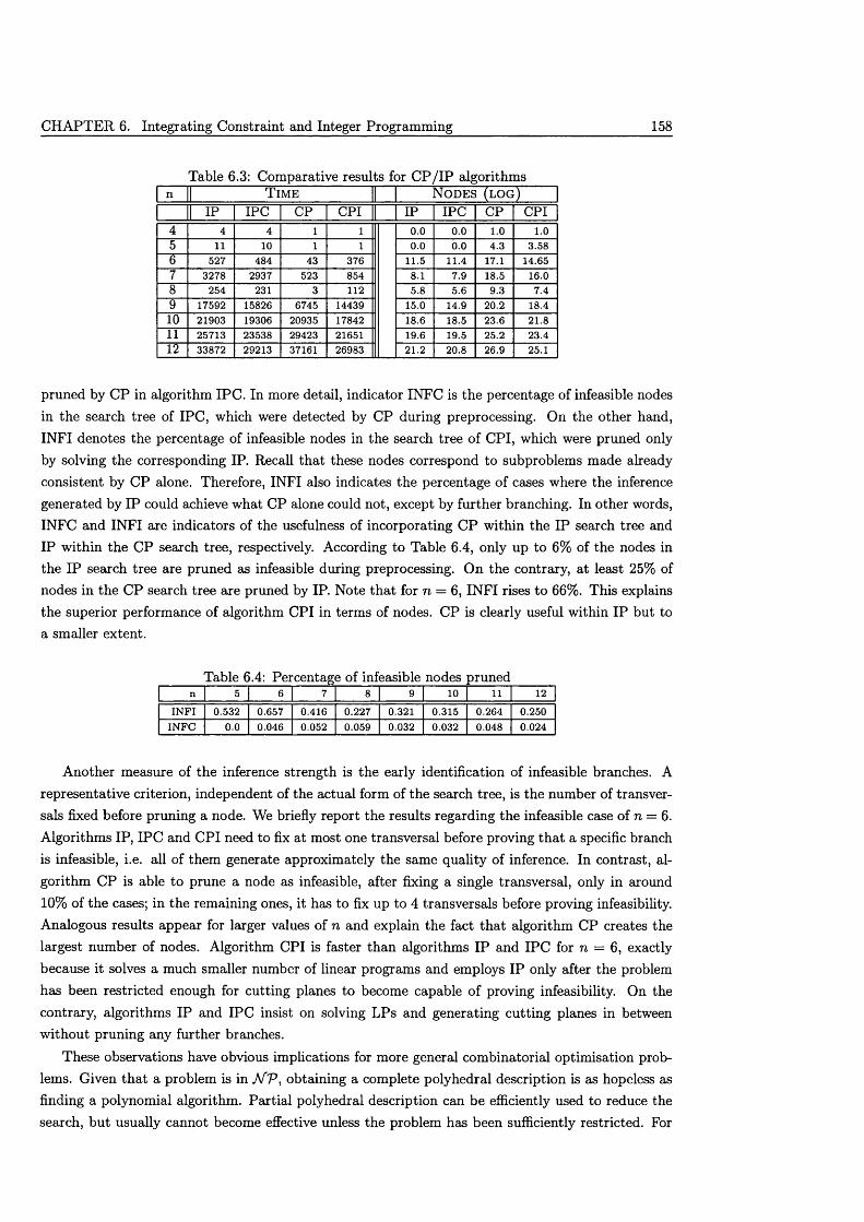
CHAPTER 6. Integrating Constraint and Integer Programming 158
Table 6.3: Comparative results for C P /IP algorithmsn T ime N o d e s ( l o g )
L IP IPC CP CPI IP IPC CP CPI4 4 4 1 1 0.0 0.0 1.0 1.05 11 10 1 1 0.0 0.0 4.3 3.586 527 484 43 376 11.5 11.4 17.1 14.657 3278 2937 523 854 8.1 7.9 18.5 16.08 254 231 3 112 5.8 5.6 9.3 7.49 17592 15826 6745 14439 15.0 14.9 20.2 18.410 21903 19306 20935 17842 18.6 18.5 23.6 21.811 25713 23538 29423 21651 19.6 19.5 25.2 23.412 33872 29213 37161 26983 21.2 20.8 26.9 25.1
pruned by CP in algorithm IPC. In more detail, indicator INFC is the percentage of infeasible nodes in the search tree of IPC, which were detected by CP during preprocessing. On the other hand, INFI denotes the percentage of infeasible nodes in the search tree of CPI, which were pruned only by solving the corresponding IP. Recall th a t these nodes correspond to subproblems made already consistent by CP alone. Therefore, INFI also indicates the percentage of cases where the inference generated by IP could achieve what CP alone could not, except by further branching. In other words, INFC and INFI are indicators of the usefulness of incorporating CP within the IP search tree and IP within the CP search tree, respectively. According to Table 6.4, only up to 6% of the nodes in the IP search tree are pruned as infeasible during preprocessing. On the contrary, at least 25% of nodes in the CP search tree are pruned by IP. Note th a t for n — 6, INFI rises to 66%. This explains the superior performance of algorithm CPI in terms of nodes. CP is clearly useful within IP but to a smaller extent.
Table 6.4: Percentage of infeasible nodes prunedn 5 6 7 8 9 10 11 12
INFI 0.532 0.657 0.416 0.227 0.321 0.315 0.264 0.250INFC 0.0 0.046 0.052 0.059 0.032 0.032 0.048 0.024
Another measure of the inference strength is the early identification of infeasible branches. A representative criterion, independent of the actual form of the search tree, is the number of transversals fixed before pruning a node. We briefly report the results regarding the infeasible case of n = 6. Algorithms IP, IPC and CPI need to fix at most one transversal before proving th a t a specific branch is infeasible, i.e. all of them generate approximately the same quality of inference. In contrast, algorithm CP is able to prune a node as infeasible, after fixing a single transversal, only in around 10% of the cases; in the remaining ones, it has to fix up to 4 transversals before proving infeasibility. Analogous results appear for larger values of n and explain the fact th a t algorithm CP creates the largest number of nodes. Algorithm CPI is faster than algorithms IP and IPC for n = 6, exactly because it solves a much smaller number of linear programs and employs IP only after the problem has been restricted enough for cutting planes to become capable of proving infeasibility. On the contrary, algorithms IP and IPC insist on solving LPs and generating cutting planes in between without pruning any further branches.
These observations have obvious implications for more general combinatorial optimisation problems. Given th a t a problem is in N V , obtaining a complete polyhedral description is as hopeless as finding a polynomial algorithm. Partial polyhedral description can be efficiently used to reduce the search, but usually cannot become effective unless the problem has been sufficiently restricted. For
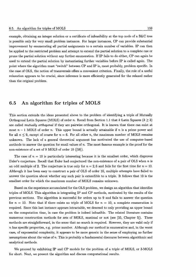
6.5. An algorithm for triples of MOLS 159
example, obtaining an integer solution or a certificate of infeasibility at the top node of a B&C tree is possible only for very small problem instances. For larger instances, CP can provide substantial improvement by enumerating all partial assignments to a certain number of variables. IP can then be applied to the restricted problem and attem pt to extend the partia l solution to a complete one or prune the partial solution without any further enumeration. If IP fails to do either, CP can again be used to extend the partial solution by instantiating further variables before IP is called again. The point where the algorithm must “switch” between CP and IP is, most probably, problem specific. In the case of OLS, the notion of transversals offers a convenient criterion. Finally, the role of a useful relaxation appears to be crucial, since inference is more efficiently generated for the relaxed rather than the original problem.
6.5 An algorithm for triples of MOLS
This section extends the ideas presented above to the problem of identifying a triple of Mutually Orthogonal Latin Squares (MOLS) of order n. Recall from Section 1.1 th a t k Latin Squares (k > 3) are called mutually orthogonal if they are pairwise orthogonal. I t is known th a t there can exist at most n — 1 MOLS of order n. This upper bound is actually attainable if n is a prime power and for all n < 9, except of course for n = 6. For all other n, the maximum number of MOLS remains unknown. The lack of a general theoretical argument has motivated the use of computer-based methods to answer the question for small values of n. The most famous example is the proof for the non-existence of a set of 9 MOLS of order 10 ([58]).
The case of n = 10 is particularly interesting because it is the smallest order, which disproves Euler’s conjecture. Recall that Euler had conjectured the non-existence of a pair of OLS when n is an odd multiple of 2. The conjecture is true only for n = 2,6 and fails for the first time for n = 10. Although it has been easy to construct a pair of OLS of order 10, multiple attem pts have failed to answer the question about whether any such pair is extendible to a triple. It follows th a t 10 is the smallest order for which the maximum number of MOLS remains unknown.
Based on the experience accumulated for the OLS problem, we design an algorithm th a t identifies triples of MOLS. This algorithm is integrating IP and CP methods, motivated by the results of the previous sections. The algorithm is successful for orders up to 9 and fails to answer the question for n = 10. Note th a t if there exists no triple of MOLS for n = 10, a complete enumeration is required. Since this last instance appears intractable, we descend to only providing an upper bound on the computation time, in case the problem is indeed infeasible. The related literature contains numerous construction methods for sets of MOLS, maximal or not (see [35, Chapter 5]). These methods are straightforward, in the sense that no search is required. However, they are valid only if n has specific properties, e.g. prime number. Although our method is enumerative and, in the worst case, of exponential complexity, it appears to be more generic in the sense of employing no further assumptions about the value of n. This is probably a fundamental discourse between algorithmic and analytical methods.
We proceed by exhibiting IP and CP models for the problem of a triple of MOLS, or 3-MOLS for short. Next, we present the algorithm and discuss computational results.
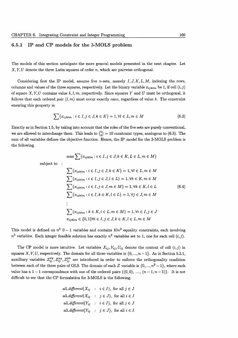
CHAPTER 6. Integrating Constraint and Integer Programming 160
6.5.1 IP and CP m odels for the 3-MOLS problem
The models of this section anticipate the more general models presented in the next chapter. Let X , Y, U denote the three Latin squares of order n, which are pairwise orthogonal.
Considering first the IP model, assume five n-sets, namely I , J , K , L , M, indexing the rows, columns and values of the three squares, respectively. Let the binary variable X i j k i m be 1, if cell (i , j) of square X , Y, U contains value k , l ,m , respectively. Since squares Y and U must be orthogonal, it follows th a t each ordered pair (l ,m ) must occur exactly once, regardless of value k. The constraint ensuring this property is:
^ ~ 2 { x i j k i m : i € I , j £ J ,k £ K ] = l , V l £ L ,m £ M (6.3)
Exactly as in Section 1.5, by taking into account th a t the roles of the five sets are purely conventional, we are allowed to interchange them. This leads to (2) = 10 constraint types, analogous to (6.3). The sum of all variables defines the objective function. Hence, the IP model for the 3-MOLS problem is the following.
max ^ 2 { x i j klm : i £ I , j G J ,k £ K , L £ L ,m € M }
subject to :
^ { x i j k i m - i £ l , j £ J , k £ K } = 1 ,VZ € L ,m e M
^ { x i j k i m : i £ I , j £ J , l £ L} = l,Vfc £ K , m £ M
5 ~2, {x i j k i m : i £ I , j £ j , m £ M } = 1 , V k £ K , l £ L (6.4)
2 ~ 2 { x i j k i m • i £ I , k £ K , l £ L } = 1 , Vj £ J , m £ M
' ^ {X i jk im : k £ K , I £ L ,m £ M } = l,V i G I , j £ J
Xijkim G {0, l}Vz £ I , j £ J ,k e K , l £ L ,m e M
This model is defined on n 5 0 —1 variables and contains 10n2 equality constraints, each involving n 3 variables. Each integer feasible solution has exactly n 2 variables set to 1, one for each cell
The CP model is more intuitive. Let variables X i j , Y ij , Uij denote the content of cell ( i , j) in squares X , Y, U, respectively. The domain for all these variables is {0, ...,n — 1}. As in Section 5.3.1, auxilliary variables Z™, Zf™ are introduced in order to enforce the orthogonality condition between each of the three pairs of OLS. The domain of each Z variable is {0,..., n 2 — 1}, where each value has a 1 — 1 correspondence with one of the ordered pairs {(0,0), ...., (n — 1, n — 1)}. It is not difficult to see th a t the CP formulation for 3-MOLS is the following.
alLdifferent{Xij
alLdifferent{ Xij
al Ldifferent{ Y\j
al L different{ Y.\j
i £ I} , for all j G J
j £ J] , for a l i i £ I
i £ /} , for all j £ J
j £ J} , for all i £ I
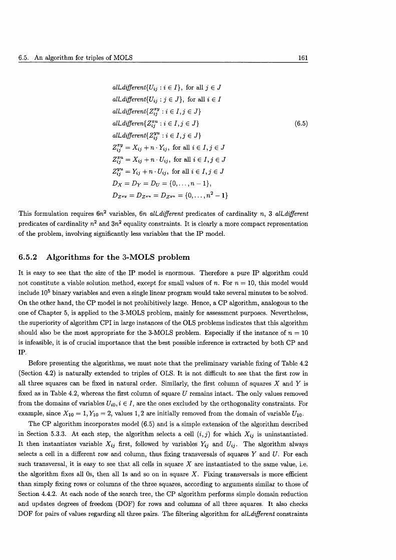
6.5. An algorithm for triples of MOLS 161
alLdifferent{Uij : i E I} , for all j E J
alLdifferent{Uij : j E J} , for a llz G /
a l L d i f f e r e n t { Z : i E I , j E J}
alLdiffere^Zfff : i E I , j E J } (6.5)
alLdifferent{Zf™ : i E I , j E J}
Z f/ = Xij + n • Yy, for all i E l j E J
Zfj1 — X{j + n • Uij, for all i E I , j E J
Zfj = Yij + n ■ Uij, for all i E I , j E J
Dx = Dy = A / = {0, . . . ,n — 1},
= { 0 , . . . , n 2 — 1}
This formulation requires 6n2 variables, 6n alLdifferent predicates of cardinality n, 3 alLdifferent predicates of cardinality n 2 and 3n2 equality constraints. It is clearly a more compact representation of the problem, involving significantly less variables th a t the IP model.
6.5.2 A lgorithm s for the 3-MOLS problem
It is easy to see th a t the size of the IP model is enormous. Therefore a pure IP algorithm could not constitute a viable solution method, except for small values of n. For n = 10, this model wouldinclude 105 binary variables and even a single linear program would take several minutes to be solved.On the other hand, the CP model is not prohibitively large. Hence, a CP algorithm, analogous to the one of Chapter 5, is applied to the 3-MOLS problem, mainly for assessment purposes. Nevertheless, the superiority of algorithm CPI in large instances of the OLS problems indicates th a t this algorithm should also be the most appropriate for the 3-MOLS problem. Especially if the instance of n = 10 is infeasible, it is of crucial importance th a t the best possible inference is extracted by both CP and IP.
Before presenting the algorithms, we must note th a t the preliminary variable fixing of Table 4.2 (Section 4.2) is naturally extended to triples of OLS. It is not difficult to see th a t the first row in all three squares can be fixed in natural order. Similarly, the first column of squares X and Y is fixed as in Table 4.2, whereas the first column of square U remains intact. The only values removed from the domains of variables Uio, i E I , are the ones excluded by the orthogonality constraints. For example, since Xio = 1, Yio = 2, values 1,2 are initially removed from the domain of variable Uiq.
The CP algorithm incorporates model (6.5) and is a simple extension of the algorithm described in Section 5.3.3. At each step, the algorithm selects a cell (i , j ) for which X ij is uninstantiated. It then instantiates variable X ^ first, followed by variables Yij and Uij. The algorithm always selects a cell in a different row and column, thus fixing transversals of squares Y and U. For each such transversal, it is easy to see th a t all cells in square X are instantiated to the same value, i.e. the algorithm fixes all Os, then all Is and so on in square X . Fixing transversals is more efficient than simply fixing rows or columns of the three squares, according to arguments similar to those of Section 4.4.2. At each node of the search tree, the CP algorithm performs simple domain reduction and updates degrees of freedom (DOF) for rows and columns of all three squares. It also checks DOF for pairs of values regarding all three pairs. The filtering algorithm for alLdifferent constraints
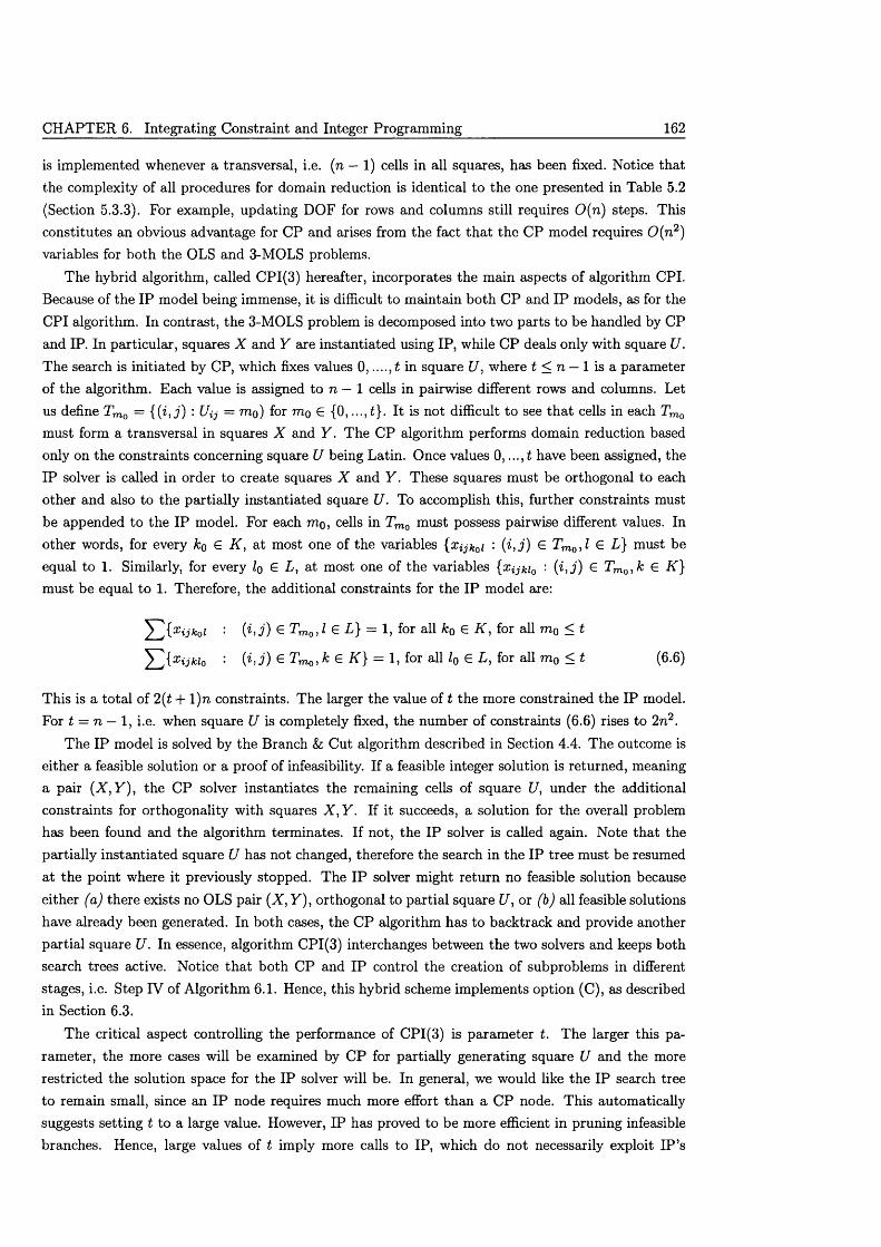
CHAPTER 6. Integrating Constraint and Integer Programming 162
is implemented whenever a transversal, i.e. (n — 1) cells in all squares, has been fixed. Notice that the complexity of all procedures for domain reduction is identical to the one presented in Table 5.2 (Section 5.3.3). For example, updating DOF for rows and columns still requires 0 ( n ) steps. This constitutes an obvious advantage for CP and arises from the fact th a t the CP model requires 0 ( n 2) variables for both the OLS and 3-MOLS problems.
The hybrid algorithm, called CPI(3) hereafter, incorporates the main aspects of algorithm CPI. Because of the IP model being immense, it is difficult to m aintain both CP and IP models, as for the CPI algorithm. In contrast, the 3-MOLS problem is decomposed into two parts to be handled by CP and IP. In particular, squares X and Y are instantiated using IP, while CP deals only with square U. The search is initiated by CP, which fixes values 0,...., t in square U, where t < n — 1 is a parameter of the algorithm. Each value is assigned to n — 1 cells in pairwise different rows and columns. Let us define Tm0 = { {h j ) : Uij = mo) for mo E {0, ...,i}. It is not difficult to see th a t cells in each Tm0 must form a transversal in squares X and Y . The CP algorithm performs domain reduction based only on the constraints concerning square U being Latin. Once values 0,..., i have been assigned, the IP solver is called in order to create squares X and Y . These squares must be orthogonal to each other and also to the partially instantiated square U. To accomplish this, further constraints must be appended to the IP model. For each mo, cells in 'U'mo must possess pairwise different values. Inother words, for every ko E K , at most one of the variables {xijk0i : { i , j) £ Tmo > I E L} must beequal to 1. Similarly, for every lo E L, at most one of the variables {xijhi0 : ( i , j ) e Tmo,k e K } must be equal to 1. Therefore, the additional constraints for the IP model are:
: (*’■?) € TmoJ e £} = 1, for all k0 E K , for all m 0 < t
: ( i , j ) E Tmo, k E K } = 1, for all l0 E L, for all m 0 < t (6.6)
This is a total of 2(t + l)n constraints. The larger the value of t the more constrained the IP model. For t = n — 1, i.e. when square U is completely fixed, the number of constraints (6.6) rises to 2n2.
The IP model is solved by the Branch Sz Cut algorithm described in Section 4.4. The outcome is either a feasible solution or a proof of infeasibility. If a feasible integer solution is returned, meaning a pair (X, Y ) , the CP solver instantiates the remaining cells of square U, under the additional constraints for orthogonality with squares X , Y . If it succeeds, a solution for the overall problem has been found and the algorithm terminates. If not, the IP solver is called again. Note th a t the partially instantiated square U has not changed, therefore the search in the IP tree must be resumed at the point where it previously stopped. The IP solver might return no feasible solution because either (a) there exists no OLS pair (A, Y ), orthogonal to partial square [/, or (b) all feasible solutions have already been generated. In both cases, the CP algorithm has to backtrack and provide another partial square U. In essence, algorithm CPI(3) interchanges between the two solvers and keeps both search trees active. Notice th a t both CP and IP control the creation of subproblems in different stages, i.e. Step IV of Algorithm 6.1. Hence, this hybrid scheme implements option (C), as described in Section 6.3.
The critical aspect controlling the performance of CPI(3) is param eter t. The larger this parameter, the more cases will be examined by CP for partially generating square U and the more restricted the solution space for the IP solver will be. In general, we would like the IP search tree to remain small, since an IP node requires much more effort than a CP node. This automatically suggests setting t to a large value. However, IP has proved to be more efficient in pruning infeasible branches. Hence, large values of t imply more calls to IP, which do not necessarily exploit IP ’s
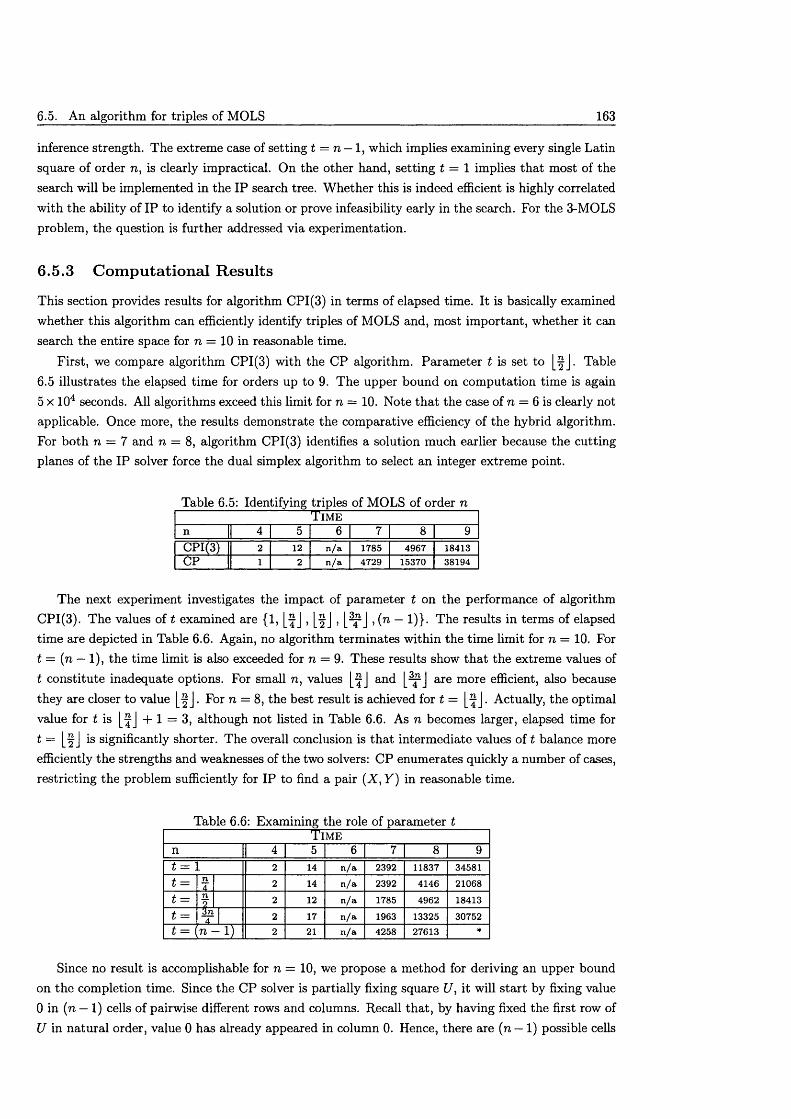
6.5. An algorithm for triples of MOLS 163
inference strength. The extreme case of setting t = n — 1, which implies examining every single Latin square of order n, is clearly impractical. On the other hand, setting t — 1 implies th a t most of the search will be implemented in the IP search tree. W hether this is indeed efficient is highly correlated with the ability of IP to identify a solution or prove infeasibility early in the search. For the 3-MOLS problem, the question is further addressed via experimentation.
6.5.3 C om putational R esults
This section provides results for algorithm CPI(3) in terms of elapsed time. It is basically examined whether this algorithm can efficiently identify triples of MOLS and, most im portant, whether it can search the entire space for n = 10 in reasonable time.
First, we compare algorithm CPI(3) with the CP algorithm. Param eter t is set to [ ^ J . Table 6.5 illustrates the elapsed time for orders up to 9. The upper bound on computation time is again 5 x 10⁴ seconds. All algorithms exceed this limit for n = 10. Note th a t the case of n = 6 is clearly not applicable. Once more, the results demonstrate the comparative efficiency of the hybrid algorithm. For both n = 7 and n = 8, algorithm CPI(3) identifies a solution much earlier because the cutting planes of the IP solver force the dual simplex algorithm to select an integer extreme point.
Table 6.5: Identifying triples of MOLS of order nT ime
n 4 5 6 7 8 9CPI(3) 2 12 n/a 1785 4967 18413CP I 2 n/a 4729 15370 38194
The next experiment investigates the impact of param eter t on the performance of algorithm CPI(3). The values of t examined are {1, [ j J , , (n — 1)}. The results in terms of elapsedtime are depicted in Table 6.6. Again, no algorithm terminates within the time limit for n = 10. For t = (n — 1), the time limit is also exceeded for n = 9. These results show th a t the extreme values of t constitute inadequate options. For small n, values and are more efficient, also because they are closer to value [ p j . For n = 8, the best result is achieved for t = . Actually, the optimalvalue for t is |_f J + 1 = 3, although not listed in Table 6.6. As n becomes larger, elapsed time for t = [p j is significantly shorter. The overall conclusion is th a t intermediate values of t balance more efficiently the strengths and weaknesses of the two solvers: CP enumerates quickly a number of cases, restricting the problem sufficiently for IP to find a pair (X, Y ) in reasonable time.
Table 6.6: Examining the role of param eter tT i m e
n 4 5 6 7 8 9t - 2 14 n/a 2392 11837 34581t = n
4 2 14 n/a 2392 4146 21068t = n
22 12 n/a 1785 4962 18413
t = 3 n4 2 17 n/a 1963 13325 30752
t = (n — 1) 2 21 n/a 4258 27613 *
Since no result is accomplishable for n = 10, we propose a method for deriving an upper bound on the completion time. Since the CP solver is partially fixing square 17, it will s ta rt by fixing value 0 in (n — 1) cells of pairwise different rows and columns. Recall that, by having fixed the first row of U in natural order, value 0 has already appeared in column 0. Hence, there are (n — 1) possible cells
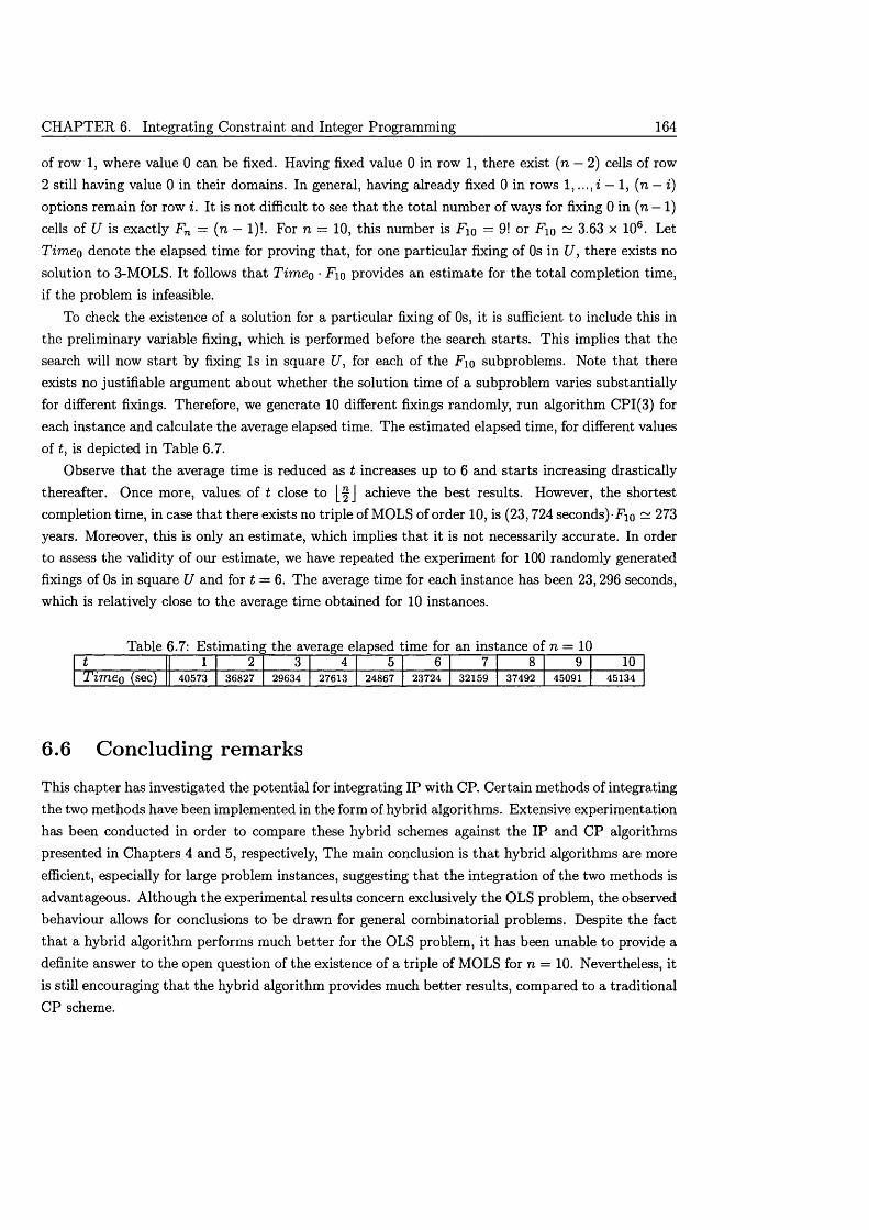
CHAPTER 6. Integrating Constraint and Integer Programming 164
of row 1, where value 0 can be fixed. Having fixed value 0 in row 1, there exist (n — 2) cells of row 2 still having value 0 in their domains. In general, having already fixed 0 in rows 1, ..., i — 1, (n — i) options remain for row i. It is not difficult to see th a t the total number of ways for fixing 0 in (n — 1) cells of U is exactly Fn — (n — 1)!. For n — 10, this number is Fio = 9! or Fio — 3.63 x 10⁶. Let T im eo denote the elapsed time for proving that, for one particular fixing of Os in U , there exists no solution to 3-MOLS. It follows th a t T im eo • Fio provides an estim ate for the to tal completion time, if the problem is infeasible.
To check the existence of a solution for a particular fixing of Os, it is sufficient to include this in the preliminary variable fixing, which is performed before the search starts. This implies th a t the search will now start by fixing Is in square U, for each of the .Fio subproblems. Note that there exists no justifiable argument about whether the solution time of a subproblem varies substantially for different fixings. Therefore, we generate 10 different fixings randomly, run algorithm CPI(3) for each instance and calculate the average elapsed time. The estimated elapsed time, for different values of t, is depicted in Table 6.7.
Observe th a t the average time is reduced as t increases up to 6 and starts increasing drastically thereafter. Once more, values of t close to achieve the best results. However, the shortest completion time, in case th a t there exists no triple of MOLS of order 10, is (23,724 seconds)-Fio — 273 years. Moreover, this is only an estimate, which implies th a t it is not necessarily accurate. In order to assess the validity of our estimate, we have repeated the experiment for 100 randomly generated fixings of 0s in square U and for t = 6. The average time for each instance has been 23,296 seconds, which is relatively close to the average time obtained for 10 instances.
Table 6.7: Estimating the average elapsed time for an instance of n = 10t 1 2 3 4 5 6 7 8 9 10T im eo (se c ) 40573 36827 29634 27613 24867 23724 32159 37492 45091 45134
6.6 Concluding remarks
This chapter has investigated the potential for integrating IP with CP. Certain methods of integrating the two methods have been implemented in the form of hybrid algorithms. Extensive experimentation has been conducted in order to compare these hybrid schemes against the IP and CP algorithms presented in Chapters 4 and 5, respectively, The main conclusion is th a t hybrid algorithms are more efficient, especially for large problem instances, suggesting th a t the integration of the two methods is advantageous. Although the experimental results concern exclusively the OLS problem, the observed behaviour allows for conclusions to be drawn for general combinatorial problems. Despite the fact th a t a hybrid algorithm performs much better for the OLS problem, it has been unable to provide a definite answer to the open question of the existence of a triple of MOLS for n = 10. Nevertheless, it is still encouraging th a t the hybrid algorithm provides much better results, compared to a traditional CP scheme.
Chapter 7
M ultidim ensional Assignm ent Problem s
This chapter generalises the results, derived for the OLS problem, to multidimensional assignment problems. Assignment structures are embedded in numerous combinatorial optimisation problems. An assignment occurs whenever a member of an entity must be allocated/m apped to a member of another entity. The simplest case of an assignment problem is the well-known 2-index assignment, which is equivalent to the weighted bipartite matching problem. Applications include the assignment of facilities to locations and the assignment of delivery points to vehicles.
Extensions of the assignment structure to more than two entities give rise to multidimensional (or multi-index) assignment problems, formally introduced in [70, 71]. These problems essentially ask for a minimum weight clique partition of the complete fc-partite graph (see also [12]). A k- index assignment problem is defined on k sets, usually (but not always) assumed to be of the same cardinality n. The goal is to identify a minimum weight collection of n disjoint tuples, each including a single element from each set. This is the class of axial assignment problems ([9, 79]). Its IP formulation involves 0 — 1 variables with k indices and the constraint sets are derived by summing over all possible sets of k — 1 indices. The weighted sum of the variables constitutes the objective function, a fact th a t justifies the alternative term linear sum assignment problems ([22]). As an example, recall the formulation of the 3-index assignment problem (3A A P n), presented at Section 2 . 1 .
If the aim is, instead, to identify a collection of n 2 tuples, partitioned into n disjoint sets of n disjoint tuples, a different structure appears. By way of illustration, consider the problem of allocating n teachers to n student groups for sessions in one of n classrooms and using one of n laboratory facilities (i.e. n 2 quadruples), in such a way th a t all teachers teach all groups, using each time a different classroom or a different facility (for a relevant case, see [39]). These assignment problems are called planar and are directly linked to Mutually Orthogonal Latin Squares (MOLS) ([60]). The IP formulation of planar problems can be defined on n k 0 — 1 variables (each having k indices) and the constraint sets are derived by summing over all possible sets of k — 2 indices. Examples are the formulations of the Latin square problem (3P A P n) and the OLS problem (APAPn), presented at Section 2.1.
Generalising this concept, we could ask for a minimum weight collection of n s tuples, thus defining the (k , s) assignment problem of order n, hereafter denoted as (k , s)A P n . According to this notation, (k, l)A P n and (k, 2)APn denote the A;-index axial and planar problems, respectively. A more formal
165
CHAPTER 7. Multidimensional Assignment Problems 166
definition appears in the following section. The IP formulation of (k , s)A P n requires n k 0—1 variables. Its constraints are derived by summing over all possible sets of k — s out of k indices.
An excellent review for assignment problems is [79], where complexity and approximability issues are covered. It is known th a t the 2-index problem is polynomially solvable, whereas the 3-index axial and planar problems are A/’P-hard (see [43] and [55], respectively). The authors of [21] prove th a t the multidimensional (axial) assignment problem remains AfP-hard for k > 4, if the coefficient vector of the objective function fulfills an Anti-Monge condition.
Apart from its theoretical significance, the (k ,s )A P n has interesting applications. Multidimensional (axial) assignment structures have recently received substantial attention, because of their applicability in problems of d ata association. Such problems arise naturally in m ulti-target/m ulti- sensor tracking in satellite surveillance systems (see [72]). An application to the problem of tracking elementary particles at the large electron-positron collider of CERN is reported in [75]. The planar problems share the diverse application fields of MOLS, discussed in Section 1.4.
This chapter provides an Integer Programming formulation of the (k ,s )A P n (Section 7.1) for general values of k, s, n. The framework introduced enables the polyhedral study of entire families of assignment problems. A number of boundary conditions is exhibited in Section 7.2.1. The dimension of the linear assignment polytope is established in Section 7.3. In Section 7.4, we examine certain properties of the convex hull of integer vectors, provide a necessary condition for the existence of a solution to the (k, s)APn and propose a hierarchy of assignment problems. The dimension of the axial assignment polytopes is established in Section 7.5, while a family of facets is exhibited in Section 7.6. Section 7.7 establishes the dimension of the planar assignment polytopes. Finally, modelling the (k ,s )A P n via Constraint Programming is the topic of Section 7.8.
7.1 M athem atical formulation
This section provides a formal definition of the (k ,s )A P n . As mentioned before, we consider an IP model derived by summing over all possible subsets of k — s out of k indices. Such a formulation unifies and generalises known IP models for assignment problems. In order to exhibit this compact formulation, we need to formally define the associated problem, i.e. the (A;, s)A P n , which encompasses the definitions of axial and planar assignment problems.
Let us motivate our discussion with a number of examples. Table 7.1 exhibits a pair of OLS of order 4. The sets of rows and columns correspond to student groups and classrooms, while the sets of values for the two squares denote teachers and topics. The (2, 1)AP4 asks for an allocation of teachers to groups. A solution consists of 4 ordered pairs or 2-tuples, e.g. {(1,1), (2,2), (3,3), (4,4)}. The (3 ,1)AP4 is the problem of allocating each teacher to a single group and a single classroom. A solution is composed of 4 3-tuples of the form (group,classroom,teacher). The solution {(0,0,0), (1 ,1 ,3), (2 ,2,1), (3,3,2)} is illustrated by the bordered cells of the first square. Evidently, a solution to (3, l)A P n defines a transversal of a Latin square of order n.
If all teachers must teach all groups in all classrooms, the underlying problem is the (3,2)AP4. It follows th a t each (group,classroom) tuple must be included exactly once and each teacher must be allocated to a set of 4 disjoint 2-tuples. For example, the solution indicated by the first Latin square implies th a t teacher 0 is allocated to the pairs {(0,0), (1,2), (2,3), (3,1)}. Hence, the (3, 2)APn asks for n 2 2-tuples, which can be partitioned into n disjoint sets of n disjoint 2-tuples. The (4 ,2)AP4 includes the additional requirement th a t all topics should be taught to all groups
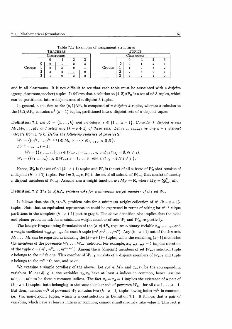
7.1. M athematical formulation 167
Table 7.1: Examples of assignment structuresT e a c h e r s
C la ssr o o m s0 1 2 3
0 0 1 2 3G r o u p s 1 2 3 0 1
2 3 2 1 03 1 0 3 2
T o p i c s
C la ssr o o m s0 1 2 3
0 0 1 2 3G ro u p s 1 1 0 3 2
2 2 3 0 13 3 2 1 0
and in all classrooms. It is not difficult to see th a t each topic must be associated with 4 disjoint(group,classroom,teacher) tuples. It follows that a solution to (4,2) APn is a set of n 2 3-tuples, whichcan be partitioned into n disjoint sets of n disjoint 3-tuples.
In general, a solution to the (k, l)A P n is composed of n disjoint fc-tuples, whereas a solution to the (A;,2)APn contains n 2 (k — l)-tuples, partitioned into n disjoint sets of n disjoint tuples.
D e fin itio n 7.1 Let K = { 1 , . . . , A:} and an integer s E {1,...,A: — 1}. Consider k disjoint n-sets M i, M2, . . . ,Mfc and select any (k — s + 1) of these sets. Let zi, . .. ,ik~s+i be any k — s distinct integers from 1 to k. Define the following sequence of powersets:
W0 = {(mM, ...,m tfe- s+1) E M ^ x ■ • • x M»fc_.+1, i t G K }\For t = 1,..., s — 1 :
W t = { { z i , . . . , z n} : Zi E Wt_!,z = 1 , . . . , n, and Zi D Zj = 0 ,V z^ j} \Ws = {{zi , ... ,zn } : Zi E W 8- \ , i = l , . . . , n , and z t D zj = 0,V z ^ j };
Hence, W q is the set of all (k — s + l)-tuples and W\ is the set of all subsets of Wo th a t consists of n disjoint (k — s + l)-tuples. For t = 2,..., s, Wt is the set of all subsets of W t_i th a t consist of exactly n disjoint members of Wt~\. Assume also a weight function w : M k —> where M k = Mj.
D e fin itio n 7.2 The (k , s)A Pn problem asks for a minimum weight member o f the set W s .
It follows th a t the (k ,s )A P n problem asks for a minimum weight collection of n® (k — s + 1)- tuples. Note th a t an equivalent representation could be expressed in terms of asking for n®-1 clique partitions in the complete (k — s -f- l)-partite graph. The above definition also implies th a t the axial and planar problems ask for a minimum weight member of sets Wi and W2, respectively.
The Integer Programming formulation of the (k , s)A P n requires a binary variable xmim2...mfc and a weight coefficient wm for each fc-tuple (m 1, m 2, . . . , m k). Any (k — s + 1 ) out of the k n-sets M i , . . . , Mk can be regarded as indexing the (k — s + 1)— tuples, while the remaining (s — 1) sets index the members of the powersets W i , . . . , Ws_i selected. For example, xmim2...mfc = 1 implies selection of the tuple c = (ra1,?™2, . .. , m k~s+1). Among the n (disjoint) members of set Ws_i selected, tuple c belongs to the m kth one. This member of Ws_i consists of n disjoint members of Ws_2 and tuple c belongs to the m k~1th one, and so on.
We examine a simple corollary of the above. Let c, d E M k and x c,xa be the corresponding variables. If \c D d\ > s, the variables x c,Xd have at least s indices in common, hence, assume m %1, . . . , m la to be these s common indices. The fact x c = Xd = 1 implies the existence of a pair of (k — s + l)-tuples, both belonging to the same member m %t of powerset Wit , for all £ = 1 , . . . , s — 1. But then, member m %1 of powerset Wi contains two ( f c - s + l)-tuples having index m %B in common, i.e. two non-disjoint tuples, which is a contradiction to Definition 7.1. It follows that a pair of variables, which have at least s indices in common, cannot simultaneously take value 1. This fact is
CHAPTER 7. Multidimensional Assignment Problems 168
reflected in the integer programming formulation of (k , s)A P n , which is derived by summing over all possible subsets of k — s out of k indices.
min ^ ■•■mk ' ^ > • • • > ^ ^ }
^ { x m ima...mfc : m l £ M i, . . . ,m k 3 1 £ M k 3 1, m k 3 £ M k_3} = 1
for all m k~3+l £ M k- s+i , m k~3+2 £ M k- 3+2, . . . ,m k £ M k
: m 1 £ M i , . . . )m k~3~1 £ M k~3~ 1, m k~3+l £ M k- s+i}
for all m k~s £ M k- S, m k~s+2 £ M *_s+2, . . . ,m k £ M k
(7.1)
^ { x mim2.i>Tnfc : m 3 £ M s ,m s+2 £ M s+2, . . . ,m k £ M k} = 1
for all m 1 £ M \, £ M s , m 3+1 £ M s+1
^ { x mim2...mfc : m 3+1 £ M s+1,m 3+2 £ M 3+2, . . . ,m k £ M k} = 1
for all m 1 £ M \, . . . ,m 3~ 1 £ M s- \ , m s £ M s
Xm'm2...mk € {0, 1}, i™}, m 2, . . . , 771*) G M K ] (7.2)
For any S C A , define M s = 0 M*. For s £ K , define Q k>3 = {5 C K : |S| = s}, i.e. QkjS isies
the set of all subsets of K w ith cardinality s, also called s-subsets. Observe th a t each constraint set corresponds to a single S £ Q kiS. There are exactly s “fixed” indices in each constraint. The set of indices appearing in the sum is M K\ s , whereas M s is the set of indices common to all variables in a constraint. Let A ^ ’s denote the (0,1) m atrix of the constraints (7.1). The matrix has n kcolumns and (*) • n 3 rows, i.e. n 3 constraints for each of the (*) distinct S £ Q k,s- Each constraintinvolves n k~3 variables with coefficient 1.
Under these definitions, it is obvious th a t (2,1 )A P n refers to the 2-index assignment problem, (3,1 )APn to the 3-index axial assignment problem ([9, 38]), (3 ,2 )A P n to the 3-index planar assignment problem ([37, 63]), and (4,2)APn to the 4-index planar assignment problem ([2]). Note that param eter s is central to the type of assignment required at each problem, i.e. the axial problems imply s = 1 and the planar problems imply s — 2. An alternative formulation and classification appears in [79].
7.2 Assignm ent polytopes and related structures
7.2.1 General concepts
Definitions from polyhedral theory were given in Section 3.1. Recall that, if denotes the matrixof the minimum equality system for a polyhedron P, it holds that:
dimF = n — r a n k B = (7.3)
The convex hull of the integer points satisfying the constraints (7.1) is the (k , s ) assignment polytope, denoted as P jk,s\ Formally, P^k’3 = conv{x £ {0,1}™* : A n ’ x = e}, where e is a column vector of ones. The linear relaxation of p ^k,3\ also called the linear assignment polytope, is the

7.3. The (k , s ) linear assignment polytope 169
polytope p ( k’s) = [x £ Rnfc : A ^ ’s x = e,x > 0}. Obviously, p ( k,s C p ( fc>s).
Clearly, the assignment polytope is a special case of the set-partitioning polytope defined as Ps p = {y G {0, l} g : B y = e}, where B is a 0 — 1 matrix. A close relative of P sp is the set-packing polytope P s p , defined exactly as P sp but with “= ” replaced by “< ” . In our case, Pfk,a) = conv{x £ {0, l} nfc : A ^ ' ^ x < e}. A relation, inherited from the general case, is th a t p j k,s is a face of p j k,s^implying d im P jk's < dim P\k,s\ Polytope p^k,s is full dimensional, hence dim P \k's = n k, i.e. itsdimension is independent of s. For a survey on Ps p , Ps p and on related problems, see [8].
Another class of polytopes related specifically to P jk’ is given by the multi-index generalised assignment problems. The simplest representative is the 2-index generalised assignment problem (GAP) ([64]). These problems are defined for s = 1, i.e. they constitute an extension of the axial assignment problems. One of the constraint sets consists of equalities of the type “ = 1” , whereas the rest consist of inequalities of the type “ < 6t” , where bt £ t £ K \ {1}. The IP model for thefc-index generalised assignment problem is illustrated in [3]. Applications of this model, for k = 3, can be found in [41, 42, 64]. Finally, we note th a t a similar approach can be used for modelling an extension of the transportation problem, called the solid (multi-index) transportation problem, introduced in [48].
7.2.2 Two special cases
For s = k, constraints (7.1) reduce to the system of trivial equalities
= 1. V ^ 1, 7712, . . . , 771*) £ M K (7.4)
whereas, for s = 0, constraints (7.1) result in the single equality constraint
: {m1 , m 2, . . . , m k) £ M k } - 1 (7.5)
L em m a 7.1 rankAn = n k and d im P (k,k) = d im P \k,k = 0.
P ro o f . Trivially, A ^ ' k = I ( n k). Therefore, rankA ^ ’k = n k and both polytopes contain the single point x = e. ■
L em m a 7.2 rank Ank’° = 1 and d im P (k,°) = dim P jk,0 — n k — 1.
P ro o f . From (7.5), rank A 1*’° = 1. The n k unit vectors belong to both p ( fc’°) and p ^k,Q\ The result follows from (7.3). ■
C o ro lla ry 7.3 p j k,° is a facet of P jk'°K
P ro o f . p ( k,°) c p ( k,0\ since point x = (0, . . . , 0 ) T belongs to p ^k,° but not to p ( k,0\ The result follows from Lemma (7.2) and from the fact th a t dim P jk,° — n k. ■
7.3 The (&;, s) linear assignment polytope
This section establishes the dimension of polytope p (*’s) by determining the rank of m atrix An'8'*. Before illustrating the main proof, certain intermediate results are presented.
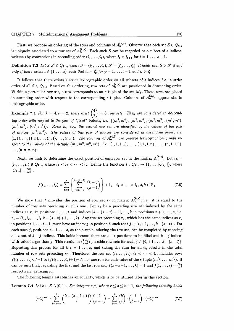
CHAPTER 7. Multidimensional Assignment Problems 170
First, we propose an ordering of the rows and columns of A ^ ' s\ Observe th a t each set S G Qk,s is uniquely associated to a row set of A ^ ’s\ Each such S can be regarded as a subset of s indices, written (by convention) in ascending order ( i \ , .. . , i a), where i t < it+i for t = 1 , . . . , s — 1.
D e fin itio n 7.3 Let S , S" G Qk,s, where S = (i\ , . . . , i s), S ' = (i[ , . . . , i's). It holds that S > S ' i f and only i f there exists t G { 1 , . . . , s} such that iv — i'p for p = 1 , . . . , t — 1 and i t > i't .
It follows th a t there exists a strict lexicographic order on all subsets of s indices, i.e. a strict order of all S G Qk)S- Based on this ordering, row sets of are positioned in descending order.W ithin a particular row set, a row corresponds to an s-tuple of the set Ms- These rows are placed in ascending order with respect to the corresponding s-tuples. Columns of A ^ ’s appear also in lexicographic order.
/ 4 \E x am p le 7.1 For k = 4, s = 2, there exist I J — 6 row sets. They are considered in descend
ing order with respect to the pair of “fixed” indices, i.e. {(m3, m 4), (m2, m 4), (m2,m 3), (m 1,m 4), ( m ^ m 3), (m},rn2)}. Rows in, say, the second row set are identified by the values of the pair of indices (m2, m 4). The values of this pair of indices are considered in ascending order, i.e.( 1 ,1 ) , . . . , (1, n ) , . . . , (n, 1 ) , . . . , (n, n). The columns of A^4,2 are ordered lexicographically with respect to the values of the 4-tuple (m1,m 2,ra3, ra4), i.e. (1 ,1 ,1 ,1), . . . , (1,1, l ,n ) , . . . , (n, 1,1,1),. . . , (n, n, n, n).
Next, we wish to determine the exact position of each row set in the m atrix A n ’s\ Let ro =
(*i, .. - , i 3) € Qk,s» where ii < i2 < • • • < i s - Define the function / : Qk,s —► {1, • • •, |Q*,*I}> where
10*,.I = (*) =
s ( k—(s—t) . \
= E ( I t ) r + 1, <7-6)t=i [ j = i t+i ' )
We show th a t / provides the position of row set ro in m atrix A ^ ,s\ i.e. it is equal to the number of row sets preceding ro plus one. Let r\ be a preceding row set indexed by the same indices as r 0 in positions 1 , . . . , t and indices [fc — (s — t) + 1] , . . . , k in positions t + 1 , . . . , s, i.e. n = { h , *2) ■ • •, U, k — (s — t) + 1 , . . . , k). Any row set preceding r\, which has the same indices as ro in positions 1 , . . . , t — 1, must have an index j in position t, such th a t j G {it + 1, - - - , k — (s — t)}. For each such j , positions t + 1 , . . . , s, at the s-tuple indexing the row set, can be completed by choosing s — t out of k — j indices. This holds because there are s — t positions to be filled and k — j indices with value larger than j . This results in (*1^) possible row sets for each j G {it + 1, •. •, k — (s — t)}. Repeating this process for all i t , t = 1 , . . . , s , and taking the sum for all i t , results in the total number of row sets preceding ro. Therefore, the row set (* i , . .. , i s), i\ < • • • < i s, includes rows f ( i i) • • •»i s)-ns-\-l to ( f ( i i , . . . , i s) + l ) -n s , i.e. one row for each value of the s-tuple (m %1, . . . ,m ta). It can be seen that, regarding the first and the last row set, f ( k — s + 1 , . . . , k) = 1 and / ( l , . . . , s) = (*) respectively, as required.
The following lemma establishes an equality, which is to be utilised later in this section.
L em m a 7.4 Let k e z+ \{ 0 ,1}. For integers s ,r , where r < s < k — 1, the following identity holds
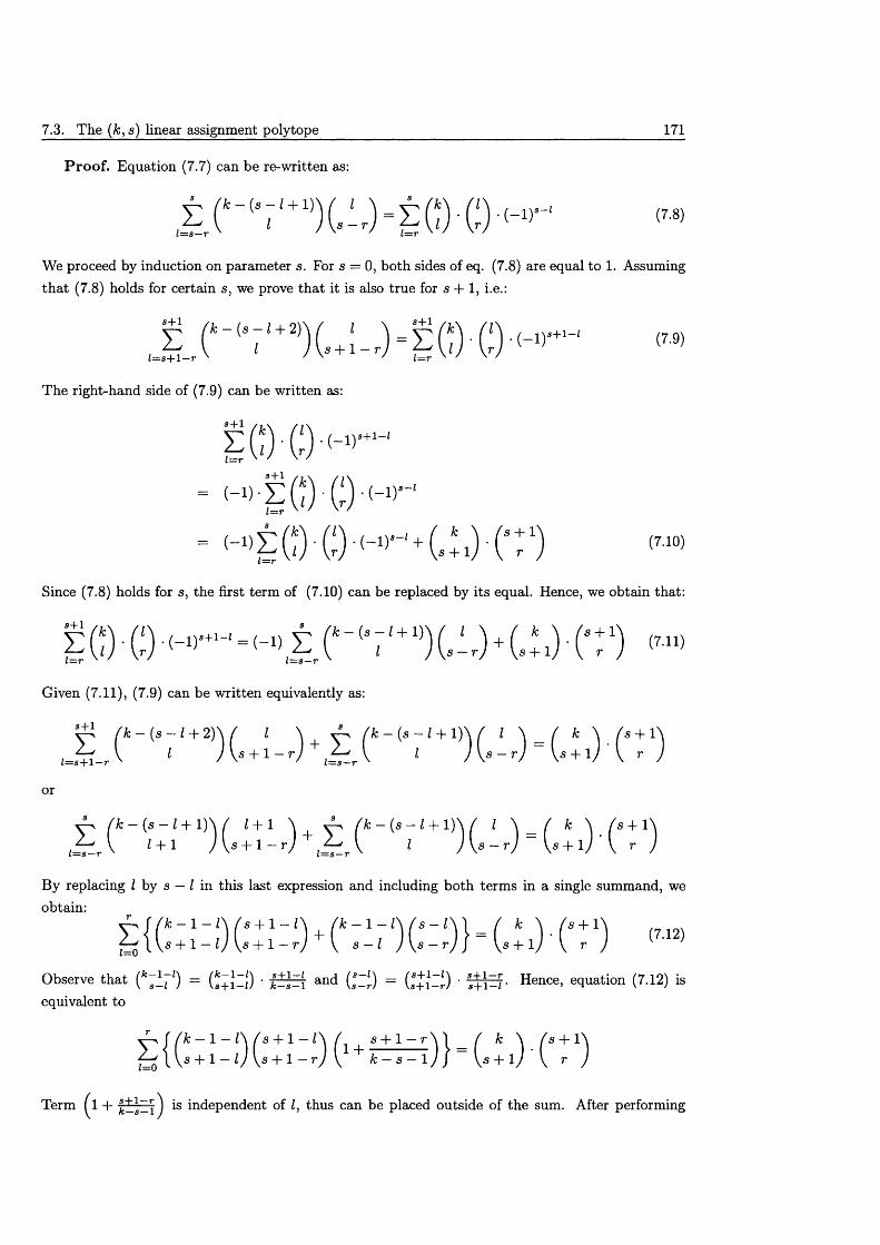
7.3. The (k,s) linear assignment polytope 171
P ro o f. Equation (7.7) can be re-written as:
£ + m ) _ £ ( * ) . ( ; ) . ( _ i r . (7.8)
We proceed by induction on param eter s. For s = 0, both sides of eq. (7.8) are equal to 1. Assuming th a t (7.8) holds for certain s, we prove th a t it is also true for s + 1, i.e.:
_ , ) - ! ( ; ) 0 - < - « — ■ r n
The right-hand side of (7.9) can be w ritten as:
gO-■
- <-)■g o - c ) ( - » -
- < - ■ > ± 0 0 < - w <™>/ / V r / Vs + l / V r ,Z=r x
Since (7.8) holds for s, the first term of (7.10) can be replaced by its equal. Hence, we obtain that:
| 0 (* - " 7 ■+ i>) C : 1)
Given (7.11), (7.9) can be w ritten equivalently as:
k - ( s - l + 2 ) \ / I \ ' / k - ( s - l + l ) \ { I \ ( k \ ( s + 1£ (*-(7 ,+2)) U J + 1, vs + 1 — r j V J \ s ~ f"J Vs + 1/ V r/= s+ l—r N ' l = s —r '
or
f k — (s — I + 1 )\ / I + 1 \ \ f k — (s — I + 1 )\ / I \ / k \ / s -f-1^ r V l + l J \ s + l - r ) + I J \ s - r ) = \ s + 1 ) \ r
By replacing I by s — I in this last expression and including both term s in a single summand, we obtain:
StCil 10Ctj-O * Ci-rOC*-')} - c;0 - Cto ™Observe th a t (k~ ^ 1) = ( ^ J z j ) • and (aaZ lr) = C + J l ') ■ Hence, equation (7.12) isequivalent to
Term ^1 + ) *s independent of I, thus can be placed outside of the sum. After performing
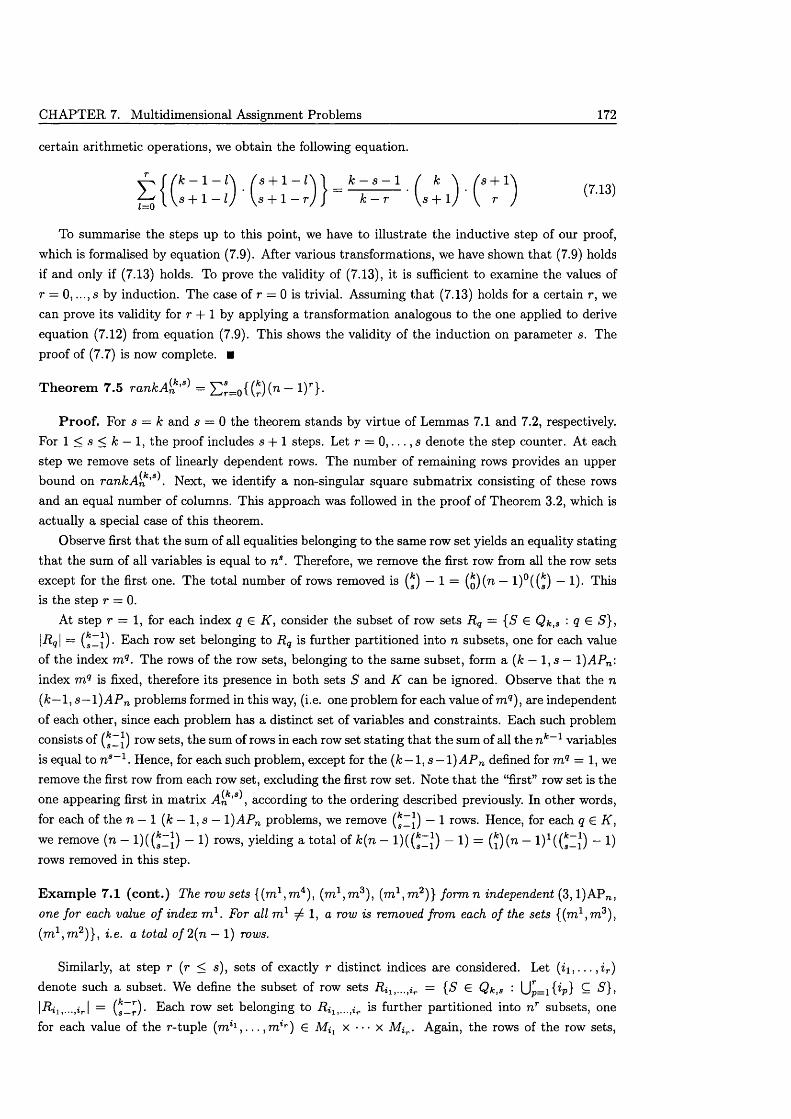
CHAPTER 7. Multidimensional Assignment Problems 172
certain arithm etic operations, we obtain the following equation.
To summarise the steps up to this point, we have to illustrate the inductive step of our proof, which is formalised by equation (7.9). After various transformations, we have shown that (7.9) holds if and only if (7.13) holds. To prove the validity of (7.13), it is sufficient to examine the values of r — 0, ...,s by induction. The case of r — 0 is trivial. Assuming th a t (7.13) holds for a certain r, we can prove its validity for r + 1 by applying a transformation analogous to the one applied to derive equation (7.12) from equation (7.9). This shows the validity of the induction on parameter s. The proof of (7.7) is now complete. ■
T h e o re m 7.5 r a n k A £ ,s>) — X)r=o((r)(n ~ 1)r }-
P ro o f. For s = k and s = 0 the theorem stands by virtue of Lemmas 7.1 and 7.2, respectively. For 1 < s < k — 1, the proof includes s + 1 steps. Let r = 0 , . . . , s denote the step counter. At each step we remove sets of linearly dependent rows. The number of remaining rows provides an upper
(k s)bound on rank An ’ . Next, we identify a non-singular square subm atrix consisting of these rows and an equal number of columns. This approach was followed in the proof of Theorem 3.2, which is actually a special case of this theorem.
Observe first th a t the sum of all equalities belonging to the same row set yields an equality stating th a t the sum of all variables is equal to n 3. Therefore, we remove the first row from all the row sets except for the first one. The total number of rows removed is (*) — 1 = (q)(ti — l)°((s) — !)• This is the step r = 0.
At step r = 1, for each index q £ K , consider the subset of row sets R q = {S' € Q k , s '■ q € S}, |iig| = (*Zi)- Each row set belonging to R q is further partitioned into n subsets, one for each value of the index m q. The rows of the row sets, belonging to the same subset, form a (k — 1, s — 1 )APn: index m q is fixed, therefore its presence in both sets S and K can be ignored. Observe that the n (k—1, s —\ ) A P n problems formed in this way, (i.e. one problem for each value of m q), are independent of each other, since each problem has a distinct set of variables and constraints. Each such problem consists of (*Zi) row set s) the sum of rows in each row set stating th a t the sum of all the n k~ l variables is equal to n s_1. Hence, for each such problem, except for the (k — 1, s — l ) A P n defined for m q = 1, we remove the first row from each row set, excluding the first row set. Note th a t the “first” row set is the one appearing first in m atrix A n ,s^, according to the ordering described previously. In other words, for each of the n — 1 (k — 1, s — 1 )APn problems, we remove (*Zj) — 1 rows. Hence, for each q 6 K ,
we remove (n — l ) ( ( * l j ) — 1) rows, yielding a total of k{n — l)((*Zi) — 1) = (J)(n — l ) 1(( s l j ) — 1) rows removed in this step.
E x am p le 7.1 (co n t.) The row sets {(m l ,m 4), ( m ^ r a 3), (m l , m 2)} f o r m n independent (3, l )A Pn , one for each value of index m 1. For all m 1 ^ 1, a row is removed from each of the sets {(ra1,?™3), (m 1^ 2)}, i.e. a total o /2 (n — 1) rows.
Similarly, at step r (r < s), sets of exactly r distinct indices are considered. Let denote such a subset. We define the subset of row sets R i 1>,. . ti r = { S € Q k , s • Up=i(^p} — ^}> |-Rii,...,ir | = CZrr)- Each row set belonging to R i lt...iir is further partitioned into n T subsets, one for each value of the r-tuple (m 11, . . . ,m lr) € M i y x • • • x M i r . Again, the rows of the row sets,

7.3. The (k , s ) linear assignment polytope 173
belonging to the same subset (identified by the same value of the r-tuple (m*1, . .. , m v )) form a (k — r ,s — r )A P n . Since there are n T distinct subsets, we have n r independent (k — r ,s — r)APn . Each (k — r ,s — r )A P n consists of row sets, the sum of rows in each row set stating that thesum of all the n k~r variables is equal to n s~r . Hence, for each of these problems, excluding the ones defined by the r-tuples (rri11, . . . , m lr) for which at least one of the indices is equal to 1, we remove the first row from each of its last (*l£) — 1 row sets. Therefore, for each (k — r ,s — r)A P n , defined by the r-tuple (raM, . . . , m lr), rri1? ^ 1, Vp = 1 , . . . , r, we remove (*l£) — 1 rows. The exact rows removed for the problem identified by (m %1, . . . , m lr) are defined via the following remark.
R e m a rk 7.1 Let t* denote the maximal element of i.e. t* > t for all t E R ilt...,ir (Definition 7.3). For each t E .... i T. \ { ^ * } > we remove the row which has m i = 1 for every j E t \ { i i , . . . , ir }and (m11, . . . , m %r) in positions ( i i , . . . , i r), where m lp 1, Vp = 1 , . . . , r. There is a 1 — 1 correspondence between each t E R ilj...Iir \ {t*} and each row removed. Obviously, \ {t*}\ =
Because there are (n — l ) r such problems, we remove (n — l ) r • ((*l£) — 1) rows for each distinct r-set («i , . . . , i r). There are (*) distinct r-sets of indices, therefore the number of rows removed at step r is a t most
Assume, without loss of generality, th a t row removal is implemented (i) in increasing order with respect to r and (ii) for a certain r, in increasing order w ith respect to row ordering. For example, the step r = 1 is preceding step r — 2 and the {k — 2, s — 2)A P n problems corresponding to the pair of indices (m 1 , m 2) are considered before the (k — 2 ,s — 2)A P n problems corresponding to the pair (■m l ,m ,3). To show th a t the upper bound defined by (7.14) is attainable, we need to prove the following lemma.
L em m a 7.6
(i) No rows of the (k — r ,s — r)A P n problems indexed by the r-tuple ro were removed at a previousstep involving an r-tuple fo examined before ro.
(ii) No rows of the (k — r ,s — r)APn problems indexed by the r-tuple ro were removed at a previousstep involving a v-tuple Vo where v < r.
P ro o f . To prove (i), let ro = ( i i , . . . , i r), fo = ( ? i , . . . , 2r ) be two distinct r-tuples, i.e. there exists at least one q E ( 1 , . . . , r}, such that i q ^ i q. Let fo be considered first and let t be an s-tuple, indexing a row set, such th a t r0,fo C t. If t = t* (or t = £*), where t* (t *) is the maximal elementof R ix ir {Ri1,...,ir respectively), then no row is removed from row set t with respect to ro (fo).Thus, we assume th a t t ^ t*,t*. This implies th a t the rows of t belong to the (k — r ,s — r)APn problems considered for both ro and fo- Let m r° = (m 11, . . . , m lr) and m r° = [m%l, . . . , m %r). For each value of m r°, where m lp ^ 1, for all p = 1 , . . . , r , a row having mJ = 1, for all j E t \ f o is removed (Remark 7.1). This implies th a t this row has raJ = 1 for all j E ro \ (ro D fo) Recall th a t when considering ro, only (k — r ,s — r)A P n problems corresponding to values of m r° with no index equal to 1 are examined. Therefore, all rows removed when considering r-tuples m r° belong to (k — r ,s — r)A P n problems not examined when considering r-tuples m r°.
The proof of (ii) follows the same idea. Assume ro = ( i i , . . . , i r ) and vq = (? i, . . . , i v), v < r. There exists at least one index i t belonging to ro but not to vq. Let also t be an s-tuple indexing a
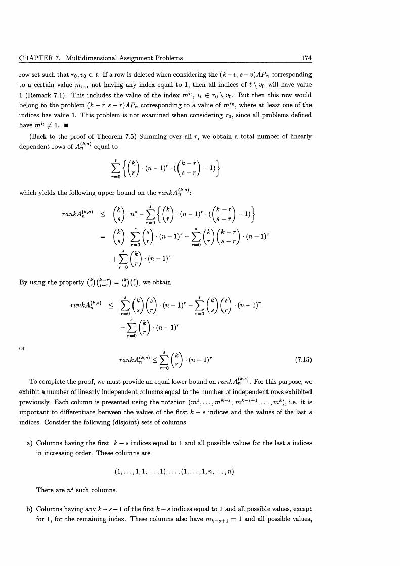
CHAPTER 7. Multidimensional Assignment Problems 174
row set such that ro, C t. If a row is deleted when considering the (k — v ,s — v)APn corresponding to a certain value m Vo, not having any index equal to 1, then all indices of t \ vq will have value 1 (Remark 7.1). This includes the value of the index m lt , i t G ro \ vq. But then this row would belong to the problem (k — r ,s — r)A P n corresponding to a value of rar°, where at least one of the indices has value 1. This problem is not examined when considering ro, since all problems defined have m lt ^ 1. ■
(Back to the proof of Theorem 7.5) Summing over all r, we obtain a total number of linearly dependent rows of equal to
which yields the following upper bound on the r a n k A ^ ’s :
rank A £*■•> < ( * ) ■ n ‘ - £ { (*) • (n - I)' - ((J "') - 1)}
r = 0 ' '
By using the property (*) (*~^) = (J) (*), we obtain
™ "“ “ 5 SOC) - s 0 0 -l" - " ’
+ £ ( * ) > - i rr = 0 ' '
or
rankA
To complete the proof, we must provide an equal lower bound on rankAn'^ ■ For this purpose, we exhibit a number of linearly independent columns equal to the number of independent rows exhibited previously. Each column is presented using the notation (m1, . . . , m k~s , m fc-s+1, . . . , m k), i.e. it is im portant to differentiate between the values of the first k — s indices and the values of the last s
indices. Consider the following (disjoint) sets of columns.
a) Columns having the first k — s indices equal to 1 and all possible values for the last s indices in increasing order. These columns are
( l , . . . , l , l , . . . , l ) , . . . , ( l , . . . , l , n , . . . , n )
There are ns such columns.
b) Columns having any k — s — 1 of the first k — s indices equal to 1 and all possible values, except for 1, for the remaining index. These columns also have ra*;_s+i = 1 and all possible values,
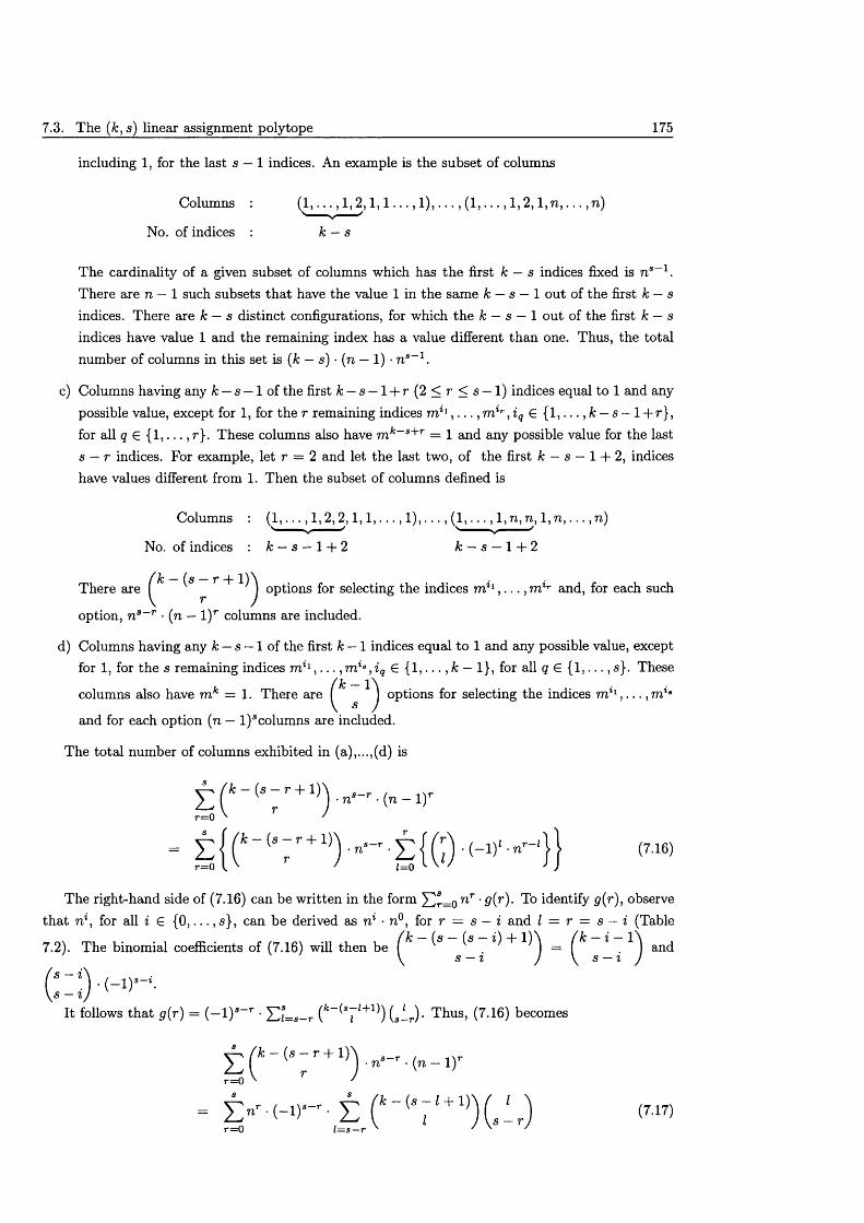
7.3. The (k , s) linear assignment polytope 175
including 1, for the last s — 1 indices. An example is the subset of columns
Columns : ( 1 , . . . , 1 , 2 , 1 , 1 . . . , 1 ) , . . . , ( 1 , . . . , 1,2, l , n , . . . ,n)'-----------V----------- '
No. of indices : k — s
The cardinality of a given subset of columns which has the first k — s indices fixed is n s~ l . There are n — 1 such subsets th a t have the value 1 in the same k — s — 1 out of the first k — s indices. There are k — s distinct configurations, for which the k — s — 1 out of the first k — s indices have value 1 and the remaining index has a value different than one. Thus, the total number of columns in this set is (k — s) ■ (n — 1) • n s_1.
c) Columns having any k — s — 1 of the first k — s — 1 + r (2 < r < s — 1) indices equal to 1 and any possible value, except for 1, for the r remaining indices m n , . . . , m %r, iq € { 1 , . . . , A; — s — 1 + r} , for all q E { 1 , . . . , r}. These columns also have m k~s+r = 1 and any possible value for the last s — t indices. For example, let r = 2 and let the last two, of the first k — s — 1 + 2, indices have values different from 1. Then the subset of columns defined is
Columns : ( 1 , . . . , 1 , 2 ,2 ,1 ,1 , . . . , 1 ) , . . . , ( 1 , . . . , l , n , n , 1,n , . . . ,n)s v.. — ✓ v ^ ✓
No. of indices : k — s — 1 + 2 k — s — 1 + 2
g j* J \ \J options for selecting the indices rri11, . . . , rriLr and, for each such
option, n s~r ■ (n — l ) r columns are included.
d) Columns having any k — s — l of the first k — 1 indices equal to 1 and any possible value, except for 1, for the s remaining indices ral1, . . . , m la , i q £ { 1 , . . . , k — 1}, for all q € { 1 , . . . , s}. These
columns also have m k = 1. There are ^ ^ options for selecting the indices m %1, . . . ,m %a
and for each option (n — l ) scolumns are included.
The total number of columns exhibited in (a),...,(d) is
- t { ( ‘ - v + v - - g { Q - < - ^ i } <“ >
The right-hand side of (7.16) can be w ritten in the form X)r=o nT ' 9(r )- To identify g(r), observe th a t n l , for all i € {0 , . . . , s}, can be derived as n l • n°, for r = s — i and I = r = s — i (Table
7.2). The binomial coefficients of (7.16) will then be ^ ^S ^ = ^
n w * .s — IJIt follows th a t g(r) = (—I)5-7- • Y a =s- t (fc_^ “ z+1 ) (s^ r). Thus, (7.16) becomes
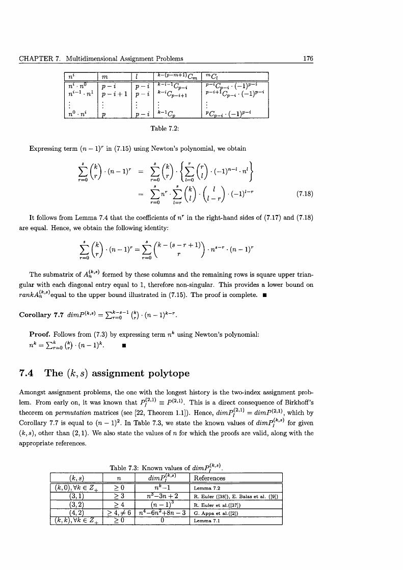
CHAPTER 7. Multidimensional Assignment Problems 176
n l m I '■-'771 mCin { ■ n° n i_1 • n 1
p — i p — i + 1
p — i p — i
k—i— \sp—ik—i/~i^p —i+l
P-'Cp-i • ( - l ) P - 1P-i+fCp- i • ( - l ) P - {
n° ■ n { P p — i k—l f iOp PCv- i • (-1)*-*
Table 7.2:
Expressing term (n — l ) r in (7.15) using Newton’s polynomial, we obtain
SQ-'""’’ - S© { § ( 0
It follows from Lemma 7.4 th a t the coefficients of n r in the right-hand sides of (7.17) and (7.18) are equal. Hence, we obtain the following identity:
£ ( * ) > - i r = £ ( * " (T +1)) - n'_r'(n- 1>rr=0 r=0
The subm atrix of A 1*’ formed by these columns and the remaining rows is square upper triangular with each diagonal entry equal to 1, therefore non-singular. This provides a lower bound on r a n k A ^ ’9 equal to the upper bound illustrated in (7.15). The proof is complete. ■
C o ro lla ry 7.7 dim,P(k,s) = Ylr=o 1 (r ) ‘ (n — *
P ro o f. Follows from (7.3) by expressing term n k using Newton’s polynomial:
* * = e :u e ) - ( " - ! ) * • ■
7.4 The ( k , s ) assignment polytope
Amongst assignment problems, the one with the longest history is the two-index assignment problem. From early on, it was known th a t p j 2>1 = This is a direct consequence of Birkhoff’stheorem on permutation matrices (see [22, Theorem 1.1]). Hence, dim P j2,1 = d im P(2,1\ which by Corollary 7.7 is equal to (n — l )2. In Table 7.3, we state the known values of d im P jk,s for given (k , s ), other than (2,1). We also state the values of n for which the proofs are valid, along with the appropriate references.
Table 7.3: Known values of dim P jk,s\(k ,s) n d im P \k'9 References
(A;,0), VA; E > 0 n k- 1 Lemma 7.2
(3,1) > 3 n 3—3 t2 + 2 R. Euler ([38]), E. Balas et al. ([9])
(3,2) > 4 { n - l f R. Euler et al.([37])
; (4,2) > 4 , ^ 6 774 —6?72+8n — 3 G. Appa et al.([2])(k, k) ,Vk E Z+ > 0 0 Lemma 7.1
7.4. The (k , s ) assignment polytope 177
For general (k , s ), Corollary 7.7 implies dim P jk,a < X^r=o_1 (r) '( n — since P jk,s C p (k>s). However, establishing the exact value of d im P \k,s is not straightforward. Note also th a t p j k,s = 0 for certain values of k, s, n (for example, consider the polytope for k = 4, s — 2, n = 2).
First, let us take a closer look at the integer vectors of P jk,a\ Definition 7.1 implies th a t n s A:-tuples have to be selected, therefore an integer vector must have exactly n s variables equal to 1. Moreover, any integer vector must signify n disjoint members of powerset Ws_i , each one containing n s~ l tuples (i.e. variables). Since any index m 1 G Mt, t G K, can be regarded as indexing powerset W s- 1, any of its values rriQ must appear in exactly n s_1 non-zero variables. Hence, at an integer point of p ( k,s\ each element of any of the sets M i , . . . , Mk appears in exactly n s_1 variables set to one. This remark is very useful in terms of providing a mechanism for transition from one integer point to another. Consider an arbitrary integer point x G p j k,a\ and a pair of index values mQ,m\ G M t , t G K . We set m 1 — m \ for all the (k — s + l)-tuples with m* = tuq and also m l = ttiq for all the (k — s + l)-tuples with m 1 = m \. The derived structure corresponds to another integer point x € since there are again exactly n s_1 “new” variables set to one with m 1 = rriQ andn s_1 “new” variables set to one with m 1 = m \. The variables, w ith m 1 = tuq and m* = m \, set to one at point x , are set to zero at point x and vice versa. The values for the rest of the variables remain the same at both points. This notion of interchanging the role of two index values is formalised with the introduction of the interchange operator (<->). Hence, by setting x = x(mQ *-*■ m j ) t , we imply that, at point x, we interchange the index values mg and m \ , thus deriving point x. The conditional interchange is defined accordingly (See Section 3.2).
Given (A:,s,n), an im portant issue is whether p j k,s ^ 0. This question is difficult to answer for general (k , s ,n) . However, for certain values of s, we know th a t p f k,s) ^ 0. We have seen two such cases in Section 7.2.2. Another such case is obtained for s = 1. It is easy to see th a t P ^ ’1 ^ 0, Vfc,n G Z +. This is because the diagonal solution, noted as x (xn...\ = ■ • • = x nn...n = 1), always satisfies constraints (7.1), (7.2), for 3 = 1. For general s > 2, we provide the following necessary condition for P^k,s to be non-empty.
P ro p o s itio n 7.8 For s > 2, o necessary condition for the existence of a solution to the (k ,s )APn is k < n + s — 1.
P ro o f. Observe first that, according to (7.1), variables appear at the same row if and only if they have at least s indices in common (common values for indices belonging to m s ).
Given th a t p ^k,s ^ 0 and s > 2, consider the point x' G P^k,s having x 1...lma...mk = x 1...lTns...mk = ■ ■ • = = 1. Such a point always exists, since rows ( 1 , . . . , 1, rrij) G Mi x M2 • • • x M s ,j = 1 , . . . , n must have exactly one variable equal to 1. Also note th a t all indices , j = 1 , . . . ,n,must be pairwise different since otherwise a constraint would have a left-hand side equal to 2. Consider the following sequence of points:
x s = x '(m \ 7 1 ?mf «-► l ) s (m,2 7 21ms2 2)s • • • (m* 7 n?m* <-> n )s
x s+1 = x s (m 3 1 ± l? m j+1 <-> l ) s+i (m 2+1 7 2?ms2+1 2)a+i • • • (m ®+1 7 n?msn+1 n )a+1
x k = 7 17m* l)fc(ra2 7 2?m2 2)k ■ ■ • (m* 7 n?m* <-> n)k
Let x = x k . At point x we have X1...H...1 = x i...i2 --2 = • • • = x\...in...n = 1. The notation implies th a t the first s — 1 indices are equal to 1 and the indices s , . . . , k have the same value. Point x must
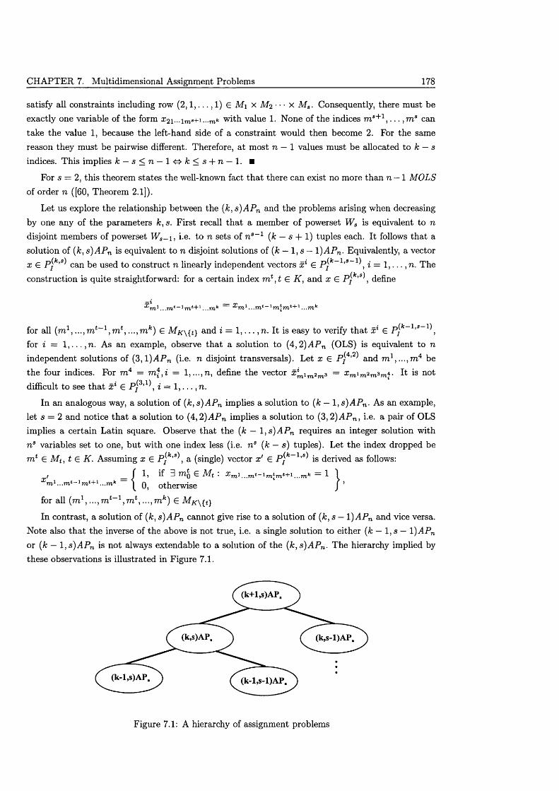
CHAPTER 7. Multidimensional Assignment Problems 178
satisfy all constraints including row (2 ,1 , . . . , 1) G M \ x M2 • • • x M s. Consequently, there must be exactly one variable of the form £21 with value 1. None of the indices m s+1, . . . ,m s cantake the value 1, because the left-hand side of a constraint would then become 2. For the same reason they must be pairwise different. Therefore, at most n — 1 values must be allocated to k — s indices. This implies k — s < n — l < & k < s + n — 1. ■
For s = 2, this theorem states the well-known fact th a t there can exist no more than n — 1 MOLS of order n ([60, Theorem 2.1]).
Let us explore the relationship between the (k ,s )A P n and the problems arising when decreasing by one any of the parameters k,s. First recall th a t a member of powerset W s is equivalent to n disjoint members of powerset Ws- 1, i.e. to n sets of n s~ l (k — s + 1) tuples each. It follows that a solution of (k , s)A P n is equivalent to n disjoint solutions of (k — 1, s — 1 )A P n. Equivalently, a vector x G p ( k,s can be used to construct n linearly independent vectors x % G p ( k~1,s~ 1 i = 1 , . . . , n. The construction is quite straightforward: for a certain index ra* , £ G K , and x G P^k,s\ define
'^mi ...7nt_1mt+1 ...mk ^m1 ...mk
for all (m1, ...,m t_1, m t ) . . . ,m k) G M ^ \y ty and i = 1 , . . . , 71. It is easy to verify th a t x 1 G for i = 1 , . . . , n . As an example, observe that a solution to (4 ,2)APn (OLS) is equivalent to n independent solutions of (3,1 )A P n (i.e. n disjoint transversals). Let x G P j4’2 and m 1,.. .,™4 be the four indices. For m 4 = m j , i = l , . . . ,n , define the vector ^ lm2m3 = xm 1m2m3m*■ ^ is not difficult to see th a t x l G P j3,1\ i = 1 , . . . , n.
In an analogous way, a solution of (k , s)APn implies a solution to (k — 1, s)A P n . As an example,let s = 2 and notice th a t a solution to (4,2)APn implies a solution to (3,2)APn , i.e. a pair of OLSimplies a certain Latin square. Observe th a t the (k — 1, s)A P n requires an integer solution withn s variables set to one, but with one index less (i.e. n s (k — s) tuples). Let the index dropped bem* € M t , t e K. Assuming x G p j k,s\ a (single) vector x' G p ^ k~ 1,s is derived as follows:
/_________________ f if 3 m 0 G Mt . x mi mt - imtmt+ 1 mk 1 1m1...mt- 1mt+1...mfc | o, otherwise J ’
for all (m 1, ...,77it-1 ,ra t , . . . ,m k) G
In contrast, a solution of (A;, s)APn cannot give rise to a solution of (&, s — 1) APn and vice versa. Note also th a t the inverse of the above is not true, i.e. a single solution to either (k — 1, s — 1 )APn or (k — 1 , s )A P n is not always extendable to a solution of the (k ,s )A P n . The hierarchy implied by these observations is illustrated in Figure 7.1.
(M A P .
(k-l,s)AP. (k-l,s-l)AP.
Figure 7.1: A hierarchy of assignment problems
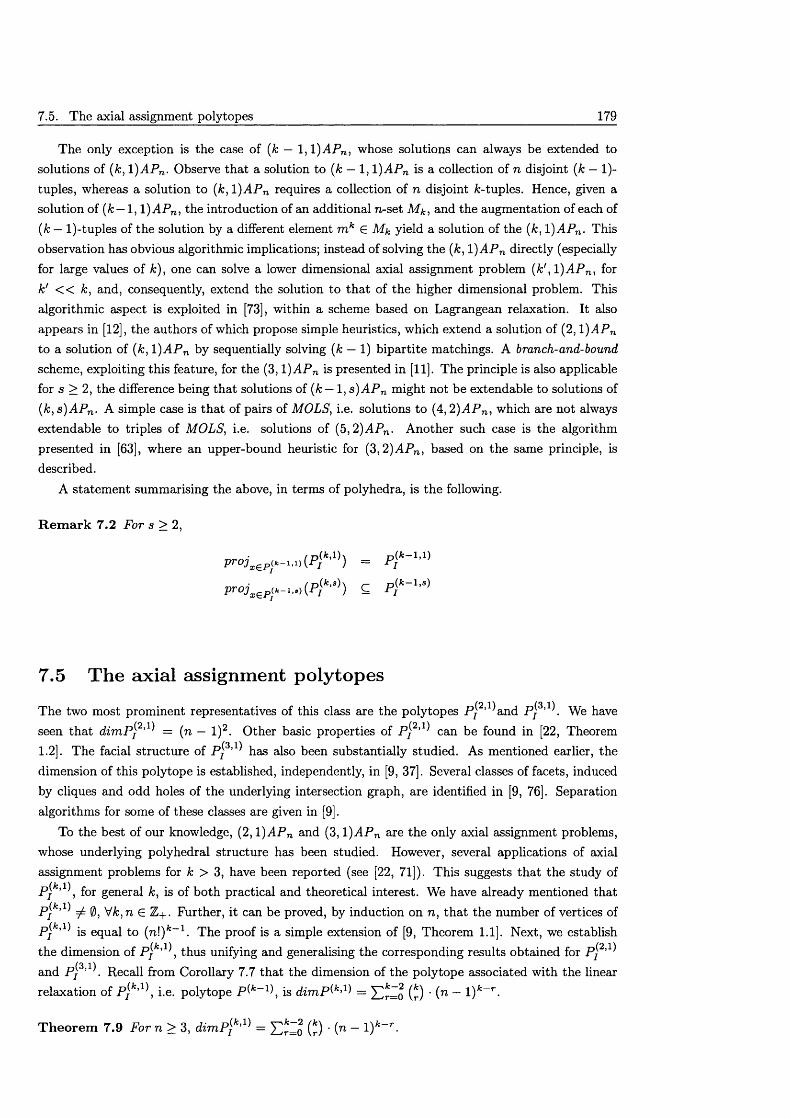
7.5. The axial assignment poly topes 179
The only exception is the case of (k — 1,1 )APn , whose solutions can always be extended to solutions of (k , l )A P n . Observe th a t a solution to (k — 1, l )A P n is a collection of n disjoint (k — 1)- tuples, whereas a solution to (k, l ) A P n requires a collection of n disjoint /c-tuples. Hence, given a solution of (fc — 1, l )A P n , the introduction of an additional n-set Mk, and the augmentation of each of (k — l)-tuples of the solution by a different element m k 6 Mk yield a solution of the (k , 1 )A P n - This observation has obvious algorithmic implications; instead of solving the (k , 1 )A P n directly (especially for large values of k), one can solve a lower dimensional axial assignment problem ( k ' , l ) A P n , for k' << k, and, consequently, extend the solution to th a t of the higher dimensional problem. This algorithmic aspect is exploited in [73], within a scheme based on Lagrangean relaxation. It also appears in [12], the authors of which propose simple heuristics, which extend a solution of (2, l )A P n to a solution of (k, l ) A P n by sequentially solving (k — 1) bipartite matchings. A branch-and-bound scheme, exploiting this feature, for the (3,1 )A P n is presented in [11]. The principle is also applicable for s > 2, the difference being that solutions of (k — 1, s )A P n might not be extendable to solutions of (k ,s )A P n . A simple case is th a t of pairs of MOLS, i.e. solutions to (4,2)A P n , which are not always extendable to triples of MOLS , i.e. solutions of (5,2)APn . Another such case is the algorithm presented in [63], where an upper-bound heuristic for (3,2)A P n , based on the same principle, is described.
A statem ent summarising the above, in terms of polyhedra, is the following.
R e m a rk 7.2 For s > 2,
) = p i
projxep,k- 1>a){Pik's)) C P f - 1>s)
7.5 The axial assignment polytopes(2 1} (3 1)The two most prominent representatives of this class are the polytopes P ) ’ and P ) . We have
seen th a t d im P j2,1 = (n — l ) 2. Other basic properties of P j2,1 can be found in [22, Theorem1.2]. The facial structure of P j3’1 has also been substantially studied. As mentioned earlier, the dimension of this polytope is established, independently, in [9, 37]. Several classes of facets, induced by cliques and odd holes of the underlying intersection graph, are identified in [9, 76]. Separation algorithms for some of these classes are given in [9].
To the best of our knowledge, (2, l ) A P n and (3, l ) A P n are the only axial assignment problems, whose underlying polyhedral structure has been studied. However, several applications of axial assignment problems for k > 3, have been reported (see [22, 71]). This suggests th a t the study of
(k 1)Pj ’ , for general k, is of both practical and theoretical interest. We have already mentioned that p j* ’1) ^ 0} \Jk,n 6 Z+. Further, it can be proved, by induction on n, th a t the number of vertices of p j* ’1) is equal to (n!)fe_1. The proof is a simple extension of [9, Theorem 1.1]. Next, we establish the dimension of P jk,1\ thus unifying and generalising the corresponding results obtained for P j2,1^
( 3 1)and Pj . Recall from Corollary 7.7 that the dimension of the poly tope associated with the linear relaxation of P jk,1\ i.e. polytope pf*-1 ), is d im P ^ ’1) = Ylr=o ir) ‘ (n ~ ^)k~r -
T h e o re m 7.9 For n > 3, dim P jk = X^=o 0 ' (n — ■*■)* T•
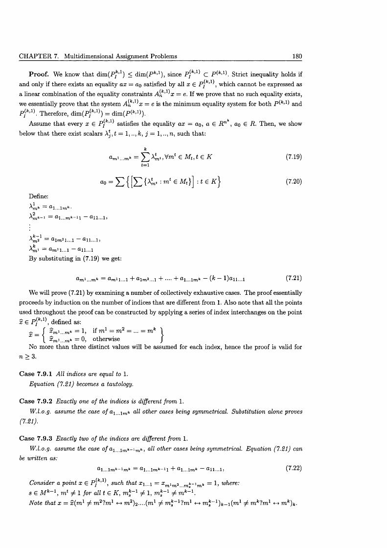
CHAPTER 7. Multidimensional Assignment Problems 180
P ro o f. We know th a t dim (P*’1) < dim (Pfc’1), since p j k’ c P ^ ’1) Strict inequality holds if and only if there exists an equality ax = ao satisfied by all x E P^fc,1\ which cannot be expressed as a linear combination of the equality constraints A ^ ' ^ x — e. If we prove th a t no such equality exists, we essentially prove th a t the system A^f ’ x = e is the minimum equality system for both p ( fc>1) an(j p (M ) Therefore, d im (P jfc’1 ) = dim (P(fc,:l)).
Assume th a t every x E p j k’1 satisfies the equality ax = ao, a E R nk, ao £ R. Then, we show below th a t there exist scalars A* ,£ = 1 , k, j = 1, . .,n, such that:
k
G M u t G K (7<19)t = 1
“o = E { [ E (A- * : mt 6 M‘} ] : t £ K } (7-2°)Define:
^m k mk •\2 _
771*-— 1 . . .T T lk 1
\ A:—1A 77l 2 — a l 77l 2 l . . . l — a l l . . . l )\ kA m l = a m i 1...1 — a i l . . . l
By substituting in (7.19) we get:
^TTl1 . . .m k ^ 771 1... 1 T ® l 77l 2 . . . l "f- '••• “I” ® l . . . l 77l fc l ) ® l l . . . l
We will prove (7.21) by examining a number of collectively exhaustive cases. The proof essentially proceeds by induction on the number of indices that are different from 1. Also note th a t all the points used throughout the proof can be constructed by applying a series of index interchanges on the point x E P jk,1\ defined as:
Xmi...mk = 1) if m 1 = m 2 = ... = m kx m\ mk = 0, otherwise
No more than three distinct values will be assumed for each index, hence the proof is valid forn > 3.
C ase 7.9.1 All indices are equal to 1.Equation (7.21) becomes a tautology.
C ase 7.9.2 Exactly one of the indices is different from 1.W.l.o.g. assume the case of al i m k all other cases being symmetrical. Substitution alone proves
(7.21).
C ase 7 .9 .3 Exactly two of the indices are different from 1.W.l.o.g. assume the case of a- l m k - i m k, all other cases being symmetrical. Equation (7.21) can
be written as:
Q‘l...lmk~1mk ® l . . . l m fc —*1 ”b ® l . . . l m fc ®11...1» (7.22)
Consider a point x E Prk,1\ such that x \ i = x , * = 1, where:r l ' 1 . . . 1 m L m * . . . m 3 7 T i *
s E M k~l , m l 7 1 for all t E K, m k~ l ^ 1, m k~l 7 m k~1.Note that x = x (m 1 ^ m 2l m 1 m 2)2 . ...(m1 7 m k-1l m l m k~1) k - i ( m 1 7 m k?m1 <-> m k)k-
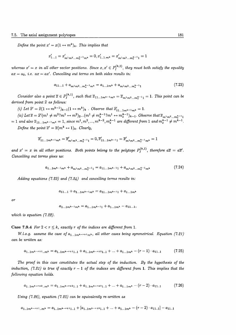
7.5. The axial assignment poly topes 181
Define the point x' = x{ l <-» m k)k. This implies that
X 'l 1 = X ' \ r r , 2 fc = 0 , X ' i fc = X ' f c_ J = 1a...i m 1 raz .. .ma m K * m 1m z . . .m 3 1
whereas x' = x in all other vector positions. Since x , x ' G P jk,l\ they must both satisfy the equalityax — ao, i.e. ax = ax'. Cancelling out terms on both sides results in:
O H . . . 1 + a m i m 2 . . . m £ - 1m fc = a l...lm * + a m i m 2 . . . m * - 1 l ( 7 -2 3 )
Consider also a point x G P jk,1\ such that ’x \ \ . . . \ rn k- 1m.k = #mim2 = 1- This point can bederived from point x as follows:
(i) Let x ' -- x(l <-> m*-1 )fc_ i ( l m k)k . Observe that x'n lmk_lmk - 1.
(ii) L e tx = x ^ m 1 m 2l m l <-► m 2)2...(m 1 m k~l lm } «-> Observe th a txmlfn2 ^ - 4= 1 a n d a /s o = 1, since m 1,m 2, . . . ,m k~2, m k~l are different from 1 a n d m k_1 m k~1.
Define the point x' = x ( m k *-* 1)*. Clearly,
X l l . . . l m k~ 1m k = = 0 > 1 = Xm l m 2 ...m *-l m fc = 1
a n d x ' = x in all other positions. Both points belong to the polytope P jk,l\ therefore ax = ax'. Cancelling out terms gives us:
a l . . . l m k- 1m k + a m 1m 2. . .m s ~ 1l = a H . . . l m fc- 1 l + a m 1m 2 ...rris~1m k ( 7 , ^ 4)
Adding equations (7.23) and (7.24) and cancelling terms results in:
a l l . . . l + a l . . . l m k- 1m k — ® ll. . . lm fc-1l + a l . . . lm fc
or
m k~ 1m k 11 ®11...1>
which is equation (7.22).
C ase 7 .9 .4 For 2 < r < k, exactly r of the indices are different from 1.
W.l.o.g. assume the case of ai lmk-r+1mki aM other cases being symmetrical. Equation (7.21) can be written as:
a l . . lm fc- r+ 1..m fc = a l . . lm fc- r+ 1l . . l + a l . . lm fe- r+2l . . l + ••• + a l . . . lm fc — (r — 1) ' a l l . . l ( 7 -25)
The proof in this case constitutes the actual step of the induction. By the hypothesis of the induction, (7.21) is true i f exactly r — 1 of the indices are different from 1. This implies that the following equation holds.
a l . . l m k- r+'2. .m k = fll . . lm fc- ’’+21„1 + a l . . lm fc~ r+3l . . l + ••• + a l . . . lm fc ~ (r — 2) • a i l . . l (7.26)
Using (7.26), equation (7.25) can be equivalently re-written as
r+1l . . l "h [® l..lm fc-r+ 2 l„ l "I- ••• “f" ® l...lm fc (T ® ll . .l ] ® ll. .l
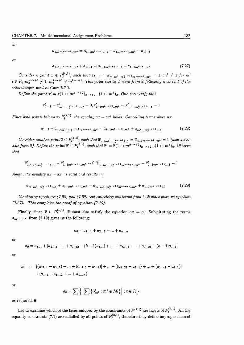
CHAPTER 7. Multidimensional Assignment Problems 182
or
® l..lm k~r+ 1. . mk ® l..lm fc_T'+1l . . l ”1“ . . l m k~ r . . mk ® l l . . l
or
® l . . lm k~r+1 , . mk “I” ® l l . . l ® l . . lm fc_T'+1l . . l “I” ® l . . lm k~ r . . mk (7 .2 7 )
Consider a point x £ such that X 1 ...1 = £ m i m 2 m fc -^ + im fc-r- + 2 m /t = 1 , wi* / 1 for allt £ K , m k~r+1 7 1, m j" r+1 m*-r+ 1 . 77iis point can be derived from x following a variant of the interchanges used in Case 7.9.3.
Define the point x' = x{ \ m k~r+2)k - r+2 ---{l *-> rnk)k■ One can verify that
x l . . . l = Xm i 1.m i-r + 1 ..m* = ^ l . . l m fc- r+2.,mfc = Xm 1...mJ_r+1l . . l = 1
Since both points belong to P jk,1\ the equality ax = ax' holds. Cancelling terms gives us:
a l . . . l + a m l m 2..m £ - - + l m k - r +2._rnk = a i . , l m fc -r+ 2 . .m fc + ®m i,,,m J_r+1i . , i ( 7 -2 8 )
Consider another point x £ P jfc,1\ 5uc/i th a tx mlm2 mfc- r+1i i = ®i..imk- r+1..mfc = 1 (also derivable from x). Define the point x' £ p j k,1\ such tha tx ' = x ( l <-► m k~r+2) k - r+ r n k)k- Observe that
a;m 1m a..m i~r+Il . . l = ,.mfc = 0 , X rTl1 m 2 . . m ^ - r+1m k- r +^ . .mk = X l . . l m k~r + 1l . . l ~ 1
Again, the equality ax = ax' is valid and results in:
a m 1m 2..m £-r+11..1 + a l . . lm fc- ’~+1..mfc = a m 1m 2 . .m ;-T’+1mfc-^+2..mfc + a l . . l m fc- ”+ 1l . l (7 .2 9 )
Combining equations (7.28) and (7.29) and cancelling out terms from both sides gives us equation (7.27). This completes the proof of equation (7.19).
^ ( k 1) ^Finally, since x £ P ) ’ , x must also satisfy the equation ax = ao. Substituting the terms a m 1 . . . mk from (7 .1 9 ) gives us the following:
ao = o i . . . i 4 - U 2 ...2 + ••• + an...7i
or
ao = a 1 ..1 + [<2,21..1 + •• + <21..12 — (k ~ l)&i..i] + . . . + [uni..i + •• + <21.,in — (k — l)ai..i]
or
a 0 — [(a 21..1 — a l . . l ) + ••• + (a n l . . l — a l . . l ) ] + + [(a 1..21 — a l . . l ) + ••• + (a l . .n l — a l . . l ) ]
+ (&!..1 + Ul.,12 + ••• + & l..ln )
or
as required. ■
Let us examine which of the faces induced by the constraints of p (* ’ are facets of P jk,1K All the equality constraints (7.1) are satisfied by all points of p \ k,1\ therefore they define improper faces of
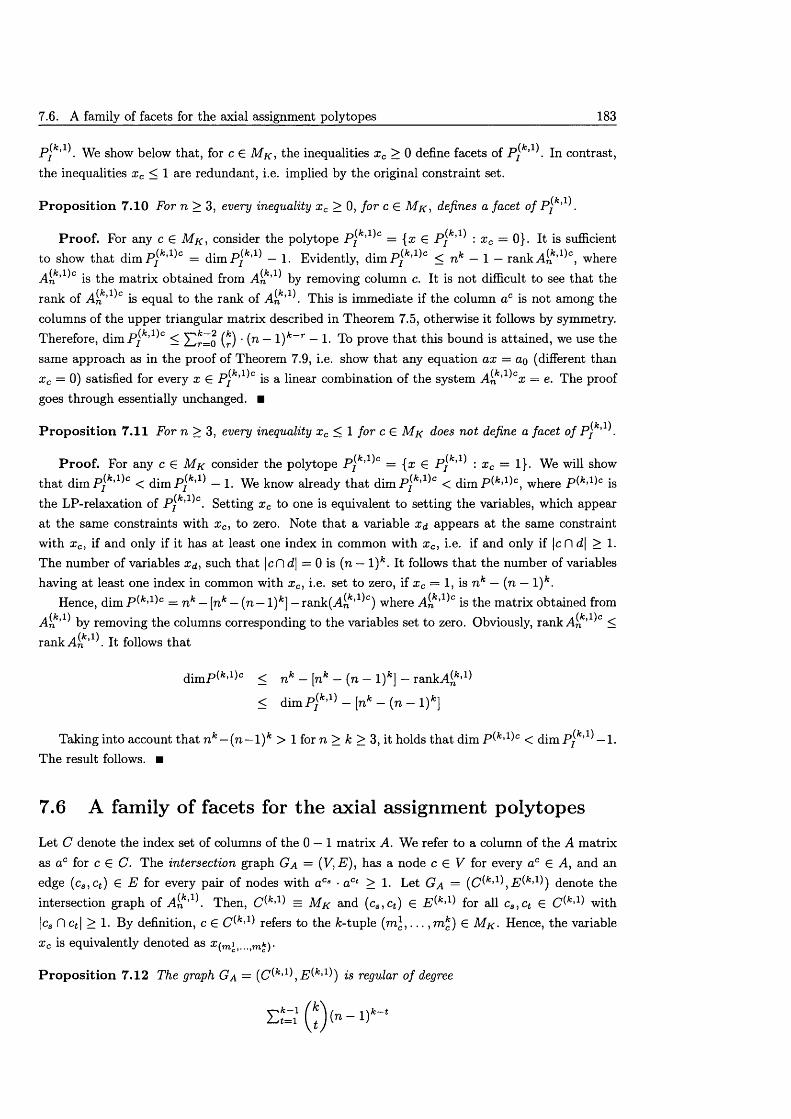
7.6. A family of facets for the axial assignment polytopes 183
p(M ) show below that, for c E M k , the inequalities x c > 0 define facets of P jk,1\ In contrast, the inequalities x c < 1 are redundant, i.e. implied by the original constraint set.
P rop osition 7.10 For n > 3, every inequality x c > 0, for c E M k , defines a facet of P jk,1\
P ro o f. For any c E M k , consider the polytope p ( k,1 c = {x E p^k,V) : x c = 0}. It is sufficient to show th a t dim P jfc,1 c = d im P j* ’1 — 1. Evidently, d im P j* ’1 < n k — 1 — rank Ai*’1 , where A is the m atrix obtained from by removing column c. It is not difficult to see th a t therank of A^f'1 0 is equal to the rank of A ^ ’1 . This is immediate if the column a° is not among the columns of the upper triangular matrix described in Theorem 7.5, otherwise it follows by symmetry.
Therefore, dim P j fc,1 c < X)r=o (r) ' (n — — 1- To prove th a t this bound is attained, we use thesame approach as in the proof of Theorem 7.9, i.e. show th a t any equation ax = ao (different than x c = 0) satisfied for every x E P^k,1 c is a linear combination of the system A ^ ' ^ ° x — e. The proof goes through essentially unchanged. ■
( k 1)P rop osition 7.11 For n > 3, every inequality x c < 1 for c E M k does not define a facet of Pj ’ .
P ro o f. For any c E M k consider the polytope p ( k,1 c = {x E p j k>1 : x c = 1}. We will show th a t d im P j* ’1 < d im P ^ ’1 — 1. We know already th a t d im P j* ’1 < d im P (fc,1)c, where p ( k'l )c is the LP-relaxation of P ^ ’1 . Setting xc to one is equivalent to setting the variables, which appear at the same constraints with x c, to zero. Note th a t a variable xa appears at the same constraint with x c, if and only if it has a t least one index in common with xc, i.e. if and only if |c fl d\ > 1. The number of variables Xd, such th a t |cfl d\ = 0 is (n — l ) fc. It follows th a t the number of variables having at least one index in common with x c, i.e. set to zero, if x c = 1, is n k — (n — l ) fc.
Hence, dim p ( /c’1)c _ n k _ ^n k _ _ rank(Aifc,1 c) where Ai*’1 0 is the m atrix obtained from
A ^ ’1'1 by removing the columns corresponding to the variables set to zero. Obviously, rank A ^ ’1 < rankA i*’1 . It follows that
dim Pl*’1)0 < n k - [nk - (n - 1)*] - rankA ^-1*
< d im P jfc,1) — [nk — (n — 1)*]
Taking into account th a t n k — {n—l ) k > 1 for n > k > 3, it holds th a t dim p ( k'l )c < d im Pj*’1 — 1. The result follows. ■
7.6 A family of facets for the axial assignm ent polytopes
Let C denote the index set of columns of the 0 — 1 m atrix A. We refer to a column of the A matrix as ac for c E C. The intersection graph Ga = {V,E), has a node c E V for every ac E A, and an edge (cs ,ct ) E E for every pair of nodes with aCs • aCt > 1. Let Ga = (C^k,1\ E ^ ’1 ) denote the intersection graph of A n ’l \ Then, C ^ ’1) = M k and (cs ,ct ) E P ^ ’1) for ap cs ,ct E with\c, fl Ct| > 1. By definition, c E C^*’1) refers to the fc-tuple (m*, . . . , m k) E M k - Hence, the variable x c is equivalently denoted as x^mit...jTnfc).
P rop osition 7.12 The graph G a = (C^k,1\ E ^ ' 1 ) is regular o f degree
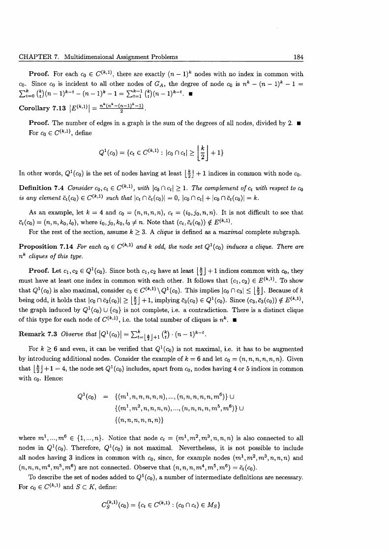
CHAPTER 7. Multidimensional Assignment Problems 184
P ro o f. For each Co G C^k,1\ there are exactly (n — l ) fc nodes with no index in common with Co. Since Co is incident to all other nodes of G a , the degree of node Co is n k — (n — l ) fc — 1 =
E L (?) (» - 1) *- ‘ - (» - 1)* - 1 = E t , 1 (J) (» - ■
C orollary 7.13 I#**'1)! =
P ro o f. The number of edges in a graph is the sum of the degrees of all nodes, divided by 2. ■ For cq G C^k,1\ define
Q1 ) = { c t G : |cq n c t | > + 1}
In other words, Q 1 ( c q ) is the set of nodes having a t least + 1 indices in common with node c q .
D e fin itio n 7.4 Consider CQ,ct G C^k,l\ with \ c q D ct \ > 1. The complement of ct with respect to Co is any element ct (co) G C*^’1) such that \ct fl ct (co)| = 0, |co fl ct \ + |co fl c*(co)| = k.
As an example, let k = 4 and Co = (72, 72, 72, 72), ct = (io , jo ,n ,n ). It is not difficult to see that Ct(co) = (n , n , k 0, l0), where io , jo ,k0,l0 ± n. Note th a t {ct ,c t (co)) g E^k'l \
For the rest of the section, assume k > 3. A clique is defined as a maximal complete subgraph.
P ro p o s itio n 7.14 For each cq G C^k’1 and k odd, the node set Q ^co) induces a clique. There are n k cliques o f this type.
P ro o f. Let ci,C2 G Q 1(co)- Since both ci,C2 have a t least [ |J + 1 indices common with Co, they must have at least one index in common with each other. It follows th a t (ci,C2) G E^k,l\ To show th a t Q 1(co) is also maximal, consider C3 G C ^ ' 1 \ Q 2(c0). This implies |co D C31 < [ | J . Because of k being odd, it holds th a t |c0 D c3(co)| > [ |J + 1 , implying c3(co) G Q x(c0). Since (c3,c3(co)) ^ E (ktl\ the graph induced by Q a(c0 ) U {C3} is not complete, i.e. a contradiction. There is a distinct clique of this type for each node of , i.e. the total number of cliques is n k. M
R em ark 7. 3 Observe that |Q1(c0)| = J+i (?) ' (n “ 1)*"
For k > 6 and even, it can be verified th a t Q1(c0) is not maximal, i.e. it has to be augmented by introducing additional nodes. Consider the example of k = 6 and let Co = ( n , n , n , n ,n , n ) . Given th a t [ |J + 1 = 4, the node set Q 1(c0) includes, apart from Co, nodes having 4 or 5 indices in common with Co. Hence:
0) = {(m 1, 71, n , n , n , n ) , ..., ( n , n , n , n , n , m 6)} U
{(m 1, m 2, n, n, n, n ) ,..., (72, 72, n , n , m 5, m 6)} U
{(72 , 72 , 72 , 72 , 72 , 72)}
where m 1, . . . ,m 6 € {l,...,7i}. Notice that node ct = (7?21,7T22,7723, 72, 72, 72) is also connected to all nodes in Q 1(co). Therefore, Q 1(co) is not maximal. Nevertheless, it is not possible to include all nodes having 3 indices in common with Co, since, for example nodes (m 1,m 2,7723, 72, 72, 72) and (72,72,72,7724,7725,7T26) are not connected. Observe th a t (n , n , n , m 4, m 5, m 6) = ct(co).
To describe the set of nodes added to Q 1(co), a number of intermediate definitions are necessary. For Cq G and S C K, define:
4 M)(co) = {c, € : (co n Ct) € M s )
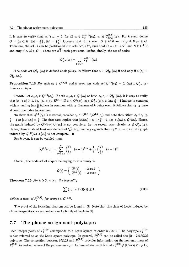
7.7. The planar assignment polytopes 185
It is easy to verify th a t \ct fl cu \ = 0, for all ct £ ( ^ ’ (co), cu £ (c° )- ^or ^ even> defineG = { S C K : \S\ — 1} , |G| = (fc). Observe that, for k even, S € G if and only if K \ S € G. Therefore, the set G can be partitioned into sets G+ , G ~ , such th a t G = G+ U G~ and S € G+ if and only if K \ S £ G ~ . There are 2J"2"L such partitions. Define, finally, the set of nodes
<?G+(C») = (J C'S*'I>( C ° )5eG +
The node set Q2G- (co) is defined analogously. It follows th a t ct G Q ^ +(c0) if and only if ct (co) G
Q g - (c°)-
P ro p o s itio n 7.15 For each cq G C^*’1) and k even, the node set Q 1,2(co) = Q l (co) U Q‘g+(co) induces a clique.
P ro o f. Let ci,C2 G Q 1,2(co). If both ci,C2 G Q 1(co) or both ci,C2 G Q g+(cq), it is easy to verify th a t |ci 0 C2I > 1, i.e. (01, 02) £ E^k,1h If c\ £ Q 1(c0), C2 G Q g+(cq), c\ has f + 1 indices in common with cq, and C2 has | indices in common with cq. Because of k being even, it follows th a t ci, C2 have at least one index in common.
To show th a t Q 1,2{cq) is maximal, consider C3 G C^k>1 \ Q 1,2{cq) and note th a t either |c3 fl cq| < | — 1 or |c3 fl co| = f . The first case implies that |c3(co) fl co| > § + 1, i.e. 03(00) G Q 1^ ) . Hence, the graph induced by Q 1,2(cq) U {03} is not complete. In the second case, clearly, 03 ^ Q q+(co). Hence, there exists at least one element of Q‘g+(cq), namely 04, such th a t |c3 fl 041 = 0, i.e. the graph induced by Q 1,2(co) U {03} is not complete. ■
For k even, it can be verified that:
|QI,SM = E (!0 > ~ 1)*~, + H i ) ' (n“ 1)4t=-J + 1
Overall, the node set of cliques belonging to this family is:
0 ( C) = I Ql(C) : k ° dd 1\ Q 1,2(c) '■ b even J
T h e o re m 7.16 For k > 3, n > 4, the inequality
: 9 e ^(<01 - 1 (7-30)
defines a facet of P jk,1\ for every c £ C ^ ' 1 .
The proof of the following theorem can be found in [3]. Note th a t this class of facets induced by clique inequalities is a generalisation of a family of facets in [9].
7 , 7 The planar assignment polytopes
Each integer point of P^3,2) corresponds to a Latin square of order n ([37]). The polytope p j3,2 is also referred to as the Latin square polytope. In general, P^k’2 can be called the (k — 2)MOLS polytope. The connection between MOLS and p j k'2 provides information on the non-emptiness of p ( fc.2) £or certain values of the parameters k, n. An immediate result is th a t p j 3,2 ^ 0, Vn G Z+ \{1},
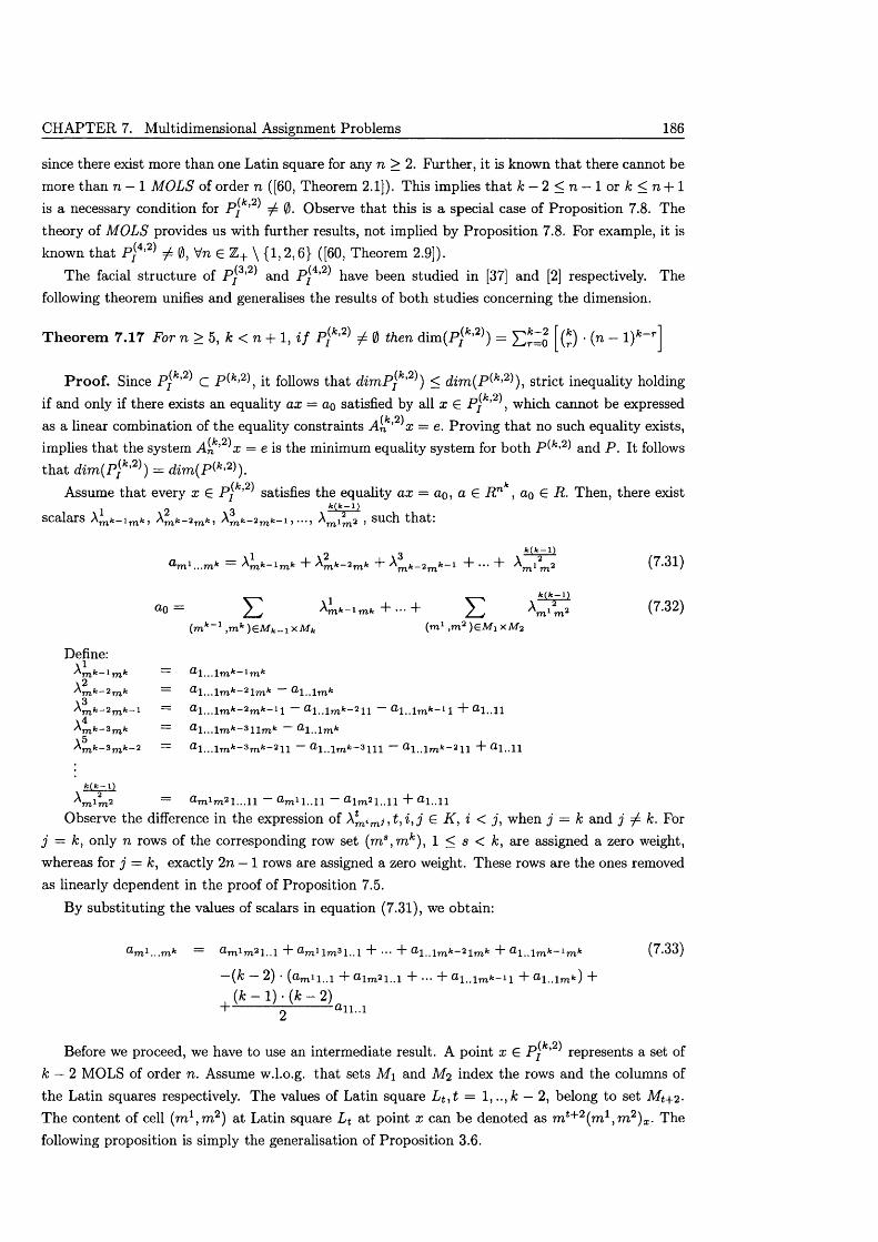
CHAPTER 7. Multidimensional Assignment Problems 186
since there exist more than one Latin square for any n > 2 . Further, it is known th a t there cannot be more than n — 1 M OLS of order n ([60, Theorem 2.1]). This implies th a t k — 2 < n — 1 or A: < n 4-1 is a necessary condition for P^k'2 ^ 0. Observe th a t this is a special case of Proposition 7.8. The theory of M O LS provides us with further results, not implied by Proposition 7.8. For example, it is known th a t p )4,2 ^ 0, Vn £ Z + \ {1,2,6} ([60, Theorem 2.9]).
The facial structure of P )3,2 and P}4,2 have been studied in [37] and [2] respectively. The following theorem unifies and generalises the results of both studies concerning the dimension.
T h e o re m 7.17 For n > 5, k < n 4- 1, i f P^k’2 ^ 0 then d im (P jfc’2 ) = ]Cr=o 0 ' (n —
P ro o f. Since p j k'2 c p ( fc>2), it follows that d im P jk’2 ) < d im (P (k,2)), strict inequality holding if and only if there exists an equality ax = ao satisfied by all x £ p ^k,2>>} which cannot be expressed
( k 2 )as a linear combination of the equality constraints A n ’ x — e. Proving th a t no such equality exists, implies th a t the system A ^ ’2^x = e is the minimum equality system for both p ( fc’2) and P . It follows th a t dim {P jk'2 ) = dim (P^k'2^).
Assume th a t every x £ p j fc’2) satisfies the equality ax = ao, a £ R n>c, ao £ R. Then, there exist1 2 S fc(fc~1}scalars Amfc- i mfc, Amfc_2mfc, Amfc_2mfc_ i , ..., A , 2 . , such that:
ami
ao =
\ i i \ 2
Ai
4 -A c-i + ... + A.*(*-*>
E(mfc_1 ,mfc)GMfc_ i x M fc
Define:\ *
m k~ 1 m k m k~ l m kA2m k~ 2m k ® l.. . lm *_ 2 lm fc ®l.. l m k
^ m k~ 2m k~ l ® l. . . lm fc-2m fc_11 ® l.. l m kA4m fc-3m fc ® l. . . lm fc_3 l l m fc\5/^m k~ ^ m k~ 2 ® l. . . lm fc_3m fc_2l l
fc(fc-i)A 2
m l m 2
1 mk “I- 4* ^ ^(m1 ,m 2 )£M i x M 2
m - nA 2s\ i 2m m
(7.31)
(7.32)
Observe the difference in the expression of A^imj , t, i , j £ K , i < j , when j = k and j / /c. For j — k, only n rows of the corresponding row set (m s,m k), 1 < s < k, are assigned a zero weight, whereas for j = k, exactly 2n — 1 rows are assigned a zero weight. These rows are the ones removed as linearly dependent in the proof of Proposition 7.5.
By substituting the values of scalars in equation (7.31), we obtain:
Q*<m 1 Q 'm 1Tn2 l . . l “I” ^ m 1 l m 3 l . . l 4" 4" “I”
- ( * - 2) - (Q"m 1 l . . l 4- U l m 2 l . . l 4- ••• 4- a l . . l m fc- 1 l 4- +
(ft - 1) - (* - 2)H-------------- n------------- 011..1
(7.33)
Before we proceed, we have to use an intermediate result. A point x £ P^k'2 represents a set of k — 2 MOLS of order n. Assume w.l.o.g. th a t sets M \ and M 2 index the rows and the columns of the Latin squares respectively. The values of Latin square L t , t = — 2, belong to set M t+2-The content of cell (m 1 ,m 2) at Latin square L t at point x can be denoted as m t+2(m l ,m 2)x . The following proposition is simply the generalisation of Proposition 3.6.
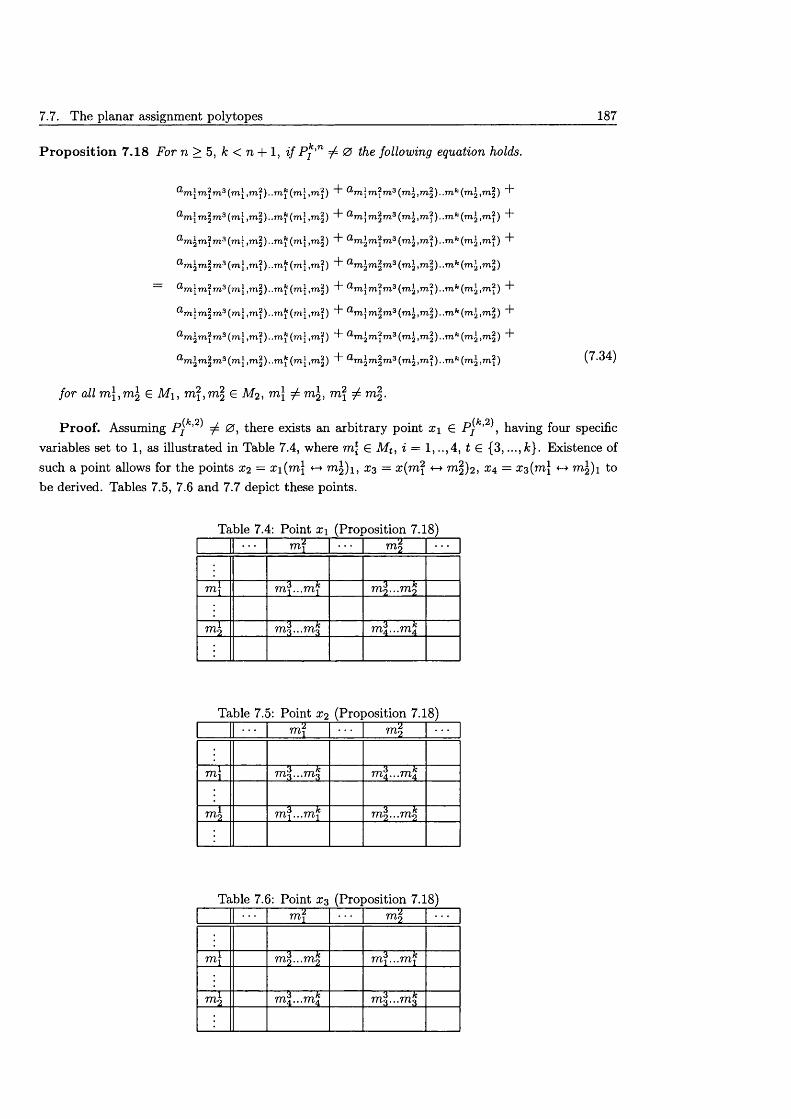
7.7. The planar assignment polytopes 187
P ro p o s itio n 7.18 For n > 5, k < n + 1, i f P k'n ^ 0 the following equation holds.
m 3m 3(m >m i ) .m k (m d - ® m ] m \ m 3 ( ttI j m | ) , m fcK ™ ! ) +
m 2m 3 (m ^ 2 ) ,m k (m ,777*2 d “ ® m ] m 3m 3 ( m l tti3 ) ■ 777fc(m2m ? ) d -
a m \ .m k (m ,7 2 d " ‘m ^m ^m 3 ( m l 7772) . m fc(m2 m ? ) +
a m \ m ^ m 3 ( m , m f ) .m k (m ,771.2 d " ^ m ^ m ^ m 3 (m*l m 2) , m fc (m l m | )
a m \ m 3m 3(rn im l ) .m k (m ,777*2 d " 7773 (777^ m ? ) , m fc (m l m f ) d -
a m \ . m * ( m ,777 d ” 777 J T773 7773 (77I2 m | ) . m fc ( m l m 2) +
a m \ m \ m 3(m. .m?) .m k (m ,777 j a777 l 7n 2 7773 ( 777l m | ) , m fc(m2, m 2) +
a m \ rrv^m3 (m .m k (m ,7772 d - & m \ m \ m 3 (777*2 m f ) ,m k ( m l , m ? )
for all m \ ,m \ G M i , m \ ,m \ G M 2 , m \ 7 m^, m \ ^ m^.
P ro o f. Assuming P^k’2 ^ 0 , there exists an arbitrary point X\ G P jk,2\ having four specific variables set to 1, as illustrated in Table 7.4, where 777} G M t , i = 1, ..,4, t G {3,..., &}. Existence of such a point allows for the points x?, = x \(m \ <-> m ^ i , £3 = x (m \ 7712)2, £4 = £3(7711 <-> 7772)1 to be derived. Tables 7.5, 7.6 and 7.7 depict these points.
Table 7.4: Point x i (Proposition 7.18)771*1 ^ 2
m ]3 A-
. . . m *3 k
m ^ . . . 777,2
m \3 k
m ^ . . . 777,3 777,4 . . .777,4
Table 7.5: Point X2 (Proposition 7.18)777,| m 2
777, { 7 7 7 , |. . .7 7 7 ,J
777,23 A-
777,i ...7 7 7 ,1 7 7 1 2 - - -777,2
Table 7.6: Point x$ (Proposition 7.18)777,'i 7 772
777,} 7 7 7 * 2 ... 777,2 7 7 7 i . . . 7 7 7 i
77^2 7 7 7 ]} . . .7 7 7 ^3 A-
7773 . . . 7 7 7 3
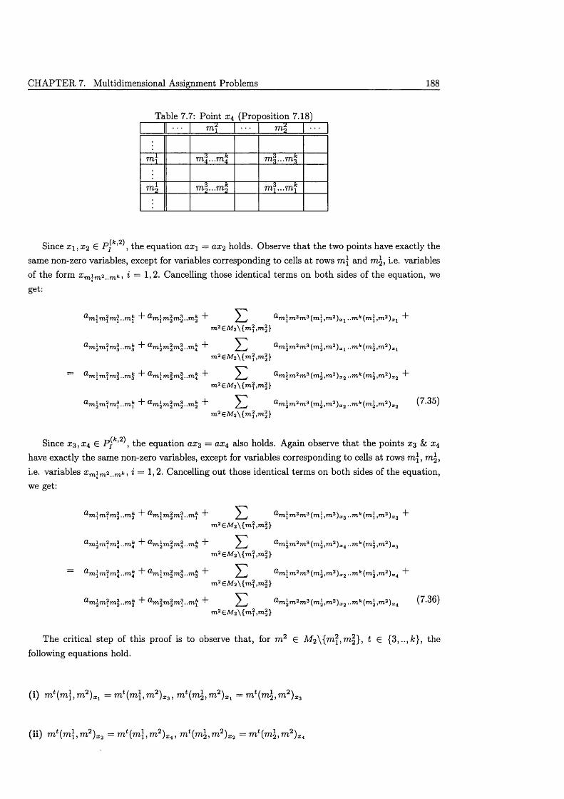
CHAPTER 7. Multidimensional Assignment Problems 188
Table 7.7: Point (Proposition 7.18)m i
m j
m \
Since x i, X2 £ P \k,2\ the equation ax\ = ax2 holds. Observe th a t the two points have exactly the same non-zero variables, except for variables corresponding to cells a t rows m \ and m \, i.e. variables of the form s miTn2..mfc> * = 1,2. Cancelling those identical terms on both sides of the equation, we get:
®‘m \ m \ m \ . . m k d" m fc + ^ ] & m \ m 2m 3 (m \,rn 2)xi . .m k ( m \ , m 2)xi d "
d" flm i m 2m 3 m fc ^ ] a rn2Tn2rn3(rn2,m2)xl ..rnk(m2,rn2)xi
f l r a } r a j m 3 . . m 3 d - t t m i m 2 m 3 m fc - ) - ^ ] ® m l m 2 m 3 ( m b m 2 ) x a . , m k ( m ^ , m 2 ) X 2 d “
m 2£ M 2 \{ m b » r i |}
a “m \ T n \ m \ ..mf d" a m \ m \ m \ , . m % d~ ^ ^ a r n \ r n 2 r n 3 { m \ , r a 2 ) X 2 . . r n k { r n \ , T n 2 ) X2 (7.35)m 2G M 2 \{ m | , m |}
Since S3, X4 G P^k,2\ the equation <2x3 = ax± also holds. Again observe that the points X3 & S4 have exactly the same non-zero variables, except for variables corresponding to cells at rows m \ , m \, i.e. variables x mim 2 _mk, i = 1,2. Cancelling out those identical terms on both sides of the equation, we get:
^ m \ m \ r n 2 . . m 2 d - & m \ m ‘2 r n \ . . m k d ~ ^ ^ & m \ m 2 m 3 ( m \ , m 2 ) X 3 . . m k ( m \ , m 2 ) X 3 d "
m2£M 2\{m 2,m2}
a m 2 m \ m \ . . m k d" ^ m ^ m ^ m 3 . . m ^ d" ^ a m 2 m 2 m a { m 2 , r n 2 ) X i . . r n k { r r i 2 , r n 2 ) X3
m2(E.M2\{m2,m2}
Q ' m \ m \ m \ . .m k P a m \ m 2m^..m^ d~ ^ a m } m 2m 3(rrij,m 2)X2, ,m fc( m l ,m2)I4 d ~
m 2GM2\{m.3,m2}
/m 2m2m2..mk d” &m^m2m\..rnk d- ^ &rn2rn2m2(rn2,rn2)X2..mk{Tn2,rri2)Xtk (7.36)m 2£ M 2\ { m j ,m |}
The critical step of this proof is to observe that, for m 2 G M 2 \{m i,rr i 2 }, t G {3,..,/s}, the following equations hold.
(i) m t (m J,m 2)Xl = m t (m \im 2)X31 ra^ra^, m 2) ^ = m t { m \,m 2)x,
(ii) m t (m \ ,m 2)X2 = m 2)Xi, m t (m ^im 2)X2 = m t (m ^,m 2)s
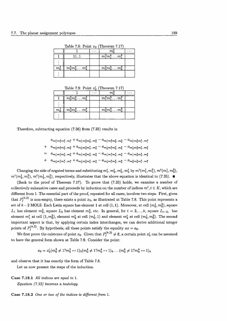
7.7. The planax assignment polytopes 189
Table 7.8: Point x q (Theorem 7.17)1
NOe
1 1 1 . . 1T 4 1cm*rn{ . . . m*
m 0 7772777,2 . . . 777^X 4 k .
. . . m 3
Table 7.9: Point x'Q (Theorem 7.17)1
NO
12 ,
777Q 777Q . . . 777q* 1 4 k
777^ 777^ . . . 7 7 7 *
777Jt 4 Jtrn\m \ . . .
7 4 h 7 7 7 3 7 7 7 3 . . . 7773
Therefore, subtracting equation (7.36) from (7.35) results in
^ m f r n f r n f ..m f + a m\ m jm ^ . .m f a mJ m f m f . .m f ' d> 1 2 n_-|_i 3m^ tt% 2 •.m‘
+ ^ m ^ m ^ m ^ . .m f + a m\ m ^ m f . ■ m ’l a m f m f m f . ■ m ’l - a m f m f m f .. .m.
= a m } m f m | . .m f + a m\ m f m f . ■ m'l — a“m \rn\m \. ■m'l - a m f m f m f . .771.
+ ^ m f m f m f . fc.m f + a m\ m 2m 2- .m f m f m f .. m f ”~ ^ m f m f m f ..m-
Changing the side of negated terms and substituting m \, m^, m \, m \ by m t (m \,m \) , m t {m \,m 2 ), m f i jn ^ m 2), respectively, illustrates th a t the above equation is identical to (7.35). ■
(Back to the proof of Theorem 7.17). To prove th a t (7.33) holds, we examine a number of collectively exhaustive cases and proceeds by induction on the number of indices m t , t € K , which are different from 1. The essential part of the proof, repeated for all cases, involves two steps. First, given th a t p ( k’2 is non-empty, there exists a point x q , as illustrated at Table 7.8. This point represents a set of A: — 2 MOLS. Each Latin square has element 1 at cell (1, 1). Moreover, at cell (m j, m 2), square L \ has element m \, square L 2 has element 777,3, etc. In general, for t = 3 , . . . ,A;, square L t - 2, has element m \ at cell ( l ,m 2), element at cell (m j, 1) and element 777.3 ce^ (m o>m o)- The second im portant aspect is that, by applying certain index interchanges, we can derive additional integer
(A; 2)points of Pj ’. By hypothesis, all these points satisfy the equality ax = ao.We first prove the existence of point x q . Given th a t P^k’2 0, a certain point x'Q can be assumed
to have the general form shown at Table 7.9. Consider the point:
x 0 = x i(m j ^ l?777o «-+ 1)3(t^o ^ 1?mo 1)4 • • • (^0 ^ l ?m o !)fc
and observe th a t it has exactly the form of Table 7.8.
Let us now present the steps of the induction.
C ase 7.18.1 All indices are equal to 1.
Equation (7.33) becomes a tautology.
C ase 7.18.2 One or two of the indices is different from 1.
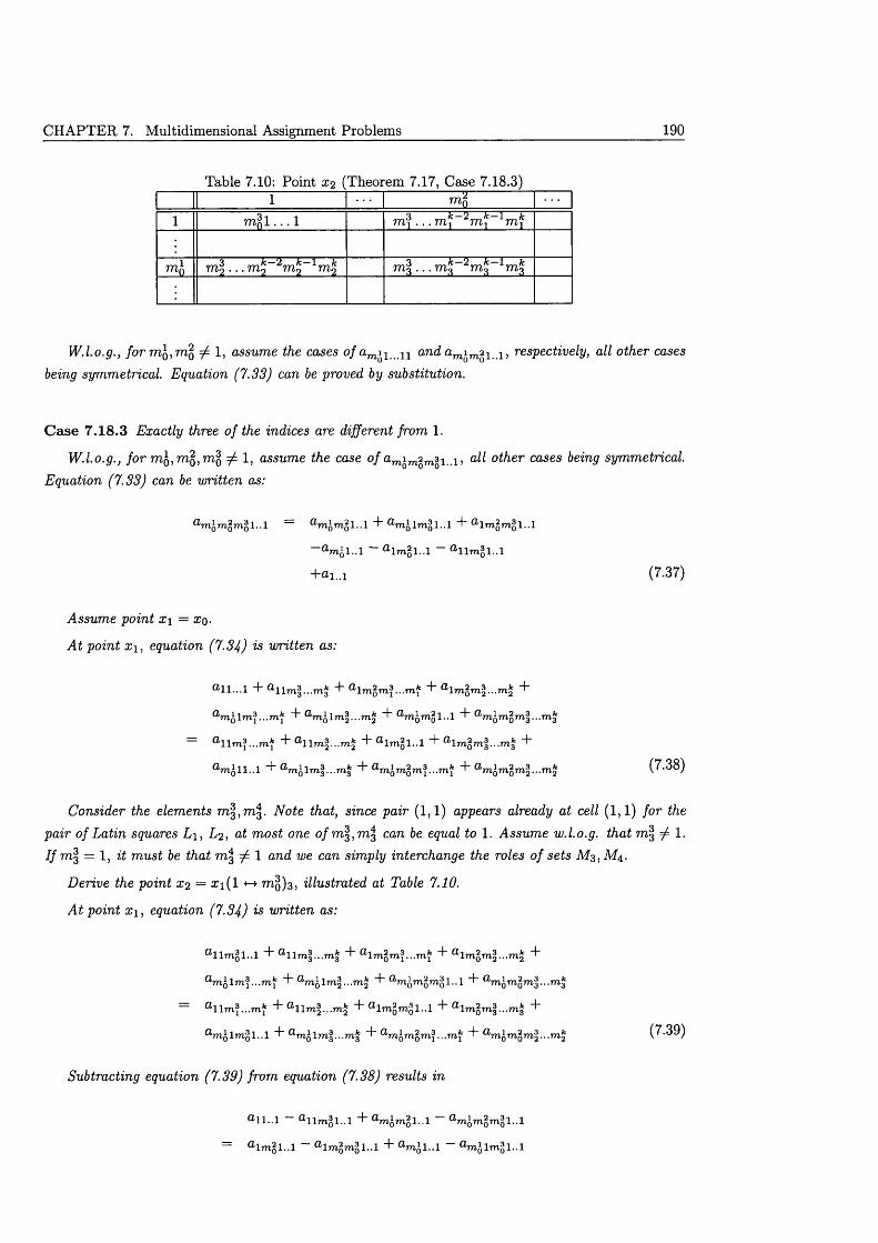
CHAPTER 7. Multidimensional Assignment Problems 190
Table 7 .10 : Point X2 (Theorem 7 .17 , Case 7 .18.3 )1
NO
1 7 7 2 0 1 . . . 1
m 0 7722 • • • 7 7 2 * - 2 7 7 2 2 _ 1 7722 777,3 • • • 777,3 _ 2 7 7 2 3 _ 1 777,3
W.l.o.g., forrriQ,mQ ^ 1 , assume the cases of aTn 1 n and amim21..1, respectively, all other cases being symmetrical. Equation (7 .33) can be proved by substitution.
C ase 7 .1 8 .3 Exactly three of the indices are different from 1 .
W.l.o.g., /o r rag, rag, mg ^ 1 , assume the case of amim2m3lifl, all other cases being symmetrical. Equation (7.33) can be written as:
(7 .37)
Assume point x\ = x q .
At point x \, equation (7 .34) ^ written as:
a l l . . . l “I" “I” a lm §m f.. .m f "b "b
...mf "b ^ m o l " b omol-.l <»Tiomom 3’"m3
"b "b ® lm §l. . l "b "b
a m o l l . . l "b a molm|. . .m3 "b "b a,mQmQm\.. .m^ (7 .38)
Consider the elements 7723,777,3. Ao£e that, since pair (1, 1) appears already at cell (1 , 1) for the pair of Latin squares L \, L2, at most one 0/7713,777,3 can be equal to 1 . Assume w.l.o.g. that 777,3 7 1 - 7/777,3 = 1, it must be that 777,3 7 1 anc iye can simply interchange the roles of sets M3, M4.
Derive the point X2 = x \{ \ <-» 7720)3, illustrated at Table 7 .1 0 .
A t point Xi, equation (7 .34) *5 written as:
a l lm g l . . l + a llm3...mJ + a lmgm?.. .mf + a l m X - m 2 +
"b "b ®mQm§mol..l ~b a mJmQm3.,.mJ
"b ...m£ "b a lm§m^l..l "b a lm §m |.. .m £ *b
^m olm ol- . l b- b~ <2m i)7Tl2m3 m fc *b <2m i m 2m3 mfc (7 .39)
Subtracting equation (7.39) from equation (7.38) results in
® l l . . l ^ l l m o l . , 1 b” ® m o 7 T i Q l . . l . 1
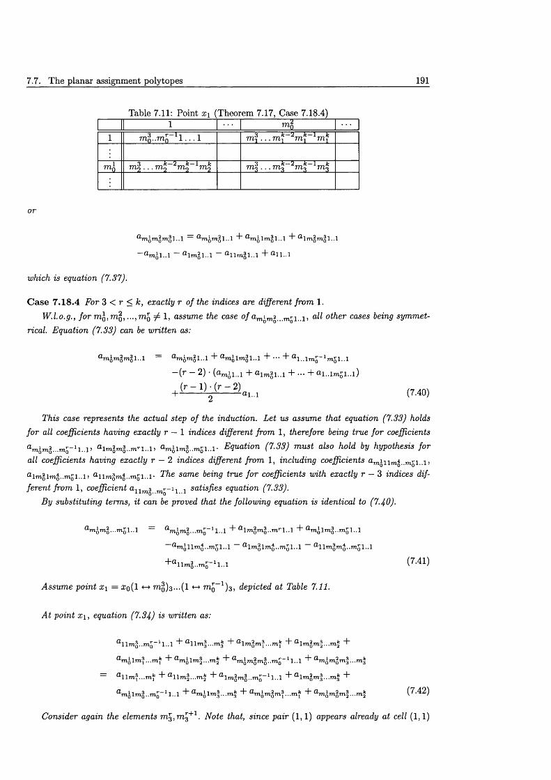
7.7. The planar assignment polytopes 191
Table 7.11: Point x \ (Theorem 7.17, Case 7.18.4)1
NO
1 m n . . m f j _ 1 l . . . 1 7 7 1 ? . . . 7 7 7 ? 2 7 7 l t 1 7 7 l f
m n 777-2 • • • 777,2 ~ 2 777-2 _ 1 777,2 777-3 • • • 777-^ _ 2 777, 3 _ 1 777,3
or
^rnQmgl.-l 4” 4“ fllmomQl..l
_ a m J 1 ..1 — a l m g l . . l — a l l m g l . . l + a l l . . l
which is equation (7.37).
C ase 7 .18.4 For 3 < r < k, exactly r of the indices are different from 1.W.l.o.g., for m o,ra0, . .. ,m rQ ^ 1, assume the case o / a mim2 mr! 1; all other cases being symmet
rical. Equation (7.33) can be written as:
a m j 7n g m g l . . l = a m ^ m g l . . l + a m i l m g l . . l + ••• +
— ( r — 2 ) • + a i m g i . . i + ••• + a i . . i m | ; i . . i )
+ (’-_- l ) ± _-2 j 0 l l (7.40)
This case represents the actual step of the induction. Let us assume that equation (7.33) holds for all coefficients having exactly r — 1 indices different from 1, therefore being true for coefficients
a m'0m l . . . m r0- 1 i.. i> a im § m 3 . .m n . . i . OmJimg..m5i..i- Equation (7.33) must also hold by hypothesis for all coefficients having exactly r — 2 indices different from 1, including coefficients flmi n mi„mrliil, a imgim^..m5i..i) a iimgmg..m5i.. i• The same being true for coefficients with exactly r — 3 indices different from 1, coefficient aUm3 j satisfies equation (7.33).
By substituting terms, it can be proved that the following equation is identical to (7-40).
a m*m%...m£ 1..1 = 1..1 "P a lm lm % ..m r l . . l +
a'mollmo..mol..l ®lmolmo..mol..l a llmQmQ..mQl..l
+ a i l m g . . m 5 - 1 l . . l ( 7 -4 1 )
Assume point x \ = rco(l 777,0)3...(1 mQ- 1)3, depicted at Table 7.11.
A t point x \ , equation (7.34) is written as:
a i lm 3 . .m 5 -1l . . l + a l l + a l m gm ^„m 2fc +
= G l l m f - m * + a l l m 3. . . m £ + a l 7n g m § . . m ; ; - 1 l . . l + a l m g m f . . . m * +
amilm3..mS_1l..l + (7.42)
Consider again the elements m ^ ,m ^+1. Note that, since pair (1,1) appears already at cell (1,1)
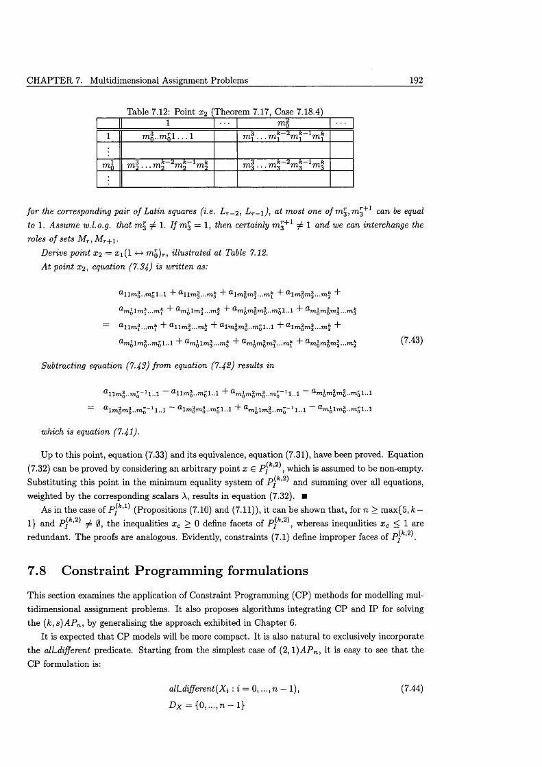
CHAPTER 7. Multidimensional Assignment Problems 192
Table 7.12: Point X2 (Theorem 7.17, Case 7.18.4)1 mg
1 m ^..m (A . . . 1 mi • ■ • rnk~2m k~l m k
m l m 2 . . . m k~2m k~1m k raj* . . . m k~2m k~l m k
for the corresponding pair o f Latin squares (i.e. L r- 2 , L r - i ) , at most one of can be equalto 1. Assume w.l.o.g. that m 3 ^ 1. I f m 3 = 1, then certainly m ^+1 7 1 and we can interchange the roles of sets M r ,M r+\.
Derive point X2 = £ i( l Tng)r , illustrated at Table 7.12.A t point X2 , equation (7.34) ^ written as:
® l l m Q . . m Q l . . l " b 4 * O i m 2 m 3 m fc + U i m 2 m 3 _ m k +
. . .m i "h 4” ®mgmQmg..m51 . ,l "b ...m*
= a llrnf.- .mf + "h a l " b
®mQlmQ..mol..l "b ,rnQlm^...m^ d" n m i m 2m3_ _m fc + 0,m i m 2m3__ m fc (7.43)
Subtracting equation (7.43) from equation (7.42) results in
a llm g..m 5_1l . . l — a llmg..mj;i .. l + a,m£mgmg..mS~11..1 — a mimgmg..mS 1..1
= a lmgmg..mo- 1 l . . l ~ a lm§mg..m51 .,l + a m£lmg..m£_11..1 ~ a m£lmg..m|;i. .l
which is equation (7-41) •
Up to this point, equation (7.33) and its equivalence, equation (7.31), have been proved. Equation (7.32) can be proved by considering an arbitrary point x E P jk,2\ which is assumed to be non-empty. Substituting this point in the minimum equality system of and summing over all equations,weighted by the corresponding scalars A, results in equation (7.32). ■
As in the case of p ( k>1 (Propositions (7.10) and (7.11)), it can be shown that, for n > max{5, k — 1} and p ( k'2 zfz 05 the inequalities x c > 0 define facets of P jk,2\ whereas inequalities x c < 1 are redundant. The proofs are analogous. Evidently, constraints (7.1) define improper faces of P jk,2K
7.8 Constraint Programming formulations
This section examines the application of Constraint Programming (CP) methods for modelling multidimensional assignment problems. It also proposes algorithms integrating CP and IP for solving the (k ,s )A P n , by generalising the approach exhibited in Chapter 6.
It is expected th a t CP models will be more compact. It is also natural to exclusively incorporate the all-different predicate. Starting from the simplest case of (2,1 )A P n) it is easy to see that the CP formulation is:
all-different(Xi : i = 0, ...,n — 1),
D x = {0, ...,n - 1}
(7.44)
7.8. Constraint Programming formulations 193
Hence, the above formulation provides n pairs (z, X i), i = 0,..., n — 1. In other words, Xij = 1 if and only if X i = j (see also [53], [89]).
Concerning the (3, l )A P n , recall that a solution to this problem is a set of n disjoint triples. Hence, define variables X } , X f and the auxilliary variable Z\. We wish to form n triples (z, X f , X f ) , for i = 0 ,..., n — 1. Variables X f must be pairwise different and the same must hold for variables X f . The formulation is the following:
all-different(Xf : z = 0 ,. . . ,n — 1)
alLdifferent(X f : z = 0,..., n — 1)
D x = {0, ...,n — 1}
Notice again th a t Xijk = 1 if and only if X* = j and X f = k.
Generalising this approach, the formulation of (k , l)^4Pn is the following:
alLdifferent(X f : z = 0, ...,n — l),fo r p = 1,..., k — 1
D x = {0 , ...,n - 1}
This is a formulation involving (k — 1) • n variables and (k — 1) all-different constraints. The variable of the IP model is 1 if and only if X ^ i = m 2, ..., X ^ 1 = m k.
The constraints for the Latin square problem ((3,2)i4Pn) and for the OLS problem ((4 ,2)AP n) have already been given in Section 5.3.1, while the CP formulation for a triple of MOLS ((5,2)A P n) was presented in Section 6.5.1. We examine the generalisation of this formulation to the problem of finding k — 2 MOLS ((k , 2)A P n), where k < n + 1 (Proposition 7.8). The formulation for the 3-MOLS problem was presented in Section 6.5.1. Let variables X f j , p = 1,..., A: — 2 denote the contents of the p th Latin square. Let also variables ZfJ, q, r = 1 , . . . ,n ,q < r, enforce the orthogonality betweenany of the Q) pairs (q, r) of Latin squares, by imposing th a t = X \- + n • Xf-. Variables Xf-and Zfj have domains of cardinality n and n 2, respectively. All-different constraints are required to ensure th a t (a) cells in each row and column of all squares contain pairwise different values and (b) all ordered pairs of values appear exactly once in any pair of Latin squares (i.e. all Zfff variables are pairwise different, for a certain pair (L q,L r) of Latin squares. The CP formulation is the following:
all-different (Xf j : i = 0 , ...,n — 1), for j = 0 ,..., n — 1, p = l , . . . , k — 2
alLdifferent(Xfj : j = 0, ...,n — 1), for z = 0,..., n — 1, p = l , . . . ,k — 2
all-different(Zfj : z, j = 0, ...,n — 1), for <7, r = 1,.., k — s, q < r (7-45)
z ij = x ij + n ' X f j , for i , j , = 0,..., n — 1, q ,r = l,..,fc - 2,q < r
D x = {0, ...,n — 1}, D z = {0, ...,n 2 — 1}
This is a model involving (k — 1) • n 2 variables and (2) (1 + n 2) +2- (k — 2) -n constraints. Notice th a t the number of indices for each variable is 2, i.e. equal to param eter s, and th a t the number of X variables is A: — 2, i.e. k — s.
Hence, for s > 2, k — s < n — 1 (Proposition 7.8), the CP formulation requires (k — s) n-ary variables with s indices, i.e. variables X ^ mS, p = 1, . . . ,k — s , and m l G {0, ...,n — 1} for z = 1,It also requires (™) auxilliary variables again with s indices and domains of cardinality n s , in order to
1 senforce the “hyper-orthogonality” constraints among the X variables. These are variables Z ^ 1.. mS,
CHAPTER 7. Multidimensional Assignment Problems 194
where p 1 < ... < ps and pl € {l,...,fc — s} for i = 1 , ...,p. The CP formulation for (k ,s )A P n is the following:
alLdifferent(X^ll mS : m 1 = 0,..., n — 1), for m 2, ..., m s = 0 ,..., n — 1, p = 1,..., k — s
alLdifferent(X^ll ma : m s = 0, ...,n — 1), for m 1, ..., m s~l = 0 ,..., n — 1, p = 1,..., A; — s
alLdifferent( ' [pmB : m 1, ...ms = 0, ...,n - 1), for p 1, ...,ps = 1,.., fc - s, p 1 < ... < ps(7.46)
m 1, m '" 1 = 0, . . , 71 - 1, p 1 < ... < pSi = 1
-Dx = {0, ...,n - 1}, D z = {0, ...,7is - 1}
These formulations can be used to solve the ( k , s )APn via CP methods. The central procedure to be applied is the algorithm of [77], which achieves generalised arc-consistency for alLdifferent constraints. Recall th a t this algorithm runs in 0 (p 2d2) steps for p variables with domains of cardinality a t most d. For an alLdifferent constraint on the Z variables in (7.46), this algorithm requires 0 ( (n s)2 • (tis)2) = 0 ( n 4s) steps.
Algorithms integrating CP and IP are easy to design. First, recall algorithm CPI of Chapter 6, i.e. an algorithm incorporating IP within a CP search tree. This scheme is naturally generalised for the (k , s)A P n . The main principle is to assign values to subsets of variables with CP and periodically call IP in order to (a) derive a tighter bound on the objective function or (b) prove infeasibility or (c) extend a partial CP assignment to a complete one.
For an extension of algorithm IPC (Chapter 6), one would have to incorporate CP techniques to preprocess each subproblem of the IP search tree. Observe that each constraint set of (k ,s )A P n can be associated to an alLdifferent constraint. As an example, consider one of the constraint sets of the OLS problem:
, 7712 = 0, ...,77. - 1} = 1, for m 3,77l4 = 0, ...,77 - 1
The alLdifferent constraint associated to this constraint set is
alLdifferent{Wmim 2 : m 1 ,m 2 = 0, ...,ti — 1}
D w = {0, • •., 7i2 — 1}
where each value of D w has an 1 — 1 correspondence to each ordered pair (m 3,m 4). Hence, two indices are retained explicitly in the CP variables, while the remaining two indices are incorporated in the domain. If constraint propagation implies that (7n3,77i4) ^ D w mim2 then variable xmim2Tn3m4 of the IP model must be set to 0. Note that, by symmetry, an equivalent constraint would be:
alLdifferent{Wm2 mi : m 3,m 4 = 0, ...,ti — 1}
D w = {0, • • •, 7i2 — 1}
where each value of D w would have an 1 — 1 correspondence to each ordered pair (rn1,7n2).
7.9. Concluding remarks 195
For the (k , s ) A P n consider, without loss of generality, the constraint set:
i m 2 , . . m fc : m 1 G M 1,.. . ,m k~s~1 £ M k~s~ l , m k~s £ M k_s} = 1
for all m k~s+1 £ M k- s+i ,m k~s+2 £ M k -s+2 , •••, m k £ M k
There are s indices left “free” , i.e. outside the sum, and k — s used for the summation. An associated alLdifferent constraint should incorporate all indices either in the variables or in their domains, exactly as for the OLS problem. The constraint is as follows:
alLdifferent{Wmi...rnk-3 : m 1, ... ,m k~s = 0, ...,n — 1} (7.47)
D w = {0, ... ,n s — 1}
if k — s < s, i.e. s > and
alLdifferent{WTnk-s+i...rnk : m k~s+1, ... ,m k = 0, ...,n — 1} (7-48)
D w = {
if s < | . The reason we have to distinguish between these two cases is th a t an alLdifferent is feasible only if the number of variables is less than or equal to the cardinality of the domains (Remark 5.2 . Notice for example that, for s < constraint (7.47) is infeasible.
7.9 Concluding remarks
This chapter introduced IP and CP models for general assignment problems. The IP model establishes a framework for unifying the polyhedral analysis of all assignment polytopes belonging to this class. In particular, the dimension of the linear relaxation of all members of this class is derived. A hierarchy among assignment polytopes is naturally imposed. Focusing on the classes of axial and planar assignment polytopes, it has been proved th a t their dimension equals a sum of terms from Newton’s polynomial. The potential of this unified approach is dem onstrated by identifying a familyof clique facets for all axial assignment polytopes, for k > 3. We also proposed CP models, whichcan be linked to the IP ones within a framework integrating CP and IP.

CHAPTER 7. Multidimensional Assignment Problems 196
List of Figures
2.1 The antiweb AW(8,3) ............................................................................................................... 182.2 The antiweb A (c ,d ) ...................................................................................................................... 192.3 A wheel of size 7 ......................................................................................................................... 202.4 The nodes of a lifted wheel inequality .................................................................................. 282.5 A 5-wheel with triple sets on the s p o k e s .............................................................................. 302.6 A 9-cycle of type I ...................................................................................................................... 322.7 A 9-cycle of type II, ( m = 3 ) ..................................................................................................... 342.8 An 11-cycle of type II ( m = 4 ) .................................................................................................. 352.9 Nodes of a lifted 9-cycle in e q u a lity ........................................................................................ 372.10 The antihole of Case 2 .3 4 .1 ..................................................................................................... 392.11 The antihole of Case 2 .3 4 .5 ..................................................................................................... 402.12 The antihole of Case 2 .3 4 .6 ..................................................................................................... 412.13 The antihole of Prop. 2 .3 5 ......................................................................................................... 42
3.1 The m atrix A for n = 2 ............................................................................................................ 453.2 The upper triangular m atrix for n = 2 .................................................................................. 483.3 A solution violating (3.31) for n = 6......................................................................................... 603.4 A solution violating (3.31) for n o d d ...................................................................................... 603.5 A solution violating (3.31) for n = 7 ...................................................................................... 61
4.1 An example of the branching m echanism .............................................................................. 105
5.1 An example of arc-consistency.................................................................................................. 1275.2 Second step in achieving arc-consistency.............................................................................. 1275.3 Arc consistent s u b g ra p h ............................................................................................................ 1275.4 An example of a BT search t r e e ............................................................................................... 1305.5 The search tree for FC ............................................................................................................ 1325.6 The BJ s c h e m e ............................................................................................................................ 134
7.1 A hierarchy of assignment problems ..................................................................................... 178
197

LIST OF FIGURES 198
List of Tables
1.1 A pair of OLS of order 4 ............................................................................................................ 11.2 The multiplication table of (Z±, + ) ........................................................................................ 21.3 Isotopic and isomorphic squares of L\ ................................................................................. 41.4 A pair of incomplete OLS of order 2 ..................................................................................... 10
2.1 Odd cycle for m odd and m e v e n ........................................................................................... 342.2 Odd cycle of G a , m odd ........................................................................................................ 35
3.1 Linearly dependent rows removed at Step I ........................................................................ 463.2 Linearly dependent rows removed at Steps I - I I .................................................................. 463.3 Linearly dependent rows removed at Steps I - I I I ................................................................ 473.4 Linearly dependent rows removed at Steps I - I V ................................................................ 473.5 Linearly dependent rows removed at Steps I - V .................................................................. 473.6 Point x q ......................................................................................................................................... 503.7 An arbitrary point x E Pj (Lemma 3 . 4 ) .............................................................................. 503.8 Point x Proposition 3 . 6 ) ........................................................................................................... 513.9 Point x' (Proposition 3 . 6 ) ........................................................................................................ 523.10 Point x (Proposition 3.6) 523.11 Point x' Proposition 3 .6 ) ............................................................................................................ 523.12 Point ^ (T h eo rem 3 .5 ) ............................................................................................................... 543.13 Point X3 (Theorem 3 .5 ) ............................................................................................................... 553.14 Point x (Lemma 3 .2 4 ) ............................................................................................................... 673.15 Point x (Lemma 3 .2 4 ) ............................................................................................................... 673.16 Point x (Lemma 3 .2 5 ) ............................................................................................................... 693.17 Point x (Step 1) ......................................................................................................................... 713.18 Point x (Step 2) ......................................................................................................................... 713.19 Point x (Step 4) ......................................................................................................................... 733.20 Point x t a b l e ............................................................................................................................... 733.21 Rectangle R 1 ............................................................................................................................... 783.22 Rectangle R 2 ............................................................................................................................... 793.23 Rectangle R1 & R2 for m =5 793.24 Rectangle R1 for Case 3.29.1, k o d d ....................................................................................... 803.25 Rectangle R1 for Case 3.29.1, k e v e n ....................................................................................... 803.26 Rectangle R1 for m =5 for Case 3.29.1, k odd & even resp.................................................. 803.27 Rectangle R1 for Case 3.29.2, j o d d .......................................................................................... 813.28 Rectangle R1 for Case 3.29.2, j e v e n ...................................................................................... 81
199
LIST OF TABLES 200
3.29 Rectangle R1 for m =5 for Case 3.29.2, j odd & even resp.................................................... 813.30 Rectangle R1 for Case 3.29.3, i o d d .......................................................................................... 823.31 Rectangle R1 for Case 3.29.3, i e v e n ...................................................................................... 823.32 Rectangle R1 for m =5 for Case 3.29.3, i odd & even resp.................................................... 833.33 Remaining cases to be e x a m in e d ............................................................................................. 833.34 Rectangle R1 for Case 3 .2 9 .4 .................................................................................................. 843.35 Rectangle R1 for m =5, Case 3 .2 9 .4 ......................................................................................... 843.36 Rectangle R1 for Case 3.29.5, k=m +2,...,n 843.37 Rectangle R1 for Case 3.29.5, k = 4 ................................................................................ 853.38 Rectangle R1 for Case 3.29.7, k=m +2,...,n 853.39 Rectangle R1 for Case 3.29.7, k = 3 ................................................................................ 863.40 Rectangle R1 for Case 3.29.7, k=m +2,...,n 863.41 Rectangle R1 not belonging to Q ............................................................................................ 863.42 Rectangle R2 belonging to Q .................................................................................................. 87
4.1 A pair of OLS of order 4 ............................................................................................................ 914.2 Variable fixing and domain red u ctio n ..................................................................................... 944.3 The two Latin squares of order 2 ............................................................................................. 944.4 Dual values for a reduced Latin square of order 2 ................................................................ 954.5 A Latin square of order 6, belonging to the second main c l a s s .......................................... 964.6 Dual values for a reduced Latin square of main class 2 ....................................................... 984.7 Counting the number of values removed from square Y .................................................... 1034.8 A pair of OLS after preliminary variable f i x i n g ................................................................. 1054.9 Allowed values at the first row ............................................................................................... 1054.10 Results for LP-solving a lg o rith m s............................................................................................ I l l4.11 Results for the branching s tra teg ie s ......................................................................................... 1124.12 The impact of a random objective f u n c t io n ........................................................................ 1124.13 Results for preprocessing............................................................................................................ 1134.14 Branch &; Cut with a single family of cutting p l a n e s ....................................................... 1144.15 Number of nodes when a single family of cutting planes is u s e d ................................... 1154.16 Cuts added per n o d e ................................................................................................................... 1154.17 Branch & Cut with different orders of s e p a ra t io n .............................................................. 1154.18 Strategies for cut a d d it io n ......................................................................................................... 1174.19 Results for three cut s t r a te g ie s ............................................................................................... 1174.20 Improvements over simple Branch & B o u n d ........................................................................ 117
5.1 Formula for OLS of order 2 ...................................................................................................... 1235.2 Methods for constraint p ropagation ........................................................................................ 1425.3 Counting the number of reduced Latin s q u a r e s .................................................................... 1435.4 Comparing branching rules for the BT a lg o r ith m ................................................................ 1435.5 Comparing branching rules for the FC a lg o r i th m ................................................................ 1445.6 Comparing propagation p rocedures........................................................................................ 1445.7 Frequency of filtering ................................................................................................................... 145
6.1 Results for algorithm I P C ........................................................................................................... 1566.2 Results for algorithm C P I ........................................................................................................... 157
LIST OF TABLES 201
6.3 Comparative results for C P /IP a lg o rith m s............................................................................. 1586.4 Percentage of infeasible nodes pruned .................................................................................... 1586.5 Identifying triples of MOLS of order n .................................................................................... 1636.6 Examining the role of parameter t .......................................................................................... 1636.7 Estim ating the average elapsed time for an instance of n = 1 0 ......................................... 164
7.1 Examples of assignment s t r u c tu r e s .......................................................................................... 1677.2 1767.3 Known values of d im P jk,s^............................................................................................................ 1767.4 Point x \ (Proposition 7 . 1 8 ) ........................................................................................................ 1877.5 Point X2 (Proposition 7 . 1 8 ) ........................................................................................................ 1877.6 Point £3 (Proposition 7 . 1 8 ) ........................................................................................................ 1877.7 Point £4 (Proposition 7 . 1 8 ) ........................................................................................................ 1887.8 Point £q (Theorem 7 .1 7 ) ............................................................................................................. 1897.9 Point x'Q (Theorem 7 .1 7 ) ............................................................................................................. 1897.10 Point £2 (Theorem 7.17, Case 7 .18.3)...................................................................................... 1907.11 Point £1 (Theorem 7.17, Case 7 .18.4)...................................................................................... 1917.12 Point £2 (Theorem 7.17, Case 7 .18.4)...................................................................................... 192

LIST OF TABLES 202
Bibliography
[1] Appa G., M athematical programming formulations of the orthogonal Latin square problem. LSEO R Working Paper Series: LSEOR 01.37.
[2] Appa G, Magos D., Mourtos I., Janssen J.C.M. (2001): On the Orthogonal Latin Squares polytope. Discrete Mathematics, accepted subject to revision (URL: http://www.cdam .lse.ac.uk/Reports/Files/cdam -2001-04.pdf)
[3] Appa G., Magos D., Mourtos I. (2002): On the assignment polytope. Submitted to Mathematical Programming. (URL: http://www .cdam .lse.ac.uk/Reports/Files/cdam -2002-01.pdf)
[4] Appa G., Mourtos I., Magos D. (2002): Integrating Constraint and Integer Programming for the Orthogonal Latin Squares Problem. In van Hentenryck P. (ed.), Principles and Practice of Constraint Programming (CP2002), Lecture Notes in Computer Science 2470, Springer-Verlag, 17-32.
[5] Applegate D., Bixby B., Chvatal V., Cook W. (2001): TSP cuts which do not conform to the tem plate paradigm. In Jiinger M., Naddef D. (eds.) Computational Combinatorial Optimization, Lecture Notes in Computer Science 2241, Springer Verlag, 261-304.
[6] Atamtiirk A., Nemhauser G.L., Savelsbergh M.W.P. (2000): Conflict graphs in solving integer programming problems. European Journal o f Operational Research 121, 40-55.
[7] Balas E. (1965): An additive algorithm for solving linear programs with zero-one variables. Operations Research 13, 517-546.
[8] Balas E., Padberg M. (1976): Set partitioning: a survey. SIA M Rev. 18, 710-760.
[9] Balas E., Saltzman M.J. (1989): Facets of the three-index assignment polytope. Discrete Applied Mathematics 23, 201-229.
[10] Balas E., Qi L. (1993): Linear-time separation algorithms for the three-index assignment polytope. Discrete Applied Mathematics 43, 201-209.
[11] Balas E. and Saltzman M.J. (1991): An algorithm for the three-index assignment problem. Operations Research 39, 150-161.
[12] Bandelt H.J., Crama Y. and Spieksma C.R. (1994): Approximation algorithms for multidimensional assignment problems with decomposable costs. Discrete Applied Mathematics 49, 25-50.
[13] Beale E.M.L., Forrest J.J.H . (1976): Global optimization using special ordered sets. Mathematical Programming 10, 52-69.
203
BIBLIOGRAPHY 204
[14] Bessiere C., Freuder E.C., Regin J.C. (1999): Using constraint meta-knowledge to reduce arc- consistency computation. Artificial Intelligence 107, 125-148.
[15] Blair C., Jeroslow R.G., Lowe J.K. (1988): Some results and experiments in programming techniques for propositional logic. Computers and Operations Research 13, 633-645.
[16] Bockmayr A., Casper T. (1998): Branch and infer: a unifying framework for integer and finite domain constraint programming. INFORM S Journal on Computing 10, 187-200.
[17] Bollobas B. (2002): Modem Graph Theory. Springer
[18] Borndorfer R. (1998): Aspects of Set Packing, Partitioning and Covering. PhD thesis, TU Berlin.
[19] Bose R.C., Shrikhande S.S. (1960): On the construction of sets of mutually orthogonal Latin squares and the falsity of a conjecture of Euler. Transactions o f the American Mathematics Society 93, 191-209.
[20] Bose R.C., Shrikhande S.S., Parker T.E. (1960): Further results on the construction of sets of mutually orthogonal Latin squares and the falsity of Euler’s conjecture. Canadian Journal of Mathematics 12, 189-203.
[21] Burkard R.E., Rudolf R., Woeginger G.J. (1996): Three-dimensional assignment problems with decomposable cost coefficients. Discrete Applied Mathematics 65, 123-139.
[22] Burkard R.E., Qela E. (1999): Linear Assignment problems and Extentions. In Pardalos P., Du D.Z. (eds.), Handbook o f Combinatorial Optimization, Kluwer Academic Publishers.
[23] Chandru V., Hooker J.N. (1999): Optimization methods fo r logical inference. J.Wiley (NY).
[24] Christof T., Loebel A. (1997), The PORTA software, University of Heidelberg.
[25] Chvatal V. (1973): Edmonds polytopes and a hierarchy of combinatorial problems. Discrete Mathematics 4, 305-337
[26] Chvatal V. (1975): On certain polytopes associated w ith graphs. Journal of Combinatorial Theory Series B 13, 138-154.
[27] Cook W., Coullard C.R., Turan G. (1975): On the complexity of cutting plane proofs. Discrete Applied Mathematics 18, 25-38.
[28] Cooper M.C. (1989): An optimal k-consistency algorithm. Artificial Intelligence 41, 89-95
[29] Dantzig G.B. (1963): Linear programming and extensions. Princeton University Press.
[30] Darby-Dowman K., Little J., M itra G., Zaffalon M. (1997): Constrain logic programming and integer programming approaches and their collaboration in solving an assignment scheduling problem. Constraints 1, 245-264.
[31] Dash Associates (2001): XPRESS-M P Optimiser Subroutine Library XOSL Version 12, Reference Manual.
[32] Davis M., P utnam H. (1960): A computing procedure for quantification theory. Journal of the AC M 7, 201-215.
BIBLIOGRAPHY 205
[33] Dechter R. (1990): Enhancement schemes for constraint processing: backjumping, learning and cutset decomposition. Artificial Intelligence 41, 273-312.
[34] Denes J., Keedwell A.D. (1974): Latin Squares and their applications. Academic Press, North Holland.
[35] Denes J., Keedwell A.D. (1991): Latin Squares: New developments in the Theory and Applications. North-Holland.
[36] Euler L. (1849): Recherches sur une nouvelle espece de quarres magiques, Memoire de la Societe de Flessingue. Commentationes arithmetice collectae 2 (eloge St. Petersburg 1783), 302-361.
[37] Euler R., Burkard R.E., Grommes R. (1986): On latin squares and the facial structure of related polytopes. Discrete Mathematics 62, 155-181.
[38] Euler R. (1987): Odd cycles and a class of facets of the axial 3-index assignment polytope. Zastosowania Matematyki XIX(3-4), 375-386.
[39] Euler R., Le Verge H. (1996): Time-tables, polyhedra and the greedy algorithm. Discrete Applied Mathematics 65, 207-221.
[40] Freuder E.C., Wallace R .J., editors, (1998): Constraint Programming and Large Scale Discrete Optimization. DIM A C S Series in Discrete Mathematics and Theoretical Computer Science 57, American Mathematics Society.
[41] Frieze A.M. (1974): A Bilinear programming formulation of the 3-dimensional assignment problem. Mathematical Programming 7, 376-379.
[42] Frieze A.M., Yadegar J. (1981): An algorithm for solving 3-dimensional assignment problems with application to scheduling a teaching practice. Journal o f the Operational Research Society 32, 989-995.
[43] Frieze A.M. (1983): Complexity of a 3-dimensional assignment problem. Journal o f the Operational Research Society 13, 161-164.
[44] Gomes C., Shmoys D. (2002): The Promise of LP to Boost CSP Techniques for Combinatorial Problems. CP-AI-O R’02, 291-305, Le Croisic, France.
[45] Gomory R.E. (1960): Faces of an Integer Polyhedron. Proceedings of the National Academy of Science 57, 16-18
[46] Grossmann I.E., Hooker J.N., Raman R., Yan H. (1997): Logic cuts for processing networks with fixed charges. Computers and Operations Research 21, 265-279.
[47] Grotschel M., Padberg M.W. (1985): Polyhedral Theory. In Lawler E.L., Lenstra J.K ., Rinnooy Kan A.H.G., Shmoys D.B. (eds.) The Traveling Salesman Problem: a guided tour of combinatorial optimization, 251-305, J.Wiley & Sons.
[48] Haley K.B. (1963): The multi-index problem. Operations Research 11, 368-379.
[49] Van Hentenryck P., Deville Y., Teng C.M. (1992): A generic arc-consistency algorithm and its specialisations. Artificial Intelligence 57, 291-321.
BIBLIOGRAPHY 206
[50] Hoffman K.L., Padberg M. (1993): Solving airline crew scheduling problems by branch-and-cut. Management Science 39, 657-682.
[51] Hooker J.N. (1992): Generalised resolution for 0-1 linear inequalities. Annals of Mathematics and Artificial Intelligence 6, 271-286.
[52] Hooker J.N., Osorio M.A. (1999): Mixed logical/linear programming. Discrete Applied Mathematics 96-97, 395-442.
[53] Hooker J.N. (2000): Logic-Based Methods for Optimization: Combining Optimization and Constraint Satisfaction. J. Wiley (NY).
[54] Jeroslow R.E. (1987): Representability in mixed integer programming, I: Characterization results. Discrete Applied Mathematics 17, 223-243.
[55] Karp R.M. (1972): Reducibility among combinatorial problems. In Miller R.E., Thatcher J.W. (eds.), Complexity o f Computer Computations, 85-103, Plenum Press, NY.
[56] Kondrak G., van Beek P. (1997): A theoretical evaluation of selected backtracking algorithms. Artificial Intelligence 89, 365-387.
[57] Kumar V. (1992): Algorithms for Constraint Satisfaction Problems: a Survey. Artificial Intelligence 13, 32-44.
[58] Lam C.W.H. (1991): The Search for a Finite Projective Plane of Order 10. Amer. Math. Monthly 98, 305-318.
[59] Land A.H., Doig A.G. (1960): An automatic method for solving discrete programming problems. Econometrica 28, 497-520.
[60] Laywine C.F., Mullen G.L. (1998), Discrete Mathematics using latin squares. J.Wiley &; Sons.
[61] Little J.D .C., Murty K.G., Sweeney D.W., Karel C. (1963): An algorithm for the traveling salesman problem. Operations Research 11, 972-989.
[62] Magos D. (1993): Solution Methods for Three-Dimensional Assignment Problems. Ph. D. Thesis, Athens School of Economics and Business.
[63] Magos D., Miliotis P. (1994): An algorithm for the planar three-index assignment problem. European Journal of Operational Research 77 141-153.
[64] Martello S., Toth P. (1987): Linear assignment problems. Annals o f Discrete Mathematics 31, 259-282.
[65] Milano M., van Hoeve W .J. (2002): Reduced cost-based ranking for generating promising subproblems. In van Hentenryck P. (ed.), Principles and Practice of Constraint Programming (CP2002), Lecture Notes in Computer Science 2470, Springer-Verlag, 1-16.
[66] Miliotis P. (1978): Using cutting planes to solve the symmetric travelling salesman problem. Mathematical Programming 15, 177-188.
[67] Mohr R., Henderson T.C. (1986): Arc and path consistency revisited. Artificial Intelligence 28, 225-233.
BIBLIOGRAPHY 207
[68] Nemhauser G.L., Wolsey L.A. (1988): Integer and Combinatorial Optimization, J.Wiley.
[69] Padberg M.W. (1973): On the facial structure of set packing polyhedra. Mathematical Programming 5,199-215.
[70] Pierskalla W.P. (1967): The tri-substitution method for the three-dimensional assignment problem. CORS Journal 5, 71-81.
[71] Pierskalla W.P. (1968): The multidimensional assignment problem. Operations Research 16, 422-431.
[72] Poore A.B. (1994): Multidimensional assignment formulation of data association problems arising from m ultitarget and multisensor tracking. Computational Optimisation and Applications 3, 27-57.
[73] Poore A.B., Robertson A.J. (1997): A new Lagrangian relaxation based algorithm for a class of multidimensional assignment problems. Computational Optimisation and Applications 8, 129- 150.
[74] Pulleyblank W.R. (1989): Polyhedral Combinatorics. In Nemhauser G.L., Rinnooy Kan A.H.G., Todd M.J. (eds.) Optimization, 371-446, North Holland.
[75] Pusztaszeri J.F ., Rensing P.E., Liebling T.M. (1996): Tracking elementary particles near their primary vertex: a combinatorial approach. Journal o f Global Optimization 9, 41-64.
[76] Qi L., Balas E., Gwan G. (1993): A new class of facet-defining inequalities for the three index assignment polytope. In Dong-Zu Du and Jie Sun (eds.) Advances in Optimization and Approximation, 256-274, Kluwer Academic Publishers.
[77] Regin J.C . (1994), A filtering algorithm for constraints of difference in CSPs. Proceedings of National Conference on Artificial Intelligence, 362-367.
[78] Savelsbergh M.W.P. (1994), Preprocessing and Probing for Mixed Integer Programming Problems. ORSA Journal on Computing 6, 445-454.
[79] Spieksma F.C.R. (2000): Multi-index assignment problems: complexity, approximation, applications. In Pitsoulis L., Pardalos P. (eds.), Nonlinear Assignment Problems, Algorithms and Applications, 1-12, Kluwer Academic Publishers.
[80] Stinson D.R. (1984): A short proof of the non-existence of a pair of orthogonal Latin squares of order 6. Journal of Combinatorial Theory, series A 36, 373-376.
[81] Tarry G. (1900): Le Probleme de 36 officiers. C. R. Assoc. France Av. S c i 29, P art 2, 170-203.
[82] Trotter L.E. (1975): A class of facet producing graphs for vertex packing polytopes. Discrete Mathematics 12, 373-388.
[83] Tsang E. (1993): Foundations of Constraint Satisfaction. Academic Press (London).
[84] Tsang E. (1998): No more “Partial” and “Full Looking Ahead” . Artificial Intelligence 98, 351- 361.
BIBLIOGRAPHY 208
[85] Williams H.P. (1976): Fourier-Motzkin elimination extension to integer programming problems. Journal o f Combinatorial Theory 21, 118-123.
[86] Williams H.P. (1977): Logical problems and integer programming. Bulletin of the Institute of Mathematics and its Implications 13, 18-20.
[87] Williams H.P. (1995): Logic applied to integer programming and integer programming applied to logic. European Journal of Operations Research 81, 605-616.
[88] Williams H.P., Wilson, J.M. (1998): Connections between Integer Linear Programming and C onstraint Logic Programming - An Overview and Introduction to the Cluster of Articles. INFO RM S Journal on Computing 10 (3), 261-264.
[89] Williams H.P., Yang H. (2001): Representations of the all-different Predicate of Constraint Satisfaction in Integer Programming. INFORM S Journal on Computing 13, 96-103.
[90] Wilson, J.M. (1990): Compact Normal Forms in Propositional Logic and Integer Programming Formulation. Computers and Operations Research 17 (3), 309-314 .
[91] Wright S.J. (1997): Primal-dual interior-point methods. Society for Industrial and Applicable M athematics (SIAM).
[92] Yan H., Hooker J.N. (1999): Tight representation of logical constraints as cardinality rules. Mathematical Programming 85, 363-377.
[93] Zhang H., Hsiang J. (1994): Solving open quasigroup problems by propositional reasoning. Proceedings o f International Computer Symposium , Hsinchu, Taiwan.