Embed Size (px)
Citation preview
Department of Science and Technology Institutionen för teknik och naturvetenskap Linköping University Linköpings universitet
gnipökrroN 47 106 nedewS ,gnipökrroN 47 106-ES
LiU-ITN-TEK-A--21/022-SE
Simulated Laser Triangulationwith Focus on Subsurface
ScatteringHilma Kihl
Simon Källberg
2021-06-11

Department of Science and Technology Institutionen för teknik och naturvetenskap Linköping University Linköpings universitet
gnipökrroN 47 106 nedewS ,gnipökrroN 47 106-ES
LiU-ITN-TEK-A--21/022-SE
Simulated Laser Triangulationwith Focus on Subsurface
Scattering The thesis work carried out in Datateknik
at Tekniska högskolan atLinköpings universitet
Hilma KihlSimon Källberg
Norrköping 2021-06-11

Upphovsrätt
Detta dokument hålls tillgängligt på Internet – eller dess framtida ersättare –under en längre tid från publiceringsdatum under förutsättning att inga extra-ordinära omständigheter uppstår.
Tillgång till dokumentet innebär tillstånd för var och en att läsa, ladda ner,skriva ut enstaka kopior för enskilt bruk och att använda det oförändrat förickekommersiell forskning och för undervisning. Överföring av upphovsrättenvid en senare tidpunkt kan inte upphäva detta tillstånd. All annan användning avdokumentet kräver upphovsmannens medgivande. För att garantera äktheten,säkerheten och tillgängligheten finns det lösningar av teknisk och administrativart.
Upphovsmannens ideella rätt innefattar rätt att bli nämnd som upphovsman iden omfattning som god sed kräver vid användning av dokumentet på ovanbeskrivna sätt samt skydd mot att dokumentet ändras eller presenteras i sådanform eller i sådant sammanhang som är kränkande för upphovsmannens litteräraeller konstnärliga anseende eller egenart.
För ytterligare information om Linköping University Electronic Press seförlagets hemsida http://www.ep.liu.se/
Copyright
The publishers will keep this document online on the Internet - or its possiblereplacement - for a considerable time from the date of publication barringexceptional circumstances.
The online availability of the document implies a permanent permission foranyone to read, to download, to print out single copies for your own use and touse it unchanged for any non-commercial research and educational purpose.Subsequent transfers of copyright cannot revoke this permission. All other usesof the document are conditional on the consent of the copyright owner. Thepublisher has taken technical and administrative measures to assure authenticity,security and accessibility.
According to intellectual property law the author has the right to bementioned when his/her work is accessed as described above and to be protectedagainst infringement.
For additional information about the Linköping University Electronic Pressand its procedures for publication and for assurance of document integrity,please refer to its WWW home page: http://www.ep.liu.se/
© Hilma Kihl, Simon Källberg

Linköpings universitetSE–581 83 Linköping
+46 13 28 10 00 , www.liu.se
Linköping University | Department of Science and TechnologyMaster’s thesis, 30 ECTS | Media Technology
2021 | LIU-ITN/LITH-EX-A--2021/001--SE
Simulated Laser Triangulationwith Focus on Subsurface Scat-teringSimulerad lasertrianguleringmed fokus på subsurface scattering
Simon KällbergHilma Kihl
Supervisor : Patric LjungExaminer : Martin Falk
External supervisor : Jens Edhammer

Abstract
Laser triangulation is a contact-free and optical measurement technique that can beused to derive optical surface properties such as reflectance and scattering, in addition tothe shape of the object. A laser triangulation system consists of a laser, a camera and anobject to be measured. These system parts can be simulated to create a set-up that is moreflexible, time efficient and requires less work force than a physical laser triangulation sys-tem. The thesis work was performed at SICK IVP AB, using Blender, and it included twomeasurement objects: a wooden spruce plank and a blister package. Methods for realis-tic simulation of each system part were explored. Approaches for including subsurfacescattering in the simulated measurement objects were also examined. Lastly, the thesis an-swers how a simulated laser triangulation system can be compared with a practical systemin order to evaluate the realism of the simulation.
Practical laser triangulation sessions were performed for each measurement object toobtain ground truth data. Three methods for laser line simulations were implemented:reshaping the built-in light sources of Blender, creating a texture projector and approxi-mating a Gaussian beam as a light emitting volume. The camera simulation was based onthe default camera of Blender together with settings from the physical camera. Three ap-proaches for creating wood material were tested: procedural texturing, using microscopicimage textures to create 3D-material and UV-mapping high resolution photograph onto thegeometry. The blister package was simulated with one material for the pills and anotherfor the semi-transparent plastic packaging. A stand-alone Python script was implementedto simulate anisotropic/directed subsurface scattering of a point laser in wood. This al-gorithm included an approach for creating vector fields that represented subsurface scat-tering directions. Three post-processing scripts were produced to simulate sensor noise,blurring/blooming of the laser line and lastly to apply simulated speckle patterns to thelaser lines. Sensor images were simulated by rendering a laser line projected onto a mea-surement object. The sensor images were post-processed with the three mentioned scripts.Thousands of sensor images were simulated, with a small displacement of the measure-ment object between each image. After post-processing, these images were combined to asingle scattering image. SICK provided the algorithms needed for laser centre extractionas well as for scattering image creation.
All laser methods worked and gave sufficiently realistic results, except for the estima-tion of a Gaussian beam that was not finalised. This method could perhaps be completedusing a different renderer. The speckle pattern and sensor noise simulations resulted inimages that visually and statistically resembled ground truth data. Parameter tweakingfor each script and system part could potentially increase the realism of the simulation. Aslong as the measurement object does not scatter anisotropically, it is possible to simulate afull laser triangulation system using Blender.

Contents
Abstract ii
Contents iii
1 Introduction 11.1 Motivation . . . . . . . . . . . . . . . . . . . . . . . . . . . . . . . . . . . . . . . . 21.2 Aim . . . . . . . . . . . . . . . . . . . . . . . . . . . . . . . . . . . . . . . . . . . . 21.3 Research questions . . . . . . . . . . . . . . . . . . . . . . . . . . . . . . . . . . . 21.4 Delimitations . . . . . . . . . . . . . . . . . . . . . . . . . . . . . . . . . . . . . . 3
2 Theory 42.1 System parts . . . . . . . . . . . . . . . . . . . . . . . . . . . . . . . . . . . . . . . 5
2.1.1 Movement . . . . . . . . . . . . . . . . . . . . . . . . . . . . . . . . . . . . 52.1.2 Laser . . . . . . . . . . . . . . . . . . . . . . . . . . . . . . . . . . . . . . . 62.1.3 Camera . . . . . . . . . . . . . . . . . . . . . . . . . . . . . . . . . . . . . . 72.1.4 Measurement object . . . . . . . . . . . . . . . . . . . . . . . . . . . . . . 10
2.2 Improving measurement accuracy . . . . . . . . . . . . . . . . . . . . . . . . . . 112.3 Simulating laser triangulation . . . . . . . . . . . . . . . . . . . . . . . . . . . . . 13
2.3.1 Simulating movement . . . . . . . . . . . . . . . . . . . . . . . . . . . . . 132.3.2 Simulating laser . . . . . . . . . . . . . . . . . . . . . . . . . . . . . . . . . 132.3.3 Simulating camera . . . . . . . . . . . . . . . . . . . . . . . . . . . . . . . 142.3.4 Simulating measurement objects . . . . . . . . . . . . . . . . . . . . . . . 14
3 Method 173.1 Practical laser triangulation . . . . . . . . . . . . . . . . . . . . . . . . . . . . . . 183.2 Simulated laser triangulation . . . . . . . . . . . . . . . . . . . . . . . . . . . . . 19
3.2.1 Laser line simulation . . . . . . . . . . . . . . . . . . . . . . . . . . . . . . 193.2.2 Camera simulation . . . . . . . . . . . . . . . . . . . . . . . . . . . . . . . 233.2.3 Measurement objects . . . . . . . . . . . . . . . . . . . . . . . . . . . . . . 24
3.3 Post-processing . . . . . . . . . . . . . . . . . . . . . . . . . . . . . . . . . . . . . 293.3.1 Simulating scattering images . . . . . . . . . . . . . . . . . . . . . . . . . 30
3.4 Comparison and evaluation . . . . . . . . . . . . . . . . . . . . . . . . . . . . . . 31
4 Results 324.1 Practical laser triangulation . . . . . . . . . . . . . . . . . . . . . . . . . . . . . . 324.2 Simulated laser triangulation . . . . . . . . . . . . . . . . . . . . . . . . . . . . . 33
4.2.1 Laser line simulation . . . . . . . . . . . . . . . . . . . . . . . . . . . . . . 334.2.2 Camera simulation . . . . . . . . . . . . . . . . . . . . . . . . . . . . . . . 394.2.3 Measurement objects simulation . . . . . . . . . . . . . . . . . . . . . . . 404.2.4 Post processing . . . . . . . . . . . . . . . . . . . . . . . . . . . . . . . . . 45
5 Discussion 48
iii

5.1 Results . . . . . . . . . . . . . . . . . . . . . . . . . . . . . . . . . . . . . . . . . . 485.1.1 Laser line simulation . . . . . . . . . . . . . . . . . . . . . . . . . . . . . . 485.1.2 Camera simulation . . . . . . . . . . . . . . . . . . . . . . . . . . . . . . . 495.1.3 Wooden plank simulation . . . . . . . . . . . . . . . . . . . . . . . . . . . 495.1.4 Blister package simulation . . . . . . . . . . . . . . . . . . . . . . . . . . . 495.1.5 Post-processing . . . . . . . . . . . . . . . . . . . . . . . . . . . . . . . . . 50
5.2 Method . . . . . . . . . . . . . . . . . . . . . . . . . . . . . . . . . . . . . . . . . . 505.2.1 Practical laser triangulation . . . . . . . . . . . . . . . . . . . . . . . . . . 505.2.2 Laser line simulation . . . . . . . . . . . . . . . . . . . . . . . . . . . . . . 505.2.3 Camera simulation . . . . . . . . . . . . . . . . . . . . . . . . . . . . . . . 515.2.4 Measurement objects simulation . . . . . . . . . . . . . . . . . . . . . . . 515.2.5 Anisotropic subsurface scattering simulation . . . . . . . . . . . . . . . . 525.2.6 Post-processing . . . . . . . . . . . . . . . . . . . . . . . . . . . . . . . . . 525.2.7 Comparison and evaluation . . . . . . . . . . . . . . . . . . . . . . . . . . 525.2.8 Source criticism . . . . . . . . . . . . . . . . . . . . . . . . . . . . . . . . . 53
6 Conclusion 546.1 Research questions . . . . . . . . . . . . . . . . . . . . . . . . . . . . . . . . . . . 556.2 Future work . . . . . . . . . . . . . . . . . . . . . . . . . . . . . . . . . . . . . . . 55
Bibliography 57
A Speckle pattern coordinate 61
B Division of work - responsibilities 63
iv

1 Introduction
Laser triangulation is a measuring technique that can be used to produce many types of mea-surements with high accuracy, from thickness, width and height to outer and inner diameters,profiles and distances [1]. These measurement are derived from sensor images and by com-bining different measurements, three dimensional data can be obtained. In addition to 3Ddata, laser triangulation can also be used to extract reflectance and scattering informationfrom the measurement objects. System parts that are needed in order to perform laser tri-angulation are the object to be measured, a laser emitter, a camera with a laser sensor andmovement.
SICK IVP AB, further referred to as SICK, manufactures instruments for laser triangu-lation, among other things. They are offering their measuring techniques for various uses,such as for quality assurance, identification and inspections. Several industries have need forprecise production and therefore also for highly accurate measurements. The constructionindustry is one example and companies developing medical instruments are another.
By analysing the pixel intensity of the sensor images produced by laser triangulation,different optical properties of the measured object can be obtained. One such property isthe amount of subsurface scattering, which describes how a material, depending on its trans-parency, absorbs, reflects and transmits light. Subsurface scattering can be used for identifica-tion and classification cases, by distinguishing materials by their different optical properties.
Laser triangulation is essential for the wood industry; precise measurements, quality con-trol and creating prototypes are large parts of the industry. Subsurface scattering in wood isespecially interesting due to the varying properties of the material. Light, for instance, travelsdifferently in and outside of branches or knots. The amount of knots, rot and resin - impor-tant factors for quality control of wood - can all be measured using laser triangulation withsubsurface scattering.
Another use case for laser triangulation is to make sure that blister packages are readyfor shipping. Detecting defects and presence/absence of pills is relatively easy in transpar-ent blister packages. Once these packages are coloured and instead semi-transparent, morecomplex methods are needed for quality assurance. Laser triangulation can be used for thispurpose; the amount of subsurface scattering in the triangulation result can be used to tellwhether or not each blister contains a pill. This is due to the fact that light behaves differentlydepending on if it reaches a pill or the bottom of the blister package. Laser triangulation in-
1

1.1. Motivation
cluding subsurface scattering can be used in the pharmaceutical industry to make sure thatcoloured blister packages are defect free and contain the right amount of pills.
1.1. Motivation
Determining set-ups for laser triangulation is a time consuming process that requires workforce as well as a proper physical object to be measured. Testing new ideas, rethinking orchanging the plan is often inevitable and something that can lead to a great loss in timeand labour. Factors that make laser triangulation hard to set up and time demanding includefinding suitable measurement objects that contain all interesting variations. Further time con-suming tasks consist of moving large measurement objects around and having to re-calibratethe relations between the system parts after each movement.
Simulating laser triangulation has many benefits, saving time and work force. The al-gorithms for the practical/physical triangulation can be developed and improved withoutexpensive and time consuming practical tests. Prototypes for new products can easily be cre-ated, altered and fine-tuned in a simulation before they are physically produced. Trainingdata for various algorithms can be generated through simulated laser triangulation as well.Simulations enable for flexible and easy accessible work; with a computer as a tool new ideascan be tested, developed and scrapped with less loss in time, material and work compared topractical laser triangulation.
One way of simulating is through a rendering software. Blender is free, open source andallows for plug-ins and add-ons, making it suitable for this thesis [2].
In order to achieve realism in simulated laser triangulation, physical artefacts or phenom-ena must be included. Examples of such artefacts are optical phenomena (interference, re-fraction), aberrations in the camera/optics (astigmatism, distortions) as well as variations inthe laser (speckle, varying thickness/focus/wavelength). Since subsurface scattering can beused in many cases, by several industries, this phenomenon is the focus of this thesis. SICK’slatest 3D camera sensor supports a technique for easy measuring of subsurface scattering.This allows for comparisons of simulated and physical subsurface scattering.
1.2. Aim
The aim of the work is to examine methods for simulating laser triangulation with high re-alism. These methods entail modelling of each separate part of a laser triangulation system:camera (with sensor), laser, measurement object (geometries with materials) and movement.Further explorations are to be made on approaches for including subsurface scattering in themeasurement objects where the phenomenon naturally occurs. In order to evaluate the re-alism of the simulation, the simulated results are to be compared with results from practicallaser triangulation.
1.3. Research questions
The work aims to answer the following research questions:
1. How can realistic line lasers be simulated in the rendering software Blender?
2. How can realistic wood and blister package materials that include subsurface scatteringbe simulated in Blender?
3. How can the realism of simulated laser triangulation be evaluated through comparisonwith practical laser triangulation?
2

1.4. Delimitations
1.4. Delimitations
Simulation of laser triangulation will be implemented for the two measurement objects ofraw spruce wood and coloured blister packages. Methods for post-processing of the sensorimages will not be explored extensively. These methods include how to extract the laserline, how to measure subsurface scattering and how to combine the simulated sensor imagesto scattering images. Instead SICK’s library of implemented algorithms will be used for thepost-processing, saving time for simulating the different system parts. Calibration of the lasertriangulation set-up, including camera calibration, is also considered out of the scope of thisthesis.
3

2 Theory
Laser triangulation is a contact-free and optical measurement method. The term laser trian-gulation originates from the triangle that is created between the laser, the camera and theobject to be measured, see Figure 2.1. For scanning 3D-objects laser triangulation is the mostused contact-free measurement method, partly because of the fact that it cannot damage themeasurement object, but also since the method is time efficient [3], accurate and allows forrelatively easy system construction [4].
When a laser is projected onto a measurement object it is deformed and reflected off of theobject’s surface. The reflected laser light will then contain information about the surface fromwhich it was reflected. The fixated camera captures this reflected light, the object or laser ismoved and the method is repeated. Some situations require the entire measurement objectto be scanned, whereas in other cases only the interesting parts of the object are triangulated.In order to produce full 3D-models, for example, the whole object has to be covered by thelaser. For measuring certain surface properties however, it might be sufficient to scan onlyselected areas. The result of a laser triangulation session is a fully/partly scanned object, withthe wanted surface information captured by the camera [5][6].
Figure 2.1: Illustration of a basic laser triangulation system including a camera, a laser and ameasurement object.
4

2.1. System parts
To obtain 3D-models and/or data, an algorithm is needed to define what pixels in thesensor images that are the reflected laser light. Once the laser line has been extracted, theremaining bright pixels of the image can be classified as lit by subsurface scattering. Usinganother algorithm for measuring the amount of subsurface scattering in a sensor image, thescattering of each point of a measurement object can be calculated. These algorithms are, asmentioned in the delimitation, outside the scope of this thesis. An overview of the steps of alaser triangulation session is seen in the following list:
1. Set up laser triangulation scene with measurement object, laser and camera.
2. Project laser onto the measurement object.
3. Capture a sensor image with the camera, depicting the laser on top of the measurementobject.
4. Extract the laser line from the sensor image from step 3.
5. Measure surface properties in the sensor image from step 3, using the extracted laserline from step 4.
6. Move the laser or the measurement object and repeat step 2-5 until the desired area ofthe measurement object has been scanned by the laser.
7. Combine data from several sensor images to obtain 3D-data.
Theory of each part of a laser triangulation system is presented below, followed by asection on methods for improving the measurement accuracy of laser triangulation. Lastly,approaches for simulating each system part are introduced.
2.1. System parts
The needed instruments for laser triangulation are, as previously mentioned, a laser, a cam-era, an object to be measured and also the movement of the laser or the geometry. All partsexcept for the movement are illustrated in Figure 2.1 above.
The following sections will cover how movement can be included in a laser triangulationsystem. Further, basic laser theory is presented together with an introduction to the laserproperty speckle. The main parts of digital cameras are described with sections on camerasensors and frame rate. Interesting properties of the objects to be measured are discussed aswell as the phenomenon of subsurface scattering.
2.1.1. Movement
In order to measure or scan an object the laser has to traverse the whole object surface. Thiscan be done either by sequentially moving the laser or the object [7]. The movement of thelaser and/or geometry does not have to be performed along an axis. Rotation can also beused as movement, for instance similarly to how Babar et al. rotate the measurement objectsin a full circle to obtain a 3D-model [5]. Another common scanning method is to use faststeering mirrors (FSMs) to move the laser point or line over the object surface. The laser is thenaimed at a mirror that can be sequentially rotated. Depending on the tilt/angle of this mirror,the laser is projected onto different positions on the measurement object [8].
When choosing a movement method factors to consider are the shape of the object, thewanted result format and the type of laser. For example, a point laser requires more move-ment than a line laser to cover the entire measurement object. When planning the movementthe collision of system parts and camera/laser occlusion should also be considered [3]. Thereare naturally physical boundaries of a system set-up; the system parts cannot be placed at the
5

2.1. System parts
same position and the camera or laser cannot see or hit objects that are occluded or blockedfrom their view.
2.1.2. Laser
Laser is, unlike most common light sources, a coherent light source. This entails that the light isrepresented by a single wavelength with a constant phase and frequency. An incoherent lightsource, in comparison, has varying phases and could also consist of several wavelengths.”Normal” white light is an example of an incoherent light, consisting of all wavelengths in thevisual range. Coherent light sources, like lasers, are often used when scanning objects. Thisis mainly because coherent light can be subject to effects caused by diffraction [9].
There are different types of laser emitters or projection devices that can be used in lasertriangulation, where the most common ones are point and line lasers. Babar et al. also includedual line laser as part of the conventional laser triangulation set-ups [5]. Point lasers can betransformed to shape line lasers. This is done by emitting a point laser through a lens, either acylindrical lens or a so called Powell lens, fanning out the point into a plane [9]. The differentlaser shapes (line or point) have separate advantages making them suitable for various usecases.
With line lasers the direction or rotation of the line relative to the measurement object hasto be taken into consideration, whereas point lasers are uniform and their relative rotationhave no impact on the measurement results. According to Zhang et al. the accuracy of thetriangulation is higher when using a point laser, especially when scanning materials withvarying properties, also called heterogeneous materials [10]. This is partly because a laserpoint covers less surface area than a laser line in one projection, allowing for more detailedinformation to be captured. Furthermore, the point laser is less likely to cover several char-acteristics of a material at once. Since the point laser will most often interact with a singlesurface property in each projection, the laser power and camera settings can be adjusted forevery different surface characteristic. Point lasers can also be used to measure directionalscattering, which is not possible with a line laser [11]. Scanning a larger object would be sig-nificantly more time consuming with a point laser than with a line laser, which is why mostlaser triangulation systems use a line laser.
Laser properties
Depending on the colour and material of the measurement object, different wavelengths maywork better than others. This is due to the fact that different colours reflect and absorb dif-ferent wavelengths. The various types of laser triangulation results can also benefit fromdifferent coloured lasers. If a triangulation system uses a red laser, surfaces with high redcolour components will yield more accurate scanning results than any other colours [12] [13].
Another important characteristic of lasers, similar to their wavelength, is their intensity orpower. Laser power also has to be adjusted to fit the colour and material of the measurementobject. Dark surfaces demand stronger lasers in order to be seen; this is because they absorbthe majority of the incident light. The opposite is true for brighter surfaces: they need lowerlaser intensities to be seen since they already reflect most of the incoming light [12].
Depending on the type of laser emitter, different types of laser properties will be present.Most laser beams can be approximated to have a Gaussian intensity distribution along thetransverse plane (cross section). Gaussian beams cannot be focused on a single point, whichcauses them to never be perfectly sharp. Two further important properties of the Gaussianbeam is the beam waist together with the beam width. The beam waist describes the pointwhere the laser is most concentrated (most in focus). The width of the laser beam will varydepending on the distance to the beam waist [9].
6

2.1. System parts
Speckle patterns
Whenever using lasers as light sources on optically rough surfaces, diffraction can cause theoccurrence of speckle, which is an important factor for laser measurements [14]. Opticallyrough means that the surface has spatial differences that causes the reflected light rays totravel separate distances, making them phase shifted. These delayed or phase shifted rayscan either reinforce (constructive interference) or cancel each other out (destructive interference),creating a pattern of brighter and darker areas in the reflected laser light [9]. These specklepatterns can either be objective (viewed directly in free-space) or subjective (imaged throughanother diffracting element, like a digital camera) [14][9]. An example of a speckle pattern isseen in Figure 2.2 below.
Figure 2.2: Photograph of a speckle pattern, captured by Christophe Finot, accessed fromWikimedia Commons 2021-06-16, showing a noisy pattern created by a red coherent lightsource.
2.1.3. Camera
The basic laser triangulation set-ups use a digital camera with optics suitable for the mea-surement scene [3]. Some camera and optics characteristics that affect the accuracy of lasertriangulation are the distance between lens centre and laser (or target) in the different direc-tions, the lens’ focal length as well as the tilt of the lens [15].
Lenses and stops are used to control the essential light passage throughout a camera.These lenses and stops are often spherically shaped, made out of plastic or glass and placedon a shared axis. One of the most important stops is the aperture, which regulates the size ofthe hole through which light passes to the sensor or image plane. Shutter speed controls forhow long this aperture should be kept open and together with the aperture, they constitutethe base of a camera’s exposure system [16]. Newer camera systems have refrained frommechanical shutters. Instead of a physical stop opening and closing, the light sensitivity ofthe sensor pixels is turned on and off. Rolling and Global shutters are the main types ofelectronic shutters. Global shutters are commonly used in various imaging applications, toavoid known artefacts and distortions of the rolling shutters [17].
Moving the lenses of a camera does not only affect the light passage, but it also alters thefield of view (FoV) and at which distance the camera is focused [16]. The field of view, fieldangle, or angle of view, describes the entrance angle of the incoming light [18]. Assuming alens focused at infinity, the field of view is defined in accordance with equation 2.1 [19].
FoV = 2ˆ arctan(
sensor size(d)2ˆ focal length( f )
)(2.1)
For lenses that assume infinite focus, the focal length/focal distance is the distance be-tween the lens and the sensor, see Figure 2.3. From equation 2.1, it is seen that the focal length
7

2.1. System parts
and the FoV are inversely proportional. Setting a longer focal length shifts the lens furtheraway from the sensor, causing the FoV to decrease, see Figure 2.3. A larger focal length, alongwith the smaller FoV, results in a magnification of the image [3][16]. Assuming infinite focusor not, the focus of a camera always depends on the distance between the sensor and the lens;if the target of a photograph is moved closer to the camera, the distance between sensor andlens must be increased in order for the target to remain in focus [18].
Figure 2.3: Illustration of the relation between the camera parameters field of view (FOV) andfocal length assuming a lens focused at infinity; shorter focal lengths yields wider FOV’s andvice versa.
The f-number (f#) describes the diameter of the aperture as a function of focal length. Morein detail, the f-number represents the amount of light that travels through the objective tothe sensor per unit of time as the aperture is opened. The f-number is given by the ratiof/n, see equation 2.2, where f is the previously mentioned focal length/distance and n is theluminosity of the objective or optics [18].
f # =fnùñ n =
ff #
(2.2)
Looking at equation 2.2, it can be seen that a longer focal distance will not only cause asmaller entrance angle (FoV), but also a bigger f-number. Large f-numbers equals small aper-ture diameter, due to the parameters being multiplicative inverses, and vice versa. A smallaperture (caused by a large f-number) will cause less light to be gathered in the objective,leading to a darker image [18]. Similarly, larger apertures will let through more light andresult in a brighter image.
During laser triangulation, the measurement object and laser line or point should bewithin the area of focus. To ensure this, the correct focal length, or distance between thelens and the sensor, must be chosen. Since the focal length has an impact on the aperture size(via f-number), which in turn controls the exposure, there is a trade-off between the level ofsharpness and the brightness of the image.
8

2.1. System parts
Diffraction occurs as light passes through the aperture stop. A large amount of diffrac-tion will result in less sharpness in the final image [18], thus making this effect unwanted.Mohammadikaji et al. state that the amount of diffraction can be decreased but never fullyremoved with larger aperture openings (smaller f-number) [14]. They further present thatlarger aperture diameters also reduce the size of speckles in the laser, which could be desir-able in some cases. However, larger apertures are not all good; using a large aperture (and alow f-value) also means using a short focal length. A short focal length means that an entireobject might not fit within the focal plane, causing parts further away to be out of focus.
Quintana et al. agree with Mohammadikaji et al. that smaller f-values (larger aperturesand smaller focal lengths) have advantages. However, they also present that larger f-values,either caused by larger focal lengths or smaller apertures, have benefits as well. For example,they state that optical distortions, mostly introduced by imperfections in the camera, oftencan be reduced with a larger focal length. This would however, as stated before, also decreasethe FoV. Aberrations are harder to avoid and correct with shorter focal distances and to reduceaberrations, Quintana et al. therefore suggest using higher f-values [18].
To conclude, bigger aperture sizes (smaller f-number) seems good to reduce diffractionand longer focal lengths (larger f-values) should decrease distortion, but having both largeaperture and focal length is not possible. In most digital cameras, the main parameters thatcan be altered are the f-number, the shutter speed and the ISO-value, which will be coveredin the next section on sensors.
Camera sensor
The sensor is the part of the camera where the analogue 3D-data of the world is transformedinto digital 2D-pixels. The theory behind this transformation is beyond the scope of this the-sis. CCD and CMOS are the most common types of sensors, with their separate advantages.CCD sensors usually work better in darker scenes, due to them suffering smaller amountsof noise than CMOS sensors. The biggest positive of CMOS sensors is that they enable us-ing a sub-section of the full sensor. Restricting the capture area like this allows for highermaximum frame rates and lower acquisition times [3].
The main characteristics of a sensor are its resolution (density of digitalised surface points)and its size, along with its amount of electronic noise [3]. The bigger the sensor is, the largerthe amounts of gathered light and aberrations become. By combining the resolution andsize of the sensor, it is possible to derive its pixel size. This pixel size is the main factoraffecting the sensor noise; the larger the pixel size, the smaller the amount of noise. Anotherimportant parameter is the sensitivity of the sensor, often measured in the ISO-scale. ThisISO-sensitivity also affects the extent of noise, where higher ISO-values cause more noise.Low ISO-values means that the sensor is less sensitive to light, thus needing more light fora proper exposure. The sensitivity of the sensor is increased by amplifying the signal that isgathered by the sensor and this may be needed in situations where the shutter speed cannotbe further lowered, but the scene is still too dark [18]. 1
Frame rate and scanning speed
The frame rate of a laser triangulation system describes how often an image, frame or profile,should be captured. This rate can be described either by time passed or by displacement ofthe object/laser, for example as number of profiles per second or millimetre.
The frame rate has to be sufficiently high for capturing the necessary details [5] and tokeep the scanning time of the measurement objects reasonably low. It should however notbe so high that it forces the system into using a too reduced exposure time, which dark-ens the image. Higher ISO-values might then be needed to brighten the image but thiswould increase the sensor’s electronic noise. Higher number of captured profiles per mil-limetre/second corresponds to a lower maximum roof for exposure time, possibly resulting
9
2.1. System parts
in lower quality profiles. High scanning speeds also demand a fast system for tracking po-sitions and displacements [3]. This results in another trade-off, this time between the speedof the laser triangulation system and the image quality, which is directly connected to themeasurement accuracy.
2.1.4. Measurement object
The material of the measurement objects has great impact on the quality of the laser triangu-lation result. The colour and the roughness of the material have already been mentioned, insection 2.1.2, to affect the laser in various ways (reflecting/absorbing properties and speckle).Another important characteristic is the material’s opacity; laser points or lines will not be re-flected off of perfectly transparent materials. Instead the light waves will go via the surface ofthe object, passing right through, to be reflected on an eventual surface underneath/behindthe transparent object. This will result in a flawed 3D representation of the object, since thesensor cannot capture any light that is reflected off of the geometry that is to be recreated. Forsurfaces that are not completely transparent (like most surfaces), the reflected light commonlyconsists of a combination of reflections from the top and bottom surfaces. Similar flaws, asthose caused by transparency, will occur when a material has excessive amount of specularreflection. The laser light will then only be reflected in a specific direction which may eithersaturate or miss the sensor completely. Fernandez et al. state that the best laser triangula-tion results are produced using objects with Lambertian materials [12]. Dizeu et al. confirmthat laser triangulation will not work on transparent materials, due to their low levels of re-flection. They also establish that laser triangulating semi-transparent objects results in loweraccuracy in comparison to triangulating fully opaque materials [20].
Subsurface scattering
Scattering is the light transport phenomenon where the propagation (energy transfer) direc-tion is changed due to a participating medium (material affecting light transport) [21]. Sub-surface scattering describes how light scatters (changes directions) beneath a surface that isnot fully opaque. One part of an incident light ray is directly reflected off the surface (spec-ular reflection). The other part will penetrate the object surface and hit particles within thesurface until all energy is lost, or until the light scatters back out of the surface, see Figure 2.4[22].
Figure 2.4: Illustration of the subsurface scattering phenomenon occurring in (semi-) trans-parent materials.
Nicodemus et al. state that the opacity of a surface material determines how far into thematerial an incoming light ray travels before it is absorbed or scattered back to the surface.
10

2.2. Improving measurement accuracy
The point at which a scattered light beam exits the surface is rarely the same as the ray’spoint of incidence. The more translucent the material is, the further apart are the entry andexit points [23]
Subsurface scattering can be isotropic or anisotropic. Isotropic materials have the sameprobability of light bouncing in any direction within the material; the direction of the re-flected light does not depend on the direction of the incoming light. In anisotropic materialson the other hand, each pair of incoming and outgoing light directions is described by a phasefunction. Different phase functions increase the likelihood of light bouncing in certain direc-tions [24]. A simplified illustration comparing anisotropic and isotropic subsurface scatteringis seen in Figure 2.5.
Figure 2.5: Illustration of isotropic subsurface scattering (left incident beam) compared toanisotropic subsurface scattering (right incident beam).
2.2. Improving measurement accuracy
The precision of laser triangulation is mainly affected by the set-up of the optical parts, thelaser centroid extraction algorithm and the features of the measurement object surface as wellas of the laser source [15]. The image acquisition step can be seen as a bottleneck, since thefollowing image processing steps all depend on the quality of the captured profiles [3].
The detector or camera is placed non-parallel to the laser plane in order to compute thedimensions of the measurement object and thus also obtain its height data [4]. Placing thecamera at an angle towards the object and laser plane limits how much of the object that canfit within the camera’s plane of focus. In order to maximise how much of the measurementobject that is in focus, one can tilt the camera lens according to the Scheimpflug condition. Thelens is then rotated so that the lens and the image/sensor plane of the camera intersect ata point on the laser plane, see Figure 2.6. With the measurement object in focus, the laserline projected onto the object is sharp over the entire field of view [25] [15]. When the lensis rotated, its distance to the sensor is increased, causing the field of view to shrink and theobject to be magnified.
11

2.2. Improving measurement accuracy
Figure 2.6: Illustration of a laser triangulation set-up that satisfies the Scheimpflug condition.
Different methods can be used to extract the centre of the laser point or laser line. Oneapproach, presented by Babar et al., is to compare all the pixels of the sensor images to agiven brightness threshold, flagging the bright pixels as the laser centre [5]. Other methodsinclude using the centre of gravity [14], assuming Gaussian intensity profiles, estimating theintensity spread with linear interpolation or using Taylor series expansion around the peaks[26]. Kienle et al. state that the error caused by the laser centroid extraction algorithm can bereduced by averaging positions from several lasers or by improving the other image process-ing steps [15]. Further discussion on this topic is out of the scope of this thesis, since it willemploy a laser extraction algorithm provided by SICK.
The transparency of the measurement object can cause issues for a laser triangulation sys-tem, as discussed in section 2.1.4. If it is not suitable to paint the object, possible workaroundsfor these cases include altering the laser centre extraction algorithm to focus on the first ratherthan the strongest intensity peak. This is done since the highest peaks are likely sourced fromanother surface than the measurement object.
Using lasers with wavelength and power that are appropriate to the specific surface isimportant for obtaining accurate triangulation results, as mentioned in section 2.1.2. Furtherlaser properties of importance are speckle, focus and occlusion. Points where the laser is outof focus or that are darkened by the destructive interference in the speckle pattern as wellas areas occluded from the laser cannot be properly scanned. The choice of laser and usinglarger apertures to reduce speckle size should be considered when laser triangulating. Leeet al. state that modern laser triangulation set-ups use multiple cameras or lasers to avoidocclusion. However, using more system parts naturally entails a higher production cost [27].
Fernández et al. state in their report that laser triangulation gives the best result whenno external lighting is present. If an external lighting is inevitable however, Fernández etal. further conclude through experiments that the Mercury Vapour Lamp (MVL) is the bestchoice [12]. An alternative method for avoiding ambient or external lighting in laser triangu-lation is by adopting selective wavelength filtering. Optical filters can be applied to the cameraso that only light of certain wavelengths are let through to the sensor. Not to be forgottenwhen using these filters is that since white light contains all wavelengths, some unwantedinformation might be captured in the presence of white light.
12
2.3. Simulating laser triangulation
2.3. Simulating laser triangulation
In order to simulate laser triangulation each part of the system has to be modelled accord-ingly, including movement, laser, camera and the object to be measured.
Mohammadikaji et al. present in their work from 2020, a physically accurate method forsimulating optical measurement systems, with a Gaussian beam laser including speckle andwith realistic camera sensors [14]. They state that diffraction and lens aberrations are some ofthe most important artefacts to include when simulating laser triangulation.
Another approach for simulating a full laser triangulation system was presented by Beer-mann et al. in 2018 [6]. They use ray-tracing, a pinhole camera and a laser plane in Hesse’sstandard/normal form (alternative formulation of a plane, derived from the general planeequation [28]) to virtually measure a cylinder object. The following sections of this chapterexemplify methods for simulating each system part of a laser triangulation set-up, togetherwith important parameters to be considered.
2.3.1. Simulating movement
Since there are several methods for including movement into the laser triangulation systems,there are also several ways of simulating these different kinds of displacements. A simpleapproach is to sequentially alter the position of the measurement object or the laser untilthe whole surface has been scanned. Rotating the object a full cycle, in accordance with thepreviously mentioned method of Babar et al. is also possible (stated in section 2.1.1) [5]. FSMscan be simulated using ray-tracing, as demonstrated by Schlarp et al. [8].
2.3.2. Simulating laser
Different models can be used to approximate and simulate lasers, where one of the most com-mon methods is to model the laser as a Gaussian beam. Important properties when simulatingrealistic lasers as Gaussian beams are shape, intensity, focus and speckle [9].
Simulating a Gaussian point laser requires, according to Bergmann et al., the wavelengthof the laser, the size of the beam at focus (beam waist width), the position of the beam waist,the laser direction and the optical power of the laser [9]. To maintain the Gaussian propertieswhen transforming the laser point into a laser line, a cylindrical lens should be used.
A line laser can also be modelled as a plane, for example from the Hessian normal form[6], as mentioned above. Cajal et al. concluded in their work on simulated laser triangulationfrom 2015 that a higher precision can be achieved if the laser is modelled as a triangle insteadof a rectangular plane [3]. This is because a triangle better represents the reality where thelaser originates from a single point.
In rendering software, lasers can be simulated by altering the built-in light sources or bycreating custom emitters based on physics. Some rendering software have built-in laser lightsources as well, such as the LuxCoreRenderer for Blender [29].
Simulating speckle patterns
Speckle patterns can be approximated by simulating noise with statistical properties and be-haviour known from speckle theory. Most characteristics of surface materials do not affectspeckle statistics; the property of importance is, as described in section 2.1.2, that the surfaceis optically rough. Duncan and Kirkpatrick introduced a way to create objective and sub-jective speckle patterns with different intensity distributions (exponential and Rayleigh forexample) in their work from 2008 [30]. Their method includes pattern generation for staticand moving objects. Goodman et al. reworked Duncan and Kirkpatricks method, integrat-ing theory from other researchers and introduced a technique to generate a stack of patternsto simulate dynamic speckle behaviour [9]. Mohammadikaji et al. state that speckle cannot
13

2.3. Simulating laser triangulation
be efficiently simulated using current ray-tracing algorithms that are based on geometricaloptics [14]. In order to create interference patterns ray-tracers would become complex andrequire a lot of time, thus making other approaches more suitable.
2.3.3. Simulating camera
A camera can be simulated as a pin-hole camera (camera obscura), based on perspective pro-jection. Each 3D point within the camera’s field of view is projected to a corresponding 2Dpoint on the image/sensor plane [3]. In an ideal pin-hole camera the aperture is assumed tobe infinitely small but yet leak enough light to the image plane. Additionally, the focus areais estimated to infinity and blur, lens distortions, light diffraction and other aberrations arenot considered. This standard camera is commonly used in simulations, despite not beingphysically accurate, due to the simplicity of transforming the world 3D points into the pixelson the 2D sensor [6].
In rendering software the built-in camera can be altered to resemble a physical camerathrough a number of parameters (aperture, focal length and so on), which often also includefields to resemble specific sensors.
Simulating sensor
Mohammadikaji et al. simulated realistic camera sensors, as previously mentioned, and con-cluded that the most important properties to include are the sensor’s dimension (1, 2, 2.5 or3), size (width and height), pixel size and the amount of noise [14]. The electronic noise ofa camera sensor is commonly modelled as Gaussian noise, with given mean and standarddeviation. The sensor noise should be included in the simulation prior to the execution of alaser centre extraction algorithm in order to be properly modelled [3].
2.3.4. Simulating measurement objects
A measurement object can be simulated at minimum as geometry with a material. Most ren-dering software have pre-defined meshes that can be altered to resemble physical objects andthen various methods for creating and applying materials. The materials can either describethe surface or the entire volume of the geometry. They can be homogeneous and have the samecharacteristics all over, or heterogeneous, meaning that the material has varying properties.
Simulating subsurface scattering
Subsurface scattering determines, as previously explained, how much the light travels withina material before it is absorbed and/or reflected. Jensen et al. stated in their work on sub-surface scattering in fur from 2017, that James F. Blinn was the first to introduce subsurfacescattering to computer graphics in 1982 [31]. They further stated that many methods havebeen tested to solve for subsurface scattering, such as path tracing, scattering equations, pho-ton mapping and (anisotropic) dipole solutions.
Blinn explained subsurface scattering in order to synthesise the rings of Saturn [32]. Inorder for a light ray to be visible after travelling through a material, Blinn stated that theremust be no particles in the way along the path of the ray. Modelling this scattering prob-ability with Poisson and inserting it into a function of brightness, Blinn could describe anytranslucent material. Examples of different types of scattering (Rayleigh and anisotropic forexample) was presented together with a few approaches that have been tested to synthesisesubsurface scattering, like the Henyey-Greenstein method, different solutions with Lambert’slaw as well as weighted averages of several functions.
In 2001, Jensen with colleagues were among the first to use subsurface scattering to en-hance realism in computer graphics. They then introduced subsurface scattering as a method
14
2.3. Simulating laser triangulation
to more realistically simulate diffuse surfaces that were not fully opaque [33]. Subsurfacescattering is considered an important phenomena in physics based rendering, to produceproper lighting in (semi-) transparent materials, such as skin, wax, marble and wood. Thecommonly used lighting model BRDF (bidirectional reflectance distribution function) is oftennot effective for materials with scattering. Instead, materials with subsurface scattering canbe modelled using combinations of BRDF’s and BTDF’s (bidirectional transmittance distribu-tion function) or combinations of the more complex BSSRDF (bidirectional scattering-surfacereflectance distribution function) and BSSTDF (bidirectional scattering-surface transmittancedistribution function). The last functions are more complex due to their allowance of theincoming light to leave the object surface at another point than the point of incidence [34].
Wrenninge et al. state that most subsurface scattering models assume isotropic behaviourand to simulate anisotropic subsurface scattering, they present a path tracing method [24].
Stam introduces a way to approximate multiple scattering events with a diffusion process[21]. This diffusion method assumes optically thick materials, where scattering is so frequentthat the scattered photons are insignificantly dependent on directions. Subsurface scatteringcan be modelled by performing diffusion on thin material slices representing each subsurfacelayer. By discretising the scattering directions, Stam further states that anisotropic effects canbe simulated.
Simulating raw wood
When light hits a wooden plank it is separated into two components (as in most surfaces):one that is directly reflected off of the surface at the point of incidence and another one thatenters the plank, bounces around inside and (possibly) reflects off of the surface at anotherpoint. Wood consists of so called tracheids, cells that are shaped to follow the fibres of thewood.
Light that hits wood will mostly spread in the direction of the fibres and create an ellipticalspread shape, see Figure 2.7a. This happens because the tracheids inside of the wood have ahigh amount of light transmission. This elliptical effect is called the tracheid effect. When lighthits a branch on a wooden plank the light will have a circular spread instead, see Figure 2.7b.This is due to the fact that the fibres inside of a branch or knot are perpendicular to the fibresin the smooth/clear parts of the plank. Light rays incident at knots will therefore mostlytravel into the wood, following the fibres. Törmänen and Mäkynen introduced a method todetect branches on a plank through scanning with a point laser and analysing the differentspread effects [11].
(a) (b)
Figure 2.7: Point laser on a wooden plank where light scatters elliptically along the tracheidsor fibres of the wood (a), compared to the same point laser on the knot of the wooden plank,causing a circular spread shape in (b).Images provided by SICK IVP AB.
15

2.3. Simulating laser triangulation
About 90% of all the wood cells grow in the same direction. Apart from branches, sometrees also have cell clusters that grow perpendicularly to the tracheids. These clusters arecalled rays and they affect the reflectance and scattering at the wood surface. Knots and raysare properties that make wood anisotropic, meaning that it has different features in differentdirections [35].
Spruces often form clusters of knots, which allow fibre deviations caused by one knotto interfere or overlap with deviations from another. Lukacevic et al. introduce this as animportant property that needs to be considered in any fibre modelling algorithm [36].
Wood textures have been modelled and simulated in various ways. Procedural methods,projection of 2D images onto geometries and using BRDF’s are a few examples [35]. Lukace-vic et al. presented a more high end method for modelling wood in 2019, as they developed3D-models for fibre directions on and around knots, including an algorithm for knot recon-struction. Three planks of Norway spruce were modelled and evaluated based on whetheror not they were suitable for use in quality controls and for assessments of mechanical prop-erties such as stiffness and bending [36].
To picture and analyse scattering data of wood, Törmänen and Mäkynen state that pointlasers are preferred. This is mainly due to the fact that a line laser must be placed perpendic-ular to the tracheids of the wood in order to show fibre direction and scattering [11].
Simulating blister packages
Blister packages are common in the pharmaceutical production industry. They consist ofthe four components forming film, lidding material, heat-seal coating and printing ink, wherethe first component (forming film) makes up the majority of the package (80-85%). Formingfilm can be made out of different plastic materials (PVC, polypropylene (PP) and polyester(PET)), aluminium and/or combinations of several materials. Lidding material is composedof different types of aluminium or mixes of aluminium, plastics and paper. 15-20% of blisterpackages is the lidding material. Heat-seal coating is what combines the forming film withthe lidding material and it can be solvent or water based. The last component is the printingink, which is some type of high quality ink [37].
Forming film is often transparent and without colour, so that the pills can be easilysighted. To protect medicines that are sensitive to light the forming film is sometimescoloured white. One pill that is distributed in coloured blister packages is Ibuprofen Orifarm400 mg film coated tablet. According to the product resume, this particular blister packageconsists of PVC (polyvinyl chloride) and aluminium foil [38].
Laser triangulation can be used to discover defects and damages in coloured blister pack-ages. The method can also be used to tell whether or not each blister contains a pill. Defectsand damages can be found by looking at the profile of the package, represented in the heightmaps (2D images with height data in each pixel) that is a result of the measuring technique.By looking at the spread or scattering of the reflected laser light instead, Matthias Johannes-son produced images where it was clearly visible which blisters that contained a pill andwhich did not. This was possible due to the different amounts of absorption and reflection inthe semi-transparent blister and the pill [39].
Optical properties of PVC and aluminium foil have not been found to be commonly doc-umented. Yousif et al. presented in 2013 a table of the index of refraction (IOR)/refractiveindex for pure PVC under light of wavelengths between 300 and 600 nanometres. The IORwas found to increase from just below 1.5 at 300 nm to become static at 1 for all wavelengthslonger than or equal to 350 nm [40]. Further information on how light scatters in the mainmaterials of the chosen blister package was not found.
16
3 Method
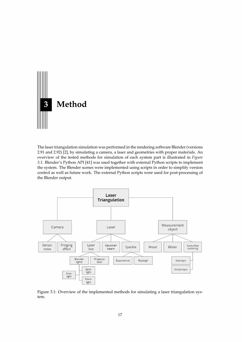
The laser triangulation simulation was performed in the rendering software Blender (versions2.91 and 2.92) [2], by simulating a camera, a laser and geometries with proper materials. Anoverview of the tested methods for simulation of each system part is illustrated in Figure3.1. Blender’s Python API [41] was used together with external Python scripts to implementthe system. The Blender scenes were implemented using scripts in order to simplify versioncontrol as well as future work. The external Python scripts were used for post-processing ofthe Blender output.
Figure 3.1: Overview of the implemented methods for simulating a laser triangulation sys-tem.
17

3.1. Practical laser triangulation
3.1. Practical laser triangulation
In order to create a simulation as realistic as possible, reference results were needed to enablecomparison. These results were collected through practical laser triangulation sessions oftwo physical measurement objects. These objects consisted of a wooden plank and a partiallyemptied blister package. The plank was from a spruce, seen in Figure 3.2. The blister packageused was from a pack of Ibuprofen Orifarm 400 mg film coated tablets, seen in Figure 3.3.
Figure 3.2: Raw wooden plank from a spruce, with three knots, two to the right and a smallone far to the left. There is also rot along the entire top of the plank and some regions of dirtto the left. The fibre direction is along the horizontal axis of this image.
Figure 3.3: Blister package of Ibuprofen Orifarm 400 mg film coated tablets. The centre blisterof the top row and the leftmost blister of the bottom row are empty.
To be able to achieve a trustworthy simulation, crucial properties and data were gatheredfrom the instruments that were used in the physical laser triangulation (laser, sensor andcamera). Optical power of the laser, various parameters of the camera and optics (focal length,aperture, and so on), as well as the resolution and noise properties of the sensor were neededto resemble the physical scene. Different parameters were used for the two measurementobjects, due to their separate characteristics. The blister package reflected more light than theraw wood and therefore a shorter exposure time was programmed for the blister object.
SICK enabled the physical laser triangulation to be performed in an environment not af-fected by external lighting. This was achieved through the use of a selective wavelength filter
18

3.2. Simulated laser triangulation
that blocked all wavelengths but the ones interesting for the triangulation. The laser triangu-lation set-up used by SICK to triangulate blisters and wooden planks worked by successivelymoving the measurement object (and not the laser) along one axis.
A red line laser, a 25 millimetre lens and camera with a CMOS-sensor was placed at 420millimetres above the measurement objects. The laser had a wavelength of 660 nanometres(˘15nm) and a red band-pass filter was used to exclude other wavelengths. The camerawas placed at a ´25˝ angle from the baseline (axis perpendicular to the measurement object)and a Scheimpflug-adapter was used to get focus throughout the whole laser plane. Thesystem was pre-calibrated and utilised global shutter technology. Sensor images or profileswere captured for every 6.8ˆ 10´5 m displacement of the measurement object. 4000 profileswere combined to create the resulting scattering images for the wooden plank, whereas 1000profiles were used for the blister package.
3.2. Simulated laser triangulation
Several methods were tested for modelling each part of the laser triangulation system.Different plug-ins were considered and tested for the simulation of laser lines and sen-sors/scanners, such as BlenSor[42], Gazebo [43] and MORSE [44]. BlenSor is a simulationpackage specifically designed for sensor simulation. BlenSor was of interest since it can han-dle complex scenarios and analyse algorithms. Gazebo and MORSE are robot simulationplug-ins. Gazebo was interesting since it could generate sensor data with noise. Gazeboand MORSE also allowed for emulation of a line laser. MORSE was particularly interestingsince it also offered a model of a laser scanner from SICK. Research showed that all threeplug-ins were built for and/or assumed that the user ran Linux/Ubuntu [44][42][43]. Themachines used during this thesis used Windows as operating system. Despite this, MORSEwas installed together with the required old versions of Python and Blender. The other plug-ins were not further considered due to the results of testing MORSE. The installation andoutdated documentation/requirements was considered too time consuming and not propor-tional to the outcome of testing a plug-in. More on this in the result section 4.2.
The simulation was performed without any external lighting, in accordance with Fernan-dez et al. [12]. Thus, both the simulated and the physical laser triangulation results wereobtained in scenes only affected by the laser light. The movement of the simulated lasertriangulation system was also executed in the same manner as in the physical system, bymoving the measurement object along one axis between each frame. Sensor images weresimulated by rendering 2D-images of a Blender scene including a laser line projected ontoa measurement object. As the measurement object was moved, new frames were rendered,resulting in simulated sensor images.
3.2.1. Laser line simulation
Several techniques were adopted when simulating laser lines in Blender. Among them weretwo fast methods, along with a more complex and time consuming one. One quick laser sim-ulation was performed by reshaping the different built-in light sources of Blender using twotechniques. The first reshaping method was to use slits created by geometries, whereas thesecond approach was to utilise a tree of shader nodes. Another quick method was to trans-form the built-in point-light to a projector that projected a pre-constructed 2D image texturerepresenting a laser. The more high-end laser simulation technique involved approximatinga point laser as a Gaussian beam with a tree of shader nodes and then reshaping it using acylinder lens. All methods had the common aim to resemble a realistic laser with varyingthickness and intensity. Speckle was another laser property that was considered importantfor realism and therefore a phenomenon to be applied to all simulated lasers.
19
3.2. Simulated laser triangulation
Reshaping Blender’s built-in light sources
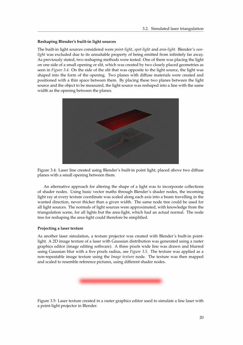
The built-in light sources considered were point-light, spot-light and area-light. Blender’s sun-light was excluded due to its unsuitable property of being emitted from infinitely far away.As previously stated, two reshaping methods were tested. One of them was placing the lighton one side of a small opening or slit, which was created by two closely placed geometries asseen in Figure 3.4. On the side of the slit that was opposite to the light source, the light wasshaped into the form of the opening. Two planes with diffuse materials were created andpositioned with a thin space between them. By placing these two planes between the lightsource and the object to be measured, the light source was reshaped into a line with the samewidth as the opening between the planes.
Figure 3.4: Laser line created using Blender’s built-in point light, placed above two diffuseplanes with a small opening between them.
An alternative approach for altering the shape of a light was to incorporate collectionsof shader nodes. Using basic vector maths through Blender’s shader nodes, the incominglight ray at every texture coordinate was scaled along each axis into a beam travelling in thewanted direction, never thicker than a given width. The same node tree could be used forall light sources. The normals of light sources were approximated, with knowledge from thetriangulation scene, for all lights but the area-light, which had an actual normal. The nodetree for reshaping the area-light could therefore be simplified.
Projecting a laser texture
As another laser simulation, a texture projector was created with Blender’s built-in point-light. A 2D image texture of a laser with Gaussian distribution was generated using a rastergraphics editor (image editing software). A three pixels wide line was drawn and blurredusing Gaussian blur with a five pixels radius, see Figure 3.5. The texture was applied as anon-repeatable image texture using the Image texture node. The texture was then mappedand scaled to resemble reference pictures, using different shader nodes.
Figure 3.5: Laser texture created in a raster graphics editor used to simulate a line laser witha point-light projector in Blender.
20
3.2. Simulated laser triangulation
Gaussian beam approximation
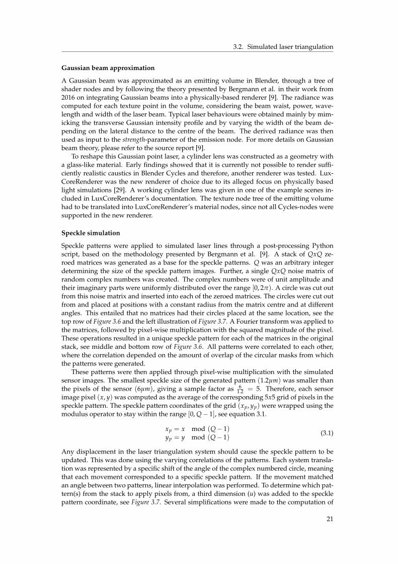
A Gaussian beam was approximated as an emitting volume in Blender, through a tree ofshader nodes and by following the theory presented by Bergmann et al. in their work from2016 on integrating Gaussian beams into a physically-based renderer [9]. The radiance wascomputed for each texture point in the volume, considering the beam waist, power, wave-length and width of the laser beam. Typical laser behaviours were obtained mainly by mim-icking the transverse Gaussian intensity profile and by varying the width of the beam de-pending on the lateral distance to the centre of the beam. The derived radiance was thenused as input to the strength-parameter of the emission node. For more details on Gaussianbeam theory, please refer to the source report [9].
To reshape this Gaussian point laser, a cylinder lens was constructed as a geometry witha glass-like material. Early findings showed that it is currently not possible to render suffi-ciently realistic caustics in Blender Cycles and therefore, another renderer was tested. Lux-CoreRenderer was the new renderer of choice due to its alleged focus on physically basedlight simulations [29]. A working cylinder lens was given in one of the example scenes in-cluded in LuxCoreRenderer’s documentation. The texture node tree of the emitting volumehad to be translated into LuxCoreRenderer’s material nodes, since not all Cycles-nodes weresupported in the new renderer.
Speckle simulation
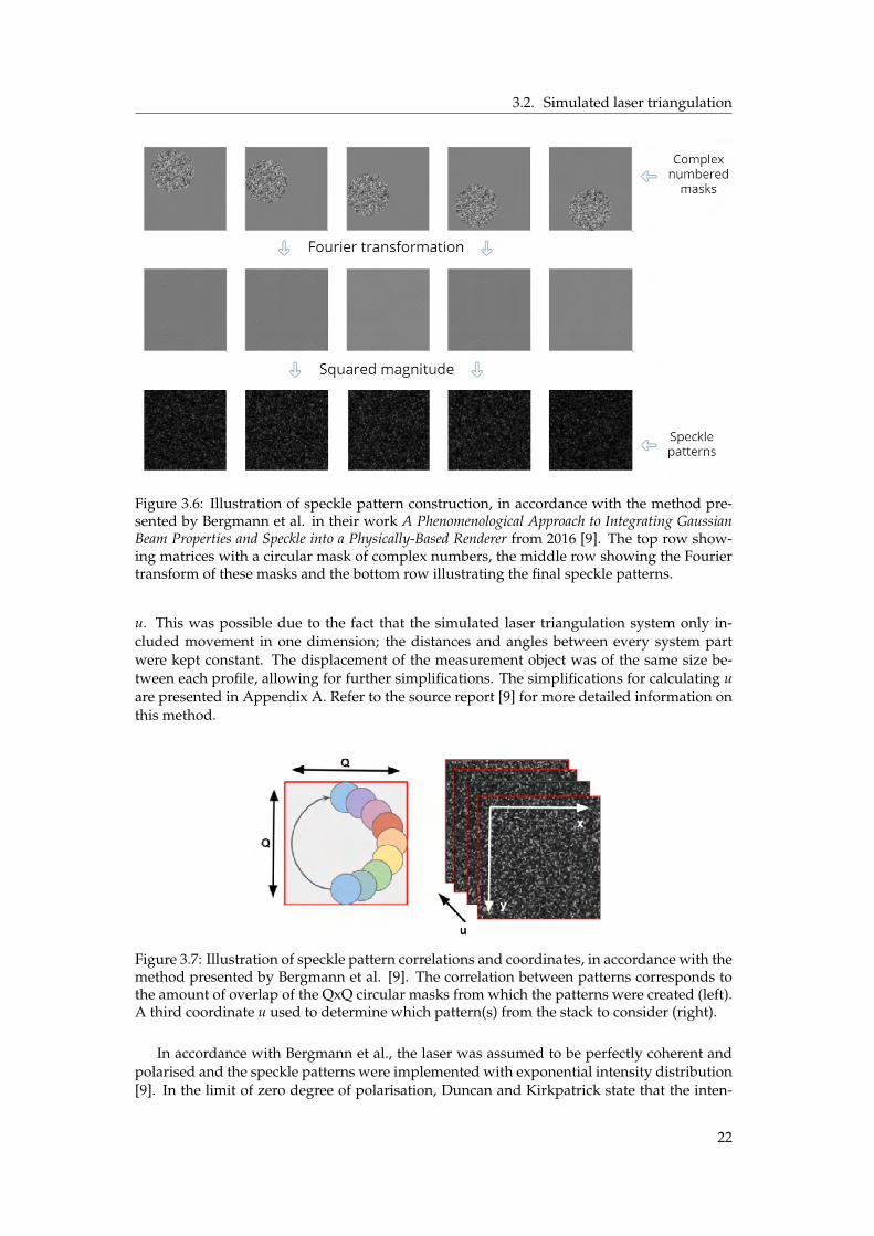
Speckle patterns were applied to simulated laser lines through a post-processing Pythonscript, based on the methodology presented by Bergmann et al. [9]. A stack of QxQ ze-roed matrices was generated as a base for the speckle patterns. Q was an arbitrary integerdetermining the size of the speckle pattern images. Further, a single QxQ noise matrix ofrandom complex numbers was created. The complex numbers were of unit amplitude andtheir imaginary parts were uniformly distributed over the range [0, 2π). A circle was cut outfrom this noise matrix and inserted into each of the zeroed matrices. The circles were cut outfrom and placed at positions with a constant radius from the matrix centre and at differentangles. This entailed that no matrices had their circles placed at the same location, see thetop row of Figure 3.6 and the left illustration of Figure 3.7. A Fourier transform was applied tothe matrices, followed by pixel-wise multiplication with the squared magnitude of the pixel.These operations resulted in a unique speckle pattern for each of the matrices in the originalstack, see middle and bottom row of Figure 3.6. All patterns were correlated to each other,where the correlation depended on the amount of overlap of the circular masks from whichthe patterns were generated.
These patterns were then applied through pixel-wise multiplication with the simulatedsensor images. The smallest speckle size of the generated pattern (1.2µm) was smaller thanthe pixels of the sensor (6µm), giving a sample factor as 6
1.2 = 5. Therefore, each sensorimage pixel (x, y) was computed as the average of the corresponding 5x5 grid of pixels in thespeckle pattern. The speckle pattern coordinates of the grid (xp, yp) were wrapped using themodulus operator to stay within the range [0, Q´ 1], see equation 3.1.
xp = x mod (Q´ 1)yp = y mod (Q´ 1)
(3.1)
Any displacement in the laser triangulation system should cause the speckle pattern to beupdated. This was done using the varying correlations of the patterns. Each system transla-tion was represented by a specific shift of the angle of the complex numbered circle, meaningthat each movement corresponded to a specific speckle pattern. If the movement matchedan angle between two patterns, linear interpolation was performed. To determine which pat-tern(s) from the stack to apply pixels from, a third dimension (u) was added to the specklepattern coordinate, see Figure 3.7. Several simplifications were made to the computation of
21
3.2. Simulated laser triangulation
Figure 3.6: Illustration of speckle pattern construction, in accordance with the method pre-sented by Bergmann et al. in their work A Phenomenological Approach to Integrating GaussianBeam Properties and Speckle into a Physically-Based Renderer from 2016 [9]. The top row show-ing matrices with a circular mask of complex numbers, the middle row showing the Fouriertransform of these masks and the bottom row illustrating the final speckle patterns.
u. This was possible due to the fact that the simulated laser triangulation system only in-cluded movement in one dimension; the distances and angles between every system partwere kept constant. The displacement of the measurement object was of the same size be-tween each profile, allowing for further simplifications. The simplifications for calculating uare presented in Appendix A. Refer to the source report [9] for more detailed information onthis method.
Figure 3.7: Illustration of speckle pattern correlations and coordinates, in accordance with themethod presented by Bergmann et al. [9]. The correlation between patterns corresponds tothe amount of overlap of the QxQ circular masks from which the patterns were created (left).A third coordinate u used to determine which pattern(s) from the stack to consider (right).
In accordance with Bergmann et al., the laser was assumed to be perfectly coherent andpolarised and the speckle patterns were implemented with exponential intensity distribution[9]. In the limit of zero degree of polarisation, Duncan and Kirkpatrick state that the inten-
22

3.2. Simulated laser triangulation
sity distribution of a speckle pattern is a Rayleigh distribution. Applying the square rootto the squared magnitude of the Fourier transformed masks would reshape the exponentialdistribution to the wanted Rayleigh one [30]. Even though lasers are polarised with higherdegrees of polarisation, speckle patterns with Rayleigh distribution were implemented. Thiswas done partly to enable comparison of patterns with the two intensity distributions, butalso to better resemble ground truth images.
For both distributions, energy was lost when the speckle pattern was applied to the laserline. This was due to the fact that the majority of the QxQ matrices were zeroed after insertionof the circle as well as after the Fourier transform. A simple scaling factor was thereforeadded to ensure that the algorithm was approximately energy preserving. The intensity ofthe speckle pattern was then scaled further to better resemble the different exposures of thereference images. An overview of the speckle pattern simulation is seen in the following list:
1. Generate a stack of QxQ zeroed matrices.
2. Create a QxQ noise matrix of random complex numbers.
3. Cut out circles from the noise matrix (at same radius but different angles) and insertone into each zeroed matrix (at the same position as they were cut from).
4. Apply a Fourier transform to each circular mask (zeroed matrix with inserted circle).
5. Multiply the masks from the previous step pixel-wise with the squared magnitude ofthe pixel.
6. Change the intensity distribution from exponential to Rayleigh by taking the squareroot of the masks from the previous step.
7. Scale the intensity distribution to approximate conservation of energy.
8. Compute the sampling_ f actor as sensor pixel size divided by smallest speckle size.
9. For each sensor image pixel, derive pattern coordinates for a sampling_ f actor ˆsampling_ f actor grid. Wrap the coordinates: (x, y) P [0, Q´ 1] and u P [0, #patterns]
10. Multiply the sensor image pixel-wise with the average of the corresponding grid.
3.2.2. Camera simulation
The built-in camera in Blender allowed the following parameters to be altered: aperture, focallength, focus distance and sensor size. Data from the physical laser triangulation scene wasused to resemble the used camera in accordance with Table 3.1. The physically measureddistance between the object and the camera was also recreated in the scene. The simulatedcamera was assumed to have a perfect and aberration-free lens and the Scheimpflug-adapterthat was used in the physical laser triangulation, was completely neglected in the simulation.
Table 3.1: Camera parameter values in Blender for simulating a laser triangulation system
Camera parameter Value
Aperture (f-stop): 2.8Focal length: 25 mmFocus distance: 8
Sensor size (width): 15.36 mmDistance camera-object: 410 mm
23

3.2. Simulated laser triangulation
Sensor simulation
As discussed above, Blender allowed input parameters for sensor size, but to simulate thenoise of the sensor, a post-processing Python-script was implemented. A ground truth sen-sor image from a physical laser triangulation session was used to plot histograms of the noisedistribution. To identify the intensity distribution profile of the noise, only regions with no (orvery little) laser impact were considered. The profile was identified as approximately Gaus-sian and the mean and standard deviation of the ground truth sensor image was extracted.These parameters were then used to create a matrix of random numbers with Gaussian dis-tribution, which was later added to the simulated sensor images.
Fringing effect
Looking at ground truth images, it was seen that some unknown phenomenon occurredaround the laser line making it look "hairy", see Figure 3.8. This effect could possibly beblooming, a material effect, pixel bleeding or a combination of several events. This effect wassimulated using Gaussian blur as a simplification.
Figure 3.8: Magnified region of ground truth sensor image showing an unknown bleed-ing/blurring/blooming effect around the laser line.
3.2.3. Measurement objects
The objects to be measured were simulated as geometries with associated materials inBlender. Tracheids (grain direction) and branches (knots) were considered the most importantfeatures of the wood, whereas the leading property of a blister package was the difference inthe pill and package materials.
Raw wooden plank
Measurements of the reference plank were used to create the geometry for the simulatedwooden plank. A primitive cube was modelled into a plank of the following dimensions:94x210x22 (mm).
Several approaches were tested for creating a spruce wood material with fibre directionsand knots. The first method was to create a volumetric 3D-material from 2D-texture images.Microscopic photographs of the three different wood planes (transverse, tangential and ra-dial) were loaded into Blender with the Image texture node. The textures were then mapped,scaled and repeated onto a geometry, so that the level of detail and density resembled realwood. This volumetric texture was applied alone as well as in combination with varioussurface materials.
24

3.2. Simulated laser triangulation
Another approach to simulate wood was as a heterogeneous volume with LuxCoreRen-derer. LuxCoreRenderer supported creating complex volumes through the Heterogeneous Vol-ume texture node [45]. Several node trees were constructed and applied to plank-like geome-tries.
Yet another method was to generate a procedural texture using Blenderkit [46]. Blenderkitis an add-on for Blender which offers free textures. The chosen procedural texture had highlevel of detail with adjustable parameters for lines and knots to resemble spruce wood.
To have more freedom and understanding with the procedural texture, a custom proce-dural texture was created. This was done by combining the existing nodes of Blender toreplicate desired properties of a wooden plank.
Furthermore, another method was to include a photograph of the wooden plank thatwas used in the physical laser triangulation system, seen in Figure 3.2. This image was thencropped, rotated, scaled and UV-mapped onto the wood geometry in Blender.
Subsurface scattering
There are several ways of including subsurface scattering in Blender materials. The Princi-pled BSDF shader node, for example, has input fields for Subsurface Radius for each of theRGB-channels as well as the parameter Subsurface, which is used in the mixing of diffuseand subsurface scattering as a scaling factor for the scattering radii. For more control of thescattering, there also exists the Subsurface Scattering node (as well as the Volume scatter node),specifically made for handling this phenomenon [47]. However, none of the shader nodes thatinclude subsurface scattering can be used to simulate 360˝ anisotropic (directional) subsur-face scattering. The anisotropy parameters in the various shader nodes have shown throughexperiments to only be able to produce uniform forward and backwards scattering. Sinceraw wood experience anisotropic scattering, an external Python-script was implemented tosimulate anisotropic subsurface scattering.
Anisotropic subsurface scattering simulation
In order to simulate directional scattering, a method for representing different scattering di-rections was needed. In an image describing a measurement object, each pixel should beassigned a direction value corresponding to the direction in which incoming light shouldscatter the most. This was done by mapping the scatter direction of each pixel as a vectorwith direction and unit magnitude. To, as effortlessly as possible, generate images to de-scribe scattering directions of an object, directions were represented as RGB-colours. Thisenabled easy production of direction maps with areas of different colours. These coloureddirection maps were created by interpolating between different colours using a gradient tool.
The anisotropic subsurface scattering script was built to scatter light along a given slopein both directions (positive and negative). Due to this, a half circle was enough to representall the possible slopes. Colours between the red and green axes corresponded to slopes in thefirst and third quadrants of the unit circle, given by R
G . Similarly, slopes in the second andforth quadrants were represented by colours between the blue and green axes through´( B
G ).
25

3.2. Simulated laser triangulation
Figure 3.9: Illustration of how to represent directions as RGB-values. A yellow colour repre-sents scattering in the ascending diagonal and a cyan colour corresponds to scattering in thedescending diagonal.
Figure 3.9 roughly illustrates how the various colours were mapped to represent differentdirections. As an example, a yellow direction map (R = G = 255) corresponds to subsurfacescattering along the ascending diagonal. The alpha channel of the colour was utilised torepresent the scatter intensity, which described how much of the incoming light that eachpixel should scatter forward in a given direction. In areas with lower alpha-values, it wouldscatter less, meaning that the pixel intensity would be spread a shorter distance. The coloureddirection maps were then translated into a normalised vector field as seen in Figure 3.10.
Figure 3.10: Illustration of how a subsurface scattering direction map is translated from RGB-colours to a vector field.
Once the scattering directions had been generated for an object, the subsurface scatteringcould be simulated as an iterative process, scattering more light for each iteration. The twophotographs seen in Figure 2.7 were used as references for the simulation. One illustratedscattering along the tracheids and the other showed scattering of a laser point placed on aknot. One zeroed matrix was created for each of the two reference images. Two laser pointswere then simulated as circles with diameter of 55 pixels and with Gaussian distribution.One laser point, placed on top of the knot of the wooden plank, was inserted into one of thematrices, whereas the second laser point was placed beside the knot and inserted into theother zeroed matrix.
26

3.2. Simulated laser triangulation
Different approaches were tested for the scattering simulation, where the first one wasto loop over each matrix and find the pixels that were lit by the laser. From these pixels,the intensity was spread into a number of nearby pixels in the direction retrieved from thedirection map. Several methods were implemented for finding which pixels to scatter to,following the given direction. The initial method was to calculate the linear equation y =kx + m for each direction and lit pixel. The coordinates of the pixels to scatter into could thenbe computed using the lit pixel’s coordinate incremented along one axis. Bresenham’s linealgorithm [48] was also implemented, as well as a third line algorithm utilising the Pythonlibrary Scikit-image. From the module Draw of this library, a function for generating pixelcoordinates of anti-aliased lines was tested.
An alternative method for simulating anisotropic subsurface scattering included imple-menting the first part of a stable fluid solver as a diffusion process. Only the first part of themethod was considered since it was based on a static vector field, rather than the dynamicones used later in the algorithm. This method was performed in accordance with the paperpublished by Jos Stam [49], with an extension implemented to allow anisotropic scattering.
Stam’s diffusion process was an iterative method for evenly spreading pixel values whilstobtaining a stable system. The method was based on the Navier-Stokes equations togetherwith Gauss-Seidel relaxation. Stam’s algorithm used the same coefficients for the four neigh-bouring pixels (above, below, to the left and to the right) to obtain a uniform spread and astable flow [49]. By adding the four diagonal pixels, see Figure 3.11, the flow was distributedover more directions in each iteration. The intensity spread was then directed by havingthe coefficients for each neighbouring pixel depend on the directions of a given vector field.Stam’s uniform flow was thus transformed into a simulation of anisotropic scattering.
Figure 3.11: Illustration of uniform diffusion between neighbouring pixels, with the diago-nals as an extension to the methodology presented by Jos Stam in his work Real-Time FluidDynamics for Games from 2003.
27

3.2. Simulated laser triangulation
In order to simulate the scattering in wooden knots, the mentioned alpha-values wereused. Since the fibres of the knots were perpendicular to the tracheids, as presented in section2.3.4, the light transportation could be simulated as absorption. The lower the alpha-valueof a pixel, the more absorption and the less scattering would occur in that pixel. Measure-ments from the practical laser triangulation session showed that the intensity of the reflectedlight was about half as high in the knot as in the clear wood. Suitable alpha-values in theknot-regions of the coloured direction map were therefore set to 0.5. The scattering in theseknot-areas was set to be uniform, to resemble the reference image, by giving all the diffusiondirection coefficients the same value. A lower number of diffusion iteration was used for thelaser point placed on the knot than for the one placed on the clear wood. This was also doneto achieve scattering effects that were similar to the reference images.
Absorption was performed in a separate pass where the whole image was multipliedpixel-wise with the corresponding alpha-value. For the diffusion approach, the absorptionalgorithm was applied between each diffusion iteration. The alpha-values were thereforedivided by the number of iterations so that the combined effect of all the absorption itera-tions corresponded to the given alpha-value for each pixel. Due to these absorption passes,the diffusion process was no longer energy conserving. An overview of the algorithm forsimulating anisotropic subsurface scattering is seen in the following list:
1. Describe the scattering directions and absorption of different areas of a photographusing RGBA-colours.
2. Transform the colour of each pixel in the map from step 1 into a slope of a vector togenerate a vector field.
3. Create a circle with Gaussian distribution to simulate a point laser.
4. Diffuse or iteratively spread the intensity of the laser point following the directions ofthe vector field, for a given number of iterations.
5. Scale the spread intensity using the alpha-value of each pixel to simulate absorption.
Blister package
The blister package geometry was created by merging half ellipsoids with a plane. Someof the blisters contained pills that were shaped as whole ellipsoids. The reference blisterpackage consisted of PVC and aluminium foil, but since PVC was the main component ofthe package and also the material where the laser hit, the simulation was performed with asingle material for the entire package. Two Blender materials were constructed, one for theblister package and one for the pills. The package material was created as a mix betweenthe Translucent BSDF shader and the Principled BSDF shader with white as base colour andwith the Subsurface parameter set to zero. The pill material was also white, but fully opaqueand therefore simulated using only the Principled BSDF shader, with a Subsurface coefficientjust below one and Subsurface Radius of one for each colour channel. Screenshots of the twomaterials are seen in Figure 3.12.
28
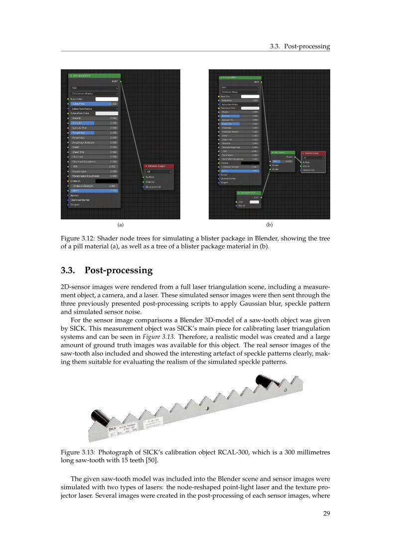
3.3. Post-processing
(a) (b)
Figure 3.12: Shader node trees for simulating a blister package in Blender, showing the treeof a pill material (a), as well as a tree of a blister package material in (b).
3.3. Post-processing
2D-sensor images were rendered from a full laser triangulation scene, including a measure-ment object, a camera, and a laser. These simulated sensor images were then sent through thethree previously presented post-processing scripts to apply Gaussian blur, speckle patternand simulated sensor noise.
For the sensor image comparisons a Blender 3D-model of a saw-tooth object was givenby SICK. This measurement object was SICK’s main piece for calibrating laser triangulationsystems and can be seen in Figure 3.13. Therefore, a realistic model was created and a largeamount of ground truth images was available for this object. The real sensor images of thesaw-tooth also included and showed the interesting artefact of speckle patterns clearly, mak-ing them suitable for evaluating the realism of the simulated speckle patterns.
Figure 3.13: Photograph of SICK’s calibration object RCAL-300, which is a 300 millimetreslong saw-tooth with 15 teeth [50].
The given saw-tooth model was included into the Blender scene and sensor images weresimulated with two types of lasers: the node-reshaped point-light laser and the texture pro-jector laser. Several images were created in the post-processing of each sensor images, where
29

3.3. Post-processing
different numbers of scripts were applied in different orders. Following are examples of afew post-processing scripting orders (leftmost script applied first):
• sensor noise, speckle
• Gaussian blur, sensor noise
• speckle, Gaussian blur, sensor noise
• Gaussian blur, speckle, sensor noise
The parameters of each script were also altered to resemble the ground truth images as muchas possible. Some of these variables were the radius of the Gaussian blur and the size of thesmallest speckle in the speckle patterns. Final parameter values are seen in Table 3.2 below.
Table 3.2: Post-processing script parameters for each measurement object and for the threescripts blur, speckle and noise.
Script parameter Saw-tooth Wood Blister packBlurring radius: 0.5 1.0 0.5
Speckle pattern size: (pixels) 1000x1000 1000x1000 1000x1000Mask diameter: (pixels) 500 500 500Intensity scale factor: 3.5 6.0 7.0Sampling factor: 5 5 5
Mean: 11.6 11.6 11.6Standard deviation: 1.09 1.09 1.09
3.3.1. Simulating scattering images
Simulated wood and blister packages were used to simulate the subsurface scattering images.1000 profiles were rendered of the scene with a blister package and 4000 profiles were createdfor the wooden plank scene. These simulated sensor images were all lit by the same textureprojector laser and both of the measurement objects were moved 6.8ˆ 10´5 m along the y-axis between each profile. All three of the post-processing scripts were applied to each sensorimage, with different parameters for the two objects, see Table 3.2.
SICK provided an algorithm for combining the profiles into a subsurface scattering image.Laser line extraction was included in this algorithm and performed before the subsurfacescattering was measured. The laser centre was derived through centre of gravity. From thisdetected laser line, the area in which to compute scattering was defined by the two parame-ters scatter offset and scatter range. Scatter offset was the distance (in pixels) from the detectedlaser line to the first pixel to be measured. From this pixel the scatter range defined the widthof how many pixels that scattering was to be measured in, see Figure 3.14. The parametervalues for wood and blister packages are seen in Table 3.3 below. All algorithms and inputswere set to match the settings of the physical laser triangulation sessions.
30

3.4. Comparison and evaluation
Figure 3.14: Illustration of the two parameters scatter offset and scatter range used in the algo-rithm to measure subsurface scattering in sensor images.
Table 3.3: Script parameters of the subsurface scattering measurement algorithm for the twomeasurement objects wood and blister package.
Script parameter Wood Blister packScatter offset: 1.0 7.0Scatter range: 8.0 5.0
3.4. Comparison and evaluation
The results from the simulated laser triangulation were compared to results from the practicallaser triangulation. As presented, both triangulations were performed with similar set-upsand measurement objects. The outputs that were possible to compare were the sensor imagesand the subsurface scattering images.
The definition of a realistic line laser was considered as a laser that includes the mainproperties: intensity variation and visible speckle pattern. A realistic line laser would alsovisually resemble ground truth data. A material (for a measurement object) was defined asrealistic, in this thesis, if it affected light in accordance with behaviours seen in ground truthimages. The material should also match the visual appearance of the reference object.
31

4 Results
4.1. Practical laser triangulation
The practical laser triangulation sessions, covered in section 3.1, resulted in sensor and scat-tering images for both of the measurement objects: wooden plank and blister package. Thesensor images of the blister package were overexposed, see Figure 4.1, destroying most inter-esting phenomena. Relatively small amounts of speckle were seen in the wood sensor images,making them unsuitable for comparison with the results of the simulated speckle patterns,see Figure 4.2.
Figure 4.1: Result from practical laser triangulation session of a blister package, showing asensor image containing a laser line projected onto the blister package seen in Figure 3.3.
Figure 4.2: Result from practical laser triangulation session of a wooden plank, showing asensor image containing a laser line projected onto the plank illustrated in Figure 3.2.
32

4.2. Simulated laser triangulation
Results from a laser triangulation session, performed by SICK, of the previously men-tioned saw-tooth object will therefore be used to compare the different laser line simulationmethods as well as the post-processing scripts: sensor noise simulation, speckle pattern sim-ulation and fringing effect simulation. A sensor image from the physical laser triangulationsession of the saw-tooth is seen in Figure 4.3.
Figure 4.3: Sensor image from a practical laser triangulation session, performed by SICK, ofthe saw-tooth calibration object depicted in Figure 3.13.
4.2. Simulated laser triangulation
Three plug-ins were considered as an alternative method for simulating lasers and or lasersensors, as stated in section 3.2: MORSE, BlenSor and Gazebo. Installing MORSE resultedin no working lasers or sensors and it was decided that no plug-ins were to be used. Thecomplexity in set-up along with the requirements for old programs did not seem proportionalto the actual outcome of the plug-ins. Since BlenSor and Gazebo were also aimed for otheroperating systems than the one used in the project, and since they had similar requirementsto MORSE, the idea of using plug-ins was cancelled as a whole.
4.2.1. Laser line simulation
Laser lines were simulated, as presented in section 3.2.1, by altering the built-in light sourcesof Blender and by creating custom light sources as emitting volumes. Different approacheswere used to reshape the different lights into laser lines. All simulated laser lines were pro-jected onto the standard Blender geometry Suzanne and rendered with the same scene pa-rameters.
Reshaping Blender’s built-in light sources
Altering the shape of the built-in lights into laser beams was accomplished in Blender usingshader nodes or a slit between two geometries, in accordance with section 3.2.1. Realisticproperties such as varying thickness and intensity were however not achieved using thesereshaping methods. Figure 4.4 below shows a comparison of the two reshaping methods fora point-light. The slit and shader node methods resulted in identical laser lines with constantintensity and thickness. The results of reshaping the spot-light, point-light and area-lightwith shader nodes are seen in Figure 4.5a-c. No visual difference is seen in these renderedimages, regarding the interesting factors of line shape or intensity.
33
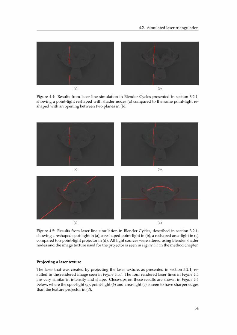
4.2. Simulated laser triangulation
(a) (b)
Figure 4.4: Results from laser line simulation in Blender Cycles presented in section 3.2.1,showing a point-light reshaped with shader nodes (a) compared to the same point-light re-shaped with an opening between two planes in (b).
(a) (b)
(c) (d)
Figure 4.5: Results from laser line simulation in Blender Cycles, described in section 3.2.1,showing a reshaped spot-light in (a), a reshaped point-light in (b), a reshaped area-light in (c)compared to a point-light projector in (d). All light sources were altered using Blender shadernodes and the image texture used for the projector is seen in Figure 3.5 in the method chapter.
Projecting a laser texture
The laser that was created by projecting the laser texture, as presented in section 3.2.1, re-sulted in the rendered image seen in Figure 4.5d. The four rendered laser lines in Figure 4.5are very similar in intensity and shape. Close-ups on these results are shown in Figure 4.6below, where the spot-light (a), point-light (b) and area-light (c) is seen to have sharper edgesthan the texture projector in (d).
34
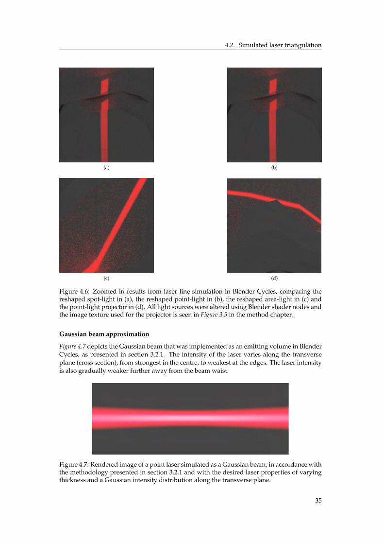
4.2. Simulated laser triangulation
(a) (b)
(c) (d)
Figure 4.6: Zoomed in results from laser line simulation in Blender Cycles, comparing thereshaped spot-light in (a), the reshaped point-light in (b), the reshaped area-light in (c) andthe point-light projector in (d). All light sources were altered using Blender shader nodes andthe image texture used for the projector is seen in Figure 3.5 in the method chapter.
Gaussian beam approximation
Figure 4.7 depicts the Gaussian beam that was implemented as an emitting volume in BlenderCycles, as presented in section 3.2.1. The intensity of the laser varies along the transverseplane (cross section), from strongest in the centre, to weakest at the edges. The laser intensityis also gradually weaker further away from the beam waist.
Figure 4.7: Rendered image of a point laser simulated as a Gaussian beam, in accordance withthe methodology presented in section 3.2.1 and with the desired laser properties of varyingthickness and a Gaussian intensity distribution along the transverse plane.
35

4.2. Simulated laser triangulation
Figure 4.8: Results of the Gaussian beam initially implemented in Blender Cycles, see Figure4.7, translated into the LuxCoreRenderer, as described in section 3.2.1.
(a) (b)
Figure 4.9: A scene where the built-in area-light laser of LuxCoreRenderer is reshaped intoa laser line using a cylinder lens (a), together with a rendered image of the constructed laserline in (b).
This point laser was, as stated in section 3.2.1, not possible to reshape into a line using Cy-cles. An attempt to translate the Cycles shader nodes into LuxCoreRenderer material nodesresulted in the rendered image depicted in Figure 4.8.
The scene for LuxCoreRenderer also includes a cylinder lens, with purpose to reshapethe point laser into a line laser. Figure 4.9 shows a scene where the built-in area-light laser(incident from the right) is successfully reshaped into a line using a cylinder lens in a and arendered image of the scene in b.
Speckle simulation
Stacks of speckle patterns were simulated with exponential and Rayleigh intensity distribu-tions respectively, as stated in section 3.2.1. Figure 4.10 includes one pattern of each distribu-tion and illustrates that the exponential patterns were darker than the Rayleigh-distributedones.
36

4.2. Simulated laser triangulation
Figure 4.10: Results from the speckle pattern simulation presented in section 3.2.1, illustrat-ing a pattern with exponential intensity distribution (top row), compared to a Rayleigh dis-tributed speckle pattern (bottom row), with a corresponding histogram.
Figure 4.11 below depicts an attempt to match the intensity of the simulated laser linesthat included speckle patterns (middle and bottom row) to the intensity of ground truth data(top row). The exponential speckle patterns (bottom row) were scaled with a factor of 10.0,whereas the Rayleigh-distributed speckle patterns (middle row) were scaled with 3.5. Simu-lated sensor noise was applied to both of the simulated sensor images. This resulted in laserlines with sufficiently small visual differences to the reference image. The simulated laserlines used for these comparisons were from the texture projector.
Figure 4.12 presents the simulated and Rayleigh-distributed speckle patterns applied ontorendered sensor images of the saw-tooth. The sensor images were created using either areshaped point-light laser or a texture projector laser.
37
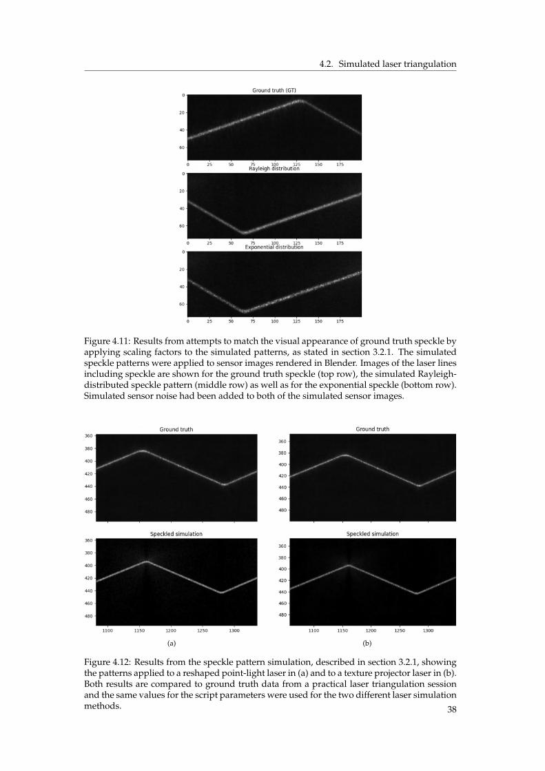
4.2. Simulated laser triangulation
Figure 4.11: Results from attempts to match the visual appearance of ground truth speckle byapplying scaling factors to the simulated patterns, as stated in section 3.2.1. The simulatedspeckle patterns were applied to sensor images rendered in Blender. Images of the laser linesincluding speckle are shown for the ground truth speckle (top row), the simulated Rayleigh-distributed speckle pattern (middle row) as well as for the exponential speckle (bottom row).Simulated sensor noise had been added to both of the simulated sensor images.
(a) (b)
Figure 4.12: Results from the speckle pattern simulation, described in section 3.2.1, showingthe patterns applied to a reshaped point-light laser in (a) and to a texture projector laser in (b).Both results are compared to ground truth data from a practical laser triangulation sessionand the same values for the script parameters were used for the two different laser simulationmethods. 38
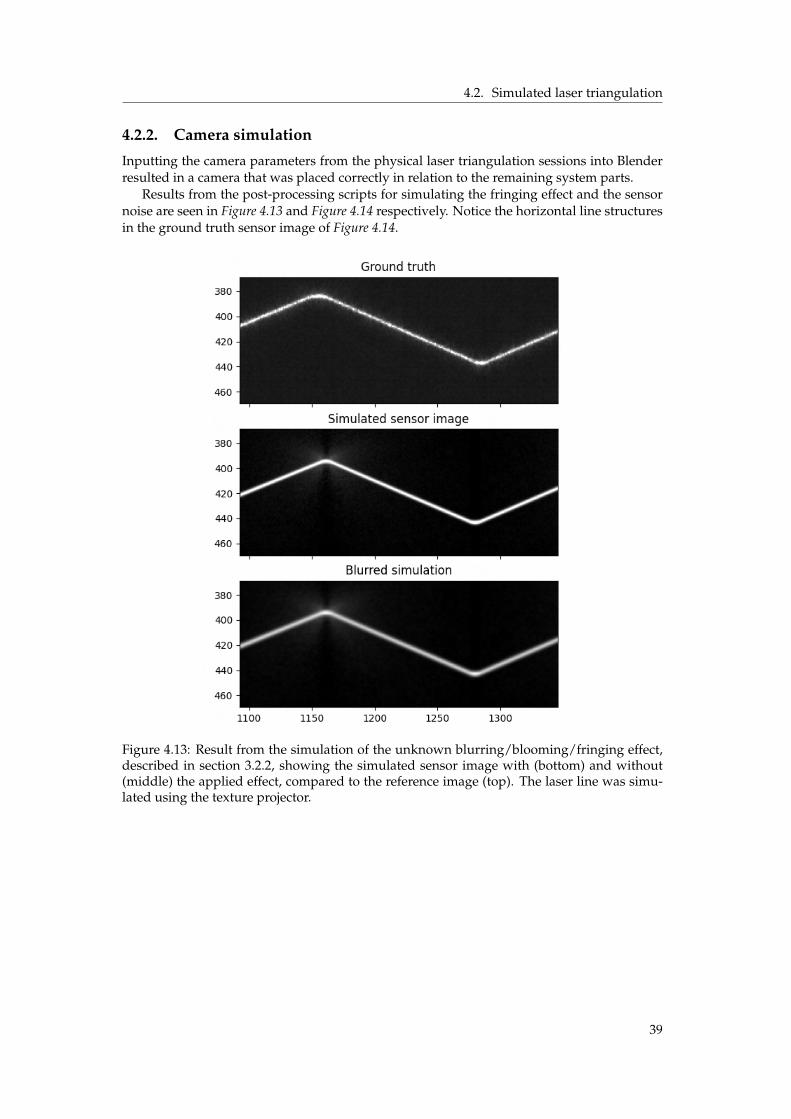
4.2. Simulated laser triangulation
4.2.2. Camera simulation
Inputting the camera parameters from the physical laser triangulation sessions into Blenderresulted in a camera that was placed correctly in relation to the remaining system parts.
Results from the post-processing scripts for simulating the fringing effect and the sensornoise are seen in Figure 4.13 and Figure 4.14 respectively. Notice the horizontal line structuresin the ground truth sensor image of Figure 4.14.
Figure 4.13: Result from the simulation of the unknown blurring/blooming/fringing effect,described in section 3.2.2, showing the simulated sensor image with (bottom) and without(middle) the applied effect, compared to the reference image (top). The laser line was simu-lated using the texture projector.
39

4.2. Simulated laser triangulation
Figure 4.14: Results from the sensor noise simulation, presented in section 3.2.2, showing aclose-up of a small and unlit region of the sensor images (left) together with their intensitydistributions (right).
4.2.3. Measurement objects simulation
The following sections present the results of simulating a wooden plank and a blister package.Results from the various approaches for simulating anisotropic subsurface scattering are alsopresented.
Raw wooden plank
Figure 4.15 shows results from the wood simulation approach that was based on proceduraltextures. The method using microscopic images resulted in the renderings seen in Figure 4.16.Note how the red spot-lights in Figures 4.15b and 4.16b maintain their circular shape on top ofthe wooden textures. Anisotropic subsurface scattering was not achieved using any of thesemethods.
40
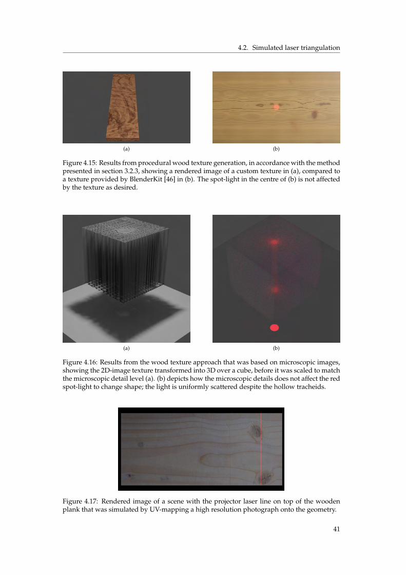
4.2. Simulated laser triangulation
(a) (b)
Figure 4.15: Results from procedural wood texture generation, in accordance with the methodpresented in section 3.2.3, showing a rendered image of a custom texture in (a), compared toa texture provided by BlenderKit [46] in (b). The spot-light in the centre of (b) is not affectedby the texture as desired.
(a) (b)
Figure 4.16: Results from the wood texture approach that was based on microscopic images,showing the 2D-image texture transformed into 3D over a cube, before it was scaled to matchthe microscopic detail level (a). (b) depicts how the microscopic details does not affect the redspot-light to change shape; the light is uniformly scattered despite the hollow tracheids.
Figure 4.17: Rendered image of a scene with the projector laser line on top of the woodenplank that was simulated by UV-mapping a high resolution photograph onto the geometry.
41

4.2. Simulated laser triangulation
Figure 4.17 presents the result from the approach of UV-mapping a wood texture onto arectangle. To show the wooden texture, environmental lighting was included in the scene,withering the scattering effect of the texture projector laser somewhat.
Figure 4.18 shows the difference in the sensor image from the physical laser triangulationof a wooden plank and the result of the simulation of a sensor image. Both sensor imagesillustrate a laser line placed on top of the same knot of the wooden plank. The simulatedsensor image was produced using the texture projector laser and the UV-mapping approachfor the wood material.
(a) (b)
Figure 4.18: The reference sensor image from the physical laser triangulation session of awooden plank (a), compared to the result of the simulation of sensor images in (b).
Blister package
The simulated blister package is depicted in Figure 4.19, showing the geometry and materiallit by an environmental point-light, as well as by the texture projector laser.
Figure 4.19: Rendered image of a scene with the projector laser line on top of the simulatedblister package.
Figure 4.20 compares the sensor image from the physical laser triangulation with the resultof the simulated sensor image of a blister package. The laser line is placed on the top row ofblisters, where the leftmost blister does not contain a pill.
(a) (b)
Figure 4.20: The reference sensor image from the physical laser triangulation session of ablister package (a), compared to the result of the simulation of sensor images in (b).
42

4.2. Simulated laser triangulation
Anisotropic subsurface scattering
The subsurface scattering directions of the reference image of a wooden plank is illustratedin Figure 4.21 below, showing both the initial colour direction map and the correspondingvector field. All regions of the colour map are fully opaque except for the knot-area that hasa alpha-value of 0.5. The vector field is illustrated on top of a photograph of the referenceplank.
(a)
(b)
Figure 4.21: Result of the method for representing subsurface scattering directions of differentregions of a wooden plank (background of (b)) as RGBA-colours (method presented in section3.2.3). The coloured map illustrated in (a), together with the corresponding vector field thatwas obtained by translating the colour map to slopes in (b).
43

4.2. Simulated laser triangulation
Figure 4.22 shows results of the anisotropic subsurface scattering script, presented in sec-tion 3.2.3, where the following line algorithms were used: linear equation, anti-aliasing linesand Bresenham’s lines. Figure 4.22a depicts directed scattering along the ascending diagonalof a solid and red laser point. b and c illustrate scattering along the descending diagonal ofa circular area with Gaussian distribution. The linear equation was used in a, anti-aliasinglines were used in b and the scattering of c was performed using Bresenham’s lines. All threeresults include unwanted lines or streakiness due to the instability of the methods.
(a) (b) (c)
Figure 4.22: Results from the anisotropic subsurface scattering simulation using line algo-rithms, showing undesired streakiness due to instability. The algorithms used were the linearequation (a), anti-aliasing lines (b) and Bresenham’s lines in (c), as presented in section 3.2.3.
Figure 4.23: Result from the diffusion approximation process, presented in section 3.2.3,where a point laser was simulated as a filled circle with Gaussian intensity distribution andplaced on an area without grain deviations (no knots). 20 iterations of diffusion were exe-cuted to spread the laser intensity according to the direction map shown in Figure 3.10.
The diffusion approach, presented in section 3.2.3, resulted in the images depicted in Fig-ures 4.23 and 4.24, where the top rows compare the simulation results (right) with the refer-ence images (left). The bottom rows of these figures illustrate the initial laser points before(left) and after (right) being diffused a given number of iterations. Figure 4.23 shows the resultof simulated anisotropic subsurface scattering on clear wood, whereas Figure 4.24 illustratesthe phenomenon when a point laser is lit on a knot of a wooden plank.
44

4.2. Simulated laser triangulation
Figure 4.24: Result from the diffusion approximation process, section 3.2.3, where a pointlaser was simulated as a filled circle with Gaussian intensity distribution and placed on aknot area. 10 iterations of diffusion were executed to spread the laser intensity according tothe direction map shown in Figure 3.10.
4.2.4. Post processing
The three post-processing scripts simulating speckle, blooming and sensor noise were ap-plied in different orders, as presented in section 3.3. Figure 4.25 compares the result of per-forming the blurring/blooming script first (followed by speckle and sensor noise), with theresult of applying speckle first (followed by blurring and sensor noise).
(a) (b)
Figure 4.25: Results of applying the post-processing scripts in different orders, showing theorder bloom - speckle - noise in (a), compared to the order speckle - bloom - noise in (b).
45

4.2. Simulated laser triangulation
Scattering images
The scatter image from the physical laser triangulation is shown together with the simulatedscatter image of a wooden plank in Figure 4.26. Knots and dirt are visible in the simulatedscatter image. The rot along on the right side of the wooden plank is however barely visible inthe simulated scatter image. Figure 4.27 compares the simulated scattering image of a blisterpackage with the scattering image from the practical laser triangulation. The figure shows adifference in the amount of scattered light in the empty and filled blisters, both in the groundtruth and the simulated scatter images. The blisters where a pill is present are brighter thanthe hollow ones. As further seen in Figure 4.27b, the simulated blister shape differs from theground truth and there are no specular reflections in the simulated image.
(a) (b)
Figure 4.26: Reference scattering image from the physical laser triangulation session of awooden plank (a), compared to the result of the scattering image simulation, presented insection 3.3.1, in (b).
46

4.2. Simulated laser triangulation
(a)
(b)
Figure 4.27: Result from the simulation of scattering images, in accordance with the method-ology presented in section 3.3.1, showing a reference image from the practical laser triangu-lation session of a blister package (a), compared to the simulated scattering image in (b).
47

5 Discussion
This chapter presents a discussion about the results covered in the previous chapter. Further,some of the used methods are discussed with hypotheses as to why they did not perform asexpected, along with possible improvements.
5.1. Results
Most resulting images were presented highly magnified in this thesis. This was to showeffects like scattering, sensor noise and the speckle patterns. Results that do not match theground truth data at this level of detail may still be sufficiently realistic for many applications.
5.1.1. Laser line simulation
The results of the reshaped point-light, spot-light and area-light, depicted in Figures 4.5 and4.6 showed differences so small that they could be considered negligible. The same appliesto the results of the two reshaping methods slit and shader nodes, seen in Figure 4.4; resultswith the same visual appearance could be obtained using both methods. For simplicity in thefollowing discussions, these methods will all be referred to as reshaped light laser.
The texture projector laser was a better approximation of a Gaussian beam than the re-shaped light laser. This was due to the blurred/faded edges, seen in Figure 4.6d. Because ofthis, the texture projector laser could perhaps be considered more realistic than the sharp andsolid line of the reshaped light laser.
Due to it being a point laser, the volumetric Gaussian beam created with Cycles, shownin Figure 4.7, could not be considered finished for the aim of this thesis. It did possess theproperties wanted for realistic laser simulation and could perhaps give satisfactory results ifproperly reshaped. The volumetric beam from LuxCoreRenderer, seen in Figure 4.8 was notfinalised either. Neither the varying thickness, nor the Gaussian intensity distribution wasachieved. A cylinder lens was however proved to be a working method for reshaping pointlasers, as seen in Figure 4.9.
When applying speckle onto a reshaped light laser and a projector laser there was a smalldifference in the brightness of the laser lines as seen in Figure 4.12. This was expected since theGaussian blurring of the projector laser distributed the intensity over a larger area, making
48

5.1. Results
the line appear darker. Using Rayleigh intensity distribution resulted in a brighter specklepattern. This was expected since the sum of the Rayleigh histogram, presented in Figure4.10, was larger than the sum of the exponential intensity distribution histogram. Figure 4.11shows that the appearance of the laser lines differed slightly depending on which intensitydistribution the applied speckle patterns had.
5.1.2. Camera simulation
Figures 4.11 and 4.12 demonstrate effects that were likely caused by using focus at infinity andneglecting the Scheimpflug-adapter. A Scheimpflug-adapter together with a lens focused atinfinity is expected to decrease the field of view, which in turn should magnify the depictedobject. As seen in these figures, the perspective seemed to differ between the simulated andthe ground truth images. The ground truth images appear slightly more zoomed-in or mag-nified. Simulation of the fringing/blooming effect as Gaussian blur did not result in thehairy/spiky phenomenon that was seen in the ground truth images, see Figure 4.13. This wasexpected and considered as a sufficiently good approximation for this thesis.
In the comparison of close-ups of ground truth and simulated sensor images, seen inFigure 4.14, horizontal lines or structures were seen in an unlit area of the ground truth data.These effects were not considered when simulating the sensor noise and thus not found inthe resulting image. The histograms show that the simulated sensor images had a level ofnoise that matched the reference data, despite the absence of horizontal lines.
5.1.3. Wooden plank simulation
The simulated wood material that best resembled the reference plank visually was the onecreated through UV-mapping, seen in Figure 4.17. This was because the desired surface prop-erties, like knots, rays and rot, were included and placed in accordance with the referenceplank. The UV-mapped wood material had different scattering properties depending onwhether the laser line was on top of the clear wood or a knot. The cause of the differedscattering is likely because of the darker colour of the knot.
The simulated sensor images of the wood were darker than the ground truth sensor im-ages, as seen in Figure 4.18. Despite this, the simulated scattering image was brighter than theone obtained from physical laser triangulation, as seen in 4.26. This was not expected and thecause for this is unknown.
5.1.4. Blister package simulation
The modelled geometry of the blister package did not match the reference object properly, asseen when comparing Figures 3.3 and 4.19. The simulated blisters were slightly too roundedand they did not contain the small bumps and crevices seen in the reference package. Thesimplifications of the simulated geometry were seen in the differences between the simulatedand the ground truth sensor images, presented in Figure 4.20. Because of this simplificationthe laser line of the simulated image may be considered too intact or ideal to be a properrepresentation of the ground truth data. The intensity of the laser line was also lower inthe simulation result than in the results from the physical laser triangulation. The scatteringdifference between empty and filled blisters was minimal and hard to see in both the groundtruth and simulated sensor images.
The blister packages, both ground truth and simulated, were elongated in the direction ofdisplacement in the scattering images, seen in Figure 4.27. This was not expected, not wantedand possibly made the blister shape differences even clearer. The scattering images also il-lustrated that the simulated package material had less specular reflectance than the referencepackage. The difference between empty and filled blisters in the simulated scattering imagewas however similar to the ground truth image.
49

5.2. Method
5.1.5. Post-processing
In the comparison of the post-processing script orders, seen in Figure 4.25, one resultinglaser line appeared darker and/or smoother than the other. When performing the blur-ring/fringing script after the speckle script, the applied speckle pattern was blurred. Thiscaused the brighter speckles to be softened, thus resulting in a laser line with flattened in-tensity. The intensity of the second result, where speckle was applied after blurring, wascloser to ground truth laser line. This script order (blur - speckle - noise) could therefore beconsidered the best.
5.2. Method
The following sections include discussions of the chosen methodology for simulating thesystem parts of a laser triangulation set-up. A validation analysis along with possible im-provements is also presented.
5.2.1. Practical laser triangulation
Since the practical laser triangulation result images were (partly) overexposed, they were notsuitable for use as ground truth data. Not ideal and unrealistic reference images likely resultin simulations that are, at a minimum, just as flawed as the ground truth. The data of thesaw-tooth object was better suited for usage as ground truth, since it was properly exposedand contained the interesting phenomena.
5.2.2. Laser line simulation
Creating a slit or opening between two geometries was a time efficient and easy to set upmethod. It did not require any mathematical computations but it could clutter the scenesomewhat, if it already contained many elements. Using shader nodes to reshape a light intoa beam took more time to implement than the slit-method, due to the building of the nodetree. Expressing the required maths with a node tree was perhaps not as straight forward ascreating and placing two geometries.
The results from the finalised laser line methods proved that the texture projector wasthe best choice in the following aspects: it was fast and easy to set up and the image tex-ture could be altered to include the wanted laser properties. Nevertheless, all laser methodscould potentially be used to produce similar results, by varying the parameters of the post-processing scripts. The blurred edges of the projector laser could possibly be obtained forthe reshaped light lasers as well. For example, a bigger blurring radius could be used in theblooming script, resulting in stronger fading of the edges. If there would still be a differencein intensity between the two laser methods after this, a smaller speckle scaling factor couldbe used for the reshaped light laser to darken the result. However, the post-processing scriptsaffect the measurement object as well as the laser line. Using a larger blurring radius wouldcause sharp edges of the object to lose their sharpness, possibly lowering the realism of thesimulated object. This further adds to the advantages of using the texture projector laser; thepost-processing required for this method has less effect on the simulated measurement object.
The desired laser property of varying thickness could potentially be added to the reshapedlight lasers. For the slit method, the geometries could be shaped and placed so that the thick-ness of the slit varied. Using shader nodes, the thickness of the beam could be defined to varydepending on the texture coordinates. For the shader node approaches, the same texture co-ordinates could also be used to vary the intensity of the light beam. Achieving intensityvariations with the slit method would perhaps not be as straight forward. The transparencyof the slit-creating geometries could potentially be varied to successively let through more or
50

5.2. Method
less light. All of these approaches would however most likely be more complicated to imple-ment than the texture projector laser. A new image texture with varying thickness could begenerated for the projector, by gradually adding thicker lines towards the ends of the laser,before applying the Gaussian blur. After studying ground truth lasers in large magnification,the variations in beam thickness could however be considered to be insignificantly small.
The extent of this thesis was not enough for the research needed in order to properlyfamiliarise with LuxCoreRenderer. The Gaussian beam that was approximated using thisrenderer could potentially be developed to a highly realistic and physically accurate laserline. Comparisons of such a line with the texture projector laser would be interesting toperform.
Speckle theory stated that the intensity distribution of a speckle pattern should be expo-nential, as presented in sections 2.3.2 and 3.2.1. Despite this, the results of Figure 4.11 suggestthat Rayleigh-distributed speckle patterns also could be used to simulate laser lines that re-semble ground truth data. Patterns of either of the two distributions require intensity scalingto match the reference laser. The fact that a scaling factor was needed can be seen to reducethe physical accuracy of the method.
5.2.3. Camera simulation
Since the simulation was performed in Blender and because the software included relativelyfew camera properties, the realism of the camera simulation was also limited. By using infi-nite focus distance, the entire Blender scene was rendered sharply in a not physically accuratemanner. If another rendering software was used, that allowed for more parameter specifica-tions, the simulation could potentially have been more alike the physical camera. The per-spective, FoV and magnification of the ground truth image could perhaps have been obtainedif a Scheimpflug-adapter was simulated and if the focus was set to match the settings of thepractical laser triangulation set-up.
The bloom/fringe effect that occurred on the physical laser line could be simulated to bet-ter resemble ground truth images. The effect was probably caused by different aberrationsin the camera and/or sensor. The fringing could be approximated in a number of alternativeways rather than as a Gaussian blur. One possible method would be to use some kernel, toachieve different blurring directions depending on the laser line angle. This would resultin a laser line more alike the one used in the physical laser triangulation. There is furthera node in Blender to simulate camera distortions and aberrations. It is called the Lens Dis-tortion Node and it could be included in the compositing step to add effects like jitter andchromatic aberrations, possibly resulting in a more realistic fringing effect [51]. Since thisthesis mainly focused on scatter and speckle, realistic simulation of this blooming/fringingeffect was considered out of the scope. The sensor noise simulation could perhaps be im-proved by performing a frequency analysis. This was however considered to be too detailedfor the extent of the thesis.
5.2.4. Measurement objects simulation
The procedural methods used to simulate wood texture was proven efficient but impracticalsince the shape of the laser was not altered, as seen in Figure 4.15. The procedural texture wasalso hard to modify to replicate the wooden plank used in the physical laser triangulation.All properties of the physical plank were not generated with the procedural method. Rot, forexample, was excluded since it made the node tree in Blender too complex.
The final approach, which was to UV-map a photograph of a wooden plank, resulted inscatter and sensor images that were similar to the ground truth data. As mentioned in themethod section, the geometry of the wooden plank was modelled as a perfect 3D-rectangle.The reference plank however, did not have perfectly straight sides and edges. When UV-mapping a photograph of this not perfectly rectangular plank onto the ideal geometry, parts
51
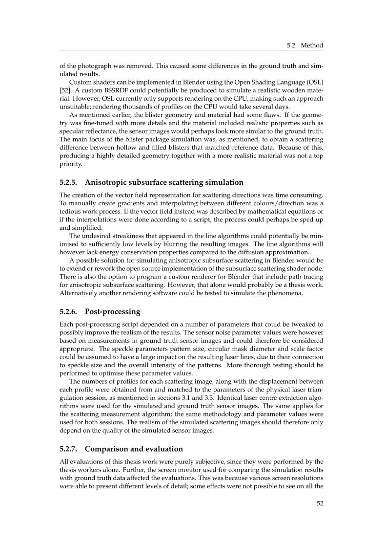
5.2. Method
of the photograph was removed. This caused some differences in the ground truth and sim-ulated results.
Custom shaders can be implemented in Blender using the Open Shading Language (OSL)[52]. A custom BSSRDF could potentially be produced to simulate a realistic wooden mate-rial. However, OSL currently only supports rendering on the CPU, making such an approachunsuitable; rendering thousands of profiles on the CPU would take several days.
As mentioned earlier, the blister geometry and material had some flaws. If the geome-try was fine-tuned with more details and the material included realistic properties such asspecular reflectance, the sensor images would perhaps look more similar to the ground truth.The main focus of the blister package simulation was, as mentioned, to obtain a scatteringdifference between hollow and filled blisters that matched reference data. Because of this,producing a highly detailed geometry together with a more realistic material was not a toppriority.
5.2.5. Anisotropic subsurface scattering simulation
The creation of the vector field representation for scattering directions was time consuming.To manually create gradients and interpolating between different colours/direction was atedious work process. If the vector field instead was described by mathematical equations orif the interpolations were done according to a script, the process could perhaps be sped upand simplified.
The undesired streakiness that appeared in the line algorithms could potentially be min-imised to sufficiently low levels by blurring the resulting images. The line algorithms willhowever lack energy conservation properties compared to the diffusion approximation.
A possible solution for simulating anisotropic subsurface scattering in Blender would beto extend or rework the open source implementation of the subsurface scattering shader node.There is also the option to program a custom renderer for Blender that include path tracingfor anisotropic subsurface scattering. However, that alone would probably be a thesis work.Alternatively another rendering software could be tested to simulate the phenomena.
5.2.6. Post-processing
Each post-processing script depended on a number of parameters that could be tweaked topossibly improve the realism of the results. The sensor noise parameter values were howeverbased on measurements in ground truth sensor images and could therefore be consideredappropriate. The speckle parameters pattern size, circular mask diameter and scale factorcould be assumed to have a large impact on the resulting laser lines, due to their connectionto speckle size and the overall intensity of the patterns. More thorough testing should beperformed to optimise these parameter values.
The numbers of profiles for each scattering image, along with the displacement betweeneach profile were obtained from and matched to the parameters of the physical laser trian-gulation session, as mentioned in sections 3.1 and 3.3. Identical laser centre extraction algo-rithms were used for the simulated and ground truth sensor images. The same applies forthe scattering measurement algorithm; the same methodology and parameter values wereused for both sessions. The realism of the simulated scattering images should therefore onlydepend on the quality of the simulated sensor images.
5.2.7. Comparison and evaluation
All evaluations of this thesis work were purely subjective, since they were performed by thethesis workers alone. Further, the screen monitor used for comparing the simulation resultswith ground truth data affected the evaluations. This was because various screen resolutionswere able to present different levels of detail; some effects were not possible to see on all the
52

5.2. Method
screens used during the thesis work. Since not all result images were viewed on differentscreens, anomalies and unwanted effects could have been missed.
Thorough user test should be performed to validate the results and discussions presented.Due to the relatively detailed level of theory researched in this thesis, qualitative testingwould perhaps be more efficient than quantitative. Background knowledge is most likelyneeded for a tester to be able to compare the sensor and scattering images properly.
5.2.8. Source criticism
The majority of articles, papers and reports used in this thesis work were peer-reviewed. Forthe references that deviated from this, other peer-reviewed sources, on the same topic, wereused to support the theory and/or method in question.
53

6 Conclusion
The aim of this thesis was to examine methods for realistically simulating each system partof a laser triangulation set-up. Simulated measurement objects were supposed to include thesubsurface scattering phenomenon and the simulation results should be validated throughcomparison with ground truth data.
Various methods for simulating system parts have been presented together with resultsand possible improvements. These include three laser line simulation approaches, a camerasimulation, three methods for wood simulation and one approach for simulating blister pack-ages. Materials with varying subsurface scattering were constructed for the blister packagesimulation. To extensively explore subsurface scattering of wood, an isolated algorithm wasimplemented to anisotropically diffuse a simulated point laser. All resulting images werecompared to corresponding ground truth data.
The texture projector method was the best out of the three tested laser line approaches,because it was simple to set up and since it gave realistic results. Blender Cycles was provento not be able to reshape a simulated volumetric Gaussian laser beam using a cylinder lens.LuxCoreRenderer allows reshaping of a volumetric beam with the usage of a cylinder lens,but the Cycles shader node tree was not successfully translated into LuxCoreRenderer texturenodes. Results of the camera simulation suffered from not including a Scheimpflug-adapteras well as from assuming infinite focus. For the wooden material simulation, the results of theUV-mapping approach best resembled the reference plank. This method was also the moststraight forward to implement. None of the simulated wooden materials caused light to scat-ter anisotropically. Because of this, the script for simulating anisotropic subsurface scatteringwas implemented. The representation of scattering directions, through colour mapping, wasinefficient and not very accurate, due to it being roughly drawn by hand. The blister packagesimulation resulted in a scattering image with clear visible difference between the hollow andfilled blisters.
54

6.1. Research questions
6.1. Research questions
The research questions of the thesis could be answered as follows:1. How can realistic line lasers be simulated in the rendering software Blender? Line
lasers can be simulated in Blender using various approaches, as presented throughout thisreport. The built-in light sources can be reshaped with shader node trees or by creating thinopenings between planes. These approaches result in laser lines with constant thickness andintensity. Blur and speckle patterns can be added through post-processing scripts, which maycause these laser lines to achieve relatively high realism.
Line laser textures can be included via the Image texture node. These textures can then beprojected through a built-in light source to generate laser lines. The realism of such a resultinglaser line depends mostly on the realism of the laser texture. With a texture containing themain characteristics of a real laser, the texture projector laser can be used to simulate laserlines of high realism.
A point laser can be generated as a geometry with an emitting volume material. Thematerial can be implemented using Cycles shader nodes to approximate the irradiance of aGaussian beam. Point lasers can be reshaped into line lasers using a cylinder lens. Creat-ing realistic cylinder lenses is currently not possible using Cycles renderer. However, Lux-CoreRenderer includes better caustics, enabling for creation of cylinder lenses. The Gaussianbeam approximation can potentially be implemented using this renderer as well. Combinedwith the working cylinder lens, this would result in a realistic line laser.
2. How can realistic wood and blister package materials that include subsurface scat-tering be simulated in Blender? Anisotropic subsurface scattering can currently not be sim-ulated in Blender. Uniform scattering can be applied to materials through various shadernodes, such as the Subsurface scattering and Volume scatter nodes. Blister package materialscan be simulated, for example, in accordance with the node trees presented in Figure 3.12. Pa-rameters such as specular reflectance should however be tweaked in order to obtain higher re-alism. Realistically appearing wooden materials are efficiently created through UV-mappinghigh resolution photographs. Wooden materials that affect light truthfully are not possible tosimulate in Blender due to the limited subsurface scattering support/implementation.
3. How can the realism of simulated laser triangulation be evaluated through com-parison with practical laser triangulation? Evaluation of each system part isolated is notpossible. Dimensions, colours, power and other properties are simulated to match the set-tings of the physical system parts. To evaluate the realism of this parameter matching, theonly data available are the captured or simulated result images. Sensor images are createdduring a physical laser triangulation session. In post-processing, these images or profiles canbe combined to generate scattering images. The simulated laser triangulation set-up can beevaluated by comparing the simulated and ground truth sensor images. Looking at close-upsof these images, factors and occurrence of phenomena like intensity, scattering, speckle andblur can be used to determine the quality of the simulation. The smaller visual differencesbetween the sensor images, the better is the simulation. The simulated sensor images can alsobe combined to scattering images. Comparison of the simulated and ground truth scatteringimages can also be used to evaluate the simulated laser triangulation system.
6.2. Future work
Future work of this thesis includes finalising the approximation of a Gaussian beam usingLuxCoreRenderer. With more knowledge about the LuxCoreRenderer, the shader node treethat was built in Cycles should be properly translated into a volumetric texture supported bythe LuxCoreRenderer. The image texture for the projector laser should also be improved toinclude more laser properties. Local variations in wavelength and focus, as well as varying
55

6.2. Future work
thickness through a beam waist, should be introduced to the image texture to enhance therealism of the resulting laser.
The blooming/fringing effect should be properly investigated to allow for realistic sim-ulation. Further, exploration of alternative methods for efficient vector field generation ishighly interesting. A more automated algorithm would be desired that could translated animage of a measurement object into a vector field representation of the object’s scatteringdirections. Combinations of various image processing approaches like edge detection andHough transform could be tested and evaluated.
Other approaches for simulating subsurface scattering of a point laser in wood shouldalso be researched, perhaps using other rendering software or by implementing a custompath-tracer. The diffusion algorithm for simulating anisotropic subsurface scattering shouldbe extended from the 2D image/sensor space to the three dimensional object space. Sub-surface scattering is naturally a 3D phenomenon that cannot be realistically simulated by a2D diffusion process. Extensive user tests should further be performed to acquire objectiveresults.
56

Bibliography
1. SICK. Precision möter kvalitet - Intelligent mätteknik för kvalitet i varje processteg.https : / / www . sick . com / se / sv / precision - moeter - kvalitet / w /measurement-sensors/. Fetched: 2020-11-13
2. Foundation B. Blender 2.91. https://www.blender.org/. Fetched: 2021-03-03
3. Cajal C, Santolaria J, Samper D, and Garrido A. SIMULATION OF LASER TRIANGU-LATION SENSORS SCANNING FOR DESIGN AND EVALUATION PURPOSES. Inter-national Journal of Simulation Modelling (IJSIMM) 2015; 14:250–64. DOI: 10.2507/IJSIMM14(2)6.296
4. Siekanski P, Magda K, Malowany K, Rutkiewicz J, Styk A, Krzesłowski J, Kowaluk T,and Zagórski A. On-Line Laser Triangulation Scanner for Wood Logs Surface GeometryMeasurement. Sensors 2019; 19. DOI: 10.3390/s19051074
5. Babar M, Khan IM, Misal, and Mudassir M u. A Fundamental Analysis of ConventionalLaser Triangulation Technique for the Development of Revamped 3D Scanning System.2020 International Conference on Engineering and Emerging Technologies (ICEET). 2020 :1–6.DOI: 10.1109/ICEET48479.2020.9048238
6. Beermann R, Quentin L, Stein G, Reithmeier E, and Kästner M. Full simulation modelfor laser triangulation measurement in an inhomogeneous refractive index field. OpticalEngineering 2018; 57:1–13. DOI: 10.1117/1.OE.57.11.114107
7. Tu D, Jin P, and Zhang X. Geometrical Model of Laser Triangulation System Based onSynchronized Scanners. Mathematical Problems in Engineering 2019; 2019. DOI: 10.1155/2019/3503192
8. Schlarp J, Csencsics E, and Schitter G. Optical Scanning of a Laser Triangulation Sen-sor for 3-D Imaging. IEEE Transactions on Instrumentation and Measurement 2020;69:3606–13. DOI: 10.1109/TIM.2019.2933343
9. Bergmann S, Mohammadikaji M, Irgenfried S, Wörn H, Beyerer J, and Dachsbacher C. APhenomenological Approach to Integrating Gaussian Beam Properties and Speckle intoa Physically-Based Renderer. Vision, Modeling & Visualization. Ed. by Hullin M, Stam-minger M, and Weinkauf T. The Eurographics Association, 2016. DOI: 10.2312/vmv.20161357
57

Bibliography
10. Zhang H, Ren Y, Liu C, and Zhu J. Flying spot laser triangulation scanner using lat-eral synchronization for surface profile precision measurement. Appl. Opt. 2014 Jul;53:4405–12. DOI: 10.1364/AO.53.004405
11. Tormanen VO and Makynen AJ. Detection of knots in veneer surface by using laser scat-tering based on the tracheid effect. 2009 IEEE Instrumentation and Measurement TechnologyConference. 2009 :1439–43. DOI: 10.1109/IMTC.2009.5168681
12. Fernandez D, Fernández P, Cuesta E, Mateos S, and Beltrán N. Influence of SurfaceMaterial on the Quality of Laser Triangulation Digitized Point Clouds for Reverse En-gineering Tasks. ETFA 2009 - 2009 IEEE Conference on Emerging Technologies and FactoryAutomation. 2009 Sep :1–8. DOI: 10.1109/ETFA.2009.5347115
13. Zaimovic-Uzunovic N and Lemeš S. Influences of Surface Parameters On Laser 3D Scan-ning. 2010 Sep
14. Mohammadikaji M, Bergmann S, Beyerer J, Burke J, and Dachsbacher C. Sensor-RealisticSimulations for Evaluation and Planning of Optical Measurement Systems With an Ap-plication to Laser Triangulation. IEEE Sensors Journal 2020; 20:5336–49. DOI: 10.1109/JSEN.2020.2971683
15. Kienle P, Batarilo L, Akgül M, Köhler MH, Wang K, Jakobi M, and Koch AW. OpticalSetup for Error Compensation in a Laser Triangulation System. Sensors 2020; 20. DOI:10.3390/s20174949
16. Kolb C, Mitchell D, and Hanrahan P. A Realistic Camera Model for Computer Graphics.Proceedings of the 22nd Annual Conference on Computer Graphics and Interactive Techniques.SIGGRAPH ’95. New York, NY, USA: Association for Computing Machinery, 1995 :317–24. DOI: 10.1145/218380.218463
17. Miyauchi K, Mori K, Otaka T, Isozaki T, Yasuda N, Tsai A, Sawai Y, Owada H,Takayanagi I, and Nakamura J. A Stacked Back Side-Illuminated Voltage Domain GlobalShutter CMOS Image Sensor with a 4.0 µm Multiple Gain Readout Pixel. Sensors 2020;20. DOI: 10.3390/s20020486
18. Quintana X, Geday M, Caño-Garcia M, Otón E, and Otón J. Image sensors for digitalphotography: a short course for undergraduates. I: Optics. Optica Pura y Aplicada 2020Mar; 53:1–23. DOI: 10.7149/OPA.53.1.51040
19. McCollough E. Industry: A Monthly Magazine Devoted to Science, Engineering and Me-chanic Arts. San Francisco: Industrial Publishing Company, 1893. Chap. PhotographicTopography:399–406. Available from: https://books.google.se/books?id=eCkAAAAAMAAJ
20. Dizeu F, Rivard M, Boisvert J, and Lamouche G. Comparison of laser triangulation,phase shift triangulation and swept source optical coherence Tomography for nonde-structive inspection of objects with micrometric accuracy. AIP Conference Proceedings.Vol. 2102. 2019 May :070004. DOI: 10.1063/1.5099804
21. Stam J. Multiple scattering as a diffusion process. Rendering Techniques ’95. Ed. by Hanra-han PM and Purgathofer W. Vienna: Springer Vienna, 1995 :41–50. DOI: 10.1007/978-3-7091-9430-0_5
22. Pai H. An imitation of realistic subsurface scattering texture for physically based ren-dering workflow. 2019 IEEE 2nd International Conference on Knowledge Innovation and In-vention (ICKII). 2019 :41–4. DOI: 10.1109/ICKII46306.2019.9042655
23. Nicodemus FE, Richmond JC, Hsia JJ, Ginsberg IW, and Limperis T. Geometrical Con-siderations and Nomenclature for Reflectance. Radiometry. USA: Jones and Bartlett Pub-lishers, Inc., 1992 :94–145
58

Bibliography
24. Wrenninge M, Villemin R, and Hery C. Path Traced Subsurface Scattering usingAnisotropic Phase Functions and Non-Exponential Free Flights. Pixar Online Li-brary 2017. Available from: https : / / graphics . pixar . com / library /PathTracedSubsurface/
25. Schlarp J, Csencsics E, and Schitter G. Design and evaluation of an integrated scanninglaser triangulation sensor. Mechatronics 2020; 72:102453. DOI: https://doi.org/10.1016/j.mechatronics.2020.102453
26. Fisher RB and Naidu DK. A Comparison of Algorithms for Subpixel Peak Detection. Im-age Technology: Advances in Image Processing, Multimedia and Machine Vision. Ed. by SanzJLC. Berlin, Heidelberg: Springer Berlin Heidelberg, 1996 :385–404. DOI: 10.1007/978-3-642-58288-2_15
27. Lee MJ, Baek SH, and Park SY. 3D foot scanner based on 360 degree rotating-type lasertriangulation sensor. 2017 Sep :1065–70. DOI: 10.23919/SICE.2017.8105700
28. Weisstein EW. Hessian Normal Form. https : / / mathworld . wolfram . com /HessianNormalForm.html. Fetched: 2021-05-19
29. LuxCoreRender. LuxCoreRenderer - open source physically based renderer. https://luxcorerender.org/. Fetched: 2021-03-01
30. Duncan DD and Kirkpatrick SJ. Algorithms for simulation of speckle (laser and other-wise). Complex Dynamics and Fluctuations in Biomedical Photonics V. Ed. by Tuchin VV andWang LV. Vol. 6855. International Society for Optics and Photonics. SPIE, 2008 :23–30.DOI: 10.1117/12.760518
31. Yan LQ, Sun W, Jensen HW, and Ramamoorthi R. A BSSRDF Model for Efficient Render-ing of Fur with Global Illumination. ACM Trans. Graph. 2017 Nov; 36. DOI: 10.1145/3130800.3130802
32. Blinn JF. Light Reflection Functions for Simulation of Clouds and Dusty Surfaces. SIGGRAPHComput. Graph. 1982 Jul; 16:21–9. DOI: 10.1145/965145.801255
33. Jensen HW, Marschner SR, Levoy M, and Hanrahan P. A Practical Model for Subsur-face Light Transport. Proceedings of the 28th Annual Conference on Computer Graphics andInteractive Techniques. SIGGRAPH ’01. New York, NY, USA: Association for ComputingMachinery, 2001 :511–8. DOI: 10.1145/383259.383319
34. Pai H. An imitation of realistic subsurface scattering texture for physically based ren-dering workflow. 2019 IEEE 2nd International Conference on Knowledge Innovation and In-vention (ICKII). 2019 :41–4. DOI: 10.1109/ICKII46306.2019.9042655
35. Liu AJ, Dong Z, Hašan M, and Marschner S. Simulating the Structure and Texture ofSolid Wood. ACM Trans. Graph. 2016 Nov; 35. DOI: 10.1145/2980179.2980255
36. Lukacevic M, Kandler G, Hu M, Olsson A, and Füssl J. A 3D model for knots and re-lated fiber deviations in sawn timber for prediction of mechanical properties of boards.Materials & Design 2019; 166:107617. DOI: 10.1016/j.matdes.2019.107617
37. Pilchik R. Pharmaceutical blister packaging, Part I: Rationale and materials. 2000 Jan;24:68–78. Available from: http://pharmanet.com.br/pdf/blister.pdf
38. Läkemedelsverket. Ibuprofen Orifarm 400 mg filmdragerad tablett. https://www.lakemedelsverket . se / sv / sok - lakemedelsfakta / lakemedel ? id =20060817000079. Fetched: 2021-01-28
39. Wilson A. 3-D profiling makes drug inspection easy. Vision Systems Design 2006; 11:17.Available from: https://www.vision- systems.com/factory/consumer-packaged - goods / article / 16736681 / 3d - profiling - makes - drug -inspection-easy
59

Bibliography
40. Yousif E, Abdallh M, Hashim H, Salih N, Salimon J, Abdullah B, and Win YF. Opticalproperties of pure and modified poly(vinyl chloride). International Journal of IndustrialChemistry 2013 Jan; 4. DOI: 10.1186/2228-5547-4-4
41. Foundation B. Blender 2.92.0 Python API Documentation. https://docs.blender.org/api/current/index.html. Fetched: 2021-05-19
42. BlenSor. Blender Sensor Simulation. https://www.blensor.org/. Fetched: 2020-12-09
43. Gazebo. Gazebo - Robot simulation made easy. http://gazebosim.org/. Fetched:2020-12-09
44. MORSE. Laser Scanner Sensors. https://www.openrobots.org/morse/doc/stable/user/sensors/laserscanner.html. Fetched: 2020-12-09
45. LuxCoreRender. LuxCoreRender 2.5 - Volumes. https://wiki.luxcorerender.org/LuxCoreRender_Volumes. Fetched: 2021-03-01
46. BlenderKit. BlenderKit - Get free 3D assets directly in Blender. https : / / www .blenderkit.com/. Fetched: 2021-02-18
47. Blender. Blender 2.91 Manual - shader nodes. https : / / docs . blender . org /manual/en/latest/render/shader_nodes. Fetched: 2021-02-15
48. Bresenham JE. Algorithm for Computer Control of a Digital Plotter. IBM Syst. J. 1965Mar; 4:25–30. DOI: 10.1147/sj.41.0025
49. Stam J. Real-Time Fluid Dynamics for Games. 2003 May
50. SICK. RCAL-300. https://www.sick.com/ag/en/rcal- 300/p/p249292.Fetched: 2021-05-17
51. Foundation B. Lens Distortion Node. https://docs.blender.org/manual/en/2.92/compositing/types/distort/lens_distortion.html. Fetched: 2021-06-17
52. Foundation B. Open Shading Language. https://docs.blender.org/manual/en/latest/render/shader_nodes/osl.html. Fetched: 2021-06-17
60

Appendix A
Speckle pattern coordinate
According to Bergmann et al., the third pattern coordinate u was derived as follows:
u =
(|ac
p + asp|
D+
dzdz0
)ˆM, (A.1)
where the parameters were defined as:
• acp: camera movement
• asp: aperture displacement caused by surface/object movement
• dzdz0
: change in distance between camera and surface
• D: lens diameter
• M: half the number of patterns.
The practical and simulated laser triangulation system only had movement in one di-mension and the measurement object was the only system part that moved. Therefore,ac
p = dzdz0
= 0, allowing for equation A.1 to be rewritten as follows:
u =|as
p|
DˆM. (A.2)
asp is divided into two components as
p,x and asp,y, defined as follows:
asp,x = ´ dSP
cos(q1)
(ax
(l2sx´1dSL
+ l2x´1dSP
)+ ay
(lsx lsydSL
+lx lydSP
)+ az
(lsx lszdSL
+ lx lzdSP
))+dSP
sin(q1)sin(q2)cos(q1)cos(q2)
(ax
(lsx lsydSL
+lx lydSP
)+ ay
(l2sy´1dSL
+l2y´1dSP
)+ az
(lsy lszdSL
+ly lzdSP
))as
p,y = ´ dSPcos(q2)
(ax
(lsx lsydSL
+lx lydSP
)+ ay
(l2sy´1dSL
+l2y´1dSP
)+ az
(lsy lszdSL
+ly lzdSP
)).
(A.3)
The parameters of these equations were defined as:
• q1: rotation around the x-axis of the surface coordinate system (to get the first axis ofthe sensor coordinate system)
• q2: rotation around the first axis of the intermediate coordinate system
• a(ax, ay, az): surface displacement
• l(lx, ly, lz): sensor normal (in surface coordinate system)
61

• ls(lsx, lsy, lsz): normalised vector between surface and laser (in surface coordinate sys-tem)
• dSP: distance between surface and pupil/lens
• dSL: distance between surface and laser.
Since the object only moved along the y-axis, ax = az = 0. ls was known to be (0, 0, 1) andq2 = 0. Equation A.3 could therefore be simplified as follows:
asp,x = ´
ay lx lycos(q1)
asp,y = ´dSP ˆ ay
(´1dSL
+l2y´1dSP
).
(A.4)
62

Appendix B
Division of work - responsibilities
Table B.1: Division of responsibilities
HeadTask responsibleLaser simulation methods
Spot-light: HK1
Point-light: HKArea-light: SK2
Texture projector: SKGaussian beam in Cycles: SKGaussian beam in LuxCoreRenderer: HK
Simulation of measurement objects
Wood - volumetric material in Cycles SKWood - volumetric material in LuxCoreRenderer HKWood - procedural textures SKWood - UV-mapping photograph HKBlister - geometry SKBlister - material HK
Profile rendering for scatter images
Wood SKBlister HK
Rendering and post-processing scripts
Scenes and scripts for rendering SKBlurring simulation HKSpeckle pattern simulation HKSensor noise simulation SKSimulated anisotropic subsurface scattering HK and SK
Comparisons
Laser methods and post-processing scripts HKScatter images SK
1Hilma Kihl, Media Technology Student at Linköping University, [email protected] Källberg, Media Technology Student at Linköping University, [email protected]
63


