Efficient Exact Inference in Planar Ising Models

Efficient Exact Inference in Planar Ising Models

Nicol N. Schraudolph [email protected]

Dmitry Kamenetsky [email protected]

Research School of Information Sciences and EngineeringAustralian National University –and–NICTA, Locked Bag 8001Canberra ACT 2601, Australia

Editor: unknown

Abstract

We give polynomial-time algorithms for the exact computation of lowest-energy (ground)states, worst margin violators, log partition functions, and marginal edge probabilities incertain binary undirected graphical models. Our approach provides an interesting alterna-tive to the well-known graph cut paradigm in that it does not impose any submodularityconstraints; instead we require planarity to establish a correspondence with perfect match-ings (dimer coverings) in an expanded dual graph. We implement a unified frameworkwhile delegating complex but well-understood subproblems (planar embedding, maximum-weight perfect matching) to established algorithms for which efficient implementations arefreely available. Unlike graph cut methods, we can perform penalized maximum-likelihoodas well as maximum-margin parameter estimation in the associated conditional randomfields (CRFs), and employ marginal posterior probabilities as well as maximum a posteri-ori (MAP) states for prediction. Maximum-margin CRF parameter estimation on imagedenoising and segmentation problems shows our approach to be efficient and effective. AC++ implementation is available from http://nic.schraudolph.org/isinf/.

Keywords: Markov random fields, spin glasses, plane embedding, blossom shrinking,marginal posterior mode

1. Introduction

Undirected graphical models are a popular tool in machine learning; they represent real-valued energy functions of the form

E′(y) :=∑i∈V

E′i(yi) +∑

(i,j)∈E

E′ij(yi, yj) , (1)

where the terms in the first sum range over the nodes V = {1, 2, . . . n}, and those in thesecond sum over the edges E ⊆ V × V of an undirected graph G(V, E).

The junction tree decomposition provides an efficient framework for exact statisticalinference in graphs that are (or can be turned into) trees of small cliques. The resultingalgorithms, however, require time exponential in the clique size, i.e., the treewidth of theoriginal graph. The treewidth of many graphs of practical interest is prohibitively large —for instance, it grows as O(n) for an n × n square lattice. A large number of approximate

arX

iv:0

810.

4401

v2 [

cs.L

G]

17

Dec

200

8

http://nic.schraudolph.org/isinf/

Schraudolph and Kamenetsky

inference techniques have been developed so as to deal with such graphs, such as pseudo-likelihood (Besag, 1986), mean field approximation, loopy belief propagation (Weiss, 2001;Yedidia et al., 2003), tree reweighting (Wainwright et al., 2003, 2005), and tree sampling(Hamze and de Freitas, 2004).

1.1 The Ising Model

Efficient exact inference is possible in certain graphical models with binary node labels.Here we focus on Ising models, whose energy functions have the form E : {0, 1}n → R with

E(y) :=∑

(i,j)∈E

[yi 6= yj ]Eij , (2)

where [·] denotes the indicator function, i.e., the cost Eij is incurred only in those states ywhere yi and yj disagree. Compared to the general model (1) for binary nodes, (2) imposestwo additional restrictions: zero node energies, and edge energies in the form of disagreementcosts. At first glance these constraints look severe; for instance, such systems must obeythe symmetry E(y) = E(¬y), where ¬ denotes Boolean negation (ones’ complement).However, it is well known (e.g., Globerson and Jaakkola, 2007) that adding a single nodemakes the Ising model (2) as expressive as the general model (1) for binary variables:

Theorem 1 Every energy function of the form (1) over n binary variables is equivalent toan Ising energy function of the form (2) over n + 1 variables, with the additional variableheld constant.

Proof by construction: Two energy functions are equivalent if they differ only by a con-stant. Without loss of generality, denote the additional variable y0 and hold it constant aty0 := 0. Given an energy function of the form (1), construct an Ising model with disagree-ment costs as follows:

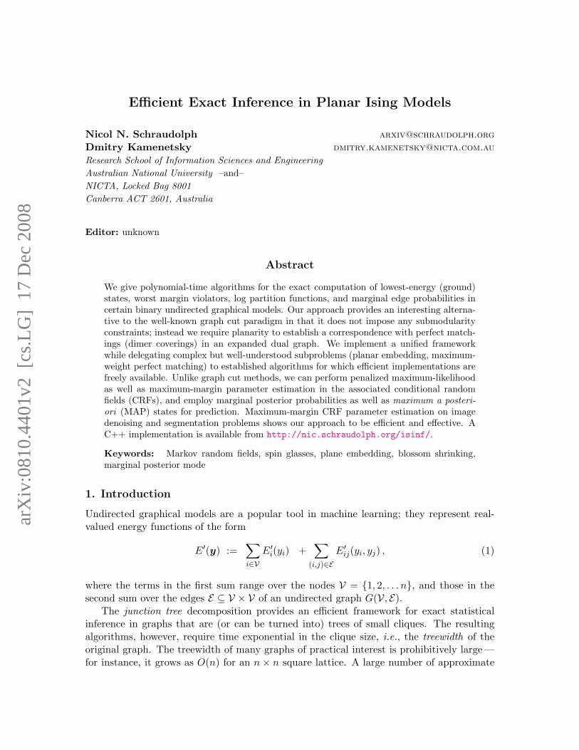
1. For each node energy function E′i(yi), add a disagreement cost of E0i := E′i(1)−E′i(0),as shown in Figure 1a. Note that in both states of yi, the energy of the resulting Isingmodel is shifted relative to E′i(yi) by the same constant amount, namely E′i(0):

yi general Ising energy0 E′i(0) 0 = E′i(0)− E′i(0)1 E′i(1) E0i = E′i(1)− E′i(0)

2. For each edge energy function E′ij(yi, yj), add the three disagreement cost terms

Eij := 12 [(E′ij(0, 1) + E′ij(1, 0))− (E′ij(0, 0) + E′ij(1, 1))],

E0i := E′ij(1, 0)− E′ij(0, 0)− Eij , and (3)

E0j := E′ij(0, 1)− E′ij(0, 0)− Eij ,

as shown in Figure 1b. Note that for all states of yi and yj , the energy of the resultingIsing model is shifted relative to E′i(yi) by the same constant amount, namely E′ij(0, 0):

2


ni

n0E

0i

:=

E′ i(1

)−E′ i(0

)

ni

n0

nj��

@@

@@@@

E′ij(1,0)−

E′ij(0,0)

−Eij

E ′ij (0,1)−

E ′ij (0,0)

−E

ij

Eij :=12[(E′ij(0,1) + E′ij(1,0))− (E′ij(0,0) + E′ij(1,1))]

nin0

njn1

��

��

E0i

Eij

−E0j

nin0

njn1

��

��

-E ij

+E0i

2Eij

E ij−E

0j

(a) (b) (c) (d)

Figure 1: Equivalent Ising model (with disagreement costs) for a given (a) node energy E′i,(b) edge energy E′ij in a binary graphical model; (c) equivalent submodular modelif Eij > 0 and E0i > 0 but E0j < 0; (d) equivalent directed model of Kolmogorovand Zabih (2004, Fig. 2d).

yi yj general Ising energy0 0 E′ij(0, 0) 0 = E′ij(0, 0)− E′ij(0, 0)0 1 E′ij(0, 1) E0j + Eij = E′ij(0, 1)− E′ij(0, 0)1 0 E′ij(1, 0) E0i + Eij = E′ij(1, 0)− E′ij(0, 0)1 1 E′ij(1, 1) E0i + E0j = E′ij(1, 1)− E′ij(0, 0)

Summing the above terms, the total bias of node i (i.e., its disagreement cost with the biasnode) is

E0i = E′i(1)− E′i(0) +∑

j:(i,j)∈E

[E′ij(1, 0)− E′ij(0, 0)− Eij ] . (4)

This construction defines an Ising model whose energy in every configuration y is shifted,relative to that of the general model we started with, by the same constant amount, namelyE′(0):

∀y ∈ {0, 1}n : E

([0y

])= E′(y) −

∑i∈V

E′i(0) −∑

(i,j)∈E

E′ij(0, 0)

= E′(y)− E′(0). (5)

The two models’ energy functions are therefore equivalent.

Note how in the above construction the label symmetry E(y) = E(¬y) of the plain Isingmodel (2) is conveniently broken by the introduction of a bias node, through the conventionthat y0 := 0.

1.2 Energy Minimization via Graph Cuts

Definition 2 The cut C of a binary graphical model G(V, E) induced by state y ∈ {0, 1}nis the set C(y) := {(i, j) ∈ E : yi 6= yj}; its weight |C(y)| is the sum of the weights of itsedges.

3


Any given state y partitions the nodes of a binary graphical model into two sets: thoselabeled ‘0’, and those labeled ‘1’. The corresponding graph cut is the set of edges crossingthe partition; since only they contribute disagreement costs to the Ising model (2), wehave ∀y : |C(y)| = E(y). The lowest-energy state of an Ising model therefore induces itsminimum-weight cut. Conversely, the ground state of an Ising model (in absence of a biasnode: up to label symmetry) can be determined from its minimum-weight cut via a simple(e.g., depth-first) graph traversal (see Algorithm 1).

Minimum-weight cuts can be computed in polynomial time in graphs whose edge weightsare all non-negative. Introducing one more node, with the constraint yn+1 := 1, allows usto construct an equivalent energy function by replacing each negatively weighted bias edgeE0i < 0 by an edge to the new node n + 1 with the positive weight Ei,n+1 := −E0i > 0(Figure 1c). This still leaves us with the requirement that all non-bias edges be non-negative. This submodularity constraint implies that agreement between nodes must belocally preferable to disagreement — a severe limitation.

The now widespread use of graph cuts in machine learning to find lowest-energy con-figurations, in particular in image processing, was pioneered by Greig et al. (1989). Ourconstruction (Figure 1c) differs from that of Kolmogorov and Zabih (2004) (Figure 1d) inthat we do not employ the notion of directed edges. (In directed graphs, the weight of acut is the sum of the weights of only those edges crossing the cut in a given direction.)We note that a more elaborate construction can give partial answers in graphs with somenegative edge weights (Kolmogorov and Rother, 2007; Rother et al., 2007b), and that asequence of expansion moves (energy minimizations in binary graphs) can efficiently yieldan approximate answer for graphs with discrete but non-binary node labels (Boykov et al.,2001).

The remainder of this paper is organized as follows: Section 2 describes the planarityand connectivity conditions that our approach imposes upon the graphs, and how we handlethem. Section 3 describes the construction of an expanded dual graph, and the algorithmfor computing optimal (ground) states of the Ising model from it. The calculation of thepartition function and marginal probabilities is dealt with in Section 4. These algorithms arethen used in Section 5 to implement maximum-likelihood and maximum-margin parameterestimation in conditional random fields (CRFs). Section 6 describes our experiments usinggrid CRFs for image denoising and boundary detection, and Section 7 concludes with adiscussion and outlook. We are making open source C++ code implementing our algorithmsfreely available for download from http://nic.schraudolph.org/isinf/.

2. Planarity and Connectivity

Unlike graph cut methods, the inference algorithms we will describe do not depend onsubmodularity; instead they require that the model graph be planar, and that a planarembedding be provided. They may also work only for connected graphs, and be the mostefficient only for biconnected graphs. In this section we review these concepts, discuss theirimplications for our approach, and describe how to best handle them.

4

http://nic.schraudolph.org/isinf/


1

2 3

45

2

1 3

45

12

34

5 1 2

34

5

(a) (b) (c) (d)

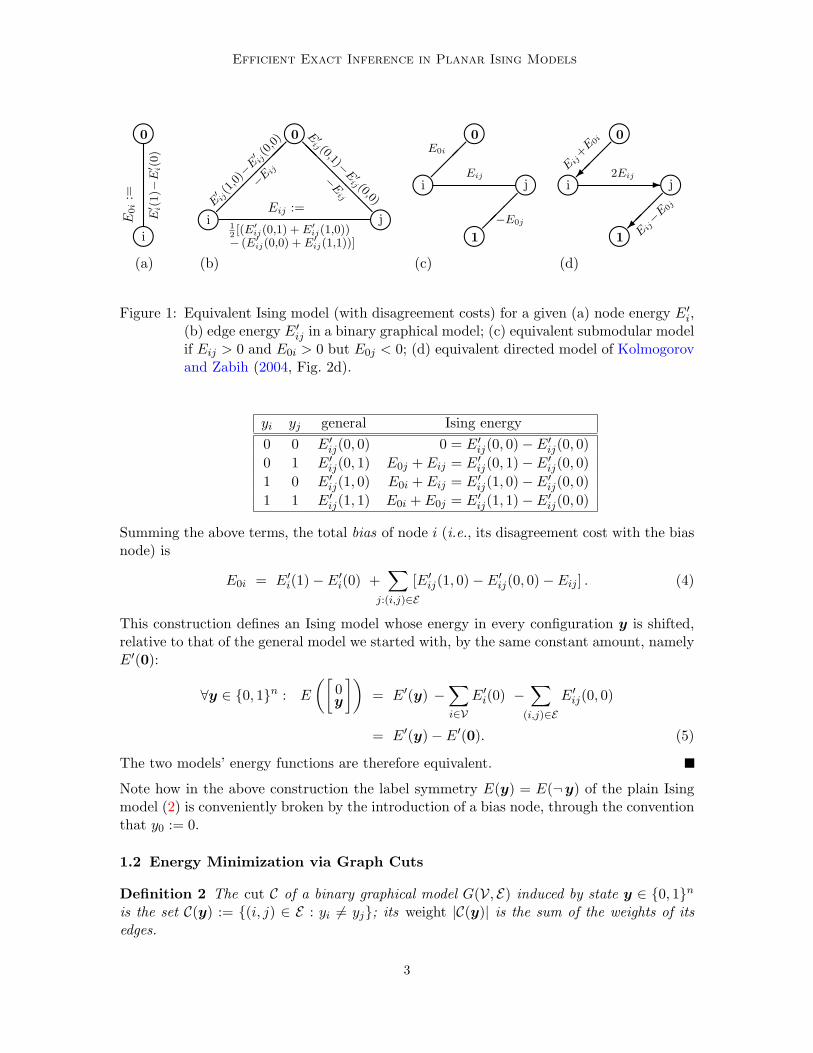
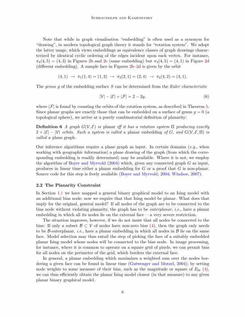
Figure 2: (a) a non-plane drawing of a planar graph; (b) a plane drawing of the same graph;(c) a different plane drawing of same graph, with the same planar embedding as(b); (d) a plane drawing of the same graph with a different planar embedding.

2.1 Embedding Planar Graphs

Definition 3 A graph is planar if it can be drawn in the plane R2 without edge inter-sections. The regions into which such a plane drawing partitions R2 are the faces of thedrawing; the unbounded region is the external face.

The operational nature of this definition would suggest that our algorithms must produce(or have access to) a plane drawing of the model graph. This is unsatisfactory in thatsuch a drawing contains much information (such as the precise location of the vertices, andthe exact shape of the edges) that we will not need. All we care about is the cyclic (say,clockwise) ordering of the edges incident upon each vertex. In topological graph theory,this is formalized in the notion of a rotation system (White and Beineke, 1978, p. 21f):

Definition 4 Let G(V, E) be an undirected, connected graph. For each vertex i ∈ V, letEi denote the set of edges in E incident upon i, considered as being oriented away from i,and let πi be a cyclic permutation of Ei. A rotation system for G is a set of permutationsΠ = {πi : i ∈ V}.

To define the sets Ei of oriented edges more formally, construct the directed graph G(V, E ′),where E ′ contains a pair of directed edges (known as edgelets) for each undirected edge inE , that is, (i, j) ∈ E ′ ⇐⇒ [(i, j) ∈ E ∨ (j, i) ∈ E ]. Then Ei = {(j, k) ∈ E ′ : i = j}.

Rotation systems directly correspond to topological graph embeddings in orientablesurfaces:

Theorem 5 Each rotation system determines an embedding of G in some orientable surfaceS such that ∀i ∈ V, any edge (i, j) ∈ Ei is followed by πi(i, j) in (say) clockwise orientation,and such that the faces F of the embedding, given by the orbits of the mapping (i, j) →πj(j, i), are 2-cells (topological disks).

Proof see White and Beineke (1978, p. 22f).

5


Note that while in graph visualisation “embedding” is often used as a synonym for“drawing”, in modern topological graph theory it stands for “rotation system”. We adoptthe latter usage, which views embeddings as equivalence classes of graph drawings charac-terized by identical cyclic ordering of the edges incident upon each vertex. For instance,π4(4, 5) = (4, 3) in Figures 2b and 2c (same embedding) but π4(4, 5) = (4, 1) in Figure 2d(different embedding). A sample face in Figures 2b–2d is given by the orbit

(4, 1) → π1(1, 4) = (1, 2) → π2(2, 1) = (2, 4) → π4(4, 2) = (4, 1).

The genus g of the embedding surface S can be determined from the Euler characteristic

|V| − |E|+ |F| = 2− 2g, (6)

where |F| is found by counting the orbits of the rotation system, as described in Theorem 5.Since planar graphs are exactly those that can be embedded on a surface of genus g = 0 (atopological sphere), we arrive at a purely combinatorial definition of planarity:

Definition 6 A graph G(V, E) is planar iff it has a rotation system Π producing exactly2 + |E| − |V| orbits. Such a system is called a planar embedding of G, and G(V, E ,Π) iscalled a plane graph.

Our inference algorithms require a plane graph as input. In certain domains (e.g., whenworking with geographic information) a plane drawing of the graph (from which the corre-sponding embedding is readily determined) may be available. Where it is not, we employthe algorithm of Boyer and Myrvold (2004) which, given any connected graph G as input,produces in linear time either a planar embedding for G or a proof that G is non-planar.Source code for this step is freely available (Boyer and Myrvold, 2004; Windsor, 2007).

2.2 The Planarity Constraint

In Section 1.1 we have mapped a general binary graphical model to an Ising model withan additional bias node; now we require that that Ising model be planar. What does thatimply for the original, general model? If all nodes of the graph are to be connected to thebias node without violating planarity, the graph has to be outerplanar, i.e., have a planarembedding in which all its nodes lie on the external face — a very severe restriction.

The situation improves, however, if we do not insist that all nodes be connected to thebias: If only a subset B ⊂ V of nodes have non-zero bias (4), then the graph only needsto be B-outerplanar, i.e., have a planar embedding in which all nodes in B lie on the sameface. Model selection may thus entail the step of picking the face of a suitably embeddedplanar Ising model whose nodes will be connected to the bias node. In image processing,for instance, where it is common to operate on a square grid of pixels, we can permit biasfor all nodes on the perimeter of the grid, which borders the external face.

In general, a planar embedding which maximizes a weighted sum over the nodes bor-dering a given face can be found in linear time (Gutwenger and Mutzel, 2004); by settingnode weights to some measure of their bias, such as the magnitude or square of E0i (4),we can thus efficiently obtain the planar Ising model closest (in that measure) to any givenplanar binary graphical model.

6


In contrast to submodularity, B-outerplanarity is a structural constraint. This has theadvantage that once a model obeying the constraint is selected, inference (e.g., parameterestimation) can proceed via unconstrained methods (e.g., optimization).

Finally, we note that all our algorithms can be extended to work for non-planar graphs aswell. They then take time exponential in the genus of the embedding though still polynomialin the size of the graph; for graphs of low genus this may well be preferable to currentapproximative methods.

2.3 Connectivity

All algorithms in this paper assume that the graph G(V, E) is connected, i.e., that E containsat least one path between any two nodes of V. Where this is not the case, one can simplydetermine the connected components1 of G in linear time (Hopcroft and Tarjan, 1973),then invoke the algorithm in question separately on each of them. Since each component isunconditionally independent of all others (as they have no edges between them), the resultscan be trivially combined. Specifically,

• G is planar iff all of its connected components are planar; any concatenation of aplanar embedding for each connected component is a planar embedding of G.

• Any concatenation of a ground state for each connected component of G is a groundstate of G.

• The log partition function of G is the sum of the log partition functions of its connectedcomponents.

• The edge marginal probabilities of G are the concatenation of edge marginal proba-bilities of its connected components.

2.4 Biconnectivity

Definition 7 A graph is biconnected iff it is connected and does not have any articulationvertex. An articulation vertex is a vertex whose removal (along with any incident edges)disconnects the graph.

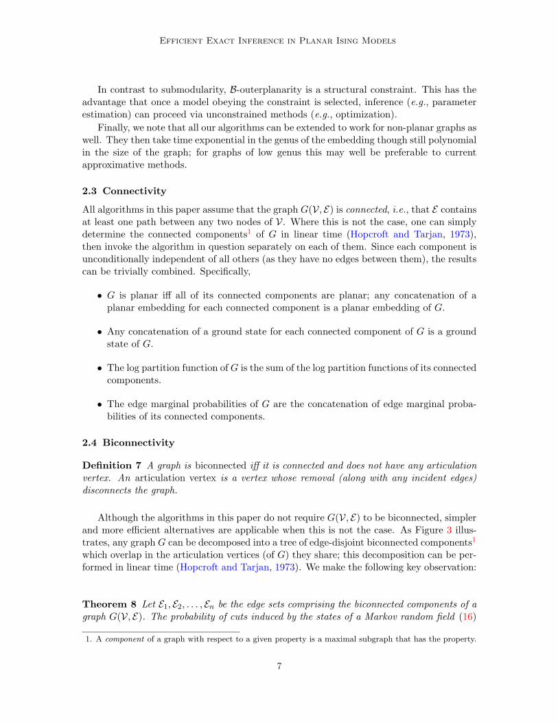
Although the algorithms in this paper do not require G(V, E) to be biconnected, simplerand more efficient alternatives are applicable when this is not the case. As Figure 3 illus-trates, any graph G can be decomposed into a tree of edge-disjoint biconnected components1

which overlap in the articulation vertices (of G) they share; this decomposition can be per-formed in linear time (Hopcroft and Tarjan, 1973). We make the following key observation:

Theorem 8 Let E1, E2, . . . , En be the edge sets comprising the biconnected components of agraph G(V, E). The probability of cuts induced by the states of a Markov random field (16)

1. A component of a graph with respect to a given property is a maximal subgraph that has the property.

7


Figure 3: Skeletal chemical structures (images courtesy of Wikipedia) of phosphorus trioxide(bottom left), nitroglycerine (left of center), and quinine (right), with decomposi-tion into a tree of biconnected components indicated (shaded ovals). Phosphoroustrioxide is biconnected (i.e., all one component); nitroglycerine is a tree (i.e., hasonly trivial biconnected components).

over an Ising model 2 (2) on G factors into that of its biconnected components:

P[C(y)] =n∏k=1

P[C(y) ∩ Ek]. (7)

Proof If G(V, E) is biconnected, n = 1 and E1 = E , making Theorem 8 trivially true. Oth-erwise split G into a biconnected component G1(V1, E1) which is a leaf of the decompositiontree, and the remainder G′(V ′, E ′). It is always possible to find such a split. Because it isa leaf, G1 connects to G′ through a single articulation vertex of G, which we call v1. Tosummarize:

V1 ∪ V ′ = V, V1 ∩ V ′ = {v1},E1 ∪ E ′ = E , E1 ∩ E ′ = ∅, G1 biconnected. (8)

Let y1 and y′ be the state y of the model restricted to vertices in V1 and V ′, respectively.By definition, y1 is independent of y′ when both are conditioned on the state yv1 of thearticulation vertex connecting them. We now make use of the label symmetry of Isingmodels, resp. the fact that it is broken by conditioning on a single node: P[C(y)] = P(y|yi)for any choice of i. We therefore have

P[C(y)] = P(y|yv1) = P(y1,y′|yv1)

= P(y1|yv1) P(y′|yv1) = P[C(y) ∩ E1] P[C(y) ∩ E ′]. (9)

2. Recall that we consider an Ising model to be an undirected graphical model with binary node states, nonode potentials, edge potentials in the form of disagreement costs, and an optional bias node.

8

http://wikipedia.org/


Recursively applying this argument to G′ yields Theorem 8.

The independence of biconnected components with respect to cuts C(y) stated by The-orem 8 may come as a surprise, given that the corresponding node states y do correlatethrough the articulation vertices. What happens is that label symmetry — specifically, thefact that C(y) = C(¬y) — folds the state space so as to exactly cancel any moments betweenbiconnected components. By decoupling their biconnected components, this facilitates effi-cient inference in graphs that are not biconnected themselves.

2.4.1 Ising Trees

Note in Figure 3 how edges which are not part of any cycle of G form trivial biconnectedcomponents comprising only themselves and the two articulation vertices they connect. Atthe most extreme, a tree T does not contain any cycles, hence consists entirely of trivialbiconnected components (Figure 3, left of center). Theorem 8 then implies that each edgecan be considered individually, making inference in an Ising tree T (V, E) very simple:

• T is planar; any embedding of T is a planar embedding.

• The minimum-weight cut of T is the set E− := {(i, j) ∈ E : Eij < 0}.(Use Algorithm 1 to obtain the corresponding ground state.)

• The log partition function of T is

lnZ = ln∏

(i,j)∈E

(e0 + e−Eij ) =∑

(i,j)∈E

ln(1 + e−Eij ). (10)

• The marginal probability of any edge (i, j) of T is

P[(i, j) ∈ C] =e−Eij

e0 + e−Eij=

11 + eEij

. (11)

2.4.2 The General Case

The most efficient way to employ the inference algorithms in this paper on graphs G thatare neither biconnected nor trees (e.g., Figure 3, right) is to apply them to each nontrivialbiconnected component of G in turn, then use Theorem 8 to combine the results, along withthe simple solutions given in Section 2.4.1 above for trivial biconnected components, intoa result for the full graph. Letting ET ⊆ E denote the set of edges that belong to trivialbiconnected components of G, we have:

• A planar embedding of G is obtained by arbitrarily combining a planar embeddingfor each of its nontrivial biconnected components and the edges in ET .

• A minimum-weight cut of G is the union between the edges in E−∩ ET and a minimum-weight cut for each of G’s nontrivial biconnected components; Algorithm 1 can be usedto obtain the corresponding ground state.

9


• The log partition function of G is the sum of the log partition functions of its nontrivialbiconnected components, plus

∑(i,j)∈ET ln(1 + e−Eij ).

• The marginal probability of an edge (i, j) ∈ E is (1 + eEij )−1 if (i, j) ∈ ET, or com-puted (by the method of Section 4) from the biconnected component it belongs to.

This concludes our discussion of conditions on the Ising model graph G. In what follows,we assume that G is connected and planar, and that a plane embedding is provided. Wedo not require that G is biconnected, though where this is not the case, it is generally moreefficient to decompose G into biconnected components as discussed above.

3. Computing Ground States via Maximum-Weight Perfect Matching

Definition 9 A frustrated cycle O ⊆ E of a graph G(V, E) with non-zero edge weights Eis a simple cycle whose product of edge weights is negative, i.e.,

∏(i,j)∈O Eij < 0. (A simple

cycle is a closed path with no repeated edges or vertices.)

A weighted graph is said to be frustrated if it contains any frustrated cycles. Note thattrees can never be frustrated because they do not contain any cycles to begin with.

The lowest-energy (ground) state y∗ := argminy E(y) of an unfrustrated Ising model iseasily found via essentially the same method as in a tree (Section 2.4.1): paint nodes as youtraverse the graph, flipping the binary color of your paintbrush whenever you traverse anedge with negative disagreement cost (as done by Algorithm 1 below when invoked on thecut C = {(i, j) ∈ E : Eij < 0}). This cannot lead to a contradiction because by Definition 9you will flip brush color an even number of times along any cycle in the graph, hence alwaysend a cycle on the same color you started it with.

The presence of frustration unfortunately makes the computation of ground states muchharder — in fact, it is known to be NP-hard in general (Barahona, 1982). As shown below,the ground state of a planar Ising model can be computed in polynomial time via maximum-weight perfect matching on an expanded dual of its embedded graph.

A relationship between the states of a planar Ising model and perfect matchings (“dimercoverings” to physicists) was first established by Kasteleyn (1961, 1963, 1967) and Fisher(1961, 1966). Perfect matchings in dual graph constructs were used by Bieche et al. (1980)and Barahona (1982) to compute Ising ground states; below we generalize a simpler con-struction for triangulated graphs due to Globerson and Jaakkola (2007). For rectangularlattices our approach reduces to the construction of Thomas and Middleton (2007), thoughtheir algorithm to compute ground states is somewhat less straightforward. Pardella andLiers (2008) apply this construction to very large square lattices (up to 3000×3000 nodes),and find it to be more efficient than earlier methods (Bieche et al., 1980; Barahona, 1982).

3.1 The Expanded Dual Graph

Definition 10 The dual G∗(F , E) of an embedded graph G(V, E ,Π) has a vertex for eachface of G, with edges connecting vertices corresponding to faces that are adjacent ( i.e., sharean edge) in G.

10


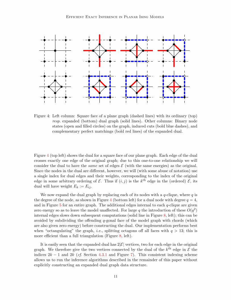
Figure 4: Left column: Square face of a plane graph (dashed lines) with its ordinary (top)resp. expanded (bottom) dual graph (solid lines). Other columns: Binary nodestates (open and filled circles) on the graph, induced cuts (bold blue dashes), andcomplementary perfect matchings (bold red lines) of the expanded dual.

Figure 4 (top left) shows the dual for a square face of our plane graph. Each edge of the dualcrosses exactly one edge of the original graph; due to this one-to-one relationship we willconsider the dual to have the same set of edges E (with the same energies) as the original.Since the nodes in the dual are different, however, we will (with some abuse of notation) usea single index for dual edges and their weights, corresponding to the index of the originaledge in some arbitrary ordering of E . Thus if (i, j) is the kth edge in the (ordered) E , itsdual will have weight Ek := Eij .

We now expand the dual graph by replacing each of its nodes with a q-clique, where q isthe degree of the node, as shown in Figure 4 (bottom left) for a dual node with degree q = 4,and in Figure 5 for an entire graph. The additional edges internal to each q-clique are givenzero energy so as to leave the model unaffected. For large q the introduction of these O(q2)internal edges slows down subsequent computations (solid line in Figure 8, left); this can beavoided by subdividing the offending q-gonal face of the model graph with chords (whichare also given zero energy) before constructing the dual. Our implementation performs bestwhen “octangulating” the graph, i.e., splitting octagons off all faces with q > 13; this ismore efficient than a full triangulation (Figure 8, left).

It is easily seen that the expanded dual has 2|E| vertices, two for each edge in the originalgraph. We therefore give the two vertices connected by the dual of the kth edge in E theindices 2k − 1 and 2k (cf. Section 4.3.1 and Figure 7). This consistent indexing schemeallows us to run the inference algorithms described in the remainder of this paper withoutexplicitly constructing an expanded dual graph data structure.

11


bias bias0

0 1

0 1

0

1 1

0 1

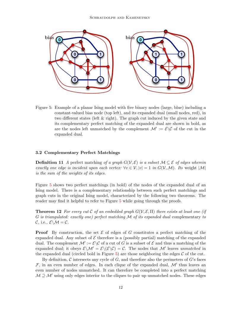
Figure 5: Example of a planar Ising model with five binary nodes (large, blue) including aconstant-valued bias node (top left), and its expanded dual (small nodes, red), intwo different states (left & right). The graph cut induced by the given state andits complementary perfect matching of the expanded dual are shown in bold, asare the nodes left unmatched by the complement M′ := E\C of the cut in theexpanded dual.

3.2 Complementary Perfect Matchings

Definition 11 A perfect matching of a graph G(V, E) is a subset M⊆ E of edges whereinexactly one edge is incident upon each vertex: ∀v ∈ V, |v| = 1 in G(V,M). Its weight |M|is the sum of the weights of its edges.

Figure 5 shows two perfect matchings (in bold) of the nodes of the expanded dual of anIsing model. There is a complementary relationship between such perfect matchings andgraph cuts in the original Ising model, characterized by the following two theorems. Thereader may find it helpful to refer to Figure 5 while going through the proofs.

Theorem 12 For every cut C of an embedded graph G(V, E ,Π) there exists at least one (ifG is triangulated: exactly one) perfect matching M of its expanded dual complementary toC, i.e., E\M = C.

Proof By construction, the set E of edges of G constitutes a perfect matching of theexpanded dual. Any subset of E therefore is a (possibly partial) matching of the expandeddual. The complementM′ := E\C of a cut of G is a subset of E and thus a matching of theexpanded dual; it obeys E\M′ = E\(E\C) = C. The nodes that M′ leaves unmatched inthe expanded dual (circled bold in Figure 5) are those neighboring the edges C of the cut.

By definition, C intersects any cycle of G, and therefore also the perimeters of G’s facesF , in an even number of edges. In each clique of the expanded dual, M′ thus leaves aneven number of nodes unmatched. It can therefore be completed into a perfect matchingM⊇M′ using only edges interior to the cliques to pair up unmatched nodes. These edges

12


have no counterpart in the original graph: (M\M′) ∩ E = ∅. We thus have

E\M = E\[(M\M′) ∪M′] = [E\(M\M′)]\M′ = E\M′ = C. (12)

In a 3-clique of the expanded dual, M′ will leave two nodes unmatched or none at all; ineither case there is only one way to complete the matching, by adding one edge resp. noneat all. By construction, if G is triangulated all cliques in its expanded dual are 3-cliques,and so M is unique.

In other words, there exists a surjection from perfect matchings in the expanded dual of Gto cuts in G. Furthermore, since we have given edges interior to the cliques of the expandeddual zero energy (i.e., |M\M′| = 0), every perfect matching M complementary to a cut Cof our Ising model (2) obeys the relation

|M|+ |C| = |M′|+ |C| =∑

(i,j)∈E

Eij = const. (13)

This means that instead of a minimum-weight cut in a graph we can look for a maximum-weight perfect matching in its expanded dual. But will that matching always be comple-mentary to a cut? The following theorem shows that this is true for plane graphs:

Theorem 13 Every perfect matching M of the expanded dual of a plane graph G(V, E ,Π)is complementary to a cut C of G, i.e., E\M = C.

Proof By definition, E\M is a cut of G iff it intersects every cycle O ⊆ E of G an evennumber of times. This can be shown by induction over the faces of the embedding:

Base case — let O ⊆ E be the perimeter of a face of the embedding, and considerthe corresponding clique of the expanded dual: M matches an even number of nodes inthe clique via interior edges; all other nodes must be matched by edges crossing O. Thecomplement of the matching in G thus intersects O an even number of times:

|(E\M) ∩ O| ≡ 0 mod 2. (14)

Induction — let O1,O2 ⊆ E be cycles in G obeying (14), and consider their symmetricdifference O1∆O2 := (O1 ∪ O2)\(O1 ∩ O2):

|(E\M) ∩ (O1∆O2)| = |[(E\M) ∩ (O1 ∪ O2)]\(O1 ∩ O2)|= |[(E\M) ∩ O1] ∪ [(E\M) ∩ O2]| − |(E\M) ∩ (O1 ∩ O2)|= |(E\M) ∩ O1|+ |(E\M) ∩ O2| − 2|(E\M) ∩ (O1 ∩ O2)|≡ 0 + 0− 2n ≡ 0 mod 2. (n ∈ N) (15)

We see that property (14) is preserved under composition of cycles via symmetric differences,and thus holds for all cycles that can be composed from face perimeters of the embeddingof G in this fashion.

All cycles in a plane graph G are contractible on its embedding surface (a plane resp.sphere) because that surface has zero genus, and is therefore simply connected. All con-tractible cycles of G can be constructed by composition of face perimeters via symmetricdifferences, thus have an even intersection with E\M, which is therefore a cut.

13


This is where planarity matters: Surfaces of non-zero genus are not simply connected, andthus non-plane graphs may contain non-contractible cycles (e.g., encircling the hole of atorus). In the presence of frustration, our construction does not guarantee that the comple-ment E\M of a perfect matching of the expanded dual contains an even number of edgesalong such cycles. For planar graphs, however, the above theorems allow us to leverageknown polynomial-time algorithms for perfect matchings into inference methods for Isingmodels. This approach also works for non-planar Ising models that contain no frustratednon-conctractible cycle.

We note that if all cliques of the expanded dual are of even size, there is also a direct (non-complementary) surjection from perfect matchings to cuts in the original graph. In contrastto our complementary map, the direct surjection requires the addition of dummy verticesinto the expanded dual for faces of G with odd perimeter so as to make the correspondingcliques even (Kasteleyn, 1963; Fisher, 1966; Liers and Pardella, 2008).

3.3 Computing the Ground State

The blossom-shrinking algorithm (Edmonds, 1965a,b) is a sophisticated method to effi-ciently compute the maximum-weight perfect matching of a graph. It can be implemented(Mehlhorn and Schafer, 2002) to run in as little as O(|E| |V| log |V|) time (Galil et al., 1986).Although the Blossom IV code we are using (Cook and Rohe, 1999) is asymptotically lessefficient —O(|E| |V|2) — we have found it to be very fast in practice (Figure 8, left).

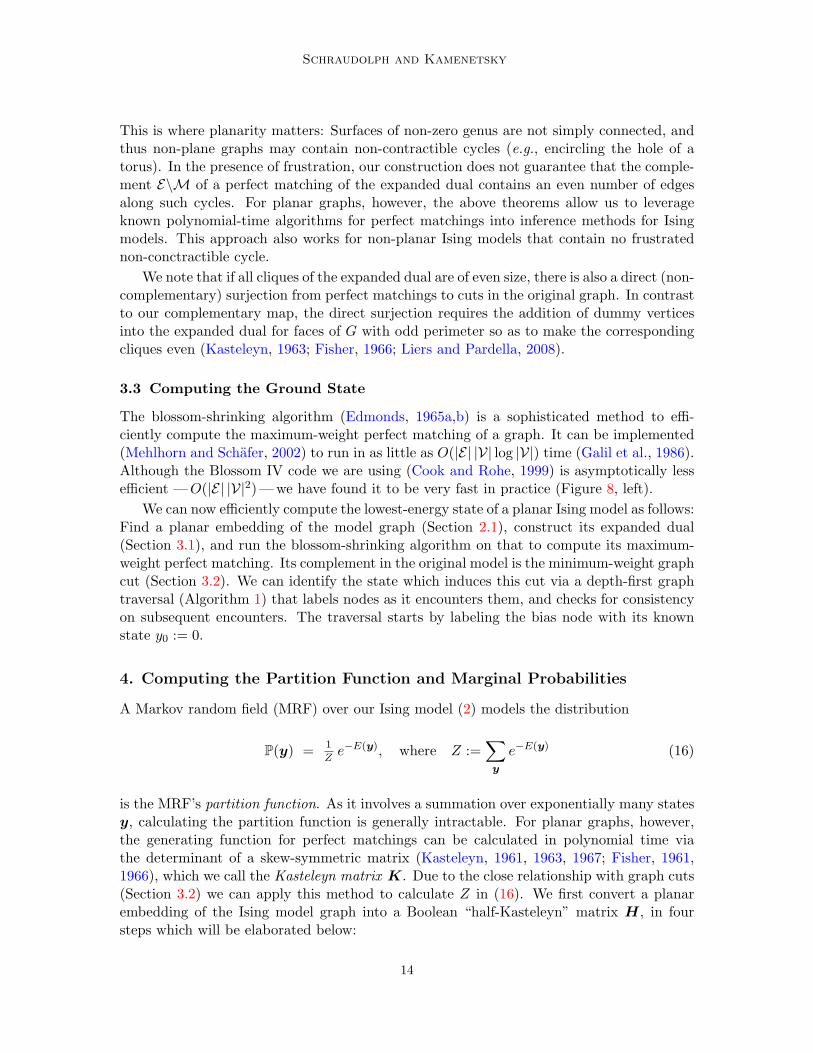
We can now efficiently compute the lowest-energy state of a planar Ising model as follows:Find a planar embedding of the model graph (Section 2.1), construct its expanded dual(Section 3.1), and run the blossom-shrinking algorithm on that to compute its maximum-weight perfect matching. Its complement in the original model is the minimum-weight graphcut (Section 3.2). We can identify the state which induces this cut via a depth-first graphtraversal (Algorithm 1) that labels nodes as it encounters them, and checks for consistencyon subsequent encounters. The traversal starts by labeling the bias node with its knownstate y0 := 0.

4. Computing the Partition Function and Marginal Probabilities

A Markov random field (MRF) over our Ising model (2) models the distribution

P(y) = 1

Ze−E(y), where Z :=

∑y

e−E(y) (16)

is the MRF’s partition function. As it involves a summation over exponentially many statesy, calculating the partition function is generally intractable. For planar graphs, however,the generating function for perfect matchings can be calculated in polynomial time viathe determinant of a skew-symmetric matrix (Kasteleyn, 1961, 1963, 1967; Fisher, 1961,1966), which we call the Kasteleyn matrix K. Due to the close relationship with graph cuts(Section 3.2) we can apply this method to calculate Z in (16). We first convert a planarembedding of the Ising model graph into a Boolean “half-Kasteleyn” matrix H, in foursteps which will be elaborated below:

14


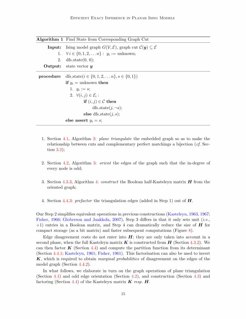
Algorithm 1 Find State from Corresponding Graph Cut

Input: Ising model graph G(V, E), graph cut C(y) ⊆ E1. ∀ i ∈ {0, 1, 2, . . . n} : yi := unknown;2. dfs state(0, 0);

Output: state vector y

procedure dfs state(i ∈ {0, 1, 2, . . . n}, s ∈ {0, 1})if yi = unknown then

1. yi := s;2. ∀(i, j) ∈ Ei :

if (i, j) ∈ C thendfs state(j,¬s);

else dfs state(j, s);else assert yi = s;

1. Section 4.1, Algorithm 2: plane triangulate the embedded graph so as to make therelationship between cuts and complementary perfect matchings a bijection (cf. Sec-tion 3.2);

2. Section 4.2, Algorithm 3: orient the edges of the graph such that the in-degree ofevery node is odd;

3. Section 4.3.3, Algorithm 4: construct the Boolean half-Kasteleyn matrix H from theoriented graph;

4. Section 4.4.3: prefactor the triangulation edges (added in Step 1) out of H.

Our Step 2 simplifies equivalent operations in previous constructions (Kasteleyn, 1963, 1967;Fisher, 1966; Globerson and Jaakkola, 2007), Step 3 differs in that it only sets unit (i.e.,+1) entries in a Boolean matrix, and Step 4 can dramatically reduce the size of H forcompact storage (as a bit matrix) and faster subsequent computations (Figure 8).

Edge disagreement costs do not enter into H; they are only taken into account in asecond phase, when the full Kasteleyn matrix K is constructed from H (Section 4.3.2). Wecan then factor K (Section 4.4) and compute the partition function from its determinant(Section 4.4.1; Kasteleyn, 1961; Fisher, 1961). This factorisation can also be used to invertK, which is required to obtain marginal probabilities of disagreement on the edges of themodel graph (Section 4.4.2).

In what follows, we elaborate in turn on the graph operations of plane triangulation(Section 4.1) and odd edge orientation (Section 4.2), and construction (Section 4.3) andfactoring (Section 4.4) of the Kasteleyn matrix K resp. H.

15


1 2

34

5

1 2

34

5

(a) (b) (c) (d)

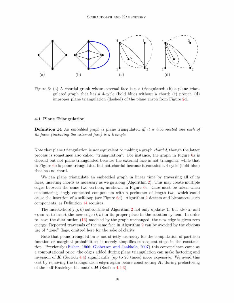
Figure 6: (a) A chordal graph whose external face is not triangulated; (b) a plane trian-gulated graph that has a 4-cycle (bold blue) without a chord; (c) proper, (d)improper plane triangulation (dashed) of the plane graph from Figure 2d.

4.1 Plane Triangulation

Definition 14 An embedded graph is plane triangulated iff it is biconnected and each ofits faces (including the external face) is a triangle.

Note that plane triangulation is not equivalent to making a graph chordal, though the latterprocess is sometimes also called “triangulation”. For instance, the graph in Figure 6a ischordal but not plane triangulated because the external face is not triangular, while thatin Figure 6b is plane triangulated but not chordal because it contains a 4-cycle (bold blue)that has no chord.

We can plane triangulate an embedded graph in linear time by traversing all of itsfaces, inserting chords as necessary as we go along (Algorithm 2). This may create multipleedges between the same two vertices, as shown in Figure 6c. Care must be taken whenencountering singly connected components with a perimeter of length two, which couldcause the insertion of a self-loop (see Figure 6d). Algorithm 2 detects and biconnects suchcomponents, as Definition 14 requires.

The insert chord(i, j, k) subroutine of Algorithm 2 not only updates E , but also πi andπk so as to insert the new edge (i, k) in its proper place in the rotation system. In orderto leave the distribution (16) modeled by the graph unchanged, the new edge is given zeroenergy. Repeated traversals of the same face in Algorithm 2 can be avoided by the obvioususe of “done” flags, omitted here for the sake of clarity.

Note that plane triangulation is not strictly necessary for the computation of partitionfunction or marginal probabilities; it merely simplifies subsequent steps in the construc-tion. Previously (Fisher, 1966; Globerson and Jaakkola, 2007) this convencience came ata computational price: the edges added during plane triangulation can make factoring andinversion of K (Section 4.4) significantly (up to 20 times) more expensive. We avoid thiscost by removing the triangulation edges again before constructing K, during prefactoringof the half-Kasteleyn bit matrix H (Section 4.4.3).

16


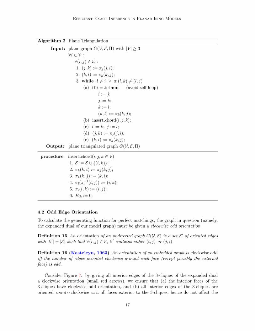
Algorithm 2 Plane Triangulation

Input: plane graph G(V, E ,Π) with |V| ≥ 3∀i ∈ V :∀(i, j) ∈ Ei :1. (j, k) := πj(j, i);2. (k, l) := πk(k, j);3. while l 6= i ∨ πl(l, k) 6= (l, j)

(a) if i = k then (avoid self-loop)i := j;j := k;k := l;(k, l) := πk(k, j);

(b) insert chord(i, j, k);(c) i := k; j := l;(d) (j, k) := πj(j, i);(e) (k, l) := πk(k, j);

Output: plane triangulated graph G(V, E ,Π)

procedure insert chord(i, j, k ∈ V)1. E := E ∪ {(i, k)};2. πk(k, i) := πk(k, j);3. πk(k, j) := (k, i);4. πi(π−1

i (i, j)) := (i, k);5. πi(i, k) := (i, j);6. Eik := 0;

4.2 Odd Edge Orientation

To calculate the generating function for perfect matchings, the graph in question (namely,the expanded dual of our model graph) must be given a clockwise odd orientation.

Definition 15 An orientation of an undirected graph G(V, E) is a set E ′ of oriented edgeswith |E ′| = |E| such that ∀(i, j) ∈ E, E ′ contains either (i, j) or (j, i).

Definition 16 (Kasteleyn, 1963) An orientation of an embedded graph is clockwise oddiff the number of edges oriented clockwise around each face (except possibly the externalface) is odd.

Consider Figure 7: by giving all interior edges of the 3-cliques of the expanded duala clockwise orientation (small red arrows), we ensure that (a) the interior faces of the3-cliques have clockwise odd orientation, and (b) all interior edges of the 3-cliques areoriented counterclockwise wrt. all faces exterior to the 3-cliques, hence do not affect the

17


1

2

3

4

6

5

7

89

10

15 18

1

2

3

4

56

7

8

9 10

12

11

13

14

16 17

19

20

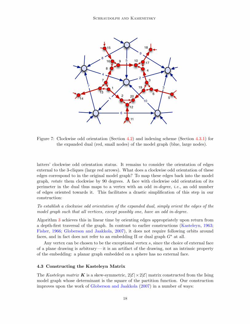
Figure 7: Clockwise odd orientation (Section 4.2) and indexing scheme (Section 4.3.1) forthe expanded dual (red, small nodes) of the model graph (blue, large nodes).

latters’ clockwise odd orientation status. It remains to consider the orientation of edgesexternal to the 3-cliques (large red arrows). What does a clockwise odd orientation of theseedges correspond to in the original model graph? To map these edges back into the modelgraph, rotate them clockwise by 90 degrees. A face with clockwise odd orientation of itsperimeter in the dual thus maps to a vertex with an odd in-degree, i.e., an odd numberof edges oriented towards it. This facilitates a drastic simplification of this step in ourconstruction:

To establish a clockwise odd orientation of the expanded dual, simply orient the edges of themodel graph such that all vertices, except possibly one, have an odd in-degree.

Algorithm 3 achieves this in linear time by orienting edges appropriately upon return froma depth-first traversal of the graph. In contrast to earlier constructions (Kasteleyn, 1963;Fisher, 1966; Globerson and Jaakkola, 2007), it does not require following orbits aroundfaces, and in fact does not refer to an embedding Π or dual graph G∗ at all.

Any vertex can be chosen to be the exceptional vertex s, since the choice of external faceof a plane drawing is arbitrary — it is an artifact of the drawing, not an intrinsic propertyof the embedding: a planar graph embedded on a sphere has no external face.

4.3 Constructing the Kasteleyn Matrix

The Kasteleyn matrix K is a skew-symmetric, 2|E|×2|E| matrix constructed from the Isingmodel graph whose determinant is the square of the partition function. Our constructionimproves upon the work of Globerson and Jaakkola (2007) in a number of ways:

18


Algorithm 3 Construct Odd Edge Orientation

Input: undirected graph G(V, E)1. ∀ v ∈ V : v.visited = false;2. pick arbitrary edge (r, s) ∈ E ;3. E ′ := {(r, s)};4. make odd(r, s);

Output: orientation E ′ of E : ∀ v ∈ V\{s},in-degree(v) ≡ 1 mod 2 in G(V, E ′)

function make odd: (u, v ∈ V)→ {true, false}1. E := E\(u, v);2. if v.visited then return true;3. v.visited := true;4. odd := false;5. ∀w ∈ V : {v, w} ∈ E

if make odd(v, w) then(a) E ′ := E ′ ∪ {(w, v)};(b) odd := ¬ odd;

else E ′ := E ′ ∪ {(v, w)};6. return odd;

• We employ an indexing scheme that obviates any need to refer to the expanded dualof the model graph (which we consequently never explicitly construct at all);

• We break construction of the Kasteleyn matrix into two phases, the first of which isinvariant with respect to the model’s disagreement costs;

• We make the “half-Kasteleyn” matrix H computed in the first phase very compactby prefactoring out the triangulation edges (see Section 4.4.3) and storing it as a bitmatrix.

4.3.1 Indexing Scheme

Without loss of generality, let E = {e1, e2, . . . e|E|}. Note that the expanded dual has 2|E|vertices, one lying to either side of every edge in the model graph. When viewing edgeek along its direction in E ′, we label the dual node to its right 2k− 1 and that to itsleft 2k; see Figure 7 for an example (cf. Section 3.1). One benefit of this scheme is thatquantities relating to the edges of the model graph (as opposed to internal edges of thecliques of the expanded dual) will always be found on the superdiagonal of K. We alsonotationally extend the rotation system from Section 2.1 to support this indexing scheme:ek = (i, j)⇐⇒ eπi(k) = πi(i, j).

19


10 100 1e3 1e4 1e5

1

0.1

0.01

1e-3

1e-4

CP

U t

ime

(se

cond

s)

originaltriang.octang.

10 100 1000

0.001

0.01

0.1

1

10

CP

U t

ime

(se

cond

s)

no prefact.prefactored

10 100 1000

1e3

1e6

1e9

mem

ory

(by

tes) K

H

uncompressedcompressed

ring size (nodes) ring size (nodes) ring size (nodes)

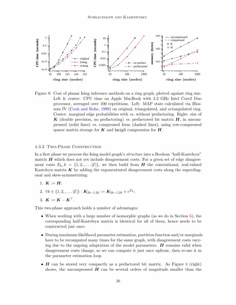
Figure 8: Cost of planar Ising inference methods on a ring graph, plotted against ring size.Left & center: CPU time on Apple MacBook with 2.2 GHz Intel Core2 Duoprocessor, averaged over 100 repetitions. Left: MAP state calculated via Blos-som IV (Cook and Rohe, 1999) on original, triangulated, and octangulated ring.Center: marginal edge probabilities with vs. without prefactoring. Right: size ofK (double precision, no prefactoring) vs. prefactored bit matrix H, in uncom-pressed (solid lines) vs. compressed form (dashed lines), using row-compressedsparse matrix storage for K and bzip2 compression for H.

4.3.2 Two-Phase Construction

In a first phase we process the Ising model graph’s structure into a Boolean “half-Kasteleyn”matrix H which does not yet include disagreement costs. For a given set of edge disagree-ment costs Ek, k = {1, 2, , . . . |E|}, we then build from H the conventional, real-valuedKasteleyn matrix K by adding the exponentiated disagreement costs along the superdiag-onal and skew-symmetrizing:

1. K := H;

2. ∀k ∈ {1, 2, , . . . |E|} : K2k−1,2k := K2k−1,2k + eEk ;

3. K := K −K>.

This two-phase approach holds a number of advantages:

• When working with a large number of isomorphic graphs (as we do in Section 6), thecorresponding half-Kasteleyn matrix is identical for all of them, hence needs to beconstructed just once.

• During maximum likelihood parameter estimation, partition function and/or marginalshave to be recomputed many times for the same graph, with disagreement costs vary-ing due to the ongoing adaptation of the model parameters. H remains valid whendisagreement costs change, so we can compute it just once upfront, then re-use it inthe parameter estimation loop.

• H can be stored very compactly as a prefactored bit matrix. As Figure 8 (right)shows, the uncompressed H can be several orders of magnitude smaller than the

20


corresponding Kasteleyn matrix K. Row-compressed sparse storage of K (which hasexactly 3 non-zero entries in each row and column) is more efficient, but applying thebzip2 compressor3 to the prefactored bit matrix H yields by far the most compactstorage format. Such memory efficiency becomes very important when working withlarge data sets of non-isomorphic graphs.

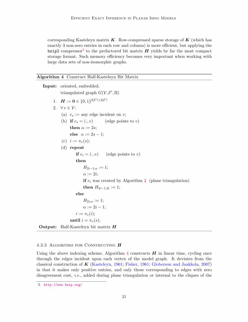
Algorithm 4 Construct Half-Kasteleyn Bit Matrix

Input: oriented, embedded,triangulated graph G(V, E ′,Π)

1. H := 0 ∈ {0, 1}2|E ′|×2|E ′|

2. ∀ v ∈ V :(a) es := any edge incident on v;(b) if es = (·, v) (edge points to v)

then α := 2s;else α := 2s− 1;

(c) i := πv(s);(d) repeat

if ei = (·, v) (edge points to v)then

H2i−1,α := 1;α := 2i;if ei was created by Algorithm 2 (plane triangulation)then H2i−1,2i := 1;

elseH2i,α := 1;α := 2i− 1;

i := πv(i);until i = πv(s);

Output: Half-Kasteleyn bit matrix H

4.3.3 Algorithm for Constructing H

Using the above indexing scheme, Algorithm 4 constructs H in linear time, cycling oncethrough the edges incident upon each vertex of the model graph. It deviates from theclassical construction of K (Kasteleyn, 1961; Fisher, 1961; Globerson and Jaakkola, 2007)in that it makes only positive entries, and only those corresponding to edges with zerodisagreement cost, i.e., added during plane triangulation or internal to the cliques of the

3. http://www.bzip.org/

21

http://www.bzip.org/


expanded dual. All such entries have the value e0 = 1, making H a Boolean matrix, whichcan be stored compactly as a bit matrix.

4.4 Factoring Kasteleyn Matrices

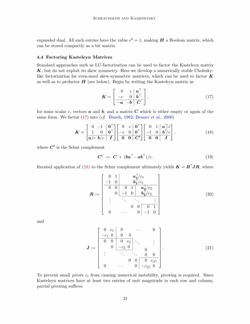
Standard approaches such as LU-factorization can be used to factor the Kasteleyn matrixK, but do not exploit its skew symmetry. Here we develop a numerically stable Cholesky-like factorization for even-sized skew-symmetric matrices, which can be used to factor Kas well as to prefactor H (see below). Begin by writing the Kasteleyn matrix as

K =

0 c a>

−c 0 b>

−a −b C

, (17)

for some scalar c, vectors a and b, and a matrix C which is either empty or again of thesame form. We factor (17) into (cf. Bunch, 1982; Benner et al., 2000)

K =

0 −1 0>

1 0 0>

a/c b/c I

0 c 0>

−c 0 0>

0 0 C′

0 1 a>/c−1 0 b>/c

0 0 I

, (18)

where C′ is the Schur complement

C′ := C + (ba>− ab>)/c. (19)

Iterated application of (18) to the Schur complement ultimately yields K = R>JR, where

R :=

0 1 a>1/c1−1 0 b>1/c1

0 0 0 1 a>2/c20 −1 0 b>2/c2

.... . . . . .

...0 0 0 1

0 · · · 0 −1 0

(20)

and

J :=

0 c1 0 · · · 0−c1 0 0 0

0 0 0 c2 . . ....

0 −c2 00...

. . . . . . 0 00 0 0 c|E|

0 · · · 0 −c|E| 0

. (21)

To prevent small pivots ci from causing numerical instability, pivoting is required. SinceKasteleyn matrices have at least two entries of unit magnitude in each row and column,partial pivoting suffices.

22


4.4.1 Partition Function

The partition function for perfect matchings is√|K| (Kasteleyn, 1961; Fisher, 1961). Our

factoring gives |R| = 1 and |J | =∏i c

2i , so we have

√|K| =

√|R>| |J | |R| =

√|J | =

|E|∏i=1

|ci|. (22)

Calculation of the product in (22) is prone to numerical overflow; this is easily avoided byworking with logarithms instead. Using the complementary relationship (13) with graphcuts in planar Ising models, we obtain the log partition function for the latter as

lnZ := ln∑y

e−P

k∈C(y) Ek = ln∑y

e−(P

k∈E Ek−P

k/∈C(y) Ek) (23)

= ln(e−P

k∈E Ek∑y

eP

k/∈C(y) Ek) = ln√|K| −

∑k∈E

Ek =|E|∑i=1

(ln |ci| − Ei).

4.4.2 Marginal Probabilities

The marginal probability of disagreement along an edge equals the negative gradient of thelog partition function (23) with respect to the disagreement costs. Computing this involvesthe inverse of K:

P(k ∈ C) =∑

y: k∈C(y)

P(y) = 1

Z

∑y: k∈C(y)

e−E(y) = − 1Z

∂Z

∂Ek= − ∂ lnZ

∂Ek

= 1− 12|K|

∂|K|∂Ek

= 1− 12 tr(K−1 ∂K

∂Ek

)= 1 +K−1

2k−1,2kK2k−1,2k, (24)

where tr denotes the matrix trace, and we have used the fact that K−1 is skew-symmetricas well. To invert K, observe from (20) resp. (21) that R and J are essentially triangularresp. diagonal (simply swap rows 2k−1 and 2k, k = 1, 2, . . . |E|), and thus easily inverted.Then use K−1 = R−1J−1R−> to obtain

[K−1]2k−1,2k =2|E|∑i=1

2|E|∑j=1

[R−1]2k−1,i[J−1]i,j [R−>]j,2k =−1ck

+|E|∑

i=k+1

dik, (25)

where dik :=[R−1]2k−1,2i[R−1]2k,2i−1 − [R−1]2k−1,2i−1[R−1]2k,2i

ci.

4.4.3 Prefactoring

Consider the rows and columns of K corresponding to an edge added during plane trian-gulation (Section 4.1). Re-order K to bring those rows and columns to the top left, so thatthey form the a, b, and c of (17). Since the disagreement cost of a triangulation edge iszero, we now have a unity pivot: c = e0 = 1. This has two advantageous consequences:

Size reduction: The unity pivot does not affect the value of the partition function.Since we are not interested in the marginal probability of triangulation edges (which after all

23


are not part of the original model), we do not need a or b either, once we have computed theSchur complement (19). We can therefore discard the first two rows and first two columnsof K after factoring (17). Factoring out all triangulation edges in this fashion reduces thesize of K (resp. R and J) to range only over the edges of the original Ising model graph.This reduces storage requirements and speeds up subsequent computation of the inverse(Figure 8, center).

Boolean closure: The unity pivot eliminates the division from the Schur complement(19); in fact we show below that applying (18) to prefactor H −H> yields a Schur com-plement that can be expressed as H ′ −H ′>, where H ′ is again a Boolean matrix. Thisclosure property allows us to simply prefactor triangulation edges directly out of H withoutexplicitly constructing K.

Specifically, let K := H −H> for a half-Kasteleyn matrix H with elements in {0, 1}.Without loss of generality, assume that H and its transpose are disjoint, i.e., have nonon-zero element in common: H �H>= 0, where � denotes Hadamard (element-wise)multiplication. Algorithm 4 respects this condition; violations would cancel in the con-struction of K anyway. Expressing H as

H =

0 1 a>1

0 0 b>1

a2 b2 C1

, (26)

we can write K = H−H> as (17) with a = a1−a2, b = b1−b2, c = 1, and C = C1−C>1 .The Schur complement (19) then becomes

C′ = C1 −C>1 + (b1 − b2)(a1 − a2)>− (a1 − a2)(b1 − b2)>

= (C1 + b1a>1 + b2a>2 + a1b>2 + a2b

>1 )− (C>1 + a1b

>1 + a2b

>2 + b2a>1 + b1a>2 )

=: H ′ −H ′>, (27)

where

H ′ = C1 + b1a>1 + b2a>2 + a1b>2 + a2b

>1 . (28)

It remains to show that all elements of H ′ are in {0, 1}. By definition of H (26), allelements of C1,a1,a2, b1, b2 are in {0, 1}, and by closure of multiplication in {0, 1} so aretheir products. Thus an element of H ′ will be in {0, 1} iff it is non-zero in at most one termon the right-hand side of (28), or (equivalently) iff all pairs formed from the five terms inquestion are disjoint. This can indeed be shown to be the case:

• Because H �H>= 0, we know that neither a1 and a2 nor b1 and b2 can have anynon-zero elements in common, so b1a>1 and b2a>2 are disjoint, as are a1b

>2 and a2b

>1 .

• By construction of H (Algorithm 4), a1 and b1 (resp. a2 and b2) can only havean element in common if the dual nodes on both sides of the corresponding edge aremembers of the same clique. This cannot happen because we explicitly ensure thatthe graph becomes biconnected during plane triangulation (Section 4.1), so that anedge cannot border the same face of the model graph on both sides. Thus all fourouter products in (28) are pairwise disjoint.

24


• Finally, each outer product in (28) is disjoint from C1 as long as the edges beingfactored out do not form a cut of the model graph (i.e., cycle of the dual). Weare prefactoring only edges added during triangulation; for these to form a cut themodel graph would have to have been disconnected prior to triangulation. This can-not happen here because we deal with (and eliminate) this possibility during earlierpreprocessing (Section 2.3).

In summary, all five terms on the right-hand side of (28) are pairwise disjoint. Thus theSchur complement H ′ is a Boolean matrix as well, and can be computed from H (26) veryefficiently by replacing the additions and multiplications in (28) with bitwise OR and ANDoperations, respectively. As long as further triangulation edges remain in H ′, we then setH := H ′ and iteratively apply (26) and (28) so as to prefactor them out as well.

5. Application to CRF Parameter Estimation

Our algorithms can be applied to regularized maximum likelihood and maximum marginparameter estimation in conditional random fields (CRFs). In a standard planar Ising CRF,the disagreement costs in (2) are computed as Ek := θ>xk, i.e., as inner products betweenlocal features (sufficient statistics) xk of the modeled data at each edge k, and correspondingparameters θ of the model. The conditional distribution P(y|x,θ) (where x represents theunion of all local features) is then modeled as a Markov random field (16).

5.1 Maximum Likelihood

Maximum-likelihood (ML) CRF parameter estimation seeks to minimize wrt. θ the L2-regularized negative log likelihood

LML(θ) := 12 λ‖θ‖

2 − ln P(y∗|x,θ)

= 12 λ‖θ‖

2 + E(y∗|x,θ) + lnZ(θ|x) (29)

of a given target labeling y∗,4 with regularization parameter λ. This is a smooth, convex,non-negative objective that can be optimized via gradient methods such as LBFGS, eitherin conventional batch mode (Nocedal, 1980; Liu and Nocedal, 1989) or online (Schraudolphet al., 2007). The gradient of (29) with respect to the parameters θ is given by

∂

∂θLML(θ) = λθ +

∑k∈E

([k ∈ C(y∗)] − P(k ∈ C(y|x,θ))

)xk. (30)

The contribution of each edge k to the gradient (30) is given by the product between itslocal features xk and the difference between the indicator function for membership of k inthe cut induced by the target state y∗ and the marginal probability of k being contained ina cut, given x and θ. We compute the latter via the inverse of the Kasteleyn matrix (24).

4. For notational clarity we suppress here the fact that we are usually modeling a collection of data items;the objective function for such a set is simply the sum of objectives for each individual item in it.

25


5.2 Maximum Margin

For maximum-margin (MM) parameter estimation (Taskar et al., 2004) we instead minimize

LMM(θ) := 12 λ‖θ‖

2 + E(y∗|x,θ)−minyM(y|y∗,x,θ) (31)

= 12 λ‖θ‖

2 + E(y∗|x,θ)− E(y|x,θ) + d(y|y∗),

where y := argminy M(y|y∗,x,θ) is the worst margin violator, i.e., the state that minimizes,relative to a given target state y∗,4 the margin energy

M(y|y∗) := E(y)− d(y|y∗), (32)

where d(·|·) is a measure of divergence in state space. If d(·|·) is a weighted Hammingdistance between induced cuts:

d(y|y∗) :=∑k∈E

[[k ∈ C(y)] 6= [k ∈ C(y∗)]] vk, (33)

where the vk > 0 are constant weighting factors (in the simplest case: all ones) on the edgesof our Ising model, then it is easily verified that the margin energy (32) is implemented (upto a shift that depends only on y∗) by an isomorphic Ising model with disagreement costs

Ek + (2[k ∈ C(y∗)]− 1) vk. (34)

We can thus use our algorithm of Section 3.3 to efficiently find the worst margin violator.5

The maximum-margin objective (31) is convex but non-smooth; its gradient is

∂

∂θLMM(θ) = λθ +

∑k∈E

([k ∈ C(y∗)] − [k ∈ C(y)]

)xk, (35)

i.e., local features xk are multiplied by one of {−1, 0, 1}, depending on the membership ofedge k in the cuts induced by y∗ and y, respectively. We can minimize (31) via bundlemethods, such as the BT bundle trust algorithm (Schramm and Zowe, 1992), making useof the convenient lower bound ∀θ : LMM(θ) ≥ 0, which holds because

minyM(y|y∗,x,θ) ≤ M(y∗|y∗,x,θ) = E(y∗|x,θ)− d(y∗|y∗) = E(y∗|x,θ). (36)

6. Experiments

We now demonstrate the scalability of our approach to CRF parameter estimation (Sec-tion 5) on two simple computer vision problems: the synthetic binary image denoising taskof Kumar and Hebert (2004, 2006), and the detection of segmentation boundaries in noisymasks from the GrabCut Ground Truth image segmentation database (Rother et al., 2007a).

5. Thomas and Middleton (2007) employ a similar approach to obtain the ground state from a given statey∗ by setting up an isomorphic Ising model with disagreement costs (1− 2 [k ∈ C(y∗)])Ek.

26


6.1 Synthetic Binary Image Denoising

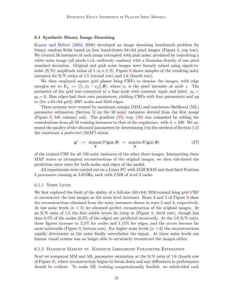
Kumar and Hebert (2004, 2006) developed an image denoising benchmark problem forbinary random fields based on four hand-drawn 64×64 pixel images (Figure 9, top row).We created 50 instances of each image corrupted with pink noise, produced by convolving awhite noise image (all pixels i.i.d. uniformly random) with a Gaussian density of one pixelstandard deviation. Original and pink noise images were linearly mixed using signal-to-noise (S/N) amplitude ratios of 1 :n, n ∈ N. Figure 9 shows samples of the resulting noisyinstances for S/N ratios of 1:5 (second row) and 1:6 (fourth row).

We then employed square grid planar Ising CRFs to denoise the images, with edgeenergies set to Eij := 〈[1, |xi − xj |],θ〉, where xi is the pixel intensity at node i. Theperimeter of the grid was connected to a bias node with constant input and label: x0 =y0 = 0. Bias edges had their own parameters, yielding CRFs with four parameters and upto (for a 64×64 grid) 4097 nodes and 8316 edges.

These systems were trained by maximum margin (MM) and maximum likelihood (ML)parameter estimation (Section 5) on the 50 noisy instances derived from the first image(Figure 9, left column) only. The gradient (35) resp. (30) was computed by adding thecontributions from all 50 training instances to that of the regularizer, with λ = 100. We as-sessed the quality of the obtained parameters by determining (via the method of Section 3.3)the maximum a posteriori (MAP) states

y∗ := argmaxy

P(y|x,θ) = argminy

E(y|x,θ) (37)

of the trained CRF for all 150 noisy instances of the other three images. Interpreting theseMAP states as attempted reconstructions of the original images, we then calculated theprediction error rates for both nodes and edges of the model.

All experiments were carried out on a Linux PC with 3 GB RAM and dual Intel Pentium4 processors running at 3.6 GHz, each with 2 MB of level 2 cache.

6.1.1 Noise Level

We first explored the limit of the ability of a full-size (64×64) MM-trained Ising grid CRFto reconstruct the test images as the noise level increases. Rows 3 and 5 of Figure 9 showthe reconstructions obtained from the noisy instances shown in rows 2 and 4, respectively.At low noise levels (n < 5) we obtained perfect reconstruction of the original images. Atan S/N ratio of 1:5 the first subtle errors do creep in (Figure 9, third row), though lessthan 0.5% of the nodes (0.3% of the edges) are predicted incorrectly. At the 1:6 S/N ratio,these figures increase to 2.1% for nodes and 1.15% for edges, and the errors become farmore noticeable (Figure 9, bottom row). For higher noise levels (n > 6) the reconstructionsrapidly deteriorate as the noise finally overwhelms the signal. At these noise levels ourhuman visual system was no longer able to accurately reconstruct the images either.

6.1.2 Maximum Margin vs. Maximum Likelihood Parameter Estimation

Next we compared MM and ML parameter estimation at the S/N ratio of 1:6 (fourth rowof Figure 9), where reconstruction begins to break down and any differences in performanceshould be evident. To make ML training computationally feasible, we subdivided each

27


(used fortraining)

(used fortraining)

Figure 9: Denoising of binary images by maximum-margin training of planar Ising grids;from top to bottom: original images (Kumar and Hebert, 2004, 2006), imagesmixed with pink noise in a 1:5 ratio, reconstruction via MAP state of 64×64Ising grid CRF from those noisy instances, images mixed with pink noise in a 1:6ratio, and reconstruction from those noisy instances. Only the left-most imagewas used for training (max-margin CRF parameter estimation, λ = 100), theothers for reconstruction.

28


Table 1: Performance comparison of parameter estimation methods on the denoising task;image reconstruction via MAP on the full (64×64) model and images. The mini-mum in each result column is boldfaced.

Train Method Patch Size Train Time Edge Error Node Error

MM

64× 64 490.4 s 1.15 % 2.10 %32× 32 174.7 s 1.16 % 2.15 %16× 16 91.4 s 1.12 % 1.98 %

8× 878.1 s 1.10 % 1.83 %

ML 5468.2 s 1.11 % 1.93 %

training image into 64 8×8 patches, then trained an 8×8 grid CRF on those patches. ForMM training we used the full (64×64) images and model, as well as 32×32, 16×16, and 8×8patches, so as to assess how this subdividision impacts the quality of the model. Testingalways employed the MAP state of the full model on the full images.

Table 1 reports the edge and node errors obtained under each experimental condition.To assess statistical significance, we performed binomial pairwise comparison tests at a 95%confidence level against the null hypothesis that each of the two algorithms being comparedhas an equal (50%) chance of outperforming the other on a given test image.

We found no statistically significant difference here between 8×8 CRFs trained by MMvs. ML. However, ML training took 70 times as long to achieve this, so MM training ismuch preferable on computational grounds.

Counter to our expectations, the node and edge errors suggest that MM training actuallyworks better on small (8×8 and 16×16) image patches. We surmise that this is becausesmall patches have a relatively larger perimeter, leading to better training of the bias edges.Pairwise comparison tests, however, only found the node error for the 32×32 patch-trainedCRF to be significantly worse than for the smaller patches; all other differences were belowthe significance threshold. What we can confidently state is that subdividing the imagesinto small patches did not hurt performance, and yielded much shorter training times.

6.1.3 Maximum A Posteriori vs. Marginal Posterior Reconstruction

Fox and Nicholls (2001) have argued that the MAP state does not summarize well theinformation in the posterior distribution of an Ising model of noisy binary images, andproposed reconstruction via the marginal posterior mode (MPM) instead. For binary labels,the MPM is simply obtained by thresholding the marginal posterior node probabilities:(∀i ∈ V) yi := [P(yi = 1 |x,θ) > 0.5]. In our Ising models, however, we have marginalposterior probabilities for edges (Section 4.4.2), and infer node states from graph cuts(Algorithm 1). Here implementing the MPM runs into a difficulty: since the edge set

{k ∈ E : P(k ∈ C(y|x,θ)) > 0.5} (38)

may not be a cut of the model graph, hence may not unambiguously induce a node state.What we really need is the cut closest (in some given sense) to (38). For this purpose we

29


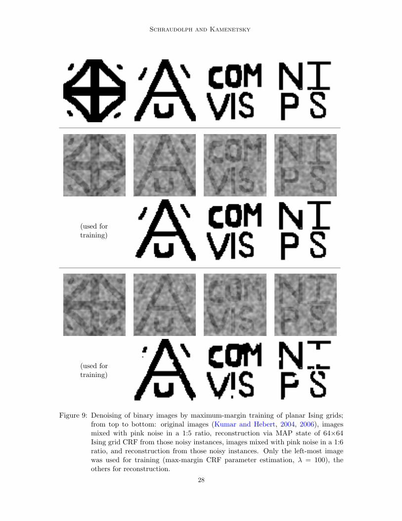
Table 2: Comparison of reconstruction methods on the denoising task, using the parametersof an MM-trained 8×8 CRF. The minimum in each result column is boldfaced;“test time” is the time required to reconstruct all 150 images.

Test Method Patch Size Test Time Edge Error Node Error

MAP64×64 3.7 s 1.10 % 1.83 %

8×83.2 s 1.96 % 5.21 %

M3P 397.5 s 1.95 % 3.32 %

formulate the state y+ with the maximal minimum marginal posterior (M3P):

y+ := argmaxy′

mink∈E

{P(k ∈ C(y|x,θ)) if k ∈ C(y′),

1− P(k ∈ C(y|x,θ)) otherwise.(39)

In other words, the M3P state (39) is induced by the cut whose edges (and those of itscomplement) have the largest minimum marginal probability. We can efficiently computey+ as follows:

1. Find the minimum-weight spanning tree E+ ⊆ E of the model graph G(V, E) withedge weights −|P(k ∈ C(y|x,θ))− 0.5|. (This can be done in O(|E| log |E|) time.)

2. Run Algorithm 1 on G(V, E+) to find y+ as the state induced in the spanning treeby the MPM edge set (38).

Since G(V, E+) is a tree, it contains no cycles, and Algorithm 1 will therefore unambiguouslyidentify the M3P state.

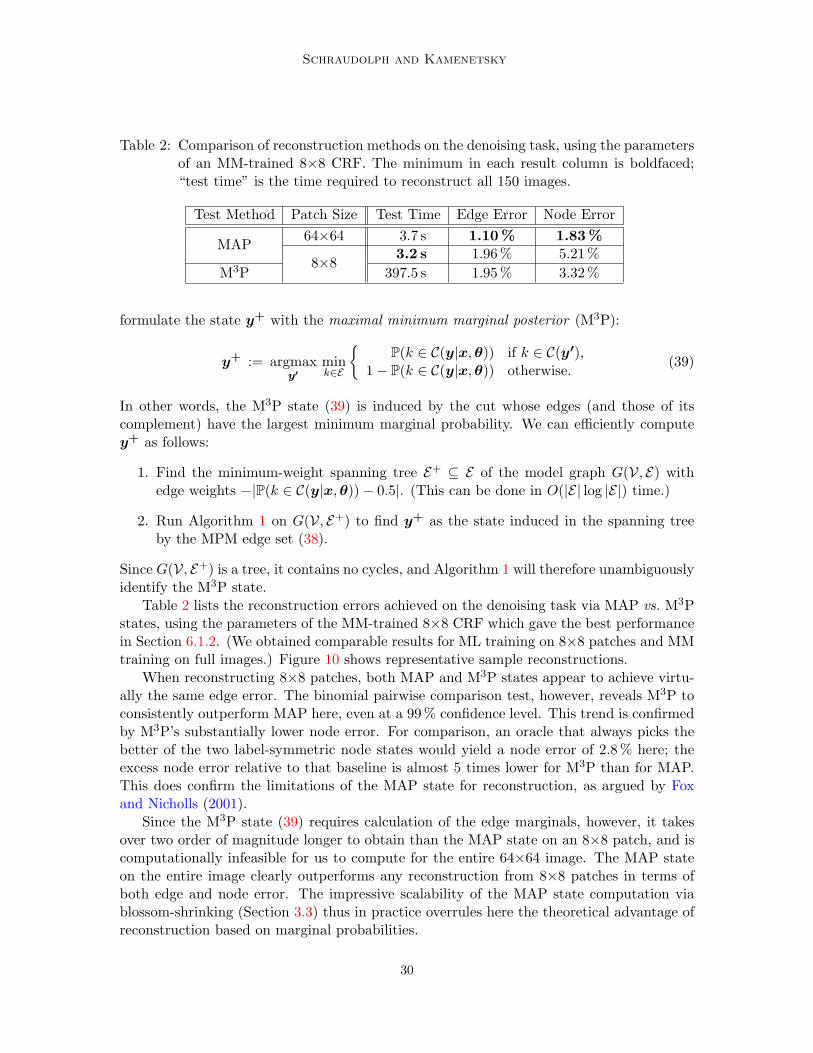
Table 2 lists the reconstruction errors achieved on the denoising task via MAP vs. M3Pstates, using the parameters of the MM-trained 8×8 CRF which gave the best performancein Section 6.1.2. (We obtained comparable results for ML training on 8×8 patches and MMtraining on full images.) Figure 10 shows representative sample reconstructions.

When reconstructing 8×8 patches, both MAP and M3P states appear to achieve virtu-ally the same edge error. The binomial pairwise comparison test, however, reveals M3P toconsistently outperform MAP here, even at a 99 % confidence level. This trend is confirmedby M3P’s substantially lower node error. For comparison, an oracle that always picks thebetter of the two label-symmetric node states would yield a node error of 2.8 % here; theexcess node error relative to that baseline is almost 5 times lower for M3P than for MAP.This does confirm the limitations of the MAP state for reconstruction, as argued by Foxand Nicholls (2001).

Since the M3P state (39) requires calculation of the edge marginals, however, it takesover two order of magnitude longer to obtain than the MAP state on an 8×8 patch, and iscomputationally infeasible for us to compute for the entire 64×64 image. The MAP stateon the entire image clearly outperforms any reconstruction from 8×8 patches in terms ofboth edge and node error. The impressive scalability of the MAP state computation viablossom-shrinking (Section 3.3) thus in practice overrules here the theoretical advantage ofreconstruction based on marginal probabilities.

30


Figure 10: Image reconstructions on the denoising task; columns from left to right: Noisy64×64 image, MAP reconstruction of full image, MAP reconstruction of 8×8patches, and M3P reconstruction of 8×8 patches.

6.2 Boundary Detection

To further scale up our approach, we designed a simple boundary detection task basedon images from the GrabCut Ground Truth image segmentation database (Rother et al.,2007a). We took 100×100 pixel subregions of images that depicted a segmentation bound-ary, and corrupted the segmentation mask with pink noise, produced by convolving a whitenoise image (all pixels i.i.d. uniformly random) with a Gaussian density with one pixelstandard deviation.

We then employed a planar Ising model to recover the original boundary — namely,a 100×100 square grid with one additional edge pegged to a high energy, encoding priorknowledge that the bottom left and top right corners of the grid depict different regions.As before, the energy of the other edges was set to Eij := 〈[1, |xi − xj |],θ〉, where xi is thepixel intensity at node i. We did not employ a bias node for this task, and simply set theregularization constant to λ = 1.

Note that this is a huge model: 10 000 nodes and 19 801 edges. Computing the partitionfunction or marginals would require inverting a Kasteleyn matrix with over 1.5 ·109 entries;minimizing (29) is therefore computationally infeasible for us. Computing a ground state

31


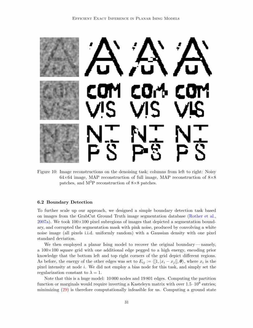
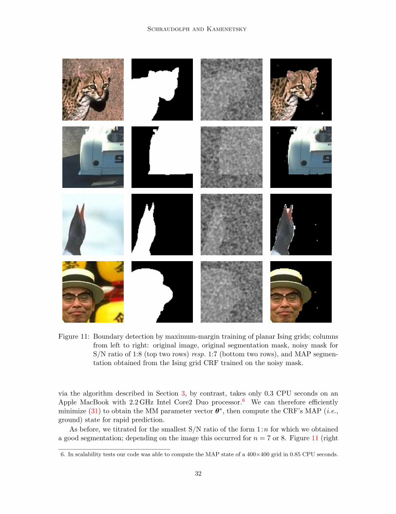
Figure 11: Boundary detection by maximum-margin training of planar Ising grids; columnsfrom left to right: original image, original segmentation mask, noisy mask forS/N ratio of 1:8 (top two rows) resp. 1:7 (bottom two rows), and MAP segmen-tation obtained from the Ising grid CRF trained on the noisy mask.

via the algorithm described in Section 3, by contrast, takes only 0.3 CPU seconds on anApple MacBook with 2.2 GHz Intel Core2 Duo processor.6 We can therefore efficientlyminimize (31) to obtain the MM parameter vector θ∗, then compute the CRF’s MAP (i.e.,ground) state for rapid prediction.

As before, we titrated for the smallest S/N ratio of the form 1:n for which we obtaineda good segmentation; depending on the image this occurred for n = 7 or 8. Figure 11 (right

6. In scalability tests our code was able to compute the MAP state of a 400×400 grid in 0.85 CPU seconds.

32


column) shows that at these noise levels our approach is capable of recovering the originalsegmentation boundary quite well, with less than 1% of nodes mislabeled. For S/N ratiosof 1:9 and lower the system was unable to locate the boundary; for S/N ratios of 1:6 andhigher we obtained perfect reconstruction. Again this corresponded closely to our humanability to visually locate the segmentation boundary accurately.

7. Discussion and Outlook

We have proposed an alternative algorithmic framework for efficient exact inference inbinary graphical models, which replaces the submodularity constraint of graph cut methodswith a planarity constraint. Besides proving efficient and effective in first experiments, ourapproach opens up a number of interesting research directions to be explored:

Our algorithms can all be extended to nonplanar graphs, at a cost exponential in thegenus of the embedding. We are currently developing these extensions, which may prove ofgreat practical value for graphs that are “almost” planar; examples include road networks(where edge crossings arise from overpasses without on-ramps) and graphs describing thetertiary structure of proteins (Vishwanathan et al., 2007).

Our algorithms also provide a foundation for efforts to develop efficient approximateinference methods for nonplanar Ising models. Our method for calculating the groundstate (Section 3) actually works for nonplanar graphs whose ground state does not containfrustrated non-contractible cycles. The QPBO graph cut method (Kolmogorov and Rother,2007) finds ground states that do not contain any frustrated cycles, and otherwise yields apartial labeling. Can we likewise obtain a partial labeling of ground states with frustratednon-contractible cycles?

The existence of two distinct tractable frameworks for inference in binary graphicalmodels implies a more powerful hybrid: Consider a graph each of whose biconnected com-ponents is either planar or submodular. In its entirety, this graph may be neither planar norsubmodular, yet efficient exact inference in it is clearly possible by applying the appropriateframework to each component, then combining the results (Section 2.4.2). Can this hybridapproach be extended to cover less obvious situations?

Acknowledgments

Earlier drafts of this paper have appeared on the arXiv preprint server (Schraudolph andKamenetsky, 2008) and (in condensed form) at the 2008 NIPS conference (Schraudolph andKamenetsky, 2009). We thank the anonymous NIPS reviewers for their valuable feedback.

NICTA is a national research institute with a charter to build Australia’s pre-eminentcentre of excellence for information and communications technology (ICT). NICTA is build-ing capabilities in ICT research, research training and commercialisation for the generationof national benefit. NICTA is funded by the Australian Government as represented by theDepartment of Broadband, Communications and the Digital Economy and the AustralianResearch Council through the ICT Centre of Excellence program.

33


References

Francisco Barahona. On the computational complexity of Ising spin glass models. Journalof Physics A: Mathematical, Nuclear and General, 15(10):3241–3253, 1982.

Peter Benner, Ralph Byers, Heike Fassbender, Volker Mehrmann, and David Watkins.Cholesky-like factorizations of skew-symmetric matrices. Electronic Transactions on Nu-merical Analysis, 11:85–93, 2000.

J. Besag. On the statistical analysis of dirty pictures. Journal of the Royal Statistical SocietyB, 48(3):259–302, 1986.

I. Bieche, R. Maynard, R. Rammal, and J. P. Uhry. On the ground states of the frustrationmodel of a spin glass by a matching method of graph theory. Journal of Physics A:Mathematical, Nuclear and General, 13:2553–2576, 1980.

John M. Boyer and Wendy J. Myrvold. On the cutting edge: Simplified O(n) pla-narity by edge addition. Journal of Graph Algorithms and Applications, 8(3):241–273,2004. Reference implementation (C source code): http://jgaa.info/accepted/2004/

BoyerMyrvold2004.8.3/planarity.zip.

Yuri Boykov, Olga Veksler, and Ramin Zabih. Fast approximate energy minimization viagraph cuts. IEEE Transactions on Pattern Analysis and Machine Intelligence, 23(11):1222–1239, 2001.

James R. Bunch. A note on the stable decomposition of skew-symmetric matrices. Mathe-matics of Computation, 38(158):475–479, April 1982.

William Cook and Andre Rohe. Computing minimum-weight perfect matchings. INFORMSJournal on Computing, 11(2):138–148, 1999. C source code available at http://www.isye.gatech.edu/∼wcook/blossom4/.

Jack Edmonds. Maximum matching and a polyhedron with 0,1-vertices. Journal of Researchof the National Bureau of Standards, 69B:125–130, 1965a.

Jack Edmonds. Paths, trees, and flowers. Canadian Journal of Mathematics, 17:449–467,1965b.

Michael E. Fisher. Statistical mechanics of dimers on a plane lattice. Physical Review, 124(6):1664–1672, 1961.

Michael E. Fisher. On the dimer solution of planar Ising models. Journal of MathematicalPhysics, 7(10):1776–1781, 1966.

C. Fox and G. K. Nicholls. Exact map states and expectations from perfect sampling: Greig,Porteous and Seheult revisited. In A. Mohammad-Djafari, editor, Bayesian Inference andMaximum Entropy Methods in Science and Engineering, volume 568 of American Instituteof Physics Conference Series, pages 252–263, 2001.

34

http://jgaa.info/accepted/2004/BoyerMyrvold2004.8.3/planarity.zip

http://jgaa.info/accepted/2004/BoyerMyrvold2004.8.3/planarity.zip

http://www.isye.gatech.edu/~wcook/blossom4/

http://www.isye.gatech.edu/~wcook/blossom4/


Zvi Galil, Silvio Micali, and Harold N. Gabow. An O(EV logV ) algorithm for finding amaximal weighted matching in general graphs. SIAM Journal of Computing, 15:120–130,1986.

Amir Globerson and Tommi Jaakkola. Approximate inference using planar graph decompo-sition. In B. Scholkopf, J. Platt, and T. Hofmann, editors, Advances in Neural InformationProcessing Systems 19, pages 473–480, Cambridge, MA, 2007. MIT Press.

D. M. Greig, B. T. Porteous, and A. H. Seheult. Exact maximum a posteriori estimationfor binary images. Journal of the Royal Statistical Society B, 51(2):271–279, 1989.

Carsten Gutwenger and Petra Mutzel. Graph embedding with minimum depth and max-imum external face. In G. Liotta, editor, Graph Drawing 2003, volume 2912 of LectureNotes in Computer Science, pages 259–272. Springer Verlag, 2004.

F. Hamze and N. de Freitas. From fields to trees. In Uncertainty in Artificial Intelligence(UAI), 2004.

John E. Hopcroft and Robert E. Tarjan. Algorithm 447: Efficient algorithms for graphmanipulation. Communications of the ACM, 16(6):372–378, 1973.

Pieter W. Kasteleyn. The statistics of dimers on a lattice: I. the number of dimer arrange-ments on a quadratic lattice. Physica, 27(12):1209–1225, 1961.

Pieter W. Kasteleyn. Dimer statistics and phase transitions. Journal of MathematicalPhysics, 4(2):287–293, 1963.

Pieter W. Kasteleyn. Graph theory and crystal physics. In Frank Harary, editor, GraphTheory and Theoretical Physics, chapter 2, pages 43–110. Academic Press, London andNew York, 1967.

Vladimir Kolmogorov and Carsten Rother. Minimizing nonsubmodular functions with graphcuts – a review. IEEE Trans. Pattern Analysis and Machine Intelligence, 29(7):1274–1279,July 2007.

Vladimir Kolmogorov and Ramin Zabih. What energy functions can be minimized via graphcuts? IEEE Trans. Pattern Analysis and Machine Intelligence, 26(2):147–159, Feb. 2004.

Sanjiv Kumar and Martial Hebert. Discriminative fields for modeling spatial dependenciesin natural images. In S. Thrun, L. Saul, and B. Scholkopf, editors, Advances in NeuralInformation Processing Systems 16, 2004.

Sanjiv Kumar and Martial Hebert. Discriminative random fields. International Journal ofComputer Vision, 68(2):179–201, 2006. http://www-2.cs.cmu.edu/∼skumar/DRF IJCV.pdf.

Frauke Liers and Gregor Pardella. A simple max-cut algorithm for planar graphs. TechnicalReport zaik2008-579, Zentrum fur Angewandte Informatik, Universitat Koln, September2008. http://www.zaik.uni-koeln.de/∼paper/preprints.html?show=zaik2008-579.

Dong C. Liu and Jorge Nocedal. On the limited memory BFGS method for large scaleoptimization. Mathematical Programming, 45(3):503–528, 1989.

35

http://www-2.cs.cmu.edu/~skumar/DRF_IJCV.pdf

http://www.zaik.uni-koeln.de/~paper/preprints.html?show=zaik2008-579


Kurt Mehlhorn and Guido Schafer. Implementation of O(nm log n) weighted matchings ingeneral graphs: The power of data structures. ACM Journal of Experimental Algorithms,7:138–148, 2002. Article and C source code (requires LEDA 4.2 or higher) at http:

//www.jea.acm.org/2002/MehlhornMatching/.

Jorge Nocedal. Updating quasi-Newton matrices with limited storage. Mathematics ofComputation, 35:773–782, 1980.

Gregor Pardella and Frauke Liers. Exact ground states of huge two-dimensional planar isingspin glasses. Technical Report 0801.3143, arXiv, January 2008. http://aps.arxiv.org/

abs/0801.3143, to appear in Phys Rev E.

C. Rother, V. Kolmogorov, A. Blake, and M. Brown. GrabCut ground truth database. http://research.microsoft.com/vision/cambridge/i3l/segmentation/GrabCut.htm, 2007a.

Carsten Rother, Vladimir Kolmogorov, Victor Lempitsky, and Martin Szummer. Optimiz-ing binary MRFs via extended roof duality. In Proc. IEEE Conf. Computer Vision andPattern Recognition, Minneapolis, MN, June 2007b.

Helga Schramm and Jochem Zowe. A version of the bundle idea for minimizing a non-smooth function: Conceptual idea, convergence analysis, numerical results. SIAM J.Optimization, 2:121–152, 1992.

Nicol N. Schraudolph and Dmitry Kamenetsky. Efficient exact inference in planar Isingmodels. Technical Report 0810.4401, arXiv, October 2008. http://aps.arxiv.org/abs/

0810.4401.

Nicol N. Schraudolph and Dmitry Kamenetsky. Efficient exact inference in planar Isingmodels. In Advances in Neural Information Processing Systems 21, Cambridge, MA, toappear 2009. MIT Press.

Nicol N. Schraudolph, Jin Yu, and Simon Gunter. A stochastic quasi-Newton method foronline convex optimization. In Proc. 11th Intl. Conf. Artificial Intelligence and Statistics(AIstats), San Juan, Puerto Rico, March 2007. Society for Artificial Intelligence andStatistics. http://nic.schraudolph.org/pubs/SchYuGue07.pdf.

B. Taskar, C. Guestrin, and D. Koller. Max-margin Markov networks. In S. Thrun, L. Saul,and B. Scholkopf, editors, Advances in Neural Information Processing Systems 16, pages25–32, Cambridge, MA, 2004. MIT Press.

Creighton K. Thomas and A. Alan Middleton. Matching Kasteleyn cities for spin glassground states. Physical Review B, 76(22):22406, 2007.

S. V. N. Vishwanathan, Karsten Borgwardt, and Nicol N. Schraudolph. Fast computationof graph kernels. In B. Scholkopf, J. Platt, and T. Hofmann, editors, Advances in NeuralInformation Processing Systems 19, Cambridge MA, 2007. MIT Press.

Martin J. Wainwright, Tommi S. Jaakkola, and Alan S. Willsky. Tree-based reparameteri-zation framework for analysis of sum-product and related algorithms. IEEE Transactionson Information Theory, 49(5):1120–1146, 2003.

36

http://www.jea.acm.org/2002/MehlhornMatching/

http://www.jea.acm.org/2002/MehlhornMatching/

http://aps.arxiv.org/abs/0801.3143


http://research.microsoft.com/vision/cambridge/i3l/segmentation/GrabCut.htm

http://research.microsoft.com/vision/cambridge/i3l/segmentation/GrabCut.htm



http://nic.schraudolph.org/pubs/SchYuGue07.pdf


Martin J. Wainwright, Tommi S. Jaakkola, and Alan S. Willsky. A new class of upperbounds on the log partition function. IEEE Transactions on Information Theory, 51(7):2313–2335, 2005.

Yair Weiss. Comparing the mean field method and belief propagation for approximateinference in MRFs. In David Saad and Manfred Opper, editors, Advanced Mean FieldMethods. MIT Press, 2001.

Arthur T. White and Lowell W. Beineke. Topological graph theory. In Lowell W. Beinekeand Robin J. Wilson, editors, Selected Topics in Graph Theory, chapter 2, pages 15–49.Academic Press, 1978.

Aaron Windsor. Planar graph functions for the boost graph library. C++ source code, boostfile vault: http://boost-consulting.com/vault/index.php?directory=Algorithms/graph,2007.

J.S. Yedidia, W.T. Freeman, and Y. Weiss. Understanding belief propagation and its gen-eralizations. In Exploring Artificial Intelligence in the New Millennium, chapter 8, pages239–236. Science & Technology Books, 2003.

37

http://boost-consulting.com/vault/index.php?directory=Algorithms/graph

Documents

Efficient Exact Inference in Planar Ising Models