arX

iv:1

012.

4478

v2 [

hep-

th]

23

Dec

201

0

Lorentzian AdS, Wormholes and Holography

Raúl E. Arias †, Marcelo Botta Cantcheff ‡ † and Guillermo A. Silva †

†IFLP-CONICET and Departamento de Física

Facultad de Ciencias Exactas, Universidad Nacional de La Plata

CC 67, 1900, La Plata, Argentina‡CERN, Theory Division, 1211 Geneva 23, Switzerland

Abstract

We investigate the structure of two point functions for the QFT dual to an asymptotically Lorentzian

AdS-wormhole. The bulk geometry is a solution of 5-dimensional second order Einstein Gauss Bonnet

gravity and causally connects two asymptotically AdS space times. We revisit the GKPW prescription

for computing two-point correlation functions for dual QFT operators O in Lorentzian signature and

we propose to express the bulk fields in terms of the independent boundary values φ±

0 at each of the

two asymptotic AdS regions, along the way we exhibit how the ambiguity of normalizable modes in

the bulk, related to initial and final states, show up in the computations. The independent boundary

values are interpreted as sources for dual operators O± and we argue that, apart from the possibility

of entanglement, there exists a coupling between the degrees of freedom leaving at each boundary. The

AdS1+1 geometry is also discussed in view of its similar boundary structure. Based on the analysis, we

propose a very simple geometric criterium to distinguish coupling from entanglement effects among the

two set of degrees of freedom associated to each of the disconnected parts of the boundary.

1 Introduction

Asymptotically AdS geometries play an important role in the gauge/gravity correspondence [1, 2, 3], sincethey provide gravity duals to quantum field theories (QFT) with UV conformal fixed points. There isa general consensus, based on several checks, for the dual interpretation of various asymptotically AdSgeometries: a big black hole solution is supposed to describe a thermal QFT state [4], a bulk solutioninterpolating between an AdS horizon (corresponding to an IR conformal field fixed point) and an AdSgeometry at infinity of different radii realizes the renormalization group flow between two conformal fixedpoints [5]. As a third possibility, certain regular (solitonic) charged AdS solutions are interpreted as excitedQFT coherent states [6].

We would like to discuss in this work the more intriguing situation that appears when a wormhole in thebulk causally connects two asymptotic AdSd+1 (Lorentzian) boundaries. Holography and the AdS/CFT cor-respondence in the presence of multiple boundaries is less understood. The implementation of the AdS/CFTparadigm for such cases suggests that the dual field theory lives on the union of the disjoint boundaries,and therefore to be the product of field theories on the different boundaries (see [7]). We would revisit thisstatement and discuss the issue of whether the two dual theories are independent, decoupled or not.

For Lorentzian signature, wormhole geometries are ruled out for d ≥ 2 dimensions as a solution of anEinstein-Hilbert action satisfying natural causality conditions: disconnected boundaries must be separatedby horizons [8] (see [9] for recent work in 2+1 dimensions). Studies of wormholes in string theory andin the context of the AdS/CFT correspondence have therefore concentrated on Euclidean signature spacesparticulary motivated from applications to cosmology (see references to [10, 11]). For completeness we quotethat in the Euclidean context a theorem states that disconnected positive scalar curvature boundaries arealso ruled for complete Einstein manifolds of negative curvature [12] (see also [13]). Moreover, [12] provesthat for negative curvature boundaries the holographic theory living on them would be unstable for d ≥ 3(see also [14]). The wormholes studied in [10] avoided the theorem in [12] since they were constructed ashyperbolic slicings of AdS and supported by extra supegravity fields.

The canonical Lorentzian example of two boundaries separated by a horizon is the Eternal black holegeometry and the proposal put forward in [16] makes contact with the thermo field dynamics (TFD) formu-lation of QFT at finite temperature [19]: the two disconnected boundaries amount to two decoupled copiesH± of the dual field theory and non vanishing correlators 〈O+(x)O−(x′)〉 are interpreted as being averagedover an entangled state encoding the statistical/thermal information of the bulk geometry (see also [20]and [17] for recent work). An interesting second Lorentzian example with two disconnected boundaries wasconstructed in [18] by performing a non-singular orbifold of AdS3. The result of the construction led to twocausally connected cylindrical boundaries with the dual field theory involving the DLCQ limit of the D1-D5conformal field theory, but the coupling between the different boundaries degrees of freedom was not clarified.The main difference between these two examples is that in the last case causal contact exists between theconformal boundaries. The no-go theorem [8] is bypassed in the second case because the performed quotientresults in the presence of compact direction with the geometry effectively being a S1 fibration over AdS2

where the aforementioned theorem does not apply.The no-go Lorentzian wormholes theorem [8] is also bypassed when working with a higher order gravity

theory, moreover, higher order curvature corrections to standard Einstein gravity are generically expected forany quantum theory of gravity. However, not much is known about the precise forms of the higher derivativecorrections, other than for a few maximally supersymmetric cases. Since from the pure gravity point of viewthe most general theory that leads to second-order field equations for the metric is of the Lovelock type [21],we will choose to work with the simplest among them known as Einstein-Gauss-Bonnet theory. The actionfor this theory only contains terms up to quadratic order in the curvature and our interest in the wormhole

1

solution, found in [22], is that its simplicity permits an analytic treatment. The geometry corresponds to astatic wormhole connecting two asymptotically AdS regions with base manifold Σ, which in d+ 1 = 5 takesthe form Σ = H3 or S1 × H2, where H2 and H3 are two and three-dimensional (quotiented) hyperbolicspaces. The resulting geometry is smooth, does not contain horizons anywhere, and the two asymptoticregions turn out to be causally connected. A perturbative stability study for the 5-dimensional solution caseof [22] was performed in [15].

We will revisit in the present paper the Gubser-Klebanov-Polyakov-Witten (GKPW) prescription [2, 3]for extracting QFT correlators from gravity computations and discuss its application for the Lorentzianwormhole solution found in [22] mentioning along the way the similarities and differences with the AdS2

case (see [15, 24] for other work on the wormhole background discussed here). We recall that the GKPWprescription in Lorentzian signature involves not only boundary data at the conformal boundary of thespacetime but also the specification of initial and final states, we will show how these states make theirappearance in the computations (see [23, 28, 29, 30, 39, 40] for discussions on Lorentzian issues related tothe GKWP prescription). It is commonly accepted that the QFT dual to a wormhole geometry shouldcorrespond to two independent gauge theories living at each boundary and the wormhole geometry encodesan entangled state among them. On the other hand, the causal connection between the boundaries has beenargued to give rise to a non-trivial coupling between the two dual theories [18]. We will argue, by performingan analytic continuation to the Euclidean section of the space time, that the non vanishing result obtainedfor the correlator 〈O+(x)O−(x′)〉 between operators located at opposite boundaries signals the existence ofa coupling between the fields associated to each boundary.

The paper is organized as follows: in section 2 we review the GKPW prescription for computing QFTcorrelation functions from gravity computations mentioning the peculiarities of Lorentzian signature, insection 3 we extend the GKPW prescription for the case of two asymptotic independent boundary data.We apply it to AdS2, reproducing the results appearing in the literature, and to the wormhole [22] showingtheir similarities. In section 4 we discuss several arguments regarding the possibility of entanglement and/orinteractions among the two dual QFT. We summarize in section 5 the results of the paper.

2 GKPW prescription with a single asymptotic boundary

The GKPW prescription [2, 3] instructs to equates the gravity (bulk) partition function for an asymptoti-cally AdSd+1 spacetime M, understood as a functional of boundary data, to the generating functional forcorrelators of a CFT defined on the spacetime conformal boundary ∂M. Explicitly the prescription is

Zgravity [φ(φ0)] = 〈ei∫∂M

ddx φ0(x)O(x)〉 . (1)

In the left hand side φ0 = φ0(x) stands for the boundary value of the field φ, and the right hand side is theCFT generating functional of correlators of the operator O dual to the (bulk) field φ. In the present paperwe will be working in the semiclassical spacetime limit (large N limit of the CFT) and therefore the lhs in(1) will be aproximated by the on-shell action of the field φ which for simplicity will be taken to be a scalarfield of mass m. We are interested in real time (Lorentzian) geometries and in this case, the prescription (1)is incomplete, since a specification of the initial and final states ψi,f on which we compute the correlator onthe rhs need to be specified, we will discuss this issue below.

To set out the notation we summarize the prescription for massive scalar fields highlighting the pointsimportant for our arguments. The AdSd+1 metric in Poincaré coordinates reads

ds2 =R2

z2(dx2 + dz2) , (2)

2

where the term dx2 stands for −dt2 + d~x2. The (conformal) boundary of AdS is located at z = 0 and ahorizon exists at z = ∞1. The solution to the φ field equation subject to boundary data φ0 set at theconformal boundary is commonly written as

φ(x, z) =

∫

∂M

dyK(x, z | y)φ0(y) . (3)

In the free field limit, the KG equation shows that the asymptotic behavior for φ is

φ(x, z) ∼ z∆±φ0(x), z → 0 (4)

where2

∆± =d

2± µ, µ =

√

d2

4+m2R2 . (5)

The bulk-boundary propagator K in (3) is therefore demanded to satisfy [2, 3]

(2−m2)K(x, z | y) = 0 (6)

with boundary conditionK(x, z | y) ∼ z∆−δ(x− y) , z → 0 . (7)

Finally, the bulk-boundary propagator K can be related to the Dirichlet bulk-bulk Green function G(x, z|y, z′)through Green’s second identity, the result being that K can be obtained from the normal derivative of Gevaluated at the spacetime boundary (see [26, 27]) as

K(x, z | y) = limz′→0

√−ggz′z′

∂z′G (x, z | y, z′) . (8)

Two comments are in order: i) the bulk solution for a given boundary data φ0 computed from (3) is notunique since Lorentzian AdS spaces admit normalizable solutions ϕ(x, z) that can be added at will to (3)without altering the boundary behavior (7), explicitly

φ(x, z) =

∫

∂M

dyK(x, z | y)φ0(y) + ϕ(x, z) . (9)

The consequence of their inclusion on the CFT is interpreted as fixing the initial and final states |ψi,f〉 onwhich one computes the expectation value on the rhs of (1). Our second observation is ii) in Lorentziansignature the z = ∞ surface is a Killing horizon and therefore an additional boundary where the bulk fieldneeds to be specified for having a well posed Dirichlet problem (see fig. 2(a)). These two observations turnout to be related to the fact that a second condition is required to fully fix the bulk-boundary propagator K

(recall that in Euclidean space demanding regularity in the bulk impliesK → 0 when z → ∞). The remainingcondition on K imposed at the horizon (z = ∞) is best expressed in terms of Fourier modes as purely ingoingwaves (exponentially decaying) for timelike (spacelike) momenta, this is a well known problem for QFTin curved spacetimes and amounts to the choice of vacuum. The incorporation of normalizable (timelike)modes induce an outgoing component from the horizon which is naturally interpreted as an excitation (see[2, 28, 29, 30] and [17, 31, 32, 33] for related work).

1In the euclidean case z = ∞ is just a point, leading to the half plane z ≥ 0 in (2) being compactified to a sphere.2Negative mass scalar fields are allowed in AdS as long as µ ≥ 0. The minimum allowed mass for a scalar field in AdSd+1 is

given by the so called Breitenlohner-Freedman (BF) bound µBF = 0, or equivalently m2BF

= −d2/4 [25].

3

We are interested in computing two point correlation functions on the dual field theory, to this end weneed the on-shell action for a scalar field to quadratic order

S = −1

2

∫

dxdz√−g

(

gµν∂µφ∂νφ+m2φ2)

. (10)

Integrating by parts and evaluating on shell, the contribution from the conformal boundary is given by (see[32] for a discussion on the horizon contribution)

S[φ0] =1

2

∫

dx[√

−ggzzφ(x, z) ∂zφ(x, z)]

z=0. (11)

Inserting (3) into this expression gives the on-shell action as a functional of the boundary data φ0

S[φ0] =1

2

∫

dydy′φ0(y)∆(y,y′)φ0(y′) (12)

where

∆(y,y′) =

∫

dx[√−ggzzK(x, z | y)∂zK(x, z | y′)

]

z=0. (13)

Taking into account (7) and (8) in (13) one obtains

∆(y,y′) ∼[√

−ggzz∂zK(y, z | y′)]

z=0(14)

∼ limz,z′→0

(√−ggzz)(√−ggz′z′

)∂2

∂z ∂z′G(y, z | y′, z′) . (15)

This relation has been used to relate, in the semiclassical limit, the two point function to the geodesics ofthe geometry [34].

Summarizing, the two point function for an operator O dual to the bulk field φ is obtained from the onshell action as

〈ψf |O(y)O(y′)|ψi〉 = −i δ2S[φ0]

δφ0(y) δφ0(y′)= −i∆i,f(y,y′) . (16)

The initial and final states ψi,f on the lhs encode to the ambiguity in adding a normalizable solution to (3),in the following section we will show explicitly how they manifest in (13).

AdS global coordinates

The recipe for obtaining QFT correlators from gravity computations involves evaluating bulk quantities atthe conformal boundary, as might be suspected from (4), (7) and (13) the evaluation leads to singularitiesand therefore requires a regularization. We will discuss in what follows how this is done in the AdS globalcoordinate system since the wormhole case we will discuss later coincides in its asymptotic region with thatcoordinate system and will therefore be regularized in the same way. Along the way we will show how thespecification of the initial and final states ψi,f appear in the computation.

The regularization of (16) is performed imposing the boundary data at some finite distance in the bulkand taking the limit to the boundary at the end of the computations (see [35] for a subtlety when taking thelimit). The AdSd+1 manifold is fully covered by the so called global coordinates where the metric takes theform

ds2 = R2

[

− dt2

1− x2+

dx2

(1− x2)2+

x2

1− x2dΩ2

d−1

]

(17)

4

where we have changed variables to x = tanh ρ from the standard radial ρ variable to map the conformalboundary to x = 1.

We impose the boundary data at a finite distance xǫ = 1− ǫ, therefore consistency demands that

limx→xǫ

K(t,Ω, x | t′,Ω′, xǫ) =δ(t− t′)δ(Ω− Ω′)

√gΩ

. (18)

and K regular in the interior. The boundary-bulk propagator K satisfying (18) can be obtained from theKlein-Gordon equation solutions φ(t,Ω, x) = e−iωtYlm(Ω)flω(x) as

K(t,Ω, x | t′,Ω′, xǫ) =

∫ ∞

−∞

dω

2π

∑

lm

e−iω(t−t′)Ylm(Ω)Y ∗lm(Ω′)flω(x) (19)

if we normalize flω(xǫ) = 13. For later comparison we quote the differential equation satisfied by flω(x)

(1− x2)d2flω

dx2+d− 1− x2

x

dflω

dx+

(

ω2 − q2

x2− m2R2

1− x2

)

flω = 0 . (20)

The solution to this equation is a linear combination of two hypergeometric functions, but one of themdiverges as x→ 0 so regularity in the bulk demands to discard it. The properly normalized regular solutionreads

flω(x) =x−

d2+ν+1

(

1− x2)

12∆+

(1 − ǫ)−d2+ν+1((2− ǫ)ǫ)

12∆+

2F1

(

12 (µ+ ν − ω + 1), 12 (µ+ ν + ω + 1); ν + 1;x2

)

2F1

(

12 (µ+ ν − ω + 1), 12 (µ+ ν + ω + 1); ν + 1; (1− ǫ)2

) (21)

here 2F1 is Gauss hypergeometric function with µ given by (5) and ν =√

(d−22 )2 + q2, the symmetry of the

hypergeometric function in its first two arguments implies that flω(x) = fl−ω(x). The asymptotic behaviorof the solution (21) near the boundary look

flω(x) ∼ C+ (1− x)12∆+ + C− (1 − x)

12∆− , (22)

where ∆± are given by (5) and C± = C±(µ, ν, ω). In Lorentzian signature the KG operator posses normali-zable solutions, these appear for particular values of ω given by [25, 28, 36]

ωnl = ±(2n+ ν + µ+ 1)

= ±(2n+ l +∆+), n, l = 0, 1, 2 . . . , (23)

or stated otherwise, these are the frequencies for which C− = 04. The discreteness of the spectrum manifeststhe “box” character of AdS and from the dual perspective arises from the compactness of S3. The quantizationof the states (23) in the bulk is interpreted as dual to the QFT states defined on the S3×R conformal boundaryof AdS.

The two point correlation functions for the dual QFT operators are obtained by plugging

φ(t,Ω, x) =

∫

dt′dΩ′√gΩ′ K(t,Ω, x | t′,Ω′, xǫ)φ0(t

′,Ω′) (24)

3The spherical harmonics Ylm on the d− 1 sphere satisfy ∇2Ylm = −q2Ylm with q2 = l(l + d− 2), l = 0, 1, . . .4See [25] for an alternative quantization condition for 0 ≤ µ ≤ 1 and [37] for its interpretation in the AdS/CFT context.

5

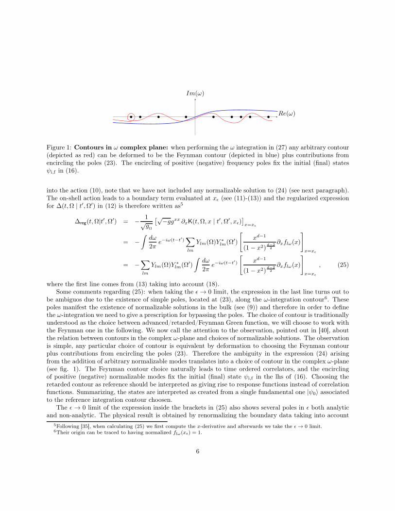
b b b b b b b b b

Im(ω)

Re(ω)

Figure 1: Contours in ω complex plane: when performing the ω integration in (27) any arbitrary contour(depicted as red) can be deformed to be the Feynman contour (depicted in blue) plus contributions fromencircling the poles (23). The encircling of positive (negative) frequency poles fix the initial (final) statesψi,f in (16).

into the action (10), note that we have not included any normalizable solution to (24) (see next paragraph).The on-shell action leads to a boundary term evaluated at xǫ (see (11)-(13)) and the regularized expressionfor ∆(t,Ω | t′,Ω′) in (12) is therefore written as5

∆reg(t,Ω|t′,Ω′) = − 1√gΩ

[√−ggxx ∂xK(t,Ω, x | t′,Ω′, xǫ)]

x=xǫ

= −∫

dω

2πe−iω(t−t′)

∑

lm

Ylm(Ω)Y ∗lm(Ω′)

[

xd−1

(1− x2)d−22

∂xflω(x)

]

x=xǫ

= −∑

lm

Ylm(Ω)Y ∗lm(Ω′)

∫

dω

2πe−iω(t−t′)

[

xd−1

(1− x2)d−2

2

∂xflω(x)

]

x=xǫ

, (25)

where the first line comes from (13) taking into account (18).Some comments regarding (25): when taking the ǫ→ 0 limit, the expression in the last line turns out to

be ambiguos due to the existence of simple poles, located at (23), along the ω-integration contour6. Thesepoles manifest the existence of normalizable solutions in the bulk (see (9)) and therefore in order to definethe ω-integration we need to give a prescription for bypassing the poles. The choice of contour is traditionallyunderstood as the choice between advanced/retarded/Feynman Green function, we will choose to work withthe Feynman one in the following. We now call the attention to the observation, pointed out in [40], aboutthe relation between contours in the complex ω-plane and choices of normalizable solutions. The observationis simple, any particular choice of contour is equivalent by deformation to choosing the Feynman contourplus contributions from encircling the poles (23). Therefore the ambiguity in the expression (24) arisingfrom the addition of arbitrary normalizable modes translates into a choice of contour in the complex ω-plane(see fig. 1). The Feynman contour choice naturally leads to time ordered correlators, and the encirclingof positive (negative) normalizable modes fix the initial (final) state ψi,f in the lhs of (16). Choosing theretarded contour as reference should be interpreted as giving rise to response functions instead of correlationfunctions. Summarizing, the states are interpreted as created from a single fundamental one |ψ0〉 associatedto the reference integration contour choosen.

The ǫ → 0 limit of the expression inside the brackets in (25) also shows several poles in ǫ both analyticand non-analytic. The physical result is obtained by renormalizing the boundary data taking into account

5Following [35], when calculating (25) we first compute the x-derivative and afterwards we take the ǫ → 0 limit.6Their origin can be traced to having normalized flω(xǫ) = 1.

6

the asymptotic behavior in the radial direction (see (22)), in the present case it amounts to rescale φ0 as(see [3, 35, 27])

φ0(t,Ω) = ǫ12∆−φren(t,Ω) . (26)

Moreover, since eventually we are interested in correlation functions for separated points, (contact) termsproportional to positive integer powers of q2 are dropped. The finite term in the ǫ→ 0 limit reads

∆ren(t,Ω|t′,Ω′) ≡ limǫ→0

ǫ∆− ∆reg(t,Ω|t′,Ω′)

=∑

lm

Ylm(Ω)Y ∗lm(Ω′)

∫

dω

2πe−iω(t−t′)

× ∆+

2∆−

Γ(1 − µ)

Γ(1 + µ)

Γ(

12 (−ω + ν + µ+ 1)

)

Γ(

12 (ω + ν + µ+ 1)

)

Γ(

12 (−ω + ν − µ+ 1)

)

Γ(

12 (ω + ν − µ+ 1)

) . (27)

The numerator of this last expression shows explicitly the appearance of poles along the integration contourprecisely at frequencies ωnl given by (23). The specification of a contour C in the complex ω plane fixes theinitial and final states ψi,f when compared to the standard Feynman one (see fig. 1).

From the discussion following (25) it should be clear that correlation functions computed on the QFT vac-uum state are obtained by choosing the standard Feynman contour for the ω integration in (27). Performingthe ω integration we obtain7

∆Fren(t,Ω|t′,Ω′) = 2i

∆+ Γ(1− µ)

2∆−Γ(1 + µ)

∑

lm

Ylm(Ω)Y ∗lm(Ω′)

×[

∞∑

n=0

(−1)n

n!

Γ(n+ l +∆+)

Γ(n+ l + d2 )Γ(−(n+ µ))

e−i|t−t′|(2n+l+∆+)

]

(28)

The sum over the residues can be computed analytically giving

〈0|TO(t,Ω)O(t′,Ω′)|0〉 = −i∆Fren(t,Ω|t′,Ω′) = − 2∆+

2∆−Γ(µ)

∑

lm

Ylm(Ω)Y ∗lm(Ω′)

Γ(l +∆+)

Γ(l + d2 )

× e−i|t−t′|(l+∆+)2F1

(

1 + µ, l +∆+, l +d

2; e−2i|t−t′|

)

. (29)

3 GKPW prescription for Lorentzian wormholes

Our goal in this section will be to extend the GKPW prescription to the case of multiple timelike boundaries,we will discuss the two boundaries case for simplicity. On general grounds AdS/CFT suggests that thepresence of two time-like boundaries should be associated to the existence of two sets O± of dual operatorscorresponding to the two independent boundary conditions φ±0 that must be imposed on the field φ whensolving the wave equation8.

7Generically (23) are the only divergencies in (27), special care must be taken for integer values of µ. We will not discussthe details of this in the present work since experience with the AdS/CFT correspondence has shown that correlation functionsdo not change qualitatively in the integer limit.

8Some authors have assumed than the two dual field theories are decoupled because of the disconnected structure of theboundary [20].

7

b

(a)

z=

0φ0

φH

φz=∞, t

=∞

z=∞

, t = −∞

b

(b)

x+x−

φ+0φ−0

φ

φ(n)i

φ(n)f

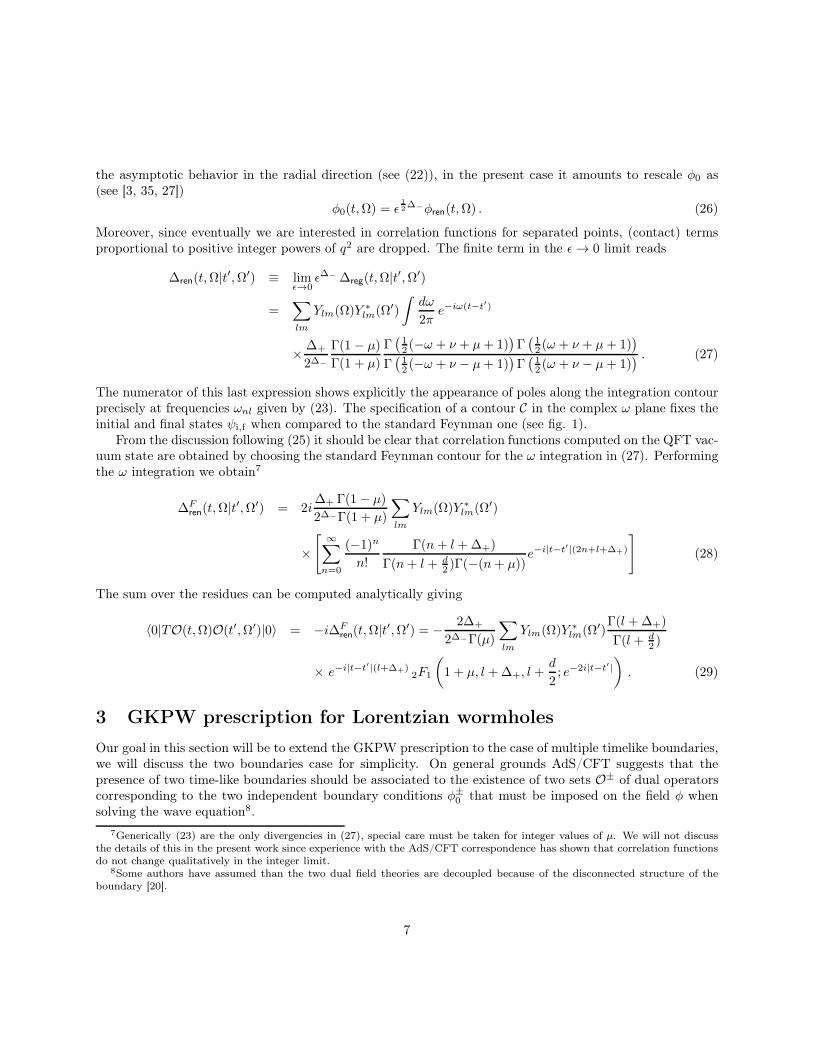
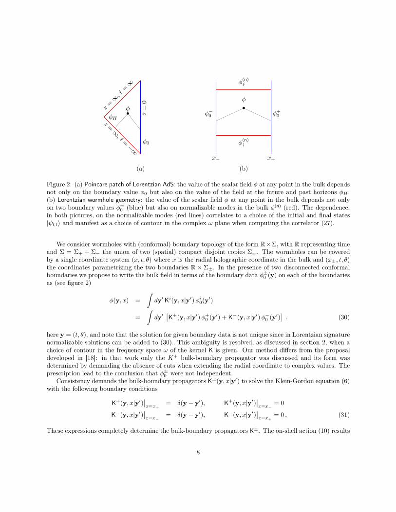
Figure 2: (a) Poincare patch of Lorentzian AdS: the value of the scalar field φ at any point in the bulk dependsnot only on the boundary value φ0 but also on the value of the field at the future and past horizons φH .(b) Lorentzian wormhole geometry: the value of the scalar field φ at any point in the bulk depends not onlyon two boundary values φ±0 (blue) but also on normalizable modes in the bulk φ(n) (red). The dependence,in both pictures, on the normalizable modes (red lines) correlates to a choice of the initial and final states|ψi,f〉 and manifest as a choice of contour in the complex ω plane when computing the correlator (27).

We consider wormholes with (conformal) boundary topology of the form R×Σ, with R representing timeand Σ = Σ+ + Σ− the union of two (spatial) compact disjoint copies Σ±. The wormholes can be coveredby a single coordinate system (x, t, θ) where x is the radial holographic coordinate in the bulk and (x±, t, θ)the coordinates parametrizing the two boundaries R × Σ±. In the presence of two disconnected conformalboundaries we propose to write the bulk field in terms of the boundary data φ±0 (y) on each of the boundariesas (see figure 2)

φ(y, x) =

∫

dy′Ki(y, x|y′)φi0(y

′)

=

∫

dy′[

K+(y, x|y′)φ+0 (y

′) + K−(y, x|y′)φ−0 (y

′)]

. (30)

here y = (t, θ), and note that the solution for given boundary data is not unique since in Lorentzian signaturenormalizable solutions can be added to (30). This ambiguity is resolved, as discussed in section 2, when achoice of contour in the frequency space ω of the kernel K is given. Our method differs from the proposaldeveloped in [18]: in that work only the K+ bulk-boundary propagator was discussed and its form wasdetermined by demanding the absence of cuts when extending the radial coordinate to complex values. Theprescription lead to the conclusion that φ±0 were not independent.

Consistency demands the bulk-boundary propagators K±(y, x|y′) to solve the Klein-Gordon equation (6)with the following boundary conditions

K+(y, x|y′)

∣

∣

x=x+= δ(y − y

′), K+(y, x|y′)

∣

∣

x=x−= 0

K−(y, x|y′)

∣

∣

x=x−= δ(y − y

′), K−(y, x|y′)

∣

∣

x=x+= 0 , (31)

These expressions completely determine the bulk-boundary propagators K±. The on-shell action (10) results

8

in two terms arising from the boundaries which take the form

S = −1

2

∫

dy(

[√−ggxxφ(y, x)∂xφ(y, x)]

x=x+−

[√−ggxxφ(y, x)∂xφ(y, x)]

x=x−

)

(32)

Inserting the solution (30) into (32) one obtains

S[φ0] = −1

2

∫

dy dy′φi0(y)∆ij(y,y′)φj0(y

′) (33)

with i, j = +,− denoting the two boundaries and ∆ij the generalization of (13). Their explicit forms are

∆+i(y,y′) =

[√−ggxx∂xKi(y, x|y′)]

x=x+, ∆−i(y,y

′) = −[√−ggxx∂xKi(y, x|y′)

]

x=x−(34)

As in Section 2 the two point functions of operators on the same boundary result

〈ψf |O±(y)O±(y′)|ψi〉 ∼ −i∆±±(y,y′) (35)

and the correlators between operators on opposite boundaries read

〈ψf |O±(y)O∓(y′)|ψi〉 ∼ −i∆±∓(y,y′) . (36)

The generalization of the expressions (8) and (15) to backgrounds with two boundaries take the form

Ki(y, x | y′) = lim

x′→xi

√−g gx′x′

∂x′G(y, x | y′, x′), (37)

which gives

∆ij(y,y′) ∼ lim

x→xi, x′→xj(√−ggxx)(√−ggx′x′

)∂2

∂x∂x′G(y, x | y′, x′) . (38)

Note that the ∆±∓ correlation function involves in the semiclassical limit a geodesic through the bulkconnecting two points, one at each boundary.

AdS2 Lorentzian strip

We will apply in this section the prescription developed above to Lorentzian AdS2 reobtaining previousresults. The AdS2 Lorentzian metric can be written as

ds2 = R2

[

− dt2

1− x2+

dx2

(1− x2)2

]

, (39)

the timelike boundaries are located at x = ±1 and the (t, x) coordinate system covers the whole spacetime.To find the bulk-boundary propagators K± in (30) we propose

K±(t, x) =

∫ ∞

−∞

dω

2πe−iωtf±

ω (x) . (40)

Inserting into the KG equation (6) we obtain the following differential equation for fω

(1 − x2)d2f±

ω (x)

dx2− x

df±ω (x)

dx+

(

ω2 − m2R2

1− x2

)

f±ω (x) = 0 . (41)

9

The solution to (41) can be written in terms of generalized Legendre Polynomials as

f±ω (x) = (1− x2)

14 [a±ω P

µν (x) + b±ω Q

µν (x)] (42)

with µ =√

14 +m2R2, ν = ω − 1

2 and a±ω , b±ω arbitrary constants which get fixed when we impose the

conditions (31). The conditions translate into9

f±ω (±xǫ) = 1 , f±

ω (∓xǫ) = 0 . (43)

The solutions to (43) read

f+ω (x) =

(1− x2)1/4

(1− x2ǫ )1/4

Qµν (x)P

µν (−xǫ)−Qµ

ν (−xǫ)Pµν (x)

Qµν (xǫ)P

µν (−xǫ)−Q

µν (−xǫ)Pµ

ν (xǫ)(44)

f−ω (x) =

(1− x2)1/4

(1− x2ǫ )1/4

Qµν (x)P

µν (xǫ)−Qµ

ν (xǫ)Pµν (x)

Qµν (−xǫ)Pµ

ν (xǫ)−Qµν (xǫ)P

µν (−xǫ)

. (45)

Analyzing the asymptotic behavior near the boundary in (42) one finds normalizable modes for

ωn = ±(

n+ µ+1

2

)

, n = 0, 1, 2 . . . andbωQ

aωQ= −2 tanπµ

π(46)

The renormalized ∆ij functions disregarding contact terms result

∆ren±±(t, t′) = ∓2∆−

2π

Γ(1− µ)

Γ(1 + µ)

∫

dω

2πe−iω(t−t′)Γ

(

1

2+ µ− ω

)

Γ

(

1

2+ µ+ ω

)

cos(πω) (47)

∆ren±∓(t, t′) = ∓ 2∆−

Γ(µ)2

∫

dω

2πe−iω(t−t′)Γ

(

1

2+ µ− ω

)

Γ

(

1

2+ µ+ ω

)

, (48)

as before, the integrands in these expressions show poles in ω at the values given by (46).The integrals (47)-(48) can be computed using the residue theorem once a contour in the complex plane

is chosen. For the Feynman contour we obtain

∆Fren±±

(t, t′) = ∓ i∆−−∆+

8∆+π12

Γ(12 + µ)

Γ(µ) sin2∆+(

t−t′

2

)

∆Fren±∓

(t, t′) = ∓8∆−i

4

Γ(1 + 2µ)

Γ(µ)2 cos2∆+

(

t−t′

2

) (49)

The vacuum expectation values between operators on the same and opposite boundaries result (cf. [20])

〈0|TO±(t)O±(t′)|0〉 = ±4∆−i2∆−

8∆+

Γ(2µ)

Γ(µ)2 sin2∆+( t−t′

2 ), (50)

〈0|TO±(t)O∓(t′)|0〉 = ∓8∆−

4

Γ(1 + 2µ)

Γ(µ)2 cos2∆+( t−t′

2 ). (51)

9As discussed in section 2 the boundary data is imposed at a finite distance x = ±xǫ where xǫ = 1− ǫ.

10

The first line gives the result for operators on the same boundary and has the expected conformal behavior|t − t′|−2∆+ when the operators approach each other. The second line corresponding to operators locatedon different boundaries becomes singular for t = t′ + (2n+ 1)π, n ∈ Z, this singularity reflects the existenceof causal (null) curves connecting the boundaries and it has been argued that their existence hints for aninteraction between the two sets of degrees of freedom O± [18]10. The observed periodicity in time relatesto a peculiar property of AdS, this is the convergence of null geodesics when passing to the universal coverand can be also understood as a consequence of the eigenmodes (46) being equally spaced (see [36]-[38]).

In the massless case (µ = 12 ) the two point functions take the form

〈0|TO±(t)O±(t′)|0〉 = ± 1

8π sin2(

t−t′

2

) , 〈0|TO±(t)O∓(t′)|0〉 = ∓ 1

4π cos2(

t−t′

2

) (52)

Wormhole

We now turn to the analysis of two point functions in a wormhole background, this is, a spacetime geometrywith two conformal boundaries connected through the bulk. We will work with a toy model wormhole, whichpermits analytical treatment, consisting on a static geometry that connects two asymptotically AdS regionswith base manifolds of the form H3 or S1 × H2, with Hn a n-dimensional (quotiented) hyperbolic space.The geometry does not contain horizons anywhere, and the two asymptotic regions are causally connected.The spacetime was found as a solution of Einstein-Gauss-Bonnet gravity, which in d + 1 = 5 dimensionstakes the form

S5 = κ

∫

ǫabcde

(

RabRcd +2

3l2Rabeced +

1

5l4eaebeced

)

ee ,

here Rab = dωab + ωafω

fb is the curvature two form for the spin connection ωab, and ea is the vielbein. The(d+ 1)-dimensional wormhole metric found in [22] reads

ds2 = R2[

− cosh2ρ dt2 + dρ2 + cosh2ρ dΣ2d−1

]

= R2

[

− dt2

1− x2+

dx2

(1− x2)2+dΣ2

d−1

1− x2

]

(53)

where dΣ2d−1 is a constant negative curvature metric on the compact base manifold Σ2

d−1, two disconnectedconformal boundaries are located at x = ±1.

To construct the boundary to bulk propagators K± discussed above we propose

K±(t, x, θ|t′, θ′) =

∫ ∞

−∞

dω

2π

∑

Q

e−iω(t−t′) YQ(θ)Y∗Q(θ

′)f±ωQ(x) (54)

where YQ(θ) are the spherical harmonics on the base manifold11. Inserting (54) into the KG equation (6)one finds that fωQ satisfies

(1− x2)d2f±

ωQ(x)

dx2+ (d− 2)x

df±ωQ(x)

dx+

[

(ω2 −Q2)− m2R2

1− x2

]

f±ωQ(x) = 0 . (55)

10 This interpretation assumes that the boundary spatial foliations Σ(t)+ and Σ

(t′)−

should be identified as being the same

Cauchy surface Σ of a single base manifold where the dual field theory lives in.11The spherical harmonics satisfy ∇2

ΣYQ = −Q2 YQ and a compact manifold without boundaries has Q2 ≥ 0.

11

The solutions to (55) can be written in terms of generalized Legendre polinomials as [15]

f±ωQ(x) = (1− x2)

d4 [a±ωQ P

µν (x) + b±ωQQ

µν (x)] (56)

where µ is given by (5) and

ν = − 1

2=

√

(

d− 1

2

)2

+ ω2 −Q2 − 1

2. (57)

a±ωQ, b±ωQ in (56) are constant coefficients which get fixed when we impose the conditions (31), these are

f±ωQ(±xǫ) = 1 , f±

ωQ(∓xǫ) = 0 . (58)

The solutions for (56) satisfying (58) are

f+ωQ(x) =

(

1− x2)d4

(1− x2ǫ)d4

Pµν (x)Q

µν (−xǫ)− Pµ

ν (−xǫ)Qµν (x)

Pµν (xǫ)Q

µν (−xǫ)− P

µν (−xǫ)Qµ

ν (xǫ)

f−ωQ(x) =

(

1− x2)d4

(1− x2ǫ)d4

Pµν (x)Q

µν (xǫ)− Pµ

ν (xǫ)Qµν (x)

Pµν (−xǫ)Qµ

ν (xǫ)− Pµν (xǫ)Q

µν (−xǫ)

, (59)

The possibility for two independent bulk-boundary propagators arises from the fact that the base manifoldΣ never shrinks to zero size inside the bulk (see (53)) and therefore regularity in the interior imposes noconstraint in the solutions (56). Normalizable modes appear for

ωnQ = ±

√

(

µ+1

2+ n

)2

+Q2 −(

d− 1

2

)2

, n = 0, 1, . . . , andbωQ

aωQ= −2 tanπµ

π(60)

For these frequencies the index ν in (57) takes the value νn = µ + n and the resulting solution becomesnormalizable. The two point functions (35)-(36) between operators O± on the same boundary and oppositeboundaries take the form

〈ψf |TO±(t, θ)O±(t′, θ′)|ψi〉 = ± i2∆−d

π2dΓ(1− µ)

Γ(1 + µ)

∑

Q

YQ(θ)Y∗Q(θ

′)

×∫

dω

2πe−iω(t−t′)Γ(

1

2+ µ−)Γ(

1

2+ µ+) cos(π) (61)

〈ψf |TO±(t, θ)O∓(t′, θ′)|ψi〉 = ± i2∆−

2d−1

1

Γ(µ)2

∑

Q

YQ(θ)Y∗Q(θ

′)

×∫

dω

2πe−iω(t−t′)Γ(

1

2+ µ−)Γ(

1

2+ µ+). (62)

A few comments on these expressions: (i) in the large frequency limit ∼ ω and the integrands in (61)-(62)coincide with those of AdS2 (cf. (47)-(48)), (ii) when a Feynman contour is chosen, a time ordered productshould be understood on the rhs of (61)-(62) and (iii) although the Gamma functions Γ(12 + µ±) present

two branch cuts at ω = ±√

Q2 −(

d−12

)2(see (57)), the product in the integrands (61)-(62) is free of them.

12

The correlation between operators inserted on opposite boundaries is non vanishing, and this result hasbeen explained in different ways depending on the context: (i) as the result of being computing the correlator(62) on an entangled state of two non-interacting boundary theories (BH context [16]) or (ii) as due to aninteraction between the theories defined on each of the boundaries (D1/D5 orbifold in [18]). The crucialpoint in both arguments was the absence/existence of causal connection between the asymptotic regions.

4 Entanglement vs. Coupling

In this section we will review several thoughts regarding the interpretation of the results (51) and (62). Wewould like to address the issue of whether the results (51) and (62) are the consequence of: (i) an interactionbetween the two dual QFT theories or (ii) due to the correlators being evaluated on an entangled state or(iii) both.

Entanglement Entropy

The entanglement entropy SA

is a non local quantity (as opposed to correlation functions) that measureshow two subsystems A and B are correlated. For a d-dimensional QFT, it is defined as the von Neumannentropy of the reduced density matrix ρA obtained when we trace out the degrees of freedom inside a(d− 1)-dimensional spacelike submanifold B which is the complement of A (see [44] for a review).

In [41, 42] a proposal was made for a holographic formula for the entanglement entropy of a CFTd dualto an AdSd+1 geometry, it reads

SA=

Area(γA)

4G(d+1)N

, (63)

where γA

is a (d − 1)-dimensional minimal surface in AdSd+1 whose boundary S, located at AdS infinity,

coincides with that of A, this is S = ∂γA= ∂A and G

(d+1)N is the Newton constant in AdSd+1. This formula,

which assumes the supergravity approximation of the full string theory, has been applied in the AdS3/CFT2

setup showing agreement with known 2D CFT results [44].One can imagine applying a generalization of (63) to the wormhole geometry (53) as follows12: the

wormhole presents two disconnected spatial regionsΣ± at which two identical degrees of freedom are supposedto be living on. Imagine constructing a codimension 1 closed surface S bounding a small region B on Σ−,experience from Wilson loops and brane embeddings show that as B remains small, the minimal surface willbe located near x = −1. As we gradually increase the size of B, the minimal surface anchored on Σ− dipsdeeper into the bulk and in the limit when B occupies all space B→ Σ− the boundary S collapses and theminimal surface gets localized at the throat x = 0 of the geometry, giving a non zero result

SΣ=

Area(Σ)

4G(d+1)N

. (64)

This result should be understood as indicating that the quantum state in the dual QFT described by thewormhole geometry is not separable, or stated otherwise, the result (62) can be attributed to the wormholegeometry realizing an entangled state on the Hilbert space product H = H+ ⊗ H− with the entropy (64)resulting from integrating out H−.

12 See [43] for an generalization of (63) to the euclidean wormhole constructed in [10].

13

Interaction between the dual copies

We will now argue that apart from the entanglement discussed above, the causal contact between thewormhole asymptotic boundaries leads to an interaction term between the two sets of degrees of freedomliving at each boundary. In particular we argue that a coupling between the field theories will exist wheneverthe asymptotic regions are in causal contact.

We start quoting the partition function on the gravity side for the wormhole geometry in the semiclassicallimit, its form is

Zgravity

[

φ(φ+0 , φ−0 , C)

]

∼ e−i2

∫dy dy′φi0(y)∆ij(y,y

′)φj0(y′) (65)

here y = (t, θ) denote the boundary points and i, j = +,− refer to the asymptotic boundaries whereprescribed data φ±0 is given, the contour C fixes the normalizable solution in the bulk and the expressionfor ∆ij is given by (34). According to the GKPW prescription the partition function (65) is the generatingfunctional for O± correlators, this is

Zgravity

[

φ(φ+0 , φ−0 , C)

]

=⟨

ψf

∣

∣

∣Tei

∫dyφ+

0 (y)O+(y)+i∫dy φ−

0 (y)O−(y)∣

∣

∣ψi

⟩

QFT

, (66)

where the observables O± should be constructed as local functionals of the fundamental fields Ψ± living oneach boundary. These fields are assumed to describe independent degrees of freedom: [O+,O−] = 0 on thesame spatial slice (see footnote 10).

Consider the simplest situation corresponding to choosing C to be the Feynman contour, this is, we arecomputing the vacuum to vacuum transition amplitude on the field theory side. The rhs in (66) can bewritten as

⟨

ψ0

∣

∣

∣Tei

∫dyφ+

0 (y)O+(y)+ i∫dy φ−

0 (y)O−(y)∣

∣

∣ψ0

⟩

QFT

= Tr

[

ρψ0Tei

∫dyφ+

0 (y)O+(y)+ i∫dy φ−

0 (y)O−(y)]

, (67)

where the trace operation is performed over a complete set of states of the dual field theory Hilbert space andρψ0

= |ψ0〉〈ψ0| is the density matrix associated to the vacuum wormhole state. This vacuum state belongsto the Hilbert space H = H+ ⊗H− and according to the arguments reviewed in the last subsection, it is notseparable as a single tensor product |ψ0〉 6= |ψ+〉 ⊗ |ψ−〉.

To analyze the possibility of interaction between the fields living at each boundary we consider the systemat finite temperature T = β−1. The absence of singularities in the Euclidean continuation implies that thewormhole spacetime can be in equilibrium with a thermal reservoir of arbitrary temperature, or statedotherwise, the periodicity in Euclidean time is arbitrary. At thermal equilibrium the field theory state isdescribed by the Boltzmann distribution ρ

β= e−βH , with H = H+[Ψ+] +H−[Ψ−] +Hint[Ψ+,Ψ−] the dual

field theory Hamiltonian, and Hint a possible coupling between the two identical sets of degrees of freedomΨ±.

Let us see now that an interaction term Hint should be present in the Hamiltonian in order to avoid acontradiction. The argument goes as follows: finite temperature correlation functions on the field theoryside are obtained from the Euclidean rotation of (67), which reads

⟨

e−∫dy φ+

0 (y)O+(y)−∫dyφ−

0 (y)O−(y)⟩

β= Tr

[

ρβe−

∫dy φ+

0 (y)O+(y)−∫dy φ−

0 (y)O−(y)]

, (68)

the field theory is defined on an Euclidean manifold with S1β × Σ topology (see footnote 10). The AdS/CFT

proposal equates this expression to the Euclidean continuation of the lhs in (66), the result is

Tr

[

e−βH e−∫dyφ+

0(y)O+(y)−

∫dy φ−

0(y)O−(y)

]

= ZEgravity

[

φ(φ+0 , φ−0 )

]

∼ e−SE [φ+0, φ−

0] , (69)

14

on the right SE [φ+0 , φ

−0 ] corresponds to the on shell scalar field action on the Euclidean wormhole background,

with time compactified on a circle of radius β. Upon Euclidean rotation and time compactification, theresulting geometry is cylinder like with topology S1

β × I × Σ, the two boundaries at which one imposes the

boundary data φ±0 are located at the endpoints x± of the finite interval I13. Note that in the Euclideancontext the solution in the interior (bulk) is completely specified by the boundary data, no normalizablesolutions exist and rotating the Feynman contour to the imaginary time axis is straightforward and leads toa non-singular solution. The explicit expression for the rhs of (69) is

ZEgravity

[

φ(φ+0 , φ−0 )

]

∼ e−12

∫dy dy′φi0(y) ∆ij(y,y

′) φj0(y′), (70)

where ∆ij denote the Euclidean rotated bulk-boundary propagators (34). Finally, from (69) and (70) weobtain for the gauge/gravity prescription for a wormhole at finite temperature

Tr

[

e−βH e−∫dy φ+

0 (y)O+(y)−∫dy φ−

0 (y)O−(y)]

∼ e−12

∫dy dy′φi0(y) ∆ij(y,y

′)φj0(y′) . (71)

This is the key formula for our argumentation because if one now assumes that the degrees of freedomΨ+,Ψ− are decoupled, this is

H [Ψ+,Ψ−] = H+[Ψ+] +H−[Ψ−] , (72)

then ρβ= e−βH+ e−βH− , and the lhs of (71) factorizes into a product of two quantities: one depending on

φ+0 and one depending on φ−014. However the gravity computation does not factorize because of the non

vanishing ∆±∓ terms. We interpret this result as manifesting the existence of a non-trivial coupling Hint

between the two dual degrees of freedom Ψ±: the field theory dual to the wormhole geometry contains anon-trivial coupling term between the two boundary degrees of freedom Ψ+ and Ψ−.

Highlights and Applications

The outcome of the above observations is that the wormhole geometry encodes the description of a dual fieldtheory with two copies of fundamental fields in interaction. Moreover, the quantum state described by thewormhole is entangled. In particular, the Euclidean continuation can be seen as prescription to separate, inthe dual field theory, entanglement effects from possible interaction terms Hint. A non vanishing Euclideantwo point function between operators located at different boundaries must be interpreted as originated froman interaction term Hint, rather than an entanglement effect. In the following we confront this point of viewwith two other relevant geometries appearing in the literature: the AdS1+1 geometry and the eternal AdSblack hole [16].

AdS1+1 geometry: The treatment for the AdS1+1 background (39) is entirely analogous to the one per-formed for the wormhole case. The Euclidean section of the global metric (39) has two boundaries uponcompactifying the time direction, and the Euclidean correlation functions can be explicitly obtained fromthe formulas (51). By virtue of this the arguments above aply, and we can conclude that AdS1+1 is dual toa conformal quantum mechanics composed of two interacting sectors.

13 Note the similarity with the geometry studied in [10].14Note that in the absence of interaction [O+,O−] = 0 no matter if the operators insertion points are spacelike/timelike

separated.

15

Eternal AdS Black Hole: The crucial difference between the wormhole (53) and the maximally extendedAdS-BH gravity solution is well known [16]: upon performing the Euclidean continuation of the AdS-BHsolution, the existence of a horizon in Lorentzian signature generates a conical singularity in the Euclideanmanifold, that can only be avoided by demanding a precise periodicity in Euclidean time. The resultingRiemannian geometry has inevitably only one asymptotic boundary, and therefore requires imposing onlyone asymptotic boundary data φ0, this indicates the existence of a single set of degrees of freedom Ψ and aunique Bulk-Boundary propagator ∆. The system in equilibrium with a thermal bath of fixed temperature(determined by the BH mass) has a generating function that reads

Tr

[

e−βHe−∫dyφ0(y)O(y)

]

∼ e−12

∫dydy′ φ0(y) ∆(y,y′) φ0(y

′), (73)

The real time (maximally extended BH) solution was analyzed and interpreted in the AdS/CFT contextin [16]. The second causally disconnected boundary, present in Lorentzian signature, was understood assupporting the TFD partners needed for obtaining a thermal state upon their integration and lead to adoubling of the Hilbert space as H = H+ ⊗H−. We stress the fact that the second set of degrees of freedomis causally disconnected from the original zero temperature set; although they appear in Lorentzian signatureand give rise to a non-trivial ∆ij , they are ficticious from a physical point of view. The causal disconnectionbetween the boundaries relates to the two point function ∆±∓ never becoming singular.

5 Discussion

We have reviewed the GKPW prescription in the Lorentzian context relating the ambiguity in adding nor-malizable modes to (3) to the integration contour C required to bypass the integrand singularities in (27),(61)arising from the existence of normalizable modes. To compute Lorentzian quantities one needs to fix a refer-ence contour Cref and the two sensible choice are retarded or Feynman. These choices relate on the QFT sideto being computing either response or correlation functions. When choosing the Feynman path as referencecontour, any given contour C differs from CF by contributions from encircling poles, these encircled poles fixthe initial and final states that appear in the correlation functions (see (16)).

In section 3 we extended the GKPW prescription to spacetimes with more than one asymptotic timelikeboundaries, in particular we studied the simplest two boundaries case. We proposed to write the bulk field interms of the two independent asymptotic boundary values and as a toy example we applied the constructionto AdS1+1 reobtaining previous results, we afterwards computed the two point correlation functions for theEinstein-Gauss-Bonnet wormhole (53). At this point we must emphasize that the principal difference of ourmethod with the one performed in [18], for an AdS3 orbifold, consists in that we considered the boundaryvalues φ±0 of the bulk scalar field as independent quantities, moreover, we explicitly showed the possibilityof constructing two boundary-bulk propagators K± (their boundary conditions were given in (31)). Theconstruction performed in [18] showed a relation between the boundary values φ±0 and this was understoodas indicating that the ± sources for the dual field theory are turned on in a correlated way. A questionremained as whether the two sets of data are independent or redundant in the dual formulation, on theother hand another question is the origin of the non-zero result for operators located at different boundaries(∆±∓) this could either be due to entanglement or interactions or both.

In section 4 we applied the ideas on holographic entanglement entropy developed in [42] to the wormholegeometry. The non vanishing of S

Σobtained for the degrees of freedom living on opposite boundaries

suggests that the wormhole should be understood as representing an entangled state in H = H+ ⊗ H−.On the other hand, the causal connection between the boundaries suggest that a coupling might exist as

16

well. To attack this issue we consider putting the wormhole system in contact with a thermal bath, uponEuclideanization, the resulting geometry still has two boundaries connected through the bulk, this indicated,to avoid a contradiction, that the dual QFT consists of two copies H± in interaction. Summarizing, thenumber of disconnected boundaries of the Euclidean section determines the amount of physical degrees offreedom.

We would like to emphasize finally the implications of this approach on quantum gravity, which could beseen as one of our main motivations. This subject has been discussed in different contexts in the last yearsand referred to as Emergent Spacetime [45]. In this sense, we showed how important topological and causalproperties (connectivity) of the space time geometry are encoded in the QFT action, and that part of thisinformation is not only in the ground state but in its interacting structure. We hope this conclusion mightcontribute to the construction of rules towards a geometry engineering.

We should mention that in the presence of interactions one needs to address the way the points on oppositeboundaries are identified. A first approach to this problem is to identify the points y,y′ in configuration spaceat which ∆±∓ diverges and study the consistency of identifying them, this is currently under investigationand will be reported elsewhere.

Acknowledgments

We thank D. Correa, N. Grandi, A. Lugo and J.M. Maldacena for useful discussions and correspondence.This work was partially supported by ANPCyT PICT 2007-0849 and CONICET PIP 2010-0396.

References

[1] J.M. Maldacena, Adv. Theor. Math. Phys. 2, 231 (1998), hep-th/9711200.

[2] S.S. Gubser, I.R. Klebanov and A.M. Polyakov, Phys. Lett. B428, 105 (1998), hep-th/9802109.

[3] E.Witten, Adv. Theor. Math. Phys. 2, 253 (1998), hep-th/9802150.

[4] E. Witten, Adv. Theor. Math. Phys. 2, 505 (1998), hep-th/9803131.

[5] D.Z. Freedman, S.S. Gubser, K. Pilch and N.P. Warner, Adv. Theor. Math. Phys. 3, 363 (1999),hep-th/9904017.

[6] H. Lin, O. Lunin and J.M. Maldacena, JHEP 0410, 025 (2004), hep-th/0409174.

[7] J. de Boer, L. Maoz and A. Naqvi, hep-th/0407212.

[8] G.J. Galloway, K. Schleich, D. Witt and E. Woolgar, Phys. Lett. B505, 255 (2001), hep-th/9912119.

[9] K. Skenderis and B. C. van Rees, arXiv:0912.2090 [hep-th].

[10] J.M. Maldacena and L. Maoz, JHEP 0402, 053 (2004), hep-th/0401024.

[11] N. Arkani-Hamed, J. Orgera and J. Polchinski, JHEP 0712, 018 (2007), 0705.2768 [hep-th].

[12] E. Witten and S. T. Yau, Adv. Theor. Math. Phys. 3 (1999) 1635, hep-th/9910245.

[13] M. l. Cai and G. J. Galloway, Adv. Theor. Math. Phys. 3 (1999) 1769, hep-th/0003046.

17

[14] A. Buchel, Phys. Rev. D70 (2004) 066004, hep-th/0402174.

[15] D. H. Correa, J. Oliva and R. Troncoso, JHEP 0808 (2008) 081, 0805.1513 [hep-th].

[16] J. M. Maldacena, JHEP 0304 (2003) 021, hep-th/0106112.

[17] E. Barnes, D. Vaman, C. Wu and P. Arnold, 1004.1179 [hep-th].

[18] V. Balasubramanian, A. Naqvi and J. Simon, JHEP 0408 (2004) 023, hep-th/0311237.

[19] P. Martin and J. Schwinger, Phys. Rev. 115, 1342 (1959); J. Schwinger, Jour. Math. Phys. 2, 407(1961);K.T. Mahanthappa, Phys. Rev. 126, 329 (1962); P.M. Bakshi and K.T. Mahanthappa, Jour. Math.Phys. , 1 and 12 (1963); Keldysh, JETP 47, 1515 (1964); Y. Takahashi and H. Umezawa, CollectivePhenomena 2, 55 (1975).

[20] T. Azeyanagi, T. Nishioka and T. Takayanagi, Phys. Rev. D 77 (2008) 064005, 0710.2956 [hep-th].

[21] D. Lovelock, J. Math. Phys. 12, 498 (1971).

[22] G. Dotti, J. Oliva and R. Troncoso, Phys. Rev. D 75 (2007) 024002, hep-th/0607062; G. Dotti, J. Olivaand R. Troncoso, Phys. Rev. D 76 (2007) 064038, 0706.1830 [hep-th].

[23] C. P. Herzog and D. T. Son, JHEP 0303 (2003) 046, [arXiv:hep-th/0212072].

[24] M. Ali, F. Ruiz, C. Saint-Victor and J. F. Vazquez-Poritz, Phys. Rev. D 80 (2009) 046002, 0905.4766[hep-th].

[25] P. Breitenlohner and D. Z. Freedman, Phys. Lett. B 115 (1982) 197, Annals Phys. 144 (1982) 249;L. Mezincescu and P. K. Townsend, Annals Phys. 160 (1985) 406.

[26] E. D’Hoker and D. Z. Freedman, arXiv:hep-th/0201253.

[27] J. McGreevy, Lectures on String theory, MIT Open Course,

http://ocw.mit.edu/courses/physics/8-821-string-theory-fall-2008/lecture-notes/

[28] V. Balasubramanian, P. Kraus and A. E. Lawrence, Phys. Rev. D 59, 046003 (1999) hep-th/9805171.

[29] V. Balasubramanian, P. Kraus, A. E. Lawrence and S. P. Trivedi, Phys. Rev. D 59 (1999) 104021,hep-th/9808017.

[30] V. Balasubramanian, S. B. Giddings and A. E. Lawrence, JHEP 9903 (1999) 001, hep-th/9902052.

[31] U. H. Danielsson, E. Keski-Vakkuri and M. Kruczenski, JHEP 9901, 002 (1999), hep-th/9812007.

[32] D. T. Son and A. O. Starinets, JHEP 0209, 042 (2002), hep-th/0205051.

[33] C. P. Herzog and D. T. Son, JHEP 0303, 046 (2003), hep-th/0212072.

[34] L. Fidkowski, V. Hubeny, M. Kleban and S. Shenker, JHEP 0402 (2004) 014, hep-th/0306170.

[35] D. Z. Freedman, S. D. Mathur, A. Matusis and L. Rastelli, Nucl. Phys. B 546 (1999) 96, hep-th/9804058.

[36] S. J. Avis, C. J. Isham and D. Storey, Phys. Rev. D 18, 3565 (1978).

18

[37] I. R. Klebanov and E. Witten, Nucl. Phys. B 556 (1999) 89 arXiv:hep-th/9905104; E. Witten,arXiv:hep-th/0112258.

[38] S. W. Hawking and G. F. R. Ellis, The Large scale structure of space-time, CUP, 1973.

[39] D. Marolf, JHEP 0505 (2005) 042 hep-th/0412032.

[40] K. Skenderis and B. C. van Rees, Phys. Rev. Lett. 101 (2008) 081601, 0805.0150 [hep-th]; JHEP 0905

(2009) 085, arXiv:0812.2909 [hep-th].

[41] S. Ryu and T. Takayanagi, Phys. Rev. Lett. 96 (2006) 181602, hep-th/0603001.

[42] S. Ryu and T. Takayanagi, JHEP 0608 (2006) 045, hep-th/0605073.

[43] V. E. Hubeny, M. Rangamani and T. Takayanagi, JHEP 0707 (2007) 062, 0705.0016 [hep-th].

[44] T. Nishioka, S. Ryu and T. Takayanagi, J. Phys. A 42 (2009) 504008, arXiv:0905.0932 [hep-th].

[45] N. Seiberg, hep-th/0601234.

19