Embed Size (px)
Citation preview
OOLALA –
FROM NUMERICAL LINEAR ALGEBRA
TO COMPILER TECHNOLOGY
FOR DESIGN PATTERNS
A thesis submitted to the University of Manchester
for the degree of Doctor of Philosophy
in the Faculty of Science and Engineering
October 2002
By
Miguel Angel Lujan Moreno (Mikel Lujan)
Department of Computer Science
Contents
Abstract 17
Declaration 19
Copyright 20
Acknowledgements 22
1 Introduction 23
1.1 Overview . . . . . . . . . . . . . . . . . . . . . . . . . . . . . . . . 23
1.2 The Problem . . . . . . . . . . . . . . . . . . . . . . . . . . . . . 25
1.3 Contributions . . . . . . . . . . . . . . . . . . . . . . . . . . . . . 27
1.3.1 OoLaLa – A Novel Object Oriented Linear Algebra Library 27
1.3.2 Elimination of Array Bounds Checks . . . . . . . . . . . . 29
1.3.3 How and When Can OoLaLa Be Optimised? . . . . . . . 30
1.3.4 Generalisation to Design Patterns-Based Applications . . . 31
1.3.5 Limitations of a Library Approach . . . . . . . . . . . . . 31
1.4 Thesis Outline . . . . . . . . . . . . . . . . . . . . . . . . . . . . . 32
2 Numerical Linear Algebra 35
2.1 Introduction . . . . . . . . . . . . . . . . . . . . . . . . . . . . . . 35
2.2 Basic Background . . . . . . . . . . . . . . . . . . . . . . . . . . . 36
2.2.1 Matrix . . . . . . . . . . . . . . . . . . . . . . . . . . . . . 37
2.2.2 Matrix Operations . . . . . . . . . . . . . . . . . . . . . . 38
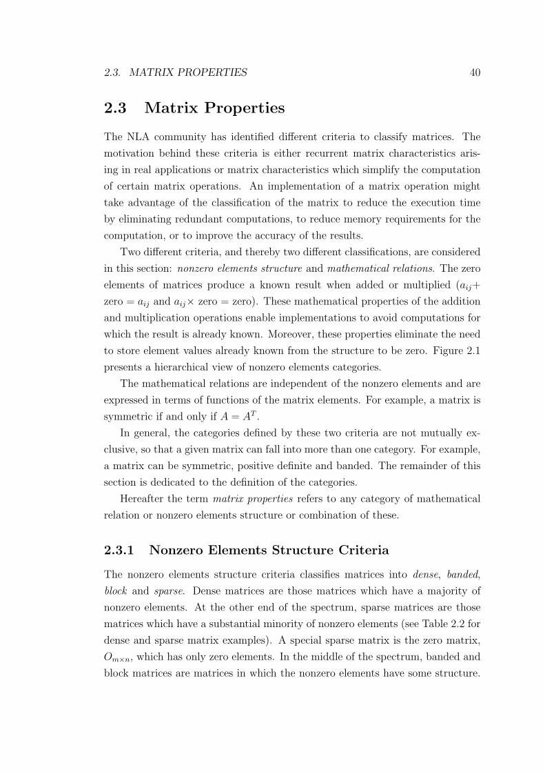
2.3 Matrix Properties . . . . . . . . . . . . . . . . . . . . . . . . . . . 40
2.3.1 Nonzero Elements Structure Criteria . . . . . . . . . . . . 40
2.3.2 Mathematical Relation Criteria . . . . . . . . . . . . . . . 44
2.4 Storage Formats . . . . . . . . . . . . . . . . . . . . . . . . . . . . 44
2
2.4.1 Dense Format . . . . . . . . . . . . . . . . . . . . . . . . . 46
2.4.2 Band Format . . . . . . . . . . . . . . . . . . . . . . . . . 46
2.4.3 Packed Format . . . . . . . . . . . . . . . . . . . . . . . . 47
2.4.4 Coordinate Format . . . . . . . . . . . . . . . . . . . . . . 48
2.4.5 Compressed Sparse Row Format . . . . . . . . . . . . . . . 49
2.4.6 Compressed Sparse Column Format . . . . . . . . . . . . . 50
2.4.7 Summary . . . . . . . . . . . . . . . . . . . . . . . . . . . 52
2.5 Exploiting Matrix Properties . . . . . . . . . . . . . . . . . . . . . 53
2.5.1 Matrix-Matrix Multiplication . . . . . . . . . . . . . . . . 53
2.5.2 Solving Systems of Linear Equations . . . . . . . . . . . . 56
2.5.3 Storage Format Abstraction Level . . . . . . . . . . . . . . 59
2.5.4 Summary . . . . . . . . . . . . . . . . . . . . . . . . . . . 60
2.6 Developing Numerical Linear Algebra Programs . . . . . . . . . . 61
2.6.1 Using BLAS and LAPACK . . . . . . . . . . . . . . . . . . 62
2.6.2 Using Matlab . . . . . . . . . . . . . . . . . . . . . . . . . 67
2.6.3 Using the Sparse Compiler . . . . . . . . . . . . . . . . . . 69
2.6.4 Advantages and Disadvantages . . . . . . . . . . . . . . . 70
2.7 Summary . . . . . . . . . . . . . . . . . . . . . . . . . . . . . . . 71
3 Object Oriented Software Construction 73
3.1 Introduction . . . . . . . . . . . . . . . . . . . . . . . . . . . . . . 73
3.2 Motivation . . . . . . . . . . . . . . . . . . . . . . . . . . . . . . . 75
3.3 Basic Concepts . . . . . . . . . . . . . . . . . . . . . . . . . . . . 76
3.4 Implementation Related Concepts . . . . . . . . . . . . . . . . . . 81
3.5 The Software Development Process . . . . . . . . . . . . . . . . . 83
3.6 Some Recommendations . . . . . . . . . . . . . . . . . . . . . . . 84
3.6.1 Bridge Pattern . . . . . . . . . . . . . . . . . . . . . . . . 85
3.6.2 Iterator Pattern . . . . . . . . . . . . . . . . . . . . . . . . 86
3.6.3 Simulation of Generic Classes . . . . . . . . . . . . . . . . 87
3.7 Summary . . . . . . . . . . . . . . . . . . . . . . . . . . . . . . . 89
4 Design of OOLALA 91
4.1 Introduction . . . . . . . . . . . . . . . . . . . . . . . . . . . . . . 91
4.2 Matrices, Properties and Storage Formats . . . . . . . . . . . . . 94
4.2.1 Proposals . . . . . . . . . . . . . . . . . . . . . . . . . . . 94
4.2.2 Discussion . . . . . . . . . . . . . . . . . . . . . . . . . . . 97
3
4.3 Matrix Abstraction Level . . . . . . . . . . . . . . . . . . . . . . . 100
4.4 Iterator Abstraction Level . . . . . . . . . . . . . . . . . . . . . . 100
4.4.1 One-Dimensional Matrix Iterator . . . . . . . . . . . . . . 101
4.4.2 Matrix Iterator . . . . . . . . . . . . . . . . . . . . . . . . 101
4.4.3 Discussion . . . . . . . . . . . . . . . . . . . . . . . . . . . 102
4.5 Views of Matrices . . . . . . . . . . . . . . . . . . . . . . . . . . . 103
4.5.1 Design . . . . . . . . . . . . . . . . . . . . . . . . . . . . . 104
4.5.2 Discussion . . . . . . . . . . . . . . . . . . . . . . . . . . . 106
4.6 Matrix Operations . . . . . . . . . . . . . . . . . . . . . . . . . . 108
4.6.1 Basic Matrix Operations . . . . . . . . . . . . . . . . . . . 109
4.6.2 Solvers of Matrix Equations . . . . . . . . . . . . . . . . . 110
4.7 Related Work . . . . . . . . . . . . . . . . . . . . . . . . . . . . . 119
4.8 Summary . . . . . . . . . . . . . . . . . . . . . . . . . . . . . . . 120
5 Java Implementation of OOLALA 123
5.1 Introduction . . . . . . . . . . . . . . . . . . . . . . . . . . . . . . 123
5.2 Implementation in Java . . . . . . . . . . . . . . . . . . . . . . . . 124
5.3 Declare and Access Matrices . . . . . . . . . . . . . . . . . . . . . 131
5.4 Create Views . . . . . . . . . . . . . . . . . . . . . . . . . . . . . 135
5.5 Management of Properties and Storage Formats . . . . . . . . . . 144
5.6 Implementation of Matrix Operations . . . . . . . . . . . . . . . . 147
5.6.1 Different Abstraction Levels . . . . . . . . . . . . . . . . . 148
5.6.2 Selecting an Implementation of a Matrix Operation . . . . 149
5.7 Summary . . . . . . . . . . . . . . . . . . . . . . . . . . . . . . . 154
6 Performance Evaluation of OOLALA 156
6.1 Introduction . . . . . . . . . . . . . . . . . . . . . . . . . . . . . . 156
6.2 Experimental Set Up . . . . . . . . . . . . . . . . . . . . . . . . . 157
6.3 SFA-Level: Java vs. Fortran . . . . . . . . . . . . . . . . . . . . . 159
6.4 MA-level vs. SFA-level: Java . . . . . . . . . . . . . . . . . . . . . 163
6.5 IA-level vs. SFA-level: Java . . . . . . . . . . . . . . . . . . . . . 171
6.6 Discussion . . . . . . . . . . . . . . . . . . . . . . . . . . . . . . . 179
6.7 Summary . . . . . . . . . . . . . . . . . . . . . . . . . . . . . . . 180
7 Elimination of Array Bounds Checks 185
7.1 Introduction . . . . . . . . . . . . . . . . . . . . . . . . . . . . . . 185
4
7.2 Definition of the Problem . . . . . . . . . . . . . . . . . . . . . . 187
7.3 Related Work . . . . . . . . . . . . . . . . . . . . . . . . . . . . . 188
7.4 Strategies . . . . . . . . . . . . . . . . . . . . . . . . . . . . . . . 191
7.4.1 ImmutableIntMultiarray1D . . . . . . . . . . . . . . . . . 194
7.4.2 MutableImmutableStateIntMultiarray1D . . . . . . . . . . 198
7.4.3 ValueBoundedIntMultiarray1D . . . . . . . . . . . . . . . 201
7.4.4 Usage of the Classes . . . . . . . . . . . . . . . . . . . . . 202
7.5 Experiments . . . . . . . . . . . . . . . . . . . . . . . . . . . . . . 203
7.6 Discussion . . . . . . . . . . . . . . . . . . . . . . . . . . . . . . . 211
7.7 Summary . . . . . . . . . . . . . . . . . . . . . . . . . . . . . . . 213
8 How and When Can OOLALA Be Optimised? 215
8.1 Introduction . . . . . . . . . . . . . . . . . . . . . . . . . . . . . . 215
8.2 Preliminaries . . . . . . . . . . . . . . . . . . . . . . . . . . . . . 217
8.2.1 The Role of a General Purpose Compiler . . . . . . . . . . 218
8.2.2 Definitions . . . . . . . . . . . . . . . . . . . . . . . . . . . 218
8.3 Matrix Abstraction Level . . . . . . . . . . . . . . . . . . . . . . . 219
8.3.1 Dense Case . . . . . . . . . . . . . . . . . . . . . . . . . . 219
8.3.2 Upper Triangular Case . . . . . . . . . . . . . . . . . . . . 224
8.3.3 Generalisation . . . . . . . . . . . . . . . . . . . . . . . . . 225
8.3.4 Discussion . . . . . . . . . . . . . . . . . . . . . . . . . . . 228
8.4 Iterator Abstraction Level . . . . . . . . . . . . . . . . . . . . . . 230
8.4.1 Upper Triangular Case . . . . . . . . . . . . . . . . . . . . 230
8.4.2 Generalisation . . . . . . . . . . . . . . . . . . . . . . . . . 235
8.5 Discussion and Related Work . . . . . . . . . . . . . . . . . . . . 239
8.6 Summary . . . . . . . . . . . . . . . . . . . . . . . . . . . . . . . 241
9 Generalisation to Design Pattern-Based Applications 242
9.1 Introduction . . . . . . . . . . . . . . . . . . . . . . . . . . . . . . 242
9.2 Using Design Patterns . . . . . . . . . . . . . . . . . . . . . . . . 244
9.3 Case Study: The Multiarray package . . . . . . . . . . . . . . . . 248
9.3.1 Overview . . . . . . . . . . . . . . . . . . . . . . . . . . . 248
9.3.2 Random Access Abstraction-Level . . . . . . . . . . . . . . 248
9.3.3 Iterator Abstraction-level . . . . . . . . . . . . . . . . . . . 251
9.4 The Algorithm . . . . . . . . . . . . . . . . . . . . . . . . . . . . 255
9.5 Related Work . . . . . . . . . . . . . . . . . . . . . . . . . . . . . 260
5

9.6 Summary . . . . . . . . . . . . . . . . . . . . . . . . . . . . . . . 261
10 Limitations of the Library Approach 262
10.1 Introduction . . . . . . . . . . . . . . . . . . . . . . . . . . . . . . 262
10.2 The Best Order Problem . . . . . . . . . . . . . . . . . . . . . . . 263
10.3 The Best Association Problem . . . . . . . . . . . . . . . . . . . . 265
10.4 The Maximum Common Factor Problem . . . . . . . . . . . . . . 266
10.5 The Matrix Property Propagation Problem . . . . . . . . . . . . . 268
10.6 The Best Storage Format Problem . . . . . . . . . . . . . . . . . 269
10.7 A Linear Algebra Problem Solving Environment . . . . . . . . . . 270
11 Conclusions 273
11.1 Thesis Overview . . . . . . . . . . . . . . . . . . . . . . . . . . . . 273
11.2 Critique . . . . . . . . . . . . . . . . . . . . . . . . . . . . . . . . 277
11.3 Future Work . . . . . . . . . . . . . . . . . . . . . . . . . . . . . . 277
A Addendum to Chapter 6: Time Results 280
B Chapters 4 and 5 in a Nutshell 290
B.1 Storage Format Abstraction Level . . . . . . . . . . . . . . . . . . 291
B.2 Matrix Abstraction Level . . . . . . . . . . . . . . . . . . . . . . . 292
B.3 Iterator Abstraction Level . . . . . . . . . . . . . . . . . . . . . . 294
C Addendum to Chapter 8 295
C.1 Complete Tables for Section 8.4.1 . . . . . . . . . . . . . . . . . . 295
C.2 Complete Tables for Section 8.4.2 . . . . . . . . . . . . . . . . . . 299
C.3 Transformations . . . . . . . . . . . . . . . . . . . . . . . . . . . . 301
C.4 Extracts of the Classes Used in Chapter 8 . . . . . . . . . . . . . 303
Bibliography 309
6
List of Tables
2.1 Definition of some basic matrix operations. . . . . . . . . . . . . . 38
2.2 Examples of dense and sparse matrices – �’s represent nonzero
elements and blanks represent 0. . . . . . . . . . . . . . . . . . . . 42
2.3 Examples of banded matrices – �’s represent nonzero elements and
blanks represent 0. . . . . . . . . . . . . . . . . . . . . . . . . . . 43
2.4 Examples of block matrices – �’s represent nonzero elements and
blanks represent 0. . . . . . . . . . . . . . . . . . . . . . . . . . . 45
2.5 Recommended factorisations for systems of linear equations with
dense and banded matrices. . . . . . . . . . . . . . . . . . . . . . 59
2.6 BLAS subroutines for matrix-matrix multiplication – op(A) repre-
sents A or AT and, unless indicated, matrices are stored in dense
format. . . . . . . . . . . . . . . . . . . . . . . . . . . . . . . . . . 64
4.1 Surveyed OO NLA libraries. . . . . . . . . . . . . . . . . . . . . . 93
4.2 Class structure of surveyed OO NLA libraries. . . . . . . . . . . . 99
4.3 Support for views of matrices in surveyed OO NLA libraries. . . . 106
4.4 Representation of basic matrix operations in surveyed OO NLA
libraries. . . . . . . . . . . . . . . . . . . . . . . . . . . . . . . . . 111
4.5 Representation of matrix equations and the operation of solving
them in surveyed OO NLA libraries. . . . . . . . . . . . . . . . . 113
4.6 Solvers of matrix equations provided by surveyed OO NLA libraries.114
5.1 Storage format selected for each matrix property. . . . . . . . . . 145
5.2 Consistency between storage formats and matrix properties. . . . 145
5.3 Rules for determining the properties of the result matrix C for the
addition of matrices C ← A + B. . . . . . . . . . . . . . . . . . . 146
5.4 Storage formats transitions triggered by a new matrix property. . 147
7
6.1 Summary of the performance results that compare both MA- and
IA-level with SFA-level. . . . . . . . . . . . . . . . . . . . . . . . 181
7.1 Times in seconds for the JA implementation of mvmCOO. . . . . . . 208
7.2 Average times in seconds for the four different implementations of
mvmCOO. . . . . . . . . . . . . . . . . . . . . . . . . . . . . . . . . 209
7.3 Average times in seconds for the four different implementations of
mvmCOO. . . . . . . . . . . . . . . . . . . . . . . . . . . . . . . . . 210
7.4 Comparison between JA and VB-MA considering semantic expan-
sion. . . . . . . . . . . . . . . . . . . . . . . . . . . . . . . . . . . 211
8.1 Resulting code after applying method inlining to Figure 8.16. . . . 232
8.2 Resulting code after applying method inlining to an implementa-
tion of a matrix operation at IA-level. . . . . . . . . . . . . . . . . 236
10.1 Number of instructions for programs implementing A+B +C and
C + A + B, where A and B are m×m diagonal matrices (�) and
C is a m×m dense matrix (�). . . . . . . . . . . . . . . . . . . . 264
C.1 Resulting code after applying method inlining to Figure 8.16. . . . 296
C.2 Resulting code after applying method inlining to Figure 8.16 (cont.).297
C.3 Resulting code after applying method inlining to an implementa-
tion of a matrix operation at IA-level. . . . . . . . . . . . . . . . . 299
C.4 Resulting code after applying method inlining to an implementa-
tion of a matrix operation at IA-level. . . . . . . . . . . . . . . . . 300
8
List of Figures
1.1 Alternative orders for reading the thesis. . . . . . . . . . . . . . . 33
2.1 Hierarchical view of nonzero elements structures. . . . . . . . . . 41
2.2 Example of a matrix partitioned into sub-matrices. . . . . . . . . 42
2.3 Row versus column-wise memory layout for arrays. . . . . . . . . 46
2.4 Examples of matrices stored in dense format. . . . . . . . . . . . . 47
2.5 Examples of matrices stored in band format. . . . . . . . . . . . . 48
2.6 Examples of matrices stored in packed format. . . . . . . . . . . . 48
2.7 Examples of matrices stored in coordinate format. . . . . . . . . . 49
2.8 Examples of matrices stored in compressed sparse row format. . . 51
2.9 Examples of matrices stored in compressed sparse column format. 52
2.10 Algorithm for matrix-matrix multiplication C ← AB with both A
and B dense. . . . . . . . . . . . . . . . . . . . . . . . . . . . . . 54
2.11 Algorithm for matrix-matrix multiplication C ← AB with A upper
triangular and B dense. . . . . . . . . . . . . . . . . . . . . . . . 54
2.12 Algorithm for matrix-matrix multiplication C ← AB with A upper
triangular and B lower triangular. . . . . . . . . . . . . . . . . . . 55
2.13 Algorithm for matrix-matrix multiplication C ← AB with both A
and B upper triangular. . . . . . . . . . . . . . . . . . . . . . . . 55
2.14 Algorithm for a system of linear equations with A diagonal. . . . 56
2.15 Forward-substitution algorithm for a system of linear equations
with A lower triangular. . . . . . . . . . . . . . . . . . . . . . . . 57
2.16 Implementation of matrix-matrix multiplication C ← AB with A
upper triangular and B dense, both stored in dense format. . . . . 60
2.17 Implementation of matrix-matrix multiplication C ← AB with A
upper triangular stored in packed format and B dense stored in
dense format. . . . . . . . . . . . . . . . . . . . . . . . . . . . . . 61
9
2.18 Programs using BLAS and LAPACK to solve the system of equa-
tions ABx = c where A and B are n× n dense matrices. . . . . . 66
2.19 Programs using BLAS and LAPACK to solve the system of equa-
tions ABx = c where A and B are n×n upper triangular matrices
stored in dense format. . . . . . . . . . . . . . . . . . . . . . . . . 66
2.20 Programs using BLAS and LAPACK to solve the system of equa-
tions ABx = c where A and B are n×n upper triangular matrices
stored in packed format, whenever possible. . . . . . . . . . . . . 67
2.21 Matlab programs to solve the system of equations ABx = c where
A and B are n× n dense matrices. . . . . . . . . . . . . . . . . . 68
2.22 Matlab Programs to solve the system of equations ABx = c where
A and B are n× n upper triangular matrices. . . . . . . . . . . . 68
2.23 Comments for the Sparse Compiler to specify that both A and B
are n× n upper triangular matrices. . . . . . . . . . . . . . . . . 70
3.1 UML class diagram and object diagram for a naıve version of ma-
trices. . . . . . . . . . . . . . . . . . . . . . . . . . . . . . . . . . 78
3.2 UML class diagram with a naıve inheritance hierarchy for matrices. 78
3.3 UML class diagrams with associations between two classes. . . . . 80
3.4 UML class diagram of a naıve abstract class Matrix. . . . . . . . 82
3.5 Class diagram of the bridge pattern. . . . . . . . . . . . . . . . . 86
3.6 Class diagram of an application of the bridge pattern. . . . . . . . 87
3.7 Class diagram of the iterator pattern. . . . . . . . . . . . . . . . . 87
3.8 Class diagram emulating generic classes by hand code. . . . . . . 88
3.9 Class diagram of generic classes simulated by inheritance and client
relation. . . . . . . . . . . . . . . . . . . . . . . . . . . . . . . . . 89
4.1 A simple Matrix class. . . . . . . . . . . . . . . . . . . . . . . . . 94
4.2 Generalised class diagram for Matrix version 1. . . . . . . . . . . 95
4.3 Generalised class diagram for Matrix version 2. . . . . . . . . . . 96
4.4 Generalised class diagram for Matrix version 3. . . . . . . . . . . 96
4.5 Concrete class diagram for Matrix version 3. . . . . . . . . . . . . 96
4.6 Naıve implementation of the method get in DenseProperty, Banded-
Property, DenseFormat and BandFormat classes. . . . . . . . . . 100
4.7 Class diagram for MatrixIterator1D. . . . . . . . . . . . . . . . 101
4.8 Class diagram for MatrixIterator. . . . . . . . . . . . . . . . . . 102
10
4.9 Examples of matrix sections. . . . . . . . . . . . . . . . . . . . . . 104
4.10 Class diagram for OoLaLa including views. . . . . . . . . . . . . 105
4.11 Example object diagram for a matrix created by merging matrices. 107
4.12 Graphical representation of the example matrix a presented in Fig-
ure 4.11. . . . . . . . . . . . . . . . . . . . . . . . . . . . . . . . . 107
4.13 Different representations of matrix addition. . . . . . . . . . . . . 109
4.14 Class diagram for general Solver of matrix equations. . . . . . . . 112
4.15 Direct Solvers – Class diagram for class LinearSystemSolver. . . 116
4.16 Direct Solvers – Class diagram for class KindOfPhase. . . . . . . . 116
4.17 Direct Solvers – Class diagram for class Ordering. . . . . . . . . . 117
4.18 Direct Solvers – Class diagram for class GeneralFactorisation. . 117
4.19 Iterative Solvers – Class diagram for class LinearSystemSolver
and LinearSystemIterativeSolver. . . . . . . . . . . . . . . . . 118
5.1 Simple Java benchmark which implements with i-j-k loops the op-
eration matrix-matrix multiplication. . . . . . . . . . . . . . . . . 127
5.2 Performance results for the Java benchmark shown in Figure 5.1. 128
5.3 Class diagram for class Property and its sub-classes, adapted to
Java. . . . . . . . . . . . . . . . . . . . . . . . . . . . . . . . . . . 129
5.4 Class diagram of class Property and its sub-classes adapted to Java.130
5.5 Example program of how to declare and access matrices using
OoLaLa. . . . . . . . . . . . . . . . . . . . . . . . . . . . . . . . 132
5.6 UML sequence diagram notation. . . . . . . . . . . . . . . . . . . 133
5.7 Sequence diagram for declaring a dense matrix using OoLaLa. . 133
5.8 Object diagram after declaring and setting properties of matrices. 134
5.9 Sequence diagram for access methods. . . . . . . . . . . . . . . . . 134
5.10 Example program of how to create sections of matrices using OoLaLa.136
5.11 Graphical representation of the sections of matrices and matrices
created in Figure 5.10. . . . . . . . . . . . . . . . . . . . . . . . . 136
5.12 Sequence diagram for the sections created in Figure 5.10. . . . . . 137
5.13 Object diagram after the sections have been created in Figure 5.10. 138
5.14 Example program of how to create a matrix by merging matrices
using OoLaLa. . . . . . . . . . . . . . . . . . . . . . . . . . . . . 140
5.15 Object diagram for example program in Figure 5.14. . . . . . . . 141
5.16 Example program using OoLaLa for nested packed format. . . . 142
11
5.17 Memory representation for object a shown in Figure 5.16 stored in
nested packed format. . . . . . . . . . . . . . . . . . . . . . . . . 142
5.18 Implementation of ||A||1 at SFA-level where A is a dense matrix
stored in dense format. . . . . . . . . . . . . . . . . . . . . . . . . 150
5.19 Implementation of ||A||1 at SFA-level where A is an upper trian-
gular matrix stored in dense format. . . . . . . . . . . . . . . . . . 150
5.20 Implementation of ||A||1 at SFA-level where A is an upper trian-
gular matrix stored in packed format (right). . . . . . . . . . . . . 151
5.21 Implementation of ||A||1 at MA-level where A is a dense matrix. . 151
5.22 Implementation of ||A||1 at MA-level where A is an upper trian-
gular matrix. . . . . . . . . . . . . . . . . . . . . . . . . . . . . . 152
5.23 Implementation of ||A||1 at IA-level. . . . . . . . . . . . . . . . . . 152
5.24 Implementation of ||A||1 at IA-level. . . . . . . . . . . . . . . . . . 153
6.1 Performance at SFA-level Part I: Java vs. Fortran. . . . . . . . . . 161
6.2 Performance at SFA-level Part II: Java vs. Fortran. . . . . . . . . 162
6.3 MA-level vs. SFA-level for C = AB Part I – Java. . . . . . . . . . 165
6.4 MA-level vs. SFA-level for C = AB Part II – Java. . . . . . . . . 166
6.5 MA-level vs. SFA-level for y = Ax Part I – Java. . . . . . . . . . 167
6.6 MA-level vs. SFA-level for y = Ax Part II – Java. . . . . . . . . . 168
6.7 MA-level vs. SFA-level for ||A||1 Part I – Java. . . . . . . . . . . . 169
6.8 MA-level vs. SFA-level for ||A||1 Part II – Java. . . . . . . . . . . 170
6.9 IA-level vs. SFA-level for C = AB Part I – Java. . . . . . . . . . . 173
6.10 IA-level vs. SFA-level for C = AB Part II – Java. . . . . . . . . . 174
6.11 IA-level vs. SFA-level for y = Ax Part I – Java. . . . . . . . . . . 175
6.12 IA-level vs. SFA-level for y = Ax Part II – Java. . . . . . . . . . . 176
6.13 IA-level vs. SFA-level for ||A||1 Part I – Java. . . . . . . . . . . . 177
6.14 IA-level vs. SFA-level for ||A||1 Part II – Java. . . . . . . . . . . . 178
6.15 IA- and MA-level vs. SFA-level for C = AB in the year 2000. . . 182
7.1 Sparse matrix-vector multiplication using coordinate storage format.188
7.2 Example of array indirection. . . . . . . . . . . . . . . . . . . . . 188
7.3 Public interface for classes that substitute Java arrays of int and
constitute a multi-dimensional array package, multiarray. . . . . 192
7.4 Simplified implementation of class ImmutableIntMultiarray1D. . 195
12
7.5 Methods that enable the instance variable array to escape the
scope of the class ImmutableIntMultiarray1D. . . . . . . . . . . 196
7.6 An example program modifies the contents of the instance vari-
able array using the method and the constructor implemented in
Figure 7.5. . . . . . . . . . . . . . . . . . . . . . . . . . . . . . . . 197
7.7 Simplified implementation of class MutableImmutableStateInt-
Multiarray1D. . . . . . . . . . . . . . . . . . . . . . . . . . . . . 199
7.8 Simplified implementation of class ValueBoundedIntMultiarray1D.201
7.9 Sparse matrix-vector multiplication using coordinate storage for-
mat and Ninja group’s recommendations. . . . . . . . . . . . . . . 202
7.10 An example of array aliases. . . . . . . . . . . . . . . . . . . . . . 203
7.11 Sparse matrix-vector multiplication using coordinate storage for-
mat, and the classes described in Figures 7.4, 7.7 and 7.8. . . . . . 204
7.12 Graphical representations for the sparse matrices used in the ex-
periments. . . . . . . . . . . . . . . . . . . . . . . . . . . . . . . . 206
8.1 Implementation of ||A||1 at SFA-level where A is a dense matrix
stored in dense format. . . . . . . . . . . . . . . . . . . . . . . . . 219
8.2 Implementation of ||A||1 at MA-level where A is a dense matrix. . 220
8.3 Sequence diagram for ||A||1 implemented at MA-level where A is
a dense matrix stored in dense format. . . . . . . . . . . . . . . . 220
8.4 Statements inside the nested loop after applying method inlining
to the code in Figure 8.2. . . . . . . . . . . . . . . . . . . . . . . . 221
8.5 Implementation of ||A||1, as described in Figure 8.2, after removing
the guards and the try-catch clause from the code in Figure 8.4. 222
8.6 Implementation of ||A||1 at SFA-level where A is an upper trian-
gular matrix stored in packed format. . . . . . . . . . . . . . . . . 222
8.7 Implementation of ||A||1 at MA-level where A is an upper trian-
gular matrix. . . . . . . . . . . . . . . . . . . . . . . . . . . . . . 223
8.8 Sequence diagram for ||A||1 implemented at MA-level where A is
an upper triangular matrix stored in packed format. . . . . . . . . 223
8.9 The body of the inner loop resulting from applying method inlining
in Figure 8.7. . . . . . . . . . . . . . . . . . . . . . . . . . . . . . 224
8.10 General form of matrix operations implemented at MA-level. . . . 225
8.11 General form of matrix operations implemented at MA-level after
method inlining. . . . . . . . . . . . . . . . . . . . . . . . . . . . . 226
13
8.12 General form of matrix operations implemented at MA-level after
applying method inlining and moving the try-catch clause. . . . 227
8.13 General form of matrix operations implemented at MA-level af-
ter method inlining and removing exceptions ElementNotFound-
Exception. . . . . . . . . . . . . . . . . . . . . . . . . . . . . . . 227
8.14 An example of applying index set splitting. . . . . . . . . . . . . . 228
8.15 Implementation of ||A||1 at MA-level where A is an upper trian-
gular matrix stored in dense format using an algorithm for dense
matrices. The code has been transformed applying method inlin-
ing, the try-catch clause has been removed and the guards for
the inlined methods have been moved surrounding the loops. . . . 229
8.16 Implementation of ||A||1 at IA-level. . . . . . . . . . . . . . . . . . 230
8.17 Sequence diagram for ||A||1 implemented at IA-level with A upper
triangular matrix stored in dense format. . . . . . . . . . . . . . . 231
8.18 Implementation of ||A||1 at IA-level obtained by applying the op-
timisation steps 1 to 4. . . . . . . . . . . . . . . . . . . . . . . . . 234
8.19 Implementation of ||A||1 at IA-level obtained by elemininating re-
dundant computations from the code in Figure 8.18. . . . . . . . . 235
8.20 Implementation of a matrix operation at IA-level obtained by ap-
plying the described steps except the transformation of while-loops
into for-loops. . . . . . . . . . . . . . . . . . . . . . . . . . . . . . 238
8.21 Equivalent for-loops to the while-loops presented in Figure 8.20. . 239
9.1 Implementation at SFA-level for an algorithm that calculates the
average value of a set of elements. . . . . . . . . . . . . . . . . . . 244
9.2 Implementation at SFA-level for a sorting algorithm. . . . . . . . 245
9.3 Implementation at IA-level for an algorithm that calculates the
average value of a set of elements. . . . . . . . . . . . . . . . . . . 245
9.4 Implementation at RAA-level for the sorting algorithm. . . . . . . 246
9.5 Sequence diagram for the implementation of Figure 9.4. . . . . . . 249
9.6 Implementation at RAA-level for the sorting algorithm, after ap-
plying method inlining to one statement. . . . . . . . . . . . . . . 250
9.7 Implementation at RAA-level for the sorting algorithm, after ap-
plying method inlining and Step 2. . . . . . . . . . . . . . . . . . 252
9.8 Implementation at RAA-level for the sorting algorithm, after ap-
plying up to Step 3. . . . . . . . . . . . . . . . . . . . . . . . . . . 253
14
9.9 Implementation at RAA-level for the sorting algorithm, after ap-
plying up to Step 6. . . . . . . . . . . . . . . . . . . . . . . . . . . 254
9.10 Sequence diagram for the implementation of Figure 9.3. . . . . . . 255
9.11 Implementation at IA-level for an algorithm that calculates the
average after applying up to Step 2. . . . . . . . . . . . . . . . . . 256
9.12 Implementation at IA-level for an algorithm that calculates the
average after applying up to Step 4. . . . . . . . . . . . . . . . . . 257
9.13 Implementation at IA-level for an algorithm that calculates the
average after applying up to Step 6. . . . . . . . . . . . . . . . . . 258
10.1 Example of applying standard compiler optimisations in order to
solve the maximum common factor problem. . . . . . . . . . . . . 267
A.1 Times at SFA-level Part I: Java vs. Fortran. . . . . . . . . . . . . 281
A.2 Times at SFA-level Part II: Java vs. Fortran . . . . . . . . . . . . 282
A.3 Times for C = AB Part I – all Java. . . . . . . . . . . . . . . . . 283
A.4 Times for C = AB Part II – all Java. . . . . . . . . . . . . . . . . 284
A.5 Times for y = Ax Part I – all Java. . . . . . . . . . . . . . . . . . 285
A.6 Times for y = Ax Part II – all Java. . . . . . . . . . . . . . . . . . 286
A.7 Times for ||A||1 Part I – all Java. . . . . . . . . . . . . . . . . . . 287
A.8 Times for ||A||1 Part II – all Java. . . . . . . . . . . . . . . . . . . 288
A.9 Times for C = AB: IA- and MA-level vs. SFA-level in the year
2000. . . . . . . . . . . . . . . . . . . . . . . . . . . . . . . . . . . 289
B.1 Generalised class diagram of OoLaLa. . . . . . . . . . . . . . . . 290
B.2 Implementation of ||A||1 at SFA-level where A is a dense matrix
stored in dense format. . . . . . . . . . . . . . . . . . . . . . . . . 292
B.3 Implementations of ||A||1 at SFA-level where A is an upper trian-
gular matrix stored in packed format. . . . . . . . . . . . . . . . . 292
B.4 Implementations of ||A||1 at MA-level where A is a dense matrix. 293
B.5 Implementations of ||A||1 at MA-level where A is an upper trian-
gular matrix. . . . . . . . . . . . . . . . . . . . . . . . . . . . . . 293
B.6 Implementation of ||A||1 at IA-level. . . . . . . . . . . . . . . . . . 294
C.1 Implementation of ||A||1 at IA-level where A is an upper triangular
matrix stored in dense format, and method inlining together with
the creation of local copies of attributes have been applied. . . . . 298
15
C.2 Implementation of ||A||1 at IA-level obtained by eliminating re-
dundant computations involving the local variable elementHas-
BeenVisited from the inner while-loop in Figure C.1. . . . . . . . 303
C.3 Implementation of ||A||1 at IA-level obtained by eliminating redun-
dant computations involving the local variables elementHasBeen-
Visited and vectorHasBeenVisited from the outer while-loop in
Figure C.1. . . . . . . . . . . . . . . . . . . . . . . . . . . . . . . 303
C.4 Class StorageFormat. . . . . . . . . . . . . . . . . . . . . . . . . 304
C.5 Class UpperPackedFormat. . . . . . . . . . . . . . . . . . . . . . . 304
C.6 Class DenseFormat. . . . . . . . . . . . . . . . . . . . . . . . . . . 304
C.7 Class StorageFormatPosition. . . . . . . . . . . . . . . . . . . . 304
C.8 Class DenseFormatPosition. . . . . . . . . . . . . . . . . . . . . 305
C.9 Class Property. . . . . . . . . . . . . . . . . . . . . . . . . . . . . 306
C.10 Class DenseProperty. . . . . . . . . . . . . . . . . . . . . . . . . 306
C.11 Class UpperTriangularProperty. . . . . . . . . . . . . . . . . . . 307
C.12 Class UpperTriangularProperty continued. . . . . . . . . . . . . 308
16
Abstract
OOLALA – From Numerical Linear Algebra to
Compiler Technology for Design Patterns
This title introduces three areas of knowledge – numerical linear algebra,
software engineering and compiler technology – and proposes, metaphorically
speaking, a journey. The common theme which brings together the three areas is
the objective of improving the software development process for Computational
Science & Engineering (CS&E).
CS&E is a tool that helps scientists and engineers understand the rules govern-
ing phenomena as diverse as the universe, atoms, proteins or climate. Numerical
Linear Algebra (NLA) plays a central role in CS&E since a large majority of
CS&E applications involve the solution of some NLA problem.
Due to the computationally intensive nature of CS&E applications, high per-
formance execution has been their primary requirement. CS&E has sacrificed
sound software engineering practices, such as abstraction, information hiding,
object oriented programming and design patterns, at the altar of performance.
CS&E does, however, follow an accepted application development process based
on software libraries. But, due to the sacrifices, these software libraries suffer (a)
complex interfaces (every implementation detail is exposed to users) and (b) a
combinatorial explosion of subroutines (as a result of the different combinations
of data structures and algorithms for the same mathematical operation).
Starting from this unsatisfactory situation, the journey takes the train of
Object Oriented (OO) software construction and studies this in the context of
NLA libraries. The distinguishing emphasis of this journey is on “design first,
then performance”. The highlights are that (1) this journey demonstrates that the
two identified weaknesses in traditional software libraries can be overcome and
that (2) initially encountered degraded performance can be recovered without
compromising sound designs by applying compiler technology improvements.
17
The first stop is a station called OoLaLa, a novel Object Oriented Linear
Algebra LibrAry. OoLaLa’s new representation of matrices is capable of deal-
ing with certain matrix operations that, although mathematically valid, are not
handled correctly by existing OO NLA libraries. OoLaLa also allows implemen-
tations of matrix operations at various abstraction levels ranging from the rela-
tively low-level abstraction of a Fortran-like implementation to two higher-level
abstractions that hide many implementation details and reduce the combinatorial
explosion significantly. The station provides a waiting room in which existing OO
NLA libraries are presented.
The second and third stations are a Java implementation of OoLaLa and its
performance evaluation, respectively. The performance results reveal a significant
gap (up to two orders of magnitude) for the use of the two higher-level abstrac-
tions. Nevertheless, the journey continues without compromising the design.
The fourth station is the elimination of Java array bounds checks in the pres-
ence of indirection. Array indirection is ubiquitous in NLA when dealing with
(sparse) matrices generated by CS&E applications. This station presents a novel
technique for eliminating this kind of check for programming languages with dy-
namic code loading and built-in multi-threading.
In contrast with the previous station, which removes a performance overhead
intrinsic in the selected programming language, the fifth station removes the per-
formance overhead introduced by using the two higher abstraction levels. This
station defines a subset of storage formats (data structures) and matrix proper-
ties (special features) for which a sequence of standard source-to-source compiler
transformations are able to map implementations at the two higher abstraction
levels into implementations at the lower (more efficient) abstraction level.
The sixth and final station takes a step back from the specifics of NLA and
OoLaLa, and illustrates that the sequence of standard transformations is also
beneficial for applications using two commonly used design patterns which deal
with the access to data structures, as long as the data structures are implemented
as arrays.
This journey takes NLA software libraries a long way, but without ever ques-
tioning the fundamental limitations of the accepted development process for NLA
applications. A final reflection on these limitations advocates a future journey
along the line to NLA problem solving environments, in which software libraries
are hidden away from their users.
18
Declaration
The work of this PhD thesis is a direct extension of the
work of the MPhil thesis by the same author submitted to
this university in December 1999. As a result, Sections
1.2, 1.3.1, 1.3.5, Chapters 2, 3, 4 and 10 are extended
versions of equivalent sections and chapters submitted in
the MPhil thesis.
No other portion of the work referred to in this thesis has
been submitted in support of an application for another
degree or qualification of this or any other university or
other institution of learning.
19
Copyright
Copyright in text of this thesis rests with the Author. Copies (by any process)
either in full, or of extracts, may be made only in accordance with instruc-
tions given by the Author and lodged in the John Rylands University Library of
Manchester. Details may be obtained from the Librarian. This page must form
part of any such copies made. Further copies (by any process) of copies made in
accordance with such instructions may not be made without the permission (in
writing) of the Author.
The ownership of any intellectual property rights which may be described
in this thesis is vested in the University of Manchester, subject to any prior
agreement to the contrary, and may not be made available for use by third parties
without the written permission of the University, which will prescribe the terms
and conditions of any such agreement.
Further information on the conditions under which disclosures and exploita-
tion may take place is available from the head of Department of Computer Science.
20

To my mother, Juli,
who saw me starting this PhD,
but could not have the joy
of seeing me finish it.
A mi madre, Juli,
quien me vio empezar este doctorado,
pero no pudo disfrutar
viendome acabarlo.
21
Acknowledgements
I would like to thank Professor John Gurd and Dr. Len Freeman for their support
and guidance during this work. Dr. Len Freeman soon left its role as adviser to
become a supervisor. This joint supervision has been very successful in this
multidisciplinary thesis (mathematics and computer science). I really appreciate
all your support in the ups and downs of research and life. You have taught me
a lot!
During the last four years, I have enjoyed the company of the members of
the Centre for Novel Computing, specially in the tea breaks and in Rhodes. At
different points, every one has provided his expertise and I want to thank you
for this. In particular, Cliff Addison (who suggested the nested pack format)
Pedro Sampaio, Rizos Sakellarious, Nicolas Fournier and Boby Cheng offered
useful comments and discussions during the writing-up of this thesis and related
articles.
Normally I would have dedicated this thesis to my wife Agurtzane and my
family (Domingo, Paqui, Jose Luis, Ana, Sara y Javier), but this time I felt I
owed it to mom. Nonetheless, I want you to know that I would not have been
able to finish this PhD without your love.
This work has been supported by a research scholarship from the Department
of Education, Universities and Research of the Basque Government.
22
Chapter 1
Introduction
1.1 Overview
Three areas of knowledge are encountered in the thesis. The first area is Nu-
merical Linear Algebra (NLA) which lies at the intersection of computer science,
numerical analysis and linear algebra. NLA plays a major role in scientific and
engineering computer applications, also known as Computational Science and
Engineering (CS&E).
“Numerical linear algebra is a very important subject in numerical
analysis because linear problems occur so often in applications. It has
been estimated, for example, that about 75% of all scientific problems
require the solution of a system of linear equations at one stage or
another.” Johnston [144]
CS&E is a tool that helps scientists and engineers understand the rules gov-
erning phenomena as diverse as the universe, atoms, proteins or climate. The
advantage of CS&E over real experiments is the limited cost and absence of risk.
Real experiments consume products in each experiment and thus the cost is ac-
cumulating. In addition, real experiments, such as chemical reactions, can have
associated high risk (e.g. explosions, environmental pollution) which do not exist
in computer simulations. By contrast, CS&E involves the fixed costs of software
development and computational platform. Provided with this, scientists and en-
gineers can repeat experiments an (almost) unlimited number of times. The thesis
does not attempt to make any contribution in the area of NLA.
23
1.1. OVERVIEW 24
The second area involved in the thesis is software engineering. Due to the
computationally intensive nature of CS&E applications, high performance exe-
cution has been their primary requirement. CS&E has sacrificed sound software
engineering practices, such as abstraction, information hiding, object oriented pro-
gramming and design patterns, at the altar of performance. CS&E does, however,
follow the accepted application development process based on software libraries.
But, due to above the sacrifices, these software libraries suffer:
(a) complex interfaces (every implementation detail is exposed to users); and
(b) a combinatorial explosion of the number of subroutines (as a result of the
different combinations of data structures for the operands, and algorithms
for the same mathematical operation).
The software engineering objective of the thesis is to improve the software devel-
opment process for sequential NLA applications.
The third area involved in the thesis is compilation. Compiler technology plays
two roles in computer science. The first role enables the development of better
(less error prone, more clear, easier to use, etc.) high level programming languages
by translating programs in these languages into machine code. The second role
enables the improvement of a program’s performance execution without modi-
fying the program. The thesis makes no attempt to develop new programming
languages to improve the software development process for NLA applications.
Rather, the thesis seeks to eliminate part of the performance overhead that might
be introduced by using an Object Oriented Programming (OOP) language, such
as Java. The thesis also seeks to determine how and when it would be possible to
eliminate the performance overhead that might be introduced by using abstraction,
information hiding and OOP in the specific context of Object Oriented (OO) NLA
libraries.
The thesis builds on the library approach but rather than using existing li-
braries it focuses on OO Software Construction (OOSC) for NLA applications.
The contributions can be summarised as follows:
1. A survey and classification of OO NLA libraries;
2. A new design, for the Object Oriented Linear Algebra LibrAry (OoLaLa),
which spans the functionality of existing libraries;
1.2. THE PROBLEM 25
3. The implementation and performance evaluation of a Java implementation
for parts of OoLaLa;
4. A new technique for the elimination of array bounds checks in the presence
of indirection;
5. The definition of a subset of storage formats and matrix properties for
which a sequence of standard compiler transformations can eliminate the
performance overhead introduced by using high-level OO abstractions;
6. The generalisation of the benefits of the sequence of standard compiler
transformations for applications based on certain design patterns; and
7. Identification of problems, or limitations, which a library approach to the
development of NLA programs cannot solve.
Metaphorically speaking, the thesis is an intellectual journey that begins with
an unsatisfactory development process for NLA applications based on a library
approach (Section 1.2). The journey builds on the library approach and explores
the benefits of OOSC (Section 1.3). The journey ends where the library ap-
proach can be dispensed with, and problems that any library cannot overcome
are identified. Section 1.4 presents the outline of the thesis.
1.2 The Problem
Over the last 40 years the NLA community has developed a large number of sub-
routines which compute recurring NLA operations. These subroutines have been
grouped into different libraries, each library targeting a set of NLA operations.
A major benefit of numerical libraries is that they are a means of reusing expert
knowledge in the form of code. Ideally, a NLA program would be the declaration
of data structures used by the library and a succession of calls to library subrou-
tines. However, sometimes users’ requirements (e.g. multiplication of two sparse
matrices) go beyond the scope of available libraries; and the users then have to
write code themselves.
A second benefit is portability. Some libraries undergo a community stan-
dardisation process in which the functionality to be included is embodied in the
form of subroutine declarations and data structures (storage formats) in specific
programming languages. The implementations are not standardised, although
1.2. THE PROBLEM 26
reference ones are made available. This enables vendors to supply implemen-
tations optimised for their specific architectures. In this way, not only is the
library portable, since the programming language itself is portable, but also the
performance can be ported from architecture to architecture.
The term traditional libraries is applied to the libraries developed by this
research community, using a top-down methodology, and implemented in im-
perative languages. The predominant language in this field is Fortran 77 and
examples of these libraries are LINPACK [81], EISPACK [210, 110]) and, more
recently, the BLAS [39]1 and LAPACK [12].
Given these traditional libraries, the development process of NLA applications
can be summarised as follows:
1. describe the problem to be solved in terms of NLA (i.e. matrix operations
— see Chapter 2);
2. select the numerical library (or libraries) which solves the problem;
3. translate the NLA problem so that it is defined in terms of the specific
situations (storage formats and subroutines) supported by the library (or
libraries).
The third step of this development process is non-trivial. A common char-
acteristic of traditional libraries is that they provide many implementations for
one mathematical operation. Knowing information about the matrices (matrix
properties) involved in a matrix operation has enabled the NLA community to
develop optimised implementations. This means that the number of combinations
of different matrix properties supported by a library is the number of different
implementations of each matrix operation. Moreover, some traditional libraries
provide the facility of storing matrices in different storage formats. Hence, the
number of implementations of each matrix operation is the number of combina-
tions of the different matrix properties together with the possible storage formats
supported by a library.
Certain matrix operations can be implemented using different algorithms (not
developed by exploiting matrix properties) and the NLA community is not always
able to identify the situations for which each algorithm is most appropriate. This
is the case for iterative and direct algorithms applied to sparse systems of linear
equations (see [27, 23, 92]).
1Historical references for the BLAS can be found in [154, 153, 85, 84, 83, 82].
1.3. CONTRIBUTIONS 27
Traditional libraries do not encapsulate or hide information; subroutine names
and parameters reveal implementation details. Each subroutine name describes
the basic type of the matrices, the properties of matrices, the storage format
and the operation. The subroutine parameters are arrays that store matrices or
vectors, integer values that declare the dimensions of matrices or vectors, and
string values that declare more precisely the properties of matrices.
To sum up, the program development process requires:
• the analysis of the properties of matrices;
• the selection of the storage formats; and
• the selection of the subroutines that will deliver the best performance.
To improve the process of developing NLA programs, the intellectual distance
from a description of the problem in terms of linear algebra to a description
in terms of traditional libraries must be reduced. Following the trend in other
areas of computer science, OO NLA libraries are a possible avenue to improve
the software development process for NLA programs. OO NLA libraries provide
abstractions closer to linear algebra and, thereby, a reduced intellectual jump.
1.3 Contributions
1.3.1 OOLALA – A Novel Object Oriented Linear Algebra
Library
In contrast with traditional libraries, there is no consensus in the NLA commu-
nity about OO NLA libraries, possibly due to their relatively immature state
(one decade of history versus four decades for traditional libraries). The first
paper on object oriented linear algebra [173] appeared in 1989 and the first inter-
national conference dedicated to OO numerical applications [197] was not until
1993. Several OO NLA libraries have been developed each encapsulating matri-
ces and vectors in classes in different ways. They also differ in the sets of matrix
properties for which they implement optimised versions of matrix operations, and
in the storage formats for each matrix property. When there is only one storage
format provided, “by pure luck” users are relieved of managing the storage for-
mat, but as a result there is a loss of flexibility that might result in an excessive

1.3. CONTRIBUTIONS 28
memory requirement. When there are many storage formats, users have to select
the appropriate storage format explicitly.
The visible benefit for the user of OO NLA libraries is a simpler interface
than those of traditional libraries. Most OO NLA libraries provide one visible
method for one matrix operation. The different implementations are hidden be-
hind the visible method. Each of these visible methods incorporates a set of rules
that are sufficient to decide the appropriate implementation. Obviously, in the
cases where the NLA community has not been able to identify which implemen-
tation is appropriate, the OO NLA libraries have enabled access to the different
implementations.
The hidden implementations of matrix operations access the representation
of storage formats, as in traditional libraries. This level of abstraction is referred
to in the thesis as the storage format abstraction level.
A significantly different level of abstraction, called iterator abstraction level
in the thesis, is used to implement the mathematical operations in the Matrix
Template Library (MTL) [206, 208, 207]. MTL combines OOP and generic pro-
gramming to reduce the number of implementations. The key for this change
comes from the concept of an iterator. An iterator is a generic abstraction layer
that provides a set of methods to traverse data structures. Each data structure
implements the traversal methods in a different way, nevertheless these meth-
ods provide the same functionality. When applying iterators to linear algebra,
the data structures are matrices with associated properties and storage formats.
The classes of MTL implement the iterator methods taking advantage of a given
matrix property. The implementation of a matrix operation changes from being
written in terms of loop bounds to being written in terms of iterators.
Alternatively, a storage format can be considered as a mapping of element
positions to memory positions. Given that every class representing a matrix
implements (differently) the same methods to access (read and write) elements
of the matrix, an implementation of a matrix operation can use these access
methods and be independent of the storage formats. This level of abstraction is
referred to in the thesis as the matrix abstraction level.
The thesis proposes a new design basis for the Object Oriented Linear Al-
gebra LibrAry (OoLaLa). A new class structure is designed and it enables a
library to dynamically vary the properties and storage format of a given matrix
by propagating the matrix properties. The idea of propagation of properties is
1.3. CONTRIBUTIONS 29
not new (see [31, 168]), but it is novel for a NLA library. The class structure also
addresses sections of matrices, and matrices formed by merging other matrices
can be created without the need to replicate matrix elements and can be used
like any other matrix. Hence, the new matrices (sections and merged) can have
any property and storage format, in contrast with existing OO NLA libraries
that consider these new matrices always to be dense. This capability generalises
existing storage formats for block matrices.
The thesis designs OoLaLa independently of any programming language,
but eventually it adapts OoLaLa to the specific characteristics of Java. The
thesis makes no attempt to describe Java but relies heavily on the language.
Computer scientists not familiar with Java can find introductory material in
[93, 62]; scientists and engineers can find it in [64, 38]. The thesis provides
a preliminary performance evaluation of a Java implementation of OoLaLa.
The performance experiments compare, on three different machines (architecture-
operating system), implementations of a set of BLAS operations at the three
abstraction levels in Java and implementations at storage format abstraction
level in Fortran 77. These performance experiments reveal some performance
overheads which motivate the contributions described in Sections 1.3.2, 1.3.3 and
1.3.4.
1.3.2 Elimination of Array Bounds Checks
Motivated by the performance overhead for non-OO implementations between
Java Virtual Machines (JVMs) and Fortran compilers, the thesis presents a tech-
nique for eliminating the overhead of array bounds checks. Array bounds checks
are intrinsic in Java due to the specification of the language. The thesis concen-
trates on the specific subset of array bounds checks which occur when accessing
an array through an index stored in another array – array indirection.
Most of the techniques for the elimination of array bounds checks have been
developed for programming languages that neither support multi-threading nor
enable dynamic class loading. These two characteristics make most of these tech-
niques unsuitable for Java. Techniques developed specifically for Java have not
addressed the elimination of array bounds checks in the presence of indirection.
The difficulty of Java, compared with other main stream programming lan-
guages, is that several threads can be running in parallel, and more than one
thread can access an indirection array. Thus, it is possible for the elements of
1.3. CONTRIBUTIONS 30
an indirection array to be modified so as to cause, eventually, an out of bounds
access. Even if a JVM could check all the classes loaded to make sure that
no other thread could access the indirection array, new classes could be loaded
subsequently and invalidate such analysis.
The thesis proposes and evaluates three implementation strategies, each im-
plemented as a Java class. The classes provide the functionality of Java arrays of
type int so that objects of the classes can be used instead of indirection arrays.
Each strategy enables JVMs, when examining only one of these classes at a time,
to obtain enough information to remove array bounds checks in the presence of
indirection.
To the best of the author’s knowledge, this is the first technique to eliminate
array bounds checks in the presence of indirection for programming languages
with dynamic loading and built-in threads.
1.3.3 How and When Can OOLALA Be Optimised?
The preliminary performance evaluation of the Java implementation of OoLaLa
shows that, currently, implementations at matrix and iterator abstraction level
are not competitive with those at storage format abstraction level. This motivates
the following two questions addressed later in the thesis:
• how might implementations of matrix operations at matrix and iterator ab-
straction level be transformed into efficient implementations at SFA-level?
and
• under what conditions can such transformations be applied? (i.e. for which
sets of storage formats and matrix properties can this be done automati-
cally?)
The former question is answered by presenting a sequence of standard compiler
transformations. The latter question is addressed by the definition of a subset
of matrix properties, namely linear combination matrix properties and a subset
of storage formats, namely constant time element access storage formats, which
guarantee that these transformations can be applied. Instead of implementing
these transformations in a JVM or compiler, their effectiveness is established by
construction.
1.3. CONTRIBUTIONS 31
1.3.4 Generalisation to Design Patterns-Based Applica-
tions
Almost a decade has passed since the Gang of Four (Gamma, Helm, Johnson and
Vlissides) published their influential book [107] on design patterns. Since then,
two other books [60, 200] and several annual conferences (PLoP since 1994, Euro-
PLoP since 1996, ChilliPLoP since 1998, KoalaPLoP since 2000, and SugarLoaf-
PLoP and MensorePLoP since 2001) are proof of the active research community
that has been formed.
Given that most recent computer science graduates have been (and future
graduates will continue to be) trained to use design patterns, arguably in the
near future the majority of newly developed applications will implement known
design patterns. In other words, an important common characteristic among
future applications will be known design patterns.
The thesis focuses on the performance overhead for using design patterns re-
lated to storage formats; specifically, for the iterator pattern ([107] page 257) and
the random access pattern2 implemented for storage formats based on arrays. Ex-
amples of these are the Java classes java.util.ArrayList, java.util.HashMap
and java.util.HashSet, the classes in the Multiarray package (a collection pack-
age for multi-dimensional arrays), to be standardised in the Java Specification
Request (JSR) 0833, and OoLaLa. The contribution is an (heuristic) algorithm
to determine when and where the sequence of standard compiler transforma-
tions, introduced to improve OoLaLa’s performance (see previous section) can
be applied. This sequence can eliminate the performance gap between software
built from design patterns, using storage formats based on arrays, and software
developed specifically for performance.
1.3.5 Limitations of a Library Approach
At this point, it is convenient to reconsider the intellectual distance between linear
algebra and OoLaLa. The distance has been reduced, but the following tasks
still remain:
1. analysis of the mathematical properties of the matrices that are the inputs
2This pattern is not included in the book by the Gang of Four [107], but it has been included,for example, in the Standard Template Library C++ and in the Java collections framework.
3JSR-083 – Multiarray Package web site http://jcp.org/jsr/detail/083.jsp
1.4. THESIS OUTLINE 32
of the linear algebra problem;
2. parsing of linear algebra expressions to the language defined by the visible
methods of OoLaLa; and
3. selection of the appropriate method.
Bik and Wijshoff [31, 35] have developed efficient algorithms to automatically
analyse certain matrix properties. This analysis, when included in OoLaLa,
could simplify the first task.
The second remaining task can be seen as a compilation problem. The source
language is defined by expressions accepted in linear algebra and the target lan-
guage is the one defined by the visible methods of OoLaLa. The parser tech-
niques need to have access to the whole program in order to generate efficient
code, but access to the whole program is incompatible with a library approach.
The limitations of the library approach are a consequence of its passive role.
A library is only active when a subroutine (or method) is called (or invoked). At
that moment, a library is not able to look ahead to subsequent computations,
and therefore the library can only offer a correct solution at that point of the
program.
The third task remains an open problem. Rice and Boisvert [194], among
other ideas, propose expert systems or knowledge-based systems as a possible
solution for this kind of problem [195]. They also remark that “the current
state-of-the-art of knowledge-based frameworks is low-level and far from adequate
for building Problem Solving Environments”. A problem solving environment
is a software system that integrates any discipline in order to enable users to
develop programs using the notation or language of their specific problem domain
[106]. The different tasks described for developing a NLA program constitute the
description of a NLA problem solving environment.
1.4 Thesis Outline
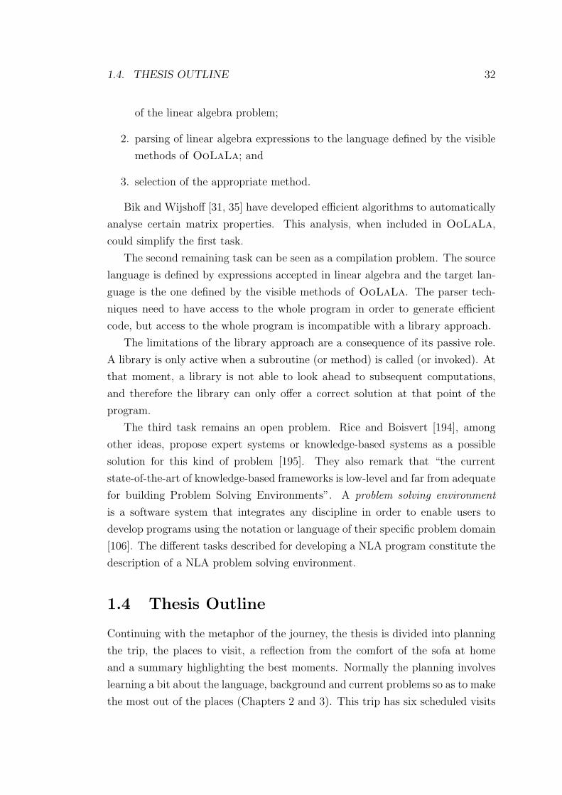
Continuing with the metaphor of the journey, the thesis is divided into planning
the trip, the places to visit, a reflection from the comfort of the sofa at home
and a summary highlighting the best moments. Normally the planning involves
learning a bit about the language, background and current problems so as to make
the most out of the places (Chapters 2 and 3). This trip has six scheduled visits
1.4. THESIS OUTLINE 33
Chp 11Chp 10Chp 9Chp 8Chp 7Chp 6
Chp 1 − Introduction ALALOChp 4 − O
App B
Chp 11 − ConclusionsChp 10 − LimitsChp 9 − GeneralisationChp 8 − Compiler Transformations
Chp 6 − Performance Evaluation
Chp 7 − Array Bounds Checks
Chp 5 − ImplementationChp 3 − OOSCChp 2 − NLA
Classic order
Chp 5Chp 4Chp 3Chp 2Chp 1
NLA interest only order NLA knowledgeableOO knowledgeableCompiler technology interest only order
Figure 1.1: Alternative orders for reading the thesis.
(Chapters 4 – 9) in an incremental order. Other travellers may prefer other orders
(see Figure 1.1), but bear in mind that, although each visit has been planned to
be as self-contained as possible, each stop motivates the next one. The stop in
Chapter 7 is the most self-contained and can be visited almost independently of
the others.
The remainder of the thesis is organised as follows:
Chapter 2 introduces basic concepts of NLA, and describes the BLAS and LA-
PACK designs. It is shown that the top-down design results in a complex
interface. Matlab and a Sparse Compiler are introduced as alternative ap-
proaches.
Chapter 3 reviews OOSC, and describes some design patterns that are used in
the following chapter.
Chapter 4 presents the design of OoLaLa and a survey of existing OO NLA
libraries. The design is balanced between the requirements of expert and
non-experts users, and enables OoLaLa to manage the storage formats and
to propagate matrix properties through matrix operations, a novel function-
ality for a library. Iterator and matrix abstraction levels are described as
a way of reducing the number of implementations of matrix operations.
The contents of this chapter, although with fewer surveyed libraries, are
published in [163].
Chapter 5 provides a high level description of the implementation issues of
OoLaLa. The design of OoLaLa is adapted to the restrictions of the
1.4. THESIS OUTLINE 34
programming language Java. This chapter compares matrix operations im-
plemented at storage format, at iterator level and at matrix abstraction
level to illustrate the reduction in the number of implementations of matrix
operations. Part of the contents of this chapter are published in [163].
Chapter 6 compares the performance obtained for a subset of BLAS matrix
operations implemented in Java at all three abstraction levels. It also com-
pares performance of storage format abstraction level implementations in
Java versus Fortran 77.
Chapter 7 introduces a new technique for the elimination of array bounds checks
in the presence of indirection. Array indirection is ubiquitous among the
storage formats for sparse matrices (i.e. most matrix elements have value
zero). The contents of this chapter are published in [165].
Chapter 8 defines a subset of storage formats (data structures) and matrix
properties (special features) for which a sequence of standard transforma-
tions are applied in order to eliminate the significant performance gap found
in Chapter 5. The contents of this chapter are published in [164].
Chapter 9 illustrates that the sequence of standard transformations is more
widely beneficial for applications using two design patterns which deal with
the access to data structures, as long as the data structures are implemented
as arrays.
Chapter 10 identifies limitations of a library approach in the context of linear
algebra. Some of these limitations are due to the inherent difficulty of
parsing a linear algebra expression to an optimum set of calls to library
subroutines.
Chapter 11 reviews the contributions of the thesis to the software development
process of sequential NLA programs and proposes future research directions.
Chapter 2
Numerical Linear Algebra
2.1 Introduction
“Numerical linear algebra is a very important subject in numerical
analysis because linear problems occur so often in applications. It has
been estimated, for example, that about 75% of all scientific problems
require the solution of a system of linear equations at one stage or
another.” Johnston [144]
“One of the most frequent problems encountered in scientific com-
putation is the solution of a system of linear equations.” Forsythe,
Malcolm and Moler [96]
Since the 1950s, the Numerical Linear Algebra (NLA) community has been
investigating the way to write programs for matrix operations so that the solutions
are accurate and the execution times are minimised. This research area, in which
numerical analysis and linear algebra are combined, continues to be active. The
importance of NLA is its widespread applicability to real applications such as
computational fluid dynamics, circuit simulations, data fitting, graph theory, etc.
[14].
During the ensuing 50 years, valuable knowledge has been collected in the
form of algorithms which have been made reusable as software libraries. To
understand the functionality that is provided, as well as the way the libraries are
organised, are the main objectives of this chapter. A further important aspect
is to analyse the influence on the user of the organisation and functionality of
these libraries. Since Chapter 4 includes an object oriented analysis and design
35
2.2. BASIC BACKGROUND 36
of NLA, this chapter can also be interpreted as a “requirements document” that
summarises the domain.
The requirements document begins with a review of the basic concepts of ma-
trices and matrix operations (Section 2.2). Then matrices are classified according
to two criteria (Section 2.3) and the way a given matrix can be represented in
different storage formats is examined (Section 2.4). The defined categories, or ma-
trix properties, allow the creation of specialised algorithms which take advantage
of certain specific matrix properties (Section 2.5). The algorithms and storage
formats are combined to provide implementations for matrix operations. Storage
format abstraction level (SFA-level) is the term used in the thesis to describe how
libraries are traditionally implemented. The limitations of this abstraction level
are discussed in Chapter 4 which proposes two further abstraction levels.
The final part of the requirements document examines how BLAS and LA-
PACK are organised; these are two prime examples of libraries developed by
community consensus (Section 2.6). These libraries are compared with two soft-
ware environments: Matlab and the Sparse Compiler. Matlab and the Sparse
Compiler represent alternatives to the libraries approach of NLA program con-
struction, and permit examination of the difficulties, or steps to follow, in devel-
oping NLA programs.
2.2 Basic Background
NLA is primarily concerned with matrix operations. These operations can be
subdivided into two groups. The first group consists of basic matrix operations
(such as transpose, addition, multiplation, etc.) and the second group involves
more complex matrix operations (such as systems of linear equations, eigenvalue
and eigenvector problems, and least squares problems). It is out of the scope
of the thesis to introduce and describe all the work and state-of-the-art of this
research area. Nevertheless, it is the aim of this section to familiarise the reader
with the necessary notation and definitions.
2.2. BASIC BACKGROUND 37
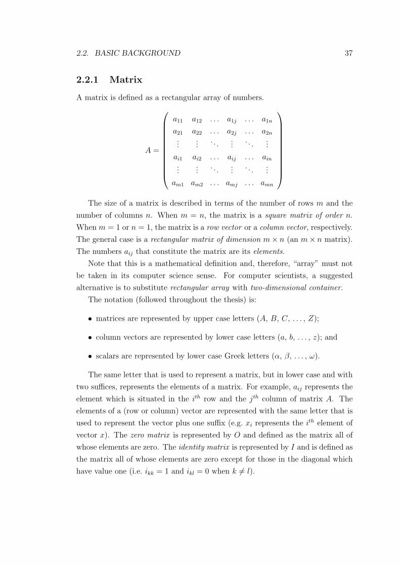
2.2.1 Matrix
A matrix is defined as a rectangular array of numbers.
A =
a11 a12 . . . a1j . . . a1n
a21 a22 . . . a2j . . . a2n
......
. . ....
. . ....
ai1 ai2 . . . aij . . . ain
......
. . ....
. . ....
am1 am2 . . . amj . . . amn
The size of a matrix is described in terms of the number of rows m and the
number of columns n. When m = n, the matrix is a square matrix of order n.
When m = 1 or n = 1, the matrix is a row vector or a column vector, respectively.
The general case is a rectangular matrix of dimension m× n (an m× n matrix).
The numbers aij that constitute the matrix are its elements.
Note that this is a mathematical definition and, therefore, “array” must not
be taken in its computer science sense. For computer scientists, a suggested
alternative is to substitute rectangular array with two-dimensional container.
The notation (followed throughout the thesis) is:
• matrices are represented by upper case letters (A, B, C, . . . , Z);
• column vectors are represented by lower case letters (a, b, . . . , z); and
• scalars are represented by lower case Greek letters (α, β, . . . , ω).
The same letter that is used to represent a matrix, but in lower case and with
two suffices, represents the elements of a matrix. For example, aij represents the
element which is situated in the ith row and the jth column of matrix A. The
elements of a (row or column) vector are represented with the same letter that is
used to represent the vector plus one suffix (e.g. xi represents the ith element of
vector x). The zero matrix is represented by O and defined as the matrix all of
whose elements are zero. The identity matrix is represented by I and is defined as
the matrix all of whose elements are zero except for those in the diagonal which
have value one (i.e. ikk = 1 and ikl = 0 when k 6= l).
2.2. BASIC BACKGROUND 38
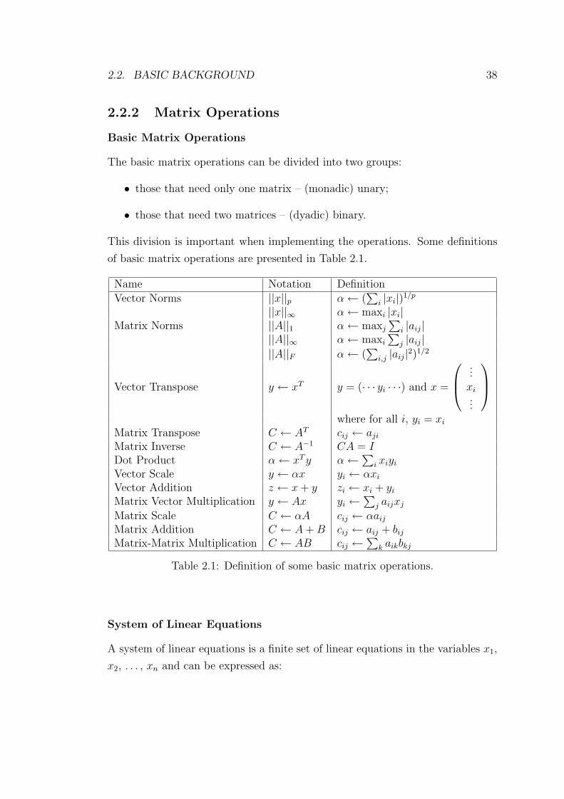
2.2.2 Matrix Operations
Basic Matrix Operations
The basic matrix operations can be divided into two groups:
• those that need only one matrix – (monadic) unary;
• those that need two matrices – (dyadic) binary.
This division is important when implementing the operations. Some definitions
of basic matrix operations are presented in Table 2.1.
Name Notation Definition
Vector Norms ||x||p α← (∑
i |xi|)1/p
||x||∞ α← maxi |xi|Matrix Norms ||A||1 α← maxj
∑i |aij|
||A||∞ α← maxi
∑j |aij|
||A||F α← (∑
i,j |aij|2)1/2
Vector Transpose y ← xT y = (· · · yi · · ·) and x =
...xi...
where for all i, yi = xi
Matrix Transpose C ← AT cij ← aji
Matrix Inverse C ← A−1 CA = IDot Product α← xT y α←
∑i xiyi
Vector Scale y ← αx yi ← αxi
Vector Addition z ← x + y zi ← xi + yi
Matrix Vector Multiplication y ← Ax yi ←∑
j aijxj
Matrix Scale C ← αA cij ← αaij
Matrix Addition C ← A + B cij ← aij + bij
Matrix-Matrix Multiplication C ← AB cij ←∑
k aikbkj
Table 2.1: Definition of some basic matrix operations.
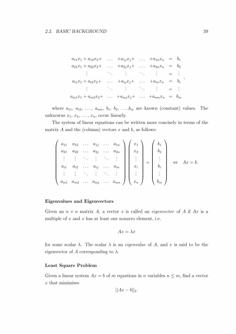
System of Linear Equations
A system of linear equations is a finite set of linear equations in the variables x1,
x2, . . . , xn and can be expressed as:
2.2. BASIC BACKGROUND 39
a11x1 + a12x2+ . . . +a1jxj+ . . . +a1nxn = b1
a21x1 + a22x2+ . . . +a2jxj+ . . . +a2nxn = b2
.... . .
.... . .
... =...
ai1x1 + ai2x2+ . . . +aijxj+ . . . +ainxn = bi
.... . .
.... . .
... =...
am1x1 + am2x2+ . . . +amjxj+ . . . +amnxn = bm
,
where a11, a12, . . . , amn, b1, b2, . . . ,bm are known (constant) values. The
unknowns x1, x2, . . . , xn, occur linearly.
The system of linear equations can be written more concisely in terms of the
matrix A and the (column) vectors x and b, as follows:
a11 a12 . . . a1j . . . a1n
a21 a22 . . . a2j . . . a2n
......
. . ....
. . ....
ai1 ai2 . . . aij . . . ain
......
. . ....
. . ....
am1 am2 . . . amj . . . amn
x1
x2
...
xi
...
xn
=
b1
b2
...
bi
...
bm
⇔ Ax = b.
Eigenvalues and Eigenvectors
Given an n × n matrix A, a vector x is called an eigenvector of A if Ax is a
multiple of x and x has at least one nonzero element, i.e.
Ax = λx
for some scalar λ. The scalar λ is an eigenvalue of A, and x is said to be the
eigenvector of A corresponding to λ.
Least Square Problem
Given a linear system Ax = b of m equations in n variables n ≤ m, find a vector
x that minimises
||Ax− b||2.
2.3. MATRIX PROPERTIES 40
2.3 Matrix Properties
The NLA community has identified different criteria to classify matrices. The
motivation behind these criteria is either recurrent matrix characteristics aris-
ing in real applications or matrix characteristics which simplify the computation
of certain matrix operations. An implementation of a matrix operation might
take advantage of the classification of the matrix to reduce the execution time
by eliminating redundant computations, to reduce memory requirements for the
computation, or to improve the accuracy of the results.
Two different criteria, and thereby two different classifications, are considered
in this section: nonzero elements structure and mathematical relations. The zero
elements of matrices produce a known result when added or multiplied (aij+
zero = aij and aij× zero = zero). These mathematical properties of the addition
and multiplication operations enable implementations to avoid computations for
which the result is already known. Moreover, these properties eliminate the need
to store element values already known from the structure to be zero. Figure 2.1
presents a hierarchical view of nonzero elements categories.
The mathematical relations are independent of the nonzero elements and are
expressed in terms of functions of the matrix elements. For example, a matrix is
symmetric if and only if A = AT .
In general, the categories defined by these two criteria are not mutually ex-
clusive, so that a given matrix can fall into more than one category. For example,
a matrix can be symmetric, positive definite and banded. The remainder of this
section is dedicated to the definition of the categories.
Hereafter the term matrix properties refers to any category of mathematical
relation or nonzero elements structure or combination of these.
2.3.1 Nonzero Elements Structure Criteria
The nonzero elements structure criteria classifies matrices into dense, banded,
block and sparse. Dense matrices are those matrices which have a majority of
nonzero elements. At the other end of the spectrum, sparse matrices are those
matrices which have a substantial minority of nonzero elements (see Table 2.2 for
dense and sparse matrix examples). A special sparse matrix is the zero matrix,
Om×n, which has only zero elements. In the middle of the spectrum, banded and
block matrices are matrices in which the nonzero elements have some structure.
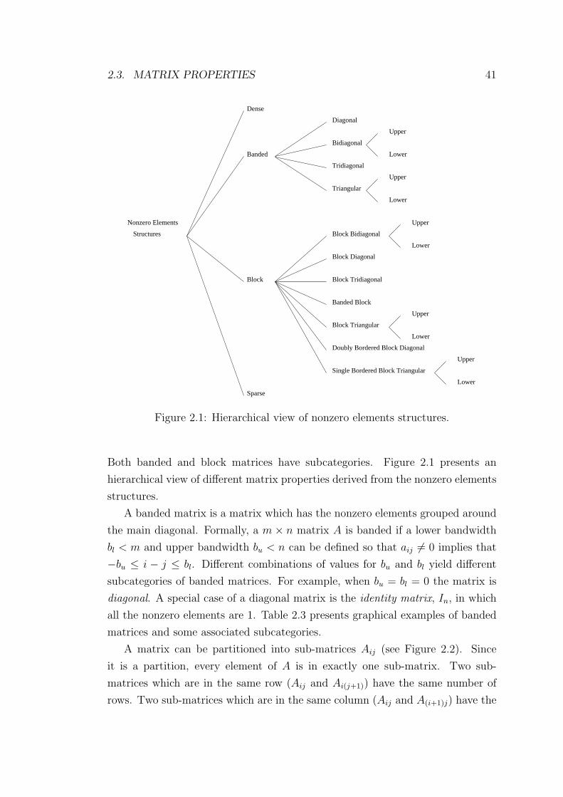
2.3. MATRIX PROPERTIES 41
Block Tridiagonal
Dense
Nonzero Elements
Structures
Block
Banded
Block Diagonal
Block Bidiagonal
Upper
Lower
Sparse
Banded Block
Single Bordered Block Triangular
Doubly Bordered Block Diagonal
Block Triangular
Upper
Lower
Upper
Lower
Diagonal
Bidiagonal
Tridiagonal
Triangular
Lower
Upper
Upper
Lower
Figure 2.1: Hierarchical view of nonzero elements structures.
Both banded and block matrices have subcategories. Figure 2.1 presents an
hierarchical view of different matrix properties derived from the nonzero elements
structures.
A banded matrix is a matrix which has the nonzero elements grouped around
the main diagonal. Formally, a m × n matrix A is banded if a lower bandwidth
bl < m and upper bandwidth bu < n can be defined so that aij 6= 0 implies that
−bu ≤ i − j ≤ bl. Different combinations of values for bu and bl yield different
subcategories of banded matrices. For example, when bu = bl = 0 the matrix is
diagonal. A special case of a diagonal matrix is the identity matrix, In, in which
all the nonzero elements are 1. Table 2.3 presents graphical examples of banded
matrices and some associated subcategories.
A matrix can be partitioned into sub-matrices Aij (see Figure 2.2). Since
it is a partition, every element of A is in exactly one sub-matrix. Two sub-
matrices which are in the same row (Aij and Ai(j+1)) have the same number of
rows. Two sub-matrices which are in the same column (Aij and A(i+1)j) have the
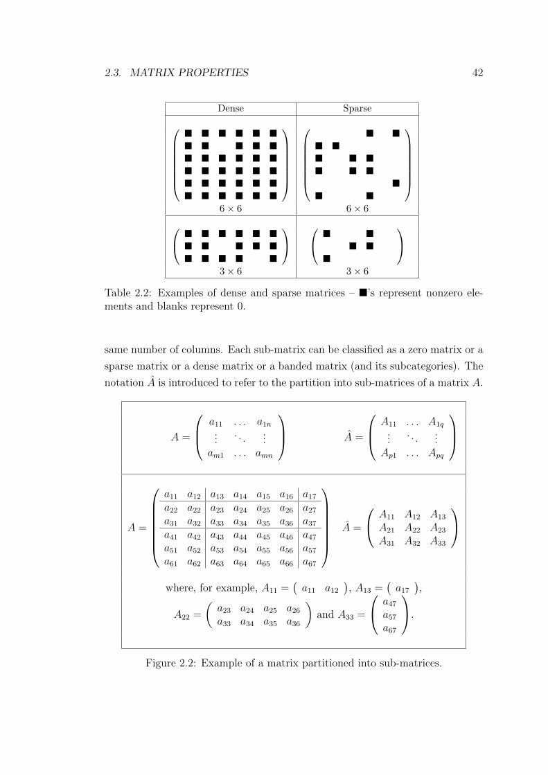
2.3. MATRIX PROPERTIES 42
Dense Sparse
� � � � � �� � � � �� � � � � �� � � � � �� � � � � �� � � � � �
� �� �� � �� � �
�� �
6× 6 6× 6 � � � � � �
� � � � �� � � � �
� �� �
�
3× 6 3× 6
Table 2.2: Examples of dense and sparse matrices – �’s represent nonzero ele-ments and blanks represent 0.
same number of columns. Each sub-matrix can be classified as a zero matrix or a
sparse matrix or a dense matrix or a banded matrix (and its subcategories). The
notation A is introduced to refer to the partition into sub-matrices of a matrix A.
A =
a11 . . . a1n...
. . ....
am1 . . . amn
A =
A11 . . . A1q...
. . ....
Ap1 . . . Apq
A =
a11 a12 a13 a14 a15 a16 a17
a22 a22 a23 a24 a25 a26 a27
a31 a32 a33 a34 a35 a36 a37
a41 a42 a43 a44 a45 a46 a47
a51 a52 a53 a54 a55 a56 a57
a61 a62 a63 a64 a65 a66 a67
A =
A11 A12 A13
A21 A22 A23
A31 A32 A33
where, for example, A11 =(
a11 a12
), A13 =
(a17
),
A22 =
(a23 a24 a25 a26
a33 a34 a35 a36
)and A33 =
a47
a57
a67
.
Figure 2.2: Example of a matrix partitioned into sub-matrices.
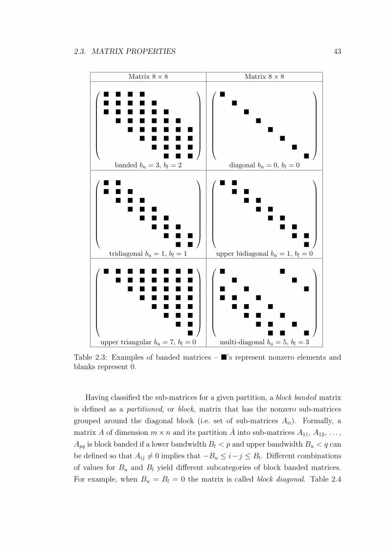
2.3. MATRIX PROPERTIES 43
Matrix 8× 8 Matrix 8× 8
� � � �� � � � �� � � � � �
� � � � � �� � � � � �
� � � � �� � � �
� � �
��
��
��
��
banded bu = 3, bl = 2 diagonal bu = 0, bl = 0
� �� � �
� � �� � �
� � �� � �
� � �� �
� �� �
� �� �
� �� �
� ��
tridiagonal bu = 1, bl = 1 upper bidiagonal bu = 1, bl = 0
� � � � � � � �� � � � � � �
� � � � � �� � � � �
� � � �� � �
� ��
� �� �
� � �� � �
� � �� � �
� � �� � �
upper triangular bu = 7, bl = 0 multi-diagonal bu = 5, bl = 3
Table 2.3: Examples of banded matrices – �’s represent nonzero elements andblanks represent 0.
Having classified the sub-matrices for a given partition, a block banded matrix
is defined as a partitioned, or block, matrix that has the nonzero sub-matrices
grouped around the diagonal block (i.e. set of sub-matrices Aii). Formally, a
matrix A of dimension m×n and its partition A into sub-matrices A11, A12, . . . ,
Apq is block banded if a lower bandwidth Bl < p and upper bandwidth Bu < q can
be defined so that Aij 6= 0 implies that −Bu ≤ i−j ≤ Bl. Different combinations
of values for Bu and Bl yield different subcategories of block banded matrices.
For example, when Bu = Bl = 0 the matrix is called block diagonal. Table 2.4
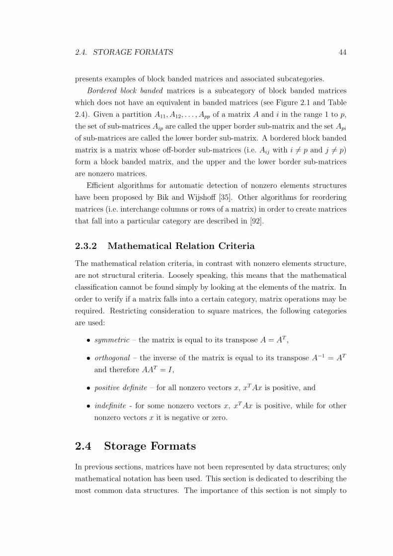
2.4. STORAGE FORMATS 44
presents examples of block banded matrices and associated subcategories.
Bordered block banded matrices is a subcategory of block banded matrices
which does not have an equivalent in banded matrices (see Figure 2.1 and Table
2.4). Given a partition A11, A12, . . . , App of a matrix A and i in the range 1 to p,
the set of sub-matrices Aip are called the upper border sub-matrix and the set Api
of sub-matrices are called the lower border sub-matrix. A bordered block banded
matrix is a matrix whose off-border sub-matrices (i.e. Aij with i 6= p and j 6= p)
form a block banded matrix, and the upper and the lower border sub-matrices
are nonzero matrices.
Efficient algorithms for automatic detection of nonzero elements structures
have been proposed by Bik and Wijshoff [35]. Other algorithms for reordering
matrices (i.e. interchange columns or rows of a matrix) in order to create matrices
that fall into a particular category are described in [92].
2.3.2 Mathematical Relation Criteria
The mathematical relation criteria, in contrast with nonzero elements structure,
are not structural criteria. Loosely speaking, this means that the mathematical
classification cannot be found simply by looking at the elements of the matrix. In
order to verify if a matrix falls into a certain category, matrix operations may be
required. Restricting consideration to square matrices, the following categories
are used:
• symmetric – the matrix is equal to its transpose A = AT ,
• orthogonal – the inverse of the matrix is equal to its transpose A−1 = AT
and therefore AAT = I,
• positive definite – for all nonzero vectors x, xT Ax is positive, and
• indefinite - for some nonzero vectors x, xT Ax is positive, while for other
nonzero vectors x it is negative or zero.
2.4 Storage Formats
In previous sections, matrices have not been represented by data structures; only
mathematical notation has been used. This section is dedicated to describing the
most common data structures. The importance of this section is not simply to
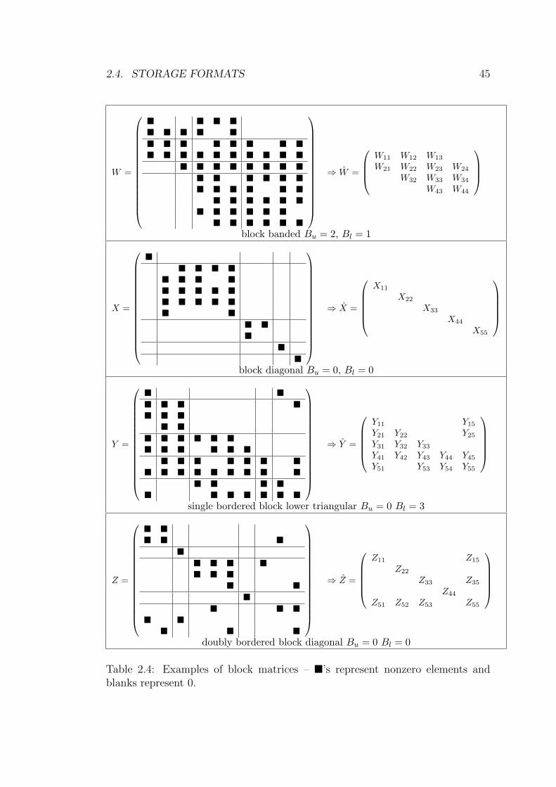
2.4. STORAGE FORMATS 45
W =
� � � �� � � � �� � � � � � � �� � � � � � � � � �
� � � � � � � �� � � � � �� � � � � �
� � � � � �� � � � � �
� � � � � �
⇒ W =
W11 W12 W13
W21 W22 W23 W24
W32 W33 W34
W43 W44
block banded Bu = 2, Bl = 1
X =
�� � � �
� � � �� � � � �� � � � �� �
� ��
��
⇒ X =
X11
X22
X33
X44
X55
block diagonal Bu = 0, Bl = 0
Y =
� �� � � �� � �
� �� � � � � �� � � � � �
� � � � � � �� � � � � � � � �
� � � �� � � � � � �
⇒ Y =
Y11 Y15
Y21 Y22 Y25
Y31 Y32 Y33
Y41 Y42 Y43 Y44 Y45
Y51 Y53 Y54 Y55
single bordered block lower triangular Bu = 0 Bl = 3
Z =
� �� � �
�� � � �� � �
� ��
� � �� �
� � �
⇒ Z =
Z11 Z15
Z22
Z33 Z35
Z44
Z51 Z52 Z53 Z55
doubly bordered block diagonal Bu = 0 Bl = 0
Table 2.4: Examples of block matrices – �’s represent nonzero elements andblanks represent 0.
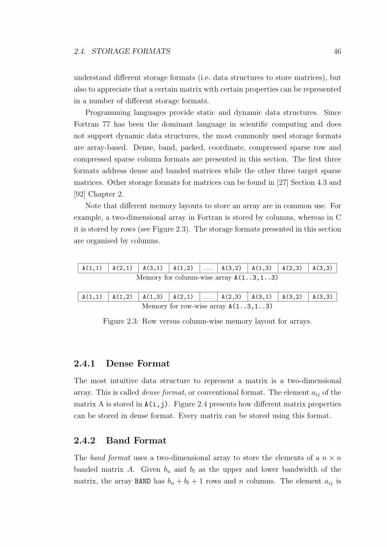
2.4. STORAGE FORMATS 46
understand different storage formats (i.e. data structures to store matrices), but
also to appreciate that a certain matrix with certain properties can be represented
in a number of different storage formats.
Programming languages provide static and dynamic data structures. Since
Fortran 77 has been the dominant language in scientific computing and does
not support dynamic data structures, the most commonly used storage formats
are array-based. Dense, band, packed, coordinate, compressed sparse row and
compressed sparse column formats are presented in this section. The first three
formats address dense and banded matrices while the other three target sparse
matrices. Other storage formats for matrices can be found in [27] Section 4.3 and
[92] Chapter 2.
Note that different memory layouts to store an array are in common use. For
example, a two-dimensional array in Fortran is stored by columns, whereas in C
it is stored by rows (see Figure 2.3). The storage formats presented in this section
are organised by columns.
A(1,1) A(2,1) A(3,1) A(1,2) . . . A(3,2) A(1,3) A(2,3) A(3,3)
Memory for column-wise array A(1..3,1..3)
A(1,1) A(1,2) A(1,3) A(2,1) . . . A(2,3) A(3,1) A(3,2) A(3,3)
Memory for row-wise array A(1..3,1..3)
Figure 2.3: Row versus column-wise memory layout for arrays.
2.4.1 Dense Format
The most intuitive data structure to represent a matrix is a two-dimensional
array. This is called dense format, or conventional format. The element aij of the
matrix A is stored in A(i,j). Figure 2.4 presents how different matrix properties
can be stored in dense format. Every matrix can be stored using this format.
2.4.2 Band Format
The band format uses a two-dimensional array to store the elements of a n × n
banded matrix A. Given bu and bl as the upper and lower bandwidth of the
matrix, the array BAND has bu + bl + 1 rows and n columns. The element aij is
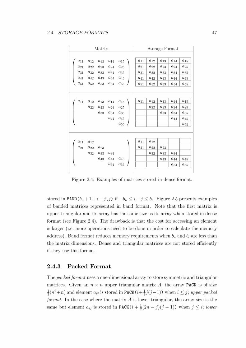
2.4. STORAGE FORMATS 47
Matrix Storage Format
a11 a12 a13 a14 a15
a21 a22 a23 a24 a25
a31 a32 a33 a34 a35
a41 a42 a43 a44 a45
a51 a52 a53 a54 a55
a11 a12 a13 a14 a15
a21 a22 a23 a24 a25
a31 a32 a33 a34 a35
a41 a42 a43 a44 a45
a51 a52 a53 a54 a55
a11 a12 a13 a14 a15
a22 a23 a24 a25
a33 a34 a35
a44 a45
a55
a11 a12 a13 a14 a15
a22 a23 a24 a25
a33 a34 a35
a44 a45
a55
a11 a12
a21 a22 a23
a32 a33 a34
a43 a44 a45
a54 a55
a11 a12
a21 a22 a23
a32 a33 a34
a43 a44 a45
a54 a55
Figure 2.4: Examples of matrices stored in dense format.
stored in BAND(bu +1+ i− j,j) if −bu ≤ i− j ≤ bl. Figure 2.5 presents examples
of banded matrices represented in band format. Note that the first matrix is
upper triangular and its array has the same size as its array when stored in dense
format (see Figure 2.4). The drawback is that the cost for accessing an element
is larger (i.e. more operations need to be done in order to calculate the memory
address). Band format reduces memory requirements when bu and bl are less than
the matrix dimensions. Dense and triangular matrices are not stored efficiently
if they use this format.
2.4.3 Packed Format
The packed format uses a one-dimensional array to store symmetric and triangular
matrices. Given an n × n upper triangular matrix A, the array PACK is of size12(n2+n) and element aij is stored in PACK(i+ 1
2j(j−1)) when i ≤ j; upper packed
format. In the case where the matrix A is lower triangular, the array size is the
same but element aij is stored in PACK(i + 12(2n − j)(j − 1)) when j ≤ i; lower
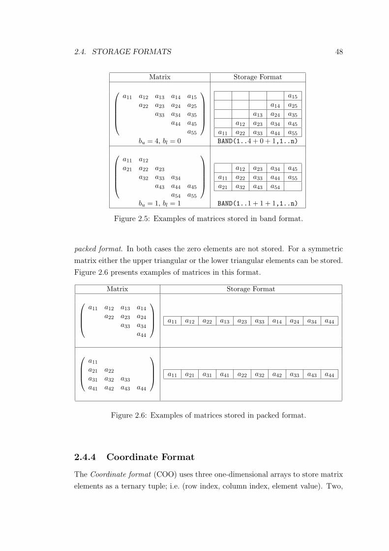
2.4. STORAGE FORMATS 48
Matrix Storage Format
a11 a12 a13 a14 a15
a22 a23 a24 a25
a33 a34 a35
a44 a45
a55
a15
a14 a25
a13 a24 a35
a12 a23 a34 a45
a11 a22 a33 a44 a55
bu = 4, bl = 0 BAND(1..4 + 0 + 1,1..n)a11 a12
a21 a22 a23
a32 a33 a34
a43 a44 a45
a54 a55
a12 a23 a34 a45
a11 a22 a33 a44 a55
a21 a32 a43 a54
bu = 1, bl = 1 BAND(1..1 + 1 + 1,1..n)
Figure 2.5: Examples of matrices stored in band format.
packed format. In both cases the zero elements are not stored. For a symmetric
matrix either the upper triangular or the lower triangular elements can be stored.
Figure 2.6 presents examples of matrices in this format.
Matrix Storage Formata11 a12 a13 a14
a22 a23 a24
a33 a34
a44
a11 a12 a22 a13 a23 a33 a14 a24 a34 a44
a11
a21 a22
a31 a32 a33
a41 a42 a43 a44
a11 a21 a31 a41 a22 a32 a42 a33 a43 a44
Figure 2.6: Examples of matrices stored in packed format.
2.4.4 Coordinate Format
The Coordinate format (COO) uses three one-dimensional arrays to store matrix
elements as a ternary tuple; i.e. (row index, column index, element value). Two,

2.4. STORAGE FORMATS 49
indx and jndx, of these arrays store the integer row and column indices, respec-
tively. The third array, namely value, stores the scalar values of the matrix
elements.
In COO format the elements of a matrix are stored in any order and, thus, to
find an element aij both indx and jndx have to be searched. The element aij is
found when for a given position k, the integer in indx(k) is equals to i and the
integer in jndx(k) is equals to j. Then, the scalar in value(k) is the element
aij. Only nonzero elements are stored in COO format. When the condition is
not satisfied for any value of k, then the corresponding matrix element is known
to be zero.
The lengths of indx, jndx and value are the same and are, at least, the
Number of Nonzero Elements (NNZEs) for the stored matrix. Figure 2.7 presents
examples of matrices stored in COO format.
Matrix Storage Formata11 a13
a22 a24
a34
a44
indxjndxvalue
2 1 1 4 3 22 3 1 4 4 4
a22 a13 a11 a44 a34 a24
a11
a22
a33
a41 a42 a43 a44
indxjndxvalue
4 2 1 4 3 4 41 2 1 4 3 2 3
a41 a22 a11 a44 a33 a42 a43
Figure 2.7: Examples of matrices stored in coordinate format.
2.4.5 Compressed Sparse Row Format
The Compressed Sparse Row format (CSR) stores matrices by rows and for each
row it holds the binary tuples (column index, scalar value) of the nonzero matrix
elements. The row indices are stored implicitly. The CSR format uses four
one-dimensional arrays. The arrays value and jndx, as in COO format, store
the values of the matrix elements and column indices, respectively. Both arrays
value and jndx have length, at least, the NNZEs of the stored matrix. The other
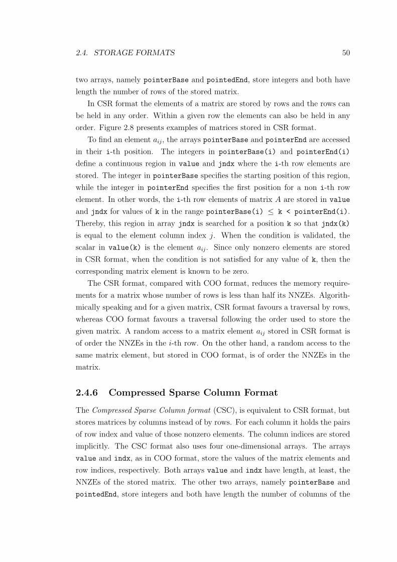
2.4. STORAGE FORMATS 50
two arrays, namely pointerBase and pointedEnd, store integers and both have
length the number of rows of the stored matrix.
In CSR format the elements of a matrix are stored by rows and the rows can
be held in any order. Within a given row the elements can also be held in any
order. Figure 2.8 presents examples of matrices stored in CSR format.
To find an element aij, the arrays pointerBase and pointerEnd are accessed
in their i-th position. The integers in pointerBase(i) and pointerEnd(i)
define a continuous region in value and jndx where the i-th row elements are
stored. The integer in pointerBase specifies the starting position of this region,
while the integer in pointerEnd specifies the first position for a non i-th row
element. In other words, the i-th row elements of matrix A are stored in value
and jndx for values of k in the range pointerBase(i) ≤ k < pointerEnd(i).
Thereby, this region in array jndx is searched for a position k so that jndx(k)
is equal to the element column index j. When the condition is validated, the
scalar in value(k) is the element aij. Since only nonzero elements are stored
in CSR format, when the condition is not satisfied for any value of k, then the
corresponding matrix element is known to be zero.
The CSR format, compared with COO format, reduces the memory require-
ments for a matrix whose number of rows is less than half its NNZEs. Algorith-
mically speaking and for a given matrix, CSR format favours a traversal by rows,
whereas COO format favours a traversal following the order used to store the
given matrix. A random access to a matrix element aij stored in CSR format is
of order the NNZEs in the i-th row. On the other hand, a random access to the
same matrix element, but stored in COO format, is of order the NNZEs in the
matrix.
2.4.6 Compressed Sparse Column Format
The Compressed Sparse Column format (CSC), is equivalent to CSR format, but
stores matrices by columns instead of by rows. For each column it holds the pairs
of row index and value of those nonzero elements. The column indices are stored
implicitly. The CSC format also uses four one-dimensional arrays. The arrays
value and indx, as in COO format, store the values of the matrix elements and
row indices, respectively. Both arrays value and indx have length, at least, the
NNZEs of the stored matrix. The other two arrays, namely pointerBase and
pointedEnd, store integers and both have length the number of columns of the
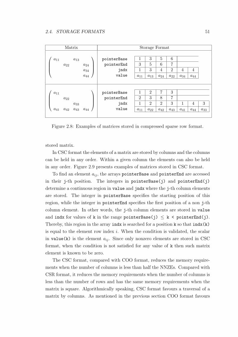
2.4. STORAGE FORMATS 51
Matrix Storage Format
a11 a13
a22 a24
a34
a44
pointerBasepointerEnd
jndxvalue
1 3 5 63 5 6 71 3 4 2 4 4
a11 a13 a24 a22 a34 a44
a11
a22
a33
a41 a42 a43 a44
pointerBasepointerEnd
jndxvalue
1 2 7 32 3 8 71 2 2 3 1 4 3
a11 a22 a42 a43 a41 a44 a33
Figure 2.8: Examples of matrices stored in compressed sparse row format.
stored matrix.
In CSC format the elements of a matrix are stored by columns and the columns
can be held in any order. Within a given column the elements can also be held
in any order. Figure 2.9 presents examples of matrices stored in CSC format.
To find an element aij, the arrays pointerBase and pointerEnd are accessed
in their j-th position. The integers in pointerBase(j) and pointerEnd(j)
determine a continuous region in value and jndx where the j-th column elements
are stored. The integer in pointerBase specifies the starting position of this
region, while the integer in pointerEnd specifies the first position of a non j-th
column element. In other words, the j-th column elements are stored in value
and indx for values of k in the range pointerBase(j) ≤ k < pointerEnd(j).
Thereby, this region in the array indx is searched for a position k so that indx(k)
is equal to the element row index i. When the condition is validated, the scalar
in value(k) is the element aij. Since only nonzero elements are stored in CSC
format, when the condition is not satisfied for any value of k then such matrix
element is known to be zero.
The CSC format, compared with COO format, reduces the memory require-
ments when the number of columns is less than half the NNZEs. Compared with
CSR format, it reduces the memory requirements when the number of columns is
less than the number of rows and has the same memory requirements when the
matrix is square. Algorithmically speaking, CSC format favours a traversal of a
matrix by columns. As mentioned in the previous section COO format favours
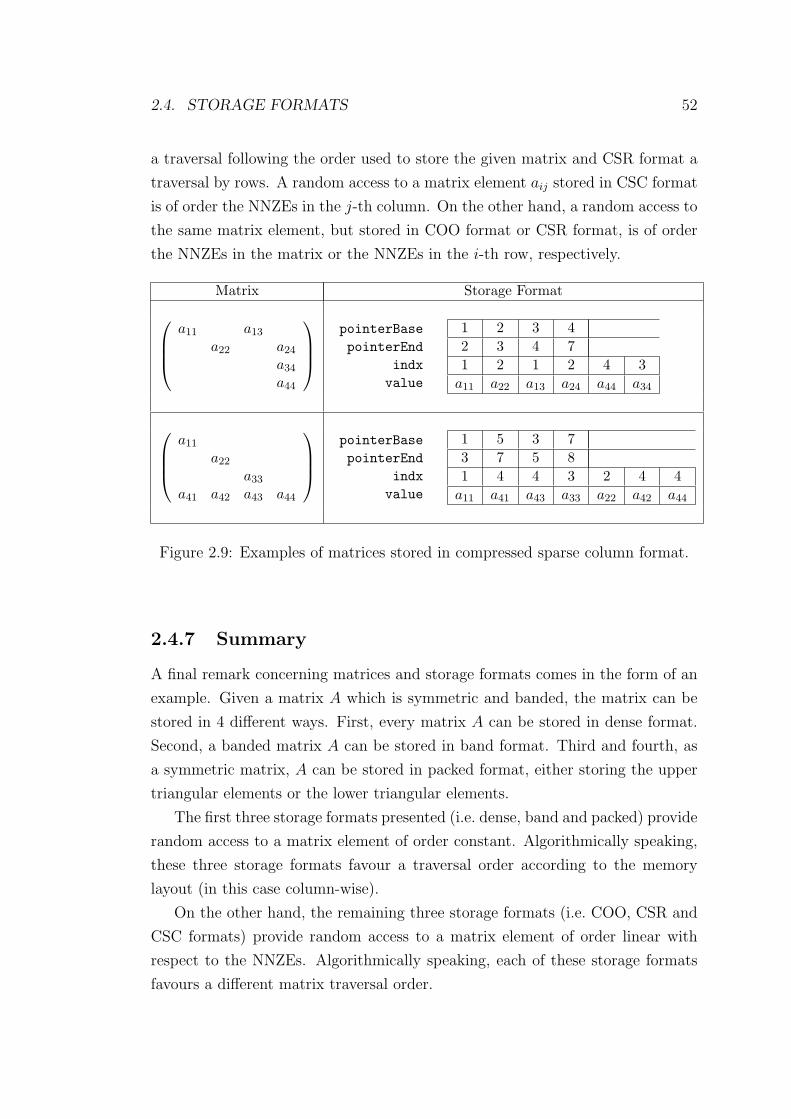
2.4. STORAGE FORMATS 52
a traversal following the order used to store the given matrix and CSR format a
traversal by rows. A random access to a matrix element aij stored in CSC format
is of order the NNZEs in the j-th column. On the other hand, a random access to
the same matrix element, but stored in COO format or CSR format, is of order
the NNZEs in the matrix or the NNZEs in the i-th row, respectively.
Matrix Storage Format
a11 a13
a22 a24
a34
a44
pointerBasepointerEnd
indxvalue
1 2 3 42 3 4 71 2 1 2 4 3
a11 a22 a13 a24 a44 a34
a11
a22
a33
a41 a42 a43 a44
pointerBasepointerEnd
indxvalue
1 5 3 73 7 5 81 4 4 3 2 4 4
a11 a41 a43 a33 a22 a42 a44
Figure 2.9: Examples of matrices stored in compressed sparse column format.
2.4.7 Summary
A final remark concerning matrices and storage formats comes in the form of an
example. Given a matrix A which is symmetric and banded, the matrix can be
stored in 4 different ways. First, every matrix A can be stored in dense format.
Second, a banded matrix A can be stored in band format. Third and fourth, as
a symmetric matrix, A can be stored in packed format, either storing the upper
triangular elements or the lower triangular elements.
The first three storage formats presented (i.e. dense, band and packed) provide
random access to a matrix element of order constant. Algorithmically speaking,
these three storage formats favour a traversal order according to the memory
layout (in this case column-wise).
On the other hand, the remaining three storage formats (i.e. COO, CSR and
CSC formats) provide random access to a matrix element of order linear with
respect to the NNZEs. Algorithmically speaking, each of these storage formats
favours a different matrix traversal order.
2.5. EXPLOITING MATRIX PROPERTIES 53
2.5 Exploiting Matrix Properties
Two matrix operations are used to illustrate their implementation in traditional
libraries. The first operation, matrix-matrix multiplication, is a basic binary ma-
trix operation. However, this operation is enough to show that for one matrix
operation many algorithms can be derived. Each algorithm is specialised for cer-
tain matrix properties, taking advantage of knowledge implied by the properties.
The second example is the solution of a system of linear equations. Two
families of methods can be applied to solve systems of linear equations: direct
methods and iterative methods. A direct method is an algorithm that calculates
the solution in a known finite number of instructions. On the other hand, an
iterative method is an algorithm that is executed repeatedly; each execution of
the algorithm produces an approximate solution of the problem, and execution is
stopped when the approximate solution is sufficiently accurate. The distinctive
nature of the two families makes it clear that, in contrast with the algorithms
for basic matrix operations, the different algorithms for solving systems of linear
equations are not simple specialisations derived from the matrix properties.
The final subsection defines the storage format abstraction level; the abstrac-
tion level at which, traditionally, matrix operations have been implemented. It is
shown that, for each specialised algorithm when combined with storage formats
for the matrix operands, different implementations are required.
The terms algorithm, storage format and implementation are used in the com-
puter science sense; i.e. an implementation (program) is an algorithm plus some
storage format (data structure) [226].
2.5.1 Matrix-Matrix Multiplication
The product of a matrix A of dimension m × p with a matrix B of dimension
p× n is another matrix C of dimension m× n with elements defined as
cij ←p∑
k=1
aikbkj.
When describing the algorithm, given by the above definition, three nested
loops are necessary (see Figure 2.10). This algorithm assumes that both A and
B are dense matrices.
The next algorithm is an example of matrix-matrix multiplication where one
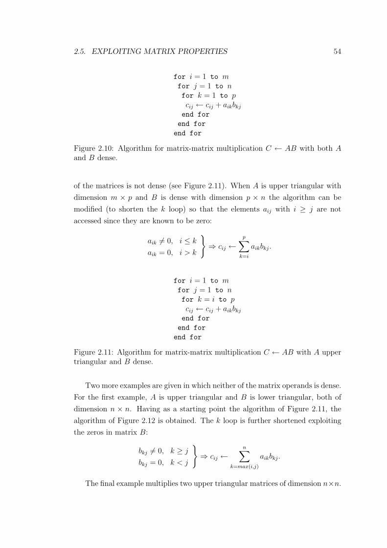
2.5. EXPLOITING MATRIX PROPERTIES 54
for i = 1 to mfor j = 1 to nfor k = 1 to pcij ← cij + aikbkj
end for
end for
end for
Figure 2.10: Algorithm for matrix-matrix multiplication C ← AB with both Aand B dense.
of the matrices is not dense (see Figure 2.11). When A is upper triangular with
dimension m × p and B is dense with dimension p × n the algorithm can be
modified (to shorten the k loop) so that the elements aij with i ≥ j are not
accessed since they are known to be zero:
aik 6= 0, i ≤ k
aik = 0, i > k
}⇒ cij ←
p∑k=i
aikbkj.
for i = 1 to mfor j = 1 to nfor k = i to pcij ← cij + aikbkj
end for
end for
end for
Figure 2.11: Algorithm for matrix-matrix multiplication C ← AB with A uppertriangular and B dense.
Two more examples are given in which neither of the matrix operands is dense.
For the first example, A is upper triangular and B is lower triangular, both of
dimension n × n. Having as a starting point the algorithm of Figure 2.11, the
algorithm of Figure 2.12 is obtained. The k loop is further shortened exploiting
the zeros in matrix B:
bkj 6= 0, k ≥ j
bkj = 0, k < j
}⇒ cij ←
n∑k=max(i,j)
aikbkj.
The final example multiplies two upper triangular matrices of dimension n×n.
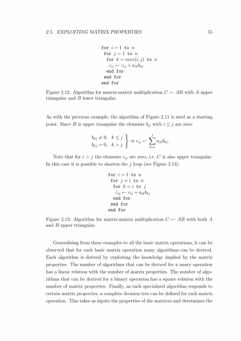
2.5. EXPLOITING MATRIX PROPERTIES 55
for i = 1 to nfor j = 1 to nfor k = max(i, j) to ncij ← cij + aikbkj
end for
end for
end for
Figure 2.12: Algorithm for matrix-matrix multiplication C ← AB with A uppertriangular and B lower triangular.
As with the previous example, the algorithm of Figure 2.11 is used as a starting
point. Since B is upper triangular the elements bij with i ≤ j are zero:
bkj 6= 0, k ≤ j
bkj = 0, k > j
}⇒ cij ←
j∑k=i
aikbkj.
Note that for i > j the elements cij are zero, i.e. C is also upper triangular.
In this case it is possible to shorten the j loop (see Figure 2.13).
for i = 1 to nfor j = i to nfor k = i to jcij ← cij + aikbkj
end for
end for
end for
Figure 2.13: Algorithm for matrix-matrix multiplication C ← AB with both Aand B upper triangular.
Generalising from these examples to all the basic matrix operations, it can be
observed that for each basic matrix operation many algorithms can be derived.
Each algorithm is derived by exploiting the knowledge implied by the matrix
properties. The number of algorithms that can be derived for a unary operation
has a linear relation with the number of matrix properties. The number of algo-
rithms that can be derived for a binary operation has a square relation with the
number of matrix properties. Finally, as each specialised algorithm responds to
certain matrix properties, a complete decision tree can be defined for each matrix
operation. This takes as inputs the properties of the matrices and determines the
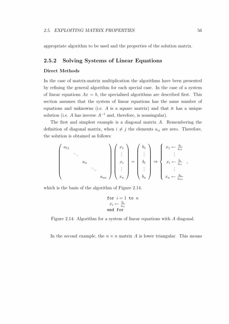
2.5. EXPLOITING MATRIX PROPERTIES 56
appropriate algorithm to be used and the properties of the solution matrix.
2.5.2 Solving Systems of Linear Equations
Direct Methods
In the case of matrix-matrix multiplication the algorithms have been presented
by refining the general algorithm for each special case. In the case of a system
of linear equations Ax = b, the specialised algorithms are described first. This
section assumes that the system of linear equations has the same number of
equations and unknowns (i.e. A is a square matrix) and that it has a unique
solution (i.e. A has inverse A−1 and, therefore, is nonsingular).
The first and simplest example is a diagonal matrix A. Remembering the
definition of diagonal matrix, when i 6= j the elements aij are zero. Therefore,
the solution is obtained as follows:
a11
. . .
aii
. . .
ann
x1
...
xi
...
xn
=
b1
...
bi
...
bn
⇒
x1 ← b1a11
...
xi ← bi
aii...
xn ← bn
ann
,
which is the basis of the algorithm of Figure 2.14.
for i = 1 to nxi ← bi
aii
end for
Figure 2.14: Algorithm for a system of linear equations with A diagonal.
In the second example, the n × n matrix A is lower triangular. This means
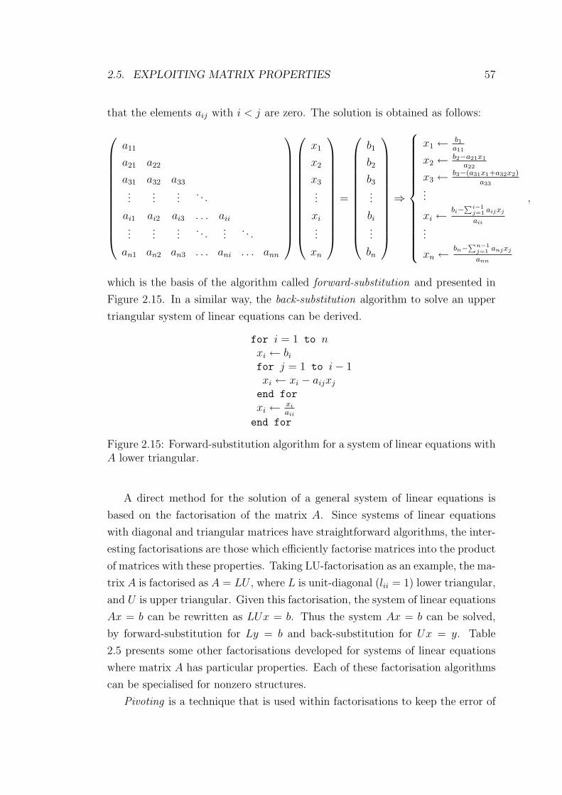
2.5. EXPLOITING MATRIX PROPERTIES 57
that the elements aij with i < j are zero. The solution is obtained as follows:
a11
a21 a22
a31 a32 a33
......
.... . .
ai1 ai2 ai3 . . . aii
......
.... . .
.... . .
an1 an2 an3 . . . ani . . . ann
x1
x2
x3
...
xi
...
xn
=
b1
b2
b3
...
bi
...
bn
⇒
x1 ← b1a11
x2 ← b2−a21x1
a22
x3 ← b3−(a31x1+a32x2)a33
...
xi ←bi−
∑i−1j=1 aijxj
aii...
xn ←bn−
∑n−1j=1 anjxj
ann
,
which is the basis of the algorithm called forward-substitution and presented in
Figure 2.15. In a similar way, the back-substitution algorithm to solve an upper
triangular system of linear equations can be derived.
for i = 1 to nxi ← bi
for j = 1 to i− 1xi ← xi − aijxj
end for
xi ← xi
aii
end for
Figure 2.15: Forward-substitution algorithm for a system of linear equations withA lower triangular.
A direct method for the solution of a general system of linear equations is
based on the factorisation of the matrix A. Since systems of linear equations
with diagonal and triangular matrices have straightforward algorithms, the inter-
esting factorisations are those which efficiently factorise matrices into the product
of matrices with these properties. Taking LU-factorisation as an example, the ma-
trix A is factorised as A = LU , where L is unit-diagonal (lii = 1) lower triangular,
and U is upper triangular. Given this factorisation, the system of linear equations
Ax = b can be rewritten as LUx = b. Thus the system Ax = b can be solved,
by forward-substitution for Ly = b and back-substitution for Ux = y. Table
2.5 presents some other factorisations developed for systems of linear equations
where matrix A has particular properties. Each of these factorisation algorithms
can be specialised for nonzero structures.
Pivoting is a technique that is used within factorisations to keep the error of
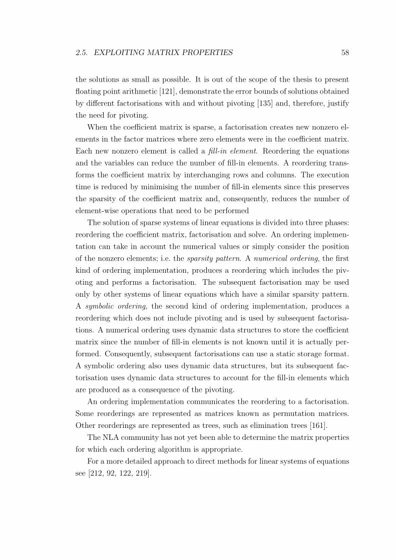
2.5. EXPLOITING MATRIX PROPERTIES 58
the solutions as small as possible. It is out of the scope of the thesis to present
floating point arithmetic [121], demonstrate the error bounds of solutions obtained
by different factorisations with and without pivoting [135] and, therefore, justify
the need for pivoting.
When the coefficient matrix is sparse, a factorisation creates new nonzero el-
ements in the factor matrices where zero elements were in the coefficient matrix.
Each new nonzero element is called a fill-in element. Reordering the equations
and the variables can reduce the number of fill-in elements. A reordering trans-
forms the coefficient matrix by interchanging rows and columns. The execution
time is reduced by minimising the number of fill-in elements since this preserves
the sparsity of the coefficient matrix and, consequently, reduces the number of
element-wise operations that need to be performed
The solution of sparse systems of linear equations is divided into three phases:
reordering the coefficient matrix, factorisation and solve. An ordering implemen-
tation can take in account the numerical values or simply consider the position
of the nonzero elements; i.e. the sparsity pattern. A numerical ordering, the first
kind of ordering implementation, produces a reordering which includes the piv-
oting and performs a factorisation. The subsequent factorisation may be used
only by other systems of linear equations which have a similar sparsity pattern.
A symbolic ordering, the second kind of ordering implementation, produces a
reordering which does not include pivoting and is used by subsequent factorisa-
tions. A numerical ordering uses dynamic data structures to store the coefficient
matrix since the number of fill-in elements is not known until it is actually per-
formed. Consequently, subsequent factorisations can use a static storage format.
A symbolic ordering also uses dynamic data structures, but its subsequent fac-
torisation uses dynamic data structures to account for the fill-in elements which
are produced as a consequence of the pivoting.
An ordering implementation communicates the reordering to a factorisation.
Some reorderings are represented as matrices known as permutation matrices.
Other reorderings are represented as trees, such as elimination trees [161].
The NLA community has not yet been able to determine the matrix properties
for which each ordering algorithm is appropriate.
For a more detailed approach to direct methods for linear systems of equations
see [212, 92, 122, 219].
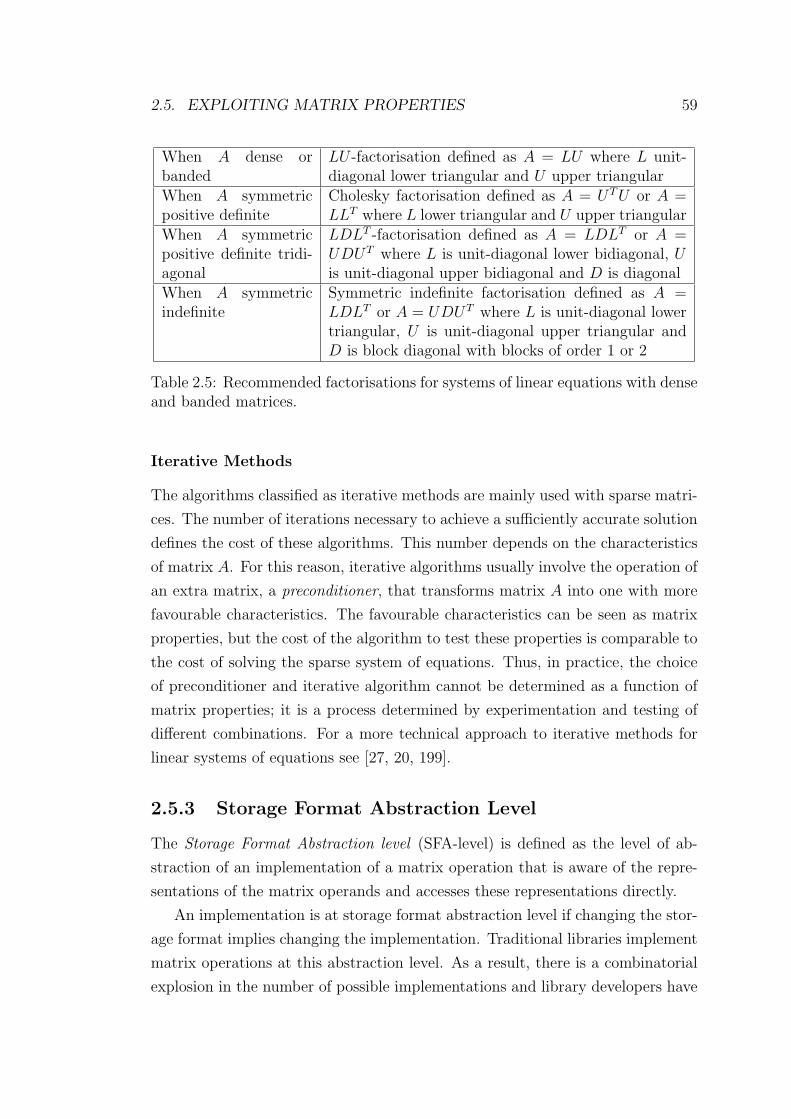
2.5. EXPLOITING MATRIX PROPERTIES 59
When A dense orbanded
LU -factorisation defined as A = LU where L unit-diagonal lower triangular and U upper triangular
When A symmetricpositive definite
Cholesky factorisation defined as A = UT U or A =LLT where L lower triangular and U upper triangular
When A symmetricpositive definite tridi-agonal
LDLT -factorisation defined as A = LDLT or A =UDUT where L is unit-diagonal lower bidiagonal, Uis unit-diagonal upper bidiagonal and D is diagonal
When A symmetricindefinite
Symmetric indefinite factorisation defined as A =LDLT or A = UDUT where L is unit-diagonal lowertriangular, U is unit-diagonal upper triangular andD is block diagonal with blocks of order 1 or 2
Table 2.5: Recommended factorisations for systems of linear equations with denseand banded matrices.
Iterative Methods
The algorithms classified as iterative methods are mainly used with sparse matri-
ces. The number of iterations necessary to achieve a sufficiently accurate solution
defines the cost of these algorithms. This number depends on the characteristics
of matrix A. For this reason, iterative algorithms usually involve the operation of
an extra matrix, a preconditioner, that transforms matrix A into one with more
favourable characteristics. The favourable characteristics can be seen as matrix
properties, but the cost of the algorithm to test these properties is comparable to
the cost of solving the sparse system of equations. Thus, in practice, the choice
of preconditioner and iterative algorithm cannot be determined as a function of
matrix properties; it is a process determined by experimentation and testing of
different combinations. For a more technical approach to iterative methods for
linear systems of equations see [27, 20, 199].
2.5.3 Storage Format Abstraction Level
The Storage Format Abstraction level (SFA-level) is defined as the level of ab-
straction of an implementation of a matrix operation that is aware of the repre-
sentations of the matrix operands and accesses these representations directly.
An implementation is at storage format abstraction level if changing the stor-
age format implies changing the implementation. Traditional libraries implement
matrix operations at this abstraction level. As a result, there is a combinatorial
explosion in the number of possible implementations and library developers have
2.5. EXPLOITING MATRIX PROPERTIES 60
to balance the number of implementations that are supported with the effort of
developing the code.
As an example, take the matrix-matrix multiplication algorithm with A upper
triangular and B dense (see Figure 2.11). An implementation of this algorithm
using dense format for both A and B is presented in Figure 2.16. NumType is
the data type of the matrix elements (real, double, complex, . . . ). Reading the
code of this implementation, it can be seen that each matrix is stored in a two-
dimensional array (i.e. dense format). This means that, when, for example, A
is stored instead in packed format then the implementation is no longer valid.
Figure 2.17 presents an implementation of the same algorithm, but with A stored
in packed format (i.e. as a one-dimensional array).
NumType A(m,m)
NumType B(m,n)
NumType C(m,n)
do j=1,n
do i=1,m
temp = 0
do k=i,m
temp = temp + A(i,k)*B(k,j)
end do
C(i,j) = temp
end do
end do
Figure 2.16: Implementation of matrix-matrix multiplication C ← AB with Aupper triangular and B dense, both stored in dense format.
2.5.4 Summary
A given matrix operation has many specialised algorithms. For each of these
algorithms there can be many implementations corresponding to different storage
formats for the matrix operands. Thus there is an explosion in the number
of possible implementations. The developers of NLA libraries have to balance
the number of implementations (i.e. algorithms and storage formats) that are
supported with the effort of developing the code.
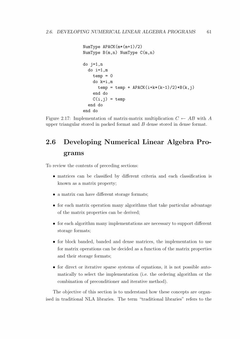
2.6. DEVELOPING NUMERICAL LINEAR ALGEBRA PROGRAMS 61
NumType APACK(m*(m+1)/2)
NumType B(m,n) NumType C(m,n)
do j=1,n
do i=1,m
temp = 0
do k=i,m
temp = temp + APACK(i+k*(k-1)/2)*B(k,j)
end do
C(i,j) = temp
end do
end do
Figure 2.17: Implementation of matrix-matrix multiplication C ← AB with Aupper triangular stored in packed format and B dense stored in dense format.
2.6 Developing Numerical Linear Algebra Pro-
grams
To review the contents of preceding sections:
• matrices can be classified by different criteria and each classification is
known as a matrix property;
• a matrix can have different storage formats;
• for each matrix operation many algorithms that take particular advantage
of the matrix properties can be derived;
• for each algorithm many implementations are necessary to support different
storage formats;
• for block banded, banded and dense matrices, the implementation to use
for matrix operations can be decided as a function of the matrix properties
and their storage formats;
• for direct or iterative sparse systems of equations, it is not possible auto-
matically to select the implementation (i.e. the ordering algorithm or the
combination of preconditioner and iterative method).
The objective of this section is to understand how these concepts are organ-
ised in traditional NLA libraries. The term “traditional libraries” refers to the
2.6. DEVELOPING NUMERICAL LINEAR ALGEBRA PROGRAMS 62
libraries developed, in this case by the NLA community, using top-down method-
ology and implemented in imperative languages, predominantly Fortran, with no
programmer-defined data types. BLAS [39] and LAPACK [12] are chosen as ex-
amples of traditional libraries to be described. An important characteristic is the
community consensus or de facto standardisation process which is behind their
design. Other examples of libraries are LINPACK [81], EISPACK [210, 110],
NAG1, IMSL2, SPARSPAK [111, 112], YSMP [94], MA28 [91].
BLAS and LAPACK are compared with two alternative NLA environments:
Matlab [171] and the Sparse Compiler [31, 34, 35, 32]. Rather than a theoreti-
cal discussion about the three alternatives, the matrix operations introduced in
Section 2.5 are used to illustrate the differences, advantages and disadvantages.
Matlab is a computing environment and programming language for numeri-
cal computations. Its main characteristic is that the programming language is
matrix-based. Thus, a Matlab program for NLA resembles its mathematical form.
The Sparse Compiler parses a given dense Fortran 77 program into an equiv-
alent sparse Fortran 77 program. A dense program means a NLA program that
stores its matrices in dense format even if some of the matrices have some nonzero
elements structure. An equivalent sparse program means a NLA program that
implements the same operations but those matrices with nonzero elements struc-
tures are stored in appropriate storage formats. The Sparse Compiler analyses
the nonzero elements structure of matrices and transforms the parts of the dense
program that define the matrices detected to have nonzero elements structure,
and the parts of the dense program that operate on these matrices. The dense
program is transformed so that it uses the new storage formats selected by the
compiler and exploits the nonzero elements structure of the matrices.
2.6.1 Using BLAS and LAPACK
BLAS (Basic Linear Algebra Subprograms) offer subroutines for basic matrix op-
eration while LAPACK (Linear Algebra Package) offers subroutines for systems of
linear equations, least square problems, and eigenvector and eigenvalue problems.
Both libraries are implemented in Fortran 77 and are designed to provide high
performance [88], i.e. to achieve maximum performance from a given computer.
1A commercial product of Numerical Algorithms Group Inc. http://www.nag.com2International Mathematical and Statistical Libraries (IMSL) a commercial product of Visual
Numerics Inc. http://www.vni.com
2.6. DEVELOPING NUMERICAL LINEAR ALGEBRA PROGRAMS 63
The routines provided by the BLAS are divided into three groups:
• Level 1 BLAS – routines that require O(n) floating point operations and
involve O(n) data items [154, 153], e.g. dot product xT y or a vector norm
||x||1;
• Level 2 BLAS – routines that require O(n2) floating point operations and
involve O(n2) data items [85, 84], e.g. matrix vector multiplication Ax; and
• Level 3 BLAS – routines that require O(n3) floating point operations and
involve O(n2) data items [83, 82], e.g. matrix-matrix multiplication AB.
The BLAS have been specified for dense, banded, sparse, symmetric, symmet-
ric banded, upper and lower triangular, and upper and lower triangular banded
matrices. Dense matrices are stored in dense format (GE). Banded matrices are
stored in band format (GB). Symmetric matrices are stored in dense (SY) or
packed format (SP). Triangular matrices are stored in dense (TR) or packed for-
mat (TP). Triangular band matrices are stored in band format (TB) and also
symmetric banded (SB). Finally, sparse matrices (US) are stored in an undis-
closed and implementation dependent format. In other words, each implemen-
tation is optimised for a specific platform and it will adopt the storage format
which delivers the best performance for that platform.
Based on the case of matrix-matrix multiplication (Section 2.5), the process
of developing a NLA program with the BLAS is described below. Given the
problem description C ← AB where A and B are known to be dense, the first
task is to find the correct BLAS subroutine. The subroutine names follow a
strict naming scheme: the first letter of the name indicates the numerical data
type (REAL, DOUBLE PRECISION, COMPLEX and DOUBLE COMPLEX) of the operands;
the next two letters specify the matrix properties and the storage format (in the
preceding paragraph, the pairs of letters between parenthesis show the different
combinations and their meanings); the final three letters indicate the matrix
operation. Table 2.6 includes the specification of the different subroutines for
matrix-matrix multiplication. Apart from the number of subroutines, the long
lists of parameters make for an unfriendly interface.
Following the naming scheme, the xGEMM subroutine is selected. The param-
eters pass information about the sizes of matrix operands, the representation of
the three matrix storage formats, and flags to indicate if any of the matrices have
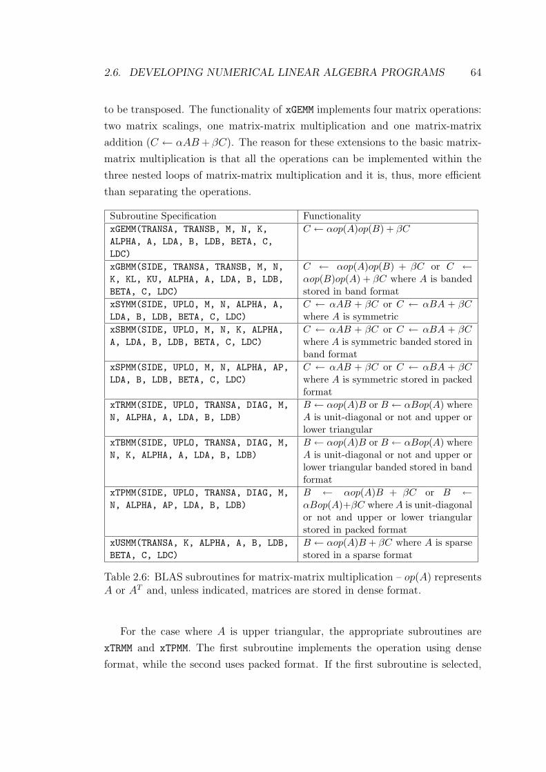
2.6. DEVELOPING NUMERICAL LINEAR ALGEBRA PROGRAMS 64
to be transposed. The functionality of xGEMM implements four matrix operations:
two matrix scalings, one matrix-matrix multiplication and one matrix-matrix
addition (C ← αAB + βC). The reason for these extensions to the basic matrix-
matrix multiplication is that all the operations can be implemented within the
three nested loops of matrix-matrix multiplication and it is, thus, more efficient
than separating the operations.
Subroutine Specification FunctionalityxGEMM(TRANSA, TRANSB, M, N, K,ALPHA, A, LDA, B, LDB, BETA, C,LDC)
C ← αop(A)op(B) + βC
xGBMM(SIDE, TRANSA, TRANSB, M, N,K, KL, KU, ALPHA, A, LDA, B, LDB,BETA, C, LDC)
C ← αop(A)op(B) + βC or C ←αop(B)op(A) + βC where A is bandedstored in band format
xSYMM(SIDE, UPLO, M, N, ALPHA, A,LDA, B, LDB, BETA, C, LDC)
C ← αAB + βC or C ← αBA + βCwhere A is symmetric
xSBMM(SIDE, UPLO, M, N, K, ALPHA,A, LDA, B, LDB, BETA, C, LDC)
C ← αAB + βC or C ← αBA + βCwhere A is symmetric banded stored inband format
xSPMM(SIDE, UPLO, M, N, ALPHA, AP,LDA, B, LDB, BETA, C, LDC)
C ← αAB + βC or C ← αBA + βCwhere A is symmetric stored in packedformat
xTRMM(SIDE, UPLO, TRANSA, DIAG, M,N, ALPHA, A, LDA, B, LDB)
B ← αop(A)B or B ← αBop(A) whereA is unit-diagonal or not and upper orlower triangular
xTBMM(SIDE, UPLO, TRANSA, DIAG, M,N, K, ALPHA, A, LDA, B, LDB)
B ← αop(A)B or B ← αBop(A) whereA is unit-diagonal or not and upper orlower triangular banded stored in bandformat
xTPMM(SIDE, UPLO, TRANSA, DIAG, M,N, ALPHA, AP, LDA, B, LDB)
B ← αop(A)B + βC or B ←αBop(A)+βC where A is unit-diagonalor not and upper or lower triangularstored in packed format
xUSMM(TRANSA, K, ALPHA, A, B, LDB,BETA, C, LDC)
B ← αop(A)B + βC where A is sparsestored in a sparse format
Table 2.6: BLAS subroutines for matrix-matrix multiplication – op(A) representsA or AT and, unless indicated, matrices are stored in dense format.
For the case where A is upper triangular, the appropriate subroutines are
xTRMM and xTPMM. The first subroutine implements the operation using dense
format, while the second uses packed format. If the first subroutine is selected,

2.6. DEVELOPING NUMERICAL LINEAR ALGEBRA PROGRAMS 65
memory space might be wasted, whereas if xTPMM is selected, the user must under-
stand and create the representation (packed format) required by the subroutine.
For the case where A and B are both upper triangular, the appropriate sub-
routines are again xTRMM and xTPMM. BLAS subroutines have been developed in
such a way that only one of the input matrices (for binary operations) is con-
sidered to have properties other than dense. Hence, the BLAS are not complete
in the sense that not all of the possible implementations are included. In this
case, the waste of memory space is larger since the three matrices involved are
all upper triangular, and only one matrix can be stored in packed format.
LAPACK subroutines are divided into those that solve standard problems,
called driver subroutines, and presented in Section 2.2, and those which com-
pute factorisations and other operations used by the driver subroutines. Another
long list of matrix properties and storage formats is supported and is organised
following the naming scheme described with the BLAS.
Figures 2.18, 2.19 and 2.20 present pseudo-Fortran programs to solve the
system of linear equations ABx = c where A and B are n × n matrices. The
programs on the left hand side of these figures follow an algorithm which first
performs the matrix-matrix multiplication and then solves the system of equa-
tions. Alternatively, the programs on the right hand side of these figures follow an
algorithm which first solves the system of linear equations Ay = c and then the
system Bx = y. Both algorithms are semantically equivalent, i.e. they calculate
the same result assuming perfect floating point arithmetic. Figure 2.18 presents
programs to solve the system of linear equations ABx = c where A and B are
n× n dense matrices. Figures 2.19 and 2.20 presents programs to solve the same
problem, but here A and B are upper triangular matrices. The first figure uses
dense format while the second figure uses packed format, whenever possible.
To summarise, this process can be generalised to describe the development of
NLA programs with traditional libraries as:
• describe the problem in terms of matrix operations;
• analyse the matrices to determine their properties;
• select the library or libraries which support the operations and properties;
• select the subroutines which best fit the matrix properties; and
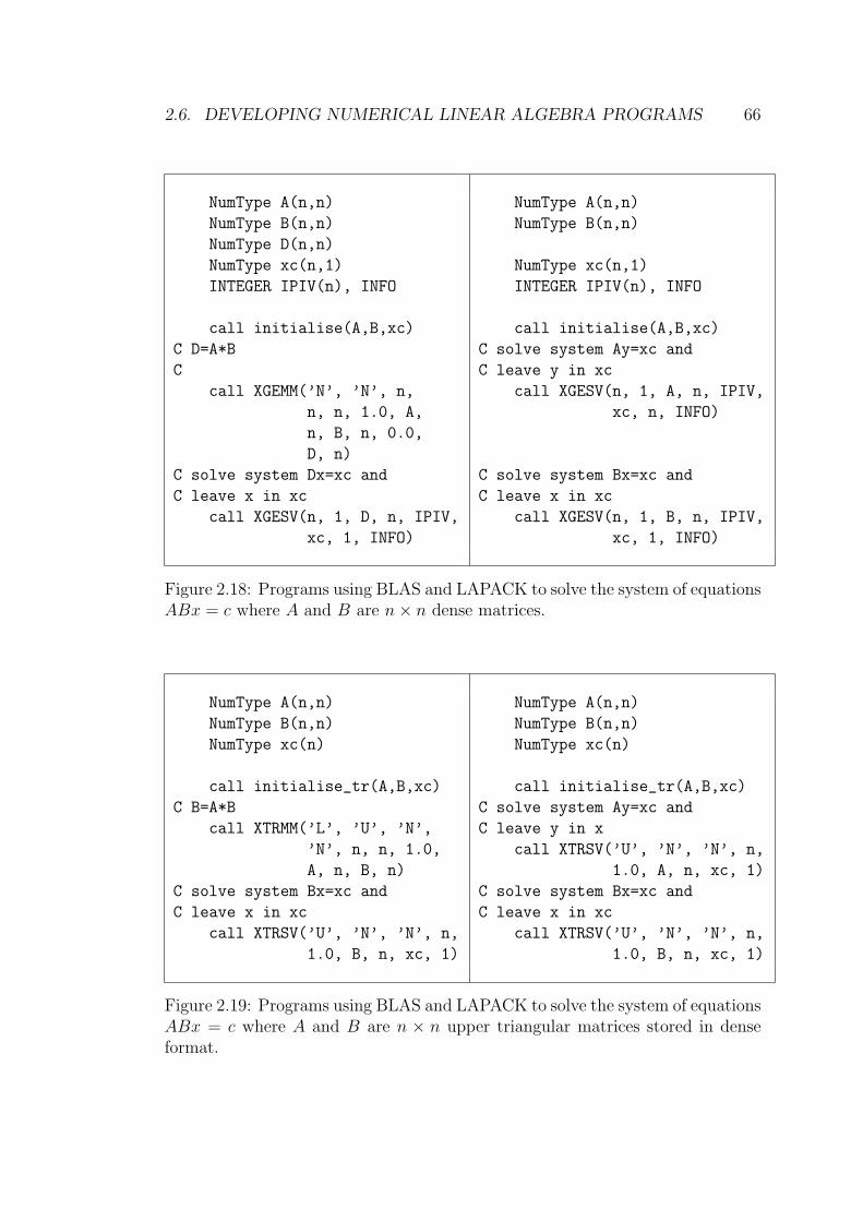
2.6. DEVELOPING NUMERICAL LINEAR ALGEBRA PROGRAMS 66
NumType A(n,n)
NumType B(n,n)
NumType D(n,n)
NumType xc(n,1)
INTEGER IPIV(n), INFO
call initialise(A,B,xc)
C D=A*B
C
call XGEMM(’N’, ’N’, n,
n, n, 1.0, A,
n, B, n, 0.0,
D, n)
C solve system Dx=xc and
C leave x in xc
call XGESV(n, 1, D, n, IPIV,
xc, 1, INFO)
NumType A(n,n)
NumType B(n,n)
NumType xc(n,1)
INTEGER IPIV(n), INFO
call initialise(A,B,xc)
C solve system Ay=xc and
C leave y in xc
call XGESV(n, 1, A, n, IPIV,
xc, n, INFO)
C solve system Bx=xc and
C leave x in xc
call XGESV(n, 1, B, n, IPIV,
xc, 1, INFO)
Figure 2.18: Programs using BLAS and LAPACK to solve the system of equationsABx = c where A and B are n× n dense matrices.
NumType A(n,n)
NumType B(n,n)
NumType xc(n)
call initialise_tr(A,B,xc)
C B=A*B
call XTRMM(’L’, ’U’, ’N’,
’N’, n, n, 1.0,
A, n, B, n)
C solve system Bx=xc and
C leave x in xc
call XTRSV(’U’, ’N’, ’N’, n,
1.0, B, n, xc, 1)
NumType A(n,n)
NumType B(n,n)
NumType xc(n)
call initialise_tr(A,B,xc)
C solve system Ay=xc and
C leave y in x
call XTRSV(’U’, ’N’, ’N’, n,
1.0, A, n, xc, 1)
C solve system Bx=xc and
C leave x in xc
call XTRSV(’U’, ’N’, ’N’, n,
1.0, B, n, xc, 1)
Figure 2.19: Programs using BLAS and LAPACK to solve the system of equationsABx = c where A and B are n × n upper triangular matrices stored in denseformat.
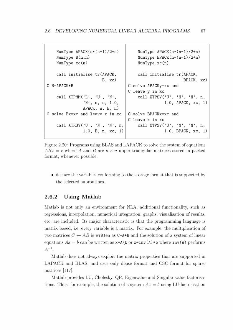
2.6. DEVELOPING NUMERICAL LINEAR ALGEBRA PROGRAMS 67
NumType APACK(n*(n-1)/2+n)
NumType B(n,n)
NumType xc(n)
call initialise_tr(APACK,
B, xc)
C B=APACK*B
call XTPMM(’L’, ’U’, ’N’,
’N’, n, n, 1.0,
APACK, n, B, n)
C solve Bx=xc and leave x in xc
call XTRSV(’U’, ’N’, ’N’, n,
1.0, B, n, xc, 1)
NumType APACK(n*(n-1)/2+n)
NumType BPACK(n*(n-1)/2+n)
NumType xc(n)
call initialise_tr(APACK,
BPACK, xc)
C solve APACKy=xc and
C leave y in xc
call XTPSV(’U’, ’N’, ’N’, n,
1.0, APACK, xc, 1)
C solve BPACKx=xc and
C leave x in xc
call XTPSV(’U’, ’N’, ’N’, n,
1.0, BPACK, xc, 1)
Figure 2.20: Programs using BLAS and LAPACK to solve the system of equationsABx = c where A and B are n × n upper triangular matrices stored in packedformat, whenever possible.
• declare the variables conforming to the storage format that is supported by
the selected subroutines.
2.6.2 Using Matlab
Matlab is not only an environment for NLA; additional functionality, such as
regressions, interpolation, numerical integration, graphs, visualisation of results,
etc. are included. Its major characteristic is that the programming language is
matrix based, i.e. every variable is a matrix. For example, the multiplication of
two matrices C ← AB is written as C=A*B and the solution of a system of linear
equations Ax = b can be written as x=A\b or x=inv(A)*b where inv(A) performs
A−1.
Matlab does not always exploit the matrix properties that are supported in
LAPACK and BLAS, and uses only dense format and CSC format for sparse
matrices [117].
Matlab provides LU, Cholesky, QR, Eigenvalue and Singular value factorisa-
tions. Thus, for example, the solution of a system Ax = b using LU-factorisation
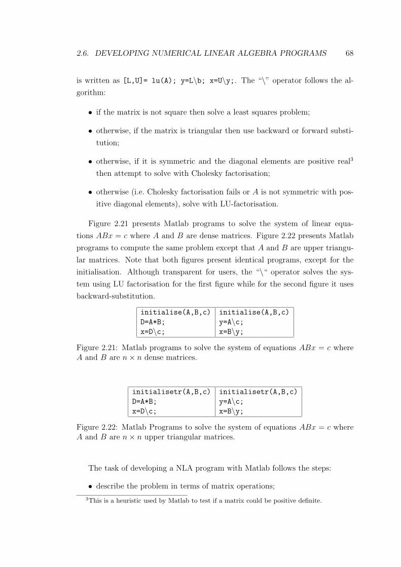
2.6. DEVELOPING NUMERICAL LINEAR ALGEBRA PROGRAMS 68
is written as [L,U]= lu(A); y=L\b; x=U\y;. The “\” operator follows the al-
gorithm:
• if the matrix is not square then solve a least squares problem;
• otherwise, if the matrix is triangular then use backward or forward substi-
tution;
• otherwise, if it is symmetric and the diagonal elements are positive real3
then attempt to solve with Cholesky factorisation;
• otherwise (i.e. Cholesky factorisation fails or A is not symmetric with pos-
itive diagonal elements), solve with LU-factorisation.
Figure 2.21 presents Matlab programs to solve the system of linear equa-
tions ABx = c where A and B are dense matrices. Figure 2.22 presents Matlab
programs to compute the same problem except that A and B are upper triangu-
lar matrices. Note that both figures present identical programs, except for the
initialisation. Although transparent for users, the “\“ operator solves the sys-
tem using LU factorisation for the first figure while for the second figure it uses
backward-substitution.
initialise(A,B,c) initialise(A,B,c)
D=A*B; y=A\c;x=D\c; x=B\y;
Figure 2.21: Matlab programs to solve the system of equations ABx = c whereA and B are n× n dense matrices.
initialisetr(A,B,c) initialisetr(A,B,c)
D=A*B; y=A\c;x=D\c; x=B\y;
Figure 2.22: Matlab Programs to solve the system of equations ABx = c whereA and B are n× n upper triangular matrices.
The task of developing a NLA program with Matlab follows the steps:
• describe the problem in terms of matrix operations;
3This is a heuristic used by Matlab to test if a matrix could be positive definite.
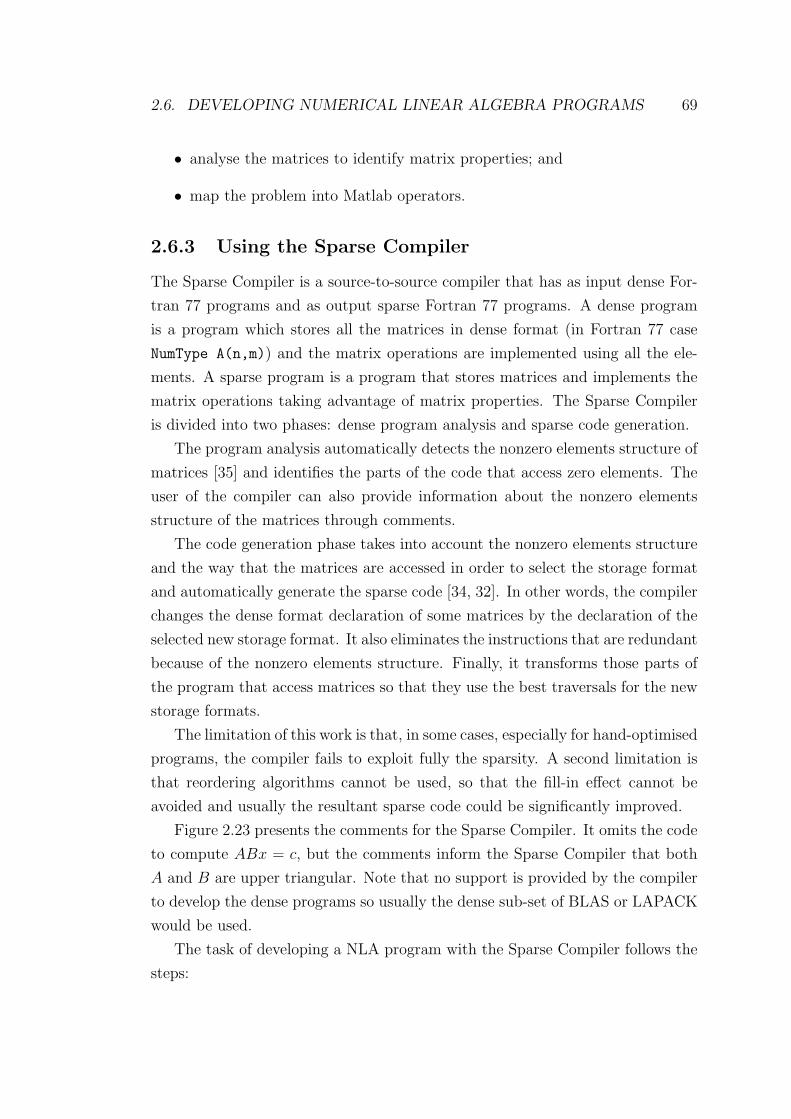
2.6. DEVELOPING NUMERICAL LINEAR ALGEBRA PROGRAMS 69
• analyse the matrices to identify matrix properties; and
• map the problem into Matlab operators.
2.6.3 Using the Sparse Compiler
The Sparse Compiler is a source-to-source compiler that has as input dense For-
tran 77 programs and as output sparse Fortran 77 programs. A dense program
is a program which stores all the matrices in dense format (in Fortran 77 case
NumType A(n,m)) and the matrix operations are implemented using all the ele-
ments. A sparse program is a program that stores matrices and implements the
matrix operations taking advantage of matrix properties. The Sparse Compiler
is divided into two phases: dense program analysis and sparse code generation.
The program analysis automatically detects the nonzero elements structure of
matrices [35] and identifies the parts of the code that access zero elements. The
user of the compiler can also provide information about the nonzero elements
structure of the matrices through comments.
The code generation phase takes into account the nonzero elements structure
and the way that the matrices are accessed in order to select the storage format
and automatically generate the sparse code [34, 32]. In other words, the compiler
changes the dense format declaration of some matrices by the declaration of the
selected new storage format. It also eliminates the instructions that are redundant
because of the nonzero elements structure. Finally, it transforms those parts of
the program that access matrices so that they use the best traversals for the new
storage formats.
The limitation of this work is that, in some cases, especially for hand-optimised
programs, the compiler fails to exploit fully the sparsity. A second limitation is
that reordering algorithms cannot be used, so that the fill-in effect cannot be
avoided and usually the resultant sparse code could be significantly improved.
Figure 2.23 presents the comments for the Sparse Compiler. It omits the code
to compute ABx = c, but the comments inform the Sparse Compiler that both
A and B are upper triangular. Note that no support is provided by the compiler
to develop the dense programs so usually the dense sub-set of BLAS or LAPACK
would be used.
The task of developing a NLA program with the Sparse Compiler follows the
steps:
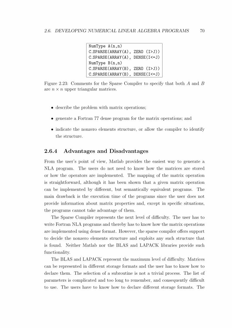
2.6. DEVELOPING NUMERICAL LINEAR ALGEBRA PROGRAMS 70
NumType A(n,n)
C SPARSE(ARRAY(A), ZERO (I>J))
C SPARSE(ARRAY(A), DENSE(I<=J)
NumType B(n,n)
C SPARSE(ARRAY(B), ZERO (I>J))
C SPARSE(ARRAY(B), DENSE(I<=J)
Figure 2.23: Comments for the Sparse Compiler to specify that both A and Bare n× n upper triangular matrices.
• describe the problem with matrix operations;
• generate a Fortran 77 dense program for the matrix operations; and
• indicate the nonzero elements structure, or allow the compiler to identify
the structure.
2.6.4 Advantages and Disadvantages
From the user’s point of view, Matlab provides the easiest way to generate a
NLA program. The users do not need to know how the matrices are stored
or how the operators are implemented. The mapping of the matrix operation
is straightforward, although it has been shown that a given matrix operation
can be implemented by different, but semantically equivalent programs. The
main drawback is the execution time of the programs since the user does not
provide information about matrix properties and, except in specific situations,
the programs cannot take advantage of them.
The Sparse Compiler represents the next level of difficulty. The user has to
write Fortran NLA programs and thereby has to know how the matrix operations
are implemented using dense format. However, the sparse compiler offers support
to decide the nonzero elements structure and exploits any such structure that
is found. Neither Matlab nor the BLAS and LAPACK libraries provide such
functionality.
The BLAS and LAPACK represent the maximum level of difficulty. Matrices
can be represented in different storage formats and the user has to know how to
declare them. The selection of a subroutine is not a trivial process. The list of
parameters is complicated and too long to remember, and consequently difficult
to use. The users have to know how to declare different storage formats. The
2.7. SUMMARY 71
functionality is not complete, not all possibilities of matrix properties and storage
format operands are supported. On the other hand, the BLAS and LAPACK
subroutines deliver the minimum execution time as they utilise state-of-the-art
implementations.
The user perceives the difficulty of developing a NLA program as the step
from the problem defined in terms of matrix operations to the specific software
environment expression (subroutines in traditional libraries, operators in Matlab
and comments and dense program in the Sparse Compiler). This step is repre-
sented by the tasks that need to be completed in order to develop the program.
These tasks are:
• matrix properties analysis;
• selection of storage formats; and
• selection of specific environment expressions that align with the properties
and storage formats.
2.7 Summary
Matrix operations are the core of this chapter; beginning with their definitions,
continuing with examples of how matrix operations are implemented, and ending
with how they are organised in libraries.
Matrix operations have been divided into basic matrix operations and matrix
equations. Due to certain matrix properties, the definition of a basic matrix
operation can be specialised, and thus different algorithms that exploit the matrix
properties are created. Due to the different storage formats of a matrix, the set
of algorithms are further extended into a set of implementations.
Linear equations can be solved either with direct or iterative methods. Di-
rect methods perform a factorisation and then solve the systems for the factored
matrices. When the matrix equations are sparse, the matrix can be reordered to
preserve the sparsity of the factored matrices. However, it is not possible to de-
cide efficiently which of the different ordering algorithms is the most appropriate.
Iterative methods are usually combined with preconditioners. Some iterative al-
gorithms are known to fail to converge to a solution for specific matrix properties.
In practice, the appropriate combination of iterative method and preconditioner
for a system of linear equations cannot be decided automatically.
2.7. SUMMARY 72
Traditional libraries are organised by strict naming schemes. For each sub-
routine the naming scheme describes the matrix operation, the matrix properties
of the input matrices and their storage formats. The parameters describe how
the storage formats are represented.
The comparison of the BLAS and LAPACK with Matlab and with the Sparse
Compiler shows that, when developing a NLA program, the BLAS and LAPACK
based programs constitute the maximum level of difficulty. The difficulty is sum-
marised by the tasks to be completed:
• describe the problem in terms of matrix operations;
• analyse matrices to determine their properties;
• select the library or libraries that support the matrix operations and prop-
erties;
• select the subroutines which best fit the matrix properties; and
• declare the variables conforming to the storage format that is supported by
the selected subroutines.
The information of this chapter is reused mainly in Chapter 4, which reports
an object oriented analysis and design of NLA.
Readers are referred to [108] and [109] for a more detailed, analytical, ap-
proach to NLA. Descriptions and analysis of algorithms for matrix operations
can be found in [212, 122, 219]. Detailed study of accuracy and stability of these
algorithms can be found in [135].
Chapter 3
Object Oriented Software
Construction
3.1 Introduction
“A word of warning. Given today’s apparent prominence of object
technology, some reader might think that the battle has been won and
that no further rationale is necessary. This would be a mistake: we
need to understand the basis of the method, if only to avoid common
misuses and pitfalls. It is in fact frequent to see the word object-
oriented (like structured in an earlier era) used as mere veneer over
the most conventional techniques. Only by carefully building the case
for object technology can we learn to detect improper uses of the
buzzword, and stay away from common mistakes reviewed later in
this chapter.” Meyer [174]
“Algorithmic versus Object-Oriented Decomposition.
Which is the right way to decompose a complex system - by algo-
rithms or by objects? Actually, this is a trick question, because the
right answer is that both views are important . . . However the fact
remains that we cannot construct a complex system in both ways
simultaneously, for they are completely orthogonal views. . . .
Object-oriented decomposition has a number of highly significant ad-
vantages over algorithmic decomposition. Object-oriented decomposi-
tion yields smaller systems through the reuse of common mechanism,
73
3.1. INTRODUCTION 74
thus providing an important economy of expression. Object-oriented
systems are also more resilient to change and thus better able to
evolve over time . . . Indeed, object-oriented decomposition greatly re-
duces the risk of building complex systems because they are designed
to evolve incrementally from smaller systems in which we already have
confidence.” Booch [49]
“We (humans) have developed an exceptionally powerful technique
for dealing with complexity. We abstract from it. Unable to master
the entirety of a complex object, we choose to ignore its inessential
details, dealing instead with the generalized, idealized model of the
object.” Wulf [229]
“Abstraction arises from a recognition of similarities between certain
objects, situations, or processes in the real world, and the decision to
concentrate upon these similarities and to ignore for the time being
the differences.” Hoare [136]
Design patterns – “Each pattern describes a problem which occurs
over and over again in our environment, and then describes the core
of the solution to that problem, in such a way that you can use this
solution a million times over, without ever doing it the same way
twice.” Alexander et al. [7]
Each of the above quotes emphasises the contents of the chapter. Readers
knowledgeable in Object Oriented (OO) technology, UML notation and design
patterns can skip it.
The basic concepts of OO Software Construction (OOSC) are not new. The
recipients, Ole-Johan Dahl and Kristen Nygaard, of last years’ (2001) ACM
A. M. Turing Award were honored for their role in the invention of OO Program-
ming (OOP). Their work in the programming languages Simula I and Simula 67,
which started in the 1960s, introduced the basic concepts of class, object and
inheritance. Sadly, both have died within two months of each other during this
summer. However, their seminal work, although not until the mid 1980s, has
impacted significantly on the software industry and continues to influence most
computer scientists of the present day. Over the last decade, software develop-
ment for commercial applications has switched almost entirely to the use of OO
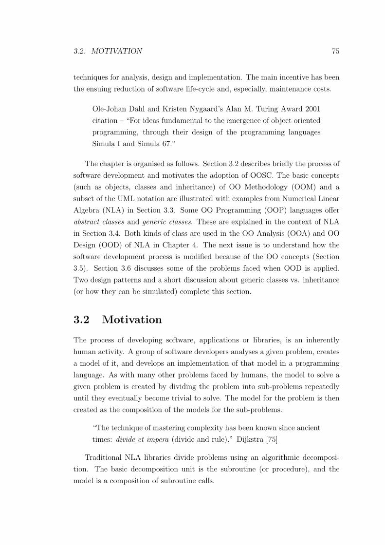
3.2. MOTIVATION 75
techniques for analysis, design and implementation. The main incentive has been
the ensuing reduction of software life-cycle and, especially, maintenance costs.
Ole-Johan Dahl and Kristen Nygaard’s Alan M. Turing Award 2001
citation – “For ideas fundamental to the emergence of object oriented
programming, through their design of the programming languages
Simula I and Simula 67.”
The chapter is organised as follows. Section 3.2 describes briefly the process of
software development and motivates the adoption of OOSC. The basic concepts
(such as objects, classes and inheritance) of OO Methodology (OOM) and a
subset of the UML notation are illustrated with examples from Numerical Linear
Algebra (NLA) in Section 3.3. Some OO Programming (OOP) languages offer
abstract classes and generic classes. These are explained in the context of NLA
in Section 3.4. Both kinds of class are used in the OO Analysis (OOA) and OO
Design (OOD) of NLA in Chapter 4. The next issue is to understand how the
software development process is modified because of the OO concepts (Section
3.5). Section 3.6 discusses some of the problems faced when OOD is applied.
Two design patterns and a short discussion about generic classes vs. inheritance
(or how they can be simulated) complete this section.
3.2 Motivation
The process of developing software, applications or libraries, is an inherently
human activity. A group of software developers analyses a given problem, creates
a model of it, and develops an implementation of that model in a programming
language. As with many other problems faced by humans, the model to solve a
given problem is created by dividing the problem into sub-problems repeatedly
until they eventually become trivial to solve. The model for the problem is then
created as the composition of the models for the sub-problems.
“The technique of mastering complexity has been known since ancient
times: divide et impera (divide and rule).” Dijkstra [75]
Traditional NLA libraries divide problems using an algorithmic decomposi-
tion. The basic decomposition unit is the subroutine (or procedure), and the
model is a composition of subroutine calls.
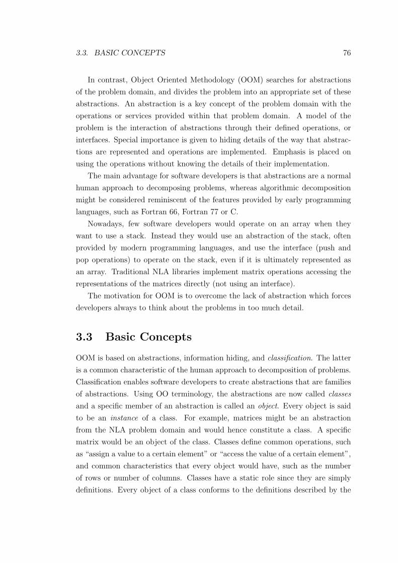
3.3. BASIC CONCEPTS 76
In contrast, Object Oriented Methodology (OOM) searches for abstractions
of the problem domain, and divides the problem into an appropriate set of these
abstractions. An abstraction is a key concept of the problem domain with the
operations or services provided within that problem domain. A model of the
problem is the interaction of abstractions through their defined operations, or
interfaces. Special importance is given to hiding details of the way that abstrac-
tions are represented and operations are implemented. Emphasis is placed on
using the operations without knowing the details of their implementation.
The main advantage for software developers is that abstractions are a normal
human approach to decomposing problems, whereas algorithmic decomposition
might be considered reminiscent of the features provided by early programming
languages, such as Fortran 66, Fortran 77 or C.
Nowadays, few software developers would operate on an array when they
want to use a stack. Instead they would use an abstraction of the stack, often
provided by modern programming languages, and use the interface (push and
pop operations) to operate on the stack, even if it is ultimately represented as
an array. Traditional NLA libraries implement matrix operations accessing the
representations of the matrices directly (not using an interface).
The motivation for OOM is to overcome the lack of abstraction which forces
developers always to think about the problems in too much detail.
3.3 Basic Concepts
OOM is based on abstractions, information hiding, and classification. The latter
is a common characteristic of the human approach to decomposition of problems.
Classification enables software developers to create abstractions that are families
of abstractions. Using OO terminology, the abstractions are now called classes
and a specific member of an abstraction is called an object. Every object is said
to be an instance of a class. For example, matrices might be an abstraction
from the NLA problem domain and would hence constitute a class. A specific
matrix would be an object of the class. Classes define common operations, such
as “assign a value to a certain element” or “access the value of a certain element”,
and common characteristics that every object would have, such as the number
of rows or number of columns. Classes have a static role since they are simply
definitions. Every object of a class conforms to the definitions described by the
3.3. BASIC CONCEPTS 77
class. It also gives values to these definitions, known as the state of the object.
An object is dynamic since it is a run-time entity whose state can be modified; it
is created, other objects use its operations, it uses the operations of other objects,
and eventually it dies. The death of an object can be due to an explicit action
of the program, or to implicit background garbage collection. The latter is a run-
time mechanism which detects objects that cannot be reached by the remaining
instructions of the program and eliminates these objects.
Figure 3.1 presents a simple UML class diagram and object diagram for ma-
trices. UML stands for Unified Modeling Language [50], which is the Object
Management Group standard notation to document OO software development.
Class diagrams are used to represent classes graphically using a rectangle
divided into three sub-rectangles. The first sub-rectangle contains the class name,
the second contains the characteristics called attributes and the third contains
the operations called methods. An object diagram is used to represent objects at
a fixed point in time; it is similar to the class diagram. The first sub-rectangle
contains the name of the object and its class, separated by a colon and underlined.
The second sub-rectangle contains the attributes that define the state of the
object, and the third contains the methods. As can be seen in the class diagram
(Figure 3.1), there is a method create which creates new objects of class Matrix.
This method is a class method and hence is underlined. A class method is a
method that cannot be invoked in an object; it is invoked in the class. For the
sake of clarity, objects and classes are often represented in class diagrams and
object diagrams only by their first sub-rectangle, thus avoiding the reappearance
of known information. UML specifies the syntax for declaring attributes and
methods. However, the thesis uses a pseudo-code based on Java syntax.
Humans create hierarchies of abstractions using criteria by which each classi-
fication adds new characteristics or re-adapts existing ones. In OOM, the classes
can be organised into inheritance hierarchies. Each class is a classification, and
traversing upwards in the class hierarchy means a more general class, whereas
traversing down the class hierarchy means a more specialised class. Using the ex-
ample of matrices, a vector can be considered to be a special kind of matrix, since
a vector is nothing more than a matrix with either only one column or one row.
In a similar way, a square matrix can be considered to be a special class of matrix
since it is a matrix whose numbers of columns and rows are equal. These examples
should be taken as naıve examples to illustrate the general concepts. Figure 3.2
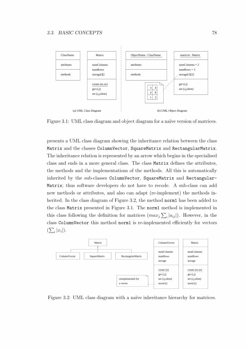
3.3. BASIC CONCEPTS 78
ClassName
attributes
methods
numColumns
numRows
storage[][]
Matrix
get (i,j)
create (nc,nr)
set (i,j,elem)
ObjectName : ClassName
methods
attributes numColumns = 2
numRows = 3
storage[3][2]
matrixA : Matrix
get (i,j)
set (i,j,elem)3 4
4 8
1 2
(a) UML Class Diagram (b) UML Object Diagram
Figure 3.1: UML class diagram and object diagram for a naıve version of matrices.
presents a UML class diagram showing the inheritance relation between the class
Matrix and the classes ColumnVector, SquareMatrix and RectangularMatrix.
The inheritance relation is represented by an arrow which begins in the specialised
class and ends in a more general class. The class Matrix defines the attributes,
the methods and the implementations of the methods. All this is automatically
inherited by the sub-classes ColumnVector, SquareMatrix and Rectangular-
Matrix; thus software developers do not have to recode. A sub-class can add
new methods or attributes, and also can adapt (re-implement) the methods in-
herited. In the class diagram of Figure 3.2, the method norm1 has been added to
the class Matrix presented in Figure 3.1. The norm1 method is implemented in
this class following the definition for matrices (maxj
∑i |aij|). However, in the
class ColumnVector this method norm1 is re-implemented efficiently for vectors
(∑
i |xi|).
SquareMatrix
Matrix
ColumnVector RectangularMatrix
numColumns
numRows
norm1()
storage
ColumnVector
numColumns
numRows
norm1()
storage
Matrix
reimplemented for
a vector
set (i,j,elem)
get (i,j) get (i,j)
set (i,j,elem)
create (n) create (nc,nr)
Figure 3.2: UML class diagram with a naıve inheritance hierarchy for matrices.
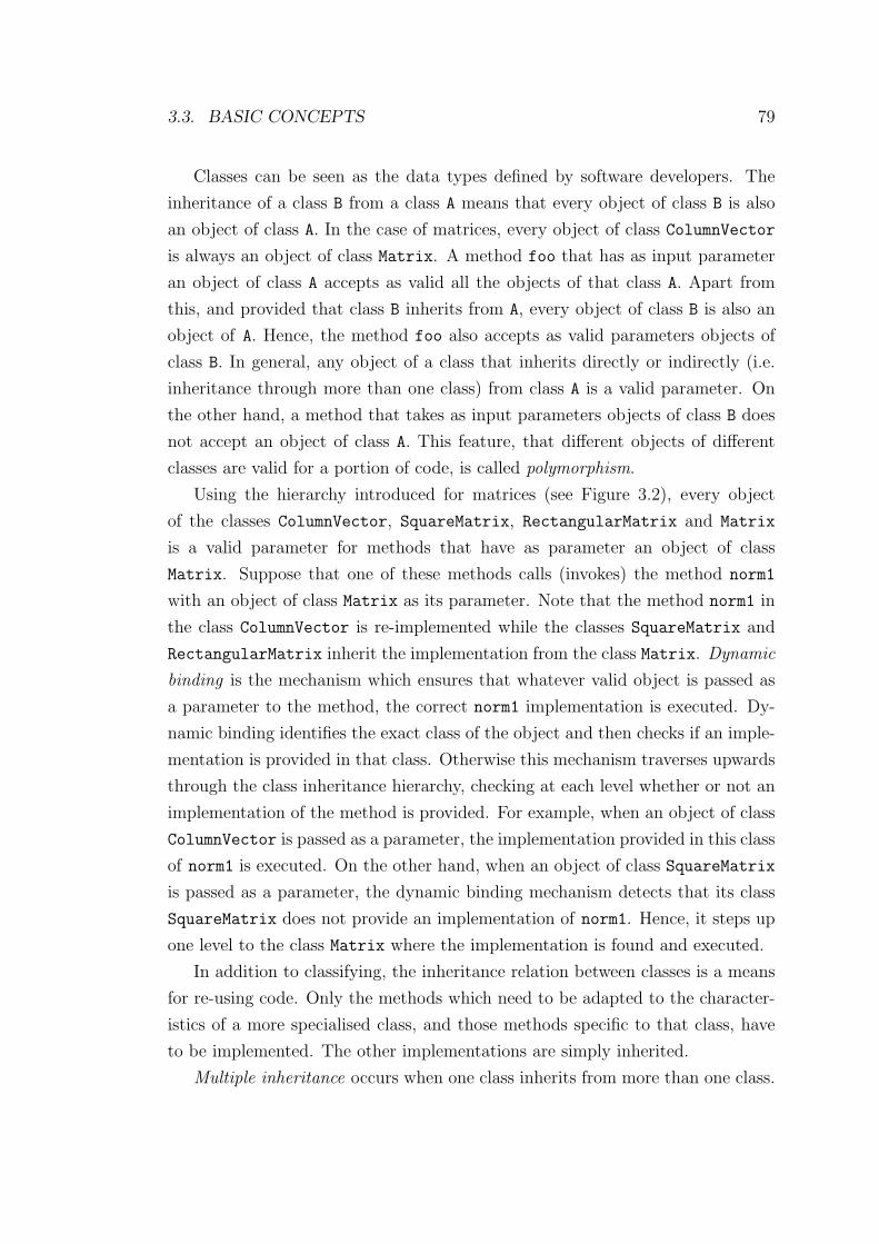
3.3. BASIC CONCEPTS 79
Classes can be seen as the data types defined by software developers. The
inheritance of a class B from a class A means that every object of class B is also
an object of class A. In the case of matrices, every object of class ColumnVector
is always an object of class Matrix. A method foo that has as input parameter
an object of class A accepts as valid all the objects of that class A. Apart from
this, and provided that class B inherits from A, every object of class B is also an
object of A. Hence, the method foo also accepts as valid parameters objects of
class B. In general, any object of a class that inherits directly or indirectly (i.e.
inheritance through more than one class) from class A is a valid parameter. On
the other hand, a method that takes as input parameters objects of class B does
not accept an object of class A. This feature, that different objects of different
classes are valid for a portion of code, is called polymorphism.
Using the hierarchy introduced for matrices (see Figure 3.2), every object
of the classes ColumnVector, SquareMatrix, RectangularMatrix and Matrix
is a valid parameter for methods that have as parameter an object of class
Matrix. Suppose that one of these methods calls (invokes) the method norm1
with an object of class Matrix as its parameter. Note that the method norm1 in
the class ColumnVector is re-implemented while the classes SquareMatrix and
RectangularMatrix inherit the implementation from the class Matrix. Dynamic
binding is the mechanism which ensures that whatever valid object is passed as
a parameter to the method, the correct norm1 implementation is executed. Dy-
namic binding identifies the exact class of the object and then checks if an imple-
mentation is provided in that class. Otherwise this mechanism traverses upwards
through the class inheritance hierarchy, checking at each level whether or not an
implementation of the method is provided. For example, when an object of class
ColumnVector is passed as a parameter, the implementation provided in this class
of norm1 is executed. On the other hand, when an object of class SquareMatrix
is passed as a parameter, the dynamic binding mechanism detects that its class
SquareMatrix does not provide an implementation of norm1. Hence, it steps up
one level to the class Matrix where the implementation is found and executed.
In addition to classifying, the inheritance relation between classes is a means
for re-using code. Only the methods which need to be adapted to the character-
istics of a more specialised class, and those methods specific to that class, have
to be implemented. The other implementations are simply inherited.
Multiple inheritance occurs when one class inherits from more than one class.
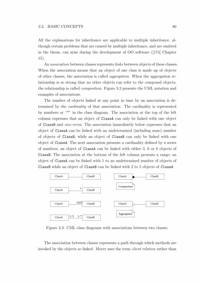
3.3. BASIC CONCEPTS 80
All the explanations for inheritance are applicable to multiple inheritance, al-
though certain problems that are caused by multiple inheritance, and are omitted
in the thesis, can arise during the development of OO software ([174] Chapter
15).
An association between classes represents links between objects of these classes.
When the association means that an object of one class is made up of objects
of other classes, the association is called aggregation. When the aggregation re-
lationship is so strong that no other objects can refer to the composed objects,
the relationship is called composition. Figure 3.3 presents the UML notation and
examples of associations.
The number of objects linked at any point in time by an association is de-
termined by the cardinality of that association. The cardinality is represented
by numbers or “*” in the class diagram. The association at the top of the left
column expresses that an object of ClassA can only be linked with one object
of ClassB and vice-versa. The association immediately below expresses that an
object of ClassA can be linked with an undetermined (including none) number
of objects of ClassB, while an object of ClassB can only be linked with one
object of ClassA. The next association presents a cardinality defined by a series
of numbers; an object of ClassA can be linked with either 3, 6 or 8 objects of
ClassB. The association at the bottom of the left column presents a range; an
object of ClassA can be linked with 1 to an undetermined number of objects of
ClassB while an object of ClassB can be linked with 2 to 5 objects of ClassA.
* ClassBClassA
ClassBClassA ClassBClassA
ClassBClassA
Composition
Aggregation
ClassA ClassB
ClassA ClassB
3,6,8
2..5 1..*
Figure 3.3: UML class diagrams with associations between two classes.
The association between classes represents a path through which methods are
invoked by the objects so linked. Meyer uses the term client relation rather than
3.4. IMPLEMENTATION RELATED CONCEPTS 81
association [174]. This term comes from the fact that an object is using the
interface of another object (the services provided by the other object) and, thus,
the two objects become client and supplier. The term client relation, rather than
association, is used throughout the thesis.
3.4 Implementation Related Concepts
Generic programming and abstract classes are two advanced concepts which are
sometimes supported by OOP languages. These concepts are related to imple-
mentation aspects, whereas those already explained are methodological.
In general, generic programming enables developers to write parts of programs
that have as a parameter the data type of some variables. Generic programming
is a response to the observation that some algorithms could be written inde-
pendently of the data types. A typical example is a sorting algorithm. The
implementation of a sorting algorithm could be the same as long as the data type
of the elements to be sorted has defined the comparison functions “<”, “>” and
“=”.
In OOP languages, a generic class is a class that has as parameters the data
types or classes of some of its attributes or parameters of its methods. Generic
classes are also known as template classes in the context of C++. Generic classes
cannot instantiate any object since they are not complete classes. The typical
examples for generic classes are the containers of elements. Lists, stacks, trees,
etc. are well documented container classes that benefit from generic programming
(see the Standard Template Library [19]). Using generic classes, the containers
can be defined independently from the class of the elements they hold at run-
time. In the particular case of NLA, the Matrix class might be considered to be
a generic class whose parameter is a numerical data type.
Abstract classes are classes which declare methods and attributes but do not
implement all the methods. The implemented methods are allowed to invoke
the non-implemented methods (also called abstract methods). Hence, an abstract
class is a completely declared but partially implemented class. No object can be
instantiated from an abstract class, and only those classes that inherit from an
abstract class and provide implementations for all the inherited abstract methods
are non-abstract classes.
Figure 3.4 presents the UML notation for abstract classes and describes a
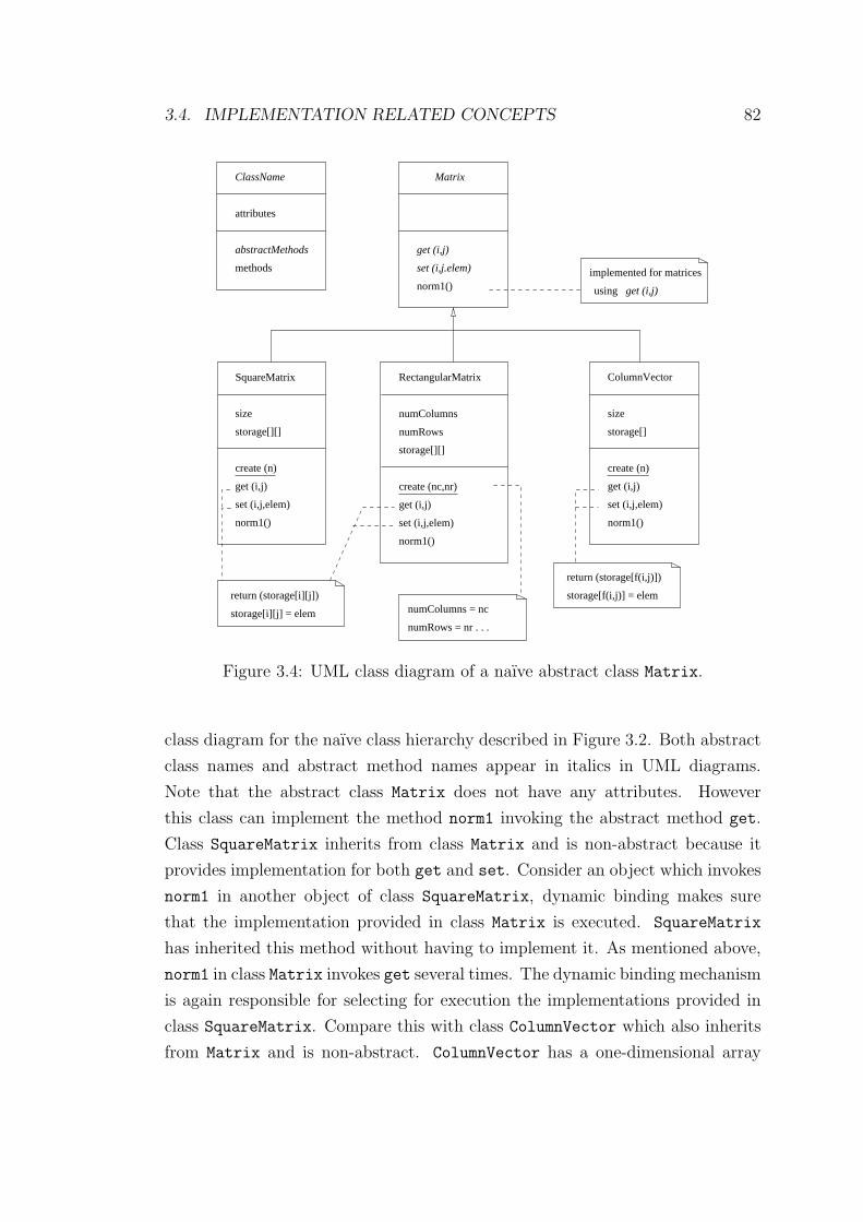
3.4. IMPLEMENTATION RELATED CONCEPTS 82
numColumns = nc
numRows = nr . . .storage[i][j] = elem
return (storage[i][j])
return (storage[f(i,j)])
storage[f(i,j)] = elem
attributes
methods
norm1()
size
storage[][]
norm1()
ClassName
abstractMethods
SquareMatrix
numColumns
numRows
norm1()
storage[][]
size
storage[]
norm1()
RectangularMatrix
Matrix
ColumnVector
using
implemented for matrices
get (i,j)
set (i,j.elem)
get (i,j)
set (i,j,elem) get (i,j)
set (i,j,elem)
get (i,j)
set (i,j,elem)
create (n)
create (nc,nr)
create (n)
get (i,j)
Figure 3.4: UML class diagram of a naıve abstract class Matrix.
class diagram for the naıve class hierarchy described in Figure 3.2. Both abstract
class names and abstract method names appear in italics in UML diagrams.
Note that the abstract class Matrix does not have any attributes. However
this class can implement the method norm1 invoking the abstract method get.
Class SquareMatrix inherits from class Matrix and is non-abstract because it
provides implementation for both get and set. Consider an object which invokes
norm1 in another object of class SquareMatrix, dynamic binding makes sure
that the implementation provided in class Matrix is executed. SquareMatrix
has inherited this method without having to implement it. As mentioned above,
norm1 in class Matrix invokes get several times. The dynamic binding mechanism
is again responsible for selecting for execution the implementations provided in
class SquareMatrix. Compare this with class ColumnVector which also inherits
from Matrix and is non-abstract. ColumnVector has a one-dimensional array
3.5. THE SOFTWARE DEVELOPMENT PROCESS 83
as its attribute which stores the matrix elements instead of the two-dimensional
arrays used in SquareMatrix and RectangularMatrix. Consequently, Column-
Vector has to implement get and set differently. Again, the dynamic mechanism
makes sure that, when invoking norm1 in an object of class ColumnVector, the
appropriate implementations are executed (i.e. norm1 from class Matrix and set
from class ColumnVector).
3.5 The Software Development Process
Traditionally, the software development process has been divided into analysis,
design, implementation, testing and maintenance phases using top-down decom-
position. Each phase begins when the preceding phase has finished, and so the
process can be seen as a linear execution of phases. This life cycle is known as
the linear sequential model, or waterfall model [191].
OOM does not change the abstract definition of the different phases. However,
the way in which they are carried out, and the products of each phase are dif-
ferent. The OO life-cycle is characterised by being iterative and incremental. At
each iteration, OO Analysis (OOA), OO Design (OOD), OO implementation or
OO Programming (OOP) and OO testing are carried out, thereby incrementally
increasing the part of the problem that is covered.
Of special interest for this thesis are OOA, OOD and OOP. OOA proposes
classes, relations between classes, and the attributes and methods. The objective
is to discover and understand the problem domain by modelling with objects
and classes. OOD refines the classes by giving declarations in the classes and
specification of the functionality of each method. At the same time, the model
created by OOA is refined, adapting it to the restrictions of the application. The
objective is to plan how the model is going to be implemented. Finally, OOP is
the implementation of the OOD in a given programming language. Ideally, the
implementation should be made in an OOP language; otherwise, the developers
are forced to emulate the OO concepts. Guidelines for implementing OO models
in non OOP languages, such as Fortran 77 or C, are described by Meyer ([174]
Chapters 33 and 34) or by Decyk et al. [71, 72, 73].
The division between OOA and OOD phases is fuzzy, although the focus and
the products of both phases are clear. The analysis phase focuses on modelling
the problem by proposing candidate classes and relations between the classes,

3.6. SOME RECOMMENDATIONS 84
evaluating them and rejecting the unsuitable proposals. Heuristics to find can-
didate classes are collected by Booch ([49] Chapter 4) and Meyer ([174] Chapter
22). Both authors identify as a source of candidate classes tangible things, roles,
events, records of interactions, etc., from the problem domain [205, 15]. Also,
both authors present a method based on studying a requirements document.
The nouns and verbs expressing actions over them that are repeatedly used in
this document become candidate classes and candidate methods [1]. However,
due to the complexity of natural language this approach has enjoyed only limited
success.
Booch and Meyer strongly disagree about the use case analysis formalised by
Jacobson [141]. Use case analysis describes different scenarios, which are user-
initiated transactions with the software. The scenarios represent the functions
of the software. The analysis then takes each scenario, one-by-one, identifying
possible classes and relations. In Booch’s opinion, use case analysis provides an
organised framework to discover the functionality required by an application and,
as such, a good guide to follow in the design. In Meyer’s opinion, use case analysis
is influenced by the users’ vision about what the application has to do. This might
lead non-expert OO developers to an algorithmic decomposition instead of an OO
decomposition.
The OOD phase brings different requirements to the development process.
Concurrency and synchronisation, mapping of the software onto the hardware
(networks, modems, processors, etc.), and division of the OO model into packages,
grouping related classes, are aspects that might be included during this phase
[149].
3.6 Some Recommendations
The “rules” given in the literature for deciding what the relations are between
classes, can be considered more to be heuristics; they always include examples
of “exceptions”. Design patterns are class structures which model problems that
repeatedly appear in almost every development of software. The definition of
design patterns, and a collection of them, is described by Gamma et al. [107].
Design patterns can be considered as heuristics extracted from the experience
of expert OO developers. Each design pattern describes the characteristics of a
repeatedly faced problem for which an “elegant” and tested solution is known.
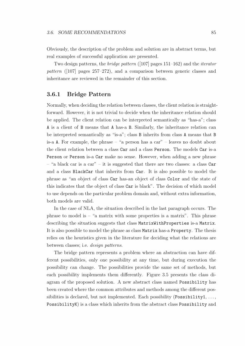
3.6. SOME RECOMMENDATIONS 85
Obviously, the description of the problem and solution are in abstract terms, but
real examples of successful application are presented.
Two design patterns, the bridge pattern ([107] pages 151–162) and the iterator
pattern ([107] pages 257–272), and a comparison between generic classes and
inheritance are reviewed in the remainder of this section.
3.6.1 Bridge Pattern
Normally, when deciding the relation between classes, the client relation is straight-
forward. However, it is not trivial to decide when the inheritance relation should
be applied. The client relation can be interpreted semantically as “has-a”; class
A is a client of B means that A has-a B. Similarly, the inheritance relation can
be interpreted semantically as “is-a”; class B inherits from class A means that B
is-a A. For example, the phrase – “a person has a car” – leaves no doubt about
the client relation between a class Car and a class Person. The models Car is-a
Person or Person is-a Car make no sense. However, when adding a new phrase
– “a black car is a car” – it is suggested that there are two classes: a class Car
and a class BlackCar that inherits from Car. It is also possible to model the
phrase as “an object of class Car has-an object of class Color and the state of
this indicates that the object of class Car is black”. The decision of which model
to use depends on the particular problem domain and, without extra information,
both models are valid.
In the case of NLA, the situation described in the last paragraph occurs. The
phrase to model is – “a matrix with some properties is a matrix”. This phrase
describing the situation suggests that class MatrixWithProperties is-a Matrix.
It is also possible to model the phrase as class Matrix has-a Property. The thesis
relies on the heuristics given in the literature for deciding what the relations are
between classes; i.e. design patterns.
The bridge pattern represents a problem where an abstraction can have dif-
ferent possibilities, only one possibility at any time, but during execution the
possibility can change. The possibilities provide the same set of methods, but
each possibility implements them differently. Figure 3.5 presents the class di-
agram of the proposed solution. A new abstract class named Possibility has
been created where the common attributes and methods among the different pos-
sibilities is declared, but not implemented. Each possibility (Possibility1, . . . ,
PossibilityK) is a class which inherits from the abstract class Possibility and
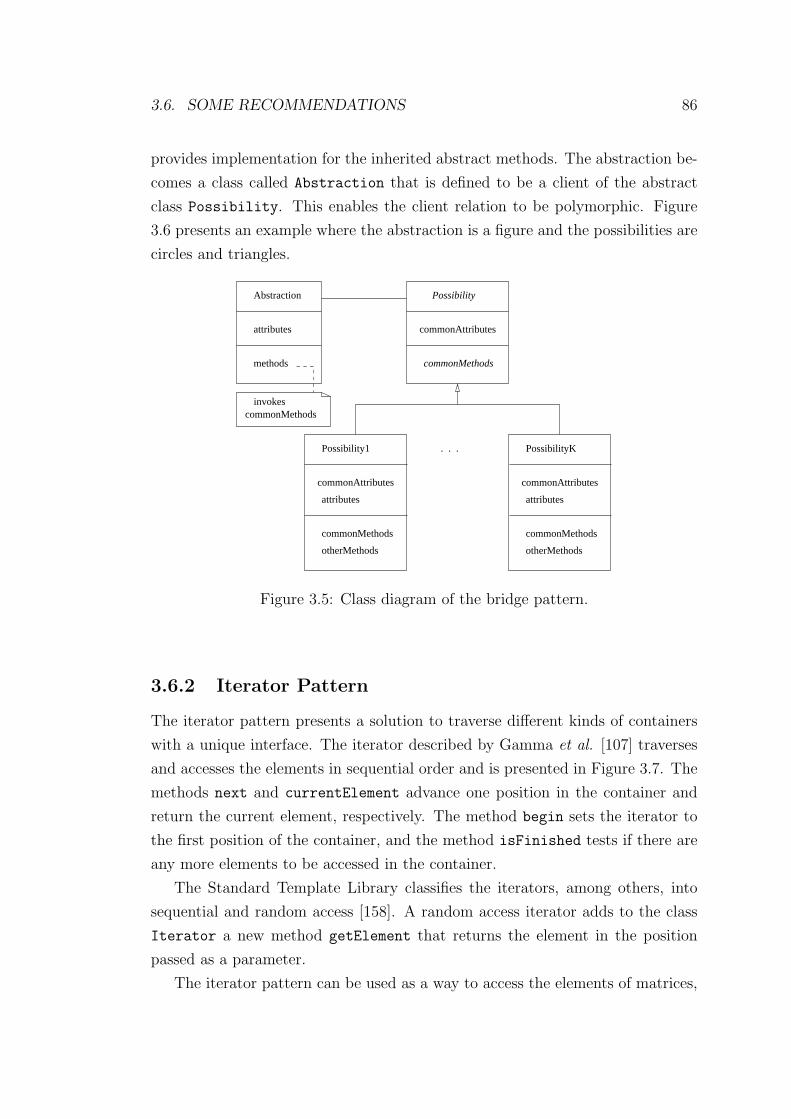
3.6. SOME RECOMMENDATIONS 86
provides implementation for the inherited abstract methods. The abstraction be-
comes a class called Abstraction that is defined to be a client of the abstract
class Possibility. This enables the client relation to be polymorphic. Figure
3.6 presents an example where the abstraction is a figure and the possibilities are
circles and triangles.
attributes
methods commonMethods
commonAttributes
. . .
commonAttributes
attributes
commonMethods
otherMethods
invokescommonMethods
commonAttributes
attributes
commonMethods
otherMethods
Possibility1 PossibilityK
Abstraction Possibility
Figure 3.5: Class diagram of the bridge pattern.
3.6.2 Iterator Pattern
The iterator pattern presents a solution to traverse different kinds of containers
with a unique interface. The iterator described by Gamma et al. [107] traverses
and accesses the elements in sequential order and is presented in Figure 3.7. The
methods next and currentElement advance one position in the container and
return the current element, respectively. The method begin sets the iterator to
the first position of the container, and the method isFinished tests if there are
any more elements to be accessed in the container.
The Standard Template Library classifies the iterators, among others, into
sequential and random access [158]. A random access iterator adds to the class
Iterator a new method getElement that returns the element in the position
passed as a parameter.
The iterator pattern can be used as a way to access the elements of matrices,
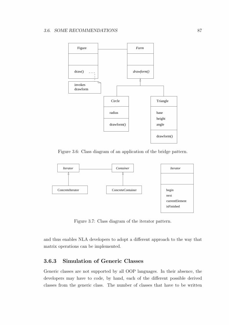
3.6. SOME RECOMMENDATIONS 87
invokesdrawform
Figure
base
height
TriangleCircle
Form
radius
draw()
drawform()
drawform()
angle
drawform()
Figure 3.6: Class diagram of an application of the bridge pattern.
begin
next
currentElement
isFinished
Iterator
ConcreteIterator
Iterator
ConcreteContainer
Container
Figure 3.7: Class diagram of the iterator pattern.
and thus enables NLA developers to adopt a different approach to the way that
matrix operations can be implemented.
3.6.3 Simulation of Generic Classes
Generic classes are not supported by all OOP languages. In their absence, the
developers may have to code, by hand, each of the different possible derived
classes from the generic class. The number of classes that have to be written
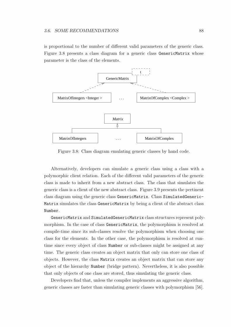
3.6. SOME RECOMMENDATIONS 88
is proportional to the number of different valid parameters of the generic class.
Figure 3.8 presents a class diagram for a generic class GenericMatrix whose
parameter is the class of the elements.
. . .
t
. . .
GenericMatrix
MatrixOfIntegers <Integer > MatrixOfComplex <Complex >
MatrixOfIntegers
Matrix
MatrixOfComplex
Figure 3.8: Class diagram emulating generic classes by hand code.
Alternatively, developers can simulate a generic class using a class with a
polymorphic client relation. Each of the different valid parameters of the generic
class is made to inherit from a new abstract class. The class that simulates the
generic class is a client of the new abstract class. Figure 3.9 presents the pertinent
class diagram using the generic class GenericMatrix. Class SimulatedGeneric-
Matrix simulates the class GenericMatrix by being a client of the abstract class
Number.
GenericMatrix and SimulatedGenericMatrix class structures represent poly-
morphism. In the case of class GenericMatrix, the polymorphism is resolved at
compile-time since its sub-classes resolve the polymorphism when choosing one
class for the elements. In the other case, the polymorphism is resolved at run-
time since every object of class Number or sub-classes might be assigned at any
time. The generic class creates an object matrix that only can store one class of
objects. However, the class Matrix creates an object matrix that can store any
object of the hierarchy Number (bridge pattern). Nevertheless, it is also possible
that only objects of one class are stored, thus simulating the generic class.
Developers find that, unless the compiler implements an aggressive algorithm,
generic classes are faster than simulating generic classes with polymorphism [56].
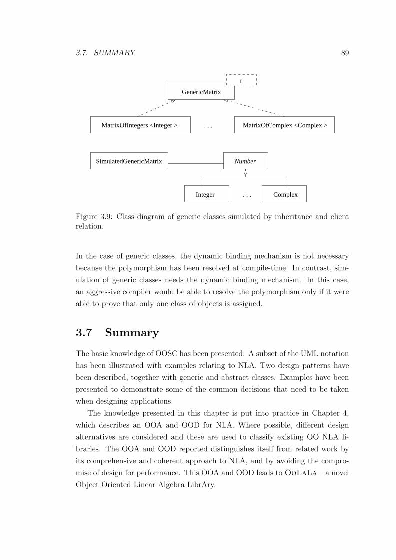
3.7. SUMMARY 89
. . .
t
MatrixOfIntegers <Integer > MatrixOfComplex <Complex >
GenericMatrix
SimulatedGenericMatrix
. . . ComplexInteger
Number
Figure 3.9: Class diagram of generic classes simulated by inheritance and clientrelation.
In the case of generic classes, the dynamic binding mechanism is not necessary
because the polymorphism has been resolved at compile-time. In contrast, sim-
ulation of generic classes needs the dynamic binding mechanism. In this case,
an aggressive compiler would be able to resolve the polymorphism only if it were
able to prove that only one class of objects is assigned.
3.7 Summary
The basic knowledge of OOSC has been presented. A subset of the UML notation
has been illustrated with examples relating to NLA. Two design patterns have
been described, together with generic and abstract classes. Examples have been
presented to demonstrate some of the common decisions that need to be taken
when designing applications.
The knowledge presented in this chapter is put into practice in Chapter 4,
which describes an OOA and OOD for NLA. Where possible, different design
alternatives are considered and these are used to classify existing OO NLA li-
braries. The OOA and OOD reported distinguishes itself from related work by
its comprehensive and coherent approach to NLA, and by avoiding the compro-
mise of design for performance. This OOA and OOD leads to OoLaLa – a novel
Object Oriented Linear Algebra LibrAry.
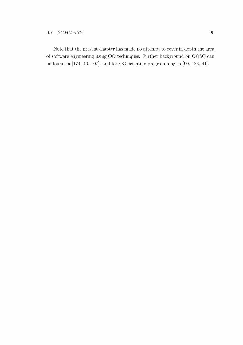
3.7. SUMMARY 90
Note that the present chapter has made no attempt to cover in depth the area
of software engineering using OO techniques. Further background on OOSC can
be found in [174, 49, 107], and for OO scientific programming in [90, 183, 41].
Chapter 4
Design of OOLALA
4.1 Introduction
Object Oriented (OO) software construction has characteristics that could im-
prove the development process and usability of mathematical software libraries.
OoLaLa, a novel Object Oriented Linear Algebra LibrAry, is the outcome of
a study of these possible benefits in the context of sequential Numerical Lin-
ear Algebra (NLA). This chapter and subsequent chapters cover the design of
the library, its implementation and performance evaluation, optimisation, and
limitations of a library-based approach to the development of NLA programs.
The development of NLA programs is based mainly on software libraries.
Mathematical expressions modelling a problem are mapped into calls to the sub-
routines provided by NLA libraries. Most NLA libraries exhibit two weaknesses:
complex interfaces and an explosion of implementations of matrix operations. The
first weakness affects users since it is relatively hard to develop NLA programs
using these libraries. The second weakness affects library developers since they
have to code, test and maintain the many different implementations. The source
of both weaknesses is either that these libraries are developed in programming
languages lacking user defined abstractions (data types) or else abstraction has
been sacrificed for performance. For a given matrix operation, library developers
might need to develop as many implementations as the number of combinations
of data representations and matrix properties of the matrix operands. This pro-
duces an explosion in the number of implementations of a given matrix operation.
Not only do users have to design their programs considering the storage format
of matrices, but they also have to select the appropriate implementation of each
91
4.1. INTRODUCTION 92
operation. This abstraction level is called the Storage Format Abstraction level
(SFA-level) and, together with an introduction to NLA, was presented in Chapter
2. Chapter 3 has provided an overview of OO software construction, introduced
the UML notation and two design patterns used in this chapter.
As the title indicates, the core of this chapter is the design of OoLaLa.
Several designs are evaluated and used to classify a survey of existing sequential
OO NLA libraries. The classification is based on the way that matrices and matrix
operations are represented. OoLaLa’s new representation of matrices is capable
of dealing with certain matrix operations that, although mathematically valid,
are not handled correctly by existing OO NLA libraries. This representation
has the unique feature of being able to propagate matrix properties through
matrix operations. OoLaLa also enables implementations of matrix operations
at various abstraction levels ranging from the relatively low-level abstraction of
a Fortran-like implementation (i.e. SFA-level) to two higher-level abstractions
that hide many implementation details. Another strength of the library is that
OoLaLa covers a wide range of NLA functionality while the reviewed OO NLA
libraries concentrate on parts of such functionality. As a side effect of OoLaLa’s
representation of matrices, block matrices can store each block in any storage
format and have any matrix property. Thus, OoLaLa generalises existing storage
formats and creates a new family of storage formats known as general nested
format.
The description of the OO Analysis (OOA) and OO Design (OOD) of NLA
is divided into five sections. Section 4.2 presents the basic design of OoLaLa.
This covers the representation of matrices, properties and storage formats. Sec-
tion 4.3 introduces the first higher abstraction level for matrix operations. This
abstraction level, referred to as Matrix Abstraction level (MA-level), treats ma-
trices as indexed containers which provide random access to elements. Section
4.4 introduces the Iterator Abstraction level (IA-level) which treats matrices as
containers that can be accessed sequentially. Section 4.5 illustrates the design
of matrix views (i.e. section - a set of elements of a matrix which constitutes
a sub-matrix; and merged matrix - a matrix formed from other matrices) which
can themselves be treated as matrices, each with their own properties and storage
formats, without having to take copies of the underlying elements. Matrix oper-
ations are incorporated into the OOD in Section 4.6. Related work is discussed
in Section 4.7.
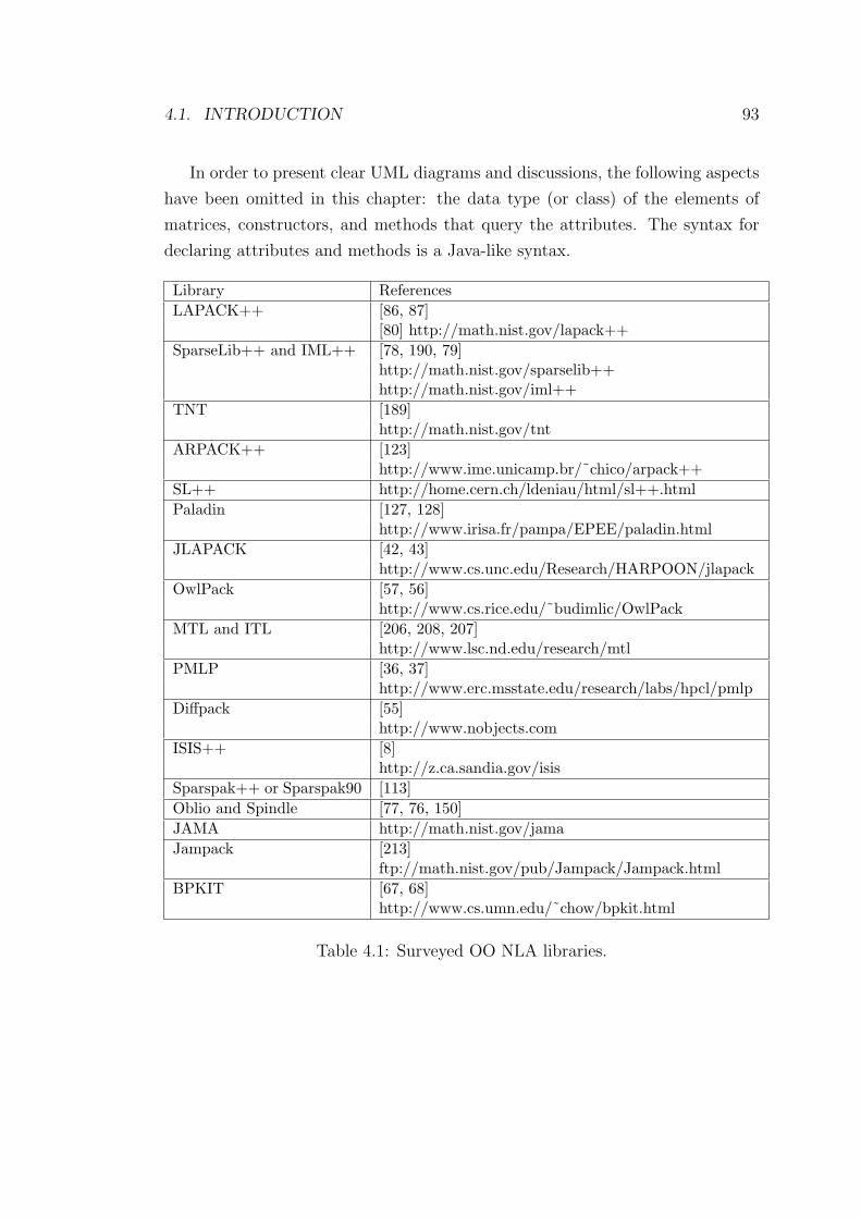
4.1. INTRODUCTION 93
In order to present clear UML diagrams and discussions, the following aspects
have been omitted in this chapter: the data type (or class) of the elements of
matrices, constructors, and methods that query the attributes. The syntax for
declaring attributes and methods is a Java-like syntax.
Library ReferencesLAPACK++ [86, 87]
[80] http://math.nist.gov/lapack++SparseLib++ and IML++ [78, 190, 79]
http://math.nist.gov/sparselib++http://math.nist.gov/iml++
TNT [189]http://math.nist.gov/tnt
ARPACK++ [123]http://www.ime.unicamp.br/˜chico/arpack++
SL++ http://home.cern.ch/ldeniau/html/sl++.htmlPaladin [127, 128]
http://www.irisa.fr/pampa/EPEE/paladin.htmlJLAPACK [42, 43]
http://www.cs.unc.edu/Research/HARPOON/jlapackOwlPack [57, 56]
http://www.cs.rice.edu/˜budimlic/OwlPackMTL and ITL [206, 208, 207]
http://www.lsc.nd.edu/research/mtlPMLP [36, 37]
http://www.erc.msstate.edu/research/labs/hpcl/pmlpDiffpack [55]
http://www.nobjects.comISIS++ [8]
http://z.ca.sandia.gov/isisSparspak++ or Sparspak90 [113]Oblio and Spindle [77, 76, 150]JAMA http://math.nist.gov/jamaJampack [213]
ftp://math.nist.gov/pub/Jampack/Jampack.htmlBPKIT [67, 68]
http://www.cs.umn.edu/˜chow/bpkit.html
Table 4.1: Surveyed OO NLA libraries.
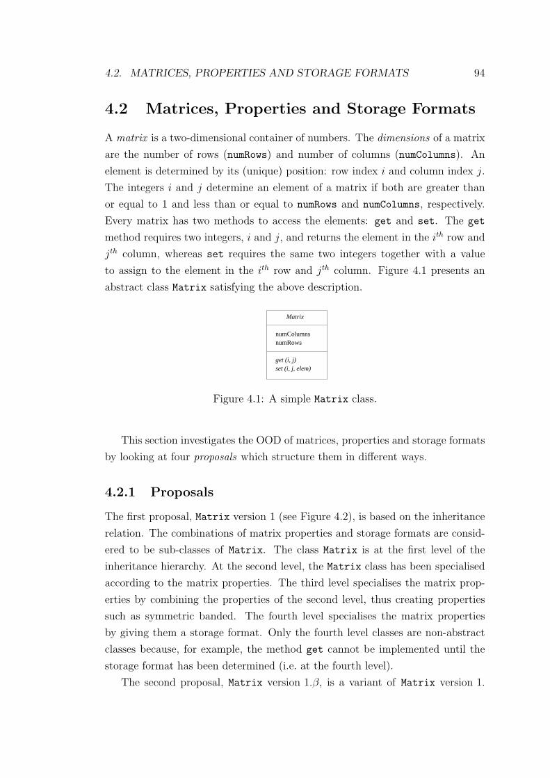
4.2. MATRICES, PROPERTIES AND STORAGE FORMATS 94
4.2 Matrices, Properties and Storage Formats
A matrix is a two-dimensional container of numbers. The dimensions of a matrix
are the number of rows (numRows) and number of columns (numColumns). An
element is determined by its (unique) position: row index i and column index j.
The integers i and j determine an element of a matrix if both are greater than
or equal to 1 and less than or equal to numRows and numColumns, respectively.
Every matrix has two methods to access the elements: get and set. The get
method requires two integers, i and j, and returns the element in the ith row and
jth column, whereas set requires the same two integers together with a value
to assign to the element in the ith row and jth column. Figure 4.1 presents an
abstract class Matrix satisfying the above description.
numColumnsnumRows
Matrix
get (i, j)set (i, j, elem)
Figure 4.1: A simple Matrix class.
This section investigates the OOD of matrices, properties and storage formats
by looking at four proposals which structure them in different ways.
4.2.1 Proposals
The first proposal, Matrix version 1 (see Figure 4.2), is based on the inheritance
relation. The combinations of matrix properties and storage formats are consid-
ered to be sub-classes of Matrix. The class Matrix is at the first level of the
inheritance hierarchy. At the second level, the Matrix class has been specialised
according to the matrix properties. The third level specialises the matrix prop-
erties by combining the properties of the second level, thus creating properties
such as symmetric banded. The fourth level specialises the matrix properties
by giving them a storage format. Only the fourth level classes are non-abstract
classes because, for example, the method get cannot be implemented until the
storage format has been determined (i.e. at the fourth level).
The second proposal, Matrix version 1.β, is a variant of Matrix version 1.
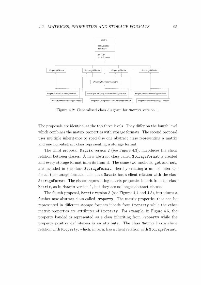
4.2. MATRICES, PROPERTIES AND STORAGE FORMATS 95
Matrix
numRowsnumColumns
Property1Matrix PropertyHMatrix PropertyJMatrix PropertyNMatrix
PropertyH..PropertyJMatrix
PropertyH..PropertyJMatrixInStorageFormatL
PropertyH..PropertyJMatrixInStorageFormatI PropertyNMatrixInStorageFormatPProperty1MatrixInStorageFormat1
PropertyNMatrixInStorageFormatZProperty1MatrixInStorageFormatF
get (i, j)set (i, j, elem)
Figure 4.2: Generalised class diagram for Matrix version 1.
The proposals are identical at the top three levels. They differ on the fourth level
which combines the matrix properties with storage formats. The second proposal
uses multiple inheritance to specialise one abstract class representing a matrix
and one non-abstract class representing a storage format.
The third proposal, Matrix version 2 (see Figure 4.3), introduces the client
relation between classes. A new abstract class called StorageFormat is created
and every storage format inherits from it. The same two methods, get and set,
are included in the class StorageFormat, thereby creating a unified interface
for all the storage formats. The class Matrix has a client relation with the class
StorageFormat. The classes representing matrix properties inherit from the class
Matrix, as in Matrix version 1, but they are no longer abstract classes.
The fourth proposal, Matrix version 3 (see Figures 4.4 and 4.5), introduces a
further new abstract class called Property. The matrix properties that can be
represented in different storage formats inherit from Property while the other
matrix properties are attributes of Property. For example, in Figure 4.5, the
property banded is represented as a class inheriting from Property while the
property positive definiteness is an attribute. The class Matrix has a client
relation with Property, which, in turn, has a client relation with StorageFormat.
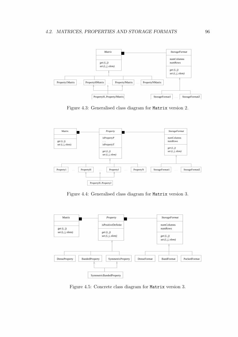
4.2. MATRICES, PROPERTIES AND STORAGE FORMATS 96
������Matrix StorageFormat
numColumnsnumRows
Property1Matrix
StorageFormat1 StorageFormatZ
PropertyNMatrixPropertyJMatrix
PropertyH..PropertyJMatrix
PropertyHMatrix
get (i, j)set (i, j, elem)
get (i, j)set (i, j, elem)
Figure 4.3: Generalised class diagram for Matrix version 2.
������ ������Matrix Property
isPropertyP. . .isPropertyT
Property1 PropertyJPropertyH
PropertyH..PropertyJ
PropertyN StorageFormat1 StorageFormatZ
numColumnsnumRows
StorageFormat
get (i, j)set (i, j, elem)
get (i, j)set (i, j, elem)
get (i, j)set (i, j, elem)
Figure 4.4: Generalised class diagram for Matrix version 3.
������ ������
isPositiveDefinite
SymmetricBandedProperty
DenseProperty BandedProperty SymmetricProperty
Property
DenseFormat BandFormat PackedFormat
numRowsnumColumns
StorageFormatMatrix
get (i, j)set (i, j, elem) get (i, j)
set (i, j, elem)
get (i, j)set (i, j, elem)
Figure 4.5: Concrete class diagram for Matrix version 3.
4.2. MATRICES, PROPERTIES AND STORAGE FORMATS 97
4.2.2 Discussion
In Matrix version 1 and version 1.β, a class at the bottom of the hierarchy can
be seen as a possible combination of matrix properties and a storage format.
Comparing these classes with the BLAS naming scheme, which uses two letters to
represent matrix properties and a storage format (e.g. GE – dense matrix in dense
format or TP – triangular matrix in pack format), a class would be created for
each two-letter code. LAPACK++, SparseLib++, OwlPack, Diffpack, ISIS++,
Oblio and Spindle, and Jampack libraries (Table 4.1) are examples of Matrix
version 1 while Paladin and SL++ are examples of Matrix version 1.β.
The drawback of Matrix version 1 and version 1.β is the large number of
classes that have to be implemented. For each matrix property, a matrix can be
represented in many storage formats; therefore the number of required classes is
of order the number of matrix properties multiplied by the number of storage
formats.
Matrix version 2 uses the client relationship, or more precisely the bridge pat-
tern [107], in order to reduce the number of classes needed for Matrix version 1
and version 1.β. The class diagram (Figure 4.3) can be read as “a matrix, what-
ever its properties, has a storage format”. The storage format can be any of
those in the hierarchy and can vary at run-time. The effect is that all the classes
on the lowest level of the hierarchy of Matrix version 1 (Figure 4.2) are elimi-
nated, and new ones encapsulating the storage format appear. The abstract class
StorageFormat has the same two methods as Matrix: get and set. This creates
a unified access interface and, thus, the sub-classes of Matrix do not need to
know the storage format in which they are represented in order to access an ele-
ment. Using generic programming, class Matrix can become a generic class, with
a sub-class of StorageFormat as its parameter, and a similar model is obtained.
This variation of Matrix version 2 is referred to as version 2.β and both PMLP
and MTL1 follow it.
PMLP and MTL face a common problem. Users do not need to know how
a storage format is represented because it is encapsulated in the sub-classes of
StorageFormat. Thus they can create inadvisable combinations, such as a dense
matrix stored in a sparse storage format, or impossible combinations, such as a
dense matrix stored in packed format.
Matrix version 3 introduces the possibility that some matrix properties are
1MTL includes other options as parameters, such as column-wise or row-wise array layouts.
4.2. MATRICES, PROPERTIES AND STORAGE FORMATS 98
not represented by classes. The positive definite property is a property that does
not enable a matrix to be represented in different storage formats; it is simply
a factor that influences the selection of an implementation for certain matrix
operations. Furthermore, it can be combined with any other property, but the
combination does not change the advisable storage formats of the original prop-
erties. The positive definite property is represented as an attribute of Property,
and is thus inherited by every sub-class producing all the combinations. The rule
to apply in general to determine if a matrix property is represented as a class
or as an attribute is whether the property enables a matrix to be represented in
different storage formats and can occur together with any of the properties rep-
resented as classes. The second modification introduced in version 3 is that class
Matrix becomes a client of Property from which the different matrix properties
inherit. The class Property follows the same unified access interface of Matrix
and no changes are needed for the sub-classes representing matrix properties.
The following example of a linear algebra operation presents a situation that
both Matrix version 2 and Matrix version 1 fail to model, and which further mo-
tivates Matrix version 3. Suppose that a program requires the matrix operation
B ← A + B, where A is a dense matrix and B is a banded matrix. Mathemati-
cally speaking, this operation is correct as long as both A and B have the same
number of rows and columns. In other words, a matrix operation is correct as
long as it conforms to its definition and the properties of the matrices do not
interfere. However, using Matrix version 1, version 1.β, version 2 or version 2.β,
this matrix operation is either not accepted or is performed incorrectly. A sensible
program which uses Matrix version 2 creates an object a of class DenseMatrix
and an object b of class BandedMatrix. After executing a method that assigns
to b the sum of a and b, two different problems may arise. The first problem
is that, if the object b had an object of class BandFormat, an exception should
be raised since a dense matrix cannot be stored efficiently in band format; the
solution to this problem is to allow the library to change the storage format. The
second problem arises from the change of properties of b; although the library
can change the storage format it is impossible for it to change b to be an object
of class DenseMatrix, because DenseMatrix is not a sub-class of BandedMatrix.
Consequently, b is an object of the class BandedMatrix when it should be an
object of class DenseMatrix.
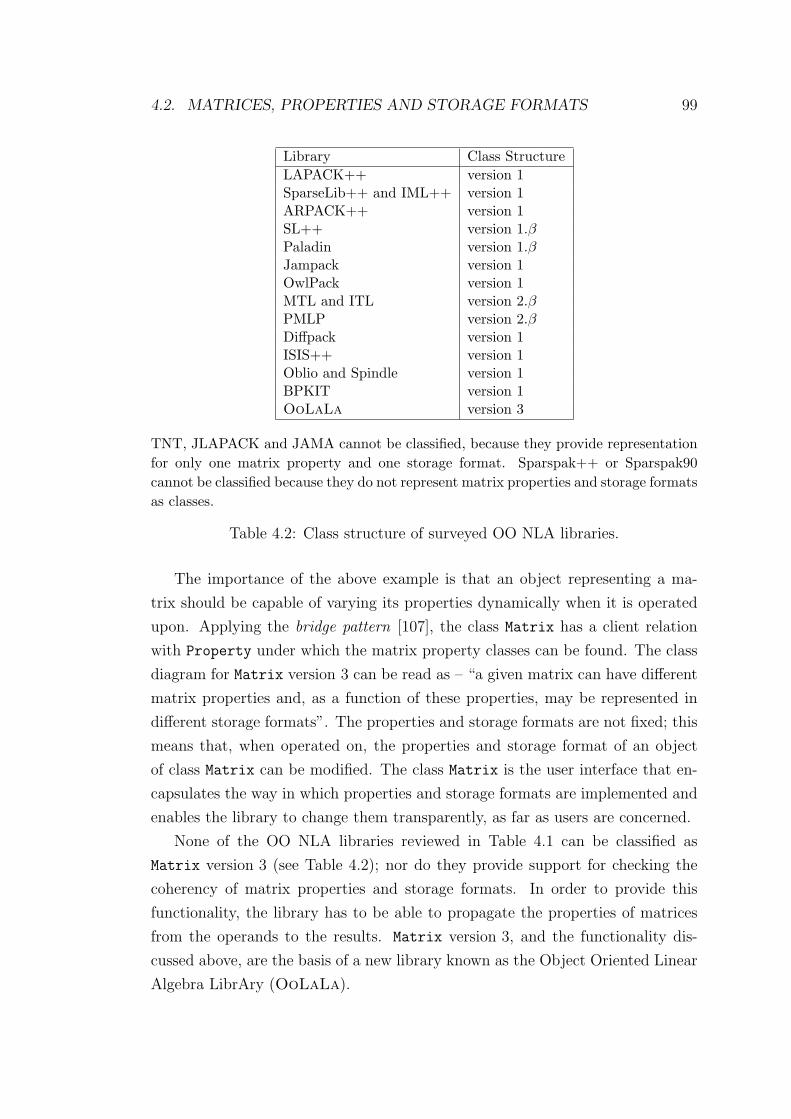
4.2. MATRICES, PROPERTIES AND STORAGE FORMATS 99
Library Class StructureLAPACK++ version 1SparseLib++ and IML++ version 1ARPACK++ version 1SL++ version 1.βPaladin version 1.βJampack version 1OwlPack version 1MTL and ITL version 2.βPMLP version 2.βDiffpack version 1ISIS++ version 1Oblio and Spindle version 1BPKIT version 1OoLaLa version 3
TNT, JLAPACK and JAMA cannot be classified, because they provide representationfor only one matrix property and one storage format. Sparspak++ or Sparspak90cannot be classified because they do not represent matrix properties and storage formatsas classes.
Table 4.2: Class structure of surveyed OO NLA libraries.
The importance of the above example is that an object representing a ma-
trix should be capable of varying its properties dynamically when it is operated
upon. Applying the bridge pattern [107], the class Matrix has a client relation
with Property under which the matrix property classes can be found. The class
diagram for Matrix version 3 can be read as – “a given matrix can have different
matrix properties and, as a function of these properties, may be represented in
different storage formats”. The properties and storage formats are not fixed; this
means that, when operated on, the properties and storage format of an object
of class Matrix can be modified. The class Matrix is the user interface that en-
capsulates the way in which properties and storage formats are implemented and
enables the library to change them transparently, as far as users are concerned.
None of the OO NLA libraries reviewed in Table 4.1 can be classified as
Matrix version 3 (see Table 4.2); nor do they provide support for checking the
coherency of matrix properties and storage formats. In order to provide this
functionality, the library has to be able to propagate the properties of matrices
from the operands to the results. Matrix version 3, and the functionality dis-
cussed above, are the basis of a new library known as the Object Oriented Linear
Algebra LibrAry (OoLaLa).
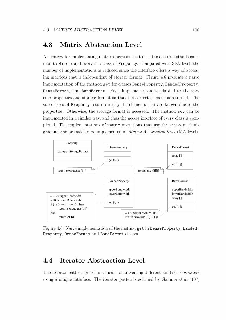
4.3. MATRIX ABSTRACTION LEVEL 100
4.3 Matrix Abstraction Level
A strategy for implementing matrix operations is to use the access methods com-
mon to Matrix and every sub-class of Property. Compared with SFA-level, the
number of implementations is reduced since the interface offers a way of access-
ing matrices that is independent of storage format. Figure 4.6 presents a naıve
implementation of the method get for classes DenseProperty, BandedProperty,
DenseFormat, and BandFormat. Each implementation is adapted to the spe-
cific properties and storage format so that the correct element is returned. The
sub-classes of Property return directly the elements that are known due to the
properties. Otherwise, the storage format is accessed. The method set can be
implemented in a similar way, and thus the access interface of every class is com-
pleted. The implementations of matrix operations that use the access methods
get and set are said to be implemented at Matrix Abstraction level (MA-level).
storage : StorageFormat
PropertyDenseFormat
array [][]
get (i, j)
DenseProperty
get (i, j)
return storage.get (i, j)
upperBandwidth
BandedProperty
lowerBandwidth
get (i, j)
// uB is upperBandwidthreturn array[uB+i−j+1][j]
BandFormat
upperBandwidthlowerBandwidtharray [][]
get (i, j)
return array[i][j]
// uB is upperBandwidth// lB is lowerBandwidthif (−uB <= i−j <= lB) then
elsereturn ZERO
return storage.get (i, j)
Figure 4.6: Naıve implementation of the method get in DenseProperty, Banded-Property, DenseFormat and BandFormat classes.
4.4 Iterator Abstraction Level
The iterator pattern presents a means of traversing different kinds of containers
using a unique interface. The iterator pattern described by Gamma et al. [107]
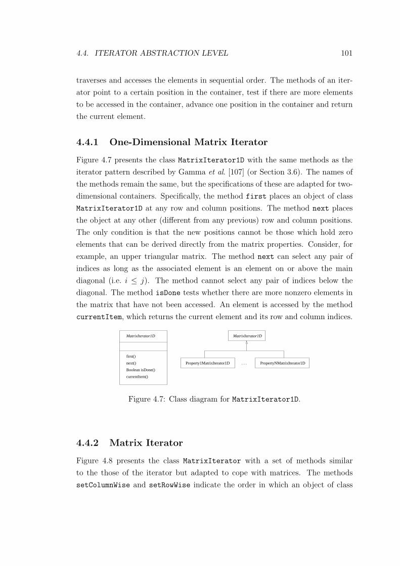
4.4. ITERATOR ABSTRACTION LEVEL 101
traverses and accesses the elements in sequential order. The methods of an iter-
ator point to a certain position in the container, test if there are more elements
to be accessed in the container, advance one position in the container and return
the current element.
4.4.1 One-Dimensional Matrix Iterator
Figure 4.7 presents the class MatrixIterator1D with the same methods as the
iterator pattern described by Gamma et al. [107] (or Section 3.6). The names of
the methods remain the same, but the specifications of these are adapted for two-
dimensional containers. Specifically, the method first places an object of class
MatrixIterator1D at any row and column positions. The method next places
the object at any other (different from any previous) row and column positions.
The only condition is that the new positions cannot be those which hold zero
elements that can be derived directly from the matrix properties. Consider, for
example, an upper triangular matrix. The method next can select any pair of
indices as long as the associated element is an element on or above the main
diagonal (i.e. i ≤ j). The method cannot select any pair of indices below the
diagonal. The method isDone tests whether there are more nonzero elements in
the matrix that have not been accessed. An element is accessed by the method
currentItem, which returns the current element and its row and column indices.
first()
next()
currentItem()
Boolean isDone()
MatrixIterator1D
. . .Property1MatrixIterator1D PropertyNMatrixIterator1D
MatrixIterator1D
Figure 4.7: Class diagram for MatrixIterator1D.
4.4.2 Matrix Iterator
Figure 4.8 presents the class MatrixIterator with a set of methods similar
to the those of the iterator but adapted to cope with matrices. The methods
setColumnWise and setRowWise indicate the order in which an object of class

4.4. ITERATOR ABSTRACTION LEVEL 102
MatrixIterator traverses a matrix. The class MatrixIterator considers a vec-
tor as either a column or a row of the matrix according to the selected order. Thus,
a matrix is traversed by passing through each of its vectors. The method begin
sets the object at the first column and first row. The method beginAt places
the object at the position specified as a parameter. The method nextVector
increases one index of the current position, and modifies the other index so that
it points to the first position. The index that is increased or modified depends
on the selected order. The method isMatrixFinished tests to see if there are
more vectors to traverse in the matrix. A vector is traversed using the meth-
ods nextElement and isVectorFinished. The method nextElement searches
accordingly to the properties for the next nonzero element in the vector, while
isVectorFinished tests whether there are more nonzero elements in the vec-
tor. An element is accessed by the method currentElement, which returns the
current value of the element together with its row and column indices.
nextVector()
currentElement()
Boolean isVectorFinished()
nextElement()
Boolean isMatrixFinished()
beginAt(i,j)
begin()
setColumnWise()
setRowWise()
MatrixIterator
. . .
MatrixIterator
PropertyNMatrixIteratorProperty1MatrixIterator
Figure 4.8: Class diagram for MatrixIterator.
4.4.3 Discussion
Since a matrix iterator traverses a matrix skipping the zero elements, iterators
constitute a new abstraction level at which matrix operations can be implemented,
namely Iterator Abstraction level (IA-level). An implementation of a matrix op-
eration using the IA-level interface implicitly changes the elements to be accessed
when properties of the matrices are changed. This further reduces the number
of implementations of a matrix operation. MTL and PMLP have reported on
the use of iterators, but with contradictory results. MTL [207] reports results
comparable with highly optimised NLA libraries, while PMLP [36] states that:
4.5. VIEWS OF MATRICES 103
“iterators are not an efficient mechanism for accessing elements in sparse matri-
ces.” MTL uses an iterator similar to MatrixIterator. PMLP does not state
the kind of iterator tested.
From the point of view of the matrix traversals that can be achieved with
either of the presented matrix iterators, MatrixIterator is more general than
MatrixIterator1D and, thus, can be used in implementations of more matrix
operations. However MatrixIterator1D is suitable only for the implementations
of certain matrix operations and offers a better (constant time) element access
compared with MatrixIterator. For these matrix operations, and depending on
the storage format, MatrixIterator normally offers between constant and linear
(with respect to the number of nonzero elements) access times. More details
about this issue appear in Chapter 5.
For completeness OoLaLa provides another two iterator classes, namely
Container2DIterator and Container2DIterator1D, and these have the same
interface as MatrixIterator and MatrixIterator1D respectively. Although
these iterators can also traverse matrices, they access all the elements, even those
known to be zero.
4.5 Views of Matrices
Often for high performance, applications need to work on sub-matrices treating
each of them as if they were matrices in their own right. For example, subrou-
tines of LAPACK partition the matrices into blocks and work on these blocks
independently. The transpose of a matrix can be treated as a section that is
accessed by interchanging the indices. An LU factorisation can store the L and
U matrices in the matrix A (such an implementation of LU factorisation is called
in-place factorisation). The subsequent phase of solving the triangular systems
with coefficient matrices L and U accesses only the lower triangular section or
the upper triangular section. On other occasions, applications need to merge
matrices in order to create a new matrix; for example, a block matrix can be
created by merging its blocks.
Other examples of matrix sections are a row or a column of an m×n matrix,
which can be viewed as a row vector of size n or a column vector of size m, or three
consecutive rows, which can be viewed as a 3×n matrix. A block lower triangular
matrix can be formed by merging its blocks with appropriate zero matrices.
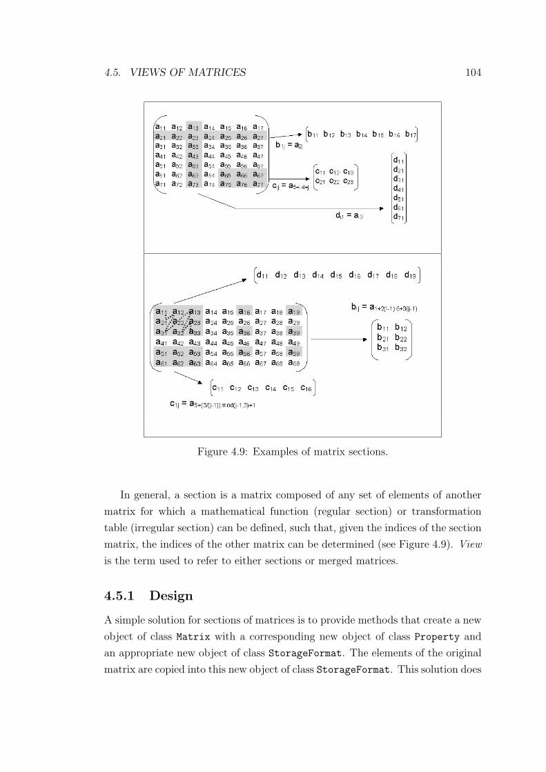
4.5. VIEWS OF MATRICES 104
Figure 4.9: Examples of matrix sections.
In general, a section is a matrix composed of any set of elements of another
matrix for which a mathematical function (regular section) or transformation
table (irregular section) can be defined, such that, given the indices of the section
matrix, the indices of the other matrix can be determined (see Figure 4.9). View
is the term used to refer to either sections or merged matrices.
4.5.1 Design
A simple solution for sections of matrices is to provide methods that create a new
object of class Matrix with a corresponding new object of class Property and
an appropriate new object of class StorageFormat. The elements of the original
matrix are copied into this new object of class StorageFormat. This solution does
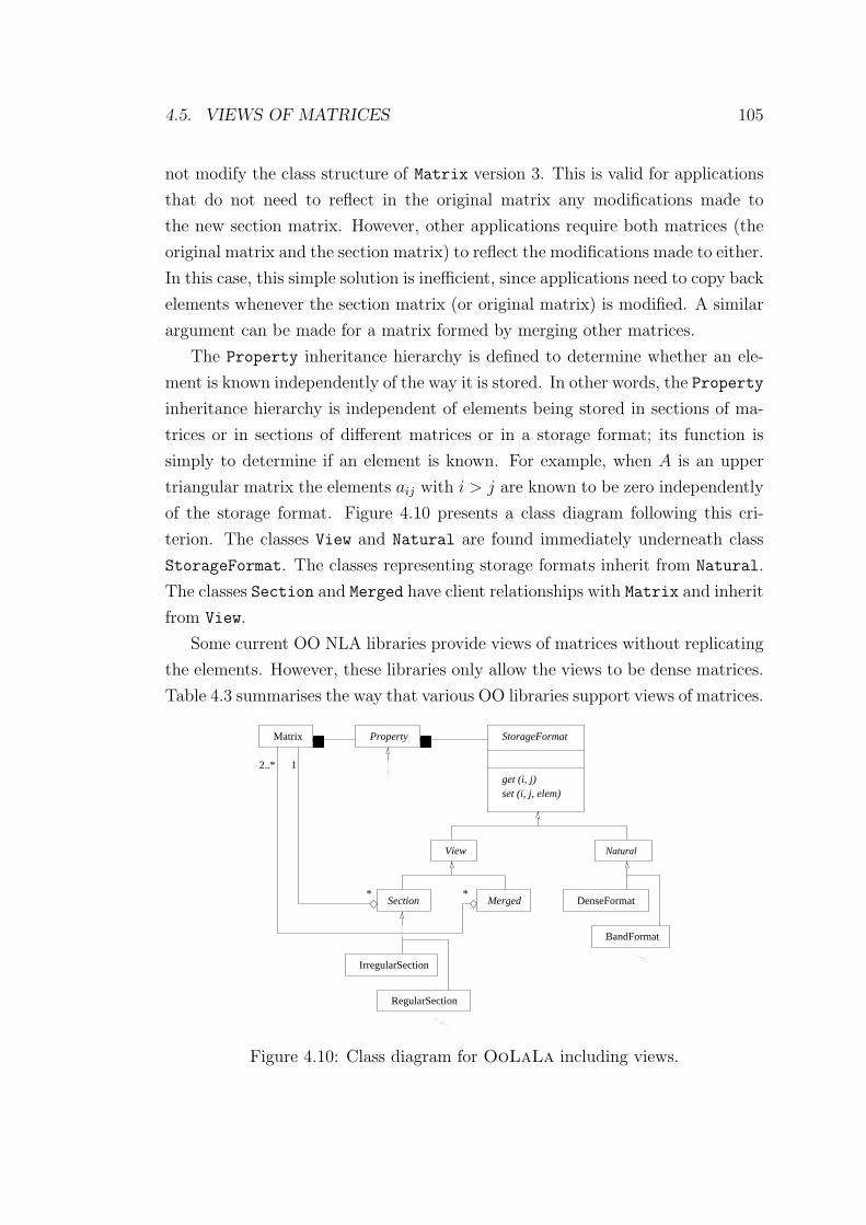
4.5. VIEWS OF MATRICES 105
not modify the class structure of Matrix version 3. This is valid for applications
that do not need to reflect in the original matrix any modifications made to
the new section matrix. However, other applications require both matrices (the
original matrix and the section matrix) to reflect the modifications made to either.
In this case, this simple solution is inefficient, since applications need to copy back
elements whenever the section matrix (or original matrix) is modified. A similar
argument can be made for a matrix formed by merging other matrices.
The Property inheritance hierarchy is defined to determine whether an ele-
ment is known independently of the way it is stored. In other words, the Property
inheritance hierarchy is independent of elements being stored in sections of ma-
trices or in sections of different matrices or in a storage format; its function is
simply to determine if an element is known. For example, when A is an upper
triangular matrix the elements aij with i > j are known to be zero independently
of the storage format. Figure 4.10 presents a class diagram following this cri-
terion. The classes View and Natural are found immediately underneath class
StorageFormat. The classes representing storage formats inherit from Natural.
The classes Section and Merged have client relationships with Matrix and inherit
from View.
Some current OO NLA libraries provide views of matrices without replicating
the elements. However, these libraries only allow the views to be dense matrices.
Table 4.3 summarises the way that various OO libraries support views of matrices.
Natural
Section* *
Merged
IrregularSection
DenseFormat
BandFormat
������ ������
RegularSection
2..*
Property
View
Matrix
1
StorageFormat
get (i, j)set (i, j, elem)
Figure 4.10: Class diagram for OoLaLa including views.
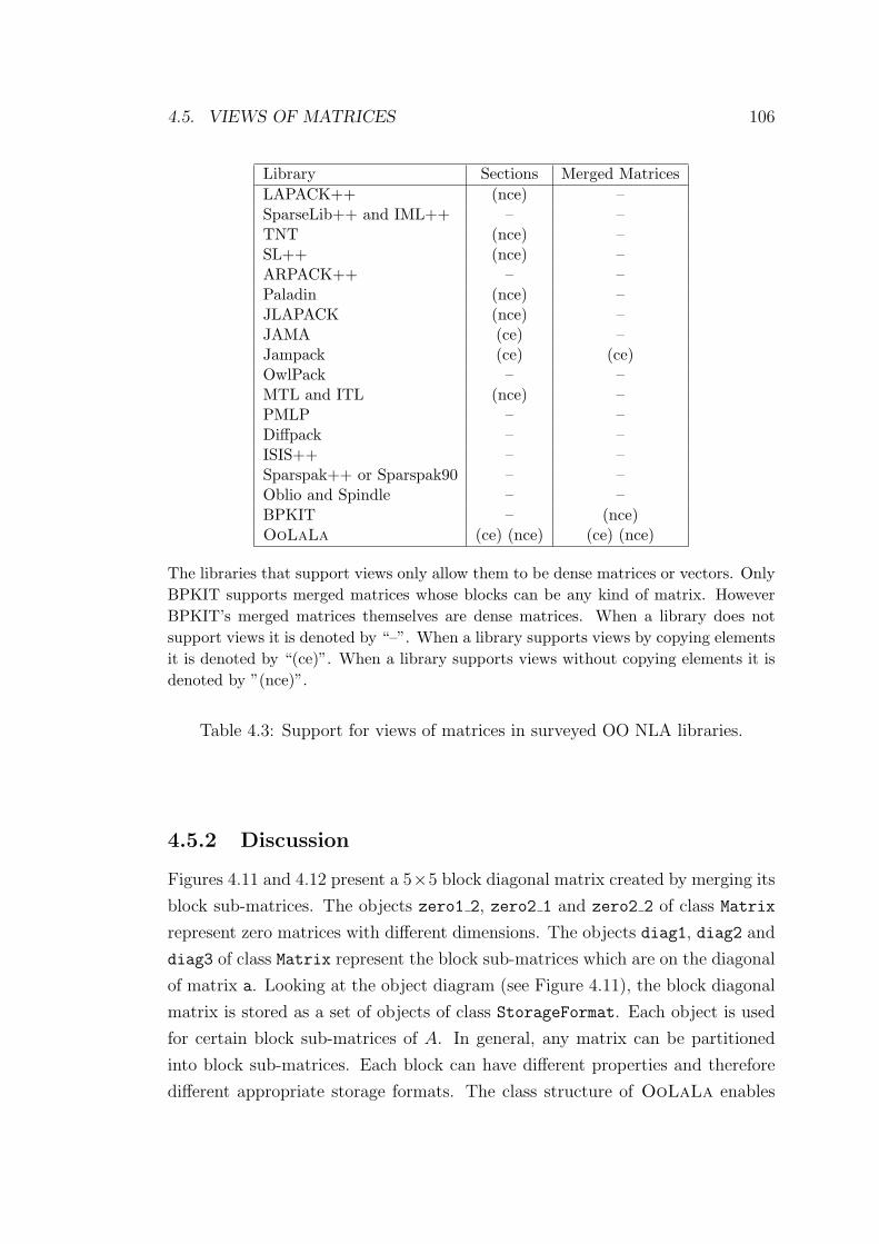
4.5. VIEWS OF MATRICES 106
Library Sections Merged MatricesLAPACK++ (nce) –SparseLib++ and IML++ – –TNT (nce) –SL++ (nce) –ARPACK++ – –Paladin (nce) –JLAPACK (nce) –JAMA (ce) –Jampack (ce) (ce)OwlPack – –MTL and ITL (nce) –PMLP – –Diffpack – –ISIS++ – –Sparspak++ or Sparspak90 – –Oblio and Spindle – –BPKIT – (nce)OoLaLa (ce) (nce) (ce) (nce)
The libraries that support views only allow them to be dense matrices or vectors. OnlyBPKIT supports merged matrices whose blocks can be any kind of matrix. HoweverBPKIT’s merged matrices themselves are dense matrices. When a library does notsupport views it is denoted by “–”. When a library supports views by copying elementsit is denoted by “(ce)”. When a library supports views without copying elements it isdenoted by ”(nce)”.
Table 4.3: Support for views of matrices in surveyed OO NLA libraries.
4.5.2 Discussion
Figures 4.11 and 4.12 present a 5×5 block diagonal matrix created by merging its
block sub-matrices. The objects zero1 2, zero2 1 and zero2 2 of class Matrix
represent zero matrices with different dimensions. The objects diag1, diag2 and
diag3 of class Matrix represent the block sub-matrices which are on the diagonal
of matrix a. Looking at the object diagram (see Figure 4.11), the block diagonal
matrix is stored as a set of objects of class StorageFormat. Each object is used
for certain block sub-matrices of A. In general, any matrix can be partitioned
into block sub-matrices. Each block can have different properties and therefore
different appropriate storage formats. The class structure of OoLaLa enables
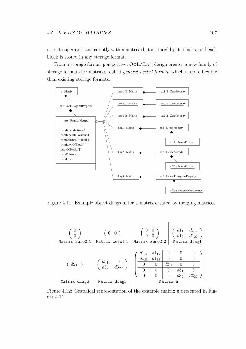
4.5. VIEWS OF MATRICES 107
users to operate transparently with a matrix that is stored by its blocks, and each
block is stored in any storage format.
From a storage format perspective, OoLaLa’s design creates a new family of
storage formats for matrices, called general nested format, which is more flexible
than existing storage formats.
zero2_1 : Matrix pz2_1 : ZeroProperty
zero2_2 : Matrix pz2_2 : ZeroProperty
sfd3 : LowerPackedFormat
numBlocksInRow=3
numBlocksInColumn=3
numRowsOfBlock[][]
numColumnsOfBlock[][]
arrayOfBlocks[][]
numColumns
numRows
ma : RegularMerged
zero1_2 : Matrix pz1_2 : ZeroProperty
pa : BlockDiagonalProperty
a : Matrix
diag1 : Matrix pd1 : DenseProperty
sfd1 : DenseFormat
diag2 : Matrix pd2 : DenseProperty
diag3 : Matrix pd3 : LowerTriangularProperty
sfd2 : DenseFormat
Figure 4.11: Example object diagram for a matrix created by merging matrices.
(00
) (0 0
) (0 00 0
) (d111 d112
d121 d122
)Matrix zero2 1 Matrix zero1 2 Matrix zero2 2 Matrix diag1
(d211
) (d311 0d321 d322
) d111 d112 0 0 0d121 d122 0 0 0
0 0 d211 0 00 0 0 d311 00 0 0 d321 d322
Matrix diag2 Matrix diag3 Matrix a
Figure 4.12: Graphical representation of the example matrix a presented in Fig-ure 4.11.
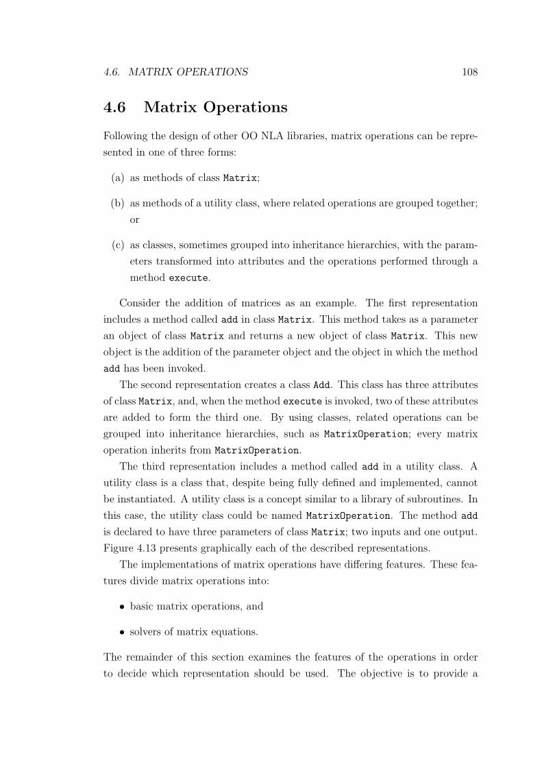
4.6. MATRIX OPERATIONS 108
4.6 Matrix Operations
Following the design of other OO NLA libraries, matrix operations can be repre-
sented in one of three forms:
(a) as methods of class Matrix;
(b) as methods of a utility class, where related operations are grouped together;
or
(c) as classes, sometimes grouped into inheritance hierarchies, with the param-
eters transformed into attributes and the operations performed through a
method execute.
Consider the addition of matrices as an example. The first representation
includes a method called add in class Matrix. This method takes as a parameter
an object of class Matrix and returns a new object of class Matrix. This new
object is the addition of the parameter object and the object in which the method
add has been invoked.
The second representation creates a class Add. This class has three attributes
of class Matrix, and, when the method execute is invoked, two of these attributes
are added to form the third one. By using classes, related operations can be
grouped into inheritance hierarchies, such as MatrixOperation; every matrix
operation inherits from MatrixOperation.
The third representation includes a method called add in a utility class. A
utility class is a class that, despite being fully defined and implemented, cannot
be instantiated. A utility class is a concept similar to a library of subroutines. In
this case, the utility class could be named MatrixOperation. The method add
is declared to have three parameters of class Matrix; two inputs and one output.
Figure 4.13 presents graphically each of the described representations.
The implementations of matrix operations have differing features. These fea-
tures divide matrix operations into:
• basic matrix operations, and
• solvers of matrix equations.
The remainder of this section examines the features of the operations in order
to decide which representation should be used. The objective is to provide a
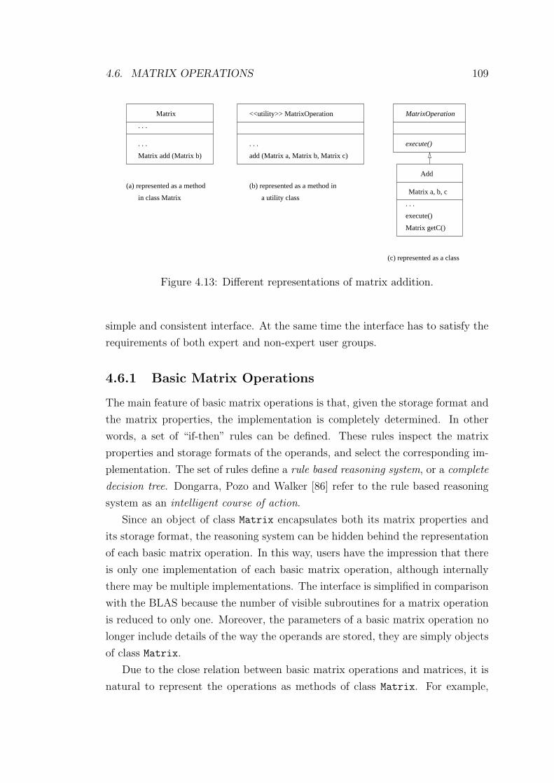
4.6. MATRIX OPERATIONS 109
(a) represented as a method
in class Matrix
Matrix
. . .
. . .
Matrix add (Matrix b)
(b) represented as a method in
a utility class
<<utility>> MatrixOperation
. . .
add (Matrix a, Matrix b, Matrix c)
MatrixOperation
execute()
Add
Matrix a, b, c
. . .
execute()
Matrix getC()
(c) represented as a class
Figure 4.13: Different representations of matrix addition.
simple and consistent interface. At the same time the interface has to satisfy the
requirements of both expert and non-expert user groups.
4.6.1 Basic Matrix Operations
The main feature of basic matrix operations is that, given the storage format and
the matrix properties, the implementation is completely determined. In other
words, a set of “if-then” rules can be defined. These rules inspect the matrix
properties and storage formats of the operands, and select the corresponding im-
plementation. The set of rules define a rule based reasoning system, or a complete
decision tree. Dongarra, Pozo and Walker [86] refer to the rule based reasoning
system as an intelligent course of action.
Since an object of class Matrix encapsulates both its matrix properties and
its storage format, the reasoning system can be hidden behind the representation
of each basic matrix operation. In this way, users have the impression that there
is only one implementation of each basic matrix operation, although internally
there may be multiple implementations. The interface is simplified in comparison
with the BLAS because the number of visible subroutines for a matrix operation
is reduced to only one. Moreover, the parameters of a basic matrix operation no
longer include details of the way the operands are stored, they are simply objects
of class Matrix.
Due to the close relation between basic matrix operations and matrices, it is
natural to represent the operations as methods of class Matrix. For example,
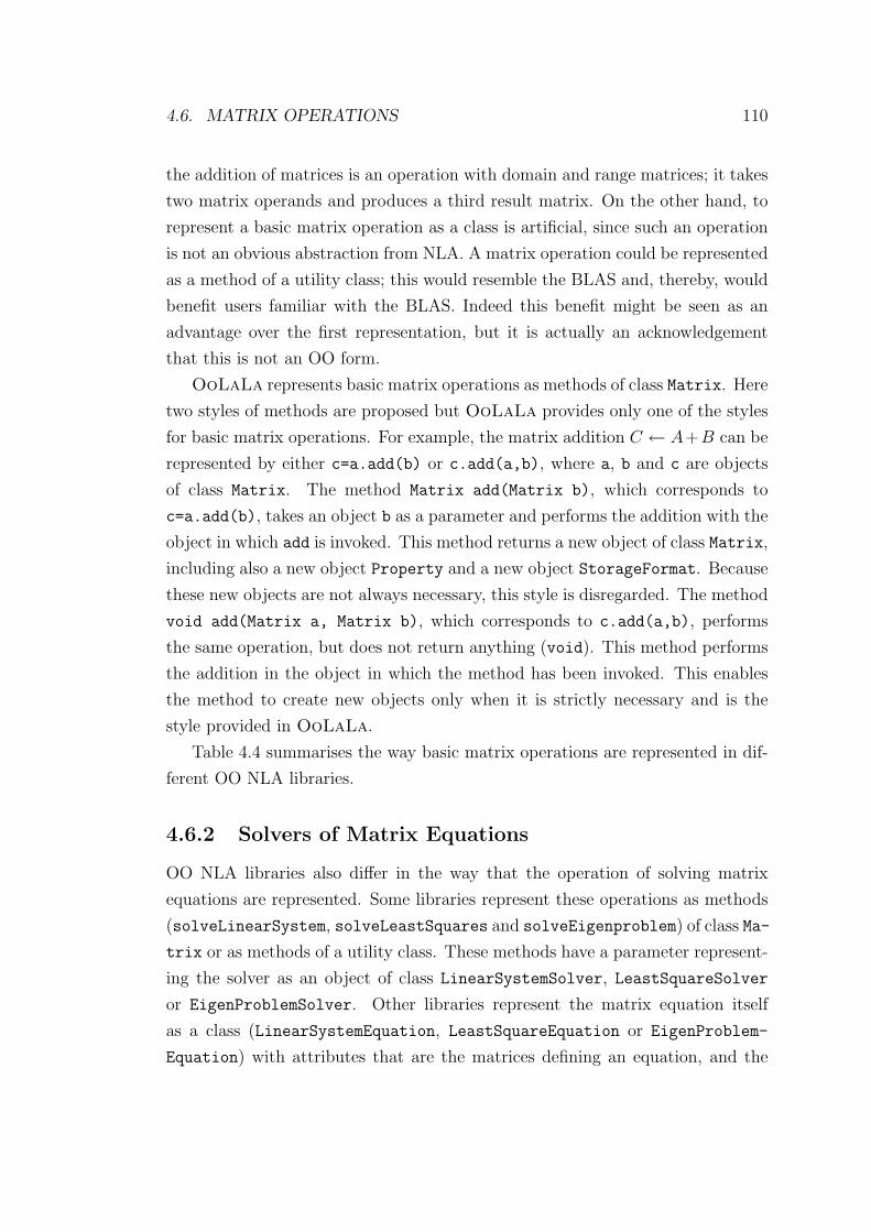
4.6. MATRIX OPERATIONS 110
the addition of matrices is an operation with domain and range matrices; it takes
two matrix operands and produces a third result matrix. On the other hand, to
represent a basic matrix operation as a class is artificial, since such an operation
is not an obvious abstraction from NLA. A matrix operation could be represented
as a method of a utility class; this would resemble the BLAS and, thereby, would
benefit users familiar with the BLAS. Indeed this benefit might be seen as an
advantage over the first representation, but it is actually an acknowledgement
that this is not an OO form.
OoLaLa represents basic matrix operations as methods of class Matrix. Here
two styles of methods are proposed but OoLaLa provides only one of the styles
for basic matrix operations. For example, the matrix addition C ← A+B can be
represented by either c=a.add(b) or c.add(a,b), where a, b and c are objects
of class Matrix. The method Matrix add(Matrix b), which corresponds to
c=a.add(b), takes an object b as a parameter and performs the addition with the
object in which add is invoked. This method returns a new object of class Matrix,
including also a new object Property and a new object StorageFormat. Because
these new objects are not always necessary, this style is disregarded. The method
void add(Matrix a, Matrix b), which corresponds to c.add(a,b), performs
the same operation, but does not return anything (void). This method performs
the addition in the object in which the method has been invoked. This enables
the method to create new objects only when it is strictly necessary and is the
style provided in OoLaLa.
Table 4.4 summarises the way basic matrix operations are represented in dif-
ferent OO NLA libraries.
4.6.2 Solvers of Matrix Equations
OO NLA libraries also differ in the way that the operation of solving matrix
equations are represented. Some libraries represent these operations as methods
(solveLinearSystem, solveLeastSquares and solveEigenproblem) of class Ma-
trix or as methods of a utility class. These methods have a parameter represent-
ing the solver as an object of class LinearSystemSolver, LeastSquareSolver
or EigenProblemSolver. Other libraries represent the matrix equation itself
as a class (LinearSystemEquation, LeastSquareEquation or EigenProblem-
Equation) with attributes that are the matrices defining an equation, and the
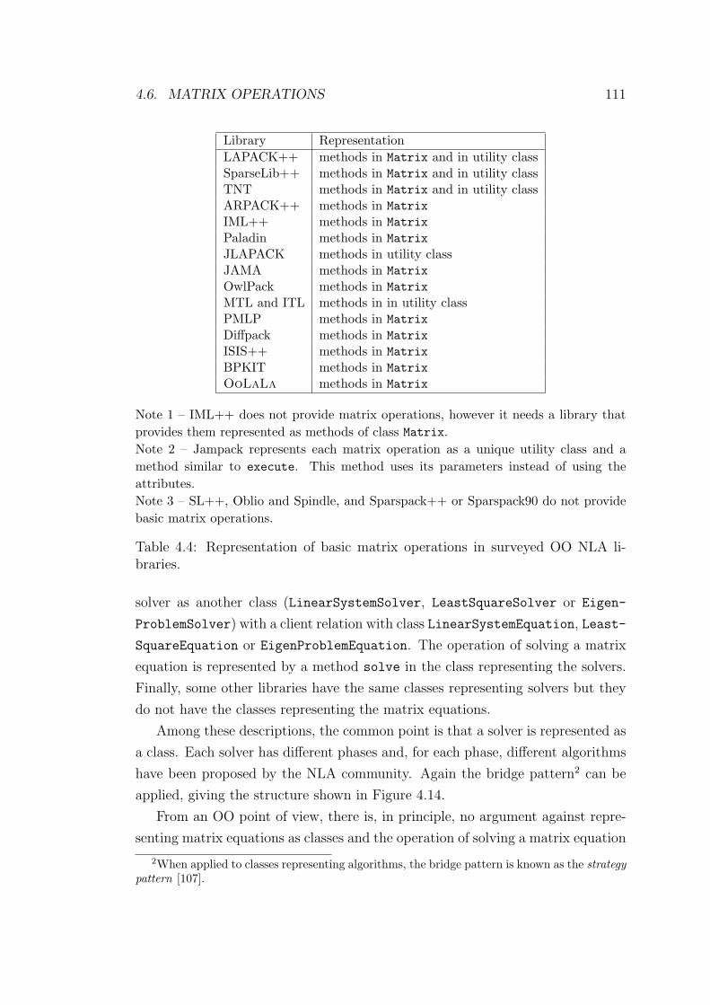
4.6. MATRIX OPERATIONS 111
Library RepresentationLAPACK++ methods in Matrix and in utility classSparseLib++ methods in Matrix and in utility classTNT methods in Matrix and in utility classARPACK++ methods in MatrixIML++ methods in MatrixPaladin methods in MatrixJLAPACK methods in utility classJAMA methods in MatrixOwlPack methods in MatrixMTL and ITL methods in in utility classPMLP methods in MatrixDiffpack methods in MatrixISIS++ methods in MatrixBPKIT methods in MatrixOoLaLa methods in Matrix
Note 1 – IML++ does not provide matrix operations, however it needs a library thatprovides them represented as methods of class Matrix.Note 2 – Jampack represents each matrix operation as a unique utility class and amethod similar to execute. This method uses its parameters instead of using theattributes.Note 3 – SL++, Oblio and Spindle, and Sparspack++ or Sparspack90 do not providebasic matrix operations.
Table 4.4: Representation of basic matrix operations in surveyed OO NLA li-braries.
solver as another class (LinearSystemSolver, LeastSquareSolver or Eigen-
ProblemSolver) with a client relation with class LinearSystemEquation, Least-
SquareEquation or EigenProblemEquation. The operation of solving a matrix
equation is represented by a method solve in the class representing the solvers.
Finally, some other libraries have the same classes representing solvers but they
do not have the classes representing the matrix equations.
Among these descriptions, the common point is that a solver is represented as
a class. Each solver has different phases and, for each phase, different algorithms
have been proposed by the NLA community. Again the bridge pattern2 can be
applied, giving the structure shown in Figure 4.14.
From an OO point of view, there is, in principle, no argument against repre-
senting matrix equations as classes and the operation of solving a matrix equation
2When applied to classes representing algorithms, the bridge pattern is known as the strategypattern [107].
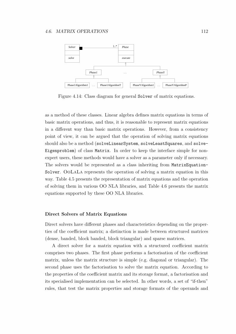
4.6. MATRIX OPERATIONS 112
Phase
execute
. . .PhaseYAlgorithm1 PhaseYAlgorithmP
���
. . .
Solver
solve
Phase1
Phase1Algorithm1 Phase1AlgorithmT
PhaseY
. . .
1..*
Figure 4.14: Class diagram for general Solver of matrix equations.
as a method of these classes. Linear algebra defines matrix equations in terms of
basic matrix operations, and thus, it is reasonable to represent matrix equations
in a different way than basic matrix operations. However, from a consistency
point of view, it can be argued that the operation of solving matrix equations
should also be a method (solveLinearSystem, solveLeastSquares, and solve-
Eigenproblem) of class Matrix. In order to keep the interface simple for non-
expert users, these methods would have a solver as a parameter only if necessary.
The solvers would be represented as a class inheriting from MatrixEquation-
Solver. OoLaLa represents the operation of solving a matrix equation in this
way. Table 4.5 presents the representation of matrix equations and the operation
of solving them in various OO NLA libraries, and Table 4.6 presents the matrix
equations supported by these OO NLA libraries.
Direct Solvers of Matrix Equations
Direct solvers have different phases and characteristics depending on the proper-
ties of the coefficient matrix; a distinction is made between structured matrices
(dense, banded, block banded, block triangular) and sparse matrices.
A direct solver for a matrix equation with a structured coefficient matrix
comprises two phases. The first phase performs a factorisation of the coefficient
matrix, unless the matrix structure is simple (e.g. diagonal or triangular). The
second phase uses the factorisation to solve the matrix equation. According to
the properties of the coefficient matrix and its storage format, a factorisation and
its specialised implementation can be selected. In other words, a set of “if-then”
rules, that test the matrix properties and storage formats of the operands and

4.6. MATRIX OPERATIONS 113
Library Solve Operation Matrix EquationLAPACK++ method in a utility class parameters of the methodSparseLib++ and IML++ method in a utility class parameters of the methodTNT method in a utility class parameters of the methodSL++ method in a utility class parameter of the methodARPACK++ method in Solver attributes of SolverPaladin method in Matrix parameters of the methodJLAPACK method in a utility class parameters of the methodOwlPack method in Matrix parameters of the methodMTL and ITL method in a utility class parameters of the methodPMLP method in Solver attributes of SolverDiffpack method in MatrixEquation class MatrixEquationISIS++ method in MatrixEquation class MatrixEquationSparspak++ or Sparspak90 method in Solver class MatrixEquationOblio and Spindle method in Solver attributes of SolverJAMA method in Matrix and Solver parameters of the method
or attributes of SolverJampack method in utility class parameters of the methodOoLaLa method in Matrix parameters of the method
Table 4.5: Representation of matrix equations and the operation of solving themin surveyed OO NLA libraries.
determine the corresponding implementation, can be defined. This set of rules
defines another rule based reasoning system.
As with basic matrix operations, different factorisations and their specialised
algorithms can be encapsulated behind the methods solveLinearSystem, solve-
LeastSquares, and solveEigenproblem. Users thereby have the impression that
there is only one implementation, although internally there are multiple imple-
mentations.
In general, the factorisation phase can be characterised as pivoting or no-
pivoting. (This characteristic distinguishes between a factorisation that needs to
check stability or not.) Hence, using method overloading, a method with different
parameters but the same name (solveLinearSystem, solveLeastSquares, and
solveEigenproblem) is included. The parameters are the same, except for an
object of class MatrixEquationSolver that indicates the characteristic of piv-
oting or no-pivoting. Table 4.6 presents various OO NLA libraries that provide
direct solvers for structured matrix equations.
A direct solver of a system of linear equations with a sparse coefficient matrix
has three different phases. The first phase produces a reordering of the coefficient
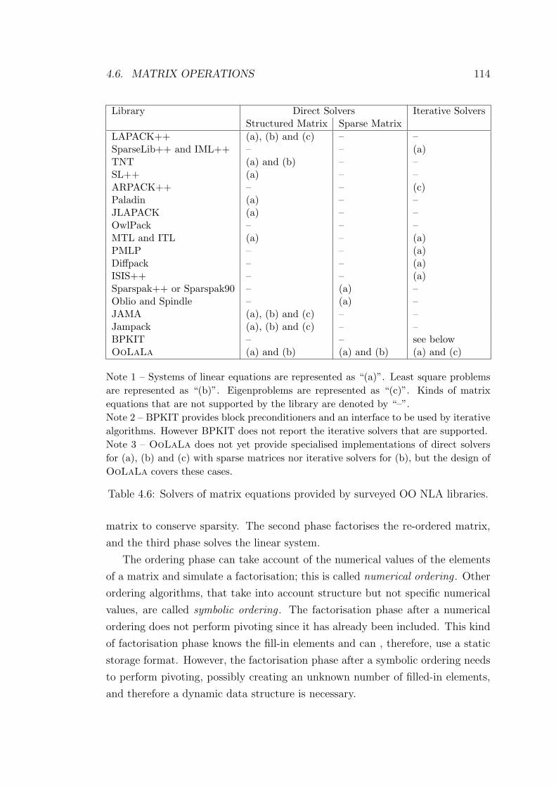
4.6. MATRIX OPERATIONS 114
Library Direct Solvers Iterative SolversStructured Matrix Sparse Matrix
LAPACK++ (a), (b) and (c) – –SparseLib++ and IML++ – – (a)TNT (a) and (b) – –SL++ (a) – –ARPACK++ – – (c)Paladin (a) – –JLAPACK (a) – –OwlPack – – –MTL and ITL (a) – (a)PMLP – – (a)Diffpack – – (a)ISIS++ – – (a)Sparspak++ or Sparspak90 – (a) –Oblio and Spindle – (a) –JAMA (a), (b) and (c) – –Jampack (a), (b) and (c) – –BPKIT – – see belowOoLaLa (a) and (b) (a) and (b) (a) and (c)
Note 1 – Systems of linear equations are represented as “(a)”. Least square problemsare represented as “(b)”. Eigenproblems are represented as “(c)”. Kinds of matrixequations that are not supported by the library are denoted by “–”.Note 2 – BPKIT provides block preconditioners and an interface to be used by iterativealgorithms. However BPKIT does not report the iterative solvers that are supported.Note 3 – OoLaLa does not yet provide specialised implementations of direct solversfor (a), (b) and (c) with sparse matrices nor iterative solvers for (b), but the design ofOoLaLa covers these cases.
Table 4.6: Solvers of matrix equations provided by surveyed OO NLA libraries.
matrix to conserve sparsity. The second phase factorises the re-ordered matrix,
and the third phase solves the linear system.
The ordering phase can take account of the numerical values of the elements
of a matrix and simulate a factorisation; this is called numerical ordering . Other
ordering algorithms, that take into account structure but not specific numerical
values, are called symbolic ordering . The factorisation phase after a numerical
ordering does not perform pivoting since it has already been included. This kind
of factorisation phase knows the fill-in elements and can , therefore, use a static
storage format. However, the factorisation phase after a symbolic ordering needs
to perform pivoting, possibly creating an unknown number of filled-in elements,
and therefore a dynamic data structure is necessary.
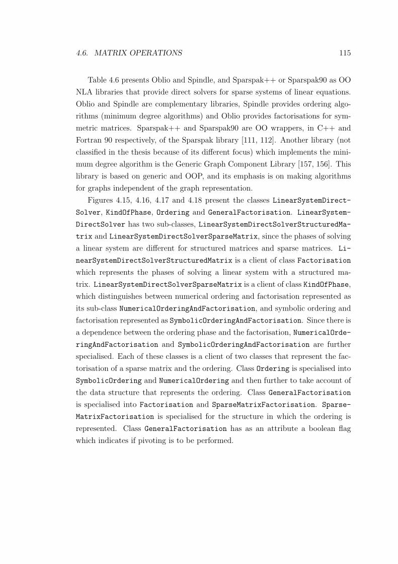
4.6. MATRIX OPERATIONS 115
Table 4.6 presents Oblio and Spindle, and Sparspak++ or Sparspak90 as OO
NLA libraries that provide direct solvers for sparse systems of linear equations.
Oblio and Spindle are complementary libraries, Spindle provides ordering algo-
rithms (minimum degree algorithms) and Oblio provides factorisations for sym-
metric matrices. Sparspak++ and Sparspak90 are OO wrappers, in C++ and
Fortran 90 respectively, of the Sparspak library [111, 112]. Another library (not
classified in the thesis because of its different focus) which implements the mini-
mum degree algorithm is the Generic Graph Component Library [157, 156]. This
library is based on generic and OOP, and its emphasis is on making algorithms
for graphs independent of the graph representation.
Figures 4.15, 4.16, 4.17 and 4.18 present the classes LinearSystemDirect-
Solver, KindOfPhase, Ordering and GeneralFactorisation. LinearSystem-
DirectSolver has two sub-classes, LinearSystemDirectSolverStructuredMa-
trix and LinearSystemDirectSolverSparseMatrix, since the phases of solving
a linear system are different for structured matrices and sparse matrices. Li-
nearSystemDirectSolverStructuredMatrix is a client of class Factorisation
which represents the phases of solving a linear system with a structured ma-
trix. LinearSystemDirectSolverSparseMatrix is a client of class KindOfPhase,
which distinguishes between numerical ordering and factorisation represented as
its sub-class NumericalOrderingAndFactorisation, and symbolic ordering and
factorisation represented as SymbolicOrderingAndFactorisation. Since there is
a dependence between the ordering phase and the factorisation, NumericalOrde-
ringAndFactorisation and SymbolicOrderingAndFactorisation are further
specialised. Each of these classes is a client of two classes that represent the fac-
torisation of a sparse matrix and the ordering. Class Ordering is specialised into
SymbolicOrdering and NumericalOrdering and then further to take account of
the data structure that represents the ordering. Class GeneralFactorisation
is specialised into Factorisation and SparseMatrixFactorisation. Sparse-
MatrixFactorisation is specialised for the structure in which the ordering is
represented. Class GeneralFactorisation has as an attribute a boolean flag
which indicates if pivoting is to be performed.
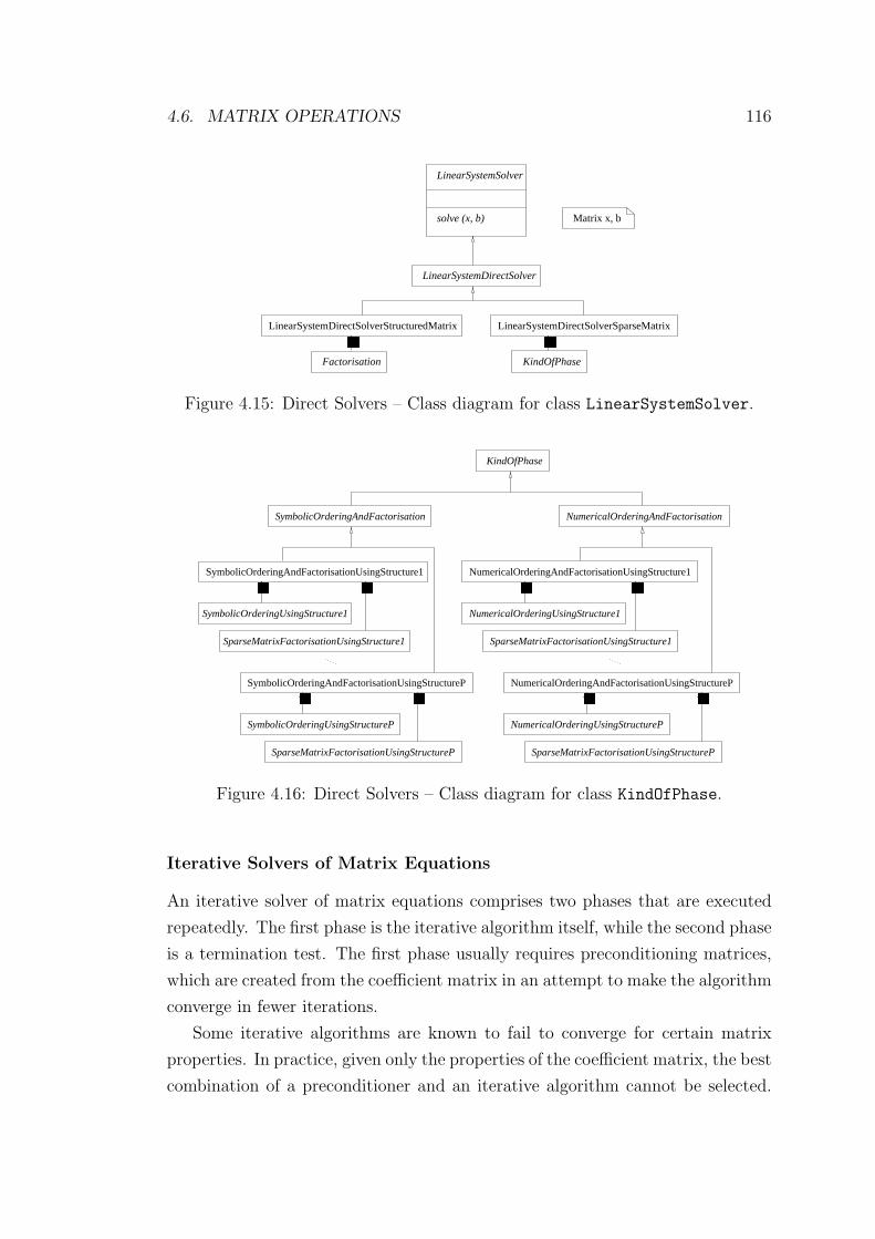
4.6. MATRIX OPERATIONS 116
������ ������
LinearSystemSolver
solve (x, b)
LinearSystemDirectSolver
Factorisation KindOfPhase
Matrix x, b
LinearSystemDirectSolverStructuredMatrix LinearSystemDirectSolverSparseMatrix
Figure 4.15: Direct Solvers – Class diagram for class LinearSystemSolver.
������
������ ������
������ �� ������
� ��� ������
KindOfPhase
SparseMatrixFactorisationUsingStructureP
SymbolicOrderingUsingStructureP
SparseMatrixFactorisationUsingStructure1
SparseMatrixFactorisationUsingStructureP
NumericalOrderingUsingStructureP
SymbolicOrderingAndFactorisation NumericalOrderingAndFactorisation
SymbolicOrderingAndFactorisationUsingStructure1
SymbolicOrderingUsingStructure1
SparseMatrixFactorisationUsingStructure1
NumericalOrderingUsingStructure1
NumericalOrderingAndFactorisationUsingStructureP
NumericalOrderingAndFactorisationUsingStructure1
SymbolicOrderingAndFactorisationUsingStructureP
Figure 4.16: Direct Solvers – Class diagram for class KindOfPhase.
Iterative Solvers of Matrix Equations
An iterative solver of matrix equations comprises two phases that are executed
repeatedly. The first phase is the iterative algorithm itself, while the second phase
is a termination test. The first phase usually requires preconditioning matrices,
which are created from the coefficient matrix in an attempt to make the algorithm
converge in fewer iterations.
Some iterative algorithms are known to fail to converge for certain matrix
properties. In practice, given only the properties of the coefficient matrix, the best
combination of a preconditioner and an iterative algorithm cannot be selected.
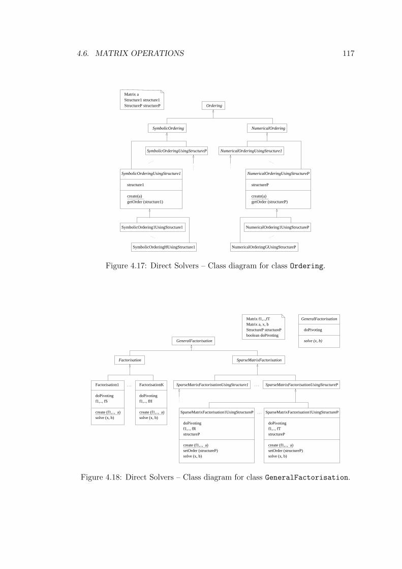
4.6. MATRIX OPERATIONS 117
StructureP structurePStructure1 structure1Matrix a
Ordering
NumericalOrderingSymbolicOrdering
SymbolicOrderingUsingStructureP
create(a)getOrder (structureP)
structureP
NumericalOrderingUsingStructureP
structure1
create(a)getOrder (structure1)
SymbolicOrderingUsingStructure1
SymbolicOrdering1UsingStructure1
SymbolicOrderingHUsingStructure1 NumericalOrderingGUsingStructureP
NumericalOrdering1UsingStructureP
NumericalOrderingUsingStructure1
Figure 4.17: Direct Solvers – Class diagram for class Ordering.
Matrix a, x, bStructureP structurePboolean doPivoting
Matrix f1,..,fT
GeneralFactorisation
Factorisation
SparseMatrixFactorisationUsingStructure1 SparseMatrixFactorisationUsingStructureP
SparseMatrixFactorisation
Factorisation1 FactorisationK
doPivotingf1,.., fS
doPivotingf1,.., fH
structureP
doPivotingf1,.., fT
create (f1,.., a) create (f1,.., a)
create (f1,.., a)
solve (x, b)
solve (x, b)
solve (x, b)
setOrder (structureP)
. . . . . .
doPivotingf1,.., fRstructureP
create (f1,.., a)
solve (x, b)setOrder (structureP)
SparseMatrixFactorisation1UsingStructureP . . . SparseMatrixFactorisation1UsingStructureP
GeneralFactorisation
doPivoting
solve (x, b)
Figure 4.18: Direct Solvers – Class diagram for class GeneralFactorisation.
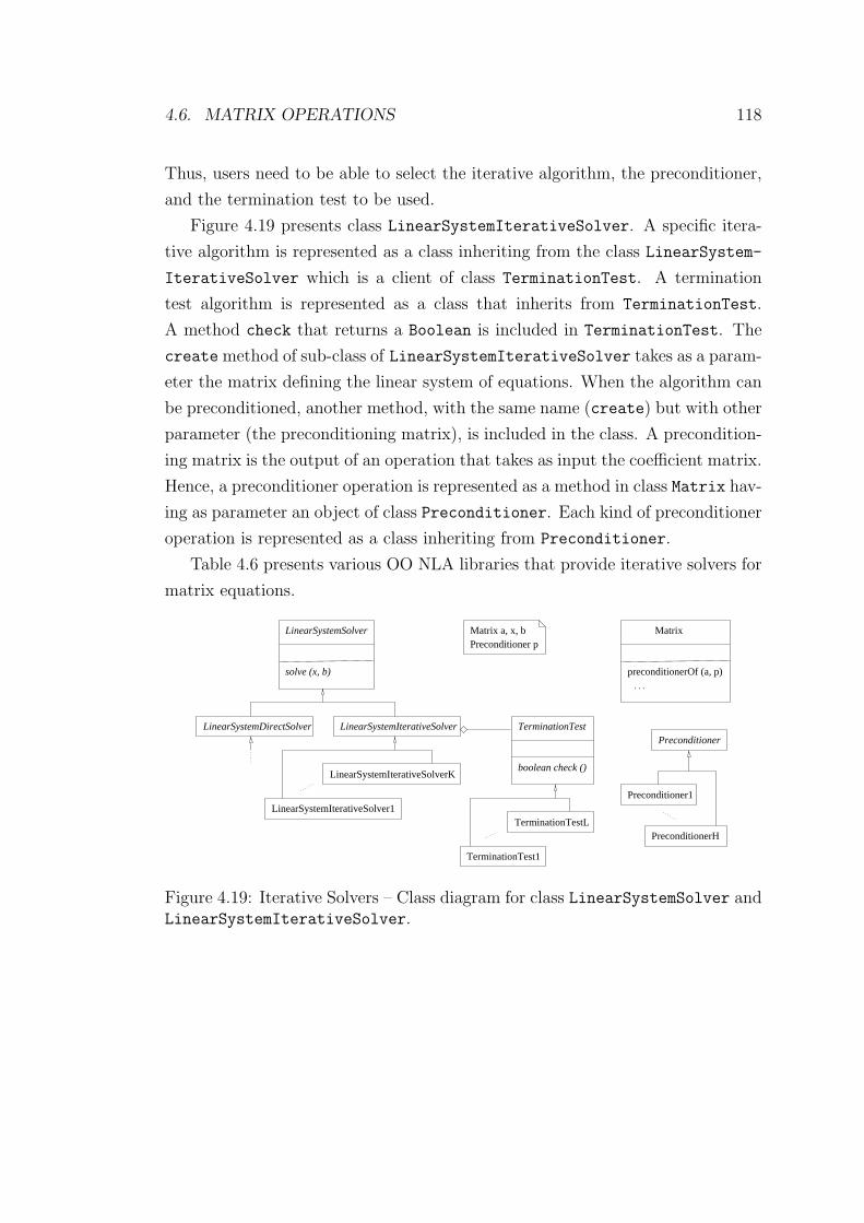
4.6. MATRIX OPERATIONS 118
Thus, users need to be able to select the iterative algorithm, the preconditioner,
and the termination test to be used.
Figure 4.19 presents class LinearSystemIterativeSolver. A specific itera-
tive algorithm is represented as a class inheriting from the class LinearSystem-
IterativeSolver which is a client of class TerminationTest. A termination
test algorithm is represented as a class that inherits from TerminationTest.
A method check that returns a Boolean is included in TerminationTest. The
create method of sub-class of LinearSystemIterativeSolver takes as a param-
eter the matrix defining the linear system of equations. When the algorithm can
be preconditioned, another method, with the same name (create) but with other
parameter (the preconditioning matrix), is included in the class. A precondition-
ing matrix is the output of an operation that takes as input the coefficient matrix.
Hence, a preconditioner operation is represented as a method in class Matrix hav-
ing as parameter an object of class Preconditioner. Each kind of preconditioner
operation is represented as a class inheriting from Preconditioner.
Table 4.6 presents various OO NLA libraries that provide iterative solvers for
matrix equations.
LinearSystemSolver
solve (x, b)
TerminationTestL
TerminationTest1
. . .
preconditionerOf (a, p)
Matrix
Preconditioner1
Preconditioner
PreconditionerH
Matrix a, x, bPreconditioner p
LinearSystemDirectSolver LinearSystemIterativeSolver
LinearSystemIterativeSolver1
LinearSystemIterativeSolverK
TerminationTest
boolean check ()
Figure 4.19: Iterative Solvers – Class diagram for class LinearSystemSolver andLinearSystemIterativeSolver.

4.7. RELATED WORK 119
4.7 Related Work
Although this chapter has already classified many OO NLA libraries, other OO
NLA libraries, such as SLES (a library of iterative solvers of systems of linear
equations that is part of PETSc3 [24, 25]), SMOOTH4 [17] (an ordering library of
sparse matrices) and SPOOLES5 [16] (a library of direct solvers for sparse linear
equations), have not been classified because they are implemented in C (a non
OOP language) and, consequently, their designs are limited.
Some other OO NLA libraries have a different design objective. LAKe [184]
focuses on using the same code for sequential and parallel iterative solvers, Cactus
[173] focuses on finite dimensional vector spaces instead of matrix algebra, and the
Hilbert Class Library (HCL6) targets optimisation problems but provides repre-
sentation for vectors, vector spaces, linear operators, etc. [119]. Other OO NLA li-
braries that have not been reviewed can be found at http://oonumerics.org/oon.
OO multi-dimensional arrays libraries, such as Blitz++7 [222], A++/P++
[186], POOMA8 [134, 145] (in C++) and IBM’s Array Package [176, 9, 178] (in
Java), are related to OO NLA since the one-dimensional and two-dimensional ar-
rays provide methods that implement matrix operations. These libraries have the
common characteristic that they provide classes representing multi-dimensional
arrays and provide random access to the elements. These classes normally en-
capsulate a block of memory that is used to store the multi-dimensional arrays,
using a function to map from n-dimensions to 1-dimension. These classes have as
attributes information related to the base and end index of each dimension, and
the storage direction (e.g. row-wise or column-wise). They all provide sections of
multi-dimensional arrays without copying elements. The sections are represented
with the same multi-dimensional array classes simply by modifying certain at-
tributes (some of which are not needed for normal multi-dimensional arrays), so
that when an element of the section is needed the correct position in the block of
memory is accessed.
POOMA and Blitz++ rely on generic programming. Blitz++ uses this for
the class of the elements of the multi-dimensional arrays and POOMA uses it
3PETSc web site http://www.mcs.anl.gov/petsc4SMOOTH web site http://www.cs.yorku.ca/˜joseph/Smooth/SMOOTH.html5SPOOLES web site http://www.netlib.org/linalg/spooles/spooles.2.2.html6HCL web site http://www.trip.caam.rice.edu/txt/hcldoc/html/7Blitz++ web site http://oonumerics.org/blitz/8POOMA web site http://www.acl.lanl.gov/Pooma
4.8. SUMMARY 120
for the same purpose and also for the class that stores the elements. Thus,
POOMA is the only one of these libraries able to provide multi-dimensional ar-
rays that are not only stored in a one-dimensional language array, but also in
sparse storage formats and other formats. POOMA and Blitz++ rely on expres-
sion templates techniques [221] to achieve high performance implementations of
multi-dimensional operations. Expression template techniques use generic pro-
gramming to perform compile time optimisations that have been the traditional
preserve of optimising compilers (loop unrolling, loop interchange, etc.)
A++ provides sequential multi-dimensional arrays and P++ is a library that
specifies a partition of A++ multi-dimensional arrays. Together they provide
transparent random access to elements of multi-dimensional arrays.
Assuming that two-dimensional and one-dimensional arrays are matrices, Blitz++,
IBM’s Array Package and A++ can be classified as Matrix version 1 (see Section
4.2) because of their close relationship with the storage format. POOMA can be
classified as the generic programming variation of Matrix version 2.β, similar to
PMLP and MTL.
Modelica9 [172, 102], and ObjectMath10 [104, 103, 101, 105, 13] offer an
OO mathematical language that allows users to represent equation-based mod-
els directly. The projects Overture11 [53, 52, 54], POOMA [134, 145], Cogito12
[193, 4, 180, 218], Diffpack [55, 151, 152] and PETSc [24, 25] provide OO software
for solving partial differential equations.
4.8 Summary
This chapter has developed a comprehensive OOD for NLA and has considered
the requirements of both users (expert and non-expert) and library developers.
Traditional NLA libraries provide users with complex interfaces, and library de-
velopers are faced with a combinatorial explosion of implementations for matrix
operations.
Existing OO NLA library designs do not fully model NLA because they de-
fine matrix operations in terms of matrix properties and storage formats rather
than in terms of matrices and their dimensions only. Further, existing OO NLA
9Modelica web site http://www.modelica.org10ObjectMath web site http://www.ida.liu.se/labs/pelab/omath/11Overture web site http://www.llnl.gov/casc/Overture/12Cogito web site http://www.tdb.uu.se/research/swtools/cogito.html
4.8. SUMMARY 121
libraries do not allow a matrix to vary its properties dynamically. Existing OO
NLA libraries provide basic matrix operations, and solution of matrix equations
with iterative and direct algorithms. However, none support all of these matrix
operations (Tables 4.4 and 4.6).
In this chapter, a new class structure has been designed which enables a
library to dynamically vary the properties and storage format of a given matrix
by propagating the matrix properties. The class structure has been extended
so that sections of matrices and matrices formed by merging other matrices can
be created without the need to replicate matrix elements and can be used like
any other matrix. Hence, the new matrices (sections and merged) can have
any property and storage format, in contrast with existing OO NLA libraries
which consider these new matrices always to be dense. This capability generalises
existing storage formats for block matrices.
The following guidelines support the creation of simpler interfaces:
• matrices are represented by classes that encapsulate the way they are stored;
• each matrix operation is represented as a unique visible method, although
different implementations and a rule based reasoning system that selects the
appropriated implementation are hidden behind the visible method; and
• where the reasoning system cannot be defined, the different algorithms,
and not the implementations, are presented as classes, and objects of these
classes are passed as parameters.
Following the above guidelines, a library interface that supports all these
matrix operations has been proposed. This class structure and the proposed
library interface constitute the design of a new library known as OoLaLa.
Developers of NLA libraries benefit from two abstraction levels at which ma-
trix calculations can be implemented. These abstraction levels reduce the number
of implementations. MA-level enables matrices to be accessed independently of
their storage formats by providing a random access to matrix elements. IA-level
is an implicit way of sequentially traversing matrices; that is, a matrix is tra-
versed sequentially without explicitly expressing the indices of the elements that
are accessed. Matrix iterators are defined so that they access only the elements
that can be implied to be nonzero from the matrix properties.
The next two chapters present the implementation and evaluation of OoLaLa,
respectively. The library is implemented in Java and some modifications are
4.8. SUMMARY 122
needed to conform with this specific OOP language. The description of the im-
plementation illustrates how the high abstraction levels introduced in this chapter
reduce the combinatorial explosion of the number of implementations in tradi-
tional libraries. A performance evaluation follows the description of the imple-
mentation. The evaluation compares the performance results of matrix operations
implemented in Java at the different abstraction levels with SFA-level and with
traditional NLA libraries implemented in Fortran.
Chapter 5
Java Implementation of OOLALA
5.1 Introduction
Object Oriented (OO) software construction has characteristics that could im-
prove the development process and usability of mathematical software libraries.
OoLaLa, a novel Object Oriented Linear Algebra LibrAry, is the outcome of
a study of these possible benefits in the context of sequential Numerical Linear
Algebra (NLA). The previous chapter has reported the design of OoLaLa inde-
pendently of any programming language. This chapter covers the implementation
of a Java version of part of OoLaLa. Subsequent chapters report OoLaLa’s
performance evaluation, describe compiler optimisations to improve the perfor-
mance results and enumerate the limitations of a library-based approach to the
development of NLA programs. The thesis, and specifically this and subsequent
chapters, make no attempt to describe Java but rely heavily on the language.
Computer scientists not familiar with Java can find introductory material in
[93, 62]; scientists and engineers can find it in [64, 38].
OoLaLa offers a novel functionality for NLA libraries: propagation of matrix
properties and management of storage formats. OoLaLa also enables library de-
velopers to implement matrix operations at two higher abstraction levels: Matrix
(MA-level) and Iterator Abstraction levels (IA-level). This chapter illustrates the
way that these abstraction levels reduce the number of implementations of a given
matrix operation compared with Storage Format Abstraction level (SFA-level).
MA-level is independent of the storage format in which matrices are represented
and provides an indexed random access interface for matrix elements. IA-level,
123
5.2. IMPLEMENTATION IN JAVA 124
apart from also being independent of the storage format, traverses matrices se-
quentially without explicitly indicating the positions of the elements that are
accessed. Matrix iterators are defined so that only the nonzero elements of ma-
trices are accessed. Moreover, OoLaLa generalises existing storage formats for
block matrices.
The chapter is organised as follows. First, OoLaLa is adapted to the specific
characteristics of Java (Section 5.2). An example program that declares, creates
and initialises matrices, illustrates how these are implemented using UML object
diagrams (introduced in Chapter 3) and UML sequence diagrams (introduced
in this chapter) (Section 5.3). Another example program shows how views (i.e.
sections of a matrix or matrices formed by merging other matrices) are created and
how they are implemented (Section 5.4). The management of storage formats is
presented in conjunction with the propagation of properties (Section 5.5). Matrix
operations are implemented at MA- and IA-level (Section 5.6). The description of
these implementations illustrates how MA- and IA-level reduce the combinatorial
explosion of the number of implementations in traditional NLA libraries.
5.2 Implementation in Java
The Java Grande Forum1 (JGF), an open forum to academia, industry or govern-
ment interested in high performance computing, was constituted in March 1998
to explore the potential benefits of Java in this research area.
“Java has potential to be a better environment for Grande Applica-
tions development than any previous languages such as Fortran and
C++” JGF [142].
From this perspective the forum has observed Java’s limitations and noted solu-
tions [142, 143, 188, 47, 217]. The term grande2 application refers to “an appli-
cation of large-scale nature, potentially requiring any combination of computers,
networks, I/O, and memory” [142].
The Java language [125] is a clean and strongly typed OO Programming
(OOP) language and was designed from scratch so as to avoid the most common
errors made by software developers. Arguably, these are memory leaks, array
1Java Grande Forum web site http://www.javagrande.org/2Grande — Spanish word for large or big. Normally used in southern USA states when
asking for coffee: java grande.
5.2. IMPLEMENTATION IN JAVA 125
indices out-of-bounds and type inconsistencies. These language features are the
basic pillars that make Java an attractive language for software development. On
these basic pillars Java builds a rich set of class libraries for distributed (network)
and graphical programming, and has built-in threads. Underneath these, Java
provides a virtual machine [160] which, together with the language specification,
realises the portability of programs – “write once, run anywhere”.
Java programs are compiled into an intermediate representation known as
bytecodes. A Java Virtual Machine (JVM) is defined as an interpreter of byte-
codes, although this does not mean that bytecodes have to be interpreted. Both
the language and the JVM have been fully specified, leaving no details to the
discretion of compiler developers. The first generation of JVMs were simply
bytecode interpreters and concentrated on functionality, not performance. Much
of the reputation of Java as a slow language comes from early performance bench-
marks with these immature JVMs. Nowadays, JVMs are in their third generation
and are characterised by:
• mixed execution of interpreted bytecodes and machine code generated just-
in-time;
• profiling of application execution;
• selective application of compiler transformations to time-consuming parts
of the application – “hot spots”; and
• deoptimisation of parts of the application when the analysis that allowed
their optimisation is not longer valid.
The alternative approach of static compilers (i.e. compilers of Java or bytecodes
which generate machine code ahead of execution) until recently was incompatible
with the language definition, specifically the dynamic loading of classes at run-
time. TowerJ3 has been the first Java static compiler which has passed the Java
compatibility test. It generates machine code for the parts of a given program
which are accessible at compilation. It also includes in the generated machine
code a JVM which can dynamically load other classes available only at run-time
for the given program.
The performance of modern JVMs is increasing steadily and getting closer
to that of C and C++ compilers (see for example the Scimark benchmark4 and
3TowerJ web site http://www.towerj.com4Scimark web page http://math.nist.gov/scimark2
5.2. IMPLEMENTATION IN JAVA 126
the JGF Benchmark Suite5 [59]), especially on commodity processors/operating
systems. Figure 5.1 presents a simple Java program with i-j-k loops which imple-
ment a matrix-matrix multiplication. Figure 5.2 shows the results of running the
program shown in Figure 5.1 on different two computers using a set of available
JVMs dating from 1996 to 2002. Overall the improvements in these years are
about 17 times faster for one computer and about 5 times faster for the other.
Note that times measure the execution of the method mm, plus any garbage col-
lection and just-in-time activity that the JVMs might decide to perform.
Note the possible confusion between compilers which translate Java into byte-
codes and static compilers or just-in-time compilers inside a JVM which generate
machine code. The thesis refers to the latter group as JVMs or compilers, while
it refers to the former group as javac compilers.
Despite all the good features of Java, it has some inadequate characteristics
for implementing OoLaLa:
• Java does not support multiple inheritance;
• Java does not support generic classes;
• Java does not support complex numbers as a primitive data type or as a
standard class;
• Java does not support light-weight classes; and
• Java specifies a multi-dimensional array as an array of arrays.
The following paragraphs discuss the problems that these characteristics of
Java cause and the decisions taken to overcome them.
Multiple inheritance has been used in the class structure of OoLaLa to model
matrix properties that result from composing other matrix properties. For ex-
ample, class SymmetricBandedProperty inherits from SymmetricProperty and
BandedProperty. Since multiple inheritance is not available in Java, every class
representing matrix properties simply inherits from the class Property. The
alternative, composite pattern [107], does not offer any advantage in this case.
Figure 5.3 presents the changes to the Property class inheritance hierarchy.
Ideally, generic classes would be used to develop only one version of OoLaLa
independent of the data type of the matrix elements. Users would choose the data
5JGF Benchmark Suite web page http://www.epcc.ed.ac.uk/javagrande
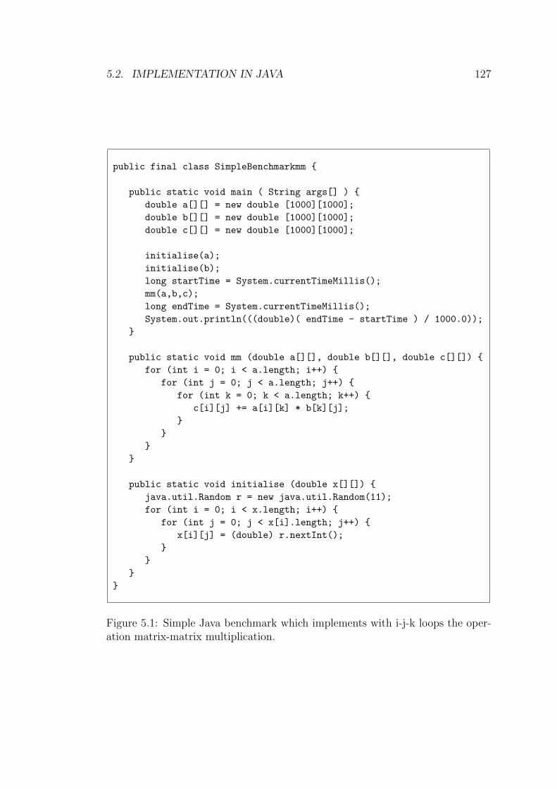
5.2. IMPLEMENTATION IN JAVA 127
public final class SimpleBenchmarkmm {
public static void main ( String args[] ) {double a[][] = new double [1000][1000];double b[][] = new double [1000][1000];double c[][] = new double [1000][1000];
initialise(a);initialise(b);long startTime = System.currentTimeMillis();mm(a,b,c);long endTime = System.currentTimeMillis();System.out.println(((double)( endTime - startTime ) / 1000.0));
}
public static void mm (double a[][], double b[][], double c[][]) {for (int i = 0; i < a.length; i++) {
for (int j = 0; j < a.length; j++) {for (int k = 0; k < a.length; k++) {
c[i][j] += a[i][k] * b[k][j];}
}}
}
public static void initialise (double x[][]) {java.util.Random r = new java.util.Random(11);for (int i = 0; i < x.length; i++) {
for (int j = 0; j < x[i].length; j++) {x[i][j] = (double) r.nextInt();
}}
}}
Figure 5.1: Simple Java benchmark which implements with i-j-k loops the oper-ation matrix-matrix multiplication.

5.2. IMPLEMENTATION IN JAVA 128
Times (s.) Windows Times (s.) SolarisJVM 1.0.2 860.13 2602.120JVM 1.1.8 009 57.79 1420.893JVM 1.2.2 013 54.99 496.819JVM 1.3.0 05 79.98 580.239JVM -client 1.3.1 04 296.21 641.279JVM -server 1.3.1 04 76.61 539.427JVM -client 1.4.0 78.45 586.405JVM -server 1.4.0 51.79 462.771
Windows is a 1GHz Pentium III with 256MB running Windows 2000 and service pack2. Solaris is a 333Mhz Sun Ultra-5 with 256Mb of memory running Solaris 5.8. Thetimes are measured in seconds (s.) and correspond to the minimum execution time outof 4 runs. The timer used on W2000 has an accuracy of 10 milliseconds and of onemillisecond on Solaris.
Figure 5.2: Performance results for the Java benchmark shown in Figure 5.1.
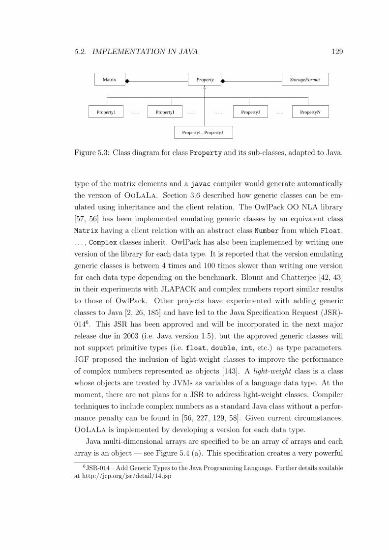
5.2. IMPLEMENTATION IN JAVA 129
Property
Property1
PropertyI...PropertyJ
StorageFormat
PropertyJ PropertyNPropertyI
Matrix
Figure 5.3: Class diagram for class Property and its sub-classes, adapted to Java.
type of the matrix elements and a javac compiler would generate automatically
the version of OoLaLa. Section 3.6 described how generic classes can be em-
ulated using inheritance and the client relation. The OwlPack OO NLA library
[57, 56] has been implemented emulating generic classes by an equivalent class
Matrix having a client relation with an abstract class Number from which Float,
. . . , Complex classes inherit. OwlPack has also been implemented by writing one
version of the library for each data type. It is reported that the version emulating
generic classes is between 4 times and 100 times slower than writing one version
for each data type depending on the benchmark. Blount and Chatterjee [42, 43]
in their experiments with JLAPACK and complex numbers report similar results
to those of OwlPack. Other projects have experimented with adding generic
classes to Java [2, 26, 185] and have led to the Java Specification Request (JSR)-
0146. This JSR has been approved and will be incorporated in the next major
release due in 2003 (i.e. Java version 1.5), but the approved generic classes will
not support primitive types (i.e. float, double, int, etc.) as type parameters.
JGF proposed the inclusion of light-weight classes to improve the performance
of complex numbers represented as objects [143]. A light-weight class is a class
whose objects are treated by JVMs as variables of a language data type. At the
moment, there are not plans for a JSR to address light-weight classes. Compiler
techniques to include complex numbers as a standard Java class without a perfor-
mance penalty can be found in [56, 227, 129, 58]. Given current circumstances,
OoLaLa is implemented by developing a version for each data type.
Java multi-dimensional arrays are specified to be an array of arrays and each
array is an object — see Figure 5.4 (a). This specification creates a very powerful
6JSR-014 – Add Generic Types to the Java Programming Language. Further details availableat http://jcp.org/jsr/detail/14.jsp
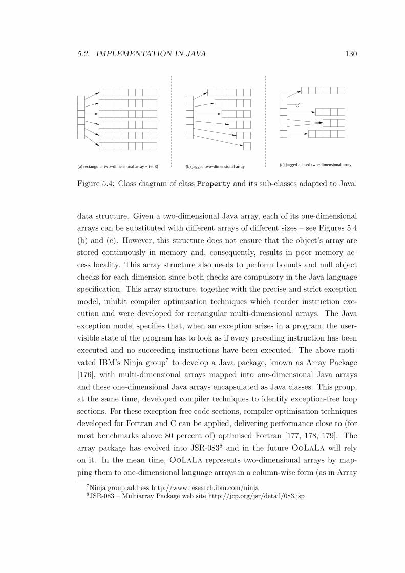
5.2. IMPLEMENTATION IN JAVA 130
(a) rectangular two−dimensional array − (6, 8) (b) jagged two−dimensional array (c) jagged aliased two−dimensional array
Figure 5.4: Class diagram of class Property and its sub-classes adapted to Java.
data structure. Given a two-dimensional Java array, each of its one-dimensional
arrays can be substituted with different arrays of different sizes – see Figures 5.4
(b) and (c). However, this structure does not ensure that the object’s array are
stored continuously in memory and, consequently, results in poor memory ac-
cess locality. This array structure also needs to perform bounds and null object
checks for each dimension since both checks are compulsory in the Java language
specification. This array structure, together with the precise and strict exception
model, inhibit compiler optimisation techniques which reorder instruction exe-
cution and were developed for rectangular multi-dimensional arrays. The Java
exception model specifies that, when an exception arises in a program, the user-
visible state of the program has to look as if every preceding instruction has been
executed and no succeeding instructions have been executed. The above moti-
vated IBM’s Ninja group7 to develop a Java package, known as Array Package
[176], with multi-dimensional arrays mapped into one-dimensional Java arrays
and these one-dimensional Java arrays encapsulated as Java classes. This group,
at the same time, developed compiler techniques to identify exception-free loop
sections. For these exception-free code sections, compiler optimisation techniques
developed for Fortran and C can be applied, delivering performance close to (for
most benchmarks above 80 percent of) optimised Fortran [177, 178, 179]. The
array package has evolved into JSR-0838 and in the future OoLaLa will rely
on it. In the mean time, OoLaLa represents two-dimensional arrays by map-
ping them to one-dimensional language arrays in a column-wise form (as in Array
7Ninja group address http://www.research.ibm.com/ninja8JSR-083 – Multiarray Package web site http://jcp.org/jsr/detail/083.jsp
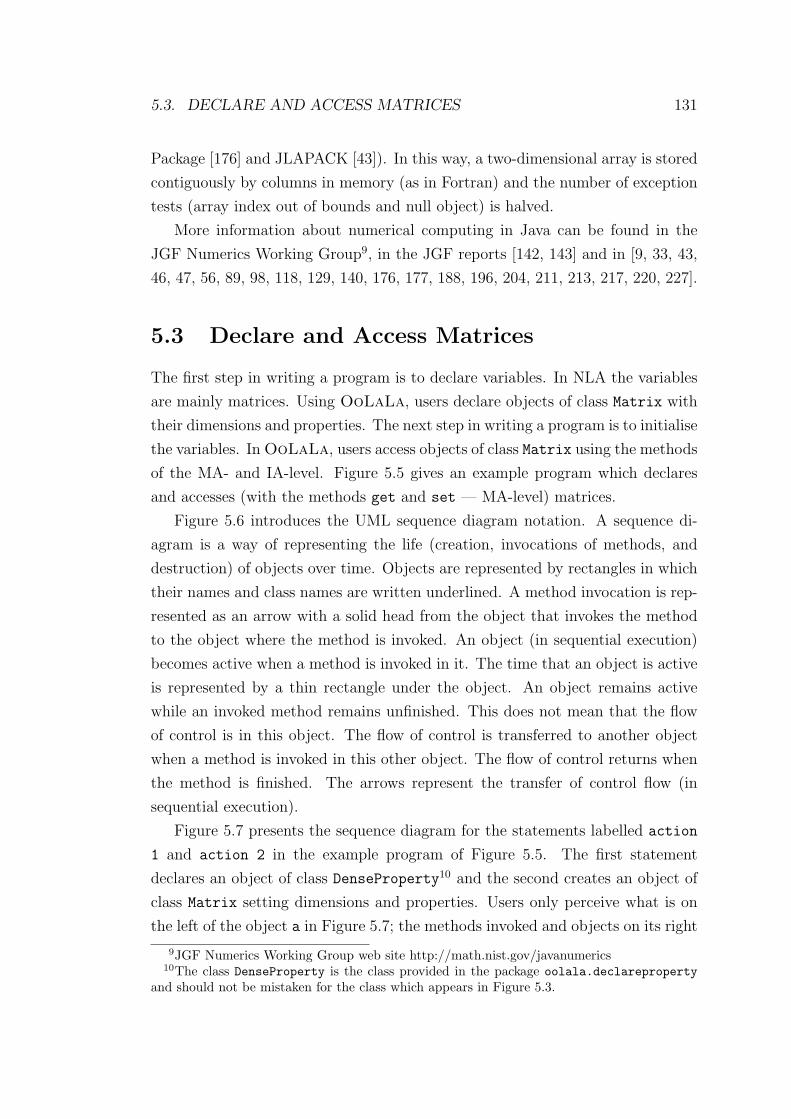
5.3. DECLARE AND ACCESS MATRICES 131
Package [176] and JLAPACK [43]). In this way, a two-dimensional array is stored
contiguously by columns in memory (as in Fortran) and the number of exception
tests (array index out of bounds and null object) is halved.
More information about numerical computing in Java can be found in the
JGF Numerics Working Group9, in the JGF reports [142, 143] and in [9, 33, 43,
46, 47, 56, 89, 98, 118, 129, 140, 176, 177, 188, 196, 204, 211, 213, 217, 220, 227].
5.3 Declare and Access Matrices
The first step in writing a program is to declare variables. In NLA the variables
are mainly matrices. Using OoLaLa, users declare objects of class Matrix with
their dimensions and properties. The next step in writing a program is to initialise
the variables. In OoLaLa, users access objects of class Matrix using the methods
of the MA- and IA-level. Figure 5.5 gives an example program which declares
and accesses (with the methods get and set — MA-level) matrices.
Figure 5.6 introduces the UML sequence diagram notation. A sequence di-
agram is a way of representing the life (creation, invocations of methods, and
destruction) of objects over time. Objects are represented by rectangles in which
their names and class names are written underlined. A method invocation is rep-
resented as an arrow with a solid head from the object that invokes the method
to the object where the method is invoked. An object (in sequential execution)
becomes active when a method is invoked in it. The time that an object is active
is represented by a thin rectangle under the object. An object remains active
while an invoked method remains unfinished. This does not mean that the flow
of control is in this object. The flow of control is transferred to another object
when a method is invoked in this other object. The flow of control returns when
the method is finished. The arrows represent the transfer of control flow (in
sequential execution).
Figure 5.7 presents the sequence diagram for the statements labelled action
1 and action 2 in the example program of Figure 5.5. The first statement
declares an object of class DenseProperty10 and the second creates an object of
class Matrix setting dimensions and properties. Users only perceive what is on
the left of the object a in Figure 5.7; the methods invoked and objects on its right
9JGF Numerics Working Group web site http://math.nist.gov/javanumerics10The class DenseProperty is the class provided in the package oolala.declareproperty
and should not be mistaken for the class which appears in Figure 5.3.
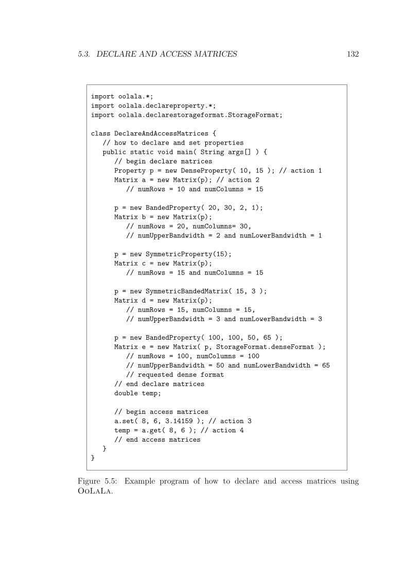
5.3. DECLARE AND ACCESS MATRICES 132
import oolala.*;import oolala.declareproperty.*;import oolala.declarestorageformat.StorageFormat;
class DeclareAndAccessMatrices {// how to declare and set propertiespublic static void main( String args[] ) {
// begin declare matricesProperty p = new DenseProperty( 10, 15 ); // action 1Matrix a = new Matrix(p); // action 2
// numRows = 10 and numColumns = 15
p = new BandedProperty( 20, 30, 2, 1);Matrix b = new Matrix(p);
// numRows = 20, numColumns= 30,// numUpperBandwidth = 2 and numLowerBandwidth = 1
p = new SymmetricProperty(15);Matrix c = new Matrix(p);
// numRows = 15 and numColumns = 15
p = new SymmetricBandedMatrix( 15, 3 );Matrix d = new Matrix(p);
// numRows = 15, numColumns = 15,// numUpperBandwidth = 3 and numLowerBandwidth = 3
p = new BandedProperty( 100, 100, 50, 65 );Matrix e = new Matrix( p, StorageFormat.denseFormat );
// numRows = 100, numColumns = 100// numUpperBandwidth = 50 and numLowerBandwidth = 65// requested dense format
// end declare matricesdouble temp;
// begin access matricesa.set( 8, 6, 3.14159 ); // action 3temp = a.get( 8, 6 ); // action 4// end access matrices
}}
Figure 5.5: Example program of how to declare and access matrices usingOoLaLa.
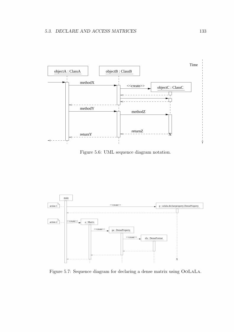
5.3. DECLARE AND ACCESS MATRICES 133
objectB : ClassBobjectA : ClassA
<<create>>methodX
methodY
returnY
objectC : ClassC
methodZ
returnZX
Time
Figure 5.6: UML sequence diagram notation.
X
action 1
<<create>> a : Matrixaction 2
main
<<create>> p : oolala.declareproperty.DenseProperty
<<create>>
<<create>> sfa : DenseFormat
pa : DenseProperty
Figure 5.7: Sequence diagram for declaring a dense matrix using OoLaLa.
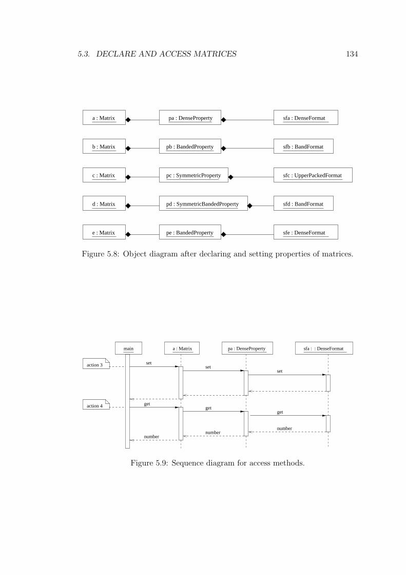
5.3. DECLARE AND ACCESS MATRICES 134
sfe : DenseFormat
a : Matrix
c : Matrix
b : Matrix
d : Matrix
e : Matrix
sfd : BandFormat
sfc : UpperPackedFormat
sfb : BandFormat
sfa : DenseFormat
pe : BandedProperty
pc : SymmetricProperty
pd : SymmetricBandedProperty
pa : DenseProperty
pb : BandedProperty
Figure 5.8: Object diagram after declaring and setting properties of matrices.
action 3
action 4
main a : Matrix sfa : : DenseFormat
numbernumber
number
pa : DenseProperty
setset
set
getget
get
Figure 5.9: Sequence diagram for access methods.
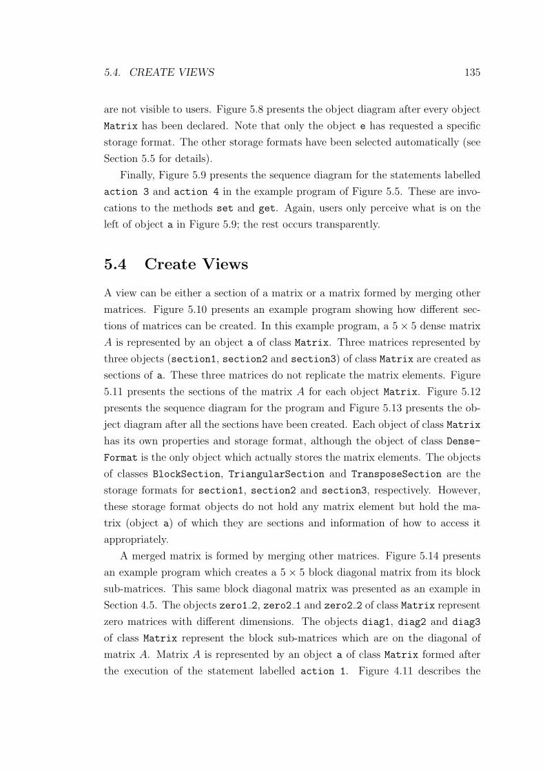
5.4. CREATE VIEWS 135
are not visible to users. Figure 5.8 presents the object diagram after every object
Matrix has been declared. Note that only the object e has requested a specific
storage format. The other storage formats have been selected automatically (see
Section 5.5 for details).
Finally, Figure 5.9 presents the sequence diagram for the statements labelled
action 3 and action 4 in the example program of Figure 5.5. These are invo-
cations to the methods set and get. Again, users only perceive what is on the
left of object a in Figure 5.9; the rest occurs transparently.
5.4 Create Views
A view can be either a section of a matrix or a matrix formed by merging other
matrices. Figure 5.10 presents an example program showing how different sec-
tions of matrices can be created. In this example program, a 5× 5 dense matrix
A is represented by an object a of class Matrix. Three matrices represented by
three objects (section1, section2 and section3) of class Matrix are created as
sections of a. These three matrices do not replicate the matrix elements. Figure
5.11 presents the sections of the matrix A for each object Matrix. Figure 5.12
presents the sequence diagram for the program and Figure 5.13 presents the ob-
ject diagram after all the sections have been created. Each object of class Matrix
has its own properties and storage format, although the object of class Dense-
Format is the only object which actually stores the matrix elements. The objects
of classes BlockSection, TriangularSection and TransposeSection are the
storage formats for section1, section2 and section3, respectively. However,
these storage format objects do not hold any matrix element but hold the ma-
trix (object a) of which they are sections and information of how to access it
appropriately.
A merged matrix is formed by merging other matrices. Figure 5.14 presents
an example program which creates a 5 × 5 block diagonal matrix from its block
sub-matrices. This same block diagonal matrix was presented as an example in
Section 4.5. The objects zero1 2, zero2 1 and zero2 2 of class Matrix represent
zero matrices with different dimensions. The objects diag1, diag2 and diag3
of class Matrix represent the block sub-matrices which are on the diagonal of
matrix A. Matrix A is represented by an object a of class Matrix formed after
the execution of the statement labelled action 1. Figure 4.11 describes the
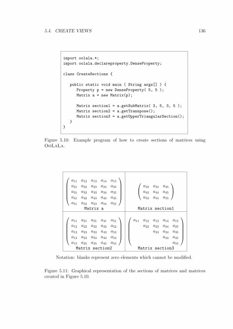
5.4. CREATE VIEWS 136
import oolala.*;import oolala.declareproperty.DenseProperty;
class CreateSections {
public static void main ( String args[] ) {Property p = new DenseProperty( 5, 5 );Matrix a = new Matrix(p);
Matrix section1 = a.getSubMatrix( 3, 5, 3, 5 );Matrix section2 = a.getTranspose();Matrix section3 = a.getUpperTriangularSection();
}}
Figure 5.10: Example program of how to create sections of matrices usingOoLaLa.
a11 a12 a13 a14 a15
a21 a22 a23 a24 a25
a31 a32 a33 a34 a35
a41 a42 a43 a44 a45
a51 a52 a53 a54 a55
a33 a34 a35
a43 a44 a45
a53 a54 a55
Matrix a Matrix section1
a11 a21 a31 a41 a51
a12 a22 a32 a42 a52
a13 a23 a33 a43 a53
a14 a24 a34 a44 a54
a15 a25 a35 a45 a55
a11 a12 a13 a14 a15
a22 a23 a24 a25
a33 a34 a35
a44 a45
a55
Matrix section2 Matrix section3
Notation: blanks represent zero elements which cannot be modified.
Figure 5.11: Graphical representation of the sections of matrices and matricescreated in Figure 5.10.

5.4. CREATE VIEWS 137
<<
crea
te>
>
<<
crea
te>
>
<<
crea
te>
>
ps3
: Den
sePr
oper
ty
ps2
: Upp
erT
rian
gula
rPro
pert
y
ps1
: Den
sePr
oper
ty
ss3
: Tra
nspo
seSe
ctio
n
ss1
: Blo
ckSe
ctio
n
ss2
: Tri
angu
larS
ectio
n
<<
crea
te>
>
<<
crea
te>
>ge
tTra
nspo
se
<<
crea
te>
>
<<
crea
te>
>
getU
pper
Tri
angu
lar
<<
crea
te>
>
<<
crea
te>
>
a : M
atri
x
getS
ubM
atri
x
mai
n
sect
ion3
: M
atri
x
sect
ion2
: M
atri
x
sect
ion1
: M
atri
x
Figure 5.12: Sequence diagram for the sections created in Figure 5.10.
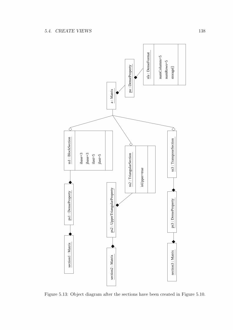
5.4. CREATE VIEWS 138
num
Row
s=5
pa :
Den
sePr
oper
ty
ps3
: Den
sePr
oper
ty
ps2
: Upp
erT
rian
gula
rPro
pert
y
sfa
: Den
seFo
rmat
stor
age[
]
num
Col
umns
=5
ss1
: Blo
ckSe
ctio
n
sect
ion2
: M
atri
x
sect
ion3
: M
atri
xss
3 : T
rans
pose
Sect
ion
a : M
atri
x
ibas
e=3
isU
pper
=tr
ue
ss2
: Tri
angu
larS
ectio
n
ps1
: Den
sePr
oper
tyse
ctio
n1 :
Mat
rix
jlast
=5
ilast
=5
jbas
e=3
Figure 5.13: Object diagram after the sections have been created in Figure 5.10.
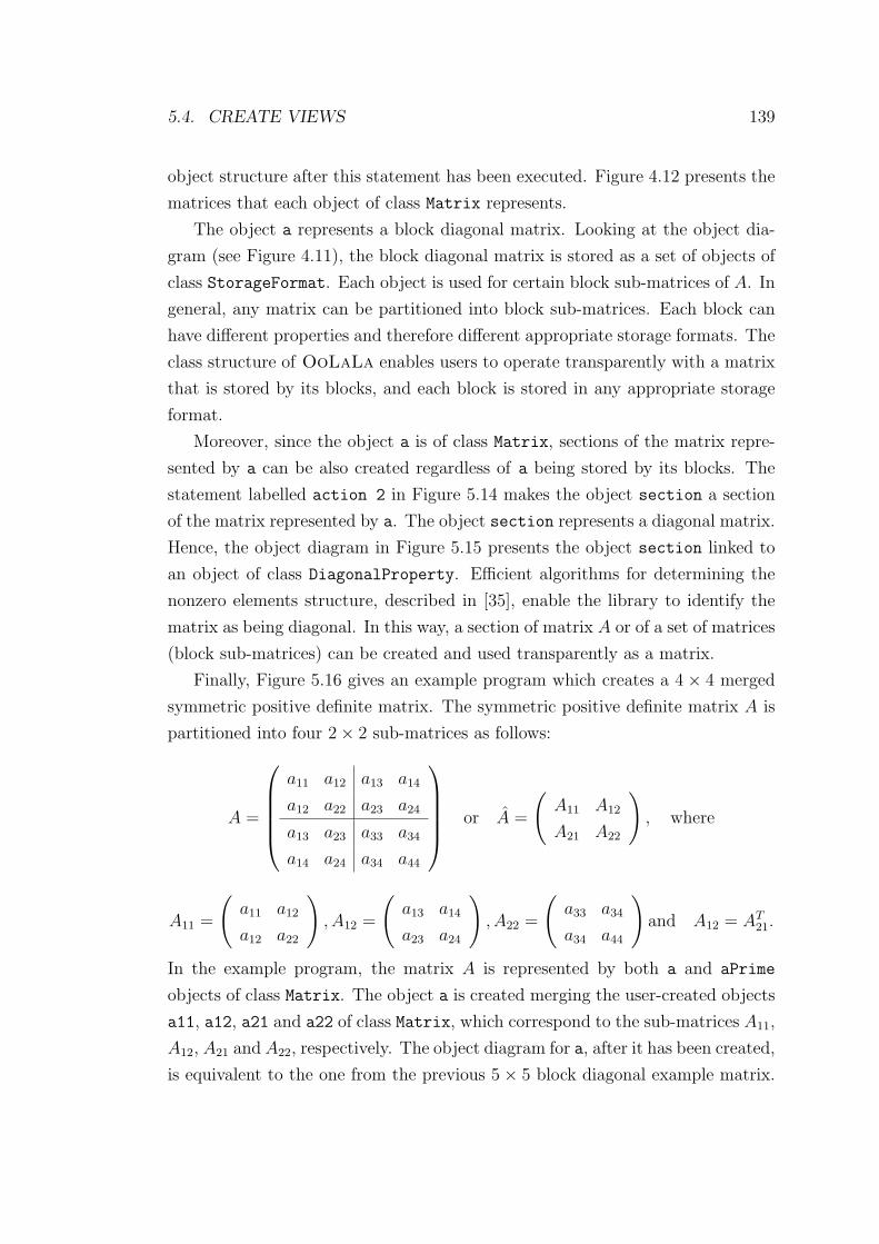
5.4. CREATE VIEWS 139
object structure after this statement has been executed. Figure 4.12 presents the
matrices that each object of class Matrix represents.
The object a represents a block diagonal matrix. Looking at the object dia-
gram (see Figure 4.11), the block diagonal matrix is stored as a set of objects of
class StorageFormat. Each object is used for certain block sub-matrices of A. In
general, any matrix can be partitioned into block sub-matrices. Each block can
have different properties and therefore different appropriate storage formats. The
class structure of OoLaLa enables users to operate transparently with a matrix
that is stored by its blocks, and each block is stored in any appropriate storage
format.
Moreover, since the object a is of class Matrix, sections of the matrix repre-
sented by a can be also created regardless of a being stored by its blocks. The
statement labelled action 2 in Figure 5.14 makes the object section a section
of the matrix represented by a. The object section represents a diagonal matrix.
Hence, the object diagram in Figure 5.15 presents the object section linked to
an object of class DiagonalProperty. Efficient algorithms for determining the
nonzero elements structure, described in [35], enable the library to identify the
matrix as being diagonal. In this way, a section of matrix A or of a set of matrices
(block sub-matrices) can be created and used transparently as a matrix.
Finally, Figure 5.16 gives an example program which creates a 4 × 4 merged
symmetric positive definite matrix. The symmetric positive definite matrix A is
partitioned into four 2× 2 sub-matrices as follows:
A =
a11 a12 a13 a14
a12 a22 a23 a24
a13 a23 a33 a34
a14 a24 a34 a44
or A =
(A11 A12
A21 A22
), where
A11 =
(a11 a12
a12 a22
), A12 =
(a13 a14
a23 a24
), A22 =
(a33 a34
a34 a44
)and A12 = AT
21.
In the example program, the matrix A is represented by both a and aPrime
objects of class Matrix. The object a is created merging the user-created objects
a11, a12, a21 and a22 of class Matrix, which correspond to the sub-matrices A11,
A12, A21 and A22, respectively. The object diagram for a, after it has been created,
is equivalent to the one from the previous 5× 5 block diagonal example matrix.
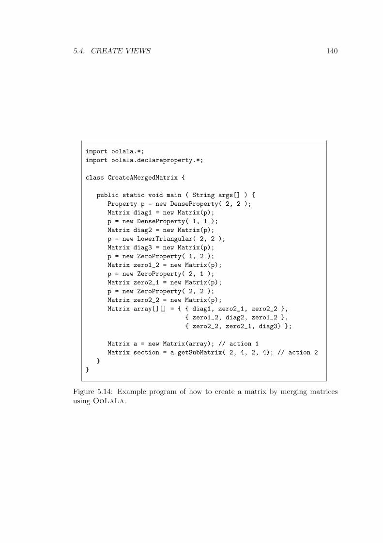
5.4. CREATE VIEWS 140
import oolala.*;import oolala.declareproperty.*;
class CreateAMergedMatrix {
public static void main ( String args[] ) {Property p = new DenseProperty( 2, 2 );Matrix diag1 = new Matrix(p);p = new DenseProperty( 1, 1 );Matrix diag2 = new Matrix(p);p = new LowerTriangular( 2, 2 );Matrix diag3 = new Matrix(p);p = new ZeroProperty( 1, 2 );Matrix zero1_2 = new Matrix(p);p = new ZeroProperty( 2, 1 );Matrix zero2_1 = new Matrix(p);p = new ZeroProperty( 2, 2 );Matrix zero2_2 = new Matrix(p);Matrix array[][] = { { diag1, zero2_1, zero2_2 },
{ zero1_2, diag2, zero1_2 },{ zero2_2, zero2_1, diag3} };
Matrix a = new Matrix(array); // action 1Matrix section = a.getSubMatrix( 2, 4, 2, 4); // action 2
}}
Figure 5.14: Example program of how to create a matrix by merging matricesusing OoLaLa.
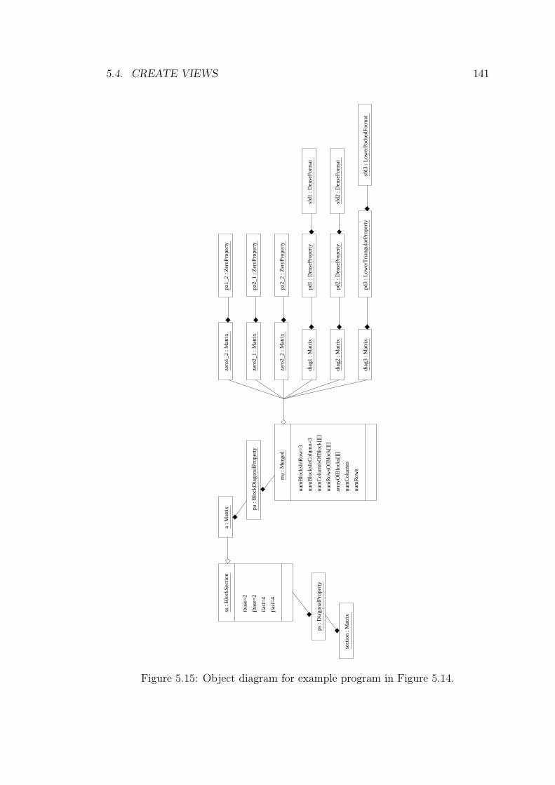
5.4. CREATE VIEWS 141
jbas
e=2
ilast
=4
pd3
: Low
erT
rian
gula
rPro
pert
y
pd2
: Den
sePr
oper
ty
pd1
: Den
sePr
oper
ty
pz2_
2 : Z
eroP
rope
rty
pz2_
1 : Z
eroP
rope
rty
pz1_
2 : Z
eroP
rope
rty
pa :
Blo
ckD
iago
nalP
rope
rty
ps :
Dia
gona
lPro
pert
y
num
Row
s
num
Col
umns
arra
yOfB
lock
s[][
]
num
Col
umns
OfB
lock
[][]
num
Row
sOfB
lock
[][]
num
Blo
cksI
nCol
umn=
3
num
Blo
cksI
nRow
=3
sfd3
: L
ower
Pack
edFo
rmat
sfd2
: D
ense
Form
at
sfd1
: D
ense
Form
at
diag
3 : M
atri
x
diag
2 : M
atri
x
diag
1 : M
atri
x
zero
2_2
: Mat
rix
zero
2_1
: Mat
rix
zero
1_2
: Mat
rix
ss :
Blo
ckSe
ctio
n
ibas
e=2
jlast
=4
sect
ion
: Mat
rix
ma
: Mer
ged
a : M
atri
x
Figure 5.15: Object diagram for example program in Figure 5.14.
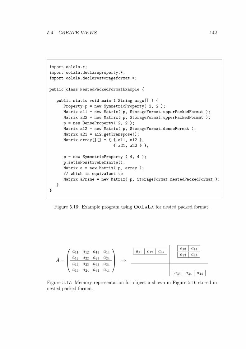
5.4. CREATE VIEWS 142
import oolala.*;import oolala.declareproperty.*;import oolala.declarestorageformat.*;
public class NestedPackedFormatExample {
public static void main ( String args[] ) {Property p = new SymmetricProperty( 2, 2 );Matrix a11 = new Matrix( p, StorageFormat.upperPackedFormat );Matrix a22 = new Matrix( p, StorageFormat.upperPackedFormat );p = new DenseProperty( 2, 2 );Matrix a12 = new Matrix( p, StorageFormat.denseFormat );Matrix a21 = a12.getTranspose();Matrix array[][] = { { a11, a12 },
{ a21, a22 } };
p = new SymmetricProperty ( 4, 4 );p.setIsPositiveDefinite();Matrix a = new Matrix( p, array );// which is equivalent toMatrix aPrime = new Matrix( p, StorageFormat.nestedPackedFormat );
}}
Figure 5.16: Example program using OoLaLa for nested packed format.
A =
a11 a12 a13 a14
a12 a22 a23 a24
a13 a23 a33 a34
a14 a24 a34 a44
⇒
a11 a12 a22a13 a14
a23 a24
a33 a34 a44
Figure 5.17: Memory representation for object a shown in Figure 5.16 stored innested packed format.
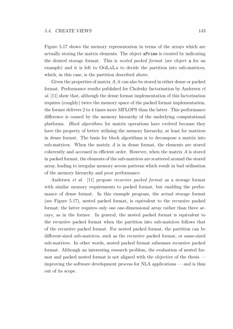
5.4. CREATE VIEWS 143
Figure 5.17 shows the memory representation in terms of the arrays which are
actually storing the matrix elements. The object aPrime is created by indicating
the desired storage format. This is nested packed format (see object a for an
example) and it is left to OoLaLa to decide the partition into sub-matrices,
which, in this case, is the partition described above.
Given the properties of matrix A, it can also be stored in either dense or packed
format. Performance results published for Cholesky factorisation by Andersen et
al. [11] show that, although the dense format implementation of this factorisation
requires (roughly) twice the memory space of the packed format implementation,
the former delivers 2 to 4 times more MFLOPS than the latter. This performance
difference is caused by the memory hierarchy of the underlying computational
platforms. Block algorithms for matrix operations have evolved because they
have the property of better utilising the memory hierarchy, at least for matrices
in dense format. The basis for block algorithms is to decompose a matrix into
sub-matrices. When the matrix A is in dense format, the elements are stored
coherently and accessed in efficient order. However, when the matrix A is stored
in packed format, the elements of the sub-matrices are scattered around the stored
array, leading to irregular memory access patterns which result in bad utilisation
of the memory hierarchy and poor performance.
Andersen et al. [11] propose recursive packed format as a storage format
with similar memory requirements to packed format, but enabling the perfor-
mance of dense format. In this example program, the actual storage format
(see Figure 5.17), nested packed format, is equivalent to the recursive packed
format; the latter requires only one one-dimensional array rather than three ar-
rays, as in the former. In general, the nested packed format is equivalent to
the recursive packed format when the partition into sub-matrices follows that
of the recursive packed format. For nested packed format, the partition can be
different-sized sub-matrices, such as the recursive packed format, or same-sized
sub-matrices. In other words, nested packed format subsumes recursive packed
format. Although an interesting research problem, the evaluation of nested for-
mat and packed nested format is not aligned with the objective of the thesis —
improving the software development process for NLA applications — and is thus
out of its scope.

5.5. MANAGEMENT OF PROPERTIES AND STORAGE FORMATS 144
5.5 Management of Properties and Storage For-
mats
Before invoking any matrix operation that changes the matrix elements, OoLaLa
decides whether the storage format and properties need to be changed. Consider,
for example, the addition C ← A+B where A and B are tridiagonal matrices and
C is a bidiagonal matrix. After performing the addition C also becomes tridiago-
nal. A program using OoLaLa would create objects a, b, c of class Matrix and
set the correspondent properties of each matrix. The program would continue
with the statement c.addInto(a,b). This method, invoked in c, would change
its linked object of class BidiagonalProperty to be one of class Tridiagonal-
Property. Depending on the class of the linked object that represents the storage
format, different action could be taken. Suppose the actual storage format is large
enough to store the extra elements that will be created and it is appropriate to
have the result matrix in this storage format, then no action is needed. This
would be the case if c were linked with an object of class DenseFormat. Oth-
erwise (either the storage format is not large enough or it is not appropriate to
store the result matrix in that storage format), the linked object representing the
storage format would be changed.
The following paragraphs explain how to select a storage format for a given
property, how to detect inconsistency between properties and storage formats,
and how consistency is recovered. The description is limited to a subset of prop-
erties — dense (de), banded (ba), symmetric (sy), symmetric banded (sb), upper
triangular (ut), and lower triangular (lt) — and a subset of storage formats —
dense (df), band (bf), upper packed (upf) and lower packed (lpf).
The first question to answer is how OoLaLa chooses a storage format for a
matrix with given properties. Table 5.1 presents recommended storage formats
for each matrix property as a set of static “if-then” rules. The rules select,
whenever possible, a storage format which uses the least memory space. Note
that some rules can choose between band format and another format. The band
format is selected when the upper bandwidth and lower bandwidth are less than
one quarter of the number of columns and number of rows, respectively. This
condition is an initial guess that needs validation by experiment.
The second question is how to detect inconsistency between matrix properties
and storage formats. An inconsistent situation can only arise when a user sets a
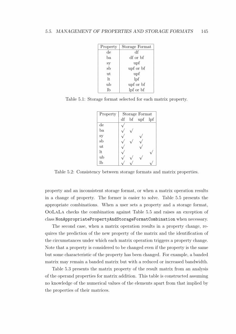
5.5. MANAGEMENT OF PROPERTIES AND STORAGE FORMATS 145
Property Storage Formatde dfba df or bfsy upfsb upf or bfut upflt lpfub upf or bflb lpf or bf
Table 5.1: Storage format selected for each matrix property.
Property Storage Formatdf bf upf lpf
de√
ba√ √
sy√ √
sb√ √ √
ut√ √
lt√ √
ub√ √ √
lb√ √ √
Table 5.2: Consistency between storage formats and matrix properties.
property and an inconsistent storage format, or when a matrix operation results
in a change of property. The former is easier to solve. Table 5.5 presents the
appropriate combinations. When a user sets a property and a storage format,
OoLaLa checks the combination against Table 5.5 and raises an exception of
class NonAppropriatePropertyAndStorageFormatCombination when necessary.
The second case, when a matrix operation results in a property change, re-
quires the prediction of the new property of the matrix and the identification of
the circumstances under which each matrix operation triggers a property change.
Note that a property is considered to be changed even if the property is the same
but some characteristic of the property has been changed. For example, a banded
matrix may remain a banded matrix but with a reduced or increased bandwidth.
Table 5.3 presents the matrix property of the result matrix from an analysis
of the operand properties for matrix addition. This table is constructed assuming
no knowledge of the numerical values of the elements apart from that implied by
the properties of their matrices.
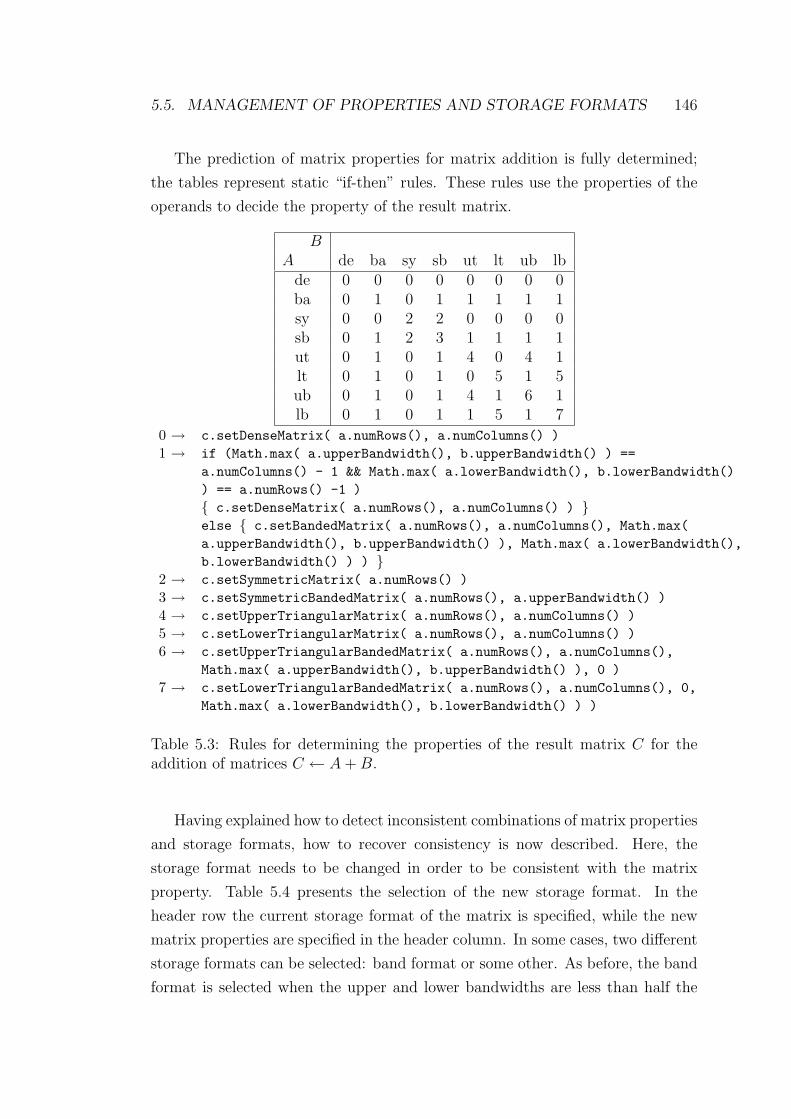
5.5. MANAGEMENT OF PROPERTIES AND STORAGE FORMATS 146
The prediction of matrix properties for matrix addition is fully determined;
the tables represent static “if-then” rules. These rules use the properties of the
operands to decide the property of the result matrix.
BA de ba sy sb ut lt ub lb
de 0 0 0 0 0 0 0 0ba 0 1 0 1 1 1 1 1sy 0 0 2 2 0 0 0 0sb 0 1 2 3 1 1 1 1ut 0 1 0 1 4 0 4 1lt 0 1 0 1 0 5 1 5ub 0 1 0 1 4 1 6 1lb 0 1 0 1 1 5 1 7
0 → c.setDenseMatrix( a.numRows(), a.numColumns() )1 → if (Math.max( a.upperBandwidth(), b.upperBandwidth() ) ==
a.numColumns() - 1 && Math.max( a.lowerBandwidth(), b.lowerBandwidth()) == a.numRows() -1 ){ c.setDenseMatrix( a.numRows(), a.numColumns() ) }else { c.setBandedMatrix( a.numRows(), a.numColumns(), Math.max(a.upperBandwidth(), b.upperBandwidth() ), Math.max( a.lowerBandwidth(),b.lowerBandwidth() ) ) }
2 → c.setSymmetricMatrix( a.numRows() )3 → c.setSymmetricBandedMatrix( a.numRows(), a.upperBandwidth() )4 → c.setUpperTriangularMatrix( a.numRows(), a.numColumns() )5 → c.setLowerTriangularMatrix( a.numRows(), a.numColumns() )6 → c.setUpperTriangularBandedMatrix( a.numRows(), a.numColumns(),
Math.max( a.upperBandwidth(), b.upperBandwidth() ), 0 )7 → c.setLowerTriangularBandedMatrix( a.numRows(), a.numColumns(), 0,
Math.max( a.lowerBandwidth(), b.lowerBandwidth() ) )
Table 5.3: Rules for determining the properties of the result matrix C for theaddition of matrices C ← A + B.
Having explained how to detect inconsistent combinations of matrix properties
and storage formats, how to recover consistency is now described. Here, the
storage format needs to be changed in order to be consistent with the matrix
property. Table 5.4 presents the selection of the new storage format. In the
header row the current storage format of the matrix is specified, while the new
matrix properties are specified in the header column. In some cases, two different
storage formats can be selected: band format or some other. As before, the band
format is selected when the upper and lower bandwidths are less than half the
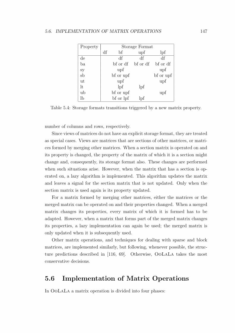
5.6. IMPLEMENTATION OF MATRIX OPERATIONS 147
Property Storage Formatdf bf upf lpf
de df df dfba bf or df bf or df bf or dfsy upf upfsb bf or upf bf or upfut upf upflt lpf lpfub bf or upf upflb bf or lpf lpf
Table 5.4: Storage formats transitions triggered by a new matrix property.
number of columns and rows, respectively.
Since views of matrices do not have an explicit storage format, they are treated
as special cases. Views are matrices that are sections of other matrices, or matri-
ces formed by merging other matrices. When a section matrix is operated on and
its property is changed, the property of the matrix of which it is a section might
change and, consequently, its storage format also. These changes are performed
when such situations arise. However, when the matrix that has a section is op-
erated on, a lazy algorithm is implemented. This algorithm updates the matrix
and leaves a signal for the section matrix that is not updated. Only when the
section matrix is used again is its property updated.
For a matrix formed by merging other matrices, either the matrices or the
merged matrix can be operated on and their properties changed. When a merged
matrix changes its properties, every matrix of which it is formed has to be
adapted. However, when a matrix that forms part of the merged matrix changes
its properties, a lazy implementation can again be used; the merged matrix is
only updated when it is subsequently used.
Other matrix operations, and techniques for dealing with sparse and block
matrices, are implemented similarly, but following, whenever possible, the struc-
ture predictions described in [116, 69]. Otherwise, OoLaLa takes the most
conservative decisions.
5.6 Implementation of Matrix Operations
In OoLaLa a matrix operation is divided into four phases:
5.6. IMPLEMENTATION OF MATRIX OPERATIONS 148
• select the appropriate functionality;
• check correctness of parameters;
• predict the properties of the result matrix; and
• execute the specialised implementation of the matrix operation.
Matrix operations are defined only for certain (conformable) matrices. For
example, the addition of matrices is defined only for matrices that have the same
number of rows and columns. Similarly, the matrix-matrix multiplication C ←AB is defined only for A an n × k matrix and B a k × m matrix. These tests
are straightforward to implement and are, therefore, omitted in the following
description. Simply note that the test is performed before any of the instructions
of the matrix operation implementation are executed. When the test fails, an
exception is raised and the matrices are left unmodified.
In traditional NLA libraries, users have to select a subroutine that implements
the matrix operation for matrices with certain properties and certain storage for-
mats. Since OoLaLa encapsulates, whenever possible, the different implemen-
tations behind a single method, a selection algorithm is needed.
5.6.1 Different Abstraction Levels
The operation norm1 (||A||1) is used to illustrate how MA-level and IA-level
can reduce the number of implementations compared with SFA-level. Among
the different possible combinations of storage formats and matrix properties, the
following combinations are selected to illustrate the abstraction levels for the
operation ||A||1:
• A is a dense matrix stored in dense format;
• A is an upper triangular matrix stored in dense format; and
• A is an upper triangular matrix stored in packed format.
Figures 5.18, 5.19 and 5.20 present implementations of ||A||1 at SFA-level.
Note that these implementations use two-dimensional Java arrays for the sake
of clarity (on the right hand side of Figure 5.18 the same implementation is
presented but the arrays are mapped into one-dimensional Java arrays). Since an
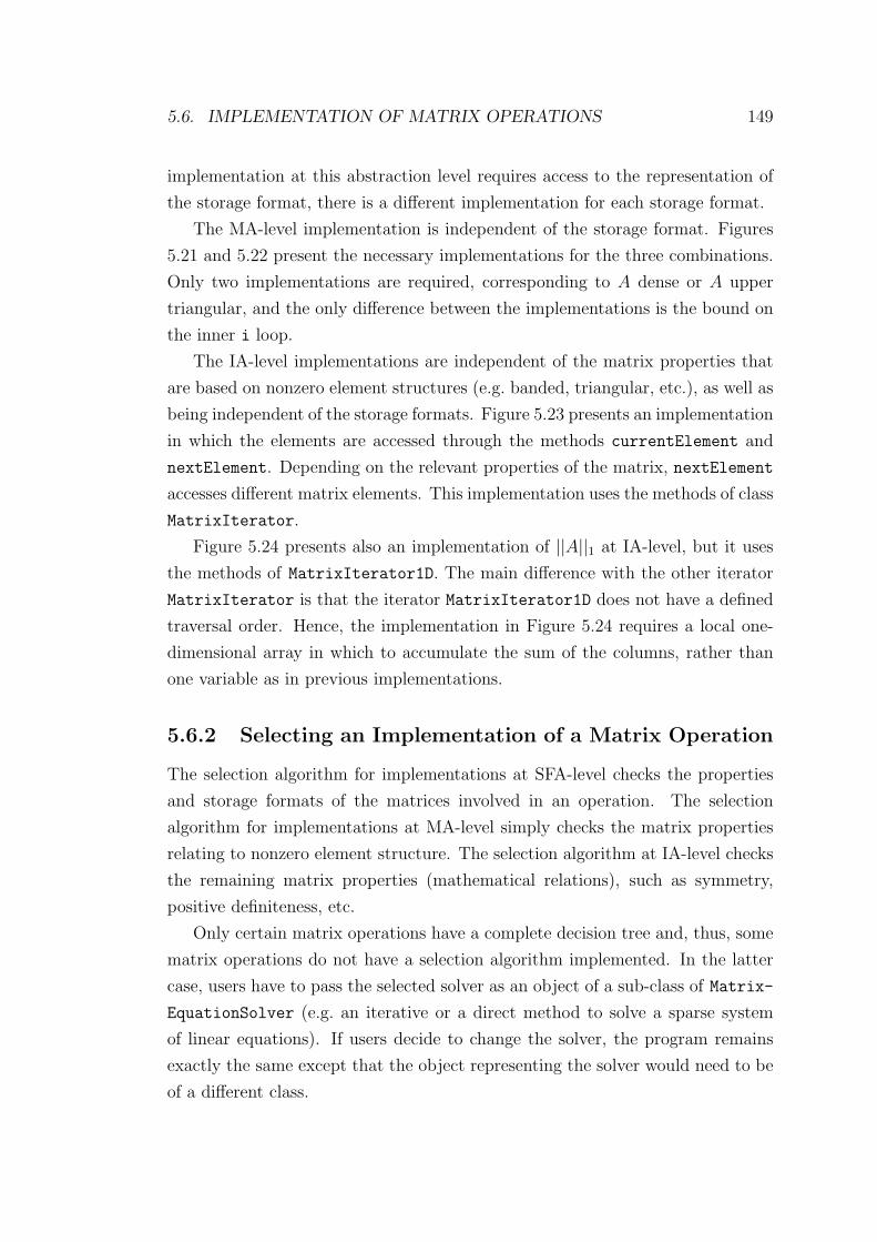
5.6. IMPLEMENTATION OF MATRIX OPERATIONS 149
implementation at this abstraction level requires access to the representation of
the storage format, there is a different implementation for each storage format.
The MA-level implementation is independent of the storage format. Figures
5.21 and 5.22 present the necessary implementations for the three combinations.
Only two implementations are required, corresponding to A dense or A upper
triangular, and the only difference between the implementations is the bound on
the inner i loop.
The IA-level implementations are independent of the matrix properties that
are based on nonzero element structures (e.g. banded, triangular, etc.), as well as
being independent of the storage formats. Figure 5.23 presents an implementation
in which the elements are accessed through the methods currentElement and
nextElement. Depending on the relevant properties of the matrix, nextElement
accesses different matrix elements. This implementation uses the methods of class
MatrixIterator.
Figure 5.24 presents also an implementation of ||A||1 at IA-level, but it uses
the methods of MatrixIterator1D. The main difference with the other iterator
MatrixIterator is that the iterator MatrixIterator1D does not have a defined
traversal order. Hence, the implementation in Figure 5.24 requires a local one-
dimensional array in which to accumulate the sum of the columns, rather than
one variable as in previous implementations.
5.6.2 Selecting an Implementation of a Matrix Operation
The selection algorithm for implementations at SFA-level checks the properties
and storage formats of the matrices involved in an operation. The selection
algorithm for implementations at MA-level simply checks the matrix properties
relating to nonzero element structure. The selection algorithm at IA-level checks
the remaining matrix properties (mathematical relations), such as symmetry,
positive definiteness, etc.
Only certain matrix operations have a complete decision tree and, thus, some
matrix operations do not have a selection algorithm implemented. In the latter
case, users have to pass the selected solver as an object of a sub-class of Matrix-
EquationSolver (e.g. an iterative or a direct method to solve a sparse system
of linear equations). If users decide to change the solver, the program remains
exactly the same except that the object representing the solver would need to be
of a different class.
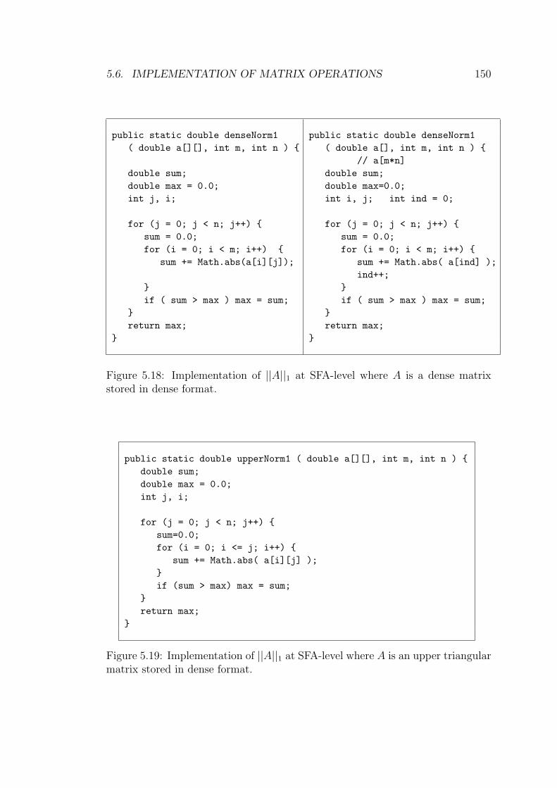
5.6. IMPLEMENTATION OF MATRIX OPERATIONS 150
public static double denseNorm1( double a[][], int m, int n ) {
double sum;double max = 0.0;int j, i;
for (j = 0; j < n; j++) {sum = 0.0;for (i = 0; i < m; i++) {
sum += Math.abs(a[i][j]);
}if ( sum > max ) max = sum;
}return max;
}
public static double denseNorm1( double a[], int m, int n ) {
// a[m*n]double sum;double max=0.0;int i, j; int ind = 0;
for (j = 0; j < n; j++) {sum = 0.0;for (i = 0; i < m; i++) {
sum += Math.abs( a[ind] );ind++;
}if ( sum > max ) max = sum;
}return max;
}
Figure 5.18: Implementation of ||A||1 at SFA-level where A is a dense matrixstored in dense format.
public static double upperNorm1 ( double a[][], int m, int n ) {double sum;double max = 0.0;int j, i;
for (j = 0; j < n; j++) {sum=0.0;for (i = 0; i <= j; i++) {
sum += Math.abs( a[i][j] );}if (sum > max) max = sum;
}return max;
}
Figure 5.19: Implementation of ||A||1 at SFA-level where A is an upper triangularmatrix stored in dense format.
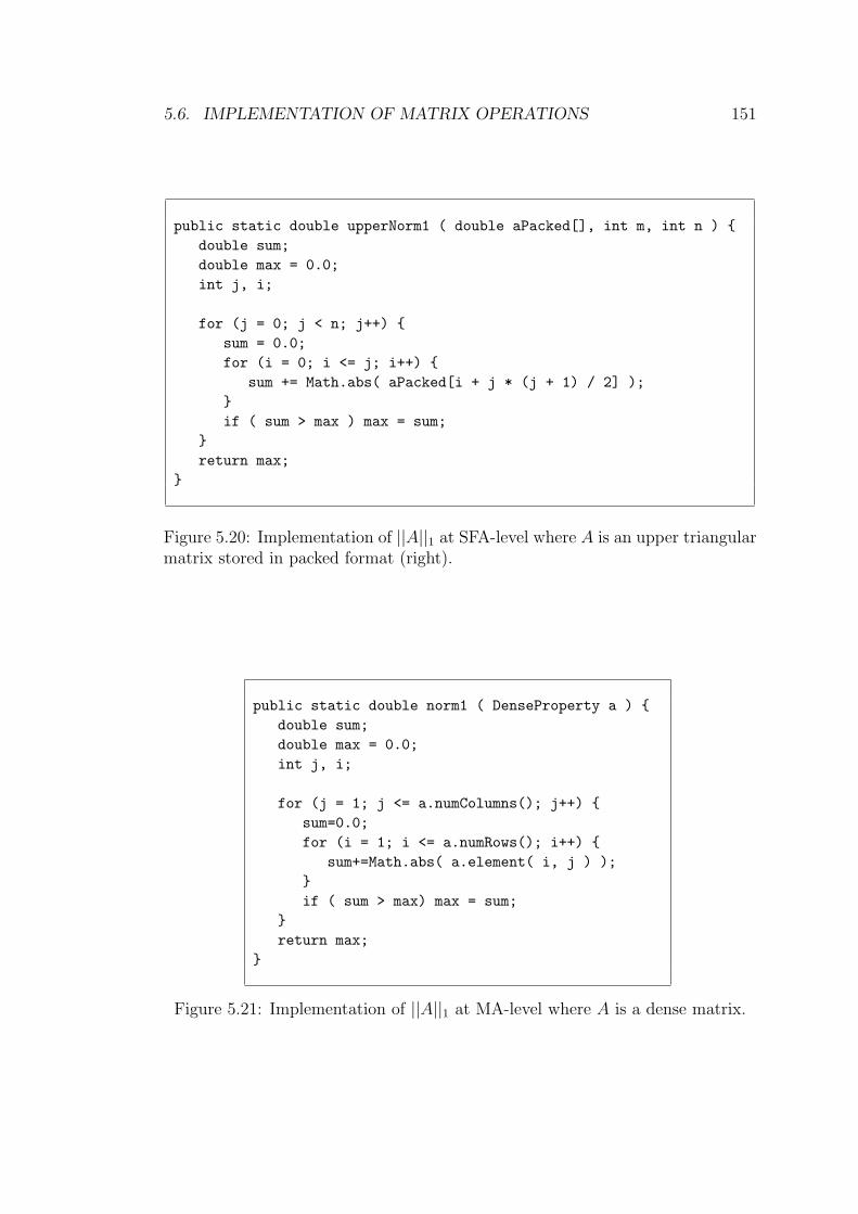
5.6. IMPLEMENTATION OF MATRIX OPERATIONS 151
public static double upperNorm1 ( double aPacked[], int m, int n ) {double sum;double max = 0.0;int j, i;
for (j = 0; j < n; j++) {sum = 0.0;for (i = 0; i <= j; i++) {
sum += Math.abs( aPacked[i + j * (j + 1) / 2] );}if ( sum > max ) max = sum;
}return max;
}
Figure 5.20: Implementation of ||A||1 at SFA-level where A is an upper triangularmatrix stored in packed format (right).
public static double norm1 ( DenseProperty a ) {double sum;double max = 0.0;int j, i;
for (j = 1; j <= a.numColumns(); j++) {sum=0.0;for (i = 1; i <= a.numRows(); i++) {
sum+=Math.abs( a.element( i, j ) );}if ( sum > max) max = sum;
}return max;
}
Figure 5.21: Implementation of ||A||1 at MA-level where A is a dense matrix.
5.6. IMPLEMENTATION OF MATRIX OPERATIONS 152
public static double norm1 ( UpperTriangularProperty a ) {double sum;double max = 0.0;int j,i;
for ( j = 1; j <= a.numColumns(); j++) {sum=0.0;for (i = 1; i <= j; i++) {
sum+=Math.abs( a.element( i, j ) );}if ( sum > max ) max = sum;
}return max;
}
Figure 5.22: Implementation of ||A||1 at MA-level where A is an upper triangularmatrix.
public static double norm1 ( Property a ) {double sum;double max = 0.0;
a.setColumnWise();a.begin();while ( !a.isMatrixFinished() ) {
sum = 0.0;a.nextVector();while ( !a.isVectorFinished() ) {
a.nextElement();sum += Math.abs( a.currentElement() );
}if ( sum > max) max = sum;
}return max;
}
Figure 5.23: Implementation of ||A||1 at IA-level.
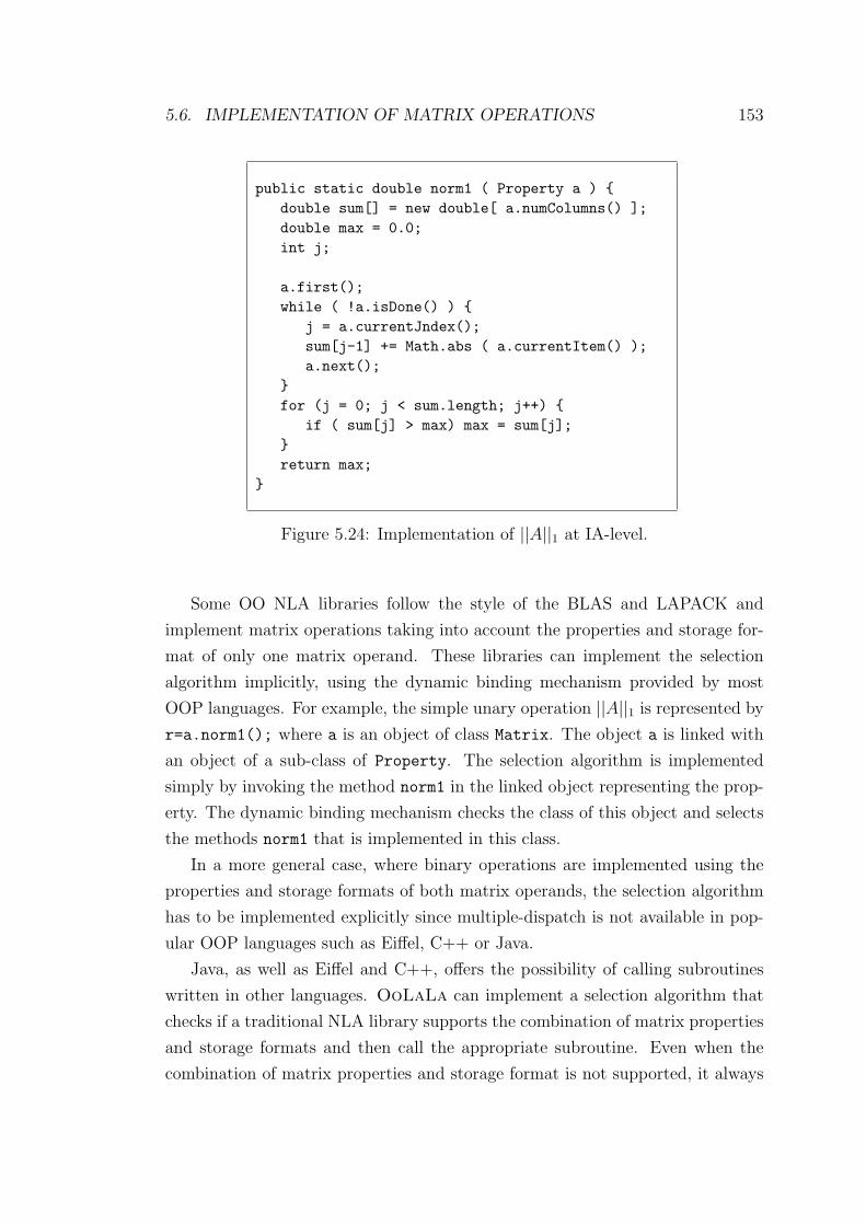
5.6. IMPLEMENTATION OF MATRIX OPERATIONS 153
public static double norm1 ( Property a ) {double sum[] = new double[ a.numColumns() ];double max = 0.0;int j;
a.first();while ( !a.isDone() ) {
j = a.currentJndex();sum[j-1] += Math.abs ( a.currentItem() );a.next();
}for (j = 0; j < sum.length; j++) {
if ( sum[j] > max) max = sum[j];}return max;
}
Figure 5.24: Implementation of ||A||1 at IA-level.
Some OO NLA libraries follow the style of the BLAS and LAPACK and
implement matrix operations taking into account the properties and storage for-
mat of only one matrix operand. These libraries can implement the selection
algorithm implicitly, using the dynamic binding mechanism provided by most
OOP languages. For example, the simple unary operation ||A||1 is represented by
r=a.norm1(); where a is an object of class Matrix. The object a is linked with
an object of a sub-class of Property. The selection algorithm is implemented
simply by invoking the method norm1 in the linked object representing the prop-
erty. The dynamic binding mechanism checks the class of this object and selects
the methods norm1 that is implemented in this class.
In a more general case, where binary operations are implemented using the
properties and storage formats of both matrix operands, the selection algorithm
has to be implemented explicitly since multiple-dispatch is not available in pop-
ular OOP languages such as Eiffel, C++ or Java.
Java, as well as Eiffel and C++, offers the possibility of calling subroutines
written in other languages. OoLaLa can implement a selection algorithm that
checks if a traditional NLA library supports the combination of matrix properties
and storage formats and then call the appropriate subroutine. Even when the
combination of matrix properties and storage format is not supported, it always
5.7. SUMMARY 154
remains possible to call a traditional NLA library subroutine. (For example, the
multiplication of two upper triangular matrices stored in packed format cannot
be performed with the BLAS, since the BLAS does not support this combination
of storage formats. However, it is possible to change one of the storage formats
to dense and thereby the combination of operands is supported.) In this way,
OoLaLa can become simply a wrapper of traditional NLA libraries; users of
OoLaLa benefit from a simpler interface and library developers can re-use their
legacy code and concentrate on developing new functionality. Experiences with
the Java Native Interface, and with C++ and Eiffel accessing Fortran BLAS or
LAPACK, have reported performance similar to the Fortran BLAS or LAPACK
(Java [33, 43, 114], Eiffel [128], and C++ [86]).
5.7 Summary
This chapter has offered an insight into the way that OoLaLa is implemented
in Java. No attempt has been made to describe Java. Nonetheless, this chapter
has reviewed Java’s strong and weak points for scientific computing, in general,
and for OoLaLa, specifically. A simple benchmark has tracked the performance
improvement of JVMs over the last 6 years. This benchmark has shown a 17-fold
performance improvement on one computing of platform and a 5-fold improve-
ment on another. Using example programs, this chapter has illustrated the way to
create matrices and views, and the way to access matrix elements. UML sequence
diagrams have been used for these example programs to expose the hidden details
of OoLaLa’s implementation. For one of these example programs, the relation
between the novel storage format generalised by OoLaLa’s support of views
(nested formats, specifically nested packed format) and the recursive packed for-
mat has been discussed. Another part of this chapter has described OoLaLa’s
rules to manage storage formats and propagation of properties automatically.
Finally, different combinations of matrix properties and storage formats for a
specific matrix operation have demonstrated that implementations at MA- and
IA-levels are both independent of storage formats. In the case of IA-level, such im-
plementations are also independent of matrix properties based on nonzero element
structures. Hence, both abstraction levels reduce the combinatorial explosion of
implementations at SFA-level.
5.7. SUMMARY 155
The next chapter, Chapter 6, offers a performance evaluation of the Java im-
plementation of OoLaLa described in this chapter. The evaluation compares
the performance results of a set of BLAS matrix operations implemented in Java
at the different abstraction levels and, in some cases, with SFA-level implemen-
tations in Fortran (i.e. traditional NLA libraries). These performance results
motivate the subsequent chapters which address the performance penalties ob-
served.
Chapter 6
Performance Evaluation of
OOLALA
6.1 Introduction
Object Oriented (OO) software construction has characteristics that could im-
prove the development process and usability of mathematical software libraries.
OoLaLa, a novel Object Oriented Linear Algebra LibrAry, is the outcome of
a study of these possible benefits in the context of sequential Numerical Linear
Algebra (NLA). The two previous chapters have reported the design of OoLaLa
and its Java implementation. This chapter covers the performance evaluation
of the latter. Subsequent chapters describe compiler optimisations to improve
the performance observed in this chapter and the limitations of a library-based
approach to the development of NLA programs.
OoLaLa enables library developers to implement matrix operations at two
higher abstraction levels: Matrix (MA-level) and Iterator Abstraction levels (IA-
level). The previous chapter has shown that these abstraction levels reduce the
number of implementations of a given matrix operation compared with Storage
Format Abstraction level (SFA-level). This chapter provides a performance eval-
uation of the cost for such reduction. The evaluation compares the performance
results of a set of BLAS matrix operations implemented in Java at IA-, MA- and
SFA-level and, in some cases, in Fortran 77 at SFA-level (i.e. traditional NLA
libraries). All implementations at IA-level rely on MatrixIterator; implemen-
tations based on MatrixIterator1D are omitted.
156
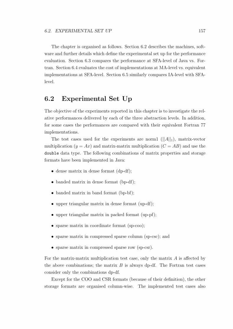
6.2. EXPERIMENTAL SET UP 157
The chapter is organised as follows. Section 6.2 describes the machines, soft-
ware and further details which define the experimental set up for the performance
evaluation. Section 6.3 compares the performance at SFA-level of Java vs. For-
tran. Section 6.4 evaluates the cost of implementations at MA-level vs. equivalent
implementations at SFA-level. Section 6.5 similarly compares IA-level with SFA-
level.
6.2 Experimental Set Up
The objective of the experiments reported in this chapter is to investigate the rel-
ative performances delivered by each of the three abstraction levels. In addition,
for some cases the performances are compared with their equivalent Fortran 77
implementations.
The test cases used for the experiments are norm1 (||A||1), matrix-vector
multiplication (y = Ax) and matrix-matrix multiplication (C = AB) and use the
double data type. The following combinations of matrix properties and storage
formats have been implemented in Java:
• dense matrix in dense format (dp-df);
• banded matrix in dense format (bp-df);
• banded matrix in band format (bp-bf);
• upper triangular matrix in dense format (up-df);
• upper triangular matrix in packed format (up-pf);
• sparse matrix in coordinate format (sp-coo);
• sparse matrix in compressed sparse column (sp-csc); and
• sparse matrix in compressed sparse row (sp-csr).
For the matrix-matrix multiplication test case, only the matrix A is affected by
the above combinations; the matrix B is always dp-df. The Fortran test cases
consider only the combinations dp-df.
Except for the COO and CSR formats (because of their definition), the other
storage formats are organised column-wise. The implemented test cases also
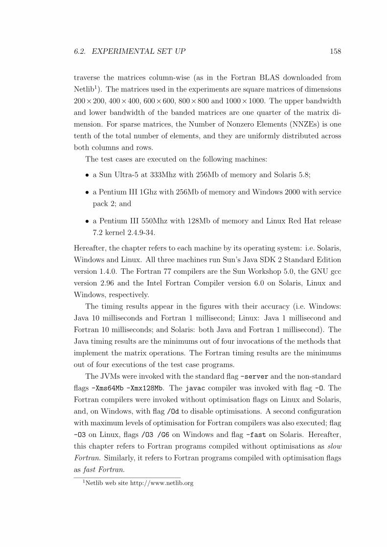
6.2. EXPERIMENTAL SET UP 158
traverse the matrices column-wise (as in the Fortran BLAS downloaded from
Netlib1). The matrices used in the experiments are square matrices of dimensions
200×200, 400×400, 600×600, 800×800 and 1000×1000. The upper bandwidth
and lower bandwidth of the banded matrices are one quarter of the matrix di-
mension. For sparse matrices, the Number of Nonzero Elements (NNZEs) is one
tenth of the total number of elements, and they are uniformly distributed across
both columns and rows.
The test cases are executed on the following machines:
• a Sun Ultra-5 at 333Mhz with 256Mb of memory and Solaris 5.8;
• a Pentium III 1Ghz with 256Mb of memory and Windows 2000 with service
pack 2; and
• a Pentium III 550Mhz with 128Mb of memory and Linux Red Hat release
7.2 kernel 2.4.9-34.
Hereafter, the chapter refers to each machine by its operating system: i.e. Solaris,
Windows and Linux. All three machines run Sun’s Java SDK 2 Standard Edition
version 1.4.0. The Fortran 77 compilers are the Sun Workshop 5.0, the GNU gcc
version 2.96 and the Intel Fortran Compiler version 6.0 on Solaris, Linux and
Windows, respectively.
The timing results appear in the figures with their accuracy (i.e. Windows:
Java 10 milliseconds and Fortran 1 millisecond; Linux: Java 1 millisecond and
Fortran 10 milliseconds; and Solaris: both Java and Fortran 1 millisecond). The
Java timing results are the minimums out of four invocations of the methods that
implement the matrix operations. The Fortran timing results are the minimums
out of four executions of the test case programs.
The JVMs were invoked with the standard flag -server and the non-standard
flags -Xms64Mb -Xmx128Mb. The javac compiler was invoked with flag -O. The
Fortran compilers were invoked without optimisation flags on Linux and Solaris,
and, on Windows, with flag /Od to disable optimisations. A second configuration
with maximum levels of optimisation for Fortran compilers was also executed; flag
-O3 on Linux, flags /O3 /G6 on Windows and flag -fast on Solaris. Hereafter,
this chapter refers to Fortran programs compiled without optimisations as slow
Fortran. Similarly, it refers to Fortran programs compiled with optimisation flags
as fast Fortran.
1Netlib web site http://www.netlib.org
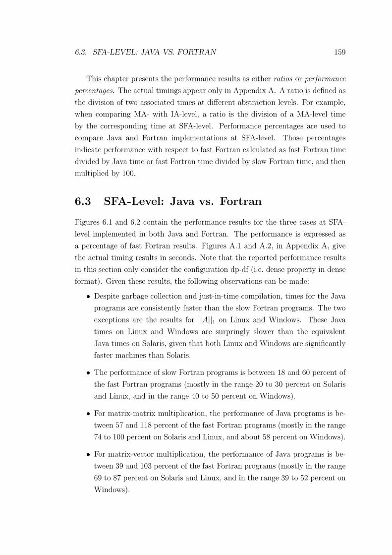
6.3. SFA-LEVEL: JAVA VS. FORTRAN 159
This chapter presents the performance results as either ratios or performance
percentages. The actual timings appear only in Appendix A. A ratio is defined as
the division of two associated times at different abstraction levels. For example,
when comparing MA- with IA-level, a ratio is the division of a MA-level time
by the corresponding time at SFA-level. Performance percentages are used to
compare Java and Fortran implementations at SFA-level. Those percentages
indicate performance with respect to fast Fortran calculated as fast Fortran time
divided by Java time or fast Fortran time divided by slow Fortran time, and then
multiplied by 100.
6.3 SFA-Level: Java vs. Fortran
Figures 6.1 and 6.2 contain the performance results for the three cases at SFA-
level implemented in both Java and Fortran. The performance is expressed as
a percentage of fast Fortran results. Figures A.1 and A.2, in Appendix A, give
the actual timing results in seconds. Note that the reported performance results
in this section only consider the configuration dp-df (i.e. dense property in dense
format). Given these results, the following observations can be made:
• Despite garbage collection and just-in-time compilation, times for the Java
programs are consistently faster than the slow Fortran programs. The two
exceptions are the results for ||A||1 on Linux and Windows. These Java
times on Linux and Windows are surpringly slower than the equivalent
Java times on Solaris, given that both Linux and Windows are significantly
faster machines than Solaris.
• The performance of slow Fortran programs is between 18 and 60 percent of
the fast Fortran programs (mostly in the range 20 to 30 percent on Solaris
and Linux, and in the range 40 to 50 percent on Windows).
• For matrix-matrix multiplication, the performance of Java programs is be-
tween 57 and 118 percent of the fast Fortran programs (mostly in the range
74 to 100 percent on Solaris and Linux, and about 58 percent on Windows).
• For matrix-vector multiplication, the performance of Java programs is be-
tween 39 and 103 percent of the fast Fortran programs (mostly in the range
69 to 87 percent on Solaris and Linux, and in the range 39 to 52 percent on
Windows).

6.3. SFA-LEVEL: JAVA VS. FORTRAN 160
• For norm1, the performance of Java programs has the two odd cases on
Linux and Windows, as mentioned above. The performance on Linux is
about half of the slow Fortran programs and about 10 percent of the fast
Fortran programs. On Solaris, the performance is about 50 percent of the
fast Fortran programs. On Windows, the performance of Java is between
11 and 14 percent of the fast Fortran programs.
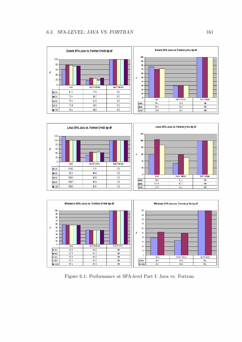
6.3. SFA-LEVEL: JAVA VS. FORTRAN 161
Figure 6.1: Performance at SFA-level Part I: Java vs. Fortran.
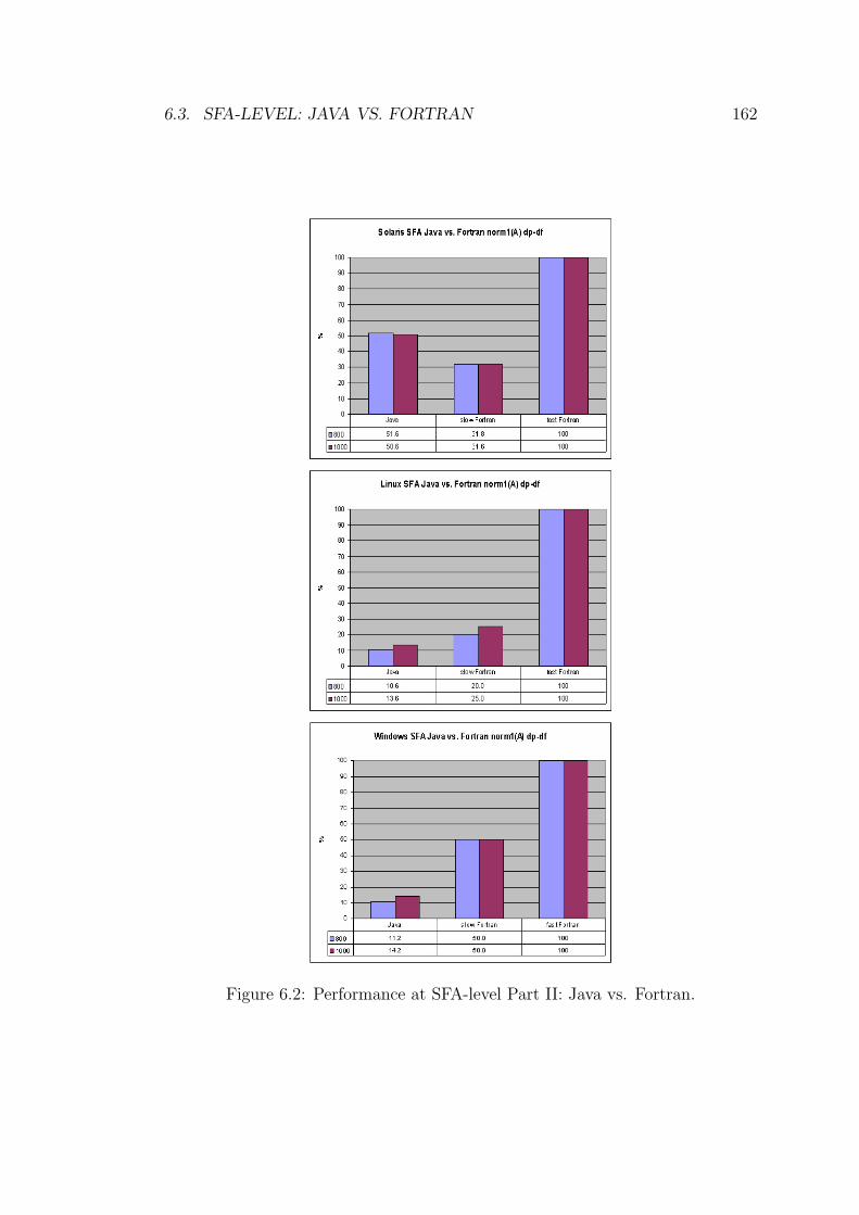
6.3. SFA-LEVEL: JAVA VS. FORTRAN 162
Figure 6.2: Performance at SFA-level Part II: Java vs. Fortran.
6.4. MA-LEVEL VS. SFA-LEVEL: JAVA 163
6.4 MA-level vs. SFA-level: Java
Figures 6.3 and 6.4 present the ratios between implementations in Java for matrix-
matrix multiplication at MA-level and SFA-level. Each ratio ia calculated as the
MA-level execution time divided by the corresponding SFA-level execution time.
Figures 6.5 and 6.6 give the ratios for matrix-vector multiplication while Figures
6.7 and 6.8 show the ratios for norm1. The times are reported in Figures A.3 to
A.8. Given these results, the following observations can be made:
• For matrix-matrix multiplication with non-sparse matrices on Linux and
Windows, the ratios lie between 1.21 and 1.73 (mostly in the range 1.25 to
1.30).
• For matrix-matrix multiplication dp-df (non-sparse matrix) on Solaris, the
ratios are remarkably close to 1 (between 0.95 and 1.05).
• For matrix-matrix multiplication with the other non-sparse matrices on
Solaris, the ratios reveal a significant performance penalty. SFA-level is
between 4.61 and 7.19 times faster than MA-level (mostly in the range 4.7
to 5).
• For matrix-matrix multiplication on all three machines, the ratios for sparse
matrices expose another significant performance penalty. SFA-level is from
3.26 times up to, as much as, two orders of magnitude faster than MA-level.
• For matrix-vector multiplication dp-df on all three machines, the ratios are
again remarkably close to 1 (between 0.91 and 1.04).
• For matrix-vector multiplication with the other non-sparse matrices on So-
laris, the ratios show another significant performance penalty. SFA-level is
between 4.34 and 9.79 times faster than MA-level.
• For matrix-vector multiplication with the other non-sparse matrices on
Linux, the ratios illustrate two different behaviours. For bp-df and up-df,
SFA-level is between 1.20 and 1.70 times faster than MA-level. For bp-bf
and up-pf, SFA-level is between 3.53 and 3.88 times faster than MA-level.
In other words, for the latter combinations, MA-level suffers roughly twice
the performance penalty compared with the former combinations.
6.4. MA-LEVEL VS. SFA-LEVEL: JAVA 164
• For matrix-vector multiplication with sparse matrices, the ratios reveal a
severe performance penalty; three orders of magnitude.
• On Windows and Linux for norm1 with non-sparse matrices, the ratios are
between 1.02 and 1.53.
• On Solaris for norm1 de-df, the ratios are around 1.42. On Linux and
Windows the ratios are close 1 (between 1.02 and 1.14). However, this is
not due to MA-level delivering good performance, but SFA-level delivering
poor performance. A closer look at the times in Figure A.7 indicates that
both Linux and Windows machines are faster than the Solaris machine, yet
their times for norm1 dp-df at SFA-level are slower than the corresponding
Solaris times.
• On Solaris for norm1 with the other non-sparse matrices, the ratios are
between 1.71 and 2.79 (mostly between 2.3 and 2.6).
• On all three platforms for norm1 with sparse matrices, the ratios again are
a severe performance penalty; three orders of magnitude.
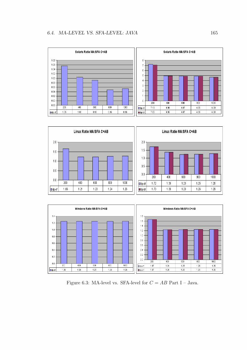
6.4. MA-LEVEL VS. SFA-LEVEL: JAVA 165
Figure 6.3: MA-level vs. SFA-level for C = AB Part I – Java.
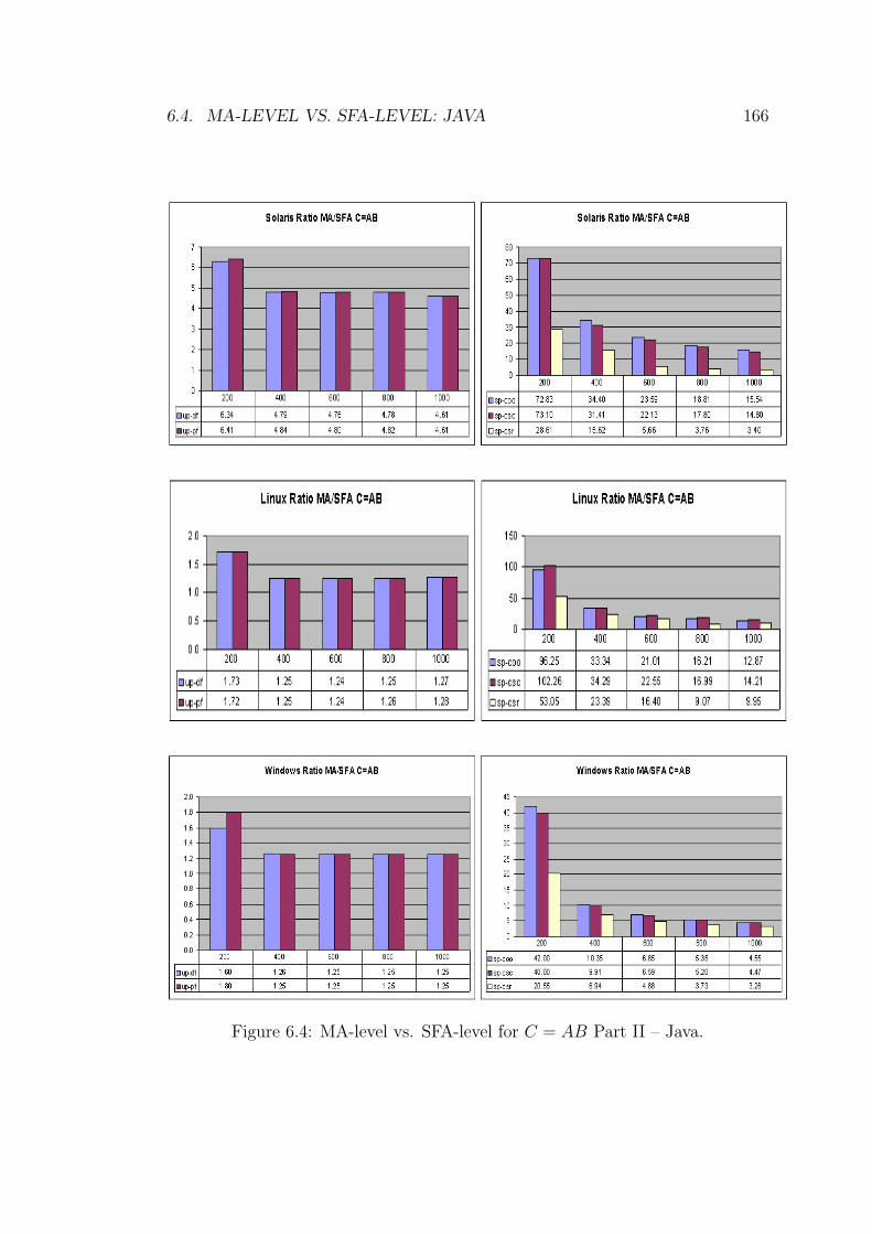
6.4. MA-LEVEL VS. SFA-LEVEL: JAVA 166
Figure 6.4: MA-level vs. SFA-level for C = AB Part II – Java.
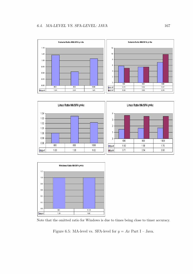
6.4. MA-LEVEL VS. SFA-LEVEL: JAVA 167
Note that the omitted ratio for Windows is due to times being close to timer accuracy.
Figure 6.5: MA-level vs. SFA-level for y = Ax Part I – Java.
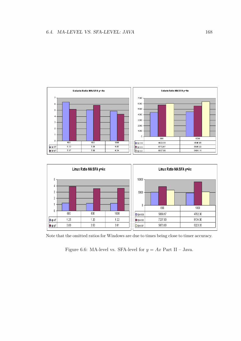
6.4. MA-LEVEL VS. SFA-LEVEL: JAVA 168
Note that the omitted ratios for Windows are due to times being close to timer accuracy.
Figure 6.6: MA-level vs. SFA-level for y = Ax Part II – Java.
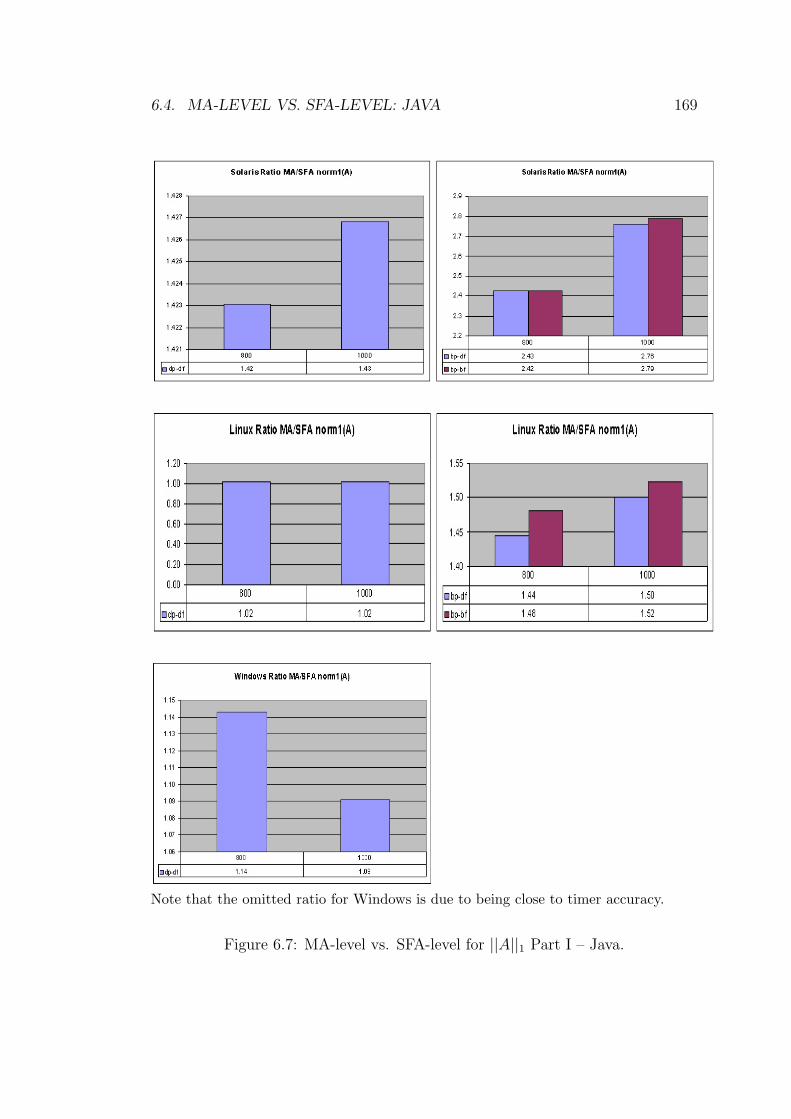
6.4. MA-LEVEL VS. SFA-LEVEL: JAVA 169
Note that the omitted ratio for Windows is due to being close to timer accuracy.
Figure 6.7: MA-level vs. SFA-level for ||A||1 Part I – Java.
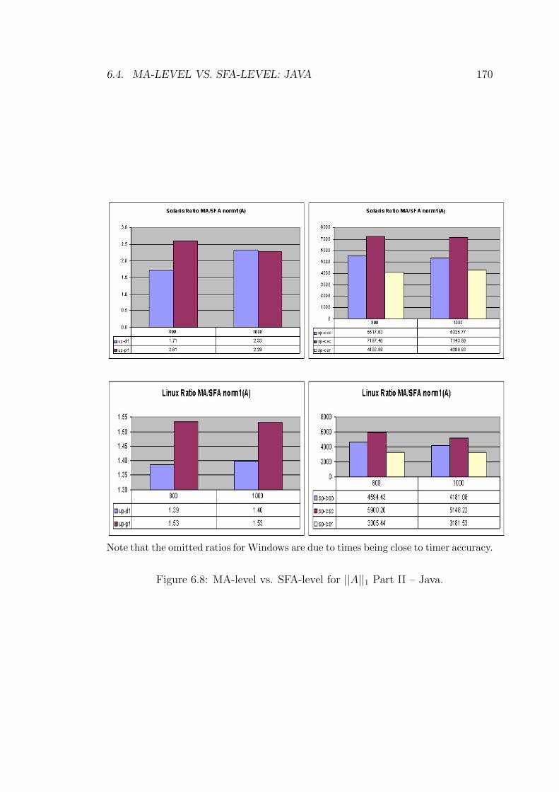
6.4. MA-LEVEL VS. SFA-LEVEL: JAVA 170
Note that the omitted ratios for Windows are due to times being close to timer accuracy.
Figure 6.8: MA-level vs. SFA-level for ||A||1 Part II – Java.
6.5. IA-LEVEL VS. SFA-LEVEL: JAVA 171
6.5 IA-level vs. SFA-level: Java
Figures 6.9 and 6.10 present the ratios between implementations in Java for
matrix-matrix multiplication at IA-level and SFA-level. Each ratios is calculated
as the IA-level execution time divided by the corresponding SFA-level execution
time. Figures 6.11 and 6.12 give the ratios for matrix-vector multiplication while
Figures 6.13 and 6.14 show the ratios for norm1. The times are reported in Fig-
ures A.3 to A.8 (Appendix A). Given these results, the following observations
can be made:
• For matrix-matrix multiplication dp-df (non-sparse matrix) on all three
platforms, the ratios are in the range 3.53 to 8.25. However, for each plat-
form most of the ratios are closer together; on Solaris mostly between 4.91
and 5.24, on Linux mostly between 4.21 and 4.30, and on Windows mostly
between 3.53 and 3.59.
• For matrix-matrix multiplication with the other non-sparse matrices on all
three machines, the ratios are between 4.05 and 16.74.
• For matrix-matrix multiplication with sparse matrices on all three machines,
the ratios are between 3.32 and 16.10.
• Overall for matrix-matrix multiplication on all three machines, the ratios
show a significant performance penalty; IA-level is always more three times
slower than SFA-level.
• For matrix-vector multiplication dp-df (non-sparse matrix) on all three plat-
forms, the ratios are in the range 3.55 to 5.04. However, for each platform
most of the ratios are closer together; on Solaris mostly between 4.42 and
5.04, on Linux mostly between 3.94 and 4.00, and on Windows mostly be-
tween 3.55 and 3.67.
• For matrix-vector multiplication with the other non-sparse matrices on
Linux and Solaris, the ratios are between 7.07 and 12.91.
• For matrix-vector multiplication with sparse matrices on all three machines,
the ratios are between 13.90 and two orders of magnitude.
• For norm1 dp-df on Solaris, the ratios are between 4.43 and 4.48.

6.5. IA-LEVEL VS. SFA-LEVEL: JAVA 172
• For norm1 dp-df on Linux and Windows, the ratios are close to 1. However,
this is not due to IA-level delivering good performance, but due to SFA-level
delivering poor performance.
• For norm1 on Linux and Windows with the other non-sparse matrices, the
ratios are between 3.77 and 10.50.
• For norm1 with sparse matrices, the ratios are between 9.92 and two orders
of magnitude.
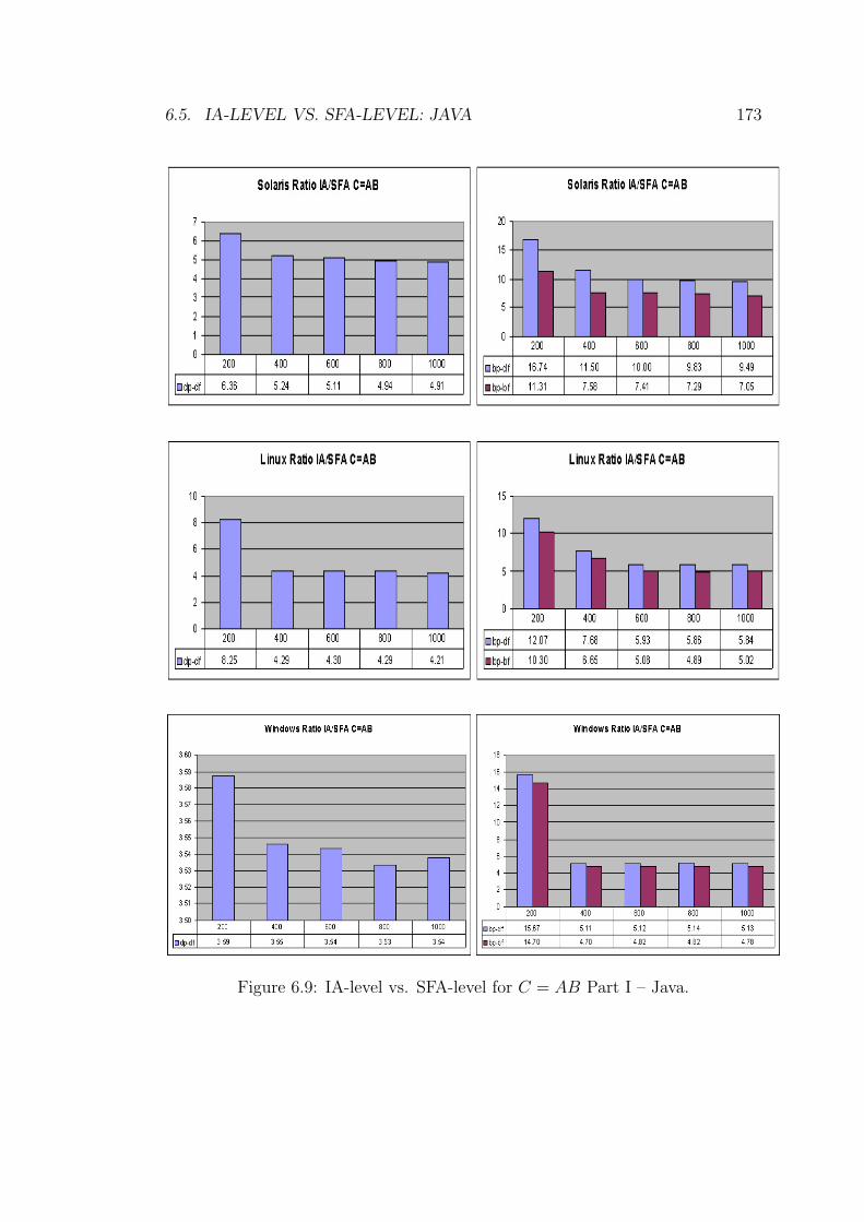
6.5. IA-LEVEL VS. SFA-LEVEL: JAVA 173
Figure 6.9: IA-level vs. SFA-level for C = AB Part I – Java.
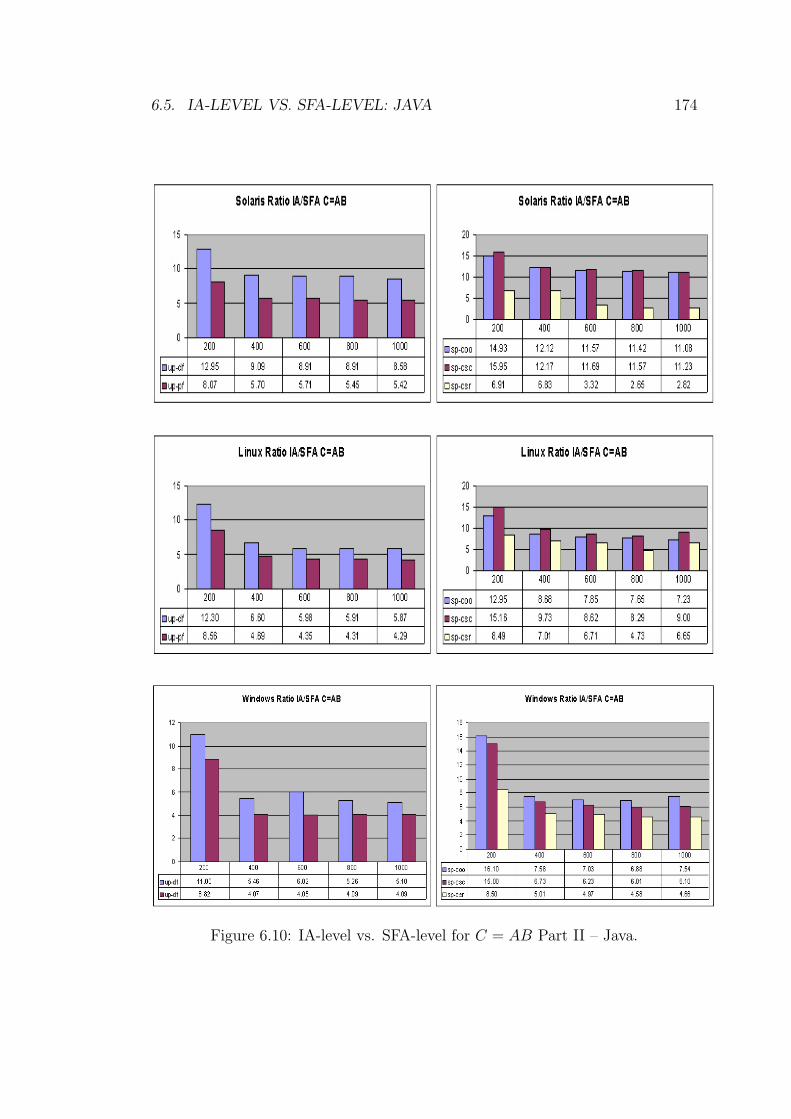
6.5. IA-LEVEL VS. SFA-LEVEL: JAVA 174
Figure 6.10: IA-level vs. SFA-level for C = AB Part II – Java.
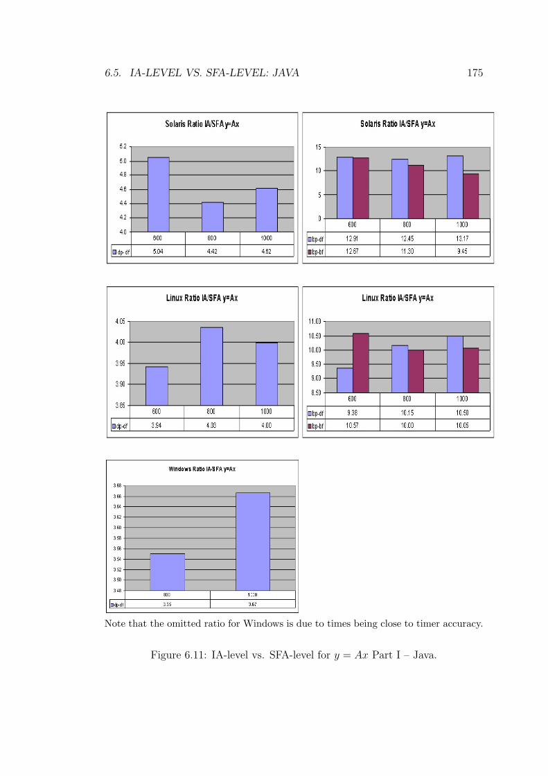
6.5. IA-LEVEL VS. SFA-LEVEL: JAVA 175
Note that the omitted ratio for Windows is due to times being close to timer accuracy.
Figure 6.11: IA-level vs. SFA-level for y = Ax Part I – Java.
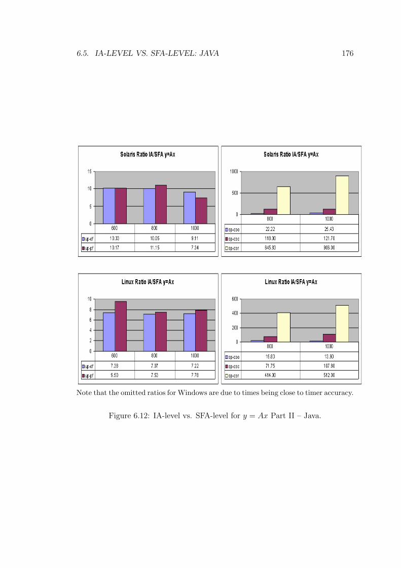
6.5. IA-LEVEL VS. SFA-LEVEL: JAVA 176
Note that the omitted ratios for Windows are due to times being close to timer accuracy.
Figure 6.12: IA-level vs. SFA-level for y = Ax Part II – Java.
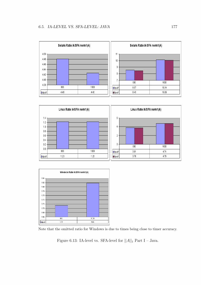
6.5. IA-LEVEL VS. SFA-LEVEL: JAVA 177
Note that the omitted ratio for Windows is due to times being close to timer accuracy.
Figure 6.13: IA-level vs. SFA-level for ||A||1 Part I – Java.
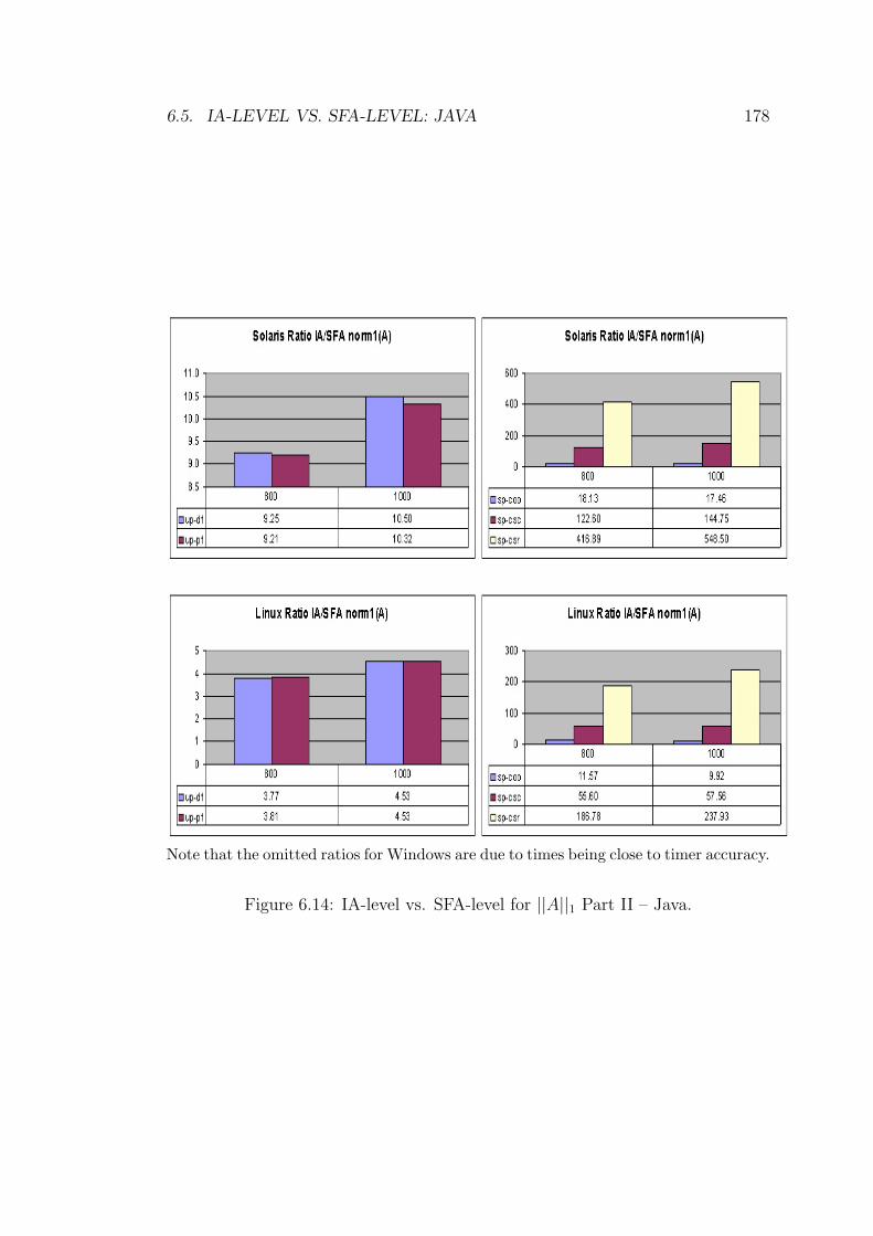
6.5. IA-LEVEL VS. SFA-LEVEL: JAVA 178
Note that the omitted ratios for Windows are due to times being close to timer accuracy.
Figure 6.14: IA-level vs. SFA-level for ||A||1 Part II – Java.
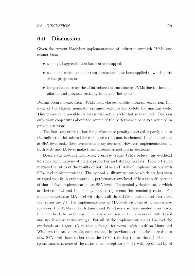
6.6. DISCUSSION 179
6.6 Discussion
Given the current black-box implementations of industrial strength JVMs, one
cannot know
• when garbage collection has started-stopped;
• when and which compiler transformations have been applied to which parts
of the program; or
• the performance overhead introduced at run time by JVMs due to the com-
pilation and program profiling to detect “hot spots”.
During program execution, JVMs load classes, profile program execution, (for
some of the classes) generate, optimise, execute and delete the machine code.
This makes it impossible to access the actual code that is executed. One can
only draw conjectures about the source of the performance penalties revealed in
previous sections.
The first conjecture is that the performance penalty observed is partly due to
the indirection introduced for each access to a matrix element. Implementations
at SFA-level make these accesses as array accesses. However, implementations at
both MA- and IA-level make these accesses as method invocations.
Despite the method invocation overhead, some JVMs reduce this overhead
for some combinations of matrix properties and storage formats. Table 6.1 sum-
marises the ratios of the results of both MA- and IA-level implementations with
SFA-level implementations. The symbol X illustrates ratios which are less than
or equal to 1.5; in other words, a performance overhead of less than 50 percent
of that of Java implementations at SFA-level. The symbol χ depicts ratios which
are between 1.5 and 10. The symbol ∞ represents the remaining ratios. For
implementations at MA-level with dp-df, all three JVMs have modest overheads
(i.e. ratios are X). For implementations at MA-level with the other non-sparse
matrices, the JVMs on both Linux and Windows also have modest overheads,
but not the JVM on Solaris. The only exception on Linux is norm1 with bp-bf
and up-pf whose ratios are χs. For all of the implementations at IA-level the
overheads are larger. (Note that although for norm1 with dp-df on Linux and
Windows the ratios are Xs, as mentioned in previous sections, these are due to
slow SFA-level times rather than the JVMs reducing the overhead.) For non-
sparse matrices, none of the ratios is ∞, except for y = Ax with bp-df and bp-bf
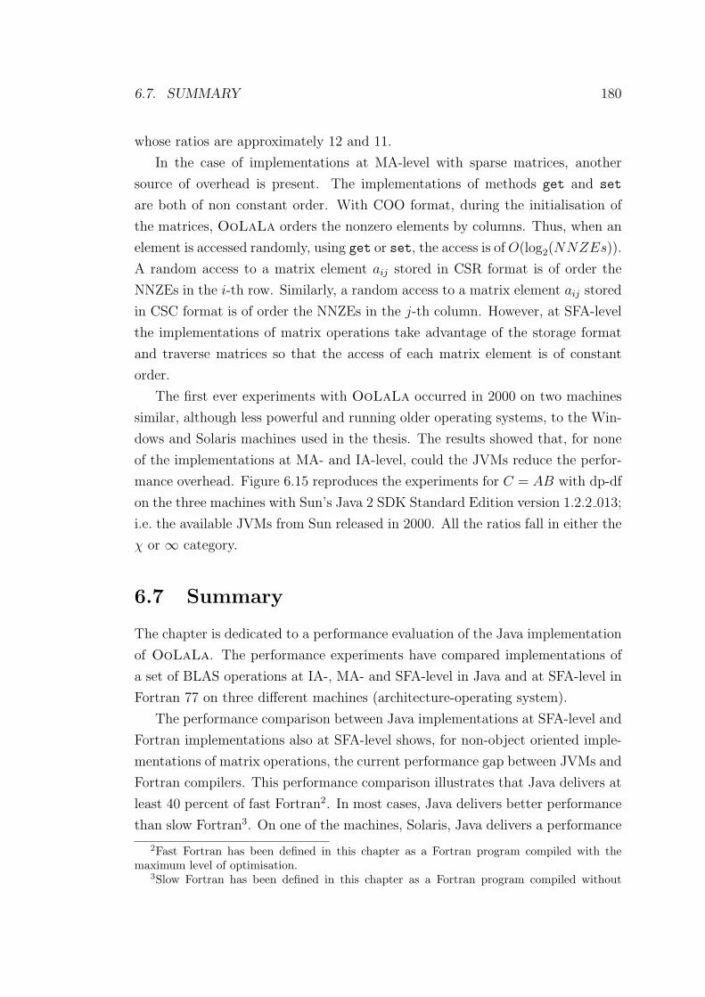
6.7. SUMMARY 180
whose ratios are approximately 12 and 11.
In the case of implementations at MA-level with sparse matrices, another
source of overhead is present. The implementations of methods get and set
are both of non constant order. With COO format, during the initialisation of
the matrices, OoLaLa orders the nonzero elements by columns. Thus, when an
element is accessed randomly, using get or set, the access is of O(log2(NNZEs)).
A random access to a matrix element aij stored in CSR format is of order the
NNZEs in the i-th row. Similarly, a random access to a matrix element aij stored
in CSC format is of order the NNZEs in the j-th column. However, at SFA-level
the implementations of matrix operations take advantage of the storage format
and traverse matrices so that the access of each matrix element is of constant
order.
The first ever experiments with OoLaLa occurred in 2000 on two machines
similar, although less powerful and running older operating systems, to the Win-
dows and Solaris machines used in the thesis. The results showed that, for none
of the implementations at MA- and IA-level, could the JVMs reduce the perfor-
mance overhead. Figure 6.15 reproduces the experiments for C = AB with dp-df
on the three machines with Sun’s Java 2 SDK Standard Edition version 1.2.2 013;
i.e. the available JVMs from Sun released in 2000. All the ratios fall in either the
χ or ∞ category.
6.7 Summary
The chapter is dedicated to a performance evaluation of the Java implementation
of OoLaLa. The performance experiments have compared implementations of
a set of BLAS operations at IA-, MA- and SFA-level in Java and at SFA-level in
Fortran 77 on three different machines (architecture-operating system).
The performance comparison between Java implementations at SFA-level and
Fortran implementations also at SFA-level shows, for non-object oriented imple-
mentations of matrix operations, the current performance gap between JVMs and
Fortran compilers. This performance comparison illustrates that Java delivers at
least 40 percent of fast Fortran2. In most cases, Java delivers better performance
than slow Fortran3. On one of the machines, Solaris, Java delivers a performance
2Fast Fortran has been defined in this chapter as a Fortran program compiled with themaximum level of optimisation.
3Slow Fortran has been defined in this chapter as a Fortran program compiled without
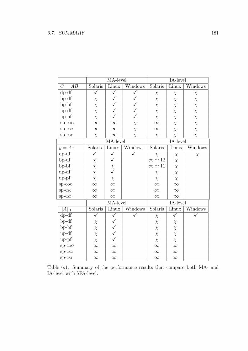
6.7. SUMMARY 181
MA-level IA-levelC = AB Solaris Linux Windows Solaris Linux Windowsdp-df X X X χ χ χbp-df χ X X χ χ χbp-bf χ X X χ χ χup-df χ X X χ χ χup-pf χ X X χ χ χsp-coo ∞ ∞ χ ∞ χ χsp-csc ∞ ∞ χ ∞ χ χsp-csr χ ∞ χ χ χ χ
MA-level IA-levely = Ax Solaris Linux Windows Solaris Linux Windowsdp-df X X X χ χ χbp-df χ X ∞ ' 12 χbp-bf χ χ ∞ ' 11 χup-df χ X χ χup-pf χ χ χ χsp-coo ∞ ∞ ∞ ∞sp-csc ∞ ∞ ∞ ∞sp-csr ∞ ∞ ∞ ∞
MA-level IA-level||A||1 Solaris Linux Windows Solaris Linux Windowsdp-df X X X χ X Xbp-df χ X χ χbp-bf χ X χ χup-df χ X χ χup-pf χ X χ χsp-coo ∞ ∞ ∞ ∞sp-csc ∞ ∞ ∞ ∞sp-csr ∞ ∞ ∞ ∞
Table 6.1: Summary of the performance results that compare both MA- andIA-level with SFA-level.
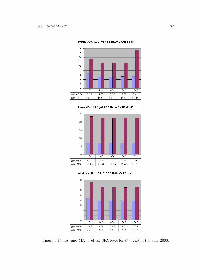
6.7. SUMMARY 182
Figure 6.15: IA- and MA-level vs. SFA-level for C = AB in the year 2000.
6.7. SUMMARY 183
mostly in the range 60 to 75 percent of fast Fortran. On the second machine,
Linux, Java can deliver in the range 87 to 118 percent of fast Fortran. On the
third machine, Windows, Java delivers mostly in the range 52 to 58 percent of
fast Fortran.
Motivated by the performance gap between JVMs and Fortran compilers,
Chapter 7 presents a means for eliminating the overhead of array bounds checks.
Array bounds checks are intrinsic in Java due to the specification of the language.
Chapter 7 concentrates on the specific subset of array bounds checks which oc-
cur when accessing an array through an index stored in another array – array
indirection.
The performance comparison of Java implementations at IA- and MA-level
with respect to Java implementations at SFA-level has been summarised in Table
6.1. For non-sparse matrices the ratios fall into either of two proposed categories.
The first category is represented as X and depicts cases where JVMs have been
able to eliminate most of the performance gap between the abstraction levels (i.e.
ratios less than or equal to 1.5). The second category is represented as χ and
illustrates cases where JVMs have not been able to eliminate the performance gap.
A third category ∞ covers ratios where JVMs have not been able to eliminate
the performance gap and the ratios are greater than one order of magnitude. For
sparse matrices the ratios fall in either χ or ∞ category.
The conjecture is that the performance penalty observed is partly due to the
indirection introduced for each access to a matrix element. Implementations at
SFA-level make these accesses as array accesses. However, implementations at
both MA- and IA-level make these accesses as method invocations. Another con-
jecture is that the performance penalty observed for implementations at MA-level
with sparse matrices is also due to an algorithmic difference. The implementations
of methods get and set are both of non constant order. However, at SFA-level
the implementations of matrix operations take advantage of the storage format
and traverse matrices so that each access to a matrix element is of constant order.
Chapter 8 is motivated by the performance results of Java implementations
at IA- and MA-level compared with Java implementations at SFA-level. Chapter
8 looks at the two following questions:
• how might implementations of matrix operations at MA-level and IA-level
be transformed into efficient implementations at SFA-level? and
optimisations.
6.7. SUMMARY 184
• under what conditions can such transformations be applied? (i.e. for which
sets of storage formats and matrix properties can this be done automati-
cally?)
Chapter 7
Elimination of Array Bounds
Checks
7.1 Introduction
Object Oriented (OO) software construction has characteristics that could im-
prove the development process and usability of mathematical software libraries.
OoLaLa, a novel Object Oriented Linear Algebra LibrAry, is the outcome of
a study of these possible benefits in the context of sequential Numerical Linear
Algebra (NLA). Previous chapters have covered the design of the library, imple-
mentation and performance evaluation. This chapter is the first chapter dedicated
to the optimisation of OoLaLa, specifically the elimination of the performance
penalty of array bounds checks in the presence of indirection. Chapters 8 and 9
continue with the optimisation of the library.
The Java language specification [125] states that every access to an array
needs to be within the bounds of that array. Different techniques for different
programming languages have been proposed to eliminate explicit bounds checks.
Some of these techniques are implemented in off-the-shelf Java Virtual Machines
[160] (JVMs). The underlying principle of these techniques is that bounds checks
can be removed when a JVM/compiler has enough information to guarantee that
a sequence of accesses (e.g. inside a for-loop) is safe (within the bounds).
Most of the techniques for the elimination of array bounds checks have been
developed for programming languages that do not support multi-threading and/or
enable dynamic class loading. These two characteristics make most of these tech-
niques unsuitable for Java. Techniques developed specifically for Java have not
185
7.1. INTRODUCTION 186
addressed the elimination of array bounds checks in the presence of indirection,
that is, when the index is stored in another array (indirection array).
Given that array indirection is ubiquitous in storage formats for sparse matri-
ces (see Chapter 2), the objective of this chapter is to minimise the consequent
performance overhead that is intrinsic in the language. Java’s specification re-
quires that:
• all array accesses are checked at run time; and
• any access outside the bounds (index less than zero or greater than or equal
to the length) of an array throws an ArrayIndexOutOfBoundsException.
This chapter proposes and evaluates three implementation strategies, each
implemented as a Java class. The classes provide the functionality of Java arrays
of type int so that objects of the classes can be used instead of indirection arrays.
Each strategy enables JVMs, when examining only one of these classes at a time,
to obtain enough information to remove array bounds checks in the presence of
indirection.
When an array bounds check is eliminated from a Java program, two things
are accomplished from a performance point of view. The first, direct, reward
is the elimination of the check itself (at least two integer comparisons). The
second, indirect, reward is the possibility for other compiler transformations. Due
to the strict exception model specified by Java, instructions capable of causing
exceptions are inhibitors of compiler transformations. When an exception arises
in a Java program the user-visible state of the program has to look as if every
preceding instruction has been executed and no succeeding instructions have been
executed. This exception model prevents, in general, instruction reordering. Since
many important compiler transformations improve performance by reordering
instructions, this is a severe restriction whose lifting could result in substantial
performance improvements.
The following section motivates the work and defines the problem to be solved.
Section 7.3 describes related work. Section 7.4 presents the three implementation
strategies that enable JVMs to examine only one class at a time to decide whether
the array bounds checks can be removed. The solutions are described as classes to
be included in the Multiarray package (JSR-0831). The strategies were generated
1JSR-083 – Multiarray Package web site http://jcp.org/jsr/detail/083.jsp
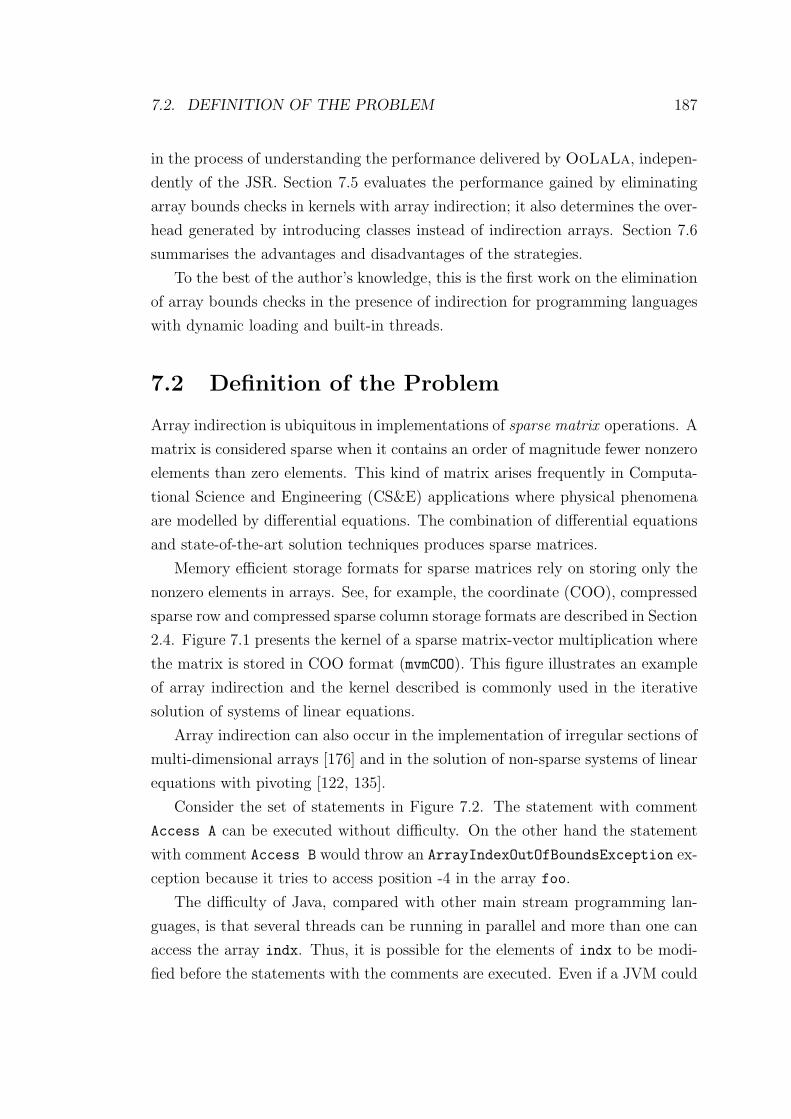
7.2. DEFINITION OF THE PROBLEM 187
in the process of understanding the performance delivered by OoLaLa, indepen-
dently of the JSR. Section 7.5 evaluates the performance gained by eliminating
array bounds checks in kernels with array indirection; it also determines the over-
head generated by introducing classes instead of indirection arrays. Section 7.6
summarises the advantages and disadvantages of the strategies.
To the best of the author’s knowledge, this is the first work on the elimination
of array bounds checks in the presence of indirection for programming languages
with dynamic loading and built-in threads.
7.2 Definition of the Problem
Array indirection is ubiquitous in implementations of sparse matrix operations. A
matrix is considered sparse when it contains an order of magnitude fewer nonzero
elements than zero elements. This kind of matrix arises frequently in Computa-
tional Science and Engineering (CS&E) applications where physical phenomena
are modelled by differential equations. The combination of differential equations
and state-of-the-art solution techniques produces sparse matrices.
Memory efficient storage formats for sparse matrices rely on storing only the
nonzero elements in arrays. See, for example, the coordinate (COO), compressed
sparse row and compressed sparse column storage formats are described in Section
2.4. Figure 7.1 presents the kernel of a sparse matrix-vector multiplication where
the matrix is stored in COO format (mvmCOO). This figure illustrates an example
of array indirection and the kernel described is commonly used in the iterative
solution of systems of linear equations.
Array indirection can also occur in the implementation of irregular sections of
multi-dimensional arrays [176] and in the solution of non-sparse systems of linear
equations with pivoting [122, 135].
Consider the set of statements in Figure 7.2. The statement with comment
Access A can be executed without difficulty. On the other hand the statement
with comment Access B would throw an ArrayIndexOutOfBoundsException ex-
ception because it tries to access position -4 in the array foo.
The difficulty of Java, compared with other main stream programming lan-
guages, is that several threads can be running in parallel and more than one can
access the array indx. Thus, it is possible for the elements of indx to be modi-
fied before the statements with the comments are executed. Even if a JVM could
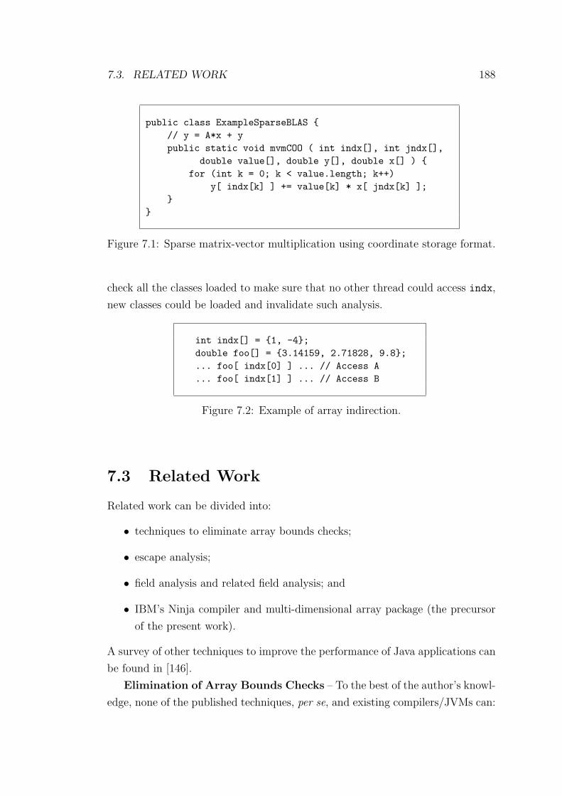
7.3. RELATED WORK 188
public class ExampleSparseBLAS {// y = A*x + ypublic static void mvmCOO ( int indx[], int jndx[],
double value[], double y[], double x[] ) {for (int k = 0; k < value.length; k++)
y[ indx[k] ] += value[k] * x[ jndx[k] ];}
}
Figure 7.1: Sparse matrix-vector multiplication using coordinate storage format.
check all the classes loaded to make sure that no other thread could access indx,
new classes could be loaded and invalidate such analysis.
int indx[] = {1, -4};double foo[] = {3.14159, 2.71828, 9.8};... foo[ indx[0] ] ... // Access A... foo[ indx[1] ] ... // Access B
Figure 7.2: Example of array indirection.
7.3 Related Work
Related work can be divided into:
• techniques to eliminate array bounds checks;
• escape analysis;
• field analysis and related field analysis; and
• IBM’s Ninja compiler and multi-dimensional array package (the precursor
of the present work).
A survey of other techniques to improve the performance of Java applications can
be found in [146].
Elimination of Array Bounds Checks – To the best of the author’s knowl-
edge, none of the published techniques, per se, and existing compilers/JVMs can:
7.3. RELATED WORK 189
• optimise array bounds checks in the presence of indirection;
• are suitable for adaptive just-in-time compilation;
• support multi-threading; and
• support dynamic class loading.
Techniques based on theorem provers [216, 182, 231] are too heavy-weight. Algo-
rithms based on a data-flow-style have been published extensively [167, 131, 132,
147, 18, 65], but only for languages without multi-threading. Another technique
is based on type analysis and has its application in functional languages [230].
Linear program solvers have also been proposed [198].
Bodik, Gupta and Sarkar developed the ABCD (Array Bounds Check on
Demand) algorithm [44] for Java. It is designed to fit the time constraints of
analysing the program and applying the transformation at run-time. ABCD
targets business-style applications and uses a sparse representation of the program
which does not include information about multi-threading. Thus, the algorithm,
although the most interesting for the purposes of this chapter, cannot handle
indirection since the origin of the problem is multi-threading. The strategies
proposed in Section 7.4 can provide cheaply that extra information to enable
ABCD to eliminate checks in the presence of indirection.
Escape Analysis – In 1999, four papers were published in the same confer-
ence describing escape analysis algorithms and the possibilities of optimising Java
programs by the optimal allocation of objects (heap vs. stack) and the removal
of synchronization [66, 45, 40, 224]. Escape analysis tries to determine whether
an object that has been created by a method, a thread, or another object escapes
the scope of its creator. Escape means that another object can get a reference to
the object and, thus, make it live (not garbage collected) beyond the execution
of the method, the thread, or the object that created it. The three strategies
presented in Section 7.4 require a simple escape analysis. The strategies can only
provide information (class invariants) if every instance variable does not escape
the object. Otherwise, a different thread can get access to instance variables and
update them, possibly breaking the desired class invariant.
Field Analysis and Related Field Analysis – Both field analysis [115]
and related field analysis [3] are techniques that look at one class at a time and
try to extract as much information as possible. This information can be used,
7.3. RELATED WORK 190
for example, for the resolution of method calls or object inlining. Related field
analysis looks for relations among the instance variables of objects. Aggarwal and
Randall [3] demonstrate how related field analysis can be used to eliminate array
bounds checks for a class following the iterator pattern [107]. The strategies
presented later in this chapter make use of the concept of field analysis. The
objective is to provide a meaningful class invariant and this is represented in the
instance variables (fields). However, the actual algorithms to test the relations
have not been used in previous work on field analysis. The demonstration of
eliminating array bounds checks given in [3] cannot be applied in the presence of
indirection.
IBM Ninja project and multi-dimensional array package – IBM’s
Ninja group [175, 176, 177, 178, 179] has focused on optimising Java numerical
intensive applications based on arrays. Midkiff, Moreira and Snir [175] devel-
oped a loop versioning algorithm so that iteration spaces of nested loops can be
partitioned into safe regions for which it can be proved that no exceptions (null
checks and array bound checks) and no synchronisations can occur. Having found
these exception-free and syncronisation-free regions, traditional loop reordering
transformations can be applied without violating the strict exception model.
The Ninja group designed and implemented a multi-dimensional array pack-
age [176] (to replace Java arrays) for which the discovery of safe regions becomes
easier. To eliminate the overhead introduced by using classes, they have devel-
oped semantic expansion2 [228]. Semantic expansion is a compilation strategy by
which selected classes are treated as language primitives by the compiler. In the
prototype Ninja static compiler, they successfully implement the elimination of ar-
ray bounds checks, together with semantic expansion for their multi-dimensional
array package and other loop reordering transformations.
The Ninja compiler is not compatible with the specification of Java since
it does not support dynamic class loading. The semantic expansion technique
ensures only that computations that directly use the multi-dimensional array
package do not suffer overheard. Although the compiler is not compatible with
Java, this does not mean that the techniques they have developed could not be
incorporated into a JVM. These techniques would be especially attractive for
quasi-static compilers [203].
2Since first publishing this work [228], the Ninja gruop has decided to change their originalterm, “semantic inlining”, to “semantic expansion” [179].
7.4. STRATEGIES 191
This chapter extends the Ninja group’s work by tackling the problem of
eliminating array bounds checks in the presence of indirection. The strategies,
described in Section 7.4, generate classes that are incorporated into a multi-
dimensional array package proposed in the Java Specification Request (JSR) -
083. If accepted, this JSR will define the standard Java multi-dimensional array
package and it is a direct consequence of the Ninja group’s work.
7.4 Strategies
The strategies that are described in this section have a common goal: to produce
a class for which JVMs can discover the pertinent invariants simply by examining
the class and, thereby, derive information to eliminate array bounds checks. Each
class provides at least the same functionality as Java arrays of type int and,
thus, can substitute for them. Objects of these classes would be used instead
of indirection arrays. The three strategies generate three different classes that
naturally fit into a multi-dimensional array library such as the one described in
the JSR-083. Figure 7.3 presents a subset of the public methods that the three
classes implement; the three classes extend the abstract class IntIndirection-
Multiarray1D.
Part of the class invariant that JVMs should discover is common to all three
strategies; the values returned by the methods getMin and getMax are always
lower bounds and upper bounds, respectively, of the elements stored. This com-
mon part of the invariant can be computed, for example, using the algorithm
for constraint propagation proposed in the ABCD algorithm [44], suitable for
just-in-time dynamic compilation.
The reflection mechanism provided by Java can interfere with the three strate-
gies. For example, a program using reflection can access instance variables and
methods without knowing the names. Even private instance variables and meth-
ods can be accessed! In this way a program can read from or write to instance
variables and, thereby, violate the visibility rules. The circumstances under which
this can happen depend on the security policy in-place for each JVM. In order to
avoid this interference, hereafter the security policy is assumed to:
1. have a security manager in-place;
2. not allow programs to create a new security manager or replace the existing
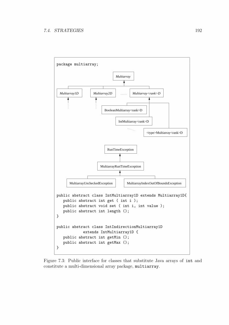
7.4. STRATEGIES 192
package multiarray;
MultiarrayUncheckedException MultiarrayIndexOutOfBoundsException
MultiarrayRunTimeException
RunTimeException
Multiarray
Multiarray1D Multiarray2D Multiarray<rank>D
BooleanMultiarray<rank>D
IntMultiarray<rank>D
<type>Multiarray<rank>D
public abstract class IntMultiarray1D extends Multiarray1D{public abstract int get ( int i );public abstract void set ( int i, int value );public abstract int length ();
}
public abstract class IntIndirectionMultiarray1Dextends IntMultiarray1D {
public abstract int getMin ();public abstract int getMax ();
}
Figure 7.3: Public interface for classes that substitute Java arrays of int andconstitute a multi-dimensional array package, multiarray.

7.4. STRATEGIES 193
one (i.e. permissions setSecurityManager and createSecurityManager
are not granted; see java.lang.RuntimePermission);
3. not allow programs to change the current security policy (i.e. permissions
getPolicy, setPolicy, insertProvider, removeProvider, write to secu-
rity policy files are not granted; see java.security.SecurityPermission
and java.io.FilePermission); and
4. not allow programs to gain access to private instance variables and methods
(i.e. permission suppressAccessChecks are not granted; see java.lang-
.reflect.ReflectPermission).
JVMs can test these assumptions in linear time by invoking specific methods in
the java.lang.SecurityManager and java.security.AccessController ob-
jects at start-up. These assumptions do not imply any loss of generality since
CS&E applications do not require reflection for accessing private instance vari-
ables or methods. In addition, the described security policy assumptions repre-
sent good security management practice for general purpose Java programs. For
a more authoritative and detailed description of Java security, see [124].
The first strategy is the simplest. Given that the problem arises from parallel
execution of multiple threads, a trivial situation occurs when no thread can write
in the indirection array. In other words, part of the problem disappears when the
indirection array is immutable: ImmutableIntMultiarray1D class.
The second strategy uses the synchronization mechanisms defined in Java.
The objects of this class, namely MutableImmutableStateIntMultiarray1D, are
in either of two states. The default state is the mutable state and it allows writes
and reads. The other state is the immutable state which allows only reads. This
second strategy can be thought of as a way to simplify the general case to the
trivial case proposed in the first strategy.
The third and final strategy takes a different approach and does not seek im-
mutability. Only an index that is outside the bounds of an array can generate an
ArrayIndexOutOfBoundsException: i.e. JVMs need to include explicit bounds
checks. The number of threads simultaneously accessing (writing/reading) an
indirection array is irrelevant as long as every element in the indirection array is
within the bounds of the arrays accessed through indirection. The third class,
ValueBoundedIntMultiarray1D, enforces that every element stored in an object
of this class is within the range of zero to a given parameter. The parameter
7.4. STRATEGIES 194
must be greater than or equal to zero, cannot be modified and is passed in to the
constructors.
7.4.1 ImmutableIntMultiarray1D
The methods of a given class can be divided into constructors, queries and com-
mands [174]. Constructors are those methods of a class that, once executed
(without anomalies), create a new object of that class. Moreover, in Java, a
constructor must have the same name as its class. Queries are those methods
that return information about the state (instance variables) of an object. These
methods do not modify the state of any object, and can depend on an expression
of several instance variables. Commands are those methods that change the state
(modify the instance variables) of an object.
The class ImmutableIntMultiarray1D follows the simple idea of making its
objects immutable. Consider the abstract class IntIndirectionMultiarray1D
(see Figure 7.3), the methods get, length, getMin and getMax are query meth-
ods. The method set is a command method. Since the class is abstract, it does
not declare constructors.
Figure 7.4 presents a simplified implementation of the class ImmutableInt-
Multiarray1D. In order to make ImmutableIntMultiarray1D objects immutable,
the command methods are implemented simply by throwing a MultiarrayUn-
checkedException.3 By definition, the query methods do not modify any in-
stance variable. The instance variables (array, length, min and max) are declared
as final4 and every instance variable is initialised by each constructor.
Note that the only statements (bytecodes in the JVMs) that write to the in-
stance variables occur in constructors and that the instance variables are private
and final. These two conditions are almost enough to derive that every object
is immutable. However they do not guarantee that a method of another class
cannot modify an object of class ImmutableIntMultiarray1D. For this purpose,
it is also necessary that the instance variables do not escape the scope of the class
3MultiarrayUncheckedException inherits from RuntimeException – is an unchecked ex-ception – and, thus, methods need to neither include it in their signature nor provide try-catchclauses.
4The declaration of an instance variable as final means that it cannot be modified once ithas been initialised. Specifically, The declaration of an instance variable of type array as finalindicates that once an array has been assigned to the instance variable then no other assignmentcan be applied to that instance variable. However, the elements of the assigned array can bemodified without restriction.
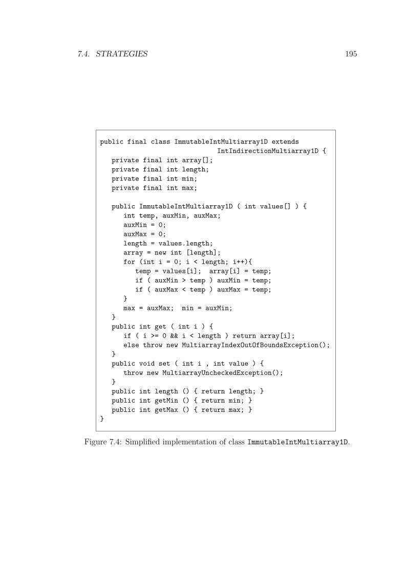
7.4. STRATEGIES 195
public final class ImmutableIntMultiarray1D extendsIntIndirectionMultiarray1D {
private final int array[];private final int length;private final int min;private final int max;
public ImmutableIntMultiarray1D ( int values[] ) {int temp, auxMin, auxMax;auxMin = 0;auxMax = 0;length = values.length;array = new int [length];for (int i = 0; i < length; i++){
temp = values[i]; array[i] = temp;if ( auxMin > temp ) auxMin = temp;if ( auxMax < temp ) auxMax = temp;
}max = auxMax; min = auxMin;
}public int get ( int i ) {
if ( i >= 0 && i < length ) return array[i];else throw new MultiarrayIndexOutOfBoundsException();
}public void set ( int i , int value ) {
throw new MultiarrayUncheckedException();}public int length () { return length; }public int getMin () { return min; }public int getMax () { return max; }
}
Figure 7.4: Simplified implementation of class ImmutableIntMultiarray1D.

7.4. STRATEGIES 196
(i.e. escape analysis — see Section 7.3 — is required). This is ensured when
• these instance variables are created by a method of the class Immutable-
IntMultiarray1D;
• they are all declared as private; and
• none of the methods of class ImmutableIntMultiarray1D returns a refer-
ence to any instance variable.
The life span of these instance variables therefore cannot exceed that of its creator
object.
In contrast the instance variable array would escape the scope of the class
if a constructor were to be implemented as shown in Figure 7.5. It would also
escape the scope of the class if the non-private method getArray (see Figure
7.5) were included in the class. In both cases, any number of threads can get
a reference to the instance variable array and modify its contents (as shown in
Figure 7.6).
public final class ImmutableIntMultiarray1D extendsIntIndirectionMultiarray1D {
...public ImmutableIntMultiarray1D ( int values[] ) {
int temp, auxMin, auxMax;length = values.length;array = values;for (int i = 0; i < length; i++){
temp = values[i];if ( auxMin > temp ) auxMin = temp;if ( auxMax < temp ) auxMax = temp;
}max = auxMax;min = auxMin;
}...
public Object getArray () { return array; }...}
Figure 7.5: Methods that enable the instance variable array to escape the scopeof the class ImmutableIntMultiarray1D.

7.4. STRATEGIES 197
public class ExampleBreakImmutability {public static void main ( String args[] ) {
int fib[] = {1, 1, 2, 3, 5, 8};ImmutableIntMultiarray1D indx = new
ImmutableIntMultiarray1D( fib );fib[0] = -1;System.out.println( indx.get( 0 ) ); // Output: -1int aux[] = (int[]) indx.getArray();aux[0] = -8;System.out.println( indx.get( 0 ) ); // Output: -8
}}
Figure 7.6: An example program modifies the contents of the instance variablearray using the method and the constructor implemented in Figure 7.5.
Consider an algorithm which checks that:
• only bytecodes in constructors write to any instance variable;
• every instance variable is private and final; and
• any instance variable whose type is not primitive does not escape the class.
Such an algorithm can:
• determine whether any class produces immutable objects; and
• it is of complexity O(#b×#iv), where #b is the number of bytecodes and
#iv is the number of instance variables.
Hence, the algorithm is suitable for just-in-time compilers. Further, once the
JSR-083 becomes the Java standard multi-dimensional array package, JVMs can
treat the class ImmutableIntMultiarray1D as a special case and produce the
invariant without doing any check.
The constructor provided in the class ImmutableIntMultiarray1D is ineffi-
cient in terms of memory requirements. This constructor implies that, at some
point during execution, a program would consume double the necessary memory
space in order to hold the elements of an indirection array. This constructor is
included mainly for the sake of clarity. A more complete implementation of this
7.4. STRATEGIES 198
class will provide other constructors that read the elements from files or input
streams.
The implementation of the method get includes a specific test for the pa-
rameter i before accessing the instance variable array. This test ensures that
accesses to array are not out of bounds. Tests of this kind are implemented in
every method set and get in the subsequent classes. For clarity, these tests are
omitted in the implementations of classes shown hereafter.
7.4.2 MutableImmutableStateIntMultiarray1D
Figure 7.7 presents a simplified and non-optimised implementation of the second
strategy. The idea behind this strategy is to ensure that objects of class Mutable-
ImmutableStateIntMultiarray1D can be in only one of two states:
Mutable state – Default state. The elements stored in an object of the class
can be modified and read (at the user’s own risk).
Immutable state – The elements stored in an object of the class can be read
but not modified.
The strategy relies on the synchronization mechanisms provided by Java to
implement the class. Every object in Java has associated with it a lock. The
execution of a synchronized method5 or synchronized block 6 is a critical section.
Given an object with a synchronized method, before any thread can start exe-
cution of the method it must first acquire the lock of that object. Upon return
from the method the thread releases the lock. The same applies to synchronized
blocks. At any point in time at most one thread can be executing a synchronized
method or a synchronized block for the given object.
The Java syntax and the standard Java API do not provide the concept of
acquiring and releasing an object’s lock. Thus, a Java application does not contain
special keywords nor does it invoke a method of the standard Java API to access
the lock of an object. These concepts are part of the specification for execution
of Java applications. Further details about multi-threading in Java can be found
in [125, 155].
5A synchronized method is a method whose declaration contains the keyword synchronized.6A synchronized block is a set of consecutive statements in the body of a method not declared
as synchronized which are surrounded by the clause synchronized (object) {...} .
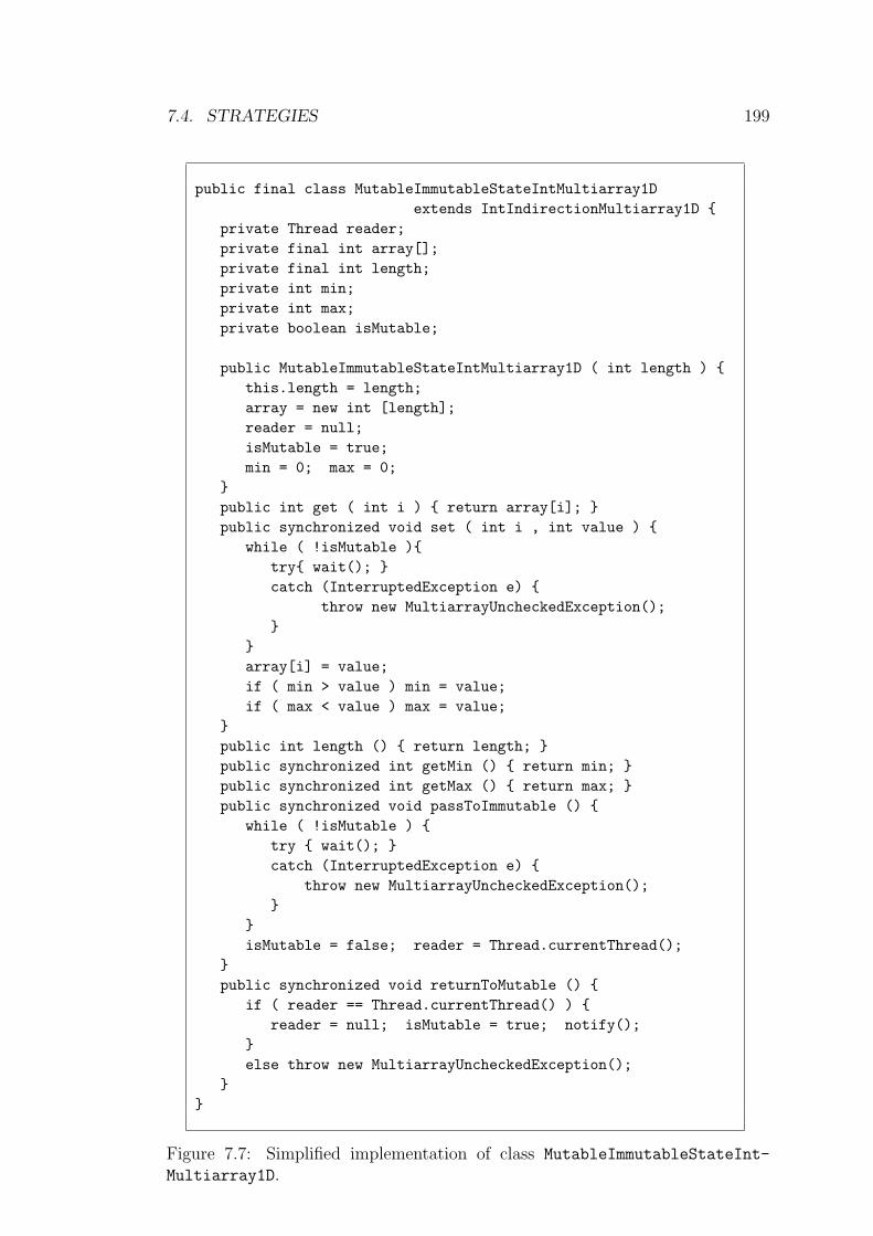
7.4. STRATEGIES 199
public final class MutableImmutableStateIntMultiarray1Dextends IntIndirectionMultiarray1D {
private Thread reader;private final int array[];private final int length;private int min;private int max;private boolean isMutable;
public MutableImmutableStateIntMultiarray1D ( int length ) {this.length = length;array = new int [length];reader = null;isMutable = true;min = 0; max = 0;
}public int get ( int i ) { return array[i]; }public synchronized void set ( int i , int value ) {
while ( !isMutable ){try{ wait(); }catch (InterruptedException e) {
throw new MultiarrayUncheckedException();}
}array[i] = value;if ( min > value ) min = value;if ( max < value ) max = value;
}public int length () { return length; }public synchronized int getMin () { return min; }public synchronized int getMax () { return max; }public synchronized void passToImmutable () {
while ( !isMutable ) {try { wait(); }catch (InterruptedException e) {
throw new MultiarrayUncheckedException();}
}isMutable = false; reader = Thread.currentThread();
}public synchronized void returnToMutable () {
if ( reader == Thread.currentThread() ) {reader = null; isMutable = true; notify();
}else throw new MultiarrayUncheckedException();
}}
Figure 7.7: Simplified implementation of class MutableImmutableStateInt-
Multiarray1D.
7.4. STRATEGIES 200
Consider an object indx of class MutableImmutableStateIntMultiarray-
1D. The implementation of this class (see Figure 7.7) enforces that indx starts
in the mutable state. The state is stored in the boolean instance variable is-
Mutable whose value is kept equivalent to the boolean expression (reader ==
null). For the mutable state, the implementations of the methods get and set
are as expected.
The object indx can only change its state when a thread invokes its synchro-
nized method passToImmutable. When the state is mutable indx changes its
instance variable isMutable to false and stores the thread that executed the
method in the instance variable reader. When the state is immutable, the thread
executing the method stops7 until the state becomes mutable and then proceeds
as explained for the mutable state.
Once indx is in the immutable state, the get method is implemented as
expected while the set method cannot modify the elements of array until indx
returns to the mutable state.
The object indx returns to the mutable state when the same thread that
successfully provoked the transition mutable-to-immutable invokes in indx the
synchronized method returnToMutable. When the transition is completed, this
thread notifies one of the threads, if any, waiting in indx of the state transition.
Given the complexity of matching the lock-wait-notify logic with the state-
ments (bytecodes) that access the instance variables, it is unlikely that JVMs will
incorporate tests for this kind of class invariant. Thus, the remaining alternative
is that JVMs recognise the class as being part of the standard Java API and
automatically produce the desired class invariant.
7The wait and notify methods are part of the standard Java API and both are mem-bers of the class java.lang.Object. In Java every class is a subclass (directly or indirectly)of java.lang.Object and, thus, every object inherits the methods wait and notify. Bothmethods are part of a communication mechanism for Java threads.
For example, suppose the thread executing the method passToImmutable finds indx in im-mutable state. The thread starts executing the synchronized method after acquiring the lockof indx. After checking the state, it needs to wait until the state of indx is mutable. Thethread itself cannot force the state transition. It needs to wait for another thread to provokethat transition. The first thread stops execution by invoking the method wait in indx. Thismethod makes the first thread release the lock of indx, wait until a second thread invokes themethod notify in indx and then reacquire the lock prior to return from wait. Several threadscan be waiting in indx (i.e. have invoked wait), but only one thread is notified when the secondthread invokes notify in indx. Further information about threads in Java and the wait/notifymechanism can be found in [125, 155].
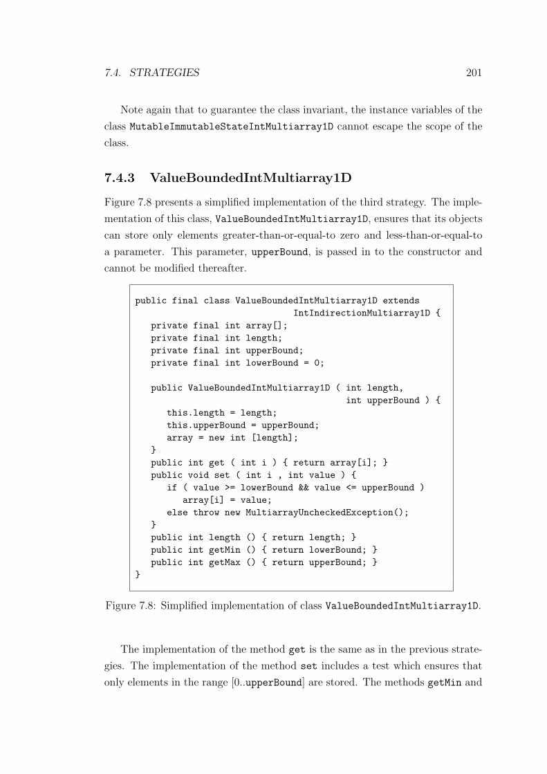
7.4. STRATEGIES 201
Note again that to guarantee the class invariant, the instance variables of the
class MutableImmutableStateIntMultiarray1D cannot escape the scope of the
class.
7.4.3 ValueBoundedIntMultiarray1D
Figure 7.8 presents a simplified implementation of the third strategy. The imple-
mentation of this class, ValueBoundedIntMultiarray1D, ensures that its objects
can store only elements greater-than-or-equal-to zero and less-than-or-equal-to
a parameter. This parameter, upperBound, is passed in to the constructor and
cannot be modified thereafter.
public final class ValueBoundedIntMultiarray1D extendsIntIndirectionMultiarray1D {
private final int array[];private final int length;private final int upperBound;private final int lowerBound = 0;
public ValueBoundedIntMultiarray1D ( int length,int upperBound ) {
this.length = length;this.upperBound = upperBound;array = new int [length];
}public int get ( int i ) { return array[i]; }public void set ( int i , int value ) {
if ( value >= lowerBound && value <= upperBound )array[i] = value;
else throw new MultiarrayUncheckedException();}public int length () { return length; }public int getMin () { return lowerBound; }public int getMax () { return upperBound; }
}
Figure 7.8: Simplified implementation of class ValueBoundedIntMultiarray1D.
The implementation of the method get is the same as in the previous strate-
gies. The implementation of the method set includes a test which ensures that
only elements in the range [0..upperBound] are stored. The methods getMin and
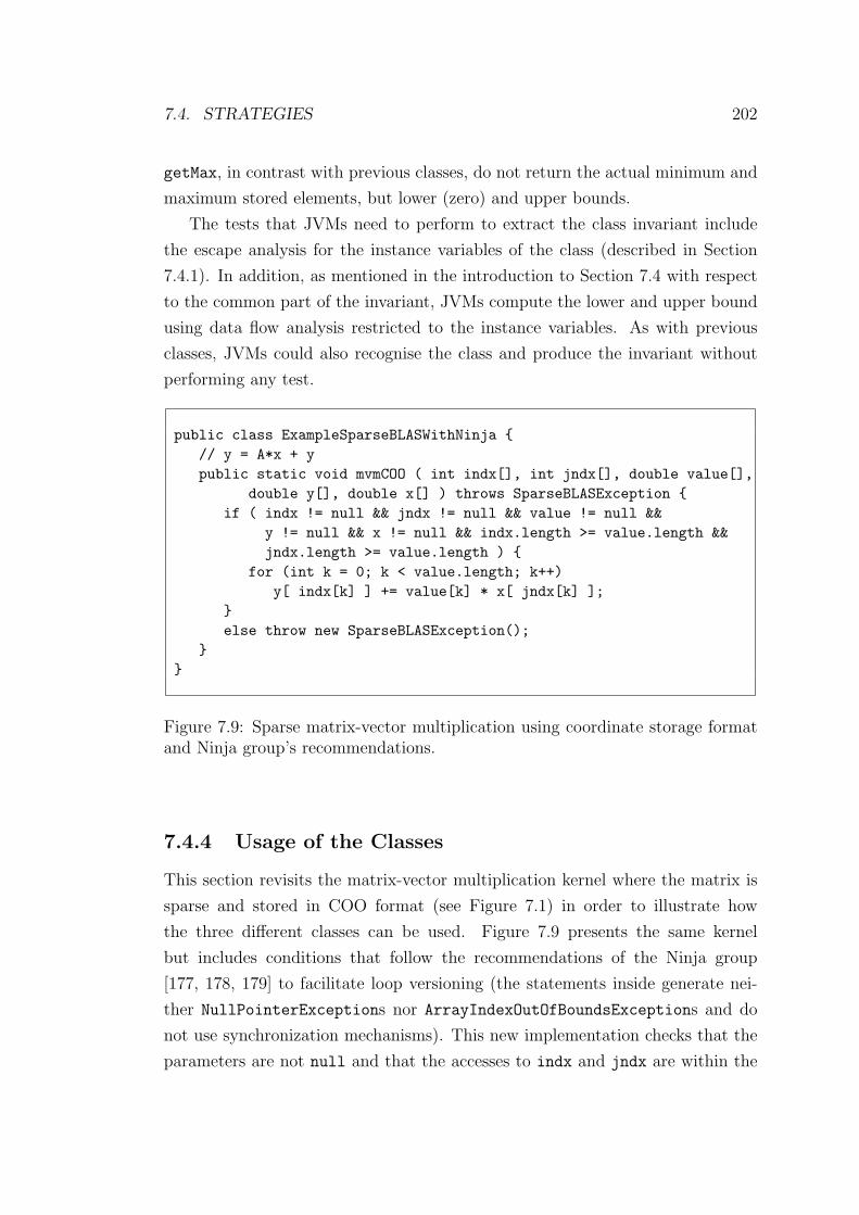
7.4. STRATEGIES 202
getMax, in contrast with previous classes, do not return the actual minimum and
maximum stored elements, but lower (zero) and upper bounds.
The tests that JVMs need to perform to extract the class invariant include
the escape analysis for the instance variables of the class (described in Section
7.4.1). In addition, as mentioned in the introduction to Section 7.4 with respect
to the common part of the invariant, JVMs compute the lower and upper bound
using data flow analysis restricted to the instance variables. As with previous
classes, JVMs could also recognise the class and produce the invariant without
performing any test.
public class ExampleSparseBLASWithNinja {// y = A*x + ypublic static void mvmCOO ( int indx[], int jndx[], double value[],
double y[], double x[] ) throws SparseBLASException {if ( indx != null && jndx != null && value != null &&
y != null && x != null && indx.length >= value.length &&jndx.length >= value.length ) {
for (int k = 0; k < value.length; k++)y[ indx[k] ] += value[k] * x[ jndx[k] ];
}else throw new SparseBLASException();
}}
Figure 7.9: Sparse matrix-vector multiplication using coordinate storage formatand Ninja group’s recommendations.
7.4.4 Usage of the Classes
This section revisits the matrix-vector multiplication kernel where the matrix is
sparse and stored in COO format (see Figure 7.1) in order to illustrate how
the three different classes can be used. Figure 7.9 presents the same kernel
but includes conditions that follow the recommendations of the Ninja group
[177, 178, 179] to facilitate loop versioning (the statements inside generate nei-
ther NullPointerExceptions nor ArrayIndexOutOfBoundsExceptions and do
not use synchronization mechanisms). This new implementation checks that the
parameters are not null and that the accesses to indx and jndx are within the
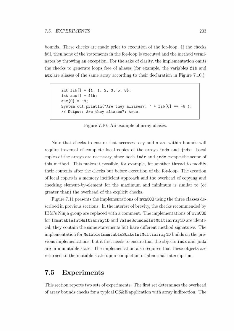
7.5. EXPERIMENTS 203
bounds. These checks are made prior to execution of the for-loop. If the checks
fail, then none of the statements in the for-loop is executed and the method termi-
nates by throwing an exception. For the sake of clarity, the implementation omits
the checks to generate loops free of aliases (for example, the variables fib and
aux are aliases of the same array according to their declaration in Figure 7.10.)
int fib[] = {1, 1, 2, 3, 5, 8};int aux[] = fib;aux[0] = -8;System.out.println("Are they aliases?: " + fib[0] == -8 );// Output: Are they aliases?: true
Figure 7.10: An example of array aliases.
Note that checks to ensure that accesses to y and x are within bounds will
require traversal of complete local copies of the arrays indx and jndx. Local
copies of the arrays are necessary, since both indx and jndx escape the scope of
this method. This makes it possible, for example, for another thread to modify
their contents after the checks but before execution of the for-loop. The creation
of local copies is a memory inefficient approach and the overhead of copying and
checking element-by-element for the maximum and minimum is similar to (or
greater than) the overhead of the explicit checks.
Figure 7.11 presents the implementations of mvmCOO using the three classes de-
scribed in previous sections. In the interest of brevity, the checks recommended by
IBM’s Ninja group are replaced with a comment. The implementations of mvmCOO
for ImmutableIntMultiarray1D and ValueBoundedIntMultiarray1D are identi-
cal; they contain the same statements but have different method signatures. The
implementation for MutableImmutableStateIntMultiarray1D builds on the pre-
vious implementations, but it first needs to ensure that the objects indx and jndx
are in immutable state. The implementation also requires that these objects are
returned to the mutable state upon completion or abnormal interruption.
7.5 Experiments
This section reports two sets of experiments. The first set determines the overhead
of array bounds checks for a typical CS&E application with array indirection. The
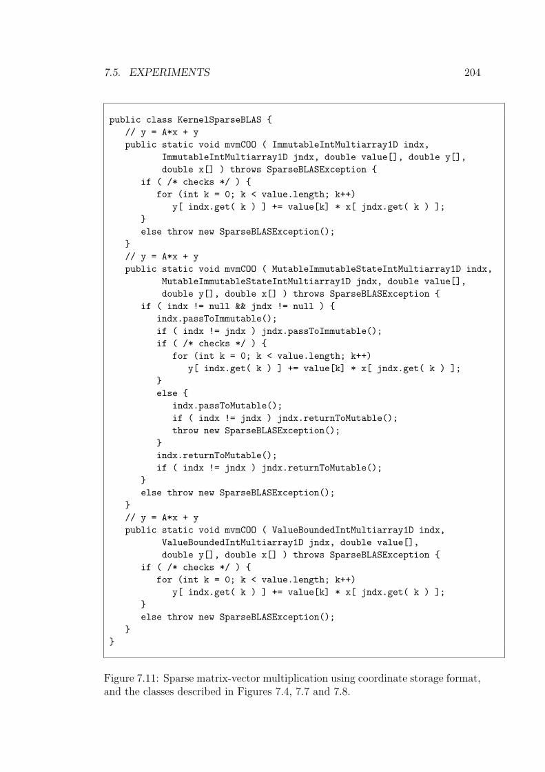
7.5. EXPERIMENTS 204
public class KernelSparseBLAS {// y = A*x + ypublic static void mvmCOO ( ImmutableIntMultiarray1D indx,
ImmutableIntMultiarray1D jndx, double value[], double y[],double x[] ) throws SparseBLASException {
if ( /* checks */ ) {for (int k = 0; k < value.length; k++)
y[ indx.get( k ) ] += value[k] * x[ jndx.get( k ) ];}else throw new SparseBLASException();
}// y = A*x + ypublic static void mvmCOO ( MutableImmutableStateIntMultiarray1D indx,
MutableImmutableStateIntMultiarray1D jndx, double value[],double y[], double x[] ) throws SparseBLASException {
if ( indx != null && jndx != null ) {indx.passToImmutable();if ( indx != jndx ) jndx.passToImmutable();if ( /* checks */ ) {
for (int k = 0; k < value.length; k++)y[ indx.get( k ) ] += value[k] * x[ jndx.get( k ) ];
}else {
indx.passToMutable();if ( indx != jndx ) jndx.returnToMutable();throw new SparseBLASException();
}indx.returnToMutable();if ( indx != jndx ) jndx.returnToMutable();
}else throw new SparseBLASException();
}// y = A*x + ypublic static void mvmCOO ( ValueBoundedIntMultiarray1D indx,
ValueBoundedIntMultiarray1D jndx, double value[],double y[], double x[] ) throws SparseBLASException {
if ( /* checks */ ) {for (int k = 0; k < value.length; k++)
y[ indx.get( k ) ] += value[k] * x[ jndx.get( k ) ];}else throw new SparseBLASException();
}}
Figure 7.11: Sparse matrix-vector multiplication using coordinate storage format,and the classes described in Figures 7.4, 7.7 and 7.8.
7.5. EXPERIMENTS 205
aim is to find an experimental lower bound for the performance improvement
that can be achieved when array bounds checks are eliminated. This is a lower
bound because array bounds checks, together with Java’s strict exception model,
are inhibitors of other optimising transformations [177, 178, 179] that can further
improve the performance. The second set of experiments, also for the same CS&E
application, determines the overhead of using the classes proposed in Section 7.4
rather than accessing Java arrays directly.
The CS&E application considered is the solution of systems of linear equations
using iterative solvers [122]. The experiments focus on the kernel operation of
matrix-vector multiplication. Specifically, matrix-vector multiplication where the
matrix is in COO format (mvmCOO) is used, because this is the only benchmark
proposed by the JGF Benchmark and Scimark that addresses array indirection.
The iterative nature of the solver implies that the matrix-vector multiplication
operation is executed repeatedly until sufficient accuracy is achieved or an upper
bound on the number of iterations is reached. The experiments implement an
iterative method that executes mvmCOO 100 times.
Results are reported for four different implementations for mvmCOO (see Figures
7.9 and 7.11). The four implementations of mvmCOO are derived using:
1. only Java arrays (JA implementation);
2. objects of class ImmutableIntMultiarray1D (I-MA implementation);
3. objects of class MutableImmutableStateIntMultiarray1D (MI-MA imple-
mentation); and
4. objects of class ValueBoundedIntMultiarray1D (VB-MA implementation).
The experiments consider three different square sparse matrices from the Ma-
trix Market collection [48] (see Figure 7.12). The three matrices are: utm5940
(size 5940 with 83842 nonzero elements), s3rmt3m3 (symmetric and size 5357 with
106526 nonzero entries), and s3dkt3m2 (symmetric and size 90449 with 1921955
nonzero entries). The implementations do not take advantage of symmetry and,
thus, s2rmt3m3 and s3dkt3m2 are stored and operated on using all their nonzero
elements. The vector x (see Figures 7.9 and 7.11) is initialised with random num-
bers from a uniform distribution with values ranging between 0 and 5, and the
vector y is initialised with zeros.
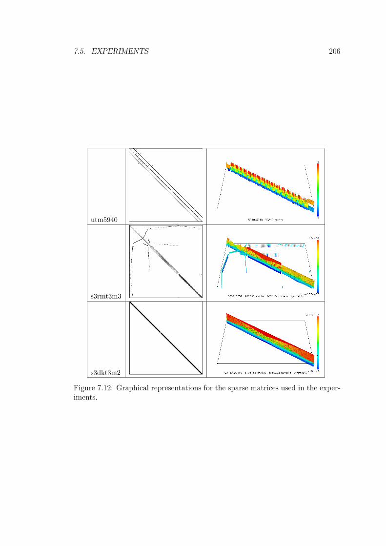
7.5. EXPERIMENTS 206
utm5940
s3rmt3m3
s3dkt3m2
Figure 7.12: Graphical representations for the sparse matrices used in the exper-iments.
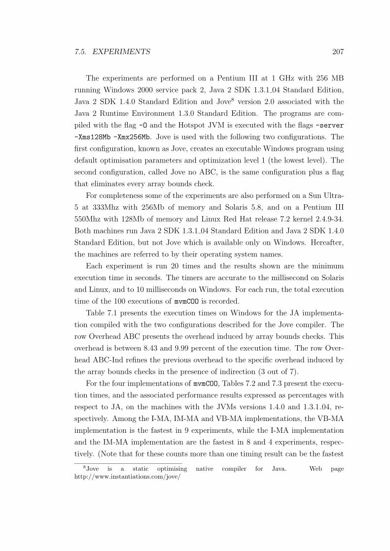
7.5. EXPERIMENTS 207
The experiments are performed on a Pentium III at 1 GHz with 256 MB
running Windows 2000 service pack 2, Java 2 SDK 1.3.1 04 Standard Edition,
Java 2 SDK 1.4.0 Standard Edition and Jove8 version 2.0 associated with the
Java 2 Runtime Environment 1.3.0 Standard Edition. The programs are com-
piled with the flag -O and the Hotspot JVM is executed with the flags -server
-Xms128Mb -Xmx256Mb. Jove is used with the following two configurations. The
first configuration, known as Jove, creates an executable Windows program using
default optimisation parameters and optimization level 1 (the lowest level). The
second configuration, called Jove no ABC, is the same configuration plus a flag
that eliminates every array bounds check.
For completeness some of the experiments are also performed on a Sun Ultra-
5 at 333Mhz with 256Mb of memory and Solaris 5.8, and on a Pentium III
550Mhz with 128Mb of memory and Linux Red Hat release 7.2 kernel 2.4.9-34.
Both machines run Java 2 SDK 1.3.1 04 Standard Edition and Java 2 SDK 1.4.0
Standard Edition, but not Jove which is available only on Windows. Hereafter,
the machines are referred to by their operating system names.
Each experiment is run 20 times and the results shown are the minimum
execution time in seconds. The timers are accurate to the millisecond on Solaris
and Linux, and to 10 milliseconds on Windows. For each run, the total execution
time of the 100 executions of mvmCOO is recorded.
Table 7.1 presents the execution times on Windows for the JA implementa-
tion compiled with the two configurations described for the Jove compiler. The
row Overhead ABC presents the overhead induced by array bounds checks. This
overhead is between 8.43 and 9.99 percent of the execution time. The row Over-
head ABC-Ind refines the previous overhead to the specific overhead induced by
the array bounds checks in the presence of indirection (3 out of 7).
For the four implementations of mvmCOO, Tables 7.2 and 7.3 present the execu-
tion times, and the associated performance results expressed as percentages with
respect to JA, on the machines with the JVMs versions 1.4.0 and 1.3.1 04, re-
spectively. Among the I-MA, IM-MA and VB-MA implementations, the VB-MA
implementation is the fastest in 9 experiments, while the I-MA implementation
and the IM-MA implementation are the fastest in 8 and 4 experiments, respec-
tively. (Note that for these counts more than one timing result can be the fastest
8Jove is a static optimising native compiler for Java. Web pagehttp://www.instantiations.com/jove/
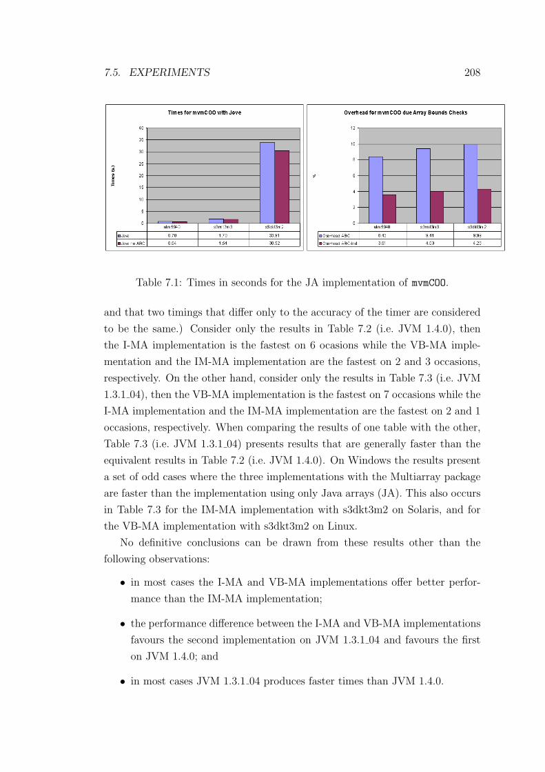
7.5. EXPERIMENTS 208
Table 7.1: Times in seconds for the JA implementation of mvmCOO.
and that two timings that differ only to the accuracy of the timer are considered
to be the same.) Consider only the results in Table 7.2 (i.e. JVM 1.4.0), then
the I-MA implementation is the fastest on 6 ocasions while the VB-MA imple-
mentation and the IM-MA implementation are the fastest on 2 and 3 occasions,
respectively. On the other hand, consider only the results in Table 7.3 (i.e. JVM
1.3.1 04), then the VB-MA implementation is the fastest on 7 occasions while the
I-MA implementation and the IM-MA implementation are the fastest on 2 and 1
occasions, respectively. When comparing the results of one table with the other,
Table 7.3 (i.e. JVM 1.3.1 04) presents results that are generally faster than the
equivalent results in Table 7.2 (i.e. JVM 1.4.0). On Windows the results present
a set of odd cases where the three implementations with the Multiarray package
are faster than the implementation using only Java arrays (JA). This also occurs
in Table 7.3 for the IM-MA implementation with s3dkt3m2 on Solaris, and for
the VB-MA implementation with s3dkt3m2 on Linux.
No definitive conclusions can be drawn from these results other than the
following observations:
• in most cases the I-MA and VB-MA implementations offer better perfor-
mance than the IM-MA implementation;
• the performance difference between the I-MA and VB-MA implementations
favours the second implementation on JVM 1.3.1 04 and favours the first
on JVM 1.4.0; and
• in most cases JVM 1.3.1 04 produces faster times than JVM 1.4.0.
7.5. EXPERIMENTS 209
Table 7.2: Average times in seconds for the four different implementations ofmvmCOO.
Table 7.4 takes a closer look at the execution times of the JA and VB-MA
implementations on Windows with JVM version 1.4.0 and combines them with
semantic expansion [228, 176, 177, 178]. Experiments with semantic expansion re-
ported in [176, 178] indicate that, for scientific codes with real number arithmetic,
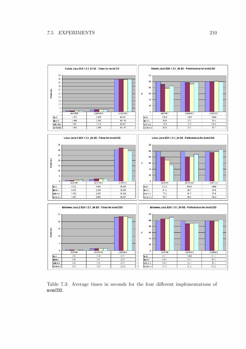
7.5. EXPERIMENTS 210
Table 7.3: Average times in seconds for the four different implementations ofmvmCOO.
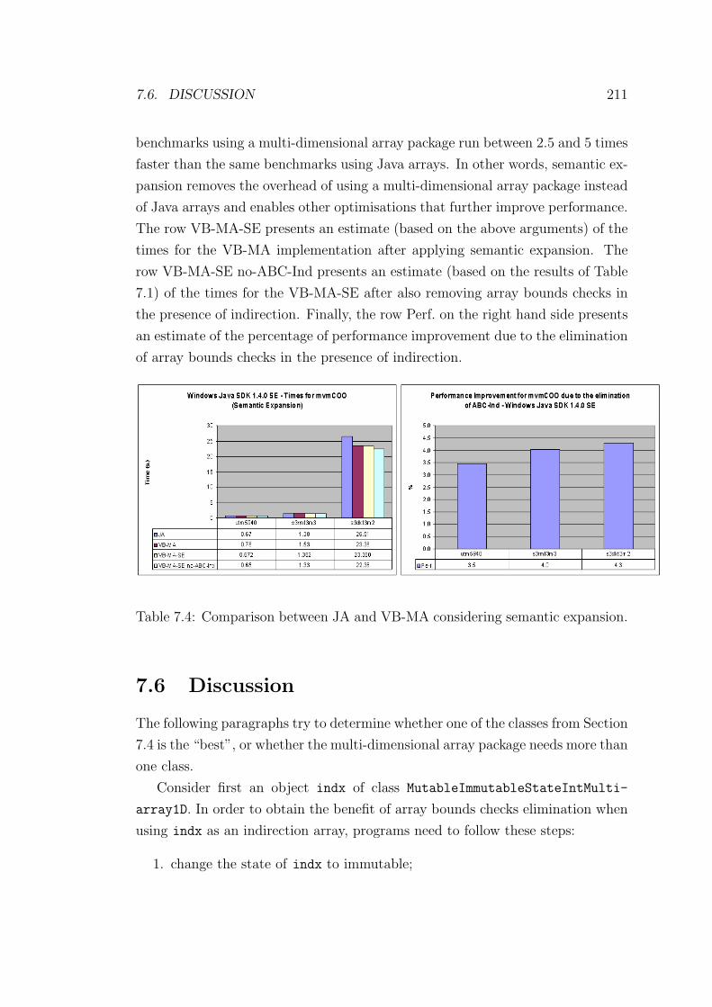
7.6. DISCUSSION 211
benchmarks using a multi-dimensional array package run between 2.5 and 5 times
faster than the same benchmarks using Java arrays. In other words, semantic ex-
pansion removes the overhead of using a multi-dimensional array package instead
of Java arrays and enables other optimisations that further improve performance.
The row VB-MA-SE presents an estimate (based on the above arguments) of the
times for the VB-MA implementation after applying semantic expansion. The
row VB-MA-SE no-ABC-Ind presents an estimate (based on the results of Table
7.1) of the times for the VB-MA-SE after also removing array bounds checks in
the presence of indirection. Finally, the row Perf. on the right hand side presents
an estimate of the percentage of performance improvement due to the elimination
of array bounds checks in the presence of indirection.
Table 7.4: Comparison between JA and VB-MA considering semantic expansion.
7.6 Discussion
The following paragraphs try to determine whether one of the classes from Section
7.4 is the “best”, or whether the multi-dimensional array package needs more than
one class.
Consider first an object indx of class MutableImmutableStateIntMulti-
array1D. In order to obtain the benefit of array bounds checks elimination when
using indx as an indirection array, programs need to follow these steps:
1. change the state of indx to immutable;
7.6. DISCUSSION 212
2. execute any other actions (normally inside loops) that access the elements
stored in indx; and
3. change the state of indx back to mutable.
An example of these steps is the implementation of matrix-vector multiplication
using class MutableImmutableStateIntMultiarray1D (see Figure 7.11).
If the third step is omitted, possibly accidentally, the indirection array indx
becomes useless for the purpose of eliminating array bounds checks. Other
threads (or a thread that abandoned execution without adequate clean up) would
be left waiting indefinitely for notification that indx has returned to the mutable
state.
Another problem can arise when several threads are executing in parallel and
at least two threads need indx and jndx (another object of the same class) at
the same time. Depending on the order of execution, or if both are aliases of the
same object, a deadlock can occur.
One might think that these problems could be overcome by modifying the
implementation of the class so that it maintains a complete list of thread readers
instead of just one thread reader. However, omission of the third step then leads
to starvation of writers.
Given that these problems are not inherent in the other two classes, and that
the experiments of Section 7.5 do not show a performance benefit in favour of
class MutableImmutableStateIntMultiarray1D, the decision is to disregard this
class.
The discussion now considers scenarios in CS&E applications where the two
remaining classes can be used. The functionalities of classes ImmutableInt-
Multiarray1D and ValueBoundedIntMultiarray1D are contrasted with regard
to the requirements of such applications.
Remember that the two classes have the same public interface, but provide
different functionality. As the name suggests, class ImmutableIntMultiarray1D
implements the method set without modifying any instance variable; it simply
throws an unchecked exception (see Figure 7.4). In contrast, class ValueBounded-
IntMultiarray1D provides the expected functionality for this method as long as
the parameter value of the method is positive and less than or equal to the
instance variable upperBound (see Figure 7.8).
In CS&E scenarios, such as LU-factorisation of dense and banded matrices
with pivoting, and Gauss Elimination for sparse matrices with fill-in, applications
7.7. SUMMARY 213
need to update the content of indirection arrays [122, 135]. For example, fill-
in means that new nonzero elements are created where zero elements existed
previously. Thus, the Gauss Elimination algorithm progressively creates new
nonzero matrix elements. Assuming that the matrix is stored in COO format,
the indirection arrays indx and jndx need to be updated with the row and column
indices, respectively, for each new nonzero element.
Given that, in other CS&E applications, indirection arrays remain unaltered
after initialisation, the only reason for including class ImmutableIntMultiarray-
1D would be performance. However the performance evaluation reveals that there
is no significance performance advantage. Therefore, the conclusion is to incor-
porate only the class ValueBoundedIntMultiarray1D into the multi-dimensional
array package.
7.7 Summary
Array indirection is ubiquitous in CS&E applications with sparse matrices. With
the specification of array accesses in Java and with current techniques for eliminat-
ing array bounds checks, applications with array indirection suffer the overhead
of explicitly checking each access made through an indirection array.
Building on previous work by IBM’s Ninja and Jalapeno groups, three new
strategies to eliminate array bounds checks in the presence of indirection have
been presented. Each strategy is implemented as a Java class that can replace
indirection arrays of type int. The aim of the three strategies is to provide extra
information to JVMs so that array bounds checks in the presence of indirection
can be removed. For normal Java arrays of type int this extra information would
require access to the whole application (i.e. no dynamic loading) or be heavy
weight. The algorithm to remove the array bounds checks is a combination of
loop versioning (as used by the Ninja group [175, 177, 178, 179]), escape analysis
[66] and construction of constraints based on data flow analysis (ABCD algorithm
[44]).
The experiments have estimated the performance benefit of eliminating array
bound checks in the presence of indirection. The benefit has been estimated at
about 4 percent of the execution time. The experiments have also evaluated the
overhead of using a Java class to replace Java arrays on off-the-shelf JVMs. This
overhead varies for each class, JVM, machine architecture and matrix, but it is
7.7. SUMMARY 214
an average of 8 percent of the execution time. This kind of overhead essentially
can be eliminated using semantic expansion [228, 178] or a sequence of standard
transformations as described in Chapter 8 and illustrated in Chapter 9.
The evaluation of the three strategies also includes a discussion of their ad-
vantages and disadvantages. Overall, the third strategy, class ValueBounded-
IntMultiarray1D, is the best. It takes a different approach by not seeking im-
mutability of objects. The number of threads accessing an indirection array at a
given time is irrelevant as long as every element in the indirection array is within
the bounds of the arrays accessed through indirection. The class enforces that
every element stored in an object of the class contains a value between zero and
a given parameter. The parameter must be greater than or equal to zero, cannot
be modified and is passed in to the constructor.
Chapter 8
How and When Can OOLALA Be
Optimised?
8.1 Introduction
Object Oriented (OO) software construction has characteristics that can im-
prove the development process and usability of mathematical software libraries.
OoLaLa, a novel Object Oriented Linear Algebra LibrAry, is the outcome of
a study of these benefits in the context of sequential Numerical Linear Algebra
(NLA). Previous chapters have covered the design of the library, its implemen-
tation and performance evaluation and the first part of the optimisation (elimi-
nation of array bounds checks in the presence of indirection). This and the next
chapter cover the second part of the optimisation of OoLaLa.
OO software construction can be used to simplify the interface of NLA li-
braries and thus make them easier to use. It can also be used to arrive at several
fundamentally different implementations of matrix operations. In contrast with
traditional NLA libraries, OoLaLa provides two higher abstraction levels at
which matrix operations are implemented. Traditional NLA libraries sacrifice
abstraction (when provided by the programming language) as a trade-off for per-
formance. In traditional NLA libraries, the implementations of matrix operations
have embedded knowledge about the storage formats and properties of the ma-
trices that are passed in as parameters. These implementations are said to be at
Storage Format Abstraction level (SFA-level). OoLaLa adopts the philosophy
that abstraction should not be compromised for performance. The first higher
abstraction level, Matrix Abstraction level (MA-level), provides random access
215
8.1. INTRODUCTION 216
to matrix elements. The second higher abstraction level, Iterator Abstraction
level (IA-level) (based on the iterator pattern [107]), provides sequential access
to matrix elements regardless of storage formats or matrix properties based on
the structure of nonzero elements. Both abstraction levels reduce the number of
implementations required for any given matrix operation (Chapter 5).
Chapter 6 presented a preliminary performance evaluation of a Java imple-
mentation of a subset of OoLaLa which shows that implementations at MA-level
and IA-level are not competitive with those at SFA-level. This motivates the two
questions addressed in this chapter:
• how might implementations of matrix operations at MA-level and IA-level
be transformed into efficient implementations at SFA-level? and
• under what conditions can such transformations be applied? (i.e. for which
sets of storage formats and matrix properties can this be done automati-
cally?)
The former question is answered by presenting a sequence of standard compiler
transformations. The latter question is addressed by the definition of a subset
of matrix properties, namely linear combination matrix properties and a subset
of storage formats, namely constant time element access storage formats, which
guarantee that these transformations can be applied. Instead of implementing
these transformations in a Java Virtual Machine [160] (JVM) or compiler, their
effectiveness is established by construction.
The sequence of standard compiler transformations used to tackle the former
question is:
1. method inlining [61, 126, 70, 6, 22, 74, 139, 215],
2. move the guards1 for the inlined methods to surround the loop (or loops)
and include nullity test for every object,
3. remove try-catch and throw clauses,
4. make local copies of the accessed attributes (class and instance variables),
5. disambiguate aliases,
1For the sake of clarity, method inlining with guarded class tests is assumed. Further,although not the most efficient [74, 139], it generates the most general code.
8.2. PRELIMINARIES 217
6. remove redundant computations, and
7. transform while-loops into for-loops,
The chapter is organised as follows. Section 8.2 delimits the extent of the
transformations that a general purpose compiler might apply. It also defines
specific subsets of matrix properties and storage formats. Sections 8.3 and 8.4
illustrate the sequence of standard compiler transformations for the defined sub-
sets of matrix properties and storage formats. For these subsets, the sequence
transforms implementations at MA-level (Section 8.3) and IA-level (Section 8.4)
into efficient implementations at SFA-level. For brevity, this chapter focuses on
implementations at IA-level using MatrixIterator. Hence, the illustration of
the sequence of standard compiler transformations and the generalisation for im-
plementations at IA-level using MatrixIterator1D are omitted. Note that cache
optimising transformations to obtain blocked [63, 88] or recursive implementa-
tions [133, 10] are not included in the sequence. Such transformations are out
of the scope of the thesis and are omitted because previous work (IBM’s Ninja
group [177, 179]) has enabled JVM/compilers to apply these transformations to
implementations at SFA-level. Related work is presented in Section 8.5.
8.2 Preliminaries
Remember the subdivision of matrix properties introduced in Section 2.3. A sub-
set of the matrix properties, namely the mathematical relation properties, are
properties of the whole matrix, rather than of the individual elements of the ma-
trix. Examples of mathematical relation properties are symmetry (A=AT ), and
orthogonality (AT =A−1 or AAT = I). Mathematical relation properties enable
NLA researchers to formulate different algorithms for a given matrix operation.
A second subset of matrix properties, namely nonzero elements structure prop-
erties, is based on the structure of the nonzero matrix elements. Examples are
upper triangular property, banded property, block diagonal property and sparse
property (see Section 2.3). This latter group of matrix properties enables spe-
cialised algorithms by elimininating those steps of the algorithm that are known
to be redundant or unnecessary (e.g. x=x+zero and y=y*one).
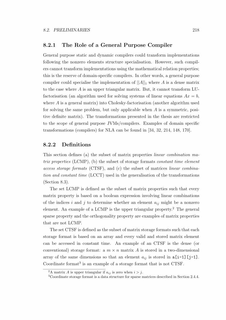
8.2. PRELIMINARIES 218
8.2.1 The Role of a General Purpose Compiler
General purpose static and dynamic compilers could transform implementations
following the nonzero elements structure specialisation. However, such compil-
ers cannot transform implementations using the mathematical relation properties;
this is the reserve of domain-specific compilers. In other words, a general purpose
compiler could specialise the implementation of ||A||1 where A is a dense matrix
to the case where A is an upper triangular matrix. But, it cannot transform LU-
factorisation (an algorithm used for solving systems of linear equations Ax = b,
where A is a general matrix) into Cholesky-factorisation (another algorithm used
for solving the same problem, but only applicable when A is a symmetric, posi-
tive definite matrix). The transformations presented in the thesis are restricted
to the scope of general purpose JVMs/compilers. Examples of domain specific
transformations (compilers) for NLA can be found in [34, 32, 214, 148, 170].
8.2.2 Definitions
This section defines (a) the subset of matrix properties linear combination ma-
trix properties (LCMP), (b) the subset of storage formats constant time element
access storage formats (CTSF), and (c) the subset of matrices linear combina-
tion and constant time (LCCT) used in the generalisation of the transformations
(Section 8.3).
The set LCMP is defined as the subset of matrix properties such that every
matrix property is based on a boolean expression involving linear combinations
of the indices i and j to determine whether an element aij might be a nonzero
element. An example of a LCMP is the upper triangular property.2 The general
sparse property and the orthogonality property are examples of matrix properties
that are not LCMP.
The set CTSF is defined as the subset of matrix storage formats such that each
storage format is based on an array and every valid and stored matrix element
can be accessed in constant time. An example of an CTSF is the dense (or
conventional) storage format: a m × n matrix A is stored in a two-dimensional
array of the same dimensions so that an element aij is stored in a[i-1][j-1].
Coordinate format3 is an example of a storage format that is not CTSF.
2A matrix A is upper triangular if aij is zero when i > j.3Coordinate storage format is a data structure for sparse matrices described in Section 2.4.4.
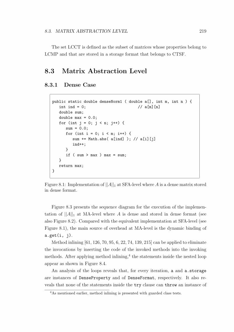
8.3. MATRIX ABSTRACTION LEVEL 219
The set LCCT is defined as the subset of matrices whose properties belong to
LCMP and that are stored in a storage format that belongs to CTSF.
8.3 Matrix Abstraction Level
8.3.1 Dense Case
public static double denseNorm1 ( double a[], int m, int n ) {int ind = 0; // a[m][n]double sum;double max = 0.0;for (int j = 0; j < n; j++) {
sum = 0.0;for (int i = 0; i < m; i++) {
sum += Math.abs( a[ind] ); // a[i][j]ind++;
}if ( sum > max ) max = sum;
}return max;
}
Figure 8.1: Implementation of ||A||1 at SFA-level where A is a dense matrix storedin dense format.
Figure 8.3 presents the sequence diagram for the execution of the implemen-
tation of ||A||1 at MA-level where A is dense and stored in dense format (see
also Figure 8.2). Compared with the equivalent implementation at SFA-level (see
Figure 8.1), the main source of overhead at MA-level is the dynamic binding of
a.get(i, j).
Method inlining [61, 126, 70, 95, 6, 22, 74, 139, 215] can be applied to eliminate
the invocations by inserting the code of the invoked methods into the invoking
methods. After applying method inlining,4 the statements inside the nested loop
appear as shown in Figure 8.4.
An analysis of the loops reveals that, for every iteration, a and a.storage
are instances of DenseProperty and of DenseFormat, respectively. It also re-
veals that none of the statements inside the try clause can throw an instance of
4As mentioned earlier, method inlining is presented with guarded class tests.
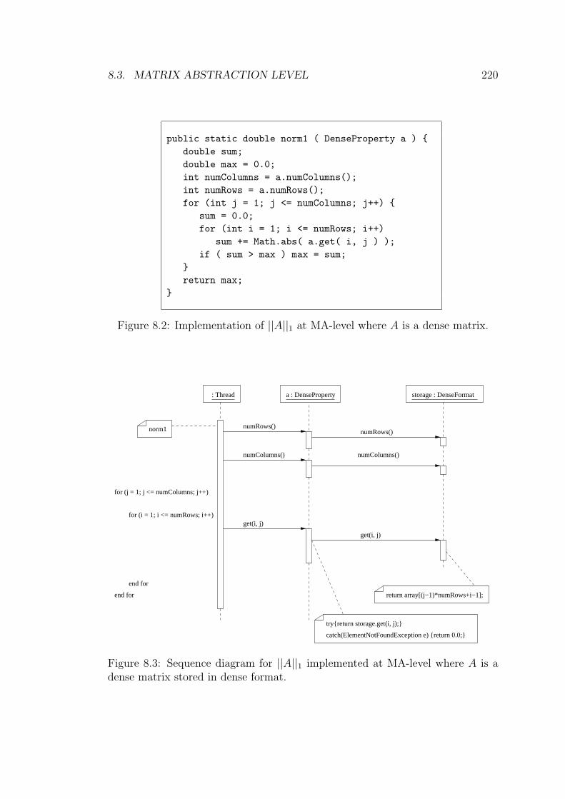
8.3. MATRIX ABSTRACTION LEVEL 220
public static double norm1 ( DenseProperty a ) {double sum;double max = 0.0;int numColumns = a.numColumns();int numRows = a.numRows();for (int j = 1; j <= numColumns; j++) {
sum = 0.0;for (int i = 1; i <= numRows; i++)
sum += Math.abs( a.get( i, j ) );if ( sum > max ) max = sum;
}return max;
}
Figure 8.2: Implementation of ||A||1 at MA-level where A is a dense matrix.
return array[(j−1)*numRows+i−1];
a : DenseProperty storage : DenseFormat
numRows()
numColumns()
numRows()
numColumns()
: Thread
norm1
get(i, j)
get(i, j)
catch(ElementNotFoundException e) {return 0.0;}
try{return storage.get(i, j);}
for (i = 1; i <= numRows; i++)
end for
for (j = 1; j <= numColumns; j++)
end for
Figure 8.3: Sequence diagram for ||A||1 implemented at MA-level where A is adense matrix stored in dense format.
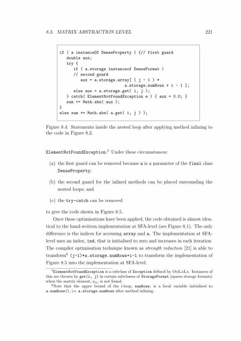
8.3. MATRIX ABSTRACTION LEVEL 221
if ( a instanceOf DenseProperty ) {// first guarddouble aux;try {
if ( a.storage instanceof DenseFormat )// second guard
aux = a.storage.array[ ( j - 1 ) *a.storage.numRows + i - 1 ];
else aux = a.storage.get( i, j );} catch( ElementNotFoundException e ) { aux = 0.0; }sum += Math.abs( aux );
}else sum += Math.abs( a.get( i, j ) );
Figure 8.4: Statements inside the nested loop after applying method inlining tothe code in Figure 8.2.
ElementNotFoundException.5 Under these circumstances:
(a) the first guard can be removed because a is a parameter of the final class
DenseProperty;
(b) the second guard for the inlined methods can be placed surrounding the
nested loops; and
(c) the try-catch can be removed
to give the code shown in Figure 8.5.
Once these optimisations have been applied, the code obtained is almost iden-
tical to the hand-written implementation at SFA-level (see Figure 8.1). The only
difference is the indices for accessing array and a. The implementation at SFA-
level uses an index, ind, that is initialised to zero and increases in each iteration.
The compiler optimisation technique known as strength reduction [21] is able to
transform6 (j-1)*a.storage.numRows+i-1 to transform the implementation of
Figure 8.5 into the implementation at SFA-level.
5ElementNotFoundException is a subclass of Exception defined by OoLaLa. Instances ofthis are thrown by get(i, j) in certain subclasses of StorageFormat (sparse storage formats)when the matrix element, aij , is not found.
6Note that the upper bound of the i-loop, numRows, is a local variable initialised toa.numRows(), i.e. a.storage.numRows after method inlining.
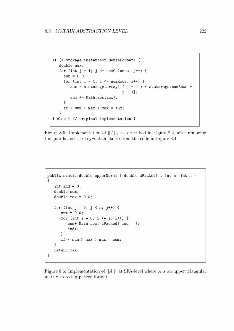
8.3. MATRIX ABSTRACTION LEVEL 222
if (a.storage instanceof DenseFormat) {double aux;for (int j = 1; j <= numColumns; j++) {
sum = 0.0;for (int i = 1; i <= numRows; i++) {
aux = a.storage.array[ ( j - 1 ) * a.storage.numRows +i - 1];
sum += Math.abs(aux);}if ( sum > max ) max = sum;
}} else { // original implementation }
Figure 8.5: Implementation of ||A||1, as described in Figure 8.2, after removingthe guards and the try-catch clause from the code in Figure 8.4.
public static double upperNorm1 ( double aPacked[], int m, int n ){
int ind = 0;double sum;double max = 0.0;
for (int j = 0; j < n; j++) {sum = 0.0;for (int i = 0; i <= j; i++) {
sum+=Math.abs( aPacked[ ind ] );ind++;
}if ( sum > max ) max = sum;
}return max;
}
Figure 8.6: Implementation of ||A||1 at SFA-level where A is an upper triangularmatrix stored in packed format.
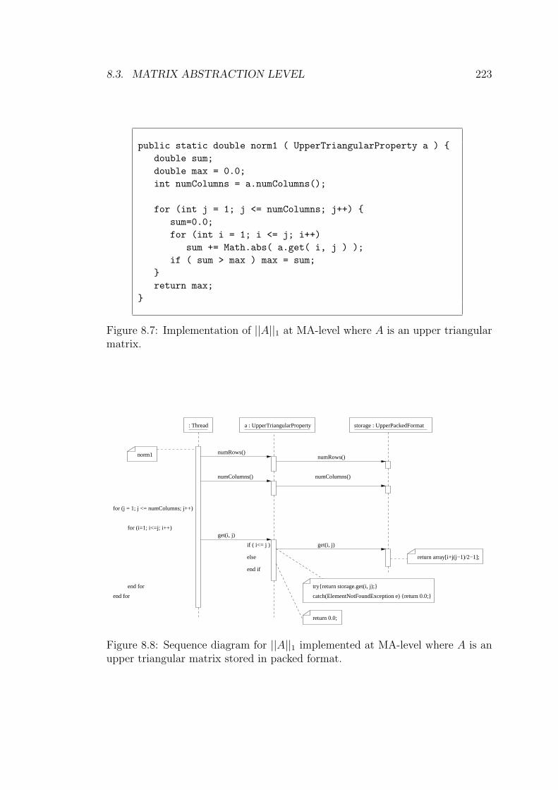
8.3. MATRIX ABSTRACTION LEVEL 223
public static double norm1 ( UpperTriangularProperty a ) {double sum;double max = 0.0;int numColumns = a.numColumns();
for (int j = 1; j <= numColumns; j++) {sum=0.0;for (int i = 1; i <= j; i++)
sum += Math.abs( a.get( i, j ) );if ( sum > max ) max = sum;
}return max;
}
Figure 8.7: Implementation of ||A||1 at MA-level where A is an upper triangularmatrix.
return 0.0;
a : UpperTriangularProperty
numRows()
numColumns()
numRows()
numColumns()
end for
for (i=1; i<=j; i++)
storage : UpperPackedFormat
return array[i+j(j−1)/2−1];
norm1
: Thread
else
end if
get(i, j)
for (j = 1; j <= numColumns; j++)
end for
if ( i<= j ) get(i, j)
catch(ElementNotFoundException e) {return 0.0;}
try{return storage.get(i, j);}
Figure 8.8: Sequence diagram for ||A||1 implemented at MA-level where A is anupper triangular matrix stored in packed format.
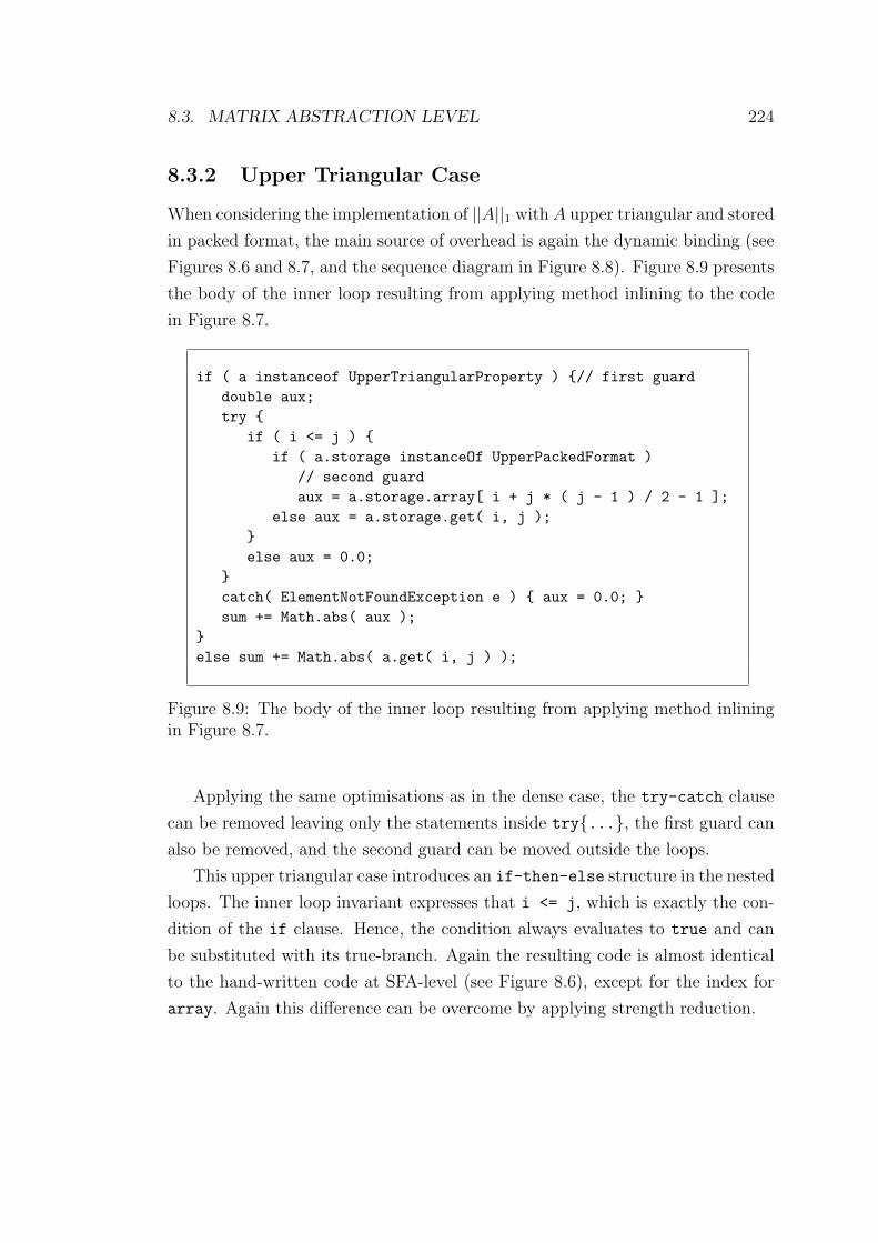
8.3. MATRIX ABSTRACTION LEVEL 224
8.3.2 Upper Triangular Case
When considering the implementation of ||A||1 with A upper triangular and stored
in packed format, the main source of overhead is again the dynamic binding (see
Figures 8.6 and 8.7, and the sequence diagram in Figure 8.8). Figure 8.9 presents
the body of the inner loop resulting from applying method inlining to the code
in Figure 8.7.
if ( a instanceof UpperTriangularProperty ) {// first guarddouble aux;try {
if ( i <= j ) {if ( a.storage instanceOf UpperPackedFormat )
// second guardaux = a.storage.array[ i + j * ( j - 1 ) / 2 - 1 ];
else aux = a.storage.get( i, j );}else aux = 0.0;
}catch( ElementNotFoundException e ) { aux = 0.0; }sum += Math.abs( aux );
}else sum += Math.abs( a.get( i, j ) );
Figure 8.9: The body of the inner loop resulting from applying method inliningin Figure 8.7.
Applying the same optimisations as in the dense case, the try-catch clause
can be removed leaving only the statements inside try{...}, the first guard can
also be removed, and the second guard can be moved outside the loops.
This upper triangular case introduces an if-then-else structure in the nested
loops. The inner loop invariant expresses that i <= j, which is exactly the con-
dition of the if clause. Hence, the condition always evaluates to true and can
be substituted with its true-branch. Again the resulting code is almost identical
to the hand-written code at SFA-level (see Figure 8.6), except for the index for
array. Again this difference can be overcome by applying strength reduction.
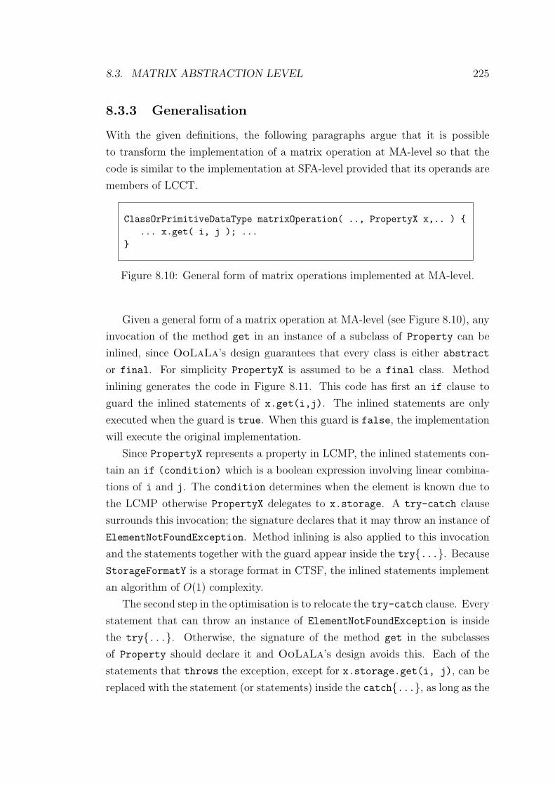
8.3. MATRIX ABSTRACTION LEVEL 225
8.3.3 Generalisation
With the given definitions, the following paragraphs argue that it is possible
to transform the implementation of a matrix operation at MA-level so that the
code is similar to the implementation at SFA-level provided that its operands are
members of LCCT.
ClassOrPrimitiveDataType matrixOperation( .., PropertyX x,.. ) {... x.get( i, j ); ...
}
Figure 8.10: General form of matrix operations implemented at MA-level.
Given a general form of a matrix operation at MA-level (see Figure 8.10), any
invocation of the method get in an instance of a subclass of Property can be
inlined, since OoLaLa’s design guarantees that every class is either abstract
or final. For simplicity PropertyX is assumed to be a final class. Method
inlining generates the code in Figure 8.11. This code has first an if clause to
guard the inlined statements of x.get(i,j). The inlined statements are only
executed when the guard is true. When this guard is false, the implementation
will execute the original implementation.
Since PropertyX represents a property in LCMP, the inlined statements con-
tain an if (condition) which is a boolean expression involving linear combina-
tions of i and j. The condition determines when the element is known due to
the LCMP otherwise PropertyX delegates to x.storage. A try-catch clause
surrounds this invocation; the signature declares that it may throw an instance of
ElementNotFoundException. Method inlining is also applied to this invocation
and the statements together with the guard appear inside the try{...}. Because
StorageFormatY is a storage format in CTSF, the inlined statements implement
an algorithm of O(1) complexity.
The second step in the optimisation is to relocate the try-catch clause. Every
statement that can throw an instance of ElementNotFoundException is inside
the try{...}. Otherwise, the signature of the method get in the subclasses
of Property should declare it and OoLaLa’s design avoids this. Each of the
statements that throws the exception, except for x.storage.get(i, j), can be
replaced with the statement (or statements) inside the catch{...}, as long as the
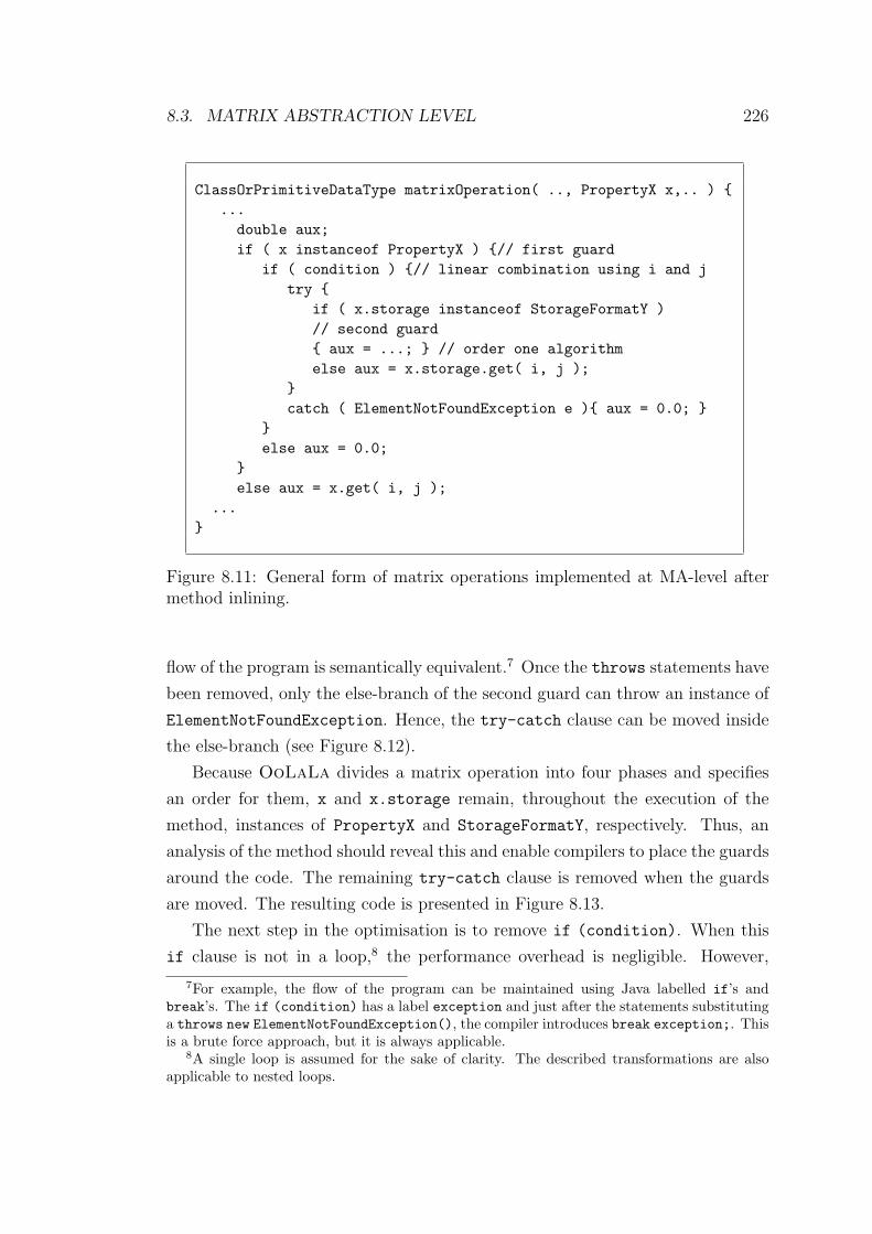
8.3. MATRIX ABSTRACTION LEVEL 226
ClassOrPrimitiveDataType matrixOperation( .., PropertyX x,.. ) {...
double aux;if ( x instanceof PropertyX ) {// first guard
if ( condition ) {// linear combination using i and jtry {
if ( x.storage instanceof StorageFormatY )// second guard{ aux = ...; } // order one algorithmelse aux = x.storage.get( i, j );
}catch ( ElementNotFoundException e ){ aux = 0.0; }
}else aux = 0.0;
}else aux = x.get( i, j );
...}
Figure 8.11: General form of matrix operations implemented at MA-level aftermethod inlining.
flow of the program is semantically equivalent.7 Once the throws statements have
been removed, only the else-branch of the second guard can throw an instance of
ElementNotFoundException. Hence, the try-catch clause can be moved inside
the else-branch (see Figure 8.12).
Because OoLaLa divides a matrix operation into four phases and specifies
an order for them, x and x.storage remain, throughout the execution of the
method, instances of PropertyX and StorageFormatY, respectively. Thus, an
analysis of the method should reveal this and enable compilers to place the guards
around the code. The remaining try-catch clause is removed when the guards
are moved. The resulting code is presented in Figure 8.13.
The next step in the optimisation is to remove if (condition). When this
if clause is not in a loop,8 the performance overhead is negligible. However,
7For example, the flow of the program can be maintained using Java labelled if’s andbreak’s. The if (condition) has a label exception and just after the statements substitutinga throws new ElementNotFoundException(), the compiler introduces break exception;. Thisis a brute force approach, but it is always applicable.
8A single loop is assumed for the sake of clarity. The described transformations are alsoapplicable to nested loops.
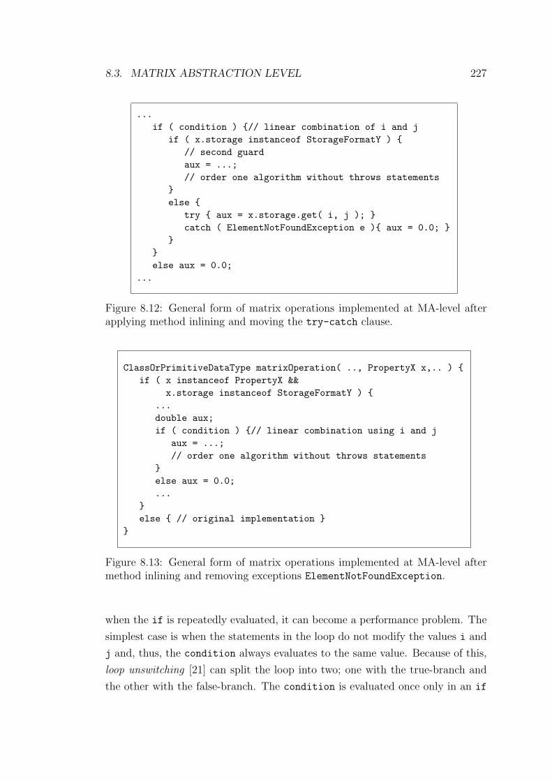
8.3. MATRIX ABSTRACTION LEVEL 227
...if ( condition ) {// linear combination of i and j
if ( x.storage instanceof StorageFormatY ) {// second guardaux = ...;// order one algorithm without throws statements
}else {
try { aux = x.storage.get( i, j ); }catch ( ElementNotFoundException e ){ aux = 0.0; }
}}else aux = 0.0;
...
Figure 8.12: General form of matrix operations implemented at MA-level afterapplying method inlining and moving the try-catch clause.
ClassOrPrimitiveDataType matrixOperation( .., PropertyX x,.. ) {if ( x instanceof PropertyX &&
x.storage instanceof StorageFormatY ) {...double aux;if ( condition ) {// linear combination using i and j
aux = ...;// order one algorithm without throws statements
}else aux = 0.0;...
}else { // original implementation }
}
Figure 8.13: General form of matrix operations implemented at MA-level aftermethod inlining and removing exceptions ElementNotFoundException.
when the if is repeatedly evaluated, it can become a performance problem. The
simplest case is when the statements in the loop do not modify the values i and
j and, thus, the condition always evaluates to the same value. Because of this,
loop unswitching [21] can split the loop into two; one with the true-branch and
the other with the false-branch. The condition is evaluated once only in an if
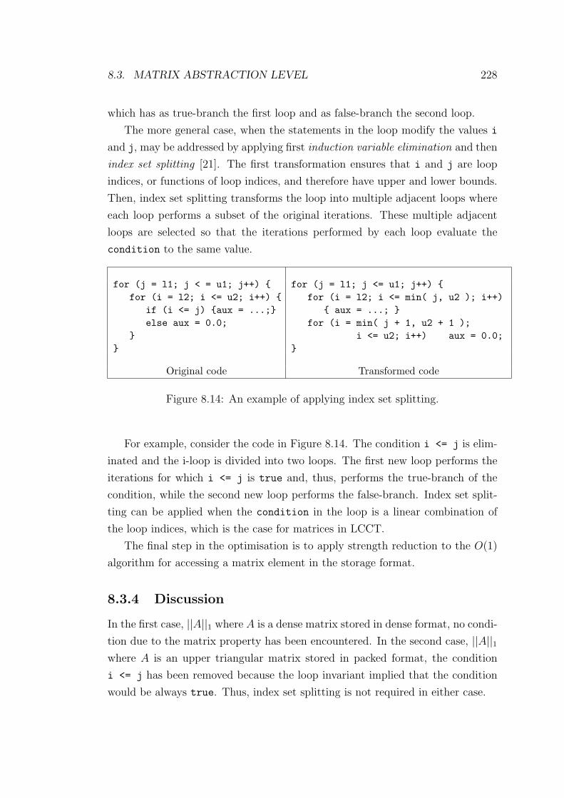
8.3. MATRIX ABSTRACTION LEVEL 228
which has as true-branch the first loop and as false-branch the second loop.
The more general case, when the statements in the loop modify the values i
and j, may be addressed by applying first induction variable elimination and then
index set splitting [21]. The first transformation ensures that i and j are loop
indices, or functions of loop indices, and therefore have upper and lower bounds.
Then, index set splitting transforms the loop into multiple adjacent loops where
each loop performs a subset of the original iterations. These multiple adjacent
loops are selected so that the iterations performed by each loop evaluate the
condition to the same value.
for (j = l1; j < = u1; j++) {for (i = l2; i <= u2; i++) {
if (i <= j) {aux = ...;}else aux = 0.0;
}}
for (j = l1; j <= u1; j++) {for (i = l2; i <= min( j, u2 ); i++)
{ aux = ...; }for (i = min( j + 1, u2 + 1 );
i <= u2; i++) aux = 0.0;}
Original code Transformed code
Figure 8.14: An example of applying index set splitting.
For example, consider the code in Figure 8.14. The condition i <= j is elim-
inated and the i-loop is divided into two loops. The first new loop performs the
iterations for which i <= j is true and, thus, performs the true-branch of the
condition, while the second new loop performs the false-branch. Index set split-
ting can be applied when the condition in the loop is a linear combination of
the loop indices, which is the case for matrices in LCCT.
The final step in the optimisation is to apply strength reduction to the O(1)
algorithm for accessing a matrix element in the storage format.
8.3.4 Discussion
In the first case, ||A||1 where A is a dense matrix stored in dense format, no condi-
tion due to the matrix property has been encountered. In the second case, ||A||1where A is an upper triangular matrix stored in packed format, the condition
i <= j has been removed because the loop invariant implied that the condition
would be always true. Thus, index set splitting is not required in either case.
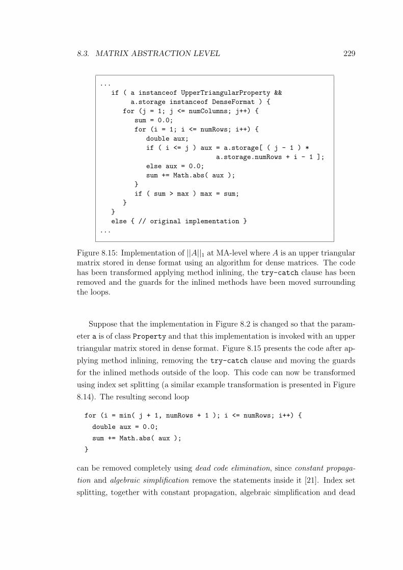
8.3. MATRIX ABSTRACTION LEVEL 229
...if ( a instanceof UpperTriangularProperty &&
a.storage instanceof DenseFormat ) {for (j = 1; j <= numColumns; j++) {
sum = 0.0;for (i = 1; i <= numRows; i++) {
double aux;if ( i <= j ) aux = a.storage[ ( j - 1 ) *
a.storage.numRows + i - 1 ];else aux = 0.0;sum += Math.abs( aux );
}if ( sum > max ) max = sum;
}}else { // original implementation }
...
Figure 8.15: Implementation of ||A||1 at MA-level where A is an upper triangularmatrix stored in dense format using an algorithm for dense matrices. The codehas been transformed applying method inlining, the try-catch clause has beenremoved and the guards for the inlined methods have been moved surroundingthe loops.
Suppose that the implementation in Figure 8.2 is changed so that the param-
eter a is of class Property and that this implementation is invoked with an upper
triangular matrix stored in dense format. Figure 8.15 presents the code after ap-
plying method inlining, removing the try-catch clause and moving the guards
for the inlined methods outside of the loop. This code can now be transformed
using index set splitting (a similar example transformation is presented in Figure
8.14). The resulting second loop
for (i = min( j + 1, numRows + 1 ); i <= numRows; i++) {
double aux = 0.0;
sum += Math.abs( aux );
}
can be removed completely using dead code elimination, since constant propaga-
tion and algebraic simplification remove the statements inside it [21]. Index set
splitting, together with constant propagation, algebraic simplification and dead
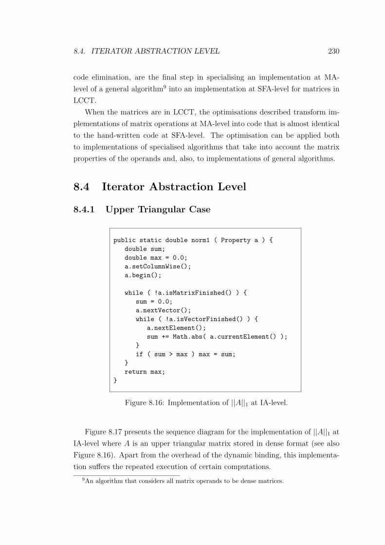
8.4. ITERATOR ABSTRACTION LEVEL 230
code elimination, are the final step in specialising an implementation at MA-
level of a general algorithm9 into an implementation at SFA-level for matrices in
LCCT.
When the matrices are in LCCT, the optimisations described transform im-
plementations of matrix operations at MA-level into code that is almost identical
to the hand-written code at SFA-level. The optimisation can be applied both
to implementations of specialised algorithms that take into account the matrix
properties of the operands and, also, to implementations of general algorithms.
8.4 Iterator Abstraction Level
8.4.1 Upper Triangular Case
public static double norm1 ( Property a ) {double sum;double max = 0.0;a.setColumnWise();a.begin();
while ( !a.isMatrixFinished() ) {sum = 0.0;a.nextVector();while ( !a.isVectorFinished() ) {
a.nextElement();sum += Math.abs( a.currentElement() );
}if ( sum > max ) max = sum;
}return max;
}
Figure 8.16: Implementation of ||A||1 at IA-level.
Figure 8.17 presents the sequence diagram for the implementation of ||A||1 at
IA-level where A is an upper triangular matrix stored in dense format (see also
Figure 8.16). Apart from the overhead of the dynamic binding, this implementa-
tion suffers the repeated execution of certain computations.
9An algorithm that considers all matrix operands to be dense matrices.
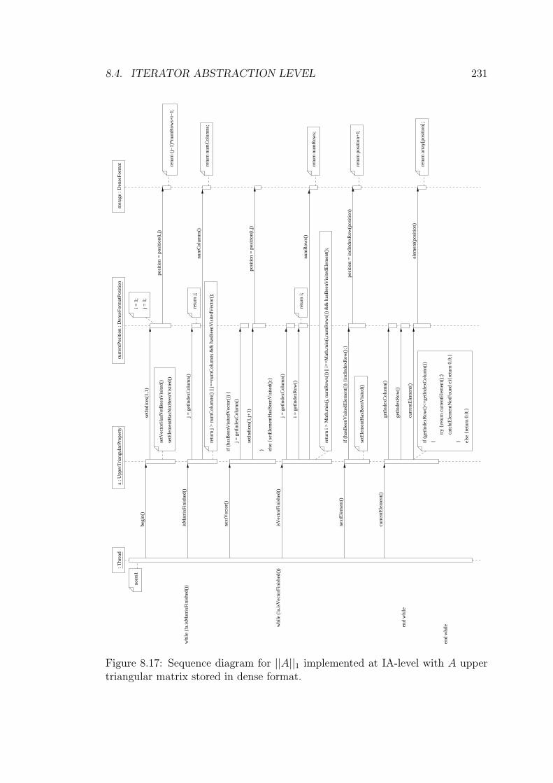
8.4. ITERATOR ABSTRACTION LEVEL 231
whi
le (
!a.is
Mat
rixF
inis
hed(
))
end
whi
le
end
whi
le
: Thr
ead
norm
1
a : U
pper
Tri
angu
larP
rope
rty
curr
entP
ositi
on :
Den
seFo
rmat
Posi
tion
stor
age
: Den
seFo
rmat
setI
ndic
es(1
,1)
begi
n()
isM
atri
xFin
ishe
d()
num
Col
umns
()
posi
tion
= p
ositi
on(i
,j)
i = 1
;
j = 1
;
retu
rn j;
retu
rn n
umC
olum
ns;
retu
rn (
j−1)
*num
Row
s+i−
1;
next
Vec
tor(
)
whi
le (
!a.is
Vec
torF
inis
hed(
))is
Vec
torF
inis
hed(
)
num
Row
s()
retu
rn n
umR
ows;
retu
rn i;
else
{re
turn
0.0
;}
curr
entE
lem
ent(
)ge
tInd
exC
olum
n()
getI
ndex
Row
()
elem
ent(
posi
tion)
curr
entE
lem
ent(
)
if (
getI
ndex
Row
()<
=ge
tInd
exC
olum
n())
{ }
retu
rn a
rray
[pos
ition
];
try
{ret
urn
curr
entE
lem
ent(
);}
catc
h(E
lem
entN
otFo
und
e){r
etur
n 0.
0;}
setV
ecto
rHas
Not
Bee
nVis
ited(
)
setE
lem
entH
asN
otB
eenV
isite
d()
j = g
etIn
dexC
olum
n()
retu
rn j
> n
umC
olum
ns()
|| j=
=nu
mC
olum
ns &
& h
asB
eenV
isite
dVec
tor(
);
j = g
etIn
dexC
olum
n()
i = g
etIn
dexR
ow()
retu
rn i
> M
ath.
min
(j, n
umR
ows(
)) ||
i==
Mat
h.m
in(i
,num
Row
s())
&&
has
Bee
nVis
itedE
lem
ent(
);
next
Ele
men
t()
posi
tion
= in
cInd
exR
ow(p
ositi
on)
retu
rn p
ositi
on+
1;
if (
hasB
eenV
isite
dEle
men
t())
{in
cInd
exR
ow()
;}
setE
lem
entH
asB
eenV
isite
d()
}
posi
tion
= p
ositi
on(i
,j)
else
{se
tEle
men
tHas
Bee
nVis
ited(
);}
j = g
etIn
dexC
olum
n()
setI
ndic
es(1
,j+1)
if (
hasB
eenV
isite
dVec
tor(
)) {
Figure 8.17: Sequence diagram for ||A||1 implemented at IA-level with A uppertriangular matrix stored in dense format.
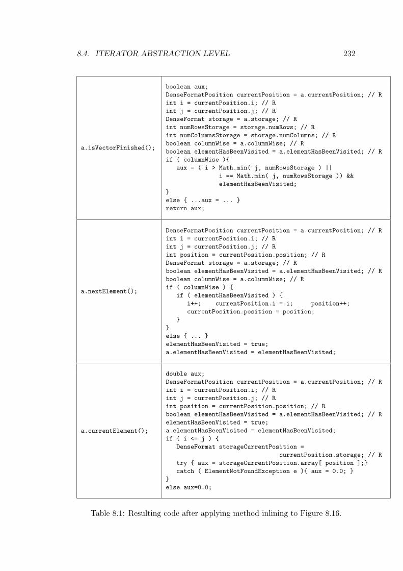
8.4. ITERATOR ABSTRACTION LEVEL 232
a.isVectorFinished();
boolean aux;DenseFormatPosition currentPosition = a.currentPosition; // Rint i = currentPosition.i; // Rint j = currentPosition.j; // RDenseFormat storage = a.storage; // Rint numRowsStorage = storage.numRows; // Rint numColumnsStorage = storage.numColumns; // Rboolean columnWise = a.columnWise; // Rboolean elementHasBeenVisited = a.elementHasBeenVisited; // Rif ( columnWise ){
aux = ( i > Math.min( j, numRowsStorage ) ||i == Math.min( j, numRowsStorage )) &&elementHasBeenVisited;
}else { ...aux = ... }return aux;
a.nextElement();
DenseFormatPosition currentPosition = a.currentPosition; // Rint i = currentPosition.i; // Rint j = currentPosition.j; // Rint position = currentPosition.position; // RDenseFormat storage = a.storage; // Rboolean elementHasBeenVisited = a.elementHasBeenVisited; // Rboolean columnWise = a.columnWise; // Rif ( columnWise ) {
if ( elementHasBeenVisited ) {i++; currentPosition.i = i; position++;currentPosition.position = position;
}}else { ... }elementHasBeenVisited = true;a.elementHasBeenVisited = elementHasBeenVisited;
a.currentElement();
double aux;DenseFormatPosition currentPosition = a.currentPosition; // Rint i = currentPosition.i; // Rint j = currentPosition.j; // Rint position = currentPosition.position; // Rboolean elementHasBeenVisited = a.elementHasBeenVisited; // RelementHasBeenVisited = true;a.elementHasBeenVisited = elementHasBeenVisited;if ( i <= j ) {
DenseFormat storageCurrentPosition =currentPosition.storage; // R
try { aux = storageCurrentPosition.array[ position ];}catch ( ElementNotFoundException e ){ aux = 0.0; }
}else aux=0.0;
Table 8.1: Resulting code after applying method inlining to Figure 8.16.
8.4. ITERATOR ABSTRACTION LEVEL 233
For a representative selection of the methods invoked in a, Table 8.1 gives the
resulting code after applying method inlining. Since the code becomes verbose
when including the inlined statements with guards, the table presents them with-
out the guards. The table also excludes the else-branch for the if (columnWise)
statements.
The optimisation of moving the guards to surround the code has been de-
scribed in the context of implementations at MA-level. The circumstances that
enable compilers to perform this optimisation are guaranteed by OoLaLa’s de-
sign and, also apply to implementations at IA-level. OoLaLa’s design divides
the implementation of any matrix operation into different phases and specifies
an order among the phases. Thus, OoLaLa ensures that a, a.storage and
a.currentPosition remain, throughout the execution of the method norm1, in-
stances of UpperTriangularProperty, DenseFormat and DenseFormatPosition.
Another optimisation described in the context of optimisations at MA-level
and needed for this implementation, is the removal of try-catch clauses. The
method currentPosition (see Table 8.1) does not throw any exception. It
catches instances of ElementNotFoundException and, in accordance with the
corresponding property, resolves the value of the element. The optimisation sub-
stitutes the statements that throw new ElementNotFoundException() with the
statements inside the catch{...} and maintains an equivalent flow of the pro-
gram.
Some statements in Table 8.1 have the line-comment // R. This indicates that
these statements are repeated, at least once more, among the statements inlined
due to the other methods. These statements make local copies of the attributes
in a, a.storage and a.currentPosition; this is the third step in optimisation.
The fourth step is to remove these repeated statements by declaring and
initialising local copies at the beginning and only writing back to the attributes
at the end. This step also removes all tests of the form if (columnWise), leaving
only the true-branch. The computations involving elementHasBeenVisited can
also be removed, but the details are omitted for the sake of clarity.
The fifth step, alias disambiguation, notes that a.storage and a.current-
Position.storage are both references to the same object. Thus in Figure 8.18,
the local variables numRowsStorage and numRowsCurrentPosition are copies of
the same attribute. Both variables can now be renamed as numRows. When
considering other matrix operations which involve more than one matrix, alias
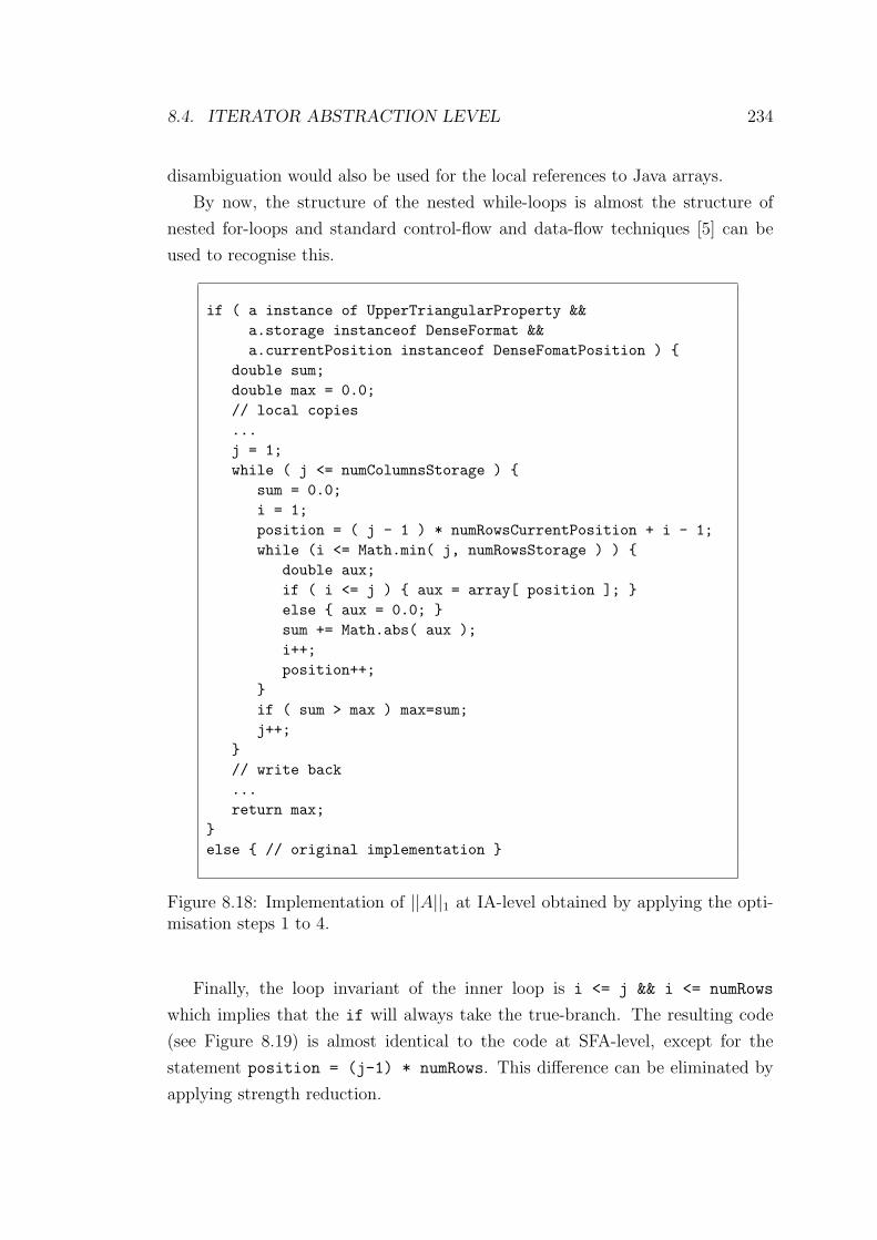
8.4. ITERATOR ABSTRACTION LEVEL 234
disambiguation would also be used for the local references to Java arrays.
By now, the structure of the nested while-loops is almost the structure of
nested for-loops and standard control-flow and data-flow techniques [5] can be
used to recognise this.
if ( a instance of UpperTriangularProperty &&a.storage instanceof DenseFormat &&a.currentPosition instanceof DenseFomatPosition ) {
double sum;double max = 0.0;// local copies...j = 1;while ( j <= numColumnsStorage ) {
sum = 0.0;i = 1;position = ( j - 1 ) * numRowsCurrentPosition + i - 1;while (i <= Math.min( j, numRowsStorage ) ) {
double aux;if ( i <= j ) { aux = array[ position ]; }else { aux = 0.0; }sum += Math.abs( aux );i++;position++;
}if ( sum > max ) max=sum;j++;
}// write back...return max;
}else { // original implementation }
Figure 8.18: Implementation of ||A||1 at IA-level obtained by applying the opti-misation steps 1 to 4.
Finally, the loop invariant of the inner loop is i <= j && i <= numRows
which implies that the if will always take the true-branch. The resulting code
(see Figure 8.19) is almost identical to the code at SFA-level, except for the
statement position = (j-1) * numRows. This difference can be eliminated by
applying strength reduction.
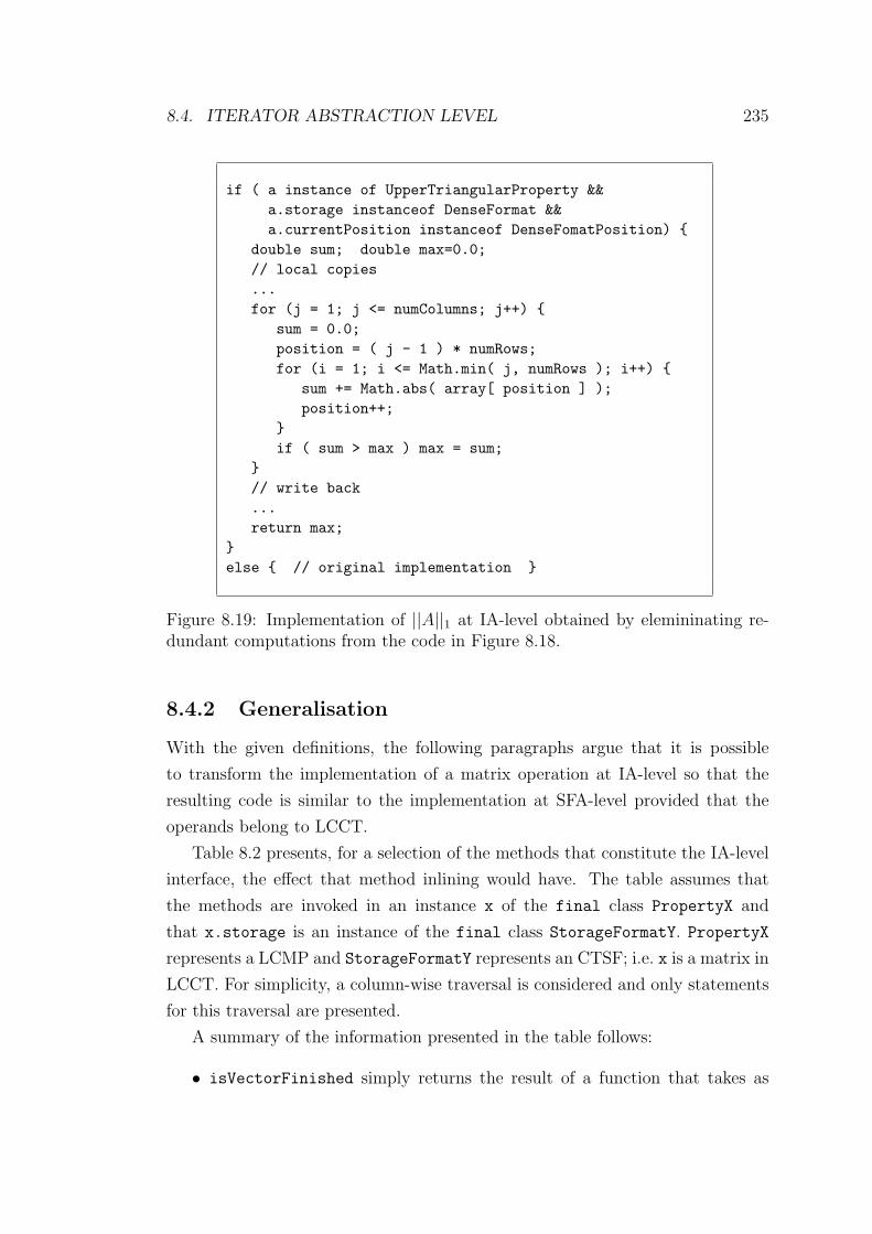
8.4. ITERATOR ABSTRACTION LEVEL 235
if ( a instance of UpperTriangularProperty &&a.storage instanceof DenseFormat &&a.currentPosition instanceof DenseFomatPosition) {
double sum; double max=0.0;// local copies...for (j = 1; j <= numColumns; j++) {
sum = 0.0;position = ( j - 1 ) * numRows;for (i = 1; i <= Math.min( j, numRows ); i++) {
sum += Math.abs( array[ position ] );position++;
}if ( sum > max ) max = sum;
}// write back...return max;
}else { // original implementation }
Figure 8.19: Implementation of ||A||1 at IA-level obtained by elemininating re-dundant computations from the code in Figure 8.18.
8.4.2 Generalisation
With the given definitions, the following paragraphs argue that it is possible
to transform the implementation of a matrix operation at IA-level so that the
resulting code is similar to the implementation at SFA-level provided that the
operands belong to LCCT.
Table 8.2 presents, for a selection of the methods that constitute the IA-level
interface, the effect that method inlining would have. The table assumes that
the methods are invoked in an instance x of the final class PropertyX and
that x.storage is an instance of the final class StorageFormatY. PropertyX
represents a LCMP and StorageFormatY represents an CTSF; i.e. x is a matrix in
LCCT. For simplicity, a column-wise traversal is considered and only statements
for this traversal are presented.
A summary of the information presented in the table follows:
• isVectorFinished simply returns the result of a function that takes as
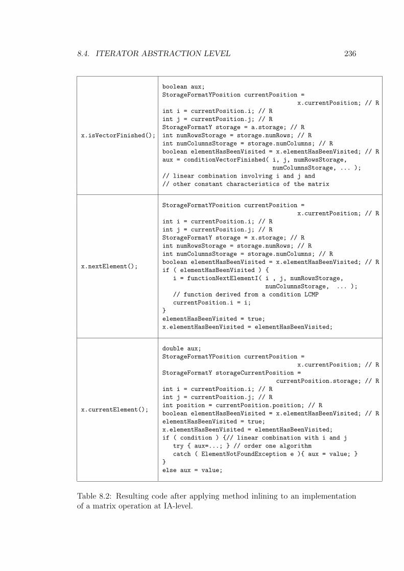
8.4. ITERATOR ABSTRACTION LEVEL 236
x.isVectorFinished();
boolean aux;StorageFormatYPosition currentPosition =
x.currentPosition; // Rint i = currentPosition.i; // Rint j = currentPosition.j; // RStorageFormatY storage = a.storage; // Rint numRowsStorage = storage.numRows; // Rint numColumnsStorage = storage.numColumns; // Rboolean elementHasBeenVisited = x.elementHasBeenVisited; // Raux = conditionVectorFinished( i, j, numRowsStorage,
numColumnsStorage, ... );// linear combination involving i and j and// other constant characteristics of the matrix
x.nextElement();
StorageFormatYPosition currentPosition =x.currentPosition; // R
int i = currentPosition.i; // Rint j = currentPosition.j; // RStorageFormatY storage = x.storage; // Rint numRowsStorage = storage.numRows; // Rint numColumnsStorage = storage.numColumns; // Rboolean elementHasBeenVisited = x.elementHasBeenVisited; // Rif ( elementHasBeenVisited ) {
i = functionNextElementI( i , j, numRowsStorage,numColumnsStorage, ... );
// function derived from a condition LCMPcurrentPosition.i = i;
}elementHasBeenVisited = true;x.elementHasBeenVisited = elementHasBeenVisited;
x.currentElement();
double aux;StorageFormatYPosition currentPosition =
x.currentPosition; // RStorageFormatY storageCurrentPosition =
currentPosition.storage; // Rint i = currentPosition.i; // Rint j = currentPosition.j; // Rint position = currentPosition.position; // Rboolean elementHasBeenVisited = x.elementHasBeenVisited; // RelementHasBeenVisited = true;x.elementHasBeenVisited = elementHasBeenVisited;if ( condition ) {// linear combination with i and j
try { aux=...; } // order one algorithmcatch ( ElementNotFoundException e ){ aux = value; }
}else aux = value;
Table 8.2: Resulting code after applying method inlining to an implementationof a matrix operation at IA-level.
8.4. ITERATOR ABSTRACTION LEVEL 237
parameters constant characteristics of the matrix (e.g. number of rows,
number of columns, etc.) and the indices of the current position;
• nextElement modifies the indices for the next position using a function
that also take as parameters constant characteristics of the matrix and the
indices of the current position;
• currentElement implements an O(1) algorithm for finding the element
indicated by the current position indices.
The functions, either boolean (isVectorFinished) or integer (nextVector
and nextElement), are derived from a LCMP condition. In the simplest form,
these functions are constants. In the most complex form, they are linear combi-
nations involving the indices of the current position and constant characteristics
of the matrix.
The first optimising steps (method inlining for x, x.currentPosition and
x.storage, movement of the guards for the inlined statements, removal of try-catch
clauses, to local copies of the accessed attributes of x, and alias disambiguation)
do not present any problems and have been described in previous cases. The
description of how to eliminate the computations involving the local variable
elementHasBeenVisited is omitted for the sake of conciseness.
Figure 8.20 presents the code after applying the preceding optimisations to
the general case. Now, it can be shown that the indices i and j have lower bounds
and upper bounds, since independently of the matrix and traversing column-wise,
the condition for isMatrixFinished() always includes a term so that j is in the
range 1 to numColumns. A similar argument applies to i. Thus, the while-loops
can be transformed into for-loops (see Figure 8.21). Finally, this form of for-loops
can be transformed into the traditional form by dividing the iteration spaces so
that:
• conditionMatrixFinished(...) and conditionVectorFinished(...)
are simplified to the form index <= CONSTANT, and
• functionNextVectorJ(...), functionNextVectorI(...), and function-
NextElementI(...) are simplified to the form index +=CONSTANT.
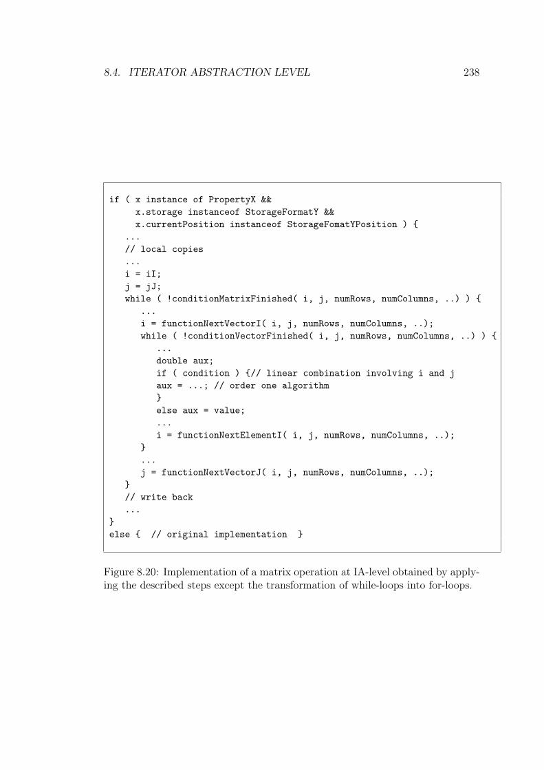
8.4. ITERATOR ABSTRACTION LEVEL 238
if ( x instance of PropertyX &&x.storage instanceof StorageFormatY &&x.currentPosition instanceof StorageFomatYPosition ) {
...// local copies...i = iI;j = jJ;while ( !conditionMatrixFinished( i, j, numRows, numColumns, ..) ) {
...i = functionNextVectorI( i, j, numRows, numColumns, ..);while ( !conditionVectorFinished( i, j, numRows, numColumns, ..) ) {
...double aux;if ( condition ) {// linear combination involving i and jaux = ...; // order one algorithm}else aux = value;...i = functionNextElementI( i, j, numRows, numColumns, ..);
}...j = functionNextVectorJ( i, j, numRows, numColumns, ..);
}// write back...
}else { // original implementation }
Figure 8.20: Implementation of a matrix operation at IA-level obtained by apply-ing the described steps except the transformation of while-loops into for-loops.
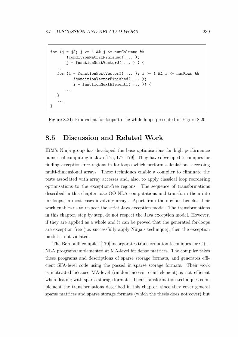
8.5. DISCUSSION AND RELATED WORK 239
for (j = jJ; j >= 1 && j <= numColumns &&!conditionMatrixFinished( ... );j = functionNextVectorJ( ... ) ) {
...for (i = functionNextVectorI( ... ); i >= 1 && i <= numRows &&
!conditionVectorFinished( ... );i = functionNextElementI( ... )) {
...}...
}
Figure 8.21: Equivalent for-loops to the while-loops presented in Figure 8.20.
8.5 Discussion and Related Work
IBM’s Ninja group has developed the base optimisations for high performance
numerical computing in Java [175, 177, 179]. They have developed techniques for
finding exception-free regions in for-loops which perform calculations accessing
multi-dimensional arrays. These techniques enable a compiler to eliminate the
tests associated with array accesses and, also, to apply classical loop reordering
optimisations to the exception-free regions. The sequence of transformations
described in this chapter take OO NLA computations and transform them into
for-loops, in most cases involving arrays. Apart from the obvious benefit, their
work enables us to respect the strict Java exception model. The transformations
in this chapter, step by step, do not respect the Java exception model. However,
if they are applied as a whole and it can be proved that the generated for-loops
are exception free (i.e. successfully apply Ninja’s technique), then the exception
model is not violated.
The Bernoulli compiler [170] incorporates transformation techniques for C++
NLA programs implemented at MA-level for dense matrices. The compiler takes
these programs and descriptions of sparse storage formats, and generates effi-
cient SFA-level code using the passed in sparse storage formats. Their work
is motivated because MA-level (random access to an element) is not efficient
when dealing with sparse storage formats. Their transformation techniques com-
plement the transformations described in this chapter, since they cover general
sparse matrices and sparse storage formats (which the thesis does not cover) but

8.5. DISCUSSION AND RELATED WORK 240
they do not cover LCCT. The main difference is that the Bernoulli compiler is
a domain-specific compiler, while the sequence of transformations are for general
purpose compilers.
One of the transformations applied to implementations at MA-level and IA-
level is the removal of try-catch clauses. General techniques for optimising Java
programs in the presence of exceptions are described in [130, 159].
OoLaLa as a Generator of Specialised Implementations – From an alter-
native point of view, the described transformations automatically generate the
specialised implementations of most matrix operations covered by the dense and
banded BLAS [39] and LAPACK. The generation process simply needs imple-
mentations at MA- or IA-level. The implementations that cannot be generated
in this way are those that exploit mathematical relation properties. Bik and Wi-
jshoff [34, 32] (the Sparse Compiler introduced in Chapter 2) and also Pingali
et al. [214, 148] developed domain-specific compilers to automatically generate
sparse BLAS operations from descriptions of the matrix properties and dense
BLAS operations.
Thread Safety – The Java language provides threads as part of the language.
In general, it is not possible to prove whether two or more threads will be accessing
the same data, but the Java memory model enables threads to keep private copies
of shared data between synchronization points.
Note that OoLaLa is a sequential library and that the portions of the code,
to which the transformation have to be applied, do not have synchronization
points. Thus, in order to make the transformations thread safe, all the attributes
of the instances accessed have to be copied into private local variables. For the
sake of clarity this has been not presented explicitly in the case of MA-level
implementations.
Block and Recursive Algorithms – Given the trend towards more complex
and deeper computer memory hierarchies, block and recursive algorithms [63, 88,
133, 10] have been proposed for NLA. The main advantage of these algorithms
is better utilisation of the memory hierarchy. As mentioned earlier, compiler
transformations that pursue these objectives are out of the scope of the thesis; the
work by IBM’s Ninja group [177, 179] has enabled Java compilers to apply such
transformations to the kind of code produced by the sequences of transformations
presented in this section.
8.6. SUMMARY 241
On the other hand, the sequence of standard compiler transformations pre-
sented in this chapter do not impose any constraint to prevent block and recursive
algorithms implemented at MA- and IA-level being transformed into SFA-level.
In addition, none of the transformations change the order in which matrix ele-
ments are accessed and, thus, the memory access pattern remains unmodified.
In other words, block and recursive algorithms implemented at MA- and IA-level
can be transformed into block and recursive implementations at SFA-level.
8.6 Summary
OoLaLa provides both MA- and IA-level as alternatives to the SFA-level, copied
from traditional (Fortran-based) libraries. MA-level provides library developers
with an interface to access matrices independent of the storage format and with
random access to matrix elements. IA-level provides library developers with an
interface to access matrices that is also independent of the storage format but
with sequential access to the non-zero elements.
This chapter has characterised a set of matrix properties and storage formats,
together with associated transformations, that enable implementations at MA-
and IA-level to be transformed into efficient implementations at SFA-level. The
transformations can be applied provided that the operands have certain matrix
properties and certain storage formats and these matrix properties and storage
formats are not overly restrictive since they cover the dense and banded BLAS
and part of LAPACK.
Chapter 9 illustrates that the above sequence of standard transformations is
also beneficial for applications using two commonly encountered design patterns
which deal with the access to data structures, as long as the data structures are
implemented as arrays. For example, the sequence of standard transformations
can also eliminate the performance overhead of using the multi-dimensional array
package (which was introduced in Chapter 7) instead of Java arrays.
Chapter 9
Generalisation to Design
Pattern-Based Applications
9.1 Introduction
Object Oriented (OO) software construction has characteristics that can im-
prove the development process and usability of mathematical software libraries.
OoLaLa, a novel Object Oriented Linear Algebra LibrAry, is the outcome of
a study of these benefits in the context of sequential Numerical Linear Algebra
(NLA). Previous chapters have covered the design of the library, its implementa-
tion and performance evaluation, the elimination of array bounds checks in the
presence of indirection, and the optimisation of OoLaLa. This chapter takes a
step back from the specifics of NLA and OoLaLa, and illustrates that optimi-
sations described for OoLaLa in Chapter 8 are also beneficial for applications
using two design patterns which deal with the access to storage formats based on
arrays.
Almost a decade has passed since the Gang of Four (Gamma, Helm, Johnson
and Vlissides) published their influential book [107] on design patterns. Since
then, two other books [60, 200] and several annual conferences (PLoP since 1994,
EuroPLoP since 1996, ChilliPLoP since 1998, KoalaPLoP since 2000, and Sug-
arLoafPLoP and MensorePLoP since 2001) are proof of the active research com-
munity that has been formed.
Both the standard benchmarks community and the compiler research com-
munity could overlook the design patterns community on the grounds that the
latter is restricted to software engineering. However, design patterns due to their
242
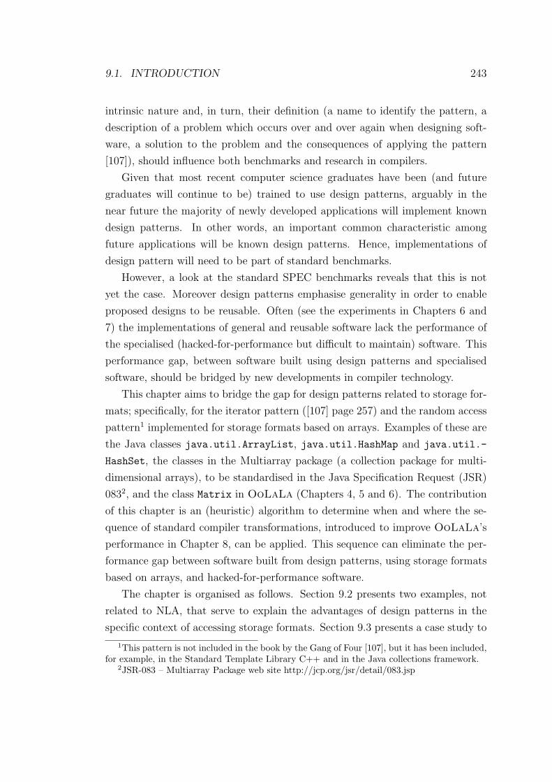
9.1. INTRODUCTION 243
intrinsic nature and, in turn, their definition (a name to identify the pattern, a
description of a problem which occurs over and over again when designing soft-
ware, a solution to the problem and the consequences of applying the pattern
[107]), should influence both benchmarks and research in compilers.
Given that most recent computer science graduates have been (and future
graduates will continue to be) trained to use design patterns, arguably in the
near future the majority of newly developed applications will implement known
design patterns. In other words, an important common characteristic among
future applications will be known design patterns. Hence, implementations of
design pattern will need to be part of standard benchmarks.
However, a look at the standard SPEC benchmarks reveals that this is not
yet the case. Moreover design patterns emphasise generality in order to enable
proposed designs to be reusable. Often (see the experiments in Chapters 6 and
7) the implementations of general and reusable software lack the performance of
the specialised (hacked-for-performance but difficult to maintain) software. This
performance gap, between software built using design patterns and specialised
software, should be bridged by new developments in compiler technology.
This chapter aims to bridge the gap for design patterns related to storage for-
mats; specifically, for the iterator pattern ([107] page 257) and the random access
pattern1 implemented for storage formats based on arrays. Examples of these are
the Java classes java.util.ArrayList, java.util.HashMap and java.util.-
HashSet, the classes in the Multiarray package (a collection package for multi-
dimensional arrays), to be standardised in the Java Specification Request (JSR)
0832, and the class Matrix in OoLaLa (Chapters 4, 5 and 6). The contribution
of this chapter is an (heuristic) algorithm to determine when and where the se-
quence of standard compiler transformations, introduced to improve OoLaLa’s
performance in Chapter 8, can be applied. This sequence can eliminate the per-
formance gap between software built from design patterns, using storage formats
based on arrays, and hacked-for-performance software.
The chapter is organised as follows. Section 9.2 presents two examples, not
related to NLA, that serve to explain the advantages of design patterns in the
specific context of accessing storage formats. Section 9.3 presents a case study to
1This pattern is not included in the book by the Gang of Four [107], but it has been included,for example, in the Standard Template Library C++ and in the Java collections framework.
2JSR-083 – Multiarray Package web site http://jcp.org/jsr/detail/083.jsp
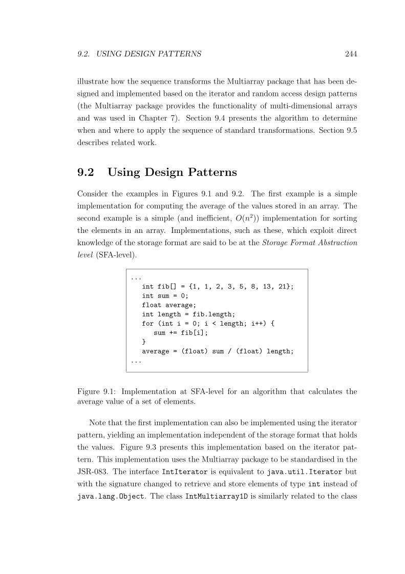
9.2. USING DESIGN PATTERNS 244
illustrate how the sequence transforms the Multiarray package that has been de-
signed and implemented based on the iterator and random access design patterns
(the Multiarray package provides the functionality of multi-dimensional arrays
and was used in Chapter 7). Section 9.4 presents the algorithm to determine
when and where to apply the sequence of standard transformations. Section 9.5
describes related work.
9.2 Using Design Patterns
Consider the examples in Figures 9.1 and 9.2. The first example is a simple
implementation for computing the average of the values stored in an array. The
second example is a simple (and inefficient, O(n2)) implementation for sorting
the elements in an array. Implementations, such as these, which exploit direct
knowledge of the storage format are said to be at the Storage Format Abstraction
level (SFA-level).
...int fib[] = {1, 1, 2, 3, 5, 8, 13, 21};int sum = 0;float average;int length = fib.length;for (int i = 0; i < length; i++) {
sum += fib[i];}average = (float) sum / (float) length;
...
Figure 9.1: Implementation at SFA-level for an algorithm that calculates theaverage value of a set of elements.
Note that the first implementation can also be implemented using the iterator
pattern, yielding an implementation independent of the storage format that holds
the values. Figure 9.3 presents this implementation based on the iterator pat-
tern. This implementation uses the Multiarray package to be standardised in the
JSR-083. The interface IntIterator is equivalent to java.util.Iterator but
with the signature changed to retrieve and store elements of type int instead of
java.lang.Object. The class IntMultiarray1D is similarly related to the class
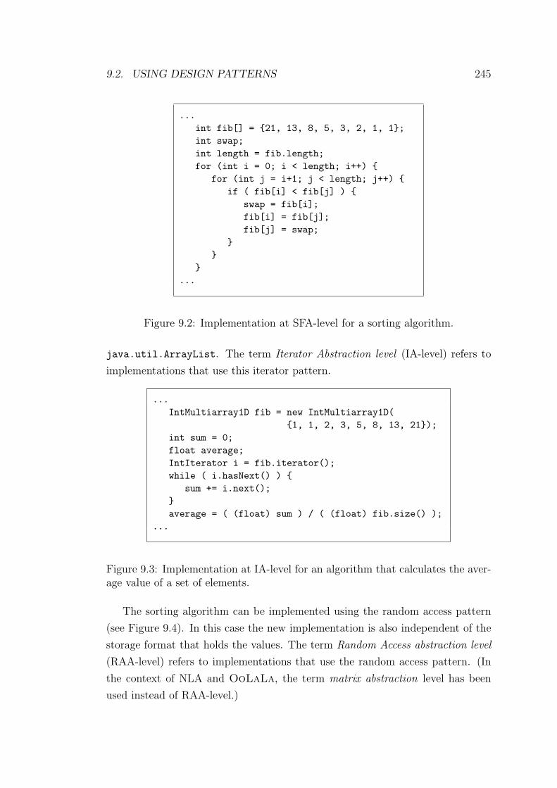
9.2. USING DESIGN PATTERNS 245
...int fib[] = {21, 13, 8, 5, 3, 2, 1, 1};int swap;int length = fib.length;for (int i = 0; i < length; i++) {
for (int j = i+1; j < length; j++) {if ( fib[i] < fib[j] ) {
swap = fib[i];fib[i] = fib[j];fib[j] = swap;
}}
}...
Figure 9.2: Implementation at SFA-level for a sorting algorithm.
java.util.ArrayList. The term Iterator Abstraction level (IA-level) refers to
implementations that use this iterator pattern.
...IntMultiarray1D fib = new IntMultiarray1D(
{1, 1, 2, 3, 5, 8, 13, 21});int sum = 0;float average;IntIterator i = fib.iterator();while ( i.hasNext() ) {
sum += i.next();}average = ( (float) sum ) / ( (float) fib.size() );
...
Figure 9.3: Implementation at IA-level for an algorithm that calculates the aver-age value of a set of elements.
The sorting algorithm can be implemented using the random access pattern
(see Figure 9.4). In this case the new implementation is also independent of the
storage format that holds the values. The term Random Access abstraction level
(RAA-level) refers to implementations that use the random access pattern. (In
the context of NLA and OoLaLa, the term matrix abstraction level has been
used instead of RAA-level.)
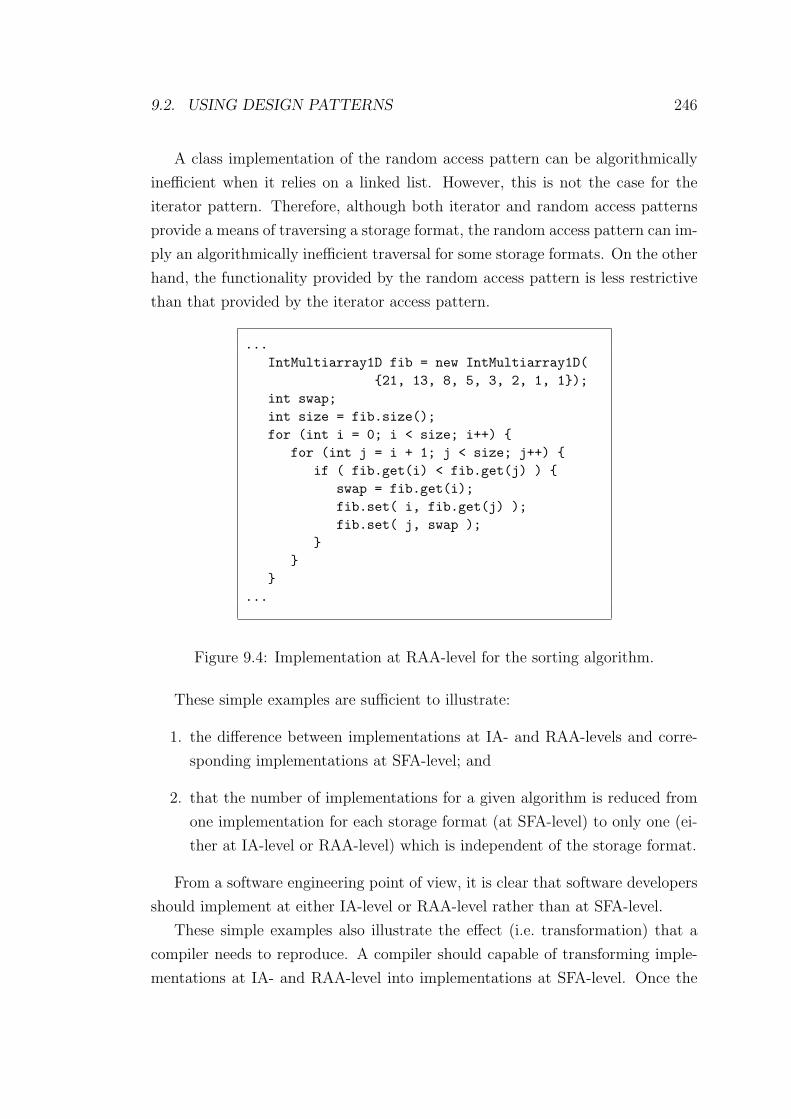
9.2. USING DESIGN PATTERNS 246
A class implementation of the random access pattern can be algorithmically
inefficient when it relies on a linked list. However, this is not the case for the
iterator pattern. Therefore, although both iterator and random access patterns
provide a means of traversing a storage format, the random access pattern can im-
ply an algorithmically inefficient traversal for some storage formats. On the other
hand, the functionality provided by the random access pattern is less restrictive
than that provided by the iterator access pattern.
...IntMultiarray1D fib = new IntMultiarray1D(
{21, 13, 8, 5, 3, 2, 1, 1});int swap;int size = fib.size();for (int i = 0; i < size; i++) {
for (int j = i + 1; j < size; j++) {if ( fib.get(i) < fib.get(j) ) {
swap = fib.get(i);fib.set( i, fib.get(j) );fib.set( j, swap );
}}
}...
Figure 9.4: Implementation at RAA-level for the sorting algorithm.
These simple examples are sufficient to illustrate:
1. the difference between implementations at IA- and RAA-levels and corre-
sponding implementations at SFA-level; and
2. that the number of implementations for a given algorithm is reduced from
one implementation for each storage format (at SFA-level) to only one (ei-
ther at IA-level or RAA-level) which is independent of the storage format.
From a software engineering point of view, it is clear that software developers
should implement at either IA-level or RAA-level rather than at SFA-level.
These simple examples also illustrate the effect (i.e. transformation) that a
compiler needs to reproduce. A compiler should capable of transforming imple-
mentations at IA- and RAA-level into implementations at SFA-level. Once the
9.2. USING DESIGN PATTERNS 247
compiler or Java Virtual Machine (JVM) has identified a section of the applica-
tion implemented with the iterator pattern or with the random access pattern
and has performed a successful analysis of the code, this transformation to an
SFA-level implementation can be achieved by the following sequence:
1. method inlining [61, 126, 70, 6, 22, 74, 139, 215];
2. move the guards3 for the inlined methods to surround the loop (or loops)
and include nullity test for every object;
3. remove try-catch and throw clauses;
4. make local copies of the accessed attributes (class and instance variables);
5. disambiguate aliases;
6. remove redundant computations;
7. transform while-loops into for-loops;
8. other standard transformations developed for non-OO languages and for
loop-based codes without reordering of instructions (such as loop unswitch-
ing, loop unrolling, induction variable elimination, index set splitting, strength
reduction, dead code elimination, constant propagation, algebraic simplifi-
cation [21]); and
9. other standard transformations developed for non-OO languages and for
loop-based codes involving reordering of instructions (such as loop reversal,
loop fusion, loop tiling and loop interchange [21]).
Section 9.3 illustrates, for the JSR-083 Multiarray package, how the above
sequence transforms implementations at either at IA- or RAA-level into SFA-level
implementations. Note that Step 9 (i.e. standard transformations that reorder
instructions, such as cache optimising transformations to obtain blocked [63, 88]
or recursive implementations [133, 10]) are not included in these illustrations,
since previous work (by IBM’s Ninja group [177, 179]) has enabled compilers to
apply these transformations to implementations at SFA-level. For the sake of
clarity Step 8 is thus omitted hereafter.
3As in Chapter 8, method inlining is presented with guarded class tests. Again, althoughnot the most efficient [74, 139], this generates the most general code.
9.3. CASE STUDY: THE MULTIARRAY PACKAGE 248
9.3 Case Study: The Multiarray package
9.3.1 Overview
The Multiarray package, proposed in the JSR-083, provides a set of interfaces
and classes with the functionality of Java multi-dimensional arrays. In addition
to this functionality, the package offers the possibility to work with sections of
multi-dimensional arrays, aggregation operations (e.g. the sum of all the elements,
the maximum, etc.), unary operations (e.g. the boolean negation ! or the integer
unitary increase ++), and binary operations available for primitive data types
(e.g. integer addition and floating point division).
The examples presented in the previous section (see Figures 9.3 and 9.4) intro-
duce the set of methods that implement the RAA- and IA-levels. Section 9.3.2
presents the assumptions about the implementation of the Multiarray package
and illustrates the effect of transformations for implementations at RAA-level.
Section 9.3.3 does the equivalent for implementations at IA-level. Both sections
use the examples presented in Figures 9.3 and 9.4.
9.3.2 Random Access Abstraction-Level
Figure 9.5 presents the sequence diagram for the sorting algorithm introduced
in Figure 9.4. The comments in this sequence diagram reflect assumptions (the
implementation of the Multiarray package has not yet been released) about the
implementation of the methods that constitute the RAA-level. Compared with
the implementation of the same algorithm at SFA-level (see Figure 9.2), the main
difference is the indirection introduced by the invocation, and subsequent dynamic
binding, of the methods get and set. The implementations of both get and set
first check that the passed-in index is within the bounds of the array. This check,
independently of the number of dimensions, is a conjunction of pairs of the form
index < upperBound && lowerBound <= index, where index, upperBound and
lowerBound are variables of type int. For the one-dimensional case, the check
is composed only of one pair of inequalities. For the two-dimensional case, the
check is composed of two pairs, and, in general, for the n-dimensional case, the
check is composed of n pairs. The check is affine, independently of the number
of dimensions.
When the check is false, none of the instance variables is modified and the
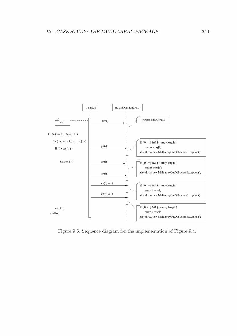
9.3. CASE STUDY: THE MULTIARRAY PACKAGE 249
array[i] = val;
array[j] = val;
if ( 0 <= i && i < array.length )
return array[i];
else throw new MultiarrayOutOfBoundsException();
else throw new MultiarrayOutOfBoundsException();
else throw new MultiarrayOutOfBoundsException();
if ( 0 <= i && i < array.length )
set( j, val )
return array[j];
if ( 0 <= j && j < array.length )
else throw new MultiarrayOutOfBoundsException();
get(j)fib.get( j ) )
get(i)if (fib.get ( i ) <
for (int i = 0; i <size; i++)
for (int j = i +1; j < size; j++)
rerturn array.length;size()
fib : IntMultiarray1D
sort
if ( 0 <= j && j < array.length )
get(i)
set( i, val )
: Thread
end for
end for
Figure 9.5: Sequence diagram for the implementation of Figure 9.4.
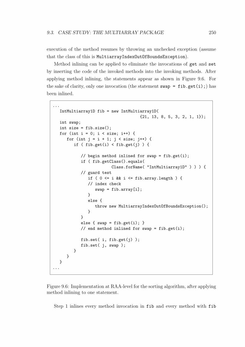
9.3. CASE STUDY: THE MULTIARRAY PACKAGE 250
execution of the method resumes by throwing an unchecked exception (assume
that the class of this is MultiarrayIndexOutOfBoundsException).
Method inlining can be applied to eliminate the invocations of get and set
by inserting the code of the invoked methods into the invoking methods. After
applying method inlining, the statements appear as shown in Figure 9.6. For
the sake of clarity, only one invocation (the statement swap = fib.get(i);) has
been inlined.
...IntMultiarray1D fib = new IntMultiarray1D(
{21, 13, 8, 5, 3, 2, 1, 1});int swap;int size = fib.size();for (int i = 0; i < size; i++) {
for (int j = i + 1; j < size; j++) {if ( fib.get(i) < fib.get(j) ) {
// begin method inlined for swap = fib.get(i);if ( fib.getClass().equals(
Class.forName( "IntMultiarray1D" ) ) ) {// guard test
if ( 0 <= i && i <= fib.array.length ) {// index check
swap = fib.array[i];}else {
throw new MultiarrayIndexOutOfBoundsException();}
}else { swap = fib.get(i); }// end method inlined for swap = fib.get(i);
fib.set( i, fib.get(j) );fib.set( j, swap );
}}
}...
Figure 9.6: Implementation at RAA-level for the sorting algorithm, after applyingmethod inlining to one statement.
Step 1 inlines every method invocation in fib and every method with fib
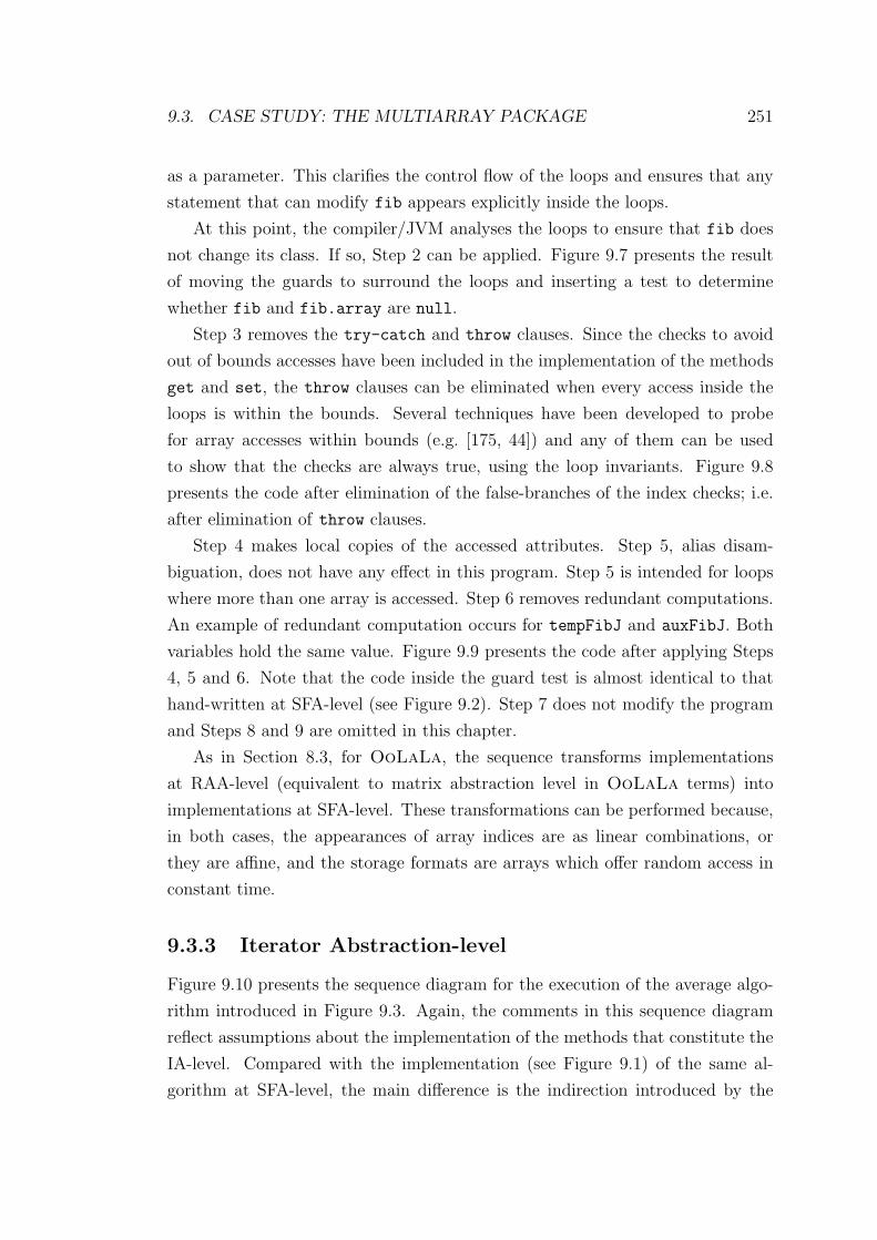
9.3. CASE STUDY: THE MULTIARRAY PACKAGE 251
as a parameter. This clarifies the control flow of the loops and ensures that any
statement that can modify fib appears explicitly inside the loops.
At this point, the compiler/JVM analyses the loops to ensure that fib does
not change its class. If so, Step 2 can be applied. Figure 9.7 presents the result
of moving the guards to surround the loops and inserting a test to determine
whether fib and fib.array are null.
Step 3 removes the try-catch and throw clauses. Since the checks to avoid
out of bounds accesses have been included in the implementation of the methods
get and set, the throw clauses can be eliminated when every access inside the
loops is within the bounds. Several techniques have been developed to probe
for array accesses within bounds (e.g. [175, 44]) and any of them can be used
to show that the checks are always true, using the loop invariants. Figure 9.8
presents the code after elimination of the false-branches of the index checks; i.e.
after elimination of throw clauses.
Step 4 makes local copies of the accessed attributes. Step 5, alias disam-
biguation, does not have any effect in this program. Step 5 is intended for loops
where more than one array is accessed. Step 6 removes redundant computations.
An example of redundant computation occurs for tempFibJ and auxFibJ. Both
variables hold the same value. Figure 9.9 presents the code after applying Steps
4, 5 and 6. Note that the code inside the guard test is almost identical to that
hand-written at SFA-level (see Figure 9.2). Step 7 does not modify the program
and Steps 8 and 9 are omitted in this chapter.
As in Section 8.3, for OoLaLa, the sequence transforms implementations
at RAA-level (equivalent to matrix abstraction level in OoLaLa terms) into
implementations at SFA-level. These transformations can be performed because,
in both cases, the appearances of array indices are as linear combinations, or
they are affine, and the storage formats are arrays which offer random access in
constant time.
9.3.3 Iterator Abstraction-level
Figure 9.10 presents the sequence diagram for the execution of the average algo-
rithm introduced in Figure 9.3. Again, the comments in this sequence diagram
reflect assumptions about the implementation of the methods that constitute the
IA-level. Compared with the implementation (see Figure 9.1) of the same al-
gorithm at SFA-level, the main difference is the indirection introduced by the
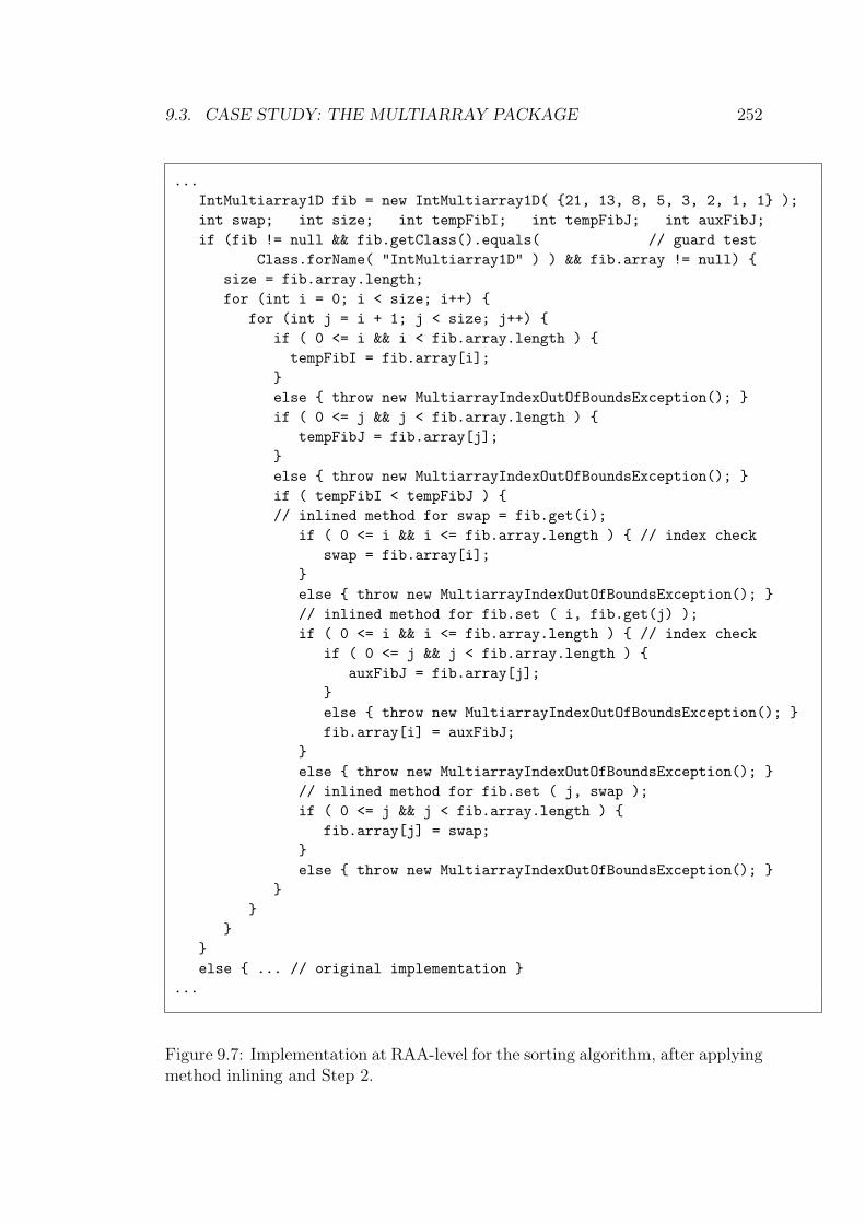
9.3. CASE STUDY: THE MULTIARRAY PACKAGE 252
...IntMultiarray1D fib = new IntMultiarray1D( {21, 13, 8, 5, 3, 2, 1, 1} );int swap; int size; int tempFibI; int tempFibJ; int auxFibJ;if (fib != null && fib.getClass().equals( // guard test
Class.forName( "IntMultiarray1D" ) ) && fib.array != null) {size = fib.array.length;for (int i = 0; i < size; i++) {
for (int j = i + 1; j < size; j++) {if ( 0 <= i && i < fib.array.length ) {tempFibI = fib.array[i];
}else { throw new MultiarrayIndexOutOfBoundsException(); }if ( 0 <= j && j < fib.array.length ) {
tempFibJ = fib.array[j];}else { throw new MultiarrayIndexOutOfBoundsException(); }if ( tempFibI < tempFibJ ) {// inlined method for swap = fib.get(i);
if ( 0 <= i && i <= fib.array.length ) { // index checkswap = fib.array[i];
}else { throw new MultiarrayIndexOutOfBoundsException(); }// inlined method for fib.set ( i, fib.get(j) );if ( 0 <= i && i <= fib.array.length ) { // index check
if ( 0 <= j && j < fib.array.length ) {auxFibJ = fib.array[j];
}else { throw new MultiarrayIndexOutOfBoundsException(); }fib.array[i] = auxFibJ;
}else { throw new MultiarrayIndexOutOfBoundsException(); }// inlined method for fib.set ( j, swap );if ( 0 <= j && j < fib.array.length ) {
fib.array[j] = swap;}else { throw new MultiarrayIndexOutOfBoundsException(); }
}}
}}else { ... // original implementation }
...
Figure 9.7: Implementation at RAA-level for the sorting algorithm, after applyingmethod inlining and Step 2.
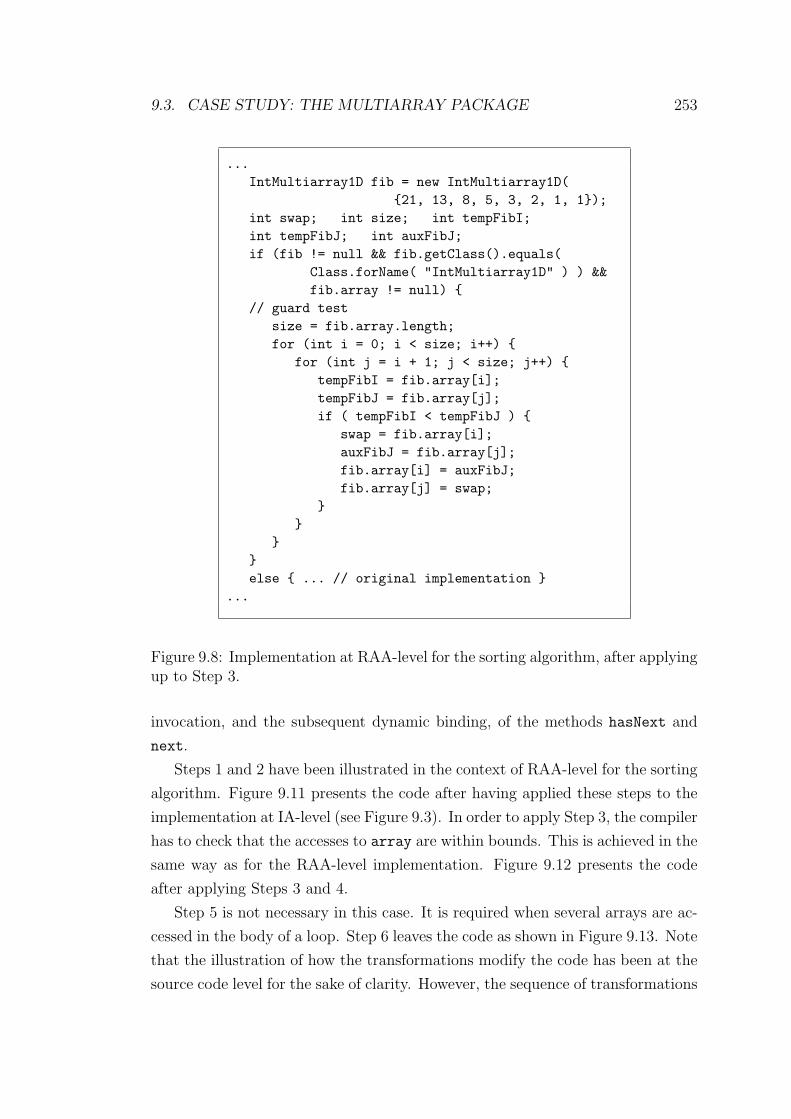
9.3. CASE STUDY: THE MULTIARRAY PACKAGE 253
...IntMultiarray1D fib = new IntMultiarray1D(
{21, 13, 8, 5, 3, 2, 1, 1});int swap; int size; int tempFibI;int tempFibJ; int auxFibJ;if (fib != null && fib.getClass().equals(
Class.forName( "IntMultiarray1D" ) ) &&fib.array != null) {
// guard testsize = fib.array.length;for (int i = 0; i < size; i++) {
for (int j = i + 1; j < size; j++) {tempFibI = fib.array[i];tempFibJ = fib.array[j];if ( tempFibI < tempFibJ ) {
swap = fib.array[i];auxFibJ = fib.array[j];fib.array[i] = auxFibJ;fib.array[j] = swap;
}}
}}else { ... // original implementation }
...
Figure 9.8: Implementation at RAA-level for the sorting algorithm, after applyingup to Step 3.
invocation, and the subsequent dynamic binding, of the methods hasNext and
next.
Steps 1 and 2 have been illustrated in the context of RAA-level for the sorting
algorithm. Figure 9.11 presents the code after having applied these steps to the
implementation at IA-level (see Figure 9.3). In order to apply Step 3, the compiler
has to check that the accesses to array are within bounds. This is achieved in the
same way as for the RAA-level implementation. Figure 9.12 presents the code
after applying Steps 3 and 4.
Step 5 is not necessary in this case. It is required when several arrays are ac-
cessed in the body of a loop. Step 6 leaves the code as shown in Figure 9.13. Note
that the illustration of how the transformations modify the code has been at the
source code level for the sake of clarity. However, the sequence of transformations
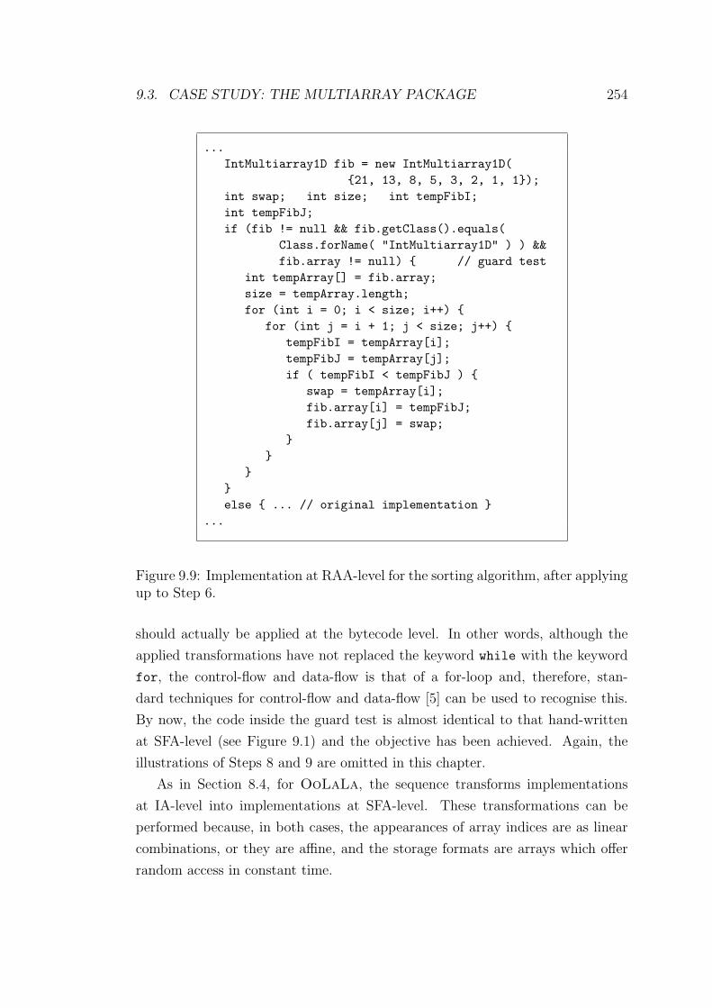
9.3. CASE STUDY: THE MULTIARRAY PACKAGE 254
...IntMultiarray1D fib = new IntMultiarray1D(
{21, 13, 8, 5, 3, 2, 1, 1});int swap; int size; int tempFibI;int tempFibJ;if (fib != null && fib.getClass().equals(
Class.forName( "IntMultiarray1D" ) ) &&fib.array != null) { // guard test
int tempArray[] = fib.array;size = tempArray.length;for (int i = 0; i < size; i++) {
for (int j = i + 1; j < size; j++) {tempFibI = tempArray[i];tempFibJ = tempArray[j];if ( tempFibI < tempFibJ ) {
swap = tempArray[i];fib.array[i] = tempFibJ;fib.array[j] = swap;
}}
}}else { ... // original implementation }
...
Figure 9.9: Implementation at RAA-level for the sorting algorithm, after applyingup to Step 6.
should actually be applied at the bytecode level. In other words, although the
applied transformations have not replaced the keyword while with the keyword
for, the control-flow and data-flow is that of a for-loop and, therefore, stan-
dard techniques for control-flow and data-flow [5] can be used to recognise this.
By now, the code inside the guard test is almost identical to that hand-written
at SFA-level (see Figure 9.1) and the objective has been achieved. Again, the
illustrations of Steps 8 and 9 are omitted in this chapter.
As in Section 8.4, for OoLaLa, the sequence transforms implementations
at IA-level into implementations at SFA-level. These transformations can be
performed because, in both cases, the appearances of array indices are as linear
combinations, or they are affine, and the storage formats are arrays which offer
random access in constant time.
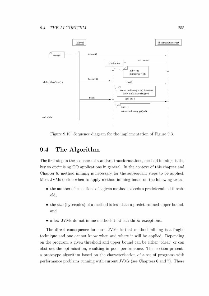
9.4. THE ALGORITHM 255
average iterator()
ind = −1;
fib : IntMultiarray1D
multiarray = fib;
while ( i.hasNext() )
<<create>>
get( ind )
return multiarray.get(ind);
ind ++;
next()
i : IntIterator
hasNext()size()
return multiarray.size() ! = 0 &&ind < multiarray.size() −1
: Thread
end while
Figure 9.10: Sequence diagram for the implementation of Figure 9.3.
9.4 The Algorithm
The first step in the sequence of standard transformations, method inlining, is the
key to optimising OO applications in general. In the context of this chapter and
Chapter 8, method inlining is necessary for the subsequent steps to be applied.
Most JVMs decide when to apply method inlining based on the following tests:
• the number of executions of a given method exceeds a predetermined thresh-
old,
• the size (bytecodes) of a method is less than a predetermined upper bound,
and
• a few JVMs do not inline methods that can throw exceptions.
The direct consequence for most JVMs is that method inlining is a fragile
technique and one cannot know when and where it will be applied. Depending
on the program, a given threshold and upper bound can be either “ideal” or can
obstruct the optimisation, resulting in poor performance. This section presents
a prototype algorithm based on the characterisation of a set of programs with
performance problems running with current JVMs (see Chapters 6 and 7). These
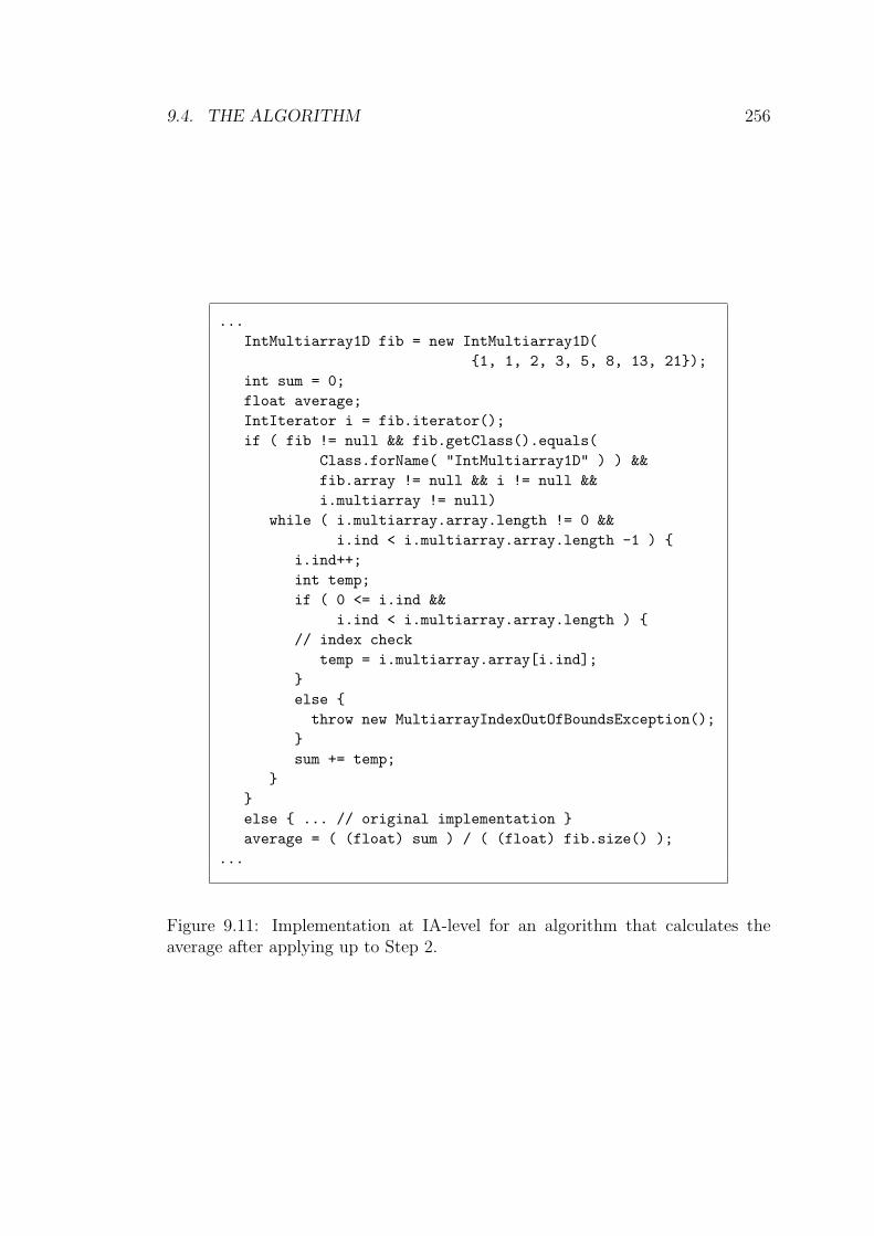
9.4. THE ALGORITHM 256
...IntMultiarray1D fib = new IntMultiarray1D(
{1, 1, 2, 3, 5, 8, 13, 21});int sum = 0;float average;IntIterator i = fib.iterator();if ( fib != null && fib.getClass().equals(
Class.forName( "IntMultiarray1D" ) ) &&fib.array != null && i != null &&i.multiarray != null)
while ( i.multiarray.array.length != 0 &&i.ind < i.multiarray.array.length -1 ) {
i.ind++;int temp;if ( 0 <= i.ind &&
i.ind < i.multiarray.array.length ) {// index check
temp = i.multiarray.array[i.ind];}else {throw new MultiarrayIndexOutOfBoundsException();
}sum += temp;
}}else { ... // original implementation }average = ( (float) sum ) / ( (float) fib.size() );
...
Figure 9.11: Implementation at IA-level for an algorithm that calculates theaverage after applying up to Step 2.

9.4. THE ALGORITHM 257
...IntMultiarray1D fib = new IntMultiarray1D(
{1, 1, 2, 3, 5, 8, 13, 21});int sum = 0;float average;IntIterator i = fib.iterator();if ( fib != null && fib.getClass().equals(
Class.forName( "IntMultiarray1D" ) ) &&fib.array != null && i != null &&i.multiarray != null)
int tempInd = i.ind;IntMultiarray1D tempMultiarray = i.multiarray;int tempArray [] = tempMultiarray.array;int tempLength = tempArray.length;while ( tempLength != 0 &&
tempInd < tempLength -1 ) {tempInd++;int temp;temp = tempArray[tempInd];sum += temp;
}}else { ... // original implementation }average = ( (float) sum ) / ( (float) fib.size() );
...
Figure 9.12: Implementation at IA-level for an algorithm that calculates theaverage after applying up to Step 4.
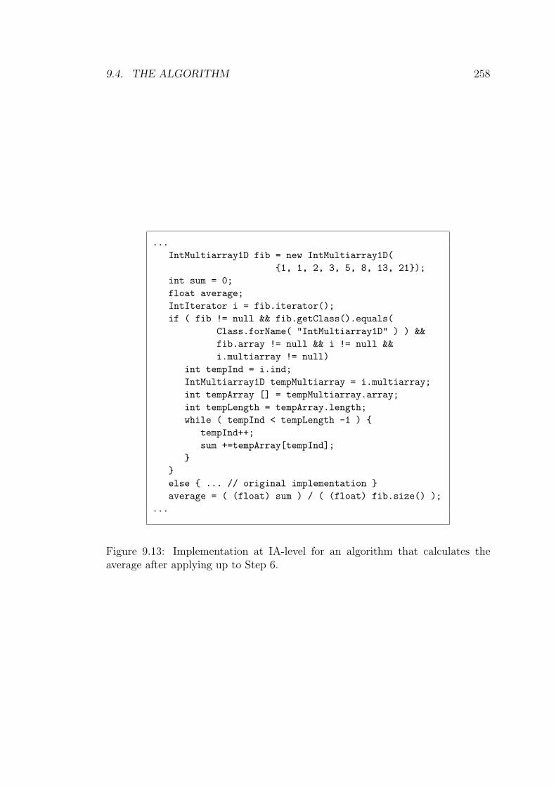
9.4. THE ALGORITHM 258
...IntMultiarray1D fib = new IntMultiarray1D(
{1, 1, 2, 3, 5, 8, 13, 21});int sum = 0;float average;IntIterator i = fib.iterator();if ( fib != null && fib.getClass().equals(
Class.forName( "IntMultiarray1D" ) ) &&fib.array != null && i != null &&i.multiarray != null)
int tempInd = i.ind;IntMultiarray1D tempMultiarray = i.multiarray;int tempArray [] = tempMultiarray.array;int tempLength = tempArray.length;while ( tempInd < tempLength -1 ) {
tempInd++;sum +=tempArray[tempInd];
}}else { ... // original implementation }average = ( (float) sum ) / ( (float) fib.size() );
...
Figure 9.13: Implementation at IA-level for an algorithm that calculates theaverage after applying up to Step 6.
9.4. THE ALGORITHM 259
programs are built from design patterns for storage formats implemented with
arrays. The aim of the algorithm is to determine when and where to apply the
sequence of transformations.
The first part of the algorithm selects a set of classes that might be the
implementation of storage formats. To this end, the algorithm uses field analysis.
When a class is loaded in the JVM (or, in the case of a static compiler, when
the compiler reaches a class), the algorithm examines the attributes (fields). If
any of the attributes is an array, and either other attributes or parameters of the
methods are used as indices into this array, then the loaded class is a Collection
Candidate (CC) class and has depth 0. Otherwise, if any of the attributes is an
object of a CC class of depth d and either other attributes or parameters of the
methods are used as indices into this object, then the loaded class is also a CC
class and its depth is d + 1.
Once the algorithm has constructed the set of CC classes, it moves on to
detect where to apply the sequence of standard transformations. The algorithm
divides into an adaptive compilation version and a static compilation version.
Both variants focus on finding loops which are accessing objects of CC classes.
First consider the static compilation version. There are no constraints on the
number of times the algorithm tries to apply the sequence of standard transforma-
tions. Thus, the algorithm examines the implementations of reachable methods,
classifying each loop as a CC loop when a statement of the body accesses directly
an object of a CC class. This loop has distance 0 from a CC class. A loop with a
statement that invokes a method that reaches a CC loop of distance δ is also a CC
loop and its distance is δ + 1. The sequence of transformations is applied to the
set of CC loops of distance 0, and then recursively to those of distance 1 and so
on. The algorithm terminates when the variables in the method or attributes in
the object that holds the CC loop do not determine which elements are accessed
in an object of a CC class.
The adaptive compilation version follows a similar algorithm (from CC loops
with distance 0 to 1, 2 and so on). However, the adaptive compilation version
will not consider the whole set of CC loops and classes. It will concentrate on
detected “hot spots”. The most promising CC loops with distance 0 and with
access to a CC with the highest depth. Below this, we find the CC loops are those
with distance 0 with access to a CC with highest depth −1; and so forth. This
is because depth represents the number of indirections or consecutive invocations
9.5. RELATED WORK 260
to access a stored element. Further experimentation is needed to determine when
to stop recursively applying the algorithm backwards, although the condition
described for the static version still holds as the final condition.
9.5 Related Work
Most of the related work was discussed in Section 8.5, i.e. in the chapter where
the sequence of compiler transformations was first introduced, and is not re-
peated here. Specifically related to this chapter is the work of IBM’s Ninja
group on semantic expansion [228, 179] and the work on specialization patterns
by IRISA/INRIA’s Compose group [223, 181, 202, 201]
The Ninja group designed and implemented a multi-dimensional array pack-
age [176] which is the precursor of the one submitted for Java standardisation
and is described in this chapter and in Chapter 7. To eliminate the overhead
introduced by using classes, they have developed semantic expansion [228]. Se-
mantic expansion is a compilation strategy by which selected classes are treated
as language primitives by the compiler. In the prototype Ninja static compiler,
they successfully implement the elimination of array bounds checks, together with
semantic expansion for their multi-dimensional array package and other loop re-
ordering transformations. The sequence of standard compiler transformations,
plus the algorithm presented in Section 9.4, have the same effect as semantic
expansion, but without being so ad-hoc (semantic expansion is effective only for
specific known libraries).
The Compose group has proposed specialization patterns as a way of optimis-
ing sections of programs which use design patterns. Users select sections of pro-
grams where design patterns are used and then specialization patterns are applied
to that section to generate an optimised version of the program. A specialization
pattern is associated with both a design pattern and a set of transformations
to optimise that design pattern. The set of transformations includes standard
transformations that can be represented at language level, e.g. object inlining,
method inlining, etc., but cannot apply elimination of exceptions or register al-
location. The Compose group defines specialization patterns for the iterator,
visitor, builder and strategy patterns. From this point of view, they cover more
design patterns than are covered in this chapter. However, the specialization pat-
terns that they propose do not fully eliminate the performance gap. They have
9.6. SUMMARY 261
not considered the SFA-level as the performance target and do not attempt to get
close to the SFA-level. Moreover, in specialization patterns, users are responsible
for selecting the transformed sections of the program, whereas this chapter has
described an algorithm that selects automatically sections of the programs where
the transformations should be applied.
9.6 Summary
This chapter has described a prototype algorithm to determine when and where to
apply the sequence of standard compiler transformations introduced in Chapter 8
for optimising OoLaLa. Such a sequence has been illustrated for one case study
and has shown that the sequence can eliminate the performance gap between
software built from design patterns (iterator and random access patterns for data
structures based on arrays – IA- and RAA-level) and hacked-for-performance
software (SFA-level).
RAA-level provides library developers with an interface to collections inde-
pendent of the storage format and with random access to the stored elements.
IA-level provides library developers with an interface to access collections also
independent of the storage format.
The prototype algorithm looks for appearances of RAA- and IA-level imple-
mentations and for implementations of storage formats based on arrays, and the
algorithm concentrates on loops which access these storage formats.
Chapter 10
Limitations of the Library
Approach
10.1 Introduction
The thesis has followed a library approach as the way of improving the devel-
opment of sequential Numerical Linear Algebra (NLA) programs. An Object
Oriented (OO) NLA library has been designed with the following properties:
• encapsulation of storage formats, properties and matrices in classes;
• selection of appropriate implementations of certain matrix operations given
the properties and storage formats of the matrix operands; and
• capability to manage the storage formats and to propagate matrix proper-
ties (a novel functionality for NLA libraries).
The objective of this chapter is to investigate the difficulties faced in aiming
to develop a NLA program with minimum execution time. The conclusion is that
NLA libraries, both traditional and OO, are not able to meet this challenge on
their own.
The difficulties can be in one of two forms. The first form is derived from
the fact that distinct, yet semantically equivalent matrix expressions can be im-
plemented which yield different programs and corresponding execution times.
The term semantically equivalent is used since it is only in the case that exact
arithmetic is assumed that the programs are really equivalent. The equivalent ex-
pressions are obtained from the mathematical properties of the matrix operations.
262
10.2. THE BEST ORDER PROBLEM 263
In particular, the commutative property of matrix addition (Section 10.2), the
associative property of matrix multiplication (Section 10.3), and the distributive
property of matrix multiplication (Section 10.4) are discussed.
The second form is related directly to the novel functionality of OoLaLa.
Section 10.5 presents examples where a library approach cannot efficiently propa-
gate the properties through matrix operations. Section 10.6 describes the problem
of selecting the best storage format for each matrix of a NLA program.
The chapter concludes (Section 10.7) with an overview of a software environ-
ment for the development of NLA programs (a problem solving environment) that
merges a library approach with techniques to address the difficulties referred to
above .
10.2 The Best Order Problem
The commutative property of matrix addition states that
A + B = B + A. (10.1)
When adding 3 matrices, the commutative property yields the following identities:
A + B + C = A + C + B
= B + A + C
= B + C + A
= C + A + B
= C + B + A
.
the number of different ways of representing the addition of 3 matrices is 3×2 = 6.
When the number of matrices is increased to 4, the commutative property
yields 4! = 24 different representations (ordering of the additions). In general,
when adding n matrices the commutative property yields n! different represen-
tations. Users who want to develop a program that calculates the addition of n
matrices can develop n! different programs; each program corresponds to a differ-
ent order of addition. For example, the addition A+B+C can be programmed as
R=(A+B)+C or R=(B+C)+A or R=(C+B)+A or . . . , all being semantically equivalent
programs. However, the execution time of each program varies depending on the
order of addition and the properties of A, B and C.
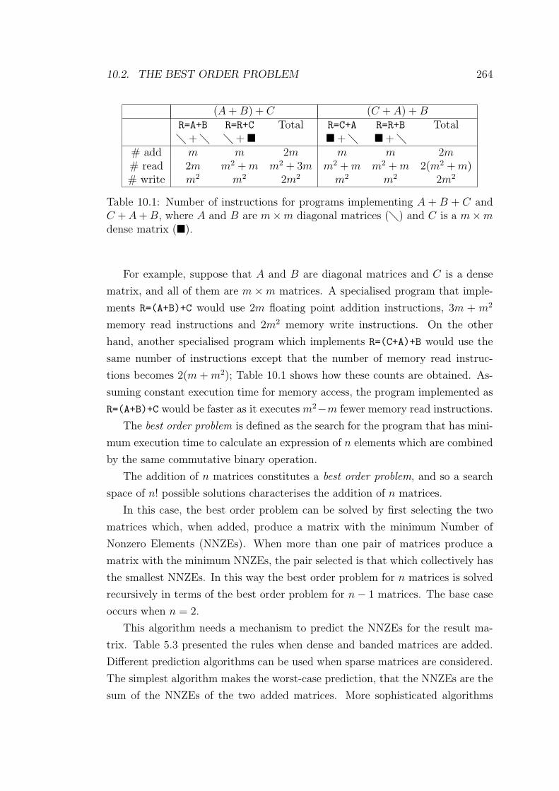
10.2. THE BEST ORDER PROBLEM 264
(A + B) + C (C + A) + BR=A+B R=R+C Total R=C+A R=R+B Total� + � � + � � + � � + �
# add m m 2m m m 2m# read 2m m2 + m m2 + 3m m2 + m m2 + m 2(m2 + m)# write m2 m2 2m2 m2 m2 2m2
Table 10.1: Number of instructions for programs implementing A + B + C andC + A + B, where A and B are m×m diagonal matrices (�) and C is a m×mdense matrix (�).
For example, suppose that A and B are diagonal matrices and C is a dense
matrix, and all of them are m ×m matrices. A specialised program that imple-
ments R=(A+B)+C would use 2m floating point addition instructions, 3m + m2
memory read instructions and 2m2 memory write instructions. On the other
hand, another specialised program which implements R=(C+A)+B would use the
same number of instructions except that the number of memory read instruc-
tions becomes 2(m + m2); Table 10.1 shows how these counts are obtained. As-
suming constant execution time for memory access, the program implemented as
R=(A+B)+C would be faster as it executes m2−m fewer memory read instructions.
The best order problem is defined as the search for the program that has mini-
mum execution time to calculate an expression of n elements which are combined
by the same commutative binary operation.
The addition of n matrices constitutes a best order problem, and so a search
space of n! possible solutions characterises the addition of n matrices.
In this case, the best order problem can be solved by first selecting the two
matrices which, when added, produce a matrix with the minimum Number of
Nonzero Elements (NNZEs). When more than one pair of matrices produce a
matrix with the minimum NNZEs, the pair selected is that which collectively has
the smallest NNZEs. In this way the best order problem for n matrices is solved
recursively in terms of the best order problem for n− 1 matrices. The base case
occurs when n = 2.
This algorithm needs a mechanism to predict the NNZEs for the result ma-
trix. Table 5.3 presented the rules when dense and banded matrices are added.
Different prediction algorithms can be used when sparse matrices are considered.
The simplest algorithm makes the worst-case prediction, that the NNZEs are the
sum of the NNZEs of the two added matrices. More sophisticated algorithms
10.3. THE BEST ASSOCIATION PROBLEM 265
would need to exploit the specific structures of the matrices.
Note that the best order problem cannot be solved by a library unless a
subroutine (or method) is provided which implements the addition of n matrices.
This is not the usual practice.
10.3 The Best Association Problem
The associative property of matrix multiplication states that
(AB)C = A(BC). (10.2)
When 4 matrices are multiplied, the associative property yields
((AB)C)D = (A(BC))D
= A(B(CD))
= A((BC)D)
= (AB)(CD)
.
Each representation is formed dividing the 4 matrix multiplication into two
subsets by introducing parenthesis (e.g. (AB)(CD) or (A)(BCD)). When a sub-
set has only one or two matrices, that subset is a base case. Otherwise, the subset
is recursively subdivided until a base case is found.
Let ANI(n) be the number of ways of representing the multiplication of n
matrices (i.e. the association of the n− 1 matrix multiplications). It is straight-
forward to show that ANI(3) = 2, ANI(4) = 6 and, in general, ANI(n) =∑n−1i=1 ANI(i)ANI(n − i). ANI(n) is known as the catalan number [209, 192].
Other examples of catalan numbers are ANI(5) = 14 and ANI(15) = 2674440.
Each representation is the basis of a different program, and all such programs
are semantically equivalent. However, the execution times of these programs
vary. The variation is due to matrix dimensions and matrix properties. For
example, consider the matrix multiplication ABC where A and B are n×n dense
matrices and C is an n × 1 dense matrix. The association (AB)C performs one
matrix-matrix multiplication (O(n3) floating point operations) and one matrix-
vector multiplication (O(n2) floating point operations). On the other hand, the
association A(BC) performs two matrix-vector multiplications (2O(n2) floating
point operations).
10.4. THE MAXIMUM COMMON FACTOR PROBLEM 266
The best association problem, also referred to as the chain multiplication prob-
lem [120], is defined as the search for the program to calculate an expression
of n elements which are combined by the same binary associative and non-
commutative operation.
The multiplication of n matrices constitutes a best association problem and so
a search space of ANI(n) (catalan numbers) possible solutions characterises the
multiplication of n matrices. Algorithms to solve the best association problem
can be found in [137, 138, 69].
A library can only solve the best association problem if a subroutine (or
method) is provided which implements the multiplication of n matrices. Again,
this is not the usual case.
10.4 The Maximum Common Factor Problem
The distributive property of matrix multiplication states that
A(B + C) = AB + AC. (10.3)
The right hand side of Equation 10.3 implies that the implementation would
require two matrix multiplications and one addition. On the other hand, the
left hand side of Equation 10.3 implies that the implementation would require
one multiplication and one addition. The execution times would be significantly
different and the left hand side of Equation 10.3 would be faster.
The distributive property can be generalised as
A(B1 + B2 + · · ·+ Bh) = AB1 + AB2 + · · ·+ ABh,
where A, B1, B2, . . . , Bh are matrices or combinations of matrix operations that
produce a matrix. With this generalisation in mind, the maximum common factor
problem is defined as finding the matrix A, so that the expression A(B1 + B2 +
· · ·+Bh) has no further common factors. That is, there is no matrix X, different
from the identity matrix, such that Bi = XYi and i = 1, 2, . . . , h.
Assuming a language that allows a matrix to be a variable, the maximum
common factor problem can be solved applying standard compiler techniques.
In the first phase, forward substitution is applied to replace variables by their
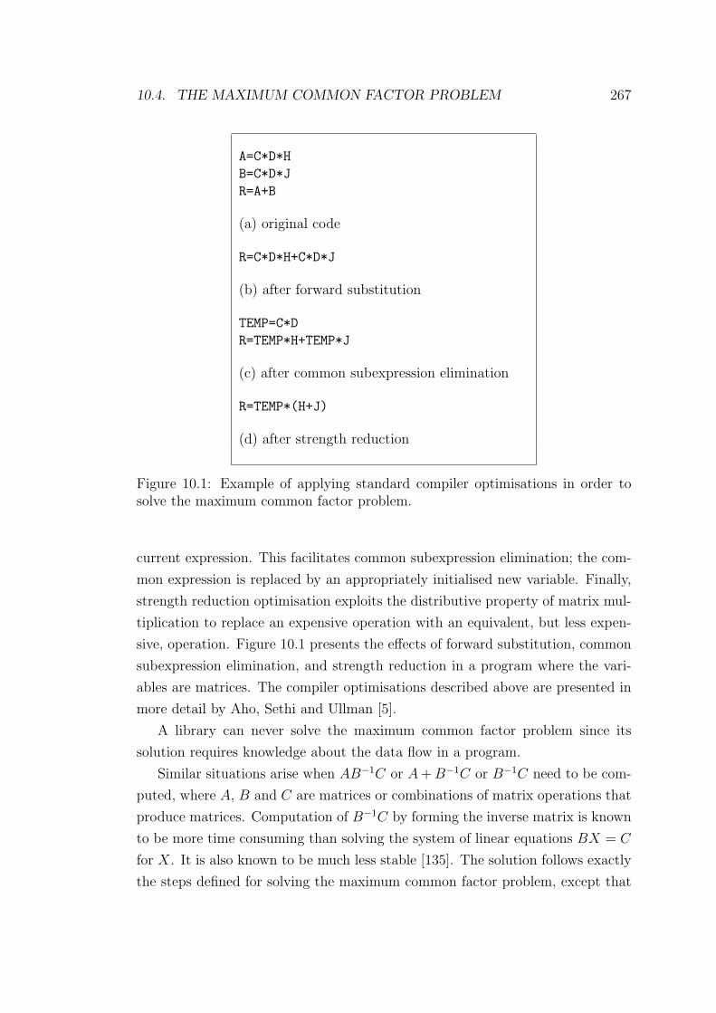
10.4. THE MAXIMUM COMMON FACTOR PROBLEM 267
A=C*D*H
B=C*D*J
R=A+B
(a) original code
R=C*D*H+C*D*J
(b) after forward substitution
TEMP=C*D
R=TEMP*H+TEMP*J
(c) after common subexpression elimination
R=TEMP*(H+J)
(d) after strength reduction
Figure 10.1: Example of applying standard compiler optimisations in order tosolve the maximum common factor problem.
current expression. This facilitates common subexpression elimination; the com-
mon expression is replaced by an appropriately initialised new variable. Finally,
strength reduction optimisation exploits the distributive property of matrix mul-
tiplication to replace an expensive operation with an equivalent, but less expen-
sive, operation. Figure 10.1 presents the effects of forward substitution, common
subexpression elimination, and strength reduction in a program where the vari-
ables are matrices. The compiler optimisations described above are presented in
more detail by Aho, Sethi and Ullman [5].
A library can never solve the maximum common factor problem since its
solution requires knowledge about the data flow in a program.
Similar situations arise when AB−1C or A + B−1C or B−1C need to be com-
puted, where A, B and C are matrices or combinations of matrix operations that
produce matrices. Computation of B−1C by forming the inverse matrix is known
to be more time consuming than solving the system of linear equations BX = C
for X. It is also known to be much less stable [135]. The solution follows exactly
the steps defined for solving the maximum common factor problem, except that
10.5. THE MATRIX PROPERTY PROPAGATION PROBLEM 268
the strength reduction rule is different.
A further example is the system of linear equations A1A2 . . . Apx = b where
A1, A2, . . . , Ap are square matrices. This system is a generalisation of the one
introduced in Section 2.6 (i.e. ABx = c where A and B are n × n matrices).
Instead of carrying out the chained matrix multiplication, with a cost of 2n3 +
O(n2) floating point operations for each multiplication, each matrix can be LU-
factorised (A1 = LiUi and i = 1, 2, . . . , p) at a cost less than or equal to 23n3 +
O(n2) floating point operations per factorisation. This latter approach leads to
more forward and backward substitutions, but these are O(n2).
The work of Marsolf [168, 169] in the Falcon project uses transformation pat-
terns for interactively restructuring Matlab’s programs. Users define patterns
to be found in a Matlab program and specify how the code that matches with
a pattern should be restructured ([168] Chapter 4). These transformation pat-
terns enable the Falcon environment to apply traditional restructuring compiler
transformations ([168] Chapter 5), such as loop unrolling [21], and basic algebraic
transformations ([168] Chapter 6). Among other basic algebraic transformations,
Marsolf presents a limited solution to the multiplication of n matrices (best asso-
ciation problem of Section 10.3) and a solution to the above example, where the
inversion of a matrix is avoided by solving a system of linear equations. Marsolf’s
solution to the multiplication of n matrices identifies the vectors and multiplies
these first. However, transformation patterns cannot implement the algorithm
presented in [69] for the general best association problem. This algorithm uses
information related to the NNZEs in rows and columns and this information is
not represented by the transformation patterns. Transformation patterns are
able to perform the strength reductions presented in this section, but Marsolf
does not show how forward substitution or common subexpression elimination
can be implemented with the transformation patterns.
10.5 The Matrix Property Propagation Prob-
lem
OoLaLa is able to propagate the properties of a matrix through matrix oper-
ations. However, a library cannot efficiently propagate matrix properties that
are a consequence of the history of previous matrix operations. For example, the
matrix multiplication AB where A and B are symmetric is known to generate a
10.6. THE BEST STORAGE FORMAT PROBLEM 269
dense unsymmetric result matrix. Similarly, the matrix multiplication BA also
generates a dense unsymmetric matrix. Applying the rules of addition, AB +BA
is the addition of two dense unsymmetric matrices and generates a dense unsym-
metric matrix. However, for A and B symmetric, AB + BA is also a symmetric
matrix (AB + (AB)T = AB + BA).
In order to address this problem, a library would have to keep a history for each
matrix. This history would record the matrix operations that have been carried
out on each matrix and matrix properties of the parameters of those matrix
operations. On the other hand, a compiler is able to identify these situations as
long as they can be specified by a set of if-then rules. The implementation is
similar to the way a compiler checks the type of an expression; when it detects an
incorrect type, it sends an error message. Similarly, the compiler could check an
expression of matrices and detect a special situation; instead of sending an error
message, the compiler could change the matrix properties of the expression. For
a more technical approach to these compiler techniques consult [5], Chapters 4
and 5.
Despite the fact that Marsolf’s work [168, 169]) in the Falcon environment and
Bik and Wijshoff’s Sparse Compiler [31, 34, 32, 35] propagate matrix properties,
they do not identify the difficulty noted in this section nor present any solution.
10.6 The Best Storage Format Problem
Matrices can be stored using different storage formats. Table 5.5 presents the
advisable combinations of matrix properties and storage formats in the context of
OoLaLa. The storage format influences the execution time of implementations
of matrix operations and it determines the memory position where each element
of a matrix is kept. An implementation of a matrix calculation determines a
logical access pattern to the matrix elements, which is mapped to a physical
access pattern to the memory. When the storage format is changed, the logical
access pattern to the elements of a matrix remains unchanged, but the physical
access pattern varies. Different physical access patterns have different rates of
cache reuse. Consider, for example, the well-known case of arrays stored row-
wise or column-wise. For this case, compiler optimisation techniques have been
developed to modify loops so that an array is traversed in the order in which it
is stored in memory [21].
10.7. A LINEAR ALGEBRA PROBLEM SOLVING ENVIRONMENT 270
OoLaLa enables users to abstract their programs from the storage formats
and the propagation of the matrix properties through matrix calculations. Hence,
the structure of a NLA program is divided into two parts. The first part declares
the input matrices and their matrix properties (and optionally their storage for-
mats). In the second part, the matrices are operated on and auxiliary matrices
are created to hold intermediate or final results. Before each matrix calculation is
performed, the storage format of the associated matrices can be changed. These
changes in storage format could be represented by invocations of mapping meth-
ods, which would map from a current storage format of a matrix to a specified
new storage format. These mapping methods can be inserted at any point of the
program and the semantics of the program remain unchanged. The program pro-
duces the same result (assuming exact arithmetic) independently of the number
and the location of the mapping methods in the program. The noticeable effects
of mapping methods are in the execution time and memory requirement. The
execution time decreases when the time of executing the mapping methods added
to the time of executing the matrix calculations with the new storage formats is
less than the time of executing the matrix operations with the previous storage
formats; otherwise the execution time increases (or remains unchanged).
The best storage format problem is defined as the search for the NLA pro-
gram with the minimum execution time, among those programs with equivalent
functionality but with different storage formats.
In general, the solution of the best storage format problem is computationally
infeasible [166]. Bik and Wijshoff have proposed an heuristic to automatically
select the storage format [34]; this heuristic is integrated with their Sparse Com-
piler and, since it requires knowledge of the instruction flow, it cannot be included
in a library.
10.7 A Linear Algebra Problem Solving Envi-
ronment
The preceding sections have identified problems or limitations associated with
NLA libraries. Some, for example the best order and the best association prob-
lems, can be solved within a library, but this is unusual. Others, the maximum
common factor, the matrix properties propagation and the best storage format
problems, can be addressed only at compile time, and motivate a move from
10.7. A LINEAR ALGEBRA PROBLEM SOLVING ENVIRONMENT 271
NLA libraries to problem solving environments. A problem solving environment
is software, often with graphical user interfaces, which enables users to develop
programs using the problem domain language as the programming language. A
problem solving environment integrates domain specific libraries, compiler tech-
niques, artificial intelligence, visualisation and any other computer science disci-
pline that may help users in developing their programs [106].
A NLA problem solving environment should provide support for, and encap-
sulate, the different tasks that users have to perform when developing a NLA
program, namely:
(a) description of the problem in terms of matrix operations,
(b) analysis of the matrices to determine their properties,
(c) selection of a library or libraries which support the operations and proper-
ties,
(d) mapping of the matrix operations onto the implementations provided by
the library,
(e) analysis of the propagation of the matrix properties through the matrix
operations,
(f) declaration of the variables conforming to the storage format which is sup-
ported by the selected implementations,
(g) selection of the best combination of preconditioner and iterative solver for
a given system of linear equations, and
(h) selection of the best ordering algorithm for a direct solver for a given sparse
system of linear equations.
OoLaLa has encapsulated tasks (c) and (f), and, partially, tasks (d) and
(e). This chapter has presented examples of the ways user could efficiently map
their matrix operations into matrix implementations provided by libraries, i.e.
task (d). To this end, matrix operation properties have been presented as a
way of describing different, semantically equivalent, programs that have different
execution times. Solutions to the best association problem are proposed by Hu
and Shing [137, 138] and by Cohen [69].
10.7. A LINEAR ALGEBRA PROBLEM SOLVING ENVIRONMENT 272
The basis for the solution of the maximum common factor problem is based
on standard compiler optimisation techniques applied to variables of type ma-
trix. Marsolf [168] partially implements some of the solution of the maximum
common factor problem together with solutions to other related problems based
on strength reduction.
The solution to the problem of propagation of matrix properties through more
than one operation at each time, i.e. task (e), is based on syntax directed trans-
lation [5], a standard compiler technique to parse programming languages.
Automatic detection of nonzero structure, i.e. task (b), has been addressed by
Bik and Wijshoff [35]. They have also proposed a heuristic for solving the best
storage format problem [34].
The selection of the best combination of preconditioner and iterative solver,
i.e. task (g), together with the best ordering algorithm, i.e. task (h), for sparse
systems of linear equations, remain open research problems.
Chapter 11
Conclusions
11.1 Thesis Overview
The thesis has proposed, metaphorically speaking, a journey which brings to-
gether three areas of knowledge – numerical linear algebra, software engineering
and compiler technology. The objective is to improve the software development
process for sequential Numerical Linear Algebra (NLA) applications.
Due to the computationally intensive nature of NLA applications, high perfor-
mance execution has been their primary requirement. Sound software engineering
practices, such as abstraction, information hiding, object oriented programming
and design patterns, have been sacrificed at the altar of performance. The NLA
community does, however, follow an application development process based on
software libraries. But due to the above sacrifices, these software libraries suffer
(a) complex interfaces (every implementation detail is exposed to users) and (b)
a combinatorial explosion of subroutines (as a result of the different combinations
of data structures and algorithms for the same mathematical operation).
Starting from this unsatisfactory situation, the journey has taken the train of
Object Oriented (OO) software construction and studies this in the context of
NLA libraries. The distinguishing emphasis of this journey has been on “design
first, then performance”. The highlights are that (1) this journey demonstrates
that the two identified weaknesses in traditional software libraries can be over-
come and that (2) initially encountered degraded performance can be recovered
without compromising sound designs by applying compiler technology improve-
ments.
The first stop has been a station called OoLaLa, a novel Object Oriented
273
11.1. THESIS OVERVIEW 274
Linear Algebra LibrAry. This station provided a waiting room where existing OO
NLA libraries have been surveyed and classified. OoLaLa’s new representation
of matrices is capable of dealing with certain matrix operations that, although
mathematically valid, are not handled correctly by existing OO libraries. This
new representation of matrices enables a library to dynamically vary the proper-
ties and storage format of a given matrix by propagating the matrix properties.
The idea of propagation of properties is not new (see [31, 168]), but it is a novel
functionality for a NLA library. OoLaLa also supports sections of matrices, and
matrices formed by merging other matrices can be created without the need to
replicate matrix elements and can be used in the same way as any other matrix.
Hence, the new matrices (sections and merged) can have any property and stor-
age format, in contrast with existing OO NLA libraries that consider such new
matrices always to be dense. This capability generalises existing storage formats
for block matrices.
Developers of NLA libraries benefit from two abstraction levels at which ma-
trix calculations can be implemented. These abstraction levels reduce the number
of implementations. Matrix Abstraction level (MA-level) enables matrices to be
accessed independently of their storage formats by providing random access to
matrix elements. Iterator Abstraction level (IA-level) is an implicit way of se-
quentially traversing matrices; that is, a matrix is traversed sequentially without
explicitly expressing the indices of the elements that are accessed. Matrix itera-
tors have been defined so that they access only the elements that can be implied
to be nonzero from the matrix properties.
The second and third stations of the journey have been a Java implementation
of OoLaLa and its performance evaluation, respectively. Java’s strong and weak
points for scientific computing, in general, and for OoLaLa, specifically, have
been reviewed. A simple benchmark has tracked the performance improvement of
Java Virtual Machines (JVMs) over the last 6 years. This benchmark has shown
a 17-fold performance improvement on one computing of platform and a 5-fold on
another. Using example programs, this station has illustrated the way to create
matrices and views, and the way to access matrix elements. Moreover, at this sta-
tion, different combinations of matrix properties and storage formats for a specific
matrix operation have demonstrated that implementations at MA- and IA-level
are both independent of storage formats. In the case of IA-level, such imple-
mentations are also independent of matrix properties based on nonzero element
11.1. THESIS OVERVIEW 275
structures. Hence, both abstraction levels reduce the combinatorial explosion of
implementations at SFA-level.
The performance comparison between Java implementations at SFA-level and
Fortran implementations also at SFA-level has shown that, for non-OO imple-
mentations of matrix operations, there is a current performance gap between
JVMs and Fortran compilers. This performance comparison illustrates that Java
delivers at least 40 percent of fast Fortran1. In most cases, Java delivers better
performance than slow Fortran2. On one of the machines, Java delivers a perfor-
mance mostly in the range 60 to 75 percent of fast Fortran. On a second machine,
Java delivers mostly in the range 87 to 118 percent of fast Fortran. On a third
machine, Java delivers mostly in the range 52 to 58 percent of fast Fortran.
The performance comparison of Java implementations at IA- and MA-level
with Java implementations at SFA-level has been summarised in Table 6.1. For
non-sparse matrices the ratios fall between 0.95 and one order of magnitude. For
sparse matrices the ratios fall between 3.26 and two orders of magnitude. The
results of this performance evaluation have uncovered a significant performance
gap for the two higher-level abstractions offered by OoLaLa. Nevertheless, the
journey has continued without attempting to compromise the design.
The fourth station has been the elimination of Java array bounds checks in the
presence of indirection. Array indirection is ubiquitous in NLA when dealing with
sparse matrices. This station has presented a novel technique for eliminating this
kind of check for programming languages with dynamic code loading and built-in
multi-threading.
The difficulty of Java, compared with other main stream programming lan-
guages, is that several threads can be running in parallel and more than one can
access an indirection array. Thus, it is possible for the elements of an indirection
array to be modified so as to cause, eventually, an out of bounds access. Even if
a JVM could check all the classes loaded to make sure that no other thread could
access the indirection array generating an access out of bounds, new classes could
be loaded and invalidate such analysis.
This station has proposed and evaluated three strategies, each implemented as
a Java class whose objects substitute Java arrays as indirection arrays. Overall,
the best strategy does not seek immutability of objects, as the other two strategies
1Fast Fortran has been defined as a Fortran program compiled with the maximum level ofoptimisation.
2Slow Fortran has been defined as a Fortran program compiled without optimisations.
11.1. THESIS OVERVIEW 276
do, but enforces that every element stored in an object of its associated Java
class contains a value between zero and a given parameter. The experiments
have estimated the performance benefit of eliminating array bound checks in the
presence of indirection at about 4 percent of the execution time. The experiments
have also evaluated the overhead of using a Java class to replace Java arrays on off-
the-shelf JVMs. This overhead varies for each class, JVM, machine architecture
and matrix, but it is an average of 8 percent of the execution time.
In contrast with the previous station, which removes a performance over-
head intrinsic in the selected programming language, the fifth station removes
the performance overhead introduced by using the two higher abstraction levels
in OoLaLa. This station has defined a subset of storage formats and matrix
properties for which a sequence of standard transformations can be applied so
as to map implementations at the two higher abstraction levels into implementa-
tions at the lower (more efficient) abstraction level. These matrix properties and
storage formats are not overly restrictive since they cover the dense and banded
BLAS and part of LAPACK. Instead of implementing these transformations in a
JVM or compiler, their effectiveness has been established by construction.
The sixth and final station has taken a step back from the specifics of NLA
and OoLaLa, and has illustrated that the sequence of standard transformations
is also beneficial for applications using two commonly encountered design pat-
terns which deal with the access to data structures, as long as the data structures
are implemented as arrays. This station has described a prototype algorithm to
determine when and where to apply the sequence of standard compiler trans-
formations. Such a sequence has been illustrated for one case study; the multi-
dimensional array package used at the fourth station. The prototype algorithm
looks for appearances of two design pattern implementations and for implemen-
tations of storage formats based on arrays. Then, the algorithm concentrates on
loops which access these storage formats.
This journey has taken NLA software libraries a long way, and only at the
end has the fundamental limitations of a development process based on a library
approach been questioned. The limitations define the difficulties faced when
aiming to develop a NLA program with minimum execution time. The difficulties
can be in one of two forms. The first is derived from the fact that distinct,
yet semantically equivalent matrix expressions can be implemented which yield
different programs and corresponding execution times. The equivalent expressions
11.2. CRITIQUE 277
are obtained from the mathematical properties of the matrix operations. The
second is related directly to the novel functionality of OoLaLa; propagation
of matrix properties and automatic management of storage formats. Neither
traditional nor OO libraries are able to meet these limitations on their own due
to their passive role. A final reflection on these limitations advocates a future
journey along the line to NLA problem solving environments, in which software
libraries are hidden away from their users.
11.2 Critique
The main omission from the thesis is that it has not been possible to implement
in a JVM or compiler the different proposed compiler techniques. The thesis
has opted for demonstrations by construction to illustrate the proposed compiler
techniques. Robust and sophisticated JVM source code has not been made avail-
able to the research community until the later stages of the PhD. This, together
with an initial PhD plan which did not contemplate research in compiler tech-
niques [162], and the adequacy of the demonstrations presented earlier justifies
the absence of implementation.
The design of OoLaLa has been partially validated by its implementation in
Java. However, due to time constraints, only parts of OoLaLa can have been
implemented. Strictly speaking, in order to fully validate the design of OoLaLa,
implementations of the remaining parts, such as direct solvers for sparse matrices
and reordering algorithms, are required.
The thesis has asserted that OO NLA libraries are easier to use and maintain
than traditional libraries, and this has been supported by clear arguments. How-
ever, a more scientific approach would have used metrics defined by the software
engineering community or experiments with software developers to justify this
claim.
11.3 Future Work
The immediate future work has been described in the previous section as the main
omission in the thesis. This is to implement the described compiler techniques
in a JVM. Ideally, these techniques would be incorporated into Sun’s JVMs, but
per se, given the commercial nature of the JVM, this would be more of a software
11.3. FUTURE WORK 278
engineering exercise than a research exercise.
The second part of the immediate future work is to validate fully the design
of OoLaLa by completing its implementation. During the implementation, two
new interesting research problems are anticipated. The first concerns a hybrid
OoLaLa, where some matrix operations are implemented at SFA-level and oth-
ers at either IA- or MA-level. At which abstraction level should a given matrix
operation be implemented so as to minimise execution time? Should several ab-
straction levels be mixed when implementing one matrix operation? The second
research problem relates to storage formats. OoLaLa’s design has created the
family of nested storage formats, because its design enables matrices to be cre-
ated (without copying the matrix elements) from other matrices each of which
has its own properties and storage formats. The research problem is to evaluate
this family of storage formats to determine if and when it should be used.
The next research breakthroughs in CS&E seem likely to be oriented towards
distributed computing or grid computing [97]. The thesis has concentrated on
sequential NLA. A logical extension is to design and implement OoLaLa for
grid computing.
Given the complexity of building fabric (middleware software) for grid com-
puting, the research community is exploring advanced software engineering method-
ologies and practices (e.g. service-based, peer-to-peer-based, component-based,
object-based and aspect-based computing). Possibly, the first breakthroughs
will come from applying these methodologies and, then, from merging them
with Performance-Oriented Knowledge Engineering (POKE); i.e. machine learn-
ing techniques based on performance data. More specifically, the author is a
strong believer in POKE on a “per user” or on a “per kind of application” basis;
not in a general situation.
Similar to the development of the thesis, the application of advanced software
engineering practices will, most likely, incur prohibitive performance penalties,
but will enable the development of robust grid fabric and novel functionality.
These performance penalties will motivate the need for further compiler tech-
nology research. Current trends in compiler research seem to be based on (i)
adaptive compilation integrated in Virtual Machines (VMs) and (ii) application
specific transformations. In the short term, compilers will target design patterns
since most computer scientist have been (and will be) trained to use them and,
by definition, they are recurrent in applications. A long-term research question
11.3. FUTURE WORK 279
is “how can compilers optimise applications across boundaries, such as software
components and services, and deployed on grid resources running heterogeneous
VMs?”
The long-term research objective of the thesis is the implementation of the
outlined NLA problem solving environment for sequential and grid environments.
The development of such a problem solving environment would require the fol-
lowing tasks:
1. development of generic techniques for automatically tuning libraries to ar-
chitectures – FFTW [100, 99] and ATLAS [225];
2. analysis of matrices to determine their properties – [31, 35];
3. mapping of the matrix calculations into the implementations provided by
libraries – [168, 169];
4. analysis of propagation of matrix properties through matrix operations, –
[31, 32, 168, 169]);
5. selection of the best combination of preconditioner and iterative solver for
a given system of linear equations – open problem;
6. selection of the best ordering algorithm for a direct solver for a given sparse
system of linear equations – open problem; and
7. discovery/selection of the best computational resources available and re-
shape the remaining computations according to the selection – open prob-
lem [51, 28, 29, 30, 187].
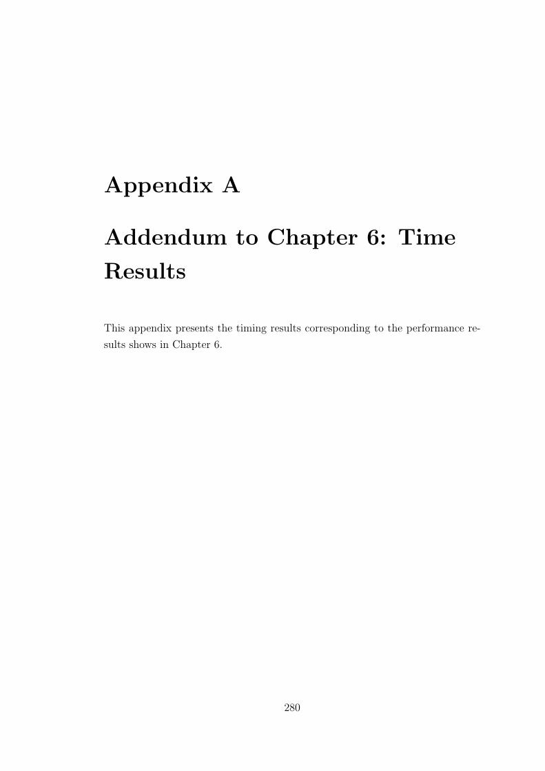
Appendix A
Addendum to Chapter 6: Time
Results
This appendix presents the timing results corresponding to the performance re-
sults shows in Chapter 6.
280
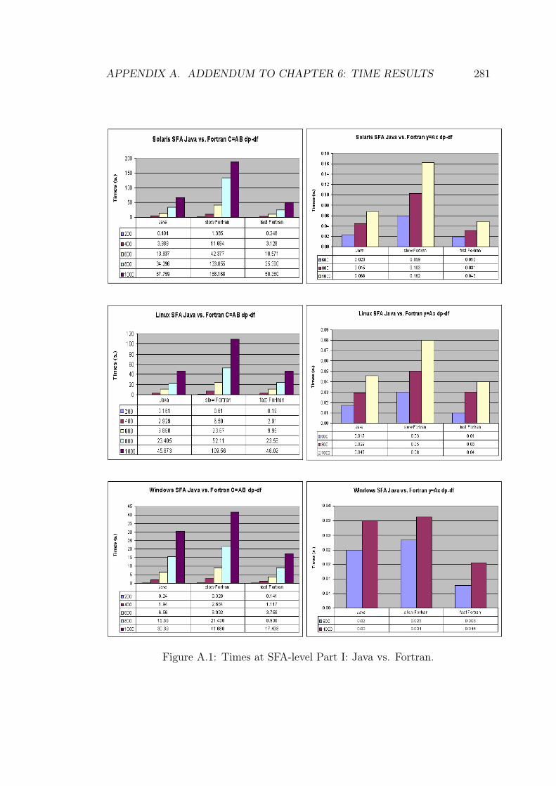
APPENDIX A. ADDENDUM TO CHAPTER 6: TIME RESULTS 281
Figure A.1: Times at SFA-level Part I: Java vs. Fortran.
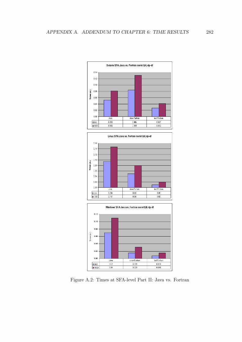
APPENDIX A. ADDENDUM TO CHAPTER 6: TIME RESULTS 282
Figure A.2: Times at SFA-level Part II: Java vs. Fortran
APPENDIX A. ADDENDUM TO CHAPTER 6: TIME RESULTS 283
Figure A.3: Times for C = AB Part I – all Java.
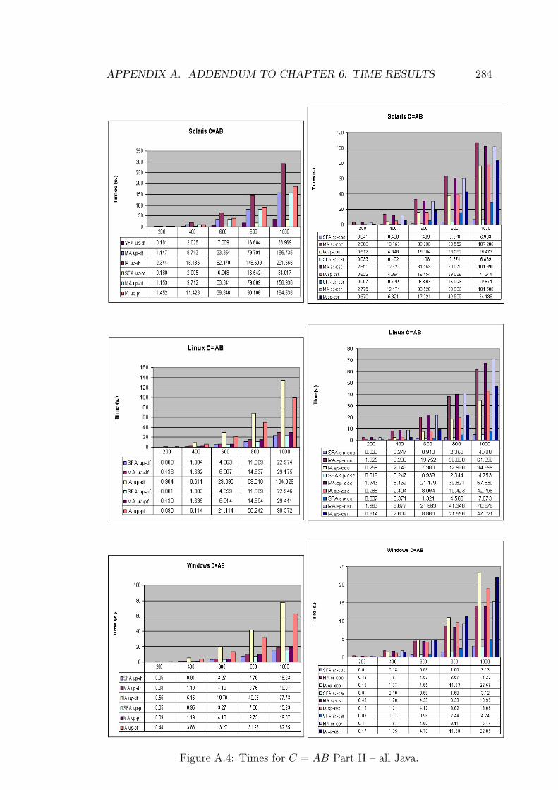
APPENDIX A. ADDENDUM TO CHAPTER 6: TIME RESULTS 284
Figure A.4: Times for C = AB Part II – all Java.
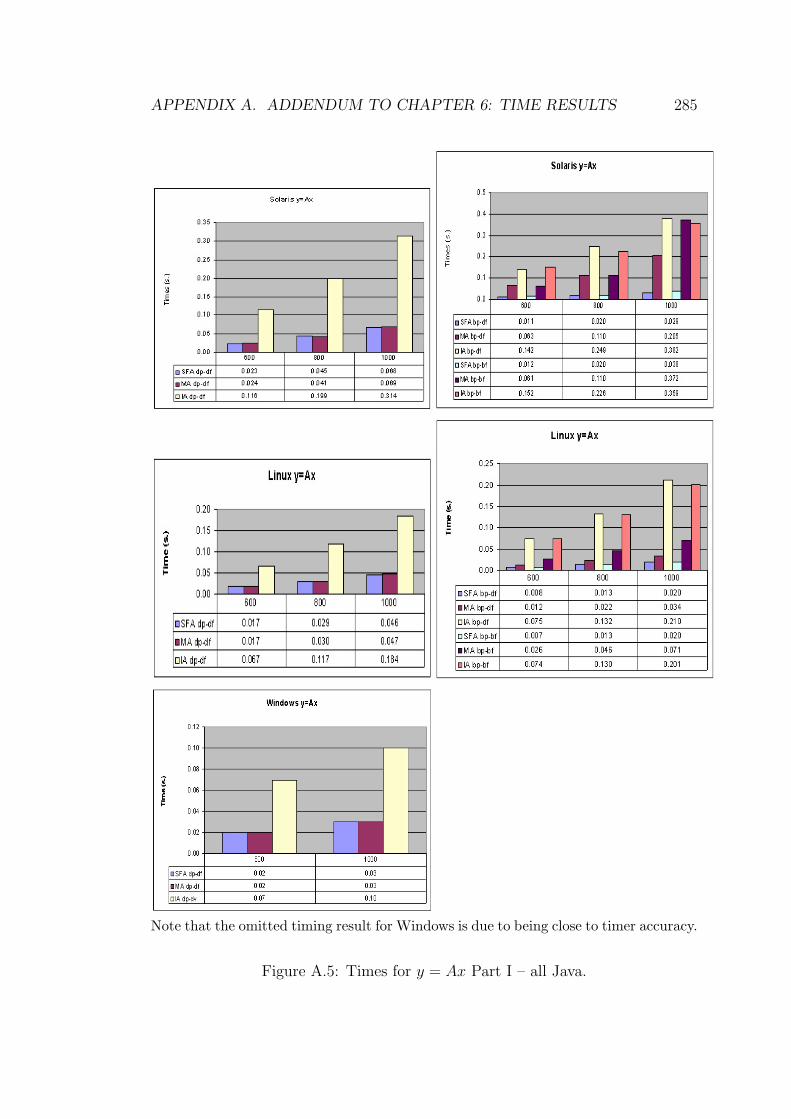
APPENDIX A. ADDENDUM TO CHAPTER 6: TIME RESULTS 285
Note that the omitted timing result for Windows is due to being close to timer accuracy.
Figure A.5: Times for y = Ax Part I – all Java.
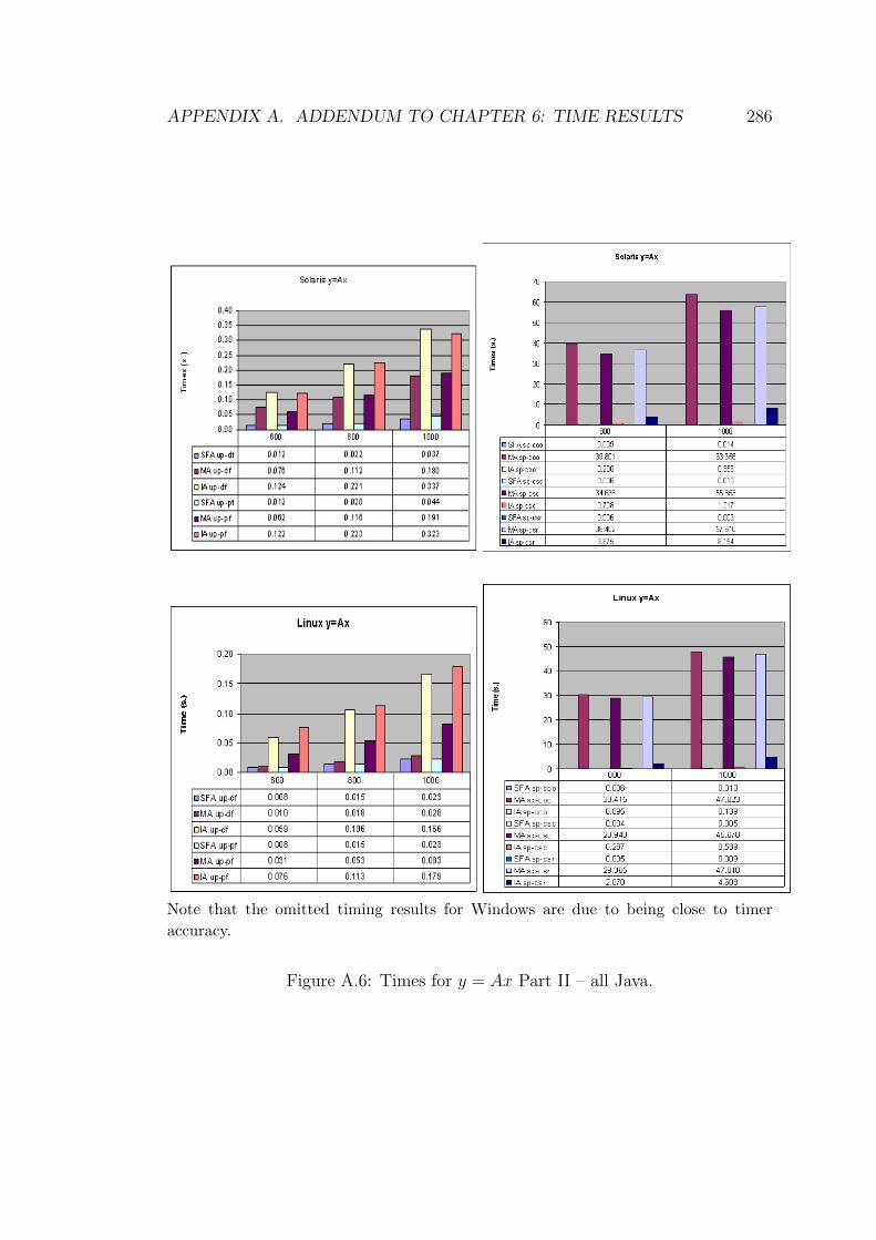
APPENDIX A. ADDENDUM TO CHAPTER 6: TIME RESULTS 286
Note that the omitted timing results for Windows are due to being close to timeraccuracy.
Figure A.6: Times for y = Ax Part II – all Java.
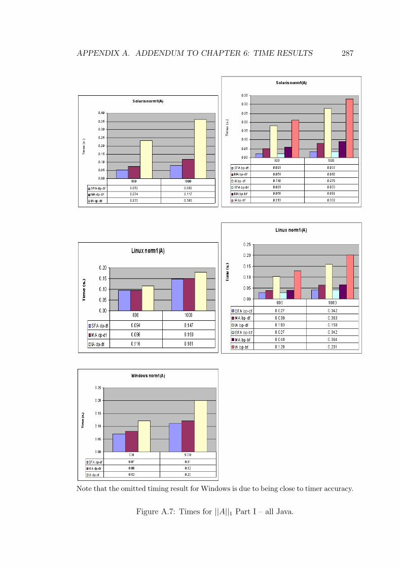
APPENDIX A. ADDENDUM TO CHAPTER 6: TIME RESULTS 287
Note that the omitted timing result for Windows is due to being close to timer accuracy.
Figure A.7: Times for ||A||1 Part I – all Java.
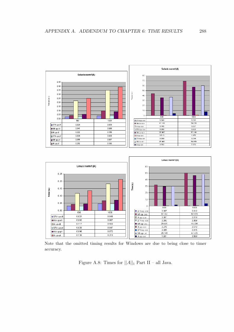
APPENDIX A. ADDENDUM TO CHAPTER 6: TIME RESULTS 288
Note that the omitted timing results for Windows are due to being close to timeraccuracy.
Figure A.8: Times for ||A||1 Part II – all Java.
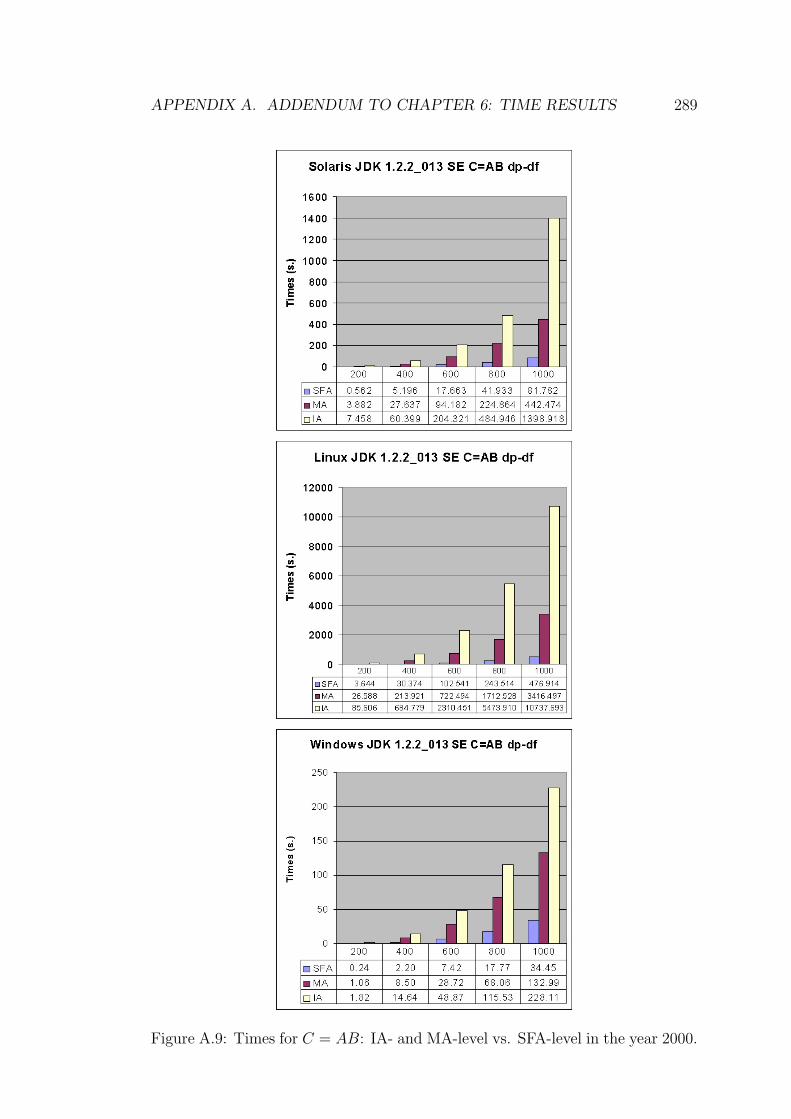
APPENDIX A. ADDENDUM TO CHAPTER 6: TIME RESULTS 289
Figure A.9: Times for C = AB: IA- and MA-level vs. SFA-level in the year 2000.
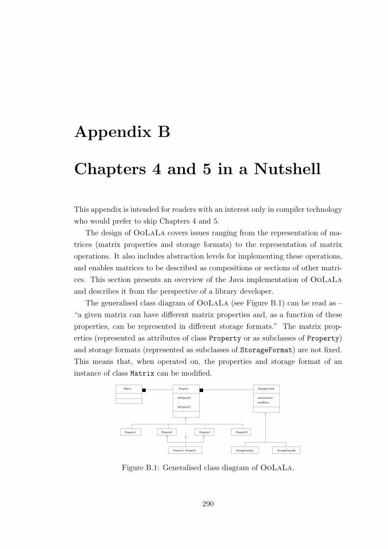
Appendix B
Chapters 4 and 5 in a Nutshell
This appendix is intended for readers with an interest only in compiler technology
who would prefer to skip Chapters 4 and 5.
The design of OoLaLa covers issues ranging from the representation of ma-
trices (matrix properties and storage formats) to the representation of matrix
operations. It also includes abstraction levels for implementing these operations,
and enables matrices to be described as compositions or sections of other matri-
ces. This section presents an overview of the Java implementation of OoLaLa
and describes it from the perspective of a library developer.
The generalised class diagram of OoLaLa (see Figure B.1) can be read as –
“a given matrix can have different matrix properties and, as a function of these
properties, can be represented in different storage formats.” The matrix prop-
erties (represented as attributes of class Property or as subclasses of Property)
and storage formats (represented as subclasses of StorageFormat) are not fixed.
This means that, when operated on, the properties and storage format of an
instance of class Matrix can be modified.
StorageFormatKStorageFormat1
������ ������
isPropertyP
...
isPropertyT
Property
numColumns
numRows
StorageFormatMatrix
PropertyNProperty1 PropertyI PropertyJ
PropertyI...PropertyJ
Figure B.1: Generalised class diagram of OoLaLa.
290
B.1. STORAGE FORMAT ABSTRACTION LEVEL 291
As multiple inheritance is not included in Java, OoLaLa modifies its class
diagram and represents each matrix property, that has a multiple inheritance
relation in Figure B.1, as a final subclass of Property. Every class and method
is either abstract or final. Ideally, generic classes would be used so as to develop
only one version of OoLaLa, independent of the data type of the matrix elements.
However, given that (a) Java does not currently support generic classes, that (b)
the official plans1 to incorporate generic classes do not support primitive types
(float, double, int, etc.), and (c) that emulating generic classes with inheritance
delivers poor performance [56, 43], OoLaLa is implemented by developing a
version for each numerical data type. This performance penalty can be handled
as in [56]. OoLaLa represents two-dimensional arrays by mapping them to one-
dimensional arrays in a column-wise form (as in the Array Package [176] and
JLAPACK [43]). In this way, a two-dimensional array is stored continuously by
columns in memory (as in Fortran) and the number of exception tests (array
index out of bounds and null object) is halved.
The operation norm1 (||A||1) is used to illustrate and understand the differ-
ences between implementations at the three abstraction levels. The implemen-
tations presented illustrate the final phase into which OoLaLa divides a ma-
trix operation. Before executing the implementations presented, OoLaLa has
checked the correctness of the parameters (e.g. null references, coherent matrix
dimensions, etc.), predicted matrix properties (and, if necessary, modified matrix
properties or storage formats), and selected the appropriate implementation for
the matrix operation. This appendix does not describe these three phases.
B.1 Storage Format Abstraction Level
An implementation is said to be at SFA-level if changing the storage format of
any of the parameters implies that the implementation is invalid. These imple-
mentations know the representations of the storage formats and make explicit use
of this information in order to access elements and to achieve good performance.
Figure B.2 presents an implementation of ||A||1 where A is a dense matrix
stored in dense format, while Figure B.3 presents an equivalent implementation
1JSR-014 – Add Generic Types to the Java Programming Language. Further details availableat http://jcp.org/jsr/detail/14.jsp

B.2. MATRIX ABSTRACTION LEVEL 292
public static double denseNorm1 (double a[], int m, int n) {
int ind=0; // a[m][n]
double sum; double max=0.0;
for (int j=0; j<n; j++) {
sum=0.0;
for (int i=0; i<m; i++) {
sum+=Math.abs(a[ind]); // a[i][j]
ind++;
}
if (sum>max) max=sum;
}
return max;
}
Figure B.2: Implementation of ||A||1 at SFA-level where A is a dense matrixstored in dense format.
public static double upperNorm1 (double aPacked[], int m, int n) {
int ind=0; double sum; double max=0.0;
for (int j=0; j<n; j++) {
sum=0.0;
for (int i=0; i<=j; i++) {
sum+=Math.abs(aPacked[ind]);
ind++;
}
if (sum>max) max=sum;
}
return max;
}
Figure B.3: Implementations of ||A||1 at SFA-level where A is an upper triangularmatrix stored in packed format.
where A is an upper triangular matrix stored in packed format. The main differ-
ence is the inner loop (i-loop) which is shortened because it is known that when
i>j the matrix elements are zeros and, therefore, these iterations are redundant.
B.2 Matrix Abstraction Level
The MA-level resembles the mathematical definition of a matrix; it provides
random access to matrix elements. From a programming point of view, a matrix
is a two-dimensional container of numbers. The basic operations are to obtain an
element of the matrix and to assign a value to an element of the matrix. An
element is determined by its (unique) position: number of row i and column j.
The two access methods, element(i,j) and assign(i,j,value), constitute the
MA-level interface.
Matrix, Property and StorageFormat provide these two methods. Matrix
implements the methods by delegating to its attribute that is an instance of a
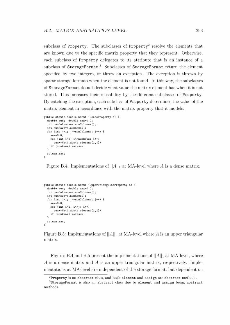
B.2. MATRIX ABSTRACTION LEVEL 293
subclass of Property. The subclasses of Property2 resolve the elements that
are known due to the specific matrix property that they represent. Otherwise,
each subclass of Property delegates to its attribute that is an instance of a
subclass of StorageFormat.3 Subclasses of StorageFormat return the element
specified by two integers, or throw an exception. The exception is thrown by
sparse storage formats when the element is not found. In this way, the subclasses
of StorageFormat do not decide what value the matrix element has when it is not
stored. This increases their reusability by the different subclasses of Property.
By catching the exception, each subclass of Property determines the value of the
matrix element in accordance with the matrix property that it models.
public static double norm1 (DenseProperty a) {
double sum; double max=0.0;
int numColumns=a.numColumns();
int numRows=a.numRows();
for (int j=1; j<=numColumns; j++) {
sum=0.0;
for (int i=1; i<=numRows; i++)
sum+=Math.abs(a.element(i,j));
if (sum>max) max=sum;
}
return max;
}
Figure B.4: Implementations of ||A||1 at MA-level where A is a dense matrix.
public static double norm1 (UpperTriangularProperty a) {
double sum; double max=0.0;
int numColumns=a.numColumns();
int numRows=a.numRows();
for (int j=1; j<=numColumns; j++) {
sum=0.0;
for (int i=1; i<=j; i++)
sum+=Math.abs(a.element(i,j));
if (sum>max) max=sum;
}
return max;
}
Figure B.5: Implementations of ||A||1 at MA-level where A is an upper triangularmatrix.
Figures B.4 and B.5 present the implementations of ||A||1 at MA-level, where
A is a dense matrix and A is an upper triangular matrix, respectively. Imple-
mentations at MA-level are independent of the storage format, but dependent on
2Property is an abstract class, and both element and assign are abstract methods.3StorageFormat is also an abstract class due to element and assign being abstract
methods.
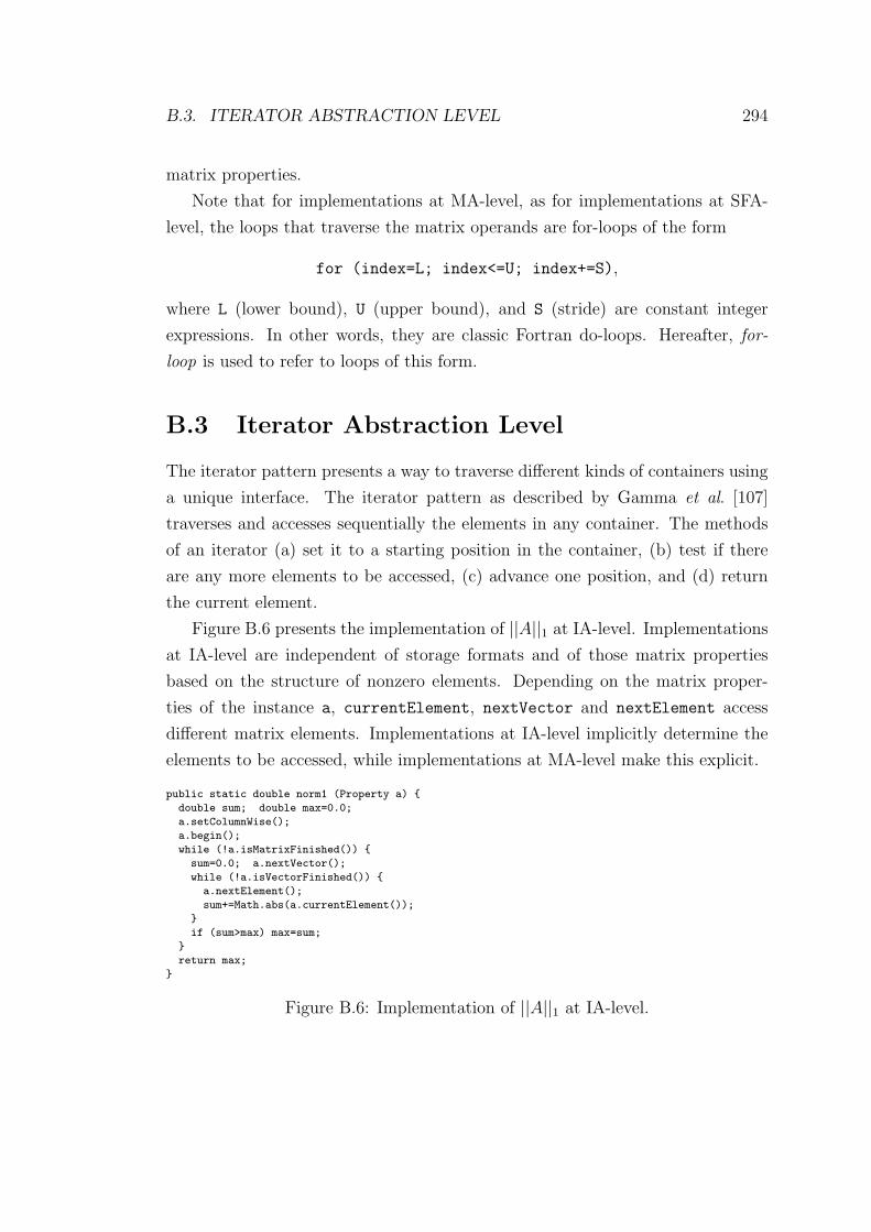
B.3. ITERATOR ABSTRACTION LEVEL 294
matrix properties.
Note that for implementations at MA-level, as for implementations at SFA-
level, the loops that traverse the matrix operands are for-loops of the form
for (index=L; index<=U; index+=S),
where L (lower bound), U (upper bound), and S (stride) are constant integer
expressions. In other words, they are classic Fortran do-loops. Hereafter, for-
loop is used to refer to loops of this form.
B.3 Iterator Abstraction Level
The iterator pattern presents a way to traverse different kinds of containers using
a unique interface. The iterator pattern as described by Gamma et al. [107]
traverses and accesses sequentially the elements in any container. The methods
of an iterator (a) set it to a starting position in the container, (b) test if there
are any more elements to be accessed, (c) advance one position, and (d) return
the current element.
Figure B.6 presents the implementation of ||A||1 at IA-level. Implementations
at IA-level are independent of storage formats and of those matrix properties
based on the structure of nonzero elements. Depending on the matrix proper-
ties of the instance a, currentElement, nextVector and nextElement access
different matrix elements. Implementations at IA-level implicitly determine the
elements to be accessed, while implementations at MA-level make this explicit.
public static double norm1 (Property a) {
double sum; double max=0.0;
a.setColumnWise();
a.begin();
while (!a.isMatrixFinished()) {
sum=0.0; a.nextVector();
while (!a.isVectorFinished()) {
a.nextElement();
sum+=Math.abs(a.currentElement());
}
if (sum>max) max=sum;
}
return max;
}
Figure B.6: Implementation of ||A||1 at IA-level.

Appendix C
Addendum to Chapter 8
This appendix is included for completeness and to enable a detailed review of the
transformations steps of Chapter 8.
C.1 Complete Tables for Section 8.4.1
Tables C.1 and C.2 present, for each method invoked in a, the resulting code
after applying method inlining. The first table (Table C.1) presents the inlined
statements guarded with a class test for the first two methods. Since the code
becomes verbose, the rest of Table C.1 and Table C.2 present the inlined state-
ments without the guards. These tables also exclude the else-branch for the if
(columnWise) statements.
Some statements in Tables C.1 and C.2 have the line-comment // R. This
indicates that these statements are repeated, at least once more, among the
inlined statements for the other methods. These statements make local copies of
the attributes in a, a.storage and a.currentPosition; this is the third step in
optimisation.
In Section 8.4.1, the fourth step for optimising implementations at IA-Level
is described as removing the repeated statements (those with line-comments //
R) by declaring and initialising local copies at the beginning and only writing
back to the attributes at the end. This step also removes all tests of the form
if (columnWise), leaving only the true-branch. Figure C.1 presents the code
after applying these optimisations. The computations involving elementHas-
BeenVisited and vectorHasBeenVisited can also be removed (see Appendix
C.3 for details), leaving the code in Figure 8.18.
295
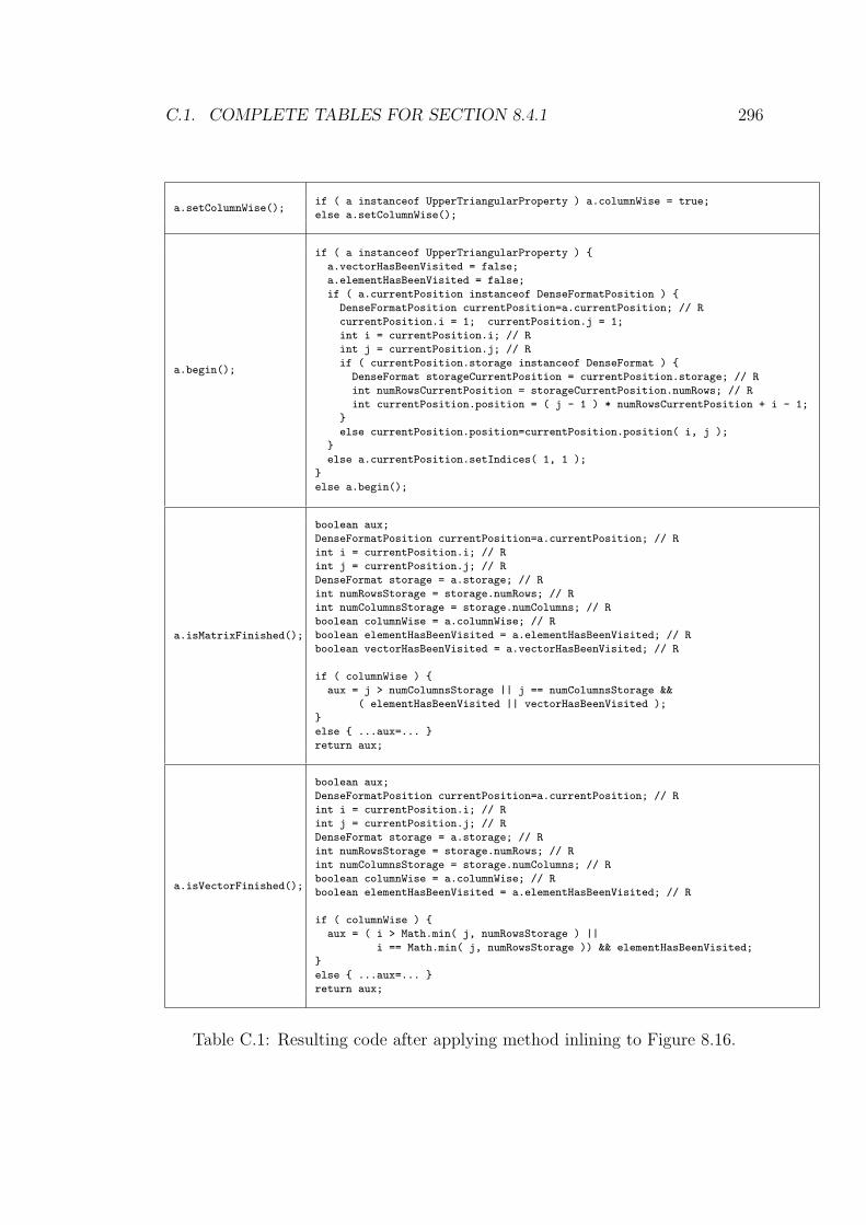
C.1. COMPLETE TABLES FOR SECTION 8.4.1 296
a.setColumnWise();if ( a instanceof UpperTriangularProperty ) a.columnWise = true;
else a.setColumnWise();
a.begin();
if ( a instanceof UpperTriangularProperty ) {
a.vectorHasBeenVisited = false;
a.elementHasBeenVisited = false;
if ( a.currentPosition instanceof DenseFormatPosition ) {
DenseFormatPosition currentPosition=a.currentPosition; // R
currentPosition.i = 1; currentPosition.j = 1;
int i = currentPosition.i; // R
int j = currentPosition.j; // R
if ( currentPosition.storage instanceof DenseFormat ) {
DenseFormat storageCurrentPosition = currentPosition.storage; // R
int numRowsCurrentPosition = storageCurrentPosition.numRows; // R
int currentPosition.position = ( j - 1 ) * numRowsCurrentPosition + i - 1;
}
else currentPosition.position=currentPosition.position( i, j );
}
else a.currentPosition.setIndices( 1, 1 );
}
else a.begin();
a.isMatrixFinished();
boolean aux;
DenseFormatPosition currentPosition=a.currentPosition; // R
int i = currentPosition.i; // R
int j = currentPosition.j; // R
DenseFormat storage = a.storage; // R
int numRowsStorage = storage.numRows; // R
int numColumnsStorage = storage.numColumns; // R
boolean columnWise = a.columnWise; // R
boolean elementHasBeenVisited = a.elementHasBeenVisited; // R
boolean vectorHasBeenVisited = a.vectorHasBeenVisited; // R
if ( columnWise ) {
aux = j > numColumnsStorage || j == numColumnsStorage &&
( elementHasBeenVisited || vectorHasBeenVisited );
}
else { ...aux=... }
return aux;
a.isVectorFinished();
boolean aux;
DenseFormatPosition currentPosition=a.currentPosition; // R
int i = currentPosition.i; // R
int j = currentPosition.j; // R
DenseFormat storage = a.storage; // R
int numRowsStorage = storage.numRows; // R
int numColumnsStorage = storage.numColumns; // R
boolean columnWise = a.columnWise; // R
boolean elementHasBeenVisited = a.elementHasBeenVisited; // R
if ( columnWise ) {
aux = ( i > Math.min( j, numRowsStorage ) ||
i == Math.min( j, numRowsStorage )) && elementHasBeenVisited;
}
else { ...aux=... }
return aux;
Table C.1: Resulting code after applying method inlining to Figure 8.16.
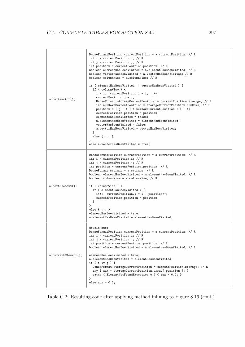
C.1. COMPLETE TABLES FOR SECTION 8.4.1 297
a.nextVector();
DenseFormatPosition currentPosition = a.currentPosition; // R
int i = currentPosition.i; // R
int j = currentPosition.j; // R
int position = currentPosition.position; // R
boolean elementHasBeenVisited = a.elementHasBeenVisited; // R
boolean vectorHasBeenVisited = a.vectorHasBeenVisited; // R
boolean columnWise = a.columnWise; // R
if ( elementHasBeenVisited || vectorHasBeenVisited ) {
if ( columnWise ) {
i = 1; currentPosition.i = i; j++;
currentPosition.j = j;
DenseFormat storageCurrentPosition = currentPosition.storage; // R
int numRowsCurrentPosition = storageCurrentPosition.numRows; // R
position = ( j - 1 ) * numRowsCurrentPosition + i - 1;
currentPosition.position = position;
elementHasBeenVisited = false;
a.elementHasBeenVisited = elementHasBeenVisited;
vectorHasBeenVisited = false;
a.vectorHasBeenVisited = vectorHasBeenVisited;
}
else { ... }
}
else a.vectorHasBeenVisited = true;
a.nextElement();
DenseFormatPosition currentPosition = a.currentPosition; // R
int i = currentPosition.i; // R
int j = currentPosition.j; // R
int position = currentPosition.position; // R
DenseFormat storage = a.storage; // R
boolean elementHasBeenVisited = a.elementHasBeenVisited; // R
boolean columnWise = a.columnWise; // R
if ( columnWise ) {
if ( elementHasBeenVisited ) {
i++; currentPosition.i = i; position++;
currentPosition.position = position;
}
}
else { ... }
elementHasBeenVisited = true;
a.elementHasBeenVisited = elementHasBeenVisited;
a.currentElement();
double aux;
DenseFormatPosition currentPosition = a.currentPosition; // R
int i = currentPosition.i; // R
int j = currentPosition.j; // R
int position = currentPosition.position; // R
boolean elementHasBeenVisited = a.elementHasBeenVisited; // R
elementHasBeenVisited = true;
a.elementHasBeenVisited = elementHasBeenVisited;
if ( i <= j ) {
DenseFormat storageCurrentPosition = currentPosition.storage; // R
try { aux = storageCurrentPosition.array[ position ]; }
catch ( ElementNotFoundException e ) { aux = 0.0; }
}
else aux = 0.0;
Table C.2: Resulting code after applying method inlining to Figure 8.16 (cont.).
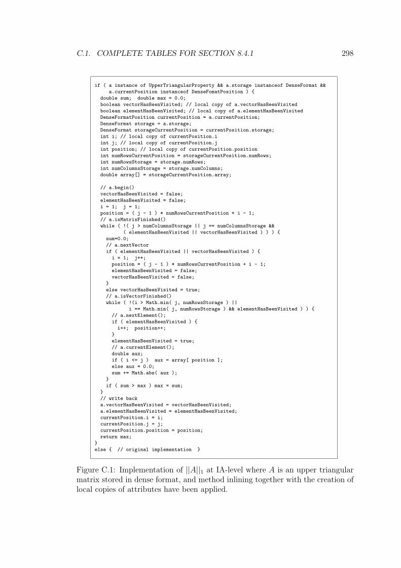
C.1. COMPLETE TABLES FOR SECTION 8.4.1 298
if ( a instance of UpperTriangularProperty && a.storage instanceof DenseFormat &&
a.currentPosition instanceof DenseFomatPosition ) {
double sum; double max = 0.0;
boolean vectorHasBeenVisited; // local copy of a.vectorHasBeenVisited
boolean elementHasBeenVisited; // local copy of a.elementHasBeenVisited
DenseFormatPosition currentPosition = a.currentPosition;
DenseFormat storage = a.storage;
DenseFormat storageCurrentPosition = currentPosition.storage;
int i; // local copy of currentPosition.i
int j; // local copy of currentPosition.j
int position; // local copy of currentPosition.position
int numRowsCurrentPosition = storageCurrentPosition.numRows;
int numRowsStorage = storage.numRows;
int numColumnsStorage = storage.numColumns;
double array[] = storageCurrentPosition.array;
// a.begin()
vectorHasBeenVisited = false;
elementHasBeenVisited = false;
i = 1; j = 1;
position = ( j - 1 ) * numRowsCurrentPosition + i - 1;
// a.isMatrixFinished()
while ( !( j > numColumnsStorage || j == numColumnsStorage &&
( elementHasBeenVisited || vectorHasBeenVisited ) ) ) {
sum=0.0;
// a.nextVector
if ( elementHasBeenVisited || vectorHasBeenVisited ) {
i = 1; j++;
position = ( j - 1 ) * numRowsCurrentPosition + i - 1;
elementHasBeenVisited = false;
vectorHasBeenVisited = false;
}
else vectorHasBeenVisited = true;
// a.isVectorFinished()
while ( !(i > Math.min( j, numRowsStorage ) ||
i == Math.min( j, numRowsStorage ) && elementHasBeenVisited ) ) {
// a.nextElement();
if ( elementHasBeenVisited ) {
i++; position++;
}
elementHasBeenVisited = true;
// a.currentElement();
double aux;
if ( i <= j ) aux = array[ position ];
else aux = 0.0;
sum += Math.abs( aux );
}
if ( sum > max ) max = sum;
}
// write back
a.vectorHasBeenVisited = vectorHasBeenVisited;
a.elementHasBeenVisited = elementHasBeenVisited;
currentPosition.i = i;
currentPosition.j = j;
currentPosition.position = position;
return max;
}
else { // original implementation }
Figure C.1: Implementation of ||A||1 at IA-level where A is an upper triangularmatrix stored in dense format, and method inlining together with the creation oflocal copies of attributes have been applied.
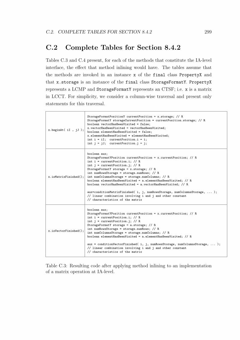
C.2. COMPLETE TABLES FOR SECTION 8.4.2 299
C.2 Complete Tables for Section 8.4.2
Tables C.3 and C.4 present, for each of the methods that constitute the IA-level
interface, the effect that method inlining would have. The tables assume that
the methods are invoked in an instance x of the final class PropertyX and
that x.storage is an instance of the final class StorageFormatY. PropertyX
represents a LCMP and StorageFormatY represents an CTSF; i.e. x is a matrix
in LCCT. For simplicity, we consider a column-wise traversal and present only
statements for this traversal.
x.beginAt( iI , jJ );
StorageFormatPositionY currentPosition = x.storage; // R
StorageFormatY storageCurrentPosition = currentPosition.storage; // R
boolean vectorHasBeenVisited = false;
x.vectorHasBeenVisited = vectorHasBeenVisited;
boolean elementHasBeenVisited = false;
x.elementHasBeenVisited = elementHasBeenVisited;
int i = iI; currentPosition.i = i;
int j = jJ; currentPosition.j = j;
x.isMatrixFinished();
boolean aux;
StorageFormatYPosition currentPosition = x.currentPosition; // R
int i = currentPosition.i; // R
int j = currentPosition.j; // R
StorageFormatY storage = x.storage; // R
int numRowsStorage = storage.numRows; // R
int numColumnsStorage = storage.numColumns; // R
boolean elementHasBeenVisited = a.elementHasBeenVisited; // R
boolean vectorHasBeenVisited = a.vectorHasBeenVisited; // R
aux=conditionMatrixFinished( i, j, numRowsStorage, numColumnsStorage, ... );
// linear combination involving i and j and other constant
// characteristics of the matrix
x.isVectorFinished();
boolean aux;
StorageFormatYPosition currentPosition = x.currentPosition; // R
int i = currentPosition.i; // R
int j = currentPosition.j; // R
StorageFormatY storage = a.storage; // R
int numRowsStorage = storage.numRows; // R
int numColumnsStorage = storage.numColumns; // R
boolean elementHasBeenVisited = a.elementHasBeenVisited; // R
aux = conditionVectorFinished( i, j, numRowsStorage, numColumnsStorage, ... );
// linear combination involving i and j and other constant
// characteristics of the matrix
Table C.3: Resulting code after applying method inlining to an implementationof a matrix operation at IA-level.
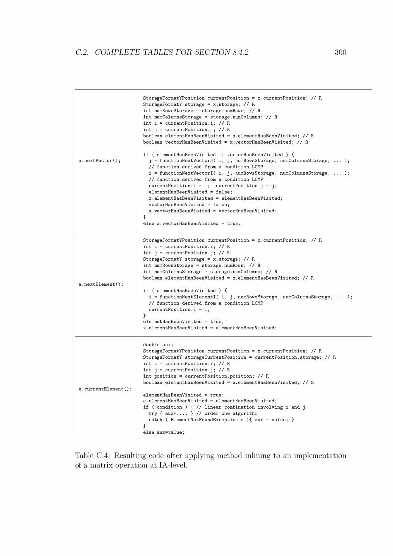
C.2. COMPLETE TABLES FOR SECTION 8.4.2 300
a.nextVector();
StorageFormatYPosition currentPosition = x.currentPosition; // R
StorageFormatY storage = x.storage; // R
int numRowsStorage = storage.numRows; // R
int numColumnsStorage = storage.numColumns; // R
int i = currentPosition.i; // R
int j = currentPosition.j; // R
boolean elementHasBeenVisited = x.elementHasBeenVisited; // R
boolean vectorHasBeenVisited = x.vectorHasBeenVisited; // R
if ( elementHasBeenVisited || vectorHasBeenVisited ) {
j = functionNextVectorJ( i, j, numRowsStorage, numColumnsStorage, ... );
// function derived from a condition LCMP
i = functionNextVectorI( i, j, numRowsStorage, numColumnsStorage, ... );
// function derived from a condition LCMP
currentPosition.i = i; currentPosition.j = j;
elementHasBeenVisited = false;
x.elementHasBeenVisited = elementHasBeenVisited;
vectorHasBeenVisited = false;
x.vectorHasBeenVisited = vectorHasBeenVisited;
}
else x.vectorHasBeenVisited = true;
a.nextElement();
StorageFormatYPosition currentPosition = x.currentPosition; // R
int i = currentPosition.i; // R
int j = currentPosition.j; // R
StorageFormatY storage = x.storage; // R
int numRowsStorage = storage.numRows; // R
int numColumnsStorage = storage.numColumns; // R
boolean elementHasBeenVisited = x.elementHasBeenVisited; // R
if ( elementHasBeenVisited ) {
i = functionNextElementI( i, j, numRowsStorage, numColumnsStorage, ... );
// function derived from a condition LCMP
currentPosition.i = i;
}
elementHasBeenVisited = true;
x.elementHasBeenVisited = elementHasBeenVisited;
a.currentElement();
double aux;
StorageFormatYPosition currentPosition = x.currentPosition; // R
StorageFormatY storageCurrentPosition = currentPosition.storage; // R
int i = currentPosition.i; // R
int j = currentPosition.j; // R
int position = currentPosition.position; // R
boolean elementHasBeenVisited = a.elementHasBeenVisited; // R
elementHasBeenVisited = true;
a.elementHasBeenVisited = elementHasBeenVisited;
if ( condition ) { // linear combination involving i and j
try { aux=...; } // order one algorithm
catch ( ElementNotFoundException e ){ aux = value; }
}
else aux=value;
Table C.4: Resulting code after applying method inlining to an implementationof a matrix operation at IA-level.
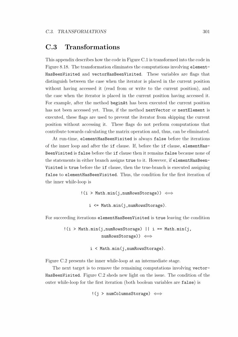
C.3. TRANSFORMATIONS 301
C.3 Transformations
This appendix describes how the code in Figure C.1 is transformed into the code in
Figure 8.18. The transformation eliminates the computations involving element-
HasBeenVisited and vectorHasBeenVisited. These variables are flags that
distinguish between the case when the iterator is placed in the current position
without having accessed it (read from or write to the current position), and
the case when the iterator is placed in the current position having accessed it.
For example, after the method beginAt has been executed the current position
has not been accessed yet. Thus, if the method nextVector or nextElement is
executed, these flags are used to prevent the iterator from skipping the current
position without accessing it. These flags do not perform computations that
contribute towards calculating the matrix operation and, thus, can be eliminated.
At run-time, elementHasBeenVisited is always false before the iterations
of the inner loop and after the if clause. If, before the if clause, elementHas-
BeenVisited is false before the if clause then it remains false because none of
the statements in either branch assigns true to it. However, if elementHasBeen-
Visited is true before the if clause, then the true-branch is executed assigning
false to elementHasBeenVisited. Thus, the condition for the first iteration of
the inner while-loop is
!(i > Math.min(j,numRowsStorage)) ⇐⇒
i <= Math.min(j,numRowsStorage).
For succeeding iterations elementHasBeenVisited is true leaving the condition
!(i > Math.min(j,numRowsStorage) || i == Math.min(j,
numRowsStorage)) ⇐⇒
i < Math.min(j,numRowsStorage).
Figure C.2 presents the inner while-loop at an intermediate stage.
The next target is to remove the remaining computations involving vector-
HasBeenVisited. Figure C.2 sheds new light on the issue. The condition of the
outer while-loop for the first iteration (both boolean variables are false) is
!(j > numColumnsStorage) ⇐⇒
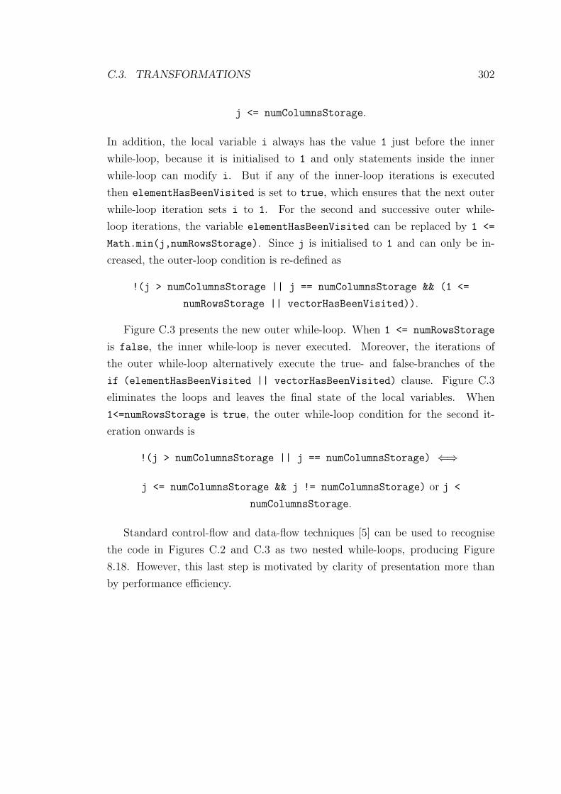
C.3. TRANSFORMATIONS 302
j <= numColumnsStorage.
In addition, the local variable i always has the value 1 just before the inner
while-loop, because it is initialised to 1 and only statements inside the inner
while-loop can modify i. But if any of the inner-loop iterations is executed
then elementHasBeenVisited is set to true, which ensures that the next outer
while-loop iteration sets i to 1. For the second and successive outer while-
loop iterations, the variable elementHasBeenVisited can be replaced by 1 <=
Math.min(j,numRowsStorage). Since j is initialised to 1 and can only be in-
creased, the outer-loop condition is re-defined as
!(j > numColumnsStorage || j == numColumnsStorage && (1 <=
numRowsStorage || vectorHasBeenVisited)).
Figure C.3 presents the new outer while-loop. When 1 <= numRowsStorage
is false, the inner while-loop is never executed. Moreover, the iterations of
the outer while-loop alternatively execute the true- and false-branches of the
if (elementHasBeenVisited || vectorHasBeenVisited) clause. Figure C.3
eliminates the loops and leaves the final state of the local variables. When
1<=numRowsStorage is true, the outer while-loop condition for the second it-
eration onwards is
!(j > numColumnsStorage || j == numColumnsStorage) ⇐⇒
j <= numColumnsStorage && j != numColumnsStorage) or j <
numColumnsStorage.
Standard control-flow and data-flow techniques [5] can be used to recognise
the code in Figures C.2 and C.3 as two nested while-loops, producing Figure
8.18. However, this last step is motivated by clarity of presentation more than
by performance efficiency.
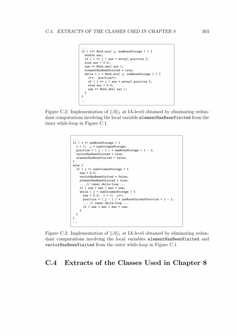
C.4. EXTRACTS OF THE CLASSES USED IN CHAPTER 8 303
...
if ( i<= Math.min( j, numRowsStorage ) ) {
double aux;
if ( i <= j ) aux = array[ position ];
else aux = 0.0;
sum += Math.abs( aux );
elementHasBeenVisited = true;
while ( i < Math.min( j, numRowsStorage ) ) {
i++; position++;
if ( i <= j ) aux = array[ position ];
else aux = 0.0;
sum += Math.abs( aux );
}
}
...
Figure C.2: Implementation of ||A||1 at IA-level obtained by eliminating redun-dant computations involving the local variable elementHasBeenVisited from theinner while-loop in Figure C.1.
...
if ( 1 <= numRowsStorage ) {
i = 1; j = numColumnsStorage;
position = ( j - 1 ) * numRowsStorage + i - 1;
vectorHasBeenVisited = true;
elementHasBeenVisited = false;
}
else {
if ( j <= numColumnsStorage ) {
sum = 0.0;
vectorHasBeenVisited = false;
elementHasBeenVisited = true;
... // inner while-loop ...
if ( sum > max ) max = sum;
while ( j < numColumnsStorage ) {
sum = 0.0; i = 1; j++;
position = ( j - 1 ) * numRowsCurrentPosition + i - 1;
... // inner while-loop ...
if ( sum < max ) max = sum;
}
}
}
...
Figure C.3: Implementation of ||A||1 at IA-level obtained by eliminating redun-dant computations involving the local variables elementHasBeenVisited andvectorHasBeenVisited from the outer while-loop in Figure C.1.
C.4 Extracts of the Classes Used in Chapter 8
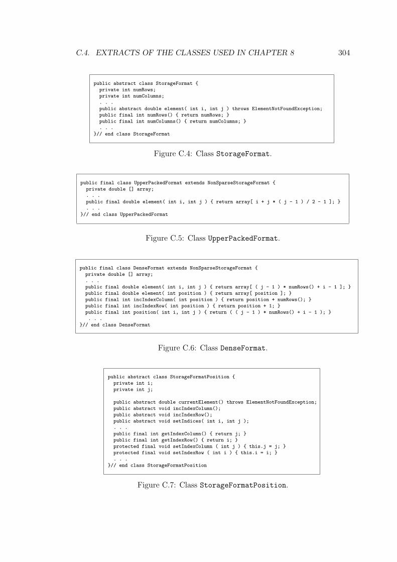
C.4. EXTRACTS OF THE CLASSES USED IN CHAPTER 8 304
public abstract class StorageFormat {
private int numRows;
private int numColumns;
. . .
public abstract double element( int i, int j ) throws ElementNotFoundException;
public final int numRows() { return numRows; }
public final int numColumns() { return numColumns; }
. . .
}// end class StorageFormat
Figure C.4: Class StorageFormat.
public final class UpperPackedFormat extends NonSparseStorageFormat {
private double [] array;
. . .
public final double element( int i, int j ) { return array[ i + j * ( j - 1 ) / 2 - 1 ]; }
. . .
}// end class UpperPackedFormat
Figure C.5: Class UpperPackedFormat.
public final class DenseFormat extends NonSparseStorageFormat {
private double [] array;
. . .
public final double element( int i, int j ) { return array[ ( j - 1 ) * numRows() + i - 1 ]; }
public final double element( int position ) { return array[ position ]; }
public final int incIndexColumn( int position ) { return position + numRows(); }
public final int incIndexRow( int position ) { return position + 1; }
public final int position( int i, int j ) { return ( ( j - 1 ) * numRows() + i - 1 ); }
. . .
}// end class DenseFormat
Figure C.6: Class DenseFormat.
public abstract class StorageFormatPosition {
private int i;
private int j;
public abstract double currentElement() throws ElementNotFoundException;
public abstract void incIndexColumn();
public abstract void incIndexRow();
public abstract void setIndices( int i, int j );
. . .
public final int getIndexColumn() { return j; }
public final int getIndexRow() { return i; }
protected final void setIndexColumn ( int j ) { this.j = j; }
protected final void setIndexRow ( int i ) { this.i = i; }
. . .
}// end class StorageFormatPosition
Figure C.7: Class StorageFormatPosition.
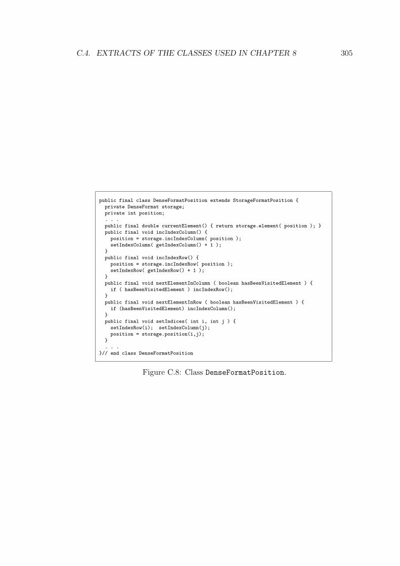
C.4. EXTRACTS OF THE CLASSES USED IN CHAPTER 8 305
public final class DenseFormatPosition extends StorageFormatPosition {
private DenseFormat storage;
private int position;
. . .
public final double currentElement() { return storage.element( position ); }
public final void incIndexColumn() {
position = storage.incIndexColumn( position );
setIndexColumn( getIndexColumn() + 1 );
}
public final void incIndexRow() {
position = storage.incIndexRow( position );
setIndexRow( getIndexRow() + 1 );
}
public final void nextElementInColumn ( boolean hasBeenVisitedElement ) {
if ( hasBeenVisitedElement ) incIndexRow();
}
public final void nextElementInRow ( boolean hasBeenVisitedElement ) {
if (hasBeenVisitedElement) incIndexColumn();
}
public final void setIndices( int i, int j ) {
setIndexRow(i); setIndexColumn(j);
position = storage.position(i,j);
}
. . .
}// end class DenseFormatPosition
Figure C.8: Class DenseFormatPosition.
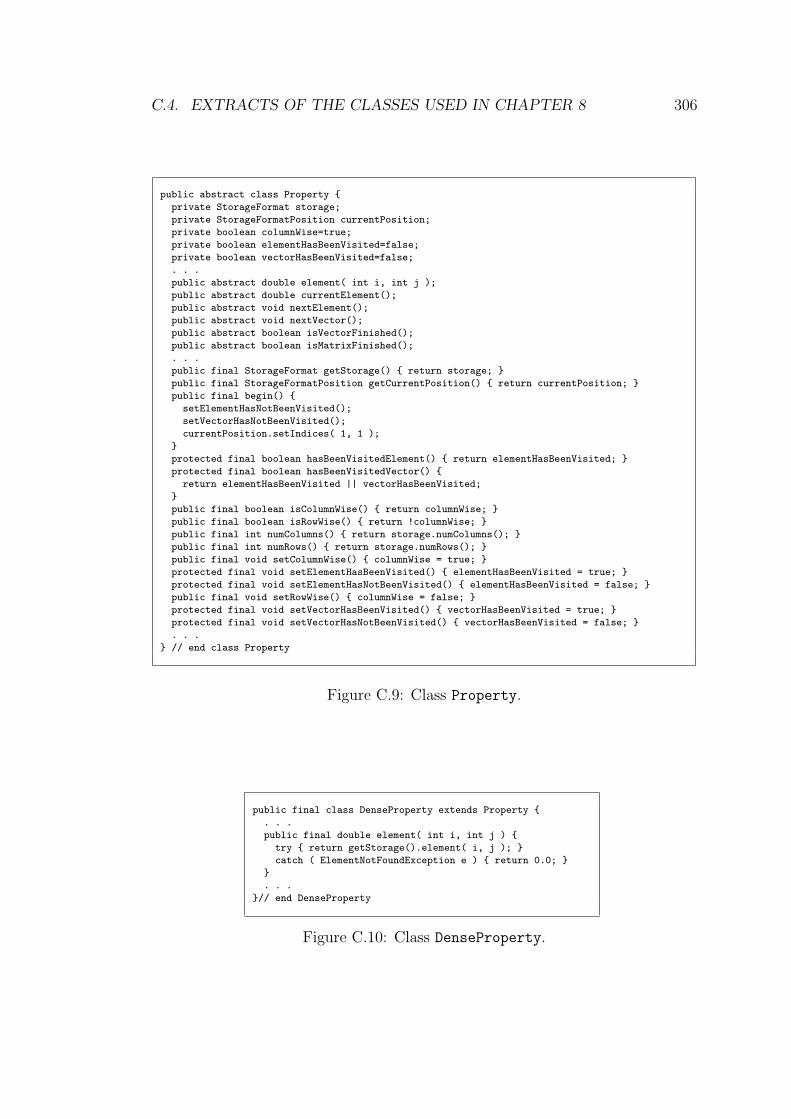
C.4. EXTRACTS OF THE CLASSES USED IN CHAPTER 8 306
public abstract class Property {
private StorageFormat storage;
private StorageFormatPosition currentPosition;
private boolean columnWise=true;
private boolean elementHasBeenVisited=false;
private boolean vectorHasBeenVisited=false;
. . .
public abstract double element( int i, int j );
public abstract double currentElement();
public abstract void nextElement();
public abstract void nextVector();
public abstract boolean isVectorFinished();
public abstract boolean isMatrixFinished();
. . .
public final StorageFormat getStorage() { return storage; }
public final StorageFormatPosition getCurrentPosition() { return currentPosition; }
public final begin() {
setElementHasNotBeenVisited();
setVectorHasNotBeenVisited();
currentPosition.setIndices( 1, 1 );
}
protected final boolean hasBeenVisitedElement() { return elementHasBeenVisited; }
protected final boolean hasBeenVisitedVector() {
return elementHasBeenVisited || vectorHasBeenVisited;
}
public final boolean isColumnWise() { return columnWise; }
public final boolean isRowWise() { return !columnWise; }
public final int numColumns() { return storage.numColumns(); }
public final int numRows() { return storage.numRows(); }
public final void setColumnWise() { columnWise = true; }
protected final void setElementHasBeenVisited() { elementHasBeenVisited = true; }
protected final void setElementHasNotBeenVisited() { elementHasBeenVisited = false; }
public final void setRowWise() { columnWise = false; }
protected final void setVectorHasBeenVisited() { vectorHasBeenVisited = true; }
protected final void setVectorHasNotBeenVisited() { vectorHasBeenVisited = false; }
. . .
} // end class Property
Figure C.9: Class Property.
public final class DenseProperty extends Property {
. . .
public final double element( int i, int j ) {
try { return getStorage().element( i, j ); }
catch ( ElementNotFoundException e ) { return 0.0; }
}
. . .
}// end DenseProperty
Figure C.10: Class DenseProperty.
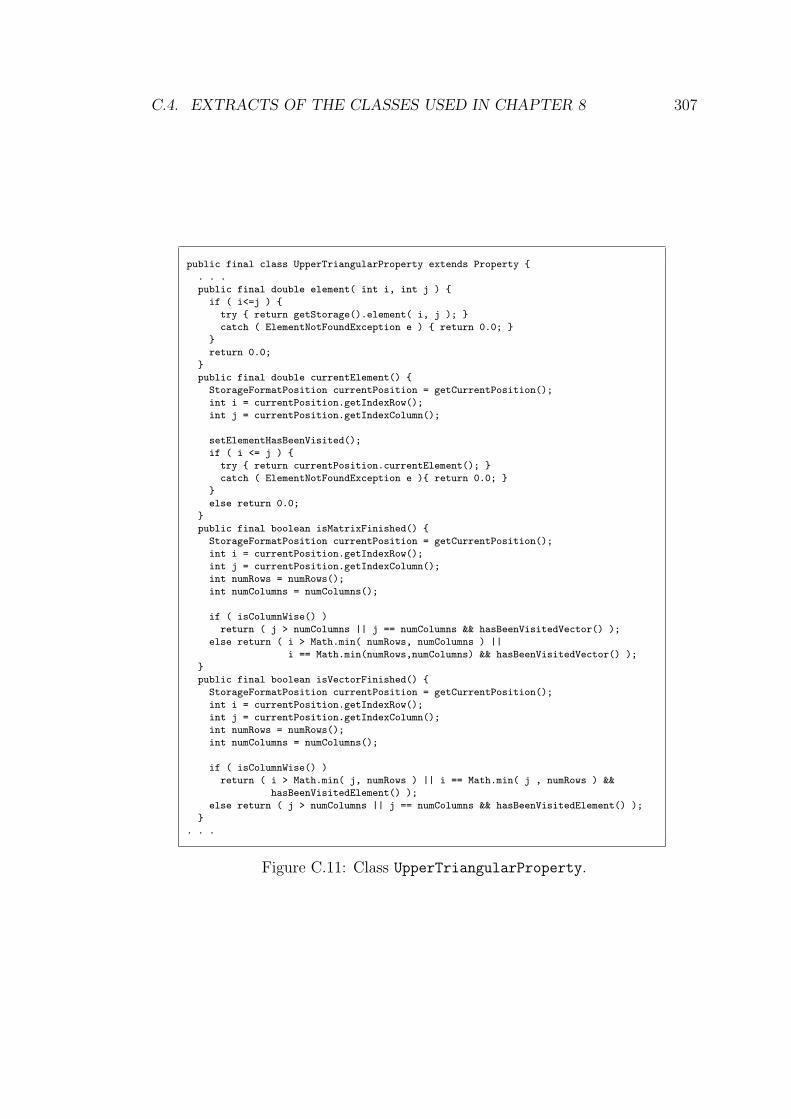
C.4. EXTRACTS OF THE CLASSES USED IN CHAPTER 8 307
public final class UpperTriangularProperty extends Property {
. . .
public final double element( int i, int j ) {
if ( i<=j ) {
try { return getStorage().element( i, j ); }
catch ( ElementNotFoundException e ) { return 0.0; }
}
return 0.0;
}
public final double currentElement() {
StorageFormatPosition currentPosition = getCurrentPosition();
int i = currentPosition.getIndexRow();
int j = currentPosition.getIndexColumn();
setElementHasBeenVisited();
if ( i <= j ) {
try { return currentPosition.currentElement(); }
catch ( ElementNotFoundException e ){ return 0.0; }
}
else return 0.0;
}
public final boolean isMatrixFinished() {
StorageFormatPosition currentPosition = getCurrentPosition();
int i = currentPosition.getIndexRow();
int j = currentPosition.getIndexColumn();
int numRows = numRows();
int numColumns = numColumns();
if ( isColumnWise() )
return ( j > numColumns || j == numColumns && hasBeenVisitedVector() );
else return ( i > Math.min( numRows, numColumns ) ||
i == Math.min(numRows,numColumns) && hasBeenVisitedVector() );
}
public final boolean isVectorFinished() {
StorageFormatPosition currentPosition = getCurrentPosition();
int i = currentPosition.getIndexRow();
int j = currentPosition.getIndexColumn();
int numRows = numRows();
int numColumns = numColumns();
if ( isColumnWise() )
return ( i > Math.min( j, numRows ) || i == Math.min( j , numRows ) &&
hasBeenVisitedElement() );
else return ( j > numColumns || j == numColumns && hasBeenVisitedElement() );
}
. . .
Figure C.11: Class UpperTriangularProperty.
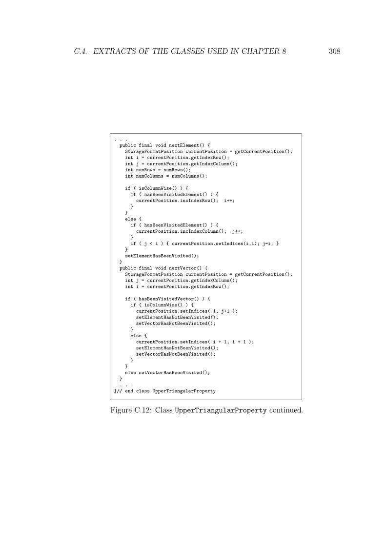
C.4. EXTRACTS OF THE CLASSES USED IN CHAPTER 8 308
. . .
public final void nextElement() {
StorageFormatPosition currentPosition = getCurrentPosition();
int i = currentPosition.getIndexRow();
int j = currentPosition.getIndexColumn();
int numRows = numRows();
int numColumns = numColumns();
if ( isColumnWise() ) {
if ( hasBeenVisitedElement() ) {
currentPosition.incIndexRow(); i++;
}
}
else {
if ( hasBeenVisitedElement() ) {
currentPosition.incIndexColumn(); j++;
}
if ( j < i ) { currentPosition.setIndices(i,i); j=i; }
}
setElementHasBeenVisited();
}
public final void nextVector() {
StorageFormatPosition currentPosition = getCurrentPosition();
int j = currentPosition.getIndexColumn();
int i = currentPosition.getIndexRow();
if ( hasBeenVisitedVector() ) {
if ( isColumnWise() ) {
currentPosition.setIndices( 1, j+1 );
setElementHasNotBeenVisited();
setVectorHasNotBeenVisited();
}
else {
currentPosition.setIndices( i + 1, i + 1 );
setElementHasNotBeenVisited();
setVectorHasNotBeenVisited();
}
}
else setVectorHasBeenVisited();
}
. . .
}// end class UpperTriangularProperty
Figure C.12: Class UpperTriangularProperty continued.
Bibliography
[1] R. J. Abbot. Program design by informal English descriptions. Communi-
cations of the ACM, 26(11):882–894, 1983.
[2] O. Agesin, S. Freund, and J. Mitchell. Adding type parameterization to
the Java language. In Proceedings of the Symposium on Object Oriented
Programming: Systems, Languages, and Applications, pages 49–65, 1997.
[3] A. Aggarwal and K. H. Randall. Related field analysis. In Proceedings of the
ACM Conference on Programming Language Design and Implementation –
PLDI’01, pages 214–20, 2001.
[4] K. Ahlander. An object-oriented approach to construct PDE solvers. Tech-
nical Report 180, Department of Scientific Computing, Uppsala University,
1996.
[5] A. V. Aho, R. Sethi, and J. D. Ullman. Compilers. Principles, Techniques
and Tools. Addison-Wesley, 1985. ISBN: 0201101947.
[6] G. Aigner and U. Holzle. Eliminating virtual function calls in C++ pro-
grams. In Proceedings of the 10th European Conference on Object-Oriented
Programming – ECOOP’96, volume 1098 of Lecture Notes in Computer
Science, pages 142–166. Springer-Verlag, 1996.
[7] C. Alexander, S. Ishikawa, M. Silverstein, M. Jacobson, I. Fiksdahl-King,
and S. Angel. A Pattern Language. Oxford University Press, 1977. ISBN:
0195019199.
[8] B. A. Allan, R. L. Clay, K. D. Mish, and A. B. Williams. ISIS++ Refer-
ence Guide: Iterative Scalable Implicit Solver in C++ version 1.1. Sandia
National Laboratories Livermore, 1999.
309
BIBLIOGRAPHY 310
[9] G. Almasi, F. G. Gustavson, and J. E. Moreira. Design and evaluation of
a linear algebra package for Java. In Proceedings of the ACM 2000 Java
Grande, pages 150–159, 2000.
[10] B. S. Andersen, F. Gustavson, A. Karaivanov, M. Marinova, J. Wasniewski,
and P. Y. Yalamov. Lawra – linear algebra with recursive algorithms. In
Procedings of the 5th International Workshop on Applied Parallel Com-
puting, New Paradigms for HPC in Industry and Academia – PARA2000,
volume 1947 of Lecture Notes in Computer Science, pages 38–51. Springer-
Verlag, 2000.
[11] B. S. Andersen, F. G. Gustavson, and J. Wasniewski. A recursive for-
mulation of Cholesky factorization of a matrix in packed storage. ACM
Transactions on Mathematical Software, 27(2):214–244, 2001.
[12] E. Anderson, Z. Bai, C. Bischof, S. Blackford, J. Demmel, J. Dongarra,
J. Du Croz, A. Greenbaum, S. Hammarling, A. McKenney, and D. Sorensen.
LAPACK User’s Guide. SIAM Press, 3rd edition, 1999. ISBN: 0898714478.
[13] N. Andersson and P. Fritzson. Generating parallel code from object oriented
mathematical models. In Proceedings of the 5th ACM SIGPLAN Symposium
on Principles and Practice of Parallel Programming, pages 48–57, 1995.
[14] H. Anton and C. Rorres. Elementary Linear Algebra: Applications Versions.
John Wiley & Sons, 7th edition, 1994. ISBN: 0471587419.
[15] G. Arango. Domain analysis: From art to engineering discipline. SISOFT
Engineering Notes, 14(3), 1989.
[16] C. Ashcraft and R. Grimes. SPOOLES: An object-oriented sparse matrix
library. In SIAM Conference on Parallel Processing for Scientific Comput-
ing, 1999.
[17] C. Ashcraft and J. W. H. Liu. SMOOTH: A Software Pack-
age For Ordering Sparse Matrices, November 1996. Available at
http://www.cs.yorku.ca/ joseph/Smooth/SMOOTH.html.
[18] J. M. Asuru. Optimization of array subscript range. ACM Letters on
Programming Languages and Systems, 1(2):109–118, 1992.
BIBLIOGRAPHY 311
[19] M. H. Austern. Generic Programming and the STL: Using and Extend-
ing the C++ Standard Template Library. Addison-Wesley, 1998. ISBN:
0201309564.
[20] O. Axelsson. Iterative Solution Methods. Cambridge University Press, 1994.
ISBN: 0521555698.
[21] D. F. Bacon, S. L. Graham, and O. J. Sharp. Compiler transformations for
high-performance computing. Computing Surveys, 26(4):345–420, 1994.
[22] D. F. Bacon and P. F. Sweeny. Fast static analysis of C++ virtual function
calls. In Proceedings of the ACM Conference on Object-Oriented Program-
ming, Systems, Languages, and Applications – OOPSLA’96, pages 324–341,
1996.
[23] Z. Bai, D. Day, J. Demmel, J. Dongarra, M. Gu, A. Ruhe, and H. van der
Vorst. Templates for linear algebra problems. In Computer Science To-
day: Recent Trends and Developments, volume 1000 of Lecture Notes in
Computer Science, pages 115–140. Springer-Verlag, 1995.
[24] S. Balay, W. D. Gropp, L. C. McInnes, and B. F. Smith. Efficient man-
agement of parallelism in object oriented numerical software libraries. In
E. Arge, A. M. Bruaset, and H. P. Langtangen, editors, Modern Software
Tools in Scientific Computing, pages 163–202. Birkhauser Press, 1997.
[25] S. Balay, W. D. Gropp, L. C. McInnes, and B. F. Smith. PETSc 2.0 users
manual. Technical Report ANL-95/11 - Revision 2.0.24, Argonne National
Laboratory, 1999.
[26] J. A. Bandk, A. C. Myers, and B. Liskov. Parametized types for Java. In
Proceedings of the 24th ACM SIGPLAN-SIGACT Symposium on Principles
of Programming Languages, pages 132–145, 1997.
[27] R. Barrett, M. Berry, T. Chan, J. Demmel, J. Donato, J. J. Dongarra,
V. Eijkhout, R. Pozo, C. Romine, and H. van der Vorst. Templates for the
Solution of Linear Systems: Building Blocks for Iterative Methods. SIAM,
1993. ISBN: 0898713285.

BIBLIOGRAPHY 312
[28] O. Beaumont, V. Boudet, F. Rastello, and Y. Robert. Matrix multiplication
on heterogeneous platforms. IEEE Transactions on Parallel and Distributed
Systems, 12(10):1033–1051, 2001.
[29] O. Beaumont, V. Boudet, F. Rastello, and Y. Robert. A proposal for a het-
erogeneous cluster ScaLAPACK (dense linear solvers). IEEE Transactions
on Computers, 50(10):1052–1070, 2001.
[30] O. Beaumont, A. Legrand, F. Rastello, and Y. Robert. Dense linear al-
gebra kernel on heterogeneous platforms: Redistribution issues. Parallel
Computing, 28(2):155–185, 2002.
[31] A. J. C. Bik. Compiler Support for Sparse Matrix Computations. PhD
thesis, Department of Computer Science, Leiden University, 1996.
[32] A. J. C. Bik, P. J. H. Brinkhaus, P. M. W. Knijnenburg, and H. A. Wi-
jshoff. The automatic generation of sparse primitives. ACM Transactions
on Mathematical Software, 24(2):190–225, June 1998.
[33] A. J. C. Bik and D. B. Gannon. A note on native level 1 BLAS in Java.
Concurrency: Practice and Experience, 9(11):1091–1099, 1997.
[34] A. J. C. Bik and H. A. G. Wijshoff. Automatic data structure selection
and transformation for sparse matrix computations. IEEE Transactions on
Parallel and Distributed Systems, 7(2):109–126, 1996.
[35] A. J. C. Bik and H. A. G. Wijshoff. Automatic nonzero structure analysis.
SIAM Journal of Computing, 28(5):1576–1587, 1999.
[36] L. Birov, Y. Bartenev, A. Vargin, A. Purkayastha, A. Skjellum, Y. Dandass,
and P. Bangalore. The parallel mathematical libraries project (PMLP) – a
next generation scalable sparse object oriented mathematical library suite.
In Proceedings of the Ninth SIAM Conference on Parallel Processing for
Scientific Computing, March 1999.
[37] L. Birov, A. Prokofiev, Y. Bartenev, A. Vargin, A. Purkayastha, Y. Dan-
dass, V. Erzunov, E. Shanikova, A. Skjellum, P. Bangalore, E. Shuvalov,
V. Ovechkin, N. Frolova, S. Orlov, and S. Egorov. The parallel mathe-
matical libraries project (PMLP): Overview, innovations and design issues.
In Fifth International Conference on Parallel Computing Technologies –
BIBLIOGRAPHY 313
PaCT’99, volume 1662 of Lecture Notes in Computer Science. Springer-
Verlag, 1999.
[38] J. Bishop and N. Bishop. Java Gently for Engineers and Scientists.
Addison-Wesley, 2000. ISBN: 0201343045.
[39] S. Blackford, J. Demmel, J. Dongarra, I. Duff, S. Hammarling, G. Henry,
M. Heroux, L. Kaufman, A. Lumsdaine, A. Petitet, R. Pozo, K. Reming-
ton, and R. C. Whaley. An updated set of basic linear algebra subpro-
grams (BLAS). ACM Transactions on Mathematical Software, 28(2):135–
151, 2002.
[40] B. Blanchet. Escape analysis for object oriented languages. Application to
Java. In Proceedings of the ACM Conference on Object-Oriented Program-
ming, Systems, Languages, and Application – OOPSLA’99, pages 20–34,
1999.
[41] C. Blilie. Paterns in scientific software: An introduction. IEEE Computing
in Science and Engineering, 4(3):48–53, 2002.
[42] B. Blount and S. Chatterjee. An evaluation of Java for numerical com-
puting. In Computing in Object-Oriented Parallel Environments, Second
International Symposium ISCOPE 98, volume 1505 of Lecture Notes in
Computer Science, pages 35–46. Springer-Verlag, 1998.
[43] B. Blount and S. Chatterjee. An evaluation of Java for numerical comput-
ing. Scientific Programming, 7(2):97–110, 1999.
[44] R. Bodik, R. Gupta, and V. Sarkar. ABCD: Eliminating array bounds
checks on demand. In Proceedings of the ACM Conference on Programming
Language Design and Implementation – PLDI 2000, pages 321–333, 2000.
[45] J. Bogda and U. Holzle. Removing unnecessary synchronization. In Proceed-
ings of the ACM Conference on Object-Oriented Programming, Systems,
Languages, and Application – OOPSLA’99, pages 35–46, 1999.
[46] R. F. Boisvert, J. J. Dongarra, R. Pozo, K. A. Remington, and G. W.
Stewart. Developing numerical libraries in Java. Concurrency: Practice
and Experience, 10(11-13):1117–1129, 1998.
BIBLIOGRAPHY 314
[47] R. F. Boisvert, J. E. Moreira, M. Philippsen, and R. Pozo. Java and numer-
ical computing. IEEE Computing in Science and Engineering, 3(2):18–24,
2001.
[48] R. F. Boisvert, R. Pozo, K. Remington, R. Barrett, and J. J. Dongarra. The
Matrix Market: A web resource for test matrix collections. In Quality of
Numerical Software, Assessment and Enhancement, pages 125–137. Chap-
man & Hall, 1997. Matrix Market http://math.nist.gov/MatrixMarket/.
[49] G. Booch. Object-oriented analysis and design with applications. Benjamin
Cummings, 1994. ISBN: 0805353402.
[50] G. Booch, J. Rumbaugh, and I. Jacobson. The Unified Modeling Language
User Guide. Addison-Wesley, 1999. ISBN: 0201571684.
[51] P. Boulet, J. Dongarra, F. Rastello, Y. Robert, and F. Vivien. Algorithmic
issues on heterogeneous computing platforms. Parallel Processing Letters,
9(2):197–213, 1999.
[52] D. L. Brown, G. S. Chesshire, W. D. Henshaw, and D. J. Quinlan. OVER-
TURE: An object oriented software system for solving partial differential
equations in serial and parallel environments. In Proceedings of the Eighth
SIAM Conference on Parallel Processing for Scientific Computing, 1997.
[53] D. L. Brown, W. D. Henshaw, and D. J. Quinlan. OVERTURE: An object-
oriented framework for solving partial differential equations. In Scientific
Computing in Object-Oriented Parallel Environments, First International
Conference ISCOPE 97, volume 1343 of Lecture Notes in Computer Science,
pages 177–184. Springer-Verlag, 1998.
[54] D. L. Brown, W. D. Henshaw, and D. J. Quinlan. OVERTURE: An object-
oriented framework for solving partial differential equations on overlapping
grids. In Object Oriented Methods for Interoperable Scientific and Engi-
neering Computing, SIAM Proceedings in Applied Mathematics, 1999.
[55] A. M. Bruaset and H. P. Langatangen. Object-oriented design of precondi-
tioned iterative methods in Diffpack. ACM Transactions on Mathematical
Software, 23(1):50–80, 1997.
BIBLIOGRAPHY 315
[56] Z. Budimlic and K. Kennedy. The cost of being object-oriented: A prelim-
inary study. Scientific Programming, 7(2):87–96, 1999.
[57] Z. Budimlic and K. Kennedy. Prospects for scientific computing in polymor-
phic object-oriented style. In Proceedings of the Ninth SIAM Conference
on Parallel Processing for Scientific Computing, March 1999.
[58] Z. Budimlic and K. Kennedy. JaMake: A java compiler environment. In
In Proceedings of the Third International Conference on Large-Scale Scien-
tific Computing – LSSC 2001, volume 2179 of Lecture Notes in Computer
Science, pages 201–209. Springer-Verlag, 2001.
[59] J. M. Bull, L. A. Smith, L. Pottage, and R. Freeman. Benchmarking Java
against C and Fortran for scientific applications. In Proceedings of the ACM
2001 Java Grande/ISCOPE Conference, pages 97–105, 2001.
[60] F. Buschmann, R. Meunier, H. Rohnert, P. Sommerlad, and M. Stal.
Pattern-Oriented Software Architecture: A System of Patterns. John Wiley
& Sons, 1996. ISBN: 0471958697.
[61] B. Calder and D. Grunwald. Reducing indirect function call overhead in
C++ programs. In ACM SIGPLAN’94 Symposium on Principles of Pro-
gramming Languages, pages 397–408, 1994.
[62] M. Campione, K. Walrath, and A. Huml. The Java Tutorial. The Java Se-
ries. Addision-Wesley, 3rd edition, 2001. ISBN: 0201703939. Also available
online at http://java.sun.com/docs/books/tutorial.
[63] S. Carr and K. Kennedy. Blocking linear algebra code for memory hierar-
chies. In Proceedings of the SIAM Conference on Parallel Processing for
Scientific Computing, 1989.
[64] S. J. Chapman. Java for Engineers and Scientists. Prentice Hall, 2000.
ISBN: 0139195238.
[65] W.-N. Chin and E.-K. Goh. A reexamination of “optimization of array
subscript range checks”. ACM Transactions on Programming Languages
and Systems, 17(2):217–227, 1996.
BIBLIOGRAPHY 316
[66] J.-D. Choi, M. Gupta, M. Serrano, B. C. Sreedhar, and S. Midkiff. Escape
analysis for Java. In Proceedings of the ACM Conference on Object-Oriented
Programming, Systems, Languages, and Applications – OOPSLA’99, pages
1–19, 1999.
[67] E. Chow and M. A. Heroux. Block preconditioning toolkit reference manual.
Technical Report UMSI 96/183, University of Minnesota Supercomputing
Institute, September 1996.
[68] E. Chow and M. A. Heroux. An object-oriented framework for block pre-
conditioning. ACM Transactions on Mathematical Software, 24(2):159–183,
1998.
[69] E. Cohen. Structure prediction and computation of sparse matrix products.
Journal of Combinatorial Optimization, 2(4):307–332, 1999.
[70] J. Dean, D. Grove, and C. Chambers. Optimization of object-oriented
programs using static class hierarchy. In Proceedings of the 9th European
Conference on Object-Oriented Programming – ECOOP’95, Lecture Notes
in Computer Science, pages 77–101. Springer-Verlag, 1995.
[71] V. K. Decyk, C. D. Norton, and B. K. Szymanski. Expressing object-
oriented concepts in Fortran 90. ACM Fortran Forum, 16(1):13–18, 1997.
[72] V. K. Decyk, C. D. Norton, and B. K. Szymanski. How to express C++
concepts in Fortran 90. Scientific Programming, 6(4):363–390, 1997.
[73] V. K. Decyk, C. D. Norton, and B. K. Szymanski. How to support in-
heritance and run-time polymorphism in Fortran 90. Computer Physics
Communications, 115:9–17, 1998.
[74] D. Detlefs and O. Agesen. Inlining of virtual methods. In Proceed-
ings of the 13th European Conference on Object-Oriented Programming –
ECOOP’99, volume 1628 of Lecture Notes in Computer Science, pages 258–
278. Springer-Verlag, 1999.
[75] E. Dijkstra. Programming as a human activity. In Classics in Software
Engineering. Yourdon Press, 1979.
BIBLIOGRAPHY 317
[76] F. Dobrian, G. Kumfert, and A. Pothen. Object-oriented design for sparse
direct solvers. In Computing in Object-Oriented Parallel Environments,
Second International Symposium ISCOPE 98, volume 1505 of Lecture Notes
in Computer Science, pages 207–214. Springer-Verlag, 1998.
[77] F. Dobrian, G. Kumfert, and A. Pothen. The design of sparse direct solvers
using object-oriented techniques. In A. M. Bruaset, H. P. Langtangen, and
E. Quak, editors, Advances in Software Tools for Scientific Computing,
volume 10 of Lecture Notes in Computational Science and Engineering.
Springer-Verlag, 1999.
[78] J. Dongarra, A. Lumsdaine, X. Niu, R. Pozo, and K. Remington. Sparse
matrix libraries in C++ for high performance architectures. In Proceedings
of the Conference on Object Oriented Numerics OON-SKI, pages 122–138,
1994.
[79] J. Dongarra, A. Lumsdaine, R. Pozo, and K. A. Remington. IML++ v.
1.2: Iterative Methods Library Reference Guide, April 1996. Available at
http://math.nist.gov/iml++/.
[80] J. Dongarra, R. Pozo, and D. Walker. LAPACK++ v. 1.1: High
Performance Linear Algebra Users’ Guide, April 1996. Available at
http://math.nist.gov/lapack++/.
[81] J. J. Dongarra, J. R. Bunch, C. B. Moler, and G. W. Stewart. LINPACK
Users’ Guide. SIAM Press, 1979. ISBN: 089871172X.
[82] J. J. Dongarra, J. Du Croz, S. Hammarling, and I. Duff. Algorithm 679:
A set of level 3 basic linear algebra subprograms. ACM Transactions on
Mathematical Software, 16(1):18–28, 1990.
[83] J. J. Dongarra, J. Du Croz, S. Hammarling, and I. Duff. A set of level
3 basic linear algebra subprograms. ACM Transactions on Mathematical
Software, 16(1):1–17, 1990.
[84] J. J. Dongarra, J. Du Croz, S. Hammarling, and R. J. Hanson. Algorithm
656: An extended set of FORTRAN basic linear algebra subprograms. ACM
Transactions on Mathematical Software, 14(1):18–32, 1988.
BIBLIOGRAPHY 318
[85] J. J. Dongarra, J. Du Croz, S. Hammarling, and R. J. Hanson. An extended
set of FORTRAN basic linear algebra subprograms. ACM Transactions on
Mathematical Software, 14(1):1–17, 1988.
[86] J. J. Dongarra, R. Pozo, and D. W. Walker. LAPACK++: A design
overview of object-oriented extensions for high performance linear alge-
bra. In Proceedings of Supercomputing ’93, pages 162–171. IEEE Computer
Society Press, 1993.
[87] J. J. Dongarra, R. Pozo, and D. W. Walker. An object oriented design
for high performance linear algebra on distributed memory architectures.
In Proceedings of the Conference on Object Oriented Numerics OON-SKI,
1993.
[88] J. J. Dongarra and D. W. Walker. Software libraries for linear algebra
computations on high performance computers. SIAM Review, 37(2):151–
180, June 1995.
[89] D. M. Dooling, J. Dongarra, and K. Seymour. JLAPACK – compiling
LAPACK FORTRAN to Java. Scientific Programming, 7(2):111–138, 1999.
[90] P. F. Dubois. Object Technology for Scientific Computing. Prentice-Hall,
1997. ISBN: 013267808X.
[91] I. S. Duff. MA28 : A set of FORTRAN subroutines for sparse unsym-
metric linear equations. Technical Report R-8730, HMSO, AERE Harwell
Laboratory, 1977.
[92] I. S. Duff, A. M. Erisman, and J. K. Reid. Direct Methods for Sparse
Matrices. Oxford Science Publications, 1986. ISBN: 0198534086.
[93] B. Eckel. Thinking in Java. Prentice Hall, 2nd edition, 2000. ISBN:
0130273625.
[94] S. C. Eisenstat, M. C. Gursky, M. H. Schultz, and A. H. Sherman. Yale
sparse matrix package. International Journal of Numerical Methods for
Engineering, pages 1145–1151, 1982.
[95] M. F. Fernandez. Simple and effective link-time optimization of Modula-3
programs. In Proceedings of the ACM Conference on Programming Lan-
guage Design and Implementation – PLDI 1995, pages 103–115, 1995.
BIBLIOGRAPHY 319
[96] G. E. Forsythe, M. A. Malcolm, and C. B. Moler. Computer Methods for
Mathematical Computations. Prentice-Hall, 1977. ISBN: 0131653326.
[97] I. Foster and C. Kesselman, editors. The Grid: Blueprint for a New Com-
puting Infrastructure. Morgan Kaufmmann, 1999. ISBN: 1558604758.
[98] G. C. Fox and W. Furmanski. Java for parallel computing and as a general
language for scientific and engineering simulation and modeling. Concur-
rency: Practice and Experience, 9(6):415–425, 1997.
[99] M. Frigo. A fast fourier transform compiler. In Proceedings of the ACM Con-
ference on Programming Language Design and Implementation – PLDI’99,
pages 169–180, 1999.
[100] M. Frigo and S. G. Johnson. FFTW: An adaptive software architecture for
the FFT. In Proceedings of the IEEE International Conference on Acous-
tics, Speech and Signal Processing, pages 1381–1384, 1998.
[101] P. Fritzson and N. Andersson. Generating parallel code from equations
in the ObjectMath programming environments. In Parallel Computation,
Second International ACPC Conference, volume 734 of Lecture Notes in
Computer Science, pages 219–232. Springer-Verlag, 1993.
[102] P. Fritzson and V. Engelson. Modelica - a unified object-oriented language
for system modelling and simulation. In Proceedings of the 12th European
Conference on Object-Oriented Programming – ECOOP’98, volume 1445 of
Lecture Notes in Computer Science, pages 67–90. Springer-Verlag, 1998.
[103] P. Fritzson, V. Engelson, and L. Viklund. Variant handling, inheritance
and composition in the ObjectMath computer algebra environment. In De-
sign and Implementation of Symbolic Computation Systems, volume 722 of
Lecture Notes in Computer Science, pages 145–160. Springer-Verlag, 1993.
[104] P. Fritzson, L. Viklund, J. Herber, and D. Fritzson. Industrial application
of object-oriented mathematical modelling and computer algebra in me-
chanical analysis. In Technology of Object-Oriented Languages and Systems
– TOOLS 7, pages 167–181. Prentice Hall, 1992.
[105] P. Fritzson, L. Viklund, J. Herber, and D. Fritzson. High-level mathematical
modelling and programming. IEEE Software, 12(4):77–87, 1995.
BIBLIOGRAPHY 320
[106] E. Gallopoulos, E. N. Houstis, and J. R. Rice. Computer as thinker/doer:
Problem solving environments for computational science. IEEE Computa-
tional Science Engineering Magazine, 1(2):11–23, 1994.
[107] E. Gamma, R. Helm, R. Johnson, and J. Vlissides. Design Patterns: Ele-
ments of Reusable Object Oriented Software. Addison-Wesley, 1995. ISBN:
0201633612.
[108] F. R. Gantmacher. The Theory of Matrices Vol. 1. Chelsea, 1959.
[109] F. R. Gantmacher. The Theory of Matrices Vol. 2. Chelsea, 1959.
[110] B. S. Garbow, J. M. Boyle, J. J. Dongarra, and C. B. Moler. Matrix
Eigensystem Routines: EISPACK Guide Extension, volume 51 of Lecture
Notes in Computer Science. Springer-Verlag, 1977.
[111] A. George and J. W. H. Liu. The design of a user interface for a sparse
matrix package. ACM Transactions on Mathematical Software, 5:134–162,
1979.
[112] A. George and J. W. H. Liu. Computer Solution of Large Sparse Positive
Definite Systems. Prentice Hall, 1981. ISBN: 0131652745.
[113] A. George and J. W. H. Liu. An object-oriented approach to the design
of a user interface for a sparse matrix package. SIAM Journal of Matrix
Analysis and Applications, 20(4):953–969, 1999.
[114] V. Getov, P. Gray, S. Mintcheva, and V. Sunderam. Multi-language pro-
gramming environments for high performance Java computing. Scientific
Programming, 7(2):139–146, 1999.
[115] S. Ghemawat, K. H. Randall, and D. J. Scales. Field analysis: Getting
useful and low-cost interprocedural information. In Proceedings of the
ACM Conference on Programming Language Design and Implementation
– PLDI’00, pages 334–344, 2000.
[116] J. R. Gilbert. Predicting structure in sparse matrix computations. SIAM
Journal of Matrix Analysis and Applications, 15(1):62–79, 1994.
BIBLIOGRAPHY 321
[117] J. R. Gilbert, C. Moler, and R. Schereiber. Sparse matrices in Matlab:
Design and implementation. SIAM Journal on Matrix Analysis and Appli-
cations, 13(1):333–356, 1992.
[118] J. Glossner, J. Thilo, and S. Vassiliadis. Java signal processing: FFTs with
bytecodes. Concurrency: Practice and Experience, 10(11–13):1173–1178,
1998.
[119] M. S. Gockenbach, M. J. Petro, and W. W. Symes. C++ classes for linking
optimizations with complex simulations. ACM Transactions on Mathemat-
ical Software, 25(2):191–212, 1999.
[120] S. S. Godbole. On efficient computation of matrix chain products. IEEE
Transactions on Computer, C-22(9):864–866, 1973.
[121] D. Goldberg. What every computer scientist should know about floating-
point arithmetic. ACM Computing Surveys, 23(1):5–48, 1991.
[122] G. H. Golub and C. F. van Loan. Matrix Computations. John Hopkins
University Press, 3rd edition, 1996. ISBN: 0801854148.
[123] F. M. Gomes and D. C. Sorensen. ARPACK++: An Object-Oriented ver-
sion of ARPACK Eigenvalue Package, May 2000. Version 1.2, available at
http://www.ime.unicamp.br/˜chico/arpack++/.
[124] L. Gong. Java 2 Platform Security Architecture. Sun Microsystems, 1998.
Available at http://java.sun.com/j2se/1.3/docs/.
[125] J. Gosling, B. Joy, G. Steele, and G. Bracha. The Java Language Spec-
ification. The Java Series. Addison-Wesley, 2nd edition, 2000. ISBN:
0201310082.
[126] D. Grove, J. Dean, C. Garrett, and C. Chambers. Profile-guided receiver
class prediction. In Proceedings of the ACM Object Oriented Programming
Systems, Languages, and Applications – OOPSLA’95, pages 108–123, 1995.
[127] F. Guidec and J. M. Jezequel. Polymorphic matrices in Paladin. In Object-
based Parallel and Distributed Computation OBPDC’95, volume 1107 of
Lecture Notes in Computer Science, pages 18–37. Springer-Verlag, 1996.
BIBLIOGRAPHY 322
[128] F. Guidec, J. M. Jezequel, and J. L. Pacherie. An object-oriented framework
for supercomputing. Systems and Software, 33(3):239–251, June 1996.
[129] E. Gunthner and M. Philippsen. Complex numbers for Java. Concurrency:
Practice and Experience, 12(6):477–491, 2000.
[130] M. Gupta, J.-D. Choi, and M. Hind. Optimizing Java programs in the
presence of exceptions. In Proceedings of the 14th European Conference
on Object-Oriented Programming – ECOOP 2000, volume 1850 of Lectures
Notes in Computer Science, pages 422–446. Springer-Verlag, 2000.
[131] R. Gupta. A fresh look at optimizing array bound checking. In Proceedings
of the ACM Conference on Programming Language Design and Implemen-
tation – PLDI’90, pages 272–282, 1990.
[132] R. Gupta. Optimizing array bound checks using flow analysis. ACM Letters
on Programming Languages and Systems, 2(1–4):135–150, 1993.
[133] F. Gustavson. Recursion leads to automatic variable blocking for dense
linear-algebra algorithms. IBM Journal of Research and Development,
41(6):737–756, 1997.
[134] S. Haney and J. Crotinger. How templates enable high-performance sci-
entific computing in C++. IEEE Computing in Science and Engineering,
1(4):66–72, 1999.
[135] N. J. Higham. Accuracy and Stability of Numerical Algorithms. SIAM
Publications, 2nd edition, 2002. ISBN: 0898715210.
[136] C. A. R. Hoare. Notes on data structuring. In Structured Programming,
pages 83–174. Academic Press, 1972.
[137] T. C. Hu and M. T. Shing. Computation of matrix chain products. Part I.
SIAM Journal on Computing, 11(2):362–373, 1982.
[138] T. C. Hu and M. T. Shing. Computation of matrix chain products. Part
II. SIAM Journal on Computing, 13(2):228–251, 1984.
[139] K. Ishizaki, M. Kawashito, T. Yassue, H. Komatsu, and T. Nakatani. A
study of devirtualization techniques for a Java Just-In-Time compiler. In
BIBLIOGRAPHY 323
Proceedings of the ACM Conference on Object-Oriented Programming, Sys-
tems, Languages, and Applications – OOPSLA’00, pages 294–310, 2000.
[140] S. Itou, S. Matsuoka, and H. Hasegawa. AJaPACK: Experiments in per-
formance portable parallel Java numerical libraries. In Proceedings of the
ACM 2000 Java Grande, pages 140–149, 2000.
[141] I. Jacobson, M. Christenson, P. Johnson, and G. Overgaard. Object-
Oriented Software Engineering: A Use Case Driven Approach. Addison-
Wesley, 1992. ISBN: 0201544350.
[142] Java Grande Forum. Making Java Work for High-End Computing, Novem-
ber 1998. Available at http://www.javagrande.org/reports.htm.
[143] Java Grande Forum. Interim Java Grande Forum Report, June 1999. Avail-
able at http://www.javagrande.org/reports.htm.
[144] R. L. Johnston. Numerical Methods: A Sofware Approach. John Wiley and
Sons, 1982. ISBN: 0471866644.
[145] S. Karmesin, J. Crotinger, J. Cummings, S. Haney, W. Humphrey, J. Reyn-
ders, S. Smith, and T. Williams. Array design and expression evaluation in
POOMA II. In Computing in Object-Oriented Parallel Environments, Sec-
ond International Symposium – ISCOPE 98, volume 1505 of Lecture Notes
in Computer Science, pages 231–238. Springer-Verlag, 1998.
[146] I. H. Kazi, H. H. Chen, B. Stanley, and D. Lilja. Techniques for obtaining
high performance in Java programs. ACM Computing Surveys, 32(3):213–
240, 2000.
[147] P. Kolte and M. Wolfe. Elimination of redundant array subscript range
checks. In Proceedings of the ACM Conference on Programming Language
Design and Implementation – PLDI’95, pages 270–278, 1995.
[148] V. Kotlyar, K. Pingali, and P. Stodghill. A relational approach to the
compilation of sparse matrix programs. In Proceedings of Euro-Par’97,
volume 1300 of Lecture Notes in Computer Science. Springer-Verlag, 1997.
[149] P. Kruchten. The “4+1” view model of software architecture. IEEE Soft-
ware, 12(6):42–50, 1995.
BIBLIOGRAPHY 324
[150] G. Kumfert and A. Pothen. An object-oriented collection of minimum
degree algorithms. In Computing in Object-Oriented Parallel Environments,
Second International Symposium ISCOPE 98, volume 1505 of Lecture Notes
in Computer Science, pages 95–106. Springer-Verlag, 1998.
[151] H. P. Langtangen. Computational Partial Differential Equations, Numerical
Methods and Diffpack Programming, volume 2 of Lecture Notes in Computa-
tional Science and Engineering. Springer-Verlag, 1999. ISBN: 3540652744.
[152] H. P. Langtangen and O. Munthe. Solving systems of partial differential
equations using object-oriented programming techniques with coupled heat
and fluid flow as example. ACM Transactions on Mathematical Software,
27(1):1–26, 2001.
[153] C. L. Lawson, R. J. Hanson, D. Kincaid, and F. T. Krogh. Algorithm 539:
Basic linear algebra subprograms for Fortran usage [F1]. ACM Transactions
on Mathematical Software, 5(3):324–325, 1979.
[154] C. L. Lawson, R. J. Hanson, D. Kincaid, and F. T. Krogh. Basic linear al-
gebra subprograms for Fortran usage. ACM Transactions on Mathematical
Software, 5(3):308–323, 1979.
[155] D. Lea. Concurrent Programming in Java: Design Principles and Patterns.
The Java Series. Addison-Wesley, 2nd edition, 1999. ISBN: 0201310090.
[156] L.-Q. Lee, J. G. Siek, and A. Lumsdaine. Generic graph algorithms for
sparse matrix ordering. In Computing in Object-Oriented Parallel Envi-
ronment, Third International Symposium – ISCOPE 99, volume 1732 of
Lecture Notes in Computer Science. Springer-Verlag, 1999.
[157] L.-Q. Lee, J. G. Siek, and A. Lumsdaine. The generic graph component
library. In Proceedings of the ACM Conference on Object-oriented Program-
ming Systems, Languages, and Applications – OOPSLA’99, pages 399–414,
1999.
[158] M. Lee and A. Stepanov. The Standard Template Library. Technical report,
Hewlett Packard Laboratories, Menlo Park, California, 1995.
BIBLIOGRAPHY 325
[159] S. Lee, B.-S. Yang, S. Kim, S. Park, S.-M. Moon, K. Ebcioglu, and E. Alt-
man. Efficient Java exception handling in just-in-time compilation. In
Proceedings of the ACM 2000 Conference on Java Grande, pages 1–8, 2000.
[160] T. Lindholm and F. Yellin. The Java Virtual Machine Specification. The
Java Series. Addison-Wesley, 2nd edition, 1999. ISBN: 0201432943.
[161] J. W. H. Liu. The role of elimination trees in sparse factorization. SIAM
Journal of Matrix Analysis and Applications, 11(1):134–172, 1990.
[162] M. Lujan. Building an object oriented problem solving environment for
the parallel numerical solution of PDEs. In OOPSLA Companion, pages
149–150. ACM, 2000.
[163] M. Lujan, T. L. Freeman, and J. R. Gurd. OoLaLa: an object oriented
analysis and design of numerical linear algebra. In Proceedings of the ACM
Conference on Object-Oriented Programming, Systems, Languages, and Ap-
plications – OOPSLA’00, pages 229–252, 2000.
[164] M. Lujan, J. R. Gurd, and T. L. Freeman. OoLaLa: Transformations for
implementations of matrix operations at high abstraction levels. In Proceed-
ings of the 4th Workshop on Parallel Object-Oriented Scientific Computing
– POOSC’01, 2001.
[165] M. Lujan, J. R. Gurd, T. L. Freeman, and J. Miguel. Elimination of Java
array bounds checks in the presence of indirection. In Proceedings of the
Joint ACM Java Grande-Iscope Conference, pages 76–85, 2002.
[166] M. E. Mace. Memory Storage Patterns in Parallel Processing. Kluwer
Academic Publishers, 1987. ISBN: 0898382394.
[167] V. Markstein, J. Cocke, and P. Markstein. Optimization of range checking.
In Proceedings of a Symposium on Compiler Optimization, pages 114–119,
1982.
[168] B. A. Marsolf. Techniques for the Interactive Development of Numerical
Linear Algebra Libraries for Scientific Computation. PhD thesis, University
of Illinois At Urbana-Champaign, 1997.
BIBLIOGRAPHY 326
[169] B. A. Marsolf, K. A. Gallivan, and E. Gallopoulos. On the use of alge-
braic and structural information in a library prototyping and development
environment. In Proceedings 15th IMACS World Congress on Scientific
Computation, Modelling and Applied Mathematics, pages 565–570, 1997.
[170] N. Mateev, K. Pingali, V. Kotlyar, and P. Stodghill. Next-generation
generic programming and its application to sparse matrix computation.
In Proceedings of the International Conference on Supercomputing, pages
88–99. ACM, 2000.
[171] The MathWorks. PRO-MATLAB User’s Guide.
[172] S. E. Mattsson, H. Elmqvist, and M. Otter. Physical system modelling with
Modelica. Control Engineering Practice, 6(4):501–510, 1998.
[173] J. A. McDonald. Object-oriented programming for linear algebra. In Pro-
ceedings of the ACM Conference on Object-Oriented Programming, Sys-
tems, Languages, and Applications – OOPSLA’89, pages 175–184, October
1989.
[174] B. Meyer. Object Oriented Software Construction. Prentice Hall, 2nd edi-
tion, 1997. ISBN: 0136291554.
[175] S. P. Midkiff, J. E. Moreira, and M. Snir. Optimizing array reference check-
ing in Java programs. IBM Systems Journal, 37(3):409–453, 1998.
[176] J. E. Moreira, S. P. Midkiff, and M. Gupta. A standard Java array package
for technical computing. In Proceedings of the Ninth SIAM Conference on
Parallel Processing for Scientific Computing, 1999.
[177] J. E. Moreira, S. P. Midkiff, and M. Gupta. From flop to megaflops: Java
for technical computing. ACM Transactions on Programming Languages
and Systems, 22(2):265–295, 2000.
[178] J. E. Moreira, S. P. Midkiff, M. Gupta, P. V. Artigas, M. Snir, and R. D.
Lawrence. Java programming for high-performance numerical computing.
IBM Systems Journal, 39(1):21–56, 2000.
[179] J. E. Moreira, S. P. Midkiff, M. Gupta, P. V. Artigas, P. Wu, and G. Almasi.
The Ninja project. Communications of the ACM, 44(10):102–109, 2001.
BIBLIOGRAPHY 327
[180] E. Mossberg, K. Otto, and M. Thune. Object-oriented software tools for the
construction of preconditioners. Scientific Programming, 6:285–295, 1997.
[181] G. Muller and U. P. Schultz. Harissa: A hybrid approach to java execution.
IEEE Sofware, 16(2):44–51, 1999.
[182] G. C. Necula and P. Lee. The design and implementation of a certifying
compiler. In Proceedings of the ACM Conference on Programming Language
Design and Implementation – PLDI’98, pages 333–344, 1998.
[183] C. D. Norton. Object-Oriented Programming Paradigms in Scientific Com-
puting. PhD thesis, Department of Computer Science, Rensselaer Polytech-
nic Institute, New York, 1996.
[184] E. Noulard and N. Emad. Object oriented design for reusable parallel linear
algebra software. In Proceedings of Euro-Par’99, volume 1685 of Lecture
Notes in Computer Science, pages 1385–1392. Springer-Verlag, 1999.
[185] M. Odersky and P. Wadler. Pizza into java: Translating theory into prac-
tice. In Proceedings of the 24th ACM SIGPLAN-SIGACT Symposium on
Principles of Programming Languages, pages 146–159, 1997.
[186] R. Parsons and D. Quinlan. A++/P++ array classes for architecture inde-
pendent finite difference computations. In Proceedings of the Second Annual
Object-Oriented Numerics Conference (OON-SKI’94), pages 408–418, 1994.
[187] A. Petitet, S. Blackford, J. Dongarra, B. Ellis, G. Fagg, K. Roche, and
S. Vadhiyar. Numerical libraries and the Grid. The International Journal
of High Performance Computing Applications, 15(4):356–374, 2001.
[188] M. Philippsen, R. F. Boisvert, V. S. Getov, R. Pozo, J. Moreira, D. Gan-
non, and G. C. Fox. JavaGrande – high performance computing with Java.
In Procedings of the 5th International Workshop on Applied Parallel Com-
puting, New Paradigms for HPC in Industry and Academia – PARA2000,
volume 1947 of Lecture Notes in Computer Science, pages 20–36. Springer-
Verlag, 2000.
[189] R. Pozo. Template numerical toolkit for linear algebra: High performance
BIBLIOGRAPHY 328
programming with C++ and the Standard Template Library. The Interna-
tional Journal of Supercomputer Applications and High Performance Com-
puting, 11(3):251–263, 1997.
[190] R. Pozo, K. A. Remington, and A. Lumsdaine. SparseLib++ v. 1.5:
Sparse Matrix Class Library Reference Guide, April 1996. Available at
http://math.nist.gov/sparselib++/.
[191] R. S. Pressman. Software Engineering: a Practioner’s Approach. McGraw
Hill, 4th edition, 1997.
[192] P. W. Purdom and C. A. Brown. The Analysis of Algorithms. Holt, Rinehart
and Winston, 1985.
[193] J. Rantakokko. Object-oriented software tools for composite-grid meth-
ods on parallel computers. Technical Report 165, Department of Scientific
Computing, Uppsala University, 1995.
[194] J. R. Rice. Scalable scientific software libraries and problem solving envi-
ronments. Technical Report TR-96-001, Department of Computer Science,
Purdue University, 1996.
[195] J. R. Rice and R. F. Boisvert. From scientific software libraries to prob-
lem solving environments. IEEE Computational Science and Engineering
Magazine, 3(3):44–53, 1996.
[196] C. Riley, S. Chatterjee, and R. Biswas. High-performance Java codes
for computational fluid dynamics. In Proceedings of the ACM Java
Grande/ISCOPE Conference, pages 143–152, 2001.
[197] Rogue Wave Software Inc. First Annual Object Oriented Numerics Confer-
ence, 1993.
[198] R. Rugina and M. Rinard. Symbolic bounds analysis of pointer, array in-
dices, and accessed memory regions. In Proceedings of the ACM Conference
on Programming Language Design and Implementation – PLDI 2000, pages
182–195, 2000.
[199] Y. Saad. Iterative Methods for Sparse Linear Systems. PWS, 1996. ISBN:
053494776X.
BIBLIOGRAPHY 329
[200] D. Schmidt, M. Stal, H. Rohnert, and F. Buschmann. Pattern-Oriented
Software Architecture volume 2: Patterns for Concurrent and Networked
Objects. John Wiley & Sons, 2000. ISBN: 0471606952.
[201] U. P. Schultz, J. L. Lawall, and C. Consel. Specialization patterns. In Pro-
ceedings of the 15th IEEE International Conference on Automated Software
Engineering – ASE 2000, pages 197–206, 2000.
[202] U. P. Schultz, J. L. Lawall, C. Consel, and G. Muller. Towards automatic
specialization of java programs. In Proceedings of the European Confer-
ence on Object-oriented Programming – ECOOP’99, volume 1628 of Lecture
Notes in Computer Science, pages 367–390. Springer-Verlag, 1999.
[203] M. J. Serrano, R. Bordawekar, S. P. Midkiff, and M. Gupta. Quicksilver:
a quasi-static compiler for Java. In Proceedings of the ACM Conference
on Object-Oriented Programming, Systems, Languages, and Application –
OOPSLA’00, pages 66–82, 2000.
[204] K. Seymour and J. Dongarra. Automatic translation of Fortran to JVM
Bytecode. In Proceedings of the ACM 2001 Java Grande/ISCOPE Confer-
ence, pages 126–133, 2001.
[205] S. Shlaer and S. Mellor. Object-Oriented Systems Analysis: Modelling the
World in Data. Yourdon Press, 1988.
[206] J. G. Siek and A. Lumsdaine. The matrix template library: A generic
programming approach to high performance numerical linear algebra. In
Computing in Object-Oriented Parallel Environments, Second International
Symposium – ISCOPE 98, volume 1505 of Lecture Notes in Computer Sci-
ence, pages 59–70. Springer-Verlag, 1998.
[207] J. G. Siek and A. Lumsdaine. The matrix template library: Generic com-
ponents for high-performance scientific computing. IEEE Computing in
Science and Engineering, 1(6):70–78, 1999.
[208] J. G. Siek, A. Lumsdaine, and L.-Q. Lee. Generic programming for high
performance numerical linear algebra. In Object Oriented Methods for In-
teroperable Scientific and Engineering Computing, SIAM Proceedings in
Applied Mathematics, 1999.
BIBLIOGRAPHY 330
[209] N. J. A. Sloane. A Handbook of Integer Sequences. Academic Press, 1973.
[210] B. T. Smith, J. M. Boyle, J. J. Dongarra, B. S. Garbow, Y. Ikebe, V. C.
Klema, and C. B. Moler. Matrix eigensystem routines: EISPACK guide.,
volume 5 of Lecture Notes in Computer Science. Springer-Verlag, 2nd edi-
tion, 1976.
[211] T. H. Smith, A. E. Gower, and D. S. Boning. A matrix math library for
Java. Concurrency: Practice and Experience, 9(11):1127–1138, 1997.
[212] G. W. Stewart. Introduction to Matrix Computations. Academic Press,
1973. ISBN: 0126703507.
[213] G. W. Stewart. The Jampack Owner’s Manual, 1999. Available at
ftp://math.nist.gov/pub/Jampack/AboutJampack.html.
[214] P. Stodghill. A Relational Approach to the Automatic Generation of Se-
quential Sparse Matrix Codes. PhD thesis, Cornell University,, 1997.
[215] V. Sundaresan, L. Hendren, C. Razafimahefa, R. Vallee-Rai, P. Lam,
E. Gagnon, and C. Godin. Practical virtual method call resolution for Java.
In Proceedings of the ACM Conference on Object-Oriented Programming,
Systems, Languages, and Applications – OOPSLA’00, pages 264–280, 2000.
[216] N. Suzuki and K. Ishihata. Implementation of an array bound checker. In
Conference Record of the ACM Symposium of Principles of Programming
Languages, pages 132–143, 1977.
[217] G. K. Thiruvathukal. Java at middle age: Enabling Java for computational
science. IEEE Computing in Science and Engineering, 4(1):74–84, 2002.
[218] M. Thune, E. Mossberg, P. Olsson, J. Rantakokko, K. Ahlander, and
K. Otto. Object-oriented construction of parallel PDE solvers. In E. Arge,
A. M. Bruaset, and H. P. Langtangen, editors, Modern Software Tools for
Scientific Computing, pages 203–226. Birkhauser, 1997.
[219] L. N. Trefethen and D. Bau III. Numerical Linear Algebra. SIAM Press,
1997. ISBN: 0898713617.
BIBLIOGRAPHY 331
[220] K. van Reeuwijk, F. Kuijlman, and H. J. Sips. Spar: A set of extensions
to Java for scientific computation. In Proceedings of the ACM 2001 Java
Grande/ISCOPE Conference, pages 58–67, 2001.
[221] T. L. Veldhuizen. Expression templates. C++ Report, 7(5):26–31, June
1995.
[222] T. L. Veldhuizen. Arrays in Blitz++. In Computing in Object-Oriented Par-
allel Environments, Second International Symposium ISCOPE 98, volume
1505 of Lecture Notes in Computer Science, pages 223–230. Springer-Verlag,
1998.
[223] E. N. Volanschi, C. Counsel, G. Muller, and C. Cowan. Declarative special-
ization of object-oriented programs. In Proceedings of the ACM Conference
on Object-Oriented Programming, Systems, Languages, and Application –
OOPSLA’97, pages 286–300, 1997.
[224] J. Whaley and M. Rinard. Compositional pointer and escape analysis for
Java programs. In Proceedings of the ACM Conference on Object-Oriented
Programming, Systems, Languages, and Application – OOPSLA’99, pages
187–206, 1999.
[225] R. C. Whaley, A. Petitet, and J. J. Dongarra. Automated empirical opti-
mizations of software and the ATLAS project. Parallel Computing, 27(1-
2):3–35, 2001.
[226] N. Wirth. Algirthms + Data Structures = Programs. Prentice-Hall, 1975.
ISBN: 013022418.
[227] P. Wu, S. Midkiff, J. E. Moreira, and M. Gupta. Efficient support for
complex numbers in Java. In Proceedings of the ACM 1999 Java Grande,
pages 109–118, 1999.
[228] P. Wu, S. P. Midkiff, J. E. Moreira, and M. Gupta. Improving Java perfor-
mance through semantic inlining. Technical Report 21313, IBM Research
Division, 1998.
[229] W. Wulf. An information definition of Alphard. In M. Shaw, editor, AL-
PHARD: Form and Content. Springer-Verlag, 1981. ISBN: 0387906630.
BIBLIOGRAPHY 332
[230] H. Xi and F. Pfenning. Elinating array bound checking through dependent
types. In Proceedings of the ACM Conference on Programming Language
Design and Implementation – PLDI’98, pages 249–257, 1998.
[231] Z. Xu, B. P. Miller, and T. Reps. Safety checking of machine code. In
Proceedings of the ACM Conference on Programming Language Design and
Implementation – PLDI’00, pages 70–82, 2000.


