Journal of Computational and Applied Mathematics 235 (2011) 3195–3206

Contents lists available at ScienceDirect

Journal of Computational and AppliedMathematics

journal homepage: www.elsevier.com/locate/cam

On the semilocal convergence of efficient Chebyshev–Secant-typemethodsI.K. Argyros a, J.A. Ezquerro b, J.M. Gutiérrez b, M.A. Hernández b, S. Hilout c,∗a Cameron University, Department of Mathematics Sciences, Lawton, OK 73505, USAb Department of Mathematics and Computation, University of La Rioja, 26004 Logroño, Spainc Poitiers University, Laboratoire de Mathématiques et Applications, 86962 Futuroscope Chasseneuil Cedex, France

a r t i c l e i n f o

Article history:Received 14 May 2010Received in revised form 7 January 2011

MSC:65J1565G9947H9949M15

Keywords:Banach spaceChebyshev’s methodThe secant methodNewton’s methodDivided differenceRecurrence relations

a b s t r a c t

We introduce a three-step Chebyshev–Secant-type method (CSTM) with high efficiencyindex for solving nonlinear equations in a Banach space setting. We provide a semilocalconvergence analysis for (CSTM)using recurrence relations. Numerical examples validatingour theoretical results are also provided in this study.

© 2011 Elsevier B.V. All rights reserved.

1. Introduction

In this study we are concerned with the problem of approximating a locally unique solution x⋆ of an equation

F(x) = 0, (1.1)

where F is a Fréchet-differentiable operator defined on a non-empty, open, convex subset D of a Banach space X withvalues in a Banach space Y.

A large number of problems in applied mathematics and engineering are solved by finding the solutions of certainequations. For example, dynamic systems are mathematically modeled by difference or differential equations, and theirsolutions usually represent the states of the systems. For the sake of simplicity, we assume that a time-invariant systemis driven by the equation x = Q (x), for some suitable operator Q , where x is the state. Then the equilibrium states aredetermined by solving Eq. (1.1). Similar equations are used in the case of discrete systems. The unknowns of engineeringequations can be functions (difference, differential, and integral equations), vectors (systems of linear or nonlinear algebraicequations), or real or complex numbers (single algebraic equations with single unknowns). Except in special cases, themost commonly used solution methods are iterative. In fact, starting from one or several initial approximations a sequenceis constructed that converges to a solution of the equation. Iteration methods are also applied for solving optimization

∗ Corresponding author.E-mail addresses: iargyros@cameron.edu (I.K. Argyros), jezquer@unirioja.es (J.A. Ezquerro), jmguti@unirioja.es (J.M. Gutiérrez), mahernan@unirioja.es

(M.A. Hernández), said.hilout@math.univ-poitiers.fr (S. Hilout).

0377-0427/$ – see front matter© 2011 Elsevier B.V. All rights reserved.doi:10.1016/j.cam.2011.01.005

3196 I.K. Argyros et al. / Journal of Computational and Applied Mathematics 235 (2011) 3195–3206

problems. In such cases, the iteration sequences converge to an optimal solution of the problem at hand. Since all of thesemethods have the same recursive structure, they can be introduced and discussed in a general framework.

A classic iterative process for solving nonlinear equations is Chebyshev’s method (see [1,2]):x0 ∈ D,

yk = xk − F ′(xk)−1 F(xk),

xk+1 = yk −12F ′(xk)−1F ′′(xk)(yk − xk)2, k ≥ 0.

This one-point iterative process depends explicitly on the two first derivatives of F (namely, xn+1 = ψ(xn, F(xn), F ′(xn),F ′′(xn))). Ezquerro and Hernández introduced in [1] somemodifications of Chebyshev’s method that avoid the computationof the second derivative of F and reduce the number of evaluations of the first derivative of F . Actually, these authors haveobtained a modification of the Chebyshev iterative process which only need to evaluate the first derivative of F , (namely,xn+1 = ψ(xn, F ′(xn))), but with third-order of convergence. In this paper we recall this method as the Chebyshev–Newton-type method (CNTM) and it is written as follows:

x0 ∈ D,

yk = xk − F ′(xk)−1 F(xk),zk = xk + a (yk − xk)

xk+1 = xk −1a2

F ′(xk)−1 ((a2 + a − 1) F(xk)+ F(zk)), k ≥ 0,

where F ′(x)(x ∈ D) is the Fréchet-derivative of F . A semilocal convergence analysis was provided by Ezquerro andHernández in [1].

The main aim of this paper is focused on constructing a family of iterative processes free of derivatives as the classicSecant method (SM) [3]. To obtain this new family we consider an approximation of the first derivative of F from a divideddifference of first order, that is, F ′(xn) ≈ [xn−1, xn, F ], where, [x, y; F ] is a divided difference of order one for the operator Fat the points x, y ∈ D . Then, we introduce the Chebyshev–Secant-type method (CSTM)

x−1, x0 ∈ D,

yk = xk − A−1k F(xk), Ak = [xk−1, xk; F ],

zk = xk + a (yk − xk),xk+1 = xk − A−1

k (b F(xk)+ c F(zk)), k ≥ 0,

where a, b, c are non-negative parameters to be chosen so that sequence {xk} converges to x⋆. Note that (CSTM) is reducedto (SM) if a = 0, b = c = 1/2, and yk = xk+1. Moreover, if xk−1 = xk, and F is differentiable on D , then, F ′(xk) = [xk, xk; F ],and (CSTM) reduces to Newton’s method (NM).

Bosarge and Falb [4], Dennis [5], Potra [6], Argyros [7–11], Hernández et al. [12] and others [3,13,14], have providedsufficient convergence conditions for the (SM) based on Lipschitz-type conditions on divided difference operator (see, alsorelevant works in [15,4,16,5,17,18,6,19–21]).

Here, we provide a semilocal convergence analysis for (CSTM) using recurrence relations, as it was done in [1] for (CNTM).Three numerical examples are also provided. First, we consider a scalar equation where the main study of the paper isapplied. Second, we discretize a nonlinear integral equation and approximate a numerical solution by a method of (CSTM)and its computational order of convergence. Thirdly, we do a comparative study of the methods of (CSTM), depending onthe parameter c.

2. Semilocal convergence analysis of (CSTM)

We shall show the semilocal convergence of (CSTM) under the following conditions(C1) F : D ⊆ X −→ Y is a Fréchet-differentiable operator, and there exists a divided difference denoted by [x, y; F ]

satisfying

[x, y; F ](x − y) = F(x)− F(y) for all x, y ∈ D;

(C2) There exist x−1 and x0 in D such that

A−10 = [x−1, x0; F ]

−1∈ L(Y,X)

exists and

0 < ‖A−10 ‖ ≤ β;

(C3) There exists d > 0 such that

‖x0 − x−1‖ ≤ d;

(C4) There exists η > 0 such that

0 < ‖A−10 F(x0)‖ ≤ η;

I.K. Argyros et al. / Journal of Computational and Applied Mathematics 235 (2011) 3195–3206 3197

(C5) There exists a constantM > 0, such that for all x, y, z in D

‖[x, y; F ] − F ′(z)‖ ≤M2(‖x − z‖ + ‖y − z‖);

(C6) For a ∈ [0, 1], b ∈ [0, 1] and c > 0 given in (CSTM), we suppose

(1 − a)c = 1 − b.

Note that in view of (C5), the following assumption holds:

(C7) There exists M0 > 0 such that, for all z in D ,

‖[x−1, x0; F ] − F ′(z)‖ ≤M0

2(‖x−1 − z‖ + ‖x0 − z‖).

(C8)

α = (1 + d + a c γ (a + d0)) γ < 1,

where,

γ =β M η

2, d0 =

dη;

(C9)

U(x0, r η) = {x ∈ X : ‖x − x0‖ ≤ r η} ⊆ D,

for some r > 0 to be precised later in Theorem 2.5.

Note thatM0

M= λ ≤ 1

holds in general, and λ can be arbitrarily large [9–11,15].We note by (C) the set of conditions (C1)–(C9).

Definition 2.1. Let γ and d0 as defined in (C8). It is convenient to define for µ0 = w0 = 1, q−1 = d0, and n ≥ 0, thefollowing sequences

pn = a c γ µn(awn + qn−1) wn,

qn = pn + wn,

µn+1 =µn

1 − γ µn (qn−1 + qn),

cn =M2((qn + qn−1) qn + a c (awn + qn−1) wn),

and

wn+1 = γ µn+1 ((qn + qn−1) qn + a c (awn + qn−1) wn).

Note that

wn+1 = β η µn+1 cn.

Next, we give some Ostrowski-type approximations for (CSTM) that are needed later.

Lemma 2.2. Assume sequence {xk} generated by (CSTM) is well-defined, (1− a) c = 1− b holds for a ∈ [0, 1], b ∈ [0, 1], andc ≥ 0.

Then, the following items hold for all k ≥ 0:

F(zk) = (1 − a)F(xk)+ a∫ 1

0(F ′(xk + a t (yk − xk))− F ′(xk))(yk − xk) dt + a (F ′(xk)− Ak)(yk − xk), (2.1)

xk+1 − yk = −a c A−1k

∫ 1

0(F ′(xk + a t (yk − xk))− F ′(xk))(yk − xk) dt + (F ′(xk)− Ak)(yk − xk)

, (2.2)

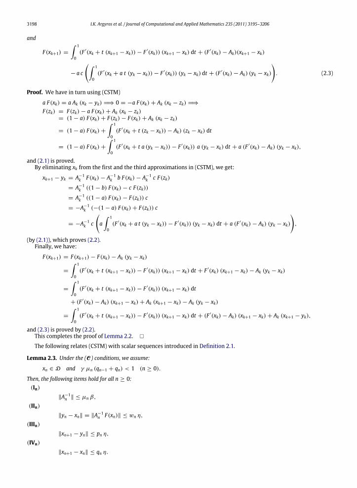
3198 I.K. Argyros et al. / Journal of Computational and Applied Mathematics 235 (2011) 3195–3206

and

F(xk+1) =

∫ 1

0(F ′(xk + t (xk+1 − xk))− F ′(xk)) (xk+1 − xk) dt + (F ′(xk)− Ak)(xk+1 − xk)

− a c

∫ 1

0(F ′(xk + a t (yk − xk))− F ′(xk)) (yk − xk) dt + (F ′(xk)− Ak) (yk − xk)

. (2.3)

Proof. We have in turn using (CSTM)

a F(xk) = a Ak (xk − yk) H⇒ 0 = −a F(xk)+ Ak (xk − zk) H⇒

F(zk) = F(zk)− a F(xk)+ Ak (xk − zk)= (1 − a) F(xk)+ F(zk)− F(xk)+ Ak (xk − zk)

= (1 − a) F(xk)+

∫ 1

0(F ′(xk + t (zk − xk))− Ak) (zk − xk) dt

= (1 − a) F(xk)+

∫ 1

0(F ′(xk + t a (yk − xk))− F ′(xk)) a (yk − xk) dt + a (F ′(xk)− Ak) (yk − xk),

and (2.1) is proved.By eliminating xk from the first and the third approximations in (CSTM), we get:

xk+1 − yk = A−1k F(xk)− A−1

k b F(xk)− A−1k c F(zk)

= A−1k ((1 − b) F(xk)− c F(zk))

= A−1k ((1 − a) F(xk)− F(zk)) c

= −A−1k (−(1 − a) F(xk)+ F(zk)) c

= −A−1k c

a∫ 1

0(F ′(xk + a t (yk − xk))− F ′(xk)) (yk − xk) dt + a (F ′(xk)− Ak) (yk − xk)

,

(by (2.1)), which proves (2.2).Finally, we have:

F(xk+1) = F(xk+1)− F(xk)− Ak (yk − xk)

=

∫ 1

0(F ′(xk + t (xk+1 − xk))− F ′(xk)) (xk+1 − xk) dt + F ′(xk) (xk+1 − xk)− Ak (yk − xk)

=

∫ 1

0(F ′(xk + t (xk+1 − xk))− F ′(xk)) (xk+1 − xk) dt

+ (F ′(xk)− Ak) (xk+1 − xk)+ Ak (xk+1 − xk)− Ak (yk − xk)

=

∫ 1

0(F ′(xk + t (xk+1 − xk))− F ′(xk)) (xk+1 − xk) dt + (F ′(xk)− Ak) (xk+1 − xk)+ Ak (xk+1 − yk),

and (2.3) is proved by (2.2).This completes the proof of Lemma 2.2. �

The following relates (CSTM) with scalar sequences introduced in Definition 2.1.

Lemma 2.3. Under the (C) conditions, we assume:

xn ∈ D and γ µn (qn−1 + qn) < 1 (n ≥ 0).

Then, the following items hold for all n ≥ 0:(In)

‖A−1n ‖ ≤ µn β,

(IIn)‖yn − xn‖ = ‖A−1

n F(xn)‖ ≤ wn η,

(IIIn)‖xn+1 − yn‖ ≤ pn η,

(IVn)

‖xn+1 − xn‖ ≤ qn η.

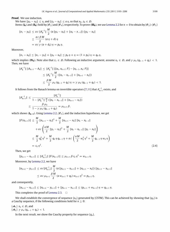
I.K. Argyros et al. / Journal of Computational and Applied Mathematics 235 (2011) 3195–3206 3199

Proof. We use induction.We have ‖y0 − x0‖ ≤ η, and ‖z0 − x0‖ ≤ a η, so that x0, z0 ∈ D .Items (I0) and (II0) hold by (C2) and (C4), respectively. To prove (III0), we use Lemma2.2 for n = 0 to obtain by (C2)–(C5)

‖x1 − y0‖ ≤ a c ‖A−10 ‖

M2(a ‖y0 − x0‖ + ‖x0 − x−1‖) ‖y0 − x0‖

≤a c β M

2(a η + d) η

= a c γ (a + d0) η = p0 η.

Moreover,

‖x1 − x0‖ ≤ ‖x1 − y0‖ + ‖y0 − x0‖ ≤ p0 η + η = (1 + p0) η = q0 η,

which implies (IV0). Note also that z1 ∈ D . Following an inductive argument, assume xk ∈ D , and γ µk (qk−1 + qk) < 1.Then, we have

‖A−1k ‖ ‖Ak+1 − Ak‖ ≤ ‖A−1

k ‖ ‖[xk, xk+1; F ] − [xk−1, xk; F ]‖

≤ ‖A−1k ‖

M2(‖xk − xk−1‖ + ‖xk+1 − xk‖)

≤β M2µk (qk−1 + qk) η = γ µk (qk−1 + qk) < 1.

It follows from the Banach lemma on invertible operators [7,11] that A−1k+1 exists, and

‖A−1k+1‖ ≤

‖A−1k ‖

1 − ‖A−1k ‖

M2 (‖xk − xk−1‖ + ‖xk+1 − xk‖)

≤β µk

1 − γ µk (qk−1 + qk)= µk+1 β,

which shows (Ik+1). Using Lemma 2.2, (C5), and the induction hypotheses, we get

‖F(xk+1)‖ ≤M2

‖xk+1 − xk‖2+

M2

‖xk+1 − xk‖ ‖xk − xk−1‖

+ a c

aM2

‖yk − xk‖2+

M2

‖xk − xk−1‖ ‖yk − xk‖

≤M2

q2k η2+

M2

qk η qk−1 η + a caM2w2

k η2+

M2

qk−1 ηwk η

= ck η2. (2.4)

Then, we get

‖yk+1 − xk+1‖ ≤ ‖A−1k+1‖ ‖F(xk+1)‖ ≤ µk+1 β ck η2 = wk+1 η.

Moreover, by Lemma 2.2, we have

‖xk+2 − yk+1‖ ≤ a c‖A−1k+1‖

M2(a ‖yk+1 − xk+1‖ + ‖xk+1 − xk‖) ‖yk+1 − xk+1‖

≤ a c µk+1β M2(awk+1 + qk) wk+1 η

2= pk+1 η,

and consequently,

‖xk+2 − xk+1‖ ≤ ‖xk+2 − yk+1‖ + ‖yk+1 − xk+1‖ ≤ (pk+1 + wk+1) η = qk+1 η.

This completes the proof of Lemma 2.3. �

We shall establish the convergence of sequence {xn} generated by (CSTM). This can be achieved by showing that {qn} isa Cauchy sequence, if the following conditions hold for n ≥ 0:

(A1) xn ∈ D , and(A2) γ µn (qn−1 + qn) < 1.

In the next result, we show the Cauchy property for sequence {qn}.

3200 I.K. Argyros et al. / Journal of Computational and Applied Mathematics 235 (2011) 3195–3206

Lemma 2.4. Assume (C8). Note that α ∈ [0, 1) implies γ (q−1 + q0) < 1. Then, the scalar sequence:(a) {µn} is increasing.(b) {qn} is decreasing and limn−→∞ qn = 0.Proof. (a) We show using induction that all scalar sequences involved are positive. By Definition 2.1, and (C8), we have for

j = 0:µj, pj, qj,wj, cj, and 1−γ µj (qj−1 +qj) are positive. Assumeµk, pk, qk,wk, ck, and 1−γ µk (qk−1 +qk) are positivefor all k ≤ n. Since ck > 0, it follows from the definition of the scalar sequences that wk+1, µk+1, pk+1, dk+1 have thesame sign. Assume the common sign to be negative. Then

qk−1 + qk + qk+1 < qk−1 + qk H⇒ 1 − γ µk (qk−1 + qk + qk+1) > 1 − γ µk (qk−1 + qk)

H⇒1 − γ µk (qk−1 + qk + qk+1)

1 − γ µk (qk−1 + qk)> 1.

But it follows from the definition of sequence {µk} that

1 − γ µk+1 (qk + qk+1) =1 − γ µk (qk−1 + 2 qk + qk+1)

1 − γ µk (qk−1 + qk)

H⇒ 1 − γ µk+1 qk+1 =1 − γ µk (qk−1 + 2 qk + qk+1)

1 − γ µk (qk−1 + qk)+ γ µk+1 qk

=1 − γ µk (qk−1 + qk + qk+1)

1 − γ µk (qk−1 + qk)> 1,

which is a contradiction, since we get γ µk+1 qk+1 < 0, but µk+1 qk+1 have the same sign, and γ > 0. The induction isthen completed.

By the definition of sequence {µn} and µ0 = 1, we have

1 − γ µk (qk−1 + qk) =µk

µk+1

H⇒ qk−1 + qk =1γ

1µk

−1

µk+1

H⇒

k−1−i=0

(qi−1 + qi) =1γ

1µ0

−1µk

=

1γ

1 −

1µk

H⇒ µk =

1

1 − γk−1∑i=0(qi−1 + qi)

.

But 1 − γ∑k−1

i=0 (qi−1 + qi) decreases. Therefore, sequence {µk} increases, and consequently µk ≥ µ0 = 1.(b) We have that sequenceµk > 1 is increasing, so that 0 ≤

1µk

≤ 1. Since

1µk

is monotonic on a compact set, it converges

to 1µ∞

. Then, we have

limk−→∞

(qk−1 + qk) =1γ

limk−→∞

1µk

−1

µk+1

=

1γ

1µ∞

−1µ∞

= 0.

This completes the proof of Lemma 2.4. �

We can show the main semilocal convergence theorem for (CSTM).

Theorem 2.5. Let F : D ⊆ X −→ Y be a Fréchet-differentiable operator defined on a non-empty open, convex domain D of aBanach space X, with values in a Banach space Y. Assume that the (C) conditions hold. Then, sequence {xn} (n ≥ −1), generatedby (CSTM), is well-defined, remains in U(x0, r η) for all n ≥ 0, and converges to a solution x⋆ ∈ U(x0, r η) of equation F(x) = 0,where,

r =

∞−n=0

qn. (2.5)

Moreover, the following estimate holds

‖xn − x⋆‖ ≤

∞−k=n+1

qk η < r η.

Furthermore, x⋆ is the unique solution of F(x) = 0 in U(x0, r0) ∩ D , provided that r0 ≥ r η, where,

r0 =2

β M0− d − r η. (2.6)

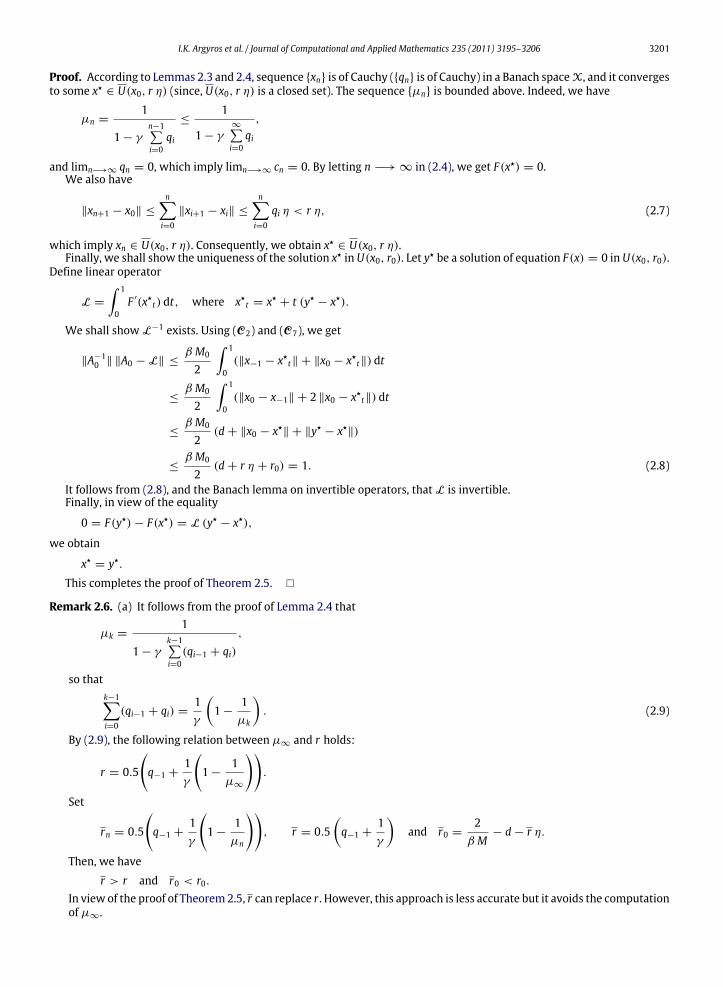
I.K. Argyros et al. / Journal of Computational and Applied Mathematics 235 (2011) 3195–3206 3201

Proof. According to Lemmas 2.3 and 2.4, sequence {xn} is of Cauchy ({qn} is of Cauchy) in a Banach spaceX, and it convergesto some x⋆ ∈ U(x0, r η) (since, U(x0, r η) is a closed set). The sequence {µn} is bounded above. Indeed, we have

µn =1

1 − γn−1∑i=0

qi

≤1

1 − γ∞∑i=0

qi,

and limn−→∞ qn = 0, which imply limn−→∞ cn = 0. By letting n −→ ∞ in (2.4), we get F(x⋆) = 0.We also have

‖xn+1 − x0‖ ≤

n−i=0

‖xi+1 − xi‖ ≤

n−i=0

qi η < r η, (2.7)

which imply xn ∈ U(x0, r η). Consequently, we obtain x⋆ ∈ U(x0, r η).Finally, we shall show the uniqueness of the solution x⋆ in U(x0, r0). Let y⋆ be a solution of equation F(x) = 0 in U(x0, r0).

Define linear operator

L =

∫ 1

0F ′(x⋆t) dt, where x⋆t = x⋆ + t (y⋆ − x⋆).

We shall show L−1 exists. Using (C2) and (C7), we get

‖A−10 ‖ ‖A0 − L‖ ≤

β M0

2

∫ 1

0(‖x−1 − x⋆t‖ + ‖x0 − x⋆t‖) dt

≤β M0

2

∫ 1

0(‖x0 − x−1‖ + 2 ‖x0 − x⋆t‖) dt

≤β M0

2(d + ‖x0 − x⋆‖ + ‖y⋆ − x⋆‖)

≤β M0

2(d + r η + r0) = 1. (2.8)

It follows from (2.8), and the Banach lemma on invertible operators, that L is invertible.Finally, in view of the equality

0 = F(y⋆)− F(x⋆) = L (y⋆ − x⋆),

we obtain

x⋆ = y⋆.

This completes the proof of Theorem 2.5. �

Remark 2.6. (a) It follows from the proof of Lemma 2.4 that

µk =1

1 − γk−1∑i=0(qi−1 + qi)

,

so thatk−1−i=0

(qi−1 + qi) =1γ

1 −

1µk

. (2.9)

By (2.9), the following relation between µ∞ and r holds:

r = 0.5

q−1 +

1γ

1 −

1µ∞

.

Set

rn = 0.5

q−1 +

1γ

1 −

1µn

, r = 0.5

q−1 +

1γ

and r0 =

2β M

− d − r η.

Then, we have

r > r and r0 < r0.In view of the proof of Theorem2.5, r can replace r . However, this approach is less accurate but it avoids the computationof µ∞.

3202 I.K. Argyros et al. / Journal of Computational and Applied Mathematics 235 (2011) 3195–3206

(b) Condition (C5) implies that for x = y,

‖F ′(x0)−1 (F ′(x)− F ′(z))‖ ≤ M‖x − z‖ for all x, z ∈ D.

Then the conclusions of [1, Theorem 4.4] can be obtained from Theorem 2.5 for

b =a2 + a − 1

a2, c =

1a2.

Theorem 2.5 provides a larger uniqueness ball if M0 < M . To obtain the uniqueness ball of [1, Theorem 4.4], simply setM = M0.

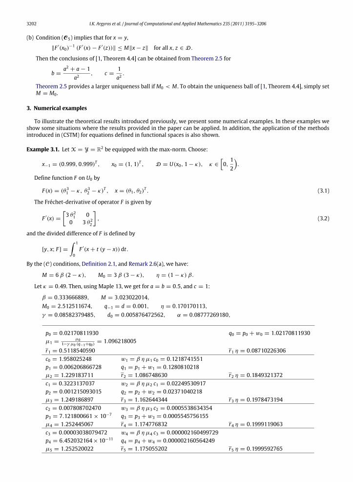
3. Numerical examples

To illustrate the theoretical results introduced previously, we present some numerical examples. In these examples weshow some situations where the results provided in the paper can be applied. In addition, the application of the methodsintroduced in (CSTM) for equations defined in functional spaces is also shown.

Example 3.1. Let X = Y = R2 be equipped with the max-norm. Choose:

x−1 = (0.999, 0.999)T , x0 = (1, 1)T , D = U(x0, 1 − κ), κ ∈

0,

12

.

Define function F on U0 by

F(x) = (θ31 − κ, θ32 − κ)T , x = (θ1, θ2)T . (3.1)

The Fréchet-derivative of operator F is given by

F ′(x) =

[3 θ21 00 3 θ22

], (3.2)

and the divided difference of F is defined by

[y, x; F ] =

∫ 1

0F ′(x + t (y − x)) dt.

By the (C) conditions, Definition 2.1, and Remark 2.6(a), we have:

M = 6 β (2 − κ), M0 = 3 β (3 − κ), η = (1 − κ) β.

Let κ = 0.49. Then, using Maple 13, we get for a = b = 0.5, and c = 1:

β = 0.333666889, M = 3.023022014,M0 = 2.512511674, q−1 = d = 0.001, η = 0.170170113,γ = 0.08582379485, d0 = 0.005876472562, α = 0.08777269180,

p0 = 0.02170811930 q0 = p0 + w0 = 1.02170811930µ1 =

µ01−γ µ0 (q−1+q0)

= 1.096218005

r1 = 0.5118540590 r1 η = 0.08710226306c0 = 1.958025248 w1 = β η µ1 c0 = 0.1218741551p1 = 0.006206866728 q1 = p1 + w1 = 0.1280810218µ2 = 1.229183711 r2 = 1.086748630 r2 η = 0.1849321372c1 = 0.3223137037 w2 = β η µ2 c1 = 0.02249530917p2 = 0.001215093015 q2 = p2 + w2 = 0.02371040218µ3 = 1.249186897 r3 = 1.162644344 r3 η = 0.1978473194c2 = 0.007808702470 w3 = β η µ3 c2 = 0.0005538634354p3 = 7.121800661 × 10−7 q3 = p3 + w3 = 0.0005545756155µ4 = 1.252445067 r4 = 1.174776832 r4 η = 0.1999119063c3 = 0.00003038079472 w4 = β η µ4 c3 = 0.000002160499729p4 = 6.452032164×10−11 q4 = p4 + w4 = 0.000002160564249µ5 = 1.252520022 r5 = 1.175055202 r5 η = 0.1999592765

I.K. Argyros et al. / Journal of Computational and Applied Mathematics 235 (2011) 3195–3206 3203

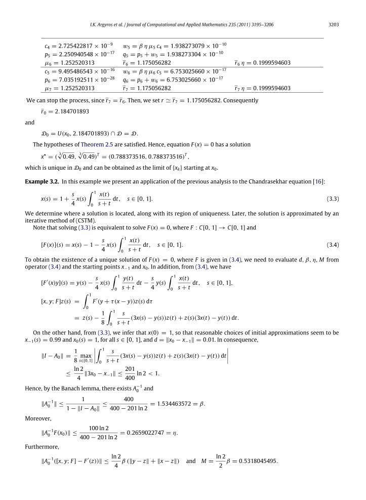
c4 = 2.725422817 × 10−9 w5 = β η µ5 c4 = 1.938273079× 10−10

p5 = 2.250940548×10−17 q5 = p5 + w5 = 1.938273304 × 10−10

µ6 = 1.252520313 r6 = 1.175056282 r6 η = 0.1999594603c5 = 9.495486543 × 10−16 w6 = β η µ6 c5 = 6.753025660× 10−17

p6 = 7.035192511×10−28 q6 = p6 + w6 = 6.753025660 × 10−17

µ7 = 1.252520313 r7 = 1.175056282 r7 η = 0.1999594603

We can stop the process, since r7 = r6. Then, we set r ≃ r7 = 1.175056282. Consequently

r0 = 2.184701893

and

D0 = U(x0, 2.184701893) ∩ D = D.

The hypotheses of Theorem 2.5 are satisfied. Hence, equation F(x) = 0 has a solution

x⋆ = (3√0.49, 3√0.49)T = (0.788373516, 0.788373516)T ,

which is unique in D0 and can be obtained as the limit of {xk} starting at x0.

Example 3.2. In this example we present an application of the previous analysis to the Chandrasekhar equation [16]:

x(s) = 1 +s4x(s)

∫ 1

0

x(t)s + t

dt, s ∈ [0, 1]. (3.3)

We determine where a solution is located, along with its region of uniqueness. Later, the solution is approximated by aniterative method of (CSTM).

Note that solving (3.3) is equivalent to solve F(x) = 0, where F : C[0, 1] → C[0, 1] and

[F(x)](s) = x(s)− 1 −s4x(s)

∫ 1

0

x(t)s + t

dt, s ∈ [0, 1]. (3.4)

To obtain the existence of a unique solution of F(x) = 0, where F is given in (3.4), we need to evaluate d, β, η, M fromoperator (3.4) and the starting points x−1 and x0. In addition, from (3.4), we have

[F ′(x)y](s) = y(s)−s4x(s)

∫ 1

0

y(t)s + t

dt −s4y(s)

∫ 1

0

x(t)s + t

dt, s ∈ [0, 1],

[x, y; F ]z(s) =

∫ 1

0F ′(y + τ(x − y))z(s) dτ

= z(s)−18

∫ 1

0

ss + t

(3x(s)− y(s))z(t)+ z(s)(3x(t)− y(t)) dt.

On the other hand, from (3.3), we infer that x(0) = 1, so that reasonable choices of initial approximations seem to bex−1(s) = 0.99 and x0(s) = 1, for all s ∈ [0, 1], and d = ‖x0 − x−1‖ = 0.01. In consequence,

‖I − A0‖ =18

maxs∈[0,1]

∫ 1

0

ss + t

(3x(s)− y(s))z(t)+ z(s)(3x(t)− y(t)) dt

≤ln 24

‖3x0 − x−1‖ ≤201400

ln 2 < 1.

Hence, by the Banach lemma, there exists A−10 and

‖A−10 ‖ ≤

11 − ‖I − A0‖

≤400

400 − 201 ln 2= 1.534463572 = β.

Moreover,

‖A−10 F(x0)‖ ≤

100 ln 2400 − 201 ln 2

= 0.2659022747 = η.

Furthermore,

‖A−10 ([x, y; F ] − F ′(z))‖ ≤

ln 24β (‖y − z‖ + ‖x − z‖) and M =

ln 22β = 0.5318045495.

3204 I.K. Argyros et al. / Journal of Computational and Applied Mathematics 235 (2011) 3195–3206

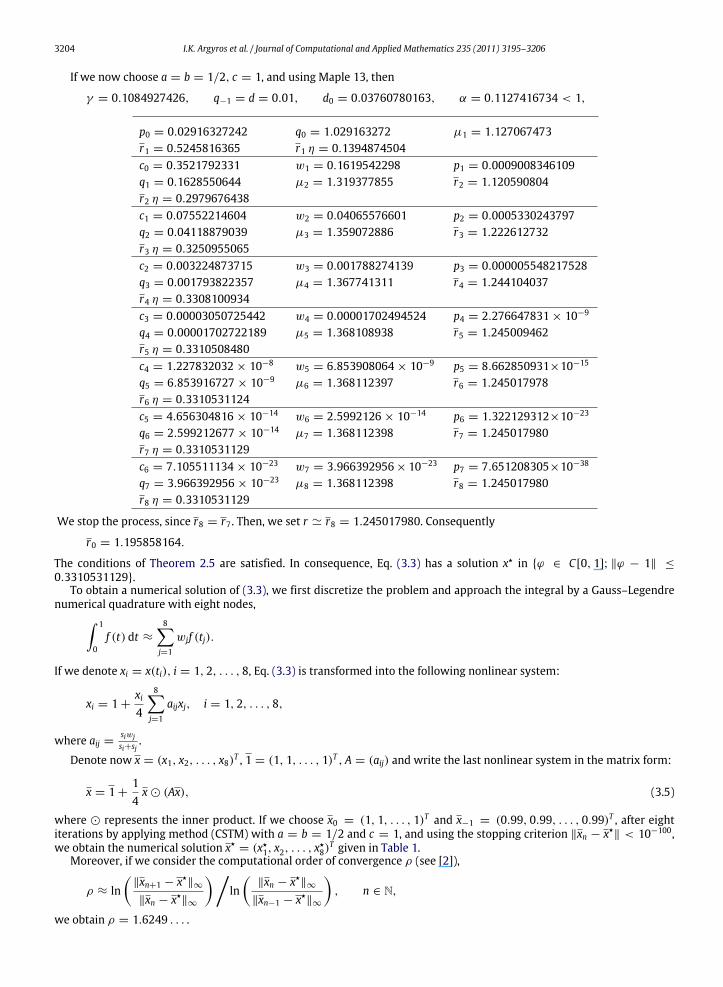
If we now choose a = b = 1/2, c = 1, and using Maple 13, then

γ = 0.1084927426, q−1 = d = 0.01, d0 = 0.03760780163, α = 0.1127416734 < 1,

p0 = 0.02916327242 q0 = 1.029163272 µ1 = 1.127067473r1 = 0.5245816365 r1 η = 0.1394874504c0 = 0.3521792331 w1 = 0.1619542298 p1 = 0.0009008346109q1 = 0.1628550644 µ2 = 1.319377855 r2 = 1.120590804r2 η = 0.2979676438c1 = 0.07552214604 w2 = 0.04065576601 p2 = 0.0005330243797q2 = 0.04118879039 µ3 = 1.359072886 r3 = 1.222612732r3 η = 0.3250955065c2 = 0.003224873715 w3 = 0.001788274139 p3 = 0.000005548217528q3 = 0.001793822357 µ4 = 1.367741311 r4 = 1.244104037r4 η = 0.3308100934c3 = 0.00003050725442 w4 = 0.00001702494524 p4 = 2.276647831 × 10−9

q4 = 0.00001702722189 µ5 = 1.368108938 r5 = 1.245009462r5 η = 0.3310508480c4 = 1.227832032 × 10−8 w5 = 6.853908064 × 10−9 p5 = 8.662850931×10−15

q5 = 6.853916727 × 10−9 µ6 = 1.368112397 r6 = 1.245017978r6 η = 0.3310531124c5 = 4.656304816 × 10−14 w6 = 2.5992126 × 10−14 p6 = 1.322129312×10−23

q6 = 2.599212677 × 10−14 µ7 = 1.368112398 r7 = 1.245017980r7 η = 0.3310531129c6 = 7.105511134 × 10−23 w7 = 3.966392956× 10−23 p7 = 7.651208305×10−38

q7 = 3.966392956 × 10−23 µ8 = 1.368112398 r8 = 1.245017980r8 η = 0.3310531129

We stop the process, since r8 = r7. Then, we set r ≃ r8 = 1.245017980. Consequently

r0 = 1.195858164.

The conditions of Theorem 2.5 are satisfied. In consequence, Eq. (3.3) has a solution x⋆ in {ϕ ∈ C[0, 1]; ‖ϕ − 1‖ ≤

0.3310531129}.To obtain a numerical solution of (3.3), we first discretize the problem and approach the integral by a Gauss–Legendre

numerical quadrature with eight nodes,∫ 1

0f (t) dt ≈

8−j=1

wjf (tj).

If we denote xi = x(ti), i = 1, 2, . . . , 8, Eq. (3.3) is transformed into the following nonlinear system:

xi = 1 +xi4

8−j=1

aijxj, i = 1, 2, . . . , 8,

where aij =siwjsi+sj

.

Denote now x = (x1, x2, . . . , x8)T , 1 = (1, 1, . . . , 1)T , A = (aij) and write the last nonlinear system in the matrix form:

x = 1 +14x ⊙ (Ax), (3.5)

where ⊙ represents the inner product. If we choose x0 = (1, 1, . . . , 1)T and x−1 = (0.99, 0.99, . . . , 0.99)T , after eightiterations by applying method (CSTM) with a = b = 1/2 and c = 1, and using the stopping criterion ‖xn − x⋆‖ < 10−100,we obtain the numerical solution x⋆ = (x⋆1, x2, . . . , x

⋆8)

T given in Table 1.Moreover, if we consider the computational order of convergence ρ (see [2]),

ρ ≈ ln

‖xn+1 − x⋆‖∞

‖xn − x⋆‖∞

ln

‖xn − x⋆‖∞

‖xn−1 − x⋆‖∞

, n ∈ N,

we obtain ρ = 1.6249 . . . .

I.K. Argyros et al. / Journal of Computational and Applied Mathematics 235 (2011) 3195–3206 3205

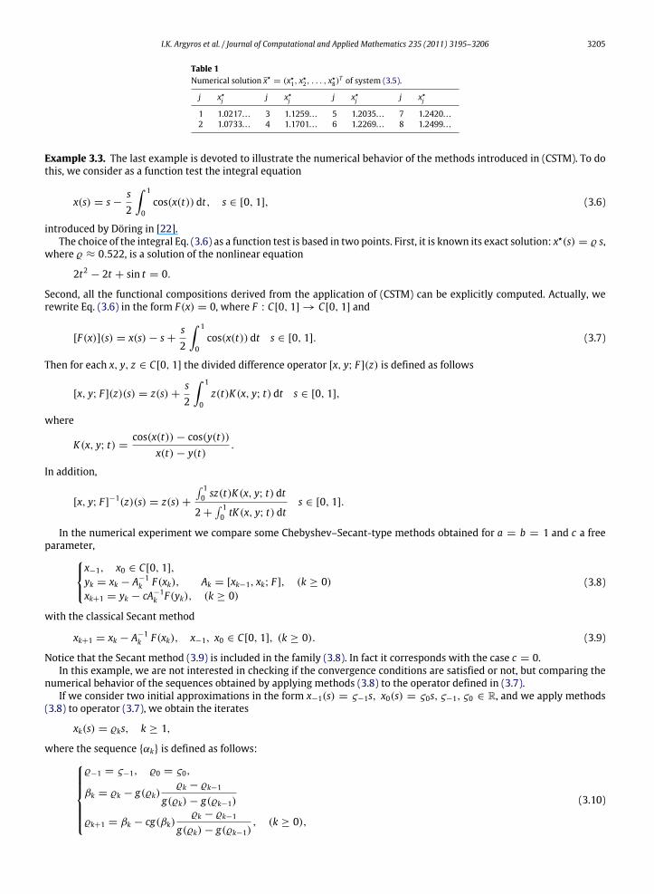
Table 1Numerical solution x⋆ = (x⋆1, x

⋆2, . . . , x

⋆8)

T of system (3.5).

j x⋆j j x⋆j j x⋆j j x⋆j

1 1.0217. . . 3 1.1259. . . 5 1.2035. . . 7 1.2420. . .2 1.0733. . . 4 1.1701. . . 6 1.2269. . . 8 1.2499. . .

Example 3.3. The last example is devoted to illustrate the numerical behavior of the methods introduced in (CSTM). To dothis, we consider as a function test the integral equation

x(s) = s −s2

∫ 1

0cos(x(t)) dt, s ∈ [0, 1], (3.6)

introduced by Döring in [22].The choice of the integral Eq. (3.6) as a function test is based in two points. First, it is known its exact solution: x⋆(s) = ϱ s,

where ϱ ≈ 0.522, is a solution of the nonlinear equation

2t2 − 2t + sin t = 0.

Second, all the functional compositions derived from the application of (CSTM) can be explicitly computed. Actually, werewrite Eq. (3.6) in the form F(x) = 0, where F : C[0, 1] → C[0, 1] and

[F(x)](s) = x(s)− s +s2

∫ 1

0cos(x(t)) dt s ∈ [0, 1]. (3.7)

Then for each x, y, z ∈ C[0, 1] the divided difference operator [x, y; F ](z) is defined as follows

[x, y; F ](z)(s) = z(s)+s2

∫ 1

0z(t)K(x, y; t) dt s ∈ [0, 1],

where

K(x, y; t) =cos(x(t))− cos(y(t))

x(t)− y(t).

In addition,

[x, y; F ]−1(z)(s) = z(s)+

10 sz(t)K(x, y; t) dt

2 + 10 tK(x, y; t) dt

s ∈ [0, 1].

In the numerical experiment we compare some Chebyshev–Secant-type methods obtained for a = b = 1 and c a freeparameter,

x−1, x0 ∈ C[0, 1],yk = xk − A−1

k F(xk), Ak = [xk−1, xk; F ], (k ≥ 0)xk+1 = yk − cA−1

k F(yk), (k ≥ 0)(3.8)

with the classical Secant method

xk+1 = xk − A−1k F(xk), x−1, x0 ∈ C[0, 1], (k ≥ 0). (3.9)

Notice that the Secant method (3.9) is included in the family (3.8). In fact it corresponds with the case c = 0.In this example, we are not interested in checking if the convergence conditions are satisfied or not, but comparing the

numerical behavior of the sequences obtained by applying methods (3.8) to the operator defined in (3.7).If we consider two initial approximations in the form x−1(s) = ς−1s, x0(s) = ς0s, ς−1, ς0 ∈ R, and we apply methods

(3.8) to operator (3.7), we obtain the iterates

xk(s) = ϱks, k ≥ 1,

where the sequence {αk} is defined as follows:ϱ−1 = ς−1, ϱ0 = ς0,

βk = ϱk − g(ϱk)ϱk − ϱk−1

g(ϱk)− g(ϱk−1)

ϱk+1 = βk − cg(βk)ϱk − ϱk−1

g(ϱk)− g(ϱk−1), (k ≥ 0),

(3.10)

3206 I.K. Argyros et al. / Journal of Computational and Applied Mathematics 235 (2011) 3195–3206

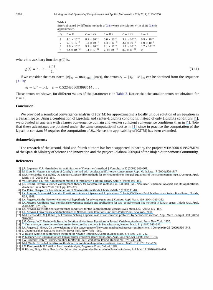
Table 2Errors obtained by different methods of (3.8) when the solution x⋆(s) of Eq. (3.6) isapproximated.

ek c = 0 c = 0.25 c = 0.5 c = 0.75 c = 1

1 1.1 × 10−2 8.7 × 10−3 6.0 × 10−3 3.4 × 10−3 6.9 × 10−4

2 3.1 × 10−4 1.8 × 10−4 8.4 × 10−5 2.5 × 10−5 5.0 × 10−7

3 2.9 × 10−7 9.7 × 10−8 2.1 × 10−8 1.7 × 10−9 1.7×10−15

4 7.5×10−12 1.1×10−12 7.4×10−14 8.9×10−16 0

where the auxiliary function g(t) is:

g(t) = t − t −sin t2t

. (3.11)

If we consider the max-norm ‖x‖∞ = maxt∈[0,1] |x(t)|, the errors ek = ‖xk − x⋆‖∞ can be obtained from the sequence(3.10):

ek = |ϱ⋆ − ϱk|, ϱ = 0.5224366093993514 . . . .

These errors are shown, for different values of the parameter c , in Table 2. Notice that the smaller errors are obtained forc = 1.

Conclusion

We provided a semilocal convergence analysis of (CSTM) for approximating a locally unique solution of an equation ina Banach space. Using a combination of Lipschitz and center-Lipschitz conditions, instead of only Lipschitz conditions [1],we provided an analysis with a larger convergence domain and weaker sufficient convergence conditions than in [1]. Notethat these advantages are obtained under the same computational cost as in [1], since in practice the computation of theLipschitz constantM requires the computation ofM0. Hence, the applicability of (CSTM) has been extended.

Acknowledgements

The research of the second, third and fourth authors has been supported in part by the project MTM2008-01952/MTMof the Spanish Ministry of Science and Innovation and the project Colabora 2009/04 of the Riojan Autonomous Community.

References

[1] J.A. Ezquerro, M.A. Hernández, An optimization of Chebyshev’s method, J. Complexity 25 (2009) 343–361.[2] M. Grau, M. Noguera, A variant of Cauchy’s method with accelerated fifth-order convergence, Appl. Math. Lett. 17 (2004) 509–517.[3] M.A. Hernández, M.J. Rubio, J.A. Ezquerro, Secant-like methods for solving nonlinear integral equations of the Hammerstein type, J. Comput. Appl.

Math. 115 (2000) 245–254.[4] W.E. Bosarge, P.L. Falb, A multipoint method of third order, J. Optim. Theory Appl. 4 (1969) 156–166.[5] J.E. Dennis, Toward a unified convergence theory for Newton-like methods, in: L.B. Rall (Ed.), Nonlinear Functional Analysis and its Applications,

Academic Press, New York, 1971, pp. 425–472.[6] F.A. Potra, Sharp error bounds for a class of Newton-like methods, Libertas Math. 5 (1985) 71–84.[7] I.K. Argyros, Polynomial Operator Equations in Abstract Spaces and Applications, St.Lucie/CRC/Lewis Publ. Mathematics Series, Boca Raton, Florida,

USA, 1998.[8] I.K. Argyros, On the Newton–Kantorovich hypothesis for solving equations, J. Comput. Appl. Math. 169 (2004) 315–332.[9] I.K. Argyros, A unifying local-semilocal convergence analysis and applications for two-point Newton-likemethods in Banach space, J. Math. Anal. Appl.

298 (2004) 374–397.[10] I.K. Argyros, New sufficient convergence conditions for the Secant method, Czechoslovak Math. J. 55 (2005) 175–187.[11] I.K. Argyros, Convergence and Applications of Newton-Type Iterations, Springer-Verlag Publ., New York, 2008.[12] M.A. Hernández, M.J. Rubio, J.A. Ezquerro, Solving a special case of conservative problems by Secant-like method, Appl. Math. Comput. 169 (2005)

926–942.[13] J.M. Ortega, W.C. Rheinboldt, Iterative Solution of Nonlinear Equations in Several Variables, Academic Press, New York, 1970.[14] T. Yamamoto, A convergence theorem for Newton-like methods in Banach spaces, Numer. Math. 51 (1987) 545–557.[15] I.K. Argyros, S. Hilout, On the weakening of the convergence of Newton’s method using recurrent functions, J. Complexity 25 (2009) 530–543.[16] S. Chandrasekhar, Radiative Transfer, Dover Publ., New York, 1960.[17] Z. Huang, A note of Kantorovich theorem for Newton iteration, J. Comput. Appl. Math. 47 (1993) 211–217.[18] P. Laasonen, Ein überquadratisch konvergenter iterativer algorithmus, Ann. Acad. Sci. Fenn. Ser I 450 (1969) 1–10.[19] J.W. Schmidt, Untere Fehlerschranken fur Regula–Falsi Verhafren, Period. Hungar. 9 (1978) 241–247.[20] M.A. Wolfe, Extended iterative methods for the solution of operator equations, Numer. Math. 31 (1978) 153–174.[21] L.V. Kantorovich, G.P. Akilov, Functional Analysis, Pergamon Press, Oxford, 1982.[22] B. Döring, Einige Sätze über das Verfahren der tangierenden Hyperbeln in Banach–Raümen, Apl. Mat. 15 (1970) 418–464.