Applied Mathematics and Computation 170 (2005) 633–647

www.elsevier.com/locate/amc

Vandermonde systems on Gauss–LobattoChebyshev nodes

A. Eisinberg, G. Fedele *

Dip. Elettronica Informatica e Sistemistica, Universita degli Studi della Calabria,

87036 Rende (Cs), Italy

Abstract

This paper deals with Vandermonde matrices Vn whose nodes are the Gauss–Lobatto

Chebyshev nodes, also called extrema Chebyshev nodes. We give an analytic factoriza-

tion and explicit formula for the entries of their inverse, and explore its computational

issues. We also give asymptotic estimates of the Frobenius norm of both Vn and its

inverse and present an explicit formula for the determinant of Vn.

� 2005 Elsevier Inc. All rights reserved.

Keywords: Vandermonde matrices; Polynomial interpolation; Conditioning

1. Introduction

Vandermonde matrices defined by eV nði; jÞ ¼ xi�1j ; i; j ¼ 1; 2 . . . ; n; xj 2 C are

still a topical subject in matrix theory and numerical analysis. The interest

arises as they occur in applications, for example in polynomial and exponential

interpolation, and because they are ill-conditioned, at least for positive or

0096-3003/$ - see front matter � 2005 Elsevier Inc. All rights reserved.

doi:10.1016/j.amc.2004.12.046

* Corresponding author.

E-mail address: fedele@si.deis.unical.it (G. Fedele).

634 A. Eisinberg, G. Fedele / Appl. Math. Comput. 170 (2005) 633–647

symmetric real nodes [1]. The primal system eV na ¼ b represents a moment

problem, which arises, for example, when determining the weights for a quad-

rature rule, while the matrix V n ¼ eV T

n involved in the dual system Vnc = f plays

an important role in polynomial approximation and interpolation problems

[2,3]. The special structure of Vn allows us to use ad hoc algorithms that require

O(n2) elementary operations for solving a Vandermonde system. The most cel-ebrated of them is the one by Bjorck and Pereyra [4]; these algorithms fre-

quently produce surprisingly accurate solution, even when Vn is ill-

conditioned [2]. Bounds or estimates of the norm of both Vn and V �1n are also

interesting, for example to investigate the condition of the polynomial interpo-

lation problem. Answer to these problems have been given first for special con-

figurations of the nodes and recently for general ones [5].

Polynomial interpolation on several set of nodes has received much

attention over the past decade [6]. Theoretically, any discretization gridcan be used to construct the interpolation polynomial. However, the inter-

polated solution between discretization points are accurate only if the indi-

vidual building blocks behave well between points. Lagrangian polynomials

with a uniform grid suffer for the effect of the Runge phenomenon: small

data near the center of the interval are associated with wild oscillations in

the interpolant, on the order 2n times bigger, near the edges of the interval,

[7,8]. The best choice is to use nodes that are clustered near the edges of the

interval with an asymptotic density proportional to (1 � x2)�1/2 as n ! 1,[9]. The family of Chebyshev points, obtained by projecting equally spaced

points on the unit circle down to the unit interval [�1,1] have such density

properties. The classical Chebyshev grids are [10]:

• Chebyshev nodes

T 1 ¼ xk ¼ cos2k � 1

2np

� �; k ¼ 1; 2; . . . ; n

� �ð1Þ

• Extended Chebyshev nodes

T 2 ¼ xk ¼ �cos 2k�1

2n p� �

cos p2n

� � ; k ¼ 1; 2; . . . ; n

( )ð2Þ

• Gauss–Lobatto Chebyshev nodes (extrema)

T 3 ¼ xk ¼ � cosk � 1

n� 1p

� �; k ¼ 1; 2; . . . ; n

� �ð3Þ

In [11] it is proved that interpolation on the Chebyshev polynomial extrema

minimizes the diameter of the set of the vectors of the coefficients of all possible

polynomials interpolating the perturbed data. Although the set of Gauss–

Lobatto Chebyshev nodes failed to be a good approximation to the optimal

A. Eisinberg, G. Fedele / Appl. Math. Comput. 170 (2005) 633–647 635

interpolation set, such set is of considerable interest since the norm of corre-

sponding interpolation operator Pn(T3) is less than the norm of the operator

Pn(T1) induced by interpolation at the Chebyshev roots [12].

This paper deals with Vandermonde matrices on Gauss–Lobatto Chebyshev

nodes. Through the paper we present a factorization of the inverse of such ma-

trix and derive an algorithm for solving primal and dual system. We also giveasymptotic estimates of the Frobenius norm of both Vn and its inverse and an

explicit formula for det(Vn). A point of interest in this matrix is the (relative)

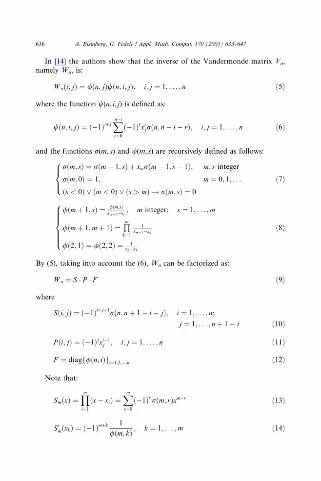
moderate growth, versus n, of the condition number j2(Vn), [13,3]. Fig. 1 shows

the j2 comparison between the Vandermonde matrix on the Chebyshev nodes

(Vn(T1)), Chebyshev extesa nodes (Vn(T2)) and Gauss–Lobatto Chebyshev

nodes (Vn(T3)).

2. Preliminaries

Let Vn be the Vandermonde matrix defined on the set of n distinct nodes

Xn = {x1, . . ., xn}:

V nði; jÞ ¼ xj�1

i ; i; j ¼ 1; . . . ; n ð4Þ

0 10 20 30 40 50 60 70 80 90 1000.7

0.75

0.8

0.85

0.9

0.95

1

n

κ2(Vn(T3)/κ2(Vn(T1))κ2(Vn(T3)/κ2(Vn(T2))

Fig. 1. Plot of the ratios j2ðV nðT 3ÞÞj2ðV nðT 1ÞÞ

and j2ðV nðT 3ÞÞj2ðV nðT 2ÞÞ

.

636 A. Eisinberg, G. Fedele / Appl. Math. Comput. 170 (2005) 633–647

In [14] the authors show that the inverse of the Vandermonde matrix Vn,

namely Wn, is:

W nði; jÞ ¼ /ðn; jÞwðn; i; jÞ; i; j ¼ 1; . . . ; n ð5Þ

where the function w(n, i, j) is defined as:

wðn; i; jÞ ¼ ð�1ÞiþjXn�i

r¼0

ð�1Þrxrjrðn; n� i� rÞ; i; j ¼ 1; . . . ; n ð6Þ

and the functions r(m, s) and /(m, s) are recursively defined as follows:

rðm; sÞ ¼ rðm� 1; sÞ þ xmrðm� 1; s� 1Þ; m; s integer

rðm; 0Þ ¼ 1; m ¼ 0; 1; . . .

ðs < 0Þ _ ðm < 0Þ _ ðs > mÞ ! rðm; sÞ ¼ 0

8><>: ð7Þ

/ðmþ 1; sÞ ¼ /ðm;sÞxmþ1�xs

; m integer; s ¼ 1; . . . ;m

/ðmþ 1;mþ 1Þ ¼Qmk¼1

1xmþ1�xk

/ð2; 1Þ ¼ /ð2; 2Þ ¼ 1x2�x1

8>>>><>>>>: ð8Þ

By (5), taking into account the (6), Wn can be factorized as:

W n ¼ S P F ð9Þ

where

Sði; jÞ ¼ ð�1Þiþjþ1rðn; nþ 1� i� jÞ; i ¼ 1; . . . ; n;

j ¼ 1; . . . ; nþ 1� i ð10Þ

P ði; jÞ ¼ ð�1Þjxi�1j ; i; j ¼ 1; . . . ; n ð11Þ

F ¼ diagf/ðn; iÞgi¼1;2;...;n ð12Þ

Note that:

SmðxÞ ¼Ymi¼1

ðx� xiÞ ¼Xmr¼0

ð�1Þr rðm; rÞxm�r ð13Þ

S0mðxkÞ ¼ ð�1Þmþk 1

/ðm; kÞ ; k ¼ 1; . . . ;m ð14Þ

A. Eisinberg, G. Fedele / Appl. Math. Comput. 170 (2005) 633–647 637

3. Main results

We start by noting that, for some sets of interpolation nodes, explicit expres-

sion for r and / may be found in [15]. We consider the set of Gauss–Lobatto

Chebyshev nodes (Xn = T3) and give the proof of some properties useful in the

sequel.

Lemma 1

rðn; 2sÞ ¼ ð�1Þs 1

2n�2

Pbn2cq¼1

n� 1

2q� 1

!q

s

!; s ¼ 0; . . . ; bn

2c

rðn; 2sþ 1Þ ¼ 0; s ¼ 0; . . . ; dn2e

8>><>>: ð15Þ

where notations bÆcand dÆedenote the floor and ceiling functions, respectively [16].

Proof. It is easy to show that (13) can be rewritten as:

SnðxÞ ¼1

2n�2ðx� 1Þðxþ 1ÞUn�2ðxÞ ð16Þ

where

UmðxÞ ¼sin½ðmþ 1Þ arccosðxÞ�

sin½arccosðxÞ�

is the m-order Chebyshev polynomial of the second kind.

But [17]:

Un�2ðxÞ ¼Xbn2cq¼1

ð�1Þqþ1 n� 1

2q� 1

� �xn�2qð1� x2Þq�1 ð17Þ

by substituting the (17) in (16) one has:

SnðxÞ ¼Xbn2cq¼1

Xqs¼0

ð�1Þsn� 1

2q� 1

� �q

s

� �xn�2s ð18Þ

and, therefore, the (15) follows. h

Lemma 2

S0nðxkÞ ¼

n� 1

2n�2ð�1Þnþk � ð�1Þndk;1 þ dk;n

h ið19Þ

638 A. Eisinberg, G. Fedele / Appl. Math. Comput. 170 (2005) 633–647

Proof. The (16) can be rewritten as:

SnðxÞ ¼1

2n�2ðx� 1Þðxþ 1Þ sin½ðnþ 1Þ arccosðxÞ�

sin½arccosðxÞ�therefore, by standard algebraic manipulations:

S0nðxkÞ ¼

1

2n�2ðn� 1Þ cos½ðn� kÞp� � 1

2n�2

cos k�1n�1

p� �ffiffiffiffiffiffiffiffiffiffiffiffiffiffiffiffiffiffiffiffiffiffiffiffiffiffiffiffiffiffi

1� cos2 k�1n�1

p� �q sin½ðn� kÞp�

Noting that:

limk!1

cos k�1n�1

p� �ffiffiffiffiffiffiffiffiffiffiffiffiffiffiffiffiffiffiffiffiffiffiffiffiffiffiffiffiffiffi

1� cos2 k�1n�1

p� �q sin½ðn� kÞp� ¼ ð�1Þnðn� 1Þ

limk!n

cos k�1n�1

p� �ffiffiffiffiffiffiffiffiffiffiffiffiffiffiffiffiffiffiffiffiffiffiffiffiffiffiffiffiffiffi

1� cos2 k�1n�1

p� �q sin½ðn� kÞp� ¼ �ðn� 1Þ

the (19) follows. h

By substituting the (19) in (14), one has:

/ðn; kÞ ¼2n�3

n�1k ¼ 1; n

2n�2

n�1k ¼ 2; . . . ; n� 1

(ð20Þ

Lemma 3. An alternative formulation of (15) is:

rðn; 2sÞ ¼ ð�1Þs 1

22s

n� s

s

� �n2 � n� 2s

ðn� s� 1Þðn� sÞ ; s ¼ 0; 1; . . . ;n2

j kð21Þ

Proof. By the recurrence properties of the second-kind Chebyshev polynomials

[18], one has:

SnðxÞ � xSn�1ðxÞ þ1

4Sn�2ðxÞ ¼ 0

thereforeXn2b c

s¼0

rðn; 2sÞxn�2s � xXn�1

2b c

s¼0

rðn� 1; 2sÞxn�2s�1 þ 1

4

Xn�22b c

s¼0

rðn� 2; 2sÞxn�2s�2 ¼ 0

ð22Þ

A. Eisinberg, G. Fedele / Appl. Math. Comput. 170 (2005) 633–647 639

must holds. The (22) can be proved by standard algebraic manipulations when

n is both odd and even. h

By rearranging (10)–(12), one has:

Sði; jÞ ¼ ð�1Þirðn; nþ 1� i� jÞ; i ¼ 1; . . . ; n;

j ¼ 1; . . . ; nþ 1� i

P ði; jÞ ¼ cos j�1

n�1p

� �i�1; i; j ¼ 1; . . . ; n

F ði; iÞ ¼ ð�1Þi/ðn; iÞ; i ¼ 1; . . . ; n

8>>>><>>>>: ð23Þ

Following the same line in [19], the matrix P can be factorized as:

P ¼ D U H ð24Þ

where

Dði; iÞ ¼ 1

2i�2 ; i ¼ 2; . . . ; n

Dð1; 1Þ ¼ 1

�ð25Þ

Uð2i� 1; 1Þ ¼2i� 3

i� 1

� �; i ¼ 1; . . . ; n

2

� �Uð2i; 2jÞ ¼

2i� 1

i� j

� �; j ¼ 1; . . . ; n

2

!; i ¼ j; . . . ; n

2

!Uð2i� 1; 2j� 1Þ ¼

2i� 2

i� j

� �; j ¼ 2; . . . ; n

2

� �; i ¼ j; . . . ; n

2

� �

8>>>>>>>><>>>>>>>>:ð26Þ

Hði; jÞ ¼ cosði� 1Þðj� 1Þ

n� 1p

� �; i ¼ 1; . . . ; n; j ¼ 1; . . . ; n ð27Þ

If one defines the matrix Q as:

Qði; jÞ ¼ 2n�i�1 S D U½ �ði; jÞ; i; j ¼ 1; . . . ; n ð28Þthe (9) becomes:

W n ¼1

n� 1K Q H F ð29Þ

where

K ¼ diagf2i�1gi¼1;2;...;n ð30Þ

F ð1; 1Þ ¼ � 12

F ði; iÞ ¼ ð�1Þi; i ¼ 2; . . . ; n� 1

F ðn; nÞ ¼ ð�1Þn 12

8><>: ð31Þ

640 A. Eisinberg, G. Fedele / Appl. Math. Comput. 170 (2005) 633–647

We present here an efficient scheme for the computation Q. It can be shown

that Q can be build by the following equalities:

Qð1; n� 2Þ ¼ 2

Qði; nþ 1� iÞ ¼ ð�1Þi; i ¼ 1; 2; . . . ; n

Qð1; n� 2j� 2Þ ¼ �Qð1; n� 2jÞ; j ¼ 1; 2; . . . ; dn�42e

Qði; nþ 1� i� 2jÞ ¼ �Qði; nþ 3� i� 2jÞ�Qði� 1; nþ 2� i� 2jÞ; i ¼ 2; 3; . . . ; n;

j ¼ 1; 2; . . . ; j�

Qði; 1Þ ¼ Qði; 1Þ=2; i ¼ 1; 2; . . . ; n

8>>>>>>>>>>><>>>>>>>>>>>:ð32Þ

where

j� ¼bn�i

2c n even

dn�1�i2

e n odd

(

4. The Frobenius norm of Vn and Wn

Proposition 1. The Frobenius norm of Vn is

kV nkF ¼

ffiffiffiffiffiffiffiffiffiffiffiffiffiffiffiffiffiffiffiffiffiffiffiffiffiffiffiffiffiffiffiffiffiffiffiffiffiffiffiffiffiffiffiffiffiffiffiffiffiffiffiffiffiffiffiffiffiffiffiffiffiffiffiffiffinþ n� 1

22n�3þ 2ffiffiffi

pp ðn� 1Þ

C nþ 12

� �CðnÞ

sð33Þ

where C(x) is the gamma function [20].

Proof

kV nk2

F ¼Xni¼1

Xns¼1

coss� 1

n� 1p

� �� �2i�2

: ð34Þ

But

coss� 1

n� 1p

� �� �2i�2

¼ 1

22i�2

2i� 2

i� 1

� �þ 1

22i�2

Xi�2

k¼0

22i� 2

k

� �� cos

2ði� 1� kÞðs� 1Þn� 1

p

� �ð35Þ

then (34) becomes:

kV nk2F ¼

Xni¼1

Xns¼1

1

22i�2

2i� 2

i� 1

� �þXni¼1

Xns¼1

Xi�2

k¼0

2

22i�2

2i� 2

k

� �� cos

2ði� 1� kÞðs� 1Þn� 1

p

� �ð36Þ

A. Eisinberg, G. Fedele / Appl. Math. Comput. 170 (2005) 633–647 641

By using the identityXni¼1

Xns¼1

1

22i�2

2i� 2

i� 1

� �¼ 2ffiffiffi

pp n

C nþ 12

� �CðnÞ ð37Þ

and by standard algebraic manipulations the (33) follows. h

Proposition 2. The Frobenius norm of Wn is given by

kW nk2F ¼ 1

2ðn� 1Þ þ22n�4

n� 1b1ðnÞ þ

1

n� 1b2ðnÞ

� �ð38Þ

where

b1ðnÞ ¼Xnk¼1

Xbn�k2c

r¼0

Xbn�k2c

s¼0

ð�1Þnþkþrþs � 12

n� k � r � s

� �rð2rÞrð2sÞ ð39Þ

and

b2ðnÞ ¼Xnk¼1

Xbn�k2c

r¼0

Xbn�k2c

s¼0

1

2rð2rÞrð2sÞ ð40Þ

Proof. The (38) follows from standard algebraic manipulations. h

Taking into account only the term b1(n) in (38) and using the facts

Xnk¼1

Xbn�k2c

r¼0

Xbn�k2c

s¼0

½� ¼Xbn�1

2c

r¼0

Xbn�12c

s¼0

Xn�2maxðr;sÞ

k¼1

½�

Xqs¼0

p � 32

s� 1

� �q

s

� �¼ p þ q� 3

2

q� 1

� �we give the following conjecture.

Conjecture 1

kW nkF �

ffiffiffiffiffiffiffiffiffiffiffiffiffiffiffiffiffiffiffiffiffiffiffiffiffiffiffiffiffiffiffiffiffiffiffiffiffiffiffiffiffiffiffiffiffiffiffiffiffiffiffiffiffiffiffiffiffiffiffiffiffiffiffiffiffiffiffiffiffiffiffiffiffiffiffiffiffiffiffiffiffiffiffiffiffiffiffiffiffiffiffiffiffiffiffiffiffiffiffiffiffiffi2

n� 1

Xbn2c�1

p¼1

Xbn2c�1

q¼1

n� 1

2p � 1

� �n� 1

2q� 1

� �p þ q� 3

2

q� 1

� �;

vuut n ! 1

ð41Þ

Fig. 2 shows the accuracy of the estimate of the Frobenius norm of Wn in

term of relative error for n in the interval [20,100] by Eq. (41).

20 30 40 50 60 70 80 90 1001

2

3

4

5

6

7

8

9

10x 10

3

n

Fig. 2. Relative error estimating kWnkF.

642 A. Eisinberg, G. Fedele / Appl. Math. Comput. 170 (2005) 633–647

5. The determinant of Vn

The next proposition gives the value of the determinant of Vn.

Proposition 3

detðV nÞ ¼ 2

ffiffiffiffiffiffiffiffiffiffiffiffiffiffiffiffiffiðn� 1Þn

2nðn�2Þ

sð42Þ

Proof. By the definition of the Vandermonde determinant we have

detðV nÞ ¼Y

16i<j6n

cosi� 1

n� 1p

� �� cos

j� 1

n� 1p

� �� �

¼ 2nðn�1Þ

2

Y16i<j6n

siniþ j� 2

2n� 2p

� �sin

j� i2n� 2

p

� �

and, simply rearranging the terms we can write

A. Eisinberg, G. Fedele / Appl. Math. Comput. 170 (2005) 633–647 643

detðV nÞ ¼ 2nðn�1Þ

2

Ybn2ck¼1

sin2k � 1

2n� 2p

� �nþ1

Ybn2c�1

k¼1

sin2k

2n� 2p

� �n

Finally [17]

Ybn2ck¼1

sin2k � 1

2n� 2p

� �nþ1

¼ 22þn�n2

2 ;Ybn2c�1

k¼1

sin2k

2n� 2p

� �n

¼

ffiffiffiffiffiffiffiffiffiffiffiffiffiffiffiffiffiðn� 1Þn

2nðn�2Þ

s

which concludes the proof. h

6. Numerical experiments

This section shows some numerical experiments, aimed at investigating

the accuracy of the proposed factorization. We have solved several dual sys-

tems Vnc = f and primal systems eV na ¼ b and have compared our results

with those obtained by the Bjorck–Pereyra algorithms. We have used pack-

age Mathematica [21] to compute the approximate solutions c and a, the

exact ones (using extended precision of 1024 significant digits) and theerrors

�c ¼ max16i6n

jci � cijjcij

ð43Þ

�a ¼ max16i6n

jai � aijjaij

ð44Þ

of both our and Bjorck–Pereyra algorithm. A set of experiments has been run,

for n = 3–10,20,30,40,50,100. We have generated the right-hand sides f and b

with random entries uniformly distributed in the interval [�1,1]. Tables 1 and 2

shows maximum and mean value of (43) and (44) over 10000 runs, the fractionof trials in which the proposed algorithms (EF) give equal or more accurate re-

sult than Bjorck–Pereyra ones (BP) and also the probability that �c and �a is

less or equal than 10nu where u = 2�53 is the unit roundoff. As to the compu-

tational cost the EF algorithms require 3n2 + O(n) while BP algorithms cost

2.5n2 + O(n) flops. EF algorithms seem to perform better than the Bjorck–

Pereyra ones in terms of numerical accuracy and stability as it can be seen

for high value of n. Same results are obtained by computing the approximate

solutions c and a in Matlab package and then by migrating the output in Math-ematica in order to compare it with the ‘‘exact’’ one. For Matlab code refer to

Appendix A.

Table 1

Dual problem

n BP EF s.r. p(�c 6 10nu)

Max Mean Max Mean EF vs BP

3 2.34�13 3.07�16 2.15�15 4.02�17 0.98 0.99

4 1.73�12 2.53�15 4.03�13 1.09�15 0.75 0.99

5 9.31�12 5.82�15 4.65�12 1.51�15 0.93 0.98

6 1.43�11 1.40�14 1.54�12 2.41�15 0.94 0.97

7 2.47�11 2.35�14 6.60�12 4.36�15 0.96 0.97

8 3.24�10 7.90�14 5.67�12 4.69�15 0.99 0.95

9 6.20�11 6.12�14 1.12�12 2.94�15 0.99 0.96

10 1.56�10 1.98�13 9.00�12 6.66�15 0.99 0.95

20 1.17�06 4.10�10 5.47�11 2.54�14 1.00 0.92

30 2.10�03 9.79�07 2.22�09 3.86�13 1.00 0.91

40 5.68+00 3.77�03 1.91�10 1.01�13 1.00 0.92

50 7.61+03 1.38+01 4.04�11 9.49�14 1.00 0.90

100 8.52+20 1.69+18 1.68�09 7.45�13 1.00 0.88

Maximum and mean value of �c. Success rate of EF algorithm over 10000 runs.

Table 2

Primal problem

n BP EF s.r. p(�a 6 10nu)

Max Mean Max Mean EF vs BP

3 1.70�13 2.90�16 5.46�13 3.26�16 0.79 0.99

4 1.06�10 1.33�14 3.25�11 3.99�15 0.74 0.98

5 3.96�11 8.87�15 7.94�13 1.32�15 0.86 0.97

6 6.69�11 2.68�14 3.68�12 2.57�15 0.91 0.97

7 2.93�11 1.66�14 4.69�12 2.91�15 0.95 0.97

8 6.00�11 3.52�14 2.48�12 3.15�15 0.98 0.96

9 9.70�11 4.33�14 6.00�12 3.16�15 0.96 0.96

10 8.44�11 7.77�14 3.06�11 7.37�15 0.98 0.95

20 1.12�08 3.25�12 4.49�11 1.98�14 1.00 0.94

30 1.89�07 9.62�11 2.43�11 2.81�14 1.00 0.93

40 1.22�05 4.26�09 2.13�10 4.33�14 1.00 0.95

50 1.52�05 3.18�08 1.84�11 2.56�14 1.00 0.94

100 3.88+02 1.68�01 1.71�10 7.30�14 1.00 0.94

Maximum and mean value of �a. Success rate of EF algorithm over 10000 runs.

644 A. Eisinberg, G. Fedele / Appl. Math. Comput. 170 (2005) 633–647

7. Conclusion

In this paper we derived an explicit factorization of the Vandermonde ma-

trix on Gauss–Lobatto Chebyshev nodes. Such factorization allows to design

an efficient algorithm to solve Vandermonde systems. The numerical experi-

ments indicate that our approach is more stable compared with existing

A. Eisinberg, G. Fedele / Appl. Math. Comput. 170 (2005) 633–647 645

Bjorck-Pereyra algorithm. Starting from these theoretical results we are work-

ing with a conjecture on discrete orthogonal polynomials on Gauss–Lobatto

Chebyshev nodes and its proof. The operation count and the accuracy ob-

tained in the experiments on least-squares problems seems to be very

competitive.

Appendix A. Matlab code

function c=glc(f);

n=max(size(f));

nf=floor(n/2);

f(1)=f(1)/2;

f(n)=f(n)/2;

for i=1:n

f(i)=(-1)^i*f(i);

end

% Matrix H

% -- - - - - - - - - - - - - - - - - - - - - - - - - - - - - - - - - - - - - - - - - - - - - - - - - - - - - - - - - - - - - - -

H=zeros(n);

H(1,1:nf)=ones(1,nf);

H(1:nf,1)=ones(nf,1);

if rem(n,2)==0

start=1;

else

for j=1:ceil(n/2)

H(nf+1,2*j-1)=(-1)^(j+1);

end

H(:,nf+1)=H(nf+1,:)�;start=2;

end

for i=2:nf

for j=i:nf

H(i,j)=cos(rem((i-1)*(j-1),2*n-2)*pi/(n-1));

H(j,i)=H(i,j);

end

end

for j=1:nf

if rem(j,2)==0

H(nf+start:n,j)=-flipud(H(1:nf,j));

else

H(nf+start:n,j)=flipud(H(1:nf,j));

end

646 A. Eisinberg, G. Fedele / Appl. Math. Comput. 170 (2005) 633–647

end

for i=1:n

if rem(i,2)==0

H(i,nf+start:n)=-fliplr(H(i,1:nf));

else

H(i,nf+start:n)=fliplr(H(i,1:nf));

end

end

% -- - - - - - - - - - - - - - - - - - - - - - - - - - - - - - - - - - - - - - - - - - - - - - - - - - - - - - - - - - - - - - -

% Matrix Q

% -- - - - - - - - - - - - - - - - - - - - - - - - - - - - - - - - - - - - - - - - - - - - - - - - - - - - - - - - - - - - - - -

Q=zeros(n);

for i=1:n

Q(i,n+1-i)=(-1)^i;

end

Q(1,n-2)=2;

for j=1:ceil((n-4)/2)

Q(1,n-2*j-2)=-Q(1,n-2*j);

end

for i=2:n

if rem(i,2)==0

jmax=floor((n-i)/2);

else

jmax=ceil((n-1-i)/2);

end

for j=1:jmax

Q(i,n+1-i-2*j)=-Q(i,n+3-i-2*j)-Q(i-1,n+2-i-2*j);

end

end

Q(:,1)=Q(:,1)/2;

% -- - - - - - - - - - - - - - - - - - - - - - - - - - - - - - - - - - - - - - - - - - - - - - - - - - - - - - - - - - - - - - -

aux=H*f;

c=zeros(n,1);

for i=1:n

for j=rem(n+i,2)+1:2:n+1-i

c(i)=c(i)+Q(i,j)*aux(j);

end

end

for i=1:n

c(i)=2^(i-1)*c(i);

end

c=c/(n-1);

A. Eisinberg, G. Fedele / Appl. Math. Comput. 170 (2005) 633–647 647

References

[1] W. Gautschi, G. Inglese, Lower bounds for the condition number of Vandermonde matrix,

Numer. Math. 52 (1998) 241–250.

[2] G.H. Golub, C.F. Van Loan, Matrix Computation, third ed., Johns Hopkins Univ. Press,

Baltimore, MD, 1996.

[3] N.J. Higham, Accuracy and Stability of Numerical Algorithms, SIAM, Philadelphia, PA,

1996.

[4] A. Bjorck, V. Pereyra, Solution of Vandermonde systems of linear equations, Math. Comput.

24 (1970) 893–903.

[5] E. Tyrtyshnikov, How bad are Hankel matrices, Numer. Math. 67 (1994) 261–269.

[6] E. Meijering, A chronology of interpolation: from ancient astronomy to modern signal and

image processing, Proc. IEEE 90 (2002) 319–342.

[7] A. Bjorck, G. Dahlquist, Numerical Methods, Prentice-Hall, Englewood Cliffs, NJ, 1974.

[8] P. Henrici, Essentials of Numerical Analysis, Wiley, New York, 1982.

[9] J.P. Berrut, L.N. Trefethen, Barycentric Lagrange interpolation, SIAM Rev. 46 (2004) 501–

517.

[10] L. Brutman, Lebesgue functions for polynomial interpolation—a survey, Ann. Numer. Math.

4 (1997) 111–127.

[11] G. Belforte, P. Gay, G. Monegato, Some new properties of Chebyshev polynomials, J.

Comput. Appl. Math. 117 (2000) 175–181.

[12] L. Brutman, A note on polynomial interpolation at the Chebyshev extrema nodes, J. Approx.

Theory 42 (1984) 283–292.

[13] W. Gautschi, Norms estimates for inverses of Vandermonde matrices, Numer. Math. 23 (1974)

337–347.

[14] A. Eisinberg, C. Picardi, On the inversion of Vandermonde matrix, in: Proc. of the 8th

Triennial IFAC World Congress, Kyoto, Japan, 1981.

[15] A. Eisinberg, G. Fedele, Polynomial interpolation and related algorithms, in: Twelfth

International Colloquium on Num. Anal. and Computer Science with Appl., Plovdiv, 2003.

[16] D.E. Knuth, The Art of Computer Programming, Vol. 1, second ed., Addison-Wesley,

Reading, MA, 1973.

[17] I.S. Gradshteyn, I.M. Ryzhik, Table of Integrals, Series and Products, third ed., Academic

Press, New York, 1965.

[18] T.J. Rivlin, The Chebyshev Polynomials, John Wiley & Sons, New York, 1974.

[19] A. Eisinberg, G. Franze, N. Salerno, Rectangular Vandermonde matrices on Chebyshev

nodes, Linear Algebra Appl. 338 (2001) 27–36.

[20] L. Gatteschi, Funzioni Speciali, UTET, 1973.

[21] S. Wolfram, Mathematica: a System for Doing Mathematics by Computers, second ed.,

Addison-Wesley, 1991.