Regular Boundary Value Problems on a Path

throughout Chebyshev Polynomials

E. Bendito, A. Carmona, A.M. Encinas and J.M. Gesto

Departament de Matematica Aplicada III. Universitat Politecnica de Catalunya.Spain

Abstract

In this work we study the different types of regular boundary value problemson a path associated with the Schrodinger operator. In particular, we obtain theGreen function for each problem and we emphasize the case of Sturm-Liouvilleboundary conditions. In addition, we study the periodic boundary value problemthat corresponds to the Poisson equation in a cycle. In any case, the Green functionsare given in terms of Chebyshev polynomials since they verify a recurrence lawsimilar to the one verified by the Schodinger operator on a path.

Key words: Discrete Schrodinger operator, Path, Boundary value problems, Greenfunction, Chebyshev polynomials

1 Introduction

In this work, we analyze the linear boundary value problem in the context ofsecond order difference equations with constant coefficients associated with theSchrodinger operator on a finite path. Our study runs in parallel to the knownfor boundary value problems associated with ordinary differential equations.In particular we concentrate on determining explicit expressions for the Greenfunction associated with regular boundary value problems on a path.

The boundary value problems here considered are of three types that corre-spond to the cases in which the boundary has two, one or no vertices. In any

Email address: angeles.carmona@upc.edu (E. Bendito, A. Carmona, A.M.Encinas and J.M. Gesto).

URL: http://www-ma3.upc.es/users/bencar/index.html (E. Bendito, A.Carmona, A.M. Encinas and J.M. Gesto).

Preprint submitted to Elsevier 27 September 2006

case it is essential to describe the solutions of the Schrondinger equation onthe interior nodes of the path. In this particular situation, it is possible toobtain explicitly such solutions in terms of second kind Chebyshev polynomi-als. As an immediate consequence of this property, we can easily characterizethose boundary value problems that are regular and then we obtain theircorresponding Green function in terms of Chebyshev polynomials.

In the literature the most studied boundary value problems are those known asSturm-Liouville boundary value problems, that we obtain here as a particularcase, since in this work we analyze general boundary conditions. A survey onSturm-Liouville boundary value problems can be found in (4), see also (1). Inaddition, when the boundary conditions are of Dirichlet type the expressionof the Green function for the Schrodinger operator was already obtained in(2; 3), using techniques different to the ones we will use here. We also treatwith the Poisson equation on a cycle and we show that this problem can beseen as a two-point boundary value problem on a path by introducing theso-called periodic boundary conditions.

To end this section, we will describe some basic properties of the so-calledChebyshev Polynomials, that will be useful in this work. For all the resultsgiven here we refer to the reader to (5).

A sequence of complex polynomials {Qn}+∞n=−∞ is called Chebyshev sequence if

it verifies the recurrence law

Qn+2(z) = 2zQn+1(z)−Qn(z), for each n ∈ Z. (1)

The recurrence law (1) shows that any Chebyshev sequence is univocally de-termined by the choice of the corresponding zero and one order Chebyshevpolynomials. In particular, the sequences {Tn}+∞

n=−∞, {Un}+∞n=−∞ and {Vn}+∞

n=−∞of first, second and third kind Chebyshev polynomials are obtained when wechoose T0(z) = U0(z) = V0(z) = 1, T1(z) = z, U1(z) = 2z and V1(z) = 2z − 1.

The different kinds of Chebyshev polynomials are closely related. The nextresults show the properties and relations that we will use along the paper,see (5). Moreover, these relationships display the relevance of the second kindChebyshev polynomials.

Lemma 1.1 It is verified that Tn+1(z) = zUn(z)−Un−1(z), U−n(z) = −Un−2(z)and Vn(z) = Un(z)− Un−1(z), n ∈ Z. In particular, U−1 = 0.

Lemma 1.2 For each n ∈ N∗ the roots of the n-order Chebyshev polynomialof second kind are real, simple and belong to the interval (−1, 1) and are given

by un,k = cos(

kπn+1

), k = 1, . . . , n. In addition, Tn+1(z) = 1 iff either z = 1 or

z = un,2k, k = 1, . . . , dn2e.

2

2 The Schrodinger equation on a path

Our purpose in this section is to formulate the difference equations relatedwith the Schrodinger operator on a connected subset of the finite path of n+2vertices, Pn. Moreover, we can suppose without loss of generality that the setof vertices of Pn is {0, . . . , n+1} ⊂ N. Along the paper F will denote the vertexsubset F = {1, . . . , n}. Therefore, the boundary, of F is δ(F ) = {0, n+1} andthe closure of F is F = {0, . . . , n + 1}, the vertex set of Pn.

For any s ∈ F , εs will stand for the Dirac delta on s. Moreover, if H ⊂ F , wewill denote by C(H) the vector space of functions u: F −→ C that vanish onF \H.

For each q ∈ C, the operator Lq: C(F ) −→ C(F ) defined for each u ∈ C(F ) as

Lq(u)(0) = (2q − 1)u(0)− u(1)

Lq(u)(k) = 2qu(k)− u(k + 1)− u(k − 1), k ∈ F,

Lq(u)(n + 1) = (2q − 1)u(n + 1)− u(n),

(2)

will be called Schrodinger operator on F . Moreover the value 2(q − 1) is usu-ally called the potential or ground state associated with Lq. Observe that theSchrodinger operator with null ground state is nothing else that the combina-torial Laplacian of Pn.

For each f ∈ C(F ), we will call Schrodinger equation on F with data f theidentity Lq(u) = f on F . In particular Lq(u) = 0 on F , will be called homo-geneous Schrodinger equation on F .

If u, v ∈ C(F ) the wronskian of u and v, denoted by w[u, v] ∈ C(F ), see (4),is defined as,

w[u, v](k) = u(k)v(k + 1)− u(k + 1)v(k), k = 0, . . . , n (3)

and w[u, v](n + 1) = w[u, v](n). Note that in some works function w[u, v] iscalled casoratian of u and v, see for instance (1).

We call Green function of the Schrodinger equation the function gp ∈ C(F×F )such that for any s ∈ F , gq(·, s) is the unique solution of the homogeneousSchrodinger equation verifying that gq(s, s) = 0 and gq(s + 1, s) = −1 whens = 0, . . . , n and gq(n + 1, n + 1) = 0 and gq(n, n + 1) = 1.

The following results are the reformulation for the Schodinger equation on a

3

path of some well-known facts in the context of difference equations and theywill be useful throughout the paper, see (1).

Proposition 2.1 If u, v ∈ C(F ) are solutions of the homogeneous Schrodingerequation on F then w[u, v] is constant. Moreover u and v are linearly inde-pendent iff w[u, v] 6= 0 and then,

gq(k, s) =1

w[u, v]

[v(s) u(k)− u(s) v(k)

], k, s ∈ F

and for any x0, x1 ∈ C and f ∈ C(F ) the function

x(k) =1

w[u, v]

[(x0v(1)−x1v(0)

)u(k)−

(x0u(1)−x1u(0)

)v(k)

]+

k∑s=0

gq(k, s)f(s),

is the unique solution of the Schrodinger equation on F with data f verifyingthat x(0) = x0 and x(1) = x1.

The above proposition is true for any second order difference equation on F .Now, the special characteristics of the Schrodinger equation we have raisedhere allow us to describe its solutions in terms of Chebyshev polynomials.First, observe that Identity (1) implies that if {Qk}∞k=−∞ is a Chebyshev se-quence, then for any m ∈ Z the function u ∈ C(F ) defined as u(k) = Qk−m(q)for k ∈ F is a solution of the homogeneous Schrodinger equation on F . Thefollowing result shows the importance of the second kind Chebyshev polyno-mials.

Proposition 2.2 Consider the functions u, v ∈ C(F ) given by u(k) = Uk−1(q)and v(k) = Uk−2(q), k ∈ F . Then, w[u, v] = 1 and for any x0, x1 ∈ C thefunction

x(k) = x1Uk−1(q)− x0Uk−2(q), k ∈ F ,

is the unique solution of the homogeneous Schrodinger equation on F veri-fying that x(0) = x0 and x(1) = x1. In addition the Green function of theSchrodinger equation on F is given by

gq(k, s) = −Uk−s−1(q), k, s ∈ F .

Proof. Of course, u and v are solutions of the homogeneous Schrodingerequation and hence

w[u, v] = w[u, v](0) = −U0(q)U−2(q) = U0(q)2 = 1.

In conclusion, {u, v} is a basis of solutions of the homogeneous Schrodingerequation and for any x0, x1 ∈ C, x(k) = x1Uk−1(q)− x0Uk−2(q) is the uniquesolution of the homogeneous Schrodinger equation such that x(0) = x0 andx(1) = x1. In particular, −Uk−1(q) is precisely the unique solution of the

4

homogeneous Schrodinger equation such that x(0) = 0 and x(1) = −1. There-fore, for each s ∈ F , the unique solution of the homogeneous Schrodingerequation such that x(s) = 0 and x(s) = −1 is given by −Uk−s−1(q), sogq(k, s) = −Uk−s−1(q) for any k, s ∈ F .

From the above proposition and taking into account the expression for theGreen function given in Proposition 2.1 in terms of a basis, we can deduce thefollowing identity

Uk−s−1(q) = Us−1(q)Uk−2(q)− Uk−1(q)Us−2(q), k, s ∈ F . (4)

3 Two-point boundary value problems

Our aim in this section is to analyze the different boundary value problems onF associated with the Schrodinger operator. As δ(F ) has exactly two points,these problems are generally known as two-point boundary value problems. Ouranalysis runs in a parallel way to the two-point boundary value problems forordinary differential equations and many techniques and results are the samein the discrete setting.

Given a, b, c, d ∈ C non simultaneously null, we will call (linear) boundarycondition on F with coefficients a, b, c and d the linear map U : C(F ) −→ Cdetermined by the expression

U(u) = au(0) + bu(1) + cu(n) + du(n + 1), for any u ∈ C(F ). (5)

Let U1,U2: C(F ) −→ C be boundary conditions on F with coefficients a11, a12,b11, b12 and a21, a22, b21, b22, respectively. Then, for any u ∈ C(F ) it is verifiedthat U1(u)

U2(u)

=

a11 a12

a21 a22

u(0)

u(1)

+

b11 b12

b21 b22

u(n)

u(n + 1)

. (6)

As we want to assure that the boundary conditions are linearly independentand that the vertices 0 and n + 1 are always involved, we need to impose thata11b22 6= a21b12. Then, it is easy to verify that there exists a, b, c, d ∈ C suchthat the above boundary conditions are equivalent to the following ones:

U1(u) = u(0) + au(1) + bu(n) and U2(u) = cu(1) + du(n) + u(n + 1). (7)

5

In particular, when b = c = 0 the above pair of boundary conditions are calledSturm-Liouville conditions.

We also consider the so-called periodic boundary conditions on Pn,

U1(u) = u(0)− u(n + 1) and U2(u) = 2qu(0)− u(1)− u(n), (8)

that when q 6= 0 are equivalent to conditions (7) for a = b = c = d = − 12q

.

The periodic boundary conditions appear associated with the so-called Poissonequation for the Schrodinger operator on the cycle Cn with n + 1 vertices. Ifwe suppose that the vertex set of Cn is {0, . . . , n}, then

Lq(u)(0) = 2qu(0)− u(1)− u(n) = f(0)

Lq(u)(k) = 2qu(k)− u(k + 1)− u(k − 1) = f(k), k = 1, . . . , n− 1,

Lq(u)(n) = 2qu(n)− u(n− 1)− u(0) = f(n)

(9)

where f is defined on {0, . . . , n}. The equivalence between the two problemsis carried out by duplicating vertex 0 and labeling the new vertex as n + 1, asis shown in Figure 1.

0=n+1

n10

Fn+1

Fig. 1. Periodic boundary conditions

Then the first equation in (8) corresponds to a continuity condition, the secondone is the first of (9), whereas the last equation in (9), corresponds to theequality Lq(u)(n) = f(n) on the path, since u(0) = u(n + 1).

In the sequel we will suppose that the boundary conditions (7) are fixed. Then,

6

a boundary value problem on F consists in finding u ∈ C(F ) such that

Lq(u) = f, on F, U1(u) = g1 and U2(u) = g2, (10)

for any f ∈ C(F ) and g1, g2 ∈ C. In particular, the problem is called semiho-mogeneous when g1 = g2 = 0, whereas it is called homogeneous when f = 0and g1 = g2 = 0.

Clearly, the homogeneous problem has the null function as a solution. Wewill say that the boundary value problem (10) is regular if the correspond-ing homogenous boundary value problem has the null function as its uniquesolution.

The following result shows that we can restrict our analysis of two-pointboundary value problems to the study of the semihomogeneous ones.

Lemma 3.1 Given g1, g2 ∈ C then for any f ∈ C(F ), the function u ∈ C(F )satisfies that Lq(u) = f on F , U1(u) = g1 and U2(u) = g2 iff the functionv = u− g1ε0− g2εn+1 satisfies that Lq(v) = f + g1ε1 + g2εn on F and U1(v) =U2(v) = 0.

Proposition 3.2 Consider the n-order polynomial

W (z) = Un(z) + (a + d)Un−1(z) + (ad− bc)Un−2(z) + b + c.

Then the boundary value problem (10) is regular iff W (q) 6= 0 and this con-dition is equivalent to the fact that any boundary value problem has a uniquesolution.

Proof. If {u, v} is a basis of solutions of the homogeneous Schrodinger equa-tion, then y ∈ C(F ) is a solution of the homogeneous boundary value problemiff there exists α, β ∈ C such that y = αu + βv and it is verified thatU1(u) U1(v)

U2(u) U2(v)

α

β

=

0

0

.

Therefore, the problem is regular iff U1(u)U2(v)− U1(v)U2(u) 6= 0.

If we consider the basis given in Proposition 2.2, i.e. u(k) = Uk−1(q) andv(k) = Uk−2(q), thenU1(u) U1(v)

U2(u) U2(v)

=

a + bUn−1(q) bUn−2(q)− 1

c + dUn−1(q) + Un dUn−2(q) + Un−1(q)

.

7

Hence,

U1(u)U2(v)− U1(v)U2(u) = Un(q) + (a + d)Un−1(q) + (ad− bc)Un−2(q) + c

+ b(U2

n−1(q)− Un(q)Un−2(q))

= W (q),

since U2n−1(q)− Un(q)Un−2(q) = w[u, v](n) = 1.

The last claim follows by standard arguments.

We aim now to tackle the resolution of any regular semihomogeneous boundaryvalue problem by considering its resolvent kernel, that is, the Green’s functionassociated with the problem. Moreover, since we are studying problems thatinvolve the Schrodinger operator Lq on a path we can express all formulae interms of Chebyshev polynomials.

If we suppose that the boundary value problem (10) is regular, accordingwith the above proposition, for any f ∈ C(F ) the boundary value problemLq(u) = f on F and U1(u) = U2(u) = 0 has a unique solution. In theseconditions we call Green function for the semihomogenoeus boundary valueproblem Lq(u) = f on F , U1(u) = U2(u) = 0 the function Gq ∈ C(F × F )characterized by the following equalities

Lq(Gq(·, s)) = εs on F, U1(Gq(·, s)) = U2(Gq(·, s)) = 0, s ∈ F. (11)

Therefore, given f ∈ C(F ) the function u(k) =n∑

s=1

Gq(k, s) f(s), k ∈ F is the

unique solution of the semihomogeneous boundary value problem.

Fixed s ∈ F , from Propositions 2.1 and 2.2 we get that for any k ∈ F ,

Gq(k, s) = z(k)−k∑

r=0

Uk−r−1(q)εs(r) = z(k)−

0, if k ≤ s

Uk−s−1(q), if k ≥ s.(12)

where z satisfies that Lq(z) = 0 on F . So, for any regular boundary valueproblem the determination of its Green function is reduced to obtain, for fixeds ∈ F , the function z. In consequence, it will be useful to assign to a givenregular boundary problem an specific basis of the homogeneous Schrodingerequation.

8

Lemma 3.3 The functions u, v ∈ C(F ) defined for any k ∈ F as

u(k) = Uk−1(q) + aUk−2(q)− bUn−k−1(q)

v(k) = Un−k(q) + dUn−k−1(q)− cUk−2(q)

verify that U1(u) = U2(v) = 0 and −w[u, v] = U1(v) = U2(u) = W (q).

Proof. If we take u1(k) = Uk−1(q) and v1(k) = Uk−2(q), k ∈ F , then the func-tions u(k) = U1(u1)v1(k)−U1(v1)u1(k) and v(k) = U2(v1)u1(k)−U2(u1)v1(k),k ∈ F , verify that U1(u) = U2(v) = 0 and moreover

−w[u, v] = U1(v) = U2(u) = U1(u1)U2(v1)− U2(u1)U1(v1) = W (q),

since w[u1, v1] = 1. On the other hand,

u(k) =(a + bUn−1(q)

)Uk−2(q) +

(1− bUn−2(q)

)Uk−1(q)

= Uk−1(q) + aUk−2(q)− b(Un−2(q)Uk−1(q)− Un−1(q)Uk−2(q)

)= Uk−1(q) + aUk−2(q)− bUn−k−1(q),

since Un−k−1(q) = Un−2(q)Uk−1(q) − Un−1(q)Uk−2(q), from Proposition 2.2.The same arguments work for v.

Theorem 3.4 If W (q) 6= 0, then the Green function for the semihomogeneousboundary value problem Lq(z) = f on F and U1(z) = U2(z) = 0 is given by

Gq(k, s) =bUk−s−1(q)− bcUn−s−1(q)Uk−2(q)

Un(q) + (a + d)Un−1(q) + (ad− bc)Un−2(q) + b + c

+

(Uk−1(q) + aUk−2(q)

)(dUn−s−1(q) + Un−s(q)

)Un(q) + (a + d)Un−1(q) + (ad− bc)Un−2(q) + b + c

for 1 ≤ s ≤ n and 0 ≤ k ≤ s and

Gq(k, s) =cUs−k−1(q)− bcUn−k−1(q)Us−2(q)

Un(q) + (a + d)Un−1(q) + (ad− bc)Un−2(q) + b + c

+

(Us−1(q) + aUs−2(q)

)(dUn−k−1(q) + Un−k(q)

)Un(q) + (a + d)Un−1(q) + (ad− bc)Un−2(q) + b + c

for 1 ≤ s ≤ n and s ≤ k ≤ n + 1.

9

Proof. As W (q) 6= 0, Lemma 3.3 assures that the functions

u(k) = Uk−1(q) + aUk−2(q)− bUn−k−1(q),

v(k) = Un−k(q) + dUn−k−1(q)− cUk−2(q)

are a basis of solutions of the homogeneous Schrodinger equation on F . There-fore, taking into account Identity (12), there exist α, β ∈ C(F ) such that forany k ∈ F and any s ∈ F

Gq(k, s) = α(s) u(k) + β(s) v(k)−

0, if k ≤ s

Uk−s−1(q), if k ≥ s

which implies that

U1(Gq(·, s)) = β(s)W (q)− bUn−s−1(q),

U2(Gq(·, s)) = α(s)W (q)− dUn−s−1(q)− Un−s(q).

Therefore, to verify that U1(Gq(·, s)) = U2(Gq(·, s)) = 0 for any s ∈ F , thefunctions α and β must satisfy the equalities

β(s) =bUn−s−1(q)

W (q)and α(s) =

dUn−s−1(q) + Un−s(q)

W (q)

On the other hand, from Proposition 2.1 we know that

−Uk−s−1(q) =1

w[u, v]

(v(s)u(k)− u(s)v(k)

)=

1

W (q)

(u(s)v(k)− v(s)u(k)

),

which implies that

Gq(k, s) =

(dUn−s−1(q) + Un−s(q)

)u(k) + bUn−s−1(q)v(k)

W (q), if k ≤ s,

cUs−2(q)u(k) +(Us−1(q) + aUs−2(q)

)v(k)

W (q), if k ≥ s.

10

Finally, for 0 ≤ k ≤ s ≤ n we get that(Un−s(q) + dUn−s−1(q)

)u(k) + bUn−s−1(q)v(k)

=(Uk−1(q) + aUk−2(q)

)(dUn−s−1(q) + Un−s(q)

)+ b

(Un−s−1(q)Un−k(q)− Un−k−1(q)Un−s(q)− cUn−s−1(q)Uk−2(q)

)=

(Uk−1(q) + aUk−2(q)

)(dUn−s−1(q) + Un−s(q)

)+ b

(Uk−s−1(q)− cUn−s−1(q)Uk−2(q)

),

where the last equality follows from Identity (4). The case 1 ≤ s ≤ k ≤ n + 1follows by similar arguments.

Corollary 3.5 The Sturm-Liouville problem is regular iff

Un(q) + (a + d)Un−1(q) + adUn−2(q) 6= 0

in which case the Green function is given by

Gq(k, s) =

(Uk−1(q) + aUk−2(q)

)(dUn−s−1(q) + Un−s(q)

)Un(q) + (a + d)Un−1(q) + adUn−2(q)

, 0 ≤ k ≤ s ≤ n,

(Us−1(q) + aUs−2(q)

)(dUn−k−1(q) + Un−k(q)

)Un(q) + (a + d)Un−1(q) + adUn−2(q)

, 1 ≤ s ≤ k ≤ n + 1.

The most popular Sturm-Liouville problems are the so-called Dirichlet andNeumann problems that correspond to take a = d = 0 and a = d = −1,respectively. Therefore, the Dirichlet problem is regular iff q 6= cos

(kπ

n+1

),

k = 1, . . . , n in which case the Green function is given by

Gq(k, s) =1

Un(q)

Uk−1(q) Un−s(q), si 0 ≤ k ≤ s ≤ n,

Us−1(q) Un−k(q), si 1 ≤ s ≤ k ≤ n + 1,

whereas the Neumann problem is regular iff q 6= cos(

kπn

), k = 0, . . . , n− 1 in

which case the Green function is given by

Gq(k, s) =1

2(q − 1) Un−1(q)

Vk−1(q) Vn−s(q), si 0 ≤ k ≤ s ≤ n,

Vs−1(q) Vn−k(q), si 1 ≤ s ≤ k ≤ n + 1.

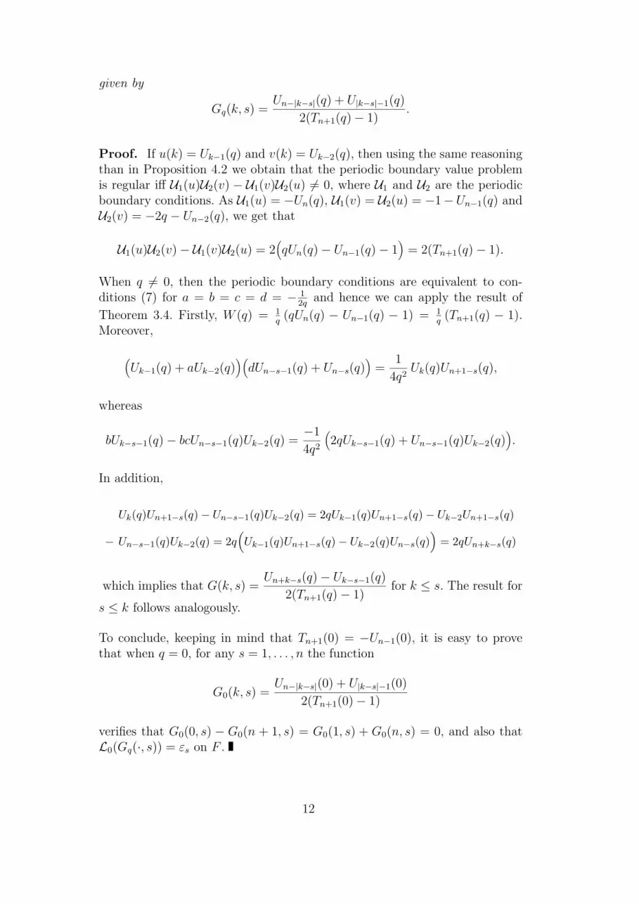
Proposition 3.6 The periodic boundary value problem is regular iff it is ver-ified that q 6= cos

(2kπn+1

), k = 0, . . . , dn+1

2e, in which case the Green function is

11

given by

Gq(k, s) =Un−|k−s|(q) + U|k−s|−1(q)

2(Tn+1(q)− 1).

Proof. If u(k) = Uk−1(q) and v(k) = Uk−2(q), then using the same reasoningthan in Proposition 4.2 we obtain that the periodic boundary value problemis regular iff U1(u)U2(v) − U1(v)U2(u) 6= 0, where U1 and U2 are the periodicboundary conditions. As U1(u) = −Un(q), U1(v) = U2(u) = −1−Un−1(q) andU2(v) = −2q − Un−2(q), we get that

U1(u)U2(v)− U1(v)U2(u) = 2(qUn(q)− Un−1(q)− 1

)= 2(Tn+1(q)− 1).

When q 6= 0, then the periodic boundary conditions are equivalent to con-ditions (7) for a = b = c = d = − 1

2qand hence we can apply the result of

Theorem 3.4. Firstly, W (q) = 1q(qUn(q) − Un−1(q) − 1) = 1

q(Tn+1(q) − 1).

Moreover,

(Uk−1(q) + aUk−2(q)

)(dUn−s−1(q) + Un−s(q)

)=

1

4q2Uk(q)Un+1−s(q),

whereas

bUk−s−1(q)− bcUn−s−1(q)Uk−2(q) =−1

4q2

(2qUk−s−1(q) + Un−s−1(q)Uk−2(q)

).

In addition,

Uk(q)Un+1−s(q)− Un−s−1(q)Uk−2(q) = 2qUk−1(q)Un+1−s(q)− Uk−2Un+1−s(q)

− Un−s−1(q)Uk−2(q) = 2q(Uk−1(q)Un+1−s(q)− Uk−2(q)Un−s(q)

)= 2qUn+k−s(q)

which implies that G(k, s) =Un+k−s(q)− Uk−s−1(q)

2(Tn+1(q)− 1)for k ≤ s. The result for

s ≤ k follows analogously.

To conclude, keeping in mind that Tn+1(0) = −Un−1(0), it is easy to provethat when q = 0, for any s = 1, . . . , n the function

G0(k, s) =Un−|k−s|(0) + U|k−s|−1(0)

2(Tn+1(0)− 1)

verifies that G0(0, s) − G0(n + 1, s) = G0(1, s) + G0(n, s) = 0, and also thatL0(Gq(·, s)) = εs on F .

12

4 One-point boundary value problems

Our aim in this section is to analyze the boundary value problems associatedwith the Schrodinger operator on a subset of a finite path with exactly onevertex on its boundary. Such a subset will be denoted by F and we can sup-pose without loss of generality that F = {0, 1, . . . , n}, which implies that itsboundary is δ(F ) = {n + 1}. The case when F = {1, . . . , n + 1} and henceδ(F ) = {0} can be carried out with obvious modifications.

In this scenario a boundary condition on F is given by

U(u) = au(n) + bu(n + 1), for any u ∈ C(F ) (13)

where we must impose that b 6= 0 in order that the condition involves thevertex on the boundary. Therefore, we can assume without loss of generalitythat

U(u) = au(n) + u(n + 1), for any u ∈ C(F ) where a ∈ C. (14)

Fixed the boundary condition U , given in (14), a boundary value problemproblem on F consists in finding u ∈ C(F ) such that

Lq(u) = f, on F , U(u) = g, (15)

for any f ∈ C(F ) and g ∈ C. In particular, the boundary value problem iscalled semihomogeneous when g = 0, whereas it is called homogeneous whenf = 0 and g = 0.

We will say that the boundary value problem (15) is regular if the correspond-ing homogenous boundary value problem Lq(u) = 0 on F and U(u) = 0 hasthe null function as its unique solution.

Analogously to the two-point boundary value problems, we can reduce thestudy of boundary value problems on F to the study of the semihomogeneousones.

Lemma 4.1 Given g ∈ C, then for any f ∈ C(F ) the function u ∈ C(F )satisfies that Lq(u) = f on F and U(u) = g iff v = u − gεn+1 satisfies that

Lq(v) = f + gεn on F and U(v) = 0.

Proposition 4.2 Let the (n+1)-order polynomial W (z) = Vn+1(z)+ aVn(z).Then the boundary value problem (15) is regular iff W (q) 6= 0 and this con-dition is equivalent to the fact that any boundary value problem has a uniquesolution.

13

Proof. If y ∈ C(F ) is a solution of the homogeneous boundary value problem,then y is a solution of the homogeneous Schrodinger equation on F . Therefore,there exist α, β ∈ C such that y(k) = αUk−1(q) + βUk−2(q) for any k ∈ F .Moreover, as Lq(y)(0) = U(y) = 0, α and β must verify

−1 1− 2q

Un(q) + aUn−1(q) Un−1(q) + aUn−2(q)

α

β

=

0

0

.

Therefore, the problem is regular iff

0 6= (2q − 1)Un(q) +[a(2q − 1)− 1

]Un−1(q)− aUn−2(q)

= Un+1(q) + Un−1(q)− Un(q) + aUn(q) + aUn−2(q)

− (1 + a)Un−1(q)− aUn−2(q) = W (q).

Newly, the last claim follows by standard arguments.

When the problem is regular we define the Green function for the boundaryvalue problem Lq(u) = f on F , U(u) = 0 as the function Gq ∈ C(F × F )characterized by

Lq(Gq(·, s)) = εs on F , U(Gq(·, s)) = 0, for any s ∈ F . (16)

We can derive expressions for the Green function in terms of Chebyshev poly-nomials.

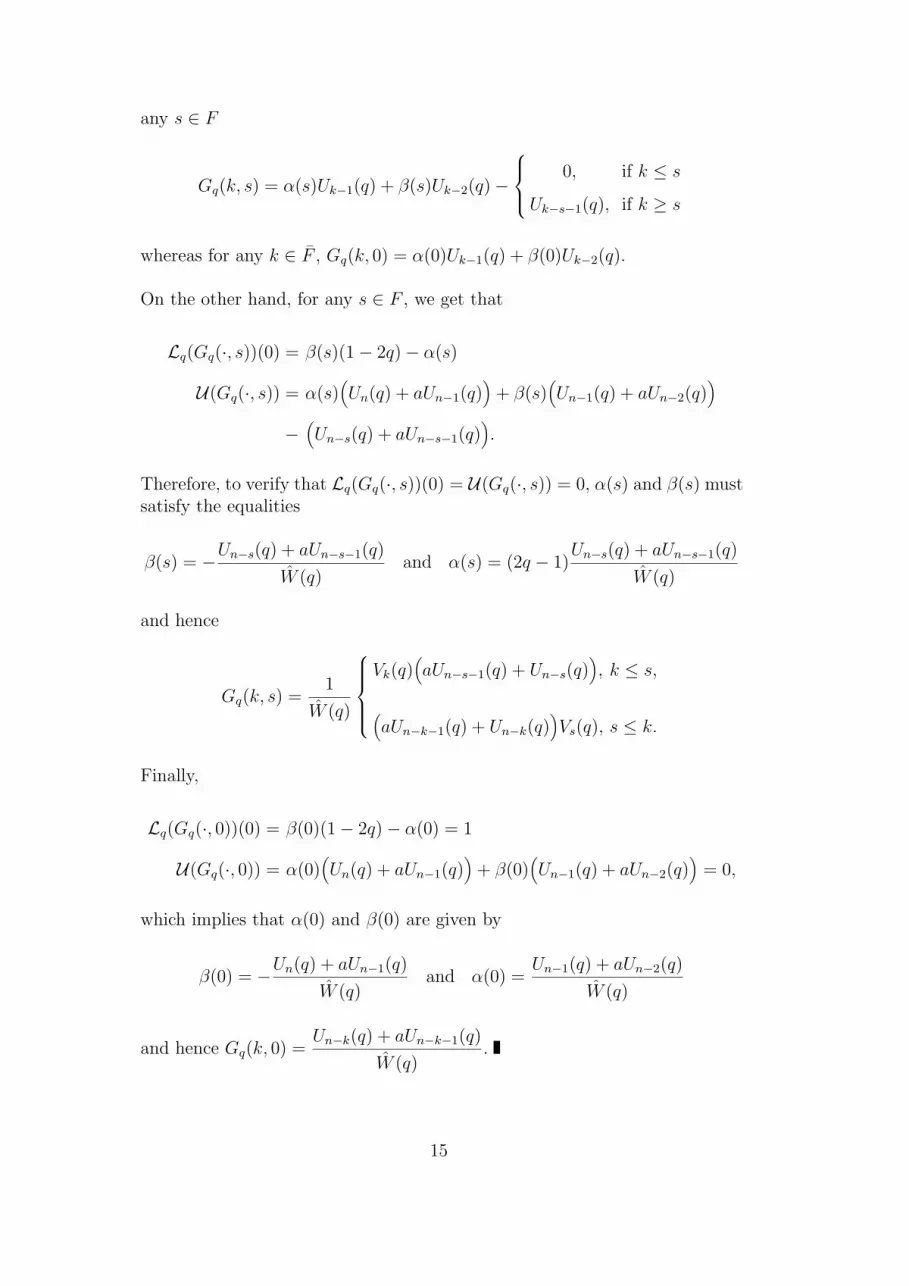
Proposition 4.3 If W (q) 6= 0, the Green function for the semihomogeneousboundary value problem Lq(u) = f on F , U(u) = 0 is given by

Gq(k, s) =

Vk(q)(aUn−s−1(q) + Un−s(q)

)Vn+1(q) + aVn(q)

, if 0 ≤ k ≤ s ≤ n,

(aUn−k−1(q) + Un−k(q)

)Vs(q)

Vn+1(q) + aVn(q), if 0 ≤ s ≤ k ≤ n + 1.

Proof. For each s ∈ F , Gq(·, s) is, in particular, a solution of a Schrodinger

equation on F and hence there exist α, β ∈ C(F ) such that for any k ∈ F and

14

any s ∈ F

Gq(k, s) = α(s)Uk−1(q) + β(s)Uk−2(q)−

0, if k ≤ s

Uk−s−1(q), if k ≥ s

whereas for any k ∈ F , Gq(k, 0) = α(0)Uk−1(q) + β(0)Uk−2(q).

On the other hand, for any s ∈ F , we get that

Lq(Gq(·, s))(0) = β(s)(1− 2q)− α(s)

U(Gq(·, s)) = α(s)(Un(q) + aUn−1(q)

)+ β(s)

(Un−1(q) + aUn−2(q)

)−

(Un−s(q) + aUn−s−1(q)

).

Therefore, to verify that Lq(Gq(·, s))(0) = U(Gq(·, s)) = 0, α(s) and β(s) mustsatisfy the equalities

β(s) = −Un−s(q) + aUn−s−1(q)

W (q)and α(s) = (2q − 1)

Un−s(q) + aUn−s−1(q)

W (q)

and hence

Gq(k, s) =1

W (q)

Vk(q)

(aUn−s−1(q) + Un−s(q)

), k ≤ s,

(aUn−k−1(q) + Un−k(q)

)Vs(q), s ≤ k.

Finally,

Lq(Gq(·, 0))(0) = β(0)(1− 2q)− α(0) = 1

U(Gq(·, 0)) = α(0)(Un(q) + aUn−1(q)

)+ β(0)

(Un−1(q) + aUn−2(q)

)= 0,

which implies that α(0) and β(0) are given by

β(0) = −Un(q) + aUn−1(q)

W (q)and α(0) =

Un−1(q) + aUn−2(q)

W (q)

and hence Gq(k, 0) =Un−k(q) + aUn−k−1(q)

W (q).

15

5 Poisson equation

In this section we study the Poisson equation associated with the Schrodingeroperator on the finite path Pn. The Poisson equation on F consists in findingu ∈ C(F ) such that Lq(u) = f on F for any f ∈ C(F ) and it is called regular ifthe corresponding homogeneous problem Lq(u) = 0 on F has the null functionas its unique solution.

Proposition 5.1 The Poisson equation is regular iff q 6= cos(

kπn+2

), for any

k = 0, . . . , n + 1 and this condition is equivalent to the fact that any Poissonequation has a unique solution.

Proof. If y ∈ C(F ) is a solution of the homogeneous Poisson equation, then yis a solution of the homogeneous Schrodinger equation on F . Therefore, thereexist α, β ∈ C such that y(k) = αUk−1(q)+βUk−2(q) for any k ∈ F . Moreover,as Lq(y)(0) = Lq(y)(n + 1) = 0, α and β must verify

−1 1− 2q

Vn+1(q) Vn(q)

α

β

=

0

0

.

Therefore, the problem is regular iff

0 6= (2q − 1)Vn+1(q)− Vn(q) = Vn+2(q)− Vn+1(q) = 2(q − 1)Un+1(q).

Newly, the last claim follows by standard arguments.

When the Poisson equation is regular we define the Green function for thePoisson equation on F as the function Gq ∈ C(F × F ) characterized by

Lq(Gq(·, s)) = εs on F , for any s ∈ F . (17)

Proposition 5.2 If q 6= cos(

kπn+2

), k = 0, . . . , n + 1, then the Green function

for the Poisson equation is given by

Gq(k, s) =1

2(q − 1) Un+1(q)

Vk(q) Vn+1−s(q), if 0 ≤ k ≤ s ≤ n + 1,

Vs(q) Vn+1−k(q), if 0 ≤ s ≤ k ≤ n + 1.

Proof. For each s ∈ F , Gq(·, s) is, in particular, a solution of a Schrodinger

equation on F and hence there exist α, β ∈ C(F ) such that for any k ∈ F and

16

any s ∈ F

Gq(k, s) = α(s)Uk−1(q) + β(s)Uk−2(q)−

0, if k ≤ s

Uk−s−1(q), if k ≥ s

whereas when s = 0, n + 1, Gq(k, s) = α(s)Uk−1(q) + β(s)Uk−2(q), for anyk ∈ F .

On the other hand, for any s ∈ F , we get that

Lq(Gq(·, s))(0) = β(s)(1− 2q)− α(s)

Lq(Gq(·, s))(n + 1) = α(s)Vn+1(q) + β(s)Vn(q)− Vn+1−s(q).

Therefore, to verify that Lq(Gq(·, s))(0) = Lq(Gq(·, s))(n + 1) = 0, α(s) andβ(s) must satisfy the equalities

β(s) = − Vn+1−s(q)

2(q − 1)Un+1(q)and α(s) = (2q − 1)

Vn+1−s(q)

2(q − 1)Un+1(q)

and hence

Gq(k, s) =1

2(q − 1)Un+1(q)

Vk(q)Vn+1−s(q), k ≤ s,

Vs(q)Vn+1−k(q), s ≤ k.

Finally, for s = 0, n + 1 we get that

Lq(Gq(·, s))(0) = β(s)(1− 2q)− α(s) = εs(0)

Lq(Gq(·, s))(n + 1) = α(s)Vn+1(q) + β(s)Vn(q) = εs(n + 1),

which imply that

α(0) =Vn(q)

2(q − 1)Un+1(q), β(0) = − Vn+1(q)

2(q − 1)Un+1(q),

α(n + 1) =2q − 1

2(q − 1)Un+1(q), β(n + 1) = − 1

2(q − 1)Un+1(q)

and hence Gq(k, 0) =Vn+1−k(q)

2(q − 1)Un+1(q)and Gq(k, n + 1) =

Vk(q)

2(q − 1)Un+1(q).

Acknowledgements

This work has been partly supported by the Spanish Research Council (ComisionInterministerial de Ciencia and Tecnologıa), under project BFM2003-06014.

17

References

[1] R.P. Agarwal, Difference equations and inequalities, Marcel Dekker,2000.

[2] F.R.K. Chung and S.T. Yau, Discrete Green’s functions, J. Combin.Theory A, 91, (2000), 191-214.

[3] R. Ellis, Chip-firing games with Dirichlet eigenvalues and discreteGreen’s functions, PhD Thesis, University of California at San Diego,2002.

[4] A. Jirari, Second-order Sturm-Liouville diference equations and orthog-onal polynomials, Memoirs of the AMS, 542, 1995.

[5] J.C. Mason and D.C. Handscomb, Chebyshev Polynomials, Chapman &Hall/CRC, 2003.

18