arX

iv:m

ath/

0606

092v

2 [

mat

h.C

A]

12

Dec

200

7 Projection formulas for orthogonal polynomials

W lodzimierz Bryc∗

Department of Mathematical SciencesUniversity of Cincinnati

Cincinnati, OH 45221-0025

Wojciech MatysiakFaculty of Mathematics and Information Science

Warsaw University of Technologypl. Politechniki 1

00-661 Warszawa, Poland

Ryszard Szwarc†

Institute of MathematicsUniversity of Wroc law,

pl. Grunwaldzki 2/4, 50-384 Wroc law, Polandand

Institute of Mathematics and Computer Science,University of Opole, ul. Oleska 48, 45-052 Opole, Poland

Jacek Weso lowskiFaculty of Mathematics and Information Science

Warsaw University of Technologypl. Politechniki 1

00-661 Warszawa, Poland

June 3, 2006; revised February 2, 2008

Abstract

We prove a projection formula for the four-parameter family of or-

thogonal polynomials that are a reparameterization of the polynomials in

the Askey-Wilson class. By carefully analyzing the recurrence relations

we manage to avoid using the explicit expression for the orthogonality

measure, which would be cumbersome due to the complexity of the repa-

rameterization.

∗Research partially supported by NSF grants #INT-03-32062, #DMS-05-04198, and bythe C.P. Taft Memorial Fund.

†Research partially supported by KBN (Poland) under grant 2 P03A 028 25

1

1 Introduction

Projection formulas of the type

qn(x) =

∫pn(y)νx(dy), (1.1)

where {νx} is a family of probability measures, are of interest in the theory oforthogonal polynomials and in probability.

Explicit formulas for the measure νx have been known since [2] when qn(x)and pn(y) are both Jacobi polynomials. These formulas were extended to pairsof Askey-Wilson polynomials in [13, 14] and to pairs of associated Askey-Wilsonpolynomials in [15]. The proofs rely on explicit evaluation of certain integrals,which is a topic of independent interest.

Projection formulas of the type (1.1) were used as a basis of constructionof certain Markov processes in [7, 9, 4, 5]. The technique of proof in thesepapers is less constructive and relies on an implicit definition of the probabilitymeasure νx as the orthogonality measure of the auxiliary family of orthogonalpolynomials. With the exception of [5], these projection formulas dealt withthe pairs of polynomials within the Askey-Wilson class and in fact differ from[13, 14] only in the allowed ranges for the parameters. The purpose of this note isto provide a related projection formula that covers one more parameter, but alsofalls into the Askey-Wilson class. Our method does not rely on the knowledgeof explicit orthogonality measures and has a more combinatorial character.

Our goal is to analyze in detail the family of orthogonal polynomials

pn(y; t) = p(η,θ,τ,q)n (y; t) which appeared in the study of stochastic processes

with linear regressions and quadratic conditional variances in [6, Theorem 4.5].Let p−1 = 0, p0 = 1. Fix η, θ ∈ R, τ ≥ 0, −1 < q ≤ 1. For t > 0, n ≥ 0 let

ypn(y; t) = pn+1(y; t) + bn(t)pn(y; t) + an−1cn(t)pn−1(y; t), (1.2)

where for η 6= 0

an = η−1 + θ[n]q + [n]2qητ, (1.3)

bn(t) = (tη + θ + ([n]q + [n − 1]q)ητ) [n]q, (1.4)

cn(t) = η(t + τ [n − 1]q)[n]q . (1.5)

For η = 0 we need to interpret an−1cn(t) as (t + τ [n − 1]q)[n]q. Our reason forthe separation of ηη−1 between two factors is that for η > 0 we have

bn(t) = an + cn(t) −1

η, (1.6)

a property which will be exploited later on. We use the notation

[n]q = 1 + q + · · · + qn−1, [n]q! = [1]q[2]q . . . [n]q,

[nk

]

q

=[n]q!

[n − k]q![k]q!,

2

with the usual conventions [0]q = 0, [0]q! = 1.Throughout this paper, by µt we denote the orthogonality measure of poly-

nomials {pn(y; t)}. A sufficient condition for existence of such a probabilitymeasure is that ηθ ≥ 0, τ ≥ 0, and 0 ≤ q ≤ 1. It is plausible that our results arevalid for a more general range of the parameters (compare [4] and [5]), but anattempt to cover such a range is likely to lead to additional technical complica-tions which should be avoided in a paper that already has a significant degreeof computational complexity.

We now compare the polynomials defined by (1.2) with the monic Askey-Wilson [3] polynomials wn for the “generic” values of parameters of the recur-rences. Recall that polynomials wn are defined by the recurrence

(x−1

2(a+a−1))wn(x) = wn+1(x)−

1

2(An +Cn)wn +

1

4An−1Cnwn−1(x), n ≥ 0,

(1.7)where

An =(1 − abcdqn−1)(1 − abqn)(1 − acqn)(1 − adqn)

a(1 − abcdq2n−1)(1 − abcdq2n),

Cn =a(1 − qn)(1 − bcqn−1)(1 − bdqn−1)(1 − cdqn−1)

(1 − abcdq2n−2)(1 − abcdq2n−1).

This form of the Askey-Wilson recurrence is a minor rewrite of the recurrencein [11, (4.3)]. The initial condition is the usual w−1 = 0 and w0 = 1.

If we multiply (1.7) by (−2α)n+1, substitute y = −2α(x− (a+ a−1)/2), andintroduce polynomials pn(y) := (−2α)nwn(x), we get the following recurrence

ypn(y) = pn+1(y) + α(An + Cn)pn(y) + α2CnAn−1pn−1(y). (1.8)

On the other hand,

an =(1 − q)2 + ηθ(1 − q) + η2τ

η(1 − q)2

(1 −

ηθ(1 − q) + 2η2τ

(1 − q)2 + ηθ(1 − q) + η2τqn

+η2τ

(1 − q)2 + ηθ(1 − q) + η2τq2n),

and

cn(t) = η(1 − q)t + τ

(1 − q)2

(1 −

τ

(1 − q)t + τqn−1

)(1 − qn).

This can be written as an = αAAn, and cn(t) = αCCn, where the Askey-Wilsonparameters are d = 0, and the remaining parameters a, b, c are determined fromthe system of three equations

a(b + c) =ηθ(1 − q) + 2η2τ

(1 − q)2 + ηθ(1 − q) + η2τ(1.9)

a2bc =η2τ

(1 − q)2 + ηθ(1 − q) + η2τ, bc =

τ

(1 − q)t + τ. (1.10)

3

The auxiliary coefficients are then

αA =(1 − q)2 + ηθ(1 − q) + η2τ

η(1 − q)2a, αC = η

(1 − q)t + τ

(1 − q)2a. (1.11)

From this and (1.6) we see that recurrence (1.2) can be re-written using a newvariable x = y + 1/η and polynomials rn(x) := pn(y) as

xrn(x) = rn+1(x) + (αAAn + αCCn)rn(x) + αAαCAn−1Cnrn−1(x), (1.12)

To see that (1.12) is equivalent to the Askey-Wilson recurrence (1.8) we onlyneed to show that αA = αC . Equations (1.10) give

a = η

√(1 − q)t + τ√

(1 − q)2 + ηθ(1 − q) + η2τ.

Inserting this into the expressions for αA and αC , we see that

αA = αC =

√(1 − q)t + τ

√(1 − q)2 + ηθ(1 − q) + η2τ

(1 − q)2.

Our main result is the following projection formula.

Theorem 1.1. If 0 ≤ s ≤ t, 0 ≤ q ≤ 1, ηθ ≥ 0, τ ≥ 0, then for all x in thesupport of the orthogonality measure µs there exists a unique probability measureνx = νx,t,s such that

pn(x; s) =

∫pn(y; t)νx(dy). (1.13)

Of course, probability measure νx = νx,t,s depends also on parameters 0 ≤s ≤ t as well as on the remaining parameters η, θ, τ, q.

Remark 1.1. Since Askey-Wilson polynomials are symmetric with respect pa-rameters b, c, d, [13, Formula (2.4)] can be written as

∫wn(y; a, b, c, d)νx(dy) = wn(x; µa, µ−1b, µ−1c, µd).

Under this parametrization, from (1.9) and (1.10) e can see that Theorem 1.1is essentially this formula with d = 0, and µ2 = ((1− q)s + τ)/(1− q)t + τ) ≤ 1.The only improvement over [13] is that due to our interest in applications toprobability, our range of parameters leads to measures νx(dy) that might havea discrete component.

The proof of Theorem 1.1 appears in Section 5.4, after a number of prelimi-nary results. The plan of the proof is as follows. In Section 5 we define a familyof monic polynomials {Qn} in variable y. We verify that the assumptions ofFavard’s theorem are satisfied for the relevant pairs (x, s), so that their orthog-onality measure νx,t,s exists. We show that this measure is unique (a fact that

4

is nontrivial only when q = 1). We then use the formula for the connectioncoefficients between polynomials {Qn} and {pn} to deduce (1.13).

When η > 0, we will find it convenient to consider the following non-monicpolynomials

ypn(y; t) = anpn+1(y; t) + bn(t)pn(y; t) + cn(t)pn−1(y; t). (1.14)

Clearly they have the same orthogonality measure µt as the monic polynomials.

2 Identities

We will need a number of auxiliary identities.

Lemma 2.1. Fix a sequence {pn : n ≥ 0} of real numbers. Let {βn,k : 0 ≤ k ≤n, n = 0, 1, . . . } be defined by βn,k = 0 for n < 0 or k > n and for 0 ≤ k ≤ n bythe recurrence

[k + 1]qβn,k+1 = qk[n − k]qβn,k + [n]qβn−1,k, (2.1)

with the initial values βn,0 = pn, n = 0, 1, . . . . Then

βn,k =

[nk

]

q

k∑

j=0

[kj

]

q

q(k−j)(k−j−1)/2pn−j . (2.2)

Proof. This follows by a routine induction argument with respect to k. Clearly(2.2) holds true for k = 0 and all n ≥ 0. Suppose (2.2) holds true for somek ≥ 0 and all n ≥ 0. Then by (2.1) and the induction assumption, we have

βn,k+1 =[n − k]q[k + 1]q

[nk

]

q

k∑

j=0

[kj

]

q

qk+(k−j)(k−j−1)/2pn−j+

[n]q[k + 1]q

[n − 1

k

]

q

k∑

j=0

[kj

]

q

q(k−j)(k−j−1)/2pn−1−j

=

[n

k + 1

]

q

pn−(k+1) +

[n

k + 1

]

q

q(k+1)k/2pn

+

[n

k + 1

]

q

k∑

j=1

(qj

[kj

]

q

+

[k

j − 1

]

q

)q(k+1−j)(k−j)/2pn−j .

The well known formula [10, (I.45)]

[k + 1

j

]

q

= qj

[kj

]

q

+

[k

j − 1

]

q

=

[kj

]

q

+qk−j+1

[k

j − 1

]

q

, 1 ≤ j ≤ k,

(2.3)ends the proof.

5

It turns out that expressions of the form (2.2) can sometimes be written asproducts.

Proposition 2.2. If polynomials {pn(y; t)} satisfy recurrence (1.14) and

An(x, s) = an + qnx − sηqn[n]q , (2.4)

then for all k ≥ 1 we have

k∑

j=0

[kj

]

q

q(k−j)(k−j−1)/2pk−j(x; s) =

k−1∏

j=0

Aj(x, s)

aj. (2.5)

Proof. We proceed by induction with respect to k. Formula (2.5) holds true fork = 0 by convention, and for k = 1 by a calculation: p1(x; s)+p0(x; s) = 1+ηx.

Let βn,k(x, s) be defined by (2.2) with pn = pn(x; s), n = 0, 1, . . . . Theinduction assumption says that

βk,k(x, s) =

k−1∏

j=0

Aj(x, s)

aj(2.6)

for some k ≥ 1. From (2.1) we see that

βk+1,k+1(x, s) = βk,k(x, s) + qkk∑

j=0

[kj

]

q

q(k−j)(k−j−1)/2pk+1−j(x; s). (2.7)

On the other hand, multiplying both sides of (2.6) by Ak(x,s)ak

= 1 +x−sη[k]q

akqk

and using (1.14) we see that

k∏

j=0

Aj(x, s)

aj= βk,k(x, s) − qk sη[k]q

ak

k∑

j=0

[kj

]

q

q(k−j)(k−j−1)/2pk−j(x; s)

+qk

ak

k∑

j=0

[kj

]

q

q(k−j)(k−j−1)/2(ak−jpk+1−j(x; s) + bk−j(s)pk−j(x; s)

+ ck−j(s)pk−1−j(x; s)). (2.8)

Writing the right hand side of (2.8) as

βk,k(x, s) +qk

ak

k+1∑

j=0

[kj

]

q

q(k−j)(k−j−1)/2γk,jpk+1−j(x; s), (2.9)

from (1.3), (1.4) and (1.5) it is not difficult to see that γk,0 = ak and γk,k+1 =

6

−sη[k]q + sη[k]q = 0. Similarly, for 1 ≤ j ≤ k we have

γk,j = ak−j +qk−j [j]q

[k + 1 − j]q(bk+1−j(s) − sη[k]q)

+q2k−2j+1[j]q[j − 1]q

[k + 2 − j]q[k + 1 − j]qck+2−j(s) = η−1 + θ[k − j]q + ητ [k − j]2q + [j]qθq

k−j

+ ητ([j]q[k + 1 − j]qq

k−j + [j]q[k − j]qqk−j + [j]q[j − 1]qq

2k+1−2j)

= η−1 + θ([k − j]q + qk−j [j]q

)

+ ητ([k − j]q

([k − j]q + qk−j [j]q

)+ [j]qq

k−j([k + 1 − j]q + [j − 1]qq

k+1−j))

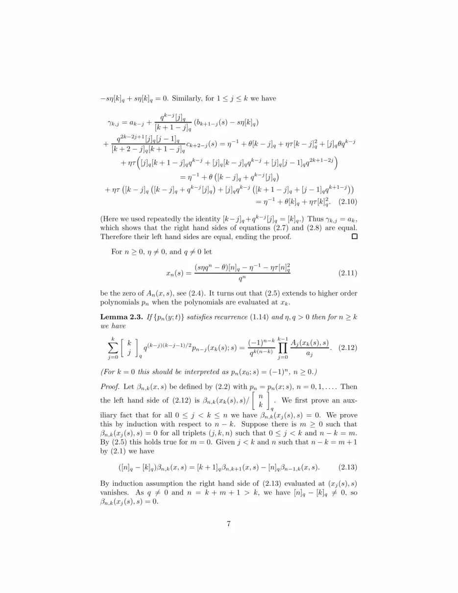
= η−1 + θ[k]q + ητ [k]2q . (2.10)

(Here we used repeatedly the identity [k−j]q +qk−j [j]q = [k]q.) Thus γk,j = ak,which shows that the right hand sides of equations (2.7) and (2.8) are equal.Therefore their left hand sides are equal, ending the proof.

For n ≥ 0, η 6= 0, and q 6= 0 let

xn(s) =(sηqn − θ)[n]q − η−1 − ητ [n]2q

qn(2.11)

be the zero of An(x, s), see (2.4). It turns out that (2.5) extends to higher orderpolynomials pn when the polynomials are evaluated at xk.

Lemma 2.3. If {pn(y; t)} satisfies recurrence (1.14) and η, q > 0 then for n ≥ kwe have

k∑

j=0

[kj

]

q

q(k−j)(k−j−1)/2pn−j(xk(s); s) =(−1)n−k

qk(n−k)

k−1∏

j=0

Aj(xk(s), s)

aj. (2.12)

(For k = 0 this should be interpreted as pn(x0; s) = (−1)n, n ≥ 0.)

Proof. Let βn,k(x, s) be defined by (2.2) with pn = pn(x; s), n = 0, 1, . . . . Then

the left hand side of (2.12) is βn,k(xk(s), s)/

[nk

]

q

. We first prove an aux-

iliary fact that for all 0 ≤ j < k ≤ n we have βn,k(xj(s), s) = 0. We provethis by induction with respect to n − k. Suppose there is m ≥ 0 such thatβn,k(xj(s), s) = 0 for all triplets (j, k, n) such that 0 ≤ j < k and n − k = m.By (2.5) this holds true for m = 0. Given j < k and n such that n− k = m + 1by (2.1) we have

([n]q − [k]q)βn,k(x, s) = [k + 1]qβn,k+1(x, s) − [n]qβn−1,k(x, s). (2.13)

By induction assumption the right hand side of (2.13) evaluated at (xj(s), s)vanishes. As q 6= 0 and n = k + m + 1 > k, we have [n]q − [k]q 6= 0, soβn,k(xj(s), s) = 0.

7

We now prove (2.12). From (1.6) it is easy to see by induction thatpn(x0; s) = pn(−η−1; s) = (−1)n. For k ≥ 1, we will prove (2.12) by induc-tion with respect to n.

If n = k then formula (2.12) holds by Proposition 2.2. Suppose (2.12) holdsfor some n ≥ k. Then from (2.1) and the fact that βn+1,k+1(xk(s), s) = 0 wesee that

βn+1,k(xk(s), s) = −[n + 1]q

qk[n + 1 − k]qβn,k(xk(s), s)

= −[n + 1]q

qk[n + 1 − k]q

[nk

]

q

(−1)n−k

qk(n−k)

k−1∏

j=0

Aj(xk(s), s)

aj.

Therefore,

k∑

j=0

[kj

]

q

q(k−j)(k−j−1)/2pn+1−j(xk(s); s) =βn+1,k(xk(s), s)[

n + 1k

]

q

=(−1)n+1−k

qk(n+1−k)

k−1∏

j=0

Aj(xk(s), s)

aj.

We need to analyze equation (2.12) in more detail.

Lemma 2.4. Fix k ≥ 1, q 6= 0, Πk > 0. Suppose that (pn)n≥0 is the generalsolution of the recurrence

k∑

j=0

[kj

]

q

q(k−j)(k−j−1)/2pn−j =(−1)n−k

qk(n−k)Πk, n ≥ k. (2.14)

Then

pn = (−1)n−kq−nkqk(k+1)/2

([nk

]

q

+

k∑

r=1

Crqnr

[n

k − r

]

q

)Πk, n ≥ 0,

(2.15)where C1, . . . , Ck are arbitrary constants.

Proof. Substitute

yn =(−1)n−kqk(2n−k−1)/2

Πkpn.

Then with y = (yn)n≥0 the equation takes the form of an initial value problemfor a linear recurrence with constant coefficients:

(∆q,ky)n = 1, n ≥ k, (2.16)

8

where

(∆q,ky)n =

k∑

j=0

(−1)j

[kj

]

q

qj(j+1)/2yn−j.

We remark that when q = 1 we trivially have ∆1,k = ∆k1,1. Since ∆1,1 is

the usual difference operator, in this case the general solution of (2.16) is wellknown. The q-generalization of this formula follows from (2.3) by inductionwith respect to k. We have

∆q,k = R1R2 . . . Rk, (2.17)

where Rj = ∆qj ,1 are commuting difference operators, (Rjy)n = yn − qjyn−1

for n ≥ 1.The general theory of linear difference equations implies that (2.15) is a

consequence of the following two observations.

Claim 2.5. (i) (∆q,ky)n = 1 for n ≥ k when

yn =

[nk

]

q

, (2.18)

(ii) (∆q,ky)n = 0 for n ≥ k − r when

yn =

[n

k − r

]

q

qrn, r = 1, 2, . . . , k. (2.19)

Proof of Claim 2.5. We note that (2.18) is just r = 0 case of (2.19).For fixed r ≥ 0 and n ≥ k ≥ r we have

(Rk

([n

k − r

]

q

qrn

))

n

=

[n

k − r

]

q

qrn −

[n − 1k − r

]

q

qrn+k−r

= qrn [n − k + r + 1]q . . . [n − 1]q[k − r]q!

([n]q − qk−r[n − k + r]q

)

= qrn [n − k + r + 1]q . . . [n − 1]q[k − r]q !

[k − r]q

=

[n − 1

k − 1 − r

]

q

qrn.

Therefore(

Rr+1Rr+2 . . . Rk

([n

k − r

]

q

qrn

))

n

=

[n − k + r

0

]

q

qrn = qrn.

If r = 0 this implies (2.18) by (2.17). If r ≥ 1 then to prove (2.19) it remains tonotice that since n ≥ k ≥ r ≥ 1 we have (Rr(q

nr))n = qrn − qrq(n−1)r = 0.

9

The constants C1, . . . , Ck are determined from the condition that formula(2.15) holds for p0, . . . , pk−1.

Proposition 2.6. Suppose {pn(y; t)} satisfies recurrence (1.14). Then thereare constants ck(s) that do not depend on n such that:

(i) if 0 < q < 1 then |pn(xk(s); s)| ≤ ck(s)q−kn;

(ii) if q = 1 then |pn(xk(s); s)| ≤ ck(s)nk.

Proof. This follows from (2.15) and (2.12).

3 Uniqueness of the moment problem

Proposition 3.1. Suppose 0 ≤ q ≤ 1, η > 0, θ ≥ 0, τ ≥ 0. Let {pn(y; t)} bedefined by (1.14). Then the orthogonality measure µt of polynomials {pn(y; t)}is determined uniquely by moments.

Proof. For |q| < 1, the coefficients of the recurrence are bounded, so the onlycase that requires proof is q = 1. Furthermore, the conclusion holds for τ = 0,as in this case µt is a negative binomial law, see [8]. It therefore remains toconsider the case q = 1, τ > 0.

In this case, we use the fact that with x0 = −η−1 we have pn(x0; t) =(−1)n, see Lemma 2.3. Let qn(y; t) be the associated polynomials which satisfyrecurrence (1.14) for n ≥ 1 with the initial terms q0 = 0, q1 = 1/a0. Then

x0qn(x0) = anqn+1(x0) + (an + cn + x0)qn(x0) + cnqn−1(x0).

Therefore with fn(t) := (−1)n−1qn(x0; t) we have

fn+1 − fn =cn(t)

an(fn − fn−1) =

c1(t)c2(t) . . . cn(t)

a1a2 . . . an(f1 − f0)

=c1(t)c2(t) . . . cn(t)

a0a2 . . . an−1

1

an.

Thus with a suitable convention for n = 1 we can write the solution as

fn+1(t) =

n∑

k=0

c1(t)c2(t) . . . ck(t)

a0a2 . . . ak−1

1

ak. (3.1)

Let

pn(x; t) =

√a0a2 . . . an−1

c1(t)c2(t) . . . cn(t)pn(x; t) (3.2)

and

qn(x; t) =

√a0a2 . . . an−1

c1(t)c2(t) . . . cn(t)qn(x; t)

be the corresponding orthonormal polynomials.

10

By [1, page 84], the moment problem is determined uniquely, if

∑

n

|pn(x0)|2 +

∑

n

|qn(x0)|2 = ∞. (3.3)

We have|pn(x0)|

2 =a0a2 . . . an−1

c1(t)c2(t) . . . cn(t),

and from (3.1) we get

|qn(x0)|2 =

a0a2 . . . an−1

c1(t)c2(t) . . . cn(t)

(n∑

k=0

c1(t)c2(t) . . . ck(t)

a0a2 . . . ak−1

1

ak

)2

.

To verify (3.3) we use the fact that

an ≈ ητn2,cn+1(t)

an= 1+

α(t)

n+O(1/n2),

an

cn+1(t)= 1−

α(t)

n+O(1/n2), (3.4)

where

α(t) =tη − θ

ητ+ 1, (3.5)

and an ≈ bn means that an/bn → 1.If t ≤ θ/η then α(t) ≤ 1 and

n∏

k=1

(1 −

α(t)

k

)≈ exp

(−α(t)

n∑

k=1

1

k

)≈ n−α(t) ≥ n−1,

so the first series in (3.3) diverges. On the other hand, if t > θ/η so thatα(t) > 1, then

|qn(x0)|2 ≈ n−α(t)

(n−1∑

k=1

kα(t) 1

k2

)2

≈ n−α(t)(nα(t)−1

)2

= nα(t)−2 > n−1,

so the second series in (3.3) diverges.

4 Support of the orthogonality measure

Recall that µt denotes the orthogonality measure of polynomials {pn(y; t)}. Thefollowing result will be used to define the orthogonality measure of auxiliarypolynomials in Section 5.

Proposition 4.1. Suppose 0 ≤ q ≤ 1, η > 0, θ ≥ 0, τ ≥ 0. If x ∈ supp(µs),then

n∏

j=0

Aj(x, s) ≥ 0 for all n ≥ 0. (4.1)

11

We prove Proposition 4.1 from rudimentary information about the supportof µs.

Lemma 4.2. Let xj(t) be given by (2.11). Then the support of µt is a subsetof the interval [x0(t),∞). In addition, if t > θ

η + 1−qη2 then

supp(µt) ⊂ {x0(t), x1(t), . . . , xk∗(t)} ∪ [y∗,∞)

with y∗ = max{xk∗(t), xk∗+1(t)} and

k∗ =

max{k : t > θ

η + 2τk}

, q = 1;

max

{k : q2k >

(1 − q)2 + (1 − q)ηθ + η2τ

η2(t(1 − q) + τ)

}, 0 < q < 1.

(4.2)

Remark 4.1. We note that y∗ = xm∗(t) with

m∗ =

{max{j : t > θ

η + 2τj − 1}, q = 1;

max{j : q2j−1η2(t(1 − q) + τ) > (1 − q)2 + (1 − q)ηθ + η2τ}, q < 1.

We will use the following criterion to show that there are at most k∗ + 1atoms below y∗.

Theorem A. Suppose pn(x) are orthogonal polynomials with unique orthog-onality measure µ. If the sequence {(−1)npn(a) : n ≥ 0} changes sign k-times,then there is a finite set D with at most k points such that

supp(µt) ⊂ D ∪ [a,∞).

In particular, µ has at most k atoms in (−∞, a).

Proof. This follows from the interlacing property of zeros of orthogonal polyno-mials. The details are omitted.

Proof of Lemma 4.2. We first observe that supp(µs) ⊂ [−η−1,∞). This followsfrom the fact that by Proposition 3.1 measure µs is determined uniquely, so wecan combine Lemma 2.3 applied to k = 0 with Theorem A applied to a = x0 =−η−1.

We now verify that if t > θη + 1−q

η2 then there are k∗ + 1 atoms at

{x0(t), x1(t), . . . , xk∗(t)}. Recall that xj(t) is an atom of µt if the orthonor-

mal polynomials (3.2) are square-summable at x = xj(t), see [1, page 84]. Wewill consider separately the cases q = 1 and 0 < q < 1.

Suppose q = 1. Then by Proposition 2.6 we have

∑

n

|pn(xj ; t)|2 ≤ cj

∑

n

n2j a0a2 . . . an−1

c1(t)c2(t) . . . cn(t)≈ cj

∑

n

n2j−α(t).

(See (3.5).) Therefore from (3.4), the series converges if t > θη + 2jτ .

12

Suppose now that 0 < q < 1. Then by Proposition 2.6 we have

∑

n

|pn(xj ; t)|2 ≤ cj

∑

n

q−2nj a0a2 . . . an−1

c1(t)c2(t) . . . cn(t).

Since

limn→∞

an

cn+1(t)=

(1 − q)2 + (1 − q)ηθ + η2τ

η2(t(1 − q) + τ),

the series converges if (1−q)2+(1−q)ηθ+η2τq2jη2(t(1−q)+τ) < 1. This proves that xj(t), 0 ≤ j ≤ k∗

is an atom under the condition (4.2).To estimate that there are at most k∗ +1 atoms below y∗ we use Lemma 2.4

to verify that there are at most k atoms of µt below xk(t). Namely, Lemma 2.4states that there exists a polynomial r(x) of degree k such that

pn(xk(t); t) =

{r(n), q = 1;

r(q−n), 0 < q < 1.

Since r(x) = 0 has at most k real solutions, the sequence {pn(xk(t); t) : n ≥ 0}has at most k changes of sign. Proposition 3.1 implies that we can use TheoremA to end the proof.

Proof of Proposition 4.1. If q = 0 then An(x, s) = η−1 does not depend on xfor n ≥ 1. Since A0(x, s) = 1/η + θ + ητ + x, (4.1) follows from supp(µs) ⊂[−η−1,∞).

In the remaining part of the proof, we assume 0 < q ≤ 1. We use the trivialobservation that Aj(x, s) increases as a function of x and decreases as a functionof s.

Suppose 0 ≤ s ≤ θ/η + (1 − q)/η2. From x ∈ supp(µs) ⊂ [−η−1,∞) we get

An(x, s) ≥ An

(−

1

η,θ

η+

1 − q

η2

)=

(1 − qn)2

η+ θ[n]q(1 − qn) + [n]2qητ ≥ 0.

Thus (4.1) holds.Suppose s > θ/η + (1 − q)/η2 so that k∗ = k∗(s) ≥ 0 is well defined. We

notice that

x0(s) ≤ x1(s) ≤ · · · ≤ xk∗(s) ≤ y∗ and xj(s) ≤ y∗ for all j > k∗. (4.3)

Omitting the easier case of q = 1, write xn(s) = h(qn), where

h(z) = −1

ηz+

(1 − z) (szη − θ)

z(1 − q)−

(1 − z)2ητ

z (1 − q)2 .

A calculation shows that

h′′(z) = −2(1 − q) (1 − q + ηθ) + η2τ

(1 − q)2z3η

< 0

13

on the interval 0 < z < 1. Since h tends to −∞ at the endpoints, therefore ithas a unique maximum z∗ ∈ (0, 1) given by

z2∗η

2 ((1 − q) s + τ) = (1 − q) (1 − q + ηθ) + η2τ.

In particular, qk∗+1 ≤ z∗ < qk∗ , so h(z) increases on (0, qk∗+1) and decreases on(qk∗ , 1]. Thus h(qk∗+1) ≥ h(qk∗+2) ≥ . . . , and h(q0) ≤ h(q1) ≤ · · · ≤ h(qk∗).

Inequality (4.3) ends the proof as follows. If x = xk(s) for some k ≤ k∗ thenAj(x, s) ≥ Aj(xj(s), s) = 0 for 0 ≤ j ≤ k, so (4.1) holds for 0 ≤ n < k. On theother hand, Ak(x, s) = 0, so (4.1) holds trivially for all n ≥ k.

Suppose now that x ≥ y∗. Then (4.3) implies Aj(x, s) ≥ Aj(y∗, s) ≥Aj(xj(s), s) = 0 for all j = 0, 1, 2 . . . . Thus (4.1) follows.

5 Auxiliary polynomials

For the proof of Theorem 1.1 we construct measure ν as a measure of orthogo-nality of auxiliary monic polynomials Qn(y; x, t, s) in variable y. We begin witha non-monic version of these polynomials, defined by the three step recurrence

y Qn(y; x, t, s) = An(x, s)Qn+1(y; x, t, s) + Bn(x, t, s)Qn(y; x, t, s)

+ Cn(t, s)Qn−1(y; x, t, s), (5.1)

where An is defined by (2.4) and

Bn(x, t, s) = bn(t) + qnx − (1 + q)qn−1ηs[n]q , (5.2)

Cn(t, s) = cn(t) − qn−1ηs[n]q . (5.3)

with Q−1 = 0, Q0 = 1. The Jacobi matrix of this recurrence arises as a solutionof the q-commutation equation [6, (1)] with the appropriately modified initialcondition; for more details see [5]. Polynomials {Qn} are well defined for allx, s, t as long as x 6∈ {x0(s), x1(s), . . . }.

5.1 Connection Coefficients

For x 6∈ {x0(s), x1(s), . . . }, the connection coefficients βn,k(x, t, s) are definedimplicitly by

pn(y; t) =

n∑

k=0

βn,k(x, t, s)Qk(y; x, t, s). (5.4)

Our next goal is to find the connection coefficients βn,k(x, t, s) explicitly and toshow that they do not depend on t.

Define two linear operators K, L : R∞ → R

∞ acting on infinite matricesβ = [βn,k]n,k≥0 by the rule

[Kβ]n,k = anβn+1,k + bn(t)βn,k + cn(t)βn−1,k,

14

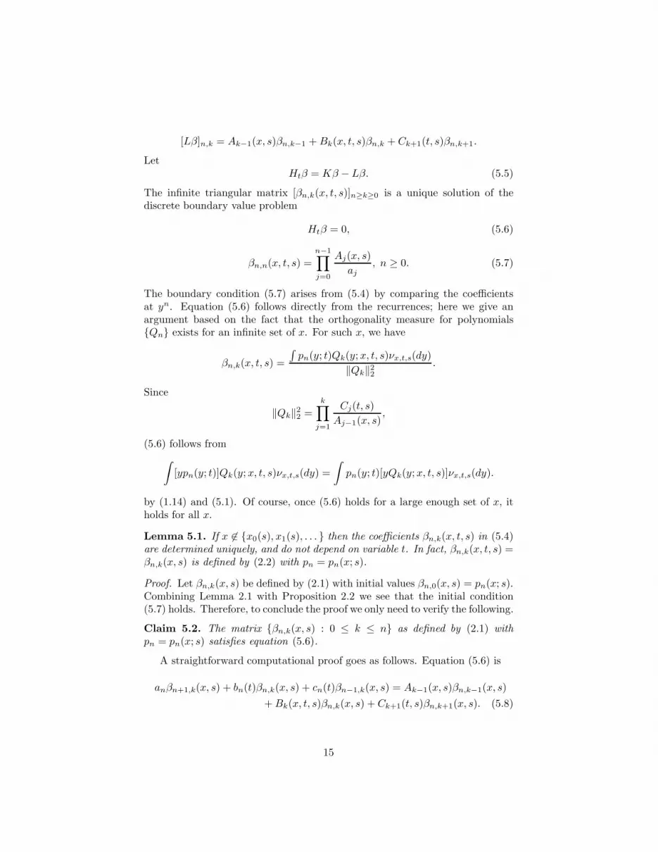
[Lβ]n,k = Ak−1(x, s)βn,k−1 + Bk(x, t, s)βn,k + Ck+1(t, s)βn,k+1.

LetHtβ = Kβ − Lβ. (5.5)

The infinite triangular matrix [βn,k(x, t, s)]n≥k≥0 is a unique solution of thediscrete boundary value problem

Htβ = 0, (5.6)

βn,n(x, t, s) =n−1∏

j=0

Aj(x, s)

aj, n ≥ 0. (5.7)

The boundary condition (5.7) arises from (5.4) by comparing the coefficientsat yn. Equation (5.6) follows directly from the recurrences; here we give anargument based on the fact that the orthogonality measure for polynomials{Qn} exists for an infinite set of x. For such x, we have

βn,k(x, t, s) =

∫pn(y; t)Qk(y; x, t, s)νx,t,s(dy)

‖Qk‖22

.

Since

‖Qk‖22 =

k∏

j=1

Cj(t, s)

Aj−1(x, s),

(5.6) follows from

∫[ypn(y; t)]Qk(y; x, t, s)νx,t,s(dy) =

∫pn(y; t)[yQk(y; x, t, s)]νx,t,s(dy).

by (1.14) and (5.1). Of course, once (5.6) holds for a large enough set of x, itholds for all x.

Lemma 5.1. If x 6∈ {x0(s), x1(s), . . . } then the coefficients βn,k(x, t, s) in (5.4)are determined uniquely, and do not depend on variable t. In fact, βn,k(x, t, s) =βn,k(x, s) is defined by (2.2) with pn = pn(x; s).

Proof. Let βn,k(x, s) be defined by (2.1) with initial values βn,0(x, s) = pn(x; s).Combining Lemma 2.1 with Proposition 2.2 we see that the initial condition(5.7) holds. Therefore, to conclude the proof we only need to verify the following.

Claim 5.2. The matrix {βn,k(x, s) : 0 ≤ k ≤ n} as defined by (2.1) withpn = pn(x; s) satisfies equation (5.6).

A straightforward computational proof goes as follows. Equation (5.6) is

anβn+1,k(x, s) + bn(t)βn,k(x, s) + cn(t)βn−1,k(x, s) = Ak−1(x, s)βn,k−1(x, s)

+ Bk(x, t, s)βn,k(x, s) + Ck+1(t, s)βn,k+1(x, s). (5.8)

15

In view of (2.1), and using the explicit form (1.4), (1.5) we verify that the coeffi-cients at variable t of this equation cancel out. Therefore, in (5.8) without loss of

generality we may take t = 0. We now write βn,k(x, s) as∑k

j=0 γn,k,jpn−j(x; s)where according to (2.2), we have

γn,k,j = q(k−j)(k−j−1)/2 [n]q!

[n − k]q![j]q![k − j]q!. (5.9)

(We will also use the conventions that γn,k,j = 0 unless 0 ≤ k ≤ n and 0 ≤j ≤ k.) Then (5.8) is equivalent to a number of identities that arise fromcomparing the coefficients at pn−j(x; s). Here we use (1.14) to rewrite theterms Ak(x, s)pn−j(x; s) and Bk(x, 0, s)pn−j(x; s) as the linear combinations ofthe polynomials {pr(x; s)}. We get

anγn+1,k,j+1 + bn(0)γn,k,j + cn(0)γn−1,k,j−1 = ak−1γn,k−1,j

− sηqk−1[k − 1]qγn,k−1,j + qk−1an−j−1γn,k−1,j+1 + qk−1bn−j(s)γn,k−1,j

+ qk−1cn+1−j(s)γn,k−1,j−1 + bk(0)γn,k,j − (1 + q)qk−1sη[k]qγn,k,j

+ qkan−j−1(s)γn,k,j+1 + qkbn−j(s)γn,k,j

+ qkcn+1−j(s)γn,k,j−1 + ck+1(0)γn,k+1,j − sηqk[k + 1]qγn,k+1,j . (5.10)

Using the identities

γn,k−1,j

γn,k,j= qj−k+1 [k − j]q

[n − k + 1]q,

γn,k−1,j−1

γn,k,j=

[j]q[n − k + 1]q

,

γn,k+1,j

γn,k,j= qk−j [n − k]q

[k + 1 − j]q,

γn+1,k,j+1

γn,k,j= qj−k+1 [n + 1]q[k − j]q

[n − k + 1]q[j + 1]q,

γn−1,k,j−1

γn,k,j= qk−j [n − k]q[j]q

[n]q[k + 1 − j]q,

γn,k,j+1

γn,k,j= qj−k+1 [k − j]q

[j + 1]q,

γn,k,j−1

γn,k,j= qk−j [j]q

[k + 1 − j]q,

γn,k−1,j+1

γn,k,j= q2j−2k+3 [k − j]q[k − j − 1]q

[n − k + 1]q[j + 1]q,

equation (5.10) reduces to the following two identities between q-numbers. Thefirst identity comes from comparing the coefficients at s,

0 = −qj [k − 1]q[k − j]q[n − k + 1]q

+ qj [n − j]q[k − j]q[n − k + 1]q

+ qk−1 [n + 1 − j]q[j]q[n − k + 1]q

− (1+ q)qk−1[k]q + qk[n− j]q + q2k−j [n + 1 − j]q[j]q[k + 1 − j]q

− q2k−j [k + 1]q[n − k]q[k + 1 − j]q

.

(5.11)

16

The second identity arises from comparing the coefficients free of s,

anqj−k+1 [n + 1]q[k − j]q[n + 1 − k]q[j + 1]q

+ bn(0) − bk(0) + cn(0)qk−j [n − k]q[j]q[n]q[k + 1 − j]q

= ak−1qj−k+1 [k − j]q

[n + 1 − k]q+ an−j−1q

2j−k+2 [k − j]q[k − j − 1]q[n + 1 − k]q[j + 1]q

+ bn−j(0)qj [k − j]q[n + 1 − k]q

+ cn+1−j(0)qk−1 [j]q[n + 1 − k]q

+ an−j−1qj+1 [k − j]q

[j + 1]q

+ bn−j(0)qk + cn+1−j(0)q2k−j [j]q[k + 1 − j]q

+ ck+1(0)qk−j [n − k]q[k + 1 − j]q

. (5.12)

Identities (5.11) and (5.12) are in the form suitable for computer-assisted veri-fication. We used Mathematica to confirm their validity.

5.2 Monic polynomials

Let Qn(y; x, t, s) denote the monic version of polynomials Qn; these polynomialssatisfy the recurrence

yQn(y; x, t, s) = Qn+1(y; x, t, s) + Bn(x, t, s)Qn(y; x, t, s)

+ An−1(x, s)Cn(t, s)Qn−1(y; x, t, s), n ≥ 0, (5.13)

with the usual initial conditions Q−1 = 0, Q0 = 1. Here An, Bn, Cn are defined

by (2.4), (5.2), and (5.3), respectively. Let pn(y; t) = Qn(y; 0, t, 0) be the monicversion of polynomials pn. The monic polynomials {Qn} are well defined for allx, s, leading to the following version of Lemma 5.1.

Corollary 5.3. Suppose 0 ≤ q ≤ 1, η > 0, θ ≥ 0, τ ≥ 0. For all s, t > 0,x, y ∈ R we have

pn(y; t) =n∑

k=0

βn,k(x, s)Qk(y; x, t, s), n ≥ 0. (5.14)

Proof. Suppose x 6∈ {x0(s), x1(s), . . . }. Then polynomials Qn(y; x, t, s) are welldefined and from Lemma 5.1 we know that (5.4) holds with βn,k(x, t, s) =βn,k(x, 0, s) which do not depend on t.

It is well known that the monic polynomials Qn can be written as

Qn(y; x, t, s) =Qn(y; x, t, s)∏n−1

j=0 Aj(x, s). (5.15)

Therefore for such x 6∈ {x0(s), x1(s), . . . }, we get (5.14) with

βn,k(x, s) =βn,k(x, 0, s)

∏k−1j=0 Aj(x, s)

∏n−1j=0 aj

. (5.16)

We now extend this relation to all x. From (2.1) and (5.16) we see that (5.14)is a relation between the polynomials in variable x and holds on an infinite setof x. Therefore, it extends to all x ∈ R.

17

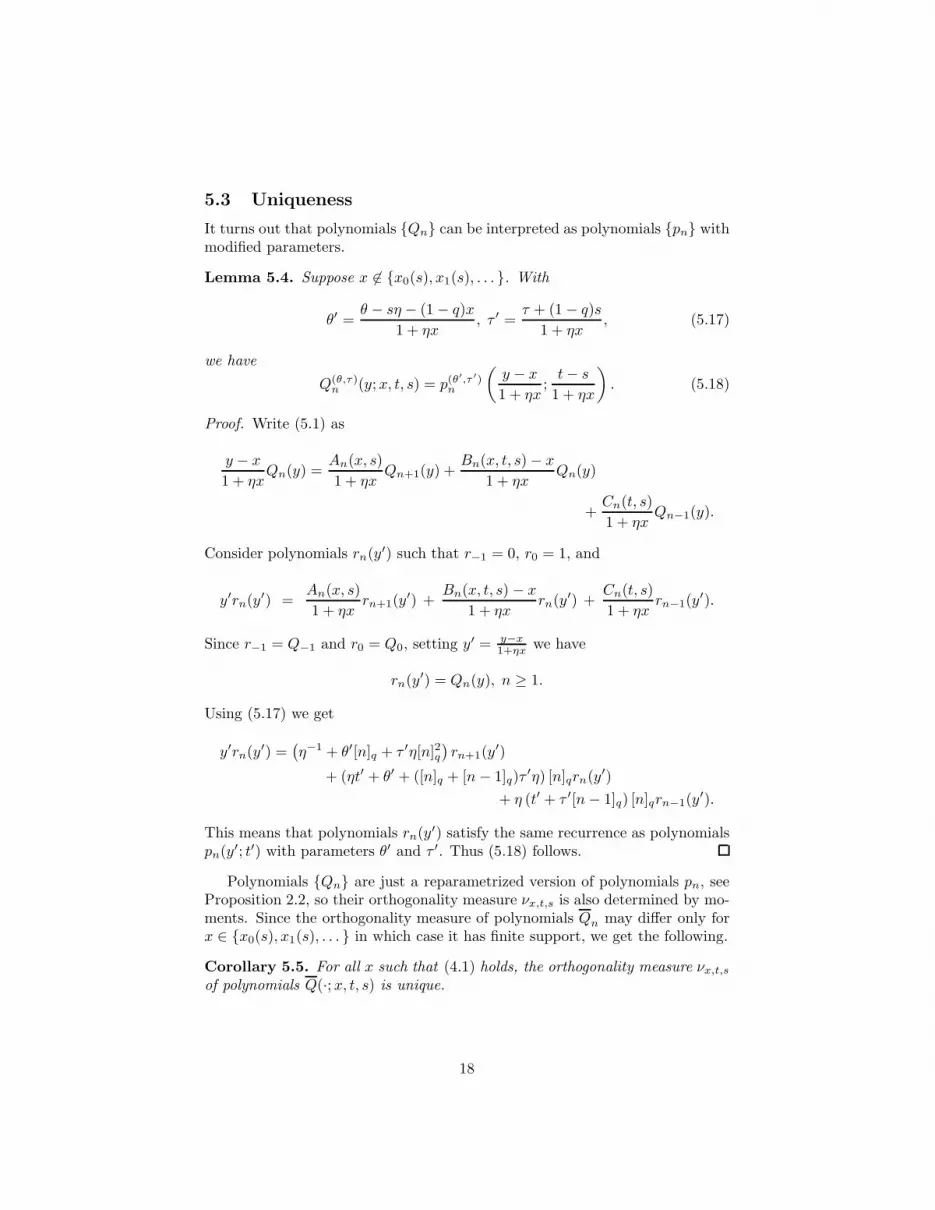
5.3 Uniqueness

It turns out that polynomials {Qn} can be interpreted as polynomials {pn} withmodified parameters.

Lemma 5.4. Suppose x 6∈ {x0(s), x1(s), . . . }. With

θ′ =θ − sη − (1 − q)x

1 + ηx, τ ′ =

τ + (1 − q)s

1 + ηx, (5.17)

we have

Q(θ,τ)n (y; x, t, s) = p(θ′,τ ′)

n

(y − x

1 + ηx;

t − s

1 + ηx

). (5.18)

Proof. Write (5.1) as

y − x

1 + ηxQn(y) =

An(x, s)

1 + ηxQn+1(y) +

Bn(x, t, s) − x

1 + ηxQn(y)

+Cn(t, s)

1 + ηxQn−1(y).

Consider polynomials rn(y′) such that r−1 = 0, r0 = 1, and

y′rn(y′) =An(x, s)

1 + ηxrn+1(y

′) +Bn(x, t, s) − x

1 + ηxrn(y′) +

Cn(t, s)

1 + ηxrn−1(y

′).

Since r−1 = Q−1 and r0 = Q0, setting y′ = y−x1+ηx we have

rn(y′) = Qn(y), n ≥ 1.

Using (5.17) we get

y′rn(y′) =(η−1 + θ′[n]q + τ ′η[n]2q

)rn+1(y

′)

+ (ηt′ + θ′ + ([n]q + [n − 1]q)τ′η) [n]qrn(y′)

+ η (t′ + τ ′[n − 1]q) [n]qrn−1(y′).

This means that polynomials rn(y′) satisfy the same recurrence as polynomialspn(y′; t′) with parameters θ′ and τ ′. Thus (5.18) follows.

Polynomials {Qn} are just a reparametrized version of polynomials pn, seeProposition 2.2, so their orthogonality measure νx,t,s is also determined by mo-ments. Since the orthogonality measure of polynomials Qn may differ only forx ∈ {x0(s), x1(s), . . . } in which case it has finite support, we get the following.

Corollary 5.5. For all x such that (4.1) holds, the orthogonality measure νx,t,s

of polynomials Q(·; x, t, s) is unique.

18

5.4 Proof of Theorem 1.1

Proof of Theorem 1.1. Replacing x by −x in (1.2), changes η, θ to −η,−θ. Sowithout loss of generality we may assume η ≥ 0. Furthermore, the case η = 0is known from [7], so we only consider η > 0.

Let νx,t,s(dy) be the orthogonality measure of polynomials Qn(y; x, t, s), see(5.13). By Proposition 4.1, measure νx,t,s(dy) is well defined for all 0 < s < t,x ∈ supp(µs).

Corollary 5.3 implies that

βn,k(x, s) =

∫pn(y; t)Qk(y; x, t, s)νx,t,s(dy)

‖Qk‖22

.

Since pn(x; s) = βn,0(x, s), using the above with k = 0 we see that projectionformula (1.13) holds for all x ∈ supp(µs).

Projection formula (1.13) determines the moments of νx. By Corollary 5.5,this determines νx uniquely.

Acknowledgement

The first-named author (WB) thanks Mourad Ismail for several helpful conver-sations. The authors are grateful to the anonymous referees for ConstructiveApproximation who helped us to avoid an embarrassing blunder.

References

[1] N. I. Akhiezer, The classical moment problem and some related questionsin analysis, Translated by N. Kemmer, Hafner Publishing Co., New York,1965.

[2] R. Askey and J. Fitch, Integral representations for Jacobi polynomialsand some applications., J. Math. Anal. Appl., 26 (1969), pp. 411–437.

[3] R. Askey and J. Wilson, Some basic hypergeometric orthogonal poly-nomials that generalize Jacobi polynomials, Mem. Amer. Math. Soc., 54(1985), pp. iv+55.

[4] W. Bryc, W. Matysiak, and J. Weso lowski, The bi-Poissonprocess: a quadratic harness, Ann. Probab., (2007). to appear;arxiv.org/abs/math.PR/0510208.

[5] , Free quadratic harness (tentative title). In preparation, 2007.

[6] , Quadratic harnesses, q-commutations, and orthogonal martin-gale polynomials, Trans. Amer. Math. Soc., 359 (2007), pp. 5449–5483.arxiv.org/abs/math.PR/0504194.

19

[7] W. Bryc and J. Weso lowski, Conditional moments of q-Meixnerprocesses, Probab. Theory Related Fields, 131 (2005), pp. 415–441.arxiv.org/abs/math.PR/0403016.

[8] , Classical bi-Poisson process: an invertible quadratic harness, Statist.Probab. Lett., 76 (2006), pp. 1664–1674. arxiv.org/abs/math.PR/0508383.

[9] , Bi-Poisson process, Infin. Dimens. Anal. Quantum Probab. Relat.Top., 10 (2007), pp. 277–291. arxiv.org/abs/math.PR/0404241.

[10] G. Gasper and M. Rahman, Basic hypergeometric series, vol. 35 ofEncyclopedia of Mathematics and its Applications, Cambridge UniversityPress, Cambridge, 1990. With a foreword by Richard Askey.

[11] M. E. H. Ismail and D. R. Masson, Generalized orthogonality and con-tinued fractions, J. Approx. Theory, 83 (1995), pp. 1–40.

[12] A. Mate and P. Nevai, Orthogonal polynomials and absolutely continu-ous measures, in Approximation theory, IV (College Station, Tex., 1983),Academic Press, New York, 1983, pp. 611–617.

[13] B. Nassrallah and M. Rahman, Projection formulas, a reproducingkernel and a generating function for q-Wilson polynomials, SIAM J. Math.Anal., 16 (1985), pp. 186–197.

[14] M. Rahman, A projection formula for the Askey-Wilson polynomials andan application, Proc. Amer. Math. Soc., 103 (1988), pp. 1099–1107.

[15] M. Rahman and Q. M. Tariq, A projection formula and a reproducingkernel for the associated Askey-Wilson polynomials, Int. J. Math. Stat. Sci.,6 (1997), pp. 141–160.

[16] R. Szwarc, Uniform subexponential growth of orthogonal polynomials, J.Approx. Theory, 81 (1995), pp. 296–302.

[17] , Sharp estimates for Jacobi matrices and chain sequences, J. Approx.Theory, 118 (2002), pp. 94–105.

20