Embed Size (px)
Citation preview

arX
iv:1
102.
1578
v1 [
mat
h.C
A]
8 F
eb 2
011
ORTHOGONAL MATRIX POLYNOMIALS SATISFYING
DIFFERENTIAL EQUATIONS WITH RECURRENCE
COEFFICIENTS HAVING NON-SCALAR LIMITS
JORGE BORREGO, MIRTA CASTRO, AND ANTONIO J. DURAN
Abstract. We introduce a family of weight matrices W of the form T (t)T ∗(t),
T (t) = eA teDt2
, where A is certain nilpotent matrix and D is a diagonalmatrix with negative real entries. The weight matrices W have arbitrary sizeN ×N and depend on N parameters.
The orthogonal polynomials with respect to this family of weight matricessatisfy a second order differential equation with differential coefficients that arematrix polynomials F2, F1 and F0 (independent of n) of degrees not biggerthan 2, 1 and 0 respectively.
For size 2 × 2, we find an explicit expression for a sequence of orthonor-mal polynomials with respect to W . In particular, we show that one of therecurrence coefficients for this sequence of orthonormal polynomials does notasymptotically behave as a scalar multiple of the identity, as it happens in theexamples studied up to now in the literature.
1. Introduction
In the last few years a large class of families of N × N weight matrices W havingsymmetric second order differential operators of the form
(
d
dt
)2
F2(t) +
(
d
dt
)1
F1(t) + F0(t)(1.1)
has been introduced (see [DG1], [DG3], [D2], [D3], [DdI1], [DdI2], [G], [GPT1],[GPT2], [CMV], [PT]). The differential coefficients F2, F1 and F0 are matrix poly-nomials (which do not depend on n) of degrees less than or equal to 2, 1 and 0,respectively. As usual, the symmetry of an operator D with respect to the weightmatrix W is defined by
∫
D(P )dWQ∗ =∫
PdW (D(Q))∗, for any matrix polyno-mials P,Q.
A sequence (Pn)n of orthogonal polynomials with respect to a weight matrix W isa sequence of matrix polynomials satisfying that Pn, n ≥ 0, is a matrix polynomialof degree n with non singular leading coefficient, and
∫
PndWP ∗m = ∆nδn,m, where
1991 Mathematics Subject Classification. 42C05.Key words and phrases. Orthogonal polynomials. Matrix orthogonality. Differential equations.The work of the authors is partially supported by MCI ref. MTM2009-12740-C03-01 (first
author) and MCI ref. MTM2009-12740-C03-02, (Junta de Andalucıa) ref. FQM-262, FQM-4643(second and third authors).
1

2 JORGE BORREGO, MIRTA CASTRO, AND ANTONIO J. DURAN
∆n, n ≥ 0, is a positive definite matrix. When ∆n = I, we say that the polynomials(Pn)n are orthonormal (we denote by I the identity matrix).
Just as in the scalar case, any sequence (Pn)n of orthonormal polynomials withrespect to a weight matrix satisfies a three term recurrence relation
(1.2) tPn(t) = An+1Pn+1(t) +BnPn(t) +A∗nPn−1(t), n ≥ 0,
where An, n ≥ 1, are nonsingular and Bn, n ≥ 0, Hermitian.
If (Pn)n is a sequence of orthonormal matrix polynomials with respect to W , thesymmetry of the second order differential operator (1.1) is equivalent to the secondorder differential equation
P ′′n (t)F2(t) + P ′
n(t)F1(t) + Pn(t)F0(t) = ΛnPn(t),(1.3)
where Λn are Hermitian matrices (see Lemma 4 of [D1]).
The theory of matrix valued orthogonal polynomials was started by M. G. Krein in1949 [K1, K2] (see also [Be] or [Atk]), but more than 50 years have been necessaryto see the first examples of orthogonal matrix polynomials satisfying that kind ofdifferential equations (see [DG1, G, GPT1]). These examples will likely play, in thecase of matrix orthogonality, the role of the classical families of Hermite, Laguerreand Jacobi in the case of scalar orthogonality.
As their scalar relatives, these families of orthogonal matrix polynomials also satisfymany formal properties, relationships and structural formulas (see [DG2, DL, D4]).These structural formulas have been very useful to compute explicitly the orthonor-mal polynomials related to several of these families, and, in particular, their recu-rrence coefficients (1.2). The recurrence coefficients of these examples asymptoti-cally behave as scalar multiples of the identity. More precisely, either limn An = aIand limn Bn = bI ([DL, GdI]), or limn anAn = aI, a 6= 0, and limn bnBn = bI, forcertain divergent sequences (an)n, (bn)n of positive real numbers ([DG2, DL, D4]).
The purpose of this paper is to introduce a new family of weight matrices ha-ving orthonormal polynomials satisfying second order differential equations andwhose recurrence coefficients do not asymptotically behave as scalar multiples ofthe identity.
Our example is the family of weight matrices of arbitrary size N ×N constructedfrom the N − 1 non-null complex parameters a1, · · · aN−1 and the positive realparameter b (b 6= 1) as follows. Consider the nilpotent matrix A and the diagonalmatrices J and Ψ defined by
A =
0 a1 0 · · · 00 0 a2 · · · 0...
......
. . ....
0 0 0 · · · aN−1
0 0 0 · · · 0
J =
0 0 0 · · · 00 1 0 · · · 00 0 2 · · · 0...
......
. . ....
0 0 0 · · · N − 1
,(1.4)
Ψ = I +b− 1
N − 1J .(1.5)
3
Let the diagonal matrix D and the upper triangular nilpotent matrix A be definedby
D = − b
2Ψ−1,(1.6)
A =
[N2 ]−1∑
j=0
αjA2j+1,(1.7)
where
αj =(1 − b)j(2j + 1)j−1
(4b)j(N − 1)jj!, j ≥ 0.
Our weight matrix W is then defined by
(1.8) W (t) = T (t)T ∗(t), T (t) = eA teDt2 .
Since A is nilpotent of order N , eA t is always a polynomial of degree N − 1.
For b = 1 (considering α0 = 1), we recover the example 5.1 of [DG1].
For the benefit of the reader, we display here our weight matrix for size 2× 2. ForN = 2 we have
A = A =
(
0 a0 0
)
, D =
(
− b2 00 − 1
2
)
and then
(1.9) W =
(
|a|2t2e−t2 + e−bt2 ate−t2
ate−t2 e−t2
)
, T =
(
e−bt2/2 ate−t2/2
0 e−t2/2
)
.
The content of this paper is the following. In Section 3, we prove that our weightmatrix W always has a symmetric second order differential operator like (1.1):
Theorem 1.1. The second order differential operator (1.1) with differential coeffi-cients F2, F1 and F0 given by
F2(t) = Ψ +b− 1
N − 1[A ,J ] t,(1.10)
F1(t) = 2A Ψ+ 2
(
−bI +b− 1
N − 1A [A ,J ]
)
t,(1.11)
F0(t) = 2bJ + A 2Ψ,(1.12)
is symmetric with respect to the weight matrix W (1.8) (as usual [X,Y ] denotes thecommutator of the matrices X,Y : [X,Y ] = XY − Y X).
For N = 2, these differential coefficients are
F2(t) =
(
1 a(b − 1)t0 b
)
, F1(t) =
(
−2bt 2ab0 −2bt
)
, F0(t) =
(
0 00 2b
)
.
The rest of the Sections are devoted to study in depth the orthogonal polynomialswith respect to our weigh matrix for size 2 × 2. The study of the orthogonalpolynomials for higher size N , N ≥ 3, remains a challenge.
4 JORGE BORREGO, MIRTA CASTRO, AND ANTONIO J. DURAN
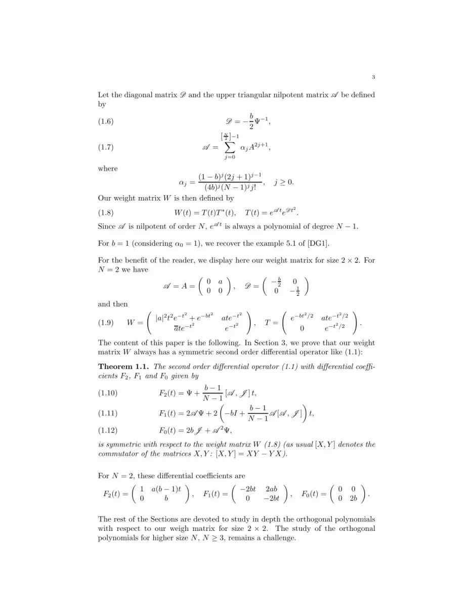
In Section 4, we construct the following Rodrigues’ formula for a sequence of or-thogonal polynomials with respect to the weight matrix W (1.9):
Theorem 1.2. Let the function Pn, n ≥ 1, be defined by(1.13)
Pn(t) = (−1)n
e−t2
b−ne(1−b)t2 +|a|22
(n+ 2t2) at
a[
2t+ et2√
πn(
Erf(√bt)− Erf(t)
)]
2
(n)
W−1,
where Erf denotes the error function Erf(z) =2√π
∫ z
0
e−x2
dx. Then Pn, n ≥ 1, is
a polynomial of degree n with nonsingular leading coefficient equal to
(1.14) Γn = 2n(
1 00 γn
)
, γn = 2 + |a|2bn− 12n.
Moreover, defining P0 =
(
1 00 2
)
, (Pn)n is a sequence of orthogonal polynomials
with respect to W .
This Rodrigues’ formula allows us to find an explicit expression for the polynomials(Pn)n in terms of the Hermite polynomials.
Corollary 1.3. For n ≥ 1, we have
(1.15) Pn(t) =
(
b−n/2Hn(√bt) −atb−n/2Hn(
√bt) + a
2Hn+1(t)
−2abn/2nHn−1(√bt) 2|a|2bn/2ntHn−1(
√bt) + 2Hn(t)
)
,
where Hn is the n-th Hermite polynomial defined by Hn(t) = (−1)n(
e−t2)(n)
et2
.
In Section 6, using again the Rodrigues’ formula (1.13), we find the following threeterm recurrence relation for a sequence (Pn)n of orthonormal polynomials withrespect to W .
Theorem 1.4. The sequence of matrix polynomials defined by P−1 = 0, P0 =
(π)−14
√
2√b
γ10
0 1
and
(1.16) tPn(t) = An+1Pn+1(t) +BnPn(t) +A∗nPn−1(t), n ≥ 0,
where
An =√n
√
γn+1
2bγn0
0
√
γn−1
2γn
,(1.17)
Bn =b
2n−3
4 (b+ (b− 1)n)√γnγn+1
(
0 aa 0
)
,(1.18)
are orthonormal with respect to W (1.9) (where the sequence (γn)n is defined by(1.14)).

5
This gives for the recurrence coefficients (An)n the asymptotic behaviour
limn→∞
An√n=
1√2
0
01√2b
if b > 1
1√2b
0
01√2
for 0 < b < 1
.
This limit shows that the recurrence coefficients (An)n do not asymptotically behaveas a scalar multiple of the identity, as it happens in the examples studied up to nowin the literature.
2. Preliminaries
A weight matrix W is an N × N matrix of measures supported in the real linesatisfying that (1) W (A) is positive semidefinite for any Borel set A ∈ R, (2) W hasfinite moments
∫
tndW (t) of every order, and (3)∫
P (t)dW (t)P ∗(t) is nonsingularif the leading coefficient of the matrix polynomial P is nonsingular (all the matricesconsidered in this paper are square matrices of size N ×N). When all the entriesof the matrix W have a smooth density with respect to the Lebesgue measure,we will write W (t) for the matrix whose entries are these densities. Condition (3)above is necessary and sufficient to guarantee the existence of a sequence (Pn)n oforthogonal matrix polynomials with respect to W . Condition (3) above is fulfilled,in particular, when W (t) is positive definite in an interval of the real line. This isthe case of the weight matrix (1.8) introduced in this paper.
The key concept to study orthogonal matrix polynomials (Pn)n satisfying secondorder differential equations of the form
(2.1) P ′′n (t)F2(t) + P ′
n(t)F1(t) + Pn(t)F0(t) = ΛnPn(t),
where the differential coefficients F2, F1 and F0 are matrix polynomials (which donot depend on n) of degrees less than or equal to 2, 1 and 0, respectively, is thatof the symmetry of a differential operator with respect to a weight matrix. Indeed,if we write
D =
(
d
dt
)2
F2(t) +
(
d
dt
)1
F1(t) + F0(t),
then D is symmetric with respect to W if and only if the orthonormal matrix poly-nomials (Pn)n with respect to W satisfy (2.1), where Λn, n ≥ 0, are Hermitianmatrices (see [D1]). If Λn are not Hermitian, then the operator D can be decom-posed as D = D1 + iD2, where D1 and D2 are second order differential operatorsof the form (1.1) symmetric with respect to W (see [GT]).
The symmetry of a second order differential operator as (1.1) with respect to aweight matrix can be guaranteed by a set of differential equations (which is thematrix analogous to the Pearson equation (f2w)
′ = f1w of the scalar case):
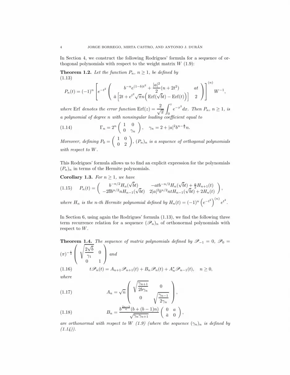
6 JORGE BORREGO, MIRTA CASTRO, AND ANTONIO J. DURAN
Theorem 2.1. For a weight matrix dW = W (t)dt, t ∈ (a, b) (a and b finite orinfinite) and matrix polynomials F2, F1, F0 of degrees not larger than 2, 1 and 0, thesymmetry of the second order differential operator (1.1) with respect to W followsfrom the set of equations
F2W = WF ∗2 ,(2.2)
2(F2W )′ − F1W = WF ∗1 , (F2W )′′ − (F1W )′ + F0W = WF ∗
0 ,(2.3)
under the boundary conditions
limt→a+,b−
tnF2(t)W (t) = 0, limt→a+,b−
tn[(F2(t)W (t))′ − F1(t)W (t)] = 0, n ≥ 0.
(2.4)
(See [DG1] or [GPT1]).
To check that the weight matrix W (1.8) and the coefficients defined by (1.10),(1.11) and (1.12) satisfy the differential equations (2.3) we will use the followingtheorem:
Theorem 2.2. Let Ω be an open set of the real line. Let F2, F1, F and T be twicedifferentiable N × N matrix functions on Ω, (with T (t0) nonsingular for certaint0 ∈ Ω), and define W (t) = T (t)T ∗(t). Under the assumptions
F2W = WF ∗2 ,(2.5)
T ′(t) = F (t)T (t), and(2.6)
F1 = F2F + FF2 + F ′2,(2.7)
we have
(1) The weight matrix W satisfies the first order differential equation
2(F2W )′ = F1W +WF ∗1 .
(2) For a given matrix F0, the second order differential equation
(F2W )′′ − (F1W )′ + F0W = WF ∗0 ,
holds if and only if the matrix function
(2.8) χ = T−1(−FF2F − F ′F2 − FF ′2 + F0)T,
is Hermitian at each point of Ω.
Theorem 2.2 is a particular case of Theorem 2.3 of [D3] (the special case when F2
is a scalar function is Theorem 4.1 of [DG1]).
We will need the following theorem (see [D4]) to find the Rodrigues’ formula dis-played in Theorem 1.2 for the orthogonal polynomials with respect to the weightmatrix W (1.9):
Theorem 2.3. Let F2, F1 and F0 be matrix polynomials of degrees not larger than2, 1, and 0, respectively. Let W , Rn be N ×N matrix functions twice and n timesdifferentiable, respectively, in an open set Ω of the real line. Assume that W (t)

7
is nonsingular for t ∈ Ω and that satisfies the identity (2.2), and the differentialequations (2.3). Define the functions Pn, n ≥ 1, by
Pn = R(n)n W−1.(2.9)
If for a matrix Λn, the function Rn satisfies
(RnF∗2 )
′′ −(
Rn
[
F ∗1 + n(F ∗
2 )′])′
+Rn
[
F ∗0 + n(F ∗
1 )′ +
(
n
2
)
(F ∗2 )
′′
]
= ΛnRn.
(2.10)
then the function Pn satisfies
P′′n(t)F2(t) + P
′n(t)F1(t) + Pn(t)F0(t) = ΛnPn(t).(2.11)
We will also make use of the following well known formula: for any matrices X,Y ∈CN×N :
(2.12) eXY =
∑
n≥0
tn
n!adnXY
eX ,
where we use the standard notation
ad0X Y = Y, ad1X Y = [X,Y ] = XY − Y X, ad2X Y = [X, [X,Y ]],
and in general, adn+1X Y = [X, [adnX Y ]].
3. Symmetric differential operator
In this Section we prove Theorem 1.1, that is, the second order differential operatorwith coefficients given by (1.10), (1.11) and (1.12) is symmetric with respect to theweight matrix W (1.8).
We now list some technical relations which we will need in the proof of Theorem1.1 (they will be proved later).
Lemma 3.1. Let the function F2 and the matrices A, A , Ψ, D and J be definedby (1.10), (1.4), (1.5), (1.6) and (1.7), respectively. Then
[A ,J ] =
[N2 ]−1∑
j=0
(2j + 1)αjA2j+1.(3.1)
eA tΨ = F2eA t.(3.2)
eA tDe−A tΨ = − b
2I − (b − 1)t
N − 1eA tDe−A t[A ,J ].(3.3)
ΨeA tDe−A t = − b
2I − (b − 1)t
N − 1[A ,J ]eA tDe−A t.(3.4)
A [A ,J ] =2b(N − 1)
1− b
[N−1
2 ]∑
j=1
αj(2j)j
(2j + 1)j−1A2j .(3.5)
[A ,J ]− A =(1− b)
2b(N − 1)A 2 [A ,J ] .(3.6)

8 JORGE BORREGO, MIRTA CASTRO, AND ANTONIO J. DURAN
We are now ready to prove Theorem 1.1.
Proof. (of Theorem 1.1)
The symmetry of the second order differential operator with respect to the weightmatrix W will be a consequence of Theorems 2.1 and 2.2. We have to check theboundary conditions (2.4) and the three equations (2.2) and (2.3).
To make the proof easier to follow, we proceed in four steps.
First step: Boundary conditions (2.4). Proof: Since A is nilpotent, we deduce that
eA t is a polynomial. The matrix function T = eA teDt2 then decays exponentiallyat ∞ because the entries of the diagonal matrix D are negative. Hence the weightmatrix W = TT ∗ also decays exponentially at ∞. Since F2 and F1 are polyno-mials, it follows straightforwardly that tnF2W and tn[(F2W )′ −F1W ], n ≥ 0, havevanishing limits at ∞.
Second step: F2W = WF ∗2 . Proof: Formula (3.2) of Lemma 3.1 shows that F2T =
TΨ, where Ψ is the diagonal matrix (real entries) defined by (1.5) and T = eA teDt2.Then
F2TT∗ = TΨT ∗ = T (TΨ)∗ = T (F2T )
∗ = TT ∗F ∗2 .
Since W = TT ∗, we get that F2W = WF ∗2 .
Third step: 2(F2W )′ = F1W + WF ∗1 . Proof: To check the equation 2(F2W )′ =
F1W +WF ∗1 , we use the first part of Theorem 2.2 with Ω = R. Hence, we have to
prove that T satisfies T ′(t) = F (t)T (t), where F is a solution of the matrix equation
(3.7) F1(t) = F2(t)F (t) + F (t)F2(t) + F ′2(t).
Taking into account that T = eA teDt2, a direct computation gives that
(3.8) F (t) = A + 2teA tDe−A t.
The definition of F2 (1.10) and (3.8) give
F2F + FF2 = A Ψ+ ΨA +2(b− 1)t
N − 1A [A ,J ] + 2t(ΨeA tDe−A t + eA tDe−A tΨ)
+2(b− 1)t2
N − 1(eA tDe−A t[A ,J ] + [A ,J ]eA tDe−A t).
Using the definition of Ψ (1.5), (3.3) and (3.4) of Lemma 3.1 we get
F2F + FF2 = 2A +(b − 1)
N − 1(J A + A J ) +
2t(b− 1)
N − 1A [A ,J ]− 2bIt.
Formula (3.7) now follows easily taking into account the definitions of F2 (1.10),F1 (1.11) and Ψ (1.5).
Fourth step: (F2W )′′ − (F1W )′ + F0W = WF ∗0 . Proof:
9
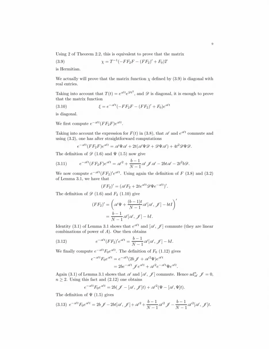
Using 2 of Theorem 2.2, this is equivalent to prove that the matrix
(3.9) χ = T−1(−FF2F − (FF2)′ + F0)T
is Hermitian.
We actually will prove that the matrix function χ defined by (3.9) is diagonal withreal entries.
Taking into account that T (t) = eA teDt2 , and D is diagonal, it is enough to provethat the matrix function
(3.10) ξ = e−A t(−FF2F − (FF2)′ + F0)e
A t
is diagonal.
We first compute e−A t(FF2F )eA t.
Taking into account the expression for F (t) in (3.8), that A and eA t commute andusing (3.2), one has after straightforward computations
e−A t(FF2F )eA t = A ΨA + 2t(A ΨD + DΨA ) + 4t2DΨD .
The definition of D (1.6) and Ψ (1.5) now give
(3.11) e−A t(FF2F )eA t = A 2 +b− 1
N − 1A J A − 2btA − 2t2bD .
We now compute e−A t(FF2)′eA t. Using again the definition of F (3.8) and (3.2)
of Lemma 3.1, we have that
(FF2)′ = (A F2 + 2teA tDΨe−A t)′.
The definition of D (1.6) and F2 (1.10) give
(FF2)′ =
(
A Ψ+(b− 1)t
N − 1A [A ,J ]− btI
)′
=b− 1
N − 1A [A ,J ]− bI.
Identity (3.1) of Lemma 3.1 shows that eA t and [A ,J ] commute (they are linearcombinations of power of A). One then obtains
(3.12) e−A t(FF2)′eA t =
b− 1
N − 1A [A ,J ]− bI.
We finally compute e−A tF0eA t. The definition of F0 (1.12) gives
e−A tF0eA t = e−A t(2bJ + A 2Ψ)eA t
= 2be−A tJ eA t + A 2e−A tΨeA t.
Again (3.1) of Lemma 3.1 shows that A and [A ,J ] commute. Hence adnA J = 0,n ≥ 2. Using this fact and (2.12) one obtains
e−A tF0eA t = 2b(J − [A ,J ]t) + A 2(Ψ− [A ,Ψ]t).
The definition of Ψ (1.5) gives
(3.13) e−A tF0eA t = 2bJ −2bt[A ,J ]+A 2+
b− 1
N − 1A 2J − b− 1
N − 1A 2[A ,J ]t.

10 JORGE BORREGO, MIRTA CASTRO, AND ANTONIO J. DURAN
We now substitute (3.11), (3.12) and (3.13) in the definition of ξ (3.10) obtaining
ξ =b− 1
N − 1(−A J A − A [A ,J ] + A 2J ) + 2bt(A − [A ,J ]
− b− 1
2b(N − 1)A 2[A ,J ]) + 2bt2D + bI + 2bJ ,
(3.6) of lemma 3.1 finally gives
ξ = bI + 2bt2D + 2bJ ,
which it is indeed a diagonal matrix.
This finishes the proof of Theorem 1.1.
It remains to prove Lemma 3.1.
Proof. (of Lemma 3.1)
First step. Proof of (3.1):
Using induction on k, we easily find that [Ak,J ] = kA, k ≥ 1. This shows thatadnA J = 0, n ≥ 2. The definition of A (1.7) gives now (3.1).
Second step. Proof of (3.2), (3.3) and (3.4):
First of all, the definition of Ψ (1.5) gives
(3.14) [A ,Ψ] =b− 1
N − 1[A ,J ].
The definition of A (1.7) and (3.1) show that the matrices A , [A ,J ] and eA t
commute (they are linear combination of powers of A). We then have
adnA (Ψ) = 0, n ≥ 2,(3.15)
[A ,J ]eA t = eA t[A ,J ].(3.16)
Using (2.12) and (3.15) we get
eA tΨe−A t =
∞∑
n=0
tn
n!adnA Ψ = Ψ+ t[A ,Ψ].
The definition of Ψ (1.5) and F2 (1.10) give now (3.2).
In a similar way, we have
e−A tΨeA t = Ψ− t[A ,Ψ].
Using now the definition of D (1.6), (3.14) and (3.16) we have
eA tDe−A tΨ = eA tD(Ψ− t[A ,Ψ])e−A t
= − b
2I − (b− 1)t
N − 1eA tDe−A t[A ,J ].
This proves (3.3). The proof of (3.4) is similar.

11
Third step. Proof of (3.5): Using the definition of A in (1.7) and (3.1), we have toprove the following identity
[N2 ]−1∑
j=0
αjA2j+1
[N2 ]−1∑
j=0
(2j + 1)αjA2j+1 =
2b(N − 1)
1− b
[N−1
2 ]∑
j=1
αj(2j)j
(2j + 1)j−1A2j .
This is equivalent to prove
(3.17)
[N2 ]−1∑
j,s=0
αjαs(2s+ 1)A2(j+s+1) =2b(N − 1)
1− b
[N−1
2 ]∑
j=1
αj(2j)j
(2j + 1)j−1A2j .
Taking into account that A is nilpotent,
(3.18) αsαj = αj+s(2j + 1)j−1(2s+ 1)s−1
(2(j + s) + 1)j+s−1
(
s+ js
)
,
and writing k = j + s, we find
[N2 ]−1∑
j,s=0
αjαs(2s+ 1)A2(j+s+1)
(3.19)
=
[N−1
2 ]−1∑
k=0
αk
(2k + 1)k−1A2(k+1)
k∑
m=0
(
km
)
(2m+ 1)m(2(k −m) + 1)k−m−1.
We now use Abel’s binomial identity (see for instance [Ro, p. 18]): for z, w ∈ C,w 6= 0,
(3.20)
k∑
m=0
(
km
)
(m+ z)m(k −m+ w)k−m−1 = w−1(z + w + k)k.
Thenk∑
m=0
(
km
)
(2m+ 1)m(2(k −m) + 1)k−m−1 = 2k(1 + k)k,
(3.19) now gives
[N2 ]−1∑
j,s=0
αjαs(2s+ 1)A2(j+s+1) =
[N−1
2 ]−1∑
j=0
αj2j(j + 1)j
(2j + 1)j−1A2(j+1).
Using (3.18) one has
αjα1 =αj+1(j + 1)(2j + 1)j−1
(2j + 3)j, with α1 =
1− b
4b(N − 1).
Thus,
[N−1
2 ]−1∑
j=0
αj2j(j + 1)j
(2j + 1)j−1A2(j+1) =
2b(N − 1)
1− b
[N−1
2 ]−1∑
j=0
αj+12j+1(j + 1)j+1
(2j + 3)jA2(j+1).

12 JORGE BORREGO, MIRTA CASTRO, AND ANTONIO J. DURAN
This proves (3.17) and then (3.5) as well.
Four step. Proof of (3.6): Taking into account (3.1) and (3.5), we have to provethe following identity
[N2 ]−1∑
j=1
2jαjA2j+1 =
[N2 ]−1∑
j=0
αjA2j+1
[N−1
2 ]∑
j=1
αj(2j)j
(2j + 1)j−1A2j .
This is equivalent to prove
(3.21)
[N2 ]−1∑
j=1
2jαjA2j+1 =
[N2 ]−1∑
s=0
[N−1
2 ]∑
j=1
αsαj(2j)j
(2j + 1)j−1A2(s+j)+1.
Using (3.18) once again, we have
[N2 ]−1∑
s=0
[N−1
2 ]∑
j=1
αsαj(2j)j
(2j + 1)j−1A2(s+j)+1
=
[N2 ]−1∑
s=0
[N−1
2 ]∑
j=1
αs+j(2j)j(2s+ 1)s−1
(2(j + s) + 1)j+s−1
(
s+ js
)
A2(s+j)+1.
Writing k = s+ j, and taking into account that A is nilpotent of order N , we getfor the right hand side of (3.21) the expression
[N2 ]−1∑
k=1
αk
(2k + 1)k−1A2k+1
k∑
j=1
(
kj
)
(2j)j(2(k − j) + 1)k−j−1.
Writing m = k − j, one obtains
[N2 ]−1∑
k=1
2k−1αk
(2k + 1)k−1A2k+1
k−1∑
m=0
(
km
)
(k −m)k−m(m+1
2)m−1.
Abel’s binomial identity (3.20) now gives
k−1∑
m=0
(
km
)
(k −m)k−m(m+1
2)m−1 =
1
2k−1
(
(2k + 1)k − (2k + 1)k−1)
.
From where one can easily deduce (3.21).
This proves (3.6).
The proof of the Lemma is now complete.

13
4. Rodrigues formula
In this section we will prove Theorem 1.2 which provides a Rodrigues’ formula fora sequence of orthogonal polynomials with respect to the weight matrix W for size2× 2 (1.9).
Write Rn for the functions
(4.1) Rn = (−1)ne−t2
b−ne(1−b)t2 +|a|22
(n+ 2t2) at
a[
2t+ et2√
πn(
Erf(√bt)− Erf(t)
)]
2
,
where, as usual, Erf denotes the error function Erf(z) =2√π
∫ z
0
e−x2
dx.
The Rodrigues’ formula (1.13) can then be written as Pn = R(n)n W−1.
First of all, we explain how one can use Theorem 2.3 to find these functions Rn,n ≥ 1.
Indeed, Theorem 1.1 for size 2 × 2 gives for the weight matrix W the followingsymmetric second order differential operator
(4.2) D =
(
d
dt
)2(1 a(b − 1)t0 b
)
+
(
d
dt
)(
−2bt 2ab0 −2bt
)
+
(
0 00 2b
)
.
Since the operator D is symmetric with respect to W , the n-th monic orthogonalpolynomial Pn with respect to W satisfies the differential equation D(Pn) = ΛnPn,where the eigenvalues Λn are given by
Λn =
(
−2bn 00 −2b(n− 1)
)
.
Theorem 2.3 associates the following second order differential equation (2.10) tothe differential operator D (4.2):(4.3)[
Rn
(
1 0a(b− 1)t b
)]′′
−[
Rn
(
−2bt 0a[b(2 + n)− n] −2bt
)]′
+RnΛn = ΛnRn.
Take now a solution Rn of this differential equation and write Yn = R(n)n W−1.
Theorem 2.3 guarantees that the function Yn satisfies the differential equationD(Yn) = ΛnYn. Notice that Yn and Pn satisfy the same differential equation.We have hence looked for a solution Rn of the differential equation (4.3) such that
the matrix function R(n)n W−1 is also a matrix polynomial of degree n with nonsin-
gular leading coefficient. This is the procedure we have used to find the functionsRn given by (4.1).
We now prove Theorem 1.2, which establishes that actually the functions R(n)n W−1
define a sequence of orthogonal polynomials with respect to W .
Proof. (of Theorem 1.2)
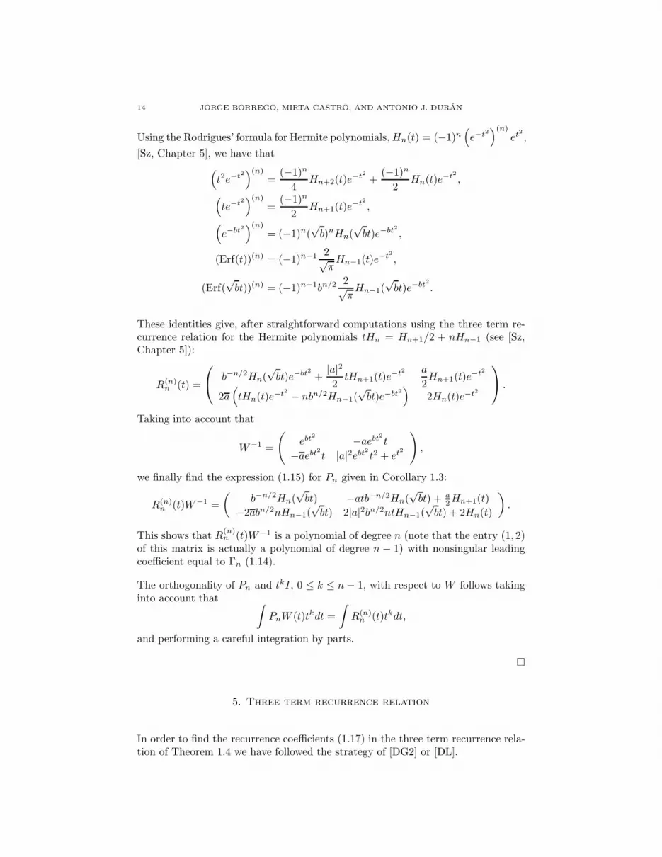
14 JORGE BORREGO, MIRTA CASTRO, AND ANTONIO J. DURAN
Using the Rodrigues’ formula for Hermite polynomials,Hn(t) = (−1)n(
e−t2)(n)
et2
,
[Sz, Chapter 5], we have that
(
t2e−t2)(n)
=(−1)n
4Hn+2(t)e
−t2 +(−1)n
2Hn(t)e
−t2 ,
(
te−t2)(n)
=(−1)n
2Hn+1(t)e
−t2 ,
(
e−bt2)(n)
= (−1)n(√b)nHn(
√bt)e−bt2 ,
(Erf(t))(n) = (−1)n−1 2√πHn−1(t)e
−t2 ,
(Erf(√bt))(n) = (−1)n−1bn/2
2√πHn−1(
√bt)e−bt2 .
These identities give, after straightforward computations using the three term re-currence relation for the Hermite polynomials tHn = Hn+1/2 + nHn−1 (see [Sz,Chapter 5]):
R(n)n (t) =
b−n/2Hn(√bt)e−bt2 +
|a|22
tHn+1(t)e−t2 a
2Hn+1(t)e
−t2
2a(
tHn(t)e−t2 − nbn/2Hn−1(
√bt)e−bt2
)
2Hn(t)e−t2
.
Taking into account that
W−1 =
(
ebt2 −aebt
2
t
−aebt2
t |a|2ebt2t2 + et2
)
,
we finally find the expression (1.15) for Pn given in Corollary 1.3:
R(n)n (t)W−1 =
(
b−n/2Hn(√bt) −atb−n/2Hn(
√bt) + a
2Hn+1(t)
−2abn/2nHn−1(√bt) 2|a|2bn/2ntHn−1(
√bt) + 2Hn(t)
)
.
This shows that R(n)n (t)W−1 is a polynomial of degree n (note that the entry (1, 2)
of this matrix is actually a polynomial of degree n − 1) with nonsingular leadingcoefficient equal to Γn (1.14).
The orthogonality of Pn and tkI, 0 ≤ k ≤ n− 1, with respect to W follows takinginto account that
∫
PnW (t)tkdt =
∫
R(n)n (t)tkdt,
and performing a careful integration by parts.
5. Three term recurrence relation
In order to find the recurrence coefficients (1.17) in the three term recurrence rela-tion of Theorem 1.4 we have followed the strategy of [DG2] or [DL].
15
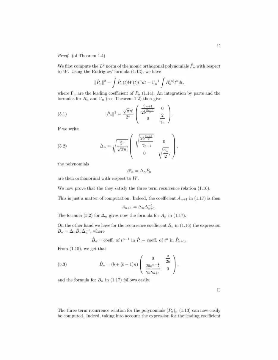
Proof. (of Theorem 1.4)
We first compute the L2 norm of the monic orthogonal polynomials Pn with respectto W . Using the Rodrigues’ formula (1.13), we have
‖Pn‖2 =∫
Pn(t)W (t)tndt = Γ−1n
∫
R(n)n tndt,
where Γn are the leading coefficient of Pn (1.14). An integration by parts and theformulas for Rn and Γn (see Theorem 1.2) then give
(5.1) ‖Pn‖2 =√πn!
2n
γn+1
2b2n+1
2
0
02
γn
.
If we write
(5.2) ∆n =
√
2n√πn!
√
2b2n+1
2
γn+10
0
√
γn2,
,
the polynomials
Pn = ∆nPn
are then orthonormal with respect to W .
We now prove that the they satisfy the three term recurrence relation (1.16).
This is just a matter of computation. Indeed, the coefficient An+1 in (1.17) is then
An+1 = ∆n∆−1n+1.
The formula (5.2) for ∆n gives now the formula for An in (1.17).
On the other hand we have for the recurrence coefficient Bn in (1.16) the expression
Bn = ∆nBn∆−1n , where
Bn = coeff. of tn−1 in Pn− coeff. of tn in Pn+1.
From (1.15), we get that
(5.3) Bn = (b + (b− 1)n)
0a
2b2abn−
12
γnγn+10
,
and the formula for Bn in (1.17) follows easily.
The three term recurrence relation for the polynomials (Pn)n (1.13) can now easilybe computed. Indeed, taking into account the expression for the leading coefficient

16 JORGE BORREGO, MIRTA CASTRO, AND ANTONIO J. DURAN
Γn (1.14) of Pn and ∆n (5.2) of Pn, we find that Pn = GnPn where
(5.4) Gn = Γn∆−1n =
√
2n√πn!
√
γn+1
2b2n+1
2
0
0√2γn
.
In particular, this gives P0 =
(
1 00 2
)
. If we write
(5.5) tPn(t) = An+1Pn+1(t) + BnPn(t) + CnPn−1(t), n ≥ 0,
it follows from (1.16) that An+1 = GnAn+1G−1n+1, Bn = GnBnG
−1n and Cn =
GnA∗nG
−1n−1. An easy computation gives now
An =1
2
(
1 0
0γn−1
γn
)
, Bn = (−n+ (n+ 1)b)
0a
2bγn2abn−
12
γn+10
,
Cn = n
( γn+1
bγn0
0 1
)
.
The L2 norm of the polynomials Pn follows easily from the formula (5.4) for thematrices Gn:
‖Pn‖2 = 2n√πn!
( γn+1
2bn+12
0
0 2γn
)
.
In a similar way, the three term recurrence relation for the monic orthogonal poly-nomials (Pn)n can be deduced:
tPn(t) = Pn+1(t) + BnPn(t) + CnPn−1(t), n ≥ 0,
where Bn is the one in (5.3) and
Cn =n
2b
γn+1
γn0
0bγn−1
γn
.
References
[Atk] Atkinson, F.V., Discrete and continous boundary problems, Academic Press, New York,1964.
[Be] Berezanskii, Ju.M., Expansions in eigenfunctions of selfadjoint operators, Transl. Math.Monographs, AMS 17 (1968).
[CMV] Cantero, M.J., Moral, L. and Velazquez, L., Matrix orthogonal polynomials whose deriva-
tives are also orthogonal, J. Approx. Theory 146 (2007), 174–211.[D1] Duran, A.J., Matrix inner product having a matrix symmetric second order differential
operator, Rocky Mountain J. Math. 27 (1997), 585–600.
[D2] Duran, A.J., Generating orthogonal matrix polynomials satisfying second order differen-
tial equations from a trio of triangular matrices, J. Approx. Theory 161 (2009), 88-113.[D3] Duran, A.J., A method to find weight matrices having symmetric second-order differential
operators with matrix leading coefficents, Const. Approx 29 (2009), 181-205.
17
[D4] Duran, A.J., Rodrigues’ formulas for orthogonal matrix polynomials satisfying second-
order differential equations, Int. Math. Res. Not., (2009), doi:10.1093/imrn/rnp156. 461–484.
[DG1] Duran, A.J. and Grunbaum, F.A., Orthogonal matrix polynomials satisfying second order
differential equations, Int. Math. Res. Not. 10 (2004) 461–484.[DG2] Duran, A.J. and Grunbaum, F.A., Structural formulas for orthogonal matrix polynomials
satisfying second order differential equations, I, Constr. Approx. 22 (2005), 255–271.[DG3] Duran, A.J. and Grunbaum, F.A., Matrix orthogonal polynomials satisfying second order
differential equations: coping without help from group representation theory, J. Approx.Theory 148 (2007), 35–48.
[DdI1] Duran, A.J. and de la Iglesia, M.D., Some examples of orthogonal matrix polynomials
satisfying odd order differential equations, J. Approx. Theory 150 (2008), 153-174.[DdI2] Duran, A.J. and de la Iglesia, M.D., Second order differential operators having several
families of orthogonal matrix polynomials as eigenfunctions, Int. Math. Res. Not. (2008),Art ID rnn 084.
[DL] Duran, A.J. and Lopez-Rodrıguez, P., Structural formulas for orthogonal matrix polyno-
mials satisfying second order differential equations, II, Constr. Approx. 26, No. 1, (2007)29–47.
[G] Grunbaum, F.A., Matrix valued Jacobi polynomials, Bull. Sci. Math. 127, (2003) 207–
214.[GdI] Grunbaum, F.A. and de la Iglesia, M. D., Matrix valued orthogonal polynomials arising
from group representation theory and a family of quasi-birth-and death processes, SIAMJ. Matrix Anal. Appl., 30, (2008), 741–761.
[GPT1] Grunbaum, F.A., Pacharoni, I. and Tirao, J. A., Matrix valued orthogonal polynomials
of the Jacobi type, Indag. Math. 14 3,4 (2003), 353–366.[GPT2] Grunbaum, F.A., Pacharoni, I. and Tirao, J. A., Matrix valued orthogonal polynomials of
the Jacobi type: The role of group representation theory, Ann. Inst. Fourier (Grenoble)55 , 6, (2005), 2051–2068.
[GT] Grunbaum, F.A. and Tirao, J.A., The algebra of differential operators associate to a
weight matrix, Integral Equations Operator Theory 58 (2007), 449–475.[K1] Krein, M.G., Fundamental aspects of the representation theory of hermitian operators
with deficiency index (m,m), AMS Translations, Series 2, vol. 97, Providence, RhodeIsland (1971), 75–143.
[K2] Krein, M.G., Infinite J-matrices and a matrix moment problem, Dokl. Akad. Nauk SSSR69 nr. 2 (1949), 125–128.
[PT] Pacharoni, I. and Tirao, J. A., Matrix valued orthogonal polynomials arising from the
complex proyective space, Constr. Approx. 25 (2007), 177–192.[Ro] Riordan, J., Combinatorial identities, N. York, Wiley, 1978.[Sz] Szego, G., Orthogonal Polynomials, Coll. Publ., XXIII, American Mahematical Society,
Providence, RI, 1975.
J. Borrego, Departamento de Matematicas, Universidad Carlos III de Madrid, Avda. dela Universidad 30, 28911 Leganes, Madrid, Spain.
E-mail address: [email protected]
M. Castro, Departamento de Matematica Aplicada II, Universidad de Sevilla, E.P.S.,
c/Virgen de Africa 7, 41011 Sevilla, Spain.
E-mail address: [email protected]
A. J. Duran, Departamento de Analisis Matematico, Universidad de Sevilla, Apdo (P.O. BOX) 1160, 41080 Sevilla. Spain.
E-mail address: [email protected]