Embed Size (px)
Citation preview
arX
iv:0
903.
4494
v2 [
mat
h.C
A]
12
Aug
201
0Commun. Contemp. Math., to appear
Orlicz-Hardy Spaces Associated with Operators Satisfying
Davies-Gaffney Estimates
Renjin Jiang and Dachun Yang ∗
Abstract. Let X be a metric space with doubling measure, L a nonnegative self-adjointoperator in L2(X ) satisfying the Davies-Gaffney estimate, ω a concave function on (0,∞)of strictly lower type pω ∈ (0, 1] and ρ(t) = t−1/ω−1(t−1) for all t ∈ (0,∞). The authorsintroduce the Orlicz-Hardy space Hω,L(X ) via the Lusin area function associated tothe heat semigroup, and the BMO-type space BMOρ,L(X ). The authors then estab-lish the duality between Hω,L(X ) and BMOρ,L(X ); as a corollary, the authors obtainthe ρ-Carleson measure characterization of the space BMOρ,L(X ). Characterizationsof Hω,L(X ), including the atomic and molecular characterizations and the Lusin areafunction characterization associated to the Poisson semigroup, are also presented. LetX = Rn and L = −∆ + V be a Schrodinger operator, where V ∈ L1
loc(Rn) is a non-
negative potential. As applications, the authors show that the Riesz transform ∇L−1/2
is bounded from Hω,L(Rn) to L(ω); moreover, if there exist q1, q2 ∈ (0,∞) such that
q1 < 1 < q2 and [ω(tq2)]q1 is a convex function on (0,∞), then several characteriza-tions of the Orlicz-Hardy space Hω,L(R
n), in terms of the Lusin-area functions, the non-tangential maximal functions, the radial maximal functions, the atoms and the molecules,are obtained. All these results are new even when ω(t) = tp for all t ∈ (0,∞) andp ∈ (0, 1).
1 Introduction
The theory of Hardy spaces Hp in various settings plays an important role in analysisand partial differential equations. However, the classical theory of Hardy spaces on R
n
is intimately connected with the Laplacian operator. In recent years, the study of Hardyspaces and BMO spaces associated with different operators inspired great interests; see,for example, [1, 2, 3, 11, 12, 13, 14, 18, 17, 21, 33] and their references. In [1], Auscher,Duong and McIntosh studied the Hardy space H1
L(Rn) associated to an operator L whose
heat kernel satisfies a pointwise Poisson upper bound. Later, in [11, 12], Duong and Yanintroduced the BMO-type space BMOL(R
n) associated to such an L and established theduality between H1
L(Rn) and BMOL∗(Rn), where L∗ denotes the adjoint operator of L
in L2(Rn). Yan [33] further generalized these results to the Hardy space HpL(R
n) withp ∈ (0, 1] close to 1 and its dual space. Very recently, Auscher, McIntosh and Russ [2]
2000 Mathematics Subject Classification. Primary 42B35; Secondary 42B30; 42B25.Key words and phrases. nonnegative self-adjoint operator, Schrodinger operator, Riesz transform,
Davies-Gaffney estimate, Orlicz function, Orlicz-Hardy space, Lusin area function, maximal function,atom, molecule, dual, BMO.
Dachun Yang is supported by the National Natural Science Foundation (Grant No. 10871025) of China.∗ Corresponding author.
1

2 Renjin Jiang and Dachun Yang
treated the Hardy space H1 associated to the Hodge Laplacian on a Riemannian manifoldwith doubling measure; Hofmann and Mayboroda [18] introduced the Hardy spaceH1
L(Rn)
and its dual space adapted to a second order divergence form elliptic operator L on Rn
with complex coefficients. Notice that these operators may not have the pointwise heatkernel bounds. Furthermore, Hofmann et al [17] studied the Hardy space H1
L(X ) on ametric measured space X adapted to L, which is nonnegative self-adjoint, and satisfies theso-called Davies-Gaffney estimate.
On the other hand, as another generalization of Lp(Rn), the Orlicz space was introducedby Birnbaum-Orlicz in [4] and Orlicz in [23]. Since then, the theory of the Orlicz spacesthemselves has been well developed and the spaces have been widely used in probability,statistics, potential theory, partial differential equations, as well as harmonic analysis andsome other fields of analysis; see, for example, [24, 25]. Moreover, the Orlicz-Hardy spacesare also good substitutes of the Orlicz spaces in dealing with many problems of analysis.In particular, Stromberg [30], Janson [20] and Viviani [32] studied Orlicz-Hardy spacesand their dual spaces.
Recall that the Orlicz-Hardy spaces associated operators on Rn have been studied in
[22, 21]. In [22], the heat kernel is assumed to enjoy a pointwise Poisson type upper bound;while in [21], L is a second order divergence form elliptic operator on R
n with complexcoefficients. Motivated by [18, 17, 20, 32], in this paper, we study the Orlicz-Hardy spaceHω,L(X ) and its dual space associated with a nonnegative self-adjoint operator L on ametric measured space X .
Let X be a metric space with doubling measure and L a nonnegative self-adjoint op-erator in L2(X ) satisfying the Davies-Gaffney estimate. Let ω on (0,∞) be a concavefunction of strictly lower type pω ∈ (0, 1] and ρ(t) = t−1/ω−1(t−1) for all t ∈ (0,∞). Atypical example of such Orlicz functions is ω(t) = tp for all t ∈ (0,∞) and p ∈ (0, 1].To develop a real-variable theory of the Orlicz-Hardy space Hω,L(X ), the key step is toestablish an atomic (molecular) characterization of these spaces. To this end, we inherita method used in [2, 21]. We first establish the atomic decomposition of the tent spaceTω(X ), whose proof implies that if F ∈ Tω(X ) ∩ T 2
2 (X ), then the atomic decomposi-tion of F holds in both Tω(X ) and T 2
2 (X ). Then by the fact that the operator πΨ,L
(see (4.6)) is bounded from T 22 (X ) to L2(X ), we further obtain the L2(X )-convergence of
the corresponding atomic decomposition for functions in Hω,L(X ) ∩ L2(X ), since for all
f ∈ Hω,L(X ) ∩ L2(X ), t2Le−t2Lf ∈ T 22 (X ) ∩ Tω(X ). This technique plays a fundamental
role in the whole paper.
With the help of the atomic decomposition, we establish the dual relation betweenthe spaces Hω,L(X ) and BMOρ,L(X ). As a corollary, we obtain the ρ-Carleson measurecharacterization of the space BMOρ,L(X ). Having at hand the duality relation, we thenobtain the atomic and molecular characterizations of the spaceHω,L(X ). We also introducethe Orlicz-Hardy space Hω,SP
(X ) via the Lusin area function associated to the Poissonsemigroup. With the atomic characterization of Hω,L(X ), we finally show that the spacesHω,SP
(X ) and Hω,L(X ) coincide with equivalent norms. Let X = Rn and L = −∆+ V ,
where V ∈ L1loc (R
n) is a nonnegative potential. As applications, we show that the Riesztransform ∇L−1/2 is bounded from Hω,L(R
n) to L(ω); moreover, if there exist q1, q2 ∈(0,∞) such that q1 < 1 < q2 and [ω(tq2)]q1 is a convex function on (0,∞), then we
Orlicz-Hardy Spaces 3
obtain several characterizations ofHω,L(Rn), in terms of the Lusin-area functions, the non-
tangential maximal functions, the radial maximal functions, the atoms and the molecules.Notice that here, the potential V is not assumed to satisfy the reverse Holder inequality.
Notice that the assumption that L is nonnegative self-adjoint enables us to obtain anatomic characterization of Hω,L(X ). The method used in the proof of atomic characteri-zation depends on the finite speed propagation property for solutions of the correspondingwave equation of L and hence the self-adjointness of L. Without self-adjointness, as in[1, 12, 18, 22, 21, 33], where L satisfies H∞-functional calculus and the heat kernel gener-ated by L satisfies a pointwise Poisson type upper bound or the Davies-Gaffney estimate,a corresponding (Orlicz-)Hardy space theory with the molecular (not atomic) characteri-zation was also established in [1, 12, 18, 22, 21, 33].
Precisely, this paper is organized as follows. In Section 2, we first recall some definitionsand notation concerning metric measured spaces X , then describe some basic assumptionson the operator L and the Orlicz function ω and present some properties of the operatorL and Orlicz functions considered in this paper.
In Section 3, we first recall some notions about tent spaces and then study the tentspace Tω(X ) associated to the Orlicz function ω. The main result of this section is that wecharacterize the tent space Tω(X ) by the atoms; see Theorem 3.1 below. As a byproduct,we see that if f ∈ Tω(X )∩T 2
2 (X ), then the atomic decomposition holds in both Tω(X ) andT 22 (X ), which plays an important role in the remaining part of this paper; see Corollary
3.1 below.
In Section 4, we first introduce the Orlicz-Hardy space Hω,L(X ) and prove that theoperator πΨ,L (see (4.6) below) maps the tent space Tω(X ) continuously into Hω,L(X )(see Proposition 4.2 below). By this and the atomic decomposition of Tω(X ), we obtainthat for each f ∈ Hω,L(X ), there is an atomic decomposition of f holding in Hω,L(X ) (seeProposition 4.3 below). We should point out that to obtain the atomic decomposition ofHω,L(X ), we borrow a key idea from [17], namely, for a nonnegative self-adjoint operatorL in L2(X ), then L satisfies the Davies-Gaffney estimate if and only if it has the finitespeed propagation property; see [17] (or Lemma 2.2 below). Via this atomic decompo-sition of Hω,L(X ), we further obtain the duality between Hω,L(X ) and BMOρ,L(X ) (seeTheorem 4.1 below). As an application of this duality, we establish a ρ-Carleson measurecharacterization of the space BMOρ,L(X ); see Theorem 4.2 below. We point out that if
X = Rn, L = −∆ ≡ −∑n
i=1∂2
∂x2iand ω is as above with pω ∈ (n/(n + 1), 1], then the
Orlicz-Hardy space Hω,L(Rn) in this case coincides with the Orlicz-Hardy space in [22] and
it was proved there that Hω,L(Rn) = Hω(R
n); see [20, 32] for the definition of Hω(Rn).
In Section 5, by Proposition 4.3 and Theorem 4.1, we establish the equivalence ofHω,L(X ) and the atomic (resp. molecular) Orlicz-Hardy HM
ω,at(X ) (resp. HM,ǫω,mol(X )); see
Theorem 5.1 below. We notice that the series in HMω,at(X ) (resp. HM,ǫ
ω,mol(X )) is defined toconverge in the norm of (BMOρ,L(X ))∗; while in Corollary 4.1 below, the atomic decom-position holds in Hω,L(X ). Applying the atomic characterization, we further characterizethe Orlicz-Hardy space Hω,L(X ) in terms of the Lusin area function associated to thePoisson semigroup; see Theorem 5.2 below.
As applications, in Section 6, we study the Hardy spaces Hω,L(Rn) associated to the
4 Renjin Jiang and Dachun Yang
Schrodinger operator L = −∆+ V , where V ∈ L1loc (R
n) is a nonnegative potential. Wecharacterize Hω,L(R
n) in terms of the Lusin-area functions, the atoms and the molecules;see Theorem 6.1 below. Moreover, we show that the Riesz transform ∇L−1/2 is boundedfrom Hω,L(R
n) to L(ω) and from Hω,L(Rn) to the classical Orlicz-Hardy space Hω(R
n),if pω ∈ ( n
n+1 , 1]; see Theorems 6.2 and 6.3 below. If there exist q1, q2 ∈ (0,∞) suchthat q1 < 1 < q2 and [ω(tq2)]q1 is a convex function on (0,∞), then we obtain severalcharacterizations of Hω,L(R
n), in terms of the non-tangential maximal functions and theradial maximal functions; see Theorem 6.4 below. Denote Hω,L(R
n) by HpL(R
n), whenp ∈ (0, 1] and ω(t) = tp for all t ∈ (0,∞). We remark that the boundedness of ∇L−1/2
from H1L(R
n) to the classical Hardy space H1(Rn) was established in [17]. Moreover, ifn = 1 and p = 1, the Hardy space H1
L(Rn) coincides with the Hardy space introduced by
Czaja and Zienkiewicz in [9]; if L = −∆ + V and V belongs to the reverse Holder classHq(R
n) for some q ≥ n/2 with n ≥ 3, then the Hardy spaceHpL(R
n) when p ∈ (n/(n+1), 1]coincides with the Hardy space introduced by Dziubanski and Zienkiewicz [13, 14].
Finally, we make some conventions. Throughout the paper, we denote by C a positiveconstant which is independent of the main parameters, but it may vary from line to line.The symbol X . Y means that there exists a positive constant C such that X ≤ CY ;the symbol ⌊α ⌋ for α ∈ R denotes the maximal integer no greater than α; B(zB , rB)denotes an open ball with center zB and radius rB and CB(zB, rB) ≡ B(zB, CrB). SetN ≡ {1, 2, · · · } and Z+ ≡ N ∪ {0}. For any subset E of X , we denote by E∁ the setX \ E. We also use C(γ, β, · · · ) to denote a positive constant depending on the indicatedparameters γ, β, · · · .
2 Preliminaries
In this section, we first recall some notions and notation on metric measured spaces andthen describe some basic assumptions on the operator L studied in this paper; finally wepresent some basic properties on Orlicz functions and also describe some basic assumptionsof them.
2.1 Metric measured spaces
Throughout the whole paper, we let X be a set, d a metric on X and µ a nonnegativeBorel regular measure on X . Moreover, we assume that there exists a constant C1 ≥ 1such that for all x ∈ X and r > 0,
(2.1) V (x, 2r) ≤ C1V (x, r) <∞,
where B(x, r) ≡ {y ∈ X : d(x, y) < r} and
(2.2) V (x, r) ≡ µ(B(x, r)).
Observe that if d is a quasi-metric, then (X , d, µ) is called a space of homogeneous typein the sense of Coifman and Weiss [8].

Orlicz-Hardy Spaces 5
Notice that the doubling property (2.1) implies the following strong homogeneity prop-erty that
(2.3) V (x, λr) ≤ CλnV (x, r)
for some positive constants C and n uniformly for all λ ≥ 1, x ∈ X and r > 0. Theparameter n measures the dimension of the space X in some sense. There also existconstants C > 0 and 0 ≤ N ≤ n such that
(2.4) V (x, r) ≤ C
(1 +
d(x, y)
r
)N
V (y, r)
uniformly for all x, y ∈ X and r > 0. Indeed, the property (2.4) with N = n is a simplecorollary of the strong homogeneity property (2.3). In the cases of Euclidean spaces,Lie groups of polynomial growth and more generally in Ahlfors regular spaces, N can bechosen to be 0.
In what follows, for each ball B ⊂ X , we set
(2.5) U0(B) ≡ B and Uj(B) ≡ 2jB\2j−1B for j ∈ N.
2.2 Assumptions on operators L
Throughout the whole paper, as in [17], we always suppose that the considered opera-tors L satisfy the following assumptions.
Assumption (A). The operator L is a nonnegative self-adjoint operator in L2(X ).
Assumption (B). The semigroup {e−tL}t>0 generated by L is analytic on L2(X ) andsatisfies the Davies-Gaffney estimates, namely, there exist positive constants C2 and C3
such that for all closed sets E and F in X , t ∈ (0,∞) and f ∈ L2(E),
(2.6) ‖e−tLf‖L2(F ) ≤ C2 exp
{− dist (E,F )2
C3t
}‖f‖L2(E),
where and in what follows, dist (E,F ) ≡ infx∈E,y∈F d(x, y) and L2(E) is the set of allµ-measurable functions on E such that ‖f‖L2(E) = {
∫E |f(x)|2 dµ(x)}1/2 <∞.
Examples of operators satisfying Assumptions (A) and (B) include second order el-liptic self-adjoint operators in divergence form on R
n, degenerate Schrodinger operatorswith nonnegative potential, Schrodinger operators with nonnegative potential and mag-netic field and Laplace-Beltrami operators on all complete Riemannian manifolds; see forexample, [10, 15, 28, 29].
By Assumptions (A) and (B), we have the following results which were established in[17].
Lemma 2.1. Let L satisfy Assumptions (A) and (B). Then for any fixed k ∈ Z+ (resp.j, k ∈ Z+ with j ≤ k), the family {(t2L)ke−t2L}t>0 (resp. {(t2L)j(I+ t2L)−k}t>0) of oper-ators satisfies the Davies-Gaffney estimates (2.6) with positive constants C2, C3 dependingon n, k (resp. n, j, k) only.

6 Renjin Jiang and Dachun Yang
In what follows, for any operator T , let KT denote its integral kernel when this kernelexists. By [17, Proposition 3.4], we know that if L satisfies Assumptions (A) and (B), andT = cos(t
√L), then there exists a positive constant C4 such that
(2.7) suppKT ⊂ Dt ≡ {(x, y) ∈ X × X : d(x, y) ≤ C4t} .This observation plays a key role in obtaining the atomic characterization of the Orlicz-Hardy space Hω,L(X ); see [17] and Proposition 4.3 below.
Lemma 2.2. Suppose that the operator L satisfies Assumptions (A) and (B). Let ϕ ∈C∞0 (R) be even and suppϕ ⊂ (−C−1
4 , C−14 ), where C4 is as in (2.7). Let Φ denote the
Fourier transform of ϕ. Then for every κ ∈ Z+ and t > 0, the kernel K(t2L)κΦ(t√L) of
(t2L)κΦ(t√L) satisfies that suppK(t2L)κΦ(t
√L) ⊂ {(x, y) ∈ X × X : d(x, y) ≤ t} .
The following estimate is often used in this paper. Let LC→C denote the set of allmeasurable functions from C to C. For δ > 0, define
F (δ) ≡{ψ ∈ LC→C : there exists C > 0 such that for all z ∈ C, |ψ(z)| ≤ C
|z|δ1 + |z|2δ
}.
Then for any non-zero function ψ ∈ F (δ), we have∫∞0 |ψ(t)|2 dt
t < ∞. It was proved in[17] that for all f ∈ L2(X ),
(2.8)
∫ ∞
0‖ψ(t
√L)f‖2L2(X )
dt
t=
∫ ∞
0|ψ(t)|2 dt
t‖f‖2L2(X ).
2.3 Orlicz functions
Let ω be a positive function defined on R+ ≡ (0, ∞). The function ω is said to be ofupper (resp. lower) type p for some p ∈ [0, ∞), if there exists a positive constant C suchthat for all t ≥ 1 (resp. t ∈ (0, 1]) and s ∈ (0,∞),
(2.9) ω(st) ≤ Ctpω(s).
Obviously, if ω is of lower type p for some p > 0, then limt→0+ ω(t) = 0. So for the sakeof convenience, if it is necessary, we may assume that ω(0) = 0. If ω is of both upper typep1 and lower type p0, then ω is said to be of type (p0, p1). Let
p+ω ≡ inf{p > 0 : there exists C > 0 such that (2.9) holds for all t ∈ [1,∞), s ∈ (0,∞)},and
p−ω ≡ sup{p > 0 : there exists C > 0 such that (2.9) holds for all t ∈ (0, 1], s ∈ (0,∞)}.The function ω is said to be of strictly lower type p if for all t ∈ (0, 1) and s ∈ (0,∞),ω(st) ≤ tpω(s), and we define
pω ≡ sup{p > 0 : ω(st) ≤ tpω(s) holds for all s ∈ (0,∞) and t ∈ (0, 1)}.It is easy to see that pω ≤ p−ω ≤ p+ω for all ω. In what follows, pω, p
−ω and p+ω are called
the strictly critical lower type index, the critical lower type index and the critical uppertype index of ω, respectively.

Orlicz-Hardy Spaces 7
Remark 2.1. We claim that if pω is defined as above, then ω is also of strictly lower typepω. In other words, pω is attainable. In fact, if this is not the case, then there exist somes ∈ (0,∞) and t ∈ (0, 1) such that ω(st) > tpωω(s). Hence there exists ǫ ∈ (0, pω) smallenough such that ω(st) > tpω−ǫω(s), which is contrary to the definition of pω. Thus, ω isof strictly lower type pω.
Throughout the whole paper, we always assume that ω satisfies the following assump-tion.
Assumption (C). Let ω be a positive function defined on R+, which is of strictly lowertype and its strictly lower type index pω ∈ (0, 1]. Also assume that ω is continuous, strictlyincreasing and concave.
Notice that if ω satisfies Assumption (C), then ω(0) = 0 and ω is obviously of uppertype 1. Since ω is concave, it is subadditive. In fact, let 0 < s < t, then
ω(s+ t) ≤ s+ t
tω(t) ≤ ω(t) +
s
t
t
sω(s) = ω(s) + ω(t).
For any concave function ω of strictly lower type p, if we set ω(t) ≡∫ t0
ω(s)s ds for t ∈ [0,∞),
then by [32, Proposition 3.1], ω is equivalent to ω, namely, there exists a positive constantC such that C−1ω(t) ≤ ω(t) ≤ Cω(t) for all t ∈ [0,∞); moreover, ω is strictly increasing,concave, subadditive and continuous function of strictly lower type p. Since all our resultsare invariant on equivalent functions, we always assume that ω satisfies Assumption (C);otherwise, we may replace ω by ω.
Convention. From Assumption (C), it follows that 0 < pω ≤ p−ω ≤ p+ω ≤ 1. In whatfollows, if (2.9) holds for p+ω with t ∈ [1,∞), then we choose pω ≡ p+ω ; otherwise p
+ω < 1
and we choose pω ∈ (p+ω , 1) to be close enough to p+ω , the meaning will be made clear inthe context.
For example, if ω(t) = tp with p ∈ (0, 1] for all t ∈ (0,∞), then pω = p+ω = pω = p; ifω(t) = t1/2 ln(e4 + t) for all t ∈ (0,∞), then pω = p+ω = 1/2, but 1/2 < pω < 1.
Let ω satisfy Assumption (C). A measurable function f on X is said to be in the spaceL(ω) if
∫X ω(|f(x)|) dµ(x) <∞. Moreover, for any f ∈ L(ω), define
‖f‖L(ω) ≡ inf
{λ > 0 :
∫
Xω
( |f(x)|λ
)dµ(x) ≤ 1
}.
Since ω is strictly increasing, we define the function ρ(t) on R+ by
(2.10) ρ(t) ≡ t−1
ω−1(t−1)
for all t ∈ (0,∞), where ω−1 is the inverse function of ω. Then the types of ω and ρ havethe following relation; see [32] for a proof.
Proposition 2.1. Let 0 < p0 ≤ p1 ≤ 1 and w be an increasing function. Then ω is oftype (p0, p1) if and only if ρ is of type (p−1
1 − 1, p−10 − 1).
8 Renjin Jiang and Dachun Yang
3 Tent spaces associated to Orlicz functions
In this section, we study the tent spaces associated to Orlicz functions ω satisfyingAssumption (C). We first recall some notions.
For any ν > 0 and x ∈ X , let Γν(x) ≡ {(y, t) ∈ X × (0,∞) : d(x, y) < νt} denote thecone of aperture ν with vertex x ∈ X . For any closed set F of X , denote by RνF theunion of all cones with vertices in F , namely, RνF ≡ ⋃
x∈F Γν(x); and for any open set
O in X , denote the tent over O by Tν(O), which is defined as Tν(O) ≡ [Rν(O∁)]∁. It is
easy to see that Tν(O) = {(x, t) ∈ X × (0,∞) : d(x,O∁) ≥ νt}. In what follows, we denoteR1(F ), Γ1(x) and T1(O) simply by R(F ), Γ(x) and O, respectively.
For all measurable function g on X × (0,∞) and x ∈ X , define
Aν(g)(x) ≡(∫
Γν(x)|g(y, t)|2 dµ(y)
V (x, t)
dt
t
)1/2
and denote A1(g) simply by A(g).
If X = Rn, Coifman, Meyer and Stein [7] introduced the tent space T p
2 (Rn+1+ ) for
p ∈ (0,∞). The tent spaces T p2 (X ) on spaces of homogenous type were studied by Russ
[26]. Recall that a measurable function g is said to belong to the space T p2 (X ) with
p ∈ (0,∞), if ‖g‖T p2 (X ) ≡ ‖A(g)‖Lp(X ) < ∞. On the other hand, Harboure, Salinas and
Viviani [16] introduced the tent space Tω(Rn+1+ ) associated to the function ω.
In what follows, we denote by Tω(X ) the space of all measurable function g on X×(0,∞)such that A(g) ∈ L(ω), and for any g ∈ Tω(X ), define its norm by
‖g‖Tω(X ) ≡ ‖A(g)‖L(ω) = inf
{λ > 0 :
∫
Xω
(A(g)(x)
λ
)dµ(x) ≤ 1
}.
A function a on X × (0,∞) is called a Tω(X )-atom if
(i) there exists a ball B ⊂ X such that suppa ⊂ B;
(ii)∫B|a(x, t)|2 dµ(x) dt
t ≤ [V (B)]−1[ρ(V (B))]−2.
Since ω is concave, it is easy to see that for all Tω(X )-atom a, we have ‖a‖Tω(X ) ≤ 1.In fact, since ω−1 is convex, by the Jensen inequality and the Holder inequality, we have
ω−1
(∫B ω(A(a)(x)) dµ(x)
V (B)
)≤ 1
V (B)
∫
BA(a)(x) dµ(x) ≤
‖a‖T 22 (X )
[V (B)]1/2≤ 1
V (B)ρ(V (B)),
which implies that
∫
Bω(A(a)(x)) dµ(x) ≤ V (B)ω
(1
V (B)ρ(V (B))
)= 1.
Thus, the claim holds.
For functions in the space Tω(X ), we have the following atomic decomposition. Theproof of Theorem 3.1 is similarly to those of [7, Theorem 1], [26, Theorem 1.1] and [21,Theorem 3.1]; we omit the details.
Orlicz-Hardy Spaces 9
Theorem 3.1. Let ω satisfy Assumption (C). Then for any f ∈ Tω(X ), there exist Tω(X )-atoms {aj}∞j=1 and {λj}∞j=1 ⊂ C such that for almost every (x, t) ∈ X × (0,∞),
(3.1) f(x, t) =
∞∑
j=1
λjaj(x, t),
and the series converges in the space Tω(X ). Moreover, there exists a positive constant Csuch that for all f ∈ Tω(X ),
(3.2) Λ({λjaj}j) ≡ inf
λ > 0 :
∞∑
j=1
V (Bj)ω
( |λj|λV (Bj)ρ(V (Bj))
)≤ 1
≤ C‖f‖Tω(X ),
where Bj appears as the support of aj .
Remark 3.1. (i) Let {λij}i,j and {aij}i,j satisfy Λ({λijaij}j) <∞, where i = 1, 2. Since ω
is of strictly lower type pω, we have [Λ({λijaij}i,j)]pω ≤∑2i=1[Λ({λijaij}j)]pω .
(ii) Since ω is concave, it is of upper type 1. Thus,∑
j |λj | . Λ({λjaj}j) . ‖f‖Tω(X ).
The following conclusions on the convergence of (3.1) play an important role in theremaining part of this paper.
Corollary 3.1. Let ω satisfy Assumption (C). If f ∈ T 22 (X ) ∩ Tω(X ), then the decompo-
sition (3.1) holds in both Tω(X ) and T 22 (X ).
The proof of Corollary 3.1 is similar to that of [21, Proposition 3.1]; we omit the details.
In what follows, let T bω(X ) and T p,b
2 (X ) denote, respectively, the spaces of all functionsin Tω(X ) and T p
2 (X ) with bounded support, where p ∈ (0,∞). Here and in what follows,a function f on X × (0,∞) having bounded support means that there exist a ball B ⊂ Xand 0 < c1 < c2 such that supp f ⊂ B × (c1, c2).
Lemma 3.1. (i) For all p ∈ (0, ∞), T p,b2 (X ) ⊂ T 2,b
2 (X ). In particular, if p ∈ (0, 2], then
T p,b2 (X ) coincides with T 2,b
2 (X ).
(ii) Let ω satisfy Assumption (C). Then T bω(X ) coincides with T 2,b
2 (X ).
The proof of Lemma 3.1 is similar to that of [21, Lemma 3.3] and we omit the details.
4 Orlicz-Hardy spaces and their dual spaces
In this section, we always assume that the operator L satisfies Assumptions (A) and(B), and the Orlicz function ω satisfies Assumption (C). We introduce the Orlicz-Hardyspace associated to L via the Lusin-area function and give its dual space via the atomicand molecular decompositions of the Orlicz-Hardy space. Let us begin with some notionsand notation.
10 Renjin Jiang and Dachun Yang
For all function f ∈ L2(X ), the Lusin-area function SL(f) is defined by setting, for allx ∈ X ,
(4.1) SLf(x) ≡(∫∫
Γ(x)|t2Le−t2Lf(y)|2 dµ(y)
V (x, t)
dt
t
)1/2
.
From (2.8), it follows that SL is bounded on L2(X ). Hofmann and Mayboroda [18] in-troduced the Hardy space H1
L(Rn) associated with a second order divergence form elliptic
operator L as the completion of {f ∈ L2(Rn) : SL(f) ∈ L1(Rn)} with respect to thenorm ‖f‖H1
L(Rn) ≡ ‖SL(f)‖L1(Rn). Similarly, Hofmann et al [17] introduced the Hardy
space H1L(X ) associated to the nonnegative self-adjoint operator L satisfying the Davies-
Gaffney estimate on metric measured spaces in the same way.Let R(L) denote the range of L in L2(X ) and N (L) its null space. Then R(L) and
N (L) are orthogonal and
(4.2) L2(X ) = R(L)⊕N (L).
Following [2, 17], we introduce the Orlicz-Hardy space Hω,L(X ) associated to L and ω asfollows.
Definition 4.1. Let L satisfy Assumptions (A) and (B) and ω satisfy Assumption (C).A function f ∈ R(L) is said to be in Hω,L(X ) if SL(f) ∈ L(ω); moreover, define
‖f‖Hω,L(X ) ≡ ‖SL(f)‖L(ω) ≡ inf
{λ > 0 :
∫
Xω
(SL(f)(x)
λ
)dµ(x) ≤ 1
}.
The Orlicz-Hardy space Hω,L(X ) is defined to be the completion of Hω,L(X ) in the norm‖ · ‖Hω,L(X ).
Remark 4.1. (i) Notice that for 0 6= f ∈ L2(X ), ‖SL(f)‖L(ω) = 0 holds if and only if f ∈N (L). Indeed, if f ∈ N (L), then t2Le−t2Lf = 0 and hence ‖SL(f)‖L(ω) = 0. Conversely,
if ‖SL(f)‖L(ω) = 0, then t2Le−t2Lf = 0 for all t ∈ (0,∞). Hence for all t ∈ (0,∞),
(e−t2L − I)f =∫ t0 −2sLe−s2Lf ds = 0, which further implies that Lf = Le−t2Lf = 0
and f ∈ N (L). Thus, in Definition 4.1, it is necessary to use R(L) rather than L2(X )to guarantee ‖ · ‖Hω,L(X ) to be a norm. For example, if µ(X ) < ∞ and e−tL1 = 1, then
we have 1 ∈ L2(X ) and L1 = Le−tL1 = ddte
−tL1 = 0, which implies that 1 ∈ N (L) and‖SL(1)‖L(ω) = 0.
(ii) From the strictly lower type property of ω, it is easy to see that for all f1, f2 ∈Hω,L(X ), ‖f1 + f2‖pωHω,L(X ) ≤ ‖f1‖pωHω,L(X ) + ‖f2‖pωHω,L(X ).
(iii) From the theorem of completion of Yosida [34, p. 56], it follows that Hω,L(X ) isdense in Hω,L(X ), namely, for any f ∈ Hω, L(X ), there exists a Cauchy sequence {fk}∞k=1
in Hω, L(X ) such that limk→∞ ‖fk − f‖Hω,L(X ) = 0.
(iv) If ω(t) = t for all t ∈ (0,∞), then the space Hω,L(X ) is just the space H1L(X )
introduced by Hofmann et al [17]. Moreover, if ω(t) = tp for all t ∈ (0,∞), where p ∈ (0, 1],we then denote the Orlicz-Hardy space Hω,L(X ) by Hp
L(X ).
Orlicz-Hardy Spaces 11
(v) If X = Rn, L = −∆ and ω satisfies Assumption (C) with pω ∈ (n/(n + 1), 1], then
the Orlicz-Hardy space Hω,L(Rn) coincides with the Orlicz-Hardy space in [22] and it was
proved there that Hω,L(Rn) = Hω(R
n); see [20, 32] for the definition of Hω(Rn).
We now introduce the notions of (ω,M)-atoms and (ω,M, ǫ)-molecules as follows.
Definition 4.2. Let M ∈ N. A function α ∈ L2(X ) is called an (ω,M)-atom associatedto the operator L if there exists a function b ∈ D(LM ) and a ball B such that
(i) α = LMb;(ii) suppLkb ⊂ B, k ∈ {0, 1, · · · ,M};(iii) ‖(r2BL)kb‖L2(X ) ≤ r2MB [V (B)]−1/2[ρ(V (B))]−1, k ∈ {0, 1, · · · ,M}.
Definition 4.3. Let M ∈ N and ǫ ∈ (0,∞). A function β ∈ L2(X ) is called an (ω,M, ǫ)-molecule associated to the operator L if there exist a function b ∈ D(LM ) and a ball Bsuch that
(i) β = LMb;(ii) For every k ∈ {0, 1, · · · ,M} and j ∈ Z+, there holds
‖(r2BL)kb‖L2(Uj(B)) ≤ r2MB 2−jǫ[V (2jB)]−1/2[ρ(V (2jB))]−1,
where Uj(B) for j ∈ Z+ is as in (2.5).
It is easy see that each (ω,M)-atom is an (ω,M, ǫ)-molecule for any ǫ ∈ (0,∞).
Proposition 4.1. Let L satisfy Assumptions (A) and (B), ω satisfy Assumption (C),ǫ > n(1/pω − 1/p+ω ) and M > n
2 (1pω
− 12). Then all (ω,M)-atoms and (ω,M, ǫ)-molecules
are in Hω,L(X ) with norms bounded by a positive constant.
Proof. Since each (ω,M)-atom is an (ω,M, ǫ)-molecule, we only need to prove the propo-sition with an arbitrary (ω,M, ǫ)-molecule β associated to a ball B ≡ B(xB, rB).
Let pω be as in Convention such that ǫ > n(1/pω −1/pω) and λ ∈ C. Then there existsb ∈ L2(X ) such that β = LMb. Write∫
Xω(SL(λβ)(x)) dµ(x)
≤∫
Xω(|λ|SL([I − e−r2BL]Mβ)(x)) dµ(x) +
∫
Xω(|λ|SL((I − [I − e−r2BL]M )β)(x)) dµ(x)
≤∞∑
j=0
∫
Xω(|λ|SL([I − e−r2BL]M (βχUj(B)))(x)) dµ(x)
+
∞∑
j=0
∫
Xω(|λ|SL((I − [I − e−r2BL]M )(LM [bχUj(B)]))(x)) dµ(x) ≡
∞∑
j=0
Hj +
∞∑
j=0
Ij.
Let us estimate the first term. For each j ≥ 0, let Bj ≡ 2jB in this proof. Since ω isconcave, by the Jensen inequality and the Holder inequality, we obtain
Hj ≤∞∑
k=0
∫
Uk(Bj)ω(|λ|SL([I − e−r2BL]M (βχUj(B)))(x)) dµ(x)
12 Renjin Jiang and Dachun Yang
≤∞∑
k=0
V (2kBj)ω
( |λ|V (2kBj)
∫
Uk(Bj )SL([I − e−r2BL]M (βχUj(B)))(x) dµ(x)
)
≤∞∑
k=0
V (2kBj)ω
( |λ|[V (2kBj)]1/2
‖SL([I − e−r2BL]M (βχUj(B)))‖L2(Uk(Bj ))
).
For k = 0, 1, 2, by the L2(X )-boundedness of SL and e−r2BL, we obtain
(4.3) ‖SL([I − e−r2BL]M (βχUj(B)))‖L2(Uk(Bj )) . ‖β‖L2(Uj(B)).
The proof of the case k ≥ 3 involves much more complicated calculation, which is similarto the proof of [18, Lemma 4.2]. We give the details for the completeness. Write
‖SL([I − e−r2BL]M (βχUj(B)))‖2L2(Uk(Bj))
.
∫∫
R(Uk(Bj))|t2Le−t2L[I − e−r2BL]M (βχUj(B))(x)|2
dµ(x) dt
t
.
∫ ∞
0
∫
Rn\2k−2Bj
∣∣∣t2Le−t2L[I − e−r2BL]M (βχUj(B))(x)∣∣∣2 dµ(x) dt
t
+k−2∑
i=0
∫ ∞
(2k−1−2i)2jrB
∫
Ui(Bj )· · · dµ(x) dt
t≡ J +
k−2∑
i=0
Ji.
Using the fact that I − e−r2BL =∫ r2B0 Le−sL ds, Lemma 2.1 and the Minkowski inequality,
we obtain
J =
∫ ∞
0
∫
Rn\2k−2Bj
∣∣∣∣∫ r2B
0· · ·∫ r2B
0t2LM+1e−(t2+s1+···+sM )L
×(βχUj(B))(x) ds1 · · · dsM∣∣∣∣2 dµ(x) dt
t
.
{∫ r2B
0· · ·∫ r2B
0
[∫ ∞
0
t4‖β‖2L2(Uj(B))
(t2 + s1 + · · ·+ sM)2(M+1)
× exp
{− dist (Bj ,R
n \ 2k−1Bj)2
t2 + s1 + · · ·+ sM
}dt
t
]1/2ds1 · · · dsM
}2
. r4MB ‖β‖2L2(Uj(B))
∫ ∞
0(2k+jrB)
−4M min
{2k+jrB
t,
t
2k+jrB
}dt
t
. 2−4M(k+j)‖β‖2L2(Uj(B)).
Similarly,
k−2∑
i=0
Ji =
k−2∑
i=0
∫
Ui(Bj)
∫ ∞
(2k−1−2i)2jrB
∣∣∣∣∫ r2B
0· · ·∫ r2B
0t2LM+1e−(t2+s1+···+sM )L
Orlicz-Hardy Spaces 13
×(βχUj(B))(x) ds1 · · · dsM∣∣∣∣2 dµ(x) dt
t
.k−2∑
i=0
∫ r2B
0· · ·∫ r2B
0
[∫ ∞
2k+j−2rB
t4‖β‖2L2(Uj(B))
(t2 + s1 + · · ·+ sM)2(M+1)
dt
t
]1/2ds1 · · · dsM
2
. (k − 2)2−4M(k+j)‖β‖2L2(Uj(B)).
Combining the estimates of J and Ji, we obtain that
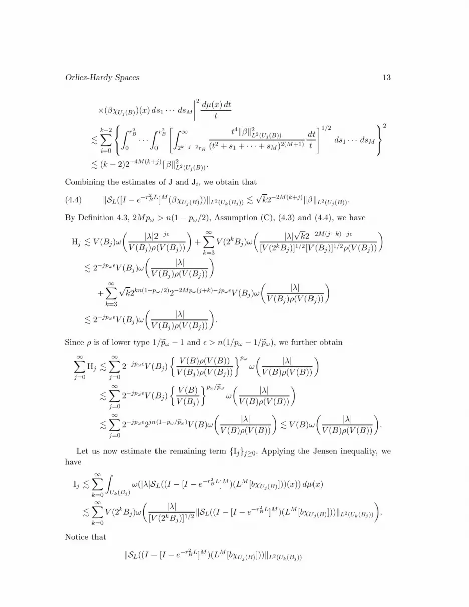
‖SL([I − e−r2BL]M (βχUj(B)))‖L2(Uk(Bj)) .√k2−2M(k+j)‖β‖L2(Uj(B)).(4.4)
By Definition 4.3, 2Mpω > n(1− pω/2), Assumption (C), (4.3) and (4.4), we have
Hj . V (Bj)ω
( |λ|2−jǫ
V (Bj)ρ(V (Bj))
)+
∞∑
k=3
V (2kBj)ω
( |λ|√k2−2M(j+k)−jǫ
[V (2kBj)]1/2[V (Bj)]1/2ρ(V (Bj))
)
. 2−jpωǫV (Bj)ω
( |λ|V (Bj)ρ(V (Bj))
)
+
∞∑
k=3
√k2kn(1−pω/2)2−2Mpω(j+k)−jpωǫV (Bj)ω
( |λ|V (Bj)ρ(V (Bj))
)
. 2−jpωǫV (Bj)ω
( |λ|V (Bj)ρ(V (Bj))
).
Since ρ is of lower type 1/pω − 1 and ǫ > n(1/pω − 1/pω), we further obtain
∞∑
j=0
Hj .∞∑
j=0
2−jpωǫV (Bj)
{V (B)ρ(V (B))
V (Bj)ρ(V (Bj))
}pω
ω
( |λ|V (B)ρ(V (B))
)
.∞∑
j=0
2−jpωǫV (Bj)
{V (B)
V (Bj)
}pω/pω
ω
( |λ|V (B)ρ(V (B))
)
.∞∑
j=0
2−jpωǫ2jn(1−pω/pω)V (B)ω
( |λ|V (B)ρ(V (B))
). V (B)ω
( |λ|V (B)ρ(V (B))
).
Let us now estimate the remaining term {Ij}j≥0. Applying the Jensen inequality, wehave
Ij .∞∑
k=0
∫
Uk(Bj)ω(|λ|SL((I − [I − e−r2BL]M )(LM [bχUj(B)]))(x)) dµ(x)
.∞∑
k=0
V (2kBj)ω
( |λ|[V (2kBj)]1/2
‖SL((I − [I − e−r2BL]M )(LM [bχUj(B)]))‖L2(Uk(Bj))
).
Notice that
‖SL((I − [I − e−r2BL]M )(LM [bχUj(B)]))‖L2(Uk(Bj))
14 Renjin Jiang and Dachun Yang
. r−2MB sup
1≤l≤M‖SL((lr
2BL)
Me−lr2BL[bχUj(B)]))‖L2(Uk(Bj)).
For k = 0, 1, 2, by the L2(X )-boundedness of SL and (lr2BL)Me−lr2BL, we have
‖SL((lr2BL)
Me−lr2BL[bχUj(B)]))‖L2(Uk(Bj )) . ‖b‖L2(Uj(B)).
For k ≥ 3, Lemma 2.1 yields that
‖SL((lr2BL)
Me−lr2BL[bχUj(B)]))‖2L2(Uk(Bj))
. r4MB
∫∫
R(Uk(Bj ))|t2LM+1e−(t2+lr2B)L[bχUj(B)](x)|2
dµ(x) dt
t
. r4MB
{∫ ∞
0
∫
Rn\2k−2Bj
∣∣∣∣∣t2[(t2 + lr2B)L]
M+1e−(t2+lr2B)L[bχUj(B)](x)
(t2 + lr2B)M+1
∣∣∣∣∣
2dµ(x) dt
t
+
∫ ∞
(2k−1−2i)2jrB
k−2∑
i=0
∫
Ui(Bj)· · · dµ(x) dt
t
}
. r4MB ‖b‖2L2(Uj(B))
[ ∫ ∞
0
t4
(t2 + lr2B)2(M+1)
exp
{− dist (Bj ,R
n \ 2k−1Bj)2
t2 + lr2B
}dt
t
+(k − 2)
∫ ∞
2k−2+jrB
dt
t4M+1
]. k2−4M(k+j)‖b‖2L2(Uj(B)).
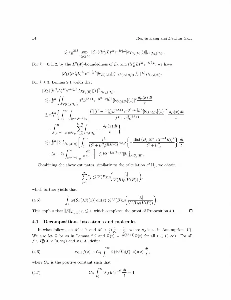
Combining the above estimates, similarly to the calculation of Hj , we obtain
∞∑
j=0
Ij . V (B)ω
( |λ|V (B)ρ(V (B))
),
which further yields that∫
Xω(SL(λβ)(x)) dµ(x) . V (B)ω
( |λ|V (B)ρ(V (B))
).(4.5)
This implies that ‖β‖Hω,L(X ) . 1, which completes the proof of Proposition 4.1.
4.1 Decompositions into atoms and molecules
In what follows, let M ∈ N and M > n2 (
1pω
− 12 ), where pω is as in Assumption (C).
We also let Φ be as in Lemma 2.2 and Ψ(t) = t2(M+1)Φ(t) for all t ∈ (0,∞). For allf ∈ L2
b(X × (0,∞)) and x ∈ X , define
(4.6) πΨ,Lf(x) ≡ CΨ
∫ ∞
0Ψ(t
√L)(f(·, t))(x) dt
t,
where CΨ is the positive constant such that
(4.7) CΨ
∫ ∞
0Ψ(t)t2e−t2 dt
t= 1.
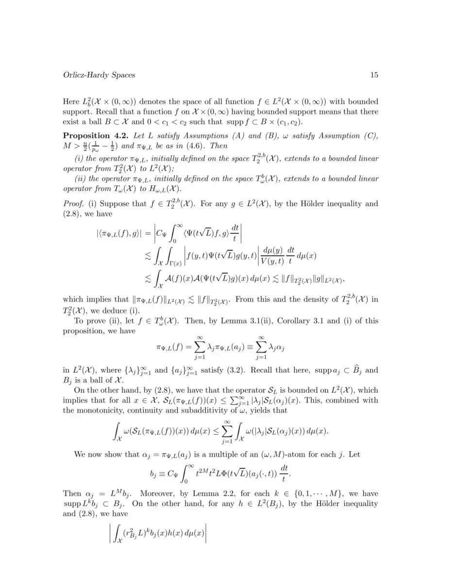
Orlicz-Hardy Spaces 15
Here L2b(X × (0,∞)) denotes the space of all function f ∈ L2(X × (0,∞)) with bounded
support. Recall that a function f on X ×(0,∞) having bounded support means that thereexist a ball B ⊂ X and 0 < c1 < c2 such that supp f ⊂ B × (c1, c2).
Proposition 4.2. Let L satisfy Assumptions (A) and (B), ω satisfy Assumption (C),M > n
2 (1pω
− 12) and πΨ,L be as in (4.6). Then
(i) the operator πΨ,L, initially defined on the space T 2,b2 (X ), extends to a bounded linear
operator from T 22 (X ) to L2(X );
(ii) the operator πΨ,L, initially defined on the space T bω(X ), extends to a bounded linear
operator from Tω(X ) to Hω,L(X ).
Proof. (i) Suppose that f ∈ T 2,b2 (X ). For any g ∈ L2(X ), by the Holder inequality and
(2.8), we have
|〈πΨ,L(f), g〉| =∣∣∣∣CΨ
∫ ∞
0〈Ψ(t
√L)f, g〉 dt
t
∣∣∣∣
.
∫
X
∫
Γ(x)
∣∣∣∣f(y, t)Ψ(t√L)g(y, t)
∣∣∣∣dµ(y)
V (y, t)
dt
tdµ(x)
.
∫
XA(f)(x)A(Ψ(t
√L)g)(x) dµ(x) . ‖f‖T 2
2 (X )‖g‖L2(X ),
which implies that ‖πΨ,L(f)‖L2(X ) . ‖f‖T 22 (X ). From this and the density of T 2,b
2 (X ) in
T 22 (X ), we deduce (i).To prove (ii), let f ∈ T b
ω(X ). Then, by Lemma 3.1(ii), Corollary 3.1 and (i) of thisproposition, we have
πΨ,L(f) =
∞∑
j=1
λjπΨ,L(aj) ≡∞∑
j=1
λjαj
in L2(X ), where {λj}∞j=1 and {aj}∞j=1 satisfy (3.2). Recall that here, supp aj ⊂ Bj andBj is a ball of X .
On the other hand, by (2.8), we have that the operator SL is bounded on L2(X ), whichimplies that for all x ∈ X , SL(πΨ,L(f))(x) ≤ ∑∞
j=1 |λj |SL(αj)(x). This, combined withthe monotonicity, continuity and subadditivity of ω, yields that
∫
Xω(SL(πΨ,L(f))(x)) dµ(x) ≤
∞∑
j=1
∫
Xω(|λj |SL(αj)(x)) dµ(x).
We now show that αj = πΨ,L(aj) is a multiple of an (ω,M)-atom for each j. Let
bj ≡ CΨ
∫ ∞
0t2M t2LΦ(t
√L)(aj(·, t))
dt
t.
Then αj = LMbj . Moreover, by Lemma 2.2, for each k ∈ {0, 1, · · · ,M}, we havesuppLkbj ⊂ Bj . On the other hand, for any h ∈ L2(Bj), by the Holder inequalityand (2.8), we have
∣∣∣∣∫
X(r2Bj
L)kbj(x)h(x) dµ(x)
∣∣∣∣
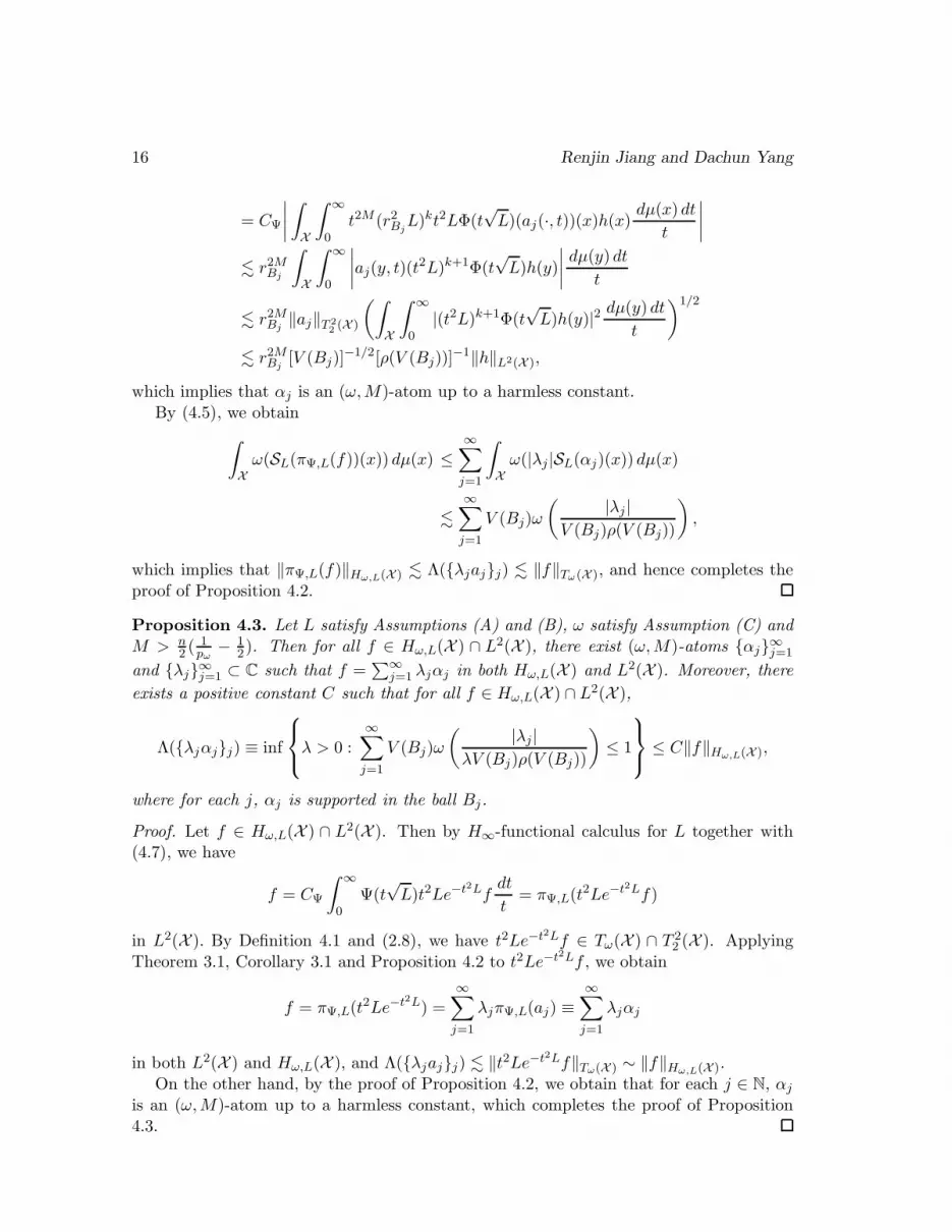
16 Renjin Jiang and Dachun Yang
= CΨ
∣∣∣∣∫
X
∫ ∞
0t2M (r2Bj
L)kt2LΦ(t√L)(aj(·, t))(x)h(x)
dµ(x) dt
t
∣∣∣∣
. r2MBj
∫
X
∫ ∞
0
∣∣∣∣aj(y, t)(t2L)k+1Φ(t√L)h(y)
∣∣∣∣dµ(y) dt
t
. r2MBj‖aj‖T 2
2 (X )
(∫
X
∫ ∞
0|(t2L)k+1Φ(t
√L)h(y)|2 dµ(y) dt
t
)1/2
. r2MBj[V (Bj)]
−1/2[ρ(V (Bj))]−1‖h‖L2(X ),
which implies that αj is an (ω,M)-atom up to a harmless constant.By (4.5), we obtain
∫
Xω(SL(πΨ,L(f))(x)) dµ(x) ≤
∞∑
j=1
∫
Xω(|λj |SL(αj)(x)) dµ(x)
.∞∑
j=1
V (Bj)ω
( |λj |V (Bj)ρ(V (Bj))
),
which implies that ‖πΨ,L(f)‖Hω,L(X ) . Λ({λjaj}j) . ‖f‖Tω(X ), and hence completes theproof of Proposition 4.2.
Proposition 4.3. Let L satisfy Assumptions (A) and (B), ω satisfy Assumption (C) andM > n
2 (1pω
− 12). Then for all f ∈ Hω,L(X ) ∩ L2(X ), there exist (ω,M)-atoms {αj}∞j=1
and {λj}∞j=1 ⊂ C such that f =∑∞
j=1 λjαj in both Hω,L(X ) and L2(X ). Moreover, there
exists a positive constant C such that for all f ∈ Hω,L(X ) ∩ L2(X ),
Λ({λjαj}j) ≡ inf
λ > 0 :
∞∑
j=1
V (Bj)ω
( |λj|λV (Bj)ρ(V (Bj))
)≤ 1
≤ C‖f‖Hω,L(X ),
where for each j, αj is supported in the ball Bj.
Proof. Let f ∈ Hω,L(X ) ∩ L2(X ). Then by H∞-functional calculus for L together with(4.7), we have
f = CΨ
∫ ∞
0Ψ(t
√L)t2Le−t2Lf
dt
t= πΨ,L(t
2Le−t2Lf)
in L2(X ). By Definition 4.1 and (2.8), we have t2Le−t2Lf ∈ Tω(X ) ∩ T 22 (X ). Applying
Theorem 3.1, Corollary 3.1 and Proposition 4.2 to t2Le−t2Lf , we obtain
f = πΨ,L(t2Le−t2L) =
∞∑
j=1
λjπΨ,L(aj) ≡∞∑
j=1
λjαj
in both L2(X ) and Hω,L(X ), and Λ({λjaj}j) . ‖t2Le−t2Lf‖Tω(X ) ∼ ‖f‖Hω,L(X ).On the other hand, by the proof of Proposition 4.2, we obtain that for each j ∈ N, αj
is an (ω,M)-atom up to a harmless constant, which completes the proof of Proposition4.3.
Orlicz-Hardy Spaces 17
From Proposition 4.3, similarly to the proof of [21, Corollary 4.1], we deduce thefollowing result. We omit the details.
Corollary 4.1. Let L satisfy Assumptions (A) and (B), ω satisfy Assumption (C) andM > n
2 (1pω
− 12). Then for all f ∈ Hω,L(X ), there exist (ω,M)-atoms {αj}∞j=1 and
{λj}∞j=1 ⊂ C such that f =∑∞
j=1 λjαj in Hω,L(X ). Moreover, there exists a positiveconstant C independent of f such that Λ({λjαj}j) ≤ C‖f‖Hω,L(X ).
Let Hat,Mω,fin (X ) and Hmol,M, ǫ
ω,fin (X ) denote the spaces of finite combinations of (ω,M)-atoms and (ω,M, ǫ)-molecules, respectively. From Corollary 4.1 and Proposition 4.1, wededuce the following density conclusions.
Corollary 4.2. Let L satisfy Assumptions (A) and (B), ω satisfy Assumption (C), ǫ >
n(1/pω − 1/p+ω ) and M > n2 (
1pω
− 12 ). Then both the spaces Hat,M
ω,fin (X ) and Hmol,M, ǫω,fin (X )
are dense in the space Hω,L(X ).
4.2 Dual spaces of Orlicz-Hardy spaces
In this subsection, we study the dual space of the Orlicz-Hardy space Hω,L(X ). Webegin with some notions.
Let φ = LMν be a function in L2(X ), where ν ∈ D(LM ). Following [18, 17], for ǫ > 0,M ∈ N and fixed x0 ∈ X , we introduce the space
MM,ǫω (L) ≡ {φ = LMν ∈ L2(X ) : ‖φ‖MM,ǫ
ω (L)<∞},
where
‖φ‖MM,ǫω (L)
≡ supj∈Z+
{2jǫ[V (x0, 2
j)]1/2ρ(V (x0, 2j))
M∑
k=0
‖Lkν‖L2(Uj(B(x0,1)))
}.
Notice that if φ ∈ MM,ǫω (L) for some ǫ > 0 with norm 1, then φ is an (ω,M, ǫ)-molecule
adapted to the ball B(x0, 1). Conversely, if β is an (ω,M, ǫ)-molecule adapted to any ball,then β ∈ MM,ǫ
ω (L).Let At denote either (I + t2L)−1 or e−t2L and f ∈ (MM,ǫ
ω (L))∗, the dual space ofMM,ǫ
ω (L). We claim that (I − At)Mf ∈ L2
loc (X ) in the sense of distributions. In fact,for any ball B, if ψ ∈ L2(B), then it follows from the Davies-Gaffney estimate (2.6) that(I −At)
Mψ ∈ MM,ǫω (L) for every ǫ > 0. Thus,
|〈(I −At)Mf, ψ〉| ≡ |〈f, (I −At)
Mψ〉| ≤ C(t, rB, dist (B,x0))‖f‖(MM,ǫω (L))∗
‖ψ‖L2(B),
which implies that (I −At)Mf ∈ L2
loc (X ) in the sense of distributions.
Finally, for any M ∈ N, define
MMω (X ) ≡
⋂
ǫ>n(1/pω−1/p+ω )
(MM,ǫω (L))∗.
18 Renjin Jiang and Dachun Yang
Definition 4.4. Let L satisfy Assumptions (A) and (B), ω satisfy Assumption (C), ρ beas in (2.10) and M > n
2 (1pω
− 12). A functional f ∈ MM
ω (X ) is said to be in BMOMρ,L(X )
if
‖f‖BMOMρ,L(X ) ≡ sup
B⊂X
1
ρ(V (B))
[1
V (B)
∫
B|(I − e−r2BL)Mf(x)|2 dµ(x)
]1/2<∞,
where the supremum is taken over all ball B of X .
The proofs of the following two propositions are similar to those of Lemmas 8.1 and8.3 of [18], respectively; we omit the details.
Proposition 4.4. Let L, ω, ρ and M be as in Definition 4.4. Then f ∈ BMOMρ,L(X ) if
and only if f ∈ MMω (X ) and
supB⊂X
1
ρ(V (B))
[1
V (B)
∫
B|(I − (I + r2BL)
−1)Mf(x)|2 dµ(x)]1/2
<∞.
Moreover, the quantity appeared in the left-hand side of the above formula is equivalent to‖f‖BMOM
ρ,L(X ).
Proposition 4.5. Let L, ω, ρ and M be as in Definition 4.4. Then there exists a positiveconstant C such that for all f ∈ BMOM
ρ,L(X ),
supB⊂X
1
ρ(V (B))
[1
V (B)
∫
B|(t2L)Me−t2Lf(x)|2 dµ(x) dt
t
]1/2≤ C‖f‖BMOM
ρ,L(X ).
The following Proposition 4.6 and Corollary 4.3 are a kind of Calderon reproducingformulae.
Proposition 4.6. Let L, ω, ρ and M be as in Definition 4.4, ǫ > 0 and M > M + ǫ +n4 + N
2 (1pω
− 1), where N is as in (2.4). Fix x0 ∈ X . Assume that f ∈ MMω (X ) satisfies
(4.8)
∫
X
|(I − (I + L)−1)Mf(x)|21 + [d(x, x0)]n+ǫ+2N(1/pω−1)
dµ(x) <∞.
Then for all (ω, M)-atom α,
〈f, α〉 = CM
∫
X×(0,∞)(t2L)Me−t2Lf(x)t2Le−t2Lα(x)
dµ(x) dt
t,
where CM is the positive constant satisfying CM
∫∞0 t2(M+1)e−2t2 dt
t = 1.
Proof. Let α be an (ω, M )-atom supported in B ≡ B(xB , rB). Notice that (4.8) impliesthat ∫
X
|(I − (I + L)−1)Mf(x)|2rB + [d(x, xB)]n+ǫ+2N(1/pω−1)
dµ(x) <∞.
Orlicz-Hardy Spaces 19
For R > δ > 0, write
CM
∫ R
δ
∫
X(t2L)Me−t2Lf(x)t2Le−t2Lα(x)
dµ(x) dt
t
=
⟨f, CM
∫ R
δ(t2L)M+1e−2t2Lα
dt
t
⟩= 〈f, α〉 −
⟨f, α− CM
∫ R
δ(t2L)M+1e−2t2Lα
dt
t
⟩.
Since α is an (ω, M )-atom, by Definition 4.2, there exists b ∈ L2(X ) such that α = LMb.
Thus, by the fact that M > M + n4 + N
2 (1pω
− 1) + ǫ, we obtain
α = LMb = (L− L(I + L)−1 + L(I + L)−1)MLM−Mb
=M∑
k=0
CkM(L− L(I + L)−1)M−k(L(I + L)−1)kLM−Mb
=
M∑
k=0
CkM(I − (I + L)−1)MLM−kb,
where CkM denotes the combinatorial number, which together with H∞-functional calculus
further implies that
⟨f, α− CM
∫ R
δ(t2L)M+1e−2t2Lα
dt
t
⟩
=M∑
k=0
CkM
⟨(I − (I + L)−1)Mf, LM−kb− CM
∫ R
δ(t2L)M+1e−2t2LLM−kb
dt
t
⟩
=
M∑
k=0
CkM
⟨(I − (I + L)−1)Mf, CM
∫ δ
0(t2L)M+1e−2t2LLM−kb
dt
t
⟩
+
M∑
k=0
CkM
⟨(I − (I + L)−1)Mf, CM
∫ ∞
R(t2L)M+1e−2t2LLM−kb
dt
t
⟩≡ H+ I.
By (4.8), we see that up to a harmless constant, the term I is bounded by
{∫
X
|(I − (I + L)−1)Mf(x)|2
rB + [d(x, xB)]n+ǫ+2N( 1
pω−1)
dµ(x)
}1/2
sup0≤k≤M
{∫
X
∣∣∣∣∫ ∞
R(t2L)M+1
×e−2t2LLM−kb(x)dt
t
∣∣∣∣2
(rB + [d(x, xB)]n+ǫ+2N( 1
pω−1)
) dµ(x)
}1/2
. sup0≤k≤M
∞∑
j=0
(2jrB)n+ǫ2
+N( 1pω
−1)∫ ∞
R‖(t2L)M+M+1−ke−2t2Lb‖L2(Uj(B))
dt
t2(M−k)+1
. sup0≤k≤M
2∑
j=0
(2jrB)n+ǫ2
+N( 1pω
−1)‖b‖L2(X )
∫ ∞
R
dt
t2(M−k)+1
20 Renjin Jiang and Dachun Yang
+ sup0≤k≤M
∞∑
j=3
(2jrB)n+ǫ2
+N( 1pω
−1)‖b‖L2(X )
∫ ∞
Rexp
{− dist (B,Uj(B))2
t2
}dt
t2(M−k)+1
. R−2(M−M) +
∞∑
j=3
(2jrB)n+ǫ2
+N( 1pω
−1)∫ ∞
R
(t
2jrB
)n/2+ǫ+N( 1pω
−1) dt
t2(M−M)+1
. R−ǫ → 0,
as R→ ∞.Similarly, the term H is controlled by
{∫
X
|(I − (I + L)−1)Mf(x)|2
rB + [d(x, xB)]n+ǫ+2N( 1
pω−1)
dµ(x)
}1/2
sup0≤k≤M
{∫
X
∣∣∣∣∫ δ
0(t2L)M+1
× e−2t2LLM−kb(x)dt
t
∣∣∣∣2
(rB + [d(x, xB)]n+ǫ+2N( 1
pω−1)) dµ(x)
}1/2
.∞∑
j=0
sup0≤k≤M
(2jrB)(n+ǫ)/2+N( 1
pω−1)
×{∫
Uj(B)
∣∣∣∣∫ δ
0(t2L)M+1e−2t2LLM−kb(x)
dt
t
∣∣∣∣2
dµ(x)
}1/2
∼∞∑
j=0
Hj.
For j ≥ 3, we further have
Hj . sup0≤k≤M
(2jrB)n+ǫ2
+N( 1pω
−1)∫ δ
0‖(t2L)M+1e−2t2LLM−kb‖L2(Uj(B))
dt
t(4.9)
. sup0≤k≤M
(2jrB)n+ǫ2
+N( 1pω
−1)‖LM−kb‖L2(X )
∫ δ
0exp
{− dist (B,Uj(B))2
t2
}dt
t
. (2jrB)n+ǫ2
+N( 1pω
−1)∫ δ
0
(t
2jrB
)n/2+ǫ+N( 1pω
−1) dt
t. 2−jǫ/2δ
n/2+ǫ+N( 1pω
−1).
Notice that for each i ∈ N, (δ2L)ie−2δ2L → 0 and e−2δ2L − I → 0 in the strong operatortopology as δ → 0. Thus, for j = 0, 1, 2, we obtain
Hj . sup0≤k≤M
∥∥∥∥∫ δ
0(t2L)(M+1)e−2t2LLM−kb(x)
dt
t
∥∥∥∥L2(Uj(B))
(4.10)
. sup0≤k≤M
[ M∑
i=1
‖(δ2L)ie−2δ2L(LM−kb)‖L2(Uj(B))
+‖(e−2δ2L − I)(LM−kb)‖L2(Uj(B))
]→ 0,
as δ → 0. The estimates (4.9) and (4.10) imply that H → 0 as δ → 0, and hence completethe proof of Proposition 4.6.
Orlicz-Hardy Spaces 21
To prove that Proposition 4.6 holds for all f ∈ BMOMρ,L(X ), we need the following
“dyadic cubes” on spaces of homogeneous type constructed by Christ [6, Theorem 11].
Lemma 4.1. There exists a collection {Qkα ⊂ X : k ∈ Z, α ∈ Ik} of open subsets,
where Ik denotes some (possibly finite) index set depending on k, and constants δ ∈ (0, 1),a0 ∈ (0, 1) and C5 ∈ (0,∞) such that
(i) µ(X \ ∪αQkα) = 0 for all k ∈ Z;
(ii) if i ≥ k, then either Qiα ⊂ Qk
β or Qiα ∩Qk
β = ∅;(iii) for each (k, α) and each i < k, there exists a unique β such that Qk
α ⊂ Qiβ;
(iv) the diameter of Qkα is no more than C5δ
k;(v) each Qk
α contains certain ball B(zkα, a0δk).
From Proposition 4.6 and Lemma 4.1, we deduce the following conclusion.
Corollary 4.3. Let L, ω, ρ and M be as in Definition 4.4 and M > M + n4 +
N2 (
1pω
− 1).
Then for all (ω, M)-atom α and f ∈ BMOMρ,L(X ),
〈f, α〉 = CM
∫
X×(0,∞)(t2L)Me−t2Lf(x)t2Le−t2Lα(x)
dµ(x) dt
t,
where CM is as in Proposition 4.6.
Proof. Let ǫ ∈ (0, M −M − n4 − N
2 (1pω
− 1)). By Proposition 4.6, we only need to show
that (4.8) with such an ǫ holds for all f ∈ BMOMρ,L(X ).
Let all the notation be the same as in Lemma 4.1. For each j ∈ Z, choose kj ∈ Z suchthat C5δ
kj ≤ 2j < C5δkj−1. Let B = B(x0, 1), where x0 is as in (4.8), and
Mj ≡ {β ∈ Ik0 : Qk0β ∩B(x0, C5δ
kj−1) 6= ∅}.
Then for each j ∈ Z+,
(4.11) Uj(B) ⊂ B(x0, C5δkj−1) ⊂
⋃
β∈Mj
Qk0β ⊂ B(x0, 2C5δ
kj−1).
By Lemma 4.1, the sets Qk0β for all β ∈ Mj are disjoint. Moreover, by (iv) and (v) of
Lemma 4.1, there exists zk0β ∈ Qk0β such that
(4.12) B(zk0β , a0δk0) ⊂ Qk0
β ⊂ B(zk0β , C5δk0) ⊂ B(zk0β , 1).
Thus, by Proposition 4.4, (2.4) and the fact that ρ is of upper type 1/pω − 1, we have
H ≡{∫
X
|(I − (I + L)−1)Mf(x)|21 + [d(x, x0)]n+ǫ+2N(1/pω−1)
dµ(x)
}1/2
.∞∑
j=0
2−j[(n+ǫ)/2+N(1/pω−1)]
∑
β∈Mj
∫
Qk0β
|(I − (I + L)−1)Mf(x)|2 dµ(x)
1/2
22 Renjin Jiang and Dachun Yang
.∞∑
j=0
2−j[(n+ǫ)/2+N(1/pω−1)]
∑
β∈Mj
[ρ(V (zk0β , 1))]2V (zk0β , 1)‖f‖2BMOM
ρ,L(X )
1/2
.∞∑
j=0
2−j[(n+ǫ)/2+N(1/pω−1)]
∑
β∈Mj
22jN(1/pω−1)[ρ(V (x0, 1))]2V (zk0β , 1)
1/2
.∞∑
j=0
2−j(n+ǫ)/2
∑
β∈Mj
V (zk0β , 1)
1/2
.
By (4.11), (4.12) and (2.3), we obtain∑
β∈Mj
V (zk0β , 1) .∑
β∈Mj
V (zk0β , aδk0) .
∑
β∈Mj
V (Qk0β ) . V (x0, 2C5δ
kj−1) . 2jnV (B),
which further implies that H <∞, and hence completes the proof of Corollary 4.3.
Using Corollary 4.3, we now establish the duality between Hω,L(X ) and BMOMρ,L(X ).
Theorem 4.1. Let L satisfy Assumptions (A) and (B), ω satisfy Assumption (C), ρ be
as in (2.10), M > n2 (
1pω
− 12) and M > M + n
4 + N2 (
1pω
− 1). Then (Hω,L(X ))∗, the dual
space of Hω,L(X ), coincides with BMOMρ,L(X ) in the following sense.
(i) Let g ∈ BMOMρ,L(X ). Then the linear functional ℓg, which is initially defined on
Hat,Mω,fin (X ) by
(4.13) ℓg(f) ≡ 〈g, f〉,
has a unique extension to Hω,L(X ) with ‖ℓg‖(Hω,L(X ))∗ ≤ C‖g‖BMOMρ,L(X ), where C is a
positive constant independent of g.(ii) Conversely, let ǫ > n(1/pω−1/p+ω ). Then for any ℓ ∈ (Hω,L(X ))∗, ℓ ∈ BMOM
ρ,L(X )
with ‖ℓ‖BMOMρ,L(X ) ≤ C‖ℓ‖(Hω,L(X ))∗ and (4.13) holds for all f ∈ Hmol,M,ǫ
ω,fin (X ), where C is
a positive constant independent of ℓ.
Proof. Let g ∈ BMOMρ,L(X ). For any f ∈ Hat,M
ω,fin (X ), by Proposition 4.1, we have that
t2Le−t2Lf ∈ Tω(X ). By Theorem 3.1, there exist {λj}∞j=1 ⊂ C and Tω(X )-atoms {aj}∞j=1
supported in {Bj}∞j=1 such that (3.1) and (3.2) hold. This, together with Corollary 4.3,the Holder inequality, Proposition 4.5 and Remark 3.1(ii), yields that
|〈g, f〉| =∣∣∣∣CM
∫ ∞
0
∫
X(t2L)Me−t2Lg(x)t2Le−t2Lf(x)
dµ(x) dt
t
∣∣∣∣(4.14)
.∑
j
|λj |∫ ∞
0
∫
X|(t2L)Me−t2Lg(x)aj(x, t)|
dµ(x) dt
t
.∑
j
|λj |‖aj‖T 22 (X )
(∫
Bj
|(t2L)Me−t2Lg(x)|2 dµ(x) dtt
)1/2
Orlicz-Hardy Spaces 23
.∑
j
|λj |‖g‖BMOMρ,L(X ) . ‖t2Le−t2Lf‖Tω(X )‖g‖BMOM
ρ,L(X )
∼ ‖f‖Hω,L(X )‖g‖BMOMρ,L(X ).
Then by Proposition 4.2, we obtain (i).
Conversely, let ℓ ∈ (Hω,L(X ))∗. If g ∈ MM,ǫω (L), then g is a multiple of an (ω,M, ǫ)-
molecule. Moreover, if ǫ > n(1/pω −1/p+ω ), then by Proposition 4.1, we have g ∈ Hω,L(X )
and hence MM,ǫω (L) ⊂ Hω,L(X ). Then ℓ ∈ MM
ω (X ).
On the other hand, for any ball B, let φ ∈ L2(B) with ‖φ‖L2(B) ≤ 1[V (B)]1/2ρ(V (B))
and
β ≡ (I − [I + r2BL]−1)Mφ. Obviously, β = (r2BL)
M (I + r2BL)−Mφ ≡ LM b. Then from
the fact that {(t2L)k(I+r2BL)−M}0≤k≤M satisfy the Davies-Gaffney estimate (see Lemma2.1), we deduce that for each j ∈ Z+ and k = 0, 1, · · · ,M , we have
‖(r2BL)k b‖L2(Uj(B)) = r2MB ‖(I − [I + r2BL]−1)k(I + r2BL)
−(M−k)φ‖L2(Uj(B))
. r2MB exp
{− dist (B,Uj(B))
rB
}‖φ‖L2(B)
. r2MB 2−2j(M+ǫ)2jn(1/pω−1/2)[V (2jB)]−1/2[ρ(V (2jB))]−1
. r2MB 2−2jǫ[V (2jB)]−1/2[ρ(V (2jB))]−1,
since 2M > n(1/pω − 1/2). Thus, β is a multiple of an (ω,M, ǫ)-molecule. Since (I −[I + t2L]−1)Mℓ is well defined and belongs to L2
loc (X ) for every t > 0, by the fact that
‖β‖Hω,L(X ) . 1, we have
|〈(I − [I + r2BL]−1)M ℓ, φ〉| = |〈ℓ, (I − [I + r2BL]
−1)Mφ〉| = |〈ℓ, β〉| . ‖ℓ‖(Hω,L(X ))∗ ,
which further implies that
1
ρ(V (B))
(1
V (B)
∫
B|(I − [I + r2BL]
−1)Mℓ(x)|2 dµ(x))1/2
= sup‖φ‖L2(B)≤1
∣∣∣∣⟨ℓ, (I − [I + r2BL]
−1)Mφ
[V (B)]1/2ρ(V (B))
⟩∣∣∣∣ . ‖ℓ‖(Hω,L(X ))∗ .
Thus, by Proposition 4.4, we obtain ℓ ∈ BMOMρ,L(X ), which completes the proof of Theo-
rem 4.1.
Remark 4.2. By Theorem 4.1, we have that for allM > n2 (
1pω
− 12), the spaces BMOM
ρ,L(X )
coincide with equivalent norms; thus, in what follows, we denote BMOMρ,L(X ) simply by
BMOρ,L(X ).
Recall that a measure dµ on X × (0,∞) is called a ρ-Carleson measure if
‖dµ‖ρ ≡ supB⊂X
{1
V (B)[ρ(V (B))]2
∫
B|dµ|
}1/2
<∞,
24 Renjin Jiang and Dachun Yang
where the supremum is taken over all balls B of X and B denotes the tent over B; see[16].
Using Theorem 4.1 and Proposition 4.5, we obtain the following ρ-Carleson measurecharacterization of BMOρ,L(X ).
Theorem 4.2. Let L satisfy Assumptions (A) and (B), ω satisfy Assumption (C), ρ beas in (2.10) and M > n
2 (1pω
− 12). Then the following conditions are equivalent:
(i) f ∈ BMOρ,L(X );(ii) f ∈ MM
ω (X ) satisfies (4.8) for some ǫ > 0, and dµf is a ρ-Carleson measure,
where dµf is defined by dµf ≡ |(t2L)Me−t2Lf(x)|2 dµ(x) dtt .
Moreover, ‖f‖BMOρ,L(X ) and ‖dµf‖ρ are comparable.
Proof. It follows from Proposition 4.5 and the proof of Corollary 4.3 that (i) implies (ii).
Conversely, let M > M + ǫ+ n4 + N
2 (1pω
− 1). By Proposition 4.6, we have
〈f, g〉 = CM
∫
X×(0,∞)(t2L)Me−t2Lf(x)t2Le−t2Lg(x)
dµ(x) dt
t,
where g is any finite combination of (ω, M )-atoms. Then similarly to the estimate of(4.14), we obtain that
(4.15) |〈f, g〉| . ‖dµf‖ρ‖g‖Hω,L(X ).
Since, by Corollary 4.2, Hat,Mω,fin (X ) is dense in Hω,L(X ), this together with Theorem 4.1
and (4.15) implies that f ∈ (Hω,L(X ))∗ = BMOρ,L(X ), which completes the proof ofTheorem 4.2.
5 Characterizations of Orlicz-Hardy spaces
In this section, we characterize the Orlicz-Hardy spaces by atoms, molecules and theLusin-area function associated with the Poisson semigroup. Let us begin with some no-tions.
Definition 5.1. Let L satisfy Assumptions (A) and (B), ω satisfy Assumption (C) andM > n
2 (1pω
− 12). A distribution f ∈ (BMOρ,L(X ))∗ is said to be in the space HM
ω,at(X ) if
there exist {λj}∞j=1 ⊂ C and (ω,M)−atoms {αj}∞j=1 such that f =∑∞
j=1 λjαj in the norm
of (BMOρ,L(X ))∗ and∑∞
j=1 V (Bj)ω(|λj |
V (Bj)ρ(V (Bj))) <∞, where for each j, suppαj ⊂ Bj .
Moreover, for any f ∈ HMω,at(X ), its norm is defined by ‖f‖HM
ω,at(X ) ≡ inf Λ({λjαj}j),where Λ({λjαj}j) is the same as in Proposition 4.3 and the infimum is taken over allpossible decompositions of f .
Definition 5.2. Let L satisfy Assumptions (A) and (B), ω satisfy Assumption (C), M >n2 (
1pω
− 12) and ǫ > n(1/pω − 1/p+ω ). A distribution f ∈ (BMOρ,L(X ))∗ is said to be in
the space HM,ǫω,mol(X ) if there exist {λj}∞j=1 ⊂ C and (ω,M, ǫ)−molecules {βj}∞j=1 such that
Orlicz-Hardy Spaces 25
f =∑∞
j=1 λjβj in the norm of (BMOρ,L(X ))∗ and∑∞
j=1 V (Bj)ω(|λj |
V (Bj)ρ(V (Bj))) < ∞,
where for each j, βj is associated to the ball Bj .
Moreover, for any f ∈ HM,ǫω,mol(X ), its norm is defined by ‖f‖
HM,ǫω,mol(X )
≡ inf Λ({λjβj}j),where Λ({λjβj}j) is the same as in Proposition 4.3 and the infimum is taken over allpossible decompositions of f .
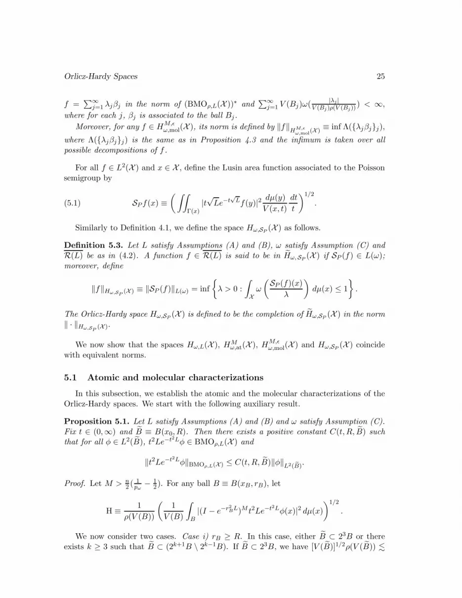
For all f ∈ L2(X ) and x ∈ X , define the Lusin area function associated to the Poissonsemigroup by
(5.1) SPf(x) ≡(∫∫
Γ(x)|t√Le−t
√Lf(y)|2 dµ(y)
V (x, t)
dt
t
)1/2
.
Similarly to Definition 4.1, we define the space Hω,SP(X ) as follows.
Definition 5.3. Let L satisfy Assumptions (A) and (B), ω satisfy Assumption (C) andR(L) be as in (4.2). A function f ∈ R(L) is said to be in Hω,SP
(X ) if SP (f) ∈ L(ω);moreover, define
‖f‖Hω,SP(X ) ≡ ‖SP (f)‖L(ω) = inf
{λ > 0 :
∫
Xω
(SP (f)(x)
λ
)dµ(x) ≤ 1
}.
The Orlicz-Hardy space Hω,SP(X ) is defined to be the completion of Hω,SP
(X ) in the norm‖ · ‖Hω,SP
(X ).
We now show that the spaces Hω,L(X ), HMω,at(X ), HM,ǫ
ω,mol(X ) and Hω,SP(X ) coincide
with equivalent norms.
5.1 Atomic and molecular characterizations
In this subsection, we establish the atomic and the molecular characterizations of theOrlicz-Hardy spaces. We start with the following auxiliary result.
Proposition 5.1. Let L satisfy Assumptions (A) and (B) and ω satisfy Assumption (C).Fix t ∈ (0,∞) and B ≡ B(x0, R). Then there exists a positive constant C(t, R, B) suchthat for all φ ∈ L2(B), t2Le−t2Lφ ∈ BMOρ,L(X ) and
‖t2Le−t2Lφ‖BMOρ,L(X ) ≤ C(t, R, B)‖φ‖L2(B).
Proof. Let M > n2 (
1pω
− 12). For any ball B ≡ B(xB , rB), let
H ≡ 1
ρ(V (B))
(1
V (B)
∫
B|(I − e−r2BL)M t2Le−t2Lφ(x)|2 dµ(x)
)1/2
.
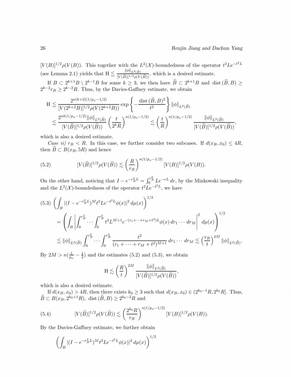
We now consider two cases. Case i) rB ≥ R. In this case, either B ⊂ 23B or thereexists k ≥ 3 such that B ⊂ (2k+1B \ 2k−1B). If B ⊂ 23B, we have [V (B)]1/2ρ(V (B)) .
26 Renjin Jiang and Dachun Yang
[V (B)]1/2ρ(V (B)). This together with the L2(X )-boundedness of the operator t2Le−t2L
(see Lemma 2.1) yields that H .‖φ‖
L2(B)
[V (B)]1/2ρ(V (B)), which is a desired estimate.
If B ⊂ 2k+1B \ 2k−1B for some k ≥ 3, we then have B ⊂ 2k+1B and dist (B, B) ≥2k−2rB ≥ 2k−2R. Thus, by the Davies-Gaffney estimate, we obtain
H .2n(k+2)(1/pω−1/2)
[V (2k+2B)]1/2ρ(V (2k+2B))exp
{− dist (B, B)2
t2
}‖φ‖
L2(B)
.2nk(1/pω−1/2)‖φ‖L2(B)
[V (B)]1/2ρ(V (B))
(t
2kR
)n(1/pω−1/2)
.
(t
R
)n(1/pω−1/2) ‖φ‖L2(B)
[V (B)]1/2ρ(V (B)),
which is also a desired estimate.Case ii) rB < R. In this case, we further consider two subcases. If d(xB , x0) ≤ 4R,
then B ⊂ B(xB , 5R) and hence
(5.2) [V (B)]1/2ρ(V (B)) .
(R
rB
)n(1/pω−1/2)
[V (B)]1/2ρ(V (B)).
On the other hand, noticing that I − e−r2BL =∫ r2B0 Le−rL dr, by the Minkowski inequality
and the L2(X )-boundedness of the operator t2Le−t2L, we have
(∫
B|(I − e−r2BL)M t2Le−t2Lφ(x)|2 dµ(x)
)1/2
(5.3)
=
∫
B
∣∣∣∣∣
∫ r2B
0· · ·∫ r2B
0t2LM+1e−(r1+···+rM+t2)Lφ(x) dr1 · · · drM
∣∣∣∣∣
2
dµ(x)
1/2
. ‖φ‖L2(B)
∫ r2B
0· · ·∫ r2B
0
t2
(r1 + · · ·+ rM + t2)M+1dr1 · · · drM .
(rBt
)2M‖φ‖L2(B).
By 2M > n( 1pω
− 12) and the estimates (5.2) and (5.3), we obtain
H .
(R
t
)2M ‖φ‖L2(B)
[V (B)]1/2ρ(V (B)),
which is also a desired estimate.If d(xB , x0) > 4R, then there exists k0 ≥ 3 such that d(xB , x0) ∈ (2k0−1R, 2k0R]. Thus,
B ⊂ B(xB , 2k0+1R), dist (B, B) ≥ 2k0−2R and
(5.4) [V (B)]1/2ρ(V (B)) .
(2k0R
rB
)n(1/pω−1/2)
[V (B)]1/2ρ(V (B)).
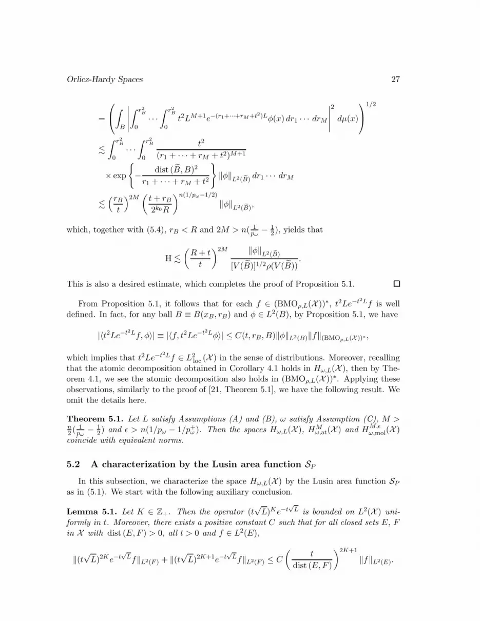
By the Davies-Gaffney estimate, we further obtain
(∫
B|(I − e−r2BL)M t2Le−t2Lφ(x)|2 dµ(x)
)1/2
Orlicz-Hardy Spaces 27
=
∫
B
∣∣∣∣∣
∫ r2B
0· · ·∫ r2B
0t2LM+1e−(r1+···+rM+t2)Lφ(x) dr1 · · · drM
∣∣∣∣∣
2
dµ(x)
1/2
.
∫ r2B
0· · ·∫ r2B
0
t2
(r1 + · · ·+ rM + t2)M+1
× exp
{− dist (B, B)2
r1 + · · · + rM + t2
}‖φ‖L2(B) dr1 · · · drM
.(rBt
)2M ( t+ rB2k0R
)n(1/pω−1/2)
‖φ‖L2(B)
,
which, together with (5.4), rB < R and 2M > n( 1pω
− 12), yields that
H .
(R+ t
t
)2M ‖φ‖L2(B)
[V (B)]1/2ρ(V (B)).
This is also a desired estimate, which completes the proof of Proposition 5.1.
From Proposition 5.1, it follows that for each f ∈ (BMOρ,L(X ))∗, t2Le−t2Lf is welldefined. In fact, for any ball B ≡ B(xB , rB) and φ ∈ L2(B), by Proposition 5.1, we have
|〈t2Le−t2Lf, φ〉| ≡ |〈f, t2Le−t2Lφ〉| ≤ C(t, rB , B)‖φ‖L2(B)‖f‖(BMOρ,L(X ))∗ ,
which implies that t2Le−t2Lf ∈ L2loc (X ) in the sense of distributions. Moreover, recalling
that the atomic decomposition obtained in Corollary 4.1 holds in Hω,L(X ), then by The-orem 4.1, we see the atomic decomposition also holds in (BMOρ,L(X ))∗. Applying theseobservations, similarly to the proof of [21, Theorem 5.1], we have the following result. Weomit the details here.
Theorem 5.1. Let L satisfy Assumptions (A) and (B), ω satisfy Assumption (C), M >n2 (
1pω
− 12) and ǫ > n(1/pω − 1/p+ω ). Then the spaces Hω,L(X ), HM
ω,at(X ) and HM,ǫω,mol(X )
coincide with equivalent norms.
5.2 A characterization by the Lusin area function SP
In this subsection, we characterize the space Hω,L(X ) by the Lusin area function SP
as in (5.1). We start with the following auxiliary conclusion.
Lemma 5.1. Let K ∈ Z+. Then the operator (t√L)Ke−t
√L is bounded on L2(X ) uni-
formly in t. Moreover, there exists a positive constant C such that for all closed sets E, Fin X with dist (E,F ) > 0, all t > 0 and f ∈ L2(E),
‖(t√L)2Ke−t
√Lf‖L2(F ) + ‖(t
√L)2K+1e−t
√Lf‖L2(F ) ≤ C
(t
dist (E,F )
)2K+1
‖f‖L2(E).
28 Renjin Jiang and Dachun Yang
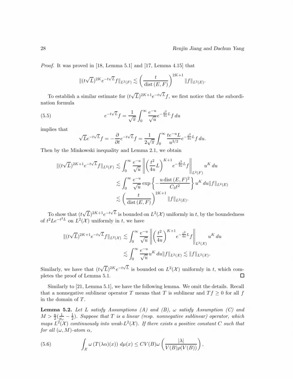
Proof. It was proved in [18, Lemma 5.1] and [17, Lemma 4.15] that
‖(t√L)2Ke−t
√Lf‖L2(F ) .
(t
dist (E,F )
)2K+1
‖f‖L2(E).
To establish a similar estimate for (t√L)2K+1e−t
√Lf , we first notice that the subordi-
nation formula
(5.5) e−t√Lf =
1√π
∫ ∞
0
e−u
√ue−
t2
4uLf du
implies that√Le−t
√Lf = − ∂
∂te−t
√Lf =
1
2√π
∫ ∞
0
te−uL
u3/2e−
t2
4uLf du.
Then by the Minkowski inequality and Lemma 2.1, we obtain
‖(t√L)2K+1e−t
√Lf‖L2(F ) .
∫ ∞
0
e−u
√u
∥∥∥∥∥
(t2
4uL
)K+1
e−t2
4uLf
∥∥∥∥∥L2(F )
uK du
.
∫ ∞
0
e−u
√uexp
{−udist (E,F )
2
C3t2
}uK du‖f‖L2(E)
.
(t
dist (E,F )
)2K+1
‖f‖L2(E).
To show that (t√L)2K+1e−t
√L is bounded on L2(X ) uniformly in t, by the boundedness
of t2Le−t2L on L2(X ) uniformly in t, we have
‖(t√L)2K+1e−t
√Lf‖L2(X ) .
∫ ∞
0
e−u
√u
∥∥∥∥∥
(t2
4u
)K+1
e−t2
4uLf
∥∥∥∥∥L2(X )
uK du
.
∫ ∞
0
e−u
√uuK du‖f‖L2(X ) . ‖f‖L2(X ).
Similarly, we have that (t√L)2Ke−t
√L is bounded on L2(X ) uniformly in t, which com-
pletes the proof of Lemma 5.1.
Similarly to [21, Lemma 5.1], we have the following lemma. We omit the details. Recallthat a nonnegative sublinear operator T means that T is sublinear and Tf ≥ 0 for all fin the domain of T .
Lemma 5.2. Let L satisfy Assumptions (A) and (B), ω satisfy Assumption (C) andM > n
2 (1pω
− 12 ). Suppose that T is a linear (resp. nonnegative sublinear) operator, which
maps L2(X ) continuously into weak-L2(X ). If there exists a positive constant C such thatfor all (ω,M)-atom α,
(5.6)
∫
Xω (T (λα)(x)) dµ(x) ≤ CV (B)ω
( |λ|V (B)ρ(V (B))
),
Orlicz-Hardy Spaces 29
then T extends to a bounded linear (resp. sublinear) operator from Hω,L(X ) to L(ω);
moreover, there exists a positive constant C such that for all f ∈ Hω,L(X ), ‖Tf‖L(ω) ≤C‖f‖Hω,L(X ).
Theorem 5.2. Let L satisfy Assumptions (A) and (B) and ω satisfy Assumption (C).Then the spaces Hω,L(X ) and Hω,SP
(X ) coincide with equivalent norms.
Proof. Let us first prove that Hω,L(X ) ⊂ Hω,SP(X ). By (2.8), we have that the operator
SP is bounded on L2(Rn). Thus, by Lemma 5.2, to show that Hω,L(X ) ⊂ Hω,SP(X ), we
only need to show that (5.6) holds with T = SP , where M ∈ N and M > n2 (
1pω
− 12).
Indeed, it is enough to show that for all f ∈ Hω,L(X )∩L2(X ), ‖SP (f)‖L(ω) . ‖f‖Hω,L(X ),
which implies that (Hω,L(X )∩L2(X )) ⊂ Hω,SP(X ). Then by the completeness of Hω,L(X )
and Hω,SP(X ), we see that Hω,L(X ) ⊂ Hω,SP
(X ).Suppose that λ ∈ C and α is an (ω,M)-atom supported in B ≡ B(xB , rB). Since ω is
concave, by the Jensen inequality and the Holder inequality, we have
∫
Xω(SP (λα)(x)) dµ(x) =
∞∑
k=0
∫
Uk(B)ω(|λ|SP (α)(x)) dµ(x)
≤∞∑
k=0
V (2kB)ω
( |λ|∫Uk(B) SP (α)(x) dµ(x)
V (2kB)
)
≤∞∑
k=0
V (2kB)ω
( |λ|‖SP (α)‖L2(Uk(B))
[V (2kB)]1/2
).
Since SP is bounded on L2(X ), for k = 0, 1, 2, we have
‖SL(α)‖L2(Uk(B)) . ‖α‖L2(X ) . [V (B)]−1/2[ρ(V (B))]−1.
For k ≥ 3, write
‖SP (α)‖2L2(Uk(B)) =
∫
Uk(B)
∫ d(x,xB)
4
0
∫
d(x,y)<t|t√Le−t
√Lα(y)|2 dµ(y)
V (x, t)
dt
tdµ(x)
+
∫
Uk(B)
∫ ∞
d(x,xB)
4
∫
d(x,y)<t· · · ≡ Ik + Jk.
Since α is an (ω,M)-atom, by Definition 4.2, we have α = LMb with b as in Definition4.2. To estimate Ik, let Fk(B) ≡ {y ∈ X : d(x, y) < d(x, xB)/4 for some x ∈ Uk(B)}.Then we have d(y, z) ≥ d(x, xB) − d(z, xB) − d(y, x) ≥ 3
4d(x, xB) − rB ≥ 2k−2rB. ByLemma 5.1, we have
Ik .
∫ 2k−2rB
0
∫
Fk(B)|(t
√L)2M+1e−t
√Lb(y)|2 dµ(y) dt
t4M+1
. ‖b‖2L2(X )
∫ 2k−2rB
0
(t
dist (Fk(B), B)
)4M+2 dt
t4M+1. 2−4kM [V (B)]−1[ρ(V (B))]−2.
30 Renjin Jiang and Dachun Yang
For the term Jk, notice that if x ∈ Uk(B), then we have d(x, xB) ≥ 2k−1rB , whichtogether with Lemma 5.1 yields that
Jk .
∫ ∞
2k−3rB
∫
X|(t
√L)2M+1e−t
√Lb(y)|2 dµ(y) dt
t4M+1
.
∫ ∞
2k−3rB
‖b‖2L2(X )
dt
t4M+1. 2−4kM [V (B)]−1[ρ(V (B))]−2.
Using the estimates of Ik and Jk together with the strictly lower type pω of ω, we obtain
V (2kB)ω
( |λ|‖SP (α)‖L2(Uk(B))
[V (2kB)]1/2
). 2−2kMpωV (2kB)
(V (B)
V (2kB)
)pω/2
ω
( |λ|V (B)ρ(V (B))
)
. 2−k[2Mpω−n(1−pω/2)]V (B)ω
( |λ|V (B)ρ(V (B))
),
where 2Mpω > n(1− pω/2). Thus, we finally obtain that
∫
Xω(SP (λα)(x)) dµ(x) . V (B)ω
( |λ|V (B)ρ(V (B))
),
that is, (5.6) holds. This finishes the proof of the inclusion of Hω,L(X ) into Hω,SP(X ).
Conversely, for any f ∈ Hω,SP(X ) ∩ L2(X ), we have t
√Le−t
√Lf ∈ Tω(X ), which
together with Proposition 4.2(ii) implies that πΨ,L(t√Le−t
√Lf) ∈ Hω,L(X ).
On the other hand, by H∞-functional calculus, we have f = CΨCΨπΨ,L(t
√Le−t
√Lf) in
L2(X ), where CΨ is the positive constant such that CΨ
∫∞0 Ψ(t)te−t dt
t = 1 and CΨ is
as in (4.7). This, combined with the fact πΨ,L(t√Le−t
√Lf) ∈ Hω,L(X ), implies that
f ∈ Hω,L(X ). Via a density argument, we further obtain Hω,SP(X ) ⊂ Hω,L(X ), which
completes the proof of Theorem 5.2.
Remark 5.1. (i) Since the atoms are associated with L, they do not have vanishingintegral in general. Hofmann et al [17] introduced the so-called the conservation propertyof the semigroup, namely, e−tL1 = 1 in L2
loc (X ), and showed that under this assumptionand Assumptions (A) and (B), then for each (1,M)-atom α,
∫X α(x) dµ(x) = 0. From this
and Proposition 4.3, we immediately deduce that if L satisfies Assumptions (A) and (B)and has the conservation property, and ω satisfies Assumption (C) with pω ∈ (n/(n+1), 1],then Hω,L(X ) ⊂ Hω(X ), where X is an Ahlfors n-regular space (see [32]). In particular,Hp
L(X ) ⊂ Hp(X ) for all p ∈ (n/(n + 1), 1].(ii) Let s ∈ Z+. The semigroup {e−tL}t>0 is said to have the s-generalized conservation
property, if for all γ ∈ Zn+ with |γ| ≤ s,
e−tL((·)γ)(x) = xγ in L2loc (R
n),(5.7)
namely, for every φ ∈ L2(Rn) with bounded support,
∫
Rn
xγe−tLφ(x) dx ≡∫
Rn
e−tL((·)γ)(x)φ(x) dx =
∫
Rn
xγφ(x) dx,(5.8)
Orlicz-Hardy Spaces 31
where xγ = xγ11 · · · xγnn for x = (x1, · · · , xn) ∈ Rn and γ = (γ1, · · · , γn) ∈ Z
n+.
Notice that for any φ with bounded support and γ ∈ Zn+, by the Davies-Gaffney
estimate, one can easily check that xγe−tLφ(x), xγ(I + L)−1φ(x) ∈ L1(Rn). Hence, by(5.8) and the L2(Rn)-functional calculus, we obtain
∫
Rn
xγ(I + L)−1φ(x) dx =
∫ ∞
0e−t
[∫
Rn
xγe−tLφ(x) dx
]dt =
∫
Rn
xγφ(x) dx.(5.9)
Let α be an (ω,M)-atom and s ≡ ⌊n( 1pω
−1)⌋. By Definition 4.2, there exists b ∈ D(LM )
such that α = LMb. Thus, if L satisfies (5.7), then for all γ ∈ Zn+ and |γ| ≤ s, by (5.8)
and (5.9), we obtain
∫
Rn
xγα(x) dµ(x)
=
∫
Rn
xγ(I + L)−1α(x) dµ(x)
=
∫
Rn
xγ(I + L)−1(I + L)LM−1b(x) dµ(x) −∫
Rn
xγ(I + L)−1LM−1b(x) dµ(x)
=
∫
Rn
xγLM−1b(x) dµ(x) −∫
Rn
xγ(I + L)−1LM−1b(x) dµ(x) = 0,
which implies that α is a classical Hω(Rn)-atom; for the definition of Hω(R
n)-atoms, see[32].
Thus, if L satisfies (5.7) and Assumptions (A) and (B), and ω satisfies Assumption(C), then by Proposition 4.3, we know that Hω,L(R
n) ⊂ Hω(Rn). In particular, Hp
L(Rn) ⊂
Hp(Rn) for all p ∈ (0, 1].
6 Applications to Schrodinger operators
In this section, let X ≡ Rn and L ≡ −∆ + V be a Schrodinger operator, where
V ∈ L1loc (R
n) is a nonnegative potential. We establish several characterizations of thecorresponding Orlicz-Hardy spaces Hω,L(R
n) by beginning with some notions.Since V is a nonnegative function, by the Feynman-Kac formula, we obtain that ht,
the kernel of the semigroup e−tL, satisfies that for all x, y ∈ Rn and t ∈ (0,∞),
(6.1) 0 ≤ ht(x, y) ≤ (4πt)−n/2 exp
(−|x− y|2
4t
).
It is easy to see that L satisfies Assumptions (A) and (B).From Theorems 5.1 and 5.2, we deduce the following conclusions on Hardy spaces
associated with L.
Theorem 6.1. Let ω be as in Assumption (C), M > n2 (
1pω
− 12) and ǫ > n(1/pω − 1/p+ω ).
Then the spaces Hω,L(Rn), HM
ω,at(Rn), HM,ǫ
ω,mol(Rn) and Hω,SP
(Rn) coincide with equivalentnorms.
32 Renjin Jiang and Dachun Yang
Let us now establish the boundedness of the Riesz transform ∇L−1/2 on Hω,L(Rn). We
first recall a lemma established in [17].
Lemma 6.1. There exist two positive constants C and c such that for all closed sets Eand F in R
n and f ∈ L2(E),
‖t∇e−t2Lf‖L2(F ) ≤ C exp
{− dist (E,F )2
ct2
}‖f‖L2(E).
Theorem 6.2. Let ω be as in Assumption (C). Then the Riesz transform ∇L−1/2 isbounded from Hω,L(R
n) to L(ω).
Proof. It was proved in [17] that the Riesz transform ∇L−1/2 is bounded on L2(Rn); thus,to prove Theorem 6.2, by Lemma 5.2, it suffices to show that (5.6) holds.
Suppose that λ ∈ C and α = LMb is an (ω,M)-atom supported in B ≡ B(xB , rB),where b is as in Definition 4.2 and we choose M ∈ N such that M > n
2 (1pω
− 12).
For j = 0, 1, 2, by the Jensen inequality, the Holder inequality and the L2(Rn)-boundedness of ∇L−1/2, we obtain
∫
Uj(B)ω(|λ∇L−1/2α(x)|) dx . |B|ω
(‖λ∇L−1/2α‖L2(Uj(B))
|B|1/2
). |B|ω
( |λ|ρ(|B|)|B|
).
Let us estimate the case j ≥ 3. By [18, Lemma 2.3], we see that the operatort∇(t2L)Me−t2L also satisfies the Davies-Gaffney estimate. By this, the fact that ω−1
is convex, the Jensen inequality, the Holder inequality and Lemma 6.1, we obtain
ω−1
(1
|Uj(B)|
∫
Uj(B)ω(|λ∇L−1/2α(x)|) dx
)
.1
|Uj(B)|
∫
Uj(B)ω−1 ◦ ω
(∣∣∣∣∫ ∞
0λ∇e−t2Lα(x) dt
∣∣∣∣)dx
.1
|Uj(B)|
∫ ∞
0
∫
Uj(B)|λt∇(t2L)Me−t2Lb(x)| dx dt
t2M+1
.|λ|‖b‖L2(Rn)
|Uj(B)|1/2∫ ∞
0exp
{− dist (B,Uj(B))2
ct2
}dt
t2M+1
.|λ|‖b‖L2(Rn)
|Uj(B)|1/2∫ ∞
0(2jrB)
−2M min
{t
2jrB,2jrBt
}dt
t. 2−j(2M+n/2) |λ|
ρ(|B|)|B| ,
where c is a positive constant. Since ω is of lower type pω, we obtain∫
Uj(B)ω(|λ∇L−1/2α(x)|) dx . |Uj(B)|ω
(2−j(2M+n/2) |λ|
ρ(|B|)|B|
)
. 2−j[2Mpω+n(pω/2−1)]|B|ω( |λ|ρ(|B|)|B|
).
Combining the above estimates and using M > n2 (
1pω
− 12), we obtain that (5.6) holds
for ∇L−1/2, which completes the proof of Theorem 6.2.
Orlicz-Hardy Spaces 33
It was proved in [17] that the Riesz transform ∇L−1/2 is bounded from H1L(R
n) toH1(Rn). Similarly to [21, Theorem 7.4], we have the following result. We omit the detailshere; see [20, 32, 27] for more details about the Hardy-Orlicz space Hω(R
n).
Theorem 6.3. Let ω be as in Assumption (C) and pω ∈ ( nn+1 , 1]. Then the Riesz trans-
form ∇L−1/2 is bounded from Hω,L(Rn) to Hω(R
n).
We next characterize the Orlicz-Hardy space Hω,L(Rn) via maximal functions. To this
end, we first introduce some notions.Let ν > 0. Recall that for all measurable function g on R
n+1+ and x ∈ R
n, the Lusin
area function Aν(g)(x) is defined by Aν(g)(x) ≡ (∫Γν(x)
|g(y, t)|2 dy dttn+1 )
1/2. Also the non-
tangential maximal function is defined by N ν(g)(x) ≡ sup(y,t)∈Γν (x) |g(y, t)|.
Lemma 6.2. Let η, ν ∈ (0,∞). Then there exists a positive constant C, depending on ηand ν, such that for all measurable function g on R
n+1+ ,
(6.2) C−1
∫
Rn
ω(Aη(g)(x)) dx ≤∫
Rn
ω(Aν(g)(x)) dx ≤ C
∫
Rn
ω(Aη(g)(x)) dx
and
(6.3) C−1
∫
Rn
ω(N η(g)(x)) dx ≤∫
Rn
ω(N ν(g)(x)) dx ≤ C
∫
Rn
ω(N η(g)(x)) dx.
Proof. (6.2) was established in [21, Lemma 3.2], while (6.3) can be proved by an argumentsimilar to those used in the proofs of [5, Theorem 2.3] and [21, Lemma 5.3]. We omit thedetails, which completes the proof of Lemma 6.2.
For any β ∈ (0,∞), f ∈ L2(Rn) and x ∈ Rn, let N β
h (f)(x) ≡ N β(e−t2Lf)(x),
N βP (f)(x) ≡ N β(e−t
√Lf)(x), Rh(f)(x) ≡ supt>0 |e−t2Lf(x)| and
RP (f)(x) ≡ supt>0
|e−t√Lf(x)|.
We denote N 1h (f) and N 1
P (f) simply by Nh(f) and NP (f), respectively.Similarly to Definition 4.1, we introduce the space Hω,Nh
(Rn) as follows.
Definition 6.1. Let ω be as in Assumption (C) and R(L) as in (4.2). A function f ∈R(L) is said to be in Hω,Nh
(Rn) if Nh(f) ∈ L(ω); moreover, define
‖f‖Hω,Nh(Rn) ≡ ‖Nh(f)‖L(ω) = inf
{λ > 0 :
∫
Rn
ω
(Nh(f)(x)
λ
)dx ≤ 1
}.
The Hardy space Hω,Nh(Rn) is defined to be the completion of Hω,Nh
(Rn) in the norm‖ · ‖Hω,Nh
(Rn).
The spaces Hω,NP(Rn), Hω,Rh
(Rn) and Hω,RP(Rn) are defined in a similar way.
The following Moser type local boundedness estimate was established in [17].

34 Renjin Jiang and Dachun Yang
Lemma 6.3. Let u be a weak solution of Lu ≡ Lu−∂2t u = 0 in the ball B(Y0, 2r) ⊂ Rn+1+ .
Then for all p ∈ (0,∞), there exists a positive constant C(n, p) such that
supY ∈B(Y0,r)
|u(Y )| ≤ C(n, p)
(1
rn+1
∫
B(Y0,2r)|u(Y )|p dY
)1/p
.
To establish the maximal function characterizations of Hω,L(Rn), an extra assumption
on ω is needed.
Assumption (D). Let ω satisfy Assumption (C). Suppose that there exist q1, q2 ∈ (0,∞)such that q1 < 1 < q2 and [ω(tq2)]q1 is a convex function on (0,∞).
Notice that if ω(t) = tp with p ∈ (0, 1] for all t ∈ (0,∞), then for all q1 ∈ (0, 1) andq2 ∈ [1/(pq1),∞), [ω(tq2)]q1 is a convex function on (0,∞); if ω(t) = t1/2 ln(e4 + t) for allt ∈ (0,∞), then it is easy to check that [ω(t4)]1/2 is a convex function on (0,∞).
Theorem 6.4. Let ω be as in Assumption (D). Then the spaces Hω,L(Rn), Hω,Nh
(Rn),Hω,NP
(Rn), Hω,Rh(Rn) and Hω,RP
(Rn) coincide with equivalent norms.
Proof. We first show that Hω,L(Rn) ⊂ Hω,Nh
(Rn). By (6.1), for all f ∈ L2(Rn) andx ∈ R
n, we have
Nh(f)(x) . supy∈B(x,t)
t−n
∫
Rn
exp
(−|y − z|2
4t2
)|f(z)| dz
.∞∑
j=0
supy∈B(x,t)
t−n
∫
Uj(B(y,2t))exp
(−|y − z|2
4t2
)|f(z)| dz
. M(f)(x) +
∞∑
j=2
supy∈B(x,t)
t−n2−j(n+1)
∫
Uj(B(y,2t))|f(z)| dz . M(f)(x),
where M is the Hardy-Littlewood maximal function on Rn. Thus, Nh is bounded on
L2(Rn).Thus, by Lemma 5.2 and the completeness of Hω,L(R
n) and Hω,Nh(Rn), similarly to
the proof of Theorem 5.2, we only need to show that for each (ω,M)-atom α, (5.6) holdswith T = Nh, where M ∈ N and M > n
2 (1pω
− 12).
To this end, suppose that α is an (ω,M)-atom and suppα ⊂ B ≡ B(xB, rB). Forj = 0, · · · , 10, since Nh is bounded on L2(Rn), by the Jensen inequality and the Holderinequality, we have that for any λ ∈ C,
∫
Uj(B)ω (Nh(λα)(x)) dx . |Uj(B)|ω
(‖λNh(α)‖L2(Uj(B))
|B|1/2)
. |B|ω( |λ|ρ(|B|)|B|
).
For j ≥ 11 and x ∈ Uj(B), let a ∈ (0, 1) such that apω(2M + n) > n. Write
Nh(α)(x) ≤ supy∈B(x,t), t≤2aj−2rB
|e−t2L(α)(y)| + supy∈B(x,t), t>2aj−2rB
|e−t2L(α)(y)| ≡ Hj + Ij .

Orlicz-Hardy Spaces 35
To estimate Hj , observe that if x ∈ Uj(B), then we have |x− xB| > 2j−1rB , and if z ∈ Band y ∈ Fj(B) ≡ {y ∈ X : |x− y| < 2aj−2rB for some x ∈ Uj(B)}, then we have
|y − z| ≥ |x− xB | − |z − xB | − |y − x| ≥ 2j−1rB − rB − 2aj−2rB ≥ 2j−3rB .
By (6.1), we obtain
Hj . supy∈B(x,t), t≤2aj−2rB
1
tn
∫
Be−
|z−y|2
4t2 |α(z)| dz
. supt≤2aj−2rB
1
tn
(t
2jrB
)N+n
‖α‖L1(B) . 2−j[n+(1−a)N ]|B|−1[ρ(|B|)]−1,
where N ∈ N satisfies that pω[n+ (1− a)N ] > n.
For the term Ij, notice that since the kernel ht of {e−t2L}t>0 satisfies (6.1), we havethat for each k ∈ N, there exist two positive constants ck and ck such that for almost everyx, y ∈ R
n,
(6.4)
∣∣∣∣∂k
∂tkht(x, y)
∣∣∣∣ ≤ck
tk+n/2exp
{−|x− y|2
ckt
};
see [10, 17]. On the other hand, since α is an (ω,M)-atom, by Definition 4.2, we haveα = LMb with b as in Definition 4.2, which together with (6.4) implies that
Ij = supy∈B(x,t), t>2aj−2rB
t−2M |(t2L)Me−t2L(b)(y)|
. supy∈B(x,t), t>2aj−2rB
t−2M−n
∫
Be− |z−y|2
cMt2 |b(z)| dz . 2−aj(2M+n)|B|−1[ρ(|B|)]−1.
Combining the above two estimates, we obtain
∞∑
j=11
∫
Uj(B)ω(Nh(λα)(x)) dx
.∞∑
j=11
|Uj(B)|[2−jpω[n+(1−a)N ] + 2−japω [n+2M ]
]ω
( |λ|ρ(|B|)|B|
). |B|ω
( |λ|ρ(|B|)|B|
).
Thus, (5.6) holds with T = Nh, and hence Hω,L(Rn) ⊂ Hω,Nh
(Rn).
From the fact that for all f ∈ L2(Rn), Rh(f) ≤ Nh(f), it follows that for all f ∈Hω,Nh
(Rn) ∩ L2(Rn), ‖f‖Hω,Rh(Rn) ≤ ‖f‖Hω,Nh
(Rn), which together with a density argu-
ment implies that Hω,Nh(Rn) ⊂ Hω,Rh
(Rn).
To show that Hω,Rh(Rn) ⊂ Hω,RP
(Rn), by (5.5), we have that for all f ∈ L2(Rn) andx ∈ R
n,
RP (f)(x) = supt>0
|e−t√Lf(x)| . sup
t>0
∫ ∞
0
e−u
√u|e− t2
4uLf(x)| du
36 Renjin Jiang and Dachun Yang
. Rh(f)(x)
∫ ∞
0
e−u
√udu . Rh(f)(x),
which implies that for all f ∈ Hω,Rh(Rn) ∩ L2(Rn), ‖f‖Hω,RP
(Rn) . ‖f‖Hω,Rh(Rn). Then
by a density argument, we obtain Hω,Rh(Rn) ⊂ Hω,RP
(Rn).Let us now show that Hω,RP
(Rn) ⊂ Hω,NP(Rn). Since ω satisfies Assumption (D),
there exist q1, q2 ∈ (0,∞) such that q1 < 1 < q2 and [ω(tq2)]q1 is a convex function on(0,∞).
For all x ∈ Rn, t ∈ (0,∞) and f ∈ L2(Rn), let u(x, t) ≡ e−t
√Lf(x). Then Lu = Lu−
∂2t u = 0. Applying Lemma 6.3 to such a u with 1/q2, we obtain that for all y ∈ B(x, t/4),
|e−t√Lf(y)|1/q2 .
1
tn+1
∫ 3t/2
t/2
∫
B(x,t/2)|e−s
√Lf(z)|1/q2 dz ds . 1
tn
∫
B(x,t)[RP (f)(z)]
1/q2 dz.
Since [ω(tq2)]q1 is convex on (0,∞), by the Jensen inequality, we obtain
[ω(|e−t
√Lf(y)|)
]q1.
[ω
((1
tn
∫
B(x,t)[RP (f)(z)]
1/q2 dz
)q2)]q1
.1
tn
∫
B(x,t)[ω(RP (f)(z))]
q1 dz . M ([ω(RP (f))]q1) (x),
which together with the fact that ω is continuous implies that for all x ∈ Rn,
ω(N 1/4
P (f)(x)). [M ([ω(RP (f))]
q1) (x)]1/q1 .
Now by (6.3) and the fact that M is bounded on L1/q1(Rn), we obtain
‖ω(NP (f))‖L1(Rn) . ‖ω(N 1/4P (f))‖L1(Rn)
. ‖ [M ([ω(RP (f))]q1)]1/q1 ‖L1(Rn) . ‖ω(RP (f))‖L1(Rn),
and hence ‖f‖Hω,NP(Rn) . ‖f‖Hω,RP
(Rn). Then by a density argument, we obtain that
Hω,RP(Rn) ⊂ Hω,NP
(Rn).Finally, let us show that Hω,NP
(Rn) ⊂ Hω,L(Rn). For all x ∈ R
n, β ∈ (0,∞) and
f ∈ L2(Rn), define SβP f(x) ≡ (
∫∫Γβ(x)
|t∇e−t√Lf(y)|2 dy dt
tn+1 )1/2, where ∇ ≡ (∇, ∂t) and
|∇|2 = |∇|2 + (∂t)2. It is easy to see that SPf ≤ S1
P f .It was proved in the proof of [17, Theorem 8.2] that for all f ∈ L2(Rn) and u > 0,
(6.5) σS1/2P f
(u) .1
u2
∫ u
0tσNβ
P(t) dt+ σNβ
P(u),
where β ∈ (0,∞) is large enough, and σg denotes the distribution of the function g.
Since ω is of upper type 1 and lower type pω ∈ (0, 1], we have ω(t) ∼∫ t0
ω(u)u du for each
t ∈ (0,∞), which together with (6.2), (6.3), (6.5) and SP f ≤ S1P f , further implies that
∫
Rn
ω(SP (f)(x)) dx .
∫
Rn
ω(S1P (f)(x)) dx .
∫
Rn
ω(S1/2P (f)(x)) dx
Orlicz-Hardy Spaces 37
∼∫
Rn
∫ S1/2P (f)(x)
0
ω(t)
tdt dx ∼
∫ ∞
0σS1/2
P (f)(t)ω(t)
tdt
.
∫ ∞
0
ω(t)
t
[1
t2
∫ t
0uσNβ
P(u) du+ σNβ
P(t)
]dt
.
∫ ∞
0uσNβ
P(u)
∫ ∞
u
ω(t)
t3dt du+
∫
Rn
ω(N βP (x)) dx
.
∫
Rn
ω(N βP (x)) dx .
∫
Rn
ω(NP (x)) dx.
Thus, we obtain that ‖f‖Hω,SP(Rn) . ‖f‖Hω,NP
(Rn). By Theorem 6.1, we finally obtain
that Hω,NP(Rn) ⊂ Hω,SP
(Rn) = Hω,L(Rn), which completes the proof of Theorem 6.4.
Remark 6.1. (i) If n = 1 and p = 1, the Hardy space H1L(R
n) coincides with the Hardyspace introduced by Czaja and Zienkiewicz in [9].
(ii) If L = −∆+V and V belongs to the reverse Holder class Hq(Rn) for some q ≥ n/2
with n ≥ 3, then the Hardy space HpL(R
n) when p ∈ (n/(n + 1), 1] coincides with theHardy space introduced by Dziubanski and Zienkiewicz [13, 14].
Acknowledgements. Dachun Yang would like to thank Professor Lixin Yan andProfessor Pascal Auscher for some helpful discussions on the subject of this paper. Theauthors sincerely wish to express their deeply thanks to the referee for her/his very care-fully reading and also her/his so many careful, valuable and suggestive remarks whichessentially improve the presentation of this article.
References
[1] P. Auscher, X. T. Duong and A. McIntosh, Boundedness of Banach space valuedsingular integral operators and Hardy spaces, Unpublished Manuscript, 2005.
[2] P. Auscher, A. McIntosh and E. Russ, Hardy spaces of differential forms on Rieman-nian manifolds, J. Geom. Anal. 18 (2008), 192-248.
[3] P. Auscher and E. Russ, Hardy spaces and divergence operators on strongly Lipschitzdomains of Rn, J. Funct. Anal. 201 (2003), 148-184.
[4] Z. Birnbaum and W. Orlicz, Uber die verallgemeinerung des begriffes der zueinanderkonjugierten potenzen, Studia Math. 3 (1931), 1-67.
[5] A. P. Calderon and A. Torchinsky, Parabolic maximal functions associated with adistribution, Adv. Math. 16 (1975), 1-64.
[6] M. Christ, A T (b) theorem with remarks on analytic capacity and the Cauchy inte-gral, Colloq. Math. 60/61 (1990), 601-628.
[7] R. R. Coifman, Y. Meyer and E. M. Stein, Some new functions and their applicationsto harmonic analysis, J. Funct. Anal. 62 (1985), 304-315.
[8] R. R. Coifman and G. Weiss, Analyse harmonique non-commutative sur certainsespaces homogenes, Lecture Notes in Math. 242, Springer, Berlin, 1971.
[9] W. Czaja and J. Zienkiewicz, Atomic characterization of the Hardy space H1L(R)
of one-dimensional Schrodinger operators with nonnegative potentials, Proc. Amer.Math. Soc. 136 (2008), 89-94.
38 Renjin Jiang and Dachun Yang
[10] E. B. Davies, Heat kernel bounds, conservation of probability and the Feller property,J. Anal. Math. 58 (1992), 99-119.
[11] X. T. Duong and L. Yan, New function spaces of BMO type, the John-Nirenberginequality, interpolation, and applications, Comm. Pure Appl. Math. 58 (2005),1375-1420.
[12] X. T. Duong and L. Yan, Duality of Hardy and BMO spaces associated with oper-ators with heat kernel bounds, J. Amer. Math. Soc. 18 (2005), 943-973.
[13] J. Dziubanski and J. Zienkiewicz, Hardy spaceH1 associated to Schrodinger operatorwith potential satisfying reverse Holder inequality, Rev. Mat. Iber. 15 (1999), 279-296.
[14] J. Dziubanski and J. Zienkiewicz, Hp spaces associated with Schrodinger operatorswith potentials from reverse Holder classes, Colloq. Math. 98 (2003), 5-38.
[15] M. P. Gaffney, The conservation property of the heat equation on Riemannian man-ifolds, Comm. Pure Appl. Math. 12 (1959), 1-11.
[16] E. Harboure, O. Salinas and B. Viviani, A look at BMOϕ(ω) through Carlesonmeasures, J. Fourier Anal. Appl. 13 (2007), 267-284.
[17] S. Hofmann, G. Lu, D. Mitrea, M. Mitrea and L. Yan, Hardy spaces associated tonon-negative self-adjoint operators satisfying Davies-Gaffney estimates, Mem. Amer.Math. Soc. (to appear).
[18] S. Hofmann and S. Mayboroda, Hardy and BMO spaces associated to divergenceform elliptic operators, Math. Ann. 344 (2009), 37-116.
[19] S. Hofmann and S. Mayboroda, Correction to “Hardy and BMO spaces associatedto divergence form elliptic operators”, Math. Ann. (to appear or arXiv: 0907.0129).
[20] S. Janson, Generalizations of Lipschitz spaces and an application to Hardy spacesand bounded mean oscillation, Duke Math. J. 47 (1980), 959-982.
[21] R. Jiang and D. Yang, New Orlicz-Hardy spaces associated with divergence formelliptic operators, J. Funct. Anal. 258 (2010), 1167-1224.
[22] R. Jiang, D. Yang and Y. Zhou, Orlicz-Hardy spaces associated with operators, Sci.China Ser. A 52 (2009), 1042-1080.
[23] W. Orlicz, Uber eine gewisse Klasse von Raumen vom Typus B, Bull. Int. Acad.Pol. Ser. A 8 (1932), 207-220.
[24] M. Rao and Z. Ren, Theory of Orlicz spaces, Dekker, New York, 1991
[25] M. Rao and Z. Ren, Applications of Orlicz Spaces, Dekker, New York, 2000.
[26] E. Russ, The atomic decomposition for tent spaces on spaces of homogeneous type,Proc. Centre Math. Appl. Austral. Nat. Univ. 42 (2007), 125-135.
[27] C. F. Serra, Molecular characterization of Hardy-Orlicz spaces, Rev. Un. Mat. Ar-gentina 40 (1996), 203-217.
[28] Z. Shen, Lp estimates for Schrodinger operators with certain potentials, Ann. Inst.Fourier (Grenoble) 45 (1995), 513-546.
[29] A. Sikora, Riesz transform, Gaussian bounds and the method of wave equation,Math. Z. 247 (2004), 643-662.
[30] J.-O. Stromberg, Bounded mean oscillation with Orlicz norms and duality of Hardyspaces, Indiana Univ. Math. J. 28 (1979), 511-544.
Orlicz-Hardy Spaces 39
[31] A. Torchinsky, Real-variable Methods in Harmonic Analysis, Dover Publications,Inc., Mineola, N. Y., 2004.
[32] B. E. Viviani, An atomic decomposition of the predual of BMO(ρ), Rev. Mat. Iber.3 (1987), 401-425.
[33] L. Yan, Classes of Hardy spaces associated with operators, duality theorem andapplications, Trans. Amer. Math. Soc. 360 (2008), 4383-4408.
[34] K. Yosida, Functional Analysis, Sixth Edition, Spring-Verlag, Berlin, 1978.
Renjin Jiang:School of Mathematical Sciences, Beijing Normal UniversityLaboratory of Mathematics and Complex Systems, Ministry of Education100875 BeijingPeople’s Republic of ChinaE-mail: [email protected]
Present addressDepartment of Mathematics and Statistics, University of JyvaskylaP.O. Box 35 (MaD), 40014, Finland
Dachun Yang (corresponding author)School of Mathematical Sciences, Beijing Normal UniversityLaboratory of Mathematics and Complex Systems, Ministry of Education100875 BeijingPeople’s Republic of ChinaE-mail: [email protected]


