Summability of multilinear mappings: Littlewood, Orlicz

and beyond

Oscar Blasco∗, Geraldo Botelho, Daniel Pellegrino† and Pilar Rueda‡

Abstract

In this paper we prove a plenty of new results concerning summabililty propertiesof multilinear mappings between Banach spaces, such as an extension of Littlewood’s4/3 Theorem. Among other features, it is shown that every continuous n-linear formon the disc algebra A or the Hardy space H∞ is (1; 2, . . . , 2)-summing, the role of theLittlewood-Orlicz property in the theory is established and the interplay with almostsumming multilinear mappings is explored.

Introduction

Motivated by several matters related to linear functional analysis, such as integral equa-tions, Fourier analysis and analytic number theory, the theory of multilinear forms andpolynomials on Banach spaces was initiated in the beginning of the last century with theworks of several outstanding mathematicians like Banach, Bohr, Bohnenblust, Hille, Lit-tlewood, Orlicz, Schur, etc. In 1930, Littlewood [27] proved a celebrated theorem assertingthat

∞∑

i,j=1

|A(ei, ej)|43

34

≤√

2 ‖A‖

for every continuous bilinear form A on c0 × c0. One year later, Bohnenblust and Hille [6]realized the importance of this result to the convergence of ordinary Dirichlet series andextended Littlewood’s result to multilinear mappings in the following fashion:

If A is a continuous n-linear form on c0×· · ·×c0, then there is a constant Cn (dependingonly on n) such that

∞∑

i1,...,in=1

|A(ei1 , ..., ein)| 2nn+1

n+12n

≤ Cn ‖A‖ .

These results can be regarded as the beginning of the study of summability propertiesof multilinear mappings between Banach spaces. This line of investigation has been de-veloped since then and more recently it has found its place within the theory of ideals of

∗Supported by MEC and FEDER Projects MTM2005-08350-C03-03 and MTM2008-04594/MTM.†Supported by CNPq Project 471054/2006-2 and Grant 308084/2006-3.‡Supported by MEC and FEDER Project MTM2005-08210.

2000 Mathematics Subject Classification. Primary 46G25; Secondary 47B10.Keywords: absolutely summing multilinear mapping, type and cotype, Littlewood Theorem.

1

multilinear mappings outlined by Pietsch [36] in 1983. In this context classes of absolutelysumming multilinear mappings are studied as generalizations of the very successful theoryof absolutely summing linear operators. The theory has been successfully developed byseveral authors (a list of references is omitted because it would grow very large) and evenapplications to Quantum Mechanics have been recently found (see [35]). One of the trendsof the theory of absolutely summing multilinear mappings is the search for summabilityproperties in the spirit of those of Littlewood’s and Bohnenblust-Hille’s theorems (see,e.g., [2, 10, 13, 17, 28, 33, 34]). In this paper we aim to give new contributions to this lineof investigation in several directions, which we describe next.

Two well known results related to the linear theory are Grothendieck’s theorem, thatasserts that every continuous linear operator from `1 to `2 is absolutely summing, and theweak Dvoretzky-Rogers theorem, that asserts that the identity operator of any infinitedimensional Banach space fails to be absolutely p-summing for any 1 ≤ p < ∞. These twoimportant results can be considered as the roots of what has been known as coincidenceand non-coincidence results. The passage from the linear to the multilinear case has occa-sioned the emergence of several coincidence and non-coincidence situations for absolutelysumming multilinear mappings (see [1, 7, 11, 12, 13, 30, 31, 32, 33, 34]). The scope ofthe present paper is to prove new coincidence theorems, some of them generalizing knownresults and some giving new perspectives to the subject.

Respecting the historical development of the subject we start in Section 2 by extendingthe classical Littlewood 4/3-Theorem by proving that, given 1 ≤ p ≤ 2 and 1

q = 12 + 1

p′ ,any continuous bilinear functional A defined on co × co satisfies that (A(ej , ek))jk belongsto `p(`q), where (ej)j is the unit basis. Actually we prove a more general version of thisresult, in which by taking p = 4/3 we recover Littlewood’s theorem. In Section 3 weprove coincidence and inclusion theorems that will be useful in later sections. While therole of the Orlicz property in the theory is well established, in Section 4 we show thatthe Littlewood-Orlicz property can be used to get even stronger results. More precisely,we prove that for suitable n, p1, p2, . . . , pn, any continuous n-linear mapping defined ona product of Banach spaces, one of which has a dual with the Littlewood-Orlicz prop-erty, is absolutely (p; p1, . . . , pn)-summing. We also generalize a coincidence result due toPerez-Garcıa (see Theorem 4.3). Inspired by this generalization, in Section 5 we developa general technique of extending bilinear coincidences to n-linear coincidences, n ≥ 3. InSection 6 almost summing operators are used to get some more summability properties ofmultilinear mappings. Calling on the type/cotype theory we get for instance that for any1 ≤ p < ∞, every continuous bilinear functional A defined on `p×F , where F is a Banachspace whose dual has type 2, is absolutely (1; 2, 1)-summing. Moreover, if 1 ≤ p ≤ 2 thenA is absolutely (rp; rp, rp)-summing for any 1 ≤ rp ≤ 2p

3p−2 .

1 Notation and background

Henceforth E1, . . . , En, E, F will be Banach spaces over the scalar field K = R or C, BE

represents the closed unit ball of E and the topological dual of E will be denoted by E′.The Banach space of all continuous n-linear mappings from E1×· · ·×En into F is denotedby L(E1, . . . , En; F ). As usual we write L(nE; F ) if E1 = · · · = En = E. For the generaltheory of polynomials/multilinear mappings between Banach spaces we refer to [22, 29].

Let p ≥ 1. By `p(E) we denote the Banach space of all absolutely p-summable se-quences (xj)∞j=1 in E endowed with its usual `p-norm. Let `w

p (E) be the space of those

2

sequences (xj)∞j=1 in E such that (ϕ(xj))∞j=1 ∈ `p for every ϕ ∈ E′ endowed with the norm

‖(xj)∞j=1‖`wp (E) = sup

ϕ∈BE′(∞∑

j=1

|ϕ(xj)|p)1p .

Let `up(E) denote the closed subspace of `w

p (E) formed by the sequences (xj)∞j=1 ∈ `wp (E)

such that limk→∞ ‖(xj)∞j=k‖`wp (E) = 0.

Let A ∈ L(E1, . . . , En;F ) and let X1 . . . , Xn, Y be spaces of sequences in E1, . . . , En, Frespectively. Whenever we say that A : X1×· · ·×Xn −→ Y is bounded we mean that thecorrespondence

((x1j )∞j=1, . . . , (x

nj )∞j=1) ∈ X1 × · · · ×Xn 7→

A((x1j )∞j=1, . . . , (x

nj )∞j=1) := (A(x1

j , . . . , xnj ))∞j=1 ∈ Y

is well defined into Y (hence multilinear) and continuous.For 0 < p, p1, p2, . . . , pn ≤ ∞ , we assume that 1

p ≤ 1p1

+· · ·+ 1pn

. A multilinear mappingA ∈ L(E1, . . . , En; F ) is absolutely (p; p1, p2, . . . , pn)-summing if there exists C > 0 suchthat

‖(A(x1j , x

2j , . . . , x

nj ))j‖p ≤ C

n∏

i=1

‖(xij)j‖`w

pi(Ei)

for all finite family of vectors xij in Ei for i = 1, 2, . . . , n. The infimum of such C > 0

is called the (p; p1, . . . , pn)-summing norm of A and is denoted by π(p;p1,...,pn)(A). LetΠ(p;p1,p2,...,pn)(E1, . . . , En;F ) denote the space of all absolutely (p; p1, p2, . . . , pn)-summingn-linear mappings from E1 × · · · × En to F endowed with the norm π(p;p1...,pn). Thus,A ∈ Π(p;p1,p2,...,pn)(E1, . . . , En;F ) if and only if

A : `wp1

(E1)× `wp2

(E2)× · · · × `wpn

(En) → `p(F ) is bounded.

It is well known that we can replace `wpk

(Ek) by `upk

(Ek) in the definition of absolutelysumming mappings.

Absolutely ( pn ; p, . . . , p)-summing n-linear mappings are usually called p-dominated.

They satisfy the following factorization result (see [36, Theorem 13]):A ∈ Π( p

n;p,...,p)(E1, . . . , En;F ) if and only if there are Banach spaces G1, . . . , Gn, oper-

ators uj ∈ Πp(Ej ;Gj) and B ∈ L(G1, . . . , Gn;F ) such that

A = B ◦ (u1, . . . , un). (1)

Let us now recall some basic facts about Rademacher functions and its use in Banachspace theory. For each 1 ≤ p ≤ ∞, we denote by Radp(E) the space of sequences (xj)∞j=1

in E such that

‖(xj)∞j=1‖Radp(E) = supn∈N

‖n∑

j=1

rjxj‖Lp([0,1],E) < ∞,

where (rj)j∈N are the Rademacher functions on [0, 1] defined by rj(t) = sign(sin 2jπt).The reader is referred to [21, 41, 42] for the difference between this space and the spaceof sequences (xn) for which the series

∑∞n=1 xnrn is convergent in Lp([0, 1], E). It is easy

to see that Rad∞(E) coincides with `w1 (E). Making use of the Kahane’s inequalities (see

[21, p. 211]) it follows that the spaces Radp(E) coincide up to equivalent norms for all

3

1 ≤ p < ∞. The unique vector space so obtained will therefore be denoted by Rad(E),and we agree to (mostly) use the norm ‖ · ‖Rad(E) := ‖ · ‖Rad2(E) on Rad(E).

Recall also that a linear operator u : E → F is said to be almost summing if there isa C > 0 such that we have

‖ (u(xj))mj=1 ‖Rad(F ) ≤ C

∥∥(xj)mj=1

∥∥`w2 (E)

for any finite set of vectors {x1, . . . , xm} in E. The space of all almost summing linearoperators from E to F is denoted by Πa.s(E;F ) and the infimum of all C > 0 fulfilling theabove inequality is denoted by ‖u‖a.s. Note that this definition differs from the definitionof almost summing operators given in [21, p. 234] but coincides with the characteri-zation which appears a few lines after that definition (yes, the definition and the statedcharacterization are not equivalent). Since the proof of [21, Proposition 12.5] uses the char-acterization (which is our definition) we can conclude that every absolutely p-summinglinear operator, 1 ≤ p < +∞, is almost summing.

The concept of almost summing multilinear mappings was considered in [8, 9] as readsas follows: A multilinear map A ∈ L(E1, ..., En;F ) is said to be almost summing if thereexists C > 0 such that we have

‖ (A(x1

j , ..., xnj )

)m

j=1‖Rad(F ) ≤ C

n∏

i=1

‖(xij)

mj=1‖`w

2 (Ei) (2)

for any finite set of vectors (xij)

mj=1 ⊂ Ei for i = 1, ..., n. We write Πa.s(E1, ..., En; F ) for

the space of almost summing multilinear maps, which is endowed with the norm

‖A‖as := inf{C > 0 | such that (2) holds}.

For the theory of type and cotype in Banach spaces the reader is referred to [21,Chapter 11]. Recall that a Banach space E is said to have the Orlicz property if thereexists a constant C > 0 such that

n∑

j=1

‖xj‖2

1/2

≤ C supt∈[0,1]

||n∑

j=1

xjrj(t)||

for any finite family x1, x2, . . . xn of vectors in E. In other words, E has the Orlicz propertywhen the identity operator idE is absolutely (2; 1)-summing.

One should notice that, due to results by Talagrand (see [39, 40]), while the Orliczproperty is weaker than cotype 2, having cotype q > 2 is equivalent to the existence of aconstant C > 0 such that

n∑

j=1

‖xj‖q

1/q

≤ C supt∈[0,1]

||n∑

j=1

xjrj(t)||

for any finite family x1, x2, . . . xn of vectors in E.A relevant property for our purposes is the following: We say that a Banach space E

has the Littlewood-Orlicz property if `w1 (E) is continuously contained in the projective

tensor product `2 ⊗π E (for a related concept of Littlewood-Orlicz operator we refer to[16, Section 4]). Of course, since `2 ⊗π E ⊂ `2(E), the Littlewood-Orlicz property impliesOrlicz-property.

4

In [18], J. S. Cohen introduces the space

`p 〈E〉 :=

{(xn)∞n=1 ⊂ E :

∞∑

n=1

|x∗n(xn)| < ∞ for each (x∗n)∞n=1 ∈ `wp′(E

′)

},

where 1/p + 1/p′ = 1 and the space of operators p-Cohen-nuclear u ∈ L(E, F ) such that

‖(u(xj))mj=1‖lp〈F 〉 ≤ C‖(xj)m

j=1‖`wp (E) (3)

for all finite family of vectors x1, x2, . . . , xm in E.It was first shown that `p ⊗π E ⊂ `p 〈E〉 (see [18, Theorem 1.1.3 (i)]) and, later the

space `p 〈E〉 was shown to coincide with `p⊗π E (see [15, Theorem 1] or [4]) for 1 < p < ∞.The reader is referred to [3] for a description in terms of integral operators, where

`p 〈E〉 is denoted `π1,p′ (E), and for a proof of `2 〈E〉 ⊂ Rad(E). Therefore we always have

(`2 ⊗π E)) ∩ `w1 (E) ⊂ Rad(E) ⊂ `w

2 (E).

The following result was obtained in [3, Theorem 9]:

`2 ⊗π E = Rad(E) ⇐⇒ E is a GT-space of cotype 2 (4)

where E being a GT -space means that every continuous linear mapping from E to `2 isabsolutely 1-summing. In particular every GT-space with cotype 2 has the Littlewood-Orlicz property. The basic examples are L1-spaces and other examples of GT-spaces withcotype 2 can be found in [37].

Let us end this preliminary section by mentioning that the complex interpolationmethod, for which the reader is referred to [5, Theorem 5.1.2] or [41, Theorem 3.1], and acomplexification technique (see [33, Section IV.2]) will be applied several times in Section5. The complexification technique will allow us reduce proofs to the complex case. Similarapplications of this interpolation-complexification argument can be found in [10, 24, 33].

2 An extension of Littlewood’s 4/3 theorem

Littlewood [27] proved that if A : c0 × c0 → K is a continuous bilinear form, then

(∑

j,k

∣∣A(ej , ek)∣∣4/3

)3/4≤ c

∥∥A∥∥ (5)

with c =√

2. It is well-known that the constant c =√

2 is far from being optimal, forexample in [19, Theorem 34.11] or [41, Theorem 11.11] it is proved that in the complexcase the best constant c satisfying (5) is dominated by 21/4K

1/2G , i.e.,

c ≤ 21/4K1/2G , (6)

where KG is Grothendieck’s constant (note that 21/4K1/2G <

√2 in the complex case since

KG <√

2 in this case). To the best of our knowledge the best estimate known for thisconstant is c ≤ KG [26, Corollary 2, p. 280].

In this section we extend Littlewood’s Theorem in the complex case to a more generalsetting in which the estimate for the best constant remains KG, that is, we improve theresult keeping the best known constant.

5

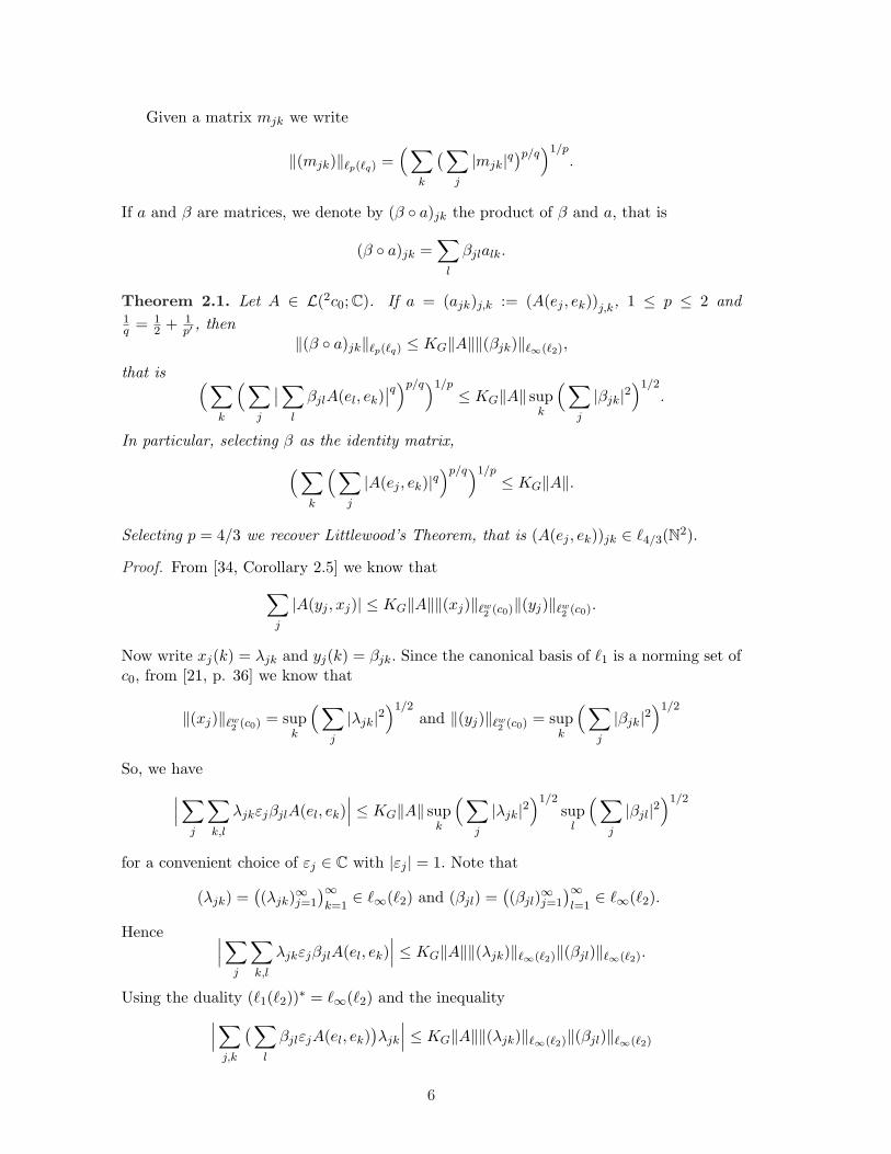
Given a matrix mjk we write

‖(mjk)‖`p(`q) =(∑

k

( ∑

j

|mjk|q)p/q

)1/p.

If a and β are matrices, we denote by (β ◦ a)jk the product of β and a, that is

(β ◦ a)jk =∑

l

βjlalk.

Theorem 2.1. Let A ∈ L(2c0;C). If a = (ajk)j,k := (A(ej , ek))j,k, 1 ≤ p ≤ 2 and1q = 1

2 + 1p′ , then

‖(β ◦ a)jk‖`p(`q) ≤ KG‖A‖‖(βjk)‖`∞(`2),

that is (∑

k

(∑

j

∣∣ ∑

l

βjlA(el, ek)∣∣q

)p/q)1/p≤ KG‖A‖ sup

k

(∑

j

|βjk|2)1/2

.

In particular, selecting β as the identity matrix,

(∑

k

(∑

j

|A(ej , ek)|q)p/q)1/p

≤ KG‖A‖.

Selecting p = 4/3 we recover Littlewood’s Theorem, that is (A(ej , ek))jk ∈ `4/3(N2).

Proof. From [34, Corollary 2.5] we know that∑

j

|A(yj , xj)| ≤ KG‖A‖‖(xj)‖`w2 (c0)‖(yj)‖`w

2 (c0).

Now write xj(k) = λjk and yj(k) = βjk. Since the canonical basis of `1 is a norming set ofc0, from [21, p. 36] we know that

‖(xj)‖`w2 (c0) = sup

k

(∑

j

|λjk|2)1/2

and ‖(yj)‖`w2 (c0) = sup

k

(∑

j

|βjk|2)1/2

So, we have∣∣∣∑

j

∑

k,l

λjkεjβjlA(el, ek)∣∣∣ ≤ KG‖A‖ sup

k

(∑

j

|λjk|2)1/2

supl

(∑

j

|βjl|2)1/2

for a convenient choice of εj ∈ C with |εj | = 1. Note that

(λjk) =((λjk)∞j=1

)∞k=1

∈ `∞(`2) and (βjl) =((βjl)∞j=1

)∞l=1

∈ `∞(`2).

Hence ∣∣∣∑

j

∑

k,l

λjkεjβjlA(el, ek)∣∣∣ ≤ KG‖A‖‖(λjk)‖`∞(`2)‖(βjl)‖`∞(`2).

Using the duality (`1(`2))∗ = `∞(`2) and the inequality∣∣∣∑

j,k

(∑

l

βjlεjA(el, ek))λjk

∣∣∣ ≤ KG‖A‖‖(λjk)‖`∞(`2)‖(βjl)‖`∞(`2)

6

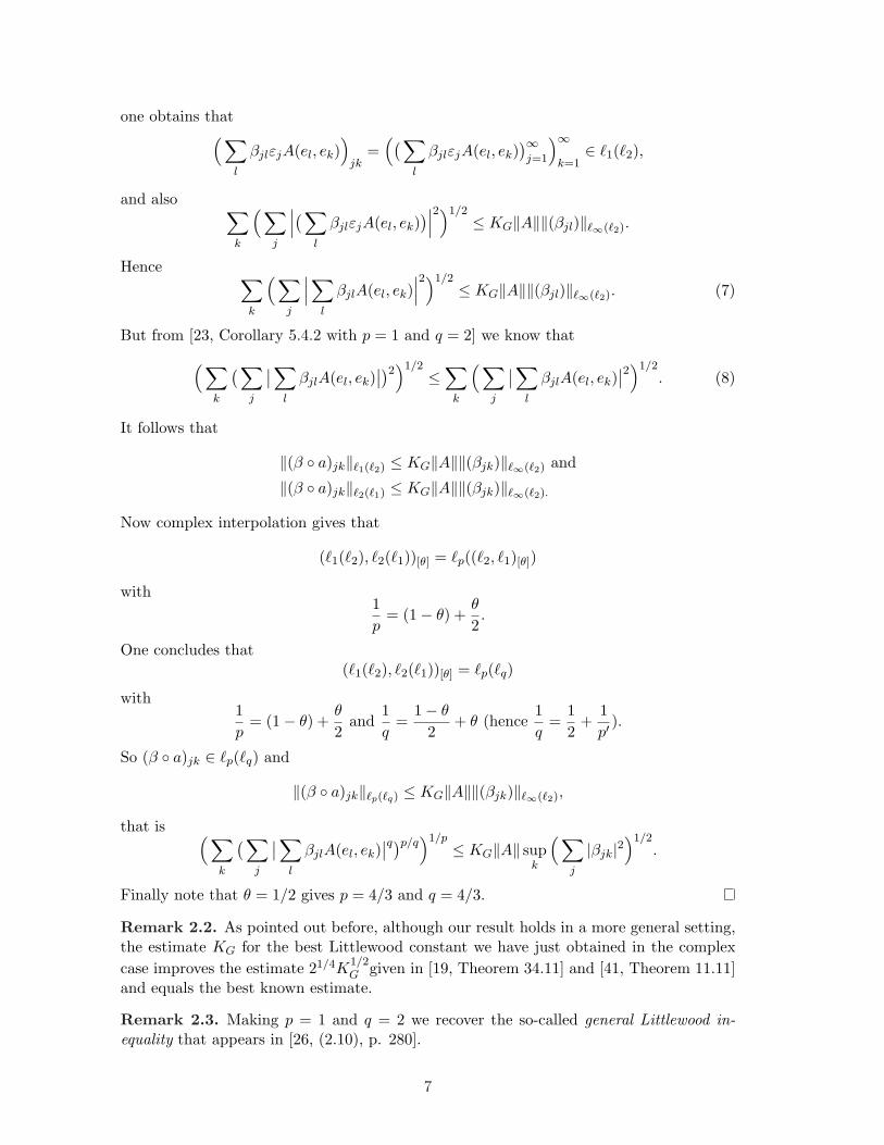
one obtains that(∑

l

βjlεjA(el, ek))

jk=

((∑

l

βjlεjA(el, ek))∞j=1

)∞k=1

∈ `1(`2),

and also ∑

k

(∑

j

∣∣∣( ∑

l

βjlεjA(el, ek))∣∣∣

2)1/2≤ KG‖A‖‖(βjl)‖`∞(`2).

Hence ∑

k

(∑

j

∣∣∣∑

l

βjlA(el, ek)∣∣∣2)1/2

≤ KG‖A‖‖(βjl)‖`∞(`2). (7)

But from [23, Corollary 5.4.2 with p = 1 and q = 2] we know that

( ∑

k

(∑

j

∣∣ ∑

l

βjlA(el, ek)∣∣)2

)1/2≤

∑

k

(∑

j

∣∣∑

l

βjlA(el, ek)∣∣2

)1/2. (8)

It follows that

‖(β ◦ a)jk‖`1(`2) ≤ KG‖A‖‖(βjk)‖`∞(`2) and

‖(β ◦ a)jk‖`2(`1) ≤ KG‖A‖‖(βjk)‖`∞(`2).

Now complex interpolation gives that

(`1(`2), `2(`1))[θ] = `p((`2, `1)[θ])

with1p

= (1− θ) +θ

2.

One concludes that(`1(`2), `2(`1))[θ] = `p(`q)

with1p

= (1− θ) +θ

2and

1q

=1− θ

2+ θ (hence

1q

=12

+1p′

).

So (β ◦ a)jk ∈ `p(`q) and

‖(β ◦ a)jk‖`p(`q) ≤ KG‖A‖‖(βjk)‖`∞(`2),

that is (∑

k

(∑

j

∣∣ ∑

l

βjlA(el, ek)∣∣q)p/q

)1/p≤ KG‖A‖ sup

k

( ∑

j

|βjk|2)1/2

.

Finally note that θ = 1/2 gives p = 4/3 and q = 4/3.

Remark 2.2. As pointed out before, although our result holds in a more general setting,the estimate KG for the best Littlewood constant we have just obtained in the complexcase improves the estimate 21/4K

1/2G given in [19, Theorem 34.11] and [41, Theorem 11.11]

and equals the best known estimate.

Remark 2.3. Making p = 1 and q = 2 we recover the so-called general Littlewood in-equality that appears in [26, (2.10), p. 280].

7

3 Some general coincidence results

Defant-Voigt Theorem (see [1, Theorem 3.10]) stating that

L(E1, . . . , En;K) = Π(1;1,...,1)(E1, . . . , En;K) (9)

is probably the first and most folkloric coincidence result in the theory of absolutelysumming multilinear mappings. The next result gives a slightly more general version.

Proposition 3.1. Let n ≥ 2 and A ∈ L(E1, . . . , En;K). Then

A : Rad(E1)× · · · ×Rad(En) → `1

is bounded. Moreover ‖A‖ = ‖A‖.Proof. Let (xi

j) be finite sequences in Ei for i = 1, . . . , n. One can find a sequence (αj) ofnorm one scalars so that

∑

j

∣∣A(x1j , . . . , x

nj )

∣∣ =∑

j

A(αjx1j , . . . , x

nj ).

Let

fα(t1) =∑

j

αjrj(t1)xij ,

fi(ti) =∑

j

rj(ti)xij , i = 2, . . . , n− 1, and

fn(t1, . . . , tn−1) =∑

j

rj(t1) · · · rj(tn−1)xnj

for t1, . . . , tn−1 ∈ [0, 1]. Using the orthogonality of the Rademacher system and the Con-traction Principle (see [21, page 231]) we have∑

j

A(αjx1j , . . . , x

nj )

=∫ 1

0· · ·

∫ 1

0A(fα(t1), . . . , fn−1(tn−1), fn(t1, . . . , tn−1))dt1 · · · dtn−1

≤ ‖A‖∫ 1

0· · ·

∫ 1

0· · ·

(∫ 1

0‖fα(t1)‖‖fn(t1, . . . , tn−1)‖dt1

)‖f2(t2)‖ · · · ‖fn−1(tn−1)‖dt2 · · · dtn−1

≤ ‖A‖∫ 1

0· · ·

∫ 1

0‖(x1

j )j‖Rad2‖(xnj )j‖Rad2‖f2(t2)‖ · · · ‖fn−1(tn−1)‖dt2 · · · dtn−1

= ‖A‖‖(x1j )j‖Rad2‖(x2

j )j‖Rad1 . . . ‖(xn−1j )j‖Rad1‖(xn

j )j‖Rad2

≤ ‖A‖‖(x1j )j‖Rad · · · ‖(xn

j )j‖Rad.

It is easy to see that ‖A‖ ≥ ‖A‖ and we conclude the proof.

The following result, which appears in [33, Proposition 3.3], will be used several timesin this paper (we include a short proof for the sake of completeness):

8

Proposition 3.2 (Inclusion Theorem). Let 0 < q ≤ p ≤ ∞, 0 < qj ≤ pj ≤ ∞ for allj = 1, . . . , n. If 1

q1+ · · ·+ 1

qn− 1

q ≤ 1p1

+ · · ·+ 1pn− 1

p then

Π(q;q1,...,qn)(E1, . . . , En; F ) ⊂ Π(p;p1,...,pn)(E1, . . . , En; F )

and π(p;p1,...,pn) ≤ π(q;q1,...,qn).

Proof. By the monotonicity of the `p-norms we may assume 1q1

+ · · ·+ 1qn− 1

q = 1p1

+ · · ·+1pn− 1

p . Let A ∈ Π(q;q1,...,qn)(E1, . . . , En; F ) and (xkj )∞j=1 ∈ `w

pk(Ek), k = 1, . . . , n, be given.

We should prove that (A(x1j , . . . , x

nj ))∞j=1 ∈ `p(F ), and for that it suffices to show that

(αj ·A(x1j , . . . , x

nj ))∞j=1 ∈ `q(F ) for every (αj)∞j=1 ∈ `r where 1

p + 1r = 1

q . Defining r1, . . . , rn

by 1pj

+ 1rj

= 1qj

, j = 1, . . . , n, it follows that 1r = 1

r1+ · · ·+ 1

rn. So `r = `r1 · · · `rn . Given

(αj)∞j=1 ∈ `r, we write (αj)∞j=1 = (α1j · · ·αn

j )∞j=1 where (αkj )∞j=1 ∈ `rk

, k = 1, . . . , n. Since(αk

j )∞j=1 ∈ `rk

and (xkj )∞j=1 ∈ `w

pk(Ek) it follows that (αk

j xkj )∞j=1 ∈ `w

qk(Ek), k = 1, . . . , n.

Therefore

(αj ·A(x1j , . . . , x

nj ))∞j=1 = (α1

j · · ·αnj ·A(x1

j , . . . , xnj ))∞j=1 = (A(α1

jx1j , . . . , α

nj xn

j ))∞j=1 ∈ `q(F )

because A is (q; q1, . . . , qn)-summing. The identifications and embeddings we used are allisometric, so the inequality between the norms follows.

Using Proposition 3.1 and the inclusion `w1 (E) ⊂ Rad(E) one obtains Defant-Voigt’s

result. Now combining (9) with the inclusion theorem it is easy to prove that for n ≥ 2and 1

p1+ · · ·+ 1

pn≥ 1

p one has

L(E1, . . . , En;K) = Π(p;p1,...,pn)(E1, . . . , En;K) whenever1p1

+ · · ·+ 1pn− 1

p≥ n− 1. (10)

Before start exploring the inclusion theorem we show that sometimes the inclusionrelationship turns out to be an equality. The next result is simple (it appeared in essencein [28, Theorem 16]) but indicates a good direction to be followed.

Proposition 3.3. Let E1, . . . , En be cotype 2 spaces. Then

Π( 1n

;1,...,1)(E1, . . . , En; F ) = Π( 2n

;2,...,2)(E1, . . . , En; F )

for every Banach space F .

Proof. It follows by combining (1) and the result saying that if Ej has cotype 2 thenΠ1(Ej ; Gj) = Π2(Ej ; Gj) (see [21, Corollary 11.16(a)]).

We aim to prove a more general result for cotype 2 spaces:

Theorem 3.4. Let 1 ≤ k ≤ n and assume that E1, . . . , Ek have cotype 2. If p ≤ q and1 ≤ qi ≤ 2, i = 1, . . . , k, satisfy that

∑ki=1

1qi− 1

q = k − 1p then

Π(p;1,...,1,pk+1,...,pn)(E1, . . . , En; F ) = Π(q;q1,...,qk,pk+1,....,pn)(E1, . . . , En; F )

for every Banach space F .

9

Proof. The inclusion

Π(p;1,...,1,pk+1,...,pn)(E1, . . . , En; F ) ⊂ Π(q;q1,...,qk,pk+1,....,pn)(E1, . . . , En; F )

follows from the Inclusion Theorem. Assume first that qi = 2 for i = 1, ..., k and A ∈Π(q0;2,...,2,pk+1,...,pn)(E1, . . . , En; F ) where k

2 + 1q0

= 1p . Let (xi

j)∞j=1 ∈ `w

1 (Ei) for i = 1, . . . , k

and (xij)∞j=1 ∈ `w

pi(Ei) for i = k+1, . . . , n. Since Ei has cotype 2, by [3, Proposition 6(a)] we

know that `w1 (Ei) = `2 · `w

2 (Ei), i = 1, . . . , k. Hence there are (αij)∞j=1 ∈ `2 and (yi

j)∞j=1 ∈

`w2 (Ek) such that (xi

j)∞j=1 = (αk

j yij)∞j=1, i = 1, . . . , k. In this fashion, (α1

j · · ·αkj )∞j=1 ∈

`2 · · · `2 = ` 2k

and (A(y1j , . . . , y

kj , xk+1

j , ..., xnj ))∞j=1 ∈ `q0(F ). Since k

2 + 1q0

= 1p it follows that

(A(x1j , . . . , x

nj ))∞j=1 = (α1

j · · ·αkj A(y1

j , . . . , ykj , xk+1

j , . . . , xnj ))∞j=1 ∈ `p(F ).

Now the general case follows again from the inclusion theorem, because the assumptiongives that

∑ni=1

1qi− 1

q = k2 − 1

q0and then

Π(q;q1,...,qk,pk+1,...,pn)(E1, . . . , En; F ) ⊂ Π(q0;2,...,2,pk+1,...,pn)(E1, . . . , En; F ).

Corollary 3.5. Let 1 ≤ k ≤ n. Assume that L(E1, . . . , Ek; F ) = Π(p;q1,...,qk)(E1, . . . , Ek; F )and that Ek+1, . . . , En have cotype 2. If p ≤ q and 1 ≤ qi ≤ 2, i = k + 1, . . . , n, satisfythat

∑ni=k+1

1qi− 1

q = n− k − 1p then

L(E1, . . . , En; F ) = Π(q;q1,...,qn)(E1, . . . , En; F ).

Proof. From [12, Corollary 3.2] if L(E1, . . . , Ek; F ) = Π(p;q1,...,qk)(E1, . . . , Ek; F ) thenL(E1, . . . , En; F ) = Π(p;q1,...,qk,1...,1)(E1, . . . , En;F ). An application of Theorem 3.4 yieldsthe result.

4 The role of the Littlewood-Orlicz property

The aim of this section is to show how the Littlewood-Orlicz property can be used to obtaincoincidence results stronger than (10). The proof of Theorem 4.1 will be also invoked inorder to obtain new coincidence results for n-linear functionals on the disc algebra and onthe Hardy space H∞.

Theorem 4.1. Let n ≥ 2, 1 ≤ pi ≤ ∞, pn ≥ 2 and

n− 32≤ 1

p1+ · · ·+ 1

pn.

If A ∈ L(E1, . . . , En;K), E′n has the Littlewood-Orlicz property and

n− 32≤ 1

p1+ · · ·+ 1

pn− 1

p,

then A : `wp1

(E1) × · · · × `wpn

(En) → `p is bounded. In other words, L(E1, . . . , , En;K) =Π(p;p1,...,pn)(E1, . . . , En;K). Moreover ‖A‖ ≤ ‖A‖.

10

Proof. Denote by An−1 : E1 × · · · ×En−1 → E′n the corresponding (n− 1)-linear mapping

defined byAn−1(x1, . . . , xn−1)(xn) = A(x1, . . . , xn−1, xn).

One has, using the previous results that

An−1 : `w1 (E1)× · · · × `w

1 (En−1) → `w1 (E′

n)

is bounded. In particular

An−1 : `w1 (E1)× · · · × `w

1 (En−1) → `2 ⊗π E′n

is bounded. Now we use a duality argument. Note that

An−1 : `w1 (E1)× · · · × `w

1 (En−1) → `w1 (E′

n) ↪→ `2 ⊗π E′n

A1

((x1

j )j , . . . , (xn−1j )j

)=

(A(x1

j , . . . , xn−1j , ·)

)j

↪→∞∑

j=1

ej ⊗A(x1j , . . . , x

n−1j , ·)

is bounded. We have for some suitable εj that∥∥∥A

((x1

j )j , . . . , (xnj )j

)∥∥∥1

=∑

j

∣∣A(x1j , . . . , x

nj )

∣∣

=

∣∣∣∣∣∣∑

j

A(εjx1j , . . . , x

nj )

∣∣∣∣∣∣

=

∣∣∣∣∣∣∣

∑

j

A(εjx1j , . . . ,

xnj∥∥∥(xn

j )j

∥∥∥`w2 (En)

)

∣∣∣∣∣∣∣∥∥(xn

j )j

∥∥`w2 (En)

≤ max‖(yj)j‖`w

2 (En)≤1, (yj)j∈`w2 (En)

∣∣∣∣∣∣∑

j

A(εjx1j , . . . , yj)

∣∣∣∣∣∣∥∥(xn

j )j

∥∥`w2 (En)

≤ max‖u‖≤1,u∈L(`2;En)

∣∣∣∣∣∣∑

j

A(εjx1j , . . . , u(ej))

∣∣∣∣∣∣∥∥(xn

j )j

∥∥`w2 (En)

= (∗).

In this last inequality we used the identification:

`w2 (En) ←→ L(`2; En)(yj)j ←→ T(yj)j

given by T(yj)j((zj)j) =

∑j yjzj . Now, using the inclusion

L(`2;En) ↪→ (`2 ⊗π E′

n

)′u → ϕ : `2 ⊗π E′

n → Kϕ

((λj)j ⊗ x′

)= x′(u((λj)j))

and the identification

L(`2;E′′n) =

(`2 ⊗π E′

n

)′S → ϕS : `2 ⊗π E′

n → KϕS(x⊗ y) = S(x)(y)

11

we get

(∗) = max‖u‖≤1,u∈L(`2;En)

∣∣∣∣∣∣∑

j

A(εjx1j , . . . , x

n−1j , u(ej))

∣∣∣∣∣∣∥∥(xn

j )j

∥∥`w2 (En)

≤ max‖ϕ‖≤1,ϕ∈(`2⊗πE′n)′

∣∣∣∣∣∣∑

j

ϕ(ej ⊗A(εjx

1j , . . . , x

n−1j , ·)

)∣∣∣∣∣∣∥∥(xn

j )j

∥∥`w2 (En)

= max‖ϕ‖≤1,ϕ∈(`2⊗πE′n)′

∣∣∣∣∣∣ϕ

∑

j

ej ⊗A(εjx1j , . . . , x

n−1j , ·)

∣∣∣∣∣∣∥∥(xn

j )j

∥∥`w2 (En)

=

∥∥∥∥∥∥∑

j

ej ⊗A(εjx1j , . . . , x

n−1j , ·)

∥∥∥∥∥∥`2⊗πE′n

∥∥(xnj )j

∥∥`w2 (En)

(∗∗)≤ C

∥∥∥∥(A(εjx

1j , . . . , x

n−1j , ·)

)j

∥∥∥∥`w1 (E′n)

∥∥(xnj )j

∥∥`w2 (En)

= C∥∥∥A1

((εjx

1j )j , . . . , (xn−1

j )j

)∥∥∥`w1 (E′n)

∥∥(xnj )j

∥∥`w2 (En)

≤ C∥∥∥A1

∥∥∥∥∥(x1

j )j

∥∥`w1 (E1)

. . .∥∥∥(xn−1

j )j

∥∥∥`w1 (En−1)

∥∥(xnj )j

∥∥`w2 (En)

< ∞,

where in (**) we used that the inclusion `w1 (E′

n) ↪→ `2 ⊗π E′n is continuous. We have just

proved thatA : `w

1 (E1)× · · · × `w1 (En−1)× `w

2 (En) → `1

is bounded. The proof is completed by using the Inclusion Theorem.

Taking into account the inclusion Rad(E) ⊂ `w2 (E), our aim is now to analyze when the

result in Proposition 3.1 can be lifted to `w2 (Ei). In other words, when L(E1, . . . , , En) =

Π(1;2,...,2)(E1, . . . , En). In this direction D. Perez-Garcıa proved the following result:

Theorem 4.2. [34, Corollary 2.5] Let E1, . . . , En be L∞-spaces. If A : E1×· · ·×En −→ Kis multilinear and bounded, then A : `w

2 (E1)×· · ·×`w2 (En) −→ `1 is also bounded. In other

words, L(E1, . . . , En;K) = Π(1;2,...,2)(E1, . . . , En;K).

Applying the idea used in the proof of Theorem 4.1 we can reprove the result aboveand generalize it to a larger class of spaces. Recall that a bilinear form A : E1×E2 −→ K is2-dominated if and only if it is absolutely (1; 2, 2)-summing, i.e., if and only if A : `w

2 (E1)×`w2 (E2) −→ `1 is bounded.

Theorem 4.3. Let n ≥ 2 and E1, . . . , En be Banach spaces such that E′3, . . . , E

′n have the

Littlewood-Orlicz property and every continuous bilinear form on E1×E2 is 2-dominated.If A : E1×· · ·×En −→ K is multilinear and bounded, then A : `w

2 (E1)×· · ·×`w2 (En) −→ `1

is also bounded. In other words, L(E1, . . . , En;K) = Π(1;2,...,2)(E1, . . . , En;K).

Proof. We proceed by induction on n. The case n = 2 follows by assumption. Assumethat the result holds for n ≥ 2. Let B : E1 × · · · × En −→ K be given. By the inductionhypothesis B : `w

2 (E1)× · · · × `w2 (En) −→ `1 is bounded. It follows that for every Banach

space F and every C : E1×· · ·×En −→ F , the mapping C : `w2 (E1)×· · ·×`w

2 (En) −→ `w1 (F )

is bounded. Given A : E1× · · · ×En+1 −→ K, defining An : E1× · · · ×En −→ E′n+1 in the

12

obvious way, we have that An : `w2 (E1)×· · ·×`w

2 (En) −→ `w1 (E′

n+1) is bounded. Since E′n+1

has the Littlewood-Orlicz property we have that An : `w2 (E1)×· · ·×`w

2 (En) −→ `2⊗π E′n+1

is bounded. Using the duality argument from the proof of Theorem 4.1 it follows thatA : `w

2 (E1)× · · · × `w2 (En+1) −→ `1 is bounded as well.

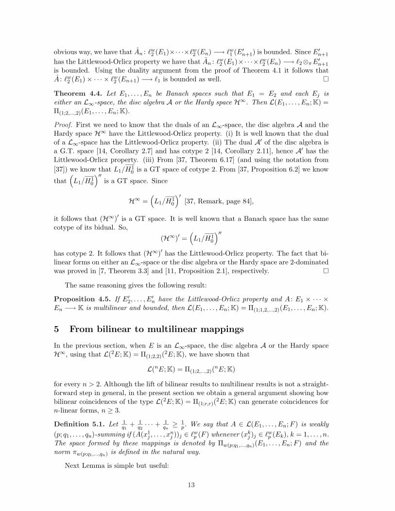
Theorem 4.4. Let E1, . . . , En be Banach spaces such that E1 = E2 and each Ej iseither an L∞-space, the disc algebra A or the Hardy space H∞. Then L(E1, . . . , En;K) =Π(1;2,...,2)(E1, . . . , En;K).

Proof. First we need to know that the duals of an L∞-space, the disc algebra A and theHardy space H∞ have the Littlewood-Orlicz property. (i) It is well known that the dualof a L∞-space has the Littlewood-Orlicz property. (ii) The dual A′ of the disc algebra isa G.T. space [14, Corollary 2.7] and has cotype 2 [14, Corollary 2.11], hence A′ has theLittlewood-Orlicz property. (iii) From [37, Theorem 6.17] (and using the notation from[37]) we know that L1/H1

0 is a GT space of cotype 2. From [37, Proposition 6.2] we know

that(L1/H1

0

)′′is a GT space. Since

H∞ =(L1/H1

0

)′[37, Remark, page 84],

it follows that (H∞)′ is a GT space. It is well known that a Banach space has the samecotype of its bidual. So,

(H∞)′ =(L1/H1

0

)′′

has cotype 2. It follows that (H∞)′ has the Littlewood-Orlicz property. The fact that bi-linear forms on either an L∞-space or the disc algebra or the Hardy space are 2-dominatedwas proved in [7, Theorem 3.3] and [11, Proposition 2.1], respectively.

The same reasoning gives the following result:

Proposition 4.5. If E′2, . . . , E

′n have the Littlewood-Orlicz property and A : E1 × · · · ×

En −→ K is multilinear and bounded, then L(E1, . . . , En;K) = Π(1;1,2,...,2)(E1, . . . , En;K).

5 From bilinear to multilinear mappings

In the previous section, when E is an L∞-space, the disc algebra A or the Hardy spaceH∞, using that L(2E;K) = Π(1;2,2)(2E;K), we have shown that

L(nE;K) = Π(1;2,...,2)(nE;K)

for every n > 2. Although the lift of bilinear results to multilinear results is not a straight-forward step in general, in the present section we obtain a general argument showing howbilinear coincidences of the type L(2E;K) = Π(1;r,r)(2E;K) can generate coincidences forn-linear forms, n ≥ 3.

Definition 5.1. Let 1q1

+ 1q2· · · + 1

qn≥ 1

p . We say that A ∈ L(E1, . . . , En;F ) is weakly(p; q1, . . . , qn)-summing if (A(x1

j , . . . , xnj ))j ∈ `w

p (F ) whenever (xkj )j ∈ `w

p (Ek), k = 1, . . . , n.The space formed by these mappings is denoted by Πw(p;q1,...,qn)(E1, . . . , En; F ) and thenorm πw(p;q1,...,qn) is defined in the natural way.

Next Lemma is simple but useful:

13

Lemma 5.2. Let n ∈ N and let E1, . . . , En be Banach spaces. The following are equivalent:(i) L(E1, . . . , En;K) = Π(p;q1,...,qn)(E1, . . . , En;K) and π(p;q1,...,qn) ≤ C‖ · ‖.(ii) L(E1, . . . , En; F ) = Πw(p;q1,...,qn)(E1, . . . , En; F ) for every Banach space F and

πw(p;q1,...,qn) ≤ C‖ · ‖.(iii) There exists C > 0 such that

‖(x1j ⊗ · · · ⊗ xn

j )j‖`wp (E1⊗π···⊗πEn) ≤ C

n∏

i=1

‖(xij)j‖`w

qi(Ei)

for all (xij)j ∈ `w

qi(Ei), i = 1, . . . , n.

Proof. (i) =⇒ (ii) Let A ∈ L(E1, . . . , En;F ). If (xkj )j ∈ `w

qk(Ek), k = 1, . . . , n, then

supϕ∈BF ′

∑

j

∣∣ϕ(A(x1j , . . . , x

nj ))

∣∣p

1/p

≤ supϕ∈BF ′

π(p;q1,...,qn)(ϕ ◦A)∥∥(x1

j )j

∥∥`wq1

(E1)· · · ∥∥(xn

j )j

∥∥`wqn (En)

≤ supϕ∈BF ′

C ‖ϕ ◦ T‖∥∥(x1j )j

∥∥`wq1

(E1)· · ·∥∥(xn

j )j

∥∥`wqn (En)

≤ C ‖A‖∥∥(x1j )j

∥∥`wq1

(E1)· · ·∥∥(xn

j )j

∥∥`wqn (En)

(ii) =⇒ (iii) Take F = E1 ⊗π · · · ⊗π En and A : E1 × · · · × En → E1 ⊗π · · · ⊗π En givenby A(x1, . . . , xn) = x1 ⊗ · · · ⊗ xn.(iii) =⇒ (i) Given A ∈ L(E1, . . . , En;K), its linearization T : E1 ⊗π · · · ⊗π En → K isbounded and then T : `w

p (E1 ⊗π · · · ⊗π En) → `p is bounded. Now

‖(A(x1j , . . . , x

nj ))j‖p = ‖(T (x1

j ⊗ · · · ⊗ xnj ))j‖p

≤ ‖T‖‖(x1j ⊗ · · · ⊗ xn

j )j‖`wp (E1⊗π···⊗πEn)

≤ C‖T‖n∏

i=1

‖(xij)j‖`w

qi(Ei).

Theorem 5.3. Let 1 ≤ r ≤ 2. If L(2E;K) = Π(1;r,r)(2E;K) and π(1;r,r) ≤ C‖ · ‖, then

(i) For n even, L(nE;K) = Π(1;r,...,r)(nE;K) and π(1;r,...,r) ≤ Cn/2‖ · ‖.

(ii) For n ≥ 3 and odd, L(nE;K) = Π(r;r,...,r)(nE;K) and π(r;r,...,r) ≤ C(n−1)/2‖ · ‖.

Proof. (i) Let n = 2m, m ∈ N, and A ∈ L(2mE;K). Using the associativity of theprojective norm π it is easy to see that there is an m-linear mapping B ∈ L(m(E⊗πE);K)such that

B(x1 ⊗ x2, . . . , x2m−1 ⊗ x2m) = A(x1, x2, . . . , x2m−1, x2m).

14

Using Defant-Voigt Theorem and Lemma 5.2 we get∑

j

∣∣A(x1j , . . . , x

2mj )

∣∣

=∑

j

∣∣∣B(x1j ⊗ x2

j , . . . , x2m−1j ⊗ x2m

j )∣∣∣

≤ π(1;1,...,1)(B)∥∥(x1

j ⊗ x2j )j

∥∥`w1 (E⊗πE)

· · ·∥∥∥(x2m−1

j ⊗ x2mj )j

∥∥∥`w1 (E⊗πE)

≤ ‖B‖(C

∥∥(x1j )j

∥∥`wr (E)

∥∥(x2j )j

∥∥`wr (E)

)· · ·

(C

∥∥∥(x2m−1j )j

∥∥∥`wr (E)

∥∥(x2mj )j

∥∥`wr (E)

)

≤ Cm ‖A‖∥∥(x1j )j

∥∥`wr (E)

· · ·∥∥(x2mj )j

∥∥`wr (E)

(ii) Let n = 2m + 1, m ∈ N, and A ∈ L(2m+1E;K). From (i) and [12, Corollary 3.2] weconclude that A ∈ Π(1;r,...,r,1)(2m+1E;K) and it is not difficult to check that π(1;r,...,r,1) ≤Cm‖ · ‖. Using the Inclusion Theorem we conclude that A ∈ Π(p;r,...,r,p)(2m+1E;K) for any1 ≤ p < ∞. The result is now finished.

Let us point out some connection of Littlewood-Orlicz property on E′ and L(2E;K) =Π(1;r,r)(2E;K).

Proposition 5.4. Let E be a Banach space. The following statements are equivalent.(i) E′ has the Littlewood-Orlicz property.(ii) L(X, E;K) = Π(1;1,2)(X, E;K) for any Banach space X.(iii) `w

1 (X)⊗π `w2 (E) ⊂ `w

1 (X ⊗π E).

Proof. (i) =⇒ (ii) Let A : X × E → K be a bounded bilinear map and denote, as in theintroduction, TA : X → E′ the corresponding linear operator. Assume that (xj)j ∈ `w

1 (X)and (yj)j ∈ `w

2 (E).∑

j

|A(xj , yj)| =∑

j

|TA(xj)(yj)|

= sup|αj |=1

|∑

j

TA(xj)(αjyj)|

≤ ‖(TA(xj))j‖`2⊗π(E′)‖(yj)j‖`w2 (E)

≤ C‖(TA(xj))j‖`w1 (E′)‖(yj)j‖`w

2 (E)

≤ C‖A‖‖(xj)j‖`w1 (X)‖(yj)j‖`w

2 (E)

(ii) =⇒ (i) Let (x′j)j ∈ `w1 (E′) be given. Consider the bounded bilinear map A : c0×E → K

defined by the condition A(ej , x) = x′j(x) for x ∈ E. To show that (x′j)j ∈ `2 ⊗π (E′) itsuffices to see that ∑

j

|x′j(xj)| ≤ C‖(xj)j‖`w2 (E)

and, using X = c0 in the assumption, this follows using that∑

j

|x′j(xj)| =∑

j

|A(ej , xj)| ≤ ‖A‖‖(ej)j‖`w1 (c0)‖(xj)j‖`w

2 (E).

(ii) ⇐⇒ (iii) It is a particular case in Lemma 5.2.

15

The same idea used in the proof of Theorem 5.3 provides the following slight improve-ment:

Theorem 5.5. Let n be a positive integer. For i = 1, . . . , 2n + 1 let Ei be a Banach spaceand 1 ≤ r2n+1 ≤ r1, . . . , r2n ≤ 2. If

L(E1, E2;K) = Π(1;r1,r2)(E1, E2;K) and π(1;r1,r2) ≤ C2‖ · ‖,

L(E3, E4;K) = Π(1;r3,r4)(E3, E4;K) and π(1;r3,r4) ≤ C4‖ · ‖, . . .

L(E2n−1, E2n;K) = Π(1;r2n−1,r2n)(E2n−1, E2n;K) and π(1;r2n−1,r2n) ≤ C2n‖ · ‖,then

L(E1, . . . , E2n;K) = Π(1;r1,...,r2n)(E1, . . . , E2n;K) and π(1;r1,...,r2n) ≤ C2 · · ·C2n‖ · ‖,

L(E1, . . . , E2n+1;K) = Π(r2n+1;r1,...,r2n+1)(E1, . . . , E2n+1;K) and π(r2n+1;r1,...,r2n+1) ≤ C2 · · ·C2n‖·‖.

6 The role of almost summing mappings

Let n ≥ 2, A ∈ L(E1, . . . , En;F ) and 1 ≤ k ≤ n. Recall that the k-linear mapping Ak isdefined by

Ak : E1 × · · · × Ek → L(Ek+1, . . . , En;F ) , Ak(x1, . . . , xk)(xk+1, . . . , xn) = A(x1, . . . , xn).

We first mention several connections between absolutely summing and almost summingmultilinear mappings. Clearly Πa.s(E1, ..., En;F ) coincides with Π(2;2,...2)(E1, ..., En; F )whenever F is a Hilbert space because Rad(F ) = `2(F ), and the corresponding inclusionshold whenever F has type p or cotype q.

In the linear case one has (see [21])⋃

p>0 Πp(E;F ) ⊂ Πa.s(E;F ). Using this linearcontainment relationship and (1) - see also [8] - it is not difficult to see that this relationshipalso holds for p-dominated multilinear maps, i.e.

⋃

p>0

Π(p/n;p...,p)(E1, . . . , En; F ) ⊂ Πa.s(E1, . . . , En; F ).

Proposition 6.1. Let A ∈ L(E1, . . . , En;K) and An−1 ∈ L(E1, . . . , En−1; E′n).

(i) If A ∈ Π(1;2,...,2)(E1, . . . , En;K) then An−1 ∈ Πa.s(E1, . . . , En−1; E′n)

(ii) If E′n is a GT -space of cotype 2 and An−1 ∈ Πa.s(E1, . . . , En−1; E′

n) then A ∈Π(1;2,...,2)(E1, . . . , En;K).

Proof. (i) Assume A ∈ Π(1;2,...,2)(E1, . . . , En;K). Using that `2 ⊗π F ⊂ Rad(F ) one has

‖(An−1(x1j , . . . , x

n−1j ))j‖Rad(E′n) ≤ C‖(An−1(x1

j , . . . , xn−1j ))j‖`2⊗πE′n

= sup‖(xn

j )j‖`w2 (En)=1

|∑

j

An−1(x1j , . . . , x

n−1j )(xn

j )|

≤ π(1;2,...,2)(A)n−1∏

i=1

‖(xij)j‖`w

2 (Ei).

16

(ii)Assume that An−1 ∈ Πa.s(E1, . . . , En−1;E′n). From (4) one has `2 ⊗π E′

n = Rad(E′n).

Hence we obtain, for any |αj | = 1,∑

j

A(αjx1j , . . . , x

nj ) =

∑

j

An−1(αjx1j , . . . , x

n−1j )(xn

j )

≤ ‖(An−1(αjx1j , . . . , x

n−1j ))j‖`2⊗πE′n‖(xn

j )j‖`w2 (En)

≤ C‖(An−1(αjx1j , . . . , x

n−1j ))j‖Rad(E′n)‖(xn

j )j‖`w2 (En)

≤ C‖An−1‖a.s

n∏

i=1

‖(xij)j‖`w

2 (Ei)

Theorem 6.2. Let 1 ≤ k < n and A ∈ L(E1, ..., En;K) be such that

Ak ∈ Πa.s(E1, ..., Ek;L(Ek+1, .., En;K)).

Then,A : `w

2 (E1)× ...× `w2 (Ek)×Rad(Ek+1)× · · · ×Rad(En) → `1

is bounded. Moreover ‖A‖ ≤ ‖Ak‖a.s.

Proof. Let (xij)j be a finite sequence in Ei for i = 1, . . . , n. Take a scalar sequence (αj)j ,

denote Ajk = Ak(x1

j , x2j , ..., x

kj ) and define

fα(tk) =∑

j

αjAjkrj(tk); fi(ti) =

∑

j

rj(ti)xij , i = k + 1, . . . , n− 1; and

fn(tk, . . . , tn−1) =∑

j

rj(tk) · · · rj(tn−1)xnj , tk, . . . , tn−1 ∈ [0, 1].

The orthogonality of the Rademacher system shows that∑

j

A(αjx1j , . . . , x

nj )

=∑

j

Ak(αjx1j , . . . , x

kj )(x

k+1j , · · · , xn

j )

=∑

j

αjAjk(x

k+1j , · · · , xn

j )

=∫ 1

0· · ·

∫ 1

0fα(tk)(fk+1(tk+1), . . . , fn−1(tn−1), fn(tk, . . . , tn−1))dtk · · · dtn−1

≤∫ 1

0· · ·

∫ 1

0

(∫ 1

0‖fα(tk)‖‖fn(tk, . . . , tn−1)‖dtk

)‖fk+1(tk+1)‖ · · · ‖fn−1(tn−1)‖ dtk+1 · · · dtn−1

≤ ‖Ak‖a.s

k∏

i=1

‖(xij)j‖`w

2 (Ei)

.

∫ 1

0· · ·

∫ 1

0

(∫ 1

0‖fn(tk, ..., tn−1)‖2dtk

)1/2‖fk+1(tk+1)‖ · · · ‖fn−1(tn−1)‖dtk+1 · · · dtn−1

≤ ‖Ak‖a.s

k∏

i=1

‖(xij)j‖`w

2 (Ei)

( n−1∏

i=k+1

‖(xij)j‖Rad1

)‖(xn

j )j‖Rad2 .

This allows to conclude the proof.

17

Let us see that Theorem 6.2 has nice consequences.

Theorem 6.3. If 1 ≤ p ≤ 2 and E′2 has type 2, then

L(`p, E2;K) = Π(p;2,1)(`p, E2;K) = Π(2p/(2+p);1,1)(`p, E2;K) = Π(rp;rp,rp)(`p, E2;K),

for every 1 ≤ rp ≤ 2p3p−2 .

Proof. We only treat the case K = C. The case K = R follows from a complexificationargument (see [10, 33] for details).

Assume first that p = 1. Let A ∈ L(`1, E2;K). Since E′2 has type 2, it follows from

[21, Theorem 12.10] that A1 ∈ Πa.s(`1;E′2). So, from the previous theorem it follows that

A : `w2 (`1)× `w

1 (E2) → `1

is bounded. Hence A ∈ Π(1;2,1)(`1, E2;K). On the other hand, from the inclusion theoremwe know that L(`2, E2;K) = Π(2;2,1)(`2, E2;K).

Let now 1 < p ≤ 2 and A ∈ L(`p, E2;K).Fix (yj) ∈ `w

1 (E2) and consider the linear mappings

T (1) : `w2 (`2) → `2 and T (2) : `w

2 (`1) → `1

given byT (k)((xj)j) = (A(xj , yj))j for k = 1, 2.

Clearly T (1) and T (2) are well-defined and continuous. Using that `w2 (`t) = L(`2; `t) for

t = 1, 2, [38, proof of the Theorem] gives that

`w2 (`p) ⊂ (`w

2 (`2), `w2 (`1))θ

for θ = 1− 1p . So the complex interpolation method implies that

T : `w2 (`p) → `p

T ((xj)j) = (A(xj , yj))j

is continuous. It follows that A ∈ Π(p;2,1)(`p, E2;K). Now use Theorem 3.4 to obtainΠ(p;2,1)(`p, E2;K) = Π(2p/(2+p);1,1)(`p, E2;K). Now using the inclusion theorem once againone has Π(2p/(2+p);1,1)(`p, E2;K) ⊂ Π(sp;sp,sp)(`p, E2;K) for 2 − 2+p

2p = 1sp

, which gives us

sp = 2p3p−2 . Since E′

2 has type 2, it follows from [21, page 220] that E2 has cotype 2. So,since 1 ≤ sp ≤ 2, from [24, Theorem 3] it follows that Π(rp;rp,rp)(`p, E2;K) = L(`p, E2;K)whenever 1 ≤ rp ≤ sp.

Corollary 6.4. If 1 ≤ p ≤ 2 and 1 < q ≤ 2 then(i) L(`p, `q;K) = Π(p;2,1)(`p, `q;K).(ii) L(`1, `q;K) = Π(r;r,r)(`1, `q;K) for 1 ≤ r ≤ 2.

The following result (for n-linear mappings) can also be obtained using results from[12] and the idea of the proof of Theorem 6.3.

Proposition 6.5. Let n ≥ 2 and 1 < p ≤ 2. Then every n-linear mapping A ∈ L(`1, n−1. . . , `1, `p;K)is (rn; rn, . . . , rn)-summing for every 1 ≤ rn ≤ 2n−1

2n−1−1.

18

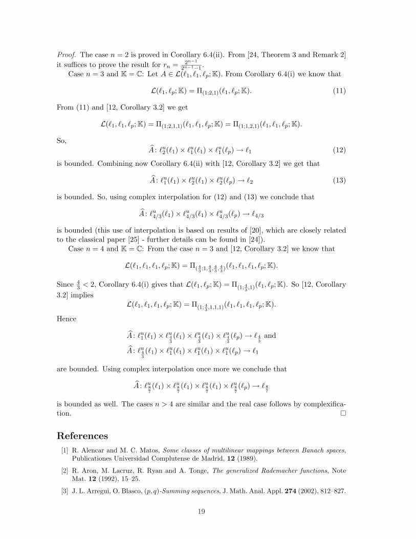
Proof. The case n = 2 is proved in Corollary 6.4(ii). From [24, Theorem 3 and Remark 2]it suffices to prove the result for rn = 2n−1

2n−1−1.

Case n = 3 and K = C: Let A ∈ L(`1, `1, `p;K). From Corollary 6.4(i) we know that

L(`1, `p;K) = Π(1;2,1)(`1, `p;K). (11)

From (11) and [12, Corollary 3.2] we get

L(`1, `1, `p;K) = Π(1;2,1,1)(`1, `1, `p;K) = Π(1;1,2,1)(`1, `1, `p;K).

So,A : `u

2(`1)× `u1(`1)× `u

1(`p) → `1 (12)

is bounded. Combining now Corollary 6.4(ii) with [12, Corollary 3.2] we get that

A : `u1(`1)× `u

2(`1)× `u2(`p) → `2 (13)

is bounded. So, using complex interpolation for (12) and (13) we conclude that

A : `u4/3(`1)× `u

4/3(`1)× `u4/3(`p) → `4/3

is bounded (this use of interpolation is based on results of [20], which are closely relatedto the classical paper [25] - further details can be found in [24]).

Case n = 4 and K = C: From the case n = 3 and [12, Corollary 3.2] we know that

L(`1, `1, `1, `p;K) = Π( 43;1, 4

3, 43, 43)(`1, `1, `1, `p;K).

Since 43 < 2, Corollary 6.4(i) gives that L(`1, `p;K) = Π(1; 4

3,1)(`1, `p;K). So [12, Corollary

3.2] impliesL(`1, `1, `1, `p;K) = Π(1; 4

3,1,1,1)(`1, `1, `1, `p;K).

Hence

A : `u1(`1)× `u

43

(`1)× `u43

(`1)× `u43

(`p) → ` 43

and

A : `u43(`1)× `u

1(`1)× `u1(`1)× `u

1(`p) → `1

are bounded. Using complex interpolation once more we conclude that

A : `u87(`1)× `u

87(`1)× `u

87(`1)× `u

87(`p) → ` 8

7

is bounded as well. The cases n > 4 are similar and the real case follows by complexifica-tion.

References

[1] R. Alencar and M. C. Matos, Some classes of multilinear mappings between Banach spaces,Publicationes Universidad Complutense de Madrid, 12 (1989).

[2] R. Aron, M. Lacruz, R. Ryan and A. Tonge, The generalized Rademacher functions, NoteMat. 12 (1992), 15–25.

[3] J. L. Arregui, O. Blasco, (p, q)-Summing sequences, J. Math. Anal. Appl. 274 (2002), 812–827.

19

[4] S. Aywa, J. H. Fourie, On summing multipliers and applications. J. Math. Anal. Appl. 253(2001), 166–186.

[5] J. Bergh and J. Lofstrom, Interpolation spaces, Springer-Verlag, 1976.

[6] H. F. Bohnenblust and E. Hille, On the absolute convergence of Dirichlet series, Ann. ofMath. (2) 32 (1931), 600-622.

[7] G. Botelho, Cotype and absolutely summing multilinear mappings and homogeneous poly-nomials, Proc. Roy. Irish Acad. Sect. A 97 (1997), 145–153.

[8] G. Botelho, Almost summing polynomials, Math. Nachr. 212 (2000), 25–36.

[9] G. Botelho, H.-A. Braunss, H. Junek, Almost p-summing polynomials and multilinear map-pings, Arch. Math. 76 (2001), 109–118.

[10] G. Botelho, H.-A. Braunss, H. Junek and D. Pellegrino, On inclusion and coincidence resultsfor multilinear and holomorphic mappings, Proc. Amer. Math. Soc., to appear.

[11] G. Botelho and D. Pellegrino, Scalar-valued dominated polynomials on Banach spaces, Proc.Amer. Math. Soc. 134 (2006), 1743–1751.

[12] G. Botelho and D. Pellegrino, Coincidence situations for absolutely summing non-linear map-pings, Port. Math. 64 (2007), 176–191.

[13] G. Botelho, D. Pellegrino and P. Rueda, Summability and estimates for polynomials andmultilinear mappings, Indag. Math., to appear.

[14] J. Bourgain, New Banach space properties of the disc algebra and H∞, Acta Math. 152(1984), 1–48.

[15] Q. Bu and J. Diestel, Observations about the projective tensor product of Banach spaces, I -

`p

∧⊗X, 1 < p < ∞, Quaest. Math. 24 (2001), 519–533.

[16] Q. Bu, On Banach spaces verifying Grothendieck’s Theorem, Bull. London Math. Soc. 35(2003), 738– 748.

[17] Y. S. Choi, S. G. Kim, Y. Melendez and A. Tonge , Estimates for absolutely summing normsof polynomials and multilinear maps, Q. J. Math. 52 (2001), 1–12.

[18] J. S. Cohen, Absolutely p-summing, p-nuclear operators and their conjugates. Math. Ann.201 (1973), 177–200.

[19] A. Defant, K. Floret, Tensor Norms and Operator Ideals. North-Holland Publishing Co.,Amsterdam, 1993.

[20] A. Defant and C. Michels, A complex interpolation formula for tensor products of vector-valuedBanach function spaces, Arch. Math. 74 (2000), 441- 451.

[21] J. Diestel, H. Jarchow, A. Tonge, Absolutely summing operators. Cambridge University Press,1995.

[22] S. Dineen, Complex Analysis on Infinite Dimensional Spaces, Springer Verlag, London, 1999.

[23] D. J. H. Garling, Inequalities: a journey into linear analysis, Cambridge University Press,2007.

[24] H. Junek, M. Matos, D. Pellegrino, Inclusion theorems for absolutely summing holomorphicmappings, Proc. Amer. Math. Soc. 136 (2008), 3983-3991.

[25] O. Kouba, On interpolation of injective or projective tensor products of Banach spaces, J.Funct. Anal. 96 (1991), 38-61.

[26] J. Lindenstrauss and A. PeÃlczynski, Absolutely summing operators in Lp-spaces and theirapplications, Studia Math. 29 (1968), 275–325.

20

[27] J. Littlewood, On bounded bilinear forms in an infinite number of variables, Q. J. Math. 2(1930), 167-171.

[28] Y. Melendez and A. Tonge, Polynomials and the Pietsch Domination Theorem, Math. Proc.R. Ir. Acad 99A (1999), 195-212.

[29] J. Mujica, Complex Analysis in Banach Spaces, North-Holland Mathematics Studies, North-Holland, 1986.

[30] D. Pellegrino, Cotype and absolutely summing homogeneous polynomials in Lp spaces, StudiaMath. 157 (2003), 121–131.

[31] D. Pellegrino, Almost summing mappings, Arch. Math. 82 (2004), 68–80.

[32] D. Pellegrino, On scalar valued nonlinear absolutely summing mappings, Ann. Pol. Math. 83(2004), 281–288.

[33] D. Perez-Garcıa, Operadores multilineales absolutamente sumantes, Thesis, Universidad Com-plutense de Madrid, 2003.

[34] D. Perez-Garcıa, The trace class is a Q-algebra, Ann. Acad. Sci. Fenn. Math. 21 (2006),287–295.

[35] D. Perez-Garcıa, M. M. Wolf, C. Palazuelos, I. Villanueva, M. Junge, Unbounded violation oftripartite Bell inequalities, Commun. Math. Phys. 279 (2008), 455–486.

[36] A. Pietsch, Ideals of multilinear functionals (designs of a theory), Proceedings of the secondinternational conference on operator algebras, ideals, and their applications in theoreticalphysics (Leipzig, 1983), 185–199, Teubner-Texte Math., 67, Teubner, Leipzig, 1984.

[37] G. Pisier, Factorization of Linear Operators and Geometry of Banach spaces. CBMS 60.Amer. Math. Soc. Providence R.I., 1986.

[38] G. Pisier, A remark on Π2(`p, `p). Math. Nachr. 148 (1990), 243-245.

[39] M. Talagrand, Cotype of operators from C(K). Invent. Math. 107 (1992), 1–40.

[40] M. Talagrand, Cotype and (1, q)-summing norm in a Banach space. Invent. Math. 110 (1992),545–556.

[41] N. Tomczak-Jaegermann, Banach-Mazur distances and finite-dimensional Operator Ideals.Longman Scientific and Technical, 1989.

[42] N. N. Vakhania, V. I. Tarieladze, S. A. Chobanyan, Probability distributions on Banach spacesD. Reidel, Dordrecht, 1987.

[Oscar Blasco] Departamento de Analisis Matematico, Universidad de Valencia, 46.100Burjasot - Valencia, Spain, e-mail: oscar.blasco@uv.es

[Geraldo Botelho] Faculdade de Matematica, Universidade Federal de Uberlandia, 38.400-902 - Uberlandia, Brazil, e-mail: botelho@ufu.br

[Daniel Pellegrino] Departamento de Matematica, Universidade Federal da Paraıba, 58.051-900 - Joao Pessoa, Brazil, e-mail: dmpellegrino@gmail.com

[Pilar Rueda] Departamento de Analisis Matematico, Universidad de Valencia, 46.100Burjasot - Valencia, Spain, e-mail: pilar.rueda@uv.es

21