An Advanced Conjugate Gradient Training Algorithm Based on a Modified Secant Equation

International Scholarly Research NetworkISRN Artificial IntelligenceVolume 2012, Article ID 486361, 9 pagesdoi:10.5402/2012/486361

Research Article

An Advanced Conjugate Gradient Training Algorithm Based ona Modified Secant Equation

Ioannis E. Livieris1, 2 and Panagiotis Pintelas1, 2

1 Department of Mathematics, University of Patras, 26500 Patras, Greece2 Educational Software Development Laboratory, Department of Mathematics, University of Patras, 26500 Patras, Greece

Correspondence should be addressed to Ioannis E. Livieris, [email protected]

Received 5 August 2011; Accepted 4 September 2011

Academic Editors: T. Kurita and Z. Liu

Copyright © 2012 I. E. Livieris and P. Pintelas. This is an open access article distributed under the Creative Commons AttributionLicense, which permits unrestricted use, distribution, and reproduction in any medium, provided the original work is properlycited.

Conjugate gradient methods constitute excellent neural network training methods characterized by their simplicity, numericalefficiency, and their very low memory requirements. In this paper, we propose a conjugate gradient neural network trainingalgorithm which guarantees sufficient descent using any line search, avoiding thereby the usually inefficient restarts. Moreover,it achieves a high-order accuracy in approximating the second-order curvature information of the error surface by utilizing themodified secant condition proposed by Li et al. (2007). Under mild conditions, we establish that the proposed method is globallyconvergent for general functions under the strong Wolfe conditions. Experimental results provide evidence that our proposedmethod is preferable and in general superior to the classical conjugate gradient methods and has a potential to significantly enhancethe computational efficiency and robustness of the training process.

1. Introduction

Learning systems, such as multilayer feedforward neuralnetworks (FNN), are parallel computational models com-prised of densely interconnected, adaptive processing units,characterized by an inherent propensity for learning fromexperience and also discovering new knowledge. Due to theirexcellent capability of self-learning and self-adapting, theyhave been successfully applied in many areas of artificialintelligence [1–5] and are often found to be more efficientand accurate than other classification techniques [6]. Theoperation of a FNN is usually based on the followingequations:

netlj =Nl−1∑

i=1

wl−1,li j yl−1

i + blj , ylj = f(netlj

), (1)

where netlj is the sum of its weighted inputs for the jth node

in the lth layer ( j = 1, . . . ,Nl), wl−1,li j are the weights from the

ith neuron at the (l−1) layer to the jth neuron at the lth layer,blj is the bias of the jth neuron at the lth layer, yli is the output

of the jth neuron that belongs to the lth layer, and f (netlj) isthe jth neuron activation function.

The problem of training a neural network is to iterativelyadjust its weights, in order to globally minimize a measureof difference between the actual output of the network andthe desired output for all examples of the training set [7].More mathematically, the training process can be formulatedas the minimization of the error function E(w), defined bythe sum of square differences between the actual output ofthe FNN, denoted by yLj,p and the desired output, denoted byt j,p, relative to the appeared output, namely,

E(w) =P∑

p=1

NL∑

j=1

(yLj,p − t j,p

)2, (2)

where w ∈ Rn is the vector network weights and P representsthe number of patterns used in the training set.

Conjugate gradient methods are probably the mostfamous iterative methods for efficiently training neural net-works due to their simplicity, numerical efficiency, and their

2 ISRN Artificial Intelligence

very low memory requirements. These methods generate asequence of weights {wk} using the iterative formula

wk+1 = wk + ηkdk, k = 0, 1, . . . , (3)

where k is the current iteration usually called epoch, w0 ∈ Rn

is a given initial point, ηk > 0 is the learning rate, and dk is adescent search direction defined by

dk =⎧⎨⎩−g0, if k = 0,

−gk + βkdk−1, otherwise,(4)

where gk is the gradient of E at wk and βk is a scalar. Inthe literature, there have been proposed several choices forβk which give rise to distinct conjugate gradient methods.The most well-known conjugate gradient methods includethe Fletcher-Reeves (FR) method [8], the Hestenes-Stiefel(HS) method [9], and the Polak-Ribiere (PR) method [10].The update parameters of these methods are, respectively,specified as follows:

βHSk = gTk yk−1

yTk−1dk−1, βFR

k =∥∥gk

∥∥2

∥∥gk−1∥∥2 , βPR

k = gTk yk−1∥∥gk−1∥∥2 , (5)

where sk−1 = xk − xk−1, yk−1 = gk − gk−1 and ‖ · ‖ denotesthe Euclidean norm.

The PR method behaves like the HS method in practicalcomputation and it is generally believed to be one ofthe most efficient conjugate gradient methods. However,despite the practical advantages of this method, it has themajor drawback of not being globally convergent for generalfunctions and as a result it may be trapped and cycleinfinitely without presenting any substantial progress [11].For rectifying the convergence failure of the PR method,Gilbert and Nocedal [12], motivated by Powell’s work [13],proposed to restrict the update parameter βk of beingnonnegative, namely, βPR+

k = max{βPRk , 0}. The authors

conducted an elegant analysis of this conjugate gradientmethod (PR+) and established that it is globally convergentunder strong assumptions. Moreover, although that the PRmethod and the PR+ method usually perform better than theother conjugate gradient methods, they cannot guarantee togenerate descent directions, hence restarts are employed inorder to guarantee convergence. Nevertheless, there is alsoa worry with restart algorithms that their restarts may betriggered too often; thus degrading the overall efficiency androbustness of the minimization process [14].

During the last decade, much effort has been devoted todevelop new conjugate gradient methods which are not onlyglobally convergent for general functions but also compu-tationally superior to classical methods and are classified intwo classes. The first class utilizes second-order informationto accelerate conjugate gradient methods by utilizing newsecant equations (see [15–18]). Sample works include thenonlinear conjugate gradient methods proposed by Zhanget al. [19–21] which are based on MBFGS secant equation[15]. Ford et al. [22] proposed a multistep conjugate gradientmethod that is based on the multistep quasi-Newton meth-ods proposed in [16, 17]. Recently, Yabe and Takano [23] and

Li et al. [18] proposed conjugate gradient methods which arebased on modified secant equation using both the gradientand function values with higher orders of accuracy in theapproximation of the curvature. Under proper conditions,these methods are globally convergent and sometimes theirnumerical performance is superior to classical conjugategradient methods. However, these methods do not ensure togenerate descent directions; therefore the descent conditionis usually assumed in their analysis and implementations.

The second class aims at developing conjugate gradientmethods which generate descent directions, in order to avoidthe usually inefficient restarts. On the basis of this idea,Zhang et al. [20, 24–26] modified the search direction inorder to ensure sufficient descent, that is, dTk gk = −‖gk‖2,independent of the performed line search. Independently,Hager and Zhang [27] modified the parameter βk andproposed a new descent conjugate gradient method, calledthe CG-DESCENT method. More analytically, they proposeda modification of the Hestenes-Stiefel formula βHS

k in thefollowing way:

βHZk = βHS

k − 2

∥∥yk−1∥∥2

(dTk−1yk−1

)2 gTk dk−1. (6)

Along this line, Yuan [28] based on [12, 27, 29], proposed amodified PR method, that is,

βDPR+k = βPR

k −min

{βPRk ,C

∥∥yk−1∥∥2

∥∥gk−1∥∥4 g

Tk dk−1

}, (7)

where C is a parameter which essentially controls the relativeweight between conjugacy and descent and in case C > 1/4then the above formula satisfies gTk dk ≤ −(1 − 1/4C)‖gk‖2.An important feature of this method is that it is globallyconvergent for general functions. Recently, Livieris et al. [30–32] motivated by the previous works presented some descentconjugate gradient training algorithms providing somepromising results. Based on their numerical experiments, theauthors concluded that the sufficient descent property led toa significant improvement of the training process.

In this paper, we proposed a new conjugate gradienttraining algorithm which has both characteristics of theprevious presented classes. Our method ensures sufficientdescent independent of the accuracy of the line search,avoiding thereby the usually inefficient restarts. Moreover, itachieves a high-order accuracy in approximating the second-order curvature information of the error surface by utilizingthe modified secant condition proposed in [18]. Undermild conditions, we establish the global convergence of ourproposed method.

The remainder of this paper is organized as follows. InSection 2, we present our proposed conjugate gradient train-ing algorithm and in Section 3, we present its global con-vergence analysis. The experimental results are reported inSection 4 using the performance profiles of Dolan and More[33]. Finally, Section 5 presents our concluding remarks.

ISRN Artificial Intelligence 3

2. Modified Polak-Ribiere+ ConjugateGradient Algorithm

Firstly, we recall that for quasi-Newton methods, an approxi-mation matrix Bk−1 to the Hessian∇2E(wk−1) of a nonlinearfunction E is updated so that a new matrix Bk satisfies thefollowing secant condition:

Bksk−1 = yk−1. (8)

Obviously, only two gradients are exploited in the secantequation (8), while the function values available are neg-lected. Recently, Li et al. [18] proposed a conjugate gradientmethod based on the modified secant condition

Bksk−1 = yk−1, yk−1 = yk−1 +max{θk−1, 0}‖sk−1‖2 sk−1, (9)

where θk−1 is defined by

θk−1 = 2(Ek−1 − Ek) +(gk + gk−1

)Tsk−1, (10)

and Ek denotes E(wk). The authors proved that this newsecant equation (9) is superior to the classical one (8) in thesense that yk−1 better approximates ∇2E(wk)sk−1 than yk−1

(see [18]).Motivated by the theoretical advantages of this modified

secant condition (9), we propose a modification of formula(7), in the following way:

βMPR+k = gTk yk−1∥∥gk−1

∥∥2 −min

{gTk yk−1∥∥gk−1

∥∥2 ,C

∥∥ yk−1∥∥2

∥∥gk−1∥∥4 g

Tk dk−1

},

(11)

with C > 1/4. It is easy to see from (4) and (11) thatour proposed formula βMPR+

k satisfies the sufficient descentcondition

gTk dk ≤ −(

1− 14C

)∥∥gk∥∥2, (12)

independent of the line search used.At this point, we present a high level description of

our proposed algorithm, called modified Polak-Ribiere+

conjugate gradient algorithm (MPR+-CG).

Algorithm 1 (modified Polak-Ribiere+ conjugate gradientalgorithm).

Step 1. Initiate w0, 0 < σ1 < σ2 < 1, EG and kMAX; set k = 0.

Step 2. Calculate the error function value Ek and its gradientgk.

Step 3. If (Ek < EG), return w∗ = wk and E∗ = Ek.

Step 4. If (gk = 0), return “Error goal not met”.

Step 5. Compute the descent direction dk using (4) and (11).

Step 6. Compute the learning rate ηk using the strong Wolfeline search conditions

E(wk + αkdk)− E(wk) ≤ σ1αkgTk dk, (13)

∣∣∣g(wk + αkdk)Tdk∣∣∣ ≤ σ2

∣∣∣gTk dk∣∣∣. (14)

Step 7. Update the weights

wk+1 = wk + ηkdk (15)

and set k = k + 1.

Step 8. If (k > kMAX) return “error goal not met”, else go toStep 2.

3. Global Convergence Analysis

In order to establish the global convergence result for ourproposed method, we will impose the following assumptionson the error function E.

Assumption 1. The level set L = {w ∈ Rn | E(w) ≤ E(w0)}is bounded.

Assumption 2. In some neighborhood N ∈ L, E isdifferentiable and its gradient g is Lipschitz continuous,namely, there exists a positive constant L > 0 such that

∥∥g(w)− g(w)∥∥ ≤ L

∥∥w − w∥∥, and ∀w, w ∈ N . (16)

Since {E(wk)} is a decreasing sequence, it is clear thatthe sequence {wk} is contained in L. In addition, it followsdirectly from Assumptions 1 and 2 that there exist positiveconstraints B and M, such that

∥∥w − w∥∥ ≤ B, ∀w, w ∈ L, (17)

∥∥g(w)∥∥ ≤M, ∀w ∈ L. (18)

Furthermore, notice that since the error function E isbounded below in Rn by zero, it is differentiable and itsgradient is Lipschitz continuous [34]. Assumptions 1 and 2always hold.

The following lemma is very useful for the global con-vergence analysis.

Lemma 2 (see [18]). Suppose that Assumptions 1 and 2 holdand the line search satisfies the strong Wolfe line search con-ditions (13) and (14). For θk and yk defined in (10) and (9),respectively, one has

|θk| ≤ L‖sk‖2,∥∥ yk

∥∥ ≤ 2L‖sk‖. (19)

Subsequently, we will establish the global convergenceof Algorithm MPR+-CG for general functions. Firstly, wepresent a lemma that Algorithm MPR+-CG prevents theinefficient behavior of the jamming phenomenon [35] fromoccurring. This property is similar to but slightly differentfrom Property(∗), which was derived by Gilbert and Nocedal[12].

Lemma 3. Suppose that Assumptions 1 and 2 hold. Let {wk}and {dk} be generated by Algorithm MPR+-CG, if there existsa positive constant μ > 0 such that

∥∥gk∥∥ ≥ μ, ∀ k ≥ 0, (20)


then there exist constants b > 1 and λ > 0 such that∣∣∣βMPR+

k

∣∣∣ ≤ b, (21)

‖sk−1‖ ≤ λ =⇒∣∣∣βMPR+

k

∣∣∣ ≤ 1b. (22)

Proof. Utilizing Lemma 2 together with Assumption 2 andrelations (12), (14), (17), (18), (20) we have

∣∣∣βMPR+k

∣∣∣ ≤∣∣∣gTk yk−1

∣∣∣∥∥gk−1

∥∥2 + C

∥∥ yk−1∥∥2

∥∥gk−1∥∥4

∣∣∣gTk dk−1

∣∣∣

≤∥∥gk

∥∥∥∥ yk−1∥∥

∥∥gk−1∥∥2 + C

∥∥ yk−1∥∥2σ2

∣∣∣gTk−1dk−1

∣∣∣∥∥gk−1

∥∥4

≤ 2ML‖sk−1‖∥∥gk−1∥∥2 + C

4L2‖sk−1‖2

∥∥gk−1∥∥4 σ2

(1− 1

4C

)∥∥gk−1∥∥2

≤(

2ML + 4L2BCσ2(1− 1/4C)μ2

)‖sk−1‖�D‖sk−1‖.

(23)

Therefore, by setting b:= max{2, 2DB} and λ:= 1/Db, we haverelations (21) and (22) hold. The proof is completed.

Subsequently, we present a lemma which shows that,asymptotically, the search directions wk change slowly. Thislemma corresponds to Lemma 4.1 of Gilbert and Nocedal[12] and the proof is exactly the same as that of Lemma 4.1in [12], thus we omit it.

Lemma 4. Suppose that Assumptions 1 and 2 hold. Let {wk}and {dk} be generated by Algorithm MPR+-CG, if there existsa positive constant μ > 0 such that (21) holds; then dk /= 0 and

∑

k≥1

‖uk − uk−1‖2 <∞, (24)

where uk = dk/‖dk‖ .

Next, by making use of Lemmas 3 and 4, we establish theglobal convergence theorem for Algorithm MPR+-CG underthe strong Wolfe line search.

Theorem 5. Suppose that Assumptions 1 and 2 hold. If {wk} isobtained by Algorithm MPR+-CG where the line search satisfiesthe strong Wolfe line search conditions (13) and (14), then onehas

limk→∞

inf∥∥gk

∥∥ = 0. (25)

Proof. We proceed by contraction. Suppose that there existsa positive constant μ > 0 such that for all k ≥ 0

∥∥gk∥∥ ≥ μ. (26)

The proof is divided in the following two steps.

Step I. A bound on the step sk. Let Δ be a positive integer,chosen large enough that

Δ ≥ 4BD, (27)

where B and D are defined in (17) and (23), respectively. Forany l > k ≥ k0 with l − k ≤ Δ, following the same proof asthe case II of Theorem 3.2 in [27], we get

l−1∑

j=k

∥∥∥s j∥∥∥ < 2B. (28)

Step II. A bound on the search directions of dl. It followsfrom the definition of dk in (4) together with (18) and (23),we obtain

‖dl‖2 ≤ ∥∥gl∥∥2 +

∣∣∣βMPR+k

∣∣∣2‖dl−1‖2 ≤M2 + D2‖sl−1‖2‖dl−1‖2.

(29)

Now, the remaining argument is standard in the same wayas case III in Theorem 3.2 in [27], thus we omit it. Thiscompletes the proof.

4. Experimental Results

In this section, we will present experimental results in orderto evaluate the performance of our proposed conjugategradient algorithm MPR+-CG in five famous classificationproblems acquired by the UCI Repository of MachineLearning Databases [36]: the iris problem, the diabetesproblem, the sonar problem, the yeast problem, and theEscherichia coli problem.

The implementation code was written in Matlab 6.5 on aPentium IV computer (2.4 MHz, 512 Mbyte RAM) runningWindows XP operating system based on the SCG code ofBirgin and Martınez [37]. All methods are implemented withthe line search proposed in CONMIN [38] which employsvarious polynomial interpolation schemes and safeguardsin satisfying the strong Wolfe line search conditions. Theheuristic parameters were set as σ1 = 10−4 and σ2 = 0.5 asin [30, 39]. All networks have received the same sequenceof input patterns and the initial weights were generatedusing the Nguyen-Widrow method [40]. For evaluatingclassification accuracy we, have used the standard procedurecalled k-fold cross-validation [41]. The results have beenaveraged over 500 simulations.

4.1. Training Performance. The cumulative total for a per-formance metric over all simulations does not seem to betoo informative, since a small number of simulations cantend to dominate these results. For this reason, we use theperformance profiles proposed by Dolan and More [33] topresent perhaps the most complete information in terms ofrobustness, efficiency, and solution quality. The performanceprofile plots the fraction P of simulations for which any givenmethod is within a factor τ of the best training method.The horizontal axis of each plot shows the percentage of thesimulations for which a method is the fastest (efficiency),


100.1 100.2 100.3 100.4 100.5 100.6 100.7 100.80

0.1

0.2

0.3

0.4

0.5

0.6

0.7

0.8

0.9

1

τ

P

PR

PR+

MPR+

(a) Performance based on CPU time

100.1 100.2 100.3 100.4 100.5 100.6 100.70

0.1

0.2

0.3

0.4

0.5

0.6

0.7

0.8

0.9

1

τ

P

PR

PR+

MPR+

(b) Performance based on FE/GE

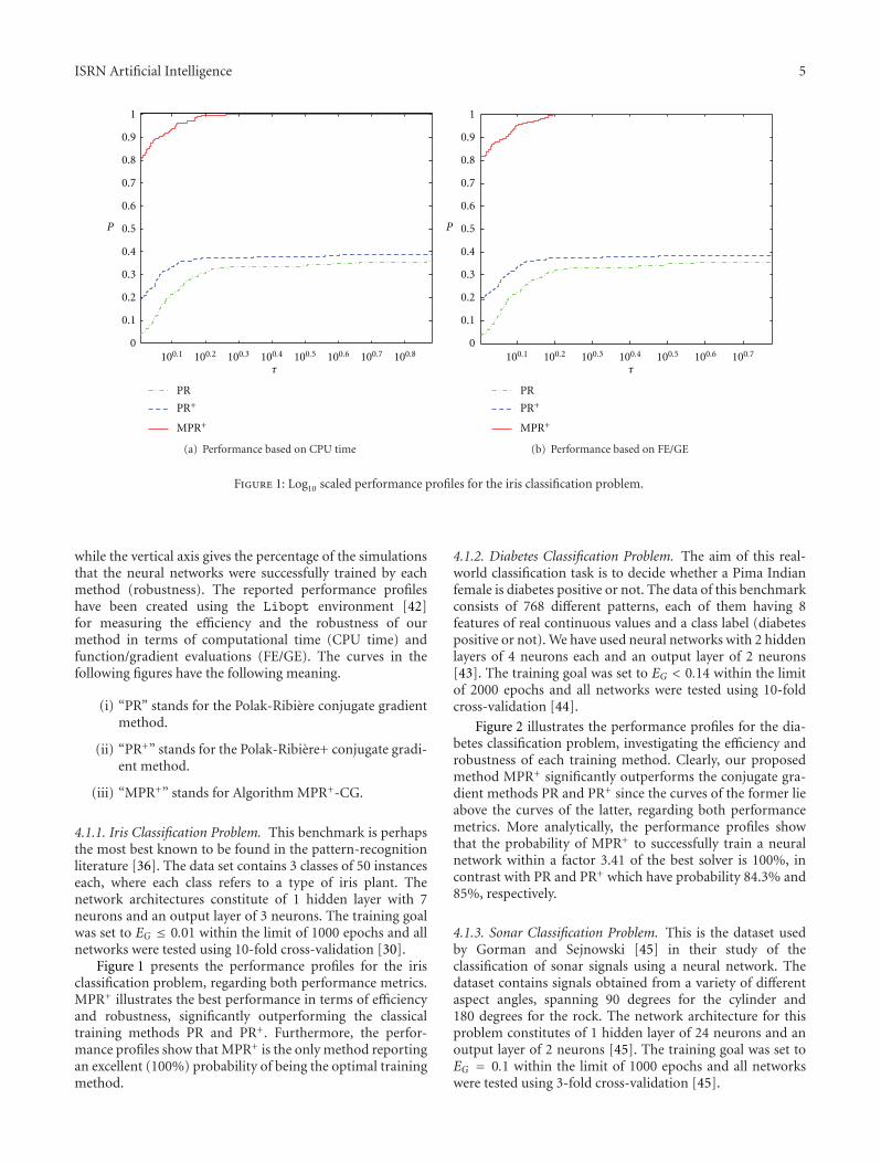
Figure 1: Log10 scaled performance profiles for the iris classification problem.

while the vertical axis gives the percentage of the simulationsthat the neural networks were successfully trained by eachmethod (robustness). The reported performance profileshave been created using the Libopt environment [42]for measuring the efficiency and the robustness of ourmethod in terms of computational time (CPU time) andfunction/gradient evaluations (FE/GE). The curves in thefollowing figures have the following meaning.

(i) “PR” stands for the Polak-Ribiere conjugate gradientmethod.

(ii) “PR+” stands for the Polak-Ribiere+ conjugate gradi-ent method.

(iii) “MPR+” stands for Algorithm MPR+-CG.

4.1.1. Iris Classification Problem. This benchmark is perhapsthe most best known to be found in the pattern-recognitionliterature [36]. The data set contains 3 classes of 50 instanceseach, where each class refers to a type of iris plant. Thenetwork architectures constitute of 1 hidden layer with 7neurons and an output layer of 3 neurons. The training goalwas set to EG ≤ 0.01 within the limit of 1000 epochs and allnetworks were tested using 10-fold cross-validation [30].

Figure 1 presents the performance profiles for the irisclassification problem, regarding both performance metrics.MPR+ illustrates the best performance in terms of efficiencyand robustness, significantly outperforming the classicaltraining methods PR and PR+. Furthermore, the perfor-mance profiles show that MPR+ is the only method reportingan excellent (100%) probability of being the optimal trainingmethod.

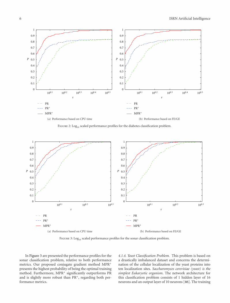
4.1.2. Diabetes Classification Problem. The aim of this real-world classification task is to decide whether a Pima Indianfemale is diabetes positive or not. The data of this benchmarkconsists of 768 different patterns, each of them having 8features of real continuous values and a class label (diabetespositive or not). We have used neural networks with 2 hiddenlayers of 4 neurons each and an output layer of 2 neurons[43]. The training goal was set to EG < 0.14 within the limitof 2000 epochs and all networks were tested using 10-foldcross-validation [44].

Figure 2 illustrates the performance profiles for the dia-betes classification problem, investigating the efficiency androbustness of each training method. Clearly, our proposedmethod MPR+ significantly outperforms the conjugate gra-dient methods PR and PR+ since the curves of the former lieabove the curves of the latter, regarding both performancemetrics. More analytically, the performance profiles showthat the probability of MPR+ to successfully train a neuralnetwork within a factor 3.41 of the best solver is 100%, incontrast with PR and PR+ which have probability 84.3% and85%, respectively.

4.1.3. Sonar Classification Problem. This is the dataset usedby Gorman and Sejnowski [45] in their study of theclassification of sonar signals using a neural network. Thedataset contains signals obtained from a variety of differentaspect angles, spanning 90 degrees for the cylinder and180 degrees for the rock. The network architecture for thisproblem constitutes of 1 hidden layer of 24 neurons and anoutput layer of 2 neurons [45]. The training goal was set toEG = 0.1 within the limit of 1000 epochs and all networkswere tested using 3-fold cross-validation [45].


100.1 100.2 100.3 100.4 100.50

0.1

0.2

0.3

0.4

0.5

0.6

0.7

0.8

0.9

1

τ

P

PR

PR+

MPR+


100.1 100.2 100.3 100.4 100.50

0.1

0.2

0.3

0.4

0.5

0.6

0.7

0.8

0.9

1

τ

P

PR

PR+

MPR+


Figure 2: Log10 scaled performance profiles for the diabetes classification problem.

100.1 100.2 100.30

0.1

0.2

0.3

0.4

0.5

0.6

0.7

0.8

0.9

1

τ

P

PR

PR+

MPR+


100.1 100.2 100.30

0.1

0.2

0.3

0.4

0.5

0.6

0.7

0.8

0.9

1

τ

P

PR

PR+

MPR+


Figure 3: Log10 scaled performance profiles for the sonar classification problem.

In Figure 3 are presented the performance profiles for thesonar classification problem, relative to both performancemetrics. Our proposed conjugate gradient method MPR+

presents the highest probability of being the optimal trainingmethod. Furthermore, MPR+ significantly outperforms PRand is slightly more robust than PR+, regarding both per-formance metrics.

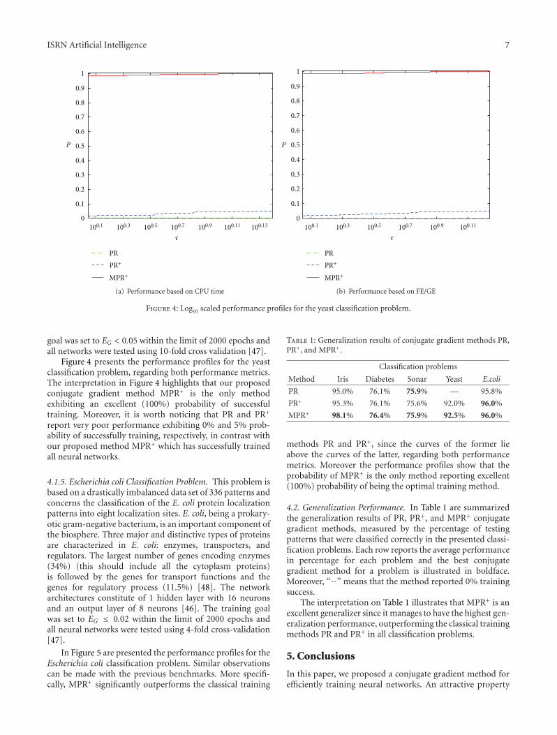
4.1.4. Yeast Classification Problem. This problem is based ona drastically imbalanced dataset and concerns the determi-nation of the cellular localization of the yeast proteins intoten localization sites. Saccharomyces cerevisiae (yeast) is thesimplest Eukaryotic organism. The network architecture forthis classification problem consists of 1 hidden layer of 16neurons and an output layer of 10 neurons [46]. The training


100.1 100.3 100.5 100.7 100.9 100.11 100.13

τ

PR

PR+

MPR+

0

0.1

0.2

0.3

0.4

0.5

0.6

0.7

0.8

0.9

1

P


100.1 100.3 100.5 100.7 100.9 100.11

τ

PR

PR+

MPR+

0

0.1

0.2

0.3

0.4

0.5

0.6

0.7

0.8

0.9

1

P


Figure 4: Log10 scaled performance profiles for the yeast classification problem.

goal was set to EG < 0.05 within the limit of 2000 epochs andall networks were tested using 10-fold cross validation [47].

Figure 4 presents the performance profiles for the yeastclassification problem, regarding both performance metrics.The interpretation in Figure 4 highlights that our proposedconjugate gradient method MPR+ is the only methodexhibiting an excellent (100%) probability of successfultraining. Moreover, it is worth noticing that PR and PR+

report very poor performance exhibiting 0% and 5% prob-ability of successfully training, respectively, in contrast withour proposed method MPR+ which has successfully trainedall neural networks.

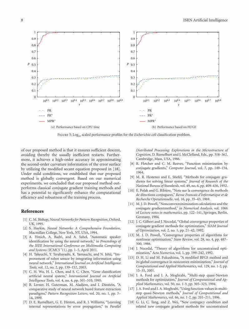
4.1.5. Escherichia coli Classification Problem. This problem isbased on a drastically imbalanced data set of 336 patterns andconcerns the classification of the E. coli protein localizationpatterns into eight localization sites. E. coli, being a prokary-otic gram-negative bacterium, is an important component ofthe biosphere. Three major and distinctive types of proteinsare characterized in E. coli: enzymes, transporters, andregulators. The largest number of genes encoding enzymes(34%) (this should include all the cytoplasm proteins)is followed by the genes for transport functions and thegenes for regulatory process (11.5%) [48]. The networkarchitectures constitute of 1 hidden layer with 16 neuronsand an output layer of 8 neurons [46]. The training goalwas set to EG ≤ 0.02 within the limit of 2000 epochs andall neural networks were tested using 4-fold cross-validation[47].

In Figure 5 are presented the performance profiles for theEscherichia coli classification problem. Similar observationscan be made with the previous benchmarks. More specifi-cally, MPR+ significantly outperforms the classical training

Table 1: Generalization results of conjugate gradient methods PR,PR+, and MPR+.

Classification problems

Method Iris Diabetes Sonar Yeast E.coli

PR 95.0% 76.1% 75.9% — 95.8%

PR+ 95.3% 76.1% 75.6% 92.0% 96.0%

MPR+ 98.1% 76.4% 75.9% 92.5% 96.0%

methods PR and PR+, since the curves of the former lieabove the curves of the latter, regarding both performancemetrics. Moreover the performance profiles show that theprobability of MPR+ is the only method reporting excellent(100%) probability of being the optimal training method.

4.2. Generalization Performance. In Table 1 are summarizedthe generalization results of PR, PR+, and MPR+ conjugategradient methods, measured by the percentage of testingpatterns that were classified correctly in the presented classi-fication problems. Each row reports the average performancein percentage for each problem and the best conjugategradient method for a problem is illustrated in boldface.Moreover, “−” means that the method reported 0% trainingsuccess.

The interpretation on Table 1 illustrates that MPR+ is anexcellent generalizer since it manages to have the highest gen-eralization performance, outperforming the classical trainingmethods PR and PR+ in all classification problems.

5. Conclusions

In this paper, we proposed a conjugate gradient method forefficiently training neural networks. An attractive property


100.1 100.2 100.3 100.4 100.5 100.6 100.7 100.8 100.90

0.1

0.2

0.3

0.4

0.5

0.6

0.7

0.8

0.9

1

τ

P

PR

PR+

MPR+


100.1 100.2 100.3 100.4 100.5 100.6 100.7 100.80

0.1

0.2

0.3

0.4

0.5

0.6

0.7

0.8

0.9

1

τ

P

PR

PR+

MPR+


Figure 5: Log10 scaled performance profiles for the Escherichia coli classification problem.

of our proposed method is that it ensures sufficient descent,avoiding thereby the usually inefficient restarts. Further-more, it achieves a high-order accuracy in approximatingthe second-order curvature information of the error surfaceby utilizing the modified secant equation proposed in [18].Under mild conditions, we established that our proposedmethod is globally convergent. Based on our numericalexperiments, we concluded that our proposed method out-performs classical conjugate gradient training methods andhas a potential to significantly enhance the computationalefficiency and robustness of the training process.

References

[1] C. M. Bishop, Neural Networks for Pattern Recognition, Oxford,UK, 1995.

[2] S. Haykin, Neural Networks: A Comprehensive Foundation,Macmillan College, New York, NY, USA, 1994.

[3] A. Hmich, A. Badri, and A. Sahel, “Automatic speakeridentification by using the neural network,” in Proceedings ofthe IEEE International Conference on Multimedia Computingand Systems (ICMCS ’11), pp. 1–5, April 2011.

[4] H. Takeuchi, Y. Terabayashi, K. Yamauchi, and N. Ishii, “Im-provement of robot sensor by integrating information usingneural network,” International Journal on Artificial IntelligenceTools, vol. 12, no. 2, pp. 139–152, 2003.

[5] C. H. Wu, H. L. Chen, and S. C. Chen, “Gene classificationartificial neural system,” International Journal on ArtificialIntelligence Tools, vol. 4, no. 4, pp. 501–510, 1995.

[6] B. Lerner, H. Guterman, M. Aladjem, and I. Dinstein, “Acomparative study of neural network based feature extractionparadigms,” Pattern Recognition Letters, vol. 20, no. 1, pp. 7–14, 1999.

[7] D. E. Rumelhart, G. E. Hinton, and R. J. Williams, “Learninginternal representations by error propagation,” in Parallel

Distributed Processing: Explorations in the Microstructure ofCognition, D. Rumelhart and J. McClelland, Eds., pp. 318–362,Cambridge, Mass, USA, 1986.

[8] R. Fletcher and C. M. Reeves, “Function minimization byconjugate gradients,” Computer Journal, vol. 7, pp. 149–154,1964.

[9] M. R. Hestenes and E. Stiefel, “Methods for conjugate gra-dients for solving linear systems,” Journal of Research of theNational Bureau of Standards, vol. 49, no. 6, pp. 409–436, 1952.

[10] E. Polak and G. Ribiere, “Note sur la convergence de methodsde directions conjuguees,” Revue Francais d’Informatique et deRecherche Operationnelle, vol. 16, pp. 35–43, 1969.

[11] M. J. D. Powell, “Nonconvexminimization calculations and theconjugate gradientmethod,” in Numerical Analysis, vol. 1066of Lecture notes in mathematics, pp. 122–141, Springer, Berlin,Germany, 1984.

[12] J. C. Gilbert and J. Nocedal, “Global convergence properties ofconjugate gradient methods for optimization,” SIAM Journalof Optimization, vol. 2, no. 1, pp. 21–42, 1992.

[13] M. J. D. Powell, “Convergence properties of algorithms fornonlinear optimization,” Siam Review, vol. 28, no. 4, pp. 487–500, 1986.

[14] J. Nocedal, “Theory of algorithms for unconstrained opti-mization,” Acta Numerica, vol. 1, pp. 199–242, 1992.

[15] D. H. Li and M. Fukushima, “A modified BFGS method andits global convergence in nonconvex minimization,” Journal ofComputational and Applied Mathematics, vol. 129, no. 1-2, pp.15–35, 2001.

[16] J. A. Ford and I. A. Moghrabi, “Multi-step quasi-Newtonmethods for optimization,” Journal of Computational and Ap-plied Mathematics, vol. 50, no. 1-3, pp. 305–323, 1994.

[17] J. A. Ford and I. A. Moghrabi, “Using function-values in multi-step quasi-Newton methods,” Journal of Computational andApplied Mathematics, vol. 66, no. 1-2, pp. 201–211, 1996.

[18] G. Li, C. Tang, and Z. Wei, “New conjugacy condition andrelated new conjugate gradient methods for unconstrained


optimization,” Journal of Computational and Applied Mathe-matics, vol. 202, no. 2, pp. 523–539, 2007.

[19] L. Zhang, “Two modified Dai-Yuan nonlinear conjugate gra-dient methods,” Numerical Algorithms, vol. 50, no. 1, pp. 1–16,2009.

[20] L. Zhang, W. Zhou, and D. Li, “Some descent three-term con-jugate gradient methods and their global convergence,” Opti-mization Methods and Software, vol. 22, no. 4, pp. 697–711,2007.

[21] W. Zhou and L. Zhang, “A nonlinear conjugate gradientmethod based on the MBFGS secant condition,” OptimizationMethods and Software, vol. 21, no. 5, pp. 707–714, 2006.

[22] J. A. Ford, Y. Narushima, and H. Yabe, “Multi-step nonlinearconjugate gradient methods for unconstrained minimization,”Computational Optimization and Applications, vol. 40, no. 2,pp. 191–216, 2008.

[23] H. Yabe and M. Takano, “Global convergence properties ofnonlinear conjugate gradient methods with modified secantcondition,” Computational Optimization and Applications, vol.28, no. 2, pp. 203–225, 2004.

[24] L. Zhang, W. Zhou, and D. Li, “Global convergence of amodified Fletcher-Reeves conjugate gradient method withArmijo-type line search,” Numerische Mathematik, vol. 104,no. 4, pp. 561–572, 2006.

[25] L. Zhang, W. Zhou, and D. Li, “A descent modified Polak-Ribiere-Polyak conjugate gradient method and its globalconvergence,” IMA Journal of Numerical Analysis, vol. 26, no.4, pp. 629–640, 2006.

[26] L. Zhang and W. Zhou, “Two descent hybrid conjugategradient methods for optimization,” Journal of Computationaland Applied Mathematics, vol. 216, no. 1, pp. 251–264, 2008.

[27] W. W. Hager and H. Zhang, “A new conjugate gradientmethod with guaranteed descent and an efficient line search,”SIAM Journal on Optimization, vol. 16, no. 1, pp. 170–192,2005.

[28] G. Yuan, “Modified nonlinear conjugate gradient methodswith sufficient descent property for large-scale optimizationproblems,” Optimization Letters, vol. 3, no. 1, pp. 11–21, 2009.

[29] G. H. Yu., Nonlinear self-scaling conjugate gradient methodsfor large-scale optimization problems, Ph.D. thesis, Sun Yat-SenUniversity, 2007.

[30] I. E. Livieris and P. Pintelas, “Performance evaluation ofdescent CG methods for neural network training,” in Pro-ceedings of the 9th Hellenic European Research on ComputerMathematics & its Applications Conference (HERCMA ’09), E.A. Lipitakis, Ed., pp. 40–46, 2009.

[31] I. E. Livieris and P. Pintelas, “An improved spectral conjugategradient neural network training algorithm,” InternationalJournal on Artificial Intelligence Tools. In press.

[32] I. E. Livieris, D. G. Sotiropoulos, and P. Pintelas, “Ondescent spectral CG algorithms for training recurrent neuralnetworks,” in Proceedings of the 13th Panellenic Conference ofInformatics, pp. 65–69, 2009.

[33] E. Dolan and J. J. More, “Benchmarking optimization softwarewith performance profiles,” Mathematical Programming, vol.91, no. 2, pp. 201–213, 2002.

[34] J. Hertz, A. Krogh, and R. Palmer, Introduction to the Theoryof Neural Computation, Addison-Wesley, Reading, Mass, USA,1991.

[35] M. J. D. Powell, “Restart procedures for the conjugate gradientmethod,” Mathematical Programming, vol. 12, no. 1, pp. 241–254, 1977.

[36] P. M. Murphy and D. W. Aha, UCI Repository of MachineLearning Databases, University of California, Department ofInformation and Computer Science, Irvine, Calif, USA, 1994.

[37] E. G. Birgin and J. M. Martınez, “A spectral conjugategradient method for unconstrained optimization,” AppliedMathematics and Optimization, vol. 43, no. 2, pp. 117–128,2001.

[38] D. F. Shanno and K. H. Phua, “Minimization of unconstrainedmultivariate functions,” ACM Transactions on MathematicalSoftware, vol. 2, pp. 87–94, 1976.

[39] G. Yu, L. Guan, and W. Chen, “Spectral conjugate gra-dient methods with sufficient descent property for large-scale unconstrained optimization,” Optimization Methods andSoftware, vol. 23, no. 2, pp. 275–293, 2008.

[40] D. Nguyen and B. Widrow, “Improving the learning speed of2-layer neural network by choosing initial values of adaptiveweights,” Biological Cybernetics, vol. 59, pp. 71–113, 1990.

[41] R. Kohavi, “A study of cross-validation and bootstrap foraccuracy estimation and model selection,” in Proceedings ofthe IEEE International Joint Conference on Artificial Intelligence,pp. 223–228, AAAI Press and MIT Press, 1995.

[42] J. C. Gilbert and X. Jonsson, LIBOPT-an enviroment fortesting solvers on heterogeneous collections of problems—version 1. CoRR, abs/cs/0703025, 2007.

[43] L. Prechelt, “PROBEN1-a set of benchmarks and benchmark-ing rules for neural network training algorithms,” Tech. Rep.21/94, Fakultat fur Informatik, University of Karlsruhe, 1994.

[44] J. Yu, S. Wang, and L. Xi, “Evolving artificial neural networksusing an improved PSO and DPSO,” Neurocomputing, vol. 71,no. 4–6, pp. 1054–1060, 2008.

[45] R. P. Gorman and T. J. Sejnowski, “Analysis of hidden unitsin a layered network trained to classify sonar targets,” NeuralNetworks, vol. 1, no. 1, pp. 75–89, 1988.

[46] A. D. Anastasiadis, G. D. Magoulas, and M. N. Vrahatis, “Newglobally convergent training scheme based on the resilientpropagation algorithm,” Neurocomputing, vol. 64, no. 1–4, pp.253–270, 2005.

[47] P. Horton and K. Nakai, “Better prediction of protein cellularlocalization sites with the k nearest neighbors classifier,”Intelligent Systems for Molecular Biology, pp. 368–383, 1997.

[48] P. Liang, B. Labedan, and M. Riley, “Physiological genomics ofescherichia coli protein families,” Physiological Genomics, vol.2002, no. 9, pp. 15–26, 2002.

Submit your manuscripts athttp://www.hindawi.com

Computer Games Technology

International Journal of

Hindawi Publishing Corporationhttp://www.hindawi.com Volume 2014


Distributed Sensor Networks


Advances in

FuzzySystems

Hindawi Publishing Corporationhttp://www.hindawi.com

Volume 2014


ReconfigurableComputing

Hindawi Publishing Corporation http://www.hindawi.com Volume 2014


Applied Computational Intelligence and Soft Computing

Advances in

Artificial Intelligence


Advances inSoftware EngineeringHindawi Publishing Corporationhttp://www.hindawi.com Volume 2014


Electrical and Computer Engineering

Journal of

Journal of

Computer Networks and Communications


Hindawi Publishing Corporation

http://www.hindawi.com Volume 2014

Advances in

Multimedia


Biomedical Imaging


ArtificialNeural Systems

Advances in


RoboticsJournal of


ComputationalIntelligence &Neuroscience


Industrial EngineeringJournal of


Modelling & Simulation in EngineeringHindawi Publishing Corporation http://www.hindawi.com Volume 2014

The Scientific World JournalHindawi Publishing Corporation http://www.hindawi.com Volume 2014


Human-ComputerInteraction

Advances in

Computer EngineeringAdvances in


Documents

An Advanced Conjugate Gradient Training Algorithm Based on a Modified Secant Equation