A theoretical and computational model of eddy-current probes incorporating volume integral and conjugate gradient methods

2650 IEEE TRANSACTIONS ON MAGNETICS, VOL. 25. NO. 3. MAY 19x9

A Theoretical and Computational Model of Eddy- Current Probes Incorporating Volume Integral

and Conjugate Gradient Methods JOHN R. BOWLER, L. DAVID SABBAGH, MEMBER, IEEE, AND

HAROLD A. SABBAGH, SENIOR MEMBER, IEEE

Abstract-A general three-dimensional computational model of ferrite-core eddy-current probes has been developed for research and design studies in nondestructive evaluation. The model is based on a volume integral approach for finding the magnetization of the ferrite core excited by an ac current-carrying coil in the presence of a conducting workpiece. By using the moment method, the integral equation is approximated by a matrix equation and solved using conjugate gradient techniques. Illustrative results are presented showing the impedance characteristics and field distributions for practical eddy-current probe configurations.

I. INTRODUCTION NALYSIS and computer design studies of eddy-cur- A rent probes for nondestructive evaluation have in the

past been largely based on the behavior of axially symmetric air-cored coils. This is because closed-form analytical expressions can be used to calculate their electromagnetic fields and impedances in the presence of multilayered conducting slabs or infinite cylindrical workpieces [1]-[3]. A good deal of important information can be gathered from these analytical results but most com- mercial probes use femte cores, therefore, a comprehen- sive model of eddy-current probes needs to take account of the magnetization of the ferrite.

Computational models which determine the magnetization of ferromagnetic regions usually rely on either finite element or integral equation techniques. Electromag- netic field codes using finite elements tend to be more general but expensive in CPU time. Integral equation methods, on the other hand, are often most efficient when a large proportion of the calculation is treated analytically by using Green’s functions which automatically account for many of the boundary and interface conditions. A good strategy therefore, if one is prepared to accept solutions to a restricted class of problems, is to use integral equation methods and to load much of the complexity of the problem into the analysis of the Green’s functions. This relieves some of the burden on the code by simplifying it

Manuscript received July 15, 1988; revised January 19, 1989. This work was supported by the Naval Surface Weapons Center (White Oak Labs) under Contract N60921-86-C-0172 with Sabbagh Associates.

The authors are with Sabbagh Associates, Inc., Bloomington, IN 47401. IEEE Log Number 8926999.

and reducing its development cost as well as making the final algorithm compact and efficient.

Our previous work on eddy-current probes was confined to axially symmetric systems [4] but this restriction has now been removed allowing us to run computer sim- ulations for arbitrary three-dimensional ferrite and coil configurations. For example, the performance of differ- ential probes with split cores or coils wound on C-cores may now be evaluated. Most three-dimensional codes with the capacity to handle arbitrary material geometries, require enormous computer resources if they are to be used effectively. However, the volume integral technique and modem numerical methods together make it possible to take full advantage of the translational symmetry properties of planar structures in the calculation. Indeed the Ir - r’ 1 dependence of the free-space Green’s function represents a powerful symmetry property of space itself, showing that three and not six independent spatial variables are necessary for transforming an electric or magnetic source into the electromagnetic field.

The approach we have developed uses a volume integral equation for the magnetization vector which is transformed into a matrix equation by taking moments. The matrix equation is then solved iteratively using a conjugate gradient algorithm. As we shall show, the matrix consists of two parts, both of which have a form allowing matrix-vector products to be computed efficiently using fast Fourier transforms (FFT’s) in three dimensions with- out the need for calculating and storing the full matrix explicitly [5].

Apart from removing the restriction to axially symmetric systems, the model has been extended to include Green’s functions for calculating the field in the presence of multi-layered anisotropic workpieces [6]. This development is motivated by the need to determine optimum conditions for inspecting modern composite materials such as laminated graphite-epoxy. In the more general cases of arbitrary lay-ups, the Green’s functions are computed nu- merically [6]; however, for simpler structures such as a unidirectional half-space, closed-form expressions can be derived [7] and used as a partial check on the general calculation.

0018-9464/89/0500-2650$01 .OO O 1989 IEEE

BOWLER et a l . : THEORETICAL AND COMPUTATIONAL MODEL OF EDDY-CURRENT PROBES 265 I

11. FERRITE CORE PROBE MODEL A . Integral Equation f o r the Magnetization

The problem we aim to solve, shown schematically in Fig. 1, consists of three components; a predefined electric current source J e , an arbitrary three-dimensional ferrite, and a planar stratified conducting workpiece. We take as a starting point the formal solution of the field equations in integral form using a magnetic current source Jm = - jwpoM to represent the effects of the ferrite. With the surface of the workpiece in the plane z = 0, the magnetic field is related to the source terms by

H ( r ) = [ G ( m e ) ( r l r ’ ) * J J r ’ ) coil +core

+ G ( m ‘ n ) ( r l r r ) . J m ( r ’ ) d r ’ . (1)

The first superscript on the dyadic Green’s functions, G ( m r ) and G(m’n) , refers to the type of field, rn for magnetic and e for electric, and the second indicates the type of source current. These dyads give the total magnetic field as the sum of a direct contribution from the current sources, plus the magnetic field reflected from the surface of the workpiece. In calculating Jm or M the effects of the workpiece are determined by a set of reflection coefficients contained in the Green’s functions. For example, if the workpiece is a multi-layered anisotropic planar structure, then the reflection coefficients for the upper surface of the workpiece must be calculated taking account of the material properties and depth of every layer. The magnetization of the core in free space is determined by setting the reflection coefficients to zero.

The first part of the integral in (1) is the incident magnetic field H“ ) generated by the coil current indepen- dently of the magnetization. Therefore, assuming the core is nonconducting

H ( r ) = H ( ’ ) ( r ) + s G ( m m ) ( r ( r ’ ) J m ( r ’ ) d r ’ . core

(2’1 , I

To get an integral equation for the magnetization, (2) is multiplied by a permeability function v ( r ) = 1 - p o / p ( r ) then defining an incident magnetization, M ( ’ ) = v ~ ( i 1 and using the fact that p o M / p = ( 1 - p o / p ) H , gives

Composite workpiece __

-

Fig. 1. Ferrite-core eddy-current probe over stratified anisotropic conducting workpiece.

as

where the tilde here, and throughout, implies a dependence on the Fourier space coordinates k, and k,,. By substituting this into (3), the integration with respect to the source coordinates x and y becomes a Fourier transform of the magnetic source giving

03

dk, dk,. ( 5 ) . fi(z’) e - j ( k x x + k , g )

Equation (5) will be used to develop a discrete form of (3) using the moment method.

B. Dyadic Green’s Functions It is convenient to express the Green’s function in com-

ponent parts; a free-space part independent of the presence of the slab, and a term GiY) which transforms the source into the reflected field. The two-dimensional Fou- rier representation of the free-space dyadic Green’s function, in turn, consists of two parts; G::;), and a “depolarization” term Gi;;). Thus

G ( m m ) ( 2 , 2 ’ ) = GI,) ( 2 , z ’ ) + G i ; y ) ( z , 2 ’ ) - mm)

+ G;;m;”’(z, z ’ ) . Gi;r;”’ is given by

- s ( r - r ’ ) I ] . M ( r ’ ) dr’ ( 3 ) G::;)(z, 2 ’ )

1 - k : / k i -k ,k , /ki + jk ,ho /k i

1 - k ; / k i + j k , X o / k i

+ j k , h o / k i + j k , X , / k i 1 + h i / k i

( 7 )

jwcL0 Z being the unit tensor. Equation (3) is used to determine the magnetic source strength due to the ferrite. Once we have a solution, the electromagnetic field and the driving- point impedance of the probe can be found.

The Green’s functions for infinite planar regions can be e - h o / z - z ’ l

2x0 written, using a two-dimensional Fourier representation,

2652 IEEE TRANSACTIONS ON MAGNETICS, VOL. 25. NO. 3. MAY 1989

where the ( + ) sign applies when z > z ’ and the ( - ) si n whenz < z’. k i = u2eopOand X o = ( k : + k; - k , ) , taking the root with a positive real part. The “depolarization” term is discussed by Yaghjian [8] and is given by

2 172

The reflection Green’s function is defined in terms of reflection coefficients rxx, rxy, etc., whose values depend upon the nature of the slab and are independent of the location of the source and field points. Thus the reflection Green’s function has the general structure

We are going to use Galerkin’s variant of the method of moments to complete the discretization. In Galerkin’s method, we “test” the integral equation ( 3 ) with the same pulse functions that we used to expand the unknown M in (10). That is, we form moments of ( 3 ) by multiplying ( 5 )

given by (lo), and then integrating with respect to x , y , and z over each cell. This yields a linear system for ZlmJ

by P / ( x / 6 x ) Pm( y / 6 , ) Pj (2 - ~ 0 / 6 : ) / 6 x 6 , 6 : with M

Nx-1 N , - l N:-1

-(mm)(k,, k y ) [sin (kx6r/2)12 Further details of the reflection coefficients are given in Appendix I. * ~ J J

The x - x ’ and y - y ’ dependence of the complete Green’s tensor G(mm) implies that the source coordinate integration of ( 3 ) is a convolution in x and y . In addition, the free-space Green’s tensor has a z - z’ dependence while the reflection Green’s tensor has a z + z’ dependence. Therefore, ( 3 ) contains the sum of a convolution

for computing M from a discrete version of ( 3 ) , we have

structure.

C. Discretization of the Integral Equation

k A / 2

sin (k , 6, / 2 ) ] ’

‘i”&*’ is defined by letting zk = zo + k6;; k = 0 , N2 - 1 , as

(14) dk, dk,.

and a correlation in z . In designing a numerical algorithm

taken full advantage of this convolutional/correlational Zk ZJ

Z k + l z, + I

‘i”iym)(kx, k , ) = 1 dz s dz’

The discretization of the integral equation ( 3 ) is done by subdividing the region of space occupied by the core into N , layers, each of depth 6,, and then approximating the magnetization vector and the permeability function v by a pulse function expansion in x and y as well as in z . Thus

Pj(?)

and

where zo is the perpendicular distance from the workpiece to the bottom of the source grid and the pulse functions are defined by

1, 0, otherwise.

i f k I s < k + 1.0 ( 1 2 ) p k ( s ) =

(15) Equation ( 1 3 ) is the equation we use to calculate moments of the femte core magnetization. As well as being of Toe- plitz form in (1, L ) and ( m , M ) as the I - L, and m - M dependence implies, the coefficient matrix decomposes into two matrices, one of which has the Toeplitz form in ( j , J ) and the other beingj + J dependent, has a Hankel form in ( j , J ) . This structure, which is a direct conse- quence of the convolutionaUcorrelationa1 nature of the basic integral equation, allows us to use the fast Fourier transform for computing the result of multiplying an arbitrary vector by the matrix GI - L , m - M , J , J . It is important that this operation be carried out efficiently since it is used repeatedly in the conjugate gradient procedure.

111. FIELD AND IMPEDANCE CALCULATION A . Incident Field

The incident field vector Z!hi is determined by the electric current source in the coil. Zihi may be computed for an arbitrary current, but because we usually have a cylindrical coil, it is more efficient, where appropriate, to determine the incident term from a specialized expression. Similarly, the probe impedance calculations can be done for cylindrical coils or a more general equation as re- quired. We will not assume that the workpiece is iso-

BOWLER et a/.: THEORETICAL AND COMPUTATIONAL MODEL OF EDDY-CURRENT PROBES 2653

tropic, so that the results will be valid for composite lay- ups, as well as isotropic workpieces.

In calculating the incident vector we use the incident magnetic field from (l) , multiplied by U = ( 1 - po/p) and expressed as

Here we use the functions F3 = F3 (z,, z b , zk , zk + ), and F5 = F 5 ( z k , Z k + l , z,, z b ) . In all, there are five such functions F 1 , F2, . - , F,, that arise naturally in this approach from integrations with respect to z . These functions are defined in Appendix 11. Also we have introduced

m

PI, ~ 2 9 k r ) = d 3 ( ~ 2 , k r ) - P : ~ ( P I , k r ) ( 2 1 )

and used the dyadic Green's function giving the magnetic field due to an electric current source (Appendix I).

B. Driving-Point Impedance

electric field at the coil and given by

z= --

G ( m e ) ( z , z l ) M ( ' ) ( r ) v(r)

4T2 scoll dz' s s -

-m PO

. j e (zr ) e - J ( k r X f k , r ) dk,dk, (16)

where is derived in Appendix I. The coil Current will be defined in cylindrical coordinates with a+ as a unit azimuthal vector. Assuming a densely and uniformly

In general, the probe impedance z is dependent on the

( 2 2 ) wound cylindrical coil occupying the region p I 5 p I p 2 , z , 5 z 5 zb with a turns density n, each turn carrying

E ( r ) e J e ( r ) dr I 2 cod

where the electric field has contributions from both the coil current and the magnetic dipole density of the core. Again using the two-dimensional Fourier representation

a current I , we have

J,( P , z , 4) a,nl, z , I z I zb and p I I p I p 2 as a basis for the calculation, we have

m

1 4n

otherwise. (17) E ( r ) = 7 s dz' s s [ G ' " ) ( z , z ' ) . J e ( z ' )

= i o ,

The two-dimensional Fourier transform of a cylindrical -m

current involves the radial integral of a first-order Bessel function [9]

3 ( s ) = s; PJI ( P S ) dP

2T = - [ J l ( 4 Ho(s ) - J o ( s ) HIW] (18)

S

where H0 and HI are Struve functions. This allows us to write the Fourier transform of (17) as

k,. k, j2anI -a, - + a - k , ' kr

( 0, otherwise

where kr = ( k : + k ; ) ' / 2 , a, and ay being unit vectors. Taking moments of (16) by multiplying by the pulse

function product PI (x/6,) Pm( y/6,.) PI ( z - z0/6,)/ 6,6,6, and integrating over x, y , and z with j e given by (19) we get

- japoG(em)(z, z l ) . M ( z ' ) ]

(23 1 . e - l ( k r x + k \ Y ) dk dk x g .

Because Je is defined as uniform over a cylinder and M is approximated by a piecewise-constant basis, it is convenient to compute their individual contributions to 2 sep- arately putting

2 = Z C O I ~ + zcore. ( 2 4 ) For the coil contribution we use (19) and the electric-

electric dyadic Green's function to give

m

2654 IEEE TRANSACTIONS ON MAGNETICS. V O L 25. NO 3. MAY 1989

In computing the core contribution to ( 2 4 ) we recognize that the magnetization vector has a z component as well as x and y components. With a piecewise-constant ap- proximation for M ( r )

( 2 9 ) . e/(k,6,~+k,6,m)dk, dk,

To calculate Z'"" the C ' s are accurately precomputed, the magnetization vector is found, and finally probe impedance in the presence of the workpiece is determined from ( 2 7 ) . To get the free-space probe impedance, the core magnetization in free space is used and Cl;; excluded from the summation of ( 2 7 ) .

C. Electric Field Calculation In finding the electric field due to a cylindrical coil cur-

rent and a piecewise-constant magnetic core, the general expression ( 2 3 ) is used, with the coil current given by ( 1 9 ) and the core magnetization by ( 2 6 ) . The coil contribution is then

and the electric field due to the ferrite core is given by Nr-1 N , -1 N, -1

where m

and

I ) ' dk, dk , . ( 3 3 )

Here we have a more compact notation for the F ' s defined in Appendix 11, putting

. e - J [ k r ( r - / 6 , ) + k , ( \ -m6

F: ' ) = F I ( Z k ? Z k + I )

F12' = F2(Zk, Z k + l , Z)

Fi4' = F d ( ~ k , z ~ + I , 2). (34) The integrals that represent the quantities GI - - J ,

Zj$, and Ciii, CiA; are all of the type that can be computed by FFT. In each case the integrands have factors of the form sin ( k r 6 , / 2 ) / ( k , 6 , / 2 ) , sin ( k , 6 , / 2 ) / ( k I 6 , / 2 ) . In evaluating these integrals, we want to avoid using very large FFT's and yet require the range of integration to be sufficiently large so that the numerical routine will converge. The method used divides the ( k , , k , ) plane into rectangles where ( 2 4 , - 1)n I k,6, I ( 2 4 , + l ) ~ , ( 2 4 , - l ) ? r I k ,6 , I (2 i k , + 1 )7r and then approximate the infinite integral by a sum over the rectangles of finite

BOWLER et al . : THEORETICAL A N D COMPUTATIONAL MODEL OF EDDY-CURRENT PROBES 2655

of Fourier transforms that are computed using FFT’s, each having a modest range. 0 9 -

‘Test’ 0 8 - IV. NUMERICAL ALGORITHM

then, clearly, vlmJ are row-multipliers. Let us write this When we interpret (13) as a vector-matrix equation,

0 7 -

vector-matrix equation as the operator equation O h -

. .

Y = ax where

y =

and N - - 1 Nr- I N , - I

az = z,, + v/,J c c c J = O L = O M = O

( 3 5 )

GjJ( l - L, m - M ) * ZLMJ. (37)

“‘1 “.21 ”.‘ 1

. . . . ’ . . . . 0.04 I I I ’ , I I , I I , I 1 , We will need the adjoint operator @*, which corre- 0 1 2 3 4 5 6 7 8 9 1 0 1 1 1 2 1 3 1 4 1 5

sponds to the conjugate transpose of the matrix Iteration no. N;-1 N r - l N \ - l

@*I = I),,, + C C C GJ,(L - I , M - m ) J = O L = O M = O

* ~ L M J ~ L M J . (38) The symbol t denotes the conjugate transpose of a dyadic. Note that vlmj are real numbers.

The conjugate gradient algorithm [lo], [ 1 I ] starts with an initial guess Xo from which we compute Ro = Y - axo, PI = Q, = a*Ro. In addition, we have a convergence parameter E . Then, for k = 1, 2, * * , if Test = I( Rk 11 / 11 Y 11 < E , stop; Xk is the optimal solution of (35). Otherwise, update xk by the following steps:

s k = apk

Fig. 2. Convergence Tesr versus iteration count.

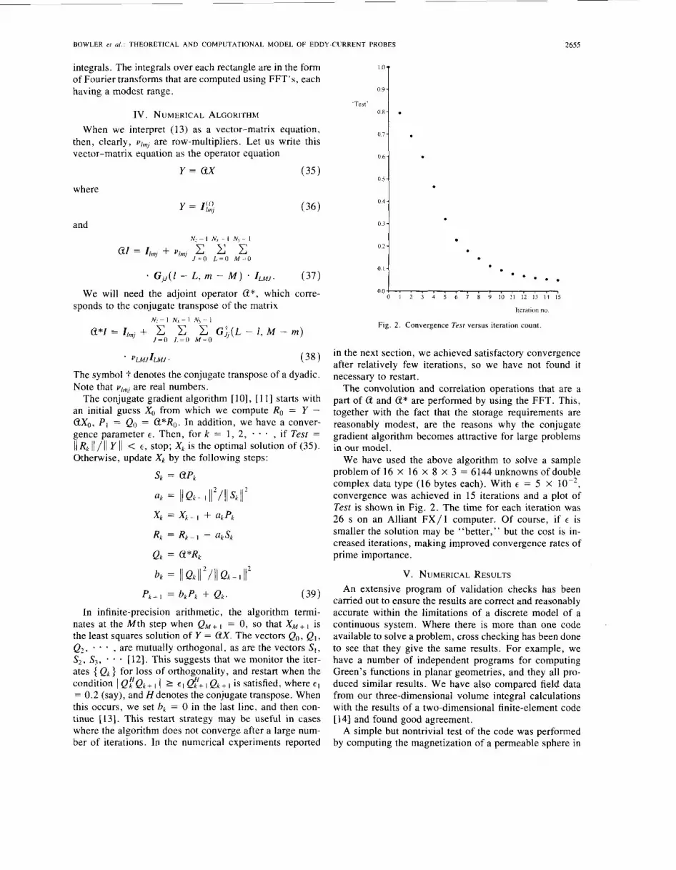
in the next section, we achieved satisfactory convergence after relatively few iterations, so we have not found it necessary to restart.

The convolution and correlation operations that are a part of a and @* are performed by using the FFT. This, together with the fact that the storage requirements are reasonably modest, are the reasons why the conjugate gradient algorithm becomes attractive for large problems in our model.

We have used the above algorithm to solve a sample problem of 16 X 16 x 8 x 3 = 6144 unknowns of double complex data type (16 bytes each). With E = 5 X

convergence was achieved in 15 iterations and a plot of Test is shown in Fig. 2. The time for each iteration was 26 s on an Alliant FX/1 computer. Of course, if E is smaller the solution may be “better,” but the cost is in- creased iterations, making improved convergence rates of prime importance.

(39) In infinite-precision arithmetic, the algorithm termi-

nates at the Mth step when QM+ I = 0 , so that X M + I is the least squares solution of Y = ax. The vectors Q,, Q , , Q2, * . * , are mutually orthogonal, as are the vectors SI , Sz, S 3 , . [12]. This suggests that we monitor the iter- ates { Q k } for loss of orthogonality, and restart when the condition I erek+ I I 1 e l &+I Qk+ I is satisfied, where = 0.2 (say), and Hdenotes the conjugate transpose. When this occurs, we set bk = 0 in the last line, and then con- tinue [13]. This restart strategy may be useful in cases where the algorithm does not converge after a large number of iterations. In the numerical experiments reported

An extensive program of validation checks has been carried out to ensure the results are correct and reasonably accurate within the limitations of a discrete model of a continuous system. Where there is more than one code available to solve a problem, cross checking has been done to see that they give the same results. For example, we have a number of independent programs for computing Green’s functions in planar geometries, and they all produced similar results. We have also compared field data from our three-dimensional volume integral calculations with the results of a two-dimensional finite-element code [14] and found good agreement.

A simple but nontrivial test of the code was performed by computing the magnetization of a permeable sphere in

2656

0.035 - E(ri

(V/mi 0.03 -

0.025 -

0.02 -

0.015-

0.01 -

0005-

0.0,

IEEE TRANSACTIONS ON MAGNETICS. VOL 25 . NO. 3. MAY 1989

I I I I 0.0 7.5 15.0 22 5 30.0 37.5 45.0 52 5 611 (1

1 3.5

x x x x x

X 1_1 2 0

0

0.5 -I X

r (11,111 1

Fig. 3 . Magnetization of a 20-mm-diameter sphere in free space due to a uniform incident magnetic field Ho. Crosses correspond to infinite relative permeability case (theoretically, M / H , = 3.0) and diamonds represent the computed solution for a relative permeability of 2 (for which theory gives M / H o = 1.5).

a uniform incident magnetic field. Assuming an infinite relative permeability, vImk was defined on a 16 X 16 X 16 cubic grid with the value 1.0 for cubic elements entirely within the sphere, zero for elements entirely outside the sphere, and an intermediate value if the spherical surface passed through the element. The intermediate value was simply assigned a value in proportion to the fraction of the cube inside the sphere. The sphere magnetization was also calculated assuming its relative permeability was 2 by assigning vlmk = 0.5 for a volume elements totally within the sphere.

Fig. 3 shows the z component of the magnetization vector due to an incident magnetic field Ho in the z direction for infinite permeability and a permeability of 2. These results are to be compared with expected constant values of M / H o = 3 and M / H o = 1.5, respectively. A compar- ison of the external field computed from the general code and from an analytical expression for the dipole field due to a uniformly magnetized sphere is shown in Fig. 4.

A wide range of probes designed for a variety of applications are used in eddy-current nondestructive evaluation. For graphite-epoxy inspection good probe-workpiece coupling is more important than resolution and excitation frequencies are often in excess of 1 MHz. Ex- periments have shown that cup-core probes are very ef- fective for flaw detection in conducting composites, es- pecially if they are constructed to give good coupling [ 151. Fig. 5 shows a typical ferrite cup-core geometry.

The probe performance can be assessed from the variation of its impedance on the workpiece Z with frequency. This information is commonly presented on a normalized impedance diagram showing how Z, = Z / X o varies with Z/6, X , being the free-space reactance and G / 6 the ratio of the probe mean radius to skin depth. Conventionally, we take the mean radius as (outside diameter)/3. Z, has been calculated for different values of the liftoff parame-

7.5

7

Fig. 5 . Ferrite cup-core eddy-current probe. Dimensions are in millime- ters.

ter, which is the perpendicular distance from the probe base to the workpiece, and the results plotted in Fig. 6 for an isotropic half-space and in Fig. 7 for an anisotropic half-space. Note the difference in the shape of the impedance characteristic when the material is anisotropic. Impedance predictions in this form enable us to quantify the coupling of the probe to the workpiece through an es- timate of the normalized reactance in the high-frequency limit X,. X , is estimated by extrapolating the impedance characteristic to the reactance axis. For example, the zero liftoff data (Fig. 6) give X , 2: 0.5. The coupling coefficient k , given by k2 = 1 - X,, gives a figure of merit for

BOWLER et a l . : THEORETICAL A N D COMPUTATIONAL MODEL OF EDDY-CURRENT PROBES 2657

0.9 -

0.8 -

0.7 -

0.6 -

1 . 0.5 + 1.2 mrn.

X 0.hmrn. Fig. 8 . Azimuthal electric field at the surface of the workpiece due to a

cup-core eddy-current probe (Fig. 5).

* OOmm 12 i m m

0 4 0 0 0 0 2 004 006 on8 0 I 0 1 2 0 1 4 016

R"

Fig 6 Normalized impedance diagram for a cup-core probe (Fig 5 ) above an isotropic half-space for various liftoff values Points are plotted for a / & = 2" X 0 175, n = 1 , 2, . ' . , 8 and is the "mean" probe radius

~

I

0 5 -

X

+

+ X

+ X

X

Lift-off

+ 1.2 mrn.

X 0.6mm.

0 .0mm.

0 4 4 0.0 0.02 004 006 0 . 0 ~ 0.1 0.12 014 0 1 6

Rn

Fig. 7. Normalized impedance diagram for cup-core probe (Fig. 5) above a uniaxial half-space ( U = uvv = U;: , U # uxx) for various liftoff values. Conductivity ratio u x x / u = 200. Points are plotted for i / 6 , , = 2" X 0.175, n = 1, 2, . . . , 9 and a is the "mean" probe radius.

the probe-workpiece interaction. Clearly, k is sensitive to liftoff as well as being dependent on the probe.

One of the principal advantages of the cup-core config- uration is that the field is largely confined within the probe region. The effect is illustrated in Fig. 8 where the azimuthal electric field at the surface of the workpiece is shown as a function of distance from the axis. Because

Fig. 9. C-core eddy-current probe. Coil OD 2.677 mrn. ID 1.677 mrn, axial length 3 mm.

the coil current is taken as the phase reference, the real part of the field is in phase with the coil current and the imaginary part in quadrature. Note that the field intensity beyond the perimeter of the core is small.

A useful probe for specialist applications such as the detection of cracks under installed fasteners in aircraft structures is the C-core probe [16] (Fig. 9). The electric field as the surface of the workpiece where it intersects the plane of symmetry of the probe in plotted in Fig. 10 showing a rapid local variation in field intensity in the vicinity of the coil.

VI. CONCLUSION A computational electromagnetic field model has been

developed for the evaluation of eddy-current probes with femte cores in the presence of homogeneous or anisotropic layered workpiece. It has the capability of predict- ing the impedance characteristics or the field produced by three-dimensional probe configurations and of modeling the effects of composite materials such as graphite-epoxy . The approach uses the moment method to get an approximate matrix representation of a volume integral equation for the core magnetization. By using the conjugate gradient method and taking advantage of the matrix structure to implement it, using FFT techniques, we have developed an algorithm that is both efficient in CPU time and has modest storage requirements.

2658

12.0, y-component of Electric Field

x real pan (in-phase) -6.0

h a g . pan (quadrature)

-10.0 .. - 12.0 -8.0j

Fig, 10. Electric field at the surface of the workpiece and at the plane of symmetry through the center of the C-core probe (Fig. 9).

IEEE TRANSACTIONS ON MAGNETICS. VOL. 25 . NO. 3, MAY 1989

ferential equation

The tilde denotes a function defined in the transform domain ( k x , k , , ) , and ( iLx , t,, izz) are the principal values of the generalized dielectric permittivity tensor of the body. j p , I,,, are, respectively, the transformed input electric and magnetic current densities.

The system and forcing matrices are given by, respectively,

0 0 r

r o o k x / w i , o o 7

1 - j k x k y / w i , -jwpo + j k : / w i , 2 jwpo - j k y / w i , j k x k y / w i ,

L - 1 0 0 O - k y / w p o J

In solving (Al) and (A2) for the Green's function, we must account for the presence of a point source of either electric or magnetic current. Such a singular current will produce a discontinuity in the tangential components of the electromagnetic field. The amount of discontinuity can be inferred from (AI), in which the imposed Source current, which is located at (x', y', z ' ) , has the form

APPENDIX I COMPUTATION OF DYADIC GREEN'S FUNCTIONS

INTRODUCTION Maxwell's equations for an electrically anisotropic body

V x E = - jwpoH - j w p o M

are - - J'" = J e W e J k d q z - z ' ) ,

= - jwpoH + J,,, -

V x H = jwg * E + J ,

where we have included a magnetic current source J,,, to account for the presence of the ferrite core. 2 is the generalized permittivity tensor of the body.

If the body is homogeneous with respect to (x, y) , then Maxwell's equations can be Fourier transformed with respect to (x, y) , and written as the four-vector matrix dif-

- Here, 7 and 5 are six-vectors, with the latter being a unit vector that identifies the type of current, and its direction.

Upon integrating (Al) an infinitesimal distance across the plane z = z ' , we get

- A -

('43) E ; + ) - ?(-) = n J e i k " ' e J k i y '

for the discontinuity in the tangential components of the field vectors. Here, ( + ) denotes the limit immediately above z ' , and ( - ) denotes the limit immediately below.

For example, if the field is excited by a unit magnetic current source that is first oriented along the x , then y , and, finally, the z direction, then (A2) shows that the right- hand side of (A3) is given by, respectively,

In writing (A4) we suppress the exponential terms in (A3). The “magnetic-magnetic’’ dyadic Green’s function,

that was used in Section I1 has the following interpretation: its first column is the magnetic field vector produced by a point source of magnetic current that is oriented in the x direction, its second column is the magnetic field vector produced by a point source of magnetic current that is oriented in the y direction, and similarly for the third column. Of course, we are still working in the Fourier domain, so that the only spatial variables are ( z , z ’ ) , where z is the field point, and z’ the source point. Hence, we can write

BOWLER et al. : THEORETICAL A N D COMPUTATIONAL MODEL OF EDDY-CURRENT PROBES 2659

where we assume that i22 = 233 = 2, as is typical of many graphite-epoxy composites. XI corresponds to the extraordinary wave, and X3 to the ordinary wave. Clearly, when 211 = i , then X I = X3, and the extraordinary wave becomes ordinary, which agrees with the results for an isotropic medium (such as free space).

Corresponding to each eigenvalue is an eigenvector. We have some liberty in choosing the two independent equations that generate the eigenvectors; hence, there is some arbitrariness in choosing the eigenvectors. We choose the following:

The superscripts on the field components in each column denote the direction of the applied magnetic point-current source. The delta function term that appears in the zz component of (A5) is due to the fact that Hz contains a term that is directly proportional to the z component of the applied magnetic current density, as shown in (Al) . Hence, when this current density is a Dirac delta function, as it is when computing the dyadic Green’s function, the same delta function appears in the Green’s function. This term is the “depolarization” Green’s function that is shown in (8).

COMPUTING A NUMERICAL GREEN’S FUNCTION FOR A

HALF-SPACE In this section, we develop a computational method for

generating the Green’s function for a half-space. The approach we use is based on our need to generalize to workpieces of finite extent in the z direction and to multi-layered anisotropically conducting media, and this need is best met by introducing an eigenmode analysis of (Al) and (A2).

The eigenmodes are solutions of (Al) and (A2), with the input currents set equal to zero. It is straightforward to compute the eigenvalues f h l and + A 3 of the system

E 4 = [ where

Q ( I = s14/X1 Q(2 = s24/X1 TI = s32/X3

Y2 = S31/X3 (A81 and the S, are defined in (A2). 3, and V2 are associated with + X I , - X I , respectively, whereas V 3 and V4 are associated with +A,, - A 3 , respectively. The second and fourth vectors are the two ( + )-going modes, and the first and third are the two ( - )-going modes, in the z direction. Corresponding functions in free space are designated by the subscript 0. Note that E , , V 2 are transverse magnetic (TM) to x , and E3, V4 are transverse electric (TE) to x .

In the present development, there are three regions; Re- gion A is above the source, Region B is between the source and the half-space, and Region C is in the half- space. If we assume that the source is at z‘ > 0 and the

2 6 6 0 IEEE TRANSACTIONS ON MAGNETICS. VOL. 25. NO. 3. MAY 1989

half-space is located at z = 0, then the Green's function may be expanded in terms of the eigenmodes as - G(z, z ' )

, z ' < z a j j O e - h O ( Z - Z ' ) + b/40 e - A0 ( Z - Z '1

e U I O e A ~ ( ~ - - 2 ' ) + d320e-hl(Z-2')

+ ev e A ~ ( ~ - ~ ' ) + fz40e-Xo(z-"') 30 ,

O < Z < Z '

z < 0. (A9 1 =i C r v , e x l z + e ' v 3 e x 3 z ,

The terms with a and b are upward-going waves, above the source point, whereas the terms with d and f are upward-going waves, below the source point, but above the half-space. Hence, the d and f terms correspond to reflected waves that originate at the boundary of the half- space.

Similarly, the c and e terms correspond to downward- going waves below the source point, but above the half- space, which means that they are incident waves due entirely to the source. Of course, the e' and e' terms are downward-going waves within the workpiece, so they are transmitted waves.

These interpretations of the coefficients are important in defining the incident and reflected Green's functions, as we will see shortly.

The eight unknowns a, b, e , d, e , f, e ' , e' in each column vector are computed with the aid of four boundary conditions at the half-space-air boundary and four boundary conditions at the location of the source. The source boundary conditions are given by (A3) and (A4), the latter being the result for a point source of magnetic current. Thus single-ply Green's matrices can be computed by solving 8 X 8 systems of equations. However, by care- fully examining the conditions at the source, we see that the c and e are computed from the source values and that a is a function of d while b is a function off. Hence, we can reduce the computation to solving a 4 X 4 system for d , f , e ' , e ' .

The following two tables give the expressions for a, b , c , e in terms of their values and functional relationships with d and f.

Magnetic Sources

Coefficient X Directed Y Directed t Directed

The entries within these tables support our previous interpretation of the coefficients. c and e are independent of all other coefficients, which means that they do not depend upon the half-space. Hence, they contribute to the incident Green's function, which propagates downward as if it were in infinite free space.

Similarly, those parts of a and b that are independent of d and f contribute to the upward-going free-space Green's function. The remaining parts of a and b are equal to d and f , which means that they are the continuation of the reflected waves above the source point.

The actual 4 x 4 system that we solve is

sx = Y (A10) with

- - s = ( 3 2 0 , v40 - U ] , -q)

x = (a, f, cl, e o 7

Y = (-bloc - Eloe)e-'OZ'

f = fe'oz'. (A1 1 ) d = dehZ'

Note that the right-hand side Y is a function of the source type, magnetic or electric, and the direction of the source x, y , or z .

The solution of (A10) gives d( -+ d ) , f ( -+ f ), e ' , and e ' . From d and f, we can find a and b, thus giving all coefficients in (A9). A careful study of (A9)-(All) shows that the products de2'Oz' and feZx"" are independent of z ' . Because d and f correspond to reflected waves, we call these two products reflection coefficients R, and R,, respectively.

If all we desire are Rd and R ,, then we solve the system

('412) for x1 and x2.

It is important to understand that those coefficients e, a , e , b, that are known, or partly known a priori, contribute to the "incident" or "free-space'' dyadic Green's function. This follows because their values are independent of the existence of the scattering half-space. The values of these coefficients depend on the type of excitation source, and are given in the two tables in this section.

Incident Thus if we use only these coefficients in computing the

fields in (A9), and then substitute the results into (A5), we arrive at the free-space magnetic-magnetic Green's function (7).

Electric Sources

i Directed Coefficient X Directed Y Directed

C 1 / 2 -Yzo/2Ylo - k , / 2 a 1 , w ? Consider, for example, the first column of the Green's dyad, which is the response to an x-directed magnetic cur-

r 0 - 1 /2YI,l - ( a l o k \ - a 2 ~ k ~ ) / 2 u a ~ ~ 1 ' rent source. According to the table, the only contribution c1 d - 1 / 2 d + ~ x i / 2 ~ 1 , 1 d - k , / 2 a 1 &

b f f - 1 / 2 ~ 1 , 1 f + ( a i o k , - a x i ~ l ) / 2 ~ a i o ~ t o t h e d y a d i s b = - 1 / 2 f o r z > z ' , a n d e = 1 / 2 f o r z

266 I BOWLER er a l . : THEORETICAL AND COMPUTATIONAL MODEL OF EDDY-CURRENT PROBES

- -

< z ' , which means, by (A9), that the relevant eigenmode contributions are

(Al) , which shows that the z component of the electric field is coupled directly to only the z-component of the electric current density, not the magnetic current density.

, z I < z These Green's functions are computed in exactly the same way as was the magnetic-magnetic function, except that we use the appropriate sources from the table in this section, and compute the appropriate fields, after the reflection coefficients de2hK , feZx0" are computed. Hence, the reflected parts have the structure shown in (9).

The incident parts, however, can be written down by inspection, because they satisfy Maxwell's equations in a homogeneous space. Hence

(A13)

We use (A7) to compute the relevant field components

, 0 < z < z ' .

that go into the first column of (A5). Thus

, z ' < z

, O < z < z ' A&, z ' ) =

( a j j , y A o ( : - ~ ' ) + &j e-Ao(:-:')

C V I O e h O ( Z - Z ' ) - + da20e-hl(Z--"')

20 40

2 ' < z

+ ev e x o ( z - z ' ) + j - ~ ~ ~ ~ - b ( : - z ' ) 30

O < Z < Z I

' E , e X I Z + d + e1E3eh3z + f 'z4e-x3:

9

- 2 , < 2 < 0 g v l o e x o ( z + ' " ~ + ha

30 , 2 < - z , .

e -xo 1 : - z ' 1

2x0 = j w t o ( 1 - kz /k ,Z) ~

Upon substituting (7) into (A13), and working in ( k y , , z ' < z - Xo(: - : 7 - t Y 2 e - ; y2 - :'I A\(Z, z ' ) = k , ) space, we get

, O < z < z ' i

B , ( z , 2 ' ) = 0

We compute A:( z , z' ) by substituting the expressions for E, and E, into (A5). The result is

These results are identical with the first column of (7). The remaining two columns are computed in a similar manner, using the appropriate values of ( c , a , e , b ) from the table, for magnetic sources in the y and z directions.

This is the dyadic Green's function that is incident upon the workpiece from free space. Because it is independent of the workpiece, it will be the same when computed in any of the sections of this Appendix.

The remaining part of the Green's function comes from the coefficients that are not known a priori, but must be computed. This part depends upon the nature of the workpiece (i.e., the scatterer), and, therefore, produces the reflection coefficients that generate the "reflected" Green's function, shown in (9).

As pointed out in the text, we use the electric-magnetic G("J", magnetic-electric, G'""'), and electric-electric, G""" dyadic Green's functions. Each of these functions has a free space (incident) and reflected part, as does the magnetic-magnetic function, but only the electric-electric function has a depolarizing term. This follows from

2662 IEEE TRANSACTIONS ON MAGNETICS. VOL. 2 5 . NO. 3. MAY 1989

Again using the boundary conditions and the conditions at the source, we can find the unknowns by solving an 8 x 8 system of equations for d , f , c' , e ' , d ' , f I , g , h, and then use the table for Magnetic Sources or Electric Sources to find c, a , e , b. The actual 8 X 8 system that we solve is

sx = Y ('419) where

and

COMPUTING A GREEN'S FUNCTION FOR A LAYERED WORKPIECE

In this section, we extend our method to layered workpieces of finite extent in the z direction. Again there are four regions; however Region C is now divided into, say, 10, subregions, which are defined as follows:

Layer 1:

Layer 2:

zl < z < zo = 0

z2 < z < z l

Layer 10: -zw, = zlo < z < z9.

The Green's function now becomes

e -hIz* 0 0 0

= [ a 0 eh3z>,

X = (a, f, c', e ' , d ' , f', g , h)'

Again, if all we desire are the reflection coefficients, then solve the above equation for the first two unknowns

Equation (A21) is ill-conditioned as it is defined; hence, we must do some scaling in order to get meaningful results. Examination of S shows that column 5 is multiplied by and column 6 by e"'". If we divide these columns by the exponential factors, S is better conditioned, which allows us to solve for X . This, of course, means that the 5th and 6th positions in the solution must be "unscaled," which is accomplished by dividing these positions by exliu and e X X ~ % , respectively.

omitted from Y. with e - h O Z '

+ f" ) 3 ; I ) ( 2 - Zr ~ I )

9

z , < 2 < Z,-I, i = 1, . . . , 10

, z < -z,,. g ~ l O e h O ( Z + f ~ s ) + hjj ,hJ(Z+&) 30

( A22 1 i

Again using the boundary conditions and the conditions at the source, we can find the unknowns by solving (in the case of 10 layers) a 44 x 44 system of equations for

g , h and then use the table for Magnetic Sources or Elec- tric Sources to find c , a , e , b. In general, if there are n1 layers, then the system to solve is (4n( + 4 ) x (4nl + 4) . The form of this system is

c ( l ) e " ) d ( ' ) f'" . . . c( 10) e' I O ) , ( $ I O ) , f ' I O ) , d,f, 9 7 3 , 9

sx = Y ('423) where

BOWLER er al.: THEORETICAL AND COMPUTATIONAL MODEL OF EDDY-CURRENT PROBES 2663

with the terms not previously defined being

Again, if all we desire is the reflection coefficients, then solve the above equation for the first two unknowns with e-hoz’ omitted from Y.

As before, (A25) is ill-conditioned, as it is defined. The columns of S that contain the factors and e-h3h1 (re- member, hi < 0 ) are the ones that need to be scaled, and this is done by dividing these columns by the exponential factors. Again, we must be sure that the corresponding positions in the solution vector are “unscaled” to give the correct solution.

Careful examination of S shows that it is a banded matrix with its upper bandwidth mu = 5 , its lower bandwidth m, = 5 , and its (total) m = mu + ml + 1 = 11. We used subroutines zgbco and zgbsl from LINPACK to solve the system.

Up to this point, we have assumed that all layers are oriented in the same direction with respect to a global coordinate system. Let us now suppose that each layer can be rotated. Since eigenvalues are unchanged and eigenvectors are merely transformed by the rotation, it is straightforward to set up the equations in this situation. The rotation matrix in this case is

where

cos (e) sin ( e ) -sin (e) cos ( e ) @ ( e ) =

If we let 8, be the angle of rotation of the i th layer with respect to the global system, then the eigenvectors for this layer become

$” = 3(e,)i711)

$)’ = 3 ( e , ) ~ 4 ~ ) 54,)‘ = 3(e,)i7ji) (AX)

jjl’)’ = 3 ( e , ) ~p

and only the change in (A23) is the definition of S ‘ ” , which becomes

($)‘ - ( I ) ’ - ( 1 ) ’ , U3 , U 2 , E‘“’) $ I ) ‘ =

- - (3-‘” u1 , 3 U i 1 ) , JVl”, %if)). (A27)

This is a general model for the computation of the Green’s function and the computation of reflection coefficients that has been implemented into our computer codes. In our model, we have assumed that the conductivities of each layer are the same. However, the gener- alization to a model where each layer has its own unique conductivities could be easily accomplished by computing the eigenvalues and eigenvectors of each layer in its own “local” coordinate system and then proceeding with the rotation stage above.

APPENDIX I1 DEFINITIONS OF SPECIAL FUNCTIONS

dz b

F , ( a , b ) = j, e - a02

F2(a, b, C ) = j: e-aOlc-z l dz

n h nd

(+): z < z’ i ( - ) : z’ < z .

REFERENCES [I ] C. V . Dodd and W. E. Deeds, “Analytical solutions to eddy-current

probe-coil problems,” J . Appl. Phys. , vol. 39, pp. 2829-2838, 1968. [2] J. W. Luquire, W. E. Deeds, and C. V. Dodd, “Alternating current

distributions between olanar conductors.” J . A d . Phvs.. vol. 41. .‘ I

pp. 3983-3991, 1970. C. C. Cheng, C. V. Dodd, and W. E. Deeds, “General analysis of probe coils near stratified conductors,” Int. J . Nondestructive Tesr- ing, vol. 3, pp. 109-130, 1971. H . A. Sabbagh, “A model of eddy-current probes with ferrite cores,” IEEE Trans. Magn . , vol. MAG-23, no. 3, pp. 1888-1904. May 1987. T. K . Sarkar, E. Arvas, and S . M. Rao, “Application of FFT and the conjugate gradient method for the solution of electromagnetic radia- tion from electrically large and small bodies,” IEEE Trans. Antennas Propagar., vol. AP-34, pp. 635-640, May 1986. H. A. Sabbagh and T. M. Roberts, “A model for eddy-current inter- actions with advanced composites,” in Review of Progress in Quan- tirarive Nondesrrucrive Evaluarion, vol. 5B, D. 0. Thompson and D. E. Chimenti, Eds. New York, NY: Plenum, 1986, pp. 1105-1 1 1 1 . J . R. Bowler, H. A. Sabbagh, and L. D. Sabbagh. “Eddy-current probe impedances due to interaction with advanced composites,” in Review of Progress in Quanrirative Nondesrructiw Et*alua/ion, vol. 7B, D. 0. Thompson and D. E. Chimenti, Eds. New York, NY: Plenum, 1988, pp. 1021-1027.

2664 IEEE TRANSACTIONS ON MAGNETICS. VOL. 2.5. NO. 3, MAY 1989

[8] A. D. Yaghjian, “Electric dyadic Green’s functions in the source region,” Proc. IEEE, vol. 68, pp. 248-263, Feb. 1980.

191 J . R . Bowler. “Eddy-current probe interaction with subsurface cracks,” in Review of Progress in Quantitative Nondestructive Eval- uation, vol. 6A, D. 0. Thompson and D. E. Chimenti, Eds. New York, NY: Plenum, 1987, pp. 185-191.

[ IO] A. F. Peterson and R . Mittra, “Method of conjugate gradients for the numerical solution of large-body electromagnetic scattering problems,” J . Opt. Soc. Amer. , A , vol. 2, no. 6 , June 1985.

[ 1 I ] -, “On the implementation and performance of iterative methods for computational electromagnetics,” Electromag. Commun. Lab. Tech. Rep. 85-9, University of Illinois, Urbana, 1985.

[ 121 M. Hestenes, Conjugate Direction Methods in Optimization. New York, NY: Springer-Verlag, 1980.

[I31 A. McIntosh, Fitting Linear Models: An Application of Conjugate Gradient Algorithms.

[I41 A. G. A. Armstrong and C . S. Biddlecombe, “The PE2D package for transient eddy-current analysis,” IEEE Trans. Magn. , vol. MAG- 18, no. 2 , pp. 411-415, 1982.

New York, NY: Springer-Verlag, 1982.

[ 151 S . N. Vernon, “Eddy-current nondestructive inspection of graphite- epoxy using femte core probes,” Naval Surface Warfare Center Rep. NSWC TR 87-148, 1987.

1161 D. J. Harrison, “The detection of cracks under installed fasteners by means of a scanning eddy-current method,” in Review of Progress in Quantitative Nondestructive Evaluation, vol. 6A, D. 0. Thompson and D. E. Chimenti, Eds. New York, NY: Plenum, 1987, pp. 1013- 1017.

John R. Bowler, for a biography please see page 2649 of this issue.

L. David Sabbagh (M’83) , for a biography please see page 2649 of this issue.

Harold A. Sabbagh (S’54-M’58-SM’79), for a biography please see page 2649 of this issue.

Documents

A theoretical and computational model of eddy-current probes incorporating volume integral and conjugate gradient methods