Comparison of preconditioners for collocation Chebyshev approximation of 2D and 3D generalized Stokes problem

Journal of Computational Physics 191 (2003) 282–304

www.elsevier.com/locate/jcp

Comparison of preconditioners for collocationChebyshev approximation of 2D and 3D generalized

Stokes problem

Abdou Garba a,*, Pierre Haldenwang b

a Departamento de Matem�aatica, Universidade Federal do Cear�aa Campus do Pici, Bl. 914, Cep: 60455-760 Fortaleza, CE, Brazilb Laboratoire de Mod�eelisation et Simulation Num�eerique en M�eecanique, IMT/La Jet�eee/L3M, 38, Av. Fr�eederic Juliot–Curie,

13451 Marseille Cedex 20, France

Received 14 September 2002; received in revised form 7 April 2003; accepted 10 June 2003

Abstract

The aim of the paper is concerned with the iterative resolution of the generalized Stokes problem in the framework

of collocation Chebyshev approximation. More precisely, we analyze the performance of several preconditioners im-

proving the classical Uzawa method. We first recall that the general Stokes problem (GSP) is an elementary substep of

general interest for computing not only incompressible flows but also low Mach number flows. We then remark that

performances of the classical Uzawa algorithm for solving the GSP are in fact closely related to the Reynolds number.

In order to overcome this dependence, preconditioners are needed. The preconditioners we analyze here are recom-

mended by Fourier analysis of the pressure operator. We additionally give interpretation of the preconditioners in terms

of influence (or capacitance) techniques. We give a detailed analysis of the conditioning of the discrete collocation

Chebyshev versions of the operators. Numerical comparison is conducted in 2D as well as in 3D rectangular geometry.

Our comparative study shows that the fictitious wall permeability (FWP) method is the most efficient preconditioner. If

complemented with a suitable pressure filtering, its efficiency still increases.

� 2003 Elsevier B.V. All rights reserved.

Keywords: Generalized Stokes problem; Uzawa method; Preconditioned pressure operator; Chebyshev collocation method; Filtering

for Chebychev spectral methods

1. Introduction

The computation of Navier–Stokes equations (NSEs) for incompressible flows (and also for low Mach

number flow) is made difficult by the fact that pressure is not governed by an equation of evolution. In fact

pressure serves as a field of Lagrange multiplier that ensures mass conservation. A wide diversity of ways

*Corresponding author. Tel.: +55-85-288-9890; fax: +55-85-288-9889.

E-mail addresses: [email protected], [email protected] (A. Garba), [email protected] (P. Haldenwang).

0021-9991/$ - see front matter � 2003 Elsevier B.V. All rights reserved.

doi:10.1016/S0021-9991(03)00317-6

mail to: [email protected],

A. Garba, P. Haldenwang / Journal of Computational Physics 191 (2003) 282–304 283

for approximating NSEs exists in the literature. Almost invariably adopting a semi-implicit scheme for

these equations leads to a sequence of generalized Stokes problems (GSPs). Therefore good solvers for the

GSP are needed for efficient resolution of NSEs. Computational Fluid Dynamic literature on the subject is

composed of two large classes of methods: projection methods and Uzawa algorithm based methods.

Contrarily to projection methods, which are founded on the concept of an operator splitting applied to the

unsteady Stokes problem (and involve some time stepping error), Uzawa�s iterative method solves at each

time step a steady problem as given in (12)–(14), and does not refer to any time stepping at that level. The

present paper exclusively considers Uzawa�s algorithm based methods. In the framework of spectralmethods a classical way for solving the GSP is the influence matrix (or capacitance matrix) technique [1–3].

The influence matrix method is efficient for 2D problem. However because of excessive memory require-

ment and difficulties related to the inversion of the influence matrix, this method turns out to be inadequate

for problem having a large amount of degrees of freedom at the boundary as in 3D-periodic situation. This

is reason why, we shall first study an alternative which consists of an approximated influence relationship

between pressure and incompressibility constraint on domain boundary, hereafter called approximated

influence technique (AIT). Other alternatives have been proposed in the literature. Haldenwang [4,5] de-

veloped the fictitious wall permeability (FWP) method that also avoids the influence matrix; this method ishereafter denoted FWP. At the end of the 1980s, Cahouet and Chabard [6] have proposed a precondi-

tioning that they qualified as ‘‘optimal’’ accordingly with an operator Fourier analysis. An implementation

in the framework of finite elements confirmed the efficiency of the method hereafter denoted Cahouet and

Chabard (CC) method. For sufficiently smooth solutions, it turns out that both AIT and CC methods have

the same properties and the results for both methods will be refered to as CC/AIT method. The objective of

the present work is mostly to carry out comparison between FWP method and CC/AIT method in the

framework of pseudo-spectral Chebyshev discretization in 2D and 3D confined geometry.

The paper splits up into the following parts: in Section 2, we first show that the GSP is an elementarystep for solving incompressible and also low Mach number (or dilatable) flows. We then derive in Section 3

the pressure operator and based on a heuristic operator analysis, we show that the Uzawa algorithm needs

to be preconditioned for large Reynolds number. In Section 4, we present the preconditioned methods and

interpret them as approximate influence techniques. In Section 5, we analyze the conditioning of the dis-

crete 2D collocation Chebyshev version of the operators. The analysis is done by computing numerically

the eigenvalues of the operators. Section 6 is devoted to numerical implementation of the algorithms. We

compare the convergence of the various algorithms in both 2D and 3D situations. Finally we implement a

filtering procedure that allow an enhancement of the FWP algorithm.

2. Generalized Stokes problem

In this section we show how the GSP arises as part of solution process of incompressible and com-

pressible NSEs in bounded domain when semi-implicit treatment is adopted for time-advancing.

2.1. Incompressible flow

Let X be a bounded domain in Rd (d ¼ 2; 3). We consider the incompressible NSEs in X:

otu� mDuþrp ¼ �ðu � rÞuþ f; ð1Þ

r � u ¼ 0; ð2Þ

where u is the velocity field, p is the pressure, m is the viscosity and f is an external force. We consider alsoinitial condition and for the shake of simplicity Dirichlet boundary conditions for the velocity field. Usually

https://www.researchgate.net/publication/234284262_Treatment_of_Incompressibility_and_Boundary_Conditions_in_3-D_Numerical_Spectral_Simulations_of_Plane_Channel_Flows?el=1_x_8&enrichId=rgreq-4d7c2e59-aa62-46be-8c1c-569e172c4864&enrichSource=Y292ZXJQYWdlOzIyMjU3OTQxMztBUzoxMDE2OTIxMjEwMjY1NzVAMTQwMTI1NjcwMDE3Ng==

https://www.researchgate.net/publication/51992121_Some_fast_3D_solvers_for_the_generalized_Stokes_problem?el=1_x_8&enrichId=rgreq-4d7c2e59-aa62-46be-8c1c-569e172c4864&enrichSource=Y292ZXJQYWdlOzIyMjU3OTQxMztBUzoxMDE2OTIxMjEwMjY1NzVAMTQwMTI1NjcwMDE3Ng==

284 A. Garba, P. Haldenwang / Journal of Computational Physics 191 (2003) 282–304

a semi-implicit discretization is used for the diffusive part of (1) and the advective part is discretized in an

explicit manner. Then, the following GSP is to be solved at each time step

au� mDuþrp ¼ F; ð3Þ

r � u ¼ 0; ð4Þ

where the coefficient a is proportional to the inverse of Dt the time step, F is a known vector field that

depends on extrapolations of velocities from previous times. The time stepping is typically limited by CFL-

like conditions based on the first derivatives contained in the explicit part (i.e., in the advection terms).

2.2. Flow at low Mach number

An equivalent system that concerns a momentum–pressure formulation can be derived for dilatable

flows when using a semi-implicit treatment that exhibits the same CFL limitation on time stepping. Starting

now from the compressible NSEs:

otð.uÞ � lDuþrp ¼ l3rðr � uÞ � r � ð.u� uÞ þ f; ð5Þ

r � ð.uÞ ¼ �ot.; ð6Þ

where . is the density, l the viscosity coefficient and as before, initial and boundary conditions are prescribed

for the velocity field. Because density variations with respect to pressure fluctuations in the flow are pro-

portional to the square of the Mach number, one assumes in the lowMach number approximation that fluid

density only depends on average pressure, this is, thermodynamic pressure (and also on scalar variables as

temperature). In other words, dynamic pressure has a negligible influence on density variations. Therefore

the right-hand side of (6) is determined by integrating scalar equations [7]. For instance, when a semi-implicitdiscretization is used, one can consider that the density field is known at time level nþ 1 by integrating the

equation of energy. Thus, temporal and spatial derivatives of density are known at time level nþ 1 thanks to

a semi-implicit scheme with the same CFL-like stability criterion. We consider now the vector identity:

Du ¼ 1

.Dð.uÞ � 1

.ðD.Þu� 2

.r. � ru: ð7Þ

We claim that in fact, a not more unstable time scheme on the viscous part is obtained when (7) is dis-

cretized as

Du ¼ 1

.Dð.uÞ � fn;...1 ; ð8Þ

where fn;...1 only contains extrapolations at time nþ 1 of the velocity and its first derivatives from the

previous times. This transformation allows us to introduce at time level nþ 1 an implicit term of dissipationrelated to momentum diffusion, the coefficient of which is kinematic viscosity. Furthermore, the velocity

divergence at time level nþ 1 can be estimated from the continuity (6) as

r � u ¼ h � 1

.ðr. � u

�� ot.Þ

�nþ1;n;...

: ð9Þ

Remark that the right-hand side of (9) can be estimated with extrapolations of velocity field that are stable

since no velocity derivatives are involved. Taking the gradient of (9), one obtains an explicit estimate of the

https://www.researchgate.net/publication/247827494_The_Derivation_and_Numerical_Solution_of_the_Equations_for_Zero_Mach_Number_Combustion?el=1_x_8&enrichId=rgreq-4d7c2e59-aa62-46be-8c1c-569e172c4864&enrichSource=Y292ZXJQYWdlOzIyMjU3OTQxMztBUzoxMDE2OTIxMjEwMjY1NzVAMTQwMTI1NjcwMDE3Ng==


viscous dissipative term related to volumic expansion. It is worth noticing that the latter extrapolation only

contains the first derivatives of velocities. Therefore this explicit treatment of the volumic viscous term is

concerned with the same type of CFL-like stability criterion. Actually, if the pressure field is not needed, the

volumic viscous term can be incorporated with pressure (we can then set h ¼ 0). Taking into account all the

above semi-implicit treatments, we get at time nþ 1 the following ‘‘unsteady’’ Stokes problem for the

momentum–pressure formulation:

otð.uÞ �l.Dð.uÞ þ rp ¼ F �

n� lf1 þ

l3rðhÞ � r � ð.u� uÞ þ f

onþ1;n;...; ð10Þ

r � ð.uÞ ¼ g � f�ot.gnþ1; ð11Þ

where F is a vector field that, at most, contains extrapolations of velocity first derivatives from previous

times. Consequently, time integration of (10) leads to a GSP problem that is formally identical to the one

defined by (3) and (4). The only difference could be in the variation of the viscosity coefficient m ¼ l=.. Thisdifficulty can however be avoided by just retaining a constant viscosity m0 in the left-hand side of (10) and by

transferring the fluctuating viscosity m� m0 in the right-hand side of the equation. The latter quantity then

appears as the viscosity coefficient of an extrapolation at time ðnþ 1ÞDt of the momentum Laplacian. The

procedure leading to the Stokes problem defined by (10) and (11) has already received two successful

applications: Non-Boussinesq convective flows by Fr€oohlich and Peyret [8] and flows with combustion byDenet and Haldenwang [9].

3. Pressure operator and Uzawa algorithm

Instead of solving a large system that arises from the time discretization of GSP, it has been recognized

for a long time that iterative procedures that solve a cascade of elliptic problems is an efficient way to split

up the former system. The construction of such iterative procedures is based on the analysis of the pressureoperator. In this section we present the pressure operator and, anticipating numerical results, we give an

heuristic analysis of the conditioning of the operator. Let us consider the GSP problem in X a bounded

domain in Rd (d ¼ 2; 3) with boundary C:

au� mDuþrp ¼ F; ð12Þ

r � u ¼ 0; ð13Þ

with Dirichlet boundary conditions

u ¼ uC on C: ð14Þ

In the continuity constraint (13) we have considered a homogeneous right-hand side only for simplicity of

the the presentation. Let I be the identity operator. We define formally HD to be the Helmholtz operator

HD � ðaI� mDÞD; ð15Þ

equipped with Dirichlet boundary conditions. It is well known that HD is invertible and therefore we can

solve (12) subject to boundary condition (14) for u:

u ¼ H�1D ð~FF�rpÞ; ð16Þ

where ~FF is a modified right-hand side that takes accounts non-homogeneous boundary conditions. Inserting

expression (16) of u in the continuity (13), we get

https://www.researchgate.net/publication/235283640_Direct_spectral_methods_for_the_low_Mach_number_equations?el=1_x_8&enrichId=rgreq-4d7c2e59-aa62-46be-8c1c-569e172c4864&enrichSource=Y292ZXJQYWdlOzIyMjU3OTQxMztBUzoxMDE2OTIxMjEwMjY1NzVAMTQwMTI1NjcwMDE3Ng==


r � u ¼ r �H�1D ð~FF�rpÞ ¼ 0: ð17Þ

This leads to a linear equation for pressure

Ap ¼ g � �r �H�1D ð~FFÞ; ð18Þ

where pressure operator A is defined by

A � �r �H�1D r: ð19Þ

If the weak formulation of problem (12)–(14) is considered, it can be shown that operator A is symmetric,

positive definite from L20ðXÞ to L2

0ðXÞ (cf. [10] for instance), where L20ðXÞ is the space of square integrable

functions in X with zero mean

L20ðXÞ � / 2 L2ðXÞ

ZX/

��¼ 0

�:

Thus, iterative methods of gradient type can be apply to solve problem (12)–(14). The simplest iterative

method for solving the GSP is the classical Uzawa algorithm which can be sumarized as follows:

1. Chose an initial guess p0.2. For mP 0 repeat steps 2.1 and 2.2 until convergence is reached:

2.1. solve HDðumÞ ¼ F�rpm,2.2. relaxation: pmþ1 ¼ pm þ .mþ1ðg �ApmÞ ¼ pm � .mþ1r � um.

The integer m above is the iterations counter and .mþ1 is a relaxation parameter. The convergence ofUzawa algorithm is guaranteed provided the relaxation parameter is sufficiently small. The performance of

the algorithm is fairly good for small values of the ratio r ¼ a=m. However for large values of r, theconvergence of the algorithm is very slow due to the bad-conditioning of the pressure operator. This is

unfortunately the case in most situations of interest where the Reynolds number is high (say m small) and

the time step Dt must be taken small for CFL stability reasons. A qualitative analysis of the conditioning of

the discrete collocation Chebyshev version of A is presented in Section 5 in 2D case. However we can for

the time being give an heuristic analysis that is helpful to understand the behavior of the Uzawa algorithm.

Indeed if r ¼ a=m is small (i.e., r � 1), neglecting the boundary conditions, we can make the followingestimate for operator A:

A ¼ �r � ðaI� mDÞ�1r ¼ � 1

mr � ðrI� DÞ�1r ’ 1

mr � D�1r: ð20Þ

If we make the heuristic assumption that the operators in the right-hand side of (20) commute with each

other (this is true for periodic boundary conditions) we obtain

A ’ 1

mI; ð21Þ

i.e., A behaves like a constant times unity operator, therefore one expects a fairly good convergence of the

Uzawa algorithm if r is small. On the other hand if r � 1 we have

A ¼ � 1

ar � I

�� 1

rD

��1

r ’ � 1

aD: ð22Þ

This time, A behaves like the Laplacian operator. It is well known that the eigenvalues of the second order

derivation operator grow like OðN 2Þ for finite elements method or Fourier method and OðN 4Þ for

Chebyshev method, where N is the degree of freedom. Thus one expects a slow convergence of the Uzawa


algorithm if r is large. In conclusion, preconditioner is needed in order to obtain effective iterative solvers if

r is large. In what follows, we present several preconditioning methods for the Uzawa algorithm.

4. The preconditioned methods

If we assume heuristically that divergence operator nearly commutes with the inverse of Helmholtz

operator we can approximate operator A as

A ¼ �r �H�1D r ’ �H�1

D D: ð23Þ

The commutativity holds if periodic boundary conditions were considered. Indeed, let us assume that the

problem is periodic with period length L in all directions. We then introduce the Fourier expansions of u

and p:

uðxÞ ¼Xk2Zd

uke2ipk�x=L; pðxÞ ¼

Xk2Zd

pke2ipk�x=L; d ¼ 2; 3; ð24Þ

where i2 ¼ �1. The momentum (12) (setting F ¼ 0) reduces to

a

þ 4p2jkj2m

L2

!uk ¼ � i2pk

Lpk; k 2 Zd ; ð25Þ

and the divergence operator reduces to

ðr � uÞk ¼i2pL

k � uk; k 2 Zd : ð26Þ

Taking the scalar product of (25) with i2pk=L and using (26), we see that in the Fourier space the relationAp ¼ �r � u takes the simple form

Akpk ¼ kkpk; ð27Þ

where

kk ¼4p2jkj2

4p2jkj2mþ aL2: ð28Þ

In the same way, one can easily show that operator

C1 � �ðaI� mDÞ�1D ¼ �H�1D ð29Þ

associated with the same periodic boundary conditions reduces to (27) with the kk�s given by (28). Thus, incase of periodicity conditions, the equality A ¼ C1 is true. However, in the general case the different op-

erators in the expression ofA do not commute because of the boundary conditions. This is particularly true

for the discrete version of the operators. Nevertheless one expects the operator C1 to provide a reasonable

approximation for A at the interior points. Let us consider operator C1 defined by (29) as preconditioner

for A. The preconditioning process consists then in replacing step 2 in the Uzawa algorithm (see Section 3)

by

H�1D Dðpmþ1 � pmÞ ¼ .mþ1ðg �ApmÞ ¼ �.mþ1r � um: ð30Þ

Applying operator H to both sides of (30) leads to the Poisson equation


Dðdpmþ1Þ ¼ �Hðr � umÞ in X; ð31Þ

for the pressure correction (or increment)

dpmþ1 � pmþ1 � pm

.mþ1

: ð32Þ

Boundary conditions for (31) will be presented later. It follows from (31) that if the iterative process

converges (i.e., dpm ! 0), one forces the divergence of the velocity to be solution of an homogeneous

Helmholtz equation. Therefore the divergence will be identically zero if it satisfies some homogeneous

boundary conditions (for example Dirichlet or Neumann conditions). We then extend the initial GSP in the

Following manner: the continuity constraint must be satisfied up to the domain boundary (which is true for

classical solution).

Many authors used the influence matrix technic in which pressure distribution on the boundary is de-termined so as to satisfy the continuity constraint on the boundary C. A detailed analysis and implemen-

tation of this method can be found in [1–3] in the framework of spectral approximations. In situations where

this technique can be applied, it leads to very accurate solution. However the influence matrix method is

efficient only in case of Stokes problems with constant coefficients and when the problem has to be solved

many times. Furthermore, the dimension of the influence matrix grows like the number of the boundary

points, this is 2ðN1 þ N2Þ for 2D problems and 2ðN1N2 þ N1N3 þ N2N3Þ for 3D problems, where Ni, i ¼ 1; 2; 3are the degrees of discretization in the respective directions. Due to its excessive memory requirement as well

as inaccuracy related to the inversion of the matrix of influence, this technic is prohibitive in 3D situations.In the next three sections, we present several approaches that avoid recourse to influence matrix.

4.1. The approximated influence technique (AIT)

In Computational Fluid Dynamic literature, Poisson equation is often used to compute (or correct)

pressure field and the problem of closing this PDE with suitable boundary conditions is invariably ad-

dressed. Most of the time boundary conditions for pressure are deduced from the normal component of the

momentum equation on the boundary. Here we need to complement (31) with boundary conditions that

ensure at convergence a divergence free velocity field. To start with, let us notice that from (12) it follows

that

opon

¼ ðF� auÞ � nþ moðr � uÞ

on

��r� ðr � uÞ � n

�on C; ð33Þ

where n is the unit normal vector on C. In the present method, we propose to drop the term r� ðr � uÞ � nin the right-hand side of (33) and consider the following approximated equation:

opon

’ ðF� auÞ � nþ moðr � uÞ

onon C: ð34Þ

Now we write (34) at iterations mþ 1 and m and subtract the two resulting expressions. Furthermore if we

assume (heuristically) thatr � umþ1 is small with respect tor � um, we get the following boundary conditions:

oðdpmþ1Þon

¼ �moðr � umÞ

onð35Þ

for (31). The fact of the matter is that, if the overall process converges (i.e., dpmþ1 ! 0), the divergence field

is solution of a homogeneous Helmholtz equation (right-hand side of (31)) with homogeneous Neumann

boundary condition (right-hand side of (35)).


In contrast to influence matrix technique where boundary conditions for the pressure are determined so

that r � u ¼ 0 on C (35), involves proportionality between two local quantities at the wall. It indeed cor-

responds to a poorer influence relationship between pressure and divergence at the wall. This is why we

suggest the name ‘‘approximated influence technic (AIT)’’ for this first preconditioning.

Remark. If r ¼ a=m ’ 0, it follows from (31) and (35) that dpnþ1 ’ �mr � unþ1, which means that the AIT

preconditioner behaves like a constant times unity operator. Therefore the AIT preconditioning has little

effect if r is small.

4.2. The fictitious wall permeability method

The FWP method was developed [4,5] in the same context as the AIT method, i.e., how to impose the

continuity constraint on the boundary of the domain? To this end we note that if the continuity constraint

is assumed to be satisfied up to the boundary of the domain (which is true for classical solution), sup-

plementary boundary condition is obtained for the velocity field. Thus in situations where the normal

velocity is always one of the velocity components (for example in rectangular geometries), one may solvethe momentum (12) for the velocity field with the following boundary conditions:

• Original Dirichlet conditions (14) when the velocity component is parallel to the wall.

• Neumann conditions when the velocity component is normal to the wall.

Thus the Neumann condition on the normal velocity,

ounon

¼ �rt � ut; ð36Þ

is related to the tangential part of the velocity divergence (known at the wall: rt � ut ¼ rt � ðuCÞt) and

permits to enforce the continuity constraint on the boundary of the domain. Hereafter subscripts t and nrefer, respectively, to tangential and normal quantities.

To be concrete, let us consider the case where X is the square domain ð�1; 1Þ � ð�1; 1Þ in R2 and the

velocity components are u; v in the x and y directions respectively. Then at each iteration one solves for u themomentum (12) associated with Dirichlet conditions

um ¼ uC ð37Þ

on the sides x ¼ �1 and x ¼ 1 and Neumann conditions

oum

ox¼ � ovC

oyð38Þ

on the sides y ¼ �1 and y ¼ 1. For the y component of the velocity one solves the momentum (12) subjected

to Dirichlet conditions

vm ¼ vC ð39Þ

on the sides y ¼ �1 and y ¼ 1 and Neumann conditions

ovm

oy¼ � ouC

oxð40Þ

on the other sides. The iterative process includes step (31) for the computation of the pressure increment

dpmþ1. Therefore, after convergence of the algorithm the divergence field satisfies an homogeneous

Helmholtz equation. This ensures the divergence free condition in the whole domain since by construction

the divergence is zero on the boundary. The remaining point is to impose the original Dirichlet condition


(14) on the velocity components normal to the boundary. This is achieved by duality thanks to boundary

condition on the pressure correction

oðdpmþ1Þon

¼ Htðumn � ðuCÞnÞ; ð41Þ

which are derived from an approximation of the normal projection of the momentum equation on the

boundary. In (41), Ht � aI� mDt and Dt is the tangential part of the Laplacian operator. It follows from(41) that after convergence of the iterative process one has solved for un � ðuCÞn the homogeneous Helmholz

problem

Htðun � ðuCÞnÞ ¼ 0 ð42Þ

with homogeneous Dirichlet boundary conditions on each side of the domain. This ensures that un ¼ ðuCÞnon the boundary. Thus, after convergence, all equations of the GSP (12)–(14) are satisfied.

No theoretical convergence property of FWP algorithm has yet been proved. However, numerical

experiments in the case of spectral Chebyshev Tau method [4,5] show a fast rate of convergence of the

algorithm.

Remark. If the boundary conditions are impermeable(this is ðuCÞn ¼ 0) then the FWP method allows the

boundary to be initially permeable (i.e., umn is not necessary zero on C in the first iterations). The imper-meability condition is obtained only after convergence of the algorithm. The name ‘‘fictitious wall per-

meability’’ of the method originates from this fact.

4.3. The Cahouet and Chabard method

In the periodic case the eigenvalues of operator A are kk ¼ 4p2jkj2=ð4p2jkj2mþ aL2Þ (see (27) and (28)).

When they are rewritten into the form kk ¼ ðmþ a=4p2jkj2Þ�1, these eigenvalues may also be seen as those of

the operator

C2 � ðmI� aD�1Þ�1: ð43Þ

This observation led Cahouet and Chabard [6] to consider operator (43) as preconditioner for A. Then the

CC procedure consists in substituting Step 3 in the Uzawa algorithm (cf. Section 2.3) by

pmþ1 ¼ pm � .mþ1ðmI� aD�1b Þðr � umÞ; ð44Þ

where D�1b is the inverse of the Laplacian operator with Neumann boundary conditions. More precisely at

iteration mþ 1 the authors [6] solve the Poisson equation

Dumþ1 ¼ r � um in X ð45Þ

with homogeneous Neumann boundary conditions

oumþ1

on¼ 0 on C; ð46Þ

then set

dpmþ1 ¼ aumþ1 � mr � um: ð47Þ

When finite elements method is associated with the conjugated gradient method, Cahouet and Chabard [6]

found that the rate of convergence of the algorithm does not depend on the degree of approximation.


Actually the CC method may be interpreted in term of approximated influence technique. More pre-

cisely, we have:

Proposition 1. For sufficiently smooth solution, the CC method and the AIT method are equivalent.

Proof. We assume that the divergence is sufficiently smooth and we take the Laplacian of both sides

of (47)

Dðdpmþ1Þ ¼ aDumþ1 � mDðr � umÞ: ð48Þ

Using (45) in (48) we see that dpmþ1 satisfies the Poisson (31). Furthermore by taking the normal derivative

of (47) and using (46) one gets the boundary conditions (35) for dpmþ1. On the other hand, if dpmþ1 satisfies

(31) then umþ1 ¼ ðdpmþ1 þ mr � umÞ=a is solution of the Poisson problem (45) and (46). Thus the two for-mulations (31), (35) and (45), (47) are equivalent.

4.4. Description of the iterative procedures

Here we give the description of the iterative algorithms. In order to allow for dynamical choices of the

relaxation parameter, we introduce also a correction term dumþ1 for the velocity. The preconditioned al-

gorithms can be summarized as follows:

1. Initialization:

1.1. Choose p0.1.2. Solve Hbðu0Þ ¼ ~FF�rp0.

2. Iterations: ðum; pmÞ are known:

2.1. Solve Dbðdpmþ1Þ ¼ Hðr � umÞ.2.2. Solve Hbðdumþ1Þ ¼ �rðdpmþ1Þ.2.3. Compute .mþ1.

2.4. Relaxation: pmþ1 ¼ pm þ .mþ1dpmþ1, umþ1 ¼ um þ .mþ1du

mþ1.

2.5. If kr � umþ1k6 e, then u ¼ umþ1 else return to step 2.1.

The parameter e is a criterion of convergence. Here Hb stands for the Helmholtz operator sup-

plemented with the appropriate boundary conditions (i.e., Dirichlet conditions for the CC/AIT method,

Dirichlet/Neumann conditions in 2D and Dirichlet/Dirichlet/Neumann conditions in 3D for the FWP

method) and Db is the Laplace operator with appropriate Neumann boundary conditions. Theparameter .mþ1 is the relaxation parameter. Because of the non-symmetrical formulation of the

Chebyshev collocation methods, our iterative procedures cannot use conjugated gradient method. We

have implemented three different methods for selecting the relaxation parameter. The simplest choice is

the Richardson method in which .mþ1 is kept constant during the iterations. The best choices of the

parameter . are determined by numerical tests. We also have considered two dynamical methods

for choosing the relaxation parameter. The first method is the preconditioned minimal residual

(PMR) technique where at each iteration .m is computed in order to minimize the residual. This leads

to

.mþ1 ¼hr � um;r � dumþ1i

hr � dumþ1;r � dumþ1i ; ð49Þ

where h�i stands for the Euclidian inner product. In some cases (namely when r is small) we have observed

that when the PMR method is used, the FWP algorithm stagnates too soon. To remedy such a situation, we

have implemented an alternative method in which the relaxation parameter is taken as


.mþ1 ¼kr � umk

kr � dumþ1k ; ð50Þ

where k � k is the Euclidian norm. Unlike the PMR method, the latter choice of the relaxation parameter is

not optimal. However, when the method is associated to a good preconditioning, it leads to a significant

decrease of the residual at each iteration. This method will be refered to as the quasi-preconditionedminimal residual (QPMR) method for reasons that will be justified next.

4.4.1. Analysis of the quasi-minimal residual method

Let us consider the general linear problem

Au ¼ f : ð51Þ

One iteration of a preconditioned iterative method for solving (51) consists of the following steps:

1. solve A0dumþ1 ¼ Rm � f �Aum,

2. then set umþ1 ¼ um þ .dumþ1,

3. and Rmþ1 ¼ Rm � .Adumþ1,

where A0 is a preconditioner for A, . is the relaxation parameter and Rm is the residual at iteration m.From step 3, the square of the Euclidian norm of the residual Rmþ1 is given by

kRmþ1k2 ¼ kRmk2 � 2.hRm;Adumþ1i þ .2kAdumþ1k2: ð52Þ

In the case of the PMR method the parameter . is chosen in order to minimize the quantity kRmþ1k. Thisleads to (49) in the specific case of the GSP. In the case of the general linear system (51), the choice (50) for

the QPMR method corresponds to

. ¼ kRmkkAdumþ1k ¼ kA0dumþ1k

kAdumþ1k : ð53Þ

If we substitute (53) in (52) we get

kRmþ1k2 ¼ 2kRmk2ð1� h~uu;~vviÞ; ð54Þ

where ~uu and~vv are the unitary vectors in the directions of Adumþ1 and A0dumþ1, respectively. If the pre-

conditioner A0 is a good approximation of A, one has h~uu;~vvi ’ 1 so that the reduction factorbQPMR ¼

ffiffiffiffiffiffiffiffiffiffiffiffiffiffiffiffiffiffiffiffiffiffiffiffiffi2ð1� h~uu;~vviÞ

pof the residual is close to zero. In practice one reasonably expects a reduction

factor at least smaller than one at each iteration, guaranteeing the convergence of the method. Observe that

in the case of the PMR method, the same calculation lead to a reduction factor bPMR ¼ffiffiffiffiffiffiffiffiffiffiffiffiffiffiffiffiffiffiffiffiffi1� h~uu;~vvi2

q. If we

assume that h~uu;~vvi ’ 1, we get bPMR ’ffiffiffiffiffiffiffiffiffiffiffiffiffiffiffiffiffiffiffiffiffiffiffiffiffi2ð1� h~uu;~vviÞ

p. Thus with a good preconditioner the rate of con-

vergence of the QPMR method is similar to that of PMR method .

Let us mention that the QPMR method have been used in [11] for the computation of free surfaceflow and in situations where the solution is stiff this method is found to be more robust than the PMR

method.

Before we go through the numerical implementation of the algorithms, we give a qualitative analysis of

the conditioning of the various operators.

5. Eigenvalues analysis

In this section we analyze the conditioning of the discrete collocation Chebyshev versions of the oper-

ators. This is done in the 2D case. The discretization is based on the Gauss–Lobatto points


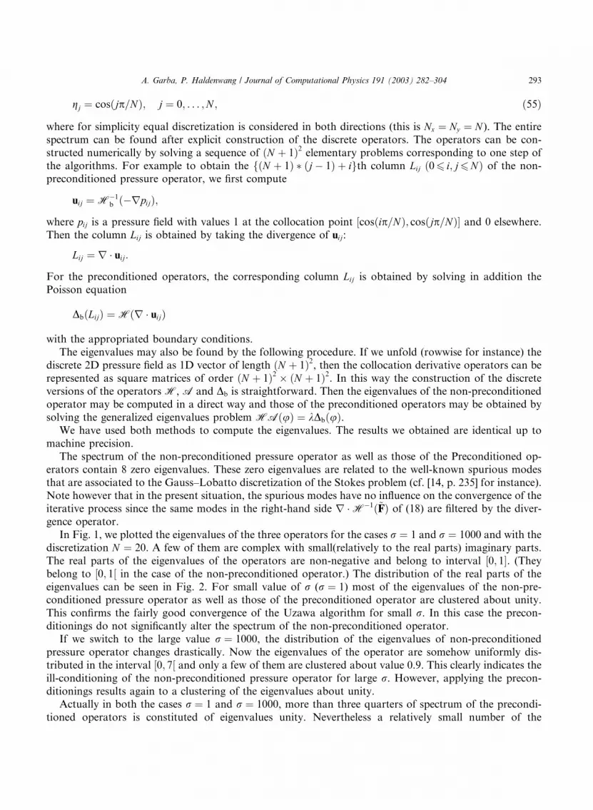
gj ¼ cosðjp=NÞ; j ¼ 0; . . . ;N ; ð55Þ

where for simplicity equal discretization is considered in both directions (this is Nx ¼ Ny ¼ N ). The entire

spectrum can be found after explicit construction of the discrete operators. The operators can be con-

structed numerically by solving a sequence of ðN þ 1Þ2 elementary problems corresponding to one step of

the algorithms. For example to obtain the fðN þ 1Þ � ðj� 1Þ þ igth column Lij ð06 i; j6NÞ of the non-preconditioned pressure operator, we first compute

uij ¼ H�1b ð�rpijÞ;

where pij is a pressure field with values 1 at the collocation point ½cosðip=NÞ; cosðjp=NÞ and 0 elsewhere.

Then the column Lij is obtained by taking the divergence of uij:

Lij ¼ r � uij:

For the preconditioned operators, the corresponding column Lij is obtained by solving in addition the

Poisson equation

DbðLijÞ ¼ Hðr � uijÞ

with the appropriated boundary conditions.

The eigenvalues may also be found by the following procedure. If we unfold (rowwise for instance) the

discrete 2D pressure field as 1D vector of length ðN þ 1Þ2, then the collocation derivative operators can be

represented as square matrices of order ðN þ 1Þ2 � ðN þ 1Þ2. In this way the construction of the discreteversions of the operators H, A and Db is straightforward. Then the eigenvalues of the non-preconditioned

operator may be computed in a direct way and those of the preconditioned operators may be obtained by

solving the generalized eigenvalues problem HAðuÞ ¼ kDbðuÞ.We have used both methods to compute the eigenvalues. The results we obtained are identical up to

machine precision.

The spectrum of the non-preconditioned pressure operator as well as those of the Preconditioned op-

erators contain 8 zero eigenvalues. These zero eigenvalues are related to the well-known spurious modes

that are associated to the Gauss–Lobatto discretization of the Stokes problem (cf. [14, p. 235] for instance).Note however that in the present situation, the spurious modes have no influence on the convergence of the

iterative process since the same modes in the right-hand side r �H�1ð~FFÞ of (18) are filtered by the diver-

gence operator.

In Fig. 1, we plotted the eigenvalues of the three operators for the cases r ¼ 1 and r ¼ 1000 and with the

discretization N ¼ 20. A few of them are complex with small(relatively to the real parts) imaginary parts.

The real parts of the eigenvalues of the operators are non-negative and belong to interval ½0; 1. (Theybelong to ½0; 1½ in the case of the non-preconditioned operator.) The distribution of the real parts of the

eigenvalues can be seen in Fig. 2. For small value of r (r ¼ 1) most of the eigenvalues of the non-pre-conditioned pressure operator as well as those of the preconditioned operator are clustered about unity.

This confirms the fairly good convergence of the Uzawa algorithm for small r. In this case the precon-

ditionings do not significantly alter the spectrum of the non-preconditioned operator.

If we switch to the large value r ¼ 1000, the distribution of the eigenvalues of non-preconditioned

pressure operator changes drastically. Now the eigenvalues of the operator are somehow uniformly dis-

tributed in the interval ½0; 7½ and only a few of them are clustered about value 0.9. This clearly indicates the

ill-conditioning of the non-preconditioned pressure operator for large r. However, applying the precon-

ditionings results again to a clustering of the eigenvalues about unity.Actually in both the cases r ¼ 1 and r ¼ 1000, more than three quarters of spectrum of the precondi-

tioned operators is constituted of eigenvalues unity. Nevertheless a relatively small number of the

Fig. 2. Distribution of the real parts of the eigenvalues for the three operators in the cases r ¼ 1 (a) and r ¼ 1000 (b). The degree of the

approximation is Nx ¼ Ny ¼ 20. The left-hand pictures refer to the pressure operator (�) and the CC operator (s). The right-hand ones

refer to the pressure operator (�) and the FWP operator (s).

Fig. 1. Eigenvalues distribution of the pressure operator (a), the CC/AIT operator (b) and the FWP operator (c). The degree of the

approximation is Nx ¼ Ny ¼ 20. The left-hand pictures refer to r ¼ 1 and the right-hand ones to r ¼ 1000.


Table 1

Conditioning of the non-preconditioned pressure operator

N 5 10 20

r 1 1000 1 1000 1 1000

kmin 5:1� 10�2 1:87� 10�3 1:32� 10�2 1:77� 10�3 3:22� 10�3 1:16� 10�3

kmax 0.973 3:94� 10�2 0.997 0.361 1 0.893

jðAÞ 19.08 21.07 75.55 203.95 310.56 769.83

Table 2

Conditioning of the FWP preconditioned operator

N 5 10 20

r 1 1000 1 1000 1 1000

kmin 5:29� 10�2 4:36� 10�2 1:52� 10�2 7:75� 10�3 3:44� 10�3 2:26� 10�3

jðAÞ 18.90 22.96 65.79 129.03 290.7 442.48

Table 3

Conditioning of the CC/AIT preconditioned operator

N 5 10 20

r 1 1000 1 1000 1 1000

kmin 5:19� 10�2 2:96� 10�3 1:32� 10�2 4:57� 10�3 3:22� 10�3 2:18� 10�3

jðAÞ 19.27 337.84 75.76 218.82 310.56 458.72


eigenvalues are still small. As a consequence the global condition number is still bad and it deteriorates as

the degree of approximation increases. In Tables 1–3 we report an estimate of the condition number of the

operators. The ‘‘condition number’’ j is defined as the ratio between the maximum absolute value kmax to

the minimum absolute value kmin of the eigenvalues. For memory limitation we could not compute theeigenvalues for value of N greater than 20. Observe that for small value of r the condition number behaves

like N 2.

In view of the distribution of the eigenvalues, the bad condition number of the preconditioned operators

seems somehow pessimistic. Indeed the few weak eigenvalues that are responsible for the bad condition

number are associated to Chebyshev modes of high frequencies. Therefore these eigenvalues may not have

any influence on the convergence of the algorithms as long as the residual is higher than the contribution of

the last Chebyshev modes in the representation of the divergence. One however expects these eigenvalues to

hold back the convergence as the residual becomes sufficiently small. This analysis is confirmed by thenumerical results presented in the next section.

6. Numerical experiments

In this section we present results of numerical experiments for both the 2D and 3D GSP. The domain is

X ¼ ð�1; 1Þd , d ¼ 2; 3, and the discretization is done by the Chebyshev collocation method based on the

Gauss–Lobatto points (55). For simplicity equal discretization is considered in all direc-tions(Nx ¼ Ny ¼ Nz ¼ N ). The discrete Helmholtz problems for velocity components and the Laplace

problem for pressure are solved by the successive diagonalization method [12,13].


We first consider the 2D case.

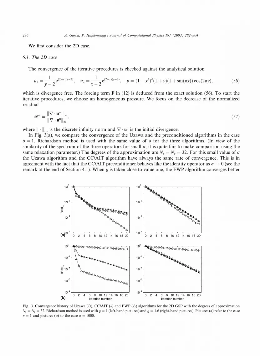
6.1. The 2D case

The convergence of the iterative procedures is checked against the analytical solution

u1 ¼1

y � 2eð2�xÞðy�2Þ; u2 ¼

1

x� 2eð2�xÞðy�2Þ; p ¼ ð1� x2Þ2ð1þ yÞð1þ sinðpxÞÞ cosð2pyÞ; ð56Þ

which is divergence free. The forcing term F in (12) is deduced from the exact solution (56). To start the

iterative procedures, we choose an homogeneous pressure. We focus on the decrease of the normalized

residual

Rm ¼ kr � umk1kr � u0k1

; ð57Þ

where k � k1 is the discrete infinity norm and r � u0 is the initial divergence.

In Fig. 3(a), we compare the convergence of the Uzawa and the preconditioned algorithms in the case

r ¼ 1. Richardson method is used with the same value of . for the three algorithms. (In view of the

similarity of the spectrum of the three operators for small r, it is quite fair to make comparison using the

same relaxation parameter.) The degrees of the approximation are Nx ¼ Ny ¼ 32. For this small value of rthe Uzawa algorithm and the CC/AIT algorithm have always the same rate of convergence. This is in

agreement with the fact that the CC/AIT preconditioner behaves like the identity operator as r ! 0 (see theremark at the end of Section 4.1). When . is taken close to value one, the FWP algorithm converges better

Fig. 3. Convergence history of Uzawa (s), CC/AIT (�) and FWP (n) algorithms for the 2D GSP with the degrees of approximation

Nx ¼ Ny ¼ 32. Richardson method is used with . ¼ 1 (left-hand pictures) and . ¼ 1:6 (right-hand pictures). Pictures (a) refer to the case

r ¼ 1 and pictures (b) to the case r ¼ 1000.


than the Uzawa and the CC/AIT algorithm, though initially the three algorithms have a similar rate of

convergence. The convergence of the Uzawa and the CC/AIT algorithms improves if we take values of .bigger than one and with . ¼ 1:6 both preconditioned methods give virtually the same results. Note that as

. increases the rate of convergence of FWP method decreases. Actually in the first iterations the reduction

factor of the three algorithms behaves like kr � umþ1k1=kr � umk1 ’ .� 1. This means that in the first

iterations, the algorithms behave as if the condition number of the operators were one.

The results in Fig. 3(b) obtained with r ¼ 1000 and Nx ¼ Ny ¼ 32 show that for large r, the convergenceof the Uzawa algorithm becomes very slow. Now both preconditioned methods improve substantially theconvergence. Also as for the case r ¼ 1, the FWP algorithm converges better than the CC/AIT if the re-

laxation parameter is taken close to value one. Note however that the convergence of the FWP method

slows down as the residual becomes small confirming the analysis at the end of Section 5.

In Fig. 4, we show the influence of the discretization on the convergence of the algorithms. The Rich-

ardson method is used with . ¼ 1. One can see that the convergence of the FWP method improves as the

degree of the approximation increases. In contrast the convergence of the CC/AIT method deteriorates as

the discretization becomes finer.

Now we consider the dynamical methods. We first compare PMR method with QPMR method whenthey are associated to each preconditioned algorithm. For the CC/AIT method, we found that both choices

of relaxation parameter always lead to similar results (see Fig. 5(a)). The two methods also lead to similar

results if r is sufficiently large in the case of the FWP algorithm. However, for small value of r we found

that the QPMR method gives better results (see the case r ¼ 1 in Fig. 5(b)). The same behavior is observed

when we change the degree of approximation.

Fig. 4. Convergence history of CC/AIT algorithm (a) and FWP algorithm (b) for the 2D GSP with the degrees of approximation

Nx ¼ Ny ¼ 32 (s) and Nx ¼ Ny ¼ 64 (�). Richardson method is used with . ¼ 1. The left-hand pictures correspond to the case r ¼ 1

and the right-hand one to the case r ¼ 1000.

Fig. 5. Convergence history of CC/AIT algorithm (a) and FWP (b) algorithm for the 2D GSP with the degrees of approximation

Nx ¼ Ny ¼ 32. The PMR (s) and the QPMR (�) methods are used. The left-hand pictures correspond to the case r ¼ 1 and the right-

hand ones to r ¼ 1000.


In Fig. 6, we compare the convergence of the algorithms when the QPMR method (quasi-minimal re-

sidual ‘‘QMR’’ in the case of the Uzawa algorithm) is used. Here too, the results obtained by Uzawa andCC/AIT algorithms are very close when r is small. The behavior of the algorithms is quite similar to the

case . ¼ 1 in the static Richardson method. The superiority of FWP over the CC/AIT method becomes

clear particularly when r becomes large. Note again the slowing down of the FWP algorithm as the residual

becomes small.

Next we present some numerical experiments for the 3D GSP.

6.2. The 3D case

The convergence of the algorithms is checked against the exact solution

u1 ¼ð5þ xÞ5

y � 2eð2�xÞðy�2Þð1þzÞ; u2 ¼

ð3þ yÞ5

x� 2cosðpzÞeð2�xÞðy�2Þ;

u3 ¼ð5þ zÞ5

2� xcosð2pzÞeð2�xÞðy�2Þ; p ¼ 2ð1� x2Þ2ð1þ yÞð1þ sinpxÞ cosð2pyÞð1þ z3Þe1þz:

ð58Þ

As before the exact solution gives the forcing terms in the Generalized Stokes problem (12) and (13).

Moreover this solution (58) is not divergence free and therefore a non-homogeneous term is also added for

the continuity equation. To start the iterative procedures we select as previously a homogeneous pressure

field.

Fig. 6. Convergence history of Uzawa (s), CC (�) and FWP (n) algorithms for the 2D GSP in the cases r ¼ 1 (a) and r ¼ 1000 (b).

The QPMR method is used. The left-hand pictures correspond to the approximation Nx ¼ Ny ¼ 32 and the right-hand side ones to

Nx ¼ Ny ¼ 64.


As the results for the 3D case are quite similar to those for the 2D case, we only present results obtainedwith the PMR. Here for both FWP and CC/AIT algorithms, the PMR and QPMR methods always give

similar results.

In Fig. 7 we compare the convergence of the various algorithms when associated to the PMR method

(MR in the case of the Uzawa algorithm). Here too, the FWP method has the best rate of convergence. As

for the 2D case, the convergence of the FWP method slows down when the residual reaches a certain level

of precision. Here the level is is slightly higher because the exact solution (58) is more complex than the

exact solution (56) in the 2D case.

Thus for both the 2D and 3D cases, the preconditioned methods give satisfactory results. The best resultsbeing obtained when the FWP method is employed. This shows that the modification of the boundary

conditions for the velocity in the case of FWP method plays a beneficial role for the convergence. The

eigenvalues analysis in conjunction with the convergence history indicate that the slowing down of the FWP

algorithm at low residual reflects the effect of weekly spurious eigenvalues. As these eigenvalues are as-

sociated to Chebyshev modes of high order, they can influence the convergence only at low residual. This

argument is supported by the fact that, when the degree of approximation increases, the residual decreases

to a lower level before the algorithm stagnates. This suggests an improvement of the FWP algorithm by

using a filtering procedure to remove the highest Chebyshev modes from the pressure. This will be thesubject of the next section. The same argument however does not hold for the CC/AIT method. Indeed in

some cases (Fig. 3 for instance), we do observe a change in regime of convergence of the CC/AIT algorithm,

but it occurs when the residual is too high for this to reflect the convergence of the last Chebyshev modes.

Moreover, we saw that the convergence of the CC/AIT algorithm deteriorates as the degree of approxi-

mation increases.

Fig. 7. Convergence history of Uzawa (s), CC/AIT (�) and FWP (n) algorithms for the 3D GSP with the degrees of approximation

Nx ¼ Ny ¼ Nz ¼ 24 (left-hand pictures) and Nx ¼ Ny ¼ Nz ¼ 32 (right-hand pictures). Pictures (a) refer to the case r ¼ 1 and pictures

(b) to the case r ¼ 1000. PMR method is used.


6.3. Enhancement of the FWP preconditioning

The use of half-staggered grid can partly overcome the problem of the spurious and weakly spuriousmodes (i.e., the modes with small eigenvalues). The pressure is represented by polynomials of degree N � 1

in both directions and the continuity equation is imposed on the N � N Gauss points

½cosðð2iþ 1Þp=2NÞ; cosðð2jþ 1Þp=2NÞ; 16 i; j6N . This procedure is known to contain only a single

spurious mode. In addition this discretization still contains some weakly spurious modes. Since the slowing

down of the convergence is related to the weakly spurious modes (we recall that the strictly spurious modes

have no influence on the convergence since these modes are filtered by the divergence operator) this dis-

cretization may not lead to a significant improvement of convergence. Therefore a procedure which allows

also a filtering of the weak eigenvalues is much suitable. This can be achieved by using a representation ofpressure on Gauss–Lobatto points ½cosðip=ðN � KÞÞ; cosðjp=ðN � KÞÞ; 06 i; j6N � K, where K is an

integer greater than 1 and less than N . Chebyshev interpolation is used to move from a grid to another. Let

R be the interpolating operator which transfers variables from the finest grid to the coarse grid and P the

operator that performs the reverse process. Then the proposed procedure is the following:

Starting from a pressure field pm:1. Filtering ~pp ¼ PRpm.2. Solve Hbu

mþ1 ¼ r~pp.3. Compute Dbdpmþ1 ¼ Hðr � umÞ.4. pmþ1 ¼ pm þ .mdp

mþ1.

Fig. 8. Distribution of real parts of the eigenvalues for the FWP operator in the case of the approximation PN (a), PN�2 (b), PN�4 (c) and

PN�6 (d), N ¼ 20 for the pressure.

Fig. 9. Convergence history of FWP algorithm for the 2D GSP with r ¼ 1 and approximations PN (�), PN�2 (s) and PN�4 (�), N ¼ 32

for the pressure. Richardson method is used with . ¼ 1:4. The data are defined by the smooth solution (56).



In step 1, applying operator PR has the effect of removing the last K Chebyshev modes of the pressure.

Thus at each iteration a filtering procedure is applied to remove the last Chebyshev modes of pressure

before the computation of velocity. Observe that in step 2 the pressure is actually computed on the finest

grid. Indeed, in the FWP method, values of the normal velocity are used as boundary conditions for

pressure. Therefore if the pressure were computed on the coarse grid, after convergence of the algorithm,

the Dirichlet boundary condition on the normal velocity component would be satisfied only on the coarser

grid and this is not convenient.

When the filtering procedure is applied with KP 2, all the non-constant spurious modes are eliminated.Moreover (and this is important in view of what has been previously said) as K increases, the smallest non-

zero eigenvalues are eliminated, thus resulting to better conditioning. This can be seen in Fig. 8 where the

real parts of the eigenvalues are reported. Few of the eigenvalues are still complex with relatively small

imaginary part. The results in Fig. 8 correspond to r ¼ 1000 and N ¼ 20. Similar results are obtained with

small r.The validity of the present approach has been checked by conducting numerical experiments in 2D with

both smooth and non-smooth data.

The smooth data are obtained from the analytical velocity and pressure (56) as in Section 6.1. In Figs. 9and 10 we report results corresponding to the case r ¼ 1 and r ¼ 1000, respectively. In both cases we used

the static Richardson method with . ¼ 1:4 and the degrees of approximation Nx ¼ Ny ¼ 32. It can be seen

that the different filterings virtually lead to the same rate of convergence during the first iterations. After

this stage the convergence slows down when the high modes are retained for the pressure. The convergence

Fig. 10. Convergence history of FWP algorithm for the 2D GSP with r ¼ 1000 and approximations PN (�), PN�2 (s) and PN�4 (�),

N ¼ 32 for the pressure. Richardson method is used with . ¼ 1:4. The data are defined by the smooth solution (56).

Fig. 11. Convergence history of FWP algorithm for the 2D GSP with r ¼ 1000 and approximations PN (s), PN�2 (}) and PN�4 (�),PN�6 (�) and PN�8 (n), N ¼ 32 for the pressure. The PMR method is used. Non smooth exact pressure data are used (see Section 6.3).


is then gradually improved when we use filterings with increasing value of K. Of course beyond a certain

value of K, no further improvement is obtained.

In Fig. 11, we show results of the filtering when non-smooth data are used. The non-smooth data are

obtained by choosing randomly the Chebyshev coefficients of the exact pressure in interval 0; 1½. The exactvelocity is still given by (56). Here we have used the PMR method. We observe the same improvement of

the rate of convergence as K increases. Note that here the bifurcation among these different curves of

convergence occurs earlier because the coefficients of the last Chebyshev modes of the pressure can be

relatively high.

It should be noticed that in practice the procedure for filtering the parasitic modes does not work well in

the case of the CC/AIT preconditioning confirming our argument at the end of Section 6.2.

7. Conclusion

Two iterative approaches for solving the GSP has been analyzed and implemented in the framework of

collocation Chebyshev approximation. The iterative procedures use two kinds of preconditioning for the

Uzawa algorithm. One of them, the AIT/CC method is a reformulation of the preconditioning due to

Cahouet and Chabard [6] in the case of finite elements discretization. This method has the advantage of

being applicable in arbitrary domain and it leads to accurate results when associated to conjugated gradient

method. However even with the lack of symmetry of the collocation Chebyshev version of the operator, weobtained quite satisfactory results when the AIT/CC is associated with the static Richardson or PMR like


methods. The second preconditioning considered, the FWP method is restricted to rectangular domains.

For such geometries we found this method well suited when associated to spectral Chebyshev methods.

Comparison of the two preconditioning shows an advantage of the FWP method over the AIT/CC method.

However, we noted that the convergence of the various preconditioned algorithms slows down as the re-

sidual becomes small. This is due to the fact that, though the direct application of the preconditioning

results in a clustering of the eigenvalues about unity, it does not eliminate the weekly spurious eigenvalues

that are related to the last Chebyshev modes. Thanks to an suitable filtering process, it has been possible to

remedy to this situation for the FWP algorithm only (the filtering enhancement does not work for CC/AITpreconditioning). The filtering consists in removing the last modes of the Chebyshev expansion of pressure

field. Numerical tests with both smooth and non-smooth (i.e., random) data confirm the effectiveness of the

filtering procedure.

References

[1] L. Kleiser, U. Schumann, Treatment of the incompressibility and boundary conditions in 3-D numerical spectral simulations of

plane channel flows, in: E.H. Hirschel (Ed.), Proc. 3rd GAMM Conf. Numerical Methods in Fluid Mechanics, Vieweg,

Braunschweig, 1980, pp. 165–173.

[2] P. Le Qu�eer�ee, Aziary de Rocquefort, Sur une m�eethode semi-implicite pour la r�eesolution des �eequations de Navier–Stokes d�un�eecoulement visqueux incompressible, C.R. Acad. Sci. Paris, s�eerie II 294 (1982) 941–944.

[3] L. Tukerman, Divergence-free velocity in nonperiodic geometries, J. Comput. Phys. 80 (1989) 403–441.

[4] P. Haldenwang, Unsteady numerical simulation by Chebycshev spectral methods of natural convection at high Rayleigh number,

in: J.A.C. Humphrey (Ed.), Significant questions in buoyancy affected enclosure or cavity flow, ASME/HTD, 60, 1986, pp. 45–51.

[5] P. Haldenwang, G. Labrosse, 2-D and 3-D spectral Chebyshev solutions for free convection at high Rayleigh number, in: M.O.

Bristeau, R. Glowinski, A. Haussel, J. Periaux (Eds.), Proc. 6th Int. Symp. on Finite Elements in Flow Problems, Antibes, France,

1986, pp. 261–266.

[6] J. Cahouet, J.P. Chabard, Some fast 3D finite elements solver for the generalized Stokes problem, Int. J. Numer. Meth. Fluids 8

(1988) 869–895.

[7] A. Majda, J. Sethian, The derivation and numerical solution of the equations for zero Mach number combustion, Combust. Sci.

Technol. 42 (1985) 185–205.

[8] J. Fr€oohlich, R. Peyret, Direct spectral method for the low-Mach number equations, Int. J. Numer. Methods Heat and Fluid Flow

2 (1992) 195–213.

[9] B. Denet, P. Haldenwang, Combust. Sci. Technol. 104 (1995) 143–167.

[10] R. Glowinski, Ensuring well-posedness by analogy; Stokes problem and boundary control for the wave equation, J. Comput.

Phys. 103 (1992) 189–221.

[11] A. Garba, M�eethodes Spectrales en Domaines non Rectangulaires: Applications au Calcul d’�eecoulements �aa Surface libre, Th�eese de

l�Universit�ee de Nice–Sohia Antipolis, France, 1993.

[12] P. Haldenwang, G. Labrosse, S. Abboudi, Chebyshev 3-D Spectral and 2-D pseudospectral solvers for the Helmholtz equation, J.

Comput. Phys. 55 (1984) 115–128.

[13] U. Ehreinstein, R. Peyret, A Chebyshev-collocation method for Navier–Stokes equations with application to double-duffision

convection, Int. J. Numer. Methods Fluids 9 (1989) 429–452.

[14] C. Canuto, M.Y. Hussaini, A. Quateroni, T.A. Zang, Spectral Methods in Fluid Dynamics, Springer, New York, 1988.

Documents

Comparison of preconditioners for collocation Chebyshev approximation of 2D and 3D generalized Stokes problem