UNCORRECTED PROOFS

Solving Two-DimensionalChemical EngineeringProblems Using the ChebyshevOrthogonal CollocationTechniqueHOUSAMQ1 BINOUS,1 SLIM KADDECHE,2 AHMED BELLAGI3

1Department of Chemical Engineering, King Fahd University of Petroleum and Minerals, Dhahran 31261, Saudi Arabia

2University of Carthage, National Institute of Applied Sciences and Technology, D�epartement G�enie Physique etInstrumentation, Laboratoire Mat�eriaux, Mesures et Applications, LR-11-ES-25, 1080, Tunisia

3D�epartement de G�enie Energ�etique (Energy Engineering Department), Ecole Nationale d’Ing�enieurs de Monastir–ENIM,

University of Monastir, Tunisia

Received 27 April 2015; accepted 27 July 2015

ABSTRACT: The present paper describes how to apply theQ2 Chebyshev orthogonal collocation technique to

solve steady-state and unsteady-steady two-dimensional problems. All problems are solved using one single

computer algebra, Mathematica�. The problems include: (1) steady-state heat transfer in a rectangular bar, (2)

steady-state flow in a rectangular duct, (2) steady-state heat transfer in a cooling cylindrical pin fin, (4) steady-state

heat conduction in an annulus, (5) unsteady-state heat transfer in a rectangular bar, and finally (6) unsteady-state

diffusion reaction system.Whenever possible the results obtainedwith orthogonal collocation are compared to the

analytical solution in order to validate the applied numerical technique. � 2015 Wiley Periodicals, Inc. ComputAppl Eng Educ 9999:1–11, 2015; View this article online at wileyonlinelibrary.com/journal/cae; DOI 10.1002/cae.21680

Keywords: orthogonal collocation; chebyshev polynomials; momentum – heat – mass transfer; numerical

methods; graduate-level education; MATHEMATICA

INTRODUCTION

Many interesting problems in transport phenomena and generallyengineering education are governed by partial differentialequations (PDE) such as the heat equation, the Laplace equationand the wave equation. These equations are often solvedanalytically using separation of variables in graduate-levelcourses. However, these courses frequently do not address themore realistic nonlinear problems, which admit only numericalsolutions. In addition, in many cases, it is actually nowadays

simpler and faster to find a numerical solution to a particularproblem. The objective of the present paper is to show how one canreadily solve partial differential equations for two-dimensionalproblems using the Chebyshev orthogonal collocation techniquein association with MATHEMATICA

©. Although, the usage ofcomputer software such as MATHEMATICA

©, MAPLE, MATLAB1

,POLYMATH, MATHCAD, JAVA, ASPEN-HYSYS or EXCEL is common inchemical engineering pedagogical literature [1–12], only onepaper applies this technique [12]. And the paper (i.e., Ref. 12) isrestricted to only one-dimensional problems.

Several research papers using the orthogonal collocationtechnique can be found in the literature [13–16]. Here, a specialemphasis is given to the utilization of this technique in theclassroom in order to solve miscellaneous graduate-level prob-lems. Also, we choose to implement this numerical technique with

1234567891011121314151617181920212223242526272829303132333435363738394041424344454647484950515253545556575859606162

Correspondence to: H. Binous (binoushousam@yahoo.com).

© 2015 Wiley Periodicals, Inc.

Journal MSP No. Dispatch: August 3, 2015 CE: Manish

CAE 21680 No. of Pages: 11 PE: Laura Espinet

1

UNCORRECTED PROOFS

1234567891011121314151617181920212223242526272829303132333435363738394041424344454647484950515253545556575859606162

MATHEMATICA©. However, one can easy apply the same solution

methodology with MATLAB1

. The present work is expected toachieve the goal that the present treatment of two-dimensionalproblems will motivate more chemical engineering students,faculties, and professionals to use this versatile orthogonalcollocation method.

The present paper is divided into three main parts:

1. Description of the application of the 2D Chebyshevorthogonal collocation technique in solving steady-stateand unsteady-state two dimensional problems,

2. Resolution of six chemical engineering problems related tomomentum, heat, and mass transfer, and

3. Conclusion giving our thought about this technique as ateaching tool in the chemical engineering graduate-levelcurriculum.

THEORETICAL CONSIDERATION ABOUT 2DCHEBYSHEV ORTHOGONAL COLLOCATION

The spectral collocation method using Chebyshev orthogonalpolynomial basis is known for its efficiency in term of accuracy.This is despite the fact that a relatively small number ofcollocation points, N, are used to solve many engineeringproblems. Indeed, the associated error is of the order ofOð1=NNÞ, which is better than finite difference or finite elementmethods [16–17]. The main difficulty in the transition from aone-dimensional case to a two-dimensional case lies in buildingthe derivative matrix. Let DN (N is the number of collocationpoints) be the first order derivative matrix for a one-dimensionalproblems, the partial first order derivative matrix relative to thefirst space variable is obtained by performing the Kroneckerproduct of IN and DN denotes by IN � DN . On the other hand, thesecond space variable first order derivative matrix is obtained byperforming the Kronecker product of DN and IN denotes byDN � IN . The same procedure is used to compute the p orderderivative for 2D problems by replacing DN by Dp

N where DpN is

the one dimensional p order derivative for 1D problem. For themixed derivatives (of order p with respect to the first variableand q with respect to the second variable), one has to form thefollowing Kronecker product: Dp

N � DqN .

Explicitly, the first order derivative matrixDNwrites [17–18]:

DN ¼ ½dij�0 � i; j � N

dkj ¼ ckð�1Þjþk

cjðjk � jjÞ; for j 6¼ k

dkk ¼ � �jk2ð1� jk2Þ

; for k 6¼ 0 and k 6¼ N

d00 ¼ 2N2 þ 16

¼ �dNN

8>>>>>>>><>>>>>>>>:

where,

ck ¼2k ¼ 0 or N

1otherwise

(

and the p order derivativeDpN is equal to the product ofDN p times:

DpN ¼ DN � DN � . . . ::� DN

The two dimensional spectral collocation method consists infinding the values of the unknown functionc such thatc ji; hj

� � ¼cij onGauss-Lobatto-Chebychev points, namely: ji ¼ cos ip

N

� �and

hj ¼ cos jpN

� �where 0 � i; j � N with ji and hj belonging to the

mapped numerical domain ½�1; 1�. If the physical space is a therectangle ½�Ax;Ax� � ½�Ay;Ay�, the 2D–Cartesian coordinates canbe written as following:

xðjÞ ¼ Axj

y hð Þ ¼ Ayh

(

The unknown function c is the interpolated into apolynomial basis:

PNNcðj; hÞ ¼XNi¼0

XNj¼0

aijTiðjiÞTjðhjÞ

where Ti and Tj are the Chebyshev orthogonal polynomial ofdegree N. The derivatives of PNNcðj; hÞ with respect to j and h atthe collection points write:

@PNNc j; hð Þ@j

¼ 1Ax

IN � DN

� �PNNc j; hð Þ

@PNNc j; hð Þ@h

¼ 1Ay

DN � IN

� �PNNc j; hð Þ

This method makes it possible the resolution of any partialdifferential equation by finding the expansion coefficients, aij,which allow us to find the values of the unknown function c onGauss-Lobatto-Chebychev points ji and hj, namely:cij ¼ c ji; hj

� �:

For example, the 2D–Laplacian in the rectangle ½�Ax;Ax� �½�Ay;Ay� is then:

D ¼ 1

A2x

IN � D2N

!þ 1

A2y

D2N � IN

!

The above presentation makes it clear that the derivativematrix DN plays a key role in the implementation of the spectralcollocation technique. Its calculation, for any number of nodes Nusing Mathematica©, is straightforward as can be seen in theAppendix. Authors compare forN¼ 5 thematricesD5 andD2

5 withpage 7 of Ref. [19]. To evaluate the partial derivative matrices, thebuilt-in functions IdentityMatrix and KroneckerProduct areused, for instance and in the case of N¼3 in both directions (x andy), the first order partial derivate matrices relative to x, Dx ¼I4 � D3 and to y, Dy ¼ D3 � I4 are evaluated by the instructionsequences respectively,

KroneckerProduct[IdentityMatrix[4], dM[3]]

KroneckerProduct[dM[3], IdentityMatrix[4]]

and the second order partial derivate matrices relative to x,D

2x ¼ I4 � D2

3 and to y, D2y ¼ D2

3 � I4 respectively by theinstruction sequences,

KroneckerProduct[IdentityMatrix[4], dM[3].dM[3]]

KroneckerProduct[dM[3].dM[3], IdentityMatrix[4]]

The results of these calculations can be compared with thosegiven in page 79 of Ref. [19].

2 BINOUS, KADDECHE, AND BELLAGI

UNCORRECTED PROOFS

1234567891011121314151617181920212223242526272829303132333435363738394041424344454647484950515253545556575859606162

CHEMICAL ENGINEERING CASE STUDIES

Heat Transfer in a Bar of Rectangular Cross Section

Let us consider a bar of rectangular cross section subject to bothtemperature and heat flux boundary conditions (see Fig. 1). Thegoverning equation and boundary conditions in dimensionlessform are as follows:

@2u

@x2þ @2u

@y2¼ 0

with 0 � x � L and 0 � y � W

@u

@x

� �x¼0

¼ � qwallk

ðContinuity of heat flux at x ¼ 0 boundaryÞ

u x ¼ Lð Þ ¼ 0 ðConstant temperature T0 at x ¼ L boundaryÞu y ¼ 0ð Þ ¼ 0 ðSame constant temperature T0 at y ¼ 0 boundaryÞ

u y ¼ Wð Þ ¼ ubðDifferent constant temperature Tb at y ¼ W boundaryÞ

For this case study an analytical solution can be obtainedusing the separation of variables technique (Ref. [20]):

u ¼X1n¼0

2Lln

ubsin ln Lð Þsinhðln yÞsinh lnWð Þ

�

þ qwallk

1� sinh lnyð Þ þ sinh lnðW � yÞð Þsinh lnWð Þ

� ��cos lnxð Þ

with

ln ¼ 2nþ 1ð Þp2L

for n ¼ 0; 1; 2:::

The Chebyshev orthogonal collocation method implementedin MATHEMATICA

© with Np¼ 41 collocation points delivers thetemperature distribution in the bar represented in Figure 2. Thesolution steps are as follows. First, the spatial variables (i.e., x andy) are discretized to transform the partial differential equation(PDE) into a systems of 1681linear algebraic equations where the

unknowns are the values of u at the nodes. This linear equationssystem is then readily solved using the built-in command NSolve.Table 1 shows that the numerical technique and the analyticalsolution agree almost perfectly. The summation in the analyticalsolution is truncated up to n¼ 200.

Fluid Flow Through A Rectangular Duct

Consider the fluid flow through a rectangular duct (see Fig. 3). Theflow velocity in the cross section obeys the following governingequation with the associated boundary conditions:

@2vz@x2

þ @2vz@y2

¼ @P@z

� �=m

with 0 � x � L and 0 � y � W

@vz@x

� �x¼0

¼ 0 Symmetry conditionð Þvz x ¼ Lð Þ ¼ 0 No slip conditionð Þ@vz@y

� �y¼0

¼ 0 Symmetry conditionð Þ

vz y ¼ Wð Þ ¼ 0 No slip conditionð Þ

The separation of variables technique yields the followinganalytical solution (Ref. [20]):

vz ¼ 2m

�@P@z

� �X1n¼0

ð�1ÞnLl3n

1� cosh ln yð ÞcoshðlnWÞ

� �cos lnxð Þ

with

ln ¼ nþ 1=2ð ÞpL

for n ¼ 0; 1; 2; . . .

This 2D–problem is readily solved using Chebyshevorthogonal collocation with Np¼ 41 collocation points. Theprocedure is similar to that applied in case study 1: Discretization

Figure 1 Case study 1: Boundary conditions at the edges of the rectangular bar cross section. [Color figure can be viewedin the online issue, which is available at wileyonlinelibrary.com.]

SOLVING CHEMICAL ENGINEERING PROBLEMS 3

UNCORRECTED PROOFS

1234567891011121314151617181920212223242526272829303132333435363738394041424344454647484950515253545556575859606162

Figure 2 Case study 1: Temperature distribution uðx; yÞ obtained using Chebyshev orthogonal collocation (L¼ 1,W¼ 1,k¼ 0.01, qwall¼ 1, and ub¼ 20). [Color figure can be viewed in the online issue, which is available at wileyonlinelibrary.com.]

Table 1 Case Study 1: Numerical and Analytical Values of

u x ¼ 0:119797; 0 � y � Wð Þ for L¼ 1, W¼ 1, k¼ 0.01, qwall¼ 1, and

ub¼ 20

y– position Chebyshev Analytical

0 �1.6156 10�9 00.00615583 0.75737 0.7576610.0244717 3.00066 3.000960.0544967 6.5918 6.59210.0954915 11.1934 11.19370.146447 16.299 16.29930.206107 21.3945 21.39480.273005 26.0737 26.0740.345492 30.0519 30.05220.421783 33.1408 33.14110.5 35.2237 35.2240.578217 36.2405 36.24080.654508 36.1814 36.18170.726995 35.0925 35.09280.793893 33.0908 33.09110.853553 30.392 30.39230.904508 27.3389 27.33920.945503 24.3912 24.39150.975528 22.0123 22.01260.993844 20.5087 20.50971. 20. 20.0312

Figure 3 Case study 2: Boundary conditions for the rectangular ductproblem (Only the domain 0;L½ � � 0;W½ � is considered). [Color figure canbe viewed in the online issue, which is available at wileyonlinelibrary.com.]

4 BINOUS, KADDECHE, AND BELLAGI

UNCORRECTED PROOFS

1234567891011121314151617181920212223242526272829303132333435363738394041424344454647484950515253545556575859606162

of the spatial variables to transform the PDE into a system of 1681linear algebraic equations where the unknowns are now the valuesof vz at the nodes followed by its numerical solution using thebuilt-in MATHEMATICA

© command NSolve. Figure 4 gives thevelocity distribution in the rectangular duct. The comparisonbetween both solution techniques (Table 2) makes clear that thenumerical techniques and the analytical solution agree very well.Again, the summation in the analytical solution is truncated up ton¼ 200.

Cooling by a Cylindrical Pin Fin

Let us consider now a problem with a cylindrical geometry. Inelectronic systems, a fin is a heat sink or a passive heat exchangerthat cools a device by dissipating heat into the surroundingmedium (i.e., air). A cylindrical pin fin, used to maximize heattransfer to a fluid between two walls, is depicted in Figure 5. Thewalls are at a high temperature Tw. The fluid flowing over the pinhas a free stream temperature T1. The heat transfer coefficientbetween pin wall and surrounding medium is labeledhðW=ðm2KÞÞ. If one introduces the dimensionless temperature,f ¼ T�T1

Tw�T1, the governing equation writes (see Fig. 6):

1r@

@rr@f

@r

� �þ @2f

@z2¼ 0

0 � r � r0 and 0 � z � LThe associated boundary conditions are then as follows

@f

@z

� �z¼0

¼ 0 Axial symmetry conditionð Þ

@f

@r

� �r¼0

¼ 0 Radial symmetry conditionð Þ

@f

@rþ h

kf

� �r¼r0

¼ 0 Continuity of heat flux at the boundary fin=surrounding airð Þ

f z ¼ Lð Þ ¼ fw ¼ 1 Constant temperature at the wallð Þ

kðW=ðmKÞÞ is the thermal conductivity of the cylindrical pin fin.

The analytical solution of the differential equation obtainedusing the separation of variables technique (Ref. [20]) is given by:

f ¼X1n¼1

2 Bi J0 lnrð Þcoshðln zÞcosh lnLð ÞJ0 lnr0ð Þ lnr0ð Þ2 þ Bi2

h iwhere Bi is the Biot number

Bi ¼ hr0k

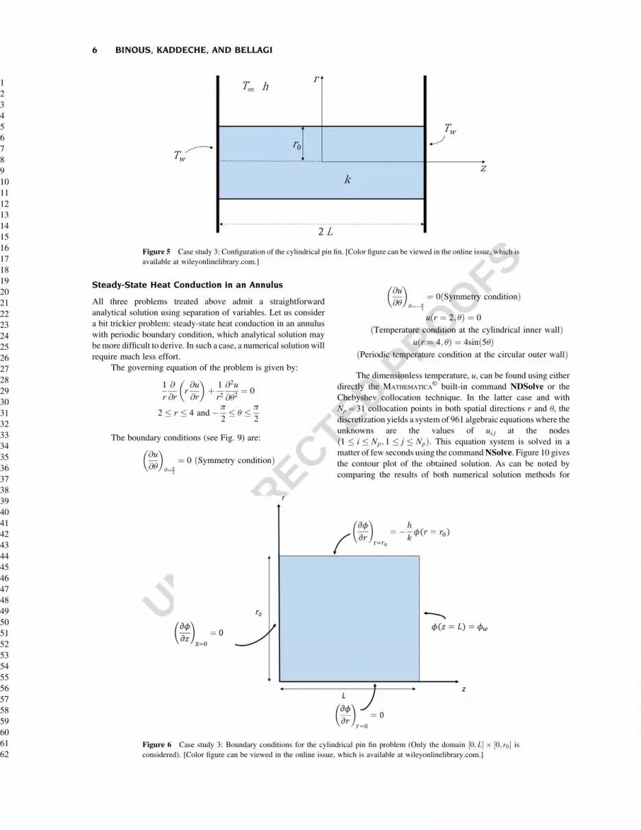
and ln the zeros of the nonlinear function

f lð Þ ¼ lr0ð ÞJ1 lr0ð Þ � J0 lr0ð ÞBi

A plot of f(l) vs. l is shown in Figure 7. To find out all zerosof f(l) the systematic graphical approach developed byWagon [21] is adopted (See Table 3 for the first 16 roots of thisequation).

The numerical solution of this 2-D problem obtained usingour MATHEMATICA

© implementation of the Chebyshev orthogonalcollocation withNp¼ 41 collocation points is depicted in Figure 8.Again, the consecutive steps in the solution procedure are the sameas in both foregoing case studies. First, one discretizes the spatialvariables z and r to transform the partial differential equation(PDE) into a system of 1681 linear algebraic equations, where theunknowns are the values of F at the nodes. Then, this is followedby the resolution of the algebraic system. The comparison of thenumerical and analytical solutions for a particular value of theaxial position z (Table 4) shows that the results are in almostperfect concordance. Here, the summation in the analyticalsolution was truncated up to n¼ 16 rather than 200 (i.e., the valueof n used in study cases 1 and 2). Two reasons motivated thischoice: (1) in case study 3, increasing of the value of n beyond 14did not have a substantial effect on the accuracy of the obtainedresults, and (2) only in case studies 1 and 2, straightforwardexpressions are available for the eigenvalues, ln (i.e., in case study3, one has to solve a complicated transcendental algebraicequation).

Figure 4 Case study 2: Velocity distribution vzðx; yÞ obtained using

Chebyshev orthogonal collocation (L¼ 1, W¼ 1, and@P@zð Þm

¼ �10). [Color

figure can be viewed in the online issue, which is available atwileyonlinelibrary.com.]

Table 2 Case Study 2: Numerical and Analytical Values of

vz x ¼ 0:119797; 0 � y � Wð Þfor L¼ 1, W¼ 1, and@P@zð Þm

¼ �10

y– position Chebyshev Analytical

0 2.91088 2.910880.00615583 2.91079 2.910790.0244717 2.90941 2.909410.0544967 2.90357 2.903570.0954915 2.88841 2.888410.146447 2.8579 2.85790.206107 2.80553 2.805530.273005 2.72495 2.724950.345492 2.61066 2.610660.421783 2.45868 2.458680.5 2.26719 2.267190.578217 2.0372 2.03720.654508 1.77313 1.773130.726995 1.48319 1.483190.793893 1.17947 1.179470.853553 0.877396 0.8773960.904508 0.594772 0.5947720.945503 0.350128 0.3501280.975528 0.160816 0.1608160.993844 0.0410119 0.04101191. 0 0

SOLVING CHEMICAL ENGINEERING PROBLEMS 5

UNCORRECTED PROOFS

1234567891011121314151617181920212223242526272829303132333435363738394041424344454647484950515253545556575859606162

Steady-State Heat Conduction in an Annulus

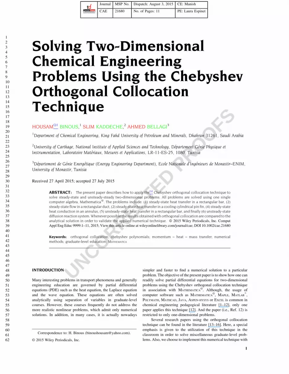
All three problems treated above admit a straightforwardanalytical solution using separation of variables. Let us considera bit trickier problem: steady-state heat conduction in an annuluswith periodic boundary condition, which analytical solution maybemore difficult to derive. In such a case, a numerical solution willrequire much less effort.

The governing equation of the problem is given by:

1r@

@rr@u@r

� �þ 1r2@2u

@u2¼ 0

2 � r � 4 and� p

2� u � p

2

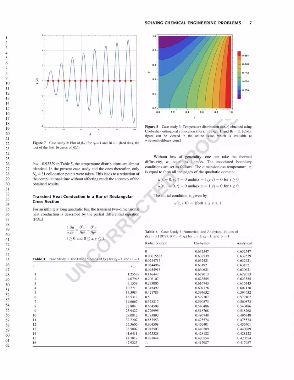
The boundary conditions (see Fig. 9) are:

@u@u

� �u¼p

2

¼ 0 Symmetry conditionð Þ

@u@u

� �u¼�p

2

¼ 0 Symmetry conditionð Þ

uðr ¼ 2; uÞ ¼ 0Temperature condition at the cylindrical inner wallð Þ

u r ¼ 4; uð Þ ¼ 4sinð5uÞPeriodic temperature condition at the circular outer wallð Þ

The dimensionless temperature, u, can be found using eitherdirectly the MATHEMATICA

© built-in command NDSolve or theChebyshev collocation technique. In the latter case and withNp¼ 31 collocation points in both spatial directions r and u, thediscretization yields a system of 961 algebraic equations where theunknowns are the values of ui,j at the nodesð1 � i � Np; 1 � j � NpÞ. This equation system is solved in amatter of few seconds using the commandNSolve. Figure 10 givesthe contour plot of the obtained solution. As can be noted bycomparing the results of both numerical solution methods for

Figure 5 Case study 3: Configuration of the cylindrical pin fin. [Color figure can be viewed in the online issue, which isavailable at wileyonlinelibrary.com.]

Figure 6 Case study 3: Boundary conditions for the cylindrical pin fin problem (Only the domain 0; L½ � � 0; r0½ � isconsidered). [Color figure can be viewed in the online issue, which is available at wileyonlinelibrary.com.]

6 BINOUS, KADDECHE, AND BELLAGI

UNCORRECTED PROOFS

1234567891011121314151617181920212223242526272829303132333435363738394041424344454647484950515253545556575859606162

u¼�0.92329 in Table 5, the temperature distributions are almostidentical. In the present case study and the ones thereafter, onlyNp¼ 31 collocation points were taken. This leads to a reduction ofthe computational time without affecting much the accuracy of theobtained results.

Transient Heat Conduction in a Bar of RectangularCross Section

For an infinitely long quadratic bar, the transient two-dimensionalheat conduction is described by the partial differential equation(PDE)

1a

@u@t

¼ @2u@x2

þ @2u@y2

t � 0 and 0 � x; y � 1:

Without loss of generality, one can take the thermaldiffusivity, a, equal to 1 cm2/s. The associated boundaryconditions are set as follows: The dimensionless temperature, u,is equal to 0 on all the edges of the quadratic domain:

uðx ¼ 0; y; tÞ ¼ 0 anduðx ¼ 1; y; tÞ ¼ 0 for t � 0

uðx; y ¼ 0; tÞ ¼ 0 anduðx; y ¼ 1; tÞ ¼ 0 for t � 0

The initial condition is given by

uðx; y; 0Þ ¼ 1for0 � x; y � 1:

Figure 7 Case study 3: Plot of f(l) for r0¼ 1 and Bi¼ 1 (Red dots, theloci of the first 16 zeros of f(l)).

Table 3 Case Study 3: The First 16 Zeros of f(l) for r0¼ 1 and Bi¼ 1

n ln

1 1.255782 4.079483 7.15584 10.2715 13.39846 16.53127 19.66678 22.8049 25.9422

10 29.081211 32.220712 35.360613 38.500714 41.641115 44.781716 47.9223

Figure 8 Case study 3: Temperature distribution fðz; rÞ obtained usingChebyshev orthogonal collocation (For L¼ 1, r0¼ 1, and Bi¼ 1). [Colorfigure can be viewed in the online issue, which is available atwileyonlinelibrary.com.]

Table 4 Case Study 3: Numerical and Analytical Values of

f z ¼ 0:119797; 0 � r � r0ð Þ for L¼ 1, r0¼ 1, and Bi¼ 1

Radial position Chebyshev Analytical

0 0.632547 0.6325470.00615583 0.632539 0.6325390.0244717 0.632421 0.6324210.0544967 0.63192 0.631920.0954915 0.630621 0.6306210.146447 0.628013 0.6280130.206107 0.623555 0.6235550.273005 0.616743 0.6167430.345492 0.607178 0.6071780.421783 0.594632 0.5946320.5 0.579107 0.5791070.578217 0.560873 0.5608730.654508 0.540486 0.5404860.726995 0.518768 0.5187680.793893 0.496748 0.4967480.853553 0.475574 0.4755740.904508 0.456401 0.4564010.945503 0.440289 0.4402890.975528 0.428122 0.4281220.993844 0.420554 0.4205541. 0.417987 0.417987

SOLVING CHEMICAL ENGINEERING PROBLEMS 7

UNCORRECTED PROOFS

1234567891011121314151617181920212223242526272829303132333435363738394041424344454647484950515253545556575859606162

It is then a transient cooling process of a solid bar. Thedimensionless temperature distribution in the solid can be foundusing either directly the MATHEMATICA

© built-in commandNDSolve or the Chebyshev collocation technique. If we adoptthe latter method with a number of collocation points Np¼ 31 inboth directions, the discretization of the spatial variables transformthe PDE into a systems of 441 linear and coupled first-order

ordinary differential equations (ODEs) where the unknowns arethe time dependent values of ui;jðtÞ at the nodesð1 � i � Np; 1 � j � NpÞ. This system of ODEs is then solvedin a matter of few seconds using the built-in Mathematica©

commandNDSolve. As illustration of the results of this numericalprocedure a typical map of the obtained dimensionless isotherms(for t¼ 0.1 is depicted in Figure 11. Table 6 on the other handcompares the dimensionless temperature data obtained for t¼ 0.1and at x¼ 0.421782 by both numerical methods considered,NDSolve and the Chebyshev collocation. As can be noted the twomethods give almost same results.

Reaction-Diffusion System

In the last decades, developmental biologists have extensivelyused the reaction–diffusion model to explain the pattern formationin living organisms. Turing proposed the original model in1952 [22]. The model is based on the idea that the patternformation results from two fundamental mechanisms: (1) coupledcatalytic and autocatalytic reactions in a space element betweentwo species, an activator and an inhibitor, and (2) transfer of theinteracting species to and from the neighboring space elementsthrough a diffusional transport mechanism. Under appropriatereaction and diffusion conditions, a periodic pattern is formedfrom an initially homogeneous spatial distribution of activator andinhibitor [23,24].

Examples of pattern formation can be found in Biology,Chemistry (the famous Belousov–Zhabotinskii reaction!), Physicsand Mathematics [25,26].

Figure 9 Case study 4: Geometry and boundary conditions of the heat transfer in an annulus problem. [Color figure canbe viewed in the online issue, which is available at wileyonlinelibrary.com.]

Figure 10 Case study 4: Temperature distribution in the first quadrant forthe heat transfer in annulus problem. [Color figure can be viewed in theonline issue, which is available at wileyonlinelibrary.com.]

8 BINOUS, KADDECHE, AND BELLAGI

UNCORRECTED PROOFS

1234567891011121314151617181920212223242526272829303132333435363738394041424344454647484950515253545556575859606162

To illustrate the mechanism of pattern formation let usconsider the following hypothetical activator-inhibitor reaction set:

2Aþ C ! 3A ðR1Þ2Aþ D ! 2Aþ B ðR2Þ

Bþ C @ E ðR3ÞA ! F ðR4ÞB ! G ðR5Þ

The species D, E, F and G are supposed so abundant in thereaction mixture that their respective concentrations [D], [E],[F] and [G] can be considered constant. The activator A reacts withspecies C to produce more A by the autocatalytic reaction R1–A isreactant, catalyst and product–but it alsopromotes theproductionofthe inhibitor B by the catalytic reaction R2– A is here catalyst. Bothactivator and inhibitor decay with time (Reactions R4 and R5).

Because of the equilibrium reaction R3, the concentrations ofB and C are such that: ½B� / 1=½C�. Denoting by kj the reaction

constant of reaction jwe have for the reaction rates of A and B

rA ¼ k1½A�2 C½ � � k4½A� ¼ k01½A�2�1 � k4½A�rB ¼ k2½A�2 � k5½B�

As can be noted from the last expression of the reaction rateof A, rA, the species B inhibits the activator production, hence itsname: the larger its concentration the lower is the production rateof A.

Introducing the variables u / ½A� and v / ½B� the governingequations of the reaction-diffusion system in 2D can be written inthe following non-dimensional form:

@u@t

¼ DA@2u@x2

þ @2u@y2

� �þ u2=v� bu

@v@t

¼ DB@2v@x2

þ @2v@y2

� �þ u2 � v

with 0 � x; y � 1: In the present study we set b¼ 1. For theformation of spatial patterns the diffusion rates of activator andinhibitor should be very different: We set for the diffusioncoefficients respectively DA ¼ 0:0005cm2=s andDB ¼ 0:01cm2=s. For the numerical solution of the ODEs system,we adopt further (1) periodic boundary conditions as well as (2)the initial conditions:

uðx; y; t ¼ 0Þ ¼ cuxy;

v x; y; t ¼ 0ð Þ ¼ 0:1þ cvxy;

where cuxy and cvxy are numbers taken randomly in the interval[0,1].

The Chebyshev orthogonal collocation method applied withNp¼ 31 nodes in both spatial directions transforms the system oftwo coupled nonlinear PDEs into a system of 1922 nonlinearcoupled first-order ordinary differential equations. This system ofODEs is solved in a couple of seconds using the built-inMATHEMATICA

© command NDSolve. Figures 12a and 12b show asillustration of the obtained results the 2D inhibitor concentration

Table 5 Case Study 4: Chebyshev and NDSolve Values of

u 2 � r � 4; u ¼ �0:92329ð Þ.Radial position Chebyshev NDSolve

2. 0 02.02185 0.0135411 0.01347942.08645 0.0531012 0.05312422.19098 0.117569 0.1175292.33087 0.209848 0.209792.5 0.339275 0.3391252.69098 0.520965 0.5207872.89547 0.772515 0.7722143.10453 1.10861 1.108293.30902 1.53406 1.533643.5 2.03661 2.036023.66913 2.58221 2.581573.80902 3.1157 3.115023.91355 3.56867 3.567933.97815 3.87382 3.873174. 3.98161 3.98085

Figure 11 Case study 5: Contour plot of the dimensionless temperature attime t¼ 0.028. (a) t¼ 0, (b) t¼ 100. [Color figure can be viewed in theonline issue, which is available at wileyonlinelibrary.com.]

Table 6 Case Study 5: Chebyshev and NDSolve Values of u

x ¼ 0:421782; 0 � y � 1; t ¼ 0:1ð Þ.y – position Chebyshev NDSolve

0 0 00.00615583 0.00422514 0.004224140.0244717 0.016781 0.0167770.0544967 0.037224 0.03721510.0954915 0.0645645 0.06454980.146447 0.0970036 0.09698330.206107 0.131769 0.1317430.273005 0.165202 0.1651680.345492 0.193177 0.1931410.421783 0.211828 0.2117860.5 0.218382 0.2183430.578217 0.211828 0.2117860.654508 0.193177 0.1931410.726995 0.165202 0.1651680.793893 0.131769 0.1317430.853553 0.0970036 0.09698330.904508 0.0645645 0.06454980.945503 0.037224 0.03721510.975528 0.016781 0.0167770.993844 0.00422514 0.004224141. 0 0

SOLVING CHEMICAL ENGINEERING PROBLEMS 9

UNCORRECTED PROOFS

1234567891011121314151617181920212223242526272829303132333435363738394041424344454647484950515253545556575859606162

distribution vðx; yÞ at two different times, t¼ 0 and at t¼ 100,respectively. It is interesting to note in particular the emergence ofTuring patterns, similar to the “leopard spots”, in the concentrationdistribution at t¼ 100.

CONCLUSION

We illustrated in this paper by several examples how one can usethe Chebyshev orthogonal collocation method for solvingcomplex two-dimensional linear and nonlinear partial differentialequations from the field of chemical engineering education. Bothsteady-state and unsteady-state problems were considered. Thisnumerical technique is used in combination with an appropriatecomputer algebra; in the present work we adopted the softwareMATHEMATICA

©.This numerical technique is usually applied by students in

order to work out long term-projects in graduate-level courses such

as Transport Phenomena, Reaction Engineering or NumericalMethods. The authors do think that these term-project assignmentsare more profitable, if students tackle problems that are morerealistic and not limited to the few cases where analytical solutionexist using separation of variables or similarity transform.We hopethat the present paperwill help the students and faculties focusmoreattention on this powerful numerical technique.

Finally, the various MATHEMATICA© codes written for the

considered six case studies in this paper are available upon requestfrom the corresponding author.

REFERENCES

[1] R. Baur, J. Bailey, B. Brol, A. Tatusko, and R. Taylor, Maple and theart of thermodynamics, Comput Appl Eng Educ 6 (1998), 223–234.

[2] F. Cruz-Perag�on, J. M. Palomar, E. Torres-Jimenez, and R. Dorado,Spreadsheet for teaching reciprocating engine cycles, Comput ApplEng Educ 20 (2012), 681–691.

[3] N. Brauner and M. Shacham, Numerical experiments in fluidmechanics with a tank and draining pipe, Comput Appl Eng Educ 2(1994), 175–183.

[4] H. Binous, E. Al-Mutairi, and N. Faqir, Study of the separation ofsimple binary and ternary mixtures of aromatic compounds, ComputAppl Eng Educ 22 (2014), 87–98.

[5] H. Binous and M. A. Al-Harthi, Simple batch distillation of a binarymixture, Comput Appl Eng Educ 22 (2014), 649–657.

[6] T. Castrell�on, D. C. Bot�ıa, R. G�omez, G. Orozco, and I. D. Gil, Usingprocess simulators in the study, design, and control of distillationcolumns for undergraduate chemical engineering courses, Comput 19(2011), 621–630.

[7] J. F. Granjo, M. G. Rasteiro, L. M. Gando-Ferreira, F. P. Bernardo,M. G. Carvalho, and A. G. Ferreira, A virtual platform to teachseparation processes, Comput Appl Eng Educ 20 (2012), 175–186.

[8] S. X. Liu andM. Peng, The simulation of the simple batch distillationof multiple-component mixtures via Rayleigh’s equation, ComputAppl Eng Educ 15 (2007), 198–204.

[9] L. M. Porto and R. H. Ogeda, Java applets for chemical reactionengineering, Comput Appl Eng Educ 6 (1998), 67–77.

[10] R. Rodrigues, R. P. Soares, and A. R. Secchi, Teaching chemicalreaction engineering using EMSO simulator, Comput Appl Eng Educ18 (2010), 607–618.

[11] H. Binous and A. A. Shaikh, Introduction of the arc-lengthcontinuation technique in the chemical engineering graduate programat KFUPM, Comput Appl Eng Educ 23 (2015), 344–351.

[12] H. Binous, A. A. Shaikh, and A. Bellagi, Chebyshev orthogonalcollocation technique to solve transport phenomena problems withMatlab and Mathematica, Comput Appl Eng Educ 23 (2015),422–431.

[13] D. A. Benson, G. T. Huntington, T. P. Thorvaldsen, and A. V. Rao,Direct trajectory optimization and costate estimation via anorthogonal collocation method, J Guid Contr Dynam 29 (2006),1435–1440.

[14] C. R. Schneidesch and M. O. Deville, Chebyshev collocation methodand multi-domain decomposition for Navier-Stokes equations incomplex curved geometries, J Comput Phys 106 (1993), 234–257.

[15] R. W. Serth, Solution of a viscoelastic boundary layer equation byorthogonal collocation, J Eng Math 8 (1974), 89–92.

[16] A. H.-D. Cheng, M. A. Golberg, E. J. Kansa, and G. Zammito,Exponential convergence and H-c multiquadric collocation methodfor partial differential equations, Numer Meth Partial Diff Eqns 19(2003), 571–594.

[17] N. L. Trefethen, Spectral methods inMATLAB. SIAM, Philadelphia,2000.

[18] J. P. Boyd, Chebyshev and fourier spectral methods: 2nd ed. Dover,Mineola, 2001.

Figure 12 Case study 6: Inhibitor concentration distribution vðx; y; tÞ attwo different times. [Color figure can be viewed in the online issue, which isavailable at wileyonlinelibrary.com.]

10 BINOUS, KADDECHE, AND BELLAGI

UNCORRECTED PROOFS

1234567891011121314151617181920212223242526272829303132333435363738394041424344454647484950515253545556575859606162

[19] W. Guo, G. Labrosse, and R. Narayanan, The application of theChebyshev-Spectral method in transport phenomena. Springer-Verlag, Berlin, 2012.

[20] T. D. Bennett, Transport by advection and diffusion. Wiley, NewYork, 2013.

[21] S. Wagon, Mathematica in action: Problem solving throughvisualization and computation, 3rd ed. Springer-Verlag, Berlin, 2010.

[22] A. M. Turing, The chemical basis of morphogenesis, Phils Trans RSoc B 237 (1952), 37–72.

[23] H. Meinhardt, The algorythmic beauty of sea shells. Springer-Verlag,Berlin, 1995.

[24] T. Miura and P. K. Maini, Periodic pattern formation in reaction-diffusion systems: An introduction for numerical simulation, AnatomSci Int 79 (2004), 112–123.

[25] J. D. Murray, Mathematical biology I: An introduction, 3rd ed.Springer, New York, 2001.

[26] J. D. Murray, Mathematical biology I: Spatial models and biomedicalapplications, 3rd ed. Springer, New York, 2003.

APPENDIX 1

1- Derivative matrix DN:

dM½Np� :¼ Module fd;i;j;k;y;cg;½y½i� :¼ Cos i

p

Np

� �;

d½i;i� :¼ If i 6¼ 0i 6¼ Np;� y½i�2ð1� y½i�2Þ

" #;

c½i� :¼ If½i 6¼ 0ori 6¼ Np; 1; 2�;d½j;k� :¼ If j 6¼ k;

c½j�ð�1Þjþk

c½k�ðy½j� � y½k�Þ

" #;

d½0; 0� ¼ 2Np2 þ 16

; d½Np;Np� ¼ �d½0;0�;d½0;Np� ¼ ð�1ÞNp

2; d½Np; 0� ¼ �d½0;Np�;

Table½d½i;j��;fi;0;Npg;fj;0;Npg�==N�2- Application: Calculation of D5 and D2

5

NumberForm½MatrixForm½dM½5�;TableAlignments ! Right�; f3; 2g�8:50 �10:50 2:89 �1:53 1:11 �0:50

2:62 �1:17 �2:00 0:89 �0:62 0:28

�0:72 2:00 �0:17 �1:62 0:89 �0:38

0:38 �0:89 1:62 0:17 �2:00 0:72

�0:28 0:62 �0:89 2:00 1:17 �2:62

0:50 �1:11 1:53 �2:89 10:50 �8:50

0BBBBBBBBBBBB@

1CCCCCCCCCCCCA

NumberForm½MatrixForm½dM½5�:dM5;TableAlignments ! Right�; f3; 2g�41:60 �68:40 40:80 �23:60 17:60 �8:00

21:30 �31:50 12:70 �3:69 2:21 �0:95

�1:85 7:32 �10:10 5:79 �1:91 0:71

0:71 �1:91 5:79 �10:10 7:32 �1:85

�0:95 2:21 �3:69 12:70 �31:50 21:30

8:00 17:60 �23:60 40:80 �66:40 41:60

0BBBBBBBBBBBB@

1CCCCCCCCCCCCA

SOLVING CHEMICAL ENGINEERING PROBLEMS 11