1 23

MetrikaInternational Journal for Theoretical andApplied Statistics ISSN 0026-1335 MetrikaDOI 10.1007/s00184-014-0488-6

On shrinkage estimators in matrix variateelliptical models

M. Arashi, B. M. Golam Kibria &A. Tajadod

1 23

Your article is protected by copyright and

all rights are held exclusively by Springer-

Verlag Berlin Heidelberg. This e-offprint is

for personal use only and shall not be self-

archived in electronic repositories. If you wish

to self-archive your article, please use the

accepted manuscript version for posting on

your own website. You may further deposit

the accepted manuscript version in any

repository, provided it is only made publicly

available 12 months after official publication

or later and provided acknowledgement is

given to the original source of publication

and a link is inserted to the published article

on Springer's website. The link must be

accompanied by the following text: "The final

publication is available at link.springer.com”.

MetrikaDOI 10.1007/s00184-014-0488-6

On shrinkage estimators in matrix variate ellipticalmodels

M. Arashi · B. M. Golam Kibria · A. Tajadod

Received: 1 September 2013© Springer-Verlag Berlin Heidelberg 2014

Abstract This paper derives the risk functions of a class of shrinkage estimators forthe mean parameter matrix of a matrix variate elliptically contoured distribution. Itis showed that the positive rule shrinkage estimator outperformed the shrinkage andunrestricted (maximum likelihood) estimators. To illustrate the findings of the paper,the relative risk functions for different degrees of freedoms are given for a multivariate tdistribution. Shrinkage estimators for the matrix variate regression model under matrixnormal, matrix t or Pearson VII error distributions would be special cases of this paper.

Keywords Elliptically contoured distribution · Multivariate t · Risk function ·Shrinkage estimation

1 Introduction

Generally, the regression parameters are estimated by using observed data alone. How-ever, the inclusion of the prior information in the estimation process would improvethe quality of the estimators in the sense of smaller quadratic risk (Saleh and Sen1985; Sen and Saleh 1985). It is well known that the estimators with the prior infor-mation (called restricted estimator, RE) performs better than the estimators with noprior information (called the unrestricted estimator, UE). However, when the priorinformation is suspected, one may combine the restricted and unrestricted estimators

M. Arashi · A. TajadodDepartment of Statistics, School of Mathematical Sciences, Shahrood University of Technology,Shahrood, Iran

B. M. G. Kibria (B)Department of Mathematics and Statistics, Florida International University, Miami, FL 33193, USAe-mail: kibriag@fiu.edu

123

Author's personal copy

M. Arashi et al.

to obtain a better performance of the estimator, which leads to the preliminary testleast squares estimator. The preliminary test approach estimation under the Gaussianassumption has been pioneered by Bancroft (1944), followed by Bancroft (1964),Han and Bancroft (1968), Judge and Bock (1978), Giles (1991), Benda (1996), Kib-ria and Saleh (2006), Saleh (2006), Arashi (2009), Saleh et al. (2010), Kibria andSaleh (2011) and very recently Saleh et al. (2012) among others. Note that, the pre-liminary test estimator (PT) has two characteristics: (1) it produces only two values,the unrestricted estimator and the restricted estimator, (2) it depends heavily on thelevel of significance of the preliminary test (PT). What about the intermediate valuebetween UE and RE? To overcome this shortcoming, one may consider the alternativechoices to PTE, namely the Stein-type shrinkage estimator which incorporates theuncertain prior information and combines the restricted and unrestricted estimators ina superior manner. The properties of Stein-type estimators for the linear regressionmodel have been discussed under normally assumption by various researchers. Tomention a few, James and Stein (1961), Judge and Bock (1978), Saleh and Sen (1985),Sen and Saleh (1985), Gupta et al. (1989), Ohtani (1993) and Saleh (2006) amongothers.

In practice, most of the researchers assumed that the error variables of the regressionmodel is normally and independently distributed. However, such assumptions may notbe appropriate in many practical situation (see Gnanadesikan 1977 and Zellner 1976).This is the case in particular if the error distribution has heavier tails. For instance,some economic data may be generated by processes whose distribution have morekurtosis than the normal distribution. The multivariate Student t distribution can over-come both the problems of outliers and dependent but uncorrelated data. Moreover,the multivariate normal distribution is a special case of multivariate Student t distrib-ution for large degrees of freedoms. Shrinkage estimation under the multivariate t isnecessary and has been considered by different researches: Singh (1989, 1991), Kibria(1996), Tabatabaey et al. (2004), to mention a few.

Since, elliptically contoured distribution contains a lot of distributions, shrinkageestimators for the elliptically contoured error distribution would be a valuable asset forthe researchers of this field. Shrinkage estimation for the linear regression model withelliptically contoured error distribution were considered by Arashi and Tabatabaey(2010) and Arashi et al. (2010) among others. The shrinkage estimation under thematrix variate model is limited and have received less attention. Very recently, Nku-runziza (2011), Nkurunziza and Ahmed (2011) and Nkurunziza (2012) developedthe risk function of a class of shrinkage estimator for the mean parameter matrix ofa matric variate normal distribution. Since matrix elliptically contoured distributioncontains both matrix variate normal and matrix t distributions, this paper derived therisk functions of a class of shrinkage estimators for the mean parameter matrix of amatrix variate elliptically contoured distribution (ECD). To examine the superiorityof the proposed estimators over unrestricted or restricted estimators, the quadratic riskfunction of the estimators are considered.

The organization of the paper is as follows: The proposed shrinkage estimators andtheir corresponding risk functions is carried out in Sect. 2. The risk analysis are givenin Sect. 3. An application is presented in Sect. 4. Finally some concluding remarksare given in Sect. 5.

123

Author's personal copy

Matrix variate elliptical models

2 Proposed estimators and risk functions

2.1 Shrinkage estimator

Suppose that X ∼ Eq,k(θ,� ⊗ Ik, f ), where θ is a random q × k matrix and � aknown positive definite matrix of rank q. The details on elliptically contoured distri-bution (ECD) and some related distributions are presented in “Appendix”. FollowingNkurunziza (2012) let A be a matrix and ‖A‖2

�1,�2= trace(A′�1 A�2) with �1 and

�2 both known positive definite matrices. Further, let h be a known Borel measurableand real-valued integrable function, L1 and L2 be, respectively, p × q and k × mknown matrices of full rank with p < q and m ≤ k, and d be a p × m known matrix.

Consider the following class of shrinkage estimators defined by

θ = θ + h(‖(X − θ)L2‖2�1,�2

)(X − θ), (2.1)

where X and θ are the maximum likelihood estimator (MLE) and any target estimatorof θ , respectively. The target estimator can be chosen under any setting by the meansof making improvement upon X in terms of risk function.

Under the conditions in which the mean matrix parameter θ may belong to thefollowing subspace

L1θ L2 = d (2.2)

the MLE of θ is not X anymore. Applying the result of Kollo and Rosen (2005), theMLE of θ is given by

θ = X − �L′1(L1�L′

1)−1(L1 X L2 − d)(L′

2 L2)−1 L′

2. (2.3)

It is noticed that X is the unrestricted MLE of θ , whereas θ is the restricted MLEof θ with respect to the restriction (2.2).

Some special cases of shrinkage estimators in (2.1) are given below.

1. Taking h(x) = 0; gives the restricted MLE θ R = θ .2. Taking h(x) = 1; results in the unrestricted MLE θU = X .3. Taking h(x) = 1 − pq−2

x ; proposes the following Stein-type shrinkage estimator

θ S = θ +(

1 − pq − 2

ψ

)(X − θ),

where

ψ = tr{(L′

2 L2)−1(X − θ)′L′

1(L1�L′1)

−1 L1(X − θ)}.

4. Finally substituting h(x) = (1 − d

x

)I (x > d) in (2.1) gives the following positive

part of the Stein-type shrinkage estimator

123

Author's personal copy

M. Arashi et al.

θ S+ = θ +[(

1 − d

ψ

)I (ψ > d)

](X − θ),

for some non-negative values d and I (A) denotes the indicator function of theevent A.

In this paper, we consider the loss function L(θ , θ; W) = tr[L′2(θ − θ)′W(θ −

θ)L2], for a non-negative definite matrix W , and thus, we shall compute risk functionof θ , using

R(θ , θ) = E[tr(L′2(θ − θ)′W(θ − θ)L2)].

2.2 Risk derivation

We need the following lemmas which are the extensions of the result of Judge and Bock(1978) for deriving the risk function of θ . The proof of these lemmas directly followfrom Nkurunziza (2012), Arashi et al. (2012a) and the Theorem 6.1 in “Appendix”.

Lemma 2.1 Let X ∼ Eq×k(M,ϒ ⊗ �1, f ), where �1 is a positive definite matrixand ϒ is a non-negative definite matrix with rank p ≤ k. Also, let � be a symmetricand positive definite matrix which satisfies the following two conditions:

(i) ϒ� is an idempotent matrix;(ii) �ϒ�M = �M.

Then, for any Borel measurable and integrable function h, we have

E[h(tr(�−11 X ′�ϒ�X))X] = κ

1,02 (tr �−1

1 M ′�ϒ�M)M,

where

κi,kj (x) =

∫R+

(1

z

)k

E[hi (χ2pq+ j (zx))]w(z)dz, (2.4)

and w(.) is defined by (6.4) in the “Appendix”.

Lemma 2.2 Let

(X ′,Y ′)′ ∼ E2q×k

((M ′

1, M ′2)

′,(

ϒ11 ⊗ �11 00 ϒ22 ⊗ �22

), f

),

where �11 is a positive definite matrix, and ϒ11, ϒ22, �22 are non-negative definitematrices with rank p ≤ k. Also, let � be a symmetric and positive definite matrixwhich satisfies the following two conditions:

(i) ϒ11� is an idempotent matrix;(ii) �ϒ11�M1 = �M1.

123

Author's personal copy

Matrix variate elliptical models

Then, for any Borel measurable and integrable function h, and any non-negativedefinite matrix A we have

E[h(trace(�−111 X ′�ϒ11�X))Y ′ AX] = κ

1,02 (tr(�−1

11 M ′1�M1))M ′

2 AM1,

where κ1,02 (x) is given by (2.4).

Lemma 2.3 Let X ∼ Eq×k(M,ϒ ⊗ �, f ), where � is a positive definite matrix andϒ is a non-negative definite matrix with rank p ≤ k. Also, let A and � be positivedefinite symmetric matrices and assume that� satisfies the following two conditions:

(i) ϒ� is an idempotent matrix;(ii) �ϒ�M = �M.

Then, for any Borel measurable and integrable function h, we have

E[h(trace(�−1 X ′�ϒ�X))trace(X ′ AX)]= κ

1,12 (tr(�−1 M ′�ϒ�M)) tr(Aϒ) tr(�)

+κ1,04 (tr(�−1 M ′�ϒ�M)) tr(M ′ AM).

Lemma 2.4 Let �∗ = �L′1(L1�L′

1)−1 L1�, and δ = �L′

1(L1�L′1)

−1(L1θ L2 −d). If X ∼ Eq,k(θ,� ⊗ Ik, f ), then

((X−θ)L2, (θ−θ)L2) ∼ Eq,2m

((δ,−δ),

(�∗ ⊗ L′

2 L2 00 (� − �∗)⊗ L′

2 L2

), f

).

Theorem 2.1 The risk function of the estimator θ is given by

R(θ , θ; W) = κ0,11 tr(W(� − �∗)) tr(L′

2 L2)+ tr(δ′Wδ)

−2κ1,02 (tr((L′

2 L2)−1δ′�1δ)) tr(δ′Wδ)

+κ2,12 (tr((L′

2 L2)−1δ′�1δ)) tr(W�∗) tr(L′

2 L2)

+κ2,04 (tr((L′

2 L2)−1δ′�1δ)) tr(δ′Wδ).

Proof To simplify notation, let η = (θ − θ)L2 and ξ = (X − θ)L2. Then from (2.1)we have that

R(θ, θ; W) = E{

tr[(η + h(‖ξ‖2

�1,�2)ξ)′W(η + h(‖ξ‖2

�1,�2)ξ)

]}

= E[tr(η′Wη)] + 2E[h(‖ξ‖2�1,�2

) tr(ξ ′Wη)]+E[h2(‖ξ‖2

�1,�2) tr(ξ ′Wξ)]

123

Author's personal copy

M. Arashi et al.

Then using Lemmas 2.2–2.4, we get

E[tr(η′Wη)] = κ0,11 tr(W(� − �∗)) tr(L′

2 L2)+ tr(δ′Wδ)

E[h(‖ξ‖2�1,�2

) tr(ξ ′Wη)] = −κ1,02 (tr(�−1

11 δ′�1δ)) tr(δ′Wδ)

E[h2(‖ξ‖2�1,�2

) tr(ξ ′Wξ)] = κ2,04 (tr((L′

2 L2)−1δ′�1δ)) tr(δ′Wδ)

+ κ2,12 (tr((L′

2 L2)−1δ′�1δ)) tr(W�∗) tr(L′

2 L2),

which completes the proof. �Now we derive the risk function for unrestricted maximum likelihood estimator.Using Theorem 2.1, we directly obtain

R(θU , θ; W) = κ0,11 tr(L′

2 L2) tr(W�). (2.5)

R(θ R, θ; W) = R(θU , θ; W)− κ0,11 tr(L′

2 L2) tr(W�∗)+ tr(δ′Wδ). (2.6)

Direct computations using the result of Arashi et al. (2010), we can obtain

R(θ S, θ; W) = R(θU , θ; W)− dpqκ0,11 tr(L′

2 L2) tr(W�∗)

×{2E (1)(χ∗−2

pq+2(�))− (pq − 2)E (1)(χ∗−4

pq+2(�))} + dpq tr(δ′Wδ)

×{(pq − 2)E (2)(χ∗−4

pq+4(�))+ 2[

E (2)(χ∗−2

pq+2(�))− E (2)(χ∗−2

pq+4(�))]},

(2.7)

where � = tr(δ′�1δ(L′2 L2)

−1) and

E ( j)[χ∗−2

pq+s(�)] =∑r≥0

1

r ! K (�)(r+ j−2)(pq + s − 2 + 2r)−1,

E ( j)[χ∗−4

pq+s(�)] =∑r≥0

1

r ! K (�)(r+ j−2)(pq + s − 2 + 2r)−1(pq + s − 4 + 2r)−1,

K (�)(r) =

∞∫0

w(t)(−� ′(0)t�

)re�

′(0)t�dt,

� ′(0) is the first derivative of the characteristic generator (see Gupta and Varga 1995)of MEC distribution at origin.Note that (see Arashi et al. 2012a)

E (2)(χ∗−2

pq (�))− E (2)(χ∗−2

pq+2(�)) = 2E (2)(χ∗−4

pq+2(�))

E (1)(χ∗−2

pq+2(�))− (pq − 2)E (1)(χ∗−4

pq+2(�)) = �E (2)(χ∗−4

pq+4(�)). (2.8)

To obtain the final form of R(θ S, θ; W), we use the identities (2.8), to get

123

Author's personal copy

Matrix variate elliptical models

R(θ S, θ; W)=R(θU , θ; W)−dpqκ0,11 tr(L′

2 L2) tr(W�∗){(pq−2)E (1)(χ∗−4

pq+2(�))

+[

1 − (pq + 2) tr(δ′Wδ)

2κ0,11 � tr(L′

2 L2) tr(W�∗)

](2�)E (2)(χ∗−4

pq+4(�))

}(2.9)

Also

R(θ S+, θ; W) = R(θ S, θ; W)− κ0,11 tr(L′

2 L2) tr(W�∗)E (1)

×[(1−dχ∗−2

pq+2(�))2 I (χ∗2

pq+2(�) < d)]+2 tr(δ′Wδ)E (2)[(1 − dχ∗−2

pq+2(�))I (χ∗2

pq+2(�) < d)]−E (2)[(1 − dχ∗−2

pq+4(�))2 I (χ∗2

pq+4(�) < c2)]. (2.10)

For complete discussions on the applications and advantages of the above improvedestimators, see Judge and Bock (1978) and Saleh (2006) under normal theory andnon-parametric, respectively.

3 Risk analysis

In this section we compare the risk functions of the proposed special cases namelyunrestricted and restricted MLEs, and Stein-type and its positive part shrinkage esti-mators.

Consider that taking W = �−1, results in tr(W�∗) = p. Then from (2.5) and(2.6), we have

D1 = R(θU , θ;�−1)− R(θ R, θ;�−1)

= pκ0,11 tr(L′

2 L2)− tr(δ′�−1δ)

= pκ0,11 tr(L′

2 L2)− tr{(L1θ L2 − d)′(L1�L′

1)−1(L1θ L2 − d)

}(3.1)

It is easily seen that under the restriction (2.2), D1 > 0, i.e. θ R performs better thanθU denoted by θ R � θU .

A stronger result can be stated as follows: if pκ0,11 L′

2 L2−(L1θ L2−d)′(L1�L′1)

−1

(L1θ L2 − d) is positive definite matrix then D1 > 0, i.e.,

pκ0,11 L′

2 L2 > (L1θ L2 − d)′(L1�L′1)

−1(L1θ L2 − d). (3.2)

Since ��1 is an idempotent matrix, ��1��1 = ��1 which gives ��1� = � forpositive definite matrix �1. Thus we obtain

δ′�1δ = (L1θ L2 − d)′(L1�L′1)

−1 L1��1�L′1(L1�L′

1)−1(L1θ L2 − d)

= (L1θ L2 − d)′(L1�L′1)

−1(L1θ L2 − d). (3.3)

123

Author's personal copy

M. Arashi et al.

Substituting (3.3) in (3.2), one concludes that D1 > 0 if

pκ0,11 L′

2 L2 > δ′�1δ

or equivalently, for all non-zero m-dimensional vector l

pκ0,11 l ′l > l ′δ′�1δ(L′

2 L2)−1l

Thus D1 > 0 according as for all l

l ′(

pκ0,11

)−1δ′�1δ(L′

2 L2)−1l

l ′l< 1.

Let

maxl

l ′(

pκ0,11

)−1δ′�1δ(L′

2 L2)−1l

l ′l=

(pκ0,1

1

)−1λmax

(δ′�1δ(L′

2 L2)−1

)

=(

pκ0,11

)−1λ1,

where λmax (A) is the largest eigenvalue of A.Therefore

D1 > 0 provided that λ1 < pκ0,11 . (3.4)

Using (2.9) and (3.3), the difference in risk between unrestricted and shrinkageestimators is given by

D2 = R(θU , θ;�−1)− R(θ S, θ;�−1)

= dp2qκ0,11 tr(L′

2 L2)

{(pq − 2)E (1)(χ∗−4

pq+2(�))

−[

1 − (pq + 2) tr(δ′�−1δ)

2pκ0,11 � tr(L′

2 L2)

](2�)E (2)(χ∗−4

pq+4(�))

}

= dp2qκ0,11 tr(L′

2 L2)

{(pq − 2)E (1)(χ∗−4

pq+2(�))

−[

1 − (pq + 2) tr(δ′�1δ)

2pκ0,11 � tr(L′

2 L2)

](2�)E (2)(χ∗−4

pq+4(�))

}. (3.5)

First we note from Lemma 1 in Wang et al. (1986) that, since δ′�1δ is a real non-negative definite matrix and (L ′

2L2)−1 is a real symmetric matrix, we have

λmin((L′2L2)

−1)tr(δ′�1δ) ≤ tr(δ′�1δ(L′2L2)

−1)=� ≤ λmax ((L′2L2)

−1)tr(δ′�1δ).

(3.6)

123

Author's personal copy

Matrix variate elliptical models

Second, the expression in curly bracket in (3.5) is positive provided that[1 − (pq+2)tr(δ′�1δ)

2pκ0,11 �tr(L ′

2 L2)

]is negative. That is, when

� <(pq + 2)tr(δ′�1δ)

2pκ0,11 tr(L ′

2L2). (3.7)

For the inequality in (3.7) to hold, it suffices to have

λmax ((L′2L2)

−1)tr(δ′�1δ) <(pq + 2)tr(δ′�1δ)

2pκ0,11 tr(L ′

2L2). (3.8)

Below, we show that the case tr(δ′�1δ) = 0 leads trivially to R(θS, θ; �−1) <

R(θU , θ; �−1) for all pq > 2, d > 0.Thus, we only focus on the nontrivial case for which tr(δ′�1δ) > 0. In this case,

the inequality in (3.8) holds if and only if

tr(L ′2L2)λmax ((L

′2L2)

−1) <(pq + 2)

2pκ0,11

. (3.9)

That is the risk difference in (3.5) is positive for all p, q ∈ A where

A ={(p, q) : p ≥ 2 and tr(L ′

2L2)λmax ((L′2L2)

−1) <(pq + 2)

2pκ0,11

}. (3.10)

Remark 3.1 From the relation in (3.6), note that tr(δ′�1δ) = 0 if and only if� = 0. But, from the relation in (3.5), if � = 0, D2 = dp2qκ0,1(pq −2)tr(L ′

2L2)E (1)(χ−4pq+2) > 0, provided that p ≥ 2, d > 0.

Finally consider the risk difference between shrinkage and positive rule shrinkageestimators for a general weight matrix W , we have

D3 = R(θ S, θ; W)− R(θ S+, θ; W)

= κ0,11 tr(L′

2 L2) tr(W�∗)E (1)[(1 − dχ∗−2

pq+2(�))2 I (χ∗2

pq+2(�) < d)]− 2 tr(δ′Wδ)E (2)[(1 − dχ∗−2

pq+2(�))I (χ∗2

pq+2(�) < d)]+ E (2)[(1 − dχ∗−2

pq+4(�))2 I (χ∗2

pq+4(�) < c2)]. (3.11)

The RHS of (3.11) is positive since for χ∗2

pq+2(�) < d, we have(

1 − dχ∗−2

pq+2(�))

< 0 and therefore

−2 tr(δ′Wδ)E (2)[(1 − dχ∗−2

pq+2(�))I (χ∗2

pq+2(�) < d)]> 0.

123

Author's personal copy

M. Arashi et al.

Also the expectation of a positive random variable is positive, so

E (1)[(1 − dχ∗−2

pq+2(�))2 I (χ∗2

pq+2(�) < d)]> 0.

Thus we conclude θ S+ � θ S .

4 Application to multivariate t distribution

To illustrate the findings of the paper, we consider multivariate t distribution (see“Appendix”). Thus suppose that under the assumptions of #2 (“Appendix”), X ∼MTq,k(θ ,�, Ik, ν). Then by making use of Theorem 6.1 (Appendix) we get

w(t) =(ν

2

) ν2 t

ν2 −1e− νt

2

(ν2

) . (4.1)

Further we have

E ( j)[χ∗−2

pq+s(�)] =∑r≥0

(ν2

)2− j (ν2 + r + j − 2

) (r + 1)

(ν2

)(pq + s − 2 + 2r)

×(�ν−2

)r

(1 + �

ν−2

) ν2 +r+ j−2

,

E ( j)[χ∗−4

pq+s(�)] =∑r≥0

(ν2

)2− j (ν2 + r + j − 2

) (�ν−2

)r

(r + 1) (ν2

) (1 + �

ν−2

) ν2 +r+ j−2

× 1

(pq + s − 2 + 2r)(pq + s − 4 + 2r).

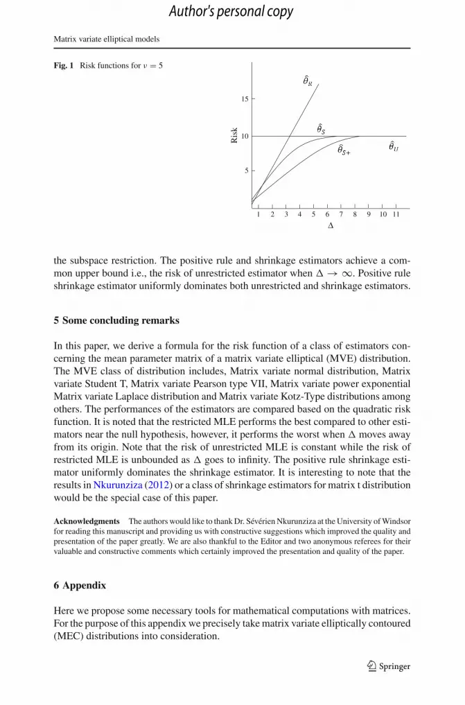
The risks of θU , θ R, θ S and θ S+ for the special value ν = 5 is displayed in Fig. 1.For the sake of simplicity take p = 1, q = 3, k = m = 1, L2 = 1, L1 = (0, 1,−1)′,� = Diag(0.2, 2, 10) and d = (10, 20)′. Then for the weight function W = �1 =�−1. Then we have tr(δ′Wδ) = �, and we display the graphs based on �. It shouldbe noted that here

κ0,11 =

∫R+

z−1w(z)dz = ν

ν − 2= 5

3.

From Fig. 1 we observed that the restricted estimator dominates the unrestricted esti-mator, shrinkage estimator and positive rule estimator near the null hypothesis. How-ever, the performance of restricted estimator becomes worst when�moves away from

123

Author's personal copy

Matrix variate elliptical models

Fig. 1 Risk functions for ν = 5

15

1 2 3 4 5 6 7 8 9 10 11

ΔR

isk

10

5

the subspace restriction. The positive rule and shrinkage estimators achieve a com-mon upper bound i.e., the risk of unrestricted estimator when � → ∞. Positive ruleshrinkage estimator uniformly dominates both unrestricted and shrinkage estimators.

5 Some concluding remarks

In this paper, we derive a formula for the risk function of a class of estimators con-cerning the mean parameter matrix of a matrix variate elliptical (MVE) distribution.The MVE class of distribution includes, Matrix variate normal distribution, Matrixvariate Student T, Matrix variate Pearson type VII, Matrix variate power exponentialMatrix variate Laplace distribution and Matrix variate Kotz-Type distributions amongothers. The performances of the estimators are compared based on the quadratic riskfunction. It is noted that the restricted MLE performs the best compared to other esti-mators near the null hypothesis, however, it performs the worst when � moves awayfrom its origin. Note that the risk of unrestricted MLE is constant while the risk ofrestricted MLE is unbounded as � goes to infinity. The positive rule shrinkage esti-mator uniformly dominates the shrinkage estimator. It is interesting to note that theresults in Nkurunziza (2012) or a class of shrinkage estimators for matrix t distributionwould be the special case of this paper.

Acknowledgments The authors would like to thank Dr. Sévérien Nkurunziza at the University of Windsorfor reading this manuscript and providing us with constructive suggestions which improved the quality andpresentation of the paper greatly. We are also thankful to the Editor and two anonymous referees for theirvaluable and constructive comments which certainly improved the presentation and quality of the paper.

6 Appendix

Here we propose some necessary tools for mathematical computations with matrices.For the purpose of this appendix we precisely take matrix variate elliptically contoured(MEC) distributions into consideration.

123

Author's personal copy

M. Arashi et al.

Let X be an n × p random matrix, which can be expressed in terms of its elements,column and rows as

X = (xi j ) = (x1, . . . , x p) = (x(1), . . . , x(n))′. (6.1)

Here x(1), . . . , x(n) can be regarded as a sample of size n from a p-dimensionalpopulation.

As pointed by Fang and Li (1999), there are many ways (not completely different)to define elliptical matrix distributions. Four classes of elliptical matrix distributionsare defined and discussed by Dawid (1977) and Anderson and Fang (1990). For thepurpose of this appendix we specifically consider the following situations.

Definition 6.1 The n × p random matrix X has a MEC distribution if its density hasthe form

g(X) = dn,p||− n2 |�|− p

2 f{−1(X − 1μ′)′�−1(X − 1μ′)

}, (6.2)

where μ ∈ Rp, and � are p×p and n×n positive definite matrices. This distribution

is denoted by X ∼ En,p(μ,� ⊗ , f ). For notational convenience we may also useX ∼ En,p(μ,�,, f ) where needed.

Definition 6.1 imposes the condition f (AB) = f (B A) on the density generator ffor any p × p positive definite symmetric matrices A and B. Throughout, without lossof generality, we take tr operation from the argument of f (.).

Some examples of MEC distributions are given below.

(i) Matrix Variate Normal (MN) DistributionX ∈ R

n×p has MN distribution, with mean M, row and column covariance matri-ces and �, respectively denoted by X ∼ M Nn,p(M,�,), if its pdf is givenby

f (X) = ||− n2 |�|− p

2

(2π)np2

exp

{−1

2tr

[−1(X − M)′�−1(X − M)

]}.

(ii) Matrix Variate Student-t (MT) DistributionX ∈ R

n×p has MT distribution, with mean M, row and column scale matrices

and �, respectively and ν d.f. denoted by X ∼ MTn,p(M,�,, ν), if its pdf isgiven by

f (X) = ||− n2 |�|− p

2

gn,p

∣∣∣In + −1(X − M)′�−1(X − M)

∣∣∣−n+p+ν−1

2,

where

gn,p =(νπ)

np2 p

(ν+p−1

2

)

p

(ν+n+p−1

2

) .

123

Author's personal copy

Matrix variate elliptical models

(iii) Matrix Variate Pearson Type-VII (MPVII) DistributionX ∈ R

n×p has MPVII distribution, with mean M, row and column scalematrices and �, respectively and parameters m and q denoted by X ∼M PV I In,p(M,�,,m, q), if its pdf is given by

f (X) = ||− n2 |�|− p

2

hn,p,m,q

∣∣∣∣In + 1

q−1(X − M)′�−1(X − M)

∣∣∣∣−m

,

where

hn,p,m,q = (qπ)np2 p

(m − n

2

) p (m)

.

(iv) Matrix Variate Power Exponential (MPE) DistributionX ∈ R

n×p has MPE distribution, with mean M, row and column scalematrices and �, respectively and parameters r and s denoted by X ∼M P En,p(M,�,, r, s), if its pdf is given by

f (X) = ||− n2 |�|− p

2

jn,p,r,sexp

{− r

2

(tr

[−1(X − M)′�−1(X − M)

])s},

where

jn,p,r,s = (2π)np2

( np2s

)s

( np2

)r

np2s.

(v) Matrix Variate Laplace (ML) DistributionX ∈ R

n×p has ML distribution, with mean M, row and column scale matrices

and �, respectively denoted by X ∼ M Ln,p(M,�,), if its pdf is given by

f (X) = ||− n2 |�|− p

2

ln,pexp

{−

√2

2

(tr

[−1(X − M)′�−1(X − M)

]) 12

},

where

in,p = 2πnp2 (np)

( np

2

) .

(vi) Matrix Variate Kotz-Type (MK) DistributionX ∈ R

n×p has MK distribution, with mean M, row and column scale matrices

and �, respectively and parameter s denoted by X ∼ M Kn,p(M,�,, s), if itspdf is given by

f (X) = ||− n2 |�|− p

2

tn,p,rexp

{− r

2

(tr

[−1(X − M)′�−1(X − M)

])},

123

Author's personal copy

M. Arashi et al.

where

tn,p,r = (2π)np2

( np2

)

( np2

)r

np2

.

Theorem 6.1 Let X ∼ En,p(μ,� ⊗ , f ) where the p.d.f. g(X) of X is defined by

g(X) = |�|− p2 ||− n

2 h[tr −1(X − μ)′�−1(X − μ)

].

If h(t), t ∈ [0,∞) has the inverse Laplace transform (denoted by L−1[h(t)]), thenwe have

g(X) =∫

R+w(z) fN (μ,z−1�⊗)(X) dz, (6.3)

where fN (μ,z−1�⊗)(X) stands for the p.d.f. of the n × p matrix X distributed as

matrix variate normal with the mean matrix μ and the covariance matrix z−1� ⊗ ,and w(z) is the weight function given by

w(z) = (2π)np/2z−np/2L−1[h(2t)]. (6.4)

For the proof we refer the readers to Theorem 4.2.1 of Gupta and Varga (1995).

Remark 6.1 An important issue raises when considering Theorem 6.1, is the mixturerepresentation given by (1.3) and the form of the weighting function w(.). Note thatw(.) is not always nonnegative [(see examples in Chu (1973), Provost and Cheong(2002) and Arashi et al. (2012b)]. This makes a difference with respect to that of theclass of multivariate scale mixtures of matrix normal distributions.

Remark 6.2 It is worthwhile to consider that for the special case for which � and

are not invertible, i.e. singular matrix elliptical contoured distribution, one may getsimilar result, as stated in the above, by the method proposed in Díaz-García et al.(2002). Further discussion on how to get similar result to Theorem 6.1 using rankdecomposition is provided in Arashi and Nadarajah (2012).

Remark 6.3 In Theorem 6.1 it is stated that f is the density of Nn,p(μ, z−1� ⊗ ).It is realized from the proof that f can even has one of the following densities

(1) Nn,p(μ, z−1�,) or(2) Nn,p(μ,�, z−1) or

(3) Nn,p(μ, z− 12 �, z− 1

2 ).This fact enables us to adopt each representation whenever is needed for practicaluse.

123

Author's personal copy

Matrix variate elliptical models

References

Anderson TW, Fang KT (1990) Inference in multivariate elliptically contoured distribution based on max-imum likelihood. In: Fang KT, Anderson TW (eds) Statistical inference in elliptically contoured andrelated distribution. Allerton Press, New York, pp 201–216

Arashi M (2009) Preliminary test estimation of the mean vector under balanced loss function. J Stat Res43(2):55–65

Arashi M, Nadarajah S (2012) On singular elliptical models. ManuscriptArashi M, Tabatabaey SMM (2010) A note on classical Stein-type estimators in elliptically contoured

models. J Stat Plan Inference 140:1206–1213Arashi M, Saleh AKMdE, Tabatabaey SMM (2010) Estimation of parameters of parallelism model with

elliptically distributed errors. Metrika 71:79–100Arashi M, Saleh AKMdE, Tabatabaey SMM (2012a) Regression model with elliptically contoured errors.

Stat J Theor Appl Stat. doi:10.1080/02331888.2012.694442Arashi M, Roux JJJ, Bekker A (2012b) Advance mathematical statistics for elliptical models, Technical

Report, 2012/02 ISBN: 978-1-86854-983-2. University of Pretoria, South AfricaBancroft TA (1944) On biases in estimation due to use of preliminary tests of significance. Ann Math Stat

15:190–204Bancroft TA (1964) Analysis and inference for incompletely specified models involving the use of prelim-

inary test(s) of significance. Biometrics 20:427–442Benda N (1996) Pre-test estimation and design in the linear model. J Stat Plan Inference 52:225–240Chu KC (1973) Estimation and decision for linear systems with elliptically random process. IEEE Trans

Autom Control 18:499–505Dawid AP (1977) Spherical matrix distributions and a multivariate model. J R Stat Soc B 39(2):254–261Díaz-García José A, Leiva-Sánchez V, Galea M (2002) Singular elliptical distribution: density and appli-

cations. Commun Stat Theory Methods 31(5):665–681Fang KT, Li R (1999) Bayesian statistical inference on elliptical matrix distributions. J Multivar Anal

70(1):66–85Giles AJ (1991) Pretesting for linear restrictions in a regression model with spherically symmetric distrib-

utions. J Econom 50:377–398Gnanadesikan R (1977) Methods for statistical data analysis of multivariate observations. Wiley, New YorkGupta AK, Varga T (1995) Normal mixture representations of matrix variate elliptically contoured distrib-

utions. Sankhya 57:68–78Gupta AK, Saleh AKMdE, Sen PK (1989) Improved estimation in a contingency table: independence

structure. J Am Stat Assoc 84:525–532Han C-P, Bancroft TA (1968) On Pooling means when variance is unknown. J Am Stat Assoc 63:1333–1342James W, Stein C (1961) Estimation with quadratic loss. In: Proceeding of the fourth Berkeley symposium

on mathematical statistics and probability. University of California Press, Berkeley, CAJudge GG, Bock ME (1978) The statistical implication of pre-test and stein-rule estimators in econometrics.

North Holland, AmsterdamKibria BMG (1996) On shrinkage ridge regression estimators for restricted linear models with multivariate

t disturbances. Students 1(3):177–188Kibria BMG, Saleh AKMdE (2006) Optimum critical value for pretest estimators. Commun Stat Simul

Comput 35(2):309–319Kibria BMG, Saleh AKMdE (2011) Improving the estimators of the parameters of a probit regression

model: a ridge regression approach. J Stat Plan Inference 142:1421–1435Kollo T, von Rosen D (2005) Advanced multivariate statistics with matrices. Springer, BerilnNkurunziza S (2011) Shrinkage strategy in stratified random sample subject to measurement error. Stat

Probab Lett 81(2):317–325Nkurunziza S (2012) The risk of pretest and shrinkage estimators. Stat J Theor Appl Stat 46(3):305–312Nkurunziza S, Ahmed SE (2011) Estimation strategies for the regression coefficient parameter matrix in

multivariate multiple regression. Statistica Neerlandica 65(4):387–406Ohtani K (1993) A comparison of the Stein-rule and positive part Stein-rule estimators in a misspecified

linear regression models. Econom Theory 9:668–679Provost SB, Cheong Y-H (2002) The distribution of Hermitian quadratic forms in elliptically contoured

random vectors. J Stat Plan Inference 102:303–316Saleh AKMdE (2006) Preliminary test and Stein-type estimation with applications. Wiley, New York

123

Author's personal copy

M. Arashi et al.

Saleh AKMdE, Sen PK (1985) On shrinkage M-estimators of location parameters. Commun Stat TheoryMethods 24:2313–2329

Saleh AKMdE, Picek J, Kalian J (2010) Nonparamteric estimation of regression parameters in measurementerorrs model. Metron LXVII:177–200

Saleh AKMdE, Picek J, Kalian J (2012) R-estimation of the parameters of a multiple regression model withmeasurement erorrs. Metrika 75:311–328

Sen PK, Saleh AKMdE (1985) On some shrinkage estimators of multivariate location. Ann Stat 13:272–281Singh RS (1989) Estimation of error variance in linear regression models with errors having multivariate

Student- t distribution with unknown degrees of freedom. Econ Lett 27:47–53Singh RS (1991) James–Stein rule estimators in linear regression models with multivariate t distributed

error. Aust J Stat 33:145–158Tabatabaey SMM, Saleh AKMdE, Kibria BMG (2004) Estimation strategies for the parameters of the linear

regression models under spherically symmetric distributions. J Stat Res 38:13–31Wang S-D, Kuo T-S, Hsu C-F (1986) Trace bounds on the solution of the algebraic matrix Riccati and

Lyapunov equation. IEEE Trans Autom Control 31(7):654–656Zellner A (1976) Bayesian and non-Bayesian analysis of the regression model with multivariate Student t

error terms. J Am Stat Assoc 71:400–405

123

Author's personal copy