Nonlinear dynamic analysis for elastic robotic arms

RESEARCH ARTICLE

M. H. KORAYEM, H. N. RAHIMI

Nonlinear dynamic analysis for elastic robotic arms

© Higher Education Press and Springer-Verlag Berlin Heidelberg 2011

Abstract The aim of the paper is to analyze the nonlineardynamics of robotic arms with elastic links and joints. Themain contribution of the paper is the comparativeassessment of assumed modes and finite element methodsas more convenient approaches for computing the non-linear dynamic of robotic systems. Numerical simulationscomprising both methods are carried out and results arediscussed. Hence, advantages and disadvantages of eachmethod are illustrated. Then, adding the joint flexibility tothe system is dealt with and the obtained model isdemonstrated. Finally, a brief description of the optimalmotion generation is presented and the simulation iscarried out to investigate the role of robot dynamicmodeling in the control of robots.

Keywords robotic arms, elastic link, elastic joint, non-linear dynamics, optimal control

1 Introduction

Analyzing the nonlinear dynamics of elastic manipulatorsis a complex task that plays a crucial role in the design andapplication of robots in task space. This complexity arisesfrom very lengthy, fluctuating and highly nonlinear andcoupled set of dynamic equations due to the flexible natureof both links and joints. The original dynamics of roboticmanipulators with elastic arms are described by nonlinearcoupled partial differential equations. They are continuousnonlinear dynamical systems distinguished by an infinitenumber of degrees of freedom. The exact solution of suchsystems does not exist. However, most commonly the

dynamic equations are truncated to some finite dimen-sional models with either the assumed modes method(AMM) or the finite element method (FEM). Note that thelumped parameter is another method for analyzing suchsystems. In this method the manipulator is modeled as aspring and mass system. Hence, the problem often does notyield to sufficiently accurate results [1,2]. Accordingly,very few researchers dealt with this method, so it is notconsidered in the present paper.The assumed mode expansion method was used by

Sasiadek and Green [3,4] to derive the dynamic equation ofthe flexible manipulator. Subudhi and Morris [5] presenteda dynamic modeling technique for a manipulator withmultiple flexible links and flexible joints based on acombined Euler–Lagrange formulation and assumedmodes method. Then, they controlled such system byformulating a singularly perturbed model and used it todesign a reduced-order controller. In Ref. [6] combinedEuler–Lagrange formulation and assumed modes methodwas used for driving the equation of motions withconsideration of the simply supported mode shapes.Then, open-loop optimal control method was proposedfor trajectory optimization of a flexible link mobilemanipulator for a given two-end-point task in point-to-point motion.In finite element method, the elastic deformations are

analyzed by assuming a known rigid body motion and latersuperposing the elastic deformation with the rigid bodymotion [7,8]. In Ref. [9] with the Timoshenko beam theoryand the finite element method, the dynamic equation ofplanar cooperative manipulators with link flexibility wasproposed in absolute coordinates. Mohamed and Tokhi[10] derived the dynamic model of a single-link flexiblemanipulator using FEM and then studied the feed-forwardcontrol strategies for controlling the vibration. Yue et al.[11] used the finite element method for describing thedynamics of the system and computed the maximumpayload of kinematically redundant flexible manipulators.Finally, they numerically simulated a planar flexible robotmanipulator to validate their research work.Joint flexibility considerably influences the performance

of robotic arms and it is one of the major sources of

Received August 7, 2010; accepted November 22, 2010

M. H. KORAYEMRobotic Research Lab, College of Mechanical Engineering, IranUniversity of Science and Technology, Tehran, Iran

H. N. RAHIMI (✉)Mechanical Engineering department, Islamic Azad University, Dama-vand, IranE-mail: [email protected]

Front. Mech. Eng.DOI 10.1007/s11465-011-0218-y

1

5

10

15

20

25

30

35

40

45

50

55

1

5

10

15

20

25

30

35

40

45

50

55

FME-11018-RH.3d 21/4/011 9:5:2

nonlinearity and the system’s oscillatory behavior. It canbe caused by transmission elements between actuators andlinks such as harmonic drives, belts, or long shafts; and itcan be modeled by considering the position and velocity ofthe motor rotor, and the position and velocity of the link.Therefore, the order of the dynamic model for a flexiblejoint is twice that of a rigid joint. A review of recentliterature shows that extensive researches have addressedthe elastic joints robotic arms [12]. However, only a limitednumber of research works have been reported on acomprehensive model that describes both link and jointelasticity [5]. Moreover, in almost all cases, linearizedmodels of the link flexibility are considered which reducedthe complexity of the model based controller [13].The present literature review shows that there are

numerous papers that used AMM or FEM to analyze thedynamics of elastic robotic arms. Hence, in the face ofincreased attention of elastic manipulators, a comprehen-sive comparison of available methods for dynamic robotanalysis, can provide a unified framework for designers tochoose a more suitable method. The main objective of thepresent paper is to provide a comparative view of theaforementioned methods. Hence, methods are formulatedand the comprehensive numerical simulations that com-pare rigid robotic arms with elastic ones with AMM (bothpinned-pinned and clamped-free boundary conditions) andFEM are carried out. Results are discussed and advantagesor disadvantages of each method are highlighted. Then, forthe investigation on the effects of joint elasticity on therobot dynamics, a manipulator with both elastic links andelastic joints is modeled and the impressive factors on itsjoint elasticity are investigated through the simple casestudy simulation. Finally, a concise explanation for generaloptimal motion planning and Two-Point Boundary-Value(TPBV) problems are presented and the simulation iscarried out to investigate the role of robot dynamics in thecontrol of robots.

2 System modeling

2.1 Assumed modes method

A large number of researchers use assumed modes ofvibration to model robot dynamics in order to capture theinteraction between flexural vibrations and nonlineardynamics. In the assumed modes method, the dynamicmodel of the robot manipulator is described by a set ofvibration modes other than its natural modes. Usingassumed modes to model flexibility requires Euler–Bernoulli beam theory boundary conditions and accom-modates changes in configuration during operation,whereas natural modes must be continually recomputed.According to this method an approximate deflection of anycontinuous elastic beam subjected to transverse vibrations,can be expressed through truncated modal expansion,

under the planar small deflection assumption of the link as

viðxi,tÞ ¼Xnij¼1

φijðxiÞeijðtÞ,i ¼ 1,:::,n,, (1)

where viðxi,tÞ is the bending deflection of the ith link at aspatial point xið0£xi£liÞ and li is the length of the ith link.ni is the number of modes used to describe the deflection oflink i; φijðxiÞ and eijðtÞ are the jth assumed mode shapefunction and jth modal displacement for the ith link,respectively. The position and velocity of each point onlink i can be obtained with respect to the inertial coordinateframe using the transformation matrices between the rigidand flexible coordinate systems. Then, by employing theLagrange formulation, dynamic equations of the systemcan be derived as

d

dt

∂T∂ _qk

� �–

∂T∂qk

� �þ ∂U

∂qk

� �¼ Uk , (2)

where T is the kinetic energy of the system, U is thepotential (strain) energy of the system, qk is the kth elementof the generalized coordinates vector q ¼ �i eij

� �, and

Uk is the generalized force corresponding to qk .In the AMM there are numerous ways to choose the

boundary conditions. The present study addresses fourwell-known conditions and chooses them in the numericalsimulations. Ideally, the optimum set of assumed modes isthat closest to natural modes of the system. Hence, there isno stipulation as to which set of assumed modes should beused. Natural modes depend on several factors such as sizeof hub inertia and size of payload mass. Choosingappropriate conditions is very important and it may causebetter consequences in the results. Hence, the ultimatechoice requires an assessment based on the actual robotstructure and for example, anticipated range of payloadstogether with its natural modes [14].First, four normal modes for some familiar mode

conditions are described as follows.Clamped-free mode shapes are given by

φðxÞ ¼ sinðB:xÞ – sinhðB:xÞ þ A�cosðB:xÞ – coshðB:xÞ

�,

where

A ¼ cosðB:LÞ þ coshðB:LÞsinðB:LÞ – sinhðB:LÞ , (3)

B:L : 1:87 4:69 7:85 10:99:Also, clamped–clamped mode shapes are determined as


�,

where

A ¼ cosðB:LÞ – coshðB:LÞsinðB:LÞ þ sinhðB:LÞ, (4)

B:L : 4:73 7:85 10:99 14:13:In addition, mode shape functions with clamped-pinned

2 Front. Mech. Eng.

1

5

10

15

20

25

30

35

40

45

50

55

1

5

10

15

20

25

30

35

40

45

50

55

FME-11018-RH.3d 21/4/011 9:5:4

boundary conditions are given by


�,

where

A ¼ –sinðB:LÞ þ sinhðB:LÞcosðB:LÞ þ coshðB:LÞ, (5)

B:L : 3:92 7:06 10:21 13:35:Similarly, pinned–pinned mode shapes are determined

asφðxÞ ¼ AsinðB:xÞ,

A ¼ coshðB:LÞcosðB:LÞ , (6)

B:L : 3:14 6:28 9:42 12:56:Although the assumed modes method has been widely

used, there are several ways to choose link boundaryconditions and mode eigen-functions. This drawback mayincrease drastically when finding modes for links with non-regular cross sections and multi-link manipulators isobjected. In addition, using the AMM to derive theequations of motion of the flexible manipulators, only thefirst several modes are usually retained by truncation andthe higher modes are neglected.

2.2 Finite element method

The finite element method is broadly used to derivedynamic equations of elastic robotic arms. Researchersusually use the Euler–Bernoulli beam element withmultiple nodes and Lagrange shape function to achievethe reasonable finite element model. The node number canbe selected according to the requirement on precision.However, increasing the node number may enlarge thestiffness matrix and result in long and complex equations.Hence, choosing the proper node number is very importantin the finite element analysis.The overall finite element approach involves treating

each link of the manipulator as an assemblage of nelements of length li. Consider link i to be divided intoelements ‘i1’, ‘i2’, …, ‘ij’, …, ‘ini’ of equal length, li,where ni is the number of elements of the ith link. Let usdefine the following notation, where subscript ij refer to thejth element of link i. OXY is the inertia system ofcoordinates,OiXiYi is the body-fixed system of coordinatesattached to link i. ui,2j – 1 is the flexural displacement at thecommon junction of elements ‘i(j – 1)’ and ‘ij’ of linki. ui,2j is the flexural slope at the tip of the common junctionof elements ‘i(j – 1)’ and ‘ij’ of link i. This slope ismeasured with respect to axis OiXi. For each element thekinetic energy, Tij, and potential energy, Vij, are computedin terms of a selected system of generalized coordinate, q,and their rate of change with respect to time, _q. It isconvenient to define ri as the position vector of link i in theinertia reference frame in terms of the position of each

point in the body-fixed coordinate system:

r↕ ↓

1 ¼ T10

ðj – 1Þl1 þ x1jy1j

� ,

r↕ ↓

i ¼ T10

L1u2n1þ1

� þ � � � þ T1

0T21 þ � � � þ Ti – 1

i – 2

Liu2niþ1

� � �

þ T10T

21 þ � � � þ Ti

i – 1

ðj – 1Þli þ x2jy2j

� ,

(7)

for i ¼ 2,3,:::,NLðnumber of linksÞ,where Ti

i – 1 is the transformation matrix from OiXiYi to itsprevious body-fixed coordinate system. It is obvious thatO0X0Y0 ¼ OXY is the inertia system of coordinates.

T10 ¼

cosð�1Þ – sinð�1Þsinð�1Þ cosð�1Þ

" #,

T10 ¼

cosð�i þ u2ni – 1þ2Þ – sinð�i þ u2ni – 1þ2Þsinð�i þ u2ni – 1þ2Þ cosð�i þ u2ni – 1þ2Þ

" #,

(8)

for i ¼ 2,3,:::,NL,where xij is the distance along OiXi in a body-fixedcoordinate system from node ‘j – 1’, li is the length of theelements in the ith link and �i is the joint angle betweenlink i and ‘i – 1’. Finally, yij is defined as the elementdisplacement and expresses the deformation of each linkdue to its original shape:

yij ¼X4k¼1

φkðxijÞui,2j – 2þkðtÞ, (9)

where u is flexural displacement at the common junction ofelements ‘i(j – 1)’ and ‘ij’ of link i and φk are the shapefunctions (Hermitian functions) of a beam element(Appendix A2). Consequently, kinetic energy, Tij, andpotential energy, Vij, for the jth element of link i can becomputed by the following equation:

Tij ¼1

2!

li

0mi

∂rTi∂t

$∂ri∂t

� dxij (10)

and

Vij ¼ Vgij þ Veij

¼ !li

0mig 0 1½ �T1

0

ðj – 1Þli þ xijyij

� dxij

þ 1

2!

li

0EIi

∂2yij∂x2ij

" #2

dxij: (11)

In the above equation, the potential energy consists oftwo parts. One part is due to gravity ðVgijÞ and another isrelated to elasticity of links ðVeijÞ. mi and EIi are the massand the flexural rigidity of ith element, respectively. These

M. H. KORAYEM et al. Nonlinear dynamic analysis for elastic robotic arms 3

1

5

10

15

20

25

30

35

40

45

50

55

1

5

10

15

20

25

30

35

40

45

50

55

FME-11018-RH.3d 21/4/011 9:5:6

energies of elements are then combined to obtain the totalkinetic energy T, and potential energy V, for each link.Then, the dynamic equations can be derived by replacingthe selected system of a local generalized coordinate, q,applying Lagrange's equation, performing some algebraicmanipulations and applying associated boundary condi-tions. Note that the applied local generalized coordinatesystem, q, consisting of all variables used in the modeling,is considered as

q ¼ f�1,�2,:::,�m,u1,1,u1,2,:::,u1,2n1þ2,:::,um,1,um,2,

:::,um,2nmþ2g: (12)

The use of the finite element method in modeling ofelastic robotics systems is detailed in Ref. [7].As can be seen, modeling of flexural vibrations of

robotic elements using finite element is a well-establishedtechnique. Therefore, researchers can handle nonlinearconditions with this method. However, in order to solve alarge set of differential equations derived by the finiteelement method, a lot of boundary conditions have to beconsidered, which are in most situations, uncertain forflexible manipulators. Also, although there are significantadvantages of FEM over analytical solution techniquessuch as easy to handle with nonlinear conditions, thisapproach seems more complex over AMM. The mainreason is that use of the finite element model toapproximate flexibility usually gives rise to an over-estimated stiffness matrix. Moreover, because of the largenumber of equations, the numerical simulation time maybe exhausting for the finite element models [8].

3 Numerical Simulations

3.1 Link flexibility

The dynamic equations of the flexible robotic arms areverified in this section by undertaking a computer

simulation. Simulating both FEM and AMM (pinned-pinned and clamped-free) models and comparing themwith the rigid links in this simulation shows the oscillatorybehavior of the nonlinear robotic system advisably. In thissimulation, the case of harmonic motion of a nonlinearmodel of flexible two links robotic arms is considered inthe simulation. The robot is hung freely and it is influencedonly under gravity effect. The physical parameters wereL1 ¼ L2 ¼ 1 m, I1 ¼ I2 ¼ 5� 10 – 9 m4, m1 ¼ m2 ¼ 5 kgand E1 ¼ E2 ¼ 2� 1011 kg=m2. These parameters weretaken from [7].Considering the equations described in Section 2 for

FEM and AMM, the set of equations of motion for eachmethod can be derived in compact form as

MðqÞ€q þ C q, _qð Þ ¼ U , (13)

where M is the inertia matrix, C is the vector of Coriolisand centrifugal forces in addition to the gravity effectsvector and U is the generalized force vector inserted intothe actuator. Details of the driving the dynamic equationsare given in the Appendix A. Open loop system responseof changing the initial condition from normal equilibriumposition to the relative angle between the first and secondlink of this system ð�2Þ to the deviation of 5 degrees [7] isstudied in this simulation.The responses of the system are presented in Figs. 1–3.

Figures show the differences between rigid and flexiblerobotic arms also between the FEM and AMM with bothpinned-pinned and clamped-free boundary conditions.Figures 1 and 2 show the angular positions and angularvelocities of joints. It is obvious from the figures that thelink elasticity appears in the velocity graph more than theposition graph. As can be seen from Fig. 1, because thesmall deflection of links in the flexible model isconsidered, the flexible graph is smoother than the rigidone, especially in the peaks of the graph. Figures plotted inthis section clearly show a good agreement between the

Fig. 1 Angular position of joints. (a) Joint 1; (b) joint 2

4 Front. Mech. Eng.

1

5

10

15

20

25

30

35

40

45

50

55

1

5

10

15

20

25

30

35

40

45

50

55

FME-11018-RH.3d 21/4/011 9:5:7

obtained results in this study and those presented inRef. [7].The corresponding amplitudes of vibration modes in the

AMM are shown in Fig. 3. It is clear that link flexibilitysignificantly affects the link vibrations. In addition,pictures show that these effects appeared more when theclamped–free boundary condition is considered.

3.2 Joint Elasticity

To model a flexible joint manipulator (FJM) the linkpositions are allowed to be in the state vector as is the casewith rigid manipulators. Actuator positions must be alsoconsidered because in contradiction to rigid robots theseare related to the link position through the dynamics of theflexible element. By defining the link number of a flexiblejoint manipulator as m, position of the ith link is shownwith �2i – 1 : i ¼ 1,2,:::,m and the position of the ith actuator

with �2i : i ¼ 1,2,:::,m; it is usual in the FJM literature toarrange these angles in a vector as follows:

Q ¼ ½�1,�3,:::,�2m – 1 �2,�4,:::,�2mj �T ¼ ½qT1 ,qT2 �T: (14)

Therefore, by adding the joint flexibility by consideringthe elastic mechanical coupling between the ith joint andith link, as a linear torsional spring with constant stiffnesscoefficient ki, the set of equations of motion (Eq. (13)) canbe rearranged into the following form:

Mðq1Þ€q1 þ C q1, _q1ð Þ þ Kðq1 – q2Þ ¼ 0,

J€q2 þ Kðq2 – q1Þ ¼ U , (15)

where K = diag[k1, k2,..., km] is a diagonal stiffness matrixwhich models the joint elasticity and J ¼ diag½J1,J2,:::,Jm�is the diagonal matrix representing motor inertia.Now, a simulation is performed to investigate the effect

of joint flexibility on the response of the model. Hence, the

Fig. 2 Angular velocity of joints. (a) Joint 1; (b) joint 2

Fig. 3 Amplitudes of vibration’s modes. (a) Link 1; (b) link 2


1

5

10

15

20

25

30

35

40

45

50

55

1

5

10

15

20

25

30

35

40

45

50

55

FME-11018-RH.3d 21/4/011 9:5:9

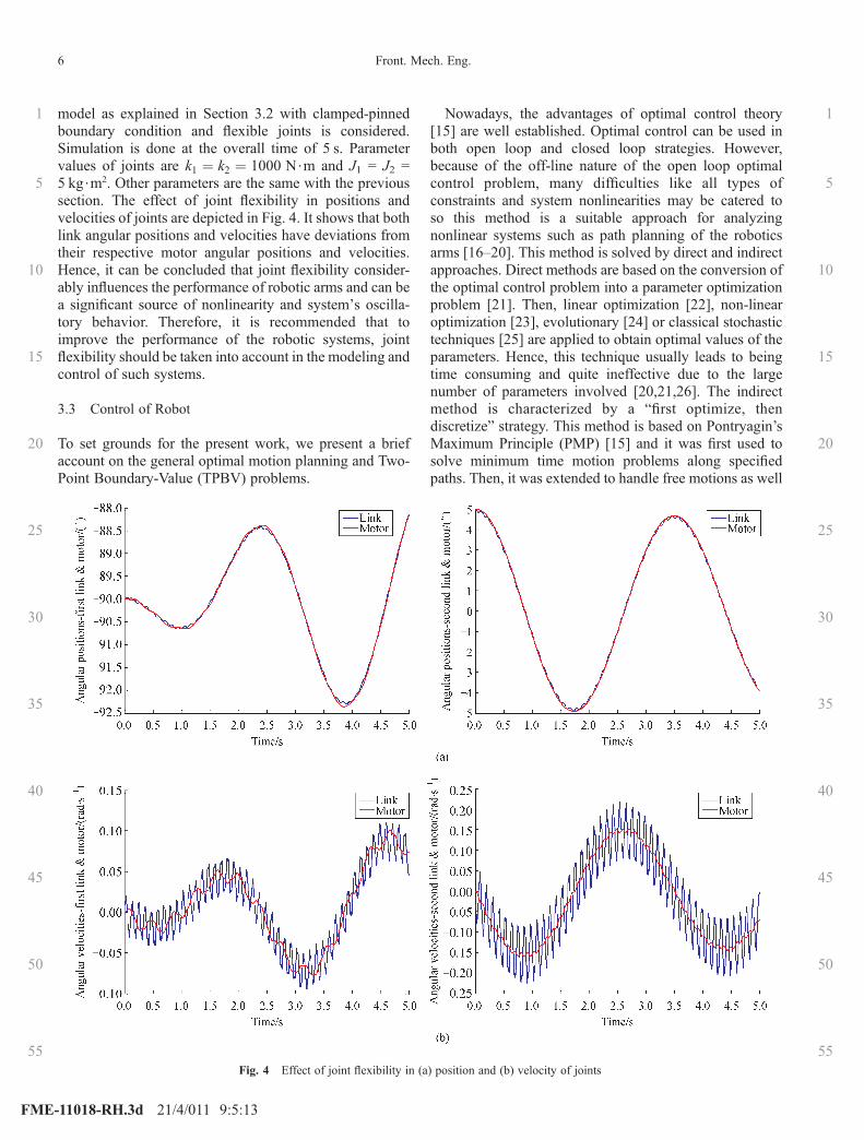
model as explained in Section 3.2 with clamped-pinnedboundary condition and flexible joints is considered.Simulation is done at the overall time of 5 s. Parametervalues of joints are k1 ¼ k2 ¼ 1000 N$m and J1 = J2 =5 kg$m2. Other parameters are the same with the previoussection. The effect of joint flexibility in positions andvelocities of joints are depicted in Fig. 4. It shows that bothlink angular positions and velocities have deviations fromtheir respective motor angular positions and velocities.Hence, it can be concluded that joint flexibility consider-ably influences the performance of robotic arms and can bea significant source of nonlinearity and system’s oscilla-tory behavior. Therefore, it is recommended that toimprove the performance of the robotic systems, jointflexibility should be taken into account in the modeling andcontrol of such systems.

3.3 Control of Robot

To set grounds for the present work, we present a briefaccount on the general optimal motion planning and Two-Point Boundary-Value (TPBV) problems.

Nowadays, the advantages of optimal control theory[15] are well established. Optimal control can be used inboth open loop and closed loop strategies. However,because of the off-line nature of the open loop optimalcontrol problem, many difficulties like all types ofconstraints and system nonlinearities may be catered toso this method is a suitable approach for analyzingnonlinear systems such as path planning of the roboticsarms [16–20]. This method is solved by direct and indirectapproaches. Direct methods are based on the conversion ofthe optimal control problem into a parameter optimizationproblem [21]. Then, linear optimization [22], non-linearoptimization [23], evolutionary [24] or classical stochastictechniques [25] are applied to obtain optimal values of theparameters. Hence, this technique usually leads to beingtime consuming and quite ineffective due to the largenumber of parameters involved [20,21,26]. The indirectmethod is characterized by a “first optimize, thendiscretize” strategy. This method is based on Pontryagin’sMaximum Principle (PMP) [15] and it was first used tosolve minimum time motion problems along specifiedpaths. Then, it was extended to handle free motions as well

Fig. 4 Effect of joint flexibility in (a) position and (b) velocity of joints

6 Front. Mech. Eng.

1

5

10

15

20

25

30

35

40

45

50

55

1

5

10

15

20

25

30

35

40

45

50

55

FME-11018-RH.3d 21/4/011 9:5:13

[27]. PMP is used also to treat directly the optimal dynamicmotion planning problem [28]. The optimality conditionsfor transfer modalities are expressed as a set of differentialequations. This boundary values problem is solved byspecific numerical techniques such as shooting or relaxa-tion methods. This method is widely used as a powerfuland efficient tool in analyzing the nonlinear system andpath planning of different types of systems [29–33]. Anindirect method is a good candidate for the cases where thesystem has a large number of degrees of freedom oroptimization of the various objectives is targeted [31,32],.This method is often applied to the generation of highlyaccurate trajectories and in combination with the structuralanalysis of optimal control problems in robotics.By defining the state vector as

X ¼ X1 X2½ �T ¼ q _q½ �T: (16)

Eq. (13) can be rewritten in state space form as

_X ¼ _X 1_X 2

� �T¼ X2 –M – 1

�U –CðX1,X2Þ

�h iT:

(17)

Assume that the optimal trajectory is desired for thesystem describe in Eq. (17) such that the followingperformance index will be minimized.

J ðuÞ ¼ !tf

t0

g�X ðtÞ,UðtÞ,t

�dt, (18)

where X(t) and U(t) represent the state and control inputvectors, respectively, and J is a function describing thedesired objective function. On the basis of variationalcalculus, the necessary conditions for optimal trajectoriesare obtained as stated by Kirck [15] and given here by Eq.(20). Note that the variable H in Eq. (20) is calledHamiltonian and defined as

H�X ðtÞ,UðtÞ,PðtÞ,t

�¼g

�X ðtÞ,UðtÞ,t

�þ PTðtÞ:½f

�X ðtÞ,UðtÞ,t

��: (19)

Eq. (20-a) represents a combination of the differentialand algebraic equations which must be satisfied throughoutthe interval ½t0,tf �, while Eq. (20-b) shows the boundaryvalue conditions.

_X *ðtÞ ¼ ∂H∂P

�X *ðtÞ,U*ðtÞ,P*ðtÞ,t

�_P*ðtÞ ¼ –

∂H∂X

�X *ðtÞ,U *ðtÞ,P*ðtÞ,t

�0 ¼ ∂H

∂U

�X *ðtÞ,U*ðtÞ,P*ðtÞ,t

�

9>>>>>>=>>>>>>;,for all t 2 ½t0,tf �,

(20� a)

H�X *ðtÞ,U*ðtÞ,P*ðtÞ,t

�£H X *ðtÞ,UðtÞ,P*ðtÞ,t �

,

for all t 2 ½t0,tf � and UðtÞ 2 UðtÞ, (20� b)

where the symbol (*) refers to the final values of X(t), U(t),and P(t); and UðtÞ denotes the admissible control value.Also, it is remarked that the vector P in Eq. (20) representsthe costate vector. Therefore, if U is a set of admissiblecontrol torque over the time interval t 2 ½t0,tf �, the optimal

control problem is to obtain the U *ðtÞ 2 U in order tominimize the objective criterion given by Eqs. (18) and(21), subject to the motion Eq. (17), while steering thestates from initial boundary conditions to the finalsituations. Herein, for our minimization purpose, weconsider that the cost function is given by

J ðuÞ ¼ !tf

t0

ð X2j jj j2W þ Uj jj j2RÞdt: (21)

Note that Xj jj j2K is the generalized squared weightednorm X TKX , W and R are the user-defined symmetric,positive-definite matrices. Hence, in the above perfor-mance index, the designer can decide on the relativeimportance among the velocity and control effort by thenumerical choice of W and R. In this formulation, if therobot starts from X0 at t0, and Xf is a final state to beachieved at tf , then the boundary values are as follows:

X ðt0Þ ¼ X0,

X ðtf Þ ¼ Xf :(22)

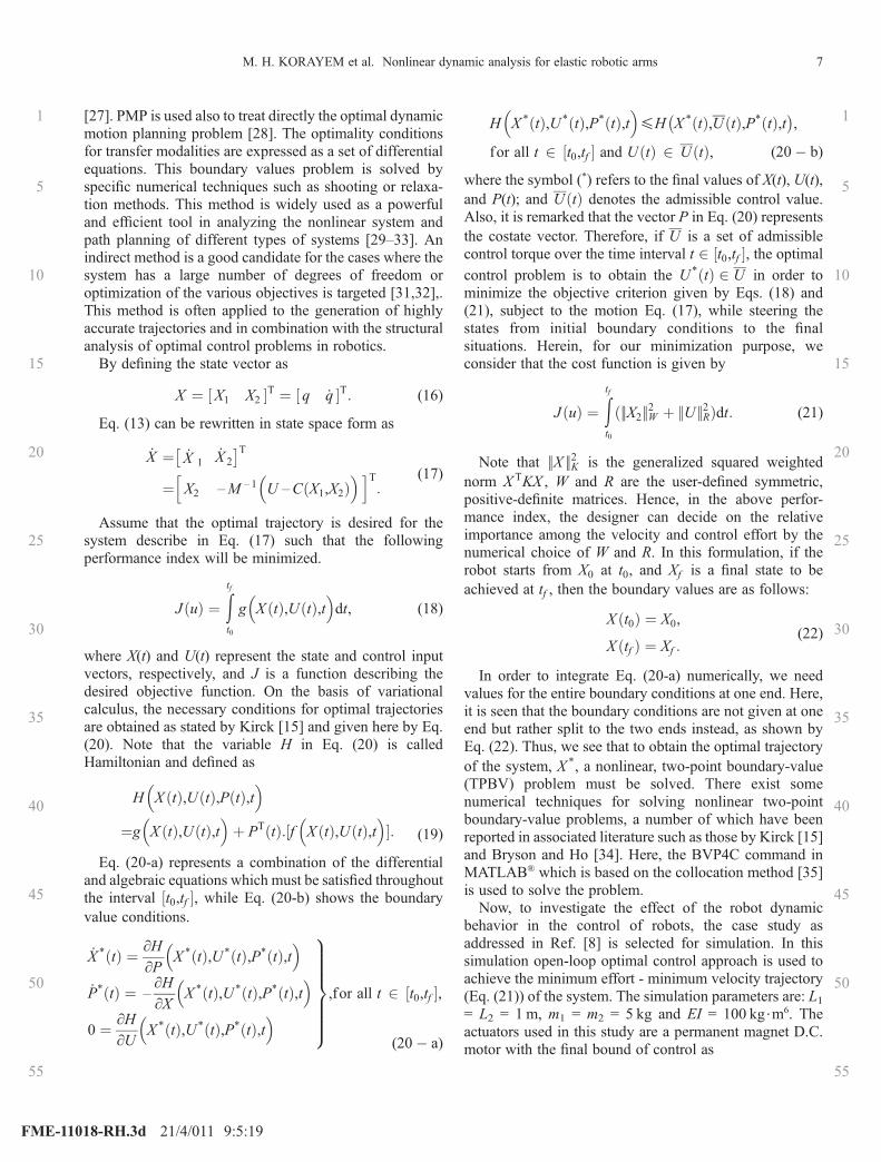
In order to integrate Eq. (20-a) numerically, we needvalues for the entire boundary conditions at one end. Here,it is seen that the boundary conditions are not given at oneend but rather split to the two ends instead, as shown byEq. (22). Thus, we see that to obtain the optimal trajectoryof the system, X *, a nonlinear, two-point boundary-value(TPBV) problem must be solved. There exist somenumerical techniques for solving nonlinear two-pointboundary-value problems, a number of which have beenreported in associated literature such as those by Kirck [15]and Bryson and Ho [34]. Here, the BVP4C command inMATLAB® which is based on the collocation method [35]is used to solve the problem.Now, to investigate the effect of the robot dynamic

behavior in the control of robots, the case study asaddressed in Ref. [8] is selected for simulation. In thissimulation open-loop optimal control approach is used toachieve the minimum effort - minimum velocity trajectory(Eq. (21)) of the system. The simulation parameters are: L1= L2 = 1 m, m1 = m2 = 5 kg and EI = 100 kg$m6. Theactuators used in this study are a permanent magnet D.C.motor with the final bound of control as


1

5

10

15

20

25

30

35

40

45

50

55

1

5

10

15

20

25

30

35

40

45

50

55

FME-11018-RH.3d 21/4/011 9:5:19

uþ1 ¼ ðτ1 – τ1=ω1Þx3, u –1 ¼ – ðτ1 þ τ1=ω1Þx3,

uþ2 ¼ ðτ2 – τ2=ω2Þx4, u –2 ¼ – ðτ2 þ τ2=ω2Þx4, (23)

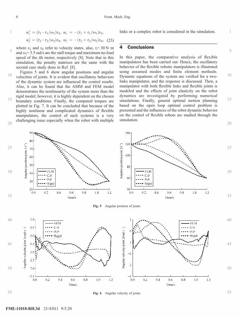
where x3 and x4 refer to velocity states, also, τi= 30 N$mandωi= 3.5 rad/s are the stall torque and maximum no-loadspeed of the ith motor, respectively [8]. Note that in thissimulation, the penalty matrixes are the same with thesecond case study done in Ref. [8].Figures 5 and 6 show angular positions and angular

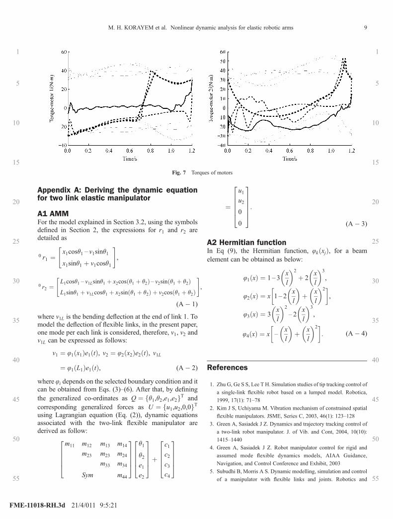
velocities of joints. It is evident that oscillatory behaviorsof the dynamic system are influenced the control results.Also, it can be found that the AMM and FEM modeldemonstrates the nonlinearity of the system more than therigid model; however, it is highly dependent on the chosenboundary conditions. Finally, the computed torques areplotted in Fig. 7. It can be concluded that because of thehighly nonlinear and complicated dynamics of flexiblemanipulators, the control of such systems is a verychallenging issue especially when the robot with multiple

links or a complex robot is considered in the simulation.

4 Conclusions

In this paper, the comparative analysis of flexiblemanipulators has been carried out. Hence, the oscillatorybehavior of the flexible robotic manipulators is illustratedusing assumed modes and finite element methods.Dynamic equations of the system are verified for a two-links manipulator, and the response is discussed. Then, amanipulator with both flexible links and flexible joints ismodeled and the effects of joint elasticity on the robotdynamics are investigated by performing numericalsimulations. Finally, general optimal motion planningbased on the open loop optimal control problem ispresented and the influences of the robot dynamic behavioron the control of flexible robots are studied through thesimulation.

Fig. 5 Angular position of joints

Fig. 6 Angular velocity of joints

8 Front. Mech. Eng.

1

5

10

15

20

25

30

35

40

45

50

55

1

5

10

15

20

25

30

35

40

45

50

55

FME-11018-RH.3d 21/4/011 9:5:20

Appendix A: Deriving the dynamic equationfor two link elastic manipulator

A1 AMMFor the model explained in Section 3.2, using the symbolsdefined in Section 2, the expressions for r1 and r2 aredetailed as

0 r1 ¼ x1cos�1 – v1sin�1

x1sin�1 þ v1cos�1

" #,

0 r2 ¼L1cos�1 – v1Lsin�1 þ x2cos �1 þ �2ð Þ – v2sin �1 þ �2ð ÞL1sin�1 þ v1Lcos�1 þ x2sin �1 þ �2ð Þ þ v2cos �1 þ �2ð Þ

" #,

(A� 1)

where v1L is the bending deflection at the end of link 1. Tomodel the deflection of flexible links, in the present paper,one mode per each link is considered, therefore, v1, v2 andv1L can be expressed as follows:

v1 ¼ φ1ðx1Þe1ðtÞ, v2 ¼ φ2ðx2Þe2ðtÞ, v1L¼ φ1ðL1Þe1ðtÞ, (A� 2)

where φi depends on the selected boundary condition and itcan be obtained from Eqs. (3)–(6). After that, by definingthe generalized co-ordinates as Q ¼ f�1,�2,e1,e2gT andcorresponding generalized forces as U ¼ fu1,u2,0,0gTusing Lagrangian equation (Eq. (2)), dynamic equationsassociated with the two-link flexible manipulator arederived as follow:

m11 m12 m13 m14

m23 m23 m24

m33 m34

Sym m44

26664

37775

�1

�2e1e2

26664

37775þ

c1c2c3c4

26664

37775

¼

u1u2

0

0

266664

377775:

(A� 3)

A2 Hermitian functionIn Eq (9), the Hermitian function, φkðxjÞ, for a beamelement can be obtained as below:

φ1ðxÞ ¼ 1 – 3x

l

� �2

þ 2x

l

� �3

,

φ2ðxÞ ¼ x 1 – 2x

l

� �þ x

l

� �2� ,

φ3ðxÞ ¼ 3x

l

� �2

– 2x

l

� �3

,

φ4ðxÞ ¼ x –x

l

� �þ x

l

� �2� : (A� 4)

References

1. Zhu G, Ge S S, Lee T H. Simulation studies of tip tracking control of

a single-link flexible robot based on a lumped model. Robotica,

1999, 17(1): 71–78

2. Kim J S, Uchiyama M. Vibration mechanism of constrained spatial

flexible manipulators. JSME, Series C, 2003, 46(1): 123–128

3. Green A, Sasiadek J Z. Dynamics and trajectory tracking control of

a two-link robot manipulator. J. of Vib. and Cont, 2004, 10(10):

1415–1440

4. Green A, Sasiadek J Z. Robot manipulator control for rigid and

assumed mode flexible dynamics models, AIAA Guidance,

Navigation, and Control Conference and Exhibit, 2003

5. Subudhi B, Morris A S. Dynamic modelling, simulation and control

of a manipulator with flexible links and joints. Robotics and

Fig. 7 Torques of motors


1

5

10

15

20

25

30

35

40

45

50

55

1

5

10

15

20

25

30

35

40

45

50

55

FME-11018-RH.3d 21/4/011 9:5:21

Autonomous Systems, 2002, 41(4): 257–270

6. Korayem M H, Rahimi Nohooji H. Trajectory optimization of

flexible mobile manipulators using open-loop optimal control

method. Springer-Verlag Berlin Heidelberg, LNAI, 2008, 5314(1):

54–63

7. Usoro P B, Nadira R, Mahil S S. A finite element/Lagrange

approach to modeling lightweight flexible manipulators. Journal of

Dynamic Systems, Measurement, and Control, 1986, 108(3): 198–

205

8. Korayem M H, Haghpanahi M, Rahimi H N, Nikoobin A. Finite

element method and optimal control theory for path planning of

elastic manipulators, Springer-Verlag Berlin Heidelberg. New

Advanced in Intelligent Decision Technology, SCI, 2009, 199:

107–116

9. Zhang C X, Yu Y Q. Dynamic analysis of planar cooperative

manipulators with link flexibility, ASME. Journal of Dynamic

Systems, Measurement, and Control, 2004, 126: 442–448

10. Mohamed Z, Tokhi M O. Command shaping techniques for

vibration control of a flexible robot manipulator. Mechatronics,

2004, 14(1): 69–90

11. Yue S, Tso S K, Xu W L. Maximum dynamic payload trajectory for

flexible robot manipulators with kinematic redundancy. Mechanism

and Machine Theory, 2001, 36(6): 785–800

12. Korayem M H, Rahimi H N, Nikoobin A. Analysis of four wheeled

flexible joint robotic arms with application on optimal motion

design, Springer-Verlag Berlin Heidelberg, New Advan. in Intel.

Decision Technology, 2009, 199: 117–126

13. Chen W. Dynamic modeling of multi-link flexible robotic

manipulators. Computers & Structures, 2001, 79(2): 183–195

14. Fraser A R, Daniel R W. Perturbation techniques for flexible

manipulators. Kluwer International Series in Engineering and

Computer Science, 1991, 138

15. Kirk D E. Optimal control theory, an introduction. Prentice-Hall

Inc., Englewood Cliffs, New Jersey, 1970

16. Koivo A J, Arnautovic S H. Dynamic optimum control of redundant

manipulators. In: Proceedings of IEEE International Conference on

Robotics and Automation, 1991, 466–471

17. Mohri A, Furuno S, Iwamura M, Yamamoto M. Sub-optimal

trajectory planning of mobile manipulator. In: Proceedings of IEEE

International Conference on Robotics and Automation, 2001, 1271–

1276

18. Kelly A, Nagy B. Reactive nonholonomic trajectory generation via

parametric optimal control. International Journal of Robotics

Research, 2003, 22(8): 583–601

19. Furuno S, Yamamoto M, Mohri A. Trajectory planning of mobile

manipulator with stability considerations. In: Proceedings of IEEE

International Conference on Robotics and Automation, 2003, 3403–

3408

20. Wilson D G, Robinett R D, Eisler G R. Discrete dynamic

programming for optimized path planning of flexible robots. In:

Proceedings of IEEE International Conference on lntelligent Robots

and Systems, Japan, 2004

21. Hull D G. Conversion of optimal control problems into parameter

optimization problems. Journal of Guidance, Control, and

Dynamics, 1997, 20(1): 57–60

22. Wang L T, Ravani B. Dynamic load carrying capacity of mechanical

manipulators- Part 2, J. of Dynamic Sys. Measurement and Control,

1988, 110: 53–61

23. Wang C Y E, Timoszyk W K, Bobrow J E. Payload maximization

for open chained manipulator: Finding motions for a Puma 762

robot. IEEE Transactions on Robotics and Automation, 2001, 17(2):

218–224

24. Ge X S, Chen L Q, 0. Li-Qun Chen. Optimal motion planning for

nonholonomic systems using genetic algorithm with wavelet

approximation. Applied Mathematics and Computation, 2006, 180

(1): 76–85

25. Haddad M, Chettibi T, Hanchi S, Lehtihet H E. Optimal motion

planner of mobile manipulators in generalized point-to-point task.

9th IEEE International Workshop on Advanced Motion Control,

2006, 300–306

26. Park K J. Flexible robot manipulator path design to reduce the

endpoint residual vibration under torque constraints. Journal of

Sound and Vibration, 2004, 275(3–5): 1051–1068

27. Shiller Z, Dubowsky S. Robot path planning with obstacles,

actuators, gripper and payload constraints. International Journal of

Robotics Research, 1986, 8(6): 3–18

28. Shiller Z. Time-energy optimal control of articulated systems with

geometric path constraints. In: Proceedings of IEEE International

Conference on Robotics and Automation, 1994, 4: 2680–2685

29. Fotouhi R, Szyszkowski W. An algorithm for time-optimal control

problems, Journal of Dynamic Systems, Measurement, and Control,

Transactions of the ASME, 1998, 120(3): 414–418

30. Agrawal O P, Xu Y. On the global optimum path planning for

redundant space manipulators. IEEE T sys Man Cyb, 1994, 24(9):

1306–1316

31. Bessonnet G, Chessé S. Optimal dynamics of actuated kinematic

chains, Part 2: Problem statements and computational aspects.

European Journal of Mechanics. A, Solids, 2005, 24(3): 472–490

32. Bertolazzi E, Biral F, Da Lio M. Symbolic–numeric indirect method

for solving optimal control problems for large multibody systems.

Multibody System Dynamics, 2005, 13(2): 233–252

33. Sentinella M R, Casalino L. Genetic algorithm and indirect method

coupling for low-thrust trajectory optimization. 42nd AIAA/ASME/

SAE/ASEE Joint Propulsion Conference & Exhibit, California,

2006

34. Bryson A E, Ho Y. Applied optimal control: Optimization,

estimation, and control, Ginn and company, 1969

35. Shampine L F, Reichelt M W, Kierzenka J. Solving boundary value

problems for ordinary differential equations in MATLAB with

bvp4c. Available at http://www.mathworks.com/bvp tutorial

10 Front. Mech. Eng.

1

5

10

15

20

25

30

35

40

45

50

55

1

5

10

15

20

25

30

35

40

45

50

55

FME-11018-RH.3d 21/4/011 9:5:25

Documents

Nonlinear dynamic analysis for elastic robotic arms