Embed Size (px)
Citation preview
RobotManipulator
ControlTheory and Practice
Second Edition, Revised and Expanded
Copyright © 2004 by Marcel Dekker, Inc.
CONTROL ENGINEERINGA Series of Reference Books and Textbooks
Editors
NEIL MUNRO, PH.D., D.SC.
ProfessorApplied Control Engineering
University of Manchester Institute of Science and TechnologyManchester, United Kingdom
FRANK L.LEWIS, PH.D.
Moncrief-O’Donnell Endowed Chairand Associate Director of Research
Automation & Robotics Research InstituteUniversity of Texas, Arlington
1. Nonlinear Control of Electric Machinery, Darren M.Dawson, Jun Hu,and Timothy C.Burg
2. Computational Intelligence in Control Engineering, Robert E.King3. Quantitative Feedback Theory: Fundamentals and Applications,
Constantine H.Houpis and Steven J.Rasmussen4. Self-Learning Control of Finite Markov Chains, A.S.Poznyak, K.Najlm,
and E.Gómez-Ramírez5. Robust Control and Filtering for Time-Delay Systems, Magdi
S.Mahmoud6. Classical Feedback Control: With MATLAB, Boris J.Lurie and Paul J.
Enright7. Optimal Control of Singularly Perturbed Linear Systems and
Applications: High-Accuracy Techniques, Zoran Gajic and Myo-TaegLim
8. Engineering System Dynamics: A Unified Graph-Centered Approach,Forbes T.Brown
9. Advanced Process Identification and Control, Enso Ikonen and KaddourNajim
10. Modern Control Engineering, P.N.Paraskevopoulos11. Sliding Mode Control in Engineering, edited by Wilfrid Perruquetti and
Jean Pierre Barbot12. Actuator Saturation Control, edited by Vikram Kapila and Karolos M.
Grigoriadis
Copyright © 2004 by Marcel Dekker, Inc.
13. Nonlinear Control Systems, Zoran Vukic, Ljubomir Kuljaca, DaliDonlagic,Sejid Tešnjak
14. Linear Control System Analysis and Design with MATLAB: Fifth Edition,Revised and Expanded, John J.D’Azzo, Constantine H.Houpis, andStuart N.Sheldon
15. Robot Manipulator Control: Theory and Practice, Second Edition,Revised and Expanded, Frank L.Lewis, Darren M.Dawson, and ChaoukiT.Abdallah
16. Robust Control System Design: Advanced State Space Techniques,Second Edition, Revised and Expanded, Chia-Chi Tsui
Additional Volumes in Preparation
Copyright © 2004 by Marcel Dekker, Inc.
Frank L.LewisUniversity of Texas at Arlington
Arlington, Texas, U.S.A.
Darren M.DawsonClemson University
Clemson, South Carolina, U.S.A.
Chaouki T.AbdallahUniversity of New Mexico
Albuquerque, New Mexico, U.S.A.
MARCEL DEKKER, INC. NEW YORK • BASEL
RobotManipulator
ControlTheory and Practice
Second Edition, Revised and Expanded
Copyright © 2004 by Marcel Dekker, Inc.
First edition: Control of Robot Manipulators, FL Lewis, CT Abdallah, DM Dawson,1993. This book was previously published by Prentice-Hall, Inc.
Although great care has been taken to provide accurate and current information,neither the author(s) nor the publisher, nor anyone else associated with this publication,shall be liable for any loss, damage, or liability directly or indirectly caused or allegedto be caused by this book. The material contained herein is not intended to providespecific advice or recommendations for any specific situation.
Trademark notice: Product or corporate names may be trademarks or registeredtrademarks and are used only for identification and explanation without intent toinfringe.
Library of Congress Cataloging-in-Publication DataA catalog record for this book is available from the Library of Congress.
ISBN: 0-8247-4072-6
Transferred to Digital Printing 2006
HeadquartersMarcel Dekker, Inc., 270 Madison Avenue, New York, NY 10016, U.S.A.tel: 212–696–9000; fax: 212–685–4540
Distribution and Customer ServiceMarcel Dekker, Inc., Cimarron Road, Monticello, New York 12701, U.S.A.tel: 800–228–1160; fax: 845–796–1772
Eastern Hemisphere DistributionMarcel Dekker AG, Hutgasse 4, Postfach 812, CH-4001 Basel, Switzerlandtel: 41–61–260–6300; fax: 41–61–260–6333
World Wide Webhttp://www.dekker.com
The publisher offers discounts on this book when ordered in bulk quantities. Formore information, write to Special Sales/Professional Marketing at the headquartersaddress above.
Copyright © 2004 by Marcel Dekker, Inc. All Rights Reserved.
Neither this book nor any part may be reproduced or transmitted in any form or byany means, electronic or mechanical, including photocopying, microfilming, andrecording, or by any information storage and retrieval system, without permission inwriting from the publisher.
Publisher’s Note
The publisher has gone to greatlengths to ensurethe quality of this reprint butpoints out that some imperfectionsin the original may be apparent
Copyright © 2004 by Marcel Dekker, Inc.
To My Sons Christopher and RomanF.L.L.
To My Faithful Wife, Dr. Kim DawsonD.M.D.
To My 3 C’sC.T.A.
Copyright © 2004 by Marcel Dekker, Inc.
v
Series Introduction
Many textbooks have been written on control engineering, describing newtechniques for controlling systems, or new and better ways of mathematicallyformulating existing methods to solve the ever-increasing complex problemsfaced by practicing engineers. However, few of these books fully address theapplications aspects of control engineering. It is the intention of this newseries to redress this situation.
The series will stress applications issues, and not just the mathematics ofcontrol engineering. It will provide texts that present not only both new andwell-established techniques, but also detailed examples of the application ofthese methods to the solution of real-world problems. The authors will bedrawn from both the academic world and the relevant applications sectors.
There are already many exciting examples of the application of controltechniques in the established fields of electrical, mechanical (includingaerospace), and chemical engineering. We have only to look around in today’shighly automated society to see the use of advanced robotics techniques inthe manufacturing industries; the use of automated control and navigationsystems in air and surface transport systems; the increasing use of intelligentcontrol systems in the many artifacts available to the domestic consumermarket; and the reliable supply of water, gas, and electrical power to thedomestic consumer and to industry. However, there are currently manychallenging problems that could benefit from wider exposure to theapplicability of control methodologies, and the systematic systems-orientedbasis inherent in the application of control techniques.
This series presents books that draw on expertise from both the academicworld and the applications domains, and will be useful not only asacademically recommended course texts but also as handbooks forpractitioners in many applications domains. Nonlinear Control Systems isanother outstanding entry in Dekker’s Control Engineering series.
Copyright © 2004 by Marcel Dekker, Inc.
vii
Preface
The word ‘robot’ was introduced by the Czech playwright Karel Capek inhis 1920 play Rossum’s Universal Robots. The word ‘robota’ in Czechmeans simply ‘work’. In spite of such practical beginnings, science fictionwriters and early Hollywood movies have given us a romantic notion ofrobots. The anthropomorphic nature of these machines seems to haveintroduced into the notion of robot some element of man’s search for hisown identity.
The word ‘automation’ was introduced in the 1940’s at the Ford MotorCompany, a contraction for ‘automatic motivation’. The single term‘automation’ brings together two ideas: the notion of special purpose roboticmachines designed to mechanically perform tasks, and the notion of anautomatic control system to direct them.
The history of automatic control systems has deep roots. Most of thefeedback controllers of the Greeks and Arabs regulated water clocks for theaccurate telling of time; these were made obsolete by the invention of themechanical clock in Switzerland in the fourteenth century. Automatic controlsystems only came into their own three hundred years later during theindustrial revolution with the advent of machines sophisticated enough torequire advanced controllers; we have in mind especially the windmill andthe steam engine. On the other hand, though invented by others (e.g.T.Newcomen in 1712) the credit for the steam engine is usually assigned toJames Watt, who in 1769 produced his engine which combined mechanicalinnovations with a control system that allowed automatic regulation. Thatis, modern complex machines are not useful unless equipped with a suitablecontrol system.
Watt’s centrifugal fly ball governor in 1788 provided a constant speedcontroller, allowing efficient use of the steam engine in industry. The motionof the flyball governor is clearly visible even to the untrained eye, and itsprinciple had an exotic flavor that seemed to many to embody the spirit of
Copyright © 2004 by Marcel Dekker, Inc.
PREFACEviii
the new age. Consequently the governor quickly became a sensationthroughout Europe.
Master-slave telerobotic mechanisms were used in the mid 1940’s at OakRidge and Argonne National Laboratories for remote handling of radioactivematerial. The first commercially available robot was marketed in the late1950’s by Unimation (nearly coincidentally with Sputnik in 1957-thus thespace age and the age of robots began simultaneously). Like the flyballgovernor, the motion of a robot manipulator is evident even for the untrainedeye, so that the potential of robotic devices can capture the imagination.However, the high hopes of the 1960’s for autonomous robotic automationin industry and unstructured environments have generally failed to materialize.This is because robotics today is at the same stage as the steam engine wasshortly after the work of Newcomen in 1712.
Robotics is an interdisciplinary field involving diverse disciplines such asphysics, mechanical design, statics and dynamics, electronics, control theory,sensors, vision, signal processing, computer programming, artificialintelligence (AI), and manufacturing. Various specialists study various limitedaspects of robotics, but few engineers are able to confront all these areassimultaneously. This further contributes to the romanticized nature ofrobotics, for the control theorist, for instance, has a quixotic and fancifulnotion of AI.
We might break robotics into five major areas: motion control, sensorsand vision, planning and coordination, AI and decision-making, andmanmachine interface. Without a good control system, a robotic device isuseless. The robot arm plus its control system can be encapsulated as ageneralized data abstraction; that is, robot-plus-controller is considered asingle entity, or ‘agent’, for interaction with the external world.
The capabilities of the robotic agent are determined by the mechanicalprecision of motion and force exertion capabilities, the number of degrees offreedom of the arm, the degree of manipulability of the gripper, the sensors,and the sophistication and reliability of the controller. The inputs for a robotarm are simply motor currents and voltages, or hydraulic or pneumaticpressures; however, the inputs for the robot-plus-controller agent can bedesired trajectories of motion, or desired exerted forces. Thus, the controlsystem lifts the robot up a level in a hierarchy of abstraction.
This book is intended to provide an in-depth study of control systemsfor serial-link robot arms. It is a revised and expended version of our 1993book. Chapters have been added on commercial robot manipulators anddevices, neural network intelligent control, and implementation of advancedcontrollers on actual robotic systems. Chapter 1 places this book in thecontext of existing commercial robotic systems by describing the robotsthat are available and their limitations and capabilities, sensors, andcontrollers.
Copyright © 2004 by Marcel Dekker, Inc.
PREFACE ix
We wanted this book to be suitable either for the controls engineer or theroboticist. Therefore, Appendix A provides a background in robot kine-matics and Jacobians, and Chapter 2 a background in control theory andmathematical notions. The intent was to furnish a text for a second coursein robotics at the graduate level, but given the background material it is usedat UTA as a first year graduate course for electrical engineering students.This course was also listed as part of the undergraduate curriculum, and theundergraduate students quickly digested the material.
Chapter 3 introduces the robot dynamical equations needed as the basisfor controls design. In Appendix C and examples throughout the book aregiven the dynamics of some common arms. Chapter 4 covers the essentialtopic of computed-torque control, which gives important insight while alsobringing together in a unified framework several sorts of classical and modernrobot control schemes.
Robust and adaptive control are covered in Chapters 5 and 6 in a parallelfashion to bring out the similarities and the differences of these twoapproaches to control in the face of uncertainties and disturbances. Chapter7 addresses some advanced techniques including learning control and armswith flexible joint coupling.
Modern intelligent control techniques based on biological systems havesolved many problems in the control of complex systems, including unknownnon-parametrizable dynamics and unknown disturbances, backlash, friction,and deadzone. Therefore, we have added a chapter on neural network controlsystems as Chapter 8. A robot is only useful if it comes in contact with itsenvironment, so that force control issues are treated in Chapter 9.
A key to the verification of successful controller design is computersimulation. Therefore, we address computer simulation of controllednonlinear systems and illustrate the procedure in examples throughout thetext. Simulation software is given in Appendix B. Commercially availablepackages such as MATLAB make it very easy to simulate robot controlsystems.
Having designed a robot control system it is necessary to implement it;given today’s microprocessors and digital signal processors, it is a short stepfrom computer simulation to implementation, since the controller subroutinesneeded for simulation, and contained in the book, are virtually identical tothose needed in a microprocessor for implementation on an actual arm. Infact, Chapter 10 shows the techniques for implementing the advancedcontrollers developed in this book on actual robotics systems.
All essential information and controls design algorithms are displayed intables in the book. This, along with the List of Examples and List of Tablesat the beginning of the book make for convenient reference by the student,the academician, or the practicing engineer.
We thank Wei Cheng of Milagro Design for her LATEXtypesetting and
Copyright © 2004 by Marcel Dekker, Inc.
PREFACEx
figure preparation as well as her scanning in the contents from the first editioninto electronic format.
F.L.Lewis, Arlington, TexasD.M.Dawson, Clemson, South CarolinaC.T.Abdallah, Albuquerque, New Mexico
Copyright © 2004 by Marcel Dekker, Inc.
xi
Contents
Series Introduction v
Preface vii 1 Commercial Robot Manipulators 1
1.1 Introduction 1Flexible Robotic Workcells 2
1.2 Commercial Robot Configurations and Types 3Manipulator Performance 3Common Kinematic Configurations 4Drive Types of Commercial Robots 9
1.3 Commercial Robot Controllers 101.4 Sensors 12
Types of Sensors 13Sensor Data Processing 16
References 19
2 Introduction to Control Theory 212.1 Introduction 212.2 Linear State-Variable Systems 22
Continuous-Time Systems 22Discrete-Time Systems 28
2.3 Nonlinear State-Variable Systems 31Continuous-Time Systems 31Discrete-Time Systems 35
2.4 Nonlinear Systems and Equilibrium Points 362.5 Vector Spaces, Norms, and Inner Products 39
Copyright © 2004 by Marcel Dekker, Inc.
CONTENTSxii
Linear Vector Spaces 39Norms of Signals and Systems 40Inner Products 48Matrix Properties 48
2.6 Stability Theory 512.7 Lyapunov Stability Theorems 67
Functions Of Class K 67Lyapunov Theorems 69The Autonomous Case 72
2.8 Input/Output Stability 802.9 Advanced Stability Results 82
Passive Systems 82Positive-Real Systems 84Lure’s Problem 85The MKY Lemma 86
2.10 Useful Theorems and Lemmas 88Small-Gain Theorem 88Total Stability Theorem 89
2.11 Linear Controller Design 932.12 Summary and Notes 101References 103
3 Robot Dynamics 1073.1 Introduction 1073.2 Lagrange-Euler Dynamics 108
Force, Inertia, and Energy 108Lagrange’s Equations of Motion 111Derivation of Manipulator Dynamics 119
3.3 Structure and Properties of the Robot Equation 125Properties of the Inertia Matrix 126Properties of the Coriolis/Centripetal Term 127Properties of the Gravity, Friction,
and Disturbance 134Linearity in the Parameters 136Passivity and Conservation of Energy 141
3.4 State-Variable Representations and Feedback Linearization 142Hamiltonian Formulation 143Position/Velocity Formulations 145Feedback Linearization 145
3.5 Cartesian and Other Dynamics 148Cartesian Arm Dynamics 148
Copyright © 2004 by Marcel Dekker, Inc.
CONTENTS xiii
Structure and Properties of the CartesianDynamics 150
3.6 Actuator Dynamics 152Dynamics of a Robot Arm with Actuators 152Third-Order Arm-Plus-Actuator Dynamics 154Dynamics with Joint Flexibility 155
3.7 Summary 161References 163Problems 166
4 Computed-Torque Control 1694.1 Introduction 1694.2 Path Generation 170
Converting Cartesian Trajectories to Joint Space 171Polynomial Path Interpolation 173Linear Function with Parabolic Blends 176Minimum-Time Trajectories 178
4.3 Computer Simulation of Robotic Systems 181Simulation of Robot Dynamics 181Simulation of Digital Robot Controllers 182
4.4 Computed-Torque Control 185Derivation of Inner Feedforward Loop 185PD Outer-Loop Design 188PID Outer-Loop Design 197Class of Computed-Torque-Like Controllers 202PD-Plus-Gravity Controller 205Classical Joint Control 208
4.5 Digital Robot Control 222Guaranteed Performance on Sampling 224Discretization of Inner Nonlinear Loop 225Joint Velocity Estimates from Position
Measurements 226Discretization of Outer PD/PID Control Loop 226Actuator Saturation and Integrator Antiwindup
Compensation 2284.6 Optimal Outer-Loop Design 243
Linear Quadratic Optimal Control 243Linear Quadratic Computed-Torque Design 246
4.7 Cartesian Control 248Cartesian Computed-Torque Control 248Cartesian Error Computation 250
4.8 Summary 251
Copyright © 2004 by Marcel Dekker, Inc.
CONTENTSxiv
References 253Problems 257
5 Robust Control of Robotic Manipulators 2635.1 Introduction 2635.2 Feedback-Linearization Controllers 265
Lyapunov Designs 268Input-Output Designs 273
5.3 Nonlinear Controllers 293Direct Passive Controllers 293Variable-Structure Controllers 297Saturation-Type Controllers 306
5.4 Dynamics Redesign 316Decoupled Designs 316Imaginary Robot Concept 318
5.5 Summary 320References 321Problems 324
6 Adaptive Control of Robotic Manipulators 3296.1 Introduction 3296.2 Adaptive Control by a Computed-Torque Approach 330
Approximate Computed-Torque Controller 330Adaptive Computed-Torque Controller 333
6.3 Adaptive Control by an Inertia-Related Approach 341Examination of a PD Plus Gravity Controller 343Adaptive Inertia-Related Controller 344
6.4 Adaptive Controllers Based on Passivity 349Passive Adaptive Controller 349General Adaptive Update Rule 356
6.5 Persistency of Excitation 3576.6 Composite Adaptive Controller 361
Torque Filtering 362Least-Squares Estimation 365Composite Adaptive Controller 368
6.7 Robustness of Adaptive Controllers 371Torque-Based Disturbance Rejection Method 372Estimator-Based Disturbance Rejection Method 375
6.8 Summary 377References 379Problems 381
Copyright © 2004 by Marcel Dekker, Inc.
CONTENTS xv
7 Advanced Control Techniques 3837.1 Introduction 3837.2 Robot Controllers with Reduced On-Line Computation 384
Desired Compensation Adaptation Law 384Repetitive Control Law 392
7.3 Adaptive Robust Control 3997.4 Compensation for Actuator Dynamics 407
Electrical Dynamics 408Joint Flexibilities 416
7.5 Summary 426References 427Problems 429
8 Neural Network Control of Robots 4318.1 Introduction 4318.2 Background in Neural Networks 433
Multilayer Neural Networks 433Linear-in-the-parameter neural nets 437
8.3 Tracking Control Using Static Neural Networks 440Robot Arm Dynamics and Error System 440Adaptive Control 442Neural Net Feedback Tracking Controller 443
8.4 Tuning Algorithms for Linear-in-the-Parameters NN 4458.5 Tuning Algorithms for Nonlinear-in-the-Parameters NN 449
Passivity Properties of NN Controllers 453Passivity of the Robot Tracking Error Dynamics 453Passivity Properties of 2-layer NN Controllers 455Passivity Properties of 1-Layer NN Controllers 458
8.6 Summary 458References 459
9 Force Control 4639.1 Introduction 4639.2 Stiffness Control 464
Stiffness Control of a Single-Degree-of-FreedomManipulator 464
The Jacobian Matrix and Environmental Forces 467Stiffness Control of an N-Link Manipulator 474
9.3 Hybrid Position/Force Control 478Hybrid Position/Force Control of a Cartesian
Two-Link Arm 479
Copyright © 2004 by Marcel Dekker, Inc.
CONTENTSxvi
Hybrid Position/Force Control of an N-LinkManipulator 482
Implementation Issues 4879.4 Hybrid Impedance Control 489
Modeling the Environment 490Position and Force Control Models 492Impedance Control Formulation 494Implementation Issues 499
9.5 Reduced State Position/Force Control 501Effects of Holonomic Constraints on the
Manipulator Dynamics 501Reduced State Modeling and Control 504Implementation Issues 509
9.6 Summary 510References 513Problems 514
10 Robot Control Implementation and Software 51710.1 Introduction 51810.2 Tools and Technologies 52010.3 Design of the Robotic Platform 523
Overview 523Core Classes 526Robot Control Classes 527External Device Classes 532Utility Classes 533Configuration Management 533Object Manager 534Concurrency/Communication Model 537Plotting and Control Tuning Capabilities 538Math Library 540Error Management and the Front-End GUI 542
10.4 Operation of the Robotic Platform 543Scene Viewer and Control Panels 543Utility Programs for Moving the Robot 544Writing, Compiling, Linking, and Starting
Control Programs 54510.5 Programming Examples 548
Comparison of Simulation and Implementation 548Virtual Walls 548
10.6 Summary 550References 551
Copyright © 2004 by Marcel Dekker, Inc.
CONTENTS xvii
A Review of Robot Kinematics and Jacobians 555A.1 Basic Manipulator Geometries 555A.2 Robot Kinematics 558A.3 The Manipulator Jacobian 576References 589
B Software for Controller Simulation 591References 597
C Dynamics of Some Common Robot Arms 599C.1 SCARA ARM 600C.2 Stanford Manipulator 601C.3 PUMA 560 Manipulator 603References 607
Copyright © 2004 by Marcel Dekker, Inc.
1
Chapter 1
Commercial RobotManipulators
This chapter sets the stage for this book by providing an overview ofcommercially available robotic manipulators, sensors, and controllers. Wemake the point that if one desires high performance flexible robotic workcells,then it is necessary to design advanced control systems for robot manipulatorssuch as are found in this book.
1.1 Introduction
When studying advanced techniques for robot control, planning, sensors,and human interfacing, it is important to be aware of the systems that arecommercially available. This allows one to develop new technology in thecontext of existing technology, which allows one to implement the newtechniques on existing robotic systems.
A National Association of Manufacturer’s report [NAM 1998] states thatthe two most important drivers for US commercial business manufacturingsuccess in the 1990’s have been reconfigurable manufacturing workcells andlocal area networks in the factory. In this chapter we discuss flexible roboticworkcells, commercial robot configurations, commercial robot controllers,information integration to the internet, and robot workcell sensors. Moreinformation on these topics can be found in the Mechanical EngineeringHandbook [Lewis 1998] and the Computer Science Engineering Handbook[Lewis and Fitzgerald 1997].
Copyright © 2004 by Marcel Dekker, Inc.
Commercial Robot Manipulators2
Flexible Robotic Workcells
In factory automation and elsewhere it was once common to use fixedlayouts built around conveyors or other transportation systems in whicheach robot performed a specific task. These assembly lines had distinctworkstations, each performing a dedicated function. Robots have beenused at the workstation level to perform operations such as assembly,drilling, surface finishing, welding, palletizing, and so on. In the assemblyline, parts are routed sequentially to the workstations by the transportsystem. Such systems are very expensive to install, require a cadre ofengineering experts to design and program, and are extremely difficult tomodify or reprogram as needs change. In today’s high-mix low-volume(HMLV) manufacturing scenario, these characteristics tolled the death knellfor such rigid antiquated designs.
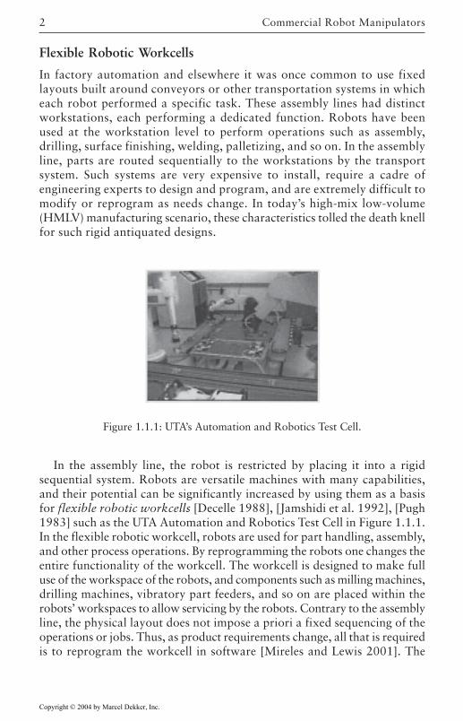
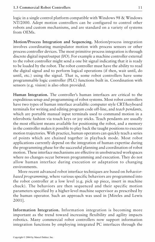
Figure 1.1.1: UTA’s Automation and Robotics Test Cell.
In the assembly line, the robot is restricted by placing it into a rigidsequential system. Robots are versatile machines with many capabilities,and their potential can be significantly increased by using them as a basisfor flexible robotic workcells [Decelle 1988], [Jamshidi et al. 1992], [Pugh1983] such as the UTA Automation and Robotics Test Cell in Figure 1.1.1.In the flexible robotic workcell, robots are used for part handling, assembly,and other process operations. By reprogramming the robots one changes theentire functionality of the workcell. The workcell is designed to make fulluse of the workspace of the robots, and components such as milling machines,drilling machines, vibratory part feeders, and so on are placed within therobots’ workspaces to allow servicing by the robots. Contrary to the assemblyline, the physical layout does not impose a priori a fixed sequencing of theoperations or jobs. Thus, as product requirements change, all that is requiredis to reprogram the workcell in software [Mireles and Lewis 2001]. The
Copyright © 2004 by Marcel Dekker, Inc.
3
workcell is ideally suited to emerging HMLV conditions in manufacturingand elsewhere.
The rising popularity of robotic workcells has taken emphasis away fromhardware design and placed new emphasis on innovative software techniquesand architectures that include planning, coordination, and control (PC&C)functions. A great deal of research into robot controllers has been requiredto give robots the flexibility, precision, and functionality needed in modernflexible workcells. The remainder of this book details such advanced controltechniques.
1.2 Commercial Robot Configurations and Types
Much of the information in this section was prepared by Mick Fitzgerald,who was then Manager at UTA’s Automation and Robotics Research Institute(ARRI).
Robots are highly reliable, dependable and technologically advancedfactory equipment. The majority of the world’s robots are supplied byestablished companies using reliable off-the-shelf component technologies.All commercial industrial robots have two physically separate basicelements—the manipulator arm and the controller. The basic architecture ofmost commercial robots is fundamentally the same, and consists of digitalservocontrolled electrical motor drives on serial-link kinematic machines,usually with no more than six axes (degrees of freedom). All are suppliedwith a proprietary controller. Virtually all robot applications requiresignificant design and implementation effort by engineers and technicians.What makes each robot unique is how the components are put together toachieve performance that yields a competitive product. The most importantconsiderations in the application of an industrial robot center on two issues:manipulation and integration.
Manipulator Performance
The combined effects of kinematic structure, axis drive mechanism design,and real-time motion control determine the major manipulation performancecharacteristics: reach and dexterity, pay load, quickness, and precision.Caution must be used when making decisions and comparisons based onmanufacturers’ published performance specifications because the methodsfor measuring and reporting them are not standardized across the industry.Usually motion testing, simulations, or other analysis techniques are used toverify performance for each application.
Reach is characterized by measuring the extent of the workspace describedby the robot motion and dexterity by the angular displacement of the
1.2 Commercial Robot Configurations and Types
Copyright © 2004 by Marcel Dekker, Inc.
Commercial Robot Manipulators4
individual joints. Some robots will have unusable spaces such as dead zones,singular poses, and wrist-wrap poses inside of the boundaries of their reach.
Payload weight is specified by the manufacturers of all industrial robots.Some manufacturers also specify inertial loading for rotational wrist axes. Itis common for the payload to be given for extreme velocity and reachconditions. Weight and inertia of all tooling, workpieces, cables and hosesmust be included as part of the payload.
Quickness is critical in determining throughput but difficult to determinefrom published robot specifications. Most manufacturers will specify amaximum speed of either individual joints or for a specific kinematic toolpoint. However, average speed in a working cycle is the quicknesscharacteristic of interest.
Precision is usually characterized by measuring repeatability. Virtuallyall robot manufacturers specify static position repeatability. Accuracy israrely specified, but it is likely to be at least four times larger thanrepeatability. Dynamic precision, or the repeatability and accuracy intracking position, velocity, and acceleration over a continuous path, is notusually specified.
Common Kinematic Configurations
All common commercial industrial robots are serial-link manipulators,usually with no more than six kinematically coupled axes of motion. Byconvention, the axes of motion are numbered in sequence as they areencountered from the base on out to the wrist. The first three axes accountfor the spatial positioning motion of the robot; their configurationdetermines the shape of the space through which the robot can be positioned.Any subsequent axes in the kinematic chain generally provide rotationalmotions to orient the end of the robot arm and are referred to as wristaxes. In a robotic wrist, three axes usually intersect to generate true
kinematic analysis of the spherical robot wrist mechanism. Note that inour 3-dimensional space, one requires three degrees of freedom for fullyindependent spatial positioning and three degrees of freedom for fullyindependent orientational positioning.
There are two primary types of motion that a robot axis can producein its driven link- either revolute or prismatic. Revolute joints areanthropomorphic (e.g. like human joints) while prismatic joints are ableto extend and retract like a car radio antenna. It is often useful to classifyrobots according to the orientation and type of their first three axes.There are four very common commercial robot configurations:Articulated, Type I SCARA, Type II SCARA, and Cartesian. Two otherconfigurations, Cylindrical and Spherical, are now much less common.
Copyright © 2004 by Marcel Dekker, Inc.
independent positioning in terms of 3-D orientation. See Appendix A for a
5
Appendix C contains the dynamics of some common robot manipulatorsfor use in controls simulation in this book.
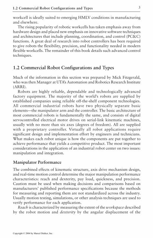
Figure 1.2.1: Articulated Arm. Six-axis CRS A465 arm (courtesy of CRSrobotics).
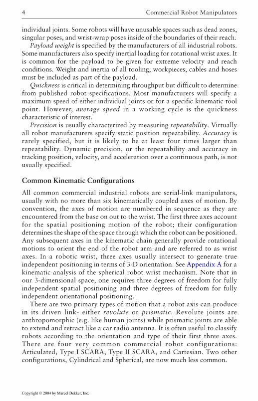
Figure 1.2.2: Type I SCARA Arm. High precision, high speed midsized SCARA I.(courtesy of Adept Technologies, Inc.).
1.2 Commercial Robot Configurations and Types
Copyright © 2004 by Marcel Dekker, Inc.
Commercial Robot Manipulators6
Articulated Arms. The variety of commercial articulated arms, most of
are re volute. The second and third axes are co-planar and work togetherto produce motion in a vertical plane. The first axis in the base is verticaland revolves the arm to sweep out a large work volume. Many differenttypes of drive mechanisms have been devised to allow wrist and forearmdrive motors and gearboxes to be mounted close to the first and secondaxis of rotation, thus minimizing the extended mass of the arm. Theworkspace efficiency of well designed articulated arms, which is the degreeof quick dexterous reach with respect to arm size, is unsurpassed by otherarm configurations when five or more degrees of freedom are needed. Amajor limiting factor in articulated arm performance is that the secondaxis has to work to lift both the subsequent arm structure and the payload. Historically, articulated arms have not been capable of achievingaccuracy as high as other arm configurations, as all axes have joint angleposition errors which are multiplied by link radius and accumulated forthe entire arm.
Type I SCARA. The Type I SCARA (selectively compliant assembly robot
in the horizontal plane. The arm structure is weight-bearing but the first andsecond axes do no lifting. The third axis of the Type I SCARA provides workvolume by adding a vertical or z axis. A fourth revolute axis will add rotationabout the z axis to control orientation in the horizontal plane. This type ofrobot is rarely found with more than four axes. The Type I SCARA is usedextensively in the assembly of electronic components and devices, and it isused broadly for the assembly of small- and mediumsized mechanicalassemblies.
configuration, differs from Type I in that the first axis is a long verticalprismatic z stroke which lifts the two parallel revolute axis and their links.For quickly moving heavier loads (over approximately 75 pounds) over longerdistance (more than about three feet), the Type II SCARA configuration ismore efficient than the Type I.
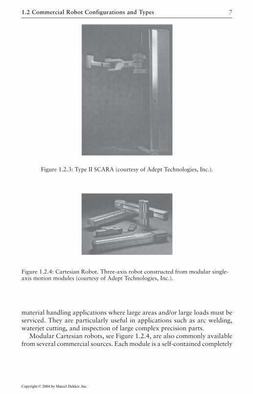
Cartesian Coordinate Robots. Cartesian coordinate robots use orthogonalprismatic axes, usually referred to as x, y, and z, to translate their end-effectoror payload through their rectangular workspace. One, two, or three revolutewrist axes may be added for orientation. Commercial robot companies supplyseveral types of Cartesian coordinate robots with workspace sizes rangingfrom a few cubic inches to tens of thousands of cubic feet, and payloadsranging to several hundred pounds. Gantry robots, which have an elevatedbridge structure, are the most common Cartesian style and are well suited to
Copyright © 2004 by Marcel Dekker, Inc.
which have six axes, is very large (Fig. 1.2.1). All of these robots’ axes
arm) arm, Figure 1.2.2, uses two parallel revolute joints to produce motion
Type II SCARA. The Type II SCARA, Figure 1.2.3, also a four axis
7
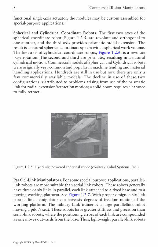
material handling applications where large areas and/or large loads must beserviced. They are particularly useful in applications such as arc welding,waterjet cutting, and inspection of large complex precision parts.
Modular Cartesian robots, see Figure 1.2.4, are also commonly availablefrom several commercial sources. Each module is a self-contained completely
Figure 1.2.3: Type II SCARA (courtesy of Adept Technologies, Inc.).
Figure 1.2.4: Cartesian Robot. Three-axis robot constructed from modular single-axis motion modules (courtesy of Adept Technologies, Inc.).
1.2 Commercial Robot Configurations and Types
Copyright © 2004 by Marcel Dekker, Inc.
Commercial Robot Manipulators8
functional single-axis actuator; the modules may be custom assembled forspecial-purpose applications.
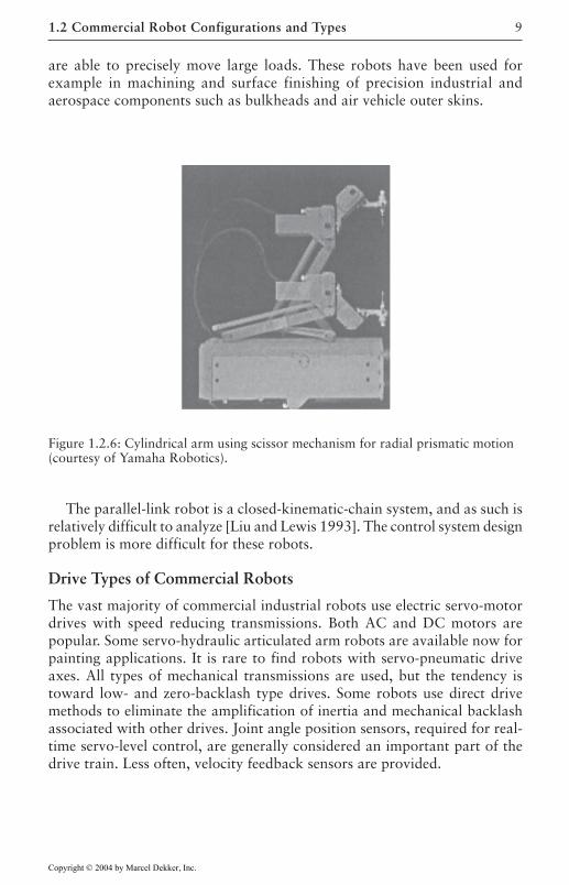
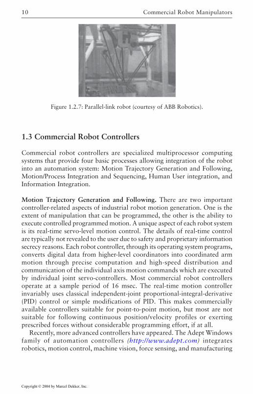
Spherical and Cylindrical Coordinate Robots. The first two axes of thespherical coordinate robot, Figure 1.2.5, are revolute and orthogonal toone another, and the third axis provides prismatic radial extension. Theresult is a natural spherical coordinate system with a spherical work volume.The first axis of cylindrical coordinate robots, Figure 1.2.6, is a revolutebase rotation. The second and third are prismatic, resulting in a naturalcylindrical motion. Commercial models of Spherical and Cylindrical robotswere originally very common and popular in machine tending and materialhandling applications. Hundreds are still in use but now there are only afew commercially available models. The decline in use of these twoconfigurations is attributed to problems arising from use of the prismaticlink for radial extension/retraction motion; a solid boom requires clearanceto fully retract.
Figure 1.2.5: Hydraulic powered spherical robot (courtesy Kohol Systems, Inc.).
Parallel-Link Manipulators. For some special purpose applications, parallel-link robots are more suitable than serial link robots. These robots generallyhave three or six links in parallel, each link attached to a fixed base and to amoving working platform. See Figure 1.2.7. With proper design, a six-linkparallel-link manipulator can have six degrees of freedom motion of theworking platform. The military Link trainer is a large parallellink robotmoving a pilot’s seat. These robots have greater stiffness and precision thanserial-link robots, where the positioning errors of each link are compoundedas one moves outwards from the base. Thus, lightweight parallel-link robots
Copyright © 2004 by Marcel Dekker, Inc.
9
are able to precisely move large loads. These robots have been used forexample in machining and surface finishing of precision industrial andaerospace components such as bulkheads and air vehicle outer skins.
Figure 1.2.6: Cylindrical arm using scissor mechanism for radial prismatic motion(courtesy of Yamaha Robotics).
The parallel-link robot is a closed-kinematic-chain system, and as such isrelatively difficult to analyze [Liu and Lewis 1993]. The control system designproblem is more difficult for these robots.
Drive Types of Commercial Robots
The vast majority of commercial industrial robots use electric servo-motordrives with speed reducing transmissions. Both AC and DC motors arepopular. Some servo-hydraulic articulated arm robots are available now forpainting applications. It is rare to find robots with servo-pneumatic driveaxes. All types of mechanical transmissions are used, but the tendency istoward low- and zero-backlash type drives. Some robots use direct drivemethods to eliminate the amplification of inertia and mechanical backlashassociated with other drives. Joint angle position sensors, required for real-time servo-level control, are generally considered an important part of thedrive train. Less often, velocity feedback sensors are provided.
1.2 Commercial Robot Configurations and Types
Copyright © 2004 by Marcel Dekker, Inc.
Commercial Robot Manipulators10
1.3 Commercial Robot Controllers
Commercial robot controllers are specialized multiprocessor computingsystems that provide four basic processes allowing integration of the robotinto an automation system: Motion Trajectory Generation and Following,Motion/Process Integration and Sequencing, Human User integration, andInformation Integration.
Motion Trajectory Generation and Following. There are two importantcontroller-related aspects of industrial robot motion generation. One is theextent of manipulation that can be programmed, the other is the ability toexecute controlled programmed motion. A unique aspect of each robot systemis its real-time servo-level motion control. The details of real-time controlare typically not revealed to the user due to safety and proprietary informationsecrecy reasons. Each robot controller, through its operating system programs,converts digital data from higher-level coordinators into coordinated armmotion through precise computation and high-speed distribution andcommunication of the individual axis motion commands which are executedby individual joint servo-controllers. Most commercial robot controllersoperate at a sample period of 16 msec. The real-time motion controllerinvariably uses classical independent-joint proportional-integral-derivative(PID) control or simple modifications of PID. This makes commerciallyavailable controllers suitable for point-to-point motion, but most are notsuitable for following continuous position/velocity profiles or exertingprescribed forces without considerable programming effort, if at all.
Recently, more advanced controllers have appeared. The Adept Windowsfamily of automation controllers (http://www.adept.com) integratesrobotics, motion control, machine vision, force sensing, and manufacturing
Figure 1.2.7: Parallel-link robot (courtesy of ABB Robotics).
Copyright © 2004 by Marcel Dekker, Inc.
11
logic in a single control platform compatible with Windows 98 & WindowsNT/2000. Adept motion controllers can be configured to control otherrobots and custom mechanisms, and are standard on a variety of systemsfrom OEMs.
Motion/Process Integration and Sequencing. Motion/process integrationinvolves coordinating manipulator motion with process sensors or otherprocess controller devices. The most primitive process integration is throughdiscrete digital input/output (I/O). For example a machine controller externalto the robot controller might send a one bit signal indicating that it is readyto be loaded by the robot. The robot controller must have the ability to readthe digital signal and to perform logical operations (if then, wait until, dountil, etc.) using the signal. That is, some robot controllers have someprogrammable logic controller (PLC) functions built in. Coordination withsensors (e.g. vision) is also often provided.
Human Integration. The controller’s human interfaces are critical to theexpeditious setup and programming of robot systems. Most robot controllershave two types of human interface available: computer style CRT/keyboardterminals for writing and editing program code off-line, and teach pendants,which are portable manual input terminals used to command motion in atelerobotic fashion via touch keys or joy sticks. Teach pendants are usuallythe most efficient means available for positioning the robot, and a memoryin the controller makes it possible to play back the taught positions to executemotion trajectories. With practice, human operators can quickly teach a seriesof points which are chained together in playback mode. Most robotapplications currently depend on the integration of human expertise duringthe programming phase for the successful planning and coordination of robotmotion. These interface mechanisms are effective in unobstructed workspaceswhere no changes occur between programming and execution. They do notallow human interface during execution or adaptation to changingenvironments.
More recent advanced robot interface techniques are based on behavior-based programming, where various specific behaviors are programmed intothe robot controller at a low level (e.g. pick up piece, insert in machinechuck). The behaviors are then sequenced and their specific motionparameters specified by a higher-level machine supervisor as prescribed bythe human operator. Such an approach was used in [Mireles and Lewis2001].
Information Integration. Information integration is becoming moreimportant as the trend toward increasing flexibility and agility impactsrobotics. Many commercial robot controllers now support informationintegration functions by employing integrated PC interfaces through the
1.3 Commercial Robot Controllers
Copyright © 2004 by Marcel Dekker, Inc.
Commercial Robot Manipulators12
communications ports (e.g. RS-232), or in some through direct connectionsto the robot controller data bus. Recent integration efforts are making itpossible to interface robotic workcells to the internet to allow remote sitemonitoring and control. There are many techniques for this, the mostconvenient of which is Lab VIEW 6.1, which doe not require programmingin Java.
1.4 Sensors
Much of the information in this section was prepared by Kok-Meng Lee[Lewis 1998]. Sensors and actuators [Tzou and Fukuda 1992] function astransducers, devices through which high-level workcell Planning,Coordination, and Control systems interface with the hardware componentsthat make up the workcell. Sensors are a vital element as they convert statesof physical devices into signals appropriate for input to the workcell PC&Ccontrol system; inappropriate sensors can introduce errors that make properoperation impossible no matter how sophisticated or expensive the PC&Csystem, while innovative selection of sensors can make the control and co-ordination problem much easier.
Sensors are of many different types and have many distinct uses. Havingin mind an analogy with biological systems, proprioceptors are sensorsinternal to a device that yield information about the internal state of thatdevice (e.g. robot arm joint-angle sensors). Exteroceptors yield informationabout other hardware external to a device. Sensors yield outputs that areeither analog or digital; digital sensors often provide information about thestatus of a machine or resource (gripper open or closed, machine loaded, jobcomplete). Sensors produce outputs that are required at all levels of the PC&Chierarchy, including uses for:
• servo-level feedback control (usually analog proprioceptors)• process monitoring and coordination (often digital exteroceptors or part
inspection sensors such as vision)• failure and safety monitoring (often digital—e.g. contact sensor,
pneumatic pressure-loss sensor)• quality control inspection (often vision or scanning laser).
Sensor output data must often be processed to convert it into a formmeaningful for PC&C purposes. The sensor plus required signal processingis shown as a Virtual Sensor. It functions as a data abstraction—a set of dataplus operations on that data (e.g. camera, plus framegrabber, plus signalprocessing algorithms such as image enhancement, edge detection,
Copyright © 2004 by Marcel Dekker, Inc.
13
segmentation, etc.). Some sensors, including the proprioceptors needed forservo-level feedback control, are integral parts of their host devices, and soprocessing of sensor data and use of the data occurs within that device; then,the sensor data is incorporated at the servocontrol level or MachineCoordination level. Other sensors, often vision systems, rival the robotmanipulator in sophistication and are coordinated by a Job Coordinator,which treats them as valuable shared resources whose use is assigned to jobsthat need them by some priority assignment (e.g. dispatching) scheme. Aninteresting coordination problem is posed by so-called active sensing, where,e.g., a robot may hold a scanning camera, and the camera effectively takescharge of the motion coordination problem, directing the robot where tomove to effect the maximum reduction in entropy (increase in information)with subsequent images.
Types of Sensors
This section summarizes sensors from an operational point of view. Moreinformation on functional and physical principles can be found in [Fraden1993], [Fu et al. 1987], [Snyder 1985].
Tactile Sensors. Tactile sensors rely on physical contact with external objects.Digital sensors such as limit switches, microswitches, and vaccuum devicesgive binary information on whether contact occurs or not. Sensors areavailable to detect the onset of slippage. Analog sensors such as spring-loadedrods give more information. Tactile sensors based on rubberlike carbon- orsilicon-based elastomers with embedded electrical or mechanical componentscan provide very detailed information about part geometry, location, andmore. Elastomers can contain resistive or capacitive elements whose electricalproperties change as the elastomer conmpresses. Designs based on LSItechnology can produce tactile grid pads with, e.g., 64×64 ‘forcel’ points ona single pad. Such sensors produce ‘tactile images’ that have properties akinto digital images from a camera and require similar data processing.Additional tactile sensors fall under the classification of ‘force sensors’discussed subsequently.
Proximity and Distance Sensors. The noncontact proximity sensors includedevices based on the Hall effect or inductive devices based on theelectromagnetic effect that can detect ferrous materials within about 5 mm.Such sensors are often digital, yielding binary information about whether ornot an object is near. Capacitance-based sensors detect any nearby solid orliquid with ranges of about 5mm. Optical and ultrasound sensors have longerranges.
1.4 Sensors
Copyright © 2004 by Marcel Dekker, Inc.
Commercial Robot Manipulators14
Distance sensors include time-of-flight rangefinder devices such as sonarand lasers. The commercially available Polaroid sonar offers accuracy ofabout 1 in. up to 5 feet, with angular sector accuracy of about 15 deg. For360 deg. coverage in navigation applications for mobile robots, both scanningsonars and ring-mounted multiple sonars are available. Sonar is typicallynoisy with spurious readings, and requires low-pass filtering and other dataprocessing aimed at reducing the false alarm rate. The more expensive laserrangefinders are extremely accurate in distance and have very high angularresolution.
Position, Velocity, and Acceleration Sensors. Linear position-measuringdevices include linear potentiometers and the sonar and laser rangefindersjust discussed. Linear velocity sensors may be laser- or sonar-based Doppler-effect devices.
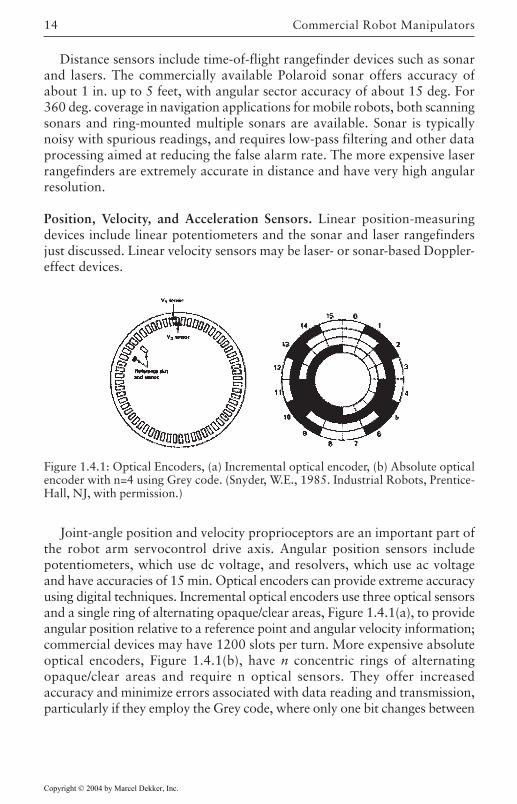
Figure 1.4.1: Optical Encoders, (a) Incremental optical encoder, (b) Absolute opticalencoder with n=4 using Grey code. (Snyder, W.E., 1985. Industrial Robots, Prentice-Hall, NJ, with permission.)
Joint-angle position and velocity proprioceptors are an important part ofthe robot arm servocontrol drive axis. Angular position sensors includepotentiometers, which use dc voltage, and resolvers, which use ac voltageand have accuracies of 15 min. Optical encoders can provide extreme accuracyusing digital techniques. Incremental optical encoders use three optical sensorsand a single ring of alternating opaque/clear areas, Figure 1.4.1(a), to provideangular position relative to a reference point and angular velocity information;commercial devices may have 1200 slots per turn. More expensive absoluteoptical encoders, Figure 1.4.1(b), have n concentric rings of alternatingopaque/clear areas and require n optical sensors. They offer increasedaccuracy and minimize errors associated with data reading and transmission,particularly if they employ the Grey code, where only one bit changes between
Copyright © 2004 by Marcel Dekker, Inc.
15
two consecutive sectors. Accuracy is 3600/2n with commercial devices havingn=12 or so.
Gyros have good accuracy if repeatability problems associated with driftare compensated for. Directional gyros have accuracies of about 1.5 deg.Vertical gyros have accuracies of 0.5 deg and are available to measuremultiaxis motion (e.g. pitch and roll). Rate gyros measure velocities directlywith thresholds of 0.05 deg/sec or so.
Various sorts of accelerometers are available based on strain gauges (nextparagraph), gyros, or crystal properties. Commercial devices are availableto measure accelerations along three axes. A popular new technology involvesmicroelectromechanical systems (MEMS), which are either surface or bulkmicromachined devices. MEMS accelerometers are very small, inexpensive,robust, and accurate. MEMS sensors have especially been used in theautomotive industry [Eddy 1998].
Force and Torque Sensors. Various torque sensors are available, though theyare often not required; for instance, the internal torques at the joints of arobot arm can be computed from the motor armature currents. Torque sensorson a drilling tool, for instance, can indicate when tools are becoming dull.Linear force can be measured using load cells or strain gauges. A strain gaugeis an elastic sensor whose resistance is a function of applied strain ordeformation. The piezoelectric effect, the generation of a voltage when aforce is applied, may also be used for force sensing. Other force sensingtechniques are based on vacuum diodes, quartz crystals (whose resonantfrequency changes with applied force), etc.
Robot arm force-torque wrist sensors are extremely useful in dexterousmanipulation tasks. Commercially available devices can measure both forceand torque along three perpendicular axes, providing full information aboutthe Cartesian force vector F. Standard transformations allow computationof forces and torques in other coordinates. Six-axis force-torque sensors arequite expensive.
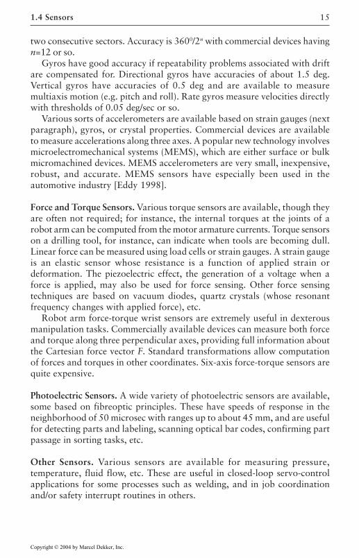
Photoelectric Sensors. A wide variety of photoelectric sensors are available,some based on fibreoptic principles. These have speeds of response in theneighborhood of 50 microsec with ranges up to about 45 mm, and are usefulfor detecting parts and labeling, scanning optical bar codes, confirming partpassage in sorting tasks, etc.
Other Sensors. Various sensors are available for measuring pressure,temperature, fluid flow, etc. These are useful in closed-loop servo-controlapplications for some processes such as welding, and in job coordinationand/or safety interrupt routines in others.
1.4 Sensors
Copyright © 2004 by Marcel Dekker, Inc.
Commercial Robot Manipulators16
Sensor Data Processing
Before any sensor can be used in a robotic workcell, it must be calibrated.Depending on the sensor, this could involve significant effort inexperimentation, computation, and tuning after installation. Manufacturersoften provide calibration procedures though in some cases, including vision,such procedures may not be obvious, requiring reference to the publishedscientific literature. Time-consuming recalibration may be needed after anymodifications to the system.
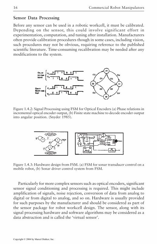
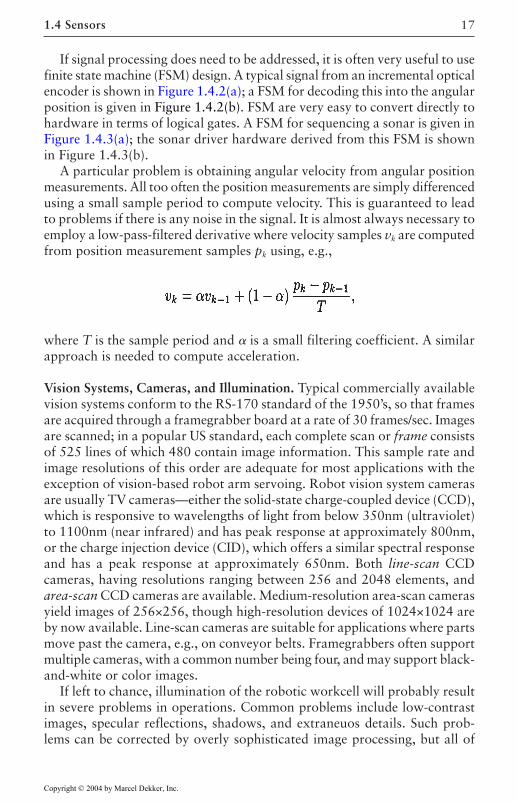
Figure 1.4.2: Signal Processing using FSM for Optical Encoders (a) Phase relations inincremental optical encoder output, (b) Finite state machine to decode encoder outputinto angular position. (Snyder 1985).
Figure 1.4.3: Hardware design from FSM. (a) FSM for sonar transducer control on amobile robot, (b) Sonar driver control system from FSM.
Particularly for more complex sensors such as optical encoders, significantsensor signal conditioning and processing is required. This might includeamplification of signals, noise rejection, conversion of data from analog todigital or from digital to analog, and so on. Hardware is usually providedfor such purposes by the manufacturer and should be considered as part ofthe sensor package for robot workcell design. The sensor, along with itssignal processing hardware and software algorithms may be considered as adata abstraction and is called the ‘virtual sensor’.
Copyright © 2004 by Marcel Dekker, Inc.
17
If signal processing does need to be addressed, it is often very useful to usefinite state machine (FSM) design. A typical signal from an incremental opticalencoder is shown in Figure 1.4.2(a); a FSM for decoding this into the angularposition is given in Figure 1.4.2(b). FSM are very easy to convert directly tohardware in terms of logical gates. A FSM for sequencing a sonar is given inFigure 1.4.3(a); the sonar driver hardware derived from this FSM is shownin Figure 1.4.3(b).
A particular problem is obtaining angular velocity from angular positionmeasurements. All too often the position measurements are simply differencedusing a small sample period to compute velocity. This is guaranteed to leadto problems if there is any noise in the signal. It is almost always necessary toemploy a low-pass-filtered derivative where velocity samples vk are computedfrom position measurement samples pk using, e.g.,
where T is the sample period and is a small filtering coefficient. A similarapproach is needed to compute acceleration.
Vision Systems, Cameras, and Illumination. Typical commercially availablevision systems conform to the RS-170 standard of the 1950’s, so that framesare acquired through a framegrabber board at a rate of 30 frames/sec. Imagesare scanned; in a popular US standard, each complete scan or frame consistsof 525 lines of which 480 contain image information. This sample rate andimage resolutions of this order are adequate for most applications with theexception of vision-based robot arm servoing. Robot vision system camerasare usually TV cameras—either the solid-state charge-coupled device (CCD),which is responsive to wavelengths of light from below 350nm (ultraviolet)to 1100nm (near infrared) and has peak response at approximately 800nm,or the charge injection device (CID), which offers a similar spectral responseand has a peak response at approximately 650nm. Both line-scan CCDcameras, having resolutions ranging between 256 and 2048 elements, andarea-scan CCD cameras are available. Medium-resolution area-scan camerasyield images of 256×256, though high-resolution devices of 1024×1024 areby now available. Line-scan cameras are suitable for applications where partsmove past the camera, e.g., on conveyor belts. Framegrabbers often supportmultiple cameras, with a common number being four, and may support black-and-white or color images.
If left to chance, illumination of the robotic workcell will probably resultin severe problems in operations. Common problems include low-contrastimages, specular reflections, shadows, and extraneuos details. Such prob-lems can be corrected by overly sophisticated image processing, but all of
1.4 Sensors
Copyright © 2004 by Marcel Dekker, Inc.
Commercial Robot Manipulators18
this can be avoided by some proper attention to details at the work-cell designstage. Illumination techniques include spectral filtering, selection of suitablespectral characteristics of the illumination source, diffuse-lighting techniques,backlighting (which produces easily processed silhouettes), structured-lighting(which provides additional depth information and simplifies object detectionand interpretation), and directional lighting.
Copyright © 2004 by Marcel Dekker, Inc.
19
REFERENCES
[Decelle 1988] Decelle, L.S., “Design of a Robotic Workstation For Compo-nent Insertions,” AT&T Technical Journal, March/April 1988, Volume67, Issue 2. pp 15–22.
[Eddy 1998] Eddy, D.S., and D.R.Sparks, “Application of MEMS technol-ogy in automotive sensors and actuators,” Proc. IEEE, vol. 86, no. 8,pp. 1747–1755, Aug. 1998.
[Fraden 1993] Fraden, J. AIP Handbook Of Modern Sensors, Physics, De-sign, and Applications, American Institute of Physics. 1993.
[Fu et al. 1987] Fu, K.S., R.C.Gonzalez, and C.S.G.Lee, Robotics, McGraw-Hill, New York, 1987.
[Jamshidi et al. 1992] Jamshidi, M., Lumia, R., Mullins, J., and Shahinpoor,M., 1992. Robotics and Manufacturing: Recent Trends in Re-search,Education, and Applications, Vol. 4, ASME Press, New York.
[Lewis and Fitzgerald 1997] Lewis, F.L., M.Fitzgerald, and K.Liu “Robotics,”in The Computer Science and Engineering Handbook, Allen B.Tucker,Jr. ed., Chapter 33, CRC Press, 1997.
[Lewis 1998] Lewis, F.L., “Robotics,” in Handbook of Mechanical Engi-neering, F.Kreith ed., chapter 14, CRC Press, 1998.
[Liu and Lewis 1993] Liu, K., F.L.Lewis, G.Lebret, and D.Taylor, “Thesingularities and dynamics of a Stewart Platform Manipulator,” J.Intelligent and Robotic Systems, vol. 8, pp. 287–308, 1993.
[Mireles and Lewis 2001] Mireles, J., and F.L.Lewis, “Intelligent Mate-rialHandling: Development and implementation of a matrix-based discrete-event controller,” IEEE Trans. Industrial Electronics, vol. 48, no. 6, pp.1087–1097, Dec. 2001.
Copyright © 2004 by Marcel Dekker, Inc.
REFERENCES20
[NAM 1998] National Assoc. Manufacturers Report, “Technology on theFactory Floor III,” ed. P.M.Swadimass, NAM Pub. Center, 1–800–637–3005, Aug. 1998.
[Pugh 1983] Pugh, A., ed., 1983. Robotic Technology, IEE Control Engi-neering Series 23, Pergrinus, London.
[Snyder 1985] Snyder, W.E., 1985, Industrial Robots: Computer Interfac-ing and Control, Prentice-Hall, Inc., Englewood Cliffs, New Jersey, USA.
[Tzou and Fukuda 1992] Tzou, H.S., and Fukuda, T., Precision Sensors,Actuators, and Systems, Kluwer Academic, 1992.
Copyright © 2004 by Marcel Dekker, Inc.
21
Chapter 2
Introduction to ControlTheory
In this chapter we review various control theory concepts that are used inthe control of robots. We first review the state-space formulation for bothlinear and nonlinear systems and present the stability concepts needed in thesequel. The chapter is intended to introduce modern control concepts, buteven readers with a background in control theory may wish to consult it fornotation and convenience.
2.1 Introduction
The control of robotic manipulators is a mature yet fruitful area for research,development, and manufacturing. Industrial robots are basically positioningand handling devices. Therefore, a useful robot is one that is able to controlits movement and the interactive forces and torques between the robot andits environment. This book is concerned with the control aspect of roboticmanipulators. To control usually requires the availability of a mathematicalmodel and of some sort of intelligence to act on the model. The mathematicalmodel of a robot is obtained from the basic physical laws governing itsmovement. Intelligence, on the other hand, requires sensory capabilities andmeans for acting and reacting to the sensed variables. These actions andreactions of the robot are the result of controller design.
In this chapter we review the concepts of control theory that are neededin this book. All proofs are omitted, but references are made to morespecialized books and papers where proofs are provided. Once a satisfactory
Copyright © 2004 by Marcel Dekker, Inc.
Introduction to Control Theory22
automatic control concepts presented in the current chapter may be used tomodify the actions and reactions of the robot to different stimuli. Subsequentchapters will therefore deal with the application of control principles to therobot equations. The particular controller used will depend on the complexityof the mathematical model, the application at hand, the available resources,and a host of other criteria.
We begin the chapter in section 2.2 with a review of the state-spacedescription for linear, continuous- and discrete-time systems. A similar reviewof nonlinear systems is presented in section 2.3. The Equilibria of nonlinearsystems is reviewed in section 2.4, while concepts of vector spaces is presentedin section 2.5. Stability theory is presented in section 2.6, which constitutesthe bulk of the chapter. In Section 2.7, Lyapunov stability results are presentedwhile input-output stability concepts are presented in section 2.8. Advancedstability concepts are compiled to make later developments more concise insection 2.9. In section 2.10 we review some useful theorems and lemmas. Insection 2.11 we the basic linear controller designs from a state-space pointof view, and the chapter is concluded in Section 2.12.
2.2 Linear State-Variable Systems
Many physical systems such as the robots considered in this book aredescribed by differential or difference equations. These describing equations,which are usually obtained from fundamental physical laws, provide thestarting point for the analysis and control of systems. There are, of course,some systems which are so complicated that describing differential (ordifference) equations are not available. We do not consider those systems inthis book.
In this section we study the state-space model of physical systems that arelinear. We limit ourselves to systems described by ordinary differentialequations which will lead to a finite-dimensional state space. Partialdifferential equations, leading to infinite-dimensional systems, are needed tostudy flexible robotic manipulators, but those are not considered in thistextbook. We stress that the material of this chapter is intended as a quickintroduction to these topics and will not be comprehensive. The readers arereferred to [Kailath 1980], [Antsaklis and Michel 1997] for more rigorouspresentations of linear control systems.
Continuous-Time Systems
A continuous-time system is said to be linear if it obeys the principle ofsuperposition] that is, if the output y1(t) results from the input u1(t) and theoutput y2(t) results from the input u2(t), then the output resulting from
Copyright © 2004 by Marcel Dekker, Inc.
model of the robot dynamics is obtained as described in Chapter 2, the
2.2 Linear State-Variable Systems 23
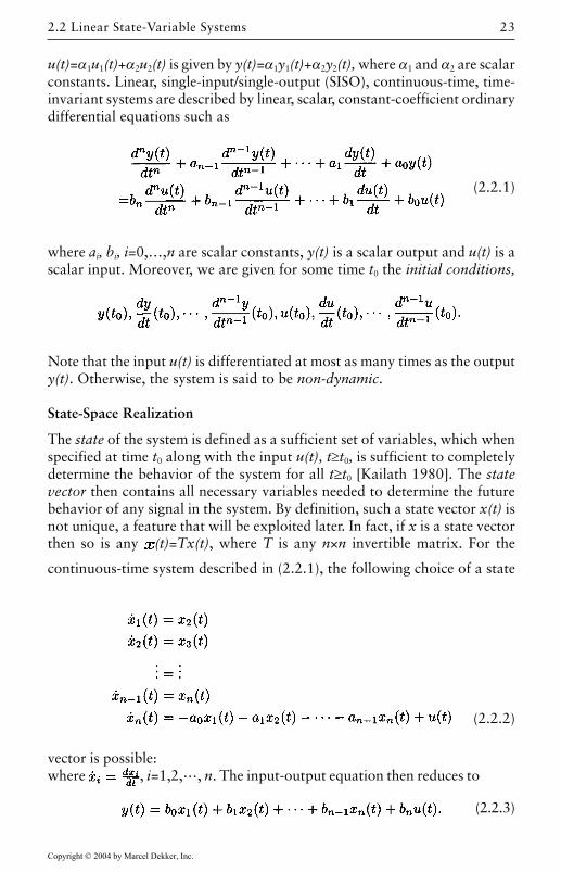
u(t)=α1u1(t)+α2u2(t) is given by y(t)=α1y1(t)+α2y2(t), where α1 and α2 are scalarconstants. Linear, single-input/single-output (SISO), continuous-time, time-invariant systems are described by linear, scalar, constant-coefficient ordinarydifferential equations such as
(2.2.1)
where ai, bi, i=0,…,n are scalar constants, y(t) is a scalar output and u(t) is ascalar input. Moreover, we are given for some time t0 the initial conditions,
Note that the input u(t) is differentiated at most as many times as the outputy(t). Otherwise, the system is said to be non-dynamic.
State-Space Realization
The state of the system is defined as a sufficient set of variables, which whenspecified at time t0 along with the input u(t), t≥t0, is sufficient to completelydetermine the behavior of the system for all t≥t0 [Kailath 1980]. The statevector then contains all necessary variables needed to determine the futurebehavior of any signal in the system. By definition, such a state vector x(t) isnot unique, a feature that will be exploited later. In fact, if x is a state vectorthen so is any (t)=Tx(t), where T is any n×n invertible matrix. For the
continuous-time system described in (2.2.1), the following choice of a state
vector is possible:where , i=1,2,…, n. The input-output equation then reduces to
(2.2.3)
(2.2.2)
Copyright © 2004 by Marcel Dekker, Inc.
Introduction to Control Theory24
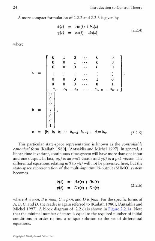
This particular state-space representation is known as the controllablecanonical form [Kailath 1980], [Antsaklis and Michel 1997]. In general, alinear, time-invariant, continuous-time system will have more than one inputand one output. In fact, u(t) is an m×1 vector and y(t) is a p×1 vector. Thedifferential equations relating u(t) to y(t) will not be presented here, but thestate-space representation of the multi-input/multi-output (MIMO) systembecomes
(2.2.6)
where A is n×n, B is n×m, C is p×n, and D is p×m. For the specific forms ofA, B, C, and D, the reader is again referred to [Kailath 1980], [Antsaklis andMichel 1997]. A block diagram of (2.2.6) is shown in Figure 2.2.1a. Notethat the minimal number of states is equal to the required number of initialconditions in order to find a unique solution to the set of differentialequations.
A more compact formulation of 2.2.2 and 2.2.3 is given by
(2.2.4)
where
(2.2.5)
Copyright © 2004 by Marcel Dekker, Inc.
2.2 Linear State-Variable Systems 25
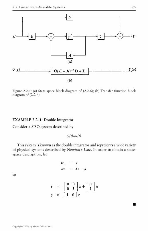
EXAMPLE 2.2–1: Double Integrator
Consider a SISO system described by
ÿ(t)=u(t)
This system is known as the double integrator and represents a wide varietyof physical systems described by Newton’s Law. In order to obtain a state-space description, let
so
Figure 2.2.1: (a) State-space block diagram of (2.2.6); (b) Transfer function blockdiagram of (2.2.6)
Copyright © 2004 by Marcel Dekker, Inc.
Introduction to Control Theory26
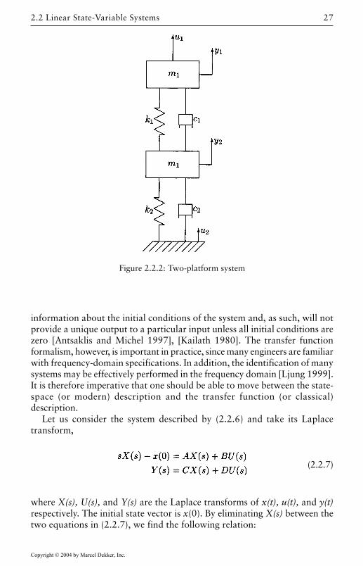
EXAMPLE 2.2–2: Two-Platform System
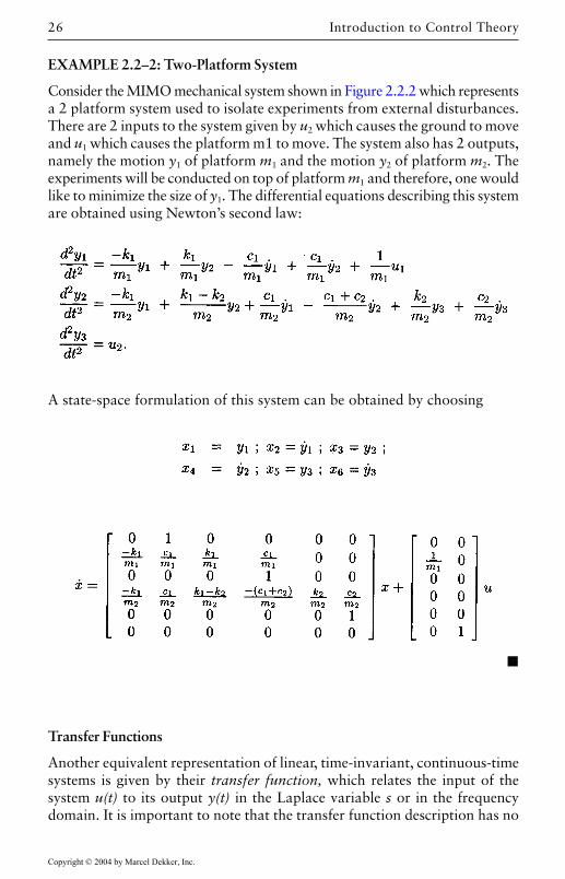
a 2 platform system used to isolate experiments from external disturbances.There are 2 inputs to the system given by u2 which causes the ground to moveand u1 which causes the platform m1 to move. The system also has 2 outputs,namely the motion y1 of platform m1 and the motion y2 of platform m2. Theexperiments will be conducted on top of platform m1 and therefore, one wouldlike to minimize the size of y1. The differential equations describing this systemare obtained using Newton’s second law:
A state-space formulation of this system can be obtained by choosing
Transfer Functions
Another equivalent representation of linear, time-invariant, continuous-timesystems is given by their transfer function, which relates the input of thesystem u(t) to its output y(t) in the Laplace variable s or in the frequencydomain. It is important to note that the transfer function description has no
Copyright © 2004 by Marcel Dekker, Inc.
Consider the MIMO mechanical system shown in Figure 2.2.2 which represents
2.2 Linear State-Variable Systems 27
information about the initial conditions of the system and, as such, will notprovide a unique output to a particular input unless all initial conditions arezero [Antsaklis and Michel 1997], [Kailath 1980]. The transfer functionformalism, however, is important in practice, since many engineers are familiarwith frequency-domain specifications. In addition, the identification of manysystems may be effectively performed in the frequency domain [Ljung 1999].It is therefore imperative that one should be able to move between the state-space (or modern) description and the transfer function (or classical)description.
Let us consider the system described by (2.2.6) and take its Laplacetransform,
(2.2.7)
where X(s), U(s), and Y(s) are the Laplace transforms of x(t), u(t), and y(t)respectively. The initial state vector is x(0). By eliminating X(s) between thetwo equations in (2.2.7), we find the following relation:
Figure 2.2.2: Two-platform system
Copyright © 2004 by Marcel Dekker, Inc.
Introduction to Control Theory28
Y(s)=[C(sI-A)-1B+D] U(s)+C(sI-A)-1x(0) (2.2.8)
As mentioned previously, the transfer function is obtained as the relationshipbetween the input U(s) and the output Y(s) when x(0)=0, that is,
Y(s)=[C(sI-A)-1B+D] U(s). (2.2.9)
The transfer function of this particular linear, time-invariant system is givenby
P(s)=C(sI-A)-1B+D (2.2.10)
Y(s)=P(s)U(s) (2.2.11)
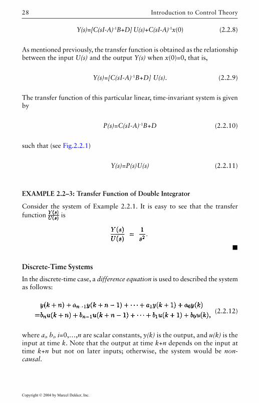
EXAMPLE 2.2–3: Transfer Function of Double Integrator
Consider the system of Example 2.2.1. It is easy to see that the transferfunction is
Discrete-Time Systems
In the discrete-time case, a difference equation is used to described the systemas follows:
(2.2.12)
where ai, bi, i=0,…,n are scalar constants, y(k) is the output, and u(k) is theinput at time k. Note that the output at time k+n depends on the input attime k+n but not on later inputs; otherwise, the system would be non-causal.
Copyright © 2004 by Marcel Dekker, Inc.
such that (see Fig.2.2.1)
2.2 Linear State-Variable Systems 29
The input-output equation then reduces to
y(k)=b0x1(k)+b1x2(k)+…+ bn-1xn(k)+u(k) (2.2.14)
A more compact formulation of (2.2.7) and (2.2.8) is given by
(2.2.15)
where
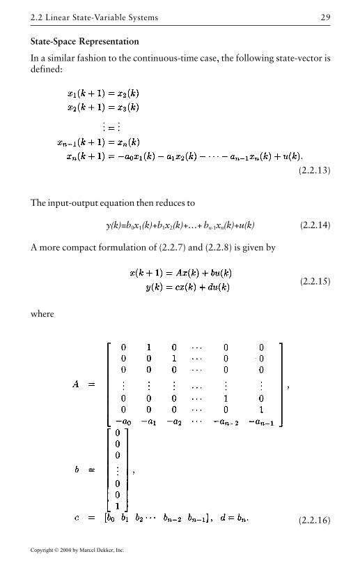
State-Space Representation
In a similar fashion to the continuous-time case, the following state-vector isdefined:
(2.2.13)
(2.2.16)
Copyright © 2004 by Marcel Dekker, Inc.
Introduction to Control Theory30
The MIMO case is similar to the continuous-time case and is given by
(2.2.17)
where A is n×n, B is n×m, C is p×n, and D is p×m.In many practical cases, such as in the control of robots, the system is a
continuous-time system, but the controller is implemented using digitalhardware. This will require the designer to translate between continuous-and discrete-time systems. There are many different approaches to“discretizing” a continuous-time system, some of which are discussed in
problem is referred to [Åström and Wittenmark 1996], [Franklin et al.1997].
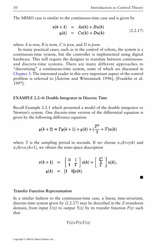
EXAMPLE 2.2–4: Double Integrator in Discrete Time
Recall Example 2.2.1 which presented a model of the double integrator orNewton’s system. One discrete-time version of the differential equation isgiven by the following difference equation
where T is the sampling period in seconds. If we choose x1(k)=y(k) andx2(k)=x1(k+1), we obtain the state-space description
Transfer Function Representation
In a similar fashion to the continuous-time case, a linear, time-invariant,discrete-time system given by (2.2.17) may be described in the Z-transformdomain, from input U(z) to output Y(z) by its transfer function P(z) suchthat
Y(z)=P(z)U(z)
Copyright © 2004 by Marcel Dekker, Inc.
Chapter 3. The interested reader in this very important aspect of the control
31
where
P(z)=C(zI-A)-1B+D
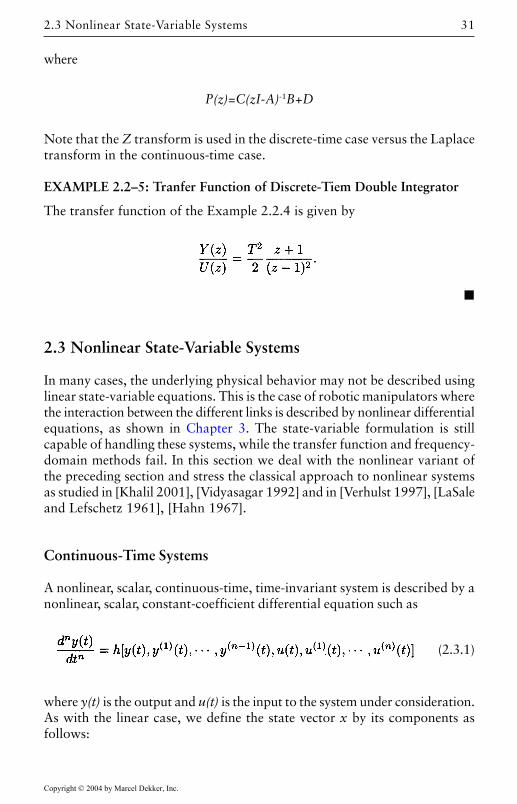
Note that the Z transform is used in the discrete-time case versus the Laplacetransform in the continuous-time case.
EXAMPLE 2.2–5: Tranfer Function of Discrete-Tiem Double Integrator
The transfer function of the Example 2.2.4 is given by
2.3 Nonlinear State-Variable Systems
In many cases, the underlying physical behavior may not be described usinglinear state-variable equations. This is the case of robotic manipulators wherethe interaction between the different links is described by nonlinear differential
capable of handling these systems, while the transfer function and frequency-domain methods fail. In this section we deal with the nonlinear variant ofthe preceding section and stress the classical approach to nonlinear systemsas studied in [Khalil 2001], [Vidyasagar 1992] and in [Verhulst 1997], [LaSaleand Lefschetz 1961], [Hahn 1967].
Continuous-Time Systems
A nonlinear, scalar, continuous-time, time-invariant system is described by anonlinear, scalar, constant-coefficient differential equation such as
(2.3.1)
where y(t) is the output and u(t) is the input to the system under consideration.As with the linear case, we define the state vector x by its components asfollows:
2.3 Nonlinear State-Variable Systems
Copyright © 2004 by Marcel Dekker, Inc.
equations, as shown in Chapter 3. The state-variable formulation is still
Introduction to Control Theory32
The output equation then reduces to:
y(t)=x1(t) (2.3.3)
A more compact formulation of (2.3.2) and (2.3.3) is given by
(2.3.4)
where
U(t)=[u(t) u(1)(t)…u(n-1) (t)]T
and
c=[1 0 0…0]. (2.3.5)
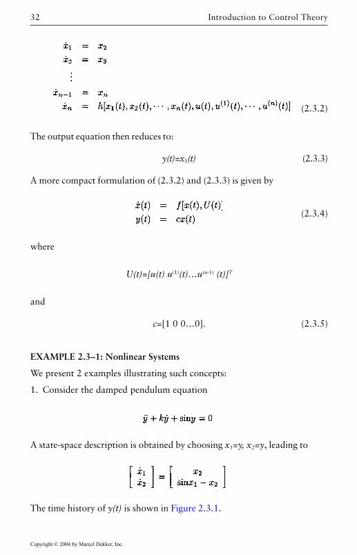
EXAMPLE 2.3–1: Nonlinear Systems
We present 2 examples illustrating such concepts:
1. Consider the damped pendulum equation
A state-space description is obtained by choosing x1=y, x2=y, leading to
(2.3.2)
Copyright © 2004 by Marcel Dekker, Inc.
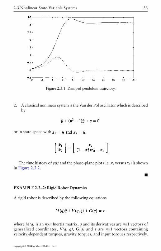
The time history of y(t) is shown in Figure 2.3.1.
33
2. A classical nonlinear system is the Van der Pol oscillator which is describedby
or in state-space with
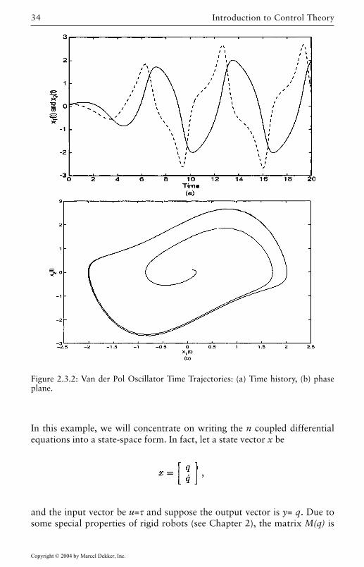
The time history of y(t) and the phase-plane plot (i.e. x2 versus x1) is shown
EXAMPLE 2.3–2: Rigid Robot Dynamics
A rigid robot is described by the following equations
where M(q) is an n×n Inertia matrix, q and its derivatives are n×1 vectors ofgeneralized coordinates, V(q, q), G(q) and τ are n×1 vectors containingvelocity-dependent torques, gravity torques, and input torques respectively.
Figure 2.3.1: Damped pendulum trajectory.
2.3 Nonlinear State-Variable Systems
Copyright © 2004 by Marcel Dekker, Inc.
in Figure 2.3.2.
Introduction to Control Theory34
In this example, we will concentrate on writing the n coupled differentialequations into a state-space form. In fact, let a state vector x be
and the input vector be u=τ and suppose the output vector is y= q. Due to
Figure 2.3.2: Van der Pol Oscillator Time Trajectories: (a) Time history, (b) phaseplane.
Copyright © 2004 by Marcel Dekker, Inc.
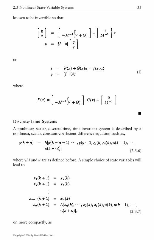
some special properties of rigid robots (see Chapter 2), the matrix M(q) is
35
known to be invertible so that
or
(1)
where
Discrete-Time Systems
A nonlinear, scalar, discrete-time, time-invariant system is described by anonlinear, scalar, constant-coefficient difference equation such as,
where y(.) and u are as defined before. A simple choice of state variables willlead to
(2.3.6)
or, more compactly, as
(2.3.7)
2.3 Nonlinear State-Variable Systems
Copyright © 2004 by Marcel Dekker, Inc.
Introduction to Control Theory36
where U(k) and c are defined similarly to those given in equation (2.3.4).
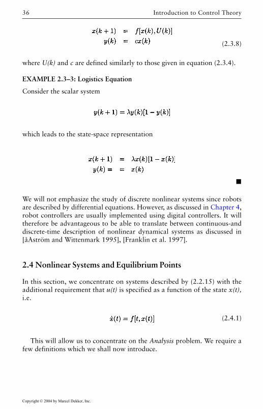
EXAMPLE 2.3–3: Logistics Equation
Consider the scalar system
which leads to the state-space representation
We will not emphasize the study of discrete nonlinear systems since robots
robot controllers are usually implemented using digital controllers. It willtherefore be advantageous to be able to translate between continuous-anddiscrete-time description of nonlinear dynamical systems as discussed in[åAström and Wittenmark 1995], [Franklin et al. 1997].
2.4 Nonlinear Systems and Equilibrium Points
In this section, we concentrate on systems described by (2.2.15) with theadditional requirement that u(t) is specified as a function of the state x(t),i.e.
(2.4.1)
This will allow us to concentrate on the Analysis problem. We require afew definitions which we shall now introduce.
(2.3.8)
Copyright © 2004 by Marcel Dekker, Inc.
are described by differential equations. However, as discussed in Chapter 4,
37
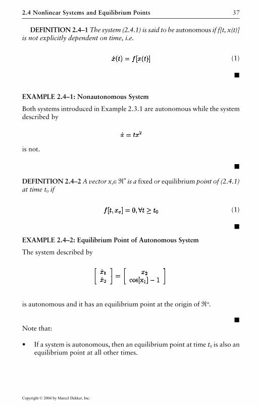
DEFINITION 2.4–1 The system (2.4.1) is said to be autonomous if f[t, x(t)]is not explicitly dependent on time, i.e.
(1)
EXAMPLE 2.4–1: Nonautonomous System
Both systems introduced in Example 2.3.1 are autonomous while the systemdescribed by
is not.
DEFINITION 2.4–2 A vector xe∈n is a fixed or equilibrium point of (2.4.1)
at time t0 if
(1)
EXAMPLE 2.4–2: Equilibrium Point of Autonomous System
The system described by
is autonomous and it has an equilibrium point at the origin of n.
Note that:
• If a system is autonomous, then an equilibrium point at time t0 is also anequilibrium point at all other times.
2.4 Nonlinear Systems and Equilibrium Points
Copyright © 2004 by Marcel Dekker, Inc.
Introduction to Control Theory38
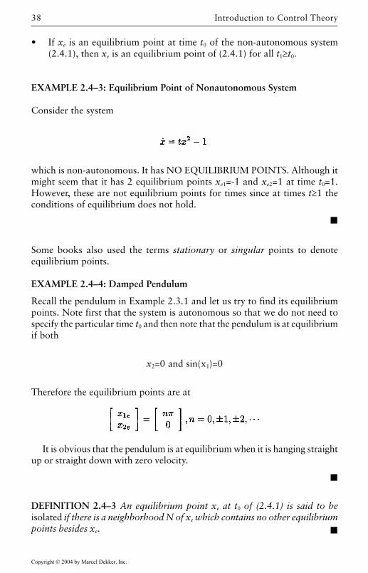
• If xe is an equilibrium point at time t0 of the non-autonomous system(2.4.1), then xe is an equilibrium point of (2.4.1) for all t1≥t0.
EXAMPLE 2.4–3: Equilibrium Point of Nonautonomous System
Consider the system
which is non-autonomous. It has NO EQUILIBRIUM POINTS. Although itmight seem that it has 2 equilibrium points xe1=-1 and xe2=1 at time t0=1.However, these are not equilibrium points for times since at times t≥1 theconditions of equilibrium does not hold.
Some books also used the terms stationary or singular points to denoteequilibrium points.
EXAMPLE 2.4–4: Damped Pendulum
Recall the pendulum in Example 2.3.1 and let us try to find its equilibriumpoints. Note first that the system is autonomous so that we do not need tospecify the particular time t0 and then note that the pendulum is at equilibriumif both
x2=0 and sin(x1)=0
Therefore the equilibrium points are at
It is obvious that the pendulum is at equilibrium when it is hanging straightup or straight down with zero velocity.
DEFINITION 2.4–3 An equilibrium point xe at t0 of (2.4.1) is said to beisolated if there is a neighborhood N of xe which contains no other equilibriumpoints besides xe.
Copyright © 2004 by Marcel Dekker, Inc.
39
EXAMPLE 2.4–5: Equilibrium Points of Pendulum
The equilibrium points of the pendulum are isolated. On the other hand, asystem described by =0 has for equilibrium points any point in R andtherefore, none of its equilibrium points is isolated.
2.5 Vector Spaces, Norms, and Inner Products
In this section, we will discuss some properties of nonlinear differentialequations and their solutions. We will need many concepts such as vectorspaces and norms which we will introduce briefly. The reader is referred to[Boyd and Barratt], [Desoer and Vidyasagar 1975], [Khalil 2001] for proofsand details.
Linear Vector Spaces
In most of our applications, we need to deal with (linear) real and complexvector spaces which are defined subsequently.
DEFINITION 2.5–1 A real linear vector space (resp. complex linear vectorspace is a set V, equipped with 2 binary operations: the addition (+) and thescalar multiplication (.) such that
2.5 Vector Spaces, Norms, and Inner Products
Copyright © 2004 by Marcel Dekker, Inc.
Introduction to Control Theory40
8. For each x∈V, we have 1.x=x where 1 is the unity in (resp. in ).
EXAMPLE 2.5–1: Vector Spaces
The following are linear vector spaces with the associated scalar fields:
with , and n with .
DEFINITION 2.5–2 A subset M of a vector space V is a subspace if it is alinear vector space in its own right. One necessary condition for M to be asubspace is that it contains the zero vector.
We can equip a vector space with many functions. One of which is theinner product which takes two vectors in V to a scalar either in or in theother one is the norm of a vector which takes a vector in V to a positivevalue in . The following section discusses the norms of vectors which isthen followed by a section on inner products.
Norms of Signals and Systems
A norm is a generalization of the ideas of distance and length. As stabilitytheory is usually concerned with the size of some vectors and matrices, wegive here a brief description of some norms that will be used in this book. Wewill consider first the norms of vectors defined on a vector space X with theassociated scalar field of real numbers then introduce the matrix inducednorms, the function norms and finally the system-induced norms or operatorgains.
Vector Norms
We start our discussion of norms by reviewing the most familiar normedspaces, that is the spaces of vectors with constant entries. In the following,||a|| denotes the absolute value of a for a real a or the magnitude of a if a iscomplex.
DEFINITION 2.5–3 A norm ||·|| of a vector x is a real-valued function definedon the vector space X such that
1. ||x||>0 for all x∈X, with ||x||=0 if and only if x=0.
2. ||αx||=|α|||x|| for all x∈X and any scalar α.
Copyright © 2004 by Marcel Dekker, Inc.
41
3. ||x+y||≤||x||+|y|| for all x,y ∈X,
EXAMPLE 2.5–2: Vector Norms (1)
The following are common norms in X=n where n is the set of n×1 vectorswith real components.
1. 1-norm:
2. 2-norm: also known as the Euclidean norm
3. p-norm:
4. 8-norm:
EXAMPLE 2.5–3: Vector Norms (2)
Consider the vector
Then, ||x||1=5, ||x||2=2 and ||x||∞=2.
We now present an important property of norms of vectors n in which willbe useful in the sequel.
LEMMA 2.5–1: Let ||x||a and ||x||b be any two norms of a vector x∈. Thenthere exists finite positive constants k1 and k2 such that
The two norms in the lemma are said to be equivalent and this particularproperty will hold for any two norms on .
2.5 Vector Spaces, Norms, and Inner Products
Copyright © 2004 by Marcel Dekker, Inc.
Introduction to Control Theory42
EXAMPLE 2.5–4: Equivalent Vector Norms
1. It can be shown that for
2. Consider again the vector of Example 2.5.3. Then we can check that
Matrix Norms
In systems applications, a particular vector x may be operated on by a matrixA to obtain another vector y=Ax. In order to relate the sizes of x and Ax wedefine the induced matrix norm as follows.
DEFINITION 2.5–4 Let ||x|| be a given norm of x∈. Then each m×n matrixA, has an induced norm defined by
where sup stands for the supremum.It is always imperative to check that the proposed norms verify the
conditions of Definition 2.5.3. The newly defined matrix norm may also beshown to satisfy
||AB||i ≤ ||A||i ||B||i
for all n×m matrices A and all m×p matrices B.
Copyright © 2004 by Marcel Dekker, Inc.
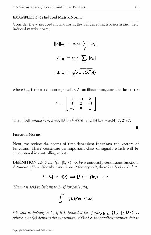
43
EXAMPLE 2.5–5: Induced Matrix Norms
Consider the ∞ induced matrix norm, the 1 induced matrix norm and the 2induced matrix norm,
where max is the maximum eigenvalue. As an illustration, consider the matrix
Then, ||A||i1=max(4, 4, 5)=5, ||A||i2=4.4576, and ||A||i∞= max(4, 7, 2)=7.
Function Norms
Next, we review the norms of time-dependent functions and vectors offunctions. These constitute an important class of signals which will beencountered in controlling robots.
DEFINITION 2.5–5 Let f(.): [0, ∞)→R be a uniformly continuous function.A function f is uniformly continuous if for any >0, there is a () such that
Then, f is said to belong to Lp if for p∈[1, ∞),
f is said to belong to L∞ if it is bounded i.e. if where sup f(t) denotes the supremum of f9t) i.e. the smallest number that is
2.5 Vector Spaces, Norms, and Inner Products
Copyright © 2004 by Marcel Dekker, Inc.
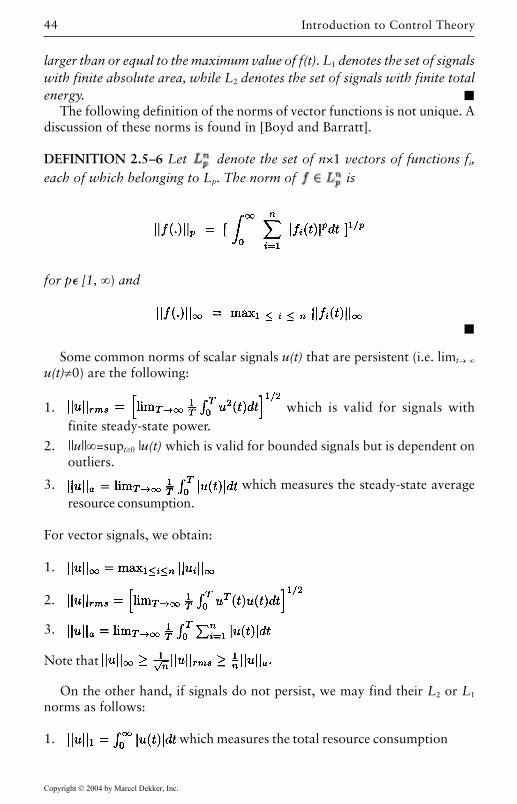
Introduction to Control Theory44
larger than or equal to the maximum value of f(t). L1 denotes the set of signalswith finite absolute area, while L2 denotes the set of signals with finite totalenergy.
The following definition of the norms of vector functions is not unique. Adiscussion of these norms is found in [Boyd and Barratt].
DEFINITION 2.5–6 Let denote the set of n×1 vectors of functions fi,each of which belonging to Lp. The norm of is
for p [1, ∞) and
Some common norms of scalar signals u(t) that are persistent (i.e. limt→ ∞u(t)≠0) are the following:
1. which is valid for signals withfinite steady-state power.
2. ||u||∞=supt≥0 |u(t) which is valid for bounded signals but is dependent onoutliers.
3. which measures the steady-state averageresource consumption.
For vector signals, we obtain:
1.
2.
3.
Note that
On the other hand, if signals do not persist, we may find their L2 or L1
norms as follows:
1. which measures the total resource consumption
Copyright © 2004 by Marcel Dekker, Inc.
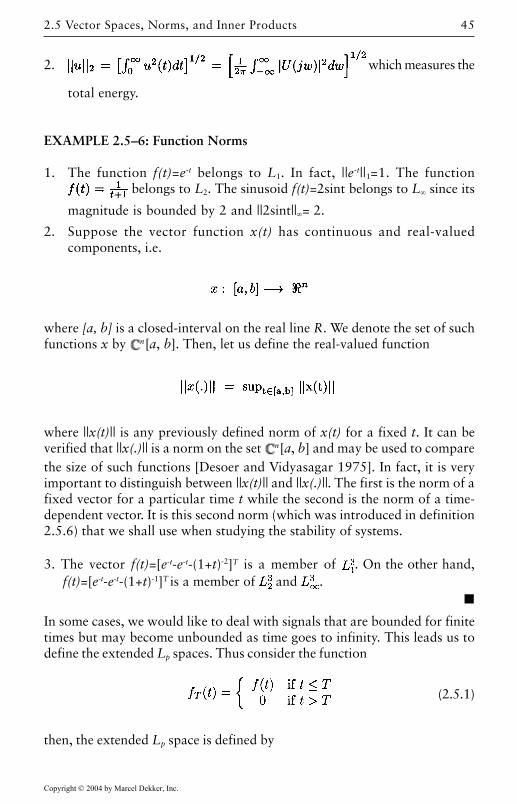
45
2. which measures the
total energy.
EXAMPLE 2.5–6: Function Norms
1. The function f(t)=e-t belongs to L1. In fact, ||e-t||1=1. The function belongs to L2. The sinusoid f(t)=2sint belongs to L∞ since its
magnitude is bounded by 2 and ||2sint||∞= 2.
2. Suppose the vector function x(t) has continuous and real-valuedcomponents, i.e.
where [a, b] is a closed-interval on the real line R. We denote the set of suchfunctions x by n[a, b]. Then, let us define the real-valued function
where ||x(t)|| is any previously defined norm of x(t) for a fixed t. It can beverified that ||x(.)|| is a norm on the set n[a, b] and may be used to comparethe size of such functions [Desoer and Vidyasagar 1975]. In fact, it is veryimportant to distinguish between ||x(t)|| and ||x(.)||. The first is the norm of afixed vector for a particular time t while the second is the norm of a time-dependent vector. It is this second norm (which was introduced in definition2.5.6) that we shall use when studying the stability of systems.
3. The vector f(t)=[e-t-e-t-(1+t)-2]T is a member of . On the other hand,f(t)=[e-t-e-t-(1+t)-1]T is a member of and .
In some cases, we would like to deal with signals that are bounded for finitetimes but may become unbounded as time goes to infinity. This leads us todefine the extended Lp spaces. Thus consider the function
(2.5.1)
then, the extended Lp space is defined by
2.5 Vector Spaces, Norms, and Inner Products
Copyright © 2004 by Marcel Dekker, Inc.
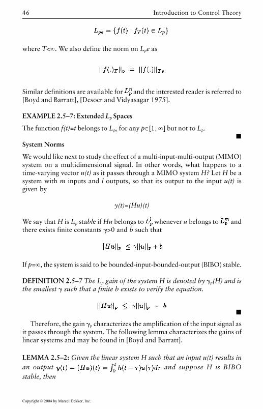
Introduction to Control Theory46
where T<∞. We also define the norm on Lpe as
Similar definitions are available for and the interested reader is referred to[Boyd and Barratt], [Desoer and Vidyasagar 1975].
EXAMPLE 2.5–7: Extended Lp Spaces
The function f(t)=t belongs to Lpe for any p∈[1, ∞] but not to Lp.
System Norms
We would like next to study the effect of a multi-input-multi-output (MIMO)system on a multidimensional signal. In other words, what happens to atime-varying vector u(t) as it passes through a MIMO system H? Let H be asystem with m inputs and l outputs, so that its output to the input u(t) isgiven by
y(t)=(Hu)(t)
We say that H is Lp stable if Hu belongs to whenever u belongs to andthere exists finite constants >0 and b such that
If p=∞, the system is said to be bounded-input-bounded-output (BIBO) stable.
DEFINITION 2.5–7 The Lp gain of the system H is denoted by p(H) and isthe smallest such that a finite b exists to verify the equation.
Therefore, the gain p characterizes the amplification of the input signal asit passes through the system. The following lemma characterizes the gains oflinear systems and may be found in [Boyd and Barratt].
LEMMA 2.5–2: Given the linear system H such that an input u(t) results inan output and suppose H is BIBOstable, then
Copyright © 2004 by Marcel Dekker, Inc.
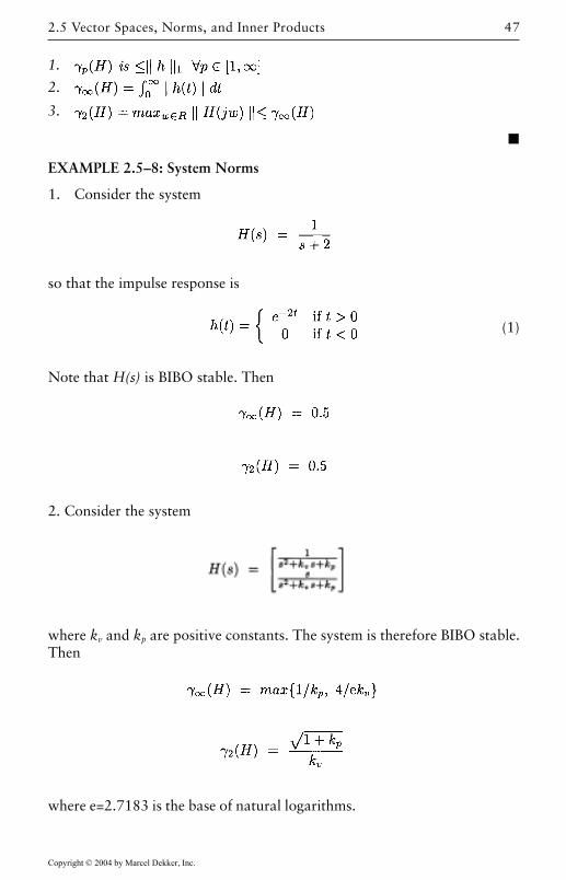
47
1.
2.
3.
EXAMPLE 2.5–8: System Norms
1. Consider the system
so that the impulse response is
(1)
Note that H(s) is BIBO stable. Then
2. Consider the system
where kv and kp are positive constants. The system is therefore BIBO stable.Then
where e=2.7183 is the base of natural logarithms.
2.5 Vector Spaces, Norms, and Inner Products
Copyright © 2004 by Marcel Dekker, Inc.
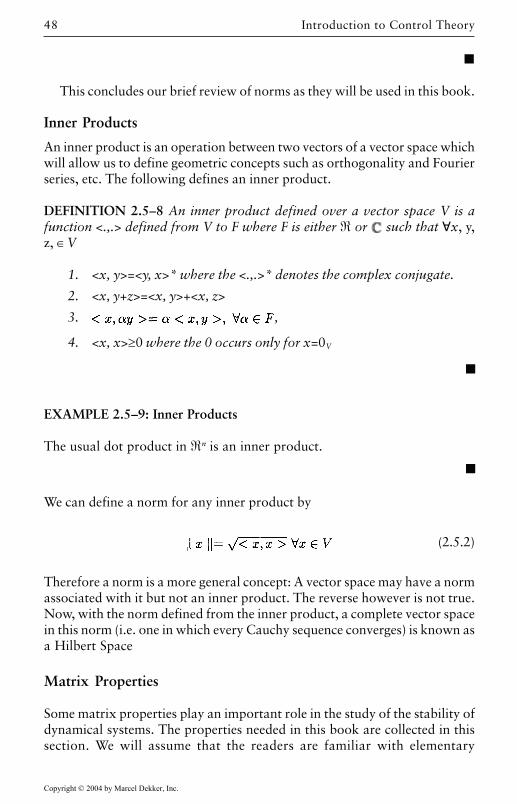
Introduction to Control Theory48
This concludes our brief review of norms as they will be used in this book.
Inner Products
An inner product is an operation between two vectors of a vector space whichwill allow us to define geometric concepts such as orthogonality and Fourierseries, etc. The following defines an inner product.
DEFINITION 2.5–8 An inner product defined over a vector space V is afunction <.,.> defined from V to F where F is either or such that x, y,z, ∈V
1. <x, y>=<y, x>* where the <.,.>* denotes the complex conjugate.
2. <x, y+z>=<x, y>+<x, z>
3. ,
4. <x, x>≥0 where the 0 occurs only for x=0V
EXAMPLE 2.5–9: Inner Products
The usual dot product in n is an inner product.
We can define a norm for any inner product by
(2.5.2)
Therefore a norm is a more general concept: A vector space may have a normassociated with it but not an inner product. The reverse however is not true.Now, with the norm defined from the inner product, a complete vector spacein this norm (i.e. one in which every Cauchy sequence converges) is known asa Hilbert Space
Matrix Properties
Some matrix properties play an important role in the study of the stability ofdynamical systems. The properties needed in this book are collected in thissection. We will assume that the readers are familiar with elementary
Copyright © 2004 by Marcel Dekker, Inc.
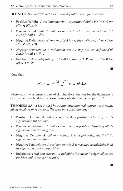
49
DEFINITION 2.5–9 All matrices in this definition are square and real.
• Positive Definite: A real n×n matrix A is positive definite if xT Ax>0 forall , x≠0.
• Positive Semidefinite: A real n×n matrix A is positive semidefinite if xT
Ax≥0 for all .
• Negative Definite: A real n×n matrix A is negative definite if xT Ax<0 forall , x≠0.
• Negative Semidefinite: A real n×n matrix A is negative semidefinite if xT
Ax≤0 for all .
• Indefinite: A is indefinite if xT Ax>0 for some and xT Ax<0 forother .
Note that
where As is the symmetric part of A. Therefore, the test for the definitenessof a matrix may be done by considering only the symmetric part of A.
THEOREM 2.5–1: Let A=[aij] be a symmetric n×n real matrix. As a result,all eigenvalues of A are real. We then have the following
• Positive Definite: A real n×n matrix A is positive definite if all itseigenvalues are positive.
• Positive semidefinite: A real n×n matrix A is positive definite if all itseigenvalues are nonnegative.
• Negative Definite: A real n×n matrix A is negative definite if all itseigenvalues are negative.
• Negative Semidefinite: A real n×n matrix A is negative semidefinite if allits eigenvalues are non-positive.
• Indefinite: A real n×n matrix A is indefinite if some of its eigenvalues arepositive and some are negative.
2.5 Vector Spaces, Norms, and Inner Products
Copyright © 2004 by Marcel Dekker, Inc.
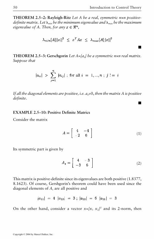
Introduction to Control Theory50
THEOREM 2.5–2: Rayleigh-Ritz Let A be a real, symmetric n×n positive-definite matrix. Let min be the minimum eigenvalue and max be the maximumeigenvalue of A. Then, for any ,
THEOREM 2.5–3: Gerschgorin Let A=[aij] be a symmetric n×n real matrix.Suppose that
If all the diagonal elements are positive, i.e. aii>0, then the matrix A is positivedefinite.
EXAMPLE 2.5–10: Positive Definite Matrics
Consider the matrix
(1)
Its symmetric part is given by
(2)
This matrix is positive-definite since its eigenvalues are both positive (1.8377,8.1623). Of course, Gershgorin’s theorem could have been used since thediagonal elements of As are all positive and
On the other hand, consider a vector x=[x1 x2]T and its 2-norm, then
Copyright © 2004 by Marcel Dekker, Inc.
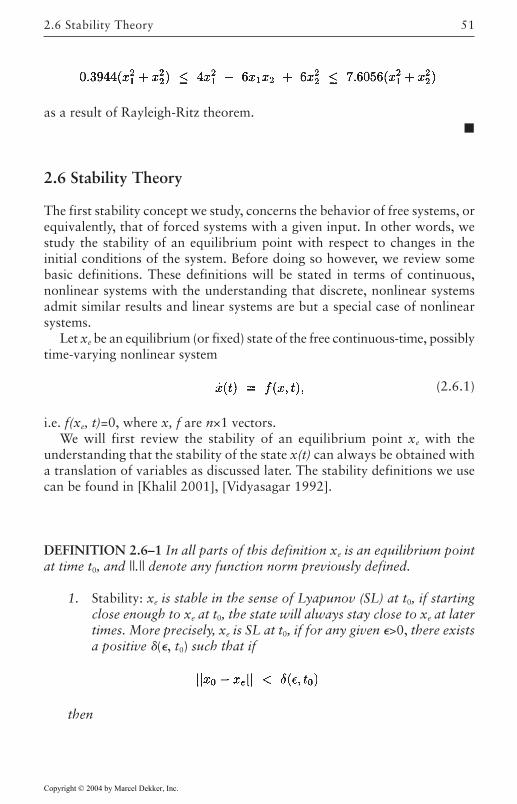
51
as a result of Rayleigh-Ritz theorem.
2.6 Stability Theory
The first stability concept we study, concerns the behavior of free systems, orequivalently, that of forced systems with a given input. In other words, westudy the stability of an equilibrium point with respect to changes in theinitial conditions of the system. Before doing so however, we review somebasic definitions. These definitions will be stated in terms of continuous,nonlinear systems with the understanding that discrete, nonlinear systemsadmit similar results and linear systems are but a special case of nonlinearsystems.
Let xe be an equilibrium (or fixed) state of the free continuous-time, possiblytime-varying nonlinear system
(2.6.1)
i.e. f(xe, t)=0, where x, f are n×1 vectors.We will first review the stability of an equilibrium point xe with the
understanding that the stability of the state x(t) can always be obtained witha translation of variables as discussed later. The stability definitions we usecan be found in [Khalil 2001], [Vidyasagar 1992].
DEFINITION 2.6–1 In all parts of this definition xe is an equilibrium pointat time t0, and ||.|| denote any function norm previously defined.
1. Stability: xe is stable in the sense of Lyapunov (SL) at t0, if startingclose enough to xe at t0, the state will always stay close to xe at latertimes. More precisely, xe is SL at t0, if for any given >0, there existsa positive (, t0) such that if
then
2.6 Stability Theory
Copyright © 2004 by Marcel Dekker, Inc.
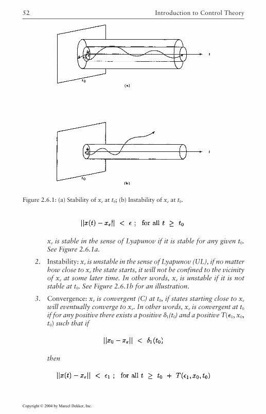
Introduction to Control Theory52
xe is stable in the sense of Lyapunov if it is stable for any given t0.See Figure 2.6.1a.
2. Instability: xe is unstable in the sense of Lyapunov (UL), if no matterhow close to xe the state starts, it will not be confined to the vicinityof xe at some later time. In other words, xe is unstable if it is notstable at t0. See Figure 2.6.1b for an illustration.
3. Convergence: xe is convergent (C) at t0, if states starting close to xe
will eventually converge to xe. In other words, xe is convergent at t0
if for any positive there exists a positive 1(t0) and a positive T(1, x0,t0) such that if
then
Figure 2.6.1: (a) Stability of xe at t0; (b) Instability of xe at t0.
Copyright © 2004 by Marcel Dekker, Inc.
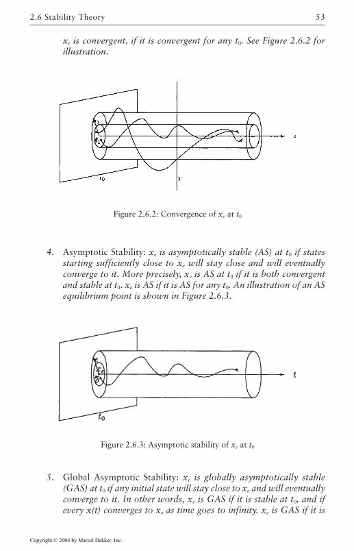
53
xe is convergent, if it is convergent for any t0. See Figure 2.6.2 forillustration.
Figure 2.6.2: Convergence of xe at t0
4. Asymptotic Stability: xe is asymptotically stable (AS) at t0 if statesstarting sufficiently close to xe will stay close and will eventuallyconverge to it. More precisely, xe is AS at t0 if it is both convergentand stable at t0. xe is AS if it is AS for any t0. An illustration of an ASequilibrium point is shown in Figure 2.6.3.
Figure 2.6.3: Asymptotic stability of xe at t0
5. Global Asymptotic Stability: xe is globally asymptotically stable(GAS) at t0 if any initial state will stay close to xe and will eventuallyconverge to it. In other words, xe is GAS if it is stable at t0, and ifevery x(t) converges to xe as time goes to infinity. xe is GAS if it is
2.6 Stability Theory
Copyright © 2004 by Marcel Dekker, Inc.
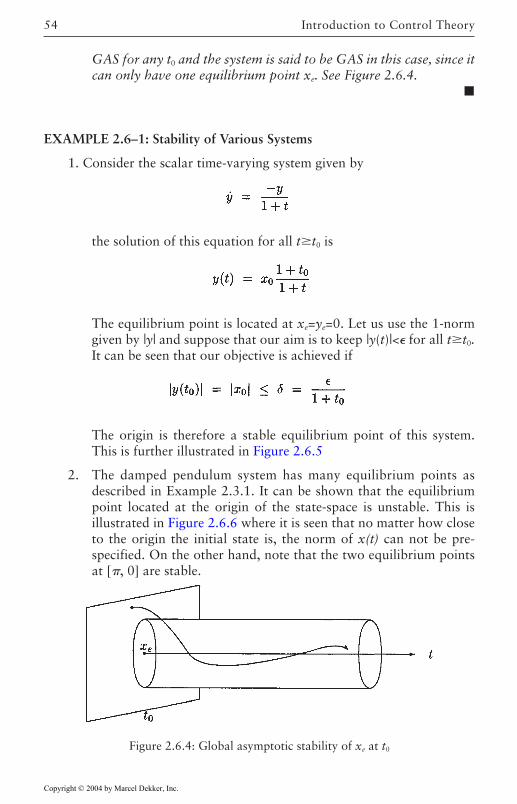
Introduction to Control Theory54
GAS for any t0 and the system is said to be GAS in this case, since itcan only have one equilibrium point xe. See Figure 2.6.4.
EXAMPLE 2.6–1: Stability of Various Systems
1. Consider the scalar time-varying system given by
the solution of this equation for all tt0 is
The equilibrium point is located at xe=ye=0. Let us use the 1-normgiven by |y| and suppose that our aim is to keep |y(t)|< for all tt0.It can be seen that our objective is achieved if
The origin is therefore a stable equilibrium point of this system.This is further illustrated in Figure 2.6.5
2. The damped pendulum system has many equilibrium points asdescribed in Example 2.3.1. It can be shown that the equilibriumpoint located at the origin of the state-space is unstable. This isillustrated in Figure 2.6.6 where it is seen that no matter how closeto the origin the initial state is, the norm of x(t) can not be pre-specified. On the other hand, note that the two equilibrium pointsat [, 0] are stable.
Figure 2.6.4: Global asymptotic stability of xe at t0
Copyright © 2004 by Marcel Dekker, Inc.
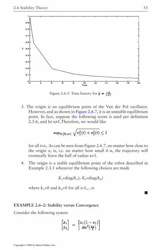
55
3. The origin is an equilibrium point of the Van der Pol oscillator.However, and as shown in Figure 2.6.7, it is an unstable equilibriumpoint. In fact, suppose the following norm is used per definition2.5.6, and let ≠1.Therefore, we would like
for all t>t0. As can be seen from Figure 2.6.7, no matter how close tothe origin x0 is, i.e. no matter how small is, the trajectory willeventually leave the ball of radius =1.
4. The origin is a stable equilibrium point of the robot described inExample 2.3.1 whenever the following choices are made
Kv=diag(kvi); Kp=diag(kpi)
where kvi>0 and kpi>0 for all i=1,…n.
EXAMPLE 2.6–2: Stability versus Convergence
Consider the following system
Figure 2.6.5: Time history for
2.6 Stability Theory
Copyright © 2004 by Marcel Dekker, Inc.
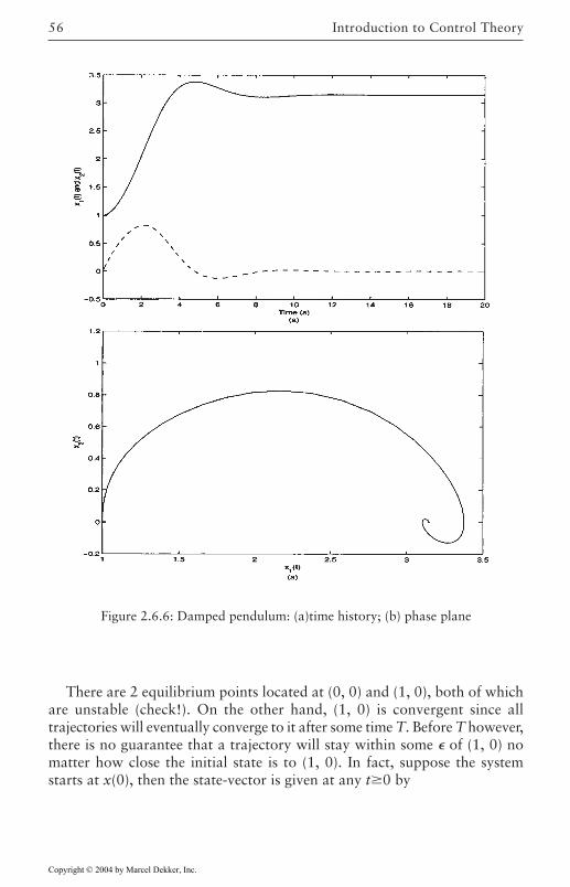
Introduction to Control Theory56
Figure 2.6.6: Damped pendulum: (a)time history; (b) phase plane
There are 2 equilibrium points located at (0, 0) and (1, 0), both of whichare unstable (check!). On the other hand, (1, 0) is convergent since alltrajectories will eventually converge to it after some time T. Before T however,there is no guarantee that a trajectory will stay within some of (1, 0) nomatter how close the initial state is to (1, 0). In fact, suppose the systemstarts at x(0), then the state-vector is given at any t0 by
Copyright © 2004 by Marcel Dekker, Inc.
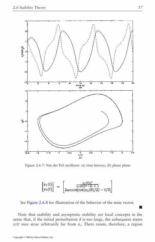
57
See Figure 2.6.8 for illustration of the behavior of the state vector.
Note that stability and asymptotic stability are local concepts in thesense that, if the initial perturbation is too large, the subsequent statesx(t) may stray arbitrarily far from xe. There exists, therefore, a region
Figure 2.6.7: Van der Pol oscillator: (a) time history; (b) phase plane
2.6 Stability Theory
Copyright © 2004 by Marcel Dekker, Inc.
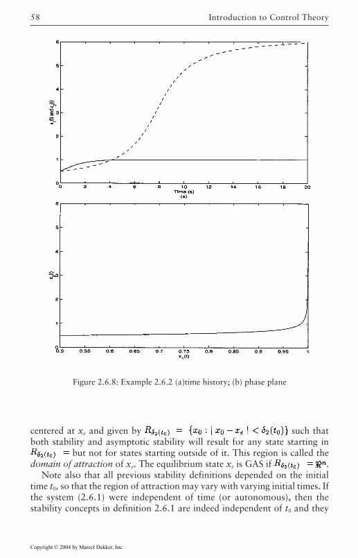
Introduction to Control Theory58
centered at xe and given by such thatboth stability and asymptotic stability will result for any state starting in
but not for states starting outside of it. This region is called thedomain of attraction of xe. The equilibrium state xe is GAS if .
Note also that all previous stability definitions depended on the initialtime t0, so that the region of attraction may vary with varying initial times. Ifthe system (2.6.1) were independent of time (or autonomous), then thestability concepts in definition 2.6.1 are indeed independent of t0 and they
Figure 2.6.8: Example 2.6.2 (a)time history; (b) phase plane
Copyright © 2004 by Marcel Dekker, Inc.
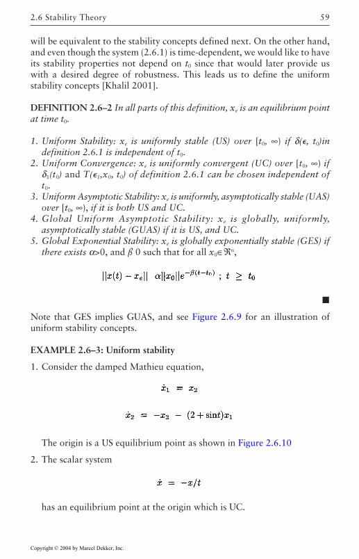
59
will be equivalent to the stability concepts defined next. On the other hand,and even though the system (2.6.1) is time-dependent, we would like to haveits stability properties not depend on t0 since that would later provide uswith a desired degree of robustness. This leads us to define the uniformstability concepts [Khalil 2001].
DEFINITION 2.6–2 In all parts of this definition, xe is an equilibrium pointat time t0.
1. Uniform Stability: xe is uniformly stable (US) over [t0, ∞) if δ(, t0)indefinition 2.6.1 is independent of t0.
2. Uniform Convergence: xe is uniformly convergent (UC) over [t0, ∞) ifδ1(t0) and T(1,x0, t0) of definition 2.6.1 can be chosen independent oft0.
3. Uniform Asymptotic Stability: xe is uniformly, asymptotically stable (UAS)over [t0, ∞), if it is both US and UC.
4. Global Uniform Asymptotic Stability: xe is globally, uniformly,asymptotically stable (GUAS) if it is US, and UC.
5. Global Exponential Stability: xe is globally exponentially stable (GES) ifthere exists α>0, and ß 0 such that for all x0∈ℜn,
Note that GES implies GUAS, and see Figure 2.6.9 for an illustration ofuniform stability concepts.
EXAMPLE 2.6–3: Uniform stability
1. Consider the damped Mathieu equation,
The origin is a US equilibrium point as shown in Figure 2.6.10
2. The scalar system
has an equilibrium point at the origin which is UC.
2.6 Stability Theory
Copyright © 2004 by Marcel Dekker, Inc.
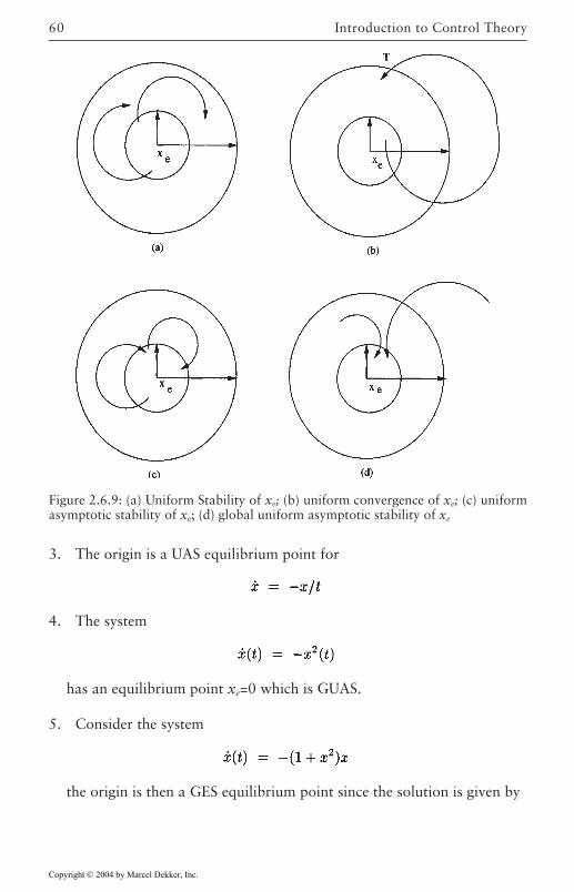
Introduction to Control Theory60
3. The origin is a UAS equilibrium point for
4. The system
has an equilibrium point xe=0 which is GUAS.
5. Consider the system
the origin is then a GES equilibrium point since the solution is given by
Figure 2.6.9: (a) Uniform Stability of xe; (b) uniform convergence of xe; (c) uniformasymptotic stability of xe; (d) global uniform asymptotic stability of xe
Copyright © 2004 by Marcel Dekker, Inc.
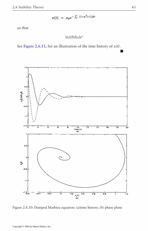
61
so that
|x(t)|≤|x0|e-t
See Figure 2.6.11, for an illustration of the time history of x(t).
Figure 2.6.10: Damped Mathieu equation: (a)time history; (b) phase plane
2.6 Stability Theory
Copyright © 2004 by Marcel Dekker, Inc.
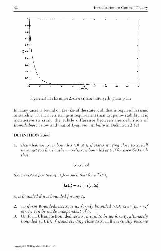
Introduction to Control Theory62
In many cases, a bound on the size of the state is all that is required in termsof stability. This is a less stringent requirement than Lyapunov stability. It isinstructive to study the subtle difference between the definition ofBoundedness below and that of Lyapunov stability in Definition 2.6.1.
DEFINITION 2.6–3
1. Boundedness: xe is bounded (B) at t0 if states starting close to xe willnever get too far. In other words, xe is bounded at t0 if for each δ>0 suchthat
||x0-xe||<δ
there exists a positive (r, t0)<∞ such that for all tt0
xe is bounded if it is bounded for any t0.
2. Uniform Boundedness: xe is uniformly bounded (UB) over [t0, ∞) if(r, t0) can be made independent of t0.
3. Uniform Ultimate Boundedness: xe is said to be uniformly, ultimatelybounded (UUB), if states starting close to xe will eventually become
Figure 2.6.11: Example 2.6.3e: (a)time history; (b) phase plane
Copyright © 2004 by Marcel Dekker, Inc.
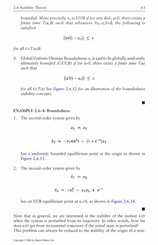
63
bounded. More precisely, xe is UUB if for any δ>0, >0, there exists afinite time T(,δ) such that whenever ||x0-xe||<δ, the following issatisfied
for all tT(,δ).
4. Global Uniform Ultimate Boundedness: xe is said to be globally, uniformly,ultimately bounded (GUUB) if for >0, there exists a finite time T()such that
for all tT() See Figure 2.6.12 for an illustration of the boundednessstability concepts.
EXAMPLE 2.6–4: Boundedness
1. The second-order system given by
has a uniformly bounded equilibrium point at the origin as shown inFigure 2.6.13.
2. The second-order system given by
has an UUB equilibrium point at xe=0, as shown in Figure 2.6.14.
Note that in general, we are interested in the stability of the motion x(t)when the system is perturbed from its trajectory. In other words, how fardoes x(t) get from its nominal trajectory if the initial state is perturbed?This problem can always be reduced to the stability of the origin of a non-
2.6 Stability Theory
Copyright © 2004 by Marcel Dekker, Inc.
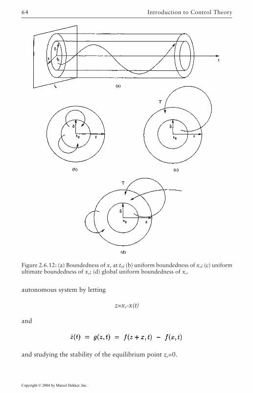
Introduction to Control Theory64
autonomous system by letting
z=xe-x(t)
and
and studying the stability of the equilibrium point ze=0.
Figure 2.6.12: (a) Boundedness of xe at t0; (b) uniform boundedness of xe; (c) uniformultimate boundedness of xe; (d) global uniform boundedness of xe.
Copyright © 2004 by Marcel Dekker, Inc.
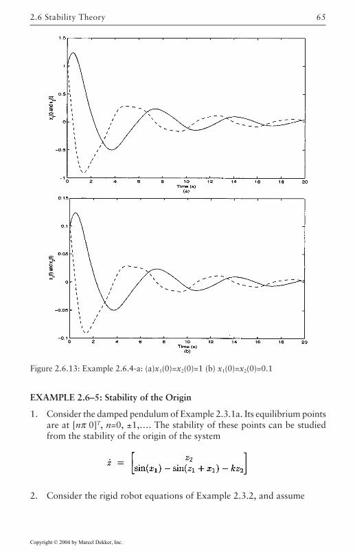
65
EXAMPLE 2.6–5: Stability of the Origin
1. Consider the damped pendulum of Example 2.3.1a. Its equilibrium pointsare at [nπ 0]T, n=0, ±1,…. The stability of these points can be studiedfrom the stability of the origin of the system
2. Consider the rigid robot equations of Example 2.3.2, and assume
Figure 2.6.13: Example 2.6.4-a: (a)x1(0)=x2(0)=1 (b) x1(0)=x2(0)=0.1
2.6 Stability Theory
Copyright © 2004 by Marcel Dekker, Inc.
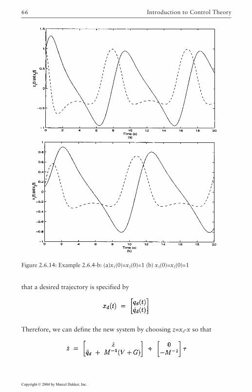
Introduction to Control Theory66
that a desired trajectory is specified by
Therefore, we can define the new system by choosing z=xd-x so that
Figure 2.6.14: Example 2.6.4-b: (a)x1(0)=x2(0)=1 (b) x1(0)=x2(0)=1
Copyright © 2004 by Marcel Dekker, Inc.
67
and verify that ze=0 is the desired equilibrium point of the modified system ifxe=xd is the desired equilibrium trajectory of the robot.
2.7 Lyapunov Stability Theorems
Lyapunov stability theory deals with the behavior of unforced nonlinearsystems described by the differential equations
(2.7.1)
where without loss of generality, the origin is an equilibrium point of (2.7.1).It may seem to the reader that such a theory is not needed since all we hadto do in the examples of the previous section is to solve the differentialequations, and study the time evolution of a norm of the state vector. Thereare at least two reasons why Lyapunov theory is needed. The first is thatLyapunov theory will allow us to determine the stability of a particularequilibrium point without actually solving the differential equations. This,as is well known to any student of nonlinear differential equations, is alarge saving. The second and related reason for using Lyapunov theory isthat it provides us with qualitative results to the stability questions, whichmay be used in designing stabilizing controllers of nonlinear dynamicalsystems.
We shall first assume that any necessary conditions for (2.7.1) to have aunique solution are satisfied [Khalil 2001], [Vidyasagar 1992]. The uniquesolution corresponding to x(t0)=x0 is x(t, t0, x0) and will be denoted simply asx(t). Before we actually introduce Lyapunov’s theorems, we review certainclasses of functions which will simplify the statement of Lyapunov theorems.
Functions of Class K
Consider a continuous function α:ℜ→ℜ
DEFINITION 2.7–1 We say that a belongs to class K, if
1. α(0)=02. α(x)>0, for all x>03. α is nondecreasing, i.e. α(x1)α(x2) for all x1>x2.
2.7 Lyapunov Stability Theorems
Copyright © 2004 by Marcel Dekker, Inc.
Introduction to Control Theory68
EXAMPLE 2.7–1: Class K Functions
The function α(x)=x2 is a class K function. The function α(x)=x2+1 is not aclass K function because (1) fails. On the other hand, α(x)=-x2 is not a classK function because (2) and (3) fail.
DEFINITION 2.7–2 In the following, ℜ+=[0,∞).
1. Locally Positive Definite: A continuous function V:ℜ+×ℜn→R is locallypositive definite (l.p.d) if there exists a class K function a(.) and aneighborhood N of the origin of ℜn such that
V(t, x)α(||x||)
for all t0, and all x∈N.
2. Positive Definite: The function V is said to be positive definite (p.d) ifN=ℜn.
3. Negative and Local Negative Definite: We say that V is (locally) negativedefinite (n.d) if -V is (locally) positive definite.
EXAMPLE 2.7–2: Locally Positive Definite Functions
[Vidyasagar 1992] The function is l.p.d but notp.d, since V(t, x)=0 at x=(0, π/2). On the other hand, is not even l.p.d because V(t, x)→0 as t→∞ for any x. The function
is p.d.
DEFINITION 2.7–3
In the following,
1. Locally Decrescent: A continuous function is locallydecrescent if There exists a class K function ß(.) and a neighborhood Nof the origin of such that
V(t, x)ß(||x||)
for all t0 and all x∈Ν.
Copyright © 2004 by Marcel Dekker, Inc.
69
2. Decrescent: We say that V is decrescent if N=ℜn.
EXAMPLE 2.7–3: Decrescent Functions
[Vidyasagar 1992] The function is locally butnot globally decrescent. On the other hand, is globallydecrescent.
DEFINITION 2.7–4 Given a continuously differentiate function V: ℜ+×ℜn→R together with a system of differential equations (2.7.1), the derivative of Valong (2.7.1) is defined as a function V: ℜ+×ℜn→R given by
EXAMPLE 2.7–4: Lyapunov Functions
Consider the function of Example 2.7.3 and assumegiven a system
Then, the derivative of V(t, x) along this system is
Lyapunov Theorems
We are now ready to state Lyapunov Theorems, which we group in Theorem2.7.1. For the proof, see [Khalil 2001], [Vidyasagar 1992].
THEOREM 2.7–1: Lyapunov
Given the nonlinear system
2.7 Lyapunov Stability Theorems
Copyright © 2004 by Marcel Dekker, Inc.
Introduction to Control Theory70
with an equilibrium point at the origin, i.e. f(t, 0)=0, and let N be aneighborhood of the origin of size i. e.
Then
1. Stability: The origin is stable in the sense of Lyapunov, if for x∈Ν, thereexists a scalar function V(t, x) with continuous partial derivative suchthat
(a) V(t, x) is positive definite(b) V is negative semi-definite
2. Uniform Stability: The origin is uniformly stable if in addition to (a) and(b) V(t, x) is decrescent for x∈Ν.
3. Asymptotic Stability: The origin is asymptotically stable if V(t, x) satisfies(a) and is negative definite for x∈Ν.
4. Global Asymptotic Stability: The origin is globally, asymptotically stableif V(t, x) verifies (a), and V(t, x) is negative definite for all x∈ℜn i.e. ifN=ℜn.
5. Uniform Asymptotic Stability: The origin is UAS if V(t, x) satisfies (a),V(t, x) is decrescent, and V(t,x) is negative definite for x∈Ν.
6. Global Uniform Asymptotic Stability: The origin is GUAS if N=ℜn, andif V(t, x) satisfies (a), V(t,x) is decrescent, V(t,x) is negative definite andV(t, x) is radially unbounded, i.e. if it goes to infinity uniformly in timeas ||x||→∞.
7. Exponential Stability: The origin is exponentially stable if there existspositive constants α, ß, γ such that
8. Global Exponential Stability: The origin is globally exponential stable ifit is exponentially stable for all x∈ℜn.
The function V(t, x) in the theorem is called a Lyapunov function. Note thatthe theorem provides sufficient conditions for the stability of the origin andthat the inability to provide a Lyapunov function candidate has no indicationon the stability of the origin for a particular system.
Copyright © 2004 by Marcel Dekker, Inc.
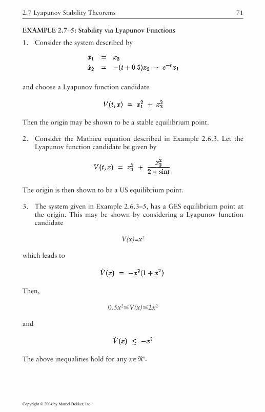
71
EXAMPLE 2.7–5: Stability via Lyapunov Functions
1. Consider the system described by
and choose a Lyapunov function candidate
Then the origin may be shown to be a stable equilibrium point.
2. Consider the Mathieu equation described in Example 2.6.3. Let theLyapunov function candidate be given by
The origin is then shown to be a US equilibrium point.
3. The system given in Example 2.6.3–5, has a GES equilibrium point atthe origin. This may be shown by considering a Lyapunov functioncandidate
V(x)=x2
which leads to
Then,
0.5x2V(x)2x2
and
The above inequalities hold for any x∈ℜn.
2.7 Lyapunov Stability Theorems
Copyright © 2004 by Marcel Dekker, Inc.
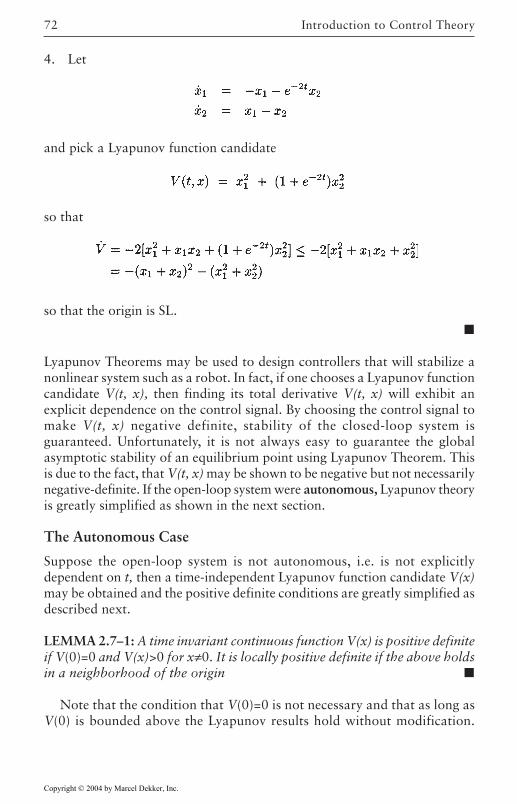
Introduction to Control Theory72
4. Let
and pick a Lyapunov function candidate
so that
so that the origin is SL.
Lyapunov Theorems may be used to design controllers that will stabilize anonlinear system such as a robot. In fact, if one chooses a Lyapunov functioncandidate V(t, x), then finding its total derivative V(t, x) will exhibit anexplicit dependence on the control signal. By choosing the control signal tomake V(t, x) negative definite, stability of the closed-loop system isguaranteed. Unfortunately, it is not always easy to guarantee the globalasymptotic stability of an equilibrium point using Lyapunov Theorem. Thisis due to the fact, that V(t, x) may be shown to be negative but not necessarilynegative-definite. If the open-loop system were autonomous, Lyapunov theoryis greatly simplified as shown in the next section.
The Autonomous Case
Suppose the open-loop system is not autonomous, i.e. is not explicitlydependent on t, then a time-independent Lyapunov function candidate V(x)may be obtained and the positive definite conditions are greatly simplified asdescribed next.
LEMMA 2.7–1: A time invariant continuous function V(x) is positive definiteif V(0)=0 and V(x)>0 for x≠0. It is locally positive definite if the above holdsin a neighborhood of the origin
Note that the condition that V(0)=0 is not necessary and that as long asV(0) is bounded above the Lyapunov results hold without modification.
Copyright © 2004 by Marcel Dekker, Inc.
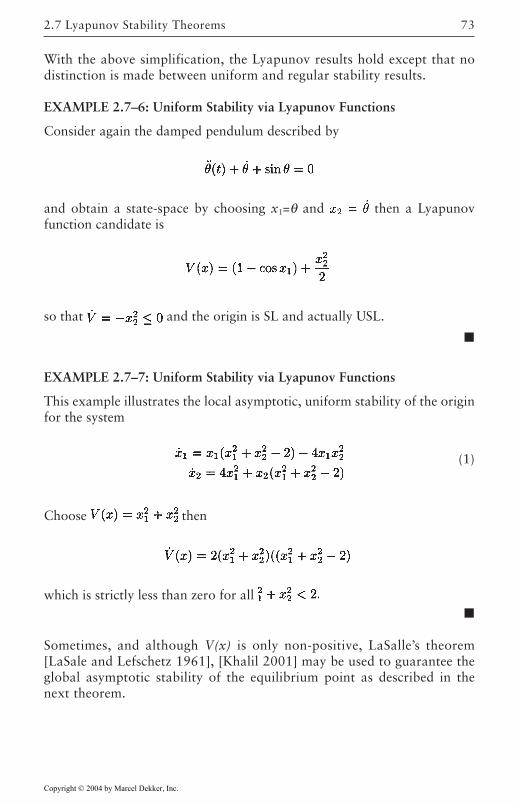
73
With the above simplification, the Lyapunov results hold except that nodistinction is made between uniform and regular stability results.
EXAMPLE 2.7–6: Uniform Stability via Lyapunov Functions
Consider again the damped pendulum described by
and obtain a state-space by choosing x1=θ and then a Lyapunovfunction candidate is
so that and the origin is SL and actually USL.
EXAMPLE 2.7–7: Uniform Stability via Lyapunov Functions
This example illustrates the local asymptotic, uniform stability of the originfor the system
(1)
Choose then
which is strictly less than zero for all
Sometimes, and although V(x) is only non-positive, LaSalle’s theorem[LaSale and Lefschetz 1961], [Khalil 2001] may be used to guarantee theglobal asymptotic stability of the equilibrium point as described in thenext theorem.
2.7 Lyapunov Stability Theorems
Copyright © 2004 by Marcel Dekker, Inc.
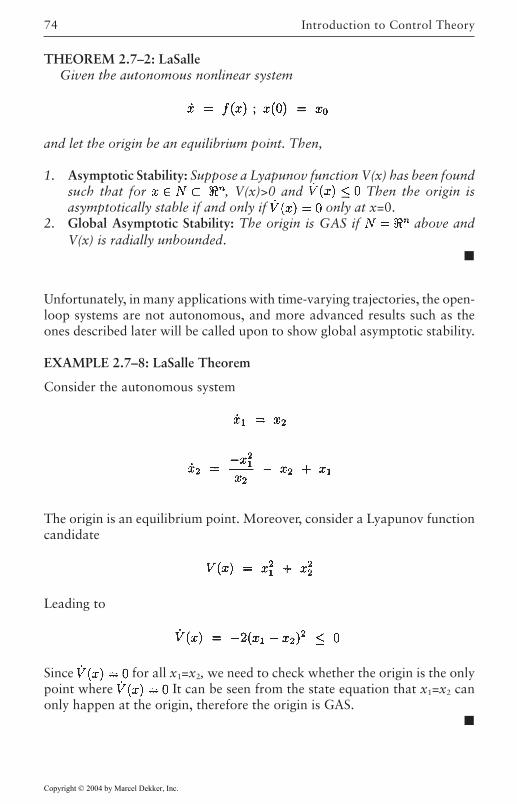
Introduction to Control Theory74
THEOREM 2.7–2: LaSalleGiven the autonomous nonlinear system
and let the origin be an equilibrium point. Then,
1. Asymptotic Stability: Suppose a Lyapunov function V(x) has been foundsuch that for , V(x)>0 and Then the origin isasymptotically stable if and only if only at x=0.
2. Global Asymptotic Stability: The origin is GAS if above andV(x) is radially unbounded.
Unfortunately, in many applications with time-varying trajectories, the open-loop systems are not autonomous, and more advanced results such as theones described later will be called upon to show global asymptotic stability.
EXAMPLE 2.7–8: LaSalle Theorem
Consider the autonomous system
The origin is an equilibrium point. Moreover, consider a Lyapunov functioncandidate
Leading to
Since for all x1=x2, we need to check whether the origin is the onlypoint where It can be seen from the state equation that x1=x2 canonly happen at the origin, therefore the origin is GAS.
Copyright © 2004 by Marcel Dekker, Inc.
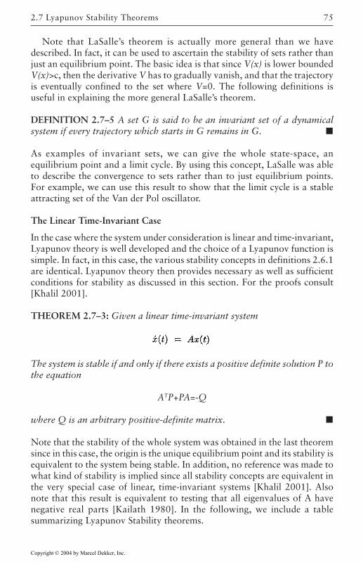
75
Note that LaSalle’s theorem is actually more general than we havedescribed. In fact, it can be used to ascertain the stability of sets rather thanjust an equilibrium point. The basic idea is that since V(x) is lower boundedV(x)>c, then the derivative V has to gradually vanish, and that the trajectoryis eventually confined to the set where V=0. The following definitions isuseful in explaining the more general LaSalle’s theorem.
DEFINITION 2.7–5 A set G is said to be an invariant set of a dynamicalsystem if every trajectory which starts in G remains in G.
As examples of invariant sets, we can give the whole state-space, anequilibrium point and a limit cycle. By using this concept, LaSalle was ableto describe the convergence to sets rather than to just equilibrium points.For example, we can use this result to show that the limit cycle is a stableattracting set of the Van der Pol oscillator.
The Linear Time-Invariant Case
In the case where the system under consideration is linear and time-invariant,Lyapunov theory is well developed and the choice of a Lyapunov function issimple. In fact, in this case, the various stability concepts in definitions 2.6.1are identical. Lyapunov theory then provides necessary as well as sufficientconditions for stability as discussed in this section. For the proofs consult[Khalil 2001].
THEOREM 2.7–3: Given a linear time-invariant system
The system is stable if and only if there exists a positive definite solution P tothe equation
ATP+PA=-Q
where Q is an arbitrary positive-definite matrix.
Note that the stability of the whole system was obtained in the last theoremsince in this case, the origin is the unique equilibrium point and its stability isequivalent to the system being stable. In addition, no reference was made towhat kind of stability is implied since all stability concepts are equivalent inthe very special case of linear, time-invariant systems [Khalil 2001]. Alsonote that this result is equivalent to testing that all eigenvalues of A havenegative real parts [Kailath 1980]. In the following, we include a tablesummarizing Lyapunov Stability theorems.
2.7 Lyapunov Stability Theorems
Copyright © 2004 by Marcel Dekker, Inc.
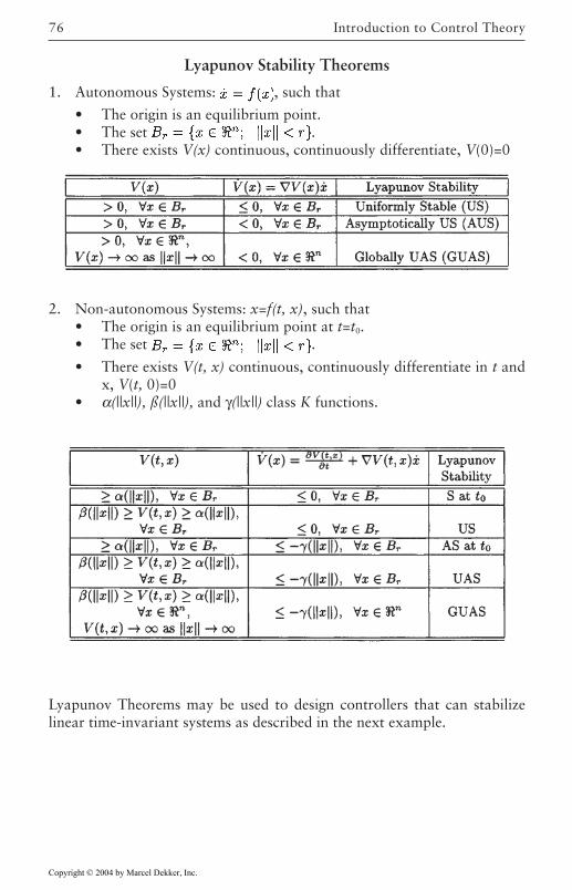
Introduction to Control Theory76
Lyapunov Stability Theorems
1. Autonomous Systems: , such that
• The origin is an equilibrium point.• The set .• There exists V(x) continuous, continuously differentiate, V(0)=0
2. Non-autonomous Systems: x=f(t, x), such that• The origin is an equilibrium point at t=t0.• The set .
• There exists V(t, x) continuous, continuously differentiate in t andx, V(t, 0)=0
• α(||x||), ß(||x||), and γ(||x||) class K functions.
Lyapunov Theorems may be used to design controllers that can stabilizelinear time-invariant systems as described in the next example.
Copyright © 2004 by Marcel Dekker, Inc.
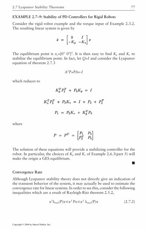
77
EXAMPLE 2.7–9: Stability of PD Controllers for Rigid Robots
Consider the rigid robot example and the torque input of Example 2.3.2.The resulting linear system is given by
The equilibrium point is xe=[0T 0T]T. It is then easy to find Kp and Kv tostabilize the equilibrium point. In fact, let Q=I and consider the Lyapunovequation of theorem 2.7.3
ATP+PA=-I
which reduces to
where
The solution of these equations will provide a stabilizing controller for therobot. In particular, the choices of Kp and Kv of Example 2.6.3(part 5) willmake the origin a GES equilibrium.
Convergence Rate
Although Lyapunov stability theory does not directly give an indication ofthe transient behavior of the system, it may actually be used to estimate theconvergence rate for linear systems. In order to see this, consider the followinginequalities which are a result of Rayleigh-Ritz theorem 2.5.2,
xTλmin(P)xxT PxxT λmax(P)x (2.7.2)
2.7 Lyapunov Stability Theorems
Copyright © 2004 by Marcel Dekker, Inc.
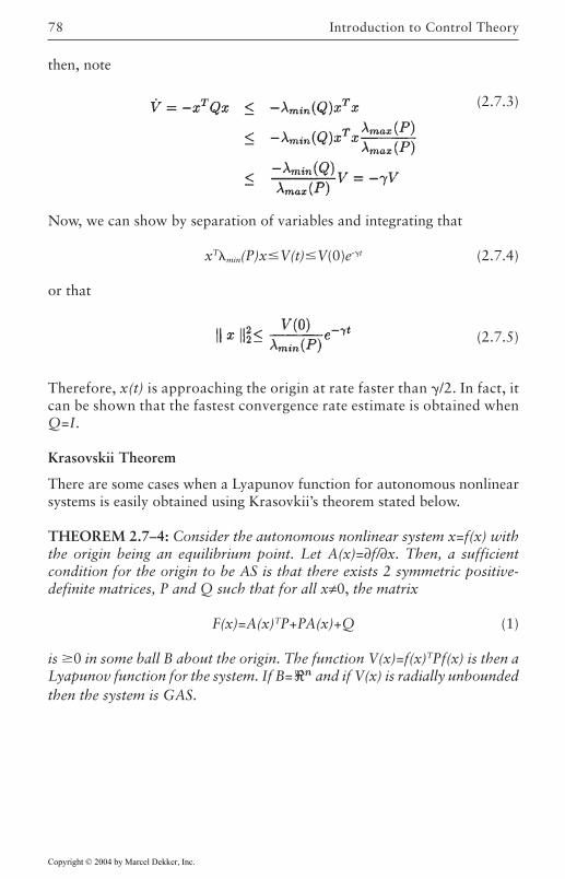
Introduction to Control Theory78
then, note
(2.7.3)
Now, we can show by separation of variables and integrating that
xTmin(P)xV(t)V(0)e-t (2.7.4)
or that
(2.7.5)
Therefore, x(t) is approaching the origin at rate faster than /2. In fact, itcan be shown that the fastest convergence rate estimate is obtained whenQ=I.
Krasovskii Theorem
There are some cases when a Lyapunov function for autonomous nonlinearsystems is easily obtained using Krasovkii’s theorem stated below.
THEOREM 2.7–4: Consider the autonomous nonlinear system x=f(x) withthe origin being an equilibrium point. Let A(x)=∂f/∂x. Then, a sufficientcondition for the origin to be AS is that there exists 2 symmetric positive-definite matrices, P and Q such that for all x≠0, the matrix
F(x)=A(x)TP+PA(x)+Q (1)
is 0 in some ball B about the origin. The function V(x)=f(x)TPf(x) is then aLyapunov function for the system. If B= and if V(x) is radially unboundedthen the system is GAS.
Copyright © 2004 by Marcel Dekker, Inc.
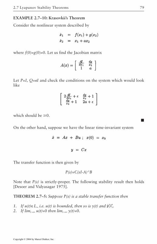
79
EXAMPLE 2.7–10: Krasovkii’s Theorem
Consider the nonlinear system described by
where f(0)=g(0)=0. Let us find the Jacobian matrix
Let P=I, Q=I and check the conditions on the system which would looklike
which should be 0.
On the other hand, suppose we have the linear time-invariant system
The transfer function is then given by
P(s)=C(sI-A)-1B
Note that P(s) is strictly-proper. The following stability result then holds[Desoer and Vidyasagar 1975].
THEOREM 2.7–5: Suppose P(s) is a stable transfer function then
1. If u(t)∈L∞ i.e. u(t) is bounded, then so is y(t) and .2. If limt→∞ u(t)=0 then limt→∞ y(t)=0.
2.7 Lyapunov Stability Theorems
Copyright © 2004 by Marcel Dekker, Inc.
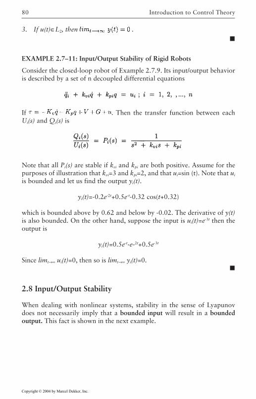
Introduction to Control Theory80
3. If u(t)∈L2, then .
EXAMPLE 2.7–11: Input/Output Stability of Rigid Robots
Consider the closed-loop robot of Example 2.7.9. Its input/output behavioris described by a set of n decoupled differential equations
If . Then the transfer function between eachUi(s) and Qi(s) is
Note that all Pi(s) are stable if kvi and kpi are both positive. Assume for thepurposes of illustration that kvi=3 and kpi=2, and that ui=sin (t). Note that ui
is bounded and let us find the output yi(t).
yi(t)=-0.2e-2t+0.5e-t-0.32 cos(t+0.32)
which is bounded above by 0.62 and below by -0.02. The derivative of y(t)is also bounded. On the other hand, suppose the input is ui(t)=e-3t then theoutput is
yi(t)=0.5e-t-e-2t+0.5e-3t
Since limt→∞ ui(t)=0, then so is limt→∞ yi(t)=0.
2.8 Input/Output Stability
When dealing with nonlinear systems, stability in the sense of Lyapunovdoes not necessarily imply that a bounded input will result in a boundedoutput. This fact is shown in the next example.
Copyright © 2004 by Marcel Dekker, Inc.
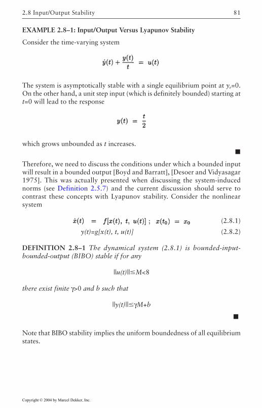
81
EXAMPLE 2.8–1: Input/Output Versus Lyapunov Stability
Consider the time-varying system
The system is asymptotically stable with a single equilibrium point at ye=0.On the other hand, a unit step input (which is definitely bounded) starting att=0 will lead to the response
which grows unbounded as t increases.
Therefore, we need to discuss the conditions under which a bounded inputwill result in a bounded output [Boyd and Barratt], [Desoer and Vidyasagar1975]. This was actually presented when discussing the system-inducednorms (see Definition 2.5.7) and the current discussion should serve tocontrast these concepts with Lyapunov stability. Consider the nonlinearsystem
(2.8.1)
y(t)=g[x(t), t, u(t)] (2.8.2)
DEFINITION 2.8–1 The dynamical system (2.8.1) is bounded-input-bounded-output (BIBO) stable if for any
||u(t)||M<8
there exist finite γ>0 and b such that
||y(t)||γM+b
Note that BIBO stability implies the uniform boundedness of all equilibriumstates.
2.8 Input/Output Stability
Copyright © 2004 by Marcel Dekker, Inc.
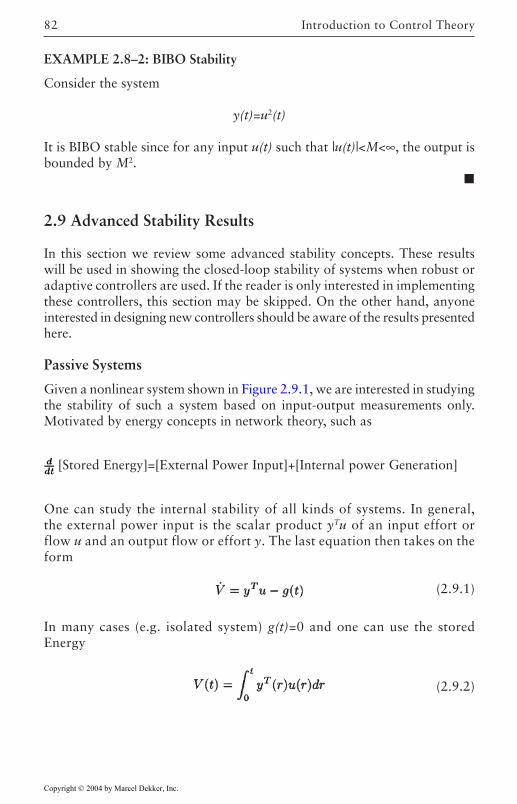
Introduction to Control Theory82
EXAMPLE 2.8–2: BIBO Stability
Consider the system
y(t)=u2(t)
It is BIBO stable since for any input u(t) such that |u(t)|<M<∞, the output isbounded by M2.
2.9 Advanced Stability Results
In this section we review some advanced stability concepts. These resultswill be used in showing the closed-loop stability of systems when robust oradaptive controllers are used. If the reader is only interested in implementingthese controllers, this section may be skipped. On the other hand, anyoneinterested in designing new controllers should be aware of the results presentedhere.
Passive Systems
Given a nonlinear system shown in Figure 2.9.1, we are interested in studyingthe stability of such a system based on input-output measurements only.Motivated by energy concepts in network theory, such as
[Stored Energy]=[External Power Input]+[Internal power Generation]
One can study the internal stability of all kinds of systems. In general,the external power input is the scalar product yTu of an input effort orflow u and an output flow or effort y. The last equation then takes on theform
(2.9.1)
In many cases (e.g. isolated system) g(t)=0 and one can use the storedEnergy
(2.9.2)
Copyright © 2004 by Marcel Dekker, Inc.
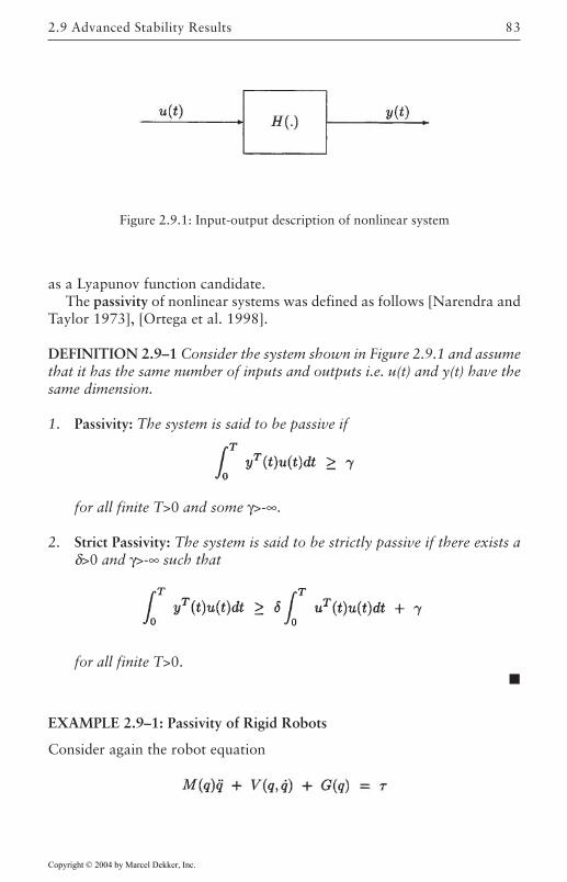
83
as a Lyapunov function candidate.The passivity of nonlinear systems was defined as follows [Narendra and
Taylor 1973], [Ortega et al. 1998].
DEFINITION 2.9–1 Consider the system shown in Figure 2.9.1 and assumethat it has the same number of inputs and outputs i.e. u(t) and y(t) have thesame dimension.
1. Passivity: The system is said to be passive if
for all finite T>0 and some γ>-∞.
2. Strict Passivity: The system is said to be strictly passive if there exists aδ>0 and γ>-∞ such that
for all finite T>0.
EXAMPLE 2.9–1: Passivity of Rigid Robots
Consider again the robot equation
Figure 2.9.1: Input-output description of nonlinear system
2.9 Advanced Stability Results
Copyright © 2004 by Marcel Dekker, Inc.
Introduction to Control Theory84
Suppose the robot is representing a system whose input is and whoseoutput is the joint velocity q. Let the sum of the kinetic energy and potentialenergy of the robot be denote by the Hamiltonian H and recall [Ortega andSpong 1988]
then
which proves that from to q, the rigid robot is a passive system.
A passive system is in effect one that does not create energy.
Positive-Real Systems
If the system under consideration is linear and time-invariant, then passivityis equivalent to positivity and may be tested in the frequency domain[Narendra and Taylor 1973]. In fact, let us describe positive-real systemsand discuss some of their properties. Consider the multi-input-multi-outputlinear time-invariant system
where x is an n vector, u is an m vector, y is a p vector, A, B, C, and D are ofthe appropriate dimensions. The corresponding transfer function matrix is
P(s)=C(sI-A)-1B+D
We will assume that the system has an equal number of inputs and outputs,i.e. p=m. To simplify our notation we will denote the Hermitian part of areal, rational transfer matrix T(s) by where s*is the complex conjugate of s. A number of definitions have been given forSPR functions and matrices [Narendra and Taylor 1973]. It appears that themost useful definition for control applications is the following.
DEFINITION 2.9–2 An m×m matrix T(s) of proper real rational functionswhich is not identically zero is positive-real or PR if
Copyright © 2004 by Marcel Dekker, Inc.
85
1. All elements of T(s) have no poles in the region Re(s)>0,2. Any poles of T(s) on the jw axis are simple with positive-definite residues,
and3. The matrix He[T(s)] is positive semidefinite for Re(s)>0.
EXAMPLE 2.9–2: PR Matrices
Consider the matrix
This matrix is PR as can be checked.
DEFINITION 2.9–3 An m×m matrix T(s) of proper real rational functionswhich is not identically zero is strictly-positive-real or SPR if
1. All elements of T(s) have no poles in the region Re(s)0, and2. The matrix He[T(s)] is positive definite for Re(s)>0.
EXAMPLE 2.9–3: SPR Matrices
Consider the matrix
This matrix is SPR as can be checked.
Lure’s Problem
Consider the following feedback interconnected system
(2.9.3)
2.9 Advanced Stability Results
Copyright © 2004 by Marcel Dekker, Inc.
Introduction to Control Theory86
where φ is continuous in both arguments. Lure then stated the followingAbsolute Stability problem which became known as Lure’s Problem: Supposethe system described by the above equations is given where:
1. All eigenvalues of A have negative real parts or that A has one eigen-value at the origin while the rest of them is in the open left-half plane(OLHP), and
2. (A, b) is controllable, and3. (c, A) is observable, and4. The nonlinearity φ(.,.) satisfies
(a) φ(t,0)=0;t0 and(b)
Then, find conditions on the linear system (A, B, C, D) such that x=0 is aGAS equilibrium point of the closed-loop system.
Note that sometimes when we know more about the nonlinearity φ, thelast condition above is replaced by the following:
where k2k10 are constants. We then say that φ belongs to the sector[k1, k2].
The first attempt to solve this problem was made by Aizerman in what isnow known as Aizerman’s conjecture [Vidyasagar 1992] followed by theefforts of Kalman [Vidyasagar 1992]. The correct solution however, was notavailable until the
In order to present the correct results, we need to present the KY andMKY lemmas.
The MKY Lemma
The following lemmas are versions of the Meyer-Kalman-Yakubovich(MKY) lemma which appears in [Narendra and Taylor 1973], [Khalil 2001]amongst other places, and will be useful in designing adaptive controllersfor robots.
LEMMA 2.9–1: Meyer-Kalman-Yakubovitch Let the system (2.9.3) withD=0 be controllable. Then the transfer function c(sI-A)-1b is SPR if andonly if
Copyright © 2004 by Marcel Dekker, Inc.
87
1. For any symmetric, positive-definite Q, there exists a symmetric, positive-definite P solution of the Lyapunov equation
ATP+PA=-Q
2. The matrices B and C satisfy
C=BTP
The MKY Lemma gives conditions under which a transfer matrix has adegree of robustness. Note that the conditions depend on both the input andoutput matrices and thus a particular system may be SPR for a certain choiceof input/output pairs and not SPR for others. A modified version of the KYlemma which relaxes the condition of controllability is given next.
LEMMA 2.9–2: Meyer-Kalman-Yakubovitch Given vector b, anasymptotically stable A, a real vector v, scalars γ0 and >0, and a positive-definite matrix Q, then, there exist a vector q and a symmetric positive definiteP such that
1.
2.
if and only if
1. is small enough and,
2. the transfer function γ/2+vT(sI-A)-1b is SPR
In most of our applications, q=0. These lemmas find many applications innonlinear systems. It is usually possible to divide a nonlinear system into alinear feed-forward subsystem, and a nonlinear, passive feedback. Thechallenge is then to make the linear subsystem SPR so that the stability of thecombined system is guaranteed.
2.9 Advanced Stability Results
Copyright © 2004 by Marcel Dekker, Inc.
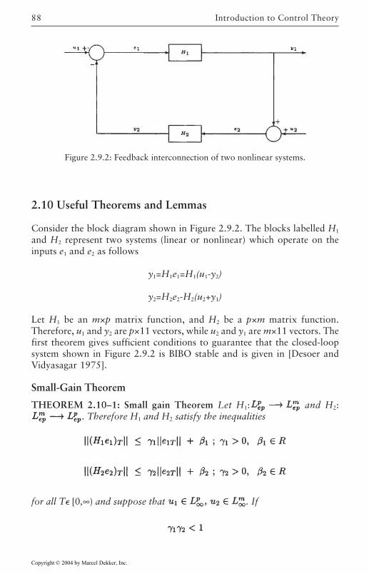
Introduction to Control Theory88
2.10 Useful Theorems and Lemmas
Consider the block diagram shown in Figure 2.9.2. The blocks labelled H1
and H2 represent two systems (linear or nonlinear) which operate on theinputs e1 and e2 as follows
y1=H1e1=H1(u1-y2)
y2=H2e2-H2(u2+y1)
Let H1 be an m×p matrix function, and H2 be a p×m matrix function.Therefore, u1 and y2 are p×11 vectors, while u2 and y1 are m×11 vectors. Thefirst theorem gives sufficient conditions to guarantee that the closed-loopsystem shown in Figure 2.9.2 is BIBO stable and is given in [Desoer andVidyasagar 1975].
Small-Gain Theorem
THEOREM 2.10–1: Small gain Theorem Let H1: and H2:. Therefore H1 and H2 satisfy the inequalities
for all T [0,∞) and suppose that . If
Figure 2.9.2: Feedback interconnection of two nonlinear systems.
Copyright © 2004 by Marcel Dekker, Inc.
89
Then e1, y2, and y1, .
Basically, the small-gain theorem states that a feedback interconnectionof two systems is BIBO stable if the loop-gain is less than unity. In otherwords, if a signal traverses the feedback-loop and decreases in magnitudethen the closed-loop system can not go unstable.
EXAMPLE 2.10–1: Applications of Small-Gain Theorem
Let the feedback connection of Figure 2.9.2 be such that
Then, we can show that
γ1=0.5; ß1=0
γ2=1; ß2=1.
Since γ1γ2=0.5<1, the feedback connection is BIBO stable.
The next theorem provides a test for the stability of a nonlinear system basedon the stability of its linear part. In fact, a certain degree of robustness isachieved if the linear system is exponentially stable as described in [Andersonet al. 1986].
Total Stability Theorem
THEOREM 2.10–2: Total Stability Consider the state-space systemdescribed by
where
1. The system is exponentially stable i.e. there are some a>0and K1, such that
||x(t)|| Ke-at; t0
2.10 Useful Theorems and Lemmas
Copyright © 2004 by Marcel Dekker, Inc.
Introduction to Control Theory90
2. f(t, 0)=0 i.e. the origin is an equilibrium point of f(t, x)
3. || f(t, x1)-f(t, x2)||ß1||x1-x2||, for some ß1>0
4. ||g(t, x1)||ß2r, for some ß2>0
5. ||g(t, x1)-g(t, x2)ß2 ||x1-x2||
6.
Then, there exists a unique solution x(t) to 1.5.5 and
The total stability theorem will be used to design controllers that willmake the linear part of the system exponentially stable. In effect, thistheorem guarantees that if the linear part of the system is “very” stable(exponentially stable), the destabilizing effect of the boundednonlinearities may not be sufficient to destabilize the system and the statewill remain bounded.
EXAMPLE 2.10–2: Total Stability
Consider the nonlinear system
Let |x0|<1, and note the following
K=1; a=2; ß1=0.5; ß2=1.
Note first that all conditions of the theorem are satisfied, then there exists aunique solution x(t) which is bounded by
A version of the Bellman-Gronwall lemma is proved in [Sastry and Bodson1989] and is presented next.
Copyright © 2004 by Marcel Dekker, Inc.
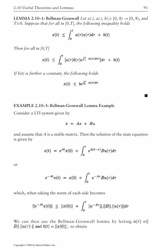
91
LEMMA 2.10–1: Bellman-Gronwall Let x(.), a(.), b(.): [0, 8) → [0, 8), andT0. Suppose that for all t [0,T], the following inequality holds
Then for all t [0,T]
If b(t) is further a constant, the following holds
EXAMPLE 2.10–3: Bellman-Gronwall Lemma Example
Consider a LTI system given by
and assume that A is a stable matrix. Then the solution of the state equationis given by
or
which, when taking the norm of each side becomes
We can then use the Bellman-Gronwall lemma by letting to obtain
2.10 Useful Theorems and Lemmas
Copyright © 2004 by Marcel Dekker, Inc.
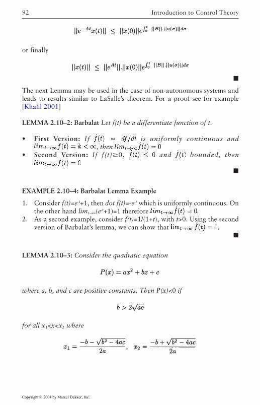
Introduction to Control Theory92
or finally
The next Lemma may be used in the case of non-autonomous systems andleads to results similar to LaSalle’s theorem. For a proof see for example[Khalil 2001]
LEMMA 2.10–2: Barbalat Let f(t) be a differentiate function of t.
• First Version: If is uniformly continuous and, then
• Second Version: If f(t)0, and bounded, then
EXAMPLE 2.10–4: Barbalat Lemma Example
1. Consider f(t)=e-t+1, then dot f(t)=-e-t which is uniformly continuous. Onthe other hand limt→∞(e-t+1)=1 therefore .
2. As a second example, consider f(t)=1/(1+t), with t>0. Using the secondversion of Barbalat’s lemma, we can show that .
LEMMA 2.10–3: Consider the quadratic equation
where a, b, and c are positive constants. Then P(x)<0 if
for all x1<x<x2 where
Copyright © 2004 by Marcel Dekker, Inc.
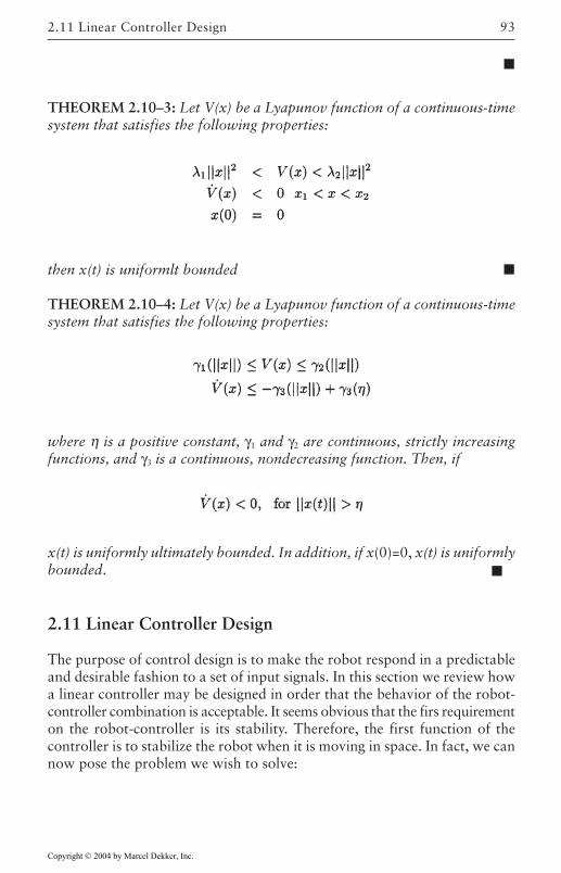
93
THEOREM 2.10–3: Let V(x) be a Lyapunov function of a continuous-timesystem that satisfies the following properties:
then x(t) is uniformlt bounded
THEOREM 2.10–4: Let V(x) be a Lyapunov function of a continuous-timesystem that satisfies the following properties:
where η is a positive constant, γ1 and γ2 are continuous, strictly increasingfunctions, and γ3 is a continuous, nondecreasing function. Then, if
x(t) is uniformly ultimately bounded. In addition, if x(0)=0, x(t) is uniformlybounded.
2.11 Linear Controller Design
The purpose of control design is to make the robot respond in a predictableand desirable fashion to a set of input signals. In this section we review howa linear controller may be designed in order that the behavior of the robot-controller combination is acceptable. It seems obvious that the firs requirementon the robot-controller is its stability. Therefore, the first function of thecontroller is to stabilize the robot when it is moving in space. In fact, we cannow pose the problem we wish to solve:
2.11 Linear Controller Design
Copyright © 2004 by Marcel Dekker, Inc.
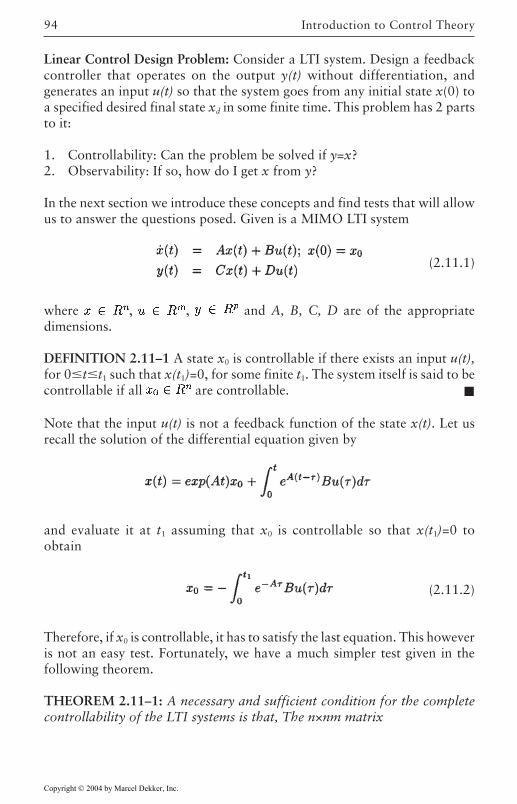
Introduction to Control Theory94
Linear Control Design Problem: Consider a LTI system. Design a feedbackcontroller that operates on the output y(t) without differentiation, andgenerates an input u(t) so that the system goes from any initial state x(0) toa specified desired final state xd in some finite time. This problem has 2 partsto it:
1. Controllability: Can the problem be solved if y=x?2. Observability: If so, how do I get x from y?
In the next section we introduce these concepts and find tests that will allowus to answer the questions posed. Given is a MIMO LTI system
(2.11.1)
where , , and A, B, C, D are of the appropriatedimensions.
DEFINITION 2.11–1 A state x0 is controllable if there exists an input u(t),for 0tt1 such that x(t1)=0, for some finite t1. The system itself is said to becontrollable if all are controllable.
Note that the input u(t) is not a feedback function of the state x(t). Let usrecall the solution of the differential equation given by
and evaluate it at t1 assuming that x0 is controllable so that x(t1)=0 toobtain
(2.11.2)
Therefore, if x0 is controllable, it has to satisfy the last equation. This howeveris not an easy test. Fortunately, we have a much simpler test given in thefollowing theorem.
THEOREM 2.11–1: A necessary and sufficient condition for the completecontrollability of the LTI systems is that, The n×nm matrix
Copyright © 2004 by Marcel Dekker, Inc.
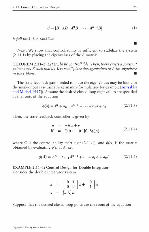
95
(1)
is full rank, i. e. rankC=n
Next, We show that controllability is sufficient to stabilize the system(2.11.1) by placing the eigenvalues of the A matrix
THEOREM 2.11–2: Let (A, b) be controllable. Then, there exists a constantgain matrix K such that u=-Kx+v will place the eigenvalues of A-bk anywherein the s plane.
The state-feedback gain needed to place the eigenvalues may be found inthe single-input case using Ackermann’s formula (see for example [Antsaklisand Michel 1997]). Assume the desired closed-loop eigenvalues are specifiedas the roots of the equation
(2.11.3)
Then, the state-feedback controller is given by
(2.11.4)
where C is the controllability matrix of (2.11.1), and φ(Α) is the matrixobtained by evaluating φ(s) at A, i.e.
(2.11.5)
EXAMPLE 2.11–1: Control Design for Double IntegratorConsider the double integrator system
Suppose that the desired closed-loop poles are the roots of the equation
2.11 Linear Controller Design
Copyright © 2004 by Marcel Dekker, Inc.
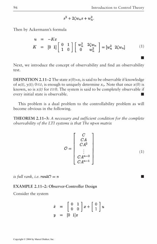
Introduction to Control Theory96
Then by Ackermann’s formula
(1)
Next, we introduce the concept of observability and find an observabilitytest.
DEFINITION 2.11–2 The state x(0)=x0 is said to be observable if knowledgeof u(t), y(t); 0t1 is enough to uniquely determine x0. Note that once x(0) isknown, so is x(t) for t0. The system is said to be completely observable ifevery initial state is observable.
This problem is a dual problem to the controllability problem as willbecome obvious in the following.
THEOREM 2.11–3: A necessary and sufficient condition for the completeobservability of the LTI systems is that The np×n matrix
(1)
is full rank, i.e.
EXAMPLE 2.11–2: Observer-Controller Design
Consider the system
Copyright © 2004 by Marcel Dekker, Inc.
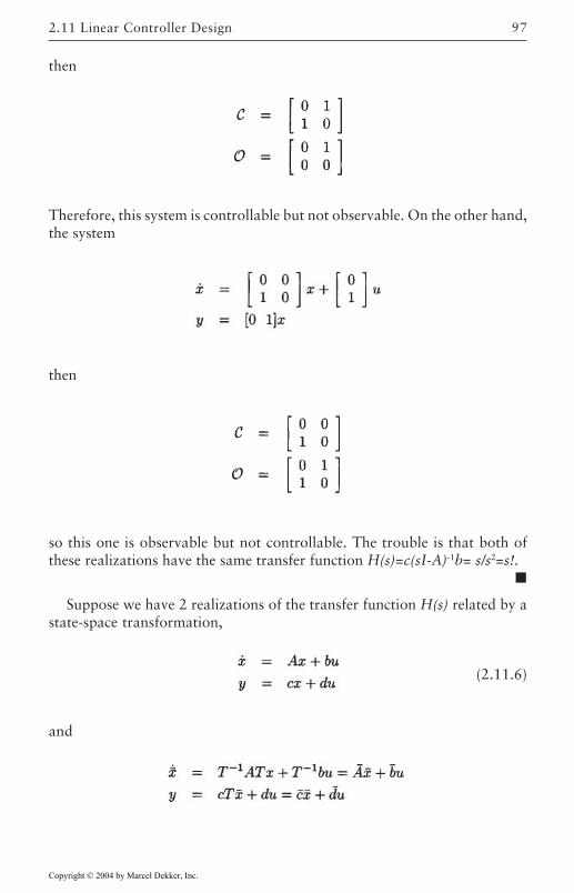
97
then
Therefore, this system is controllable but not observable. On the other hand,the system
then
so this one is observable but not controllable. The trouble is that both ofthese realizations have the same transfer function H(s)=c(sI-A)-1b= s/s2=s!.
Suppose we have 2 realizations of the transfer function H(s) related by astate-space transformation,
(2.11.6)
and
2.11 Linear Controller Design
Copyright © 2004 by Marcel Dekker, Inc.
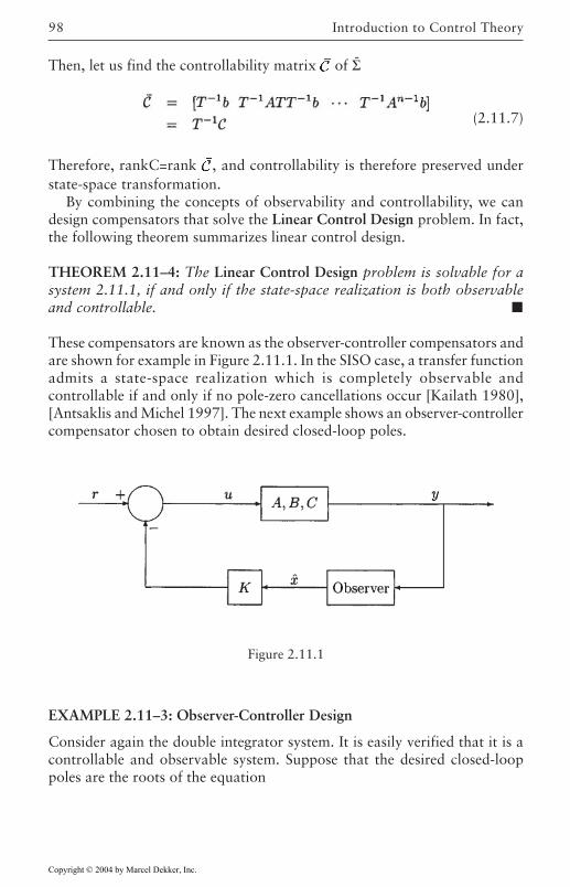
Introduction to Control Theory98
Then, let us find the controllability matrix of Σ-
(2.11.7)
Therefore, rankC=rank , and controllability is therefore preserved understate-space transformation.
By combining the concepts of observability and controllability, we candesign compensators that solve the Linear Control Design problem. In fact,the following theorem summarizes linear control design.
THEOREM 2.11–4: The Linear Control Design problem is solvable for asystem 2.11.1, if and only if the state-space realization is both observableand controllable.
These compensators are known as the observer-controller compensators andare shown for example in Figure 2.11.1. In the SISO case, a transfer functionadmits a state-space realization which is completely observable andcontrollable if and only if no pole-zero cancellations occur [Kailath 1980],[Antsaklis and Michel 1997]. The next example shows an observer-controllercompensator chosen to obtain desired closed-loop poles.
Figure 2.11.1
EXAMPLE 2.11–3: Observer-Controller Design
Consider again the double integrator system. It is easily verified that it is acontrollable and observable system. Suppose that the desired closed-looppoles are the roots of the equation
Copyright © 2004 by Marcel Dekker, Inc.
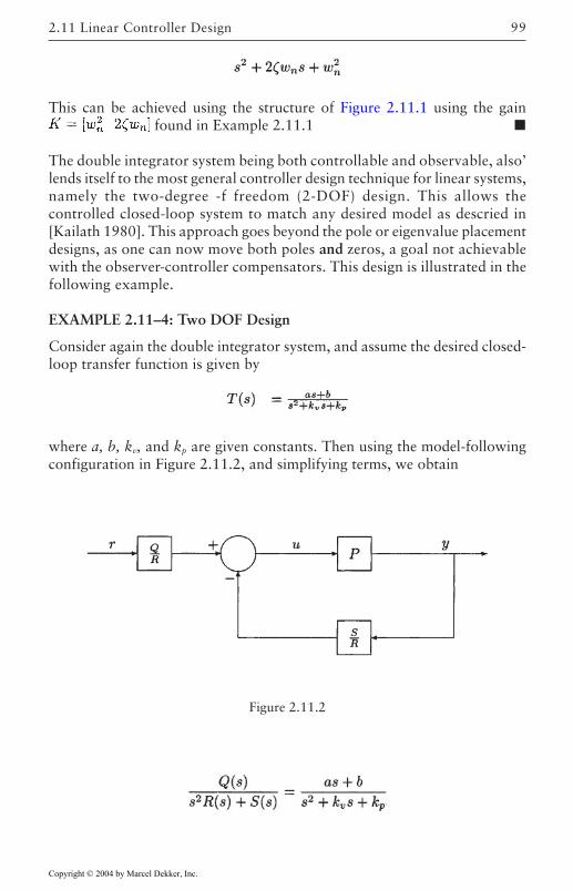
99
This can be achieved using the structure of Figure 2.11.1 using the gain found in Example 2.11.1
The double integrator system being both controllable and observable, also’lends itself to the most general controller design technique for linear systems,namely the two-degree -f freedom (2-DOF) design. This allows thecontrolled closed-loop system to match any desired model as descried in[Kailath 1980]. This approach goes beyond the pole or eigenvalue placementdesigns, as one can now move both poles and zeros, a goal not achievablewith the observer-controller compensators. This design is illustrated in thefollowing example.
EXAMPLE 2.11–4: Two DOF Design
Consider again the double integrator system, and assume the desired closed-loop transfer function is given by
where a, b, kv, and kp are given constants. Then using the model-followingconfiguration in Figure 2.11.2, and simplifying terms, we obtain
Figure 2.11.2
2.11 Linear Controller Design
Copyright © 2004 by Marcel Dekker, Inc.
Introduction to Control Theory100
or
(s2+kvs+kp)Q(s)=(as+b)[s2R(s)+S(s)].
At this stage, we may choose for example R(s)=1 and suppose for thepurpose of illustration that a=b=kp=1 and that kv=9. Then we solve for S(s)=9sand Q(s)=s. Note that in this case, the feedback block S(s)/R(s) is improperbut this does not cause any problems in cases (such as robot control) wherevelocity measurements are available.
The question addressed next is to find conditions on (2.11.1) so that astatic-output feedback controller will render the closed-loop system SPR.We will consider the SISO case only since this is the only case encounteredin this book.
(2.11.8)
or in the frequency-domain
(2.11.9)
We present a simple frequency domain result to show the existence of K andγ that will render the closed-loop system SPR. The result first appeared in[Gu 1988].
THEOREM 2.11–5: Let system (2.2.11) have no common poles and zeros.Then there exists a nonsingular K and a positive scalar γ such that the closed-loop system (2.11.8, 2.11.9) is SPR, if and only if P(s) has no zeros in theright half plane and if P(s) has n poles and n - 1 zeros. In fact, one such K isgiven by
K=P(CB)-1
where P is any symmetric, positive-definite matrix.
Copyright © 2004 by Marcel Dekker, Inc.
101
EXAMPLE 2.11-5: SPR Design
Consider the double integrator system
where c2≠0 and c1, c2 are of the same sign. The open-loop transfer function isthen
which has relative degree 1 and is minimum phase. Note that CB=c2 which isinvertible. The gain K is chosen to be
where p>0. The closed-loop system is then
which is stable for any choice of γ>0 and is SPR if γ>c1/(pc2 (check!).
2.12 Summary and Notes
This chapter is meant to be a review of various control theory concepts thatwill be used in the remainder of the book. The emphasis has been to includeenough material so that readers with little or no background in control theoryare able to follow the design of robot controllers. Simplifications were oftenmade to concentrate on the systems studied in this book, namely, mechanicalsystems and systems described by the Lagrange-Euler equations. In particular,the double integrator system was illustrated in detail, since it will result fromapplying a preliminary nonlinear feedback on mechanical manipulators. In
2.12 Summary and Notes
Copyright © 2004 by Marcel Dekker, Inc.
Chapter 3, we introduce the dynamical description of rigid robot
Introduction to Control Theory102
manipulators, and in subsequent chapters, the control concepts reviewed inthis chapter will be implemented on those manipulators.
Most of the results reviewed here can be found in greater details in thebooks by [Kailath 1980], [Antsaklis and Michel 1997] for the linear systemscase, and in [Khalil 2001], [Vidyasagar 1992] in the nonlinear systems case.
Copyright © 2004 by Marcel Dekker, Inc.
103
REFERENCES
[Anderson et al. 1986] B.D.O.Anderson and R.Bitmead and C.R.Johnson,Jr. and P.V.Kokotovic and R.L.Kosut and I.M.Y.Mareels and L.Pralyand B.D.Riedle. “Stability of Adaptive Systems: Passivity and AveragingAnalysis”. MIT Press, Cambridge, MA, 1986.
[Antsaklis and Michel 1997] P.Antsaklis and A.N.Michel. “Linear Systems”.McGraw Hill, New York, 1997.
[Åström and Wittenmark 1995] K.Åström and B.Wittenmark. “AdaptiveControl”. Addison-Wesley, Reading, MA, 2nd edition, 1995.
[Åström and Wittenmark 1996] K.Åström and B.Wittenmark. “Computer-Controlled Systems: Theory and Design”, Prentice-Hall, EnglewoodCliffs, NJ, 1996.
[Boyd and Barratt] S.Boyd and G.Barratt. “Linear Controller Design: Limitsof Performance”, Prentice-Hall, Englewood Cliffs, NJ, 1991.
[Desoer and Vidyasagar 1975] C.Desoer and M.Vidyasagar. “FeedackSystems: Input-Output Properties”, Academic Press, New York, 1975.
[Franklin et al. 1997] G.Franklin and D.Powell and M.Workman. “DigitalControl of Dynamic Systems”, Addison-Wesley, Reading, MA, 1997.
[Gu 1988] G.Gu. “Stabilizability Conditions for Multivariable Uncertainsystems via Output Feedback”, IEEE Trans. Autom. Control, vol. AC-35, pp. 988–992, 1988.
[Hahn 1967] W.Hahn. “Theory and Applications of Lyapunov’s DirectMethod”. Prentice-Hall, Englewood Cliffs, NJ, 1967.
[Horn and Johnson 1991] R.Horn and C.Johnson. “Topics in MatrixAnalysis”. Cambridge University Press, New York, 1991.
Copyright © 2004 by Marcel Dekker, Inc.
REFERENCES104
[Kailath 1980] T.Kailath. “Linear Systems”. Prentice-Hall, Englewood Cliffs,NJ, 1980.
[Khalil 2001]. H.Khalil. “Nonlinear Systems”. Prentice-Hall, EnglewoodCliffs, NJ, 2001.
[LaSale and Lefschetz 1961] P.LaSale and S.Lefschetz. “Stability byLyapunov’s Direct Method”. Academic Press, New York, 1961.
[Ljung 1999] L.Ljung. “System Identification-Theory for the User”. Prentice-Hall, Englewood Cliffs, NJ, 1999.
[Narendra and Taylor 1973] K.S.Narendra and J.H.Taylor. “FrequencyDomain Criteria for Absolute Stability”. Academic Press, New York,1973.
[Niculescu and Abdallah 2000] S.-I.Niculescu and C.T.Abdallah. “DelayEffects on Static Output Feedback Stabilization”. Submitted IEEE CDC2000, Sydney, Australia, 2000.
[Ortega and Spong 1988] R.Ortega and M.Spong. “Adaptive Motion Controlof Rigid Robots: A Tutorial”. Proc. IEEE Conf. Dec. and Cont., pp.1575–1584, 1988.
[Ortega et al. 1998] R.Ortega and A.Loria and P.J.Nicklasson and H.Sira-Ramirez. “Passivity-based Control of Euler-Lagrange Systems”. Springer-Verlag, Berlin, 1998.
[Strang 1988] G.Strang. “Linear Algebra and its Applications”. Brooks/Cole,Stamford, CT, 1988.
[Koltchinskii et al. 1999] V.Koltchinskii and C.T.Abdallah and M.Ariolaand P.Dorato and D.Panchenko. “Statistical Learning Control ofUncertain Systems: It is better than it seems”. IEEE Trans, on AutomaticControl, February 1999.
[Sastry and Bodson 1989] S.Sastry and M.Bodson. “Adaptive Control:Stability, Convergence, and Robustness”. Prentice-Hall, EnglewoodCliffs, NJ, 1989.
[ATM 1996] “ATM Forum Traffic Management Specification”. ATM ForumTraffic Management Working Group AF-TM-0056.000, version 4.0,April 1996.
[Niculescu et al. 1997] S.-I.Niculescu and E.Verriest and L.Dugard and J.-M.Dion. “Stability and robust stability of time-delay systems: A guidedtour”. LNCIS, Springer-Verlag, London, vol. 228, pp. 1–71, 1997.
Copyright © 2004 by Marcel Dekker, Inc.
105REFERENCES
[CDC 1999] “CDC 1999 Special session on time-delay systems”. Proc. 1999CDC, Phoenix, AZ, 1999.
[Verhulst 1997] H.Verhulst. “Nonlinear Differential Equations andDynamical Systems”. Springer-Verlag, Berlin, 1997.
[Vidyasagar 1992] M.Vidyasagar. “Nonlinear Systems Analysis”. Prentice-Hall, Englewood Cliffs, NJ, 1992.
Copyright © 2004 by Marcel Dekker, Inc.
107
Chapter 3
Robot Dynamics
This chapter provides the background required for the study of robotmanipulator control The arm dynamical equations are derived both in thesecond-order differential equation formulation and several state-variableformulations. Some important properties of the dynamics are introduced. Weshow how to include the dynamics of the arm actuators, which may be electricor hydraulic motors.
3.1 Introduction
Robotics is a complex field involving many diverse disciplines, such as physics,properties of materials, statics and dynamics, electronics, control theory, vision,signal processing, computer programming, and manufacturing. In this bookour main interest is control of robot manipulators. The purpose of this chapteris to study the dynamical equations needed for the study of robot control.
For those desiring a background in control theory, Chapter 2 is provided.For those desiring a background in the basics of robot manipulators, in AppendixA we examine the geometric structure of robot manipulators, covering basicmanipulator configurations, kinematics, and inverse kinematics. There wereview as well the manipulator Jacobian, which is essential for control inCartesian or workspace coordinates, where the desired trajectories of the armare usually specified to begin with.
The robot dynamics are derived in Section 3.2. Lagrangian mechanics areused in this derivation. In Section 3.3 we review some fundamental propertiesof the arm dynamical equation that are essential in subsequent chapters for
which is referred to throughout the text.The arm dynamics in Section 3.2 are in the form of a second-order vector
Copyright © 2004 by Marcel Dekker, Inc.
the derivation of robot control schemes. These are summarized in Table 3.3.1,
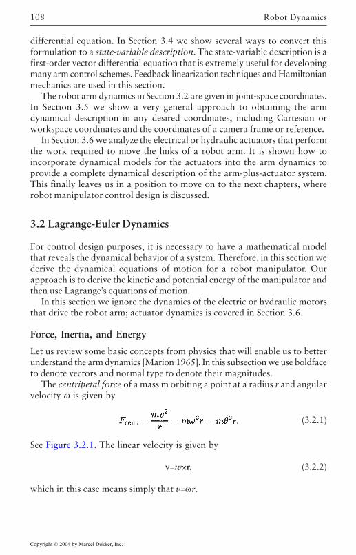
Robot Dynamics108
differential equation. In Section 3.4 we show several ways to convert thisformulation to a state-variable description. The state-variable description is afirst-order vector differential equation that is extremely useful for developingmany arm control schemes. Feedback linearization techniques and Hamiltonianmechanics are used in this section.
The robot arm dynamics in Section 3.2 are given in joint-space coordinates.In Section 3.5 we show a very general approach to obtaining the armdynamical description in any desired coordinates, including Cartesian orworkspace coordinates and the coordinates of a camera frame or reference.
In Section 3.6 we analyze the electrical or hydraulic actuators that performthe work required to move the links of a robot arm. It is shown how toincorporate dynamical models for the actuators into the arm dynamics toprovide a complete dynamical description of the arm-plus-actuator system.This finally leaves us in a position to move on to the next chapters, whererobot manipulator control design is discussed.
3.2 Lagrange-Euler Dynamics
For control design purposes, it is necessary to have a mathematical modelthat reveals the dynamical behavior of a system. Therefore, in this section wederive the dynamical equations of motion for a robot manipulator. Ourapproach is to derive the kinetic and potential energy of the manipulator andthen use Lagrange’s equations of motion.
In this section we ignore the dynamics of the electric or hydraulic motorsthat drive the robot arm; actuator dynamics is covered in Section 3.6.
Force, Inertia, and Energy
Let us review some basic concepts from physics that will enable us to betterunderstand the arm dynamics [Marion 1965]. In this subsection we use boldfaceto denote vectors and normal type to denote their magnitudes.
The centripetal force of a mass m orbiting a point at a radius r and angularvelocity ω is given by
(3.2.1)
v=w×r, (3.2.2)
which in this case means simply that v=ωr.
Copyright © 2004 by Marcel Dekker, Inc.
See Figure 3.2.1. The linear velocity is given by
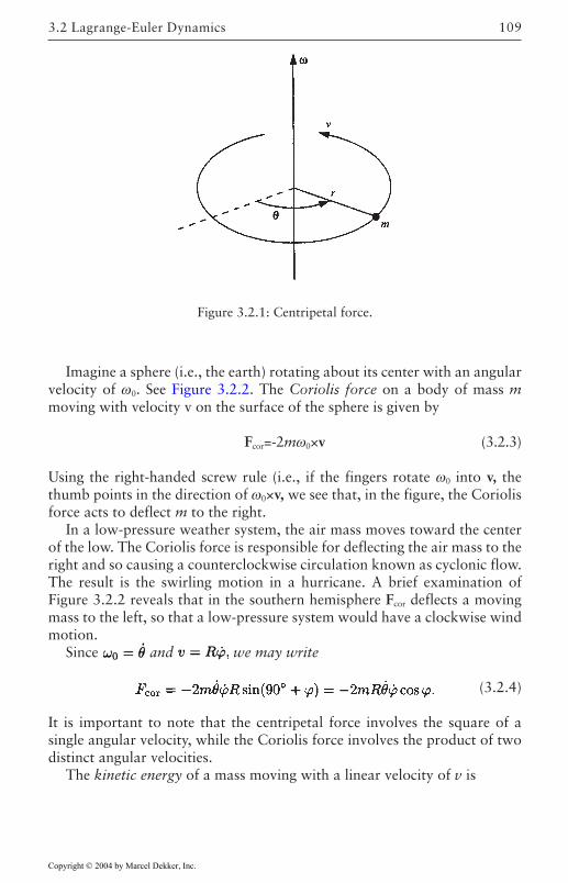
109
Imagine a sphere (i.e., the earth) rotating about its center with an angularvelocity of ω0. See Figure 3.2.2. The Coriolis force on a body of mass mmoving with velocity v on the surface of the sphere is given by
Fcor=-2mω0×v (3.2.3)
Using the right-handed screw rule (i.e., if the fingers rotate ω0 into v, thethumb points in the direction of ω0×v, we see that, in the figure, the Coriolisforce acts to deflect m to the right.
In a low-pressure weather system, the air mass moves toward the centerof the low. The Coriolis force is responsible for deflecting the air mass to theright and so causing a counterclockwise circulation known as cyclonic flow.The result is the swirling motion in a hurricane. A brief examination ofFigure 3.2.2 reveals that in the southern hemisphere Fcor deflects a movingmass to the left, so that a low-pressure system would have a clockwise windmotion.
Since and we may write
(3.2.4)
It is important to note that the centripetal force involves the square of asingle angular velocity, while the Coriolis force involves the product of twodistinct angular velocities.
The kinetic energy of a mass moving with a linear velocity of v is
Figure 3.2.1: Centripetal force.
3.2 Lagrange-Euler Dynamics
Copyright © 2004 by Marcel Dekker, Inc.
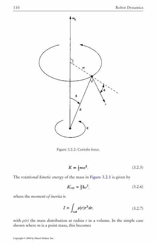
Robot Dynamics110
(3.2.5)
The rotational kinetic energy of the mass in Figure 3.2.1 is given by
(3.2.6)
where the moment of inertia is
(3.2.7)
with ρ(r) the mass distribution at radius r in a volume. In the simple caseshown where m is a point mass, this becomes
Figure 3.2.2: Coriolis force.
Copyright © 2004 by Marcel Dekker, Inc.
111
I=mr2. (3.2.8)Therefore,
(3.2.9)
The potential energy of a mass m at a height h in a gravitational field withconstant g is given by
P=mgh. (3.2.10)
The origin, corresponding to zero potential energy, may be selected arbitrarilysince only differences in potential energy are meaningful in terms of physicalforces.
The momentum of a mass m moving with velocity v is given by
p=mv. (3.2.11)
The angular momentum of a mass m with respect to an origin from whichthe mass has distance r is
Pang=r×p. (3.2.12)
The torque or moment of a force F with respect to the same origin is definedto be
N=r×F. (3.2.13)
Lagrange’s Equations of Motion
Lagrange’s equation of motion for a conservative system are given by [Marion1965]
(3.2.14)
where q is an n-vector of generalized coordinates qi, is an n-vector ofgeneralized forces i, and the Lagrangian is the difference between the kineticand potential energies
L=K-P. (3.2.15)
In our usage, q will be the joint-variable vector, consisting of joint angles θi;(in degrees or radians) and joint offsets di (in meters). Then τ is a vector thathas components ni of torque (newton-meters) corresponding to the jointangles, and fi of force (newtons) corresponding to the joint offsets. Note thatwe denote the scalar components of τ by lowercase letters.
3.2 Lagrange-Euler Dynamics
Copyright © 2004 by Marcel Dekker, Inc.
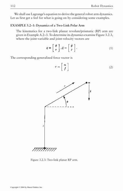
Robot Dynamics112
We shall use Lagrange’s equation to derive the general robot arm dynamics.Let us first get a feel for what is going on by considering some examples.
EXAMPLE 3.2–1: Dynamics of a Two-Link Polar Arm
The kinematics for a two-link planar revolute/prismatic (RP) arm aregiven in Example A.2–3. To determine its dynamics examine Figure 3.2.3,where the joint-variable and joint-velocity vectors are
(1)
The corresponding generalized force vector is
(2)
Figure 3.2.3: Two-link planar RP arm.
Copyright © 2004 by Marcel Dekker, Inc.
113
with n a torque and fa force. The torque n and force f may be provided byeither motors or hydraulic actuators. We discuss the dynamics of actuators inSection 3.6.
To determine the arm dynamics, we must now compute the quantitiesrequired for the Lagrange equation.
a. Kinetic and Potential Energy
The total kinetic energy due to the angular motion and the linear motion is
(3)
and the potential energy is
(4)
b. Lagrange’s Equation
The Lagrangian is
(5)
Now we obtain
(6)
(7)
(8)
Therefore, (3.2.14) shows that the arm dynamical equations are
(9)
(10)
This is a set of coupled nonlinear differential equations which describe themotion q(t)=[θ(t) r(t)]T given the control input torque n(t) and force f(t). We
3.2 Lagrange-Euler Dynamics
Copyright © 2004 by Marcel Dekker, Inc.
Robot Dynamics114
shall show how to determine q(t) given the control inputs n(t) and f(t) bycomputer simulation in Chapter 4.
Given our discussion on forces and inertias it is easy to identify the termsin the dynamical equations. The first terms in each equation are accelerationterms involving masses and inertias. The second term in (9) is a Coriolisterm, while the second term in (10) is a centripetal term. The third terms aregravity terms.
c. Manipulator Dynamics
By using vectors, the arm equations may be written in a convenient form.Indeed, note that
(11)
We symbolize this vector equation as
(12)
Note that, indeed, the inertia matrix M(q) is a function of q (i.e., of θ and r),the Coriolis/centripetal vector V(q, ) is a function of q and , and the gravityvector G(q) is a function of q.
EXAMPLE 3.2–2: Dynamics of a Two-Link Planar Elbow Arm
In Example A.2–2 are given the kinematics for a two-link planar RRarm. To determine its dynamics, examine Figure 3.2.4, where we haveassumed that the link masses are concentrated at the ends of the links.The joint variable is
q=[θ1 θ2]T (1)
and the generalized force vector is
(2)
Copyright © 2004 by Marcel Dekker, Inc.
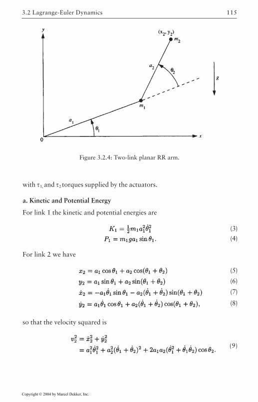
115
with τ1, and τ2 torques supplied by the actuators.
a. Kinetic and Potential Energy
For link 1 the kinetic and potential energies are
(3)
(4)
For link 2 we have
(5)
(6)
(7)
(8)
so that the velocity squared is
(9)
Figure 3.2.4: Two-link planar RR arm.
3.2 Lagrange-Euler Dynamics
Copyright © 2004 by Marcel Dekker, Inc.
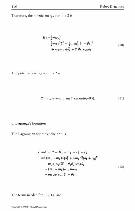
Robot Dynamics116
Therefore, the kinetic energy for link 2 is
(10)
The potential energy for link 2 is
P2=m2gy2=m2g[a1 sin θ1+a2 sin(θ1+θ2)]. (11)
b. Lagrange’s Equation
The Lagrangian for the entire arm is
(12)
The terms needed for (3.2.14) are
Copyright © 2004 by Marcel Dekker, Inc.
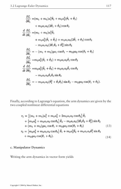
117
Finally, according to Lagrange’s equation, the arm dynamics are given by thetwo coupled nonlinear differential equations
(14)
c. Manipulator Dynamics
Writing the arm dynamics in vector form yields
(13)
3.2 Lagrange-Euler Dynamics
Copyright © 2004 by Marcel Dekker, Inc.
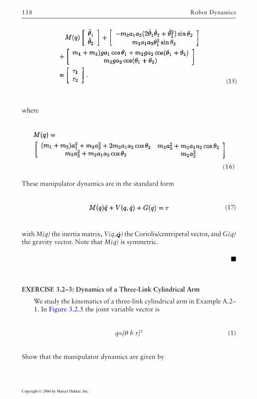
Robot Dynamics118
where
These manipulator dynamics are in the standard form
(17)
with M(q) the inertia matrix, V(q, ) the Coriolis/centripetal vector, and G(q)the gravity vector. Note that M(q) is symmetric.
EXERCISE 3.2–3: Dynamics of a Three-Link Cylindrical Arm
We study the kinematics of a three-link cylindrical arm in Example A.2–1. In Figure 3.2.5 the joint variable vector is
q=[θ h r]T (1)
Show that the manipulator dynamics are given by
(15)
(16)
Copyright © 2004 by Marcel Dekker, Inc.
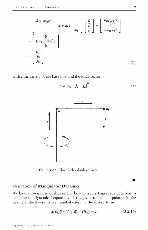
119
with J the inertia of the base link and the force vector
(3)
(2)
Figure 3.2.5: Three-link cylindrical arm.
Derivation of Manipulator Dynamics
We have shown in several examples how to apply Lagrange’s equation tocompute the dynamical equations of any given robot manipulator. In theexamples the dynamics we found always had the special form
(3.2.16)
3.2 Lagrange-Euler Dynamics
Copyright © 2004 by Marcel Dekker, Inc.
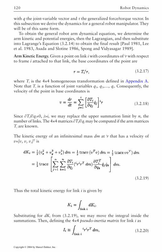
Robot Dynamics120
with q the joint-variable vector and τ the generalized force/torque vector. Inthis subsection we derive the dynamics for a general robot manipulator. Theywill be of this same form.
To obtain the general robot arm dynamical equation, we determine thearm kinetic and potential energies, then the Lagrangian, and then substituteinto Lagrange’s Equation (3.2.14) to obtain the final result [Paul 1981, Leeet al. 1983, Asada and Slotine 1986, Spong and Vidyasagar 1989].
Arm Kinetic Energy. Given a point on link i with coordinates of ir with respectto frame i attached to that link, the base coordinates of the point are
(3.2.17)
where Ti is the 4×4 homogeneous transformation defined in Appendix A.Note that Ti is a function of joint variables q1, q2,…, qi. Consequently, thevelocity of the point in base coordinates is
(3.2.18)
Since ∂Ti/∂qj=0, j>i, we may replace the upper summation limit by n, thenumber of links. The 4×4 matrices ∂Ti/∂qj may be computed if the arm matricesTi are known.
The kinetic energy of an infinitesimal mass dm at ir that has a velocity ofv=[vx vy vz]T is
(3.2.19)
Thus the total kinetic energy for link i is given by
Substituting for dKi from (3.2.19), we may move the integral inside thesummations. Then, defining the 4×4 pseudo-inertia matrix for link i as
(3.2.20)
Copyright © 2004 by Marcel Dekker, Inc.
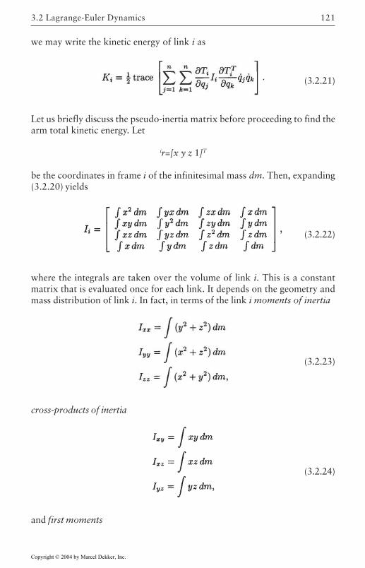
121
we may write the kinetic energy of link i as
(3.2.21)
Let us briefly discuss the pseudo-inertia matrix before proceeding to find thearm total kinetic energy. Let
ir=[x y z 1]T
be the coordinates in frame i of the infinitesimal mass dm. Then, expanding(3.2.20) yields
(3.2.22)
where the integrals are taken over the volume of link i. This is a constantmatrix that is evaluated once for each link. It depends on the geometry andmass distribution of link i. In fact, in terms of the link i moments of inertia
(3.2.23)
cross-products of inertia
(3.2.24)
and first moments
3.2 Lagrange-Euler Dynamics
Copyright © 2004 by Marcel Dekker, Inc.
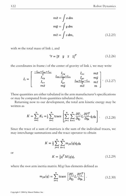
Robot Dynamics122
(3.2.25)
with m the total mass of link i, and
(3.2.26)
the coordinates in frame i of the center of gravity of link i, we may write
(3.2.27)
These quantities are either tabulated in the arm manufacturer’s specificationsor may be computed from quantities tabulated there.
Returning now to our development, the total arm kinetic energy may bewritten as
(3.2.28)
Since the trace of a sum of matrices is the sum of the individual traces, wemay interchange summations and the trace operator to obtain
or(3.2.29)
where the n×n arm inertia matrix M(q) has elements defined as
(3.2.30)
Copyright © 2004 by Marcel Dekker, Inc.
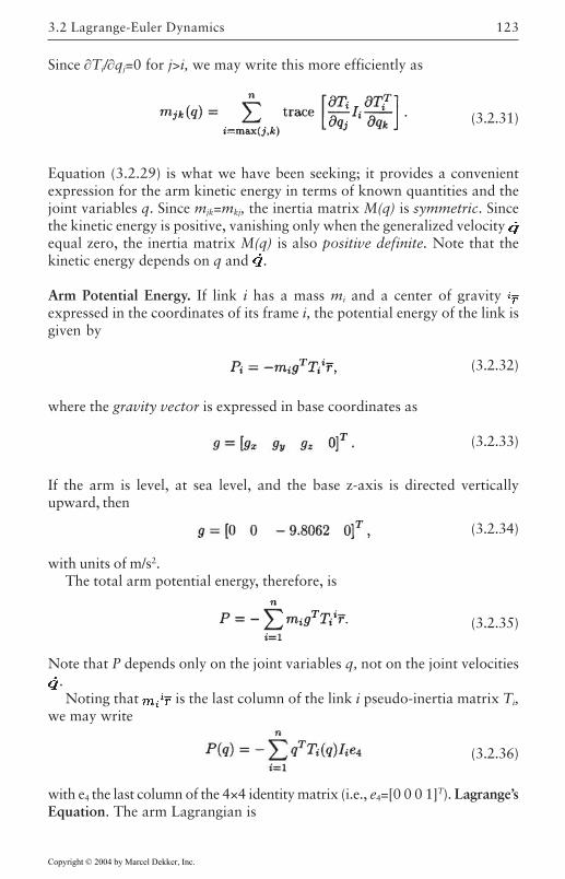
123
Since ∂Ti/∂qj=0 for j>i, we may write this more efficiently as
(3.2.31)
Equation (3.2.29) is what we have been seeking; it provides a convenientexpression for the arm kinetic energy in terms of known quantities and thejoint variables q. Since mjk=mkj, the inertia matrix M(q) is symmetric. Sincethe kinetic energy is positive, vanishing only when the generalized velocity equal zero, the inertia matrix M(q) is also positive definite. Note that thekinetic energy depends on q and .
Arm Potential Energy. If link i has a mass mi and a center of gravity expressed in the coordinates of its frame i, the potential energy of the link isgiven by
(3.2.32)
where the gravity vector is expressed in base coordinates as
(3.2.33)
If the arm is level, at sea level, and the base z-axis is directed verticallyupward, then
(3.2.34)
with units of m/s2.The total arm potential energy, therefore, is
(3.2.35)
Note that P depends only on the joint variables q, not on the joint velocities.Noting that is the last column of the link i pseudo-inertia matrix Ti,
we may write
(3.2.36)
with e4 the last column of the 4×4 identity matrix (i.e., e4=[0 0 0 1]T). Lagrange’sEquation. The arm Lagrangian is
3.2 Lagrange-Euler Dynamics
Copyright © 2004 by Marcel Dekker, Inc.
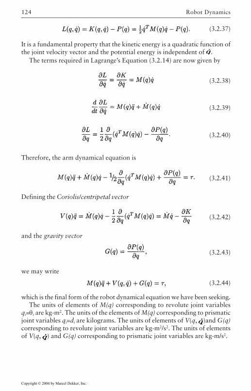
Robot Dynamics124
(3.2.37)
It is a fundamental property that the kinetic energy is a quadratic function ofthe joint velocity vector and the potential energy is independent of .
The terms required in Lagrange’s Equation (3.2.14) are now given by
(3.2.38)
(3.2.39)
(3.2.40)
Therefore, the arm dynamical equation is
(3.2.41)
Defining the Coriolis/centripetal vector
(3.2.42)
and the gravity vector
(3.2.43)
we may write
(3.2.44)
which is the final form of the robot dynamical equation we have been seeking.The units of elements of M(q) corresponding to revolute joint variables
qi=θi are kg-m2. The units of the elements of M(q) corresponding to prismaticjoint variables qi=di are kilograms. The units of elements of V(q, )and G(q)corresponding to revolute joint variables are kg-m2/s2. The units of elementsof V(q, ) and G(q) corresponding to prismatic joint variables are kg-m/s2.
Copyright © 2004 by Marcel Dekker, Inc.
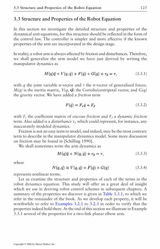
125
3.3 Structure and Properties of the Robot Equation
In this section we investigate the detailed structure and properties of thedynamical arm equations, for this structure should be reflected in the form ofthe control law. The controller is simpler and more effective if the knownproperties of the arm are incorporated in the design stage.
In reality, a robot arm is always affected by friction and disturbances. Therefore,we shall generalize the arm model we have just derived by writing themanipulator dynamics as
(3.3.1)
with q the joint variable n-vector and τ the n-vector of generalized forces.M(q) is the inertia matrix, V(q, ) the Coriolis/centripetal vector, and G(q)the gravity vector. We have added a friction term
(3.3.2)
with Fv the coefficient matrix of viscous friction and Fd a dynamic frictionterm. Also added is a disturbance τd, which could represent, for instance, anyinaccurately modeled dynamics.
Friction is not an easy term to model, and indeed, may be the most contraryterm to describe in the manipulator dynamics model. Some more discussionon friction may be found in [Schilling 1990].
We shall sometimes write the arm dynamics as
(3.3.3)
where(3.3.4)
represents nonlinear terms.Let us examine the structure and properties of each of the terms in the
robot dynamics equation. This study will offer us a great deal of insightwhich we use in deriving robot control schemes in subsequent chapters. A
refer in the remainder of the book. As we develop each property, it will beworthwhile to refer to Examples 3.2.1 to 3.2.3 in order to verify that theproperties indeed hold there. At the end of this section we illustrate in Example3.3.1 several of the properties for a two-link planar elbow arm.
3.3 Structure and Properties of the Robot Equation
Copyright © 2004 by Marcel Dekker, Inc.
summary of the properties we discover is given in Table 3.3.1, to which we
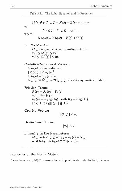
Robot Dynamics126
Properties of the Inertia Matrix
As we have seen, M(q) is symmetric and positive definite. In fact, the arm
Table 3.3.1: The Robot Equation and Its Properties
Copyright © 2004 by Marcel Dekker, Inc.
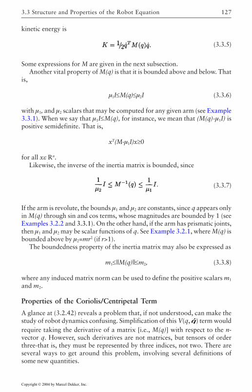
127
kinetic energy is
(3.3.5)
Some expressions for M are given in the next subsection.Another vital property of M(q) is that it is bounded above and below. That
is,
µ1I≤M(q)≤µ2I (3.3.6)
with µ1, and µ2 scalars that may be computed for any given arm (see Example3.3.1). When we say that µ1I≤M(q), for instance, we mean that (M(q)-µ1I) ispositive semidefinite. That is,
xT(M-µ1I)x≥0
for all xε Rn.Likewise, the inverse of the inertia matrix is bounded, since
(3.3.7)
If the arm is revolute, the bounds µ1 and µ2 are constants, since q appears onlyin M(q) through sin and cos terms, whose magnitudes are bounded by 1 (seeExamples 3.2.2 and 3.3.1). On the other hand, if the arm has prismatic joints,then µ1 and µ2 may be scalar functions of q. See Example 3.2.1, where M(q) isbounded above by µ2=mr2 (if r>1).
The boundedness property of the inertia matrix may also be expressed as
m1≤||M(q)||≤m2, (3.3.8)
where any induced matrix norm can be used to define the positive scalars m1
and m2.
Properties of the Coriolis/Centripetal Term
A glance at (3.2.42) reveals a problem that, if not understood, can make thestudy of robot dynamics confusing. Simplification of this V(q, ) term wouldrequire taking the derivative of a matrix [i.e., M(q)] with respect to the n-vector q. However, such derivatives are not matrices, but tensors of orderthree-that is, they must be represented by three indices, not two. There areseveral ways to get around this problem, involving several definitions ofsome new quantities.
3.3 Structure and Properties of the Robot Equation
Copyright © 2004 by Marcel Dekker, Inc.
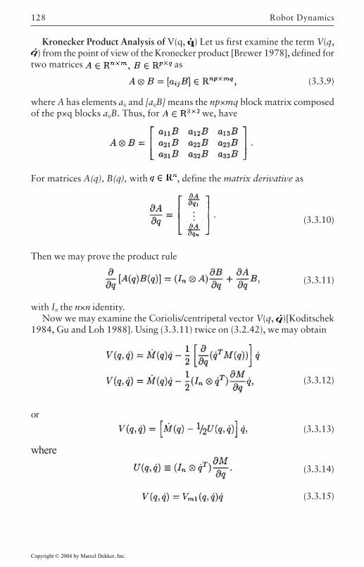
Robot Dynamics128
Kronecker Product Analysis of V(q, ) Let us first examine the term V(q,) from the point of view of the Kronecker product [Brewer 1978], defined for
two matrices as
(3.3.9)
where A has elements aij and [aijB] means the np×mq block matrix composedof the p×q blocks aijB. Thus, for we, have
For matrices A(q), B(q), with , define the matrix derivative as
(3.3.10)
Then we may prove the product rule
(3.3.11)
with In the n×n identity.Now we may examine the Coriolis/centripetal vector V(q, )[Koditschek
1984, Gu and Loh 1988]. Using (3.3.11) twice on (3.2.42), we may obtain
(3.3.12)
or
(3.3.13)
where(3.3.14)
(3.3.15)
Copyright © 2004 by Marcel Dekker, Inc.
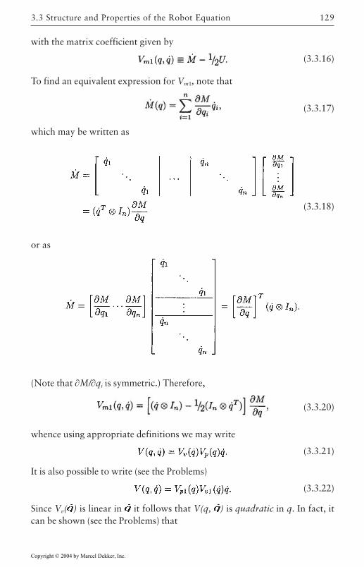
129
with the matrix coefficient given by
(3.3.16)
To find an equivalent expression for Vm1, note that
(3.3.17)
which may be written as
(3.3.18)
(Note that ∂M/∂qi is symmetric.) Therefore,
(3.3.20)
whence using appropriate definitions we may write
(3.3.21)
It is also possible to write (see the Problems)
(3.3.22)
Since Vv( ) is linear in it follows that V(q, ) is quadratic in q. In fact, itcan be shown (see the Problems) that
or as
3.3 Structure and Properties of the Robot Equation
Copyright © 2004 by Marcel Dekker, Inc.
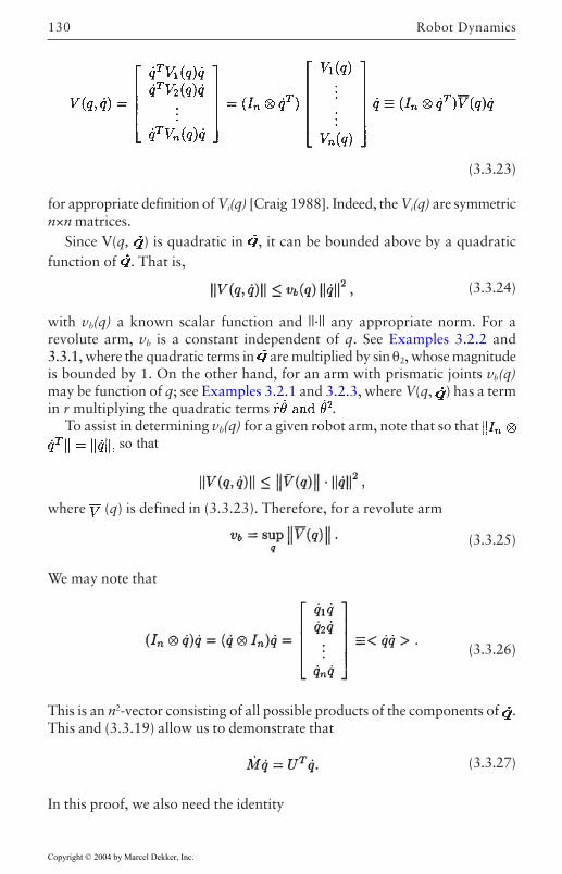
Robot Dynamics130
(3.3.23)
for appropriate definition of Vi(q) [Craig 1988]. Indeed, the Vi(q) are symmetricn×n matrices.
Since V(q, ) is quadratic in , it can be bounded above by a quadraticfunction of . That is,
(3.3.24)
with vb(q) a known scalar function and ||·|| any appropriate norm. For arevolute arm, vb is a constant independent of q. See Examples 3.2.2 and3.3.1, where the quadratic terms in are multiplied by sin θ2, whose magnitudeis bounded by 1. On the other hand, for an arm with prismatic joints vb(q)may be function of q; see Examples 3.2.1 and 3.2.3, where V(q, ) has a termin r multiplying the quadratic terms .
To assist in determining vb(q) for a given robot arm, note that so that so that
where (q) is defined in (3.3.23). Therefore, for a revolute arm
(3.3.25)
We may note that
(3.3.26)
This is an n2-vector consisting of all possible products of the components of .This and (3.3.19) allow us to demonstrate that
(3.3.27)
In this proof, we also need the identity
Copyright © 2004 by Marcel Dekker, Inc.
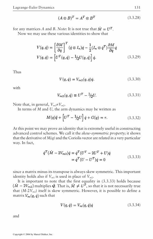
Lagrange-Euler Dynamics 131
(3.3.28)
for any matrices A and B. Note: It is not true that Now we may use these various identities to show that
(3.3.29)
Thus
(3.3.30)
with
(3.3.31)
Note that, in general, Vm1≠Vm2.In terms of M and U, the arm dynamics may be written as
(3.3.32)
At this point we may prove an identity that is extremely useful in constructingadvanced control schemes. We call it the skew-symmetric property; it showsthat the derivative of M(q) and the Coriolis vector are related in a very particularway. In fact,
(3.3.33)
since a matrix minus its transpose is always skew symmetric. This importantidentity holds also if Vm1 is used in place of Vm2.
It is important to note that the first equality in (3.3.33) holds because multiplies . That is, , so that it is not necessarily true
that (M-2Vm2) itself is skew symmetric. However, it is possible to define amatrix such that
(3.3.34)
and
Copyright © 2004 by Marcel Dekker, Inc.
Robot Dynamics132
(3.3.35)
is skew symmetric, so that xT Sx=0 for all x Rn Indeed, according to (3.3.13),(3.3.27) we may define
(3.3.36)
for then the skew-symmetric matrix is nothing but
(3.3.37)
This Vm is the standard one used in several modern adaptive and robustcontrol algorithms, and it is the definition we shall use in the remainder of thebook. Thus we shall write the arm equation either as
(3.3.38)
or
(3.3.39)
Note that it is possible to split V(q, ) into its Coriolis and centripetalcomponents as
(3.3.40)
where
(3.3.41)
and is (3.3.26) with all the square terms removed [Craig 1988] (seethe Problems).
Componentwise Analysis of . An alternative to the Kronecker productanalysis of the Coriolis/centripetal vector is an analysis in terms of the scalarcomponents of , which yields additional insight.
In terms of the components mkj(q) of the inertia matrix M(q) we may write(3.2.38)–(3.2.40) componentwise as
Copyright © 2004 by Marcel Dekker, Inc.
133
where all sums are over the number of joints n. Now, the Lagrange equationshows that the arm dynamics are expressed componentwise as
(3.3.45)
with n the number of joints.By interchanging the order of summation and taking advantage of symmetry,
(3.3.46)
Therefore, we may define
(3.3.47)
and write the arm dynamics as
(3.3.48)
The cyclic symmetry of the vijk is what allows us to derive the importantproperties of the Coriolis/centripetal vector V(q, )which corresponds to thesecond term in this equation. The quantities vijk are known as Christoffelsymbols (of the first kind) [Borisenko and Tarapov 1968].
The matrix defined in (3.3.36) has components vkj given by
(3.3.42)
(3.3.43)
(3.3.44)
3.3 Structure and Properties of the Robot Equation
Copyright © 2004 by Marcel Dekker, Inc.
Robot Dynamics134
(3.3.49)
Properties of the Gravity, Friction, and Disturbance
Properties of the Gravity Term G(q). According to (3.2.43) and (3.2.36),
whence using (3.3.11) twice reveals
(3.3.50)
A bound on the gravity term may be derived for any given robot arm. Thus
||G(q)||≤gb(q), (3.3.51)
where ||·|| is any appropriate vector norm and gb is a scalar function that maybe determined for any given arm (see Example 3.3.1). For a revolute arm, gb
is a constant independent of the joint vector q, but for an arm with prismaticlinks, gb may depend on q. See the examples in Section 3.2 and Example3.3.1 to verify these claims.
Properties of the Friction Term . The friction in the arm Equation (3.3.1)is of the form
(3.3.52)
with Fv the coefficient matrix of viscous friction, and Fd a dynamic frictionterm. The friction coefficients are among the parameters most difficult todetermine for a given arm and, in fact, (3.3.52) represents only an approximatemathematical model for their influence. For more discussion, see [Craig 1988,Schilling 1990].
Since friction is a local effect, we may assume that F ( ) is uncoupledamong the joints, so that
Copyright © 2004 by Marcel Dekker, Inc.
135
(3.3.53)
with fi(·) known scalar functions that may be determined for any given arm.We have defined the vec· function for future use.
The viscous friction may often be assumed to have the form
(3.3.54)
with vi known constant coefficients. Then Fv=diagvi, a diagonal matrix withentries vi. The dynamic friction may often be assumed to have the form
(3.3.55)
with ki known constant coefficients and the signum function defined for ascalar x by
(3.3.56)
Then
(3.3.57)
with Kd=diagki the coefficient matrix of dynamic friction and the signumfunction defined for a vector x by
(3.3.58)
A bound on the friction terms may be assumed of the form
(3.3.59)
with v and k known for a specific arm and ||·|| a suitable norm.Another friction term that may be included in F( )is the static friction,
which has components of the form
(3.3.60)
where ksi is the coefficient of static friction for joint i and is a small positiveparameter. We shall generally ignore this term.
3.3 Structure and Properties of the Robot Equation
Copyright © 2004 by Marcel Dekker, Inc.
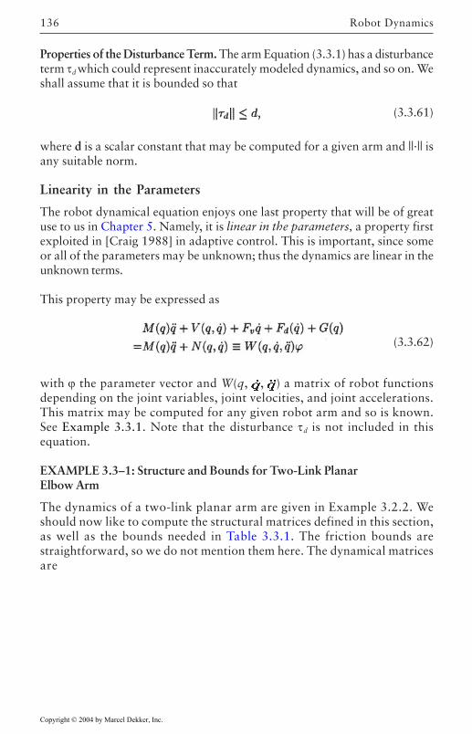
Robot Dynamics136
Properties of the Disturbance Term. The arm Equation (3.3.1) has a disturbanceterm τd which could represent inaccurately modeled dynamics, and so on. Weshall assume that it is bounded so that
(3.3.61)
where d is a scalar constant that may be computed for a given arm and ||·|| isany suitable norm.
Linearity in the Parameters
The robot dynamical equation enjoys one last property that will be of greatuse to us in Chapter 5. Namely, it is linear in the parameters, a property firstexploited in [Craig 1988] in adaptive control. This is important, since someor all of the parameters may be unknown; thus the dynamics are linear in theunknown terms.
This property may be expressed as
(3.3.62)
with ϕ the parameter vector and W(q, , ) a matrix of robot functionsdepending on the joint variables, joint velocities, and joint accelerations.This matrix may be computed for any given robot arm and so is known.See Example 3.3.1. Note that the disturbance τd is not included in thisequation.
EXAMPLE 3.3–1: Structure and Bounds for Two-Link PlanarElbow Arm
The dynamics of a two-link planar arm are given in Example 3.2.2. Weshould now like to compute the structural matrices defined in this section,
straightforward, so we do not mention them here. The dynamical matricesare
Copyright © 2004 by Marcel Dekker, Inc.
as well as the bounds needed in Table 3.3.1. The friction bounds are
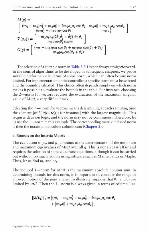
137
The selection of a suitable norm in Table 3.3.1 is not always straightforward.In the control algorithms to be developed in subsequent chapters, we provesuitable performance in terms of some norm, which can often be any normdesired. For implementation of the controller, a specific norm must be selectedand the bounds evaluated. This choice often depends simply on which normmakes it possible to evaluate the bounds in the table. For instance, choosingthe 2—norm for vectors requires the evaluation of the maximum singularvalue of M(q), a very difficult task.
Selecting the ∞—norm for vectors means determining at each sampling timethe element [of V(q(t), (t)) for instance] with the largest magnitude. Thisrequires decision logic, and the norm may not be continuous. Therefore, letus use the 1—norm in this example. The corresponding matrix induced normis then the maximum absolute column sum (Chapter 2).
a. Bounds on the Intertia Matrix
The evaluation of µ1, and µ2 amounts to the determination of the minimumand maximum eigenvalues of M(q) over all q. This is not an easy affair andrequires the solution of some quadratic equations, although it can be carriedout without too much trouble using software such as Mathematica or Maple.Thus, let us find m1 and m2.
The induced 1—norm for M(q) is the maximum absolute column sum. Indetermining bounds for this norm, it is important to consider the range ofallowed motion of the joint angles. To illustrate, suppose that θ1, and θ2 arelimited by ±π/2. Then the 1—norm is always given in terms of column 1 as
3.3 Structure and Properties of the Robot Equation
Copyright © 2004 by Marcel Dekker, Inc.
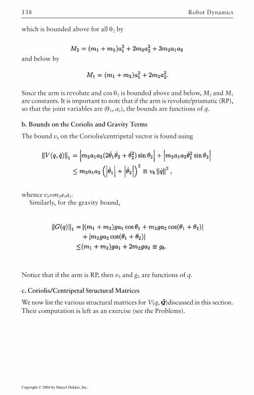
Robot Dynamics138
which is bounded above for all θ2 by
and below by
Since the arm is revolute and cos θ2 is bounded above and below, M2 and M1
are constants. It is important to note that if the arm is revolute/prismatic (RP),so that the joint variables are (θ1, a2), the bounds are functions of q.
b. Bounds on the Coriolis and Gravity Terms
The bound vb on the Coriolis/centripetal vector is found using
whence vb=m2a1a2.Similarly, for the gravity bound,
Notice that if the arm is RP, then vb and gb are functions of q.
c. Coriolis/Centripetal Structural Matrices
We now list the various structural matrices for V(q, )discussed in this section.Their computation is left as an exercise (see the Problems).
Copyright © 2004 by Marcel Dekker, Inc.
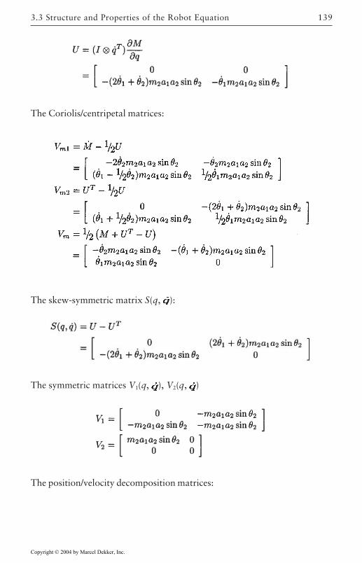
139
The Coriolis/centripetal matrices:
The skew-symmetric matrix S(q, ):
The symmetric matrices V1(q, ), V2(q, )
The position/velocity decomposition matrices:
3.3 Structure and Properties of the Robot Equation
Copyright © 2004 by Marcel Dekker, Inc.
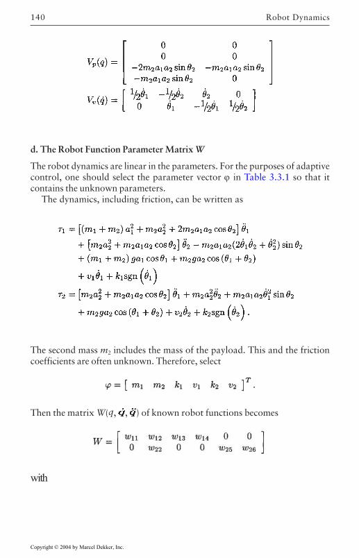
Robot Dynamics140
d. The Robot Function Parameter Matrix W
The robot dynamics are linear in the parameters. For the purposes of adaptivecontrol, one should select the parameter vector ϕ in Table 3.3.1 so that itcontains the unknown parameters.
The dynamics, including friction, can be written as
The second mass m2 includes the mass of the payload. This and the frictioncoefficients are often unknown. Therefore, select
Then the matrix W(q, , ) of known robot functions becomes
with
Copyright © 2004 by Marcel Dekker, Inc.
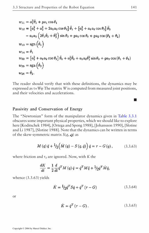
141
The reader should verify that with these definitions, the dynamics may beexpressed as τ=Wϕ The matrix W is computed from measured joint positions,and their velocities and accelerations.
Passivity and Conservation of Energy
The “Newtonian” form of the manipulator dynamics given in Table 3.3.1obscures some important physical properties, which we should like to explorehere [Koditschek 1984], [Ortega and Spong 1988], [Johansson 1990], [Slotineand Li 1987], [Slotine 1988]. Note that the dynamics can be written in termsof the skew-symmetric matrix S(q, ) as
(3.3.63)
where friction and τd are ignored. Now, with K the
whence (3.3.63) yields
(3.3.64)
or
(3.3.65)
3.3 Structure and Properties of the Robot Equation
Copyright © 2004 by Marcel Dekker, Inc.
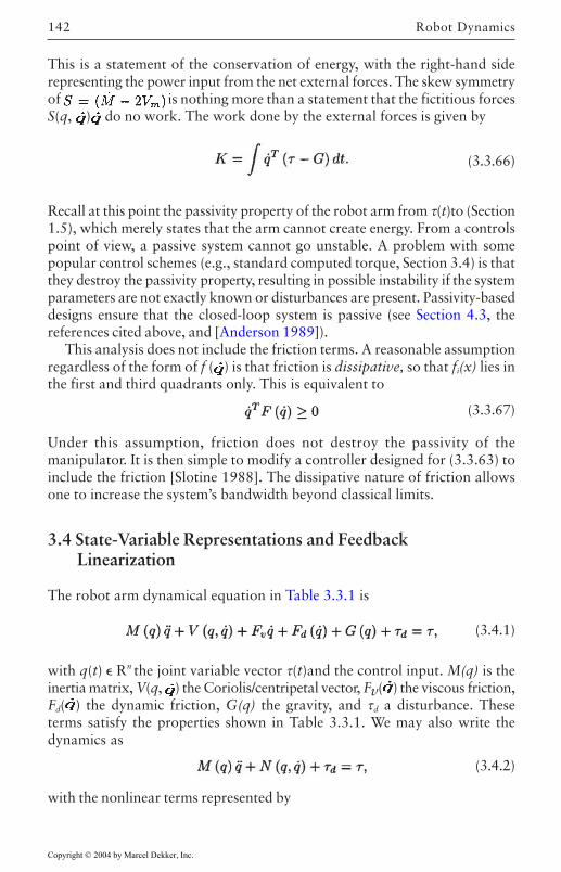
Robot Dynamics142
This is a statement of the conservation of energy, with the right-hand siderepresenting the power input from the net external forces. The skew symmetryof is nothing more than a statement that the fictitious forcesS(q, ) do no work. The work done by the external forces is given by
(3.3.66)
Recall at this point the passivity property of the robot arm from τ(t)to (Section1.5), which merely states that the arm cannot create energy. From a controlspoint of view, a passive system cannot go unstable. A problem with somepopular control schemes (e.g., standard computed torque, Section 3.4) is thatthey destroy the passivity property, resulting in possible instability if the systemparameters are not exactly known or disturbances are present. Passivity-baseddesigns ensure that the closed-loop system is passive (see Section 4.3, thereferences cited above, and [Anderson 1989]).
This analysis does not include the friction terms. A reasonable assumptionregardless of the form of f ( ) is that friction is dissipative, so that fi(x) lies inthe first and third quadrants only. This is equivalent to
(3.3.67)
Under this assumption, friction does not destroy the passivity of themanipulator. It is then simple to modify a controller designed for (3.3.63) toinclude the friction [Slotine 1988]. The dissipative nature of friction allowsone to increase the system’s bandwidth beyond classical limits.
3.4 State-Variable Representations and Feedback Linearization
The robot arm dynamical equation in Table 3.3.1 is
(3.4.1)
with q(t) Rn the joint variable vector τ(t)and the control input. M(q) is theinertia matrix, V(q, ) the Coriolis/centripetal vector, Fv( ) the viscous friction,Fd( ) the dynamic friction, G(q) the gravity, and τd a disturbance. Theseterms satisfy the properties shown in Table 3.3.1. We may also write thedynamics as
(3.4.2)
with the nonlinear terms represented by
Copyright © 2004 by Marcel Dekker, Inc.
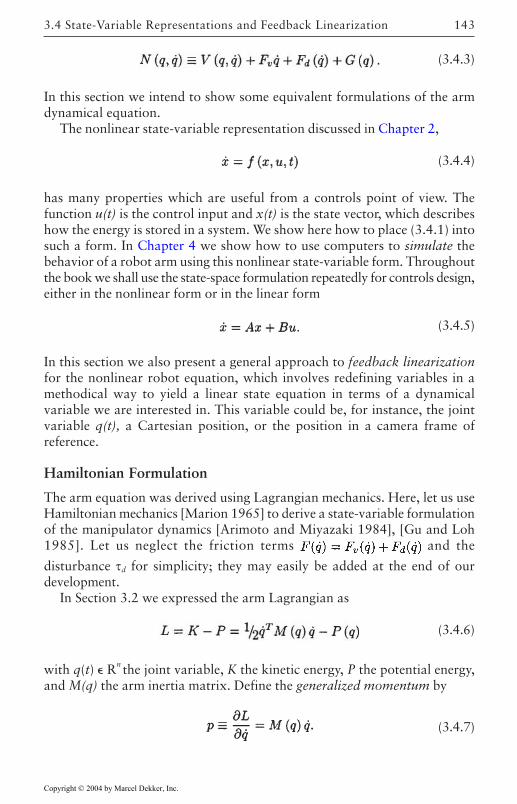
143
(3.4.3)
In this section we intend to show some equivalent formulations of the armdynamical equation.
The nonlinear state-variable representation discussed in Chapter 2,
(3.4.4)
has many properties which are useful from a controls point of view. Thefunction u(t) is the control input and x(t) is the state vector, which describeshow the energy is stored in a system. We show here how to place (3.4.1) intosuch a form. In Chapter 4 we show how to use computers to simulate thebehavior of a robot arm using this nonlinear state-variable form. Throughoutthe book we shall use the state-space formulation repeatedly for controls design,either in the nonlinear form or in the linear form
(3.4.5)
In this section we also present a general approach to feedback linearizationfor the nonlinear robot equation, which involves redefining variables in amethodical way to yield a linear state equation in terms of a dynamicalvariable we are interested in. This variable could be, for instance, the jointvariable q(t), a Cartesian position, or the position in a camera frame ofreference.
Hamiltonian Formulation
The arm equation was derived using Lagrangian mechanics. Here, let us useHamiltonian mechanics [Marion 1965] to derive a state-variable formulationof the manipulator dynamics [Arimoto and Miyazaki 1984], [Gu and Loh1985]. Let us neglect the friction terms and the
disturbance τd for simplicity; they may easily be added at the end of ourdevelopment.
In Section 3.2 we expressed the arm Lagrangian as
(3.4.6)
with q(t) Rn the joint variable, K the kinetic energy, P the potential energy,and M(q) the arm inertia matrix. Define the generalized momentum by
(3.4.7)
3.4 State-Variable Representations and Feedback Linearization
Copyright © 2004 by Marcel Dekker, Inc.
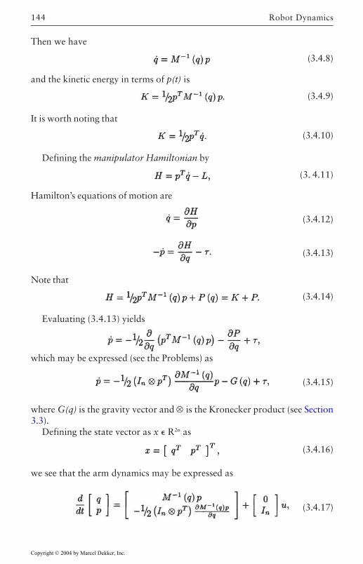
Robot Dynamics144
Then we have
(3.4.8)
and the kinetic energy in terms of p(t) is
(3.4.9)
It is worth noting that
(3.4.10)
Defining the manipulator Hamiltonian by
(3. 4.11)
Hamilton’s equations of motion are
(3.4.12)
(3.4.13)
Note that
(3.4.14)
Evaluating (3.4.13) yields
which may be expressed (see the Problems) as
(3.4.15)
where G(q) is the gravity vector and ⊗ is the Kronecker product (see Section3.3).
Defining the state vector as x R2n as
(3.4.16)
we see that the arm dynamics may be expressed as
(3.4.17)
Copyright © 2004 by Marcel Dekker, Inc.
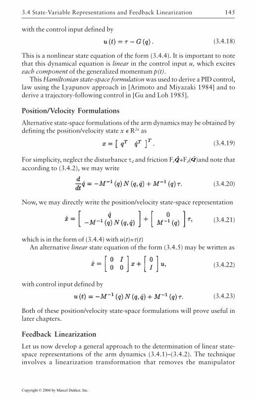
145
with the control input defined by
(3.4.18)
This is a nonlinear state equation of the form (3.4.4). It is important to notethat this dynamical equation is linear in the control input u, which exciteseach component of the generalized momentum p(t).
This Hamiltonian state-space formulation was used to derive a PID control,law using the Lyapunov approach in [Arimoto and Miyazaki 1984] and toderive a trajectory-following control in [Gu and Loh 1985].
Position/Velocity Formulations
Alternative state-space formulations of the arm dynamics may be obtained bydefining the position/velocity state x R2n as
(3.4.19)
For simplicity, neglect the disturbance τd and friction Fv +Fd( )and note thataccording to (3.4.2), we may write
(3.4.20)
Now, we may directly write the position/velocity state-space representation
(3.4.21)
which is in the form of (3.4.4) with u(t)=τ(t)An alternative linear state equation of the form (3.4.5) may be written as
(3.4.22)
with control input defined by
(3.4.23)
Both of these position/velocity state-space formulations will prove useful inlater chapters.
Feedback Linearization
Let us now develop a general approach to the determination of linear state-space representations of the arm dynamics (3.4.1)–(3.4.2). The techniqueinvolves a linearization transformation that removes the manipulator
3.4 State-Variable Representations and Feedback Linearization
Copyright © 2004 by Marcel Dekker, Inc.
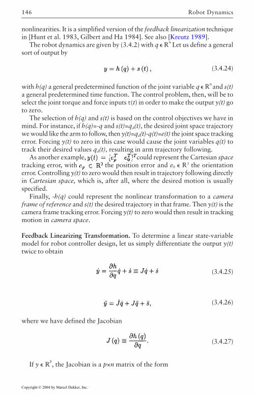
Robot Dynamics146
nonlinearities. It is a simplified version of the feedback linearization techniquein [Hunt et al. 1983, Gilbert and Ha 1984]. See also [Kreutz 1989].
The robot dynamics are given by (3.4.2) with q Rn Let us define a generalsort of output by
(3.4.24)
with h(q) a general predetermined function of the joint variable q Rn and s(t)a general predetermined time function. The control problem, then, will be toselect the joint torque and force inputs τ(t) in order to make the output y(t) goto zero.
The selection of h(q) and s(t) is based on the control objectives we have inmind. For instance, if h(q)=-q and s(t)=qd(t), the desired joint space trajectorywe would like the arm to follow, then y(t)=qd(t)-q(t)=e(t) the joint space trackingerror. Forcing y(t) to zero in this case would cause the joint variables q(t) totrack their desired values qd(t), resulting in arm trajectory following.
As another example, could represent the Cartesian spacetracking error, with the position error and e0 R3 the orientationerror. Controlling y(t) to zero would then result in trajectory following directlyin Cartesian space, which is, after all, where the desired motion is usuallyspecified.
Finally, -h(q) could represent the nonlinear transformation to a cameraframe of reference and s(t) the desired trajectory in that frame. Then y(t) is thecamera frame tracking error. Forcing y(t) to zero would then result in trackingmotion in camera space.
Feedback Linearizing Transformation. To determine a linear state-variablemodel for robot controller design, let us simply differentiate the output y(t)twice to obtain
(3.4.25)
(3.4.26)
where we have defined the Jacobian
(3.4.27)
If y Rp, the Jacobian is a p×n matrix of the form
Copyright © 2004 by Marcel Dekker, Inc.
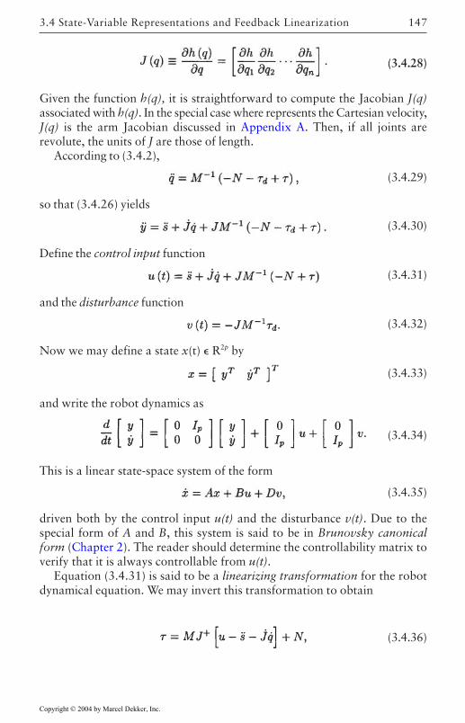
147
(3.4.28)
Given the function h(q), it is straightforward to compute the Jacobian J(q)associated with h(q). In the special case where represents the Cartesian velocity,J(q) is the arm Jacobian discussed in Appendix A. Then, if all joints arerevolute, the units of J are those of length.
According to (3.4.2),
(3.4.29)
so that (3.4.26) yields
(3.4.30)
Define the control input function
(3.4.31)
and the disturbance function
(3.4.32)
Now we may define a state x(t) R2p by
(3.4.33)
and write the robot dynamics as
(3.4.34)
This is a linear state-space system of the form
(3.4.35)
driven both by the control input u(t) and the disturbance v(t). Due to thespecial form of A and B, this system is said to be in Brunovsky canonicalform (Chapter 2). The reader should determine the controllability matrix toverify that it is always controllable from u(t).
Equation (3.4.31) is said to be a linearizing transformation for the robotdynamical equation. We may invert this transformation to obtain
(3.4.36)
3.4 State-Variable Representations and Feedback Linearization
Copyright © 2004 by Marcel Dekker, Inc.
Robot Dynamics148
where J+ is the Moore-Penrose inverse [Rao and Mitra 1971] of the JacobianJ(q). If J(q) is square (i.e., p=n) and nonsingular, then J+(q)=J-1(q) and we maywrite
(3.4.37)
As we shall see in Chapter 4, feedback linearization provides a powerfulcontrols design technique. In fact, if we select u(t) so that (3.4.34) is stable(e.g., a possibility is the PD feedback ), then the controlinput torque τ(t) defined by (3.4.36) makes the robot arm move in such a waythat y(t) goes to zero.
In the special case y(t)=q(t), then J=I and (3.4.34) reduces to the linearposition/velocity form (3.4.22).
3.5 Cartesian and Other Dynamics
In Section 3.2 we derived the robot dynamics in terms of the time behavior ofq(t). According to Table 3.3.1,
(3.5.1)
or
(3.5.2)
where the nonlinear terms are
(3.5.3)
We call this the dynamics of the arm formulated in joint space, or simply thejoint-space dynamics.
Cartesian Arm Dynamics
It is often useful to have a description of the dynamical development of variablesother than the joint variable q(t). Consequently, define
(3.5.4)
with h(q) a generally nonlinear transformation. Although y(t) could be anyvariable of interest, let us think of it here as the Cartesian or task spaceposition of the end effector (i.e., position and orientation of the end effector inbase coordinates).
Copyright © 2004 by Marcel Dekker, Inc.
149
The derivation of the Cartesian dynamics from the joint-space dynamics isakin to the feedback linearization in Section 3.4. Differentiating (3.5.4) twiceyields
(3.5.5)
(3.5.6)
where the Jacobian is
(3.5.7)
The Cartesian velocity vector is , with v R3 the linearvelocity and ω R3 the angular velocity. Let us assume that the number oflinks is n=6, so that J is square. Assuming also that we are away from workspacesingularities so that |J|≠0, according to (3.5.6), we may write
(3.5.8)
which is the “inverse acceleration” transformation. Substituting this into (3.5.2)yields
Recalling now the force transformation τ=JTF, with F the Cartesian force vector(see Appendix A) we have
(3.5.9)
This may be written as
(3.5.10)
where we have defined the Cartesian inertia matrix, nonlinear terms, anddisturbance by
(3.5.11)
(3.5.12)
(3.5.13)
Equation (3.5.9)–(3.5.10) gives the Cartesian or workspace dynamics of therobot manipulator.
3.5 Cartesian and Other Dynamics
Copyright © 2004 by Marcel Dekker, Inc.
Robot Dynamics150
Note that , , and fd depend on q and , so that strictly speaking, theCartesian dynamics are not completely given in terms of However.
, and given y(t) we could use the inverse kinematics to determineq(t), so that , , fd can be computed as functions of y and using computersubroutines.
Structure and Properties of the Cartesian Dynamics
It is important to realize that all the properties of the joint-space dynamicslisted in Table 3.3.1 carry over to the Cartesian dynamics as long as J isnonsingular [Slotine and Li 1987]. Note particularly that is symmetricand positive definite. For a revolute arm the Jacobian has units of length andis bounded. In that case, is bounded above and below.
Defining
(3.5.14)
it follows that
(3.5.15)
with
(3.5.16)
where Vm was defined in Section 3.3.It is easy to show that
(3.5.17)
is skew-symmetric. Indeed, use the identity
(3.5.18)
to see that
Copyright © 2004 by Marcel Dekker, Inc.
151
which is skew symmetric since is.The friction terms in the Cartesian dynamics are
(3.5.19)
and they satisfy bounds like those in Table 3.3.1. Notice that in Cartesiancoordinates the friction effects are not decoupled (e.g., J-TFvJ-1 is not diagonal).The Cartesian gravity vector
(3.5.20)
is bounded.The property of linearity in the parameters holds and is expressed as
(3.5.21)
where the known Cartesian function of robot functions is
(3.5.22)
and ϕ is the vector of arm parameters.
EXAMPLE 3.5–1: Cartesian Dynamics for Three-Link Cylindrical Arm
Let us show how to convert the joint space dynamics found in Example3.2.3 to Cartesian dynamics. From Example A.3–1, the arm Jacobian is
(1)
whence its inverse is
(2)
From Example 3.2.3 the arm inertia matrix is
(3)
3.5 Cartesian and Other Dynamics
Copyright © 2004 by Marcel Dekker, Inc.
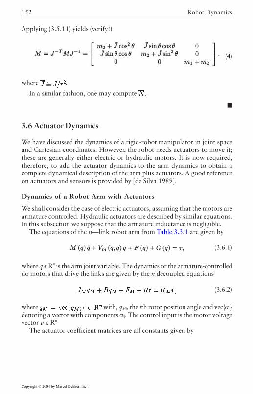
Robot Dynamics152
Applying (3.5.11) yields (verify!)
(4)
where .
In a similar fashion, one may compute .
3.6 Actuator Dynamics
We have discussed the dynamics of a rigid-robot manipulator in joint spaceand Cartesian coordinates. However, the robot needs actuators to move it;these are generally either electric or hydraulic motors. It is now required,therefore, to add the actuator dynamics to the arm dynamics to obtain acomplete dynamical description of the arm plus actuators. A good referenceon actuators and sensors is provided by [de Silva 1989].
Dynamics of a Robot Arm with Actuators
We shall consider the case of electric actuators, assuming that the motors arearmature controlled. Hydraulic actuators are described by similar equations.In this subsection we suppose that the armature inductance is negligible.
The equations of the n—link robot arm from Table 3.3.1 are given by
(3.6.1)
where q Rn is the arm joint variable. The dynamics or the armature-controlleddo motors that drive the links are given by the n decoupled equations
(3.6.2)
where with, qMi, the ith rotor position angle and vecαidenoting a vector with components αi. The control input is the motor voltagevector v Rn
The actuator coefficient matrices are all constants given by
Copyright © 2004 by Marcel Dekker, Inc.
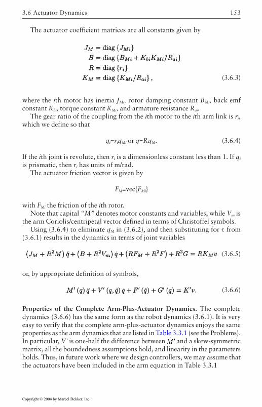
153
The actuator coefficient matrices are all constants given by
(3.6.3)
where the ith motor has inertia JMi, rotor damping constant BMi, back emfconstant Kbi, torque constant KMi, and armature resistance Rai.
The gear ratio of the coupling from the ith motor to the ith arm link is ri,which we define so that
qi=riqMi or q=RqM. (3.6.4)
If the ith joint is revolute, then ri is a dimensionless constant less than 1. If qi
is prismatic, then ri has units of m/rad.The actuator friction vector is given by
FM=vecFMi
with FMi the friction of the ith rotor.Note that capital “M” denotes motor constants and variables, while Vm is
the arm Coriolis/centripetal vector defined in terms of Christoffel symbols.Using (3.6.4) to eliminate qM in (3.6.2), and then substituting for τ from
(3.6.1) results in the dynamics in terms of joint variables
(3.6.5)
or, by appropriate definition of symbols,
(3.6.6)
Properties of the Complete Arm-Plus-Actuator Dynamics. The completedynamics (3.6.6) has the same form as the robot dynamics (3.6.1). It is veryeasy to verify that the complete arm-plus-actuator dynamics enjoys the sameproperties as the arm dynamics that are listed in Table 3.3.1 (see the Problems).In particular, V’ is one-half the difference between and a skew-symmetricmatrix, all the boundedness assumptions hold, and linearity in the parametersholds. Thus, in future work where we design controllers, we may assume thatthe actuators have been included in the arm equation in Table 3.3.1
3.6 Actuator Dynamics
Copyright © 2004 by Marcel Dekker, Inc.
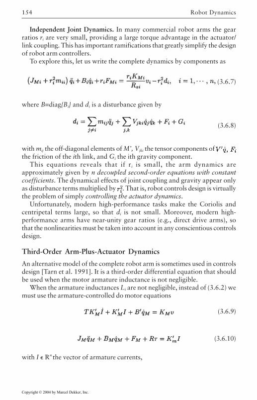
Robot Dynamics154
Independent Joint Dynamics. In many commercial robot arms the gearratios ri are very small, providing a large torque advantage in the actuator/link coupling. This has important ramifications that greatly simplify the designof robot arm controllers.
To explore this, let us write the complete dynamics by components as
(3.6.7)
where B≡diagBi and di is a disturbance given by
(3.6.8)
with mij the off-diagonal elements of M’, Vjki the tensor components of the friction of the ith link, and Gi the ith gravity component.
This equations reveals that if r i is small, the arm dynamics areapproximately given by n decoupled second-order equations with constantcoefficients. The dynamical effects of joint coupling and gravity appear onlyas disturbance terms multiplied by . That is, robot controls design is virtuallythe problem of simply controlling the actuator dynamics.
Unfortunately, modern high-performance tasks make the Coriolis andcentripetal terms large, so that di is not small. Moreover, modern high-performance arms have near-unity gear ratios (e.g., direct drive arms), sothat the nonlinearities must be taken into account in any conscientious controlsdesign.
Third-Order Arm-Plus-Actuator Dynamics
An alternative model of the complete robot arm is sometimes used in controlsdesign [Tarn et al. 1991]. It is a third-order differential equation that shouldbe used when the motor armature inductance is not negligible.
When the armature inductances Li are not negligible, instead of (3.6.2) wemust use the armature-controlled do motor equations
(3.6.9)
(3.6.10)
with I Rn the vector of armature currents,
Copyright © 2004 by Marcel Dekker, Inc.
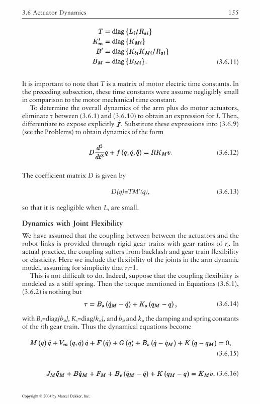
155
(3.6.11)
It is important to note that T is a matrix of motor electric time constants. Inthe preceding subsection, these time constants were assume negligibly smallin comparison to the motor mechanical time constant.
To determine the overall dynamics of the arm plus do motor actuators,eliminate τ between (3.6.1) and (3.6.10) to obtain an expression for I. Then,differentiate to expose explicitly . Substitute these expressions into (3.6.9)(see the Problems) to obtain dynamics of the form
(3.6.12)
The coefficient matrix D is given by
D(q)=TM’(q), (3.6.13)
so that it is negligible when Li are small.
Dynamics with Joint Flexibility
We have assumed that the coupling between between the actuators and therobot links is provided through rigid gear trains with gear ratios of ri. Inactual practice, the coupling suffers from backlash and gear train flexibilityor elasticity. Here we include the flexibility of the joints in the arm dynamicmodel, assuming for simplicity that ri=1.
This is not difficult to do. Indeed, suppose that the coupling flexibility ismodeled as a stiff spring. Then the torque mentioned in Equations (3.6.1),(3.6.2) is nothing but
(3.6.14)
with Bs=diagbsi, Ks=diagksi, and bsi and ksi the damping and spring constantsof the ith gear train. Thus the dynamical equations become
(3.6.15)
(3.6.16)
3.6 Actuator Dynamics
Copyright © 2004 by Marcel Dekker, Inc.
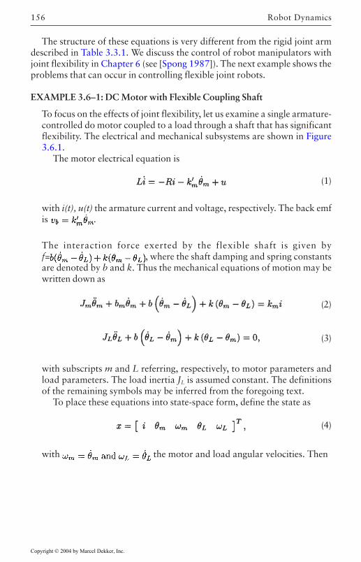
Robot Dynamics156
The structure of these equations is very different from the rigid joint armdescribed in Table 3.3.1. We discuss the control of robot manipulators withjoint flexibility in Chapter 6 (see [Spong 1987]). The next example shows theproblems that can occur in controlling flexible joint robots.
EXAMPLE 3.6–1: DC Motor with Flexible Coupling Shaft
To focus on the effects of joint flexibility, let us examine a single armature-controlled do motor coupled to a load through a shaft that has significantflexibility. The electrical and mechanical subsystems are shown in Figure3.6.1.
The motor electrical equation is
(1)
with i(t), u(t) the armature current and voltage, respectively. The back emfis .
The interaction force exerted by the flexible shaft is given byf= , where the shaft damping and spring constantsare denoted by b and k. Thus the mechanical equations of motion may bewritten down as
(2)
(3)
with subscripts m and L referring, respectively, to motor parameters andload parameters. The load inertia JL is assumed constant. The definitionsof the remaining symbols may be inferred from the foregoing text.
To place these equations into state-space form, define the state as
(4)
with the motor and load angular velocities. Then
Copyright © 2004 by Marcel Dekker, Inc.
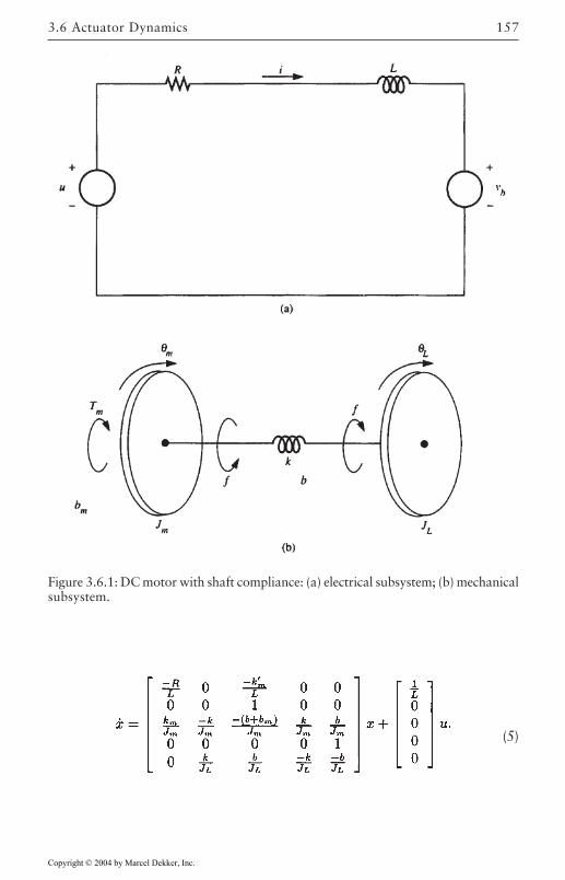
157
(5)
Figure 3.6.1: DC motor with shaft compliance: (a) electrical subsystem; (b) mechanicalsubsystem.
3.6 Actuator Dynamics
Copyright © 2004 by Marcel Dekker, Inc.
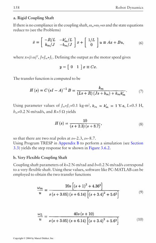
Robot Dynamics158
a. Rigid Coupling Shaft
If there is no compliance in the coupling shaft, ωm=ωL=ω and the state equationsreduce to (see the Problems)
(6)
where x=[i ω]T, J=Jm+JL. Defining the output as the motor speed gives
The transfer function is computed to be
(7)
Using parameter values of Jm=JL=0.1 kg-m2, L=0.5 H,
bm=0.2 N-m/rad/s, and R=5 Ω yields
(8)
so that there are two real poles at s=-2.3, s=-8.7.Using Program TRESP in Appendix B to perform a simulation (see Section3.3) yields the step response for w shown in Figure 3.6.2.
b. Very Flexible Coupling Shaft
Coupling shaft parameters of k=2 N-m/rad and b=0.2 N-m/rad/s correspondto a very flexible shaft. Using these values, software like PC-MATLAB can beemployed to obtain the two transfer functions
(9)
(10)
Copyright © 2004 by Marcel Dekker, Inc.
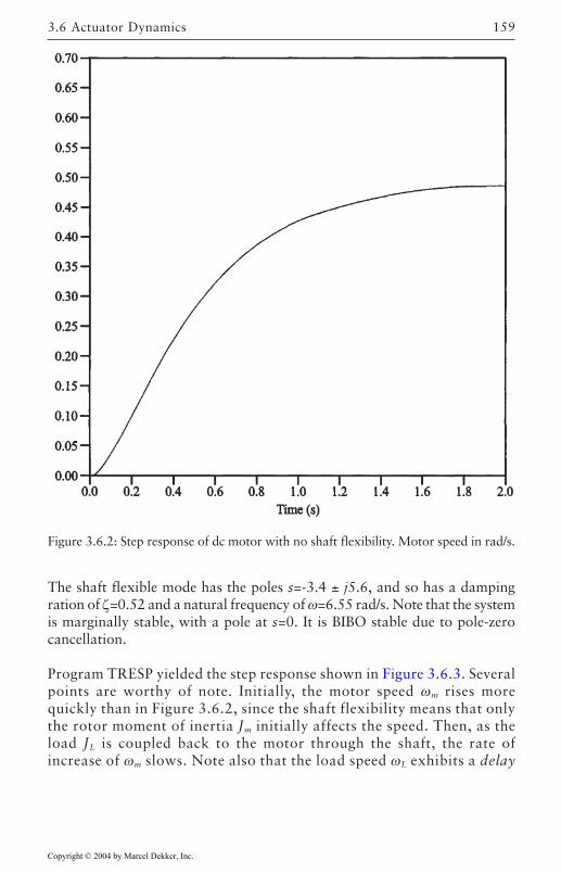
159
The shaft flexible mode has the poles s=-3.4 ± j5.6, and so has a dampingration of ζ=0.52 and a natural frequency of ω=6.55 rad/s. Note that the systemis marginally stable, with a pole at s=0. It is BIBO stable due to pole-zerocancellation.
Program TRESP yielded the step response shown in Figure 3.6.3. Severalpoints are worthy of note. Initially, the motor speed ωm rises morequickly than in Figure 3.6.2, since the shaft flexibility means that onlythe rotor moment of inertia Jm initially affects the speed. Then, as theload JL is coupled back to the motor through the shaft, the rate ofincrease of ωm slows. Note also that the load speed ωL exhibits a delay
Figure 3.6.2: Step response of dc motor with no shaft flexibility. Motor speed in rad/s.
3.6 Actuator Dynamics
Copyright © 2004 by Marcel Dekker, Inc.
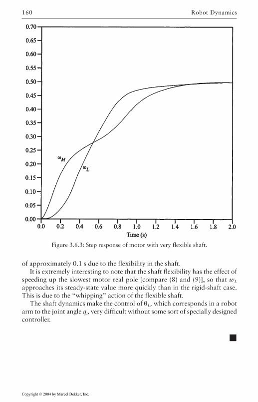
Robot Dynamics160
of approximately 0.1 s due to the flexibility in the shaft.It is extremely interesting to note that the shaft flexibility has the effect of
speeding up the slowest motor real pole [compare (8) and (9)], so that wL
approaches its steady-state value more quickly than in the rigid-shaft case.This is due to the “whipping” action of the flexible shaft.
The shaft dynamics make the control of θL, which corresponds in a robotarm to the joint angle qi, very difficult without some sort of specially designedcontroller.
Figure 3.6.3: Step response of motor with very flexible shaft.
Copyright © 2004 by Marcel Dekker, Inc.
161
3.7 Summary
In this chapter we have laid the foundation for a study of robot control systems.Using Lagrangian mechanics in Section 3.2, we derived the dynamics of somerobot arms that will be used for demonstration designs throughout the text.We provided expressions for the general robot arm dynamics for any serial-link arm.
In Section 3.3 we studied the properties of the robot dynamics such asboundedness, linearity in the parameters, and skew symmetry that are neededin controls design. Table 3.3.1 gives a summary of our findings. We used aKronecker product approach that yields great insight into the relations betweenthe terms in the robot equation.
A vital form in modern control systems design is the state-variableformulation. In Section 3.4 we derived several state-space forms of the armdynamics, setting the stage for several design techniques to be provided insubsequent chapters. The state formulation is also useful in computer simulationof robot controllers, as we see in Section 3.3.
The dynamics in Cartesian form were given in Section 3.5. The dynamicsof the actuators that drive the robot manipulator links were analyzed andincluded in Section 3.6.
3.7 Summary
Copyright © 2004 by Marcel Dekker, Inc.
163
REFERENCES
[Anderson 1989] Anderson, R.J., “Passive computed torque algorithms for robots,”Proc. IEEE Conf. Decision Control, pp. 1638–1644, Dec. 1989.
[Arimoto and Miyazaki 1984] Arimoto, S., and F.Miyazaki, “Stability and robustnessof PID feedback control for robot manipulators of sensory capability,” Proc.First Int. Symp., pp. 783–799, MIT, Cambridge, MA, 1984.
[Asada and Slotine 1986] Asada, H., and J.-J.E.Slotine, Robot Analysis and Control,New York: Wiley, 1986.
[Borisenko and Tarapov 1968] Borisenko, A.I., and I.E.Tarapov, Vector and TensorAnalysis with Applications. Englewood Cliffs, NJ: Prentice Hall, 1968.
[Brewer 1978] Brewer, J.W., “Kronecker products and matrix calculus in systemtheory,” IEEE Trans. Circuits Syst., vol. CAS-25, no. 9, pp. 772–781, Sept.1978.
[Craig 1988] Craig, J.J., Adaptive Control of Mechanical Manipulators. Reading,MA: Addison-Wesley, 1988.
[de Silva 1989] de Silva, C.W., Control Sensors and Actuators. Englewood Cliffs, NJ:Prentice Hall, 1989.
[Gilbert and Ha 1984] Gilbert, E.G., and I.J.Ha, “An approach to nonlinear feedbackcontrol with applications to robotics,” IEEE Trans. Syst. Man Cybern., vol.SMC-14, no. 6, pp. 879–884, Nov./Dec. 1984.
[Gu and Loh 1985] Gu, Y.-L., and N.K.Loh, “Dynamic model for industrial robotsbased on a compact Lagrangian formulation,” Proc. IEEE Conf. DecisionControl, pp. 1497–1501, 1985.
[Gu and Loh 1988] Gu, Y-L., and N.K.Loh, “Dynamic modeling and control byutilizing an imaginary robot model,” IEEE J. Robot. Autom., vol. 4, no. 5, pp.532–534, Oct. 1988.
Copyright © 2004 by Marcel Dekker, Inc.
164
[Hunt et al. 1983] Hunt, L.R., R.Su, and G.Meyer, “Global transformations ofnonlinear systems,” IEEE Trans. Autom. Control, vol. AC-28, no. 1, pp. 24–31,Jan. 1983.
[Johansson 1990] Johansson, R., “Quadratic optimization of motion coordinationand control,” IEEE Trans. Autom. Control, vol. 35, no. 11, pp. 1197–1208,Nov. 1990.
[Koditschek 1984] Koditschek, D., “Natural motion for robot arms,” Proc. IEEEConf. Decision Control, pp. 733–735, Dec. 1984.
[Kreutz 1989] Kreutz, K., “On manipulator control by exact linearization,” IEEETrans. Autom. Control, vol. 34, no. 7, pp. 763–767, July 1989.
[Lee et al. 1983] Lee, C.S.G., R.C.Gonzalez, and K.S.Fu, Tutorial on Robotics. NewYork: IEEE Press, 1983.
[Marion 1965] Marion, J.B., Classical Dynamics. New York: Academic Press, 1965.
[Ortega and Spong 1988] Ortega, R., and Spong, M.W., “Adaptive motion control ofrigid robots: a tutorial,” Proc. IEEE Conf. Decision Control, pp. 1575–1584,Dec. 1988.
[Paul 1981] Paul, R.P., Robot Manipulators. Cambridge, MA: MIT Press, 1981.
[Rao and Mitra 1971] Rao, C.R., and S.K.Mitra, Generalized Inverse of Matrices andIts Applications. New York: Wiley, 1971.
[Schilling 1990] Schilling, R.J., Fundamentals of Robotics. Englewood Cliffs, NJ:Prentice Hall, 1990.
[Slotine 1988] Slotine, J.-J.E., “Putting physics in control: the example of robotics,”IEEE Control Syst. Mag., pp. 12–17, Dec. 1988.
[Slotine and Li 1987] Slotine, J.-J.E., and W.Li, “Adaptive strategies in constrainedmanipulation,” Proc. IEEE Conf. Robot. Autom., pp. 595–601, 1987.
[Spong 1987] Spong, M.W., “Modeling and control of elastic joint robots,” J. Dyn.Syst. Meas. Control, vol. 109, pp. 310–319, Dec. 1987.
REFERENCES
Copyright © 2004 by Marcel Dekker, Inc.
165
[Spong and Vidyasagar 1989] Spong, M.W., and M.Vidyasagar, Robot Dynamicsand Control. New York: Wiley, 1989.
[Tarn et al. 1991] Tarn, T.-J., A.K.Bejczy, X.Yun, and Z.Li, “Effect of motor dynamicson nonlinear feedback robot arm control,” IEEE Trans. Robot. Autom., vol. 7,no. 1, pp. 114–122, Feb. 1991.
REFERENCES
Copyright © 2004 by Marcel Dekker, Inc.
166
PROBLEMS
Section 3.2
3.2–1 Dynamics. Find the dynamics for the spherical wrist in ExampleA.2–4.
3.2–2 Dynamics from Derived Equations. In Example 3.2.2 we found thedynamics of the two-link planar elbow arm from first principles. Inthis problem, begin with the expressions for the kinetic and potentialenergy in that example and:(a) Write K in the form (3.2.29) to determine M(q).(b) Use (3.2.42) and (3.2.43) to determine V(q, ) and G(q).
3.2–3 Dynamics from Derived Equations. Repeat Problem 3.2–2 for thethree-link arm in Example 3.2.3.
Section 3.3
3.3–1 Prove (3.3.22) by finding Vp1(q) and V
v1(q).
3.3–2 Prove (3.3.23) by finding the matrices Vi(q).
3.3–3 Prove (3.3.27).
3.3–4 Coriolis Term. Find Vcor(q) and Vcen(q) in (3.3.40).
3.3–5 Coriolis Term. Demonstrate that the Coriolis/centripetal term in thedynamics equation may be expressed [Paul 1981] as V(q, )= vecV(q,
)where
with
and Ti defined in Appendix A. Compare this to Vm1, Vm2, Vm asdefined in Section 3.2.
3.3–6 Bounds and Structure. Derive in detail the results in Example 3.3.1.
REFERENCES
Copyright © 2004 by Marcel Dekker, Inc.
167
3.3–7 Bounds and Structure. Derive the bounds and structural matrices forthe two-link polar arm in Example 3.2.1. Use:(a) The 1—norm.(b) The 2-norm .(c) The ∞—norm.
3.3–8 Bounds and Structure. Repeat Problem 3.3–7 for the three-linkcylindrical arm in Exercise 3.2.3.
3.3–9 Bounds Using 2-Norm. Derive the bounds for the two-link planarelbow arm in Example 3.3.1 using the 2—norm.
Section 3.43.4–1 Prove (3.4.15).
3.4–2 Hamiltonian State Formulation. Demonstrate that (3.4.15) isequivalent to
with the skew-symmetric matrix defined in Section 3.3.
3.4–3 Hamiltonian State Formulation. Use (3.4.17) to derive theHamiltonian state-variable formulation for the two-link polar armin Example 3.2.1.
3.4–4 Hamiltonian State Formulation. Repeat Problem 3.4–3 for the two-link planar elbow arm in Example 3.2.2.
Section 3.53.5–1 Cartesian Dynamics. Complete Example 3.5.1, computing the
nonlinear terms in Cartesian coordinates.
3.5–2 Cartesian Dynamics. Find the Cartesian dynamics of the two-linkpolar arm in Example 3.2.1.
3.5–3 Cartesian Dynamics. Find the Cartesian dynamics of the two-linkplanar elbow arm in Example 3.2.2.
Section 3.63.6–1 Actuator Dynamics. Verify that the arm-plus-actuator dynamics (3.6.6)
has the properties listed in Table 3.3.1.
REFERENCES
Copyright © 2004 by Marcel Dekker, Inc.
168
3.6–2 Actuator Dynamics. Derive the third-order dynamics (3.6.12),providing explicit expressions for Verify that they reduce to(3.6.5) when L
i is negligible.
3.6–3 Flexible Coupling Shaft. Verify the state equation for the rigid-shaftcase in Example 3.6.1.
REFERENCES
Copyright © 2004 by Marcel Dekker, Inc.
169
Chapter 4
Computed-Torque Control
In this chapter we examine some straightforward control schemes for robotmanipulators that fall under the class known as “computed-torque controllers.”These generally perform well when the robot arm parameters are knownfairly accurately. Some connections are given with classical robot control,and modern design techniques are provided as well. The effects of digitalimplementation of robot controllers are shown. Trajectory generation isoutlined.
4.1 Introduction
A basic problem in controlling robots is to make the manipulator follow apreplanned desired trajectory. Before the robot can do any useful work, wemust position it in the right place at the right instances. In this chapter wediscuss computed-torque control, which yields a family of easy-to-understandcontrol schemes that often work well in practice. These schemes involve thedecomposition of the controls design problem into an inner-loop design andan outer-loop design.
In Section 4.4 we provide connections with classical manipulator controlschemes based on independent joint design using PID control. In Section 4.6we show how to use some modern design techniques in conjunction withcomputed-torque control. Thus this chapter could be considered as a bridgebetween classical design techniques of the sort used several years ago in robotcontrol, and the modern design techniques in the remainder of the book whichare needed to obtain high performance in uncertain environments.
We assume here the robot is moving in free space, having no contact withits environment. Contact results in the generation of forces. The force control
Copyright © 2004 by Marcel Dekker, Inc.
Computed-Torque Control170
problem is dealt with in Chapter 7. We will also assume in this chapter thatthe robot is a well-known rigid system, thus designing controllers based on afairly well-known model. Control in the presence of uncertainties or unknownparameters (e.g., friction, payload mass) requires refined approaches. Thisproblem is dealt with using robust control in Chapter 4 and adaptive controlin Chapter 5.
An actual robot manipulator may have flexibility in its links, or compliancein its gearing (joint flexibility). In Chapter 6 we cover some aspects of controlwith joint flexibility.
Before we can control a robot arm, it is necessary to know the desired pathfor performing a task. There are many issues associated with the path planningproblem, such as avoiding obstacles and making sure that the planned pathdoes not require exceeding the voltage and torque limitations of the actuators.To reduce the control problem to its basic components, in this chapter weassume that the ultimate control objective is to move the robot along aprescribed desired trajectory. We do not concern ourselves with the actualtrajectory-planning problem; we do, however, show how to reconstruct acontinuous desired path from a given table of desired points the end effectorshould pass through. This continuous-path generation problem is covered inSection 4.2.
In most practical situations robot controllers are implemented onmicroprocessors, particularly in view of the complex nature of modern controlschemes. Therefore, in Section 4.5 we illustrate some notions of the digitalimplementation of robot controllers.
Throughout, we demonstrate how to simulate robot controllers on acomputer. This should be done to verify the effectiveness of any proposedcontrol scheme prior to actual implementation on a real robot manipulator.
4.2 Path Generation
Throughout the book we assume that there is given a prescribed path qd(t) therobot arm should follow. We design control schemes that make the manipulatorfollow this desired path or trajectory. Trajectory planning involves findingthe prescribed path and is usually considered a separate design probleminvolving collision avoidance, concerns about actuator saturation, and so on.See [Lee et al. 1983].
We do not cover trajectory planning. However, we do cover two aspects oftrajectory generation. First, we show how to convert a given prescribed pathfrom Cartesian space to joint space. Then, given a table of desired points theend effector should pass through, we show how to reconstruct a continuousdesired trajectory.
Copyright © 2004 by Marcel Dekker, Inc.
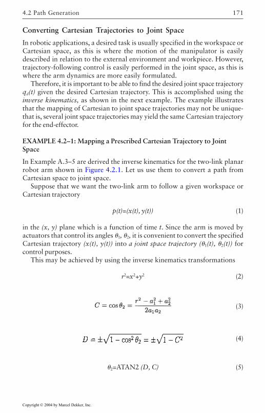
171
Converting Cartesian Trajectories to Joint Space
In robotic applications, a desired task is usually specified in the workspace orCartesian space, as this is where the motion of the manipulator is easilydescribed in relation to the external environment and workpiece. However,trajectory-following control is easily performed in the joint space, as this iswhere the arm dynamics are more easily formulated.
Therefore, it is important to be able to find the desired joint space trajectoryqd(t) given the desired Cartesian trajectory. This is accomplished using theinverse kinematics, as shown in the next example. The example illustratesthat the mapping of Cartesian to joint space trajectories may not be unique-that is, several joint space trajectories may yield the same Cartesian trajectoryfor the end-effector.
EXAMPLE 4.2–1: Mapping a Prescribed Cartesian Trajectory to JointSpace
In Example A.3–5 are derived the inverse kinematics for the two-link planarrobot arm shown in Figure 4.2.1. Let us use them to convert a path fromCartesian space to joint space.
Suppose that we want the two-link arm to follow a given workspace orCartesian trajectory
p(t)=(x(t), y(t)) (1)
in the (x, y) plane which is a function of time t. Since the arm is moved byactuators that control its angles 1, 2, it is convenient to convert the specifiedCartesian trajectory (x(t), y(t)) into a joint space trajectory (1(t), 2(t)) forcontrol purposes.
This may be achieved by using the inverse kinematics transformations
r2=x2+y2 (2)
(3)
(4)
2=ATAN2 (D, C) (5)
4.2 Path Generation
Copyright © 2004 by Marcel Dekker, Inc.
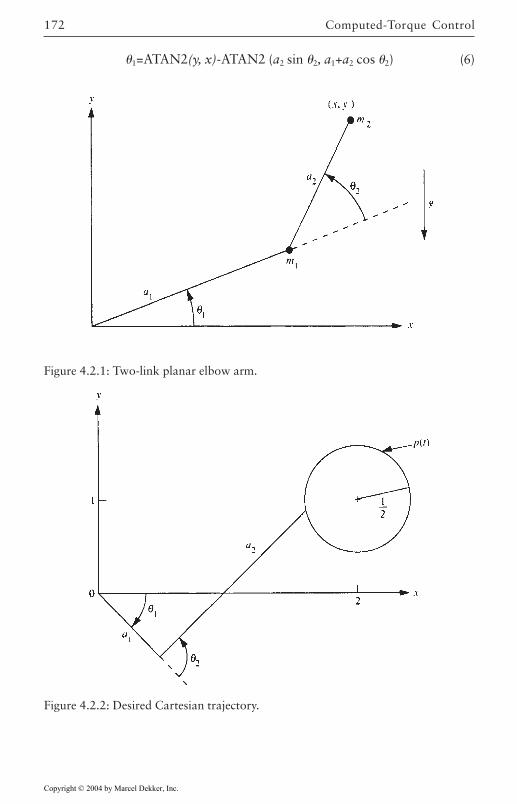
Computed-Torque Control172
1=ATAN2(y, x)-ATAN2 (a2 sin 2, a1+a2 cos 2) (6)
Figure 4.2.1: Two-link planar elbow arm.
Figure 4.2.2: Desired Cartesian trajectory.
Copyright © 2004 by Marcel Dekker, Inc.
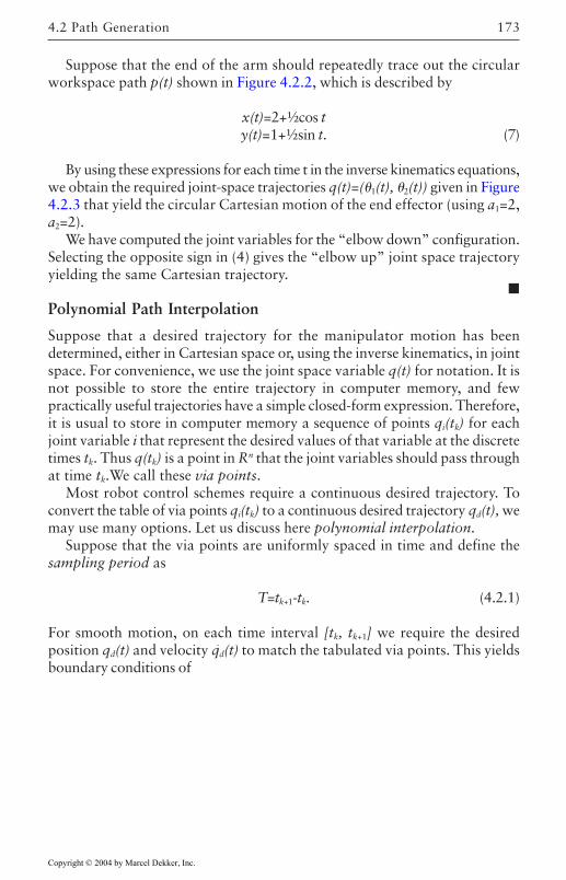
173
Suppose that the end of the arm should repeatedly trace out the circularworkspace path p(t) shown in Figure 4.2.2, which is described by
x(t)=2+½cos ty(t)=1+½sin t. (7)
By using these expressions for each time t in the inverse kinematics equations,we obtain the required joint-space trajectories q(t)=(1(t), 2(t)) given in Figure4.2.3 that yield the circular Cartesian motion of the end effector (using a1=2,a2=2).
We have computed the joint variables for the “elbow down” configuration.Selecting the opposite sign in (4) gives the “elbow up” joint space trajectoryyielding the same Cartesian trajectory.
Polynomial Path Interpolation
Suppose that a desired trajectory for the manipulator motion has beendetermined, either in Cartesian space or, using the inverse kinematics, in jointspace. For convenience, we use the joint space variable q(t) for notation. It isnot possible to store the entire trajectory in computer memory, and fewpractically useful trajectories have a simple closed-form expression. Therefore,it is usual to store in computer memory a sequence of points qi(tk) for eachjoint variable i that represent the desired values of that variable at the discretetimes tk. Thus q(tk) is a point in Rn that the joint variables should pass throughat time tk.We call these via points.
Most robot control schemes require a continuous desired trajectory. Toconvert the table of via points qi(tk) to a continuous desired trajectory qd(t), wemay use many options. Let us discuss here polynomial interpolation.
Suppose that the via points are uniformly spaced in time and define thesampling period as
T=tk+1-tk. (4.2.1)
For smooth motion, on each time interval [tk, tk+1] we require the desiredposition qd(t) and velocity q
.d(t) to match the tabulated via points. This yields
boundary conditions of
4.2 Path Generation
Copyright © 2004 by Marcel Dekker, Inc.
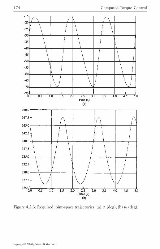
Computed-Torque Control174
Figure 4.2.3: Required joint-space trajectories: (a) 1 (deg); (b) 2 (deg).
Copyright © 2004 by Marcel Dekker, Inc.
175
(4.2.2)
To match these boundary conditions, it is necessary to use on [tk, tk+1] thecubic interpolating polynomial
(4.2.3)
which has four free variables. Then
(4.2.4)
(4.2.5)
so that the acceleration is linear on each sample period.It is easy to solve for the coefficients that guarantee matching of the boundary
conditions. In fact, we see that
(4.2.6)
This is solved to obtain the required interpolating coefficients on each interval[tk, tk+1].
(4.2.7)
Note that this technique requires storing the desired position and velocity ateach sampling point in tabular form. A variant uses a higher-order polynomialto ensure continuous position, velocity, and acceleration at each sampletime tk.
4.2 Path Generation
Copyright © 2004 by Marcel Dekker, Inc.
Computed-Torque Control176
Although we have used the joint variable notation q(t), it should beemphasized that trajectory interpolation can also be performed in Cartesianspace.
Linear Function with Parabolic Blends
Using cubic interpolating polynomials, the acceleration on each sampleperiod is linear. However, in many practical applications there are goodreasons for insisting on constant accelerations within each sample period.For instance, any real robot has upper limits on the torques that can besupplied by its actuators. For linear systems (think of Newton’s law) thistranslates into constant accelerations. Therefore, constant accelerations areless likely to saturate the actuators. Besides that, most industrial robotcontrollers are programmed to use constant accelerations on each sampleperiod.
A constant acceleration profile is shown in Figure 4.2.4(a). The associatedvelocity and position profiles are shown in Figure 4.2.4(b) and 4.2.4(c). Theposition trajectory has three parts: a quadratic or parabolic initial portion,a linear midsection, and a parabolic final portion. Therefore, let us discussinterpolation of via points using linear functions with parabolic blends (LFPB).
The time at which the position trajectory switches from parabolic tolinear is known as the blend time tb. A position qdi(t) should be specified foreach joint variable i. The trajectory in Figure 4.2.4(c) can be written forjoint i as
(4.2.8)
The coefficient vi may be interpreted as the maximum velocity allowed forjoint variable i. The design parameters are vi and tb.
It is straightforward to solve for the coefficients on each time interval [tk,tk+1] that ensure satisfaction of the boundary conditions (4.2.2). The result is
Copyright © 2004 by Marcel Dekker, Inc.
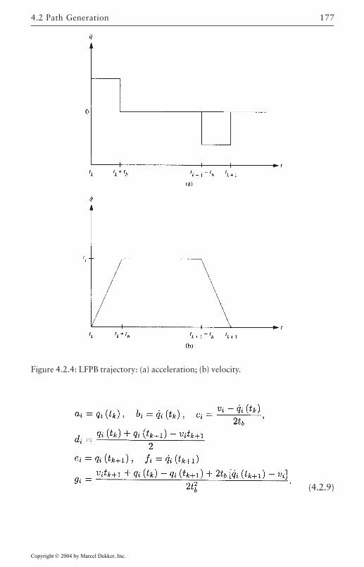
177
(4.2.9)
Figure 4.2.4: LFPB trajectory: (a) acceleration; (b) velocity.
4.2 Path Generation
Copyright © 2004 by Marcel Dekker, Inc.
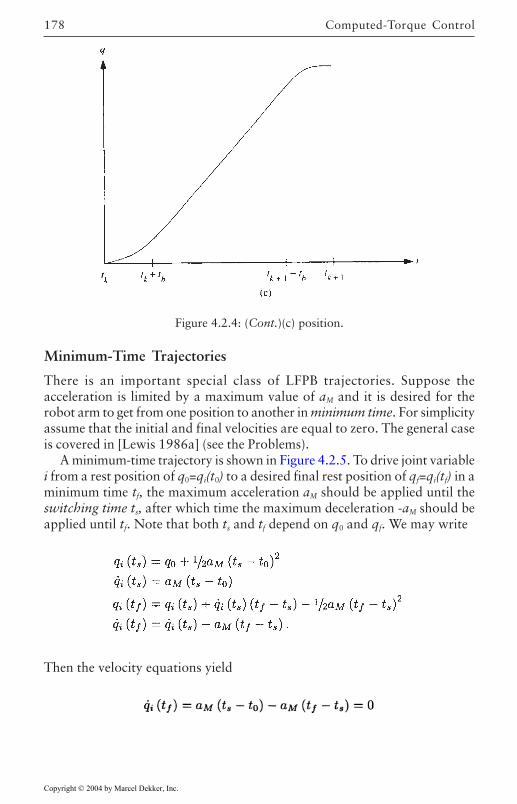
Computed-Torque Control178
Minimum-Time Trajectories
There is an important special class of LFPB trajectories. Suppose theacceleration is limited by a maximum value of aM and it is desired for therobot arm to get from one position to another in minimum time. For simplicityassume that the initial and final velocities are equal to zero. The general caseis covered in [Lewis 1986a] (see the Problems).
A minimum-time trajectory is shown in Figure 4.2.5. To drive joint variablei from a rest position of q0=qi(t0) to a desired final rest position of qf=qi(tf) in aminimum time tf, the maximum acceleration aM should be applied until theswitching time ts, after which time the maximum deceleration -aM should beapplied until tf. Note that both ts and tf depend on q0 and qf. We may write
Then the velocity equations yield
Figure 4.2.4: (Cont.)(c) position.
Copyright © 2004 by Marcel Dekker, Inc.
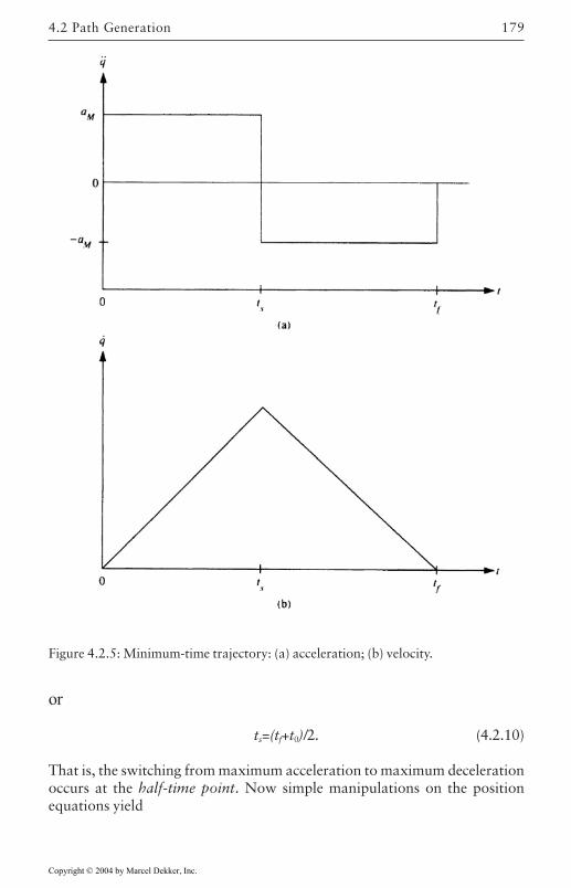
179
or
ts=(tf+t0)/2. (4.2.10)
That is, the switching from maximum acceleration to maximum decelerationoccurs at the half-time point. Now simple manipulations on the positionequations yield
Figure 4.2.5: Minimum-time trajectory: (a) acceleration; (b) velocity.
4.2 Path Generation
Copyright © 2004 by Marcel Dekker, Inc.
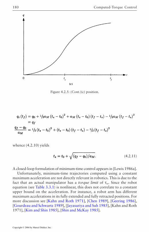
Computed-Torque Control180
whence (4.2.10) yields
(4.2.11)
A closed-loop formulation of minimum-time control appears in [Lewis 1986a].Unfortunately, minimum-time trajectories computed using a constant
maximum acceleration are not directly relevant in robotics. This is due to thefact that an actual manipulator has a torque limit of τm. Since the robotequation (see Table 3.3.1) is nonlinear, this does not correlate to a constantupper bound on the acceleration. For instance, a robot arm has differentmaximum accelerations in its fully extended and fully retracted positions. Formore discussion see [Kahn and Roth 1971], [Chen 1989], [Geering 1986],[Gourdeau and Schwartz 1989], [Jayasuriya and Suh 1985], [Kahn and Roth1971], [Kim and Shin 1985], [Shin and McKay 1985].
Figure 4.2.5: (Cont.)(c) position.
Copyright © 2004 by Marcel Dekker, Inc.
181
4.3 Computer Simulation of Robotic Systems
It is very important to simulate on a digital computer a proposed manipulatorcontrol scheme before actually implementing it on an arm. We show herehow to perform such computer simulations for robotic systems. Since mostrobot controllers are actually implemented in a digital fashion (Section 4.5),we also show how to simulate digital robot arm controllers.
Simulation of Robot Dynamics
There is a variety of software packages for the simulation of nonlineardynamical systems, including SIMNON [Åström and Wittenmark 1984],MATLAB, and others. For convenience, we include in Appendix B somesimulation programs that are quite useful for continuous and digital control.
All simulation programs require the user to write similar subroutines. Timeresponse simulators that use integration routines such as Runge-Kutta all requirethe computation of the state derivative given the current state. In Section 3.4we saw how to represent the robot arm equation
(4.3.1)
in the nonlinear state-space form
(4.3.2)
with x(t) the state and u(t) the input.Defining a state as x=[qT q.T]T, we may write the implicit form
(4.3.3)
with τ the arm control torque that is provided by the controller and τd thedisturbance torque. We say that this is an implicit form since the coefficientmatrix of the left-hand side means that is not givenexplicitly in terms of the right-hand side.
Given x(t), it is necessary to provide a subroutine for the integration programthat computes (t). One approach to solving for is to invert M(q). However,due to potential numerical problems this is not recommended. Let us represent(4.3.3) as
(4.3.4)
Note that in this case u(t) is the vector composed of the controls (t) and thedisturbances d(t).
4.3 Computer Simulation of Robotic Systems
Copyright © 2004 by Marcel Dekker, Inc.
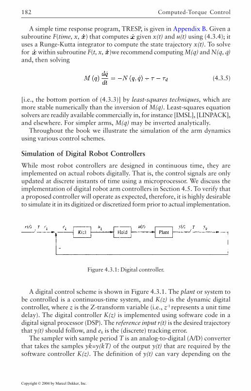
Computed-Torque Control182
A simple time response program, TRESP, is given in Appendix B. Given asubroutine F(time, x, ) that computes given x(t) and u(t) using (4.3.4); ituses a Runge-Kutta integrator to compute the state trajectory x(t). To solvefor within subroutine F(t, x, )we recommend computing M(q) and N(q, q.)and, then solving
(4.3.5)
[i.e., the bottom portion of (4.3.3)] by least-squares techniques, which aremore stable numerically than the inversion of M(q). Least-squares equationsolvers are readily available commercially in, for instance [IMSL], [LINPACK],and elsewhere. For simpler arms, M(q) may be inverted analytically.
Throughout the book we illustrate the simulation of the arm dynamicsusing various control schemes.
Simulation of Digital Robot Controllers
While most robot controllers are designed in continuous time, they areimplemented on actual robots digitally. That is, the control signals are onlyupdated at discrete instants of time using a microprocessor. We discuss theimplementation of digital robot arm controllers in Section 4.5. To verify thata proposed controller will operate as expected, therefore, it is highly desirableto simulate it in its digitized or discretized form prior to actual implementation.
Figure 4.3.1: Digital controller.
A digital control scheme is shown in Figure 4.3.1. The plant or system tobe controlled is a continuous-time system, and K(z) is the dynamic digitalcontroller, where z is the Z-transform variable (i.e., z-1 represents a unit timedelay). The digital controller K(z) is implemented using software code in adigital signal processor (DSP). The reference input r(t) is the desired trajectorythat y(t) should follow, and ek is the (discrete) tracking error.
The sampler with sample period T is an analog-to-digital (A/D) converterthat takes the samples yk=y(kT) of the output y(t) that are required by thesoftware controller K(z). The definition of y(t) can vary depending on the
Copyright © 2004 by Marcel Dekker, Inc.
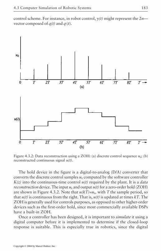
183
control scheme. For instance, in robot control, y(t) might represent the 2n—vector composed of q(t) and q.(t).
Figure 4.3.2: Data reconstruction using a ZOH: (a) discrete control sequence uk; (b)reconstructed continuous signal u(t).
The hold device in the figure is a digital-to-analog (D/A) converter thatconverts the discrete control samples uk computed by the software controllerK(z) into the continuous-time control u(t) required by the plant. It is a datareconstruction device. The input uk and output u(t) for a zero-order hold (ZOH)are shown in Figure 4.3.2. Note that u(kT)=uk, with T the sample period, sothat u(t) is continuous from the right. That is, u(t) is updated at times kT. TheZOH is generally used for controls purposes, as opposed to other higher-orderdevices such as the first-order hold, since most commercially available DSPshave a built-in ZOH.
Once a controller has been designed, it is important to simulate it using adigital computer before it is implemented to determine if the closed-loopresponse is suitable. This is especially true in robotics, since the digital
4.3 Computer Simulation of Robotic Systems
Copyright © 2004 by Marcel Dekker, Inc.
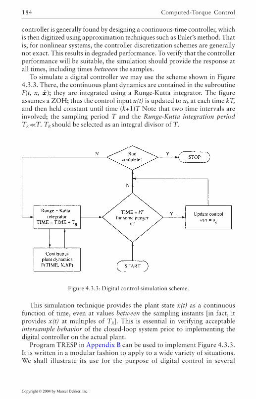
Computed-Torque Control184
controller is generally found by designing a continuous-time controller, whichis then digitized using approximation techniques such as Euler’s method. Thatis, for nonlinear systems, the controller discretization schemes are generallynot exact. This results in degraded performance. To verify that the controllerperformance will be suitable, the simulation should provide the response atall times, including times between the samples.
To simulate a digital controller we may use the scheme shown in Figure4.3.3. There, the continuous plant dynamics are contained in the subroutineF(t, x, ); they are integrated using a Runge-Kutta integrator. The figureassumes a ZOH; thus the control input u(t) is updated to uk at each time kT,and then held constant until time (k+1)T Note that two time intervals areinvolved; the sampling period T and the Runge-Kutta integration periodTR << T. TR should be selected as an integral divisor of T.
Figure 4.3.3: Digital control simulation scheme.
This simulation technique provides the plant state x(t) as a continuousfunction of time, even at values between the sampling instants [in fact, itprovides x(t) at multiples of TR]. This is essential in verifying acceptableintersample behavior of the closed-loop system prior to implementing thedigital controller on the actual plant.
Program TRESP in Appendix B can be used to implement Figure 4.3.3.It is written in a modular fashion to apply to a wide variety of situations.We shall illustrate its use for the purpose of digital control in several
Copyright © 2004 by Marcel Dekker, Inc.
185
subsequent examples. The use of such simulation software as SIMNON isquite similar.
We discuss the implementation of digital robot arm controllers in Section4.5. Some detailed discussion on digital control, simulation, and DSPimplementation of controllers is given in [Lewis 1992].
4.4 Computed-Torque Control
Through the years there have been proposed many sorts of robot controlschemes. As it happens, most of them can be considered as special cases of theclass of computed-torque controllers. Computed torque, at the same time, is aspecial application of feedback linearization of nonlinear systems, which hasgained popularity in modern systems theory [Hunt et al. 1983], [Gilbert andHa 1984]. In fact, one way to classify robot control schemes is to divide themas “computed-torque-like” or “noncomputed-torque-like.” Computed-torque-like controls appear in robust control, adaptive control, learning control, andso on.
In the remainder of this chapter we explore this class of robot controllers,which includes such a broad range of designs. Computed-torque control allowsus to conveniently derive very effective robot controllers, while providing aframework to bring together classical independent joint control and somemodern design techniques, as well as set the stage for the rest of the book. Asummary of the different computed-torque-like controllers is given at the endof the section in Table 4.4.1. We shall see that many digital robot controllersare also computed-torque-like controllers (Section 4.5).
Derivation of Inner Feedforward Loop
The robot arm dynamics are
(4.4.1)
or
(4.4.2)
with the joint variable the control torque, and d(t) adisturbance. If this equation includes motor actuator dynamics (Section 3.6),then (t) is an input voltage.
Suppose that a desired trajectory qd(t) has been selected for the arm motion,according to the discussion in Section 4.2. To ensure trajectory tracking bythe joint variable, define an output or tracking error as
4.4 Computed-Torque Control
Copyright © 2004 by Marcel Dekker, Inc.
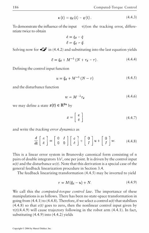
Computed-Torque Control186
(4.4.3)
To demonstrate the influence of the input (t)on the tracking error, differe-ntiate twice to obtain
Solving now for in (4.4.2) and substituting into the last equation yields
(4.4.4)
Defining the control input function
(4.4.5)
and the disturbance function
(4.4.6)
we may define a state by
(4.4.7)
and write the tracking error dynamics as
(4.4.8)
This is a linear error system in Brunovsky canonical form consisting of npairs of double integrators 1/s2, one per joint. It is driven by the control inputu(t) and the disturbance w(t). Note that this derivation is a special case of thegeneral feedback linearization procedure in Section 3.4.
The feedback linearizing transformation (4.4.5) may be inverted to yield
(4.4.9)
We call this the computed-torque control law. The importance of thesemanipulations is as follows. There has been no state-space transformation ingoing from (4.4.1) to (4.4.8). Therefore, if we select a control u(t) that stabilizes(4.4.8) so that e(t) goes to zero, then the nonlinear control input given by(t)(4.4.9) will cause trajectory following in the robot arm (4.4.1). In fact,substituting (4.4.9) into (4.4.2) yields
Copyright © 2004 by Marcel Dekker, Inc.
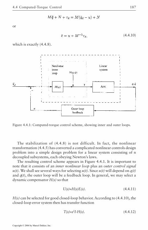
187
or
(4.4.10)
which is exactly (4.4.8).
Figure 4.4.1: Computed-torque control scheme, showing inner and outer loops.
The stabilization of (4.4.8) is not difficult. In fact, the nonlineartransformation (4.4.5) has converted a complicated nonlinear controls designproblem into a simple design problem for a linear system consisting of ndecoupled subsystems, each obeying Newton’s laws.
The resulting control scheme appears in Figure 4.4.1. It is important tonote that it consists of an inner nonlinear loop plus an outer control signalu(t). We shall see several ways for selecting u(t). Since u(t) will depend on q(t)and q.(t), the outer loop will be a feedback loop. In general, we may select adynamic compensator H(s) so that
U(s)=H(s)E(s). (4.4.11)
H(s) can be selected for good closed-loop behavior. According to (4.4.10), theclosed-loop error system then has transfer function
T(s)=s2I-H(s). (4.4.12)
4.4 Computed-Torque Control
Copyright © 2004 by Marcel Dekker, Inc.
Computed-Torque Control188
It is important to realize that computed-torque depends on the inversion ofthe robot dynamics, and indeed is sometimes called inverse dynamics controlIn fact, (4.4.9) shows that (t) is computed by substituting d–u for in (4.4.2);that is, by solving the robot inverse dynamics problem. The caveats associatedwith system inversion, including the problems resulting when the system hasnon-minimum-phase zeros, all apply here. (Note that in the linear case, thesystem zeros are the poles of the inverse. Such nonminimum-phase notionsgeneralize to nonlinear systems.) Fortunately for us, the rigid arm dynamicsare minimum phase.
There are several ways to compute (4.4.9) for implementation purposes.Formal matrix multiplication at each sample time should be avoided. In somecases the expression may be worked out analytically. A good way to computethe torque (t) is to use the efficient Newton-Euler inverse dynamics formulation[Craig 1985] with d–u in place of (t).
The outer-loop signal u(t) can be chosen using many approaches, includingrobust and adaptive control techniques. In the remainder of this chapter weexplore some choices for u(t) and some variations on computed-torque control.
PD Outer-Loop Design
One way to select the auxiliary control signal u(t) is as the proportional-plus-derivative (PD) feedback,
(4.4.13)
Then the overall robot arm input becomes
(4.4.14)
This controller is shown in Figure 4.4.6 with Ki=0. The closed-loop errordynamics are
(4.4.15)
or in state-space form,
(4.4.16)
The closed-loop characteristic polynomial is
(4.4.17)
Choice of PD Gains. It is usual to take the n×n gain matrices diagonal sothat
Copyright © 2004 by Marcel Dekker, Inc.
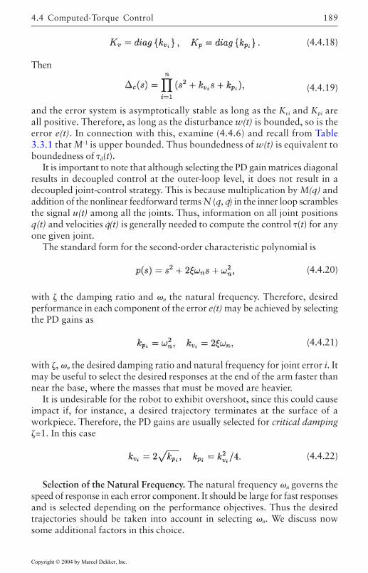
189
(4.4.18)
Then
(4.4.19)
and the error system is asymptotically stable as long as the Kvi and Kpi areall positive. Therefore, as long as the disturbance w(t) is bounded, so is theerror e(t). In connection with this, examine (4.4.6) and recall from Table3.3.1 that M-1 is upper bounded. Thus boundedness of w(t) is equivalent toboundedness of d(t).
It is important to note that although selecting the PD gain matrices diagonalresults in decoupled control at the outer-loop level, it does not result in adecoupled joint-control strategy. This is because multiplication by M(q) andaddition of the nonlinear feedforward terms N (q, q.) in the inner loop scramblesthe signal u(t) among all the joints. Thus, information on all joint positionsq(t) and velocities q.(t) is generally needed to compute the control (t) for anyone given joint.
The standard form for the second-order characteristic polynomial is
(4.4.20)
with the damping ratio and n the natural frequency. Therefore, desiredperformance in each component of the error e(t) may be achieved by selectingthe PD gains as
(4.4.21)
with , n the desired damping ratio and natural frequency for joint error i. Itmay be useful to select the desired responses at the end of the arm faster thannear the base, where the masses that must be moved are heavier.
It is undesirable for the robot to exhibit overshoot, since this could causeimpact if, for instance, a desired trajectory terminates at the surface of aworkpiece. Therefore, the PD gains are usually selected for critical damping=1. In this case
(4.4.22)
Selection of the Natural Frequency. The natural frequency n governs thespeed of response in each error component. It should be large for fast responsesand is selected depending on the performance objectives. Thus the desiredtrajectories should be taken into account in selecting n. We discuss nowsome additional factors in this choice.
4.4 Computed-Torque Control
Copyright © 2004 by Marcel Dekker, Inc.
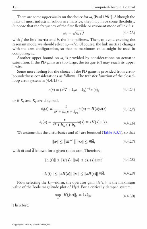
Computed-Torque Control190
There are some upper limits on the choice for n [Paul 1981]. Although thelinks of most industrial robots are massive, they may have some flexibility.Suppose that the frequency of the first flexible or resonant mode of link i is
(4.4.23)
with J the link inertia and kr the link stiffness. Then, to avoid exciting theresonant mode, we should select n<r/2. Of course, the link inertia J changeswith the arm configuration, so that its maximum value might be used incomputing r.
Another upper bound on n is provided by considerations on actuatorsaturation. If the PD gains are too large, the torque τ(t) may reach its upperlimits.
Some more feeling for the choice of the PD gains is provided from error-boundedness considerations as follows. The transfer function of the closed-loop error system in (4.4.15) is
(4.4.24)
or if Kv and Kp are diagonal,
(4.4.25)
(4.4.26)
We assume that the disturbance and M-1 are bounded (Table 3.3.1), so that
(4.4.27)
with m— and d—
known for a given robot arm. Therefore,
(4.4.28)
(4.4.29)
Now selecting the L2—norm, the operator gain ||H(s)||2 is the maximumvalue of the Bode magnitude plot of H(s). For a critically damped system,
(4.4.30)
Therefore,
Copyright © 2004 by Marcel Dekker, Inc.
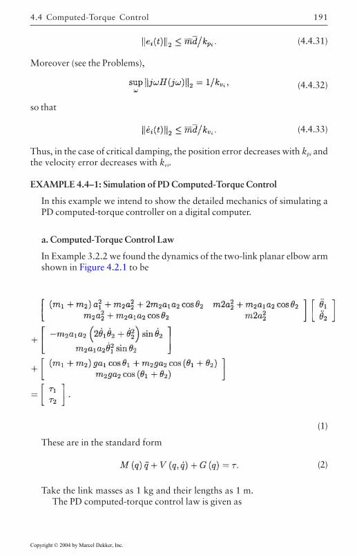
191
(4.4.31)
Moreover (see the Problems),
(4.4.32)
so that
(4.4.33)
Thus, in the case of critical damping, the position error decreases with kpi andthe velocity error decreases with kvi.
EXAMPLE 4.4–1: Simulation of PD Computed-Torque Control
In this example we intend to show the detailed mechanics of simulating aPD computed-torque controller on a digital computer.
a. Computed-Torque Control Law
In Example 3.2.2 we found the dynamics of the two-link planar elbow armshown in Figure 4.2.1 to be
(1)
These are in the standard form
(2)
Take the link masses as 1 kg and their lengths as 1 m.The PD computed-torque control law is given as
4.4 Computed-Torque Control
Copyright © 2004 by Marcel Dekker, Inc.
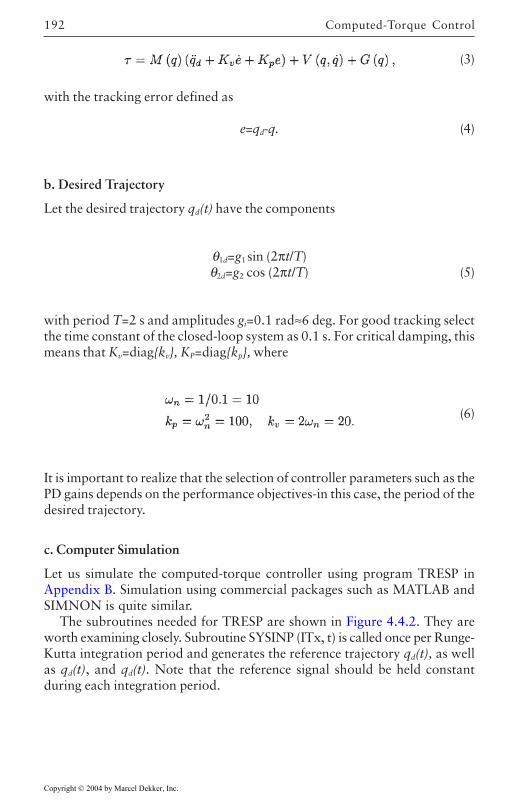
Computed-Torque Control192
(3)
with the tracking error defined as
e=qd-q. (4)
b. Desired Trajectory
Let the desired trajectory qd(t) have the components
θ1d=g1 sin (2πt/T)θ2d=g2 cos (2πt/T) (5)
with period T=2 s and amplitudes gi=0.1 rad≈6 deg. For good tracking selectthe time constant of the closed-loop system as 0.1 s. For critical damping, thismeans that Kv=diagkv, KP=diagkp, where
(6)
It is important to realize that the selection of controller parameters such as thePD gains depends on the performance objectives-in this case, the period of thedesired trajectory.
c. Computer Simulation
Let us simulate the computed-torque controller using program TRESP inAppendix B. Simulation using commercial packages such as MATLAB andSIMNON is quite similar.
The subroutines needed for TRESP are shown in Figure 4.4.2. They areworth examining closely. Subroutine SYSINP (ITx, t) is called once per Runge-Kutta integration period and generates the reference trajectory qd(t), as wellas qd(t), and qd(t). Note that the reference signal should be held constantduring each integration period.
Copyright © 2004 by Marcel Dekker, Inc.
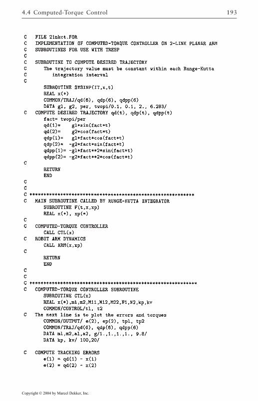
1934.4 Computed-Torque Control
Copyright © 2004 by Marcel Dekker, Inc.
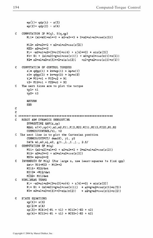
Computed-Torque Control194
Copyright © 2004 by Marcel Dekker, Inc.
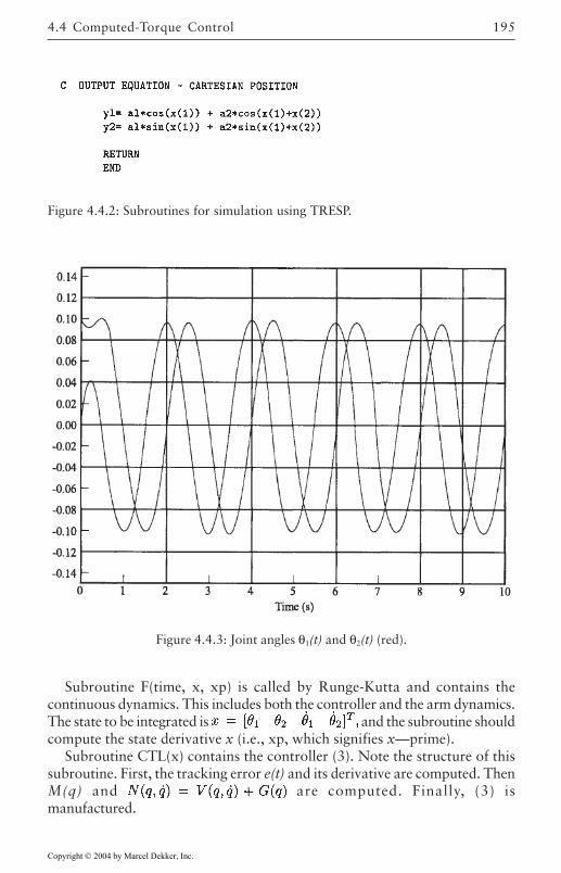
195
Subroutine F(time, x, xp) is called by Runge-Kutta and contains thecontinuous dynamics. This includes both the controller and the arm dynamics.The state to be integrated is and the subroutine shouldcompute the state derivative x (i.e., xp, which signifies x—prime).
Subroutine CTL(x) contains the controller (3). Note the structure of thissubroutine. First, the tracking error e(t) and its derivative are computed. ThenM(q) and are computed. Finally, (3) ismanufactured.
Figure 4.4.2: Subroutines for simulation using TRESP.
Figure 4.4.3: Joint angles θ1(t) and θ2(t) (red).
4.4 Computed-Torque Control
Copyright © 2004 by Marcel Dekker, Inc.
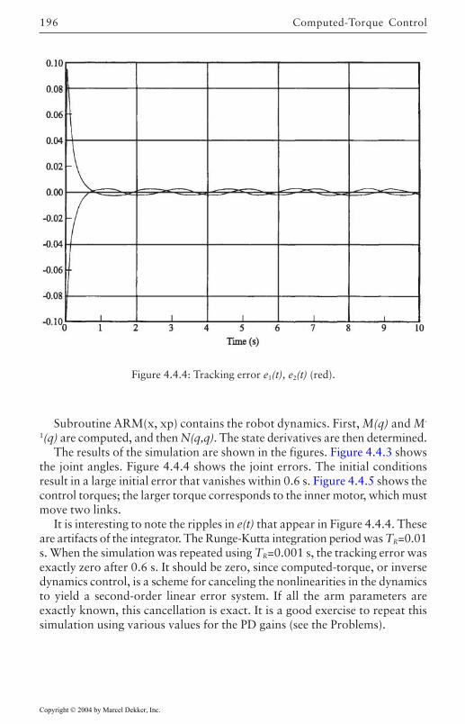
Computed-Torque Control196
Subroutine ARM(x, xp) contains the robot dynamics. First, M(q) and M-
1(q) are computed, and then N(q,q). The state derivatives are then determined.The results of the simulation are shown in the figures. Figure 4.4.3 shows
the joint angles. Figure 4.4.4 shows the joint errors. The initial conditionsresult in a large initial error that vanishes within 0.6 s. Figure 4.4.5 shows thecontrol torques; the larger torque corresponds to the inner motor, which mustmove two links.
It is interesting to note the ripples in e(t) that appear in Figure 4.4.4. Theseare artifacts of the integrator. The Runge-Kutta integration period was TR=0.01s. When the simulation was repeated using TR=0.001 s, the tracking error wasexactly zero after 0.6 s. It should be zero, since computed-torque, or inversedynamics control, is a scheme for canceling the nonlinearities in the dynamicsto yield a second-order linear error system. If all the arm parameters areexactly known, this cancellation is exact. It is a good exercise to repeat thissimulation using various values for the PD gains (see the Problems).
Figure 4.4.4: Tracking error e1(t), e2(t) (red).
Copyright © 2004 by Marcel Dekker, Inc.
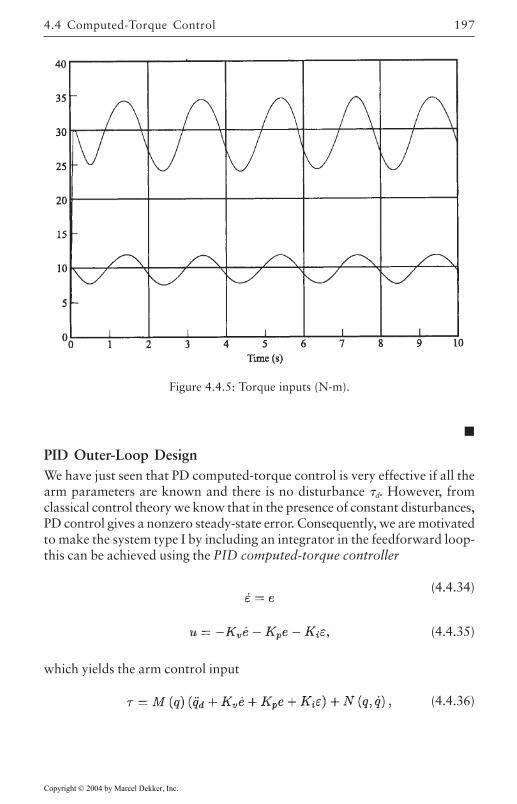
197
We have just seen that PD computed-torque control is very effective if all thearm parameters are known and there is no disturbance d. However, fromclassical control theory we know that in the presence of constant disturbances,PD control gives a nonzero steady-state error. Consequently, we are motivatedto make the system type I by including an integrator in the feedforward loop-this can be achieved using the PID computed-torque controller
(4.4.34)
(4.4.35)
which yields the arm control input
(4.4.36)
Figure 4.4.5: Torque inputs (N-m).
4.4 Computed-Torque Control
PID Outer-Loop Design
Copyright © 2004 by Marcel Dekker, Inc.
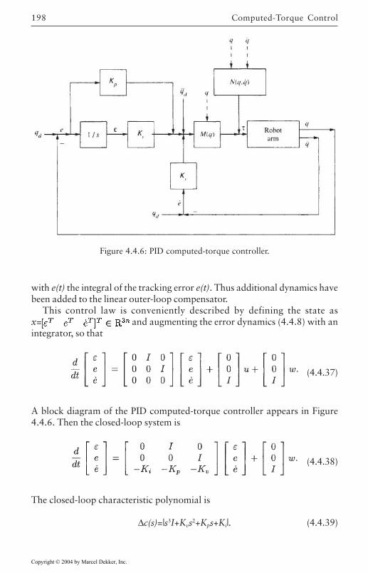
Computed-Torque Control198
with e(t) the integral of the tracking error e(t). Thus additional dynamics havebeen added to the linear outer-loop compensator.
This control law is conveniently described by defining the state asx= and augmenting the error dynamics (4.4.8) with anintegrator, so that
(4.4.37)
A block diagram of the PID computed-torque controller appears in Figure4.4.6. Then the closed-loop system is
(4.4.38)
The closed-loop characteristic polynomial is
∆c(s)=|s3I+Kvs2+Kps+Ki|. (4.4.39)
Figure 4.4.6: PID computed-torque controller.
Copyright © 2004 by Marcel Dekker, Inc.
199
Selecting diagonal control’ gains
(4.4.40)
gives
(4.4.41)
By using the Routh test it can be found that for closed-loop stability we requirethat
(4.4.42)
that is, the integral gain should not be too large.
Actuator Saturation and Integrator Windup. It is important to be aware of aneffect in implementing PID control on any actual robot manipulator that cancause serious problems if not accounted for. Any real robot arm will havelimits on the voltages and torques of its actuators. These limits may or maynot cause a problem with PD control, but are virtually guaranteed to causeproblems with integral control due to a phenomenon known as integratorwindup [Lewis 1992].
Consider the simple case where =kiε with ε(t) the integrator output. Thetorque input (t) is limited by its maximum and minimum values max and min.If kiε(t) hits max, there may or not may not be a problem. The problem arisesif the integrator input remains positive, for then the integrator continues tointegrate upwards and kiε(t) may increase well beyond max. Then, when theintegrator input becomes negative, it may take considerable time for kiε(t) todecrease below max. In the meantime is held at max, giving an incorrectcontrol input to the plant.
Integrator windup is easy to correct using antiwindup protection in a digitalcontroller. This is discussed in Section 4.5. The effects of uncorrected windupare demonstrated in Example 4.4.4.
The next example shows the usefulness of an integral term when there areunknown disturbances present.
EXAMPLE 4.4–2: Simulation of PID Computed-Torque Control
In Example 4.4.1 we simulated the PD computed-torque controller for atwo-link planar arm. In this example we add a constant unknown
4.4 Computed-Torque Control
Copyright © 2004 by Marcel Dekker, Inc.
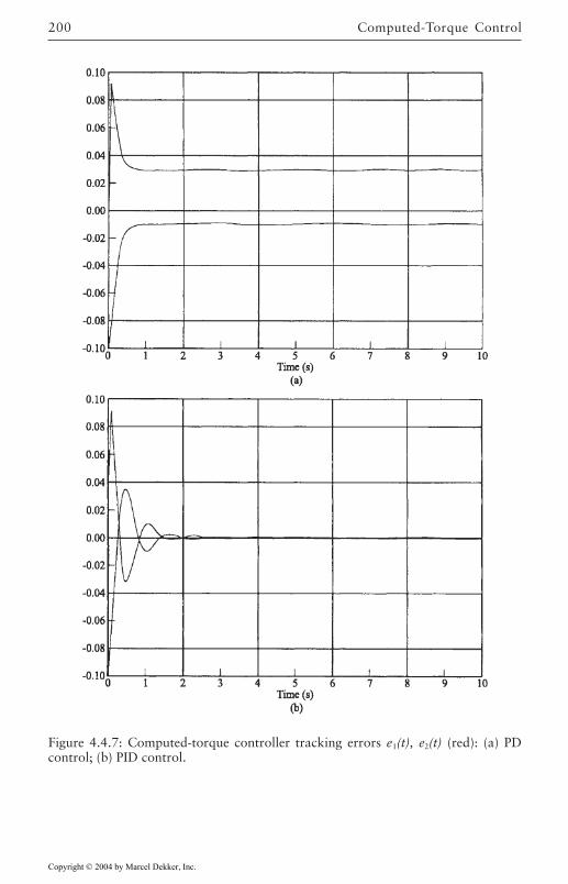
Computed-Torque Control200
Figure 4.4.7: Computed-torque controller tracking errors e1(t), e2(t) (red): (a) PDcontrol; (b) PID control.
Copyright © 2004 by Marcel Dekker, Inc.
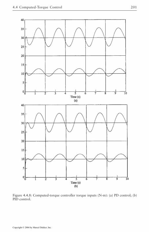
201
Figure 4.4.8: Computed-torque controller torque inputs (N-m): (a) PD control; (b)PID control.
4.4 Computed-Torque Control
Copyright © 2004 by Marcel Dekker, Inc.
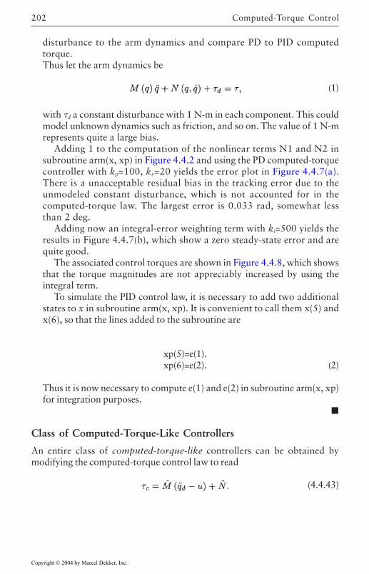
Computed-Torque Control202
disturbance to the arm dynamics and compare PD to PID computedtorque.Thus let the arm dynamics be
(1)
with d a constant disturbance with 1 N-m in each component. This couldmodel unknown dynamics such as friction, and so on. The value of 1 N-mrepresents quite a large bias.
Adding 1 to the computation of the nonlinear terms N1 and N2 insubroutine arm(x, xp) in Figure 4.4.2 and using the PD computed-torquecontroller with kp=100, kv=20 yields the error plot in Figure 4.4.7(a).There is a unacceptable residual bias in the tracking error due to theunmodeled constant disturbance, which is not accounted for in thecomputed-torque law. The largest error is 0.033 rad, somewhat lessthan 2 deg.
Adding now an integral-error weighting term with ki=500 yields theresults in Figure 4.4.7(b), which show a zero steady-state error and arequite good.
The associated control torques are shown in Figure 4.4.8, which showsthat the torque magnitudes are not appreciably increased by using theintegral term.
To simulate the PID control law, it is necessary to add two additionalstates to x in subroutine arm(x, xp). It is convenient to call them x(5) andx(6), so that the lines added to the subroutine are
xp(5)=e(1).xp(6)=e(2). (2)
Thus it is now necessary to compute e(1) and e(2) in subroutine arm(x, xp)for integration purposes.
Class of Computed-Torque-Like Controllers
An entire class of computed-torque-like controllers can be obtained bymodifying the computed-torque control law to read
(4.4.43)
Copyright © 2004 by Marcel Dekker, Inc.
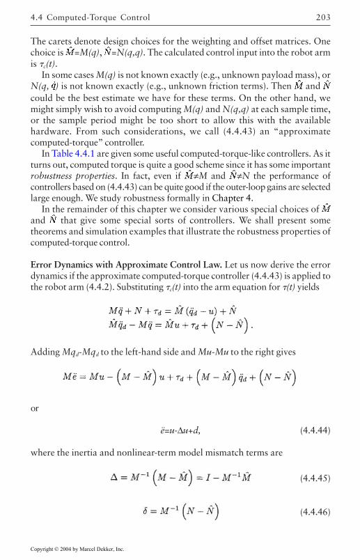
203
The carets denote design choices for the weighting and offset matrices. Onechoice is =M(q), =N(q,q). The calculated control input into the robot armis c(t).
In some cases M(q) is not known exactly (e.g., unknown payload mass), orN(q, ) is not known exactly (e.g., unknown friction terms). Then and could be the best estimate we have for these terms. On the other hand, wemight simply wish to avoid computing M(q) and N(q,q) at each sample time,or the sample period might be too short to allow this with the availablehardware. From such considerations, we call (4.4.43) an “approximatecomputed-torque” controller.
In Table 4.4.1 are given some useful computed-torque-like controllers. As itturns out, computed torque is quite a good scheme since it has some importantrobustness properties. In fact, even if ≠M and ≠N the performance ofcontrollers based on (4.4.43) can be quite good if the outer-loop gains are selectedlarge enough. We study robustness formally in Chapter 4.
In the remainder of this chapter we consider various special choices of and that give some special sorts of controllers. We shall present sometheorems and simulation examples that illustrate the robustness properties ofcomputed-torque control.
Error Dynamics with Approximate Control Law. Let us now derive the errordynamics if the approximate computed-torque controller (4.4.43) is applied tothe robot arm (4.4.2). Substituting c(t) into the arm equation for (t) yields
Adding Mqd-Mqd to the left-hand side and Mu-Mu to the right gives
or
ë=u-∆u+d, (4.4.44)
where the inertia and nonlinear-term model mismatch terms are
(4.4.45)
(4.4.46)
4.4 Computed-Torque Control
Copyright © 2004 by Marcel Dekker, Inc.
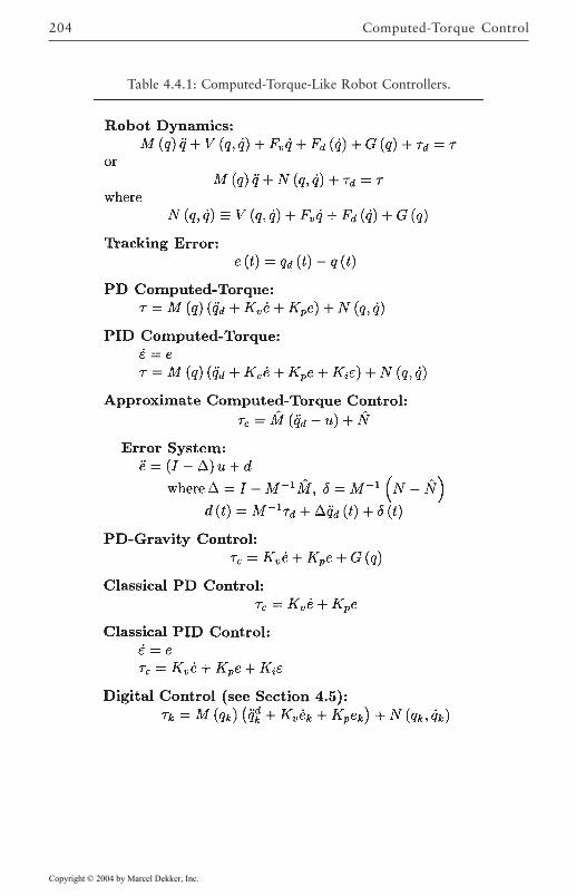
Computed-Torque Control204
Table 4.4.1: Computed-Torque-Like Robot Controllers.
Copyright © 2004 by Marcel Dekker, Inc.
205
and the disturbance is
(4.4.47)
This reduces to the error system (4.4.10) if exact computed-torque controlis used so that ∆=0, δ=0. Otherwise, the error system is driven by thedesired acceleration and the nonlinear term mismatch δ(t). Thus the trackingerror will never go exactly to zero. Moreover, the auxiliary control u(t) ismultiplied by (I -∆), which can make for a very difficult control problem.
Using outer-loop PD feedback so that u(t)=-Kve-Kpe yields the error system
(4.4.48)
The behavior of such systems is not obvious, even if Kv and Kp are selected forgood stability of the left-hand side. There are two sorts of problems: first, thedisturbance term d(t), and second the function ∆(Kve+Kpe) of the error and itsderivative.
PD-Plus-Gravity Controller
A useful controller in the computed-torque family is the PD-plus-gravitycontroller that results when M=I, N=G(q)-qd, with G(q) the gravity term ofthe manipulator dynamics. Then, selecting PD feedback for u(t) yields
(4.4.49)
This control law was treated in [Arimoto and Miyazaki 1984], [Schilling1990]. It is much simpler to implement than the exact computedtorquecontroller.
When the arm is at rest, the only nonzero terms in the dynamics (4.4.1)are the gravity G(q), the disturbance d, and possibly the control torque .
The PD-gravity controller c, includes G(q), so that we should expect goodperformance for set-point tracking, that is, when a constant qd is given sothat qd=0. The next result formalizes this. It relies on a Lyapunov proof(Chapter 1) of the sort that will be of consistent usefulness throughout thebook, drawing especially on the skew-symmetry property in Table 3.3.1.Thus it is very important to understand the steps in this proof.
4.4 Computed-Torque Control
Copyright © 2004 by Marcel Dekker, Inc.
Computed-Torque Control206
THEOREM 4.4–1: Suppose that PD-gravity control is used in the armdynamics (4.4.1) and d=0, qd=0. Then the steady-state tracking error. e=qd-q is zero.
Proof:1. Closed-Loop System
Ignoring friction, the robot dynamics are given by
(1)
When qd=0, the proposed control law (4.4.49) yields the closed-loop dynamics
(2)
2. Lyapunov FunctionSelect now the Lyapunov function
(3)
and differentiate to obtain
(4)
Substituting the closed-loop dynamics (2) yields
(5)
Now, the skew symmetry of the first term gives
(6)
The state is , so that V is positive definite but only negativesemidefinite. Therefore, we have demonstrated stability in the sense ofLyapunov, that is, that the error and joint velocity are both bounded.
3. Asymptotic Stability by LaSalle’s ExtensionThe asymptotic stability of the system may be demonstrated using Barbalat’s
lemma and a variant of LaSalle’s extension [Slotine and Li 1991] (Chapter2). Thus it is necessary to demonstrate that the only invariant set contained inthe set V=0 is the origin.
Since V is lower bounded by zero and nonpositive, it follows that Vapproaches a finite limit, which can be written
Copyright © 2004 by Marcel Dekker, Inc.
207
(7)
We now invoke Barbalat’s lemma to show that V goes to zero. For this, it isnecessary to demonstrate the uniform continuity of V. We see that
(8)
The demonstrated stability shows that a and q are bounded, whence (2) andthe boundedness of M-1(q) (see Table 3.3.1) reveal that q is bounded. Therefore,V is bounded, whence V is uniformly continuous. This guarantees by Barbalat’slemma that V goes to zero.
It is now clear that goes to zero. It remains to show that the trackingerror e(t) vanishes. Note that when q=0, (2) reveals that
(9)
Therefore, a nonzero e(t) results in nonzero and hence in q≠0, a contradiction.Therefore, the only invariant set contained in x(t)|V=0 is x(t)=0. This finallydemonstrates that both e(t) and vanish and concludes the proof.
Some notes on this proof are warranted. First, note that the Lyapunovfunction chosen is a natural one, as it contains the kinetic energy and the“artificial potential energy” associated with the virtual spring in the controllaw [Slotine and Li 1991]. Kp appears in V while Kv appears in V.
The proof of Lyapunov stability is quick and easy. The effort comes aboutin showing asymptotic stability. For this, it is required to return to the systemdynamics and study it more carefully, discussing issues such as boundednessof signals, invariant sets, and so on. The fundamental property of skewsymmetry is used in computing V. The boundedness of M-1(q) is needed inBarbalat’s lemma.
The next example illustrates the performance of the PD-gravity controllerfor trajectory tracking. In general, if qd≠0, then the PD-gravity controllerguarantees bounded tracking errors. The error bound decreases, that is, thetracking performance improves, as the PD gains become larger. This will be
EXAMPLE 4.4–3: Simulation of PD-Gravity Controller
In Example 4.4.1 we simulated the exact computed-torque control law ona two link planar manipulator. Here, let us simulate the PD-gravitycontroller. We shall take the same arm parameters and desired trajectory.
4.4 Computed-Torque Control
Copyright © 2004 by Marcel Dekker, Inc.
made rigorous in Chapter 4.
Computed-Torque Control208
Assuming identical PD gains for each link, the PD-gravity control law forthe two-link arm is
(1)
This is easily simulated by commenting out several lines of code and makinga few other modifications in subroutine CTL(x) of Figure 4.4.2.
For critical damping, the PD gains are selected as
(2)
The results of the PD-gravity controller simulation for several values of wn
are shown in Figure 4.4.9. As ωn, and hence the PD gains, increases, thetracking performance improves. However, no matter how large the PD gains,the tracking error never goes exactly to zero, but is bounded about zero by aball whose radius decreases as the gains become larger. The performance forωn=50, corresponding to kp=2500, kv=100, would be quite suitable for manyapplications.
It quite important to note that the dc value of the errors is equal to zero.One can consider the gravity terms as the “dc portion” of the computed-torque control law. If they are included in computing the torques, there willbe no error offset.
The associated control input torques are shown in Figure 4.4.10. It isextremely interesting to note that the torques are smaller for the highergains. This is contrary to popular belief, which assumes that the controltorques always increase with increasing PD gains. It is due to the fact thatlarger gains give “tighter” performance, and hence smaller tracking errors.
In view of the fact that the errors in Figure 4.4.9(a) have different magnitudes,it would probably be more reasonable to take the PD gains larger for theinner link than the outer link.
Classical Joint Control
A simple controller that often gives good results in practice is obtained byselecting in (4.4.43)
(4.4.50)
Copyright © 2004 by Marcel Dekker, Inc.
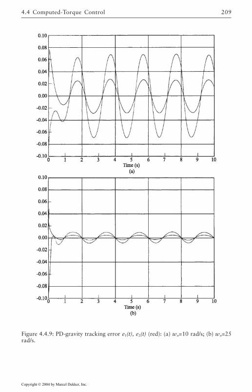
209
Figure 4.4.9: PD-gravity tracking error e1(t), e2(t) (red): (a) wn=10 rad/s; (b) wn=25rad/s.
4.4 Computed-Torque Control
Copyright © 2004 by Marcel Dekker, Inc.
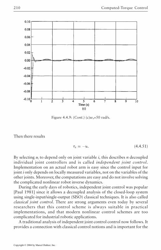
Computed-Torque Control210
Then there results
(4.4.51)
By selecting ui to depend only on joint variable i, this describes n decoupledindividual joint controllers and is called independent joint control.Implementation on an actual robot arm is easy since the control input forjoint i only depends on locally measured variables, not on the variables of theother joints. Moreover, the computations are easy and do not involve solvingthe complicated nonlinear robot inverse dynamics.
During the early days of robotics, independent joint control was popular[Paul 1981] since it allows a decoupled analysis of the closed-loop systemusing single-input/single-output (SISO) classical techniques. It is also calledclassical joint control. There are strong arguments even today by severalresearchers that this control scheme is always suitable in practicalimplementations, and that modern nonlinear control schemes are toocomplicated for industrial robotic applications.
A traditional analysis of independent joint control control now follows. Itprovides a connection with classical control notions and is important for the
Figure 4.4.9: (Cont.) (c)wn=50 rad/s.
Copyright © 2004 by Marcel Dekker, Inc.
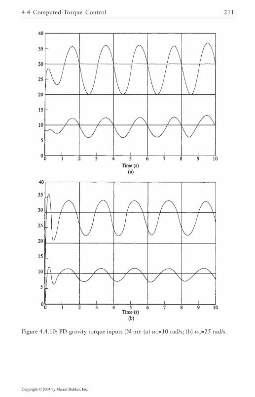
211
Figure 4.4.10: PD-gravity torque inputs (N-m): (a) wn=10 rad/s; (b) wn=25 rad/s.
4.4 Computed-Torque Control
Copyright © 2004 by Marcel Dekker, Inc.
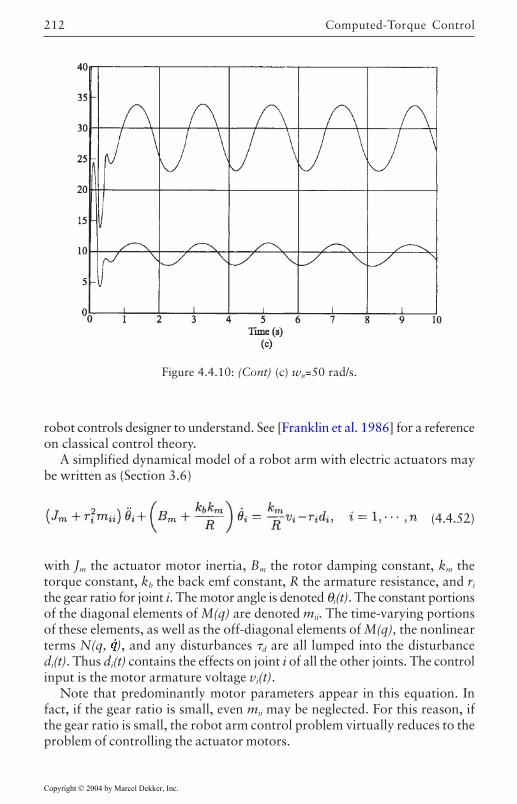
Computed-Torque Control212
robot controls designer to understand. See [Franklin et al. 1986] for a referenceon classical control theory.
A simplified dynamical model of a robot arm with electric actuators maybe written as (Section 3.6)
(4.4.52)
with Jm the actuator motor inertia, Bm the rotor damping constant, km thetorque constant, kb the back emf constant, R the armature resistance, and ri
the gear ratio for joint i. The motor angle is denoted θi(t). The constant portionsof the diagonal elements of M(q) are denoted mii. The time-varying portionsof these elements, as well as the off-diagonal elements of M(q), the nonlinearterms N(q, ), and any disturbances d are all lumped into the disturbancedi(t). Thus di(t) contains the effects on joint i of all the other joints. The controlinput is the motor armature voltage vi(t).
Note that predominantly motor parameters appear in this equation. Infact, if the gear ratio is small, even mii may be neglected. For this reason, ifthe gear ratio is small, the robot arm control problem virtually reduces to theproblem of controlling the actuator motors.
Figure 4.4.10: (Cont) (c) wn=50 rad/s.
Copyright © 2004 by Marcel Dekker, Inc.
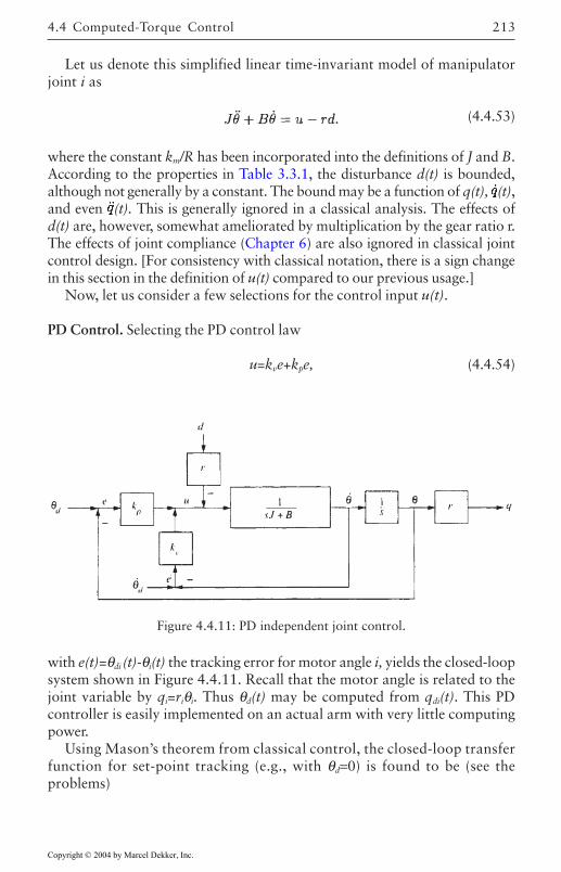
213
Let us denote this simplified linear time-invariant model of manipulatorjoint i as
(4.4.53)
where the constant km/R has been incorporated into the definitions of J and B.According to the properties in Table 3.3.1, the disturbance d(t) is bounded,although not generally by a constant. The bound may be a function of q(t), (t),and even (t). This is generally ignored in a classical analysis. The effects ofd(t) are, however, somewhat ameliorated by multiplication by the gear ratio r.The effects of joint compliance (Chapter 6) are also ignored in classical jointcontrol design. [For consistency with classical notation, there is a sign changein this section in the definition of u(t) compared to our previous usage.]
Now, let us consider a few selections for the control input u(t).
PD Control. Selecting the PD control law
u=kve+kpe, (4.4.54)
with e(t)=θdi (t)-θi(t) the tracking error for motor angle i, yields the closed-loopsystem shown in Figure 4.4.11. Recall that the motor angle is related to thejoint variable by qi=riθi. Thus θd(t) may be computed from qdi(t). This PDcontroller is easily implemented on an actual arm with very little computingpower.
Using Mason’s theorem from classical control, the closed-loop transferfunction for set-point tracking (e.g., with θd=0) is found to be (see theproblems)
Figure 4.4.11: PD independent joint control.
4.4 Computed-Torque Control
Copyright © 2004 by Marcel Dekker, Inc.
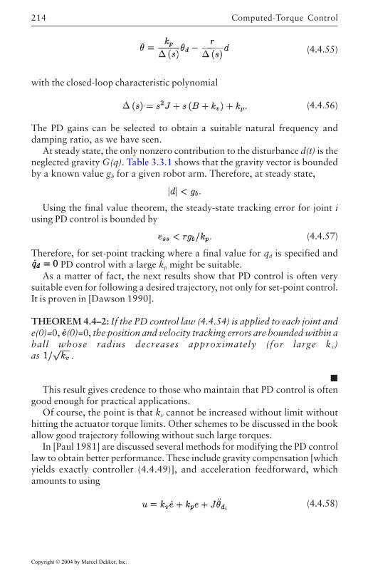
Computed-Torque Control214
(4.4.55)
with the closed-loop characteristic polynomial
(4.4.56)
The PD gains can be selected to obtain a suitable natural frequency anddamping ratio, as we have seen.
At steady state, the only nonzero contribution to the disturbance d(t) is theneglected gravity G(q). Table 3.3.1 shows that the gravity vector is boundedby a known value gb for a given robot arm. Therefore, at steady state,
Using the final value theorem, the steady-state tracking error for joint iusing PD control is bounded by
(4.4.57)
Therefore, for set-point tracking where a final value for qd is specified and PD control with a large kp might be suitable.
As a matter of fact, the next results show that PD control is often verysuitable even for following a desired trajectory, not only for set-point control.It is proven in [Dawson 1990].
THEOREM 4.4–2: If the PD control law (4.4.54) is applied to each joint ande(0)=0, (0)=0, the position and velocity tracking errors are bounded within aball whose radius decreases approximately (for large kv)as .
This result gives credence to those who maintain that PD control is oftengood enough for practical applications.
Of course, the point is that kv cannot be increased without limit withouthitting the actuator torque limits. Other schemes to be discussed in the bookallow good trajectory following without such large torques.
In [Paul 1981] are discussed several methods for modifying the PD controllaw to obtain better performance. These include gravity compensation [whichyields exactly controller (4.4.49)], and acceleration feedforward, whichamounts to using
(4.4.58)
Copyright © 2004 by Marcel Dekker, Inc.
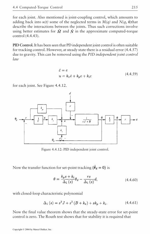
215
for each joint. Also mentioned is joint-coupling control, which amounts toadding back into u(t) some of the neglected terms in M(q) and N(q, )thatdescribe the interactions between the joints. Thus such corrections involveusing better estimates for and in the approximate computed-torquecontrol (4.4.43).
PID Control. It has been seen that PD independent joint control is often suitablefor tracking control. However, at steady state there is a residual error (4.4.57)due to gravity. This can be removed using the PID independent joint controllaw
(4.4.59)
for each joint. See Figure 4.4.12.
4.4 Computed-Torque Control
Now the transfer function for set-point tracking is
(4.4.60)
with closed-loop characteristic polynomial
(4.4.61)
Now the final value theorem shows that the steady-state error for set-pointcontrol is zero. The Routh test shows that for stability it is required that
Figure 4.4.12: PID independent joint control.
Copyright © 2004 by Marcel Dekker, Inc.
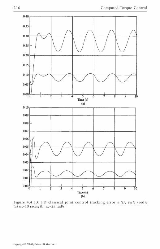
Computed-Torque Control216
Figure 4.4.13: PD classical joint control tracking error e1(t), e2(t) (red):(a) n=10 rad/s; (b) n=25 rad/s.
Copyright © 2004 by Marcel Dekker, Inc.
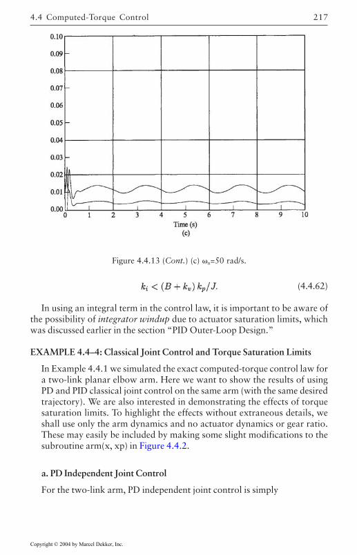
217
(4.4.62)
In using an integral term in the control law, it is important to be aware ofthe possibility of integrator windup due to actuator saturation limits, whichwas discussed earlier in the section “PID Outer-Loop Design.”
EXAMPLE 4.4–4: Classical Joint Control and Torque Saturation Limits
In Example 4.4.1 we simulated the exact computed-torque control law fora two-link planar elbow arm. Here we want to show the results of usingPD and PID classical joint control on the same arm (with the same desiredtrajectory). We are also interested in demonstrating the effects of torquesaturation limits. To highlight the effects without extraneous details, weshall use only the arm dynamics and no actuator dynamics or gear ratio.These may easily be included by making some slight modifications to thesubroutine arm(x, xp) in Figure 4.4.2.
a. PD Independent Joint Control
For the two-link arm, PD independent joint control is simply
Figure 4.4.13 (Cont.) (c) n=50 rad/s.
4.4 Computed-Torque Control
Copyright © 2004 by Marcel Dekker, Inc.
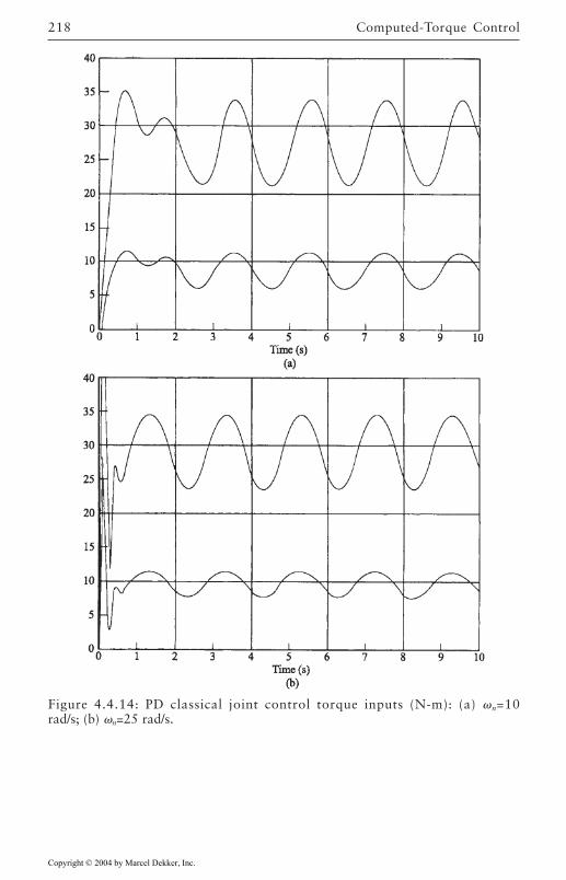
Computed-Torque Control218
Figure 4.4.14: PD classical joint control torque inputs (N-m): (a) n=10rad/s; (b) n=25 rad/s.
Copyright © 2004 by Marcel Dekker, Inc.
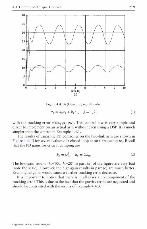
219
(1)
with the tracking error e(t)=qd(t)-q(t). This control law is very simple anddirect to implement on an actual arm without even using a DSP. It is muchsimpler than the control in Example 4.4.1.
The results of using the PD controller on the two-link arm are shown inFigure 4.4.13 for several values of a closed-loop natural frequency wn. Recallthat the PD gains for critical damping are
(2)
The low-gain results (kp=100, kv=20) in part (a) of the figure are very bad(note the scale). However, the high-gain results in part (c) are much better.Even higher gains would cause a further tracking error decrease.
It is important to notice that there is in all cases a do component of thetracking error. This is due to the fact that the gravity terms are neglected andshould be contrasted with the results of Example 4.4.3.
Figure 4.4.14 (Cont.) (c) n=50 rad/s.
4.4 Computed-Torque Control
Copyright © 2004 by Marcel Dekker, Inc.
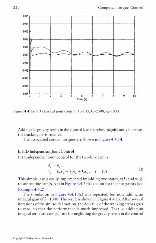
Computed-Torque Control220
Adding the gravity terms in the control law, therefore, significantly increasesthe tracking performance.
The associated control torques are shown in Figure 4.4.14.
b. PID Independent Joint ControlPID independent joint control for the two-link arm is
(3)
This simple law is easily implemented by adding two states, x(5) and x(6),to subroutine arm(x, xp) in Figure 4.4.2 to account for the integrators (seeExample 4.4.2).
The simulation in Figure 4.4.13(c) was repeated, but now adding anintegral gain of ki=1000. The result is shown in Figure 4.4.15. After severaliterations of the sinusoidal motion, the do value of the tracking errors goesto zero, so that the performance is much improved. That is, adding anintegral term can compensate for neglecting the gravity terms in the control
Figure 4.4.15: PD classical joint control: kv=100, kp=2500, ki=1000.
Copyright © 2004 by Marcel Dekker, Inc.
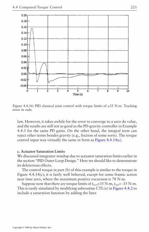
221
law. However, it takes awhile for the error to converge to a zero do value,and the results are still not as good as the PD-gravity controller in Example4.4.3 for the same PD gains. On the other hand, the integral term canreject other terms besides gravity (e.g., friction of some sorts). The torquecontrol input was virtually the same in form as Figure 4.4.14(c).
c. Actuator Saturation LimitsWe discussed integrator windup due to actuator saturation limits earlier inthe section “PID Outer-Loop Design.” Here we should like to demonstrateits deleterious effects.
The control torque in part (b) of this example is similar to the torque inFigure 4.4.14(c); it is fairly well behaved, except for some frantic actionnear time zero, where the maximum positive excursion is 78 N-m.
Suppose now that there are torque limits of tmax=35 N-m, tmin= -35 N-m.This is easily simulated by modifying subroutine CTL(x) in Figure 4.4.2 toinclude a saturation function by adding the lines
Figure 4.4.16: PID classical joint control with torque limits of ±35 N-m. Trackingerror in rads.
4.4 Computed-Torque Control
Copyright © 2004 by Marcel Dekker, Inc.
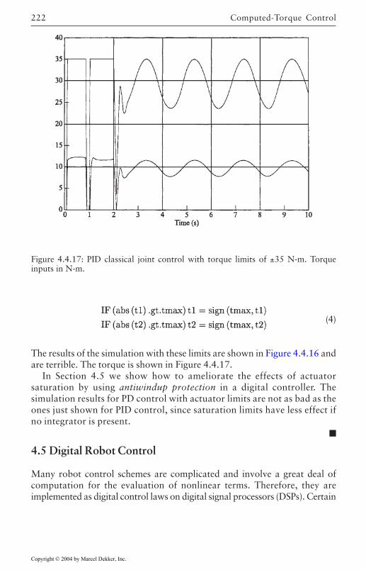
Computed-Torque Control222
(4)
The results of the simulation with these limits are shown in Figure 4.4.16 andare terrible. The torque is shown in Figure 4.4.17.
In Section 4.5 we show how to ameliorate the effects of actuatorsaturation by using antiwindup protection in a digital controller. Thesimulation results for PD control with actuator limits are not as bad as theones just shown for PID control, since saturation limits have less effect ifno integrator is present.
4.5 Digital Robot Control
Many robot control schemes are complicated and involve a great deal ofcomputation for the evaluation of nonlinear terms. Therefore, they areimplemented as digital control laws on digital signal processors (DSPs). Certain
Figure 4.4.17: PID classical joint control with torque limits of ±35 N-m. Torqueinputs in N-m.
Copyright © 2004 by Marcel Dekker, Inc.
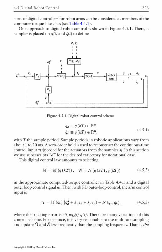
223
sorts of digital controllers for robot arms can be considered as members of thecomputer-torque-like class (see Table 4.4.1).
One approach to digital robot control is shown in Figure 4.5.1. There, asampler is placed on q(t) and q.(t) to define
Figure 4.5.1: Digital robot control scheme.
(4.5.1)
with T the sample period. Sample periods in robotic applications vary fromabout 1 to 20 ms. A zero-order hold is used to reconstruct the continuous-timecontrol input (t)needed for the actuators from the samples k. In this sectionwe use superscripts “d” for the desired trajectory for notational ease.
This digital control law amounts to selecting
(4.5.2)
in the approximate computed-torque controller in Table 4.4.1 and a digitalouter loop control signal uk. Then, with PD outer-loop control, the arm controlinput is
(4.5.3)
where the tracking error is e(t)=qd(t)-q(t). There are many variations of thiscontrol scheme. For instance, it is very reasonable to use multirate samplingand update and less frequently than the sampling frequency. That is, the
4.5 Digital Robot Control
Copyright © 2004 by Marcel Dekker, Inc.
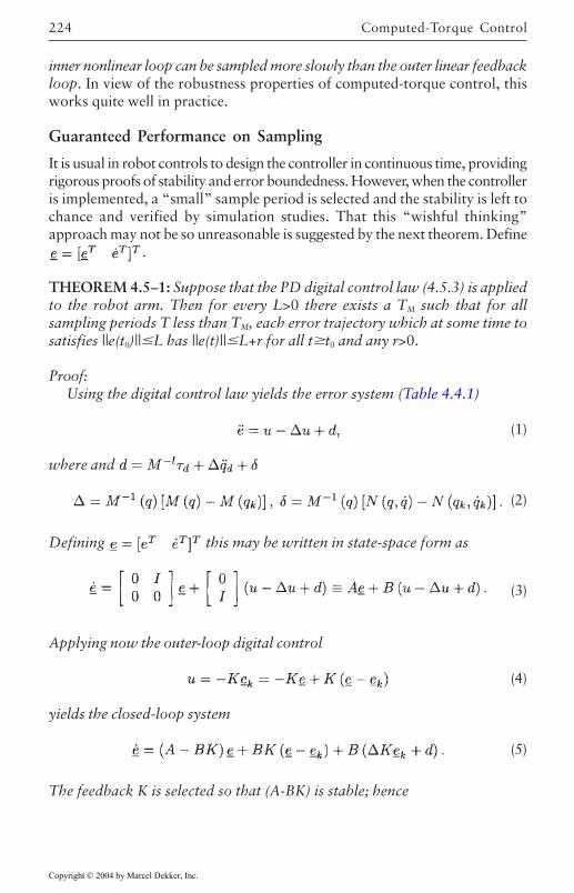
Computed-Torque Control224
inner nonlinear loop can be sampled more slowly than the outer linear feedbackloop. In view of the robustness properties of computed-torque control, thisworks quite well in practice.
Guaranteed Performance on Sampling
It is usual in robot controls to design the controller in continuous time, providingrigorous proofs of stability and error boundedness. However, when the controlleris implemented, a “small” sample period is selected and the stability is left tochance and verified by simulation studies. That this “wishful thinking”approach may not be so unreasonable is suggested by the next theorem. Define
.
THEOREM 4.5–1: Suppose that the PD digital control law (4.5.3) is appliedto the robot arm. Then for every L>0 there exists a TM such that for allsampling periods T less than TM, each error trajectory which at some time tosatisfies ||e(t0)||L has ||e(t)||L+r for all tt0 and any r>0.
Proof:Using the digital control law yields the error system (Table 4.4.1)
(1)
where and
(2)
Defining this may be written in state-space form as
(3)
Applying now the outer-loop digital control
(4)
yields the closed-loop system
(5)
The feedback K is selected so that (A-BK) is stable; hence
Copyright © 2004 by Marcel Dekker, Inc.
225
(6)
for some positive definite P and Q.Selecting now the Lyapunov function
(7)
(5) and (6) reveal
(8)
Assuming for simplicity that the disturbance d is zero, note that
(9)
is negative definite at each sample time. [If d is nonzero but bounded, thenV(ek) is negative outside some ball, and the discussion may be modified.]
The remainder of the proof follows from a theorem of [LaSalle and Lefschetz1961] by showing that:
1.2. V( (t1))<V( (t2)) for all t2t10 when || (t1)||L and
|| (t2)||>L+r.
At issue is the fact (9) and the continuity of
This result shows that good tracking is obtained for all sample periods lessthan some maximum sample period TM which depends on the specific robotarm. A more refined result can show that the errors increase as the maximumdesired acceleration increases, or equivalently, that smaller sample periodsare required for larger desired accelerations.
We now discuss some issues in discretizing the inner nonlinear loop andthen the outer linear loop.
Discretization of Inner Nonlinear Loop
There is no convenient exact way to discretize nonlinear dynamics. Givena nonlinear state-space system
(4.5.4)
Euler’s approximation yields
(4.5.5)
4.5 Digital Robot Control
Copyright © 2004 by Marcel Dekker, Inc.
Computed-Torque Control226
There do exist “exact” techniques for deriving discrete nonlinear robotdynamics. They rely on discretizing the robot arm dynamics in such a waythat energy and momentum are conserved at each sampling instant [Neumanand Tourassis 1985]. See also [Elliott 1990]. Unfortunately, these schemesresult in extremely complicated discrete dynamical equations, even for simplerobot arms. It is very difficult to derive guaranteed digital control laws forthem.
In this section we simply take the discretized inner nonlinear loop as givenby the approximation (4.5.2).
Joint Velocity Estimates from Position Measurements
Throughout this chapter in the examples we have simulated continuous-timerobot controllers assuming that both the joint positions and velocities aremeasured exactly. In point of fact, it is usual to measure the joint velocitiesusing optical encoders, and then estimate the joint velocities from these positionmeasurements. Simply computing the joint velocities using the Eulerapproximation
(4.5.6)
is virtually doomed to failure, since this high-pass filter amplifies the encodermeasurement noise.
Denote the joint velocity estimates by vk. Then a filtered derivative can beused to compute vk from qk using
(4.5.7)
where ν is a design parameter. If ν is small, it corresponds to a fast pole nearz=0, which provides some high-pass filtering to reject unwanted sensor noise.Example 4.5.1 will illustrate the use of this joint velocity estimation filter.
The velocity estimation filter design can be optimized for the given encodernoise statistics by using an alpha-beta tracker to reconstruct vk [Lewis 1986a],[Lewis 1986b], [Lowe and Lewis 1991]. This is a specialized form of Kalmanfilter. It should be noted that the velocity estimates are not only used in theouter linear loop for computing k; they must be used to compute the innernonlinear terms in (4.5.3) as well.
Discretization of Outer PD/PID Control Loop
We have seen that a useful computed-torque outer feedback loop is the PIDcontroller. Given a continuous-time PID controller, a digital PID controllerfor the outer loop may be designed as follows [Lewis 1992].
Copyright © 2004 by Marcel Dekker, Inc.
227
A continuous PID controller that only uses joint position measurements q(t)is given by
(4.5.8)
where k is the proportional gain, T1 is the integration time constant or “reset”time, TD is the derivative time constant. Rather than use pure differentiation,a “filtered derivative” is used which has a pole far left in the s-plane at s=-N/TD. The value for N is often in the range 3 to 10; it is usually fixed by themanufacturer of the controller [Åström and Wittenmark 1984]. A special caseof the PID controller, of course, is the PD controller, which is therefore alsocovered by this discussion.
A common approximate discretization technique for converting continuous-time controllers Kc(s) to digital controllers K(z) is the bilinear transform (BLT),where
(4.5.9)
(4.5.10)
This corresponds to approximating integration by the trapezoidal rule. Underthis mapping, stable continuous systems with poles at s are mapped intostable discrete systems with poles at
(4.5.11)
The finite zeros also map according to this transformation. However, thezeros at infinity in the s-plane map into zeros at z=-1.
Using the BLT to discretize (4.5.8) yields
(4.5.12)
with the discrete integral and derivative time constants
(4.5.13)
(4.5.14)
4.5 Digital Robot Control
Copyright © 2004 by Marcel Dekker, Inc.
Computed-Torque Control228
and the derivative-filtering pole at
(4.5.15)
It is easy to implement this digital outer-loop filter in terms of differenceequations on a DSP. First, write K(z) in terms of z-1, which is the unit delay inthe time domain (i.e., a delay of T seconds), as
(4.5.16)
[Note: There is some abuse in notation in denoting (4.5.16) as K(z-1); this weshall accept.]
Now suppose that the control input uk is related to the tracking error as
(4.5.17)
Then uk may be computed from past and present values of ek using auxiliaryvariables as follows:
(4.5.18)
(4.5.19)
(4.5.20)
The variables represent the integral and derivative portions of thedigital PID controller, respectively. These difference equations are easilyimplemented in software.
Actuator Saturation and Integrator Antiwindup Compensation
Actuator saturation leading to integrator windup is a problem that can occurin the outer PID loop of a robot controller. In Example 4.4.4 we saw thedeleterious effects of integrator windup. It is easy to implement antiwindupprotection digitally [Åström and Wittenmark 1984], [Lewis 1992]. Theantiwindup protection circuit would be placed into the outer linear feedbackloop of a robot control system, where the integrator (controller memory) islocated.
Suppose that the controller is given in transfer function form
(4.5.21)
Copyright © 2004 by Marcel Dekker, Inc.
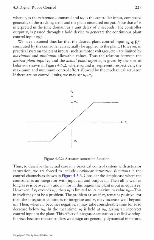
229
where rk is the reference command and wk is the controller input, composedgenerally of the tracking error and the plant measured output. Note that z-1 isinterpreted in the time domain as a unit delay of T seconds. The controlleroutput vk is passed through a hold device to generate the continuous plantcontrol input u(t).
We have assumed thus far that the desired plant control input computed by the controller can actually be applied to the plant. However, inpractical systems the plant inputs (such as motor voltages, etc.) are limited bymaximum and minimum allowable values. Thus the relation between thedesired plant input vk and the actual plant input uk is given by the sort ofbehavior shown in Figure 4.5.2, where uH and uL represent, respectively, themaximum and minimum control effort allowed by the mechanical actuator.If there are no control limits, we may set uk=vk.
Figure 4.5.2: Actuator saturation function.
Thus, to describe the actual case in a practical control system with actuatorsaturation, we are forced to include nonlinear saturation functions in thecontrol channels as shown in Figure 4.5.3. Consider the simple case where thecontroller is an integrator with input wk and output vk. Then all is well aslong as vk is between uL and uH, for in this region the plant input uk equals vk.However, if vk exceeds uH, then uk is limited to its maximum value uH—Thisin itself may not be a problem. The problem arises if wk remains positive, forthen the integrator continues to integrate and vk may increase well beyonduH. Then, when wk becomes negative, it may take considerable time for vk todecrease below uH. In the meantime, uk is held at uH, giving an incorrectcontrol input to the plant. This effect of integrator saturation is called windup.It arises because the controllers we design are generally dynamical in nature,
4.5 Digital Robot Control
Copyright © 2004 by Marcel Dekker, Inc.
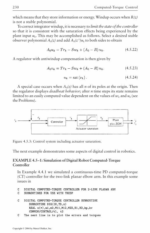
Computed-Torque Control230
which means that they store information or energy. Windup occurs when R(z)is not a stable polynomial.
To correct integrator windup, it is necessary to limit the state of the controllerso that it is consistent with the saturation effects being experienced by theplant input uk. This may be accomplished as follows. Select a desired stableobserver polynomial A0(z) and add A0(z-1)uk to both sides to obtain
(4.5.22)
A regulator with antiwindup compensation is then given by
(4.5.23)
(4.5.24)
A special case occurs when A0(z) has all n of its poles at the origin. Thenthe regulator displays deadbeat behavior; after n time steps its state remainslimited to an easily computed value dependent on the values of wk and uk (seethe Problems).
EXAMPLE 4.5–1: Simulation of Digital Robot Computed-TorqueController
In Example 4.4.1 we simulated a continuous-time PD computed-torque(CT) controller for the two-link planar elbow arm. In this example someissues in
Figure 4.5.3: Control system including actuator saturation.
The next example demonstrates some aspects of digital control in robotics.
Copyright © 2004 by Marcel Dekker, Inc.
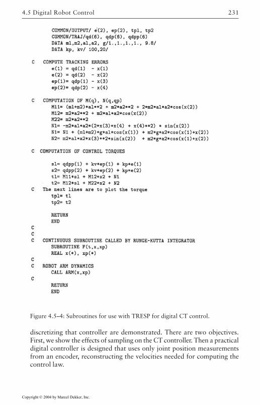
231
discretizing that controller are demonstrated. There are two objectives.First, we show the effects of sampling on the CT controller. Then a practicaldigital controller is designed that uses only joint position measurementsfrom an encoder, reconstructing the velocities needed for computing thecontrol law.
Figure 4.5–4: Subroutines for use with TRESP for digital CT control.
4.5 Digital Robot Control
Copyright © 2004 by Marcel Dekker, Inc.
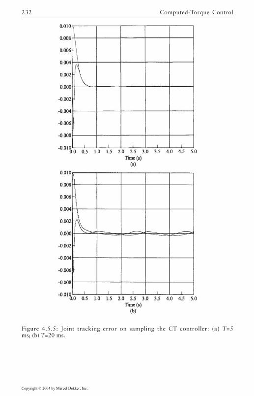
Computed-Torque Control232
Figure 4.5.5: Joint tracking error on sampling the CT controller: (a) T=5ms; (b) T=20 ms.
Copyright © 2004 by Marcel Dekker, Inc.
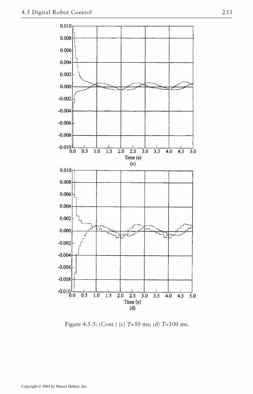
233
Figure 4.5.5: (Cont.) (c) T=50 ms; (d) T=100 ms.
4.5 Digital Robot Control
Copyright © 2004 by Marcel Dekker, Inc.
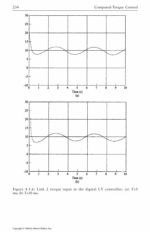
Computed-Torque Control234
Figure 4.5.6: Link 2 torque input in the digital CT controller: (a) T=5ms; (b) T=50 ms.
Copyright © 2004 by Marcel Dekker, Inc.
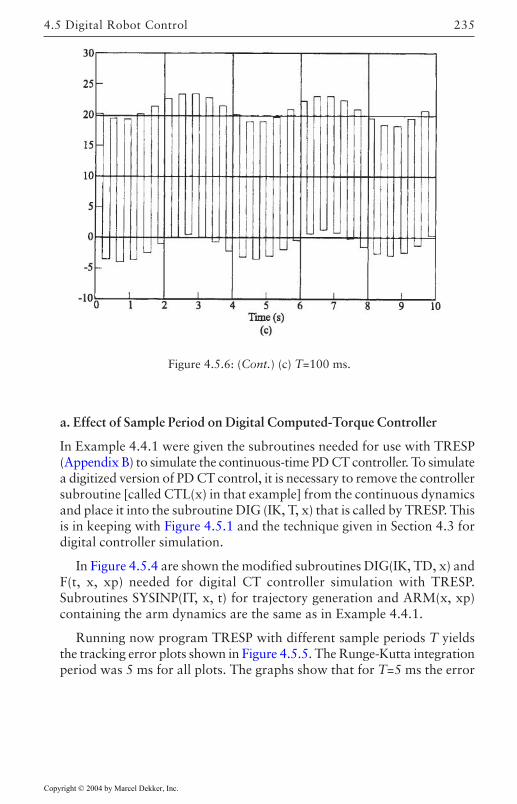
235
a. Effect of Sample Period on Digital Computed-Torque Controller
In Example 4.4.1 were given the subroutines needed for use with TRESP(Appendix B) to simulate the continuous-time PD CT controller. To simulatea digitized version of PD CT control, it is necessary to remove the controllersubroutine [called CTL(x) in that example] from the continuous dynamicsand place it into the subroutine DIG (IK, T, x) that is called by TRESP. Thisis in keeping with Figure 4.5.1 and the technique given in Section 4.3 fordigital controller simulation.
In Figure 4.5.4 are shown the modified subroutines DIG(IK, TD, x) andF(t, x, xp) needed for digital CT controller simulation with TRESP.Subroutines SYSINP(IT, x, t) for trajectory generation and ARM(x, xp)containing the arm dynamics are the same as in Example 4.4.1.
Running now program TRESP with different sample periods T yieldsthe tracking error plots shown in Figure 4.5.5. The Runge-Kutta integrationperiod was 5 ms for all plots. The graphs show that for T=5 ms the error
Figure 4.5.6: (Cont.) (c) T=100 ms.
4.5 Digital Robot Control
Copyright © 2004 by Marcel Dekker, Inc.
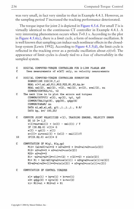
Computed-Torque Control236
was very small, in fact very similar to that in Example 4.4.1. However, asthe sampling period T increased the tracking performance deteriorated.
The torque input for joint 2 is depicted in Figure 4.5.6. For small T is isvirtually identical to the continuous CT controller in Example 4.4.1. Avery interesting phenomenon occurs when T=0.1 s. According to the plotin Figure 4.5.6(c), there is a limit cycle, a form of nonlinear oscillation. Itis well known that sampling can induce such nonlinear effects in the closed-loop system [Lewis 1992]. According to Figure 4.5.5(d), the limit cycle isreflected in the tracking error as a periodic oscillation about e(t)=0. Theappearance of limit cycles is closely tied to a loss of observability in thesampled system.
Copyright © 2004 by Marcel Dekker, Inc.
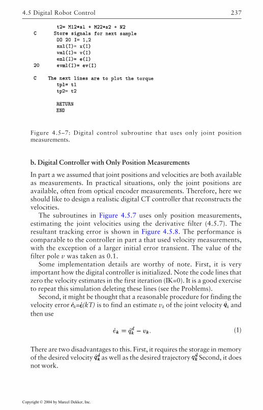
237
Figure 4.5–7: Digital control subroutine that uses only joint positionmeasurements.
b. Digital Controller with Only Position Measurements
In part a we assumed that joint positions and velocities are both availableas measurements. In practical situations, only the joint positions areavailable, often from optical encoder measurements. Therefore, here weshould like to design a realistic digital CT controller that reconstructs thevelocities.
The subroutines in Figure 4.5.7 uses only position measurements,estimating the joint velocities using the derivative filter (4.5.7). Theresultant tracking error is shown in Figure 4.5.8. The performance iscomparable to the controller in part a that used velocity measurements,with the exception of a larger initial error transient. The value of thefilter pole v was taken as 0.1.
Some implementation details are worthy of note. First, it is veryimportant how the digital controller is initialized. Note the code lines thatzero the velocity estimates in the first iteration (IK=0). It is a good exerciseto repeat this simulation deleting these lines (see the Problems).
Second, it might be thought that a reasonable procedure for finding thevelocity error k= (kT) is to find an estimate vk of the joint velocity k andthen use
(1)
There are two disadvantages to this. First, it requires the storage in memoryof the desired velocity as well as the desired trajectory Second, it doesnot work.
4.5 Digital Robot Control
Copyright © 2004 by Marcel Dekker, Inc.
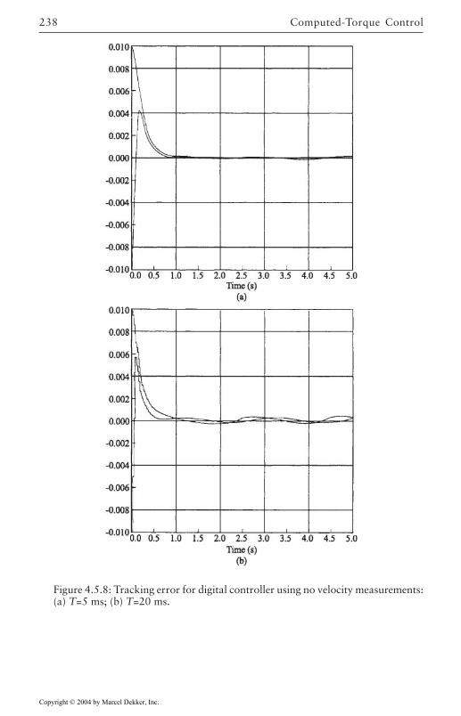
Computed-Torque Control238
Figure 4.5.8: Tracking error for digital controller using no velocity measurements:(a) T=5 ms; (b) T=20 ms.
Copyright © 2004 by Marcel Dekker, Inc.
239
Instead, it is necessary to use two derivative filters, one for estimating jointvelocities and one for providing an estimate for the velocity error k. Asimulation that attempts to use 1 makes the point quite well.
Note that the velocity estimates are also used instead of in computingthe nonlinear terms
EXAMPLE 4.5–2: Digital PI Controller with Anti-windup Compensation
A general digital PI controller with sampling period of T seconds isgiven by
(1)
We have sampled the continuous PI controller by the modified matched-polezero (MPZ) method [Lewis 1992] to obtain a delay of T seconds in theintegrator to allow for computation time. The proportional gain is k andthe reset time is TI; both are fixed in the design stage. The tracking error isek.
Multiply by (1-z-1) to write
(2)
which is in the transfer function form (4.5.21). The corresponding differenceequation form for implementation is
(3)
This controller will experience windup problems since the autoregressivepolynomial R=1- z-1 has a root at z=1, making it marginally stable. Thus,when uk is limited, the integrator will continue to integrate, “winding up”beyond the saturation level.
a. Antiwindup Compensation
To correct this problem, select an observer polynomial of
(4)
4.5 Digital Robot Control
Copyright © 2004 by Marcel Dekker, Inc.
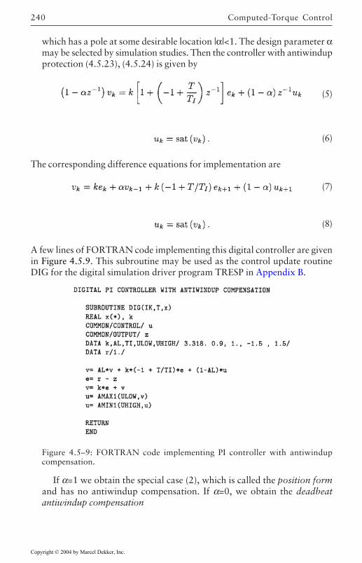
Computed-Torque Control240
which has a pole at some desirable location |α|<1. The design parameter αmay be selected by simulation studies. Then the controller with antiwindupprotection (4.5.23), (4.5.24) is given by
(5)
(6)
The corresponding difference equations for implementation are
(7)
(8)
A few lines of FORTRAN code implementing this digital controller are givenin Figure 4.5.9. This subroutine may be used as the control update routineDIG for the digital simulation driver program TRESP in Appendix B.
If α=1 we obtain the special case (2), which is called the position formand has no antiwindup compensation. If α=0, we obtain the deadbeatantiwindup compensation
Figure 4.5–9: FORTRAN code implementing PI controller with antiwindupcompensation.
Copyright © 2004 by Marcel Dekker, Inc.
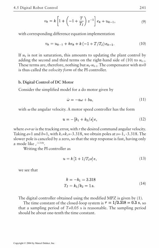
241
(9)
with corresponding difference equation implementation
(10)
If uk is not in saturation, this amounts to updating the plant control byadding the second and third terms on the right-hand side of (10) to uk-1.These terms are, therefore, nothing but uk-uk-1. The compensator with α=0is thus called the velocity form of the PI controller.
b. Digital Control of DC Motor
Consider the simplified model for a do motor given by
(11)
with the angular velocity. A motor speed controller has the form
(12)
where e=r-w is the tracking error, with r the desired command angular velocity.Taking a=1 and b=1, with k1=k2=-3.318, we obtain poles at s=-1, -3.318. Theslower pole is canceled by a zero, so that the step response is fast, having onlya mode like e
-3.318t.Writing the PI controller as
(13)
we see that
(14)
The digital controller obtained using the modified MPZ is given by (1).The time constant of the closed-loop system is so
that a sampling period of T=0.05 s is reasonable. The sampling periodshould be about one-tenth the time constant.
4.5 Digital Robot Control
Copyright © 2004 by Marcel Dekker, Inc.
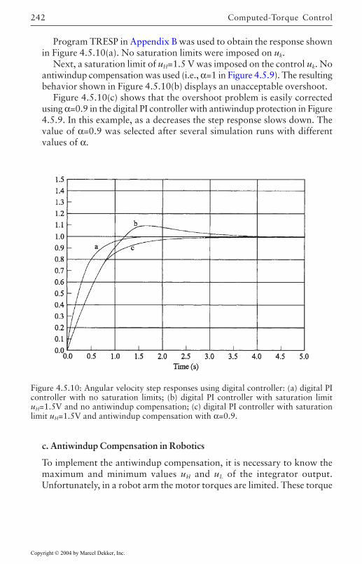
Computed-Torque Control242
Program TRESP in Appendix B was used to obtain the response shownin Figure 4.5.10(a). No saturation limits were imposed on uk.
Next, a saturation limit of uH=1.5 V was imposed on the control uk. Noantiwindup compensation was used (i.e., α=1 in Figure 4.5.9). The resultingbehavior shown in Figure 4.5.10(b) displays an unacceptable overshoot.
Figure 4.5.10(c) shows that the overshoot problem is easily correctedusing α=0.9 in the digital PI controller with antiwindup protection in Figure4.5.9. In this example, as a decreases the step response slows down. Thevalue of α=0.9 was selected after several simulation runs with differentvalues of α.
Figure 4.5.10: Angular velocity step responses using digital controller: (a) digital PIcontroller with no saturation limits; (b) digital PI controller with saturation limituH=1.5V and no antiwindup compensation; (c) digital PI controller with saturationlimit uH=1.5V and antiwindup compensation with α=0.9.
c. Antiwindup Compensation in Robotics
To implement the antiwindup compensation, it is necessary to know themaximum and minimum values uH and uL of the integrator output.Unfortunately, in a robot arm the motor torques are limited. These torque
Copyright © 2004 by Marcel Dekker, Inc.
243
limits must be mapped using the feedback linearization input transformationto determine the limits on the integrator outputs see [Bobrow et al. 1983].Thus the saturation limits needed by the antiwindup compensator arefunctions of the joint position q, the desired acceleration and so on. Thisissue is explored in the problems.
4.6 Optimal Outer-Loop Design
In Section 4.4 we discussed computed-torque control, showing how to selectthe inner control loop using exact techniques involving the inverse manipulatordynamics, as well as by a variety of approximate means. We also discussedseveral schemes for designing the outer linear feedback (tracking) loop. Theresults of our discussions are summarized in Table 4.4.1. In this section weintend to present a modern control optimal technique for selecting the outerfeedback loop. Modern optimal design yields improved robustness in thepresence of disturbances and unmodeled dynamics.
Several papers have dealt with “optimal” or “suboptimal” control of robotmanipulators [Vukobratovic and Stokic 1983], [Lee et al. 1983], [Luo andSaridis 1985], [Johansson 1990]. Although they are not all based on acomputed-torque-like approach, we would like here to present the flavor ofthis work by using optimal techniques to design the computed-torque outerfeedback loop.
Linear Quadratic Optimal Control
First, it is necessary to review modern linear-quadratic (LQ) design. Supposethat we are given the linear time-invariant system in state-space form
(4.6.1)
with It is desired to compute the state-feedbackgain in
(4.6.2)
so that the closed-loop system
(4.6.3)
is asymptotically stable. Moreover, we do not want to use too much controlenergy to stabilize the system, since in many modern systems (e.g., automobile,spacecraft), fuel or energy is limited.
4.6 Optimal Outer-Loop Design
Copyright © 2004 by Marcel Dekker, Inc.
Computed-Torque Control244
This is a complex multivariable design problem, for the feedback gainmatrix K is of dimension m×n. A classical controls approach might involve,for instance, performing mn root locus designs to close the feedback loops oneat a time. On the other hand, a solution that guarantees stability can be foundusing modern controls techniques simply by solving some standard matrixdesign equations. This modern approach closes all the feedback loopssimultaneously and guarantees a good gain and phase margin.
The feedback matrix is found using modern control theory as follows.First, define a quadratic performance index (PI) of the form
(4.6.4)
where Q is a symmetric positive semidefinite n×n matrix (denoted Q0) andR is a symmetric positive definite m×m matrix (R>0). That is, all eigenvaluesof R are greater than zero and those of Q are greater than or equal to zero. Qis called the state-weighting matrix and R the control-weighting matrix. Thesematrices are design parameters that are selected by the engineer depending,for instance, on the desired form of the closed-loop time responses.
The optimal LQ feedback gain K is the one that minimizes the PI J. Themotivation follows. The quadratic terms xTQx and uTRu in the PI aregeneralized energy functions (e.g., the energy in a capacitor is ½Cv2, thekinetic energy of motion is ½mv2). Suppose, then, that J is minimized in theclosed-loop system (4.6.3). This means that the infinite integral of[xT(t)Qx(t)+uT(t)Ru(t)] is finite, so that this function of time goes to zero as tbecomes large. However,
with the square root of a matrix defined as . Since thesenorms vanish with t and |R|0, the functions and u(t) both goto zero. Under the assumption that is observable [Kailath 1980], x(t)goes to zero if y(t) does.
Therefore, the optimal gain K guarantees that all signals go to zero withtime in the closed-loop system (4.6.3). That is, K stabilizes (A-BK).
The determination of the optimal K is easy and is a standard result inmodern control theory (see, e.g., [Lewis 1986a], [Lewis 1986b]). The optimalfeedback gain is simply found by solving the matrix design equations
Copyright © 2004 by Marcel Dekker, Inc.
245
(4.6.5)
(4.6.6)
where P is a symmetric n×n auxiliary design matrix on which the optimalgain depends. The second of these is a nonlinear matrix quadratic equationknown as the Riccati equation; it is easy to solve this equation for the auxiliarymatrix P using standard routines in, for instance, MATLAB, [MATRIXx 1989],and other software design packages.
The next result is of prime importance in modern control theory andformalizes the stability discussion just given.
THEOREM 4.6–1: Let be observable and (A, B) be controllable.
Then:
(a) There is a unique positive definite solution P to the Riccati equation.(b) The closed-loop system (A-BK) is asymptotically stable.(c) The closed-loop system has an infinite gain margin and 60° of phasemargin.
Controllability was discussed in Chapter 1. Observability means roughlyspeaking that all the system modes have an independent effect in the PI, sothat if J is bounded, all the modes independently go to zero with t. To verifythese properties is easy. The system is controllable if the controllability matrix
(4.6.7)
has full rank n. The system (A, C) is observable if the observability matrix
(4.6.8)
has full rank n. MATLAB, for instance, provides routines for these tests.Therefore, the state-weighting matrix Q may be chosen to satisfy theobservability requirement.
The theorem makes this modern design approach very powerful. No matterhow many inputs and states, a stabilizing feedback gain can always be foundunder the hypotheses that stabilizes the system. The gain is found by closing
4.6 Optimal Outer-Loop Design
Copyright © 2004 by Marcel Dekker, Inc.
Computed-Torque Control246
all the nm feedback loops simultaneously by solving the matrix designequations.
Linear Quadratic Computed-Torque Design
Now we apply these results to the control of the robot manipulator dynamics
(4.6.9)
According to Section 4.4, the computed-torque control law
(4.6.10)
yields the error system
(4.6.11)
which we may write as
(4.6.12)
with the state defined as
(4.6.13)
Now, select the outer-loop PD feedback
(4.6.14)
To find a stabilizing gain K, select the design parameter Q in the PI as
so that the position and velocity errors are independently weighted. Then,due to the simple form of the A and B matrices, which represent n de-coupledNewton’s law (i.e., double integrator) systems, the solution of the Riccatiequation is easily found (see the Problems). Using this solution in (4.6.5)yields the formula for the optimal stabilizing gains
(4.6.15)
This LQ approach reveals the relation between the PD gains and some designparameters Q and R that determine the total energy in the closed-loop system.
Copyright © 2004 by Marcel Dekker, Inc.
247
Note particularly that the relative magnitudes of x(t) and u(t) in the closed-loop system can be traded off. Indeed, if R is relatively larger than Qp and Qv,the control effort in the PI (4.6.4) is weighted more heavily that the state.Then the optimal control will attempt to keep u(t) smaller by selecting smallercontrol gains; thus the response time will increase. On the other hand, selectinga smaller R will increase the PD gains and make the error vanish more quickly.
If Qp, Qν, and R are diagonal, so then are the PD gains Kp, Kv. The LQapproach with nondiagonal Qp, Qv, and R affords the possibility of outerfeedback loops that are coupled between the joints, which can sometimesimprove performance. Another important feature of LQ design is theguaranteed robustness mentioned in the theorem. This can be very useful inapproximate computed-torque design where
(4.6.16)
and and can be simplified versions of M(q) and N(q, ). The performanceof such a controller with an LQ-design outer loop can be expected to surpassthat of a controller designed using arbitrary choices for Kp and Kv. This robustaspect of LQ design is explored in the problems.
It is important to note that this LQ design results in minimum closed-loopenergy in terms of e(t), (t), and u(t). However, the actual control input intothe robot arm is
(4.6.17)
Although the energy in τ(t) is not minimized using this approach, we can usesome norm inequalities to write
(4.6.18)
so that keeping small ||u(t)|| might be expected to make smaller. A moreformal statement can be made taking into account the bounds on ||M(q)|| and
given in Table 3.3.1.Since the energy in is not formally minimized in this approach, it is
considered as a suboptimal approach with respect to the actual arm dynamics,although with respect to the error system and u(t) it is optimal. An optimalcontrol approach that weights e(t) τ(t) and in the PI is given in [Johansson1990].
We have derived an LQ controller using a computed-torque (i.e., feedbacklinearization) approach. An alternative approach that yields the same Riccati-equation-based design is to employ the full nonlinear arm dynamics and findan approximate (i.e., time-invariant) solution to the Hamilton-Jacobi-Bellmanequation [Luo and Saridis 1985]; [Luo et al. 1986].
4.6 Optimal Outer-Loop Design
Copyright © 2004 by Marcel Dekker, Inc.
Computed-Torque Control248
4.7 Cartesian Control
We have seen how to make a robot manipulator track a desired joint spacetrajectory qd(t). However, in any practical application the desired trajectoriesof a robot arm are given in the workspace or Cartesian coordinates. An importantseries of papers dealt with resolved motion manipulator control [Whitney 1969];[Luh et al. 1980], [Wu and Paul 1982]. There the joint motions were resolvedinto the Cartesian coordinates, where the control objectives are specified. Theresult is that an operator can use a joystick to specify Cartesian motion (e.g.,for a prosthetic device), with the arm following the specified motion. Olderteleoperator devices used joysticks that directly controlled the motion of theactuators, resulting in long training times and very awkward manipulability.
There are several approaches to Cartesian robot control. For instance, onemight:
1. Use the Cartesian dynamics in Section 3.5 for controls design (see theProblems).
2. Convert the desired Cartesian trajectory yd(t) to a joint-space trajectoryqd(t) using the inverse kinematics. Then use the joint-space computed-torque control schemes in Table 4.4.1.
3. Use Cartesian computed-torque control.
Let us discuss the last of these.
Cartesian Computed-Torque Control
This approach begins with the joint space dynamics
(4.7.1)
In Section 3.4 we discussed a general feedback-linearization approach forlinearizing the arm dynamics with respect to a general output. In this sectionthe output we are interested in is the Cartesian error
(4.7.2)
with yd(t) the desired Cartesian trajectory and y(t) the end-effector Cartesianposition.
The problems associated with specifying the Cartesian position of the endeffector are covered in Appendix A. There we see that y(t) is not necessarily a6-vector, but could in fact be the 4×4 arm T matrix. Then yd(t) is a 4×4 matrixgiven by
Copyright © 2004 by Marcel Dekker, Inc.
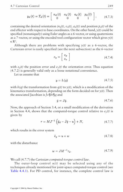
249
(4.7.3)
containing the desired orientation (nd(t), od(t), ad(t)) and position pd(t) of theend effector with respect to base coordinates. On the other hand, y(t) could bespecified (nonuniquely) using Euler angles as a 6-vector, or using quaternionsas a 7-vector, or using the encoded tool configuration vector which gives y(t) R6.
Although there are problems with specifying y(t) as a 6-vector, theCartesian error is easily specified (see the next subsection) as the 6-vector
(4.7.4)
with ep(t) the position error and eo(t) the orientation error. Thus equation(4.7.2) is generally valid only as a loose notational convenience.
Let us assume that
(4.7.5)
with h(q) the transformation from q(t) to y(t), which is a modification of thekinematics transformation, depending on the form decided on for y(t). Thenthe associated Jacobian is J=¶h/¶q and
(4.7.6)
Now, the approach of Section 3.4, or a small modification of the derivationin Section 4.4, shows that the computed-torque control relative to ey(t) isgiven by
(4.7.7)
which results in the error system
(4.7.8)
with the disturbance
(4.7.9)
We call (4.7.7) the Cartesian computed-torque control law.The outer-loop control u(t) may be selected using any of the
techniques already mentioned for joint-space computed-torque control (seeTable 4.4.1). For PD control, for instance, the complete control law is
4.7 Cartesian Control
Copyright © 2004 by Marcel Dekker, Inc.
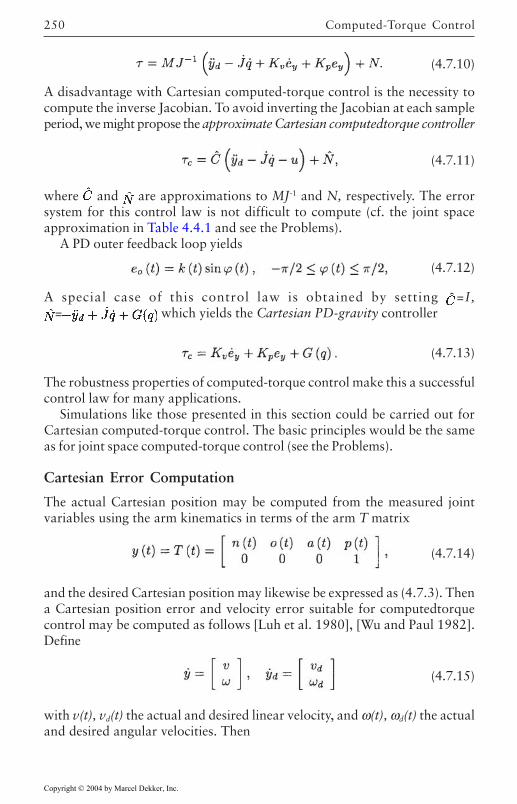
Computed-Torque Control250
(4.7.10)
A disadvantage with Cartesian computed-torque control is the necessity tocompute the inverse Jacobian. To avoid inverting the Jacobian at each sampleperiod, we might propose the approximate Cartesian computedtorque controller
(4.7.11)
where and are approximations to MJ-1 and N, respectively. The errorsystem for this control law is not difficult to compute (cf. the joint spaceapproximation in Table 4.4.1 and see the Problems).
A PD outer feedback loop yields
(4.7.12)
A special case of this control law is obtained by setting =I,= which yields the Cartesian PD-gravity controller
(4.7.13)
The robustness properties of computed-torque control make this a successfulcontrol law for many applications.
Simulations like those presented in this section could be carried out forCartesian computed-torque control. The basic principles would be the sameas for joint space computed-torque control (see the Problems).
Cartesian Error Computation
The actual Cartesian position may be computed from the measured jointvariables using the arm kinematics in terms of the arm T matrix
(4.7.14)
and the desired Cartesian position may likewise be expressed as (4.7.3). Thena Cartesian position error and velocity error suitable for computedtorquecontrol may be computed as follows [Luh et al. 1980], [Wu and Paul 1982].Define
(4.7.15)
with v(t), vd(t) the actual and desired linear velocity, and ω(t), ωd(t) the actualand desired angular velocities. Then
Copyright © 2004 by Marcel Dekker, Inc.
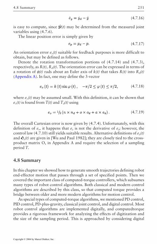
251
(4.7.16)
is easy to compute, since (t) may be determined from the measured jointvariables using (4.7.6).
The linear position error is simply given by
(4.7.17)
An orientation error eo(t) suitable for feedback purposes is more difficult toobtain, but may be defined as follows.
Denote the rotation transformation portions of (4.7.14) and (4.7.3),respectively, as R(t), Rd(t). The orientation error can be expressed in terms ofa rotation of φ(t) rads about an Euler axis of k(t) that takes R(t) into Rd(t)(Appendix A). In fact, one may define the 3-vector
(4.7.18)
where eo(t) may be assumed small. With this definition, it can be shown thateo(t) is found from T(t) and Td(t) using
(4.7.19)
The overall Cartesian error is now given by (4.7.4). Unfortunately, with thisdefinition of eo, it happens that ey is not the derivative of ey; however, thecontrol law (4.7.10) still yields suitable results. Alternative definitions of ey(t)and y(t) are given in [Wu and Paul 1982]; they are closely tied to the cross-product matrix O, in Appendix A and require the selection of a samplingperiod T.
4.8 Summary
In this chapter we showed how to generate smooth trajectories defining robotend-effector motion that passes through a set of specified points. Then wecovered the important class of computed-torque controllers, which subsumesmany types of robot control algorithms. Both classical and modern controlalgorithms are described by this class, so that computed torque provides abridge between older and more modern algorithms for motion control.
As special types of computed-torque algorithms, we mentioned PD control,PID control, PD-plus-gravity, classical joint control, and digital control. Mostrobot control algorithms are implemented digitally, and computedtorqueprovides a rigorous framework for analyzing the effects of digitization andthe size of the sampling period. This is approached by considering digital
4.8 Summary
Copyright © 2004 by Marcel Dekker, Inc.
Computed-Torque Control252
control as an approximate computed-torque law and studying the error system(cf. subsequent chapters).
We showed some aspects of modern linear quadratic outer-loop design,and concluded with a discussion of Cartesian control.
Copyright © 2004 by Marcel Dekker, Inc.
253
REFERENCES
[Arimoto and Miyazaki 1984] Arimoto, S., and F Miyazaki, “Stability and robustnessof PID feedback control for robot manipulators of sensory capability,” Proc.First Int. Symp., pp. 783–799, MIT, 1984.
[Åström and Wittenmark 1984] Åström, K.J., and B.Wittenmark, ComputerControlled Systems. Englewood Cliffs, NJ: Prentice Hall, 1984.
[Bobrow et al. 1983] Bobrow, J.E., S.Dubowsky, and J.S.Gibson, “On the optimalcontrol of robotic manipulators with actuator constraints,” Proc. Am. ControlConf, pp. 782–787, June 1983.
[Chen 1989] Chen, Y.-C., “On the structure of the time-optimal controls for roboticmanipulators,” IEEE Trans. Autom. Control, vol. 34, no. 1, pp. 115–116,Jan. 1989.
[Dawson 1990] Dawson, D.M., “Uncertainties in the control of robot manipulators,”Ph.D. thesis, School of Electrical Engineering, Georgia Institute of Technology,Mar. 1990.
[Elliott 1990] Elliott, D.L., “Discrete-time systems on manifolds,” Proc. IEEE ConfDecision Control, pp. 1908–1909, Dec. 1990.
[Franklin et al. 1986] Franklin, G.F:, J.D.Powell, and A.Emami-Naeini, FeedbackControl of Dynamic Systems. Reading, MA: Addison-Wesley, 1986.
[Geering 1986] Geering, H.P., L.Guzzella, S.A.R.Hepner, and C.H. Onder, “Time-optimal motions of robots in assembly tasks,” IEEE Trans. Autom. Control,vol. AC-31, no. 6, pp. 512–518, June 1986.
[Gilbert and Ha 1984] Gilbert, E.G., and I.J.Ha, “An approach to nonlinear feedbackcontrol with applications to robotics,” IEEE Trans. Syst. Man Cybern., vol.SMC-14, no. 6, pp. s 879–884, Nov./Dec. 1984.
Copyright © 2004 by Marcel Dekker, Inc.
REFERENCES254
[Gourdeau and Schwartz 1989] Gourdeau, R., and H.M.Schwartz, “Optimal controlof a robot manipulator using a weighted time-energy cost function,” Proc.IEEE Conf. Decision Control, pp. 1628–1631, Dec. 1989.
[Hunt et al. 1983] Hunt, L.R., R.Su, and G.Meyer, “Global transformations ofnonlinear systems,” IEEE Trans. Autom. Control, vol. AC-28, no. 1, pp. 24–31, Jan. 1983.
[IMSL] IMSL, Library Contents Document, 8th ed. Houston, TX: InternationalMathematical and Statistical Libraries.
[Jayasuriya and Suh 1985] Jayasuriya, S., and M.-S.Suh, “Sub-optimal controlstrategies for manipulators with actuator constraints: the near minimum-timeproblem,” Proc. Am. Control Conf., pp. 61–62, June 1985.
[Johansson 1990] Johansson, R., “Quadratic optimization of motion coordinationand control,” IEEE Trans. Autom. Control, vol. 35, no. 11, pp. 1197–1208,Nov. 1990.
[Kahn and Roth 1971] Kahn, M.E., and B.Roth, “The near-minimum-time control ofopen-loop articulated kinematic chains,” Trans. ASMEJ. Dyn. Syst. Meas.Control, pp. 164–172, Sept. 1971.
[Kailath 1980] Kailath, T. Linear Systems. Englewood Cliffs, NJ: Prentice Hall, 1980.
[Kim and Shin 1985] Kim, B.K., and K.G.Shin, “Suboptimal control of industrialmanipulators with a weighted minimum time-fuel criterion,” IEEE Trans.Autom. Control, vol. AC30, no. 1, pp. 1–10, Jan. 1985.
[LaSalle and Lefschetz 1961] LaSalle, J., and S.Lefschetz, Stability by Liapunov’s DirectMethod. New York: Academic Press, 1961.
[Lee et al. 1983] Lee, C.S.G., and M.H.Chen, “A suboptimal control design formechanical manipulators,” Proc. Am. Control Conf., pp. 1056–1061, June1983.
[Lewis 1986a] Lewis, F.L., Optimal Control. New York: Wiley, 1986 (a).
[Lewis 1986b] Lewis, F.L., Optimal Estimation. New York: Wiley, 1986 (b).
[Lewis 1992] Lewis, F.L., Applied Optimal Control and Estimation. Englewood Cliffs,NJ: Prentice Hall, 1992.
[LINPACK] LINPACK, User’s Guide, J.J.Dongarra, C.B.Moler, J.R. Bunch, andG.W.Stewart. Philadelphia: SIAM Press, 1979.
Copyright © 2004 by Marcel Dekker, Inc.
255REFERENCES
[Lowe and Lewis 1991] Lowe, J.A., and F.L.Lewis, “Digital signal processorimplementation of a Kalman filter for disk drive head-positioning mechanism,”in Microprocessors in Robotic and Manufacturing Systems, S.Tzafestas ed.,pp. 369–383, 1991.
[Luh et al. 1980] Luh, J.Y.S., M.W.Walker, and R.P.C.Paul, “Resolved-accelerationcontrol of mechanical manipulators,” IEEE Trans. Autom. Control, vol. AC-25, no. 3, pp. 195–200, June 1980.
[Luo and Saridis 1985] Luo, G.L., and G.N.Saridis, “L-Q design of PID controllersfor robot arms,” IEEE J. Robot. Autom., vol. RA-1, no. 3, pp. 152–159, Sept.1985.
[Luo et al. 1986] Luo, G.L., G.N.Saridis, and C.Z.Wang, “A dual-mode control forrobotic manipulators,” Proc. IEEE Conf. Decision Control, pp. 409–414,Dec. 1986.
[MATRIXx 1989] MATRIXX, Santa Clara, CA: Integrated Systems, Inc., 1989.
[Moler 1987] Moler, C., J.Little, and S.Bangert, PC-Matlab. Sherborn, MA: TheMathworks, 1987.
[Neuman and Tourassis 1985] Neuman, C.P., and V.D.Tourassis, “Discrete dynamicrobot models,” IEEE Trans. Syst. Man and Cybern., vol. SMC-15, no. 2, pp.193–204, Mar./Apr. 1985.
[Paul 1981] Paul, R.P., Robot Manipulators. Cambridge, MA: MIT Press, 1981.
[Schilling 1990] Schilling, R.J., Fundamentals of Robotics. Englewood Cliffs, NJ:Prentice Hall, 1990.
[Shin and McKay 1985] Shin, K.G., and N.D.McKay, “Minimum-time control ofrobotic manipulators with geometric path constraints,” IEEE Trans. Autom.Control, vol. AC-30, no. 6, pp. 531–541, June 1985.
[Slotine and Li 1991] Slotine, J.-J.E, and W.Li, Applied Nonlinear Control. EnglewoodCliffs, NJ: Prentice Hall, 1991.
[Vukobratovic and Stokic 1983] Vukobratovic and Stokic, “Contribution to thesuboptimal control of manipulation robots,” IEEE Trans. Autom. Control,vol. AC-28, no. 10, pp. 981–985, Oct. 1983.
[Whitney 1969] Whitney, D.E., “Resolved motion rate control of manipulators andhuman prostheses,” IEEE Trans. Man Machine Syst., vol. MMS-10, no. 2, pp.47–53, June 1969.
Copyright © 2004 by Marcel Dekker, Inc.
REFERENCES256
[Wu and Paul 1982] Wu, C.-H., and R.P.Paul, “Resolved motion force control ofrobot manipulator,” IEEE Trans. Syst. Man Cybern., vol. SMC-12, no. 3, pp.266–275, June 1982.
Copyright © 2004 by Marcel Dekker, Inc.
257REFERENCES
PROBLEMS
Section 4.24.2–1 Minimum-Time Control. Derive the minimum-time control switching time ts
[cf. (4.2.11)] when the initial and final velocities are not zero.
4.2–2 Polynomial Path Interpolation. It is desired to move a single joint from q(0)=0,(0)=0 through the point q(l)=5, (l)=40 to a final position/velocity of (2)=10,
Determine the cubic interpolating polynomials required in this two-intervalpath. Plot the path generated and verify that it meets the specified requirementson q(t) and (t) Plot (t) versus q(t).
4.2–3 LFPB. Repeat Problem 4.2–2 using LFPB.
4.2–4 Polynomial Path for Acceleration Matching. Derive the interpolatingpolynomial required to match positions, velocities, and accelerations at thevia points.
Section 4.3
4.3–1 Simulation of Flexible Coupling System. Use computer simulation to reproducethe results for the motor with flexible coupling shaft in Example 3.6.1.
4.3–2 Simulation of Nonlinear System. The Van der Pol oscillator is a nonlinearsystem with some interesting properties. The state equation is
Simulate the dynamics for initial conditions of x1(0)=0.1, x2(0)= 0.1. Usevalues for the parameter of α=0.1 and then α=0.8. Plot x1(t) and x2(t), as wellas x2(t) vs. x1(t) in the phase plane. For each simulation you should clearly seethe limit cycle that is characteristic of the Van der Pol oscillator.
Copyright © 2004 by Marcel Dekker, Inc.
REFERENCES258
Section 4.44.4–1 Prove (4.4.32).
4.4–2 PD Computed-Torque Simulation. Repeat Example 4.4.1 using various valuesfor the PD gains. Try both critical damping and underdamping to examinethe effects of overshoot on the joint trajectories.
4.4–3 Classical Joint Control. Prove (4.4.55), (4.4.57), (4.4.60), and (4.4.62). See[Franklin et al. 1986].
4.4–4 PD Computed Torque with Payload Uncertainty. The CT controller isinherently robust. In Example 4.4.1, suppose that m2 changes from 1 kg to 2kg at t=5 s, corresponding to a payload mass being picked up. The CTcontroller, however, still uses a value of m2=1. Use simulation to plot theerror time history. Does the performance improve with larger PD gains?
4.4–5 PID Computed Torque with Payload Uncertainty. Repeat Problem 4.4–4using a PID outer loop. Does the integral term help in rejecting the massuncertainty?
4.4–6 PD Computed Torque with Friction Uncertainty. Repeat Problem 4.4–4assuming now that m2=1 kg stays constant and is known to the controller.However, add friction of the form F(q, ) = Fv +Kdsgn( )(see Table 3.3.1) tothe arm dynamics, but not to the CT controller. Use vi=0.1, ki=0.1. Simulatethe performance for different PD gains.
4.4–7 PID Computed Torque with Friction Uncertainty. Repeat Problem 4.4–6using a PID outer loop.
4.4–8 PD Computed Torque with Actuator Dynamics(a) Design a CT control law for the two-link planar elbow arm with actuator
dynamics (Section 3.6) of the form
Take the link masses and lengths as 1 kg, 1 m. Take motor parametersof Jm=0.1 kg-m2, bm=0.2 N-m/rad/s, and R=5Ω, Set the gear ratio
Copyright © 2004 by Marcel Dekker, Inc.
259REFERENCES
r=0.1.
(b) Simulate the controller for various values of PD gains.
4.4–9 PD Computed Torque with Neglected Actuator Dynamics. Consider thearm-plus-dynamics in Problem 4.4–8. Suppose, however, that the CTcontroller was designed using only the arm dynamics and neglecting theactuator dynamics. Use the PD gains in Example 4.4.1. Simulate the controllaw on the arm-plus-dynamics for various values of gear ratio r. As rdecreases, the performance should deteriorate.
4.4–10 PD Computed Torque Using Only Actuator Dynamics. Consider the arm-plus-dynamics in Problem 4.4–8. Design a CT controller using only theactuator dynamics and no arm dynamics. Simulate the control law on thearm-plus-dynamics for various values of gear ratio r. As r decreases, theperformance should improve. For fixed r, it is also instructive to try differentPD gains.
4.4–11 Classical Joint Control with Actuator Dynamics. Repeat Example 4.4.4including actuator dynamics like those in Problem 4.4–8. Try different valuesof gear ratio r. Compare to Problem 4.4–10.
4.4–12 PD Computed Torque with Flexible Coupling. Combine the flexible shaft inExample 3.6.1 with the two-link arm in Example 4.4.1 to study the effects ofusing CT control on a robot with compliant motor coupling. Try differentvalues of the coupling shaft parameters.
4.4–13 Error Dynamics with Approximate CT Control. Considzer the two-linkpolar arm in Example 3.2.1 with friction of the form Find the errordynamics (4.4.44) for the cases:(a) Friction is not included in the CT control law.(b) Payload mass m2 is not exactly known in the CT control law.(c) PD-gravity CT is used.(d) PD classical joint control is used with no nonlinear terms.
Section 4.5
4.5–1 Digital Control Simulation
(a) Repeat Example 4.5.1 using a desired trajectory with period of 1
Copyright © 2004 by Marcel Dekker, Inc.
REFERENCES260
s instead of 2 s. Plot as well the Cartesian position (x2(t), y2(t)) of the endeffector in base coordinates.
(b) Redo the simulation deleting the lines in Figure 4.5.7 that zero the initialvelocity estimates.
(c) Try to simulate the digital CT controller using the alternative techniqueto compute k from and vk, as given in equation (1) in the example.
4.5–2 Digital Control Simulation. Convert the PD-gravity CT controller in Example4.4.3 to a digital controller. Try several sample periods.
4.5–3 Error Dynamics for Digital Control. Find the error system in Table 4.4.1using digital control of the form (4.5.3).
4.5–4 Antiwindup Protection. In Example 4.4.4 we saw the deleterious effects inrobot control of integrator windup due to actuator saturation. In Example4.5.2 we showed how to implement antiwindup protection on a simple PIcontroller. Implement antiwindup protection on the robot controller inExample 4.4.4. The issue is determining the limits on the integrator outputsgiven the motor torque limits. Successful and thorough completion of thisproblem might lead to a nice conference paper.
Section 4.64.6–1 Optimal LQ Outer-Loop PD Gains. Verify (4.6.15). To do this, select the
Riccati solution matrix as
with Pi Rn Substitute P, A, B, Q, R into the Riccati equation (4.6.6). You willobtain three n×n equations that can be solved for Pi. Now use (4.6.5).
4.6–2 Robust Control Using LQ Outer-Loop Design. Redo the PDgravity simulationin Example 4.4.3 using PD gains found from LQ design. Does the LQrobustness property improve the responses found in Example 4.4.3 usingnonoptimal gains? Try various choices for Qp, Qv, and R, both diagonal andnondiagonal.
Section 4.7
4.7–1 Direct Cartesian Computed-Torque Design. Begin with the Cartesiandynamics in Section 3.5 and design a computed-torque controller. Compareit to (4.7.10).
4.7–2 Approximate Cartesian Computed-Torque. Derive the error system dynamicsassociated with the approximate control law (4.7.11).
4.7–3 Cartesian PD-Plus-Gravity Control. Repeat Example 4.4.3 using Cartesiancomputed-torque control, where the trajectory is given in workspacecoordinates.
Copyright © 2004 by Marcel Dekker, Inc.
263
Chapter 5
Robust Control ofRobotic Manipulators
In this chapter we discuss the control of robots when their dynamical modelis uncertain. This may arise because the robot is carrying an unknown loador because the exact evaluation of the robot’s dynamics is too costly. Therobust controllers in this chapter are obtained from modifications to thecontrollers designed in Chapter 4.
5.1 Introduction
The control of uncertain systems is usually accomplished using either anadaptive control or a robust control philosophy. In the adaptive approach,one designs a controller that attempts to “learn” the uncertain parametersof the system and, if properly designed, will eventually be a “best” controllerfor the system in question. In the robust approach, the controller has a fixedstructure that yields “acceptable” performance for a class of plants whichinclude the plant in question. In general, the adaptive approach is applicableto a wider range of uncertainties, but robust controller are simpler toimplement and no time is required to “tune” the controller to the particularplant. In this chapter we review different robust control designs used incontrolling the motion of robots. The adaptive control approach is discussedin Chapter 6. The robust control methods presented in this chapter may beused to analyze the performance of the simple controllers used by robotmanufacturers which were discussed in Chapter 4, and to suggestimprovements and modifications. In fact, we are able to determine the range
Copyright © 2004 by Marcel Dekker, Inc.
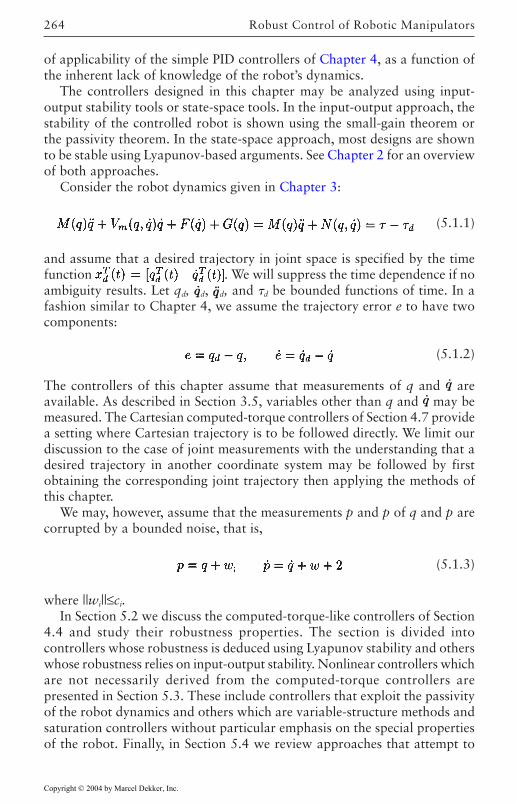
Robust Control of Robotic Manipulators264
of applicability of the simple PID controllers of Chapter 4, as a function ofthe inherent lack of knowledge of the robot’s dynamics.
The controllers designed in this chapter may be analyzed using input-output stability tools or state-space tools. In the input-output approach, thestability of the controlled robot is shown using the small-gain theorem orthe passivity theorem. In the state-space approach, most designs are shownto be stable using Lyapunov-based arguments. See Chapter 2 for an overviewof both approaches.
Consider the robot dynamics given in Chapter 3:
(5.1.1)
and assume that a desired trajectory in joint space is specified by the timefunction . We will suppress the time dependence if noambiguity results. Let qd, d, d, and d be bounded functions of time. In afashion similar to Chapter 4, we assume the trajectory error e to have twocomponents:
(5.1.2)
The controllers of this chapter assume that measurements of q and areavailable. As described in Section 3.5, variables other than q and may bemeasured. The Cartesian computed-torque controllers of Section 4.7 providea setting where Cartesian trajectory is to be followed directly. We limit ourdiscussion to the case of joint measurements with the understanding that adesired trajectory in another coordinate system may be followed by firstobtaining the corresponding joint trajectory then applying the methods ofthis chapter.
We may, however, assume that the measurements p and p of q and p arecorrupted by a bounded noise, that is,
(5.1.3)
where ||wi||≤ci.In Section 5.2 we discuss the computed-torque-like controllers of Section
4.4 and study their robustness properties. The section is divided intocontrollers whose robustness is deduced using Lyapunov stability and otherswhose robustness relies on input-output stability. Nonlinear controllers whichare not necessarily derived from the computed-torque controllers arepresented in Section 5.3. These include controllers that exploit the passivityof the robot dynamics and others which are variable-structure methods andsaturation controllers without particular emphasis on the special propertiesof the robot. Finally, in Section 5.4 we review approaches that attempt to
Copyright © 2004 by Marcel Dekker, Inc.
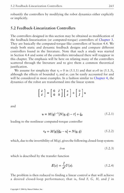
265
robustify the controllers by modifying the robot dynamics either explicitlyor implicitly.
5.2 Feedback-Linearization Controllers
The controllers designed in this section may be obtained as modification ofthe feedback-linearization (or computed-torque) controllers of Chapter 3.They are basically the computed-torque-like controllers of Section 4.4. Westudy both static and dynamic feedback designs and compare differentcontrollers found in the literature. Note that such a study was startedin Section 4.4 and some of the controllers introduced there will reappear inthis chapter. The emphasis will be here on relating many of the controllersscattered through the literature and to give them a common theoreticaljustification.
We assume for simplicity that d = 0 in (5.1.1) and that wi=0 in (5.1.3),although the effects of bounded d and wi can be easily accounted for andwill be considered in most examples. In a fashion similar to Chapter 4, thedynamics of the robot are transformed into the linear system
and
(5.2.1)
leading to the nonlinear computed-torque controller
(5.2.2)
which, due to the invertibility of M(q), gives the following closed-loop system:
ë=u (5.2.3)
which is described by the transfer function
(5.2.4)
The problem is then reduced to finding a linear control u that will achievea desired closed-loop performance; that is, find F, G, H, and J in
5.2 Feedback-Linearization Controllers
Copyright © 2004 by Marcel Dekker, Inc.
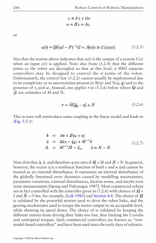
Robust Control of Robotic Manipulators266
or
(5.2.5)
Not that the notion above indicates that u(t) is the output of a system C(s)when an input e(t) is applied. Note also from (5.2.4) that the differentjoints or the robot are decoupled so that at this level, n SISO separatecontrollers may be designed to control the n joints of the robot.Unfortunately, the control law (5.2.2) cannot usually be implemented dueto its complexity or to uncertainties present in M(q) and N(q, ) and to thepresence of d and wi. Instead, one applies in (5.2.6) below where and
are estimates of M and N,
(5.2.6)
This in turn will reintroduce some coupling in the linear model and leads to(Fig. 5.5.1)
(5.2.7)
Note first that , , and therefore are zero if = M and = N. In general,however, the vector is a nonlinear function of both e and u and cannot betreated as an external disturbance. It represents an internal disturbance ofthe globally linearized error dynamics caused by modelling uncertainties,parameter variations, external disturbances, friction terms, and maybe evennoise measurements [Spong and Vidyasagar 1987]. Most commercial robotsare in fact controlled with the controller given in (5.2.6) with choices of =I and = 0 See, for example, [Luh 1983] and Section 4.4. The choice of is validated by the powerful motors used to drive the robot links, and thegearing mechanisms used to torque the motor output to an acceptable level,while showing its speed down. The choice of is validated by keeping thedifferent motors from driving their links too fast, thus limiting the Coriolisand centripetal torques. Such commercial controllers are known as “non-model-based controllers” and have been used since the early days of robotics.
Copyright © 2004 by Marcel Dekker, Inc.
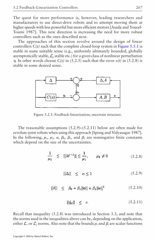
267
The quest for more performance is, however, leading researchers andmanufacturers to use direct-drive robots and to attempt moving them athigher speeds with less powerful but more efficient motors [Asada and Youcef-Toumi 1987]. This new direction is increasing the need for more robustcontrollers such as the ones described next.
The approaches of this section revolve around the design of linearcontrollers C(s) such that the complete closed-loop system in Figure 5.5.1 isstable in some suitable sense (e.g., uniformly ultimately bounded, globallyasymptotically stable, p stable etc.) for a given class of nonlinear perturbation. In other words choose C(s) in (5.2.5) such that the error e(t) in (5.2.8) isstable in some desired sense.
The reasonable assumptions (5.2.9)–(5.2.11) below are often made forrevolute-joint robots when using this approach [Spong and Vidyasagar 1987].In the following, µ1, µ2, , 0, 1, and 2 are nonnegative finite constantswhich depend on the size of the uncertainties.
(5.2.8)
(5.2.9)
(5.2.10)
(5.2.11)
Recall that inequality (5.2.8) was introduced in Section 3.3, and note thatthe norms used in the inequalities above can be, depending on the application,either ∞ or 2 norms. Also note that the bounds µi and i are scalar functions
Figure 5.2.1: Feedback-linearization; uncertain structure.
5.2 Feedback-Linearization Controllers
Copyright © 2004 by Marcel Dekker, Inc.
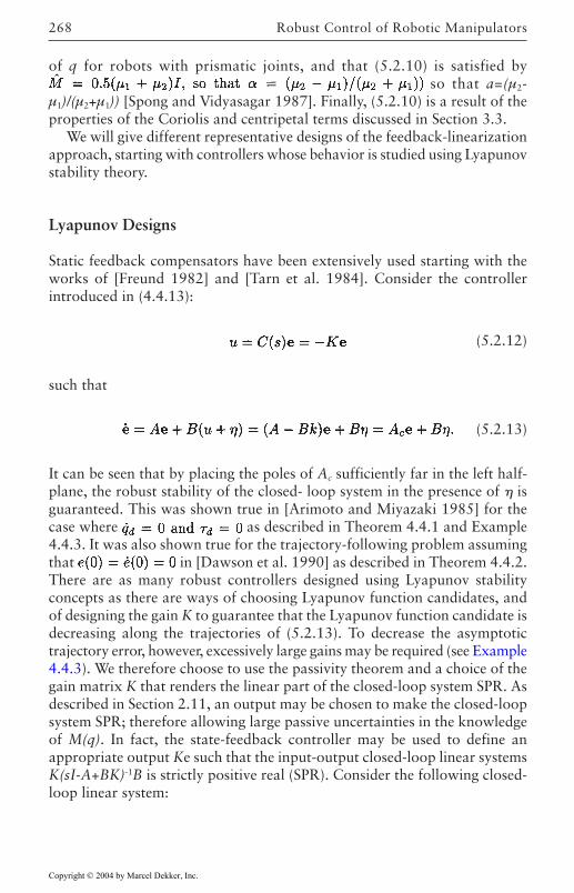
Robust Control of Robotic Manipulators268
of q for robots with prismatic joints, and that (5.2.10) is satisfied by so that a=(µ2-
µ1)/(µ2+µ1)) [Spong and Vidyasagar 1987]. Finally, (5.2.10) is a result of theproperties of the Coriolis and centripetal terms discussed in Section 3.3.
We will give different representative designs of the feedback-linearizationapproach, starting with controllers whose behavior is studied using Lyapunovstability theory.
Lyapunov Designs
Static feedback compensators have been extensively used starting with theworks of [Freund 1982] and [Tarn et al. 1984]. Consider the controllerintroduced in (4.4.13):
(5.2.12)
such that
(5.2.13)
It can be seen that by placing the poles of Ac sufficiently far in the left half-plane, the robust stability of the closed- loop system in the presence of isguaranteed. This was shown true in [Arimoto and Miyazaki 1985] for thecase where as described in Theorem 4.4.1 and Example4.4.3. It was also shown true for the trajectory-following problem assumingthat in [Dawson et al. 1990] as described in Theorem 4.4.2.There are as many robust controllers designed using Lyapunov stabilityconcepts as there are ways of choosing Lyapunov function candidates, andof designing the gain K to guarantee that the Lyapunov function candidate isdecreasing along the trajectories of (5.2.13). To decrease the asymptotictrajectory error, however, excessively large gains may be required (see Example4.4.3). We therefore choose to use the passivity theorem and a choice of thegain matrix K that renders the linear part of the closed-loop system SPR. Asdescribed in Section 2.11, an output may be chosen to make the closed-loopsystem SPR; therefore allowing large passive uncertainties in the knowledgeof M(q). In fact, the state-feedback controller may be used to define anappropriate output Ke such that the input-output closed-loop linear systemsK(sI-A+BK)-1B is strictly positive real (SPR). Consider the following closed-loop linear system:
Copyright © 2004 by Marcel Dekker, Inc.
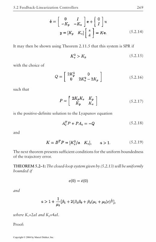
269
(5.2.14)
It may then be shown using Theorem 2.11.5 that this system is SPR if
(5.2.15)
with the choice of
(5.2.16)
such that
(5.2.17)
is the positive-definite solution to the Lyapunov equation
(5.2.18)
and
(5.2.19)
The next theorem presents sufficient conditions for the uniform boundednessof the trajectory error.
THEOREM 5.2–1: The closed-loop system given by (5.2.13) will be uniformlybounded if
and
where Kv=2aI and Kp=4aI.
Proof:
5.2 Feedback-Linearization Controllers
Copyright © 2004 by Marcel Dekker, Inc.
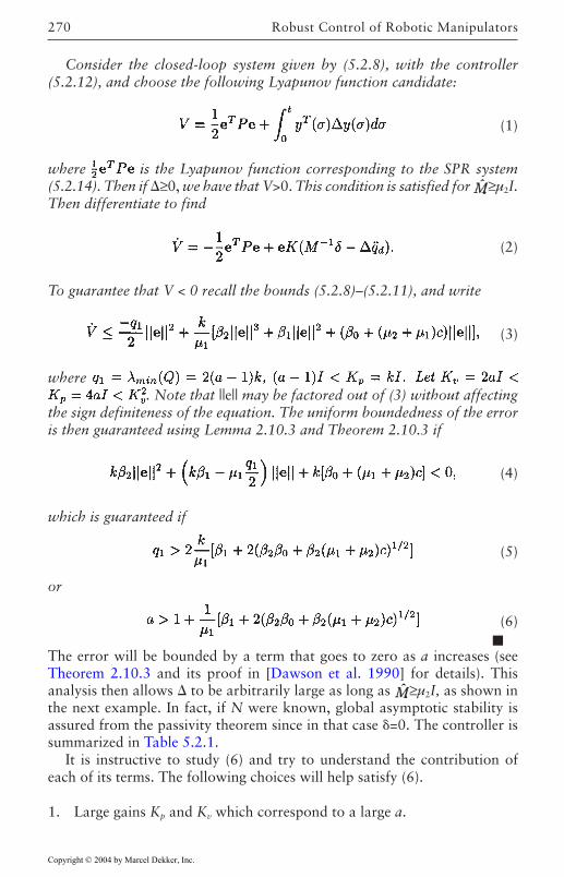
Robust Control of Robotic Manipulators270
Consider the closed-loop system given by (5.2.8), with the controller(5.2.12), and choose the following Lyapunov function candidate:
(1)
where is the Lyapunov function corresponding to the SPR system(5.2.14). Then if ≥0, we have that V>0. This condition is satisfied for ≥µ2I.Then differentiate to find
(2)
To guarantee that V < 0 recall the bounds (5.2.8)–(5.2.11), and write
(3)
where . Note that ||e|| may be factored out of (3) without affecting
the sign definiteness of the equation. The uniform boundedness of the erroris then guaranteed using Lemma 2.10.3 and Theorem 2.10.3 if
(4)
which is guaranteed if
(5)
or
(6)
The error will be bounded by a term that goes to zero as a increases (seeTheorem 2.10.3 and its proof in [Dawson et al. 1990] for details). Thisanalysis then allows to be arbitrarily large as long as ≥µ2I, as shown inthe next example. In fact, if N were known, global asymptotic stability isassured from the passivity theorem since in that case =0. The controller is
It is instructive to study (6) and try to understand the contribution ofeach of its terms. The following choices will help satisfy (6).
1. Large gains Kp and Kv which correspond to a large a.
Copyright © 2004 by Marcel Dekker, Inc.
summarized in Table 5.2.1.
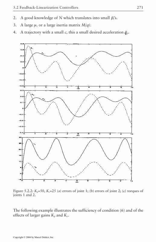
271
2. A good knowledge of N which translates into small i’s.
3. A large µ1 or a large inertia matrix M(q).
4. A trajectory with a small c, this a small desired acceleration d.
Figure 5.2.2: Kp=50, Kv=25 (a) errors of joint 1; (b) errors of joint 2; (c) torques ofjoints 1 and 2.
The following example illustrates the sufficiency of condition (6) and of theeffects of larger gains Kp and Kv.
5.2 Feedback-Linearization Controllers
Copyright © 2004 by Marcel Dekker, Inc.
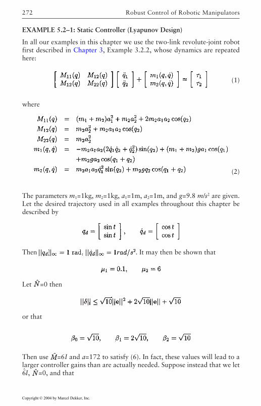
Robust Control of Robotic Manipulators272
(1)
where
EXAMPLE 5.2–1: Static Controller (Lyapunov Design)
In all our examples in this chapter we use the two-link revolute-joint robotfirst described in Chapter 3, Example 3.2.2, whose dynamics are repeatedhere:
(2)
The parameters m1=1kg, m2=1kg, a1=1m, a2=1m, and g=9.8 m/s2 are given.Let the desired trajectory used in all examples throughout this chapter bedescribed by
Then . It may then be shown that
Let =0 then
or that
Then use =6I and a=172 to satisfy (6). In fact, these values will lead to alarger controller gains than are actually needed. Suppose instead that we let6^I, =0, and that
Copyright © 2004 by Marcel Dekker, Inc.
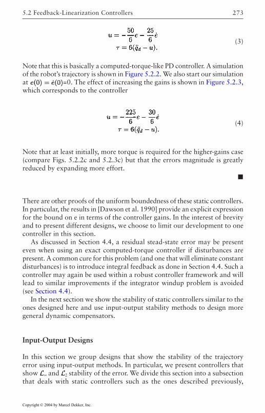
273
(3)
Note that this is basically a computed-torque-like PD controller. A simulationof the robot’s trajectory is shown in Figure 5.2.2. We also start our simulationat =0. The effect of increasing the gains is shown in Figure 5.2.3,which corresponds to the controller
(4)
Note that at least initially, more torque is required for the higher-gains case(compare Figs. 5.2.2c and 5.2.3c) but that the errors magnitude is greatlyreduced by expanding more effort.
There are other proofs of the uniform boundedness of these static controllers.In particular, the results in [Dawson et al. 1990] provide an explicit expressionfor the bound on e in terms of the controller gains. In the interest of brevityand to present different designs, we choose to limit our development to onecontroller in this section.
As discussed in Section 4.4, a residual stead-state error may be presenteven when using an exact computed-torque controller if disturbances arepresent. A common cure for this problem (and one that will eliminate constantdisturbances) is to introduce integral feedback as done in Section 4.4. Such acontroller may again be used within a robust controller framework and willlead to similar improvements if the integrator windup problem is avoided(see Section 4.4).
In the next section we show the stability of static controllers similar to theones designed here and use input-output stability methods to design moregeneral dynamic compensators.
Input-Output Designs
In this section we group designs that show the stability of the trajectoryerror using input-output methods. In particular, we present controllers thatshow ∞ and 2 stability of the error. We divide this section into a subsectionthat deals with static controllers such as the ones described previously,
5.2 Feedback-Linearization Controllers
Copyright © 2004 by Marcel Dekker, Inc.
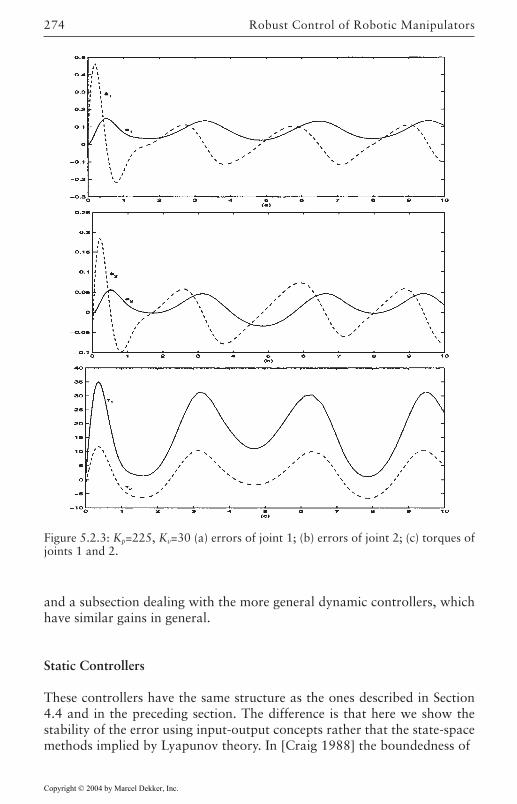
Robust Control of Robotic Manipulators274
and a subsection dealing with the more general dynamic controllers, whichhave similar gains in general.
Static Controllers
These controllers have the same structure as the ones described in Section4.4 and in the preceding section. The difference is that here we show thestability of the error using input-output concepts rather that the state-spacemethods implied by Lyapunov theory. In [Craig 1988] the boundedness of
Figure 5.2.3: Kp=225, Kv=30 (a) errors of joint 1; (b) errors of joint 2; (c) torques ofjoints 1 and 2.
Copyright © 2004 by Marcel Dekker, Inc.
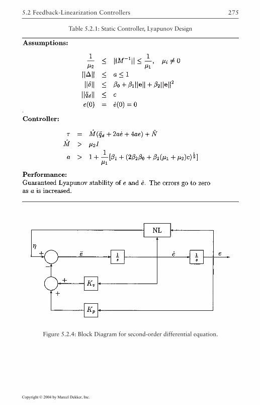
275
Table 5.2.1: Static Controller, Lyapunov Design
Figure 5.2.4: Block Diagram for second-order differential equation.
5.2 Feedback-Linearization Controllers
Copyright © 2004 by Marcel Dekker, Inc.
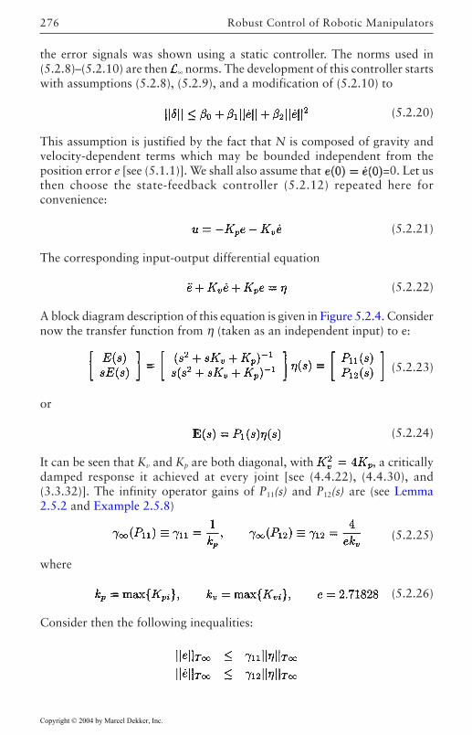
Robust Control of Robotic Manipulators276
the error signals was shown using a static controller. The norms used in(5.2.8)–(5.2.10) are then ∞ norms. The development of this controller startswith assumptions (5.2.8), (5.2.9), and a modification of (5.2.10) to
(5.2.20)
This assumption is justified by the fact that N is composed of gravity andvelocity-dependent terms which may be bounded independent from theposition error e [see (5.1.1)]. We shall also assume that =0. Let usthen choose the state-feedback controller (5.2.12) repeated here forconvenience:
(5.2.21)
The corresponding input-output differential equation
(5.2.22)
A block diagram description of this equation is given in Figure 5.2.4. Considernow the transfer function from η (taken as an independent input) to e:
(5.2.23)
or
(5.2.24)
It can be seen that Kv and Kp are both diagonal, with , a criticallydamped response it achieved at every joint [see (4.4.22), (4.4.30), and(3.3.32)]. The infinity operator gains of P11(s) and P12(s) are (see Lemma2.5.2 and Example 2.5.8)
(5.2.25)
where
(5.2.26)
Consider then the following inequalities:
Copyright © 2004 by Marcel Dekker, Inc.
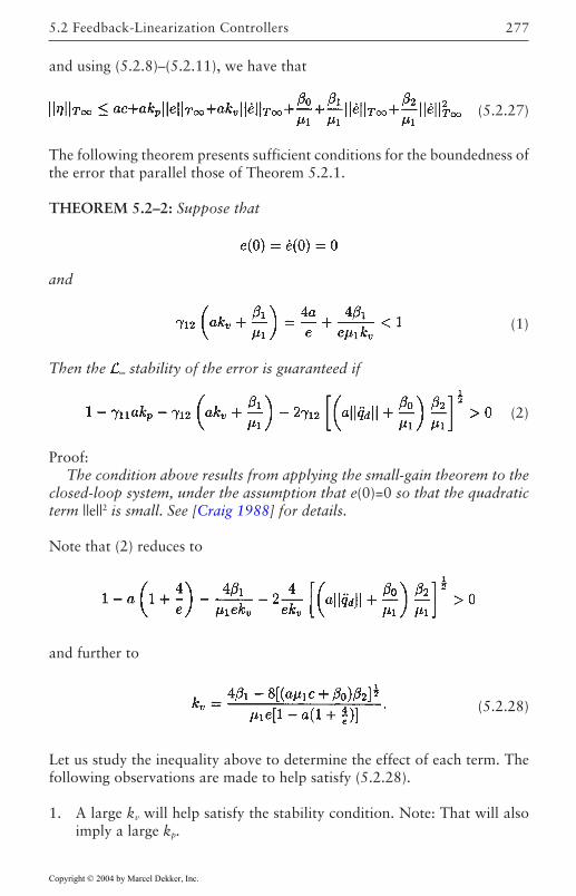
277
and using (5.2.8)–(5.2.11), we have that
(5.2.27)
The following theorem presents sufficient conditions for the boundedness ofthe error that parallel those of Theorem 5.2.1.
THEOREM 5.2–2: Suppose that
and
(1)
Then the ∞ stability of the error is guaranteed if
(2)
Proof:The condition above results from applying the small-gain theorem to the
closed-loop system, under the assumption that e(0)=0 so that the quadraticterm ||e||2 is small. See [Craig 1988] for details.
Note that (2) reduces to
and further to
(5.2.28)
Let us study the inequality above to determine the effect of each term. Thefollowing observations are made to help satisfy (5.2.28).
1. A large kv will help satisfy the stability condition. Note: That will alsoimply a large kp.
5.2 Feedback-Linearization Controllers
Copyright © 2004 by Marcel Dekker, Inc.
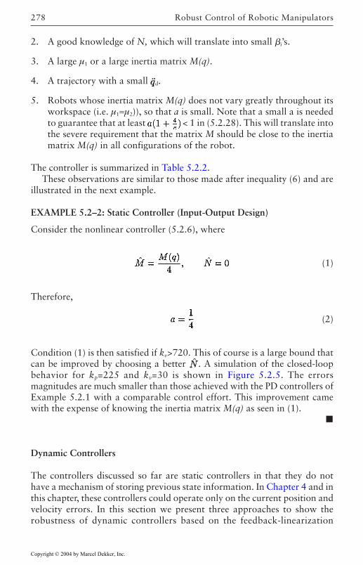
Robust Control of Robotic Manipulators278
2. A good knowledge of N, which will translate into small i’s.
3. A large µ1 or a large inertia matrix M(q).
4. A trajectory with a small d.
5. Robots whose inertia matrix M(q) does not vary greatly throughout itsworkspace (i.e. µ1≈µ2)), so that a is small. Note that a small a is neededto guarantee that at least < 1 in (5.2.28). This will translate intothe severe requirement that the matrix M should be close to the inertiamatrix M(q) in all configurations of the robot.
The controller is summarized in Table 5.2.2.These observations are similar to those made after inequality (6) and are
illustrated in the next example.
EXAMPLE 5.2–2: Static Controller (Input-Output Design)
Consider the nonlinear controller (5.2.6), where
(1)
Therefore,
(2)
Condition (1) is then satisfied if kv>720. This of course is a large bound thatcan be improved by choosing a better . A simulation of the closed-loopbehavior for kp=225 and kv=30 is shown in Figure 5.2.5. The errorsmagnitudes are much smaller than those achieved with the PD controllers ofExample 5.2.1 with a comparable control effort. This improvement camewith the expense of knowing the inertia matrix M(q) as seen in (1).
Dynamic Controllers
The controllers discussed so far are static controllers in that they do nothave a mechanism of storing previous state information. In Chapter 4 and inthis chapter, these controllers could operate only on the current position andvelocity errors. In this section we present three approaches to show therobustness of dynamic controllers based on the feedback-linearization
Copyright © 2004 by Marcel Dekker, Inc.
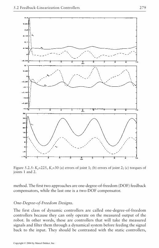
279
method. The first two approaches are one-degree-of-freedom (DOF) feedbackcompensators, while the last one is a two-DOF compensator.
One-Degree-of-Freedom Designs.
The first class of dynamic controllers are called one-degree-of-freedomcontrollers because they can only operate on the measured output of therobot. In other words, these are controllers that will take the measuredsignals and filter them through a dynamical system before feeding the signalback to the input. They should be contrasted with the static controllers,
Figure 5.2.5: Kp=225, Kv=30 (a) errors of joint 1; (b) errors of joint 2; (c) torques ofjoints 1 and 2.
5.2 Feedback-Linearization Controllers
Copyright © 2004 by Marcel Dekker, Inc.
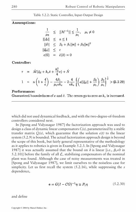
Robust Control of Robotic Manipulators280
which did not used dynamical feedback, and with the two-degree-of-freedomcontrollers considered next.
In [Spong and Vidyasagar 1987] the factorization approach was used todesign a class of dynamic linear compensators C(s), parameterized by a stabletransfer matrix Q(s), which guarantee that the solution e(t) to the linearsystem (5.2.9) is bounded. The actual factorization approach design is beyondthe scope of this book, but fairly general representative of the methodologyas it applies to robotics is given in Example 5.2.3. In [Spong and Vidyasagar1987] it was actually assumed that the bound on is linear [i.e., 2=0 in5.2.10)] before the family of all ∞ stabilizing compensators of the nominalplant was found. Although the case of noisy measurements was treated in[Spong and Vidyasagar 1987], we limit ourselves to the noiseless case forsimplicity. Let us first recall the system (5.2.16), while suppressing the sdependence,
(5.2.30)
and define
Table 5.2.2: Static Controller, Input-Output Design
Copyright © 2004 by Marcel Dekker, Inc.
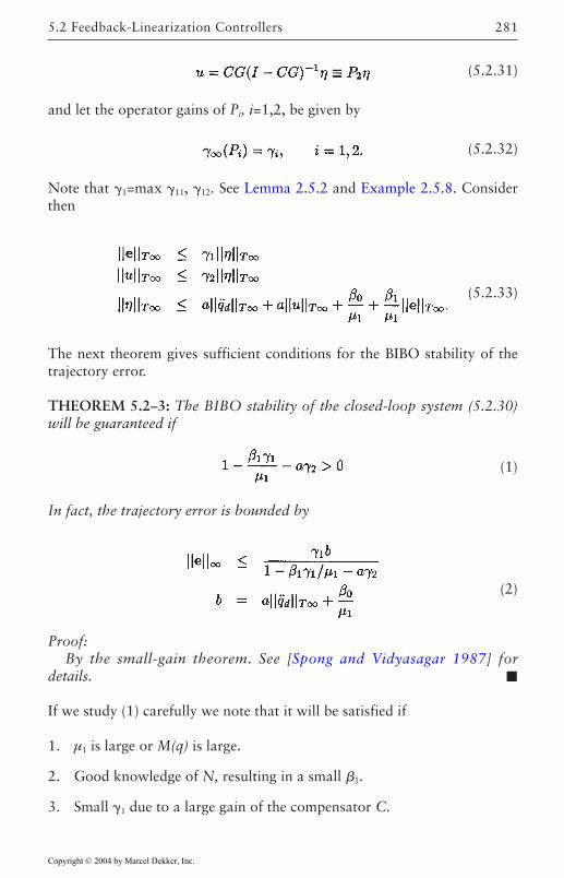
281
(5.2.31)
and let the operator gains of Pi, i=1,2, be given by
(5.2.32)
Note that 1=max 11, 12. See Lemma 2.5.2 and Example 2.5.8. Considerthen
(5.2.33)
The next theorem gives sufficient conditions for the BIBO stability of thetrajectory error.
THEOREM 5.2–3: The BIBO stability of the closed-loop system (5.2.30)will be guaranteed if
(1)
In fact, the trajectory error is bounded by
(2)
Proof:By the small-gain theorem. See [Spong and Vidyasagar 1987] for
details.
If we study (1) carefully we note that it will be satisfied if
1. µ1 is large or M(q) is large.
2. Good knowledge of N, resulting in a small 1.
3. Small 1 due to a large gain of the compensator C.
5.2 Feedback-Linearization Controllers
Copyright © 2004 by Marcel Dekker, Inc.
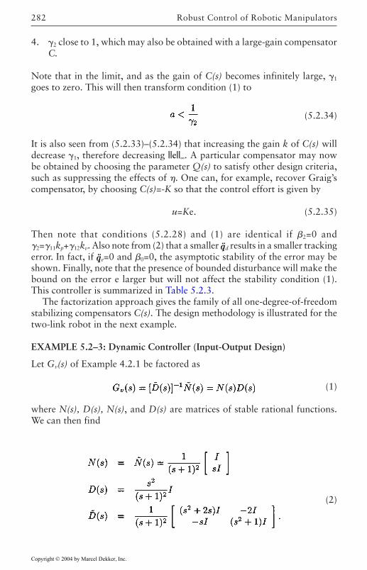
Robust Control of Robotic Manipulators282
4. 2 close to 1, which may also be obtained with a large-gain compensatorC.
Note that in the limit, and as the gain of C(s) becomes infinitely large, 1
goes to zero. This will then transform condition (1) to
(5.2.34)
It is also seen from (5.2.33)–(5.2.34) that increasing the gain k of C(s) willdecrease 1, therefore decreasing ||e||∞. A particular compensator may nowbe obtained by choosing the parameter Q(s) to satisfy other design criteria,such as suppressing the effects of . One can, for example, recover Graig’scompensator, by choosing C(s)=-K so that the control effort is given by
u=Ke. (5.2.35)
Then note that conditions (5.2.28) and (1) are identical if 2=0 and2=11kp+12kv. Also note from (2) that a smaller d results in a smaller trackingerror. In fact, if e=0 and 0=0, the asymptotic stability of the error may beshown. Finally, note that the presence of bounded disturbance will make thebound on the error e larger but will not affect the stability condition (1).This controller is summarized in Table 5.2.3.
The factorization approach gives the family of all one-degree-of-freedomstabilizing compensators C(s). The design methodology is illustrated for thetwo-link robot in the next example.
EXAMPLE 5.2–3: Dynamic Controller (Input-Output Design)
Let Gv(s) of Example 4.2.1 be factored as
(1)
where N(s), D(s), N(s), and D(s) are matrices of stable rational functions.We can then find
(2)
Copyright © 2004 by Marcel Dekker, Inc.
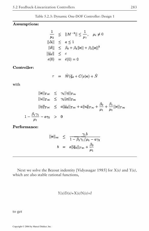
283
Next we solve the Bezout indentity [Vidyasagar 1985] for X(s) and Y(s),which are also stable rational functions,
Y(s)D(s)+X(s)N(s)=I
to get
Table 5.2.3: Dynamic One-DOF Controller: Design 1
5.2 Feedback-Linearization Controllers
Copyright © 2004 by Marcel Dekker, Inc.
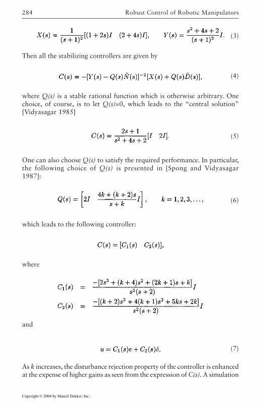
Robust Control of Robotic Manipulators284
(3)
Then all the stabilizing controllers are given by
(4)
where Q(s) is a stable rational function which is otherwise arbitrary. Onechoice, of course, is to let Q(s)=0, which leads to the “central solution”[Vidyasagar 1985]
(5)
One can also choose Q(s) to satisfy the required performance. In particular,the following choice of Q(s) is presented in [Spong and Vidyasagar1987]:
(6)
which leads to the following controller:
where
and
(7)
As k increases, the disturbance rejection property of the controller is enhancedat the expense of higher gains as seen from the expression of C(s). A simulation
Copyright © 2004 by Marcel Dekker, Inc.
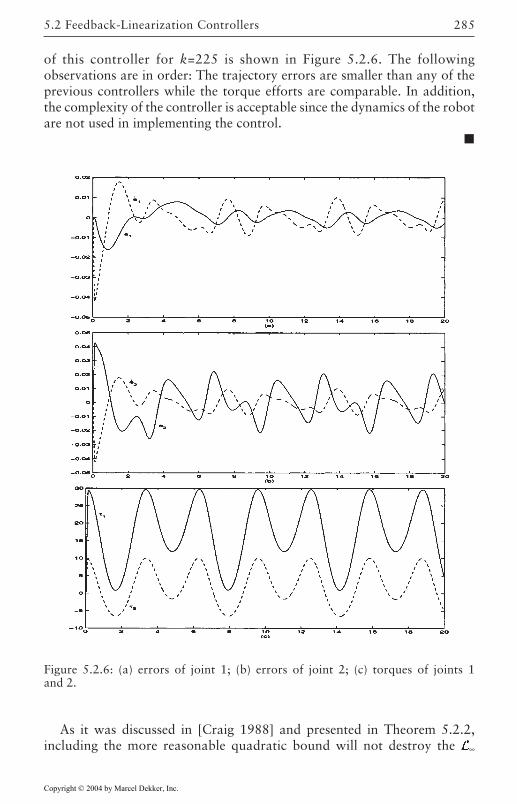
285
of this controller for k=225 is shown in Figure 5.2.6. The followingobservations are in order: The trajectory errors are smaller than any of theprevious controllers while the torque efforts are comparable. In addition,the complexity of the controller is acceptable since the dynamics of the robotare not used in implementing the control.
Figure 5.2.6: (a) errors of joint 1; (b) errors of joint 2; (c) torques of joints 1and 2.
As it was discussed in [Craig 1988] and presented in Theorem 5.2.2,including the more reasonable quadratic bound will not destroy the ∞
5.2 Feedback-Linearization Controllers
Copyright © 2004 by Marcel Dekker, Inc.
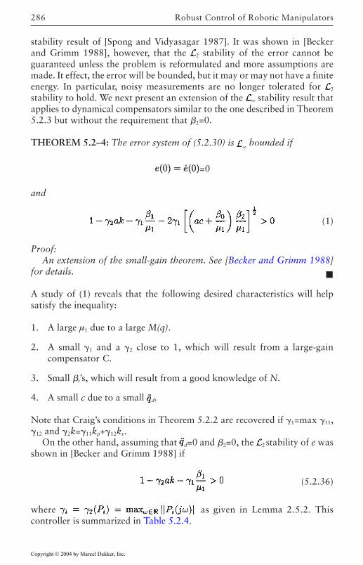
Robust Control of Robotic Manipulators286
stability result of [Spong and Vidyasagar 1987]. It was shown in [Beckerand Grimm 1988], however, that the 2 stability of the error cannot beguaranteed unless the problem is reformulated and more assumptions aremade. It effect, the error will be bounded, but it may or may not have a finiteenergy. In particular, noisy measurements are no longer tolerated for 2
stability to hold. We next present an extension of the ∞ stability result thatapplies to dynamical compensators similar to the one described in Theorem5.2.3 but without the requirement that 2=0.
THEOREM 5.2–4: The error system of (5.2.30) is ∞ bounded if
=0
and
(1)
Proof:An extension of the small-gain theorem. See [Becker and Grimm 1988]
for details.
A study of (1) reveals that the following desired characteristics will helpsatisfy the inequality:
1. A large µ1 due to a large M(q).
2. A small 1 and a 2 close to 1, which will result from a large-gaincompensator C.
3. Small i’s, which will result from a good knowledge of N.
4. A small c due to a small d.
Note that Craig’s conditions in Theorem 5.2.2 are recovered if 1=max 11,12 and 2k=11kp+12kv.
On the other hand, assuming that d=0 and 2=0, the 2 stability of e wasshown in [Becker and Grimm 1988] if
(5.2.36)
where as given in Lemma 2.5.2. Thiscontroller is summarized in Table 5.2.4.
Copyright © 2004 by Marcel Dekker, Inc.
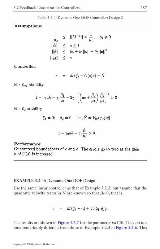
287
EXAMPLE 5.2–4: Dynamic One DOF Design
Use the same linear controller as that of Example 5.2.3, but assume that thequadratic velocity terms in N are known so that 2=0; that is
The results are shown in Figure 5.2.7 for the parameter k=150. They do notlook remarkably different from those of Example 5.2.3 in Figure 5.2.6. This
Table 5.2.4: Dynamic One-DOF Controller: Design 2
5.2 Feedback-Linearization Controllers
Copyright © 2004 by Marcel Dekker, Inc.
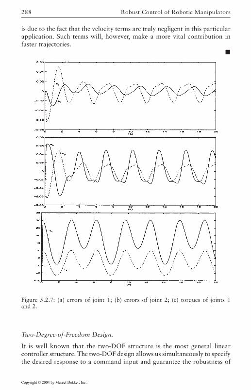
Robust Control of Robotic Manipulators288
is due to the fact that the velocity terms are truly negligent in this particularapplication. Such terms will, however, make a more vital contribution infaster trajectories.
Figure 5.2.7: (a) errors of joint 1; (b) errors of joint 2; (c) torques of joints 1and 2.
Two-Degree-of-Freedom Design.
It is well known that the two-DOF structure is the most general linearcontroller structure. The two-DOF design allows us simultaneously to specifythe desired response to a command input and guarantee the robustness of
Copyright © 2004 by Marcel Dekker, Inc.
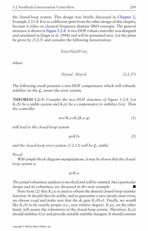
289
the closed-loop system. This design was briefly discussed in Chapter 2,Example 2.11.4. It is in a different spirit from the other design of this chapter,because it relies on classical frequency-domain SISO concepts. The generalstructure is shown in Figure 5.2.8. A two-DOF robust controller was designedand simulated in [Sugie et al. 1988] and will be presented next. Let the plantbe given by (5.2.5) and consider the following factorization:
G(s)=N(s)D-1(s),
where
D(s)=s2, N(s)=I. (5.2.37)
The following result presents a two-DOF compensator which will robustlystabilize (in the ∞ sense) the error system.
THEOREM 5.2–5: Consider the two-DOF structure of Figure 5.2.8. LetK1(S) be a stable system and K2(s) be a compensator to stabilize G(s). Thenthe controller
u=s2K1v+K2(K1v-q) (1)
will lead to the closed-loop system
q=K1v (2)
and the closed-loop error system (5.2.13) will be ∞ stable.
Proof:With simple block-diagram manipulations, it may be shown that the closed-
loop system is
q=K1v.
The actual robustness analysis is involved and will be omitted, but a particulardesign and its robustness are discussed in the next example.
Note from (2) that K1(s) is used to obtain the desired closed-loop transferfunction. It should then be stable, and to guarantee a zero steady-state error,we choose v=qd and make sure that the dc gain K1(0)=1. Finally, we wouldlike K1(S) to be exactly proper (i.e., zero relative degree). K2(s), on the otherhand, will assure the robustness of the closed-loop system. Therefore, K2(s)should stabilize G(s) and provide suitable stability margins. It should contain
5.2 Feedback-Linearization Controllers
Copyright © 2004 by Marcel Dekker, Inc.
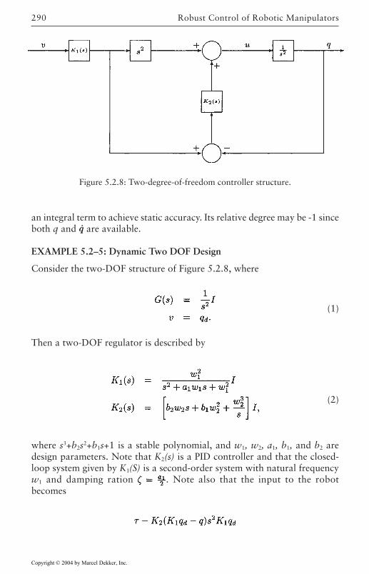
Robust Control of Robotic Manipulators290
an integral term to achieve static accuracy. Its relative degree may be -1 sinceboth q and are available.
EXAMPLE 5.2–5: Dynamic Two DOF Design
Consider the two-DOF structure of Figure 5.2.8, where
(1)
Then a two-DOF regulator is described by
(2)
where s3+b2s2+b1s+1 is a stable polynomial, and w1, w2, a1, b1, and b2 aredesign parameters. Note that K2(s) is a PID controller and that the closed-loop system given by K1(S) is a second-order system with natural frequencyw1 and damping ration . Note also that the input to the robotbecomes
Figure 5.2.8: Two-degree-of-freedom controller structure.
Copyright © 2004 by Marcel Dekker, Inc.
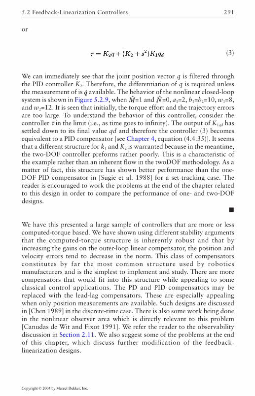
291
or
(3)
We can immediately see that the joint position vector q is filtered throughthe PID controller K2. Therefore, the differentiation of q is required unlessthe measurement of is available. The behavior of the nonlinear closed-loopsystem is shown in Figure 5.2.9, when =1 and =0, a1=2, b1=b2=10, w1=8,and w2=12. It is seen that initially, the torque effort and the trajectory errorsare too large. To understand the behavior of this controller, consider thecontroller τ in the limit (i.e., as time goes to infinity). The output of K1qd hassettled down to its final value qd and therefore the controller (3) becomesequivalent to a PID compensator [see Chapter 4, equation (4.4.35)]. It seemsthat a different structure for k1 and K2 is warranted because in the meantime,the two-DOF controller preforms rather poorly. This is a characteristic ofthe example rather than an inherent flow in the twoDOF methodology. As amatter of fact, this structure has shown better performance than the one-DOF PID compensator in [Sugie et al. 1988] for a set-tracking case. Thereader is encouraged to work the problems at the end of the chapter relatedto this design in order to compare the performance of one- and two-DOFdesigns.
We have this presented a large sample of controllers that are more or lesscomputed-torque based. We have shown using different stability argumentsthat the computed-torque structure is inherently robust and that byincreasing the gains on the outer-loop linear compensator, the position andvelocity errors tend to decrease in the norm. This class of compensatorsconstitutes by far the most common structure used by roboticsmanufacturers and is the simplest to implement and study. There are morecompensators that would fit into this structure while appealing to someclassical control applications. The PD and PID compensators may bereplaced with the lead-lag compensators. These are especially appealingwhen only position measurements are available. Such designs are discussedin [Chen 1989] in the discrete-time case. There is also some work being donein the nonlinear observer area which is directly relevant to this problem[Canudas de Wit and Fixot 1991]. We refer the reader to the observabilitydiscussion in Section 2.11. We also suggest some of the problems at the endof this chapter, which discuss further modification of the feedback-linearization designs.
5.2 Feedback-Linearization Controllers
Copyright © 2004 by Marcel Dekker, Inc.
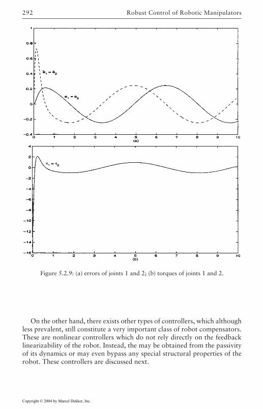
Robust Control of Robotic Manipulators292
On the other hand, there exists other types of controllers, which althoughless prevalent, still constitute a very important class of robot compensators.These are nonlinear controllers which do not rely directly on the feedbacklinearizability of the robot. Instead, the may be obtained from the passivityof its dynamics or may even bypass any special structural properties of therobot. These controllers are discussed next.
Figure 5.2.9: (a) errors of joints 1 and 2; (b) torques of joints 1 and 2.
Copyright © 2004 by Marcel Dekker, Inc.
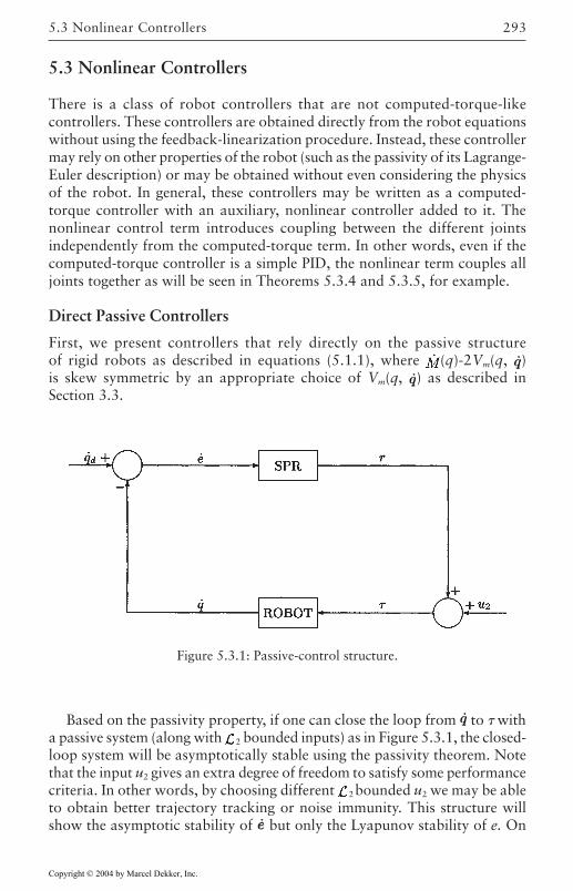
293
5.3 Nonlinear Controllers
There is a class of robot controllers that are not computed-torque-likecontrollers. These controllers are obtained directly from the robot equationswithout using the feedback-linearization procedure. Instead, these controllermay rely on other properties of the robot (such as the passivity of its Lagrange-Euler description) or may be obtained without even considering the physicsof the robot. In general, these controllers may be written as a computed-torque controller with an auxiliary, nonlinear controller added to it. Thenonlinear control term introduces coupling between the different jointsindependently from the computed-torque term. In other words, even if thecomputed-torque controller is a simple PID, the nonlinear term couples alljoints together as will be seen in Theorems 5.3.4 and 5.3.5, for example.
Direct Passive Controllers
First, we present controllers that rely directly on the passive structureof rigid robots as described in equations (5.1.1), where (q)-2Vm(q, )is skew symmetric by an appropriate choice of Vm(q, ) as described inSection 3.3.
Based on the passivity property, if one can close the loop from to witha passive system (along with 2 bounded inputs) as in Figure 5.3.1, the closed-loop system will be asymptotically stable using the passivity theorem. Notethat the input u2 gives an extra degree of freedom to satisfy some performancecriteria. In other words, by choosing different 2 bounded u2 we may be ableto obtain better trajectory tracking or noise immunity. This structure willshow the asymptotic stability of but only the Lyapunov stability of e. On
Figure 5.3.1: Passive-control structure.
5.3 Nonlinear Controllers
Copyright © 2004 by Marcel Dekker, Inc.

Robust Control of Robotic Manipulators294
the other hand, if one can show the passivity of the system, which maps toa new vector r which is a filtered version of e, a controller that closes theloop between -r and will guarantee the asymptotic stability of both e and .This indirect use of the passivity property was illustrated in [Ortega andSpong 1988] and will be discussed first.
Let the controller be given by (5.3.1), where F(s) is a strictly proper, stable,rational function, and Kr is a positive-definite matrix,
(5.3.1)
Substituting (5.3.1) into (5.1.1) and assuming no friction [i.e., F( )=0], weobtain
(5.3.2)
Then it may be shown that both e and are asymptotically stable. In fact,choose the following Lyapunov function:
Then
Substituting for M(q) from (5.3.2), we obtain
Therefore, r is asymptotically stable, which can be used to show that both eand e are asymptotically stable [Slotine 1988]. This approach was used inthe adaptive control literature to design passive controllers [Ortega and Spong1988], but its modification in the design of robust controllers when M, Vm
and G are not exactly known is not immediately obvious. Such modificationswill be given in the variable-structure designs, but first, we present a simplecontroller to illustrate the robustness of passive compensators.
Copyright © 2004 by Marcel Dekker, Inc.
295
THEOREM 5.3–1: Consider the control law (1)
(1)
where (s) is an SPR transfer function, to be chosen by the designer, and theexternal input u2 is bounded in the 2 norm. Then is asymptotically stable,and e is Lyapunov stable.
Proof:Using the control law above, one gets from Figure 5.3.1,
(2)
By an appropriate choice of (s) and u2, one can apply the passivity theoremand deduce that and r are bounded in the 2 norm, and since (s)-1 is SPR(being inverse of an SPR function), one deduces that is asymptoticallystable because
(3)
This will imply that the position error e is bounded but not its asymptoticstability in the case of time-varying trajectories . In the set-pointtracking case, however (i.e., d=0), and with gravity precompensation, theasymptotic stability of e may be deduced using LaSalle’s theorem. Therobustness of the closed-loop system is guaranteed as long as (s) is SPRand that u2 is 2 bounded, regardless of the exact values of the robot’sparameters.
The controller is summarized in Table 5.3.1.
Table 5.3.1: Passive Controller
5.3 Nonlinear Controllers
Copyright © 2004 by Marcel Dekker, Inc.
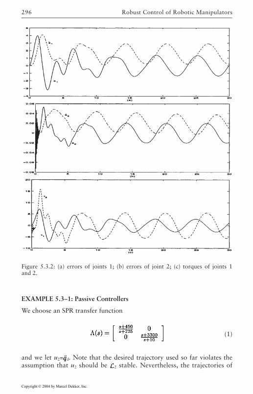
Robust Control of Robotic Manipulators296
EXAMPLE 5.3–1: Passive Controllers
We choose an SPR transfer function
(1)
and we let u2= d. Note that the desired trajectory used so far violates theassumption that u2 should be 2 stable. Nevertheless, the trajectories of
Figure 5.3.2: (a) errors of joints 1; (b) errors of joint 2; (c) torques of joints 1and 2.
Copyright © 2004 by Marcel Dekker, Inc.
297
Figure 5.3.2 show that his controller, when started at e(0)= (0)=0, performsrather well for the sinusoidal trajectory. Of course, since the passivity theoremprovides sufficient conditions for stability, this example is not contradictingthe previous theorem but merely pointing out its conservatism.
Note that the compensator of Theorem 5.3.1 is a generalization of the PDcompensators of Chapter 4 and of the preceding section. In [Anderson 1989]it was demonstrated, using network-theoretic concepts, that even in theabsence of the contact forces, a computed-torque-like controller is not passiveand may therefore cause instabilities in the presence of uncertainties. Hissolution to the problem consisted of using proportionalderivative (PD)controllers with variable gains K1(q) and K2(q) which depend on the inertiamatrix M(q), that is,
(5.3.3)
Even though M(q) is not exactly known, the stability of the closed-looperror is guaranteed by the passivity of the robot and the feedback law. Theadvantage of this approach is that contact forces and larger uncertaintiesmay now be accommodated. Its main disadvantage is that although robuststability is guaranteed, the closed-loop performance depends on theknowledge of M(q), whose singular values are needed in order to find Kp
and Kv. We will not discuss this particular design and refer the interestedreader to [Anderson 1989].
Variable-Structure Controllers
In this section we group designs that use variable-structure (VSS) controllers.The VSS theory has been applied to the control of many nonlinear processes[DeCarlo et al. 1988]. One of the main features of this approach is that oneonly needs to drive the error to a “switching surface,” after which the systemis in “sliding mode” and will not be affected by any modelling uncertaintiesand/or disturbances.
There are two main criticisms of these controllers as they apply to robots.The first is that by ignoring the physics or the robot, these controllers willnecessarily perform no better (if not worse) that controllers which exploitthe structure of the Lagrange-Euler equations. The other criticism relates tothe “chattering” problem commonly associated with variable-structurecontrollers. We shall address the second issue later in this section, and answerthe first by admitting that although initial applications of variable-structuretheory did indeed gloss over the physics of robots, later designs (such as the
5.3 Nonlinear Controllers
Copyright © 2004 by Marcel Dekker, Inc.
Robust Control of Robotic Manipulators298
ones discussed here) by [Slotine 1985] and [Chen et al. 1990] remedied theproblem.
The first application of this theory to robot control seems to be in [Young1978], where the set-point regulation problem ( d=0)was solved using thefollowing controller:
(5.3.4)
where i=1,…, n for an n-link robot, and ri are the switching planes,
(5.3.5)
It is then shown, using the hierarchy of the sliding surfaces r1, r2,…, rn andgiven bounds on the uncertainties in the manipulators model, that one canfind + and - in order to drive the error signal to the intersection of thesliding surfaces, after which the error will “slide” to zero. This controllereliminates the nonlinear coupling of the joints by forcing the system into thesliding mode. Other VSS robot controllers have since been designed.Unfortunately, for most of these schemes, the control effort as seen from(5.3.4) is discontinuous along ri=0 and will therefore create chattering, whichmay excite unmodelled high-frequency dynamics. In addition, thesecontrollers do not exploit the physics of the robot and are therefore lesseffective than controllers that do.
To address this problem, the original VSS controllers were modified in[Slotine 1985] as described in the next theorem. Let us first define a fewvariables to simplify the statement of the theorem. Let
(5.3.6)
where
THEOREM 5.3–2: Consider the controller
Copyright © 2004 by Marcel Dekker, Inc.
299
where
Then the error reaches the surface
in a finite time. In addition, once on the surface, q(t) will go to qd(t)exponentially fast.
Proof:Consider the Lyapunov function candidate
Then
Substituting for and using the skew-symmetric property of (q)-2Vm(q, )we obtain
Then, if we use the controller given by
we obtain
where
5.3 Nonlinear Controllers
Copyright © 2004 by Marcel Dekker, Inc.
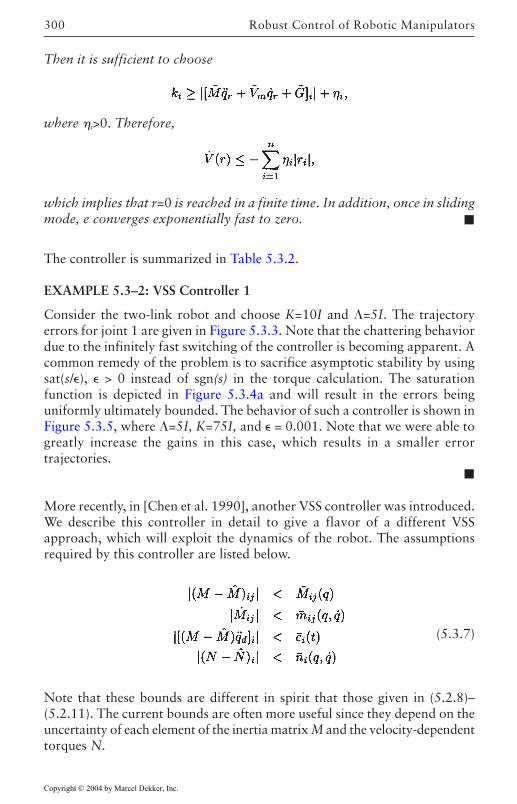
Robust Control of Robotic Manipulators300
Then it is sufficient to choose
where i>0. Therefore,
which implies that r=0 is reached in a finite time. In addition, once in slidingmode, e converges exponentially fast to zero.
The controller is summarized in Table 5.3.2.
EXAMPLE 5.3–2: VSS Controller 1
Consider the two-link robot and choose K=10I and =5I. The trajectoryerrors for joint 1 are given in Figure 5.3.3. Note that the chattering behaviordue to the infinitely fast switching of the controller is becoming apparent. Acommon remedy of the problem is to sacrifice asymptotic stability by usingsat(s/), > 0 instead of sgn(s) in the torque calculation. The saturationfunction is depicted in Figure 5.3.4a and will result in the errors beinguniformly ultimately bounded. The behavior of such a controller is shown inFigure 5.3.5, where =5I, K=75I, and = 0.001. Note that we were able togreatly increase the gains in this case, which results in a smaller errortrajectories.
More recently, in [Chen et al. 1990], another VSS controller was introduced.We describe this controller in detail to give a flavor of a different VSSapproach, which will exploit the dynamics of the robot. The assumptionsrequired by this controller are listed below.
(5.3.7)
Note that these bounds are different in spirit that those given in (5.2.8)–(5.2.11). The current bounds are often more useful since they depend on theuncertainty of each element of the inertia matrix M and the velocity-dependenttorques N.
Copyright © 2004 by Marcel Dekker, Inc.
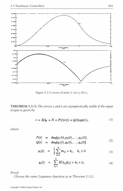
301
THEOREM 5.3–3: The errors e and e. are asymptotically stable if the inputtorque is given by
(1)
where
(2)
(3)
(4)
Proof:Choose the same Lyapunov function as in Theorem 5.3.2:
Figure 5.3.3: errors of joint 1: (a) e1; (b) e1
5.3 Nonlinear Controllers
Copyright © 2004 by Marcel Dekker, Inc.
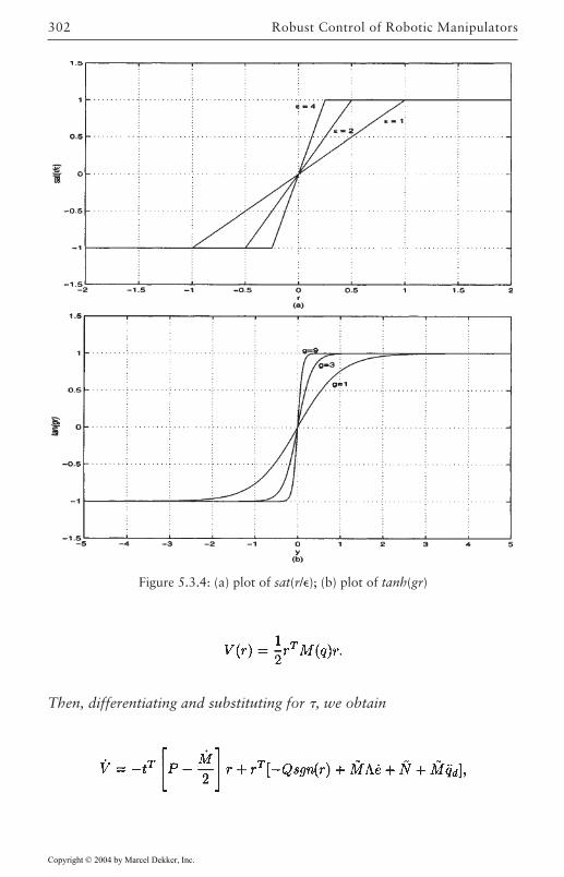
Robust Control of Robotic Manipulators302
Then, differentiating and substituting for , we obtain
Figure 5.3.4: (a) plot of sat(r/); (b) plot of tanh(gr)
Copyright © 2004 by Marcel Dekker, Inc.
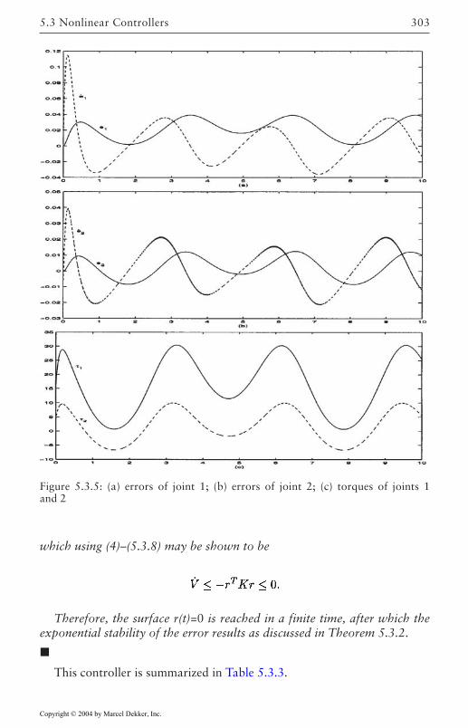
303
which using (4)–(5.3.8) may be shown to be
Therefore, the surface r(t)=0 is reached in a finite time, after which theexponential stability of the error results as discussed in Theorem 5.3.2.
This controller is summarized in Table 5.3.3.
Figure 5.3.5: (a) errors of joint 1; (b) errors of joint 2; (c) torques of joints 1and 2
5.3 Nonlinear Controllers
Copyright © 2004 by Marcel Dekker, Inc.
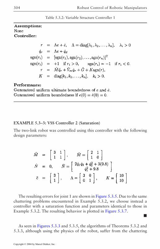
Robust Control of Robotic Manipulators304
The resulting errors for joint 1 are shown in Figure 5.3.5. Due to the samechattering problems encountered in Example 5.3.2, we choose instead acontroller with a saturation function and parameters identical to those inExample 5.3.2. The resulting behavior is plotted in Figure 5.3.7.
As seen in Figures 5.3.3 and 5.3.5, the algorithms of Theorems 5.3.2 and5.3.3, although using the physics of the robot, suffer from the chattering
Table 5.3.2: Variable Structure Controller 1
EXAMPLE 5.3–3: VSS Controller 2 (Saturation)
The two-link robot was controlled using this controller with the followingdesign parameters:
Copyright © 2004 by Marcel Dekker, Inc.
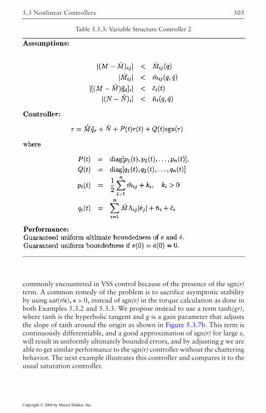
305
commonly encountered in VSS control because of the presence of the sgn(r)term. A common remedy of the problem is to sacrifice asymptotic stabilityby using sat(r/), > 0, instead of sgn(r) in the torque calculation as done inboth Examples 5.3.2 and 5.3.3. We propose instead to use a term tanh(gr),where tanh is the hyperbolic tangent and g is a gain parameter that adjuststhe slope of tanh around the origin as shown in Figure 5.3.7b. This term iscontinuously differentiable, and a good approximation of sgn(r) for large s,will result in uniformly ultimately bounded errors, and by adjusting g we areable to get similar performance to the sgn(r) controller without the chatteringbehavior. The next example illustrates this controller and compares it to theusual saturation controller.
Table 5.3.3: Variable Structure Controller 2
5.3 Nonlinear Controllers
Copyright © 2004 by Marcel Dekker, Inc.
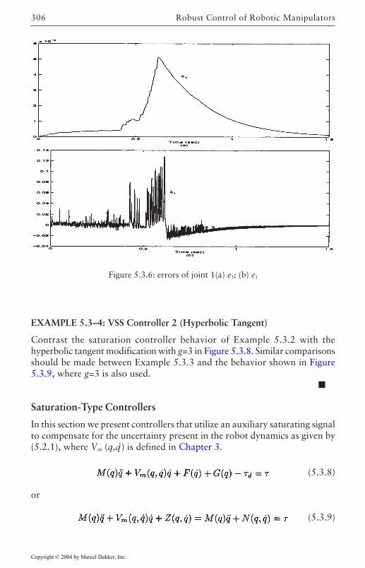
Robust Control of Robotic Manipulators306
EXAMPLE 5.3–4: VSS Controller 2 (Hyperbolic Tangent)
Contrast the saturation controller behavior of Example 5.3.2 with thehyperbolic tangent modification with g=3 in Figure 5.3.8. Similar comparisonsshould be made between Example 5.3.3 and the behavior shown in Figure5.3.9, where g=3 is also used.
Saturation-Type Controllers
In this section we present controllers that utilize an auxiliary saturating signalto compensate for the uncertainty present in the robot dynamics as given by(5.2.1), where Vm (q,q
.) is defined in Chapter 3.
(5.3.8)
or
(5.3.9)
Figure 5.3.6: errors of joint 1(a) e1; (b) e1
Copyright © 2004 by Marcel Dekker, Inc.
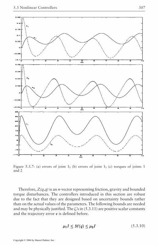
307
Therefore, Z(q,q) is an n-vector representing friction, gravity and boundedtorque disturbances. The controllers introduced in this section are robustdue to the fact that they are designed based on uncertainty bounds ratherthan on the actual values of the parameters. The following bounds are neededand may be physically justified. The i’s in (5.3.11) are positive scalar constantsand the trajectory error e is defined before.
(5.3.10)
Figure 5.3.7: (a) errors of joint 1; (b) errors of joint 1; (c) torques of joints 1and 2
5.3 Nonlinear Controllers
Copyright © 2004 by Marcel Dekker, Inc.
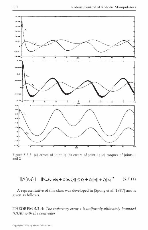
Robust Control of Robotic Manipulators308
(5.3.11)
A representative of this class was developed in [Spong et al. 1987] and isgiven as follows.
THEOREM 5.3–4: The trajectory error e is uniformly ultimately bounded(UUB) with the controller
Figure 5.3.8: (a) errors of joint 1; (b) errors of joint 1; (c) torques of joints 1and 2
Copyright © 2004 by Marcel Dekker, Inc.
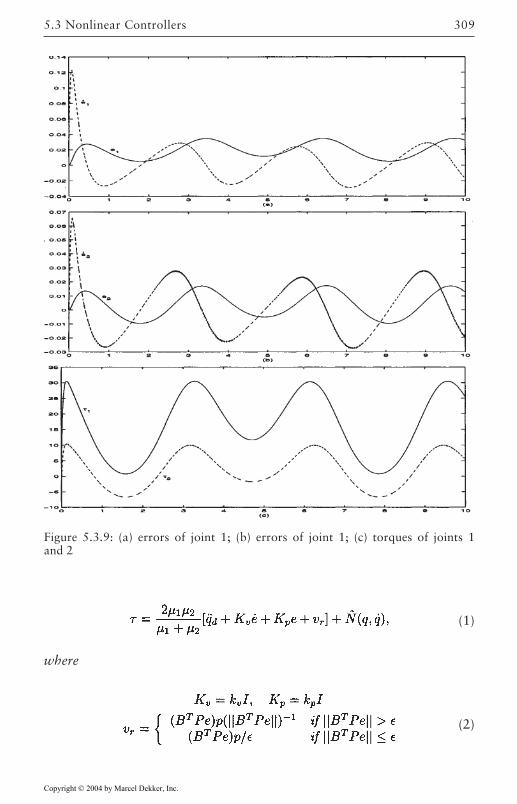
309
(1)
where
(2)
Figure 5.3.9: (a) errors of joint 1; (b) errors of joint 1; (c) torques of joints 1and 2
5.3 Nonlinear Controllers
Copyright © 2004 by Marcel Dekker, Inc.
Robust Control of Robotic Manipulators310
and
(3)
(4)
(5)
Proof:Choose the Lyapunov function
and proceed as in Theorem 2.10.4. See [Spong et al. 1987] for details.
Note that in the equations above, the matrix B is defined as in (5.2.3), thei’s are defined as in (5.2.10), and the matrix P is the symmetric, positive-definite solution of the lyapunov equation (5.3.12), where Q is symmetricand positive-definite matrix and Ac is given in (5.2.14).
(5.3.12)
In particular, the choice of Q
(5.3.13)
leads to the following P:
(5.3.14)
The expression of P in (5.3.14) may therefore be used in the expression ofvr in (2). This design is summarized in Table 5.3.4.
Copyright © 2004 by Marcel Dekker, Inc.
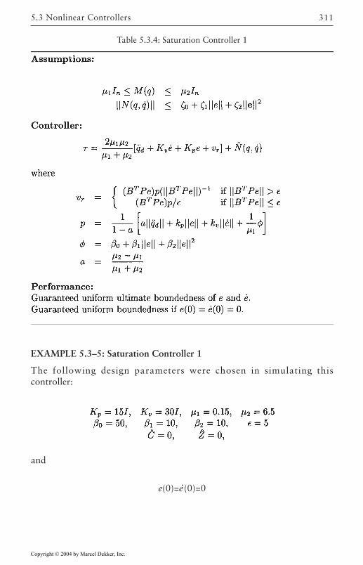
311
EXAMPLE 5.3–5: Saturation Controller 1
The following design parameters were chosen in simulating thiscontroller:
and
e(0)=e.(0)=0
Table 5.3.4: Saturation Controller 1
5.3 Nonlinear Controllers
Copyright © 2004 by Marcel Dekker, Inc.
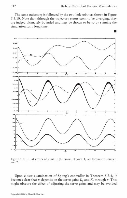
Robust Control of Robotic Manipulators312
Upon closer examination of Spong’s controller in Theorem 5.3.4, itbecomes clear that vr depends on the servo gains Kp and Kv through p. Thismight obscure the effect of adjusting the servo gains and may be avoided
The same trajectory is followed by the two-link robot as shown in Figure5.3.10. Note that although the trajectory errors seem to be diverging, theyare indeed ultimately bounded and may be shown to be so by running thesimulation for a long time.
Figure 5.3.10: (a) errors of joint 1; (b) errors of joint 1; (c) torques of joints 1and 2
Copyright © 2004 by Marcel Dekker, Inc.
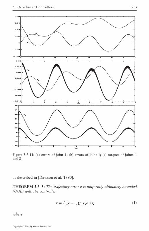
313
as described in [Dawson et al. 1990].
THEOREM 5.3–5: The trajectory error e is uniformly ultimately bounded(UUB) with the controller
(1)
where
Figure 5.3.11: (a) errors of joint 1; (b) errors of joint 1; (c) torques of joints 1and 2
5.3 Nonlinear Controllers
Copyright © 2004 by Marcel Dekker, Inc.
Robust Control of Robotic Manipulators314
and
(2)
where i’s are positive scalars.
Proof:We again choose
and
and proceed as in Theorem 2.10.4. See [Dawson et al. 1990] for details.
Note that p no longer contains the servo gains and, as such, one may adjustKp and Kv without tampering with the auxiliary control vr. As was also shownin [Dawson et al. 1990], if the initial error e(0)=0 and by choosing Kv=2Kp=kvI,the tracking error may be bounded by the following, which shows the directeffect of the control parameters on the tracking error:
(5.3.15)
Finally, note that if e(0)=e.(0)=0, the uniform boundedness of e(t) may bededuced. This controller is given in Table 5.3.5.
EXAMPLE 5.3–6: Saturation Controller 2
In this example, let
Copyright © 2004 by Marcel Dekker, Inc.
315
The results of this simulation are presented in Figure 5.3.11. The errorsare ultimately bounded as may be seen after a long simulation run.
Note that the last two controllers, although using a continuous term vr, may
be modified using the hyperbolic tangent term introduced in Example 5.3.4.In fact, there are many extensions to these types of controllers. A particularlysimple one that uses linearity of the dynamics with respect to the unknownphysical parameters of the robot 3.3.59 was given in (3.3.62), wherep=||W||
max. In this formulation, W is a matrix containing time-varying but
known terms, while is a vector of unknown but constant terms in thedynamic formulation (3.3.59) repeated here:
(5.3.16)
More on this formulation and its usage is presented in Chapter 6.
Table 5.3.5: Saturation Controller 2
5.3 Nonlinear Controllers
Copyright © 2004 by Marcel Dekker, Inc.
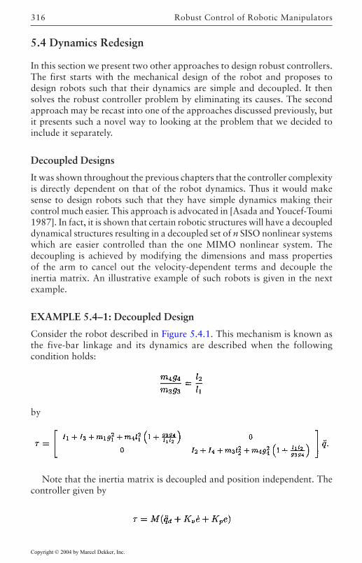
Robust Control of Robotic Manipulators316
5.4 Dynamics Redesign
In this section we present two other approaches to design robust controllers.The first starts with the mechanical design of the robot and proposes todesign robots such that their dynamics are simple and decoupled. It thensolves the robust controller problem by eliminating its causes. The secondapproach may be recast into one of the approaches discussed previously, butit presents such a novel way to looking at the problem that we decided toinclude it separately.
Decoupled Designs
It was shown throughout the previous chapters that the controller complexityis directly dependent on that of the robot dynamics. Thus it would makesense to design robots such that they have simple dynamics making theircontrol much easier. This approach is advocated in [Asada and Youcef-Toumi1987]. In fact, it is shown that certain robotic structures will have a decoupleddynamical structures resulting in a decoupled set of n SISO nonlinear systemswhich are easier controlled than the one MIMO nonlinear system. Thedecoupling is achieved by modifying the dimensions and mass propertiesof the arm to cancel out the velocity-dependent terms and decouple theinertia matrix. An illustrative example of such robots is given in the nextexample.
EXAMPLE 5.4–1: Decoupled Design
Consider the robot described in Figure 5.4.1. This mechanism is known asthe five-bar linkage and its dynamics are described when the followingcondition holds:
by
Note that the inertia matrix is decoupled and position independent. Thecontroller given by
Copyright © 2004 by Marcel Dekker, Inc.
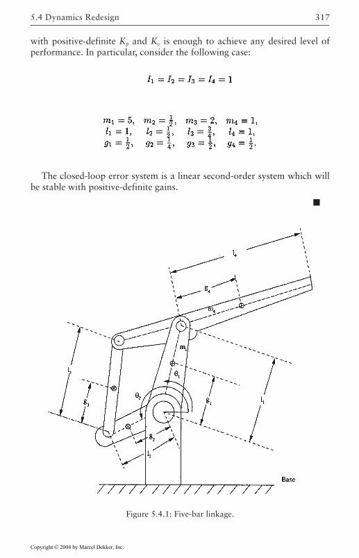
317
The closed-loop error system is a linear second-order system which willbe stable with positive-definite gains.
with positive-definite Kp and Kv is enough to achieve any desired level ofperformance. In particular, consider the following case:
Figure 5.4.1: Five-bar linkage.
5.4 Dynamics Redesign
Copyright © 2004 by Marcel Dekker, Inc.
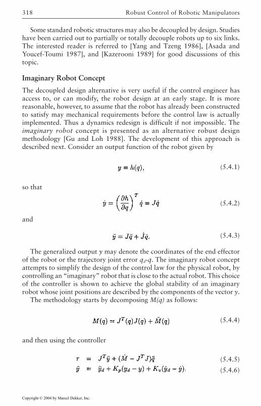
Robust Control of Robotic Manipulators318
Some standard robotic structures may also be decoupled by design. Studieshave been carried out to partially or totally decouple robots up to six links.The interested reader is referred to [Yang and Tzeng 1986], [Asada andYoucef-Toumi 1987], and [Kazerooni 1989] for good discussions of thistopic.
Imaginary Robot Concept
The decoupled design alternative is very useful if the control engineer hasaccess to, or can modify, the robot design at an early stage. It is morereasonable, however, to assume that the robot has already been constructedto satisfy may mechanical requirements before the control law is actuallyimplemented. Thus a dynamics redesign is difficult if not impossible. Theimaginary robot concept is presented as an alternative robust designmethodology [Gu and Loh 1988]. The development of this approach isdescribed next. Consider an output function of the robot given by
(5.4.1)
so that
(5.4.2)
and
(5.4.3)
The generalized output y may denote the coordinates of the end effectorof the robot or the trajectory joint error qd-q. The imaginary robot conceptattempts to simplify the design of the control law for the physical robot, bycontrolling an “imaginary” robot that is close to the actual robot. This choiceof the controller is shown to achieve the global stability of an imaginaryrobot whose joint positions are described by the components of the vector y.
The methodology starts by decomposing M(q) as follows:
(5.4.4)
and then using the controller
(5.4.5)
(5.4.6)
Copyright © 2004 by Marcel Dekker, Inc.
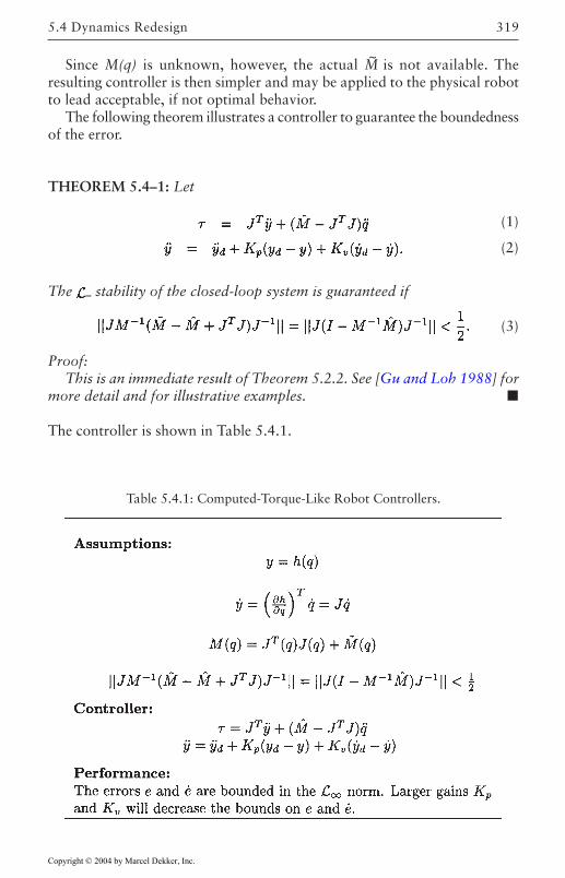
319
Since M(q) is unknown, however, the actual M~
is not available. Theresulting controller is then simpler and may be applied to the physical robotto lead acceptable, if not optimal behavior.
The following theorem illustrates a controller to guarantee the boundednessof the error.
THEOREM 5.4–1: Let
(1)
(2)
The ∞ stability of the closed-loop system is guaranteed if
(3)
Proof:This is an immediate result of Theorem 5.2.2. See [Gu and Loh 1988] for
more detail and for illustrative examples.
The controller is shown in Table 5.4.1.
Table 5.4.1: Computed-Torque-Like Robot Controllers.
5.4 Dynamics Redesign
Copyright © 2004 by Marcel Dekker, Inc.
Robust Control of Robotic Manipulators320
5.5 Summary
The design of robust motion controllers of rigid robots was reviewed. Theremain designs were identified and explained. All controllers were robust withrespect to a range of uncertain parameters and will guarantee theboundedness of the position-tracking error. In the presence of disturbancetorques, a bounded error is best achievable outcome. The question of whichrobust control method to choose is difficult to answer analytically, but thefollowing guidelines are suggested. The linear-multivariable approach isuseful when linear performance specifications (percent overshoot, dampingratio, etc.) are available. The one-DOF dynamic compensators performedrather well, with little or no knowledge of the robot dynamics. They may,however, result in high-gain control laws in the attempt to achieverobustness. The passive controllers are easy to implement but do notprovide easily quantifiable performance measures. The modified variable-structure controllers seem to preform well when using the physics of therobot without excessive torque effort. The saturation controllers are mostuseful when a short transient error can be tolerated, but ultimately, the errorwill have to be bounded.
A common thread throughout this chapter has been the fact that a high-gain controller will guarantee the robustness of the closed-loop system. Thechallenge is, however, to guarantee the robust stability of the robot withoutrequiring excessive torques. The robustness of the motion controllers whennonzero initial errors or disturbances are present was also verified throughsome of the examples and is discussed in the problems at the end of thechapter. It is useful to note that although the robot’s dynamics are highlynonlinear, most successful controllers have exploited their physics and theirvery special structure. In the next chapter we describe the design of adaptivecontrollers in the case of uncertain dynamical description of the robots.
Copyright © 2004 by Marcel Dekker, Inc.
321
REFERENCES
[Abdallah et al. 1991] C.T.Abdallah and D.Dawson and P.Dorato and M. Jamshidi.“Survey of Robust Control for Rigid Robots”. IEEE Control Syst. Mag., vol.11, number 2, pp. 24–30, 1991.
[Anderson 1989] R.J.Anderson. “A Network Approach to Force Control in Roboticsand Teleoperation”. Ph.D. Thesis, Departemnt of Electrical & ComputerEngineering. University of Illinois at Urbana-Champaign, 1989.
[Arimoto and Miyazaki 1985] S.Arimoto and F.Miyazaki. “Stabiliy and Robustnessof PID Feedback Control for Robot Manipulators of Sensory Capability”. Proc.Third Int. Symp. Robot. Res., Gouvieux, France. July, 1985.
[Asada and Youcef-Toumi 1987] H.Asada and K.Youcef-Toumi. “Direct-Drive Robots:Theory and Practice”. MIT Press, Cambridge, MA, 1987.
[Becker and Grimm 1988] N.Becker and W.M.Grimm. “On L2 and L8 StabilityApproaches for the Robust Control of Robot Manipulators”. IEEE Trans. Autom.Control, vol. 33, number 1, pp. 118–122, January, 1988.
[Canudas de Wit and Fixot 1991] C.Canudas de Wit and N.Fixot. “Robot Controlvia Robust Estimated State Feedback”. IEEE Trans. Autom. Control, vol. 36,number 12, pp. 1497–1501, December, 1991.
[Chen 1989] Y.Chen. “Replacing a PID Controller by a Lag-Lead Compensator for aRobot: A Frequency Response Approach”. IEEE Trans. Robot. Autom. vol. 5,number 2, pp. 174–182, April, 1989.
[Chen et al. 1990] Y-F Chen and T.Mita and S.Wahui. “A New and simple Algorithmfor Sliding Mode Control of Robot Arms”. IEEE Trans. Autom. Control, vol.35, number 7, pp. 828–829, 1990.
[Corless 1989] M.Corless. “Tracking Controllers for Uncertain Systems: Applicationto a Manutec R3 Robot”. J. Dyn. Syst. Meas. Control vol. 111, pp. 609–618,December, 1989.
[Craig 1988] J.J.Craig. “Adaptive Control of Mechanical Manipulators”. Addis on-Wesley, Reading, MA, 1988.
Copyright © 2004 by Marcel Dekker, Inc.
REFERENCES322
[Dawson et al. 1990] D.M.Dawson et. al. “Robust Control for the Tracking of RobotMotion”. Int. J. Control, vol. 52, number 3, pp. 581–595, 1990.
[DeCarlo et al. 1988] R.A.DeCarlo and S.H.Zak and G.P.Matthews. “VariableStructure Control of Nonlinear Multivariable Systems”. IEEE Proc. vol. 76,number 3, pp. 212–232, March, 1988.
[Freund 1982] E.Freund. “Fast Nonlinear Control with Arbitrary Pole-Placement forIndustrial Robots and Manipulators”. Int. J. Robot. Res. vol. 1, number 1, pp.65–78, 1982.
[Gu and Loh 1988] Y-L.Gu and N.K.Loh. “Dynamic Modeling and Control byUtilizing an Imaginary Robot Model”. IEEE Trans. Rob. Aut. vol. 4, number 5,1988.
[Kazerooni 1989] H.Kazerooni. “Design and Analysis of a Statically Balanced Direct-Drive Manipulator”. IEEE Control Syst. Mag. vol. 9, number 2, pp. 30–34,February, 1989.
[Luh 1983] J.Y.S.Luh. “Conventional Controller Design for Industrial Robots: ATutorial”. IEEE Trans. Syst. Man Cybern. vol. 13, pp. 298–316, May-June,1983.
[Ortega and Spong 1988] R.Ortega and M.W.Spong. “Adaptive Motion Control ofRigid Robots: A Tutorial”. Proc. IEEE Conf. Decision Control, Austin, TX,December, 1988.
[Slotine 1985] J-J.E.Slotine. “The Robust Control of Robot Manipulators”. Int. J.Rob. Res. vol. 4, number 4, pp. 49–64, 1985.
[Slotine 1988] J-J.E.Slotine. “Putting Physics Back in Control: The Example ofRobotics”. IEEE Contr. Syst. Mag. vol. 8, number 7, pp. 12–17, December,1988.
[Spong and Vidyasagar 1987] M.W.Spong and M.Vidyasagar. “Robust LinearCompensator Design for Nonlinear Robotic Control”. IEEE Trans. Robot.Autom. vol. 3, number 4, pp. 345–351, August, 1987.
[Spong et al. 1987] M.W.Spong and J.S.Thorp and J.M.Kleinwaks. “RobustMicroprocessor Control of Robot Manipulators”. Automatica. vol. 23, number3, pp. 373–379, 1987.
[Sugie et al. 1988] T.Sugie et. al. “Robust Controller Design for Robot Manipulators”.Trans. ASME Dyn. Syst. Meas. Control, vol. 110, number 1, pp. 94–96, March,1988.
[Tarn et al. 1984] T.J.Tarn and A.K.Bejczy and A.Isidori and Y.Chen. “NonlinearFeedback in Robot Arm Control”. Proc. IEEE Conf. Decision Control, LasVegas, NV. December, 1984.
[Utkin 1977] V.I. Utkin. “Variable Structure Systems with Sliding Modes”. IEEETRans. Autom. Control vol. 22, pp. 212–222, April, 1977.
Copyright © 2004 by Marcel Dekker, Inc.
323REFERENCES
[Vidyasagar 1985] M.Vidyasagar. “Control Systems Synthesis: A FactorizationApproach”. MIT Press, Cambridge, MA. 1985.
[Yang and Tzeng 1986] D.C-H.Yang and S.W.Tzeng. “Simplification and Linearizationof Manipulator Dynamics by the Design of Inertia Distribution”. Int. J. Rob.Res. vol. 5, number 3, pp. 120–128, 1986.
[Yeung and Chen 1988] K.S.Yeung and Y.P.Chen. “A New Controller Design forManipulators Using the Theory of Variable Structure Systems”. IEEE Trans.Autom. Control, vol. 33, number 2, pp. 200–206, February, 1988.
[Young 1978] K-K.D.Young. “Controller Design for a Manipulator Using theory ofVariale Structure Systems”. IEEE Trans. Syst. Man Cybern. vol. 8, number 2,pp. 210–218, February, 1978.
Copyright © 2004 by Marcel Dekker, Inc.
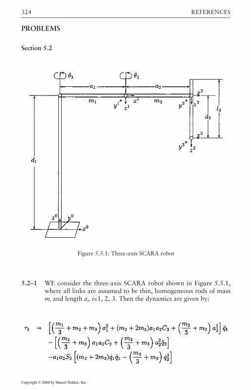
REFERENCES324
5.2–1 WE consider the three-axis SCARA robot shown in Figure 5.5.1,where all links are assumed to be thin, homogeneous rods of massmi and length ai, i=1, 2, 3. Then the dynamics are given by:
Figure 5.5.1: Three-axis SCARA robot
PROBLEMS
Section 5.2
Copyright © 2004 by Marcel Dekker, Inc.
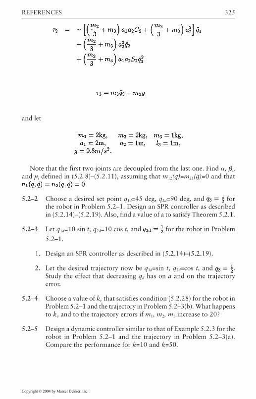
325REFERENCES
and let
Note that the first two joints are decoupled from the last one. Find , i,and µi defined in (5.2.8)–(5.2.11), assuming that m12(q)=m21(q)=0 and that
5.2–2 Choose a desired set point q1d=45 deg, q2d=90 deg, and forthe robot in Problem 5.2–1. Design an SPR controller as describedin (5.2.14)–(5.2.19). Also, find a value of a to satisfy Theorem 5.2.1.
5.2–3 Let q1d=10 sin t, q2d=10 cos t, and for the robot in Problem
5.2–1.
1. Design an SPR controller as described in (5.2.14)–(5.2.19).
2. Let the desired trajectory now be q1d=sin t, q2d=cos t, and .Study the effect that decreasing qd has on a and on the trajectoryerror.
5.2–4 Choose a value of kv that satisfies condition (5.2.28) for the robot inProblem 5.2–1 and the trajectory in Problem 5.2–3(b). What happensto kv and to the trajectory errors if m1, m2, m3 increase to 20?
5.2–5 Design a dynamic controller similar to that of Example 5.2.3 for therobot in Problem 5.2–1 and the trajectory in Problem 5.2–3(a).Compare the performance for k=10 and k=50.
Copyright © 2004 by Marcel Dekker, Inc.
REFERENCES326
5.2–6 Find the value of k that satisfies inequality (1) for you design inProblem 5.2–5. What happens to your conditions if both the velocityterms and gravity terms are available to feedback (i.e., i=0)?
5.2–7 Consider the robot in Problem 5.2–1 and the set point of Problem5.2–2. Also, assume that all i=0 so that velocity and gravity termsare available to feedback. Find a gain k to satisfy (5.2.36) andimplement the resulting controller.
5.2–8 Repeat Problem 5.2–7 with the trajectory of Problem 5.2–3(a).
5.2–9 Design a controller similar to the one in Example 5.2.5 for the robotof Problem 5.2–1 to follow the trajectory of Problem 5.2–3(a).Choose the same parameters used in that example and compare theresulting behavior to a set of parameters of your choosing.
Section 5.3
5.3–1 Design a controller similar to the one in Example 5.3.1 for the robotof Problem 5.2–1 to follow the trajectory of Problem 5.2–3(a).Choose the same parameters used in that example and compare theresulting behavior to a set of parameters of your choosing.
5.3–2 Consider the robot of Problem 5.2–1 with the desired set point ofProblem 5.2–2. Design a variable-structure controller as describedin Theorem 5.3.2. You may want to start your design with theparameter values in Example 5.3.2.
5.3–3 Repeat Problem 5.3–2 for the trajectory described in Problem 5.2–3(a).
5.3–4 Consider the robot of Problem 5.2–1 with the desired set point ofProblem 5.2–2. Design a variable-structure controller as describedin Theorem 5.3.3. You may want to start your design with theparameter values in Example 5.3.3.
5.3–5 Repeat Problem 5.3–4 for the trajectory described in Problem 5.2–3(a).
5.3–6 Consider the robot of Problem 5.2–1 with the desired set point ofProblem 5.2–2. Design a saturation-type controller as described inTheorem 5.3.4. You may want to start your design with theparameter values in Example 5.3.5.
Copyright © 2004 by Marcel Dekker, Inc.
327REFERENCES
5.3–7 Repeat Problem 5.3–6 for the trajectory described in Problem 5.2–3(a).
5.3–8 Consider the robot of Problem 5.2–1 with the desired set point ofProblem 5.2–2. Design a saturation-type controller as described inTheorem 5.3.5. You man want to start your design with theparameter values in Example 5.3.6.
5.3–9 Repeat Problem 5.3–8 for the trajectory described in Problem 5.2–3(a).
Copyright © 2004 by Marcel Dekker, Inc.
329
Chapter 6
Adaptive Control ofRobotic Manipulators
In this chapter adaptive controllers are formulated by separating unknownconstant parameters from known functions in the robot dynamic equation.The type of stability for each adaptive control strategy is discussed at lengthto motivate the formulation of the controllers. Some issues regardingparameter error convergence, persistency of excitation, and robustness arealso discussed.
6.1 Introduction
The problem of designing adaptive control laws for rigid-robot manipulatorsthat ensure asymptotic trajectory tracking has interested researchers for manyyears. The development of effective adaptive controllers represents animportant step toward high-speed/precision robotic applications. Even in awell-structured industrial facility, robots may face uncertainty regarding theparameters describing the dynamic properties of the grasp load (e.g., unknownmoments of inertia). Since these parameters are difficult to compute ormeasure, they limit the potential for robots to manipulate accurately objectsof considerable size and weight. It has recently been recognized that theaccuracy of conventional approaches in high-speed applications is greatlyaffected by parametric uncertainties.
To compensate for this parametric uncertainty, many researchers haveproposed adaptive strategies for the control of robotic manipulators. Anadvantage of the adaptive approach over the robust control strategiesdiscussed in Chapter 5 is that the accuracy of a manipulator carrying unknown
Copyright © 2004 by Marcel Dekker, Inc.
Adaptive Control of Robotic Manipulators330
extracting information from the tracking error. Therefore, adaptive controllerscan give consistent performance in the face of load variations.
It is only recently that adaptive control results have included rigorousproofs for global convergence of the tracking error. Now that the existenceof globally convergent adaptive control laws has been established, it is difficultto justify control schemes based on approximate models, local linearizationtechniques, or slowly time varying assumptions. In the control literaturethere also seems to be no general agreement as to what constitutes an adaptivecontrol algorithm; therefore, in this chapter, the discussion will be limited tocontrol schemes that explicitly incorporate parameter estimation in the controllaw.
6.2 Adaptive Control by a Computed-TorqueApproach
In Chapter 3 we motivated the use of the computed-torque control law forcontrolling the robotic manipulator dynamics given by
(6.2.1)
This motivation was actually quite simple. Specifically, if there are somenonlinear dynamics which one does not wish to deal with, one can changethe nonlinear control problem to a linear control problem by directly cancelingthe nonlinearities. There is a wealth of available knowledge for controllinglinear systems; therefore, if exact knowledge of the robot model is available,there is not much need for sophisticated nonlinear control techniques.
Approximate Computed-Torque Controller
Of course, in reality, we never have exact knowledge of the robot model dueto many problems associated with model formulation. Two commonuncertainties that do not allow exact model cancellation in roboticapplications are unknown link masses due to payload disturbances andunknown friction coefficients. One way of dealing with these types ofparametric uncertainties would be to use the computed-torque controllergiven in Chapter 3 with some fixed estimate of the unknown parameters inplace of the actual parameters. This approximate computed-torque controllerwould have the form
(6.2.2)
Copyright © 2004 by Marcel Dekker, Inc.
loads improves with time because the adaptation mechanism continues
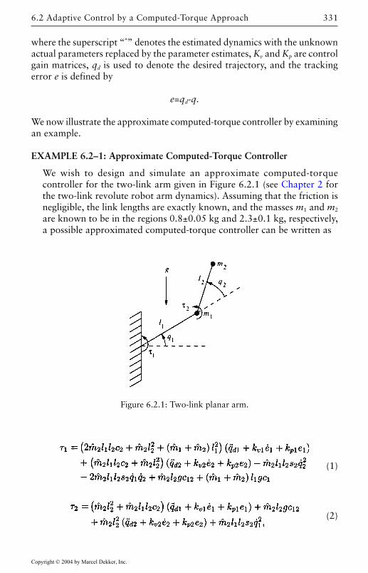
331
where the superscript “ˆ” denotes the estimated dynamics with the unknownactual parameters replaced by the parameter estimates, Kv and Kp are controlgain matrices, qd is used to denote the desired trajectory, and the trackingerror e is defined by
e=qd-q.
We now illustrate the approximate computed-torque controller by examiningan example.
EXAMPLE 6.2–1: Approximate Computed-Torque Controller
We wish to design and simulate an approximate computed-torquecontroller for the two-link arm given in Figure 6.2.1 (see Chapter 2 forthe two-link revolute robot arm dynamics). Assuming that the friction isnegligible, the link lengths are exactly known, and the masses m1 and m2
are known to be in the regions 0.8±0.05 kg and 2.3±0.1 kg, respectively,a possible approximated computed-torque controller can be written as
(1)
(2)
Figure 6.2.1: Two-link planar arm.
6.2 Adaptive Control by a Computed-Torque Approach
Copyright © 2004 by Marcel Dekker, Inc.
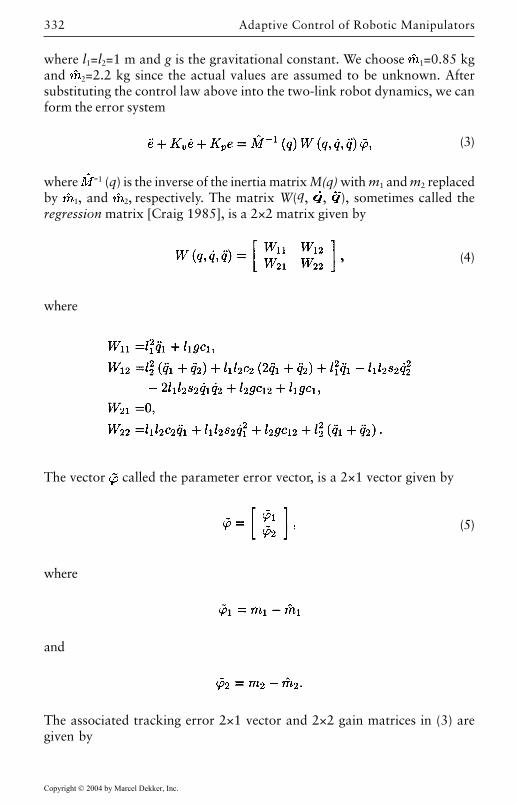
Adaptive Control of Robotic Manipulators332
where l1=l2=1 m and g is the gravitational constant. We choose 1=0.85 kgand 2=2.2 kg since the actual values are assumed to be unknown. Aftersubstituting the control law above into the two-link robot dynamics, we canform the error system
(3)
where -1 (q) is the inverse of the inertia matrix M(q) with m1 and m2 replacedby 1, and 2, respectively. The matrix W(q, , ), sometimes called theregression matrix [Craig 1985], is a 2×2 matrix given by
(4)
where
The vector called the parameter error vector, is a 2×1 vector given by
(5)
where
and
The associated tracking error 2×1 vector and 2×2 gain matrices in (3) aregiven by
,
Copyright © 2004 by Marcel Dekker, Inc.
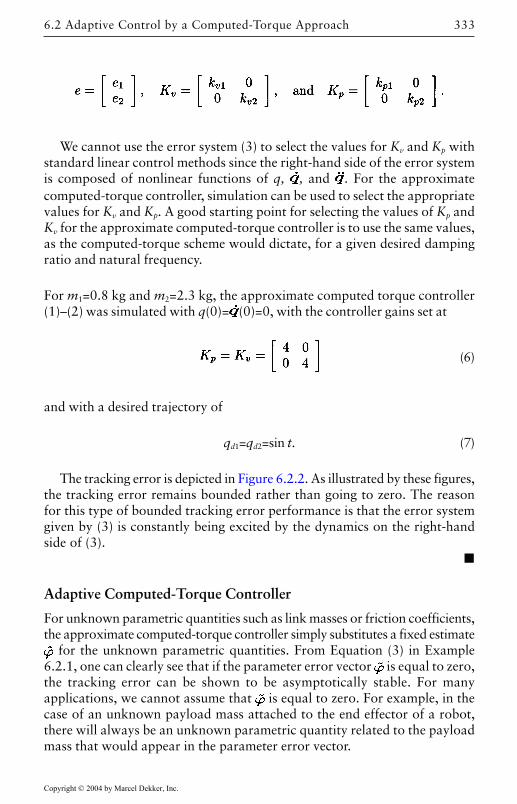
333
We cannot use the error system (3) to select the values for Kv and Kp withstandard linear control methods since the right-hand side of the error systemis composed of nonlinear functions of q, , and . For the approximatecomputed-torque controller, simulation can be used to select the appropriatevalues for Kv and Kp. A good starting point for selecting the values of Kp andKv for the approximate computed-torque controller is to use the same values,as the computed-torque scheme would dictate, for a given desired dampingratio and natural frequency.
For m1=0.8 kg and m2=2.3 kg, the approximate computed torque controller(1)–(2) was simulated with q(0)= (0)=0, with the controller gains set at
(6)
and with a desired trajectory of
qd1=qd2=sin t. (7)
The tracking error is depicted in Figure 6.2.2. As illustrated by these figures,the tracking error remains bounded rather than going to zero. The reasonfor this type of bounded tracking error performance is that the error systemgiven by (3) is constantly being excited by the dynamics on the right-handside of (3).
Adaptive Computed-Torque Controller
For unknown parametric quantities such as link masses or friction coefficients,the approximate computed-torque controller simply substitutes a fixed estimate
for the unknown parametric quantities. From Equation (3) in Example6.2.1, one can clearly see that if the parameter error vector is equal to zero,the tracking error can be shown to be asymptotically stable. For manyapplications, we cannot assume that is equal to zero. For example, in thecase of an unknown payload mass attached to the end effector of a robot,there will always be an unknown parametric quantity related to the payloadmass that would appear in the parameter error vector.
6.2 Adaptive Control by a Computed-Torque Approach
Copyright © 2004 by Marcel Dekker, Inc.
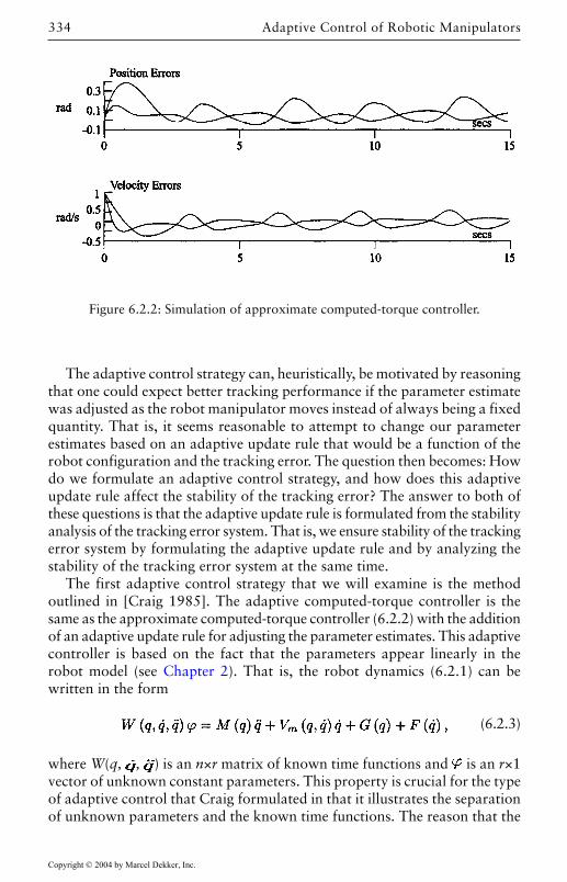
Adaptive Control of Robotic Manipulators334
The adaptive control strategy can, heuristically, be motivated by reasoningthat one could expect better tracking performance if the parameter estimatewas adjusted as the robot manipulator moves instead of always being a fixedquantity. That is, it seems reasonable to attempt to change our parameterestimates based on an adaptive update rule that would be a function of therobot configuration and the tracking error. The question then becomes: Howdo we formulate an adaptive control strategy, and how does this adaptiveupdate rule affect the stability of the tracking error? The answer to both ofthese questions is that the adaptive update rule is formulated from the stabilityanalysis of the tracking error system. That is, we ensure stability of the trackingerror system by formulating the adaptive update rule and by analyzing thestability of the tracking error system at the same time.
The first adaptive control strategy that we will examine is the methodoutlined in [Craig 1985]. The adaptive computed-torque controller is thesame as the approximate computed-torque controller (6.2.2) with the additionof an adaptive update rule for adjusting the parameter estimates. This adaptivecontroller is based on the fact that the parameters appear linearly in therobot model (see Chapter 2). That is, the robot dynamics (6.2.1) can bewritten in the form
(6.2.3)
where W(q, , ) is an n×r matrix of known time functions and is an r×1vector of unknown constant parameters. This property is crucial for the typeof adaptive control that Craig formulated in that it illustrates the separationof unknown parameters and the known time functions. The reason that the
Figure 6.2.2: Simulation of approximate computed-torque controller.
Copyright © 2004 by Marcel Dekker, Inc.
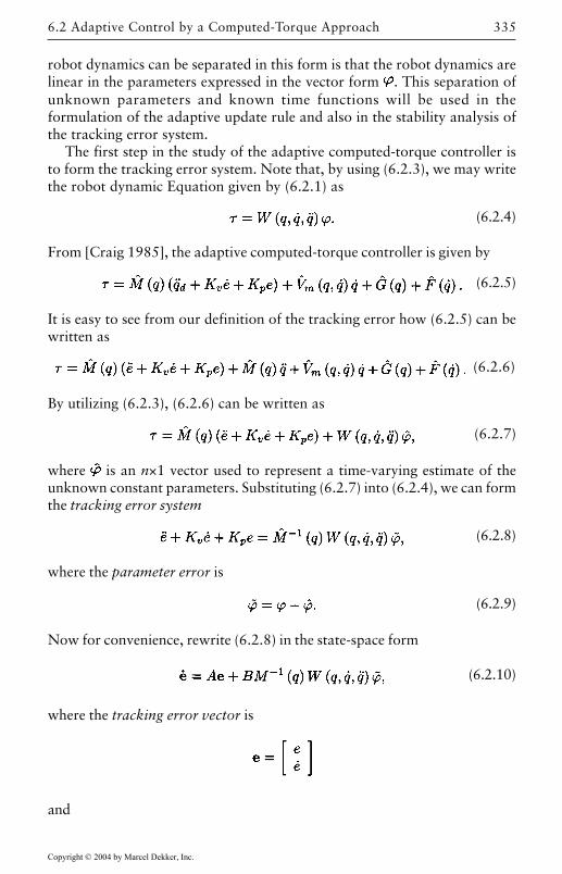
335
robot dynamics can be separated in this form is that the robot dynamics arelinear in the parameters expressed in the vector form . This separation ofunknown parameters and known time functions will be used in theformulation of the adaptive update rule and also in the stability analysis ofthe tracking error system.
The first step in the study of the adaptive computed-torque controller isto form the tracking error system. Note that, by using (6.2.3), we may writethe robot dynamic Equation given by (6.2.1) as
(6.2.4)
From [Craig 1985], the adaptive computed-torque controller is given by
(6.2.5)
It is easy to see from our definition of the tracking error how (6.2.5) can bewritten as
(6.2.6)
By utilizing (6.2.3), (6.2.6) can be written as
(6.2.7)
where is an n×1 vector used to represent a time-varying estimate of theunknown constant parameters. Substituting (6.2.7) into (6.2.4), we can formthe tracking error system
(6.2.8)
where the parameter error is
(6.2.9)
Now for convenience, rewrite (6.2.8) in the state-space form
(6.2.10)
where the tracking error vector is
and
6.2 Adaptive Control by a Computed-Torque Approach
Copyright © 2004 by Marcel Dekker, Inc.
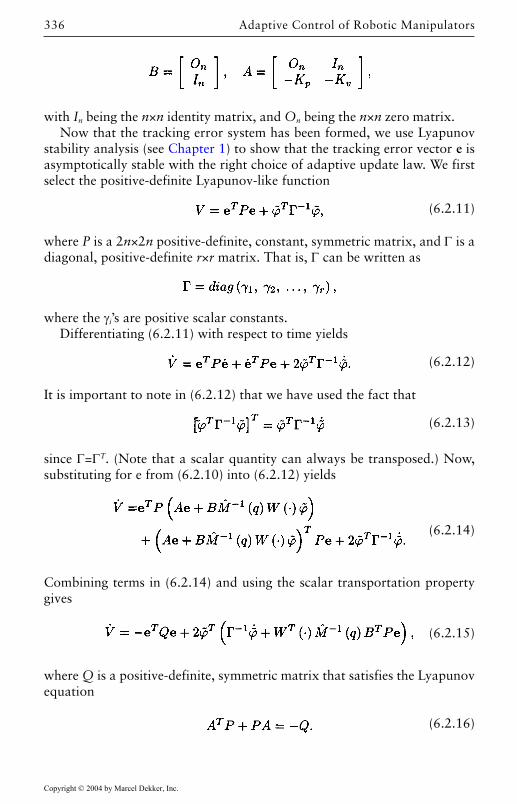
Adaptive Control of Robotic Manipulators336
with In being the n×n identity matrix, and On being the n×n zero matrix.Now that the tracking error system has been formed, we use Lyapunov
stability analysis (see Chapter 1) to show that the tracking error vector e isasymptotically stable with the right choice of adaptive update law. We firstselect the positive-definite Lyapunov-like function
(6.2.11)
where P is a 2n×2n positive-definite, constant, symmetric matrix, and Γ is adiagonal, positive-definite r×r matrix. That is, Γ can be written as
where the γi’s are positive scalar constants.Differentiating (6.2.11) with respect to time yields
(6.2.12)
It is important to note in (6.2.12) that we have used the fact that
(6.2.13)
since Γ=ΓT. (Note that a scalar quantity can always be transposed.) Now,substituting for e from (6.2.10) into (6.2.12) yields
(6.2.14)
Combining terms in (6.2.14) and using the scalar transportation propertygives
(6.2.15)
where Q is a positive-definite, symmetric matrix that satisfies the Lyapunovequation
(6.2.16)
Copyright © 2004 by Marcel Dekker, Inc.
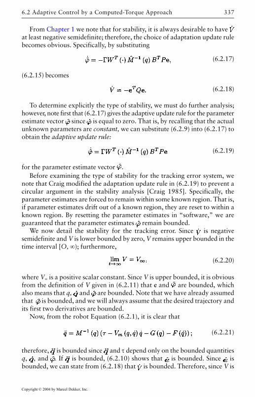
337
From Chapter 1 we note that for stability, it is always desirable to have at least negative semidefinite; therefore, the choice of adaptation update rulebecomes obvious. Specifically, by substituting
(6.2.17)
(6.2.15) becomes
(6.2.18)
To determine explicitly the type of stability, we must do further analysis;however, note first that (6.2.17) gives the adaptive update rule for the parameterestimate vector since is equal to zero. That is, by recalling that the actualunknown parameters are constant, we can substitute (6.2.9) into (6.2.17) toobtain the adaptive update rule:
(6.2.19)
for the parameter estimate vector .Before examining the type of stability for the tracking error system, we
note that Craig modified the adaptation update rule in (6.2.19) to prevent acircular argument in the stability analysis [Craig 1985]. Specifically, theparameter estimates are forced to remain within some known region. That is,if parameter estimates drift out of a known region, they are reset to within aknown region. By resetting the parameter estimates in “software,” we areguaranteed that the parameter estimates remain bounded.
We now detail the stability for the tracking error. Since is negativesemidefinite and V is lower bounded by zero, V remains upper bounded in thetime interval [O, ∞); furthermore,
(6.2.20)
where V∞ is a positive scalar constant. Since V is upper bounded, it is obviousfrom the definition of V given in (6.2.11) that e and are bounded, whichalso means that q, and are bounded. Note that we have already assumedthat is bounded, and we will always assume that the desired trajectory andits first two derivatives are bounded.
Now, from the robot Equation (6.2.1), it is clear that
(6.2.21)
therefore, is bounded since and τ depend only on the bounded quantitiesq, , and . If is bounded, (6.2.10) shows that is bounded. Since isbounded, we can state from (6.2.18) that is bounded. Therefore, since V is
6.2 Adaptive Control by a Computed-Torque Approach
Copyright © 2004 by Marcel Dekker, Inc.
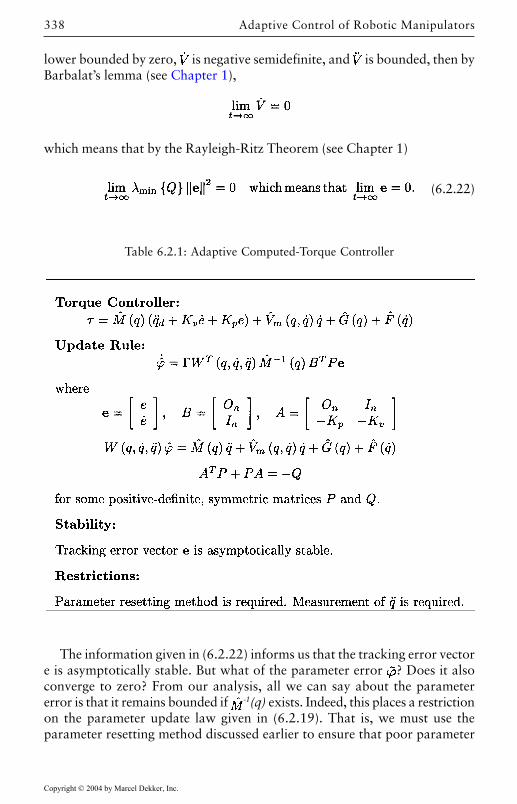
Adaptive Control of Robotic Manipulators338
lower bounded by zero, is negative semidefinite, and is bounded, then byBarbalat’s lemma (see Chapter 1),
which means that by the Rayleigh-Ritz Theorem (see Chapter 1)
(6.2.22)
Table 6.2.1: Adaptive Computed-Torque Controller
The information given in (6.2.22) informs us that the tracking error vectore is asymptotically stable. But what of the parameter error ? Does it alsoconverge to zero? From our analysis, all we can say about the parametererror is that it remains bounded if -1(q) exists. Indeed, this places a restrictionon the parameter update law given in (6.2.19). That is, we must use theparameter resetting method discussed earlier to ensure that poor parameter
Copyright © 2004 by Marcel Dekker, Inc.
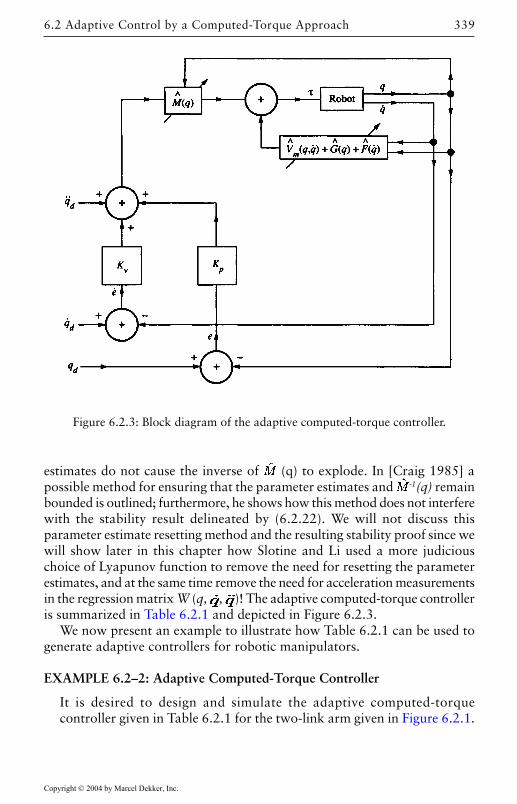
339
estimates do not cause the inverse of (q) to explode. In [Craig 1985] apossible method for ensuring that the parameter estimates and -1(q) remainbounded is outlined; furthermore, he shows how this method does not interferewith the stability result delineated by (6.2.22). We will not discuss thisparameter estimate resetting method and the resulting stability proof since wewill show later in this chapter how Slotine and Li used a more judiciouschoice of Lyapunov function to remove the need for resetting the parameterestimates, and at the same time remove the need for acceleration measurementsin the regression matrix W (q, , )! The adaptive computed-torque controlleris summarized in Table 6.2.1 and depicted in Figure 6.2.3.
We now present an example to illustrate how Table 6.2.1 can be used togenerate adaptive controllers for robotic manipulators.
EXAMPLE 6.2–2: Adaptive Computed-Torque Controller
It is desired to design and simulate the adaptive computed-torquecontroller given in Table 6.2.1 for the two-link arm given in Figure 6.2.1.
Figure 6.2.3: Block diagram of the adaptive computed-torque controller.
6.2 Adaptive Control by a Computed-Torque Approach
Copyright © 2004 by Marcel Dekker, Inc.
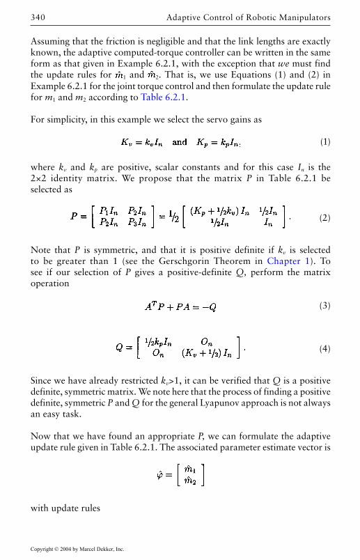
Adaptive Control of Robotic Manipulators340
Assuming that the friction is negligible and that the link lengths are exactlyknown, the adaptive computed-torque controller can be written in the sameform as that given in Example 6.2.1, with the exception that we must findthe update rules for 1 and 2. That is, we use Equations (1) and (2) inExample 6.2.1 for the joint torque control and then formulate the update rulefor m1 and m2 according to Table 6.2.1.
For simplicity, in this example we select the servo gains as
(1)
where kv and kp are positive, scalar constants and for this case In is the2×2 identity matrix. We propose that the matrix P in Table 6.2.1 beselected as
(2)
Note that P is symmetric, and that it is positive definite if kv is selectedto be greater than 1 (see the Gerschgorin Theorem in Chapter 1). Tosee if our selection of P gives a positive-definite Q, perform the matrixoperation
(3)
(4)
Since we have already restricted kv>1, it can be verified that Q is a positivedefinite, symmetric matrix. We note here that the process of finding a positivedefinite, symmetric P and Q for the general Lyapunov approach is not alwaysan easy task.
Now that we have found an appropriate P, we can formulate the adaptiveupdate rule given in Table 6.2.1. The associated parameter estimate vector is
with update rules
Copyright © 2004 by Marcel Dekker, Inc.
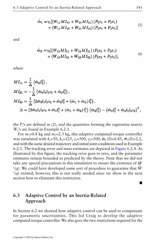
341
(5)
and
(6)
where
the Pi’s are defined in (2), and the quantities forming the regression matrixWii’s are found in Example 6.2.1.
For m1=0.8 kg and m2=2.3 kg, this adaptive computed-torque controllerwas simulated with kv=50, kp=125, γ1=500, γ2=500, 1 (0)=0.85, 2(0)=2.2,and with the same desired trajectory and initial joint conditions used in Example6.2.1. The tracking error and mass estimates are depicted in Figure 6.2.4. Asillustrated by this figure, the tracking error goes to zero, and the parameterestimates remain bounded as predicted by the theory. Note that we did nottake any special precautions in this simulation to ensure the existence of -
1(q). We could have developed some sort of procedure to guarantee that -
1(q) existed; however, this is not really needed since we show in the nextsection how to eliminate this restriction.
6.3 Adaptive Control by an Inertia-RelatedApproach
In Section 6.2 we showed how adaptive control can be used to compensatefor parametric uncertainties. This led Craig to develop the adaptivecomputed-torque controller. We also gave the two restrictions required for the
6.3 Adaptive Control by an Inertia-Related Approach
Copyright © 2004 by Marcel Dekker, Inc.
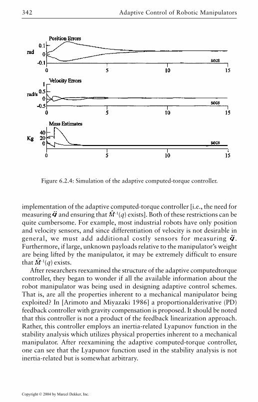
Adaptive Control of Robotic Manipulators342
implementation of the adaptive computed-torque controller [i.e., the need formeasuring and ensuring that -1(q) exists]. Both of these restrictions can bequite cumbersome. For example, most industrial robots have only positionand velocity sensors, and since differentiation of velocity is not desirable ingeneral, we must add additional costly sensors for measuring .Furthermore, if large, unknown payloads relative to the manipulator’s weightare being lifted by the manipulator, it may be extremely difficult to ensurethat -1(q) exists.
After researchers reexamined the structure of the adaptive computedtorquecontroller, they began to wonder if all the available information about therobot manipulator was being used in designing adaptive control schemes.That is, are all the properties inherent to a mechanical manipulator beingexploited? In [Arimoto and Miyazaki 1986] a proportionalderivative (PD)feedback controller with gravity compensation is proposed. It should be notedthat this controller is not a product of the feedback linearization approach.Rather, this controller employs an inertia-related Lyapunov function in thestability analysis which utilizes physical properties inherent to a mechanicalmanipulator. After reexamining the adaptive computed-torque controller,one can see that the Lyapunov function used in the stability analysis is notinertia-related but is somewhat arbitrary.
Figure 6.2.4: Simulation of the adaptive computed-torque controller.
Copyright © 2004 by Marcel Dekker, Inc.
343
Examination of a PD Plus Gravity Controller
One method [Slotine 1988] of motivating a PD plus gravity controller [Arimotoand Miyazaki 1986] is to write the manipulator dynamics in the conservation-of-energy form
(6.3.1)
where the left-hand side of (6.3.1) is the derivative of the manipulator kineticenergy, and the right-hand side of (6.3.1) represents the power supplied fromthe actuators minus the power dissipated due to gravity and friction. Notethat the Coriolis and centripetal terms are accounted for in (6.3.1) sincethese terms are related to the time derivative of the inertia matrix.
Suppose that we now want to design a constant set-point controller (i.e.,d=0) for the system given in the conservation of energy form (6.3.1). To
begin, we select the inertia-related Lyapunov function
(6.3.2)
Since a Lyapunov function can be thought of heuristically as an energy function,this Lyapunov function seems quite reasonable. That is, the Lyapunov functionis composed of the kinetic energy of the robotic manipulator system and an additional energy damping term . This energy dampingterm can be thought of as using physical springs so that the manipulator willbe better behaved.
Differentiating (6.3.2) with respect to time yields
(6.3.3)
Substituting (6.3.1) into (6.3.3), we have
(6.3.4)
since we are solving the set-point control problem. Since it is desirable for to be at least negative semidefinite, the control
(6.3.5)
is motivated by the form of (6.3.4). That is, substituting (6.3.5) into (6.3.4)yields
(6.3.6)
The analysis above illustrates that V is decreasing for all time except for equal to zero. We now use this information to illustrate that the desired set
6.3 Adaptive Control by an Inertia-Related Approach
Copyright © 2004 by Marcel Dekker, Inc.
Adaptive Control of Robotic Manipulators344
point qd is achieved. That is, if =0, then =0, and =0; hence therefore, for= =0, we can utilize (6.2.1) and (6.3.5) to write the closed-loop system in
the form Kpe=0, which implies that e=0. From Chapter 1, LaSalle’s Theoremcan now be used to show that the tracking error e is asymptotically stable.
Adaptive Inertia-Related Controller
Although the controller given in (6.3.5) utilizes the conservation of energyproperty, it has two disadvantages. First, the controller merely ensures thatthe manipulator reaches a desired set point. In general, a robot control designermust ensure that the manipulator tracks a desired time-varying trajectory.Second, the controller requires exact knowledge of any parameters associatedwith the robot manipulator model since the gravity and friction terms areincluded in the control law (6.3.5).
In [Slotine and Li 1985 (a)] the conservation of energy formulation givenin (6.3.1) is exploited to design an adaptive controller for the trajectory-following problem. This controller can be motivated in much the same wayas our treatment of the PD plus gravity controller. In other words, we use thestability analysis to guide us in finding an adaptive controller. Since we aredesigning an adaptive trajectory-following controller, we should select aLyapunov function that is a function of the tracking error and the parametererror. Slotine selected the inertia-related Lyapunov-like function
(6.3.7)
where
(6.3.8)
with Γ defined as in (6.2.11), Λ defined as positive-definite, diagonal matrixsuch that
and defined as in (6.2.9). The auxiliary signal r(t) given in (6.3.8) may beconsidered as a filtered tracking error.
After differentiating (6.3.7) with respect to time, we have
(6.3.9)
From (6.3.9) it is clear that we must substitute for the variable ; therefore,we must write the robot equation in terms of the variable r. Using (6.2.1), therobot dynamics can be rewritten as
Copyright © 2004 by Marcel Dekker, Inc.
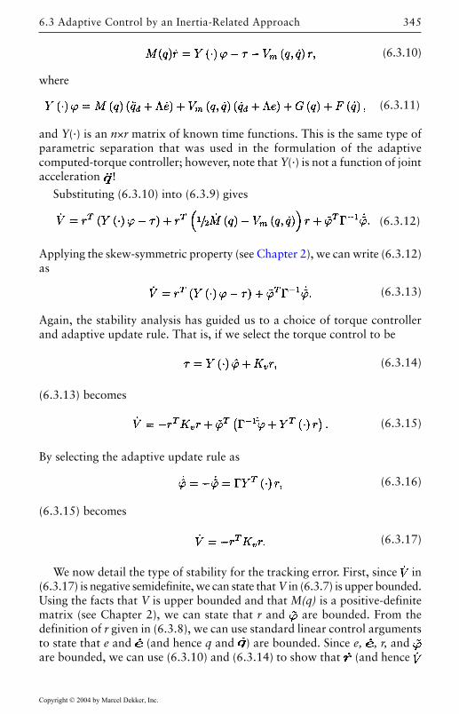
345
(6.3.10)
where
(6.3.11)
and Y(·) is an n×r matrix of known time functions. This is the same type ofparametric separation that was used in the formulation of the adaptivecomputed-torque controller; however, note that Y(·) is not a function of jointacceleration !
Substituting (6.3.10) into (6.3.9) gives
(6.3.12)
Applying the skew-symmetric property (see Chapter 2), we can write (6.3.12)as
(6.3.13)
Again, the stability analysis has guided us to a choice of torque controllerand adaptive update rule. That is, if we select the torque control to be
(6.3.14)
(6.3.13) becomes
(6.3.15)
By selecting the adaptive update rule as
(6.3.16)
(6.3.15) becomes
(6.3.17)
We now detail the type of stability for the tracking error. First, since in(6.3.17) is negative semidefinite, we can state that V in (6.3.7) is upper bounded.Using the facts that V is upper bounded and that M(q) is a positive-definitematrix (see Chapter 2), we can state that r and are bounded. From thedefinition of r given in (6.3.8), we can use standard linear control argumentsto state that e and (and hence q and ) are bounded. Since e, , r, and are bounded, we can use (6.3.10) and (6.3.14) to show that (and hence
6.3 Adaptive Control by an Inertia-Related Approach
Copyright © 2004 by Marcel Dekker, Inc.
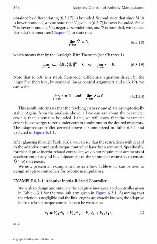
Adaptive Control of Robotic Manipulators346
obtained by differentiating (6.3.17)) is bounded. Second, note that since M(q)is lower bounded, we can state that V given in (6.3.7) is lower bounded. Since
is lower bounded, V is negative semidefinite, and is bounded, we can useBarbalat’s lemma (see Chapter 1) to state that
(6.3.18)
which means that by the Rayleigh-Ritz Theorem (see Chapter 1)
(6.3.19)
Note that (6.3.8) is a stable first-order differential equation driven by the“input” r; therefore, by standard linear control arguments and (6.3.19), wecan write
(6.3.20)
This result informs us that the tracking errors e and are asymptoticallystable. Again, from the analysis above, all we can say about the parametererror is that it remains bounded. Later, we will show that the parametererror also converges to zero under certain conditions on the desired trajectory.The adaptive controller derived above is summarized in Table 6.3.1 anddepicted in Figure 6.3.1.
After glancing through Table 6.3.1, we can see that the restrictions with regardto the adaptive computed-torque controller have been removed. Specifically,for the adaptive inertia-related controller, we do not require measurements ofacceleration or any ad hoc adjustment of the parameter estimates to ensure
-1 (q) that exists.We now present an example to illustrate how Table 6.3.1 can be used to
design adaptive controllers for robotic manipulators.
EXAMPLE 6.3–1: Adaptive Inertia-Related Controller
We wish to design and simulate the adaptive inertia-related controller givenin Table 6.3.1 for the two-link arm given in Figure 6.2.1. Assuming thatthe friction is negligible and the link lengths are exactly known, the adaptiveinertia-related torque controller can be written as
(1)
and
Copyright © 2004 by Marcel Dekker, Inc.
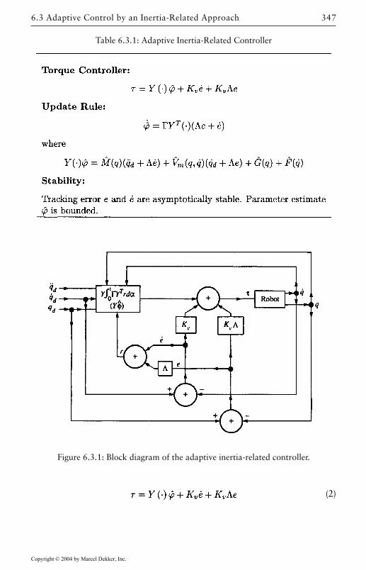
347
(2)
Table 6.3.1: Adaptive Inertia-Related Controller
Figure 6.3.1: Block diagram of the adaptive inertia-related controller.
6.3 Adaptive Control by an Inertia-Related Approach
Copyright © 2004 by Marcel Dekker, Inc.
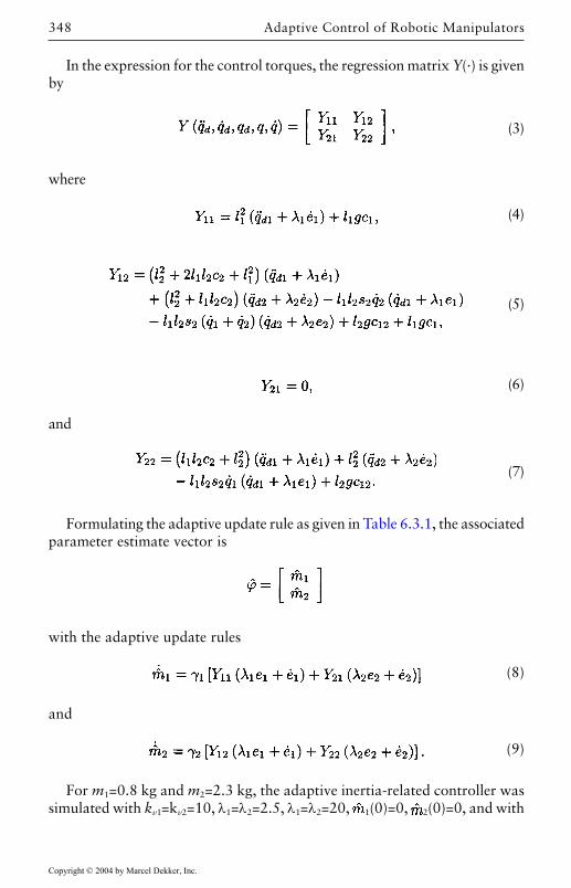
Adaptive Control of Robotic Manipulators348
In the expression for the control torques, the regression matrix Y(·) is givenby
(3)
where
(4)
(5)
(6)
and
(7)
Formulating the adaptive update rule as given in Table 6.3.1, the associatedparameter estimate vector is
with the adaptive update rules
(8)
and
(9)
For m1=0.8 kg and m2=2.3 kg, the adaptive inertia-related controller wassimulated with kv1=kv2=10, λ1=λ2=2.5, λ1=λ2=20, 1(0)=0, 2(0)=0, and with
Copyright © 2004 by Marcel Dekker, Inc.
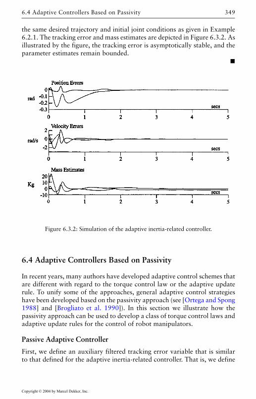
349
the same desired trajectory and initial joint conditions as given in Example6.2.1. The tracking error and mass estimates are depicted in Figure 6.3.2. Asillustrated by the figure, the tracking error is asymptotically stable, and theparameter estimates remain bounded.
6.4 Adaptive Controllers Based on Passivity
In recent years, many authors have developed adaptive control schemes thatare different with regard to the torque control law or the adaptive updaterule. To unify some of the approaches, general adaptive control strategieshave been developed based on the passivity approach (see [Ortega and Spong1988] and [Brogliato et al. 1990]). In this section we illustrate how thepassivity approach can be used to develop a class of torque control laws andadaptive update rules for the control of robot manipulators.
Passive Adaptive Controller
First, we define an auxiliary filtered tracking error variable that is similarto that defined for the adaptive inertia-related controller. That is, we define
Figure 6.3.2: Simulation of the adaptive inertia-related controller.
6.4 Adaptive Controllers Based on Passivity
Copyright © 2004 by Marcel Dekker, Inc.
Adaptive Control of Robotic Manipulators350
our tracking variable to be
(6.4.1)
where
(6.4.2)
and s is the Laplace transform variable. In (6.4.2), the n×n gain matrix K(s) ischosen such that H(s) is a strictly proper, stable transfer function matrix. Thereason for this restriction on H(s) will be clear after we analyze the stabilityof the adaptive controller that is presented later in this section.
As in the preceding sections, our adaptive control strategies have been centeredaround the ability to separate the known time functions from the unknownconstant parameters. Therefore, we use the expressions given in (6.4.1) and(6.4.2) to define
(6.4.3)
where in this control formulation, Z(·) is a known n×r regression matrix.[Note the standard abuse of notation in (6.4.3), where K(s)e is used torepresent the inverse Laplace transform of K(s) convolved with e(t).] It isimportant to note that K(s) can be selected so that Z(·) and r do not dependon measurement of . Indeed, if K(s) is selected such that H(s) has a relativedegree of 1 [Kailath 1980], Z(·) and r will not depend on .
The adaptive control formulation given in this section is called the passivityapproach because the mapping of -r → Z(.) is constructed to be a passivemapping. That is, we construct an adaptive update rule such that
(6.4.4)
is satisfied for all time and for some positive scalar constant ß. This passivityconcept is used in analyzing the stability of the error system, as we shallshow. However, for now let us illustrate the use of (6.4.4) in generating anadaptive update rule.
Copyright © 2004 by Marcel Dekker, Inc.
351
EXAMPLE 6.4–1: Adaptive Update Rule by Passivity
Let us show that the adaptive update rule
(1)
satisfies the inequality given by (6.4.4). Note that G is defined as in(6.2.11).
First rewrite (1) in the form
(2)
where we have used the fact that G is a diagonal matrix. Substituting (2)into (6.4.4) gives
(3)
Since Γ is a constant matrix, we can use the product rule to rewrite (3) as
(4)
or
(5)
From (5) it is now obvious that if ß is selected as
(6)
then the passivity integral given in (6.4.4) is satisfied for the adaptiveupdate rule given in (1).
Now that we have a feeling for how the passivity integral (6.4.4) can be usedto generate adaptive update rules, we use the concept of passivity to analyzethe stability of a class of adaptive controllers. For this class of adaptivecontrollers, the torque control is given by
(6.4.5)
6.4 Adaptive Controllers Based on Passivity
Copyright © 2004 by Marcel Dekker, Inc.
Adaptive Control of Robotic Manipulators352
Note that many types of torque controllers can be generated from (6.4.5)by selecting different transfer function matrices for K(s) in the definition of r.That is, for different K(s), we have different types of feedback because thefeedback term Kvr will change accordingly.
To form the error system, rewrite the robot dynamics (6.2.1) in terms ofthe tracking error variable r and the regression matrix Z(·) as
(6.4.6)
Substituting (6.4.5) into (6.4.6) yields the tracking error system
(6.4.7)
For analyzing the stability of this system, we use the Lyapunov-like function
(6.4.8)
[Ortega and Spong 1988]. Note that V is positive since the parameter estimateupdate rule is constructed to guarantee (6.4.4). That is, if (6.4.4) is satisfied,then
(6.4.9)
therefore, V is a positive scalar function. Differentiating (6.4.8) with respectto time gives
(6.4.10)
Substituting (6.4.7) into (6.4.10) yields
(6.4.11)
Utilizing the skew-symmetric property (see Chapter 2) allows one to write
(6.4.12)
We now detail the type of stability for the tracking error. First note from(6.4.12) that we can place the new upper bound on :
(6.4.13)
which can also be written as
Copyright © 2004 by Marcel Dekker, Inc.
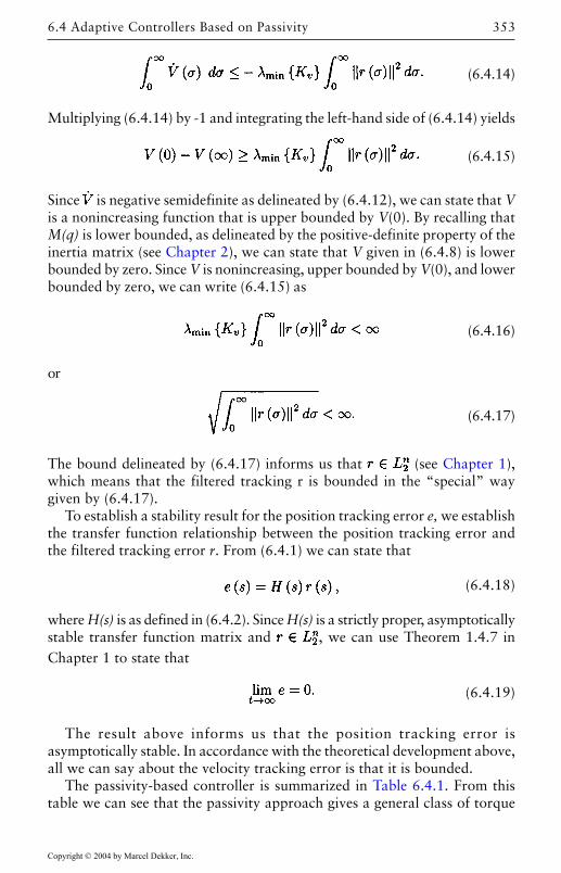
353
(6.4.14)
Multiplying (6.4.14) by -1 and integrating the left-hand side of (6.4.14) yields
(6.4.15)
Since is negative semidefinite as delineated by (6.4.12), we can state that Vis a nonincreasing function that is upper bounded by V(0). By recalling thatM(q) is lower bounded, as delineated by the positive-definite property of theinertia matrix (see Chapter 2), we can state that V given in (6.4.8) is lowerbounded by zero. Since V is nonincreasing, upper bounded by V(0), and lowerbounded by zero, we can write (6.4.15) as
(6.4.16)
or
(6.4.17)
The bound delineated by (6.4.17) informs us that (see Chapter 1),which means that the filtered tracking r is bounded in the “special” waygiven by (6.4.17).
To establish a stability result for the position tracking error e, we establishthe transfer function relationship between the position tracking error andthe filtered tracking error r. From (6.4.1) we can state that
(6.4.18)
where H(s) is as defined in (6.4.2). Since H(s) is a strictly proper, asymptoticallystable transfer function matrix and , we can use Theorem 1.4.7 inChapter 1 to state that
(6.4.19)
The result above informs us that the position tracking error isasymptotically stable. In accordance with the theoretical development above,all we can say about the velocity tracking error is that it is bounded.
The passivity-based controller is summarized in Table 6.4.1. From thistable we can see that the passivity approach gives a general class of torque
6.4 Adaptive Controllers Based on Passivity
Copyright © 2004 by Marcel Dekker, Inc.
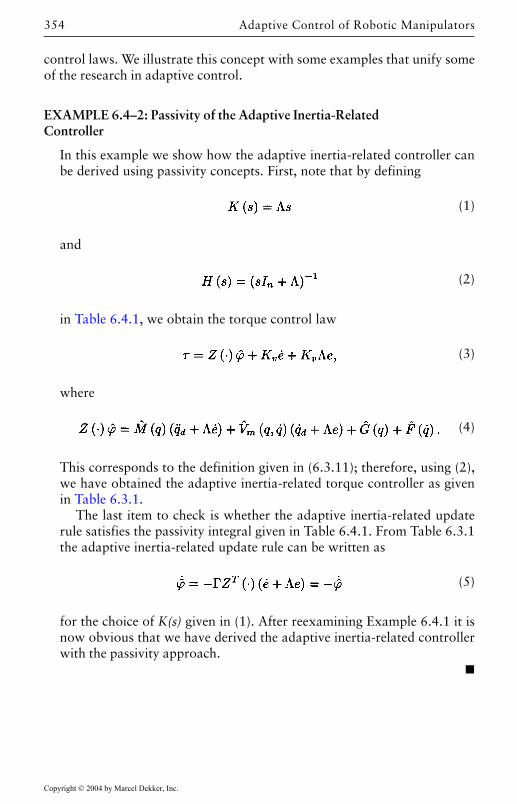
Adaptive Control of Robotic Manipulators354
control laws. We illustrate this concept with some examples that unify someof the research in adaptive control.
EXAMPLE 6.4–2: Passivity of the Adaptive Inertia-RelatedController
In this example we show how the adaptive inertia-related controller canbe derived using passivity concepts. First, note that by defining
(1)
and
(2)
in Table 6.4.1, we obtain the torque control law
(3)
where
(4)
This corresponds to the definition given in (6.3.11); therefore, using (2),we have obtained the adaptive inertia-related torque controller as givenin Table 6.3.1.
The last item to check is whether the adaptive inertia-related updaterule satisfies the passivity integral given in Table 6.4.1. From Table 6.3.1the adaptive inertia-related update rule can be written as
(5)
for the choice of K(s) given in (1). After reexamining Example 6.4.1 it isnow obvious that we have derived the adaptive inertia-related controllerwith the passivity approach.
Copyright © 2004 by Marcel Dekker, Inc.
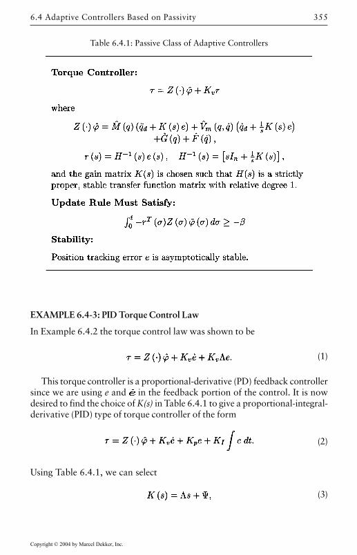
355
EXAMPLE 6.4-3: PID Torque Control Law
In Example 6.4.2 the torque control law was shown to be
(1)
This torque controller is a proportional-derivative (PD) feedback controllersince we are using e and in the feedback portion of the control. It is nowdesired to find the choice of K(s) in Table 6.4.1 to give a proportional-integral-derivative (PID) type of torque controller of the form
(2)
Using Table 6.4.1, we can select
(3)
Table 6.4.1: Passive Class of Adaptive Controllers
6.4 Adaptive Controllers Based on Passivity
Copyright © 2004 by Marcel Dekker, Inc.
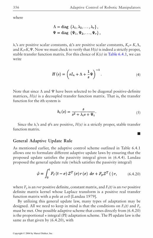
Adaptive Control of Robotic Manipulators356
where
i’s are positive scalar constants, i’s are positive scalar constants, Kp= Kv,and KI=Kv. Now we must check to verify that H(s) is indeed a strictly proper,stable transfer function matrix. For this choice of K(s) in Table 6.4.1, we canwrite
(4)
Note that since and have been selected to be diagonal positive-definitematrices, H(s) is a decoupled transfer function matrix. That is, the transferfunction for the ith system is
(5)
Since the i’s and ’s are positive, H(s) is a strictly proper, stable transferfunction matrix.
General Adaptive Update Rule
As mentioned earlier, the adaptive control scheme outlined in Table 6.4.1allows one to formulate different adaptive update laws by ensuring that theproposed update satisfies the passivity integral given in (6.4.4). Landauproposed the general update rule (which satisfies the passivity integral)
(6.4.20)
where Fp is an r×r positive definite, constant matrix, and FI(t) is an r×r positivedefinite matrix kernel whose Laplace transform is a positive real transferfunction matrix with a pole at s=0 [Landau 1979].
By utilizing this general update law, many types of adaptation may bedesigned. All we need to keep in mind is that the conditions on FI(t) and Fp
must be met. One possible adaptive scheme that comes directly from (6.4.20)is the proportional + integral (PI) adaptation scheme. The PI update law is thesame as that given by (6.4.20), with
Copyright © 2004 by Marcel Dekker, Inc.
357
FI(t)=K1, (6.4.21)
where K1 is a diagonal, constant positive-definite matrix. It has been pointedout in [Landau 1979] that with regard to adaptive model following, PIadaptation has shown a significant improvement over integral adaptation.Therefore, this type of adaptation might be beneficial for the tracking controlof robot manipulators.
6.5 Persistency of Excitation
For the adaptive controllers presented in the previous sections the trackingerror has been shown to be asymptotically stable; however, all that could besaid about the parameter error was that it was bounded. In general, parameteridentification will occur in adaptive control systems only if certain conditionson the regression matrix can be established. Specifically, several researchers[Morgan and Narendra 1977], [Anderson 1977] have studied the asymptoticstability of adaptive control systems similar to the ones we have presented inthis chapter. For example, parameter error convergence can be establishedfor the adaptive inertia-related controller if the regression matrix Y(·) satisfies
(6.5.1)
for all t0, where α, ß, and ρ are all positive scalars. Furthermore, since thetracking error is asymptotically stable, we can rewrite (6.5.1) as
(6.5.2)
where the arguments q and q have been replaced by qd and d, respectively.The condition given in (6.5.2) informs us that if Y(·) varies sufficiently
over the interval given by ρ so that the entire r-dimensional parameter spaceis spanned, we know the parameter error converges to zero. This amounts toa condition on the desired trajectory such that all parameters will be identifiedafter a sufficient learning interval. This condition can be helpful in formulatingdesired trajectories to ensure that parameters such as friction coefficients orpayload masses are identified. We now illustrate the meaning of a persistentlyexciting trajectory with some examples.
6.5 Persistency of Excitation
Copyright © 2004 by Marcel Dekker, Inc.
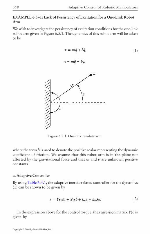
Adaptive Control of Robotic Manipulators358
where the term b is used to denote the positive scalar representing the dynamiccoefficient of friction. We assume that this robot arm is in the plane notaffected by the gravitational force and that m and b are unknown positiveconstants.
a. Adaptive Controller
By using Table 6.3.1, the adaptive inertia-related controller for the dynamics(1) can be shown to be given by
(2)
In the expression above for the control torque, the regression matrix Y(·) isgiven by
EXAMPLE 6.5–1: Lack of Persistency of Excitation for a One-Link RobotArm
We wish to investigate the persistency of excitation conditions for the one-linkrobot arm given in Figure 6.5.1. The dynamics of this robot arm will be takento be
(1)
Figure 6.5.1: One-link revolute arm.
Copyright © 2004 by Marcel Dekker, Inc.
359
(3)
where
The corresponding parameter estimate vector is given by
We can formulate the adaptive update rule given in Table 6.3.1 as
(4)
and
(5)
b. Persistency of Excitation
With this adaptive controller it is desired to show analytically that qd= 1-e-2t isnot persistently exciting. From (6.5.2), the integrand of the persistently excitingcondition for this example is given by
or
(6)
Multiplying the first column of YT(·)Y(·) by and adding it to the secondcolumn of YT(·)Y(·) gives
(7)
Since the matrix RYY has the same range space as the matrix YT(·)Y(·), wecan see from (7) that the range space of the matrix YT(·)Y(·) will always beone-dimensional; therefore, the persistent excitation condition does not holdfor
6.5 Persistency of Excitation
Copyright © 2004 by Marcel Dekker, Inc.
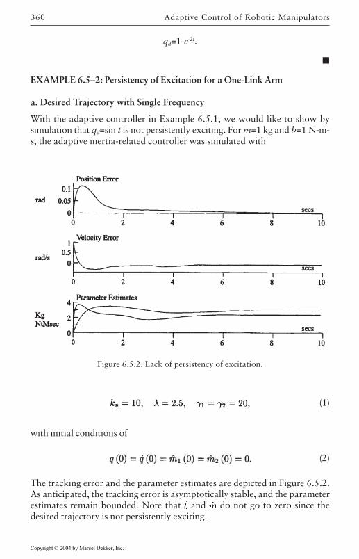
Adaptive Control of Robotic Manipulators360
(1)
with initial conditions of
(2)
The tracking error and the parameter estimates are depicted in Figure 6.5.2.As anticipated, the tracking error is asymptotically stable, and the parameterestimates remain bounded. Note that and do not go to zero since thedesired trajectory is not persistently exciting.
qd=1-e-2t.
EXAMPLE 6.5–2: Persistency of Excitation for a One-Link Arm
a. Desired Trajectory with Single Frequency
With the adaptive controller in Example 6.5.1, we would like to show bysimulation that qd=sin t is not persistently exciting. For m=1 kg and b=1 N-m-s, the adaptive inertia-related controller was simulated with
Figure 6.5.2: Lack of persistency of excitation.
Copyright © 2004 by Marcel Dekker, Inc.
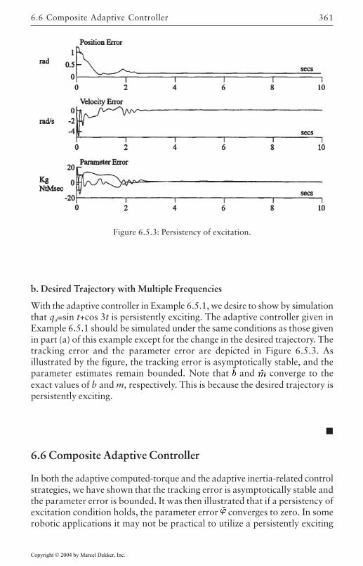
361
b. Desired Trajectory with Multiple Frequencies
With the adaptive controller in Example 6.5.1, we desire to show by simulationthat qd=sin t+cos 3t is persistently exciting. The adaptive controller given inExample 6.5.1 should be simulated under the same conditions as those givenin part (a) of this example except for the change in the desired trajectory. Thetracking error and the parameter error are depicted in Figure 6.5.3. Asillustrated by the figure, the tracking error is asymptotically stable, and theparameter estimates remain bounded. Note that and converge to theexact values of b and m, respectively. This is because the desired trajectory ispersistently exciting.
6.6 Composite Adaptive Controller
In both the adaptive computed-torque and the adaptive inertia-related controlstrategies, we have shown that the tracking error is asymptotically stable andthe parameter error is bounded. It was then illustrated that if a persistency ofexcitation condition holds, the parameter error converges to zero. In somerobotic applications it may not be practical to utilize a persistently exciting
Figure 6.5.3: Persistency of excitation.
6.6 Composite Adaptive Controller
Copyright © 2004 by Marcel Dekker, Inc.
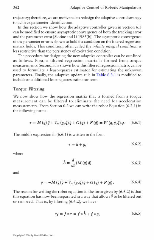
Adaptive Control of Robotic Manipulators362
trajectory; therefore, we are motivated to redesign the adaptive control strategyto achieve parameter identification.
In this section we show how the adaptive controller given in Section 6.3can be modified to ensure asymptotic convergence of both the tracking errorand the parameter error [Slotine and Li 1985(b)]. The asymptotic convergenceof the parameter error is shown to hold if a condition on the filtered regressionmatrix holds. This condition, often called the infinite integral condition, isless restrictive than the persistency of excitation condition.
The procedure for designing the new adaptive controller can be out-linedas follows. First, a filtered regression matrix is formed from torquemeasurements. Second, it is shown how this filtered regression matrix can beused to formulate a least-squares estimator for estimating the unknownparameters. Finally, the adaptive update rule in Table 6.3.1 is modified toinclude an additional least-squares estimator term.
Torque Filtering
We now show how the regression matrix that is formed from a torquemeasurement can be filtered to eliminate the need for accelerationmeasurements. From Section 6.2 we can write the robot Equation (6.2.1) inthe following form:
(6.6.1)
The middle expression in (6.6.1) is written in the form
(6.6.2)
where
(6.6.3)
and
(6.6.4)
The reason for writing the robot equation in the form given by (6.6.2) is thatthis equation has now been separated in a way that allows to be filtered outor removed. That is, by filtering (6.6.2), we have
(6.6.5)
Copyright © 2004 by Marcel Dekker, Inc.
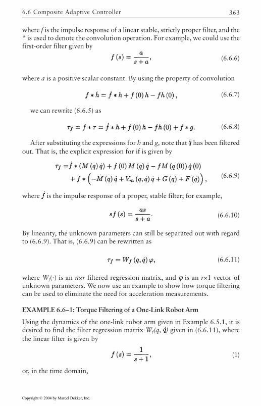
363
where f is the impulse response of a linear stable, strictly proper filter, and the* is used to denote the convolution operation. For example, we could use thefirst-order filter given by
(6.6.6)
where a is a positive scalar constant. By using the property of convolution
(6.6.7)
we can rewrite (6.6.5) as
(6.6.8)
After substituting the expressions for h and g, note that has been filteredout. That is, the explicit expression for if is given by
(6.6.9)
where is the impulse response of a proper, stable filter; for example,
(6.6.10)
By linearity, the unknown parameters can still be separated out with regardto (6.6.9). That is, (6.6.9) can be rewritten as
(6.6.11)
where Wf(·) is an n×r filtered regression matrix, and ϕ is an r×1 vector ofunknown parameters. We now use an example to show how torque filteringcan be used to eliminate the need for acceleration measurements.
EXAMPLE 6.6–1: Torque Filtering of a One-Link Robot Arm
Using the dynamics of the one-link robot arm given in Example 6.5.1, it isdesired to find the filter regression matrix Wf(q, ) given in (6.6.11), wherethe linear filter is given by
(1)
or, in the time domain,
6.6 Composite Adaptive Controller
Copyright © 2004 by Marcel Dekker, Inc.
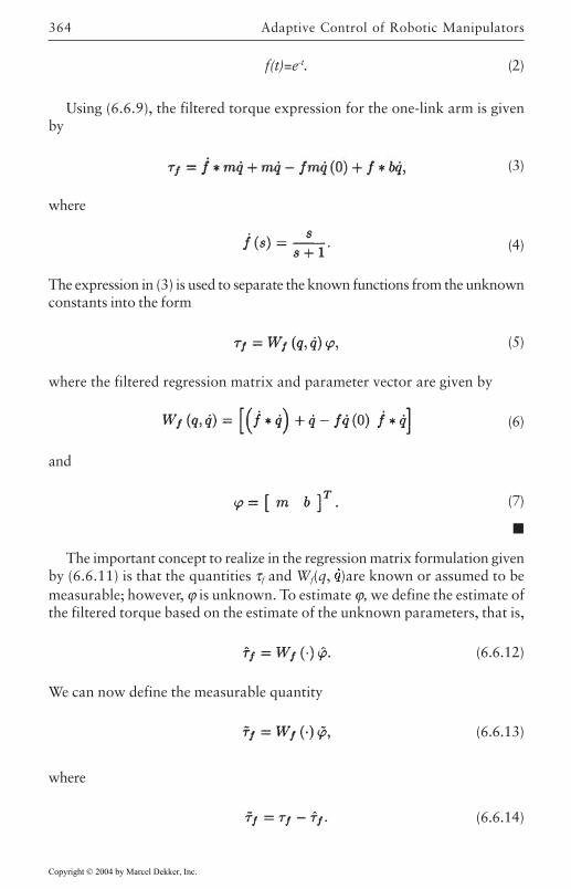
Adaptive Control of Robotic Manipulators364
f(t)=e-t. (2)
Using (6.6.9), the filtered torque expression for the one-link arm is givenby
(3)
where
(4)
The expression in (3) is used to separate the known functions from the unknownconstants into the form
(5)
where the filtered regression matrix and parameter vector are given by
(6)
and
(7)
The important concept to realize in the regression matrix formulation givenby (6.6.11) is that the quantities τf and Wf(q, )are known or assumed to bemeasurable; however, ϕ is unknown. To estimate ϕ, we define the estimate ofthe filtered torque based on the estimate of the unknown parameters, that is,
(6.6.12)
We can now define the measurable quantity
(6.6.13)
where
(6.6.14)
Copyright © 2004 by Marcel Dekker, Inc.
365
The use of f is crucial in the development of the least-squares estimatorthat is developed in the next section. We can easily see how f is measurableby writing (6.6.14) in the form
(6.6.15)
As explained earlier, f and Wf(·) are assumed to be known or measurable;therefore, all we need is the parameter estimate term [i.e., in (6.6.15)] for ifto be known. Later, we generate an adaptive update rule that will give us theparameter estimate term in (6.6.15). So for now we will assume that f isknown.
Least-Squares Estimation
Least-squares estimation methods have been used in many types of parameteridentification schemes [Astrom and Wittenmark 1989]. It turns out that thistype of estimation method extracts the maximum amount of parametricinformation even when the desired trajectory is not persistently exciting. Thisis an important fact to realize when designating adaptive control systems forrobot manipulators because in many robot applications, the persistency ofexcitation condition will not be valid. Therefore, least-squares estimationoffers an attractive solution to the design of adaptive controllers for robotmanipulators.
We now show how the least-squares estimation method can be used togenerate an adaptive update rule. First, define the least-squares update rule
(6.6.16)
where
(6.6.17)
and P is an r×r time-varying symmetric matrix.With this least-squares estimation method, if an “infinite integral” condition
holds, the parameter error converges to zero. Specifically, if
(6.6.18)
holds, then
(6.6.19)
6.6 Composite Adaptive Controller
Copyright © 2004 by Marcel Dekker, Inc.
Adaptive Control of Robotic Manipulators366
As pointed out in [Slotine and Li 1985(b)], this infinite integral condition isa weaker condition than the persistency of excitation condition. That is, inpractical robot applications, (6.6.18) can often be validated.
EXAMPLE 6.6–2: Least-Squares Estimator for a One-Link Robot Arm
Using the dynamics of the one-link robot arm given in Example 6.5.1, it isdesired to find the least-squares estimator given by (6.6.16) and (6.6.17).Since the number of unknown parameters is two, define the matrix P to be
(1)
Utilizing the filtered regression matrix from Example 6.6.1, we have
(2)
where
Using (6.6.17), it is easy to see that the matrix P should be updated in thefollowing manner:
(3)
(4)
and
(5)
Now using (6.6.16), the parameter update rules are
(6)
and
Copyright © 2004 by Marcel Dekker, Inc.
367
(7)
where, from (6.6.16), f is given by
(8)
For insight into how the least-squares estimation method extracts parameterinformation, we now show how (6.6.18) is obtained. Utilizing (6.6.13) andthe fact that the parameters are constant, we write (6.6.16) as
(6.6.20)
Using the matrix identity =–P –1P we can write (6.6.17) as
(6.6.21)
Substituting (6.6.21) into (6.6.20) yields the differential equation
(6.6.22)
We claim that
(6.6.23)
is the solution to (6.6.22). This fact can be verified by substituting (6.6.23)into the right-hand and left-hand sides of (6.6.22). That is, we obtain
(6.6.24)
therefore, (6.6.23) is the solution. Now from (6.6.21) it is easy to see that thesolution for P is given by
(6.6.25)
After examining (6.6.25), we can intuitively see that if the infinite integralcondition is satisfied, then
(6.6.26)
and
(6.6.27)
6.6 Composite Adaptive Controller
Copyright © 2004 by Marcel Dekker, Inc.
Adaptive Control of Robotic Manipulators368
Now if (6.6.26) holds, we can see from (6.6.23) that the parameter errorconverges to zero. This proof is detailed in [Li and Slotine 1987].
Composite Adaptive Controller
The composite adaptive controller is the same as the controller given in Table6.3.1, with the exception of a modification to the adaptive update rule. Thismodification is given by
(6.6.28)
To prove that the tracking error and the parameter error both converge tozero, start with the Lyapunov-like function,
(6.6.29)
Differentiating (6.6.29) with respect to time yields
(6.6.30)
From the control law given in Table 6.3.1 and the development in Section6.3, we can form the tracking error system
(6.6.31)
Substituting (6.6.31) into (6.6.30) yields
(6.6.32)
After substituting in (6.6.28), –1 in (6.6.21), and f in (6.6.13) into (6.6.32),we have
(6.6.33)
We now detail the type of stability for the tracking error and the parametererror. First, since in (6.6.33) is at least negative semidefinite in the form
(6.6.34)
we can state that V in (6.6.29) is bounded. Since V is bounded, M(q) is apositive-definite matrix, and P-1 satisfies the condition given by (6.6.27), wecan state that r and are bounded. Furthermore, from the definition of rgiven in (6.3.8), we can use standard linear control arguments to state that e
Copyright © 2004 by Marcel Dekker, Inc.
369
and e (and hence q and ) are bounded. We can now use the same argumentspresented in Section 6.4 to show that . Given that , we candetermine a stability result for the position tracking error by establishing thetransfer function relationship between the position tracking error and the filteredtracking error r. From (6.3.8), we can state that
(6.6.35)
where s is the Laplace transform variable,
(6.6.36)
I is the n×n identity matrix, and is an n×n positive-definite matrix. SinceG(s) is a strictly proper, asymptotically stable transfer function and we can use Theorem 1.4.7 in Chapter 1 to state that
(6.6.37)
Second, since is at least negative semidefinite, we know that V must benonincreasing, and hence is upper bounded by V(0). Furthermore, by theinfinite integral assumption, we have concluded in (6.6.27) that
(6.6.38)
Since the term
(6.6.39)
in V given in (6.6.29) is upper bounded by V(0), we can see that for (6.6.38)to hold, we must have
Therefore, from the argument above, the position tracking error and theparameter error are asymptotically stable for the composite adaptive controlleroutlined in Table 6.6.1. In accordance with the theoretical development above,all we can say about the velocity tracking error is that it is bounded; however,Barbalat’s lemma can be invoked to illustrate that the velocity tracking erroris also asymptotically stable (see Problem 6.6–3). We now use an example toillustrate how the composite adaptive controller is formulated.
6.6 Composite Adaptive Controller
Copyright © 2004 by Marcel Dekker, Inc.
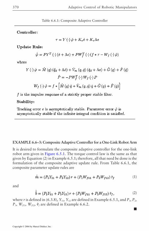
Adaptive Control of Robotic Manipulators370
EXAMPLE 6.6–3: Composite Adaptive Controller for a One-Link Robot Arm
It is desired to formulate the composite adaptive controller for the one-linkrobot arm given in Figure 6.5.1. The torque control law is the same as thatgiven by Equation (2) in Example 6.5.1; therefore, all that need be done is theformulation of the composite adaptive update rule. From Table 6.6.1, thecomposite parameter update rules are
(1)
and
(2)
where r is defined in (6.3.8), Y11, Y12 are defined in Example 6.5.1, and P1, P2,P3, Wf11, Wf12, f are defined in Example 6.6.2.
Table 6.6.1: Composite Adaptive Controller
Copyright © 2004 by Marcel Dekker, Inc.
371
6.7 Robustness of Adaptive Controllers
All of the adaptive control schemes discussed ensure asymptotic tracking of adesired reference trajectory for the robot manipulator dynamics; however, inreality we know that there will always be disturbances in any electromechanicalsystem. A simplistic way to take into account some sort of disturbance effectis to add a bounded disturbance term to the manipulator dynamic equation.With this additive disturbance term the robot equation becomes
(6.7.1)
where Td is an n×1 vector that represents an additive disturbance.Applying the adaptive inertia-related control strategy and ignoring the
term Td in (6.7.1) gives the adaptive control scheme of Table 6.3.1. However,if we reexamine the stability analysis given in Section 6.3 for the adaptiveinertia-related controller, we can see that a bounded disturbance term givesus a different type of stability result for the tracking error. Specifically, withthe addition of the bounded disturbance term in (6.7.1), the derivative of theLyapunov function in (6.3.7) becomes
(6.7.2)
From (6.7.2) it is obvious that can no longer be taken to be negativesemidefinite. From our previous experience with Lyapunov stability theory, itwas desired to have be “negative”; therefore, it stands to reason that itwould be advantageous to find the region where is negative in (6.7.2). Bythe use of the Rayleigh-Ritz Theorem (see Chapter 1), we can write (6.7.2) as
(6.7.3)
From (6.7.3), a sufficient condition on the negativity of can be obtained.That is, will be negative if
(6.7.4)
If (6.7.4) is satisfied, is negative and V will decrease. If V decreases, then byour definition of the Lyapunov function given in (6.3.7), r must eventuallydecrease. However, if r decreases such that
6.7 Robustness of Adaptive Controllers
Copyright © 2004 by Marcel Dekker, Inc.
Adaptive Control of Robotic Manipulators372
(6.7.5)
then may become positive, which means that V will start to increase. If Vstarts to increase, we gain insight into the problem by examining twopossibilities. One, the increase in V causes r to increase such that (6.7.4) issatisfied. This means that V will start to decrease and hence r will eventuallydecrease. If r increased and decreased in this fashion continually, then r and
both remain bounded. The other possibility is that the increase in V causes to increase while r stays small enough such that (6.7.5) is satisfied. For
this case, V remains positive; therefore, could continue to increase. If Vcontinues to increase in this fashion, r is bounded; however, and hence both become unbounded.
The argument above reveals that the parameter estimate in the adaptiveinertia-related control law may go unstable in the presence of a boundeddisturbance. That is, the parameter estimate may diverge under theassumption that the robot model is given by (6.7.1). If the parameter estimatebecomes too large, we can see from Table 6.3.1 that the input torque willstart to grow and possibly saturate the joint motors; therefore, it would bedesirable to modify the adaptive controller to eliminate the possibility oftorque saturation.
EXAMPLE 6.7–1: Effects of Disturbance on Adaptive Control
In this example we simulate the same adaptive controller given in Example6.3.1 with the same control parameters, initial conditions, and desiredtrajectory; however, we have added the disturbance term
(1)
to the two-link manipulator dynamics. The tracking error and parameterestimates are illustrated in Figure 6.7.1. From the figure, note that for thedisturbance given by (1), the parameter estimates do not become unbounded;however, the tracking error is no longer asymptotically stable.
Torque-Based Disturbance Rejection Method
To reject an additive disturbance term in the robot model, we illustratehow the parameter estimates remain bounded if the torque control ismodified to be
Copyright © 2004 by Marcel Dekker, Inc.
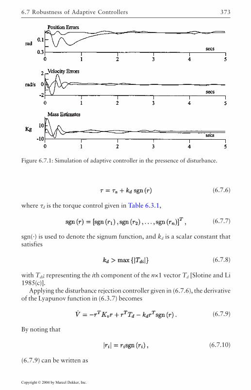
373
(6.7.6)
where d is the torque control given in Table 6.3.1,
(6.7.7)
sgn(·) is used to denote the signum function, and kd is a scalar constant thatsatisfies
(6.7.8)
with Tdi; representing the ith component of the n×1 vector Td [Slotine and Li1985(c)].
Applying the disturbance rejection controller given in (6.7.6), the derivativeof the Lyapunov function in (6.3.7) becomes
(6.7.9)
By noting that
(6.7.10)
(6.7.9) can be written as
Figure 6.7.1: Simulation of adaptive controller in the pressence of disturbance.
6.7 Robustness of Adaptive Controllers
Copyright © 2004 by Marcel Dekker, Inc.
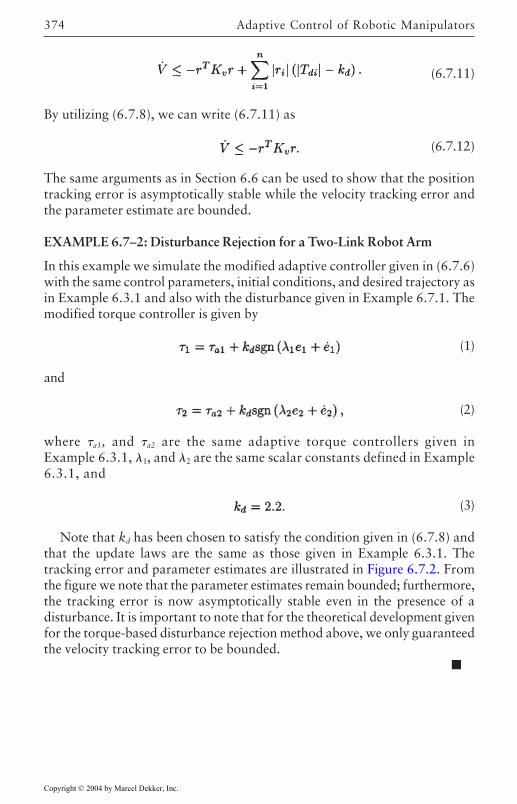
Adaptive Control of Robotic Manipulators374
(6.7.11)
By utilizing (6.7.8), we can write (6.7.11) as
(6.7.12)
The same arguments as in Section 6.6 can be used to show that the positiontracking error is asymptotically stable while the velocity tracking error andthe parameter estimate are bounded.
EXAMPLE 6.7–2: Disturbance Rejection for a Two-Link Robot Arm
In this example we simulate the modified adaptive controller given in (6.7.6)with the same control parameters, initial conditions, and desired trajectory asin Example 6.3.1 and also with the disturbance given in Example 6.7.1. Themodified torque controller is given by
(1)
and
(2)
where a1, and a2 are the same adaptive torque controllers given inExample 6.3.1, 1, and 2 are the same scalar constants defined in Example6.3.1, and
(3)
Note that kd has been chosen to satisfy the condition given in (6.7.8) andthat the update laws are the same as those given in Example 6.3.1. Thetracking error and parameter estimates are illustrated in Figure 6.7.2. Fromthe figure we note that the parameter estimates remain bounded; furthermore,the tracking error is now asymptotically stable even in the presence of adisturbance. It is important to note that for the theoretical development givenfor the torque-based disturbance rejection method above, we only guaranteedthe velocity tracking error to be bounded.
Copyright © 2004 by Marcel Dekker, Inc.
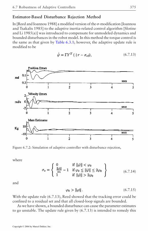
375
Estimator-Based Disturbance Rejection Method
In [Reed and Ioannou 1988] a modified version of the -modification [Ioannouand Tsakalis 1985] to the adaptive inertia-related control algorithm [Slotineand Li 1985(a)] was introduced to compensate for unmodeled dynamics andbounded disturbances in the robot model. In this method the torque control isthe same as that given by Table 6.3.1; however, the adaptive update rule ismodified to be
(6.7.13)
Figure 6.7.2: Simulation of adaptive controller with disturbance rejection,
where
(6.7.14)
and
(6.7.15)
With the update rule (6.7.13), Reed showed that the tracking error could beconfined to a residual set and that all closed-loop signals are bounded.
As we have shown, a bounded disturbance can cause the parameter estimatesto go unstable. The update rule given by (6.7.13) is intended to remedy this
6.7 Robustness of Adaptive Controllers
Copyright © 2004 by Marcel Dekker, Inc.
Adaptive Control of Robotic Manipulators376
problem by regulating on-line the size of the parameter estimates. This isdone by the scalar design constant 0. That is, by checking the size of theparameter estimates against 0, the parameter estimates are forced to remainbounded by using this new update rule. One can see clearly that if <0, theupdate rule is the same as that given by Table 6.3.1. In other words, if theparameter estimates do not get too large, the controller is the same as theadaptive inertia-related controller. On the other hand, if parameter estimatesget too large, the adaptive update rule is modified to ensure that the parameterestimates remain bounded. How this σ-modification accomplishes this task isnow discussed.
To motivate how the update rule given in (6.7.13) was formulated, examinethe case when >0. This is the stabilizing part of the update rule. That is,if the parameter estimates become too large, the update rule switches to
(6.7.16)
or in terms of the parameter error,
(6.7.17)
We now reexamine the stability analysis given in Section 6.3 for the adaptiveinertia-related controller with the parameter update rule given by (6.7.16).Specifically, with the addition of the bounded disturbance term in (6.7.1), thederivative of the Lyapunov function in (6.3.7) becomes
(6.7.18)
or
(6.7.19)
where
(6.7.20)
By the use of the Rayleigh-Ritz Theorem (see Chapter 1), we can write(6.7.19) as
(6.7.21)
From (6.7.21), will be negative if
Copyright © 2004 by Marcel Dekker, Inc.
377
(6.7.22)
It is important to note that the right-hand side of (6.7.22) is a constant;therefore, if (6.7.22) is satisfied, is negative, which causes V to decrease. IfV decreases, then by our definition of the Lyapunov function given in (6.3.7),x must eventually decrease. However, if x decreases such that
(6.7.23)
then may be positive, which means that V will start to increase. The increasein V causes x to increase such that (6.7.22) is satisfied. This means that V nowstarts to decrease again and hence x eventually decreases. This argumentillustrates how x is bounded. If x is bounded, then from (6.7.20), r and arebounded. Since r is bounded, standard linear control arguments can be usedto show that e and e are bounded.
One last point is now discussed regarding the region 0 20. for theadaptive update rule given in (6.7.13). This part of the adaptive update ruleis used to ensure that there is a smooth transition between the adaptiveinertia-related update rule and the stabilizing portion of the update rulegiven by (6.7.16). That is, this ensures that we do not obtain anydiscontinuities in the parameter estimates, which could cause a largediscontinuity in the input torque. A large discontinuity is undesirable in theinput torque signal since this type of signal could cause the robot manipulatorto jerk violently.
6.8 Summary
In this chapter an account of several of the most recent adaptive controlresults for rigid robots has been given. The intent has been to lend someperspective to the growing list of adaptive control results for robot manipulators.Some research areas, such as transient behavior, digital implementation, androbustness to unmodeled dynamics, will no doubt be addressed in the future.An issue that remains to be investigated is the comparison of the advantagesand disadvantages of the different servo and adaptive laws.
Some excellent adaptive control work with regard to robot manipulatorsby other researchers is outlined in [Ortega and Spong 1988]. Since this is sucha well-studied field and there is limited space available in this chapter, weapologize to anyone who has been left out.
6.8 Summary
Copyright © 2004 by Marcel Dekker, Inc.
379
REFERENCES
[Anderson 1977] Anderson, B., “Exponential stability of linear equationsarising in adaptive identification,” IEEE Trans. Autom. Control, Feb.1977, pp. 83–88.g
[Arimoto and Miyazaki 1986] Arimoto, S., and F.Miyazaki, “Stability androbustness of PD feedback control with gravity compensation for robotmanipulators,” Robot. Theory Pract., DSC Vol. 3, pp. 67–72, ASMEWinter Annual Meeting, Dec. 1986.
[Åström and Wittenmark 1989] K.Åström and B.Wittenmark, AdaptiveControl. Reading, MA: Addison-Wesley, 1989.
[Brogliato et al. 1990] Brogliato, B., I.Landau, and R.Lozano-Leal, “Adaptivemotion control of robot manipulators: a unified approach based onpassitivity,” Proc. IEEE Am. Controls Conf, pp. 2259–2264, San Diego,CA, May 1990.
[Craig 1985] Craig, J., Adaptive Control of Mechanical Manipulators. Reading,MA.: Addison Wesley, 1985.
[Ioannou and Tsakalis 1985] Ioannou, P., and K.Tsakalis, “A robust directadaptive controller,” IEEE Trans. Autom. Control, vol. AC-31, no. 11,pp. 1033–1043, 1985.
[Kailath 1980] Kailath, T, Linear Systems. Englewood Cliffs, NJ: PrenticeHall, 1980.
[Landau 1979] Landau, Y., Adaptive Control: The Model Reference Approach.New York: Marcel Dekker, 1979.
[Li and Slotine 1987] Li, W., and J.Slotine, “Parameter estimation strategiesfor robotic applications,” ASME Winter Annual Meeting, Boston, 1987.
[Morgan and Narendra 1977] Morgan, A., and K.Narendra, “On the uniformasymptotic stability of certain linear nonautonomous differentialequations,” SIAM J. Control Optim., 1977, p. 15.
Copyright © 2004 by Marcel Dekker, Inc.
REFERENCES380
[Ortega and Spong 1988] Ortega, R., and M.Spong, “Adaptive motion controlof rigid robots: a tutorial,” Proc. IEEE Conf Decision Control, Austin,TX, 1988.
[Reed and Ioannou 1988] Reed, J., and P.Ioannou, “Instability analysis androbust adaptive control of robotic manipulators,” Proc. IEEE ConfDecision Control, Austin, TX, 1988.
[Slotine 1988] Slotine, J., (1988), “Putting physics in control: the example ofrobotics,” Control Syst. Mag., Dec. 1988, Vol. 8, pp 12–15.
[Slotine and Li 1985(a)] Slotine, J., and W.Li, “Theoretical issues in adaptivecontrol,” 5th Yale Workshop on Applications of Adaptive Systems Theory,Yale University, New Haven, CT, 1985(a).
[Slotine and Li 1985(b)] Slotine, J., and W.Li, “Adaptive robot control: a newperspective,” Proc. IEEE Conf Decision Control, Los Angeles, 1985(b).
[Slotine and Li 1985(c)] Slotine, J., and W.Li, “Adaptive strategies inconstrained manipulation,” Proc. IEEE Int. Conf Robot. Autom., Raleigh,NC, Mar. 1985(c), pp. 595–601.
[Vidyasagar 1978] Vidyasagar, M., Nonlinear Systems Analysis. EnglewoodCliffs, NJ: Prentice Hall, 1978.
Copyright © 2004 by Marcel Dekker, Inc.
REFERENCES 381
PROBLEMS
Section 6.2
6.2–1 Design and simulate the adaptive computed-torque controller givenin Table 6.2.1 for the two-link polar robot arm given in Chapter 2.
6.2–2 Find different positive-definite, symmetric matrices, P and Q fromthat given in Example 6.2.2 that satisfy
where
Kp, Kv are diagonal positive-definite matrices, and On, In representthe n×n zero matrix and n×n identity matrix, respectively.
6.2–3: With the P and Q found in Problem 6.2–3, redo Problem 6.2–1 andreport the differences in the tracking error performance.
Section 6.3
6.3–1 Design and simulate the adaptive inertia-related controller given inTable 6.3.1 for the two-link polar robot arm given in Chapter 2.
6.3–2 For the simulation given in Problem 6.3–1, run several simulationswith different values of the control parameters (ie., , Kv, ), andreport the effects on tracking error performance.
6.3–3 Enumerate the the advantages of the adaptive controller given inTable 6.3.1 over the adaptive controller given in Table 6.2.1.
6.3–4 As given in (6.3.8), the filtered tracking error is defined by
where is a positive-definite diagonal matrix. Show that if
Section 6.4
6.4–1 Design and simulate an adaptive controller for the two-link re volutearm given in Example 6.3.1 with the PID servo law given in Example6.4.3 and the adaptation law given in Example 6.4.1. Report any
Copyright © 2004 by Marcel Dekker, Inc.
REFERENCES382
differences from that given in Example 6.3.1.
6.4–2 Redo Problem 6.4–1 with the proportional+integral adaptation lawgiven by Equations (6.4.20) and (6.4.21).
Section 6.5
6.5–1 Show analytically that qd=sin t in Example 6.5.2 is not persistentlyexciting.
Section 6.6
6.6–1 Show that
6.6–2 Simulate the composite adaptive controller given in Example 6.6.3and report the effects on the tracking error of using different valuesfor P(0) and a (i.e., the pole of the filter used for the filtered regressionmatrix).
6.6–3 Show how Barbalat’s lemma given in Chapter 1 can be used in theproof of the composite adaptive controller to yield
Section 6.7
6.7–1 Redo Problem 6.3–1 with the additive bounded disturbance
added to two-link polar robot arm dynamics given in Chapter 2.
6.7–2 Redo Problem 6.3–1 with the additive bounded disturbance given inProblem 6.7–1 and with the term
added to the adaptive controller. Run several simulations with differentvalues of kd, and report the effects on tracking error performance.
Copyright © 2004 by Marcel Dekker, Inc.
383
Chapter 7
Advanced ControlTechniques
In this chapter some advanced control techniques for the tracking control ofrobot manipulators are discussed. The controllers that are developed in thischapter address computational issues and the effects of actuator dynamics.The analytical concepts and the control developments presented in this chapterare in general more complex than those presented in the previous chapters;therefore, it is highly recommended that the previous chapters be studiedbefore examining this new material.
7.1 Introduction
As research in robot control has progressed over the last couple of years,many robot control researchers have begun to focus on implementationalissues. That is, implementational concerns, such as the reduction of on-linecomputation and the effects of actuator dynamics, are causing researchers torethink the previous theoretical development of robot controllers so that theseconcerns are addressed. This constant retooling of the previous controldevelopment to coincide with the implementational restrictions is how previousprogress in robot control research has proceeded. Utilizing this concept offorcing the theoretical development to satisfy implementational restrictions,we illustrate how some researchers have begun to address problems such asreducing on-line computation and compensating for the effects of actuatordynamics.
Copyright © 2004 by Marcel Dekker, Inc.
Advanced Control Techniques384
7.2 Robot Controllers with Reduced On-LineComputation
In this section we examine the robot controllers designed by Sadegh andcoworkers [Sadegh and Horowitz 1990], [Sadegh et al. 1990]. We separatethese controllers from related work since this work addresses the extremelyrelevant implementation issue of on-line controller computation. Specifically,this adaptive controller reduces on-line computation as opposed to othercontrol techniques, such as the adaptive controllers presented in Chapter 6.Following the development of the adaptive controller research, a “repetitive”controller is also presented. This repetitive controller also reduces onlinecomputation.
Desired Compensation Adaptation Law
One of the disadvantages of the adaptive controllers in Chapter 6 is that theregression matrix (e.g., the matrix Y(·) in the adaptive inertia-related controller)used as feedforward compensation must be calculated on-line. The regressionmatrix must be calculated on-line since it depends on the measurements of thejoint position and velocity (i.e., q and q). For the simple two-link robotcontroller given in Example 6.3.1, it is evident that online calculation of Y(·)is computationally intensive. As one can imagine, on-line computation of theregression matrix can be very computationally intensive if one desires tocontrol a robot manipulator with many degrees of freedom.
To eliminate the need for on-line computation of the regression matrix, wewill now examine the desired compensation adaptation law (DCAL) [Sadeghand Horowitz 1990]. The DCAL eliminates the need for on-line computationof the regression matrix by replacing q and q with the desired joint positionand velocity (i.e., qd and qd). That is, the DCAL regression matrix only dependson desired trajectory information; therefore, the DCAL regression matrix canbe calculated a priori off-line. Of course, this modification of the regressionmatrix forces us to reexamine the adaptive control design and the correspondingstability analysis.
For purposes of control design in this section, we assume that the roboticmanipulator is a revolute manipulator with dynamics given by
(7.2.1)
where Fd is a n×n positive-definite, diagonal matrix that is used torepresent the dynamic coefficients of friction, and all other quantitiesare as defined in Chapter 3. As in other chapters, we define the jointtracking error to be
Copyright © 2004 by Marcel Dekker, Inc.
7.2 Robot Controllers with Reduced On-Line Computation 385
e=qd-q. (7.2.2)
As explained in Chapter 6, adaptive control of robot manipulators involvesseparating the known time functions from the unknown constant parameters.For example, recall that this separation of parameters from time functions forthe adaptive inertia-related controller is given by
(7.2.3)
where Y(·) is an n×r regression matrix that depends only on known timefunctions of the actual and desired trajectory, and is an r×1 vector of unknownconstant parameters. (Note that defined Table 6.3.1 is taken to be theidentity matrix.)
In the DCAL, this separation of parameters from time functions is given by
(7.2.4)
where Yd(·) is an n×r regression matrix that depends only on known functionsof the desired trajectory. Note that if we substitute qd and qd for q and qrespectively, into (7.2.3), the regression matrix formulation given by (7.2.3)is equivalent to that given by (7.2.4).
Utilizing the regression matrix formulation given in (7.2.4), the DCAL isformulated as
(7.2.5)
where kv, kp, ka are scalar, constant, control gains, is the r×1 vector ofparameter estimates, and the filtered tracking error is defined as
r=e+ . (7.2.6)
The corresponding DCAL parameter adaptive update law is
(7.2.7)
where Γ is an r×r positive definite, diagonal, constant, adaptive gain matrix,and the parameter error is defined by
(7.2.8)
Note that the DCAL given by (7.2.5) is quite similar to adaptive controllersdiscussed in Chapter 6 with the exception of the term ka||e||2r in (7.2.5). Itturns out that this additional term is used to compensate for the
Copyright © 2004 by Marcel Dekker, Inc.
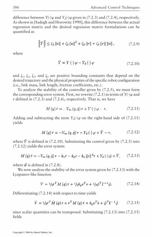
Advanced Control Techniques386
difference between Y(·) and Yd(·) given in (7.2.3) and (7.2.4), respectively.As shown in [Sadegh and Horowitz 1990], this difference between the actualregression matrix and the desired regression matrix formulations can bequantified as
and 1, 2, 3, and 4 are positive bounding constants that depend on thedesired trajectory and the physical properties of the specific robot configuration(i.e., link mass, link length, friction coefficients, etc.).
To analyze the stability of the controller given by (7.2.5), we must formthe corresponding error system. First, we rewrite (7.2.1) in terms of Y(·) andr defined in (7.2.3) and (7.2.6), respectively. That is, we have
(7.2.11)
Adding and subtracting the term Yd(·) on the right-hand side of (7.2.11)yields
(7.2.12)
where is defined in (7.2.10). Substituting the control given by (7.2.5) into(7.2.12) yields the error system
(7.2.13)
where is defined in (7.2.8).We now analyze the stability of the error system given by (7.2.13) with the
Lyapunov-like function
(7.2.14)
Differentiating (7.2.14) with respect to time yields
(7.2.15)
since scalar quantities can be transposed. Substituting (7.2.13) into (7.2.15)fields
(7.2.9)
(7.2.10)
where
Copyright © 2004 by Marcel Dekker, Inc.
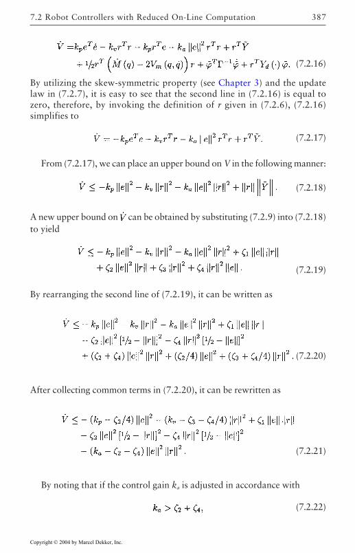
7.2 Robot Controllers with Reduced On-Line Computation 387
(7.2.16)
By utilizing the skew-symmetric property (see Chapter 3) and the updatelaw in (7.2.7), it is easy to see that the second line in (7.2.16) is equal tozero, therefore, by invoking the definition of r given in (7.2.6), (7.2.16)simplifies to
(7.2.17)
From (7.2.17), we can place an upper bound on V in the following manner:
(7.2.18)
A new upper bound on can be obtained by substituting (7.2.9) into (7.2.18)to yield
(7.2.19)
By rearranging the second line of (7.2.19), it can be written as
(7.2.20)
After collecting common terms in (7.2.20), it can be rewritten as
(7.2.21)
By noting that if the control gain ka is adjusted in accordance with
(7.2.22)
Copyright © 2004 by Marcel Dekker, Inc.
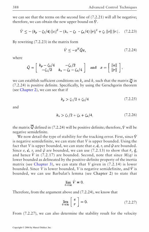
Advanced Control Techniques388
where
we can see that the terms on the second line of (7.2.21) will all be negative;therefore, we can obtain the new upper bound on .
(7.2.23)
By rewriting (7.2.23) in the matrix form
(7.2.24)
we can establish sufficient conditions on kp and kv such that the matrix in(7.2.24) is positive definite. Specifically, by using the Gerschgorin theorem(see Chapter 2), we can see that if
the matrix defined in (7.2.24) will be positive definite; therefore, will benegative semidefinite.
We now detail the type of stability for the tracking error. First, since is negative semidefinite, we can state that V is upper bounded. Using thefact that V is upper bounded, we can state that e, , r, and are bounded.Since e, , r, and are bounded, we can use (7.2.13) to show that and hence in (7.2.17) are bounded. Second, note that since M(q) islower bounded as delineated by the positive-definite property of the inertiamatrix (see Chapter 3), we can state that V given in (7.2.14) is lowerbounded. Since V is lower bounded, V is negative semidefinite, and isbounded, we can use Barbalat’s lemma (see Chapter 2) to state that
Therefore, from the argument above and (7.2.24), we know that
(7.2.27)
From (7.2.27), we can also determine the stability result for the velocity
and
(7.2.26)
(7.2.25)
Copyright © 2004 by Marcel Dekker, Inc.
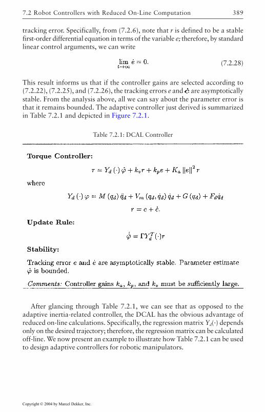
7.2 Robot Controllers with Reduced On-Line Computation 389
tracking error. Specifically, from (7.2.6), note that r is defined to be a stablefirst-order differential equation in terms of the variable e; therefore, by standardlinear control arguments, we can write
(7.2.28)
This result informs us that if the controller gains are selected according to(7.2.22), (7.2.25), and (7.2.26), the tracking errors e and are asymptoticallystable. From the analysis above, all we can say about the parameter error isthat it remains bounded. The adaptive controller just derived is summarizedin Table 7.2.1 and depicted in Figure 7.2.1.
Table 7.2.1: DCAL Controller
After glancing through Table 7.2.1, we can see that as opposed to theadaptive inertia-related controller, the DCAL has the obvious advantage ofreduced on-line calculations. Specifically, the regression matrix Yd(·) dependsonly on the desired trajectory; therefore, the regression matrix can be calculatedoff-line. We now present an example to illustrate how Table 7.2.1 can be usedto design adaptive controllers for robotic manipulators.
Copyright © 2004 by Marcel Dekker, Inc.
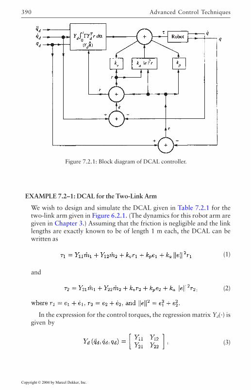
Advanced Control Techniques390
EXAMPLE 7.2–1: DCAL for the Two-Link Arm
We wish to design and simulate the DCAL given in Table 7.2.1 for thetwo-link arm given in Figure 6.2.1. (The dynamics for this robot arm aregiven in Chapter 3.) Assuming that the friction is negligible and the linklengths are exactly known to be of length 1 m each, the DCAL can bewritten as
(1)
and
(2)
In the expression for the control torques, the regression matrix Yd(·) isgiven by
(3)
Figure 7.2.1: Block diagram of DCAL controller.
Copyright © 2004 by Marcel Dekker, Inc.
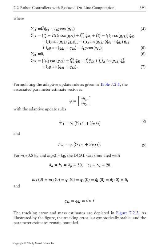
7.2 Robot Controllers with Reduced On-Line Computation 391
where
Formulating the adaptive update rule as given in Table 7.2.1, theassociated parameter estimate vector is
with the adaptive update rules
(8)
For m1=0.8 kg and m2=2.3 kg, the DCAL was simulated with
The tracking error and mass estimates are depicted in Figure 7.2.2. Asillustrated by the figure, the tracking error is asymptotically stable, and theparameter estimates remain bounded.
(9)
and
and
Copyright © 2004 by Marcel Dekker, Inc.
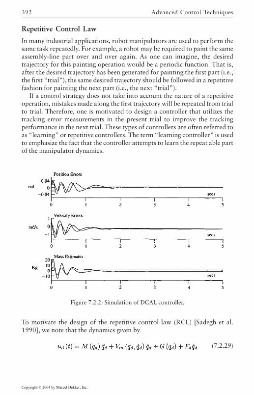
Advanced Control Techniques392
Repetitive Control Law
In many industrial applications, robot manipulators are used to perform thesame task repeatedly. For example, a robot may be required to paint the sameassembly-line part over and over again. As one can imagine, the desiredtrajectory for this painting operation would be a periodic function. That is,after the desired trajectory has been generated for painting the first part (i.e.,the first “trial”), the same desired trajectory should be followed in a repetitivefashion for painting the next part (i.e., the next “trial”).
If a control strategy does not take into account the nature of a repetitiveoperation, mistakes made along the first trajectory will be repeated from trialto trial. Therefore, one is motivated to design a controller that utilizes thetracking error measurements in the present trial to improve the trackingperformance in the next trial. These types of controllers are often referred toas “learning” or repetitive controllers. The term “learning controller” is usedto emphasize the fact that the controller attempts to learn the repeat able partof the manipulator dynamics.
To motivate the design of the repetitive control law (RCL) [Sadegh et al.1990], we note that the dynamics given by
(7.2.29)
Figure 7.2.2: Simulation of DCAL controller.
Copyright © 2004 by Marcel Dekker, Inc.
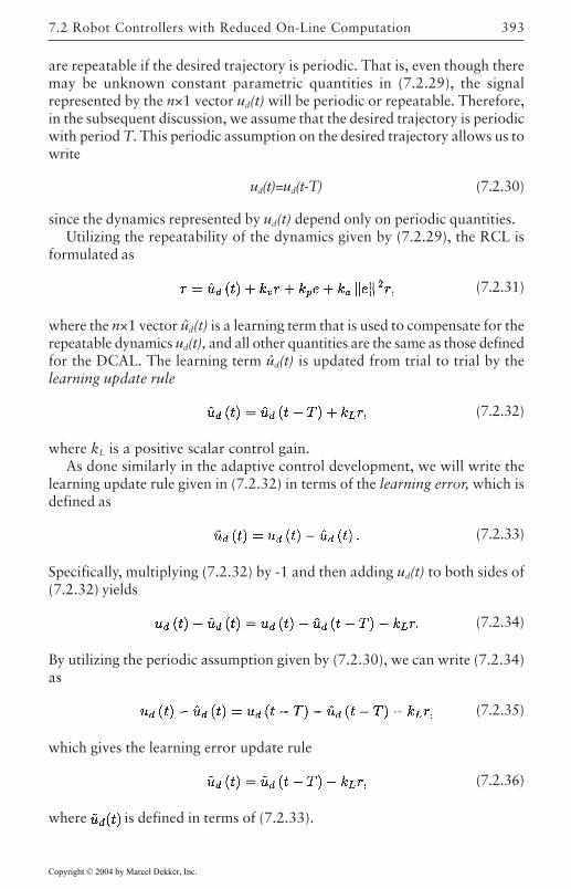
7.2 Robot Controllers with Reduced On-Line Computation 393
are repeatable if the desired trajectory is periodic. That is, even though theremay be unknown constant parametric quantities in (7.2.29), the signalrepresented by the n×1 vector ud(t) will be periodic or repeatable. Therefore,in the subsequent discussion, we assume that the desired trajectory is periodicwith period T. This periodic assumption on the desired trajectory allows us towrite
ud(t)=ud(t-T) (7.2.30)
since the dynamics represented by ud(t) depend only on periodic quantities.Utilizing the repeatability of the dynamics given by (7.2.29), the RCL is
formulated as
(7.2.31)
where the n×1 vector ûd(t) is a learning term that is used to compensate for therepeatable dynamics ud(t), and all other quantities are the same as those definedfor the DCAL. The learning term ûd(t) is updated from trial to trial by thelearning update rule
(7.2.32)
where kL is a positive scalar control gain.As done similarly in the adaptive control development, we will write the
learning update rule given in (7.2.32) in terms of the learning error, which isdefined as
(7.2.33)
Specifically, multiplying (7.2.32) by -1 and then adding ud(t) to both sides of(7.2.32) yields
(7.2.34)
By utilizing the periodic assumption given by (7.2.30), we can write (7.2.34)as
(7.2.35)
which gives the learning error update rule
(7.2.36)
where is defined in terms of (7.2.33).
Copyright © 2004 by Marcel Dekker, Inc.

Advanced Control Techniques394
Before we analyze the stability of the controller given in (7.2.31), we willform the corresponding error system. First, we rewrite (7.2.1) in terms of rdefined in (7.2.6). That is, we have
(7.2.37)
where the n×1 vector ua(t) is used to represent the “actual manipulatordynamics” given by
(7.2.38)
Adding and subtracting the term ud(t) on the right-hand side of (7.2.37) yields
(7.2.39)
where is defined as
(7.2.40)
As shown similarly in [Sadegh and Horowitz 1990], this difference betweenthe actual manipulator dynamics (i.e., ua(t)) and the repeatable manipulatordynamics (i.e., ud(t)) can be quantified as
(7.2.41)
where 1, 2, 3, and 4 are positive bounding constants that depend on thedesired trajectory and the physical properties of the specific robot configuration(i.e., link mass, link length, friction coefficients, etc.).
The last step in forming the error system is to substitute the control givenby (7.2.31) into (7.2.39) to yield
(7.2.42)
We now analyze the stability of the error system given by (7.2.42) with theLyapunov-like function
(7.2.43)
Differentiating (7.2.43) with respect to time yields
Copyright © 2004 by Marcel Dekker, Inc.
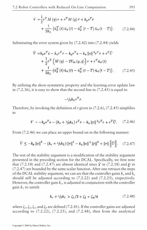
7.2 Robot Controllers with Reduced On-Line Computation 395
(7.2.44)
Substituting the error system given by (7.2.42) into (7.2.44) yields
(7.2.45)
By utilizing the skew-symmetric property and the learning error update lawin (7.2.36), it is easy to show that the second line in (7.2.45) is equal to
Therefore, by invoking the definition of r given in (7.2.6), (7.2.45) simplifiesto
(7.2.46)
From (7.2.46) we can place an upper bound on in the following manner:
(7.2.47)
The rest of the stability argument is a modification of the stability argumentpresented in the preceding section for the DCAL. Specifically, we first notethat (7.2.18) and (7.2.47) are almost identical since in (7.2.18) and in(7.2.47) are bounded by the same scalar function. After one retraces the stepsof the DCAL stability argument, we can see that the controller gains ka and kp
should still be adjusted according to (7.2.22) and (7.2.25), respectively.However, the controller gain kv, is adjusted in conjunction with the controllergain kL to satisfy
(7.2.48)
where 1, 2, 3, and 4 are defined (7.2.41). If the controller gains are adjustedaccording to (7.2.22), (7.2.25), and (7.2.48), then from the analytical
Copyright © 2004 by Marcel Dekker, Inc.
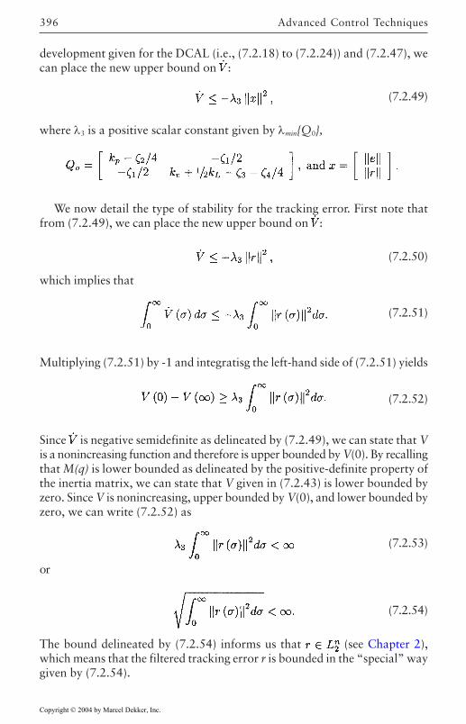
Advanced Control Techniques396
development given for the DCAL (i.e., (7.2.18) to (7.2.24)) and (7.2.47), wecan place the new upper bound on :
(7.2.49)
where λ3 is a positive scalar constant given by λminQ0,
We now detail the type of stability for the tracking error. First note thatfrom (7.2.49), we can place the new upper bound on :
Multiplying (7.2.51) by -1 and integratisg the left-hand side of (7.2.51) yields
(7.2.52)
Since is negative semidefinite as delineated by (7.2.49), we can state that Vis a nonincreasing function and therefore is upper bounded by V(0). By recallingthat M(q) is lower bounded as delineated by the positive-definite property ofthe inertia matrix, we can state that V given in (7.2.43) is lower bounded byzero. Since V is nonincreasing, upper bounded by V(0), and lower bounded byzero, we can write (7.2.52) as
(7.2.53)
or
The bound delineated by (7.2.54) informs us that (see Chapter 2),which means that the filtered tracking error r is bounded in the “special” waygiven by (7.2.54).
(7.2.50)
which implies that
(7.2.51)
(7.2.54)
Copyright © 2004 by Marcel Dekker, Inc.
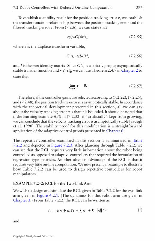
7.2 Robot Controllers with Reduced On-Line Computation 397
To establish a stability result for the position tracking error e, we establishthe transfer function relationship between the position tracking error and thefiltered tracking error r. From (7.2.6), we can state that
e(s)=G(s)r(s), (7.2.55)
where s is the Laplace transform variable,
G (s)=(sI+I)-1, (7.2.56)
and I is the n×n identity matrix. Since G(s) is a strictly proper, asymptoticallystable transfer function and , we can use Theorem 2.4.7 in Chapter 2 to
state that
(7.2.57)
Therefore, if the controller gains are selected according to (7.2.22), (7.2.25),and (7.2.48), the position tracking error e is asymptotically stable. In accordancewith the theoretical development presented in this section, all we can sayabout the velocity tracking error e is that it is bounded. It should be noted thatif the learning estimate ûd(t) in (7.2.32) is “artificially” kept from growing,we can conclude that the velocity tracking error is asymptotically stable [Sadeghet al. 1990]. The stability proof for this modification is a straightforwardapplication of the adaptive control proofs presented in Chapter 6.
The repetitive controller examined in this section is summarized in Table7.2.2 and depicted in Figure 7.2.3. After glancing through Table 7.2.2, wecan see that the RCL requires very little information about the robot beingcontrolled as opposed to adaptive controllers that required the formulation ofregression-type matrices. Another obvious advantage of the RCL is that itrequires very little on-line computation. We now present an example to illustratehow Table 7.2.2 can be used to design repetitive controllers for robotmanipulators.
EXAMPLE 7.2–2: RCL for the Two-Link Arm
We wish to design and simulate the RCL given in Table 7.2.2 for the two-linkarm given in Figure 6.2.1. (The dynamics for this robot arm are given inChapter 3.) From Table 7.2.2, the RCL can be written as
(1)
and
Copyright © 2004 by Marcel Dekker, Inc.
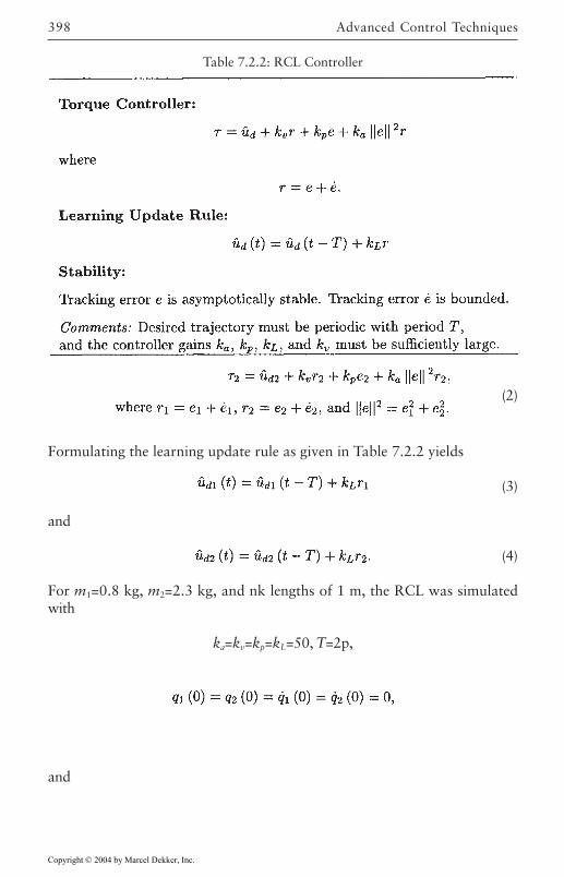
Advanced Control Techniques398
(2)
Formulating the learning update rule as given in Table 7.2.2 yields
(3)
and
(4)
For m1=0.8 kg, m2=2.3 kg, and nk lengths of 1 m, the RCL was simulatedwith
ka=kv=kp=kL=50, T=2p,
and
Table 7.2.2: RCL Controller
Copyright © 2004 by Marcel Dekker, Inc.
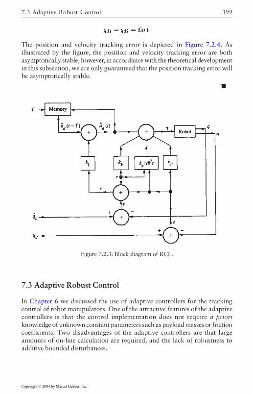
7.3 Adaptive Robust Control 399
The position and velocity tracking error is depicted in Figure 7.2.4. Asillustrated by the figure, the position and velocity tracking error are bothasymptotically stable; however, in accordance with the theoretical developmentin this subsection, we are only guaranteed that the position tracking error willbe asymptotically stable.
7.3 Adaptive Robust Control
In Chapter 6 we discussed the use of adaptive controllers for the trackingcontrol of robot manipulators. One of the attractive features of the adaptivecontrollers is that the control implementation does not require a prioriknowledge of unknown constant parameters such as payload masses or frictioncoefficients. Two disadvantages of the adaptive controllers are that largeamounts of on-line calculation are required, and the lack of robustness toadditive bounded disturbances.
Figure 7.2.3: Block diagram of RCL.
Copyright © 2004 by Marcel Dekker, Inc.
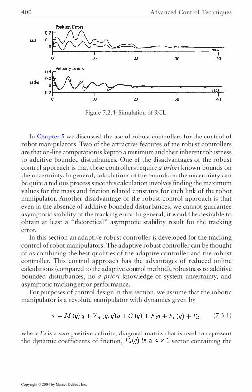
Advanced Control Techniques400
In Chapter 5 we discussed the use of robust controllers for the control ofrobot manipulators. Two of the attractive features of the robust controllersare that on-line computation is kept to a minimum and their inherent robustnessto additive bounded disturbances. One of the disadvantages of the robustcontrol approach is that these controllers require a priori known bounds onthe uncertainty. In general, calculations of the bounds on the uncertainty canbe quite a tedious process since this calculation involves finding the maximumvalues for the mass and friction related constants for each link of the robotmanipulator. Another disadvantage of the robust control approach is thateven in the absence of additive bounded disturbances, we cannot guaranteeasymptotic stability of the tracking error. In general, it would be desirable toobtain at least a “theoretical” asymptotic stability result for the trackingerror.
In this section an adaptive robust controller is developed for the trackingcontrol of robot manipulators. The adaptive robust controller can be thoughtof as combining the best qualities of the adaptive controller and the robustcontroller. This control approach has the advantages of reduced onlinecalculations (compared to the adaptive control method), robustness to additivebounded disturbances, no a priori knowledge of system uncertainty, andasymptotic tracking error performance.
For purposes of control design in this section, we assume that the roboticmanipulator is a revolute manipulator with dynamics given by
(7.3.1)
where Fd is a n×n positive definite, diagonal matrix that is used to representthe dynamic coefficients of friction, vector containing the
Figure 7.2.4: Simulation of RCL.
Copyright © 2004 by Marcel Dekker, Inc.
7.3 Adaptive Robust Control 401
static friction terms, Td is a n×1 vector representing an unknown boundeddisturbance, and all other quantities are as defined in Chapter 3.
The adaptive robust controller is very similar to the robust control strategiesdiscussed in Chapter 5 in that an auxiliary controller is used to “bound” theuncertainty. Recall from Chapter 5 that the robust controllers bounded theuncertainty by using a scalar function that was composed of tracking errornorms and positive bounding constants. For example, suppose that the dynamicsgiven by
(7.3.2)
represent the uncertainty for a given robot controller. That is, the dynamicsgiven by (7.3.2) are uncertain in that payload masses, coefficients of friction,and disturbances are not known exactly. It is assumed; however, that a positivescalar function ρ can be used to bound the uncertainty as follows:
(7.3.3)
As delineated in [Dawson et al. 1990], the physical properties of the robotmanipulator can be used to show that the dynamics given by (7.3.2) can bebounded as
(7.3.4)
and δ0, δ1, and δ2 are positive bounding constants that are based on the largestpossible payload mass, link mass, friction coefficients, disturbances, and so on.
In general, the robust controllers presented in Chapter 5 required that thebounding constants defined in (7.3.4) be formulated a priori. The adaptiverobust controller that will be developed in this section “learns” these boundingconstants on-line as the manipulator moves. That is, in the controlimplementation, we do not require knowledge of the bounding constants;rather, we only require the existence of the bounding constants defined in(7.3.4).
Similar to the general development presented in [Corless and Leitmann1983], the adaptive robust controller has the form
(7.3.6)
(7.3.5)
where
Copyright © 2004 by Marcel Dekker, Inc.
Advanced Control Techniques402
where Kv is a n×n diagonal, positive-definite matrix, r (the filtered trackingerror) is defined as in (7.2.6), and vR is a n×1 vector representing an auxiliarycontroller. The auxiliary controller vR in (7.3.6) is defined by
(7.3.7)
kε is a positive scalar control constant, is a scalar function defined as
(7.3.9)
and are the dynamic estimates of the corresponding boundingconstants δ0, δ1, and δ2 defined in (7.3.4). The bounding estimates denoted by“ˆ” are changed on-line based on an adaptive update rule. Before giving theupdate rule, we write (7.3.9) in the more convenient form
(7.3.10)
The actual bounding function ρ given in (7.3.3) can also be written in thematrix form
(7.3.11)
Note the similarity between the regression matrix formulation in the adaptiveapproach (see Chapter 6) and the formulation given by (7.3.10). Specifically,the 1×3 matrix S resembles a “regression matrix,” and the 3×1 vector resembles a “parameter estimate vector.”
The bounding estimates defined in (7.3.10) are updated on-line by therelation
(7.3.12)
where r is defined in (7.2.6), S is defined in (7.3.10), and γ is a positive scalarcontrol constant. For convenience, we also note that since δ0, δ1, and δ2 definedin (7.3.4) are constants, (7.3.12) can be written as
where
(7.3.8)
where
where
Copyright © 2004 by Marcel Dekker, Inc.
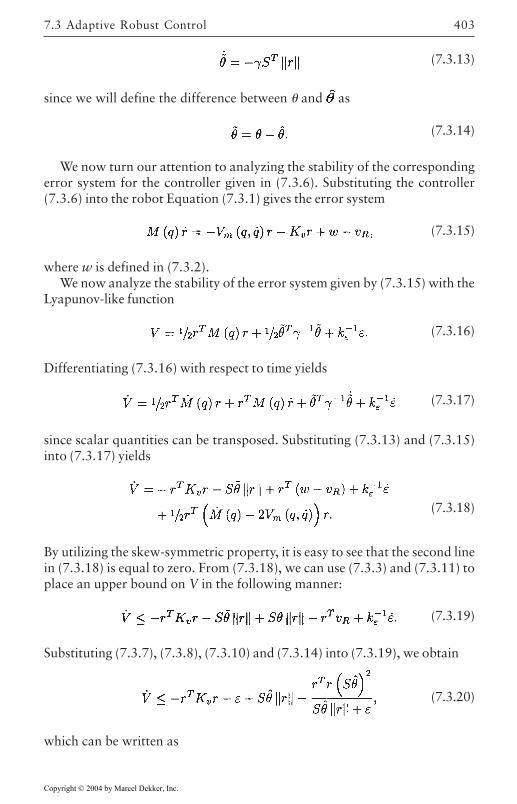
7.3 Adaptive Robust Control 403
(7.3.13)
since we will define the difference between and as
(7.3.14)
We now turn our attention to analyzing the stability of the correspondingerror system for the controller given in (7.3.6). Substituting the controller(7.3.6) into the robot Equation (7.3.1) gives the error system
(7.3.15)
where w is defined in (7.3.2).We now analyze the stability of the error system given by (7.3.15) with the
Lyapunov-like function
(7.3.16)
Differentiating (7.3.16) with respect to time yields
(7.3.17)
since scalar quantities can be transposed. Substituting (7.3.13) and (7.3.15)into (7.3.17) yields
(7.3.18)
By utilizing the skew-symmetric property, it is easy to see that the second linein (7.3.18) is equal to zero. From (7.3.18), we can use (7.3.3) and (7.3.11) toplace an upper bound on V in the following manner:
(7.3.19)
Substituting (7.3.7), (7.3.8), (7.3.10) and (7.3.14) into (7.3.19), we obtain
(7.3.20)
which can be written as
Copyright © 2004 by Marcel Dekker, Inc.
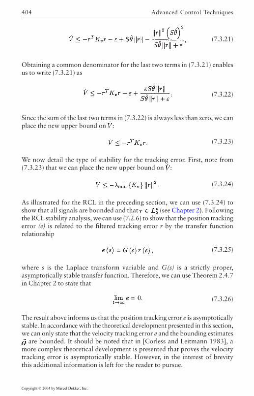
Advanced Control Techniques404
(7.3.21)
Obtaining a common denominator for the last two terms in (7.3.21) enablesus to write (7.3.21) as
(7.3.22)
Since the sum of the last two terms in (7.3.22) is always less than zero, we canplace the new upper bound on :
(7.3.23)
We now detail the type of stability for the tracking error. First, note from(7.3.23) that we can place the new upper bound on :
(7.3.24)
As illustrated for the RCL in the preceding section, we can use (7.3.24) toshow that all signals are bounded and that (see Chapter 2). Followingthe RCL stability analysis, we can use (7.2.6) to show that the position trackingerror (e) is related to the filtered tracking error r by the transfer functionrelationship
(7.3.25)
where s is the Laplace transform variable and G(s) is a strictly proper,asymptotically stable transfer function. Therefore, we can use Theorem 2.4.7in Chapter 2 to state that
(7.3.26)
The result above informs us that the position tracking error e is asymptoticallystable. In accordance with the theoretical development presented in this section,we can only state that the velocity tracking error e and the bounding estimates
are bounded. It should be noted that in [Corless and Leitmann 1983], amore complex theoretical development is presented that proves the velocitytracking error is asymptotically stable. However, in the interest of brevitythis additional information is left for the reader to pursue.
Copyright © 2004 by Marcel Dekker, Inc.
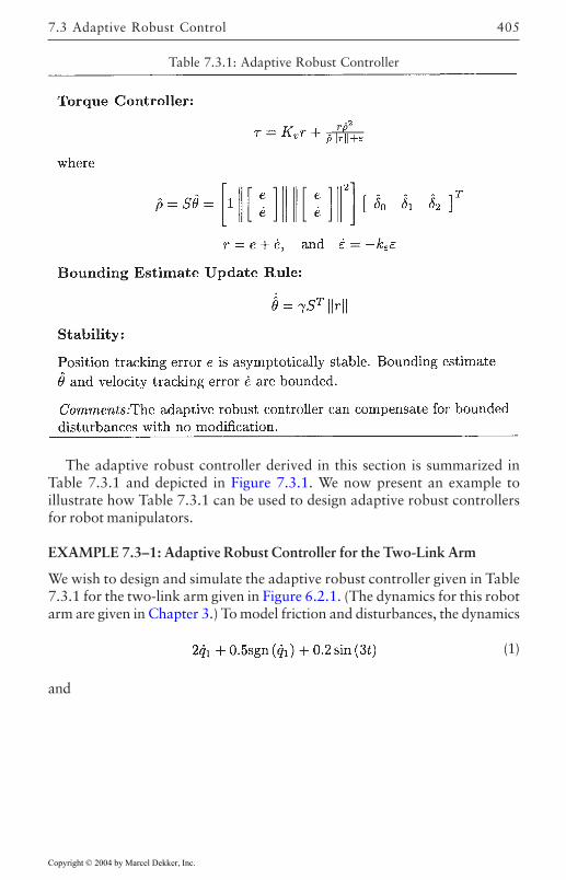
7.3 Adaptive Robust Control 405
The adaptive robust controller derived in this section is summarized inTable 7.3.1 and depicted in Figure 7.3.1. We now present an example toillustrate how Table 7.3.1 can be used to design adaptive robust controllersfor robot manipulators.
EXAMPLE 7.3–1: Adaptive Robust Controller for the Two-Link Arm
We wish to design and simulate the adaptive robust controller given in Table7.3.1 for the two-link arm given in Figure 6.2.1. (The dynamics for this robotarm are given in Chapter 3.) To model friction and disturbances, the dynamics
(1)
and
Table 7.3.1: Adaptive Robust Controller
Copyright © 2004 by Marcel Dekker, Inc.
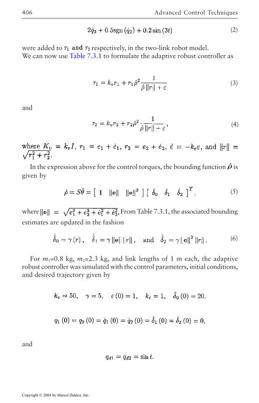
Advanced Control Techniques406
(2)
were added to respectively, in the two-link robot model.We can now use Table 7.3.1 to formulate the adaptive robust controller as
(3)
In the expression above for the control torques, the bounding function isgiven by
(5)
where From Table 7.3.1, the associated bounding
estimates are updated in the fashion
(6)
For m1=0.8 kg, m2=2.3 kg, and link lengths of 1 m each, the adaptiverobust controller was simulated with the control parameters, initial conditions,and desired trajectory given by
and
(4)
and
Copyright © 2004 by Marcel Dekker, Inc.
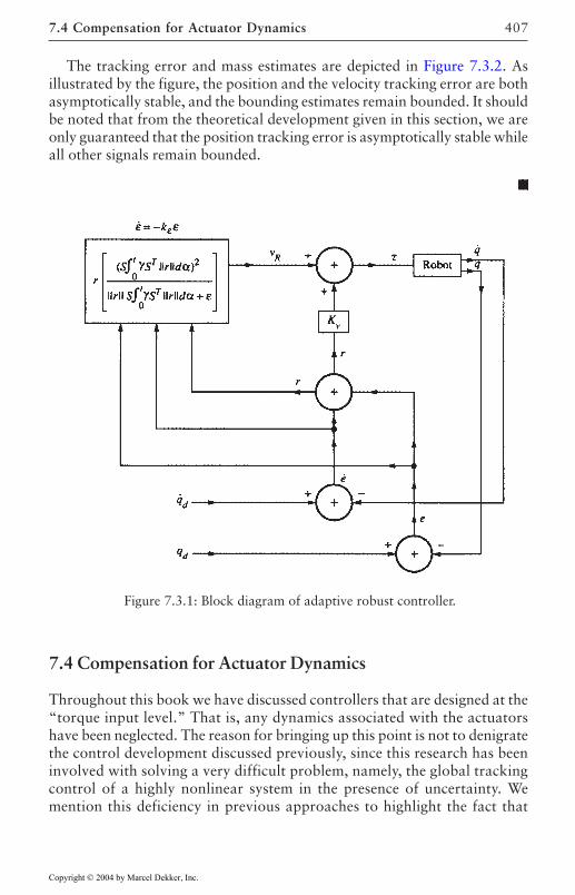
7.4 Compensation for Actuator Dynamics 407
The tracking error and mass estimates are depicted in Figure 7.3.2. Asillustrated by the figure, the position and the velocity tracking error are bothasymptotically stable, and the bounding estimates remain bounded. It shouldbe noted that from the theoretical development given in this section, we areonly guaranteed that the position tracking error is asymptotically stable whileall other signals remain bounded.
7.4 Compensation for Actuator Dynamics
Throughout this book we have discussed controllers that are designed at the“torque input level.” That is, any dynamics associated with the actuatorshave been neglected. The reason for bringing up this point is not to denigratethe control development discussed previously, since this research has beeninvolved with solving a very difficult problem, namely, the global trackingcontrol of a highly nonlinear system in the presence of uncertainty. Wemention this deficiency in previous approaches to highlight the fact that
Figure 7.3.1: Block diagram of adaptive robust controller.
Copyright © 2004 by Marcel Dekker, Inc.
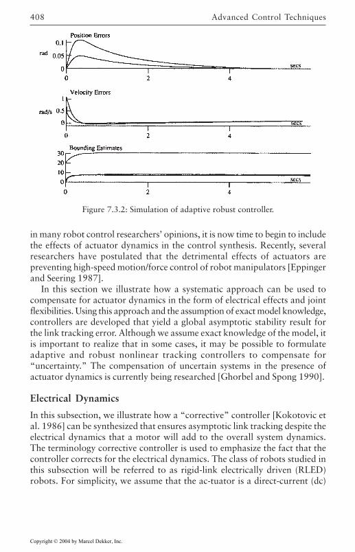
Advanced Control Techniques408
in many robot control researchers’ opinions, it is now time to begin to includethe effects of actuator dynamics in the control synthesis. Recently, severalresearchers have postulated that the detrimental effects of actuators arepreventing high-speed motion/force control of robot manipulators [Eppingerand Seering 1987].
In this section we illustrate how a systematic approach can be used tocompensate for actuator dynamics in the form of electrical effects and jointflexibilities. Using this approach and the assumption of exact model knowledge,controllers are developed that yield a global asymptotic stability result forthe link tracking error. Although we assume exact knowledge of the model, itis important to realize that in some cases, it may be possible to formulateadaptive and robust nonlinear tracking controllers to compensate for“uncertainty.” The compensation of uncertain systems in the presence ofactuator dynamics is currently being researched [Ghorbel and Spong 1990].
Electrical Dynamics
In this subsection, we illustrate how a “corrective” controller [Kokotovic etal. 1986] can be synthesized that ensures asymptotic link tracking despite theelectrical dynamics that a motor will add to the overall system dynamics.The terminology corrective controller is used to emphasize the fact that thecontroller corrects for the electrical dynamics. The class of robots studied inthis subsection will be referred to as rigid-link electrically driven (RLED)robots. For simplicity, we assume that the ac-tuator is a direct-current (dc)
Figure 7.3.2: Simulation of adaptive robust controller.
Copyright © 2004 by Marcel Dekker, Inc.
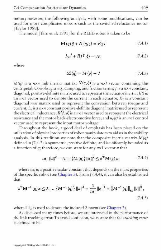
7.4 Compensation for Actuator Dynamics 409
motor; however, the following analysis, with some modifications, can beused for more complicated motors such as the switched-reluctance motor[Taylor 1989].
The model [Tarn et al. 1991] for the RLED robot is taken to be
(7.4.1)
(7.4.2)
(7.4.3)
M(q) is a n×n link inertia matrix, is a n×I vector containing thecentripetal, Coriolis, gravity, damping, and friction terms, J is a n×n constant,diagonal, positive-definite matrix used to represent the actuator inertia, I(t) isan n×1 vector used to denote the current in each actuator, KT is a constantdiagonal n×n matrix used to represent the conversion between torque andcurrent, La is a n×n constant positive-definite diagonal matrix used to representthe electrical inductance, is a n×1 vector used to represent the electricalresistance and the motor back-electromotive force, and uE(t) is an n×1 controlvector used to represent the input motor voltage.
Throughout the book, a good deal of emphasis has been placed on theutilization of physical properties of robot manipulators to aid us in the stabilityanalysis. In this tradition we note that the composite inertia matrix M(q)defined in (7.4.3) is symmetric, positive definite, and is uniformly bounded asa function of q; therefore, we can state for any n×1 vector x that
(7.4.4)
where m1 is a positive scalar constant that depends on the mass propertiesof the specific robot (see Chapter 3). From (7.4.4), it can also be establishedthat
(7.4.5)
where ||·||i2 is used to denote the induced 2-norm (see Chapter 2).As discussed many times before, we are interested in the performance of
the link tracking error. To avoid confusion, we restate that the tracking erroris defined to be
where
Copyright © 2004 by Marcel Dekker, Inc.
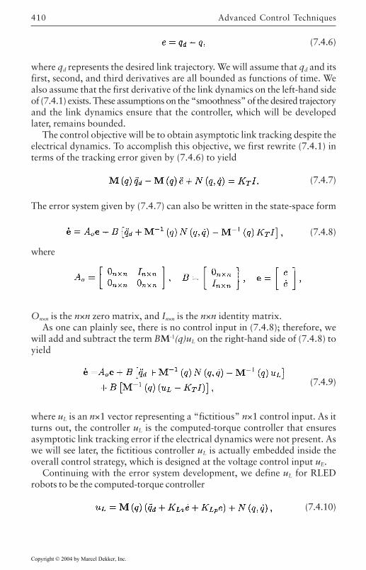
Advanced Control Techniques410
(7.4.6)
where qd represents the desired link trajectory. We will assume that qd and itsfirst, second, and third derivatives are all bounded as functions of time. Wealso assume that the first derivative of the link dynamics on the left-hand sideof (7.4.1) exists. These assumptions on the “smoothness” of the desired trajectoryand the link dynamics ensure that the controller, which will be developedlater, remains bounded.
The control objective will be to obtain asymptotic link tracking despite theelectrical dynamics. To accomplish this objective, we first rewrite (7.4.1) interms of the tracking error given by (7.4.6) to yield
(7.4.7)
The error system given by (7.4.7) can also be written in the state-space form
(7.4.8)
On×n is the n×n zero matrix, and In×n is the n×n identity matrix.As one can plainly see, there is no control input in (7.4.8); therefore, we
will add and subtract the term BM-1(q)uL on the right-hand side of (7.4.8) toyield
(7.4.9)
where uL is an n×1 vector representing a “fictitious” n×1 control input. As itturns out, the controller uL is the computed-torque controller that ensuresasymptotic link tracking error if the electrical dynamics were not present. Aswe will see later, the fictitious controller uL is actually embedded inside theoverall control strategy, which is designed at the voltage control input uE.
Continuing with the error system development, we define uL for RLEDrobots to be the computed-torque controller
(7.4.10)
where
Copyright © 2004 by Marcel Dekker, Inc.
7.4 Compensation for Actuator Dynamics 411
where KLv and KLp are defined to be n×n positive-definite diagonal matrices.Substituting (7.4.10) for only the first uL term in (7.4.9) yields the link trackingerror system
(7.4.11)
With regard to the link tracking error system given by (7.4.11), if ηE couldbe guaranteed to be zero for all time, we could easily show that the trackingerror would be asymptotically stable since AL defined in (7.4.12) has stableeigenvalues. Therefore, one can view the control objective as forcing the“perturbation” η E to go to zero.
To design a control law for ηE, we must first establish its dynamiccharacteristics. From (7.4.12), the derivative of ηE with respect to time isgiven by
(7.4.13)
To obtain the the dynamic characteristics of ηE, we substitute for in (7.4.13)from (7.4.2) to yield
(7.4.14)
We can now use (7.4.14) to design a control law at the input uE to force ηE
to go to zero. The fact that ηE should go to zero motivates the correctivecontrol law
(7.4.15)
where KEp is defined to be a n×n positive-definite diagonal matrix. Substituting(7.4.15) into (7.4.14) yields
(7.4.16)
The dynamic equations given by (7.4.11) and (7.4.16) can be thought of astwo interconnected systems representing the overall closed-loop dynamics. Asone would expect, it would be desirable to determine the type of stability ofthe overall closed-loop system. To determine the type of stability of (7.4.11)and (7.4.16), we will utilize the Lyapunov function
where
(7.4.11)
(7.4.17)
Copyright © 2004 by Marcel Dekker, Inc.
Advanced Control Techniques412
where
If the sufficient condition given by
(7.4.18)
is satisfied, then by the Gerschgorin theorem (see Chapter 2), it is obvious thatPL is a positive-definite matrix, and hence V is a Lyapunov function. Thecondition given by (7.4.18) simply means that the smallest velocity controllergain should be larger than 1.
Differentiating (7.4.17) with respect to time yields
Note that if the sufficient condition given by (7.4.18) holds, it is obvious thatthe matrix QL is positive definite. Using the fact that QL is positive definiteallows us to place an upper bound on given in (7.4.20). This upper boundis given by
(7.4.22)
where ml is defined in (7.4.5).To determine the sufficient conditions on the controller gains for asymptotic
stability, we rewrite (7.4.22) in the matrix form
(7.4.23)
where
(7.4.19)
Substituting (7.4.11) and (7.4.16) into (7.4.19) yields
where
where
Copyright © 2004 by Marcel Dekker, Inc.
7.4 Compensation for Actuator Dynamics 413
By the Gerschgorin Theorem, the matrix Q0 defined in (7.4.23) will be positive
definite if the sufficient condition
(7.4.24)
holds. Therefore, if the controller gains satisfy the conditions given by (7.4.18)and (7.4.24), we can use standard Lyapunov stability arguments (see Chapter2) to state that the vector x0 defined in (7.4.23) and hence ||e||, e, and e are allasymptotically stable. It is easy to show that if the sufficient condition
(7.4.25)
holds, the conditions given by (7.4.18) and (7.4.24) are always satisfied.It should be noted that the control given by (7.4.15) depends on the
measurement of uL, and I. At first one might be tempted to state that thiscontroller requires measurements of and I; however, since we haveassumed exact knowledge of the dynamic model given by (7.4.1) and (7.4.2),we can use this information to eliminate the need for measuring q That is, bydifferentiating (7.4.10) with respect to time, uL can be written as
(7.4.26)
After substituting for in (7.4.26), uL will depend only on the measurement ofq, and I. The actual control that would be implemented at the control inputuE can be found by making the appropriate substitution into (7.4.15). That is,the corrective control given by (7.4.15) can be written as
(7.4.27)
where is found from (7.4.1) to be
Copyright © 2004 by Marcel Dekker, Inc.
Advanced Control Techniques414
where would be given by (7.4.26).After examining the functional dependence of given in (7.4.26), it is
now obvious why we have assumed that the desired trajectory and the linkdynamics be sufficiently smooth. Specifically, we can see from (7.4.26) thatthe corrective controller requires that the first, second, and third time derivativesof the desired trajectory to be bounded while requiring the existence of thefirst derivative of the link dynamics. These assumptions on the desired trajectoryand the link dynamics ensure that the control input will remain bounded.
The corrective controller derived above is summarized in Table 7.4.1 anddepicted in Figure 7.4.1. We now present an example to illustrate how Table7.4.1 can be used to design corrective controllers for RLED robots.
EXAMPLE 7.4–1: Corrective Controller for the One-Link RLED Arm
We wish to design and simulate a corrective controller using Table 7.4.1 forthe one-link motor-driven robot arm given in Figure 7.4.2. The dynamics forthe system are taken to be
(1)
where m=1kg, KT=2 N/A, kb=0.3 V-S, fd=3 kg-m/s, L=1 m, La=0.1 H, R=5Ω, g is the gravitational coefficient, J=0.2 kg-m2, I is the motor current, and uE
is the motor input voltage.Assuming that the model given by (1) and (2) is known exactly, we can use
Table 7.4.1 to formulate the corrective controller
(3)
and
(2)
where
(4)
Copyright © 2004 by Marcel Dekker, Inc.
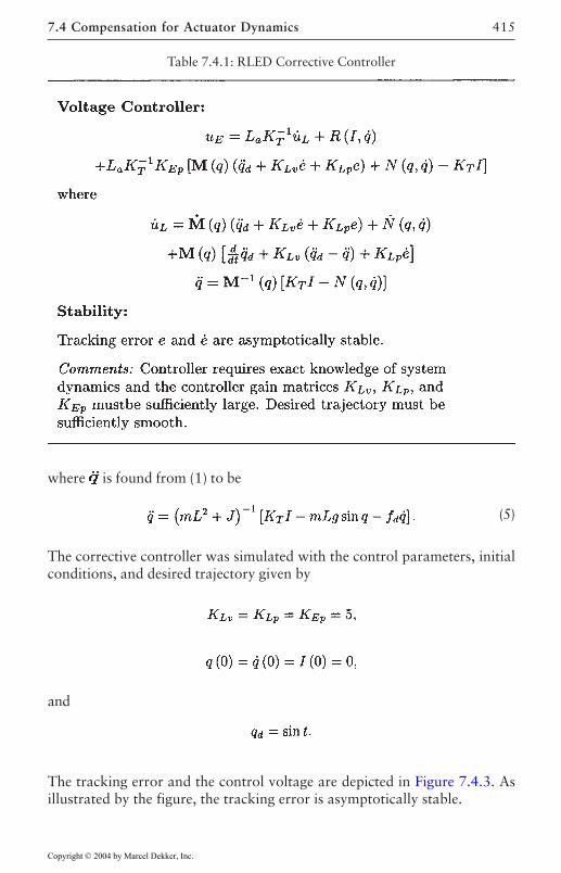
7.4 Compensation for Actuator Dynamics 415
where is found from (1) to be
(5)
The corrective controller was simulated with the control parameters, initialconditions, and desired trajectory given by
The tracking error and the control voltage are depicted in Figure 7.4.3. Asillustrated by the figure, the tracking error is asymptotically stable.
Table 7.4.1: RLED Corrective Controller
and
Copyright © 2004 by Marcel Dekker, Inc.
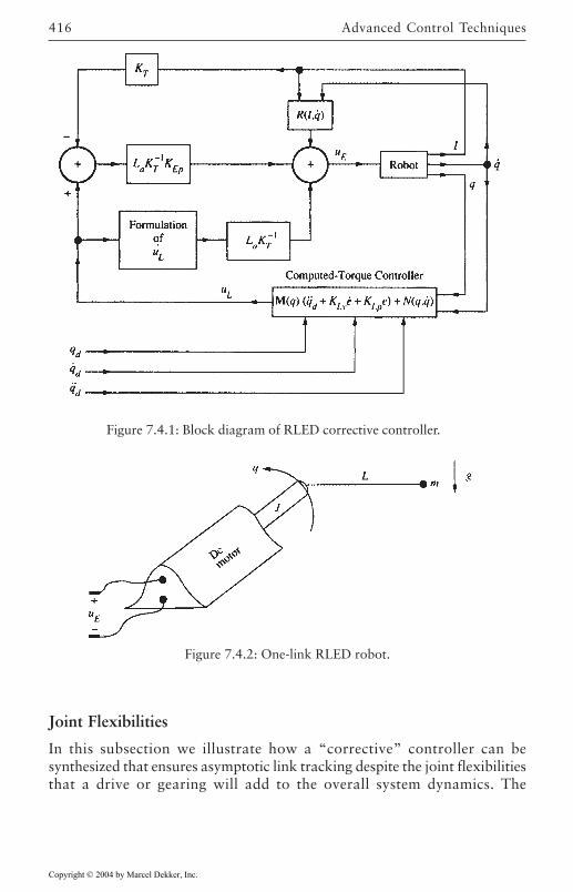
Advanced Control Techniques416
Joint Flexibilities
In this subsection we illustrate how a “corrective” controller can besynthesized that ensures asymptotic link tracking despite the joint flexibilitiesthat a drive or gearing will add to the overall system dynamics. The
Figure 7.4.1: Block diagram of RLED corrective controller.
Figure 7.4.2: One-link RLED robot.
Copyright © 2004 by Marcel Dekker, Inc.
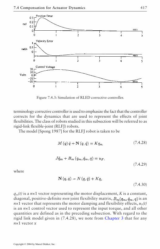
7.4 Compensation for Actuator Dynamics 417
terminology corrective controller is used to emphasize the fact that the controllercorrects for the dynamics that are used to represent the effects of jointflexibilities. The class of robots studied in this subsection will be referred to asrigid-link flexible-joint (RLFJ) robots.
The model [Spong 1987] for the RLFJ robot is taken to be
(7.4.28)
qm(t) is a n×1 vector representing the motor displacement, K is a constant,diagonal, positive-definite n×n joint flexibility matrix, is ann×1 vector that represents the motor damping and flexibility effects, uF(t)is an n×1 control vector used to represent the input torque, and all otherquantities are defined as in the preceding subsection. With regard to therigid link model given in (7.4.28), we note from Chapter 3 that for anyn×1 vector x
Figure 7.4.3: Simulation of RLED corrective controller.
where
(7.4.29)
(7.4.30)
Copyright © 2004 by Marcel Dekker, Inc.
Advanced Control Techniques418
(7.4.31)
where m1 is a positive scalar constant.As in the preceding subsection, we are interested in the performance of the
link tracking error defined in (7.4.6). For the control of RLFJ robots, we willassume that qd and its first, second, third, and fourth derivatives are all boundedas functions of time. We also assume that the first and second derivatives ofthe link dynamics on the left-hand side of (7.4.28) exist. These assumptionson the “smoothness” of the desired trajectory and the link dynamics ensurethat the controller, developed later, remains bounded.
Following the same analytical development given in the previous sections,we write (7.4.28) in terms of the tracking error given by (7.4.6) to yield thestate-space form
(7.4.32)
where A0, e, and B are defined as in (7.4.8). Again, since there is no controlinput in (7.4.32); we add and subtract the term BM-1(q)uL on the right-handside of (7.4.32) to yield
(7.4.33)
where uL is again used to represent a fictitious n×1 control input. As before,the fictitious controller uL will be embedded inside the overall control strategy,which is designed at the control input uF.
Continuing with the error system development, we define uL for RLFJ robotsto be the computed-torque controller
(7.4.34)
where KLv and KLp are defined as in (7.4.10). Substituting (7.4.34) into (7.4.33)yields the link tracking error system
(7.4.35)
where AL is defined as in (7.4.12),
Copyright © 2004 by Marcel Dekker, Inc.
7.4 Compensation for Actuator Dynamics 419
(7.4.36)
The reason for defining η F in terms of (uL-Kqm) and its derivative is that thedynamics given by (7.4.29) are second-order dynamics. That is, since theactuator dynamics are second order, we force ηF and its derivative (i.e.η. F, ) tozero to ensure that the link tracking error (e) goes to zero.
To design a control law for ηF, we must first establish its dynamiccharacteristics. From (7.4.36), the derivative of ηF is given by
(7.4.37)
To obtain the the dynamic characteristics of ηF, we substitute for qm in (7.4.37)from (7.4.29) to yield
(7.4.38)
We can now use (7.4.38) to design a control law at the input uF to force η F
to go to zero. The fact that ηF should go to zero motivates the control law
(7.4.39)
where KFv and KFp are defined to be n×n positive-definite diagonal matrices.Substituting (7.4.39) into (7.4.38) yields
(7.4.40)
The dynamic equations given by (7.4.35) and (7.4.40) can be thought of astwo interconnected systems representing the overall closed-loop dynamics.To determine the type of stability for the closed-loop dynamics, we will utilizethe Lyapunov function
(7.4.41)
where PL is defined in (7.4.17) and
where
Copyright © 2004 by Marcel Dekker, Inc.
Advanced Control Techniques420
If the sufficient condition given by
(7.4.42)
is satisfied, then by the Gerschgorin theorem it is obvious that the matrices PL
and PF given in (7.4.41) are positive-definite matrices, and hence V is aLyapunov function.
Differentiating (7.4.41) with respect to time yields
(7.4.43)
Substituting (7.4.35) and (7.4.40) into (7.4.43) yields
(7.4.44)
where QL is defined in (7.4.21) and
(7.4.45)
Note that if the sufficient condition given by (7.4.42) holds, it is obviousthat the matrices QL and QF defined in (7.4.44) are positive-definite matrices.Using the fact, that QL and QF are positive definite allows us to place anupper bound on given in (7.4.44). This upper bound is given by
(7.4.46)
where
where m1 is defined in (7.4.31).To determine the sufficient conditions on the controller gains for asymptotic
stability, we rewrite (7.4.46) in the matrix form
(7.4.47)
where
Copyright © 2004 by Marcel Dekker, Inc.
7.4 Compensation for Actuator Dynamics 421
By the Gerschgorin theorem, the matrix Q1 defined in (7.4.47) will be positive
definite if the sufficient condition
(7.4.48)
holds. Therefore, if the controller gains satisfy the conditions given by (7.4.42)and (7.4.48), we can use standard Lyapunov stability arguments to state thatthe vector x1 defined in (7.4.47), and hence ||e||, e, and e, are all asymptoticallystable. It is easy to show that if the sufficient condition
(7.4.49)
holds, the conditions given by (7.4.42) and (7.4.48) are always satisfied.It should be noted that the corrective controller given by (7.4.39) depends
on the measurement of Again, it seems that thiscontrol would require measurements of and its derivative; however, sincewe have assumed exact knowledge of the dynamic model, we can use thisinformation to eliminate the need for measuring and its derivative. That is,
can be written as
(7.4.50)
where is found from (7.4.28) to be
(7.4.51)
Substituting (7.4.51) into (7.4.50), we see that uL can be written as a functionof , and time (i.e., t) since the desired trajectory can be explicitlywritten as a function of time. We can delineate this functional dependence byuse of the equation
(7.4.52)
where is an n×1 vector given by the right-hand side of (7.4.50).We can obtain the functional dependence for üL by differentiating (7.4.52)with respect to time to yield
Copyright © 2004 by Marcel Dekker, Inc.
Advanced Control Techniques422
(7.4.53)
where is an n×1 vector. Note that (7.4.51) can be usedagain to eliminate the need for measurement of therefore, the expressionsgiven for and üL in (7.4.50) and (7.4.53), respectively, depend only on themeasurements of and The actual control that would beimplemented at the control input uF can be found by making the appropriatesubstitution into (7.4.39). That is, the corrective control given by (7.4.39) canbe written as
(7.4.54)
where and üL would be given by (7.4.50) and (7.4.53), respectively.After closely examining the functional dependence of and üL given in
(7.4.50) and (7.4.53), respectively, it is obvious why we have assumed thatthe desired trajectory and link dynamics be sufficiently smooth. Specifically,we can see from (7.4.50) and (7.4.53) that the corrective controller given in(7.4.39) will require that the first, second, third, and fourth time derivative ofthe desired trajectory be bounded while also requiring the existence of thefirst and second derivatives of the link dynamics. These assumptions on thedesired trajectory and the link dynamics ensure that the control input willremain bounded.
The corrective controller derived above is summarized in Table 7.4.2 anddepicted in Figure 7.4.4. We now present an example to illustrate how Table7.4.2 can be used to design corrective controllers for RLFJ robots.
EXAMPLE 7.4–2: Corrective Controller for the One-Link RLFJ Arm
We wish to design and simulate a corrective controller using Table 7.4.2 forthe one-link flexible joint robot arm given in Figure 7.4.5. The dynamics forthe system are taken to be
(1)
(2)and
Copyright © 2004 by Marcel Dekker, Inc.
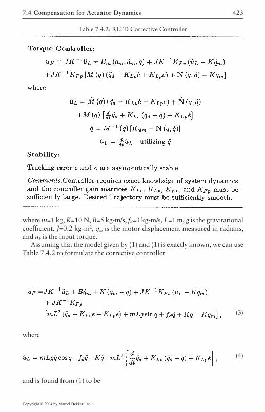
7.4 Compensation for Actuator Dynamics 423
where m=1 kg, K=10 N, B=5 kg-m/s, fd=3 kg-m/s, L=1 m, g is the gravitationalcoefficient, J=0.2 kg-m2, qm is the motor displacement measured in radians,and uF is the input torque.
Assuming that the model given by (1) and (1) is exactly known, we can useTable 7.4.2 to formulate the corrective controller
and is found from (1) to be
Table 7.4.2: RLED Corrective Controller
where
(3)
(4)
Copyright © 2004 by Marcel Dekker, Inc.
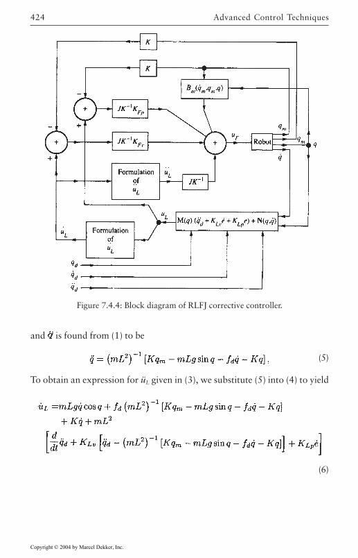
Advanced Control Techniques424
and is found from (1) to be
(5)
To obtain an expression for üL given in (3), we substitute (5) into (4) to yield
Figure 7.4.4: Block diagram of RLFJ corrective controller.
(6)
Copyright © 2004 by Marcel Dekker, Inc.
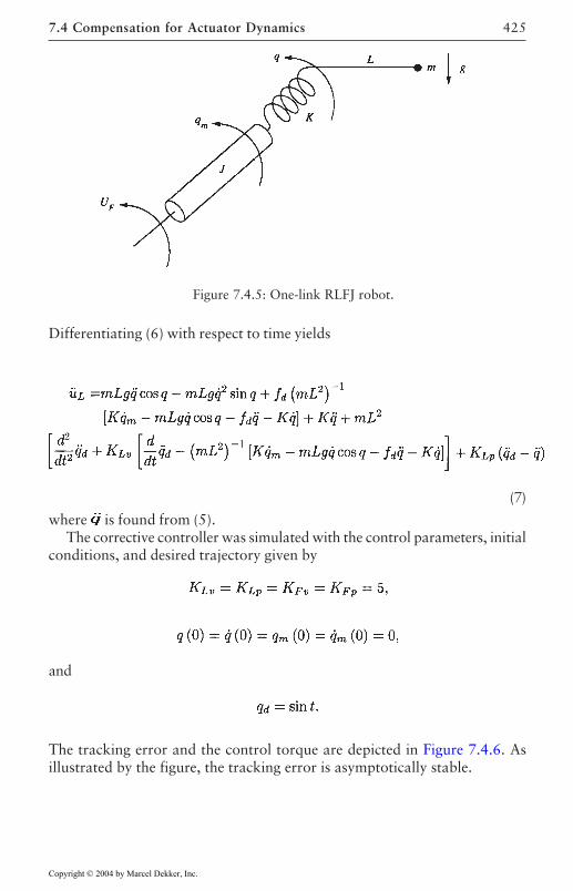
7.4 Compensation for Actuator Dynamics 425
Differentiating (6) with respect to time yields
where is found from (5).The corrective controller was simulated with the control parameters, initial
conditions, and desired trajectory given by
The tracking error and the control torque are depicted in Figure 7.4.6. Asillustrated by the figure, the tracking error is asymptotically stable.
Figure 7.4.5: One-link RLFJ robot.
(7)
and
Copyright © 2004 by Marcel Dekker, Inc.
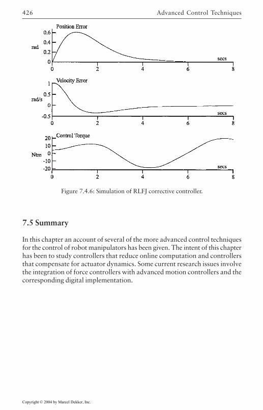
Advanced Control Techniques426
7.5 Summary
In this chapter an account of several of the more advanced control techniquesfor the control of robot manipulators has been given. The intent of this chapterhas been to study controllers that reduce online computation and controllersthat compensate for actuator dynamics. Some current research issues involvethe integration of force controllers with advanced motion controllers and thecorresponding digital implementation.
Figure 7.4.6: Simulation of RLFJ corrective controller.
Copyright © 2004 by Marcel Dekker, Inc.
427
REFERENCES
[Corless and Leitmann 1983] Corless, M., and G.Leitmann, “Adaptive control ofsystems containing uncertain functions and unknown functions with uncertainbounds,” J. Optim. Theory Appl., Jan. 1983.
[Dawson et al. 1990] Dawson, D.M., Z.Qu, F.L.Lewis, and J.F.Dorsey, “Robust controlfor the tracking of robot motion,” Int. J. Control, vol. 52, pp. 581–595, 1990.
[Eppinger and Seering 1987] Eppinger, S., and W.Seering, “Introduction to Dynamicmodels for robot force control,” IEEE Control Syst. Mag., vol. 7, no. 2, pp. 48–52, Apr. 1987.
[Ghorbel and Spong 1990] Ghorbel, F:, and M.Spong, “Stability analysis of adaptivelycontrolled flexible joint robots,” Proc. IEEE Conf. Decision Control, Honolulu,pp 2538–2544, 1990.
[Kokotovic et al. 1986] Kokotovic, P.V., H.Khalil, and J.O’Reilly, Singular PerturbationMethods in Control Analysis and Design. New York: Academic Press, 1986.
[Sadegh and Horowitz 1990] Sadegh, N., and R.Horowitz, “Stability and robustnessanalysis of a class of adaptive controllers for robotic manipulators,” Int. J.Robot. Res., vol. 9, no. 3, pp. 74–92, June 1990.
[Sadegh et al. 1990] Sadegh, N., R.Horowitz, W.Kao, and M.Tomizuka, “A unifiedapproach to the design of adaptive and repetitive controllers for roboticmanipulators,” Trans. ASME, vol. 112, pp. 618–629, Dec. 1990.
[Spong 1987] Spong, M., “Modeling and control of elastic joint robots,” J. Dyn.Syst., Meas. Control, vol. 109, pp. 310–319, Dec. 1987.
[Tarn et al. 1991] Tarn, T., A.Bejczy, X.Yun, and Z.Li, “Effect of motor dynamics onnonlinear feedback robot arm control,” IEEE Trans. Robot. Autom., vol. 7, pp.114–122, Feb. 1991.
Copyright © 2004 by Marcel Dekker, Inc.
REFERENCES428
[Taylor 1989] Taylor, D., “Composite control of direct-drive robots,” Proc. IEEEConf. Decision Control, pp. 1670–1675, Dec. 1989.
Copyright © 2004 by Marcel Dekker, Inc.
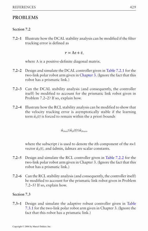
REFERENCES 429
PROBLEMS
Section 7.2
7.2–1 Illustrate how the DCAL stability analysis can be modified if the filtertracking error is defined as
where Λ is a positive-definite diagonal matrix.
7.2–2 Design and simulate the DCAL controller given in Table 7.2.1 for thetwo-link polar robot arm given in Chapter 3. (Ignore the fact that thisrobot has a prismatic link.)
7.2–3 Can the DCAL stability analysis (and consequently, the controlleritself) be modified to account for the prismatic link robot given inProblem 7.2–2? If so, explain how.
7.2–4 Illustrate how the RCL stability analysis can be modified to show thatthe velocity tracking error is asymptotically stable if the learningterm ûd(t) is forced to remain within the a priori bounds
ûdmin≤ûdi(t)≤ûdmax,
where the subscript i is used to denote the ith component of the n×1vector ûd(t), and ûdmin, ûdmax are scalar constants.
7.2–5 Design and simulate the RCL controller given in Table 7.2.2 for thetwo-link polar robot arm given in Chapter 3. (Ignore the fact that thisrobot has a prismatic link.)
7.2–6 Can the RCL stability analysis (and consequently, the controller itself)be modified to account for the prismatic link robot given in Problem7.2–5? If so, explain how.
Section 7.3
7.3–1 Design and simulate the adaptive robust controller given in Table7.3.1 for the two-link polar robot arm given in Chapter 3. (Ignore thefact that this robot has a prismatic link.)
Copyright © 2004 by Marcel Dekker, Inc.
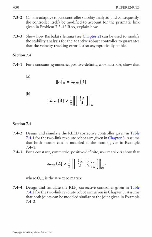
REFERENCES430
7.3–2 Can the adaptive robust controller stability analysis (and consequently,the controller itself) be modified to account for the prismatic linkgiven in Problem 7.3–1? If so, explain how.
7.3–3 Show how Barbalat’s lemma (see Chapter 2) can be used to modifythe stability analysis for the adaptive robust controller to guaranteethat the velocity tracking error is also asymptotically stable.
Section 7.4
7.4–1 For a constant, symmetric, positive-definite, n×n matrix A, show that
(a)
(b)
Section 7.4
7.4–2 Design and simulate the RLED corrective controller given in Table7.4.1 for the two-link revolute robot arm given in Chapter 3. Assumethat both motors can be modeled as the motor given in Example7.4–1.
7.4–3 For a constant, symmetric, positive-definite, n×n matrix A show that
where On×n is the n×n zero matrix.
7.4–4 Design and simulate the RLFJ corrective controller given in Table7.4.2 for the two-link revolute robot arm given in Chapter 3. Assumethat both joints can be modeled similar to the joint given in Example7.4–2.
Copyright © 2004 by Marcel Dekker, Inc.
431
Chapter 8
Neural Network Controlof Robots
A framework is given for controller design using neural networks. Thesestructures possess a universal approximation property that allows them to beused in feedback control of unknown systems without requirements for linearityin the system parameters or finding a regression matrix. Feedback controltopologies and weight tuning algorithms are given here that guarantee closed-loop stability and bounded weights.
8.1 Introduction
In recent years, there has been a great deal of effort to design feedback controlsystems that mimic the functions of living biological systems [White andSofge 1992], [Miller et al. 1991]. There has been great interest recently in‘universal model-free controllers’ that do not need a mathematical model ofthe controlled plant, but mimic the functions of biological processes to learnabout the systems they are controlling on-line, so that performance improvesautomatically. Techniques include fuzzy logic control, which mimics linguisticand reasoning functions, and artificial neural networks, which are based onbiological neuronal structures of interconnected nodes. Neural networks (NNs)have achieved great success in classification, pattern recognition, and otheropen-loop applications in digital signal processing and elsewhere. Rigorousanalyses have shown how to select NN topologies and weights, for instance,to discriminate between specified exemplar patterns. By now, the theory andapplications of NN in open-loop applications are well understood, so that
Copyright © 2004 by Marcel Dekker, Inc.
Neural Network Control of Robots432
NN have become an important tool in the repertoire of the signal processorand computer scientist.
There is a large literature on NN for feedback control of unknown plants.Until the 1990’s, design and analysis techniques were ad hoc, with no repeatabledesign algorithms or proofs of stability and guaranteed performance. In spiteof this, simulation results appearing in the literature showed good performance.Most of the early approaches used standard backpropagation weight tuning[Werbos 1992] since rigorous derivations of tuning algorithms suitable forclosed-loop control purposes were not available. Many NN design techniquesmimicked adaptive control approaches, where rigorous analysis results wereavailable [Åström and Wittenmark 1989], [Landau 1979], [Goodwin et al.1984], proposing NN feedback control topologies such as indirectidentification-based control, inverse dynamics control, series-paralleltechniques, etc.
In keeping with the philosophy of those working in control system theorysince Maxwell, Lyapunov, A.N.Whitehead, von Bertalanffy, and others, toaddress such issues it is necessary to begin with the knowledge availableabout the system being controlled. Narendra [Narendra 1991], [Narendraand Parthasarathy 1991] and others [Miller et al. 1991], [White and Sofge1992], [Werbos 1992] pioneered rigorous NN controls applications bystudying the dynamical behavior of NN in closed-loop systems, includingcomputation of the gradients needed for backprop tuning. Other groupsproviding rigorous analysis and design techniques for closed-loop NNcontrollers included [Sanner and Slotine 1991] who showed how to use radialbasis function NN in feedback control, [Chen and Khalil 1992], [Chen andLiu 1994] who provided NN tuning algorithms based on dead-zone methods,[Polycarpou and Ioannou 1991], [Polycarpou 1996] who used projectionmethods, [Lewis et al. 1993], [Lewis et al. 1995] who used an e-mod approach,[Sadegh 1993] who provided NN controllers for discrete-time systems, and[Rovithakis and Christodoulou 1994] who used dynamic NN for feedbackcontrol.
In this chapter is given an approach to the design and analysis of neuralnetwork controllers based on several PhD dissertations and a body of publishedwork, including [Lewis et al. 1999], [Kim and Lewis 1998]. The controlstructures discussed here are multiloop controllers with NN in some of theloops and an outer tracking unity-gain PD loop. There are repeatable designalgorithms and guarantees of system performance including both small trackingerrors and bounded NN weights. It is shown that as uncertainty about thecontrolled system increases or performance requirements increase, the NNcontrollers require more and more structure. An exposition of this material ingreater depth appears in [Lewis 1999], which also shows relationships withFuzzy Logic Systems.
Copyright © 2004 by Marcel Dekker, Inc.
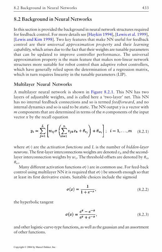
8.2 Background in Neural Networks 433
8.2 Background in Neural Networks
In this section is provided the background in neural network structures requiredfor feedback control. For more details see [Haykin 1994], [Lewis et al. 1999],[Lewis and Kim 1998]. Two key features that make NN useful for feedbackcontrol are their universal approximation property and their learningcapability, which arises due to the fact that their weights are tunable parametersthat can be updated to improve controller performance. The universalapproximation property is the main feature that makes non-linear networkstructures more suitable for robot control than adaptive robot controllers,which have generally relied upon the determination of a regression matrix,which in turn requires linearity in the tunable parameters (LIP).
Multilayer Neural Networks
A multilayer neural network is shown in Figure 8.2.1. This NN has twolayers of adjustable weights, and is called here a ‘two-layer’ net. This NNhas no internal feedback connections and so is termed feedforward, and nointernal dynamics and so is said to be static. The NN output y is a vector withm components that are determined in terms of the n components of the inputvector x by the recall equation
(8.2.1)
where (·) are the activation functions and L is the number of hidden-layerneurons. The first-layer interconnections weights are denoted vjk and the second-layer interconnection weights by wij. The threshold offsets are denoted by vj,wi.
Many different activation functions (·) are in common use. For feed-backcontrol using multilayer NN it is required that (·) be smooth enough so thatat least its first derivative exists. Suitable choices include the sigmoid
(8.2.2)
the hyperbolic tangent
(8.2.3)
and other logistic-curve-type functions, as well as the gaussian and an assortmentof other functions.
Copyright © 2004 by Marcel Dekker, Inc.
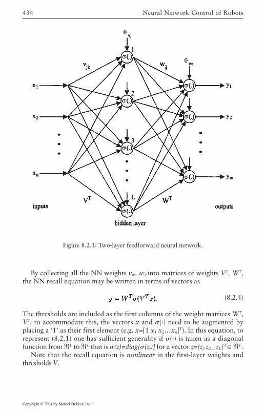
Neural Network Control of Robots434
By collecting all the NN weights vjk, wij into matrices of weights VT, WT,the NN recall equation may be written in terms of vectors as
(8.2.4)
The thresholds are included as the first columns of the weight matrices WT,VT; to accommodate this, the vectors x and (·) need to be augmented byplacing a ‘1’ as their first element (e.g. x=[1 x1 x2…xn]T). In this equation, torepresent (8.2.1) one has sufficient generality if (·) is taken as a diagonalfunction from L to L that is (z)=diag(zj) for a vector z=[z1 z2 …zL]T ∈ L.
Note that the recall equation is nonlinear in the first-layer weights andthresholds V.
Figure 8.2.1: Two-layer feedforward neural network.
Copyright © 2004 by Marcel Dekker, Inc.
8.2 Background in Neural Networks 435
Universal Function Approximation Property. NN satisfy many importantproperties. A main one of concern for feedback control purposes is the universalfunction approximation property [Hornik and Stinchombe 1989]. Let f(x) bea general smooth function from n to m. Then, it can be shown that, as longas x is restricted to a compact set S of n, there exist weights and thresholdssuch that one has
(8.2.5)
for some number of hidden-layer neurons L. This holds for a large class ofactivation functions, including those just mentioned. The value is called theNN functional approximation error, and it generally decreases as the net sizeL increases. In fact, for any choice of a positive number , one can find afeedforward NN such that
(8.2.6)
for all x in S. The selection of the net size L for a prescribed accuracy is anopen question for general unstructured fully-connected NN. This problemcan be solved for CMAC, FL nets, and other structured nonlinear nets assubsequently described.
The ideal NN weights in matrices W, V that are needed to best approximatea given nonlinear function f(x) are difficult to determine. In fact, they may noteven be unique. However, all one needs to know for controls purposes is that,for a specified value of some ideal approximating NN weights exist. Then,an estimate of f(x) can be given by
(8.2.7)
where W, V are estimates of the ideal NN weights that are provided by someon-line weight tuning algorithms subsequently to be detailed. Note that all‘hat’ quantities are known, since they may be computed using measurablesignals and current NN weight estimates.
The assumption that there exist ideal weights such that the approximationproperty holds is very much like various similar assumptions in adaptivecontrol [Åström and Wittenmark 1989], [Landau 1979], including Erzberger’sassumptions and linearity in the parameters. The very important difference isthat in the NN case, the universal approximation property always holds,while in adaptive control such assumptions often do not hold in practice, andso they imply restrictions on the form of the systems that can be controlled.Overcoming the NLIP Problem. Multilayer NN are nonlinear in the weights
Copyright © 2004 by Marcel Dekker, Inc.
Neural Network Control of Robots436
V and so weight tuning algorithms that yield guaranteed stability and boundedweights in closed-loop feedback systems have been difficult to discover until afew years ago. The NLIP problem is easily overcome if a correct and rigorousapproach is taken. One approach is the following appropriate use of theTaylor series [Lewis et al. 1996].
Define the functional estimation error
(8.2.8)
the weight estimation errors
(8.2.9)
and the hidden-layer output error
(8.2.10)
For any z one may write the Taylor series
(8.2.11)
where ’ is the jacobian and the last term means terms of order z2.Therefore,
(8.2.12)
This key equation allows one to write the functional estimation error as
(8.2.13)
The first term has W multiplied by a known quantity (in square braces), andthe second term has V multipled by a known quantity. When used subsequentlyin the closed-loop error dynamics, this form allows one to derive tuning lawsfor V and W that guarantee closed-loop stability.
Copyright © 2004 by Marcel Dekker, Inc.
8.2 Background in Neural Networks 437
Linear-in-the-parameter neural nets
If the first-layer weights and thresholds V in (8.2.4) are fixed and only thesecond-layer weights and thresholds W are tuned, then the NN has only onelayer of tunable weights. One may then define the fixed function so that such a 1-layer NN has the recall equation
(8.2.14)
where and L is the number of hidden-layerneurons. This NN is linear in the tunable parameters W, so that it is far easierto tune. In fact, standard adaptive control proofs can be used to derive suitabletuning algorithms.
Though LIP, these NN still offer an enormous advantage over standardadaptive control approaches that require the determination of a regressionmatrix since they satisfy a universal approximation property if the functions(.) are correctly chosen. Note that adaptive controllers are linear in thesystem parameters, while 1-layer NN are linear in the NN weights. Anadvantage of 1-layer NN over 2-layer NN is that firm results exist for theformer on the selection of the number of hidden layer neurons L for a specifiedapproximation accuracy. A disadvantage of LIP networks is that Barron [Barron1993] has shown a lower bound on the approximation accuracy.
Functional-Link Basis Neural Networks. More generality is gained if (·) isnot diagonal, but (.) is allowed to be a general function from n to L. Thisis called a functional-link neural net (FLNN) [Sadegh 1993]. For LIP NN, thefunctional approximation property does not generally hold. However, a 1-layer NN can still approximate functions as long as the activation functions(.) are selected as a basis, which must satisfy the following two requirementson a compact simply-connected set of S of n:
1. A constant function on S can be expressed as (8.2.14) for a finite numberL of hidden-layer neurons.
2. The functional range of (8.2.14) is dense in the space of continuous functionsfrom S to m for countable L.
If (.) provides a basis, then a smooth function f(x) from n to m can beapproximated on a compact set S of n, by
(8.2.15)
for some ideal weights and thresholds W and some number of hidden layerneurons L. In fact, for any choice of a positive number , one can find afeedforward NN such that for all x in S.
Copyright © 2004 by Marcel Dekker, Inc.
Neural Network Control of Robots438
The approximation for f(x) is given by
(8.2.16)
where W are the NN weight and threshold estimates given by the tuningalgorithm. For LIP NN, the functional estimation error is given by
(8.2.17)
which, when used subsequently in the error dynamics, directly yields tuningalgorithms for W that guarantee closed-loop stability.
Barron [Barron 1993] has shown that for all LIP approximators there is afundamental lower bound, so that is bounded below by terms on the order of1/L2/n. Thus, as the number of NN inputs n increases, increasing L to improvethe approximation accuracy becomes less effective. As shown subsequently,this is not a major limitation on adaptive controllers designed using 1-layerNN. This lower bound problem does not occur in the NLIP multilayer nonlinearnets.
A special FLNN is now discussed. We often use (·) in place of (.), withthe understanding that, for LIP nets, this activation function vector is notdiagonal, but is a general function from L to L.
Gaussian or Radial Basis Function (RBF) Networks. The selection of a basisset of activation functions is considerably simplified in various sorts ofstructured nonlinear networks, including radial basis function, CMAC, andfuzzy logic nets. It will be shown here that the key to the design of suchstructured nonlinear nets lies in a more general set of NN thresholds thanallowed in the standard equation (8.2.1), and in their appropriate selection.
A NN activation function often used is the gaussian or radial basis function(RBF) [Sanner and Slotine 1991] given when x is a scalar as
(8.2.18)
where x is the mean and p the variance. RBF NN can be written as (8.2.4),but have an advantage over the usual sigmoid NN in that the n-dimensionalgaussian function is well understood from probability theory, Kalman filtering,and elsewhere, so that n-dimensional RBF are easy to conceptualize.
The j-th activation function can be written as
Copyright © 2004 by Marcel Dekker, Inc.
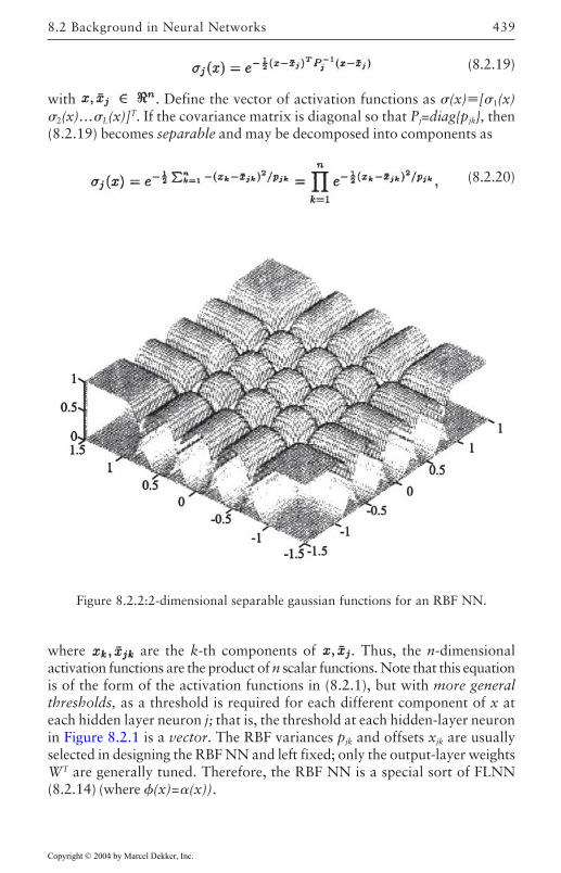
8.2 Background in Neural Networks 439
(8.2.19)
with . Define the vector of activation functions as (x)[1(x)2(x)…L(x)]T. If the covariance matrix is diagonal so that Pj=diagpjk, then(8.2.19) becomes separable and may be decomposed into components as
(8.2.20)
where are the k-th components of . Thus, the n-dimensionalactivation functions are the product of n scalar functions. Note that this equationis of the form of the activation functions in (8.2.1), but with more generalthresholds, as a threshold is required for each different component of x ateach hidden layer neuron j; that is, the threshold at each hidden-layer neuronin Figure 8.2.1 is a vector. The RBF variances pjk and offsets xjk are usuallyselected in designing the RBF NN and left fixed; only the output-layer weightsWT are generally tuned. Therefore, the RBF NN is a special sort of FLNN(8.2.14) (where (x)=(x)).
Figure 8.2.2:2-dimensional separable gaussian functions for an RBF NN.
Copyright © 2004 by Marcel Dekker, Inc.
Neural Network Control of Robots440
Figure 8.2.2 shows separable gaussians for the case x 2. In this figure,all the variances pjk are identical, and the mean values xjk are chosen in aspecial way that spaces the activation functions at the node points of a 2-Dgrid. To form an RBF NN that approximates functions over the region -1<x11, -1<x21 one has here selected L=5×5=25 hidden-layer neurons,corresponding to 5 cells along x1 and 5 along x2. Nine of these neurons have2-D gaussian activation functions, while those along the boundary require theillustrated ‘one-sided’ activation functions.
8.3 Tracking Control Using Static NeuralNetworks
In this section is discussed feedback tracking control design using nonlinearnets and assuming full state-variable feedback. For more details see [Lewis etal. 1999] and other listed references. If full state feedback is available, then astatic feedforward NN suffices for control. A control topology and net tuningalgorithms are provided here that guarantee closed-loop stability and boundedweights. The techniques to be discussed apply for general nonlinear netsincluding both neural networks and fuzzy logic systems [Wang 1997], [Lewiset al. 1997], so that the abbreviation NN might henceforth be construed asmeaning ‘nonlinear network’. The resulting multiloop control topology hasan outer PD tracking loop and an inner NN feedback linearization or actiongenerating loop. It is found that backprop tuning does not generally suffice,but modified tuning algorithms are needed for guaranteed closed-loopperformance.
Many industrial mechanical systems, as well as automobiles, aircraft, andspacecraft, have dynamics in the Lagrangian form, which are exemplified bythe class of rigid robot systems. Therefore, the Lagrangian robot dynamicswill be considered [Lewis et al. 1993], [Lewis et al. 1996]. The NN controltechniques presented may also be applied to other unknown systems includingcertain important classes of nonlinear systems [Lewis et al. 1999].
Robot Arm Dynamics and Error System
The dynamics of rigid Lagrangian systems, including robot arms, have someimportant physical, structural, and passivity properties [Craig 1988], [Lewiset al. 1993], [Slotine 1988], [Spong and Vidyasagar 1989] that make it verynatural to use NN in their control. These properties should be taken intoaccount in the design of any controller—in fact, they provide the foundationfor rigorous design algorithms for NN controllers.
The dynamics of an n-link rigid (i.e. no flexible links or high-frequency
Copyright © 2004 by Marcel Dekker, Inc.
441
joint/motor dynamics) robot manipulator may be expressed in the Lagrangeform
(8.3.1)
with q(t)n the joint variable vector, whose entries are the robot arm jointangles or link extensions. M(q) is the inertia matrix, Vm(q,q) the coriolis/centripetal matrix, G(q) the gravity vector, and F(q) the friction. Boundedunknown disturbances (including e.g. unstructured unmodelled dynamics) aredenoted by d, and the control input torque is (t) The robot dynamics havethe following standard properties:
Property 1: M(q) is a positive definite symmetric matrix bounded bym1I<M(q)<m2I, with m1, m2 positive constants.
Property 2: The norm of the matrix Vm(q, q) is bounded by vb(q)||q||, for somefunction vb(q).
Property 3: The matrix M–2Vm is skew-symmetric. This is equivalent to thefact that the internal forces do no work.
Property 4: The unknown disturbance satisfies with bD a positiveconstant.
Given a desired arm trajectory qd(t)n the tracking error is
(8.3.2)
and the filtered tracking error is
(8.3.3)
where is a symmetric positive definite design parameter matrix, usuallyselected diagonal. If a controller is found such that r(t) is bounded, then e(t) isalso bounded; in fact , with the minimum singular value of .
Differentiating r(t) and using (8.3.1), the arm dynamics may be written interms of the filtered tracking error as
(8.3.4)
where the nonlinear robot function is
(8.3.5)
8.3 Tracking Control Using Static Neural Networks
Copyright © 2004 by Marcel Dekker, Inc.
Neural Network Control of Robots442
The vector x required to compute f(x) can be defined, for instance, as
(8.3.6)
which can be measured. Function f(x) contains potentially unknown robotparameters including pay load mass and complex forms of friction.
A suitable control input for trajectory following is given by the computed-torque-like control
(8.3.7)
with a gain matrix, generally chosen diagonal, and f(x) anestimate of the robot function f(x) that is provided by some means. Therobustifying signal v(t) is needed to compensate for unmodelled unstructureddisturbances. Using this control, the closed-loop error dynamics is
(8.3.8)
In computing the control signal, the estimate f can be provided by severaltechniques, including adaptive control or neural or fuzzy networks. Theauxiliary control signal v(t) can be selected by several techniques, includingsliding-mode methods and others under the general aegis of robust controlmethods.
The desired trajectory is assumed bounded so that
(8.3.9)
with qB a known scalar bound. It is easy to show that for each time t, x(t) isbounded by
(8.3.10)
for computable positive constants c0, c1, c2.
Adaptive Control
Standard adaptive control techniques in robotics [Craig 1988], [Slotine 1988],[Spong and Vidyasagar 1989], [Lewis et al. 1993] use the assumption that thenonlinear robot function is linear in the tunable parameters so that
(8.3.11)
Copyright © 2004 by Marcel Dekker, Inc.
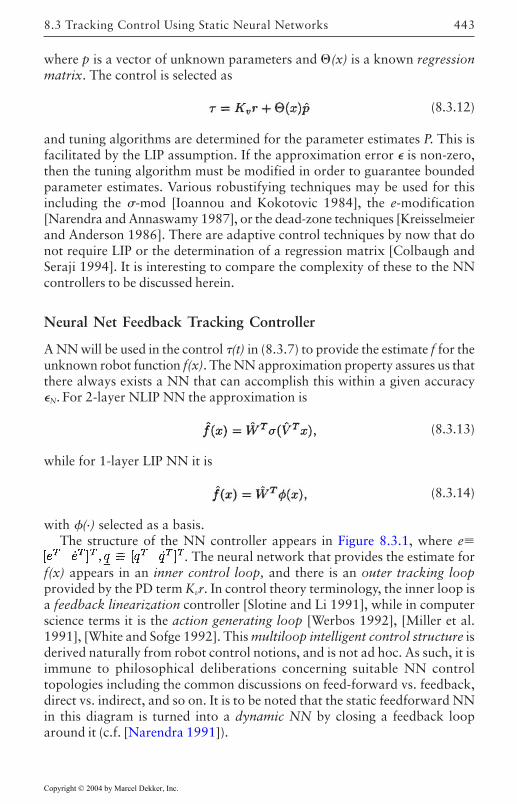
443
where p is a vector of unknown parameters and (x) is a known regressionmatrix. The control is selected as
(8.3.12)
and tuning algorithms are determined for the parameter estimates P. This isfacilitated by the LIP assumption. If the approximation error is non-zero,then the tuning algorithm must be modified in order to guarantee boundedparameter estimates. Various robustifying techniques may be used for thisincluding the -mod [Ioannou and Kokotovic 1984], the e-modification[Narendra and Annaswamy 1987], or the dead-zone techniques [Kreisselmeierand Anderson 1986]. There are adaptive control techniques by now that donot require LIP or the determination of a regression matrix [Colbaugh andSeraji 1994]. It is interesting to compare the complexity of these to the NNcontrollers to be discussed herein.
Neural Net Feedback Tracking Controller
A NN will be used in the control (t) in (8.3.7) to provide the estimate f for theunknown robot function f(x). The NN approximation property assures us thatthere always exists a NN that can accomplish this within a given accuracyN. For 2-layer NLIP NN the approximation is
(8.3.13)
while for 1-layer LIP NN it is
(8.3.14)
with (.) selected as a basis.The structure of the NN controller appears in Figure 8.3.1, where e
. The neural network that provides the estimate forf(x) appears in an inner control loop, and there is an outer tracking loopprovided by the PD term Kvr. In control theory terminology, the inner loop isa feedback linearization controller [Slotine and Li 1991], while in computerscience terms it is the action generating loop [Werbos 1992], [Miller et al.1991], [White and Sofge 1992]. This multiloop intelligent control structure isderived naturally from robot control notions, and is not ad hoc. As such, it isimmune to philosophical deliberations concerning suitable NN controltopologies including the common discussions on feed-forward vs. feedback,direct vs. indirect, and so on. It is to be noted that the static feedforward NNin this diagram is turned into a dynamic NN by closing a feedback looparound it (c.f. [Narendra 1991]).
8.3 Tracking Control Using Static Neural Networks
Copyright © 2004 by Marcel Dekker, Inc.
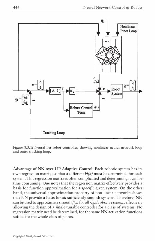
Neural Network Control of Robots444
Advantage of NN over LIP Adaptive Control. Each robotic system has itsown regression matrix, so that a different (x) must be determined for eachsystem. This regression matrix is often complicated and determining it can betime consuming. One notes that the regression matrix effectively provides abasis for function approximation for a specific given system. On the otherhand, the universal approximation property of non-linear networks showsthat NN provide a basis for all sufficiently smooth systems. Therefore, NNcan be used to approximate smooth f(x) for all rigid robotic systems, effectivelyallowing the design of a single tunable controller for a class of systems. Noregression matrix need be determined, for the same NN activation functionssuffice for the whole class of plants.
Figure 8.3.1: Neural net robot controller, showing nonlinear neural network loopand outer tracking loop.
Copyright © 2004 by Marcel Dekker, Inc.
445
Even the 1-layer NN, which is LIP, has this advantage. Note that the 1-layerNN is linear not in the system parameters, but in the NN weights. Even the LIPNN has a universal approximation property so that no regression matrix isneeded.
Initial Tracking Errors and Initial NN Weights. It is now required to determinehow to tune the NN weights to yield guaranteed closed-loop stability. Severalcases are considered for NN controller design in this section. All of them needthe following construction.
Since the NN approximation property holds on a compact set, one mustdefine an allowable initial condition set as follows. Let the NN approximationproperty hold for the function f(x) given in (8.3.5) with a given accuracy N in(8.2.6) for all x inside the ball of radius bx>qB. Define the set of allowableinitial tracking errors as
(8.3.15)
Note that the approximation accuracy of the NN determines size of Sr. Fora larger NN (i.e. more hidden-layer units), N is small for a larger radius bx.Thus, the allowed initial condition set Sr is larger. On the other hand, a moreactive desired trajectory (e.g. containing higher frequency components) resultsin a larger acceleration qd(t), which yields a larger bound qB, thereby decreasingSr. It is important to note the dependence of Sr on the PD design ratio —bothc0 and c2 depend on .
A key feature of our the Initial Condition Requirement is its independenceof the NN initial weights. This is in stark contrast to other techniques in theliterature where the proofs of stability depend on selecting some initialstabilizing NN weights, which is very difficult to do.
8.4 Tuning Algorithms for Linear-in-the-Parameters NN
Suppose now that a LIP FLNN is used to approximate the nonlinear robotfunction (8.3.5) according to (8.2.15) with on a compact set, theideal approximating weights W constant, and (x) selected as a basis. Anestimate of f(x) is given by (8.3.14). Then the control law (8.3.7) becomes
(8.4.1)
and the closed-loop filtered error dynamics (8.3.8) are
(8.4.2)
8.4 Tuning Algorithms for Linear-in-the-Parameters NN
Copyright © 2004 by Marcel Dekker, Inc.
Neural Network Control of Robots446
The next theorem derives the tuning law for a NN controller that is augmentedby an e-mod term as in [Narendra and Annaswamy 1987].
It must now be assumed that the ideal weights W are constant and boundedso that
(8.4.3)
with the bound WB known. In [Polycarpou 1996] it is shown how to usestandard adaptive robust techniques to avoid the assumption that the boundWB is known.
THEOREM 8.4–1: (NN Weight Tuning Algorithm).Let the desired trajectory qd(t) be bounded by qB and the initial tracking
error r(0) be in Sr. Let the NN reconstruction error bound N and the disturbancebound dB be constants. Assume the ideal NN target weights are bounded byWB as in (8.4.3). Let the control input for the robot arm be given by (8.4–1)with v(t)=0 and gain
(1)
Let the weight tuning be
(2)
with F=FT>0 and >0 a small design parameter. Then the filtered trackingerror r(t) and the NN weight estimates W(t) are UUB with practical boundsgiven respectively by the right-hand sides of (8), (9). Moreover, the trackingerror may be made as small as desired by increasing the tracking gain Kv.
Proof:Let the NN approximation property (8.2.15) hold for the function f(x)
given in (8.3.5) with a given accuracy N for all x in the compact set with bx>qB. Let r(0)Sr. Then the approximation
property holds at time 0.Define the Lyapunov function candidate
(3)
Differentiating yields
(4)
Copyright © 2004 by Marcel Dekker, Inc.
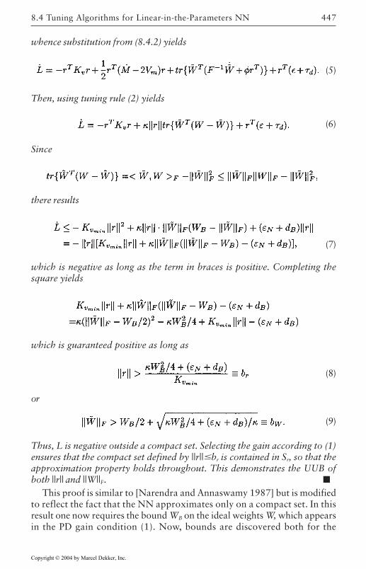
447
whence substitution from (8.4.2) yields
(5)
Then, using tuning rule (2) yields
(6)
Since
there results
(7)
which is negative as long as the term in braces is positive. Completing thesquare yields
which is guaranteed positive as long as
(8)
or
(9)
Thus, L is negative outside a compact set. Selecting the gain according to (1)ensures that the compact set defined by ||r||br is contained in Sr, so that theapproximation property holds throughout. This demonstrates the UUB ofboth ||r|| and ||W||F.
This proof is similar to [Narendra and Annaswamy 1987] but is modifiedto reflect the fact that the NN approximates only on a compact set. In thisresult one now requires the bound WB on the ideal weights W, which appearsin the PD gain condition (1). Now, bounds are discovered both for the
8.4 Tuning Algorithms for Linear-in-the-Parameters NN
Copyright © 2004 by Marcel Dekker, Inc.
Neural Network Control of Robots448
tracking error r(t) and the weights W(t). Note that no persistence of exictationcondition is needed to establish the bounds on W with the modified weighttuning algorithm.
The NN weight tuning algorithm (2) consists of a backpropagation throughtime term plus a new second term. The importance of the , term, called thee-modification, is that it adds a quadratric term in in (7), so that it ispossible to establish that L is negative outside a compact set in the
plane [Narendra and Annaswamy 1987]. The e-mod termmakes the tuning law robust to unmodelled dynamics so that the PE conditionis not needed. In [Polycarpou and Ioannou 1991] a projection algorithm isused to keep the NN weights bounded. In [Chen and Khalil 1992], [Chenand Liu 1994] a deadzone technique is employed.
Weight Initialization and On-Line Tuning. In the NN control schemes derivedin this paper there is no preliminary off-line learning phase. The weights aresimply initialized at zero, for then Figure 8.3.1 shows that the controller isjust a PD controller. Standard results in the robotics literature [Dawson et al.1990] show that a PD controller gives bounded errors if Kv is large enough.Therefore, the closed-loop system remains stable until the NN begins to learn.The weights are tuned on-line in real-time as the system tracks the desiredtrajectory. As the NN learns f(x), the tracking performance improves. This isa significant improvement over other NN control techniques where one mustfind some initial stabilizing weights, generally an impossible feat for complexnonlinear systems.
Bounds on the Tracking Error and NN Weight Estimation Errors. The right-hand side of (8) can be taken as a practical bound on the tracking error inthe sense that r(t) will never stray far above it. It is important to note fromthis equation that the tracking error increases with the NN reconstructionerror N and robot disturbances dB, yet arbitrarily small tracking errorsmay be achieved by selecting large gains Kv. This is in spite of Barron’slower bound on .
Note that the NN weights W are not guaranteed to approach the idealunknown weights W that give good approximation of f(x). However, this is ofno concern as long as W–W is bounded, as the proof guarantees. Thisguarantees bounded control inputs so that the tracking objective can beachieved.
Copyright © 2004 by Marcel Dekker, Inc.
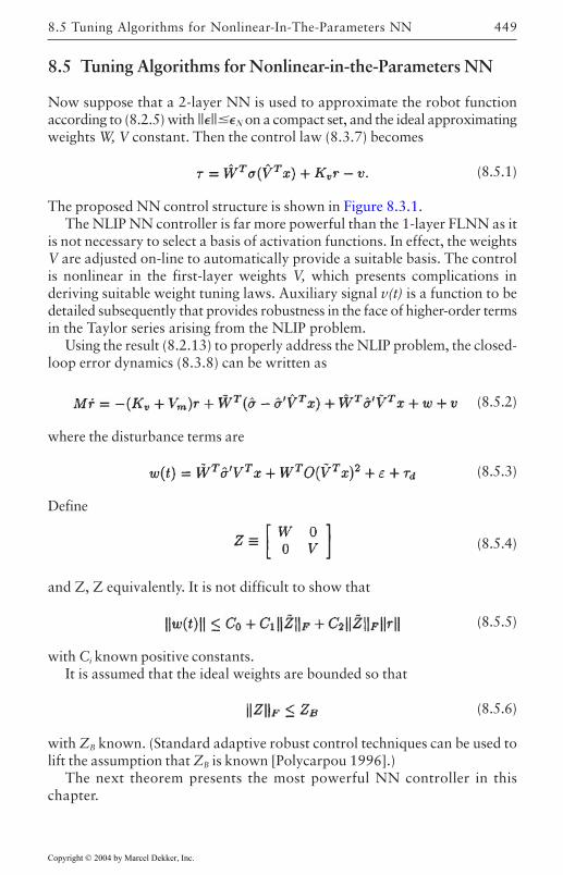
449
8.5 Tuning Algorithms for Nonlinear-in-the-Parameters NN
Now suppose that a 2-layer NN is used to approximate the robot functionaccording to (8.2.5) with |||| on a compact set, and the ideal approximatingweights W, V constant. Then the control law (8.3.7) becomes
(8.5.1)
The proposed NN control structure is shown in Figure 8.3.1.The NLIP NN controller is far more powerful than the 1-layer FLNN as it
is not necessary to select a basis of activation functions. In effect, the weightsV are adjusted on-line to automatically provide a suitable basis. The controlis nonlinear in the first-layer weights V, which presents complications inderiving suitable weight tuning laws. Auxiliary signal v(t) is a function to bedetailed subsequently that provides robustness in the face of higher-order termsin the Taylor series arising from the NLIP problem.
Using the result (8.2.13) to properly address the NLIP problem, the closed-loop error dynamics (8.3.8) can be written as
(8.5.2)
where the disturbance terms are
(8.5.3)
Define
(8.5.4)
and Z, Z equivalently. It is not difficult to show that
(8.5.5)
with Ci known positive constants.It is assumed that the ideal weights are bounded so that
(8.5.6)
with ZB known. (Standard adaptive robust control techniques can be used tolift the assumption that ZB is known [Polycarpou 1996].)
The next theorem presents the most powerful NN controller in thischapter.
8.5 Tuning Algorithms for Nonlinear-In-The-Parameters NN
Copyright © 2004 by Marcel Dekker, Inc.
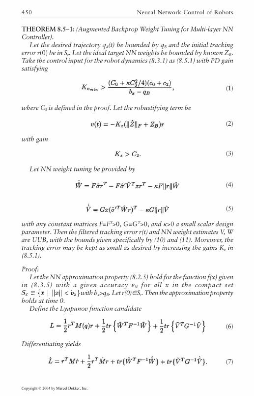
Neural Network Control of Robots450
THEOREM 8.5–1: (Augmented Backprop Weight Tuning for Multi-layer NNController).
Let the desired trajectory qd(t) be bounded by qB and the initial trackingerror r(0) be in Sr. Let the ideal target NN weights be bounded by known ZB.Take the control input for the robot dynamics (8.3.1) as (8.5.1) with PD gainsatisfying
(1)
where C3 is defined in the proof. Let the robustifying term be
(2)
with gain
(3)
Let NN weight tuning be provided by
(4)
(5)
with any constant matrices F=FT>0, G=GT>0, and >0 a small scalar designparameter. Then the filtered tracking error r(t) and NN weight estimates V, Ware UUB, with the bounds given specifically by (10) and (11). Moreover, thetracking error may be kept as small as desired by increasing the gains Kv in(8.5.1).
Proof:Let the NN approximation property (8.2.5) hold for the function f(x) given
in (8.3.5) with a given accuracy εN for all x in the compact set with bx>qB. Let r(0)Sr. Then the approximation property
holds at time 0.Define the Lyapunov function candidate
(6)
Differentiating yields
(7)
Copyright © 2004 by Marcel Dekker, Inc.
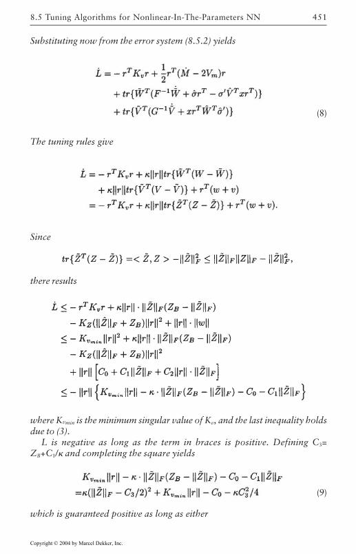
451
Substituting now from the error system (8.5.2) yields
(8)
The tuning rules give
Since
there results
where Kvmin is the minimum singular value of Kv, and the last inequality holdsdue to (3).
L is negative as long as the term in braces is positive. Defining C3=ZB+C1/ and completing the square yields
(9)
which is guaranteed positive as long as either
8.5 Tuning Algorithms for Nonlinear-In-The-Parameters NN
Copyright © 2004 by Marcel Dekker, Inc.
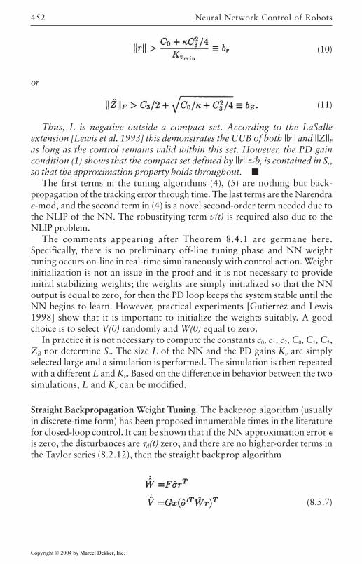
Neural Network Control of Robots452
(10)
or
(11)
Thus, L is negative outside a compact set. According to the LaSalleextension [Lewis et al. 1993] this demonstrates the UUB of both ||r|| and ||Z||Fas long as the control remains valid within this set. However, the PD gaincondition (1) shows that the compact set defined by ||r||br is contained in Sr,so that the approximation property holds throughout.
The first terms in the tuning algorithms (4), (5) are nothing but back-propagation of the tracking error through time. The last terms are the Narendrae-mod, and the second term in (4) is a novel second-order term needed due tothe NLIP of the NN. The robustifying term v(t) is required also due to theNLIP problem.
The comments appearing after Theorem 8.4.1 are germane here.Specifically, there is no preliminary off-line tuning phase and NN weighttuning occurs on-line in real-time simultaneously with control action. Weightinitialization is not an issue in the proof and it is not necessary to provideinitial stabilizing weights; the weights are simply initialized so that the NNoutput is equal to zero, for then the PD loop keeps the system stable until theNN begins to learn. However, practical experiments [Gutierrez and Lewis1998] show that it is important to initialize the weights suitably. A goodchoice is to select V(0) randomly and W(0) equal to zero.
In practice it is not necessary to compute the constants c0, c1, c2, C0, C1, C2,ZB nor determine Sr. The size L of the NN and the PD gains Kv are simplyselected large and a simulation is performed. The simulation is then repeatedwith a different L and Kv. Based on the difference in behavior between the twosimulations, L and Kv can be modified.
Straight Backpropagation Weight Tuning. The backprop algorithm (usuallyin discrete-time form) has been proposed innumerable times in the literaturefor closed-loop control. It can be shown that if the NN approximation error is zero, the disturbances are d(t) zero, and there are no higher-order terms inthe Taylor series (8.2.12), then the straight backprop algorithm
(8.5.7)
Copyright © 2004 by Marcel Dekker, Inc.
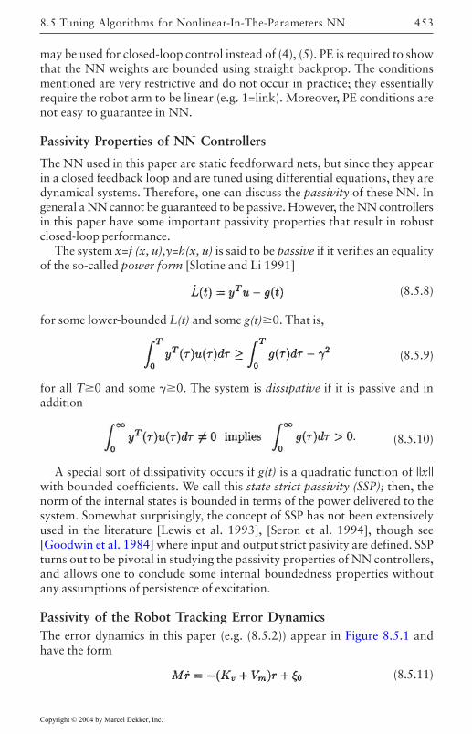
453
may be used for closed-loop control instead of (4), (5). PE is required to showthat the NN weights are bounded using straight backprop. The conditionsmentioned are very restrictive and do not occur in practice; they essentiallyrequire the robot arm to be linear (e.g. 1=link). Moreover, PE conditions arenot easy to guarantee in NN.
Passivity Properties of NN Controllers
The NN used in this paper are static feedforward nets, but since they appearin a closed feedback loop and are tuned using differential equations, they aredynamical systems. Therefore, one can discuss the passivity of these NN. Ingeneral a NN cannot be guaranteed to be passive. However, the NN controllersin this paper have some important passivity properties that result in robustclosed-loop performance.
The system x=f (x, u),y=h(x, u) is said to be passive if it verifies an equalityof the so-called power form [Slotine and Li 1991]
(8.5.8)
for some lower-bounded L(t) and some g(t)0. That is,
(8.5.9)
for all T0 and some 0. The system is dissipative if it is passive and inaddition
(8.5.10)
A special sort of dissipativity occurs if g(t) is a quadratic function of ||x||with bounded coefficients. We call this state strict passivity (SSP); then, thenorm of the internal states is bounded in terms of the power delivered to thesystem. Somewhat surprisingly, the concept of SSP has not been extensivelyused in the literature [Lewis et al. 1993], [Seron et al. 1994], though see[Goodwin et al. 1984] where input and output strict pasivity are defined. SSPturns out to be pivotal in studying the passivity properties of NN controllers,and allows one to conclude some internal boundedness properties withoutany assumptions of persistence of excitation.
Passivity of the Robot Tracking Error DynamicsThe error dynamics in this paper (e.g. (8.5.2)) appear in Figure 8.5.1 andhave the form
(8.5.11)
8.5 Tuning Algorithms for Nonlinear-In-The-Parameters NN
Copyright © 2004 by Marcel Dekker, Inc.
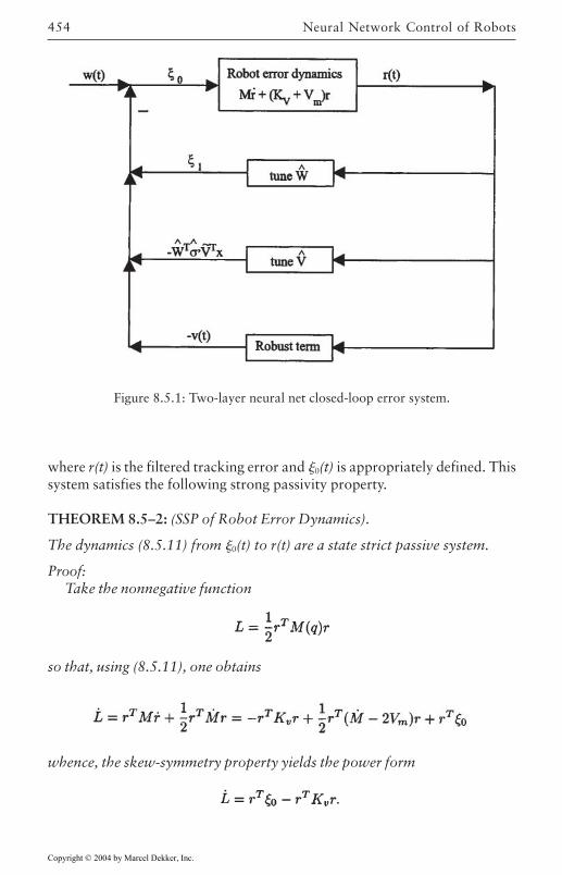
Neural Network Control of Robots454
where r(t) is the filtered tracking error and 0(t) is appropriately defined. Thissystem satisfies the following strong passivity property.
THEOREM 8.5–2: (SSP of Robot Error Dynamics).
The dynamics (8.5.11) from 0(t) to r(t) are a state strict passive system.
Proof:Take the nonnegative function
so that, using (8.5.11), one obtains
whence, the skew-symmetry property yields the power form
Figure 8.5.1: Two-layer neural net closed-loop error system.
Copyright © 2004 by Marcel Dekker, Inc.
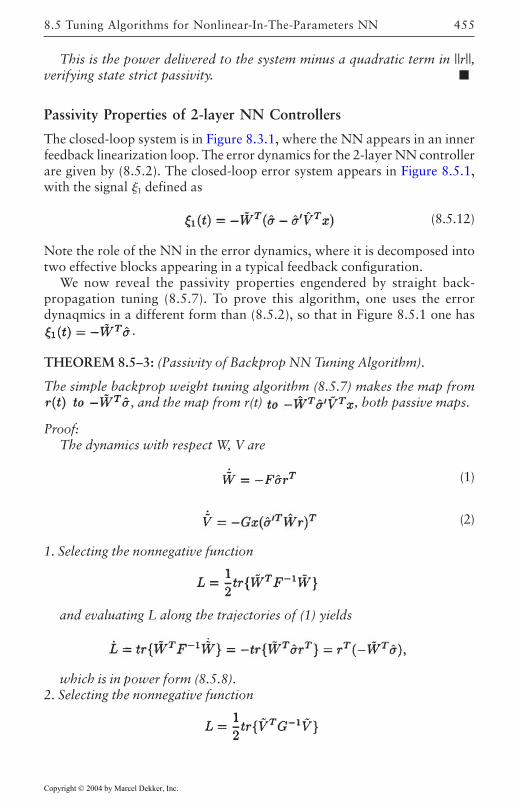
455
This is the power delivered to the system minus a quadratic term in ||r||,verifying state strict passivity.
Passivity Properties of 2-layer NN Controllers
The closed-loop system is in Figure 8.3.1, where the NN appears in an innerfeedback linearization loop. The error dynamics for the 2-layer NN controllerare given by (8.5.2). The closed-loop error system appears in Figure 8.5.1,with the signal 1 defined as
(8.5.12)
Note the role of the NN in the error dynamics, where it is decomposed intotwo effective blocks appearing in a typical feedback configuration.
We now reveal the passivity properties engendered by straight back-propagation tuning (8.5.7). To prove this algorithm, one uses the errordynaqmics in a different form than (8.5.2), so that in Figure 8.5.1 one has
.
THEOREM 8.5–3: (Passivity of Backprop NN Tuning Algorithm).
The simple backprop weight tuning algorithm (8.5.7) makes the map from, and the map from r(t) , both passive maps.
Proof:The dynamics with respect W, V are
(1)
(2)
1. Selecting the nonnegative function
and evaluating L along the trajectories of (1) yields
which is in power form (8.5.8).2. Selecting the nonnegative function
8.5 Tuning Algorithms for Nonlinear-In-The-Parameters NN
Copyright © 2004 by Marcel Dekker, Inc.
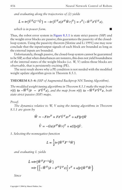
Neural Network Control of Robots456
and evaluating along the trajectories of (2) yields
which is in power form.
Thus, the robot error system in Figure 8.5.1 is state strict passive (SSP) andthe weight error blocks are passive; this guarantees the passivity of the closed-loop system. Using the passivity theorem [Slotine and Li 1991] one may nowconclude that the input/output signals of each block are bounded as long asthe external inputs are bounded.
Unfortunately, though passive, the closed-loop system cannot be guaranteedto be SSP, so that when disturbances are nonzero, this does not yield boundednessof the internal states of the weight blocks (i.e. W, V) unless those blocks areobservable, that is persistently exciting (PE).
The next result shows why a PE condition is not needed with the modifiedweight update algorithm given in Theorem 8.5.1.
THEOREM 8.5–4: (SSP of Augmented Backprop NN Tuning Algorithm).
The modified weight tuning algorithms in Theorem 8.5.1 make the map from, and the map from , both
state strict passive (SSP) maps.
Proof:The dynamics relative to W, V using the tuning algorithms in Theorem
8.5.1 are given by
1. Selecting the nonnegative function
and evaluating L yields
Since
Copyright © 2004 by Marcel Dekker, Inc.
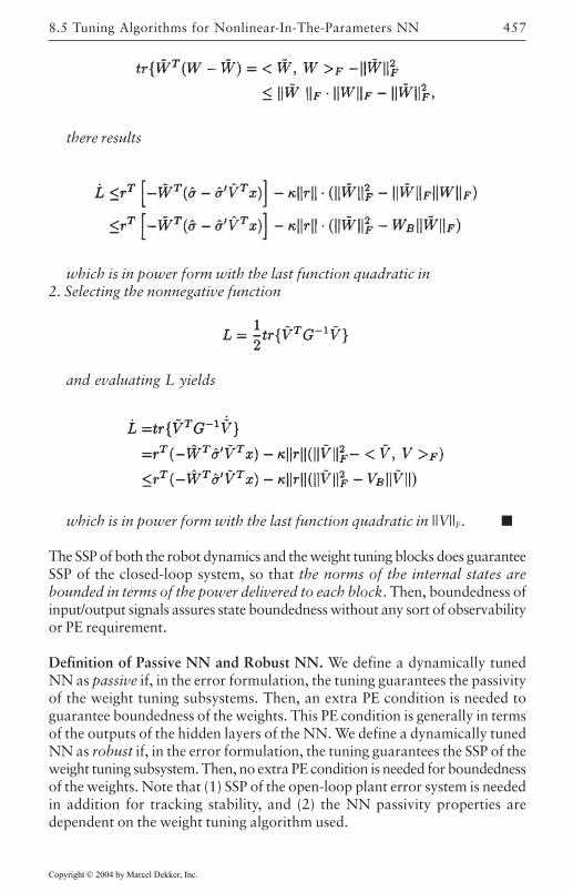
457
there results
which is in power form with the last function quadratic in2. Selecting the nonnegative function
and evaluating L yields
which is in power form with the last function quadratic in ||V||F.
The SSP of both the robot dynamics and the weight tuning blocks does guaranteeSSP of the closed-loop system, so that the norms of the internal states arebounded in terms of the power delivered to each block. Then, boundedness ofinput/output signals assures state boundedness without any sort of observabilityor PE requirement.
Definition of Passive NN and Robust NN. We define a dynamically tunedNN as passive if, in the error formulation, the tuning guarantees the passivityof the weight tuning subsystems. Then, an extra PE condition is needed toguarantee boundedness of the weights. This PE condition is generally in termsof the outputs of the hidden layers of the NN. We define a dynamically tunedNN as robust if, in the error formulation, the tuning guarantees the SSP of theweight tuning subsystem. Then, no extra PE condition is needed for boundednessof the weights. Note that (1) SSP of the open-loop plant error system is neededin addition for tracking stability, and (2) the NN passivity properties aredependent on the weight tuning algorithm used.
8.5 Tuning Algorithms for Nonlinear-In-The-Parameters NN
Copyright © 2004 by Marcel Dekker, Inc.
Neural Network Control of Robots458
Passivity Properties of 1-Layer NN Controllers
In a similar fashion, it is shown that the FLNN controller tuning algorithmmakes the system passive, so that an additional PE condition is needed toverify internal stability of the NN weights. On the other hand, the augmentedtuning algorithm in Theorem 8.4.1 yields SSP, so that no PE is needed.
8.6 Summary
Neural network controller design algorithms were given for a general class ofindustrial Lagrangian motion systems characterized by the rigid robot arms.The design procedures are based on rigorous nonlinear derivations and stabilityproofs, and yield a multiloop intelligent control structure with NN in some ofthe loops. NN weight tuning algorithms were given that do not requirecomplicated initialization procedures or any off-line learning phase, workon-line in real-time, and offer guaranteed tracking and bounded NN weightsand control signals. The NN controllers given here are model-free controllersin that they work for any system in a prescribed class without the need forextensive modeling and preliminary analysis to find a ‘regression matrix’.Unlike standard robot adaptive controllers, they do not require linearity inthe parameters (see also [Colbaugh and Seraji 1994] which does not needLIP). Proper design allows the NN controllers to avoid requirements such aspersistence of excitation and certainty equivalence. NN passivity androbustness properties are defined and studied here.
Copyright © 2004 by Marcel Dekker, Inc.
459
REFERENCES
[Åström and Wittenmark 1989] K.J.Åström and B.Wittenmark, AdaptiveControl, Addision Wesley, Reading, MA, 1989.
[Barron 1993] Barren, A.R., “Universal approximation bounds forsuperpositions of a sigmoidal function,” IEEE Trans. Info. Theory, vol.39, no. 3, pp. 930–945, May 1993.
[Chen and Khalil 1992] F.-C.Chen and H.K.Khalil, “Adaptive control ofnonlinear systems using neural networks,” Int. J. Control, vol. 55, no. 6,pp. 1299–1317, 1992.
[Chen and Liu 1994] F.-C.Chen and C.-C.Liu, “Adaptively controlling nonlinearcontinuous-time systems using multilayer neural networks,” IEEE Trans.Automat. Control, vol. 39, no. 6, pp. 1306–1310, June 1994.
[Colbaugh and Seraji 1994] R.Colbaugh, H.Seraji, and K.Glass, “A new classof adaptive controllers for robot trajectory tracking,” J. Robotic Systems,vol. 11, no. 8, pp. 761–772, 1994.
[Craig 1988] Craig, J.J., Adaptive Control of Mechanical Manipulators,Reading, MA: Addison-Wesley, 1988.
[Dawson et al. 1990] Dawson, D.M., Z.Qu, F.L.Lewis, and J.F.Dorsey, “Robustcontrol for the tracking of robot motion,” Int. J. Control, vol. 52, no. 3,pp. 581–595, 1990.
[Goodwin et al. 1984] Goodwin, C.G., and K.S.Sin, Adaptive Filtering,Prediction, and Control, Prentice-Hall, New Jersey, 1984.
[Gorinevsky 1995] D.Gorinevsky, “On the persistency of excitation in radialbasis function network identificaiton of nonlinear systems,” IEEE Trans.Neural Networks, vol. 6, no. 5, pp. 1237–1244, Sept. 1995.
[Gutierrez and Lewis 1998] L.B.Gutierrez and F.L.Lewis, “Implementation ofa neural net tracking controller for a single flexible link: comparison
Copyright © 2004 by Marcel Dekker, Inc.
REFERENCES460
with PD and PID controllers,” IEEE Trans. Industrial Electronics, toappear, April 1998.
[Haykin 1994] S.Haykin, Neural Networks, IEEE Press, New York, 1994.
[Hornik and Stinchombe 1989] K.Hornik, M.Stinchombe, and H.White,“Multilayer feedforward networks are universal approximators,” NeuralNetworks, vol. 2, pp. 359–366, 1989.
[Ioannou and Kokotovic 1984] P.A.Ioannou and P.V.Kokotovic, “Instabilityanalysis and improvement of robustness of adaptive control,” Automatica,vol. 20, no. 5, pp. 583–594, 1984.
[Kim and Lewis 1998] Y.H.Kim and F.L.Lewis, High-Level Feedback Controlwith Neural Networks, World Scientific, Singapore, 1998.
[Kreisselmeier and Anderson 1986] Kreisselmeier, G., and B.Anderson, “Robustmodel reference adaptive control,” IEEE Trans. Automat. Control, vol.AC-31, no. 2, pp. 127–133, Feb. 1986.
[Landau 1979] Y.D.Landau, Adaptive Control, Marcel Dekker, Basel, 1979.
[Lewis 1999] F.L.Lewis, “Nonlinear Network Structures for Feedback Control”,Asian Journal of Control, vol. 1, no. 4, pp.205–228, December 1999.
[Lewis et al. 1993] F.L.Lewis, C.T.Abdallah, and D.M.Dawson, Control ofRobot Manipulators, New York: Macmillam, 1993.
[Lewis et al. 1999] F.L.Lewis, S.Jagannathan, and A.Yesildirek, Neural NetworkControl of Robot Manipulators and Nonlinear Systems, Taylor andFrancis, London, 1999.
[Lewis and Kim 1998] F.L.Lewis and Y.H.Kim, “Neural Networks for FeedbackControl,” Encyclopedia of Electrical and Electronics Engineering, ed.J.G.Webster, New York: Wiley, 1998. To appear.
[Lewis et al. 1993] Lewis, F.L., K.Liu, and A.Yesildirek, “Neural net robotcontroller with guaranteed tracking performance,” Proc. Int. Symp.Intelligent Control, pp. 225–231, Chicago., Aug. 1993.
[Lewis et al. 1995] Lewis, F.L., K.Liu, and A.Yesildirek, “Neural net robotcontroller with guaranteed tracking performance,” IEEE Trans. NeuralNetworks, vol. 6, no. 3, pp. 703–715, 1995.
[Lewis et al. 1997] F.L.Lewis, K.Liu, and S.Commuri, “Neural networks andfuzzy logic systems for robot control,” in Fuzzy Logic and Neural NetworkApplications, ed. F.Wang, World Scientific Pub., to appear, 1997.
[Lewis et al. 1996] F.L.Lewis, A.Yesildirek, and K.Liu, “Multilayer neuralnet robot controller: structure and stability proofs,” IEEE Trans. NeuralNetworks, vol. 7, no. 2, pp. 1–12, Mar. 1996.
Copyright © 2004 by Marcel Dekker, Inc.
REFERENCES 461
[Miller et al. 1991] W.T.Miller, R.S.Sutton, P.J.Werbos, ed., Neural Networksfor Control, Cambridge: MIT Press, 1991.
[Narendra 1991] K.S.Narendra, “Adaptive Control Using Neural Networks,”Neural Networks for Control, pp 115–142. ed. W.T.Miller, R.S.Sutton,P.J.Werbos, Cambridge: MIT Press, 1991.
[Narendra and Annaswamy 1987] K.S.Narendra and A.M.Annaswamy, “Anew adaptive law for robust adaptive control without persistent excitation,”IEEE Trans. Automat. Control, vol. 32, pp. 134–145, Feb., 1987.
[Narendra and Parthasarathy 1991] Narendra, K.S., and K. Parthasarathy,“Gradient methods for the optimization of dynamical systems containingneural networks,” IEEE Trans. Neural Networks, vol. 2, no. 2, pp. 252–262, Mar. 1991.
[Polycarpou 1996] M.M.Polycarpou, “Stable adaptive neural control schemefor nonlinear systems,” IEEE Trans. Automat. Control, vol. 41, no. 3,pp. 447–451, Mar. 1996.
[Polycarpou and Ioannou 1991] M.M.Polycarpou and P.A.Ioannou,“Identification and control using neural network models: design andstability analysis,” Tech. Report 91–09–01, Dept. Elect. Eng. Sys., Univ.S. Cal., Sept. 1991.
[Rovithakis and Christodoulou 1994] G.A.Rovithakis and M.A. Christodoulou,“Adaptive control of unknown plants using dynamical neural networks,”IEEE Trans. Systems, Man, and Cybernetics, vol. 24, no. 3, pp. 400–412, Mar. 1994.
[Sadegh 1993] N.Sadegh, “A perceptron network for functional identificationand control of nonlinear systems,” IEEE Trans. Neural Networks, vol.4, no. 6, pp. 982–988, Nov. 1993.
[Sanner and Slotine 1991] R.M.Sanner and J.-J.E.Slotine, “Stable adaptivecontrol and recursive identification using radial gaussian networks,” Proc.IEEE Conf. Decision and Control, Brighton, 1991.
[Seron et al. 1994] Seron, M.M., D.J.Hill, and A.L.Fradkov, “Adaptivepassification of nonlinear systems,” Proc. IEEE Conf. Decision andControl, pp. 190–195, Dec. 1994.
[Slotine 1988] Slotine, J.-J.E., “Putting physics in control the example ofrobotics,” IEEE Control Systems Magazine, pp. 12–17, Dec. 1988.
[Slotine and Li 1991] J.-J.Slotine and W.Li, Applied Nonlinear Control, PrenticeHall, New Jersey, 1991.
[Spong and Vidyasagar 1989] Spong, M.W., and M.Vidyasagar, RobotDynamics and Control, New York: Wiley, 1989.
Copyright © 2004 by Marcel Dekker, Inc.
REFERENCES462
[Wang 1997] L.-X.Wang, A course in fuzzy systems and control, Prentice-Hall, New Jersey, 1997.
[Werbos 1989] P.J.Werbos, “Back propagation: past and future,” Proc. 1988Int. Conf. Neural Nets, vol. 1, pp. I343-I353, 1989.
[Werbos 1992] P.J.Werbos, “Neurocontrol and supervised learning: an overviewand evaluation,” in Handbook of Intelligent Control, ed. D.A. White andD.A.Sofge, New York: Van Nostrand Reinhold, 1992.
[White and Sofge 1992] D.A.White and D.A.Sofge, ed. Handbook of IntelligentControl, New York: Van Nostrand Reinhold, 1992.
Copyright © 2004 by Marcel Dekker, Inc.
463
Chapter 9
Force Control
In this chapter the fundamentals of position/force controllers are studied.The topics that are covered include stiffness control, hybrid position/forcecontrol, hybrid impedance control, and reduced-state position/force control.Emphasis is placed on controller development, stability, and implementationissues.
9.1 Introduction
For tasks performed by robot manipulators, such as moving payloads orpainting objects, position controllers give adequate performance becausethese types of tasks only require the robot to follow a desired trajectory.However, during grinding or an assembly task, the robot manipulator comesin contact with the environment; therefore, interaction forces developbetween the robot manipulator and the environment. Consequently, theseinteraction forces, as well as the position of the end effector, must becontrolled.
To motivate the need for using a combination of force and position control,consider the problem of controlling a manipulator to write a sentence on ablackboard. To form the letters in the sentence, we must certainly controlthe end-effector position or, equivalently, the position of the chalk. As anyonewho has written on a blackboard knows, the force with which one presseson the blackboard must also be controlled. That is, pressing too lightly canresult in letters that are not easily readable, while pressing too hard canresult in broken chalk. This example clearly illustrates that many roboticapplications will require that a desired positional trajectory and a desiredforce trajectory must be specified. In this chapter we present some general
Copyright © 2004 by Marcel Dekker, Inc.
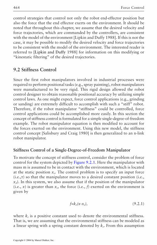
Force Control464
control strategies that control not only the robot end-effector position butalso the force that the end effector exerts on the environment. It should benoted that throughout this chapter, we assume that the desired velocity andforce trajectories, which are commanded by the controllers, are consistentwith the model of the environment [Lipkin and Duffy 1988]. If this is not thecase, it may be possible to modify the desired velocity and force trajectoriesto be consistent with the model of the environment. The interested reader isreferred to [Lipkin and Duffy 1988] for information on this modifying or“kinestatic filtering” of the desired trajectories.
9.2 Stiffness Control
Since the first robot manipulators involved in industrial processes wererequired to perform positional tasks (e.g., spray painting), robot manipulatorswere manufactured to be very rigid. This rigid design allowed the robotcontrol designer to obtain reasonable positional accuracy by utilizing simplecontrol laws. As one might expect, force control applications (e.g., grindingor sanding) are extremely difficult to accomplish with such a “stiff” robot.Therefore, if the robot manipulator “stiffness” could be controlled, forcecontrol applications could be accomplished more easily. In this section theconcept of stiffness control is formulated for a simple single-degree-of-freedomexample. The robot manipulator equation is then modified to account forthe forces exerted on the environment. Using this new model, the stiffnesscontrol concept [Salisbury and Craig 1980] is then generalized to an n-linkrobot manipulator.
Stiffness Control of a Single-Degree-of-Freedom Manipulator
To motivate the concept of stiffness control, consider the problem of forcecontrol for the system depicted by Figure 9.2.1. Here the manipulator withmass m is assumed to be in contact with the environment, which is locatedat the static position xe. The control problem is to specify an input force(i.e.,) so that the manipulator moves to a desired constant position (i.e.,xd). In this system, we also assume that if the position of the manipulator(i.e., x) is greater than xe, the force (i.e., f) exerted on the environment isgiven by
f=ke(x-xe), (9.2.1)
where ke is a positive constant used to denote the environmental stiffness.That is, we are assuming that the environmental stiffness can be modeled asa linear spring with a spring constant denoted by ke. From this assumption
Copyright © 2004 by Marcel Dekker, Inc.
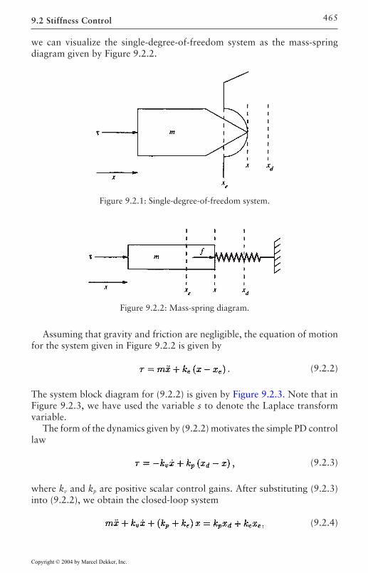
9.2 Stiffness Control 465
Assuming that gravity and friction are negligible, the equation of motionfor the system given in Figure 9.2.2 is given by
(9.2.2)
The system block diagram for (9.2.2) is given by Figure 9.2.3. Note that inFigure 9.2.3, we have used the variable s to denote the Laplace transformvariable.
The form of the dynamics given by (9.2.2) motivates the simple PD controllaw
(9.2.3)
where kv and kp are positive scalar control gains. After substituting (9.2.3)into (9.2.2), we obtain the closed-loop system
(9.2.4)
we can visualize the single-degree-of-freedom system as the mass-springdiagram given by Figure 9.2.2.
Figure 9.2.1: Single-degree-of-freedom system.
Figure 9.2.2: Mass-spring diagram.
Copyright © 2004 by Marcel Dekker, Inc.
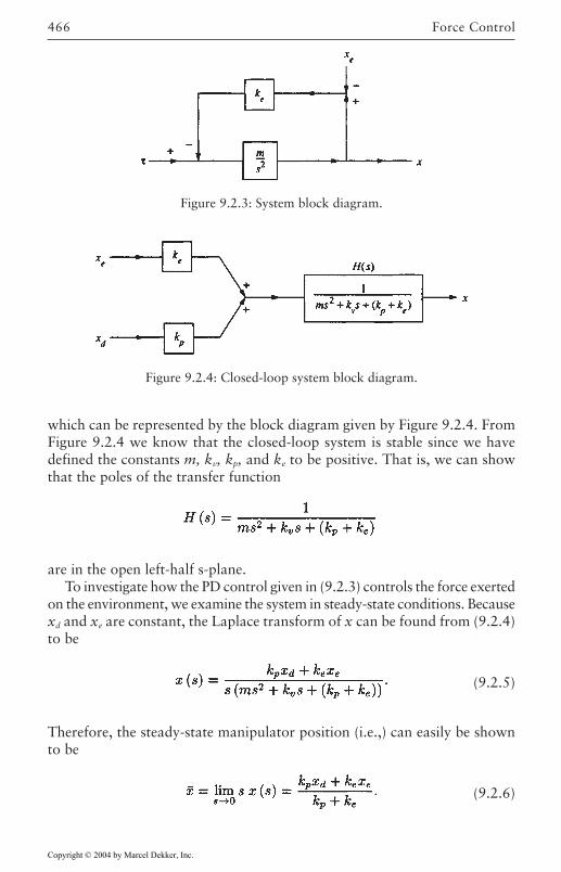
Force Control466
which can be represented by the block diagram given by Figure 9.2.4. FromFigure 9.2.4 we know that the closed-loop system is stable since we havedefined the constants m, kv, kp, and ke to be positive. That is, we can showthat the poles of the transfer function
are in the open left-half s-plane.To investigate how the PD control given in (9.2.3) controls the force exerted
on the environment, we examine the system in steady-state conditions. Becausexd and xe are constant, the Laplace transform of x can be found from (9.2.4)to be
(9.2.5)
Therefore, the steady-state manipulator position (i.e.,) can easily be shownto be
(9.2.6)
Figure 9.2.4: Closed-loop system block diagram.
Figure 9.2.3: System block diagram.
Copyright © 2004 by Marcel Dekker, Inc.
9.2 Stiffness Control 467
The steady-state manipulator position can now be used to calculate the steady-state force (i.e., f) exerted on the environment. Specifically, upon substituting(9.2.6) into (9.2.1), the steady-state force is given by
(9.2.7)
As one would expect, the spring constant of the environment is oftenconsidered to be large because the robot is pushing on a nearly rigid surfacein most robot force control applications. Thus, if we assume that wecan approximate the steady-state force in (9.2.7) as
(9.2.8)
From the discussion above, we can see that the position control strategygiven by (9.2.3) does indeed exert a force on the environment. Specifically,this force is created by commanding a desired trajectory that is slightly insidethe contact surface. In attempting to eliminate the position error, the positioncontroller exerts a steady-state force on the surface. From the approximatesteady-state force given by (9.2.8), the position gain (i.e., kp) can be thoughtof as representing the desired “stiffness” of the manipulator. That is, themanipulator can be visualized as a spring, with spring constant kp, exertinga force on the environment. Hence the term “stiffness control” has oftenbeen associated with the PD control given by (9.2.3) since the stiffness of themanipulator can be set by the adjustment of kp.
The Jacobian Matrix and Environmental Forces
Before the stiffness controller can be generalized to an n-link robotmanipulator, we must define some notation with regard to the forces thatthe robot exerts on the environment. As explained in [Spong and Vidyasagar1989], the forces are commonly transformed into the joint-space via aJacobian matrix. In this chapter we define the Jacobian matrix in terms of atask space coordinate system which is defined for the specific robot applicationin question. That is, for a certain application, we may wish to have the endeffector apply forces along a particular set of directions while moving alongother directions. This concept is illustrated in Figure 9.2.5, which depicts amanipulator moving along a slanted surface. The task space coordinate systemis given by the directions u and v since we wish to move the end effectoralong the surface in the direction v while applying a force normal to thesurface along the direction u. An appropriate task space coordinate systemis usually defined in most robotic applications from this line of reasoning.
Following this logic, let x be the n×1 task space vector defined by
Copyright © 2004 by Marcel Dekker, Inc.
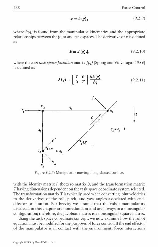
Force Control468
(9.2.9)
where h(q) is found from the manipulator kinematics and the appropriaterelationships between the joint and task spaces. The derivative of x is definedas
(9.2.10)
where the n×n task space Jacobian matrix J(q) [Spong and Vidyasagar 1989]is defined as
(9.2.11)
with the identity matrix I, the zero matrix 0, and the transformation matrixT having dimensions dependent on the task space coordinate system selected.The transformation matrix T is typically used when converting joint velocitiesto the derivatives of the roll, pitch, and yaw angles associated with end-effector orientation. For brevity we assume that the robot manipulatorsdiscussed in this chapter are nonredundant and are always in a nonsingularconfiguration; therefore, the Jacobian matrix is a nonsingular square matrix.
Using the task space coordinate concept, we now examine how the robotequation must be modified for the purposes of force control. If the end effectorof the manipulator is in contact with the environment, force interactions
Figure 9.2.5: Manipulator moving along slanted surface.
Copyright © 2004 by Marcel Dekker, Inc.
9.2 Stiffness Control 469
will exist between the end effector and the environment. If the interactionforces are measured in the joint space, the manipulator dynamic equationcan be written as
(9.2.12)
where e is an n×1 vector in joint space coordinates, which denotes the forceexerted on the environment. The dynamic equation given by (9.2.12) makessense because if the manipulator is not moving (i.e., ), then (9.2.12)reduces to
(9.2.13)
That is, if the robot manipulator is in static operation, the actuator force isequal to the force exerted on the environment plus the force needed towithstand the gravitational forces. Note that in (9.2.13), we have assumedthat static friction can be neglected.
A joint space representation for the force exerted on the environment isnot the standard notation in the robotics literature; rather, the robotmanipulator equation is usually given by
(9.2.14)
where f is the n×1 vector of contact forces and torques in task space.To understand the origin of (9.2.14), equate the right-hand sides of (9.2.12)
and (9.2.14) to yield
(9.2.15)
This equation can be shown to be true quite easily by using a conservationof energy argument. Specifically, by conservation of energy, we know that
(9.2.16)
Substituting (9.2.10) into (9.2.16) yields
Since the relationship above must hold for all q, we can see that (9.2.15)obviously represents a true statement. To shed some light on the process ofdeveloping the Jacobian and the task space formulation, two examples arenow discussed.
Copyright © 2004 by Marcel Dekker, Inc.
Force Control470
EXAMPLE 9.2–1: Task Space Formulation for a Slanted Surface
We want to find the manipulator dynamics for the Cartesian manipulatorsystem (i.e., both joints are prismatic) given in Figure 9.2.5 and todecompose the forces exerted on the surface into a normal force and atangent force. First, the motion portion of the dynamics can easily bedetermined when the robot is not constrained by the surface. Afterremoving the surface and the interaction forces f1, and f2, the manipulatordynamics can be shown to be
(1)
where
and F(q) is the 2×1 vector that models the friction asdiscussed in Chapter 2.
To account for the interaction forces, let x be the 2×1 task space vectordefined by
(2)
where u and v define a fixed coordinate system such that u represents thenormal distance to the surface, and v represents the tangent distance alongthe surface. As in (9.2.9), the task space coordinates can be expressed interms of the joint space coordinates by
(3)
where h(q) is found from the geometry of the problem to be
(4)
Copyright © 2004 by Marcel Dekker, Inc.
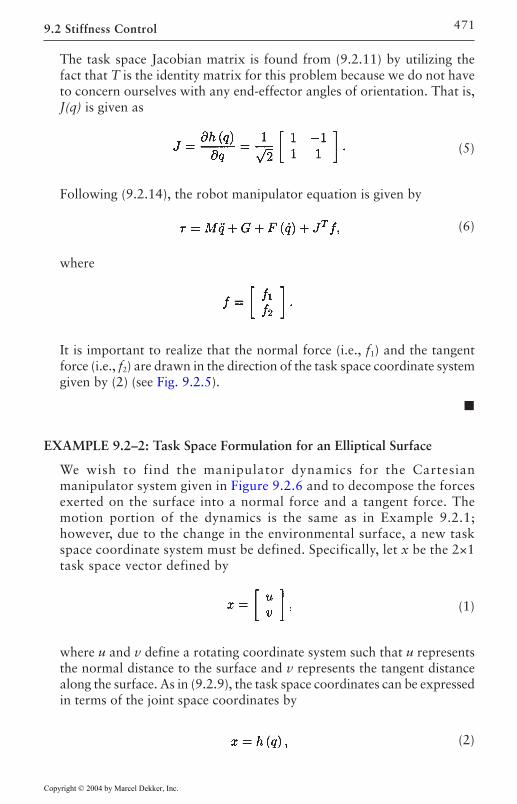
9.2 Stiffness Control 471
The task space Jacobian matrix is found from (9.2.11) by utilizing thefact that T is the identity matrix for this problem because we do not haveto concern ourselves with any end-effector angles of orientation. That is,J(q) is given as
(5)
Following (9.2.14), the robot manipulator equation is given by
(6)
where
It is important to realize that the normal force (i.e., f1) and the tangentforce (i.e., f2) are drawn in the direction of the task space coordinate systemgiven by (2) (see Fig. 9.2.5).
EXAMPLE 9.2–2: Task Space Formulation for an Elliptical Surface
We wish to find the manipulator dynamics for the Cartesianmanipulator system given in Figure 9.2.6 and to decompose the forcesexerted on the surface into a normal force and a tangent force. Themotion portion of the dynamics is the same as in Example 9.2.1;however, due to the change in the environmental surface, a new taskspace coordinate system must be defined. Specifically, let x be the 2×1task space vector defined by
(1)
where u and v define a rotating coordinate system such that u representsthe normal distance to the surface and v represents the tangent distancealong the surface. As in (9.2.9), the task space coordinates can be expressedin terms of the joint space coordinates by
(2)
Copyright © 2004 by Marcel Dekker, Inc.
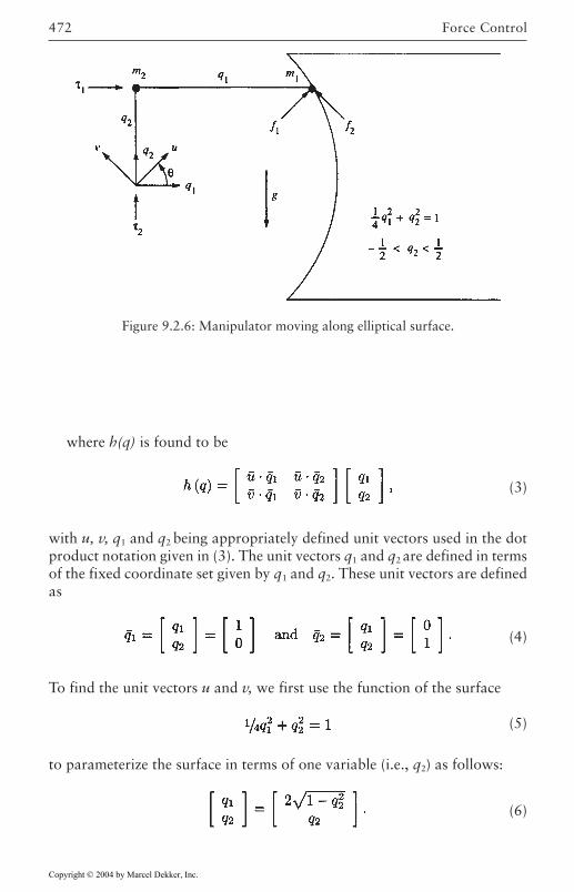
Force Control472
where h(q) is found to be
(3)
with u, v, q1 and q2 being appropriately defined unit vectors used in the dotproduct notation given in (3). The unit vectors q1 and q2 are defined in termsof the fixed coordinate set given by q1 and q2. These unit vectors are definedas
(4)
To find the unit vectors u and v, we first use the function of the surface
(5)
to parameterize the surface in terms of one variable (i.e., q2) as follows:
(6)
Figure 9.2.6: Manipulator moving along elliptical surface.
Copyright © 2004 by Marcel Dekker, Inc.
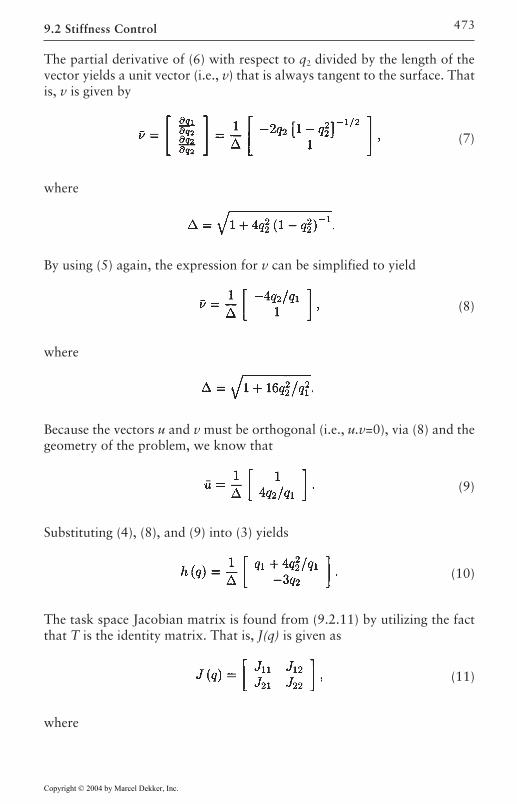
9.2 Stiffness Control 473
The partial derivative of (6) with respect to q2 divided by the length of thevector yields a unit vector (i.e., v) that is always tangent to the surface. Thatis, v is given by
(7)
where
By using (5) again, the expression for v can be simplified to yield
(8)
where
Because the vectors u and v must be orthogonal (i.e., u.v=0), via (8) and thegeometry of the problem, we know that
(9)
Substituting (4), (8), and (9) into (3) yields
(10)
The task space Jacobian matrix is found from (9.2.11) by utilizing the factthat T is the identity matrix. That is, J(q) is given as
(11)
where
Copyright © 2004 by Marcel Dekker, Inc.
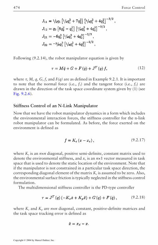
Force Control474
Following (9.2.14), the robot manipulator equation is given by
(12)
where , M, q, G, f, and F(q) are as defined in Example 9.2.1. It is importantto note that the normal force (i.e., f1) and the tangent force (i.e., f2) aredrawn in the direction of the task space coordinate system given by (1) (seeFig. 9.2.6).
Stiffness Control of an N-Link Manipulator
Now that we have the robot manipulator dynamics in a form which includesthe environmental interaction forces, the stiffness controller for the n-linkrobot manipulator can be formulated. As before, the force exerted on theenvironment is defined as
(9.2.17)
where Ke is an n×n diagonal, positive semi-definite, constant matrix used todenote the environmental stiffness, and xe is an n×1 vector measured in taskspace that is used to denote the static location of the environment. Note thatif the manipulator is not constrained in a particular task space direction, thecorresponding diagonal element of the matrix Ke is assumed to be zero. Also,the environmental surface friction is typically neglected in the stiffness controlformulation.
The multidimensional stiffness controller is the PD-type controller
(9.2.18)
where Kv and Kp are n×n diagonal, constant, positive-definite matrices andthe task space tracking error is defined as
Copyright © 2004 by Marcel Dekker, Inc.
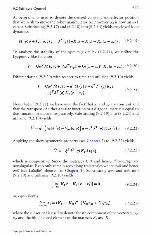
9.2 Stiffness Control 475
As before, xd is used to denote the desired constant end-effector positionthat we wish to move the robot manipulator to; however, xd is now an n×1vector. Substituting (9.2.17) and (9.2.18) into (9.2.14) yields the closed-loopdynamics
(9.2.19)
To analyze the stability of the system given by (9.2.19), we utilize theLyapunov-like function
(9.2.20)
Differentiating (9.2.20) with respect to time and utilizing (9.2.10) yields
(9.2.21)
Note that in (9.2.21) we have used the fact that xe and xd are constant andthat the transpose of either a scalar function or a diagonal matrix is equal tothat function or matrix, respectively. Substituting (9.2.19) into (9.2.21) andutilizing (9.2.10) yields
(9.2.22)
Applying the skew-symmetric property (see Chapter 2) to (9.2.22) yields
(9.2.23)
which is nonpositive. Since the matrices J(q) and hence JT(q)KvJ(q) arenonsingular, V can only remain zero along trajectories where q=0 and henceq=0 (see LaSalle’s theorem in Chapter 1). Substituting q=0 and q=0 into(9.2.19) and utilizing (9.2.10) yields
(9.2.24)
or, equivalently,
(9.2.25)
where the subscript i is used to denote the ith component of the vectors x, xd,xe, and the ith diagonal element of the matrices Kp and Ke.
Copyright © 2004 by Marcel Dekker, Inc.
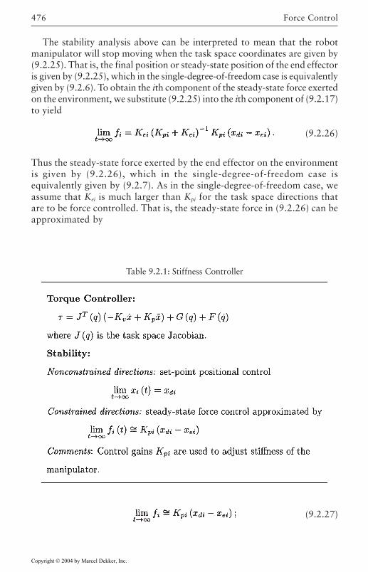
Force Control476
The stability analysis above can be interpreted to mean that the robotmanipulator will stop moving when the task space coordinates are given by(9.2.25). That is, the final position or steady-state position of the end effectoris given by (9.2.25), which in the single-degree-of-freedom case is equivalentlygiven by (9.2.6). To obtain the ith component of the steady-state force exertedon the environment, we substitute (9.2.25) into the ith component of (9.2.17)to yield
(9.2.26)
Thus the steady-state force exerted by the end effector on the environmentis given by (9.2.26), which in the single-degree-of-freedom case isequivalently given by (9.2.7). As in the single-degree-of-freedom case, weassume that Kei is much larger than Kpi for the task space directions thatare to be force controlled. That is, the steady-state force in (9.2.26) can beapproximated by
Table 9.2.1: Stiffness Controller
(9.2.27)
Copyright © 2004 by Marcel Dekker, Inc.
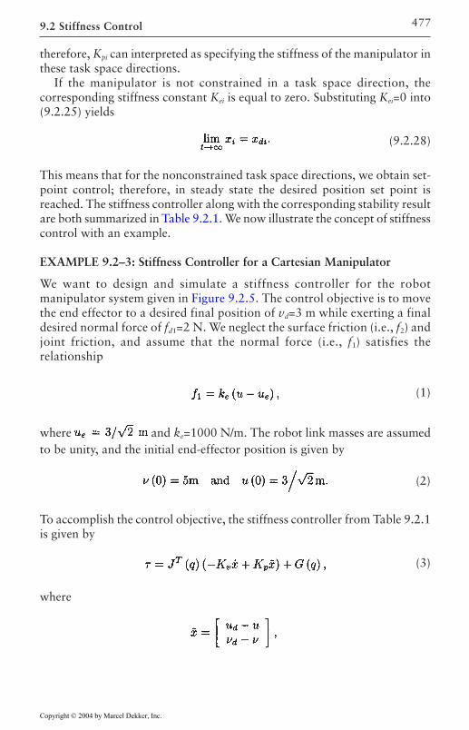
9.2 Stiffness Control 477
therefore, Kpi can interpreted as specifying the stiffness of the manipulator inthese task space directions.
If the manipulator is not constrained in a task space direction, thecorresponding stiffness constant Kei is equal to zero. Substituting Kei=0 into(9.2.25) yields
(9.2.28)
This means that for the nonconstrained task space directions, we obtain set-point control; therefore, in steady state the desired position set point isreached. The stiffness controller along with the corresponding stability resultare both summarized in Table 9.2.1. We now illustrate the concept of stiffnesscontrol with an example.
EXAMPLE 9.2–3: Stiffness Controller for a Cartesian Manipulator
We want to design and simulate a stiffness controller for the robotmanipulator system given in Figure 9.2.5. The control objective is to movethe end effector to a desired final position of vd=3 m while exerting a finaldesired normal force of fd1=2 N. We neglect the surface friction (i.e., f2) andjoint friction, and assume that the normal force (i.e., f1) satisfies therelationship
(1)
where and ke=1000 N/m. The robot link masses are assumedto be unity, and the initial end-effector position is given by
(2)
To accomplish the control objective, the stiffness controller from Table 9.2.1is given by
(3)
where
Copyright © 2004 by Marcel Dekker, Inc.
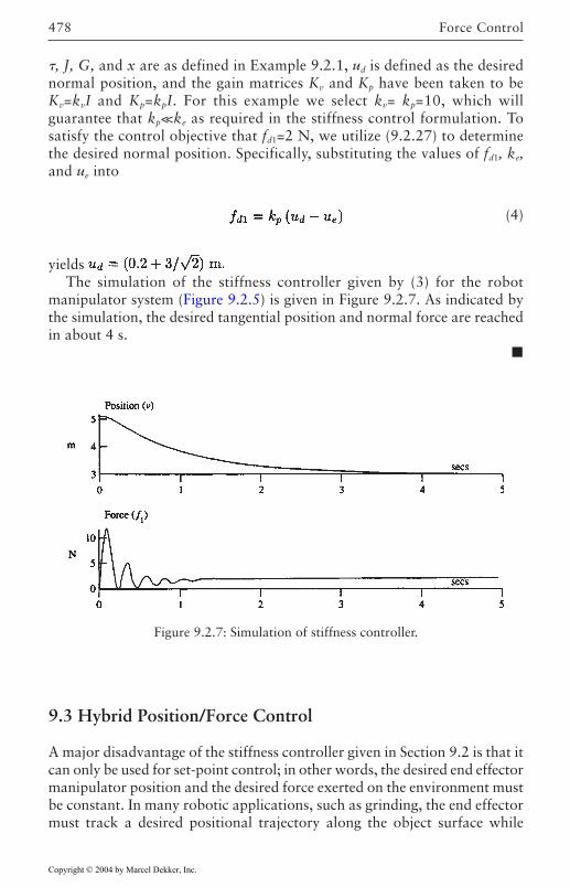
Force Control478
, J, G, and x are as defined in Example 9.2.1, ud is defined as the desirednormal position, and the gain matrices Kv and Kp have been taken to beKv=kvI and Kp=kpI. For this example we select kv= kp=10, which willguarantee that kp<< k e as required in the stiffness control formulation. Tosatisfy the control objective that fd1=2 N, we utilize (9.2.27) to determinethe desired normal position. Specifically, substituting the values of fd1, ke,and ue into
(4)
yields The simulation of the stiffness controller given by (3) for the robot
manipulator system (Figure 9.2.5) is given in Figure 9.2.7. As indicated bythe simulation, the desired tangential position and normal force are reachedin about 4 s.
9.3 Hybrid Position/Force Control
A major disadvantage of the stiffness controller given in Section 9.2 is that itcan only be used for set-point control; in other words, the desired end effectormanipulator position and the desired force exerted on the environment mustbe constant. In many robotic applications, such as grinding, the end effectormust track a desired positional trajectory along the object surface while
Figure 9.2.7: Simulation of stiffness controller.
Copyright © 2004 by Marcel Dekker, Inc.
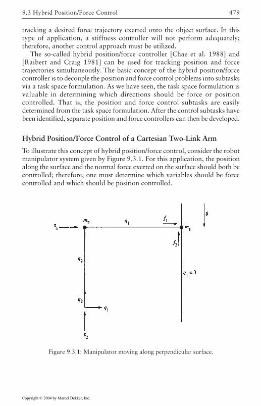
479
tracking a desired force trajectory exerted onto the object surface. In thistype of application, a stiffness controller will not perform adequately;therefore, another control approach must be utilized.
The so-called hybrid position/force controller [Chae et al. 1988] and[Raibert and Craig 1981] can be used for tracking position and forcetrajectories simultaneously. The basic concept of the hybrid position/forcecontroller is to decouple the position and force control problems into subtasksvia a task space formulation. As we have seen, the task space formulation isvaluable in determining which directions should be force or positioncontrolled. That is, the position and force control subtasks are easilydetermined from the task space formulation. After the control subtasks havebeen identified, separate position and force controllers can then be developed.
Hybrid Position/Force Control of a Cartesian Two-Link Arm
To illustrate this concept of hybrid position/force control, consider the robotmanipulator system given by Figure 9.3.1. For this application, the positionalong the surface and the normal force exerted on the surface should both becontrolled; therefore, one must determine which variables should be forcecontrolled and which should be position controlled.
9.3 Hybrid Position/Force Control
Figure 9.3.1: Manipulator moving along perpendicular surface.
Copyright © 2004 by Marcel Dekker, Inc.
Force Control480
Following the task space concept given in Section 9.2, the task spaceformulation for the manipulator system given in Figure 9.3.1 is
(9.3.1)
with the task-space Jacobian matrix given by
As illustrated by (9.3.1), the task space and the joint space are equivalent forthis problem; therefore, we will refer to joint variables as task-space variablesthroughout this problem.
To design the position/force controller for the manipulator system, wemust first determine the dynamic equations for the task space formulationgiven by (9.3.1). Using this task space formulation and neglecting jointfriction, the manipulator dynamics can be shown to be
(9.3.2)
where , M, G, and f are as defined in Example 9.2.1. The two dynamicequations given in the matrix form represented by (9.3.2) are
(9.3.3)
and
(9.3.4)
In formulating a hybrid position/force controller, we design separatecontrollers for the dynamics given by (9.3.3) and (9.3.4). As illustrated byFigure 9.3.1, the position along the task space direction q2 should be positioncontrolled; therefore, we should use (9.3.4) for designing the positioncontroller. [This is obvious because the dynamics given by (9.3.3) do notcontain the task space variable q2.]
Because we are designing a position controller to track a desired trajectory,we will define the “tangent space” tracking error to be
(9.3.5)
where qd2 represents the desired position trajectory along or tangent to thesurface. The position controller will be the computed-torque controller (seeChapter 3)
(9.3.6)
Copyright © 2004 by Marcel Dekker, Inc.
481
where
(9.3.7)
with kTv and kTp being positive control gains. Substituting (9.3.6) into (9.3.4)gives the position tracking error system
(9.3.8)
By using the fact that kTv and kTp are positive, we can apply standard linearcontrol results to (9.3.8) to yield
therefore, asymptotic positional tracking is guaranteed with the controllergiven by (9.3.6). Note that the position controller requires measurement ofthe joint position, joint velocity, and surface friction force; therefore, froman implementation point of view, force measurements are required in theposition controller.
The position controller given in (9.3.6) will ensure good position trackingalong the surface of the environment; however, we also want to control theforce exerted on the environment. For the manipulator system given in Figure9.3.1, the task space direction normal to the surface is q1; therefore, we willassume that in this direction the environment can be modeled as a spring.Specifically, the normal force f1 exerted on the environment is given by
(9.3.9)
where ke represents the environment stiffness and qe=3. Taking the secondderivative of (9.3.9) with respect to time gives the expression
(9.3.10)
where the normal task space acceleration is written in terms of the secondderivative of the normal force. Substituting (9.3.10) into (9.3.3) yields theforce dynamic equation
(9.3.11)
We can now use the force dynamic equation given in (9.3.11) to design aforce controller to track a desired force trajectory. First, define the forcetracking error to be
9.3 Hybrid Position/Force Control
Copyright © 2004 by Marcel Dekker, Inc.
Force Control482
(9.3.12)
where fd1 represents the desired normal force that is to be exerted on theenvironment. Similar to the position controller, the force controller will bethe computed-torque controller
(9.3.13)
where
(9.3.14)
with kNv and kNp being positive control gains. Substituting (9.3.13) into(9.3.11) gives the force tracking error system,
(9.3.15)
Using the fact kNv and kNp are positive in (9.3.15) yields
therefore, asymptotic force tracking is guaranteed with the controller givenby (9.3.13). It is important to realize that the force controller requiresmeasurement of the normal force and the derivative of the normal force.Because the force derivative is often not available for measurement, it ismanufactured from (9.3.9), that is,
(9.3.16)
therefore, the stiffness of the environment and the normal task space velocityare used to simulate the derivative of the force.
Hybrid Position/Force Control of an N-Link Manipulator
The hybrid position/force controller given in the preceding section can easilybe extended to the multidegree case by using the task space formulationconcept. Specifically, one can develop a feedback-linearizing control thatwill globally linearize the robot manipulator equation and then develop linearcontrollers to track the desired force and position trajectories.
First, the control designer selects a task space formulation
(9.3.17)
Copyright © 2004 by Marcel Dekker, Inc.
483
such that the normal and tangent surface motions are decomposed asdiscussed in Section 9.2. The robot dynamics given in (9.3.14) are then writtenin terms of the task space acceleration by differentiating (9.3.17) twice withrespect to time to obtain
(9.3.18)
where J(q) is the task space Jacobian defined in (9.2.11). Solving (9.3.18) forq yields
(9.3.19)
Substituting (9.3.19) into (9.2.14) yields
(9.3.20)
The corresponding feedback linearizing control for the dynamics given by(9.3.20) is given by
(9.3.21)
where a is an n×1 vector used to represent the linear position and forcecontrol strategies, which will be discussed later. After substituting (9.3.21)into (9.3.20), we have
(9.3.22)
From (9.3.22), we can see that the task space motion has been globallylinearized and decoupled; therefore, we can design the position and forcecontrollers independently in a method similar to that of the preceding section.Specifically, linear position controllers can be designed for the task spacevariables that represent tangent motion; moreover, linear force controllerscan be designed for the task space variables that represent normal force.
Because the dynamics given in (9.3.20) have been decoupled in the taskspace, we will define the tangent space components of x as xTi, where thesubscript T is used to denote the tangent space, and the subscript i is used todenote the ith component of xT. From this notation the tangent spacecomponents of (9.3.22) are given as
(9.3.23)
9.3 Hybrid Position/Force Control
Copyright © 2004 by Marcel Dekker, Inc.
Force Control484
where aTi is the ith linear tangent space position controller. For the purposeof feedback control, we define the tangent space tracking error to be
(9.3.24)
where xTdi represents the ith desired position trajectory tangent to theenvironment surface. As in the preceding section, the corresponding linearcontroller is then given as
(9.3.25)
with kTvi and kTpi being the ith positive control gains. Substituting (9.3.25)into (9.3.23) gives the position tracking error system
(9.3.26)
Using the fact that kTvi and kTpi are positive in (9.3.26) yields
therefore, asymptotic positional tracking is guaranteed.For purposes of force control, we define the normal space components of
x as xNj where the subscript N is used to denote normal space, and the subscriptj is used to denote the jth component of xN. From this notation, the normalspace components of (9.3.22) are given as
(9.3.27)
where aNj is the jth linear normal space force controller. As in the precedingsection, we assume that the environment can be modeled as a spring.Specifically, the normal force fNj exerted on the environment is given by
(9.3.28)
where kej is the jth component of environmental stiffness, and xej is used torepresent the static location of the environment in the direction of the normalspace xNj.
As done for the single-degree-of-freedom robot in the preceding subsection,we must formulate the force dynamics before we can develop the forcecontroller. Taking the second derivative of (9.3.28) with respect to time givesthe expression
(9.3.29)
Copyright © 2004 by Marcel Dekker, Inc.
485
where the normal task space acceleration is written in terms of the secondderivative of the normal force. Substituting (9.3.29) into (9.3.27) yields theforce dynamics
(9.3.30)
For the purpose of feedback control, we define the force tracking error to be
(9.3.31)
where fNdj represents the jth component of the desired force exerted normalto the environment. As in the preceding section, the corresponding linearcontroller is then given by
(9.3.32)
with kNvj and kNpj being the jth positive control gains. Substituting (9.3.32)into (9.3.30) gives the force tracking error system
(9.3.33)
Using the fact that kNvj and kNpj are positive in (9.3.33) yields
therefore, asymptotic force tracking is guaranteed.The hybrid position/force controller and the corresponding stability result
are both summarized in Table 9.3.1. We now illustrate the concept of hybridposition/force control with an example.
EXAMPLE 9.3–1: Hybrid Position/Force Control Along a Slanted Surface
We want to design and simulate a hybrid position/force controller for therobot manipulator system given in Figure 9.2.5. The control objective isto move the end effector with a desired surface trajectory of vd=sin(t) mwhile exerting a normal force trajectory of . We neglectjoint friction and assume that the normal force (i.e., f1) satisfies therelationship
(1)
9.3 Hybrid Position/Force Control
Copyright © 2004 by Marcel Dekker, Inc.
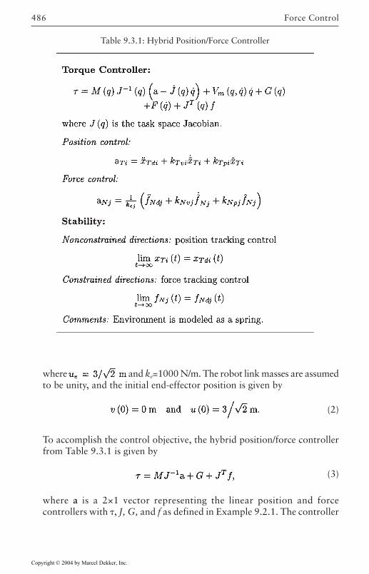
Force Control486
where and ke=1000 N/m. The robot link masses are assumedto be unity, and the initial end-effector position is given by
(2)
To accomplish the control objective, the hybrid position/force controllerfrom Table 9.3.1 is given by
(3)
where a is a 2×1 vector representing the linear position and forcecontrollers with , J, G, and f as defined in Example 9.2.1. The controller
Table 9.3.1: Hybrid Position/Force Controller
Copyright © 2004 by Marcel Dekker, Inc.
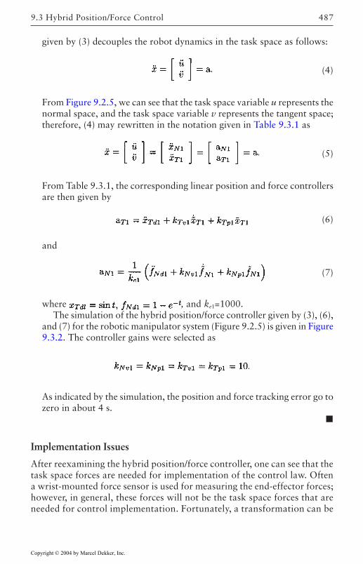
487
given by (3) decouples the robot dynamics in the task space as follows:
(4)
From Figure 9.2.5, we can see that the task space variable u represents thenormal space, and the task space variable v represents the tangent space;therefore, (4) may rewritten in the notation given in Table 9.3.1 as
(5)
From Table 9.3.1, the corresponding linear position and force controllersare then given by
(6)
and
(7)
where , and ke1=1000.The simulation of the hybrid position/force controller given by (3), (6),
and (7) for the robotic manipulator system (Figure 9.2.5) is given in Figure9.3.2. The controller gains were selected as
As indicated by the simulation, the position and force tracking error go tozero in about 4 s.
Implementation Issues
After reexamining the hybrid position/force controller, one can see that thetask space forces are needed for implementation of the control law. Oftena wrist-mounted force sensor is used for measuring the end-effector forces;however, in general, these forces will not be the task space forces that areneeded for control implementation. Fortunately, a transformation can be
9.3 Hybrid Position/Force Control
Copyright © 2004 by Marcel Dekker, Inc.
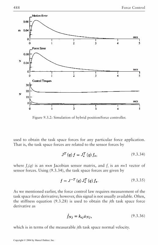
Force Control488
used to obtain the task space forces for any particular force application.That is, the task space forces are related to the sensor forces by
(9.3.34)
where Js(q) is an n×n Jacobian sensor matrix, and fs is an n×1 vector ofsensor forces. Using (9.3.34), the task space forces are given by
(9.3.35)
As we mentioned earlier, the force control law requires measurement of thetask space force derivative; however, this signal is not usually available. Often,the stiffness equation (9.3.28) is used to obtain the jth task space forcederivative as
(9.3.36)
which is in terms of the measurable jth task space normal velocity.
Figure 9.3.2: Simulation of hybrid position/force controller.
Copyright © 2004 by Marcel Dekker, Inc.
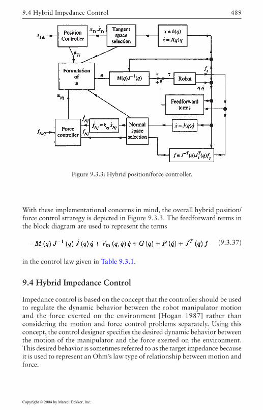
489
With these implementational concerns in mind, the overall hybrid position/force control strategy is depicted in Figure 9.3.3. The feedforward terms inthe block diagram are used to represent the terms
(9.3.37)
in the control law given in Table 9.3.1.
9.4 Hybrid Impedance Control
Impedance control is based on the concept that the controller should be usedto regulate the dynamic behavior between the robot manipulator motionand the force exerted on the environment [Hogan 1987] rather thanconsidering the motion and force control problems separately. Using thisconcept, the control designer specifies the desired dynamic behavior betweenthe motion of the manipulator and the force exerted on the environment.This desired behavior is sometimes referred to as the target impedance becauseit is used to represent an Ohm’s law type of relationship between motion andforce.
9.4 Hybrid Impedance Control
Figure 9.3.3: Hybrid position/force controller.
Copyright © 2004 by Marcel Dekker, Inc.
Force Control490
Modeling the Environment
As pointed out in [Hogan 1987], the environmental model is central to anyforce control strategy. In the force control strategies discussed previously,the environment has simply been modeled as a spring; however, as one mightimagine, a simple spring model may not adequately describe all types ofenvironments. To classify the many types of environments, we use the lineartransfer function relationship
(9.4.1)
where the variable s is the Laplace transform variable, f represents the forceexerted on the environment, x represents the velocity of the manipulator atthe environmental contact point, and Ze(s) represents the environmentalimpedance. For now, all quantities are assumed to be scalar functions;however, at the end of this section we generalize impedance control to themultidimensional case.
The quantity Ze(s) is called an impedance because (9.4.1) represents anOhm’s law type of relationship between motion and force. As in circuit theory,environmental impedances can be separated into different categories. Tofurther our impedance control discussion, we now give three commonly usedcategories which are used to classify environmental impedances.
DEFINITION 9.4–1 An impedance is inertial if and only if |Z(0)|=0.
An illustration of an inertial environment is given in Figure 9.4.1a. Thisfigure depicts a robot manipulator moving a payload of mass h with velocityx. The corresponding interaction force is given by
therefore, utilizing (9.4.1) yields an inertial environmental impedance of
(9.4.2)
We can easily verify that this impedance is indeed inertial by applyingDefinition 9.4.1.
DEFINITION 9.4–2 An impedance is resistive if and only if |Z(0)|=c where0<c<.
An illustration of a resistive environment is given in Figure 9.4.1b. This figuredepicts a robot manipulator moving through a liquid medium with velocity x.
Copyright © 2004 by Marcel Dekker, Inc.
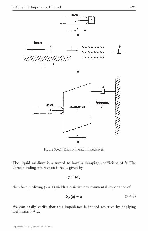
491
The liquid medium is assumed to have a damping coefficient of b. Thecorresponding interaction force is given by
therefore, utilizing (9.4.1) yields a resistive environmental impedance of
(9.4.3)
We can easily verify that this impedance is indeed resistive by applyingDefinition 9.4.2.
9.4 Hybrid Impedance Control
Figure 9.4.1: Environmental impedances.
Copyright © 2004 by Marcel Dekker, Inc.
Force Control492
DEFINITION 9.4–3 An impedance is capacitive if and only if |Z(O)|= .
An illustration of a capacitive environment is given in Figure 9.4.1c.This figure depicts a robot manipulator pushing against an object ofmass h with velocity x. The object is assumed to have a dampingcoefficient of b and a spring constant of k. The corresponding interactionforce is given by
therefore, utilizing (9.4.1) yields a capacitive environmental impedance of
(9.4.4)
We can easily verify that this impedance is indeed capacitive by applyingDefinition 9.4.3.
Position and Force Control Models
As we have seen in the preceding section, the environment can be modeled asan impedance defined by the force/velocity relationship in (9.4.1). For ourimpedance control formulation, we will assume that the environmentalimpedance is either inertial, resistive, or capacitive. The question thenbecomes: How does one design a controller for a given environmentalimpedance? The solution is obtained by formulating a manipulator impedancemodel, Zm(s) [Anderson and Spong 1988]. In other words, a manipulatorimpedance (or target impedance) is selected after the environment has beenmodeled. The criterion for selecting the manipulator impedance is related tothe dynamic performance of the manipulator. That is, the manipulatorimpedance is selected such that there is zero steadystate error to a step input(which may be a force or velocity command). As we will show, thisperformance criterion can be achieved if the manipulator impedance is thedual of the environmental impedance.
Before the concept of duality can be illustrated fully, the models for positionand force control must be formulated. For position control [Anderson andSpong 1988], the relationship between force and velocity is modeled by
(9.4.5)
where xd represents the input velocity of the manipulator at the environmentalcontact point and Zm(s) represents the manipulator impedance.
Copyright © 2004 by Marcel Dekker, Inc.
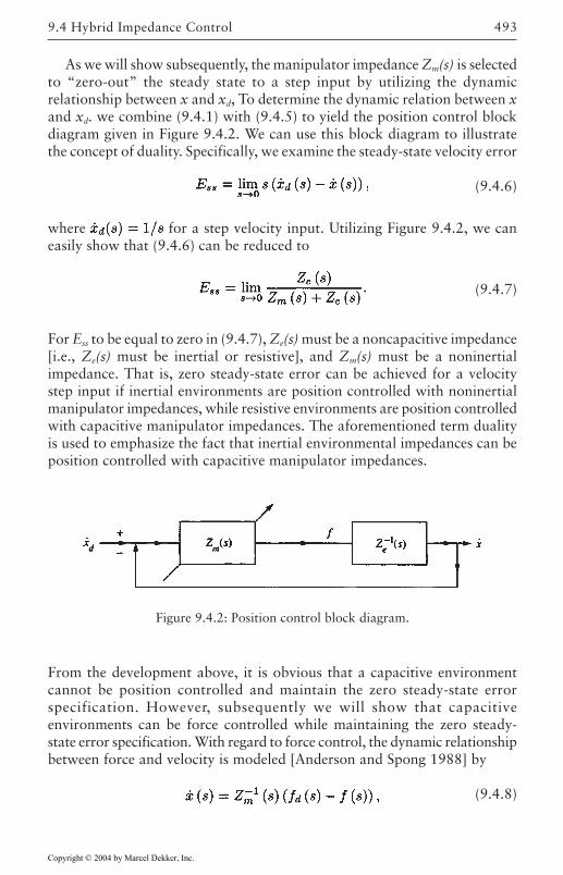
493
As we will show subsequently, the manipulator impedance Zm(s) is selectedto “zero-out” the steady state to a step input by utilizing the dynamicrelationship between x and xd, To determine the dynamic relation between xand xd. we combine (9.4.1) with (9.4.5) to yield the position control blockdiagram given in Figure 9.4.2. We can use this block diagram to illustratethe concept of duality. Specifically, we examine the steady-state velocity error
(9.4.6)
where for a step velocity input. Utilizing Figure 9.4.2, we caneasily show that (9.4.6) can be reduced to
(9.4.7)
For Ess to be equal to zero in (9.4.7), Ze(s) must be a noncapacitive impedance[i.e., Ze(s) must be inertial or resistive], and Zm(s) must be a noninertialimpedance. That is, zero steady-state error can be achieved for a velocitystep input if inertial environments are position controlled with noninertialmanipulator impedances, while resistive environments are position controlledwith capacitive manipulator impedances. The aforementioned term dualityis used to emphasize the fact that inertial environmental impedances can beposition controlled with capacitive manipulator impedances.
9.4 Hybrid Impedance Control
From the development above, it is obvious that a capacitive environmentcannot be position controlled and maintain the zero steady-state errorspecification. However, subsequently we will show that capacitiveenvironments can be force controlled while maintaining the zero steady-state error specification. With regard to force control, the dynamic relationshipbetween force and velocity is modeled [Anderson and Spong 1988] by
(9.4.8)
Figure 9.4.2: Position control block diagram.
Copyright © 2004 by Marcel Dekker, Inc.
Force Control494
where fd is used to represent the input force exerted at the environmentalcontact point.
As we will show subsequently, the manipulator impedance Zm(s) is selectedto “zero-out” the steady state to a step input by utilizing the dynamicrelationship between f and fd. To determine the dynamic relation between fand fd, we combine (9.4.1) with (9.4.8) to yield the force control block diagramgiven in Figure 9.4.3. We can use this block diagram to illustrate the conceptof duality. Specifically, we examine the steady-state force error
(9.4.9)
where fd(s)=1/s for a step force input. Utilizing Figure 9.4.3, we can easilyshow that (9.4.9) can be reduced to
(9.4.10)
For Ess to be equal to zero in (9.4.10), Ze(s) must be a noninertial impedance,and Zm(s) must be a noncapacitive impedance. That is, zero steady-stateerror can be achieved for a force step input if capacitive environments areforce controlled with noncapacitive manipulator impedances while resistiveenvironments are force controlled with inertial manipulator impedances.The term “duality” is used to emphasize the fact that capacitiveenvironmental impedances can be force controlled with inertial manipulatorimpedances.
The discussion above can be summarized by the following dualityprinciple.
DUALITY PRINCIPLE Capacitive environments are force controlled withnoncapacitive manipulator impedances, inertial environments are positioncontrolled with noninertial manipulator impedances, and resistiveenvironments are force controlled with inertial manipulator impedances orposition controlled with capacitive manipulator impedances.
Impedance Control Formulation
Now that we have illustrated how the environment and the manipulator canbe modeled as impedances, we develop an “impedance” controller based onthis model. To utilize an impedance control approach, the control designerselects a task space formulation
(9.4.11)
Copyright © 2004 by Marcel Dekker, Inc.
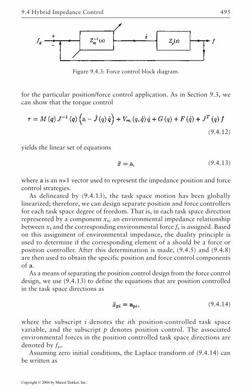
495
for the particular position/force control application. As in Section 9.3, wecan show that the torque control
(9.4.12)
yields the linear set of equations
(9.4.13)
where a is an n×1 vector used to represent the impedance position and forcecontrol strategies.
As delineated by (9.4.13), the task space motion has been globallylinearized; therefore, we can design separate position and force controllersfor each task space degree of freedom. That is, in each task space directionrepresented by a component xk, an environmental impedance relationshipbetween xk and the corresponding environmental force fk is assigned. Basedon this assignment of environmental impedance, the duality principle isused to determine if the corresponding element of a should be a force orposition controller. After this determination is made, (9.4.5) and (9.4.8)are then used to obtain the specific position and force control componentsof a.
As a means of separating the position control design from the force controldesign, we use (9.4.13) to define the equations that are position controlledin the task space directions as
(9.4.14)
where the subscript i denotes the ith position-controlled task spacevariable, and the subscript p denotes position control. The associatedenvironmental forces in the position controlled task space directions aredenoted by fpi.
Assuming zero initial conditions, the Laplace transform of (9.4.14) canbe written as
9.4 Hybrid Impedance Control
Figure 9.4.3: Force control block diagram.
Copyright © 2004 by Marcel Dekker, Inc.
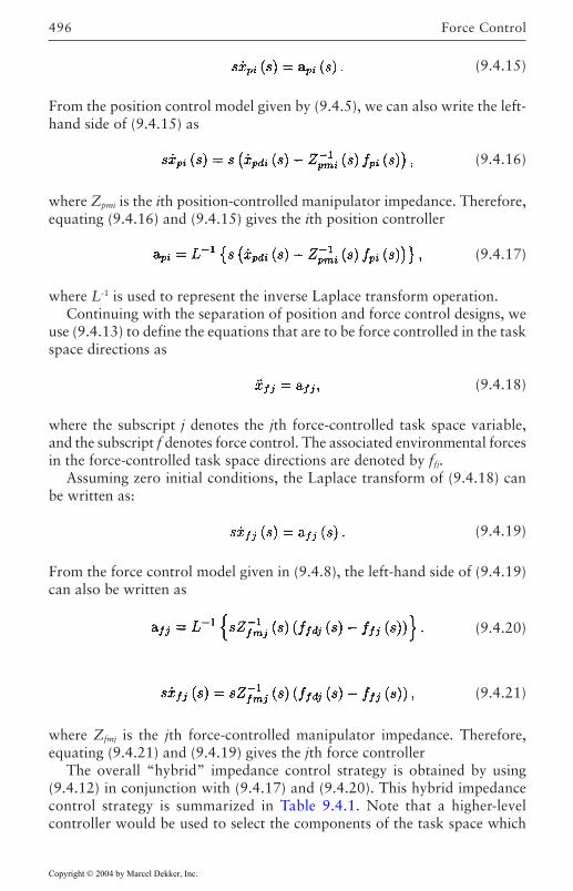
Force Control496
(9.4.15)
From the position control model given by (9.4.5), we can also write the left-hand side of (9.4.15) as
(9.4.16)
where Zpmi is the ith position-controlled manipulator impedance. Therefore,equating (9.4.16) and (9.4.15) gives the ith position controller
(9.4.17)
where L-1 is used to represent the inverse Laplace transform operation.Continuing with the separation of position and force control designs, we
use (9.4.13) to define the equations that are to be force controlled in the taskspace directions as
(9.4.18)
where the subscript j denotes the jth force-controlled task space variable,and the subscript f denotes force control. The associated environmental forcesin the force-controlled task space directions are denoted by ffj.
Assuming zero initial conditions, the Laplace transform of (9.4.18) canbe written as:
(9.4.19)
From the force control model given in (9.4.8), the left-hand side of (9.4.19)can also be written as
(9.4.20)
(9.4.21)
where Zfmj is the jth force-controlled manipulator impedance. Therefore,equating (9.4.21) and (9.4.19) gives the jth force controller
The overall “hybrid” impedance control strategy is obtained by using(9.4.12) in conjunction with (9.4.17) and (9.4.20). This hybrid impedancecontrol strategy is summarized in Table 9.4.1. Note that a higher-levelcontroller would be used to select the components of the task space which
Copyright © 2004 by Marcel Dekker, Inc.
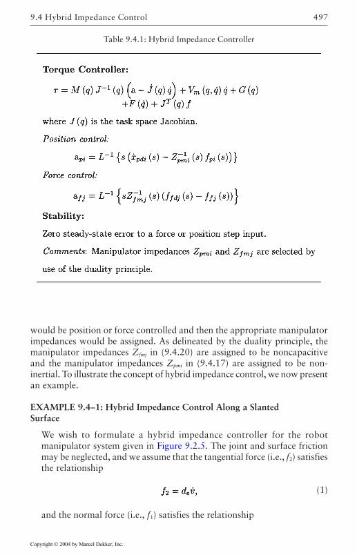
497
would be position or force controlled and then the appropriate manipulatorimpedances would be assigned. As delineated by the duality principle, themanipulator impedances Zfmj in (9.4.20) are assigned to be noncapacitiveand the manipulator impedances Zpmi in (9.4.17) are assigned to be non-inertial. To illustrate the concept of hybrid impedance control, we now presentan example.
EXAMPLE 9.4–1: Hybrid Impedance Control Along a SlantedSurface
We wish to formulate a hybrid impedance controller for the robotmanipulator system given in Figure 9.2.5. The joint and surface frictionmay be neglected, and we assume that the tangential force (i.e., f2) satisfiesthe relationship
(1)
and the normal force (i.e., f1) satisfies the relationship
9.4 Hybrid Impedance Control
Table 9.4.1: Hybrid Impedance Controller
Copyright © 2004 by Marcel Dekker, Inc.
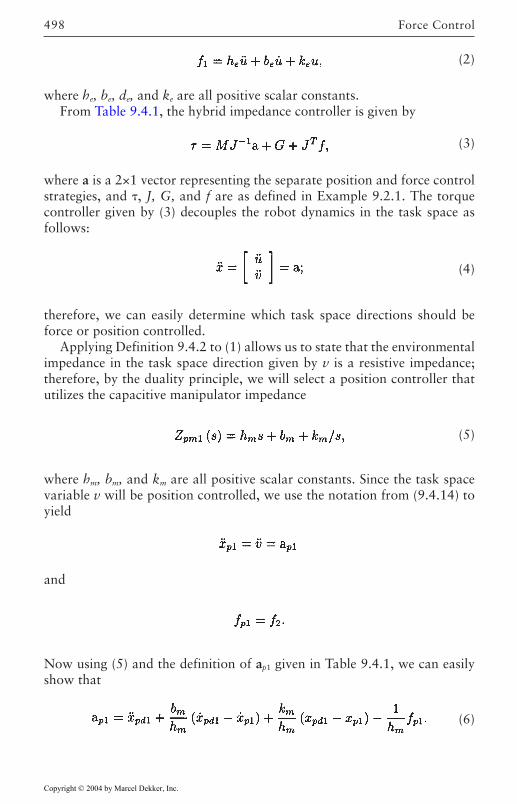
Force Control498
(2)
where he, be, de, and ke are all positive scalar constants.From Table 9.4.1, the hybrid impedance controller is given by
(3)
where a is a 2×1 vector representing the separate position and force controlstrategies, and , J, G, and f are as defined in Example 9.2.1. The torquecontroller given by (3) decouples the robot dynamics in the task space asfollows:
(4)
therefore, we can easily determine which task space directions should beforce or position controlled.
Applying Definition 9.4.2 to (1) allows us to state that the environmentalimpedance in the task space direction given by v is a resistive impedance;therefore, by the duality principle, we will select a position controller thatutilizes the capacitive manipulator impedance
(5)
where hm, bm, and km are all positive scalar constants. Since the task spacevariable v will be position controlled, we use the notation from (9.4.14) toyield
and
Now using (5) and the definition of ap1 given in Table 9.4.1, we can easilyshow that
(6)
Copyright © 2004 by Marcel Dekker, Inc.
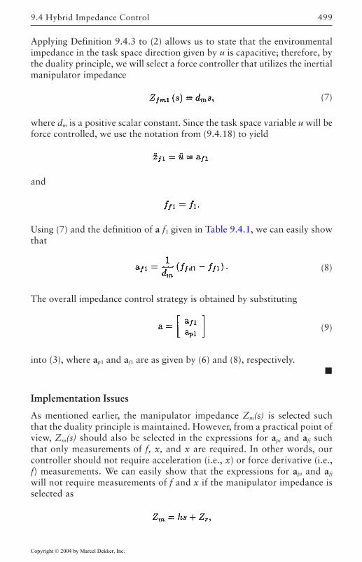
499
Applying Definition 9.4.3 to (2) allows us to state that the environmentalimpedance in the task space direction given by u is capacitive; therefore, bythe duality principle, we will select a force controller that utilizes the inertialmanipulator impedance
(7)
where dm is a positive scalar constant. Since the task space variable u will beforce controlled, we use the notation from (9.4.18) to yield
and
Using (7) and the definition of a f1 given in Table 9.4.1, we can easily showthat
(8)
The overall impedance control strategy is obtained by substituting
(9)
into (3), where ap1 and af1 are as given by (6) and (8), respectively.
Implementation Issues
As mentioned earlier, the manipulator impedance Zm(s) is selected suchthat the duality principle is maintained. However, from a practical point ofview, Zm(s) should also be selected in the expressions for api and afj suchthat only measurements of f, x, and x are required. In other words, ourcontroller should not require acceleration (i.e., x) or force derivative (i.e.,f) measurements. We can easily show that the expressions for api and afj
will not require measurements of f and x if the manipulator impedance isselected as
9.4 Hybrid Impedance Control
Copyright © 2004 by Marcel Dekker, Inc.
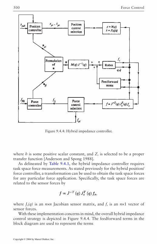
Force Control500
where h is some positive scalar constant, and Zr is selected to be a propertransfer function [Anderson and Spong 1988].
As delineated by Table 9.4.1, the hybrid impedance controller requirestask space force measurements. As stated previously for the hybrid position/force controller, a transformation can be used to obtain the task space forcesfor any particular force application. Specifically, the task space forces arerelated to the sensor forces by
where Js(q) is an n×n Jacobian sensor matrix, and fs is an n×1 vector ofsensor forces.
With these implementation concerns in mind, the overall hybrid impedancecontrol strategy is depicted in Figure 9.4.4. The feedforward terms in theblock diagram are used to represent the terms
Figure 9.4.4: Hybrid impedance controller.
Copyright © 2004 by Marcel Dekker, Inc.
501
9.5 Reduced State Position/Force Control
If a rigid manipulator is constrained by a rigid environment, the degreesof freedom are reduced because the manipulator end effector cannotmove through the environment; therefore, one or more degrees offreedom with regard to position are lost. Consequently, as themanipulator end effector contacts the environmental constraint,interaction forces between the end effector and the environment(sometimes referred to as constraint forces) develop. This process of“reducing” positional freedom while developing constraint forces leadsone to believe that position/force controllers should be designedaccording to this natural phenomenon.
Recently, researchers have begun to formulate a theoretical framework[McClamroch and Wang 1988], [Kankaanranta and Koivo 1988] thatincorporates the effects of the constraint forces into the robot manipulatormodel by utilizing classical results in dynamics. The reasoning forpostulating that controllers should be designed for a rigid manipulatorcontacting a rigid constraint is that in most force control applications, theenvironment is much more rigid than the manipulator. Therefore, it seemsunreasonable to assume that the manipulator is rigid while the environmentis compliant.
Effects of Holonomic Constraints on the Manipulator Dynamics
For the controller given in this section, we assume that the environmentalconstraints are holonomic and frictionless. That is, we assume the existenceof a constraint function (a p×1 vector function) in joint-space coordinatesthat satisfies
(9.5.1)
The relationship given by (9.5.1) illustrates that the environmental constraintsare holonomic. The dimension of the constraint function is assumed to beless than the number of joint variables (i.e., p<n). For a specific problem, thefunction is found from the robot kinematics and the environmentalconfiguration. To illustrate the holonomic concept, we now present anexample.
9.5 Reduced State Position/Force Control
Copyright © 2004 by Marcel Dekker, Inc.
Force Control502
EXAMPLE 9.5–1: Holonomic Constraints
We wish to formulate the constraint function (q) for the robot/environmental configurations given in Figs. 9.2–5 and 9.2–6. In both ofthese configurations, the joint space has a dimension of 2 and the constraintfunction has a dimension of 1 (i.e., the constraint is a one-dimensionalsurface). For the manipulator system given in Figure 9.2.5, the constraintfunction is given by
For the manipulator system given in Figure 9.2.6, the constraint functionis given by
For the general n-link robot manipulator with holonomic and frictionlessconstraints, the constrained robot dynamics can be written in the form
(9.5.2)
where is a p×1 vector that represents the generalized force multipliersassociated with the constraints, and the constraint Jacobian matrix A(q)is a p×n matrix defined by
(9.5.3)
As in [Kankaanranta and Koivo 1988], we will assume that the p columnsof AT(q) are linearly independent over the joint space. Also, note that theforce variable is independent of q and q.
To motivate the origin of (9.5.2), we reexamine Lagrange’s equation
(9.5.4)
where the modified Lagrangian for the constrained robot manipulator isgiven by
(9.5.5)
Note that the Lagrangian given in (9.5.5) is really the same Lagrangian asgiven in Chapter 2, since
Copyright © 2004 by Marcel Dekker, Inc.
503
as required by (9.5.1).From (9.5.4) and (9.5.5), we can see that the structure of the robot
manipulator dynamic equation is the same for the constrained manipulatoras for the unconstrained manipulator with the exception of any new termscontributed by the substitution of in Lagrange’s equation.Specifically, the constrained robot manipulator equation given in (9.5.2) isobtained by substituting (9.5.5) into (9.5.4) utilizing the identity
Before we develop the reduced-state position/force controller, we explainbriefly, from a heuristic point of view, how the position and force variableshave been reduced in dimension. First, note that for the constrained robotdynamics given in (9.5.2), the variable is used to represent the constraintforces that should be controlled. Note that the dimension of is p, which,by definition, is less than n. In previous formulations of the environmentalforces given in this chapter, the dimension of the forces was assumed to beequal to n. In this approach we are able to reduce the number of forcesthat must be controlled because we have initially assumed that the constraintsurface is frictionless. Of course, in reality, surface friction will exist inmost robot force control applications; however, it is often treated as adisturbance because such friction is a function of the applied normal contactforce.
Second, we examine the position constraints on robot motion given by(9.5.1). Because (q)=0 by assumption, we can differentiate (9.5.1)withrespect to time to obtain
(9.5.6)
where A(q) is defined in (9.5.3). The expression given by (9.5.6) gives aconcise form for the kinematic velocity constraints. From the position andvelocity constraints given in (9.5.1) and (9.5.6), we can state that themanipulator dynamics belong to the invariant manifold C, in R2n, defined by
That is, the motion of the robot manipulator remains on the manifold definedby C. As stated in [McClamroch and Wang 1988], the manifold C is singularon R2n; therefore, we can reduce the order of the motion dynamics.
9.5 Reduced State Position/Force Control
Copyright © 2004 by Marcel Dekker, Inc.
Force Control504
Reduced State Modeling and Control
A robot system consisting of a single n-joint nonredundant manipulatorconstrained by a rigid environment has n-p degrees of motion freedom. Note,however, that the joint variable model of a manipulator as given in (9.5.2)contains n position variables (q), which, in combination with the p forcevariables (), cause the total number of control variables (i.e., states) n+p toexceed the number of control inputs n. In this section we show how a variabletransformation can be used to reduce the states of the dynamical model andthereby reduce the number of control variables from n+p to n.
A reduced state model can be obtained by representing the manipulatordynamics given in (9.5.2) in terms of another set of independent coordinates,called the constraint space coordinates, which will be denoted by x. It isintended that x be an (n-p)×1 vector of joint space coordinates. That is, x isa subset of q.
The constrained robot model is reduced by assuming that there exists ann×1 vector function g(x) that relates the constraint space vector x [an (n-p)×1 vector] to the joint space vector q. This function is given by
(9.5.7)
where the function g(x) must be selected such that
(9.5.8)
and such that the n×(n-p) Jacobian matrix (x) defined as
(9.5.9)
contains n-p independent rows along the constraint space motion given by x.Even though the constraint space vector x is of smaller dimension than the
joint space vector q, one is usually able to find the functional mapping from xto q given in (9.5.7). For particular problems, the algebraic relations given bythe holonomic equation (9.5.1) and the robot kinematics are used to find g(x).Also note that the choice of g(x) is nonunique and that the conditions on g(x)given by (9.5.8) and on the rows of (x) are related to the reduced state model.Specifically, the condition that (x) contain n-p independent rows ensuresthat the decoupled model represents n-p independent equations. The conditionon g(x) given by (9.5.8) is used to ensure that the forces represented by canbe decoupled from the constraint space motion represented by x. It should benoted that since the constraints are assumed to be holonomic and the matrix
Copyright © 2004 by Marcel Dekker, Inc.
5059.5 Reduced State Position/Force Control
AT(q) is assumed to have p linearly independent columns, we can show thatboth of the conditions above always hold. The reader is referred to[McClamroch and Wang 1988] for details.
To obtain the reduced state dynamics in terms of the constraint spacecoordinates, we first differentiate (9.5.7) with respect to time to yield
(9.5.10)
where Σ(x) is defined in (9.5.9). Differentiating (9.5.10) with respect to timegives
(9.5.11)
After substituting q, q, and q, from (9.5.7), (9.5.10), and (9.5.11), respectively,into (9.5.2), we obtain the reduced-state model
(9.5.12)
where
The significance of the reduced state model given by (9.5.12) is illustrated bypremultiplying (9.5.12) by ΣT(x) to obtain
(9.5.13)
where
Note that the contact forces in (9.5.12) have been removed as a consequenceof (9.5.8), which ensures that The model given by (9.5.13)is useful because the dynamics that govern the motion of the manipulator onthe constraint surface have been reduced from n differential equations to n-p differential equations; furthermore, the motion has been decoupled fromthe contact forces. These two results are important in the design and stabilityanalysis of the subsequent position/force controllers.
Before the reduced state position/force controller is presented, we givesome definitions with regard to position/force tracking problems. First, theconstraint position tracking error is defined as
(9.5.14)
Copyright © 2004 by Marcel Dekker, Inc.
Force Control506
We assume that the desired constraint space trajectory and its first twoderivatives, denoted by xd, xd, and xd, respectively, are all bounded functions.We also assume that the desired force multiplier trajectory, d, is a knownbounded function, from which the corresponding force multiplier trackingerror variable is defined as
(9.5.15)
The reduced state position/force controller is a feedback linearizing controller;therefore, exact knowledge of the robot dynamics is required. The reducedstate controller [McClamroch and Wang 1988] is
(9.5.16)
where Kv and Kp are diagonal, positive-definite (n-p)×(n-p) matrices, and Kf
is a diagonal, positive-definite p×p matrix.To determine the type of stability for the position error and force tracking
error, we substitute (9.5.16) into (9.5.12) to yield
(9.5.17)
Premultiplying (9.5.17) by T(x) yields
(9.5.18)
as a consequence of (9.5.8). Because T(x) contains n-p independent columnsalong the constraint space motion and M(x) is a positive-definite symmetricmatrix, M* is a positive-definite symmetric matrix. Therefore, we canpremultiply (9.5.18) by M*-1 to obtain
(9.5.19)
Because Kv and Kp are diagonal positive-definite matrices, one can applystandard linear control arguments to (9.5.19) to yield
(9.5.20)
To obtain the stability result for the force tracking error, we substitute (9.5.20)into (9.5.17) to yield
(9.5.21)
Copyright © 2004 by Marcel Dekker, Inc.
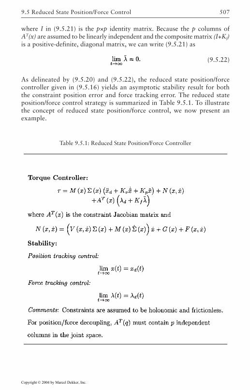
507
where I in (9.5.21) is the p×p identity matrix. Because the p columns ofAT(x) are assumed to be linearly independent and the composite matrix (I+Kf)is a positive-definite, diagonal matrix, we can write (9.5.21) as
(9.5.22)
As delineated by (9.5.20) and (9.5.22), the reduced state position/forcecontroller given in (9.5.16) yields an asymptotic stability result for boththe constraint position error and force tracking error. The reduced stateposition/force control strategy is summarized in Table 9.5.1. To illustratethe concept of reduced state position/force control, we now present anexample.
9.5 Reduced State Position/Force Control
Table 9.5.1: Reduced State Position/Force Controller
Copyright © 2004 by Marcel Dekker, Inc.
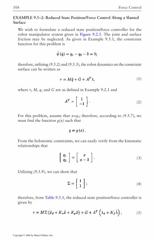
Force Control508
EXAMPLE 9.5–2: Reduced State Position/Force Control Along a SlantedSurface
We wish to formulate a reduced state position/force controller for therobot manipulator system given in Figure 9.2.5. The joint and surfacefriction may be neglected. As given in Example 9.5.1, the constraintfunction for this problem is
therefore, utilizing (9.5.2) and (9.5.3), the robot dynamics on the constraintsurface can be written as
(1)
where , M, q, and G are as defined in Example 9.2.1 and
(2)
For this problem, assume that x=q1; therefore, according to (9.5.7), wemust find the function g(x) such that
From the holonomic constraints, we can easily verify from the kinematicrelationships that
(3)
Utilizing (9.5.9), we can show that
(4)
therefore, from Table 9.5.1, the reduced state position/force controller isgiven by
(5)
Copyright © 2004 by Marcel Dekker, Inc.
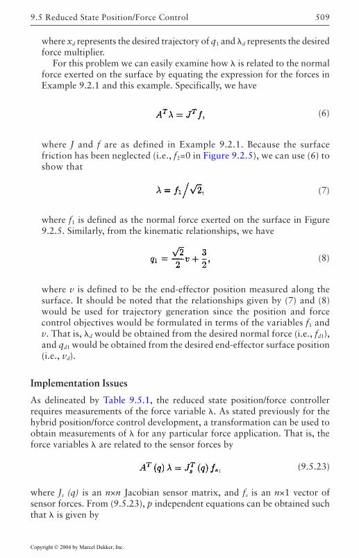
5099.5 Reduced State Position/Force Control
where xd represents the desired trajectory of q1 and d represents the desiredforce multiplier.
For this problem we can easily examine how is related to the normalforce exerted on the surface by equating the expression for the forces inExample 9.2.1 and this example. Specifically, we have
(6)
where J and f are as defined in Example 9.2.1. Because the surfacefriction has been neglected (i.e., f2=0 in Figure 9.2.5), we can use (6) toshow that
(7)
where f1 is defined as the normal force exerted on the surface in Figure9.2.5. Similarly, from the kinematic relationships, we have
(8)
where v is defined to be the end-effector position measured along thesurface. It should be noted that the relationships given by (7) and (8)would be used for trajectory generation since the position and forcecontrol objectives would be formulated in terms of the variables f1 andv. That is, d would be obtained from the desired normal force (i.e., fd1),and qd1 would be obtained from the desired end-effector surface position(i.e., vd).
Implementation Issues
As delineated by Table 9.5.1, the reduced state position/force controllerrequires measurements of the force variable . As stated previously for thehybrid position/force control development, a transformation can be used toobtain measurements of for any particular force application. That is, theforce variables are related to the sensor forces by
(9.5.23)
where Js (q) is an n×n Jacobian sensor matrix, and fs is an n×1 vector ofsensor forces. From (9.5.23), p independent equations can be obtained suchthat is given by
Copyright © 2004 by Marcel Dekker, Inc.
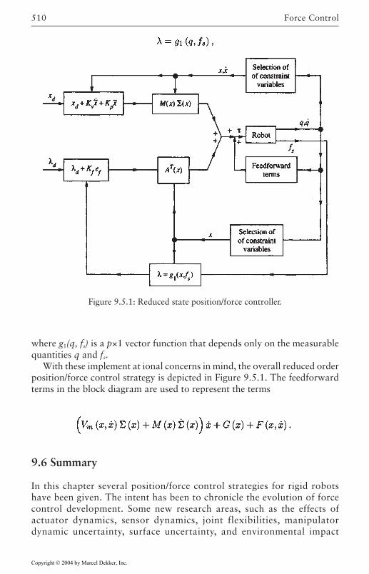
Force Control510
where g1(q, fs) is a p×1 vector function that depends only on the measurablequantities q and fs.
With these implement at ional concerns in mind, the overall reduced orderposition/force control strategy is depicted in Figure 9.5.1. The feedforwardterms in the block diagram are used to represent the terms
9.6 Summary
In this chapter several position/force control strategies for rigid robotshave been given. The intent has been to chronicle the evolution of forcecontrol development. Some new research areas, such as the effects ofactuator dynamics, sensor dynamics, joint flexibilities, manipulatordynamic uncertainty, surface uncertainty, and environmental impact
Figure 9.5.1: Reduced state position/force controller.
Copyright © 2004 by Marcel Dekker, Inc.
5119.6 Summary
instability on position/force controller performance are now being studiedby many researchers. After some of these problems have been solved, onecan expect to see robot manipulators used more frequently in force controlapplications.
Copyright © 2004 by Marcel Dekker, Inc.
513
REFERENCES
[Anderson and Spong 1988] Anderson, R., and M.Spong, “Hybrid impedance controlof robotic manipulators,” J. Robot. Autom., vol. 4, no. 5, pp. 549–556, Oct.1988.
[Chae et al. 1988] Chae, A., C.Atkeson, and J.Hollerbach, Model-Based Control of aRobot Manipulator. Cambridge, MA: MIT Press, 1988.
[Hogan 1987] Hogan, N., “Stable execution of contact tasks using impedance control,”Proc. IEEE Int. Conf Robot. Autom., pp. 595–601, Raleigh NC, Mar. 1987.
[Kankaanranta and Koivo 1988] Kankaanranta, R., and H.Koivo, “Dynamics andsimulation of compliant motion of a manipulator,” IEEE Trans. Robot. Autom.,vol. 4, pp. 163–173, Apr. 1988.
[Lipkin and Duffy 1988] Lipkin, H., and J.Duffy, “Hybrid twist and wrench controlfor a robot manipulator,” Trans. AS ME J. Median. Transmissions Autom. Design,vol. 110, pp. 138–144, June 1988.
[McClamroch and Wang 1988] McClamroch, N., and D.Wang, “Feedbackstabilization and tracking of constrained robots,” IEEE Trans. Autom. Control,vol. 33, no. 5, pp. 419–426, May 1988.
[Raibert and Craig 1981] Raibert, M., and J.Craig, “Hybrid position/force control ofmanipulators,” J. Dyn. Syst. Meas. Control, vol. 102, pp. 126–132, June 1981.
[Salisbury and Craig 1980] Salisbury, J., and J.Craig, “Active stiffness control ofmanipulator in Cartesian coordinates,” Proc. 19th IEEE Conf. Decision Control,Dec. 1980.
[Spong and Vidyasagar 1989] Spong, M., and M.Vidyasagar, Robot Dynamics andControl. New York: Wiley, 1989.
Copyright © 2004 by Marcel Dekker, Inc.
514 REFERENCES
PROBLEMS
Section 9.2
9.2–1 Find the associated task space Jacobian matrix for the normal andtangent forces exerted on the environmental surface for themanipulator given in Figure 9.2.6 with the new surface functiongiven by
9.2–2 Design and simulate a stiffness controller for the robot manipulatorsystem given in Figure 9.2.5 with the surface function given by
The control objective is to move the end effector to a desired finalposition of qd2=0.3 m while exerting a final desired normal force of2 N. Neglect the surface and joint friction and assume that the normalforce satisfies the relationship
where ke=100 N/m, and ue is the static normal distance to the surface.The robot link masses can be assumed to be unity while the initialend-effector position is assume to be given by
Section 9.3
9.3–1 Since the position and force error systems for the hybrid position/force control strategies are linear, discuss how the selection of thecontroller gains can be used to change the performance of themanipulator end effector.
9.3–2 Design and simulate a hybrid position/force controller for the robotmanipulator system given in Figure 9.2.5 with the surface functiongiven
Copyright © 2004 by Marcel Dekker, Inc.
515REFERENCES
The control objective is to move the end effector along the surfacewith trajectory
while exerting a desired normal force of
Neglect the surface and joint friction and assume that the normalforce satisfies the relationship
where ke=1000 N/m, and ue is the static normal distance to thesurface. The robot link masses can be assumed to be unity while theinitial end-effector position is assumed to be given by
9.3–3 Explain why the hybrid position/force control strategy is really apositional control strategy.
Section 9.4
9.4–1 Suppose that for force or position control, the manipulatorimpedance is selected to be
where h is positive scalar constant, and Zr(s) is a proper stable transferfunction. With the manipulator impedance above, show that thehybrid impedance controller will only require measurements of thejoint position, joint velocity, and contact force.
9.4–2 Design a hybrid impedance controller for the robot manipulatorsystem given in Figure 9.2.5 with the surface function given by
Copyright © 2004 by Marcel Dekker, Inc.
516 REFERENCES
Neglect the surface and joint friction and assume that the normalforce and tangent force satisfies the relationship
where ke=10 N/m, be=1 N-s/m, and ue is the static normal distanceto the surface.
9.4–3 Explicitly show how Table 9.4.1 can be used to find equation (6) inExample 9.4.1.
Section 9.5
9.5–1 Design a reduced state controller for the robot manipulator systemgiven in Figure 9.2.6.
9.5–2 For the controller developed in Problem 9.5–1, show how the normalforce (i.e., f1) is related to the force multiplier (i.e., ), and how thereduced motion variable (i.e., x) is related to the motion along thesurface (i.e., v).
Copyright © 2004 by Marcel Dekker, Inc.
517
Chapter 10
Robot ControlImplementation andSoftware
The diversity of robot manipulator research along with the complexrequirements of the associated hardware/software systems has alwayspresented a challenge for software developers. As a result, many of thepreviously developed software control platforms were complex, expensive,and not very user friendly. Even though several of the previous platformswere designed to provide an open architecture-based system, very few of theprevious platforms have been reused. To address previous disadvantages,this chapter describes the design and implementation of a software controlplatform called the Robotic Platform. The Robotic Platform is an opensoftware development platform for robot manipulator applications. Itincludes hardware interfacing, servo control, trajectory generation, 3Dsimulation, a graphical user interface, and a math library. As opposed todistributed solutions, the Robotic Platform implements all of thesecomponents on a single hardware platform, with a single programminglanguage (C++), and on a single operating system while guaranteeing hardreal-time performance. This design leads to an open architecture that is lesscomplex, easier to use, and easier to extend, and hence, builds on the followingstate-of-the-art technologies and general purpose components to furtherincrease simplicity and reliability: i) PC technology, ii) the QNX Real-TimeOperating System, iii) the Open Inventor and STL libraries, iv) object-orienteddesign, and v) an easy-to-use, previously-developed, low-level controlenvironment.
Copyright © 2004 by Marcel Dekker, Inc.
Robot Control Implementation and Software518
10.1 Introduction
Since the construction of a software control platform requires buildingblocks that cover a wide range of disciplines (see Figure 10.1.1), it would bedesirable to create a common generic platform that can be reused byresearchers for different applications. Considering the variety of roboticapplications and research areas, this task is made even more challenging dueto the fact that robot manipulator vendors often supply the user withproprietary robot control languages that run on proprietary hardwarecomponents. Due to the lack of flexibility and performance of proprietaryrobot control languages, some of the previous work has focused on buildingrobot control libraries on top of a commonly used programming language(RCCL [Lloyd et al. 1988] and ARCL [Corke] are examples of suchlibraries). While many of the previous software approaches achieved newlevels of flexibility and performance by using a common programminglanguage, many software control platforms developed in the 80’s and early90’s were inherently complex due to the limitations of the operating systemsand the hardware components of that time. That is, most operating systemsdid not support real-time programming, and hence, fostered thedevelopment of projects such as RCI [Lloyd 1990] and Chimera [Stewart1989]. In addition, procedural programming languages, such as “C”, tendto reach their limits with regard to reusability for complex projects. Inaddition, the limited performance of hardware components of that eraforced system developers to utilize distributed architectures (see [Miller1991], [Kapoor 1996], and [Pelich 1996]) that integrated a mix ofproprietary hardware and software. Besides the obvious advantages ofdistributed systems (e.g., greater extensibility and more computationalpower), there are several disadvantages. Specifically, a distributedarchitecture increases the complexity of the software significantly.Additionally, hard real-time behavior over network connections oftenrequires expensive proprietary hardware. Generally, the overall hardwarecost is also higher; furthermore, users have to familiarize themselves withdifferent hardware architectures and operating systems. Even though manysoftware control platforms have attempted to be flexible, reconfigurable,and open, these platforms are seldom reused (compared to non-roboticplatforms like Open Inventor or Corba). Apparently, engineers consider itfaster and easier to develop their applications from scratch. Indeed, as manyresearchers have noted, the learning curve of installing, learning, andmodifying previously developed software control platforms of the past isextremely steep.
Over the last ten years, many innovations in the computing area haveoccurred. Specifically, the advent of object-oriented software design[Stroustrup 1991] facilitated the management of more complex projects
Copyright © 2004 by Marcel Dekker, Inc.
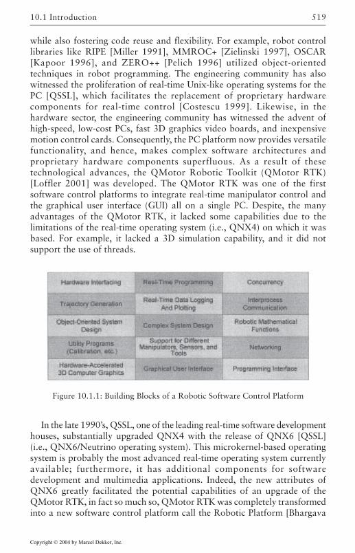
519
while also fostering code reuse and flexibility. For example, robot controllibraries like RIPE [Miller 1991], MMROC+ [Zielinski 1997], OSCAR[Kapoor 1996], and ZERO++ [Pelich 1996] utilized object-orientedtechniques in robot programming. The engineering community has alsowitnessed the proliferation of real-time Unix-like operating systems for thePC [QSSL], which facilitates the replacement of proprietary hardwarecomponents for real-time control [Costescu 1999]. Likewise, in thehardware sector, the engineering community has witnessed the advent ofhigh-speed, low-cost PCs, fast 3D graphics video boards, and inexpensivemotion control cards. Consequently, the PC platform now provides versatilefunctionality, and hence, makes complex software architectures andproprietary hardware components superfluous. As a result of thesetechnological advances, the QMotor Robotic Toolkit (QMotor RTK)[Loffler 2001] was developed. The QMotor RTK was one of the firstsoftware control platforms to integrate real-time manipulator control andthe graphical user interface (GUI) all on a single PC. Despite, the manyadvantages of the QMotor RTK, it lacked some capabilities due to thelimitations of the real-time operating system (i.e., QNX4) on which it wasbased. For example, it lacked a 3D simulation capability, and it did notsupport the use of threads.
In the late 1990’s, QSSL, one of the leading real-time software developmenthouses, substantially upgraded QNX4 with the release of QNX6 [QSSL](i.e., QNX6/Neutrino operating system). This microkernel-based operatingsystem is probably the most advanced real-time operating system currentlyavailable; furthermore, it has additional components for softwaredevelopment and multimedia applications. Indeed, the new attributes ofQNX6 greatly facilitated the potential capabilities of an upgrade of theQMotor RTK, in fact so much so, QMotor RTK was completely transformedinto a new software control platform call the Robotic Platform [Bhargava
Figure 10.1.1: Building Blocks of a Robotic Software Control Platform
10.1 Introduction
Copyright © 2004 by Marcel Dekker, Inc.
Robot Control Implementation and Software520
2001]. The rest of this chapter provides a broad overview of the RoboticPlatform by examining its advantages, its design, and its operation. The word“broad” needs to be emphasized because it is really impossible to give adetailed explanation of how a software control platform should be developedfor robot manipulators in one chapter of a book. With that being said, it ishope that this chapter will give the reader a better understanding of theassociated complexities.
10.2 Tools and Technologies
Given recent technological advances, it now seems almost obvious that newsoftware control platforms should integrate servo control loops, trajectorygeneration, task level programs, GUI programs, and 3D simulation in ahomogeneous software architecture. That is, next-generation softwarecontrol platforms should utilize one hardware platform (e.g., the PC), onlyone operating system (e.g., the QNX6 Real-Time Operating System[QSSL]), and only one programming language (e.g., C++ [Stroustrup1998]). The advantages of this next-generation software control platformare as follows:
Simplicity. A homogeneous non-distributed architecture is much smaller andsimpler than a distributed inhomogeneous architecture. It is easier toinstall, easier to understand, and easier to extend. Simplicity is criticalwith regard to motivating code reuse of the platform for differentapplications.
Performance. The homogeneous, non-distributed architecture also ensureshigh performance and hard real-time behavior, since overhead due tointerprocess communication is minimal.
Flexibility at all Levels. Every component of the platform is open forextensions and modifications. Many past platforms have utilized an openarchitecture at some levels, but other levels had been implemented onproprietary hardware such that they could not be modified.
Cost. The Robotic Platform requires fewer hardware components than adistributed platform. Basically, a single PC with one or more input/output(I/O) boards is sufficient. Additionally, PC hardware is very cost effectiveas compared to other hardware platforms.
To explain the advantages in more detail and delineate how the RoboticPlatform reduces software development and complexity, the general purposetools and technologies that are used to develop the Robotic Platform are
Copyright © 2004 by Marcel Dekker, Inc.
521
now examined. It seems logical to begin this discussion with the hardwareengine, namely the standard desktop PC. Due to its popularity in the consumermarket, the standard desktop PC has evolved dramatically over the past 20years. While in the past, only expensive UNIX workstations provided theprocessing power necessary to control robotic systems, the PC has caughtup or even exceeded the performance of workstations [Costescu 1999].Compared to UNIX workstations, a PC based system allows for a greatervariety of hardware and software components. Additionally, thesecomponents and the PC itself are usually cheaper than their UNIXcounterparts; furthermore, the PC is a well-known platform that iscomfortable for most software developers.
The second most important part of any software control platform is theoperating systems. Indeed since reliability is extremely important for robotmanipulation, the QNX6 Real-Time Operating Systems by QSSL [QSSL]was selected. The programming interface of QNX6 is compliant with thePOSIX standards and is the first platform that combines the followingfeatures:
Hard Real-Time. QNX6 provides hard real-time response (e.g., it can executea control loop at a certain frequency without falling behind). The real-time functionality is integrated in the microkernel.
Self-Hosted Development. The development and the execution of softwareare performed in the same environment and on the same PC.
Fast 3D Graphics. QNX6 provides support for hardware-accelerated 3D, asrequired for the graphical simulation of a robotic work cell.
Threads. QNX6 supports the concurrent execution of processes, known asthreads.
Device Driver Architecture. It is very easy to develop device drivers underQNX6, as is required for integrating different robotic hardware.
Cost. QNX6 is also very cost-effective as it is free for non-commercial useand runs on low-cost standard PCs.
The third most important part or design aspect of any software controlplatform is the programming philosophy. With regard to developing robotmanipulator control software, object-oriented programming has threemain benefits over procedural programming. First, it provides languageconstructs that allow for a much easier programming interface. Forexample, a matrix multiplication can be expressed by a simple “*”, similarto MATLAB programming. Second, object-oriented programming allows
10.2 Tools and Technologies
Copyright © 2004 by Marcel Dekker, Inc.
Robot Control Implementation and Software522
for a system architecture that is very flexible but yet very simple. That is,the components (classes) of a system can have a built-in default behaviorand default settings. The use of this default behavior and/or default settingsallows the programmer to reduce the code size. The programmer, however,can still override the default behavior for specific applications. Finally,object-oriented programming supports generic programming by facilitatingthe development of components that are independent from a specificimplementation (e.g., a generic class “Manipulator” will work withdifferent manipulator types). All of the above benefits are based on thegeneral concepts of object-oriented programming, such as abstraction,encapsulation, polymorphism, and inheritance [Stroustrup 1991]. As willbe shown later in this chapter, these object-oriented design concepts lead toan intuitive system architecture. As one might expect, the language ofchoice is C++, as it provides the whole spectrum of object-orientedconcepts while maintaining high performance [Stroustrup 1998] (e.g.,templates and inline functions can be used to create highly versatile andoptimized code in the Robotic Platform). The power of C++ and object-oriented programming can be further increased when using strong object-oriented libraries such as STL [Musser 1996]. STL provides standard datastructures (e.g., lists, vectors, etc.) and algorithms. These standard datastructures and algorithms simplify programming effort since these tools areoften required in common programming tasks. The data structures of theSTL are very universal since they can be used with different data types (i.e.,template programming).
The last design aspect of a software control platform has do with how theroboticist interacts with the system. Specifically, how does the roboticistanimate objects for simulation purposes and how does the roboticistimplement and tune control algorithms. For purposes of simulationanimation, Open Inventor [Wernecke] was utilized. Open Inventor,developed by Silicon Graphics, is an object-oriented C++ library for creating3D graphics and animation. Open Inventor minimizes development effort,as it is able to load 3D models that were created in the Virtual RealityModeling Language (VRML) format [Hartman 1996]. A variety of softwarepackages are available that facilitate the construction of 3D VRML models.These packages can be utilized to quickly create a graphical representationof robotic components. The Robotic Platform utilizes the built-infunctionality of Open Inventor to animate these components. OpenInventor also provides advanced features like object picking, which is veryuseful in the programming of operator interfaces. For purposes of controlimplementation, QMotor [Loffler 2002] was utilized because it allows usersto establish a real-time control loop, to log data, to tune control parameters,and to plot signals. QMotor control programs can be directly integrated inthe class design of the Robotic Platform since QMotor supports object-oriented programming.
Copyright © 2004 by Marcel Dekker, Inc.
523
10.3 Design of the Robotic Platform
Overview
Each component of the Robotic Platform (e.g., the teachpendant, thetrajectory generator, etc.) is modeled by a C++ class. A C++ class definitioncombines the data and the functions related to that component. For example,the class “Puma560” contains the data related to the Puma 560 robot (e.g.,the current joint position) as well as functions related to the Puma 560 robot(e.g., enabling of the arm power). Hence, the design of the Robotic Platformresults from grouping data and functions in a number of classes in ameaningful and intuitive way. A class can also use parts of the functionalityand the data of another class (called the base class) by deriving this classfrom the base class. The classes of the Robotic Platform include GUIcomponents and a 3D model for graphical simulation. These types ofcomponents are traditionally found in separate programs (e.g., see the RCCL
same class, one can achieve tight integration of the user interface, 3Dmodeling, and other functional parts.
To provide new capabilities for different applications, the user createsnew classes. Usually, new classes are derived from one of the alreadyexisting classes to minimize coding effort. This process is calledinheritance, and it greatly facilitates code reuse and eliminates redundancy.To illustrate how classes are derived from each other, class hierarchydiagrams are used. The main class hierarchy diagram of the RoboticPlatform is shown in Figure 10.3.1. Each arrow is drawn from the derivedclass to the parent class. The further to the right a class is listed, the morespecific it must become. The further to the left a class is listed, the moregeneric it must become. The classes of the Robotic Platform can beseparated into the following categories (note that some of the classesdiscussed below are not shown in Figure 10.3.1 since their class hierarchieswill be discussed later):
The Core Classes. The classes RoboticObject, FunctionalObject, andPhysicalObject build the core of the Robotic Platform by defining theoverall behavior of all robotic objects. These classes by themselves canbe the basis for any robotic system.
Generic Robotic Classes. Derived from the core classes are a number ofgeneric robotic classes. These classes (e.g., ServoControl, Manipulator,and Gripper) cannot be instantiated. Rather, these classes serve as baseclasses that implement common functionality while also presenting ageneric interface to the programmer (i.e., these classes can be used to
10.3 Design of the Robotic Platform
Copyright © 2004 by Marcel Dekker, Inc.
robot simulator [Lloyd et al. 1988]). However, by including them in the
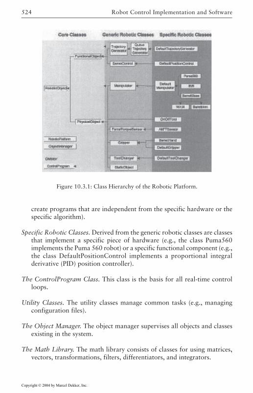
Robot Control Implementation and Software524
create programs that are independent from the specific hardware or thespecific algorithm).
Specific Robotic Classes. Derived from the generic robotic classes are classesthat implement a specific piece of hardware (e.g., the class Puma560implements the Puma 560 robot) or a specific functional component (e.g.,the class DefaultPositionControl implements a proportional integralderivative (PID) position controller).
The ControlProgram Class. This class is the basis for all real-time controlloops.
Utility Classes. The utility classes manage common tasks (e.g., managingconfiguration files).
The Object Manager. The object manager supervises all objects and classesexisting in the system.
The Math Library. The math library consists of classes for using matrices,vectors, transformations, filters, differentiators, and integrators.
Figure 10.3.1: Class Hierarchy of the Robotic Platform.
Copyright © 2004 by Marcel Dekker, Inc.
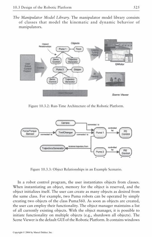
525
The Manipulator Model Library. The manipulator model library consistsof classes that model the kinematic and dynamic behavior ofmanipulators.
In a robot control program, the user instantiates objects from classes.When instantiating an object, memory for the object is reserved, and theobject initializes itself. The user can create as many objects as desired fromthe same class. For example, two Puma robots can be operated by simplycreating two objects of the class Puma560. As soon as objects are created,the user can employ their functionality. The object manager maintains a listof all currently existing objects. With the object manager, it is possible toinitiate functionality on multiple objects (e.g., shutdown all objects). TheScene Viewer is the default GUI of the Robotic Platform. It contains windows
Figure 10.3.2: Run-Time Architecture of the Robotic Platform.
Figure 10.3.3: Object Relationships in an Example Scenario.
10.3 Design of the Robotic Platform
Copyright © 2004 by Marcel Dekker, Inc.
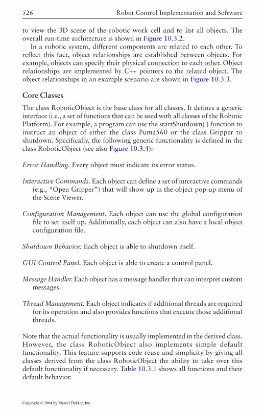
Robot Control Implementation and Software526
to view the 3D scene of the robotic work cell and to list all objects. Theoverall run-time architecture is shown in Figure 10.3.2.
In a robotic system, different components are related to each other. Toreflect this fact, object relationships are established between objects. Forexample, objects can specify their physical connection to each other. Objectrelationships are implemented by C++ pointers to the related object. Theobject relationships in an example scenario are shown in Figure 10.3.3.
Core Classes
The class RoboticObject is the base class for all classes. It defines a genericinterface (i.e., a set of functions that can be used with all classes of the RoboticPlatform). For example, a program can use the startShutdown( ) function toinstruct an object of either the class Puma560 or the class Gripper toshutdown. Specifically, the following generic functionality is defined in theclass RoboticObject (see also Figure 10.3.4):
Error Handling. Every object must indicate its error status.
Interactive Commands. Each object can define a set of interactive commands(e.g., “Open Gripper”) that will show up in the object pop-up menu ofthe Scene Viewer.
Configuration Management. Each object can use the global configurationfile to set itself up. Additionally, each object can also have a local objectconfiguration file.
Shutdown Behavior. Each object is able to shutdown itself.
GUI Control Panel. Each object is able to create a control panel.
Message Handler. Each object has a message handler that can interpret custommessages.
Thread Management. Each object indicates if additional threads are requiredfor its operation and also provides functions that execute those additionalthreads.
Note that the actual functionality is usually implemented in the derived class.However, the class RoboticObject also implements simple defaultfunctionality. This feature supports code reuse and simplicity by giving allclasses derived from the class RoboticObject the ability to take over this
default behavior.
Copyright © 2004 by Marcel Dekker, Inc.
default functionality if necessary. Table 10.3.1 shows all functions and their
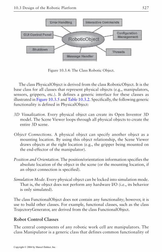
527
The class PhysicalObject is derived from the class RoboticObject. It is thebase class for all classes that represent physical objects (e.g., manipulators,sensors, grippers, etc.). It defines a generic interface for these classes asillustrated in Figure 10.3.5 and Table 10.3.2. Specifically, the following genericfunctionality is defined in PhysicalObject:
3D Visualization. Every physical object can create its Open Inventor 3Dmodel. The Scene Viewer loops through all physical objects to create theentire 3D scene.
Object Connections. A physical object can specify another object as amounting location. By using this object relationship, the Scene Viewerdraws objects at the right location (e.g., the gripper being mounted onthe end-effector of the manipulator).
Position and Orientation. The position/orientation information specifies theabsolute location of the object in the scene (or the mounting location, ifan object connection is specified).
Simulation Mode. Every physical object can be locked into simulation mode.That is, the object does not perform any hardware I/O (i.e., its behavioris only simulated).
The class FunctionalObject does not contain any functionality; however, it isuse to build other classes. For example, functional classes, such as the classTrajectoryGenerator, are derived from the class FunctionalObject.
Robot Control Classes
The central components of any robotic work cell are manipulators. Theclass Manipulator is a generic class that defines common functionality of
Figure 10.3.4: The Class Robotic Object.
10.3 Design of the Robotic Platform
Copyright © 2004 by Marcel Dekker, Inc.
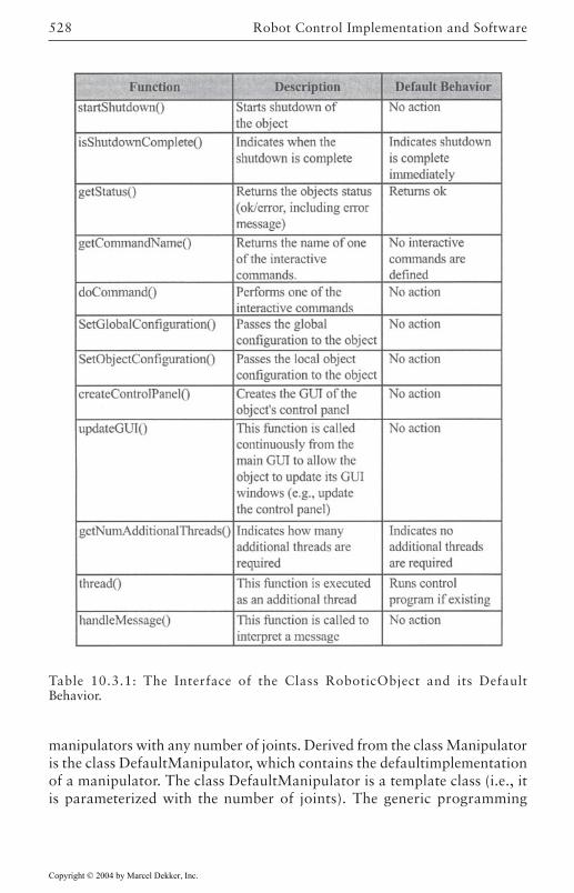
Robot Control Implementation and Software528
manipulators with any number of joints. Derived from the class Manipulatoris the class DefaultManipulator, which contains the defaultimplementationof a manipulator. The class DefaultManipulator is a template class (i.e., itis parameterized with the number of joints). The generic programming
Table 10.3.1: The Interface of the Class RoboticObject and its DefaultBehavior.
Copyright © 2004 by Marcel Dekker, Inc.
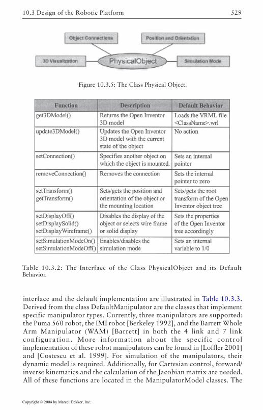
529
interface and the default implementation are illustrated in Table 10.3.3.Derived from the class DefaultManipulator are the classes that implementspecific manipulator types. Currently, three manipulators are supported:the Puma 560 robot, the IMI robot [Berkeley 1992], and the Barrett WholeArm Manipulator (WAM) [Barrett] in both the 4 link and 7 linkconfiguration. More information about the specific controlimplementation of these robot manipulators can be found in [Loffler 2001]and [Costescu et al. 1999]. For simulation of the manipulators, theirdynamic model is required. Additionally, for Cartesian control, forward/inverse kinematics and the calculation of the Jacobian matrix are needed.All of these functions are located in the ManipulatorModel classes. The
Table 10.3.2: The Interface of the Class PhysicalObject and its DefaultBehavior.
Figure 10.3.5: The Class Physical Object.
10.3 Design of the Robotic Platform
Copyright © 2004 by Marcel Dekker, Inc.
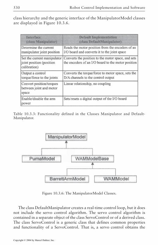
Robot Control Implementation and Software530
class hierarchy and the generic interface of the ManipulatorModel classesare displayed in Figure 10.3.6.
The class DefaultManipulator creates a real-time control loop, but it doesnot include the servo control algorithm. The servo control algorithm iscontained in a separate object of the class ServoControl or of a derived class.The class ServoControl is a generic class that defines common propertiesand functionality of a ServoControl. That is, a servo control obtains the
Table 10.3.3: Functionality defined in the Classes Manipulator and Default-Manipulator.
Figure 10.3.6: The ManipulatorModel Classes.
Copyright © 2004 by Marcel Dekker, Inc.
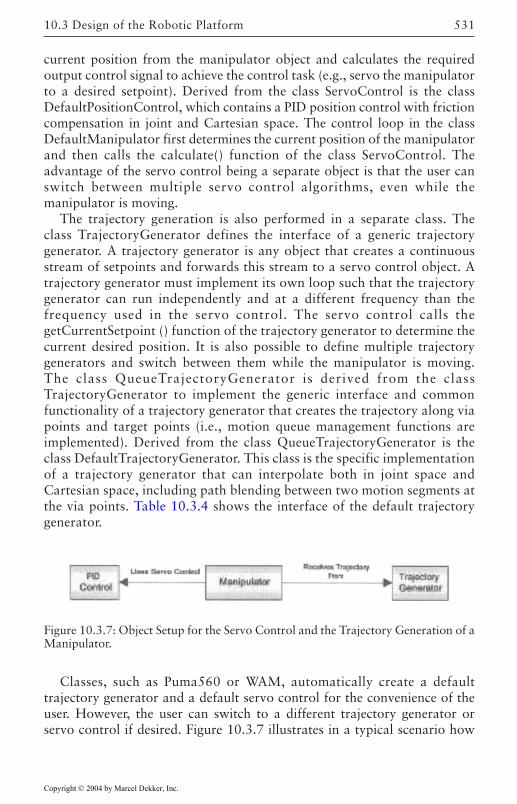
531
current position from the manipulator object and calculates the requiredoutput control signal to achieve the control task (e.g., servo the manipulatorto a desired setpoint). Derived from the class ServoControl is the classDefaultPositionControl, which contains a PID position control with frictioncompensation in joint and Cartesian space. The control loop in the classDefaultManipulator first determines the current position of the manipulatorand then calls the calculate() function of the class ServoControl. Theadvantage of the servo control being a separate object is that the user canswitch between multiple servo control algorithms, even while themanipulator is moving.
The trajectory generation is also performed in a separate class. Theclass TrajectoryGenerator defines the interface of a generic trajectorygenerator. A trajectory generator is any object that creates a continuousstream of setpoints and forwards this stream to a servo control object. Atrajectory generator must implement its own loop such that the trajectorygenerator can run independently and at a different frequency than thefrequency used in the servo control. The servo control calls thegetCurrentSetpoint () function of the trajectory generator to determine thecurrent desired position. It is also possible to define multiple trajectorygenerators and switch between them while the manipulator is moving.The class QueueTrajectoryGenerator is derived from the classTrajectoryGenerator to implement the generic interface and commonfunctionality of a trajectory generator that creates the trajectory along viapoints and target points (i.e., motion queue management functions areimplemented). Derived from the class QueueTrajectoryGenerator is theclass DefaultTrajectoryGenerator. This class is the specific implementationof a trajectory generator that can interpolate both in joint space andCartesian space, including path blending between two motion segments atthe via points. Table 10.3.4 shows the interface of the default trajectorygenerator.
Classes, such as Puma560 or WAM, automatically create a defaulttrajectory generator and a default servo control for the convenience of theuser. However, the user can switch to a different trajectory generator orservo control if desired. Figure 10.3.7 illustrates in a typical scenario how
Figure 10.3.7: Object Setup for the Servo Control and the Trajectory Generation of aManipulator.
10.3 Design of the Robotic Platform
Copyright © 2004 by Marcel Dekker, Inc.
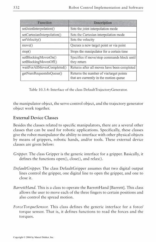
Robot Control Implementation and Software532
the manipulator object, the servo control object, and the trajectory generatorobject work together.
External Device Classes
Besides the classes related to specific manipulators, there are a several otherclasses that can be used for robotic applications. Specifically, these classesgive the robot manipulator the ability to interface with other physical objectsby means of grippers, robotic hands, and/or tools. These external deviceclasses are given below:
Gripper. The class Gripper is the generic interface for a gripper. Basically, itdefines the functions open(), close(), and relax().
DefaultGripper. The class DefaultGripper assumes that two digital outputlines control the gripper, one digital line to open the gripper, and one toclose it.
BarrettHand. This is a class to operate the BarrettHand [Barrett]. This classallows the user to move each of the three fingers to certain positions andalso control the spread motion.
ForceTorqueSensor. This class defines the generic interface for a force/torque sensor. That is, it defines functions to read the forces and thetorques.
Table 10.3.4: Interface of the class DefaultTrajectoryGenerator.
Copyright © 2004 by Marcel Dekker, Inc.
533
AtiFTSensor. This class is the specific implementation of the ATI IndustrialAutomation Gamma 30/100 Force/Torque sensor.
ToolChanger. The class ToolChanger is the generic interface of a tool changer.Basically, it defines the functions lock(), unlock(), and relax().
DefaultToolChanger. The class Def aultToolChanger assumes that one digitaloutput line controls the lock function of the toolchanger and anotherline the unlock function.
StaticObject. An object of the class StaticObject has no functionality otherthan specifying its 3D model. It can be used to add objects such as a tableor work pieces to the 3D scene.
Utility Classes
As with any complex software system, utility programs are needed forcommunication purposes and for providing the user with system relatedinformation. To this end, several separate, general-purpose utility classesare used throughout the Robotic Platform. These utility classes are givenbelow:
Status. The class Status provides functionality to stack status messages. Itreturns detailed status reports to the user. Each class has a data memberof class Status that indicates the status of the object.
Client. The class Client simplifies the sending of messages to a separate taskor thread.
Server. The class Server, the counterpart to the class Client, simplifies receivingof messages and replying to messages.
Config. The class Conf ig handles configuration files in ASCII format.
IOBoardClient. The class IOBoardClient allows communication with an I/O board (e.g., providing encoders readings, writing D/A values, readingA/D values, setting and reading digital inputs/outputs).
Lock. The class Lock provides mutual exclusion between two threads.
Configuration Management
The Robotic Platform utilizes a global configuration file, which is parsed bythe object manager and the objects to determine the system’s configuration.This file is called rp.cfg by default. The object manager searches for this file
10.3 Design of the Robotic Platform
Copyright © 2004 by Marcel Dekker, Inc.
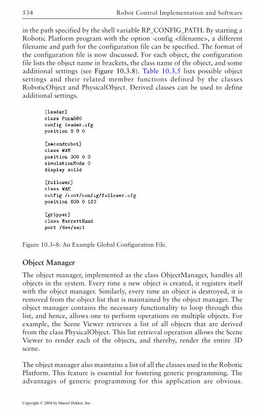
Robot Control Implementation and Software534
in the path specified by the shell variable RP_CONFIG_PATH. By starting aRobotic Platform program with the option -config <filename>, a differentfilename and path for the configuration file can be specified. The format ofthe configuration file is now discussed. For each object, the configurationfile lists the object name in brackets, the class name of the object, and someadditional settings (see Figure 10.3.8). Table 10.3.5 lists possible objectsettings and their related member functions defined by the classesRoboticObject and PhysicalObject. Derived classes can be used to defineadditional settings.
Object Manager
The object manager, implemented as the class ObjectManager, handles allobjects in the system. Every time a new object is created, it registers itselfwith the object manager. Similarly, every time an object is destroyed, it isremoved from the object list that is maintained by the object manager. Theobject manager contains the necessary functionality to loop through thislist, and hence, allows one to perform operations on multiple objects. Forexample, the Scene Viewer retrieves a list of all objects that are derivedfrom the class PhysicalObject. This list retrieval operation allows the SceneViewer to render each of the objects, and thereby, render the entire 3Dscene.
The object manager also maintains a list of all the classes used in the RoboticPlatform. This feature is essential for fostering generic programming. Theadvantages of generic programming for this application are obvious.
Figure 10.3–8: An Example Global Configuration File.
Copyright © 2004 by Marcel Dekker, Inc.
535
Specifically, generic code utilizes only components that provide a genericinterface; hence, generic code does not need to be changed when a componentwith a different implementation is used. That is, the same code can be usedfor a number of specific implementations, and hence, attributes to code reuse(e.g., a generic trajectory generator can be used with different manipulatortypes). Fortunately, C++ utilizes class inheritance and virtual functions tofacilitate generic programming. To illustrate this concept, consider a sectionof the class hierarchy as shown in Figure 10.3.9. The following snippet ofgeneric code demonstrates how to write a manipulator independent programthat works with either the Puma robot, the WAM, the IMI, or any robot thatmight be added in the future:
Manipulator *manipulator;ObjectManager om;
manipulator = om.createDerivedObject<Manipulator>(“leader”);// Creates either a Puma, an IMI or a WAM object, depending on// what is specified in the global configuration file underthe name “leader”
// Now, we can do generic operationsmanipulator->enableArmPower();Transform t = manipulator->getCurrentCartesianPosition();
To utilize generic programming in C++, the above code creates an objectof the derived class (e.g., an object of the class Puma or the class WAM),and operates the object via a pointer to the generic base class (i.e.,Manipulator *manipulator). The function createDerivedObject() of theobject manager is utilized to create an object of either the class Puma560,Barrett Arm, WAM or IMI. To create the correct object, thecreateDerivedObject() function looks for the object name in the globalconfiguration file (see Figure 10.3.8). Then, the createDerivedObject()function reads the class name of the object from the configuration file andcreates an object of this class. Hence, to switch to a different manipulatortype, only the class name in the global configuration file has to be changedwhen utilizing an existing generic program.
10.3 Design of the Robotic Platform
Copyright © 2004 by Marcel Dekker, Inc.
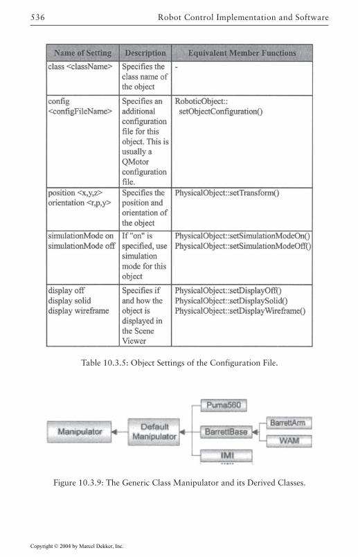
Robot Control Implementation and Software536
Table 10.3.5: Object Settings of the Configuration File.
Figure 10.3.9: The Generic Class Manipulator and its Derived Classes.
Copyright © 2004 by Marcel Dekker, Inc.
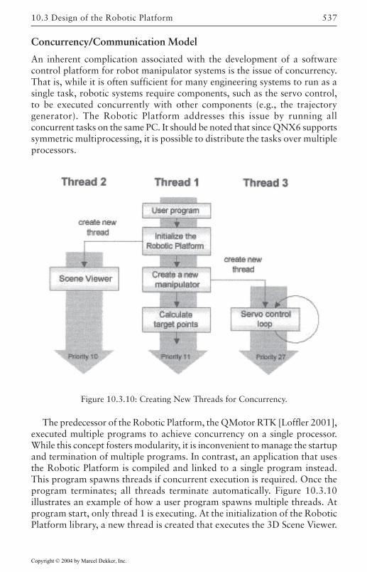
537
Concurrency/Communication Model
An inherent complication associated with the development of a softwarecontrol platform for robot manipulator systems is the issue of concurrency.That is, while it is often sufficient for many engineering systems to run as asingle task, robotic systems require components, such as the servo control,to be executed concurrently with other components (e.g., the trajectorygenerator). The Robotic Platform addresses this issue by running allconcurrent tasks on the same PC. It should be noted that since QNX6 supportssymmetric multiprocessing, it is possible to distribute the tasks over multipleprocessors.
The predecessor of the Robotic Platform, the QMotor RTK [Loffler 2001],executed multiple programs to achieve concurrency on a single processor.While this concept fosters modularity, it is inconvenient to manage the startupand termination of multiple programs. In contrast, an application that usesthe Robotic Platform is compiled and linked to a single program instead.This program spawns threads if concurrent execution is required. Once theprogram terminates; all threads terminate automatically. Figure 10.3.10illustrates an example of how a user program spawns multiple threads. Atprogram start, only thread 1 is executing. At the initialization of the RoboticPlatform library, a new thread is created that executes the 3D Scene Viewer.
Figure 10.3.10: Creating New Threads for Concurrency.
10.3 Design of the Robotic Platform
Copyright © 2004 by Marcel Dekker, Inc.
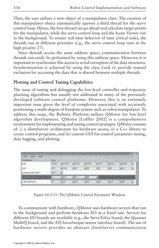
Robot Control Implementation and Software538
Then, the user utilizes a new object of a manipulator class. The creation ofthis manipulator object automatically spawns a third thread for the servocontrol loop. Hence, the first thread can go ahead and calculate target pointsfor the manipulator, while the servo control loop and the Scene Viewer runin the background. To ensure real-time behavior of time critical tasks, thethreads run at different priorities (e.g., the servo control loop runs at thehigh priority 27).
Since threads access the same address space, communication betweenthreads can easily be performed by using this address space. However, it isimportant to synchronize this access to avoid corruption of the data structures.Synchronization is achieved by using the class Lock to provide mutualexclusion for accessing the data that is shared between multiple threads.
Plotting and Control Tuning Capabilities
The issue of tuning and debugging the low-level controller and trajectoryplanning algorithms has usually not addressed in many of the previouslydeveloped software control platforms. However, this is an extremelyimportant issue given the level of complexity associated with accuratelypositioning a multi-degree of freedom system such as robot manipulator. Toaddress this issue, the Robotic Platform utilizes QMotor for low-levelalgorithm development. QMotor [Loffler 2002] is a comprehensiveenvironment for implementing and tuning control strategies. QMotor consistsof: i) a client/server architecture for hardware access, ii) a C++ library tocreate control programs, and iii) custom GUI for control parameter tuning,data logging, and plotting.
To communicate with hardware, QMotor uses hardware servers that runin the background and perform hardware I/O at a fixed rate. Servers fordifferent I/O boards are available (e.g., the ServoToGo board, the QuanserMultiQ board, and the ATI force/torque sensor interface board). The use ofhardware servers provides an abstract client/server communication
Figure 10.3.11: The QMotor Control Parameter Window.
Copyright © 2004 by Marcel Dekker, Inc.
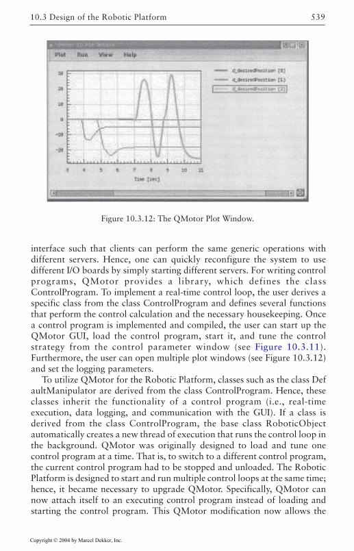
539
interface such that clients can perform the same generic operations withdifferent servers. Hence, one can quickly reconfigure the system to usedifferent I/O boards by simply starting different servers. For writing controlprograms, QMotor provides a library, which defines the classControlProgram. To implement a real-time control loop, the user derives aspecific class from the class ControlProgram and defines several functionsthat perform the control calculation and the necessary housekeeping. Oncea control program is implemented and compiled, the user can start up theQMotor GUI, load the control program, start it, and tune the controlstrategy from the control parameter window (see Figure 10.3.11).Furthermore, the user can open multiple plot windows (see Figure 10.3.12)and set the logging parameters.
To utilize QMotor for the Robotic Platform, classes such as the class DefaultManipulator are derived from the class ControlProgram. Hence, theseclasses inherit the functionality of a control program (i.e., real-timeexecution, data logging, and communication with the GUI). If a class isderived from the class ControlProgram, the base class RoboticObjectautomatically creates a new thread of execution that runs the control loop inthe background. QMotor was originally designed to load and tune onecontrol program at a time. That is, to switch to a different control program,the current control program had to be stopped and unloaded. The RoboticPlatform is designed to start and run multiple control loops at the same time;hence, it became necessary to upgrade QMotor. Specifically, QMotor cannow attach itself to an executing control program instead of loading andstarting the control program. This QMotor modification now allows the
Figure 10.3.12: The QMotor Plot Window.
10.3 Design of the Robotic Platform
Copyright © 2004 by Marcel Dekker, Inc.
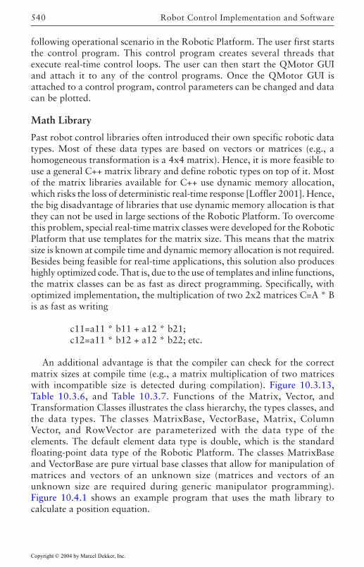
Robot Control Implementation and Software540
following operational scenario in the Robotic Platform. The user first startsthe control program. This control program creates several threads thatexecute real-time control loops. The user can then start the QMotor GUIand attach it to any of the control programs. Once the QMotor GUI isattached to a control program, control parameters can be changed and datacan be plotted.
Math Library
Past robot control libraries often introduced their own specific robotic datatypes. Most of these data types are based on vectors or matrices (e.g., ahomogeneous transformation is a 4x4 matrix). Hence, it is more feasible touse a general C++ matrix library and define robotic types on top of it. Mostof the matrix libraries available for C++ use dynamic memory allocation,which risks the loss of deterministic real-time response [Loffler 2001]. Hence,the big disadvantage of libraries that use dynamic memory allocation is thatthey can not be used in large sections of the Robotic Platform. To overcomethis problem, special real-time matrix classes were developed for the RoboticPlatform that use templates for the matrix size. This means that the matrixsize is known at compile time and dynamic memory allocation is not required.Besides being feasible for real-time applications, this solution also produceshighly optimized code. That is, due to the use of templates and inline functions,the matrix classes can be as fast as direct programming. Specifically, withoptimized implementation, the multiplication of two 2x2 matrices C=A * Bis as fast as writing
c11=a11 * b11 + a12 * b21;c12=a11 * b12 + a12 * b22; etc.
An additional advantage is that the compiler can check for the correctmatrix sizes at compile time (e.g., a matrix multiplication of two matriceswith incompatible size is detected during compilation). Figure 10.3.13,Table 10.3.6, and Table 10.3.7. Functions of the Matrix, Vector, andTransformation Classes illustrates the class hierarchy, the types classes, andthe data types. The classes MatrixBase, VectorBase, Matrix, ColumnVector, and RowVector are parameterized with the data type of theelements. The default element data type is double, which is the standardfloating-point data type of the Robotic Platform. The classes MatrixBaseand VectorBase are pure virtual base classes that allow for manipulation ofmatrices and vectors of an unknown size (matrices and vectors of anunknown size are required during generic manipulator programming).Figure 10.4.1 shows an example program that uses the math library tocalculate a position equation.
Copyright © 2004 by Marcel Dekker, Inc.
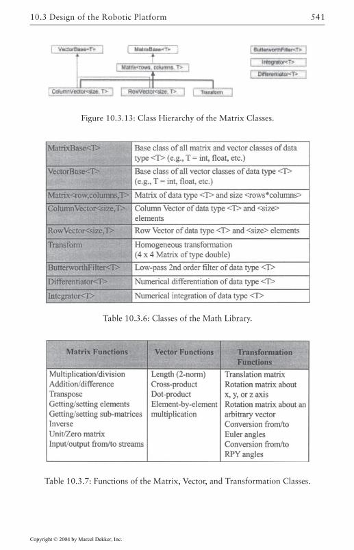
541
Figure 10.3.13: Class Hierarchy of the Matrix Classes.
Table 10.3.6: Classes of the Math Library.
Table 10.3.7: Functions of the Matrix, Vector, and Transformation Classes.
10.3 Design of the Robotic Platform
Copyright © 2004 by Marcel Dekker, Inc.
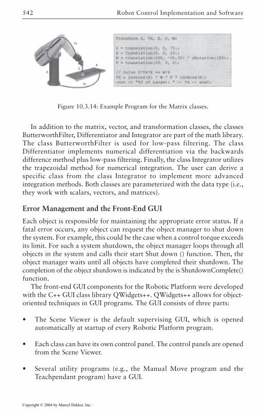
Robot Control Implementation and Software542
In addition to the matrix, vector, and transformation classes, the classesButterworthFilter, Differentiator and Integrator are part of the math library.The class ButterworthFilter is used for low-pass filtering. The classDifferentiator implements numerical differentiation via the backwardsdifference method plus low-pass filtering. Finally, the class Integrator utilizesthe trapezoidal method for numerical integration. The user can derive aspecific class from the class Integrator to implement more advancedintegration methods. Both classes are parameterized with the data type (i.e.,they work with scalars, vectors, and matrices).
Error Management and the Front-End GUI
Each object is responsible for maintaining the appropriate error status. If afatal error occurs, any object can request the object manager to shut downthe system. For example, this could be the case when a control torque exceedsits limit. For such a system shutdown, the object manager loops through allobjects in the system and calls their start Shut down () function. Then, theobject manager waits until all objects have completed their shutdown. Thecompletion of the object shutdown is indicated by the is ShutdownComplete()function.
The front-end GUI components for the Robotic Platform were developedwith the C++ GUI class library QWidgets++. QWidgets++ allows for object-oriented techniques in GUI programs. The GUI consists of three parts:
• The Scene Viewer is the default supervising GUI, which is openedautomatically at startup of every Robotic Platform program.
• Each class can have its own control panel. The control panels are openedfrom the Scene Viewer.
• Several utility programs (e.g., the Manual Move program and theTeachpendant program) have a GUI.
Figure 10.3.14: Example Program for the Matrix classes.
Copyright © 2004 by Marcel Dekker, Inc.
543
Operation of the front-end GUI for the Robotic Platform is further explainedin the next section.
10.4 Operation of the Robotic Platform
Scene Viewer and Control Panels
When a program running inside the Robotic Platform is executed, the SceneViewer window opens up. The Scene Viewer window displays the entire 3Dscene and also allows the user to open a window that displays a list ofcurrently running objects (see Figure 10.4.2). To create a 3D scene, the SceneViewer loops through all objects that are derived from the classPhysicalObject and calls the get3DModel() function to obtain the OpenInventor 3D data of that object. Then, the Scene Viewer uses the objectconnection relationships (specified by the function setConnection() of theclass PhysicalObject) to display the 3D objects at the right position (e.g., todisplay a gripper being mounted at the end-effector of a robot manipulator).Furthermore, the Scene Viewer continuously updates the 3D scene with thecurrent state of all objects (e.g., it uses the current joint position of a robotmanipulator to display the robot joints in the correct position). Hence, the3D scene rendered in the Scene Viewer window always represents thecurrent state of the actual hardware (in simulation mode, the simulated stateof the hardware is represented). To select the best viewing position, the usernavigates in the 3D scene using a mouse. The user can rotate the view, moveforward and backward, and also store/restore desired viewing positions.Additionally, the user can hide objects in the scene to increase the frame rate.Many different Scene Viewer windows can be opened to view the 3D scenefrom different viewing positions at the same time. The user can also open theObject Viewer window to display the list of all objects that are currentlybeing instantiated.
Each object also has an individual pop-up menu (See Figure 10.4.3. TheObject Pop-Up Menu). This pop-menu appears if the user either: i) rightclicks on the object in the Scene Viewer rendering area, or ii) right clickson an entry in the Object Viewer window. Options associated with pop-upmenu can be used to hide the object in the rendering area and to selectbetween a wire frame or a solid display. In addition, the pop-up menudisplays interactive commands that are defined in the specific class of theobject. For example, a gripper object has additional menu items to open,close, and relax the gripper. Finally, the user can open the control panelfrom the object pop-up menu. Figure 10.4.5 shows the control panel of theBarrett WAM as an example. Each control panel appears in a newwindow.
10.4 Operation of the Robotic Platform
Copyright © 2004 by Marcel Dekker, Inc.
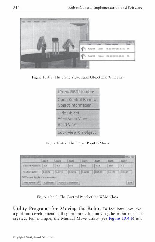
Robot Control Implementation and Software544
Utility Programs for Moving the Robot To facilitate low-levelalgorithm development, utility programs for moving the robot must becreated. For example, the Manual Move utility (see Figure 10.4.6) is a
Figure 10.4.1: The Scene Viewer and Object List Windows.
Figure 10.4.2: The Object Pop-Up Menu.
Figure 10.4.3: The Control Panel of the WAM Class.
Copyright © 2004 by Marcel Dekker, Inc.
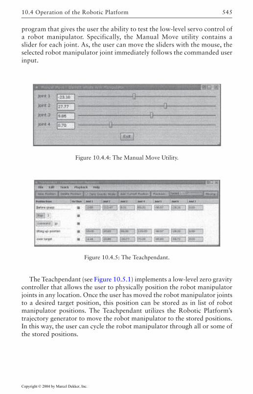
545
program that gives the user the ability to test the low-level servo control ofa robot manipulator. Specifically, the Manual Move utility contains aslider for each joint. As, the user can move the sliders with the mouse, theselected robot manipulator joint immediately follows the commanded userinput.
The Teachpendant (see Figure 10.5.1) implements a low-level zero gravitycontroller that allows the user to physically position the robot manipulatorjoints in any location. Once the user has moved the robot manipulator jointsto a desired target position, this position can be stored as in list of robotmanipulator positions. The Teachpendant utilizes the Robotic Platform’strajectory generator to move the robot manipulator to the stored positions.In this way, the user can cycle the robot manipulator through all or some ofthe stored positions.
Figure 10.4.4: The Manual Move Utility.
Figure 10.4.5: The Teachpendant.
10.4 Operation of the Robotic Platform
Copyright © 2004 by Marcel Dekker, Inc.
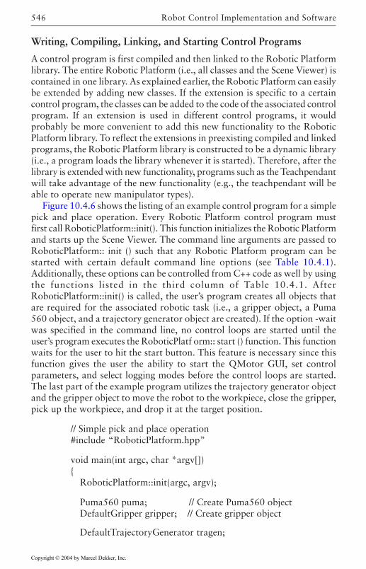
Robot Control Implementation and Software546
Writing, Compiling, Linking, and Starting Control Programs
A control program is first compiled and then linked to the Robotic Platformlibrary. The entire Robotic Platform (i.e., all classes and the Scene Viewer) iscontained in one library. As explained earlier, the Robotic Platform can easilybe extended by adding new classes. If the extension is specific to a certaincontrol program, the classes can be added to the code of the associated controlprogram. If an extension is used in different control programs, it wouldprobably be more convenient to add this new functionality to the RoboticPlatform library. To reflect the extensions in preexisting compiled and linkedprograms, the Robotic Platform library is constructed to be a dynamic library(i.e., a program loads the library whenever it is started). Therefore, after thelibrary is extended with new functionality, programs such as the Teachpendantwill take advantage of the new functionality (e.g., the teachpendant will beable to operate new manipulator types).
Figure 10.4.6 shows the listing of an example control program for a simplepick and place operation. Every Robotic Platform control program mustfirst call RoboticPlatform::init(). This function initializes the Robotic Platformand starts up the Scene Viewer. The command line arguments are passed toRoboticPlatform:: init () such that any Robotic Platform program can bestarted with certain default command line options (see Table 10.4.1).Additionally, these options can be controlled from C++ code as well by usingthe functions listed in the third column of Table 10.4.1. AfterRoboticPlatform::init() is called, the user’s program creates all objects thatare required for the associated robotic task (i.e., a gripper object, a Puma560 object, and a trajectory generator object are created). If the option -waitwas specified in the command line, no control loops are started until theuser’s program executes the RoboticPlatf orm:: start () function. This functionwaits for the user to hit the start button. This feature is necessary since thisfunction gives the user the ability to start the QMotor GUI, set controlparameters, and select logging modes before the control loops are started.The last part of the example program utilizes the trajectory generator objectand the gripper object to move the robot to the workpiece, close the gripper,pick up the workpiece, and drop it at the target position.
// Simple pick and place operation#include “RoboticPlatform.hpp”
void main(int argc, char *argv[])
RoboticPlatform::init(argc, argv);
Puma560 puma; // Create Puma560 objectDefaultGripper gripper; // Create gripper object
DefaultTrajectoryGenerator tragen;
Copyright © 2004 by Marcel Dekker, Inc.
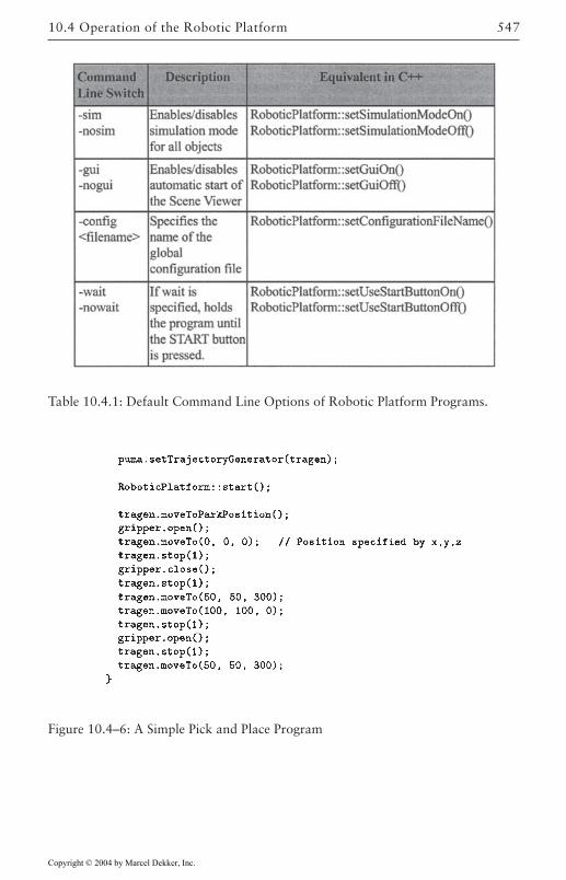
547
Table 10.4.1: Default Command Line Options of Robotic Platform Programs.
Figure 10.4–6: A Simple Pick and Place Program
10.4 Operation of the Robotic Platform
Copyright © 2004 by Marcel Dekker, Inc.
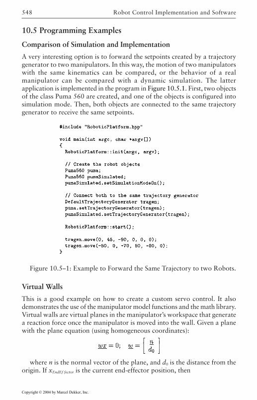
Robot Control Implementation and Software548
10.5 Programming Examples
Comparison of Simulation and Implementation
A very interesting option is to forward the setpoints created by a trajectorygenerator to two manipulators. In this way, the motion of two manipulatorswith the same kinematics can be compared, or the behavior of a realmanipulator can be compared with a dynamic simulation. The latterapplication is implemented in the program in Figure 10.5.1. First, two objectsof the class Puma 560 are created, and one of the objects is configured intosimulation mode. Then, both objects are connected to the same trajectorygenerator to receive the same setpoints.
Virtual Walls
This is a good example on how to create a custom servo control. It alsodemonstrates the use of the manipulator model functions and the math library.Virtual walls are virtual planes in the manipulator’s workspace that generatea reaction force once the manipulator is moved into the wall. Given a planewith the plane equation (using homogeneous coordinates):
where n is the normal vector of the plane, and d0 is the distance from theorigin. If xEndEf fector is the current end-effector position, then
Figure 10.5–1: Example to Forward the Same Trajectory to two Robots.
Copyright © 2004 by Marcel Dekker, Inc.
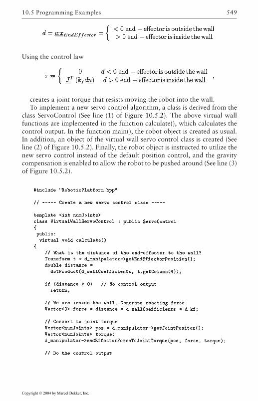
549
Using the control law
creates a joint torque that resists moving the robot into the wall.To implement a new servo control algorithm, a class is derived from the
class ServoControl (See line (1) of Figure 10.5.2). The above virtual wallfunctions are implemented in the function calculate(), which calculates thecontrol output. In the function main(), the robot object is created as usual.In addition, an object of the virtual wall servo control class is created (Seeline (2) of Figure 10.5.2). Finally, the robot object is instructed to utilize thenew servo control instead of the default position control, and the gravitycompensation is enabled to allow the robot to be pushed around (See line (3)of Figure 10.5.2).
10.5 Programming Examples
Copyright © 2004 by Marcel Dekker, Inc.
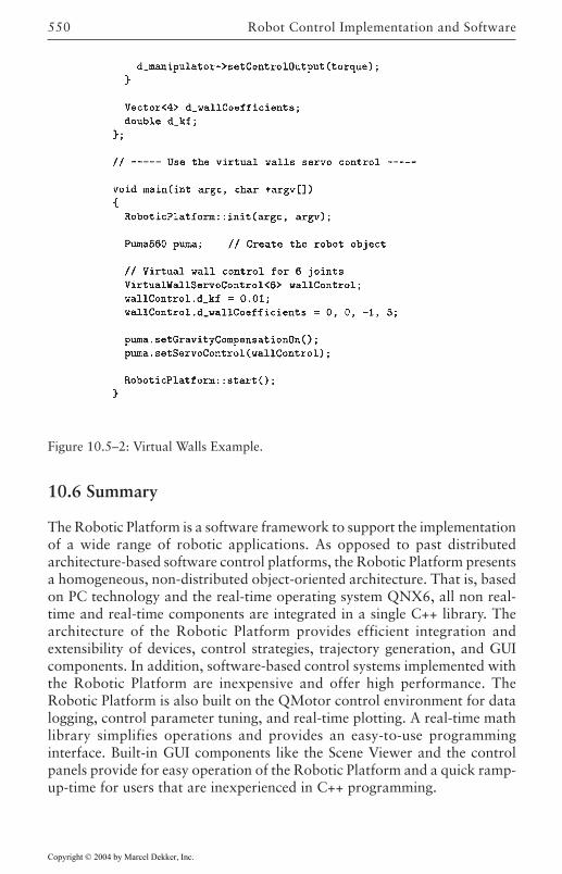
Robot Control Implementation and Software550
Figure 10.5–2: Virtual Walls Example.
10.6 Summary
The Robotic Platform is a software framework to support the implementationof a wide range of robotic applications. As opposed to past distributedarchitecture-based software control platforms, the Robotic Platform presentsa homogeneous, non-distributed object-oriented architecture. That is, basedon PC technology and the real-time operating system QNX6, all non real-time and real-time components are integrated in a single C++ library. Thearchitecture of the Robotic Platform provides efficient integration andextensibility of devices, control strategies, trajectory generation, and GUIcomponents. In addition, software-based control systems implemented withthe Robotic Platform are inexpensive and offer high performance. TheRobotic Platform is also built on the QMotor control environment for datalogging, control parameter tuning, and real-time plotting. A real-time mathlibrary simplifies operations and provides an easy-to-use programminginterface. Built-in GUI components like the Scene Viewer and the controlpanels provide for easy operation of the Robotic Platform and a quick ramp-up-time for users that are inexperienced in C++ programming.
Copyright © 2004 by Marcel Dekker, Inc.
551
REFERENCES
[Lloyd et al. 1988] J. Lloyd, M.Parker and R.McClain, “Extending the RCCLProgramming Environment to Multiple Robots and Processors”, Proc.IEEE International Conference on Robotics & Automation, 1988, pp. 465–469.
[Corke] P.Corke and R.Kirkham, “The ARCL Robot Programming System”,Proc. of the International Conference on Robots for Competitive Industries,Brisbane, Australia, pp. 484–493.
[Lloyd 1990] J.Lloyd, M.Parker and G.Holder, “Real Time Control UnderUNIX for RCCL”, Proceedings of the 3rd International Symposium onRobotics and Manufacturing (ISRAM ‘90).
[Stewart 1989] D.B.Stewart, D.E.Schmitz, and P.K.Khosla, “CHIMERA II: AReal-Time UNIX-Compatible Multiprocessor Operating System for Sensor-based Control Applications”, Technical Report CMU-RI-TR-89–24,Robotics Institute, Carnegie Mellon University, September, 1989.
[Stroustrup 1991] B.Stroustrup, “What is ‘Object-Oriented Programming’?”,Proc. 1st European Software Festival. February, 1991.
[Miller 1991] D.J.Miller and R.C.Lennox, “An Object-Oriented Environmentfor Robot System Architectures”, IEEE Control Systems Magazine, Feb.1991, pp. 14–23.
[Zielinski 1997] C.Zielinski, “Object-Oriented Robot Programming”,Robotica, Vol.15, 1997, pp. 41–48.
[Kapoor 1996] Chetan Kapoor, “A Reusable Operational Software Architecturefor Advanced Robotics”, Ph.D. thesis, University of Texas at Austin,December 1996.
Copyright © 2004 by Marcel Dekker, Inc.
552
[Pelich 1996] C.Pelich & F.M.Wahl, “A Programming Environment for aMultiprocessor-Net Based Robot Control Unit”, Proc. 10thInternational Conference on High Performance Computing, Ottawa,Canada, 1996.
[QSSL] QSSL, Corporate Headquarters, 175 Terence Matthews Crescent,Kanata, Ontario K2M 1W8 Canada, Tel: +1 800–676–0566 or +1 613–591–0931, Fax: +1 613–591–3579, Email:[email protected], http://qnx.com.
[Costescu 1999] N.Costescu, D.M.Dawson, and M.Loffler, “QMotor 2.0—APC Based Real-Time Multitasking Graphical Control Environment”, IEEEControl Systems Magazine, Vol. 19 Number 3, Jun., 1999, pp. 68–76.
[Loffler 2001] M.Loffler, D.Dawson, E.Zergeroglu, and N.Costescu, “Object-Oriented Techniques in Robot Manipulator Control SoftwareDevelopment”, Proc. of the American Control Conference, Arlington, VA,June 2001, pp. 4520–4525.
[Bhargava 2001] M.Loffler, A.Bhargava, V.Chitrakaran, and D.Dawson,“Design and Implementation of the Robotic Platform”, Proc. of the IEEEConference on Control Applications, Mexico City, Mexico, Sept., 2001, pp.357–362.
[Stroustrup 1998] B.Stroustrup, “An Overview of the C++ ProgrammingLanguage”, Handbook of Object Technology, CRC Press. 1998. ISBN 0–8493–3135–8.
[Musser 1996] D.R.Musser, A.Saini, “STL Tutorial and Reference Guide”,Addison-Wesley, 1996. ISBN 0–201–63398–1.
[Wernecke] Josie Wernecke, “The Inventor Mentor”, Addison-Wesley, ISBN 0–201–62495–8.
[Hartman 1996] Hartman, Jed and Josie Wernecke, “The VRML 2.0Handbook”, Addison-Wesley, Reading Massachusetts, 1996.
[Loffler 2002] M.Loffler, N.Costescu, and D.Dawson, “QMotor 3.0 and theQMotor Robotic Toolkit—An Advanced PC-Based Real-Time ControlPlatform”, IEEE Control Systems Magazine, Vol. 22, No. 3, pp. 12–26,June, 2002
[Berkeley 1992] “Direct Drive Manipulator Research and DevelopmentPackage, Operations Manual”, Integrated Motion Inc., Berkeley, CA,1992.
REFERENCES
Copyright © 2004 by Marcel Dekker, Inc.
553
[Barrett] Barrett Technologies, 139 Main St, Kendall Square, Cambridge, MA02142, http://www.barretttechnology.com/robot.
[Costescu et al. 1999] N.Costescu, M.Loffler, E.Zergeroglu, and D.M. Dawson,“QRobot—A Multitasking PC Based Robot Control System”,Microcomputer Applications Journal Special Issue on Robotics, Vol. 18,No. 1, pp.13–22, 1999.
REFERENCES
Copyright © 2004 by Marcel Dekker, Inc.
555
Appendix A
Review of RobotKinematics and Jacobians
We review here the basic information from a first course in robotics that isneeded for this book. This includes robot kinematics, the arm Jacobian, andthe issue of specifying the Cartesian position. The review is detailed sincethose with a background in system theory and controls may not yet have seenthis material. Several examples are given which are used throughout thebook for design and simulation purposes.
A.1 Basic Manipulator Geometries
In this section we look at some basic arm geometries. A robot arm ormanipulator is composed of a set of joints separated in space by the armlinks. The joints are where the motion in the arm occurs (cf. our own wristand elbow), while the links are of fixed construction (cf. our own forearm).Thus the links maintain a fixed relationship between the joints. [Although thelinks may be flexible (i.e., they may bend); we ignore flexibility effects here.]
The joints may be actuated by motors or hydraulic actuators. There aretwo sorts of robot joints, involving two sorts of motion. A revolute joint(denoted R) is one that allows rotary motion about an axis of rotation. Anexample is the human elbow. A prismatic joint (denoted P) is one that allowsextension or telescopic motion. An example is a telescoping automobileantenna. There is no anthropomorphous analogy to the prismatic link. Thejoint variables of a manipulator are the variable parameters of the joints. For
Copyright © 2004 by Marcel Dekker, Inc.
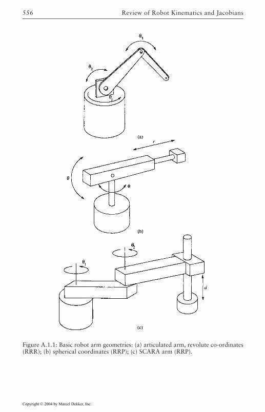
Review of Robot Kinematics and Jacobians556
Figure A.1.1: Basic robot arm geometries: (a) articulated arm, revolute co-ordinates(RRR); (b) spherical coordinates (RRP); (c) SCARA arm (RRP).
Copyright © 2004 by Marcel Dekker, Inc.
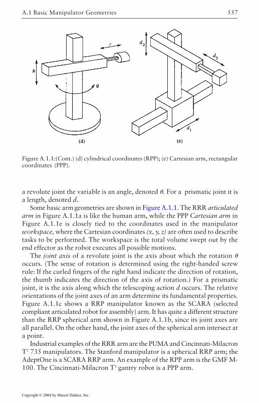
557
a revolute joint the variable is an angle, denoted . For a prismatic joint it isa length, denoted d.
Some basic arm geometries are shown in Figure A.1.1. The RRR articulatedarm in Figure A.1.1a is like the human arm, while the PPP Cartesian arm inFigure A.1.1e is closely tied to the coordinates used in the manipulatorworkspace, where the Cartesian coordinates (x, y, z) are often used to describetasks to be performed. The workspace is the total volume swept out by theend effector as the robot executes all possible motions.
The joint axis of a revolute joint is the axis about which the rotation occurs. (The sense of rotation is determined using the right-handed screwrule: If the curled fingers of the right hand indicate the direction of rotation,the thumb indicates the direction of the axis of rotation.) For a prismaticjoint, it is the axis along which the telescoping action d occurs. The relativeorientations of the joint axes of an arm determine its fundamental properties.Figure A.1.1c shows a RRP manipulator known as the SCARA (selectedcompliant articulated robot for assembly) arm. It has quite a different structurethan the RRP spherical arm shown in Figure A.1.1b, since its joint axes areall parallel. On the other hand, the joint axes of the spherical arm intersect ata point.
Industrial examples of the RRR arm are the PUMA and Cincinnati-MilacronT3 735 manipulators. The Stanford manipulator is a spherical RRP arm; theAdeptOne is a SCARA RRP arm. An example of the RPP arm is the GMF M-100. The Cincinnati-Milacron T3 gantry robot is a PPP arm.
Figure A.1.1:(Cont.) (d) cylindrical coordinates (RPP); (e) Cartesian arm, rectangularcoordinates (PPP).
A.1 Basic Manipulator Geometries
Copyright © 2004 by Marcel Dekker, Inc.
Review of Robot Kinematics and Jacobians558
Many industrial robots are serial link manipulators since they consist ofa series of links connected together by actuated joints. The base is calledlink 0, and the last link is terminated by the tool or end effector. Manyrobots have six joints, corresponding to the six degrees of freedom needed toobtain arbitrary position and orientation of the end effector in three-dimensional space.
Arms like the PUMA 560 have six revolute joints. In such an arm, thejoints may be grouped into two sets of three joints each. The first threejoints may be used to place the end effector at an arbitrary position withinthe three-dimensional workspace. The last three joints may be used toobtain an arbitrary orientation of the end effector at that position. In thePUMA 560, the axes of joints 4, 5, and 6 intersect at a common point andare mutually orthogonal. This makes orienting the end-effector convenient.The last three joints are known as the wrist mechanism (see ExampleA.2.4).
A.2 Robot Kinematics
Here we review the kinematics of robot manipulators, including the arm Amatrices, homogeneous transformations, the T matrix, forward and inversekinematics, and joint-space and Cartesian coordinates. Several illustrativeexamples are given.
A Matrices
For given values of the joint variables, it is important to be able to specify thelocations of the links with respect to each other. This is accomplished byusing the manipulator kinematic equations.
We may associate with each link i a coordinate frame (xi, yi, zi) fixed tothat link. See Figure A.2.1. A standard and consistent paradigm for so doingis the Denavit-Hartenberg (D-H) representation [Paul 1981], [Spong andVidyasagar 1989]. The frame attached to link 0 (i.e., the base of themanipulator) is called the base frame or inertial frame.
The relation between coordinate frame i-1 and coordinate frame i is givenby the transformation matrix
Copyright © 2004 by Marcel Dekker, Inc.
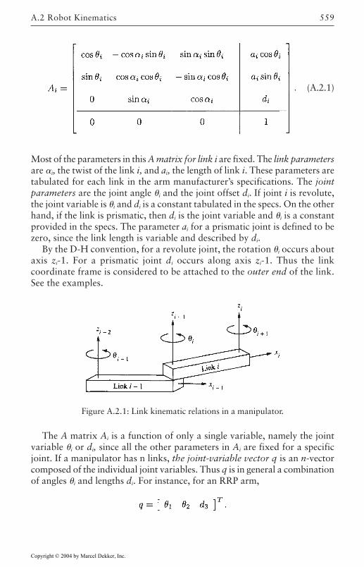
559
(A.2.1)
Most of the parameters in this A matrix for link i are fixed. The link parametersare i, the twist of the link i, and ai, the length of link i. These parameters aretabulated for each link in the arm manufacturer’s specifications. The jointparameters are the joint angle i and the joint offset di. If joint i is revolute,the joint variable is i and di is a constant tabulated in the specs. On the otherhand, if the link is prismatic, then di is the joint variable and i is a constantprovided in the specs. The parameter ai for a prismatic joint is defined to bezero, since the link length is variable and described by di.
By the D-H convention, for a revolute joint, the rotation i occurs aboutaxis zi-1. For a prismatic joint di occurs along axis zi-1. Thus the linkcoordinate frame is considered to be attached to the outer end of the link.See the examples.
The A matrix Ai is a function of only a single variable, namely the jointvariable i or di, since all the other parameters in Ai are fixed for a specificjoint. If a manipulator has n links, the joint-variable vector q is an n-vectorcomposed of the individual joint variables. Thus q is in general a combinationof angles i and lengths di. For instance, for an RRP arm,
Figure A.2.1: Link kinematic relations in a manipulator.
A.2 Robot Kinematics
Copyright © 2004 by Marcel Dekker, Inc.
Review of Robot Kinematics and Jacobians560
The components of q are denoted by qi; that is, the general joint variable qi
can represent either an angle i or a length di as appropriate.
Homogeneous TransformationsThe A matrix is a homogeneous transformation matrix of the form
(A.2.2)
where Ri is a rotation matrix and pi is a translation vector. Thus if ir is a pointdescribed with respect to the coordinate frame of link i, the same point hascoordinates i-1r with respect to the frame of link i-1 given by
(A.2.3)
The homogeneous transformation is a 4×4 matrix, so that it can describeboth rotations and translations; therefore, the vectors describing position in agiven coordinate frame are 4-vectors. They are of the form
, (A.2.4)
where (ix, iy, iz) are the coordinates of the point in frame i. Thus, according to(A.2.3) and (A.2.2),
(A.2.5)
which is just a rotation of Ri applied to the coordinates in frame i plus atranslation of pi.
We may interpret frame i-1 as the fixed (i.e., “original”) frame and framei as the rotated and translated (i.e., “new”) frame due to the followingconsiderations. According to (A.2.5), there is an easy way to find the rotationmatrix Ri that rotates a given coordinate frame i-1 into another given frame i.Set pi equal to zero and (ix, iy, iz)=(1,0,0). Then (A.2.5) is equal to the firstcolumn of Ri. That is, the first column of Ri is nothing but the representationof the new x-axis ix in terms of the original coordinates (i-1x, i-1y, i-1z). Similarly,the second (respectively third) column of Ri is the representation of the rotatedy-axis iy (respectively, z-axis and iz) in the fixed frame i-1. We shall illustratethis in Example A.2.1.
Therefore, Ai may be interpreted from several points of view. It is thetransformation that takes a representation ir of a vector in frame i to its
Copyright © 2004 by Marcel Dekker, Inc.
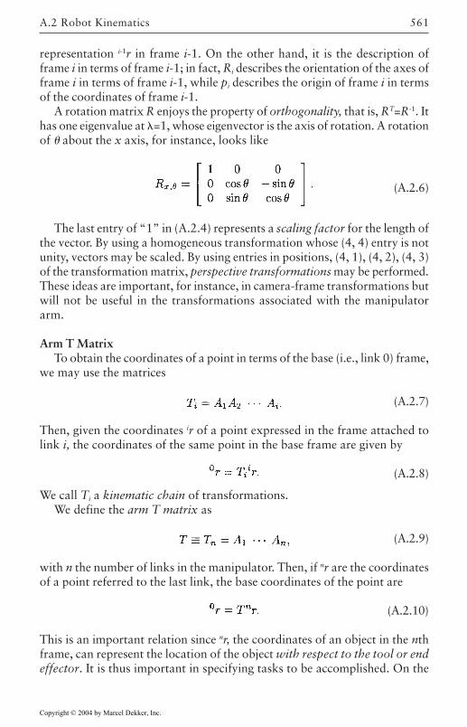
561
representation i-1r in frame i-1. On the other hand, it is the description offrame i in terms of frame i-1; in fact, Ri describes the orientation of the axes offrame i in terms of frame i-1, while pi describes the origin of frame i in termsof the coordinates of frame i-1.
A rotation matrix R enjoys the property of orthogonality, that is, RT=R-1. Ithas one eigenvalue at =1, whose eigenvector is the axis of rotation. A rotationof about the x axis, for instance, looks like
(A.2.6)
The last entry of “1” in (A.2.4) represents a scaling factor for the length ofthe vector. By using a homogeneous transformation whose (4, 4) entry is notunity, vectors may be scaled. By using entries in positions, (4, 1), (4, 2), (4, 3)of the transformation matrix, perspective transformations may be performed.These ideas are important, for instance, in camera-frame transformations butwill not be useful in the transformations associated with the manipulatorarm.
Arm T MatrixTo obtain the coordinates of a point in terms of the base (i.e., link 0) frame,
we may use the matrices
(A.2.7)
Then, given the coordinates ir of a point expressed in the frame attached tolink i, the coordinates of the same point in the base frame are given by
(A.2.8)
We call Ti a kinematic chain of transformations.We define the arm T matrix as
(A.2.9)
with n the number of links in the manipulator. Then, if nr are the coordinatesof a point referred to the last link, the base coordinates of the point are
(A.2.10)
This is an important relation since nr, the coordinates of an object in the nthframe, can represent the location of the object with respect to the tool or endeffector. It is thus important in specifying tasks to be accomplished. On the
A.2 Robot Kinematics
Copyright © 2004 by Marcel Dekker, Inc.
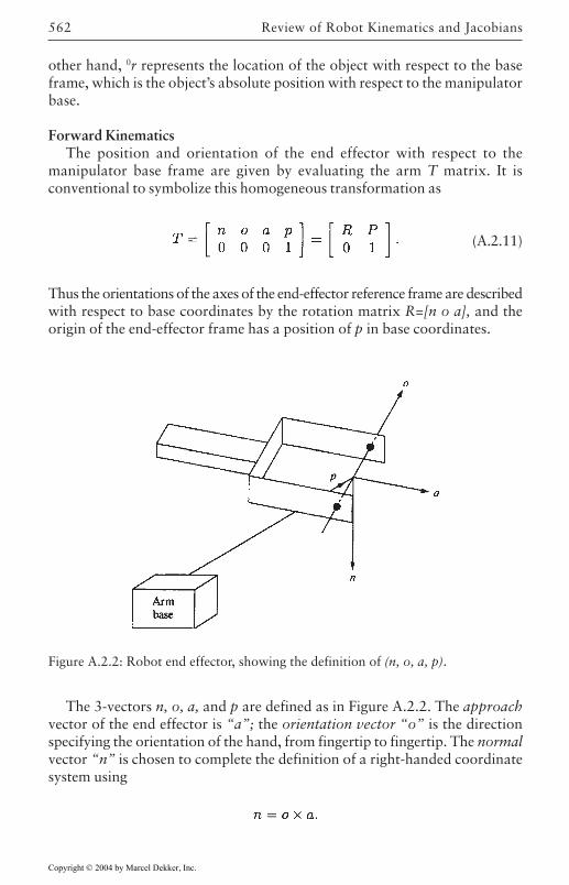
Review of Robot Kinematics and Jacobians562
other hand, 0r represents the location of the object with respect to the baseframe, which is the object’s absolute position with respect to the manipulatorbase.
Forward KinematicsThe position and orientation of the end effector with respect to the
manipulator base frame are given by evaluating the arm T matrix. It isconventional to symbolize this homogeneous transformation as
(A.2.11)
Thus the orientations of the axes of the end-effector reference frame are describedwith respect to base coordinates by the rotation matrix R=[n o a], and theorigin of the end-effector frame has a position of p in base coordinates.
Figure A.2.2: Robot end effector, showing the definition of (n, o, a, p).
The 3-vectors n, o, a, and p are defined as in Figure A.2.2. The approachvector of the end effector is “a”; the orientation vector “o” is the directionspecifying the orientation of the hand, from fingertip to fingertip. The normalvector “n” is chosen to complete the definition of a right-handed coordinatesystem using
Copyright © 2004 by Marcel Dekker, Inc.
563
Thus (n, o, a) are the base coordinates of an (x, y, z) Cartesian coordinatesystem attached to the end effector. The position vector p specifies the locationof the origin of the (n, o, a) frame with respect to the base frame.
The representation (n, o, a) for the orientation of the end effector is inefficient.Note that [n o a] is a 3×3 matrix, so that it has nine entries. However, it doesnot take nine degrees of freedom to specify orientation. Indeed, [n o a] is arotation matrix, so that its columns are orthogonal; this orthogonalityrequirement imposes extra constraints on the elements of [n o a], so that thenine entries of [n o a] are not independent. Alternative more efficient methodsof specifying the orientation of the end effector in base coordinates are theroll-pitch-yaw, Euler angle, quaternion, and tool-configuration vectordescriptions. We discuss some of these later. The reason we use (n, o, a) is thatthe arm T matrix is easily computed using the A matrices in terms of the armparameters and join variables. Then n, o, a, and p are simply read off byexamining the T matrix, as we shall see in the examples.
At this point we should like to distinguish between two sets of coordinatesdescribing the end effector. The joint variable coordinates of the end effectorare given by the n-vector.
where qi can represent angles or lengths, depending on whether the links arerevolute or prismatic. Generally, n=6, so that the arm has six degrees offreedom. The end-effector Cartesian coordinates are the description of endeffector orientation and position in terms of the arm base coordinates. Accordingto (A.2.11), where T may be computed knowing q, the joint variable andCartesian coordinates are equivalent, for both specify the location of the endeffector.
We say that q is the joint-space description of the position and orientationof the end effector, while (n, o, a, p) is the Cartesian or task space description.This terminology derives from the fact that descriptions of tasks to be performedby an arm are generally given in Cartesian coordinates, not in joint coordinates.
The robot arm kinematics problem is as follows. Given the joint variablesq, find the Cartesian position and orientation of the end of the manipulator.Thus the kinematics problem amounts to converting given joint variablesinto the Cartesian position and orientation of the end effector expressed inbase coordinates. Let us illustrate the solution of this problem for severalsimple robot arms which we use as examples throughout the book. It amountsto computing T.
It should be mentioned that there are several software packagescommercially available for computing the A matrices and the T matrix for agiven robot arm. See, for instance, [MATMAN 1986].
A.2 Robot Kinematics
Copyright © 2004 by Marcel Dekker, Inc.
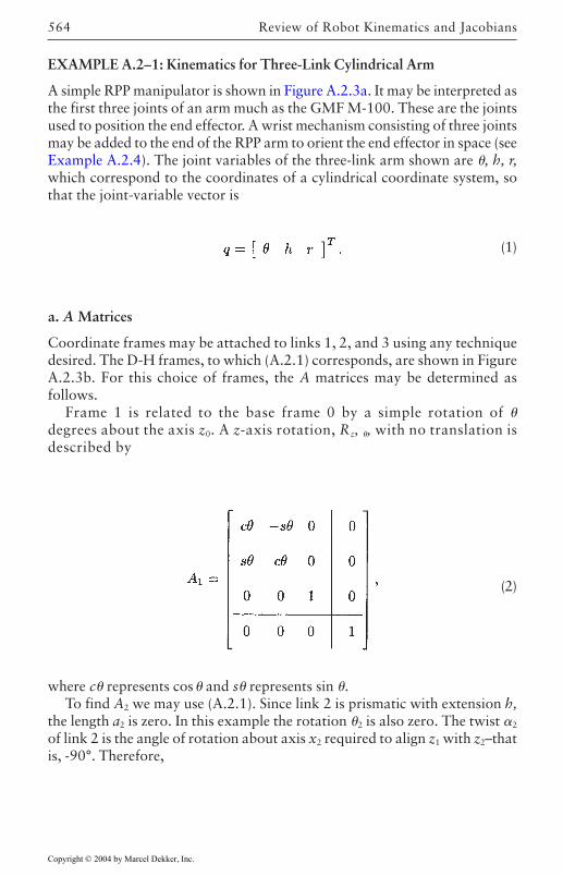
Review of Robot Kinematics and Jacobians564
EXAMPLE A.2–1: Kinematics for Three-Link Cylindrical Arm
A simple RPP manipulator is shown in Figure A.2.3a. It may be interpreted asthe first three joints of an arm much as the GMF M-100. These are the jointsused to position the end effector. A wrist mechanism consisting of three jointsmay be added to the end of the RPP arm to orient the end effector in space (seeExample A.2.4). The joint variables of the three-link arm shown are , h, r,which correspond to the coordinates of a cylindrical coordinate system, sothat the joint-variable vector is
(1)
a. A Matrices
Coordinate frames may be attached to links 1, 2, and 3 using any techniquedesired. The D-H frames, to which (A.2.1) corresponds, are shown in FigureA.2.3b. For this choice of frames, the A matrices may be determined asfollows.
Frame 1 is related to the base frame 0 by a simple rotation of degrees about the axis z0. A z-axis rotation, Rz, , with no translation isdescribed by
(2)
where c represents cos and s represents sin .To find A2 we may use (A.2.1). Since link 2 is prismatic with extension h,
the length a2 is zero. In this example the rotation 2 is also zero. The twist 2
of link 2 is the angle of rotation about axis x2 required to align z1 with z2–thatis, -90°. Therefore,
Copyright © 2004 by Marcel Dekker, Inc.
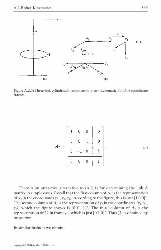
565
(3)
Figure A.2.3: Three-link cylindrical manipulator: (a) arm schematic; (b) D-H coordinateframes.
There is an attractive alternative to (A.2.1) for determining the link Amatrix in simple cases. Recall that the first column of A2 is the representationof x2 in the coordinates (x1, y1, z1). According to the figure, this is just [1 0 0]T.The second column of A2 is the representation of y2 in the coordinates (x1, y1,z1), which the figure shows is [0 0 -1]T. The third column of A2 is therepresentation of 22 in frame o1, which is just [0 1 0]T. Thus (3) is obtained byinspection.
In similar fashion we obtain,
A.2 Robot Kinematics
Copyright © 2004 by Marcel Dekker, Inc.
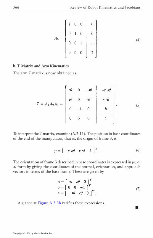
Review of Robot Kinematics and Jacobians566
(4)
b. T Matrix and Arm Kinematics
The arm T matrix is now obtained as
(5)
To interpret the T matrix, examine (A.2.11). The position in base coordinatesof the end of the manipulator, that is, the origin of frame 3, is
(6)
The orientation of frame 3 described in base coordinates is expressed in (n, o,a) form by giving the coordinates of the normal, orientation, and approachvectors in terms of the base frame. These are given by
(7)
A glance at Figure A.2.3b verifies these expressions.
Copyright © 2004 by Marcel Dekker, Inc.
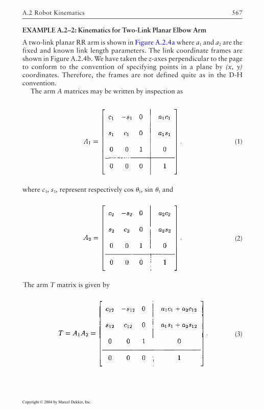
567
EXAMPLE A.2–2: Kinematics for Two-Link Planar Elbow Arm
A two-link planar RR arm is shown in Figure A.2.4a where a1 and a2 are thefixed and known link length parameters. The link coordinate frames areshown in Figure A.2.4b. We have taken the z-axes perpendicular to the pageto conform to the convention of specifying points in a plane by (x, y)coordinates. Therefore, the frames are not defined quite as in the D-Hconvention.
The arm A matrices may be written by inspection as
(1)
where c1, s1, represent respectively cos 1, sin 1 and
(2)
The arm T matrix is given by
(3)
A.2 Robot Kinematics
Copyright © 2004 by Marcel Dekker, Inc.
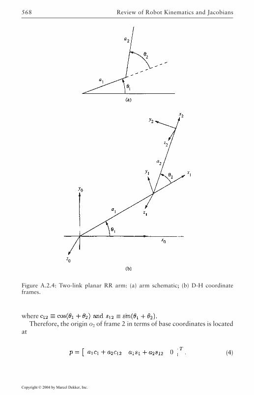
Review of Robot Kinematics and Jacobians568
where Therefore, the origin o2 of frame 2 in terms of base coordinates is located
at
(4)
Figure A.2.4: Two-link planar RR arm: (a) arm schematic; (b) D-H coordinateframes.
Copyright © 2004 by Marcel Dekker, Inc.
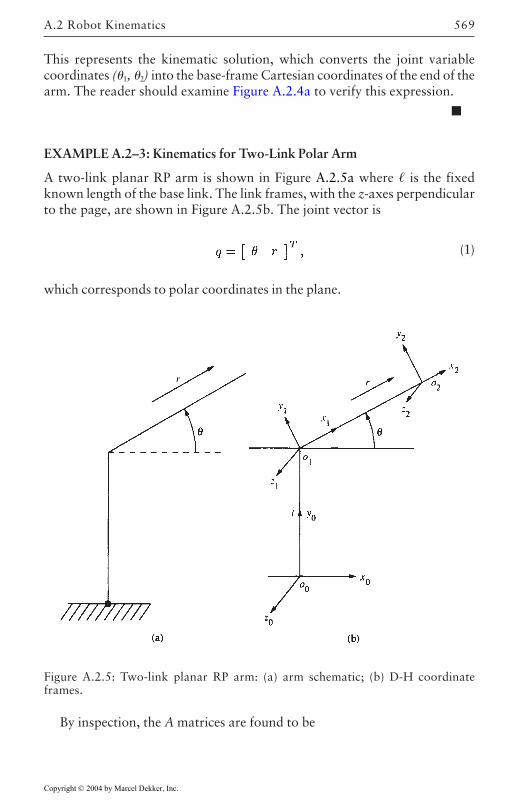
569
This represents the kinematic solution, which converts the joint variablecoordinates (1, 2) into the base-frame Cartesian coordinates of the end of thearm. The reader should examine Figure A.2.4a to verify this expression.
EXAMPLE A.2–3: Kinematics for Two-Link Polar Arm
A two-link planar RP arm is shown in Figure A.2.5a where is the fixedknown length of the base link. The link frames, with the z-axes perpendicularto the page, are shown in Figure A.2.5b. The joint vector is
(1)
which corresponds to polar coordinates in the plane.
By inspection, the A matrices are found to be
Figure A.2.5: Two-link planar RP arm: (a) arm schematic; (b) D-H coordinateframes.
A.2 Robot Kinematics
Copyright © 2004 by Marcel Dekker, Inc.
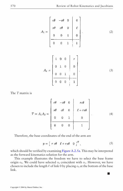
Review of Robot Kinematics and Jacobians570
(2)
(3)
The T matrix is
(4)
Therefore, the base coordinates of the end of the arm are
(5)
which should be verified by examining Figure A.2.5a. This may be interpretedas the forward kinematics solution for the arm.
This example illustrates the freedom we have to select the base frameorigin o0. We could have selected o0 coincident with o1. However, we havechosen to include the length of link 0 by placing o0 at the bottom of the baselink.
Copyright © 2004 by Marcel Dekker, Inc.
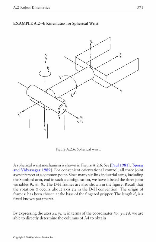
571
EXAMPLE A.2–4: Kinematics for Spherical Wrist
Figure A.2.6: Spherical wrist.
A spherical wrist mechanism is shown in Figure A.2.6. See [Paul 1981], [Spongand Vidyasagar 1989]. For convenient orientational control, all three jointaxes intersect at a common point. Since many six-link industrial arms, includingthe Stanford arm, end in such a configuration, we have labeled the three jointvariables 4, 5, 6. The D-H frames are also shown in the figure. Recall thatthe rotation i occurs about axis zi-1 in the D-H convention. The origin offrame 6 has been chosen at the base of the fingered gripper. The length d6 is afixed known parameter.
By expressing the axes x4, y4, z4 in terms of the coordinates (x3, y3, z3), we areable to directly determine the columns of A4 to obtain
A.2 Robot Kinematics
Copyright © 2004 by Marcel Dekker, Inc.
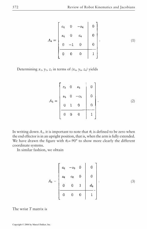
Review of Robot Kinematics and Jacobians572
(1)
Determining x5, y5, z5 in terms of (x4, y4, z4) yields
(2)
In writing down A5, it is important to note that 5 is defined to be zero whenthe end effector is in an upright position, that is, when the arm is fully extended.We have drawn the figure with 5=-90° to show more clearly the differentcoordinate systems.
In similar fashion, we obtain
(3)
The wrist T matrix is
Copyright © 2004 by Marcel Dekker, Inc.
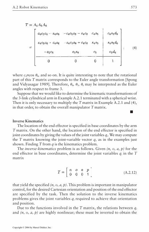
573
(4)
where c4≡cos 4, and so on. It is quite interesting to note that the rotationalpart of this T matrix corresponds to the Euler angle transformation [Spongand Vidyasagar 1989]. Therefore, 4, 5, 6 may be interpreted as the Eulerangles with respect to frame 3.
Suppose that we would like to determine the kinematic transformations ofthe 3-link cylindrical arm in Example A.2.1 terminated with a spherical wrist.Then it is only necessary to multiply the T matrix in Example A.2.1 and (4),in that order, to obtain the overall manipulator T matrix.
Inverse KinematicsThe location of the end effector is specified in base coordinates by the arm
T matrix. On the other hand, the location of the end effector is specified injoint coordinates by giving the values of the joint variables qi. We may computethe T matrix knowing the joint-variable vector q, as in the examples justshown. Finding T from q is the kinematics problem.
The inverse-kinematics problem is as follows. Given (n, o, a, p) for theend effector in base coordinates, determine the joint variables qi in the Tmatrix
(A.2.12)
that yield the specified (n, o, a, p). This problem is important in manipulatorcontrol, for the desired Cartesian orientation and position of the end effectorare specified by the task. Then the solution to the inverse kinematicsproblems gives the joint variables qi required to achieve that orientationand position.
Due to the functions involved in the T matrix, the relations between qi
and (n, o, a, p) are highly nonlinear; these must be inverted to obtain the
A.2 Robot Kinematics
Copyright © 2004 by Marcel Dekker, Inc.
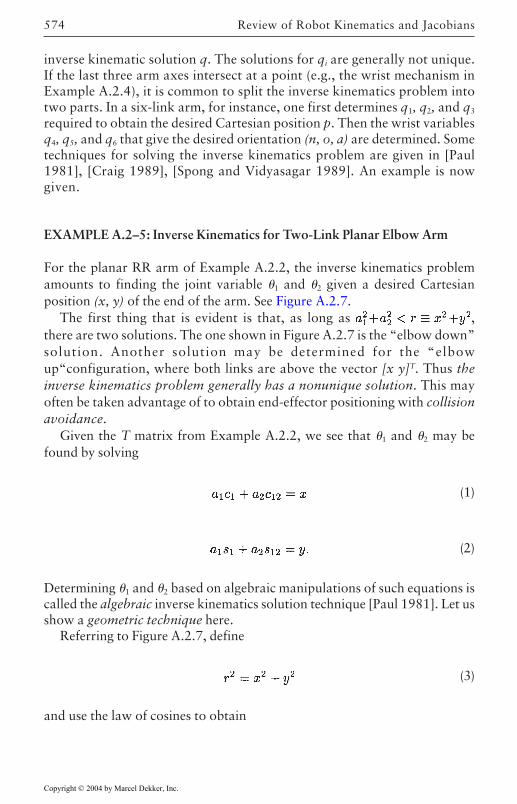
Review of Robot Kinematics and Jacobians574
inverse kinematic solution q. The solutions for qi are generally not unique.If the last three arm axes intersect at a point (e.g., the wrist mechanism inExample A.2.4), it is common to split the inverse kinematics problem intotwo parts. In a six-link arm, for instance, one first determines q1, q2, and q3
required to obtain the desired Cartesian position p. Then the wrist variablesq4, q5, and q6 that give the desired orientation (n, o, a) are determined. Sometechniques for solving the inverse kinematics problem are given in [Paul1981], [Craig 1989], [Spong and Vidyasagar 1989]. An example is nowgiven.
EXAMPLE A.2–5: Inverse Kinematics for Two-Link Planar Elbow Arm
For the planar RR arm of Example A.2.2, the inverse kinematics problemamounts to finding the joint variable 1 and 2 given a desired Cartesianposition (x, y) of the end of the arm. See Figure A.2.7.
The first thing that is evident is that, as long as ,there are two solutions. The one shown in Figure A.2.7 is the “elbow down”solution. Another solution may be determined for the “elbowup“configuration, where both links are above the vector [x y]T. Thus theinverse kinematics problem generally has a nonunique solution. This mayoften be taken advantage of to obtain end-effector positioning with collisionavoidance.
Given the T matrix from Example A.2.2, we see that 1 and 2 may befound by solving
(1)
(2)
Determining 1 and 2 based on algebraic manipulations of such equations iscalled the algebraic inverse kinematics solution technique [Paul 1981]. Let usshow a geometric technique here.
Referring to Figure A.2.7, define
(3)
and use the law of cosines to obtain
Copyright © 2004 by Marcel Dekker, Inc.
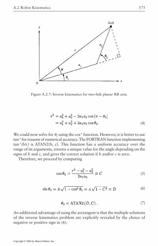
575
(4)
Figure A.2.7: Inverse kinematics for two-link planar RR arm.
We could now solve for 2 using the cos-1 function. However, it is better to usetan-1 for reasons of numerical accuracy. The FORTRAN function implementingtan-1(b/c) is ATAN2(b, c). This function has a uniform accuracy over therange of its arguments, returns a unique value for the angle depending on thesigns of b and c, and gives the correct solution if b and/or c is zero.
Therefore, we proceed by computing
(5)
(6)
(7)
An additional advantage of using the arctangent is that the multiple solutionsof the inverse kinematics problem are explicitly revealed by the choice ofnegative or positive sign in (6).
A.2 Robot Kinematics
Copyright © 2004 by Marcel Dekker, Inc.
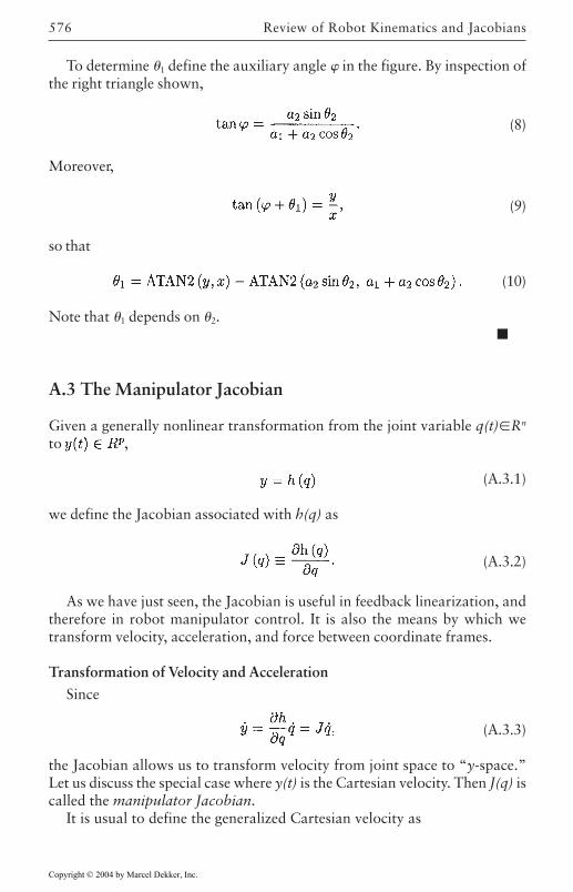
Review of Robot Kinematics and Jacobians576
To determine 1 define the auxiliary angle in the figure. By inspection ofthe right triangle shown,
(8)
Moreover,
(9)
so that
(10)
Note that 1 depends on 2.
A.3 The Manipulator Jacobian
Given a generally nonlinear transformation from the joint variable q(t)Rn
to ,
(A.3.1)
we define the Jacobian associated with h(q) as
(A.3.2)
As we have just seen, the Jacobian is useful in feedback linearization, andtherefore in robot manipulator control. It is also the means by which wetransform velocity, acceleration, and force between coordinate frames.
Transformation of Velocity and Acceleration
Since
(A.3.3)
the Jacobian allows us to transform velocity from joint space to “y-space.”Let us discuss the special case where y(t) is the Cartesian velocity. Then J(q) iscalled the manipulator Jacobian.
It is usual to define the generalized Cartesian velocity as
Copyright © 2004 by Marcel Dekker, Inc.
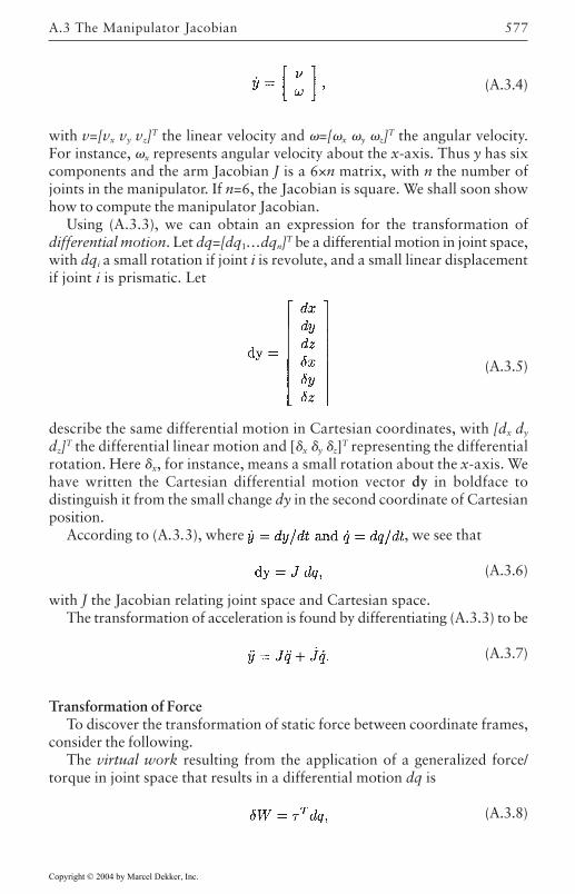
577
(A.3.4)
with v=[vx vy vz]T the linear velocity and =[x y z]T the angular velocity.For instance, x represents angular velocity about the x-axis. Thus y has sixcomponents and the arm Jacobian J is a 6×n matrix, with n the number ofjoints in the manipulator. If n=6, the Jacobian is square. We shall soon showhow to compute the manipulator Jacobian.
Using (A.3.3), we can obtain an expression for the transformation ofdifferential motion. Let dq=[dq1…dqn]T be a differential motion in joint space,with dqi a small rotation if joint i is revolute, and a small linear displacementif joint i is prismatic. Let
(A.3.5)
describe the same differential motion in Cartesian coordinates, with [dx dy
dz]T the differential linear motion and [x y z]T representing the differentialrotation. Here x, for instance, means a small rotation about the x-axis. Wehave written the Cartesian differential motion vector dy in boldface todistinguish it from the small change dy in the second coordinate of Cartesianposition.
According to (A.3.3), where , we see that
(A.3.6)
with J the Jacobian relating joint space and Cartesian space.The transformation of acceleration is found by differentiating (A.3.3) to be
(A.3.7)
Transformation of ForceTo discover the transformation of static force between coordinate frames,
consider the following.The virtual work resulting from the application of a generalized force/
torque in joint space that results in a differential motion dq is
(A.3.8)
A.3 The Manipulator Jacobian
Copyright © 2004 by Marcel Dekker, Inc.
Review of Robot Kinematics and Jacobians578
with the n-vector of arm control torques/forces, and dq=[dq1…dqn]T thedifferential change in the joint variable. If the description in another coordinateframe of the force is F and the description there of position is y, we must alsohave
(A.3.9)
Now taking (A.3.6) into account, we may write
so that the transformation from force to torque is given by
(A.3.10)
In the case that y(t) is Cartesian position, we define the Cartesian generalizedforce to be the 6-vector
(A.3.11)
with fc=[fx fy fz]T a Cartesian force 3-vector, and c=[x y z]T a 3-vectorrepresenting Cartesian torques. For instance, x represents torque exerted aboutthe x-axis.
If the arm has six links and the Jacobian is nonsingular, the transformationfrom generalized torque to generalized force is given by
(A.3.12)
The singularities in the Jacobian generally occur at the extremities of themanipulator workspace.
Specification of Cartesian Position
It is now necessary to confront an issue that is a source of confusion inrobotics. Consider Equation (A.3.2). Unfortunately, when discussing thetransformation h(q) from joint space to Cartesian space, this equation may onlybe interpreted as a convenience of notation, not as a rigorous mathematicalformula. The reason is that although the generalized Cartesian velocity (A.3.4)and acceleration, and the generalized Cartesian force (A.3.11) are bona fide 6-vectors, there is a problem with conveniently specifying the generalized Cartesianposition y(t). We now discuss several ways to specify the Cartesian position.
Representing Generalized Cartesian Position as (n, o, a, p). In our context,both the location of the origin of the end-effector frame as well as its orientation
Copyright © 2004 by Marcel Dekker, Inc.
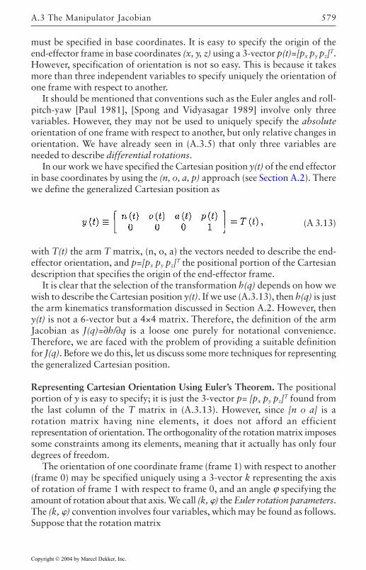
579
must be specified in base coordinates. It is easy to specify the origin of theend-effector frame in base coordinates (x, y, z) using a 3-vector p(t)=[px py pz]T.However, specification of orientation is not so easy. This is because it takesmore than three independent variables to specify uniquely the orientation ofone frame with respect to another.
It should be mentioned that conventions such as the Euler angles and roll-pitch-yaw [Paul 1981], [Spong and Vidyasagar 1989] involve only threevariables. However, they may not be used to uniquely specify the absoluteorientation of one frame with respect to another, but only relative changes inorientation. We have already seen in (A.3.5) that only three variables areneeded to describe differential rotations.
In our work we have specified the Cartesian position y(t) of the end effectorin base coordinates by using the (n, o, a, p) approach (see Section A.2). Therewe define the generalized Cartesian position as
(A 3.13)
with T(t) the arm T matrix, (n, o, a) the vectors needed to describe the end-effector orientation, and p=[px py pz]T the positional portion of the Cartesiandescription that specifies the origin of the end-effector frame.
It is clear that the selection of the transformation h(q) depends on how wewish to describe the Cartesian position y(t). If we use (A.3.13), then h(q) is justthe arm kinematics transformation discussed in Section A.2. However, theny(t) is not a 6-vector but a 4×4 matrix. Therefore, the definition of the armJacobian as J(q)=∂h/∂q is a loose one purely for notational convenience.Therefore, we are faced with the problem of providing a suitable definitionfor J(q). Before we do this, let us discuss some more techniques for representingthe generalized Cartesian position.
Representing Cartesian Orientation Using Euler’s Theorem. The positionalportion of y is easy to specify; it is just the 3-vector p= [px py pz]T found fromthe last column of the T matrix in (A.3.13). However, since [n o a] is arotation matrix having nine elements, it does not afford an efficientrepresentation of orientation. The orthogonality of the rotation matrix imposessome constraints among its elements, meaning that it actually has only fourdegrees of freedom.
The orientation of one coordinate frame (frame 1) with respect to another(frame 0) may be specified uniquely using a 3-vector k representing the axisof rotation of frame 1 with respect to frame 0, and an angle ϕ specifying theamount of rotation about that axis. We call (k, ) the Euler rotation parameters.The (k, ) convention involves four variables, which may be found as follows.Suppose that the rotation matrix
A.3 The Manipulator Jacobian
Copyright © 2004 by Marcel Dekker, Inc.
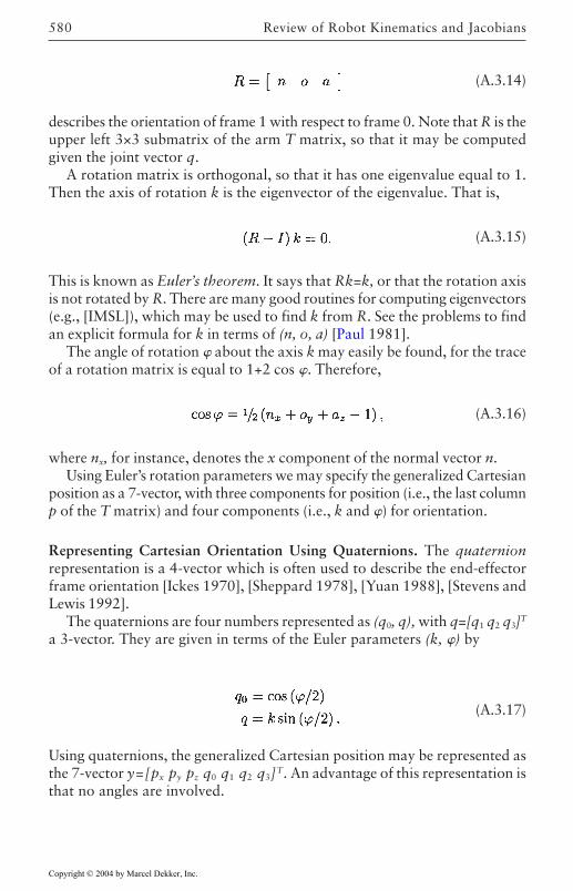
Review of Robot Kinematics and Jacobians580
(A.3.14)
describes the orientation of frame 1 with respect to frame 0. Note that R is theupper left 3×3 submatrix of the arm T matrix, so that it may be computedgiven the joint vector q.
A rotation matrix is orthogonal, so that it has one eigenvalue equal to 1.Then the axis of rotation k is the eigenvector of the eigenvalue. That is,
(A.3.15)
This is known as Euler’s theorem. It says that Rk=k, or that the rotation axisis not rotated by R. There are many good routines for computing eigenvectors(e.g., [IMSL]), which may be used to find k from R. See the problems to findan explicit formula for k in terms of (n, o, a) [Paul 1981].
The angle of rotation about the axis k may easily be found, for the traceof a rotation matrix is equal to 1+2 cos . Therefore,
(A.3.16)
where nx, for instance, denotes the x component of the normal vector n.Using Euler’s rotation parameters we may specify the generalized Cartesian
position as a 7-vector, with three components for position (i.e., the last columnp of the T matrix) and four components (i.e., k and ) for orientation.
Representing Cartesian Orientation Using Quaternions. The quaternionrepresentation is a 4-vector which is often used to describe the end-effectorframe orientation [Ickes 1970], [Sheppard 1978], [Yuan 1988], [Stevens andLewis 1992].
The quaternions are four numbers represented as (q0, q), with q=[q1 q2 q3]T
a 3-vector. They are given in terms of the Euler parameters (k, ) by
(A.3.17)
Using quaternions, the generalized Cartesian position may be represented asthe 7-vector y=[px py pz q0 q1 q2 q3]T. An advantage of this representation isthat no angles are involved.
Copyright © 2004 by Marcel Dekker, Inc.
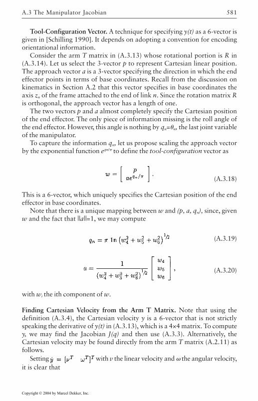
581
Tool-Configuration Vector. A technique for specifying y(t) as a 6-vector isgiven in [Schilling 1990]. It depends on adopting a convention for encodingorientational information.
Consider the arm T matrix in (A.3.13) whose rotational portion is R in(A.3.14). Let us select the 3-vector p to represent Cartesian linear position.The approach vector a is a 3-vector specifying the direction in which the endeffector points in terms of base coordinates. Recall from the discussion onkinematics in Section A.2 that this vector specifies in base coordinates theaxis zn of the frame attached to the end of link n. Since the rotation matrix Ris orthogonal, the approach vector has a length of one.
The two vectors p and a almost completely specify the Cartesian positionof the end effector. The only piece of information missing is the roll angle ofthe end effector. However, this angle is nothing by qn=n, the last joint variableof the manipulator.
To capture the information qn, let us propose scaling the approach vectorby the exponential function eqn/ to define the tool-configuration vector as
(A.3.18)
This is a 6-vector, which uniquely specifies the Cartesian position of the endeffector in base coordinates.
Note that there is a unique mapping between w and (p, a, qn), since, givenw and the fact that ||a||=1, we may compute
(A.3.19)
(A.3.20)
with wi the ith component of w.
Finding Cartesian Velocity from the Arm T Matrix. Note that using thedefinition (A.3.4), the Cartesian velocity y is a 6-vector that is not strictlyspeaking the derivative of y(t) in (A.3.13), which is a 4×4 matrix. To computey, we may find the Jacobian J(q) and then use (A.3.3). Alternatively, theCartesian velocity may be found directly from the arm T matrix (A.2.11) asfollows.
Setting with v the linear velocity and the angular velocity,it is clear that
A.3 The Manipulator Jacobian
Copyright © 2004 by Marcel Dekker, Inc.
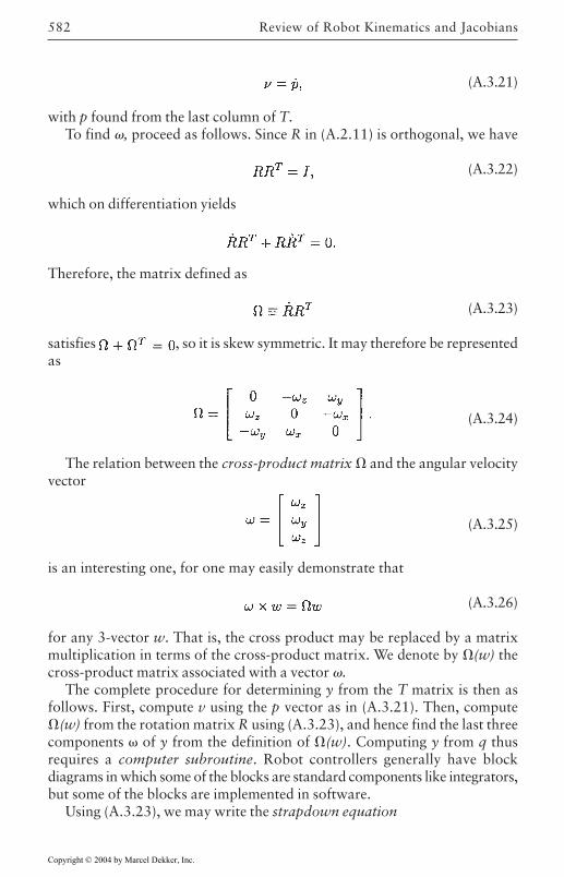
Review of Robot Kinematics and Jacobians582
(A.3.21)
with p found from the last column of T.To find , proceed as follows. Since R in (A.2.11) is orthogonal, we have
(A.3.22)
which on differentiation yields
Therefore, the matrix defined as
(A.3.23)
satisfies , so it is skew symmetric. It may therefore be representedas
(A.3.24)
The relation between the cross-product matrix and the angular velocityvector
(A.3.25)
is an interesting one, for one may easily demonstrate that
(A.3.26)
for any 3-vector w. That is, the cross product may be replaced by a matrixmultiplication in terms of the cross-product matrix. We denote by (w) thecross-product matrix associated with a vector .
The complete procedure for determining y from the T matrix is then asfollows. First, compute v using the p vector as in (A.3.21). Then, compute(w) from the rotation matrix R using (A.3.23), and hence find the last threecomponents of y from the definition of (w). Computing y from q thusrequires a computer subroutine. Robot controllers generally have blockdiagrams in which some of the blocks are standard components like integrators,but some of the blocks are implemented in software.
Using (A.3.23), we may write the strapdown equation
Copyright © 2004 by Marcel Dekker, Inc.
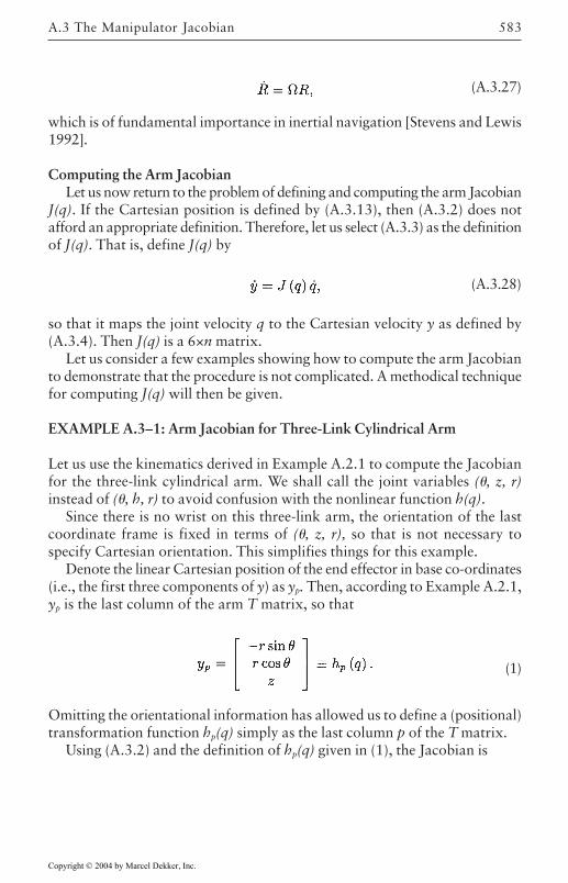
583
(A.3.27)
which is of fundamental importance in inertial navigation [Stevens and Lewis1992].
Computing the Arm JacobianLet us now return to the problem of defining and computing the arm Jacobian
J(q). If the Cartesian position is defined by (A.3.13), then (A.3.2) does notafford an appropriate definition. Therefore, let us select (A.3.3) as the definitionof J(q). That is, define J(q) by
(A.3.28)
so that it maps the joint velocity q to the Cartesian velocity y as defined by(A.3.4). Then J(q) is a 6×n matrix.
Let us consider a few examples showing how to compute the arm Jacobianto demonstrate that the procedure is not complicated. A methodical techniquefor computing J(q) will then be given.
EXAMPLE A.3–1: Arm Jacobian for Three-Link Cylindrical Arm
Let us use the kinematics derived in Example A.2.1 to compute the Jacobianfor the three-link cylindrical arm. We shall call the joint variables (, z, r)instead of (, h, r) to avoid confusion with the nonlinear function h(q).
Since there is no wrist on this three-link arm, the orientation of the lastcoordinate frame is fixed in terms of (, z, r), so that is not necessary tospecify Cartesian orientation. This simplifies things for this example.
Denote the linear Cartesian position of the end effector in base co-ordinates(i.e., the first three components of y) as yp. Then, according to Example A.2.1,yp is the last column of the arm T matrix, so that
(1)
Omitting the orientational information has allowed us to define a (positional)transformation function hp(q) simply as the last column p of the T matrix.
Using (A.3.2) and the definition of hp(q) given in (1), the Jacobian is
A.3 The Manipulator Jacobian
Copyright © 2004 by Marcel Dekker, Inc.
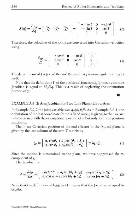
Review of Robot Kinematics and Jacobians584
(2)
Therefore, the velocities of the joints are converted into Cartesian velocitiesusing
(3)
The determinant of J is (r cos2 +r sin2 )=r, so that J is nonsingular as long asr0.
Note that the definition (1) of the positional function hp(q) means that theJacobian is equal to ∂hp/∂q. This is a result of neglecting the orientationportion of y.
EXAMPLE A.3–2: Arm Jacobian for Two-Link Planar Elbow Arm
In Example A.2.2 the joint variable was q=[1 2]T. As in Example A.3.1, theorientation of the last coordinate frame is fixed once q is given, so that we arenot concerned with the orientational portion of y, but only its linear positionportion yp.
The linear Cartesian position of the end effector in the (x1, x2)-plane isgiven by the last column of the arm T matrix as
(1)
Since the motion is constrained to the plane, we have suppressed the x3
component of yp.The Jacobian is
(2)
Note that the definition of hp(q) in (1) means that the Jacobian is equal to∂hp/∂q.
Copyright © 2004 by Marcel Dekker, Inc.
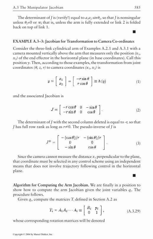
585
The determinant of J is (verify!) equal to a1a2 sin2, so that J is nonsingularunless 2=0 or ; that is, unless the arm is fully extended or link 2 is foldedback on top of link 1.
EXAMPLE A.3–3: Jacobian for Transformation to Camera Co-ordinates
Consider the three-link cylindrical arm of Examples A.2.1 and A.3.1 with acamera mounted vertically above the arm that measures only the position (x1,x2) of the end effector in the horizontal plane (in base coordinates). Call thisposition y. Then, according to those examples, the transformation from jointcoordinates (, z, r) to camera coordinates (x1, x2) is
(1)
and the associated Jacobian is
(2)
The determinant of J with the second column deleted is equal to -r, so thatJ has full row rank as long as r0. The pseudo-inverse of J is
(3)
Since the camera cannot measure the distance x3 perpendicular to the plane,that coordinate must be selected in any control scheme using an independentmeans that does not involve trajectory following control in the horizontalplane.
Algorithm for Computing the Arm Jacobian. We are finally in a position toshow how to compute the arm Jacobian given the joint variables qi. Theprocedure follows.
Given qi, compute the matrices Ti defined in Section A.2 as
(A.3.29)
whose corresponding rotation matrices will be denoted
A.3 The Manipulator Jacobian
Copyright © 2004 by Marcel Dekker, Inc.
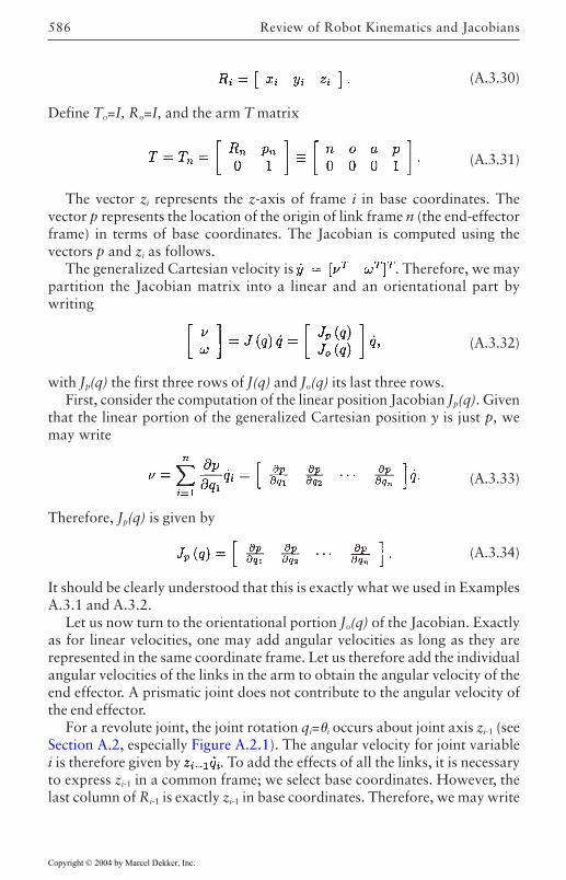
Review of Robot Kinematics and Jacobians586
(A.3.30)
Define To=I, Ro=I, and the arm T matrix
(A.3.31)
The vector zi represents the z-axis of frame i in base coordinates. Thevector p represents the location of the origin of link frame n (the end-effectorframe) in terms of base coordinates. The Jacobian is computed using thevectors p and zi as follows.
The generalized Cartesian velocity is . Therefore, we maypartition the Jacobian matrix into a linear and an orientational part bywriting
(A.3.32)
with Jp(q) the first three rows of J(q) and Jo(q) its last three rows.First, consider the computation of the linear position Jacobian Jp(q). Given
that the linear portion of the generalized Cartesian position y is just p, wemay write
(A.3.33)
Therefore, Jp(q) is given by
(A.3.34)
It should be clearly understood that this is exactly what we used in ExamplesA.3.1 and A.3.2.
Let us now turn to the orientational portion Jo(q) of the Jacobian. Exactlyas for linear velocities, one may add angular velocities as long as they arerepresented in the same coordinate frame. Let us therefore add the individualangular velocities of the links in the arm to obtain the angular velocity of theend effector. A prismatic joint does not contribute to the angular velocity ofthe end effector.
For a revolute joint, the joint rotation qi=i occurs about joint axis zi-1 (seeSection A.2, especially Figure A.2.1). The angular velocity for joint variablei is therefore given by . To add the effects of all the links, it is necessaryto express zi-1 in a common frame; we select base coordinates. However, thelast column of Ri-1 is exactly zi-1 in base coordinates. Therefore, we may write
Copyright © 2004 by Marcel Dekker, Inc.
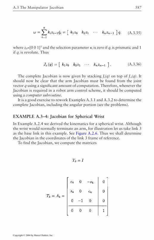
587
(A.3.35)
where z0=[0 0 1]T and the selection parameter i is zero if qi is prismatic and 1if qi is revolute. Thus
(A.3.36)
The complete Jacobian is now given by stacking Ji(q) on top of Jo(q). Itshould now be clear that the arm Jacobian must be found from the jointvector q using a significant amount of computation. Therefore, whenever theJacobian is required in a robot arm control scheme, it should be computedusing a computer subroutine.
It is a good exercise to rework Examples A.3.1 and A.3.2 to determine thecomplete Jacobian, including the angular portion (see the problems).
EXAMPLE A.3–4: Jacobian for Spherical Wrist
In Example A.2.4 we derived the kinematics for a spherical wrist. Althoughthe wrist would normally terminate an arm, for illustration let us take link 3as the base link in this example. See Figure A.2.6. Thus we shall determinethe Jacobian in the coordinates of the link 3 frame of reference.
To find the Jacobian, we compute the matrices
A.3 The Manipulator Jacobian
Copyright © 2004 by Marcel Dekker, Inc.
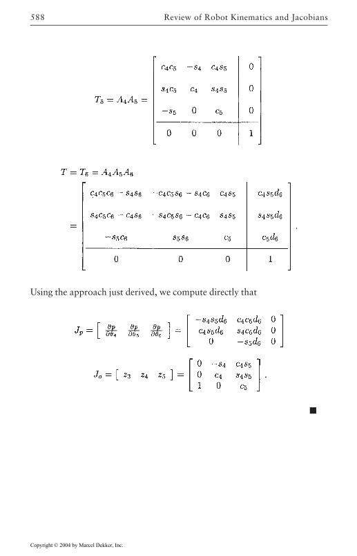
Review of Robot Kinematics and Jacobians588
Using the approach just derived, we compute directly that
Copyright © 2004 by Marcel Dekker, Inc.
589
REFERENCES
[Craig 1989] Craig, J.J., Introduction to Robotics. Reading, MA: Addison-Wesley, 1989.
[Ickes 1970] Ickes, B.P., “A new method for performing digital control systemaltitude computations using quaternions,” AIAA J., vol. 8, no. 1, pp. 13–17, Jan. 1970.
[IMSL] IMSL, Library Contents Document, 8th ed. Houston, TX: InternationalMathematical and Statistical Libraries.
[MATMAN 1986] MATMAN, Symbolic Matrix Manipulation, M.R.Driels,Pembroke, MA: Kern International, 1986.
[Paul 1981] Paul, R.P., Robot Manipulators, Cambridge, MA: MIT Press,1981.
[Schilling 1990] Schilling, R.J., Fundamentals of Robotics, Englewood Cliffs,NJ: Prentice Hall, 1990.
[Sheppard 1978] Sheppard, S.W., “Quaternion from rotation matrix,” Eng.Notes, pp. 223–224, May/June 1978.
[Spong and Vidyasagar 1989] Spong, M.W., and M.Vidyasagar, RobotDynamics and Control. New York: Wiley, 1989.
[Stevens and Lewis 1992] Stevens, B.L., and F.L.Lewis, Aircraft Modeling,Dynamics, and Control. New York: Wiley, 1992.
[Yuan 1988] Yuan, J.S.-C., “Closed-loop manipulator control using quaternionfeedback,” IEEE J. Robot. Autom., vol. 4, no. 4, pp. 434–440, Aug.1988.
Copyright © 2004 by Marcel Dekker, Inc.
591
Appendix B
Software for ControllerSimulation
An excellent way to gain an intuitive feel for control systems design andperformance is to perform computer simulations. It is conceptually a shortstep from simulation to actual implementation, since the subroutines that areused on today’s digital signal processors are very similar to those used forsimulation. This appendix contains the software used in the text for robotcontroller simulation.
There are some good software packages available for design and simulationof systems, and one should be aware of them and employ them. Examples areMATLAB, MATRIXX, Program CC, SIMNON, and so on. However, it isvery instructive to use one’s own software during the learning phase, especiallysince it is sometimes not clear exactly what is going on in some of thesepackages when dealing with digital control.
For the time-response simulation of continuous systems, a Runge-Kuttaintegrator works very well. In Figure B.1.1 is shown program TRESP, whichuses a fourth-order Runge-Kutta subroutine to implement the simulationprocedure discussed in Section 3.3. It integrates linear or nonlinear systems inthe state-variable form
In Section 2.4 we showed how to place the robot dynamics into this form.Note that MATLAB’s functions ode 23 and ode 45 are adaptive step sizeRunge-Kutta integrators that need the same form for the dynamics.
TRESP requires a subroutine F(time, x, xp), which computes x (denoted
Copyright © 2004 by Marcel Dekker, Inc.
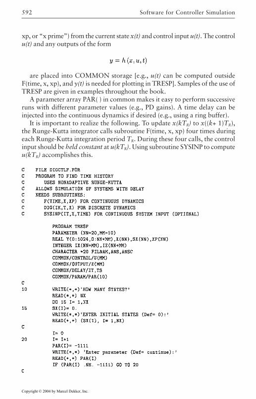
Software for Controller Simulation592
xp, or “x prime”) from the current state x(t) and control input u(t). The controlu(t) and any outputs of the form
are placed into COMMON storage [e.g., u(t) can be computed outsideF(time, x, xp), and y(t) is needed for plotting in TRESP]. Samples of the use ofTRESP are given in examples throughout the book.
A parameter array PAR( ) in common makes it easy to perform successiveruns with different parameter values (e.g., PD gains). A time delay can beinjected into the continuous dynamics if desired (e.g., using a ring buffer).
It is important to realize the following. To update x(kTR) to x((k+ 1)TR),the Runge-Kutta integrator calls subroutine F(time, x, xp) four times duringeach Runge-Kutta integration period TR. During these four calls, the controlinput should be held constant at u(kTR). Using subroutine SYSINP to computeu(kTR) accomplishes this.
Copyright © 2004 by Marcel Dekker, Inc.
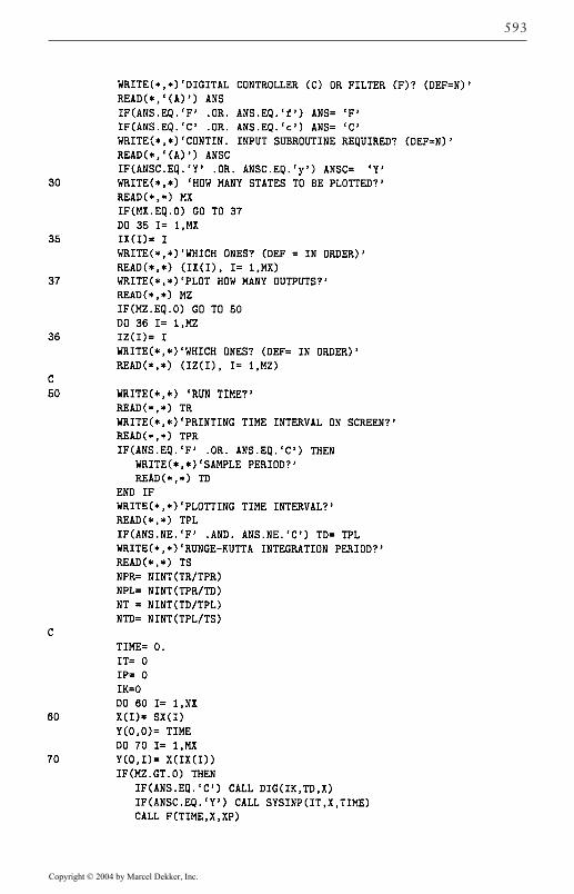
593
Copyright © 2004 by Marcel Dekker, Inc.
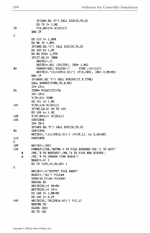
Software for Controller Simulation594
Copyright © 2004 by Marcel Dekker, Inc.
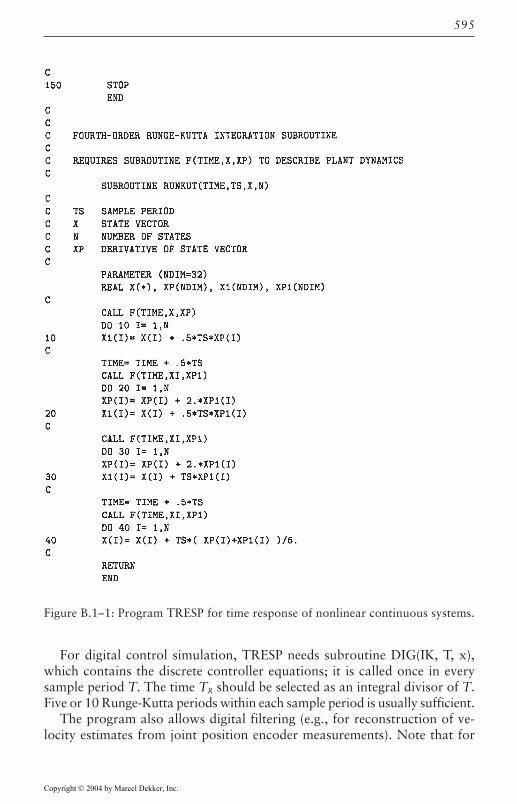
595
Figure B.1–1: Program TRESP for time response of nonlinear continuous systems.
For digital control simulation, TRESP needs subroutine DIG(IK, T, x),which contains the discrete controller equations; it is called once in everysample period T. The time TR should be selected as an integral divisor of T.Five or 10 Runge-Kutta periods within each sample period is usually sufficient.
The program also allows digital filtering (e.g., for reconstruction of ve-locity estimates from joint position encoder measurements). Note that for
Copyright © 2004 by Marcel Dekker, Inc.
Software for Controller Simulation596
digital controls purposes, subroutine DIG is called before the Runge-Kuttaroutine, while for digital filtering, DIG is called after the call to Runge-Kutta.
For some systems the Runge-Kutta integrator in the figure may not work;then an adaptive step-size Runge-Kutta routine (e.g., Runge-KuttaFehlburg)can be used [Press et al. 1986]. (Note: The program given here works for allexamples in the book.)
Copyright © 2004 by Marcel Dekker, Inc.
597
REFERENCE
[Press et al. 1986] Press, W.H., Flannery, B.P., Teukolsky, S.A., andVetterling, W.T., Numerical Recipes. New York: Cambridge UniversityPress, 1986.
Copyright © 2004 by Marcel Dekker, Inc.
599
Appendix C
Dynamics of SomeCommon Robot Arms
In this appendix we give the dynamics of some common robot arms. Weassume that the robot dynamics are given by
(C.1.1)
where the matrix M(q) is symmetric and positive definite with elements mij(q),that is,
and N (q, q) is an n×1 vector with elements ni, that is,
Note in particular that the gravity terms are indentified in the expressions ofni by the gravity constant g=9.8 meters/s2. We will also adopt the followingnotation:
Length of link i is Li in metersMass of link i is mi in kilogramsMass moment of inertia of Link i about axis u is Iuui in kg-m-mSi=sin qi and Ci=cos qi
Sij=sin(qi+qj) and Cij=cos(qi+qj)Sijk=sin(qi+qj+qk) and Cijk=cos(qi+qj+qk)SSi=sin2 qi, CCi=cos2 qi, and CSi=cos qi sin qi;SSij=sin2(qi+qj)
Copyright © 2004 by Marcel Dekker, Inc.
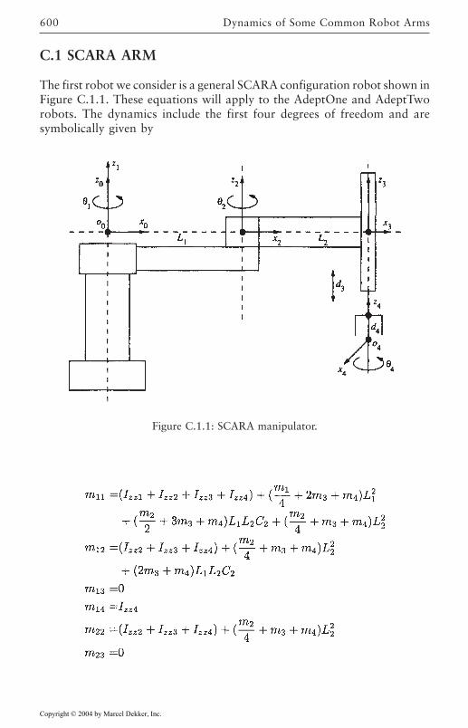
Dynamics of Some Common Robot Arms600
C.1 SCARA ARM
The first robot we consider is a general SCARA configuration robot shown inFigure C.1.1. These equations will apply to the AdeptOne and AdeptTworobots. The dynamics include the first four degrees of freedom and aresymbolically given by
Figure C.1.1: SCARA manipulator.
Copyright © 2004 by Marcel Dekker, Inc.
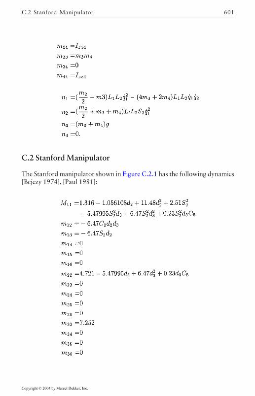
601
C.2 Stanford Manipulator
The Stanford manipulator shown in Figure C.2.1 has the following dynamics[Bejczy 1974], [Paul 1981]:
C.2 Stanford Manipulator
Copyright © 2004 by Marcel Dekker, Inc.
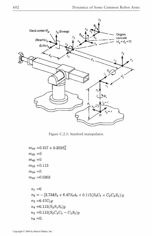
Dynamics of Some Common Robot Arms602
Figure C.2.1: Stanford manipulator.
Copyright © 2004 by Marcel Dekker, Inc.
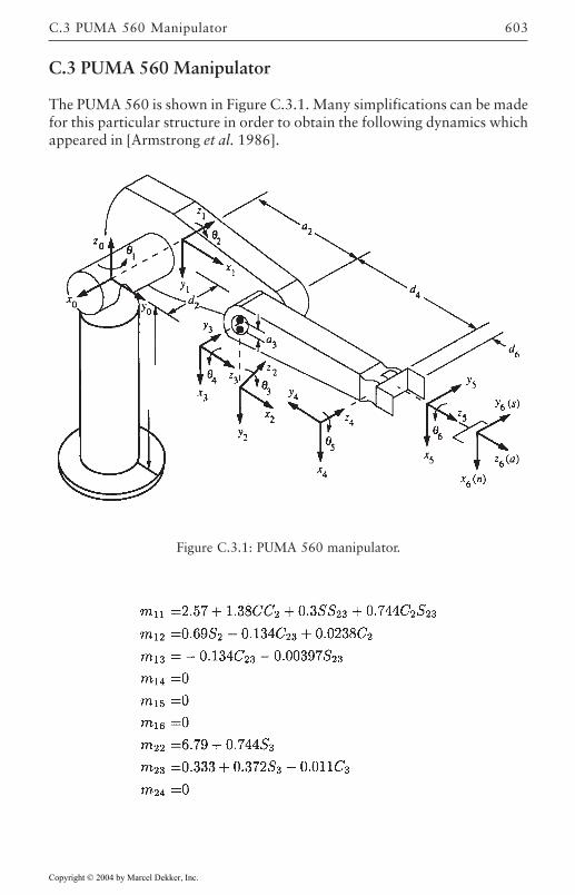
603
C.3 PUMA 560 Manipulator
The PUMA 560 is shown in Figure C.3.1. Many simplifications can be madefor this particular structure in order to obtain the following dynamics whichappeared in [Armstrong et al. 1986].
Figure C.3.1: PUMA 560 manipulator.
C.3 PUMA 560 Manipulator
Copyright © 2004 by Marcel Dekker, Inc.
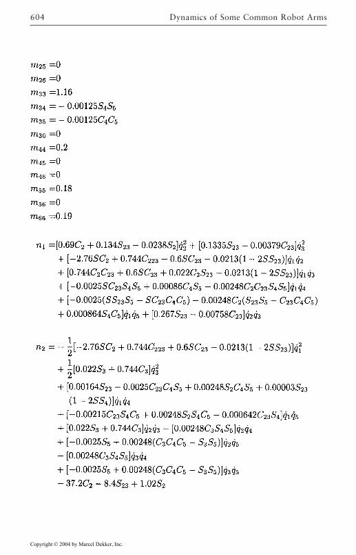
Dynamics of Some Common Robot Arms604
Copyright © 2004 by Marcel Dekker, Inc.
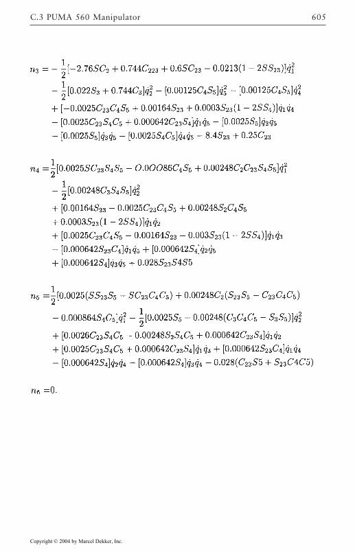
605C.3 PUMA 560 Manipulator
Copyright © 2004 by Marcel Dekker, Inc.
607
REFERENCES
[Armstrong et al. 1986] Armstrong, B., O.Khatib, and J.Burdick, “The explicitdynamic model and inertial parameters of the PUMA 560 arm,” Proc.1986 IEEE Conf. Robot. Autom., pp. 510–518, San Francisco, Apr. 7–10, 1986.
[Bejczy 1974] Bejczy, A.K., “Robot arm dynamics and control,” NASA-JPLTechnical Memorandum 33–669, 1974.
[Paul 1981] Paul, R.P., Robot Manipulators: Mathematics, Programming andControl. Cambridge, MA: MIT Press, 1981.
Copyright © 2004 by Marcel Dekker, Inc.


