arX

iv:a

stro

-ph/

0408

138v

3 1

3 O

ct 2

004

Multiple inflation and the WMAP ‘glitches’

Paul Hunt and Subir SarkarTheoretical Physics, University of Oxford, 1 Keble Road, Oxford OX1 3NP, UK

Observations of anisotropies in the cosmic microwave background by the Wilkinson Microwave

Anisotropy Probe suggest the possibility of oscillations in the primordial curvature perturbation.Such deviations from the usually assumed scale-free spectrum were predicted in the multiple in-flation model wherein ‘flat direction’ fields undergo rapid phase transitions due to the breaking ofsupersymmetry by the large vacuum energy driving inflation. This causes sudden changes in themass of the (gravitationally coupled) inflaton and interrupts its slow roll. We calculate analyticallythe resulting modifications to the curvature perturbation and demonstrate how the oscillations arise.

I. INTRODUCTION

Despite the overall success of the standard ΛCDM inflationary model in matching the results from WMAP, it isstriking that the goodness-of-fit statistics for the data are rather poor [1]. In particular, χ2

eff/ν = 1432/1342 for the fitto the TT spectrum which implies a probability of only ∼ 3% for the best fit model to be correct. The lack of powerat large scales relative to the standard ΛCDM model prediction has motivated several alternative proposals for thespectrum and nature of the primordial fluctuations [2, 3, 4, 5, 6, 7, 8, 9, 10, 11, 12], however the uncertainties (andcosmic variance) at low multipoles are large and it has been argued that the observed low quadrupole (and octupole)are unlikely only at about a few per cent level [13, 14, 15].1 In fact attempts to judge the goodness-of-fit by eye canbe misleading since neighbouring Cl’s are correlated (being ‘pseudo-Cl’s evaluated on a ‘cut’ sky); taking this intoaccount it is found [1] that the excess χ2 comes mainly from sharp features or ‘glitches’ in the power spectrum thatthe model is unable to fit. In particular there are glitches at l ∼ 120, 200 and 340 amongst the first and secondacoustic peaks.

The WMAP team have noted that these glitches may have been caused by beam asymmetry, gravitational lensing ofthe CMB, non-Gaussianity in the noise maps, or the method of power spectrum reconstruction from the CMB maps [1].However they have also considered the possibility that these glitches are due to features in the underlying primordialcurvature perturbation spectrum [18], specifically in the ‘multiple inflation’ model [19] where sudden changes in themass of the inflaton can generate characteristic localized oscillations in the spectrum. This is physically well motivatedsince spontaneous symmetry breaking can occur during inflation for ‘flat directions’ in supersymmetric theories andsuch fields are gravitationally coupled to the inflaton [19]. The resulting change in the potential of the inflaton fieldφ was modeled earlier as [20]

V (φ) =1

2m2

φφ2

[

1 + campl tanh

(

φ − φstep

dgrad

)]

, (1)

which describes a standard ‘chaotic inflation’ potential with a step starting at φstep with amplitude and gradientdetermined by the parameters campl and dgrad respectively. This was shown to result in oscillations in the primordialcurvature perturbation spectrum by numerically solving the governing Klein-Gordon equation [20]. The WMAP teamfound that the fit to the data improves if such oscillations are allowed for, with a reduction of χ2 by 10 for the modelparameters φstep = 15.5 MP, campl = 9.1 × 10−4 and dgrad = 1.4 × 10−2MP [18].

We calculate the curvature perturbation spectrum from multiple inflation more realistically, taking into account theevolution of both fields as dictated by the inflationary dynamics [19], and using a WKB approximation [21], rather thannumerical integration to solve the governing equation, in order to gain insight into how such oscillations are generated.In a subsequent publication we perform fits to the WMAP data with the cosmological parameters unconstrained, inorder to investigate the sensitivity of their inferred values to such deviations from a scale-free spectrum [22].

The possibility that the WMAP glitches are due to oscillations in the primordial spectrum has also been consideredin the context of inflationary models invoking ‘trans-Planckian’ physics [23, 24, 25, 26, 27]. Sharp features in theprimordial spectrum may also have been generated by resonant particle production [28, 29, 30]. Several authors haveattempted to reconstruct the curvature perturbation from the WMAP data and have noted possible features in itsspectrum [2, 31, 32, 33, 34, 35]. It is clearly necessary to have an analytic formulation of the modification to the

1 However there is an unexpected alignment between the quadrupole and octupole [15, 16] and there appear to be systematic differencesbetween the north and south ecliptic hemispheres [17], so this issue cannot be considered settled as yet.

2

usually assumed scale-free spectrum of the inflationary curvature perturbation, both in order to provide a link betweenCMB observables and the physics responsible for the glitches, and to distinguish between the various suggestions forsuch new physics.

II. MULTIPLE INFLATION

Supergravity (SUGRA) theories consist of a ‘visible sector’ and a ‘hidden sector’ coupled together gravitationally[36, 37]. The Standard Model particles are contained in the visible sector and supersymmetry (SUSY) breaking occursin the hidden sector. Most SUGRA models of inflation have the inflaton situated in the hidden sector. This is becauseit is easier to protect the necessary flatness of the inflaton potential against radiative corrections there. The visiblesector is usually assumed to be unimportant during inflation.

However this might not be true if one of the visible sector fields undergoes gauge symmetry breaking. Suitablecandidates for this are the so-called flat direction fields which generically exist in supersymmetric theories (for areview, see ref.[38]). These are directions in field space in which the potential vanishes, in the limit of unbrokenSUSY. During inflation in supergravity theories scalar fields typically receive a contribution of m2 ∼ ±O(H2) to theirmass-squared due to SUSY breaking by the large vacuum energy driving inflation [39, 40, 41]. (For the inflaton thisconstitutes the notorious ‘η problem’ [42]; in common with most models of inflation we need to assume that somemechanism reduces the inflaton mass-squared by a factor of a least 20 in order to allow sufficient inflation to occur.)The SUSY-breaking mass term typically dominates the potential along the flat directions. If the mass-squared isnegative at the origin in field space, the flat direction ρ will be stabilized at an intermediate scale vev of

Σ ∼(

Mn−4P m2

)1/(n−2), (2)

by higher dimensional operators ∝ ρn/Mn−4P [19]. These appear in the potential after integrating out heavy degrees

of freedom, because we are working in an effective field theory valid below some cut-off scale, which we take to be thereduced Planck mass: MP ≡ (8π GN)−1/2 ≃ 2.4 × 1018 GeV.

We assume that the inflationary era when the observed curvature perturbation was produced was preceeded by ahot phase, so that all fields were initially in thermal equilibrium. The potential along the flat direction is then [19]

V (ρ, T ) ≃{

C1T2ρ2, for ρ ≪ T,

−m2ρ2 + 190π2Nh(T )T 4 + γρn

Mn−4

P

, for T ≪ ρ < Σ, (3)

with a smooth interpolation at ρ ∼ T . Here we have included the 1-loop finite temperature correction to the potential[43, 44] with Nh(T ) being the number of helicity states with mass much less than the temperature.

The finite temperature correction therefore creates a barrier of height O(T 4) in between the origin and ρ ∼ T 2/m.The tunneling rate through the barrier is negligible and so ρ is confined at the origin until the temperature, whichfalls rapidly during inflation, reaches T ∼ m and the barrier disappears. The flat direction field ρ then undergoes aphase transition as it evolves to its global minimum at Σ. This is governed by the usual equation of motion

ρ + 3Hρ = −dV

dρ, (4)

which has solutions

ρ ≃

ρ0 exp

[

3Ht2

(

√

1 + 8m2

9H2 − 1

)]

, 〈ρ〉 ≪ Σ,

Σ + K1 exp(

− 3Ht2

)

sin

[

3Ht2

√

(n − 2)8m2

9H2 − 1 + K2

]

, 〈ρ〉 ∼ Σ.

(5)

Here we have taken

dV

dρ≃{ −2m2ρ, 〈ρ〉 ≪ Σ,

(ρ − Σ) d2Vdρ2

∣

∣

∣

ρ=Σ, 〈ρ〉 ∼ Σ. (6)

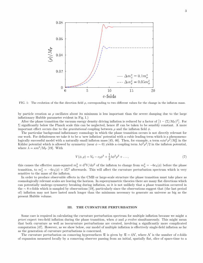
Therefore ρ evolves exponentially towards its minimum, with most of the growth occurring over the last ∼ 2 e-folds[19], and then performs a few strongly damped oscillations about Σ, as seen in Fig. 1. (We assume that damping

3

PSfragreplacementsh�i/M P e-folds �m2� = 0:05m2��m2� = 0:1m2�0 00:020:040:060:08

5 10 15 20FIG. 1: The evolution of the flat direction field ρ, corresponding to two different values for the change in the inflaton mass.

by particle creation as ρ oscillates about its minimum is less important than the severe damping due to the largeinflationary Hubble parameter evident in Fig. 1.)

After the phase transition the vacuum energy density driving inflation is reduced by a factor of[

1 − (Σ/MP)2]

. ForΣ significantly below the Planck scale this can be neglected, hence H can be taken to be sensibly constant. A moreimportant effect occurs due to the gravitational coupling between ρ and the inflaton field φ.

The particular background inflationary cosmology in which the phase transition occurs is not directly relevant forour work. For definiteness we take it to be a ‘new inflation’ potential with a cubic leading term which is a phenomeno-logically successful model with a naturally small inflaton mass [45, 46]. Then, for example, a term κφφ†ρ2/M2

P in theKahler potential which is allowed by symmetry (near φ ∼ 0) yields a coupling term λφ2ρ2/2 in the inflaton potential,where λ = κm2/MP [19]. With

V (φ, ρ) = V0 − c3φ3 +

1

2λφ2ρ2 + . . . , (7)

this causes the effective mass-squared m2φ ≡ d2V/dφ2 of the inflaton to change from m2

φ = −6c3〈φ〉 before the phase

transition, to m2φ = −6c3〈φ〉 + λΣ2 afterwards. This will affect the curvature perturbation spectrum which is very

sensitive to the mass of the inflaton.In order to produce observable effects in the CMB or large-scale structure the phase transition must take place as

cosmologically relevant scales are leaving the horizon. In supersymmetric theories there are many flat directions whichcan potentially undergo symmetry breaking during inflation, so it is not unlikely that a phase transition occurred inthe ∼ 8 e-folds which is sampled by observations [19], particularly since the observations suggest that (the last periodof) inflation may not have lasted much longer than the minimum necessary to generate an universe as big as thepresent Hubble volume.

III. THE CURVATURE PERTURBATION

Some care is required in calculating the curvature perturbation spectrum for multiple inflation because we might a

priori expect two-field inflation during the phase transition, when φ and ρ evolve simultaneously. This might meanthat both curvature as well as isocurvature perturbations are created, involving a significantly more complicatedcomputation [47]. However, as we show below, our model of multiple inflation is effectively single-field inflation as faras the generation of curvature perturbations is concerned.

The curvature perturbation on comoving hypersurfaces R is given by R = δN , where N is the number of e-foldsof expansion measured locally by a comoving observer passing from an initial, spatially flat, slice of space-time to a

4

final, comoving, slice [48]. The perturbations δφfts and δρfts are defined on the spatially flat time slice and the finalcomoving slice defines R. The first time slice is taken during inflation, soon after horizon crossing, and the secondtime slice is taken at the end of inflation, after R has become constant. During the phase transition the slow-rollconditions in φ are no longer satisfied but we assume the end of inflation to be well after this epoch. Then we have

R =∂N∂φ

δφfts +∂N∂ρ

δρfts, (8)

and so

PR =

(

∂N∂φ

)2

Pφ +

(

∂N∂ρ

)2

Pρ ≃(

dNdφ

)2

Pφ, (9)

which is just the single-field inflation expression for PR. This is because the vacuum energy is dominated by φ, whichdrives inflation, and ρ has a negligible effect on the number of e-folds of inflation.

The curvature perturbation spectrum is usually calculated analytically using the slow-roll approximation to somechosen order in the slow-roll parameters [42]. This assumes the potential is relatively smooth, which is howeverinappropriate for multiple inflation. For example, for the standard chaotic inflation potential V = 1

2m2φφ2, the usual

slow-roll expression gives

PR1/2 =

1

2√

3πM3P

∣

∣

∣

∣

V 3/2

dV/dφ

∣

∣

∣

∣

≃ 1

2√

3πM3P

V 3/2

m2φφ

, (10)

where all quantities are evaluated at horizon crossing. This gives a simple ‘step’ in the amplitude if the inflaton masschanges suddenly as in eq.(1), missing all the fine detail that we expect in the spectrum. (A discussion of the slow-rollapproximation applied to a potential with a sudden change in its slope [49] rather than in its curvature can be foundin ref.[50].)

Therefore we must resort to first principles and use the general formalism [51] for calculating the curvature pertur-bation spectrum. Instead of the slow-roll approximation we use the recently suggested WKB approximation [21, 52].

The metric describing scalar perturbations in a flat universe can be parameterized as

ds2 = a2[

(1 + 2As) dη2 − 2∂iBsdηdxi − {(1 − 2Ds) δij + 2∂i∂jEs} dxidxj]

. (11)

We employ the gauge-invariant quantity

u = aδφ(gi) + zΨ = zR, (12)

to characterize the perturbations; see refs.[53, 54, 55] for more details. Here

δφ(gi) = δφ + φ′ (Bs − E′s) , (13)

Ψ = Ds −a′

a(Bs − E′

s) , (14)

are also gauge-invariant, z = aφ/H , and

R = Ds + Hδφ

φ. (15)

The primes indicate derivatives with respect to conformal time

η =

∫

dt

a= − 1

aH, (16)

where the last equality holds in de Sitter space. The Fourier components of u satisfy the Klein-Gordon equation ofmotion

u′′k +

(

k2 − z′′

z

)

uk = 0. (17)

The spectrum depends directly on uk and is given by

PR1/2 =

√

k3

2π2|Rk| =

√

k3

2π2

∣

∣

∣

uk

z

∣

∣

∣. (18)

5

The solutions of eq.(17) are governed by the relative sizes of k2 and z′′/z. In de Sitter space z′′/z = 2/η2, thereforeinitially when k2 ≫ z′′/z and the mode uk is well inside the horizon, we have the flat spacetime solution

uk =1√2k

e−ik(η−ηi), (19)

where ηi is some arbitrary time at the beginning of inflation. In the opposite limit, k2 ≪ z′′/z, we have the solution

uk = Akz + Bkz

∫ η dµ

z2 (µ), (20)

when uk is well outside the horizon. The first term on the right is the growing mode solution and the second is thedecaying mode. Thus PR at late times is equal to k3 |Ak|2 /2π2.

We will use the WKB approximation to solve the mode equation, with eq.(19) as an initial condition. The WKBapproximation cannot be directly applied to eq.(17) because the approximation breaks down on super-horizon scales.However, as noted in ref.[21], the WKB approximation becomes relevant if we switch to the variables

x = ln

(

Ha

k

)

, (21)

U = ex/2uk. (22)

The transformed mode equation is then

d2U

dx2+ Q(x)U = 0, (23)

where the effective frequency,

Q(x) =

(

1 − z′′

zk2

)

e−2x − 1

4, (24)

generally decreases with time during inflation, passing through zero at least once.2 In de Sitter space, this is

Q(x) =

(

k

aH

)2

− 9

4. (25)

In the WKB formalism [58] we expand U as an asymptotic series

U (x) = exp

[

∞∑

n=0

Sn (x)

]

, Sn (x) ≫ Sn+1 (x) . (26)

Substituting this into eq.(23) results in the following series of equations

S′02

= −Q, (27)

2S′0S

′1 + S′′

0 = 0, (28)

2S′0S

′n + S′′

n−1 +

n−1∑

j=1

S′jS

′n−j = 0, for n ≥ 2, (29)

where the primes indicate derivatives with respect to x.This gives the first few terms as

Q > 0

S0 = ±i∫ x

Q1/2dy,

S1 = − 14 lnQ,

S2 = ±i∫ x(

− Q′′

8Q3/2 + 5Q2

32Q3/2

)

dy,

S3 = Q′′

16Q2 − 5Q2

64Q3 ,

(30)

2 Q is related to the variable gs of Refs.[56, 57] by Q = −gsη2.

6

Q < 0

S0 = ±∫ x

(−Q)1/2

dy,

S1 = − 14 ln (−Q) ,

S2 = ±∫ x[

− Q′′

8(−Q)3/2+ 5Q2

32(−Q)3/2

]

dy,

S3 = Q′′

16Q2 − 5Q2

64Q3 .

(31)

Using only the first two terms in the expansion and neglecting the rest gives the 1st-order WKB approximation (forQ > 0)

UI =A

Q1/4(x)exp

[

i

∫ x

xi

Q1/2(y)dy

]

+B

Q1/4(x)exp

[

−i

∫ x

xi

Q1/2(y)dy

]

, (32)

where A and B are constants. At early times Q ≃ e−2x which means that the WKB solution will match eq.(19) if

A = 0 and B = 1/√

2k.The solutions become inaccurate close to the roots (‘turning points’) x∗ of Q(x∗) = 0. To continue the solution

through a turning point we therefore need to match the WKB solutions valid to the right and left of the turning point,with a solution valid in the neighbourhood of the turning point. We patch the solutions together using asymptoticmatching.

We consider the case of a single turning point and divide the x-axis into three regions. Region I is defined as theregion where x < x∗, Q > 0 and the WKB approximation is valid. Region II is the neighbourhood of x∗ where Q canbe approximated by its tangent at x∗. Region III is where x > x∗, Q < 0, and the WKB solution is accurate. Weassume there is an overlap between regions I and II, and also between regions II and III.

In region II we have

Q ≃ −αX, X ≡ x − x∗, α ≡ − dQ

dx

∣

∣

∣

∣

x=x∗

> 0. (33)

We rewrite the integration limits of UI (32) as∫ x

xi

Q1/2dy =

∫ x∗

xi

Q1/2dy +

∫ x

x∗

Q1/2dy ≡ Γ +

∫ x

x∗

Q1/2dy. (34)

Then in the overlap between regions I and II, UI becomes

UI ≃α−1/4

√2k

(−X)−1/4

exp

[

−i

{

−2

3(−X)

3/2+ Γ

}]

. (35)

With Q ≃ −αX , the solution to eq.(23) is

UII ≃ CAi(

α1/3X)

+ DBi(

α1/3X)

, (36)

where Ai and Bi are Airy functions of the first and second kinds and C and D are constants. For X ≪ 0, UII becomes

UII ≃ α−1/12

2√

π(−X)−1/4

[

(D − iC) exp

{

i

(

2

3(−X)3/2 +

π

4

)}

+ (D + iC) exp

{

−i

(

2

3(−X)

3/2+

π

4

)}]

. (37)

Requiring this to match UI (35) in the overlap region fixes the coefficients

C = iD, D =

√

π

2kα−1/6 exp

[

−i(

Γ +π

4

)]

. (38)

For X ≫ 0 we have

UII ≃ α−1/12

√π

X−1/4

[

C

2exp

(

−2

3α1/2X3/2

)

+ D exp

(

2

3α1/2X3/2

)]

. (39)

7

In region III, the 1st-order WKB solution is

UIII =F

[−Q(x)]1/4

exp

{∫ x

x∗

[−Q(y)]1/2

dy

}

+G

[−Q(x)]1/4

exp

{

−∫ x

x∗

[−Q(y)]1/2 dy

}

. (40)

When Q ≃ −αX , this becomes

UIII ≃ α−1/4X−1/4

[

F exp

(

2

3α1/2X3/2

)

+ G exp

(

−2

3α1/2X3/2

)]

, (41)

which matches UII (39) in the second overlap region if

F =α1/6

√π

D, G =α1/6

2√

πC. (42)

Substituting UIII into eq.(18) gives finally the curvature perturbation spectrum

P1/2R (k) =

H2

2πφ

(

k

aH

)3/2∣

∣

∣

∣

∣

x=xf

[−Q (xf)]−1/4

exp

{∫ xf

x∗

[−Q(y)]1/2

dy

}

. (43)

where xf is the value of x at some late time well after horizon crossing when R is constant, and we have neglectedthe decaying mode proportional to G which is negligible at late times.

We now consider the 2nd-order WKB approximation where the first three terms in the expansion (26) are retained.At early times the WKB solution is

UI =1√

2kQ1/4exp

[

−i

∫ x

xi

(

Q1/2 − Q′′

8Q3/2+

5Q′2

32Q3/2

)

dy

]

,

=1√

2kQ1/4exp

[

−i

(∫ x

xi

Q1/2dy − 5Q′

48Q3/2−∫ x

xi

Q′′

48Q3/2dy

)]

, (44)

where the second line follows after an integration by parts. As before we rewrite the integration limits as

∫ x

xi

(

Q1/2dy − Q′′

48Q3/2

)

dy =

∫ x∗

xi

Q1/2dy −∫ x∗−ε

xi

Q′′

48Q3/2dy

+

∫ x

x∗

Q1/2dy −∫ x

x∗−ε

Q′′

48Q3/2dy,

≡ Υ +

∫ x

x∗

Q1/2dy −∫ x

x∗−ε

Q′′

48Q3/2dy. (45)

Here ε is a small parameter introduced to regularize the divergent integral S2. This time, region II is the neighbourhoodof x∗ where

Q ≃ −αX + βX2, β ≡ 1

2

d2Q

dx2

∣

∣

∣

∣

x=x∗

. (46)

Then in the overlap of regions I and II

UI ≃ α−1/4

√2k

(−X)−1/4

(

1 +βX

4α

)

exp

[

−i

{

−2

3(−X)3/2

− β

5α1/2(−X)5/2 +

5

48α1/2(−X)−3/2 − β

12α3/2(−X)−1/2

+β

12α3/2ε−1/2 + Υ

}]

. (47)

8

With Q ≃ −αX + βX2, eq.(23) has the approximate solution

UII ≃ K

(

1 +βX

5α

)

Ai

[

α1/3X

(

1 − βX

5α

)]

+L

(

1 +βX

5α

)

Bi

[

α1/3X

(

1 − βX

5α

)]

. (48)

For X ≪ 0,

UII ≃ α−1/12

2√

π(−X)−1/4

(

1 +βX

4α

)

×[

(L − iK) exp

{

i

(

2

3(−X)

3/2+

β

5α1/2(−X)

5/2+

π

4

)}

+ (L + iK) exp

{

−i

(

2

3(−X)3/2 +

β

5α1/2(−X)5/2 +

π

4

)}]

, (49)

which matches UI in the overlap region provided that

K = iL, L =

√

π

2kα−1/6 exp

[

−i

(

Υ +π

4− β

12α3/2ε−1/2

)]

. (50)

When X ≫ 0, we have

UII ≃ α−1/12

√π

X−1/4

(

1 +βX

4α

)[

K

2exp

(

−2

3α1/2X3/2

+β

5α1/2X5/2

)

+ L exp

(

2

3α1/2X3/2 − β

5α1/2X5/2

)]

. (51)

The 2nd-order WKB solution in region III is

UIII =M

(−Q)1/4

exp

[

∫ x

x∗

{

(−Q)1/2 dy − Q′′

8 (−Q)3/2

+5Q

′2

32 (−Q)3/2

}

dy

]

+N

(−Q)1/4

exp

[

−∫ x

x∗

{

(−Q)1/2

dy − Q′′

8 (−Q)3/2

+5Q

′2

32 (−Q)3/2

}

dy

]

,

=M

(−Q)1/4

exp

[

∫ x

x∗

(−Q)1/2

dy − 5Q′

48 (−Q)3/2

−∫ x

x∗+ε

Q′′

48 (−Q)3/2

dy

]

+N

(−Q)1/4exp

[

−∫ x

x∗

(−Q)1/2

dy +5Q′

48 (−Q)3/2+

∫ x

x∗+ε

Q′′

48 (−Q)3/2dy

]

. (52)

With Q ≃ −αX + βX2, this becomes

UIII ≃ α−1/4X−1/4

(

1 +βX

4α

)[

M exp

(

2

3α1/2X3/2 − β

5α1/2X5/2

+5

48α1/2X−3/2 +

β

12α3/2X−1/2 − β

12α3/2ε−1/2

)

+N exp

(

−2

3α1/2X3/2 +

β

5α1/2X5/2 − 5

48α1/2X−3/2

− β

12α3/2X−1/2 +

β

12α3/2ε−1/2

)]

. (53)

Hence if

M =α1/6

√π

exp

(

β

12α3/2ε−1/2

)

L,

N =α1/6

2√

πexp

(

− β

12α3/2ε−1/2

)

K, (54)

9

then UIII matches UII. Therefore in the 2nd-order approximation

P1/2R (k) =

H2

2πφ

(

k

aH

)3/2∣

∣

∣

∣

∣

x=xf

exp

(

β

12α3/2ε−1/2

)

[−Q (xf)]−1/4

× exp

[

∫ xf

x∗

(−Q)1/2

dy − 5Q′

48 (−Q)3/2

−∫ xf

x∗+ε

Q′′

48 (−Q)3/2

dy

]

. (55)

A weak dependence on the parameter ε arises because of the incomplete cancellation between exp(

β12α3/2 ε−1/2

)

and

exp[

∫ xf

x∗+εQ′′

48(−Q)3/2 dy]

above. This is because we have truncated the expansion of Q at 2nd-order (see eq.(46)) for

computational convenience.

IV. RESULTS

During the phase transition, the scalar potential can be written as

V (φ, ρ) = V0 − c3φ3 − m2ρ2 +

1

2λφ2ρ2 +

γ

Mn−4P

ρn. (56)

Then the change in the inflaton mass-squared after the phase transition is

∆m2φ = λΣ2, Σ =

[

Mn−4P

nγ

(

2m2 − λφ2)

]1/(n−2)

≃(

2m2Mn−4P

nγ

)1/(n−2)

. (57)

The equations of motion are

φ + 3Hφ = −∂V∂φ =

(

3c3φ − λρ2)

φ, (58)

ρ + 3Hρ = −∂V∂ρ =

(

2m2 − λφ2 − nγ

Mn−4P

ρn−2

)

ρ. (59)

Using these gives

z′′

z= a2

(

2H2 + 6c3φ − λρ2 − 2λρρφ

φ

)

, (60)

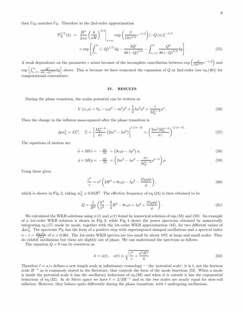
which is shown in Fig. 2, taking m2φ ≃ 0.05H2. The effective frequency of eq.(24) is then obtained to be

Q =1

H2

(

k2

a2− 9

4H2 − 6c3φ + λρ2 +

2λρρφ

φ

)

. (61)

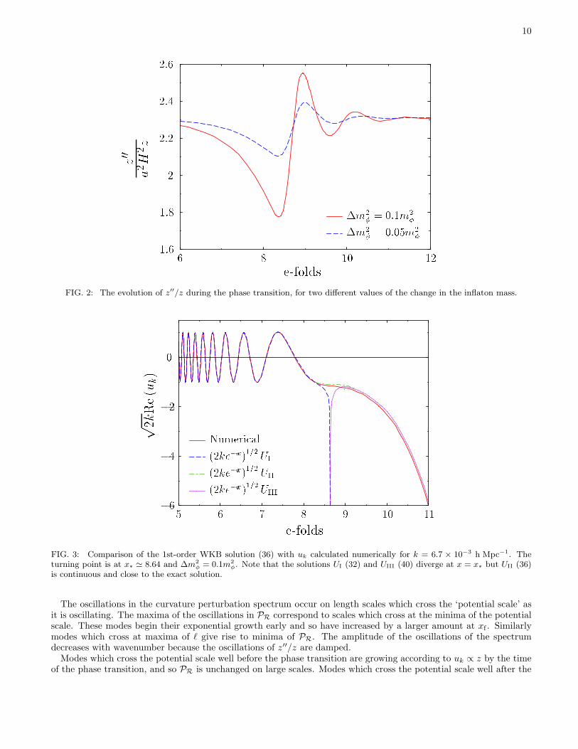
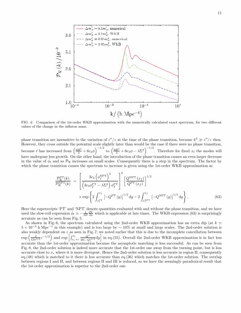
We calculated the WKB solutions using φ (t) and ρ (t) found by numerical solution of eqs.(58) and (59). An exampleof a 1st-order WKB solution is shown in Fig. 3, while Fig. 4 shows the power spectrum obtained by numericallyintegrating eq.(17) mode by mode, together with the 1st-order WKB approximation (43), for two different values of∆m2

φ. The spectrum PR has the form of a positive step with superimposed damped oscillations and a spectral index

n− 1 = d lnPR

d ln k of n ≃ 0.961. The 1st-order WKB spectra are too small by about 10% at large and small scales. Theydo exhibit oscillations but these are slightly out of phase. We can understand the spectrum as follows.

The equation Q = 0 can be rewritten as

k = s(t), s(t) ≡√

z′′

z+

a2H2

4. (62)

Therefore ℓ ≡ a/s defines a new length scale in inflationary cosmology — the ‘potential scale’; it is ℓ, not the horizonscale H−1 as is commonly stated in the literature, that controls the form of the mode functions [52]. When a modeis inside the potential scale it has the oscillatory behaviour of eq.(39) and when it is outside it has the exponentialbehaviour of eq.(32). In de Sitter space we have ℓ = 2/3H−1 and so the two scales are nearly equal for slow-rollinflation. However, they behave quite differently during the phase transition, with ℓ undergoing oscillations.

10

PSfragreplacementsz00 a2 H2 z e-folds �m2� = 0:05m2��m2� = 0:1m2�1:61:822:22:42:6

6 8 10 12FIG. 2: The evolution of z′′/z during the phase transition, for two different values of the change in the inflaton mass.

PSfragreplacementsp 2kRe(u k) e-foldsNumerical(2ke�x)1=2UI(2ke�x)1=2 UII(2ke�x)1=2UIII�6�4�2

05 6 7 8 9 10 11

FIG. 3: Comparison of the 1st-order WKB solution (36) with uk calculated numerically for k = 6.7 × 10−3 h Mpc−1. Theturning point is at x∗ ≃ 8.64 and ∆m2

φ = 0.1m2

φ. Note that the solutions UI (32) and UIII (40) diverge at x = x∗ but UII (36)is continuous and close to the exact solution.

The oscillations in the curvature perturbation spectrum occur on length scales which cross the ‘potential scale’ asit is oscillating. The maxima of the oscillations in PR correspond to scales which cross at the minima of the potentialscale. These modes begin their exponential growth early and so have increased by a larger amount at xf . Similarlymodes which cross at maxima of ℓ give rise to minima of PR. The amplitude of the oscillations of the spectrumdecreases with wavenumber because the oscillations of z′′/z are damped.

Modes which cross the potential scale well before the phase transition are growing according to uk ∝ z by the timeof the phase transition, and so PR is unchanged on large scales. Modes which cross the potential scale well after the

11

PSfragreplacementsP R(k)=10�9 k/ �h Mpc�1�

�m2� = 0:1m2�, numerical�m2� = 0:05m2�, numerical�m2� = 0:1m2�, WKB�m2� = 0:05m2�, WKB10�5 10�3 10�1 1011:62:12:63:13:6

FIG. 4: Comparison of the 1st-order WKB approximation with the numerically calculated exact spectrum, for two differentvalues of the change in the inflaton mass.

phase transition are insensitive to the variation of z′′/z at the time of the phase transition, because k2 ≫ z′′/z then.However, they cross outside the potential scale slightly later than would be the case if there were no phase transition,

because ℓ has increased from(

9H2

4 + 6c3φ)−1/2

to(

9H2

4 + 6c3φ − λΣ2)−1/2

. Therefore for fixed xf the modes will

have undergone less growth. On the other hand, the introduction of the phase transition causes an even larger decreasein the value of φf and so PR increases on small scales. Consequently there is a step in the spectrum. The factor bywhich the phase transition causes the spectrum to increase is given using the 1st-order WKB approximation as

PPTR (k)

PNPTR (k)

=

3c3

(

φNPTf

)2

(

3c3φPTf − λΣ2

)

φPTf

2[

QNPT (xf )

QPT (xf )

]1/2

× exp

{

2

∫ xf

xPT∗

[

−QPT (y)]1/2

dy − 2

∫ xf

xNPT∗

[

−QNPT (y)]1/2

dy

}

. (63)

Here the superscripts ‘PT’ and ‘NPT’ denote quantities evaluated with and without the phase transition, and we haveused the slow-roll expression φf ≃ − 1

3H∂V∂φ which is applicable at late times. The WKB expression (63) is surprisingly

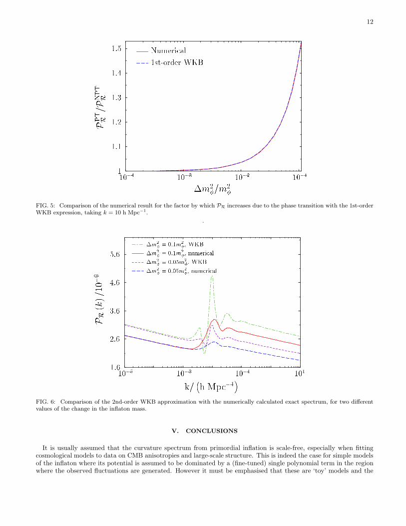
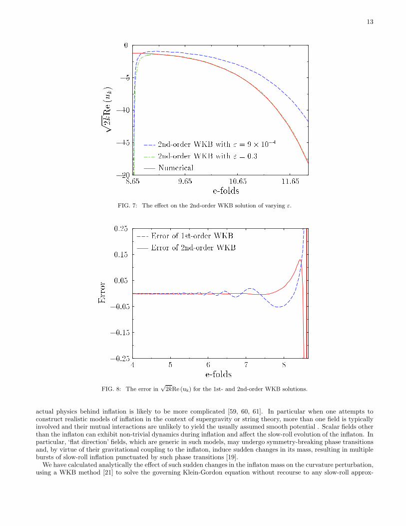
accurate as can be seen from Fig. 5.As shown in Fig. 6, the spectrum calculated using the 2nd-order WKB approximation has an extra dip (at k ≃

5 × 10−3 h Mpc−1 in this example) and is too large by ∼ 10% at small and large scales. The 2nd-order solution isalso weakly dependent on ε as seen in Fig. 7; we noted earlier that this is due to the incomplete cancellation between

exp(

β12α3/2 ε−1/2

)

and exp[

∫ xf

x∗+εQ′′

48(−Q)3/2 dy]

in eq.(55). Overall the 2nd-order WKB approximation is in fact less

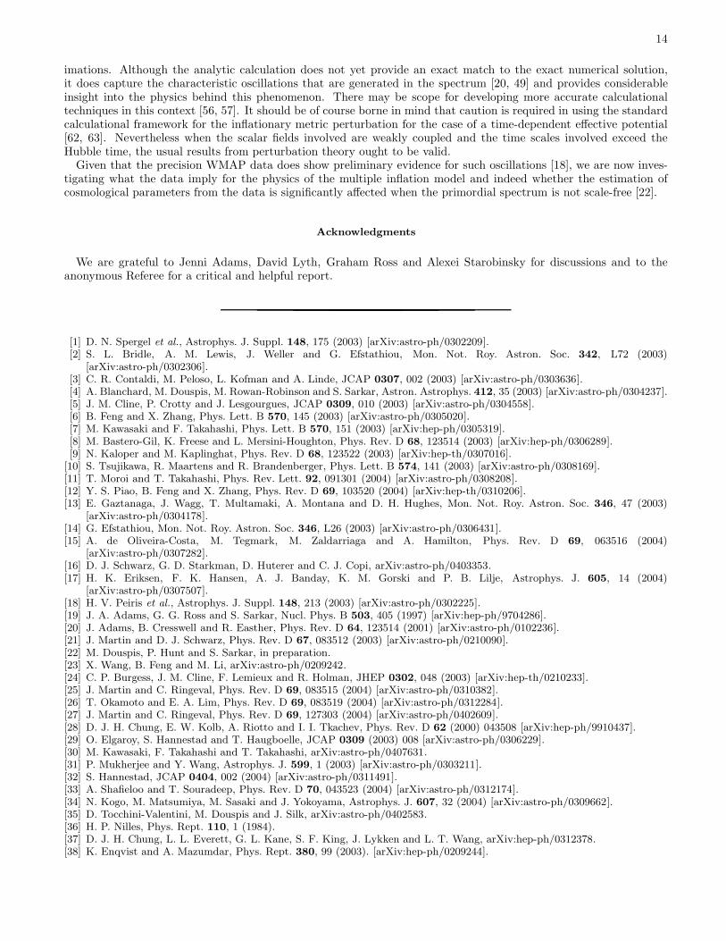
accurate than the 1st-order approximation because the asymptotic matching is less successful. As can be seen fromFig. 8, the 2nd-order solution is indeed more accurate that the 1st-order one away from the turning point, but is lessaccurate close to x∗ where it is more divergent. Hence the 2nd-order solution is less accurate in region II, consequentlyeq.(48) which is matched to it there is less accurate than eq.(36) which matches the 1st-order solution. The overlapbetween regions I and II, and between regions II and III is reduced, so we have the seemingly paradoxical result thatthe 1st-order approximation is superior to the 2nd-order one.

12

PSfragreplacementsPPT R=PNPT R �m2�=m2�

Numerical1st-order WKB10�4 10�3 10�2 10�111:11:21:31:41:5

FIG. 5: Comparison of the numerical result for the factor by which PR increases due to the phase transition with the 1st-orderWKB expression, taking k = 10 h Mpc−1.

.

PSfragreplacementsP R(k)=10�9 k/ �h Mpc�1�

�m2� = 0:1m2�, numerical�m2� = 0:05m2�, numerical�m2� = 0:1m2�, WKB�m2� = 0:05m2�, WKB10�5 10�3 10�1 1011:62:1

2:63:64:65:6FIG. 6: Comparison of the 2nd-order WKB approximation with the numerically calculated exact spectrum, for two differentvalues of the change in the inflaton mass.

V. CONCLUSIONS

It is usually assumed that the curvature spectrum from primordial inflation is scale-free, especially when fittingcosmological models to data on CMB anisotropies and large-scale structure. This is indeed the case for simple modelsof the inflaton where its potential is assumed to be dominated by a (fine-tuned) single polynomial term in the regionwhere the observed fluctuations are generated. However it must be emphasised that these are ‘toy’ models and the

13

PSfragreplacementsp 2kRe(u k) Numerical2nd-order WKB with " = 0:32nd-order WKB with " = 9� 10�4e-folds�20�15�10�508:65 9:65 10:65 11:65

FIG. 7: The effect on the 2nd-order WKB solution of varying ε.

PSfragreplacementsError e-folds

Error of 1st-order WKBError of 2nd-order WKB�0:25�0:15�0:050:050:150:25

4 5 6 7 8FIG. 8: The error in

√2kRe (uk) for the 1st- and 2nd-order WKB solutions.

actual physics behind inflation is likely to be more complicated [59, 60, 61]. In particular when one attempts toconstruct realistic models of inflation in the context of supergravity or string theory, more than one field is typicallyinvolved and their mutual interactions are unlikely to yield the usually assumed smooth potential . Scalar fields otherthan the inflaton can exhibit non-trivial dynamics during inflation and affect the slow-roll evolution of the inflaton. Inparticular, ‘flat direction’ fields, which are generic in such models, may undergo symmetry-breaking phase transitionsand, by virtue of their gravitational coupling to the inflaton, induce sudden changes in its mass, resulting in multiplebursts of slow-roll inflation punctuated by such phase transitions [19].

We have calculated analytically the effect of such sudden changes in the inflaton mass on the curvature perturbation,using a WKB method [21] to solve the governing Klein-Gordon equation without recourse to any slow-roll approx-

14

imations. Although the analytic calculation does not yet provide an exact match to the exact numerical solution,it does capture the characteristic oscillations that are generated in the spectrum [20, 49] and provides considerableinsight into the physics behind this phenomenon. There may be scope for developing more accurate calculationaltechniques in this context [56, 57]. It should be of course borne in mind that caution is required in using the standardcalculational framework for the inflationary metric perturbation for the case of a time-dependent effective potential[62, 63]. Nevertheless when the scalar fields involved are weakly coupled and the time scales involved exceed theHubble time, the usual results from perturbation theory ought to be valid.

Given that the precision WMAP data does show preliminary evidence for such oscillations [18], we are now inves-tigating what the data imply for the physics of the multiple inflation model and indeed whether the estimation ofcosmological parameters from the data is significantly affected when the primordial spectrum is not scale-free [22].

Acknowledgments

We are grateful to Jenni Adams, David Lyth, Graham Ross and Alexei Starobinsky for discussions and to theanonymous Referee for a critical and helpful report.

[1] D. N. Spergel et al., Astrophys. J. Suppl. 148, 175 (2003) [arXiv:astro-ph/0302209].[2] S. L. Bridle, A. M. Lewis, J. Weller and G. Efstathiou, Mon. Not. Roy. Astron. Soc. 342, L72 (2003)

[arXiv:astro-ph/0302306].[3] C. R. Contaldi, M. Peloso, L. Kofman and A. Linde, JCAP 0307, 002 (2003) [arXiv:astro-ph/0303636].[4] A. Blanchard, M. Douspis, M. Rowan-Robinson and S. Sarkar, Astron. Astrophys. 412, 35 (2003) [arXiv:astro-ph/0304237].[5] J. M. Cline, P. Crotty and J. Lesgourgues, JCAP 0309, 010 (2003) [arXiv:astro-ph/0304558].[6] B. Feng and X. Zhang, Phys. Lett. B 570, 145 (2003) [arXiv:astro-ph/0305020].[7] M. Kawasaki and F. Takahashi, Phys. Lett. B 570, 151 (2003) [arXiv:hep-ph/0305319].[8] M. Bastero-Gil, K. Freese and L. Mersini-Houghton, Phys. Rev. D 68, 123514 (2003) [arXiv:hep-ph/0306289].[9] N. Kaloper and M. Kaplinghat, Phys. Rev. D 68, 123522 (2003) [arXiv:hep-th/0307016].

[10] S. Tsujikawa, R. Maartens and R. Brandenberger, Phys. Lett. B 574, 141 (2003) [arXiv:astro-ph/0308169].[11] T. Moroi and T. Takahashi, Phys. Rev. Lett. 92, 091301 (2004) [arXiv:astro-ph/0308208].[12] Y. S. Piao, B. Feng and X. Zhang, Phys. Rev. D 69, 103520 (2004) [arXiv:hep-th/0310206].[13] E. Gaztanaga, J. Wagg, T. Multamaki, A. Montana and D. H. Hughes, Mon. Not. Roy. Astron. Soc. 346, 47 (2003)

[arXiv:astro-ph/0304178].[14] G. Efstathiou, Mon. Not. Roy. Astron. Soc. 346, L26 (2003) [arXiv:astro-ph/0306431].[15] A. de Oliveira-Costa, M. Tegmark, M. Zaldarriaga and A. Hamilton, Phys. Rev. D 69, 063516 (2004)

[arXiv:astro-ph/0307282].[16] D. J. Schwarz, G. D. Starkman, D. Huterer and C. J. Copi, arXiv:astro-ph/0403353.[17] H. K. Eriksen, F. K. Hansen, A. J. Banday, K. M. Gorski and P. B. Lilje, Astrophys. J. 605, 14 (2004)

[arXiv:astro-ph/0307507].[18] H. V. Peiris et al., Astrophys. J. Suppl. 148, 213 (2003) [arXiv:astro-ph/0302225].[19] J. A. Adams, G. G. Ross and S. Sarkar, Nucl. Phys. B 503, 405 (1997) [arXiv:hep-ph/9704286].[20] J. Adams, B. Cresswell and R. Easther, Phys. Rev. D 64, 123514 (2001) [arXiv:astro-ph/0102236].[21] J. Martin and D. J. Schwarz, Phys. Rev. D 67, 083512 (2003) [arXiv:astro-ph/0210090].[22] M. Douspis, P. Hunt and S. Sarkar, in preparation.[23] X. Wang, B. Feng and M. Li, arXiv:astro-ph/0209242.[24] C. P. Burgess, J. M. Cline, F. Lemieux and R. Holman, JHEP 0302, 048 (2003) [arXiv:hep-th/0210233].[25] J. Martin and C. Ringeval, Phys. Rev. D 69, 083515 (2004) [arXiv:astro-ph/0310382].[26] T. Okamoto and E. A. Lim, Phys. Rev. D 69, 083519 (2004) [arXiv:astro-ph/0312284].[27] J. Martin and C. Ringeval, Phys. Rev. D 69, 127303 (2004) [arXiv:astro-ph/0402609].[28] D. J. H. Chung, E. W. Kolb, A. Riotto and I. I. Tkachev, Phys. Rev. D 62 (2000) 043508 [arXiv:hep-ph/9910437].[29] O. Elgaroy, S. Hannestad and T. Haugboelle, JCAP 0309 (2003) 008 [arXiv:astro-ph/0306229].[30] M. Kawasaki, F. Takahashi and T. Takahashi, arXiv:astro-ph/0407631.[31] P. Mukherjee and Y. Wang, Astrophys. J. 599, 1 (2003) [arXiv:astro-ph/0303211].[32] S. Hannestad, JCAP 0404, 002 (2004) [arXiv:astro-ph/0311491].[33] A. Shafieloo and T. Souradeep, Phys. Rev. D 70, 043523 (2004) [arXiv:astro-ph/0312174].[34] N. Kogo, M. Matsumiya, M. Sasaki and J. Yokoyama, Astrophys. J. 607, 32 (2004) [arXiv:astro-ph/0309662].[35] D. Tocchini-Valentini, M. Douspis and J. Silk, arXiv:astro-ph/0402583.[36] H. P. Nilles, Phys. Rept. 110, 1 (1984).[37] D. J. H. Chung, L. L. Everett, G. L. Kane, S. F. King, J. Lykken and L. T. Wang, arXiv:hep-ph/0312378.[38] K. Enqvist and A. Mazumdar, Phys. Rept. 380, 99 (2003). [arXiv:hep-ph/0209244].

15

[39] G. D. Coughlan, R. Holman, P. Ramond and G. G. Ross, Phys. Lett. B 140, 44 (1984).[40] E. J. Copeland, A. R. Liddle, D. H. Lyth, E. D. Stewart and D. Wands, Phys. Rev. D 49, 6410 (1994)

[arXiv:astro-ph/9401011].[41] M. Dine, L. Randall and S. Thomas, Phys. Rev. Lett. 75, 398 (1995) [arXiv:hep-ph/9503303].[42] D. H. Lyth and A. Riotto, Phys. Rept. 314, 1 (1999) [arXiv:hep-ph/9807278].[43] K. Yamamoto, Phys. Lett. B 168, 341 (1986).[44] T. Barreiro, E. J. Copeland, D. H. Lyth and T. Prokopec, Phys. Rev. D 54, 1379 (1996) [arXiv:hep-ph/9602263].[45] G. G. Ross and S. Sarkar, Nucl. Phys. B 461, 597 (1996) [arXiv:hep-ph/9506283].[46] J. A. Adams, G. G. Ross and S. Sarkar, Phys. Lett. B 391, 271 (1997) [arXiv:hep-ph/9608336].[47] J. Garcia-Bellido and D. Wands, Phys. Rev. D 53, 5437 (1996) [arXiv:astro-ph/9511029].[48] M. Sasaki and E. D. Stewart, Prog. Theor. Phys. 95, 71 (1996) [arXiv:astro-ph/9507001].[49] A. A. Starobinsky, JETP Lett. 55, 489 (1992) [Pisma Zh. Eksp. Teor. Fiz. 55, 477 (1992)].[50] S. M. Leach, M. Sasaki, D. Wands and A. R. Liddle, Phys. Rev. D 64, 023512 (2001) [arXiv:astro-ph/0101406].[51] E. D. Stewart and D. H. Lyth, Phys. Lett. B 302, 171 (1993) [arXiv:gr-qc/9302019].[52] J. Martin, arXiv:astro-ph/0312492.[53] V. F. Mukhanov, H. A. Feldman and R. H. Brandenberger, Phys. Rept. 215, 203 (1992).[54] K. A. Malik, arXiv:astro-ph/0101563.[55] A. Riotto, arXiv:hep-ph/0210162.[56] S. Habib, K. Heitmann, G. Jungman and C. Molina-Paris, Phys. Rev. Lett. 89, 281301 (2002) [arXiv:astro-ph/0208443].[57] S. Habib, A. Heinen, K. Heitmann, G. Jungman and C. Molina-Paris, arXiv:astro-ph/0406134.[58] C. M. Bender and S. A. Orszag, “Advanced mathematical Methods for Scientists and Engineers”, (McGraw-Hill, 1978).[59] F. Quevedo, Class. Quant. Grav. 19, 5721 (2002) [arXiv:hep-th/0210292].[60] S. Kachru, R. Kallosh, A. Linde, J. Maldacena, L. McAllister and S. P. Trivedi, JCAP 0310, 013 (2003)

[arXiv:hep-th/0308055].[61] C. P. Burgess, arXiv:hep-th/0408037.[62] F. Cooper, S. Habib, Y. Kluger and E. Mottola, Phys. Rev. D 55, 6471 (1997) [arXiv:hep-ph/9610345].[63] D. Boyanovsky, D. Cormier, H. J. de Vega, R. Holman and S. P. Kumar, Phys. Rev. D 57, 2166 (1998)

[arXiv:hep-ph/9709232].