Embed Size (px)
Citation preview
arX
iv:1
110.
5418
v1 [
astr
o-ph
.GA
] 2
5 O
ct 2
011
Draft version October 26, 2011Preprint typeset using LATEX style emulateapj v. 08/22/09
ANALYSIS OF WMAP 7-YEAR TEMPERATURE DATA: ASTROPHYSICS OF THE GALACTIC HAZE
Davide Pietrobon1, Krzysztof M. Gorski1,2, James G. Bartlett1,3, A. J. Banday4,5,6, Gregory Dobler7,Loris P. L. Colombo8,1, Luca Pagano1, Graca Rocha1, Rajib Saha12, Jeffrey B. Jewell1,
Sergi R. Hildebrandt9, Hans Kristian Eriksen10,11, and Charles R. Lawrence1
Draft version October 26, 2011
Abstract
We analyse WMAP 7-year temperature data, jointly modeling the cosmic microwave background(CMB) and Galactic foreground emission. We use the Commander code based on Gibbs sampling.Thus, from the WMAP7 data, we derive simultaneously the CMB and Galactic components on scaleslarger than 1◦ with sensitivity improved relative to previous work. We conduct a detailed study ofthe low-frequency foreground with particular focus on the ”microwave haze” emission around theGalactic center. We demonstrate improved performance in quantifying the diffuse galactic emissionwhen Haslam 408MHz data are included together with WMAP7, and the spinning and thermal dustemission is modeled jointly. We also address the question of whether the hypothetical galactic hazecan be explained by a spatial variation of the synchrotron spectral index. The excess of emissionaround the Galactic center appears stable with respect to variations of the foreground model that westudy. Our results demonstrate that the new galactic foreground component - the microwave haze -is indeed present.Subject headings: cosmology: observations, cosmic background radiation, diffuse radiation, methods:
data analysis, numerical, statistical, Galaxy: center
1. INTRODUCTION
While data from the Wilkinson Microwave AnisotropyProbe (WMAP) (see Jarosik et al. 2010; Komatsu et al.2010, and references therein) has enabled unprecedented
Electronic address: [email protected] address: [email protected] address: [email protected] address: [email protected] address: [email protected] address: [email protected] address: [email protected] address: [email protected] address: [email protected] address: [email protected] address: [email protected] address: [email protected] address: [email protected]
1 Jet Propulsion Laboratory, California Institute of Technology,4800 Oak Grove Drive, Pasadena, CA 91109-8099, U.S.A.
2 Jet Propulsion Laboratory, California Institute of Technology4800 Oak Grove Dr. 91109 Pasadena CAWarsaw University Observatory, Aleje Ujazdowskie 4, 00478Warszawa, Poland
3 Laboratoire AstroParticule & Cosmologie (APC), UniversiteParis Diderot, 10, rue Alice Domon et Leonie Duquet, 75205 ParisCedex 13, France (UMR 7164)
4 Universie de Toulouse; UPS-OMP; IRAP; Toulouse, France5 Centre d’Etude Spatiale des Rayonnements, 9, Av du Colonel
Roche, 31028 Toulouse, France6 Max-Planck-Institut fur Astrophysik, Karl-Schwarzschild-
Str. 1, 85741 Garching, Germany7 Kavli Institute for Theoretical Physics, University of Califor-
nia, Santa Barbara Kohn Hall, Santa Barbara, CA 93106 USA8 USC Dana and David Dornsife College of Letters, Arts and
Sciences, University of Southern California, University Park Cam-pus, Los Angeles, CA 90089
12 Physics Department, Indian Institute of Science Educationand Research Bhopal, Bhopal, M.P, 462023, India
9 California Institute of Technology, 1200 East California Blvd. ,91125 Pasadena, CA
10 Institute of Theoretical Astrophysics, University of Oslo, P.O.Box 1029 Blindern, N-0315 Oslo, Norway
11 4 Centre of Mathematics for Applications, University of Oslo,P.O. Box 1053 Blindern, N-0316 Oslo, Norway
advances in the understanding of cosmology over the pastdecade via measurements of the cosmic microwave back-ground (CMB) radiation, it has also opened a uniquewindow into the fundamental physical processes of the in-terstellar medium (ISM). The choice of observing bandsfor WMAP, designed to minimize the overall amplitudeof the Galactic emissions (due to the spectral behavior ofknown ISM microwave emissions), also insured that mul-tiple emission mechanisms would be observed across thefrequency coverage. In particular, at low frequencies (23-33-41 GHz), there are at least three distinct physical pro-cesses: free-free, synchrotron, and anomalous microwaveemission (AME), that falls with frequency and is highlycorrelated with 100 µm thermal dust emission. At highfrequencies (61-94 GHz), Galactic emission is completelydominated by thermal dust emission (Gold et al. 2011).Free-free (or thermal bremsstrahlung) is generated by
scattering of ionized electrons off the proton nuclei inhot (∼ 5000 K) gas, and has a brightness tempera-ture which goes as T ∝ ν−2.15 through the WMAPbands, where ν represents frequency. The bulk of thesynchrotron observed by WMAP is caused to cosmic-ray electrons/positrons, accelerated by supernova (SN)shocks, that spiral in the Galactic magnetic field. Forthe 1st-order Fermi acceleration in shocks, the resul-tant spectrum should be T ∝ ν−2.5 at the injectionsite, softening to T ∝ ν−3 after diffusing through theISM. Remarkably, this spectrum is almost exactly whathas been observed by WMAP (Kogut et al. 2007; Dobler2011). Lastly, spinning dust (whose presence has beenobserved in small, dusty clouds (Casassus et al. 2008;Planck Collaboration et al. 2011) as well as hotter dif-fuse regions (Dobler & Finkbeiner 2008b; Dobler et al.2009)) is also the likely cause of the anomalous microwaveemission. Small dust grains with non-zero dipole mo-ments are spun up by a variety of mechanisms such as
2
ion collisions, plasma density fluctuations, photon fields,etc. and produce spinning dipole radiation (see Erickson1957; Draine & Lazarian 1998, for the original theoreti-cal realization of this idea).Using simple template regression techniques (see Sec-
tion 3) Bennett et al. (2003) and Finkbeiner (2004)showed that the Galactic emissions are highly spatiallycorrelated with maps at other frequencies. Free-free ismorphologically correlated with Hα recombination lineemission, synchrotron with low frequency radio emission(e.g., at 408 MHz), and spinning (and thermal) dust withtotal dust column (e.g., Schlegel et al. (1998) evaluatedusing models for the thermal emission to 94 GHz byFinkbeiner et al. 1999). However, after regressing outthe emission using these templates, Finkbeiner (2004)found that there was an excess signal centered on theGalactic center (GC) and extending out roughly ∼ 30degrees. A more detailed study of this Galactic “haze”by (Dobler & Finkbeiner 2008a) (and more recently withthe 7-year data Dobler 2011) showed that its spectrum(T ∝ νβ with β ∼ −2.5) was too soft to be free-freeand too hard to be synchrotron associated with accel-eration by super novae (SN) shocks (after taking intoaccount cosmic-ray diffusion). The origin of the hazeelectrons remains a mystery and has been the object ofnumerous theoretical scrutinies (e.g., Hooper et al. 2007;Cholis et al. 2009; Biermann et al. 2010; Dobler et al.2011; Crocker et al. 2011; Guo et al. 2011).However, the subject of the haze has not been with-
out controversy, most notably due to the claim by theWMAP team (as well as others, e.g., Dickinson et al.2009a) that the haze is not “seen” in their analyses. Inparticular, Gold et al. (2011) claimed lack of evidence forthe haze based on WMAP polarization data, though itis unclear that a polarization signal would be detectable(see Dobler 2011). A very comprehensive studies of com-ponent separation (and CMB cleaning) have been per-formed by Eriksen et al. (2006, 2007b); Dickinson et al.(2009a) who utilize Bayesian inference of foreground am-plitudes and spectra via Gibbs sampling. These studieshave never claimed a significant excess of emission to-wards the GC. Nevertheless, with the release of gamma-ray data from the Fermi Gamma-Ray Space Telescopein 2009, a corresponding feature at high energies wasdiscovered (Dobler et al. 2010), likely generated by thehaze electron inverse Compton (IC) scattering starlight,infrared, and CMB photons up to Fermi energies.With some exceptions (see for example Bottino et al.
2010), foreground studies using template fitting presub-tract a CMB estimate which imprints a bias in the fore-ground spectra (see Dobler & Finkbeiner 2008a) since noCMB estimate is completely clean of foregrounds. Inthis work, we attempt to minimize this issue by solvingjointly for the CMB map and angular power spectrumand Galactic emission parameters, within a Bayesianframework. We fit foreground parameters in every pixel,thus taking into account spatial variation of foregroundspectra, and we test the stability of the solution againstseveral Galactic emission models. We also desire to be in-dependent of external templates, and rather using otherdata sets as input channel maps we process through theGibbs sampler: to this end we add Haslam at 408 MHz(Haslam et al. 1982) to the WMAP data set.
In §2 we describe the data and foreground model whilein §3 we describe our Commander analysis, improvingupon previous analyses. In §4 we discuss our resultsand refine the analysis by performing a joint analysis ofWMAP 7-year dataset and Haslam at 408 MHz. Lastlyin §5 we summarize and draw our conclusions.
2. DATASETS AND FOREGROUND MODEL
The analysis discussed in this paper is based on theGibbs sampling algorithm, introduced by Jewell et al.(2004) and Wandelt et al. (2004), and further devel-oped by Eriksen et al. (2004); O’Dwyer et al. (2004);Eriksen et al. (2007b); Chu et al. (2005); Jewell et al.(2009); Rudjord et al. (2009); Larson et al. (2007). Themethod has been numerically implemented with the com-puter program called Commander, and successfully ap-plied to previous releases of the WMAP data as re-ported in Eriksen et al. (2008a), Eriksen et al. (2007a),and Dickinson et al. (2009b). Commander is a maximumlikelihood method, which generates samples from thejoint posterior density for the CMB map and angularpower spectrum, as well as foreground components forthe chosen sky model, given the data. A detailed de-scription of the algorithm and its validation on simulateddata is provided by Eriksen et al. (2007b, and referencestherein). For the reader interested in the technical as-pects of the sampling procedure we summarize it in Ap-pendix A.The main advantage of the approach we follow is the
full characterization of the probability distribution of theparameter space spanned by the sky model assumed.Each sample has a likelihood which allows to evaluatethe goodness of the model for that particular choice ofthe parameters. Any parametric model can be encoded,leaving the freedom to vary parameters pixel-by-pixel aswell as to fit templates.In the following we describe the data used in our anal-
ysis and their processing.
2.1. WMAP 7-year dataset
Our aim is to perform a comprehensive study of theWMAP 7-year temperature data (Jarosik et al. 2010),focusing not only on estimating the CMB signal and cor-responding power spectrum, but also on characterizingthe properties of the foreground emission, with particu-lar attention to evidence for the haze signal.The WMAP data set comprises data from ten Differ-
ential Assemblies (DAs) covering a range of nominal fre-quencies from 23 to 94 GHz. The WMAP team providedthe astrophysical community with 5 frequency bands, re-sulting of the coadition of DAs, which we smoothed toan effective 60 arcminute resolution. This was achievedby deconvolving the maps with the appropriately coad-ded transfer functions provided by the WMAP team,and then convolving with a Gaussian beam of 1 degreeFWHM. We then downgraded the sky maps to a work-ing resolution of Nside = 128 in the HEALPix13 scheme(Gorski et al. 2005). The choice of angular resolution,and subsequently of the pixelization, was dictated byboth the angular resolution of the available foregroundtemplates and by the need to resolve the first acousticpeak of the CMB power spectrum. This represents a
13 http://healpix.jpl.nasa.gov/
3
novel element of our analysis as compared to previouswork (Eriksen et al. 2008a; Dickinson et al. 2009b).In a further break with earlier analyses, we do
not add uniform white noise to regularize the maps(Eriksen et al. 2007a), but instead add a noise compo-nent proportional to the actual noise variance in thesmoothed, processed maps. To do so, we compute theRMS noise per pixel of the maps at the lower resolu-tion used here via a Monte Carlo approach. We generate1,000 non-uniform white noise realizations for each chan-nel following the prescription given by the WMAP team.In practice, we draw random Gaussian noise maps foreach frequency band with zero mean and a variance givenby σ2
ν/Nobs at the native WMAP resolution Nside = 512,where the Nobs value represents the number of observa-tions in a given pixel. We then smooth and downgradethe noise maps as above and finally recompute the vari-ance per pixel averaged over 1,000 simulations. Noiseis then added to each frequency based on the computednoise variance, and chosen so that the signal-to-noise ra-tio of the masked smoothed map at ℓ ≃ 2Nside is of orderunity. The scaling factors applied are [16,12,12,6,6] forthe [K,Ka,Q,V,W] channels respectively. One of the ad-vantages of this approach is that it preserves the noisestructure from the instrument scanning strategy and itis then able to describe at least the diagonal part of theinstrumental noise, which has been correlated because ofthe smoothing procedure.
2.2. Foregrounds
The diffuse Galactic emission consists of three contri-butions from well understood foregrounds – synchrotronradiation from cosmic ray electrons losing energy in theGalactic magnetic field, free-free emission in the diffuseionised medium, and radiation from dust grains heatedby the interstellar radiation field. In addition, there isa strong contribution at frequencies in the range 20 –70 GHz referred to as anomalous microwave emission(AME) that is strongly correlated with the thermal dustemission and which has been explained by rotational ex-citation of small grains - the so-called spinning dust emis-sion. In the frequency range spanned by WMAP, thesynchrotron emission is reasonably well described by apower law brightness temperature emissivity with spec-tral index β ∼ −3. The free-free emission also followsan approximate power law, well described by a spectralindex α ∼ −2.15. The thermal dust component is usu-ally modeled as a gray body with emissivity of the formT (ν) ∝ νǫB(ν, Td) with typical values for the parametersgiven by ǫ ≃ 1.6÷2.0 and Td ≈ 18K. Since the highest fre-quency WMAP band W has a nominal central frequencyof 94GHz, the overall thermal dust contribution is smalland can be approximated by a simpler power law modelwith a spectral index ǫ ≃ 1.7. The AME is not com-pletely well-characterised as yet, but falls rapidly below20 GHz. Fits to the high latitude sky suggest that it maybe reasonably well approximated by a power-law emissiv-ity over the WMAP range of wavelengths, although thismay reflect the combination of multiple spinning dustpopulations in different physical conditions along a givenline-of-sight.The total foreground intensity observed by the ν chan-
nel in a given direction p can be then summarized as
follows:
Tν(p) = M +∑
d=x,y,z
Dd(p) +( ν
ν0
)β(p)
Asynch(p)
+( ν
µ0
)α(p)
Af−f(p) +( ν
λ0
)ǫ
Adust(p)
+ AME(ν) ,
(1)
where M and D represent monopole and dipole resid-uals, respectively, Ai is the foreground amplitude in an-tenna temperature units of the ith component at the ref-erence frequency (ν0, µ0, λ0), and β, α and ǫ describethe spectral response of synchrotron, free-free and ther-mal dust emission, and an AME contribution has alsobeen included.In principle, there is no reason why these parameters
should be constant over the sky, so we should allow themto vary pixel by pixel and let Commander solve for themost likely value. In practice, we are limited by thenumber of frequency bands, five in the case of WMAP,from which we also wish to determine the CMB contri-bution. Therefore, there remain only 4 maps that canbe used to infer the foreground emission. Addressing thefull problem as posed in Eq. 1 in an independent andself-consistent way is therefore not possible. Since ourpresent analysis is motivated by a desire to assess thepresence of a hard synchrotron component in the Galac-tic center, the microwave haze, we prefer to disentanglethe foreground contributions in the low frequency range.A plausible and widely used alternative, which allows
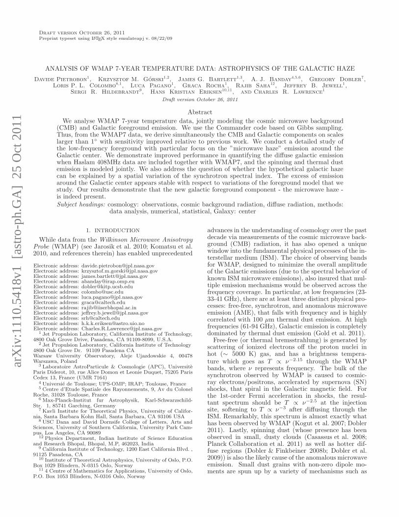
for more realistic foreground modeling, is the use of ex-ternal templates. At very low frequency (< 1 GHz),the observed sky signal is dominated by the synchrotronemission from our Galaxy, and is little contaminated byfree-free emission, at least away from the Galactic plane.A full-sky map of the synchrotron emission is providedby the 408 MHz map of Haslam et al. (1982). The op-tical Hα line is well-known to be a good tracer of thefree-free continuum emission at microwave wavelengths.Finkbeiner (2003) produced a full-sky Hα map as a com-posite of various surveys in both the northern and south-ern hemispheres. Finally, Finkbeiner et al. (1999) pre-dicted the thermal dust contribution at microwave fre-quencies from a series of models based on the COBE -DIRBE 100 and 240 µm maps tied to COBE -FIRASspectral data. We use predicted emission at 94 GHz fromthe preferred model 8 as our reference template for dustemission. These templates, smoothed to 60 arcminutesand downgraded to Nside = 128, are shown in Figure 1.Since the thermal dust contribution to the WMAP
bands is small compared to synchrotron and free-free,we can describe it by means of the FDS template with afixed spectral index β = 1.7, allowing for an overall am-plitude, b. The same can be done for the bremsstrahlungemission, assuming the Hα template as a sufficiently ac-curate description at 23 GHz and rescaling the amplitudeaccording to a power law with index α = −2.15. Thesynchrotron emission is expected to vary across the sky,and the template we have is at 408 MHz, quite a largestretch from the first band of WMAP. A wise choice isto let Commander solve for an amplitude and spectral in-dex at every pixel, choosing 23 GHz as pivot. It shouldbe noted that variations in the gas temperature will be
4
Fig. 1.— Top to bottom, the three templates used to tracesynchrotron (Haslam 408 MHz, top panel), free-free (Hα, mid-dle panel) and dust, both thermal and spinning components (FDS,lower panel).
imprinted onto the synchrotron component, as will devi-ations in the spectrum of thermal dust (which is a muchsmaller contribution).A detailed study of the foreground emission in the fre-
quency range 23-94 GHz employing external templatescan be found in Dickinson et al. (2009b). Notice thatthe value of the spectral index of the dust, 1.7, is some-what dependent on the specific method used to derive it.A direct fit to the predicted dust templates at WMAPfrequencies using the FDS8 model yields a lower value ofβ = 1.55, which is in agreement with what we find whenapplying template fitting procedure to WMAP maps (seeFigure 8). This might be a result of the presence of a lowfrequency spinning dust component.
3. WMAP ANALYSIS
Since previous works on the Haze have heavily reliedon regression against templates, and one of the centraldebates is whether this procedure creates the anomalousemission as a consequence of the assumption of constantspectral behaviour across the sky, we would like to beindependent of external templates. We decided to followan alternative approach: solving a simpler model, wherewe assume two power laws to describe the Galactic emis-
sion. The former is a low frequency component witha falling spectrum to account for synchrotron, free-freeand AME, and the latter is a higher frequency compo-nent with a rising spectrum to represent the thermal dustemission. This appears to be well-motivated in studiesof the WMAP MEM foreground solutions as in Park,Park & Gott (2007). While we can solve for one ampli-tude and spectral index at every pixel at low frequency,where the variability of the signal is larger, we have tofix the dust emissivity at high frequency. We set ǫ = 1.7,consistent with previous applications of the Gibbs sam-pling technique to the WMAP data. The drawback ofthis approach is that the three low frequency physicalemission mechanisms are combined into a single empiri-cal low frequency component, with an averaged value ofthe spectral index that may be inadequate to describethe physical nature of the problem. However, we willattempt to separate these components post-sampling inSection 3.1.
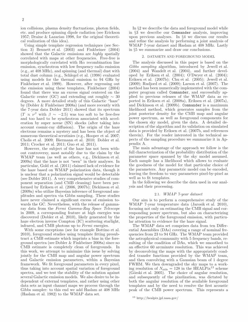
Fig. 2.— CMB Commander posterior average, rms and mean χ2
map. No particular features are present, meaning that the modelis a very good fit to the WMAP 7-year data. The upper limit,20, corresponds to 0.001 probability for a χ2 distribution with 5degrees of freedom.
The Commander result for the CMB map is shown inFigure 2. As a diagnostic, we show the mean χ2 map

5
in the lower panel of Figure 2. The number of pixelswith χ2 > 20, corresponding to the 99.9% confidencelevel for 5 degrees of freedom, is 0.7%. Most of thesepixels lie around point source and we therefore concludethat they correspond to point source bleeding outside themask after convolution with a large beam. The overalllack of feature in the χ2 map is an indication of goodnessof the model we assumed and that the residuals at eachfrequency are compatible with the noise description weprovided.We checked that the Commander power spectrum is con-
sistent with the best estimate provided by the WMAPteam (Larson et al. 2011) at the 1σ level up to ℓ = 200.Beyond that, the Commander solution has significantlymore scatter due to the regularizing noise added to thesmoothed, binned maps (see Sec. 2.1). In addition, whilethe WMAP team also used Gibbs sampling techniquesfor the low multiples, their high ℓ power spectrum wasobtained by applying a quadratic estimator to the cross-spectra of V and W bands. We emphasize though thatthe agreement between the two power spectra belowℓ = 200 is what is important for our purposes sincewe are concentrating on features in the map that aremuch larger than 1◦. The possible presence of a residualmonopole and dipole in the ∆T data has been taken intoaccount and the mean values obtained are displayed inTable 1. They are small and compatible with what foundby Dickinson et al. (2009b) in the WMAP 5-year data,though it is important to keep in mind that monopoleand dipole features become strongly coupled to fore-grounds in CMB analyses, as discussed by Eriksen et al.(2008b).
TABLE 1Mean values of the distribution of monopole and dipole
residuals at every frequency.
K-band Ka-band Q-band V-band W-band23 GHz 33 GHz 41 GHz 61 GHz 94 GHz
M 2.4± 0.9 5.6± 1.0 3.5± 1.1 2.7± 1.0 3.9± 1.0Dx −2.6± 1.2 −3.4± 1.2 −2.7± 1.2 −2.7± 1.2 −3.0± 1.2Dy −3.6± 0.9 −4.3± 0.9 −4.4± 0.9 −3.5± 0.9 −4.0± 0.9Dz 1.9± 0.2 1.9± 0.2 2.4± 0.2 1.8± 0.2 2.0± 0.2
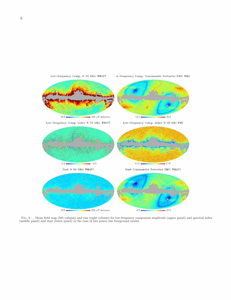
Foreground maps (left column) and associated errors(right column) for low frequency amplitude and spectralindex measured at 23 GHz and the thermal dust contri-bution at 94 GHz are shown in Figure 3.It is clear that our derived low frequency component
represents a combination of multiple emission mecha-nisms, which we now attempt to disentangle. The lowfrequency component shows a strong correlation withthermal dust emission at 94 GHz as modeled by FDS,correlation which is interpreted as signature of spinningdust contribution. The spectral index map, second rowin Figure 3, is particularly informative in this respectsince departures from the prior assumed in Commander,−3.0 ± 0.3 are driven by the data. The mean value athigh Galactic latitudes turns out to be a bit higher thanthe prior (≃ −2.9) as consequence of the superpositionalong the line of sight of multiple components, whose wemeasure an effective spectral behaviour. It is remarkablehow very bright free-free regions show up clearly, requir-
ing a spectral index close to −2.15, which saturates thescale in Figure 4. The visual correlation of these diffusegas clouds with those present in the Hα map is striking.Spectral index values lower than the prior are visible inregions where both synchrotron and dust correlated emis-sion are present, and distinguishing between the two isvery hard.
3.1. Template regression
Following a common approach to the problem (seefor example Dobler & Finkbeiner 2008b; Bottino et al.2010, and references therein), we regress out the am-plitude maps we obtained by using the three templatesshown in Figure 1.Assuming the amplitude map to be a linear combina-
tion of these contributions, the coefficients are computedfrom a χ2 minimization of the form:
χ2 =∑
ν
∑
p
(
Sν(p)−∑
i
AiTi(p))
(2)
N−1ν (p)
(
Sν(p)−∑
i
AiTi(p))
;
Ai :∂χ2
∂Ai
= 0;
∆2Ai =(∂2χ2
∂A2i
)
−1
.
where Ai denotes foreground amplitude of interest; Ti arethe foreground templates and Sν the Commander ampli-tude solution. The explicit expression for the regressionsolution is given by:
Aµi =
∑
j
Tµ−1ij Bµ
j ,
T µij =
∑
p
Ti(p)Tj(p)
N2µ(p)
,
Bµj =
∑
p
Sµi (p)Tj(p)
N2µ(p)
. (3)
T µij and Bµ
j describe the noise weighted correlation be-tween foreground templates and frequency maps andtemplates, respectively. The error ∆Aµ
i is given by√
(2Tµ)−1ii . See also (Fernandez-Cerezo et al. 2006;
Hildebrandt et al. 2007). Since templates are not reli-able in the Galactic plane, the fit is performed outsidethe Kq85 mask, which removes the plane and detectedpoint sources. In addition, the mask covers regions ofhigh dust column density where Hα extinction makes ourfree–free template a poor approximationThe coefficients of the fit are quoted in Table 2 and
the resulting template and residuals in Figures 5 and 6.Differently from the usual regression technique which isapplied to smoothed WMAP maps and then with a smallnoise contamination, we regress out the Commander pos-terior average maps, which are noisy due to the samplingprocedure and we do characterize them by means of theposterior rms, which enters as noise term in Equation 3.Notice that the error we quote and apply is obtained inte-grating the posterior distribution over the other param-eters, indices and component maps, and results larger
6
Fig. 3.— Mean field map (left column) and rms (right column) for low-frequency component amplitude (upper panel) and spectral index(middle panel) and dust (lower panel) in the case of two power law foreground model.

7
Fig. 4.— Full sky spectral index mean field map. The Galac-tic plane shows a strong variation and allows to identify regionswhere one component among synchrotron, free-free and spinningdust dominates.
than the instrumental noise. We also remind the readerthat the input maps we fed to Commander are noisier thanthe simply smoothed ones because we add noise requiredby the sampling algorithm (see Section 2.1). These twofactors increase the errors on the template amplitudes.A detailed investigation is discussed in Appendix B.As expected, the high frequency foreground compo-
nent correlates with the FDS model of thermal dust only.The low-frequency component is mainly a combinationof synchrotron emission and correlated dust, the latterbeing interpreted as spinning dust. This clarifies why,at high Galactic latitudes, we obtain a spectral indexwhich is an effective value along the line-of-sight. No-tice that the contribution of free-free emission is weakbecause the Galactic plane, where it is very bright, hasbeen masked out. To further qualify the goodness-of-fitwe show the scatter plots of the mean field Commander
solution as function of the derived linear template shownin Figure 7.
TABLE 2Regression coefficients of the Commander foreground
amplitude maps. While the thermal dust correlates withthe FDS model only, the low-frequency component is
indeed a mixture of all three templates, synchrotron anddust being the strongest. Moreover, while the thermaldust residuals are featureless and consistent with noise,the low-frequency component residuals show a clear
excess of power around the Galactic center.
WMAP 7-yr
Dataset Haslam Hα FDS rLow Freq. Comp. (3.6± 1.2) × 10−6 6± 6 7± 2 0.94Thermal Dust (0.02± 1.0)× 10−6
−0.6± 5 1.1± 1.8 0.58
Although the correlation is clearly present and followsthe y = x line, looking at the residual map is very in-structive. In the case of dust, the residuals are compat-ible with noise and this explains why the points clusterclose to y = 0 line. The situation is more intriguing forthe low frequency component where the fit is not per-fect and leaves an excess of power in the proximity ofthe Galactic center, the microwave haze, which has beenadvocated to be a distinct contribution. Fainter positiveand negative regions exist as well, perhaps suggesting anoverly-simplistic modeling of the dust component.
Fig. 5.— Low-frequency foreground amplitude maps (top) com-pared to the linear combination of templates (bottom) the differ-ence (i. e. residuals) is shown in the middle panel.
4. FURTHER ANALYSIS
The most troublesome foreground is the dust, boththermal and spinning: outside the Galactic mask ap-plied, the former is not strong at WMAP frequencies,94 GHz being only weakly contaminated; the latter how-ever is poorly characterized and mainly observed throughthe correlation between the lowest WMAP channels andthe FDS dust model, under the assumption that thermaldust traces spinning dust reasonably well. We decided toinclude this correlation in our foreground model. We firstregressed WMAP channels against Haslam, Hα and FDSto obtain a spectral energy distribution for each fore-ground, and then fed the dust SED to Commander, solv-ing for a dust component and a low frequency componentdescribed by a single power law together with the CMB.We recognize that this spinning dust model is extremelysimple and unlikely can capture the full complexity of thedust emission. More complicated models, like spatiallyvarying spinning dust index or multiple component spin-ning dust, although physically motivated, would requirea larger frequency sample to be determined. When moredata will be available the model would have to be refined.
8
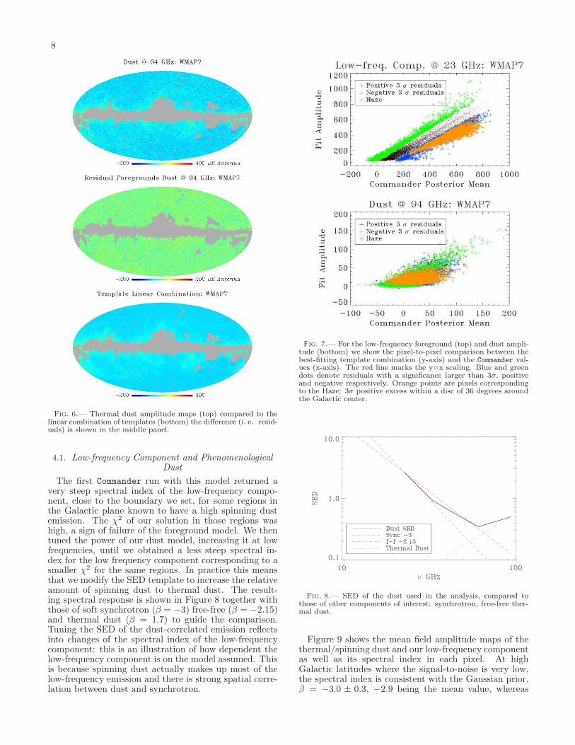
Fig. 6.— Thermal dust amplitude maps (top) compared to thelinear combination of templates (bottom) the difference (i. e. resid-uals) is shown in the middle panel.
4.1. Low-frequency Component and PhenomenologicalDust
The first Commander run with this model returned avery steep spectral index of the low-frequency compo-nent, close to the boundary we set, for some regions inthe Galactic plane known to have a high spinning dustemission. The χ2 of our solution in those regions washigh, a sign of failure of the foreground model. We thentuned the power of our dust model, increasing it at lowfrequencies, until we obtained a less steep spectral in-dex for the low frequency component corresponding to asmaller χ2 for the same regions. In practice this meansthat we modify the SED template to increase the relativeamount of spinning dust to thermal dust. The result-ing spectral response is shown in Figure 8 together withthose of soft synchrotron (β = −3) free-free (β = −2.15)and thermal dust (β = 1.7) to guide the comparison.Tuning the SED of the dust-correlated emission reflectsinto changes of the spectral index of the low-frequencycomponent: this is an illustration of how dependent thelow-frequency component is on the model assumed. Thisis because spinning dust actually makes up most of thelow-frequency emission and there is strong spatial corre-lation between dust and synchrotron.
Fig. 7.— For the low-frequency foreground (top) and dust ampli-tude (bottom) we show the pixel-to-pixel comparison between thebest-fitting template combination (y-axis) and the Commander val-ues (x-axis). The red line marks the y=x scaling. Blue and greendots denote residuals with a significance larger than 3σ, positiveand negative respectively. Orange points are pixels correspondingto the Haze: 3σ positive excess within a disc of 36 degrees aroundthe Galactic center.
Fig. 8.— SED of the dust used in the analysis, compared tothose of other components of interest: synchrotron, free-free ther-mal dust.
Figure 9 shows the mean field amplitude maps of thethermal/spinning dust and our low-frequency componentas well as its spectral index in each pixel. At highGalactic latitudes where the signal-to-noise is very low,the spectral index is consistent with the Gaussian prior,β = −3.0 ± 0.3, −2.9 being the mean value, whereas
9
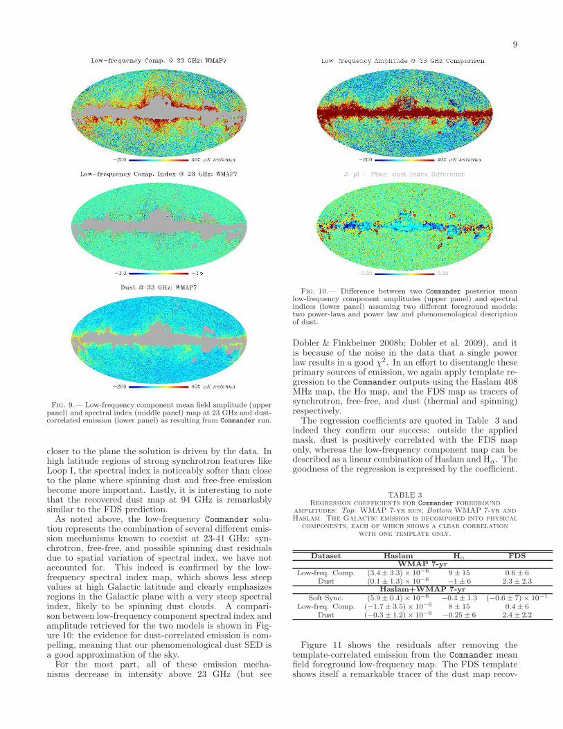
Fig. 9.— Low-frequency component mean field amplitude (upperpanel) and spectral index (middle panel) map at 23 GHz and dust-correlated emission (lower panel) as resulting from Commander run.
closer to the plane the solution is driven by the data. Inhigh latitude regions of strong synchrotron features likeLoop I, the spectral index is noticeably softer than closeto the plane where spinning dust and free-free emissionbecome more important. Lastly, it is interesting to notethat the recovered dust map at 94 GHz is remarkablysimilar to the FDS prediction.As noted above, the low-frequency Commander solu-
tion represents the combination of several different emis-sion mechanisms known to coexist at 23-41 GHz: syn-chrotron, free-free, and possible spinning dust residualsdue to spatial variation of spectral index, we have notaccounted for. This indeed is confirmed by the low-frequency spectral index map, which shows less steepvalues at high Galactic latitude and clearly emphasizesregions in the Galactic plane with a very steep spectralindex, likely to be spinning dust clouds. A compari-son between low-frequency component spectral index andamplitude retrieved for the two models is shown in Fig-ure 10: the evidence for dust-correlated emission is com-pelling, meaning that our phenomenological dust SED isa good approximation of the sky.For the most part, all of these emission mecha-
nisms decrease in intensity above 23 GHz (but see
Fig. 10.— Difference between two Commander posterior meanlow-frequency component amplitudes (upper panel) and spectralindices (lower panel) assuming two different foreground models:two power-laws and power law and phenomenological descriptionof dust.
Dobler & Finkbeiner 2008b; Dobler et al. 2009), and itis because of the noise in the data that a single powerlaw results in a good χ2. In an effort to disentangle theseprimary sources of emission, we again apply template re-gression to the Commander outputs using the Haslam 408MHz map, the Hα map, and the FDS map as tracers ofsynchrotron, free-free, and dust (thermal and spinning)respectively.The regression coefficients are quoted in Table 3 and
indeed they confirm our success: outside the appliedmask, dust is positively correlated with the FDS maponly, whereas the low-frequency component map can bedescribed as a linear combination of Haslam and Hα. Thegoodness of the regression is expressed by the coefficient.
TABLE 3Regression coefficients for Commander foreground
amplitudes: Top: WMAP 7-yr run; Bottom WMAP 7-yr andHaslam. The Galactic emission is decomposed into physical
components, each of which shows a clear correlationwith one template only.
Dataset Haslam Hα FDSWMAP 7-yr
Low-freq. Comp. (3.4± 3.3)× 10−6 9± 15 0.6± 6Dust (0.1± 1.3)× 10−6 −1± 6 2.3± 2.3
Haslam+WMAP 7-yr
Soft Sync. (5.9± 0.4)× 10−6 −0.4± 1.3 (−0.6± 7)× 10−1
Low-freq. Comp. (−1.7± 3.5) × 10−6 8± 15 0.4± 6Dust (−0.3± 1.2) × 10−6 −0.25± 6 2.4± 2.2
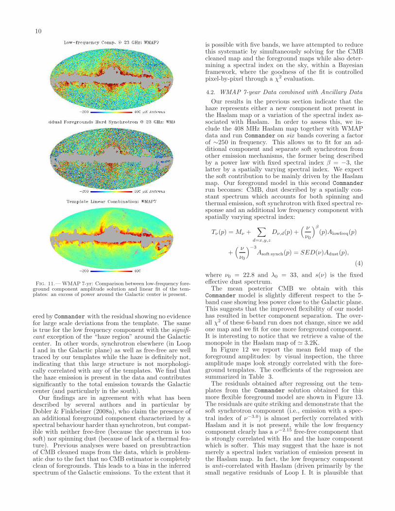
Figure 11 shows the residuals after removing thetemplate-correlated emission from the Commander meanfield foreground low-frequency map. The FDS templateshows itself a remarkable tracer of the dust map recov-
10
Fig. 11.— WMAP 7-yr: Comparison between low-frequency fore-ground component amplitude solution and linear fit of the tem-plates: an excess of power around the Galactic center is present.
ered by Commander with the residual showing no evidencefor large scale deviations from the template. The sameis true for the low frequency component with the signifi-cant exception of the “haze region” around the Galacticcenter. In other words, synchrotron elsewhere (in LoopI and in the Galactic plane) as well as free-free are welltraced by our templates while the haze is definitely not,indicating that this large structure is not morphologi-cally correlated with any of the templates. We find thatthe haze emission is present in the data and contributessignificantly to the total emission towards the Galacticcenter (and particularly in the south).Our findings are in agreement with what has been
described by several authors and in particular byDobler & Finkbeiner (2008a), who claim the presence ofan additional foreground component characterized by aspectral behaviour harder than synchrotron, but compat-ible with neither free-free (because the spectrum is toosoft) nor spinning dust (because of lack of a thermal fea-ture). Previous analyses were based on presubtractionof CMB cleaned maps from the data, which is problem-atic due to the fact that no CMB estimator is completelyclean of foregrounds. This leads to a bias in the inferredspectrum of the Galactic emissions. To the extent that it
is possible with five bands, we have attempted to reducethis systematic by simultaneously solving for the CMBcleaned map and the foreground maps while also deter-mining a spectral index on the sky, within a Bayesianframework, where the goodness of the fit is controlledpixel-by-pixel through a χ2 evaluation.
4.2. WMAP 7-year Data combined with Ancillary Data
Our results in the previous section indicate that thehaze represents either a new component not present inthe Haslam map or a variation of the spectral index as-sociated with Haslam. In order to assess this, we in-clude the 408 MHz Haslam map together with WMAPdata and run Commander on six bands covering a factorof ∼250 in frequency. This allows us to fit for an ad-ditional component and separate soft synchrotron fromother emission mechanisms, the former being describedby a power law with fixed spectral index β = −3, thelatter by a spatially varying spectral index. We expectthe soft contribution to be mainly driven by the Haslammap. Our foreground model in this second Commander
run becomes: CMB, dust described by a spatially con-stant spectrum which accounts for both spinning andthermal emission, soft synchrotron with fixed spectral re-sponse and an additional low frequency component withspatially varying spectral index:
Tν(p) = Mν +∑
d=x,y,z
Dν,d(p) +( ν
ν0
)β
(p)Alowfreq(p)
+( ν
ν0
)
−3
Asoft synch(p) = SED(ν)Adust(p),
(4)
where ν0 = 22.8 and λ0 = 33, and s(ν) is the fixedeffective dust spectrum.The mean posterior CMB we obtain with this
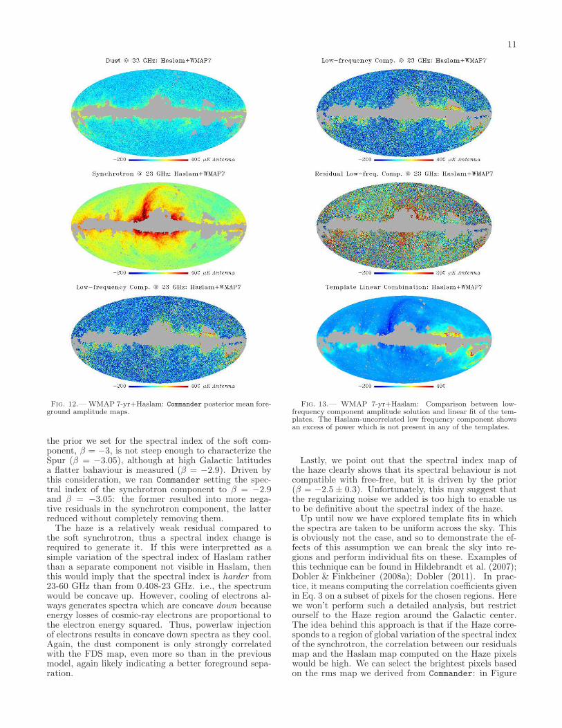
Commander model is slightly different respect to the 5-band case showing less power close to the Galactic plane.This suggests that the improved flexibility of our modelhas resulted in better component separation. The over-all χ2 of these 6-band run does not change, since we addone map and we fit for one more foreground component.It is interesting to notice that we retrieve a value of themonopole in the Haslam map of ≃ 3.2K.In Figure 12 we report the mean field map of the
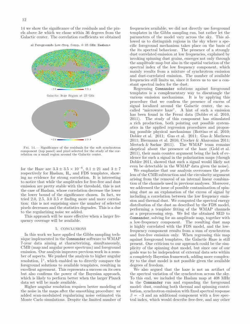
foreground amplitudes: by visual inspection, the threeamplitude maps look strongly correlated with the fore-ground templates. The coefficients of the regression aresummarized in Table 3.The residuals obtained after regressing out the tem-
plates from the Commander solution obtained for thismore flexible foreground model are shown in Figure 13.The residuals are quite striking and demonstrate that thesoft synchrotron component (i.e., emission with a spec-tral index of ν−3.0) is almost perfectly correlated withHaslam and it is not present, while the low frequencycomponent clearly has a ν−2.15 free-free component thatis strongly correlated with Hα and the haze componentwhich is softer. This may suggest that the haze is notmerely a spectral index variation of emission present inthe Haslam map. In fact, the low frequency componentis anti-correlated with Haslam (driven primarily by thesmall negative residuals of Loop I. It is plausible that
11
Fig. 12.— WMAP 7-yr+Haslam: Commander posterior mean fore-ground amplitude maps.
the prior we set for the spectral index of the soft com-ponent, β = −3, is not steep enough to characterize theSpur (β = −3.05), although at high Galactic latitudesa flatter bahaviour is measured (β = −2.9). Driven bythis consideration, we ran Commander setting the spec-tral index of the synchrotron component to β = −2.9and β = −3.05: the former resulted into more nega-tive residuals in the synchrotron component, the latterreduced without completely removing them.The haze is a relatively weak residual compared to
the soft synchrotron, thus a spectral index change isrequired to generate it. If this were interpretted as asimple variation of the spectral index of Haslam ratherthan a separate component not visible in Haslam, thenthis would imply that the spectral index is harder from23-60 GHz than from 0.408-23 GHz. i.e., the spectrumwould be concave up. However, cooling of electrons al-ways generates spectra which are concave down becauseenergy losses of cosmic-ray electrons are proportional tothe electron energy squared. Thus, powerlaw injectionof electrons results in concave down spectra as they cool.Again, the dust component is only strongly correlatedwith the FDS map, even more so than in the previousmodel, again likely indicating a better foreground sepa-ration.
Fig. 13.— WMAP 7-yr+Haslam: Comparison between low-frequency component amplitude solution and linear fit of the tem-plates. The Haslam-uncorrelated low frequency component showsan excess of power which is not present in any of the templates.
Lastly, we point out that the spectral index map ofthe haze clearly shows that its spectral behaviour is notcompatible with free-free, but it is driven by the prior(β = −2.5 ± 0.3). Unfortunately, this may suggest thatthe regularizing noise we added is too high to enable usto be definitive about the spectral index of the haze.Up until now we have explored template fits in which
the spectra are taken to be uniform across the sky. Thisis obviously not the case, and so to demonstrate the ef-fects of this assumption we can break the sky into re-gions and perform individual fits on these. Examples ofthis technique can be found in Hildebrandt et al. (2007);Dobler & Finkbeiner (2008a); Dobler (2011). In prac-tice, it means computing the correlation coefficients givenin Eq. 3 on a subset of pixels for the chosen regions. Herewe won’t perform such a detailed analysis, but restrictourself to the Haze region around the Galactic center.The idea behind this approach is that if the Haze corre-sponds to a region of global variation of the spectral indexof the synchrotron, the correlation between our residualsmap and the Haslam map computed on the Haze pixelswould be high. We can select the brightest pixels basedon the rms map we derived from Commander: in Figure
12
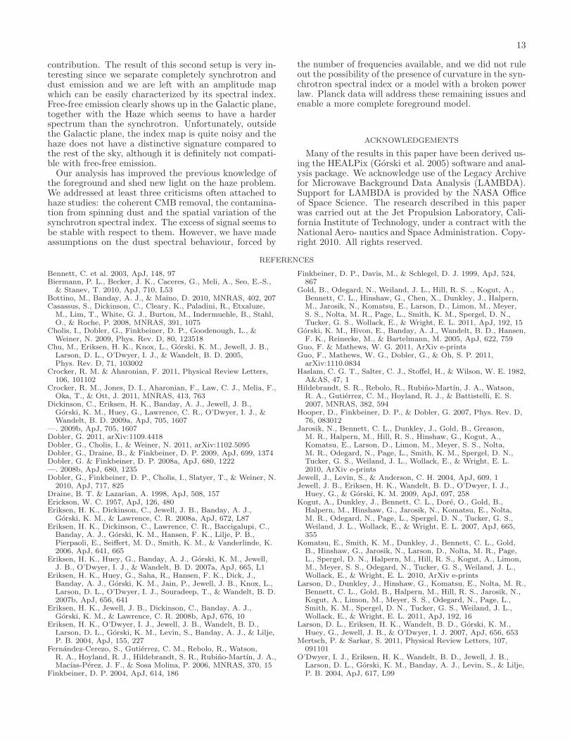
14 we show the significance of the residuals and the pix-els above 3σ which we chose within 36 degrees from theGalactic center. The correlation coefficients we obtained
Fig. 14.— Significance of the residuals for the soft synchrotroncomponent (top panel) and pixel selected for the study of the cor-relation on a small region around the Galactic center.
for the Haze are 3.3 ± 3.5 × 10⁻⁶, 0.1 ± 21 and 3 ± 7respectively for Haslam, Hα and FDS templates, show-ing no evidence for strong correlation. It is interestingto notice that while the amplitudes for free-free and dustemission are pretty stable with the threshold, this is notthe case of Haslam, whose correlation decrease the lowerthe lower bound of the significance chosen. In fact, wetried 2.0, 2.5, 3.0 3.5 σ finding more and more correla-tion: this is not surprising since the number of selectedpixels decreases and the statistics degrades. This is a dueto the regularizing noise we added.This approach will be more effective when a larger fre-
quency coverage will be available.
5. CONCLUSIONS
In this work we have applied the Gibbs sampling tech-nique implemented in the Commander software to WMAP7-year data aiming at characterizing, simultaneously,CMB (map and angular power spectrum) and foregroundemission. Our analysis improves previous work in a num-ber of aspects. We pushed the analysis to higher angularresolution, 1◦, which enabled us to directly compare theforeground solutions to available templates, resulting inexcellent agreement. This represents a success on its ownbut also confirms the power of the Bayesian approach,which is likely to perform better when the larger Planckdata set will be made available.Higher angular resolution requires better modeling of
the noise in the maps after the smoothing procedure: weadded scan-modulated regularizing noise estimated viaMonte Carlo simulations. Despite the limited number of
frequencies available, we did not directly use foregroundtemplates in the Gibbs sampling run, but rather let theparameters of the model vary across the sky. This al-lowed us to distinguish regions in the sky where a spe-cific foreground mechanism takes place on the basis ofthe its spectral behaviour. The presence of a stronglydust correlated emission at low frequencies, explained byinvoking spinning dust grains, emerges not only throughthe amplitude map but also in the spatial variation of thespectral index of the low frequency component, whichmainly results from a mixture of synchrotron emissionand dust-correlated emission. The number of availablefrequencies still limits us, since it forces us to use a con-stant spectral index for the dust.Regressing Commander solutions against foreground
templates is a complementary way to disentangle thevarious emission mechanisms. It is by applying thisprocedure that we confirm the presence of excess ofsignal localized around the Galactic center, the so-called “microwave haze”. A hint of such a emissionhas been found in the Fermi data (Dobler et al. 2010,2011). The study of this component has stimulateda rich production, both pointing out possible system-atics in the applied regression procedures and propos-ing possible physical mechanisms (Bottino et al. 2010;Dobler et al. 2011; Guo et al. 2011; Guo & Mathews2011; Biermann et al. 2010; Crocker & Aharonian 2011;Mertsch & Sarkar 2011). The WMAP team remainsskeptical about the presence of the haze (Gold et al.2011), their main counter argument being the lack of ev-idence for such a signal in the polarization maps (thoughDobler 2011, showed that such a signal would likely noteven be detectable in the WMAP data given the noise).We emphasize that our analysis overcomes the prob-
lem of the CMB subtraction and the circularity argumentarising from the removal of an internal linear combina-tion of the channels used in previous analyses. Moreover,we addressed the issue of possible contamination of spin-ning dust as an explanation of the excess of signal byincluding a correlation between the low frequency emis-sion and thermal dust. We computed the spectral energydistribution of the dust as described by the FDS model,performing a template fitting of the WMAP channelsas a preprocessing step. We fed the obtained SED toCommander, solving for an amplitude map, together witha low-frequency component. The resulting dust mapis highly correlated with the FDS model, and the low-frequency component results from a sum of synchrotronand free-free emission only. When regressing this mapagainst foreground templates, the Galactic Haze is stillpresent. One criticism to our approach could be the sim-plicity of the spinning dust model, but since one of ourgoals was to be independent of external data sets withina completely Bayesian framework, adding more complex-ity to the dust model is not possible given the availabledegrees of freedom.We also argued that the haze is not an artifact of
the spectral variation of the synchrotron across the sky.To this end, we included the Haslam map at 408 MHzin the Commander run and expanding the foregroundmodel: dust, combing both thermal and spinning contri-bution, synchrotron emission with fixed spectral responseβ = −3 and an additional component with a free spec-tral index, which would describe free-free, and any other
13
contribution. The result of this second setup is very in-teresting since we separate completely synchrotron anddust emission and we are left with an amplitude mapwhich can be easily characterized by its spectral index.Free-free emission clearly shows up in the Galactic plane,together with the Haze which seems to have a harderspectrum than the synchrotron. Unfortunately, outsidethe Galactic plane, the index map is quite noisy and thehaze does not have a distinctive signature compared tothe rest of the sky, although it is definitely not compati-ble with free-free emission.Our analysis has improved the previous knowledge of
the foreground and shed new light on the haze problem.We addressed at least three criticisms often attached tohaze studies: the coherent CMB removal, the contamina-tion from spinning dust and the spatial variation of thesynchrotron spectral index. The excess of signal seems tobe stable with respect to them. However, we have madeassumptions on the dust spectral behaviour, forced by
the number of frequencies available, and we did not ruleout the possibility of the presence of curvature in the syn-chrotron spectral index or a model with a broken powerlaw. Planck data will address these remaining issues andenable a more complete foreground model.
ACKNOWLEDGEMENTS
Many of the results in this paper have been derived us-ing the HEALPix (Gorski et al. 2005) software and anal-ysis package. We acknowledge use of the Legacy Archivefor Microwave Background Data Analysis (LAMBDA).Support for LAMBDA is provided by the NASA Officeof Space Science. The research described in this paperwas carried out at the Jet Propulsion Laboratory, Cali-fornia Institute of Technology, under a contract with theNational Aero- nautics and Space Administration. Copy-right 2010. All rights reserved.
REFERENCES
Bennett, C. et al. 2003, ApJ, 148, 97Biermann, P. L., Becker, J. K., Caceres, G., Meli, A., Seo, E.-S.,
& Stanev, T. 2010, ApJ, 710, L53Bottino, M., Banday, A. J., & Maino, D. 2010, MNRAS, 402, 207Casassus, S., Dickinson, C., Cleary, K., Paladini, R., Etxaluze,
M., Lim, T., White, G. J., Burton, M., Indermuehle, B., Stahl,O., & Roche, P. 2008, MNRAS, 391, 1075
Cholis, I., Dobler, G., Finkbeiner, D. P., Goodenough, L., &Weiner, N. 2009, Phys. Rev. D, 80, 123518
Chu, M., Eriksen, H. K., Knox, L., Gorski, K. M., Jewell, J. B.,Larson, D. L., O’Dwyer, I. J., & Wandelt, B. D. 2005,Phys. Rev. D, 71, 103002
Crocker, R. M. & Aharonian, F. 2011, Physical Review Letters,106, 101102
Crocker, R. M., Jones, D. I., Aharonian, F., Law, C. J., Melia, F.,Oka, T., & Ott, J. 2011, MNRAS, 413, 763
Dickinson, C., Eriksen, H. K., Banday, A. J., Jewell, J. B.,Gorski, K. M., Huey, G., Lawrence, C. R., O’Dwyer, I. J., &Wandelt, B. D. 2009a, ApJ, 705, 1607
—. 2009b, ApJ, 705, 1607Dobler, G. 2011, arXiv:1109.4418Dobler, G., Cholis, I., & Weiner, N. 2011, arXiv:1102.5095Dobler, G., Draine, B., & Finkbeiner, D. P. 2009, ApJ, 699, 1374Dobler, G. & Finkbeiner, D. P. 2008a, ApJ, 680, 1222—. 2008b, ApJ, 680, 1235Dobler, G., Finkbeiner, D. P., Cholis, I., Slatyer, T., & Weiner, N.
2010, ApJ, 717, 825Draine, B. T. & Lazarian, A. 1998, ApJ, 508, 157Erickson, W. C. 1957, ApJ, 126, 480Eriksen, H. K., Dickinson, C., Jewell, J. B., Banday, A. J.,
Gorski, K. M., & Lawrence, C. R. 2008a, ApJ, 672, L87Eriksen, H. K., Dickinson, C., Lawrence, C. R., Baccigalupi, C.,
Banday, A. J., Gorski, K. M., Hansen, F. K., Lilje, P. B.,Pierpaoli, E., Seiffert, M. D., Smith, K. M., & Vanderlinde, K.2006, ApJ, 641, 665
Eriksen, H. K., Huey, G., Banday, A. J., Gorski, K. M., Jewell,J. B., O’Dwyer, I. J., & Wandelt, B. D. 2007a, ApJ, 665, L1
Eriksen, H. K., Huey, G., Saha, R., Hansen, F. K., Dick, J.,Banday, A. J., Gorski, K. M., Jain, P., Jewell, J. B., Knox, L.,Larson, D. L., O’Dwyer, I. J., Souradeep, T., & Wandelt, B. D.2007b, ApJ, 656, 641
Eriksen, H. K., Jewell, J. B., Dickinson, C., Banday, A. J.,Gorski, K. M., & Lawrence, C. R. 2008b, ApJ, 676, 10
Eriksen, H. K., O’Dwyer, I. J., Jewell, J. B., Wandelt, B. D.,Larson, D. L., Gorski, K. M., Levin, S., Banday, A. J., & Lilje,P. B. 2004, ApJ, 155, 227
Fernandez-Cerezo, S., Gutierrez, C. M., Rebolo, R., Watson,R. A., Hoyland, R. J., Hildebrandt, S. R., Rubino-Martın, J. A.,Macıas-Perez, J. F., & Sosa Molina, P. 2006, MNRAS, 370, 15
Finkbeiner, D. P. 2004, ApJ, 614, 186
Finkbeiner, D. P., Davis, M., & Schlegel, D. J. 1999, ApJ, 524,867
Gold, B., Odegard, N., Weiland, J. L., Hill, R. S. ., Kogut, A.,Bennett, C. L., Hinshaw, G., Chen, X., Dunkley, J., Halpern,M., Jarosik, N., Komatsu, E., Larson, D., Limon, M., Meyer,S. S., Nolta, M. R., Page, L., Smith, K. M., Spergel, D. N.,Tucker, G. S., Wollack, E., & Wright, E. L. 2011, ApJ, 192, 15
Gorski, K. M., Hivon, E., Banday, A. J., Wandelt, B. D., Hansen,F. K., Reinecke, M., & Bartelmann, M. 2005, ApJ, 622, 759
Guo, F. & Mathews, W. G. 2011, ArXiv e-printsGuo, F., Mathews, W. G., Dobler, G., & Oh, S. P. 2011,
arXiv:1110.0834Haslam, C. G. T., Salter, C. J., Stoffel, H., & Wilson, W. E. 1982,
A&AS, 47, 1Hildebrandt, S. R., Rebolo, R., Rubino-Martın, J. A., Watson,
R. A., Gutierrez, C. M., Hoyland, R. J., & Battistelli, E. S.2007, MNRAS, 382, 594
Hooper, D., Finkbeiner, D. P., & Dobler, G. 2007, Phys. Rev. D,76, 083012
Jarosik, N., Bennett, C. L., Dunkley, J., Gold, B., Greason,M. R., Halpern, M., Hill, R. S., Hinshaw, G., Kogut, A.,Komatsu, E., Larson, D., Limon, M., Meyer, S. S., Nolta,M. R., Odegard, N., Page, L., Smith, K. M., Spergel, D. N.,Tucker, G. S., Weiland, J. L., Wollack, E., & Wright, E. L.2010, ArXiv e-prints
Jewell, J., Levin, S., & Anderson, C. H. 2004, ApJ, 609, 1Jewell, J. B., Eriksen, H. K., Wandelt, B. D., O’Dwyer, I. J.,
Huey, G., & Gorski, K. M. 2009, ApJ, 697, 258Kogut, A., Dunkley, J., Bennett, C. L., Dore, O., Gold, B.,
Halpern, M., Hinshaw, G., Jarosik, N., Komatsu, E., Nolta,M. R., Odegard, N., Page, L., Spergel, D. N., Tucker, G. S.,Weiland, J. L., Wollack, E., & Wright, E. L. 2007, ApJ, 665,355
Komatsu, E., Smith, K. M., Dunkley, J., Bennett, C. L., Gold,B., Hinshaw, G., Jarosik, N., Larson, D., Nolta, M. R., Page,L., Spergel, D. N., Halpern, M., Hill, R. S., Kogut, A., Limon,M., Meyer, S. S., Odegard, N., Tucker, G. S., Weiland, J. L.,Wollack, E., & Wright, E. L. 2010, ArXiv e-prints
Larson, D., Dunkley, J., Hinshaw, G., Komatsu, E., Nolta, M. R.,Bennett, C. L., Gold, B., Halpern, M., Hill, R. S., Jarosik, N.,Kogut, A., Limon, M., Meyer, S. S., Odegard, N., Page, L.,Smith, K. M., Spergel, D. N., Tucker, G. S., Weiland, J. L.,Wollack, E., & Wright, E. L. 2011, ApJ, 192, 16
Larson, D. L., Eriksen, H. K., Wandelt, B. D., Gorski, K. M.,Huey, G., Jewell, J. B., & O’Dwyer, I. J. 2007, ApJ, 656, 653
Mertsch, P. & Sarkar, S. 2011, Physical Review Letters, 107,091101
O’Dwyer, I. J., Eriksen, H. K., Wandelt, B. D., Jewell, J. B.,Larson, D. L., Gorski, K. M., Banday, A. J., Levin, S., & Lilje,P. B. 2004, ApJ, 617, L99
14
Planck Collaboration, Ade, P. A. R., Aghanim, N., Arnaud, M.,Ashdown, M., Aumont, J., Baccigalupi, C., Balbi, A., Banday,A. J., Barreiro, R. B., & et al. 2011, ArXiv e-prints
Rudjord, Ø., Groeneboom, N. E., Eriksen, H. K., Huey, G.,Gorski, K. M., & Jewell, J. B. 2009, ApJ, 692, 1669
Schlegel, D. J., Finkbeiner, D. P., & Davis, M. 1998, ApJ, 500,525
Wandelt, B. D., Larson, D. L., & Lakshminarayanan, A. 2004,Phys. Rev. D, 70, 083511
APPENDIX
THE CMB MAP AND POWER SPECTRUM POSTERIOR
Here we review the basic concept behind Gibbs sampling. Let us first focus on the case of one frequency map andno foregrounds. The data model for this case is
d = s+ n, (A1)
where d is the data, s the CMB sky signal, and n instrumental noise. We assume both the CMB signal and noise tobe Gaussian random fields with vanishing mean and covariance matrices S and N, respectively. The CMB sky can bewritten in spherical harmonics as s =
∑
ℓ,m aℓmYℓm, with the CMB covariance matrix then fully characterized by the
angular power spectrum Cℓ according to Cℓm,ℓ′m′ = 〈a∗ℓmaℓ′m′〉 = Cℓδℓℓ′δmm′ . The noise matrix N is left unspecifiedfor now, but we note that for white noise it is diagonal in pixel space, Nij = σ2
i δij , for pixels i and j and noise varianceσ2i .Our goal is to sample from the posterior density for both the sky signal s and the power spectrum Cℓ, given by
P (s, Cℓ|d) ∝ P (d|s, Cℓ)P (s, Cℓ) (A2)
∝ P (d|s, Cℓ)P (s|Cℓ)P (Cℓ), (A3)
In what follows we assume the prior P (Cℓ) is uniform. Since we have assumed Gaussianity, the joint posteriordistribution may be written as
P (s, Cℓ|d) ∝ e−12(d−s)tN−1(d−s)
∏
ℓ
e−
2ℓ+1
2
σℓ
Cℓ
C2ℓ+1
2
ℓ
P (Cℓ), (A4)
where we have defined the quantity σℓ ≡1
2ℓ+1
∑ℓ
m=−ℓ |aℓm|2 as the angular power spectrum of the full-sky CMB
signal.For the case here with the CMB signal assumed to be a Gaussian field, one can integrate over the CMB sky signal
and analytically solve for the marginalized posterior P (Cℓ|d). However, evaluating the posterior numerically for anyspecific angular power spectrum is computationally prohibitive as it involves the computation of the inverse anddeterminant of very large matrices. We therefore sample from the posterior using a Gibbs sampling algorithm.
Gibbs Sampling
One procedure to sample from the joint density P (s, Cℓ|d), as proposed by Jewell et al. (2004) and Wandelt et al.(2004), is to alternately sample from the respective conditional densities
si+1 ← P (s|Ciℓ,d) (A5)
Ci+1ℓ ← P (Cℓ|s
i+1,d). (A6)
Here← indicates sampling from the distribution on the right-hand side. After some “burn-in” period, the joint samples(si, Ci
ℓ) will be distributed from the joint posterior. Thus, the problem is reduced to that of sampling from the twoconditional densities P (s|Cℓ,d) and P (Cℓ|s,d).The conditional density P (Cℓ|s,d) in this case is independent of the data, P (Cℓ|s,d) = P (Cℓ|s), simply because the
underlying CMB sky signal provides all the information needed to estimate the ensemble angular power spectrum Cℓ.Under the assumption of Gaussianity and isotropy, this conditional is given by the inverse Gamma distribution, Sℓ:
P (Cℓ|s) ∝e−
12st
ℓS
−1
ℓsℓ
√
|Sℓ|=
e−
2ℓ+1
2
σℓ
Cℓ
C2ℓ+1
2
ℓ
. (A7)
In order to sample from this conditional density we first draw 2ℓ − 1 normal random variates ρkℓ , compute the sum
ρ2ℓ =∑2ℓ−1
k=1 |ρkℓ |
2, and finally set
Cℓ =σℓ
ρ2ℓ, (A8)
giving a sample distributed according to the inverse Gamma distribution.
15
The conditional density for the sky map given the angular power spectrum and data follows directly from the formof the joint Bayes posterior in Equation A4, and given by
P (s|Cℓ,d) ∝ P (d|s, Cℓ)P (s|Cℓ) (A9)
∝ e−12(d−s)tN−1(d−s) e−
12stS
−1s (A10)
∝ e−12(s−s)t(S−1+N
−1)(s−s), (A11)
where we have defined the so-called mean-field map (or Wiener filtered data) s = (S−1 + N−1)−1N−1d. Thus,P (s|Cℓ,d) is a Gaussian distribution with mean equal to s and a covariance matrix equal to (S−1 +N−1)−1. In orderto sample from this conditional, we first generate two independent white noise maps ω0 and ω1, and solve
[
S−1 +N−1]
s = N−1d+ S−12ω0 +N−
12ω1, (A12)
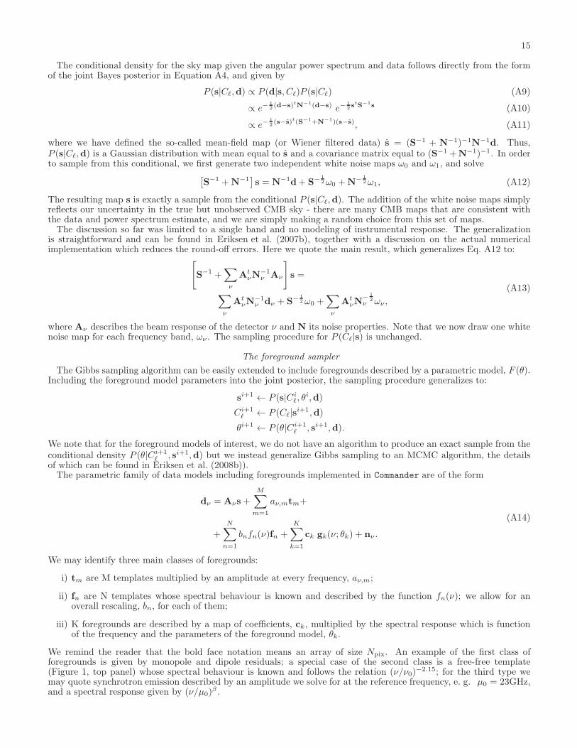
The resulting map s is exactly a sample from the conditional P (s|Cℓ,d). The addition of the white noise maps simplyreflects our uncertainty in the true but unobserved CMB sky - there are many CMB maps that are consistent withthe data and power spectrum estimate, and we are simply making a random choice from this set of maps.The discussion so far was limited to a single band and no modeling of instrumental response. The generalization
is straightforward and can be found in Eriksen et al. (2007b), together with a discussion on the actual numericalimplementation which reduces the round-off errors. Here we quote the main result, which generalizes Eq. A12 to:
[
S−1 +∑
ν
AtνN
−1ν Aν
]
s =
∑
ν
AtνN
−1ν dν + S−
12ω0 +
∑
ν
AtνN
−12
ν ων ,
(A13)
where Aν describes the beam response of the detector ν and N its noise properties. Note that we now draw one whitenoise map for each frequency band, ων . The sampling procedure for P (Cℓ|s) is unchanged.
The foreground sampler
The Gibbs sampling algorithm can be easily extended to include foregrounds described by a parametric model, F (θ).Including the foreground model parameters into the joint posterior, the sampling procedure generalizes to:
si+1 ← P (s|Ciℓ, θ
i,d)
Ci+1ℓ ← P (Cℓ|s
i+1,d)
θi+1 ← P (θ|Ci+1ℓ , si+1,d).
We note that for the foreground models of interest, we do not have an algorithm to produce an exact sample from theconditional density P (θ|Ci+1
ℓ , si+1,d) but we instead generalize Gibbs sampling to an MCMC algorithm, the detailsof which can be found in Eriksen et al. (2008b)).The parametric family of data models including foregrounds implemented in Commander are of the form
dν = Aνs+M∑
m=1
aν,mtm+
+
N∑
n=1
bnfn(ν)fn +
K∑
k=1
ck gk(ν; θk) + nν .
(A14)
We may identify three main classes of foregrounds:
i) tm are M templates multiplied by an amplitude at every frequency, aν,m;
ii) fn are N templates whose spectral behaviour is known and described by the function fn(ν); we allow for anoverall rescaling, bn, for each of them;
iii) K foregrounds are described by a map of coefficients, ck, multiplied by the spectral response which is functionof the frequency and the parameters of the foreground model, θk.
We remind the reader that the bold face notation means an array of size Npix. An example of the first class offoregrounds is given by monopole and dipole residuals; a special case of the second class is a free-free template(Figure 1, top panel) whose spectral behaviour is known and follows the relation (ν/ν0)
−2.15; for the third type wemay quote synchrotron emission described by an amplitude we solve for at the reference frequency, e. g. µ0 = 23GHz,and a spectral response given by (ν/µ0)
β .
16
It is instructive to compute the degrees of freedom for such a foreground model applied to WMAP data. We solvethree maps, s, β and Asynch, 5 monopoles and dipoles, and two overall amplitudes if we describe free-free emission andthermal dust by means of the second class of foreground models. In total we look for 3Npix + 22 parameters. This isalready pretty close to the maximum number of parameters allowed by the WMAP, ≤ 5Npix. We could ask for onemore map, either dust or free-free, assuming a single power law and fixing the spectral index, or allowing a curvatureterm in the synchrotron model. Since a simple power law for thermal dust and free-free emission has been shown tobe consistent with the data in the frequency range spanned by WMAP (Dickinson et al. 2009b), this may be used todisentangle the spinning dust contribution from thermal dust.We notice that to solve for the spectral index of a given component, the instrumental beam response of each channel
must be taken into account. Up to now, Commander is able to work with maps at the same angular resolution only.Smoothing all frequency maps and ancillary data to a common angular scale is then a necessary pre-processing step.As discussed in Eriksen et al. (2008b), it turns out to be more efficient to sample all the map amplitudes at once,
followed by the spectral response parameter, and finally the angular power spectrum, following the iterative scheme:
{si+1, am, bn, ck}i+1 ← P (s, am, bn, ck|C
iℓ, θ
i,d)
θi+1 ← P (θ|Ciℓ , s
i+1, ai+1m , bi+1
n , ci+1k ,d)
Ci+1ℓ ← P (Cℓ|s
i+1,d). (A15)
Sampling from the conditional density P (s, am, bn, ck|Ciℓ, θ
i,d) is a generalization of Eq. A13, whereas the samplingof the angular power spectrum remains unchanged, since Cℓ are functions of the sky signal only. Sampling of the non-linear degrees of freedom is through a standard inversion sampler: first compute the conditional probability densityP (x|θ), where x is the currently sampled parameter and θ denotes the set of all other parameters in the model, assumingthe likelihood to be independent pixel by pixel: −2lnL(x) = χ2 =
∑
ν(dν − sν(X, θ))2/σ2ν . Then, the corresponding
cumulative distribution is computed, F (x|θ) =∫ x
−∞P (y|θ)dy, and the value of the x variable is chosen by drawing a
uniformly distributed random number, u, and reading F (x|θ) = u.This concludes the review on the implementation of Gibbs sampling as implemented in the computer code Commander.
NOISE IMPACT ON THE REGRESSION PROCEDURE
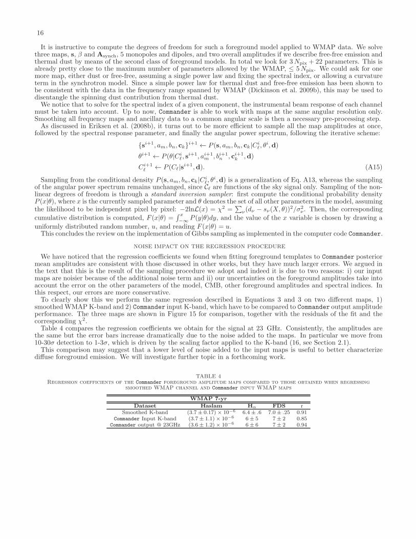
We have noticed that the regression coefficients we found when fitting foreground templates to Commander posteriormean amplitudes are consistent with those discussed in other works, but they have much larger errors. We argued inthe text that this is the result of the sampling procedure we adopt and indeed it is due to two reasons: i) our inputmaps are noisier because of the additional noise term and ii) our uncertainties on the foreground amplitudes take intoaccount the error on the other parameters of the model, CMB, other foreground amplitudes and spectral indices. Inthis respect, our errors are more conservative.To clearly show this we perform the same regression described in Equations 3 and 3 on two different maps, 1)
smoothedWMAP K-band and 2) Commander input K-band, which have to be compared to Commander output amplitudeperformance. The three maps are shown in Figure 15 for comparison, together with the residuals of the fit and thecorresponding χ2.Table 4 compares the regression coefficients we obtain for the signal at 23 GHz. Consistently, the amplitudes are
the same but the error bars increase dramatically due to the noise added to the maps. In particular we move from10-30σ detection to 1-3σ, which is driven by the scaling factor applied to the K-band (16, see Section 2.1).This comparison may suggest that a lower level of noise added to the input maps is useful to better characterize
diffuse foreground emission. We will investigate further topic in a forthcoming work.
TABLE 4Regression coefficients of the Commander foreground amplitude maps compared to those obtained when regressing
smoothed WMAP channel and Commander input WMAP maps
WMAP 7-yr
Dataset Haslam Hα FDS rSmoothed K-band (3.7± 0.17) × 10−6 6.4± .6 7.0± .25 0.91
Commander Input K-band (3.7± 1.1)× 10−6 6± 5 7± 2 0.85Commander output @ 23GHz (3.6± 1.2)× 10−6 6± 6 7± 2 0.94
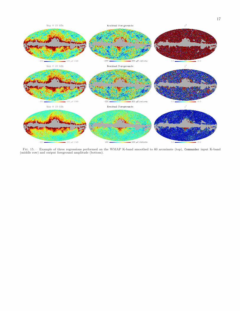
17
Fig. 15.— Example of three regressions performed on the WMAP K-band smoothed to 60 arcminute (top), Commander input K-band(middle row) and output foreground amplitude (bottom).


