Embed Size (px)
Citation preview

UNIVERSITY OF BIRMINGHAM
Multimodal Intent Recognition for Natural
Human-Robotic Interaction
by
James Rossiter
A thesis submitted for the
degree of Doctor of Philosophy
School of Electronic, Electrical and Computer Engineering
March 2011

University of Birmingham Research Archive
e-theses repository This unpublished thesis/dissertation is copyright of the author and/or third parties. The intellectual property rights of the author or third parties in respect of this work are as defined by The Copyright Designs and Patents Act 1988 or as modified by any successor legislation. Any use made of information contained in this thesis/dissertation must be in accordance with that legislation and must be properly acknowledged. Further distribution or reproduction in any format is prohibited without the permission of the copyright holder.

Abstract
The research questions posed for this work were as follows:
• Can speech recognition and techniques for topic spotting be used to identify spoken intent
in unconstrained natural speech?
• Can gesture recognition systems based on statistical speech recognition techniques be used
to bridge the gap between physical movements and recognition of gestural intent?
• How can speech and gesture be combined to identify the overall communicative intent of
a participant with better accuracy than recognisers built for individual modalities?
In order to answer these questions a corpus collection experiment for Human-Robotic Inter-
action was designed to record unconstrained natural speech and 3 dimensional motion data
from 17 different participants. A speech recognition system was built based on the popular
Hidden Markov Model Toolkit and a topic spotting algorithm based on usefulness measures
was designed. These were combined to create a speech intent recognition system capable of
identifying intent given natural unconstrained speech. A gesture intent recogniser was built
using the Hidden Markov Model Toolkit to identify intent directly from 3D motion data.
Both the speech and gesture intent recognition systems were evaluated separately. The out-
put from both systems were then combined and this integrated intent recogniser was shown to
perform better than each recogniser separately. Both linear and non-linear methods of multi-
modal intent fusion were evaluated and the same techniques were applied to the output from
individual intent recognisers. In all cases the non-linear combination of intent gave the highest
performance for all intent recognition systems.
Combination of speech and gestural intent scores gave a maximum classification performance
of 76.7% of intents correctly classified using a two layer Multi-Layer Perceptron for non-linear
fusion with human transcribed speech input to the speech classifier. When compared to simply
picking the highest scoring single modality intent, this represents an improvement of 177.9% over
gestural intent classification, 67.5% over a human transcription of speech based speech intent
classifier and 204.4% over an automatically recognised speech based speech intent classifier.

Acknowledgements
Many thanks are due to my supervisor Martin Russell, who has been instrumental in building
a cohesive thesis and answering my many questions throughout the period of my research.
Thanks to EPSRC for funding my first three years of research and the team at the Centre
for Learning, Innovation & Collaboration at the University of Birmingham for allowing me
to continue work on interesting research projects whilst completing the thesis. Many of my
colleagues at the University of Birmingham also provided encouragement and support. Thanks
especially to Paul.
Thanks also to my parents, Judith and Brian Rossiter, who have been incredibly supportive
especially during difficult periods.
Finally many thanks to my girlfriend, Sarah Leslie, who helped massively during every stage of
this work.
ii
Contents
Abstract i
Acknowledgements ii
List of Figures viii
List of Tables xiii
Abbreviations xvii
1 Introduction 1
1.1 Objective . . . . . . . . . . . . . . . . . . . . . . . . . . . . . . . . . . . . . . . . 1
1.2 Definition of Intent in This Work . . . . . . . . . . . . . . . . . . . . . . . . . . . 2
1.3 Speech Intent . . . . . . . . . . . . . . . . . . . . . . . . . . . . . . . . . . . . . . 3
1.4 Gestural Intent . . . . . . . . . . . . . . . . . . . . . . . . . . . . . . . . . . . . . 4
1.5 Combination of Modalities . . . . . . . . . . . . . . . . . . . . . . . . . . . . . . . 4
1.6 Research Questions . . . . . . . . . . . . . . . . . . . . . . . . . . . . . . . . . . . 5
1.7 Contributions . . . . . . . . . . . . . . . . . . . . . . . . . . . . . . . . . . . . . . 5
1.8 Thesis Structure . . . . . . . . . . . . . . . . . . . . . . . . . . . . . . . . . . . . 6
2 On Speech and Gesture Recognition and Combination 7
2.1 Introduction . . . . . . . . . . . . . . . . . . . . . . . . . . . . . . . . . . . . . . . 7
2.2 Speech Recognition Development . . . . . . . . . . . . . . . . . . . . . . . . . . . 8
2.2.1 Early Speech Recognition Engines . . . . . . . . . . . . . . . . . . . . . . 9
2.2.2 The 1970s . . . . . . . . . . . . . . . . . . . . . . . . . . . . . . . . . . . . 11
2.2.2.1 The ARPA Speech Understanding Project . . . . . . . . . . . . 12
2.2.3 Dynamic Programming Techniques . . . . . . . . . . . . . . . . . . . . . . 14
2.2.4 The 1980s and Growing Use of Hidden Markov Models . . . . . . . . . . . 15
2.3 Gesture and Multimodal Recognition Development . . . . . . . . . . . . . . . . . 20
2.3.1 Input Methods . . . . . . . . . . . . . . . . . . . . . . . . . . . . . . . . . 22
2.3.2 Gesture Modelling and Recognition techniques . . . . . . . . . . . . . . . 24
2.3.2.1 Inferring Communicative Intent From Raw Motion Data . . . . 24
2.3.2.2 Gesture Modelling Techniques . . . . . . . . . . . . . . . . . . . 26
2.3.3 Multimodal Data Fusion . . . . . . . . . . . . . . . . . . . . . . . . . . . . 27
2.4 Summary . . . . . . . . . . . . . . . . . . . . . . . . . . . . . . . . . . . . . . . . 28
3 A Corpus of Natural Speech and Gesture 30
iii

Contents iv
3.1 Introduction . . . . . . . . . . . . . . . . . . . . . . . . . . . . . . . . . . . . . . . 30
3.2 Apparatus Used in Corpus Collection . . . . . . . . . . . . . . . . . . . . . . . . . 31
3.2.1 The Sony AIBO Robot . . . . . . . . . . . . . . . . . . . . . . . . . . . . 32
3.2.1.1 AIBO Controlling Software . . . . . . . . . . . . . . . . . . . . . 33
3.2.2 Three Dimensional motion data capture . . . . . . . . . . . . . . . . . . . 35
3.2.2.1 A Prototype Stereoscopic Vision System for Movement Capture 36
3.2.2.2 Limitations of the Prototype System . . . . . . . . . . . . . . . . 38
3.2.2.3 The Qualisys Full Body Movement Capture System . . . . . . . 39
3.2.2.4 Error Handling . . . . . . . . . . . . . . . . . . . . . . . . . . . . 43
3.2.3 Speech Recording . . . . . . . . . . . . . . . . . . . . . . . . . . . . . . . . 45
3.2.4 Synchronisation of Speech and Gesture Recordings . . . . . . . . . . . . . 46
3.2.5 The AIBO Map and Routes . . . . . . . . . . . . . . . . . . . . . . . . . . 47
3.3 Experimental Procedure for Corpus Collection . . . . . . . . . . . . . . . . . . . 49
3.3.1 Initial Exploratory Experiment . . . . . . . . . . . . . . . . . . . . . . . . 49
3.3.2 Corpus Collection Experiment . . . . . . . . . . . . . . . . . . . . . . . . 51
3.4 Corpus Size . . . . . . . . . . . . . . . . . . . . . . . . . . . . . . . . . . . . . . . 53
3.5 An Overview of Participant Strategy . . . . . . . . . . . . . . . . . . . . . . . . . 54
3.6 Summary . . . . . . . . . . . . . . . . . . . . . . . . . . . . . . . . . . . . . . . . 56
4 Annotation Conventions 58
4.1 Introduction . . . . . . . . . . . . . . . . . . . . . . . . . . . . . . . . . . . . . . . 58
4.2 Choice of labels . . . . . . . . . . . . . . . . . . . . . . . . . . . . . . . . . . . . . 59
4.3 Overview of HTK Label Formats . . . . . . . . . . . . . . . . . . . . . . . . . . . 62
4.4 Aligning Speech and Gesture . . . . . . . . . . . . . . . . . . . . . . . . . . . . . 63
4.5 Speech Word Label Creation and Alignment of Speech Labels Using HTK . . . . 64
4.6 Multiple Transcribers Speech Intent Task to Produce Final Speech Intent Labels 65
4.7 Gesture Labelling . . . . . . . . . . . . . . . . . . . . . . . . . . . . . . . . . . . . 69
4.8 Merging Intent Labels to Produce a Final Label Set . . . . . . . . . . . . . . . . 70
4.9 Comparing Consistency Between Speech and Gesture Labels . . . . . . . . . . . 72
4.10 Summary . . . . . . . . . . . . . . . . . . . . . . . . . . . . . . . . . . . . . . . . 73
5 Hidden Markov Model Theory 75
5.1 Introduction . . . . . . . . . . . . . . . . . . . . . . . . . . . . . . . . . . . . . . . 75
5.2 Language Modelling . . . . . . . . . . . . . . . . . . . . . . . . . . . . . . . . . . 76
5.2.1 Word Networks . . . . . . . . . . . . . . . . . . . . . . . . . . . . . . . . . 77
5.2.2 Dictionaries . . . . . . . . . . . . . . . . . . . . . . . . . . . . . . . . . . . 78
5.3 Components of a Hidden Markov Model . . . . . . . . . . . . . . . . . . . . . . . 79
5.3.1 Gaussian Mixtures . . . . . . . . . . . . . . . . . . . . . . . . . . . . . . . 80
5.3.2 Training Gaussian Mixture Models . . . . . . . . . . . . . . . . . . . . . . 81
5.3.3 Hidden Markov Models . . . . . . . . . . . . . . . . . . . . . . . . . . . . 83
5.4 Recognition using Hidden Markov Models . . . . . . . . . . . . . . . . . . . . . . 85
5.5 Training Hidden Markov Models . . . . . . . . . . . . . . . . . . . . . . . . . . . 87
5.6 Adaptation of Models . . . . . . . . . . . . . . . . . . . . . . . . . . . . . . . . . 90
5.6.1 Maximum A Posteriori (MAP) Adaptation . . . . . . . . . . . . . . . . . 90
5.6.2 Maximum Likelihood Linear Regression (MLLR) . . . . . . . . . . . . . . 91
5.7 Tied State Models . . . . . . . . . . . . . . . . . . . . . . . . . . . . . . . . . . . 92
5.8 Context Dependency of Models . . . . . . . . . . . . . . . . . . . . . . . . . . . . 93
Contents v
5.9 Summary . . . . . . . . . . . . . . . . . . . . . . . . . . . . . . . . . . . . . . . . 94
6 Speech and Speech Based Intent Recognition 95
6.1 Introduction . . . . . . . . . . . . . . . . . . . . . . . . . . . . . . . . . . . . . . . 95
6.2 Front End Processing of Speech . . . . . . . . . . . . . . . . . . . . . . . . . . . . 97
6.2.1 Mel-Scale Filterbank Analysis for MFCC Production . . . . . . . . . . . . 97
6.2.1.1 Modelling Dynamic Information in MFCCs . . . . . . . . . . . . 100
6.3 Building a HMM Based Speech Recogniser Using the Hidden Markov Model Toolkit101
6.3.1 Training Corpora . . . . . . . . . . . . . . . . . . . . . . . . . . . . . . . . 101
6.3.2 Front End Processing . . . . . . . . . . . . . . . . . . . . . . . . . . . . . 102
6.3.3 Producing Acoustic Models . . . . . . . . . . . . . . . . . . . . . . . . . . 103
6.3.3.1 Monophones . . . . . . . . . . . . . . . . . . . . . . . . . . . . . 103
6.3.3.2 Tied State Triphones . . . . . . . . . . . . . . . . . . . . . . . . 103
6.3.3.3 Acoustic Adaptation . . . . . . . . . . . . . . . . . . . . . . . . . 103
6.3.3.4 Addition of AIBO Noise Model . . . . . . . . . . . . . . . . . . . 104
6.3.4 Language Model . . . . . . . . . . . . . . . . . . . . . . . . . . . . . . . . 104
6.3.5 Producing Time Aligned Correct Transcriptions . . . . . . . . . . . . . . 104
6.3.6 Producing Automatically Recognised Speech Transcriptions . . . . . . . . 105
6.4 Usefulness as an Indication of Intent . . . . . . . . . . . . . . . . . . . . . . . . . 106
6.4.1 Applying Usefulness to Classify Speech Intent . . . . . . . . . . . . . . . . 110
6.5 Summary . . . . . . . . . . . . . . . . . . . . . . . . . . . . . . . . . . . . . . . . 112
7 Gestural Intent Recognition 114
7.1 Introduction . . . . . . . . . . . . . . . . . . . . . . . . . . . . . . . . . . . . . . . 114
7.2 Data Formats . . . . . . . . . . . . . . . . . . . . . . . . . . . . . . . . . . . . . . 114
7.3 Hidden Markov Models For Intent Recognition . . . . . . . . . . . . . . . . . . . 115
7.3.1 Front End Processing . . . . . . . . . . . . . . . . . . . . . . . . . . . . . 115
7.3.2 Producing Models of Gestural Intent . . . . . . . . . . . . . . . . . . . . . 116
7.4 Gestural Intent Classification Using HTK . . . . . . . . . . . . . . . . . . . . . . 116
7.4.1 Intent Classes and Intent Transcriptions . . . . . . . . . . . . . . . . . . . 117
7.4.2 Models Produced for Gestural Intent Classification . . . . . . . . . . . . . 118
7.4.3 Results . . . . . . . . . . . . . . . . . . . . . . . . . . . . . . . . . . . . . 123
7.4.3.1 Classification Results Discussion . . . . . . . . . . . . . . . . . . 126
7.4.3.2 Classification Results Conclusions . . . . . . . . . . . . . . . . . 128
7.5 Continuous Recognition of Gestural Intent Using HTK . . . . . . . . . . . . . . . 129
7.5.1 Continuous Recognition Results Discussion . . . . . . . . . . . . . . . . . 133
7.5.2 Continuous Recognition Results Conclusions . . . . . . . . . . . . . . . . 137
7.5.3 Varying Insertion Penalty During Continuous Recognition . . . . . . . . . 137
7.5.3.1 Varying Insertion Penalty Discussion . . . . . . . . . . . . . . . 146
7.5.3.2 Varying Insertion Penalty Conclusions . . . . . . . . . . . . . . . 148
7.6 Reducing Dimensionality of Models Using Principal Component Analysis . . . . 148
7.6.1 Overview of Principal Component Analysis . . . . . . . . . . . . . . . . . 148
7.6.2 Principal Component Analysis as a Measure of Gesture Complexity . . . 151
7.6.3 Application of PCA to Continuous Gestural Intent Recognition . . . . . . 154
7.6.3.1 Application of PCA to Continuous Gestural Intent RecognitionDiscussion . . . . . . . . . . . . . . . . . . . . . . . . . . . . . . 157

Contents vi
7.6.3.2 Application of PCA to Continuous Gestural Intent RecognitionConclusions . . . . . . . . . . . . . . . . . . . . . . . . . . . . . . 158
7.6.4 Application of PCA and Varying Insertion Penalty for Continuous Ges-tural Intent Recognition . . . . . . . . . . . . . . . . . . . . . . . . . . . . 158
7.6.4.1 Application of PCA and Varying Insertion Penalty for Continu-ous Gestural Intent Recognition Discussion . . . . . . . . . . . . 161
7.6.4.2 Application of PCA and Varying Insertion Penalty for Continu-ous Gestural Intent Recognition Conclusions . . . . . . . . . . . 162
7.6.5 Application of PCA to Gestural Intent Classification . . . . . . . . . . . . 162
7.6.5.1 Application of PCA to Gestural Intent Classification Discussion 165
7.6.5.2 Application of PCA to Gestural Intent Classification Conclusions 166
7.6.6 Principal Component Analysis Conclusions . . . . . . . . . . . . . . . . . 166
7.7 Conclusions . . . . . . . . . . . . . . . . . . . . . . . . . . . . . . . . . . . . . . . 167
8 Combined, Multimodal Intent Classification 170
8.1 Introduction . . . . . . . . . . . . . . . . . . . . . . . . . . . . . . . . . . . . . . . 170
8.2 Score Combination for Multimodal Fusion . . . . . . . . . . . . . . . . . . . . . . 171
8.3 Linear Combination . . . . . . . . . . . . . . . . . . . . . . . . . . . . . . . . . . 172
8.4 Non-Linear Combination Using Artificial Neural Networks . . . . . . . . . . . . . 174
8.4.1 The Multi-Layer Perceptron . . . . . . . . . . . . . . . . . . . . . . . . . . 174
8.4.1.1 Multi-Layer Perceptron Training Methods . . . . . . . . . . . . . 176
8.4.1.2 Evaluation of Non-Linear Methods on Collected Corpus . . . . . 179
8.5 Results . . . . . . . . . . . . . . . . . . . . . . . . . . . . . . . . . . . . . . . . . . 180
8.5.1 Linear Combination Classification Results . . . . . . . . . . . . . . . . . . 181
8.5.2 Linear Combination Classification Discussion . . . . . . . . . . . . . . . . 183
8.5.3 Linear Combination Classification Conclusions . . . . . . . . . . . . . . . 188
8.5.4 Non-Linear Combination Classification Results . . . . . . . . . . . . . . . 189
8.5.5 Non-Linear Combination Classification Discussion . . . . . . . . . . . . . 191
8.5.6 Non-Linear Combination Classification Conclusions . . . . . . . . . . . . . 194
8.6 Conclusions . . . . . . . . . . . . . . . . . . . . . . . . . . . . . . . . . . . . . . . 194
9 Conclusions 198
9.1 Contributions . . . . . . . . . . . . . . . . . . . . . . . . . . . . . . . . . . . . . . 198
9.1.1 Corpus Collection . . . . . . . . . . . . . . . . . . . . . . . . . . . . . . . 199
9.1.2 Corpus Annotation . . . . . . . . . . . . . . . . . . . . . . . . . . . . . . . 199
9.1.3 Speech Intent Recognition . . . . . . . . . . . . . . . . . . . . . . . . . . . 200
9.1.4 Gestural Intent Recognition . . . . . . . . . . . . . . . . . . . . . . . . . . 200
9.1.5 Combined Multi-Modal Intent Recognition . . . . . . . . . . . . . . . . . 201
9.2 Recommendations for Future Work . . . . . . . . . . . . . . . . . . . . . . . . . . 202
A Evaluation of Neural Network Training Algorithms 205
A.1 Introduction . . . . . . . . . . . . . . . . . . . . . . . . . . . . . . . . . . . . . . . 205
A.2 Comparison of Training Methods for Non-Linear Combination Classification . . . 205
A.2.1 Conclusions . . . . . . . . . . . . . . . . . . . . . . . . . . . . . . . . . . . 212

Contents vii
Bibliography 213

List of Figures
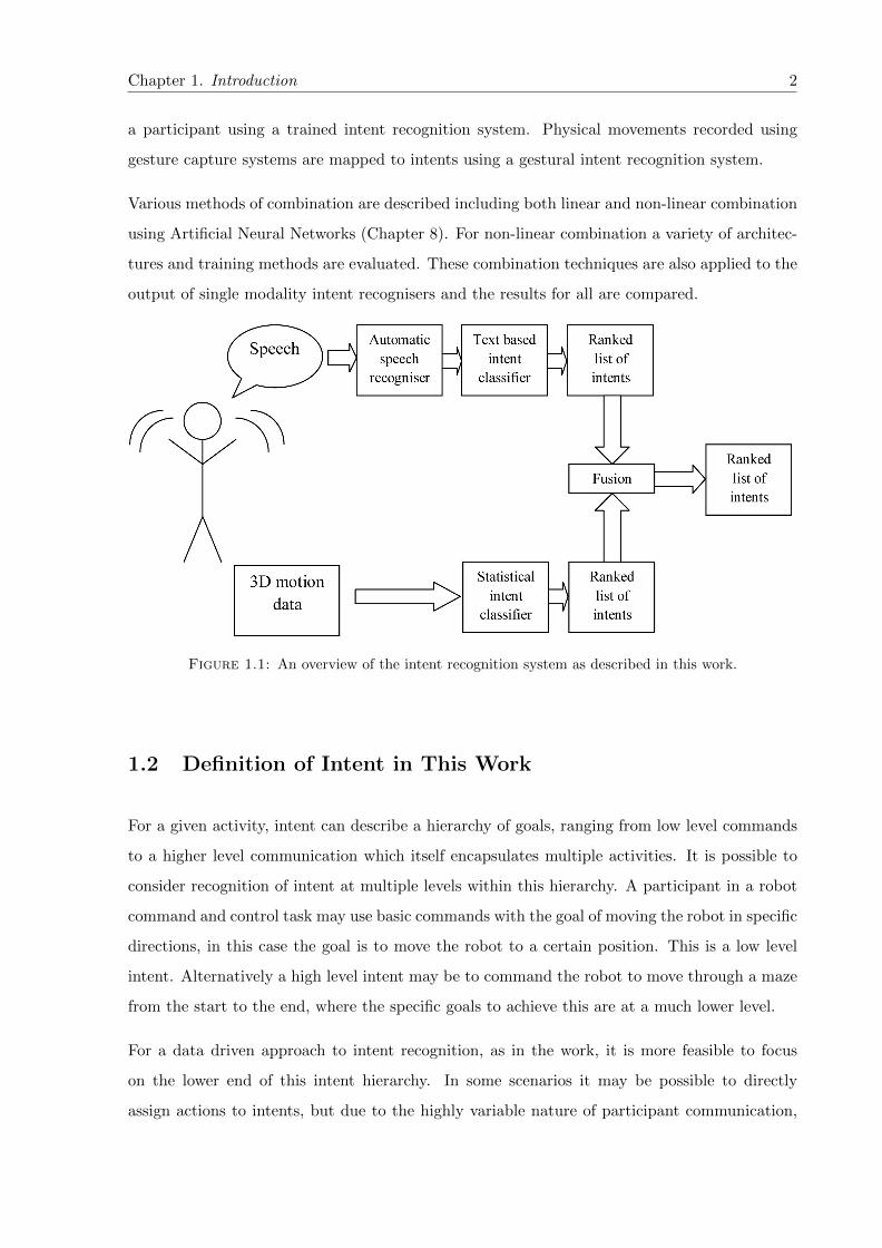
1.1 An overview of the intent recognition system as described in this work. . . . . . . 2
2.1 An overview of the DARPA/NIST evaluations of speech recognition systems.Corpora used during evaluation are labelled. . . . . . . . . . . . . . . . . . . . . . 19
2.2 An overview of two alternative methods for gestural intent recognition. A infersintent from a taxonomy of physical movements and gestures, B infers intentdirectly from raw recorded data without the intermediary steps. . . . . . . . . . 25
3.1 The Sony AIBO Robot . . . . . . . . . . . . . . . . . . . . . . . . . . . . . . . . . 32
3.2 The AIBO control software interface, as used by the robot controller. . . . . . . . 35
3.3 Early prototype of colour tracking using a stereoscopic vision system . . . . . . . 36
3.4 Marker Placement . . . . . . . . . . . . . . . . . . . . . . . . . . . . . . . . . . . 41
3.5 Qualisys Track Manager software showing a sweeping motion by a participant.The green trace lines show the previous 0.5 seconds of data. . . . . . . . . . . . . 43
3.6 Qualisys Track Manager software showing a static pose by a participant with theintention of guiding AIBO forwards. . . . . . . . . . . . . . . . . . . . . . . . . . 44
3.7 Qualisys Track Manager software showing a participant with typically complexphysical movements. The green trace lines show the previous 0.5 seconds of data. 44
3.8 The 4 routes around which AIBO was guided by participants. Both the partici-pant and the person controlling AIBO were given the same set of routes. . . . . . 48
3.9 The layout of the floor space in which both AIBO and the participant can move.The upper area containing the 7 marked points (205.5 x 197.7cm) is the area inwhich AIBO is free to move. The lower area (100 x 100cm) is the participant’sallowed movement area. All dimensions in cm. . . . . . . . . . . . . . . . . . . . 50
4.1 An example HTK label file . . . . . . . . . . . . . . . . . . . . . . . . . . . . . . 62
4.2 An example HTK N-best list label file . . . . . . . . . . . . . . . . . . . . . . . . 63
4.3 Overlay of visual representation of audio recording and motion in the Y-axis ofa marker placed on AIBO’s body. Movement of AIBO can be seen and heard atapproximately frame 360, or 3.6 seconds. . . . . . . . . . . . . . . . . . . . . . . . 64
4.4 The difference between 0 second and 120 second NULL intent thresholding. Ais an example of a 0 second threshold where NULL intents are always insertedin periods of silence. B is an example of a 120 second threshold where NULLintents are never inserted and intents are extended across periods of silence. InB the DEST intent has been extended to the start of the PATH intent. . . . . 68
4.5 An example HTK label file with 0 second NULL intent threshold, NULL intentsare always inserted in periods of silence. . . . . . . . . . . . . . . . . . . . . . . . 68
4.6 An example HTK label file with 120 second NULL intent threshold, NULLintents are never inserted. . . . . . . . . . . . . . . . . . . . . . . . . . . . . . . . 68
viii
List of Figures ix
4.7 An overview of the combination of speech and gesture intent labels to producemerged intent labels. . . . . . . . . . . . . . . . . . . . . . . . . . . . . . . . . . . 71
5.1 An overview of recognition of both speech and gestural intent. Speech at the top,gestural intent below. . . . . . . . . . . . . . . . . . . . . . . . . . . . . . . . . . 76
5.2 A left-right Hidden Markov Model . . . . . . . . . . . . . . . . . . . . . . . . . . 83
6.1 An overview of the stages in building a typical HMM based speech recogniser. . . 96
6.2 An overview of the stages associated with conversion of acoustic speech data toMFCCs . . . . . . . . . . . . . . . . . . . . . . . . . . . . . . . . . . . . . . . . . 98
6.3 An illustration of a combined filter, such as the mel-scale filterbank, with 9 tri-angle band pass filters. m1 to m8 contain the energy in each band. . . . . . . . . 99
7.1 Example poses generated from the mean values for each state in a 8 state, 16mixture components per state model for LEFT intent. As there are multiplemixture components within each state these poses are indicative. . . . . . . . . . 119
7.2 Example poses generated from the mean values for each state in a 8 state, 1mixture component per state model for LEFT intent. . . . . . . . . . . . . . . . 119
7.3 Example poses generated from the mean values for each state in a 3 state, 1mixture components per state model for LEFT intent. . . . . . . . . . . . . . . . 120
7.4 Example pose generated from the mean values for a model with a single stateand 1 mixture component per state for LEFT intent. . . . . . . . . . . . . . . . 120
7.5 Example pose generated from the mean values for a model with a single stateand 1 mixture component per state for RIGHT intent. . . . . . . . . . . . . . . 121
7.6 Example poses generated from the mean values for a model with a single stateand 16 mixture components per state for LEFT intent. . . . . . . . . . . . . . . 122
7.7 Results of intent classification experiment using the human transcription of ges-tural intent with the original 11 intent classes. . . . . . . . . . . . . . . . . . . . . 124
7.8 Results of intent classification experiment using the human transcription of ges-tural intent with the reduced set of 9 intent classes. . . . . . . . . . . . . . . . . . 124
7.9 Results of intent classification experiment based on speech intent labelling con-vention, with no NULL intents due to 120s NULL intent insertion threshold.All intents are extended across periods of silence in the speech to the start timeof the next intent. . . . . . . . . . . . . . . . . . . . . . . . . . . . . . . . . . . . 125
7.10 Results of intent classification experiment based on speech intent labelling conven-tion, with 2s NULL intent insertion threshold. NULL intents are only inserted ifa silence of 2s or more is detected in speech otherwise intent labels are extendedto the start of the next intent. Results are missing for 16 and 32 componentmixtures of the 8 state models due to a lack of training data for the parametersof the LEFT intent model when re-estimating parameters using HTK. . . . . . . 125
7.11 Results of intent classification experiment based on speech intent labelling con-vention, with 0s NULL intent insertion threshold. NULL intents are insertedwherever there is silence in the speech. . . . . . . . . . . . . . . . . . . . . . . . . 126
7.12 Results of intent classification experiment based on merged intent labelling con-vention. The human transcription of gestural intent was inserted during periodsof silence in the speech intent transcription. . . . . . . . . . . . . . . . . . . . . . 126
7.13 Results of continuous intent recognition experiment using the human transcrip-tion of gestural intent with the original 11 intent classes. . . . . . . . . . . . . . . 130

List of Figures x
7.14 Results of continuous intent recognition experimentusing the human transcriptionof gestural intent with the reduced set of 9 intent classes. . . . . . . . . . . . . . 131
7.15 Results of continuous intent recognition experiment based on speech intent la-belling convention, with no NULL intents due to 120s NULL intent insertionthreshold. All intents are extended across periods of silence in the speech to thestart time of the next intent. . . . . . . . . . . . . . . . . . . . . . . . . . . . . . 131
7.16 Results of continuous intent recognition experiment based on speech intent la-belling convention, with 2s NULL intent insertion threshold. NULL intents areonly inserted if a silence of 2s or more is detected in speech otherwise intent labelsare extended to the start of the next intent. . . . . . . . . . . . . . . . . . . . . . 132
7.17 Results of continuous intent recognition experiment based on speech intent la-belling convention, with 0s NULL intent insertion threshold. NULL intents areinserted wherever there is silence in the speech. . . . . . . . . . . . . . . . . . . . 132
7.18 Results of continuous intent recognition experiment based on merged intent la-belling convention. The human transcription of gestural intent was inserted dur-ing periods of silence in the speech intent transcription. . . . . . . . . . . . . . . 133
7.19 A visual comparison of intent period boundaries for both good (A) and poor (B)performing recognisers. The correct labels are shown above the recogniser output 135
7.20 Results of continuous intent recognition experiment using the human transcrip-tion of gestural intent with the original 11 intent classes. Varying insertionpenalty from 0 to 1000. . . . . . . . . . . . . . . . . . . . . . . . . . . . . . . . . 140
7.21 Results of continuous intent recognition experiment using the human transcrip-tion of gestural intent with the reduced set of 9 intent classes. Varying insertionpenalty from 0 to 1000. . . . . . . . . . . . . . . . . . . . . . . . . . . . . . . . . 141
7.22 Results of continuous intent recognition experiment based on speech intent la-belling convention, with no NULL intents due to 120s NULL intent insertionthreshold. All intents are extended across periods of silence in the speech to thestart time of the next intent. Varying insertion penalty from 0 to 1000. . . . . . 142
7.23 Results of continuous intent recognition experiment based on speech intent la-belling convention, with 2s NULL intent insertion threshold. NULL intents areonly inserted if a silence of 2s or more is detected in speech otherwise intent labelsare extended to the start of the next intent. Varying insertion penalty from 0 to1000. . . . . . . . . . . . . . . . . . . . . . . . . . . . . . . . . . . . . . . . . . . . 143
7.24 Results of continuous intent recognition experiment based on speech intent la-belling convention, with 0s NULL intent insertion threshold. NULL intents areinserted wherever there is silence in the speech. Varying insertion penalty from0 to 1000. . . . . . . . . . . . . . . . . . . . . . . . . . . . . . . . . . . . . . . . . 144
7.25 Results of continuous intent recognition experiment based on merged intent la-belling convention. The human transcription of gestural intent was inserted dur-ing periods of silence in the speech intent transcription. Varying insertion penaltyfrom 0 to 1000. . . . . . . . . . . . . . . . . . . . . . . . . . . . . . . . . . . . . . 145
7.26 3 frames showing movement along the primary principal component for a partic-ipant with a very limited range of body movements. . . . . . . . . . . . . . . . . 152
7.27 Number of principal components used vs. average error in mm for individualparticipants when the data is reconstructed. Accuracy of reconstruction up to20 principal components are plotted to more clearly show the variation betweenparticipants. Each curve corresponds to a different participant and participantspecific PCA. . . . . . . . . . . . . . . . . . . . . . . . . . . . . . . . . . . . . . . 153
7.28 Continuous gestural intent recognition with original 57 dimension data. . . . . . 155

List of Figures xi
7.29 Continuous gestural intent recognition with 57 principal component data. . . . . 155
7.30 Continuous gestural intent recognition with 40 principal component data. . . . . 156
7.31 Continuous gestural intent recognition with 20 principal component data. . . . . 156
7.32 Continuous gestural intent recognition with 10 principal component data. . . . . 157
7.33 Varying insertion penalty for continuous gestural intent recognition with 57 prin-cipal component data. . . . . . . . . . . . . . . . . . . . . . . . . . . . . . . . . . 159
7.34 Varying insertion penalty for continuous gestural intent recognition with 40 prin-cipal component data. . . . . . . . . . . . . . . . . . . . . . . . . . . . . . . . . . 160
7.35 Varying insertion penalty for continuous gestural intent recognition with 20 prin-cipal component data. . . . . . . . . . . . . . . . . . . . . . . . . . . . . . . . . . 160
7.36 Varying insertion penalty for continuous gestural intent recognition with 10 prin-cipal component data. . . . . . . . . . . . . . . . . . . . . . . . . . . . . . . . . . 161
7.37 Gestural intent classification with original 57 dimension input data. . . . . . . . 163
7.38 Gestural intent classification with 57 principal component input data. . . . . . . 163
7.39 Gestural intent classification with 40 principal component input data. . . . . . . 164
7.40 Gestural intent classification with 20 principal component input data. . . . . . . 164
7.41 Gestural intent classification with 10 principal component input data. . . . . . . 165
8.1 A simple Multi-Layer Perceptron Artificial Neural Network with 2 hidden layers,for 4 dimensional input and output data. . . . . . . . . . . . . . . . . . . . . . . 175
8.2 A single node within a hidden or output layer in a Multi-Layer Perceptron Arti-ficial Neural Network. . . . . . . . . . . . . . . . . . . . . . . . . . . . . . . . . . 175
8.3 Division of the corpus into full training and test sets, with further division of thetraining set into evaluation training and test sets. . . . . . . . . . . . . . . . . . . 180
8.4 Confusion matrix showing scores for each intent class for linearly combined speechintent classifier scores. Speech input to the classifier is from correct human tran-scription of speech. . . . . . . . . . . . . . . . . . . . . . . . . . . . . . . . . . . . 182
8.5 Confusion matrix showing scores for each intent class for linearly combined speechintent classifier scores. Speech input to the classifier is from automatically recog-nised speech. . . . . . . . . . . . . . . . . . . . . . . . . . . . . . . . . . . . . . . 183
8.6 Confusion matrix showing scores for each intent class for linearly combined ges-tural intent classifier scores. . . . . . . . . . . . . . . . . . . . . . . . . . . . . . . 184
8.7 Confusion matrix showing scores for each intent class for linearly combined speechand gestural intent classifiers. Speech input to the speech intent classifier is fromhuman transcription of speech. . . . . . . . . . . . . . . . . . . . . . . . . . . . . 185
8.8 Confusion matrix showing scores for each intent class for linearly combined speechand gestural intent classifiers. Speech input to the speech intent classifier isautomatically recognised speech. . . . . . . . . . . . . . . . . . . . . . . . . . . . 186
8.9 Intent classification results for MLPs with both 1 and 2 hidden layers. Input tothe MLP is the output of either speech or gestural intent classifiers. MLP trainingmethod is scaled conjugate gradient backpropagation. Trained on evaluationtraining data and tested on evaluation test data. . . . . . . . . . . . . . . . . . . 190
8.10 Combined intent classification results for MLPs with both 1 and 2 hidden lay-ers. Input to the MLP is the output of both speech or gesture intent classifiers.MLP training method is scaled conjugate gradient backpropagation. Trained onevaluation training data and tested on evaluation test data. . . . . . . . . . . . 191
List of Figures xii
A.1 Intent classification results for various training algorithms for a MLP with 18inputs, 1 hidden layer and 9 outputs. Input to the speech intent classifier isaligned correct transcriptions. . . . . . . . . . . . . . . . . . . . . . . . . . . . . . 207
A.2 Intent classification results for various training algorithms for a MLP with 18inputs, 1 hidden layer, 9 outputs. Input to the speech intent classifier is auto-matically recognised speech. . . . . . . . . . . . . . . . . . . . . . . . . . . . . . . 208
A.3 Intent classification results for various training algorithms for a MLP with 18inputs, 2 hidden layers, 9 outputs. Input to the speech intent classifier is alignedcorrect transcriptions. . . . . . . . . . . . . . . . . . . . . . . . . . . . . . . . . . 209
A.4 Intent classification results for various training algorithms for a MLP with 18 in-puts, 2 hidden layers, 9 outputs. Input to speech intent classifier is automaticallyrecognised speech. . . . . . . . . . . . . . . . . . . . . . . . . . . . . . . . . . . . 210

List of Tables
3.1 Names given to markers during motion capture recordings. . . . . . . . . . . . . 40
3.2 An overview of participant strategy (AP - OO). . . . . . . . . . . . . . . . . . . . 55
3.3 An overview of participant strategy (PG - VV). . . . . . . . . . . . . . . . . . . . 56
4.1 A comparison of the number of intents and their duration for physical motiondata labelled with the reduced set of 9 intents. . . . . . . . . . . . . . . . . . . . 70
4.2 An overview of duration of intent in seconds for the merged label set. . . . . . . 71
4.3 Consistency between gestural intent labels and speech intent labels with varyingNULL intent threshold. The speech labels are the final label set as described bythe majority of transcribers. A NULL intent threshold of 0 seconds will alwaysinsert NULL intents in periods of silence. . . . . . . . . . . . . . . . . . . . . . . 72
6.1 Speech recognition results for various corpora. When tested on the corpus col-lected for this work (AIBO), models include AIBO silence model. . . . . . . . . . 105
6.2 A comparison of the count and average word length of each intent for the speechintent labelling convention, with 0s NULL intent insertion threshold. NULLintents are inserted wherever there is silence in the speech. . . . . . . . . . . . . . 108
6.3 A comparison of the count and average word length of each intent for speechlabels with a 120 second NULL intent threshold. Intents are extended acrosssilence to the start of the next intent, there are no NULL intents. . . . . . . . . 109
6.4 A comparison of the count and average word length of each intent for the mergedintent labelling convention. The human transcription of gestural intent was in-serted during periods of silence in the speech intent transcription. . . . . . . . . . 109
6.5 The highest scoring words (using the usefulness ≥ 0.06 measure) for the mergedintent labelling convention and their associated intent class. . . . . . . . . . . . . 110
6.6 A comparison of intent recognition engines based on the merged label set. Intents% Correct indicates the percentage of intents correctly classified. . . . . . . . . . 111
6.7 A comparison of speech based intent recognition systems based on the mergedlabel set. Intents % Correct indicates the percentage of intents correctly classified.Usefulness scores for the NULL intent for “sil” words are ignored. . . . . . . . . 111
6.8 A comparison of speech based intent recognition systems based on the mergedlabel set. Intents % Correct indicates the percentage of intents correctly classified.All usefulness scores for “sil” words are ignored. . . . . . . . . . . . . . . . . . . . 111
xiii

List of Tables xiv
7.1 Results for the best performing models for gestural intent classification for vari-ous labelling conventions. A = Human transcription of gestural intent with theoriginal 11 intent classes. B = Human transcription of gestural intent with thereduced set of 9 intent classes. C = Speech intent labelling convention, with noNULL intents. D = Speech intent labelling convention, with 2s NULL intentinsertion threshold. E = Speech intent labelling convention, with NULL intentsinserted in periods of silence. F = Merged intent labelling convention. . . . . . . 127
7.2 A comparison of intent classification performance for different model architectureswhere the number of total components is fixed at 32. Models are based on thehuman transcription of gestural intent with the reduced set of 9 intent classes. . 128
7.3 % accuracy results for continuous gestural intent recognition based on the bestperforming models and various labelling conventions. A = Human transcriptionof gestural intent with the original 11 intent classes. B = Human transcription ofgestural intent with the reduced set of 9 intent classes. C = Speech intent labellingconvention, with no NULL intents. D = Speech intent labelling convention, with2s NULL intent insertion threshold. E = Speech intent labelling convention,with NULL intents inserted in periods of silence. F = Merged intent labellingconvention. . . . . . . . . . . . . . . . . . . . . . . . . . . . . . . . . . . . . . . . 133
7.4 A comparison of continuous recognition performance for different model archi-tectures where the number of total components is fixed at 32. Models are basedon the the speech intent labelling convention, with no NULL intents. . . . . . . 135
7.5 % accuracy results for continuous gestural intent recognition based on the bestperforming models and various labelling conventions and insertion penalties. “16mix” indicates 16 mixture components per state. A = Human transcription ofgestural intent with the original 11 intent classes. B = Human transcription ofgestural intent with the reduced set of 9 intent classes. C = Speech intent labellingconvention, with no NULL intents. D = Speech intent labelling convention, with2s NULL intent insertion threshold. E = Speech intent labelling convention,with NULL intents inserted in periods of silence. F = Merged intent labellingconvention. . . . . . . . . . . . . . . . . . . . . . . . . . . . . . . . . . . . . . . . 145
7.6 A comparison of % accuracy for continuous gestural intent recognition both withand without an insertion penalty (I.P.) for various labelling conventions. Modelsare all 8 state models and insertion penalties are for the best performing modelsas described in Table 7.5. A = Human transcription of gestural intent with theoriginal 11 intent classes. B = Human transcription of gestural intent with thereduced set of 9 intent classes. C = Speech intent labelling convention, with noNULL intents. D = Speech intent labelling convention, with 2s NULL intentinsertion threshold. E = Speech intent labelling convention, with NULL intentsinserted in periods of silence. F = Merged intent labelling convention. . . . . . . 146
7.7 A comparison of % accuracy for continuous gestural intent recognition both withand without an insertion penalty (I.P.) for various labelling conventions. Modelsused are all 1 state models and results are for the best performing recognis-ers where insertion penalty is used, compared with their equivalent recogniserswithout insertion penalty. A = Human transcription of gestural intent with theoriginal 11 intent classes. B = Human transcription of gestural intent with thereduced set of 9 intent classes. C = Speech intent labelling convention, with noNULL intents. D = Speech intent labelling convention, with 2s NULL intentinsertion threshold. E = Speech intent labelling convention, with NULL intentsinserted in periods of silence. F = Merged intent labelling convention. . . . . . . 147
List of Tables xv
7.8 % accuracy results for continuous gestural intent recognition based on the bestperforming models and merged intent labelling convention. Dimensionality ofinput 3D motion data is reduced using Principal Component Analysis. “16 mix”indicates 16 mixture components per state. . . . . . . . . . . . . . . . . . . . . . 157
7.9 % accuracy results for continuous gestural intent recognition based on the bestperforming models and various number of principal components and insertionpenalties. “16 mix” indicates 16 mixture components per state. . . . . . . . . . . 161
7.10 Results for the best performing models for gestural intent classification for inputdata of varying dimensionality, as reduced using Principal Component Analysis.“16 mix” indicates 16 mixture components per state. . . . . . . . . . . . . . . . . 165
8.1 A comparison of linear combination using single modality output intent scoresfrom separate intent classifiers. Speech intent score input is from the speech intentclassifier described in Chapter 6. Gestural intent score input is from the gestu-ral intent classifier described in Chapter 7. In both cases the merged labellingconvention is used, as are the training and test sets from previous experiments. . 181
8.2 A comparison of linear combination using combined output intent scores fromseparate intent classifiers. Speech intent score input is from the speech intentclassifier described in Chapter 6. Gestural intent score input is from the gestu-ral intent classifier described in Chapter 7. In both cases the merged labellingconvention is used, as are the training and test sets from previous experiments. . 184
8.3 Linear combination of speech and gestural intent scores for classifiers with bothautomatically recognised speech and correctly transcribed speech input. % changeindicates the reduction in performance between correctly transcribed and auto-matically recognised speech, the % increase in error. . . . . . . . . . . . . . . . . 187
8.4 A summary of classification performance using linear combination of output in-tent scores from separate intent classifiers for both single and multimodal linearcombination. In all cases the input is intent scores. % improvement is in compari-son to simply choosing the highest scoring intent class, as described in Chapters 6and 7. (speech) indicates improvement compared to simply choosing the highestscoring intent based on speech alone. . . . . . . . . . . . . . . . . . . . . . . . . . 188
8.5 Summary of results for classification of intent by MLPs given output scores fromspeech and gesture intent classifiers. Training method is scaled conjugate gradientbackpropagation. “2 hidden, 20 nodes” in Architecture indicates a MLP with 2hidden layers, each containing 20 nodes. Trained on evaluation training data andtested on evaluation test data. . . . . . . . . . . . . . . . . . . . . . . . . . . . . 190
8.6 Summary of results for classification of intent given output scores from speechand gestural intent classifiers. Linear relationships between input data and in-tent classes is found using the psuedo-inverse method. Non-linear (MLP) train-ing method is scaled conjugate gradient backpropagation. “MLP, 1 hidden” inMethod indicates a MLP with 1 hidden layer. All models trained and tested onfull training and test set. . . . . . . . . . . . . . . . . . . . . . . . . . . . . . . . . 192
8.7 A summary of the improvement in intent classification when comparing simplychoosing the highest scoring intent class and non-linear combination of intentclass scores using a 2 hidden layer MLP. Both single modality and multimodalintent classification are included. (speech) indicates improvement compared tosimply choosing the highest scoring intent based on speech alone. . . . . . . . . . 193
A.1 Results for a MLP with 18 inputs, 1 hidden layer containing 20 nodes and 9 outputnodes. Speech input to speech intent classifier is aligned correct transcriptions. . 206

List of Tables xvi
A.2 Summary of results for combination of speech and gesture intent classifiers. Re-sults are for aligned, transcribed speech input to the speech intent classifier. . . . 211
A.3 Summary of results for combination of speech and gesture intent classifiers. Re-sults are for automatically recognised speech input to the speech intent classifier. 211

Abbreviations
ANN Artificial Neural Network
AIBO Artificial Intelligence roBOt
ASR Automatic Speech Recognition
GMM Gaussian Mixture Model
HCI Human-Computer Interaction
HMM Hidden Markov Model
HTK The Hidden Markov Model ToolKit
HRI Human-Robotic Interaction
MAP Maximum A-Posteriori
MFCC Mel Frequency Cepstrum Coefficient
MLLR Maximum Likelihood Linear Regression
MLP Multi Layer Perceptron
NN Neural Network
PC Principal Component
PCA Principal Component Analysis
PDF Probability Density Function
xvii

Chapter 1
Introduction
This chapter outlines the objectives of the thesis. The work will be placed in its academic
context including references to relevant existing work in subsequent chapters.
1.1 Objective
The aim of the thesis is to develop a theory and set of systems to derive intent from highly
variable and unconstrained speech and gesture, as used in human guidance of a robotic assistant.
The recognition of intent is described as part of a multimodal intent recognition system, where
more than one modality is combined (see Figure 1.1).
Experimental methods are described for collection of a rich corpus of unconstrained speech and
gesture (Chapter 3). A set of intents are created covering all basic scenarios for command
and control of the robot. The labelling methodology for transcription of speech and gesture is
described as is the creation of a merged transcription, allowing for development of multimodal
intent recognition systems (Chapter 4). All recorded data is divided into training and test data.
The speech and gesture data are synchronised using common features in both modalities.
Techniques for speech and gesture recognition are developed and the two modalities are com-
bined to improve recognition of communicative intent beyond that achievable with either modal-
ity separately. The intent recognition systems described in this work allow for combination of
modalities and follow similar approaches to the statistical approaches usually used in speech
recognition. Word sequences found in speech recognition are used to describe the intent of
1
Chapter 1. Introduction 2
a participant using a trained intent recognition system. Physical movements recorded using
gesture capture systems are mapped to intents using a gestural intent recognition system.
Various methods of combination are described including both linear and non-linear combination
using Artificial Neural Networks (Chapter 8). For non-linear combination a variety of architec-
tures and training methods are evaluated. These combination techniques are also applied to the
output of single modality intent recognisers and the results for all are compared.
Figure 1.1: An overview of the intent recognition system as described in this work.
1.2 Definition of Intent in This Work
For a given activity, intent can describe a hierarchy of goals, ranging from low level commands
to a higher level communication which itself encapsulates multiple activities. It is possible to
consider recognition of intent at multiple levels within this hierarchy. A participant in a robot
command and control task may use basic commands with the goal of moving the robot in specific
directions, in this case the goal is to move the robot to a certain position. This is a low level
intent. Alternatively a high level intent may be to command the robot to move through a maze
from the start to the end, where the specific goals to achieve this are at a much lower level.
For a data driven approach to intent recognition, as in the work, it is more feasible to focus
on the lower end of this intent hierarchy. In some scenarios it may be possible to directly
assign actions to intents, but due to the highly variable nature of participant communication,
Chapter 1. Introduction 3
classifying intents at such a low level is difficult. The alternative, as used in this work, is to
classify intent of a participant by their goal in moving the robot to either a specific position
or along a set path. The physical movements or utterances during periods of communication
are assigned to intents, regardless of whether they are similar to other movements or utterances
seen previously for that intent. In this way, the intent of a person is at a higher level than the
exact communication methods they use.
1.3 Speech Intent
Well established techniques for Automatic Speech Recognition (ASR) are explored including
the use of Hidden Markov Models (HMMs) with the aim of recognising sequences of words.
Topic spotting algorithms based on measures of usefulness are used with the recognised speech
to identify the communicative intent of the speaker.
HMMs are used regularly in speech recognition research, a brief history of which is covered in
Chapter 2. Although there are other methods of speech recognition, HMMs have proven to be
suitable for most ASR tasks and can also be used for speaker verification and identification.
The theory and application of HMMs to ASR are discussed in detail in Chapters 5 and 6.
Speech data is converted through front end processing to feature vectors suitable for modelling
by HMMs. Both speech and gesture recognition systems use separate HMMs for distinct low
level units. For speech data a dictionary of words and sub-word units are used with a grammar to
recognise whole sequences of words. These sequences of words are split by multiple transcribers
into periods of intent, which are then used to create usefulness measures for each intent class
for every word in the corpus (Chapter 6).
Unconstrained speech can be difficult to recognise with a standard ASR system due to the large
variability in the contents of the speech signal. Noisy or disrupted speech, as collected during
corpus creation for this work, can also present problems for speech recognition systems which
must be adapted to cope with erroneous information. Techniques for managing variable quality
speech input to a recogniser are discussed further in Chapter 5.
The topic spotter used to determine intent from textual transcriptions of speech is described
in Chapter 6. The various methods for dealing with silence when only considering textual
transcriptions of speech are described in Chapter 4.

Chapter 1. Introduction 4
1.4 Gestural Intent
For gestural intent recognition the absence of constraint when collecting the data for this work
makes it very difficult to identify the equivalent of a set of phonemes or elementary gesture
components. Although these elementary gesture components may exist, the variability of gesture
collected between participants and even within recordings of the same participant makes them
almost impossible to identify. Whether a recognition system is attempting to identify elementary
gesture components or complete gestures there is a great deal of complexity, requiring complex
models and large amounts of training data. As a concise dictionary of physical movements
is very difficult to describe, a probabilistic method is used whereby physical movements are
mapped to intent without an intermediate stage of assigning physical movements to known
gestures.
Statistical techniques similar to those used in speech recognition systems are discussed for the
modelling of physical movements by a participant and the extraction of communicative intent
(Chapter 6). This work focuses on the application of statistical methods to gestural intent
recognition to examine the feasibility of understanding unconstrained gesture as recorded by a
3D motion tracking system.
1.5 Combination of Modalities
The combination of output of both speech and gestural intent recognition systems can be per-
formed using several methods and again a numerical approach is taken rather than the use
of a rule-based expert system. Linear combination of modalities can be expressed as an error
minimisation problem and performed using the Moore-Penrose pseudoinverse. Both linear and
non linear combination using Artificial Neural Networks are discussed in Chapter 8. A Multi-
Level Perceptron (MLP) is described which can output the single highest scoring intent given
the output of separate speech and gesture intent recognition systems. Appendix A contains an
evaluation of some of the more widely used training methods for MLPs.
Intent recognition systems based on multiple modalities are shown to perform better than
recognition based on individual modalities. Significant improvements can be made over simply
choosing the highest scoring intent class by combining the scores for all intent classes using
linear or non linear methods.

Chapter 1. Introduction 5
1.6 Research Questions
This thesis aims to address the following questions:
• Can speech recognition and techniques for topic spotting be used to identify spoken intent
in unconstrained natural speech?
• Can gesture recognition systems based on statistical speech recognition techniques be used
to bridge the gap between physical movements and recognition of gestural intent?
• How can speech and gesture be combined to identify the overall communicative intent of
a participant with better accuracy than recognisers built for individual modalities?
1.7 Contributions
In order to answer the questions above, this work contains the following contributions:
• Design and implementation of experiments for collection of a rich corpus of natural speech
and 3D motion data as used in a robotic guidance task.
• Extraction of speech and 3D motion information from recorded data suitable for use in
developing recognition engines.
• Development of a robust system for reliable automatic speech recognition of the speech
collected during corpus creation.
• Development of a topic spotting system to translate output of the speech recognition
system into spoken intent.
• Development of a gesture recognition system with the aim of translating physical move-
ments into gestural intent.
• The application of Neural Networks in multimodal fusion of speech and gesture using the
output of separate intent recognition engines.

Chapter 1. Introduction 6
1.8 Thesis Structure
The thesis is laid out in chapters as follows:
• Chapter 1: This introduction, an overview of speech and gesture intent recognition and
the structure of the thesis.
• Chapter 2: A discussion of the current state of the art and past work in speech and gesture
recognition, intent recognition and human-robotic interaction as it applies to this thesis.
• Chapter 3: A description of the planning and implementation of experiments to collect
a rich corpus of unconstrained speech and gesture as used by participants in a robotic
guidance task.
• Chapter 4: A discussion of annotation conventions for labelling of the recorded corpus
and accompanying data at the intent level.
• Chapter 5: An overview of the theory behind Hidden Markov Models and their typical
application in speech and gesture recognition.
• Chapter 6: A description of the creation and adaptation of a speech recognition engine
for recorded speech and a discussion of applied topic spotting techniques to speech data
for intent recognition.
• Chapter 7: A description of applied gestural intent recognition systems for unconstrained
gesture using techniques usually deployed in speech recognition systems.
• Chapter 8: A discussion of the combination of spoken and gestural intent using multimodal
data fusion and the application of Neural Network based systems to data fusion.
• Chapter 9: A conclusion summarising the contributions of the thesis and potential future
research.
• Appendix A: A comparison of training methods for Multi-Layer Perceptron Artificial
Neural Networks.

Chapter 2
On Speech and Gesture Recognition
and Combination
2.1 Introduction
This chapter contains a discussion of the history of speech recognition, which has resulted in the
modern Hidden Markov Model (HMM) based speech recognition engine. The core components
of a HMM speech recognition engine and techniques to improve recognition are described.
Gesture and intent recognition as they apply to this work are discussed. The varying meth-
ods for combination of multiple modalities for improved recognition are described. Topics are
chosen based on their relation to the classification of natural speech and gesture using pattern
recognition techniques typically used in speech recognition.
In addition to providing the context for work on speech recognition, this chapter also aims
to explain the rationale behind using Hidden Markov Model speech recognition techniques to
perform gestural recognition for unconstrained gesture. It can be seen from the history of
speech recognition that statistical techniques for speech recognition have proven more robust
than knowledge based recognition systems. This can be seen in both the acoustic and language
modelling used in successful modern Hidden Markov Model based systems and in the techniques
used by the most important research groups within the field during the past 40 years.
Historically, as the development of Hidden Markov Model speech recognition engines built on
generic pattern matching techniques, so too did gesture recognition engines. These generic
7

Chapter 2. On Speech and Gesture Recognition and Combination 8
pattern matching techniques are especially applicable to this work due to the task orientated
but highly unconstrained speech and gesture collected for this thesis.
2.2 Speech Recognition Development
Any account of the evolution of automatic speech recognition over the past 30 years needs to
address the topic of assessment and evaluation. Techniques for evaluation of speech recognition
systems since their initial development have varied considerably and as a result many early
speech recognition systems may be described as having similar accuracy to their more modern
counterparts. Comparisons between speech recognition systems can only be considered valid if
the exact same testing methodology is used on the same corpus of training and testing data.
In his discussion of speech recogniser evaluation, Moore [1] proposes a standard based on a
human word recognition model which allows recognition results to be normalised for comparison.
However, it was not until techniques for evaluation of speech systems as pioneered by the
DARPA Speech Recognition Benchmark Tests in the 1980s [2] were established that meaningful
comparisons could be made between speech recognition systems. DARPA’s evaluation strategies
were designed specifically to provide an equal footing for research groups and included last
minute testing of speech recognition systems at meetings that the groups were required to
attend. The arrival of standardised evaluation measures resulted in substantial gains in speech
recognition research which can be seen to the present day.
Standard measures of speech recognition performance include Word Error Rate (WER), Figure
of Merit (FOM) and the Percent Correct and Percent Accuracy, as defined in the Hidden
Markov Toolkit (HTK) [3]. The most important and most often used is the Word Error Rate
which measures the proportion of words substituted Ns, deleted Nd and inserted Ni, in the
ASR output compared to the total number of words in a known correct transcription Nt. The
percentage word error rate is defined as:
HTKWordErrorRate =Ns+Nd+Ni
Nt∗ 100 (2.1)
The HTK measure of Word Percent Correct is similar:

Chapter 2. On Speech and Gesture Recognition and Combination 9
HTKWordPercentCorrect =Nt−Nd−Ns
Nt∗ 100 (2.2)
The HTK Percent Correct score ignores insertion errors and for many purposes the Percent
Accuracy is more useful:
HTKPercentAccuracy =Nt−Nd−Ns−Ni
Nt∗ 100 (2.3)
= 100−HTKWordErrorRate (2.4)
The Figure of Merit defined by NIST [4] is an upper bound estimate on keyword accuracy for
speech over a standard time period of one hour which takes into consideration the percentage
of correctly recognised words and the number of false alarms per hour per word. FOM can
also be thought of as the average detection rate over a specified range of false alarm rates and
a measure for the understanding of a recognition system. As FOM takes into consideration
key words rather than words unrelated to the task it can be considered a more useful measure
of understanding than WER. WER can be heavily influenced by incorrectly recognised words
which have little bearing on the overall understanding of a system such as “and” and “the”
whereas FOM focuses on the recognition of important words. WER is historically used as a
performance measure more than FOM, which was developed during the early 1990s.
2.2.1 Early Speech Recognition Engines
Speech recognition systems have been in constant development since the 1950s by many re-
search groups. Early digit recognisers such as those developed in Bell labs in 1952 by Davis,
Biddulph & Balashek [5] used the properties of formants along with simple matching algorithms
to disambiguation telephone quality speech with an accuracy between 97 & 99% for a single
individual. Formants are resonance frequencies of the vocal tract and can be seen as peaks in the
frequency spectrum of speech, most noticeably during vowel sounds. Formant based single word
recognisers were improved to produce systems such as those developed by Forgie and Forgie at
the Massachusetts Institute of Technology with support from the US military [6]. Forgie and
Forgie used processed spectral data as an input to a vowel recogniser which used the position

Chapter 2. On Speech and Gesture Recognition and Combination 10
of the first two formants and further combinations of properties of the first four formants to
achieve 89% accuracy with 21 different speakers.
Other vowel recognition systems of the time include those by Smith & Klem which used a multi-
ple discriminant function approach without explicitly using formant information to achieve 94%
accuracy with multiple speakers [7]. Several Japanese groups in the 1960s also produced hard-
ware sub word level recognition systems such as the “Sonotype Phonetic Typewriter” phoneme
recognition system by Sakai & Dashita [8] and a system by Suzuki & Nakata which used a filter
bank spectrum analyser and hardware logic to describe prior knowledge of speech in order to
differentiate Japanese vowels [9].
Some of the first work using an alternative to these single item speech engines include work by
Vintsyuk, who describes improvements to 1960s recognition techniques in a system based on
automatic time normalisation of sub-word spectral segments [10]. Vintsyuk describes some of
the methods which would be formalised by others such as Sakoe & Chiba in the late 1970s [11]
as “dynamic time warping” or more generally as “dynamic programming”. Vintsyuk describes
the problem of speech recognition as finding the most likely series of phonemes given the speech
signal in work similar to that formalised later in the early 1980s [12]. Constrained by limited
computing power at the time, Vintsyuk proposed modifications to the dynamic programming
algorithms used previously for better performance including self-organisation algorithms which
reduced computational requirements by two orders of magnitude [13]. John Bridle described
the use of similar dynamic programming techniques and whole word template matching for
continuous speech recognition in the early 1980s but initially reported poor performance due
to the inherent variability of speech from multiple speakers [14]. Vintsyuk and Bridle’s work
would be incorporated into several speech recognition engines from the 1980s onwards including
the Hidden Markov Model Toolkit [3].
Apart from techniques described by Vintsyuk, early approaches to speech recognition generally
used a top down rule based approach to find meaning from utterances using prior knowledge
of phonetics and linguistics. They typically depended more on the context of speech than
the acoustic information, which resulted in systems unable to handle the natural variability of
speech. For an overview of early speech recognition see “Trends in Speech Recognition” by
W. Lea [15] which also contains examples of some of the knowledge based heuristic techniques
favoured by others such as Newell [16].

Chapter 2. On Speech and Gesture Recognition and Combination 11
2.2.2 The 1970s
One of the most important advances in speech recognition was the development of models for
the vocal tract and speech based on Linear Predictive Coding (LPC) techniques, as described by
Atal [17]. Atal developed LPC as a way of performing speech coding and compression of speech
to avoid the prohibitively large data requirements for acoustic speech data at the time. LPC
can be described as the process of predicting current samples given a set of previous samples,
which is equivalent to identifying the parameters of a filter. It was shown that the vocal tract
could be modelled by such a filter and speech signals could be described as excitation source
signals passed through this filter. The number of parameters describing the filter and excitation
signal were reduced to a small number of symbols using vector quantisation resulting in a large
reduction in the amount of data needed to describe speech.
The movements of the vocal tract were found to be at a low speed and the shape of the spectrum
was found to be of limited complexity. Once the parameters of the filter had been identified
speech signals could be compressed to as small as 10 filter coefficients which were produced every
20ms. The number of filter coefficients required is dependant on the complexity of the speech
signal but for normal human speech 10 filter coefficients were found to be sufficient [18]. LPC-10
is an example of a speech compression method designed to reduce the size of information stored
as much as possible while still producing intelligible speech.
The application of LPC to speech signals allowed for advances in statistical pattern recognition
methods for speech recognition and became the standard for front end processing of speech
signals before their use in modelling techniques such as Hidden Markov Models.
The basic theory for use of Hidden Markov Models (HMMs), which would go on to become
the most widely used statistical method for speech recognition, was introduced by Baum in
the second half of the 1960s and early 1970s in a series of theoretical papers [19] [20]. Baum’s
work was applied to subjects as diverse as ecology and the stock market [21] but not directly
to speech recognition until the application of the Baum-Welch algorithm for HMM parameter
estimation in the mid 1970s. The Viterbi algorithm used to decode speech into words using
HMMs was originally proposed by Viterbi in 1967 [22] as part of work on error correction and
was popularised by Forney [23].
James Baker, at Carnegie Mellon University, had been working on the use of stochastic modelling
“based on the theory of a probabilistic function of a Markov process” [24] to develop some of the

Chapter 2. On Speech and Gesture Recognition and Combination 12
first systems for robust speech recognition using Hidden Markov Models based on the earlier
work by Baum. Baker’s aim was to account for the natural variability in speech and avoid
the problems rule based systems had with ambiguous acoustical data [25]. Baker’s work was
unlike the rule based approach in that it used statistical methods to analyse large amounts of
speech data without using an expert system based on prior human knowledge. Baker’s work
was to be incorporated into the “Dragon” system, one of the first recognisers to apply Baum’s
HMM theory to speech recognition [26]. Where systems such as the “Hearsay” system used
problem solving techniques for speech recognition, “Dragon” encapsulated speech recognition
as understanding a Markov network with a-priori transition properties between states.
Parallel to Baker, Jelinek and his colleagues had been applying Markov processes to speech
recognition at the Speech Processing Group at IBM [27]. Jelinek applied statistical methods
to single speaker continuous speech recognition using acoustic processing and an architecture
similar to modern systems. Language models and applications of Markov processes to speech
recognition are described in Jelinek’s work pre-dating the rise in popularity of HMMs in the
1980s onwards.
2.2.2.1 The ARPA Speech Understanding Project
Running from 1971 to 1976, the ARPA Speech Understanding Project was designed to encour-
age development of speech recognition systems for speech with rigid sentence structures and a
modest vocabulary. In his review of the project Klatt [28] describes the goal of a speech under-
standing system as being able to: “Accept connected speech from many cooperative speakers
in a quiet room using a good microphone accepting 1000 words using an artificial syntax in a
constraining task yielding less than 10% semantic error in a few times real time on a 100 MIPS
machine.”. The three most successful systems to come from the Speech Understanding Project
were the “HWIM - Hear What I Mean” system presented by Wolf & Woods [29], the “Hearsay”
system presented by Erman & Lesser [30] and the “Harpy” system presented by Lowerre &
Reddy [31].
The “Hear What I Mean” system was developed as a travel budget manager’s automated assis-
tant and was scored according to how well the meaning of a phrase was recognised. Predictably
the scores for smaller vocabulary utterances were better but even with a smaller 409 word
dictionary only 52% of utterances were correctly understood [29].

Chapter 2. On Speech and Gesture Recognition and Combination 13
The “Hearsay” system was the result of work at Carnegie-Mellon University originally aimed
at “the investigation of knowledge-based problem-solving systems and the practical implemen-
tation of speech input to computers.” [30]. The “Hearsay” speech understanding system de-
scribed spoken sounds as follows: “Spoken sounds are achieved by a long chain of successive
transformations, from intentions, through semantic and syntactic structuring, to the eventually
resulting audible acoustic waves.” The aim of Hearsay was to understand the reverse of these
transformations and the framework as described “reconstructs an intention from hypothetical
interpretations formulated at various levels of abstraction” [32]. Hearsay also measured per-
formance as semantic error and achieved 92% accuracy with 81% of sentences word-for-word
correct. Hearsay is considered one of the earliest examples of a “Blackboard” system whereby
disparate and specialist knowledge sources are combined to update a common knowledge base.
Corkill proposes that blackboard systems are ideal for large complex problems where knowledge
sources can vary in design therefore encapsulating many different methods of problem solving
[33] [34]. Since their introduction, blackboard systems have been applied to several areas of AI
research, as cooperative distributed problem solving networks. This is described by Lesser in
his description of tools for evaluating alternative network designs [35].
The best performing speech understanding system proposed for the ARPA Speech Understand-
ing Project was “Harpy”, which met the aim of “understanding over 90% of a set of naturally
spoken sentences composed from a 1000-word lexicon” by achieving 93.77% word recognition
accuracy on 284 speech sentences with a 1011 word vocabulary [31]. Harpy was developed as a
derivative of Baker’s “Dragon” system and built on Baker’s early work on using Hidden Markov
Models in speech recognition.
The Harpy system described the available speech search space in the form of a network where
every possible utterance or sequence of words was described. Input speech was vector quantised
and dynamic programming techniques were used to compare the speech signal with examples
of speech at each node within the network [36]. The best scoring route through the network
corresponded to the input utterance.
Harpy combined finite state transition networks with rule based systems to improve perfor-
mance and speed, combining the advantages of statistical pattern matching methods with prior
knowledge of linguistics. Common subnets within the network were combined to reduce the
size of the search space thereby reducing the number of speech units to be detected at each
time sample. Harpy also provided semi-automatic methods for generating a language model
Chapter 2. On Speech and Gesture Recognition and Combination 14
and phonemic templates from training data and used “Juncture rules” to improve intra-word
coarticulation [37]. The resilience of Harpy to noisy input speech was tested by Yegnanarayana
where digit recognition across a telephone link was affected by noise, reduced accuracy from
99% to 93% [38].
2.2.3 Dynamic Programming Techniques
At a similar time to the ARPA Speech Understanding Project, dynamic programming ap-
proaches to speech recognition were being explored by Sakoe & Chiba. Sakoe & Chiba describe
a dynamic programming based time-normalisation algorithm for spoken word recognition [11].
A pattern matching approach is used whereby processed test and reference acoustic signals are
aligned using a dynamic time warping algorithm. Applied to speaker dependant digit recogni-
tion of sequences of between 1 and 4 digits, the system achieved 99.6% accuracy with reasonable
limits to computation time. Adjustments to Sakoe & Chiba’s dynamic programming techniques
were shown in 1979 and throughout the 1980s. Sakoe extended the Sakoe & Chiba algorithm to
connected speech recognition through his 2-pass algorithm [39]. Paliwal’s work which modifies
the original algorithm for reduced computation time and greater word recognition accuracy [40].
Myers describes an alternative level building 2-pass dynamic time warping algorithm which al-
though similar to that of Sakoe & Chiba is shown to be significantly more efficient [41]. The
algorithm described by Myers is described as a special case of the stack decoding algorithm as
described by Bahl & Jelinek [42].
The Sakoe & Chiba method of dynamic programming is compared with heuristic search by Ney
who describes recognition by these methods as finding the optimal path through a finite state
network [43]. As described in a digit recognition task both methods perform word boundary
detection and nonlinear time alignment before classification and are far more flexible than earlier
AI knowledge based systems. As the complexity of the input speech increases it is shown that
dynamic programming techniques have a far smaller memory and cpu footprint than heuristic
search and the computational power required for dynamic programming grows linearly. As
dynamic programming techniques can keep pace with the speech input they also have the
advantage of handling continuous recognition of speech without having to reach the end of an
utterance.
Modern dynamic programming techniques are used in a variety of statistical pattern matching
systems. Ney provides an overview of improvements made to dynamic programming as applied
Chapter 2. On Speech and Gesture Recognition and Combination 15
to small and large vocabulary continuous speech recognition [44]. Statistical pattern recognition
and beam search are described as “primitive techniques” that work very well if “the proper
acoustic-phonetic details are embodied in the structure” of the models used. Ney discusses
techniques for reduction of the search space produced by a large vocabulary by combining low
level acoustic information with the language model which is described as a simple structured
model.
2.2.4 The 1980s and Growing Use of Hidden Markov Models
The popularity of statistical methods for speech recognition grew throughout the 1980s as expert
systems were replaced with pattern matching techniques and the use of HMMs. Practical appli-
cations which applied the Baum-Welch algorithm for the estimation of HMM parameters further
encouraged their use in speech recognition [20]. Poritz describes modelling of speech signals of
considerable length as a sample sequence generated by HMMs and applied the technique to
speaker identification to correctly identify 10 speakers reading the same passage [45]. Liporace
describes the techniques required for parameter estimation of Markov chains by generalising the
Baum-Welch algorithm to Gaussian Mixture Models (the estimation of models based on many
different types of distribution are discussed although in the domain of speech recognition the
most important is that for generic Gaussian Mixture Models [46]) Juang had also been working
on the application of the Baum-Welch algorithm to HMMs but with more of an emphasis on
the practical applications in speech recognition than Liporace [47].
Although HMMs and their application in speech recognition were not new in the 1980s due to the
pioneering work of Baum, Baker and others such as Jelenik, it was not until Rabiner, Levinson
and others at Bell Labs popularised the practical use of HMM techniques in speech recognition
tutorials that they became widely used. Rabiner applied HMMs to vector quantised speech
for isolated word recognition, achieving 96.5% accuracy for 100 speakers when performing digit
recognition [48]. In his introduction and basic tutorial for HMMs, Rabiner explains the increase
in interest in HMMs as being due to improvements for estimation of the model parameters [49].
In his frequently cited tutorial for HMMs in speech recognition Rabiner describes the flexibility
and wide range of applications of HMMs as the main reason for continued interest [50]. From
the time these papers were published HMMs have become the primary method for speech
recognition systems and have been constantly refined and improved to improve accuracy and
reduce computational cost, a major barrier to earlier adoption of intensive statistical methods.

Chapter 2. On Speech and Gesture Recognition and Combination 16
Other more simple methods of pattern recognition and methods based on expert systems were no
longer considered suitable techniques for the improved speaker independent continuous speech
recognition engines that followed.
In the late 1980s a DARPA program for speech understanding in a 1000 word vocabulary
American Navy Resource Management task was proposed similar to that proposed by ARPA
in the 1970s. A database of over 21000 utterances from 160 speakers was designed and par-
titioned into training and test data for application of speech recognition systems by DARPA
members. The corpus of speech data was “intended for use in designing and evaluating algo-
rithms for speaker-independent, speaker-adaptive and speaker-dependent speech recognition.”
[51]. Pallett describes the standardised scoring methodology to be used by the speech recogni-
tion community for the DARPA task as focusing on word level speech recognition rather than
semantic interpretation or speech understanding [2].
The core focus of the DARPA Resource Management task was speaker independent continuous
speech recognition with a grammar constrained by the corpus to mainly commands and in-
structions rather than conversational speech. The most successful systems applied to this task
were based on the combination of HMMs with other lexical, syntactic, semantic and pragmatic
knowledge sources. Instead of modelling whole words using HMMs as in previous recognition
systems these newer systems were able to model sub-word units such as phones and triphones
to account for variation of phones due to their surroundings.
The BYBLOS system developed at BBN Laboratories, whilst originally aimed at speaker de-
pendent recognition, was adapted to use small sections of training speech to recognise previously
unheard speakers. BYBLOS reported 97% accuracy with 15 seconds of training speech for a
350 word task [52]. The BYBLOS system also demonstrates the advantages of using triphones
for speech recognition, roughly halving the error rate compared to a system without triphone
models.
The DECIPHER system at SRI took a similar approach to that of BYBLOS by combining
linguistic knowledge into the HMM framework [53]. Simple HMMs were combined with a
database of phonological rules to account for different word pronunciations and cross-word
boundaries. The use of phonological rules increased accuracy but the DECIPHER system was
unable to match the accuracy of the SPHINX system at Carnegie-Mellon for speaker independent
recognition.

Chapter 2. On Speech and Gesture Recognition and Combination 17
The SPHINX system, developed by Kai-Fu Lee, applied previous knowledge of phoneme level
HMMs and triphones combined with a pronunciation dictionary and an automatically generated
word-pair language model [54]. Much earlier work by Shannon [55] was applied to grammar
modelling to create a language model without producing an expert system based on previous
knowledge of a language’s structure. SPHINX was able to perform speaker-independent con-
tinuous speech recognition in real time, especially notable due to the limited computational
resources available at the time. The SPHINX system was designed to apply pure statistical
methods to speech recognition rather than try and apply models of other knowledge sources
and achieved better results than both BYBLOS and DECIPHER. In doing so, SPHINX provided
proof of the merit of statistical approaches to speaker-independent recognition which would go
on to form the basis of most modern systems.
The SPHINX system was based on discrete HMMs which used discrete distributions or simple
histograms to model measurements of speech. Speech input was vector quantised into a sequence
of acoustic vectors using front end processing techniques originally described by Atal [17]. The
distributions of these sequences of acoustic vectors in relation to each of the HMMs used to
model phones or triphones is described as the acoustic model.
The language model used in SPHINX was similar in design to the earlier Harpy system and
allowed for creation of a complex lexical decoding network without the use of an expert system
in a similar manner to that described by Baker [56]. Lee’s SPHINX system also showed the
benefit of using large numbers of different speakers for training of speaker independent HMMs
rather than longer recordings of fewer speakers.
After the findings of the ARPA resource management task continuous improvements to HMM
based recognition systems systems similar to SPHINX were proposed. One of the findings
was the restrictions placed on speech models by the vector quantisation process and resulting
simple distributions. The quantisation of speech signals to speech vectors used in discrete
HMMs resulted in a serious loss of information and smoothing techniques which aimed to share
information between similar vectors were proposed [57].
The most important development beyond discrete HMMs was that of semi-continuous HMMs
as originally proposed by Huang [58] and others, in which the vector quantisation stage was
removed and the HMM states were associated with parametric continuous Probability Density
Functions (PDFs), typically Gaussian Mixture Models. Tied mixture models [59] shared a
common pool of Gaussian PDFs to reduce training set requirements.

Chapter 2. On Speech and Gesture Recognition and Combination 18
As well as improvements to the acoustic modelling of speech, improvements to the language
model and techniques for representing the structure of a language were made. In the SPHINX
system statistical properties of word-pairs were used to represent the language model instead
of complex rules. The natural extension of word pairs produced the N -gram language model
whereby the probability of a word occurring depends only on the N − 1 prior words.
N -gram language models encode syntactical information directly from text input data removing
the dependance on formal grammars as used in earlier recognition engines. Unfortunately a
side effect of N -gram language models is the large amount of training data required to properly
model every possible sequence of words. As a result most speech recognition engines use bigrams
(N = 2) or trigrams (N = 3) and “discounting” and “backing-off” algorithms to modify the
probability distributions within a language model and account for data sparsity. Katz described
procedures for estimation of N -gram language models from sparse data as early as 1987 [60]
which is built on in work by Ney in 1994 [61].
After evaluation of the ARPA Resource Management task was completed, DARPA (a renamed
ARPA) produced a corpus of spontaneous speech in the Air Travel Information System (ATIS)
domain. Although the speech data contained in the ATIS corpus is spontaneous the linguistic
structure is limited due to the nature of the recordings. The DARPA ATIS task is one of the
first to include recognition of words not contained within the training lexicon, resulting in worse
performance for systems without the ability to cope with these instances [62].
The implementation of semi-continuous HMMs and the N -gram language model resulted in the
SPHINX-2 system, developed by Huang at Carnegie Mellon which achieved the lowest error
rate in the 1992 DARPA ATIS speech recognition evaluations [63].
The assessment driven methods defined during DARPA’s early speech recognition tasks continue
to the present day with the aim of improving speech recognition in a variety of contexts with
tasks of increasing difficulty. Corpus creation for DARPA tasks has resulted in several commonly
used corpora including the Wall Street Journal (WSJ0) corpus [64], SWITCHBOARD [65],
Broadcast News [66], Meeting Room [67] and various other corpora collected by NIST. The
techniques for corpus collection as described by research centres involved in DARPA tasks have
also been applied elsewhere such as in the creation of the WSJCAM0 corpus, a UK English
equivalent of a subset of the US American English WSJ0 corpus originally recorded at Cambridge
University [68]. Figure 2.1 describes the various NIST evaluations of speech recognition systems
built using corpora such as those mentioned above [69].
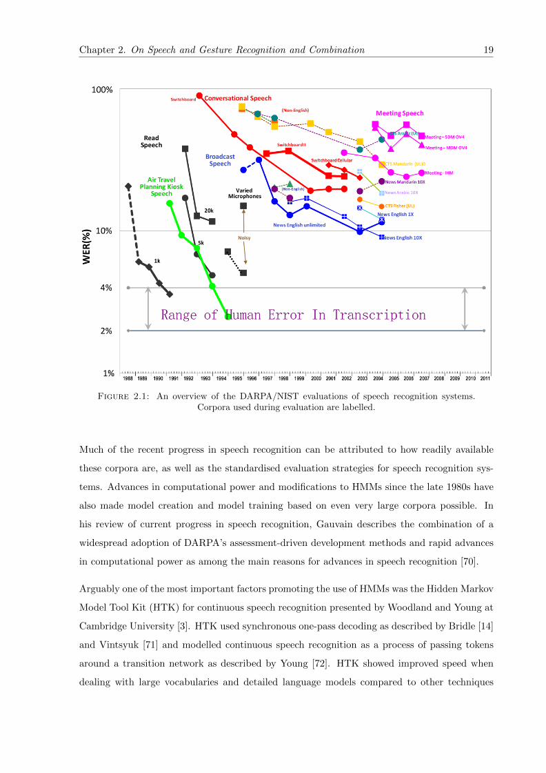
Chapter 2. On Speech and Gesture Recognition and Combination 19
Figure 2.1: An overview of the DARPA/NIST evaluations of speech recognition systems.Corpora used during evaluation are labelled.
Much of the recent progress in speech recognition can be attributed to how readily available
these corpora are, as well as the standardised evaluation strategies for speech recognition sys-
tems. Advances in computational power and modifications to HMMs since the late 1980s have
also made model creation and model training based on even very large corpora possible. In
his review of current progress in speech recognition, Gauvain describes the combination of a
widespread adoption of DARPA’s assessment-driven development methods and rapid advances
in computational power as among the main reasons for advances in speech recognition [70].
Arguably one of the most important factors promoting the use of HMMs was the Hidden Markov
Model Tool Kit (HTK) for continuous speech recognition presented by Woodland and Young at
Cambridge University [3]. HTK used synchronous one-pass decoding as described by Bridle [14]
and Vintsyuk [71] and modelled continuous speech recognition as a process of passing tokens
around a transition network as described by Young [72]. HTK showed improved speed when
dealing with large vocabularies and detailed language models compared to other techniques

Chapter 2. On Speech and Gesture Recognition and Combination 20
which used less advanced two-pass algorithms for decoding [73] and produced the most successful
recognition results overall during evaluation as part of the DARPA WSJ0 task [74]. Although
decoding of speech using HTK in these early tests is considered slow now, the advances in
cheap computational power make application of HTK to tasks such as the WSJ0 trivial. This
thesis makes extensive use of HTK for modelling both speech and gesture using various HMM
architectures.
In his review of large-vocabulary continuous speech recognition in 1996 Young describes the use
of HMMs as used in HTK as state of the art [75]. Young suggests the technology for recognition
as being usable given a reasonably controlled environment and a well defined task and also
theorised that large vocabulary recognition systems would become prevalent in transcription
and information retrieval in the following years.
An overview of the theory behind HMMs is available in Chapter 5. Detail on creation of a
speech recognition engine using HTK is included in Chapter 6.
2.3 Gesture and Multimodal Recognition Development
Gesture recognition is a broad topic covering interpretation of physical gestures and control sur-
face gesture methods such as handwriting recognition. Typical application scenarios in human-
computer interaction involve strict sets of allowed gestures and a constrained environment,
removing the need for recognition engines to compensate for spontaneous unconstrained ges-
ture. In this work, gestures are modelled in terms of the intent of a participant, not strictly
on their physical movements. This results in classification of similar physical movements in
semantically different intent classes. An emphasis is placed on natural communication using
gesture, strict taxonomies of gesture types are not described explicitly but rather encapsulated
within higher level descriptions of communicative intent.
Typical methods of gesture capture include visual recognition systems, which extract informa-
tion from video input of human gestures, and model based recognition, where a multi dimen-
sional model of the gesturer is built. Many of the vision based systems described below use a
combination of visual information and prior knowledge of the gesturer and 3D space to map
visual information to a 3D model. In this work a 3D modelling system is employed with multiple
cameras and body markers to produce a simple skeletal model of the human body. The markers
are picked up by an array of cameras which can triangulate the position of each marker to a

Chapter 2. On Speech and Gesture Recognition and Combination 21
high level of accuracy in 3D space. Previous research in the field of vision and model based
recognition is used to validate this as a relevant method of extracting gestural communicative
intent in human robotic interaction.
Improved processing power has allowed more computationally intensive recognition systems
to be developed. Since the development of interfaces such as the computer display, research
into human-computer interaction (HCI) has developed alongside that of hardware development.
Improvements to HCI allow computer users to interact more intuitively with systems that grow
increasingly complex as computer hardware and software develop. The techniques developed in
HCI research can be applied specifically to human-robotic interaction (HRI).
With some differences in design, the recognition systems produced for HCI can be applied to
human-robotic interaction (HRI) [76]. In most HRI applications the robot listener is considered
a mobile computer with various sensors to allow interaction with its environment. In this work
the sensors used by the robot are external to its own sensors and through the use of a wireless
network and external processing the robot is controlled as a simple moveable platform.
Research in gesture understanding in multimodal interaction can be approached with varying
levels of emphasis on gesture compared to other modalities. Gesture can be used as a complete
substitute for other modalities such as speech, as in systems that recognise sign language, or as
a complementary modality which together with other modalities contributes a varying percent-
age of communicative intent. By combining different modalities it has been shown that overall
understanding of natural human communication compared to single modality communication
can be increased. This is especially important in environments where the communicative abil-
ity of modalities are restricted, such as speech in noisy environments or gesture where vision
is poor. Noise can change the way each modality is used, such as shouting in noisy environ-
ments or a reversion to simpler gestures. If a modality is completely obscured then changes to
other communicative methods can be expected to cope with the loss of overall communicative
ability. Varying levels of noise during recordings can make recognition based on standard non-
noisy models difficult, especially as the behaviour of participants can be expected to change as
communicative ability decreases.
The approach to gesture as an strict alternative to other HCI/HRI input methods such as speech,
keyboard, mouse input etc, rather than a complement, precludes the combination of differing
modalities and apart from sign language, is not typically used in natural human communication.

Chapter 2. On Speech and Gesture Recognition and Combination 22
Although of interest to HCI and HRI researchers, virtual and augmented reality are not discussed
in detail. These two fields of research employ HCI to improve the naturalness of interaction
with a virtual environment and are typically explored with the use of strongly classified gesture
for command and control interfaces. Similarly, face and lip movement recognition techniques,
although of interest in HCI/HRI research, are only discussed when directly relevant to techniques
applied in this work.
2.3.1 Input Methods
Early methods of input in HCI, beyond the typical mouse and keyboard input methods favoured
previously, were typically limited to the equivalent of single finger pointing gestures [77]. An
example is the Drawing Prism described by Greene, which used a touch surface to convert
physical brush and finger strokes to their corresponding graphical representation in a frame
buffer [78]. The earliest examples of these systems include the “Put-That-There” system by Bolt,
developed in the early 1980s, which used pointing gestures with a magnetic positioning system
and a simple speech recognition system to provide a multimodal command and control interface
[79]. Although basic, the speech recognition system was developed to correctly recognise a
limited task specific vocabulary and then wait for a location on a map if required. The modalities
were not used simultaneously and the pointing (deictic) gestures were only used to reference a
set of 2 dimensional coordinates on a known map. In this way no dynamic time based gestures
were used but an operator could interact with the system without use of any physical apparatus.
These single finger physical input devices were expanded to multiple fingers with the aim of
increasing the available HCI vocabulary, such as the touch sensitive tablet described by Lee
which also allowed for varying pressure sensitivity [80]. Examples of these multi-touch pen and
finger input devices can be seen in modern commercial design and mobile computing interfaces
where they are typically used in command and control scenarios [81].
Several of the early touch-pad pointing systems were concerned with communicating map based
information and combined speech recognition with simple deictic gestures for interfaces very
similar in form to standard general user interfaces (GUIs). These systems expanded on the
“Put-That-There” system to extract information on the point of reference of deictic gestures
without using typical keyboard and mouse input. An example of this type of system is the work
by Cohen, which combines natural language understanding and direct manipulation of on screen
objects to overcome limitations in each modality [82]. More modern examples of speech and pen
Chapter 2. On Speech and Gesture Recognition and Combination 23
input include work by Oviatt, who uses pen and speech input for communication of directions
using a touch screen map interface [83], and Cohen’s “Quickset” system, in which a hand-held
PC based touch interface is combined with spoken commands for the design of airstrips [84].
Pen and speech based interfaces have progresses at a more rapid pace than full 3-dimensional
gesture recognition interfaces due to the comparative simplicity of 2-dimensional gestures com-
pared to full continuous physical movement based gesture recognition.
Whilst pen based gesture input can be used with great success in command and control it
requires the use of external equipment, which alters the strategy of participants. This work
focuses on the use of unconstrained natural speech and gesture, which is made difficult when
a participant has to learn to use equipment or in some other way act differently to how they
would with another human.
There are many examples of data capture methods for gesture that do not require modification
of a users natural communication. Glove based approaches, such as those described by Pavlovic
[85] are more intrusive than vision based systems and are generally wired to computers, which
can hinder natural movement. Glove based systems use a typically skeletal spatial description
of the hand to determine hand position. Although there are 27 bones in the human hand it is
not necessary to capture all this information to produce a skeletal model suitable for gesture
recognition.
The first commercially available hand tracker was the “Dataglove” system (1987) which used flex
sensors to determine hand pose and provided tactile feedback using vibration [86]. Improvements
to glove based systems include The “CyberGlove” system by Kramer produced in 1989 which
used more reliable strain gauges rather than flex sensors to determine hand pose [87]. Kramer’s
glove was used to allow deaf, deaf-blind or nonvocal individuals to communicate by synthesising
speech based on hand position.
Vision based systems for hand tracking are typically based on colour segmentation where pixel
based input from multiple cameras is used with a thresholding algorithm to detect human skin
tone [88], [89]. Skin tone detection can be difficult due to changing lighting and background
conditions, although by restricting the recording conditions this can be avoided.
The vision based system described by Cipolla [90] uses stereoscopic vision to interpret static
gesture for robotic control. See Chapter 3 for a description of a similar system developed for
data collection in this work which was eventually superseded by a commercial motion tracker.

Chapter 2. On Speech and Gesture Recognition and Combination 24
Systems developed for capture of full body motion data are similar to those used for hand
tracking, although with more of a focus on vision based systems. Wren describes a robust single
camera system for body tracking which can also be applied to vehicle or animal tracking [91].
Gavrila describes a 3D vision system using coloured body suits for unconstrained full body
gesture for up to 2 human participants [92].
A more common alternative to coloured body suits is the use of markers, placed at key positions
on the body. Markers can be either passive, as in systems with reflective markers and infrared
cameras, or active, as in systems where each marker sends out a radio based signal. In this
work a commercial 3D motion capture system by Qualisys [93] is used to capture 16 points on
the human body (see Chapter 3). This information can be used to create a skeletal model with
information on angle and rotation of body parts but in this case the raw 3D motion data is used
to model higher level gestural intent.
Similarly to some glove based hand trackers, mechanical joints can be attached to a participant
to record joint angles. These can be extended to full body “exoskeletal suits” such as the Meta
Motion Gypsy system [94]. The ShapeWrap system by Measurand [95] uses flexible fibre-optic
angle sensors to achieve the same goal.
Inertial tracking using physically attached accelerometer modules can be combined with a skele-
tal model of the body, as in the Xsens MTx system [96]. As well as static poses these systems
can return the instantaneous rate of movement and are not affected by lighting conditions.
Magentic field based tracking systems such as the “Flock of Birds” system by Ascension [97]
generate magnetic fields which induce a current in the passive coils attached to a participant,
to detect their location relative to the transmitter.
Mechanical, inertial and magnetic field based motion capture systems are unaffected by the
line of sight issues that affect vision based systems. Neither are they affected by poor lighting
conditions or obstructions due to the recording environment.
2.3.2 Gesture Modelling and Recognition techniques
2.3.2.1 Inferring Communicative Intent From Raw Motion Data
The objective of the gesture component of this work is to find a relationship between body
movement, as defined by a sequence of 3D body positions, and a participant’s intent. There

Chapter 2. On Speech and Gesture Recognition and Combination 25
Figure 2.2: An overview of two alternative methods for gestural intent recognition. A infersintent from a taxonomy of physical movements and gestures, B infers intent directly from raw
recorded data without the intermediary steps.
is no symbolic description of this movement. For example, we do not explicitly associate the
intent RIGHT (see Chapter 4) with “a movement of the right arm to an angle of approximately
90 degrees to the body”. Instead, we associate a segment of a participant’s interaction with the
intent RIGHT . The objective is to associate automatically the sequence of 3D body positions
in that segment with the RIGHT intent.
The word “gesture” is used throughout this work, but it refers to a sequence of raw 3D body
position vectors rather than a higher level morphological description.
Quek describes hand gesture (and by extension, full body gesture) as being split into a clear
taxonomy of gestures and ignored unintentional movements [98]. The gestures are described as
either manipulative or communicative, of which only communicative is concerned with conveying
meaning or intent.
Several gesture recognition systems use a hierarchical description of gesture, grouping types of
gesture into typically distinct groups [99], [100]. In a typical recognition engine [101] a low level
model of gesture as physical movement is collated in a dictionary of known possible movements,
each corresponding to a command or multiple commands.
Chapter 2. On Speech and Gesture Recognition and Combination 26
In unconstrained gesture, where it may be impossible to identify intent by classifying a set of
known gestures from basic physical movement, the aim is to try to determine the intent of the
gesturer directly from 3D motion data. Figure 2.2 describes the two alternatives to inferring
intent from physical movements. Method A presumes that a taxonomy of elementary physical
movements and gesture can be found, method B describes modelling motion data directly to
infer intent.
It may be possible to find a set of elementary physical movements through analysis of intent
but the highly variable nature of natural unconstrained gesture makes such a task difficult.
2.3.2.2 Gesture Modelling Techniques
Speech recognition techniques such as HMMs (see above) or time dependent Neural Networks
are commonly used for dynamic gesture recognition. The data from an input device such as a
glove or vision based system is used to train models based on a sequence of poses. The Georgia
Tech Gesture Toolkit (GT2K) [101] is an example of a HMM based gesture recognition system
built as an extension of HTK and designed to take input from any input device in the form of a
feature vector. GT2K models each known gesture as a separate HMM, relying on a taxonomy of
gesture being available rather than unconstrained gesture as in this work. More recently GT2K
has been superseded by the Gesture and Activity Recognition Toolkit (GART) [102] which aims
to reduce the extensive knowledge of machine learning required to use HTK effectively.
Lee [103] uses glove based input and HMMs to recognise specific gestures in robot command
and control. Similarly, Yang uses HMMs to represent human skills which can be learned by
a distant robot observer [104]. Yang describes intent recognition from gesture data but still
requires the definition of a set of meaningful gestures for each intent [105].
As well as direct recognition of gesture, HMMs can be used for motion control in HRI based
on gesture input. This combination of gesture recognition with trajectory analysis is described
by Zhu [106]. Several research groups use HMMs to recognise sign language, such as American
[107] and Taiwanese [108] sign language. Wilson uses secondary information to create parametric
HMMs for gesture recognition [109]. Parameters of interest, such as the size of a gesture, are
used to remove noise in the gesture domain.

Chapter 2. On Speech and Gesture Recognition and Combination 27
For static hand or full body gestures Artificial Neural Networks (ANNs or simply NNs [110])
can be used, as by Fels for the “Glove-Talk” system [111]. ANNs and the input from a data
glove can be used to recognise arbitrary gestures [100] or sign language [112].
In all these cases a set of arbitrary gesture types are specified rather than the unconstrained
natural gesture as collected in this work. Unlike the above, Yamato uses HMMs to recognise
human action, without first constructing a geometric representation of the human body or a
taxonomy of gesture [113]. Similarly to the intent recognition performed in this work, low level
input data (in this case from image data) is used to create models based on periods of action.
Oliver uses HMMs to recognise human behaviour from a camera and “blob features” using an
object detection algorithm similar to that used to identify markers in this work [114].
2.3.3 Multimodal Data Fusion
Creation of a multimodal intent recognition system relies on data fusion of seperate modalities
before a final decision is made. This data fusion can be performed at several different levels;
Hall describes fusion at data , feature and decision levels [115]. Similarly, Heading describes
sensor, feature and decision level data fusion [116]. In both cases the different levels of data
fusion available for use are dependant on the task and nature of the data. Generally, the more
distinct the input data from different sensors, the higher the level of combination, with decision
level fusion at the highest level.
Data, or sensor level fusion implies the modalities are so tightly coupled that raw sensor level
data can be combined. For example, in the 3D motion capture system used in this work, the
input from several cameras is combined at a sensor level to calculate the position of markers in
three dimensions. Richardson shows that generally, inclusion of additional sensory information
almost always improves classification [117].
Feature level fusion assumes that each sensor provides a feature vector, which in the case
of multimodal recognition is extracted from the observed information in each modality. The
features are concatenated to produce a combined feature vector, which in turn must be passed
through another level of fusion before a final decision is made.
Decision level fusion is the highest level of data fusion. For multimodal intent recognition, a
recogniser for each modality produces a single output of the most likely intent. These are then

Chapter 2. On Speech and Gesture Recognition and Combination 28
combined, typically using knowledge based systems. Decision level fusion has been shown to
improve recognition where the inputs from multiple sensors are uncorrelated [118].
Franke describes both feature and decision level fusion as alternative ways of combining the
votes of cooperating classifiers [119]. At a decision level, Franke uses the knowledge based
Dempster/Shafer theory of evidence [120] for combination, as does Xu [121]. In both cases
statistical information about the relative classification strengths of seperate classifiers is used.
Woods uses accuracy estimates for multiple classifiers to select the most correct classifier in
an alternative approach to simply combining classifiers [122]. Ayari passes information at a
decision level between specialist expert systems [123].
Artificial Neural Networks are used in gesture recognition but are also shown to be of use
in feature level multi sensor data fusion [124], [125]. This can be extended to multi-modal
recognition by feature level fusion of the output from separate recognition engines, as in this
work. Cho uses multiple Neural Networks with a measure of network reliability for data fusion
in handwriting recognition [126]. Rogova combines different architectures of Neural Networks
[127] in a similar task.
The data fusion methods described here can be applied to the combination of speech and gesture
data for intent recognition. As speech and gesture are loosely coupled it is extremely difficult
to use sensor level data fusion to improve recognition over a single modality. The alternative is
either feature or decision level data fusion.
Decision level data fusion in this case assumes that the output of speech or gestural intent
recognisers is correct for each modality. It is difficult to make this kind of judgement given
that the confidence measures for multiple intents may be similar within a modality. For this
reason, feature level combination of speech and gestural intent is considered as the best method
of improving intent recognition over single modalities.
Both linear and non-linear combination of feature vectors for multimodal data fusion in intent
recognition are described in Chapter 8.
2.4 Summary
This chapter has discussed the historical progression of speech recognition systems from single
digit recognition to continuous automatic speech recognition. The reasoning behind the increase

Chapter 2. On Speech and Gesture Recognition and Combination 29
in the popularity of Hidden Markov Models has been discussed, as have the developments to
improve their performance in speech recognition.
Input methods for gesture recognition have been discussed as have the systems for three dimen-
sional full body motion capture, as used in this work.
The difference in methodology is discussed for intent recognition engines based on a taxonomy
of physical movements, or gestures, compared to deriving intent directly from 3D motion data.
The natural, unconstrained nature of the task in this work is shown to preclude the use of the
former method.
Modelling of known gestures using various methods and the application of these methods to
gestural intent recognition has been described. In this work Hidden Markov Models are to be
used to model a participant’s gestural intent based on periods of physical movement.
Data fusion methods for classification and multimodal recognition are described. Feature level
data fusion is to be used for classification of intent given the output from separate speech and
gestural intent recognition systems.

Chapter 3
A Corpus of Natural Speech and
Gesture
3.1 Introduction
The objective of this work is to apply statistical techniques for automatic speech recognition to
interpretation and integration of synchronised, natural 3D motion and speech data. As far as
the author is aware, no suitable corpus of unconstrained, natural data is available. Therefore
the first step towards building any recognition system is to create a suitable corpus.
In order to gather a rich corpus of natural speech and gesture data it is necessary to record
participants in an experiment designed to elicit natural multimodal communication. Established
speech corpus collection techniques such as the “Map Task”, as described by Anderson [128], aim
to produce rich speech corpora and are typically designed to limit variation between experiments.
The Map Task involves two participants, each with a map containing similar items which the
other participant cannot see. The goal is for one participant to describe a known route through
the map to the other participant, where each participant has a map with slightly more or less
objects than the other participant. The participants are informed that the maps are different and
it expected that, through the course of the exercise, they will arrive at a common understanding
of the map and route.
The Map Task is similar to the experimental procedure for corpus collection for this work. In
this case there is only one human instructor, and one robotic listener.
30

Chapter 3. A Corpus of Natural Speech and Gesture 31
By instructing the participant to guide the AIBO robot to follow a set path through a map it
is possible to gather natural unconstrained speech and gesture while limiting the variability of
the experiment between participants. To this end, all participants are given the same set of
introductory instructions and the same set of tasks to complete. The robot platform used is
the Sony AIBO, a commercial entertainment robot chosen for its relatively natural animal-like
appearance.
By using a robot, such as AIBO, the corpus collected is useful in exploring typical scenarios of
human-robotic interaction (HRI) and robotic guidance. Both speech and gesture are recorded
using non intrusive methods which enable each participant to move freely within a set area.
This chapter describes the collection of a rich corpus of natural speech and gesture data in a
simple robot navigation task involving the Sony AIBO robot. It also describes the subsequent
analysis of the gesture data using Principal Component Analysis (PCA). The experimental
procedure for data capture is discussed, as are the development of a custom 3D data capture
system and its discarding in favour of a commercial 3D motion tracking system. The methods
by which AIBO is controlled during corpus collection are described as is the “Wizard of Oz”
[129] style experimental procedure employed for corpus collection.
The strategies used by participants which emerge in the data are discussed, as is the varia-
tion between participants. A brief discussion on the difficulties associated with recording and
recognition of unconstrained natural speech and gesture is also included.
This chapter also discusses the synchronisation of modalities and the standard data formats
used. The importance of data separation into training and test sets is discussed as is the
methodology used to produce standardised training/test sets used throughout the building of
an intent recognition engine.
Annotation of the recorded corpus, and example interactions between participants and AIBO
are discussed in Chapter 4.
3.2 Apparatus Used in Corpus Collection
The basic data collection procedure is as follows:
A map, with various landmarks, is placed on the floor in the centre of the data-capture area.
The AIBO robot is positioned at a fixed starting point on the map. The participant stands

Chapter 3. A Corpus of Natural Speech and Gesture 32
in front of the map and guides AIBO around a pre-determined route using natural speech and
gesture. A human “wizard”, hidden from the participant, sees a video representation of the
scene and participant and can hear the subjects speech. The wizard controls AIBO and causes
AIBO to respond appropriately to the subjects commands.
The details are described below.
3.2.1 The Sony AIBO Robot
The ERS-210 Sony Artificial Intelligence roBOt (AIBO) is a commercial robot designed by
Sony for entertainment purposes. AIBO can be described as a central processing unit attached
to multiple computer controlled stepper motors, each located in the joints of AIBO’s plastic
body. AIBO walks on 4 articulated legs. Although AIBO was designed for numerous expressive
movements, its range of movement in this experiment was constrained to simple walking and
turning motions. AIBO is capable of moving at an angle to the direction it is facing and with
a variety of walking speeds. The walking speed was set to the maximum available and the
direction of movement was constrained to directly forwards and backwards.
Figure 3.1: The Sony AIBO Robot
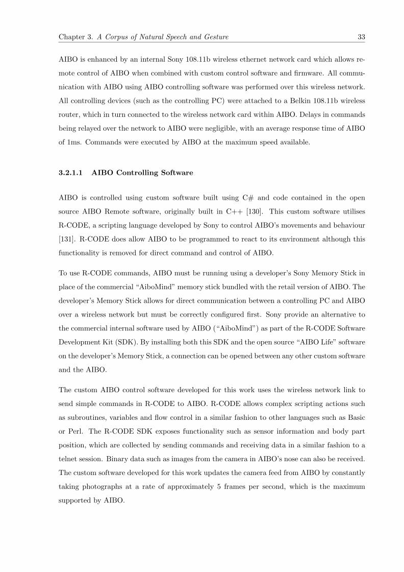
Chapter 3. A Corpus of Natural Speech and Gesture 33
AIBO is enhanced by an internal Sony 108.11b wireless ethernet network card which allows re-
mote control of AIBO when combined with custom control software and firmware. All commu-
nication with AIBO using AIBO controlling software was performed over this wireless network.
All controlling devices (such as the controlling PC) were attached to a Belkin 108.11b wireless
router, which in turn connected to the wireless network card within AIBO. Delays in commands
being relayed over the network to AIBO were negligible, with an average response time of AIBO
of 1ms. Commands were executed by AIBO at the maximum speed available.
3.2.1.1 AIBO Controlling Software
AIBO is controlled using custom software built using C# and code contained in the open
source AIBO Remote software, originally built in C++ [130]. This custom software utilises
R-CODE, a scripting language developed by Sony to control AIBO’s movements and behaviour
[131]. R-CODE does allow AIBO to be programmed to react to its environment although this
functionality is removed for direct command and control of AIBO.
To use R-CODE commands, AIBO must be running using a developer’s Sony Memory Stick in
place of the commercial “AiboMind” memory stick bundled with the retail version of AIBO. The
developer’s Memory Stick allows for direct communication between a controlling PC and AIBO
over a wireless network but must be correctly configured first. Sony provide an alternative to
the commercial internal software used by AIBO (“AiboMind”) as part of the R-CODE Software
Development Kit (SDK). By installing both this SDK and the open source “AIBO Life” software
on the developer’s Memory Stick, a connection can be opened between any other custom software
and the AIBO.
The custom AIBO control software developed for this work uses the wireless network link to
send simple commands in R-CODE to AIBO. R-CODE allows complex scripting actions such
as subroutines, variables and flow control in a similar fashion to other languages such as Basic
or Perl. The R-CODE SDK exposes functionality such as sensor information and body part
position, which are collected by sending commands and receiving data in a similar fashion to a
telnet session. Binary data such as images from the camera in AIBO’s nose can also be received.
The custom software developed for this work updates the camera feed from AIBO by constantly
taking photographs at a rate of approximately 5 frames per second, which is the maximum
supported by AIBO.

Chapter 3. A Corpus of Natural Speech and Gesture 34
The commands used to control AIBO’s movements are a subset of the available R-CODE com-
mands called “PLAY” actions. These take the form of “PLAY:ACTION:THE ACTION” where
“THE ACTION” can be a number of different instructions. The walking motion of AIBO is set
using the following command:
PLAY : ACTION : WALK.STY LE3 : 0 : 2000 (3.1)
The action in this command is “WALK.STYLE3” which is a walk command at the fastest
style of AIBO walking. The “0” following is the angle at which AIBO is to walk, relative to
AIBO’s current direction. The final number “2000” indicates a movement of 2000mm, or 20cm.
However, only a very small subset of actions are required to move AIBO around the route by
the human controller.
The control interface allows AIBO to be rotated by any orientation relative to its current
heading. AIBO can be brought to a standstill at any point, even during other movements,
which results in AIBO assuming the starting upright stationary pose.
Figure 3.2 shows the custom interface available to AIBO’s human controller (the “wizard”),
debugging controls are not included. The AIBO IP box contains the IP address of AIBO on the
wireless network, set to a static IP using a configuration file located on AIBO. The command
box allows the AIBO controller to type raw R-CODE commands for execution by AIBO. The
AIBO Vision area allows the AIBO controller to see the view from AIBO’s camera, which is
updated at approximately 5Hz. The movement controls are self explanatory apart from the
AIBO Direction area. This allows the controller to click anywhere on the area to orientate
AIBO relative to the upright direction, e.g. by clicking to the right of the area AIBO turns
between 0 and 180 degrees to the right, relative to its current heading.
By using this custom control interface the human controller of AIBO can perform all the actions
necessary to emulate an understanding by AIBO of the commands given by the experiment
participant. In this way the participant is convinced that AIBO itself is the one understanding
any communication, where in fact it is the human controller who is moving AIBO manually.

Chapter 3. A Corpus of Natural Speech and Gesture 35
Figure 3.2: The AIBO control software interface, as used by the robot controller.
3.2.2 Three Dimensional motion data capture
There are many different methods for three dimensional motion data capture, as described
in chapter 2. Vision based systems, such as those used for this work, are less intrusive and
detrimental to natural gesture than mechanical systems. Two alternative vision based systems
are described, a stereoscopic vision system and a commercial motion capture system.
The stereoscopic vision system was ultimately found to be unsuitable for use in this work.
The limitations of such a system necessitated the use of a commercial motion capture system,
described below.

Chapter 3. A Corpus of Natural Speech and Gesture 36
3.2.2.1 A Prototype Stereoscopic Vision System for Movement Capture
In order to recognise natural multi-modal communication, the movements of a participant in 3
dimensional space must be captured with enough accuracy to build models of physical move-
ments and from these movements, intent. Initially colour segmentation was used to identify
markers placed on the upper body of a participant using a custom prototype stereoscopic vision
system built using two cameras attached to a PC running custom image capture software (see
figure 3.3).
Figure 3.3: Early prototype of colour tracking using a stereoscopic vision system
This prototype system used various coloured balls as markers and connected component analysis
to label groups of pixels of the correct hue (i.e. similar marker colours). The image from the
camera is first converted into binary black and white format, where pixels are marked as white if
within a set colour range. The output of this stage of processing of each frame is a 2 dimensional
binary data set, stored in memory as a simple 2 dimensional array.
The algorithm then iterates through every element in the array until a non-background pixel is

Chapter 3. A Corpus of Natural Speech and Gesture 37
found. When a non-background pixel is found the surrounding pixels on all sides, including di-
agonals, are investigated further. By recording the connected relationship between surrounding
pixels, areas of connected pixels can be found. As the algorithm progresses through the binary
image each pixel is marked as either background or as part of a marker. With a single marker,
when multiple groups of marker pixels are found further steps are required to determine the
most likely location of the marker.
To aid marker identification, further information on each group of connected pixels is stored.
This includes the location of the centroid of each group, found from the mean average position
given all connected pixels. The number of pixels (the size of the group) is also stored. The
position and size of each group of pixels within a single frame is compared with the results of
the previous frame. Other information such as the distance moved between frames of likely
markers is used to distinguish groups that identify markers rather than noise. Groups of pixels
with a size below a certain threshold are considered noise and ignored. Initially the shape of
the marker was also considered, with only round groups of pixels above a certain measure of
“roundness” considered as markers. Due to the low resolution and reliability of the images
captured by cameras this was removed.
When markers are correctly identified the location of the centroids can be used as inputs to
a recognition system. The prototype system used a previously calibrated map of 3D space to
approximate the position of the marker in 3 dimensions. The number of pixels in each marker
group was also used as a measure of distance. To calibrate the system, a marker of fixed size
was used at locations visible to both cameras. By interpolating between set points in 3D space a
close estimate of marker position could be found from marker centroids and size of pixel groups
for both cameras.
Video information gathered using a stereoscopic vision system must be captured at a high
enough rate to accurately capture movement of the marker balls. The maximum available
framerate of 30Hz was used by the prototype system, which was limited by the cameras used.
The prototype system more accurately tracked the movement of markers in bright light and a
solid background but was easily confused by patches of colour similar to the markers in low
light. Bright surroundings improved capture by allowing a reduction in the equivalent shutter
speed of the cameras to allow faster movements without blurring, which lead to difficulties in
recognition of contiguous colour.

Chapter 3. A Corpus of Natural Speech and Gesture 38
Improvements to the recognition of contiguous colour for marker tracking include shape match-
ing whereby markers are compared to known marker shapes and typical dimensions. By ignoring
all areas of matching marker colour that do not match the typical characteristics of a marker
ball, small improvements in accuracy of marker tracking were noted.
Applying the marker system to human skin tone resulted in poorer results but the face and
hands could be identified and movements tracked. Occlusion of similar colour markers results in
confusion in marker identification by the system. Other difficulties with the prototype system
occurred as a result of hardware limitations.
3.2.2.2 Limitations of the Prototype System
Once the system had been developed the problems associated with such a simple stereoscopic
marker based system quickly became apparent. These include, but are not limited to, the
following:
Occlusion - A system with a small number of viewpoints (such as a two camera system) is easily
confused by objects passing in front of each other. A system can be adapted to predict the path
of objects based on their previous trajectories but it was still found that high levels of occlusion
prevented the system from tracking accurately. Occlusion is only a problem with vision based
systems (either visible light or IR) and can be mitigated by increasing the number of cameras
used and quality of the markers for each distinct marker location. By increasing the size and
relative difference between individual markers the hardware limitations of the cameras can be
reduced.
Speed - The prototype system captured video frames at a maximum framerate of 30Hz and
was based on relatively cheap consumer level cameras. The cameras varied the shutter speed
depending on the amount of light reaching the camera sensor. As a result fast movement,
especially in low light, blurs the markers when frames are captured. This in turn makes colour
and shape detection difficult as the object becomes a blend of background/object and is distorted
so much in shape as to be unrecognisable to the shape detection algorithm. The limitations of
the cameras used could be avoided by using better cameras and a better capture system.
Ease of expansion and computational cost - The custom software developed for the prototype
stereoscopic vision system allowed expansion to better quality and more numerous cameras
but the computational cost required for more cameras quickly became very high. The system

Chapter 3. A Corpus of Natural Speech and Gesture 39
was running on a standard Intel Pentium-4 based desktop PC, limiting the frame rate as more
visual processing stages were added. The image processing algorithms designed for connected
component analysis and marker identification were optimised but the computational cost of
more than two cameras was still found to be prohibitive using the custom software developed.
As a result of these difficulties and the reduced scope for expansion to full body tracking the
prototype system was discarded in favour of a commercially available 3D motion tracking system,
the Qualisys Track Manager (QTM) [93].
3.2.2.3 The Qualisys Full Body Movement Capture System
Full body movement was captured using the commercial Qualisys Track Manager and ProReflex
camera system. Six infrared cameras were used to trace the positions of 19 highly reflective
marker balls attached to set points on the participant’s body. These could be used to describe a
simple skeletal model of the body. Two additional markers were placed on AIBO for calibration
and synchronisation of audio and gesture data.
The markers were highly reflective plastic balls, with 20mm and 10mm diameters. The 20mm
markers were used at major joints and where obscuration of markers was expected. The 10mm
markers were used in places where dexterity was required, such as on wrists. The reflective sur-
face of the markers was similar to commercial high visibility paint and safety clothing. Markers
were fixed to participants using strong double sided tape, care was taken to only apply markers
to clothing or dry skin.
The camera system was calibrated to an identical (0,0,0) centre point for all 3 axes located in
the centre of the floor, below the participant’s available movement space, before the recording of
each participant. Calibration was performed several times until the whole system passed a set
calibration success metric provided by Qualisys. It was found that repeated calibration of the
3D capture system was not strictly necessary as the fixed camera positions allowed the (0,0,0)
centre point to remain constant throughout all recordings. The average 3D positioning error
after calibration, as given by the calibration tool in Qualisys Track Manager, was found to be in
the region of 20-40mm for all markers. Calibration was performed repeatedly until the highest
error across all markers was reduced to a maximum of 40mm, the minimum error possible even
after repeated calibrations.

Chapter 3. A Corpus of Natural Speech and Gesture 40
All participants were asked to perform a waving motion before each recording, raising the arms
to their sides at a 90 degree angle to the body. This waving motion confirmed that the markers
were correctly positioned and attached to the participant. On several occasions the tape used
to attach the markers was replaced after this motion due to markers becoming detached.
The participants were allowed to move within a set 100x100cm space located just behind the
map area in which AIBO could move (see section 3.2.5 for a description of the map and routes).
Participant’s movements and orientation were not restricted as long as their feet stayed within
the available movement space. If a participant moved outside of this space the recording was
stopped and the process repeated.
The skeletal model of the participant was designed to allow easy fixture of markers at major
joints on the human body without restricting freedom of movement. Due to the high importance
of arm movements in command and control scenarios more markers were used on the arms than
anywhere else, a total of five for each arm. Two head markers were used to allow recording of
head orientation, a chest and two hip markers were used for body orientation and two markers
on each leg were used at the knee and just above ankle joints. Figure 3.4 shows the location
of markers on the participant’s body, white spots from the reflection of the camera’s flash are
markers. Table 3.1 gives the list of markers used during recording by the motion capture system.
headfacechestleft shoulderleft upperleft elbowleft lowerleft handright shoulderright upperright elbowright lowerright handleft hipleft kneeleft footright hipright kneeright footaibo headaibo body
Table 3.1: Names given to markers during motion capture recordings.

Chapter 3. A Corpus of Natural Speech and Gesture 41
Figure 3.4: Marker Placement
Each camera used a grid of 250 infrared LEDs located around the camera lens, to reflect light
from the markers placed on the participants body. A framerate of 100Hz for all cameras was
chosen as a compromise between maximum temporal accuracy and the calibration and buffering
errors which arose when synchronising the recordings of six cameras. Each camera had an
individually set horizontal field of view of between 10 to 45 degrees with a manufacturer specified
visual measurement range of 0.2 to 70 metres. The field of view was adjusted to capture the
participant’s movements with as much accuracy as allowed by the cameras. To do this the field
of view was reduced to as small range as possible while still allowing multiple cameras to capture
all potential participant movements. The visual range from the cameras never exceeded more
than 10 metres, well within the manufacturer specification.
The cameras were located in positions which aimed to ensure that each marker was visible to
at least two cameras at all times so as to accurately triangulate their position in 3D space. A
calibration procedure was followed to allow the Qualisys system to determine the positions of
all cameras automatically using the Qualisys Track Manager software. A Qualisys hand held
rigid plastic frame with several fixed marker positions was used to calibrate the cameras. By
setting the Qualisys Track Manager to calibration mode and moving the plastic frame within
Chapter 3. A Corpus of Natural Speech and Gesture 42
the 3D space seen by all cameras, it was possible for all camera positions to be found. The
calibration of the system also meant that any other markers brought into the same 3D space
could be correctly triangulated using a minimum of two cameras.
Each camera used a 658x500 resolution CCD image sensor which was increased to an effective
resolution of 20000x15000 subpixels using proprietary Qualisys interpolation algorithms. The
gain for each camera was adjusted individually for maximum sensitivity to the reflected light
from the markers without introducing noise to the CCD.
Due to buffering issues with the camera system, all recordings were restricted to a maximum of
120 seconds, after which errors in recording increased in frequency. The recording system could
be triggered by the operator very quickly, resulting in a delay of just 2 seconds before recording
was initiated again.
Each camera was connected in a “daisy-chain” network to a recording PC, the gesture cap-
ture PC. This gesture capture PC was operated by the instructor, who gave instructions and
explained the recording methodology to the participants (see section 3.3.2 for details on partic-
ipant instruction). The instructor was responsible for re-calibration of the movement capture
system before each participant and the continued operation of the system throughout all record-
ings. An Intel Pentium 4 based PC was used for the gesture capture PC with custom Qualisys
equipment used for interfacing with the ProReflex cameras.
Each marker recorded was later labelled by hand according to its position on the simple skeletal
model. Correctly labelling each marker in every recording was time-intensive due to recording
sensitivities of the camera system. Flickering marker recordings due to occlusion or hard-
ware limitations required individual labelling of markers during each distinct recorded segment.
Markers which were not detected by the camera system for any reason during recording were
marked at position (0,0,0) by the Qualisys Track Manager software. Post processing of the
recordings was required to produce smoothly interpolated 3D data, as discussed below.
All movement data was recorded in the proprietary Qualisys Track Manager .qtm format and
converted to standard comma separated variable .csv format for use in further experiments. The
data takes the form of 57 dimensional (3 x 19 markers) data with a line for each frame in the
.csv format. Resulting .csv files are approximately 5.5-6mb in size for a 120 second recording.
The data from the 3D recordings is in the form of a 57 dimensional vector, V , of which there
are N samples per recording. Each recording is therefore a matrix H of size 57 ∗N .

Chapter 3. A Corpus of Natural Speech and Gesture 43
The Qualisys software allows for visual analysis of a participant’s strategy and motion, of which
some examples are listed here. In all cases the full interface and location of AIBO is shown.
Figure 3.5 shows a curved sweeping motion, typical of periods where participant’s are illustrating
paths on the floor. Figure 3.6 shows a static pose, where a participant’s intent is for AIBO to
continue forward. Figure 3.7 shows the motion of a participant with a typically complex and
communicative strategy.
Figure 3.5: Qualisys Track Manager software showing a sweeping motion by a participant.The green trace lines show the previous 0.5 seconds of data.
3.2.2.4 Error Handling
Errors in 3D motion tracking can be described in severity as either coarse or fine. In this work
coarse errors are those which cannot be automatically corrected using an interpolation method.
Errors in capture where markers were not visible for long periods of time are especially likely
to be described as coarse. In periods where a participant is making large physical movements,
any loss of tracking on a marker is more likely to require manual repair of the data.
Fine errors are those which can be compensated for automatically, such as minor gaps in track-
ing. Typically these fine errors can be seen as flickering markers, where the tracking system

Chapter 3. A Corpus of Natural Speech and Gesture 44
Figure 3.6: Qualisys Track Manager software showing a static pose by a participant with theintention of guiding AIBO forwards.
Figure 3.7: Qualisys Track Manager software showing a participant with typically complexphysical movements. The green trace lines show the previous 0.5 seconds of data.
Chapter 3. A Corpus of Natural Speech and Gesture 45
momentarily loses a marker for a very short period of time. Due to the short periods at which
markers are occluded it is usually possible to recover the data using interpolation.
The Qualisys 3D movement capture system was found to be less than 100% accurate after
marker tracking had been recorded. Inaccuracies in the ProReflex camera CCD sensitivity
resulted in a slight noise in all 3 axes, which remained almost constant during recordings. All
time segments of marker positioning were labelled manually, but there remained periods where
markers were invisible due to camera insensitivity or occlusion, despite attempts to avoid this.
Initially spline-based interpolation algorithms provided by Qualisys were used to bridge these
gaps in data but it was found that for larger gaps the continuous noise in all 3 axis produced
incorrect interpolated paths for the markers.
Simple linear interpolation of the data was performed for time periods above 1 second (100
frames). Although delta and acceleration properties of the markers were used initially, it was
found that the constant noise badly affected the accuracy of these methods. Data smoothing
was performed by the Qualisys system but could not entirely remove the noise in all 3 axes
without affecting the accuracy of recordings of high speed movements by participants.
Where markers were not found at the start of recordings and placed at the origin position (0,0,0)
the marker position was set to the coordinates at the first available capture of the marker. In this
way markers were not seen to suddenly jump from (0,0,0) to their position on the participant.
By combining this method with linear interpolation the time taken to manually label markers
was reduced substantially.
3.2.3 Speech Recording
All speech was recorded in mono 44khz 24bit PCM WAV format using a headset mounted
microphone and a secondary backup directional microphone located within the recording area
and aimed at the participant. The headset mounted microphone was attached via standard
audio cable to a Sony MiniDisc recorder located in the participant’s pocket. The secondary
microphone, a Shure SM48, was attached to a PC in another room but produced recordings
of a lower quality which were not used in further experiments. This lower quality was caused
by the distance between the secondary microphone and the participant and the capture of a
large amount of background noise. Care was taken to avoid any interaction with the recording

Chapter 3. A Corpus of Natural Speech and Gesture 46
equipment by the participant; all audio recordings were started before and ended after the
participant had performed the entire recording exercise.
Although audio recordings were not automatically synchronised with the gesture data, the
sensitivity of the headset microphone was adjusted to allow calibration using AIBO’s physical
movements (see below). To avoid breath noises and interference with the participant’s face the
microphone was adjusted to an angle of 45 degrees down from the eye-line of the participant
and 5cm away from the right of the participant’s mouth. Each participant was recorded in the
same way so as to avoid differences between recordings as much as possible.
Although every effort was made to keep recording conditions identical, there were environmental
factors such as variant building and wind noise throughout recordings. The room in which all
recordings were made was located in a secure building with several sealed doors but noises from
equipment, such as air conditioning systems, could not be entirely avoided.
Speech recordings were resampled to 16kHz mono format to match the models used to build
the automatic speech recognition system, as described in Chapter 6.
3.2.4 Synchronisation of Speech and Gesture Recordings
All multimodal recording systems, such as used in corpus collection for this work, require exact
synchronisation between modalities. Although several different recording techniques were used,
the accuracy of modern hardware clocks allows for synchronisation across different equipment
as long as synchronous data (such as noisy movement) exists in all modalities. Newer versions of
the Qualisys system allow for the insertion of timing information in all modalities synchronously.
This functionality was not available at the time that the current corpus was collected.
As the speech and gesture were recorded by two different processes, the 3D movement capture
system and the headset mounted microphone, it was necessary to synchronise the recordings
and trim the audio recordings to match the 3D gesture recordings. The Qualisys system allowed
for close inspection of the markers attached to AIBO, the movements of which were compared
to the corresponding noises in the audio waveform. These features were used to align the audio
recordings with the 3D gesture recordings and the audio recordings were then cropped to the
same length as the 3D gesture recordings.
Synchronisation in this manner was performed manually in several passes and confirmed at
several points throughout each of the recordings. As all recordings included some movement of

Chapter 3. A Corpus of Natural Speech and Gesture 47
AIBO it was possible to exactly synchronise the speech and 3D data. Where there were any
difficulties identifying AIBO movement sounds or 3D data the video information recorded using
the Sony DV camera was used to confirm synchronisation.
Each recording, audio or 3D data, was given a suitable distinct name XY ABC; where XY
denoted the name of the participant, A denoted the route around which AIBO was guided, B
denoted the “take” (e.g. 1 if the first recording, or 2 if the first recording failed for any reason)
and C denoted the “part” (a 120s segment of recording, the maximum length of time the camera
system could operate without introducing recording errors).
3.2.5 The AIBO Map and Routes
The designated floor space in which AIBO was allowed to move was configured as the map.
The different paths AIBO was instructed to follow were described as the routes. A total of 4
routes through the map were used during recording, although time constraints and recording
equipment issues resulted in some failures in recording all 4 routes for all participants.
The floor space was marked out with tape, including the area in which the participant was
allowed to move. 7 points were marked on the map using A4 sheets of printed paper, each
containing one of the letters B, C, D, G, P, T, V. The letters were chosen for these points based
on their phonetic similarity for use in further experiments under the assumption that partic-
ipants would use them as points of reference when directing AIBO. However, this contextual
information was found to be rarely used by participants whilst directing AIBO (see below).
All 4 routes were performed using the same map layout and participants were not given any
information other than an illustration of the routes.
Initially the route instructions were provided to the user on a stand within visual range to
the right of the participant. This was found to restrict movements as the participants had
to constantly turn to read the map. To avoid this, the route directions were placed over the
letter G on the floor. This allowed participants to move freely without adjusting their physical
movements to keep the route directions within their field of view.
4 routes through the map were designed, with an approximately equal level of complexity. The
number of right and left turns were restricted to similar amounts so as to keep the number
of directional changes equal. The routes did not include any 180 degree turns or require any
backward movements by AIBO. Figure 3.8 shows the 4 routes.
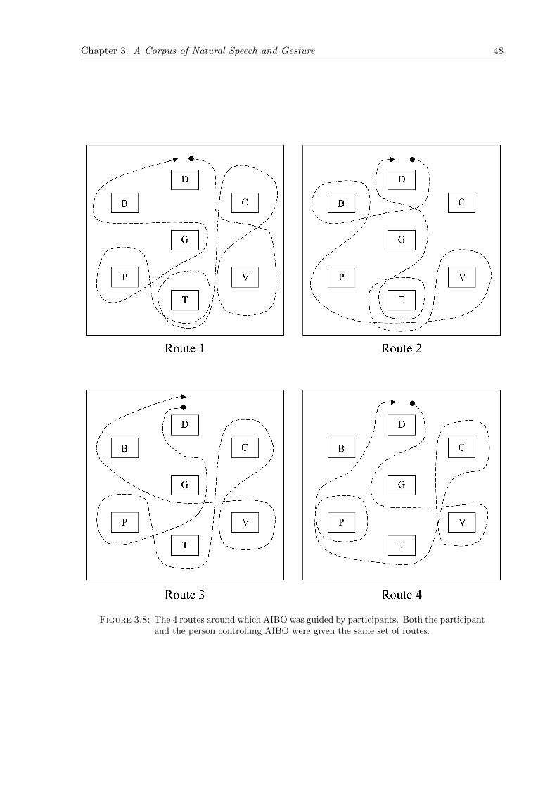
Chapter 3. A Corpus of Natural Speech and Gesture 48
Figure 3.8: The 4 routes around which AIBO was guided by participants. Both the participantand the person controlling AIBO were given the same set of routes.

Chapter 3. A Corpus of Natural Speech and Gesture 49
The whole map space was defined using markers at all four edges. The space in which the
participants were allowed to move was outside of the path, centrally located to the south of the
area in which AIBO was free to move. Figure 3.9 shows the exact layout:
3.3 Experimental Procedure for Corpus Collection
Two experiments were performed for corpus collection, an initial exploratory experiment and
the main corpus collection experiment.
3.3.1 Initial Exploratory Experiment
The first preliminary experiment was designed to address how to accurately record speech and
gesture data in human-human command and control. Human-human communication is different
to human-robot communication but basic lessons could be learned about the best methods to
acquire speed and movement data.
The initial experiment also provided a rough outline of vocabulary and gestures used by par-
ticipants. The task involved one participant guiding another around a set route defined on the
floor. To encourage the use of gesture, speech communication was impaired by playing speech
noise at varying levels to the listener through sound isolating headphones.
The aim of the guiding participant was to guide the listener around a set route on the floor
around several floor markers. The routes used were found to be too simplistic and were expanded
to form the routes used in the main experiment.
The initial experiment clearly identified problems in the recording apparatus. A headset and
MiniDisc recorder replaced the wired microphone used in the initial experiment, as it was found
that even with a lengthy connecting wire between a recording PC and the guiding participant
there was still interference with the participant’s freedom of movement. The routes were ex-
tended and modified to include a more even distribution of left and right turns. The typical
range of movement by the guiding participant was found to be an area outside the map of up
to 1m2. No guiding participant’s entered the map area or moved around the edge of the map.
The style of the communication from the guiding participant also gave an insight into natural
human-human communication. It was observed that empathy between participants allowed

Chapter 3. A Corpus of Natural Speech and Gesture 50
Figure 3.9: The layout of the floor space in which both AIBO and the participant can move.The upper area containing the 7 marked points (205.5 x 197.7cm) is the area in which AIBOis free to move. The lower area (100 x 100cm) is the participant’s allowed movement area. All
dimensions in cm.

Chapter 3. A Corpus of Natural Speech and Gesture 51
very simple contextual instructions to be understood such as “face the wall then go towards the
door”, instructions which were markedly different to those later recorded when guiding AIBO.
The strategies used by participants guiding AIBO are discussed in more detail below.
3.3.2 Corpus Collection Experiment
In broad terms the main experimental procedure for corpus collection can be described as a
“Wizard of Oz” style experiment designed to elicit as much unconstrained natural speech and
gesture as possible without directing the communication of participants. Salber [129] describes
the “Wizard of Oz” technique as an evaluation mechanism that allows the observation of a
participant operating an apparently fully functioning system where features of the system are
controlled by a hidden “wizard”.
Participants were chosen at random from volunteers at the University of Birmingham. Partici-
pants were only allowed to perform the experiment if they had no previous experience of AIBO,
to avoid any prior knowledge of AIBO’s limitations affecting their methods of communication.
A total of 17 participants were recorded, 5 female and 12 male. Participants were not excluded
from the study for any physical differences or fluency in English. By allowing variation in com-
municative style it is hoped that the final intent recognition system will be better prepared to
deal with new and varying participants.
Each participant is led to believe that they alone are responsible for AIBO’s movements and
actions. In this way they communicate with AIBO as they would with an apparently sentient
robot, their speech and gesture interpreted by an artificial intelligence. The artificial intelligence
is actually simulated by an external human “wizard”, of whom the participant is unaware, who
controls AIBO based on his interpretation of the participant’s speech and gesture.
The AIBO controlling “wizard” was given a copy of all routes and an understanding of the
participant’s task before any experiments were conducted. This controller was instructed to
follow the guidance of the participant to the best of his abilities using a video and audio link
to the experiment location. The controller was located in a completely separate room to the
experiment and was never introduced to the participant, who was unaware of their presence at
all times.
As the participant was unaware of the external controller of AIBO it was important to manage
his or her expectations of the robot’s abilities. In “Wizard of Oz” experiments such as this
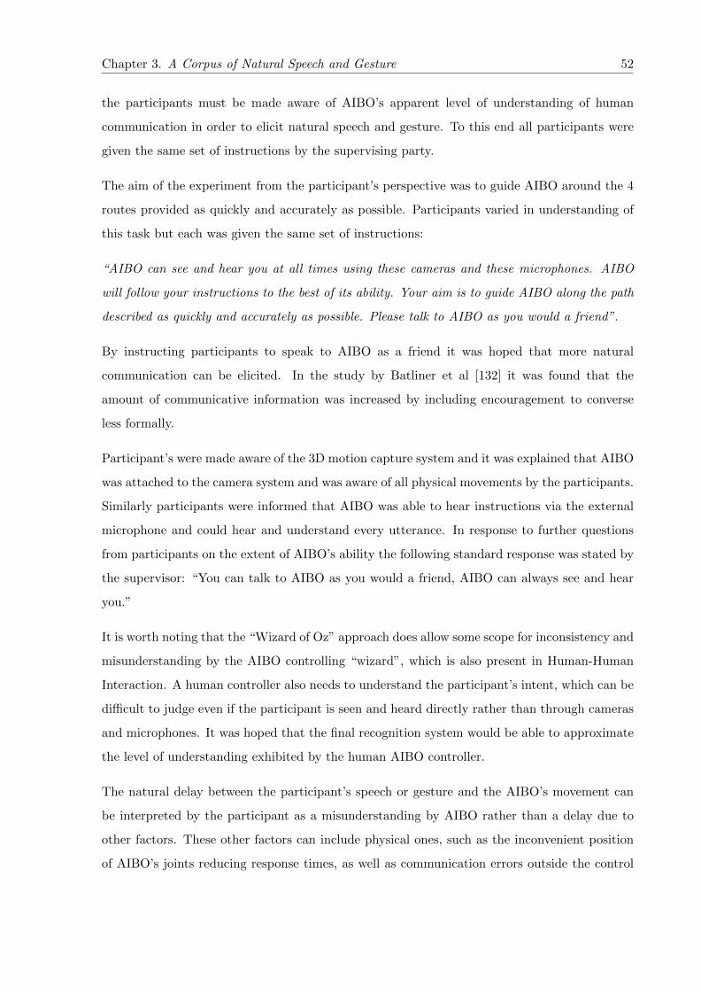
Chapter 3. A Corpus of Natural Speech and Gesture 52
the participants must be made aware of AIBO’s apparent level of understanding of human
communication in order to elicit natural speech and gesture. To this end all participants were
given the same set of instructions by the supervising party.
The aim of the experiment from the participant’s perspective was to guide AIBO around the 4
routes provided as quickly and accurately as possible. Participants varied in understanding of
this task but each was given the same set of instructions:
“AIBO can see and hear you at all times using these cameras and these microphones. AIBO
will follow your instructions to the best of its ability. Your aim is to guide AIBO along the path
described as quickly and accurately as possible. Please talk to AIBO as you would a friend”.
By instructing participants to speak to AIBO as a friend it was hoped that more natural
communication can be elicited. In the study by Batliner et al [132] it was found that the
amount of communicative information was increased by including encouragement to converse
less formally.
Participant’s were made aware of the 3D motion capture system and it was explained that AIBO
was attached to the camera system and was aware of all physical movements by the participants.
Similarly participants were informed that AIBO was able to hear instructions via the external
microphone and could hear and understand every utterance. In response to further questions
from participants on the extent of AIBO’s ability the following standard response was stated by
the supervisor: “You can talk to AIBO as you would a friend, AIBO can always see and hear
you.”
It is worth noting that the “Wizard of Oz” approach does allow some scope for inconsistency and
misunderstanding by the AIBO controlling “wizard”, which is also present in Human-Human
Interaction. A human controller also needs to understand the participant’s intent, which can be
difficult to judge even if the participant is seen and heard directly rather than through cameras
and microphones. It was hoped that the final recognition system would be able to approximate
the level of understanding exhibited by the human AIBO controller.
The natural delay between the participant’s speech or gesture and the AIBO’s movement can
be interpreted by the participant as a misunderstanding by AIBO rather than a delay due to
other factors. These other factors can include physical ones, such as the inconvenient position
of AIBO’s joints reducing response times, as well as communication errors outside the control

Chapter 3. A Corpus of Natural Speech and Gesture 53
of AIBO’s human controller. As AIBO is controlled by wireless network communication, errors
can arise as a result of delays due to network latency or an inconsistent wireless signal.
3.4 Corpus Size
In total 8 hours 43 minutes and 33 seconds of raw audio recordings were made. This data was
trimmed to match the 3D gesture data segments resulting in 6 hours 13 minutes 37 seconds of
aligned speech and gesture data. A total of 205 segments of recorded data were made, each of
length ≤120 seconds.
The data was partitioned evenly throughout the corpus, independent of participant, into training
data (184 segments) and test data (21 segments), a 8.76:1 ratio of training to test data which
was kept identical for all experiments. Every 8th segment was removed from the training set
and placed in the test set. Portable HTK format .scp files, describing a list of files, were used
to ensure consistency when describing training and test data.
The segments chosen for test and training data were chosen across all recordings to avoid bias
towards a set route, participant or strategy. Alternative methods of segmenting the data could
include using all recordings of participants guiding AIBO around a single route as the test
data. The large variation in participant strategy, even within recordings of a single route,
precludes using such a homogeneous set of recordings. Although it is not recommended, given
enough training data (many more routes per participant) it may be possible. This assumes that
participant strategy stays consistent between routes, or that it becomes consistent over time.
The training and test sets comprise samples from the same group of participants. All intent
recognition can thus be considered to be group dependent, for the closed population of par-
ticipants recorded for this corpus. The intent recognition is not participant dependent, but if
the intent recognition models used in this work were applied to an unknown participant it is
expected that the performance will decrease. By recording and modelling the intents of a much
larger population it is expected that intent recognition performance would improve for unseen
participants and that performance loss due to the large variability between participant’s strat-
egy would be reduced. This is beyond the scope of this work due to the difficulties associated
with recording and modelling the intent of a large number of participants.

Chapter 3. A Corpus of Natural Speech and Gesture 54
Errors in recording procedure due to incorrect microphone and route illustration placement
meant that all the data from the first participant was removed from the corpus. Errors in the
3D data capture system were only discovered when the recordings were found to be corrupted,
meaning some audio recordings were ignored due to a lack of corresponding gesture data and
vice versa. Where recording failed for either modality the recorded data was discarded.
3.5 An Overview of Participant Strategy
The corpus collection experiment was designed to elicit completely unconstrained and natural
speech and gesture in a human-robot command and control task. It was vital that the partici-
pants were allowed to perform the task in any way they saw fit, which in turn produced a corpus
with massive variation in communication style between participants. The strategies involved
varied from a complete lack of gesture and limited speech to extended conversations with AIBO
as if to a small child.
As the participants were told to talk to AIBO as they would to a friend it was expected that
the language used would be more expressive than simple commands. The strategy for each
participant varied by a large amount, with a wide range of approaches and resulting speech
information. Some participants used child directed speech [133] which was accompanied by a
large range of physical movements. For the majority of participants, physical movements were
restricted to use of the arms alone, with only a few participants using full body motions.
It was noted that strong deictic gestures were mainly performed when AIBO was facing the
participants, especially when AIBO was located a short distance from the participant. Although
participants were informed that AIBO used the 3D capture system to “see” all movements
most participants still treated AIBO as an animal with eyes in the front of its head. This
behaviour was deliberately not corrected in order to gather natural gesture and shows that
many participants treated AIBO like an animal despite clear indications that it was not.
The most common physical movement where no intent was clear was found to be scratching of
the forehead or adjusting clothes. As participants wore a headset microphone it is possible that
irritation due to headset placement could have increased the amount of unwanted movement.
These movements where intent was not clear were usually combined with a following clear intent
making it difficult to discern where the intent of the participant began. The two most common
stationary positions were standing with arms by the sides or standing with arms crossed. More

Chapter 3. A Corpus of Natural Speech and Gesture 55
than one participant walked back and forth within the allowed space rather than remaining
stationary.
Participants were instructed to follow the routes accurately. However, the degree of accuracy
that participants tried to achieve varied, resulting in longer recording times for participants that
tried to be more accurate. Tables 3.2 and 3.3 describe the overall strategy of each participant
and are mainly useful as an indication of the variability between participant strategies.
Participant Description of Strategy
AP Longer periods of communication with single intents taking several timeslonger than other participants. Speech is clear but difficult to categorise peri-ods of intent based on physical movements.
AS Almost no physical movements. Where present these movements are veryshort and communicate little. Speech is very structured and follows patternof LEFT , RIGHT or FORWARD intents with STOP after each. Strategyremained simple and consistent between all recording.
AY A very simple strategy where individual arms are raised to indicate LEFTor RIGHT intents. Speech was also simple although in later recordings thephysical movements and speech intents became less synchronous.
CK Combination of physical movements and speech allowed for improving speedthroughout recordings. Physical movements were mainly simple arm move-ments with an emphasis on DEST intents.
JC Unique physical movements with both arms extended outwards to the frontand lowering/raising arms individually to indicate to AIBO to rotate left orright. Limited set of intents, mainly LEFT , RIGHT and FORWARD muchlike simple commands.
KO Large full body motions with some descriptive speech. It is worth notingthat due to the larger physical movements of KO, occlusion of markers hada larger impact on capturing movements than any other participant. Intentswere mainly PATH and STOP with speed of guidance slowing as recordingsprogressed.
MD Very expressive full body physical movements, with a large number of verbalPATH intents. MD used “motherese” style language to talk to AIBO. Thestrategy remained relatively consistent between recordings with some increasein speed of communication in later recordings.
MK Most physical movements used to communicate DEST intent, throughoutmost recordings MK used an extended arm to point to the position AIBOshould be heading towards. Speech contains mainly commands to go to thedestination indicated by pointing gesture, a large number of periods of DESTintent.
OO Uses a twisting arm motion when trying to communicate LEFT or RIGHTintents. Both arms are extended and each is rotated individually. Similarstrategy to that of JC although with different physical movements. Speechis very varied, from short commands to more conversational speech. As withsome of the other participants it can be difficult to differentiate between peri-ods of intent during longer periods of speech.
Table 3.2: An overview of participant strategy (AP - OO).
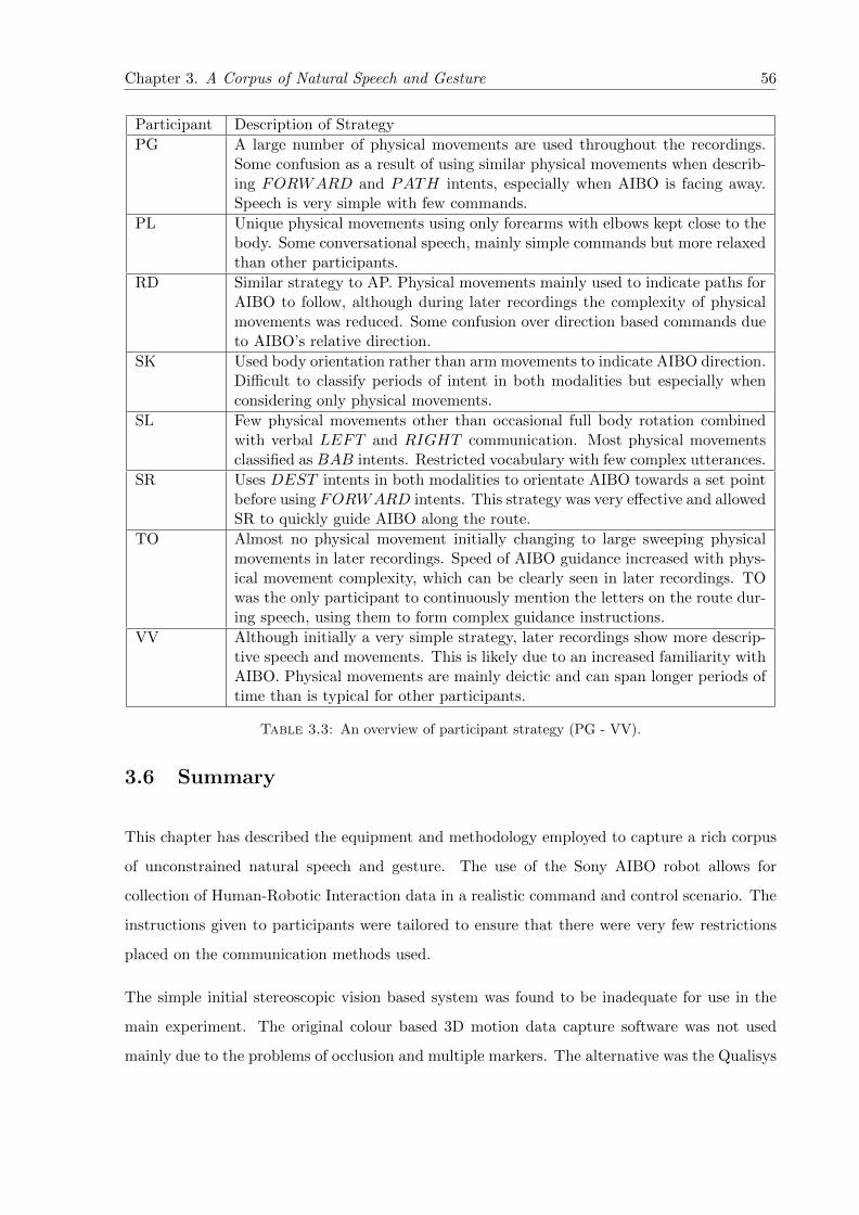
Chapter 3. A Corpus of Natural Speech and Gesture 56
Participant Description of Strategy
PG A large number of physical movements are used throughout the recordings.Some confusion as a result of using similar physical movements when describ-ing FORWARD and PATH intents, especially when AIBO is facing away.Speech is very simple with few commands.
PL Unique physical movements using only forearms with elbows kept close to thebody. Some conversational speech, mainly simple commands but more relaxedthan other participants.
RD Similar strategy to AP. Physical movements mainly used to indicate paths forAIBO to follow, although during later recordings the complexity of physicalmovements was reduced. Some confusion over direction based commands dueto AIBO’s relative direction.
SK Used body orientation rather than arm movements to indicate AIBO direction.Difficult to classify periods of intent in both modalities but especially whenconsidering only physical movements.
SL Few physical movements other than occasional full body rotation combinedwith verbal LEFT and RIGHT communication. Most physical movementsclassified as BAB intents. Restricted vocabulary with few complex utterances.
SR Uses DEST intents in both modalities to orientate AIBO towards a set pointbefore using FORWARD intents. This strategy was very effective and allowedSR to quickly guide AIBO along the route.
TO Almost no physical movement initially changing to large sweeping physicalmovements in later recordings. Speed of AIBO guidance increased with phys-ical movement complexity, which can be clearly seen in later recordings. TOwas the only participant to continuously mention the letters on the route dur-ing speech, using them to form complex guidance instructions.
VV Although initially a very simple strategy, later recordings show more descrip-tive speech and movements. This is likely due to an increased familiarity withAIBO. Physical movements are mainly deictic and can span longer periods oftime than is typical for other participants.
Table 3.3: An overview of participant strategy (PG - VV).
3.6 Summary
This chapter has described the equipment and methodology employed to capture a rich corpus
of unconstrained natural speech and gesture. The use of the Sony AIBO robot allows for
collection of Human-Robotic Interaction data in a realistic command and control scenario. The
instructions given to participants were tailored to ensure that there were very few restrictions
placed on the communication methods used.
The simple initial stereoscopic vision based system was found to be inadequate for use in the
main experiment. The original colour based 3D motion data capture software was not used
mainly due to the problems of occlusion and multiple markers. The alternative was the Qualisys

Chapter 3. A Corpus of Natural Speech and Gesture 57
Track Manager system, which was found to be reliable enough to capture 3D motion data for
the purposes of this work.
Software for control of AIBO was developed and a “Wizard of Oz” experimental method put
in place. A set of 4 routes were used to encourage the use of both speech and gesture in
guiding AIBO. The control of AIBO was performed externally without the knowledge of the
participants.
The collected speech and gesture corpus has been synchronised and partitioned into training
and test data suitable for use in further experiments.

Chapter 4
Annotation Conventions
4.1 Introduction
The objective of this work is to classify a participant’s intent from his or her speech and gestures.
To achieve this it is first necessary to identify a suitable set of intents and to label the training
and test data according to these intents. Intents are effectively semantic classes and their
definition requires some degree of subjectivity.
Intent can be assigned to individual modalities or to some combination of modalities. In this
work intent labels are assigned to speech using only speech transcripts and gesture using only 3D
motion data. The labels are then combined. Although it may be possible to produce a combined
transcription of overall intent based on both speech and gesture (e.g. from video material) this
is not covered in this work. By considering each modality individually, periods of intent can be
classified without the influence of other modalities. Intent recognition engines based on single
modalities will only have information from that modality, so labels for one modality should not
be influenced by information from others.
This chapter motivates the final intent-level label set used during the transcription of the data.
The methods for labelling both speech and gesture are described as well as the process of
combination of labels to form one set of master labels. As some of the programs and scripts
used to build a recognition system are based on the Hidden Markov Model Toolkit (HTK) the
HTK label format as it applies to this work is also described.
58

Chapter 4. Annotation Conventions 59
As the participants’ gesture and speech were captured using separate recording systems the
alignment of speech and gesture data is discussed. The time alignment of speech with speech
transcriptions is also discussed, although the process of building a speech recognition engine
capable of this task is covered in depth in Chapter 6.
The transcription of spoken intent was performed with the aid of multiple human transcribers
and the methodology of this process is described here. Further experiments are detailed in-
cluding a comparison of the similarity of speech and gesture labels and the duration of speech
intents in relation to the number of words used by participants.
4.2 Choice of labels
Intent labels must be chosen that reflect intents possible in both speech and gesture modalities;
ideally any multimodal recognition system should have the same label sets across all modalities.
The labels in this work were chosen through an iterative process, whereby a larger set of intent
labels was reduced to an optimised label set suitable for both speech and gestural intent. There
are a variety of approaches to selecting intent labels, some of which would take longer than the
time available for this work. Although useful, an objective study of perceived intent type using
multiple participants is beyond the scope of this work.
In order to model the intent of a participant it must be possible to separate the intents into
distinct categories. Intents are defined in relation to AIBO, so if the intent is to move AIBO
forward then this should be classified as a FORWARD intent.
When transcribing the intent of a participant secondary information, such as the direction AIBO
is facing relative to the participant, the position of AIBO and the route that AIBO should be
following are also considered by the transcriber. The two available viewpoints are those of AIBO
(the object viewpoint) and the participant (the character viewpoint). The problem of defining
“left” and “right” relative to an object which changes direction means that the only consistent
way to label this type of movement or intent is in relation to the object. Many participants
used similar gestures, even within the same recording, to describe an intent to rotate AIBO left
or right. Transcribers labelled intent in relation to the object (AIBO) and accepted that there
would be identical physical movements to communicate disparate intents.

Chapter 4. Annotation Conventions 60
Variation within a participant’s recordings, although large, was not as pronounced as the varia-
tion in style of movement and speech between participants. The labels used to describe gesture
and speech did not make any allowance for variation due to external factors such as sex, race,
spoken English fluency, confidence or familiarity of the participant with the task, although
these do have an impact on the gesture or speech used. The time taken to perform the task and
the speed with which intents are communicated also meant that the duration and quantity of
labelled intents varied massively between participants.
An initial intent label set was defined based on the first transcription of physical movement
data produced by the 3D motion tracking system and in consideration of the speech recordings.
This set of intents was reduced further as work progressed and finally reduced to 9 intents for
the final merged labels.
The transcription process based on physical movement data is an iterative one, where all record-
ings are seen multiple times (at least three passes were conducted for this work, see Section 4.7.
The large amount of recorded data precluded the creation of labels by multiple transcribers due
to the time and resources required (approximately 10 hours per pass). If the work was to be
repeated with a larger number of recordings and transcribers it may be possible to investigate
a different or larger set of intents. Also, comparisons between transcriptions could be made as
for speech intent transcriptions (see Section 4.6.
The initial label set is as follows:
• WAV ING - An initial calibration gesture used to make sure that the recording system was
functioning correctly. Participants were asked to wave their arms up and down alongside
their body to make sure all markers were correctly positioned and identified by the 3D
tracking system. Not strictly an intent and later merged with BAB.
• LEFT - An intent to rotate AIBO to the left, in relation to AIBO not the participant.
• RIGHT - An intent to rotate AIBO to the right, in relation to AIBO not the participant.
• FORWARD - An intent to make AIBO move or continue in the same direction AIBO is
currently facing.
• COME - An intent to bring AIBO toward the participant, including rotating if required to
face the participant. COME was included as it was the only intent containing secondary

Chapter 4. Annotation Conventions 61
information (the location of the participant) that could be directly used by a recognition
system recording only the position of the participant.
• PATH - An intent to make AIBO follow a route as described by the participant. E.g.
“Follow the path I have drawn” or “Follow a path shaped like this”.
• PATH DEST - An intent to make AIBO follow a route as described by the participant
ending in a fixed target. E.g. “Follow the path I have drawn to this point”.
• DEST - A typical deictic/pointing gesture to a location on the route with the intent of
making AIBO travel to a set location. E.g. “Go to this point I am pointing at”.
• STOP - An intent to force AIBO to stop whatever action he is performing and stand still.
• NULL - No intent communicated by the participant. Typically silence in speech or
no movement in gesture. In speech, when there is no speech data, e.g. “sil” words or
silence, we consider the intent to be NULL. “sil” words and therefore NULL intents in
speech can be considered as the participant deliberately not speaking or the person is not
communicating any intent by voice.
• BAB - An intent to communicate although not directly related to the task or an unin-
telligible movement or spoken utterance. Common babble gestures include repositioning
of clothing, scratching and placing hands in pockets. As the resting poses of participants
varied throughout recordings BAB intents also communicated that the participant was
uncomfortable and changed positions. Common speech babble includes asking questions
of the person involved in recording the participant and expressing frustration with AIBO
and the task e.g. “my microphone is loose”.
As WAV ING is considered a known series of physical movements, a gesture, rather than an
intent it was merged with BAB. Although both BAB and NULL intents describe periods
where there is no communicative intent directed at the task or AIBO by the participant, BAB
is considered a separate intent due to non task related communication whereas NULL means
no intent at all. In gesture when there is no movement the intent is NULL. Again if there is
movement not relevant to communication of intent, e.g. the participant scratches their forehead,
the intent at that time is classified as BAB.
The two intents, BAB and NULL were kept separated during creation of the gestural intent
recognition engine as it is advantageous to determine the differences between movement and

Chapter 4. Annotation Conventions 62
stillness using two separate models. Gesture is performed during BAB but not NULL so by
keeping the models separate the NULL model is not polluted by movement as in the BAB
model.
When the speech and speech intent were transcribed the label set was reduced to BAB, COME,
DEST , FORWARD, LEFT , PATH, RIGHT , NULL, STOP . PATH DEST was found to
be difficult to differentiate from PATH when only considering speech rather than gesture and
was merged with PATH. This reduction was not applied to gesture until the labels were merged
as the distinction between PATH and PATH DEST is clearer for gesture. The reduced label
set was used when the gesture and speech labels were merged.
4.3 Overview of HTK Label Formats
HTK uses standard speech label formats for most recognition and training operations with the
aim of segmenting speech files into sections corresponding to separate labels. Speech files in
HTK are usually associated with a separate label file which contains a transcription of the
speech, typically at a word level. The format of the label file can vary, although throughout
this work the standard HTK label file format is used. It is possible to combine multiple label
files into a HTK Master Label File for ease of use when performing HTK operations, but due
to the variety of non-HTK programs and scripts designed to use the label files, separate label
files were used for convenience.
2000000 49600000 bab
49600000 86700000 forward
86700000 91600000 sil
91600000 179800000 right
179800000 190000000 sil
190000000 198900000 stop
198900000 206500000 sil
206500000 210500000 forward
Figure 4.1: An example HTK label file
The above text shows a typical intent level transcription of speech or gesture data. The three
columns are; start time, end time and label name (intent as labelled by a transcriber in this
case). The time units are in standard HTK format 100ns units. More complex HTK format
labels can include a start time, end time and multiple names and floating point confidence scores
for alternative transcriptions. The HTK book defines possible elements of a label file as:

Chapter 4. Annotation Conventions 63
[start[end]]name[score]auxname[auxscore][comment] (4.1)
HTK label files can have multiple levels of information, including word/phoneme level tran-
scriptions of speech and multiple alternatives of transcription. A recogniser built using HTK
can also output alternative transcriptions in the form of an N-best list. N-best lists, where there
are multiple alternatives to a transcription, are separated by three ”/” characters as below:
0 91700000 path -248488.203125
///
0 91700000 dest -249011.812500
///
0 91700000 left -284951.625000
///
0 91700000 sil -293698.531250
///
0 91700000 forward -306751.937500
Figure 4.2: An example HTK N-best list label file
In this instance the confidence scores are present and the N-best list is ordered in descending
order by the confidence score. The N-best list format was used when comparing or combining
intent scores (Chapter 8).
Label names can be any combination of characters although the ”+” and ”-” characters are
used by HTK to identify left and right context when labels are in phone format. HTK can also
interpret label files in the ”ESPS/waves+”, ”TIMIT” and ”SCRIBES” formats but these are
not used during this work.
4.4 Aligning Speech and Gesture
Markers on AIBO were used along with a high resolution waveform image of the audio collected
from the participant’s headset to synchronise the audio and 3D position data as recorded by
the QTM system. Initial movement of AIBO was clearly visible in QTM. The resulting noise of
AIBO’s movements, including initial loading of the electric motors, was visible in the waveform
of the audio recordings in an audio editor.

Chapter 4. Annotation Conventions 64
Figure 4.3 shows an overlay of 10 seconds of both the audio recording waveform and a single
marker on AIBO. The marker in this case is the one on AIBO’s body and the single axis is the
Y-axis of the marker. There is a clear indication in both the visual representation of the audio
waveform and the marker trace where AIBO can be heard and is seen to start moving at the
same time (approximately frame 360, or at 3.6 seconds). Alignment using this visual method
was performed several times per recording to ensure the alignment remained consistent. In this
way any alignment errors were quickly removed.
The synchronised audio was cut to match the length of the 3D position recordings. Audio data
outside of the start and end times of the 3D position recording was removed.
Figure 4.3: Overlay of visual representation of audio recording and motion in the Y-axis of amarker placed on AIBO’s body. Movement of AIBO can be seen and heard at approximately
frame 360, or 3.6 seconds.
4.5 Speech Word Label Creation and Alignment of Speech La-
bels Using HTK
Recorded speech audio was transcribed to plain text format manually and checked for errors by
four transcribers. The output of this transcription was a single line label file for each recording.
This was then used with a trained HTK recogniser (with a total computation time of 6h13m
on an Intel Core2Duo PC) to time align the label files with the appropriate speech data (see
Chapter 6). The output of this time alignment was a standard HTK format label file.

Chapter 4. Annotation Conventions 65
4.6 Multiple Transcribers Speech Intent Task to Produce Final
Speech Intent Labels
In order to provide an accurate high level transcription of intent from speech data, seven tran-
scribers labelled textual speech data with their perceived intent. Transcribers were given the
simple plain text transcription of the speech data as separate files and were given the following
instructions (italics):
The text files provided are a transcription of the words spoken by a participant guiding a robot
dog (named “AIBO”) around a track marked on the floor. Your task is to describe the intent of
the person throughout the recording. To do this you will need to split the text files into ”intents”.
This means selecting a block of text, for example: ”ok AIBO now turn right” and putting it on
a new line, followed by a forward slash “/” and the name of the intent.
The intents available are:
• “dest” - The participant is trying to move AIBO to a position on the floor. Think of it as
a pointing gesture that does not move, like pointing out stars in the sky.
• “path” - The participant is trying to guide AIBO along a path on the floor. It could be
like tracing a path around an obstacle.
• “right” - The participant is trying to rotate AIBO around to the right in a clockwise
motion.
• “left” - The participant is trying to rotate AIBO to the left in an anticlockwise motion.
• “forward” - The participant is trying to guide AIBO forwards in the same direction he is
facing.
• “stop” - The participant is trying to stop AIBO moving or bring him to a halt.
• “come” - The participant is trying to move AIBO towards themselves.
• “bab” - Short for ”babble”, means the speech has nothing to do with guiding AIBO.
An example of the labelling might be as follows. The original text file may look like:
ok AIBO now turn right and head towards over there ok now stop
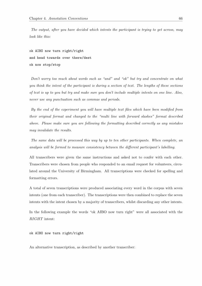
Chapter 4. Annotation Conventions 66
The output, after you have decided which intents the participant is trying to get across, may
look like this:
ok AIBO now turn right/right
and head towards over there/dest
ok now stop/stop
Don’t worry too much about words such as “and” and “ok” but try and concentrate on what
you think the intent of the participant is during a section of text. The lengths of these sections
of text is up to you but try and make sure you don’t include multiple intents on one line. Also,
never use any punctuation such as commas and periods.
By the end of the experiment you will have multiple text files which have been modified from
their original format and changed to the “multi line with forward slashes” format described
above. Please make sure you are following the formatting described correctly as any mistakes
may invalidate the results.
The same data will be processed this way by up to ten other participants. When complete, an
analysis will be formed to measure consistency between the different participant’s labelling.
All transcribers were given the same instructions and asked not to confer with each other.
Transcribers were chosen from people who responded to an email request for volunteers, circu-
lated around the University of Birmingham. All transcriptions were checked for spelling and
formatting errors.
A total of seven transcriptions were produced associating every word in the corpus with seven
intents (one from each transcriber). The transcriptions were then combined to replace the seven
intents with the intent chosen by a majority of transcribers, whilst discarding any other intents.
In the following example the words “ok AIBO now turn right” were all associated with the
RIGHT intent:
ok AIBO now turn right/right
An alternative transcription, as described by another transcriber:

Chapter 4. Annotation Conventions 67
ok AIBO/bab
now turn right/right
In this case the “ok AIBO” words are associated with the BAB intent.
A measure of consistency between transcribers was found as the number of transcribers in
agreement divided by the number of transcribers total. For the examples above, the spoken
words “ok AIBO” are only 50% consistent between transcribers, due to being described as part
of BAB and RIGHT intents alternatively. The final merged label set contained a description
of each word in the corpus, the word’s associated majority intent and the consistency score for
this intent. The average consistency score across the entire corpus was 87.34%, demonstrating
high consistency between transcribers.
Alternate combinations of the transcribers’ intent outputs included only describing intent where
there was complete agreement (100% consistency) between transcribers and an N-best list of
intents, scored by the confidence of each intent. These alternate labels were not used in further
experiments but are still available for future work.
The intents found from the multiple transcription task were converted into HTK format label
files with start and end times based on word boundaries in the time aligned transcriptions of
speech. As only a textual transcription of speech was given to the transcribers there was no
information on the silence present in the speech and thus the HTK format labels were adapted
to account for silence.
Periods of silence during speech vary in length, it could be a short period of silence (such as
when drawing breath) or a longer period, possibly indicating that gestural intent is occuring
rather than speech. To capture the varying role of silence in speech, silences of less than a
certain duration are defined as short pauses; any silence between intents is incorporated into
the first intent, extending the first intent to the start time of the next.
If the silence is above a certain duration then a NULL intent is inserted. This threshold of
silence duration is described in this work as a NULL intent threshold. E.g. for a 2 second
NULL intent threshold, NULL intents are inserted in periods of silence over 2 seconds in
length.
If a NULL intent is inserted after the current intent then the end time of an intent is no longer
the start of the next intent but the time associated with the end of the last word in the current

Chapter 4. Annotation Conventions 68
intent. Figure 4.4 describes the difference between 0 second and 120 second NULL intent
thresholds.
Figure 4.4: The difference between 0 second and 120 second NULL intent thresholding. Ais an example of a 0 second threshold where NULL intents are always inserted in periods ofsilence. B is an example of a 120 second threshold where NULL intents are never inserted andintents are extended across periods of silence. In B the DEST intent has been extended to the
start of the PATH intent.
In order to produce the final label set for speech intent labels the periods of intent are assigned
to the word boundaries from the time aligned speech transcriptions. The final label set is in
standard HTK label format, examples of which can be seen in figures 4.5 and 4.6
2000000 49600000 bab
49600000 86700000 forward
86700000 91600000 null
91600000 179800000 right
179800000 190000000 null
190000000 198900000 stop
198900000 206500000 null
206500000 210500000 forward
210500000 216600000 null
Figure 4.5: An example HTK label file with 0 second NULL intent threshold, NULL intentsare always inserted in periods of silence.
2000000 49600000 bab
49600000 91600000 forward
91600000 190000000 right
190000000 206500000 stop
206500000 216600000 forward
Figure 4.6: An example HTK label file with 120 second NULL intent threshold, NULLintents are never inserted.
In this way a variety of speech intent labels were produced with varying NULL intent thresholds.
By setting the threshold for NULL insertion to 0 seconds a NULL intent would always be
inserted if there was a gap between the end of one intent and the start of the next. The final
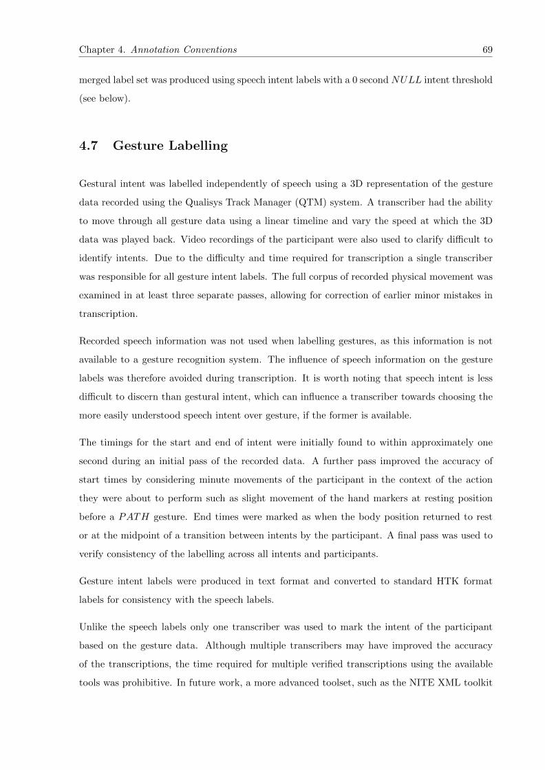
Chapter 4. Annotation Conventions 69
merged label set was produced using speech intent labels with a 0 second NULL intent threshold
(see below).
4.7 Gesture Labelling
Gestural intent was labelled independently of speech using a 3D representation of the gesture
data recorded using the Qualisys Track Manager (QTM) system. A transcriber had the ability
to move through all gesture data using a linear timeline and vary the speed at which the 3D
data was played back. Video recordings of the participant were also used to clarify difficult to
identify intents. Due to the difficulty and time required for transcription a single transcriber
was responsible for all gesture intent labels. The full corpus of recorded physical movement was
examined in at least three separate passes, allowing for correction of earlier minor mistakes in
transcription.
Recorded speech information was not used when labelling gestures, as this information is not
available to a gesture recognition system. The influence of speech information on the gesture
labels was therefore avoided during transcription. It is worth noting that speech intent is less
difficult to discern than gestural intent, which can influence a transcriber towards choosing the
more easily understood speech intent over gesture, if the former is available.
The timings for the start and end of intent were initially found to within approximately one
second during an initial pass of the recorded data. A further pass improved the accuracy of
start times by considering minute movements of the participant in the context of the action
they were about to perform such as slight movement of the hand markers at resting position
before a PATH gesture. End times were marked as when the body position returned to rest
or at the midpoint of a transition between intents by the participant. A final pass was used to
verify consistency of the labelling across all intents and participants.
Gesture intent labels were produced in text format and converted to standard HTK format
labels for consistency with the speech labels.
Unlike the speech labels only one transcriber was used to mark the intent of the participant
based on the gesture data. Although multiple transcribers may have improved the accuracy
of the transcriptions, the time required for multiple verified transcriptions using the available
tools was prohibitive. In future work, a more advanced toolset, such as the NITE XML toolkit

Chapter 4. Annotation Conventions 70
[134] used by the AMI project [135] and others will be useful in transcribing speech and gesture
simultaneously using multiple transcribers.
Table 4.1 shows the average duration in seconds for the transcription of gestural intent based
on the reduced set of 9 intents, as used in transcription of speech intent. From this it is possible
to see that the periods of intent are of varying length, with the STOP intent being the shortest
on average. Intent periods which may require more descriptive physical movements, such as
DEST and PATH require longer to convey the intent of a participant.
Intent Count Average Duration (seconds)
BAB 235 6.35COME 31 7.61DEST 400 11.28FORWARD 200 5.12LEFT 190 7.05NULL 767 9.96PATH 355 9.88RIGHT 305 6.24STOP 64 2.70
Table 4.1: A comparison of the number of intents and their duration for physical motion datalabelled with the reduced set of 9 intents.
4.8 Merging Intent Labels to Produce a Final Label Set
To produce a final set of intent labels for recognition and classification experiments the speech
and gestural intent labels must be combined. The combination requires that there are the
same number of intent classes for speech and gesture, meaning a reduction in the number of
gesture intent types to match that of speech. All instances of the PATH DEST intent in
gesture were relabelled as PATH due to the physical similarity between the two. Although
DEST and PATH DEST are similar, the strong deictic gestures used in DEST are physically
more distinct than those used in PATH DEST . Hence there are stronger similarities between
PATH DEST and PATH than PATH DEST and DEST . The waving gesture used to check
the 3D motion capture system was operating correctly and thus the WAV ING intent was
merged with BAB as although physical movement was present it did not communicate any
intent to AIBO.
During corpus collection several participants stopped gesturing entirely when they became con-
vinced it made no difference to AIBO’s movements through the route. In addition, the speech

Chapter 4. Annotation Conventions 71
intent labels were produced using several transcribers so can be considered to be more reliable.
For both these reasons the speech intent labels can be considered to take precedence over the
gesture labels.
The speech labels with a 0s NULL threshold (NULL intents inserted in silences of more than 0
seconds) were used as the base level intent transcriptions. The intent during silences in speech
must therefore be either gesture based or none existent, a NULL intent. In this way the gesture
intents were inserted during periods of silence in the speech labels to produce the final merged
label set. Figure 4.7 gives a graphical description of this merging process.
Figure 4.7: An overview of the combination of speech and gesture intent labels to producemerged intent labels.
Where identical labels were produced adjacent to each other the labels were merged to produce
one longer intent label rather than two shorter intent labels of the same class.
When the labels are merged, speech intent accounts for 52.07% and gestural intent accounts for
47.93% of the total time in the new merged labels. Table 4.2 shows the percentage duration of
intent labels from speech and gesture for each intent:
Intent % From Speech % From Gesture % Total
BAB 1.76 1.83 3.59COME 0.74 0.30 1.04DEST 5.36 10.99 16.35FORWARD 15.92 2.14 18.06LEFT 7.16 2.86 10.02NULL 0.00 21.97 21.97PATH 7.37 3.32 10.69RIGHT 10.12 4.03 14.15STOP 3.64 0.49 4.13
Table 4.2: An overview of duration of intent in seconds for the merged label set.

Chapter 4. Annotation Conventions 72
The most obvious difference in the amount of time spent per intent for each modality is that of
NULL. This is unexpected as there will be no NULL intents from speech as periods of intent
from gesture labels are always inserted in periods of silence in speech. NULL makes up 21.97%
of the total time for all recordings. After NULL, FORWARD is the most common intent if
only duration of intent is considered. More time is spent in speech on the FORWARD intent
than for gesture. This could be due to the strategy where participants provide constant spoken
encouragement in an effort to guide AIBO around the route.
4.9 Comparing Consistency Between Speech and Gesture La-
bels
As speech and gesture intent labels were transcribed separately the consistency of intent between
modalities should be considered. There are discrepancies between the original number of intent
labels in speech and gesture but comparisons are made with the final reduced intent label set
of 9 intents.
To check consistency the labels for speech and gestural intent were compared at 10ms intervals,
to match the frame rate of the audio/motion data. Overall consistency between labels was
described as the percentage of labels at all time intervals that were found to be the same. Table
4.3 shows a comparison of consistency between speech and gestural intent.
NULL Intent Threshold (seconds) Consistency
0 32.03%2 31.05%120 16.94%
Table 4.3: Consistency between gestural intent labels and speech intent labels with varyingNULL intent threshold. The speech labels are the final label set as described by the majorityof transcribers. A NULL intent threshold of 0 seconds will always insert NULL intents in
periods of silence.
Extending intent across periods of silence in speech is the equivalent of inserting intents, and
was not performed on the gesture label set. Naturally in periods of no intent in speech and
gesture, where the NULL intent threshold for the speech labels is 120 seconds there will be
a difference in the intent between modalities, even if originally both contained NULL. This
accounts for the large drop in consistency from 32.03% to 16.94% for NULL intent thresholds
of 0 and 120 seconds respectively.

Chapter 4. Annotation Conventions 73
The final merged intent label set can be compared with the gestural intent set in the same
manner. In the merged data set gesture labels are inserted during silence in the speech labels
so it is understandable that consistency is much higher. During silence in the speech labels
the inserted gesture labels are 100% consistent with the merged labels resulting in an overall
consistency across all labels of 53.25%. For comparison, when the speech labels with 0 second
NULL intent thresholds are checked for consistency against the merged labels, this figure rises
to 71.97%.
Consistency is low between speech and gesture due to how loosely coupled the modalities are
and how high level intent is compared to physical movement. For example; unlike in speech
and lip movement where the modalities are tightly coupled, speech has no bearing on the
physical movements a participant makes. During transcription of intent, a participant’s intent
in one modality may appear to be different to that of another, especially when transcription is
performed for each modality independently, as in this work.
Intents based on such loosely coupled modalities are not guaranteed to occur at exactly the same
time, as can be seen in the data captured for this work. Where periods of intent in one modality
overlap those in another it is likely that they are inconsistent for at least half of the period where
they overlap. Combined with the independent transcription performed, this accounts for the
low consistency of labels between modalities.
4.10 Summary
This chapter has described the creation of a set of 11 intent classes describing basic intents
of a participant guiding AIBO. The intents are BAB, COME, DEST , FORWARD, LEFT ,
PATH, PATH DEST , RIGHT , NULL, STOP , WAV ING. These intent classes are reduced
to a set of 9 intents by combining the PATH DEST and PATH intents and the WAV ING
and BAB intents.
The HTK standard for labelling and N-best lists were described.
Synchronisation of speech and gesture data was performed using visual cues from the 3D motion
data and visual analysis of waveform data.

Chapter 4. Annotation Conventions 74
Four transcribers transcribed the full speech recording into a textual representation. This
textual transcription of speech was then time aligned using a trained HTK recogniser (see
Chapter 6).
The word level transcription of speech was partitioned into periods of intent by seven transcribers
with 87.34% agreement. These word level speech intent transcriptions were used to create labels
of spoken intent in HTK format for use in later experiments. Multiple label sets were created to
account for the silences between participant utterances, based on a “NULL intent threshold”
(see Figure 4.4).
Gesture intent was labelled using the 3D motion data recordings. This was then combined with
the speech intent by inserting gesture intent into periods of no intent in speech. A comparison
of the gesture labels and speech labels with varying “NULL intent thresholds” was made. The
final merged label set was found to have a 53.25% overall consistency with the gesture intent
labels and 71.97% consistency with the speech intent lables where NULL is inserted in periods
of silence.

Chapter 5
Hidden Markov Model Theory
5.1 Introduction
The purpose of this chapter is to review how Hidden Markov Models (HMMs) are used in both
speech and gestural intent recognition. The fundamental components of a modern HMM based
recognition system are described, as are their application in the research described in this thesis.
Although HMMs are traditionally used in speech recognition, they have been shown to be useful
in modelling many forms of time series data, including gesture (Chapter 2). Figure 5.1 shows
the main components of both a speech and gestural intent recognition system.
In order to discuss HMM based recognition, the different components of a recognition system
must first be described. In speech recognition these components are the acoustic models, the
grammar and the dictionary. Speech data must first be converted into feature vectors and then,
combined with these components, passed through Viterbi decoding to produce text.
Gestural intent recognition for this work is similar but does not use a complex grammar or
dictionary as in speech. In gestural intent recognition, intent is modelled using HMMs in the
equivalent of a whole word level recognition system. The grammar is simply an equal weighting
for all possible intents and the dictionary contains only the intents. This chapter describes the
creation of a language model and dictionary for speech. The application of the same theory to
gestural intent recognition using a much simpler language model is discussed.
The creation of HMMs and the core components of their architecture are described, including
Gaussian Mixture Models. The identification of the most likely model sequence given a sequence
75

Chapter 5. Hidden Markov Model Theory 76
Figure 5.1: An overview of recognition of both speech and gestural intent. Speech at the top,gestural intent below.
of feature vectors using Viterbi decoding is discussed. Training of HMMs using standard Baum-
Welch re-estimation is described, as is model adaptation.
If it were possible to create a known taxonomy of gesture and then recognise these gestures
to determine gestural intent then more sophisticated speech recognition techniques could be
applied. In this work the unconstrained nature of the gestures used by participants makes
this highly difficult. The models created and trained for gestural intent recognition are simple
monophone HMMs (see Chapter 7). The concept of phones or words does not apply in gestural
intent recognition, intents are recognised without describing any sub-intent units.
Feature vector extraction through front end processing of speech is discussed in Chapter 6. The
gesture equivalent is discussed in Chapter 7.
5.2 Language Modelling
Given a sequence of feature vectors Y , the basic task in speech recognition is to find a word
sequence W such that P (W |Y ) is maximised.
From Bayes’ Theorum, for any word sequence W :
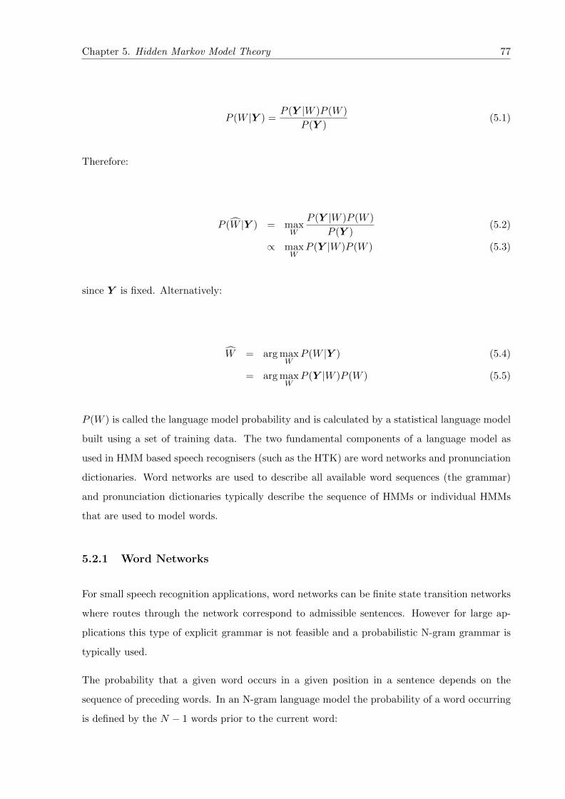
Chapter 5. Hidden Markov Model Theory 77
P (W |Y ) =P (Y |W )P (W )
P (Y )(5.1)
Therefore:
P (W |Y ) = maxW
P (Y |W )P (W )
P (Y )(5.2)
∝ maxW
P (Y |W )P (W ) (5.3)
since Y is fixed. Alternatively:
W = arg maxW
P (W |Y ) (5.4)
= arg maxW
P (Y |W )P (W ) (5.5)
P (W ) is called the language model probability and is calculated by a statistical language model
built using a set of training data. The two fundamental components of a language model as
used in HMM based speech recognisers (such as the HTK) are word networks and pronunciation
dictionaries. Word networks are used to describe all available word sequences (the grammar)
and pronunciation dictionaries typically describe the sequence of HMMs or individual HMMs
that are used to model words.
5.2.1 Word Networks
For small speech recognition applications, word networks can be finite state transition networks
where routes through the network correspond to admissible sentences. However for large ap-
plications this type of explicit grammar is not feasible and a probabilistic N-gram grammar is
typically used.
The probability that a given word occurs in a given position in a sentence depends on the
sequence of preceding words. In an N-gram language model the probability of a word occurring
is defined by the N − 1 words prior to the current word:
Chapter 5. Hidden Markov Model Theory 78
P (wi|wi−1, wi−2, ..., w1) ≈ P (wi|wi−1, wi−2, ..., wi−N+1) (5.6)
The more training data available, the bigger value of N can be supported. Subject to this con-
dition, a larger value of N gives a tighter constraint on recognition, but increases computational
load. Bigram language models (N = 2) describe word pairs where the probability of the current
word is defined only by the preceding word.
The main drawback to N-gram models is the need for a large number of samples for training.
Also an N-gram language model cannot capture long-term dependencies, or nested structures.
For example in the sentence “The girl walked, reading her book, over the bridge” the N-gram
cannot model “The girl walked over the bridge”.
N-gram models are dependent on the type of language that occurs in training corpora, e.g. lan-
guage produced for command and control applications is markedly different from that produced
in typical dictation scenarios. As when building acoustic models, richness of conversational
speech can produce N-grams unseen during training. By default, these N-grams are given a
probability of zero, harming recognition performance. Similarly N-grams can be produced dur-
ing training for very infrequent sequences of words, which although unlikely and with respective
low probability of occurring, can impact recognition.
Sparsity of training data is a significant problem to which various solutions have been suggested,
of which these are examples: Katz’s solution to data sparsity is the “backing-off” algorithm
whereby high order N-gram probabilities are replaced by lower order N-gram probabilities [60].
E.g. trigrams which occur very infrequently are reduced to bigrams based on a set cutoff.
Seymore describes an alternative approach which uses the difference in the logs of the original
and backed off N-gram probabilities as a basis for reduction in model complexity [136]. Typically
backed-off language models determine the probability of unseen N-grams as a back-off weighting
multiplied by the probability of lower order N-grams.
5.2.2 Dictionaries
In a typical HMM based speech recognition engine, the dictionary describes words as a sequence
of sub-word units, such as phones, each described by a HMM. The dictionary contains phone
Chapter 5. Hidden Markov Model Theory 79
level descriptions of all words in the corpus including multiple pronunciations where necessary.
In HTK, models of phones in context, such as triphone and diphone models, are typically
used. Triphones give a more accurate representation of the acoustic realisation of a phone in a
given context. Speech recognition engines based on triphones have much higher computational
requirements than monophone based recognisers but better account for the context dependency
of the acoustic realisation of phones and therefore typically result in lower word error rates.
Oshika discusses phonological rules which can describe the systematic variation in pronunciation
of fluent speech and also describes how rule-based approaches to this variation can be applied
to other man-machine interaction scenarios [137]. The handing of word junctures through a set
of phonological rules is described by Giachin, who avoids the training of new acoustic models
to improve recognition while hardly increasing the computational power required [138]. By
using various phonological rules the acoustic models are less affected by incorrect transcriptions
during training, resulting in improved recognition despite variations in pronunciation.
Unlike in speech recognition, where there may be multiple pronunciations of a word, there are
no alternative pronunciations for intent and therefore the dictionary of intent is very simple.
If it were possible to classify gestures from known atomic physical movements, a dictionary of
gestures could be created where the gestural equivalent of phones would be atomic physical
movements and the words, gestures. The equivalent of intent would be the language.
In this work each gestural intent is modelled using a single HMM and the equivalent of a whole
word, the dictionary is far simpler than that created for speech recognition as there are no basic
sub-intent units.
5.3 Components of a Hidden Markov Model
In a typical speech recognition system the acoustic realisation of each phone is characterised
by context-dependent HMMs. The equivalent for gestural intent is that each intent is modelled
using a single HMM, with no context dependency. Gestural intent recognition can be considered
to be similar to simple word-level speech recognition. The recognition and training algorithms
used are the same. It is only the language model, pronunciation dictionary and front end
processing which are different.

Chapter 5. Hidden Markov Model Theory 80
In order to describe HMMs, first the constituent Gaussian Probability Density Functions (PDFs)
and Gaussian Mixture Models (GMMs) must be described.
5.3.1 Gaussian Mixtures
The multivariate Gaussian PDF (also called the multivariate normal PDF) forms the basic PDF
of the Gaussian Mixture Model (GMM) and by extension the HMM used for speech and gestural
intent recognition. It is a generalisation of the normal distribution to multiple dimensions. A
single dimensional Gaussian PDF, p, is defined by its mean µ and variance σ and is given by:
p(x|µ, σ) =1√
2πσ2exp(−(x− µ)2
2σ) (5.7)
A multivariate Gaussian PDF is the vector equivalent of the single dimensional Gaussian PDF.
The vector equivalents of the mean and variance are the mean vector µ and typically diagonal
covariance matrix Σ. In this work only vector input data is considered, as in most typical HMM
based recognisers.
The probability density gm(y) of an observed vector y for component m of a GMM given a
normal distribution with mean vector µm and covariance matrix Σm is given by:
gm(y) = N(y : µm,Σm) (5.8)
=1
(2π)(D/2)|Σm|1/2exp[−1
2(y − µm)′Σm
−1(y − µm)] (5.9)
where D is the number of dimensions and |Σm| is the determinant of Σm.
A single unimodal PDF is not sufficient to model the input data in most HMM based recognisers.
The multivariate Gaussian PDF is extended to a multivariate GMM g(y), which is the weighted
sum of M component multivariate Gaussian PDFs:
g(y) =
M∑m=1
αmgm(y) (5.10)

Chapter 5. Hidden Markov Model Theory 81
where
0 ≤ αm ≤ 1 (5.11)M∑
m=1
αm = 1 (5.12)
The numbers αm are the mixture weights for each mixture component, gm(y) are the component
multivariate Gaussian probability densities and M is the number of components.
5.3.2 Training Gaussian Mixture Models
In order to fit a Gaussian PDF to a sequence of T acoustic or gestural feature vectors y =
y1, . . . ,yT the probability P (y|µ,Σ) of the data given the PDF must be maximised where:
P (y|µ,Σ) =T∏t=1
P (yt|µ,Σ) (5.13)
Maximum Likelihood (ML) estimation of µ and Σ is the process of maximising P (y|µ,Σ) with
respect to µ and Σ.
The maximum likelihood estimate of the mean µ, the sample mean, is given by:
µ =1
T
T∑t=1
yt (5.14)
The variance Σ which maximises p(x|µ,Σ) is the sample variance, given by:
Σ =1
T
T∑t=1
(yt − µ)(yt − µ)′ (5.15)
When training a multiple component GMM the relationship between the individual model
components and the training data is unknown and maximum likelihood estimation is not so

Chapter 5. Hidden Markov Model Theory 82
straightforward. The solution is to use the Expectation-Maximisation (EM) algorithm as orig-
inally described by Dempster [139].
In EM the model parameters are initialised and an iterative algorithm generates new parameter
estimates with the property that the new estimates produce models that are more representative
of the training data than the previous estimate. The final model is dependent on the initial
parameter estimates. Given an initial estimate of the GMM parameters, Θ0, EM gives a new
set of parameters, Θ1, such that p(y|Θ1) ≥ p(y|Θ0).
Typically, when the models are initialised, the model parameters for mean and variance are
taken from the entire data set. The state means are taken from the global data mean and the
state variance from the global data variance.
Using the notation in equations 5.10 to 5.12, the EM algorithm uses the current estimate of the
GMM to calculate how each feature vector yt is shared amongst the M components.
For each m, we can calculate:
P (m|yt) =P (yt|m)P (m)
P (yt)(5.16)
=gm(yt)wm∑Mn=1 gn(yt)wn
(5.17)
The probability P (m|yt) can be considered as the proportion of yt that should be used to
reestimate the mean and covariance matrix of GMM component m. The quantity P (m|yt) is
sometimes denoted by γt(m).
For example, to reestimate the new mean µm of the mth component, a weighted average,
according to γt(m), of all the feature vectors must be computed.
µm =
∑Tt=1 γt(m)yt∑Tt=1 γt(m)
(5.18)
Similarly:

Chapter 5. Hidden Markov Model Theory 83
Σm =
∑Tt=1 γt(m)(yt − µm)(yt − µm)′∑T
t=1 γt(m)(5.19)
In principle, most PDFs can be approximated using GMMs provided M is sufficiently large, but
the accuracy of models is highly dependent on the amount and quality of training data available.
It is also possible to over-fit a GMM to training data by using too complex a model (too many
mixture components and too little training material), resulting in models which represent the
training data with a high degree of accuracy but are vulnerable to incorrect classification of
unseen data.
5.3.3 Hidden Markov Models
The Hidden Markov Model (HMM) can be thought of as an extension of the GMM which can
deal more appropriately with time series data.
Figure 5.2: A left-right Hidden Markov Model
In a standard Markov model the current state can be directly observed, but in a HMM the
current state is hidden. Each state is associated with a single Gaussian mixture PDF, b , which
describes the probability of an observed speech vector, y, being emitted by that state.
The transitions between the states are determined by a transition probability matrix A. In this
thesis left-right HMMs are used (as in figure 5.2) where aij = 0 if i > j:

Chapter 5. Hidden Markov Model Theory 84
aij = p(qt+1 = j|qt = i) for 1 ≤ i, j ≤ N (5.20)
where qt describes the state at time t and N is the number of states. The transition probabilities
satisfy the following constraints:
aij ≥ 0 for 1 ≤ i, j ≤ N (5.21)
N∑j=1
aij = 1 for 1 ≤ i ≤ N (5.22)
The initial state distribution, π, of the HMM is described as:
π = {πi} (5.23)
where
πi = p(q1 = i) for 1 ≤ i ≤ N (5.24)
The output PDF, bi associated with state i, is a GMM:
bi(yt) =
M∑m=1
cimN(µim,Σim,yt) (5.25)
where µim is the mean vector for state i component m, Σim is the covariance matrix for state
i component m and cim is the weighting coefficient for state i component m. cim satisfies the
constraints:

Chapter 5. Hidden Markov Model Theory 85
cim ≥ 0 for 1 ≤ i ≤ N, 1 ≤ m ≤M (5.26)M∑
m=1
cim = 1 for 1 ≤ i ≤ N (5.27)
A HMM λ can be described in terms of the state transition probability matrix A, the set of
output PDFs B = (bi, . . . , bN ) and the initial state distribution π:
λ = (A, B, π) (5.28)
5.4 Recognition using Hidden Markov Models
In speech recognition, given a sequence y = y1, . . . ,yT of acoustic feature vectors, the objective
is to find a word sequence W such that p(W |y) is maximised.
By Bayes’ theorem:
p(W |y) =p(y|W )p(W )
p(y)(5.29)
∝ p(y|W )p(W ) (5.30)
if p(W ) 6= 0 then W is a valid sequence of words from the language model and each of these words
has one or more phone-level transcriptions in the pronunciation dictionary. By concatenating
the phone-level HMMs corresponding to each word to form word-level HMMs, and then the
word-level HMMs to form a sentence level HMM, W can be thought of as an HMM. Since p(W )
can be computed from the language model, it remains to calculate p(y|W ).
The sequence y can only be produced by W via a state sequence q of length T . Therefore:
p(y|W ) =∑q
p(y, q|W ) =∑q
p(y|q,W )p(q|W ) (5.31)

Chapter 5. Hidden Markov Model Theory 86
Where the sum is computed aver all state sequences of W of length T .
This probability can be computed using the forward pass of the Baum-Welch algorithm (see
below). However it is more common in recognition to make the approximation:
p(y|W ) =∑q
p(y, q|W ) ≈ p(y, q|W ) (5.32)
where
q = arg maxqp(y, q|W ) (5.33)
The state sequence q is called the optimal state sequence. Both the optimal state sequence q
and the probability p(y, q|W ) are computed using the Viterbi Algorithm [22].
The Viterbi algorithm gives the optimum state sequence which maximises the joint probability
of the data, Y , and state sequence, q, given the model M :
p(y, q|M) = maxqp(y, q|M) (5.34)
The Viterbi probability of generating the subsequence y1, . . . ,yt and being in state i at time t
is given by:
αt(i) = maxjαt−1(j)ajibi(yt) (5.35)
Assuming that the model ends in the final state N ,
p(y, q|M) = αT (N) (5.36)

Chapter 5. Hidden Markov Model Theory 87
During the calculation of αt(i), records are kept of the previous state j which achieves the
maximum. Using these records it is possible to recover the optimal state sequence q.
In practice, Viterbi decoding is typically applied to a complex network which integrates the
acoustic models, pronunciation dictionary and language model. The optimal state sequence
then corresponds to the best model sequence, hence the best word sequence, for the input data
y.
Gestural intent recognition is performed in the same way, the main difference being a highly
restricted dictionary and language model. In this case the intents are considered as the phones
above, where each intent corresponds to a single phone. Another view is that for gestural intent
each word (an intent) is modelled using only one HMM and sub-intent phone level HMMs
(physical movement or gesture level HMMs) are not created.
5.5 Training Hidden Markov Models
The most common training method for HMMs is Maximum Likelihood estimation, with the
aim of finding a set of HMM parameters so the probability of the training data given the
model parameters is maximised. The standard method for performing Maximum Likelihood
estimation for HMMs is the Baum-Welch algorithm, which is similar to the EM algorithm used
when training GMMs (described above). As with EM, care should be taken when training on a
small amount of training data not to over-fit at the expense of recognition of unseen test data.
Maximum Likelihood training of models produces a set of models (GMMs or HMMs) which
locally maximise P (yi|mi) where the training data yi belongs to class i = (i = 1, . . . , C),
where C is the number of classes, and mi is the model for class i. Naturally some models are
produced with similar parameters resulting in overlapping models. Speech recognition can suffer
as overlapping models can result in incorrect classification of the sub-word units described by
these models.
Discriminative training techniques aim to build models for a class i which maximise the prob-
ability of the training data but at the same time aim to produce distinct models as different
from other classes as possible. Discriminative training techniques such as Maximum Mutual
Information, as described by Bahl [140] maximise the mutual information between a sequence
of acoustic vectors and the corresponding word sequence to reduce recognition error.

Chapter 5. Hidden Markov Model Theory 88
Baum-Welch Re-estimation uses “forward” and “backward” probabilities to compute the poste-
rior probability that the ith state generated the tth observation, P (si|yt) = γt(i), in the context
of the whole sequence. Again the re-estimation of the model parameters is performed until the
difference between successive models ability to match the training data is minimised and the
algorithm reaches convergence at a local minimum.
The forward probability αt(i) is the probability of all the data up to time t, (yi, . . . ,yt) and
being in state i at time t, (st = i) given the model M :
αt(j) = P (y1, . . . ,yt; st = j|M) (5.37)
= [
I∑i=1
αi(t− 1)aij ]bj(yt) for 1 < t ≤ T (5.38)
where aij is the probability of moving from state i to state j, bj(yt) is the probability of observing
yt at state j and I is the total number of states. αt(j) is calculated recursively for each t, j
starting at t = j = 1.
The backwards probability βi(t) is defined as the probability of the model M emitting the
remaining T − t observed vectors given that at time t the ith state was occupied:
βt(i) = P (yt+1, ...,yT |st = i,M) (5.39)
=N∑j=1
aijbj(yt+1)β(t+1)(j) for 1 < t ≤ T (5.40)
Combining the forward and backward probabilities, the probability of the model M producing
all T feature vectors and that state i is occupied at time t is given as:
αt(i)βt(i) = P (y1, ...,yT ; st = i|M) (5.41)
and the probability of being in state i at time t given data y, (γt(i)), can be described as a
function of αt(i) and βt(i) as:

Chapter 5. Hidden Markov Model Theory 89
γt(i) =αt(i)βt(i)∑I
j=1 αt(j)βt(j)(5.42)
= P (st = i|y1, ...,yT ) (5.43)
γt(i) can be thought of as a measure of how well the tth observation fits the ith state. In
re-estimation the tth observation is spread across all states, the amount each state receives
depending on γt(i).
The problem of maximum likelihood estimation for general GMMs has already been addressed
in Section 5.3.2. Therefore, to simplify notation, it will be assumed that each HMM state i
corresponds to a single Gaussian PDF bi with mean µi and covariance matrix Σi.
Then, the new estimates of the state means µi, covariance matrices Σi and state transition
probabilities aij(i, j = 1, . . . , N) are given by:
µi =
∑Tt=1 γt(i)yt∑Tt=1 γt(i)
(5.44)
Similarly:
Σi =
∑Tt=1 γt(i)(yt − µi)(yt − µi)′∑T
t=1 γt(i)(5.45)
Finally, define:
γij(t) = αt(i)aijbj(yt+1)βt+1(j) (5.46)
and:

Chapter 5. Hidden Markov Model Theory 90
aij =
∑T−1t=1 γij(t)∑N
j=1
∑T−1t=1 γij(t)
(5.47)
An alternative to Baum-Welch re-estimation is to use the Viterbi algorithm. As Viterbi only
performs a forward pass, it is less computationally demanding than Baum-Welch Re-estimation.
5.6 Adaptation of Models
Although using a large amount of training data is preferable, it may not be available in real
applications. Adaptation techniques can be used to partially negate problems which arise as
a result of sparsity of training data. The two most used methods of adaptation of models to
training data are Maximum A Posteriori (MAP) adaptation and Maximum Likelihood Linear
Regression (MLLR). In this work MAP and MLLR are only applied to models for speech
recognition and are not used in gestural intent recognition.
5.6.1 Maximum A Posteriori (MAP) Adaptation
MAP adaptation [141], also referred to as Bayesian adaptation, is typically used when there is
limited training data for individual speakers and updates a trained global speaker independent
model using speaker dependent adaptation data to produce better speaker dependent models.
MAP adaptation tries to maximise p(M |y), which from Baye’s rule is:
p(M |y) =p(y|M), p(M)
p(y)(5.48)
So to maximise p(M |y), not only must p(y|M) be large but the prior probability, p(M), must
also be large. In MAP adaptation an existing speaker independent model is used as a prior
to calculate p(M) by considering the mean vectors of M as acoustic feature vectors. The new
estimates for the parameters (means) of the model are a weighted sum of the original global
model and the new adaptation data. For each state i of the model the mean µi is updated to a
new mean µi by:
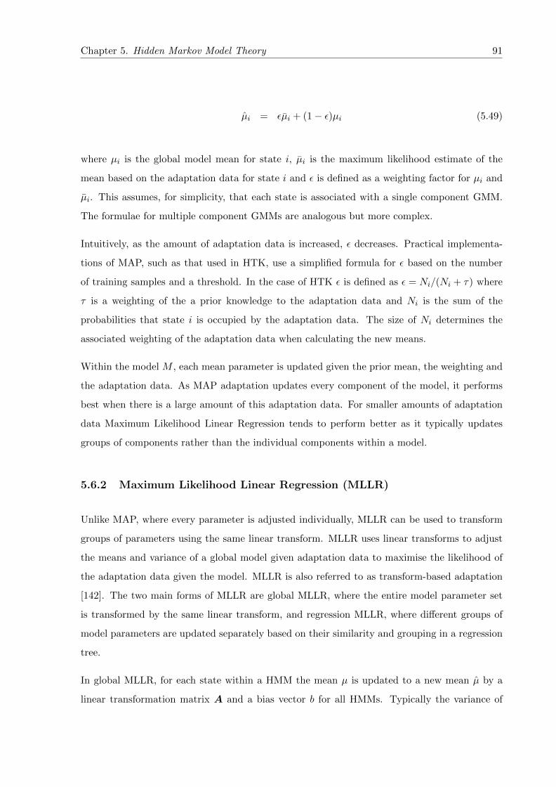
Chapter 5. Hidden Markov Model Theory 91
µi = εµi + (1− ε)µi (5.49)
where µi is the global model mean for state i, µi is the maximum likelihood estimate of the
mean based on the adaptation data for state i and ε is defined as a weighting factor for µi and
µi. This assumes, for simplicity, that each state is associated with a single component GMM.
The formulae for multiple component GMMs are analogous but more complex.
Intuitively, as the amount of adaptation data is increased, ε decreases. Practical implementa-
tions of MAP, such as that used in HTK, use a simplified formula for ε based on the number
of training samples and a threshold. In the case of HTK ε is defined as ε = Ni/(Ni + τ) where
τ is a weighting of the a prior knowledge to the adaptation data and Ni is the sum of the
probabilities that state i is occupied by the adaptation data. The size of Ni determines the
associated weighting of the adaptation data when calculating the new means.
Within the model M , each mean parameter is updated given the prior mean, the weighting and
the adaptation data. As MAP adaptation updates every component of the model, it performs
best when there is a large amount of this adaptation data. For smaller amounts of adaptation
data Maximum Likelihood Linear Regression tends to perform better as it typically updates
groups of components rather than the individual components within a model.
5.6.2 Maximum Likelihood Linear Regression (MLLR)
Unlike MAP, where every parameter is adjusted individually, MLLR can be used to transform
groups of parameters using the same linear transform. MLLR uses linear transforms to adjust
the means and variance of a global model given adaptation data to maximise the likelihood of
the adaptation data given the model. MLLR is also referred to as transform-based adaptation
[142]. The two main forms of MLLR are global MLLR, where the entire model parameter set
is transformed by the same linear transform, and regression MLLR, where different groups of
model parameters are updated separately based on their similarity and grouping in a regression
tree.
In global MLLR, for each state within a HMM the mean µ is updated to a new mean µ by a
linear transformation matrix A and a bias vector b for all HMMs. Typically the variance of
Chapter 5. Hidden Markov Model Theory 92
each state is updated using the same linear transform as the mean. The updating of a mean µ
to a new mean µ (and similarly the variance) can be given as:
µ = Aµ+ b (5.50)
Regression MLLR uses multiple linear transforms to adjust the parameters of HMMs where
the parameter values are similar. A regression tree is used where the root node of the tree
contains all HMMs in the model set and nodes further down the tree contain subsets of HMMs
(with similar parameters). The nodes on the regression tree describe parameters within the
model which can be adapted using the same transform. Linear transform matrices for mean
and variance are applied to groups of parameters on the same node.
With larger amounts of adaptation data larger sets of transformation matrices can be described
where more specific groupings of similar parameters within the model are updated. As the
amount of adaptation data increases the number of nodes on the regression tree is increased
until there are as many nodes as there are parameters, as in MAP adaptation.
With enough adaptation data MAP will produce superior results to global MLLR but the
flexibility of regression MLLR allows for successful HMM parameter adaptation based on varying
amounts of adaptation data. Adaptation can be improved by combining MLLR with MAP by
using the parameters transformed by MLLR as the priors to calculate p(M) in MAP adaptation.
5.7 Tied State Models
As the number of parameters in a model set increases, due to the complexity of each model or
the number of models used, the amount of training data required to produce accurate models
also increases. By reducing the overall complexity of the model set, more reasonable amounts
of training data can be used, reducing inaccuracies in training due to data sparsity.
One method of reducing the model complexity of a set of HMMs is to combine states within
the HMMs that contain similar parameters (and therefore model similar acoustic data) [143].
States are combined when there is not enough training data to estimate all parameters within
the model. By combining states data sparsity problems are reduced with the side effect of

Chapter 5. Hidden Markov Model Theory 93
improving the speed of adaptation techniques. In order to group similar states all states within
a model set are compared and those with parameters within a certain distance of each other are
combined.
Tied mixture systems apply the same theory to individual mixture components within a set of
Gaussian Mixture Models. Within a set of GMMs similar mixture components are grouped and
the new mixture components are shared between the GMMs.
In this work tied state models are only created for speech recognition purposes, rather than
gestural intent recognition.
5.8 Context Dependency of Models
Earlier, or simple, phone based HMM speech recognition systems used a single “monophone”
HMM to model variations in the acoustic realisation of a phone. However, one of the main factors
which causes variation is context; the acoustic realisation of a phone will depend heavily on the
phones which precede or follow it. Hence, more sophisticated systems use context sensitive
phone models.
The most common assumption is the “triphone” assumption that the contextual influence is
restricted to the immediately preceding and following phones. For example, the phone /I/ in
“six” (s I k s) would be represented as the triphone s-I+k corresponding to /I/ preceded by
/s/ and followed by /k/. This is a simplification as contextual effects can be long range, but
even the triphone assumption leads to a large increase in the number of models. As in language
modelling data sparsity becomes more of an issue as the number of models used in a recogniser
increases.
For gestural intent the context of the models is not accounted for, each model is considered
to be independent. The amount of data required to successfully model gestural intent context
is beyond that captured for this work. Unlike in speech, where a single utterance can contain
many instances of different triphones, there are not the same equivalent numbers in gestural
intent. For intents as described in this work, an entire 120 second recording may only contain
the equivalent of the number of triphones in a single utterance of speech. With enough training
data there would probably be a benefit modelling context, with gains in recognition performance
as seen in speech recognition.
Chapter 5. Hidden Markov Model Theory 94
5.9 Summary
This chapter has described the fundamental components of Hidden Markov Model (HMM) based
speech recognition and gestural intent recognition systems.
The language model, containing both the grammar and dictionary, has been described for both
speech and gestural intent recognition. Gestural intent recognition is similar in many ways to
speech recognition but requires a much simpler language model.
HMMs, built for recognition of phones, are combined with a language model to allow speech
recognition using Viterbi decoding. The gesture equivalent is to model intent as if it were the
words in simple word level speech recognition. In both cases HMMs are trained using Baum-
Welch re-estimation.
For speech recognition further advances such as adaptation using MLLR and MAP are described
as are improvements to recognition using contextual information. These improvements to HMM
based recognition are not applied to gestural intent recognition.

Chapter 6
Speech and Speech Based Intent
Recognition
6.1 Introduction
This section discusses the creation and adaptation of a speech recognition engine and the appli-
cation of topic spotting techniques to recognised speech data for intent classification. Classifica-
tion is where there are pre-segmented periods of data, as described by a transcription of intent
based on a labelling convention. In this chapter, for speech intent classification the merged in-
tent labelling convention is used, where the human transcription of gestural intent was inserted
during periods of silence in the speech intent transcription.
The development of speech recognition in the last 40 years has resulted in statistical methods
such as HMMs becoming the most popular way of automatically transcribing acoustic speech
signals into a sequence of words. The principles behind HMM speech recognisers are exemplified
in Lee’s SPHINX system [54] and Cambridge University’s HTK [3] which has been constantly
updated to take account of new developments in speech recognition. A standard modern HMM
based speech recogniser can be thought of as a modular system which combines acoustic mod-
elling, lexical representation of acoustic models, language modelling and the training, adaptation
and decoding of these models for speech recognition.
In a typical speech recognition engine sub-word acoustic units such as phonemes are modelled
using HMMs with Gaussian Mixture Model (GMM) states. As the number of mixture compo-
nents within the GMMs and the number of states is increased, so too is the potential ability of a
95
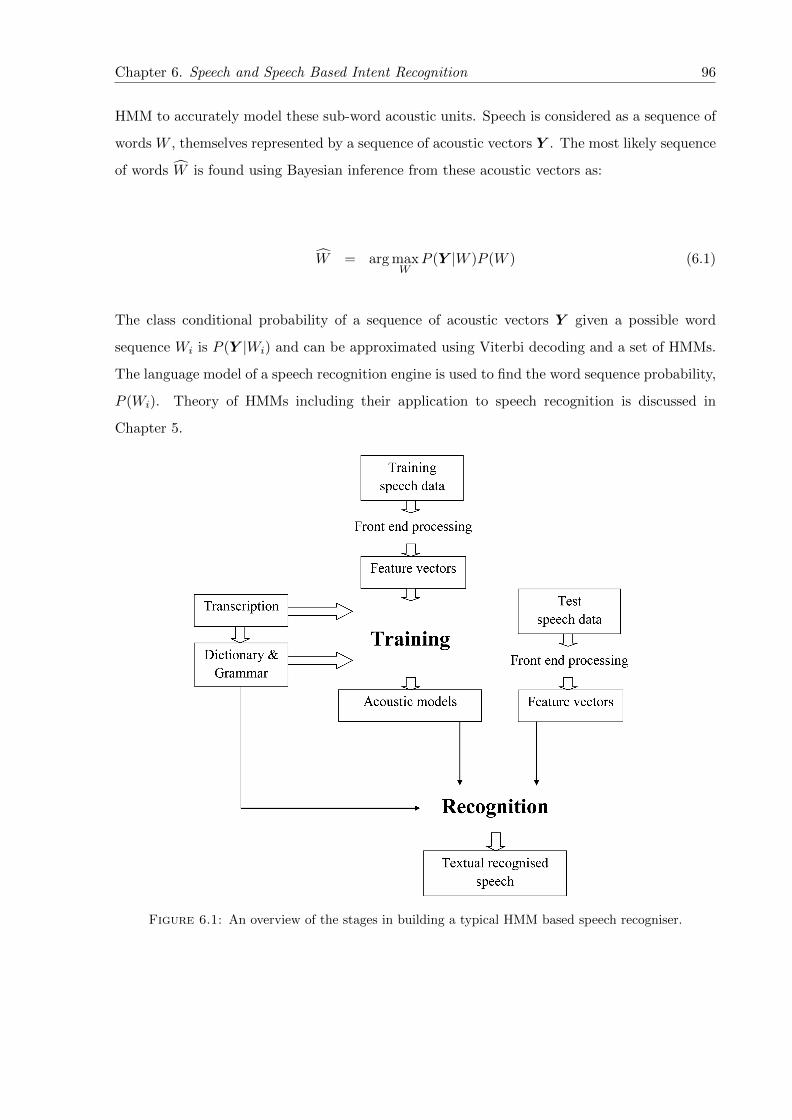
Chapter 6. Speech and Speech Based Intent Recognition 96
HMM to accurately model these sub-word acoustic units. Speech is considered as a sequence of
words W , themselves represented by a sequence of acoustic vectors Y . The most likely sequence
of words W is found using Bayesian inference from these acoustic vectors as:
W = arg maxW
P (Y |W )P (W ) (6.1)
The class conditional probability of a sequence of acoustic vectors Y given a possible word
sequence Wi is P (Y |Wi) and can be approximated using Viterbi decoding and a set of HMMs.
The language model of a speech recognition engine is used to find the word sequence probability,
P (Wi). Theory of HMMs including their application to speech recognition is discussed in
Chapter 5.
Figure 6.1: An overview of the stages in building a typical HMM based speech recogniser.

Chapter 6. Speech and Speech Based Intent Recognition 97
6.2 Front End Processing of Speech
The purpose of the front end processing is to convert the speech waveform into sequences of
feature vectors which de-emphasise the information which is not important for speech recognition
whilst emphasising the information which is. Typical examples include Mel-frequency Cepstrum
Coefficient (MFCC) analysis as described by Davis and Mermelstein [144] or Perceptual Linear
Predictive (PLP) analysis as described by Hermansky [145]. MFCCs are chosen for use in
this thesis as they are commonly used and have historically given excellent results in speech
recognition tasks [144].
Speech was recorded at 44kHz and then downsampled to 16kHz to match existing speech models
built on available speech corpora.
6.2.1 Mel-Scale Filterbank Analysis for MFCC Production
The Mel scale [146] is a non-linear perceptual frequency scale with the property that pairs of
frequencies differing by the same number of mels are percieved as equal in distance from each
other, irrespective of their frequency.
To produce MFCCs, the acoustic data is segmented into a series of overlapping frames defined
by a set window size, typically 20-25ms. The window size is chosen based on our understanding
of the human speech production system, where the vocal tract is considered to be relatively
constant for the duration of the window resulting in a relatively constant frequency spectrum.
The overlap between windows is typically set to half the window size, e.g. a 10ms interval
between windows to produce 100 features per second.
The acoustic data is initially passed through a pre-emphasis filter to balance the average spec-
trum. Each frame is multiplied by a Hamming window function which reduces the effect of
data as the time distance from the centre of the window increases. This helps to avoid abrupt
changes at the edge of the window, which can cause aliasing. The spectrum is then reduced to
an acoustic feature vector using Mel-scale filterbank analysis. The log amplitude of the discrete
Fourier transform is then applied to produce the log-power frequency spectrum of each window.
A set of triangular band pass filters are applied to each window of speech. These filters are of
equal width and spacing on the Mel scale, equating to approximately linear to 1kHz, to model
our perception of low frequency sounds and logarithmic above 1kHz, to model the reduction

Chapter 6. Speech and Speech Based Intent Recognition 98
Figure 6.2: An overview of the stages associated with conversion of acoustic speech data toMFCCs .
in human ability to discern high frequency sounds. For example, for 8kHz speech recognition
bandwidth, typically 26 mel spectrum features are produced from 26 of these varying width
triangular filters, which overlap as in 6.3.
The triangular mel filters are spaced according to critical bands which can be thought of as the
bandwidth of an auditory filter. A critical band corresponds to approximately 100 mels and
there are approximately 28 intervals of 100 mels between 0 and 2840 mels, the mel equivalent
of 8kHz [147].
The ith Mel frequency cepstral coefficient, mi, is the sum of the product of the ith window, wi,
with the power spectrum s:
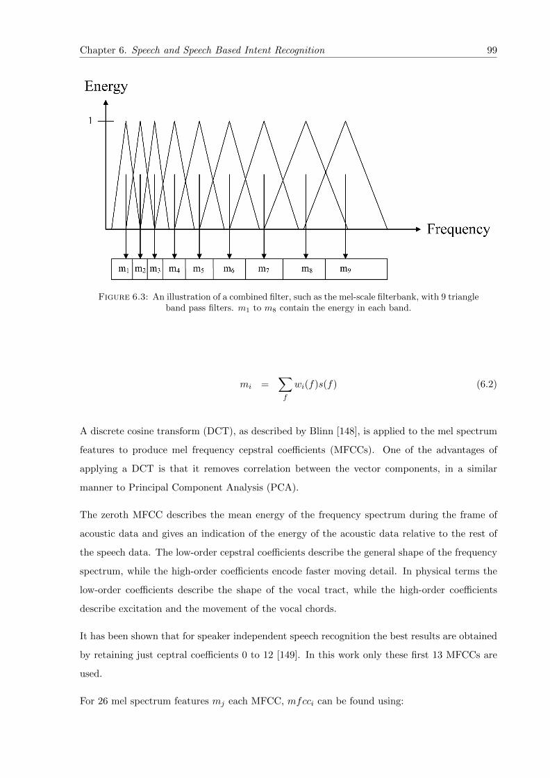
Chapter 6. Speech and Speech Based Intent Recognition 99
Figure 6.3: An illustration of a combined filter, such as the mel-scale filterbank, with 9 triangleband pass filters. m1 to m8 contain the energy in each band.
mi =∑f
wi(f)s(f) (6.2)
A discrete cosine transform (DCT), as described by Blinn [148], is applied to the mel spectrum
features to produce mel frequency cepstral coefficients (MFCCs). One of the advantages of
applying a DCT is that it removes correlation between the vector components, in a similar
manner to Principal Component Analysis (PCA).
The zeroth MFCC describes the mean energy of the frequency spectrum during the frame of
acoustic data and gives an indication of the energy of the acoustic data relative to the rest of
the speech data. The low-order cepstral coefficients describe the general shape of the frequency
spectrum, while the high-order coefficients encode faster moving detail. In physical terms the
low-order coefficients describe the shape of the vocal tract, while the high-order coefficients
describe excitation and the movement of the vocal chords.
It has been shown that for speaker independent speech recognition the best results are obtained
by retaining just ceptral coefficients 0 to 12 [149]. In this work only these first 13 MFCCs are
used.
For 26 mel spectrum features mj each MFCC, mfcci can be found using:

Chapter 6. Speech and Speech Based Intent Recognition 100
mfcci =
25∑j=0
mj cos(πi(j + 1/2)
26) (6.3)
Atal [150] describes Cepstral Mean Normalisation, which is typically applied during front end
processing. Cepstral Mean Normalisation can help to reduce the effect of the recording environ-
ment by subtracting the average for all MFCCs from each individual MFCC. Other techniques
can be applied to MFCCs to account for variations in recording environment or noise, such as
cepstral variance normalisation as described by Viikki [151]. In cepstral variance normalisation,
the variance of each cepstral coefficient is calculated and the cepstral coefficients normalised to
give a variance over all speech windows.
6.2.1.1 Modelling Dynamic Information in MFCCs
The 13 MFCCs as described above can be used as feature vector inputs to a Hidden Markov
Model based speech recognition system such as a system implemented with HTK, but improve-
ments to recognition can be made by modeling dynamic information of the MFCCs. During
HMM processing the MFCCs are assumed to be independent of each other, the way they evolve
over time is effectively ignored. To compensate for this, dynamic information is introduced and
speech recognition performance can be improved by capturing properties of the trajectory of
MFCCs.
The first order time derivatives of all MFCCs can be calculated to produce delta coefficients,
the second order time derivative is calculated to produce the acceleration coefficient. Furui
gives examples of improvements in recognition by using these delta and acceleration coefficients
when applying template matching to speech recognition [152]. By calculation of the delta and
acceleration coefficients for each of the 13 original MFCCs a total of 39 MFCCs are produced.
Other alternatives to MFCCs do exist, such as Perceptual Linear Prediction as described by
Hermansky [145] and other Linear Prediction based methods of analysis, but due to their his-
torical success in modeling acoustic information, MFCCs are typically used as the input in most
HMM based speech recognition engines, such as the HTK.
Chapter 6. Speech and Speech Based Intent Recognition 101
6.3 Building a HMM Based Speech Recogniser Using the Hid-
den Markov Model Toolkit
The Hidden Markov Model ToolKit (HTK), originally from Cambridge University as described
by Woodland [3], is used to apply the above theory to speech and speaker recognition. Due to
its extended development and widespread adoption by speech research groups, HTK has become
an industry and research standard in continuous automatic speech recognition (see chapter 2).
HTK is a set of library modules and tools written in the C language with binaries available
for most modern platforms. Development of HTK based recognisers for this thesis was per-
formed using HTK 3.3 on a variety of hardware. Most development work on gestural intent
was performed on a Windows PC with a 2.4GHz dual-core Intel processor and 4GB of memory.
Training of initial speech models for speech recognition was performed on a cluster of Intel
processor based machines running Linux Red Hat 9.0 and Sun Microsystems’ Grid Engine Dis-
tributed Source Management. Further work on HTK results, analysis and batch scripting was
performed using custom C# based programs.
The methods used to generate acoustic models using HTK are similar to that described by
Young et al in the HTK Book tutorial [153]. In typical model creation, first multiple mix-
ture monophone HMMs are defined and trained, then triphone models are generated from the
monophones and re-estimated to produce tied-state triphone HMMs.
6.3.1 Training Corpora
Several large databases of both read and conversational speech exist for use in creating speech
recognition engines. As only 6 hours of audio was recorded during experimental procedures,
with large periods of silence between utterances, it was necessary to train acoustic models on
other available corpora. The acoustic models were first estimated using the WSJCAM0 corpus
of read British English speech, specifically designed to complement the US English WSJ0 corpus
of read Wall Street Journal newspaper articles [68].
WSJCAM0 contains word and phonetic transcriptions of 110 utterances by each of 140 British
English speakers recorded in 16kHz mono format. The specification for WSJCAM0 also includes
a phonetic dictionary and two standard evaluation tasks using a 5000 word bigram and 20000

Chapter 6. Speech and Speech Based Intent Recognition 102
trigram language model. 92 of the speakers recorded are defined as the training speakers, each
producing 90 training utterances. It is on these 92 speakers that acoustic models are trained.
There are few large corpora available that are suitable for use in recognising the unconstrained
speech recorded for this work. The “eye/speech” corpus as described by Cooke [154] was used
to adapt speech models built using WSJCAM0 to more closely match spontaneously generated
speech. The task used to create the “eye/speech” corpus is similar to that of the AIBO guidance
task in this work and was conducted using a similar sample group from the University of
Birmingham. It is expected that some of the basic structure of speech is similar between
corpora. The techniques to create Cooke’s recogniser are used as a starting point for creation
of the recogniser used in this work.
The techniques for training acoustic models using WSJCAM0 closely follow Cooke’s methodol-
ogy for training his baseline automatic speech recognition system. The recognition performance
results (See section 6.3.6) show that comparable performance is seen for Cooke’s models when
tested on WSJCAM0 as for the models used in this work on the AIBO corpus.
As the speech recognition system is to be used for time alignment of correct transcriptions of
speech, both automatically recognised speech and correct time aligned transcriptions of speech
can be considered the lower and upper bounds, respectively, for speech recognition performance
in this work. Any further improvements to a speech recognition system are expected to reach
the equivalent performance of the correct, time aligned transcriptions. For this reason, although
the speech recognition performance is important, it is considered the lower bound for quality
of input to a speech intent recognition system. Later results consider both the automatically
recognised speech and the correct transcription of speech as inputs to both single and multi-
modal intent recognition systems.
6.3.2 Front End Processing
All speech audio was converted into a vector representation, as described above. A total of 39
parameters were used including 13 original MFCC coefficients with 13 delta coefficients and 13
acceleration coefficients. Cepstral mean normalisation was applied to account for the varying
recording environments of the training corpora.
Chapter 6. Speech and Speech Based Intent Recognition 103
6.3.3 Producing Acoustic Models
6.3.3.1 Monophones
An initial set of 44 single Gaussian mixture monophone 5-state (as defined in HTK; including
start and end state) HMMs were created, describing each symbol in the international phonetic
alphabet for British English. Initially all means and variances for the Gaussian distributions
were set to 0 and 1 respectively and these parameters re-estimated using Baum-Welch Re-
estimation and the HTK tools “HInit” and “HERest”.
6.3.3.2 Tied State Triphones
Using the WSJCAM0 corpus 19189 triphones were identified based on the 44 monophones
described above and the pronunciation dictionary. The triphones from the “eye/speech” corpus
were added to bring the total to 25321. A decision tree was then used to tie similar triphone
states resulting in a final number of 12015 HMMs. The single Gaussian mixture components
per state in the HMMs used was replaced with 8 Gaussian mixtures. Cooke describes a peak in
performance when testing on WSJCAM0 evaluation data using 8 Gaussian mixtures per state
in a 5-state HMM [154].
6.3.3.3 Acoustic Adaptation
The “eye/speech” corpus was chosen as a base on which to build acoustic models due to the
similarity to the corpus recorded for this thesis in terms of recording conditions (headset micro-
phones) and task (similar to the Map Task experiment [128]). As the initial models were built
on read British English using WSJCAM0, Cooke reports poor performance when testing on the
“eye/speech” corpus without adaptation. By applying MAP and MLLR, Cooke reduces word
error rate by 51.8% from 96% to give an overall mean word error rate of 46.3%.
These adapted tied state triphone HMMs were used as the base speech recognition models in
all later speech recognition experiments.

Chapter 6. Speech and Speech Based Intent Recognition 104
6.3.3.4 Addition of AIBO Noise Model
The AIBO produces distinctive regular mechanical noise whilst moving. This noise is particu-
larly prevalent during periods without speech (periods of silence). A 5 state 8 mixture HMM
acoustic model of AIBO noise was created using a sample of AIBO noise across all recordings.
This noise model was created separately to the other acoustic models and inserted into the model
set with a corresponding dictionary word of “silence” so as not to be recognised as anything but
background noise.
6.3.4 Language Model
The dictionary used for all speech recognition is based on the British English Example Pronun-
ciation (BEEP) dictionary developed at Cambridge University to be used with the WSJCAM0
corpus. Although BEEP describes words in monophone format HTK can be used to create a
triphone dictionary from these monophones. Additional words were added to the BEEP dictio-
nary based on the “eye/speech” corpus and other entirely new words found during transcription
of the corpus collected for this thesis (such as “AIBO”).
The bigram grammar used in automatic speech recognition for this thesis was built automatically
using a “leave one out” strategy and the correct transcriptions of all speech recordings. A bigram
network was created based on observation of all word pairs used in every other speech recording
than the current recording. For N recordings, N total bigram grammar networks were created.
Typically a grammar is built based on a large corpus of training data to accurately model as
much of a language as possible. In this case the relative performance of the speech recognition
engine compared to correctly transcribed speech is used as a benchmark to indicate the ability
of the overall intent recognition engine to deal with noisy or incorrect speech recognition.
6.3.5 Producing Time Aligned Correct Transcriptions
In order to produce correctly time aligned transcriptions of speech three transcribers produced
a total of three textual transcriptions of speech for every audio recording. Transcriptions were
compared and all erroneous or differing text was corrected by majority rule to produce a final
textual transcription for all audio recordings. This transcription contained 325 unique words,

Chapter 6. Speech and Speech Based Intent Recognition 105
a small vocabulary but not unexpected due to the command and control task used to collect
data. Participant strategy varied, as did their resultant vocabulary (Chapter 3).
“Forced alignment” was performed to align the transcription with the speech data. As the
constrained language model forces the recogniser to recognise every word in the recording as
manually transcribed the resulting output is considered as close to perfect as the recogniser can
produce. The output of this recogniser is used in all further experiments as an example of the
highest possible scoring speech recognition engine.
6.3.6 Producing Automatically Recognised Speech Transcriptions
The acoustic and language models described above were used in recognition of the 39 parameter
MFCC speech data. The aim of this recogniser is to produce sample recognised speech data
for use in later experiments, rather than to create a perfect recognition engine. For this reason
the HTK parameters were not changed from their settings as used in creating the time aligned,
correct transcriptions.
When recognition was performed the overall word error rate was found to be 49.7%. Although
this is high, it compares with Cooke’s finding of 46.3% when the models are adapted and applied
to his Eye/Speech Corpus [154]. If the models were adapted to the corpus it is expected the word
error rate could be reduced, although there are issues with data sparcity given the relatively
small amount of recorded speech for use in adaptation for this work. Table 6.1 shows both
Cooke’s results when models are applied to WSJCAM0 and adapted for his Eye/Speech corpus
and the results for the same models (with inclusion of the AIBO silence model) on the corpus
gathered for this work, called the AIBO corpus here.
Corpus Word Error Rate
WSJCAM0 48.7
Eye/Speech 46.3
AIBO 49.7
Table 6.1: Speech recognition results for various corpora. When tested on the corpus collectedfor this work (AIBO), models include AIBO silence model.
The automatically recognised speech described here is used as the basis for all further experi-
ments.

Chapter 6. Speech and Speech Based Intent Recognition 106
6.4 Usefulness as an Indication of Intent
The output of the speech recognition engine described above is textual and allows for statistical
analysis of the words output. This textual output is used as the basis for a topic spotting
algorithm which uses “usefulness” to define a measure of similarity between a sequence of words
(the recogniser output) and a topic (the intent of a speaker). Parris and Carey describe the
application of usefulness to speaker identification [155] and to topic spotting [156], similarly to
this work.
In [156] Carey weights keywords by the significance of their occurrence when used during certain
topics. This weighting, the usefulness, depends on the discrimination the word provides between
topic and non-topic material.
In this work the different intent classes are treated as the topics in Carey’s work. The usefulness
Ui(w) of a word w relative to an intent class i is determined as:
Ui(w) = P (w|i)logP (w|i)P (w)
(6.4)
Gorin uses the similar measure of “salience” to associate spoken words and phrases with semantic
classes [157]. This measure was exploited to learn the mapping from spoken input to machine
action for several tasks, such as the “AT&T How may I help you?” system [158]. Gorin states
that systems such as this must recognise linguistic events (such as spoken words or phrases) for
particular tasks.
The salience measure described by Gorin was successfully used for topic spotting of spoken
input from phone users to the “AT&T How may I help you?” system. Spoken phrases were
recognised and mapped to a set of call types based on salience measures for phrase fragments,
with performance of up to 70% of call types being correctly identified [159].
In this work, as in Gorin and Carey’s, the speech from a participant is associated with semantic
classes, in this case intent classes. Gorin shows that semantic information can be extracted
directly from speech, justifying the use of similar topic spotting methods in this work.
The salience Si(w) of a word w relative to an intent class i is determined as:

Chapter 6. Speech and Speech Based Intent Recognition 107
Si(w) = P (i|w)logP (i|w)
P (i)(6.5)
Salience and usefulness are very similar. The main difference is that usefulness takes into
consideration how rare a word is when assigning how indicative it is of a topic (an intent); if
a word is very rare it is not considered to be important in describing an intent. In order for a
word to be useful with respect to an intent it has to occur often within that intent and occur
more often within that intent than in other intents.
Salience and usefulness are related as:
Si(w) =P (i)
P (w)Ui(w) (6.6)
Words that produce larger salience, but not usefulness, are those that are useful in discrimination
but do not occur very often. It is not worthwhile to gather statistics on the words that do not
occur very often, rare words that occur only once in a single intent should not have an influence
on recognition. For this reason usefulness is used in this work, rather than salience.
If intent labels exist for each recording and the textual transcription of the recording is available
then each word in the corpus can be assigned a usefulness score associated with each available
intent. The usefulness scores are pre calculated from the training data for each word in the
corpus without reference to the test data. The usefulness scores for each word over a segment
of data give an indication of the most likely intent.
Combination of the scores for usefulness of words is used to provide an overall measure of intent
classes for sequences of words. Although there are many methods for combination of usefulness
scores for word sequences, in this work the sum was used as a measure of overall intent. If
W = w1, . . . , wJ is the sequence of words and i is an intent then the usefulness of the sequence
of words, given the intent Ui(W ) is defined as:
Ui(W ) =
J∑j=1
Ui(wj) (6.7)

Chapter 6. Speech and Speech Based Intent Recognition 108
and the most likely intent i is:
i = arg maxiUi(W ) (6.8)
By simply finding the sum of usefulness scores for each intent some of the information on
the number of words in intents (the number of words in the sequence) relative to usefulness
is encapsulated in the final scores for each class. The usefulness scores can be used during
combination of modalities by an Artificial Neural Network, as described in Chapter 8.
Tables 6.2, 6.3 and 6.4 show the number of occurrences and average length in spoken words
for the 0 second NULL intent threshold speech labels, the 120 second NULL intent threshold
speech labels and the final merged label set respectively. In all cases the input is from human
transcribed speech.
Intent Number of Occurrences Average Word Length
BAB 52 7.59COME 41 8.00DEST 166 9.05FORWARD 1031 3.55LEFT 403 5.37NULL 3166 1.00PATH 213 11.25RIGHT 599 5.56STOP 863 1.34
TOTAL 6534
Table 6.2: A comparison of the count and average word length of each intent for the speech in-tent labelling convention, with 0s NULL intent insertion threshold. NULL intents are inserted
wherever there is silence in the speech.
It is clear from Tables 6.2, 6.3, 6.4 that the word length of an intent is indicative of the intent
class. This is most obvious in the speech based labelling conventions (Tables 6.2, 6.3) where the
STOP intent duration is typically very short when compared to that of PATH. NULL intents
are always of length 1 as they contain only the single “sil” word to denote silence in speech.
The large increase in BAB intents in the merged labels shows that the gesture data contains
more unimportant communication than the speech. This is unsurprising as most participants
frequently changed position and moved within their allowed area, which was transcribed as
BAB. The speech shows a comparatively low number of BAB intents as participants tended
to only vocalise direct instructions to AIBO rather than speak for other reasons.

Chapter 6. Speech and Speech Based Intent Recognition 109
Intent Number of Occurrences Average Word Length
BAB 52 8.35COME 41 8.90DEST 166 9.90FORWARD 1031 4.52LEFT 403 6.28PATH 213 12.09RIGHT 599 6.50STOP 863 2.31
TOTAL 3368
Table 6.3: A comparison of the count and average word length of each intent for speech labelswith a 120 second NULL intent threshold. Intents are extended across silence to the start of
the next intent, there are no NULL intents.
Intent Number of Occurrences Average Word Length
BAB 232 2.53COME 71 5.11DEST 814 2.78FORWARD 1051 3.63LEFT 495 4.83NULL 954 1.00PATH 767 4.00RIGHT 679 5.37STOP 864 1.40
TOTAL 5927
Table 6.4: A comparison of the count and average word length of each intent for the mergedintent labelling convention. The human transcription of gestural intent was inserted during
periods of silence in the speech intent transcription.
Similarly to BAB, there are more PATH and DEST intents in the merged labels than those
based on speech alone. Both of these intents are likely to be movement based as these intent
types are more easily conveyed with physical movement than speech. For example, it is easier to
draw a path around a position on the floor using a gesture than to convey the same information
in speech. It is likely that a participant will choose their perceived easiest modality to convey
information, which in the case of PATH and DEST is gesture.
Table 6.5 describes the words with the highest scoring usefulness values (≥ 0.06) for the merged
intent labelling convention and the intent class to which this value applies. The most useful
word is “stop”, associated with the STOP intent. This is unsurprising as it is unlikely “stop”
would be used within any of the other intents, all of which are associated with movement of some
kind. Similarly the words “left”, “forward” and “right” are closely linked to their respective
intent classes LEFT , FORWARD and RIGHT . The high usefulness of “sil” words denoting

Chapter 6. Speech and Speech Based Intent Recognition 110
NULL intents does have some significant effect on intent classification using speech, as can be
seen below in 6.4.1.
Word Usefulness Intent
stop 1.80 STOPsil 0.62 NULLleft 0.51 LEFTforward 0.42 FORWARDright 0.37 RIGHTme 0.34 COMEcome 0.33 COMEtowards 0.15 COMEturn 0.11 RIGHTaround 0.09 PATHturn 0.09 LEFTthere 0.06 DEST
Table 6.5: The highest scoring words (using the usefulness ≥ 0.06 measure) for the mergedintent labelling convention and their associated intent class.
The usefulness intent classifier aims to classify a known segment of speech (based on textual
transcription of speech) given prior usefulness scores for each word to give the best intent for
a segment. Lists of scores for each intent are produced and compared to the correct labels.
Accuracy is simply the number of segments of speech that are correctly identified divided by
the total number of segments.
The output of a usefulness classifier is dependent on the performance of the speech recognition
system. In this work the upper bound for intent classification is based on the input of human
transcriptions of speech, as described above. Text output from a poor speech recognition system
is likely to lower intent classification scores [159].
6.4.1 Applying Usefulness to Classify Speech Intent
Speech Intent classification is performed based on the merged speech and gestural intent labels
as described in Chapter 4, gestural intent is inserted in periods of silence in the speech. The
usefulness scores for each word in relation to each intent are calculated based on the training data
and intent recognition is performed on each segment of correctly labelled human transcription
of intent in the test data. Accuracy as described above is used as a measure of performance.
The intent classifier was used with both the correct human transcriptions of speech and the
output of the speech recogniser as described above. In both cases it can be demonstrated
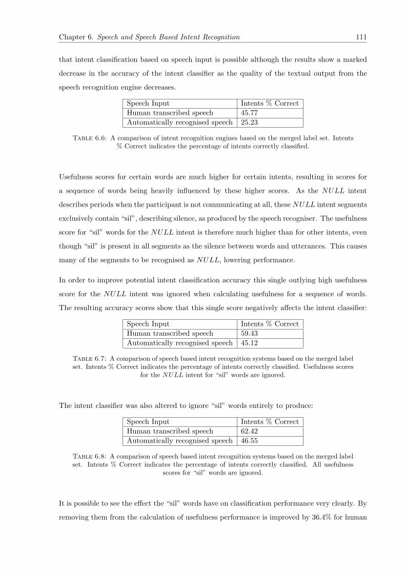
Chapter 6. Speech and Speech Based Intent Recognition 111
that intent classification based on speech input is possible although the results show a marked
decrease in the accuracy of the intent classifier as the quality of the textual output from the
speech recognition engine decreases.
Speech Input Intents % Correct
Human transcribed speech 45.77
Automatically recognised speech 25.23
Table 6.6: A comparison of intent recognition engines based on the merged label set. Intents% Correct indicates the percentage of intents correctly classified.
Usefulness scores for certain words are much higher for certain intents, resulting in scores for
a sequence of words being heavily influenced by these higher scores. As the NULL intent
describes periods when the participant is not communicating at all, these NULL intent segments
exclusively contain “sil”, describing silence, as produced by the speech recogniser. The usefulness
score for “sil” words for the NULL intent is therefore much higher than for other intents, even
though “sil” is present in all segments as the silence between words and utterances. This causes
many of the segments to be recognised as NULL, lowering performance.
In order to improve potential intent classification accuracy this single outlying high usefulness
score for the NULL intent was ignored when calculating usefulness for a sequence of words.
The resulting accuracy scores show that this single score negatively affects the intent classifier:
Speech Input Intents % Correct
Human transcribed speech 59.43
Automatically recognised speech 45.12
Table 6.7: A comparison of speech based intent recognition systems based on the merged labelset. Intents % Correct indicates the percentage of intents correctly classified. Usefulness scores
for the NULL intent for “sil” words are ignored.
The intent classifier was also altered to ignore “sil” words entirely to produce:
Speech Input Intents % Correct
Human transcribed speech 62.42
Automatically recognised speech 46.55
Table 6.8: A comparison of speech based intent recognition systems based on the merged labelset. Intents % Correct indicates the percentage of intents correctly classified. All usefulness
scores for “sil” words are ignored.
It is possible to see the effect the “sil” words have on classification performance very clearly. By
removing them from the calculation of usefulness performance is improved by 36.4% for human

Chapter 6. Speech and Speech Based Intent Recognition 112
transcribed speech and 84.5% for automatically recognised speech. The “sil” words heavily
influence classification towards the NULL intent and by removing this influence, classification
performance is improved.
Although the results suggest removal of “sil” words for recognition of intent it will be seen
that their inclusion can improve intent recognition when the usefulness scores for all intents are
combined with gesture scores for all intents using an artificial Neural Network (Chapter 8). The
frequency of “sil” words in sequences of words does provide more information on the intent of
a participant. This is only realised during combination of scores (Chapter 8).
Classification of intent from automatically recognised speech is worse than for the human tran-
scription of speech. This is unsurprising as the usefulness values are calculated based on the
human transcription of speech, not the automatically recognised speech.
As the merged label set is used, the intents in periods where the labels came from speech intent
transcriptions are more likely to be correctly classified for the human speech transcription. For
the automatically recognised speech, the textual output does not conform to the same word
boundaries, which increases the likelihood of words occurring in periods where their usefulness
is not indicative of the labelled intent.
For human transcribed speech, during periods of intent in the merged labels that originally
came from the gestural intent transcription, these periods will contain no speech and will be
classified as NULL, which may be incorrect. For automatically recognised speech words may
occur at any time, including during labelled periods of intent originally from the gestural intent
transcription, allowing for words contributing towards the correct classification of these periods
of intent. The advantage of the automatically recognised speech to allow for non-NULL intents
during these periods is outweighed by the disadvantage of not conforming to the same word
boundaries as the human transcription of speech.
6.5 Summary
This chapter has described the fundamental components of a Hidden Markov Model (HMM)
speech recognition engine and the implementation of a recogniser using the Hidden Markov
Model Toolkit (HTK). The speech recogniser was trained using the WSJCAM0 [68] and eye-
/speech [154] corpora.

Chapter 6. Speech and Speech Based Intent Recognition 113
Audio data was converted from binary wave format to HTK vector representation using front
end processing. Models of increasing complexity were created using the WSJCAM0 corpus
and adapted to the eye-speech corpus using MLLR and MAP re-estimation. The AIBO noise
model was introduced and inserted into the model set to accommodate the effect of the sound
of AIBO’s movement on speech recognition. The language model for the speech recogniser was
created based on the BEEP dictionary, with additional task specific words such as “AIBO”.
The bigram grammar as used for speech recognition of the corpus collected for this thesis was
automatically generated using the “leave-one-out” strategy and speech recognition performed
on the whole corpus to produce an example of a typical higher word error rate speech recognition
output.
The speech recognition engine was used with the recordings and a set of correctly transcribed
textual speech (by multiple transcribers) to create correctly time aligned human transcriptions
of speech. Both the automatically recognised speech and correctly time aligned transcriptions
produced output in standard HTK format and were designed to output speech for use in a
usefulness based spoken intent classification.
This chapter explained usefulness as a measure of similarity between words and intent classes.
Usefulness values for each word in the corpus was calculated and classification of intent for known
labels was performed to produce accuracy scores for both correctly aligned human transcriptions
of speech and automatically recognised speech.
Results show a reduction in performance of a spoken intent classifier when comparing automat-
ically recognised speech to human transcribed speech. The influence of “sil” words and their
associated boosting of the scores for NULL intents are explored. Performance is improved by
removing the score for NULL intents from the “sil” words and by removing the “sil” words
completely.
The output of the speech intent classifier is formatted ready for combination of speech and
gestural intent in later work.

Chapter 7
Gestural Intent Recognition
7.1 Introduction
This chapter discusses the production of an intent recognition system using 3D motion data
(gestural intent recognition) collected with a commercial motion tracking system. Processing
of raw collected motion data for use with the Hidden Markov Model Toolkit (HTK [3]) for
intent recognition is described. Principal Component Analysis is described for dimensionality
reduction of the input data.
The aim of each of the the gestural intent recognition systems is to produce output scores for
each class of intent, suitable for use in later fusion of speech and gesture modalities for overall
intent recognition. A number of different intent labelling conventions and the corpus of data
described in Chapter 3 are used to produce and evaluate HMMs of varying complexity. The
results of each gestural intent recognition system are compared in both continuous gestural
intent classification and recognition.
In this work, intent classification is described where there are pre-defined segments of 3D motion
data, continuous recognition is where these boundaries are not identified.
7.2 Data Formats
The commercial Qualisys Track Manager (QTM) camera and software suite was used to produce
a textual representation of the positions of markers attached to key points on the participant’s
114
Chapter 7. Gestural Intent Recognition 115
body in three dimensions (Chapter 3). The end result is data in textual Comma Separated
Variable (CSV) format, suitable for human reading and conversion to HTK binary format for
use in creation of Hidden Markov Models.
HTK supports a limited number of binary formats for input data, such as WAVE or MFCC, as
well as arbitrary numerical data formats as long as the data is correctly formatted. Software
was developed to convert textual data to and from HTK USER binary data format for use in
creation of HMMs.
7.3 Hidden Markov Models For Intent Recognition
HTK was used to produce HMMs of varying complexity, each corresponding to a single intent.
The process of HMM creation is similar to that of phone level HMMs in speech recognition.
Theory of HMMs, including training and recognition, is described in Chapter 5.
7.3.1 Front End Processing
The 57 dimension 3D motion data from 19 markers was converted to HTK binary format and
manually partitioned into the same training and test sets as the speech data. The front end
processing of the gesture data was much less involved than that for speech recordings.
As described in Chapter 3, errors in 3D motion data can be described as either coarse or fine,
depending on severity. Coarse errors are those where manual repair of the data is required, such
as where the automatic tracking of a marker is lost repeatedly and cannot be automatically
located. All data was checked for these larger errors before any automatic corrections were
made.
To remove fine errors all 3D motion data was linearly interpolated between data points over
any missing data. In this way all gaps in the recording due to limitations of the motion capture
system were replaced with an estimation of the marker location. Bezier curve interpolation was
attempted, although due to small errors in recording, such as perceived vibrations of the visual
markers by the cameras, this produced largely flawed results. It was found that through use of
Bezier interpolation the paths of the markers were found to stray far outside the bounds of the
human body.
Chapter 7. Gestural Intent Recognition 116
Markers which were missing information at the start of the recording were assumed to be at the
same position as their first recorded instance. Missing marker locations at the end of recordings
were assumed to be at the same position as their last known location. By combining this with
the interpolated 3D motion data all time periods were accounted for all 57 dimensions. These
automatic approximations of the missing data allow for model creation using HTK without
manually recreating data, itself a prohibitively difficult task for this work.
All software for conversion to HTK binary format and interpolation was implemented using C#
on an Intel Core2Duo based desktop PC.
7.3.2 Producing Models of Gestural Intent
Models were produced in a similar fashion to those of speech monophone models. Models were
created for each of the intents with varying degrees of complexity. HTK defines models as having
null start and end states, but in all further discussion of modelling gestural intent the number
of emitting states is used. One, three and eight state models with 1,2,4,8,16 and 32 component
GMMs per state were created. Several label sets were used in production of different model sets
such as the manually transcribed gesture labels with the original 11 intents, the labels produced
by multiple transcribers based on speech recordings, the reduced set of 9 intent gesture labels
and the final merged speech and gesture intent label set.
For a more detailed explanation of model creation and training see Chapter 5.
7.4 Gestural Intent Classification Using HTK
Gestural intent classification involves recognising gestural intent during set periods of recorded
data. Labels are used to define start and end times for each segment of data and a gestural
intent recognition system is used to produce a list of intents with scores associated with each
intent class. Recognition is constrained to the same segment boundaries as used in speech intent
recognition, allowing comparison of intent recognition accuracy between speech and gesture, and
subsequent combination of scores to produce an overall mixed modality intent for all labelled
segments.
The input data for all experiments was the same 57 dimension linearly interpolated 3D gesture
data, apart from where PCA was used to reduce the dimensionality of data.

Chapter 7. Gestural Intent Recognition 117
7.4.1 Intent Classes and Intent Transcriptions
The labelling conventions used to define the segments for classification and create the intent
transcriptions are described in Chapter 4. The intent classes used during experimental proce-
dures for testing models built for gesture intent classification were:
• The original set of 11 intent classes. These intent classes were used during the first manual
human transcriptions of gesture data: BAB, COME, DEST , FORWARD, LEFT ,
PATH, PATH DEST , RIGHT , NULL, STOP , WAV ING.
• The reduced 9 intent class set, matching the set used in transcription of speech intent
and the final merged intent transcription. PATH DEST is merged into PATH and
WAV ING is merged into BAB to give: BAB, COME, DEST , FORWARD, LEFT ,
PATH, RIGHT , NULL, STOP .
Various intent labelling conventions were used to produce several transcriptions of gestural
intent:
• Human transcription of gestural intent with 11 intent classes.
• Human transcription of gestural intent with the reduced set of 9 intent classes.
• Transcription of intent copied to the gesture data directly from the speech intent tran-
scription. This transcription of intent was originally found from the word boundaries
of the transcribed speech data by multiple transcribers (Chapter 4). As the transcribed
speech and 3D motion data were synchronised it was possible to apply the speech intent
boundaries directly to the 3D motion data. Periods of silence in the speech intent labels
were dealt with in three different ways:
– The silence in the speech was assumed to be periods where no intent occurred, thus
a NULL intent was always inserted. This can be described as a silence threshold of
0s, where periods of silence over 0s were classified as NULL.
– The silence in speech was assumed to be part of the preceding intent, thus NULL
was never inserted and the previous intent was extended to the start time of the next
intent. This can be described as a silence threshold of 120s (the maximum recording
length), where only periods of silence over 120s were classified as NULL.

Chapter 7. Gestural Intent Recognition 118
– Only silence in speech above 2s was considered a NULL intent due to its extended
length. All silence periods less than 2s meant the intents were extended across the
periods of silence to the start time of the next intent. All silence periods above 2s
resulted in a NULL intent insertion.
• The final merged transcription of intent, where the speech based intent transcriptions
were combined with the 9 intent human transcription of gestural intent. The human
transcription of gestural intent was inserted during periods of silence in speech.
7.4.2 Models Produced for Gestural Intent Classification
A variety of different models were used in gesture intent classification. A separate model was
created for each intent class, with the set of classes depending on the labelling convention used
to create the models (see above).
Producing models proved to be computationally expensive on current equipment so the model
architectures were limited. The number of states in each model (including the non emitting
initial and final states) was restricted to 1, 2, 3 and 8, with 1, 2, 4, 8, 16 and 32 component GMMs
per state. This brings the total number of different model sets for each labelling convention to
24. It is important to note that the 1 state model only has 1 emitting state, and is therefore a
GMM, all others are HMMs.
Due to the limited amount of 3D motion data, HTK could not estimate all the parameters
of several of the models with a large number of components (such as the 8 state, 32 mixture
models) for certain labelling conventions. Where models could not be produced due to this data
sparsity, the figures show no result. There are no results for intent classification systems with a
number of mixture components above 32.
HTK has a mechanism whereby if the occupancy of a particular state within a model falls
below a threshold, then estimating a parameter of that state is determined to be unreliable and
model parameter estimation is halted. When this occurs the experiment is stopped and further
models, with larger number of mixture components, cannot be created as they are based on the
lower complexity models. In these circumstances, the model parameters would not have been
estimated correctly and the accuracy of the results would not have been reliable.
It is possible to examine the poses within each state of models created for gestural intent. Where
there are multiple mixture components within a state, multiple poses can be generated. Figure

Chapter 7. Gestural Intent Recognition 119
7.1 shows the poses in a model trained using data corresponding to LEFT in the reduced set of
9 intents. For each state a single component (from 16 total components) was chosen randomly.
Poses are shown as if the camera is behind the participant.
Figure 7.1: Example poses generated from the mean values for each state in a 8 state, 16 mix-ture components per state model for LEFT intent. As there are multiple mixture components
within each state these poses are indicative.
Similarly, the average poses can be shown when there is only one mixture component per state,
as in Figure 7.2.
Figure 7.2: Example poses generated from the mean values for each state in a 8 state, 1mixture component per state model for LEFT intent.
In both Figure 7.1 and 7.2 the poses generated by the models are as expected for a LEFT
intent. In most poses the body is turned to the left or arms are outstretched to indicate an
intent to rotate AIBO to the left. Participant strategy varied substantially between participants
and recordings and it can be seen that a much greater variety of poses are possible using more
mixture components per state. At each state of a LEFT intent model the poses in Figure 7.2
are much like an average of the 16 possible poses in each state of Figure 7.1. With only one
mixture component per state the expected value corresponds to an average, neutral pose and
the poses corresponding to the intent are accommodated in a broad distribution. As a result
models with 16 mixture components per state can describe a larger variety of strategies and can
potentially allow better performance.
As poses can be generated from the models it is possible to consider the effect of reducing the
number of states. By doing this the sequential structure of the model is reduced, potentially
harming overall performance. Figure 7.3 shows models for the LEFT intent where there are

Chapter 7. Gestural Intent Recognition 120
only 3 states and 1 mixture component per state. As in figures 7.1 and 7.2 the 9 intent label
set is used to label intent based on observation of physical movement alone.
Figure 7.3: Example poses generated from the mean values for each state in a 3 state, 1mixture components per state model for LEFT intent.
As in Figure 7.2, the use of only one mixture component per state reduces the ability of the
model to capture the large variability of poses used by participants within a period of intent.
As the number of states is reduced from 8 in Figure 7.2 to 3 in Figure 7.3, the potential for
modelling variability is reduced further. By reducing the number of states to a single state,
with a single mixture component per state, it is possible to see the model which will result in
the worst performance. Figure 7.4 shows that, at this level of complexity, the expected value of
the model, at least visually, is barely representative of a LEFT intent.
Figure 7.4: Example pose generated from the mean values for a model with a single state and1 mixture component per state for LEFT intent.
Figure 7.5 shows the same very simple single state, single mixture component per state model
for the RIGHT intent. Although it is different to Figure 7.4 (and the right arm is partially
raised, as in a typical RIGHT intent) it is clear that at this level of complexity the poses
generated by the models are not fully indicative of the data recorded.

Chapter 7. Gestural Intent Recognition 121
Figure 7.5: Example pose generated from the mean values for a model with a single state and1 mixture component per state for RIGHT intent.
For further comparison, Figure 7.6 shows the 16 poses generated from a LEFT intent model
with a single state and 16 mixture components per state.

Chapter 7. Gestural Intent Recognition 122
Figure 7.6: Example poses generated from the mean values for a model with a single stateand 16 mixture components per state for LEFT intent.
Although this model cannot model the sequential structure of a period of intent, it is clear that
a larger variety of poses allows for better modelling of a participant’s physical movements. Note
that the first two poses appear to indicate a RIGHT intent. The strategy of some participants
was to orientate themselves with AIBO, thus making physical movements typical of a period
of RIGHT intent to indicate LEFT when AIBO was facing them. An overview of participant
strategy is discussed in Section 3.5.

Chapter 7. Gestural Intent Recognition 123
7.4.3 Results
The objective was to correctly classify the intents as labelled in the various labelling conventions
using an HMM for each intent class. The following figures all show intent % correct scores,
ranging from 0% for no intents correctly classified to 100% for all intents correctly classified.
In the left graph the number of states is denoted by the different coloured lines on the chart,
with the number of Gaussian mixture components per state described in the non linear x axis
as 1, 2, 4, 8, 16, 32. The right figures show the total number of components per model (number
of states * number of mixture components per state) vs. the intent % correctly classified.
The number of states and mixture components was the same for all models in the same set, e.g.
classification would always occur with the same number of states and mixture components per
state for RIGHT as LEFT intents, depending on the gesture classification experiment.
These graphs are useful as they show how many parameters can be supported by the training
data and the best way to use them. In particular, it is possible to compare models with few
states and a large number of mixture components per state against models with a large number
of states and fewer mixture components per state.
All figures use the same linearly interpolated 57 dimension gesture data, with the same training
and test sets as used during speech intent classification.
Each figure corresponds to a different labelling convention. Figure 7.7 shows the results for
intent classification using the human transcription of gestural intent with the original 11 intent
classes. Figure 7.8 shows intent classification using the human transcription of gestural intent
with the reduced set of 9 intent classes. Figure 7.9 shows intent classification based on the
speech-based intent labelling convention, where intents have been extended across periods of
silence to the start time of the next intent. Figure 7.10 shows intent classification based on
the speech-based intent labelling convention, where NULL intents are only inserted during
silence periods in speech of 2s or more, otherwise intent labels are extended to the start of the
next intent. Figure 7.11 shows intent classification based on the speech-based intent labelling
convention, where NULL intents are always inserted in periods of silence in speech. Figure 7.12
shows the results for intent classification based on the merged labelling convention, gestural
intent is inserted during periods of silence in the speech intent transcription.

Chapter 7. Gestural Intent Recognition 124
Figure 7.7: Results of intent classification experiment using the human transcription of ges-tural intent with the original 11 intent classes.
All further figures use the 9 intent classes of BAB, COME, DEST , FORWARD, LEFT ,
PATH, RIGHT , NULL, STOP .
Figure 7.8: Results of intent classification experiment using the human transcription of ges-tural intent with the reduced set of 9 intent classes.

Chapter 7. Gestural Intent Recognition 125
Figure 7.9: Results of intent classification experiment based on speech intent labelling con-vention, with no NULL intents due to 120s NULL intent insertion threshold. All intents are
extended across periods of silence in the speech to the start time of the next intent.
Figure 7.10: Results of intent classification experiment based on speech intent labelling con-vention, with 2s NULL intent insertion threshold. NULL intents are only inserted if a silenceof 2s or more is detected in speech otherwise intent labels are extended to the start of the nextintent. Results are missing for 16 and 32 component mixtures of the 8 state models due to a lackof training data for the parameters of the LEFT intent model when re-estimating parameters
using HTK.

Chapter 7. Gestural Intent Recognition 126
Figure 7.11: Results of intent classification experiment based on speech intent labelling con-vention, with 0s NULL intent insertion threshold. NULL intents are inserted wherever there
is silence in the speech.
Figure 7.12: Results of intent classification experiment based on merged intent labellingconvention. The human transcription of gestural intent was inserted during periods of silence
in the speech intent transcription.
The results for the best performing models for each labelling convention are summarised in
Table 7.1:
7.4.3.1 Classification Results Discussion
The best performance for intent classification based on 3D motion data alone is 41.4% for a 8
state, 16 mixture component per state model built using the human transcription of gestural
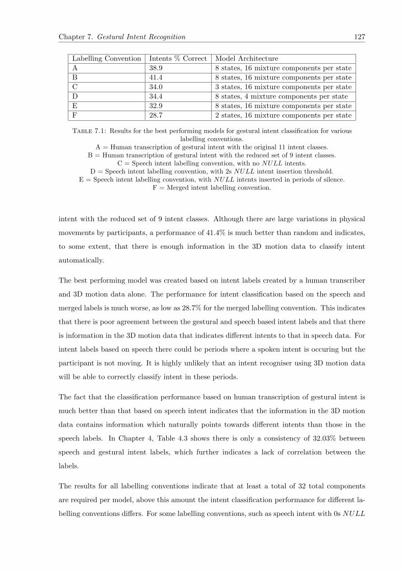
Chapter 7. Gestural Intent Recognition 127
Labelling Convention Intents % Correct Model Architecture
A 38.9 8 states, 16 mixture components per state
B 41.4 8 states, 16 mixture components per state
C 34.0 3 states, 16 mixture components per state
D 34.4 8 states, 4 mixture components per state
E 32.9 8 states, 16 mixture components per state
F 28.7 2 states, 16 mixture components per state
Table 7.1: Results for the best performing models for gestural intent classification for variouslabelling conventions.
A = Human transcription of gestural intent with the original 11 intent classes.B = Human transcription of gestural intent with the reduced set of 9 intent classes.
C = Speech intent labelling convention, with no NULL intents.D = Speech intent labelling convention, with 2s NULL intent insertion threshold.
E = Speech intent labelling convention, with NULL intents inserted in periods of silence.F = Merged intent labelling convention.
intent with the reduced set of 9 intent classes. Although there are large variations in physical
movements by participants, a performance of 41.4% is much better than random and indicates,
to some extent, that there is enough information in the 3D motion data to classify intent
automatically.
The best performing model was created based on intent labels created by a human transcriber
and 3D motion data alone. The performance for intent classification based on the speech and
merged labels is much worse, as low as 28.7% for the merged labelling convention. This indicates
that there is poor agreement between the gestural and speech based intent labels and that there
is information in the 3D motion data that indicates different intents to that in speech data. For
intent labels based on speech there could be periods where a spoken intent is occuring but the
participant is not moving. It is highly unlikely that an intent recogniser using 3D motion data
will be able to correctly classify intent in these periods.
The fact that the classification performance based on human transcription of gestural intent is
much better than that based on speech intent indicates that the information in the 3D motion
data contains information which naturally points towards different intents than those in the
speech labels. In Chapter 4, Table 4.3 shows there is only a consistency of 32.03% between
speech and gestural intent labels, which further indicates a lack of correlation between the
labels.
The results for all labelling conventions indicate that at least a total of 32 total components
are required per model, above this amount the intent classification performance for different la-
belling conventions differs. For some labelling conventions, such as speech intent with 0s NULL

Chapter 7. Gestural Intent Recognition 128
threshold (Figure 7.11), as the number of components increases beyond 32 the performance also
improves. This is contrasted with the 2s NULL intent threshold labelling convention (Figure
7.10) which shows a decrease in performance above 32 total components. This suggests that
there is enough training data to support 32 total components per model but the best physical
structure of the model may differ.
States Components per State Intents % Correct
1 32 36.0
2 16 37.0
8 4 41.7
Table 7.2: A comparison of intent classification performance for different model architec-tures where the number of total components is fixed at 32. Models are based on the human
transcription of gestural intent with the reduced set of 9 intent classes.
Table 7.2 compares the intent recognition performance for models where the total number of
components is fixed at 32 and the number of states is varied. The results indicate that for
an equal number of total components, the performance of a model is generally better with a
larger number of states. This is significant as it shows that intent classification performance is
improved by modelling the time based sequential structure of an intent rather than modelling
detail.
It is expected that with a larger corpus of training data the number of states and mixture
components per state can be increased without errors in model parameter estimation due to data
sparsity. A larger corpus would allow for further examination of the importance of sequential
structure vs. detail in intent classification. Unfortunately, it is prohibitively difficult to gather
more training data. The equipment used for recordings is a heavily used resource and the time
required to make and transcribe the recorded data and create labels is significant.
7.4.3.2 Classification Results Conclusions
• It is possible to automatically infer intent based on information in the 3D motion data,
as shown using models based on human transcriptions of gestural intent (41.4% of intents
correctly classified).
• The intent labels determined by the human transcription of gestural intent are far easier
to recover than those based on speech.

Chapter 7. Gestural Intent Recognition 129
• The information present in speech and 3D motion data may not be consistent, reducing
performance when intents are classified based on speech or merged intent. There also may
not be enough information in the 3D motion data to infer intent for labelled segments
based on speech.
• For a fixed number of total components, models containing multiple states perform better
than those with fewer states and more components per state. The sequential structure of
3D motion data is more important than detail on the position of a participant.
7.5 Continuous Recognition of Gestural Intent Using HTK
Continuous recognition of gestural intent was performed using the same procedure as models
produced for gestural intent classification using HTK. One, two, three and eight state models
with 1, 2, 4, 8, 16 and 32 components GMMs per state were created. Several labelling con-
ventions were used in generation of models, which are the same as those described above in
7.4.1. As in gesture intent classification, some results are not available for the larger complexity
models due to data sparsity problems found during their creation by HTK.
Continuous recognition using HTK means there are no defined intent boundaries between which
to perform recognition. This makes the task of recognition more difficult and requires the use
of the performance measures HTK % Correct and HTK % Accuracy as described in Chapter 2:
PercentCorrect =Nt −Nd −Ns
Nt∗ 100 (7.1)
PercentAccuracy =Nt −Nd −Ns −Ni
Nt∗ 100 (7.2)
Where intents substituted Ns, deleted Nd and inserted Ni during recognition, are compared to
the total number of intents Nt in a known correct transcription Nt.
All figures use the same linearly interpolated 57 dimension gesture data, with the same training
and test sets as used during speech and gestural intent classification.
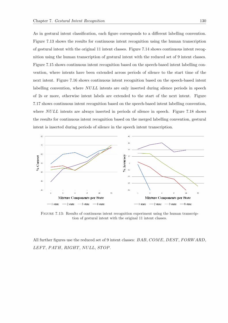
Chapter 7. Gestural Intent Recognition 130
As in gestural intent classification, each figure corresponds to a different labelling convention.
Figure 7.13 shows the results for continuous intent recognition using the human transcription
of gestural intent with the original 11 intent classes. Figure 7.14 shows continuous intent recog-
nition using the human transcription of gestural intent with the reduced set of 9 intent classes.
Figure 7.15 shows continuous intent recognition based on the speech-based intent labelling con-
vention, where intents have been extended across periods of silence to the start time of the
next intent. Figure 7.16 shows continuous intent recognition based on the speech-based intent
labelling convention, where NULL intents are only inserted during silence periods in speech
of 2s or more, otherwise intent labels are extended to the start of the next intent. Figure
7.17 shows continuous intent recognition based on the speech-based intent labelling convention,
where NULL intents are always inserted in periods of silence in speech. Figure 7.18 shows
the results for continuous intent recognition based on the merged labelling convention, gestural
intent is inserted during periods of silence in the speech intent transcription.
Figure 7.13: Results of continuous intent recognition experiment using the human transcrip-tion of gestural intent with the original 11 intent classes.
All further figures use the reduced set of 9 intent classes: BAB, COME, DEST , FORWARD,
LEFT , PATH, RIGHT , NULL, STOP .
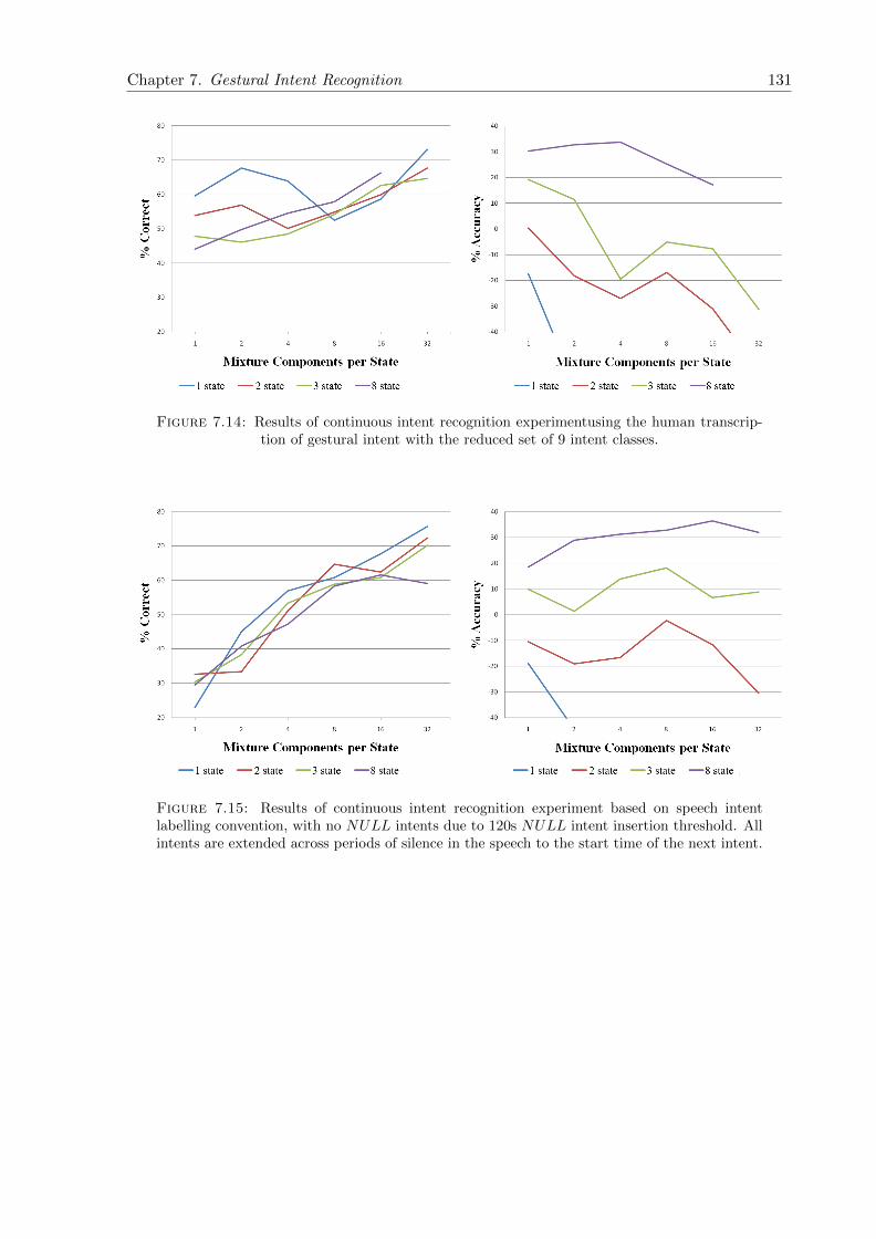
Chapter 7. Gestural Intent Recognition 131
Figure 7.14: Results of continuous intent recognition experimentusing the human transcrip-tion of gestural intent with the reduced set of 9 intent classes.
Figure 7.15: Results of continuous intent recognition experiment based on speech intentlabelling convention, with no NULL intents due to 120s NULL intent insertion threshold. Allintents are extended across periods of silence in the speech to the start time of the next intent.

Chapter 7. Gestural Intent Recognition 132
Figure 7.16: Results of continuous intent recognition experiment based on speech intentlabelling convention, with 2s NULL intent insertion threshold. NULL intents are only insertedif a silence of 2s or more is detected in speech otherwise intent labels are extended to the start
of the next intent.
Figure 7.17: Results of continuous intent recognition experiment based on speech intentlabelling convention, with 0s NULL intent insertion threshold. NULL intents are inserted
wherever there is silence in the speech.

Chapter 7. Gestural Intent Recognition 133
Figure 7.18: Results of continuous intent recognition experiment based on merged intentlabelling convention. The human transcription of gestural intent was inserted during periods of
silence in the speech intent transcription.
The results for the best performing models with the highest % accuracy for each labelling
convention are summarised in Table 7.3:
Labelling Convention % Accuracy Model Architecture
A 30.4 8 states, 4 mixture components per state
B 33.7 8 states, 4 mixture components per state
C 36.5 8 states, 16 mixture components per state
D 29.7 8 states, 8 mixture components per state
E 33.9 8 states, 16 mixture components per state
F 31.0 8 states, 16 mixture components per state
Table 7.3: % accuracy results for continuous gestural intent recognition based on the bestperforming models and various labelling conventions.
A = Human transcription of gestural intent with the original 11 intent classes.B = Human transcription of gestural intent with the reduced set of 9 intent classes.
C = Speech intent labelling convention, with no NULL intents.D = Speech intent labelling convention, with 2s NULL intent insertion threshold.
E = Speech intent labelling convention, with NULL intents inserted in periods of silence.F = Merged intent labelling convention.
7.5.1 Continuous Recognition Results Discussion
The best performing model for continuous intent recognition using only 3D motion data is the
8 state 16 mixture components per state model and the speech intent labelling convention with
no NULL intents, with 36.5% accuracy. This is better than randomly choosing an intent every

Chapter 7. Gestural Intent Recognition 134
frame and shows that there is enough information to continuously recognise intent from 3D
motion data.
The % accuracy performance measure is dependent on intents substituted, deleted or inserted
during recognition (see above) and can be compared with the % intents correct performance
measure for intent classification. In all labelling conventions the recognition performance is worse
than classification. For example, for the labelling convention based on human transcription of
gestural intent with 9 intent classes the classification performance was 41.4% (see above) which
is better than the continuous recognition performance of 33.7%.
% accuracy and % correct are HTK’s standard measures of performance (see Section 7.5).
During recognition it is possible for there to be a large number of inserted intents, where the
chosen model changes during a period of intent. In this case the % correct will be high as the
HTK considers the intent to have been correct at some point during this period of intent. %
accuracy is more useful as it takes into account the insertions when calculating performance.
In intent classification, where the boundaries of the periods of intent are known, it is not
possible to insert intents, only to select the correct or wrong intent for that period (there will
be no insertion errors). % correct in this case is calculated differently to the HTK measure of
% correct used in continuous recognition, where the data is not pre-segmented into periods of
known intent. In classification it is not possible to create new periods of intent, just to classify
the existing periods.
When continuous recognition is performed, the periods of intent are unlikely to have the same
boundaries as those in the correct transcription. HTK makes a judgment as to which periods
in the recogniser output correspond to periods in the correct transcription, the relationship
between the two isn’t clear. Due to this ambiguity it is not possible to compare the two by
simply taking each known segment boundary and calculating the distance between this and the
recogniser output boundary. Therefore it is better to pursue a more subjective analysis.
Figure 7.19 shows a visual representation of intent period boundaries for the output of two
recognised recordings. A visualisation of the correct boundaries is shown above that of the
recogniser output. A is for a recording where the overall recognition performance is higher, B
shows the output where recognition performance is low. It can be seen in B that a large number
of intents are inserted.

Chapter 7. Gestural Intent Recognition 135
Figure 7.19: A visual comparison of intent period boundaries for both good (A) and poor(B) performing recognisers. The correct labels are shown above the recogniser output
In most cases where performance is poor, a large number of insertion errors occur. Also, the
segment boundaries are not as close to the correct boundaries, although this can be difficult to
judge with such a large number of insertion errors.
In all labelling conventions, where the number of mixture components per state was the same,
the 8 state model based recognisers performed best.
States Components per State % Accuracy
1 32 -84.0
2 16 -11.6
8 4 31.2
Table 7.4: A comparison of continuous recognition performance for different model architec-tures where the number of total components is fixed at 32. Models are based on the the speech
intent labelling convention, with no NULL intents.
As with intent classification (see above) it is possible to compare model architectures given a
fixed number of total components, again 32. The labelling convention in this case is the best
scoring; the speech intent labelling convention, with no NULL intents. Table 7.4 clearly shows
that, as in intent classification, the sequential structure of a model is more important to intent
recognition performance than the detail within each state.

Chapter 7. Gestural Intent Recognition 136
With classification each period of pre-segmented data must correspond to a single intent and
therefore can be constrained to a single model. Insertions of incorrect intents cannot occur and
there are no insertion errors. As the boundaries of intent are not present during recognition and
this constraint is removed, transitions between models can occur in the same regions causing a
rise in insertion errors.
During each frame of data the markers on a participant’s body are in a certain position in 3D
space, defined here as a “pose” (in 57 dimensions). Each component within a GMM can be
thought of as describing a pose, so a GMM is a set of weighted poses. Therefore, each state
within a HMM contains a set of weighted poses. In the case of a 1 state model there is no
sequential information, the model simply describes a set of poses associated with an intent.
Over a given motion sequence over several frames the markers on a participant’s body pass
through a different pose each frame. In a 1 state model based intent recogniser the model can
be changed each frame which is highly likely as the pose, and therefore most likely intent model,
changes every frame. Each time the model is changed to an incorrect model this is counted as
an insertion which for the 1 state model allows for a huge number of insertions within a known
intent time period. This large number of insertions is primarily responsible for the low accuracy
scores when compared to a recogniser using 8 state models. Recognisers such as this, which use
models containing sequential information, take into account the data preceding each frame and
cannot change model every frame causing insertion errors.
Increasing the number of mixture components per state also has a varying effect on accuracy. A
smaller number of mixture components per state enforces a stricter model of intent, by increasing
this the set of recognised poses per state increases and more variability in physical movement
within an intent can be modelled. The disadvantage is that as the number of allowed poses
increases, the number of potentially incorrect poses within the model increases. It is more likely
that multiple models will describe similar overlapping regions, causing the recogniser to more
readily switch between models and causing insertion errors. This is most pronounced with the
1 state model.
Based on accuracy as a performance measure the 1 state models are clearly not suitable for
continuous gestural intent recognition. The lack of sequential information combined with the
increase in insertion error as the number of components per state is increased causes a significant
drop in accuracy for all labelling conventions.

Chapter 7. Gestural Intent Recognition 137
7.5.2 Continuous Recognition Results Conclusions
• It is possible to infer intent from 3D motion data during continuous recognition as shown
by the maximum score of 36.5% accuracy, which is higher than randomly choosing an
intent each frame.
• Although it is possible to infer intent directly from 3D motion data during continuous
recognition, the performance is worse than for classification. This is primarily caused by
the lack of boundaries on segments of intent and the number of insertion errors during
recognition.
• As in classification, for a fixed number of total components it is better to model the
sequential structure of 3D motion data than describe more detail using a larger number
of mixture components.
• Models with fewer states are more susceptible to insertion error during recognition due to
the ability of a recogniser to change models more regularly. This is most obvious in the
case of the 1 state model, where the recogniser can change model every frame of data,
causing an insertion error in cases where the wrong model is selected.
• More mixture components per state allows for modelling of a larger amount of variability
in intent. This can be an advantage as it allows for the natural variability in physical
movement within the same intent class. The disadvantage is that multiple models may
model similar overlapping regions, causing the recogniser to incorrectly choose a model
as the physical movements of a participant pass through these regions. This is most pro-
nounced for the 1 state model where, unlike in the 8 state model, the sequential structure
within an intent class is not modelled.
7.5.3 Varying Insertion Penalty During Continuous Recognition
It is clear that insertion errors have a significant impact on the accuracy of a continuous gestural
intent recogniser. This is most noticeable for models with fewer states, such as the 1 state model.
One method of reducing these errors, without changing model architecture, is to introduce an
insertion penalty.
In this case, insertion penalty is a standard HTK term to describe a fixed penalty applied
to transitions between models to reduce model insertions during continuous recognition. It is

Chapter 7. Gestural Intent Recognition 138
expected that as this value is increased the accuracy of recognisers using 1 state models will
increase due to the reduction in insertion errors. It may even be possible to reduce these insertion
errors enough that recognition performance becomes comparable with recognisers built using
models containing a larger number of states.
In HTK “Word insertion penalty is a fixed value added to [the score for] each token when
it transits from the end of one word to the start of the next” [153]. HTK probabilities are
calculated in the log domain, therefore in the linear domain:
y = y1, . . . ,yT (7.3)
w = w1, . . . , wN (7.4)
P (w|y) =P (y|w)P (w)
P (y)(7.5)
and
P (w) = P (w1)× P (w2|w1)× . . .× P (wn|w1, . . . , wn−1)× . . .× P (wN |w1, . . . , wN−1)(7.6)
With insertion penalty of I, this is modified to:
P ′(w) = (P (w1)× PI)× (P (w2|w1)× PI)× . . .× (P (wN |w1, . . . , wN−1)× PI) (7.7)
Where:
PI = eI (7.8)
P ′(w) = P (w)× (PI)N (7.9)

Chapter 7. Gestural Intent Recognition 139
Although results for recognisers built using the 2 and 3 state models were found, only the 1 and
8 state model results are shown here due to their clear differences. Performance of recognisers
built using 2 and 3 state models falls between those based on 1 and 8 state models.
As in previous sections the figures describe intent % correct on the left and intent % accuracy
on the right for different labelling conventions. The insertion penalty is varied from 0 to a
maximum of 1000 (set by HTK) for multiple architectures of models and is shown on the x-axis.
“1 Mix” indicates 1 Gaussian mixture component per state.
As previously, Figure 7.20 shows the results using the human transcription of gestural intent
with the original 11 intent classes. Figure 7.21 shows the results using the human transcription
of gestural intent with the reduced set of 9 intent classes. Figure 7.22 shows the results based on
the speech-based intent labelling convention, where intents have been extended across periods
of silence to the start time of the next intent. Figure 7.23 shows the results based on the
speech-based intent labelling convention, where NULL intents are only inserted during silence
periods in speech of 2s or more, otherwise intent labels are extended to the start of the next
intent. Figure 7.24 shows the results based on the speech-based intent labelling convention,
where NULL intents are always inserted in periods of silence in speech. Figure 7.25 shows the
results based on the merged labelling convention, gestural intent is inserted during periods of
silence in the speech intent transcription.
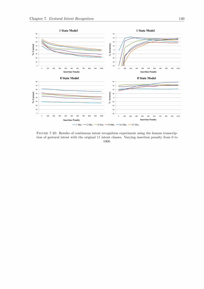
Chapter 7. Gestural Intent Recognition 140
Figure 7.20: Results of continuous intent recognition experiment using the human transcrip-tion of gestural intent with the original 11 intent classes. Varying insertion penalty from 0 to
1000.

Chapter 7. Gestural Intent Recognition 141
Figure 7.21: Results of continuous intent recognition experiment using the human transcrip-tion of gestural intent with the reduced set of 9 intent classes. Varying insertion penalty from
0 to 1000.

Chapter 7. Gestural Intent Recognition 142
Figure 7.22: Results of continuous intent recognition experiment based on speech intentlabelling convention, with no NULL intents due to 120s NULL intent insertion threshold. Allintents are extended across periods of silence in the speech to the start time of the next intent.
Varying insertion penalty from 0 to 1000.
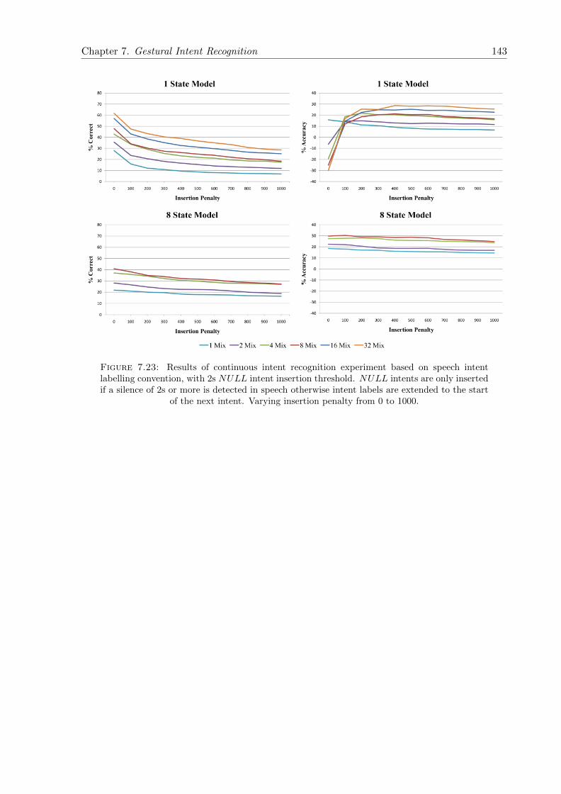
Chapter 7. Gestural Intent Recognition 143
Figure 7.23: Results of continuous intent recognition experiment based on speech intentlabelling convention, with 2s NULL intent insertion threshold. NULL intents are only insertedif a silence of 2s or more is detected in speech otherwise intent labels are extended to the start
of the next intent. Varying insertion penalty from 0 to 1000.

Chapter 7. Gestural Intent Recognition 144
Figure 7.24: Results of continuous intent recognition experiment based on speech intentlabelling convention, with 0s NULL intent insertion threshold. NULL intents are inserted
wherever there is silence in the speech. Varying insertion penalty from 0 to 1000.

Chapter 7. Gestural Intent Recognition 145
Figure 7.25: Results of continuous intent recognition experiment based on merged intentlabelling convention. The human transcription of gestural intent was inserted during periods of
silence in the speech intent transcription. Varying insertion penalty from 0 to 1000.
The results for the best performing models with the highest % accuracy for each labelling
convention and insertion penalty are summarised in Table 7.5:
Labelling Convention % Accuracy Model Architecture Insertion Penalty
A 38.6 8 states, 16 mix 1000
B 39.0 8 states, 16 mix 1000
C 40.9 8 states, 32 mix 500
D 30.4 8 states, 8 mix 100
E 33.9 8 states, 32 mix 0
F 31.2 8 states, 16 mix 100
Table 7.5: % accuracy results for continuous gestural intent recognition based on the bestperforming models and various labelling conventions and insertion penalties. “16 mix” indicates
16 mixture components per state.A = Human transcription of gestural intent with the original 11 intent classes.
B = Human transcription of gestural intent with the reduced set of 9 intent classes.C = Speech intent labelling convention, with no NULL intents.
D = Speech intent labelling convention, with 2s NULL intent insertion threshold.E = Speech intent labelling convention, with NULL intents inserted in periods of silence.
F = Merged intent labelling convention.

Chapter 7. Gestural Intent Recognition 146
It is also useful to directly compare the results in Table 7.5 with the equivalent performance
without insertion penalty for the same model architectures, as in Table 7.6. Note that the
models that gave the best performance when an insertion penalty was applied may not be the
best performing models for that labelling convention. Difference is used as a measure of change
as either number for % accuracy may be negative.
Labelling Convention % Accuracy % Accuracy (with I.P.) Difference
A 19.5 38.6 19.1
B 17.2 39.0 21.8
C 32.0 40.9 8.2
D 29.7 30.4 0.7
E 33.9 33.9 0.0
F 31.0 31.2 0.2
Table 7.6: A comparison of % accuracy for continuous gestural intent recognition both withand without an insertion penalty (I.P.) for various labelling conventions. Models are all 8 statemodels and insertion penalties are for the best performing models as described in Table 7.5.
A = Human transcription of gestural intent with the original 11 intent classes.B = Human transcription of gestural intent with the reduced set of 9 intent classes.
C = Speech intent labelling convention, with no NULL intents.D = Speech intent labelling convention, with 2s NULL intent insertion threshold.
E = Speech intent labelling convention, with NULL intents inserted in periods of silence.F = Merged intent labelling convention.
The difference is more pronounced for recognisers using 1 state models, which are particularly
susceptible to insertion errors resulting in very low accuracy (see above). Table 7.7 compares
performance of the best performing 1 state model based recognisers where insertion penalty is
used with their equivalent recognisers without insertion penalty. For brevity in this case, the
best performing model architectures and insertion penalty used are not detailed.
7.5.3.1 Varying Insertion Penalty Discussion
The best performing recogniser, with an insertion penalty applied, has 8 states and 32 mixture
components per state and is based on the speech intent labelling convention with no NULL
intents (40.9%). For the same model architecture, when an insertion penalty is not used, this
drops to 32%. The best performing model architecture (without an insertion penalty) for this
labelling convention is the 8 state, 32 mixture components per state model with 36.5%. This
shows that continuous intent recognition performance can be improved by including an insertion
penalty, even over the best performing model architecture.
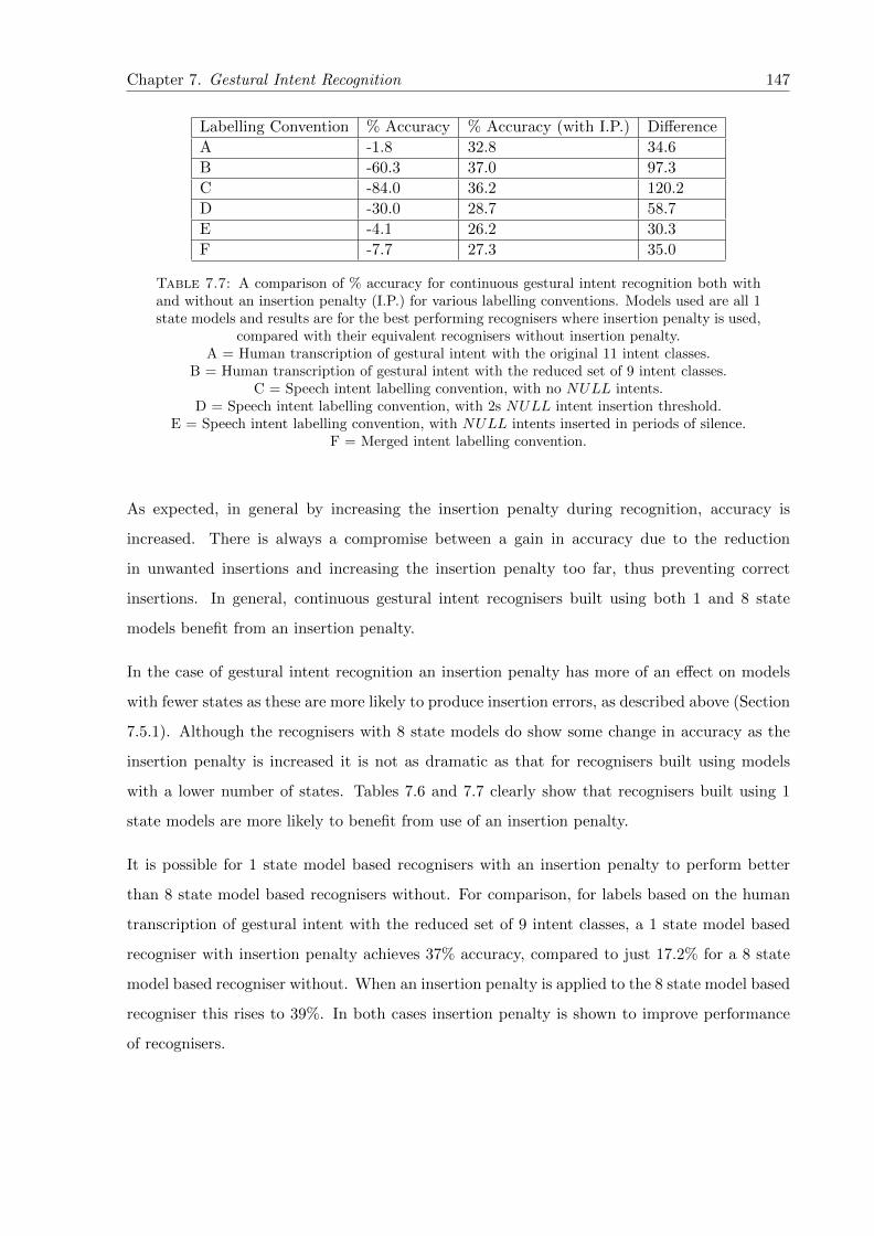
Chapter 7. Gestural Intent Recognition 147
Labelling Convention % Accuracy % Accuracy (with I.P.) Difference
A -1.8 32.8 34.6
B -60.3 37.0 97.3
C -84.0 36.2 120.2
D -30.0 28.7 58.7
E -4.1 26.2 30.3
F -7.7 27.3 35.0
Table 7.7: A comparison of % accuracy for continuous gestural intent recognition both withand without an insertion penalty (I.P.) for various labelling conventions. Models used are all 1state models and results are for the best performing recognisers where insertion penalty is used,
compared with their equivalent recognisers without insertion penalty.A = Human transcription of gestural intent with the original 11 intent classes.
B = Human transcription of gestural intent with the reduced set of 9 intent classes.C = Speech intent labelling convention, with no NULL intents.
D = Speech intent labelling convention, with 2s NULL intent insertion threshold.E = Speech intent labelling convention, with NULL intents inserted in periods of silence.
F = Merged intent labelling convention.
As expected, in general by increasing the insertion penalty during recognition, accuracy is
increased. There is always a compromise between a gain in accuracy due to the reduction
in unwanted insertions and increasing the insertion penalty too far, thus preventing correct
insertions. In general, continuous gestural intent recognisers built using both 1 and 8 state
models benefit from an insertion penalty.
In the case of gestural intent recognition an insertion penalty has more of an effect on models
with fewer states as these are more likely to produce insertion errors, as described above (Section
7.5.1). Although the recognisers with 8 state models do show some change in accuracy as the
insertion penalty is increased it is not as dramatic as that for recognisers built using models
with a lower number of states. Tables 7.6 and 7.7 clearly show that recognisers built using 1
state models are more likely to benefit from use of an insertion penalty.
It is possible for 1 state model based recognisers with an insertion penalty to perform better
than 8 state model based recognisers without. For comparison, for labels based on the human
transcription of gestural intent with the reduced set of 9 intent classes, a 1 state model based
recogniser with insertion penalty achieves 37% accuracy, compared to just 17.2% for a 8 state
model based recogniser without. When an insertion penalty is applied to the 8 state model based
recogniser this rises to 39%. In both cases insertion penalty is shown to improve performance
of recognisers.

Chapter 7. Gestural Intent Recognition 148
7.5.3.2 Varying Insertion Penalty Conclusions
• The best performing continuous gestural intent recogniser, when an insertion penalty
is applied, is for the speech intent labelling convention with no NULL intents with an
accuracy of 40.9% (models with 8 states, 32 mixture components per state with insertion
penalty 100).
• Varying the insertion penalty can improve performance of continuous intent recognisers
using 3D motion data input for all architectures of model.
• The largest increase in performance is seen for recognisers built using models with fewer
states. This is due to a reduction in the large number of insertions (seen when an insertion
penalty is not applied).
• An insertion penalty penalises a transition to a different model by the recogniser. The poor
accuracy due to lack of sequential information in recognisers built using 1 state models
(when compared to those using 8 state models) can be effectively compensated for using
a high enough insertion penalty.
7.6 Reducing Dimensionality of Models Using Principal Com-
ponent Analysis
Models were created using reduced dimensional 3D motion data produced using Principal Com-
ponent Analysis (PCA) for gestural intent classification and continuous recognition using the
merged label set, with 1, 3, 8 state models. Dimensionality of data was reduced from 57 original
dimensions to 57, 40, 20 and 10 principal components. Comparing the scores for the original
data to the reduced dimension data allows comparison of the benefits of reduced computation
time from reduced dimensionality against the resulting change in intent recognition accuracy.
7.6.1 Overview of Principal Component Analysis
Principal Component Analysis (PCA) [160] is a linear transform method used to identify dimen-
sions of maximum variation within a data set. The data is transformed into a a space spanned
by a set of orthogonal vectors called Principal Components (PCs), which are aligned along the

Chapter 7. Gestural Intent Recognition 149
axes of maximum variation. The first PC is the dimension with maximum variation with each
further PC corresponding to less variation than the previous.
The physical movement data is in the form of a 57 dimension vector v, of which there are N
total samples (see Section 3.2.2.3). For global PCA, as used for dimensionality reduction in
this work, all recordings are concatenated resulting in a large number of total samples. Given
a sequence of these 57 dimension vectors v = v1, . . . ,vT the first stage in PCA is to compute
the covariance matrix C. If the sample mean, m is:
m =1
T
T∑t=1
vt (7.10)
then, where D is the total number of dimensions in the input data (57 in the case of physical
movement data):
C = [cij ]i,j=1,...,D (7.11)
Cij =1
T
T∑t=1
(vti −mi)(vt
j −mj) (7.12)
where:
vt = (vt1, . . . ,vt
D) (7.13)
m = (m1, . . . ,mD) (7.14)
Alternatively, for each recorded session of physical movement data there is a matrix Hs where
the number of rows is the number of feature vectors v in a single recording session. A new
matrix H is created by concatenating Hs for all recordings such that:
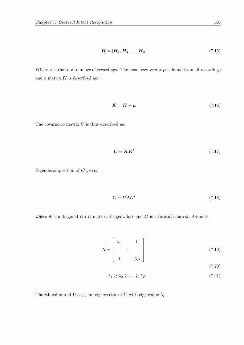
Chapter 7. Gestural Intent Recognition 150
H = [H1,H2, . . . ,Hx] (7.15)
Where x is the total number of recordings. The mean row vector µ is found from all recordings
and a matrix K is described as:
K = H − µ (7.16)
The covariance matrix C is thus described as:
C = KK ′ (7.17)
Eigendecomposition of C gives:
C = UΛU ′ (7.18)
where Λ is a diagonal D ∗D matrix of eigenvalues and U is a rotation matrix. Assume:
Λ =
λ1 0
. . .
0 λD
(7.19)
(7.20)
λ1 ≥ λ2 ≥ . . . ≥ λD (7.21)
The ith column of U , ei is an eigenvector of C with eigenvalue λi.
Chapter 7. Gestural Intent Recognition 151
In the case where C is a covariance matrix, the eigenvectors of C are called the Principal
Components (PCs) and the eigenvalue λi is the variance of the physical movement data v in
the direction of the eigenvector ei.
In pattern recognition applications it is common to assume that the dimensions of maximum
variation, the PCs, are also the dimensions which are most important for classification. If
this is the case, discarding the PCs corresponding to the smallest variances should not result
in any degradation in recognition accuracy and may result in an improvement. In any case,
in most applications the reduction in dimensions will result in a reduction in computational
load. Building identical architecture models with 20 dimension input data can be an order of
magnitude quicker on current hardware than 57 dimension input data.
In this work PCA is used as a means of dimension reduction, whereby the number of PCs is
reduced, discarding PCs with less variation. Data can be projected onto any number of PCs
and reconstructed, with the error compared to the original data dependant on the number of
PCs discarded.
7.6.2 Principal Component Analysis as a Measure of Gesture Complexity
Using PCA it is, in principle, possible to reduce the dimensionality of the data whilst preserving
the ability of a recognition system to perform classification. Participant specific PCA can be
performed to back up subjective views on participant strategy complexity, the more complex
a participant’s strategy the more principal components are required to accurately model their
movements.
By varying the number of principal components used to reconstruct input data the amount
of error with respect to the original data can be found. Large differences between original
input data with 57 dimensions and reconstructed PCA reduced dimension data show that the
participant’s movements are complex and require a large number of dimensions to account for
this complexity. Participants whose physical movements are less complex allow reconstruction
with high accuracy from very few principal components and are therefore much easier to model.
If participants’ movements were restricted to a smaller known set of physical movements it would
be possible to significantly reduce the dimensions required to create models. It is possible that
some of the participant’s movements could be captured using as little as 3 dimensions.

Chapter 7. Gestural Intent Recognition 152
As an example, it was observed that one participant’s only physical movements were a raising of
either arm to the left or the right in line with their shoulder. This movement can be captured in
1 principal component, or in 2 if both arms are raised at once. Figure 7.26 shows the movement,
correspondent to the primary principal component, for this participant with a very simple range
of physical movements.
Figure 7.26: 3 frames showing movement along the primary principal component for a par-ticipant with a very limited range of body movements.
Alternatively, if movements are restricted it may be possible to capture enough information
to recognise intent using fewer markers. This reduces the dimensionality of data even without
performing PCA.
If a participant’s movements are restricted then, even if the standard set of markers is used, it
should be possible to characterise his or her movements using lower dimensional vectors found
using PCA.
The error in reconstruction when dimensionality is reduced varied substantially between par-
ticipants. For participants with simple gesture strategies, such as a rotation of the arms, one
or two principle components are sufficient to reconstruct the motion. However, more complex
gesture strategies require more components to achieve the same accuracy.

Chapter 7. Gestural Intent Recognition 153
Figure 7.27: Number of principal components used vs. average error in mm for individualparticipants when the data is reconstructed. Accuracy of reconstruction up to 20 principalcomponents are plotted to more clearly show the variation between participants. Each curve
corresponds to a different participant and participant specific PCA.
Figure 7.27 shows reconstruction error as a function of number of PCs for each of the partici-
pants. The figure shows the large variation in complexity between participants as described by
the average error in reconstruction from a reduced number of principal components. The two
extremes, RA and TO, clearly show this variation. For an average mean squared error over all
markers of 20mm RA requires 16 dimensions for reconstruction where TO requires only 3. The
physical movement and strategy of TO was found to be very simple, with minimal movement
other than raising or lowering the arms. Figure 7.26 above shows the movement of the first
principal component of TO. RA had a completely different strategy, which involved complex
full body motions and a much more expressive set of gestures.
Small eigenvalues correspond to principal components where there is less variation than those
principal components associated with larger eigenvalues. The dimensions with less variation
contribute less to reducing the error when the data is reconstructed and can hopefully be ignored.
A large variation in the spread of eigenvalues implies that the data can be reconstructed from
fewer principal components as long as the dimensions with less variation do not contribute as
significant amount. Data which is easiest to model with fewer principal components ideally has

Chapter 7. Gestural Intent Recognition 154
very few large principal components and all other principal components with proportionally a
much smaller associated eigenvalue and therefore, variation.
If the number of principal components required for reconstruction with minimal error is very
small it is difficult to judge the effect on recognition performance. A participant may move
very little or have very simple movements, thus producing data which requires few principal
components to model but is difficult to recognise due to the limited variability between intents.
If a threshold is chosen where it is assumed that any eigenvalue below this threshold corre-
sponds to variation due to noise, by ignoring all eigenvalues below this threshold the number of
eigenvalues above this threshold indicates the complexity of a participant’s movement. So if the
eigenvalue distribution is relatively flat the movement is complex and requires a higher number
of principal components to describe it.
7.6.3 Application of PCA to Continuous Gestural Intent Recognition
PCA was applied in the creation of models based on the merged labelling convention, gestural
intent is inserted during periods of silence in the speech intent transcription (Chapter 4). Ten,
20, 40 and 57 principal component input data was used to build models with 1, 3 and 8 states
and with 1, 2, 4, 8, 16 and 32 mixture components per state. The effect of varying the HTK
insertion penalty during recognition was also studied, to see how this depends on the number
of dimensions.
HTK intent % correct (left figures) and intent % accuracy (right figures) were used as a common
measure of performance of the models, as in previous continuous recognition experiments. The
same training and test sets were used as those used during speech and gestural intent recognition.
Figure 7.28 shows the results for continuous intent recognition with standard, non-PCA reduced
57 dimensions and is included here for reference. Figure 7.29 shows the results where PCA has
been applied but dimensionality has not been reduced. Figures 7.30, 7.31, 7.32 show the results
where PCA has been applied and the data reduced to 40, 20 and 10 principal components
respectively.

Chapter 7. Gestural Intent Recognition 155
Figure 7.28: Continuous gestural intent recognition with original 57 dimension data.
Figure 7.29: Continuous gestural intent recognition with 57 principal component data.
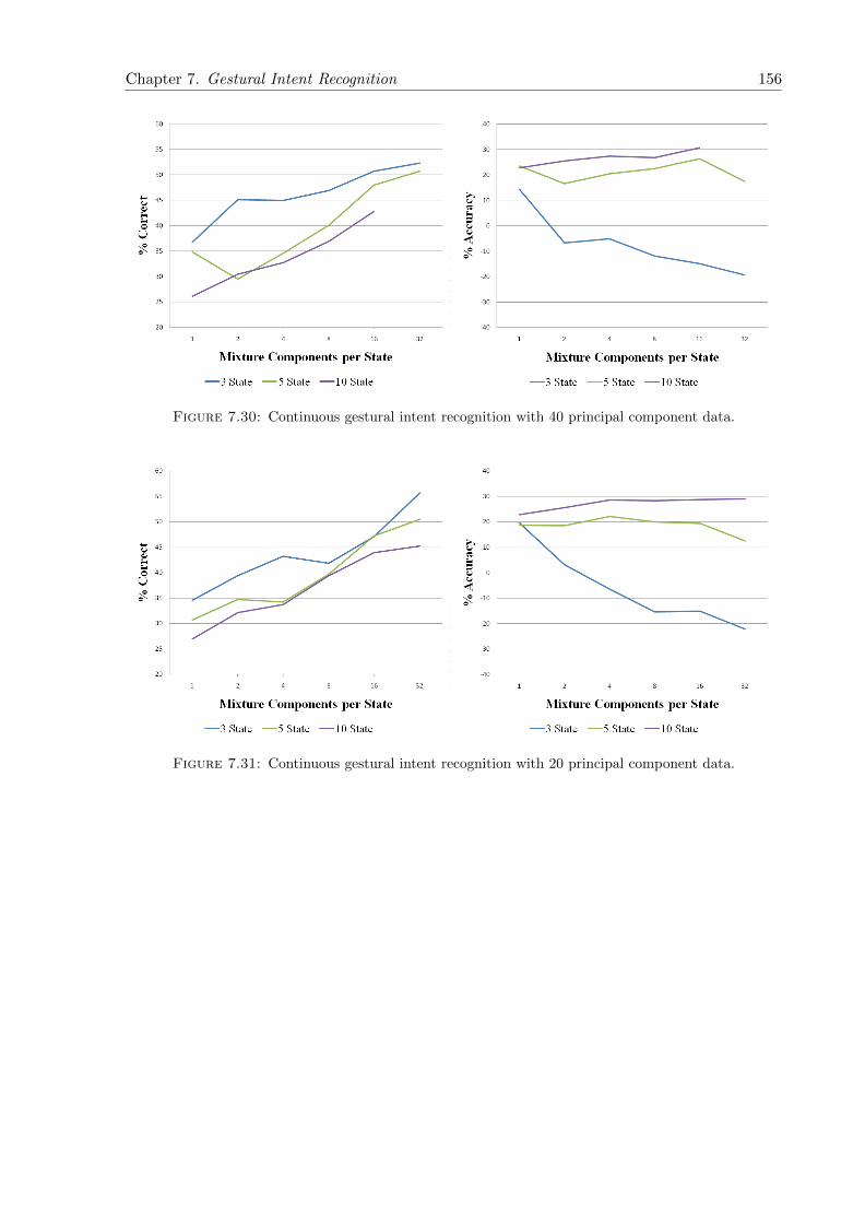
Chapter 7. Gestural Intent Recognition 156
Figure 7.30: Continuous gestural intent recognition with 40 principal component data.
Figure 7.31: Continuous gestural intent recognition with 20 principal component data.

Chapter 7. Gestural Intent Recognition 157
Figure 7.32: Continuous gestural intent recognition with 10 principal component data.
The results for the best performing models with the highest % accuracy for each number of
principal components are summarised in Table 7.8:
Principal Components % Accuracy Model Architecture
Original Data 31.0 8 states, 16 mix
57 28.7 8 states, 32 mix
40 30.7 8 states, 16 mix
20 29.0 8 states, 32 mix
10 29.0 8 states, 16 mix
Table 7.8: % accuracy results for continuous gestural intent recognition based on the bestperforming models and merged intent labelling convention. Dimensionality of input 3D motiondata is reduced using Principal Component Analysis. “16 mix” indicates 16 mixture components
per state.
7.6.3.1 Application of PCA to Continuous Gestural Intent Recognition Discussion
When comparing the results for a 8 state model with 16 mixture components across all figures
it can be seen that performance is not significantly affected by reducing the number of principal
components, even when reducing the dimensionality to 10 principal components as in Figure
7.32. The improvement in computation speed is dramatic, reducing the creation time of 8 state
models with 16 mixture components by an order of magnitude.
As in previous continuous recognition results, the 1 state models perform poorly, especially in
comparison with the 8 state models. The increase in the number of insertions by the 1 state
model as the number of mixture components increases has a negative effect on the accuracy.

Chapter 7. Gestural Intent Recognition 158
The 8 state models perform better than other model architectures for a given number of mixture
components, as in standard continuous recognition without PCA based reduction in dimension-
ality. This is due to the 8 state model’s ability to better model the sequential of the data, as
described in previous continuous recognition experiments.
The original 57 dimension data is converted to the 57 principal component data by rotating the
data to form a diagonal covariance matrix, no data is removed by dimensionality reduction. For
a lower number of mixture components this rotated data is easier to model, producing higher
recognition accuracy. If you restrict the number of mixtures it is better to have a diagonal
covariance matrix. This can be seen for the 3 and 8 state models in Figures 7.28 and 7.29 where
for up to 4 mixture components the PCA rotated data in Figure 7.29 produces models that
perform better. As the number of mixture components per state is increased this improvement
is negated by the ability of the larger model to model more complex data.
It is possible that the recogniser always fails to recognise intents for participants who use espe-
cially complex physical movements to convey an intent. In this case, reducing the dimensionality
of the data neither improves, or reduces, the performance of the recogniser.
7.6.3.2 Application of PCA to Continuous Gestural Intent Recognition Conclu-
sions
• Continuous intent recognition performance for 8 state models is not significantly affected
by reducing dimensionality of input data using PCA.
• 1 state models perform poorly compared to 8 state models for all dimensionality of input
data, as in previous experiments.
7.6.4 Application of PCA and Varying Insertion Penalty for Continuous Ges-
tural Intent Recognition
The following figures show the effect of varying the insertion penalty for a varying number of
dimensions, as reduced by PCA. As above, the merged labelling convention is used to create
models.

Chapter 7. Gestural Intent Recognition 159
In these figures the HTK insertion penalty is varied from 0 to 1000, HTK % correct (left figures)
and % accuracy (right figures) are described for 1, 3 and 8 state models with 1, 2, 4, 8 and 16
mixture components.
Figure 7.33 shows the results where PCA has been applied but dimensionality has not been
reduced. Figures 7.34, 7.35, 7.36 show the results where PCA has been applied and the data
reduced to 40, 20 and 10 principal components respectively.
Figure 7.33: Varying insertion penalty for continuous gestural intent recognition with 57principal component data.

Chapter 7. Gestural Intent Recognition 160
Figure 7.34: Varying insertion penalty for continuous gestural intent recognition with 40principal component data.
Figure 7.35: Varying insertion penalty for continuous gestural intent recognition with 20principal component data.

Chapter 7. Gestural Intent Recognition 161
Figure 7.36: Varying insertion penalty for continuous gestural intent recognition with 10principal component data.
The results for the best performing models with the highest % accuracy for each number of
principal components and insertion penalty are summarised in Table 7.9:
Principal Components % Accuracy Model Architecture Insertion Penalty
Original Data 31.2 8 states, 16 mix 100
57 32.3 8 states, 32 mix 200
40 33.7 8 states, 16 mix 100
20 31.5 8 states, 32 mix 100
10 30.7 8 states, 32 mix 100
Table 7.9: % accuracy results for continuous gestural intent recognition based on the bestperforming models and various number of principal components and insertion penalties. “16
mix” indicates 16 mixture components per state.
7.6.4.1 Application of PCA and Varying Insertion Penalty for Continuous Gestu-
ral Intent Recognition Discussion
The highest performing continuous intent recogniser (33.7%) is that based on 40 dimension input
data with 8 states, 16 mixture components per state and an insertion penalty of 100. This is

Chapter 7. Gestural Intent Recognition 162
an improvement on the best performing recogniser’s performance where insertion penalty is not
applied (31%, original input data, 8 states, 16 mixture components per state, see Table 7.8).
All figures show that for the majority of numbers of dimensions and model architectures, the best
insertion penalty in terms of intent accuracy is 100. In all cases, as in previous experiments where
PCA was not applied (see Table 7.5, application of an insertion penalty improves continuous
intent recognition performance.
As in previous experiments, the addition of an insertion penalty benefits recognisers built using
1 state models more than those built using 8 state models. The sequential information, which
allows higher performance for 8 state model recognisers, can be compensated for in 1 state
model recognisers by increasing the insertion penalty.
7.6.4.2 Application of PCA and Varying Insertion Penalty for Continuous Gestu-
ral Intent Recognition Conclusions
• As for non-PCA reduced dimensionality input data, addition of an insertion penalty im-
proves continuous gestural recognition.
• Reducing dimensionality of input data is shown to allow for some improvement in recog-
nition accuracy. An 8% improvement is seen for 40 PC input data when compared to the
original 57 dimension input data.
• As previously, insertion penalty can be applied to 1 state model based recognisers to
improve performance to almost 8 state model based recognition performance. The lack of
sequential structure in the 1 state model is compensated for by the high penalty applied
for changing models by the recogniser.
7.6.5 Application of PCA to Gestural Intent Classification
The merged intent labelling convention was used for intent classification using 3D motion data
as previously. The same measure of performance, % intents correctly classified, was also used.
1, 3 and 8 state models were produced with 1, 2, 4, 8 and 16 mixture components. The input
data was reduced using PCA from 57 dimensions to 57, 40, 20 and 10 principal components.
Figure 7.37 shows the results for intent classification with standard, non-PCA reduced 57 dimen-
sion input data. Figure 7.38 shows the results where PCA has been applied but dimensionality
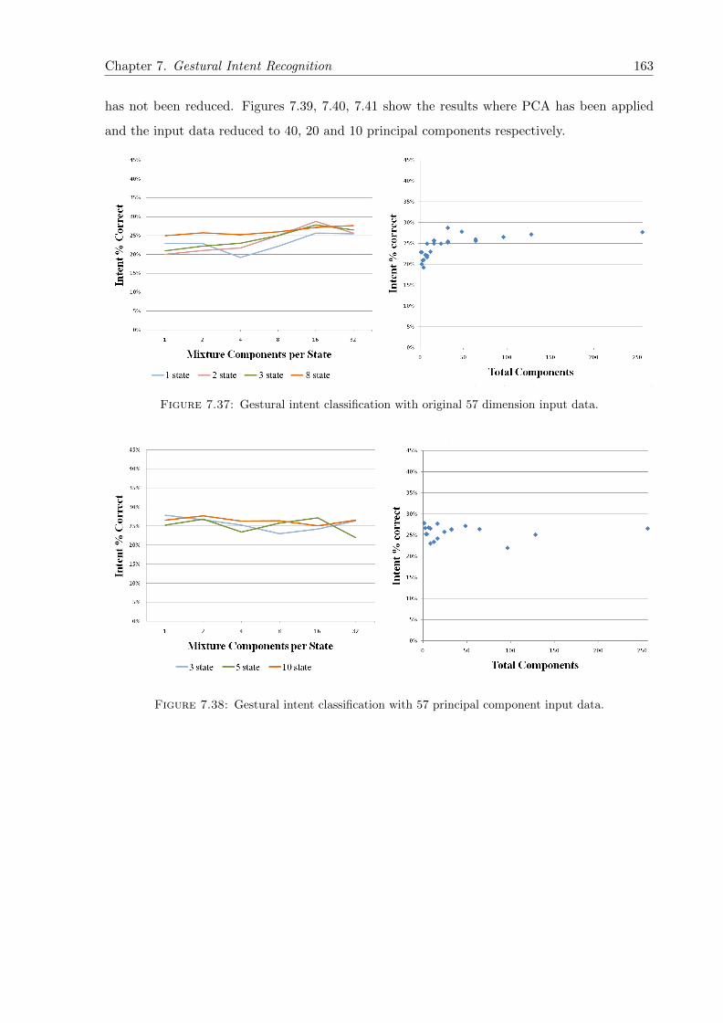
Chapter 7. Gestural Intent Recognition 163
has not been reduced. Figures 7.39, 7.40, 7.41 show the results where PCA has been applied
and the input data reduced to 40, 20 and 10 principal components respectively.
Figure 7.37: Gestural intent classification with original 57 dimension input data.
Figure 7.38: Gestural intent classification with 57 principal component input data.

Chapter 7. Gestural Intent Recognition 164
Figure 7.39: Gestural intent classification with 40 principal component input data.
Figure 7.40: Gestural intent classification with 20 principal component input data.

Chapter 7. Gestural Intent Recognition 165
Figure 7.41: Gestural intent classification with 10 principal component input data.
The results for the best performing models for each number of principal components are sum-
marised in Table 7.10:
Principal Components Intents % Correct Model Architecture
Original Data 28.7 2 states, 16 mix
57 27.8 1 states, 1 mix
40 28.6 8 states, 16 mix
20 28.9 8 states, 32 mix
10 25.7 8 states, 8 mix
Table 7.10: Results for the best performing models for gestural intent classification for inputdata of varying dimensionality, as reduced using Principal Component Analysis. “16 mix”
indicates 16 mixture components per state.
7.6.5.1 Application of PCA to Gestural Intent Classification Discussion
The best performing classifier is for 20 PCs with a 8 state, 32 mixture components per state
model based classifier (28.9%). This is only slightly better than the classification performance
with the original data (28.7%). Classification of intent based on the merged label set and
3D motion data is shown here to be difficult, the performance is poor compared with other
labelling conventions (see section 7.4). The information available for classifying intent is low
and the consistency between speech based and physical movement based intent labels (as used
in the merged label set) is low, as discussed above.

Chapter 7. Gestural Intent Recognition 166
Reduction of input data dimensionality shows that the difference in performance between dif-
ferent input dimensions is marginal, apart from in the case of the 10 dimensional input data,
where performance is generally reduced by the largest amount.
The 1 state model recognisers generally perform worse than the 8 state model recognisers, apart
from the single outlying result for the 57 PC input data. However, the difference between this
score and that of the best 8 state model recogniser is minimal (a difference of just 0.13%).
7.6.5.2 Application of PCA to Gestural Intent Classification Conclusions
• The highest scoring intent classifier was the 8 state, 32 mixture components per state
model based classifier with 20 PC input data (28.9%).
• Gesture classification using the merged label set is poor, lower than for other labelling
conventions. This in turn reduces the effect of any change in input data dimensionality.
• Classification using 10 dimension input data was poorer than using higher dimensional
input data. Above this number of dimensions the difference between classification perfor-
mance was marginal.
7.6.6 Principal Component Analysis Conclusions
In this work PCA is used to reduce the dimensionality of data from 57 to as low as 10 principal
components for both recognition of continuous gestural intent and gestural intent classification.
It can be observed that computational time for building models and performing recognition can
be reduced by an order of magnitude by constraining the input data to fewer dimensions.
The amount of error in reconstruction from a reduced set of dimensions using participant specific
PCA is shown to be a suitable measure of complexity between participants. The large variation
in strategy between participants is reflected in the average error when data is reconstructed
from a reduced set of principal components.
It can be shown that complexity of movement varies between participants. Some participants
may perform such complex movements that a 3D motion data based intent recogniser cannot
determine intent from these participants at all. For participants who perform more constrained
movements, fewer principal components are required to model their range of movements. These

Chapter 7. Gestural Intent Recognition 167
participants do potentially benefit from the reduction in noise when PCA and dimensionality
reduction is performed.
As in standard models without dimensionality reduction, 1 state model based continuous recog-
nition systems perform poorly due to the number of insertions. This reduced performance can
also be seen in the generally poor scores in classification when compared with the 8 state model
based recognisers.
Although computation time is reduced, for the larger 8 state model with 16 mixture components
per state based recognisers performance during both continuous recognition and classification is
generally comparable between the original 57 dimension data, 40 and 20 principal components.
In classification, the performance of 40 and 20 principal component models is actually better
than the original 57 dimension data. This could be due to a reduction in the amount of noise
modelled when the less significant principal components are removed.
For a small number of mixture components (up to 4 per state) PCA can be used to improve
continuous recognition due to the rotation of the data to form a diagonal covariance matrix,
which is easier to model. As the number of mixture components per state is increased and
the model increases in complexity it is more able to model complex data and this advantage is
reduced.
The effect of increasing the insertion penalty for input data reduced using PCA is similar to
that of non reduced data. Accuracy can be improved greatly for 1 state model based continuous
intent recognisers. The performance is never better than that of a 8 state model recogniser with
the same number of mixture components per state but the performance difference between the
two is reduced.
7.7 Conclusions
This chapter has shown that it is possible to use HMMs in both continuous intent recognition
and intent classification based on 3D motion data input. 3D motion data does contain some
information on the intent of a participant, which can be extracted automatically. Performance
of a recogniser or classifier depends on the model architecture and the intent labelling convention
used.

Chapter 7. Gestural Intent Recognition 168
Several model sets were produced based on different model architectures and labelling con-
ventions. The use of models of varying number of states and mixture components per state
allows for comparison between models with the same number of total components. For models
with the same number of components the architecture defines the trade off between modelling
static structure (using fewer states and a larger number of mixture components) and modelling
dynamic temporal structure (more states and fewer mixture components per state).
Natural gesture intent recognition is concerned with the sequence of physical movements re-
quired to describe an intent. In this work the unconstrained nature of the gesture reinforces
the importance of temporal information in describing the meaning of a gesture over the static
position of the gesturer. Models with a large number of states are able to describe this dynamic
data with more accuracy that models with a low number of states.
Therefore it is expected that given enough training data, for models based on gesture transcrip-
tions, as the number of states is increased the performance of the models will increase for all
natural unconstrained gestural intents.
The gestures used by many of the participants were complex, with many lasting several seconds
and containing a large amount of dynamic information, requiring models with a larger number
of states. The intent of the participants who’s gestures were very simple could be more easily
modelled using a smaller number of states and a larger number of mixture components. The
trade off between these two general types of gesture (complex, long gestures vs simple, short
gestures) means that a universal set of model architectures for all participants and all intent
types cannot be considered the optimum solution. If gesture is constrained to a set dictionary
of gestures then the differences between model architectures is expected to become more pro-
nounced. With a dictionary of simple static gestures (such as the LEFT and RIGHT gestures
as used by participants who only raised their arms to the left or right) it is expected the per-
formance of a gestural intent recognition system would improve upon the results seen in this
work.
The natural unconstrained nature of the gesture makes it difficult to model using a unified archi-
tecture model set. Creation of a dictionary and grammar of physical movements is prohibitively
difficult due to the complexity of participant movements. This complexity can be observed in
the error when data is reconstructed from a reduced number of dimensions using participant
specific PCA.
Chapter 7. Gestural Intent Recognition 169
The sparsity of training data and the computational power required to produce models beyond
8 states and 32 mixture components are the biggest barriers to improved gesture recognition. As
a result of the lack of training data several models could not be produced with this large number
of components. For the corpus of data gathered for this work the maximum reliable number
of components used in model creation is 128, comparable to a 8 state 16 mixture components
model or a 1 state 128 mixture components model.

Chapter 8
Combined, Multimodal Intent
Classification
8.1 Introduction
This chapter describes the integration of speech and gestural intent classifiers into a single
multimodal intent classifier. Chapter 6 describes the creation of a speech intent classifier,
Chapter 7 describes a gestural intent classifier. The input to the speech classifier may be either
the human transcription of speech or automatically recognised speech. The input to the gestural
intent classifier is 3D motion data.
A multimodal intent classifier, in this case, is defined as a system which integrates the scores for
a set of possible intent classes based on the output of two separate speech and gestural intent
classifiers. The recognition of intent can be thought of as a high level fusion of speech and 3D
motion data, where speech and gestural intent scores are estimated by separate classifiers based
on a set of common labels and intent classes.
As well as fusion of two separate modalities, the combination of intent scores within single
modality intent classifiers are investigated. It is apparent that the different intent scores for a
single modality give additional information on the intent of a participant, allowing for improved
classification when all intent scores are considered.
Various methods for combination of speech and gestural intent scores are compared, including
linear and non-linear combination using Neural Networks. Neural Network (NN) architectures
170
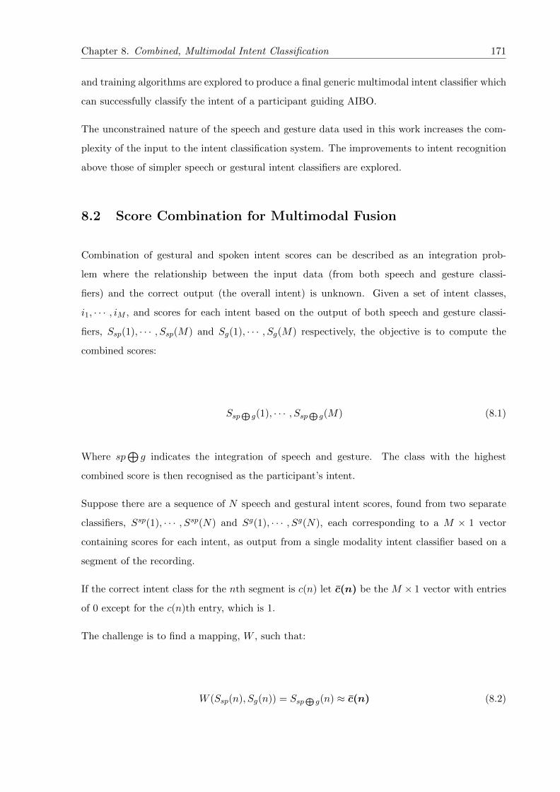
Chapter 8. Combined, Multimodal Intent Classification 171
and training algorithms are explored to produce a final generic multimodal intent classifier which
can successfully classify the intent of a participant guiding AIBO.
The unconstrained nature of the speech and gesture data used in this work increases the com-
plexity of the input to the intent classification system. The improvements to intent recognition
above those of simpler speech or gestural intent classifiers are explored.
8.2 Score Combination for Multimodal Fusion
Combination of gestural and spoken intent scores can be described as an integration prob-
lem where the relationship between the input data (from both speech and gesture classi-
fiers) and the correct output (the overall intent) is unknown. Given a set of intent classes,
i1, · · · , iM , and scores for each intent based on the output of both speech and gesture classi-
fiers, Ssp(1), · · · , Ssp(M) and Sg(1), · · · , Sg(M) respectively, the objective is to compute the
combined scores:
Ssp⊕
g(1), · · · , Ssp⊕ g(M) (8.1)
Where sp⊕g indicates the integration of speech and gesture. The class with the highest
combined score is then recognised as the participant’s intent.
Suppose there are a sequence of N speech and gestural intent scores, found from two separate
classifiers, Ssp(1), · · · , Ssp(N) and Sg(1), · · · , Sg(N), each corresponding to a M × 1 vector
containing scores for each intent, as output from a single modality intent classifier based on a
segment of the recording.
If the correct intent class for the nth segment is c(n) let c(n) be the M × 1 vector with entries
of 0 except for the c(n)th entry, which is 1.
The challenge is to find a mapping, W , such that:
W (Ssp(n), Sg(n)) = Ssp⊕
g(n) ≈ c(n) (8.2)
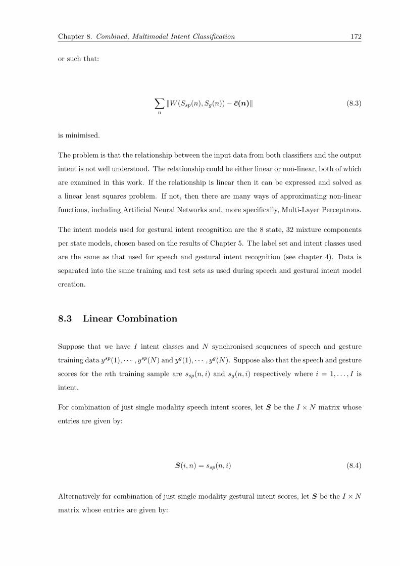
Chapter 8. Combined, Multimodal Intent Classification 172
or such that:
∑n
‖W (Ssp(n), Sg(n))− c(n)‖ (8.3)
is minimised.
The problem is that the relationship between the input data from both classifiers and the output
intent is not well understood. The relationship could be either linear or non-linear, both of which
are examined in this work. If the relationship is linear then it can be expressed and solved as
a linear least squares problem. If not, then there are many ways of approximating non-linear
functions, including Artificial Neural Networks and, more specifically, Multi-Layer Perceptrons.
The intent models used for gestural intent recognition are the 8 state, 32 mixture components
per state models, chosen based on the results of Chapter 5. The label set and intent classes used
are the same as that used for speech and gestural intent recognition (see chapter 4). Data is
separated into the same training and test sets as used during speech and gestural intent model
creation.
8.3 Linear Combination
Suppose that we have I intent classes and N synchronised sequences of speech and gesture
training data ysp(1), · · · , ysp(N) and yg(1), · · · , yg(N). Suppose also that the speech and gesture
scores for the nth training sample are ssp(n, i) and sg(n, i) respectively where i = 1, . . . , I is
intent.
For combination of just single modality speech intent scores, let S be the I ×N matrix whose
entries are given by:
S(i, n) = ssp(n, i) (8.4)
Alternatively for combination of just single modality gestural intent scores, let S be the I ×N
matrix whose entries are given by:
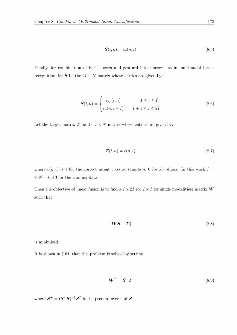
Chapter 8. Combined, Multimodal Intent Classification 173
S(i, n) = sg(n, i) (8.5)
Finally, for combination of both speech and gestural intent scores, as in multimodal intent
recognition, let S be the 2I ×N matrix whose entries are given by:
S(i, n) =
ssp(n, i) 1 ≤ i ≤ I
sg(n, i− I) I + 1 ≤ i ≤ 2I(8.6)
Let the target matrix T be the I ×N matrix whose entries are given by:
T (i, n) = c(n, i) (8.7)
where c(n, i) is 1 for the correct intent class at sample n, 0 for all others. In this work I =
9, N = 6513 for the training data.
Then the objective of linear fusion is to find a I × 2I (or I × I for single modalities) matrix W
such that
‖WS − T ‖ (8.8)
is minimised.
It is shown in [161] that this problem is solved by setting
W T = S+T (8.9)
where S+ = (STS)−1ST is the pseudo inverse of S.

Chapter 8. Combined, Multimodal Intent Classification 174
An advantage of linear combination of scores in this manner is that the optimisation procedure
can be performed in one step, rather than the iterative non-linear approach of Neural Networks.
For comparison, the computation speed for calculation of the pseudoinverse was found to be of
an order of magnitude faster than calculating the components of a Neural Network when using
standard tools.
8.4 Non-Linear Combination Using Artificial Neural Networks
There are many ways of approximating a non linear mapping between the input scores from the
two classifiers and the output target data. Cybenko [162] demonstrates that continuous feed-
forward Artificial Neural Networks (ANNs) can approximate decision regions and be used for
classification given enough input and target data. In this work, as in Cybenko’s, a Multi-Layer
Perceptron ANN (see Rumelhart et al [110]) is used to combine the output from speech and
gesture intent classifiers to produce a final score for each output class.
8.4.1 The Multi-Layer Perceptron
The Multi-Layer Perceptron (MLP) is an architecture of feed-forward ANN with an output
layer, input layer and any number of hidden layers, each containing a number of nodes, or
artificial neurons. Each node within a hidden or output layer takes as its inputs the weighted
sum of output of each node in the previous layer plus a bias. There are no connections within
a layer and there are no direct connections between the input and output layers.
The output of each node within a hidden layer is determined by the activation function within
the node. This is typically a log sigmoid or tan sigmoid function of the input x to produce the
output a:
Log Sigmoid a = f(x) =1
1 + e−x(8.10)
Tan Sigmoid a = f(x) = tanh(x/2) (8.11)
The use of nodes in an ANN can be described more easily in a simple perceptron ANN where
there are no intermediate hidden layers. The perceptron simply converts an input vector of R
dimensions to an output vector. The perceptron can be extended to the MLP by the addition of
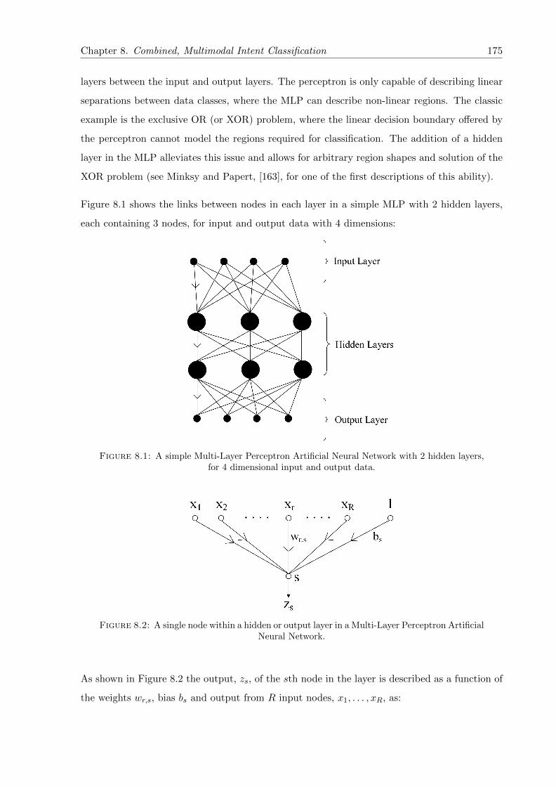
Chapter 8. Combined, Multimodal Intent Classification 175
layers between the input and output layers. The perceptron is only capable of describing linear
separations between data classes, where the MLP can describe non-linear regions. The classic
example is the exclusive OR (or XOR) problem, where the linear decision boundary offered by
the perceptron cannot model the regions required for classification. The addition of a hidden
layer in the MLP alleviates this issue and allows for arbitrary region shapes and solution of the
XOR problem (see Minksy and Papert, [163], for one of the first descriptions of this ability).
Figure 8.1 shows the links between nodes in each layer in a simple MLP with 2 hidden layers,
each containing 3 nodes, for input and output data with 4 dimensions:
Figure 8.1: A simple Multi-Layer Perceptron Artificial Neural Network with 2 hidden layers,for 4 dimensional input and output data.
Figure 8.2: A single node within a hidden or output layer in a Multi-Layer Perceptron ArtificialNeural Network.
As shown in Figure 8.2 the output, zs, of the sth node in the layer is described as a function of
the weights wr,s, bias bs and output from R input nodes, x1, . . . , xR, as:

Chapter 8. Combined, Multimodal Intent Classification 176
zs = f(
R∑r=1
xrwr,s + bs) (8.12)
The activation function for nodes within a hidden layer is typically the sigmoid function de-
scribed above. The output layer may have a different activation function, for example linear.
In a pattern recognition application, the objective is to use an MLP to find a non-linear mapping
between input vectors and class identifiers. The output class with the highest score is selected
as the correct class, in this case the correct overall intent of the participant.
By altering the weights between nodes and biases in an MLP, the non-linear relationship between
the output of the speech and gesture intent classifiers and the overall intent of the participant
can be approximated. This can be accomplished using a variety of training methods.
8.4.1.1 Multi-Layer Perceptron Training Methods
The standard training algorithm for MLPs is the backpropagation learning algorithm as de-
scribed by Rumelhart et al [110] as the “generalized delta rule”. Backpropagation is an ex-
tension of the Widrow-Hoff gradient descent algorithm, itself also known as the “delta rule”.
Backpropagation is a supervised training method which aims to minimise the mean squared
error, E, between the actual output of the MLP, Sn, and target outputs, Tn, for each training
sample n = 1, . . . , N :
E =
N∑n=1
(Sn − Tn)2 (8.13)
In this work each training sample corresponds to a segment of recorded data, which corresponds
to an intent.
This error is reduced by adjusting the weights within the MLP by calculating the derivative of
the error with respect to the weights and decrementing the weights by a proportionate amount.
This derivative cannot be calculated directly and must be decomposed into sub terms, which
can then be computed using backpropagation (see Beale and Jackson [164]).

Chapter 8. Combined, Multimodal Intent Classification 177
The change ∆ to a weight wr,s is described in terms of a learning rate η, the error δs and the
input xr:
∆wr,s = −ηδsxr (8.14)
Initialisation of the weights is performed using the “Nguyen-Widrow Initialization Method”
[165]. This method of initialisation was found to significantly reduce the time required for
training. The weights are initially set to a random value between the range set by the transfer
function used (e.g. -1 and 1 for tan sigmoid) and are then adjusted based on the number of
nodes in the MLP. This method of initialisation aims to distribute weights evenly across all
nodes given the input data. As this method does involve some randomisation it is possible that
non-identical MLP performance results will be found given the same training data.
Increasing the learning rate, η, increases the change to weights at each iteration of training and
can improve the training speed. If η is too large the training algorithm may overshoot the local
minima. Alternatively, if the learning rate is too small it can take a significantly longer time to
reach a local minima.
Since the standard gradient descent backpropagation algorithm was first introduced, a num-
ber of more efficient implementations have been developed. By using a momentum term and
considering more than the local gradient it is possible to compensate, to some extent, for local
minima. With a momentum term, m (where o < m < 1), the weight update at a given time, t,
becomes:
∆wr,s(t) = −ηδsxr +m∆wr,s(t− 1) (8.15)
The speed of the backpropogation algorithm can be improved further by adapting the learning
rate. The standard gradient descent backpropagation algorithm has a set learning rate, η, which
is set once before training occurs. This is not ideal as the best learning rate may vary as the
MLP converges on an optimal solution. With an adaptive learning rate at each new iteration
the learning rate is modified. If the previous iteration introduced a greater overall error the
new weights are discarded, the learning rate decreased and the iteration performed again. If

Chapter 8. Combined, Multimodal Intent Classification 178
the previous iteration produced a lower overall error, the opposite is performed; the weights are
kept and the learning rate is increased.
Adaptive learning rates can be combined with momentum, typically causing the backpropaga-
tion algorithm to converge to a more optimum solution faster than standard backpropagation.
Standard backpropogation can be compromised if the inputs to the sigmoid functions of each
node are very large or small. In either case the gradient can be very small due to the low
gradient of the sigmoid function, which results in a minimal change in the weights within an
MLP during each iteration of training. A solution to this is to use resilient backpropagation, as
described by Riedmiller [166] where only the direction of the gradient is used, rather than size.
The size of weight change is determined by the sign of the weight from the previous 2 iterations.
The size is decreased when the previous 2 signs are different and increased when they are the
same. So, whenever the sign of the weight is oscillating the size of the weight is reduced.
Standard backpropagation adjusts the weights by the derivative of the error function to reduce
the overall error using a set learning rate. Although this should eventually reach a local optimum
solution, it may not converge as quickly as the use of conjugate directions and a varying learning
rate which is set each iteration. In conjugate gradient backpropagation, for each iteration a
search is performed along all conjugate directions to find the learning rate and direction which
will reduce the overall error the most. There are several algorithms which perform this search
to find the optimum direction and learning rate, such as the Fletcher-Reeves and Polak-Ribiere
algorithms [167].
The conjugate gradient backpropagation methods described above are more complex than stan-
dard backpropagation as a search needs to be made each iteration, along each direction. The
search at each iteration is more computationally demanding than standard backpropagation
but fewer steps are required to reach a local optimum, resulting in much quicker training. An
improvement to conjugate backpropagation methods is the scaled conjugate gradient algorithm
(SCG), as originally described by Møller [168], which does not require the search at each itera-
tion. Møller shows speed improvements of an order of magnitude over standard backpropagation
and significant speed increases over other conjugate backpropagation methods.

Chapter 8. Combined, Multimodal Intent Classification 179
8.4.1.2 Evaluation of Non-Linear Methods on Collected Corpus
MLPs were trained to combine the intent scores output from single modality classifiers, as in
the linear combination of single modalities. Combination of all output scores from both intent
classifiers for multimodal intent classification was also performed. In both cases the training
techniques were the same, the only difference being a change in the dimensionality of input data
(9 input scores for single modality combination, 18 input scores for multimodal combination).
A variety of network architectures and training methods were used to train MLPs. The variation
in the results obtained using various training methods is explored in Appendix A. The most
successful training algorithm was found to be scaled conjugate gradient backpropogation, which
consistently produced MLPs with better classification results than other training methods. For
the purposes of intent combination this training method is used exclusively.
Whichever training data set is to be used (evaluation or full training data sets, see Figure 8.3),
training of MLPs was performed by splitting the training data into 60% training, 20% validation
and 20% test data to allow for use of the “early stopping” training technique to avoid overfitting.
The MLP weights are adjusted based on the 60% of training data each iteration. The results
of the network are then tested against the 20% validation data. If the result is a network with
poorer performance or if the performance does not improve then the network fails validation.
This occurs when there is overfitting of the MLP to the training data. The 20% test data is
used to demonstrate the performance of the trained MLP.
Validation failure is allowed to occur up to 60 times, after which training is stopped and the
MLP weights are set to those when the validation failures first occurred. Typically the number
of validation checks is lower than this but after initial training with just 6 validation checks it
was found that the training resulted in local optimum performance values below those achievable
with 60 validation checks.
Some MLPs never reached 60 validation failures, in which case the maximum number of itera-
tions allowed was set to 3000. Any more than this and the time taken to produce a result was
prohibitive, given the computer hardware and training methods used in this work.
The number of nodes used on each hidden layer of an MLP can affect the performance of the
network. This can be seen in the findings described in Appendix A, where MLPs with both
1 and 2 hidden layers trained using conjugate gradient training methods generally performed
poorly with less than 5 nodes per hidden layer.

Chapter 8. Combined, Multimodal Intent Classification 180
To test the variation due to the number of nodes in each hidden layer the full training data set
was split further into evaluation training and evaluation test data, with a 6:1 ratio. In this way
the variation due to number of nodes can be explored without contaminating the final test set.
Once the best performing architecture was found, MLPs with this architecture were trained on
the entire full training set and tested on the full test set, as in all previous experiments. Figure
8.3 shows the division of data into evaluation and full training sets. In each case (evaluation or
full training data sets) the training data is split further into 60% training, 20% validation and
20% test data as described above.
Figure 8.3: Division of the corpus into full training and test sets, with further division of thetraining set into evaluation training and test sets.
MLPs were created with both 1 and 2 hidden layers for both combination of intent scores
from separate single modality classifiers (for both speech and gestural intent) and simultaneous
combination of intent scores, as output from classifiers of both modalities.
8.5 Results
In all following experiments, the corpus is split into training and test data as in previous
experiments. The labelling convention used is the merged labelling convention, where speech
and gestural intent are merged by inserting gestural intent in periods of no speech.
PCA is not used in the following experiments, the input to the gestural intent classifier is full
57 dimension data. As the experiments are concerned only with classification of intent (rather
than continuous recognition), insertion penalties are not applicable.

Chapter 8. Combined, Multimodal Intent Classification 181
8.5.1 Linear Combination Classification Results
Linear combination was applied to the output of both speech and gestural intent classifiers
separately. In this case combination of output scores is not multimodal, each modality is
considered separately. Intent scores from classifiers with the input of human transcription of
speech, automatically recognised speech and 3D motion data were combined.
Results for linear combination are presented as confusion matrices. The confusion matrices
themselves show the output class on the left and the target class below. For example, in Figure
8.4 where BAB intents were output (marked 1 on the left) only 14.6% were correctly classified
(green % number in the right-most column on the first row). Similarly, where BAB intents were
the target intent (marked 1 below the matrix) only 24.1% were correctly output by the classifier
(green % number on the lowest row, first column). The overall score after linear combination
is the percentage of intents correctly classified, 58.5%, which is described in green in the blue
square (bottom right of the matrix).
Figure 8.4 shows the confusion matrix for linear combination of speech intent scores as found
from an intent classifier with the human transcription of speech as input. Figure 8.5 shows the
linear combination of speech intent scores from an intent classifier with automatically recognised
speech as input. Figure 8.6 shows the linear combination of gestural intent scores from an intent
classifier with 3D motion data as input.
The results for total intents % correctly classified using linear combination of output scores from
single modality intent classifiers are summarised in Table 8.1
Input Intents % Correct
Human transcribed speech intent scores 58.5
Automatically recognised speech intent scores 36.0
Gestural intent scores 27.8
Table 8.1: A comparison of linear combination using single modality output intent scoresfrom separate intent classifiers. Speech intent score input is from the speech intent classifierdescribed in Chapter 6. Gestural intent score input is from the gestural intent classifier describedin Chapter 7. In both cases the merged labelling convention is used, as are the training and
test sets from previous experiments.
The linear combination method was next applied to combine the output intent scores of speech
and gestural intent classifiers together. The speech input to the speech intent classifier was
either the human transcription of speech or automatically recognised speech. In both cases the
speech intent scores were combined with the same gestural intent classifier output scores. As

Chapter 8. Combined, Multimodal Intent Classification 182
Figure 8.4: Confusion matrix showing scores for each intent class for linearly combined speechintent classifier scores. Speech input to the classifier is from correct human transcription of
speech.
in linear combination of single modality intent scores, the results are presented as confusion
matrices.
Figure 8.7 shows multimodal linear combination where the speech intent scores are from a speech
intent classifier with the human transcription of speech as input. Figure 8.8 shows multimodal
linear combination where the speech intent scores are as output by a classifier with automatically
recognised speech as an input.
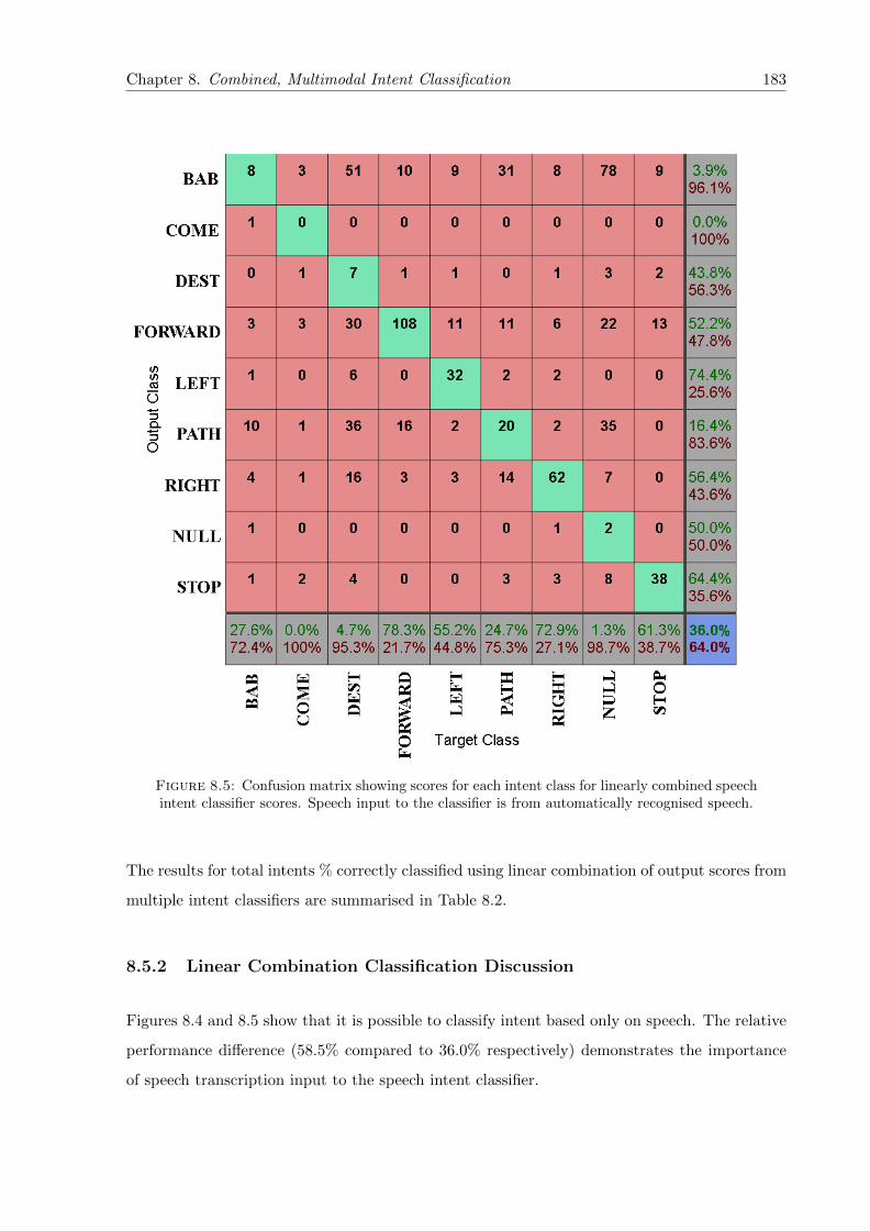
Chapter 8. Combined, Multimodal Intent Classification 183
Figure 8.5: Confusion matrix showing scores for each intent class for linearly combined speechintent classifier scores. Speech input to the classifier is from automatically recognised speech.
The results for total intents % correctly classified using linear combination of output scores from
multiple intent classifiers are summarised in Table 8.2.
8.5.2 Linear Combination Classification Discussion
Figures 8.4 and 8.5 show that it is possible to classify intent based only on speech. The relative
performance difference (58.5% compared to 36.0% respectively) demonstrates the importance
of speech transcription input to the speech intent classifier.

Chapter 8. Combined, Multimodal Intent Classification 184
Figure 8.6: Confusion matrix showing scores for each intent class for linearly combined ges-tural intent classifier scores.
Input Intents % Correct
Combined human transcribed speech & gestural intent scores 70.0
Combined automatically recognised speech & gestural intent scores 51.1
Table 8.2: A comparison of linear combination using combined output intent scores fromseparate intent classifiers. Speech intent score input is from the speech intent classifier describedin Chapter 6. Gestural intent score input is from the gestural intent classifier described inChapter 7. In both cases the merged labelling convention is used, as are the training and test
sets from previous experiments.

Chapter 8. Combined, Multimodal Intent Classification 185
Figure 8.7: Confusion matrix showing scores for each intent class for linearly combined speechand gestural intent classifiers. Speech input to the speech intent classifier is from human tran-
scription of speech.
Linear combination of gestural intent only shows that although it is possible to slightly improve
classification performance over simply choosing the highest scoring intent, the difference is
negligible (27.8% compared to 27.7%).
For the classifier based on human transcription of speech it can be seen that the majority of
intents output were NULL intents. This is unsurprising given the periods in the merged label
set where intents are inserted from the gestural intent into periods of silence in speech. During
these periods NULL will always be output by a speech intent classifier, which contributes to

Chapter 8. Combined, Multimodal Intent Classification 186
Figure 8.8: Confusion matrix showing scores for each intent class for linearly combined speechand gestural intent classifiers. Speech input to the speech intent classifier is automatically
recognised speech.
the low accuracy of the NULL intents output once linear combination of scores is performed
(31.6%).
Figure 8.7 shows that given correctly transcribed and aligned speech input the linear combina-
tion of speech and gestural intent produces a score of 70.0% intents correct. In comparison with
the speech classifier score of 45.8% with the same labels (see chapter 5) this is an improvement
of 52.8%. When compared with the gesture intent classifier score of 27.6% (see chapter 6) this
is an improvement of 153.6%.

Chapter 8. Combined, Multimodal Intent Classification 187
Figure 8.8 shows that for automatically recognised speech input the combined classification
score drops to 51.1%. This is an improvement of 102.54% using the speech intent classifier
alone and 85.35% over using the gesture intent classifier alone.
As for Figures 8.4 and 8.5, the difference between Figures 8.7 and 8.8 clearly shows the effect
that varying the quality of the speech transcription input to the speech intent classifier can have.
By reducing the input quality to the speech intent classifier the overall combined classifier score
is reduced from 70.0% to 51.1%. This can be compared to the findings of Gorin, whos “How
May I help You” call routing algorithm based on salience was reduced in performance from
99% to 70% by changing the speech input from correct human transcriptions to automatically
recognised speech [158].
The scores for each intent based on automatically recognised speech and correct transcriptions
with the same gesture classifier output can be compared further. Table 8.3 shows the percentage
of intents correctly classified with both forms of speech input when speech and gestural intent
scores are combined.
Intent Correctly transcribed % corr. Automatically recognised % corr. % change
BAB 48.3 17.2 64.4
COME 27.3 0.0 100.0
DEST 46.0 16.0 65.2
FORWARD 84.8 82.6 2.6
LEFT 72.4 53.4 26.2
PATH 30.9 22.2 28.2
RIGHT 87.1 72.9 16.3
NULL 85.2 65.2 23.5
STOP 100.0 61.3 38.7
Overall 70.0 51.1 27.0
Table 8.3: Linear combination of speech and gestural intent scores for classifiers with bothautomatically recognised speech and correctly transcribed speech input. % change indicates thereduction in performance between correctly transcribed and automatically recognised speech,
the % increase in error.
As seen in Figure 8.7, for correctly transcribed speech input the two lowest scoring intents are
COME and PATH, with 27.3% and 30.9% respectively. The score for COME is due to its
high confusion by the recogniser with the NULL intent and the low number of COME intents
in the test data. Only 11 intents in the test data were COME, of which 6 were incorrectly
identified as NULL intents. The PATH intent was also most commonly confused with NULL,
with 32 of the 81 total target PATH intents being incorrectly classified as NULL.

Chapter 8. Combined, Multimodal Intent Classification 188
The NULL intent is the most likely intent to be chosen incorrectly across all intent classes.
50.7% of the time NULL was chosen it was incorrect although when NULL was the target
intent it was chosen correctly 85.2% of the time. The NULL intent is also the most common
intent with 155 total occurences in the test set. For reference, if only NULL intents are output
from classification a score of 21.8% is produced.
As seen in Figure 8.8, by using automatically recognised speech as the input to the speech
intent classifier, the scores for all intents drop. The FORWARD intent scores do not drop as
significantly as other intents, only by 2.6% compared to an overall drop in accuracy of 27%.
This indicates that either the speech input is not as important for FORWARD intents or that
the speech used by participants is easier to recognise than for other intents.
A summary of the linear combination of both single and multiple modality intent scores and
the improvement over simply choosing the highest scoring intent is shown in Table 8.4
Input % Correct % Improvement
Human transcribed speech 58.5 27.7
Automatically recognised speech 36.0 42.9
Gestural 27.8 0.7
Combined human transcribed speech & gestural 70.0 52.8 (speech)
Combined human transcribed speech & gestural 70.0 153.6 (gestural)
Combined automatically recognised speech & gestural 51.1 102.8 (speech)
Combined automatically recognised speech & gestural 51.1 85.1 (gestural)
Table 8.4: A summary of classification performance using linear combination of output intentscores from separate intent classifiers for both single and multimodal linear combination. Inall cases the input is intent scores. % improvement is in comparison to simply choosing thehighest scoring intent class, as described in Chapters 6 and 7. (speech) indicates improvement
compared to simply choosing the highest scoring intent based on speech alone.
8.5.3 Linear Combination Classification Conclusions
• Linear combination of intent scores for single modalities improves performance over simply
choosing the highest scoring intent. The largest improvement, 153.6%, is seen when com-
paring choosing the highest scoring gestural intent and combining the human transcribed
speech based speech intent classifier output with the gestural intent classifier output.
• The highest scoring multimodal classifier using linear combination of intent scores, is based
on a human transcription of speech based speech intent classifier combined with a gestural
intent classifier (70.0%).

Chapter 8. Combined, Multimodal Intent Classification 189
• The quality of the speech input to the speech intent classifier affects linear combination of
intent scores. When simply considering the output of the speech intent classifier, perfor-
mance improves from 36.0% for automatically recognised speech input to 58.5% for human
transcribed speech input. When combinined with gestural intent scores performance rises
from 51.1% to 70% respectively.
8.5.4 Non-Linear Combination Classification Results
In order to choose the correct architecture of MLP for intent combination it is first necessary
to evaluate the effect the number of hidden layers and nodes per hidden layer has on intent
classification performance. This is explored using the evaluation training and evaluation test
set described above (Figure 8.3). Once the best performing architecture is found, this same
architecture is used in an MLP trained on the full training set and tested on the full test set.
In this work, as in linear combination, MLPs with both 1 and 2 hidden layers are used to
classify intent based on both the output scores from both single modality classifiers and the
combined scores from both speech and gestural intent classifiers. In each case the best perform-
ing architecture of MLP is found before the MLP is trained on the full training and full test
set.
Figure 8.9 shows the results for varying number of nodes per hidden layer for MLPs where
the output from either the speech or gestural intent classifier are considered individually. The
speech input to the speech intent classifier was both the aligned human transcriptions and the
automatically recognised speech. As the best performing architecture is to be investigated, these
MLPs are trained on the evaluation training data and tested on the evaluation test data.
Figure 8.10 shows the performance when varying the architecture of MLPs trained using the
output of both speech and gestural intent classifiers. In this case the scores for both modalities
are used simultaneously as input to the MLP to allow multimodal intent classification. Again,
as the best performing architecture is being found, the evaluation training and test set were
used.
The best performing MLP architectures, when tested on the evaluation training and test set,
are described in Table 8.5. It is these architectures which are used to create the final, non-linear,
MLP based intent classifiers.

Chapter 8. Combined, Multimodal Intent Classification 190
Figure 8.9: Intent classification results for MLPs with both 1 and 2 hidden layers. Input tothe MLP is the output of either speech or gestural intent classifiers. MLP training method isscaled conjugate gradient backpropagation. Trained on evaluation training data and tested on
evaluation test data.
Intent Modality % Intents Corr. Architecture
Speech (human transcribed) 66.7 1 hidden, 30 nodes
Speech (automatically recognised) 48.6 1 hidden, 23 nodes
Gestural 52.4 1 hidden, 26 nodes
Combined Speech (human transcribed) & Gestural 83.6 1 hidden, 15 nodes
Combined Speech (automatically recognised) & Gestural 66.9 1 hidden, 26 nodes
Speech (human transcribed) 67.0 2 hidden, 26 nodes
Speech (automatically recognised) 49.4 2 hidden, 15 nodes
Gestural 54.1 2 hidden, 27 nodes
Combined Speech (human transcribed) & Gestural 84.8 2 hidden, 26 nodes
Combined Speech (automatically recognised) & Gestural 67.7 2 hidden, 27 nodes
Table 8.5: Summary of results for classification of intent by MLPs given output scores fromspeech and gesture intent classifiers. Training method is scaled conjugate gradient backprop-agation. “2 hidden, 20 nodes” in Architecture indicates a MLP with 2 hidden layers, eachcontaining 20 nodes. Trained on evaluation training data and tested on evaluation test data.
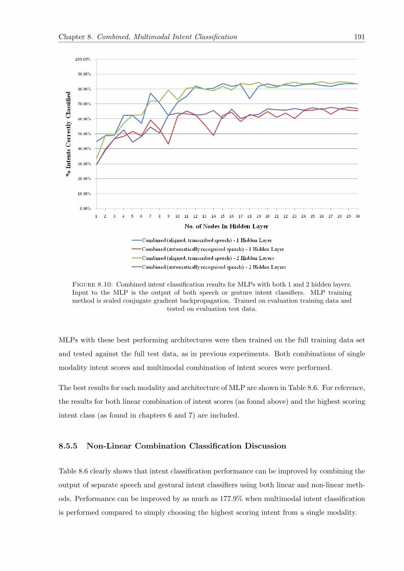
Chapter 8. Combined, Multimodal Intent Classification 191
Figure 8.10: Combined intent classification results for MLPs with both 1 and 2 hidden layers.Input to the MLP is the output of both speech or gesture intent classifiers. MLP trainingmethod is scaled conjugate gradient backpropagation. Trained on evaluation training data and
tested on evaluation test data.
MLPs with these best performing architectures were then trained on the full training data set
and tested against the full test data, as in previous experiments. Both combinations of single
modality intent scores and multimodal combination of intent scores were performed.
The best results for each modality and architecture of MLP are shown in Table 8.6. For reference,
the results for both linear combination of intent scores (as found above) and the highest scoring
intent class (as found in chapters 6 and 7) are included.
8.5.5 Non-Linear Combination Classification Discussion
Table 8.6 clearly shows that intent classification performance can be improved by combining the
output of separate speech and gestural intent classifiers using both linear and non-linear meth-
ods. Performance can be improved by as much as 177.9% when multimodal intent classification
is performed compared to simply choosing the highest scoring intent from a single modality.
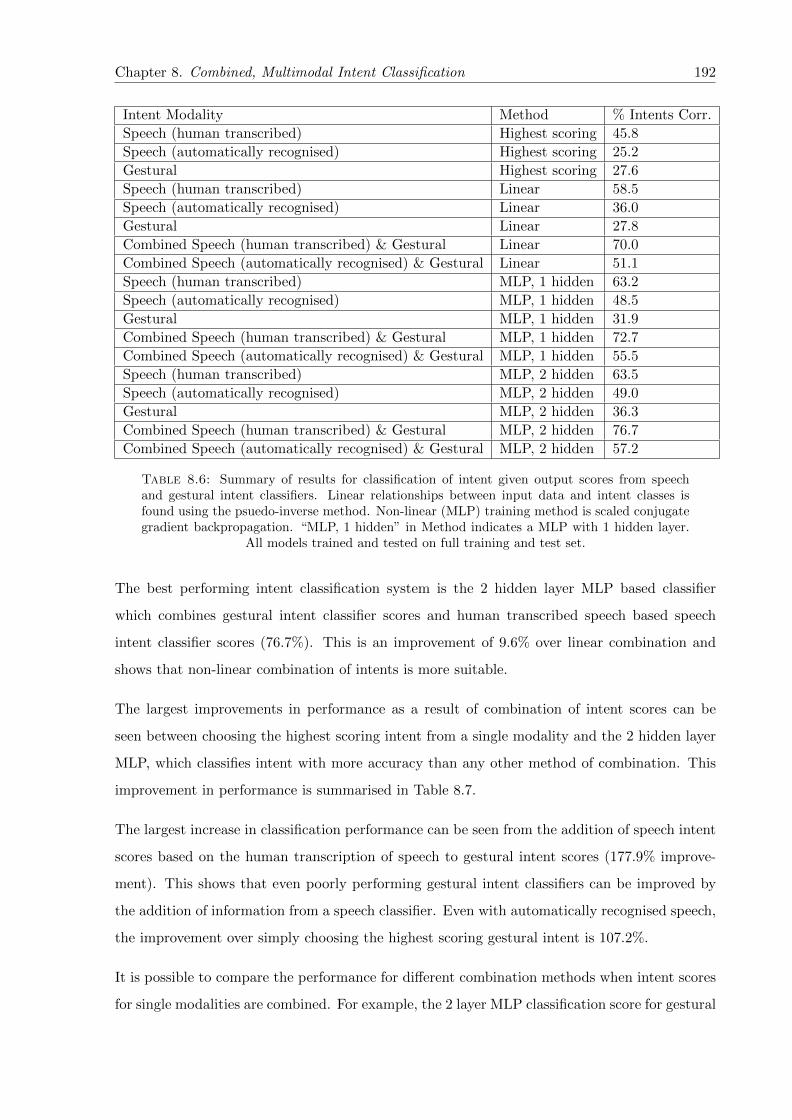
Chapter 8. Combined, Multimodal Intent Classification 192
Intent Modality Method % Intents Corr.
Speech (human transcribed) Highest scoring 45.8
Speech (automatically recognised) Highest scoring 25.2
Gestural Highest scoring 27.6
Speech (human transcribed) Linear 58.5
Speech (automatically recognised) Linear 36.0
Gestural Linear 27.8
Combined Speech (human transcribed) & Gestural Linear 70.0
Combined Speech (automatically recognised) & Gestural Linear 51.1
Speech (human transcribed) MLP, 1 hidden 63.2
Speech (automatically recognised) MLP, 1 hidden 48.5
Gestural MLP, 1 hidden 31.9
Combined Speech (human transcribed) & Gestural MLP, 1 hidden 72.7
Combined Speech (automatically recognised) & Gestural MLP, 1 hidden 55.5
Speech (human transcribed) MLP, 2 hidden 63.5
Speech (automatically recognised) MLP, 2 hidden 49.0
Gestural MLP, 2 hidden 36.3
Combined Speech (human transcribed) & Gestural MLP, 2 hidden 76.7
Combined Speech (automatically recognised) & Gestural MLP, 2 hidden 57.2
Table 8.6: Summary of results for classification of intent given output scores from speechand gestural intent classifiers. Linear relationships between input data and intent classes isfound using the psuedo-inverse method. Non-linear (MLP) training method is scaled conjugategradient backpropagation. “MLP, 1 hidden” in Method indicates a MLP with 1 hidden layer.
All models trained and tested on full training and test set.
The best performing intent classification system is the 2 hidden layer MLP based classifier
which combines gestural intent classifier scores and human transcribed speech based speech
intent classifier scores (76.7%). This is an improvement of 9.6% over linear combination and
shows that non-linear combination of intents is more suitable.
The largest improvements in performance as a result of combination of intent scores can be
seen between choosing the highest scoring intent from a single modality and the 2 hidden layer
MLP, which classifies intent with more accuracy than any other method of combination. This
improvement in performance is summarised in Table 8.7.
The largest increase in classification performance can be seen from the addition of speech intent
scores based on the human transcription of speech to gestural intent scores (177.9% improve-
ment). This shows that even poorly performing gestural intent classifiers can be improved by
the addition of information from a speech classifier. Even with automatically recognised speech,
the improvement over simply choosing the highest scoring gestural intent is 107.2%.
It is possible to compare the performance for different combination methods when intent scores
for single modalities are combined. For example, the 2 layer MLP classification score for gestural

Chapter 8. Combined, Multimodal Intent Classification 193
Input % Improvement
Human transcribed speech 38.6
Automatically recognised speech 94.4
Gestural 31.5
Combined human transcribed speech & gestural 67.5 (speech)
Combined human transcribed speech & gestural 177.9 (gesture)
Combined automatically recognised speech & gestural 127.0 (speech)
Combined automatically recognised speech & gestural 107.2 (gesture)
Table 8.7: A summary of the improvement in intent classification when comparing simplychoosing the highest scoring intent class and non-linear combination of intent class scores usinga 2 hidden layer MLP. Both single modality and multimodal intent classification are included.(speech) indicates improvement compared to simply choosing the highest scoring intent based
on speech alone.
input only (36.3%) is compared with the 2 layer MLP classification score for a speech intent
classifier based on human transcription of speech only (63.5%). Combination of the output
from both classifiers (76.7%) shows an improvement of 111.3% compared to gestural intent
scores alone and 20.8% compared to speech intent alone. When gestural intent scores are
combined with scores from a speech intent classifier based on automatically recognised speech
alone (49.0%) an improvement of 56.5% can be seen. Similar improvements over single modality
combination of intent scores can be seen for the 1 hidden layer MLP.
In all cases, the best method for combination of intent scores is the 2 hidden layer MLP. This
method shows an intent classification performance improvement when combining gestural intent
and human transcribed speech based speech intent of 9.6% over linear combination. When
applied to combination of gestural intent and automatically recognised speech based speech
intent this improvement rises to 11.9%.
Classification performance for non-linear combination of intent is influenced by the quality of
the speech classifier input, as in linear combination. Automatically recognised speech based
speech intent classifiers perform worse than those based on human transcription of speech. For
example, For combination of speech and gestural intent using a 2 layer MLP, when speech
input to the speech intent classifier is changed from automatically recognised speech to human
transcribed speech, performance improves by 34%. For a 1 hidden layer MLP the improvement
is 31% and for linear combination 37.0%.
There are some differences in the results for MLP performance when compared to the results
found in Appendix A. Although the speech input results are similar the results for gesture are
much higher when trained and tested on evaluation data sets rather than the full training and

Chapter 8. Combined, Multimodal Intent Classification 194
test set (Figure 8.3). This is because the evaluation set consists of samples where every 6th time
period in the full training set is used for testing. In comparison, when the entire training and
test set is used (as in previous experiments) the training and test data are completely separate
recordings. The variation in a participant’s physical movements between recordings is much
higher than that between time periods of the same recording. This is shown as significantly
higher performing MLPs due to the improved recognition of gestural intent.
8.5.6 Non-Linear Combination Classification Conclusions
• For all methods of non-linear combination, classification performance is improved by the
addition of intent scores from another modality.
• The largest improvement in classification performance is 177.9%, as seen when comparing
simply choosing the highest scoring gestural intent and combining the output of a gestu-
ral intent classifier with the output of a human transcribed speech based speech intent
classifier using a 2 hidden layer MLP.
• The best method for combination of intent scores from separate classifiers is to use a 2
hidden layer MLP. The highest performing multimodal classifier is the 2 hidden layer MLP
with human transcribed speech input to the speech intent classifier (76.7%).
• As in linear combination and simply choosing the highest scoring intent, the quality of
the speech input to the speech intent classifier affects performance. By changing from
automatically recognised speech input to human transcribed speech input a performance
increase of 34% can be seen when using a 2 hidden layer MLP for combination.
8.6 Conclusions
This chapter has concluded that the linear and non-linear approaches to combining speech and
gestural intent both produce far better results than the individual modality intent classifiers
described in Chapters 6 and 7. Increasing improvements in classification performance can be
seen between linear combination and the use of single and 2 hidden layer MLPs. The largest
improvements compared to simply choosing the highest scoring intent come from the use of 2
hidden layer MLPs in non-linear combination of intent scores.
Chapter 8. Combined, Multimodal Intent Classification 195
In all cases, by combining the intent scores as output by intent classifiers using either linear or
non-linear combination, the overall intent classification performance improves. This applies to
both combination of intent scores within a single modality or combination of both speech and
gestural intent scores.
The best performing intent classification system is that based on the combination of human
transcribed speech based speech intent classifier scores and gestural intent scores using a 2
hidden layer MLP (76.7%). Compared to choosing the highest scoring intent (as is chapters 6
and 7) this is an improvement of 177.9% over gestural intent, 67.5% over a human transcription
of speech based speech intent classifier and 204.4% over an automatically recognised speech
based speech intent classifier.
The highest classification performance achieved using a single modality intent classifier when
simply choosing the highest scoring intent is 45.8% from a human transcription of speech based
speech intent classifier. When linear combination is applied to the output from the same speech
intent classifier, performance increases to 58.5%. Non-linear combination of intent scores from
this classifier increases performance to 63.2% and 63.5% for single and 2 hidden layer MLPs
respectively. A similar increase in performance can be seen for single modality combination of
intent scores for automatically recognised speech input to a speech intent classifier. The same
can also be seen for single modality gestural intent classification.
Linear combination is less suitable for combination of intent scores than non-linear methods but
generally shows a large improvement over simply choosing the highest scoring intent.
When linear combination is applied to combination of scores for a single modality, classification
performance is 58.5% for combining scores from human transcribed speech input to a speech
classifier, 36.0% for automatically recognised speech input to a speech classifier and 27.8% for
combining scores from a gestural intent classifier. These are improvements of 20.6%, 42.9% and
0.7% respectively when compared to simply choosing the highest scoring intent (as in Chapters
6 and 7).
Application of linear combination to both speech and gestural intent scores simultaneously gives
a classification of 70.0% for human transcription speech input to the speech classifier and 51.1%
for automatically recognised speech input to the speech classifier. Compared to simply choosing
the highest scoring speech intent these are an improvement of 52.8% for human transcribed
speech input and 177.8% for automatically recognised speech input. The linear combination of

Chapter 8. Combined, Multimodal Intent Classification 196
scores, including the introduction of gestural intent scores, allows for significant improvements
in classification.
Both linear and non-linear combination of intent scores for individual modalities show an im-
provement over choosing the highest scoring intent. For a particular intent, strong evidence for
this intent is contained in the scores for other intents, which is ignored when only choosing the
highest scoring intent. Both linear and non-linear methods of score combination can model this
relationship between intent scores to improve overall performance. For example, for one sample
a high score for LEFT and a slightly higher score for RIGHT means there is ambiguity between
LEFT and RIGHT , although RIGHT is more likely to be the correct intent. In this case a
high score for both LEFT and RIGHT could indicate RIGHT , something not accounted for
when only choosing the highest scoring class.
There are regions in the recorded data where the participant is only using one modality. In
these cases it is impossible to recognise the intent when only considering the modality which is
not being used. Combined intent recognition performance in these regions is naturally increased
over single modality recognition. This accounts for some of the improvement over individual
modality recognisers.
As well as these regions of single modality use, there are regions where both modalities are
used. As in combination of the intent scores in a single modality, classification performance
is dependant on the scores for all intents. In these regions performance is improved by more
accurately modelling the relationship between these scores and the overall intent. There may be
instances where single modality recognisers produce the wrong intent, but combined recognition
does not. Although there may be evidence of this, there has not been an opportunity to
investigate the importance of these regions given the scope of this work.
This chapter has discussed combined, multimodal intent classification where the boundaries for
each period of intent are known. The problem of continuous recognition is different in that the
boundaries are unknown and must be found automatically. Although it is possible to perform
continuous recognition of intent in each modality separately, the integration of two continuous
recognisers is beyond the scope of this work.
In the speech domain, continuous recognition of intent can be performed on textual transcrip-
tions of speech. As in classification both the correct transcription of speech and automatically
recognised speech can be used as input to a speech intent recogniser. A possible solution is to

Chapter 8. Combined, Multimodal Intent Classification 197
assign intent to each word, based on usefulness as in this work, thereby automatically produc-
ing intent boundaries at each word boundary. Although this will produce a result, the assigned
intents for each word will always be set to the intent with the highest score. To avoid this
a window across multiple words could be used, where the surrounding words are taken into
consideration before assigning intent to the central word. Another alternative is to use dynamic
programming techniques such as those described by Sakoe [39].
Combination of modalities for continuous recognition is a larger problem and requires a measure
of confidence at every time period for each modality in order to select the correct overall intent.
These confidence measures could be explored in future work. Possible solutions include using
Neural Networks to train a system to recognise where one modality is more likely to be correct
based on the output scores at each time period. In a data driven approach, as in this work,
it has been shown that Neural Networks can be successfully used to describe the non-linear
relationship between separate modalities.
Chapter 9
Conclusions
This chapter presents an overview of the findings from all previous chapters. Corpus collection,
the results for speech and gesture intent recognition and the combination of multiple modalities
are described. Limitations of the current work are discussed as are implications for further work.
The research questions posed during the introduction to this work in Chapter 1 were as follows:
• Can speech recognition and techniques for topic spotting be used to identify spoken intent
in unconstrained natural speech?
• Can gesture recognition systems based on statistical speech recognition techniques be used
to bridge the gap between physical movements and recognition of gestural intent?
• How can speech and gesture be combined to identify the overall communicative intent of
a participant with better accuracy than recognisers built for individual modalities?
9.1 Contributions
To answer the research questions above required a rich corpus of unconstrained natural speech
and gesture. To this end an experiment was designed and carried out to record speech and 3D
motion data from 17 different participants. The data captured was transcribed and labelled for
use in all further work. A speech recognition system was built based on the popular HTK speech
recognition toolkit and a topic spotting algorithm based on usefulness measures was designed.
These were combined to create a speech intent recognition system capable of identifying intent
198

Chapter 9. Conclusions 199
given natural unconstrained speech. A gesture intent recogniser was built using HTK to identify
intent directly from 3D motion data.
Both the speech and gesture intent recognition systems were evaluated separately. The output
from both systems were then combined and this integrated intent recogniser was shown to per-
form better than each recogniser separately. Both linear and non-linear methods of multimodal
fusion were evaluated and the same techniques were applied to the output from individual recog-
nisers. In all cases the non-linear combination of intent scores gave the highest performance for
all intent recognition systems.
9.1.1 Corpus Collection
An experiment was designed with the aim of capturing natural speech and 3D motion data from
participants guiding a Sony AIBO robot around a series of set routes. Although participants
were given minimal instruction in order to elicit natural speech and gesture, the command and
control nature of the experiment allowed for a corpus that could be analysed given the time and
resources available. The robot was actually controlled externally by a human “wizard” without
the awareness of participants, who were under the impression they were controlling the robot
directly.
Initial development of a colour segmentation based stereoscopic vision system for body motion
tracking was halted in favour of a commercial marker based 3D motion capture system. This
system allowed for full body movement capture and visualisation of participant movement. High
quality speech was captured through the use of a head mounted microphone. Speech and gesture
data were synchronised based on visual assessment of speech waveforms and AIBO movement
data.
Interpolation algorithms were developed to account for unreliable 3D motion data capture, for
example, during periods of marker occlusion.
9.1.2 Corpus Annotation
A set of intents were identified that covered the range of possible participant intents for guiding
AIBO. These intents were used throughout the work.

Chapter 9. Conclusions 200
Speech data was first transcribed manually. This was then aligned to the audio recordings
using forced alignment with a trained recogniser built using HTK, which allowed for creation of
HTK format labels for all recordings. The textual aligned speech transcription was used with
multiple transcribers to produce a word level intent transcription of the entire corpus. Several
techniques for dealing with periods of silence between speech intents were explored. The speech
intent labels were created using only the text transcription of the speech.
Gestural intent was transcribed manually from 3D motion data previously synchronised with
the speech recordings. The gesture intent labels were created using only the 3D motion data.
These gesture intent labels were combined with the speech intent labels to produce the merged
label set used in further experiments.
9.1.3 Speech Intent Recognition
A speech recognition engine was built with HTK using decision tree triphone HMMs based on
the WSJCAM0 and eye/speech corpus. Models were created and inserted to account for the
noise produced by AIBO during movement. This speech recognition engine was used to align
the participant’s speech with a known textual transcription. Speech was also automatically
recognised from the recorded data for use as an example of the output from a standard speech
recogniser in further experiments.
A topic spotting algorithm was developed to classify words in the recorded corpus by usefulness
in relation to each intent class. This usefulness measure was used to create a speech intent
classifier for periods of intent in both aligned transcribed and automatically recognised speech.
The results show a decrease in performance when the topic spotting algorithm is applied to the
latter.
9.1.4 Gestural Intent Recognition
HTK was used to create HMMs of intent based on 3D physical movement data. The trade-
off between the number of HMM states and the number of GMM components per state was
explored. These models were applied to a variety of labels and evaluated. In order to build
these models tools were created to allow usage of recorded 3D motion data with HTK.
Chapter 9. Conclusions 201
It was shown that due to the sequential nature of physical movements used during periods of
gestural intent, HMMs with a larger number of states outperformed those with fewer, even when
the total number of components was the same. Unlike in speech intent recognition there is no
intermediate layer between physical movement and intent. Speech intent recognition models
sub-word units and maps these to possible words, which are then used to identify intent. This
causes complications for recognition of gestural intent which are discussed below.
Both gestural intent classification and continuous gesture intent recognition were performed.
For continuous recognition an insertion penalty was adjusted to improve performance. Global
Principal Component Analysis (PCA) was used to reduce the dimensionality of the gesture
data for both classification and continuous recognition. It was shown that PCA can be used
to reduce dimensionality and decrease computation time without substantially reducing per-
formance. Participant specific PCA, and the resultant error when reconstructing data from
reduced dimensionality, was used as a measure of physical movement complexity.
9.1.5 Combined Multi-Modal Intent Recognition
Output from speech and gesture intent recognisers were combined using linear and non-linear
methods. In both cases the objective was to minimise the error between the mapped combined
speech and gesture intent scores and a target vector comprising of 1 for the correct intent
class and 0 for others. The linear mapping was obtained using the Moore-Penrose pseudo-
inverse, while a variety of Multi-Layer Perceptron architectures were evaluated for non-linear
combination.
Speech and physical movement are not as tightly coupled as other modalities (such as speech
and lip movement) so low level fusion of data is not possible. The high level fusion of speech
and gestural intent does show a large increase in performance over individual modalities. The
largest improvement is shown for addition of gestural intent to automatically recognised speech,
for which intent recognition based on speech alone is very poor.
Results show a clear improvement for individual modalities, from simply choosing the highest
scoring intent to linear and non linear combination of the scores for all intent classes. The
same is shown when modalities are combined, with a improvement in performance from linear
to non-linear methods of combination.
Chapter 9. Conclusions 202
Combination of speech and gestural intent scores gave a maximum classification performance of
76.7%, for a 2 hidden layer MLP with human transcribed speech input to the speech classifier.
When compared to simply picking the highest scoring single modality intent, this represents an
improvement of 177.9% over gestural intent classification, 67.5% over a human transcription of
speech based speech intent classifier and 204.4% over an automatically recognised speech based
speech intent classifier.
9.2 Recommendations for Future Work
Given the advances in software for 3D motion capture more reliable data on participant physical
movement can now be obtained. Newer systems require much less manual correction enabling a
much larger corpus to be collected. Synchronisation of physical movements and recorded speech
was not directly available at the time of corpus recording. Current versions of the Qualisys
system used in data capture allow for synchronisation of not just speech and 3D motion data
but video as well.
Future research using such a system could compare the work on combining intent in this thesis
with a new overall intent recognition system based on video with speech. It may be very difficult
to identify periods in which a participants intent is constant in both speech and gesture. It is also
expected that transcribers of video with speech would be influenced by a dominant modality,
most likely speech.
The robustness of any intent recognition system would be improved by the capture of a much
larger number of participant recordings. A larger corpus of training data would reduce the
effect of the participant group dependency of gesture and combined intent recognition systems
described in this work. The time and resources required to collect enough data to allow for
participant independent intent recognition systems is beyond the scope of the current work.
An alternative to gathering more data is to restrict the participants to those who do not perform
complex physical movements. This would undoubtedly improve intent recognition performance
based on 3D motion data although the disadvantage of this approach is that the natural uncon-
strained nature of the task would be reduced.
There are large variations in the physical movements of participants when attempting to com-
municate an intent, resulting in contradictory physical movements within the same intent. The

Chapter 9. Conclusions 203
lack of an intermediate representation, such as a dictionary and grammar of known movements,
is the largest barrier to improved gestural intent recognition. Because of this, the current system
does not identify the context of physical movements (as in a dictionary) or allow for applica-
tion of any prior knowledge on likely sequences of movement (as in a grammar). A lexicon of
gesture would allow for use of more advanced speech recognition techniques such as context
dependant sub-gesture modelling. This context dependency is key to improving the gesture
intent recognition beyond that of the speech equivalent of a whole word recogniser.
It is a substantial task to attempt to manually classify physical movements in this way. Data
sparsity would remain an issue even within the constraints of a robotic command and control
task. The natural unconstrained nature of gesture as captured for this work would require a
lexicon equalling that of the equivalent speech in complexity. There are currently few examples
of gesture or gestural intent recognition where the physical movements are as unconstrained as
those in this work.
The error rate for automatically recognised speech using the speech recognition engine described
in this work is high in comparison to others. The recogniser is not optimised to the recording
environment or nature of the task used during corpus collection. There are also a number of
non-native English speakers present amongst the participants, which will further reduce the
performance of a speech recognition engine built using models of native English speakers.
The aligned transcription of speech is expected to have some errors but can be considered to
be a good approximation of a manual speech transcription. Any more improved automatic
speech recognition engine is expected to produce an intent recognition engine with performance
between the one described in this work and that based on the aligned transcription. As such,
even though the performance with automatically recognised speech is not as high, it is expected
that future work on speech recognition can be incorporated in this work to improve intent
recognition up to a similar level as the aligned transcription based intent recogniser.
An alternative to usefulness as a measure of speech intent includes the creation of separate
grammars for each intent. The scores for each grammar given a period of speech could be used
as an indication of intent. Other measures of similarity between words and intent, such as
salience, could also be explored. A thorough search of up to date spoken language and text
understanding literature would reveal alternative and potentially more powerful approaches.

Chapter 9. Conclusions 204
It may be possible to incorporate a further modality, such as eye movement, into a combined
speech and gesture intent recogniser to improve performance. As this work has shown, the addi-
tion of a modality generally does improve performance, although it is unknown if eye movement
would have the same effect. It would be impossible to include this in the current work but it
remains a possibility for collection of future corpora.
As mentioned in Chapter 4, it may be possible to attempt recognition based on a single intent-
level transcription of data, based on speech and motion data such as video recordings.
An alternative to the robot guiding task could be the introduction of a human participant, as
in the initial exploratory experiments. It is likely that the speech and physical movements of
participants would be very different to that in human-robotic interaction (HRI). Despite this,
the same labelling and intent recognition techniques could be used as in this work. The effect
of an improved understanding between human participants compared to HRI could be explored
as could the variation due to native vs. non-native speakers.

Appendix A
Evaluation of Neural Network
Training Algorithms
A.1 Introduction
This Appendix covers the training of an MLP with both 1 and 2 hidden layers using a variety of
training algorithms. It provides the justification for use of scaled conjugate gradient backpro-
pogation in the main thesis. Comparisons are also made to the linear combination of intents.
The speech and gesture intent classifiers are those described in Chapters 6 and 7.
A.2 Comparison of Training Methods for Non-Linear Combi-
nation Classification
The speech input to the speech intent classifier was either the aligned correct transcriptions or
the automatically recognised speech. The same training and test sets were used as previous
experiments. Initial weights were randomised. All network creation and training was performed
on an Intel Core 2 Duo 2.66GHz based desktop PC with 4GB of memory. For more detail on
training methods see Chapter 7.
Table A.1 shows the effect of different backpropagation (BP) training methods on a MLP with
18 inputs, 1 hidden layer containing 20 hidden nodes and an output layer with 9 nodes. The
speech input to the intent classifier was aligned correct transcriptions.
205

Appendix A. Evaluation of Neural Network Training Algorithms 206
Training Method % Intents Correctly Classified
Gradient descent BP 31.21
Gradient descent with adaptive learning rate BP 33.55
Gradient descent with momentum BP 23.41
Gradient descent with adaptive learning rate & momentum BP 59.42
Resilient BP 63.59
Fletcher-Reeves conjugate gradient BP 73.34
Polak-Ribiere conjugate gradient BP 71.65
Scaled conjugate gradient BP 71.91
Table A.1: Results for a MLP with 18 inputs, 1 hidden layer containing 20 nodes and 9 outputnodes. Speech input to speech intent classifier is aligned correct transcriptions.
It is clear that the standard gradient descent methods of backpropagation do not perform well
in comparison with the conjugate gradient methods, given the number of iterations. All 3
conjugate gradient methods perform similarly, although the Fletcher-Reeves method produces
the highest percentage of intents correctly classified (73.34%). Linear combination of speech
and gesture (described above) correctly classified 70% of the intents.
Figure A.1 shows the effect of the same training methods on MLPs with a varying number of
nodes in the single hidden layer. All MLPs have 18 inputs and 9 outputs. The input to the
speech intent classifier is aligned correct transcriptions.

Appendix A. Evaluation of Neural Network Training Algorithms 207
Figure A.1: Intent classification results for various training algorithms for a MLP with 18inputs, 1 hidden layer and 9 outputs. Input to the speech intent classifier is aligned correct
transcriptions.
Although the conjugate gradient backpropagation methods produce similar scores, there is a
difference in the number of nodes required in the hidden layer to correctly classify over 70% of
intents. In this case the Polak-Ribiere requires 6 nodes, while the scaled conjugate gradient and
Fletcher-Reeves methods require 7 and 10 respectively.
Another result of interest is that of the combined momentum and adaptive gradient descent
backpropagation. Apart from a single instance this method consistently scores higher than
momentum and adaptive methods performed separately. The momentum method especially
performs very poorly.
The highest scoring training method and architecture is the Polak-Ribiere conjugate gradient
backpropagation training algorithm and a hidden layer with 29 nodes. This gives 75.03% of
intents correctly classified; an improvement of 7.2% over linear combination of both speech and
gesture, 63.93% over the speech classifier alone and 172.14% over gesture alone.

Appendix A. Evaluation of Neural Network Training Algorithms 208
When the input to the speech intent classifier is automatically recognised speech the classifica-
tion accuracy is reduced (see chapter 5). This has a further effect on combination of speech and
gesture intent classifiers. This can clearly be seen in Figure A.2.
Figure A.2: Intent classification results for various training algorithms for a MLP with 18inputs, 1 hidden layer, 9 outputs. Input to the speech intent classifier is automatically recognised
speech.
As with the aligned correct speech transcriptions the scaled conjugate training methods pro-
duce the highest number of intents correctly classified. The highest score is for scaled conjugate
gradient backpropagation with 56.44% correct. When compared to linear combination of modal-
ities this is an improvement of 10.45%. Compared to speech alone this is an improvement of
123.70%, for gesture alone, an improvement of 104.72%. The classification using speech alone
is very poor, only 25.23% (see chapter 5), which allows for such a large improvement when the
speech and gesture classifier scores are combined.
The architecture described above can be extended by including another hidden layer, for a
total of 2. Minksy and Papert, [163], show that the addition of another hidden layer allows
for the description of more complex decision regions. This can potentially help with complex

Appendix A. Evaluation of Neural Network Training Algorithms 209
classification problems, such as the combination of intent, in this work. Figure A.3 shows the
classification accuracy for varying training methods and network architectures. In all cases the
same number of nodes were present in both hidden layers.
Figure A.3: Intent classification results for various training algorithms for a MLP with 18inputs, 2 hidden layers, 9 outputs. Input to the speech intent classifier is aligned correct
transcriptions.
The addition of another hidden layer does affect the scores for some of the training methods.
The standard gradient descent backpropagation methods are still poor, the adaptive method
actually showing worse performance than the single hidden layer MLP. The addition of another
hidden layer does not significantly affect the combined adaptive and momentum training method
scores, which peak at 61.51% correct with 26 hidden nodes. The resilient backpropagation
training method produces a 2 hidden layer MLP which scores higher than a single hidden layer
(71.78% compared to 66.84%).
The Fletcher-Reeves conjugate gradient training method is a lot more inconsistent for the 2
hidden layer MLP. Whereas with a single hidden layer with over 10 hidden nodes the Fletcher-
Reeves method stays relatively constant, averaging 72% correct, with 2 hidden layers this drops

Appendix A. Evaluation of Neural Network Training Algorithms 210
to 65.17%. The Polak-Ribiere method does score higher on average than with a single hidden
layer but the best score of 75.42% is very similar to the single hidden layer score of 75.03%.
The best score for an MLP with 2 hidden layers is for scaled conjugate gradient backpropagation.
The best score of 77.37% is the highest of all the training methods (and architecutres) and is an
improvement over the single hidden layer score of 74.12%. 77.37% represents an improvement of
10.53% over linear combination (see above), 69.04% over speech alone and 180.63% over gesture
alone.
Again the same training methods can be applied to training a 2 hidden layer MLP using the
output from both a speech intent classifier which takes in automatically recognised speech and
the same gesture intent classifier. Figure A.4 shows the classification accuracy of an MLP with
2 hidden layers for these inputs.
Figure A.4: Intent classification results for various training algorithms for a MLP with 18inputs, 2 hidden layers, 9 outputs. Input to speech intent classifier is automatically recognised
speech.
As with the single layer MLP, the scores for all training methods are reduced once the input

Appendix A. Evaluation of Neural Network Training Algorithms 211
to the speech intent classifieer is set to automatically recognised speech. Although not as
inconsistent as in Figure A.3 the Fletcher-Reeves training method shows performance generally
noticably worse than Polak-Ribiere and scaled conjugate gradient backpropagation methods.
Similarly to Figure A.3, the scaled conjugate gradient training method performs better than
other conjugate gradient backpropagation methods. This method produces the highest intent
classification score of 57.61%, a decrease of 25.54% compared to that of the classifier with
aligned transcribed speech input. This is a slight improvement on the best score of 56.44% for
a single layer MLP (see Figure A.2) although a difference this small could be accounted for by
the differing initial weights.
Tables A.2 and A.3 shows the best performance for each type of combination. In both cases
the best performing architecture (number of nodes in hidden layer) and training method result
is shown. The improvement in performance from linear through to 2 layer MLP can clearly be
seen.
Intent Combination Method % Intents Corr. Classified Training Method Architecture
Linear 70.0 NA NA
1 Hidden Layer MLP 75.0 Polak-Ribiere 30 nodes
2 Hidden Layer MLP 77.4 Scaled Conjugate 27 nodes
Table A.2: Summary of results for combination of speech and gesture intent classifiers. Resultsare for aligned, transcribed speech input to the speech intent classifier.
Intent Combination Method % Intents Corr. Classified Training Method Architecture
Linear 51.1 NA NA
1 Hidden Layer MLP 56.4 Scaled Conjugate 21 nodes
2 Hidden Layer MLP 57.6 Scaled Conjugate 28 nodes
Table A.3: Summary of results for combination of speech and gesture intent classifiers. Resultsare for automatically recognised speech input to the speech intent classifier.
The best performing training method is the scaled conjugate gradient backpropagation method.
This was also found to be the fastest method, producing a result in a shorter time than other
training methods given the computing hardware used.

Appendix A. Evaluation of Neural Network Training Algorithms 212
A.2.1 Conclusions
There are large variations in the classification performance of different training methods and
architectures of multi-layer perceptrons. It is important to use the correct training method,
which for this data set is shown to be a conjugate gradient backpropagation algorithm. The
three methods of conjugate gradient backpropagation tested were Polak-Ribiere, Fletcher-Reeves
and scaled conjugate backpropagation. The conjugate gradient training techniques were found
to reach a higher local maximum score significantly quicker than the standard gradient descent
methods. The scaled conjugate methods also produced higher scores with fewer nodes in the
hidden layer for all input data.
The simplest training algorithm evaluated was standard gradient descent backpropagation. This
performed poorly in all tests, even when the learning rate was dynamically modified using
momentum and adaptive measures. Given enough training time these methods would produce
an MLP with higher performance although the substantially longer training times required to
reach a similar performance to other training methods prohibits their use for this work.
For example, a 2 hidden layer MLP was trained using standard gradient descent backpropagation
for 30000 iterations, 10 times that described above. The same initialisation weights and biases
were used as those generated for the best performing scaled conjugate gradient trained MLP.
The result was a MLP with improved performance (48.8% compared to 28.5%) but the training
time taken was also 10 times longer and the final performance still worse than resilient, adaptive
& momentum and all the scaled conjugate gradient backpropagation training methods.
Resilient gradient descent proved to be more successful than standard gradient descent training
methods. In a 2 layer MLP with automatically recognised speech this method equalled or bested
the performance of the Fletcher-Reeves conjugate gradient descent method for many different
architectures. However, in the single layer MLP and for aligned transcribed speech, resilient
backpropagation is shown to generally perform worse than the conjugate gradient methods.

Bibliography
[1] R. Moore, “Evaluating speech recognizers,” Acoustics, Speech and Signal Processing, IEEE
Transactions on, vol. 25, no. 2, pp. 178–183, Apr 1977.
[2] D. Pallett, “Benchmark tests for darpa resource management database performance evalu-
ations,” Acoustics, Speech, and Signal Processing, 1989. ICASSP-89., 1989 International
Conference on, pp. 536–539, May 1989.
[3] P. C. Woodland and S. J. Young, “The htk continuous speech recogniser,” In Proceedings
Eurospeech 93, pp. 2207–2219, Sept 1993.
[4] NIST, “The road rally word-spotting corpora (rdrally1),” NIST Speech Disc 6-1.1,
September 1991.
[5] K. H. Davis, R. Biddulph, and S. Balashek, “Automatic recognition of spoken digits,”
The Journal of the Acoustical Society of America, vol. 24, no. 6, pp. 637–642, 1952.
[6] J. W. Forgie and C. D. Forgie, “Results obtained from a vowel recognition computer
program,” The Journal of the Acoustical Society of America, vol. 31, no. 6, pp. 844–844,
1959.
[7] J. E. K. Smith and L. Klem, “Vowel recognition using a multiple discriminant function,”
The Journal of the Acoustical Society of America, vol. 33, no. 3, pp. 358–358, 1961.
[8] T. Sakai and S. Doshita, “Phonetic typewriter,” The Journal of the Acoustical Society of
America, vol. 33, no. 11, pp. 1664–1664, 1961.
[9] J. Suzuki and K. Nakata, “Recognition of japanese vowels - preliminary to the recognition
of speech,” Journal Radio Research Laboratory, vol. 37, no. 8, pp. 193–212, 1961.
[10] T. K. Vintsyuk, “Speech discrimination by dynamic programming,” Kibernatika, vol. 4,
no. 1, pp. 81–88, 1968.
213

Bibliography 214
[11] H. Sakoe, “Dynamic programming algorithm optimization for spoken word recognition,”
IEEE Transactions on Acoustics, Speech, and Signal Processing, vol. 26, pp. 43–49, 1978.
[12] T. K. Vintsyuk, “Phoneme recognition in connected speech. part 1. basic assumptions
and statement of the problem,” Avtomatyka (Soviet Automatic Control), vol. 5, no. 6, pp.
27–34, 1972.
[13] ——, “Phoneme recognition in connected speech. part 2. recognition, training and self-
organization algorithms,” Avtomatyka (Soviet Automatic Control), vol. 6, no. 1, pp. 47–54,
1973.
[14] J. S. Bridle, M. D. Brown, and R. M. Chamberlain, “Continuous connected word recog-
nition using whole word templates,” The Radio and Electronic Engineer, vol. 53, no. 4,
pp. 167–175, April 1984.
[15] W. A. Lea, Trends in Speech Recognition. Upper Saddle River, NJ, USA: Prentice Hall
PTR, 1980.
[16] A. Newell, Heuristic programming: ill-structured problems. Cambridge, MA, USA: MIT
Press, 1993, pp. 3–54.
[17] B. S. Atal and S. L. Hanauer, “Speech analysis and synthesis by linear prediction of the
speech wave,” The Journal of the Acoustical Society of America, vol. 50, no. 2B, pp.
637–655, 1971.
[18] T. E. Tremain, “The government standard linear predictive coding algorithm: Lpc-10,”
Speech Technology Magazine, pp. 40–49, April 1982.
[19] L. E. Baum and T. Petrie, “Statistical inference for probabilistic functions of finite state
markov chains,” Annals of Mathematical Statistics, vol. 37, no. 6, pp. 1554–1563, 1966.
[20] L. E. Baum, T. Petrie, G. Soules, and N. Weiss, “A maximization technique occurring in
the statistical analysis of probabilistic functions of markov chains,” Annals of Mathemat-
ical Statistics, vol. 41, no. 1, pp. 164–171, 1970.
[21] L. E. Baum and J. A. Egon, “An inequality with applications to statistical estimation
for probabilistic functions of a markov process and to a model for ecology,” Bull. Amer.
Math. Soc., vol. 73, no. 3, pp. 360–363, 1967.

Bibliography 215
[22] A. Viterbi, “Error bounds for convolutional codes and an asymptotically optimum decod-
ing algorithm,” Information Theory, IEEE Transactions on, vol. 13, no. 2, pp. 260–269,
Apr 1967.
[23] J. Forney, G.D., “The viterbi algorithm,” Proceedings of the IEEE, vol. 61, no. 3, pp.
268–278, March 1973.
[24] J. K. Baker, Stochastic modeling for automatic speech understanding. San Francisco, CA,
USA: Morgan Kaufmann Publishers Inc., 1990, pp. 297–307.
[25] ——, “Stochastic modeling as a means of automatic speech recognition.” Ph.D. disserta-
tion, Carnegie Mellon University, Pittsburgh, PA, USA, 1975.
[26] J. Baker, “The dragon system - an overview,” Acoustics, Speech and Signal Processing,
IEEE Transactions on, vol. 23, pp. 40–47, 1975.
[27] F. Jelinek, “Continuous speech recognition by statistical methods,” Proceedings of the
IEEE, vol. 64, no. 4, pp. 532–556, 1976.
[28] D. H. Klatt, “Review of the arpa speech understanding project,” The Journal of the
Acoustical Society of America, vol. 60, no. S1, pp. S10–S10, 1976.
[29] J. Wolf and W. Woods, “The hwim speech understanding system,” Acoustics, Speech, and
Signal Processing, IEEE International Conference on ICASSP ’77., vol. 2, pp. 784–787,
1977.
[30] L. D. Erman, “Overview of the hearsay speech understanding research,” SIGART Bull.,
no. 56, pp. 9–16, 1976.
[31] B. Lowerre and R. Reddy, “The harpy speech recognition system: performance with large
vocabularies,” The Journal of the Acoustical Society of America, vol. 60, no. S1, pp.
S10–S11, 1976.
[32] L. D. Erman and V. R. Lesser, “The hearsay-ii speech understanding system: A tutorial,”
in Trends in Speech Recognition. Prentice-Hall, 1980, pp. 361–381.
[33] D. D. Corkill, K. Q. Gallagher, and K. E. Murray, “Gbb: A generic blackboard develop-
ment system,” AAAI, pp. 1008–1014, 1986.
[34] D. D. Corkill, “Blackboard systems,” AI Expert, pp. 40–47, 1991.
Bibliography 216
[35] V. R. Lesser and D. D. Corkill, “The distributed vehicle monitoring testbed: A tool for
investigating distributed problem solving networks,” AI Magazine, vol. 4, no. 3, pp. 15–33,
1983.
[36] B. Lowerre, “The harpy speech understanding system,” Readings in speech recognition,
pp. 576–586, 1990.
[37] B. T. Lowerre, “The harpy speech recognition system,” Ph.D. dissertation, CARNEGIE-
MELLON UNIV PITTSBURGH PA DEPT OF COMPUTER SCIENCE, April 1976.
[38] B. Yegnanarayana and D. R. Reddy, “Performance of harpy speech recognition system
for telephone quality speech input,” The Journal of the Acoustical Society of America,
vol. 63, no. S1, pp. S78–S78, 1978.
[39] H. Sakoe, “Two-level dp-matching - a dynamic programming-based pattern matching
algorithm for connected word recognition,” IEEE Transactions on Acoustics, Speech, and
Signal Processing, vol. 27, pp. 588–595, 1979.
[40] K. Paliwal, A. Agarwal, and S. Sinha, “A modification over sakoe and chiba’s dynamic
time warping algorithm for isolated word recognition,” Acoustics, Speech, and Signal Pro-
cessing, IEEE International Conference on ICASSP ’82, vol. 7, pp. 1259–1261, May 1982.
[41] C. Myers and L. Rabiner, “A level building dynamic time warping algorithm for con-
nected word recognition,” Acoustics, Speech and Signal Processing, IEEE Transactions
on, vol. 29, no. 2, pp. 284–297, Apr 1981.
[42] L. Bahl and F. Jelinek, “Decoding for channels with insertions, deletions, and substitutions
with applications to speech recognition,” Information Theory, IEEE Transactions on,
vol. 21, no. 4, pp. 404–411, Jul 1975.
[43] H. Ney, “A comparative study of two search strategies for connected word recognition:
Dynamic programming and heuristic search,” Pattern Analysis and Machine Intelligence,
IEEE Transactions on, vol. 14, no. 5, pp. 586–595, May 1992.
[44] H. Ney and S. Ortmanns, “Dynamic programming search for continuous speech recogni-
tion,” Signal Processing Magazine, IEEE, vol. 16, no. 5, pp. 64–83, 1999.
[45] A. Poritz, “Linear predictive hidden markov models and the speech signal,” Acoustics,
Speech, and Signal Processing, IEEE International Conference on ICASSP ’82, vol. 7, pp.
1291–1294, May 1982.

Bibliography 217
[46] L. Liporace, “Maximum likelihood estimation for multivariate observations of markov
sources,” Information Theory, IEEE Transactions on, vol. 28, no. 5, pp. 729–734, Sep
1982.
[47] B. Juang, “On the hidden Markov model and dynamic time warping for speech recognition
– A unified view,” AT&T Bell Laboratories Technical Journal, vol. 63, no. 7, pp. 1213–
1242, September 1985.
[48] L. R. Rabiner, S. E. Levinson, and M. M. Sondhi, “On the application of vector quantiza-
tion and hidden Markov models to speaker-independent, isolated word recognition,” Bell
System Technical Journal, vol. 62, no. 4, pp. 1075–1105, Apr. 1983.
[49] L. R. Rabiner and B. Juang, “An introduction to hidden markov models,” ASSP Maga-
zine, IEEE, vol. 3, no. 1, pp. 4–16, Jan. 1986.
[50] L. R. Rabiner, “A tutorial on hidden markov models and selected applications in speech
recognition,” in Proceedings of the IEEE, 1989, pp. 257–286.
[51] P. Price, W. M. Fisher, J. Bernstein, and D. S. Pallett, “The darpa 1000-word resource
management database for continuous speech recognition,” Acoustics, Speech, and Signal
Processing, 1988. ICASSP-88., 1988 International Conference on, vol. 1, pp. 651–654,
1988.
[52] Y. Chow, M. Dunham, O. Kimball, M. Krasner, G. Kubala, J. Makhoul, P. Price,
S. Roucos, and R. Schwartz, “Byblos: The bbn continuous speech recognition system,”
Acoustics, Speech, and Signal Processing, IEEE International Conference on ICASSP ’87.,
vol. 12, pp. 89–92, Apr 1987.
[53] H. Murveit, M. Cohen, P. Price, G. Baldwin, M. Weintraub, and J. Bernstein, “Sri’s
decipher system,” in proceedings of the Speech and Natural Language Workshop, pp. 94–
99, 1989.
[54] K.-F. Lee, “Automatic speech recognition: The development of the sphinx system,” PhD
Thesis, 1988.
[55] C. E. Shannon, “A mathematical theory of communication,” SIGMOBILE Mob. Comput.
Commun. Rev., vol. 5, no. 1, pp. 3–55, 2001.
[56] J. K. Baker, “Trainable grammars for speech recognition,” The Journal of the Acoustical
Society of America, vol. 65, no. 1, p. 132, 1979.

Bibliography 218
[57] X. Huang, “Phoneme classification using semicontinuous hidden markov models,” Signal
Processing, IEEE Transactions on, vol. 40, no. 5, pp. 1062–1067, May 1992.
[58] X. D. Huang and M. A. Jack, Semi-continuous hidden Markov models for speech signals.
San Francisco, CA, USA: Morgan Kaufmann Publishers Inc., 1990, pp. 340–346.
[59] J. Bellegarda and D. Nahamoo, “Tied mixture continuous parameter modeling for speech
recognition,” Acoustics, Speech and Signal Processing, IEEE Transactions on, vol. 38,
no. 12, pp. 2033–2045, Dec 1990.
[60] S. Katz, “Estimation of probabilities from sparse data for the language model component
of a speech recognizer,” Acoustics, Speech and Signal Processing, IEEE Transactions on,
vol. 35, no. 3, pp. 400–401, Mar 1987.
[61] H. Ney, U. Essen, and R. Kneser, “On structuring probabilistic dependencies in stochastic
language modelling,” Computer Speech and Language, vol. 8, pp. 1–28, 1994.
[62] D. S. Pallett, N. L. Dahlgren, J. G. Fiscus, W. M. Fisher, J. S. Garofolo, and B. C.
Tjaden, “Darpa february 1992 atis benchmark test results,” Workshop On Speech And
Natural Language, 1992.
[63] X. Huang, F. Alleva, M.-Y. Hwang, and R. Rosenfeld, “An overview of the sphinx-ii
speech recognition system,” in HLT ’93: Proceedings of the workshop on Human Language
Technology. Morristown, NJ, USA: Association for Computational Linguistics, 1993, pp.
81–86.
[64] D. B. Paul and J. M. Baker, “The design for the wall street journal-based csr corpus,”
in HLT ’91: Proceedings of the workshop on Speech and Natural Language. Morristown,
NJ, USA: Association for Computational Linguistics, 1992, pp. 357–362.
[65] J. Godfrey, E. Holliman, and J. McDaniel, “Switchboard: telephone speech corpus for
research and development,” in Acoustics, Speech, and Signal Processing, 1992. ICASSP-
92., 1992 IEEE International Conference on, vol. 1, mar. 1992, pp. 517–520.
[66] D. Graff, “The 1996 broadcast news speech and language-model corpus,” in Proceedings
of the 1997 DARPA Speech Recognition Workshop, 1996, pp. 11–14.
[67] J. Garofolo, C. Laprun, M. Miche, V. Stanford, and E. Tabassi, “The nist meeting room
pilot corpus,” in In Proc. 4th Intl. Conf. on Language Resources and Evaluation, 2004.

Bibliography 219
[68] T. Robinson, J. Fransen, D. Pye, J. Foote, and S. Renals, “Wsjcamo: a british english
speech corpus for large vocabulary continuous speech recognition,” Acoustics, Speech, and
Signal Processing, 1995. ICASSP-95., 1995 International Conference on, vol. 1, pp. 81–84,
May 1995.
[69] J. G. Fiscus, J. Ajot, and J. S. Garofolo, The Rich Transcription 2007 Meeting Recognition
Evaluation. Berlin, Heidelberg: Springer-Verlag, 2008, pp. 373–389.
[70] J.-L. Gauvain and L. Lamel, “Large-vocabulary continuous speech recognition: Advances
and applications,” Proceedings of the IEEE 2000, vol. 88, no. 8, pp. 1181–1200, 2000.
[71] T. K. Vintsyuk, “Element-wise recognition of continuous speech composed of words from
a specified dictionary,” Kibernatika, vol. 2, pp. 133–143, 1971.
[72] S. J. Young, N. H. Russell, and Thornton, “Token passing: A simple conceptual model for
connected speech recognition systems,” Cambridge University Engineering Department,
Tech. Rep., 1989.
[73] J. J. Odell, V. Valtchev, P. C. Woodland, and S. J. Young, “A one pass decoder design
for large vocabulary recognition,” in HLT ’94: Proceedings of the workshop on Human
Language Technology. Morristown, NJ, USA: Association for Computational Linguistics,
1994, pp. 405–410.
[74] D. S. Pallett, J. G. Fiscus, W. M. Fisher, J. S. Garofolo, B. A. Lund, and M. A. Przybocki,
“Benchmark tests for the arpa spoken language program,” in In Proceedings of the Spoken
Language Systems Technology Workshop. Morgan Kaufmann, 1994, pp. 5–36.
[75] S. Young, “A review of large-vocabulary continuous-speech recognition,” Signal Processing
Magazine, IEEE, vol. 13, no. 5, pp. 45–, Sep 1996.
[76] O.-I. Sucar, S. Aviles, and C. Miranda-Palma, “From hci to hri - usability inspection in
multimodal human-robot interactions,” in Robot and Human Interactive Communication,
2003. Proceedings. ROMAN 2003. The 12th IEEE International Workshop on, December
2003, pp. 37 – 41.
[77] A. G. Hauptmann, “Speech and gestures for graphic image manipulation,” in CHI ’89:
Proceedings of the SIGCHI conference on Human factors in computing systems. New
York, NY, USA: ACM, 1989, pp. 241–245.
Bibliography 220
[78] R. Greene, “The drawing prism: a versatile graphic input device,” in SIGGRAPH ’85:
Proceedings of the 12th annual conference on Computer graphics and interactive tech-
niques. New York, NY, USA: ACM, 1985, pp. 103–110.
[79] R. A. Bolt, “Put-that-there: Voice and gesture at the graphics interface,” in International
Conference on Computer Graphics and Interactive Techniques, July 1980, pp. 262–270.
[80] S. Lee, W. Buxton, and K. C. Smith, “A multi-touch three dimensional touch-sensitive
tablet,” SIGCHI Bull., vol. 16, no. 4, pp. 21–25, 1985.
[81] D. Hall, C. L. Gal, J. Martin, O. Chomat, and J. L. Crowley, “Magicboard: A contribution
to an intelligent office environment,” Robotics and Autonomous Systems, vol. 35, no. 3-4,
pp. 211 – 220, 2001.
[82] P. R. Cohen, M. Dalrymple, D. B. Moran, F. C. Pereira, and J. W. Sullivan, “Synergistic
use of direct manipulation and natural language,” SIGCHI Bull., vol. 20, no. SI, pp.
227–233, 1989.
[83] S. L. Oviatt, “Multimodal interfaces,” in The Human-Computer Interaction Handbook:
Fundamentals, Evolving Technologies and Emerging Applications, 2002, pp. 286–304.
[84] P. R. Cohen, M. Johnston, D. McGee, S. Oviatt, J. Pittman, I. Smith, L. Chen, and
J. Clow, “Quickset: multimodal interaction for distributed applications,” in MULTIME-
DIA ’97: Proceedings of the fifth ACM international conference on Multimedia. New
York, NY, USA: ACM, 1997, pp. 31–40.
[85] V. Pavlovic, R. Sharma, and T. S. Huang, “Visual interpretation of hand gestures for
human-computer interaction: A review,” IEEE Transactions on Pattern Analysis and
Machine Intelligence, vol. 19, no. 7, pp. 677–695, 1997.
[86] T. G. Zimmerman, J. Lanier, C. Blanchard, S. Bryson, and Y. Harvill, “A hand gesture
interface device,” in CHI ’87: Proceedings of the SIGCHI/GI conference on Human factors
in computing systems and graphics interface, 1987, pp. 189–192.
[87] J. Kramer and L. Leifer, “The talking glove,” SIGCAPH Comput. Phys. Handicap., no. 39,
pp. 12–16, 1988.
[88] R. Kjeldsen and J. Kender, “Finding skin in color images,” in Automatic Face and Gesture
Recognition, 1996., Proceedings of the Second International Conference on, 14-16 1996,
pp. 312 –317.

Bibliography 221
[89] S. Ahmad, “A usable real-time 3d hand tracker,” in Signals, Systems and Computers,
1994. 1994 Conference Record of the Twenty-Eighth Asilomar Conference on, vol. 2, 31
1994, pp. 1257 –1261.
[90] R. Cipolla and N. Hollinghurst, “Human-robot interface by pointing with uncalibrated
stereo vision,” Image and Vision Computing, vol. 14(3), pp. 171–178, 1996.
[91] C. Wren, A. Azarbayejani, T. Darrell, and A. Pentland, “Pfinder: real-time tracking of
the human body,” in Automatic Face and Gesture Recognition, 1996., Proceedings of the
Second International Conference on, 14-16 1996, pp. 51 –56.
[92] D. M. Gavrila and L. S. Davis, “3-d model-based tracking of humans in action: a multi-
view approach,” in IEEE Computer Vision and Pattern Recognition, 1996, pp. 73–80.
[93] Qualisys, “Qualisys track manager,” QTM, 2006.
[94] Metamotion, “Metamotion gypsy motion capture system,” metamotion.com, 2010.
[95] Measurand, “Measurand shapewrap motion capture system,” measurand.com, 2010.
[96] Xsens, “Xsens mtx motion capture system,” xsens.com, 2010.
[97] Ascension, “Ascension flock of birds motion capture system,” ascension-tech.com, 2010.
[98] F. K. H. Quek, “Toward a vision-based hand gesture interface,” in VRST ’94: Proceedings
of the conference on Virtual reality software and technology, 1994, pp. 17–31.
[99] M. Stark, M. Kohler, and P. G. Zyklop, “Video based gesture recognition for human
computer interaction,” Informatik VII, University of Dortmund, Tech. Rep., 1995.
[100] D.-T. Lin, “Spatio-temporal hand gesture recognition using neural networks,” in Neural
Networks Proceedings, 1998. IEEE World Congress on Computational Intelligence. The
1998 IEEE International Joint Conference on, vol. 3, 4-9 1998, pp. 1794 –1798.
[101] T. Westeyn, H. Brashear, A. Atrash, and T. Starner, “Georgia tech gesture toolkit: sup-
porting experiments in gesture recognition,” in ICMI ’03: Proceedings of the 5th inter-
national conference on Multimodal interfaces. New York, NY, USA: ACM, 2003, pp.
85–92.
[102] K. Lyons, H. Brashear, T. Westeyn, J. Kim, and T. Starner, “Gart: The gesture and
activity recognition toolkit,” in Human-Computer Interaction. HCI Intelligent Multimodal
Bibliography 222
Interaction Environments, ser. Lecture Notes in Computer Science, J. Jacko, Ed. Springer
Berlin / Heidelberg, 2007, vol. 4552, pp. 718–727.
[103] C. Lee and Y. Xu, “Online, interactive learning of gestures for human/robot interfaces,”
in In IEEE International Conference on Robotics and Automation, 1996, pp. 2982–2987.
[104] J. Yang, Y. Xu, and C. S. Chen, “Hidden markov model approach to skill learning and
its application to telerobotics,” Robotics and Automation, IEEE Transactions on, vol. 10,
no. 5, pp. 621–631, 1994.
[105] J. Yang, Y. Xu, and C. Chen, “Human action learning via hidden markov model,” Systems,
Man and Cybernetics, Part A: Systems and Humans, IEEE Transactions on, vol. 27, no. 1,
pp. 34–44, jan. 1997.
[106] Q. Zhu, “Hidden markov model for dynamic obstacle avoidance of mobile robot naviga-
tion,” Robotics and Automation, IEEE Transactions on, vol. 7, no. 3, pp. 390–397, August
1991.
[107] T. Starner, J. Weaver, and A. Pentland, “Real-time american sign language recognition
using desk and wearable computer based video,” IEEE Transactions on Pattern Analysis
and Machine Intelligence, vol. 20, pp. 1371–1375, 1998.
[108] R.-H. Liang and M. Ouhyoung, “A real-time continuous gesture recognition system for
sign language,” in Automatic Face and Gesture Recognition, 1998. Proceedings. Third
IEEE International Conference on, 14-16 1998, pp. 558 –567.
[109] A. Wilson and A. Bobick, “Parametric hidden markov models for gesture recognition,”
Pattern Analysis and Machine Intelligence, IEEE Transactions on, vol. 21, no. 9, pp.
884–900, sep. 1999.
[110] D. E. Rumelhart, G. E. Hinton, and R. J. Williams, Learning internal representations by
error propagation. Cambridge, MA, USA: MIT Press, 1986, pp. 318–362.
[111] S. Fels and G. Hinton, “Glove-talk: a neural network interface between a data-glove and
a speech synthesizer,” Neural Networks, IEEE Transactions on, vol. 4, no. 1, pp. 2 –8,
jan 1993.
[112] M.-C. Su, H. Huang, C.-H. Lin, C.-L. Huang, and C.-D. Lin, “Application of neural
networks in spatio-temporal hand gesture recognition,” in Neural Networks Proceedings,

Bibliography 223
1998. IEEE World Congress on Computational Intelligence. The 1998 IEEE International
Joint Conference on, vol. 3, 4-9 1998, pp. 2116 –2121.
[113] J. Yamato, J. Ohya, and K. Ishii, “Recognizing human action in time-sequential images
using hidden markov model,” jun. 1992, pp. 379 –385.
[114] N. Oliver, B. Rosario, and A. Pentland, “A bayesian computer vision system for modeling
human interactions,” Pattern Analysis and Machine Intelligence, IEEE Transactions on,
vol. 22, no. 8, pp. 831 –843, aug. 2000.
[115] D. Hall and J. Llinas, “An introduction to multisensor data fusion,” Proceedings of the
IEEE, vol. 85, no. 1, pp. 6–23, jan. 1997.
[116] A. Heading and M. Bedworth, “Data fusion for object classification,” vol. 2, oct. 1991,
pp. 837–840.
[117] J. M. Richardson and K. A. Marsh, “Fusion of multisensor data,” Int. J. Rob. Res., vol. 7,
no. 6, pp. 78–96, 1988.
[118] J. Kittler, M. Hatef, R. Duin, and J. Matas, “On combining classifiers,” Pattern Analysis
and Machine Intelligence, IEEE Transactions on, vol. 20, no. 3, pp. 226–239, mar. 1998.
[119] J. Franke and E. Mandler, “A comparison of two approaches for combining the votes of
cooperating classifiers,” aug. 1992, pp. 611–614.
[120] A. P. Dempster, “Upper and lower probabilities induced by a multivalued mapping,” The
Annals of Mathematical Statistics, vol. 38, no. 2, pp. 325–339, 1967.
[121] L. Xu, A. Krzyzak, and C. Suen, “Methods of combining multiple classifiers and their
applications to handwriting recognition,” Systems, Man and Cybernetics, IEEE Transac-
tions on, vol. 22, no. 3, pp. 418–435, may. 1992.
[122] K. Woods, K. Bowyer, and J. Kegelmeyer, W.P., “Combination of multiple classifiers
using local accuracy estimates,” jun. 1996, pp. 391–396.
[123] I. Ayari and J.-P. Haton, “A framework for multisensor data fusion,” vol. 2, oct. 1995,
pp. 51–59.
[124] D. Fincher and D. Mix, “Multi-sensor data fusion using neural networks,” in Systems,
Man and Cybernetics, 1990. Conference Proceedings., IEEE International Conference on,
4-7 1990, pp. 835 –838.

Bibliography 224
[125] J. Gu, M. Meng, A. Cook, and P. Liu, “Sensor fusion in mobile robot: some perspectives,”
in Intelligent Control and Automation, 2002. Proceedings of the 4th World Congress on,
vol. 2, 2002, pp. 1194 – 1199.
[126] S.-B. Cho and J. Kim, “Combining multiple neural networks by fuzzy integral for robust
classification,” Systems, Man and Cybernetics, IEEE Transactions on, vol. 25, no. 2, pp.
380 –384, feb. 1995.
[127] G. Rogova, “Combining the results of several neural network classifiers,” Neural Netw.,
vol. 7, no. 5, pp. 777–781, 1994.
[128] A. Anderson, M. Bader, E. Bard, E. Boyle, G. M. Doherty, S. Garrod, S. Isard, J. Kowtko,
J. McAllister, J. Miller, C. Sotillo, H. S. Thompson, and R. Weinert, “The hcrc map task
corpus,” Language and Speech, vol. 34, pp. 351–366, 1991.
[129] D. Salber and J. Coutaz, “Applying the wizard of oz technique to the study of multimodal
systems,” in EWHCI, 1993, pp. 219–230.
[130] Aibopet, “Aibopet,” aibopet.com, 2010.
[131] Sony, “Sony.com,” Sony, 2010.
[132] A. Batliner, C. Hacker, S. Steidl, E. Nth, S. D’Arcy, M. J. Russell, and M. Wong, ““you
stupid tin box”- children interacting with the aibo robot: A cross-linguistic emotional
speech corpus.” in Proc. Fourth Int’l Conf. Language Resources and Evaluation, 2004, pp.
652–655.
[133] N. R. Cattell, Children’s language : consensus and controversy / Ray Cattell. Cassell,
London :, 2000.
[134] J. C. et al, “The nite xml toolkit: Flexible annotation for multimodal language data,”
Behavior Research Methods, vol. 35, pp. 353–363, 2003.
[135] T. Hain, V. Wan, L. Burget, M. Karafiat, J. Dines, J. Vepa, G. Garau, and M. Lincoln,
“The ami system for the transcription of speech in meetings,” in Acoustics, Speech and
Signal Processing, 2007. ICASSP 2007. IEEE International Conference on, vol. 4, apr.
2007, pp. 357–360.
[136] K. Seymore and R. Rosenfeld, “Scalable backoff language models,” in Spoken Language,
1996. ICSLP 96. Proceedings., Fourth International Conference on, vol. 1, Oct 1996, pp.
232–235.

Bibliography 225
[137] B. Oshika, V. Zue, R. Weeks, H. Neu, and J. Aurbach, “The role of phonological rules in
speech understanding research,” Acoustics, Speech and Signal Processing, IEEE Transac-
tions on, vol. 23, no. 1, pp. 104–112, Feb 1975.
[138] E. Giachin, A. Rosenberg, and C.-H. Lee, “Word juncture modeling using phonological
rules for hmm-based continuous speech recognition,” Acoustics, Speech, and Signal Pro-
cessing, 1990. ICASSP-90., 1990 International Conference on, vol. 2, pp. 737–740, Apr
1990.
[139] A. P. Dempster, N. M. Laird, and D. B. Rubin, “Maximum likelihood from incomplete
data via the em algorithm,” JOURNAL OF THE ROYAL STATISTICAL SOCIETY,
SERIES B, vol. 39, no. 1, pp. 1–38, 1977.
[140] L. Bahl, P. Brown, P. de Souza, and R. Mercer, “Maximum mutual information estimation
of hidden markov model parameters for speech recognition,” in Acoustics, Speech, and
Signal Processing, IEEE International Conference on ICASSP ’86., vol. 11, Apr 1986, pp.
49–52.
[141] J. luc Gauvain and C. hui Lee, “Maximum a posteriori estimation for multivariate gaus-
sian mixture observations of markov chains,” IEEE Transactions on Speech and Audio
Processing, vol. 2, pp. 291–298, 1994.
[142] C. Leggetter and P. Woodland, “Speaker adaptation of continuous density hmms using
multivariate linear regression,” In: International Conference on Spoken Language Pro-
cessing, pp. 18–22, Sept 1994.
[143] S. Young, “The general use of tying in phoneme-based hmm speech recognisers,” vol. 1,
mar. 1992, pp. 569–572.
[144] S. Davis and P. Mermelstein, “Comparison of parametric representations for monosyl-
labic word recognition in continuously spoken sentences,” Acoustics, Speech and Signal
Processing, IEEE Transactions on, vol. 28, no. 4, pp. 357–366, Aug 1980.
[145] H. Hermansky, “Perceptual linear predictive (plp) analysis of speech,” The Journal of the
Acoustical Society of America, vol. 87, no. 4, pp. 1738–1752, 1990.
[146] J. Volkmann, S. S. Stevens, and E. B. Newman, “A scale for the measurement of the
psychological magnitude pitch,” The Journal of the Acoustical Society of America, vol. 8,
no. 3, pp. 208–208, 1937.

Bibliography 226
[147] L. L. Beranek, Acoustic measurements. New York: McGraw-Hill, 1949.
[148] J. Blinn, “What’s that deal with the dct?” Computer Graphics and Applications, IEEE,
vol. 13, no. 4, pp. 78–83, Jul 1993.
[149] R. Greene, “Appropriate baseline values for hmm-based speech recognition,” in Proceed-
ings of the 15th Annual Symposium of the Pattern Recognition Association of South Africa,
vol. 11, 2004, p. 169.
[150] B. S. Atal, “Effectiveness of linear prediction characteristics of the speech wave for au-
tomatic speaker identification and verification,” The Journal of the Acoustical Society of
America, vol. 55, no. 6, pp. 1304–1312, 1974.
[151] O. Viikki and K. Laurila, “Cepstral domain segmental feature vector normalization for
noise robust speech recognition,” Speech Commun., vol. 25, no. 1-3, pp. 133–147, 1998.
[152] S. Furui, “Speaker-independent isolated word recognition using dynamic features of speech
spectrum,” Acoustics, Speech and Signal Processing, IEEE Transactions on, vol. 34, no. 1,
pp. 52–59, Feb 1986.
[153] S. Young, The HTK Book (for Version 3.3). Cambridge University Engineering Depart-
ment, 2005.
[154] N. J. Cooke, “Gaze-contigent automatic speech recognition,” Ph.D. dissertation, Uni-
veristy of Birmingham, 2006.
[155] E. S. Parris and M. J. Carey, “Discriminative phonemes for speaker identification,” in
Third International Conference on Spoken Language Processing (ICSLP 94), 1994.
[156] M. J. Carey and E. S. Parris, “Topic spotting with task independent models,” in EU-
ROSPEECH ’95 Fourth European Conference on Speech Communication and Technology,
1995.
[157] A. Gorin, S. Levinson, and A. Sankar, “An experiment in spoken language acquisition,”
Speech and Audio Processing, IEEE Transactions on, vol. 2, no. 1, pp. 224–240, jan. 1994.
[158] A. Gorin, B. Parker, R. Sachs, and J. Wilpon, “How may i help you?” sep. 1996, pp.
57–60.
[159] A. Gorin, “Processing of semantic information in fluently spoken language,” vol. 2, oct.
1996, pp. 1001–1004.

Bibliography 227
[160] K. Pearson, “On lines and planes of closest fit to systems of points in space,” Philosophical
Magazine, vol. 2, no. 6, pp. 559–572, 1901.
[161] E. H. Moore, “On the reciprocal of the general algebraic matrix,” Bulletin of the American
Mathematical Society, vol. 26, pp. 394–395, 1920.
[162] G. Cybenko, “Approximations by superpositions of sigmoidal functions,” Math. Control,
Signals, Systems, vol. 2, pp. 303–314, 1989.
[163] M. Minksy and S. Papert, Perceptrons. Cambridge, MA, USA: MIT Press, 1969.
[164] R. Beale and T. Jackson, Neural computing: an introduction, T. Beale, R. & Jackson, Ed.
Bristol: Hilger, IOP (Institute of Physics) Publication, 1990.
[165] D. Nguyen and B. Widrow, “Improving the learning speed of 2-layer neural networks by
choosing initial values of the adaptive weights,” in Proceedings of the International Joint
Conference on Neural Networks, vol. 3, 1990, pp. 21–26.
[166] M. Riedmiller and H. Braun, “A direct adaptive method for faster backpropagation learn-
ing: the rprop algorithm,” Neural Networks, 1993., IEEE International Conference on,
vol. 1, pp. 586–591, 1993.
[167] R. Fletcher and C. M. Reeves, “Function minimization by conjugate gradients,” The
Computer Journal, vol. 7, p. 149, 1964.
[168] M. F. Møller, “A scaled conjugate gradient algorithm for fast supervised learning,” Neural
Networks, vol. 6, no. 4, pp. 525–533, 1993.


