Embed Size (px)
Citation preview

MASTER THESIS
Markers recognition in a
camera-based calibration system
for immersive applications
Author: Andrea Tresaco
Supervisor (Fraunhofer): Volker Hahn
Supervisor (UPC): Josep R. Casas
November 2009

Pg. 2 Report
This report is the result of my project (PFC) carried out at Fraunhofer IGD (Institut für
Graphische und Datenverarbeitung) in the department of Imaging and Medical Recognition
in Darmstadt (Germany).
The department of Imaging is working on applications dealing with immersive media and
teleconferencing into the European project hArtes.
I would like to thank Ferrán Marqués for helping me to find a contact in Germany disposed
to offer a project to a Spanish student. I would also thank the person who reply my petition
and offered me the opportunity to make my project and supervise it in Germany, Volker
Hahn, and also Josep R. Casas who offered to supervise it in UPC in Spain.
Specially, I would like to thank my parents, sister and Rubén for their unconditional support
and love.
I would also thank Neri for being from the first day of university until now by my side.
And finally thanks to Michael for helping me with IPP troubles.

Markers recognition in a camera-based calibration system for immersive applications Pg. 3
Table of Contents
TABLE OF CONTENTS ___________________________________________ 3
1. INTRODUCTION_____________________________________________ 5
1.1. The hArtes Project ................................................................................................. 5
1.2. hArtes Scenario and Objectives of IGD .............................................................. 6
Scenario of the hArtes Project........................................................................................6
Objectives of IGD in hArtes ............................................................................................7
Proposal of a solution .....................................................................................................9
1.3. The Objective of my Project................................................................................ 12
2. STATE OF THE ART ________________________________________ 14
2.1. Image pre-processing ......................................................................................... 14
Pixel brightness transformation: Gray-scale transformation........................................14
Local pre-processing ....................................................................................................15
2.2. Segmentation....................................................................................................... 16
2.3. Shape Classification ........................................................................................... 18
Region identification: Labelling .....................................................................................18
Region based- shape representation and description .................................................19
2.4. Object Recognition .............................................................................................. 21
Invariance: Local features.............................................................................................22
Detector + Descriptor: SIFT .........................................................................................27
3. OUR CONTRIBUTION _______________________________________ 38
3.1. Usage of existing code property of IGD ............................................................ 50
4. TOOLS AND IMPLEMENTATION ______________________________ 52
4.1. Requirements....................................................................................................... 52
4.2. Tools ..................................................................................................................... 52
4.3. OpenCV................................................................................................................ 53
4.4. Implementation..................................................................................................... 54
C++ project structure ...................................................................................................54
Design of GUI and functionality of Options ...................................................................56
5. RESULTS _________________________________________________ 73
6. CONCLUSIONS ___________________________________________ 107
7. REFERENCES ____________________________________________ 109

Pg. 4 Report
A. RIDLEY AND CALVARD’S METHOD ____________________________ 111
B. MORPHOLOGICAL OPERATORS ______________________________ 114
C. HOW ARE IMAGES FORMED? ________________________________ 115
D. GEOMETRY OF IMAGE FORMATION____________________________ 119
Coordinate transformation: homogeneous coordinates.............................................120
Image formation (geometrical) ...................................................................................122
E. PHYSICS OF LIGHT: RADIOMETRY _____________________________ 127
F. SENSING ___________________________________________________ 130
G. NOISE _____________________________________________________ 134
H. RADIOMETRICS CONCEPTS __________________________________ 135
I. REPORT OF SIFT ALGORITHM IN MATLAB ______________________ 137
Markers recognition in a camera-based calibration system for immersive applications Pg. 5
1. Introduction
1.1. The hArtes Project
My project is part of a European project called hArtes (Holistic approach to real time
configurable embedded systems) developed by the collaboration of different European
enterprises, research institutions and universities from Germany, France, United Kingdom,
Italy and The Netherlands.
The Cognitive Computing and Medical Imaging Department of the Fraunhofer Institute for
Computer Graphics (Fraunhofer-Institut für Graphische Datenverarbeitung IGD)
contributes to the project by using the hArtes platform for the development of a real-time
system for immersive audio, which will be an integrative part of an HD video based
telepresence system. The system will allow users to be virtually present at any place they
like by using the capabilities of an HD omnidirectional video camera system which, in
combination with a microphone array for 3D sound recording, will be used for real time
capturing. The audiovisual data will be rendered by an immersive video projection system
complemented by a 3D rendering based on wavefield synthesis.
Omnidirectional Camera
Microphone Array
Group Meeting
Immersive Video Projection System
Loudspeaker- / Camera Array
Projector Array
LAN
Audio / Video
Capture SystemAV-Encoder
Terminal
Office
AV Capturing /
Encoding
Audiovisual
Rendering
System
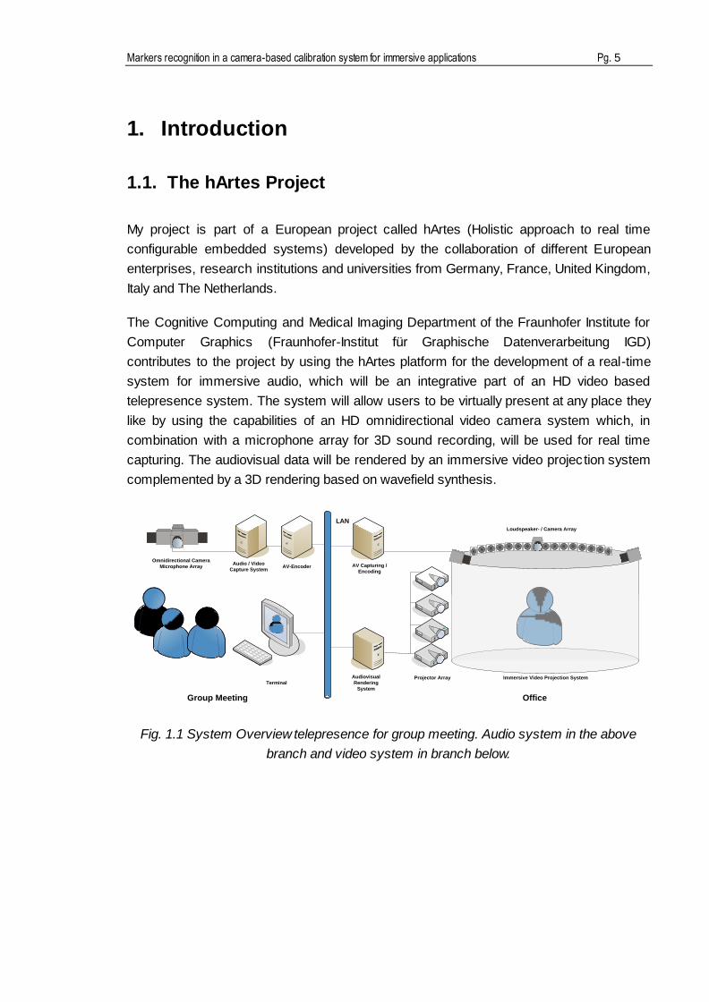
Fig. 1.1 System Overview telepresence for group meeting. Audio system in the above
branch and video system in branch below.

Pg. 6 Report
The telepresence approach reached by Fraunhofer is designed as an immersive platform
combining high definition 360 degrees video recording and playback with 3D audio using
the possibilities of parallel signal processing and audiovisual array technology as shown in
Fig. 1.1. A microphone array records the sounds that will be reproduced inside the
immersive environment (where the user is) thanks to loudspeakers and the visual
rendering system provides images to projector array which projects image onto the
cylindrical surface of the immersive platform. Its scalable camera system exploits the
potential of common graphics hardware for real time stitching and transmission of ultra
high definition video panoramas providing resolutions far beyond actual HD video
technology. Its immersive video projection environment gives users the impression of
being virtually present at any location at any time.
The system could be used for a range of applications including:
High end video-conferencing
Live broadcasting of sport events, theatre and music events.
Interactive multimedia presentations
360 degrees cinema, theatres or concerts
immersive gaming
My project is a contribution to the calibration of a projectors array and camera-based
system by analyzing features of markers through image processing techniques.
1.2. hArtes Scenario and Objectives of IGD
In this point the elements forming the scenario of the immersive platform and the
objectives of our project are described.
Scenario of the hArtes Project
Fig. 1.2 shows the scenario built by Fraunhofer institute in Darmstadt for the development
of different projects and studies dealing with hArtes project.

Markers recognition in a camera-based calibration system for immersive applications Pg. 7
Fig. 1.2 Room of IGD where the immersive scenario is placed
In the room of our work we can find a central cylindrical surface surrounded by eight
projectors and cameras fixed to this central structure and separated 45 degrees from each
other. The cameras are fixed above the projectors (in the same vertical structure) to
record what on the cylindrical structure is projected. There is also a group of loudspeakers
and microphones covering the inside surface of the cylinder as can be seen in Fig. 1.3.
Fig. 1.3 Loudspeakers can be seen from above inside the cylindrical structure
With the description of the scenario the two differentiated parts of study can be easily
seen; one is dealing with audio and the other one dealing with video. By combining these
two systems, the immersive impression pursued by hArtes can be reached and all the
applications described in Section 1.1 can be implemented.
In our particular case we are interested in video branch of the system described.
Objectives of IGD in hArtes
Once we know the scenario we are prepared to face the situation.

Pg. 8 Report
The projectors, fixed to the central cylindrical structure, project an image onto the
cylindrical surface. This images projected are coming from a computer and can be single
images or videos (already saved in the computer or real time recorded by a
omnidirectional system of video cameras as shown in Fig. 1.4 below).
Fig. 1.4 Omnidirectional camera system
There are eight projectors surrounding the 360 degrees panorama covering each of them
an angle of 45 degrees. The objective of hArtes project is that, if a user projects an image
or video through the eight projectors onto the cylindrical surface and a user is inside the
cylindrical structure he has the impression of being in the scene projected. That means
that, as a user is inside the structure he sees a scenario, decided depending on the
application (it can be a computer game, a concert, a museum….), in which he is evolved
as it reality was (immersion).
In practice, this theoretical strategy presents some problems in the projection.
Human sight is very sensitive to continuity, colour and brightness changes in image. So if
we project a video (real time or recorded) and someone, who is inside the structure, finds
a change (continuity, colour and brightness) in the junction between projections coming
from neighbouring projectors the immersive sensation is lost. (see Fig. 1.5)
Fig. 1.5 Junction between two consecutive projections projected on a non planar surface

Markers recognition in a camera-based calibration system for immersive applications Pg. 9
So one objective of IGD in the context of hArtes project is to correct those misalignments
or overlapping in the junctions between projections so the changes are not noticeable for
the person who is inside.
Proposal of a solution
Once we know which the problem is, we have to propose a solution.
We wanted to apply the necessary corrections in the calibration system in order to obtain
unnoticeable variations between consecutive projections and that can be done at the same
time image is projected or a priori, so at this point we came across a question which would
determine the direction of our project.
What is better, to make a continuous calibration of the system as it works or a pre-
calibration of the system and then running the application desired?
We analyse the possibility of working in real time or not. After some readings we decided
that real time was not a necessary condition. The decision was taken considering the
features of the system and the complexity of algorithm execution. On one hand, the
system is designed to be in a fixed place (non-portable) so once calibrated it will maintain
its features for a certain period of time and the process can be done once a week, a
month, a year... what user decides to ensure the calibration of the system. On the other
hand, if the algorithm has to be runned on real time, the number of parameters (extrinsic
and intrinsic) to consider and operations required have to be as simple and fast as
possible to allow real time execution. This fact increases the difficulty of the
implementation of the algorithm. If we do not consider real time we can make all operations
we consider necessary to provide an accurate system for markers extraction.
So the solution we chose was to make a pre-calibration of the system which can be
reached by working directly with the projections recorded by the camera placed above the
projectors and facing the problem as an image processing problem.
To reach the objective we have brought up the global solution described in Fig. 1.6.

Pg. 10 Report
Fig. 1.6 Block diagram of our proposal of solution for avoiding misalignments and
discontinuities between consecutive projections
First of all, the proposed strategy is to create a grid, an ideal grid, consisting on 9 black
squares with a small white hole in the middle, which will be our reference for the whole
process. From now on, in this report, these squares are called markers.
Secondly the image formed by all markers will be projected onto cylindrical surface see
Fig. 1.7.
Markers Detection and
Extraction
Comparing ideal markers with
real ones
Correction of the misalignment
(Calibration)
Working with overlappings
areas and junctions

Markers recognition in a camera-based calibration system for immersive applications Pg. 11
Fig. 1.7 Up: image created by us to become our reference image (grid) for calibration.
Down: projection of our grid onto the cylindrical surface. As can be seen the contours and
markers appeared deformed due to projection onto a non planar surface.
As the surface on which we are projecting is not planar, the ideal markers appeared in
different positions and orientations in the projected image and with some of their form-
features modified as described in Section 2.4. Depending on the distance and orientation
of each projector (although all the system is metrical built there can be some errors)
markers can appear in very different positions and deformed so it makes it necessary to
identify where are the markers, comparing this position to the ideal and then correcting the

Pg. 12 Report
misalignment between them. In order to determine which is the correct position we have
some external markers forming part of the structure. These markers are different from
internal ones described above; they are four circles fixed in a specific distance to the
structure and they are also affected by projective and affine features as well as in internal
case. Once detected those external markers we will have four fixed points perfectly
identified and which should be always in the same well-known place so they are a very
good reference to correct the position of projector by adjusting the distances between ideal
external and internal markers.
Once calibrated the problems remaining in the overlapping areas and junctions should be
corrected to give a total immersive appreciation.
1.3. The Objective of my Project
My objective inside hArtes, and as a result my project, is the first point in the global solution
shown in Fig. 1.6, markers detection and extraction (see Fig. 1.8)
Fig. 1.8 Our objective in hArtes project
My project consists in the development of an application (GUI) in C++ language capable of
determine univocally which of the parts in the image are the markers desired and reject the
areas undesired in the image. By applying image processing functions and
transformations we come across markers detection and extraction.
The objective of my project is to develop an application in C++ language to univocally
determine which regions in the image captured from the camera (image projected by
projectors onto the cylindrical surface) are markers and which ones not through
techniques of image processing.
In our project we come across different problems.
Light conditions: The image captured by the camera is not uniformly illuminated.
The light is not equally applied in each part of the scene and can vary depending on
the room or space where the system is placed or the focus light used. Depending
on the focus light we will find shadows which can difficult and also cause wrong
detections in the univocal determination of the markers in the image
Markers Detection and
Extraction

Markers recognition in a camera-based calibration system for immersive applications Pg. 13
Markers form: As introduced in Proposal of solution (Section 1.2) our markers
detector should be able to detect between two forms of markers; internal markers,
which are black squares with a hole in the middle; and external markers which are
orange circles with a black hole in the middle. The techniques of image processing
used to determine squares and circles are different. So the application has to be
able to detect both of them.
Perspective and affine problems: When we project internal and external markers in
the borders they become rectangles and ellipses, due to the surface‟s form. These
two features are important, so we are not only looking for squares and circles but
also rectangles and ellipses.
Taking all these points into account we have implemented a GUI in C++ language to work
with images through image processing techniques.
In what follows, in Sections 2.2, 2.3 and 2.4, segmentation, shape classification and object
recognition techniques are explained. As pre-processing techniques preceding the
classification process can greatly enhance recognition accuracy, we have included in our
system a first pre-processing step explained in Section 2.1. Thereafter, once we know the
techniques available, in Section 3 we discuss the suitable methods and techniques which
will give better solutions for our application.
In Section 4, are described the tools needed for the implementation and the details of the
application developed. Finally, the results of our GUI application are shown in Section 5.

Pg. 14 Report
2. State of the Art
The structure of this state of the Art follows the scheme shown below.
Fig. 2.1 Image processing chain used in our project
The starting point is an image obtained by camera; we apply pre-processing,
segmentation, shape classification and object recognition techniques as image processing
chain for recognizing markers. We obtain an image containing the markers we want to
extract.
The methods and techniques of each step are exposed as follows and the selection of the
better solution in our case is discussed in further Sections.
2.1. Image pre-processing
The use of pre-processing techniques preceding image processing chain can greatly
enhance recognition accuracy.
The best processing is no processing at all. If image acquisition has high quality this step
is not necessary except if what is searched is to suppress information of no relevant areas
in order to make easier the image processing or analysis. If image acquisition has low or
middle quality this step becomes useful in order to suppress undesired distortions.
There are different pre-processing techniques that can be applied to an image to improve it
before processing. In this memory are explained only explained those applied in our project
which are pixel brightness transformation and local pre-processing.
Pixel brightness transformation: Gray-scale transformation
The aim of brightness transformation is to modify pixel brightness depending on the
characteristics of each pixel.

Markers recognition in a camera-based calibration system for immersive applications Pg. 15
The process of gray-scale transformation consists in taking the image brightness and,
through a look-up-table (LUT), change it into a new image brightness in real time for
displaying. The result of the transformation is a gray-scale digital image in which the value
of each pixel is a single sample carrying all the information of brightness. The gray-scale
images intended for visual display (screen and printed) are commonly stored with 8 bits
per sampled pixel, which allows 256 different intensities to be recorded, going from black
to white and having different gray intensities (shades of gray).
Local pre-processing
The aim of the local pre-processing is filtering for enhancement details (the high spatial
frequency components), so this technique will provide a more detailed image than the
original, obtaining an improved image to our purpose. The trick with “local” contrast
enhancement is that it increases local contrast in smaller regions, while at the same time
preventing an increase in “global” contrast, thereby protecting large-scale shadow/highlight
detail.
As a spatial filtering it works with the direct manipulation of the pixels using a small
neighbourhood of the pixel in the gray-scale image to produce a new brightness value in
the output image. This contrast enhancement can be achieved by a sharpening operator,
based on derivatives of the image function.
First order operators (using first derivative measurements) are particularly good at finding
edges in images as for example Sobel and Roberts edge enhancement operators.
Laplacian is a second derivative method of enhancement. It is particularly good at finding
detail in images.
The strength of the response of a derivative operator is proportional to the degree of
discontinuity of the image at the point at which the operator is applied. Thus, image
differentiation enhances edges and other discontinuities (such as noise) and
deemphasizes areas with slowly varying gray-level values.
Sharpening operator has the objective of making edges steeper. We can obtain sharpened
output image ( , )sh i j as:
( , ) ( , ) ( , )sh i j f i j k L i j
where ( , )f i j corresponds to original image and the constant k gives the strength of
sharpening where ( , )L i j is a measure of the image function sheerness, calculated using
Laplacian.

Pg. 16 Report
Another way of writing the sharpening expression should be in terms of matrix:
Sharpened image =
where α is a value between 0 and 1 and controls the shape of the Laplacian.
A graphical sharpening example is shown in Fig. 2.2.
Fig. 2.2 Up: original image, sharpening filter and result. Down: application to the filter to an
image where details are enhanced and the rest smoothed. (slides by Bernt Schiele from
TU-Darmstadt)
Differences are accentuated and constant areas are left unchanged. Also noise is
accentuated.
2.2. Segmentation
Segmentation is the process of dividing a digital image into different regions. Each region
is formed by a set of pixels with similar characteristics such colour, intensity or pattern.
The whole image is covered by regions and adjacent regions have different features.
The goal of segmentation is to simplify the information or change the representation into
something meaningful and easier to analyze.
0 0 0 1 11 1
0 1 0 1 4 1 1 5 11 1
0 0 0 1 1

Markers recognition in a camera-based calibration system for immersive applications Pg. 17
In image processing there are many algorithms and techniques developed for image
segmentation: clustering, histogram based, edge detection, region growing, level set,
graph partitioning, model based, multi-scale and watershed transformation.
The simplest method of image segmentation is Thresholding. Sezgin and Sankur in [6]
classified thresholding methods into groups depending on the information the algorithm
manipulates:
Histogram shape based methods: it analyzes peaks, valleys and curvatures of a
smoothed histogram
Clustering based methods: gray-level samples are clustered in two parts to
separate background from foreground (object of interest). In other cases they are
modelled as a mixture of two Gaussians
Entropy based methods: uses entropy of foreground and background regions, the
cross-entropy between the original and binarized image...
Object attribute based methods: searches similarity between the gray-level image
and the binarized one (shape similarity, edge coincidence…)
Spatial methods: uses probability distribution or correlation between pixels
Local methods: adapt the threshold value on each pixel to local image
characteristics.
The goal of all these techniques is to determine a value called threshold and comparing
each pixel on the image with this value. If the value of the pixel is greater than the
threshold, its value becomes 1 (white), otherwise it becomes 0 (black). That method
assumes that the objects are brighter than the background. For that reason white or bright
pixels are supposed to be an object and black or dark ones background.
The aim of this thresholding is to change the pre-filtered greyscale image into a binary
image, so the process is used as binarization as explained in [7] and shown in Fig. 2.3.
Pg. 18 Report
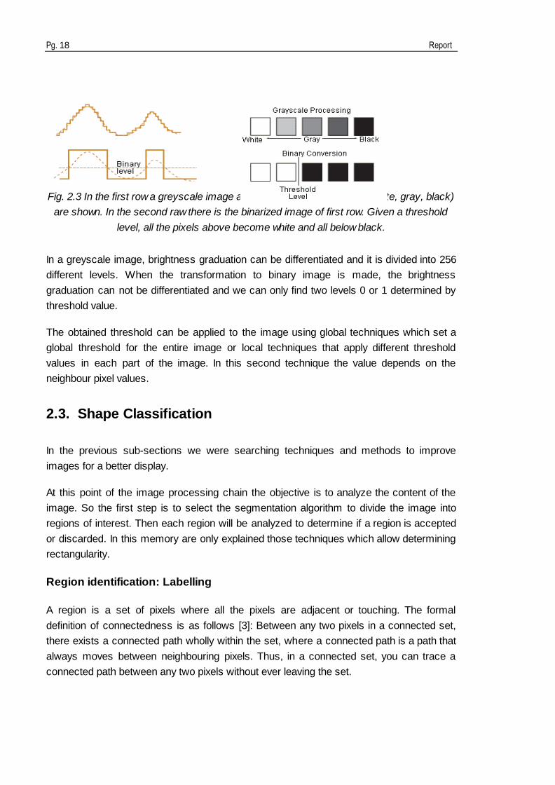
Fig. 2.3 In the first row a greyscale image and its different colour levels (white, gray, black)
are shown. In the second raw there is the binarized image of first row. Given a threshold
level, all the pixels above become white and all below black.
In a greyscale image, brightness graduation can be differentiated and it is divided into 256
different levels. When the transformation to binary image is made, the brightness
graduation can not be differentiated and we can only find two levels 0 or 1 determined by
threshold value.
The obtained threshold can be applied to the image using global techniques which set a
global threshold for the entire image or local techniques that apply different threshold
values in each part of the image. In this second technique the value depends on the
neighbour pixel values.
2.3. Shape Classification
In the previous sub-sections we were searching techniques and methods to improve
images for a better display.
At this point of the image processing chain the objective is to analyze the content of the
image. So the first step is to select the segmentation algorithm to divide the image into
regions of interest. Then each region will be analyzed to determine if a region is accepted
or discarded. In this memory are only explained those techniques which allow determining
rectangularity.
Region identification: Labelling
A region is a set of pixels where all the pixels are adjacent or touching. The formal
definition of connectedness is as follows [3]: Between any two pixels in a connected set,
there exists a connected path wholly within the set, where a connected path is a path that
always moves between neighbouring pixels. Thus, in a connected set, you can trace a
connected path between any two pixels without ever leaving the set.

Markers recognition in a camera-based calibration system for immersive applications Pg. 19
There are 2 kind of connectivity, 4 and 8 connectivity, depending on how many neighbours
are used to calculate it. They can be seen in Fig. 2.4 where actual pixel corresponds to
blue one.
(i-1,j-1) (i-1,j) (i-1,j+1)
(i,j-1) (i,j) (i,j+1)
(i+1,j-1) (i+1,j) (i+1,j+1)
Fig. 2.4 4-connectivity corresponds to yellow pixels; 8-connectivity to yellow and orange
pixels
In computing, as we run the image normally from the left-up corner (first pixel) to the right-
down (last one), we consider connectivity in terms shown in Fig. 2.5 because the rest of
pixels are not read when we are computing actual pixel (in blue).
Fig. 2.5 Left: In computing 4-connectivity;Right: in computing 8-connectivity
Region based- shape representation and description
The use of descriptors becomes very useful in shape description. In general, descriptors
are some set of numbers which describe a given shape. The shape may not be entirely
reconstructable from the descriptors but the descriptors for different shapes could be
different enough so the shapes can be discriminated.
A good descriptor is that with the greater the difference in significantly different shapes and
the lesser the difference for similar shapes. Descriptors work in a qualitative way so they
attempt to quantify shape so the human intuition does not perceive the difference between
real and descript.
Simple scalar region descriptors

Pg. 20 Report
A large group of shape description techniques are represented by heuristic approaches
which yield acceptable results in description of simple shapes. Some heuristic region
descriptors are: area, perimeter, (non)compactness, (non)circularity, eccentricity,
elongatedness, rectangularity, orientation (direction)...
These descriptors cannot be used for region reconstruction and do not work for more
complex shapes.
Moments
Moments describe numeric quantities at some distance from a reference point or axis.
They are commonly used in statistics to characterize the distribution of random variables.
The use of moments for image analysis is straightforward if we consider a binary image as
a two dimensional density distribution function. In this way, moments may be used to
characterize an image segment and extract properties that have analogies in statistics.
Considering image size MxN and i and j image coordinates, different order moments and
parameters related with them can be defined.
First order moments:
Centroids:
10
00
cm
xm
01
00
cm
ym
Central moments: translation invariance
Markers recognition in a camera-based calibration system for immersive applications Pg. 21
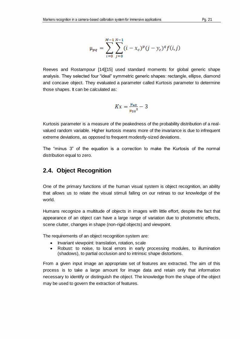
Reeves and Rostampour [14][15] used standard moments for global generic shape
analysis. They selected four “ideal” symmetric generic shapes: rectangle, ellipse, diamond
and concave object. They evaluated a parameter called Kurtosis parameter to determine
those shapes. It can be calculated as:
Kurtosis parameter is a measure of the peakedness of the probability distribution of a real-
valued random variable. Higher kurtosis means more of the invariance is due to infrequent
extreme deviations, as opposed to frequent modestly-sized deviations.
The “minus 3” of the equation is a correction to make the Kurtosis of the normal
distribution equal to zero.
2.4. Object Recognition
One of the primary functions of the human visual system is object recognition, an ability
that allows us to relate the visual stimuli falling on our retinas to our knowledge of the
world.
Humans recognize a multitude of objects in images with little effort, despite the fact that
appearance of an object can have a large range of variation due to photometric effects,
scene clutter, changes in shape (non-rigid objects) and viewpoint.
The requirements of an object recognition system are:
Invariant viewpoint: translation, rotation, scale
Robust: to noise, to local errors in early processing modules, to illumination (shadows), to partial occlusion and to intrinsic shape distortions.
From a given input image an appropriate set of features are extracted. The aim of this
process is to take a large amount for image data and retain only that information
necessary to identify or distinguish the object. The knowledge from the shape of the object
may be used to govern the extraction of features.

Pg. 22 Report
A matching algorithm (SIFT) will compare the ideal object with the object in the image and
with the help of the extracted features it will determine if the object of the image
corresponds to one of the searched objects or not.
Invariance: Local features
Invariants are properties which remain unchanged under an appropriate class of
transforms [20]. To accomplish the requirement of invariance of our object recognition
system we have to study all the invariant transformations that we can apply to our image to
obtain an invariant viewpoint. That means that the object can be identified either it is
smaller/bigger than the model, or it is rotated, or translated…
Following 5 effects of different transformations applied to a rectangle using Geometric
transformation invariants can be seen:
1. Translation
Fig. 2.6 Rectangle is moved to another position (translated) remaining invariant: length,
angle, length ratio and parallel lines.
If we have the original image coordinates (x,y) the general equations to a translation in 2D
coordinates are:
x‟=x + tx =1·x + 0·y + tx ·1

Markers recognition in a camera-based calibration system for immersive applications Pg. 23
y‟=y + ty =0·x + 1·y + ty ·1
Equations can be easily determined if we take a look to Fig. 2.6. The homogeneous
coordinates can be expressed in matricial notation: X=X’+t
The invariants are length, angle, length ratio and parallel lines.
2. Rotation
Fig. 2.7 Rectangle is rotated respect a point remaining invariant: length, angle, length ratio
and parallel lines
The equations which describe the rotation feature in 2D that can be seen in Fig. 2.7.
x‟=cos (α)·x+ sin (α)·y+tx
y‟=-sin (α)·x+ cos (α)·y+ty
These equations can be expressed in homogeneous coordinates as:
' 1 0
' 0 1
1 0 0 1 1
x
y
x t x
y t x y
' cos( ) sin( )
' sin( ) cos( )
1 0 0 1 1
x
y
x t x
y t x y

Pg. 24 Report
The invariants here are length, angle, length ratio and parallel lines.
3. Similarity
Fig. 2.8 Rectangle is smaller or bigger but relation between sides remain invariable
The equations to describe this movement are:
x‟=s·x + 0·y + tx ·1
y‟=0·x + s·y + ty ·1
In matrix notation x‟=S·x+t
4. Affine
The movement of the rectangle is shown in Fig. 2.9
' 0
' 0
1 0 0 1 1
x
y
x s t x
y s t x y

Markers recognition in a camera-based calibration system for immersive applications Pg. 25
Fig. 2.9 Red rectangles are invariant to length, angle, length ratio and parallelism. Our
interest rectangle (green one) is only invariant to parallelism
The equations to express this movement are:
x‟=cos (α1)·sx·x+ sin (α1)·sy·y+tx
y‟=-sin(α1)·sx·x+ cos (α1)·sy·y+tx
In matricial x‟=S·R(α1)·x
When we apply the movement described in Fig. 2.9 to green rectangle no length, no angle
and no length ratio are invariant, only parallelism.
Fig. 2.10 helps us to define relationships between original rectangle and the one moved.
Fig. 2.10 Expression of variables involved in this movement
2 2 1 1
2 1
2 2 1 1
cos( ) sin( ) 0 cos( ) sin( )( )· · ( ) · ·
sin( ) cos( ) 0 sin( ) cos( )
sxR S R
sy
The general expression in matrix notation:
x‟= R2·S·R1·x + t

Pg. 26 Report
2 1
'( )· · ( )
' ·0 0
1 1 1
x
y
x t xR S R
y t y
5. Projective
Fig. 2.11 Rectangle is not invariant to length, angle, length ratio and parallelism
With the transformation of Fig. 2.11 length, angle, length ratio and parallelism are not
invariant.
That can be expressed in homogeneous coordinates as:
and in image coordinates:
All these features described above can be local or global features. We are looking for local
features because global fail in image transformations (scale change), in occlusions and
background clutter (segmentation-hard), in colour (light changes) and in geometric
(contour based fail if no shape).
The key properties of a good local feature are:
11 12 13
21 22 23
31 32
'
' ·
' 1 1
x h h h x
y h h h y
z h h
'' '1
'' · ''
1 '
x x
y yz
z

Markers recognition in a camera-based calibration system for immersive applications Pg. 27
Must be highly distinctive, a good feature should allow for correct object
identification with low probability of mismatch
Should be easy to extract
Invariance, a good local feature should be tolerant to: image noise, changes in
illumination, uniform scaling, rotation and minor changes in viewing direction.
Should be easy to match against a database of local features.
Detector + Descriptor: SIFT
The local features become the interesting points on the object (marker) and they can be
extracted to provide a feature description of the object. These interesting points can be
used to identify the object when there is an image containing the object we are looking for
and many other objects. That is the reason why it is important that the set of features
extracted is robust to changes in image scale, noise, illumination and local geometric
distortion, for performing reliable recognition.
The ideal interest points/regions are those which are numerous repeatable, representative
in orientation/scale and fast to extract and match (as shown in Fig. 2.12).
Fig. 2.12 Interest points in the image on the left are matched with the same points on the
right although they are not in the same image position (M. Brown and D. G. Lowe.
Recognising Panoramas. In Proceedings of the International Conference on Computer
Vision (ICCV2003)
There is a patented algorithm developed by Lowe [16] [18] that can robustly identify objects
even among clutter and under partial occlusion called SIFT. The name comes from Scale
Invariance Feature Transform and is a good approach for detecting and extracting local
feature descriptors that are reasonably invariant to changes in illumination, image noise,
rotation, scaling and small changes in viewpoint.

Pg. 28 Report
There are other newer feature detectors as SURF (Speeded Up Robust Features)[23]. As
shown in the study [24] SURF descriptor is better than SIFT at matching computing time
but worse at match ratio and total number of correct matches as well as the quality and
total number of the created keypoints.
There are also works in which the behaviour of SURF to affine transformations is not as
good as SIFT [26].
Fig. 2.13 Four Stages of SIFT algorithm divided in two blocks, detector and descriptor
SIFT can be divided into 2 blocks: Detection and Description. Altogether has 4 stages
shown in Fig. 2.13
1st Step: Find Scale-Space Extrema: it searches over all scales and image locations. It is
implemented by using a difference-of Gaussian function to identify potential interest points
that are invariant to scale and orientation.
2nd Step: Keypoint Localization and Filtering: at each candidate location a detailed model is
fit it determine location and scale. Keypoints are selected based on measures of their
stability and this way improve keypoints and throw out bad ones.
3rd Step: Orientation assignment: removing effects of rotation and scale: On each point 1
or more orientation based on local image gradient directions are assigned.
4th Step: Create keypoint descriptor: (using histograms of orientation) The local image
gradients are measured at the selected scale in the region around each keypoint. These
are transformed into a representation that allows for significant levels of local shape
distortion and change in illumination.
As follows each step for the understanding of SIFT algorithm is widely explained.
1st Step: Detection of scale-space Extrema
Koenderink (1984) and Lindeberg (1994) show that under a variety of reasonable
assumptions the only scale-space kernel is the Gaussian function.

Markers recognition in a camera-based calibration system for immersive applications Pg. 29
The scale-space is described as a continuous function of scale σ: L(x, y, σ), the result of
the convolution between a variable-scale Gaussian G(x, y, σ) and the input image
(resulting image from segmentation) where:
Experimentally, Maxima and minima of Laplacian-of-Gaussian gives best notion of scale
([21]) producing the most stable image features compared to another image functions
such as the gradient, Hessian or Harris corner function. Thus using Laplacian-of-Gaussian
(LoG) operator:
LoG is expensive to calculate so with the help of heat diffusion equation, the definition of
Difference-of-Gaussians (DoG) and parameterized in terms of σ rather than the more
usual t=σ2:
can be computed from the finite difference approximation to using the
difference of nearby scales at kσ and σ:
The efficiency of DoG is based in a simple operation, subtraction of two images.
Therefore, isolating difference of Gaussian:
That shows that when difference of Gaussians (DoG) function has scales differing by a
constant factor it already incorporates the σ2 scale normalization required for the scale-
invariant Laplacian. The factor (k-1) in the equation is a constant over all scales and

Pg. 30 Report
therefore does not influence in extrema location. The approximation of the error will go to 0
as k goes to 1, but in practice Lowe study has almost no impact on the stability of extrema
detection of localization for even significant differences in scale such as k= 2 .
So in conclusion what is done is to construct a scale-space like shown in Fig. 2.14
Fig. 2.14 Scale Space of DoG
For each octave of scale space the initial image is repeatedly convolved with Gaussians to
produce the set of scale space images separated by a constant k. Each octave is then
divided into intervals s so k=21/s. We must procedure s+3 images in the stack of blurred
images for each octave so that final extrema detection covers a complete octave.
Adjacent Gaussians images are subtracted to produce the difference of Gaussian images.
Fig. 2.15 shows the computing of DoG.
After each octave the Gaussian image is down sampled by a factor of 2 and the process is
repeated.

Markers recognition in a camera-based calibration system for immersive applications Pg. 31
Fig. 2.15 Difference of Gaussians are computed. For each octave there are s intervals so
k=21/s, s+3 Gaussian must be processed. σ doubles for the next octave.
All extrema (maxima and minima of the DoG) within 3x3 neighbourhood are chosen so that
the pixel marked with X is compared to its 26 neighbours at the current and adjacent
scales (see Fig. 2.16)
It is selected as maxima only if it is larger than all of the neighbours or minima if it is
smaller than all of them.
The cost of this check is reasonably low due to the fact that most sample points will be
eliminated following the first few checks.

Pg. 32 Report
Fig. 2.16 Maxima and minima of DoG images are detected by comparing the pixel marked
as X to its 26 neighbours in 3x3 regions at the current and adjacent scales (marked with
circles)
2nd Step: Keypoint Localization & Filtering
In this section for each candidate keypoint is needed:
Interpolation of nearby data is use to accurately determine its position
Keypoints with low contrast are remove
Responses along edges are eliminated
The keypoint is assigned an orientation
After scale space extrema (keypoint candidates) are detected by comparing a pixel to its
neighbour, the next step is to perform a detail fit to the nearby data for location, scale and
ratio of principal curvatures. This information allows that points, with low contrast (and
therefore sensitive to noise) and poorly localized along the edge, are rejected.
The initial approach of Lowe [16] searched to locate each keypoint at he location and scale
of the central sample point. With the new approach [19] the interpolated location of the
maximum is calculated. This fact improves matching and stability.
The interpolation is done using Taylor expansion series (up to the quadratic terms) of the
Difference-of-Gaussian scale space function D(x,y,σ). It is shifted so that the origin is at
the sample point:

Markers recognition in a camera-based calibration system for immersive applications Pg. 33
D and derivatives are evaluated at the sample point and the offset from this point
x=(x,y,σ)T.
The location of extrema, xM, is determined by taking the derivative of this function with
respect to x and setting it to zero, giving:
If the offset xM is larger than 0,5 in any dimension , indicates that the extrema lies closer to
another candidate keypoint. In this case, the candidate keypoint is changed and the
interpolation performed instead about that point. Otherwise the offset is added to its
candidate keypoint to get the interpolated estimate for the location of the extrema.
To reject unstable extrema with low contrast the value of the second order Taylor
expansion is computed at the offset xM.
If this value is less than 0.03 (assuming image pixel values in the range [0, 1]), the
candidate keypoint is discarded. Otherwise is kept, with final location y+ xM and scale σ,
where y is the original location of the keypoint at the scale σ.
For stability is not sufficient to reject keypoints with low contrast. The DoG function will
have strong response along edges, even if the candidate keypoint is poorly determined and
therefore unstable to small amounts of noise. A poorly defined peak in DoG will have a
large principal curvature across the edge but a small one in the perpendicular direction,
that means that we want to reject points with strong edge response in one direction only.
The principal curvatures can be computed from 2x2 Hessian matrix at the location and
scale of the keypoint:
The eigenvalues of H are proportional to the principal curvatures of D. Borrowing from the
approach used by Harris and Stephens (1988)[25] we can avoid explicitly computing the
eigenvalues, as we are only concerned with their ratios. It turns out that the ratio r=α/β of
Dxx DxyH
Dxy Dyy

Pg. 34 Report
the two eigenvalues, where α is the larger one and β the smaller one is sufficient for SIFT
purposes.
In the unlikely event that the determinant is negative the curvatures have different signs so
the point is discarded as not being an extrema.
Then,
which depends only on the ratio of the eigenvalues rather than the individual values. R is
minimum when the eigenvalues are equal to each other. Therefore the higher the absolute
difference between the two eigenvalues, which is equivalent to a higher absolute difference
between the two principal curvatures of D, the higher the value of R.
For some threshold eigenvalues ratio rth, if R for a candidate keypoint is larger than
that keypoint is poorly localized and hence rejected. In Lowe 2004 this value
rth=10 and it is efficient to compute with less than 20 floating point operations to test each
keypoint.
3rd Step: Orientation assignment: removing effects of rotation and scale
The last step done by detector is to determine the keypoint orientation based on local
image gradient directions and this way achieving invariance to rotation. A gradient
orientation histogram is computed in the neighbourhood of the keypoint, using Gaussian
smoothed image at the closest scale to the keypoint‟s scale, L(x, y, σ), so all
computations are performed in a scale-invariant manner. Gradient magnitude and
orientation are pre-computed using pixel finite differences:

Markers recognition in a camera-based calibration system for immersive applications Pg. 35
The magnitude and direction calculations for the gradient are done fore every pixel in a
neighbouring region around the keypoint in the Gaussian smoothed image L. An orientation
histogram is formed with 36 bins covering each of them 10 degrees. Each sample in the
neighbouring window added to the histogram bin is weighted by its gradient magnitude an
by a Gaussian-weighted circular window with a σ that is 1,5 times the scale of the
keypoint, that shows Fig. 2.17.
Fig. 2.17 Creation of gradient histogram (36 bins). Weighted by magnitude and Gaussian
window (overlaid circle) with σ 1,5 times the scale of the keypoint
Peaks in the histogram correspond to dominant directions of local gradients. The highest
peak in the histogram is detected, and then any other local peak is within 80% of the
highest peak is used to also create a keypoint with that orientation. Therefore, for locations
with multiple peaks of similar magnitude, there will be multiple keypoints created at the
same location and scale but different orientations.
Only about 15% of points are assigned multiple orientations, but these contribute
significantly to the stability of matching. Finally, a parabola is fit the 3 histogram values
closest to each peak to interpolate the peak position for better accuracy.
As all the properties of the keypoints are measured relative to the keypoint orientation, we
ensure it provides invariance to rotation.
4th Step: Descriptor
Previous steps found keypoint locations at particular scales and assigned orientations to
them. This ensured invariance to image location, scale and rotation. Now we want to

Pg. 36 Report
compute descriptor vectors for these keypoints such that the descriptors are highly
distinctive and partially invariant to the remaining variations, like illumination, 3D viewpoint,
etc. This step is pretty similar to the 3rd Step: Orientation Assignment.
Fig. 2.18 Histogram of 4x4 samples per window in 8 directions with Gaussian weighted
around centre. So we have a dimensional feature vector of 128 for each point (4x4x8)
The keypoint descriptor is created by fist computing the gradient magnitude and orientation
at each image sample point in a region around the keypoint location using the scale of the
keypoint to select the level of Gaussian blur for the image. In order to achieve orientation
invariance, the coordinates of the descriptor and the gradient orientations are rotated
relative to the keypoint orientation. Gradients are illustrated with small arrows at each
sample location. The region is formed by a 16x16 set of samples. These are weighted by a
Gaussian window (with σ equal to 0,5 times the width of the descriptor window) indicated
by the overlaid circle. The purpose of this Gaussian window is to avoid sudden changes in
the descriptor with small changes in the position of the window, and to give less emphasis
to gradients that are far from the centre of the descriptor, as these are most affected by
misregistration errors. These samples are then accumulated into orientation histograms
summarizing the contents over 4x4 sub-regions with the length of each arrow
corresponding to the sum of the gradient magnitudes near that direction within the region.
So histograms contain 8 bins each, and each descriptor contains a 4x4 array of 16
histograms around the keypoint. This leads to a SIFT feature vector with 4 x 4 x 8 = 128
elements.
It is also important to avoid all boundary effects in which the descriptor abruptly changes
as a sample shifts smoothly from being within one histogram to another of one orientation
to another. Therefore, trilinear interpolation is used to distribute the value of each gradient
sample into adjacent histogram bins, that means that each entry into a bin is multiplied by
a weight of d-1 for each dimension, where d is the sample from the central value of the bin
as measured in units of the histogram bin spacing.

Markers recognition in a camera-based calibration system for immersive applications Pg. 37
Finally the feature vector is modified to reduce effects of illumination changes. First, the
vector is normalized to unit length. A change in image contrast in which each pixel value is
multiplied by a constant will multiply gradients by the same constant, so this contrast
change will be cancelled by vector normalization. A brightness change in with a constant is
added to each image pixel will not affect the gain of the gradient values. Therefore the
descriptor is invariant to affine changes in illumination.
Although the dimension of the descriptor (128) seems high, descriptors with lower
dimension than this do not perform as well across the range of matching tasks, [18].
The performance of SIFT descriptor is the best descriptor (together with GLOH, an
extension of the SIFT descriptor designed to increase its robustness and distinctiveness))
as it explains the extensive survey of Mikolajczyk & Schmid [21].
The typical usage of SIFT for a set of database images is firstly to compute SIFT features
and then save descriptors to database; for a query image firstly compute SIFT features,
then for each descriptor find the closest descriptors (Euclidean distance) in database and
finally verify matches (geometry and Hough transform).
Given SIFT's ability to find distinctive keypoints that are invariant to location, scale and
rotation, and robust to affine transformations (changes in scale, rotation, shear, and
position) and changes in illumination, they are usable for object recognition

Pg. 38 Report
3. Our contribution
Our goal is to recognize objects (where objects are our markers) in image. To identify
them there are necessary some previous steps to prepare digital image to apply shape
and object recognition techniques and, this way, distinguish desired areas from not desired
ones (described in Sections 2.3 and 2.4) and extract those of our interest.
During all this section we explain which of the terms and methods described in Section 2
will be applied in our project in order to reach the objective raised of extracting markers
from image. All the techniques described are thought to be implemented in a C++
application which will be explained more widely in Section 4.
First of all, what we are looking for is a photo (image) in which we can differentiate bright
from dark regions to distinguish our markers from the parts of the cylindrical structure.
Colour in image is not as important as the distinctiveness of the markers (internal and
external part) from the rest of picture taken, and, as we want to work with images along the
whole image processing chain, size of image (in terms of bytes) is also very important.
The biggest the image is, the more complicated the operations are.
At this point it is also remarkable the fact that we have a video camera but we are going to
use it as a photocamera as explained in Proposal of solution (Section 1) where the
question of calibration in real time is discussed.
So altogether, a good solution in our case is to take a gray-scale image. That is the result
of a gray-scale transformation in which pixel brightness of each pixel is changed without
regarding to its position in the image. It is described in Section 2.1 as pre-processing step
and it is done by the software provided by the camera provider (uEye Setup Version 3.1,
www.ids-imaging.com) which allows us choosing the pixel colour depth that we desire in
our capture from camera recording in real time.
This high quality gray-scale image taken by the camera as described in Appendix C is our
testimage (testimage.bmp), the starting point of our study and analysis. It is shown in Fig.
3.1., its original size is 2048x 1536 and the format is bmp (bitmap).
Markers recognition in a camera-based calibration system for immersive applications Pg. 39
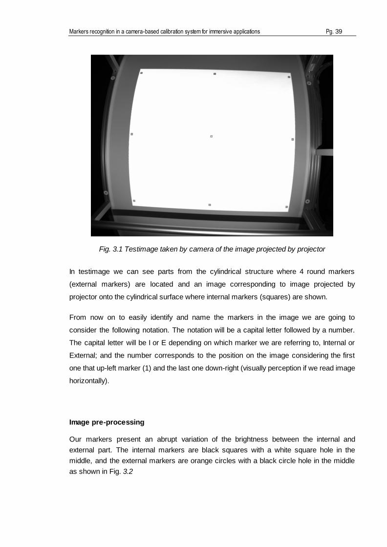
Fig. 3.1 Testimage taken by camera of the image projected by projector
In testimage we can see parts from the cylindrical structure where 4 round markers
(external markers) are located and an image corresponding to image projected by
projector onto the cylindrical surface where internal markers (squares) are shown.
From now on to easily identify and name the markers in the image we are going to
consider the following notation. The notation will be a capital letter followed by a number.
The capital letter will be I or E depending on which marker we are referring to, Internal or
External; and the number corresponds to the position on the image considering the first
one that up-left marker (1) and the last one down-right (visually perception if we read image
horizontally).
Image pre-processing
Our markers present an abrupt variation of the brightness between the internal and
external part. The internal markers are black squares with a white square hole in the
middle, and the external markers are orange circles with a black circle hole in the middle
as shown in Fig. 3.2
Pg. 40 Report
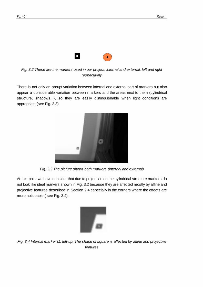
Fig. 3.2 These are the markers used in our project: internal and external, left and right
respectively
There is not only an abrupt variation between internal and external part of markers but also
appear a considerable variation between markers and the areas next to them (cylindrical
structure, shadows...), so they are easily distinguishable when light conditions are
appropriate (see Fig. 3.3)
Fig. 3.3 The picture shows both markers (internal and external)
At this point we have consider that due to projection on the cylindrical structure markers do
not look like ideal markers shown in Fig. 3.2 because they are affected mostly by affine and
projective features described in Section 2.4 especially in the corners where the effects are
more noticeable ( see Fig. 3.4).
Fig. 3.4 Internal marker I1: left-up. The shape of square is affected by affine and projective
features

Markers recognition in a camera-based calibration system for immersive applications Pg. 41
Moreover, it is important to completely identify the internal part of a marker (holes as a
distinctiveness feature of our markers) in order to, in further steps of the image processing
chain, determine correctly if a region is or not a desired marker.
The aim of the local pre-processing is filtering for improving images. In our case with the
sharpening filter, described in Section 2.1, fine details of image are enhanced, giving an
improved image to our purpose and with a simpler implementation than first-derivative as
described in [1].
This step was added before the image processing chain after seeing some results
described in Section 5 (Results) in which the inside regions of our internal markers almost
disappear. So without this step the results obtained at detecting markers are not good
enough.
With this filter differences are accentuated and constant areas are left unchanged. Also
noise is accentuated but as our image has high quality, the effect is barely noticeable. This
effect of the filter to the image can be seen in Fig. 5.13 and Fig. 5.14 from Results.
Until now what we have is a sharpened image from original one and what we want is to
label different regions in image and apply some criteria to discard not desired regions.
Segmentation
Region identification (labelling) expects a binary image to determine the different regions
so the pre-filtered gray-scale image has to be converted to a binary image (binarization).
Our case of study has a strong dependency of light conditions. This point makes important
to find a robust threshold technique in order to avoid problems if the structure is moved to
a brighter or darker place or the light in the salon varies. According to that we can come
across a situation in which a part of an image is more illuminated than other one and in the
darker one is the object we are looking for. So when there are changes in illumination
across the image, an inconstant illumination, it is better to use local instead of global
threshold. This way the threshold can vary smoothly across the image. Different
thresholds can be chosen depending on the part of the image to distinguish desirable from
undesirable objects in the image.
Now we need to find a method for dividing the image into different parts so that each part
can have a different threshold, local threshold, and thus we can solve the problem of
different lightning conditions.

Pg. 42 Report
How these parts should look is taken from Wall‟s algorithm [8]. The strategy is to divide
geometrically the image, not depending on pixel characteristics or values.
The image can be divided into blocks of different sizes m_m and n_n decided by
programmer/user, width and height of blocks can have equal or different sizes. Once
decided the height (m_m) and width (n_n) the blocks remain constant (m_m*n_n pixels) in
the whole image for that calibration except the ones in the boundaries (down or/and right),
which are as small/big as image size allows.
Our image has a height of 1536, if each Wall‟s block has 256 of height size we will have 6
blocks of size Xx256, but if each block has a height size of 200, we will have 7 blocks of
size Xx200 and the last row (the one down) of size Xx136 (1536-(7x200)). For a visually
understanding see Fig. 5.7.
Once we know how to divide image to minor effects of changes in illumination, now the
decision is how to choose the threshold value. As the regions can vary depending on
user‟s desire the threshold should be such as it varies depending on the pixels of the
block. That‟s why an adaptive threshold is needed [7]. This way and according to Wall‟s
algorithm we will find so many thresholds as blocks in image.
The threshold value can be selected by user (random, mean, median...) or also computer
can generate one automatically (automatic thresholding) and there are many different
methods (Otsu, K-means… [6]). All this information is explained in Section 2.2.
Our decision is a clustering based method that works with an iterative technique robust
against image noise and described in [9](Ridley and Calvard) .
The algorithm described by Ridley and Calvard‟s and implemented in our project consists
in six steps. In Appendix A, Ridley and Calvard‟s deduction and mathematics involved are
explained for the understanding of the algorithm used. The steps are:
1. To calculate histogram of the region of the image and set the mean intensity of the
image, set T=mean (I)
2. To divide the histogram into two parts separated by T
3. To calculate an above mean Tabv and a below mean Tbel, one for each part of the
histogram
4. To calculate the average between Tabv and Tbel resulting a new value of mean
T‟=(Tabv +Tbel)/2
5. To repeat calculation of Tabv and Tbel but now with the new mean T‟
Markers recognition in a camera-based calibration system for immersive applications Pg. 43
6. To repeat the process until threshold does not change any more
Thanks to this algorithm we are able to find a suitable threshold for each part and they are
also well adapted to changes in light conditions because it takes into account the pixel and
the characteristics of their neighbours.
The different results obtained if we apply a global or local threshold to image and different
threshold algorithm results are shown in Section 5.
As we have introduced before we were thresholding the image in order to apply labelling.
After that we will decide which properties of the objects are the best to distinguish markers.
Region identification: Labelling
From binarized image we find the different regions present in image. A region, as
described in Section 2.3, is a set of pixels where all the pixels are adjacent or touching. In
our case we have chosen an 8-connectivity, see Fig. 2.4 and Fig. 2.5. The region
identification method consists on labelling each region with a unique number where the
largest number gives the total number of regions in the image.
The algorithm for approaching the labelling assumes that zero pixels represent
background and non-zero pixels are objects. In a first iteration our algorithm searches pixel
per pixel through the entire image (row by row) a non-zero pixel. The criterion are (see Fig.
2.5):
If all the neighbours of the actual pixel (i,j) have zero value (background pixels) a
new, and as yet unused, label is given to the pixel.
If there is just one neighbouring pixel with a value different from zero, it assumes
that (i,j) has the same value as this pixel.
If there is more than one pixel with different value, the algorithm considers a label
collision and it stores the pair of pixels in another data structure as equivalent.
In a second iteration the whole image is scanned again and the algorithm decides if the
label collisions become one or another value analyzing the neighbouring pixels and the
label they have adopted.
After this second iteration all pixels in image different from zero (possible markers) are
labelled by a number which identifies them as part of a specific region.

Pg. 44 Report
Region based-shape representation
Now that all regions are identified we are going to analyze the content of the image. The
objective is to find some features of our markers (size, shape) in order to univocal identify
them from the rest of the objects in the image as for example parts of the cylindrical
structure. That means that we have to analyse for each region if those features, also called
region descriptors, are accomplished or not and depending the results discard or maintain
region as a candidate for marker.
In this project we focus our attention in three region descriptors: area (size), rectangularity
based on bounding box and rectangularity based on moments (the definition of terms has
been made in Section 2.3).
With the help of the first region descriptor mentioned we will discard regions in both cases,
internal and external markers. The other two region descriptors will be valid only in the
case of internal markers because the strategy adopted to identify external markers is
based in contours developed by Steffen Terörde in his Mater Thesis for IGD and TU-
Darmstadt. Steffen is a student who developed an algorithm for detecting ellipses in
image. We have integrated some of his programming codes into our GUI. In Section 3.1
IGD Contribution a short resume of the procedure is explained.
We have applied the following descriptor for both markers extraction:
1. Area (Size): corresponds to the number of pixels conforming the shape. It can be
calculated with zero order moment m00.
It is obvious that our markers are small and there are other regions in image really big if we
compare them. So the first criterion to discard regions will be area (size). Differences
between big and small objects are so great that it is not so important determining a frontier
upper number once we know the size of internal markers (around 300 pixels) and external
markers (around 900). In Section 5 (Results) will be shown the necessity of having a below
value for the range in order to minor the effect of noisy regions. Attending to that we have
considered for each case a range equal to ± (mean size of markers /2).
Internal markers Є (150, 350)
External markers Є (450, 1350)

Markers recognition in a camera-based calibration system for immersive applications Pg. 45
It is in those known ranges where mostly problems are found and where another criterion
is needed to discard markers from other small objects. As can be seen in Results (Section
5)
From now on we are only interested in determining features for internal markers. To
ensure rectangularity of the regions we have chosen two descriptors:
2. Rectangularity based on Bounding Box: ratio which determines how rectangular a
shape is. Attending to the conclusions of [11] and [12] and the complexity in terms of
programming of other methods (like Rotating Callipers described in [12] and [13]), one
method chosen to determine rectangularity in our project is based on minimum bounding
box.
A box is a rectangular region whose edges are parallel to the coordinate axes. Its limits can
be found as the minimum and maximum of each coordinate axes (x and y) determining 4
extreme points satisfying the inequalities:
xmin ≤ x ≤ xmax
ymin ≤ y ≤ ymax
So a minimal bounding box of a finite geometric object is the box with minimal area that
contains the object. An illustrative example is shown in Fig. 3.5.
Fig. 3.5 Minimal Bounding Box determined by xmin, xmax, ymin,ymax
This method is computationally the simplest of all linear bounding containers, and the one
most frequently used in many applications. At runtime, the inequalities do not involve any
Pg. 46 Report
arithmetic and it only compares raw coordinates with pre-computed min and max
constants.
Rectangularity ratio (R) is the result of the proportion between the area of the object or
region (OA) and the area of the bounding box (BB) or region‟s area against the area of the
minimum bounding rectangle:
OAR
BB
When both rectangles, containing and contained, have the same features this ratio is
ideally 1. In our case this ratio is not ideally 1 because our markers have a hole in the
middle and they are affected by projective and affine features. The hole of the internal
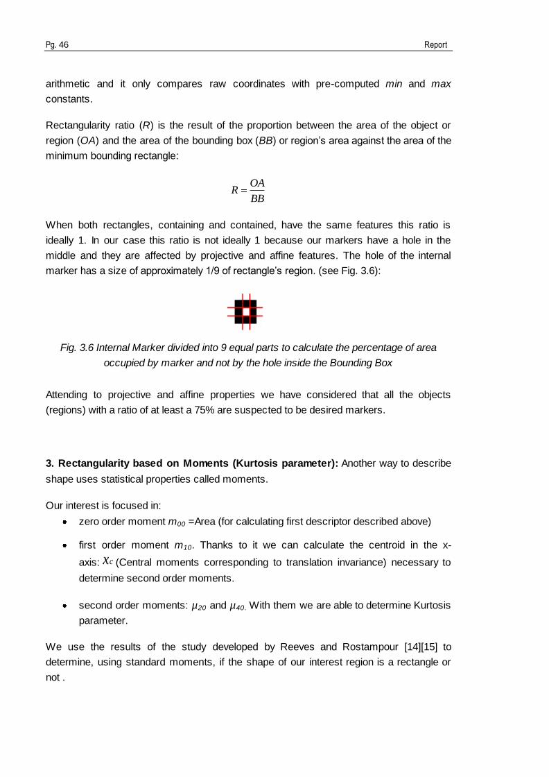
marker has a size of approximately 1/9 of rectangle‟s region. (see Fig. 3.6):
Fig. 3.6 Internal Marker divided into 9 equal parts to calculate the percentage of area
occupied by marker and not by the hole inside the Bounding Box
Attending to projective and affine properties we have considered that all the objects
(regions) with a ratio of at least a 75% are suspected to be desired markers.
3. Rectangularity based on Moments (Kurtosis parameter): Another way to describe
shape uses statistical properties called moments.
Our interest is focused in:
zero order moment m00 =Area (for calculating first descriptor described above)
first order moment m10. Thanks to it we can calculate the centroid in the x-
axis: cx (Central moments corresponding to translation invariance) necessary to
determine second order moments.
second order moments: µ20 and µ40. With them we are able to determine Kurtosis
parameter.
We use the results of the study developed by Reeves and Rostampour [14][15] to
determine, using standard moments, if the shape of our interest region is a rectangle or
not .

Markers recognition in a camera-based calibration system for immersive applications Pg. 47
The rectangle should have a Kurtosis parameter =-1.2 using:
At this point we have also considered a little margin around -1.2 (from -1.05 to -1.35) for
not being so strict because most of markers are affected by affine and projective features.
This criterion appeared to be in Section 5 a good solution at identifying markers.
We have tested different possibilities of ratios and its combination. As can be seen in
Section 5 the best solution is to combine both rectangularity descriptors and decide that a
region is rectangular when accomplish the equation:
ratio>0.75 and ((kx<-1.05 )and(kx>-1.35))
To ensure that objects extracted after feature description correspond to our internal
markers and to give robustness to the markers extraction chain we apply SIFT detector
and descriptor explained in Section 2.4
Object recognition: SIFT
From image an appropriate set of features are extracted. The aim of object recognition is
to take a large amount for image data and retain only that information necessary to identify
or distinguish the object. The knowledge we have from the shape of the object we are
looking for may be used to govern the extraction of features.
A matching algorithm will compare the ideal marker with the marker in the image and with
the help of the extracted features it will determine if the object of the image corresponds to
one of our searched markers or not.
As our application has not to run at real time (the process is done once a week, month…
what user decides) and has to attend to affine property what we are looking for is accuracy
at determining keypoints and correct matches in the whole process and is not so important
how long it takes in calculate them.
We have various possible algorithms to make this matching, the most known are SIFT and
SURF. Attending that our markers are subjected to affine features and according to [26] we
have decided that the better performance will be done by SIFT as described in Section 2.4.
The results are shown in Section 5.

Pg. 48 Report
In our case the SIFT implementation used is that described in [10] which is compatible to
Lowe‟s version. For applying the algorithm we need the image of study (marker) and a
template (See Fig. 3.2). The algorithm will do the matching between both images to
determine if they correspond to the same object or not.
The sift function returns a 4xK matrix frames containing the SIFT frames and a 128xK
matrix descriptors containing their descriptors. Each frame is characterized by four
numbers which are:
(x1; x2): for the centre of the frame
σ: The scale σ is the smoothing level at which the frame has been detected
ϴ: frame‟s orientation
The coordinates (x1; x2) are relative to the upper-left corner of the image, which is
assigned coordinates (0; 0), and may be fractional numbers (sub-pixel precision).
Fig. 3.7 Difference of Gaussian scale space of template image

Markers recognition in a camera-based calibration system for immersive applications Pg. 49
Fig. 3.8 Difference of Gaussian scale space of marker of study
In this implementation, a SIFT frame is also denoted by a circle, representing its support,
and one of its radii, representing its orientation. The support is a disk with radius equal to
six times the scale σ of the frame. If the standard parameters are used for the detector,
this corresponds to four times the standard deviation of the Gaussian window that has
been used to estimate the orientation, which is in fact equal to 1.5 times the scale σ. This
number can also be interpreted as size of the frame, which is usually visualized as a disk
of radius 6σ.
Pg. 50 Report
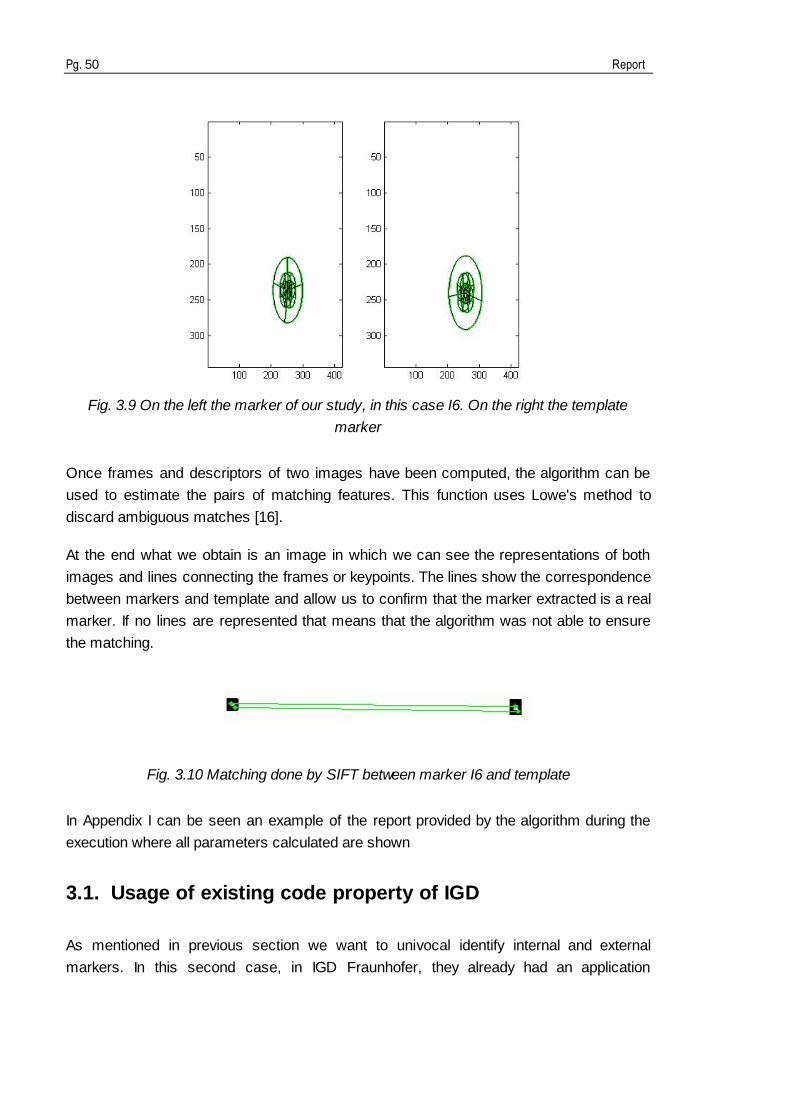
Fig. 3.9 On the left the marker of our study, in this case I6. On the right the template
marker
Once frames and descriptors of two images have been computed, the algorithm can be
used to estimate the pairs of matching features. This function uses Lowe's method to
discard ambiguous matches [16].
At the end what we obtain is an image in which we can see the representations of both
images and lines connecting the frames or keypoints. The lines show the correspondence
between markers and template and allow us to confirm that the marker extracted is a real
marker. If no lines are represented that means that the algorithm was not able to ensure
the matching.
Fig. 3.10 Matching done by SIFT between marker I6 and template
In Appendix I can be seen an example of the report provided by the algorithm during the
execution where all parameters calculated are shown
3.1. Usage of existing code property of IGD
As mentioned in previous section we want to univocal identify internal and external
markers. In this second case, in IGD Fraunhofer, they already had an application

Markers recognition in a camera-based calibration system for immersive applications Pg. 51
developed by Steffen Terörde, a student who had developed his Master Thesis in IGD for
his university, TU-Darmstadt, before I arrived. We are interested in the part of the strategy
referring to identify ellipses in image basing in contours.
The procedure used in our project is described as follows. After labelling the image and
discarding big regions we go through image pixels determining if a pixel belongs or not to
the contour we are looking for and we save this maximum and minimum coordinates in a
contour points array.
The directions used to determine contour points are visually described in Fig. 3.11. Our
interest pixel is coloured in black, and all its neighbours have a number. Some of these
pixels (0, 1, 2 and 3) are also coloured to easily identify directions described between
interest pixel and them. At the end, considering all neighbour pixels, we have covered all
possible directions and this way we are able to determine a contour.
Fig. 3.11 Left: all neighbour pixels are labelled with a number and some are coloured.
Right: show direction (colour) taken by each numbered pixel
The maximum and minimum points (same concept as Minimum Bounding Box) determine
the edges of the contour. We erase the pixels between them and we draw the line
corresponding to the contour.
With the new contour we determine where theoretically the centre of the ellipse should be
and with a tolerance determined by programming we draw a point in the middle of the
ellipse. If a point appears at the end of the execution means that the application has found
an object in the image with shape of ellipse. If not, region is not considered a ellipse and for
that reason it is discarded as external marker.
Pg. 52 Report
4. Tools and Implementation
4.1. Requirements
The requirement of the project was to program a Win 32 console application implemented
in C++ programming language. This way, the application will be compatible with some
other applications and functions already developed by IGD and the different parts and
modules can be reusable for different projects in the future.
The application should recognize markers at image, internal and external (squares and
circles) as described in previous sections.
Our application should have an interactive interface where user can select and see which
markers wants to detect. So a requirement of our GUI is having a screen where user
visually could identify the markers presents in image and also verify if the results obtained
by the code are effective at recognizing internal and external markers.
4.2. Tools
As a first approximation we have implemented our code in Matlab to see if results were
successful to our purpose. Once we have tested or rejected the different
techniques/methods for each step in the image processing chain, the final solution has
been implemented in C++ thanks to IPP and Ttmath libraries. An open source library called
OpenCV has been also tested.
The programming languages and environments shortly introduced above are explained as
follows:
MATLAB: The name stands for MATrix LABoratory. MATLAB is a high-performance
language for technical computing. It integrates computation, visualization, and
programming in an easy-to-use environment where problems and solutions are expressed
in familiar mathematical notation where the basic data element is an array that does not
require dimensioning. Some Typical uses of the application include: Math and computation,
algorithm development, modelling, simulation, prototyping, data analysis, exploration and
visualization.
Visual C++: is one of the most widespread and important languages available today for
developing applications for the Windows operating system C++, an object oriented

Markers recognition in a camera-based calibration system for immersive applications Pg. 53
programming language. It implements data abstraction using a concept called classes,
along with other features to allow object-oriented programming. Parts of the C++ program
are easily reusable and extensible; existing code is easily modifiable without actually
having to change the code. C++ maintains aspects of the C programming language and
some of its features allow low-level access to memory but also contain high level features.
OpenCV: is a computer vision library originally developed by Intel. It is free for commercial
and research use under a BSD license (open source software). The library is cross-
platform, and runs on Windows, Mac OS X, Linux, VCRT (Real-Time OS on Smart
camera) and other embedded operating systems. In fact it is 4 libraries in one: computer
vision algorithms (CV), experimental/beta (cvaux), linear algebra (cxcore) and
media/window handling (highgui). It focuses mainly on real-time image processing, as
such, if it finds Intel‟s Integrated Performance Primitives (IPP) on the system, it will use
these commercial optimized routines to accelerate itself.
IPP: Intel® Integrated Performance Primitives (Intel® IPP) is an extensive library of
multicore-ready, highly optimized software functions for digital media and data-processing
applications. Intel IPP offers thousands of optimized functions covering frequently-used
fundamental algorithms. The library supports only Intel (AMD not supported) processors
and is available for Windows, Linux and Mac OS X operating systems. Intel IPP is divided
into three major processing groups: Signal (with linear array or vector data), Image (with
2D arrays for typical colour spaces) and Matrix (with nxm arrays for matrix operations).
TTMath: is a small library which allows one to perform arithmetic operations with big
unsigned integer, big signed integer and big floating point numbers. It provides standard
mathematical operations like adding, subtracting, multiplying, dividing etc. TTMath is
developed under the BSD license which means that it is free for both personal and
commercial use. The main goal of the library is to allow one to use big values in the same
way as the standard types like int, float, etc.
4.3. OpenCV
As a first option we have tried to find a open source application already programmed which
could help to recognize our markers.
In the OpenCV library there are many examples in image processing area and one of the
demos included is called squares.cpp. Its functionality is to find squares in the image. To
do that, the code tries different threshold levels using Canny instead of zero threshold level
o helping to catch squares with gradient shading. Then applies threshold and find contours
and 4 points (vertices). Once contours are determined it looks for minimum angle between

Pg. 54 Report
joint edges and if all angles are near to 90 degrees it concludes that this contour belongs to
a square. Then it draws lines to show to user where are the squares found.
We have tested it with our reference image but it does not work properly despite adjusting
the different parameters as shown in Section 5 (Results). Our markers are not detected.
So the strategy of finding an open source application already developed is discarded and
we have to develop our own application.
4.4. Implementation
Before implementing the GUI, we have implemented a first approximation program with
MATLAB to ensure that the concepts were right and reachable before programming a GUI
with Visual Studio in C++ language.
The strategy is to work with the original image, scene of real world captured by the
camera, as a matrix, where the elements of each raw and column are pixels of the image.
Through the knowledge of image processing theory and the different instances and
functions of MATLAB we have implemented each step of the image processing chain that
represents the better solution at extracting our searched markers.
As the results in MATLAB are successful (See Section 5), the image results are
respectable with markers features and location and operations are computationally not
complicated so the time of execution is not too much (although we are not searching a real
time application) the solution implemented in C++ is a “copy” from MATLAB. It uses
algorithms and functions implemented and tested in MATLAB and potentiated by tools as
Intel Primitives.
C++ project structure
The goal of this project is to implement a GUI with Visual Studio in C++ compatible with
other projects already developed by Fraunhofer IGD and knowing the possibilities that C++
language brings. Then using the capabilities of the C++ language combined with IPP and
TTMath Mathematical Library we have searched the optimal methods to uniquely identify
our markers.
We have implemented a console Win32 Application in a Microsoft Visual C++ 8.00
programming environment. The result is a GUI that makes easy the use of the code to the
final user.

Markers recognition in a camera-based calibration system for immersive applications Pg. 55
The title of the GUI is Markers Detection and the design consists in 3 parts. The different
boxes corresponding to different blocks in the image processing chain are shown on the
left and inside them we can find different options (buttons) that can be chose by user; a big
screen for showing pictures is on the right side and a small information visor at the bottom.
All these details can be seen in the Fig. 4.1 below.
Fig. 4.1 Main window of our GUI Application where options, buttons and pictures are.
The structure of the programming code developed is as follows:

Pg. 56 Report
Fig. 4.2 Shows the structure of the project Markers and its different header and source
files. Initial image (testimage) is included in our resource files.
The project has a main function Markers_Detection.cpp in which Form1 is runned
(Form1.h).
Application::Run(gcnew Form1());
Design of GUI and functionality of Options
In this section the design of the GUI and the structure of the code are explained. After an
overview, each group of options and buttons implemented are described giving detailed
information about C++, IPP and TTMath functions needed and implemented in each case.
All includes and defines necessary to run the application properly are at the beginning of
the code followed by the initialization of global variables.
The design chose for GUI is shown in Fig. 4.3 below:

Markers recognition in a camera-based calibration system for immersive applications Pg. 57
Fig. 4.3 Main window of our GUI Application where options, buttons and pictures are. The
red rectangles enhance some details explained in the memory (Main window, GroupBox
and Information Box)
In this screenshot of our application (Fig. 4.3) we can see 3 big boxes enhanced in red
colour.
1: main window of the programme where are included all the sections, buttons, screens
and information displays.
private: System::Windows::Forms::PictureBox^ pictureBoxBigView;
2: Each step of the image processing chain needs to have its own GroupBox where all the
buttons are grouped. For example the code for Step 0 is:
private: System::Windows::Forms::GroupBox^ groupBoxOpenImage;
3: Corresponds to information box where all the comments about the process in course
are shown:
private: System::Windows::Forms::TextBox^ textBoxOutput;

Pg. 58 Report
In this particular case of GroupBox (Open Image) we also need to create a File Dialog (Fig.
4.4) so we are able to open the desired image searching it in folders of our computer. In
our case testimage.bmp:
private: System::Windows::Forms::OpenFileDialog^ openFileDialog;
Fig. 4.4 File Dialog to open the desired image(testimage.bmp) searching it in folders of our
computer
For each GroupBox there also 2 more items which have to be programmed. For example
in case of Open Image they are shown in Fig. 4.5 below.
Fig. 4.5 GroupBox Open Image and its button

Markers recognition in a camera-based calibration system for immersive applications Pg. 59
4: The label where the name of each GroupBox will be shown. It is not necessary that this
name of the label (in this step of programming) agrees with the name shown in the
console application. That is something editable after.
private: System::Windows::Forms::Label^ labelBoxStep0_OpenImage;
5: For each Button inside the GroupBox we have to implement the instruction (the only
difference is the name in each case):
private: System::Windows::Forms::Button^ buttonStep0_OpenImage;
All this windows, boxes and options need to be created and initialized. The programming of
the examples shown above is:
this->pictureBoxBigView= (gcnew System::Windows::Forms::PictureBox());
this->groupBoxOpenImage = (gcnew System::Windows::Forms::GroupBox());
this->buttonStep0_OpenImage= (gcnew System::Windows::Forms::Button());
this->labelBoxStep0_OpenImage=(gcnew System::Windows::Forms::Label());
this->openFileDialog=(gcnew System::Windows::Forms::OpenFileDialog());
this->textBoxOutput = (gcnew System::Windows::Forms::TextBox());
Once we have all boxes created we have to indicate the components of the PictureBox
and for that reason we have to run the beginning action:
cli::safe_cast<System::ComponentModel::ISupportInitialize^
>(this->pictureBoxBigView))->BeginInit();
For each element forming part of our application we have to describe the features they will
have. These features are exposed in Table 4.1.
Features
PictureBo
x
BackColor, BorderStyle, Location (Point), Name, Size, SizeMode,
TabIndex and TabStop
GroupBox Controls, Location (Point), Name, Size, TabIndex, TabStop and

Pg. 60 Report
Text
Button
Enabled, Location (Point), Name, Size, TabIndex, Text,
UseVisualStyleBackColor
Label Location (Point), Name, Size and TabIndex
FileDialog FileName
Table 4.1 Features of each statement in our Win32 Console application
In the case of Buttons we have programmed Events that will have effect when the mouse
is clicked:
this->buttonStep0_OpenImage->Click += gcnew System::EventHandler(this,
&Form1::buttonStep0_OpenImage_Click);
We configure the controls of each GroupBox and we give a name to the main window.
This way the configuration of Console Win32 is ended (EndInit).
this->Controls->Add(this->pictureBoxBigView);
this->Controls->Add(this->groupBoxOpenImage);
this->Controls->Add(this->textBoxOutput);
this->Text = L"Markers Detection";
(cli::safe_cast<System::ComponentModel::ISupportInitialize^ >(this-
>pictureBoxBigView))->EndInit();
We declare our own variables (self-defined) and we start with the programming of each
function that a click of the mouse activates.
At the end of each execution the following buttons are enabled and actual are disabled
except in GroupBox called General Options that can be selected at any time during the
execution of the programme.
Button Open in Open Image Box

Markers recognition in a camera-based calibration system for immersive applications Pg. 61
When we first run the application the only options available are Open Image and Exit. That
can be seen because they are the only buttons enabled; the others can not be selected
(see Fig. 4.6).
In the viewer on the right the image selected will be shown.
Fig. 4.6 Initial appearance of our GUI. Only Button Open from Open Image and Exit can
be selected
The selection of this button opens a FileDialogBox in which we can chose the image within
we want to work. See Fig. 4.7 below.

Pg. 62 Report
Fig. 4.7 File Dialog to open the desired image(testimage.bmp) searching it in folders of our
computer
The result is the visualization of the image on the right side screen (see Fig. 4.8).

Markers recognition in a camera-based calibration system for immersive applications Pg. 63
Fig. 4.8 Resulting appearance of GUI alter opening our testimage
Once we have opened the image, the button becomes disabled and next options available
correspond to next step of the image processing chain.
From now on, we can find two possibilities of analysis. We can search for internal markers
otherwise external markers.
Option 1: Button Internal in Marker Decision Box
In this point the goal is to obtain Internal Markers and that will be done following the steps
described in Section 3 (Our contribution). First of all we will apply a pre-processing filter,
following by a local threshold, a labelling of the resulting image and finally discarding big
regions and not rectangular objects in image.
In our GUI when Internal Button is selected it is in a flat style and External Button appears
disable, it can not be selected.
The image opened in step before can be seen on the right side. After applying all functions
in this step the result will be shown instead and it will be a good approximation image to
our final goal. All the process and results can be seen in Section 5.
Before explaining the functions involved in this step it is important to explain some
conversions made to image formats in order to execute some functions faster or easier by
using IPP.
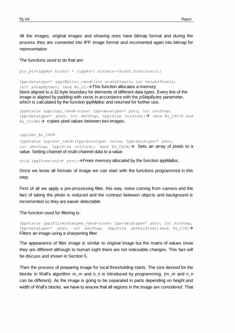
Pg. 64 Report
All the images, original images and showing ones have bitmap format and during the
process they are converted into IPP image format and reconverted again into bitmap for
representation
The functions used to do that are:
pin_ptr<Ipp8u> binSrc = (Ipp8u*) binData->Scan0.ToPointer();
Ipp<datatype>* ippiMalloc_<mod>(int widthPixels, int heightPixels,
int* pStepBytes); (mod 8u_C1)This function allocates a memory
block aligned to a 32-byte boundary for elements of different data types. Every line of the image is aligned by padding with zeros in accordance with the pStepBytes parameter, which is calculated by the function ippiMalloc and returned for further use.
IppStatus ippiCopy_<mod>(const Ipp<datatype>* pSrc, int srcStep,
Ipp<datatype>* pDst, int dstStep, IppiSize roiSize); (mod 8u_C4C1R and
8u_C1C4R) copies pixel values between two images.
ippiSet_8u_C4CR
IppStatus ippiSet_<mod>(Ipp<datatype> value, Ipp<datatype>* pDst,
int dstStep, IppiSize roiSize); (mod 8u_C4CR) Sets an array of pixels to a
value. Setting channel of multi-channel data to a value
void ippiFree(void* ptr);Frees memory allocated by the function ippiMalloc.
Once we know all formats of image we can start with the functions programmed in this
step.
First of all we apply a pre-processing filter, this way, noise coming from camera and the
fact of taking the photo is reduced and the contrast between objects and background is
incremented so they are easier detectable.
The function used for filtering is:
IppStatus ippiFilterSharpen_<mod>(const Ipp<datatype>* pSrc, int srcStep,
Ipp<datatype>* pDst, int dstStep, IppiSize dstRoiSize);(mod 8u_C1R)
Filters an image using a sharpening filter.
The appearance of filter image is similar to original image but the matrix of values show
they are different although to human sight there are not noticeable changes. This fact will
be discuss and shown in Section 5.
Then the process of preparing image for local thresholding starts. The size desired for the
blocks in Wall‟s algorithm m_m and n_n is introduced by programming. (m_m and n_n
can be different). As the image is going to be separated in parts depending on height and
width of Wall‟s blocks, we have to ensure that all regions in the image are considered. That

Markers recognition in a camera-based calibration system for immersive applications Pg. 65
is the reason why we construct some blocks with a different size at the end-right and end-
button with one or both sides of size tmp1 and tmp2.
for(int i=0;i<height;i=i+m_m)
{
for(int j=0;j<width;j=j+n_n)
{
if(width-j<n_n)
{
tmp1=width-j;
}
else
{
tmp1=n_n;
}
if(height-i<m_m)
{
tmp2=height-i;
}
else
{
tmp2=m_m;
}
We calculate histogram from Wall‟s block as an array that accumulates all the pixel values
(colour) contained in region m_m x n_n, m_m x tmp1 or tmp2 x n_n, depending on the
region. (regionArray)

Pg. 66 Report
Then the threshold of each region is calculated with Ridley and Calvard‟s algorithm as
explained in Section 2.2 and the result is applied to each region. So at the end what we
have is our pre-processed image in so many parts and within so many thresholds as
blocks with Wall‟s method were calculated. It is time to reconstruct the size of pre-
processed image from small blocks. All this programming is made with vectors:
regionArray[temps] where temps is the size of the Wall‟s block, is the array where
pixel colour property is saved
histoArray[SIZE_HIST] that is the array where the histogram of block is calculated
mean [k]: array where all values calculated are saved. The iteration in searching the
mean ends while(mean[k-1]!=mean[k]);
and the reconstruction is done by:
unsigned int f=0;
unsigned int g=0;
for(unsigned int q=0;q<temps;q++)
{
if(g==tmp1)
{
f=f+1;
g=0;
}
if(regionArray[q]<Threshold)
{
resbinImageInt->SetPixel(g+j,f+i,System::Drawing::Color::Black);
}
else
{

Markers recognition in a camera-based calibration system for immersive applications Pg. 67
resbinImageInt->SetPixel(g+j,f+i,System::Drawing::Color::White);
}
g=g+1;
}
After that process we obtain binary image (See Results) and after that we apply a closing
for cleaning all those small black regions and isolated pixels (noise) resulting from
binarization.
The closing is made with a structuring element of 3x3 called Mask by IPP.
The IPP functions used:
Ipp8u pMask[3*3]= {1,1,1,
1,1,1,
1,1,1};
IppiSize maskSize={3,3};
ippiMorphAdvInitAlloc_8u_C1R()
IppStatus ippiMorphCloseBorder_<mod>(const Ipp<datatype>* pSrc, int
srcStep, Ipp<datatype>* pDst, int dstStep, IppiSize roiSize,
IppiBorderType borderType, IppiMorphAdvState* pState);(mod
8u_C1R)performs closing of an image
ippiMorphAdvFree(pState);
Then the negative image is calculated. The black pixels become white and the white ones
become black. This contrast transformation in image is a pre-step for labelling and it is
really important. As we see in the image the desired markers are black. Labelling function
considers that a non-zero value forms part of a concrete region. That means that in our
situation, if we do not change the pixel values on the image our markers will be consider as
part of the background and that is exactly the opposite we are searching. So with this
contrast transformation the image (negative image) is prepared to apply labelling process
described in Section 2.3.
The connectivity used to calculate labelling is 8-connectivity (computing) (See Fig. 2.5) and
the functions used are mentioned below:
ippiLabelMarkersGetBufferSize_8u_C1R()

Pg. 68 Report
ippiLabelMarkers_8u_C1IR()
IppStatus ippiLabelMarkers_8u_C1IR(Ipp8u* pMarker, int markerStep,
IppiSize roiSize, int minLabel, int maxLabel, IppiNorm norm, int*
pNumber, Ipp8u* pBuffer); Labels markers in image with different values.
The resulting labelled image is shown in Section 5. (Results)
Once we have applied labelling the next step in our image chain is region based-shape
classification. In this step we will solve the problem of having not only desired regions by
analyzing the features of the objects in the picture.
Attending to descriptors described in Section 3 and with the criteria also there described
for internal markers we discard by size those regions out of range and those not
rectangular:
ratio>0.75 and ((kx<-1.05 )and(kx>-1.35))
The numbers involved in the calculation of the Kurtosis parameter are really big and C++
was not able to calculate them without errors so at this point we have to introduce an
external mathematical library called ttmath which has helped us to solve this big
operations.
The definitions of a big number using ttmath library are:
typedef ttmath::Big<1,2> MyBig;
and some variables declarations and initializations used:
MyBig Xc;
MyBig u20=0;
MyBig u40=0;
where Xc is the coordinate x of centroid (centre of gravity) and µ20 and µ40 are central
moments (translation invariance) all of them described in Sections 2.3 and 3.
At the end of the execution of this button we obtain an image containing small rectangular
regions as similar as possible to our ideal marker. We also obtain some other regions that
are not desired and which will be rejected after cleaning image from isolated pixels and
after applying matching algorithm SIFT.
Button Optimization in Optimization

Markers recognition in a camera-based calibration system for immersive applications Pg. 69
This button is only available in case of Internal Marker and the aim is to clear image from
noise, deleting isolated pixels. It can be reached thanks to IPP function
IppStatus ippiDilate_<mod>(const Ipp<datatype>* pSrc, int srcStep,
Ipp<datatype>* pDst, int dstStep, IppiSize roiSize,
const char* pMask, IppiSize maskSize, IppiPoint anchor);(mod 8u_C1R, not
in place operation) Performs dilation of an image using a specified mask
(structuring element of 3x3)
Button SIFT in Marker Decision
This button was thought to start running the C++ SIFT code as described in Section 2.4.
But we were not able to insert the code in our current project so SIFT algorithm was
applied via Matlab to the image obtained by GUI. Results are shown in Section 5.
Option 2: Button External in Marker Decision Box
The procedure of this option is the first step described in Option 1. To the digital image
taken by the camera we apply pre-processing filtering to clean image and then we prepare
image for thresholding. In Fig. 4.9 we can see binarization obtained with a m_m and n_n
block size different from the one used before (in internal markers).
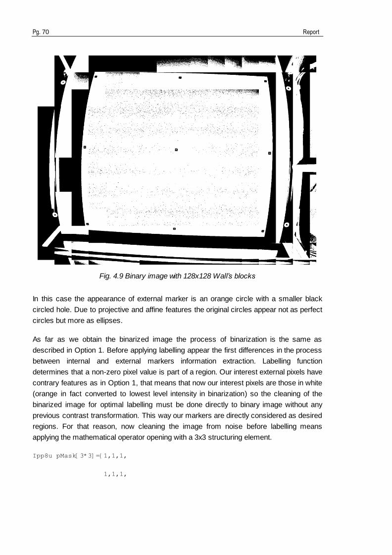
Pg. 70 Report
Fig. 4.9 Binary image with 128x128 Wall’s blocks
In this case the appearance of external marker is an orange circle with a smaller black
circled hole. Due to projective and affine features the original circles appear not as perfect
circles but more as ellipses.
As far as we obtain the binarized image the process of binarization is the same as
described in Option 1. Before applying labelling appear the first differences in the process
between internal and external markers information extraction. Labelling function
determines that a non-zero pixel value is part of a region. Our interest external pixels have
contrary features as in Option 1, that means that now our interest pixels are those in white
(orange in fact converted to lowest level intensity in binarization) so the cleaning of the
binarized image for optimal labelling must be done directly to binary image without any
previous contrast transformation. This way our markers are directly considered as desired
regions. For that reason, now cleaning the image from noise before labelling means
applying the mathematical operator opening with a 3x3 structuring element.
Ipp8u pMask[3*3]={1,1,1,
1,1,1,

Markers recognition in a camera-based calibration system for immersive applications Pg. 71
1,1,1};//structuring element
IppiSize maskSize={3,3};
IppiPoint anchor={1,1};
IppiMorphAdvState* pState;
IppiBorderType borderType=ippBorderRepl;
ippiMorphAdvInitAlloc_8u_C1R()
IppStatus ippiMorphOpenBorder_<mod>(const Ipp<datatype>* pSrc, int
srcStep, Ipp<datatype>* pDst, int dstStep, IppiSize roiSize,
IppiBorderType borderType, IppiMorphAdvState* pState); (mod
8u_C1R)performs opening of an image
ippiMorphAdvFree(pState);
Once we have all regions in image identified here we go a step after. As we know that
external markers are not considered big regions and they are bigger than internal ones we
can also apply the criterion of discarding regions by size but now not also applying a higher
threshold but also a lower one. The range chose is that going from 800 to 1300 pixels. The
results are shown in Section 5.
Then to extract useful information from image it is necessary to apply next step with next
button.
Button Ellipse Detection
After labelling the image and discarding big regions, dilation is applied to clean image from
isolated black undesirable pixels.
After that all the process described in Contribution of Section 3.1 is applied. This way we
determine if a region is or not an external marker. The results of this extraction are shown
in Section 5.
Other buttons
During the entire process of the application there are some buttons or options that can be
selected in Image Options they are Save and Done and in General Options we can find
Restart and Exit.
Save option is the function of saving an image in the current path of the project; Done
indicates that the action is finished and activates the next step of the application; Restart

Pg. 72 Report
gives us the opportunity of giving up all that was made and re-start over; and finally Exit, it
stops the current action and ends the running of the application.

Markers recognition in a camera-based calibration system for immersive applications Pg. 73
5. Results
As a starting point of our image processing chain we have the photo taken by camera
placed above the projector. This photo is our testimage (testimage.bmp) shown in Fig.
3.1. In this section we will see the results of how, from this testimage, the markers we are
looking for are extracted and recognized by applying methods and techniques described in
Section 3.
The section has been divided into two experiments. In the first one, an open source code
provided by Open CV with the aim of detecting squares is evaluated. After discarding it, the
second experiment explained corresponds to the results obtained by our designed and
implemented GUI. The results given in this second case are a combination of Matlab and
C++ experiments.
As we have only one testimage a rotated image from original has been also used to test
the application. The results are shown in Second Experiment.
First Experiment
We have included in a C++ project the code given in squares.cpp. The demo is provided
by OpenCV and we have included all libraries (cvaux) in the right path in our project in
order to run the demo.
The results of the demo with the one of the images given by default are shown in green in
Fig. 5.1. We can see different shape objects and how the demo determines which of them
are squares (overlaid green rectangle) and which ones are not (without selecting them).
Fig. 5.1 Result of squares detection with a default image provided by OpenCV

Pg. 74 Report
We are going to see the behaviour of the program with our testimage. When we prove how
works the demo with our image (testimage) configured with the default parameters the
results are as follows (See Fig. 5.2)
Fig. 5.2 Squares detected by squares.cpp with default values
As we can see it detects only big squares (obtained by joining contours with 4 vertices with
angle similar to 90 degrees as described in Section 4.3) but it also has a lot of wrong
detections. It determines many combinations that are no squares. In fact to our purpose all
of them are wrong detections because any marker is detected.
To improve results we adjust parameters this way we could see if the demo is able to
identify our internal markers or at least reduce the number of wrong squares detection.
The results obtained after the evaluation of different parameters of the application were
unsuccessful to our purpose although the application seems to consider affine features of
squares (See Fig. 5.3)

Markers recognition in a camera-based calibration system for immersive applications Pg. 75
Fig. 5.3 Result of applying squares.cpp to a square under affine features
So altogether, the code is not good to our purpose because it does not univocal
determines internal markers and adds a lot of wrong detections making results instable.
Second Experiment
The first step is to convert testimage (in greyscale) to binary image (see Section 2.2).
Segmentation
Several thresholding methods have been tested and results are shown in Fig. 5.4, Fig. 5.5
and Fig. 5.6 below:

Pg. 76 Report
Fig. 5.4 Directly applying threshold to testimage with a level threshold of 0,5

Markers recognition in a camera-based calibration system for immersive applications Pg. 77
Fig. 5.5 Binary image calculated by Otsu’s algorithm which determines the threshold level
of image in 0.6157

Pg. 78 Report
Fig. 5.6 Binary image calculated by Ridley and Calvard’s algorithm which determines the
threshold level of image in 0.6142
From images obtained we can see that applying a level threshold to the whole image does
not detect external markers.
In case of internal markers, if we apply a level of 0.5 some of them are lost (I5, I6, I7, I8 and
I9) so it is necessary the running of an algorithm to adjust this threshold value in order to
adapt it to the features of our image.
The results of the threshold level calculated by Otsu‟s and Ridley and Calvard‟s algorithms
are really nearby 0.6157 and 0.6142 respectively. It is remarkable that the marker in the
middle, I5, appear in both binarizations as a non connected region. This fact is due to
different illumination in scene where central marker receives more directly the light coming
from the lightning source making it appear brighter than the rest of the markers.
Also pixels in the upper row I1, I2 and I3 lose their inside hole, so their shape do not remain
unchanged.
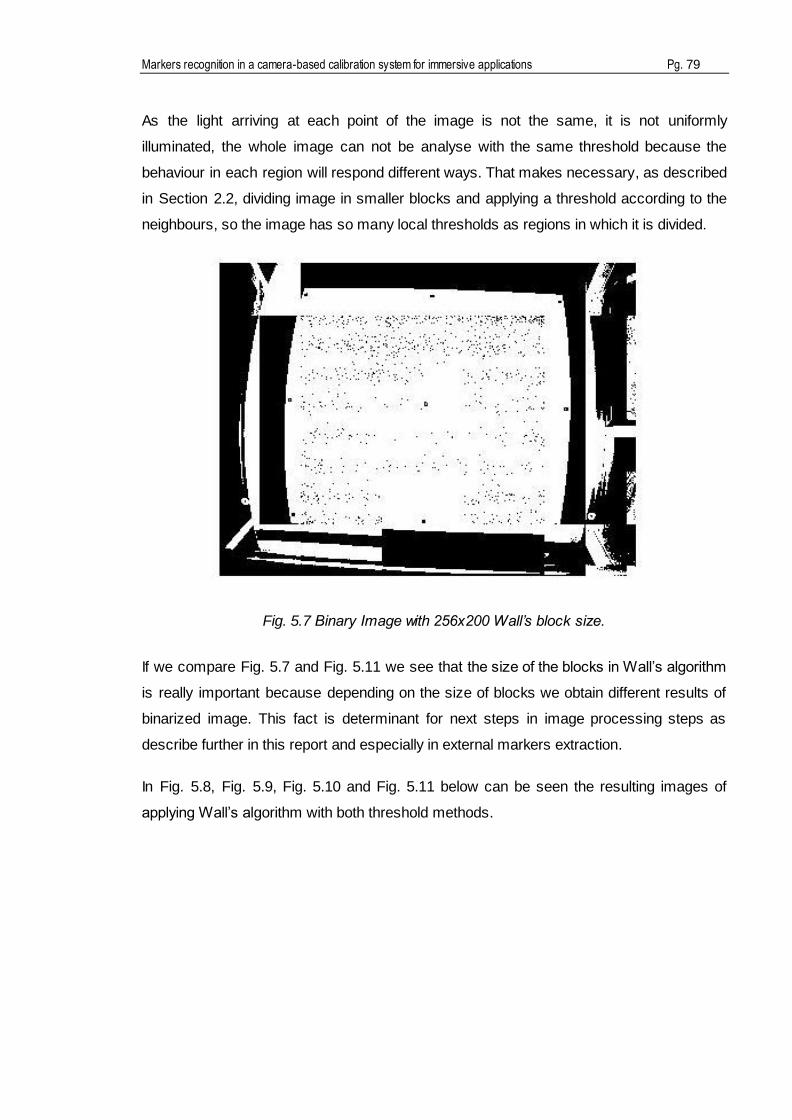
Markers recognition in a camera-based calibration system for immersive applications Pg. 79
As the light arriving at each point of the image is not the same, it is not uniformly
illuminated, the whole image can not be analyse with the same threshold because the
behaviour in each region will respond different ways. That makes necessary, as described
in Section 2.2, dividing image in smaller blocks and applying a threshold according to the
neighbours, so the image has so many local thresholds as regions in which it is divided.
Fig. 5.7 Binary Image with 256x200 Wall’s block size.
If we compare Fig. 5.7 and Fig. 5.11 we see that the size of the blocks in Wall‟s algorithm
is really important because depending on the size of blocks we obtain different results of
binarized image. This fact is determinant for next steps in image processing steps as
describe further in this report and especially in external markers extraction.
In Fig. 5.8, Fig. 5.9, Fig. 5.10 and Fig. 5.11 below can be seen the resulting images of
applying Wall‟s algorithm with both threshold methods.
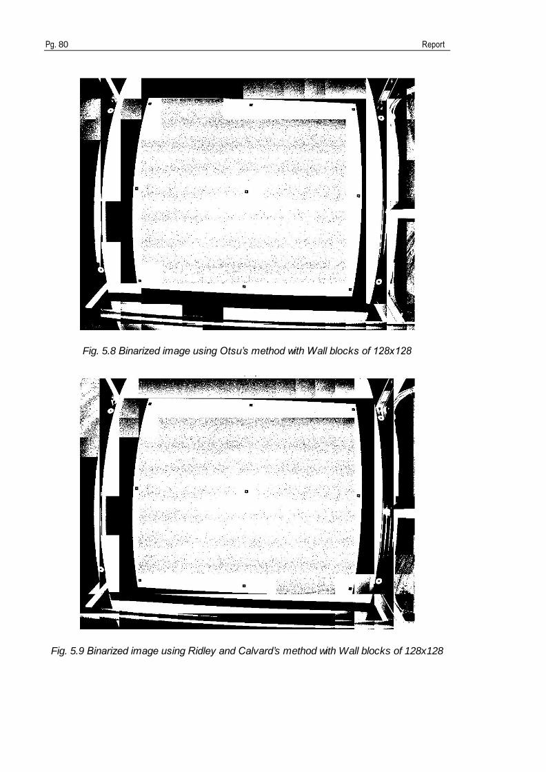
Pg. 80 Report
Fig. 5.8 Binarized image using Otsu’s method with Wall blocks of 128x128
Fig. 5.9 Binarized image using Ridley and Calvard’s method with Wall blocks of 128x128

Markers recognition in a camera-based calibration system for immersive applications Pg. 81
Fig. 5.10 Binarized image using Otsu’s method with Wall blocks of 256x256
Fig. 5.11 Binarized image using Ridley and Calvard’s method with Wall blocks of 256x256
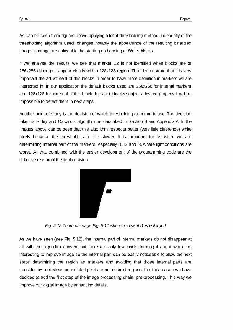
Pg. 82 Report
As can be seen from figures above applying a local-thresholding method, indepently of the
thresholding algorithm used, changes notably the appearance of the resulting binarized
image. In image are noticeable the starting and ending of Wall‟s blocks.
If we analyse the results we see that marker E2 is not identified when blocks are of
256x256 although it appear clearly with a 128x128 region. That demonstrate that it is very
important the adjustment of this blocks in order to have more definition in markers we are
interested in. In our application the default blocks used are 256x256 for internal markers
and 128x128 for external. If this block does not binarize objects desired properly it will be
impossible to detect them in next steps.
Another point of study is the decision of which thresholding algorithm to use. The decision
taken is Ridey and Calvard‟s algorithm as described in Section 3 and Appendix A. In the
images above can be seen that this algorithm respects better (very little difference) white
pixels because the threshold is a little slower. It is important for us when we are
determining internal part of the markers, especially I1, I2 and I3, where light conditions are
worst. All that combined with the easier development of the programming code are the
definitive reason of the final decision.
Fig. 5.12 Zoom of image Fig. 5.11 where a view of I1 is enlarged
As we have seen (see Fig. 5.12), the internal part of internal markers do not disappear at
all with the algorithm chosen, but there are only few pixels forming it and it would be
interesting to improve image so the internal part can be easily noticeable to allow the next
steps determining the region as markers and avoiding that those internal parts are
consider by next steps as isolated pixels or not desired regions. For this reason we have
decided to add the first step of the image processing chain, pre-processing. This way we
improve our digital image by enhancing details.

Markers recognition in a camera-based calibration system for immersive applications Pg. 83
Pre-processing
As can be seen in pictures contained in Fig. 5.13 and Fig. 5.14 (I1), visually the difference
between the two images (original and sharpened) is not noticeable but if we look the
brightness values of the pixels we see that sharpen filter modifies these values although
human eye is barely able to recognize changes.
Notice the differences shown in matrix values between Fig. 5.13 and Fig. 5.14.
Fig. 5.13 Internal marker original image. Matrix of image value.
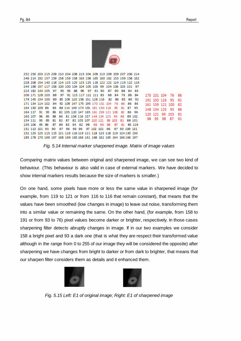
Pg. 84 Report
Fig. 5.14 Internal marker sharpened image. Matrix of image values
Comparing matrix values between original and sharpened image, we can see two kind of
behaviour. (This behaviour is also valid in case of external markers. We have decided to
show internal markers results because the size of markers is smaller.)
On one hand, some pixels have more or less the same value in sharpened image (for
example, from 119 to 121 or from 116 to 116 that remain constant), that means that the
values have been smoothed (low changes in image) to leave out noise, transforming them
into a similar value or remaining the same. On the other hand, (for example, from 158 to
191 or from 93 to 76) pixel values become darker or brighter, respectively. In those cases
sharpening filter detects abruptly changes in image. If in our two examples we consider
158 a bright pixel and 93 a dark one (that is what they are respect their transformed value
although in the range from 0 to 255 of our image they will be considered the opposite) after
sharpening we have changes from bright to darker or from dark to brighter, that means that
our sharpen filter considers them as details and it enhanced them.
Fig. 5.15 Left: E1 of original image; Right: E1 of sharpened image

Markers recognition in a camera-based calibration system for immersive applications Pg. 85
In Fig. 5.15, the sharpen filter effect is visually more noticeable than in I1 case shown in
Fig. 5.13 and Fig. 5.14. The external circle appears in sharpened image on the right
clearer, the limits, where contrast is higher, appear better defined as in original image.
So as we can see including this step before the thresholding, noise will be reduced and
details will be enhanced making more remarkable the differences between transitions and
favouring the distinction of internal parts of our markers as for example the case shown in
Fig. 5.12 above.
What we have until now is a binarization of a sharpened image. If we look back to Fig. 5.9
and Fig. 5.11 we see there are a lot of isolated pixels that do not belong to structure or
markers but have appeared after binarizing as a kind of noise in the image. So before
labelling the existent regions in the images it is necessary to clean images so the
identification of desired regions is easier.
At this point we have to differentiate between internal and external case.
In the case of internal markers, the morphological operator applied into image to clean it is
closing as described in Appendix B.
Results are shown in Fig. 5.16.
Fig. 5.16 Closing morphological operator applied to binarized image of internal markers

Pg. 86 Report
In the case of external markers, the morphological operator applied into image to clean it is
opening as described in Appendix B.
Results are shown in Fig. 5.17.
Fig. 5.17 Opening morphological operator applied to binarized image of external markers
If we compare Fig. 5.9 and Fig. 5.17 we see that black regions are accentuated, opposite
to white ones. It is very useful in our purpose because we ensure that the internal part of
the external marker do not disappear. This way, our markers maintain their appearance.
Otherwise, comparing Fig. 5.11 and Fig. 5.16 we see the opposite phenomenon and are
white ones which we want to improve for not losing the internal part of internal markers.
Our images are prepared for labelling, well, a previous step is needed in case of internal
markers (contrast transformation) as described in Section 3.1.
Labelling
As follows labelling described in Section 2.3 is done (see Fig. 5.18 and Fig. 5.19).
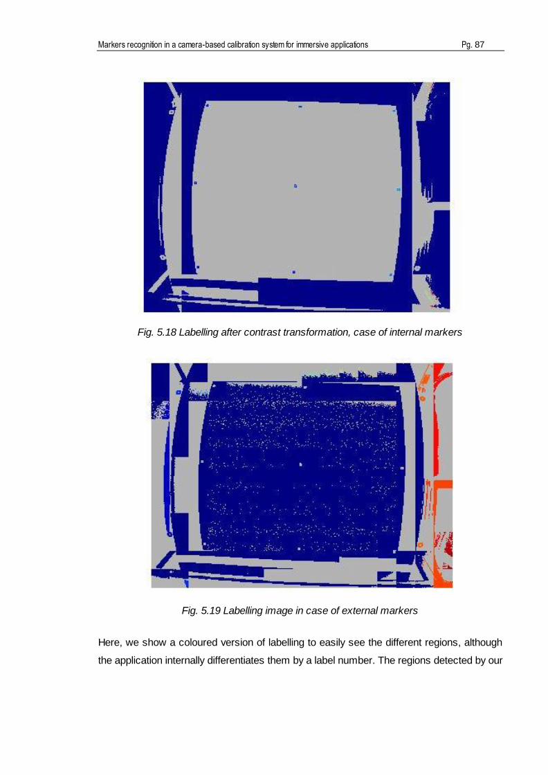
Markers recognition in a camera-based calibration system for immersive applications Pg. 87
Fig. 5.18 Labelling after contrast transformation, case of internal markers
Fig. 5.19 Labelling image in case of external markers
Here, we show a coloured version of labelling to easily see the different regions, although
the application internally differentiates them by a label number. The regions detected by our

Pg. 88 Report
development are those coloured, the ones in gray are considered as background and for
that reason they are discarded from now on, undesirable regions.
With these colours it is fast to see how all our markers are consider regions of interest and
thanks to the criteria described in Section 2.3 we will be able to reject some of those
undesirable labelled regions.
At this point we have to work separately internal and external markers. Some criteria as
size of regions is common to both markers but there are some other ones only usable for
internal markers. We are going to show the results separately depending on which kind of
marker we are extracting.
Shape classification and Object Recognition: Internal markers
In the case of internal markers the strategy was to implement SIFT in our C++ project but
we were not able to make it. So the results shown in this report correspond to the SIFT
algorithm in Matlab [10] but applied to image obtained by C++ performance.
We have considered different situations and according to the results we have get to the
final solution described in Section 3, where the range for size and the ratios of
rectangularity are described.

Markers recognition in a camera-based calibration system for immersive applications Pg. 89
Fig. 5.20 Resulting image with upper size range
As a starting point, we have considered only the upper value for range in size (not lower)
and we see in Fig. 5.20 as all markers are shown but there are also some other noisy
regions we do not want. We have also runned the application in case of only having applied
one or more of the ratios (results are explained widely below in different cases) and all
resulting images where very similar to that one shown above, noisy. What we are going to
show as follows is how affect the different criterion selected, and its combination, and how
the results change at recognizing markers when we apply SIFT algorithm.
Case 1: We have applied an upper threshold value for size and Kurtosis ratio. The image
we obtain is very close to Fig. 5.20. We see that SIFT does not detect neither the marker I1
nor I3 (see Fig. 5.21). But it is also relevant the fact that in the zone nearly I3 one of the
noisy regions is detected as marker (See Fig. 5.22). The rest of markers are properly
detected by SIFT.

Pg. 90 Report
Fig. 5.21 Marker I3. SIFT does not detect marker or noise
Fig. 5.22 Noise near I3 which is detected as a marker by SIFT
As noisy regions are smaller than our markers we thought that a good solution, although
losing relevant information from our markers, was to apply dilation (morphological operator
described in Appendix B) with an appropriate structurant element so it will erase in part or
completely the noisy regions. The tests made were with a 2x2 and 3x3 structurant
element. The problems still remained. So it is demonstrated that applying an upper range
and only kurtosis parameter for rectangularity does not grant a good detection of all our
markers.
Case 2: We have applied an upper threshold value for size and rectangularity ratio. We
see that in I7 and I9, SIFT algorithm is able to distinguish noise from marker (See Fig. 5.23
and Fig. 5.24). It analyses both regions and finally extracts only I9.

Markers recognition in a camera-based calibration system for immersive applications Pg. 91
Fig. 5.23 SIFT frame of marker I9. On the left the study marker where noise and marker
are analyse. On the right, the template marker
Fig. 5.24 SIFT detects marker as marker and reject noise (I9)
At extracting I1 we find the same situation as described in Fig. 5.22 where noise is detect
as marker and the marker is rejected as region of interest.
We apply also dilation (3x3) in this case and we see the results obtained for I9 in Fig. 5.25.
Fig. 5.25 SIFT detects marker and noise as marker I9
Now the marker is detected but also noise, two different keypoint in the image of study are
considered by SIFT as one keypoint in the template. As a result rectangularity applied with

Pg. 92 Report
an upper size range value, with or without dilation, does not ensure that a region in image
is detected as a correct internal marker.
Case 3: We have applied an upper threshold value for size and both, rectangularity and
Kurtosis, ratio.
Fig. 5.26 SIFT detects noise as marker and discards marker I1
We see there is a wrong detection. I1 remains unrecognized and in its place noise is
detected. We see also that I1 is greatly affected by affine features and that its hole in the
middle is really small. We apply dilation 2x2 (See Fig. 5.27) and dilation 3x3 (Fig. 5.28) and
we see what happens.
Fig. 5.27 Detector SIFT after applying dilation with a 2x2 structurant element. Noise and
marker are detected.
Fig. 5.28 Detector SIFT after applying dilation with a 3x3 structurant element. Marker is
detected and noise is rejected
We see that applying an appropriate structurant element the results change. With this
morphological operator we win some white pixels in the middle of the marker and this way,
SIFT is able to match the keypoints of the study marker and the template. Dilation has a

Markers recognition in a camera-based calibration system for immersive applications Pg. 93
double function, as well as it transforms the inside of the marker to something more similar
to the template it also reduces noise, making the undesirable area smaller and also more
different. So keypoints from marker of study are another ones which not correspond to the
ones in template.
From the results of 3 cases, we see that our conflictive regions are those small, which can
become wrong detections. A good solution seems to select a range with an upper and
lower size values and see if those undesirable noisy areas are reduced. If they are not
erased we can use the combining of lower and upper size range and dilation.
Case 4: We have applied an upper and lower threshold value for size without ratios. As
we have seen in all our cases, the more conflictive pixels are I1, I2 and I3. The reason is
not only noise but also their projection on the cylindrical surface (big affine effect). If we
apply both thresholding values we see that the problem of noise almost disappears and
now the detection of the markers have more keypoints in common. See Fig. 5.29 where I7
is shown.
Fig. 5.29 SIFT detection of marker I7
However, the problem of no detection of I1, I2 and I3 still remains. So dilation will be the
better solution.
As a summary, what we have decided is to use the combination of size and both
rectangularity criteria. It has been proved that small regions are the most annoying and that
the presence of a lower value of size range reduces highly these undesirable
appearances. In our GUI there is an option called Optimization (described in Section 4.4),
that can be applied after discarding regions with the methods described and which applies
dilation to improve the inside part of the marker and this way make the SIFT algorithm
extraction more robust.
Before ending this part, it is important to say that can appear problems with dilation if we
are not careful. We can not chose any structurant element and not all sizes, because
dilation is applied to whole image and we want to improve the internal part of conflictive

Pg. 94 Report
markers but not modifying so much those rightly detected. If we do not take care of that we
will alter the properties of our markers and then leading to wrong detections. See figures
below to value the effect.
Fig. 5.30 From left to right: resulting marker, dilation 2x2 and dilation 3x3 of marker I3
Fig. 5.31 From left to right: resulting marker, dilation 2x2 and dilation 3x3 of marker I5
If the structurant element is big enough the inside part of the marker can arrive to be part of
the background, and the marker lose its features.
Shape classification and Object Recognition: External markers
In the case of external markers we are not interested in rectangularity ratios and the only
problem we have is to choose an appropriate size range and contours will extract circular
markers.
As follows we can see the results of applying an upper threshold of the image.

Markers recognition in a camera-based calibration system for immersive applications Pg. 95
Fig. 5.32 Resulting image (before applying contours) with only upper size value
We can identify our markers and some other noisy regions. Internal markers do not appear
because the labelling used in external markers considers internal markers as undesirable
and they are rejected in the labelling step.

Pg. 96 Report
Fig. 5.33 Resulting image (after applying contours) with only upper size value where centre
of ellipses are detected in red
Although those regions are not detected as circles (see Fig. 5.33 where only external
markers are detected as ellipses, in red) for avoiding the possibility of wrong detections we
are going to select a lower and upper size range as in the case of internal markers. Mostly
noisy regions disappear. Detecting circles is not really the problem in this case as can be
seen in Fig. 5.34 and Fig. 5.35 where the only noisy region remaining is not a circle. For
that reason, it is not detected (in red).
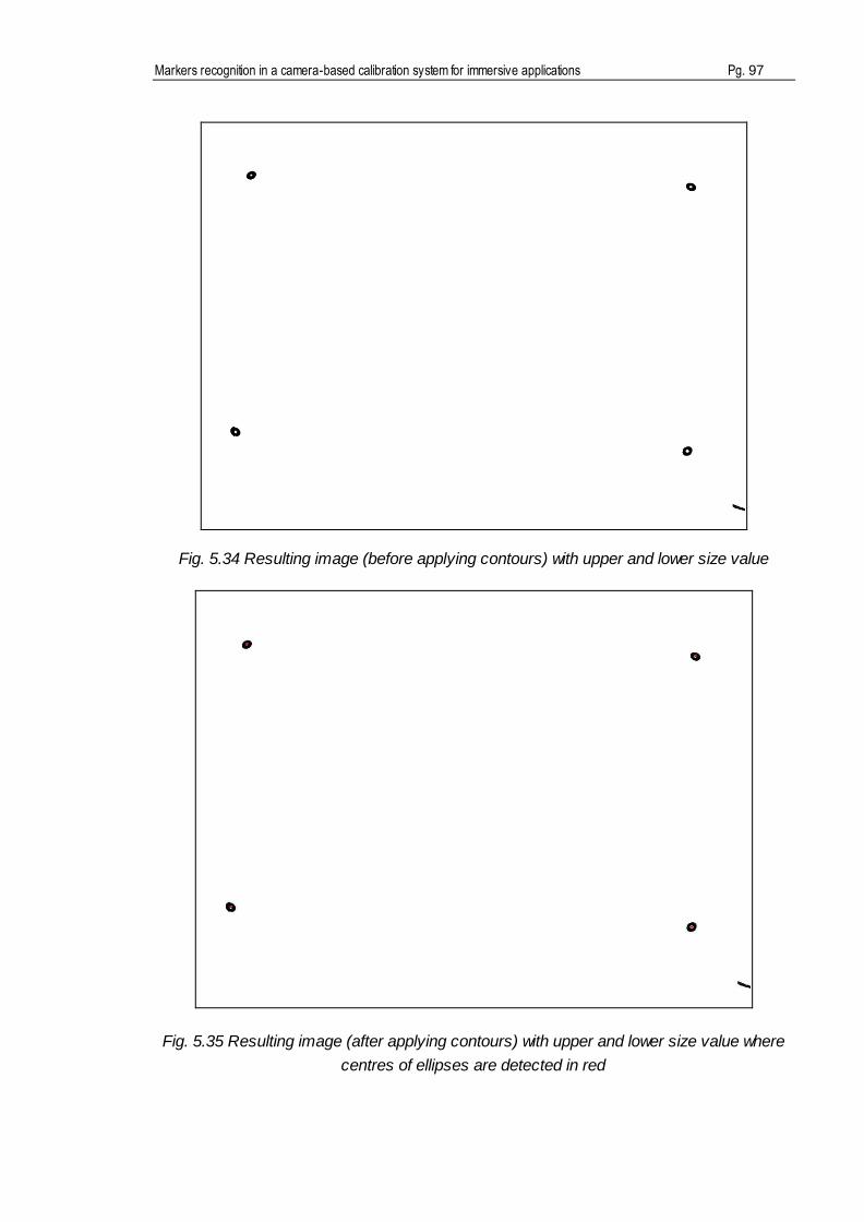
Markers recognition in a camera-based calibration system for immersive applications Pg. 97
Fig. 5.34 Resulting image (before applying contours) with upper and lower size value
Fig. 5.35 Resulting image (after applying contours) with upper and lower size value where
centres of ellipses are detected in red

Pg. 98 Report
With external markers the critical moment appears before this step, at thresholding. We
find that some of the parts of the cylindrical structure are very similar to our external
markers, in terms of brightness, and also very close. That makes that, if wrong
parameters in Wall‟s algorithm block are chose, some undesirable regions and our
markers become connected and we lose the properties of our external markers which will
not be extracted. The effect can be seen in Fig. 5.37.
Fig. 5.36 Adequate size of Wall’s algorithm for detecting external markers.
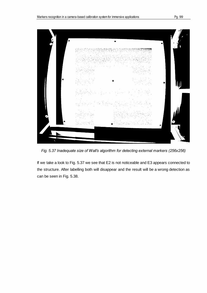
Markers recognition in a camera-based calibration system for immersive applications Pg. 99
Fig. 5.37 Inadequate size of Wall’s algorithm for detecting external markers (256x256)
If we take a look to Fig. 5.37 we see that E2 is not noticeable and E3 appears connected to
the structure. After labelling both will disappear and the result will be a wrong detection as
can be seen in Fig. 5.38.

Pg. 100 Report
Fig. 5.38 Wrong detection of External Markers. E2 and E3 are not detected
It is relevant at this point to remember that the whole process have to be controlled by a
person in order to obtain good results.
Rotation
As we have only one testimage we have done another test with the same image but
rotated (testimage_rotate.bmp).

Markers recognition in a camera-based calibration system for immersive applications Pg. 101
Fig. 5.39 testimage_rotate.bmp, a rotation 90 degrees to the left of testimage
For our application the image after rotating 90 degrees to the left becomes completely
different. Some changes in the image are mentioned as follows:
Image size: the new size of image is 1536x 2048, width and height change respect
original testimage (2048x 1536)
Light distribution: now the effect of light will affect to other markers, so the
conflictive ones (those in the upper row) will change
Size of Wall‟s algorithms: the same sizes of blocks will give different binary images
and the regions determined will not be the same.

Pg. 102 Report
The features that will remain the same are those relative to our markers, rectangularity and
ellipticity.
In the case of internal markers, if we maintain the size of Wall‟s blocks (256x256), the
resulting binary image is Fig. 5.40 which can be compared with Fig. 5.11.
Fig. 5.40 Binarization of testimage_rotate.bmp with Wall’s blocks size of 256x256
Mainly differences can be seen in noisy isolated pixels in the area enclosured by new I1, I2,
I4 and I5, and in the upper-central part and down-left parts of the structure. Binarization
respects internal markers and its internal hole so detection will follow properly.
In the case of external markers, the results of the binarization are shown in Fig. 5.41
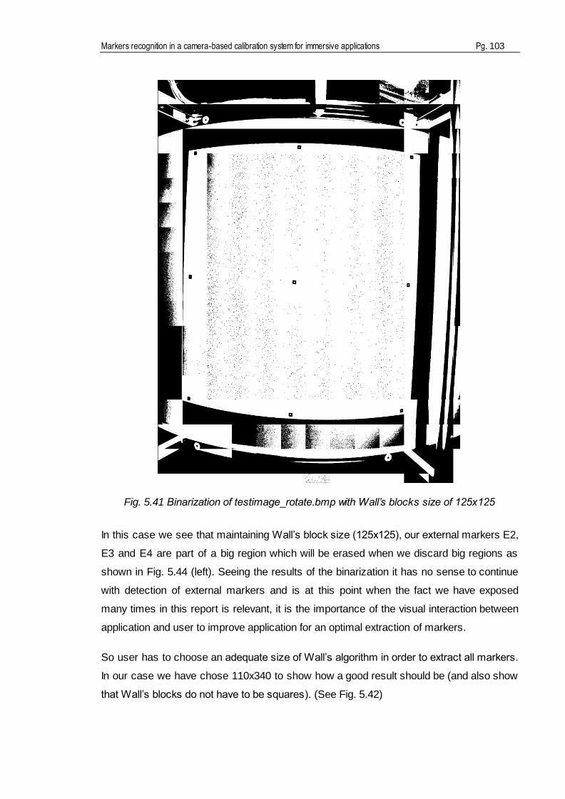
Markers recognition in a camera-based calibration system for immersive applications Pg. 103
Fig. 5.41 Binarization of testimage_rotate.bmp with Wall’s blocks size of 125x125
In this case we see that maintaining Wall‟s block size (125x125), our external markers E2,
E3 and E4 are part of a big region which will be erased when we discard big regions as
shown in Fig. 5.44 (left). Seeing the results of the binarization it has no sense to continue
with detection of external markers and is at this point when the fact we have exposed
many times in this report is relevant, it is the importance of the visual interaction between
application and user to improve application for an optimal extraction of markers.
So user has to choose an adequate size of Wall‟s algorithm in order to extract all markers.
In our case we have chose 110x340 to show how a good result should be (and also show
that Wall‟s blocks do not have to be squares). (See Fig. 5.42)
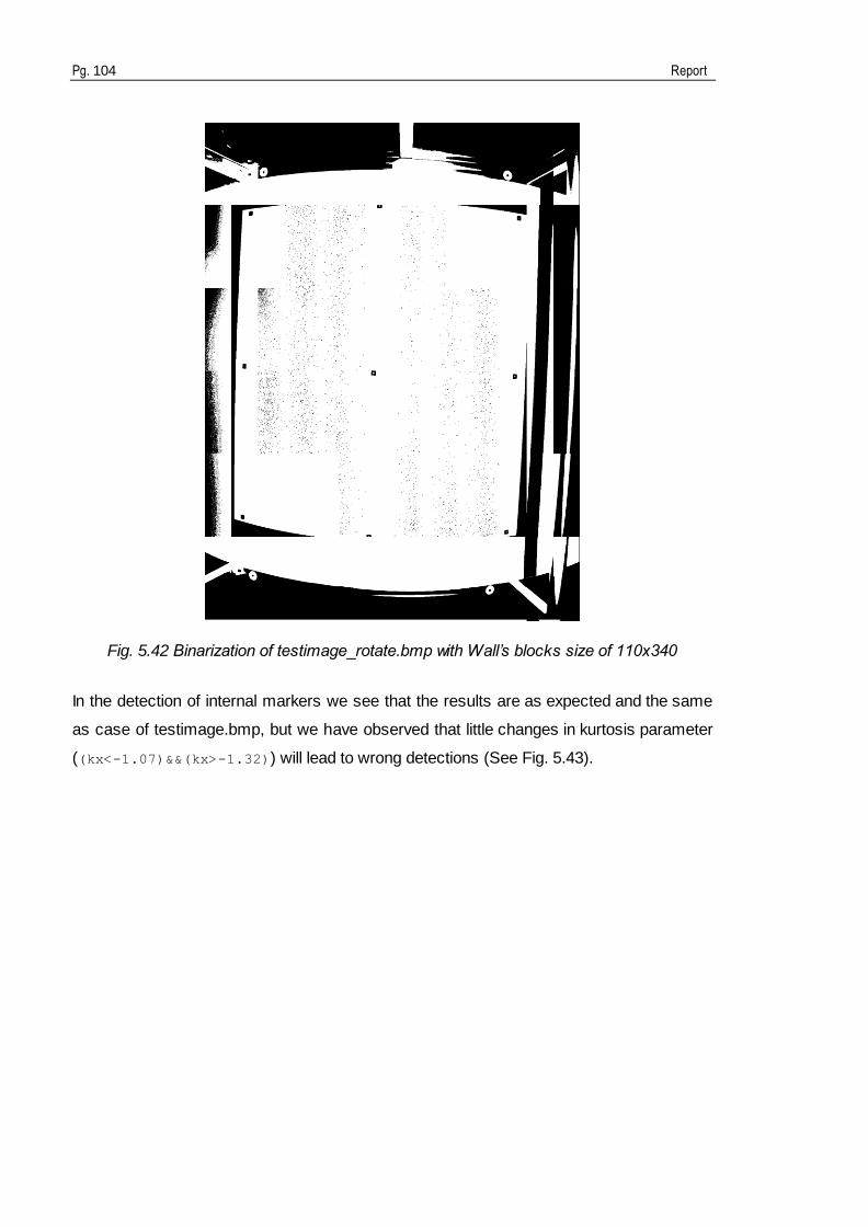
Pg. 104 Report
Fig. 5.42 Binarization of testimage_rotate.bmp with Wall’s blocks size of 110x340
In the detection of internal markers we see that the results are as expected and the same
as case of testimage.bmp, but we have observed that little changes in kurtosis parameter
((kx<-1.07)&&(kx>-1.32)) will lead to wrong detections (See Fig. 5.43).
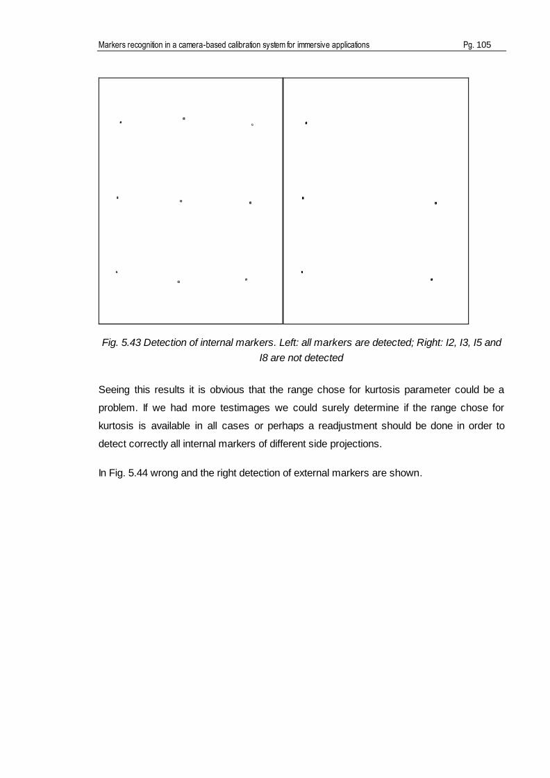
Markers recognition in a camera-based calibration system for immersive applications Pg. 105
Fig. 5.43 Detection of internal markers. Left: all markers are detected; Right: I2, I3, I5 and
I8 are not detected
Seeing this results it is obvious that the range chose for kurtosis parameter could be a
problem. If we had more testimages we could surely determine if the range chose for
kurtosis is available in all cases or perhaps a readjustment should be done in order to
detect correctly all internal markers of different side projections.
In Fig. 5.44 wrong and the right detection of external markers are shown.

Pg. 106 Report
Fig. 5.44 Detection of external markers. Left: E2, E3 and E4 are not detected because in
binarization they are connected to a big region; Right: right detection.
So altogether what we see from the results of running our application to testimage and
rotate image is that the values and ratios selected are good at extracting markers in both
cases internal and external. The first step of pre-processing is really important to ensure a
better performance of next steps in the image processing chain. The use of different sizes
for Wall‟s blocks is possible in local-thresholding but it is important the supervising of the
binarized image obtained in order not to loose relevant information of desired objects which
will cause non detections after labelling if a wrong size is chosen.
In case of internal markers the combination of 3 descriptors described performs a good
extraction and SIFT algorithm gives robustness to the object recognition. In the case of
external markers, the method based on contours obtains right detections of external
markers.
We have seen that some little changes in ratios/parameters affect to the results obtained
so the problem we find is the small amount of images of test that we have. More images
should be taken in order to conform a larger database and this way ensure that the
adjustment of the parameters and ratios respond properly to all cases.
Markers recognition in a camera-based calibration system for immersive applications Pg. 107
6. Conclusions
Immersive environments were born to provide the user a panorama of 360 degrees with
which he/she can interact. Immersion consists in giving the user the impression of being in
a real world at any place at any time although he/she is in a virtual reality recreated by
computer with the aim of giving this reality sensation. The immersive media techniques are
a very ambitious line of study in nowadays image and video processing and it can be
applied into many applications as live broadcasting of sport events, theatre, museums and
music events and also immersive video gaming. In these scenarios it is very important the
continuity of panorama recreation because human sight is very sensible to changes in
illumination and transitions and, if continuity between images is not provide, user will not
feel the total immersion. To obtain this continuity, different calibration systems are used.
In our case the scenario built in IGD Fraunhofer Institute, in the context of hArtes project, is
a system based in an array of projectors and cameras where calibration is needed to
provide immersion. So the objective is to correct those misalignments and overlappings in
the junctions between projections so the changes are not noticeable for the person who is
inside. The calibration has different steps and my contribution is the first step, which
consists in the univocal recognition of internal (squares) and external (circles) markers
from a projected image through image processing techniques. After this step a correction
between real and ideal markers followed by a correction in the misalignments in junctions
will be done.
My contribution to hArtes Project in IGD is the development and implementation of a GUI
application in C++ programming language. The application searches, through image
processing chain, the univocal recognizement of markers in a given image (desired
markers left untouched and non desired ones are rejected) by developing a graphical
interface between user and image obtained from projection onto cylindrical surface. The
Win 32 console application developed has different buttons to select different options and a
visor to see image results. As a starting point we have included a pre-processing step in
which a greyscale transformation and a sharpen filter have been applied. After that, the
processing chain has consisted in many steps. The first one is thresholding. A previous
segmentation of image was needed (Wall‟s blocks algorithm) in order to avoid the effect of
irregular illumination onto the projected image, after that a threshold value based in Ridley
and Calvard‟s algorithm has been chosen and after all we have obtained a binary image.
As a second step, we have labelled the regions in image and we have analyzed each
region for determining if shape corresponds to our markers or not (through moments,
rectangularity ratios and contours). As a final step the object recognition has been ensured
thanks to application of SIFT as matching algorithm between our marker and the ideal one.

Pg. 108 Report
The results obtained show the importance of choosing a local threshold technique and an
adequate size of Wall‟s algorithm in order to perform a binarization which preserves our
markers. It is at this point where it is also important the fact of the interaction between user
and application, where thanks to the visor of the application user can determine if the
parameters selected are valid in each case. After running the application we see that
parameters and ratios chosen are adequate at recognizing markers in testimage given,
although our images of testing are not enough (in amount) to ensure that the application
will respond correctly to all of them, because we have also seen that little changes in
parameters lead to wrong recognition. So as a further approach it will be interesting to build
a larger data base in order to adjust parameters (if required) to ensure this extraction in all
cases.
Finally, this project has been left at the disposal of IGD- Fraunhofer for hArtes project
and/or further projects in which my contribution could be useful.

Markers recognition in a camera-based calibration system for immersive applications Pg. 109
7. References
[1] RAFAEL C. GONZALEZ, RICHARD E. WOODS Digital Image Processing, Prentice
Hall Second edition 2002
[2] MILAN SONKA, VACLAV HLAVAC, ROGER BOYLE Image Processing Analysis and
Machine Vision, Pacific Grove, CA : PWS Pub. 1999
[3] KENNETH R. CASTLEMAN Digital image processing, Englewood Cliffs, N.J.
Prentice-Hall, c1979
[4] DMITRIJ CSTVERIKOV Basic Algorithms for Digital Image Analysis Eötvös Loránd
University Budapest http://visual.ipan.sztaki.hu/ELTEfoliak/
[5] BERNT SCHIELE Slides in Computer Vision Subject TU Darmstadt 2007
[6] MEHMET SEZGIN, BULENT SANKUR Survey over image thresholding techniques
and quantitative performance evaluation, Journal of Electronic Imaging 13(1), 146–
165 2004
[7] SHAPIRO, LINDA G. & STOCKMAN, GEORGE C. Computer Vision, Prentice Hall
2002
[8] PIERRE D. WELLNER Adaptive Thresholding for the Digital Desk Technical Report
EPC-1993-110
[9] T. W. RIDLER, S. CALVARD, Picture thresholding using an iterative selection
method, IEE Trans. System, Man and Cybernetics, SMC-8 (1978) 630-632
[10] ANDREA VEDALDI An implementation of SIFT detector and descriptor University of
California at Los Angeles 2006)
[11] PAUL L. ROSIN Measuring rectangularity August 1999
[12] PAUL L. ROSIN Measuring Shape: Ellipticity, Rectangularity and Triangularity IEEE
2000 and Revision of July 2002
[13] TOUSSAINT 1983, PIRZADEH 1999 Solving geometric problems with rotating
Callipers
[14] A.P. REEVES The General Theory of Moments fro Shape Analysis and the Parallel
Implementation of Moment Operations TR-EE October 1981

Pg. 110 Report
[15] A. P. REEVES AND A. ROSTAMPOUR Shape Analysis of Segmented Objects
Using Moments IEEE August 1981
[16] D. G. LOWE Object recognition from Local Scale invariant features International
Conference on Computer Vision, Corfu, Greece (September 1999)
[17] D. G. LOWE, Local feature view clustering for 3D object recognition IEEE
Conference on Computer Vision and Pattern Recognition, Kauai, Hawaii (December
2001)
[18] D. G. LOWE Distinctive Image Features from scale-Invariant Keypoints International
Journal of Computer Vision, 60, 2 (2004)
[19] M. BROWN, D. G. LOWE Invariant features from interest point groups British
Machine Vision Conference, BMVC 2002, Cardiff, Wales (September 2002)
[20] MUNDY, ZISSERMAN Geometric Invariance in Computer Vision Cambridge, MA,
The MIT Press. (1992)and REISS 1993.
[21] MIKOLAJCZYK, SCHMID A performance evaluation of Local Descriptors 2005
[22] J. BEIS , D. G. LOWE Shape indexing using approximate nearest-neighbour search
in high dimensional spaces Proceeding of IEEE Computer Society Conference on
Computer Vision and Pattern recognition 1997
[23] HERBERT BAY, TINNE TUYTELAARS AND LUC VAN GOOL SURF: Speeded Up
Robust Features, 9th European Conference on Computer Vision, 7-13 May 2006
[24] JOHANNES BANER, NIKO SÜNDERHAUF, PETER PROTZEL Comparing several
implementations of two recently published feature detectors 2007
[25] HARRIS, STEPHENS A combined corner and edge detector, Proc. 4th Alvey Vision
Conf., Manchester, 1988.
[26] M.KUDZINAVA, R. GARCIA, J.MARTI Feature based matching of underwater images

Markers recognition in a camera-based calibration system for immersive applications Pg. 111
A. Ridley and Calvard’s method
Using thresholding there is normally an error performing segmentation:
Fig. A.1 The queues of two different Gaussian distributions can lead to erroneous
detections at thresholding (from Digital Image Analysis Lars Audal July 24th
2006)
We assume that the histogram is the sum of two distributions b(z) and f(z) where b and f
are the normalized background and foreground distributions respectively and z is the gray
level.
If B and F are prior probabilities for the background and foreground, altogether have to be 1
(B+F=1) and the histogram can be written as:
Given a threshold t the probabilities of erroneously classifying a pixel is given by:
( ) ( )
t
BE t f z dz
( ) ( )F
t
E t b z dz

Pg. 112 Report
So the total error will be:
( ) ( ) ( )
t
t
E t F f z dz B b z dz
Using Leibniz‟s rule for derivation of integrals and setting the derivative equal to zero the
optimal value for t is found:
( )0 ( ) ( )
E tFf T Bb T
dt
Assuming b(z) and f(z) are Gaussians distributions it is possible to solve the above
equation explicitly. The equation becomes:
Some algebraic manipulations will transform this equation into a second order equation in
T:
If the standard deviations of the two distributions are equal (σB=σF=σ) then the expression
can be simplified:
That can be solved explicitly for T:

Markers recognition in a camera-based calibration system for immersive applications Pg. 113
If the two distributions B and F are roughly equiprobable then
and:
( )
2
B FT
This equation is the foundation of Ridley and Calvard‟s method. As μB and μF are unknown
we must estimate them based on suggested thresholds.

Pg. 114 Report
B. Morphological operators
Structuring element: consists of a pattern specified as the coordinates of a
number of discrete points relative to some origin. Normally cartesian coordinates
are used and so a convenient way of representing the element is as a small image
on a rectangular grid. The origin does not have to be in the centre of the structuring
element, but often it is.
Dilation: For each background pixel we superimpose the structuring element on
first pixel of image so that the origin of the structuring element coincides with the
image pixel position. If at least one pixel in the structuring element coincides with a
foreground pixel in the image underneath, then the input pixel is set to the
foreground value. If all the corresponding pixels in the image are background,
however, the pixel is left at the background value. We repeat the process through
whole image.
Erosion: The basic effect of the operator on a binary image is to erode away the
boundaries of regions of foreground pixels (i.e. white pixels, typically). Thus areas
of foreground pixels shrink in size, and holes within those areas become larger.
Opening: The effect of the operator is to preserve foreground regions that have a
similar shape to this structuring element, or that can completely contain the
structuring element, while eliminating all other regions of foreground pixels.
Closing: The effect of the operator is to preserve background regions that have a
similar shape to this structuring element, or that can completely contain the
structuring element, while eliminating all other regions of background pixels.

Markers recognition in a camera-based calibration system for immersive applications Pg. 115
C. How are images formed?
In this appendix we include a short explanation about how objects of real world become
digital images so we can work with them in the computer.
An image is a visual representation of a person, an object or an environment. It contains
descriptive information about what it represents.
An image can be defined as a two-dimensional continuous function ( , )f x y where x and
y are spatial (plane) coordinates and the amplitude of f at any pair of coordinates ( , )x y
is called intensity or gray-level of the image at that point.
When we project the real world onto a two-dimensional image plane, we uncover the two
key questions of image formation:
What determines where the image of one point will appear?
What determines how bright the image of some surface will be?
To answer these questions it is necessary to consider two processes to convert the
continuous sensed data (image) into digital form: sampling and quantization.
Sampling (Spatial resolution): Is the process of digitalizing the image in spatial
domain. The sampling process may be viewed as partitioning the x y plane into a
grid, with the centre of each grid being a pixel. The digitizing of the x and y
coordinate values is based on geometry of image formation which determines
where in the image plane the projection of a point in the scene will be placed (see
Appendix D for more information). Sampling determines spatial resolution, which is
the smallest discernable detail in image. The more pixels in a fixed range, the
higher resolution.
Quantization (Gray-scale resolution): is the process of digitizing amplitude f
values into discrete gray values. Physics of light determine the brightness of a
point in the image plane as a function of illumination and surface properties.
Radiometry theory demonstrates existent linear relationship between them. (See
Appendix E). Quantization determines the gray-scale resolution which refers to
smallest discernible change in gray-scale level. The more bits the higher the
resolution.

Pg. 116 Report
Fig. C.1 Upper left: continuous image; Upper right: A scan line from A to B in the
continuous image; Down left: sampling and quantization; Down right: digital scan line (by
Chapter 2 of [1])
Once we know where each pair of coordinates are projected and with which intensity, it is
time to convert optical image into an electrical image thanks to camera electronics. This
process is called sensing and it is widely explained in Appendix F. (The explanation of the
process is only valid for cameras based on CMOS sensor as used in our project to
capture the images. Some other cameras as based on CCD Sensor do not work the
same way and they are not described in this report).
After sensing the objective of generating digital image from sensed data is completed.
( , )f x y &Sampling Quantization ( , )f i j
0 ( , )f x y MxN

Markers recognition in a camera-based calibration system for immersive applications Pg. 117
Fig. C.2 Left: This image illustrates a continuous image projected onto a sensor array.
Right: result of image sampling and quantization (by Chapter 2 of [1])
The result of sampling and quantization is a matrix of real numbers. Fig. C.3 shows the
coordinate conversion used throughout this book.
Fig. C.3 Coordinate system for the representation of digital images (by Chapter 2 of [1])
We obtain the digital image of the scene we want to analyse so we are prepared to start
working on our project of detecting internal and external markers.
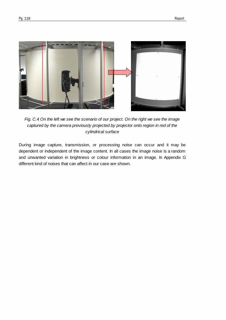
Pg. 118 Report
Fig. C.4 On the left we see the scenario of our project. On the right we see the image
captured by the camera previously projected by projector onto region in red of the
cylindrical surface
During image capture, transmission, or processing noise can occur and it may be
dependent or independent of the image content. In all cases the image noise is a random
and unwanted variation in brightness or colour information in an image. In Appendix G
different kind of noises that can affect in our case are shown.

Markers recognition in a camera-based calibration system for immersive applications Pg. 119
D. Geometry of image formation
The mathematical relationship between the coordinates of a 3D point and its projection
onto the image plane can be modelled, as a first approximation, by a pinhole camera.
The ideal pinhole camera is described as a black box with a small hole. When rays coming
from illuminated objects penetrate through the small hole you will see them inside the black
box, over one of the walls, reduced in size and inverted due to the intersection of the rays
of light that pass through.
The wall where the object projection is shown is known as the image plane and the small
hole as the camera aperture.
Fig. D. 1 Pinhole model (from slides TU-Darmstadt Bernt Schiele- Computer Vision
SS2007 )
In the ideal case (the simplest) no lenses are used to focus light, so it does not consider
the effects of optical systems on an image.
We can introduce thin lenses in the pinhole system. The mission of lenses placed in the
aperture is to focus the bundle of rays from each scene point onto the corresponding point
in the image plane. This way we obtain the same projection as the pinhole but it also
gathers a finite amount of light. The larger the lens the larger the solid angle it subtends
when seen from the object.
It can also appear degradation which can be due to effects of diffraction because of the
wave nature of light or due to lens aberration, imperfectly designed and manufactured
optical systems.
If we use a wide pinhole, light from the source spreads across the image (i.e., not properly
focussed) making it blurry.

Pg. 120 Report
If we narrow the pinhole, only a small amount of light is let in. That means that the image
sharpness is limited by diffraction, when light passes through does not travel in a straight
line and light is scattered in many directions (quantum effect).
In general the aim of using lens is to enlarge aperture size while keeping the image
focussed.
Although it is not a perfect model it is a reasonable good description for computer vision
and computer graphics and some of the effects can be compensated with an adequate
coordinate transformation of the 3D projection on the image coordinates.
Coordinate transformation: homogeneous coordinates
For mapping three dimensional points to a two dimensional plane we consider two kind of
3D projection:
Orthographic projection
These projections are a set of transformations often used to show profile, detail or precise
measurements of a real object. The camera direction (normal component of the viewing
plane) is always parallel to one of the 3D axes. If we have a 3D point (ax, ay, az) and we
want to project it to a 2D point (bx, by) using projection parallel to the y axis (Profile view).
We can use the equations
x x x xb s a c
y z z zb s a c
where s is an arbitrary scale factor and c an arbitrary offset. Constants are optional and
can be used to a better alignment of the viewpoint.
In this kind of projection, lengths of all points of the projected image have the same scale
independent of whether they are near or far away to the viewer. As a result, lengths near to
the viewer appear foreshortened. In order to solve this problem we can use Perspective
Projection.
Perspective projection
It is more complex than orthographic. For the understanding of how this projection works
we have to think about the 2D projection as a viewfinder, where the camera‟s position,
orientation and field of view control the behaviour of the projection transformation.

Markers recognition in a camera-based calibration system for immersive applications Pg. 121
We consider:
, ,x y za – object coordinates (particular concrete point of the object)
c x, y, z – location of the camera
φ x, y, z – rotation of the camera
e x, y, z – viewer position in camera coordinates
b x, y- 2D projection of , ,x y za
Note: if c x, y, z =<0,0,0> and φ x, y, z=<0,0,0>, the 3D vector <1,2,0> becomes <1,2> in the
projected 2D vector.
We define a new point , ,x y zd which is a translation of the point , ,x y za into the coordinate
system defined by c (camera coordinates). This can be achieved by subtracting c from a
and then applying a vector rotation matrix using – φ to the result. Assuming left-hand
system of axes:
1 0 0 cos 0 sin cos sin 0
0 cos sin 0 1 0 sin cos 0
0 sin cos sin 0 cos 0 0 1
x y y z z x x
y x x z z y y
z x x y y z z
d a c
d a c
d a c
If we used the projection plane as x/y, this transformed point , ,x y zd can be projected onto
the 2D plane using:
or using homogeneous coordinates to unify the representation for points and lines by
adding in one dimensionality:
1 0 0
0 1 0
0 0 1 0
110 0 0
xx x
yy y
z z
w
z
ef d
ef d
f d
fe
=( )z
x x x
z
eb e d
d=( )
zy y y
z
eb e d
d

Pg. 122 Report
with =x
x
w
fb
f and =
yy
w
fb
f
Homogeneous coordinates make possible the calculations in projective spaces just as
Cartesian coordinates do in Euclidean space.
Image formation (geometrical)
We have to be able to transform object coordinates, 3D information, onto pixel
coordinates, 2D information, so we can work with information contained in the photo
captured.
Considering a camera with a thin lens (pinhole camera), it performs a perspective
projection and we can find a matrix which describes the mapping between 3D points of the
world to 2D points on the image plane.
Object Coordinates (3D)
World Coordinates (3D)
Camera Coordinates (3D)
Pixel Coordinates (2D)
Image Plane Coordinates (2D)
Extrinsic camera parameters
Intrinsic camera parameters
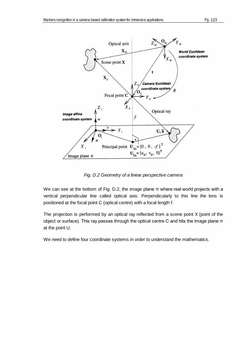
Markers recognition in a camera-based calibration system for immersive applications Pg. 123
Fig. D.2 Geometry of a linear perspective camera
We can see at the bottom of Fig. D.2, the image plane π where real world projects with a
vertical perpendicular line called optical axis. Perpendicularly to this line the lens is
positioned at the focal point C (optical centre) with a focal length f.
The projection is performed by an optical ray reflected from a scene point X (point of the
object or surface). This ray passes through the optical centre C and hits the image plane π
at the point U.
We need to define four coordinate systems in order to understand the mathematics.

Pg. 124 Report
Coordinate
system
Notation Origin Points expressed in
coordinate system
World
Euclidean
W Ow X, U
Camera
Euclidean
C Oc=C Z
Image
Euclidean
I Oi X, Y
Image affine A Oi Coordinates u,v,w
Coordinates w and v have the same orientation as Zi and Yi but this is not the case with u
and Xi. The reason why is that pixels need not to be perpendicular and axes can be scaled
differently. The affine coordinate system is induced by the arrangement of the retina.
U0 is the intersection of the optical axis with the image plane π and this point Uo in affine
coordinate system is expressed as U0a=[u0,v0,0]T.
A representation of a point in the world coordinate system, for example X, is a vector 3x1.
To express this point in the camera Euclidean coordinate system (Xc) we have to align the
coordinate systems by translating and rotating the world point.
Rotation (R) consists in three elementary rotations pan, tilt and roll, axes x, y and z
respectively. Translation (t) vector gives three elements of the translation. So there are six
degrees of freedom called extrinsic parameters.
This point is projected onto the image plane π (through the thin lens we suppose ideal), we
call it Uc.
The projected point Uc can be derived from the similar triangles of the image:
( )
c
c c w
c
x
X y R X t
z

Markers recognition in a camera-based calibration system for immersive applications Pg. 125
Fig. D.3 Similar triangles
and we obtain
c
c
x
c
y
c
f
z
fUc
z
f
It remains to derive where the projected point is positioned in the image affine coordinates
system, i.e., to determine the coordinates which the real camera actually delivers.
The origin of the image in image affine coordinate system is at the top left corner and
represents a shear and rescaling of the image Euclidean coordinate system.
Uc can be represented in the 2D image plane π by homogeneous coordinates as ũ
=[U,V,W]T and in 2D Euclidean as u =[u,v]T=[U/W,V/W]T.
Homogeneous coordinates allow us to express affine transformation as a multiplication by
a 3x3 matrix with a, b and c unknown, which describe the shear together with scaling along
the axes:
ũ
0 0
0 00 0
0 0 1 0 0 11 1
c c
c c
x
c c
y
c c
f x
z zU a b u fa fb uf y
V c v fc vz z
W

Pg. 126 Report
We can multiply both sides of the equation by per zc and this way we can remove it and
rewrite the expression depending on K, the camera calibration matrix:
zc ũ =
0
00 ( ) ( )
0 0 1
w w
fa fb u
fc v R X t KR X t
As we can see the matrix is upper-triangular and these coefficients are called intrinsic
parameters of the camera and describe the specific camera independent on its position
and orientation in space.
If we express the scene point X in homogeneous coordinates X‟w =[Xw,1]T, we can write
the perspective projection using a single 3x4 matrix. The leftmost 3x3 submatrix describes
rotation and the rightmost column a translation.
ũ | '1 1
w w
w
UX X
V KR KRt M MX
W
where X‟ is the 3D scene point in homogeneous coordinates and M is called the Projective
Matrix or camera matrix.
Thanks to the introduction of projective space and homogeneous coordinates we obtain a
linear equation to express the transformation from the 3D world to 2D.

Markers recognition in a camera-based calibration system for immersive applications Pg. 127
E. Physics of light: Radiometry
The physics of light determines the brightness of a point in the image plane as a function of
illumination and surface properties.
Fig. E.1 How rays of light project onto surface element and they onto camera sensor
The scene is illuminated by a single source
The scene reflects radiation towards the camera
The camera senses it via chemicals on film (sensing).
With the knowledge of radiometrics concepts (Appendix H) we can differentiate between
two concepts of brightness:
Scene Radiance: it is related to the energy flux emitted from a surface. This emission
depends on how the objects are illuminated and how they reflect light. Scene Radiance
can be measured by the Radiance (L).
Image Irradiance: it which is related to energy flux incident on the image plane and can be
measured by the Irradiance (E). This term depends on how much light arrives to the
surface of the object coming from the scene point X.
The measurement of the brightness in the image also depends on the spectral sensitivity
of the sensor.

Pg. 128 Report
Fig. E.2 Scheme from scene radiance to image irradiance
What is really important of all this concepts is that we are working with a linear mapping
because there is a lineal dependency between Radiance and Irradiance.
Fig. E.3 Relationship between angles and areas of the surface and the image plane
From the image we can see that solid angles (orange and blue) are the same i sdw dw
and we can find a relationship between areas s
i
dA
dA. So the solid angle subtended by the
lens is:
The flux received by lens from dAs is the same as the flux projected onto the image dA i :
( cos ) Ls iL dA dw E dA

Markers recognition in a camera-based calibration system for immersive applications Pg. 129
If we combine both equations we obtain:
which demonstrates the relationship between Image Irradiance and Scene Radiance.
The constant of proportionality depends on the optical system and with a small field of view
the effects of the 4th power cosine are small.
We must have an aperture of finite size (different from zero) because we need to gather a
finite amount of light in the image plane but with small pinhole. That is because of the wave
nature of light which has higher diffraction at the edge of the pinhole and the light is spread
over the image. As we make the pinhole smaller the larger fraction of incoming light is
deflected far from the direction of the incoming ray.
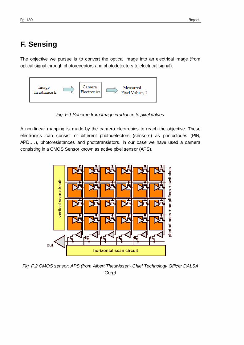
Pg. 130 Report
F. Sensing
The objective we pursue is to convert the optical image into an electrical image (from
optical signal through photoreceptors and photodetectors to electrical signal):
Fig. F.1 Scheme from image irradiance to pixel values
A non-linear mapping is made by the camera electronics to reach the objective. These
electronics can consist of different photodetectors (sensors) as photodiodes (PIN,
APD,…), photoresistances and phototransistors. In our case we have used a camera
consisting in a CMOS Sensor known as active pixel sensor (APS).
Fig. F.2 CMOS sensor: APS (from Albert Theuwissen- Chief Technology Officer DALSA
Corp)

Markers recognition in a camera-based calibration system for immersive applications Pg. 131
An APS is an image sensor consisting in an integrated circuit containing an array of pixel
sensors where each pixel gets its individual amplifier. This small amplifier boosts the
photodiode signal fed to the column line and solves the noise problem of the large column
lines. All amplifiers are analogue in nature, i.e., no two amplifiers are perfectly matched as
far as gain and off-set are concerned. Therefore the introduction of an amplifier within
every pixel increases the non-uniformity between the various pixels of the array. This effect
shows up as fixed-pattern noise. This is a disadvantage of CMOS image sensor relative to
other ones like CCD used in higher quality photographic works.
Every pixel consists of a photodetector, a transfer gate (TX), a reset gate (RST), a
selection gate (RS: row selection), source-follower readout transistor (MSF) and a selection
transistor (MSEL).
Fig.F.3 Pixel sensor and its transistors (from Albert Theuwissen- Chief Technology Officer
DALSA Corp)
The photodetector is usually a photodiode. In this case the photodiode does not have any
electrical connection to force the collected charge out of the photodiode. To initiate the
charge transport from the photodiode towards the floating diffusion (n+) the transfer gate
(TX) is pulsed.

Pg. 132 Report
When light comes it causes an accumulation or integration of charge on the „parasitic ‟
capacitance of the photodiode, creating a voltage change related to the incident light.
Transistor Mrst acts as a switch to reset the device. When this transistor is turned
on the photodiode is effectively connected to the power supply VRST. This way it
clears all integrated charge. As the reset transistor is n+ type the pixel operates in
soft reset.
Transistor Msf acts as a buffer. It is an amplifier which allows the pixel voltage to be
observed without removing the accumulated charge. Its power supply VDD is
typically tied to the power supply of the reset transistor.
Transistor Msel is a switch that allows that read-out electronics read a single row of
the pixel array.
An advantage of using electronics is that allows us to read directly the signal of each pixel
and this way we can avoid the effect of blooming. Blooming makes that light intensity
received by a pixel affects the adjacent pixels. The disadvantage is that in light receptors
(photodiodes) there is a lot of electronics (elements placed on the sensor surface) which
are not sensitive to light, and that means that thee is a factor, fill factor, which determines
the percentage of the pixel area that is exposed to light during exposure and although
ideally this would be 100%, in practice this value may be reduced to approx. 30-50%
depending on the sensor technology. A solution is the use of micro lenses which increase
the fill factor up to 70% and collect the light that falls onto the photocell increasing the
useable sensor area.
Digital image sensors can only detect light intensity but not colour information. To produce
colour sensors a colour filter is applied on each photocell (pixel). The colour filter
distribution corresponds to the colour sensitivity of the human eye and is called Bayer filter
pattern and consists of two out of every four pixels have a green filter, one pixel has a red
filter and one has a blue filter.

Markers recognition in a camera-based calibration system for immersive applications Pg. 133
Fig. F.4 Bayer filter and resulting pattern
The camera used, uEye camera, transmit the image data in Bayer format. This format can
be converted to Y8, RGB or YUV format on the PC at runtime.

Pg. 134 Report
G. Noise
Shot noise:
Photon shot noise: due to statistical quantum fluctuations because of the
variation in the number of photons sensed at a given exposure level. Shot noise
follows a Poisson distribution (similar to Gaussian) and has a root mean square
value proportional to the square root of the image intensity and the noises at
different pixels are independent from each other.
Dark-current shot noise: noise coming from the dark leakage current in the
image sensor. The higher the temperature of a pixel in the image sensor is, the
higher is the dark current. If the exposure is long enough so the hot pixel charge
exceeds the linear charge capacity it will appear impulsive noise.
Impulsive noise or salt-and-pepper noise: the image appears to be corrupted by
isolated noisy pixels whose brightness differs significantly from that of the neighbourhood
(dark pixels in bright regions and bright pixels in dark regions).
Amplifier noise: it can be described as an additive and Gaussian noise which is
independent at each pixel and independent of the signal intensity, caused by thermal noise
and including that noise coming from the reset noise of capacitors (kTC noise). In colour
cameras, as blue channel is more amplified, there is more noise in blue channel.
Quantization noise: occurs when the levels of quantization are insufficient. It has an
approximately uniform distribution and can be signal dependent, though it will be signal
independent if other noise sources are big enough to cause dithering. Dithering is a
technique to create illusion of colour depth in images with a limited colour palette (colour
quantization). When there are not enough colours available in the palette a diffusion
between coloured pixels of the palette is made. The human eye perceives this diffusion as
a mixture of the colours within it.

Markers recognition in a camera-based calibration system for immersive applications Pg. 135
H. Radiometrics concepts
Solid Angle: is the angle in three-dimensional space that an object subtends at a point
Fig. H.1 Solid angle
d : solid angle subtended by dA
dA ‟: foreshortened area
dA : surface area
(steradian)
Radiant Intensity of Source: flux per unit of solid angle from a point source into a
particular direction.
(W/steradian)
d : light flux (power) emitted
Surface irradiance (Image Irradiance): the rate at which the radiant flux is delivered to a
surface (amount of light incident at the image of the surface point). It does not depend on
where the light is coming from.
(W/m2)
2 2
' cos idA dAd
R R
dJ
d
dE
dA

Pg. 136 Report
Surface radiance (Scene radiance): is the flux per projected unit area and per unit solid
angle radiated, transmitted or reflected by a surface (amount of light incident at the image
of the surface point).
(W/m2/steradian)
Depends on direction r : angle between the normal surface and the specified
direction
Surface can radiate into whole hemisphere
L depends on reflectance properties of surface
2
( cos )
dL
dA r d
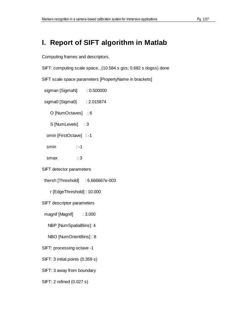
Markers recognition in a camera-based calibration system for immersive applications Pg. 137
I. Report of SIFT algorithm in Matlab
Computing frames and descriptors.
SIFT: computing scale space...(10.584 s gss; 0.682 s dogss) done
SIFT scale space parameters [PropertyName in brackets]
sigman [SigmaN] : 0.500000
sigma0 [Sigma0] : 2.015874
O [NumOctaves] : 6
S [NumLevels] : 3
omin [FirstOctave] : -1
smin : -1
smax : 3
SIFT detector parameters
thersh [Threshold] : 6.666667e-003
r [EdgeThreshold] : 10.000
SIFT descriptor parameters
magnif [Magnif] : 3.000
NBP [NumSpatialBins]: 4
NBO [NumOrientBins] : 8
SIFT: processing octave -1
SIFT: 3 initial points (0.359 s)
SIFT: 3 away from boundary
SIFT: 2 refined (0.027 s)

Pg. 138 Report
SIFT: computing descriptors...done (1.714 s)
SIFT: processing octave 0
SIFT: 4 initial points (0.120 s)
SIFT: 4 away from boundary
SIFT: 4 refined (0.000 s)
SIFT: computing descriptors...done (0.539 s)
SIFT: processing octave 1
SIFT: 1 initial points (0.019 s)
SIFT: 1 away from boundary
SIFT: 1 refined (0.000 s)
SIFT: computing descriptors...done (0.126 s)
SIFT: processing octave 2
SIFT: 0 initial points (0.005 s)
SIFT: 0 away from boundary
SIFT: 0 refined (0.000 s)
SIFT: computing descriptors...done (0.047 s)
SIFT: processing octave 3
SIFT: 0 initial points (0.002 s)
SIFT: 0 away from boundary
SIFT: 0 refined (0.000 s)
SIFT: computing descriptors...done (0.007 s)
SIFT: processing octave 4
SIFT: 0 initial points (0.001 s)
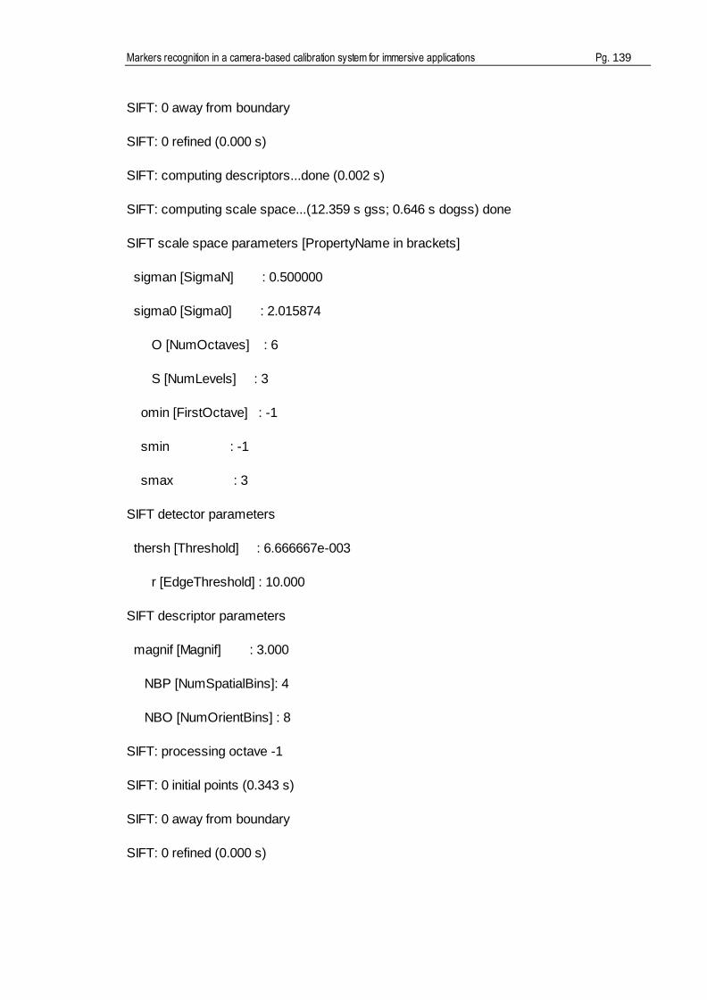
Markers recognition in a camera-based calibration system for immersive applications Pg. 139
SIFT: 0 away from boundary
SIFT: 0 refined (0.000 s)
SIFT: computing descriptors...done (0.002 s)
SIFT: computing scale space...(12.359 s gss; 0.646 s dogss) done
SIFT scale space parameters [PropertyName in brackets]
sigman [SigmaN] : 0.500000
sigma0 [Sigma0] : 2.015874
O [NumOctaves] : 6
S [NumLevels] : 3
omin [FirstOctave] : -1
smin : -1
smax : 3
SIFT detector parameters
thersh [Threshold] : 6.666667e-003
r [EdgeThreshold] : 10.000
SIFT descriptor parameters
magnif [Magnif] : 3.000
NBP [NumSpatialBins]: 4
NBO [NumOrientBins] : 8
SIFT: processing octave -1
SIFT: 0 initial points (0.343 s)
SIFT: 0 away from boundary
SIFT: 0 refined (0.000 s)

Pg. 140 Report
SIFT: computing descriptors...done (1.759 s)
SIFT: processing octave 0
SIFT: 7 initial points (0.076 s)
SIFT: 7 away from boundary
SIFT: 5 refined (0.000 s)
SIFT: computing descriptors...done (0.673 s)
SIFT: processing octave 1
SIFT: 0 initial points (0.032 s)
SIFT: 0 away from boundary
SIFT: 0 refined (0.000 s)
SIFT: computing descriptors...done (0.151 s)
SIFT: processing octave 2
SIFT: 1 initial points (0.003 s)
SIFT: 1 away from boundary
SIFT: 1 refined (0.000 s)
SIFT: computing descriptors...done (0.032 s)
SIFT: processing octave 3
SIFT: 0 initial points (0.001 s)
SIFT: 0 away from boundary
SIFT: 0 refined (0.000 s)
SIFT: computing descriptors...done (0.005 s)
SIFT: processing octave 4
SIFT: 0 initial points (0.001 s)

Markers recognition in a camera-based calibration system for immersive applications Pg. 141
SIFT: 0 away from boundary
SIFT: 0 refined (0.000 s)
SIFT: computing descriptors...done (0.002 s)
Computing matches.
Matched in 0.034 s