Simultaneous calibration of odometry and camera for a differential drive mobile robot

Intel Serv Robotics (2010) 3:163–173DOI 10.1007/s11370-010-0067-2

ORIGINAL RESEARCH PAPER

A non-iterative and effective procedure for simultaneousodometry and camera calibration for a differential drive mobilerobot based on the singular value decomposition

Gianluca Antonelli · Fabrizio Caccavale ·Flavio Grossi · Alessandro Marino

Received: 3 April 2010 / Accepted: 12 May 2010 / Published online: 3 June 2010© Springer-Verlag 2010

Abstract Differential-drive mobile robots are usuallyequipped with video cameras for navigation purposes.In order to ensure proper operational capabilities of suchsystems, several calibration steps are required to estimate thevideo-camera intrinsic and extrinsic parameters, the relativepose between the camera and the vehicle frame and the odo-metric parameters of the vehicle. In this paper, simultaneousestimation of the aforementioned quantities is achieved bya novel and effective calibration procedure. The proposedcalibration procedure needs only a proper set of landmarks,on-board measurements given by the wheels encoders, andthe camera (i.e., a number of properly taken camera snap-shots of the set of landmarks). A major advantage of theproposed technique is that the robot is not required to followa specific path: the vehicle is asked to roughly move aroundthe landmarks and acquire at least three snapshots at someapproximatively known configurations. Moreover, since thewhole calibration procedure does not use external measure-ment devices, it can be used to calibrate, on-site, a team ofmobile robots with respect to the same inertial frame, givenby the position of the landmarks’ tool. Finally, the proposedalgorithm is systematic and does not require any iterative

G. Antonelli · F. GrossiDipartimento di Automazione, Elettromagnetismo,Ingegneria dell’Informazione e Matematica Industriale,Università degli Studi di Cassino, Via G. Di Biasio 43,03043 Cassino (FR), Italye-mail: [email protected]

F. Caccavale · A. Marino (B)Dipartimento di Ingegneria e Fisica dell’Ambiente,Università degli Studi della Basilicata,Viale dell’Ateneo Lucano 10, 85100 Potenza, Italye-mail: [email protected]

F. Caccavalee-mail: [email protected]

step. Numerical simulations and experimental results,obtained by using a mobile robot Khepera III equipped witha low-cost camera, confirm the effectiveness of the proposedtechnique.

Keywords Camera calibration · Odometry calibration ·Mobile robots

1 Introduction

Differential-drive mobile robots equipped with a video-camera need careful calibration before the robot device isoperational: namely, odometry, the video-camera and the rel-ative vehicle-camera pose (hand-eye) calibration.

Odometry is the reconstruction of the mobile robotconfiguration (i.e., position and orientation) by resorting toencoders’ measurements at the wheels. Starting from a knownconfiguration, the current position and orientation of the robotis obtained by time integration of the vehicle’s velocity cor-responding to the measured wheels’ velocity.

Video-camera calibration concerns both intrinsic parame-ters (e.g., the focal length) and extrinsic parameters (e.g., therelative pose of the image frame with respect to an inertialframe). This relatively mature topic is widely tackled in theliterature (see, e.g., [9] for wide overview of existing calibra-tion techniques).

When a camera is mounted on a robot, an additional cali-bration procedure is required: namely, the so-called hand-eyecalibration [18], which is aimed at determining the relativepose between the camera and a robot-fixed frame. Althoughits name is inherited from the specific problem of a cameramounted on the end-effector of a robot manipulator, this stepis, of course, required for a camera mounted on a mobile

123

164 Intel Serv Robotics (2010) 3:163–173

robot as well. In general, such a calibration is required forany kind of sensors mounted on a robotic device.

Several research efforts have been focused on the afore-mentioned calibration problems, although they have beentackled individually; e.g., for odometry calibration, exter-nal video cameras (already calibrated) have been used, whilehand-eye calibration is usually achieved by resorting to kine-matically calibrated robots. In detail, as for the odometrycalibration, since the first attempts [19], there has been anintense research activity aimed at improving the accuracyand the effectiveness of the calibration. A widely adoptedalgorithm is presented in [3], where the sole odometry cali-bration is object of study. In [6], an algorithm, based on theboundedness property of the error for Generalized-Voronoi-Graph-based paths, has been proposed and experimentallyvalidated. In [7], it is proposed to drive the robot througha known path and then evaluate the shape of the resultingpath to estimate the unknown parameters. The works [14,15]present a method to identify two systematic and two non-systematic errors, while in [11,12], the error propagation invehicle odometry is analytically discussed, and two mainresults are given, namely, regarding the quadratic depen-dency of the estimation error with respect to the traveleddistance and the existence of path-independent systematicerrors. In [2], a calibration method aimed at identifying a4-parameter odometric model has been proposed, where thelinear relation between the unknowns and the measurementsallows to use linear estimation tools; this linear estimationapproach is further improved in [1] so as to estimate thephysical odometric parameters, thus yielding a 3-parame-ter model. It is worth noticing that all the aforementionedmethods require external measurement systems such as, e.g.,calibrated video cameras or ranging sensors. Recently, in[4] simultaneous calibration of odometry and range sensorsis achieved by resorting to on-board sensors only; the con-sidered range sensor is a laser range finder assumed to beperfectly horizontal (i.e., the problem is planar).

In this paper simultaneous calibration of the intrinsic andextrinsic video-camera parameters, hand-eye, and odometryis achieved by resorting to a novel and effective procedure.The proposed calibration procedure needs a landmarks tool,i.e., a tool on which a set of geometric landmarks has beenplaced; the landmark tool is used to define the inertial ref-erence frame as well. In addition to measurements given bythe on-board camera, only measurements given by the wheelencoders are required. In detail, the video-camera is used tosave a number of properly taken snapshots of the landmarkstool taken from different locations. A major advantage ofthe proposed technique is that no specific path is requiredto be followed: the vehicle is asked to roughly move aroundthe landmarks and acquire a minimum of three snapshotsat some approximatively known configurations. Moreover,since the whole calibration procedure does not use external

Table 1 Definition of the main variables

Σo − {Oo, xo, yo, zo} Inertial frame

Σv − {Ov, xv, yv, zv} Vehicle-fixed frame

Σc − {Oc, xc, yc, zc} Camera-fixed frame

x, y, θ Vehicle configuration

v, ω Vehicle linear/angular velocities

ωR, ωL Right/left wheel angular velocities

θR, θL Right/left wheel angular position

rR, rL , b Right/left wheel radii, wheelbase

αR, αL Intermediate odometric variables

Rr (θ) Rotation matrix representing arotation of θ around the r axis

Rba ∈ IR3×3 Rotation matrix from frame Σa

to frame Σb

α1, α2, α3 Euler angles representingRv

c = Rz(α1)Ry(α2)Rz(α3)

taab ∈ IR3 Origin of frame Σb with respect

of the origin of frame Σa expressed in Σa

Aba ∈ IR4×4 Homogeneous transformation from frame

Σa to frame Σb

p Homogeneous representation of vector p

po ∈ IR3 Landmark position expressed in theinertial frame

pc ∈ IR3 Landmark position expressed incamera frame

[pu pv]T Pixel in the image plane

f c ∈ IR2 Camera focal length expressed in pixel

kr Camera radial distortion coefficient

P Number of different poses usedfor calibration

N = P(P − 1)/2 Number of possible combinations ofcouples of poses

measurement devices, it can be used to calibrate a team ofmobile robots (performing, e.g., a search-and-rescue oper-ation) with respect to the same inertial frame, given by theposition of the landmarks tool. Finally, the proposed algo-rithm is systematic and does not require any iterative step.Numerical simulations and experimental results, obtained byusing a Khepera III mobile robot equipped with a low-costcamera, confirm the effectiveness of the proposed technique.

2 Background

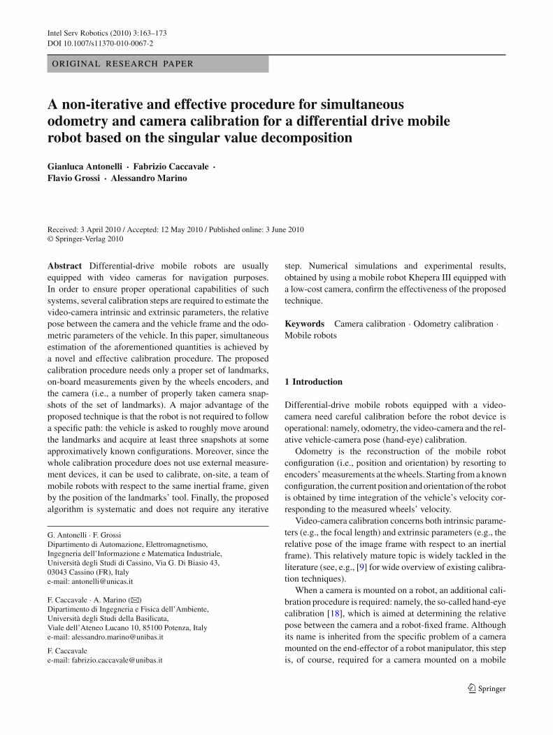
In the following, the problem to be solved, together with themain geometrical relationships and the parameters to be esti-mated will be presented in detail. In particular, all relevantquantities and symbols are listed in Table 1 (see also Fig. 2.In Fig. 1, a picture of the mobile robot Khepera III holdinga video camera used in the experiments is shown. The kine-matic structure and the main quantities of the above robot is

123

Intel Serv Robotics (2010) 3:163–173 165

Fig. 1 Picture of a mobile robot holding a video-camera

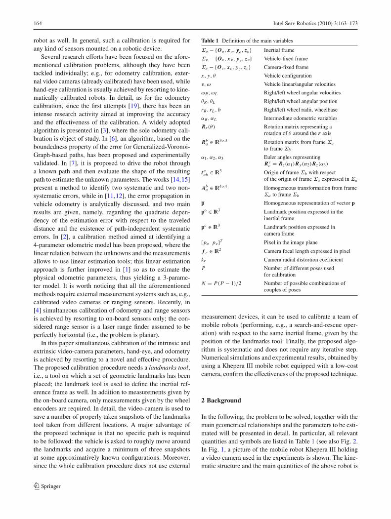
Fig. 2 Top-view sketch of a differential-drive mobile robot with rele-vant variables (without camera-fixed frame)

shown in Fig. 2; while in Fig. 3 a sketch of the camera-vehiclegeometry is presented.

2.1 Unicycle kinematics

Consider the differential-drive mobile robot depicted inFig. 2. Let x and y be the coordinates of the origin of thevehicle frame Σv , expressed in the inertial frame Σo, θ bethe heading angle between the x-axes of Σv and Σo, v andω be the vehicle linear and angular velocities, respectively.The vehicle kinematics is given by

⎧⎨

⎩

x = v cos(θ)

y = v sin(θ)

θ = ω.

(1)

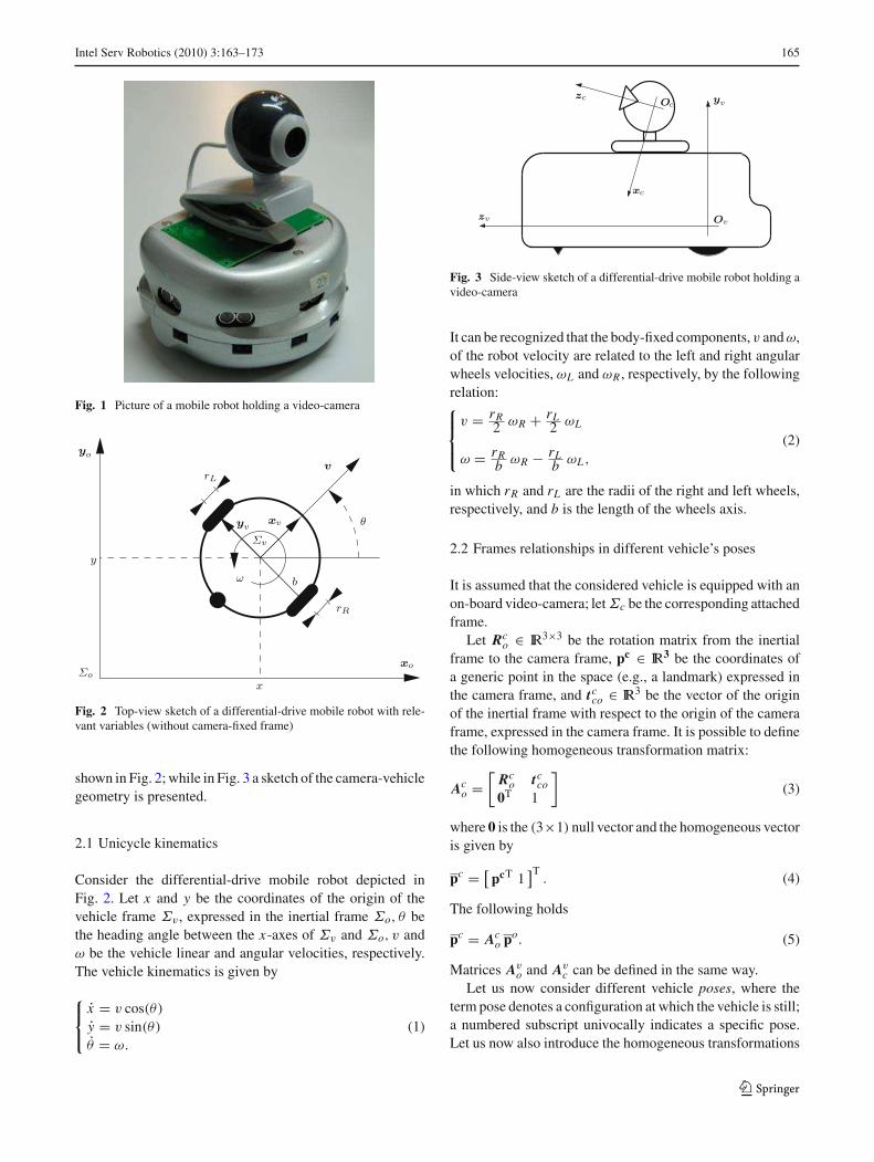
Fig. 3 Side-view sketch of a differential-drive mobile robot holding avideo-camera

It can be recognized that the body-fixed components, v and ω,of the robot velocity are related to the left and right angularwheels velocities, ωL and ωR , respectively, by the followingrelation:⎧⎪⎨

⎪⎩

v = rR2 ωR + rL

2 ωL

ω = rRb ωR − rL

b ωL ,

(2)

in which rR and rL are the radii of the right and left wheels,respectively, and b is the length of the wheels axis.

2.2 Frames relationships in different vehicle’s poses

It is assumed that the considered vehicle is equipped with anon-board video-camera; let Σc be the corresponding attachedframe.

Let Rco ∈ IR3×3 be the rotation matrix from the inertial

frame to the camera frame, pc ∈ IR3 be the coordinates ofa generic point in the space (e.g., a landmark) expressed inthe camera frame, and tc

co ∈ IR3 be the vector of the originof the inertial frame with respect to the origin of the cameraframe, expressed in the camera frame. It is possible to definethe following homogeneous transformation matrix:

Aco =

[Rc

o tcco

0T 1

]

(3)

where 0 is the (3×1) null vector and the homogeneous vectoris given by

pc = [pcT 1

]T. (4)

The following holds

pc = Aco po. (5)

Matrices Avo and Av

c can be defined in the same way.Let us now consider different vehicle poses, where the

term pose denotes a configuration at which the vehicle is still;a numbered subscript univocally indicates a specific pose.Let us now also introduce the homogeneous transformations

123


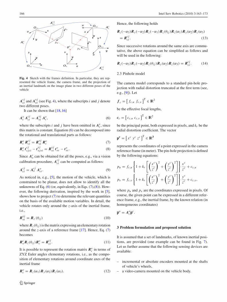
Fig. 4 Sketch with the frames definition. In particular, they are rep-resented the vehicle frame, the camera frame, and the projection ofan inertial landmark on the image plane in two different poses of thevehicle

Acjci and Av j

vi (see Fig. 4), where the subscripts i and j denotetwo different poses.

It can be shown that [18,16]

Avc Acj

ci = Av jvi Av

c , (6)

where the subscripts i and j have been omitted in Avc , since

this matrix is constant. Equation (6) can be decomposed intothe rotational and translational parts as follows:

Rvc Rcj

ci = Rv jvi Rv

c (7)

Rvc tcj

cjci − tv jv jvi = Rv j

vi tvvc − tvvc. (8)

Since Aco can be obtained for all the poses, e.g., via a vision

calibration procedure, Acjci can be computed as follows:

Acjci = Acj

o Aoci . (9)

As noticed in, e.g., [5], the motion of the vehicle, which isconstrained to be planar, does not allow to identify all theunknowns of Eq. (6) (or, equivalently, in Eqs. (7),(8)). How-ever, the following derivation, inspired by the work in [5],shows how to project (7) to determine the relevant quantitieson the basis of the available motion variables. In detail, thevehicle rotates only around the z-axis of the inertial frame,i.e.,

Rv jvi = Rz (θi j ) (10)

where Rz(θi j ) is the matrix expressing an elementary rotationaround the z-axis of a reference frame [17]. Hence, Eq. (7)becomes

Rcv Rz(θi j )Rv

c = Rcjci . (11)

It is possible to represent the rotation matrix Rvc in terms of

ZYZ Euler angles elementary rotations, i.e., as the compo-sition of elementary rotations around coordinate axes of theinertial frame

Rvc = Rz(α1)Ry(α2)Rz(α3). (12)

Hence, the following holds

Rz(−α3)Ry(−α2)Rz(−α1)Rz(θi j )Rz(α1)Ry(α2)Rz(α3)

= Rcjci . (13)

Since successive rotations around the same axis are commu-tative, the above equation can be simplified as follows andwill be used in the following:

Rz(−α3)Ry(−α2)Rz(θi j )Ry(α2)Rz(α3) = Rcjci . (14)

2.3 Pinhole model

The camera model corresponds to a standard pin-hole pro-jection with radial distortion truncated at the first term (see,e.g., [9]). Let

f c = [fc,u fc,v

]T ∈ IR2

be the effective focal lengths,

cc = [cc,u cc,v

]T ∈ IR2

be the principal point, both expressed in pixels, and kr be theradial distortion coefficient. The vector

pc = [xc yc zc

]T ∈ IR3

represents the coordinates of a point expressed in the camerareference frame (in meter). The pin-hole projection is definedby the following equations:

pu = fc,u

{

1 + kr

[(xc

zc

)2

+(

yc

zc

)2]}

xc

zc + cc,u

pv = fc,v

{

1 + kr

[(xc

zc

)2

+(

yc

zc

)2]}

yc

zc + cc,v,

where pu and pv are the coordinates expressed in pixels. Ofcourse, the given point can be expressed in a different refer-ence frame, e.g., the inertial frame, by the known relation (inhomogeneous coordinates)

po = Aocpc.

3 Problem formulation and proposed solution

It is assumed that a set of landmarks, of known inertial posi-tions, are provided (one example can be found in Fig. 7).Let us further assume that the following sensing devices areavailable:

– incremental or absolute encoders mounted at the shaftsof vehicle’s wheels,

– a video-camera mounted on the vehicle body.

123


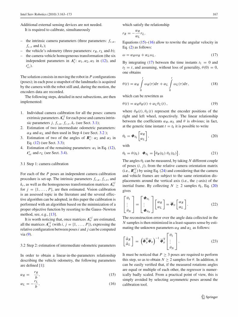
Additional external sensing devices are not needed.It is required to calibrate, simultaneously

– the intrinsic camera parameters (three parameters: fc,u,

fc,v and kr );– the vehicle’s odometry (three parameters: rR, rL and b);– the camera-vehicle homogeneous transformation (the six

independent parameters in Avc : α1, α2, α3 in (12), and

tvvc).

The solution consists in moving the robot in P configurations(poses); in each pose a snapshot of the landmarks is acquiredby the camera with the robot still and, during the motion, theencoders data are recorded.

The following steps, detailed in next subsections, are thenimplemented:

1. Individual camera calibration for all the poses: cameraextrinsic parameters Acj

o for each pose and camera intrin-sic parameters j, fc,u, fc,v, kr (see Sect. 3.1);

2. Estimation of two intermediate odometric parameters:αR and αL and then used in Step 4 (see Sect. 3.2 );

3. Estimation of two of the angles of Rvc : α2 and α3 in

Eq. (12) (see Sect. 3.3);4. Estimation of the remaining parameters: α1 in Eq. (12),

tvvc and rL (see Sect. 3.4).

3.1 Step 1: camera calibration

For each of the P poses an independent camera calibrationprocedure is set-up. The intrinsic parameters fc,u, fc,v , andkr , as well as the homogeneous transformation matrices Acj

o

for j = {1, . . . , P}, are then estimated. Vision calibrationis an assessed topic in the literature and the several effec-tive algorithm can be adopted; in this paper the calibration isperformed with an algorithm based on the minimization of aproper objective function by resorting to the Gauss–Newtonmethod, see, e.g., [13].

It is worth noticing that, once matrices Acjo are estimated,

all the matrices Acjci (with i, j = {1, . . . , P}), expressing the

relative configuration between poses i and j can be computedvia (9).

3.2 Step 2: estimation of intermediate odometric parameters

In order to obtain a linear-in-the-parameters relationshipdescribing the vehicle odometry, the following parametersare defined [1]:

αR = rR

b, (15)

αL = −rL

b, (16)

which satisfy the relationship

rR = −αR

αLrL .

Equations (15)–(16) allow to rewrite the angular velocity inEq. (2) as follows:

ω = αRωR + αLωL . (17)

By integrating (17) between the time instants t1 = 0 andt2 = t , and assuming, without loss of generality, θ(0) = 0,one obtains

θ(t) = αR

t∫

0

ωR(τ )dτ + αL

t∫

0

ωL(τ )dτ , (18)

which can be rewritten as

θ(t) = αRθR(t) + αLθL(t) , (19)

where θR(t), θL(t) represent the encoder positions of theright and left wheel, respectively. The linear relationshipbetween the coefficients αR, αL and θ is obvious; in fact,at the generic time instant t = tk it is possible to write

θk = Φθk

[αR

αL

]

, (20)

with

θk = θ(tk) Φθk = [θR(tk) θL(tk)

]. (21)

The angles θk can be measured, by taking N different coupleof poses (i, j), from the relative camera orientation matrix(i.e., Rcj

ci ) by using Eq. (24) and considering that the cameraand vehicle frames are subject to the same orientation dis-placements around the vertical axis (i.e., the z-axis) of theinertial frame. By collecting N ≥ 2 samples θk , Eq. (20)gives⎡

⎢⎣

θ1...

θN

⎤

⎥⎦ =

⎡

⎢⎣

Φθ1...

ΦθN

⎤

⎥⎦

[αR

αL

]

= Φθ

[αR

αL

]

. (22)

The reconstruction error over the angle data collected in theN samples is then minimized in a least-squares sense by esti-mating the unknown parameters αR and αL as follows:

[αR

αL

]

=(Φ

Tθ Φθ

)−1Φ

Tθ

⎡

⎢⎣

θ1...

θN

⎤

⎥⎦ . (23)

It must be noticed that P ≥ 3 poses are required to performthis step, so as to obtain N ≥ 2 samples for θ . In addition, itcan be easily verified that, if the measured rotations anglesare equal or multiple of each other, the regressor is numer-ically badly scaled. From a practical point of view, this issimply avoided by selecting asymmetric poses around thecalibration tool.

123


3.3 Step 3: estimation of α2 and α3

Angles α2 and α3 can be computed from matrix Rcjci , taken in

different couple of poses (i, j), as described in the following.The left-hand side of (14) corresponds to the usual defini-

tion of axis-angle representation of the orientation [17] (withthe proper angles’ sign). Since Rcj

ci can be computed via (9),θi j , α2 and α3, can be computed. In detail [17]

θi j = cos−1(

R11 + R22 + R33 − 1

2

)

, (24)

where Rpq denotes the generic element of Rcjci . The rotation

axis

r =⎡

⎣rx

ry

rz

⎤

⎦ = 1

2 sin θi j

⎡

⎣R32 − R23

R13 − R31

R21 − R12

⎤

⎦ (25)

allows to compute α2 and α3 as follows:

α2 = atan2(√

r2x + r2

y , rz

), (26)

α3 = atan2(ry,−rx ). (27)

Equation (14) shows that condition θi j �= 0 is required toavoid a trivial equation satisfied by an arbitrary axis–anglecouple. The physical interpretation is obvious: a nontrivialvehicle rotation is needed to estimate the relevant variablesof the left-hand side of (14).

It must be noticed that at least P = 2 poses are requiredto estimate r, α2 and α3. Of course, a larger number of posesmay be exploited to improve the estimation results.

3.4 Step 4: estimation of α1, tvvc and rL

In order to estimate the angle α1 in Rvc , the planar compo-

nents of tvvc and rL , Eq. (8) have to be used. Unidentifiabilityof the vertical component of tvvc (i.e., along the z-axis of theinertial frame) can be understood by direct observation of thefact that the third equation (8) is identically satisfied for anyset of data physically achievable with the given robot planarmobility [5].

Let us now analyze and rewrite in a different form Eq. (8)in order to estimate the remaining unknown parameters. Vec-tor tcj

cjci is known from the vision calibration (step 1), byresorting to the relationship (9). The rotation matrix Rv

c ,expressed in terms of three elementary rotations Rv

c =Rz(α1)Ry(α2)Rz(α3), is a function of the unknown α1, since

α2 and α3 are already available from step 3. The vector tv jv jvi

represents the vehicle displacement between two genericposes, expressed with respect to the final frame Σv j ; inte-gration of Eq. (1) gives the displacement expressed in theinitial pose, tvi

viv j . As shown in [1], the following discrete-

time equations for the position displacement can be devisedfrom (1)

⎡

⎣xk+1 − xk

yk+1 − yk

⎤

⎦= T

2

⎡

⎢⎢⎢⎢⎣

(

−αR

αLωR,k + ωL ,k

)

cos

(

θk + T ωk

2

)

(

−αR

αLωR,k + ωL ,k

)

sin

(

θk + T ωk

2

)

⎤

⎥⎥⎥⎥⎦

rL ,

where the subscript k denotes the kth time sample and T isthe sampling period. Clearly, the above equation defines alinear mapping between rL and the position displacement. Inparticular, the relationship between the kinematic quantitiesat a generic time step (corresponding to pose i), k = 0, andfinal time step (corresponding to pose j), k = K , is

tviviv j =

⎡

⎣xK − x0

yK − y0

⎤

⎦

= T

2

⎡

⎢⎢⎢⎢⎢⎢⎢⎣

−αR

αL

K−1∑

k=0

ωR,k ck +K−1∑

k=0

ωL ,k ck

−αR

αL

K−1∑

k=0

ωR,k sk +K−1∑

k=0

ωL ,k sk

⎤

⎥⎥⎥⎥⎥⎥⎥⎦

rL , (28)

where ck = cos(θk + T ωk/2) and sk = sin(θk + T ωk/2).It is worth noticing that θk and ωk in Eq. (28) can be computedfrom Eq. (17) and Eq. (18), respectively, since αR and αL

have already been identified in Step 2 (see Sect. 3.2).By using Eq. (28), Eq. (8) can be then rewritten compactly

as

tviviv j =

⎡

⎣β1

β2

0

⎤

⎦ rL = β i j rL , (29)

with an implicit definition of the two known coefficients β1

and β2.Equation (8) can be rewritten as follows:

Rvc tcj

cjci + Rv jvi β i j rL −

(Rv j

vi − I)

tvvc = 0. (30)

The first two rows of the above equation system are thoseto be considered for the estimation of the unknown parame-ters. Indeed, the left-hand side of the above equation containsRv

c , that is nonlinear with respect to α1. However, the term

Rvc tcj

cjci can be rewritten in a form linear in sα1 = sin(α1)

and cα1 = cos(α1). Hence, Eq. (30) can be rewritten ina form linear in the new remaining unknown parameters:[rL tvvc,x tvvc,y cα1 sα1

].

For the sake of notation compactness, let us define theindex l ∈{1, . . . , N } representing a couple of poses (indexed,in turn, by i ∈ {1, . . . , P} and j ∈ {1, . . . , P}). Then, the

123


first two components of Eq. (30) become

Φl ζ = [Rθ,l βl T θ,l Tα,l

]

⎡

⎢⎢⎢⎢⎣

rL

tvvc,xtvvc,ycα1

sα1

⎤

⎥⎥⎥⎥⎦

= 0, (31)

with

T θ,l = I − Rθ,l

Rθ,l =[

cθl −sθl

sθl cθl

]

sθl = sin(θi j

), cθl = cos

(θi j

)

Tα,l =[

al −bl

bl al

]

al = cα2 cα3 tcjcjci,x − cα2 sα3 tcj

cjci,y + sα2 tcjcjci,z

bl = sα3 tcjcjci,x +cα3 tcj

cjci,y ,

where Rv jvi has been expressed, as in (10), in terms of an

elementary rotation around the z-axis of the inertial frame.Equation (31) can be written for each of the N available

couple of poses, giving⎡

⎢⎣

Φ1...

ΦN

⎤

⎥⎦ ζ = Φζ = 0, (32)

where Φ ∈ IR2N×5. Moreover, ζ is subject to the constraint(imposed by the relation c2

α1+ s2

α1= 1):

ζ 24 + ζ 2

5 = 1.

In the Appendix, it is shown that, with a proper choice of therobot’s poses, the regressor matrix is such that rank(Φ) = 4.Thus, Φ has a 1-dimensional null space which can be deter-mined by computing the orthonormal (5 × 5) matrix, V , ofthe Singular Value Decomposition (SVD) [8]:

Φ = UΣV T , (33)

where the matrix Σ ∈ IR2N×5 contains along the main diago-nal the five non-negative singular values listed in decreasingorder with respect to their magnitude. It is now clear that thefifth column of V , v5, spans the null space of Φ. Hence, thesolution to (32) has the form

ζ ∗ = κv5,

with κ a constant value to be determined. Among the infinitesolutions the one of interest is the sole value that satisfies theconstraint ζ 2

4 + ζ 25 = 1, which can be easily computed by

choosing

κ = 1√

v25,4 + v2

5,5

. (34)

Once rL is known, it is trivial to obtain rR and b from(15)–(16):

rR = − αR

αLrL (35)

b = rR

αRor b = − rL

αL. (36)

4 Simulations

Before testing the approach on a real setup, the proposedsolution has been tested in simulation. It is easy to imaginethat, as the above procedure does not imply any approxima-tion, it is able, in ideal conditions, to exactly identify therequired parameters up to the machine precision. Extensivenumerical simulations have been carried out to verify thevalidity of the proposed approach in the presence of unavoid-able practical approximations as, for example, the camera andencoder quantization and the sampling time, etc. Then, themain algorithm parameters have been varied in order to testnumerically the robustness with respect to possible changesin the problem conditions.

In the simulations the sample time has been set to a rea-sonable value of T = 0.02 s, corresponding to cheap micro-controllers running soft real-time code. It is worth noticingthat low sampling frequencies and high vehicle velocities canbe a significant source of odometric errors. When it is notpossible to increase the sampling frequency due to hardwarelimitations, it is obviously convenient to move the vehicleamong the poses at relatively low velocity.

Pixel quantization for a 640 × 480 video-camera as wellas a 0.1302◦ encoder quantization has been further added inorder to reproduce the same experimental conditions. In suchconditions, only P = 5 poses are sufficient to achieve a rel-ative error of 0.1% on the odometry parameters and 1% onthe vehicle-camera roto-translation matrix over a 0.25 aver-age pixel error in the calibration procedure.

Moreover, looking at the numerical value of matrix Φ inEq. (32), the ratio σ5/σ4 of the last and the next-to-last sin-gular values is typically 10−3, while σ4/σ3 = 0.8, accord-ing to the property of Φ to be a 4-rank matrix. Indeed, inideal conditions, σ5 should be zero, but noise, quantization,and numerical integration (used to derive Eq. (29)) do notyield such a condition rigorously. This situation mainly arisesin experiment (where also slippage, misaligned wheels, andother effects are present) and some words need to be spent.Because of noise, the matrix Φ is not rigorously a 4-rankmatrix. Then, considering the fifth column of matrix V inEq. (33) as a basis of the null space of matrix Φ means toapproximate Φ with a new matrix Φ = UΣV T , where Uand V are the same matrices obtained by the Singular ValueDecomposition of matrix Φ, and the matrix Σ differs from Σ

123


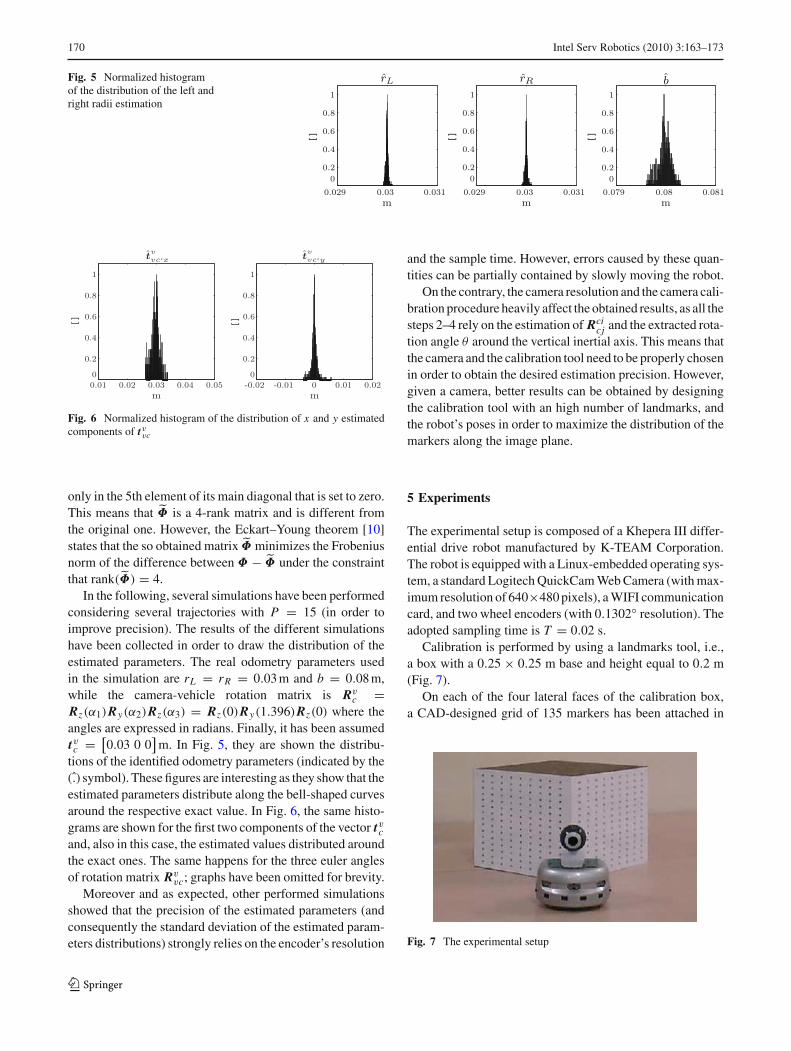
Fig. 5 Normalized histogramof the distribution of the left andright radii estimation

Fig. 6 Normalized histogram of the distribution of x and y estimatedcomponents of tvvc

only in the 5th element of its main diagonal that is set to zero.This means that Φ is a 4-rank matrix and is different fromthe original one. However, the Eckart–Young theorem [10]states that the so obtained matrix Φ minimizes the Frobeniusnorm of the difference between Φ − Φ under the constraintthat rank(Φ) = 4.

In the following, several simulations have been performedconsidering several trajectories with P = 15 (in order toimprove precision). The results of the different simulationshave been collected in order to draw the distribution of theestimated parameters. The real odometry parameters usedin the simulation are rL = rR = 0.03 m and b = 0.08 m,while the camera-vehicle rotation matrix is Rv

c =Rz(α1)Ry(α2)Rz(α3) = Rz(0)Ry(1.396)Rz(0) where theangles are expressed in radians. Finally, it has been assumedtvc = [

0.03 0 0]

m. In Fig. 5, they are shown the distribu-tions of the identified odometry parameters (indicated by the(.) symbol). These figures are interesting as they show that theestimated parameters distribute along the bell-shaped curvesaround the respective exact value. In Fig. 6, the same histo-grams are shown for the first two components of the vector tvcand, also in this case, the estimated values distributed aroundthe exact ones. The same happens for the three euler anglesof rotation matrix Rv

vc; graphs have been omitted for brevity.Moreover and as expected, other performed simulations

showed that the precision of the estimated parameters (andconsequently the standard deviation of the estimated param-eters distributions) strongly relies on the encoder’s resolution

and the sample time. However, errors caused by these quan-tities can be partially contained by slowly moving the robot.

On the contrary, the camera resolution and the camera cali-bration procedure heavily affect the obtained results, as all thesteps 2–4 rely on the estimation of Rci

cj and the extracted rota-tion angle θ around the vertical inertial axis. This means thatthe camera and the calibration tool need to be properly chosenin order to obtain the desired estimation precision. However,given a camera, better results can be obtained by designingthe calibration tool with an high number of landmarks, andthe robot’s poses in order to maximize the distribution of themarkers along the image plane.

5 Experiments

The experimental setup is composed of a Khepera III differ-ential drive robot manufactured by K-TEAM Corporation.The robot is equipped with a Linux-embedded operating sys-tem, a standard Logitech QuickCam Web Camera (with max-imum resolution of 640×480 pixels), a WIFI communicationcard, and two wheel encoders (with 0.1302◦ resolution). Theadopted sampling time is T = 0.02 s.

Calibration is performed by using a landmarks tool, i.e.,a box with a 0.25 × 0.25 m base and height equal to 0.2 m(Fig. 7).

On each of the four lateral faces of the calibration box,a CAD-designed grid of 135 markers has been attached in

Fig. 7 The experimental setup

123


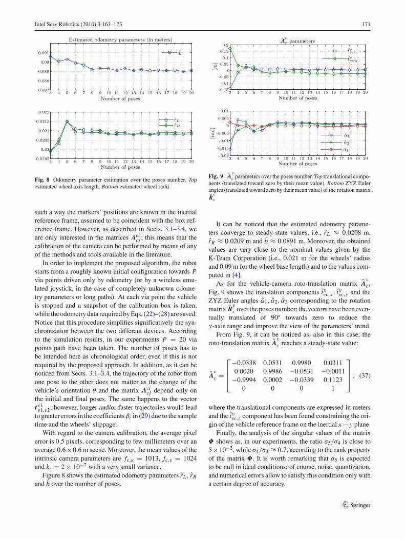
Fig. 8 Odometry parameter estimation over the poses number. Topestimated wheel axis length. Bottom estimated wheel radii

such a way the markers’ positions are known in the inertialreference frame, assumed to be coincident with the box ref-erence frame. However, as described in Sects. 3.1–3.4, weare only interested in the matrices Aci

cj ; this means that thecalibration of the camera can be performed by means of anyof the methods and tools available in the literature.

In order to implement the proposed algorithm, the robotstarts from a roughly known initial configuration towards Pvia points driven only by odometry (or by a wireless emu-lated joystick, in the case of completely unknown odome-try parameters or long paths). At each via point the vehicleis stopped and a snapshot of the calibration box is taken,while the odometry data required by Eqs. (22)–(28) are saved.Notice that this procedure simplifies significatively the syn-chronization between the two different devices. Accordingto the simulation results, in our experiments P = 20 viapoints path have been taken. The number of poses has tobe intended here as chronological order, even if this is notrequired by the proposed approach. In addition, as it can benoticed from Sects. 3.1–3.4, the trajectory of the robot fromone pose to the other does not matter as the change of thevehicle’s orientation θ and the matrix Aci

cj depend only onthe initial and final poses. The same happens to the vectortv1v1,v2; however, longer and/or faster trajectories would lead

to greater errors in the coefficients βi in (29) due to the sampletime and the wheels’ slippage.

With regard to the camera calibration, the average pixelerror is 0.5 pixels, corresponding to few millimeters over anaverage 0.6×0.6 m scene. Moreover, the mean values of theintrinsic camera parameters are fc,u = 1013, fc,v = 1024and kr = 2 × 10−7 with a very small variance.

Figure 8 shows the estimated odometry parameters rL , rR

and b over the number of poses.

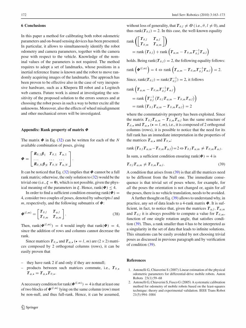
Fig. 9 Av

c parameters over the poses number. Top translational compo-nents (translated toward zero by their mean value). Bottom ZYZ Eulerangles (translated toward zero by their mean value) of the rotation matrixR

v

c

It can be noticed that the estimated odometry parame-ters converge to steady-state values, i.e., rL ≈ 0.0208 m,rR ≈ 0.0209 m and b ≈ 0.0891 m. Moreover, the obtainedvalues are very close to the nominal values given by theK-Team Corporation (i.e., 0.021 m for the wheels’ radiusand 0.09 m for the wheel base length) and to the values com-puted in [4].

As for the vehicle-camera roto-translation matrix Av

c ,Fig. 9 shows the translation components tvvc,x , tvvc,y and theZYZ Euler angles α1, α2, α3 corresponding to the rotationmatrix R

v

c over the poses number; the vectors have been even-tually translated of 90◦ towards zero to reduce they-axis range and improve the view of the parameters’ trend.

From Fig. 9, it can be noticed as, also in this case, theroto-translation matrix A

v

c reaches a steady-state value:

Av

c =

⎡

⎢⎢⎣

−0.0338 0.0531 0.9980 0.03110.0020 0.9986 −0.0531 −0.0011

−0.9994 0.0002 −0.0339 0.11230 0 0 1

⎤

⎥⎥⎦ , (37)

where the translational components are expressed in metersand the tvvc,z component has been found constraining the ori-gin of the vehicle reference frame on the inertial x − y plane.

Finally, the analysis of the singular values of the matrixΦ shows as, in our experiments, the ratio σ5/σ4 is close to5×10−2, while σ4/σ3 ≈ 0.7, according to the rank propertyof the matrix Φ. It is worth remarking that σ5 is expectedto be null in ideal conditions; of course, noise, quantization,and numerical errors allow to satisfy this condition only witha certain degree of accuracy.

123


6 Conclusions

In this paper a method for calibrating both robot odometricparameters and on-board sensing devices has been presented.In particular, it allows to simultaneously identify the robotodometry and camera parameters, together with the camerapose with respect to the vehicle. Knowledge of the nom-inal values of the parameters is not required. The methodrequires to adopt a set of landmarks, whose positions in ainertial reference frame is known and the robot to move ran-domly acquiring images of the landmarks. The approach hasbeen proven to be effective also in the case of very inexpen-sive hardware, such as a Khepera III robot and a Logitechweb camera. Future work is aimed at investigating the sen-sitivity of the proposed solution to the errors sources and atchoosing the robot poses in such a way to better excite all theunknowns. Moreover, also the effects of wheel misalignmentand other mechanical errors will be investigated.

Appendix: Rank property of matrix Φ

The matrix Φ in Eq. (32) can be written for each of the Navailable combination of poses, giving

Φ =⎡

⎣Rθ,1β1 T θ,1 Tα,1

. . . . . . . . .

Rθ,N βN T θ,N Tα,N

⎤

⎦ .

It can be noticed that Eq. (32) implies that Φ cannot be a fullrank matrix; otherwise, the only solution to (32) would be thetrivial one (i.e., ζ = 0), which is not possible, given the phys-ical meaning of the parameters in ζ . Hence, rank(Φ) ≤ 4.

In order to find a sufficient condition ensuring rank(Φ) =4, consider two couples of poses, denoted by subscripts l andm, respectively, and the following submatrix of Φ:

Φ(l,m) =[

T θ,l Tα,l

T θ,m Tα,m

]

. (38)

Then, rank(Φ(l,m)) = 4 would imply that rank(Φ) = 4,since the addition of rows and columns cannot decrease therank.

Since matrices T θ,� and Tα,� (� = l, m) are (2×2) matri-ces composed by 2 orthogonal columns (rows), it can beeasily proven that

– they have rank 2 if and only if they are nonnull;– products between such matrices commute, i.e., T θ,�

Tα,� = Tα,�T θ,�.

A necessary condition for rank(Φ(l,m)) = 4 is that at least oneof two blocks of Φ(l,m) lying on the same column (row) mustbe non-null, and thus full-rank. Hence, it can be assumed,

without loss of generality, that T θ,l �= O ( i.e., θ, l �= 0), andthus rank(T θ,l) = 2. In this case, the well-known equality

rank

([T θ,l Tα,l

T θ,m Tα,m

])

= rank(T θ,l

) + rank(

Tα,m − T θ,m T−1θ,l Tα,l

)

holds. Being rank(T θ,l) = 2, the following equality follows:

rank(Φ(l,m)

)= 4 ⇔ rank

(Tα,m − T θ,m T−1

θ,l Tα,l

)= 2.

Since, rank(T θ,l) = rank(T−1θ,l ) = 2, it follows

rank(

Tα,m − T θ,m T−1θ,l Tα,l

)

= rank(

T−1θ,l

(T θ,l Tα,m − T θ,m Tα,l

))

= rank(T θ,l Tα,m − T θ,m Tα,l

) = 2

where the commutativity property has been exploited. Sincethe matrix T θ,l Tα,m − T θ,m Tα,l has the same structure ofT θ,� and Tα,� (� = l, m), i.e., it is composed of 2 orthogonalcolumns (rows), it is possible to notice that the need for itsfull rank has an immediate interpretation in the properties ofthe matrices Tα,� and T θ,�:

rank(T θ,l Tα,m −T θ,m Tα,l

)=2⇔T θ,l Tα,m �= T θ,m Tα,l .

In sum, a sufficient condition ensuring rank(Φ) = 4 is

T θ,l Tα,m �= T θ,m Tα,l . (39)

A condition that arises from (39) is that all the matrices needto be different from the Null one. The immediate conse-quence is that trivial set of poses where, for example, forall the poses the orientation is not changed or, again for allthe poses, there is no vehicle translation, needs to be avoided.

A further thought on Eq. (39) allows to understand why, inpractice, any set of data leads to a 4-rank matrix Φ. It is suf-ficient, in fact, to notice that, given the matrices Tα,l , Tα,m

and T θ,l it is always possible to compute a value for T θ,m ,function of one single rotation angle, that satisfies condi-tion (39). Thus, a rank smaller than 4 has to be interpreted asa singularity in the set of data that leads to infinite solutions.This situations can be easily avoided by not choosing trivialposes as discussed in previous paragraph and by verificationof condition (39).

References

1. Antonelli G, Chiaverini S (2007) Linear estimation of the physicalodometric parameters for differential-drive mobile robots. AutonRobots 23(1):59–68

2. Antonelli G, Chiaverini S, Fusco G (2005) A systematic calibrationmethod for odometry of mobile robots based on the least-squarestechnique: theory and experimental validation. IEEE Trans Robot21(5):994–1004

123


3. Borenstein J, Feng L (1996) Measurement and correction of sys-tematic odometry errors in mobile robots. IEEE Trans RobotAutom 12(6):869–880

4. Censi A, Marchionni L, Oriolo G (2008) Simultaneous maximum-likelihood calibration of robot and sensor parameters. In: Pro-ceedings of the IEEE international conference on robotics andautomation (ICRA), 19–23 May

5. Chang YL, and Aggarwal JK (1991) Calibrating a mobile camera’sextrinsic parameters with respect toits platform. In: Proceedingsof the 1991 IEEE international symposium on intelligent control,pp 443–448

6. Doh N, Choset H, Chung WK (2003) Accurate relative localizationusing odometry. In: Proceedings 2003 IEEE international confer-ence on robotics and automation, Taipei, TW, pp 1606–1612

7. Doh NL, Choset H, Chung WK (2006) Relative localization usingpath odometry information. Autonomous Robots 21(2):143–154

8. Golub GH, Van Loan CF (1996) Matrix computations, 3rd edn.The Johns Hopkins University Press, Baltimore

9. Hutchinson S, Hager GD, Corke PI (1996) A tutorial on visualservo control. IEEE Trans Robot Autom 12(5):551–570

10. Johnson RM (1963) On a theorem stated by Eckart and Young.Psychometrika 28(3):259–263

11. Kelly A (2001) General solution for linearized systematic errorpropagation in vehicle odometry. In: Proceedings 2001 IEEE/RSJinternational conference on intelligent robots and systems, Maui,HI, pp 1938–1945

12. Kelly A (2002) General solution for linearized stochastic errorpropagation in vehicle odometry. In: Preprints 15th IFAC WorldCongress, Barcelona, Spain, July

13. Madsen K, Nielsen HB, Tingleff O (2004) Methods for non-linearleast squares problems. Technical University of Denmark, Lyngby,DK

14. Martinelli A (2002) The accuracy on the parameter estimation ofan odometry system of a mobile robot. In: Proceedings 2002 IEEEinternational conference on robotics and automation, Washington,DC, pp 1378–1383

15. Martinelli A (2002) The odometry error of a mobile robot with asynchronous drive system. IEEE Trans Robot Autom 18(3):399–405

16. Park FC, Martin BJ (1994) Robot sensor calibration: solvingAX=XB on the Euclidean group. IEEE Trans Robot Autom10(5):717–721

17. Siciliano B, Sciavicco L, Villani L, Oriolo G (2008) Robotics:modelling, planning and control, 3rd edn. Springer, London

18. Tsai RY, Lenz RK (1989) A new technique for fully autonomousand efficient 3D roboticshand/eye calibration. IEEE Trans RobotAutom 5(3):345–358

19. Wang CM (1988) Location estimation and uncertainty analysis formobile robots. In: 1988 IEEE international conference on roboticsand automation, Philadelphia, PA, pp 1230–1235

123

Documents

Simultaneous calibration of odometry and camera for a differential drive mobile robot