Embed Size (px)
Citation preview
3D ToF Camera Calibration and
Image Pre-processing
Deparment of Electrical Engineering and Computer ScienceUniversity of Applied Sciences Bremen
In partial fulfilment of the requirements for theMaster of Science (M.Sc.) Degree in Communication Systems Engineering
Master Thesis
by
Sheshu Kalaparambathu Ramanandan
Bremen - 15. Aug 2011
First Supervisor:
Prof. Dr.-Ing. Dieter Kraus,Institut fur Wasserschall, Sonartechnik und Signaltheorie (IWSS),Hochschule Bremen, Germany.
Second Supervisor:
Herr Claudio Uriarte,Wissenschaftliche Mitarbeiter,Bremer Institut fur Produktion und Logistik GmbH (BIBA),Bremen, Germany.


Dedicated to my dearest Guruji who is an ocean of love,knowledge and wisdom and who is a Guru to the wholeworld. . .


Acknowledgements:
I bow to my Guruji who is so pure, beautiful and intelligent like a lotus flower, whichis grown from the mud, but whose inner core is always pure and free from the ocean ofmiseries and sorrows of the outer world.
My gratitude for my Prof. Dieter Kraus cannot be explained in words. He has alwaysbeen a cornerstone in all my engagements. The excellent supervision and support I gotfrom him is the only reason for the successful completion of this thesis. Whenever I wentto him in dimlight, bulbs of ideas were always lit up.
I always cherish the guidance and support of Herr Claudio Uriarte who has always beenthere to offer help in every circumstances. The effort he put in to design the experimentalsetup requires a special thanks.
I also thank my collegue Raphael for helping out in preparing the experimental setup.
I thank Mr. Martin Profittlich from PMDTechnologies GmbH for the timely help withall our queries.
I would also like to mention my friends Rajesh, Aby, Thomas and Prasad whosestaying together in Germany has always been felt like at home.
I would also like to thank my family for giving me this wonderful opportunity to domy Masters here, eventhough many a time I take it for granted.
—Thank you
Sheshu

Abstract
The 3D Time of Flight (ToF) is an emerging imaging technology which adds a newdimension to the imaging world. The cameras equipped with this technology capture thelateral as well as the depth information of an imaging 3D scenario. The camera workson the principle of Time of Flight wherein the distance towards any imaging point in 3Dspace is calculated according to the travel time of the rays hitting the sensor pixel. Thistechnology provides an easy and fast way of capturing 3D information which is of priorinterest among the new generation image and video processing systems.
Since the response of the camera varies with the integration time, background color,distance to the object, lens, reflectivity of the surface and various other factors, perfect re-construction of the 3D scene is always a challenging task. An efficient calibration techniqueis always a basic necessity for reconstructing the imaged 3D scenes accurately.
The aim of this thesis is to develop an efficient calibration technique for the PMDCamcube 2.0 ToF camera. Parametric and non parametric methods are implementedfor the calibration procedure according to the nature of the calibration problem. Imagingmodels, correlation model and correction models are proposed for model based calibration.Calibration results are presented which demonstrates exceptional performance in par withthe proposed calibration models.
The contribution of this thesis also includes reflectivity based correction, Integrationtime offset correction and optimal Integration time selection for the PMD Camcube 2.0camera. The thesis also outlines various well known depth denoising techniques and prac-tical denoising examples by which the remaining stochastic noise after the calibrationprocedure are filtered.
The outcome of this thesis is an efficient step by step procedure for calibrating aPMD Camcube 2.0 camera. The reconstructed depth images can be used readily for postprocessing tasks such as object recognition, object tracking etc.

Thesis Overview
This thesis describes the step by step procedure for calibrating a PMD Camcube 2.0camera. Chapter 1 provides a general introduction to the 3D imaging world, outlinesthe specification of different 3D ToF cameras available in the market and provides acomparison between them.
Chapter 2 describes the working principle of 3D ToF cameras. It also briefly explainsthe procedure for calculating the depth, amplitude and intensity information of the imaged3D scenario.
Chapter 3 describes the characterization of the PMD Camcube 2.0 camera by analysingthe warm-up drift of the sensor. It also analyses the root mean square error involved indepth imaging when operating over a long duration. The results are demonstrated throughreal world examples.
Chapter 4 describes the Parametric Calibration procedure for the PMD Camcube 2.0camera. Real time calibration is performed and the calibrated focal length and principlepoint of the camera is obtained. Distortion corrected results are also presented whichclearly eliminates the barrel distortion associated with amplitude imaging.
Chapter 5 describes the imaging model, correlation model, depth estimation model,amplitude model and distance nonlinearity correction models for the PMD Camcube 2.0camera. Real time evaluation of the models are performed and excellent results are ob-tained. The depth estimation model is evaluated and is found to closely resemble thecaptured depth image. Various distance nonlinearity correction models are compared andthe results are presented.
Chapter 6 describes the Non Parametric Calibration procedure for the PMD Camcube2.0 camera. A model for theoretical offset correction is proposed and a method to findoptimal Integration time is presented by comparing the root mean square error betweenthe captured and true depth images. Calibration results are presented for reflectivitybased Integration time offset correction. Real world results for optimal integration timeselection for different target reflectivities are also presented.
Chapter 7 describes the different depth denoising techniques for the PMD Camcube 2.0camera. The accuracy of various denoising techniques are commented and the denoisingresults are presented through real world examples.
Finally Chapter 8 concludes this thesis. It provides a summary of the completed workand also proposes the scope for the future work.
Contents
1 Introduction 1
1.1 3D Cameras in Market - Comparison . . . . . . . . . . . . . . . . . . . . . . 2
2 Working Principle 3
2.1 Range Measurement . . . . . . . . . . . . . . . . . . . . . . . . . . . . . . . 4
2.2 Amplitude Measurement . . . . . . . . . . . . . . . . . . . . . . . . . . . . . 4
2.3 Intensity Measurement . . . . . . . . . . . . . . . . . . . . . . . . . . . . . . 4
3 Sensor Characterization 5
3.1 Experimental Setup: Sensor Characterization . . . . . . . . . . . . . . . . . 5
3.2 Warm-up Drift . . . . . . . . . . . . . . . . . . . . . . . . . . . . . . . . . . 6
3.3 Root Mean Square Error Evaluation . . . . . . . . . . . . . . . . . . . . . . 7
4 Parameteric Calibration 9
4.1 Camera Intrinsic Parameters . . . . . . . . . . . . . . . . . . . . . . . . . . 9
4.2 Camera Extrinsic Parameters . . . . . . . . . . . . . . . . . . . . . . . . . . 10
4.3 Photogrammetric Calibration . . . . . . . . . . . . . . . . . . . . . . . . . . 11
4.4 Experimental Setup: Parametric Calibration . . . . . . . . . . . . . . . . . 11
4.5 Calibration Results . . . . . . . . . . . . . . . . . . . . . . . . . . . . . . . . 12
5 Models, Corrections and Optimizations 13
5.1 ToF Imaging Model . . . . . . . . . . . . . . . . . . . . . . . . . . . . . . . 13
5.2 Correlation Model . . . . . . . . . . . . . . . . . . . . . . . . . . . . . . . . 19
5.3 Depth Estimation Model . . . . . . . . . . . . . . . . . . . . . . . . . . . . . 27
5.4 Amplitude Model . . . . . . . . . . . . . . . . . . . . . . . . . . . . . . . . . 33
5.4.1 Amplitude Attenuation Model . . . . . . . . . . . . . . . . . . . . . 33
5.4.2 Amplitude Distribution Model . . . . . . . . . . . . . . . . . . . . . 36
5.5 Distance Nonlinearity Models and Corrections . . . . . . . . . . . . . . . . . 38
5.5.1 Optmized Bistatic Model . . . . . . . . . . . . . . . . . . . . . . . . 40
5.5.2 Simple Bistatic Model . . . . . . . . . . . . . . . . . . . . . . . . . . 50
5.5.3 Perpendicular Illumination Model . . . . . . . . . . . . . . . . . . . 59
5.6 Experimental Setup: Modelling and Correction . . . . . . . . . . . . . . . . 62
5.7 Experimental Results . . . . . . . . . . . . . . . . . . . . . . . . . . . . . . 64
5.7.1 Comparison - Modelled and Measured ToF Images . . . . . . . . . . 64
5.7.2 Distance Nonlinearity Model Correction Results . . . . . . . . . . . 66
5.7.3 Nonlinearity Correction Statistics . . . . . . . . . . . . . . . . . . . . 72
i
ii
6 Non Parametric Calibration 756.1 Integration Time Offset Correction Model . . . . . . . . . . . . . . . . . . . 766.2 Optimal Integration Time Selection by RMSE . . . . . . . . . . . . . . . . . 786.3 Experimental Setup: Non Parametric Calibration . . . . . . . . . . . . . . . 796.4 Experimental Results . . . . . . . . . . . . . . . . . . . . . . . . . . . . . . . 80
6.4.1 Integration Time Dependent Depth Error Analysis . . . . . . . . . . 816.4.2 Integration Time Offset Matrix Correction . . . . . . . . . . . . . . . 816.4.3 Reflectivity Based Offset Matrix Correction . . . . . . . . . . . . . . 846.4.4 Reflectivity Based Optimal Integration Time Selection . . . . . . . . 91
7 Image Denoising 977.1 Noise Statistics . . . . . . . . . . . . . . . . . . . . . . . . . . . . . . . . . . 977.2 Depth Denoising . . . . . . . . . . . . . . . . . . . . . . . . . . . . . . . . . 98
7.2.1 Yaroslavsky Filtering . . . . . . . . . . . . . . . . . . . . . . . . . . . 987.2.2 Bilateral Filtering . . . . . . . . . . . . . . . . . . . . . . . . . . . . 997.2.3 Non Local Means Filtering . . . . . . . . . . . . . . . . . . . . . . . 100
7.3 Experimental Setup: Depth Denoising . . . . . . . . . . . . . . . . . . . . . 1027.4 Experimental Results . . . . . . . . . . . . . . . . . . . . . . . . . . . . . . . 103
8 Conclusions 1078.1 Summary . . . . . . . . . . . . . . . . . . . . . . . . . . . . . . . . . . . . . 1078.2 Future Work . . . . . . . . . . . . . . . . . . . . . . . . . . . . . . . . . . . 108
References 110
List of Figures
1.1 ToF Cameras in Market - I . . . . . . . . . . . . . . . . . . . . . . . . . . . 1
1.2 ToF Cameras in Market - II . . . . . . . . . . . . . . . . . . . . . . . . . . . 2
2.1 Imaging scenario with a 3D ToF Camera . . . . . . . . . . . . . . . . . . . . 3
3.1 Experimental Setup for warm up drift measurements . . . . . . . . . . . . . 6
3.2 Integration time measurements . . . . . . . . . . . . . . . . . . . . . . . . . 7
3.3 RMSE over Time measurements . . . . . . . . . . . . . . . . . . . . . . . . 8
4.1 Pinhole Camera Model . . . . . . . . . . . . . . . . . . . . . . . . . . . . . . 10
4.2 Parametric Calibration Intensity Images . . . . . . . . . . . . . . . . . . . . 12
4.3 Distortion Corrected Intensity Images . . . . . . . . . . . . . . . . . . . . . 12
5.1 Bistatic Model Diagram for the PMD Camera . . . . . . . . . . . . . . . . . 15
5.2 Light wave modulation . . . . . . . . . . . . . . . . . . . . . . . . . . . . . . 16
5.3 Interference digram for the two sources . . . . . . . . . . . . . . . . . . . . . 16
5.4 Communication Scenario for a ToF Camera . . . . . . . . . . . . . . . . . . 19
5.5 Reference signal and correlation result . . . . . . . . . . . . . . . . . . . . . 25
5.6 Ideal reference signal and ideal correlation result . . . . . . . . . . . . . . . 26
5.7 Imaging a plain perpendicular board . . . . . . . . . . . . . . . . . . . . . . 29
5.8 Theretical Distance Modelling . . . . . . . . . . . . . . . . . . . . . . . . . . 34
5.9 Theoretical normalised amplitude attenuation . . . . . . . . . . . . . . . . . 35
5.10 Theoretical normalised amplitude distribution . . . . . . . . . . . . . . . . . 37
5.11 3D camera imaging and robotics . . . . . . . . . . . . . . . . . . . . . . . . 39
5.12 Optimized Model: Perspective I . . . . . . . . . . . . . . . . . . . . . . . . . 42
5.13 Optimized Model: Perspective II . . . . . . . . . . . . . . . . . . . . . . . . 43
5.14 Optimized Model single source: Perspective I . . . . . . . . . . . . . . . . . 47
5.15 Optimized Model single source: Perspective II . . . . . . . . . . . . . . . . . 48
5.16 Simple Bistatic Model . . . . . . . . . . . . . . . . . . . . . . . . . . . . . . 53
5.17 Simple Bistatic Model single source . . . . . . . . . . . . . . . . . . . . . . . 57
5.18 Perpendicular Illumination Model . . . . . . . . . . . . . . . . . . . . . . . . 61
5.19 Experimental Setup I . . . . . . . . . . . . . . . . . . . . . . . . . . . . . . . 63
5.20 Ideal Depth Image in pixel coordinates . . . . . . . . . . . . . . . . . . . . . 64
5.21 Measured Depth Image in pixel coordinates . . . . . . . . . . . . . . . . . . 65
5.22 Ideal Normalised Amplitude Attenuation in pixel coordinates . . . . . . . . 66
5.23 Measured Normalised Amplitude Image in pixel coordinates . . . . . . . . . 66
5.24 True and measured depth images I . . . . . . . . . . . . . . . . . . . . . . . 67
5.25 Perpendicular Illumination Model nonlinearity correction . . . . . . . . . . 67
5.26 True depth image II . . . . . . . . . . . . . . . . . . . . . . . . . . . . . . . 68
iii
iv
5.27 Measured depth image II . . . . . . . . . . . . . . . . . . . . . . . . . . . . 685.28 Bistatic Model single source nonlinearity correction . . . . . . . . . . . . . . 685.29 True and measured depth images III . . . . . . . . . . . . . . . . . . . . . . 695.30 Two source Bistatic Model nonlinearity correction results . . . . . . . . . . 695.31 True depth image III . . . . . . . . . . . . . . . . . . . . . . . . . . . . . . . 715.32 Measured depth image III . . . . . . . . . . . . . . . . . . . . . . . . . . . . 715.33 Optimized Bistatic single source nonlinearity correction . . . . . . . . . . . 715.34 True and measured depth images IV . . . . . . . . . . . . . . . . . . . . . . 725.35 Two source Optimized Bistatic nonlinearity correction . . . . . . . . . . . . 72
6.1 Bistatic Model Diagram for the PMD Camera . . . . . . . . . . . . . . . . . 776.2 Experimental Setup for Integration Time Offset Correction and Reflectivity
based Depth Error Analysis . . . . . . . . . . . . . . . . . . . . . . . . . . . 806.3 Integration time depth error analysis for black target . . . . . . . . . . . . . 816.4 Integration time depth error analysis for white target . . . . . . . . . . . . . 816.5 Measured depth, Modelled depth and Non linearly Correction . . . . . . . . 826.6 Modelled True depth, Re-modelled Virtual depth and Theoretical Offset
Matrix . . . . . . . . . . . . . . . . . . . . . . . . . . . . . . . . . . . . . . . 826.7 Modelled True depth, Offset Corrected depth and Measured depth . . . . . 826.8 Non Linearly Corrected Offset Corrected Depth . . . . . . . . . . . . . . . . 836.9 RMSE Comparison Results for a white and 12.5 % black target . . . . . . . 936.10 RMSE Comparison Results for a 25 % black and 50 % black target . . . . . 946.11 RMSE Comparison Results for a 75 % black and 100 % black target . . . . 95
7.1 The ideal and noisy depth images . . . . . . . . . . . . . . . . . . . . . . . . 1027.2 Depth denoising - Yaroslavsky and Bilateral filtering . . . . . . . . . . . . . 1027.3 Depth denoising - Non Local Means filtering . . . . . . . . . . . . . . . . . . 1027.4 Experimental Setup for depth denoising . . . . . . . . . . . . . . . . . . . . 1037.5 Measured, non linearity and offset corrected images . . . . . . . . . . . . . . 1047.6 Yaroslavsky and Bilateral Filtering experimental results . . . . . . . . . . . 1047.7 Non Local Means Filtering experimental results . . . . . . . . . . . . . . . . 1047.8 Measured, non linearity and offset corrected images: Perspective II . . . . . 1057.9 Yaroslavsky and Bilateral Filtering experimental results: Perspective II . . 1057.10 Non Local Means Filtering experimental results: Perspective II . . . . . . . 1057.11 Measured, non linearity and offset corrected images: Perspective III . . . . 1067.12 Yaroslavsky and Bilateral Filtering experimental results: Perspective III . . 1067.13 Non Local Means Filtering experimental results: Perspective III . . . . . . . 106
List of Tables
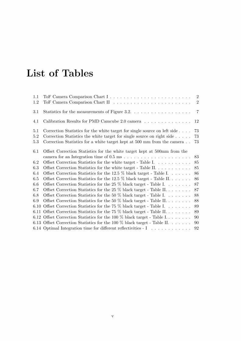
1.1 ToF Camera Comparison Chart I . . . . . . . . . . . . . . . . . . . . . . . . 21.2 ToF Camera Comparison Chart II . . . . . . . . . . . . . . . . . . . . . . . 2
3.1 Statistics for the measurements of Figure 3.2. . . . . . . . . . . . . . . . . . 7
4.1 Calibration Results for PMD Camcube 2.0 camera . . . . . . . . . . . . . . 12
5.1 Correction Statistics for the white target for single source on left side . . . . 735.2 Correction Statistics the white target for single source on right side . . . . . 735.3 Correction Statistics for a white target kept at 500 mm from the camera . . 73
6.1 Offset Correction Statistics for the white target kept at 500mm from thecamera for an Integration time of 0.5 ms . . . . . . . . . . . . . . . . . . . . 83
6.2 Offset Correction Statistics for the white target - Table I. . . . . . . . . . . 856.3 Offset Correction Statistics for the white target - Table II. . . . . . . . . . . 856.4 Offset Correction Statistics for the 12.5 % black target - Table I. . . . . . . 866.5 Offset Correction Statistics for the 12.5 % black target - Table II. . . . . . . 866.6 Offset Correction Statistics for the 25 % black target - Table I. . . . . . . . 876.7 Offset Correction Statistics for the 25 % black target - Table II. . . . . . . . 876.8 Offset Correction Statistics for the 50 % black target - Table I. . . . . . . . 886.9 Offset Correction Statistics for the 50 % black target - Table II. . . . . . . . 886.10 Offset Correction Statistics for the 75 % black target - Table I. . . . . . . . 896.11 Offset Correction Statistics for the 75 % black target - Table II. . . . . . . . 896.12 Offset Correction Statistics for the 100 % black target - Table I. . . . . . . . 906.13 Offset Correction Statistics for the 100 % black target - Table II. . . . . . . 906.14 Optimal Integration time for different reflectivities - I . . . . . . . . . . . . 92
v

vi
Chapter 1
Introduction
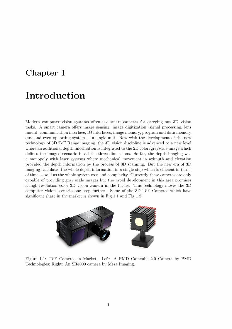
Modern computer vision systems often use smart cameras for carrying out 3D visiontasks. A smart camera offers image sensing, image digitization, signal processing, lensmount, communication interface, IO interfaces, image memory, program and data memoryetc. and even operating system as a single unit. Now with the development of the newtechnology of 3D ToF Range imaging, the 3D vision discipline is advanced to a new levelwhere an additional depth information is integrated to the 2D color/greyscale image whichdefines the imaged scenario in all the three dimensions. So far, the depth imaging wasa monopoly with laser systems where mechanical movement in azimuth and elevationprovided the depth information by the process of 3D scanning. But the new era of 3Dimaging calculates the whole depth information in a single step which is efficient in termsof time as well as the whole system cost and complexity. Currently these cameras are onlycapable of providing gray scale images but the rapid development in this area promisesa high resolution color 3D vision camera in the future. This technology moves the 3Dcomputer vision scenario one step further. Some of the 3D ToF Cameras which havesignificant share in the market is shown in Fig 1.1 and Fig 1.2.
Figure 1.1: ToF Cameras in Market. Left: A PMD Camcube 2.0 Camera by PMDTechnologies; Right: An SR4000 camera by Mesa Imaging.
1
1.1. 3D CAMERAS IN MARKET - COMPARISON 2
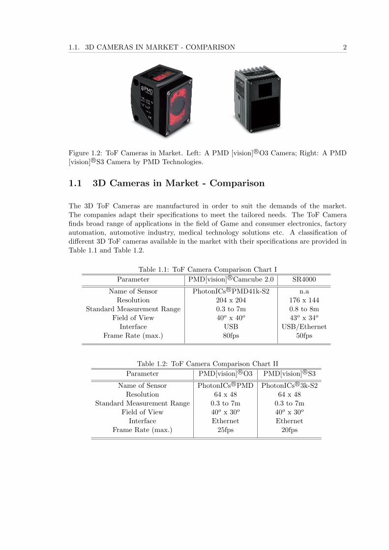
Figure 1.2: ToF Cameras in Market. Left: A PMD [vision] R©O3 Camera; Right: A PMD[vision] R©S3 Camera by PMD Technologies.
1.1 3D Cameras in Market - Comparison
The 3D ToF Cameras are manufactured in order to suit the demands of the market.The companies adapt their specifications to meet the tailored needs. The ToF Camerafinds broad range of applications in the field of Game and consumer electronics, factoryautomation, automotive industry, medical technology solutions etc. A classification ofdifferent 3D ToF cameras available in the market with their specifications are provided inTable 1.1 and Table 1.2.
Table 1.1: ToF Camera Comparison Chart I
Parameter PMD[vision] R©Camcube 2.0 SR4000
Name of Sensor PhotonICs R©PMD41k-S2 n.aResolution 204 x 204 176 x 144
Standard Measurement Range 0.3 to 7m 0.8 to 8mField of View 40o x 40o 43o x 34o
Interface USB USB/EthernetFrame Rate (max.) 80fps 50fps
Table 1.2: ToF Camera Comparison Chart II
Parameter PMD[vision] R©O3 PMD[vision] R©S3
Name of Sensor PhotonICs R©PMD PhotonICs R©3k-S2Resolution 64 x 48 64 x 48
Standard Measurement Range 0.3 to 7m 0.3 to 7mField of View 40o x 30o 40o x 30o
Interface Ethernet EthernetFrame Rate (max.) 25fps 20fps
Chapter 2
Working Principle
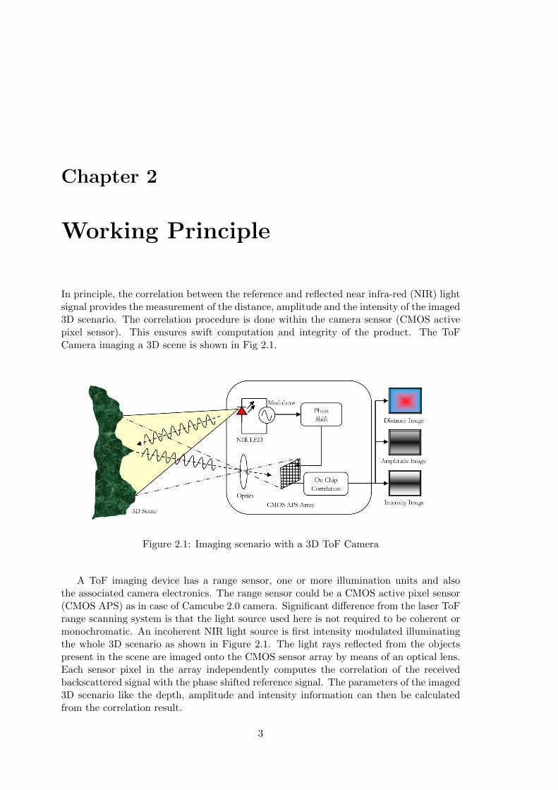
In principle, the correlation between the reference and reflected near infra-red (NIR) lightsignal provides the measurement of the distance, amplitude and the intensity of the imaged3D scenario. The correlation procedure is done within the camera sensor (CMOS activepixel sensor). This ensures swift computation and integrity of the product. The ToFCamera imaging a 3D scene is shown in Fig 2.1.
Figure 2.1: Imaging scenario with a 3D ToF Camera
A ToF imaging device has a range sensor, one or more illumination units and alsothe associated camera electronics. The range sensor could be a CMOS active pixel sensor(CMOS APS) as in case of Camcube 2.0 camera. Significant difference from the laser ToFrange scanning system is that the light source used here is not required to be coherent ormonochromatic. An incoherent NIR light source is first intensity modulated illuminatingthe whole 3D scenario as shown in Figure 2.1. The light rays reflected from the objectspresent in the scene are imaged onto the CMOS sensor array by means of an optical lens.Each sensor pixel in the array independently computes the correlation of the receivedbackscattered signal with the phase shifted reference signal. The parameters of the imaged3D scenario like the depth, amplitude and intensity information can then be calculatedfrom the correlation result.
3
2.1. RANGE MEASUREMENT 4
The correlation result c(τ) calculated at each sensor pixel is given by
c (τ) = limT→∞
T2
∫−T
2
s (t) · r (t+ τ) dt (2.1)
Here r(t) is the received backscattered signal, s(t) is the reference signal and T isthe correlation interval. Theoretically assuming ideal sinusoidal modulation of the NIRlight source [Lan00],[Lua01] the transmitted and backscattered signals can be representedrespectively as s(t) = cos(ωt) and r(t) = K + a · cos(ωt − ϕ) where ω represents themodulation frequency, K is the background offset, a is the received signal amplitude,and ϕ is the phase shift between the reference and the backscattered signal. Assumingcorrelation for infinite duration, the cross correlation function simplifies to
c (τ) =a
2· cos(ϕ+ ωτ) (2.2)
The four phase shifting evaluation is carried out by correlating the result at four phases90o shifted to each other at ωτ0 = 0o, ωτ1 = 90o, ωτ2 = 180o and ωτ3 = 270o. The phaseof the received signal is then calculated by
ϕ = arctan
{c (τ3)− c (τ1)
c (τ0)− c (τ2)
}(2.3)
Detailed explanation for the phase calculation procedure can be found in Section 5.2.
2.1 Range Measurement
From the obtained phase information ϕ, the corresponding depth information d, can bederived as
d =c
2fmod·(ϕ
2π
)(2.4)
where c is the speed of light and f mod is the frequency of the modulating light signal.
2.2 Amplitude Measurement
From the four phase algorithm, the received signal amplitude a, can be calculated as
a =1
2
√[c (τ3)− c (τ1)]2 + [c (τ0)− c (τ2)]2 (2.5)
2.3 Intensity Measurement
The corresponding background intensity I, of the received signal can then be calculatedby
I =c (τ0) + c (τ1) + c (τ2) + c (τ3)
4(2.6)
The theoretical evaluation of the correlation procedure is explained in Section 5.2.
Chapter 3
Sensor Characterization
It is very important to know the operation limits of the sensor for any application. Theknowledge of the operation limits can in turn prevent unwanted errors in the system due tothe limiting criterions. From the characterization of the sensor, the reliability and integrityof the captured data can be analysed. In this section, we evaluate the characteristics ofthe PMD Camcube 2.0 camera for analysing the reliability of the captured data. Thewarm-up drift and reliability of the sensor is studied to analyse the sensor performanceover a continuous range of operation time.
3.1 Experimental Setup: Sensor Characterization
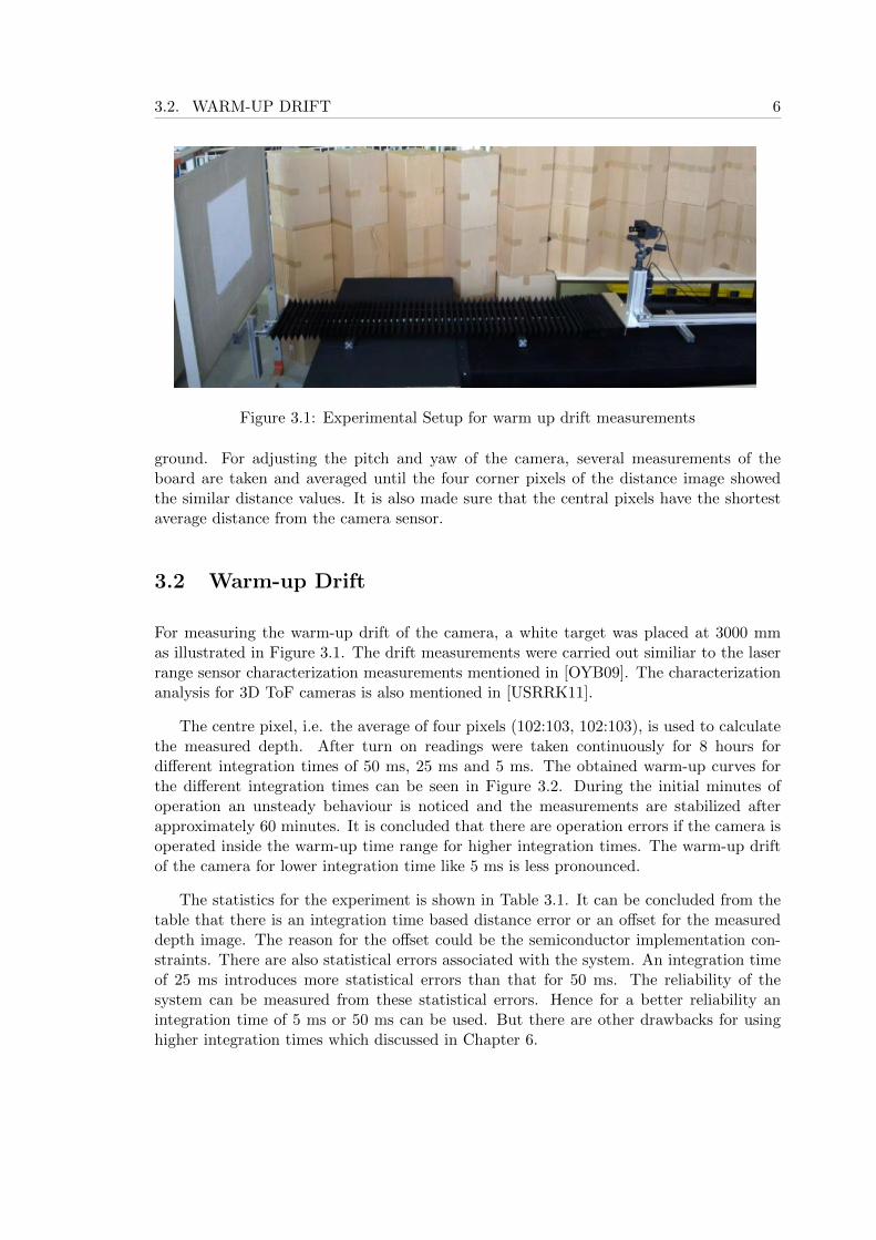
The experimental setup consists of a PMD CamCube 2.0 camera mounted on a sled on alinear motion table allowing perpendicular motion towards and away from a fixed mattedboard. The sled is driven by a stepper motor allowing a maximum travelling distanceof 7800 mm. The roll, pitch and yaw of the camera can be manually adjusted with thecamera mount. To simplify the time-consuming measurements, the data acquisition isfully automated using a PC running Windows XP SP3. A Matlab script was used both tocommunicate with the motor controller as well as to acquire the data. The measurementswere done in the dark, with only the integrated LED-array as light source. To preventunwanted reflection from the linear motion table, a zig-zag shader was built to coverthe metal guide, as proposed in [Rap07]. In the same manner, on one side of the wall,cardboard boxes were built along the linear motion table in order to prevent the reflectionsfrom the wall. The zig zag shape is maintained such that the light rays falling on the shaderis reflected to the directions other than that towards the imaging board. Even if light raysdirectly fall on the zig zag shader, the shader is imaged, whereas the unwanted reflectiontowards the board which can introduce errors in the distance measurement due to multiplereflections, are avoided. All other exposed surfaces were covered with a low reflection blackcloth. The experimental setup is shown in Figure 3.1. The accuracy of the position wasverified with an industrial grade Bosch GLM 150 Professional Laser Rangefinder1. Withthe help of level indicators it is made sure that the camera is held perpendicular to the
1Bosch GLM 150 Professional Laser Rangefinder , http://www.bosch-professional.com/gb/en/ocs/tools/101300/23315/rangefinders/glm-150/, (last accessed 25 July 2011; 09:16 hrs)
5
3.2. WARM-UP DRIFT 6
Figure 3.1: Experimental Setup for warm up drift measurements
ground. For adjusting the pitch and yaw of the camera, several measurements of theboard are taken and averaged until the four corner pixels of the distance image showedthe similar distance values. It is also made sure that the central pixels have the shortestaverage distance from the camera sensor.
3.2 Warm-up Drift
For measuring the warm-up drift of the camera, a white target was placed at 3000 mmas illustrated in Figure 3.1. The drift measurements were carried out similiar to the laserrange sensor characterization measurements mentioned in [OYB09]. The characterizationanalysis for 3D ToF cameras is also mentioned in [USRRK11].
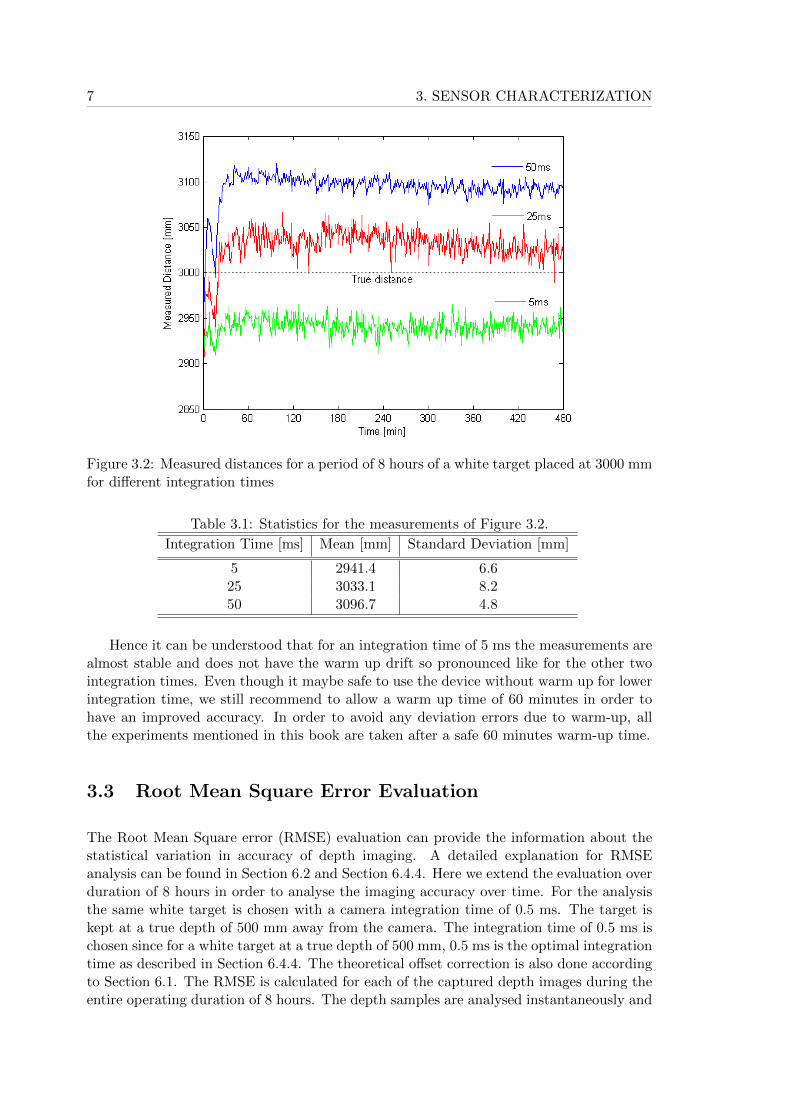
The centre pixel, i.e. the average of four pixels (102:103, 102:103), is used to calculatethe measured depth. After turn on readings were taken continuously for 8 hours fordifferent integration times of 50 ms, 25 ms and 5 ms. The obtained warm-up curves forthe different integration times can be seen in Figure 3.2. During the initial minutes ofoperation an unsteady behaviour is noticed and the measurements are stabilized afterapproximately 60 minutes. It is concluded that there are operation errors if the camera isoperated inside the warm-up time range for higher integration times. The warm-up driftof the camera for lower integration time like 5 ms is less pronounced.
The statistics for the experiment is shown in Table 3.1. It can be concluded from thetable that there is an integration time based distance error or an offset for the measureddepth image. The reason for the offset could be the semiconductor implementation con-straints. There are also statistical errors associated with the system. An integration timeof 25 ms introduces more statistical errors than that for 50 ms. The reliability of thesystem can be measured from these statistical errors. Hence for a better reliability anintegration time of 5 ms or 50 ms can be used. But there are other drawbacks for usinghigher integration times which discussed in Chapter 6.
7 3. SENSOR CHARACTERIZATION
Figure 3.2: Measured distances for a period of 8 hours of a white target placed at 3000 mmfor different integration times
Table 3.1: Statistics for the measurements of Figure 3.2.
Integration Time [ms] Mean [mm] Standard Deviation [mm]
5 2941.4 6.625 3033.1 8.250 3096.7 4.8
Hence it can be understood that for an integration time of 5 ms the measurements arealmost stable and does not have the warm up drift so pronounced like for the other twointegration times. Even though it maybe safe to use the device without warm up for lowerintegration time, we still recommend to allow a warm up time of 60 minutes in order tohave an improved accuracy. In order to avoid any deviation errors due to warm-up, allthe experiments mentioned in this book are taken after a safe 60 minutes warm-up time.
3.3 Root Mean Square Error Evaluation
The Root Mean Square error (RMSE) evaluation can provide the information about thestatistical variation in accuracy of depth imaging. A detailed explanation for RMSEanalysis can be found in Section 6.2 and Section 6.4.4. Here we extend the evaluation overduration of 8 hours in order to analyse the imaging accuracy over time. For the analysisthe same white target is chosen with a camera integration time of 0.5 ms. The target iskept at a true depth of 500 mm away from the camera. The integration time of 0.5 ms ischosen since for a white target at a true depth of 500 mm, 0.5 ms is the optimal integrationtime as described in Section 6.4.4. The theoretical offset correction is also done accordingto Section 6.1. The RMSE is calculated for each of the captured depth images during theentire operating duration of 8 hours. The depth samples are analysed instantaneously and
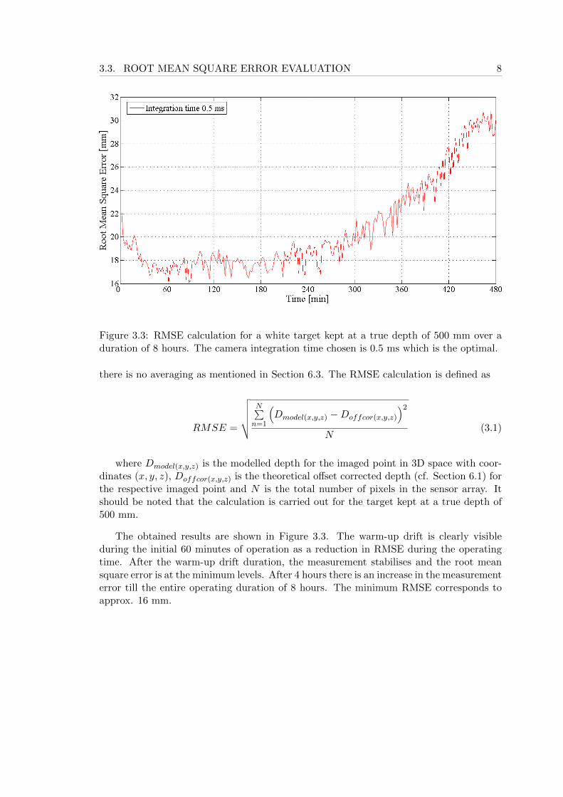
3.3. ROOT MEAN SQUARE ERROR EVALUATION 8
Figure 3.3: RMSE calculation for a white target kept at a true depth of 500 mm over aduration of 8 hours. The camera integration time chosen is 0.5 ms which is the optimal.
there is no averaging as mentioned in Section 6.3. The RMSE calculation is defined as
RMSE =
√√√√√ N∑n=1
(Dmodel(x,y,z) −Doffcor(x,y,z)
)2
N(3.1)
where Dmodel(x,y,z) is the modelled depth for the imaged point in 3D space with coor-dinates (x, y, z), Doffcor(x,y,z) is the theoretical offset corrected depth (cf. Section 6.1) forthe respective imaged point and N is the total number of pixels in the sensor array. Itshould be noted that the calculation is carried out for the target kept at a true depth of500 mm.
The obtained results are shown in Figure 3.3. The warm-up drift is clearly visibleduring the initial 60 minutes of operation as a reduction in RMSE during the operatingtime. After the warm-up drift duration, the measurement stabilises and the root meansquare error is at the minimum levels. After 4 hours there is an increase in the measurementerror till the entire operating duration of 8 hours. The minimum RMSE corresponds toapprox. 16 mm.
Chapter 4
Parameteric Calibration
The Parametric Calibration provides the necessary calibrated parameters of the camerawhich can be used to estimate the accuracy of the measured data. For any industrialgrade camera, the calibration procedure provides intrinsic parameters like the calibratedfocal length, principle point etc which can be used to derive the true information of theimaging scene. The other estimated intrinsic parameters of the calibration procedureare the distortion parameters of the camera lens. The procedure can also provide thetranslational vector and rotational matrix on the 3D space for the camera which canbe used to find the true information about the coordinate positions of the camera andthe imaging scenario. The knowledge of this extrinsic parameters can be used for poseestimation purposes. In this chapter we carry out the parametric calibration procedurefor the PMD Camcube 2.0 camera. The chapter is divided as follows. Section 4.1 andSection 4.2 explains the calculation of the intrinsic and extrinsic parameters of the camerarespectively. Section 4.3 outlines the photogrammetric calibration technique involved inthe Parametric Calibration procedure. Section 4.4 explains the experimental setup usedfor the calibration procedure and finally the calibration results are presented in Section4.5.
4.1 Camera Intrinsic Parameters
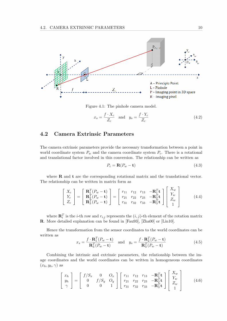
The camera intrinsic parameters provide the transformation between the image planecoordinates and the pixel coordinates of a camera. These parameters define the optical,geometric and digital characteristics of the camera. Assuming a pin hole camera model asshown in Figure 4.1, the relationship between the coordinates of the imaged point P andthe sensor pixel coordinates can be given by
xs = (xim −Ox) · Sx and ys = (yim −Oy) · Sy (4.1)
where xs and ys are the sensor array coordinates; xim and yim are the image coordi-nates, Ox and Oy is the principle point of the sensor array and Sx and Sy are the pixelsize in x and y direction respectively. Hence from the similiar triangles, the relationshipbetween the sensor coordinates and the camera coordinates of the imaged point P can bewritten as
9
4.2. CAMERA EXTRINSIC PARAMETERS 10
Figure 4.1: The pinhole camera model.
xs =f ·Xc
Zcand ys =
f · YcZc
(4.2)
4.2 Camera Extrinsic Parameters
The camera extrinsic parameters provide the necessary transformation between a point inworld coordinate system Pw and the camera coordinate system Pc. There is a rotationaland translational factor involved in this conversion. The relationship can be written as
Pc = R(Pw − t) (4.3)
where R and t are the corresponding rotational matrix and the translational vector.The relationship can be written in matrix form as Xc
YcZc
=
RT1 (Pw − t)
RT2 (Pw − t)
RT3 (Pw − t)
=
r11 r12 r13 −RT1 t
r21 r22 r23 −RT2 t
r31 r32 r33 −RT3 t
Xw
YwZw1
(4.4)
where RTi is the i-th row and ri,j represents the (i, j)-th element of the rotation matrix
R. More detailed explanation can be found in [Fau93], [Zha00] or [Lin10].
Hence the transformation from the sensor coordinates to the world coordinates can bewritten as
xs =f ·RT
1 (Pw − t)
RT3 (Pw − t)
and ys =f ·RT
2 (Pw − t)
RT3 (Pw − t)
(4.5)
Combining the intrinsic and extrinsic parameters, the relationship between the im-age coordinates and the world coordinates can be written in homogeneous coordinates(xh, yh, γ) as xh
yhγ
=
f/Sx 0 Ox0 f/Sy Oy0 0 1
r11 r12 r13 −RT
1 t
r21 r22 r23 −RT2 t
r31 r32 r33 −RT3 t
Xw
YwZw1
(4.6)
11 4. PARAMETERIC CALIBRATION
The image coordinates are then given by
xim =xhγ
and yim =yhγ
(4.7)
The Eq. (4.6) gives the relationship between the intrinsic and extrinsic parameters ofthe camera. The image distortion due to optics, cf. [Bro66], can be written as
xs = xd(1 + k1r
2 + k2r4)
and ys = yd(1 + k1r
2 + k2r4)
(4.8)
where k1 and k2 are the radial distortion coefficients; xd and yd are the distortedcoordinates where r2 = xd
2 + yd2. The next section describes the calibration technique
used for the camera.
4.3 Photogrammetric Calibration
The traditional technique of photogrammetric calibration is done by observing a calibra-tion object whose 3D geometry is known with very good precision. The calibration objectusually consists of two or three planes orthogonal to each other. The drawback of thistechnique is the expensive calibration apparatus and elaborate setup. In order to eas-ily calibrate a camera, only requiring observation of a planar pattern with few differentorientations, a calibration technique has been published in [Zha00]. Another calibrationmodel is presented in [HS97] which includes extra distortion coefficients correspondingto tangential distortion. For our calibration technique we use the Camera CalibrationToolbox for Matlab R©1 which implements the Zhang’s method with the distortion coef-ficients calculated by Heikkila’s method. The calibration technique requires imaging achequered pattern in different orientations. The calibration toolbox calculates the corre-sponding calibrated intrinsic and extrinsic parameters for the camera. An iterative methodis employed manually to optimize the correction results. An in-depth explanation of thecalibration procedure is out of scope of this work but can be found in [Zha00], [HS97],[Bro66] and [Bro71]. The next section explains the experimental setup and the chequeredplane orientations prepared for the calibration procedure.
4.4 Experimental Setup: Parametric Calibration
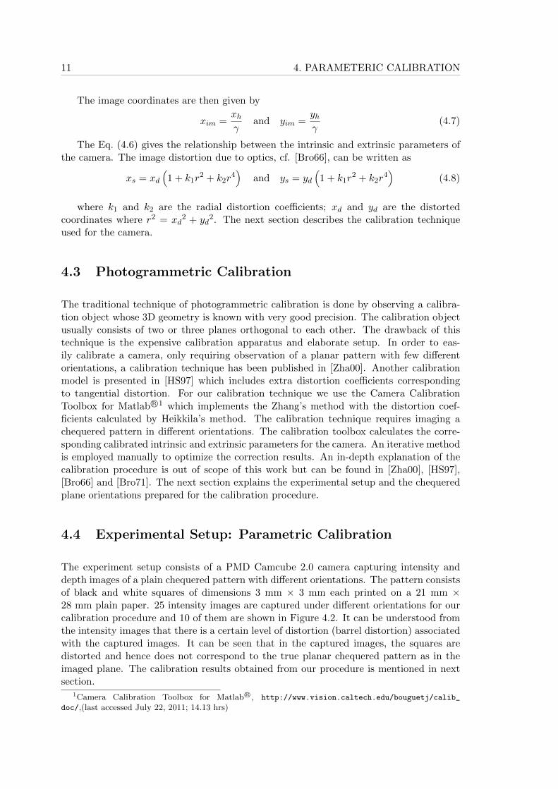
The experiment setup consists of a PMD Camcube 2.0 camera capturing intensity anddepth images of a plain chequered pattern with different orientations. The pattern consistsof black and white squares of dimensions 3 mm × 3 mm each printed on a 21 mm ×28 mm plain paper. 25 intensity images are captured under different orientations for ourcalibration procedure and 10 of them are shown in Figure 4.2. It can be understood fromthe intensity images that there is a certain level of distortion (barrel distortion) associatedwith the captured images. It can be seen that in the captured images, the squares aredistorted and hence does not correspond to the true planar chequered pattern as in theimaged plane. The calibration results obtained from our procedure is mentioned in nextsection.
1Camera Calibration Toolbox for MatlabR©, http://www.vision.caltech.edu/bouguetj/calib_
doc/,(last accessed July 22, 2011; 14.13 hrs)
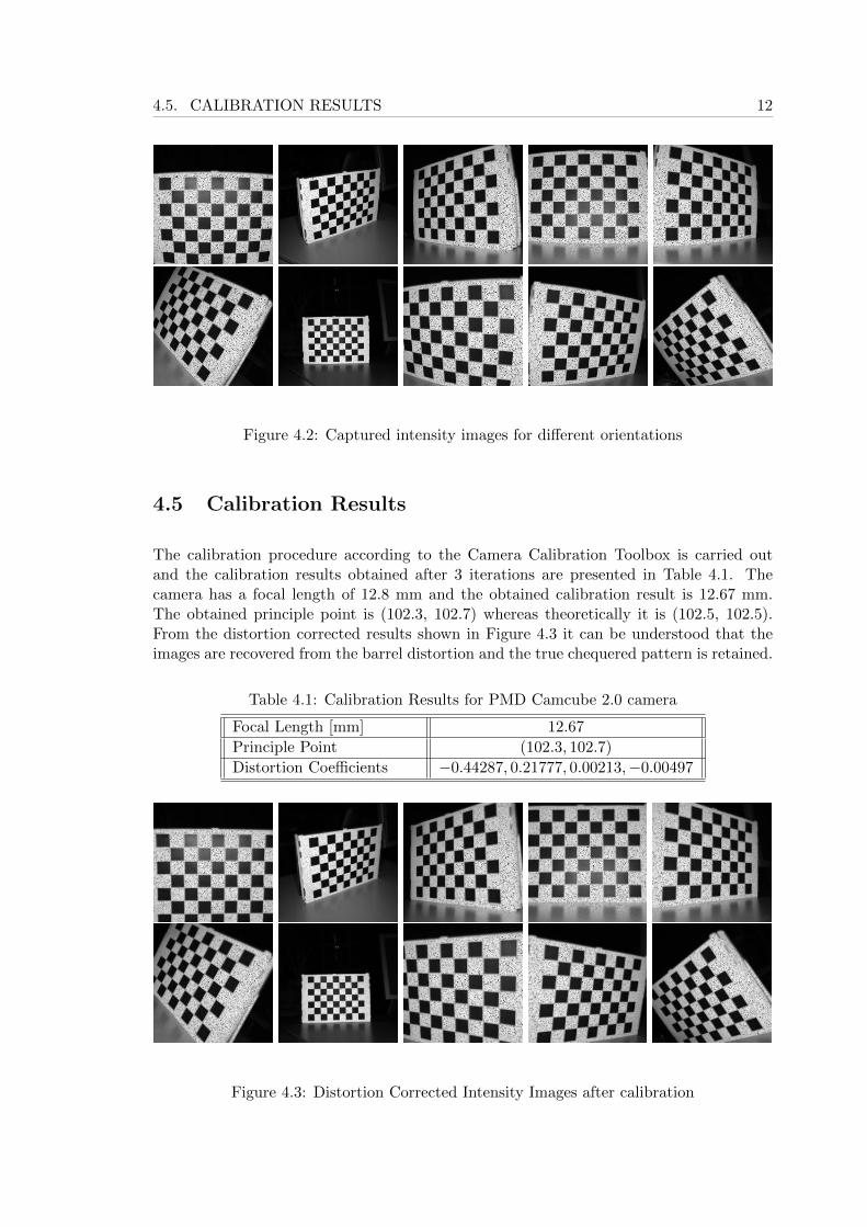
4.5. CALIBRATION RESULTS 12
Figure 4.2: Captured intensity images for different orientations
4.5 Calibration Results
The calibration procedure according to the Camera Calibration Toolbox is carried outand the calibration results obtained after 3 iterations are presented in Table 4.1. Thecamera has a focal length of 12.8 mm and the obtained calibration result is 12.67 mm.The obtained principle point is (102.3, 102.7) whereas theoretically it is (102.5, 102.5).From the distortion corrected results shown in Figure 4.3 it can be understood that theimages are recovered from the barrel distortion and the true chequered pattern is retained.
Table 4.1: Calibration Results for PMD Camcube 2.0 camera
Focal Length [mm] 12.67
Principle Point (102.3, 102.7)
Distortion Coefficients −0.44287, 0.21777, 0.00213,−0.00497
Figure 4.3: Distortion Corrected Intensity Images after calibration
Chapter 5
Models, Corrections andOptimizations
A robust imaging model is very much essential to predict the depth imaging characteristicsof the ToF camera. Even though various industrial range ToF cameras in market can havedifferences in architecture and specifications, the core principle of ’Time of Flight’ imag-ing remains the same. In this section we investigate the imaging model for ToF camerasystems. Even though the model we propose is a general one, we tailor it to suit the archi-tecture of PMD Camcube 2.0 camera under consideration. The chapter is arranged in thefollowing way. Section 5.1 proposes the imaging model for the ToF camera. Section 5.2evaluates the correlation procedure. Section 5.3 estimates the depth images captured fromthe camera according to travel time. Section 5.3 and Section 5.4 models the depth andamplitude images captured from the camera under ideal conditions. Section 5.5 describesvarious distance non linearity errors associated with the camera and three different cor-rection models namely perpendicular illumination, bistatic and optimized. Section 5.6describes the experimental setup for depth measurements and finally Section 5.7 demon-strates the experimental results and model based non linearity corrections.
5.1 ToF Imaging Model
An imaging model for the ToF camera simulates the imaging procedure of the cameraunder ideal conditions. If the practical measurement scenario correlates well with theideal situation, or is well within the tolerance trade off limits with respect to the idealsituation, the model can be taken to be a benchmark to assess the performance of theimaging system. More importantly in such cases, the imaging model can be used to assessthe quality of the measurements in order to learn the statistics of the system. Theseevaluations provide a measure for the stochastically varying noise due to the measurementprocedure. Hence the imaging model is very important to assess any systematic errors orto learn the statistics of the measurement quantities.
An architectural model for the Time of Flight camera has been first proposed in [Xu99].The thesis provides an initial structural level design for a 3D ToF system. It also ad-
13
5.1. TOF IMAGING MODEL 14
dresses structural level non linearities within the imaging system. Implementation specificinformation in the semiconductor level is described in [Lan00]. It provides a mathematicalevaluation of the correlation principle and also outlines the Fourier analysis of the imagingprinciple. It also discusses the influence of system nonlinearities in the imaging procedureand provides a mathematical analysis of the aliasing effects within the system. A muchdetailed frequency domain analysis of the imaging principle is provided in [Lua01]. It pro-vides an in depth Fourier analysis discussion about the phase shifting method, modulationand the 3D data evaluation algorithm within the imaging system. A theoretical modelfor the camera is proposed in [Rap07], considering harmonically modulated signals whichoutlined the cause of the wiggling error of the ToF camera. The thesis also illustrates anerror propagation model for the camera and also the relation between statistical deptherror and amplitude of the received signal.
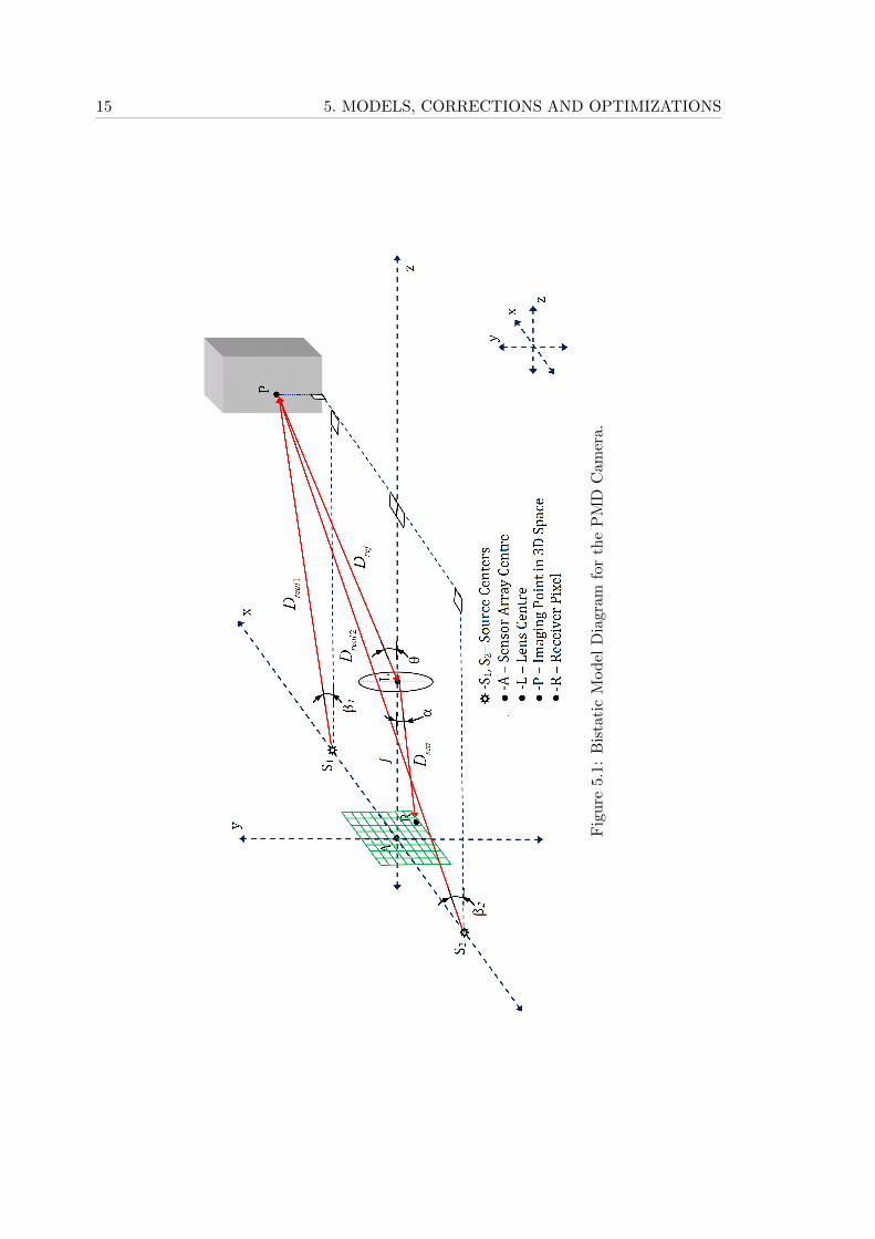
The PMD Camcube 2.0 camera uses two light sources symmetrically mounted on bothsides of the sensor array to illuminate the target for depth information. The camera hencebenefits a bistatic constellation with the sources separated from the sensor [PL07]. Thesensor array has pixel resolution of 204 × 204. The imaging scenario of the camera isshown in Figure 5.1.
Here the light sources S1 and S2 illuminate the 3D imaging scenario with incidentlight rays falling in the near infrared wavelength region. Both the sources, S1 and S2,are arranged spatially symmetric to the camera. We assume the light sources are pointsources, which mean that the sources introduce spherical wavefronts for the imaging task.The field of view of the camera lens is 400 × 400. The light rays originated from thesources are incident on a point P in 3D space. Both rays travelling from the sources makeangles β1 and β2 with the respective surface normals of the x− y plane at the sources S1
and S2. The rays impinging on the point P travel a distance of Dreal1 and Dreal2 withrespect to the sources S1 and S2 such that S1P = Dreal1 and S2P = Dreal2 as shown inFigure 5.1. The reflected ray at the point P makes an angle θ with respect to the surfacenormal parallel to that of S1 and S2 at the point L such that the length of the reflectedray PL = Dref and Dper = Dref cos θ. The light ray then gets refracted at the centre ofthe lens L and travels a distance of LR = Dsen in order to reach the receiver pixel R onthe sensor array. This refracted ray makes an angle α with respect to the surface normal,at the point A, to the sensor array as shown in the Figure 5.1. The imaging lens and thesensor array is separated by a distance of focal length f of the camera.
If we assume the maximum instantaneous amplitude of the modulating signal of the twosources S1 and S2 as A1 and A2 respectively and the phase offset for the modulating signalsas φ1 and φ2 respectively, and assuming a lossless medium, the instantaneous amplitudeof the emitted signals from the two sources S1 and S2 can be expressed respectively as
f1(t) = rectT/2(t) ·A1 · cos{ωt− φ1} (5.1)
andf2(t) = rectT/2(t− τ) ·A2 · cos{ωt− φ2} (5.2)
where ω is the angular frequency and t is the instantaneous time of the modulatingsignal. The frequency of the modulating signal is assumed practically to be 20 MHz whichenables a maximum unambiguous measurable depth of 7.5 m with the ToF camera. The
15 5. MODELS, CORRECTIONS AND OPTIMIZATIONS
Fig
ure
5.1:
Bis
tati
cM
od
elD
iagr
amfo
rth
eP
MD
Cam
era.
5.1. TOF IMAGING MODEL 16
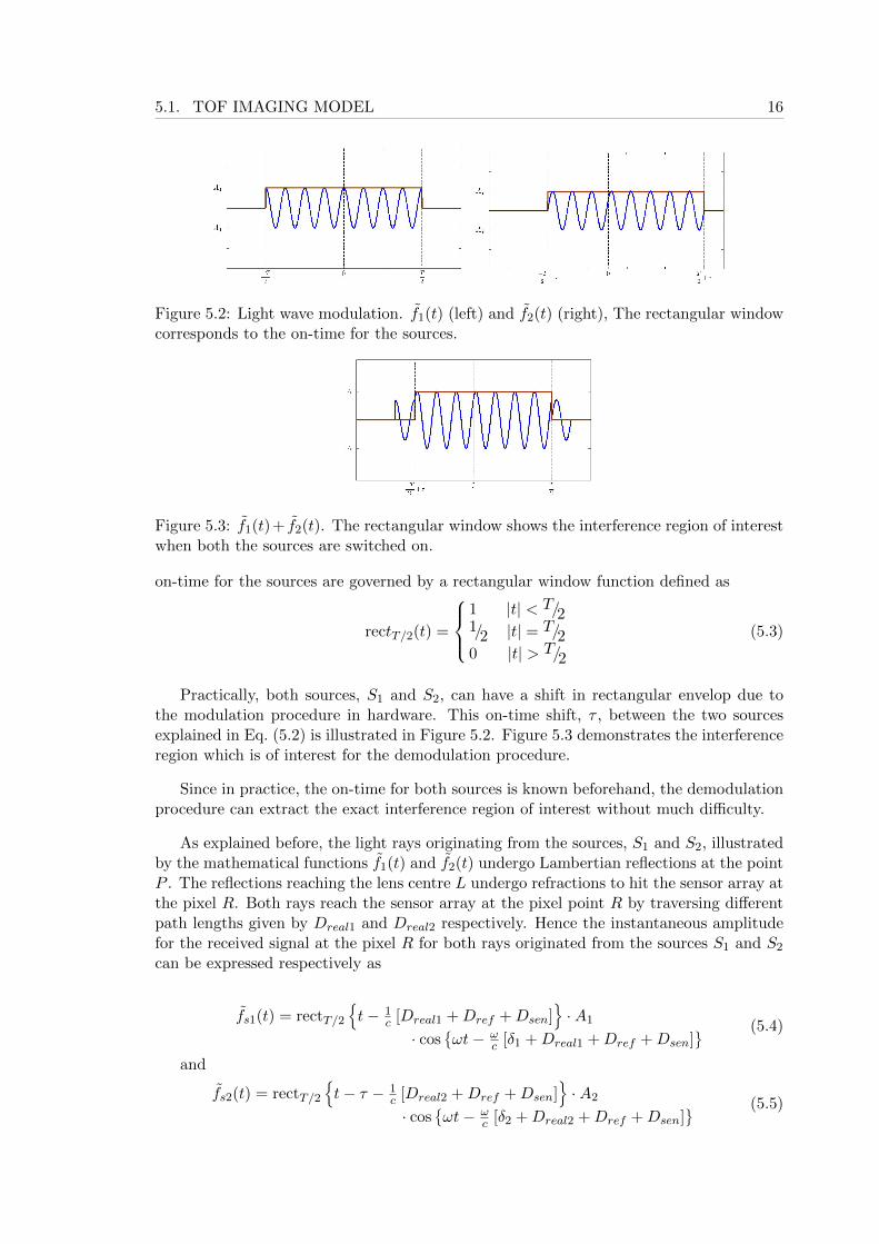
Figure 5.2: Light wave modulation. f1(t) (left) and f2(t) (right), The rectangular windowcorresponds to the on-time for the sources.
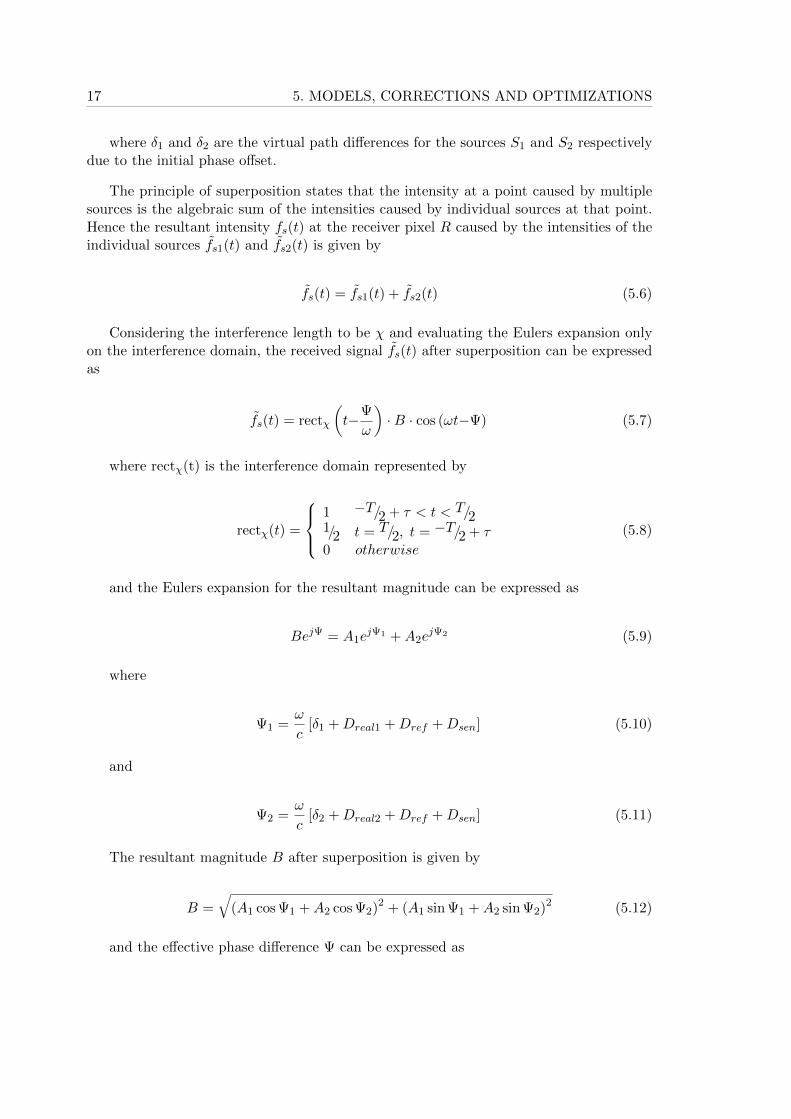
Figure 5.3: f1(t)+ f2(t). The rectangular window shows the interference region of interestwhen both the sources are switched on.
on-time for the sources are governed by a rectangular window function defined as
rectT/2(t) =
1 |t| < T/21/2 |t| = T/20 |t| > T/2
(5.3)
Practically, both sources, S1 and S2, can have a shift in rectangular envelop due tothe modulation procedure in hardware. This on-time shift, τ , between the two sourcesexplained in Eq. (5.2) is illustrated in Figure 5.2. Figure 5.3 demonstrates the interferenceregion which is of interest for the demodulation procedure.
Since in practice, the on-time for both sources is known beforehand, the demodulationprocedure can extract the exact interference region of interest without much difficulty.
As explained before, the light rays originating from the sources, S1 and S2, illustratedby the mathematical functions f1(t) and f2(t) undergo Lambertian reflections at the pointP . The reflections reaching the lens centre L undergo refractions to hit the sensor array atthe pixel R. Both rays reach the sensor array at the pixel point R by traversing differentpath lengths given by Dreal1 and Dreal2 respectively. Hence the instantaneous amplitudefor the received signal at the pixel R for both rays originated from the sources S1 and S2
can be expressed respectively as
fs1(t) = rectT/2{t− 1
c [Dreal1 +Dref +Dsen]}·A1
· cos{ωt− ω
c [δ1 +Dreal1 +Dref +Dsen]} (5.4)
and
fs2(t) = rectT/2{t− τ − 1
c [Dreal2 +Dref +Dsen]}·A2
· cos{ωt− ω
c [δ2 +Dreal2 +Dref +Dsen]} (5.5)
17 5. MODELS, CORRECTIONS AND OPTIMIZATIONS
where δ1 and δ2 are the virtual path differences for the sources S1 and S2 respectivelydue to the initial phase offset.
The principle of superposition states that the intensity at a point caused by multiplesources is the algebraic sum of the intensities caused by individual sources at that point.Hence the resultant intensity fs(t) at the receiver pixel R caused by the intensities of theindividual sources fs1(t) and fs2(t) is given by
fs(t) = fs1(t) + fs2(t) (5.6)
Considering the interference length to be χ and evaluating the Eulers expansion onlyon the interference domain, the received signal fs(t) after superposition can be expressedas
fs(t) = rectχ
(t−Ψ
ω
)·B · cos (ωt−Ψ) (5.7)
where rectχ(t) is the interference domain represented by
rectχ(t) =
1 −T/2 + τ < t < T/21/2 t = T/2, t = −T/2 + τ0 otherwise
(5.8)
and the Eulers expansion for the resultant magnitude can be expressed as
BejΨ = A1ejΨ1 +A2e
jΨ2 (5.9)
where
Ψ1 =ω
c[δ1 +Dreal1 +Dref +Dsen] (5.10)
and
Ψ2 =ω
c[δ2 +Dreal2 +Dref +Dsen] (5.11)
The resultant magnitude B after superposition is given by
B =√
(A1 cos Ψ1 +A2 cos Ψ2)2 + (A1 sin Ψ1 +A2 sin Ψ2)2 (5.12)
and the effective phase difference Ψ can be expressed as
5.1. TOF IMAGING MODEL 18
Ψ = arctan
(A1 sin Ψ1 +A2 sin Ψ2
A1 cos Ψ1 +A2 cos Ψ2
)(5.13)
Under ideal situations, we can consider the incident amplitudes of both sources to beequal, or can be assumed to be modulated from a common source. Hence the commoninstantaneous incident amplitude can be assumed to be A = A1 = A2. It can also beassumed under ideal situations that the initial phase shift of the two sources δ1 = δ2 = 0.Also assuming ideally that the on-times of both the sources are simultaneous and equal,which means τ = 0, the received signal fs(t) can be simplified as
fs(t) = rectT/2
(t−Ψ
ω
)·B · cos (ωt−Ψ) (5.14)
where
rectT/2(t) =
1 |t| < T/21/2 |t| = T/20 otherwise
(5.15)
and the instantaneous amplitude B can be simplified by applying the trigonometric iden-tities cos(A− B) = cosA · cosB + sinA · sinB and 1 + cos2A = 2 · cos2A as,
B = 2 ·A cos
(Ψ1 −Ψ2
2
)(5.16)
and the resultant phase shift Ψ expressed as
Ψ =Ψ1 + Ψ2
2(5.17)
where the individual phase components Ψ1 and Ψ2 are expressed as
Ψ1 =ω
c[Dreal1 +Dref +Dsen] (5.18)
andΨ2 =
ω
c[Dreal2 +Dref +Dsen] (5.19)
The maximum unambiguous range is 7.5 m for the modulation frequency under con-sideration which is 20 MHz. This unambiguous range corresponds to half the wavelengthλ, hence the maximum unambiguous phase difference of the received signal at point R isπ which is half the net phase difference of 2π. Substituting the values for B,Ψ,Ψ1 and Ψ2
in Eq. (5.16), the net intensity fs(t) at the receiver pixel R after simplification can beexpressed as
fs(t) = rectT/2(t− Ψ
ω
)· 2 ·A · cos
{ωc (Dreal1 −Dreal2)
}· cos
{ωt− ω
c
(Dreal1+Dreal2
2 +Dref +Dsen
)} (5.20)
19 5. MODELS, CORRECTIONS AND OPTIMIZATIONS
5.2 Correlation Model
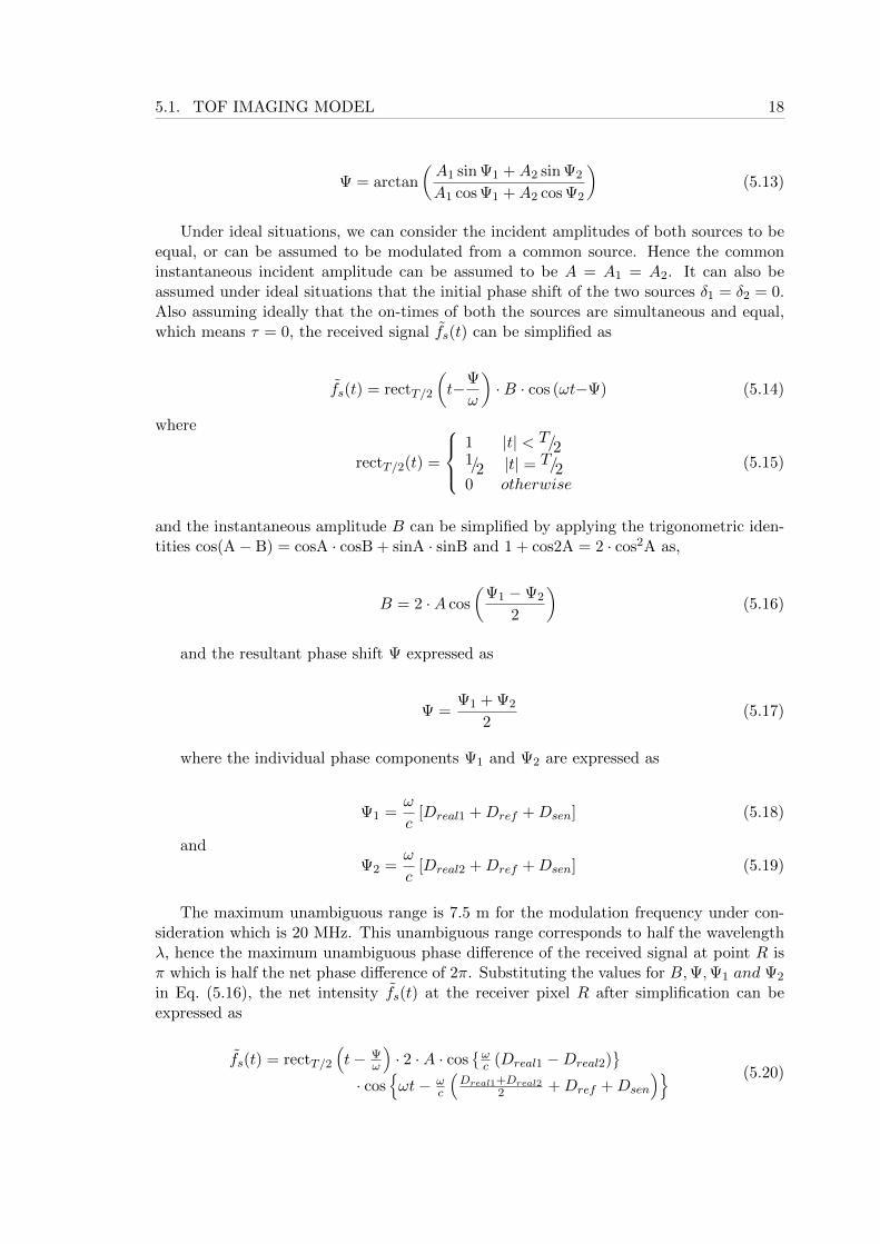
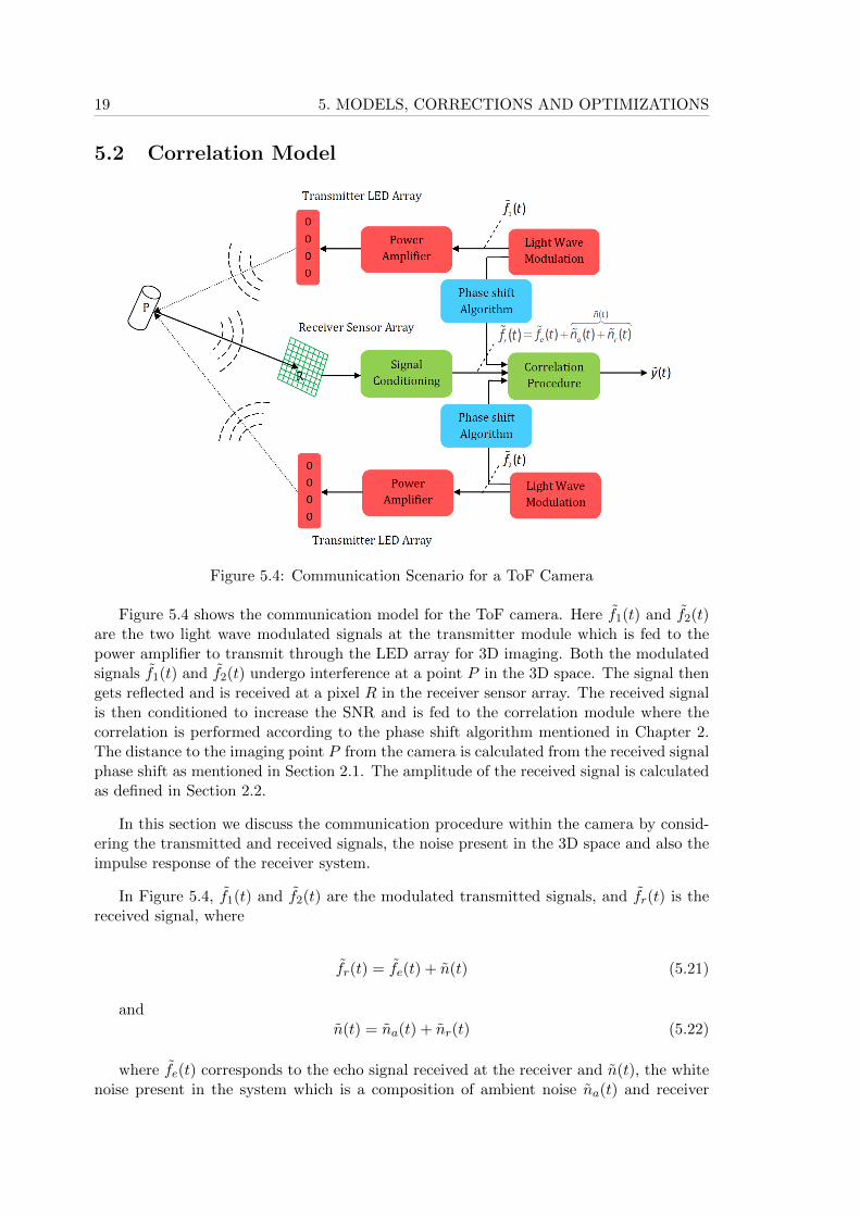
Figure 5.4: Communication Scenario for a ToF Camera
Figure 5.4 shows the communication model for the ToF camera. Here f1(t) and f2(t)are the two light wave modulated signals at the transmitter module which is fed to thepower amplifier to transmit through the LED array for 3D imaging. Both the modulatedsignals f1(t) and f2(t) undergo interference at a point P in the 3D space. The signal thengets reflected and is received at a pixel R in the receiver sensor array. The received signalis then conditioned to increase the SNR and is fed to the correlation module where thecorrelation is performed according to the phase shift algorithm mentioned in Chapter 2.The distance to the imaging point P from the camera is calculated from the received signalphase shift as mentioned in Section 2.1. The amplitude of the received signal is calculatedas defined in Section 2.2.
In this section we discuss the communication procedure within the camera by consid-ering the transmitted and received signals, the noise present in the 3D space and also theimpulse response of the receiver system.
In Figure 5.4, f1(t) and f2(t) are the modulated transmitted signals, and fr(t) is thereceived signal, where
fr(t) = fe(t) + n(t) (5.21)
andn(t) = na(t) + nr(t) (5.22)
where fe(t) corresponds to the echo signal received at the receiver and n(t), the whitenoise present in the system which is a composition of ambient noise na(t) and receiver
5.2. CORRELATION MODEL 20
noise nr(t).
Here the transmitted signals f1(t) and f2(t) are finite energy band pass signals obeyingthe criterion,
f1(t) = 0 for t /∈ [0, T1] (5.23)
and
f2(t) = 0 for t /∈ [0, T2] (5.24)
The received echo signal fe(t) after reflection is defined as
fe(t) = ` · fs(t)= ` · rectT/2(t− ν) ·B cos (ω (t− ν))
(5.25)
where ` models the propagation and reflection losses, fs(t) represents the receivedinterference signal, i.e. the superposition of f1(t) and f2(t) and ν = Ψ
ω , represents theeffective travel time with respect to the interfering source signals. The interference signalfs(t), obtained at the receiver end is defined as
fs(t) = I{f1(t− ν1), f2(t− ν2)
}(5.26)
where I represents the interference operator of the two source signals and ν1 and ν2
represents the individual travel times for the two sources.
For stability of the receiver, the impulse response h(t), of the receiver filter shouldsatisfy
∫ ∣∣∣h(t)∣∣∣dt <∞ (5.27)
The output signal y(t) after the filtering procedure (correlation) is defined as theconvolution integral
y(t) = h(t) ∗ fr(t)=∫h(t′)fr(t− t′)dt′
=∫h(t′)fe(t− t′)dt′ +
∫h(t′)n(t− t′)dt′
(5.28)
The signal to noise ratio ζ(h), at t = ν, of the receiver filter is given by
ζ(h) =
(∫h(t′)fe(ν − t′)dt′
)2
E(∫
h(t′)n(ν − t′)dt′)2 =
f2e,h
(ν)
E(n2h(ν)) =
f2e,h
(ν)
σnh
2(5.29)
21 5. MODELS, CORRECTIONS AND OPTIMIZATIONS
where the noise convolution is replaced by the expected value of the integral due to thestochastic nature and σnh
is the standard deviation of white noise present in the system.
Optimal filtering should possess at t = ν a maximum value. Here the echo signalconvolution is given by
fe,h(ν) =
∫h(t′)fe(ν − t′)dt′ = `
∫h(t′)f(−t′)dt′ (5.30)
and the white noise convolution is given by
nh(ν) =
∫h(t′)n(ν − t′)dt′ (5.31)
The second order moment (correlation) function of the zero mean wide sense stationaryprocess nh(ν), can be written as
rnhnh(ν) = E
(nh(t+ ν)nh(t)
)= E
(∫h(t′)n(t+ ν − t′)dt′ ·
∫h(t′′)n(t− t′′)dt′′
)=
∫∫h(t′)h(t′′)E
(n(t+ ν − t′)n(t− t′′)
)dt′dt′′ (5.32)
=
∫∫h(t′)h(t′′)rnn
(ν − t′ + t′′
)dt′dt′′
Applying the Wiener-Khintchine Theorem the power spectral density function of nh(t)is given by
Rnhnh(ω) =
∫rnhnh
(ν) e−jωνdν
=
∫∫∫h(t′)h(t′′)rnn
(ν − t′ + t′′
)e−jωνdνdt′dt′′
=
∫∫h(t′)h(t′′)
(∫rnn
(ν − t′ + t′′
)e−jωνdν
)dt′dt′′
=
∫∫h(t′)h(t′′)Rnn (ω) e−jω(t′−t′′)dt′dt′′ (5.33)
= Rnn (ω)
∫h(t′)e−jω(t′)dt′ ·
∫h(t′)ejω(t′′)dt′′
= Rnn (ω) H (ω) H∗ (ω) =∣∣∣H (ω)
∣∣∣2Rnn (ω)
The variance or power of nh(t) can now be describe in terms of the power spectraldensity function Rnhnh
(ω) as follows
5.2. CORRELATION MODEL 22
σnh
2 = E(n2h(ν))
= rnhnh(0)
= 12π
∫Rnhnh
(ω) dω
= 12π
∫ ∣∣∣H (ω)∣∣∣2Rnn (ω) dω
(5.34)
Since n(t) is supposed to be white noise, it exhibits a constant power spectral densityfunction. This means that
Rnn (ω) = N0/2 (5.35)
where
rnn (t) = N0/2 · δ (t) (5.36)
Thus finally, the power or variance of nh(t) is given by
σnh
2 = E(n2h(ν))
=N0
4π
∫ ∣∣∣H (ω)∣∣∣2dω (5.37)
From Parsevals theorem, we have the equality
∥∥∥h∥∥∥2=∫ ∣∣∣h (t)
∣∣∣2dt= 1
2π
∫ ∣∣∣H (ω)∣∣∣2dω = 1
2π
∥∥∥H (ω)∥∥∥2 (5.38)
Now we have all the required results to evaluate the optimal filtering criterion. Foroptimal filtering, the signal to noise ratio should be maximum. The signal to noise ratiois given by
ζ(h) =(`∫h(t)f(−t)dt)
2
N0/2·∫|h(t)|2dt = 2`2
N0
∥∥∥f∥∥∥2 (∫h(t)f(−t)dt)
2
‖h‖2‖f‖2
= 2`2
N0
∥∥∥f∥∥∥2 (∫h(t)f(t)dt)
2
‖h‖2‖f‖2(5.39)
where
f(t) = f(−t) and∥∥∥f∥∥∥2
=∥∥∥f∥∥∥2
(5.40)
Cauchy-Schwarz inequality for two functions g1(t) and g2(t) states that
∣∣∣∣∫ g1(t)g∗2(t)dt
∣∣∣∣2 ≤ ∫ |g1(t)|2dt ·∫|g2(t)|2dt (5.41)
which means the L.H.S integral has its maximum value when g1(t) = c·g2(t). Applyingthe result on Eq. (5.39), we obtain that the SNR has its maximum value at the optimalimpulse response
23 5. MODELS, CORRECTIONS AND OPTIMIZATIONS
hopt(t) = c · f(t) = c · f(−t) (5.42)
The optimal filter response is called now as the matched filter response since theimpulse response of the receiver is now matched to the transmitted signal. Hence, thereceiver filter is now called the matched filter.
The maximum signal to noise ratio is now given by
ζ(hopt) =2`2
N0
∥∥∥f∥∥∥2(5.43)
For c = 1, the matched filter output can be expressed as
y(t) =∫hopt(t
′)fr(t− t′)dt′ =∫f(−t′)fr(t− t′)dt′
=∫f(t′′)fr(t+ t′′)dt′′ = rfr f (t)
(5.44)
where rfr f (t) is the correlation between the received signal fr(t) and the reference
signal f(t). From Eq. (5.43), it can be shown that the correlation function gives themaximum signal to noise ratio for the receiver filtering procedure. The correlation canalso be interpreted as the matched filtering process of the input signal fr(t) with thereference signal f(t).
Ideally we assume the transmitted band pass signals are modulated by a commonmodulating signal f(t). We also assume that both the transmitted finite energy band passsignals are time limited simultaneously. Hence we can write
f(t) = f1(t) = f2(t) (5.45)
where
f(t) = 0 for t /∈ [0, T ] (5.46)
Hence by considering the interference between the transmitted signals, the receivedsignal at the sensor array mentioned in Eq. (5.26) can be rewritten as
fs(t) = I{f(t− ν1), f(t− ν2)
}(5.47)
where I represents the interference function between the two source signals and ν1 andν2 represents the individual travel time for the two sources.
From Section 5.1, Eq. (5.20), considering the ideal noiseless situation where n(t) = 0,we have the signal obtained at the receiver end after interference fs(t), given by
fr(t) = fe(t) = ` · fs(t) = ` · rectT/2
(t− Ψ
ω
)·B · cos (ωt−Ψ) (5.48)
5.2. CORRELATION MODEL 24
where
rectT/2(t) =
1 |t| < T/21/2 |t| = T/20 otherwise
(5.49)
and the instantaneous resultant amplitude B is expressed as
B = 2A cos
(Ψ1 −Ψ2
2
)(5.50)
and the phase shft Ψ expressed as
Ψ =ω
c
(Dreal1 +Dreal2
2+Dref +Dsen
)(5.51)
Here Ψ1 and Ψ2 are expressed as per Eq. (5.10) and Eq. (5.11).
Considering an ideal situation where the received signal has no propagation losses, i.e.` = 1, we can expressed the received signal as
fr(t) = rectT/2
(t−Ψ
ω
)·B · cos (ωt−Ψ) (5.52)
Since we assume both the signals are modulated from the same source, the referencesignal can be written as
f(t) = rectT/2 (t) ·A · cos (ωt) (5.53)
We now have the reference modulating signal as well as the received signal, hence thereceiver correlation output y(t), can now be expressed as
y(t) = hopt(t) ∗ fr (t) = f(−t) ∗ fr(t)=∫f(−t′)fr(t− t′)dt′
=∫f(t′′)fr(t+ t′′)dt′′
= A ·B∫
rectT/2 (t′′) rectT/2 (t+ t′′ − ν)
cos (ωt′′) cos {ω (t+ t′′ − ν)} dt′′(5.54)
where ν = Ψω . Substituting t = t− ν, we get
y(t) = y(t+ ν)= A ·B
∫rectT/2 (t′′) rectT/2
(t+ t′′
)· cos (ωt′′) cos
{ω(t+ t′′
)}dt′′
(5.55)
After exploiting the identity, 2 cosA cosB = cos(A + B) + cos(A − B), we get thecorrelation output as,
25 5. MODELS, CORRECTIONS AND OPTIMIZATIONS
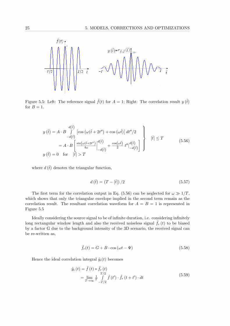
Figure 5.5: Left: The reference signal f(t) for A = 1; Right: The correlation result y(t)
for B = 1.
y(t)
= A ·Bd(t)∫−d(t)
[cos
(ω(t+ 2t′′
)+ cos
(ωt)]dt′′/2
= A ·B[
sin(ω(t+2t′′)4ω
∣∣∣∣d(t)−d(t)
+cos(ωt)
2 t′′|d(t)−d(t)
]
∣∣t∣∣ ≤ Ty(t)
= 0 for∣∣t∣∣ > T
(5.56)
where d(t)
denotes the triangular function,
d(t)
=(T −
∣∣t∣∣) /2 (5.57)
The first term for the correlation output in Eq. (5.56) can be neglected for ω � 1/T ,which shows that only the triangular envelope implied in the second term remain as thecorrelation result. The resultant correlation waveform for A = B = 1 is represented inFigure 5.5
Ideally considering the source signal to be of infinite duration, i.e. considering infinitelylong rectangular window length and also the received noiseless signal fr (t) to be biasedby a factor G due to the background intensity of the 3D scenario, the received signal canbe re-written as,
fr(t) = G+B · cos (ωt−Ψ) (5.58)
Hence the ideal correlation integral yi(t) becomes
yi (t) = f (t) ∗ fr (t)
= limT→∞
1T
T/2∫−T/2
f (t′) · fr (t+ t′) · dt (5.59)
5.2. CORRELATION MODEL 26
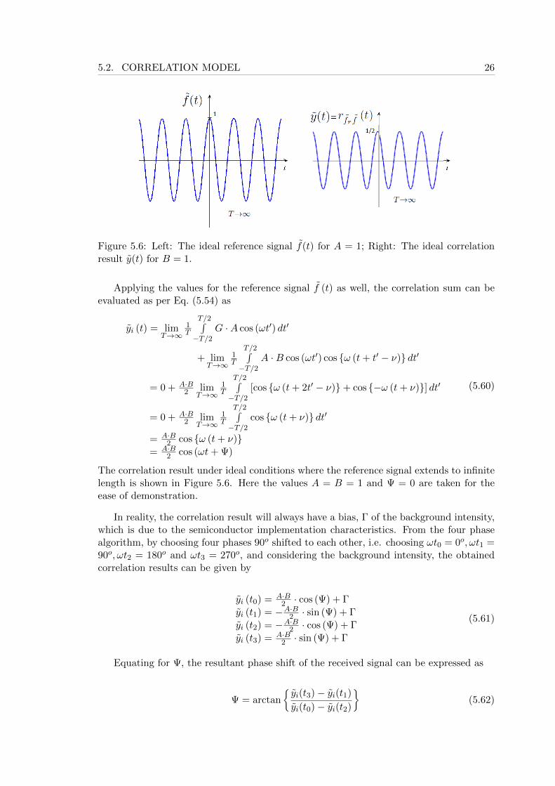
Figure 5.6: Left: The ideal reference signal f(t) for A = 1; Right: The ideal correlationresult y(t) for B = 1.
Applying the values for the reference signal f (t) as well, the correlation sum can beevaluated as per Eq. (5.54) as
yi (t) = limT→∞
1T
T/2∫−T/2
G ·A cos (ωt′) dt′
+ limT→∞
1T
T/2∫−T/2
A ·B cos (ωt′) cos {ω (t+ t′ − ν)} dt′
= 0 + A·B2 lim
T→∞1T
T/2∫−T/2
[cos {ω (t+ 2t′ − ν)}+ cos {−ω (t+ ν)}] dt′
= 0 + A·B2 lim
T→∞1T
T/2∫−T/2
cos {ω (t+ ν)} dt′
= A·B2 cos {ω (t+ ν)}
= A·B2 cos (ωt+ Ψ)
(5.60)
The correlation result under ideal conditions where the reference signal extends to infinitelength is shown in Figure 5.6. Here the values A = B = 1 and Ψ = 0 are taken for theease of demonstration.
In reality, the correlation result will always have a bias, Γ of the background intensity,which is due to the semiconductor implementation characteristics. From the four phasealgorithm, by choosing four phases 90o shifted to each other, i.e. choosing ωt0 = 0o, ωt1 =90o, ωt2 = 180o and ωt3 = 270o, and considering the background intensity, the obtainedcorrelation results can be given by
yi (t0) = A·B2 · cos (Ψ) + Γ
yi (t1) = −A·B2 · sin (Ψ) + Γ
yi (t2) = −A·B2 · cos (Ψ) + Γ
yi (t3) = A·B2 · sin (Ψ) + Γ
(5.61)
Equating for Ψ, the resultant phase shift of the received signal can be expressed as
Ψ = arctan
{yi(t3)− yi(t1)
yi(t0)− yi(t2)
}(5.62)
27 5. MODELS, CORRECTIONS AND OPTIMIZATIONS
The magnitude of the correlation result can now be expressed as
A ·B =√
[yi(t3)− yi(t1)]2 + [yi(t0)− yi(t2)]2 (5.63)
Since we know the magnitude of the reference signal A beforehand, the magnitude ofthe received signal B can now be found by the equation
B =1
A
√[yi(t3)− yi(t1)]2 + [yi(t0)− y(t2)]2 (5.64)
The background intensity bias Γ can be evaluated by the expression
Γ =yi(t0) + yi(t1) + yi(t2) + yi(t3)
4(5.65)
From Eq. (5.17), Eq. (5.18) and Eq. (5.19) the ideal value of the phase shift Ψ, of thereceived signal can also be written as
Ψ =ω
c
(Dreal1 +Dreal2
2+Dref +Dsen
)(5.66)
From Eq. (5.16), the ideal value of the magnitude B, of the received signal can also bewritten as
B = 2 ·A · cos
{ω
c(Dreal1 −Dreal2)
}(5.67)
5.3 Depth Estimation Model
From the architecture of the 3D ToF camera, it is evident that the distance informationextracted by each of the pixels is directly proportional to the forward and backward pathstraversed by the NIR light rays to that particular pixel. Hence the distance informationobtained from the sensor array after the correlation procedure has a spatial variation withrespect to the different path lengths traversed by the light rays to reach each of the receiverpixels. Due to this difference in path length, there is nonlinearity in the obtained distanceinformation when imaging 3D scenarios. An example is worth mentioning. When imaginga straight board with the 3D ToF camera, instead of obtaining a distance informationconstant for each of the pixels excluding the statistical errors, we obtain a nonlinear curvedspatial variation for the extracted distance information from the pixels. The reason forthis is the one mentioned above. Distance information in each of the pixels are modifiedaccording to the travel paths towards each pixels. Since the travel paths towards eachpixel has a spatial variation due to the generated approximately spherical wavefronts ofthe NIR light source, the extracted distance information has the same nonlinear variationspatially.
5.3. DEPTH ESTIMATION MODEL 28
In this section we model this spatial variation of the NIR light source for all the pointsin the 3D space at a constant coordinate distance from the camera. From this spatialvariation of the travel time of the NIR source, we model the ideal expected distanceinformation to be extracted from the pixels.
From Section 5.2, Eq. (5.66), the ideal phase shift Ψ of the received signal is given by
Ψ =ω
c
(Dreal1 +Dreal2
2+Dref +Dsen
)(5.68)
Each sensor pixel is associated with different travel time according to the respectiveimaging point in 3D space. Assuming the sensor array centre at the origin of the 3Dcoordinate system as demonstrated in Figure 5.1, the obtained phase shift for any sensorpixel imaging a point at a distance z in 3D space is given by
Ψ(x,y,z) =ω
c
(Dreal1(x,y,z) +Dreal2(x,y,z)
2+Dref(x,y,z) +Dsen(x,y,z)
)(5.69)
where x, y and z are coordinates for direction as well as the depth for the imaged pointin 3D space. We now propose a method to find the ideal expected distance informationfrom the knowledge of the phase shift as mentioned in Eq. (5.69).
First we assume that each of the points in the 3D space imaged by the camera is ata constant distance, in the coordinate space along z direction. This in turn means thatthe imaging points belong to a locus of a distance of (Zc + f) units from the x-y plane asdemonstrated in Figure 5.7.
From the camera intrinsic parameters mentioned in Chapter 4.1, approximating theimaging procedure to that of a pin hole camera model, we have
xs = fXc
Zcand ys = f
YcZc
(5.70)
and
xs = (xim −Ox)Sx and ys = (yim −Oy)Sy (5.71)
where xs and ys are the coordinates of the sensor array pixel under consideration in xand y directions respectively; f is the focal length of the lens used in the sensor system;Xc and Yc are the coordinates of the imaged points in the 3D space in x and y directionsrespectively; Ox and Oy are the principle points of the sensor array; xim and yim are theimage coordinates in the sensor array and Sx and Sy are the size of the sensor pixels inx and y directions respectively. Zc is the distance in z direction between the imaged 3Dpoint in space and the camera lens. The coordinates in 3D space of the imaging parameters(refer Figure 5.7) can be given by
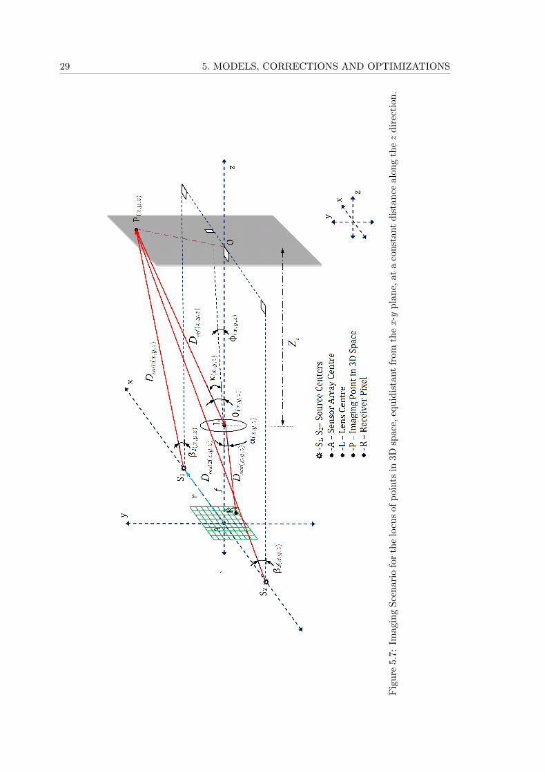
29 5. MODELS, CORRECTIONS AND OPTIMIZATIONS
Fig
ure
5.7
:Im
agin
gS
cen
ario
for
the
locu
sof
poin
tsin
3Dsp
ace,
equ
idis
tant
from
the
x-y
pla
ne,
at
aco
nst
ant
dis
tance
alo
ng
thez
dir
ecti
on
.
5.3. DEPTH ESTIMATION MODEL 30
A = [0, 0, 0]T ;S1 = [|~r| , 0, 0]T ;S2 = [− |~r| , 0, 0]T ;L = [0, 0, f ]T ;
P(x,y,z) = [Dref(x,y,z) cosκ(x,y,z) sinφ(x,y,z), Dref(x,y,z) sinκ(x,y,z), Zc + f ]T(5.72)
It is known from the architecture of the PMD Camcube 2.0 camera that the lightsources on both the sides of the sensor array are kept at a distance of |~r| = 50 mm fromthe centre of the sensor array along the x direction.
From Figure 5.7, the Pythegorous theorem implies that,
∣∣∣OP(x,y,z)
∣∣∣ =√Xc(x,y,z)
2 + Yc(x,y,z)2 (5.73)
also,
θ(x,y,z) = arctan
∣∣∣OP(x,y,z)
∣∣∣Zc
= arccos
(Zc
Dref(x,y,z)
)(5.74)
The coordinates of the imaging point P(x,y,z) states that
Xc(x,y,z) = Dref(x,y,z) cosκ(x,y,z)sinφ(x,y,z) and
Yc(x,y,z) = Dref(x,y,z) sinκ(x,y,z)
(5.75)
The distance Dsen(x,y,z), travelled by the light rays from the lens centre to the sensorarray is given by
Dsen(x,y,z) =f
cosα(x,y,z)(5.76)
The focal length f , of the camera lens is defined by the PMD Camcube datasheetto be 12.8 mm. The size of the sensor pixels in x and y directions is Sx = 40 µm andSy = 40 µm respectively according to PMD technologies1. From the similar evaluationsin Eq. (5.73) and Eq. (5.74) and considering intrinsic parameter evaluations in Eq. (5.71),the sensor angle α(i,j,k) can be written to be
α(x,y,z) = arctan
(√x2 + y2
f
)= arctan
√
[(xim −Ox)Sx]2 + [(yim −Ox)Sy]2
f
(5.77)
The coordinates of the projection of the point S1 and S2 on the imaging plane is givenby
S1p = [|~r| , 0, Zc + f ]T and S2p = [− |~r| , 0, Zc + f ]T (5.78)
1PMD Technologies, http://www.pmdtec.com, (last accessed 25 July 2011; 09:16 hrs)
31 5. MODELS, CORRECTIONS AND OPTIMIZATIONS
From the knowledge of the x and y coordinates of the imaging 3D point P(x,y,z), whichare Xc and Yc, the angles β1(x,y,z) and β2(x,y,z) made by the light rays originating from thetwo sources can be evaluated by Pythegorous theorem and trigonometry as
β1(x,y,z) = arctan
√(Xc(x,y,z)−|~rx|)2+(Yc(x,y,z)−|~ry |)
2
Zc+f
and
β2(x,y,z) = arctan
√(Xc(x,y,z)+|~rx|)2+(Yc(x,y,z)+|~ry |)
2
Zc+f
(5.79)
where |~rx| and |~ry| are the x and y coordinates of the position vector ~r of the sourceS1 or S2. It is to be noted that S1 and S2 are symmetrically opposite to each other w.r.tthe sensor array centre. For the PMD Camcube 2.0 camera, and according to our Figure5.7, |~ry| = 0. The angles θ(x,y,z) and α(x,y,z) are constant for the camera irrespective ofthe distance of the imaging 3D point. According to PMD technologies2, |~r| = 50 mm.Xc(x,y,z) and Yc(x,y,z) are calculated from Eq. (5.70) as
Xc(x,y,z) =xs(x,y,z)
fZc and Yc =
ys(x,y,z)f
Zc (5.80)
where the corresponding x and y coordinates for the imaging pixel in the sensor arrayare xs(x,y,z) and ys(x,y,z). Since all the parameters are known, for the camera imaging aplane perpendicular board kept at a constant distance Zc from the lens centre, the anglesβ1(x,y,z) and β2(x,y,z), can be calculated from the Eq. (5.79).
From the knowledge of β1(x,y,z), β2(x,y,z), α1(x,y,z), θ2(x,y,z), f and Zc, the path lengthsof the traversed rays Dreal1(x,y,z), Dreal2(x,y,z), Dref(x,y,z) and Dsen(x,y,z) can be calculatedfrom trigonometry given by the equations,
Dreal1(x,y,z) =(
Zc+fcosβ1(x,y,z)
)Dreal2(x,y,z) =
(Zc+f
cosβ2(x,y,z)
)Dref(x,y,z) =
(Zc
cos θ(x,y,z)
)Dsen(x,y,z) =
(f
cosα(x,y,z)
)(5.81)
Applying the obtained values in Eq. (5.69) the phase shift of the rays reaching the
sensor pixel can be re written as
Ψ(x,y,z) = ωc
(Zc
{1
2 cosβ1(x,y,z)+ 1
2 cosβ2(x,y,z)+ 1
cos θ(x,y,z)
}+f
{1
2 cosβ1(x,y,z)+ 1
2 cosβ2(x,y,z)+ 1
cosα(x,y,z)
}) (5.82)
2PMD Technologies, http://www.pmdtec.com, (last accessed 25 July 2011; 09:16 hrs)
5.3. DEPTH ESTIMATION MODEL 32
Once the phase shift Ψ(x,y,z) is calculated, the net travel path length Dt(x,y,z), for eachpixel can be evaulated from the expression
Dt(x,y,z) =c ·Ψ(x,y,z)
ω(5.83)
The net travel path corresponds to the forward and backward propagation of the rays.Ideally, the true depth information D, for a sensor pixel is given by
D =c · t2
(5.84)
where c is the speed of light corresponding to 299792458 ms and t corresponds to the
travel time of the depth imaging ray.
Taking the travel time in to consideration, the measured depth information Dmes(x,y,z)
from the camera can now be written as
Dmes(x,y,z) =Dt(x,y,z)
2(5.85)
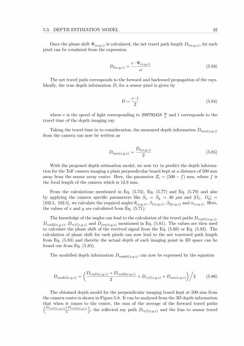
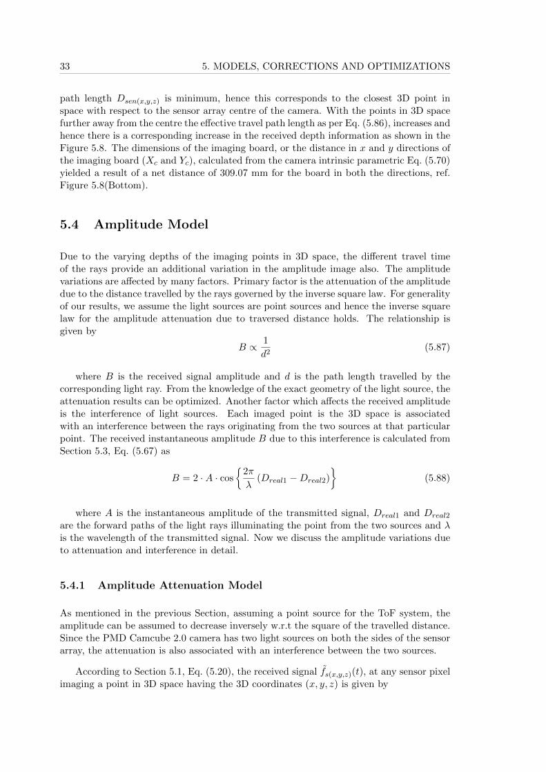
With the proposed depth estimation model, we now try to predict the depth informa-tion for the ToF camera imaging a plain perpendicular board kept at a distance of 500 mmaway from the sensor array centre. Here, the parameter Zc = (500 − f) mm, where f isthe focal length of the camera which is 12.8 mm.
From the calculations mentioned in Eq. (5.74), Eq. (5.77) and Eq. (5.79) and alsoby applying the camera specific parameters like Sx = Sy = 40 µm and [Ox, Oy] =[102.5, 102.5], we calculate the required angles θ(x,y,z), β1(x,y,z), β2(x,y,z) and α(x,y,z). Here,the values of x and y are calculated from Eq. (5.71).
The knowledge of the angles can lead to the calculation of the travel paths Dreal1(x,y,z),Dreal2(x,y,z), Dref(x,y,z) and Dsen(x,y,z) mentioned in Eq. (5.81). The values are then usedto calculate the phase shift of the received signal from the Eq. (5.69) or Eq. (5.82). Thecalculation of phase shift for each pixels can now lead to the net traversed path lengthfrom Eq. (5.83) and thereby the actual depth of each imaging point in 3D space can befound out from Eq. (5.85).
The modelled depth information Dmodel(x,y,z) can now be expressed by the equation
Dmodel(x,y,z) =
(Dreal1(x,y,z) +Dreal2(x,y,z)
2+Dref(x,y,z) +Dsen(x,y,z)
)/2 (5.86)
The obtained depth model for the perpendicular imaging board kept at 500 mm fromthe camera centre is shown in Figure 5.8. It can be analysed from the 3D depth informationthat when it comes to the centre, the sum of the average of the forward travel paths(Dreal1(x,y,z)+Dreal2(x,y,z)
2
), the reflected ray path Dref(x,y,z) and the lens to sensor travel
33 5. MODELS, CORRECTIONS AND OPTIMIZATIONS
path length Dsen(x,y,z) is minimum, hence this corresponds to the closest 3D point inspace with respect to the sensor array centre of the camera. With the points in 3D spacefurther away from the centre the effective travel path length as per Eq. (5.86), increases andhence there is a corresponding increase in the received depth information as shown in theFigure 5.8. The dimensions of the imaging board, or the distance in x and y directions ofthe imaging board (Xc and Yc), calculated from the camera intrinsic parametric Eq. (5.70)yielded a result of a net distance of 309.07 mm for the board in both the directions, ref.Figure 5.8(Bottom).
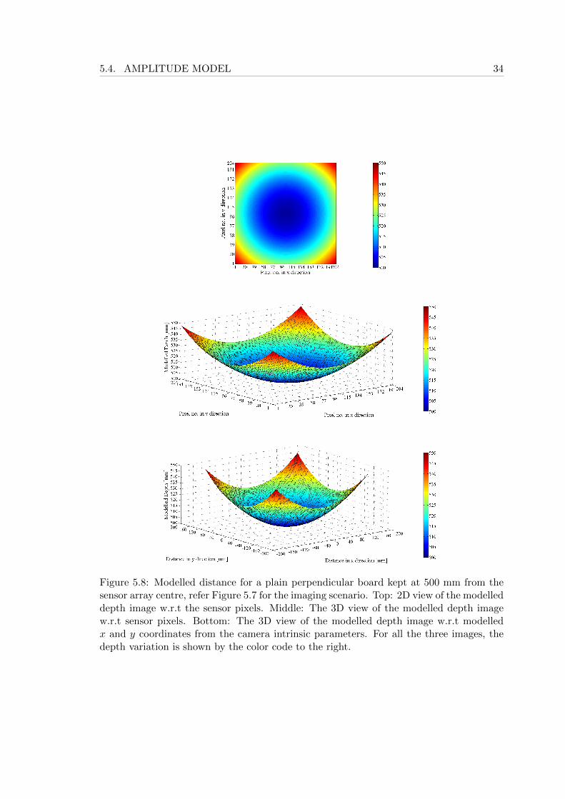
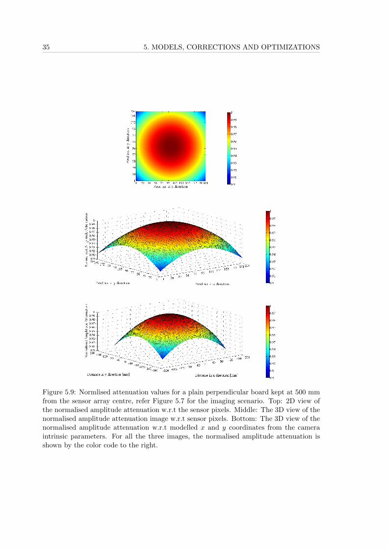
5.4 Amplitude Model
Due to the varying depths of the imaging points in 3D space, the different travel timeof the rays provide an additional variation in the amplitude image also. The amplitudevariations are affected by many factors. Primary factor is the attenuation of the amplitudedue to the distance travelled by the rays governed by the inverse square law. For generalityof our results, we assume the light sources are point sources and hence the inverse squarelaw for the amplitude attenuation due to traversed distance holds. The relationship isgiven by
B ∝ 1
d2(5.87)
where B is the received signal amplitude and d is the path length travelled by thecorresponding light ray. From the knowledge of the exact geometry of the light source, theattenuation results can be optimized. Another factor which affects the received amplitudeis the interference of light sources. Each imaged point is the 3D space is associatedwith an interference between the rays originating from the two sources at that particularpoint. The received instantaneous amplitude B due to this interference is calculated fromSection 5.3, Eq. (5.67) as
B = 2 ·A · cos
{2π
λ(Dreal1 −Dreal2)
}(5.88)
where A is the instantaneous amplitude of the transmitted signal, Dreal1 and Dreal2
are the forward paths of the light rays illuminating the point from the two sources and λis the wavelength of the transmitted signal. Now we discuss the amplitude variations dueto attenuation and interference in detail.
5.4.1 Amplitude Attenuation Model
As mentioned in the previous Section, assuming a point source for the ToF system, theamplitude can be assumed to decrease inversely w.r.t the square of the travelled distance.Since the PMD Camcube 2.0 camera has two light sources on both the sides of the sensorarray, the attenuation is also associated with an interference between the two sources.
According to Section 5.1, Eq. (5.20), the received signal fs(x,y,z)(t), at any sensor pixelimaging a point in 3D space having the 3D coordinates (x, y, z) is given by
5.4. AMPLITUDE MODEL 34
Figure 5.8: Modelled distance for a plain perpendicular board kept at 500 mm from thesensor array centre, refer Figure 5.7 for the imaging scenario. Top: 2D view of the modelleddepth image w.r.t the sensor pixels. Middle: The 3D view of the modelled depth imagew.r.t sensor pixels. Bottom: The 3D view of the modelled depth image w.r.t modelledx and y coordinates from the camera intrinsic parameters. For all the three images, thedepth variation is shown by the color code to the right.
35 5. MODELS, CORRECTIONS AND OPTIMIZATIONS
Figure 5.9: Normlised attenuation values for a plain perpendicular board kept at 500 mmfrom the sensor array centre, refer Figure 5.7 for the imaging scenario. Top: 2D view ofthe normalised amplitude attenuation w.r.t the sensor pixels. Middle: The 3D view of thenormalised amplitude attenuation image w.r.t sensor pixels. Bottom: The 3D view of thenormalised amplitude attenuation w.r.t modelled x and y coordinates from the cameraintrinsic parameters. For all the three images, the normalised amplitude attenuation isshown by the color code to the right.
5.4. AMPLITUDE MODEL 36
fs(x,y,z)(t) = rectT/2
(t−
Ψ(x,y,z)
ω
)·B(x,y,z) · cos
{ωt−Ψ(x,y,z)
}(5.89)
where the phase shift Ψ(x,y,z) is given by
Ψ(x,y,z) =ω
c
(Dreal1(x,y,z) +Dreal2(x,y,z)
2+Dref(x,y,z) +Dsen(x,y,z)
)(5.90)
Hence the net path Dt(x,y,z), travelled by the ray reaching the sensor pixel is given by
Dt(x,y,z) =c·Ψ(x,y,z)
ω
=(Dreal1(x,y,z)+Dreal2(x,y,z)
2+Dref(x,y,z) +Dsen(x,y,z)
) (5.91)
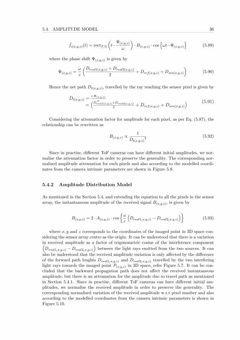
Considering the attenuation factor for amplitude for each pixel, as per Eq. (5.87), therelationship can be rewritten as
B(x,y,z) ∝1
Dt(x,y,z)2 (5.92)
Since in practise, different ToF cameras can have different initial amplitudes, we nor-malise the attenuation factor in order to preserve the generality. The corresponding nor-malised amplitude attenuation for each pixels and also according to the modelled coordi-nates from the camera intrinsic parameters are shown in Figure 5.9.
5.4.2 Amplitude Distribution Model
As mentioned in the Section 5.4, and extending the equation to all the pixels in the sensorarray, the instantaneous amplitude of the received signal B(x,y,z), is given by
B(x,y,z) = 2 ·A(x,y,z) · cos
{ω
c
(Dreal1(x,y,z) −Dreal2(x,y,z)
)}(5.93)
where x, y and z corresponds to the coordinates of the imaged point in 3D space con-sidering the sensor array centre as the origin. It can be understood that there is a variationin received amplitude as a factor of trigonometric cosine of the interference component(Dreal1(x,y,z) −Dreal2(x,y,z)
)between the light rays emitted from the two sources. It can
also be understood that the received amplitude variation is only affected by the differenceof the forward path lenghts Dreal1(x,y,z) and Dreal2(x,y,z) travelled by the two interferinglight rays towards the imaged point P(x,y,z) in 3D space, refer Figure 5.7. It can be con-cluded that the backward propagation path does not affect the received instantaneousamplitude, but there is an attenuation for the amplitude due to travel path as mentionedin Section 5.4.1. Since in practise, different ToF cameras can have different initial am-plitudes, we normalise the received amplitude in order to preserve the generality. Thecorresponding normalised variation of the received amplitude w.r.t pixel number and alsoaccording to the modelled coordinates from the camera intrinsic parameters is shown inFigure 5.10.
37 5. MODELS, CORRECTIONS AND OPTIMIZATIONS
Figure 5.10: Normlised amplitude distribution values for a plain perpendicular board keptat 500 mm from the sensor array centre, refer Figure 5.7 for the imaging scenario. Top:2D view of the normalised amplitude distribution w.r.t the sensor pixels. Middle: The3D view of the normalised amplitude distribution image w.r.t sensor pixels. Bottom: The3D view of the normalised amplitude distribution w.r.t modelled x and y coordinatesfrom the camera intrinsic parameters. For all the three images, the normalised amplitudedistribution is shown by the color code to the right.
5.5. DISTANCE NONLINEARITY MODELS AND CORRECTIONS 38
5.5 Distance Nonlinearity Models and Corrections
It is known from the camera architecture as mentioned in Section 5.1 and Section 5.3 thatthe distance information extracted from each pixel in the sensor array by the correlationprocedure is varied according to the travel time of the rays. The rays start from thesource, interferes and reflects at a particular coordinate point in the 3D space and reachesthe CMOS sensor array. The different travel times of the rays imparts a phase shift onthe received signal at the sensor pixels. The correlation procedure inside the sensor arraygives different results for different phase shifted signals as defined in Section 5.2. Ideallythe depth information is calculated according to Eq. (5.84) as
D =c · t2
(5.94)
where c is the speed of light corresponding to 299792458 ms and t corresponds to the
travel time of the depth imaging ray.
Taking the travel time for each pixels into consideration, the measured depth informa-tion Dmes(x,y,z) from the camera is given as
Dmes(x,y,z) =Dt(x,y,z)
2(5.95)
where the net travel path length for each pixel Dt(x,y,z), is given by
Dt(x,y,z) =c ·Ψ(x,y,z)
ω(5.96)
where Ψ(x,y,z) corresponds to the phase shift observed by the correlation procedure forthe imaging coordinate point in 3D space. The value of phase shift Ψ(x,y,z) is given by theexpression
Ψ(x,y,z) =ω
c
(Dreal1(x,y,z) +Dreal2(x,y,z)
2+Dref(x,y,z) +Dsen(x,y,z)
)(5.97)
where Dreal1(x,y,z), Dreal2(x,y,z), Dref(x,y,z) and Dsen(x,y,z) are the path length traversedby a particular ray travelling from the source reaching the sensor pixel (refer Figure.5.7for the imaging scenario).
The distance information obtained from the camera is not the true coordinate depthinformation, rather it is a travel path based depth information. From the camera intrinsicparameters as mentioned in Section 4.1, we have the relationship
xs = fXc
Zcand ys = f
YcZc
(5.98)
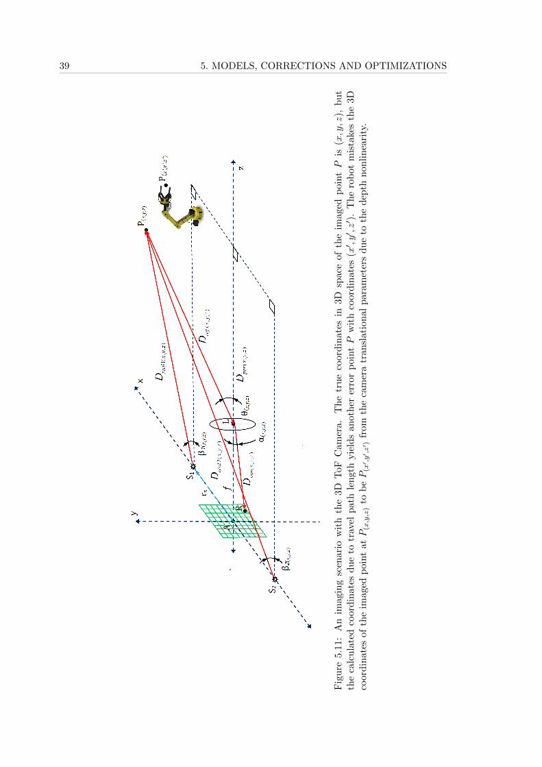
39 5. MODELS, CORRECTIONS AND OPTIMIZATIONS
Fig
ure
5.1
1:
An
imag
ing
scen
ario
wit
hth
e3D
ToF
Cam
era.
Th
etr
ue
coor
din
ates
in3D
space
ofth
eim
age
dp
oin
tP
is(x,y,z
),b
ut
the
calc
ula
ted
coord
inate
sd
ue
totr
avel
path
len
gth
yie
lds
anot
her
erro
rp
ointP
wit
hco
ord
inate
s(x′ ,y′ ,z′ )
.T
he
rob
ot
mis
take
sth
e3D
coord
inate
sof
the
imaged
poin
tatP
(x,y,z
)to
beP
(x′ ,y′ ,z′ )
from
the
cam
era
tran
slat
ion
alp
ara
met
ers
du
eto
the
dep
thn
on
lin
eari
ty.
5.5. DISTANCE NONLINEARITY MODELS AND CORRECTIONS 40
where xs and ys are the coordinates of the sensor array pixel under consideration in xand y directions respectively; f is the focal length of the lens used in the sensor system; Xc
and Yc are the true coordinates of the imaged points in the 3D space in x and y directionsrespectively. Zc is the distance in z direction from the lens centre to the imaging point.But the recalculated x and y coordinates, Xm and Ym, of the imaged point in 3D spacefrom the measured depth Zm is given by
Xm =Zmfx and Ym =
Zmfy (5.99)
Since due to the different path lengths, as mentioned before, we have Zm 6= Zc. Thisimplies that the recalculated x and y coordinates from the measured depth Zm yieldsa wrong coordinates for the corresponding point P in 3D space. An example scenariocan be seen in Figure 5.11 where the captured depth information provides an erroneouscalculation for true 3D coordinates of the target. For any practical robotic applications, itis very essential to know the exact position of the imaged targets in the 3D space. In anyapplication with 3D ToF camera, is very important to have a true translation functionfrom this travel path based depth information to the exact 3D space coordinate depthinformation. Hence it is very important to remove this depth measurement error in orderto recalculate the exact coordinates for the imaged point in 3D space.
In this section we model the distance calculation for 3D ToF camera specifically tailoredto suit the architecture of the PMD Camcube 2.0 camera. Here, we propose three modelsfor correcting this distance non linearity in the captured ToF images. We propose anoptimized model in the beginning which is the complete model and uses the calculations forthe received signal in the ToF imaging model proposed in the Section 5.1. The optimizedbistatic model takes a sufficient amount of computation time and hence we break it down totwo simpler models lesser in complexity, the bistatic model and perpendicular illuminationmodel. The bistatic model requires an exact knowledge of the angle with which the raysfrom the source falls on the target, which is possible to calculate in real time from cameraintrinsic parameters in cases where we image a plain perpendicular surface. Anothersimpler model is the perpendicular illumination model where we assume that the lightsource and the receiver sensor array are not separated and hence the forward and backwardtravel paths w.r.t the imaged point in 3D space is exactly same. We also show that theperformance of the models follow the order: the optimized model first, then the bistaticmodel and at last the perpendicular illumination model. We also show that in computationtime, the models follow the reverse order, i.e. the perpendicular illumination model iscomputationally faster than the bistatic and the optimized model.
5.5.1 Optmized Bistatic Model
The optimized bistatic model models the imaging point in 3D space by optimizing theforwards and backwards path travelled by the rays. The model assumes a bistatic constel-lation for the transmitter and receiver system. This means that the source and receiverare separated from each other by a known distance. In our model, the optimization iscarried out iteratively till the modelled depth matches that of the captured depth infor-mation for each pixel. The angles made by the light rays in the forward paths are found
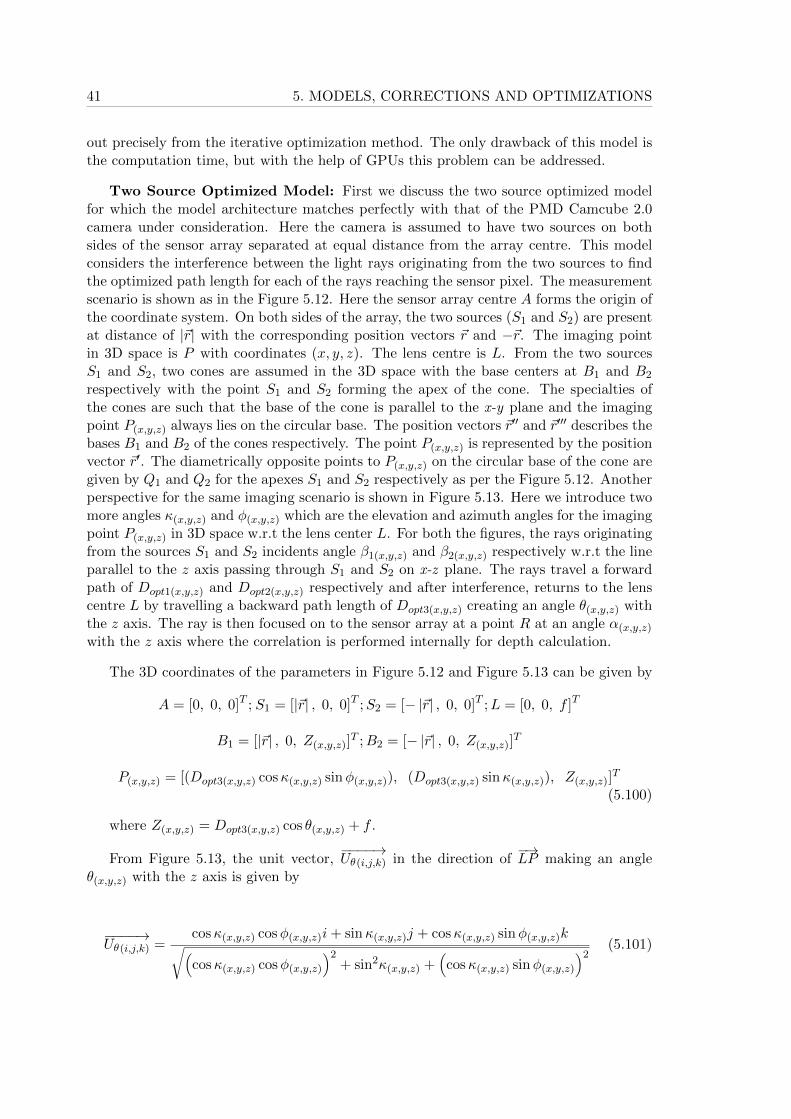
41 5. MODELS, CORRECTIONS AND OPTIMIZATIONS
out precisely from the iterative optimization method. The only drawback of this model isthe computation time, but with the help of GPUs this problem can be addressed.
Two Source Optimized Model: First we discuss the two source optimized modelfor which the model architecture matches perfectly with that of the PMD Camcube 2.0camera under consideration. Here the camera is assumed to have two sources on bothsides of the sensor array separated at equal distance from the array centre. This modelconsiders the interference between the light rays originating from the two sources to findthe optimized path length for each of the rays reaching the sensor pixel. The measurementscenario is shown as in the Figure 5.12. Here the sensor array centre A forms the origin ofthe coordinate system. On both sides of the array, the two sources (S1 and S2) are presentat distance of |~r| with the corresponding position vectors ~r and −~r. The imaging pointin 3D space is P with coordinates (x, y, z). The lens centre is L. From the two sourcesS1 and S2, two cones are assumed in the 3D space with the base centers at B1 and B2
respectively with the point S1 and S2 forming the apex of the cone. The specialties ofthe cones are such that the base of the cone is parallel to the x-y plane and the imagingpoint P(x,y,z) always lies on the circular base. The position vectors ~r′′ and ~r′′′ describes thebases B1 and B2 of the cones respectively. The point P(x,y,z) is represented by the positionvector ~r′. The diametrically opposite points to P(x,y,z) on the circular base of the cone aregiven by Q1 and Q2 for the apexes S1 and S2 respectively as per the Figure 5.12. Anotherperspective for the same imaging scenario is shown in Figure 5.13. Here we introduce twomore angles κ(x,y,z) and φ(x,y,z) which are the elevation and azimuth angles for the imagingpoint P(x,y,z) in 3D space w.r.t the lens center L. For both the figures, the rays originatingfrom the sources S1 and S2 incidents angle β1(x,y,z) and β2(x,y,z) respectively w.r.t the lineparallel to the z axis passing through S1 and S2 on x-z plane. The rays travel a forwardpath of Dopt1(x,y,z) and Dopt2(x,y,z) respectively and after interference, returns to the lenscentre L by travelling a backward path length of Dopt3(x,y,z) creating an angle θ(x,y,z) withthe z axis. The ray is then focused on to the sensor array at a point R at an angle α(x,y,z)
with the z axis where the correlation is performed internally for depth calculation.
The 3D coordinates of the parameters in Figure 5.12 and Figure 5.13 can be given by
A = [0, 0, 0]T ; S1 = [|~r| , 0, 0]T ;S2 = [− |~r| , 0, 0]T ;L = [0, 0, f ]T
B1 = [|~r| , 0, Z(x,y,z)]T ;B2 = [− |~r| , 0, Z(x,y,z)]
T
P(x,y,z) = [(Dopt3(x,y,z) cosκ(x,y,z) sinφ(x,y,z)), (Dopt3(x,y,z) sinκ(x,y,z)), Z(x,y,z)]T
(5.100)
where Z(x,y,z) = Dopt3(x,y,z) cos θ(x,y,z) + f .
From Figure 5.13, the unit vector,−−−−→Uθ(i,j,k) in the direction of
−→LP making an angle
θ(x,y,z) with the z axis is given by
−−−−→Uθ(i,j,k) =
cosκ(x,y,z) cosφ(x,y,z)i+ sinκ(x,y,z)j + cosκ(x,y,z) sinφ(x,y,z)k√(cosκ(x,y,z) cosφ(x,y,z)
)2+ sin2κ(x,y,z) +
(cosκ(x,y,z) sinφ(x,y,z)
)2(5.101)
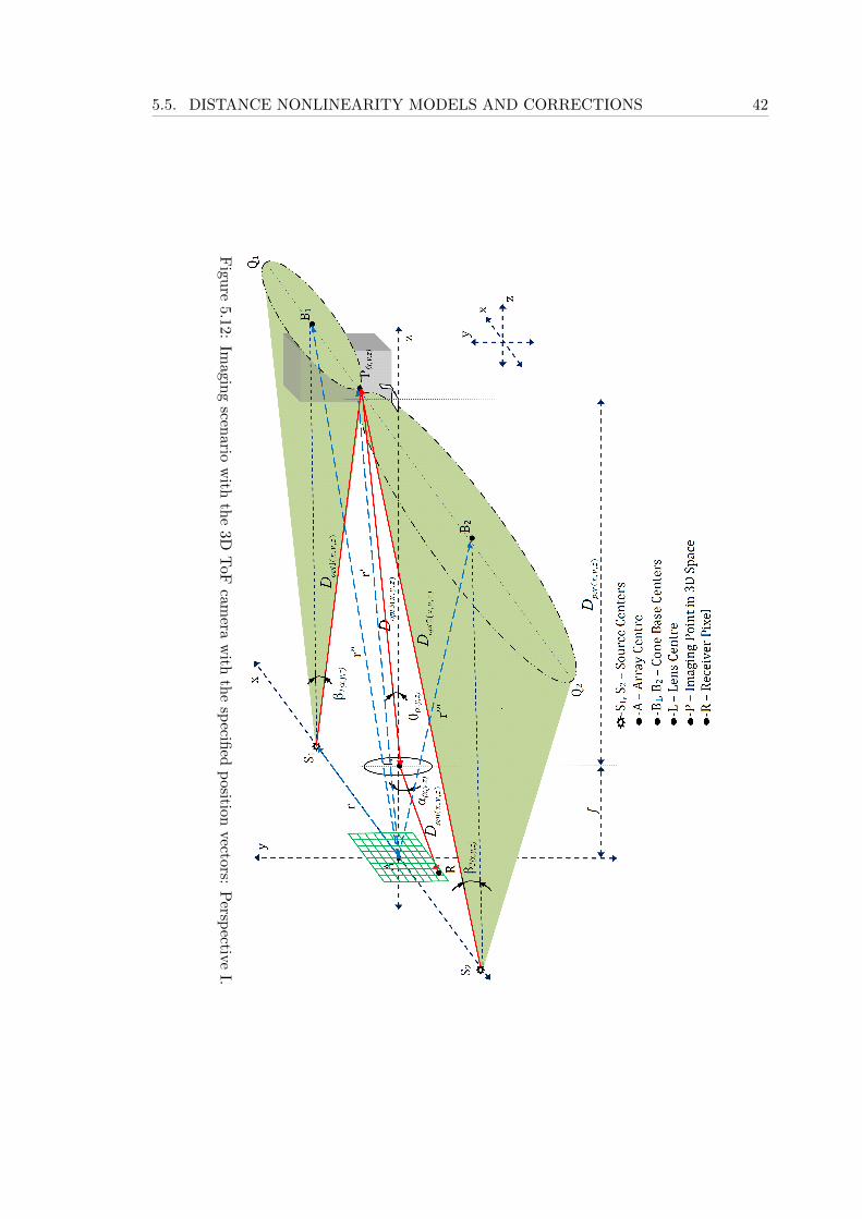
5.5. DISTANCE NONLINEARITY MODELS AND CORRECTIONS 42
Fig
ure
5.12:Im
agin
gscen
ariow
ithth
e3D
ToF
camera
with
the
specifi
edp
ositionvectors:
Persp
ectiveI.
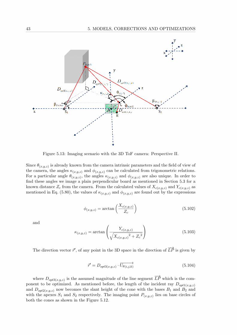
43 5. MODELS, CORRECTIONS AND OPTIMIZATIONS
Figure 5.13: Imaging scenario with the 3D ToF camera: Perspective II.
Since θ(x,y,z) is already known from the camera intrinsic parameters and the field of view ofthe camera, the angles κ(x,y,z) and φ(x,y,z) can be calculated from trigonometric relations.For a particular angle θ(x,y,z), the angles κ(x,y,z) and φ(x,y,z) are also unique. In order tofind these angles we image a plain perpendicular board as mentioned in Section 5.3 for aknown distance Zc from the camera. From the calculated values of Xc(x,y,z) and Yc(x,y,z) asmentioned in Eq. (5.80), the values of κ(x,y,z) and φ(x,y,z) are found out by the expressions
φ(x,y,z) = arctan
(Xc(x,y,z)
Zc
)(5.102)
and
κ(x,y,z) = arctan
Yc(x,y,z)√Xc(x,y,z)
2 + Zc2
(5.103)
The direction vector ~r′, of any point in the 3D space in the direction of−→LP is given by
~r′ = Dopt3(x,y,z) ·−−−−→Uθ(i,j,k) (5.104)
where Dopt3(x,y,z) is the assumed magnitude of the line segment−→LP which is the com-
ponent to be optimized. As mentioned before, the length of the incident ray Dopt1(x,y,z)
and Dopt2(x,y,z) now becomes the slant height of the cone with the bases B1 and B2 andwith the apexes S1 and S2 respectively. The imaging point P(x,y,z) lies on base circles ofboth the cones as shown in the Figure 5.12.
5.5. DISTANCE NONLINEARITY MODELS AND CORRECTIONS 44
The forward path lengths of both the rays Dopt1(x,y,z) and Dopt2(x,y,z) can now be givenby
Dopt1(x,y,z) =
√|~r′′ − ~r′|2 +
∣∣∣−−−→S1B1
∣∣∣2 (5.105)
and
Dopt2(x,y,z) =
√|~r′′′ − ~r′|2 +
∣∣∣−−−→S2B2
∣∣∣2 (5.106)
where the direction vectors−−−→S1B1 and
−−−→S2B2 are known from Eq. (5.100) . The position
vectors ~r′, ~r′′ and ~r′′′ given by
~r′ = [ x, y, z]T
~r′′ = [ |~r| , 0, z]T
~r′′′ = [ − |~r| , 0, z]T(5.107)
where x, y and z are calculated from the coefficients of ~r′ from Eq. (5.104) for anassumed magnitude Dopt3(x,y,z). It is also to be noted that the focal length f of thecamera should be added to the calculated z coordinates for ~r′ since there is an offset of ffor the unit vector
−−−−→Uθ(i,j,k) in z direction due to the camera lens situated at L.
From Section 5.1, and Section 5.3 we have the measured distance Dmes(x,y,z), obtainedat the receiver pixel in the sensor array due to the interference between the light sourcesgiven by
Dmes(x,y,z) =
(Dreal1(x,y,z) +Dreal2(x,y,z)
2+Dref(x,y,z) +Dsen(x,y,z)
)/2 (5.108)
The distance Dsen(x,y,z) travelled by the rays from the lens centre L towards the sensorarray pixels can be modelled as
Dsen(x,y,z) =
(f
cosα(x,y,z)
)(5.109)
The focal length f for the camera is constant (12.8 mm for PMD Camcube 2.0 camera).The angle α(x,y,z) for each imaging point in 3D space can be found out from the cameraintrinsic parameters by the expression
α(x,y,z) = arctan
√(
xs(x,y,z))2
+(ys(x,y,z)
)2
f
(5.110)
45 5. MODELS, CORRECTIONS AND OPTIMIZATIONS
where xs(x,y,z) and ys(x,y,z) are the sensor pixel coordinates in x and y direction respec-tively corresponding to the imaging point P(x,y,z) in 3D space as explained in Section 5.5,Eq. (5.98).
Applying the values for Dopt1(x,y,z) and Dopt2(x,y,z) calculated from Eq. (5.105) andEq. (5.106) for a particular Dopt3(x,y,z) mentioned in Eq. (5.104), the modelled distancecan be given by
Dmodel(x,y,z) =
(Dopt1(x,y,z) +Dopt2(x,y,z)
2+Dopt3(x,y,z) +Dsen(x,y,z)
)/2 (5.111)
It is now checked whether the modelled value of Dmodel(x,y,z) matches the measureddistance value Dmes(x,y,z). The magnitude of the reflected light ray Dopt3(x,y,z) is iterativelyoptimized with the values of Dopt1(x,y,z) and Dopt2(x,y,z) calculated from the Eq. (5.105)and Eq. (5.106) every time till the modelled distance Dmodel(x,y,z) equals the measureddistance Dmes(x,y,z).
We implement a bisection algorithm for the iterative optimization procedure. Firstassuming a reference interval of 0 m - 7.5 m for Dopt3(x,y,z), the model value Dmodel(x,y,z) iscalculated for both the interval boundaries from Eq. (5.111). The calculated value is thenchecked against the measured value Dmes(x,y,z). If a match is found the optimal value isobtained. Whereas if a match is not found, the average of the interval is taken as the thirdvalue for Dopt3(x,y,z). Now from the two intervals (0 m - 3.75 m and 3.75 m - 7.5 m) theone where the interval bounds are closer to the measured value is calculated and taken tobe the reference interval for the next iteration. The bisection algorithm is then repeatedlycarried out for each iteration till the optimal value for Dopt3(x,y,z) is obtained such thatthe modelled distance Dmodel(x,y,z) equals the measured distance Dmes(x,y,z) or is withinacceptable tolerance limits. This iterative optimization method provides excellent resultsfor the distance modelling.
The difference between the predicted model and the measured distance, e(x,y,z), can beused as an accuracy measure for the iterative optimization procedure. The optimizationprocedure can then be considered as the following minimization problem,
minDopt3(x,y,z)
∣∣∣e(x,y,z)
∣∣∣ ; where e(x,y,z) = Dmodel(x,y,z) −Dmes(x,y,z) (5.112)
Once the results are optimized iteratively the optimal values of the forward ray angles
β1(x,y,z) and β2(x,y,z) are given by
β1(x,y,z) = arcsin(|~r′′−~r′|
Dopt1(x,y,z)
)
β2(x,y,z) = arcsin(|~r′′′−~r′|
Dopt2(x,y,z)
) (5.113)
Hence the depth in z coordinate direction towards the point P(x,y,z) from the lenscentre L is given by
Dper(x,y,z) = Dopt3(x,y,z) cosκ(x,y,z) cosφ(x,y,z) (5.114)
5.5. DISTANCE NONLINEARITY MODELS AND CORRECTIONS 46
The corrected depth Dcor(x,y,z) towards the point P(x,y,z) from the array centre A isgiven by
Dcor(x,y,z) = Dper(x,y,z) + f
= Dopt2(x,y,z) cosκ(x,y,z) cosφ(x,y,z) + f
= Dopt1(x,y,z) cosβ1(x,y,z)
= Dopt2(x,y,z) cosβ2(x,y,z)
Single Source Optimized Model: Now we simplify the optimized model for asingle source kept at a known distance from the camera. The model assumes a bistaticconstellation as before, but here there is only one source illuminating the 3D space. Thisgeneralization can be applied to any 3D ToF camera and hence is not restricted only tothe PMD Camcube 2.0 camera.
The measurement scenario is shown in the Figure 5.14. Here the sensor array centreA forms the origin of the coordinate system. On one side of the sensor array, the sourcesS is present at distance of |~r| with the position vector ~r. The imaging point in 3D space isP with coordinates (x, y, z). The lens centre is L. From the source S, a cones is assumedin the 3D space with the base centre at B with the point S1 forming the apex of thecone. The speciality of the cone is such that the base of the cone is parallel to the x-yplane and the imaging point P(x,y,z) always lies on the circular base. The position vectors~r′′ describes the bases B of the cone. The point P(x,y,z) is represented by the positionvector ~r′. The diametrically opposite points to P(x,y,z) on the circular base of the cone isQ as per the Figure 5.14. Another perspective for the same imaging scenario is shown inFigure 5.15. Here we introduce two more angles κ(x,y,z) and φ(x,y,z) which are the elevationand azimuth angles for the imaging point P(x,y,z) in 3D space w.r.t the lens centre L. Forboth the figures, the rays originating from the source S incidents angle β(x,y,z) w.r.t the lineparallel to the z axis passing through S on the x-z plane. The ray from the source travel aforward path of Dopt1(x,y,z) and returns to the lens centre L by travelling a backward pathlength of Dopt2(x,y,z) creating an angle θ(x,y,z) with the z axis. The ray is then focused ontothe sensor array at a point R at an angle α(x,y,z) with the z axis where the correlation isperformed internally for depth calculation.
The 3D coordinates of the parameters in Figure 5.14 and 5.15 can be given by
A = [0, 0, 0]T ;S = [|~r| , 0, 0]T ;L = [0, 0, f ]T ;B = [|~r| , 0, Z(x,y,z)]T
P(x,y,z) = [(Dopt2(x,y,z) cosκ(x,y,z) sinφ(x,y,z)), (Dopt2(x,y,z) sinκ(x,y,z)), Z(x,y,z)]T
(5.115)
where Z(x,y,z) = Dopt2(x,y,z) cos θ(x,y,z) + f .
As mentioned in Eq. (5.101), the unit vector,−−−−→Uθ(i,j,k) in the direction of
−→LP making
an angle θ(x,y,z) with the z axis is given by
−−−−→Uθ(i,j,k) =
cosκ(x,y,z) cosφ(x,y,z)i+ sinκ(x,y,z)j + cosκ(x,y,z) sinφ(x,y,z)k√(cosκ(x,y,z) cosφ(x,y,z)
)2+ sin2κ(x,y,z) +
(cosκ(x,y,z) sinφ(x,y,z)
)2(5.116)
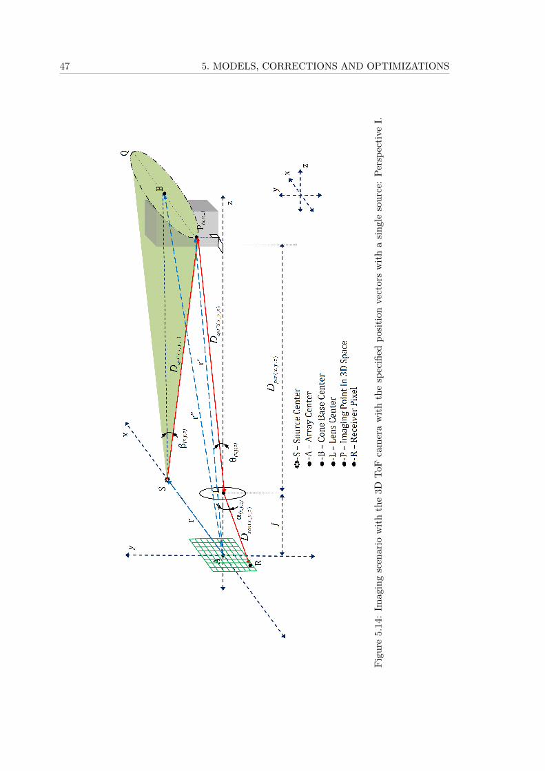
47 5. MODELS, CORRECTIONS AND OPTIMIZATIONS
Fig
ure
5.1
4:
Imag
ing
scen
ario
wit
hth
e3D
ToF
cam
era
wit
hth
esp
ecifi
edp
osit
ion
vec
tors
wit
ha
sin
gle
sou
rce:
Per
spec
tive
I.
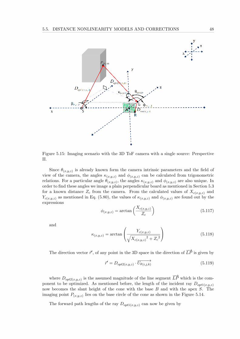
5.5. DISTANCE NONLINEARITY MODELS AND CORRECTIONS 48
Figure 5.15: Imaging scenario with the 3D ToF camera with a single source: PerspectiveII.
Since θ(x,y,z) is already known form the camera intrinsic parameters and the field ofview of the camera, the angles κ(x,y,z) and φ(x,y,z) can be calculated from trigonometricrelations. For a particular angle θ(x,y,z), the angles κ(x,y,z) and φ(x,y,z) are also unique. Inorder to find these angles we image a plain perpendicular board as mentioned in Section 5.3for a known distance Zc from the camera. From the calculated values of Xc(x,y,z) andYc(x,y,z) as mentioned in Eq. (5.80), the values of κ(x,y,z) and φ(x,y,z) are found out by theexpressions
φ(x,y,z) = arctan
(Xc(x,y,z)
Zc
)(5.117)
and
κ(x,y,z) = arctan
Yc(x,y,z)√Xc(x,y,z)
2 + Zc2
(5.118)
The direction vector ~r′, of any point in the 3D space in the direction of−→LP is given by
~r′ = Dopt2(x,y,z) ·−−−−→Uθ(i,j,k) (5.119)
where Dopt2(x,y,z) is the assumed magnitude of the line segment−→LP which is the com-
ponent to be optimized. As mentioned before, the length of the incident ray Dopt1(x,y,z)
now becomes the slant height of the cone with the base B and with the apex S. Theimaging point P(x,y,z) lies on the base circle of the cone as shown in the Figure 5.14.
The forward path lengths of the ray Dopt1(x,y,z) can now be given by
49 5. MODELS, CORRECTIONS AND OPTIMIZATIONS
Dopt1(x,y,z) =
√|~r′′ − ~r′|2 +
∣∣∣−→SB∣∣∣2 (5.120)
where the direction vector−→SB are known from expression Eq. (5.115). The position
vectors ~r′ and ~r′′ are given by
~r′ = [ x, y, z]T
~r′′ = [ |~r| , 0, z]T(5.121)
where x, y and z are calculated from the coefficients of ~r′ from Eq. (5.119) for anassumed magnitude Dopt2(x,y,z). It is also to be noted that the focal length f of thecamera should be added to the calculated z coordinates for ~r′ since there is an offset of ffor the unit vector
−−−−→Uθ(i,j,k) in z direction due to the camera lens situated at L.
From Section 5.1 and Section 5.3 we have the measured distance Dmes(x,y,z), obtainedat the receiver pixel in the sensor array for a single source given by
Dmes(x,y,z) =(Dreal(x,y,z) +Dref(x,y,z) +Dsen(x,y,z)
)/2 (5.122)
The distance Dsen(x,y,z) travelled by the rays from the lens centre L towards the sensorarray pixels can be modelled as
Dsen(x,y,z) =
(f
cosα(x,y,z)
)(5.123)
The focal length f for the camera is constant (12.8 mm for PMD Camcube 2.0 camera).The angle α(x,y,z) for each imaging point in 3D space can be found out from the cameraintrinsic parameters by the expression
α(x,y,z) = arctan
√(
xs(x,y,z))2
+(ys(x,y,z)
)2
f
(5.124)
where xs(x,y,z) and ys(x,y,z) are the sensor pixel coordinates in x and y direction respec-tively corresponding to the imaging point P(x,y,z) in 3D space as explained in Section 5.5,Eq. (5.98).
Applying the values forDopt1(x,y,z) calculated from Eq. (5.120) for a particularDopt2(x,y,z)
mentioned in Eq. (5.119), the modelled distance Dmodel(x,y,z) can be written as
Dmodel(x,y,z) =(Dopt1(x,y,z) +Dopt2(x,y,z) +Dsen(x,y,z)
)/2 (5.125)
5.5. DISTANCE NONLINEARITY MODELS AND CORRECTIONS 50
It is now checked whether the modelled value of Dmodel(x,y,z) matches the measureddistance value Dmes(x,y,z). The magnitude of the reflected light ray Dopt2(x,y,z) is iterativelyoptimized with the value of Dopt1(x,y,z) calculated from the Eq. (5.120) every time till themodelled distance Dmodel(x,y,z) equals the measured distance Dmes(x,y,z).
We implement a bisection algorithm for the iterative optimization procedure. Firstassuming a reference interval of 0 m - 7.5 m for Dopt3(x,y,z), the model value Dmodel(x,y,z) iscalculated for both the interval boundary from Eq. (5.111). The calculated value is thenchecked against the measured value Dmes(x,y,z). If a match is found the optimal value isobtained. Whereas if a match is not found, the average of the interval is taken as thethird value for Dopt3(x,y,z). Now from the two intervals (0 m - 3.75 m and 3.75 m - 7.5m) the one where the interval bounds are closer to the measured value is calculated andtaken to be the reference interval for the next iteration. The bisection algorithm is thenrepeatedly carried out for each iteration till the optimal value for Dopt3(x,y,z) is obtainedsuch that the modelled distance Dmodel(x,y,z) equals the measured distance Dmes(x,y,z) oris within acceptable tolerance limits.
The difference between the predicted model and the measured distance, e(x,y,z), can beused as an accuracy measure for the iterative optimization procedure. The optimizationprocedure can then be considered as the following minimization problem,
minDopt3(x,y,z)
∣∣∣e(x,y,z)
∣∣∣ ; where e(x,y,z) = Dmodel(x,y,z) −Dmes(x,y,z) (5.126)
Once the results are optimized iteratively the optimal value of the forward ray angleβ(x,y,z) is now given by
β(x,y,z) = arcsin
(|~r′′ − ~r′|Dopt1(x,y,z)
)(5.127)
Hence the depth in z coordinate direction towards the point P(x,y,z) from the lenscentre L is given by
Dper(x,y,z) = Dopt2(x,y,z) cosκ(x,y,z) cosφ(x,y,z) (5.128)
The corrected depth Dcor(x,y,z) from the model towards the point P(x,y,z) from thearray centre A is given by
Dcor(x,y,z) = Dper(x,y,z) + f
= Dopt2(x,y,z) cosκ(x,y,z) cosφ(x,y,z) + f
= Dopt1(x,y,z) cosβ(x,y,z)
5.5.2 Simple Bistatic Model
The drawback with the optimized bistatic model is the computation complexity. It isto be noted that for each pixel, the computation mentioned in the Section 5.5.1 has tobe performed to find the optimal value for the incident angles β1(x,y,z) and β2(x,y,z) toeach imaging pixel P(x,y,z) by the source as shown in Figure 5.11. The PMD Camcube 2.0camera has a pixel resolution of 204 × 204, hence the computation has to be done for 41616
51 5. MODELS, CORRECTIONS AND OPTIMIZATIONS
pixels. With the advent of GPUs the computation may not require considerable amountof time. But since the pixel resolution for the ToF cameras is expected to increase inthe future, the iterative procedure should be modified to decrease the computation time.In this section, we mention the simple bistatic Model which can be applied to removethe non linearity in the depth image when imaging a plain surface. The criterion whichshould be satisfied to apply the simple bistatic approach is that imaging surface should beperpendicular to the camera and is not irregular. In many of the practical scenarios thismodel can be applied. For example, in logistics this mode can be used in case of loadingand unloading boxes from containers. In almost all the cases the geometry of the boxesare known in logistics. And in many cases the planes meeting the corners of the boxes areperpendicular to each other in all the 3 dimensions. Hence from the camera intrinsic andextrinsic parameters mentioned in Chapter 4, the translational and rotational parametersof the camera for a particular pose can be known and hence this knowledge can be used tore-orient the camera to a particular position which can make the box face perpendicular tothe camera. And once this is done, the simple bistatic approach can be used to compute theexact depth information of each pixel and hence the depth nonlinearities due to the traveltime of the rays can be corrected. Since the simple bistatic model calculates the incidentangles β1(x,y,z) and β2(x,y,z) from the geometry of the target, the iterative optimizationprocedure is not employed. This reduces the considerable amount of computation timewhich was required for the optimized bistatic model.
Two Source Bistatic Model: First we discuss the two source bistatic model forwhich the model architecture matches perfectly with that of the PMD Camcube 2.0 cameraunder consideration. Here the camera is assumed to have two sources on both sides ofthe sensor array separated at equal distance from the sensor array centre. This modelconsiders the interference between the light rays originating from the two sources to findthe path length for each of the rays reaching the sensor pixel. The measurement scenariois shown as in the Figure 5.16. Here the sensor array centre A forms the origin of thecoordinate system. On both sides of the array, the two sources (S1 and S2) are present ata distance of |~r| with the corresponding position vectors ~r and −~r. The imaging point in3D space is P with coordinates (x, y, z) is represented by the position vector ~r′. The lenscentre is L. The rays originating from the sources S1 and S2 incidents angles β1(x,y,z) andβ2(x,y,z) respectively w.r.t the line parallel to the z axis passing through S1 and S2 on x-zplane. The rays travel a forward path length of Dreal1(x,y,z) and Dreal2(x,y,z) respectivelyand after interference, returns to the lens centre L by travelling a backward path lengthof Dref(x,y,z) creating an angle θ(x,y,z) with the z axis. The ray is then focused on to thesensor array at a point R at an angle α(x,y,z) with the z axis where the correlation isperformed internally for depth calculation. The camera is imaging a plain perpendicularboard as shown in Figure 5.16.
From the camera intrinsic parameters mentioned in Section 4.1, we have
xs = fXc
Zcand ys = f
YcZc
(5.129)
andxs = (xim −Ox)Sx and ys = (yim −Oy)Sy (5.130)
where xs and ys are the coordinates of the sensor array pixel under consideration in xand y directions respectively; f is the focal length of the lens used in the sensor system;
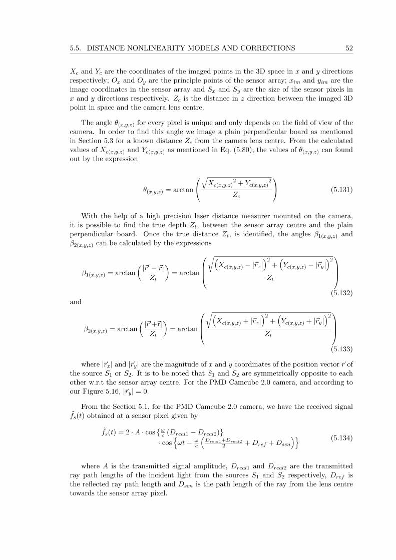
5.5. DISTANCE NONLINEARITY MODELS AND CORRECTIONS 52
Xc and Yc are the coordinates of the imaged points in the 3D space in x and y directionsrespectively; Ox and Oy are the principle points of the sensor array; xim and yim are theimage coordinates in the sensor array and Sx and Sy are the size of the sensor pixels inx and y directions respectively. Zc is the distance in z direction between the imaged 3Dpoint in space and the camera lens centre.
The angle θ(x,y,z) for every pixel is unique and only depends on the field of view of thecamera. In order to find this angle we image a plain perpendicular board as mentionedin Section 5.3 for a known distance Zc from the camera lens centre. From the calculatedvalues of Xc(x,y,z) and Yc(x,y,z) as mentioned in Eq. (5.80), the values of θ(x,y,z) can foundout by the expression
θ(x,y,z) = arctan
√Xc(x,y,z)
2 + Yc(x,y,z)2
Zc
(5.131)
With the help of a high precision laser distance measurer mounted on the camera,it is possible to find the true depth Zt, between the sensor array centre and the plainperpendicular board. Once the true distance Zt, is identified, the angles β1(x,y,z) andβ2(x,y,z) can be calculated by the expressions
β1(x,y,z) = arctan
( |~r′ − ~r|Zt
)= arctan
√(
Xc(x,y,z) − |~rx|)2
+(Yc(x,y,z) − |~ry|
)2
Zt
(5.132)
and
β2(x,y,z) = arctan
( |~r′+~r|Zt
)= arctan
√(
Xc(x,y,z) + |~rx|)2
+(Yc(x,y,z) + |~ry|
)2
Zt
(5.133)
where |~rx| and |~ry| are the magnitude of x and y coordinates of the position vector ~r ofthe source S1 or S2. It is to be noted that S1 and S2 are symmetrically opposite to eachother w.r.t the sensor array centre. For the PMD Camcube 2.0 camera, and according toour Figure 5.16, |~ry| = 0.
From the Section 5.1, for the PMD Camcube 2.0 camera, we have the received signalfs(t) obtained at a sensor pixel given by
fs(t) = 2 ·A · cos{ωc (Dreal1 −Dreal2)
}· cos
{ωt− ω
c
(Dreal1+Dreal2
2 +Dref +Dsen
)} (5.134)
where A is the transmitted signal amplitude, Dreal1 and Dreal2 are the transmittedray path lengths of the incident light from the sources S1 and S2 respectively, Dref isthe reflected ray path length and Dsen is the path length of the ray from the lens centretowards the sensor array pixel.
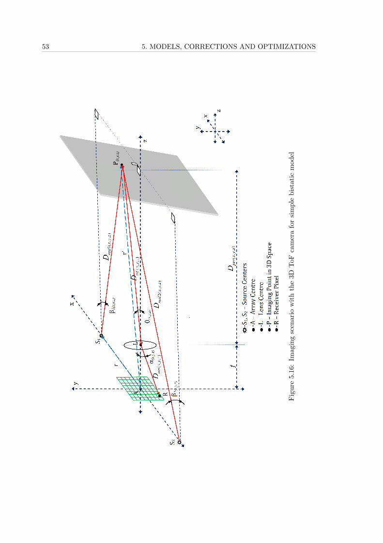
53 5. MODELS, CORRECTIONS AND OPTIMIZATIONS
Fig
ure
5.1
6:Im
agi
ng
scen
ario
wit
hth
e3D
ToF
cam
era
for
sim
ple
bis
tati
cm
od
el
5.5. DISTANCE NONLINEARITY MODELS AND CORRECTIONS 54
From Figure 5.16 the net path length Dt(x,y,z), travelled by the ray imaging a point P inthe 3D space with coordinates (x, y, z) is given by
Dt(x,y,z) =(Dreal1(x,y,z)+Dreal2(x,y,z)
2+Dref(x,y,z) +Dsen(x,y,z)
)(5.135)
and the measured depth information Dmes(x,y,z) = Dt(x,y,z)/2 is given by
Dmes(x,y,z) =
(Dreal1(x,y,z) +Dreal2(x,y,z)
2+Dref(x,y,z) +Dsen(x,y,z)
)/2 (5.136)
From the knowledge of β1(x,y,z) and β2(x,y,z) as per Eq. (5.132) and Eq. (5.133), theforwards travel paths Dreal1(x,y,z) and Dreal1(x,y,z) of both the rays can be modelled as
Dreal1(x,y,z) =
(Dper(x,y,z) + f
cosβ1(x,y,z)
)(5.137)
and
Dreal2(x,y,z) =
(Dper(x,y,z) + f
cosβ2(x,y,z)
)(5.138)
The distance Dsen(x,y,z) travelled by the rays from the lens centre L towards the sensorarray pixels can be modelled as
Dsen(x,y,z) =
(f
cosα(x,y,z)
)(5.139)
The focal length f for the camera is constant (12.8 mm for PMD Camcube 2.0 camera).The angle α(x,y,z) for each imaging point in 3D space can be found out from the cameraintrinsic parameters by the expression
α(x,y,z) = arctan
√(
xs(x,y,z))2
+(ys(x,y,z)
)2
f
(5.140)
where xs(x,y,z) and ys(x,y,z) are the sensor pixel coordinates in x and y direction respec-tively corresponding to the imaging point P(x,y,z) in 3D space as explained in Section 5.5,Eq. (5.98).
Hence the reflected ray from Eq. (5.135) for each imaging point in 3D space can bewritten after rearrangement as
Dref(x,y,z) = 2 ·Dmes(x,y,z) −(Dper(x,y,z) + f
2· d)−Dsen(x,y,z) (5.141)
55 5. MODELS, CORRECTIONS AND OPTIMIZATIONS
where
d =
{1
cosβ1(x,y,z)+
1
cosβ2(x,y,z)
}(5.142)
Substituting for Dper(x,y,z) from the known relation
Dper(x,y,z) = Dref(x,y,z) · cos θ(x,y,z) (5.143)
The reflected path length Dref(x,y,z) can be modified as
Dref(x,y,z) =
2 ·Dmes(x,y,z) −(f2 · d
)−Dsen(x,y,z)(
1 +cos θ(x,y,z)·d
2
) (5.144)
For a particular imaging point in 3D space for a perpendicular board, all the values onthe R.H.S are known and hence the reflected path length can be calculated from the aboveexpression. From the calculated reflected path length, the true perpendicular distance inz direction from the lens centre to each imaging point in 3D space Dper(x,y,z), can becalculated from Eq. (5.143).
From the obtained value of Dper(x,y,z), the non linearly corrected distance Dcor(x,y,z)
for each imaging point P(x,y,z) in 3D space is given by
Dcor(x,y,z) = Dper(x,y,z) + f (5.145)
Single Source Bistatic Model: Now we discuss the single source bistatic model forwhich the model architecture can be tailored to suit any ToF camera available in marketcomprising of a single source for illumination. Here the camera is assumed to have thesource on one side of the sensor array separated at a fixed distance from the sensor arraycentre. The measurement scenario is shown as in the Figure 5.17. Here the sensor arraycentre A forms the origin of the coordinate system. On one side of the array, the source Sis present at distance of |~r| with the corresponding position vector ~r. The imaging pointin 3D space is P with coordinates (x, y, z) is represented by the position vector ~r′. Thelens centre is L. The rays originating from the source S makes an angle β(x,y,z) w.r.t theline parallel to the z axis passing through S on x-z plane. The ray travel a forward pathlength of Dreal(x,y,z) and returns to the lens centre L by travelling a backward path lengthof Dref(x,y,z) creating an angle θ(x,y,z) with the z axis. The ray is then focused on to thesensor array at a point R at an angle α(x,y,z) with the z axis where the correlation isperformed internally for depth calculation. The camera is imaging a plain perpendicularboard as shown in Figure 5.17.
From the camera intrinsic parameters mentioned in Section 4.1, we have the relation-ship
xs = fXc
Zcand ys = f
YcZc
(5.146)
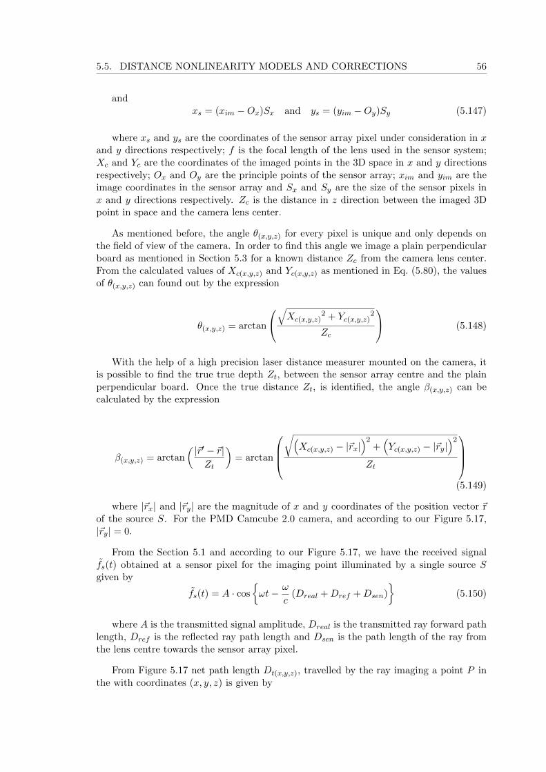
5.5. DISTANCE NONLINEARITY MODELS AND CORRECTIONS 56
andxs = (xim −Ox)Sx and ys = (yim −Oy)Sy (5.147)
where xs and ys are the coordinates of the sensor array pixel under consideration in xand y directions respectively; f is the focal length of the lens used in the sensor system;Xc and Yc are the coordinates of the imaged points in the 3D space in x and y directionsrespectively; Ox and Oy are the principle points of the sensor array; xim and yim are theimage coordinates in the sensor array and Sx and Sy are the size of the sensor pixels inx and y directions respectively. Zc is the distance in z direction between the imaged 3Dpoint in space and the camera lens center.
As mentioned before, the angle θ(x,y,z) for every pixel is unique and only depends onthe field of view of the camera. In order to find this angle we image a plain perpendicularboard as mentioned in Section 5.3 for a known distance Zc from the camera lens center.From the calculated values of Xc(x,y,z) and Yc(x,y,z) as mentioned in Eq. (5.80), the valuesof θ(x,y,z) can found out by the expression
θ(x,y,z) = arctan
√Xc(x,y,z)
2 + Yc(x,y,z)2
Zc
(5.148)
With the help of a high precision laser distance measurer mounted on the camera, itis possible to find the true true depth Zt, between the sensor array centre and the plainperpendicular board. Once the true distance Zt, is identified, the angle β(x,y,z) can becalculated by the expression
β(x,y,z) = arctan
( |~r′ − ~r|Zt
)= arctan
√(
Xc(x,y,z) − |~rx|)2
+(Yc(x,y,z) − |~ry|
)2
Zt
(5.149)
where |~rx| and |~ry| are the magnitude of x and y coordinates of the position vector ~rof the source S. For the PMD Camcube 2.0 camera, and according to our Figure 5.17,|~ry| = 0.
From the Section 5.1 and according to our Figure 5.17, we have the received signalfs(t) obtained at a sensor pixel for the imaging point illuminated by a single source Sgiven by
fs(t) = A · cos
{ωt− ω
c(Dreal +Dref +Dsen)
}(5.150)
where A is the transmitted signal amplitude, Dreal is the transmitted ray forward pathlength, Dref is the reflected ray path length and Dsen is the path length of the ray fromthe lens centre towards the sensor array pixel.
From Figure 5.17 net path length Dt(x,y,z), travelled by the ray imaging a point P inthe with coordinates (x, y, z) is given by
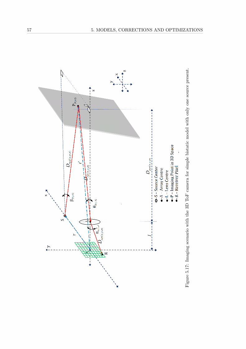
57 5. MODELS, CORRECTIONS AND OPTIMIZATIONS
Fig
ure
5.17
:Im
agin
gsc
enari
ow
ith
the
3DT
oFca
mer
afo
rsi
mp
leb
ista
tic
mod
elw
ith
only
on
eso
urc
ep
rese
nt.
5.5. DISTANCE NONLINEARITY MODELS AND CORRECTIONS 58
Dt(x,y,z) =(Dreal(x,y,z) +Dref(x,y,z) +Dsen(x,y,z)
)(5.151)
and the measured depth information Dmes(x,y,z) = Dt(x,y,z)/2 is given by
Dmes(x,y,z) =(Dreal(x,y,z) +Dref(x,y,z) +Dsen(x,y,z)
)/2 (5.152)
From the knowledge of β(x,y,z) as per Eq. (5.149), the forwards travel path Dreal(x,y,z)
of the light ray can be modelled as
Dreal(x,y,z) =
(Dper(x,y,z) + f
cosβ(x,y,z)
)(5.153)
The distance Dsen(x,y,z) travelled by the rays from the lens centre L towards the sensorarray pixels can be modelled as
Dsen(x,y,z) =
(f
cosα(x,y,z)
)(5.154)
The focal length f for the camera is constant (12.8 mm for PMD Camcube 2.0 camera).The angle α(x,y,z) for each imaging point in 3D space can be found out from the cameraintrinsic parameters by the expression
α(x,y,z) = arctan
√(
xs(x,y,z))2
+(ys(x,y,z)
)2
f
(5.155)
where xs(x,y,z) and ys(x,y,z) are the sensor pixel coordinates in x and y direction respec-tively corresponding to the imaging point P(x,y,z) in 3D space as explained in Section 5.5,Eq. (5.98).
Hence the reflected ray from Eq. (5.152) for each imaging point in 3D space can bewritten after rearrangement as
Dref(x,y,z) = 2 ·Dmes(x,y,z) −(Dper(x,y,z) + f
cosβ(x,y,z)
)−Dsen(x,y,z) (5.156)
Substituting for Dper(x,y,z) from the known relation
Dper(x,y,z) = Dref(x,y,z) · cos θ(x,y,z) (5.157)
The reflected path length Dref(x,y,z) can be modified as
59 5. MODELS, CORRECTIONS AND OPTIMIZATIONS
Dref(x,y,z) =
2 ·Dmes(x,y,z) −
(f
cosβ(x,y,z)
)−Dsen(x,y,z)(
1 +cos θ(x,y,z)cosβ(x,y,z)
) (5.158)
For a particular imaging point in 3D space for a perpendicular board, all the values onthe R.H.S are known and hence the reflected path length can be calculated from the aboveexpression. From the calculated reflected path length, the true perpendicular distance inz direction from the lens centre to each imaging point in 3D space Dper(x,y,z), can becalculated from Eq. (5.157).
From the obtained value of Dper(x,y,z), the non linearly corrected distance Dcor(x,y,z)
for each imaging point P(x,y,z) in 3D space is given by
Dcor(x,y,z) = Dper(x,y,z) + f (5.159)
5.5.3 Perpendicular Illumination Model
In this section, we present a simpler model called the perpendicular illumination modelwhich is computationally faster than the optimized as well as the simple bistatic models.The disadvantage of this model is the accuracy for the distance non linearity correction.Nevertheless this model forms the starting point in distance non linearity correction inToF cameras.
A monostatic model assumes the source and the receiver to be at the same point in 3Dspace, For the perpendicular illumination model there is only a slight variation from themonostatic model. Here we assume that each imaging point in 3D space is illuminated bya point source directly perpendicular to it on the sensor array plane. The measurementscenario is shown as in the Figure 5.18. Here the sensor array centre A forms the originof the coordinate system. On the sensor array plane i.e. the x-y plane, point sources areassumed to illuminate each imaging point in 3D space directly perpendicular to it. Anexample can be seen in Figure 5.18 where the imaging point P(x,y,z) is illuminated by thepoint source at S in the sensor array plane. Likewise, point sources illuminate each suchimaging point in 3D space. Hence each ray from the point sources travel a forward pathlength of Dled(x,y,z) towards the respective imaging point P(x,y,z) and returns to the lenscentre L by travelling a backward path length of Dref(x,y,z) creating an angle θ(x,y,z) withthe z axis. The ray is then focused onto the sensor array at a point R at an angle α(x,y,z)
with the z axis where the correlation is performed internally for depth calculation.
As mentioned in Section 5.5.1, the angle θ(x,y,z) for every pixel is unique and onlydepends on the field of view of the camera. In order to find this angle we image a plainperpendicular board as mentioned in Section 5.3 for a known distance Zc from the cameralens center. From the calculated values of Xc(x,y,z) and Yc(x,y,z) as mentioned in Eq. (5.80),the values of θ(x,y,z) can found out by the expression
θ(x,y,z) = arctan
√Xc(x,y,z)
2 + Yc(x,y,z)2
Zc
(5.160)
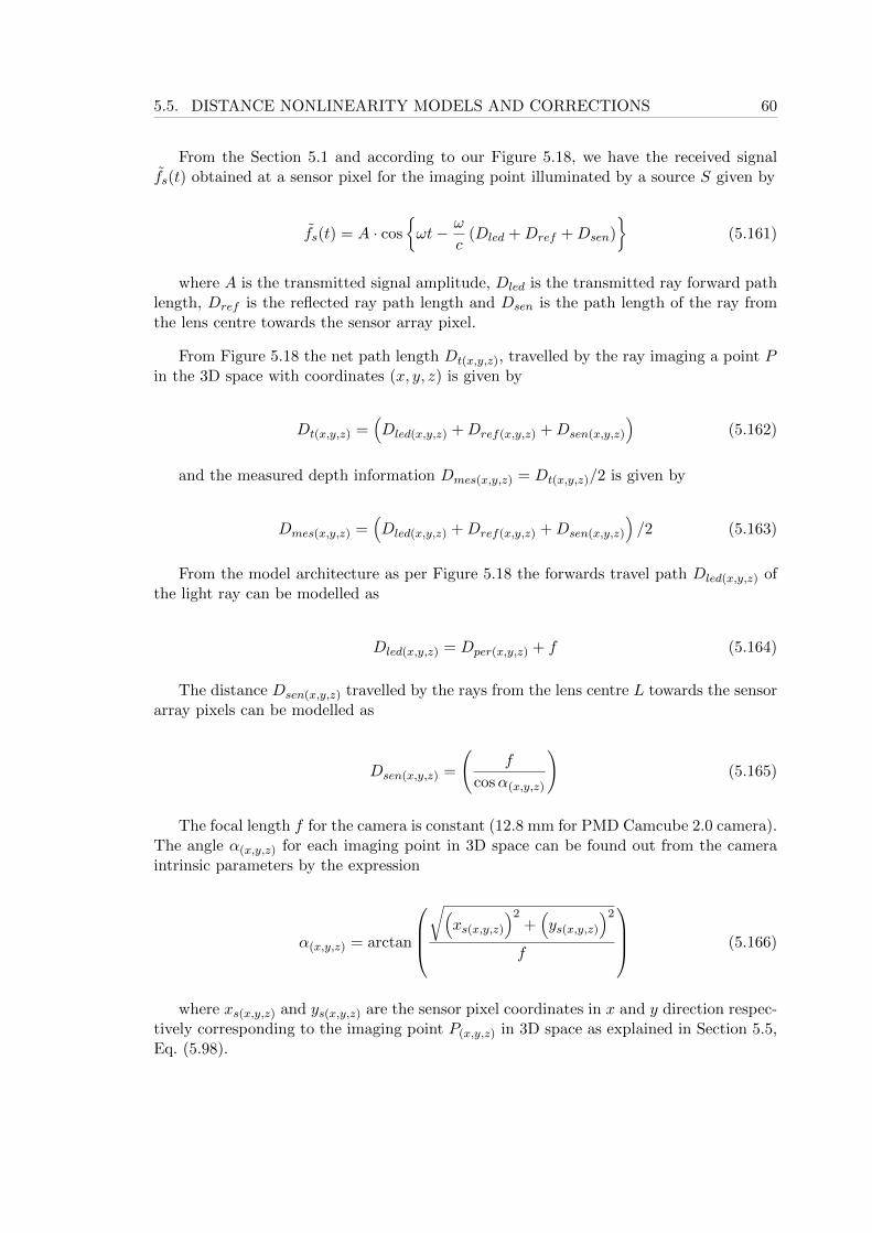
5.5. DISTANCE NONLINEARITY MODELS AND CORRECTIONS 60
From the Section 5.1 and according to our Figure 5.18, we have the received signalfs(t) obtained at a sensor pixel for the imaging point illuminated by a source S given by
fs(t) = A · cos
{ωt− ω
c(Dled +Dref +Dsen)
}(5.161)
where A is the transmitted signal amplitude, Dled is the transmitted ray forward pathlength, Dref is the reflected ray path length and Dsen is the path length of the ray fromthe lens centre towards the sensor array pixel.
From Figure 5.18 the net path length Dt(x,y,z), travelled by the ray imaging a point Pin the 3D space with coordinates (x, y, z) is given by
Dt(x,y,z) =(Dled(x,y,z) +Dref(x,y,z) +Dsen(x,y,z)
)(5.162)
and the measured depth information Dmes(x,y,z) = Dt(x,y,z)/2 is given by
Dmes(x,y,z) =(Dled(x,y,z) +Dref(x,y,z) +Dsen(x,y,z)
)/2 (5.163)
From the model architecture as per Figure 5.18 the forwards travel path Dled(x,y,z) ofthe light ray can be modelled as
Dled(x,y,z) = Dper(x,y,z) + f (5.164)
The distance Dsen(x,y,z) travelled by the rays from the lens centre L towards the sensorarray pixels can be modelled as
Dsen(x,y,z) =
(f
cosα(x,y,z)
)(5.165)
The focal length f for the camera is constant (12.8 mm for PMD Camcube 2.0 camera).The angle α(x,y,z) for each imaging point in 3D space can be found out from the cameraintrinsic parameters by the expression
α(x,y,z) = arctan
√(
xs(x,y,z))2
+(ys(x,y,z)
)2
f
(5.166)
where xs(x,y,z) and ys(x,y,z) are the sensor pixel coordinates in x and y direction respec-tively corresponding to the imaging point P(x,y,z) in 3D space as explained in Section 5.5,Eq. (5.98).
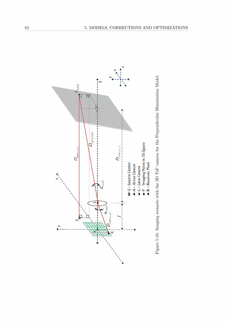
61 5. MODELS, CORRECTIONS AND OPTIMIZATIONS
Fig
ure
5.18
:Im
agin
gsc
enari
ow
ith
the
3DT
oFca
mer
afo
rth
eP
erp
end
icu
lar
Illu
min
ati
onM
od
el.
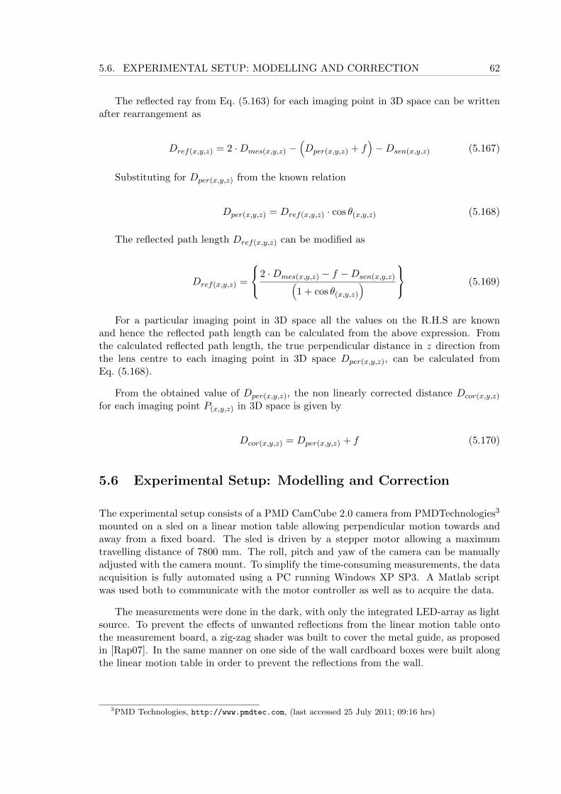
5.6. EXPERIMENTAL SETUP: MODELLING AND CORRECTION 62
The reflected ray from Eq. (5.163) for each imaging point in 3D space can be writtenafter rearrangement as
Dref(x,y,z) = 2 ·Dmes(x,y,z) −(Dper(x,y,z) + f
)−Dsen(x,y,z) (5.167)
Substituting for Dper(x,y,z) from the known relation
Dper(x,y,z) = Dref(x,y,z) · cos θ(x,y,z) (5.168)
The reflected path length Dref(x,y,z) can be modified as
Dref(x,y,z) =
2 ·Dmes(x,y,z) − f −Dsen(x,y,z)(1 + cos θ(x,y,z)
) (5.169)
For a particular imaging point in 3D space all the values on the R.H.S are knownand hence the reflected path length can be calculated from the above expression. Fromthe calculated reflected path length, the true perpendicular distance in z direction fromthe lens centre to each imaging point in 3D space Dper(x,y,z), can be calculated fromEq. (5.168).
From the obtained value of Dper(x,y,z), the non linearly corrected distance Dcor(x,y,z)
for each imaging point P(x,y,z) in 3D space is given by
Dcor(x,y,z) = Dper(x,y,z) + f (5.170)
5.6 Experimental Setup: Modelling and Correction
The experimental setup consists of a PMD CamCube 2.0 camera from PMDTechnologies3
mounted on a sled on a linear motion table allowing perpendicular motion towards andaway from a fixed board. The sled is driven by a stepper motor allowing a maximumtravelling distance of 7800 mm. The roll, pitch and yaw of the camera can be manuallyadjusted with the camera mount. To simplify the time-consuming measurements, the dataacquisition is fully automated using a PC running Windows XP SP3. A Matlab scriptwas used both to communicate with the motor controller as well as to acquire the data.
The measurements were done in the dark, with only the integrated LED-array as lightsource. To prevent the effects of unwanted reflections from the linear motion table ontothe measurement board, a zig-zag shader was built to cover the metal guide, as proposedin [Rap07]. In the same manner on one side of the wall cardboard boxes were built alongthe linear motion table in order to prevent the reflections from the wall.
3PMD Technologies, http://www.pmdtec.com, (last accessed 25 July 2011; 09:16 hrs)
63 5. MODELS, CORRECTIONS AND OPTIMIZATIONS
Figure 5.19: Experimental Setup for Depth and Amplitude measurement as well as non-linearity correction.
The zig zag shape is maintained as proposed in [Rap07], such that the light rays falling onthe shader is reflected to directions other than that towards the imaging board. Even iflight rays directly fall on the zig zag shader, the shader is imaged, whereas the unwantedreflection towards the board which can introduce errors in the distance measurement dueto multiple reflections, are avoided. All other exposed surfaces were covered with a lowreflection black cloth. The experimental setup is shown in Figure 5.19.
The camera was placed at 500 mm from the board with the accuracy of the positionwas verified with a industrial grade Bosch GLM 150 Professional Laser Rangefinder4. Thelaser distance measurer measures the distance between the PMD Camcube 2.0 camera andthe perpendicular board. At 500 mm, the field of view of the camera is such that it onlyimages the perpendicular board kept in front. With the help of water level indicators, itis made sure that the camera is held perpendicular to the ground. For adjusting the pitchand yaw of the camera, several measurements of the board are taken and averaged untilthe four corner pixels of the distance image showed the similar distance values. Due to thedistance nonlinearity mentioned in Section 5.5, the distance values does not correspondto the true distance of the target as indicated by the Bosch GLM 150 Professional LaserRangefinder. It is also made sure that the central pixels have the shortest average distancefrom the camera sensor.
4Bosch GLM 150 Professional Laser Rangefinder , http://www.bosch-professional.com/gb/en/ocs/tools/101300/23315/rangefinders/glm-150/, (last accessed 25 July 2011; 09:16 hrs)
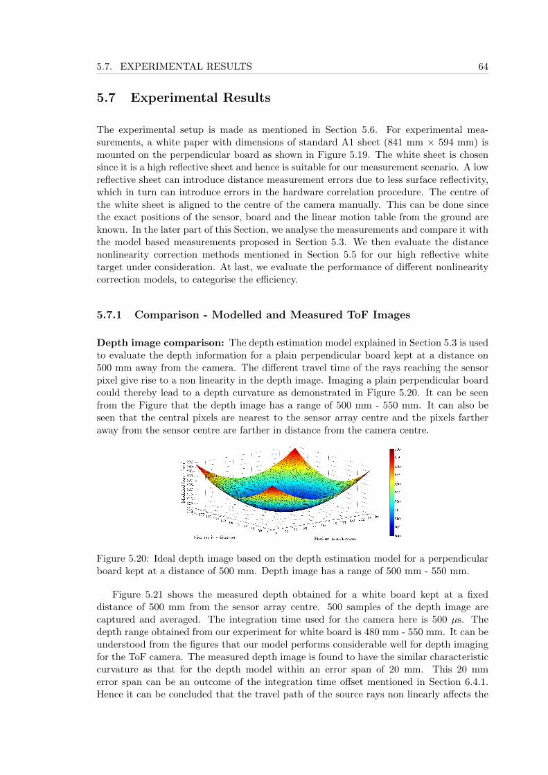
5.7. EXPERIMENTAL RESULTS 64
5.7 Experimental Results
The experimental setup is made as mentioned in Section 5.6. For experimental mea-surements, a white paper with dimensions of standard A1 sheet (841 mm × 594 mm) ismounted on the perpendicular board as shown in Figure 5.19. The white sheet is chosensince it is a high reflective sheet and hence is suitable for our measurement scenario. A lowreflective sheet can introduce distance measurement errors due to less surface reflectivity,which in turn can introduce errors in the hardware correlation procedure. The centre ofthe white sheet is aligned to the centre of the camera manually. This can be done sincethe exact positions of the sensor, board and the linear motion table from the ground areknown. In the later part of this Section, we analyse the measurements and compare it withthe model based measurements proposed in Section 5.3. We then evaluate the distancenonlinearity correction methods mentioned in Section 5.5 for our high reflective whitetarget under consideration. At last, we evaluate the performance of different nonlinearitycorrection models, to categorise the efficiency.
5.7.1 Comparison - Modelled and Measured ToF Images
Depth image comparison: The depth estimation model explained in Section 5.3 is usedto evaluate the depth information for a plain perpendicular board kept at a distance on500 mm away from the camera. The different travel time of the rays reaching the sensorpixel give rise to a non linearity in the depth image. Imaging a plain perpendicular boardcould thereby lead to a depth curvature as demonstrated in Figure 5.20. It can be seenfrom the Figure that the depth image has a range of 500 mm - 550 mm. It can also beseen that the central pixels are nearest to the sensor array centre and the pixels fartheraway from the sensor centre are farther in distance from the camera centre.
Figure 5.20: Ideal depth image based on the depth estimation model for a perpendicularboard kept at a distance of 500 mm. Depth image has a range of 500 mm - 550 mm.
Figure 5.21 shows the measured depth obtained for a white board kept at a fixeddistance of 500 mm from the sensor array centre. 500 samples of the depth image arecaptured and averaged. The integration time used for the camera here is 500 µs. Thedepth range obtained from our experiment for white board is 480 mm - 550 mm. It can beunderstood from the figures that our model performs considerable well for depth imagingfor the ToF camera. The measured depth image is found to have the similar characteristiccurvature as that for the depth model within an error span of 20 mm. This 20 mmerror span can be an outcome of the integration time offset mentioned in Section 6.4.1.Hence it can be concluded that the travel path of the source rays non linearly affects the
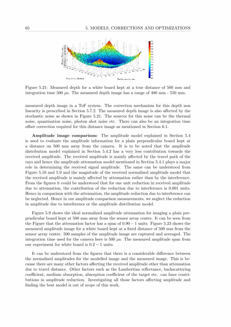
65 5. MODELS, CORRECTIONS AND OPTIMIZATIONS
Figure 5.21: Measured depth for a white board kept at a true distance of 500 mm andintegration time 500 µs. The measured depth image has a range of 480 mm - 550 mm.
measured depth image in a ToF system. The correction mechanism for this depth nonlinearity is prescribed in Section 5.7.2. The measured depth image is also affected by thestochastic noise as shown in Figure 5.21. The sources for this noise can be the thermalnoise, quantisation noise, photon shot noise etc. There can also be an integration timeoffset correction required for this distance image as mentioned in Section 6.1.
Amplitude image comparison: The amplitude model explained in Section 5.4is used to evaluate the amplitude information for a plain perpendicular board kept ata distance on 500 mm away from the camera. It is to be noted that the amplitudedistribution model explained in Section 5.4.2 has a very less contribution towards thereceived amplitude. The received amplitude is mainly affected by the travel path of therays and hence the amplitude attenuation model mentioned in Section 5.4.1 plays a majorrole in determining the received signal amplitude. The same can be understood fromFigure 5.10 and 5.9 and the magnitude of the received normalised amplitude model thatthe received amplitude is mainly affected by attenuation rather than by the interference.From the figures it could be understood that for one unit reduction in received amplitudedue to attenuation, the contribution of the reduction due to interference is 0.001 units.Hence in comparison with the attenuation, the amplitude reduction due to interference canbe neglected. Hence in our amplitude comparison measurements, we neglect the reductionin amplitude due to interference or the amplitude distribution model.
Figure 5.9 shows the ideal normalized amplitude attenuation for imaging a plain per-pendicular board kept at 500 mm away from the sensor array centre. It can be seen fromthe Figure that the attenuation factor has a span of 0.90− 1 units. Figure 5.23 shows themeasured amplitude image for a white board kept at a fixed distance of 500 mm from thesensor array centre. 500 samples of the amplitude image are captured and averaged. Theintegration time used for the camera here is 500 µs. The measured amplitude span fromour experiment for white board is 0.2− 1 units.
It can be understood from the figures that there is a considerable difference betweenthe normalised amplitudes for the modelled image and the measured image. This is be-cause there are many other factors affecting the received amplitude other than attenuationdue to travel distance. Other factors such as the Lambertian reflectance, backscatteringcoefficient, medium absorption, absorption coefficient of the target etc. can have contri-butions in amplitude reduction. Investigating all those factors affecting amplitude andfinding the best model is out of scope of this work.
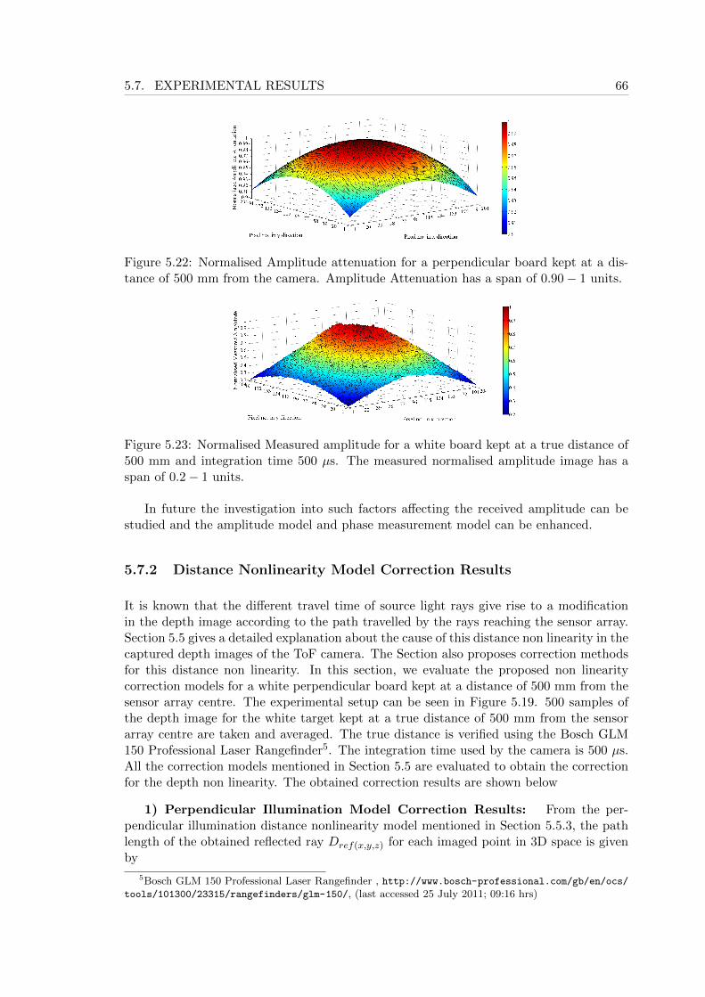
5.7. EXPERIMENTAL RESULTS 66
Figure 5.22: Normalised Amplitude attenuation for a perpendicular board kept at a dis-tance of 500 mm from the camera. Amplitude Attenuation has a span of 0.90− 1 units.
Figure 5.23: Normalised Measured amplitude for a white board kept at a true distance of500 mm and integration time 500 µs. The measured normalised amplitude image has aspan of 0.2− 1 units.
In future the investigation into such factors affecting the received amplitude can bestudied and the amplitude model and phase measurement model can be enhanced.
5.7.2 Distance Nonlinearity Model Correction Results
It is known that the different travel time of source light rays give rise to a modificationin the depth image according to the path travelled by the rays reaching the sensor array.Section 5.5 gives a detailed explanation about the cause of this distance non linearity in thecaptured depth images of the ToF camera. The Section also proposes correction methodsfor this distance non linearity. In this section, we evaluate the proposed non linearitycorrection models for a white perpendicular board kept at a distance of 500 mm from thesensor array centre. The experimental setup can be seen in Figure 5.19. 500 samples ofthe depth image for the white target kept at a true distance of 500 mm from the sensorarray centre are taken and averaged. The true distance is verified using the Bosch GLM150 Professional Laser Rangefinder5. The integration time used by the camera is 500 µs.All the correction models mentioned in Section 5.5 are evaluated to obtain the correctionfor the depth non linearity. The obtained correction results are shown below
1) Perpendicular Illumination Model Correction Results: From the per-pendicular illumination distance nonlinearity model mentioned in Section 5.5.3, the pathlength of the obtained reflected ray Dref(x,y,z) for each imaged point in 3D space is givenby
5Bosch GLM 150 Professional Laser Rangefinder , http://www.bosch-professional.com/gb/en/ocs/tools/101300/23315/rangefinders/glm-150/, (last accessed 25 July 2011; 09:16 hrs)
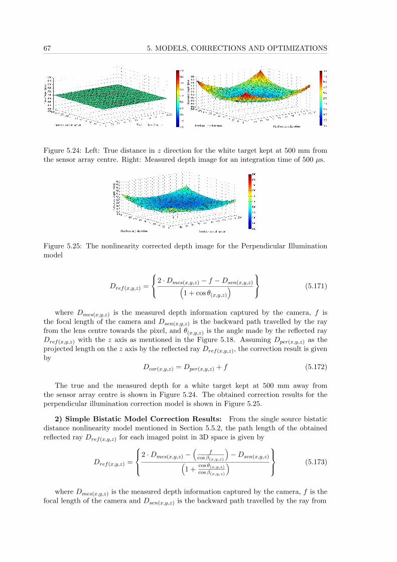
67 5. MODELS, CORRECTIONS AND OPTIMIZATIONS
Figure 5.24: Left: True distance in z direction for the white target kept at 500 mm fromthe sensor array centre. Right: Measured depth image for an integration time of 500 µs.
Figure 5.25: The nonlinearity corrected depth image for the Perpendicular Illuminationmodel
Dref(x,y,z) =
2 ·Dmes(x,y,z) − f −Dsen(x,y,z)(1 + cos θ(x,y,z)
) (5.171)
where Dmes(x,y,z) is the measured depth information captured by the camera, f isthe focal length of the camera and Dsen(x,y,z) is the backward path travelled by the rayfrom the lens centre towards the pixel, and θ(x,y,z) is the angle made by the reflected rayDref(x,y,z) with the z axis as mentioned in the Figure 5.18. Assuming Dper(x,y,z) as theprojected length on the z axis by the reflected ray Dref(x,y,z), the correction result is givenby
Dcor(x,y,z) = Dper(x,y,z) + f (5.172)
The true and the measured depth for a white target kept at 500 mm away fromthe sensor array centre is shown in Figure 5.24. The obtained correction results for theperpendicular illumination correction model is shown in Figure 5.25.
2) Simple Bistatic Model Correction Results: From the single source bistaticdistance nonlinearity model mentioned in Section 5.5.2, the path length of the obtainedreflected ray Dref(x,y,z) for each imaged point in 3D space is given by
Dref(x,y,z) =
2 ·Dmes(x,y,z) −
(f
cosβ(x,y,z)
)−Dsen(x,y,z)(
1 +cos θ(x,y,z)cosβ(x,y,z)
) (5.173)
where Dmes(x,y,z) is the measured depth information captured by the camera, f is thefocal length of the camera and Dsen(x,y,z) is the backward path travelled by the ray from
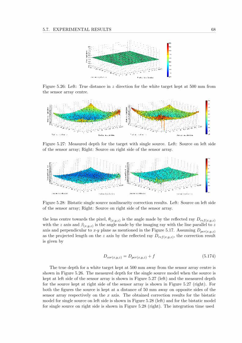
5.7. EXPERIMENTAL RESULTS 68
Figure 5.26: Left: True distance in z direction for the white target kept at 500 mm fromthe sensor array centre.
Figure 5.27: Measured depth for the target with single source. Left: Source on left sideof the sensor array; Right: Source on right side of the sensor array.
Figure 5.28: Bistatic single source nonlinearity correction results. Left: Source on left sideof the sensor array; Right: Source on right side of the sensor array.
the lens centre towards the pixel, θ(x,y,z) is the angle made by the reflected ray Dref(x,y,z)
with the z axis and β(x,y,z) is the angle made by the imaging ray with the line parallel to zaxis and perpendicular to x-y plane as mentioned in the Figure 5.17. Assuming Dper(x,y,z)
as the projected length on the z axis by the reflected ray Dref(x,y,z), the correction resultis given by
Dcor(x,y,z) = Dper(x,y,z) + f (5.174)
The true depth for a white target kept at 500 mm away from the sensor array centre isshown in Figure 5.26. The measured depth for the single source model when the source iskept at left side of the sensor array is shown in Figure 5.27 (left) and the measured depthfor the source kept at right side of the sensor array is shown in Figure 5.27 (right). Forboth the figures the source is kept at a distance of 50 mm away on opposite sides of thesensor array respectively on the x axis. The obtained correction results for the bistaticmodel for single source on left side is shown in Figure 5.28 (left) and for the bistatic modelfor single source on right side is shown in Figure 5.28 (right). The integration time used
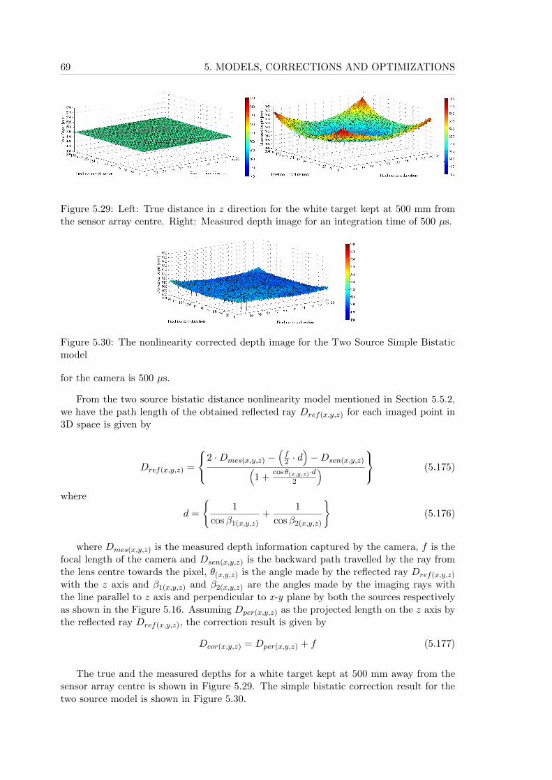
69 5. MODELS, CORRECTIONS AND OPTIMIZATIONS
Figure 5.29: Left: True distance in z direction for the white target kept at 500 mm fromthe sensor array centre. Right: Measured depth image for an integration time of 500 µs.
Figure 5.30: The nonlinearity corrected depth image for the Two Source Simple Bistaticmodel
for the camera is 500 µs.
From the two source bistatic distance nonlinearity model mentioned in Section 5.5.2,we have the path length of the obtained reflected ray Dref(x,y,z) for each imaged point in3D space is given by
Dref(x,y,z) =
2 ·Dmes(x,y,z) −(f2 · d
)−Dsen(x,y,z)(
1 +cos θ(x,y,z)·d
2
) (5.175)
where
d =
{1
cosβ1(x,y,z)+
1
cosβ2(x,y,z)
}(5.176)
where Dmes(x,y,z) is the measured depth information captured by the camera, f is thefocal length of the camera and Dsen(x,y,z) is the backward path travelled by the ray fromthe lens centre towards the pixel, θ(x,y,z) is the angle made by the reflected ray Dref(x,y,z)
with the z axis and β1(x,y,z) and β2(x,y,z) are the angles made by the imaging rays withthe line parallel to z axis and perpendicular to x-y plane by both the sources respectivelyas shown in the Figure 5.16. Assuming Dper(x,y,z) as the projected length on the z axis bythe reflected ray Dref(x,y,z), the correction result is given by
Dcor(x,y,z) = Dper(x,y,z) + f (5.177)
The true and the measured depths for a white target kept at 500 mm away from thesensor array centre is shown in Figure 5.29. The simple bistatic correction result for thetwo source model is shown in Figure 5.30.
5.7. EXPERIMENTAL RESULTS 70
3) Optimized Bistatic Model Correction Results: From the optimized singlesource bistatic distance nonlinearity model mentioned in Section 5.5.1, we have modelledthe depth image Dmodel(x,y,z) for each imaged point in 3D space as
Dmodel(x,y,z) =(Dopt1(x,y,z) +Dopt2(x,y,z) +Dsen(x,y,z)
)/2 (5.178)
where Dopt1(x,y,z) is the optimal forward travel path of the imaging light ray, Dopt2(x,y,z)
is the optimal reflected backward travel path of the ray and Dsen(x,y,z) is the backwardpath travelled by the ray from the lens centre towards the pixel as shown in Figure 5.14.Assuming Dper(x,y,z) as the projected length on the z axis by the optimal reflected rayDopt2(x,y,z), the correction result is given by
Dcor(x,y,z) = Dper(x,y,z) + f (5.179)
The true depth for a white target kept at 500 mm away from the sensor array centre isshown in Figure 5.31. The measured depth for the single source model when the source iskept at left side of the sensor array is shown in Figure 5.32 (left) and the measured depthfor the source kept at right side of the sensor array is shown in Figure 5.32 (right). Forboth figures the source is kept at a distance of 50 mm away on opposite sides of the sensorarray respectively on the x axis. The obtained correction results for the optimized modelfor a single source on left side is shown in Figure 5.33 (left) and for the optimized modelfor a single source on right side is shown in Figure 5.33 (right). The integration time usedfor the camera is 500 µs.
From the optimized two source bistatic distance nonlinearity model mentioned in Sec-tion 5.5.1, we have modelled the depth image Dmodel(x,y,z) for each imaged point in 3Dspace as
Dmodel(x,y,z) =
(Dopt1(x,y,z) +Dopt2(x,y,z)
2+Dopt3(x,y,z) +Dsen(x,y,z)
)/2 (5.180)
where Dopt1(x,y,z) and Dopt2(x,y,z) is the optimal forward travel path of the imaginglight rays of the two sources, Dopt3(x,y,z) is the optimal reflected backward travel pathof the ray and Dsen(x,y,z) is the backward path travelled by the ray from the lens centretowards the pixel as shown in Figure 5.12. Assuming Dper(x,y,z) as the projected lengthon the z axis by the optimal reflected ray Dopt2(x,y,z), the correction result is given by
Dcor(x,y,z) = Dper(x,y,z) + f (5.181)
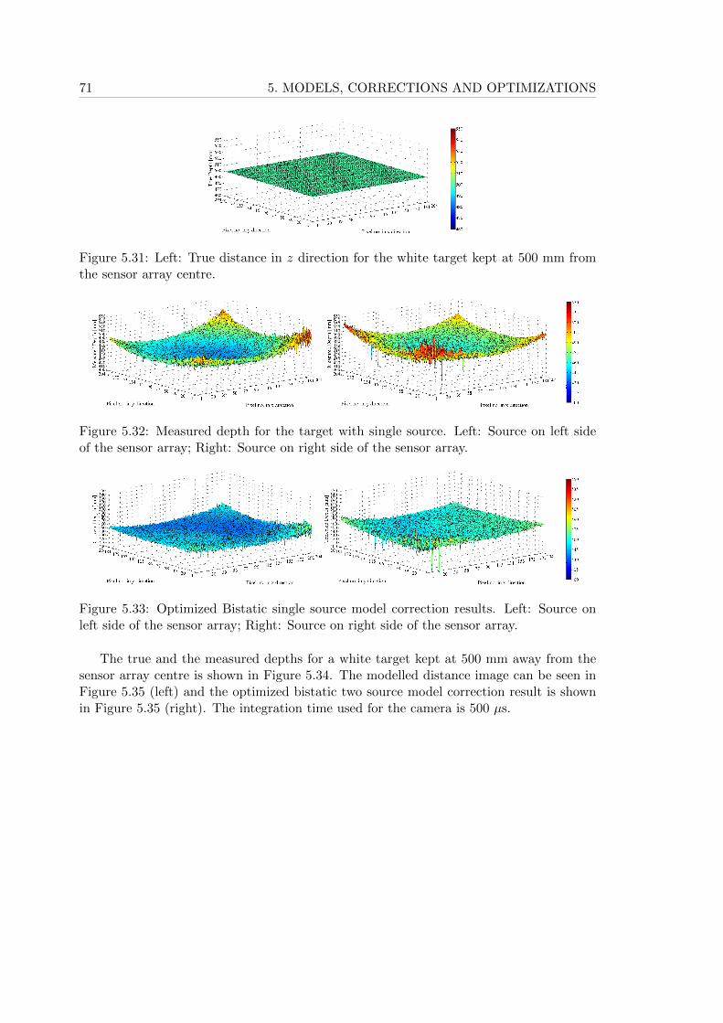
71 5. MODELS, CORRECTIONS AND OPTIMIZATIONS
Figure 5.31: Left: True distance in z direction for the white target kept at 500 mm fromthe sensor array centre.
Figure 5.32: Measured depth for the target with single source. Left: Source on left sideof the sensor array; Right: Source on right side of the sensor array.
Figure 5.33: Optimized Bistatic single source model correction results. Left: Source onleft side of the sensor array; Right: Source on right side of the sensor array.
The true and the measured depths for a white target kept at 500 mm away from thesensor array centre is shown in Figure 5.34. The modelled distance image can be seen inFigure 5.35 (left) and the optimized bistatic two source model correction result is shownin Figure 5.35 (right). The integration time used for the camera is 500 µs.
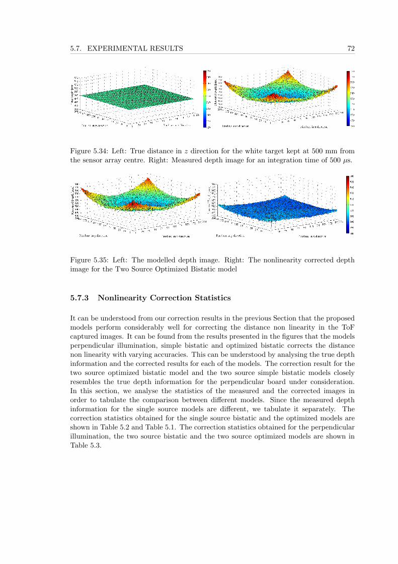
5.7. EXPERIMENTAL RESULTS 72
Figure 5.34: Left: True distance in z direction for the white target kept at 500 mm fromthe sensor array centre. Right: Measured depth image for an integration time of 500 µs.
Figure 5.35: Left: The modelled depth image. Right: The nonlinearity corrected depthimage for the Two Source Optimized Bistatic model
5.7.3 Nonlinearity Correction Statistics
It can be understood from our correction results in the previous Section that the proposedmodels perform considerably well for correcting the distance non linearity in the ToFcaptured images. It can be found from the results presented in the figures that the modelsperpendicular illumination, simple bistatic and optimized bistatic corrects the distancenon linearity with varying accuracies. This can be understood by analysing the true depthinformation and the corrected results for each of the models. The correction result for thetwo source optimized bistatic model and the two source simple bistatic models closelyresembles the true depth information for the perpendicular board under consideration.In this section, we analyse the statistics of the measured and the corrected images inorder to tabulate the comparison between different models. Since the measured depthinformation for the single source models are different, we tabulate it separately. Thecorrection statistics obtained for the single source bistatic and the optimized models areshown in Table 5.2 and Table 5.1. The correction statistics obtained for the perpendicularillumination, the two source bistatic and the two source optimized models are shown inTable 5.3.

73 5. MODELS, CORRECTIONS AND OPTIMIZATIONS
Table 5.1: Correction Statistics for the white target for single source on left side
Iopt [ms] µ [mm] σ [mm]
Ideal Depth Image n.a 500.00 0.00
Measured Depth Image 0.5 461.27 13.88
Bistatic Model 0.5 432.98 6.75
Optimized Bistatic Model 0.5 445.55 6.93
Table 5.2: Correction Statistics the white target for single source on right side
Iopt [ms] µ [mm] σ [mm]
Ideal Depth Image n.a 500.00 0.00
Measured Depth Image 0.5 476.13 13.54
Bistatic Model 0.5 447.35 5.90
Optimized Bistatic Model 0.5 459.98 6.04
Table 5.3: Correction Statistics for a white target kept at 500 mm from the camera
Iopt [ms] µ [mm] σ [mm]
Ideal Depth Image n.a 500.00 0.00
Measured Depth Image 0.5 523.57 10.89
Perpendicular Illumination Model 0.5 513.16 5.66
Simple Two Source Bistatic Model 0.5 505.07 2.76
Optimized Two Source Bistatic Model 0.5 505.02 2.77

5.7. EXPERIMENTAL RESULTS 74
Chapter 6
Non Parametric Calibration
The ToF cameras are generally affected by different kinds of measurement errors. Oneof the basic depth measurement errors associated with ToF cameras is due to the ’wig-gling effect’, cf. [Rap07], [LSKK10]. The PMD Camcube 2.0 camera houses an internalcalibration technique in order to compensate this wiggling effect and hence wiggling erroranalysis is not done in this thesis. Another factor affecting the measurement is the quan-tization limits of the ToF system which puts constraints in the measurement results fromthe correlation procedure. The integration time of the camera also plays a significant rolein depth measurements. Imaging with different integration times differs in the transmittedenergy from the system. This results in different received signals at the sensor array whenimaging the same targets. The constraints of the quantization procedure thereby limitsthe accuracy of depth imaging and hence give different results when imaging the same tar-get with different integration times. Another factor which affects the measurements is thetarget reflectivity. For the targets kept at the same depth, the received signal is modifieddue to difference in reflectivity. The quantization internal to the ToF system again plays arole in the depth measurement which results in different measurement results for differenttarget refectivities kept at same distance. In this chapter we analyse the integration timedependence of the targets having different reflectivity. The integration time dependenceis mainly seen as an offset error in the measured depth image as mentioned in [Kah07]and [KRI06]. But we extend this idea to have the correction based on offset matricescalculated theoretically. We propose a model for the integration time offset correctionusing offset matrices and extend the idea for reflectivity considerations. We analyse thedepth dependence on the targets. We also propose methods to find optimal integrationtimes for different target refectivities using RMSE analysis.
This chapter is divided as follows. Section 6.1 proposes a theoretical model for offsetcorrection using offset matrices. Section 6.2 proposes a method to find optimal integrationtimes for targets having different reflectivities. Section 6.3 describes the experimental setupused for the offset correction and optimal integration time selection. Section 6.4 describesthe experimental results where the depth error due to integration time is explained inSection 6.4.1. Section 6.4.2 outlines the integration time offset matrices obtained forthe target under consideration and Section 6.4.3 extends this idea to the different targetrefectivities. Finally Section 6.4.4 provides experimental results for optimal integrationtime selection for different reflectivities.
75
6.1. INTEGRATION TIME OFFSET CORRECTION MODEL 76
6.1 Integration Time Offset Correction Model
It is known from the ToF camera analysis in [Rap07], [USRRK11], [KRI06] etc. that thedependence on integration time with the measured depth is an offset. But all the studieswhich exists till now corrects the offset independent on the imaging point in 3D space orotherwise it assumes the offset as constant for all image pixels. Such a correction merelybased on the comparison between the true and measured depth images can modify thestatistics within the depth image. This can in fact deteriorate the depth image and canaffect the relative post-processing stages such as denoising. The noise statistics in theimage is lost or is modified which leads to errors in the post-processing tasks. Hence it isvery important to preserve the statistics of the depth image even after offset correction.
In reality the fixed offset correction is an approximated solution and is far away fromthe ideal one. As mentioned in Section 5.3, the measured depth image is modified accordingto the travel time of the rays. This in turn means that there is also a relationship betweenthe integration time offset on the travel path length. In this section we estimate thisrelationship between the offset information and the travel path length. We propose acorrection model by exploiting the nonlinearity corrected depth information captured fromthe camera and proposing theoretical offset matrices for integration time correction. Weextend the study for different target refectivities and propose correction matrices for thesame. The significance of our model is that the statistics of the measured depth imageis preserved even after the offset correction and hence the post processing tasks can becarried out efficiently.
The imaging scenario can be seen in Figure 6.1. Here the Camcube camera images aperpendicular board kept at a true distance of (Zc + f) units away from the sensor arraycentre A. Here, f represents the focal length of the camera. The two sources S1 and S2
transmits the light rays which interfere at the point P(x,y,z) on the imaging plane, reflectsback to the lens centre L and reaches the sensor pixel R. The correlation is performedinternally and the depth image is calculated.
According to Section 5.3, the ideal measured depth can be modelled as
Dmodel(x,y,z) =
(Dreal1(x,y,z) +Dreal2(x,y,z)
2+Dref(x,y,z) +Dsen(x,y,z)
)/2 (6.1)
where Dreal1(x,y,z) and Dreal2(x,y,z) are the forward path lengths of the rays travellingfrom the source towards the point P(x,y,z), Dref(x,y,z) is the path length of the reflectedray reaching the lens centre L and Dsen(x,y,z) is the reflected ray travelling from the lenscentre towards the imaging pixel R. The calculation for all the related parameters in orderto arrive at this solution is mentioned in Section 5.3.
But in practice due to the integration time offsets, reflectivity dependence and statis-tical errors, the measured depth image differs from the modelled image. We assume thatthe measured image for a particular integration time is Dmes(x,y,z). From Section 5.5, thenonlinearly corrected depth information Dcor(x,y,z) can be written as
Dcor(x,y,z) = Dper(x,y,z) + f (6.2)
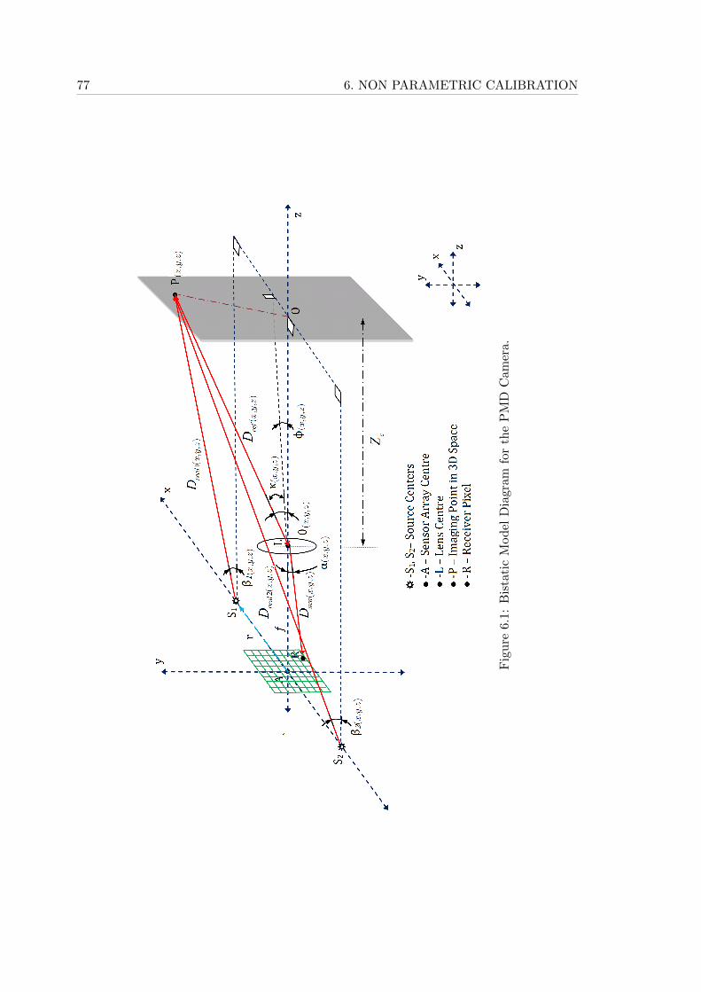
77 6. NON PARAMETRIC CALIBRATION
Fig
ure
6.1:
Bis
tati
cM
od
elD
iagr
amfo
rth
eP
MD
Cam
era.
6.2. OPTIMAL INTEGRATION TIME SELECTION BY RMSE 78
Once the correction is made, the virtual average depth, Davg of the target from thesensor array centre towards the board for a particular integration time for a true depth(Zc + f) units is given by
Davg =
N∑n=1
Dcor(x,y,z)
N(6.3)
where N is the total number of pixels in the sensor array. With the virtual averagedepth Davg, and considering that as the true depth, the depth image is remodelled, cf.Eq. (6.1) as
Dmodel1(x,y,z) =
(Dreal11(x,y,z) +Dreal21(x,y,z)
2+Dref1(x,y,z) +Dsen(x,y,z)
)/2 (6.4)
where Dreal11(x,y,z) and Dreal21(x,y,z) are the re-calculated forward path lengths of therays travelling from the source towards the point P(x,y,z), Dref1(x,y,z) is the re-calculatedreflected ray reaching the lens centre L and Dsen(x,y,z) is the path length of the reflectedray travelling from the lens centre towards the imaging pixel R. For these calculationsthe true depth from the sensor centre towards the imaging board is assumed to be Davg
instead of (Zc + f) units. The calculation for all the related parameters in order to arriveat this solution is mentioned in Section 5.3.
Once the re-modelling is done, the theoretical offset matrix for a particular integrationtime and true depth (Zc + f) units can be given by
Doffset(x,y,z) = Dmodel(x,y,z) −Dmodel1(x,y,z) (6.5)
Hence the corresponding theoretical offset corrected result is then given by
Doffcor(x,y,z) = Dmes(x,y,z) +Doffset(x,y,z) (6.6)
6.2 Optimal Integration Time Selection by RMSE
The choice of an optimal integration time reduces the statistical errors within the system.It can be understood that the choice of integration time induces deviations in the measureddepth image. As mentioned, the reflectivity of the targets also plays a role in depthvariation. In this section we analyze the performance of different integration times ondepth imaging. We also propose a method to find the optimal integration time by analyzingthe Root Mean Square Error (RMSE) between the modelled image and the measured depthimage.
The performance of a particular integration time for a true depth can be analysed bycalculating the RMSE of the captured depth image. RMSE is a measure of the differencebetween the predicted model and the values obtained from observation. In our case theobserved values become the offset corrected depth images since the parameter integration
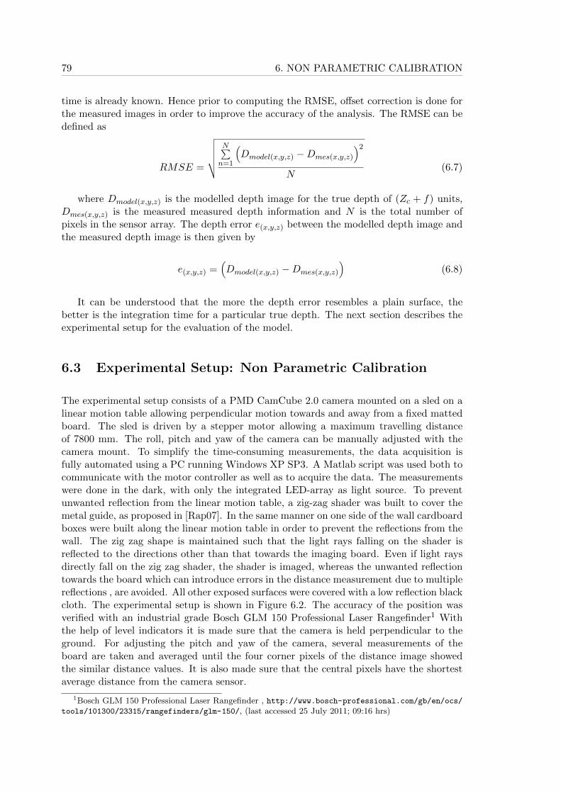
79 6. NON PARAMETRIC CALIBRATION
time is already known. Hence prior to computing the RMSE, offset correction is done forthe measured images in order to improve the accuracy of the analysis. The RMSE can bedefined as
RMSE =
√√√√√ N∑n=1
(Dmodel(x,y,z) −Dmes(x,y,z)
)2
N(6.7)
where Dmodel(x,y,z) is the modelled depth image for the true depth of (Zc + f) units,Dmes(x,y,z) is the measured measured depth information and N is the total number ofpixels in the sensor array. The depth error e(x,y,z) between the modelled depth image andthe measured depth image is then given by
e(x,y,z) =(Dmodel(x,y,z) −Dmes(x,y,z)
)(6.8)
It can be understood that the more the depth error resembles a plain surface, thebetter is the integration time for a particular true depth. The next section describes theexperimental setup for the evaluation of the model.
6.3 Experimental Setup: Non Parametric Calibration
The experimental setup consists of a PMD CamCube 2.0 camera mounted on a sled on alinear motion table allowing perpendicular motion towards and away from a fixed mattedboard. The sled is driven by a stepper motor allowing a maximum travelling distanceof 7800 mm. The roll, pitch and yaw of the camera can be manually adjusted with thecamera mount. To simplify the time-consuming measurements, the data acquisition isfully automated using a PC running Windows XP SP3. A Matlab script was used both tocommunicate with the motor controller as well as to acquire the data. The measurementswere done in the dark, with only the integrated LED-array as light source. To preventunwanted reflection from the linear motion table, a zig-zag shader was built to cover themetal guide, as proposed in [Rap07]. In the same manner on one side of the wall cardboardboxes were built along the linear motion table in order to prevent the reflections from thewall. The zig zag shape is maintained such that the light rays falling on the shader isreflected to the directions other than that towards the imaging board. Even if light raysdirectly fall on the zig zag shader, the shader is imaged, whereas the unwanted reflectiontowards the board which can introduce errors in the distance measurement due to multiplereflections , are avoided. All other exposed surfaces were covered with a low reflection blackcloth. The experimental setup is shown in Figure 6.2. The accuracy of the position wasverified with an industrial grade Bosch GLM 150 Professional Laser Rangefinder1 Withthe help of level indicators it is made sure that the camera is held perpendicular to theground. For adjusting the pitch and yaw of the camera, several measurements of theboard are taken and averaged until the four corner pixels of the distance image showedthe similar distance values. It is also made sure that the central pixels have the shortestaverage distance from the camera sensor.
1Bosch GLM 150 Professional Laser Rangefinder , http://www.bosch-professional.com/gb/en/ocs/tools/101300/23315/rangefinders/glm-150/, (last accessed 25 July 2011; 09:16 hrs)
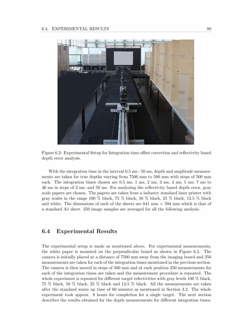
6.4. EXPERIMENTAL RESULTS 80
Figure 6.2: Experimental Setup for Integration time offset correction and reflectivity baseddepth error analysis.
With the integration time in the interval 0.5 ms - 50 ms, depth and amplitude measure-ments are taken for true depths varying from 7500 mm to 500 mm with steps of 500 mmeach. The integration times chosen are 0.5 ms, 1 ms, 2 ms, 3 ms, 4 ms, 5 ms; 7 ms to46 ms in steps of 3 ms; and 50 ms. For analyzing the reflectivity based depth error, grayscale papers are chosen. The papers are taken from a industry standard laser printer withgray scales in the range 100 % black, 75 % black, 50 % black, 25 % black, 12.5 % blackand white. The dimensions of each of the sheets are 841 mm × 594 mm which is that ofa standard A1 sheet. 250 image samples are averaged for all the following analysis.
6.4 Experimental Results
The experimental setup is made as mentioned above. For experimental measurements,the white paper is mounted on the perpendicular board as shown in Figure 6.2. Thecamera is initially placed at a distance of 7500 mm away from the imaging board and 250measurements are taken for each of the integration times mentioned in the previous section.The camera is then moved in steps of 500 mm and at each position 250 measurements foreach of the integration times are taken and the measurement procedure is repeated. Thewhole experiment is repeated for different target refectivities with gray levels 100 % black,75 % black, 50 % black, 25 % black and 12.5 % black. All the measurements are takenafter the standard warm up time of 60 minutes as mentioned in Section 3.2. The wholeexperiment took approx. 8 hours for completion for a single target. The next sectiondescribes the results obtained for the depth measurements for different integration times.
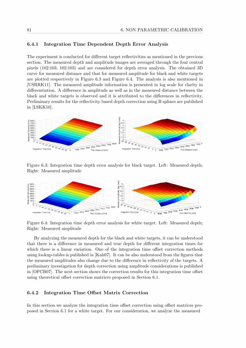
81 6. NON PARAMETRIC CALIBRATION
6.4.1 Integration Time Dependent Depth Error Analysis
The experiment is conducted for different target reflectivities as mentioned in the previoussection. The measured depth and amplitude images are averaged through the four centralpixels (102:103, 102:103) and are considered for depth error analysis. The obtained 3Dcurve for measured distance and that for measured amplitude for black and white targetsare plotted respectively in Figure 6.3 and Figure 6.4. The analysis is also mentioned in[USRRK11]. The measured amplitude information is presented in log scale for clarity indifferentiation. A difference in amplitude as well as in the measured distance between theblack and white targets is observed and it is attributed to the differences in reflectivity.Preliminary results for the reflectivity based depth correction using B splines are publishedin [LSKK10].
Figure 6.3: Integration time depth error analysis for black target. Left: Measured depth;Right: Measured amplitude
Figure 6.4: Integration time depth error analysis for white target. Left: Measured depth;Right: Measured amplitude
By analyzing the measured depth for the black and white targets, it can be understoodthat there is a difference in measured and true depth for different integration times forwhich there is a linear variation. One of the integration time offset correction methodsusing lookup-tables is published in [Kah07]. It can be also understood from the figures thatthe measured amplitudes also change due to the difference in reflectivity of the targets. Apreliminary investigation for depth correction using amplitude considerations is publishedin [OFCB07]. The next section shows the correction results for this integration time offsetusing theoretical offset correction matrices proposed in Section 6.1.
6.4.2 Integration Time Offset Matrix Correction
In this section we analyze the integration time offset correction using offset matrices pro-posed in Section 6.1 for a white target. For our consideration, we analyze the measured
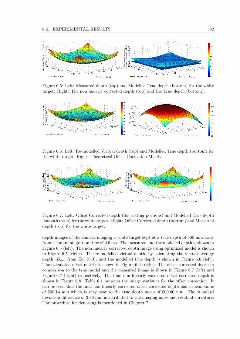
6.4. EXPERIMENTAL RESULTS 82
Figure 6.5: Left: Measured depth (top) and Modelled True depth (bottom) for the whitetarget. Right: The non linearly corrected depth (top) and the True depth (bottom).
Figure 6.6: Left: Re-modelled Virtual depth (top) and Modelled True depth (bottom) forthe white target. Right: Theoretical Offset Correction Matrix.
Figure 6.7: Left: Offset Corrected depth (fluctuating portions) and Modelled True depth(smooth mesh) for the white target. Right: Offset Corrected depth (bottom) and Measureddepth (top) for the white target.
depth images of the camera imaging a white target kept at a true depth of 500 mm awayfrom it for an integration time of 0.5 ms. The measured and the modelled depth is shown inFigure 6.5 (left). The non linearly corrected depth image using optimized model is shownin Figure 6.5 (right). The re-modelled virtual depth, by calculating the virtual averagedepth, Davg from Eq. (6.3), and the modelled true depth is shown in Figure 6.6 (left).The calculated offset matrix is shown in Figure 6.6 (right). The offset corrected depth incomparison to the true model and the measured image is shown in Figure 6.7 (left) andFigure 6.7 (right) respectively. The final non linearly corrected offset corrected depth isshown in Figure 6.8. Table 6.1 presents the image statistics for the offset correction. Itcan be seen that the final non linearly corrected offset corrected depth has a mean valueof 500.14 mm which is very near to the true depth mean of 500.00 mm. The standarddeviation difference of 3.86 mm is attributed to the imaging noise and residual curvature.The procedure for denoising is mentioned in Chapter 7.
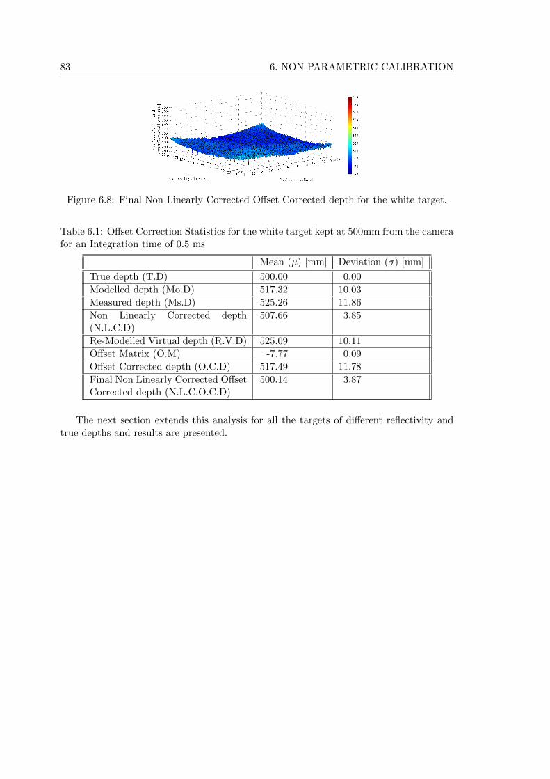
83 6. NON PARAMETRIC CALIBRATION
Figure 6.8: Final Non Linearly Corrected Offset Corrected depth for the white target.
Table 6.1: Offset Correction Statistics for the white target kept at 500mm from the camerafor an Integration time of 0.5 ms
Mean (µ) [mm] Deviation (σ) [mm]
True depth (T.D) 500.00 0.00
Modelled depth (Mo.D) 517.32 10.03
Measured depth (Ms.D) 525.26 11.86
Non Linearly Corrected depth(N.L.C.D)
507.66 3.85
Re-Modelled Virtual depth (R.V.D) 525.09 10.11
Offset Matrix (O.M) -7.77 0.09
Offset Corrected depth (O.C.D) 517.49 11.78
Final Non Linearly Corrected OffsetCorrected depth (N.L.C.O.C.D)
500.14 3.87
The next section extends this analysis for all the targets of different reflectivity andtrue depths and results are presented.
6.4. EXPERIMENTAL RESULTS 84
6.4.3 Reflectivity Based Offset Matrix Correction
In this section we extend the analysis presented in Section 6.4.2 for the targets of differentreflectivity namely, white, 12.5 % black, 25 % black, 50 % black, 75 % black and 100 %black. Analysis is done for each of the targets imaging at true depths varying from 500 mmto 7500 mm in steps of 500 mm. The depth images are captured for all the mentionedintegration times (i.e. 0.5 ms, 1 ms, 2 ms, 3 ms, 4 ms, 5 ms; 7 ms to 46 ms in steps of3 ms; and 50 ms) against each of the true depths and reflectivities. The obtained resultsfor theoretical offset correction is provided in
• Table 6.2 and Table 6.3 for white target;
• Table 6.4 and Table 6.2 for 12.5 % black target;
• Table 6.6 and Table 6.7 for 25 % black target;
• Table 6.8 and Table 6.9 for 50 % black target;
• Table 6.10 and Table 6.11 for 75 % black target; and
• Table 6.12 and Table 6.13 for 100 % black target.
The results are presented only for the optimal integration times chosen by evaluatingRMSE as mentioned in Section 6.4.4. For the ambiguous depth of 7500 mm, non optimalintegraton time is chosen. With the help of these tables, the offset correction can bedone for targets of different reflectivity. For any depth between the evaluated true depth,interpolation can be made so as to evaluate the required correction for that particulardepth. For reflectivity based depth correction, first, the reflectivity of the target canbe identified from the known amplitude variation data from Section 6.4.1. Once thereflectivity of the target is known, the required theoretical correction can be applied fromthe offset correction tables for a particular integration time and for an estimated truedepth.
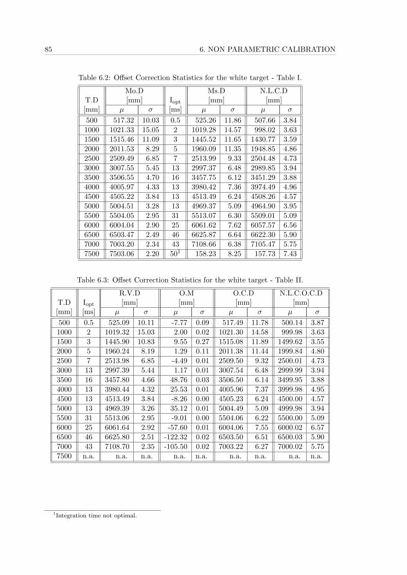
85 6. NON PARAMETRIC CALIBRATION
Table 6.2: Offset Correction Statistics for the white target - Table I.
Mo.D Ms.D N.L.C.DT.D [mm] Iopt [mm] [mm][mm] µ σ [ms] µ σ µ σ
500 517.32 10.03 0.5 525.26 11.86 507.66 3.84
1000 1021.33 15.05 2 1019.28 14.57 998.02 3.63
1500 1515.46 11.09 3 1445.52 11.65 1430.77 3.59
2000 2011.53 8.29 5 1960.09 11.35 1948.85 4.86
2500 2509.49 6.85 7 2513.99 9.33 2504.48 4.73
3000 3007.55 5.45 13 2997.37 6.48 2989.85 3.94
3500 3506.55 4.70 16 3457.75 6.12 3451.29 3.88
4000 4005.97 4.33 13 3980.42 7.36 3974.49 4.96
4500 4505.22 3.84 13 4513.49 6.24 4508.26 4.57
5000 5004.51 3.28 13 4969.37 5.09 4964.90 3.95
5500 5504.05 2.95 31 5513.07 6.30 5509.01 5.09
6000 6004.04 2.90 25 6061.62 7.62 6057.57 6.56
6500 6503.47 2.49 46 6625.87 6.64 6622.30 5.90
7000 7003.20 2.34 43 7108.66 6.38 7105.47 5.75
7500 7503.06 2.20 501 158.23 8.25 157.73 7.43
Table 6.3: Offset Correction Statistics for the white target - Table II.
R.V.D O.M O.C.D N.L.C.O.C.DT.D Iopt [mm] [mm] [mm] [mm][mm] [ms] µ σ µ σ µ σ µ σ
500 0.5 525.09 10.11 -7.77 0.09 517.49 11.78 500.14 3.87
1000 2 1019.32 15.03 2.00 0.02 1021.30 14.58 999.98 3.63
1500 3 1445.90 10.83 9.55 0.27 1515.08 11.89 1499.62 3.55
2000 5 1960.24 8.19 1.29 0.11 2011.38 11.44 1999.84 4.80
2500 7 2513.98 6.85 -4.49 0.01 2509.50 9.32 2500.01 4.73
3000 13 2997.39 5.44 1.17 0.01 3007.54 6.48 2999.99 3.94
3500 16 3457.80 4.66 48.76 0.03 3506.50 6.14 3499.95 3.88
4000 13 3980.44 4.32 25.53 0.01 4005.96 7.37 3999.98 4.95
4500 13 4513.49 3.84 -8.26 0.00 4505.23 6.24 4500.00 4.57
5000 13 4969.39 3.26 35.12 0.01 5004.49 5.09 4999.98 3.94
5500 31 5513.06 2.95 -9.01 0.00 5504.06 6.22 5500.00 5.09
6000 25 6061.64 2.92 -57.60 0.01 6004.06 7.55 6000.02 6.57
6500 46 6625.80 2.51 -122.32 0.02 6503.50 6.51 6500.03 5.90
7000 43 7108.70 2.35 -105.50 0.02 7003.22 6.27 7000.02 5.75
7500 n.a. n.a. n.a. n.a. n.a. n.a. n.a. n.a. n.a.
1Integration time not optimal.

6.4. EXPERIMENTAL RESULTS 86
Table 6.4: Offset Correction Statistics for the 12.5 % black target - Table I.
Mo.D Ms.D N.L.C.DT.D [mm] Iopt [mm] [mm][mm] µ σ [ms] µ σ µ σ
500 517.32 10.03 1 519.96 11.35 502.54 4.03
1000 1021.33 15.05 2 1009.05 15.66 987.97 3.96
1500 1515.46 11.09 5 1445.14 11.70 1430.40 3.67
2000 2011.53 8.29 7 1955.49 11.41 1944.26 5.11
2500 2509.49 6.85 13 2528.09 9.76 2518.52 4.90
3000 3007.55 5.45 19 3013.49 6.81 3005.92 4.36
3500 3506.55 4.70 22 3471.77 6.60 3465.28 4.38
4000 4005.97 4.33 22 4008.45 7.58 4002.47 5.39
4500 4505.22 3.84 10 4493.46 6.64 4488.25 4.93
5000 5004.51 3.28 25 5005.24 5.44 5000.73 4.36
5500 5504.05 2.95 50 5549.11 6.92 5545.02 5.67
6000 6004.04 2.90 40 6122.73 10.87 6118.07 8.63
6500 6503.47 2.49 40 6679.43 19.37 6672.33 8.75
7000 7003.20 2.34 50 7167.68 10.86 7163.97 9.24
7500 7503.06 2.20 501 184.58 14.28 181.54 7.80
Table 6.5: Offset Correction Statistics for the 12.5 % black target - Table II.
R.V.D O.M O.C.D N.L.C.O.C.DT.D Iopt [mm] [mm] [mm] [mm][mm] [ms] µ σ µ σ µ σ µ σ
500 1 519.89 10.06 -2.57 0.03 517.38 11.33 500.05 4.03
1000 2 1009.18 14.95 12.15 0.10 1021.20 15.75 999.87 3.94
1500 5 1445.52 10.84 69.94 0.27 1515.07 11.93 1499.62 3.61
2000 7 1955.65 8.18 55.88 0.12 2011.37 11.50 1999.83 5.04
2500 13 2528.05 6.87 -18.56 0.03 2509.53 9.74 2500.04 4.92
3000 19 3013.48 5.46 -5.93 0.01 3007.56 6.80 3000.01 4.36
3500 22 3471.80 4.67 34.75 0.02 3506.52 6.61 3499.97 4.37
4000 22 4008.45 4.33 -2.47 0.00 4005.98 7.59 4000.00 5.39
4500 10 4493.47 3.83 11.75 0.01 4505.21 6.64 4499.99 4.92
5000 25 5005.25 3.28 -0.73 0.00 5004.51 5.44 5000.00 4.36
5500 50 5549.09 2.96 -45.04 0.01 5504.07 6.92 5500.02 5.68
6000 40 6122.15 2.93 -118.11 0.03 6004.09 9.56 6000.04 8.64
6500 40 6675.84 2.52 -172.38 0.03 6503.52 9.31 6500.05 8.76
7000 50 7167.20 2.36 -164.00 0.03 7003.24 9.69 7000.04 9.25
7500 n.a. n.a. n.a. n.a. n.a. n.a. n.a. n.a. n..a.
1Integration time not optimal.
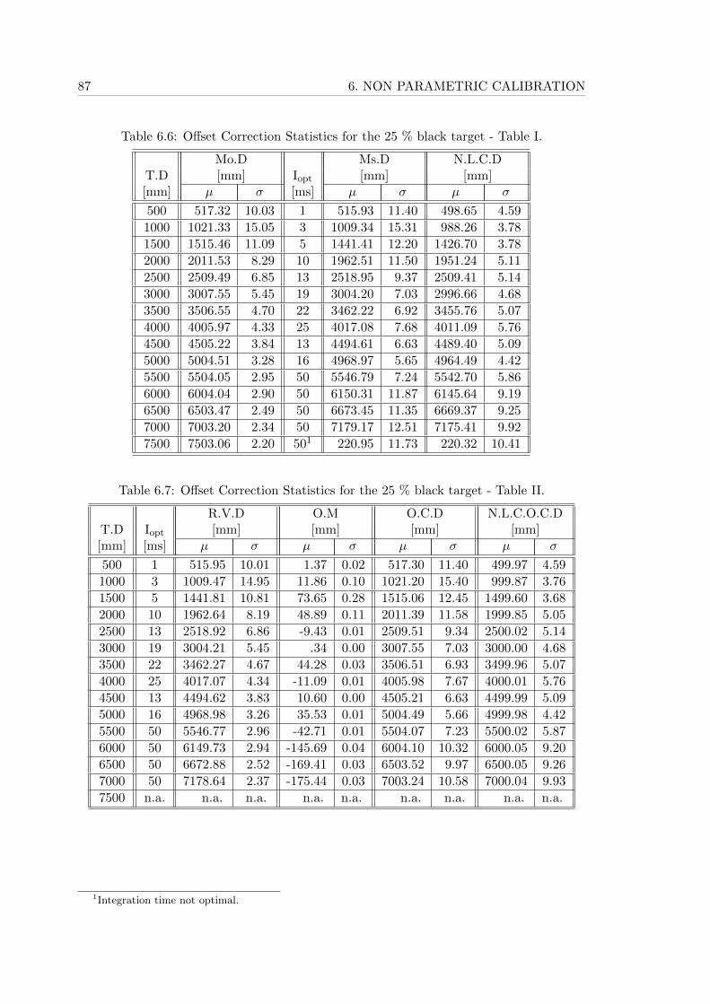
87 6. NON PARAMETRIC CALIBRATION
Table 6.6: Offset Correction Statistics for the 25 % black target - Table I.
Mo.D Ms.D N.L.C.DT.D [mm] Iopt [mm] [mm][mm] µ σ [ms] µ σ µ σ
500 517.32 10.03 1 515.93 11.40 498.65 4.59
1000 1021.33 15.05 3 1009.34 15.31 988.26 3.78
1500 1515.46 11.09 5 1441.41 12.20 1426.70 3.78
2000 2011.53 8.29 10 1962.51 11.50 1951.24 5.11
2500 2509.49 6.85 13 2518.95 9.37 2509.41 5.14
3000 3007.55 5.45 19 3004.20 7.03 2996.66 4.68
3500 3506.55 4.70 22 3462.22 6.92 3455.76 5.07
4000 4005.97 4.33 25 4017.08 7.68 4011.09 5.76
4500 4505.22 3.84 13 4494.61 6.63 4489.40 5.09
5000 5004.51 3.28 16 4968.97 5.65 4964.49 4.42
5500 5504.05 2.95 50 5546.79 7.24 5542.70 5.86
6000 6004.04 2.90 50 6150.31 11.87 6145.64 9.19
6500 6503.47 2.49 50 6673.45 11.35 6669.37 9.25
7000 7003.20 2.34 50 7179.17 12.51 7175.41 9.92
7500 7503.06 2.20 501 220.95 11.73 220.32 10.41
Table 6.7: Offset Correction Statistics for the 25 % black target - Table II.
R.V.D O.M O.C.D N.L.C.O.C.DT.D Iopt [mm] [mm] [mm] [mm][mm] [ms] µ σ µ σ µ σ µ σ
500 1 515.95 10.01 1.37 0.02 517.30 11.40 499.97 4.59
1000 3 1009.47 14.95 11.86 0.10 1021.20 15.40 999.87 3.76
1500 5 1441.81 10.81 73.65 0.28 1515.06 12.45 1499.60 3.68
2000 10 1962.64 8.19 48.89 0.11 2011.39 11.58 1999.85 5.05
2500 13 2518.92 6.86 -9.43 0.01 2509.51 9.34 2500.02 5.14
3000 19 3004.21 5.45 .34 0.00 3007.55 7.03 3000.00 4.68
3500 22 3462.27 4.67 44.28 0.03 3506.51 6.93 3499.96 5.07
4000 25 4017.07 4.34 -11.09 0.01 4005.98 7.67 4000.01 5.76
4500 13 4494.62 3.83 10.60 0.00 4505.21 6.63 4499.99 5.09
5000 16 4968.98 3.26 35.53 0.01 5004.49 5.66 4999.98 4.42
5500 50 5546.77 2.96 -42.71 0.01 5504.07 7.23 5500.02 5.87
6000 50 6149.73 2.94 -145.69 0.04 6004.10 10.32 6000.05 9.20
6500 50 6672.88 2.52 -169.41 0.03 6503.52 9.97 6500.05 9.26
7000 50 7178.64 2.37 -175.44 0.03 7003.24 10.58 7000.04 9.93
7500 n.a. n.a. n.a. n.a. n.a. n.a. n.a. n.a. n.a.
1Integration time not optimal.
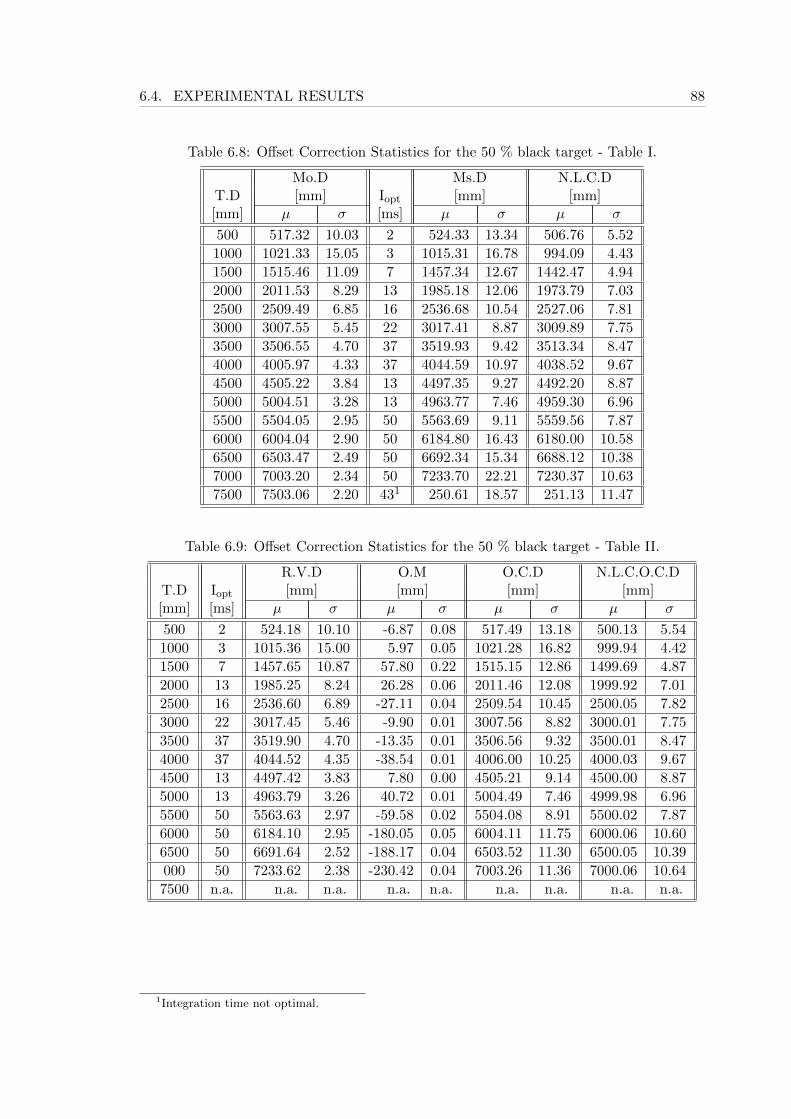
6.4. EXPERIMENTAL RESULTS 88
Table 6.8: Offset Correction Statistics for the 50 % black target - Table I.
Mo.D Ms.D N.L.C.DT.D [mm] Iopt [mm] [mm][mm] µ σ [ms] µ σ µ σ
500 517.32 10.03 2 524.33 13.34 506.76 5.52
1000 1021.33 15.05 3 1015.31 16.78 994.09 4.43
1500 1515.46 11.09 7 1457.34 12.67 1442.47 4.94
2000 2011.53 8.29 13 1985.18 12.06 1973.79 7.03
2500 2509.49 6.85 16 2536.68 10.54 2527.06 7.81
3000 3007.55 5.45 22 3017.41 8.87 3009.89 7.75
3500 3506.55 4.70 37 3519.93 9.42 3513.34 8.47
4000 4005.97 4.33 37 4044.59 10.97 4038.52 9.67
4500 4505.22 3.84 13 4497.35 9.27 4492.20 8.87
5000 5004.51 3.28 13 4963.77 7.46 4959.30 6.96
5500 5504.05 2.95 50 5563.69 9.11 5559.56 7.87
6000 6004.04 2.90 50 6184.80 16.43 6180.00 10.58
6500 6503.47 2.49 50 6692.34 15.34 6688.12 10.38
7000 7003.20 2.34 50 7233.70 22.21 7230.37 10.63
7500 7503.06 2.20 431 250.61 18.57 251.13 11.47
Table 6.9: Offset Correction Statistics for the 50 % black target - Table II.
R.V.D O.M O.C.D N.L.C.O.C.DT.D Iopt [mm] [mm] [mm] [mm][mm] [ms] µ σ µ σ µ σ µ σ
500 2 524.18 10.10 -6.87 0.08 517.49 13.18 500.13 5.54
1000 3 1015.36 15.00 5.97 0.05 1021.28 16.82 999.94 4.42
1500 7 1457.65 10.87 57.80 0.22 1515.15 12.86 1499.69 4.87
2000 13 1985.25 8.24 26.28 0.06 2011.46 12.08 1999.92 7.01
2500 16 2536.60 6.89 -27.11 0.04 2509.54 10.45 2500.05 7.82
3000 22 3017.45 5.46 -9.90 0.01 3007.56 8.82 3000.01 7.75
3500 37 3519.90 4.70 -13.35 0.01 3506.56 9.32 3500.01 8.47
4000 37 4044.52 4.35 -38.54 0.01 4006.00 10.25 4000.03 9.67
4500 13 4497.42 3.83 7.80 0.00 4505.21 9.14 4500.00 8.87
5000 13 4963.79 3.26 40.72 0.01 5004.49 7.46 4999.98 6.96
5500 50 5563.63 2.97 -59.58 0.02 5504.08 8.91 5500.02 7.87
6000 50 6184.10 2.95 -180.05 0.05 6004.11 11.75 6000.06 10.60
6500 50 6691.64 2.52 -188.17 0.04 6503.52 11.30 6500.05 10.39
000 50 7233.62 2.38 -230.42 0.04 7003.26 11.36 7000.06 10.64
7500 n.a. n.a. n.a. n.a. n.a. n.a. n.a. n.a. n.a.
1Integration time not optimal.
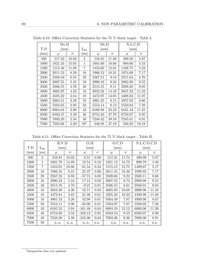
89 6. NON PARAMETRIC CALIBRATION
Table 6.10: Offset Correction Statistics for the 75 % black target - Table I.
Mo.D Ms.D N.L.C.DT.D [mm] Iopt [mm] [mm][mm] µ σ [ms] µ σ µ σ
500 517.32 10.03 2 516.85 11.80 499.50 5.87
1000 1021.33 15.05 1 1001.60 16.66 980.66 4.53
1500 1515.46 11.09 7 1453.60 12.61 1438.75 5.23
2000 2011.53 8.29 16 1986.12 10.31 1974.69 7.17
2500 2509.49 6.85 28 2567.51 9.54 2557.64 8.70
3000 3007.55 5.45 16 2990.16 9.24 2982.90 9.55
3500 3506.55 4.70 40 3515.55 9.11 3509.20 9.95
4000 4005.97 4.33 16 3952.56 14.43 3947.33 11.23
4500 4505.22 3.84 10 4472.97 13.05 4468.63 11.07
5000 5004.51 3.28 16 4961.25 8.15 4957.03 8.66
5500 5504.05 2.95 50 5554.14 8.13 5550.04 7.38
6000 6004.04 2.90 43 6166.98 22.22 6161.43 11.25
6500 6503.47 2.49 46 6754.20 37.70 6750.07 8.95
7000 7003.20 2.34 40 7248.42 39.58 7245.01 8.91
7500 7503.06 2.20 501 246.88 27.19 246.03 10.19
Table 6.11: Offset Correction Statistics for the 75 % black target - Table II.
R.V.D O.M O.C.D N.L.C.O.C.DT.D Iopt [mm] [mm] [mm] [mm][mm] [ms] µ σ µ σ µ σ µ σ
500 2 516.81 10.02 0.51 0.00 517.31 11.74 499.99 5.87
1000 1 1001.79 14.89 19.54 0.16 1021.13 16.78 999.79 4.49
1500 7 1453.91 10.86 61.54 0.24 1515.12 12.75 1499.67 5.17
2000 16 1986.16 8.24 25.37 0.06 2011.45 10.26 1999.92 7.17
2500 28 2567.23 6.93 -57.74 0.08 2509.60 9.22 2500.11 8.68
3000 16 2990.43 5.44 17.12 0.02 3007.52 8.74 2999.98 9.55
3500 40 3515.76 4.70 -9.21 0.01 3506.55 8.61 3500.01 9.94
4000 16 3953.26 4.30 52.71 0.03 4005.93 10.68 3999.96 11.24
4500 10 4473.84 3.82 31.38 0.01 4505.20 10.33 4499.98 11.08
5000 16 4961.53 3.26 42.98 0.01 5004.49 7.87 4999.98 8.67
5500 50 5554.11 2.96 -50.06 0.01 5504.07 7.87 5500.02 7.38
6000 43 6165.52 2.94 -161.48 0.04 6004.10 12.12 6000.06 11.26
6500 46 6753.60 2.53 -250.13 0.05 6503.54 9.55 6500.07 8.96
7000 40 7248.26 2.38 -245.06 0.04 7003.26 9.36 7000.06 8.91
7500 50 n..a. n..a. n..a. n.a. n.a. n.a. n.a. n.a.
1Integration time not optimal.

6.4. EXPERIMENTAL RESULTS 90
Table 6.12: Offset Correction Statistics for the 100 % black target - Table I.
Mo.D Ms.D N.L.C.DT.D [mm] Iopt [mm] [mm][mm] µ σ [ms] µ σ µ σ
500 517.32 10.03 2 513.99 12.78 496.67 6.48
1000 1021.33 15.05 2 1006.43 17.43 985.38 4.64
1500 1515.46 11.09 10 1449.17 13.39 1434.30 6.76
2000 2011.53 8.29 13 1955.05 12.65 1943.62 9.24
2500 2509.49 6.85 37 2558.48 13.55 2548.56 11.10
3000 3007.55 5.45 16 2961.54 14.76 2954.45 11.39
3500 3506.55 4.70 16 3397.80 19.15 3392.19 11.19
4000 4005.97 4.33 16 3946.87 15.43 3941.77 10.95
4500 4505.22 3.84 13 4453.93 19.60 4449.44 11.00
5000 5004.51 3.28 19 4952.59 11.90 4948.62 10.52
5500 5504.05 2.95 50 5549.21 10.21 5544.82 8.39
6000 6004.04 2.90 50 6185.61 29.89 6180.08 9.43
6500 6503.47 2.49 50 6687.36 26.75 6682.67 9.50
7000 7003.20 2.34 50 7264.37 50.12 7260.14 6.67
7500 7503.06 2.20 501 303.45 45.10 303.06 8.27
Table 6.13: Offset Correction Statistics for the 100 % black target - Table II.
R.V.D O.M O.C.D N.L.C.O.C.DT.D Iopt [mm] [mm] [mm] [mm][mm] [ms] µ σ µ σ µ σ µ σ
500 2 513.93 10.00 3.38 0.04 517.26 12.58 499.94 6.48
1000 2 1006.56 14.93 14.77 0.12 1021.19 17.51 999.84 4.60
1500 10 1449.44 10.84 66.01 0.26 1515.10 13.51 1499.64 6.69
2000 13 1955.00 8.18 56.53 0.12 2011.35 12.08 1999.83 9.23
2500 37 2558.14 6.92 -48.65 0.07 2509.58 11.12 2500.10 11.08
3000 16 2961.95 5.41 45.60 0.04 3007.48 11.12 2999.94 11.40
3500 16 3398.65 4.62 107.90 0.08 3506.44 11.09 3499.89 11.21
4000 16 3947.70 4.30 58.27 0.03 4005.92 10.92 3999.95 10.96
4500 13 4454.63 3.81 50.59 0.02 4505.19 10.82 4499.97 11.01
5000 19 4953.11 3.26 51.40 0.02 5004.48 10.72 4999.97 10.52
5500 50 5548.88 2.96 -44.83 0.01 5504.07 9.35 5500.02 8.40
6000 50 6184.19 2.95 -180.14 0.05 6004.11 9.96 6000.06 9.43
6500 50 6686.19 2.52 -182.72 0.04 6503.52 10.04 6500.05 9.50
7000 50 7263.40 2.38 -260.20 0.05 7003.26 7.03 7000.06 6.67
7500 n.a. n.a. n.a. n.a. n.a. n.a. n.a. n.a. n.a.
1Integration time not optimal.
91 6. NON PARAMETRIC CALIBRATION
6.4.4 Reflectivity Based Optimal Integration Time Selection
In this section we evaluate the root mean square error for each of the reflectivities, truedepths and integration times from the analysis mentioned in Section 6.2. The RMSEevaluation is carried out for all the different target reflectivities namely, white, 12.5 %black, 25 % black, 50 % black, 75 % black and 100 % black. RMSE analysis is done foreach of the targets imaging at true depths varying from 500 mm to 7500 mm in stepsof 500 mm. The depth images are captured for all the mentioned integration times (i.e.0.5 ms, 1 ms, 2 ms, 3 ms, 4 ms, 5 ms; 7 ms to 46 ms in steps of 3 ms; and 50 ms). Figure 6.9,Figure 6.10 and Figure 6.11 show the results for the RMSE evaluation for different targetreflectivities and true depths. The optimal integration time is defined as the one whichgives the minimum RMSE for a particular true depth. The obtained optimal integrationtime (Iopt) corresponding to the RMSE minimum (RMSEmin) for each of the reflectivityand true depths is shown in Table 6.14.
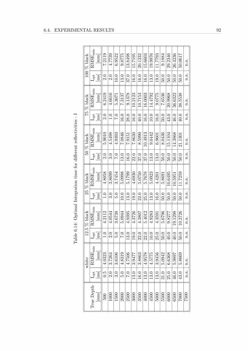
6.4. EXPERIMENTAL RESULTS 92
Tab
le6.
14:
Op
tim
alIn
tegr
atio
nti
me
for
diff
eren
tre
flec
tivit
ies
-I
wh
ite
12.5
%b
lack
25%
bla
ck50
%b
lack
75%
bla
ck100
%b
lack
Tru
eD
epth
I op
tR
MS
Em
inI o
pt
RM
SE
min
I op
tR
MS
Em
inI o
pt
RM
SE
min
I op
tR
MS
Em
inI o
pt
RM
SE
min
[mm
][m
s][m
m]
[ms]
[mm
][m
s][m
m]
[ms]
[mm
][m
s][m
m]
[ms]
[mm
]
500
0.5
4.03
231.
04.
2112
1.0
4.80
582.
05.
9010
2.0
6.2
419
2.0
7.2
119
1000
2.0
3.72
642.
04.
0544
3.0
3.86
993.
04.
5498
1.0
4.6
616
2.0
4.7
739
1500
3.0
3.61
065.
03.
6738
5.0
3.74
547.
04.
9393
7.0
5.3
071
10.0
6.9
522
2000
5.0
4.83
197.
05.
0944
10.0
5.09
9813
.07.
0846
16.0
7.3
137
13.0
9.8
775
2500
7.0
4.75
0613
.04.
9395
13.0
5.17
9916
.07.
9151
28.0
9.1
378
37.0
13.8
498
3000
13.0
3.94
7719
.04.
3726
19.0
4.69
3022
.07.
8630
16.0
10.2
123
16.0
15.7
195
3500
16.0
3.88
6322
.04.
3807
22.0
5.07
5037
.08.
5990
40.0
10.7
153
16.0
20.1
232
4000
13.0
4.95
7822
.05.
4012
25.0
5.76
7837
.010
.491
316
.016.0
003
16.0
15.6
603
4500
13.0
4.57
7510
.04.
9283
13.0
5.09
2313
.09.
0442
10.0
14.4
792
13.0
19.9
976
5000
13.0
3.94
5625
.04.
3591
16.0
4.42
0113
.06.
9601
16.0
9.0
775
19.0
11.7
793
5500
31.0
5.09
4250
.05.
6796
50.0
5.86
9150
.08.
0436
50.0
7.6
536
50.0
9.1
884
6000
25.0
6.63
6840
.09.
8277
50.0
10.6
495
50.0
15.1
104
43.0
20.9
968
50.0
29.2
346
6500
46.0
5.98
9740
.019
.129
850
.010
.595
150
.014
.386
846
.036.6
322
50.0
26.4
236
7000
43.0
5.86
6950
.010
.272
650
.011
.725
950
.021
.130
140
.038.5
538
50.0
50.0
617
7500
n.a
.n
.a.
n.a
.n
.a.
n.a
.n
.a.
n.a
.n
.a.
n.a
.n
.a.
n.a
.n
.a.
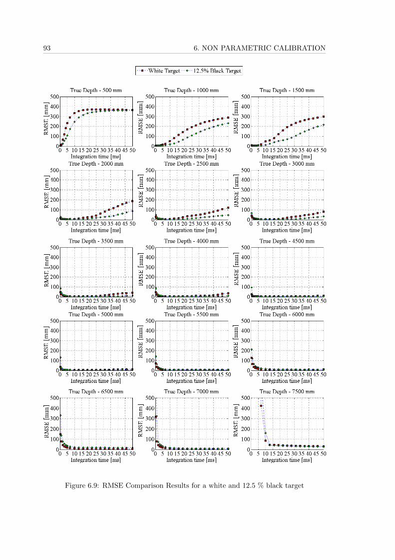
93 6. NON PARAMETRIC CALIBRATION
Figure 6.9: RMSE Comparison Results for a white and 12.5 % black target
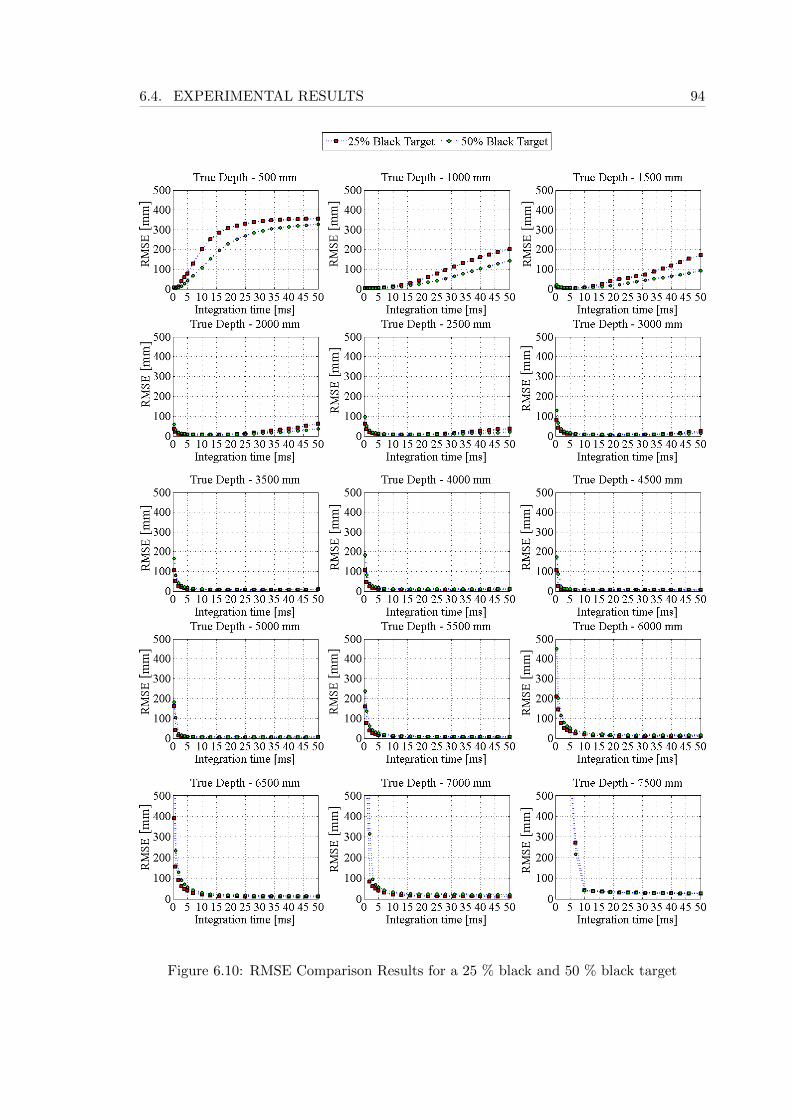
6.4. EXPERIMENTAL RESULTS 94
Figure 6.10: RMSE Comparison Results for a 25 % black and 50 % black target
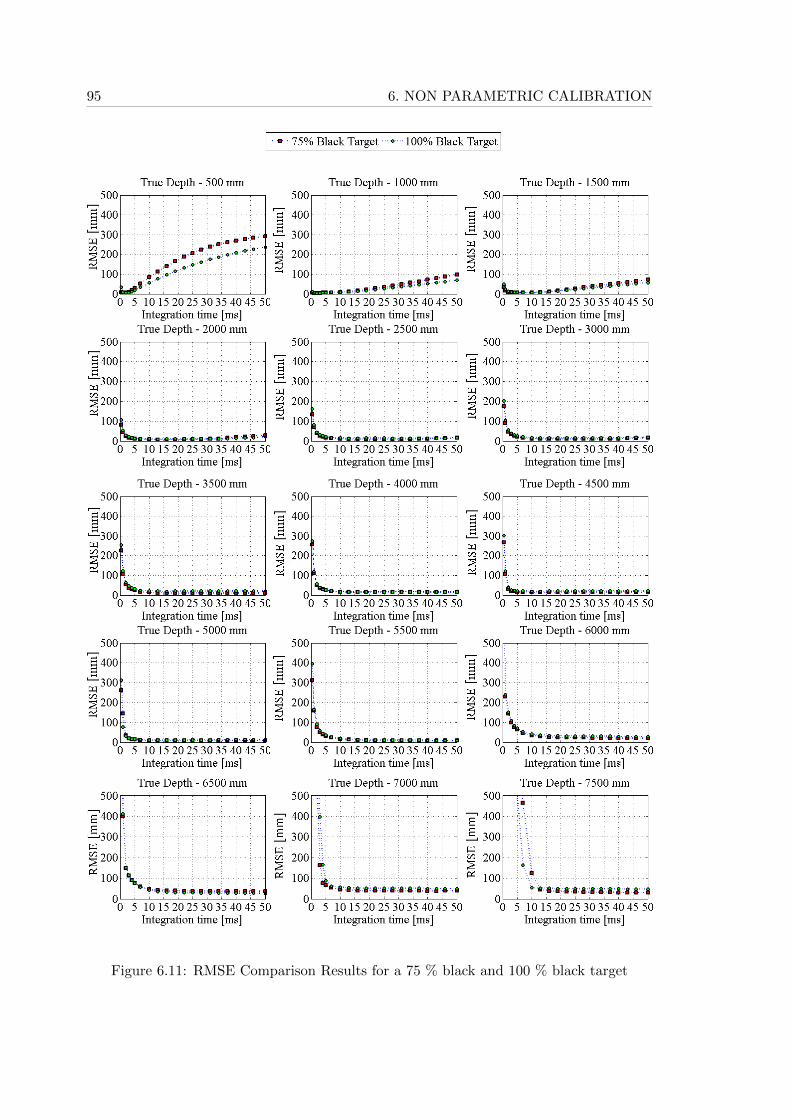
95 6. NON PARAMETRIC CALIBRATION
Figure 6.11: RMSE Comparison Results for a 75 % black and 100 % black target

6.4. EXPERIMENTAL RESULTS 96
Chapter 7
Image Denoising
The branch of image processing which usually deals with the primary image noise removalin order to carry out post processing tasks efficiently is termed broadly as image denoising.The image denoising tasks can deal with removal of the amplifier noise, salt and peppernoise, photon short noise, quantization noise, film grain noise, anisotropic noise etc fromthe captured images. In this chapter we discuss image denoising techniques which isunavoidable in case of the captured depth images from the PMD Camcube 2.0 camera.The techniques mentioned here are not specific, and hence in general can be used for anyToF camera. We assume that the captured depth image is free from all the deterministicnoise components and assume that the depth images only have the stochastic componentspresent in it. The semiconductor characteristics and response can be the source of thesestochastic noises. Another reason is the noise due to the reflectivity of the target. Targetsof different reflectivities kept at the same depth for similar integration time gives differentdepth images. It is very important to have a parametric evaluation of the system forfinding the source of these noise, but since it is a task which deals with the analysis ofsemiconductor properties of the system and implementation constraints like quantizationeffects etc., it requires a huge effort which is out of scope of this work. Hence we resorton to non parametric methods for our image denoising tasks.
7.1 Noise Statistics
The image statistics could give an account of the characteristics of the stochastic noisepresent in the image. But it should be noted that the statistics should be taken accordingto a reference known ground truth. In case of depth images, the images taken against aplain perpendicular board at a known distance from the camera kept can be taken as areference ground truth. For getting efficient results from the camera, it is required thatwe observe well reflective surfaces for depth image capture. This is due to the fact thatlow reflective surfaces for example rough surfaces, could lead to uneven reflections andthe reflected amplitude for the signal can even be considerably too less for safe detectionlevels, hence it is important to choose well reflective surfaces like a plain white board.From Chapter 5, it is known that due to the different travel times of the transmitted rays,there is a distance non linearity within the captured depth information and hence there
97
7.2. DEPTH DENOISING 98
is a distance curvature for the captured image. We have proposed nonlinearity correctionmethods in Chapter 5, Section 5.5, where the optimized model is found to be the bestmethod for efficient results. The disadvantage associated with the method was the requiredcomputation effort. Since the distance nonlinearity correction is deterministic in natureand does not alter the stochastic component present in the depth images, for analyzingthe noise statistics it is adviced to do the nonlinearity correction in order to get the truepicture of the amount of embedded noise.
The noise statistics can be a very good estimate of the stochastic noise present inthe system. Once the stochastic noise estimation is made, different noise removal filterscan be employed for depth denoising. Many of the denoising methods like the Yaroslavskyfiltering, Bilateral filtering or the Non local means filtering have filter parameters which canbe tuned according to the noise statistics in the image to obtain better filtering results.Hence it is very important to analyse the noise statistics within the image in order topropose better filter parameters for the different denoising filters.
7.2 Depth Denoising
Many denoising methods have been in practise in image processing area. We assume thatthe depth information is contaminated by additive white Gaussian noise (AWGN). Thisassumption is valid since the primary image rectification tasks for the camera can removethe deterministic amount of noise present in the depth image. The depth information hassimilar characteristics compared to that in 2D images, and hence the denoising techniquesused for 2D intensity images can be employed also for depth. In this chapter we deal withthree important denoising methods namely, the Yaroslavsky filtering, Bilateral filteringand the Non local means filtering which are very well known in 2D image intensity de-noising. First we explain the mathematical calculations behind these filters, and then weprovide general denoising examples of each. The later part of this chapter deals with thetrue denoising examples implemented for denoising the depth images captured from thePMD Camcube 2.0 camera.
7.2.1 Yaroslavsky Filtering
The Yaroslavsky filter proposed in [Yar85] is a neighbourhood filter which reduce the noiseby averaging similar pixels in the selected neighbourhood. The Yaroslavsky filter observesthe fairly general assumption that at each energy level the noise model is additive andwhite. Hence the denoising can be achieved by first finding out the pixels which receivethe same original energy and then averaging their observed grey levels. The Yaroslavskyfilter is normally used in denoising the intensity or grey level information. But in ourcase, we apply the filtering method for denoising the depth information. Hence from theoriginal assumption that the observed grey levels are averaged for pixels having the sameoriginal energy, we average the depth information for the pixels which receive the sameoriginal depth. The main benefit of Yaroslavsky filter is that it preserves edges if thefilter parameter is chosen appropriately. Normal smoothing techniques like the Gaussianconvolution or the ordinary averaging blurs the images and hence the information on theedges are lost. But the Yaroslavsky filter, since the filtering action is dependent on the
99 7. IMAGE DENOISING
image intensities in the neighbourhood, preserves the edges. The Yaroslavsky filter canbe mathematically expressed as
Y Fh,Su(x) =1
C(x)
∑y∈S(x)
(u(y) · exp
|u(x)− u(y)|2
h2
)(7.1)
where u(x) is the gray level for the pixel x, Y Fh,Su(x) is the Yaroslavsky filter output,S(x) is the spatial neighbourhood where the filter expression is calculated, u(y) is the graylevel for the selected pixel y and h is the filter parameter which controls the gray levelaveraging criterion. The normalization factor C(x) is given by
C(x) =∑
y∈S(x)
(exp|u(x)− u(y)|2
h2
)(7.2)
Since we denoise the depth information, all the inferences to the gray level in our caseis changed to the depth values. Hence, for the evaluation of Yaroslavsky filtering, insteadof gray level intensities of each pixel, the depth information of the pixel is taken intoaccount. The mathematical procedure remains the same as that for intensity images.
7.2.2 Bilateral Filtering
A Bilateral filter is a neighbourhood filter which smooths the noisy images by means of anon linear combination of nearby image values. The advantage of this technique is that itpreserves the edges as that in Yaroslavsky filtering. It was first proposed in [TM98].TheBilateral filter denoise an image by both averaging the neighbouring pixels having similargrey level values as well as weighting the distance to the reference pixel. The Bilateralfilter is built on the assumption that the pixels can have similarity in the gray level valuesas well as a spatial dependence between each other. The spatial dependence as well asthe gray level dependence is exploited simultaneously in Bilateral filtering technique. Theintensity weighting for similar pixels preserves the edges whereas the distance dependentweighting preserves the spatial dependence of the neighbourhood. From the traditionalgray level samples used in image denoising, we use our depth information for the filteringtask.
The Bilateral filter can be mathematically expressed as
BFh,Su(x) =1
C(x)
∑y∈S(x)
(u(y) · exp
|x− y|2
ρ2· exp
|u(x)− u(y)|2
h2
)(7.3)
where u(x) is the gray level for the pixel x, BFh,Su(x) is the Bilateral filter output, S(x)is the spatial neighbourhood where the filter expression is calculated, u(y) is the gray levelfor the selected pixel y, h is the filter parameter which controls the gray level averagingcriterion and ρ is the symmetry parameter which controls the spatial dependence. Thenormalization factor C(x) is given by
7.2. DEPTH DENOISING 100
C(x) =∑
y∈S(x)
(exp|x− y|2
ρ2· exp
|u(x)− u(y)|2
h2
)(7.4)
Since we denoise the depth information, all the inferences to the gray level in our caseis changed to the depth values. Hence, for the evaluation of Bilateral filtering, instead ofgray level intensities of each pixel, the depth information of the pixel is taken into account.The mathematical procedure remains the same as that for intensity images.
7.2.3 Non Local Means Filtering
The Non Local Means filtering is one of the best Neighbourhood filters available proposedby A. Buades in [BCM05]. The algorithm is based on non local averaging of all the pixelsin the image. The NL-means algorithm not only compares the grey level in a single pointbut the geometrical configuration in a whole neighbourhood. This allows the filteringaction to be more accurate than the normal Neighbourhood filters like the Yaroslavskyor the Bilateral filter which is limited to smoothing within the selected neighbourhood.The traditional NL-means algorithm is used for smoothing or denoising the gray levelimages, whereas we use this algorithm for denoising depth imaged obtained from thePMD Camcube 2.0 camera.
Given a discrete noisy image u = {u(x) | x ∈ I}, the estimated value NL[u](x), for apixel x, is computed as a weighted average of all the pixels in the image,
NL[u](x) =∑y∈I
w(x, y) · u(y) (7.5)
where the family of weights w(x, y) depends on the similarity of the pixels x andy satisfying the usual conditions 0 ≤ w(x, y) ≤ 1 and
∑j w(x, y) = 1. The similarity
between the pixels x and y depends on the similarity of the intensity grey level vectorsu (ξx) and u (ξy), where ξz denotes a square neighbourhood of fixed size and centred ata pixel z. This similarity is measured as a decreasing function of the weighted Euclideandistance, ‖u (ξx)− u (ξy)‖22,a where a > 0 is the standard deviation of the Gaussian kernel.The application of the Euclidean distance to the noisy neighbourhoods raises the followingequality
E ‖u (ξx)− u (ξy)‖22,a = ‖v (ξx)− v (ξy)‖22,a + 2σ2 (7.6)
This shows the robustness of the algorithm since in expectation the Euclidean distanceconserves the order of similarity between pixels. The weights w(x, y) are defined as
w(x, y) =1
C(x)· exp
−||(u(ξx)− u(ξy))||22,ah2
(7.7)
where the normalization constant C(x) is defined as
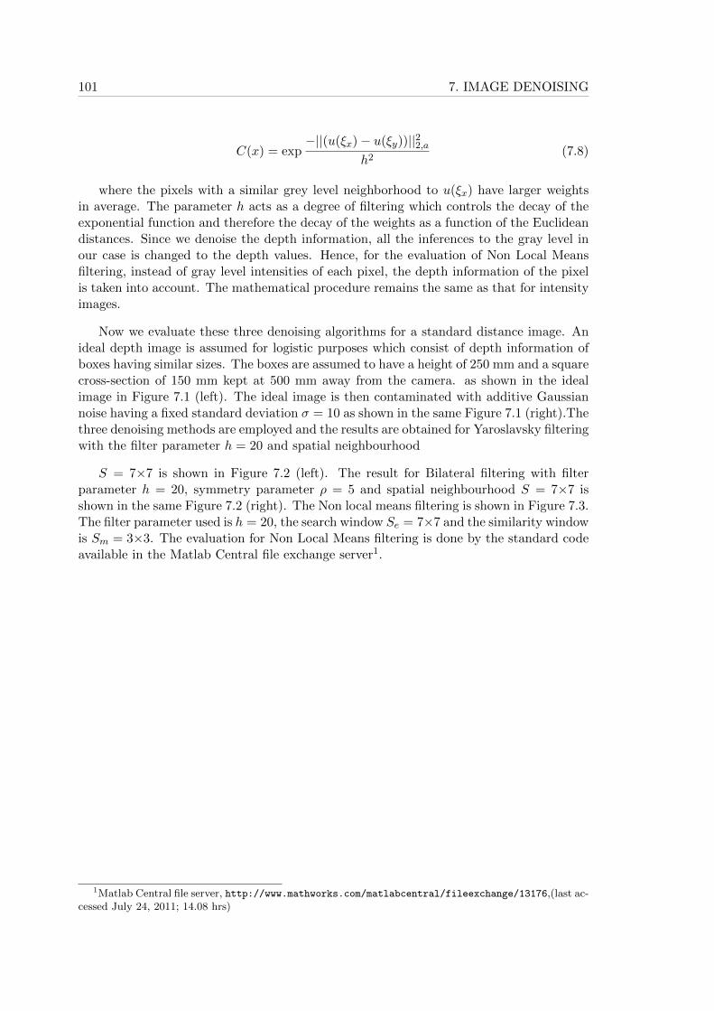
101 7. IMAGE DENOISING
C(x) = exp−||(u(ξx)− u(ξy))||22,a
h2(7.8)
where the pixels with a similar grey level neighborhood to u(ξx) have larger weightsin average. The parameter h acts as a degree of filtering which controls the decay of theexponential function and therefore the decay of the weights as a function of the Euclideandistances. Since we denoise the depth information, all the inferences to the gray level inour case is changed to the depth values. Hence, for the evaluation of Non Local Meansfiltering, instead of gray level intensities of each pixel, the depth information of the pixelis taken into account. The mathematical procedure remains the same as that for intensityimages.
Now we evaluate these three denoising algorithms for a standard distance image. Anideal depth image is assumed for logistic purposes which consist of depth information ofboxes having similar sizes. The boxes are assumed to have a height of 250 mm and a squarecross-section of 150 mm kept at 500 mm away from the camera. as shown in the idealimage in Figure 7.1 (left). The ideal image is then contaminated with additive Gaussiannoise having a fixed standard deviation σ = 10 as shown in the same Figure 7.1 (right).Thethree denoising methods are employed and the results are obtained for Yaroslavsky filteringwith the filter parameter h = 20 and spatial neighbourhood
S = 7×7 is shown in Figure 7.2 (left). The result for Bilateral filtering with filterparameter h = 20, symmetry parameter ρ = 5 and spatial neighbourhood S = 7×7 isshown in the same Figure 7.2 (right). The Non local means filtering is shown in Figure 7.3.The filter parameter used is h = 20, the search window Se = 7×7 and the similarity windowis Sm = 3×3. The evaluation for Non Local Means filtering is done by the standard codeavailable in the Matlab Central file exchange server1.
1Matlab Central file server, http://www.mathworks.com/matlabcentral/fileexchange/13176,(last ac-cessed July 24, 2011; 14.08 hrs)
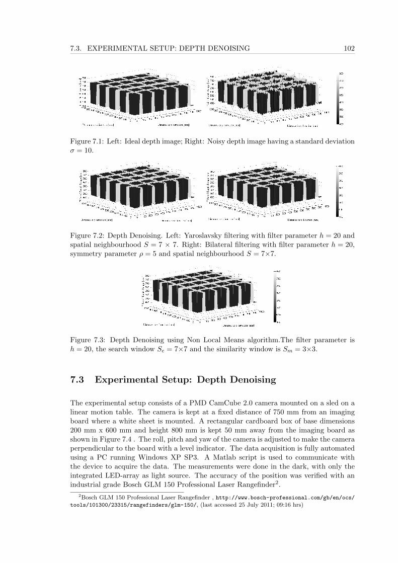
7.3. EXPERIMENTAL SETUP: DEPTH DENOISING 102
Figure 7.1: Left: Ideal depth image; Right: Noisy depth image having a standard deviationσ = 10.
Figure 7.2: Depth Denoising. Left: Yaroslavsky filtering with filter parameter h = 20 andspatial neighbourhood S = 7 × 7. Right: Bilateral filtering with filter parameter h = 20,symmetry parameter ρ = 5 and spatial neighbourhood S = 7×7.
Figure 7.3: Depth Denoising using Non Local Means algorithm.The filter parameter ish = 20, the search window Se = 7×7 and the similarity window is Sm = 3×3.
7.3 Experimental Setup: Depth Denoising
The experimental setup consists of a PMD CamCube 2.0 camera mounted on a sled on alinear motion table. The camera is kept at a fixed distance of 750 mm from an imagingboard where a white sheet is mounted. A rectangular cardboard box of base dimensions200 mm x 600 mm and height 800 mm is kept 50 mm away from the imaging board asshown in Figure 7.4 . The roll, pitch and yaw of the camera is adjusted to make the cameraperpendicular to the board with a level indicator. The data acquisition is fully automatedusing a PC running Windows XP SP3. A Matlab script is used to communicate withthe device to acquire the data. The measurements were done in the dark, with only theintegrated LED-array as light source. The accuracy of the position was verified with anindustrial grade Bosch GLM 150 Professional Laser Rangefinder2.
2Bosch GLM 150 Professional Laser Rangefinder , http://www.bosch-professional.com/gb/en/ocs/tools/101300/23315/rangefinders/glm-150/, (last accessed 25 July 2011; 09:16 hrs)
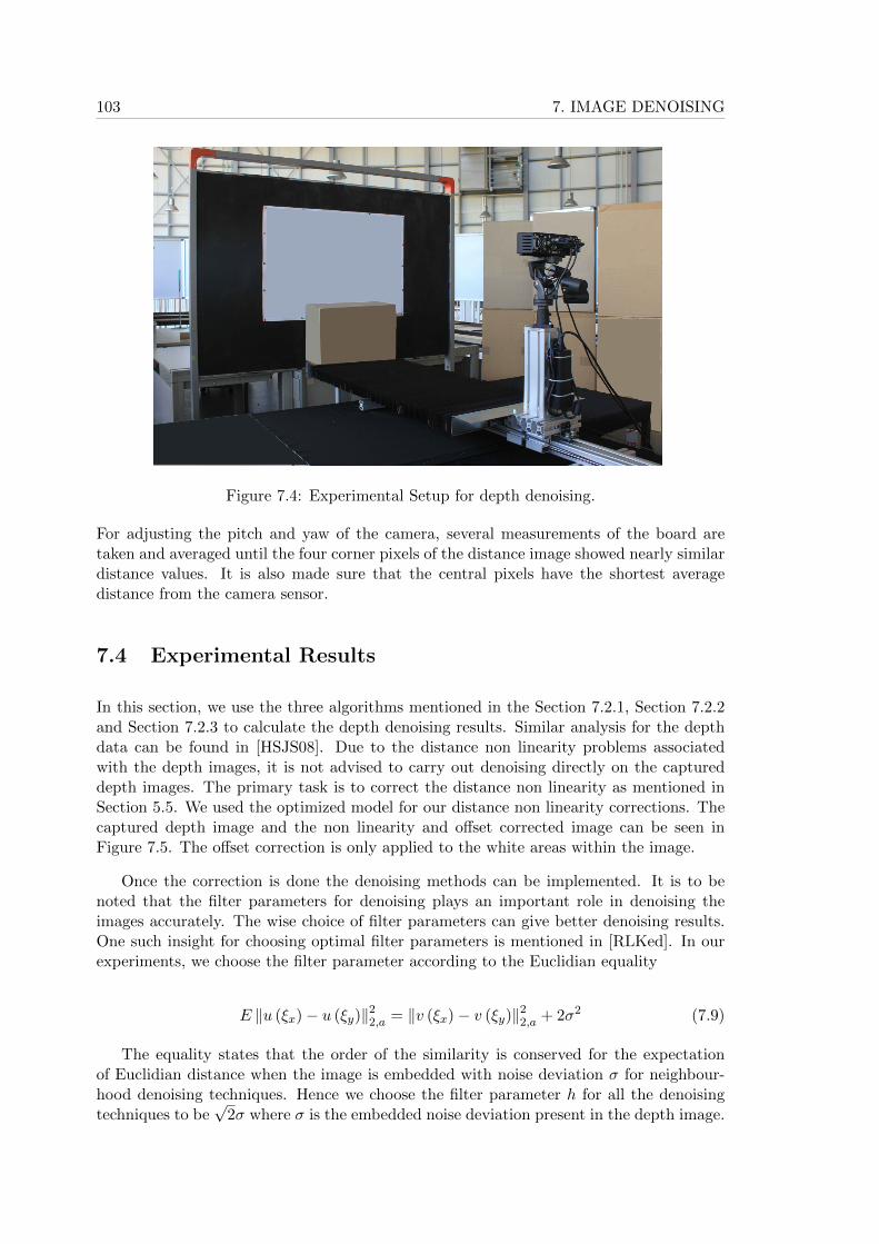
103 7. IMAGE DENOISING
Figure 7.4: Experimental Setup for depth denoising.
For adjusting the pitch and yaw of the camera, several measurements of the board aretaken and averaged until the four corner pixels of the distance image showed nearly similardistance values. It is also made sure that the central pixels have the shortest averagedistance from the camera sensor.
7.4 Experimental Results
In this section, we use the three algorithms mentioned in the Section 7.2.1, Section 7.2.2and Section 7.2.3 to calculate the depth denoising results. Similar analysis for the depthdata can be found in [HSJS08]. Due to the distance non linearity problems associatedwith the depth images, it is not advised to carry out denoising directly on the captureddepth images. The primary task is to correct the distance non linearity as mentioned inSection 5.5. We used the optimized model for our distance non linearity corrections. Thecaptured depth image and the non linearity and offset corrected image can be seen inFigure 7.5. The offset correction is only applied to the white areas within the image.
Once the correction is done the denoising methods can be implemented. It is to benoted that the filter parameters for denoising plays an important role in denoising theimages accurately. The wise choice of filter parameters can give better denoising results.One such insight for choosing optimal filter parameters is mentioned in [RLKed]. In ourexperiments, we choose the filter parameter according to the Euclidian equality
E ‖u (ξx)− u (ξy)‖22,a = ‖v (ξx)− v (ξy)‖22,a + 2σ2 (7.9)
The equality states that the order of the similarity is conserved for the expectationof Euclidian distance when the image is embedded with noise deviation σ for neighbour-hood denoising techniques. Hence we choose the filter parameter h for all the denoisingtechniques to be
√2σ where σ is the embedded noise deviation present in the depth image.
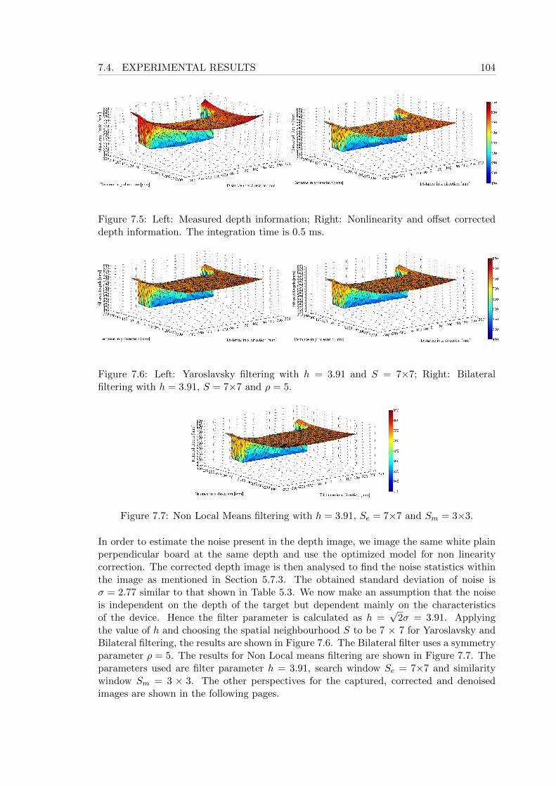
7.4. EXPERIMENTAL RESULTS 104
Figure 7.5: Left: Measured depth information; Right: Nonlinearity and offset correcteddepth information. The integration time is 0.5 ms.
Figure 7.6: Left: Yaroslavsky filtering with h = 3.91 and S = 7×7; Right: Bilateralfiltering with h = 3.91, S = 7×7 and ρ = 5.
Figure 7.7: Non Local Means filtering with h = 3.91, Se = 7×7 and Sm = 3×3.
In order to estimate the noise present in the depth image, we image the same white plainperpendicular board at the same depth and use the optimized model for non linearitycorrection. The corrected depth image is then analysed to find the noise statistics withinthe image as mentioned in Section 5.7.3. The obtained standard deviation of noise isσ = 2.77 similar to that shown in Table 5.3. We now make an assumption that the noiseis independent on the depth of the target but dependent mainly on the characteristicsof the device. Hence the filter parameter is calculated as h =
√2σ = 3.91. Applying
the value of h and choosing the spatial neighbourhood S to be 7 × 7 for Yaroslavsky andBilateral filtering, the results are shown in Figure 7.6. The Bilateral filter uses a symmetryparameter ρ = 5. The results for Non Local means filtering are shown in Figure 7.7. Theparameters used are filter parameter h = 3.91, search window Se = 7×7 and similaritywindow Sm = 3 × 3. The other perspectives for the captured, corrected and denoisedimages are shown in the following pages.
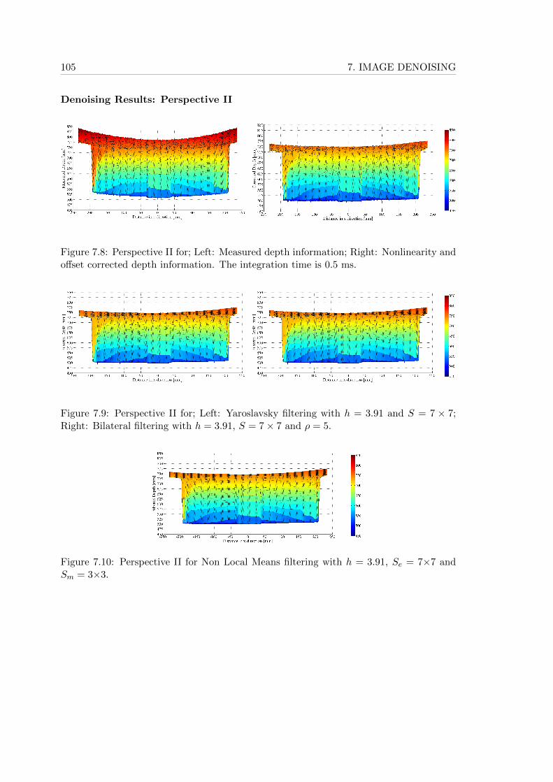
105 7. IMAGE DENOISING
Denoising Results: Perspective II
Figure 7.8: Perspective II for; Left: Measured depth information; Right: Nonlinearity andoffset corrected depth information. The integration time is 0.5 ms.
Figure 7.9: Perspective II for; Left: Yaroslavsky filtering with h = 3.91 and S = 7 × 7;Right: Bilateral filtering with h = 3.91, S = 7× 7 and ρ = 5.
Figure 7.10: Perspective II for Non Local Means filtering with h = 3.91, Se = 7×7 andSm = 3×3.
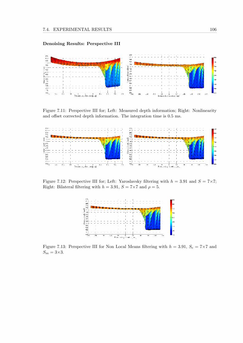
7.4. EXPERIMENTAL RESULTS 106
Denoising Results: Perspective III
Figure 7.11: Perspective III for; Left: Measured depth information; Right: Nonlinearityand offset corrected depth information. The integration time is 0.5 ms.
Figure 7.12: Perspective III for; Left: Yaroslavsky filtering with h = 3.91 and S = 7×7;Right: Bilateral filtering with h = 3.91, S = 7×7 and ρ = 5.
Figure 7.13: Perspective III for Non Local Means filtering with h = 3.91, Se = 7×7 andSm = 3×3.
Chapter 8
Conclusions
8.1 Summary
This thesis describes the step by step procedure for calibrating a PMD Camcube 2.0camera. A general introduction to the 3D imaging world is provided in Chapter 1. It alsooutlines the specification of different 3D ToF cameras available in the market and providesa comparison between them.
The working principle of 3D ToF cameras is described in Chapter 2 and procedure forcalculating the depth, amplitude and intensity information of the imaged 3D scenario ispresented.
Chapter 3 characterizes the PMD Camcube 2.0 camera. The warm-up drift of thesensor is analysed to study the operating characteristics of the camera. The reliabilityof the measured depth images are studied by analysing the measurement accuracy of thecamera over a long duration.
The Parametric Calibration procedure for the PMD Camcube 2.0 camera are describedin Chapter 4. The calibrated focal length, principle point of the camera and distortioncoefficients are obtained.
The imaging model, correlation model, depth estimation model, amplitude model anddistance nonlinearity correction models for the PMD Camcube 2.0 camera is described inChapter 5. Real time evaluations of the models are performed and excellent results areobtained. The depth estimation model is evaluated in real time and is found to closelyresemble the captured depth image. The different distance nonlinearity correction modelsare compared with real world depth images and the results are presented. It is understoodthat the optimized model produces more accurate results than the other non linearitycorrection methods.
The Non Parametric Calibration procedure for the PMD Camcube 2.0 camera is de-scribed in Chapter 6. The proposed theoretical offset correction is tested for differenttarget reflectivities and satisfactory results are obtained. The proposed method to findoptimal Integration time is evaluated for different target reflectivities and satisfactoryresults are obtained.
107
8.2. FUTURE WORK 108
For the PMD Camcube 2.0 camera, the different depth denoising techniques are evalu-ated in Chapter 7. It is found that the Non Local Means denoising provides more accurateresults than the other denoising techniques. The denoising methods are implemented inreal world situation and excellent results are obtained.
8.2 Future Work
The warm-up drift for the PMD Camcube 2.0 camera can be evaluated for a variety ofoptimal Integration times for different target reflectivities mentioned in Section 6.4.4 inorder to have an accurate picture of the reliability of the measured depth data over along duration. A correction method based on operating time, reflectivity and Integrationtime can also be proposed for integrity of the calibration procedure. The evaluation ofthe RMSE for sensor characterization can be extended for different Integration times andreflectivities from which a reliability measure can be proposed according to operatingduration and Integration time. This can improve the calibration procedure.
The rotational matrix and translational vector obtained from the Parametric Calibra-tion procedure can be used for estimating the orientation of the camera. These estimationresults can be used for Simultaneous Localization and Mapping (SLAM) techniques forrobots using 3D ToF cameras. The Parametric Calibration technique can be extended toinclude correction for the skew inherent in image capturing.
The Imaging model described in Section 5.1 can be enhanced by the practical knowl-edge of the characteristic amplitudes of both the light sources used in the camera. Theknowledge of the characteristic amplitudes of the light sources can enhance the depth es-timation model. This can in turn bridge the gap between the depth model and the realworld scenario.
There is a lot of scope for improving the Amplitude model. Analysing the Lambertianreflectance at the target surface could be the first step towards this task. An advancedreflectance model called the ’Oren-Nayar Reflectance Model’, cf. [NO95], may be used toimprove the Amplitude model considering the target reflectance.
There is a lot of scope to improve the comptation speed of the optimization procedurefor the non linearity correction model. Faster algorithms can be implemented in place ofthe bisection algorithm so as to ensure a faster convergence and to save computation time.
The offset correction can be extended to a variety of target reflectivities to improve thecorrection performance. The denoising performance can also be improved by using neweralgorithms like the Non Local Means denoising with patch based weights, cf. [HSJS08].
References
[BCM05] A. Buades, B. Coll, and J.M. Morel. A non-local algorithm for image de-noising. In IEEE International Conference on Computer vision and patternrecognition, 2005.
[Bro66] D. Brown. Decentering distortion of lenses. In Photometric Engineering,volume 32, pages 444–462, 1966.
[Bro71] D. Brown. Close-range camera calibration. In Photogrammetric Engineering,volume 37, pages 855–866, 1971.
[Fau93] O. Faugeras. Three-Dimensional Computer Vision: a Geometric Viewpoint.MIT Press, 1993.
[HS97] J. Heikkila and O. Silven. A four-step camera calibration procedure withimplicit image correction. In Proceedings of IEEE Computer Vision andPattern Recognition, pages 1106–1112, 1997.
[HSJS08] B. Huhle, T. Schairer, P. Jenke, and W. Strasser. Robust non-local denoisingof colored depth data. In IEEE Computer Society Conference on ComputerVision and Pattern Recognition Workshops., Anchorage, AK, 2008.
[Kah07] T. Kahlmann. Range Imaging Metrology: Investigation, Calibration and De-velopment. PhD thesis, ETH Zurich, 2007.
[KRI06] T. Kahlmann, F. Remondino, and H. Ingensand. Calibration for increasedaccuracy of the range imaging camera swissranger. In Image Engineeringand Vision Metrology, ISPRS Commission V Symposium, Dresden, Germany,2006.
[Lan00] R. Lange. 3D Time-of-Flight Distance Measurement with Custom Solid-StateImage Sensors in CMOS/CCD-Technology. PhD thesis, Department of Elec-trical Engineering and Computer Science, University of Siegen, 2000.
[Lin10] M. Lindner. Calibration and Real-Time Processing of Time-of-Flight RangeData. PhD thesis, Department of Electrical Engineering and Computer Sci-ence, University of Siegen, 2010.
[LSKK10] M. Lindner, I. Schiller, A. Kolb, and R. Koch. Time-of-flight sensor calibra-tion for accurate range sensing. Computer Vision and Image Understanding,114:13181328, 2010.
109
REFERENCES 110
[Lua01] X. Luan. Experimental Investigation of Photonic Mixer Device and Develop-ment of TOF 3D Ranging Systems Based on PMD Technology. PhD thesis,Department of Electrical Engineering and Computer Science, University ofSiegen, 2001.
[NO95] S.K. Nayar and M. Oren. Generalization of the lambertian model and impli-cations for machine vision. International Journal on Computer Vision, Vol.14(No.3):pp. 227–251, April 1995.
[OFCB07] S. Oprisescu, D. Falie, M. Ciuc, and V. Buzuloiu. Measurements with tofcameras and their necessary corrections. In International Symposium on Sig-nals, Circuits and Systems, pages 1–4, 2007.
[OYB09] Y. Okubo, C. Ye, and J. Borenstein. Characterization of the hokuyo urg-04lx laser rangefinder for mobile robot obstacle negotiation. In Unmanned,Robotic, and Layered Systems, Orlando, FL, 2009.
[PL07] V. Peters and O. Loffeld. A bistatic simulation approach for a high resolution3d pmd-camera. In Dynamic 3D Vision (Workshop in Conjunction withDAGM), 2007.
[Rap07] H. Rapp. Experimental and theoretical investigation of correlating tof-camerasystems. Master’s thesis, University of Heidelberg, 2007.
[RLKed] S.K. Ramanandan, B. Lehmann, and D. Kraus. Optimal parameters forbilateral filtering and sas image denoising. The Eleventh Biennial Symposiumon Ocean Electronics, Kochi, India, 2011. (submitted).
[TM98] C. Tomasi and R. Manduchi. Bilateral filtering for gray and color images. InProceedings of the 6th International Conference on Computer Vision, pages839–846, Bombay, India, 1998.
[USRRK11] C. Uriarte, B. Scholz-Reiter, S.K. Ramanandan, and D. Kraus. Modelingdistance nonlinearity in tof cameras and correction based on integration timeoffsets. In 16th Iberoamerican Congress on Pattern Recognition, Pucon, Chile,2011. (accepted).
[Xu99] Z. Xu. Investigation of 3D-Imaging Systems Based on Modulated Light andOptical RF-Interferometry (ORFI). PhD thesis, Department of ElectricalEngineering and Computer Science, University of Siegen, 1999. Discussed inZESS-Forschungsberichte, Shaker Verlag Aachen, ISBN 3-8265-6736-6.
[Yar85] L. Yaroslavsky. Digital Picture Processing. Springer Verlag, 1985.
[Zha00] Z. Zhang. A flexible new technique for camera calibration. In IEEE Trans.on Pattern Analysis and Machine Intelligence, pages 1330–1334, 2000.


Declaration
I hereby declare that this thesis entitled ’3D ToF Camera Calibration and Image Pre-processing’ is the result of my own research except as cited in the references. This thesishas not been accepted for any degree and is not concurrently submitted in candidaturefor any other degree.
Bremen, 15 August 2011
Sheshu Kalaparambathu Ramanandan