Calibration and pose estimation of a pox-slits camera from a single image

Calibration and Pose Estimation of a Pox-slits

Camera from a Single Image

N. Martins1 and H. Araujo2

1 DEIS, ISEC, Polytechnic Institute of Coimbra, Portugal2 ISR/DEEC, University of Coimbra, Portugal

Abstract. Recent developments have suggested alternative multi-pers-pective camera models potentially advantageous for the analysis of thescene structure. Two-slit cameras are one such case. The projectionmodel for these cameras is non-linear, and in this model every 3D pointis projected by a line that passes through that point and intersects twolines (or slits). One particular case of this camera model, in terms of theslits positions, is referred to as parallel-orthogonal x-slits, or pox-slits.In this paper, a non-iterative linear method for the calibration and poseestimation of pox-slits cameras is presented and discussed. A solution forthe calibration can be obtained using at least fifteen world to image cor-respondences. To achieve a higher level of accuracy, data normalizationmust be used.

1 Introduction

The mathematical model that describes the formation of the most common typeof images is the perspective projection model. Most of the commercial optical de-vices generate images whose geometrical properties are described by this model.Therefore, the classic pinhole and orthographic camera models have long beenused in 3D imaging applications.

However, certain special vision problems can benefit from the application ofalternative projection models, as recent developments have suggested. Besides,these new types of cameras have projection models that do not comply with theperspective model. Multi-perspective models have been providing advantageousimaging systems for understanding the structure of observed 3D scenes. Exam-ples of such camera models are bi-centric [1], crossed-slits (also known as x-slits)[2], general linear [3] and rational polynomial [4].

In the x-slits model the projection ray of a generic 3D point is defined bythe 3D line that passes through the point and two lines, referred as slits. Thismodel was initially designed by one of the pioneers of the colour photography,Ducos du Hauron, in 1888, under the name ”transformisme en photographie” [5].However, it was a restricted model in terms of the slits positions, which wereparallel and orthogonal between each other and parallel to the image plane (laterreferred to as parallel-orthogonal x-slits or pox-slits [2]). An interesting aspect isthat pox-slits model is similar to the bi-centric model, and, so, the pushbroomcamera is its particular case, in which the vertical slit resides on the infinity.

2 N. Martins and H. Araujo

After one century, the pox-slits model was revised and generalized by Kingslake,who concluded that it was similar to the perspective projection model in whichthe image is stretched or compressed in one direction more than the other [5].This fact shows that it can be useful for wide-screen applications.

Zomet et al, in [2], expanding the Kingslake generalization, introduced thex-slits projection model. According to their paper x-slits images can be easilygenerated from a sequence of perspective images. Another remarkable aspect ofthis camera is that perspective model is a particular case of the x-slits camera, inwhich the vertical and the horizontal slits reside in the same plane. The opticalcentre of the perspective camera is the intersection of the slits.

In [2] an extensive analysis of the x-slits cameras is done. In this paper wepresent a method for the estimation of the pose and intrinsic parameters of anx-slits camera. The method presented in this paper enables the estimation ofboth the pose and intrinsic parameters of a x-slits camera (real or synthetic)from a single image.

Most existing calibration methods are parametric and camera dependent.For example, in the case of the pinhole camera a 3x3 matrix contains the fiveintrinsic parameters (without distortion).

Grossberg et al, in [6], presented a totally different camera calibration algo-rithm, referred to as the generic imaging model. In that case calibration consistsin determining, for every image pixel, the associated 3D projection ray, beingthis idea also used in [7]. This mapping can be conveniently described using a setof virtual sensing elements, called raxels. Raxels include geometric, radiometricand optical properties. To successfully apply that mapping, several images of acalibration object are necessary as well as a displacement. The method requiresat least two images of a calibration object with known structure. Then, for eachimage and each pixel, two 3D points are obtained. Their coordinates are usuallyonly known in a coordinate frame attached to the calibration object. If the mo-tion between the two object positions is known, the coordinate frames can bealigned. Then, every pixel’s projection ray can be computed by joining the twoobserved 3D points.

As an extension to [6], [8] introduces a generic calibration approach, whichdoes not require the knowledge of the relative motion between the images. Thismethod requires at least three images of a calibration object. The projective raybeing a 3D line yields a constraint that allows the recovery of both the motionand the camera parameters. This constraint is formulated via a set of trifocaltensors that can be estimated linearly.

In order to understand the non-linear nature of the x-slits projection modelwe decided to study its calibration using a single image. This requires the knowl-edge of the 3D coordinates of a set of points, i.e, the knowledge of a calibratingobject. In particular we decided to focus our work on the special case of thepox-slits model.

The current paper is organized as follows. In section 2, the x-slits projectionmodel is defined, as well as its particular case, the pox-slits. Then, in section 3,the algorithm for the calibration and pose estimation of the pox-slits projection

Lecture Notes in Computer Science 3

model is presented. Experimental results are shown and analyzed in section 4.Finally, some conclusions are drawn in section 5.

2 X-slits Projection Model

Consider the x-slits projection configuration represented in figure 1. In this figure

Fig. 1. X-slits projection model.

the projective ray of a generic 3D point, P , must intersect two lines, or slits, l1and l2. Point P together with each slit defines one plane. The intersection ofthose planes defines the projective ray. The projection of the 3D point in theimage plane, p, is obtained by the intersection of the projective ray with theimage plane.

To define the two slits, let ui and vi, with i = 1, 2, be two generic planesdefined in a space of 3 dimensions, given by their parametric coordinates. Theslits, li, are defined through the intersection of those planes. These slits can berepresented by the dual Plucker matrix [9], whose expression is Li

∗ = uiviT−

viuiT .

The projective ray, l, is the intersection between two planes, defined by eachslit li and the 3D point P (L1

∗P and L2∗P , respectively), and can be defined

by the dual Plucker matrix, through L∗ = (L1∗P ) (L2

∗P )T− (L2

∗P ) (L1∗P )

T.

The projection of a 3D generic point P in the image plane I origins a 2Dpoint p. This projection is given by the intersection of the projective ray l withthe image plane I. This fact implies that l must belong to both planes Li

∗P .This idea can be mathematically formalized by the following linear equation,

[

PT L1∗P0 PT L1

∗P1 PT L1∗P2

PT L2∗P0 PT L2

∗P1 PT L2∗P2

]

p = 0 ⇐⇒ Mp = 0. (1)


Since (1) is a homogeneous equation system, it has the trivial solution p = 0.However, this is not the solution wanted. The solution for the equation system(1) is the right null space of the matrix M . This solution is obtained by the useof the cross product between the elements of the matrix M, as

kp =

PT L1∗(

P1P2T− P2P1

T)

L2∗P

PT L1∗(

P2P0T− P0P2

T)

L2∗P

PT L1∗(

P0P1T− P1P0

T)

L2∗P

=

PT L1I0L2P

PT L1I1L2P

PT L1I2L2P

=

PT A0P

PT C0P

PT B0P

.

(2)I0, I1 and I2 are the Plucker matrices that represent, in 3D, respectively, thex and y axis of the image and the image line at infinity. According to [2], thissolution is unique unless it resides on the line joining the intersections of the twoslits with the image plane.

Equation (2) assumes that 3D world points are in the camera coordinate sys-tem. Therefore, to calibrate a pox-slits camera positioned anywhere in the world,the model has to take into account the correspondent coordinate transformation.This coordinate transformation is usually represented by a matrix containing therotation matrix and the translation vector. This matrix transforms the coordi-nates of any point P (in the world coordinate system) into the correspondentcoordinates Pc in the camera coordinate system. In addition equation (2) doesnot use pixel coordinates. The use of pixel coordinates for the image elementsrequires that the model takes into account the intrinsic parameters. As a resultthe full model for the camera is expressed by the following equation

kp =

kx γ cx

0 ky cy

0 0 1

([

R t

0 1

]

P

)T

A0

[

R t

0 1

]

P

([

R t

0 1

]

P

)T

C0

[

R t

0 1

]

P

([

R t

0 1

]

P

)T

B0

[

R t

0 1

]

P

=

PT AP

PT CP

PT BP

. (3)

A, B and C are an upper triangular matrices with 10 elements each. These 30elements are denoted by Vi, where the first 10 belong to matrix A, the second10 elements to B and the last to C.

The pox-slits projection model is a particular case of the x-slits camera,where the slits are parallel and orthogonal between each other and parallel tothe image plane. It is a configuration of special interest because its equationsare similar to the bi-centric, to the perspective and to the pushbroom models.

Following [2], to obtain the equations of this projection model, without loss of

generality, define u1 =[

1 0 0 0]T

and v1 =[

0 0 1 −Z1

]Tto define the vertical

slit, l1, at Y = 0 and Z = Z1. The horizontal slit, l2, will be defined at X = 0

and Z = Z2, by assigning u2 =[

0 1 0 0]T

and v2 =[

0 0 1 −Z2

]T. The image

plane is the X − Y plane at Z = 0 and, therefore, is obtained by using three

points, P0 = u1, P1 = u2 and P2 =[

0 0 0 1]T

.


3 Estimating the Intrinsic Parameters and Pose

Camera calibration consists in the estimation of the intrinsic parameters of thecamera. In the case of this camera model we will deal with the estimation of boththe intrinsics and pose, since the elements of matrices A, B and C are functionsof the intrinsic parameters and pose parameters. In this case the intrinsic pa-rameters are kx, ky, cx, cy, γ and the slits parameters Z1 and Z2.

Several approaches can be used to estimate the intrinsic parameters and thepose. In this case and due to the inherently non-linear nature of the model, wedecided to base our approach on the use of a 3D pattern so that the coordinatesof a set of 3D points (X, Y, Z) are known. Those coordinates and the coordinatesof the corresponding image points (x, y) are then used to estimate the elementsof the matrices A, B and C. To estimate the elements of matrices A, B andC at least fifteen world to image correspondences are required. Each pair ofcorrespondences generates two equations. These two equations are

X2V1+XY V2+XZV3+XV4+Y 2V5+Y ZV6+Y V7+Z2V8+ZV9+V10−xX2V11−

−xXY V12−xXZV13−xXV14−xY 2V15−xY Z+V16−xY V17−xZ2V18−xZV19−

−xV20 = 0. (4)

and

−yX2V11−yXY V12−yXZV13−yXV14−yY 2V15−yY ZV16−yY V17−yZ2V18−

−yZV19 − yV20 + X2V21 + XY V22 + XZV23 + XV24 + Y 2V25 + Y ZV26 + Y V27+

+Z2V28 + ZV29 + V30 = 0. (5)

The numerical problems associated to this estimation problem can be reducedif the data are normalized as suggested by Hartley [9]. As a result the inversetransformation as to be applied to parameters estimated.

The estimated parameters Vi (with i = 1, · · · , 30) are a function of the in-trinsic and pose parameters. From these parameters the intrinsics and the posemust be estimated. Equation (3) uses homogeneous coordinates and therefore allthe estimated parameters are obtained up to a scale factor. The scale factor canbe computed from the elements of the rotation matrix since the norm of all rowsand columns is 1. The scale factor k is then given by k = −(V11 +V15 +V18). Asa result the coordinates of the principal point can be computed from

cx = −V1 + V5 + V8

kcy = −

V21 + V25 + V28

k

The estimation of the elements of the rotation matrix is performed in threesteps. First the elements of the third row of the rotation matrix are estimatedup to a sign change

r31 = ±

√

−V11

kr32 = ±

√

−V15

kr33 = ±

√

−V18

k


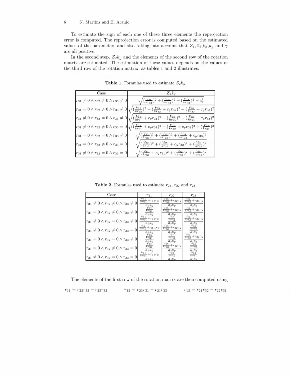
To estimate the sign of each one of these three elements the reprojectionerror is computed. The reprojection error is computed based on the estimatedvalues of the parameters and also taking into account that Z1,Z2,kx,ky and γ

are all positive.In the second step, Z2ky and the elements of the second row of the rotation

matrix are estimated. The estimation of these values depends on the values ofthe third row of the rotation matrix, as tables 1 and 2 illustrates.

Table 1. Formulas used to estimate Z2ky .

Case Z2ky

r31 6= 0 ∧ r32 6= 0 ∧ r33 6= 0√

( V21

kr31)2 + ( V25

kr32)2 + ( V28

kr33)2 − c2

y

r31 = 0 ∧ r32 6= 0 ∧ r33 6= 0√

( V22

kr32)2 + ( V25

kr32+ cyr32)2 + ( V28

kr33+ cyr33)2

r31 6= 0 ∧ r32 = 0 ∧ r33 6= 0√

( V21

kr31+ cyr31)2 + ( V26

kr33)2 + ( V28

kr33+ cyr33)2

r31 6= 0 ∧ r32 6= 0 ∧ r33 = 0√

( V21

kr31+ cyr31)2 + ( V25

kr32+ cyr32)2 + ( V23

kr31)2

r31 = 0 ∧ r32 = 0 ∧ r33 6= 0√

( V23

kr33)2 + ( V26

kr33)2 + ( V28

kr33+ cyr33)2

r31 = 0 ∧ r32 6= 0 ∧ r33 = 0√

( V22

kr32)2 + ( V25

kr32+ cyr32)2 + ( V26

kr32)2

r31 6= 0 ∧ r32 = 0 ∧ r33 = 0√

( V21

kr31+ cyr31)2 + ( V22

kr31)2 + ( V23

kr31)2

Table 2. Formulas used to estimate r21, r22 and r23.

Case r21 r22 r23

r31 6= 0 ∧ r32 6= 0 ∧ r33 6= 0V21kr31

+r31cy

Z2ky

V25kr32

+r32cy

Z2ky

V28kr33

+r33cy

Z2ky

r31 = 0 ∧ r32 6= 0 ∧ r33 6= 0V22kr32

Z2ky

V25kr32

+r32cy

Z2ky

V28kr33

+r33cy

Z2ky

r31 6= 0 ∧ r32 = 0 ∧ r33 6= 0V21kr31

+r31cy

Z2ky

V26kr33

Z2ky

V28kr33

+r33cy

Z2ky

r31 6= 0 ∧ r32 6= 0 ∧ r33 = 0V21kr31

+r3 1cy

Z2ky

V25kr32

+r32cy

Z2ky

V26kr32

Z2ky

r31 = 0 ∧ r32 = 0 ∧ r33 6= 0V23kr33

Z2ky

V26kr33

Z2ky

V28kr33

+r33cy

Z2ky

r31 = 0 ∧ r32 6= 0 ∧ r33 = 0V22kr32

Z2ky

V25kr32

+r32cy

Z2ky

V26kr32

Z2ky

r31 6= 0 ∧ r32 = 0 ∧ r33 = 0V21kr31

+r31cy

Z2ky

V22kr31

Z2ky

V23kr31

Z2ky

The elements of the first row of the rotation matrix are then computed using

r11 = r22r33 − r23r32 r12 = r23r31 − r21r33 r13 = r21r32 − r22r31


To ensure that the rotation matrix is orthogonal the algorithm proposed in[10] can be used.

The component of the translation vector along Y , ty, is computed as pre-sented in table 3.

Table 3. Formula used to estimate ty.

Case ty

if r13 6= 0r21(V27−cyV17)−r22(V24−cyV14)

kr13Z2ky

if r31 = 0 ∧ r32 = 0 ∧ r33 6= 0V29−cyV19

kr33Z2ky

if r31 = 0 ∧ r32 6= 0 ∧ r33 = 0V27−cyV17

kr32Z2ky

if r31 6= 0 ∧ r32 = 0 ∧ r33 = 0r23(V24−cyV14)−r21(V29−cyV19)

kr12Z2ky

if r31 = 0 ∧ r32 6= 0 ∧ r33 6= 0r22(V29−cyV19)−r23(V27−cyV17)

kr11Z2ky

elseV24−cyV14

kr31Z2ky

To estimate the component of the translation vector along X , tx using table4, the parameters tz −Z1, tz −Z2, γZ2 and Z1kx must be estimated first. Tables5 and 6 show how these parameters are estimated.

Table 4. Formula used to estimate tx.

Case tx

if r31 6= 0V4k

−kxZ1r11(tz−Z2)+cxr31(tz−Z1+tz−Z2)−γZ2r21(tz−Z1)−γZ2r31ty

kxZ1r31

if r32 6= 0V7k


kxZ1r32

elseV9k


kxZ1r33

Table 5. Formulas used to estimate tz − Z1 and tz − Z2.

Case tz − Z1

r21 6= 0V24−cyV14

kr21Z2ky− r31

r21ty

r22 6= 0V27−cyV17

kr22Z2ky− r32

r22ty

r23 6= 0V29−cyV19

kr23Z2ky− r33

r23ty

Case tz − Z2

r31 6= 0 − V14

kr31− (tz − Z1)

r32 6= 0 − V17

kr32− (tz − Z1)

r33 6= 0 − V19

kr33− (tz − Z1)

We assume that the aspect ratio is known. Therefore assuming that KA =ky

kx

is known, the remaining of the parameters can be obtained. Defining ∆ = (tz −


Table 6. Formulas used to estimate γZ2 and kxZ1.

Case γZ2 kxZ1

r31 6= 0 ∧ r32 6= 0 ∧ r33 6= 0r11r31

V5k

−r12r32V1k

−cxr23r31r32

r31r32r33

r22r32V1k

−r21r31V5k

−cxr13r31r32

r31r32r33

r31 = 0 ∧ r32 6= 0 ∧ r33 6= 0r11

V5k

−r12V2k

+cxr11r232

r32r33

r22V2k

−r21V5k

−cxr21r232

r32r33

r31 6= 0 ∧ r32 = 0 ∧ r33 6= 0r11

V2k

−r12V1k

−cxr12r231

r31r33

r22V1k

−r21V2k

+cxr22r231

r31r33

r31 6= 0 ∧ r32 6= 0 ∧ r33 = 0r13

V1k

−r11V3k

+cxr13r231

r31r32

r21V3k

−r23V1k

−cxr23r231

r31r32

r31 = 0 ∧ r32 = 0 ∧ r33 6= 0r11V6−r12V3

kr233

r22V3−r21V6

kr233

r31 = 0 ∧ r32 6= 0 ∧ r33 = 0r13V2−r11V6

kr232

r21V6−r23V2

kr232

r31 6= 0 ∧ r32 = 0 ∧ r33 = 0r12V3−r13V2

kr231

r23V2−r22V3

kr231

Z1) − (tz − Z2) and R1 = kxZ1

kyZ2the horizontal and vertical slit parameters are

obtained, respectively, from

Z2 =∆

1 − KAR1

Z1 = KAZ2R1

As a result the horizontal (kx) and vertical (ky) scale factors, the skew (γ)and the translation component along the axis Z (tz) are given, respectively, by

kx =kxZ1

Z1

ky =kyZ2

Z2

γ =γZ2

Z2

tz = (tz − Z1) + Z1

4 Experimental Results

This estimation problem has some particular aspects in that the rank of matricesA, B and C can take any value between one and four.

To evaluate the robustness of the estimation algorithm, Gaussian white noisewith 0 mean and σ2 variance was added to the coordinates of the image points,to the 3D coordinates of the points or to the elements of the design matrix(but not simultaneously). The effects of the noise were evaluated on the cameraparameters and on the variables of the equations, Vi. For each value of noisevariance, a pre-defined number of runs was performed. Several configurationswere tested. Two global effects and behaviors were observed.

The first, occurs for σ2 ranging between 0 and approximately 10−3, whichimplies errors in pixel coordinates between −10−1 and 10−1. In this case, theerrors in the parameters varied linearly as a function of the noise variance. Thisbehavior can be observed in figure 2. The camera configuration used had thefollowing parameters: Z1 = 10, Z2 = 5, kx = 1.1, ky = 1.3, cx = 128, cy = 64,γ = 0.1, α = 20◦, β = 40◦, θ = 60◦, tx = 5, ty = 10 and tz = 20. These resultswere obtained with σ2 changed between 0 to 10−3 with increments of 10−5. Thenumber of runs performed for each σ2 was 100. The noise was added to theimage coordinates.


Fig. 2. Relative mean error in the estimation of the camera parameters.

Figure 3(a) represents a synthetic image obtained for a camera with thefollowing parameters: Z1 = 10, Z2 = 5, kx = 1.1, ky = 1.3, cx = 128, cy = 64,γ = 0.1, α = 0◦, β = 0◦, θ = 0◦, tx = 5, ty = 10 and tz = 20. The imagecoordinates vary between 0 and 100 pixels in each axis. Changing β from 0 to0.6◦ has a significant effect: see figure 3(b). As it can be seen, this tiny change

(a) (b)

Fig. 3. Changes provoked by the application of two different models to the same 3Dpoints: (a) Configuration with β = 0◦; (b) A change of β to 0.6◦

modifies the position of all image points (image coordinates in the horizontal axisincreases up to 20% of the initial image size) which shows the highly nonlinearnature of this camera model.

The second behavior happens when σ2 has values approximately greater than10−3, for which the estimated values are strongly affected by the noise. Figure 4illustrates an example of this behavior in the case of the variables Vi. Theseresults were obtained with σ2 changing between 0 and 10 with increments of10−1. The number of runs performed for each σ2 was 1000. The noise was addedto the image coordinates.

Adding noise to the coordinates of the 3D points or to elements of the designmatrix led to the same behavior, i.e, high levels of error on the parameters.


Fig. 4. Relative mean error in the estimation of the variables of the equation system.

5 Conclusions

A non-iterative linear algorithm to estimate the intrinsic parameters and thepose of pox-slits cameras was proposed. The algorithm requires at least fifteenworld to image correspondences. Data normalization is an essential step of theestimation procedure. The total number of the degrees of freedom of the model is13. However the linearization of the model leads to a total number of unknownsof 30 (up to a scale factor). As a result the algorithm is sensitive to noise andboth the estimation of the camera parameters and the pose requires the use ofan optimization procedure with constraints.

References

1. Weinshall, D., Lee, M., Brodsky, T., Trajkovic, M., Feldman, D.: New view gene-ration with a bi-centric camera. (2002) I: 614 ff.

2. Zomet, A., Feldman, D., Peleg, S., Weinshall, D.: Mosaicing new views: the crossed-slits projection. 25 (2003) 741–754

3. Yu, J., McMillan, L.: General linear cameras. (2004) Vol II: 14–274. Hartley, R., Saxena, T.: The cubic rational polynomial camera model. (1997)

649–6545. Kingslake, R.: Optics in Photography. SPIE Optical Engineering Press (1992)6. Grossberg, M., Nayar, S.: A general imaging model and a method for finding its

parameters. (2001) II: 108–1157. Seitz, S.: The space of all stereo images. (2001) I: 26–338. Sturm, P., Ramalingam, S.: A generic concept for camera calibration. (2004) Vol

II: 1–139. Hartley, R.I., Zisserman, A.: Multiple View Geometry in Computer Vision. Second

edn. Cambridge University Press, ISBN: 0521540518 (2004)10. Zhang, Z.: A flexible new technique for camera calibration. 22 (2000) 1330–1334

Documents

Calibration and pose estimation of a pox-slits camera from a single image