LAB combine

Department of Civil Engineering

KAEA 4226 STRUCTURAL ANALYSIS

Laboratory ST2

Name : Chin Ting Seng

Matric No. : KEA 110005

Submission Date :

Experiment 1: Free Vibration with Negligible Damping Introduction The determination of free vibration of the structural members is important for structural stability analysis. Vibration of the structural member create devastating effect to the structure, collapse may occur due to happening of resonance. Concept and Theory Free vibration occurs when we set the initial condition of the beam. However, in the presence of friction (damping), that portion of the total amplitude not sustained by the external force will gradually decay. Objective

• To determine the natural frequency of the forced vibration of a rectangular beam section

• To compare the experimental results of natural frequency obtained in experiment to the theoretical value

Procedure

1. A rectangular rigid assembly beam, supported at one end by a trunnion pivoted in ball bearings located in a fixed housing was set up as shown in the figure.

2. The helical spring of known stiffness bolted to the bracket fixed to the top member of frame was supported at the outer end of the beam.

3. Free end of the beam is pulled down to perform free vibration action and released to record the free vibration movement.

4. The chart recorder (slowly rotating drum driven by synchronous motor, a roll of recording paper is fitted adjacent to the drum) is then to record the successive amplitudes of vibration.

5. As the free end of the beam is pulled down, the movement of vibrations of the beam is recorded.

Apparatus

The figure below shows the apparatus setup of this experiment.

Result and Calculation:

Experimental result:

Graph 1 (24.0mm free end before releasing)



Wavelength, S Reading 1 Reading 2 Reading 3 Average

6mm 6mm 6mm 6mm

From the oscillation we obtained,

Angular velocity, ω = 3 rev/min = 0.05 cycle/sec

Wavelength, S = 6mm (obtained from the average of above graphs)

Velocity, U = 2πrω = 2π x 46.5 x 0.05 = 14.6 mm/sec

Velocity, U = S/T

Period, T = S/U = 6/14.6 = 0.41s

Experimental frequency, f = 1/T = 1/0.41 = 2.44 Hz

Theoretical Calculation:

Parameter given:

M = 3.84 kg m = 2.13 kg S = 870 N/m Reading: AD=38.0cm = 0.380m AB=73.0cm = 0.730m AC=62.5cm = 0.625m

Moment of Inertia, X = M (AD)2 + m (AC )2

3

= 3.84(0.380) 2+2.13 [(0.625) 2/3]

= 0.83184 kgm2

Restoring moment, Y = S (AC)2Ѳ = S (AC)2

= 870(0.625)2

= 339.844 Nm

Angular velocity, ω = �YX

= √ (339.844/0.83184) = 20.21 rad/s

Theoretical value of natural frequency, n = ω/2π

= 20.21/2π

= 3.216 Hz

Discussion:

1. Natural frequency is the frequency at which a system oscillates when not subjected to a continuous or repeated external force.

2. The results obtained from experiment 1 as follows:

Natural Frequency Hz Experimental 2.440 Theoretical 3.216

3. The experimental natural frequency is lower than the theoretical natural

frequency.The percentage error between the experimental value and theoretical value of natural frequency is 24.13%.

4. There might be some errors affecting the accuracy of the result: I. Instrument error. The machine might be not very sensitive. The spring

attached at the other end of the beam might cause some friction between them. II. Parallax error. The line of view of observer is not perpendicular to the scale

read. III. Human error. Limitation for a person to release the beam and start the

stopwatch at the same time. IV. Pressure exerted by the pen on the paper causes friction within it.

Conclusion:

The experimental value is lower than theoretical value. The difference between these values with respect to theoretical value is 24.13%.

Table below summarise the values obtained.

Natural frequency(Hz)

Theoretical value 3.216

Experimental value 2.440

Experiment 2: Free Vibration with Viscous Damping

Introduction

The vibration in all physical systems will be decayed and disappeared after a certain time when the external forces that cause the vibrations are removed. The reason for this is the effect of damping, which absorbs the mechanical energy in mechanical systems. In this experiment, we will be interested a special type of damping, called viscous damping. Damping force will be proportional to the velocity as,

Fs = -rV

Concept and Theory

During vibrations energy is dissipated and thus steady amplitude cannot be maintained without continuous replacement. The simplest mathematical treatment of damping is viscous damping, in which the viscous damping force is proportional to the velocity.

A convenient means of measuring the amount of damping present in a system is to measure the rate of decay of oscillation. This is expressed by the term logarithmic decrement, defined as the natural logarithm of the ratio of two successive amplitudes.

Objective

To investigate the effect of damping coefficient by means of logarithmic decrement

Apparatus

The apparatus used is that shown in Figure 2 and Figure 3 experiment 1. Again, free vibration can be established by pulling down on the free end of the beam for a short distance of 15-25mm and releasing. Again the chart recorder is required to record the successive amplitudes of vibration.

Procedure

1. A rectangular beam, supported at one end by a trunnion pivoted in ball bearings located in a fixed housing was set up according to the figure.

2. The helical spring of known stiffness bolted to the bracket fixed to the top member of frame was supported at the outer end of the beam.

3. Free end of the beam was pulled down to perform free vibration action and released to record the free vibration movement.

4. The chart recorder (slowly rotating drum driven by synchronous motor, a roll of recording paper is fitted adjacent to the drum) is then to record the successive amplitudes of vibration.

5. A pen was fitted to the free end of the beam, touches the paper and recorded the movements of vibration.

The logarithmic decrement, periodic time of the oscillation, weight on the spring and damping coefficient were then determined through calculation.

Result and calculation:

Given parameter, S=0.87 N/mm

Formula

Damping coefficient, 𝑓𝑓 = 2𝑊𝑊𝑔𝑔𝑡𝑡𝑝𝑝

ln 𝑦𝑦𝑎𝑎𝑦𝑦𝑏𝑏

Load on the spring, W=S (loaded length- unloaded length)

Experimental values:

Unloaded length = 235 mm

Loaded length = 259 mm

Tp = 0.41s

W = 0.87 ( 259 – 235 ) = 20.88N

Figure 1

Reading ya (mm) yb (mm) ln yayb

Damping

coefficient, f (kgs-1)

1 11.5 10 0.1398 1.45 2 8.5 7 0.1942 2.02 3 5 3.5 0.3567 3.70

Average 0.2302 2.39

For reading 1:

The logarithmic decrement, K = ln 𝑦𝑦𝑎𝑎𝑦𝑦𝑏𝑏

= ln 11.510.0

= 0.1398



𝑓𝑓 = 2 (20.88)(9.81)(0.41) (0.1398)

𝑓𝑓 = 1.45 kgs-1

For reading 2:


= ln 8.57.0

= 0.1942



𝑓𝑓 = 2 (20.88)(9.81)(0.41) (0.1942)

𝑓𝑓 = 2.02 kgs-1

For reading 3:


= ln 5.03.5

= 0.3567



𝑓𝑓 = 2 (20.88)(9.81)(0.41) (0.3567)

𝑓𝑓 = 3.70 kgs-1

Discussion:

1. The logarithmic decrement, K is the rate of decay of oscillations which meant to measure the amount of damping present in a system. It is used to find the damping ratio of an under-damped system in the time domain and is expressed as mathematical equation as shown below: K = ln 𝑦𝑦𝑎𝑎

𝑦𝑦𝑏𝑏

2. There are four values for damping ratio:

i. Overdamped (ζ>1): The system returns to equilibrium without oscillating. The larger values of damping ratio, the slower it returns to equilibrium.

ii. Critically damped (ζ=1): The system returns to equilibrium as quickly as possible without oscillating. This is often desired for the damping of systems such as door.

iii. Underdamped (0 ≤ ζ< 1): The system oscillates (at reduced frequency compared to the undamped case) with the amplitude gradually decreasing to zero.

iv. Undamped (ζ=0): The system oscillates at its natural resonant frequency.

3. The damping ratio can then be found from the logarithmic decrement using the following equation:

Damping ratio, ζ = 1 / √(1+(2π/K)2

Therefore, applying the formula to our experimental values, we obtain,

Damping ratio, ζ = 1 / √(1+(2π/0.2302)2

= 0.0366

4. By referring to the above table, our experiment system is an under-damped system because the damping ratio found was 0.0366 which is in the 0 ≤ ζ< 1 range.

5. The larger the difference between ya and yb , the larger the K value. A greater damping effect will give greater value of logarithmic decrement, K.

6. Viscous damping coefficient can be determined via logarithmic decrement and hence the higher the value of logarithmic decrement, the higher the damping effect.

Conclusion

From the experiment carried out, the damping coefficient obtained by means of logarithmic decrement is 2.39kgs-1. We learned that the value of logarithmic decrement, K is proportional with damping effect.

The following table tabulates the value from the experiment:

No Parameter Value

1 Logarithmic decrement, K 0.2302

2 Periodic time of the oscillation, tp

0.41s

3 Weight of the spring, W 20.88 N

4 Damping coefficient, f 2.39 kgs-1

Experiment 3: Forced Vibration with Viscous Damping Introduction Forced vibration is when an alternating force or motion is applied to a mechanical system. The vibration of a building during an earthquake is one of the examples of this type of vibration. In forced vibration, the frequency of vibration is the frequency of the force or motion applied but the magnitude of the vibration is strongly dependent on the mechanical system itself. Concept and Theory Having established the effect of viscous damping on free vibrations in the previous experiment, the effect on forced vibrations is now analyzed. The means of assessing the relative magnitude of the forced vibrations is to use the concept of ‘Dynamic Magnifier’ which is the ratio of the amplitude of the forced vibration to the ‘static’ deflection of the spring, calculated by dividing the out of balance force ‘F’ by the spring stiffness.

Objectives

1) To investigate the effect of viscous damping to the forced vibration system. 2) To assess the relative magnitude of the forced vibration by using the concept of

‘Dynamic Magnifier’.

Apparatus

The apparatus used is as shown in Figure 1 experiment 1. Additional equipment is needed as Figure 1. It consists of a light alloy plate which clamps to the out of balance rotor, and supports a circular paper.

The recording pen is fitted to pivot(D8). The pen thus makes a trace of the locus of a point at any radius on the rotor, and since the rotor is capable of vertical as well as rotational movement- a trace will be obtained from which the phase lag can be determined.

Procedure

1. Apparatus is set as same as experiment 2, except for this experiment a light alloy plate

which clamps to the cut of balance motor is added.

2. The recording paper is not allowed to drop by switching off the drum.

3. The initial reading of exciting motor is set at 500rev/min.

4. The motor will make the beam to vibrate in small amplitude.

5. The fitted pen marks the amplitude of vibration to recording paper.

6. Drum is switched on so that the paper is moving to provide space for next marking.

7. The speed of rotor is increased in an increment of 100rev/min until the speed is up to

1000rev/min.

8. The graph of Dynamic magnifier versus nf/n is plotted.

Result and calculation:

Given parameter

Spring stiffness, S=0.87 N/mm

Formula

Exciting frequency, 𝑛𝑛𝑓𝑓 = 𝑚𝑚𝑚𝑚𝑚𝑚𝑚𝑚𝑚𝑚 𝑠𝑠𝑠𝑠𝑠𝑠𝑠𝑠𝑠𝑠60

× 2272

Where 2272

= 𝑚𝑚𝑟𝑟𝑚𝑚𝑟𝑟𝑚𝑚 𝑚𝑚𝑓𝑓 𝑠𝑠𝑟𝑟𝑠𝑠𝑑𝑑 𝑠𝑠𝑠𝑠𝑠𝑠𝑠𝑠𝑠𝑠 𝑚𝑚𝑚𝑚 𝑠𝑠𝑒𝑒𝑑𝑑𝑟𝑟𝑚𝑚𝑠𝑠𝑚𝑚 𝑚𝑚𝑚𝑚𝑚𝑚𝑚𝑚𝑚𝑚 𝑠𝑠𝑠𝑠𝑠𝑠𝑠𝑠𝑠𝑠

Static deflection, 𝑠𝑠 = 𝜔𝜔2

63𝑂𝑂𝑂𝑂× 𝐴𝐴𝐴𝐴

𝐴𝐴𝐴𝐴× 𝐴𝐴𝐴𝐴

𝐴𝐴𝐴𝐴

Actual deflection, da = 𝐴𝐴𝑚𝑚𝑠𝑠𝐴𝐴𝑟𝑟𝑚𝑚𝐴𝐴𝑠𝑠𝑠𝑠2

Dynamic Magnifier, 𝐴𝐴 = 𝑟𝑟𝑑𝑑𝑚𝑚𝐴𝐴𝑟𝑟𝐴𝐴 𝑠𝑠𝑠𝑠𝑓𝑓𝐴𝐴𝑠𝑠𝑑𝑑𝑚𝑚𝑟𝑟𝑚𝑚𝑛𝑛𝑠𝑠𝑚𝑚𝑟𝑟𝑚𝑚𝑟𝑟𝑑𝑑 𝑠𝑠𝑠𝑠𝑓𝑓𝐴𝐴𝑠𝑠𝑑𝑑𝑚𝑚𝑟𝑟𝑚𝑚𝑛𝑛

From experiment 2, tp = 0.41s,

Frequency, n = 1/tp = 1/0.41 = 2.44 Hz

Actual deflection = Amplitude/2

For 500rev/min,

i) Exiting frequency, nf = (500/60) X (22/72) = 2.55 Hz

ii) Static deflection, d = [(16.022)/(630 X 0.87)] X (0.38/0.625) X (0.73/0.625) = 0.333mm

ii) Dynamic magnifier, D = 2.0/0.333 = 6.01

iv) nf/n = 2.55/2.44 = 1.045

For 600rev/min,




iv) nf/n = 3.06/2.44 = 1.254

For 700rev/min,




iv) nf/n = 3.56/2.44 = 1.459

For 800rev/min,




iv) nf/n = 4.07/2.44 = 1.668

For 900rev/min,




iv) nf/n = 4.58/2.44 = 1.877

For 1000rev/min,




iv) nf/n = 5.09/2.44 = 2.086

No. Motor Speed (rev/min)

Exciting frequency, nf (Hz)

ω = 2πnf

(rad/s) nf/n Actual

deflection, x (mm)

Static deflection, d (mm)

Dynamic Magnifier, D

1 500 2.55 16.02 1.045 2.0 0.333 6.01

2 600 3.06 19.23 1.254 1.25 0.479 2.61

3 700 3.56 22.37 1.459 1.0 0.648 1.54

4 800 4.07 25.57 1.668 0.875 0.847 1.03

5 900 4.58 28.78 1.877 0.8 1.073 0.75

6 1000 5.09 31.98 2.086 0.75 1.325 0.57

Graph 1: The experimental graph plotted from the data obtained

0

1

2

3

4

5

6

7

8

0 0.5 1 1.5 2 2.5

Dynamic magnifier, D

nf/n

Graph of Dynamic magnifier versus nf/n

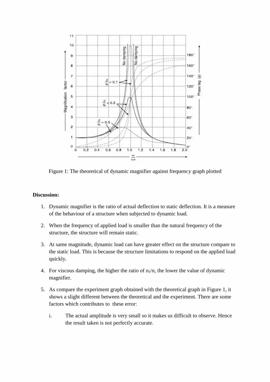
Figure 1: The theoretical of dynamic magnifier against frequency graph plotted

Discussion:

1. Dynamic magnifier is the ratio of actual deflection to static deflection. It is a measure of the behaviour of a structure when subjected to dynamic load.

2. When the frequency of applied load is smaller than the natural frequency of the structure, the structure will remain static.

3. At same magnitude, dynamic load can have greater effect on the structure compare to the static load. This is because the structure limitations to respond on the applied load quickly.

4. For viscous damping, the higher the ratio of nf/n, the lower the value of dynamic magnifier.

5. As compare the experiment graph obtained with the theoretical graph in Figure 1, it shows a slight different between the theoretical and the experiment. There are some factors which contributes to these error:

i. The actual amplitude is very small so it makes us difficult to observe. Hence the result taken is not perfectly accurate.

ii. When the speed is lower, we unable to get clear wave pattern to be recorded on the chart paper. As a result, we need to start the motor speed from 500 rpm onwards.

iii. A flatter bell shape curve would be obtained in a more viscous damping condition.

Conclusion:

1. When the frequency of applied load is smaller than the natural frequency of the structure, the structure will remain static.

2. At same magnitude, dynamic load can have greater effect on the structure compare to the static load. This is because the structure limitations to respond on the applied load quickly.

3. For viscous damping, the higher the ratio of nf/n, the lower the value of dynamic magnifier.

Documents

LAB combine