Graduate Theses, Dissertations, and Problem Reports

2007

Combine gas deliverability equation for reservoir and well Combine gas deliverability equation for reservoir and well

Hassan Daffalla Eljack West Virginia University

Follow this and additional works at: https://researchrepository.wvu.edu/etd

Recommended Citation Recommended Citation Eljack, Hassan Daffalla, "Combine gas deliverability equation for reservoir and well" (2007). Graduate Theses, Dissertations, and Problem Reports. 4298. https://researchrepository.wvu.edu/etd/4298

This Thesis is protected by copyright and/or related rights. It has been brought to you by the The Research Repository @ WVU with permission from the rights-holder(s). You are free to use this Thesis in any way that is permitted by the copyright and related rights legislation that applies to your use. For other uses you must obtain permission from the rights-holder(s) directly, unless additional rights are indicated by a Creative Commons license in the record and/ or on the work itself. This Thesis has been accepted for inclusion in WVU Graduate Theses, Dissertations, and Problem Reports collection by an authorized administrator of The Research Repository @ WVU. For more information, please contact researchrepository@mail.wvu.edu.

COMBINE GAS DELIVERABILITY EQUATION FOR RESERVOIR

AND WELL

HASSAN DAFFALLA ELJACK

THESIS SUBMITTED TO

THE COLLEGE OF ENGINEERING AND MINERAL RESOURCES

AT WEST VIRGINIA UNIVERSITY

IN PARTIAL FULLFILLMENT OF REQUIREMENTS

FOR THE DEGREE OF

MASTERS OF SCIENCE IN

PETROLEUM AND NATURAL GAS ENGINEERING

KASHY AMINIAN, PhD, CHAIR. SAMUEL AMERI, M.S. RAZI GASKARI, PhD

DEPARTMENT OF PETROLEUM AND NATURAL GAS ENGINEERING

WEST VIRGINIA UNIVERSITY 2007

ABSTRACT

COMBINE GAS DELIVERABILITY EQUATION FOR RESERVOIR AND WELL

HASSAN DAFFALLA ELJACK

A new model has been developed by combining the gas reservoir deliverability equation

for a reservoir and the well flow equation.

An existing computer program was modified to determine gas production from reservoir

against constant wellhead pressure.

Upon completion, a unique, simple, and user friendly model was developed, that will

allow the user to predict the performance of the gas reservoir against a constant wellhead

pressure.

The new model was used to generate and introduce a new set of production decline type

curves, which can be utilized to forecast gas production rates under constant wellhead

pressure condition.

The impact of the well tubing length and tubing size on the shape of the type curves were

studied.

ACKNOWLEDGEMENTS

All Praise be to Allah, Cherisher and Sustainer of Worlds, who brought me to this world

and bestowed me with life and health to complete this work. I would like to express my

indebtedness and gratefulness to my academic advisor and Professor, Dr. Kashy

Aminian, for his sustenance and unconditional inexhaustible supervision during my

graduate program. Your support, proficient espousal, and belief always piloted my

profession and made achievable what was perceived as a distant dream.

I would also like to thank Professor Sam Ameri, and Dr. Razi Gaskari for their constant

encouragement and motivation during my stay at West Virginia University. I also

appreciate their participation and enthusiasm to be part of my committee.

I dedicate my work to my Parents, My Brothers and Sisters, for their continuous prayer,

patience and encouragement. I especially dedicate this work to two great women: my

mother (Zakia) who represents the best inspiration in my life. It is like a dream coming

true to achieve this degree, her unique ways of encouragement always filled my heart

with joy and enthusiasm to progress ahead in life and I feel fortunate to be the special

one; and also to my great and lovely wife (Zahra) for her sacrifices of her health and time

to provide me with a suitable environment; her patience and encouragement was the drive

for me. Thank you my mother and my wife for your entire noble up bringing and self-

sacrificing love, guidance, support and encouragement that helped me with years to

survive this harsh phase of life.

Finally, I dedicate this work to my kids: Manar, Mohammed and Moaiad whose smiles

are the hope and whose laughs are the bright future.

iii

TABLE OF CONTENTS ABSTRACT.........................................................................................................................i

ACKNOWLEDGEMENTS................................................................................................ii

TABLE OF CONTENT.....................................................................................................iii

LIST OF FIGURES...........................................................................................................iv

LIST OF TABLES..............................................................................................................v

VI NOMENCLATURE.....................................................................................................vi

I. INTRODUCTION...........................................................................................................1

1.1 Production Type Curve ………………………..……………….….....….….…...1-2

II. LITERATURE REVIEW................................................................................................3

2.1 Gas Deliverability & flow rate...............................................................................3-5

2.2 Production Type Curves Review ……………………………………….......…..5-10

2.2.1 Aminian et al Type Curves …………………………….…………….….10-17

2.2.2 Type Curve Utilization …………………………………………….……17-19

2.2.3 Recent Type Curves Research ………………………………...….……. 19-20

2.2.4 Computer Program ………………………………………………..….…21-22

III OBJECTIVE AND METHODOLOGY……..…………..….………………..………23

3.1 Model Development………………….………………………………….…….23-30

3.2 Generation of Production Type Curves ……………………….…….….….….31-32

3.3. Impact of the Well Tubing Length & Size on the Type Curves ……...............….33

IV RESULTS AND DISCUSSION...................................................................................34

4.1 Initial Result…………….…..…………………………………………..….…34-36

4.2 Effect of Tubing Length (TL) ………………………………..……….….…...37-39

4.2 Effect of Tubing Size (ID) …………………………………….…….....….….40-43

V CONCLUSIONS AND RECOMMENDATIONS........................................................44

VI REFERENCES.......................................................................................................45-46

VII APPENDIX...........................................................................................................47-55

VIII VISTA ………………………………………….…...…...…………………..……56

iv

LIST OF FIGURES

Figure 2.1 Smith’s Type Curves for wells producing against BP with various values of n..........8

Figure 2.2 Constant back-pressure gas well production decline curves……….……...…13

Figure 2.3 Effect of non-Darcy flow on type curves.........................................................14

Figure 2.4 Cumul-production type curve for gas wells producing against constant BP....16

Figure 2.5 Sample of the type curve matching process…….............................................19

Figure 3.1 Flow Chart for computer model modification………......................................24

Figure 3.2 First page of the developed-software...............................................................26

Figure 3.3 The gas composition input window..................................................................27

Figure 3.4 The gas composition result displayed...............................................................28

Figure 3.5 Decline Curve input/output page......................................................................29

Figure 3.6 Wellhead pressure calculation as additional option for the program...............30

Figure 3.7 Out put result of the decline curve...................................................................31

Figure 3.8 Option to input the temperature for the wellhead pressure calculation............32

Figure 4.1 Effect of Tubing Length & Size in a different Xi values………….................38

Figure 4.2 Effect of Tubing Length & Size in a different Fndi values.............................39

Figure 4.3 Effect of Tubing Length for Fndi = 1.10…………..........................................40

Figure 4.4 Effect of Tubing Length for Fndi = 2.50………..............................................41

Figure 4.5 Effect of Tubing Length for Fndi = 10.00………............................................41

Figure 4.6 Effect of Tubing Length for Xi = 2.75…………….........................................42

Figure 4.7 Effect of Tubing Length for Xi = 5.00.............................................................42

Figure 4.8 Effect of Tubing Size for Fndi=1.10................................................................43

Figure 4.9 Effect of Tubing Internal Diameter for Fndi = 2.50…….................................44

Figure 4.10 Effect of Tubing Internal Diameter for Fndi = 10.0……....…….………......44

Figure 4.10 Effect of Tubing Internal Diameter for Xi = 2.75…………………....…......45

Figure 4.10 Effect of Tubing Internal Diameter for Xi = 5.00……………….…...…......45

v

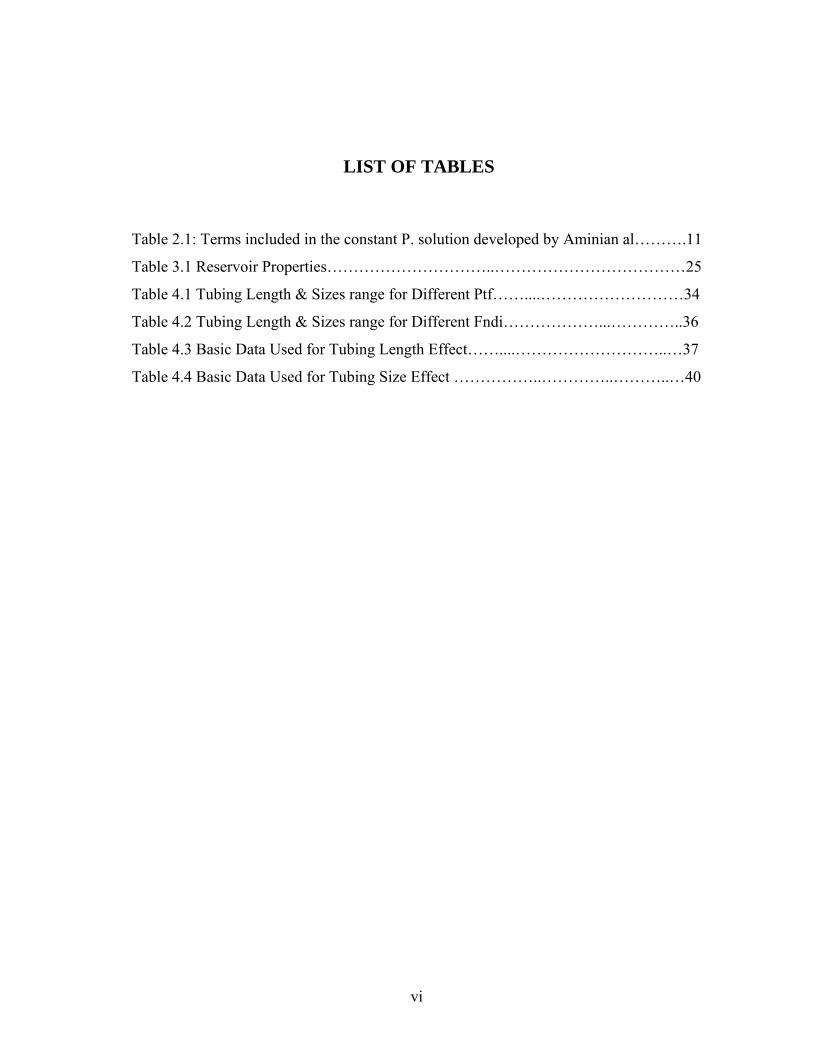
LIST OF TABLES Table 2.1: Terms included in the constant P. solution developed by Aminian al……….11

Table 3.1 Reservoir Properties…………………………..………………………………25

Table 4.1 Tubing Length & Sizes range for Different Ptf……....………………………34

Table 4.2 Tubing Length & Sizes range for Different Fndi………………...…………..36

Table 4.3 Basic Data Used for Tubing Length Effect……....………………………..…37

Table 4.4 Basic Data Used for Tubing Size Effect ……………..…………..………..…40

vi

NOMENCLATURE

a= Non- Darcy flow coefficient, psi^2/(cp)(Mscf/D)^2.

gB = Gas formation volume factor, RB/scf.

C = Back-pressure curve coefficient, Mst/D/psi^n.

AC =Reservoir shape factor, dimensionless.

=Gas compressibility, psi-1. gC

D =Decline rate, day-1.

NDiF = Non-Darcy flow ratio, dimensionless.

atDF =pseudo time ratio, dimensionless.

DG =Dimensionless cumulative production.

iG = Initial gas in place, Bcf.

pG =Gas produced, Mscf.

h = Formation thickness, ft.

k = Absolute permeability, md.

n = Exponent of back-pressure curve, dimensionless.

P= Pressure, psia.

iP = Initial Reservoir Pressure, psia.

Pp= Pseudo pressure, psi2/cp.

rP = Average reservoir pressure, psia.

scP = Reservoir pressure at the standard condition, psia.

tfP = wellhead pressure, psia.

tsP = Shut-in pressure, psia.

wfP = Bottom-hole flowing pressure, psia.

vii

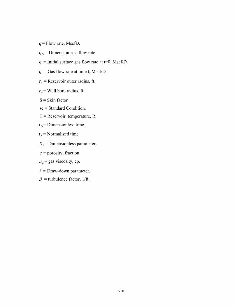
q = Flow rate, MscfD.

Dq = Dimensionless flow rate.

iq = Initial surface gas flow rate at t=0, Mscf/D.

tq = Gas flow rate at time t, Mscf/D.

er = Reservoir outer radius, ft.

wr = Well bore radius, ft.

S = Skin factor

sc = Standard Condition.

T = Reservoir temperature, R

Dt = Dimensionless time.

Nt = Normalized time.

iX = Dimensionless parameters.

φ = porosity, fraction.

gµ = gas viscosity, cp.

λ = Draw-down parameter.

β = turbulence factor, 1/ft.

viii

CHAPTER 1

INTRODUCTION

Estimation of hydrocarbon-in-place and the forecast of the gas reservoirs

production are needed to determine the economic viability of the project

development as well as to book reserves required by regulatory agencies. During

the last 70 years, various methods have been developed and published in the

literature for estimating reserves. These methods range from the basic material

balance methods to decline type curve analysis techniques. They have varying

limitations and are based on analytical solutions, graphical solutions. Examples of

these include Arp’s decline equations, Fetkovich’s decline curves, Carter’s gas type

curves, and Palacio and Blasingame`s gas equivalent decline curves. Most recently,

other papers on type curves analysis, have appeared in the SPE literatures; all that

reflect the important role of this area of study.

1.1 Production Type Curves: The production type curves, which are plots of theoretical solutions to flow

equations , are employed, in the absence of complete reservoir data, to predict the

future production rates based on past production data. The idea of using the log-log

type curves for matching and interpreting production data was first proposed by

Fetkovich (1980), however, has had widespread application to analyze the pressure

transient data for many years prior to that.

1

Fundamentally, production decline type curve is a log – log plot of a family of

production type curves with dimensionless flow rate ( ) on ordinates and

dimensionless time ( ) on abscissa.

Dq

Dt

The different curves of a family are distinguished from one another by a specific

parameter. Several sets of production decline type curves have been published in

past literature. Most of these type curves have bean developed based on a

simplifying assumption which limits their application. There are several suggested

modifications which have provided some other improvements for gas well

production decline analysis. However, the modifications involve the use of new

parameters which are difficult to evaluate and as a result complicate the matching

process. One of the most important limitations of the previous work and

development of decline type curves, is that; they were based mainly on the

assumption of a constant flowing bottom hole pressure. But, from practical view,

this assumption is violated; since most gas wells are produce under constant

wellhead pressure and different flowing bottom hole pressures condition.

The objective of this research was to develop a set of type curves that combine

formation deliverability and gas well flow equation.

2

CHAPTER 2

LITERATURE REVIEW

2.1 Gas Deliverability and Flow rate

Natural gas deliverability from the reservoir and the wells has been an area of

continuing interest for development of production facilities as well as design and

operation of storage fields. “Deliverability” of gas well relates to its ability to

produce the gas into wellbore and, subsequently to the surface facilities at a

particular rate. The rate of flow from a porous and permeable drainage area into a

well bore is a function of the properties of both the information and the fluids; as

well as the pressure gradients which is the driving force prevailing in the drainage

area. Whether in production or in storage understanding of gas deliverability

involves: (a) Flow near the well bore as affected by skin affect. (b) Flow into the

well bore through the particular completion system and up or down through the

well. (c) Flow through the gathering system that usually includes pipes, laterals,

separators, dehydration, pressure regulation, metering and other equipment. (d)

Field-to main-pipeline connection – usually through compressor station. During the

process of flow, the system adjusts to the rate of deliverability resulting from the

various components (mostly in series but sometimes in parallel). Current practice in

gas well deliverability analysis involves using the laminar solution for constant

terminal rate, along with a skin factor and rate proportional turbulence term added

to the pseudo-pressure drop at the well bore. The gas flow through the porous media

will be briefly discussed. In general, for gas flow from a reservoir, it is possible to

calculate flow rate based the following equation (The Forchheimer equation):

2vvkdx

dp βρµ+=− -------------------------------- (2.1)

3

The density, ρ , and the velocity, ν , are each functions of pressure, there fore,

Equation (2.2) became:

2)()( vvkdx

dp ρβρµρ +=− ------------------------------ (2.2)

The term ρ v is the mass rate of flow and is therefore independent of pressure. By

using the real gas law, we can express ρ v in the, following way:

RATMpq

vsc

wscsc=ρ ----------------------------------------- (2.3)

Where:

sc = standard conditions.

Substitution of the mass flow rate expression Equation (2.3) into Equation (2.4)

produces the desired universal deliverability equation:

Aq

RTMP

Aq

RTMP

kdxdp

ZRTPM sc

sc

wscsc

sc

wscw βµ+= ------- (2.4)

Separating variables, integrating and rearranging the above equation resulting our

working deliverability equation:

221

22 bqaqPP +=− ----------------------------------------(2.5)

4

We are now able to use Equation (2.5) to develop a reservoir, well, and surface flow

line model, which can then be combined with the depletion equations developed

earlier. In essence, Equation (2.5) can be applied to three different flow

configurations: (a) Flow from the reservoir to the well (b) Flow from the bottom of

the well to the wellhead, and (c) Flow from the wellhead to the power plant.

Each of these configurations will produce different values for their unknown

constants a & b in the deliverability equation.

2.2 Production type curves review

Fetkovich1 introduced the concept of type curve matching for production data

analysis. Fetkovich combined a gas stabilized back-pressure deliverability equation,

and a material balance equation to develop a set of type curves for gas well

production forecasting , ignoring the gas compressibility factor.

---------------------------- (2.6) ( nwfR PPCq 22 −= )

ipi

iR PG

GP

P +⎟⎟⎠

⎞⎜⎜⎝

⎛−= -------------------------- (2.7)

These curves are presented as dimensionless flow rate and the dimensionless time

for various values of the exponent n and the ratio between the original shut in

pressure to the constant flowing bottom pressure. Fetkovich developed a set of

empirical equations for a well producing against constant backpressure. Using

5

backpressure, Equation (2.6), he derived the following equations by setting

compressibility factor z = 1.0.

wfPPX = --------------------------------------- (2.8)

Where,

= constant backpressure wfP

P = reservoir pressure.

Fetkovich1 came out with a new plot for type curves, where he introduces the

dimensionless ration Xi:

wf

ii P

PX = ----------------------------------- (2.9)

Where,

= initial reservoir pressure iP

These curves are illustrated in, Figure 2.1 - which shows the dimensionless flow

rate, was a function of dimensionless time, . Also, Figure 2.3 shows

various values of the exponent, n ranged from 0.5 to 1.0 (laminar flow). Fetkovich

iqq / ii Gtq /)*(1

also showed that as becomes large, his assumption became equivalent to

Fetkovich assumption in which a well is producing at a constant fraction of the

shut-in pressure.

iX

6

The limitation of Fetkovich1 theoretical method, is that, does not consider the

change in gas properties as reservoir pressure is reduced. The value for C and n

were taken as constant, where, has been shown that depends on flow rate and does

not remain constant during the life of the well. The value of C depends on gas

properties and varies with pressure.

Smith2 further extended Fetkovich`s type curves, empirical method accounts for

non-Darcy flow by generating a set of curves for various values of n. These values

range from n = 1.0 (laminar flow) to 0.5 (Turbulent flow). The problem with this

method is that having many families of curves make unique match difficult. Smith

also ignore the compressibility of gas , by setting compressibility factor equal to 1,

Later, Carter3 generated a set of curves with a finite-difference reservoir model.

These types curve improved the accuracy of the analysis by plotting functions that

include the changes in gas properties with pressure. Thus, he considered the

changes of the product gµ Cg with the average reservoir pressure using a drawdown

parameter - as show in Equation (2.24).

[ ][ ]wfi

wfpipigi

zPzPPPPPPCP

)/()/(2)()()()(

−

−=µ

λ -------------------- (2.10)

Carter4 introduced a new type curves for gas wells producing at constant pressure to

fill the gap which existed with the Fetkovich decline curves. As shown, the λ =1.0

curve assumes a negligible drawdown effect and it corresponds to the = ∞ , on

the Fetkovich type curves. But ignored no-Darcy flow effects; which limited by the

fact that

iX

λ must be calculated before a match can be made and the information

needed to calculate λ is not always available.

7

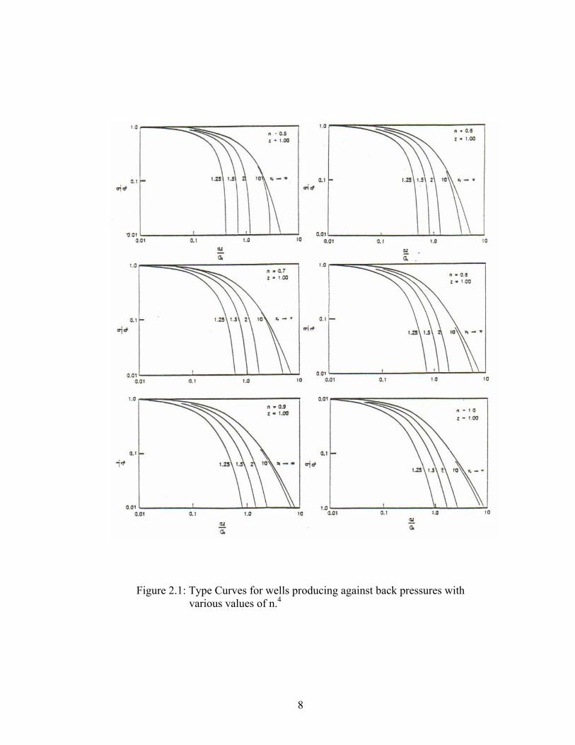
Figure 2.1: Type Curves for wells producing against back pressures with various values of n.4

8

Fraim and Wattenbarger5 used pseudotime, first introduced by Agarwal to improve

the use of Fetkovich type curves for gas. The time transformation accounts for

variation of gas properties as the average reservoir declines. Their pseudo-time is

different than that used by Agarwal because viscosity and compressibility are

evaluated at average reservoir pressures rather that wellbore pressure. They found

that, to obtain pseudo-time, value for original gas in place, G, must be assumed. The

first estimate is found by matching the actual time versus rate decline curve and

calculating a value of G. They showed that gas well production rates decline

exponentially against the normalized time as defined in Equation (2.11).

∫ ×

×=

t

gg

gigiN dt

CC

t0 µµ

------------------------------------ (2.11)

Farim and Wattenbarger6 account for variations in gas properties with pressure

using pseudo-time, but they also ignore non-Darcy flow. This method has the

disadvantage of requiring an estimate of gas in place and knowing the reservoir

drive mechanism for the material balance equation before the pseudo-time can be

calculated. As mentioned above, all these authors have neglected the impact of non-

Darcy flow in their derivation. A set of more representative curves were developed

by Schmidt et al, Caudle, and Aminian et al by combining the theoretical stabilized

gas flow equation, Equation (2.12) and the material balance for a gas reservoir,

Equation (2.13).

2)()( bqaqPPPP wfpip +=− ---------------------- (2.12)

⎥⎦

⎤⎢⎣

⎡ −=

11

2211

///

zPzPzPGp ------------------------ (2.13)

9

The model accounts for non-Darcy flow and dependency of gas properties on

pressure. The models previously discussed assume constant reservoir parameters

and operating conditions during the entire life of the reservoir. Aminian et al7 has

discussed the violation of this assumption in practice due to changes in well spacing

owing to infill drilling, back pressure changes due to compressor installation, and

changes in skin factor due well stimulation.

2.2.1 Aminian et al Constant Pressure Solution

Equation (2.14) shows the analytical solution developed by Aminian et al:

( )[ ]λi

taDNDiDNDiD X

FFqFq/11

)1)(1(2ln−

+−−+ -------------------- (2.14)

All the variables in the equations are explained and defined in Table 2.1.

The theoretical model developed to generate the type curves was based on the next

assumptions:

- Pseudo steady state flow regime

- Constant well flowing pressure

-Homogeneous and isotropic formation

- High gas flow rates into wells.

The Pressure dependency of the gas properties is represented by , which depends

on the pseudo time, and

taDF

λ , which contains pseudo pressure. Pseudo pressure as

defined by Equation (2.21) takes into account the variation of gas viscosity and gas

compressibility.

10

Table 2.1: Terms included in the constant pressure solution developed by Aminian.

Parameter Equation

Dimensionless Flow Rate i

D qqq = (2.15)

Non-Darcy Flow Ratio a

bqF i

NDi += 1 (2.16)

Darcy Flow Coefficient, 22 )/)(/( DMcfcppsi ⎥

⎦

⎤⎢⎣

⎡+−⎟⎟

⎠

⎞⎜⎜⎝

⎛=

srCAreakh

Ta

wa

75.006.10ln5.0

1422

2

(2.17)

Non- Darcy Flow coefficient, 22 )/)(/( DMcfcppsi ⎥

⎦

⎤⎢⎣

⎡−

×=

−

ew rrh

Tb11

10161.3

2

12

µ

γβ (2.18)

Turbulence Coefficient, 1−ft 1045.1

101073.2K×

=β (2.19)

Pseudo time Ratio

gigi

t

ggtaD

ct

cdt

F

µ

µ∫= 0 (2.20)

Pseudo pressure, cppsi /2 ∫=p

gp z

PdpPP0

2)(µ

(2.21)

Dimensionless Time i

iD G

tqt = (2.22)

Drawdown parameter

[ ]( )

⎥⎥⎦

⎤

⎢⎢⎣

⎡⎟⎠⎞

⎜⎝⎛÷⎟

⎠⎞

⎜⎝⎛

−=

wfi

gigiwfpp

zp

zp

CPPPP

2

)()( µλ (2.23)

Dimensionless Parameter, Xi wfi

i zp

zpX ⎟

⎠⎞

⎜⎝⎛÷⎟

⎠⎞

⎜⎝⎛= (2.24)

11

The effect of non-Darcy flow is quantified by . Aminian et al,NDiF 8 concluded that

the dependency of the previously discussed type curves on permeability, initial

pressure and skin factor are caused by variations of this parameter.

In order to generate a type curve from Equation (2.14), it is necessary to determine

for each point of the decline curve, which means for each pressure. Two

approaches have been proposed to solve this expression. Abidi introduced the first

approach known as direct method in 1991. This method solves the equation directly

by utilizing polynomial approximations for as function of . The effect of

various parameters such as , , and k on was studied by plotting vs.

on log- log paper. Sets of

taDF

taDF Dt

iP iX taDF taDF Dt

taDF × / Dt λ (1 – 1 / ), and / (1 –1 / ) were

developed in order to establish a correlation between , and the dimensionless

time, . In order to generate a type curve from these plots a polynomial regression

method was used. This technique employs the least squares fit of the data by

successive polynomials of order 1 to 4, and examines the standard deviation about

the regression line in each case. Thus, the type curves generated by using these

correlations were compared to the type curve generated by numerical methods

finding an alternative method to model Aminian et al Type curves. The second

approach is the indirect method, which utilizes a stepwise method of solving

material balance and deliverability equations simultaneously to determine rate

versus time and converts the results to dimensionless rate and time. This method is

the foundation of the computer program for generating type curves.

iX Dt iX

taDF

Dt

It has been observed that if both the non-Darcy and pressure dependency of the gas

properties is ignored, = 1, taDF λ =1.0, and , then the equation reduces to the

familiar exponential decline. This is true for single-phase liquid flow.

NDiF

12

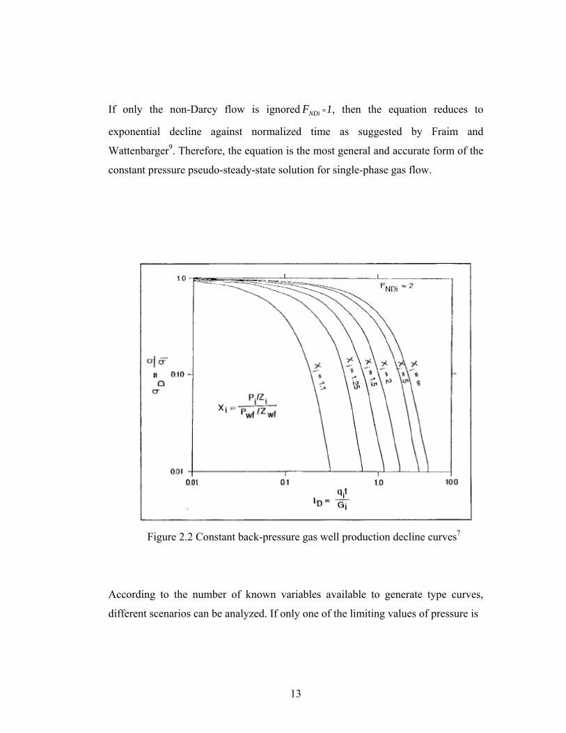
If only the non-Darcy flow is ignored =1, then the equation reduces to

exponential decline against normalized time as suggested by Fraim and

Wattenbarger

NDiF

9. Therefore, the equation is the most general and accurate form of the

constant pressure pseudo-steady-state solution for single-phase gas flow.

Figure 2.2 Constant back-pressure gas well production decline curves7

According to the number of known variables available to generate type curves,

different scenarios can be analyzed. If only one of the limiting values of pressure is

13

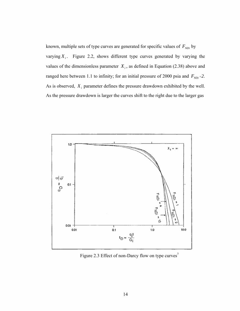
known, multiple sets of type curves are generated for specific values of by NDiF

varying . Figure 2.2, shows different type curves generated by varying the

values of the dimensionless parameter , as defined in Equation (2.38) above and

ranged here between 1.1 to infinity; for an initial pressure of 2000 psia and =2.

As is observed, parameter defines the pressure drawdown exhibited by the well.

As the pressure drawdown is larger the curves shift to the right due to the larger gas

iX

iX

NDiF

iX

Figure 2.3 Effect of non-Darcy flow on type curves7

14

production at higher differential pressure. If the limiting values of the pressure ,

and are known then

iP

wfP λ , and can be easily determined by substituting

pressure values between this intervals in their respective equations.

iX

Figure 2.3, depicts a set of type curves for = 2000 psia, and =100. As we

observed, the effect of larger (s) results in a shift of the curves to the left side

due to shorter gas production and production time. It is also the values of ,

larger than 10 do not result in significant variations in the shape of the type curve.

iP wfP

NDiF

NDiF

These sets can be obtained either by adjusting reservoir permeability or skin factor

to keep constant the values. As the figure shows, the initial pressure influences

the type curve only slightly when the non-Darcy effects are kept constant7. These

changes are the result of variations in and

NDiF

taDF λ given by Equations (2.34) and

(2.37). Also sets of cumulative production type curve were generated as shown in

Figure 2.4, was introduced by Aminian, who found that, those cumulative

production type curves can enhance the matching process when the erratic rate of

production data can not easily be matched to the production type curves.

Where the dimensionless cumulative production is defined as of the gas

cumulative production divided by the initial gas in place as follows:

DG

i

pD G

GG = ----------------------------------- (2.40)

Aminian et al10 performed many simulation runs to study the effect of various

reservoir parameters on the shape of the type curves. As a result, the formation

15

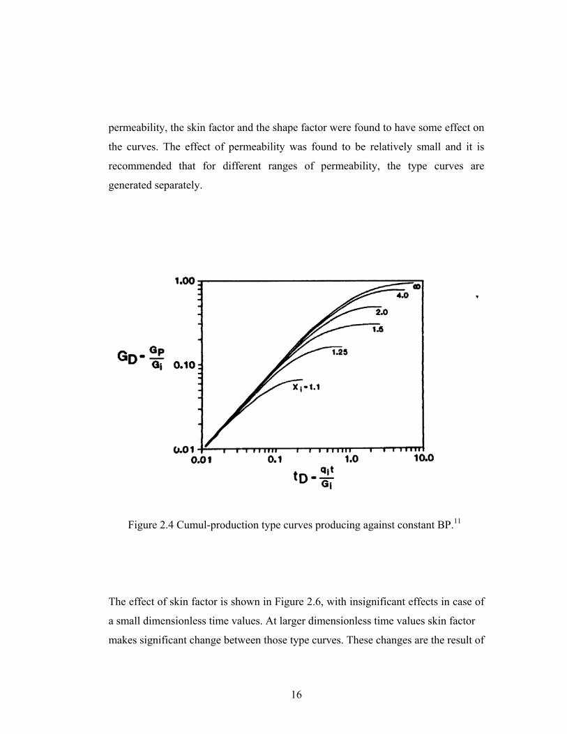
permeability, the skin factor and the shape factor were found to have some effect on

the curves. The effect of permeability was found to be relatively small and it is

recommended that for different ranges of permeability, the type curves are

enerated separately.

g

Figure 2.4 Cumul-production type curves producing against constant BP.11

akes significant change between those type curves. These changes are the result of

The effect of skin factor is shown in Figure 2.6, with insignificant effects in case of

a small dimensionless time values. At larger dimensionless time values skin factor

m

16

Non-Darcy effects, NDiF ; therefore, they are accounted for in the type curves. The

effect of the shape factor was also found very similar to that of skin factor. Aminian

type curves have limitations, that reservoir must be at pseudo-state and radial flow

conditions. Wells which are dominated by linear flow and/or an unsteady flow

egime should not be analyzed with these type curves.

2.2.2 Type Curve Utilization

versus

tc t

s are to evaluate and as defined by Equations (2.41) and

(2.42).

r

To analyze the past production data, a log-log plot of actual production rate

time is overlaid on different sets of type curve. The closest type curve to the

production history is chosen as the match for it. As a result of these match the value

of iX , iP , and NDiF are directly obtained from the type curve. As is seen in Figure

2.7, the matched type curve differs from the plot of actual data only by a shift in

coordinates. Hence, an arbitrary ma h poin should be selected, and the two sets of

coordinate used iq iG

matchDi q

qq ⎟⎟⎠

⎞⎜⎜⎝

⎛= ---------------------------------- (2.41)

matchDi t

tqG ⎟⎟⎠

⎞⎜⎜⎝

⎛= ------------------------------- (2.42)

17

As iP d iX are read from the matched type curve, the value of wfP is obtained

from iX relation. Knowing wfP , the values of non-Darcy coefficient b, and Darcy

coefficient a of the quadratic gas flow

an

equation defined by Equation (2.26) are

obtained by Equations (2.41) and (2.42).

[ ]NDii

wfpip

FqPPPP

a×

−=

)()( ----------------------- (2.43)

i

NDi

qaF

b)1( −

= ------------------------------ (2.44)

odu are

te

m

ations (2.43) and (2.44). An

xample of matching process is shown in Figure 2.5.

Thus, with this information gas deliverability can be calculated by substituting

either wfP or q into the quadratic equation. Gas reserves and times of pr ction

obtained by using the ma rial balance equation. It is essential to know iX and NDiF

to generate type curves. iX affects the position of the curve as shown in Figure 2.3,

while NDiF changes the shape of the curve as shown in Figure 2.4. Since iX is

available from the producing well, NDiF normally will be iterated for different

values and different type curves were generated. Then by superimposing the

production history of a well on the top of the generated curves, a match will be

ade and as the result, NDiF read from the matched curve. Once a match is found,

iq and Gi will be calculated using Equations (2.41) and (2.42). The deliverability

coefficient , a and b were also determined using Equ

e

18

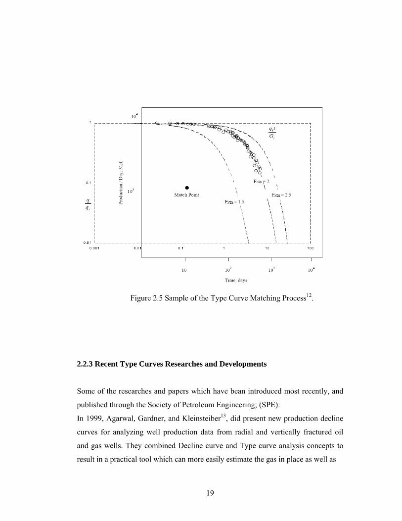
Figure 2.5 Sample of the Type Curve Matching Process12.

.2.3 Recent Type Curves Researches and Developments

ost recently, and

o

sult in a practical tool which can more easily estimate the gas in place as well as

2

Some of the researches and papers which have bean introduced m

published through the Society of Petroleum Engineering; (SPE):

In 1999, Agarwal, Gardner, and Kleinsteiber13, did present new production decline

curves for analyzing well production data from radial and vertically fractured oil

and gas wells. They combined Decline curve and Type curve analysis concepts t

re

19

to estimate reservoir permeability, skin effect, fracture length and conductivity.

In 2001, Zelghi, Tiab, and Mazighi14 introduced a newly developed equation for

decline curve analysis; a fitting equation was developed as an alternative for gas

field data analysis; which combines both depletion and transient periods. The

equation advantages: (a) Fitting with the new equation is more precise than the

conventional type curve matching to obtain decline constant, D, decline exponent,

and matching point. (b)The real production data can be fitted directly by the

equation without using smoothing techniques. (c)The radial and pseudo-steady-state

regions are determined directly from the fitting. (d) and finally, for new-developed

estimation

e limitation, in which

ost of them were based on the assumption that, some of the reservoir parameters

ch as bottom hole flowing pressure remain constant.

reservoirs, production data, which may be insufficient with the conventional type

curve matching, can be interpreted with new fitting developed - equation.

In 2001, also, Marthaendrajana and Blasingame15 introduced a new multiwell

reservoir solution to analyze single well performance data in a multiwell reservoir

system. The new solution was to "couples" the single well and multiwell reservoir

models, based on a total material balance of the system, and permits the

of total reservoir volume and flow properties within the drainage area of an

individual well, where the analysis is performed using type curve.

In 2003, Partikno, Rushing & Blasingame16 studied the methodology for decline

type curve analysis using a field case of continuously measured production rate and

surface pressure data obtained from a low permeability gas reservoir. The

traditional type curve solutions for an infinite conductivity vertical fracture are

typically inadequate - and, their new solutions for a well with a finite conductivity

vertical fracture clearly show much more representative behavior. This suggests that

the proposed type curves will have applications in low permeability gas reservoirs.

Therefore, even the most recent published papers still hav

m

su

20

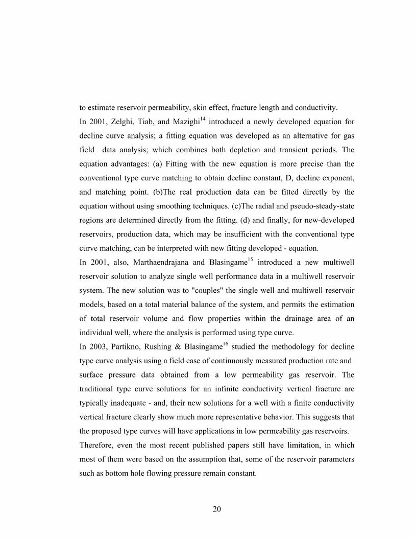
2.2.4 Computer Program

“Sfrac” is a simple analytic gas model created by Tesfasalasi, (1999)17,that

generates production decline curves of a well. The program has two parts; the first

part of the program calculates the gas pro ties and ps do-pressure for any

pressure increment. The second part generates decline production curve

per eu

s and

imensionless type curves. It also prints out , a, b, and as part of the output.

or the first part of the program, the input parameters are the initial reservoir

NDiF iG d

F

Figure 2.6 Sample of the Type Curve Matching Process17

and gas gravity or gas components. For the second part of the

rogram, porosity, permeability, skin factor, shape factor, bottom hole flowing

ressure, well bore

Pressure, temperature

p

p

21

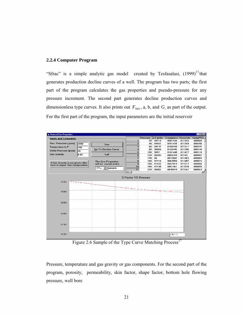
diameter, gas saturation, and area of the reservoir are the input parameters. As

o fici the

outcome of the program is a

imensionless type curve, as shown in Figure 2.7.

shown in Figure 2.6.

Abidi 12 has worked to develop a direct method of generating type curves using

polynomial regression by creating a correlation with the Armenian’s general

equation (26). The program was written in Fortran and it is updated to Visual Basic

5.0. The Second and third degree order polynomial equations were used depending

on initial reservoir pressure. Third degree order polynomial equations were used.

Abidi determined the c ef ents of polynomial equation. The input properties

of the program are iP , iX , and NDiF and the

d

Figure 2.7 Sample of the Type Curve Matching Process17

22

OBJECTIVE AND METHODOLOGY

oduce against a constant

e

ich was

e

and the behavior of the

tant Well head pressure & various bottom hole pressures.

ed into three levels:

-Generate Production Type Curves

-Evaluate the Impact of the Well Tubing Length & Size on the Type Curves.

CHAPTER 3

Most of previous and recent researches, contributions and developments that had

been done on production decline type curves analysis, were based mainly on the

assumption that, the gas well is producing under a constant flowing bottom hole

pressure; From practical point of view, was found to be untrue, most of the gas

wells are currently producing under a constant wellhead pressure and a different

flowing bottom hole pressures. There fore, what will happened to the production

forecasting in the condition where the gas well pr

wellhead pressure and different bottomhole pressures? The answer of that

challenging question was the foundation of my research.

The objective of this research was to develop a new set of type curves that combin

formation deliverability and gas well flow rate – using a new approach wh

the assumption of constant wellhead pressure and variable bottom hole pressures.

To achieve the objective, a methodology consisting of the following steps:

(1)Generate a simple and reliable model that capable to calculate & combine the

production flow rate for both gas reservoir and the well. (2)Generate and introduce

a new set of dimensionless group of gas production decline type curves.(3)Study

and investigate the impact of various reservoir and well parameters especially; th

effect of the tubing length and tubing sizes to the shape

decline curves for a cons

The methodology of this work is divid

A-Model Development

B

C

23

3.1 Model Development The Model was generated using “Sfrac”, which was used as a base to develop a

a well.

Figure 3.1: Flow Chart for Computer model modification

new all that as a base to develop a new model, that capable to combine the gas

deliverability equation for a reservoir and

The modification to the computer program, using Visual Basic 6.0 is illustrated in a

simple Flow Chart in Figure 4.1 below:

Ptf Input

Pwf Estimation.

Well Flow rate:

( )( ) ( ) ( )

5.0

2

522

*100667.0

*

⎥⎥⎦

⎤

⎢⎢⎣

⎡

××−×

×−=

ZTfe

dePPq

s

stfwf

well

Reservoir Flow rate: ( )

bPPPPbaa

q wfpipresv *2

)()(*42 −++−=

weesv q llrq =

If Yes

If No

EXIT

24

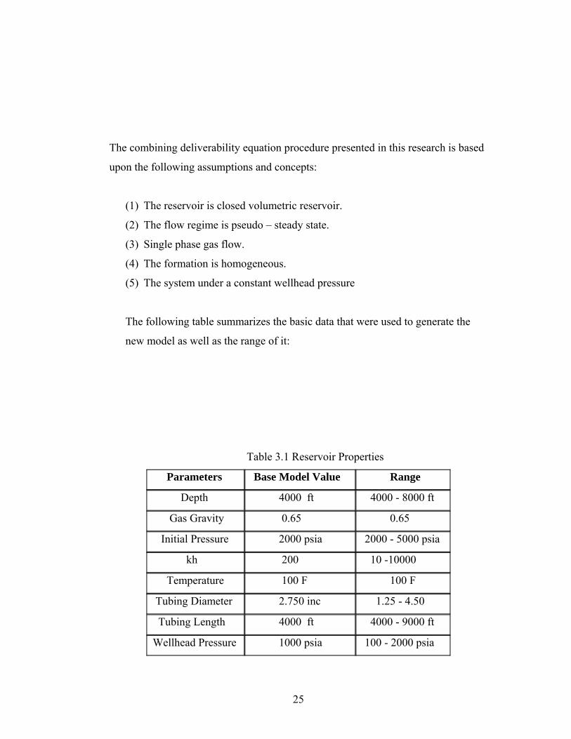
The combining deliverability equation procedure presented in this research is based

upo

olumetric reservoir.

dy state.

(4) The formation is homogeneous.

The following table summarizes the basic data that were used to generate the

new model as well as the range of it:

Table 3 oir Pro

Base Model Value Range

n the following assumptions and concepts:

(1) The reservoir is closed v

(2) The flow regime is pseudo – stea

(3) Single phase gas flow.

(5) The system under a constant wellhead pressure

.1 Reserv perties

Parameters

Depth 4000 ft 4000 - 8000 ft

Gas Gravity 0.65 0.65

Initial Pressure ia 2000 - 5000 psia 2000 ps

kh 200 10 -10000

Temperature 100 F 100 F

Tubing Diameter 2.750 inc 1.25 - 4.50

Tubing Length 4000 ft 4000 - 9000 ft

Wellhead Pressure 1000 psia 100 - 2000 psia

25

“Progress” is the new modification to the previous model “Sfrac”. The new addition

focused mainly on the second phase where the program generates the type curves.

Even though, the first phase was modified also, as show in Figures 3.2, & 3.3;

Figure 3.2: First page of the developed-software.

external file from different location.

Beside the overall look, additional features added such as; the model was developed

to allow the user to choose different

26

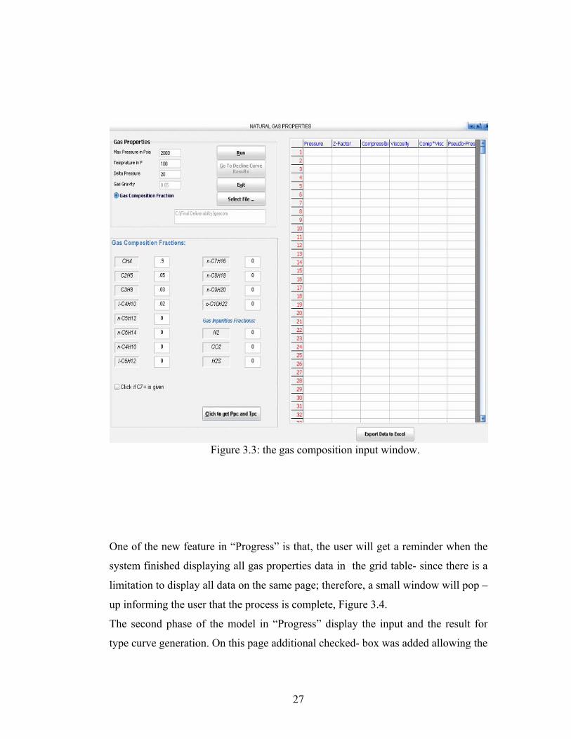
Figure 3.3: the gas composition input window.

l window will pop –

type curve generation. On this page additional checked- box was added allowing the

One of the new feature in “Progress” is that, the user will get a reminder when the

system finished displaying all gas properties data in the grid table- since there is a

limitation to display all data on the same page; therefore, a smal

up informing the user that the process is complete, Figure 3.4.

The second phase of the model in “Progress” display the input and the result for

27

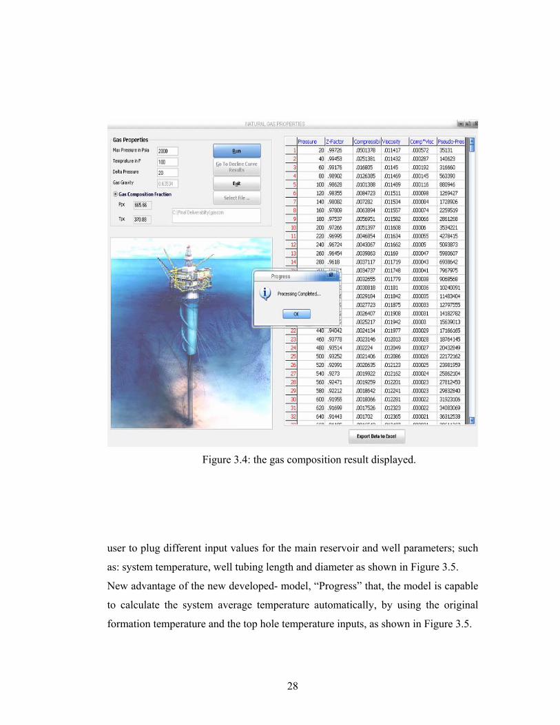
Figure 3.4: the gas composition result displayed.

ch

rmation temperature and the top hole temperature inputs, as shown in Figure 3.5.

user to plug different input values for the main reservoir and well parameters; su

as: system temperature, well tubing length and diameter as shown in Figure 3.5.

New advantage of the new developed- model, “Progress” that, the model is capable

to calculate the system average temperature automatically, by using the original

fo

28

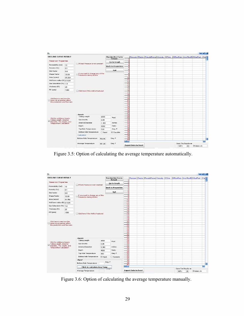
Figure 3.5: Option of calculating the average temperature automatically.

Figure 3.6: Option of calculating the average temperature manually.

29

ser to

in

different color to distinguish them from the rest outputs; as shown in Figure 3.7.

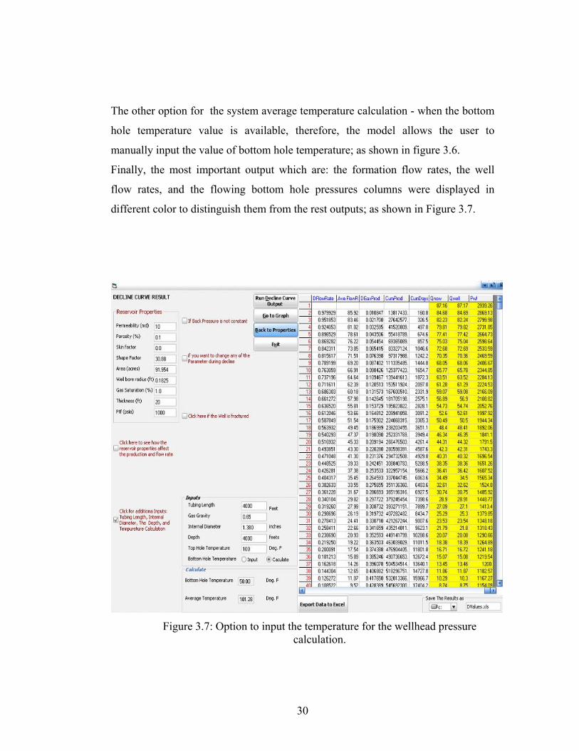
The other option for the system average temperature calculation - when the bottom

hole temperature value is available, therefore, the model allows the u

manually input the value of bottom hole temperature; as shown in figure 3.6.

Finally, the most important output which are: the formation flow rates, the well

flow rates, and the flowing bottom hole pressures columns were displayed

Figure 3.7: Option to input t e for the wellhead pressure

calculation. he temperatur

30

3.2 Generation of Production Type Curves

, is

The methods that had been utilized to generate Amenian’s solution type curves

initiated by solving the dimensionless time Dt and dimensionless flow rate Dq

using material balance equation and deliverability equation. The goal is to utilizes a

stepwise method of solving material balance and deliverability equations

simultaneously to determine reservoir flow rate and match that with the well flow

rate obtained from tubing deliverability equation using similar Pwf –Which is the

foundation of my computer model program (that I developed and was explained

previously) for combining the flow rates of the reservoir and the well in one and

closely equal flow rate In order to generate a single type curve gas properties must

be defined at every point of the proposed gas declines. As it was mentioned before,

Xi, FNDi, and initial gas in place Gi are required to generate an individual type

curve. As this information is not available to initiate type curve matching, the

program iterates on these three parameters by proposing a range of K, Pwf and Gi

to initiate the search. It is assumed that usual information as Pi, gµ , and T is known.

The next step is the calculation of the coefficients of the quadratic deliverability

equation a and b. A pressure step of twenty psia was considered to generate the

reservoir flow rate equation (Qnow), since it offers great accuracy in the process of

interpolation and curve comparison. Once a, and b coefficients are identified, gas

reservoir flow rate (Qnow) is obtained by solving the quadratic gas flow equation

iven by equation:

g

( )b

PPPPaaaq wfpip

2

)()(42 −++−= ---------------------(3.1)

31

Converting the Pseudo flowing bottom hole pressure (Pp(Pwf) to conventional

flowing bottom hole pressure (Pwf) and applying that into the well deliverability

quation to obtain the well flow rate (Qwell), using the following equations:

e

5.0

5

22242 )1(

****1067.6*

⎥⎥⎦

⎤

⎢⎢⎣

⎡−

×+=

−sgs

tfwf ed

ZTfqePP ----------(3.2)

where,

224.0

01603.0ID

f = ------------------------------------(3.3)

Where,

TZD

s g

***0375.0 γ

= ------------------------------------(3.4)

for adjusting the value of flowing bottom hole

d

flow rate ) and dimensionless time ( ) are shown in Equations

(3.5) & (3.6):

------------------------------ (3.5)

--------------------------------------- (3.6)

Then the program starts comparing the values of Qnow & Qwell to math them by

using the logic & techniques

pressure, till the match occurs.

Finally, the output results which include the combined-flow rates and their

corresponding Pwf values will export to Excel to finish generating the type curves-

by the hint of other inputs data the dimensionless rate and time will be calculated to

plot the type curves. The definition of those two imensionless parameters;

dimensionless ( Dq Dt

-----------

i

D qq =

q

i

iD G

qtt ×=

32

3.3 Impact of the Well Tubing Length & Size on the Type Curves

. is important to know that all calculations based on the new

efinition for :

The final phase of this methodology was to investigate the impacts and the

influences of the well tubing sizes and lengths on the shape and behavior of the type

curves. As mentioned earlier, the model output was exported to Excel spreadsheet

to finalize the calculation of the two dimensionless parameters ;( Dq ) And ( Dt ) as

shown in Equations (3.5) & (3.6). After that the rest of calculations were performed

to evaluate the influences of the tubing lengths and sizes to the behavior of the

decline curves It

iXd

tftsi

i zp

zpX ⎟

⎠⎞

⎜⎝⎛÷⎟

⎠⎞

⎜⎝⎛= ---------------------------------------------- (4.5)

will

impact and influence the shape or the position of the production decline curve.

After that, we start applying different values of Tubing size and Tubing diameters

while the rest of the reservoir parameters as well as the well parameters were set to

be constant . By doing that a hundreds of runs and calculations will be made till a

clear picture will occur. Then, by changing the values of the tubing lengths and

sizes we will have a clear picture of how those two important parameters

33

CHAPTER 4

RESULTS AND DISCUSSION

ults were obtained after been

ested and satisfied the enclosed parameter’s range.

.1 Initial Result

rding to the previou ork,

le generate this type

urves- showing the effect of the dimensionless parameters, .

Table 4.1: Tubing Lengths & Sizes a

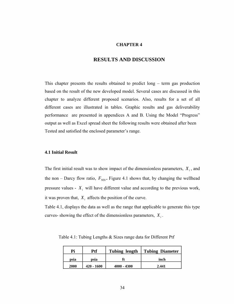
This chapter presents the results obtained to predict long – term gas production

based on the result of the new developed model. Several cases are discussed in this

chapter to analyze different proposed scenarios. Also, results for a set of all

different cases are illustrated in tables. Graphic results and gas deliverability

performance are presented in appendices A and B. Using the Model “Progress”

output as well as Excel spread sheet the following res

T

4

The first initial result was to show impact of the dimensionless parameters, iX , and

the non – Darcy flow ratio, NDiF . Figure 4.1 shows that, by changing the wellhead

pressure values - X will have different value and accoi s w

it was proven that, iX affects the position of the curve.

Table 4.1, displays the data as well as the range that applicab to

iXc

range dat for Different Ptf

Pi Ptf Tubing length Tubing Diameter

psia psia ft inch

2000 420 - 1600 4000 - 4300 2.441

34

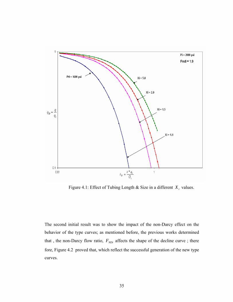
Figure 4.1: Effect of Tubing Length & Size in a different values.

en

ure 4.2 proved that, which reflect the successful generation of the new type

urves.

iX

The second initial result was to show the impact of the non-Darcy effect on the

behavior of the type curves; as m tioned before, the previous works determined

that , the non-Darcy flow ratio, NDiF affects the shape of the decline curve ; there

fore, Fig

c

35

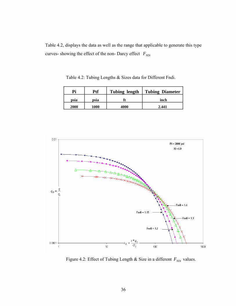
Table 4.2, displays the data as well as the range that licapp able to generate this type

urves- showing the effect of the non- Darcy effect

Table 4.2: Tubing Lengths & Sizes data for Different Fndi.

NDiF c

Pi Ptf Tubing length Tubing Diameter

psia psia ft inch

2000 1000 4000 2.441

Figure 4.2: Effect of Tubing Length & Size in a different values. NDiF

36

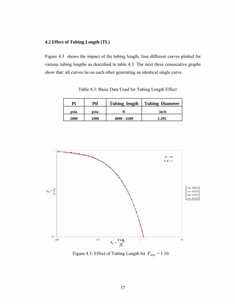
.2 Effect of Tubing Length (TL)

graphs

show that: all curves lie on each other generating an identical single curve.

Table 4.3: Basic Data Used for Tubing Length Effect

4 Figure 4.3 shows the impact of the tubing length; four different curves plotted for

various tubing lengths as described in table 4.3. The next three consecutive

Pi Ptf Tubing length Tubing Diameter

psia psia ft inch

2000 1000 4000 - 4300 2.295

Figure 4.3: Effect of Tubing Length for = 1.10. NDiF

37

Figures 4.4 and 4.5 below reflect the act of tubing length, and show the typeimp

different values of s:

NDiFcurves behavior for

Figure 4.4: Effect of Tubing Length for = 2.50.

NDiF

Figure 4.5: Effect of Tubing Length for = 10.0. NDiF

38

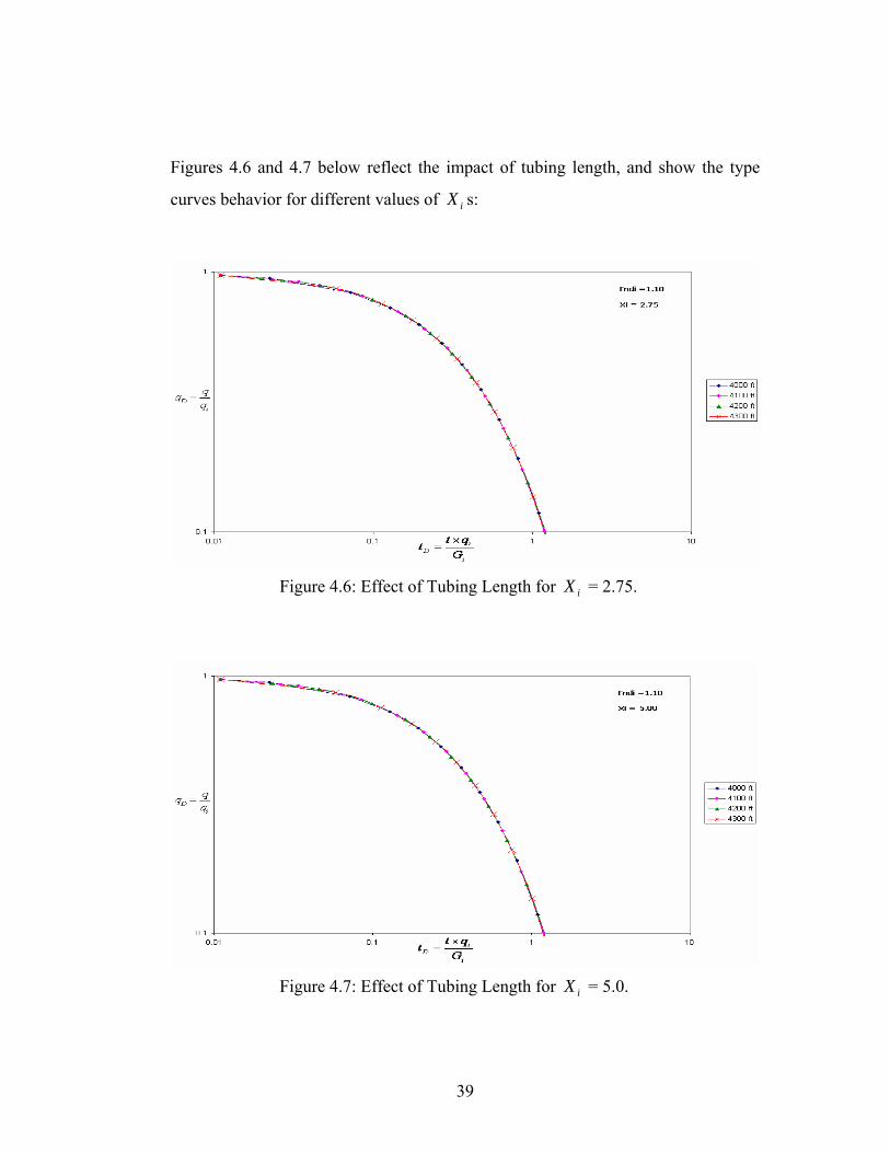
im t of tubing length, and show the type

different values of s:

Figures 4.6 and 4.7 below reflect the pac

iXcurves behavior for

Figure 4.6: Effect of Tubing Length for = 2.75.

iX

Figure 4.7: Effect of Tubing Length for = 5.0. iX

39

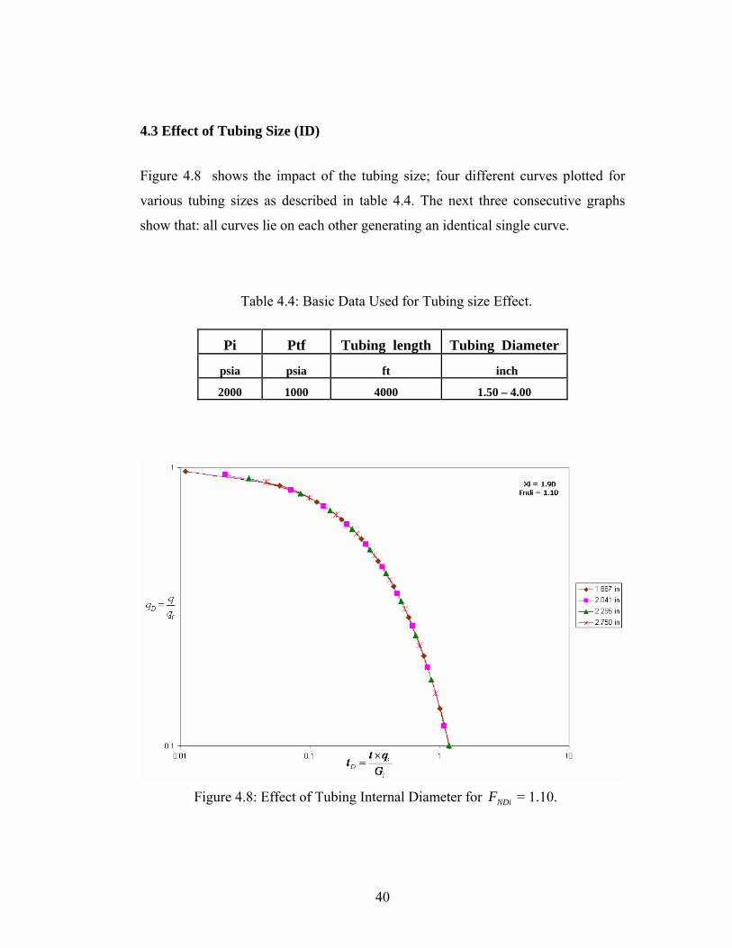
4.3 Effect of Tubing Size (ID)

graphs

show that: all curves lie on each other generating an identical single curve.

Table 4.4: Basic Data Used for Tubing size Effect.

Figure 4.8 shows the impact of the tubing size; four different curves plotted for

various tubing sizes as described in table 4.4. The next three consecutive

Pi Ptf Tubing length Tubing Diameter

psia psia ft inch

2000 1000 4000 1.50 – 4.00

Figure 4.8: Effect of Tubing Internal Diameter for = 1.10. NDiF

40

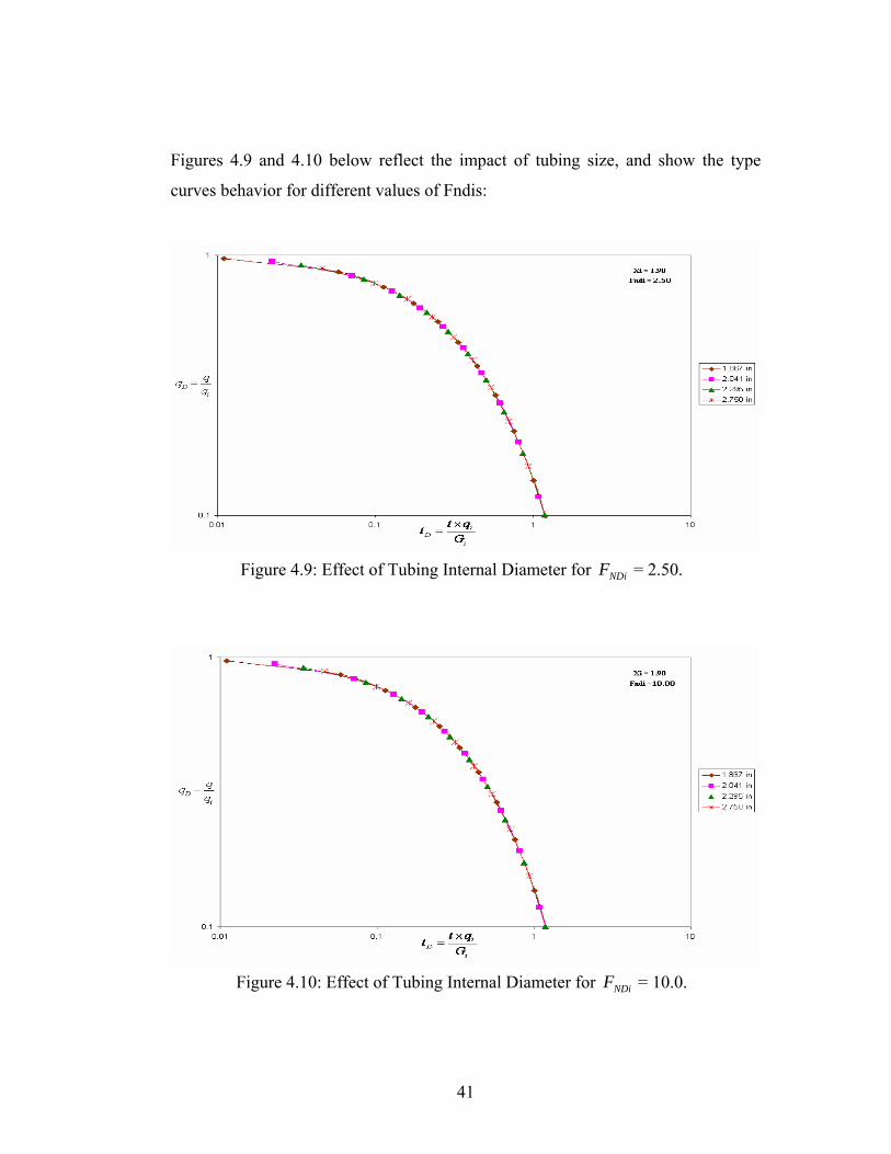
Figures 4.9 and 4.10 below reflect the impact of tubing size, and show the type

urves behavior for different values of Fndis:

c

Figure 4.9: Effect of Tubing Internal Diameter for = 2.50.

NDiF

Figure 4.10: Effect of Tubing Internal Diameter for = 10.0.

NDiF

41

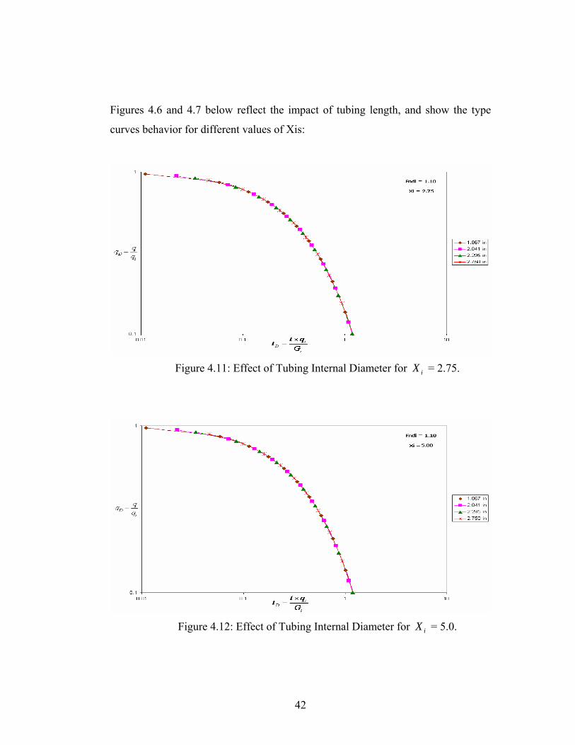
Figures 4.6 and 4.7 below reflect the impact of tubing length, and show the type

urves behavior for different values of Xis:

c

Figure 4.11: Effect of Tubing Internal Diameter for = 2.75.

iX

Figure 4.12: Effect of Tubing Internal Diameter for = 5.0.

iX

42

l single curve. This result obtained regardless of the length of

he Tubing Size (ID) is variable-still all

curves lie on each other for all scenarios.

The results show that , even by changing the dimensionless parameters iX values,

(which here was redefined for the first time, as a ration between the initial shut –in

pressure to the well head pressure), all different type curves lied on each other

generating an identica

the well tubing (TL).

Similar results will be obtained when t

43

CHAPTER 5

CONCLUSIONS AND RECOMMENDATIONS

geological and reservoir data to determine the

enerated to combine the gas deliverability equation for

ting

o generate a set of production

y the decline behavior of gas wells when the

remained as it was.;i.e they do not make any impact on

the decline curve behavior.

ecommendations:

tool integrating the correlations

he impact of fractured well to the type curve behavior.

The main focus of this research was to develop a new model for combining the gas

deliverability equation for reservoir and well and using that generate and introduce

a new set of type curves that could be used to evaluate and predict production data.

The research took into account all

impacts of each on the production.

Based on the results, the following conclusions and recommendations were made:

-A new unique model was g

both reservoir and the well.

-The accuracy of the new model has been tested and verified by genera

hundreds of runs using different scenarios for the reservoir and the well inputs.

-A general model has been developed and utilized t

decline curves for gas well production forecasting. -The model was also utilized to stud

Tubing length and sizes are change.

-It was found that, the decline behavior of a gas well after the tubing sizes and

lengths have been changed,

R

-Development of scientific, user friendly computer

and the type curves for a condensate gas reservoir.

-T

44

REFERENCES

es," Presented

eady-State Gas Flow into Gas Wells,” Jour. PetTech.

1. Fetkovich, M.J., "Decline Curve Analysis Using Type CurvSPEAIME, Las Vegas, Nevada. 1973. (SPE Serial No. 4629).

. Smith, R. V.: “Unst2(M ay 1962), pp.549. . Carter, R.D., "Type Curve for Finite Radial and Lin3 ear Gas Flow System:

formance Using Decline

Gas Pseudo-pressure and Normalized Time,"

e-Curve Analysis: What It Can Do and Can Not

ction

presented at

Approach," Master's Thesis, West

ng Using Automatic

esented at SPE Eastern Regional

the erformance of Gas Well," Morgantown, WV. Masters Thesis, 1992.

Constant-Terminal-Pressure Case," SPEJ, Oct. 1985. . Benjamin H. Thomas, “Predicting Gas Well per4

Curves”, Morgantown, WVU. Master thesis, 1997. 5. Fraim, M.L., Wattenbarger, R.A., “Gas Reservoir Decline-Curve Analysis

sing Type Curves with RealUpaper SPE Serial No. 14238. . Gringarten, C.A., "Typ6

Do," JPT, January 1987. . Aminian, K., Ameri, S., Stark, J.J., Yost II, A.B., "Gas Well Produ7

Decline in Multiwell Reservoirs," JPT, December 1990, P.1573-1579. 8. 20. Abbit, W.E., Ameri, S., Aminian, K.,: " Polynomial Approximations or Gas ,Pseudo pressure and Pseudotime", paper SPE 23439,f

the SPE Eastern Regional Meeting, Lexington, KY, Oct 1991. 9. Dascalescu, B.W., "Production Behavior of Gas Wells During the

nsteady State Period A Type Curve UVirginia U., Morgantown, WVU. 1994. 10. Jonathan Diazgranados, “Gas Production ForecastiType Curve”, Morgantown, WV. Master Thesis, 2000.

11. Aminian, K., Ameri, S., Beg, N., Yost II, A.B., "Production Forecasting f Gas Wells Under Altered Conditions," Pro

Meeting, Pittsburgh, PA. September 1987. 2. Abidi, R.H., "The Effect of Pressure Dependent Gas Properties on 1

P

45

ncepts”

Paper SPE, published in 1999.

ly Developed Fitting Equation” Paper SPE , 75532-S, published in 2001.

A&M

Multiwell Reservoir System” paper SPE 1517, published in 2001.

Using Type Curves - Fractured Wells” SPE , 84287-MS, published in 2003.

icting Gas Wells Production”, Morgantown, WVU. Master Thesis, 1999.

atural Gas Storage, PNGE 471. West Virginia

niversity: Spring 2007.

Natural Gas Engineering, PNGE 470. West Virginia University: Fall 2005.

nted at 1986 SPE Eastern Regional Meeting, Columbus, OH. ov. 12-14.

13. Ram G. Agarwal, SPE, David C. Gardner, SPE, by, Stanley William. Kleinsteiber, SPE, and Del D. Fussell, Amoco, “Analyzing Well Production Data Using Combined-Type-Curve and Decline-Curve Analysis Co

14. Ferhat Zelghi, Sonatrach Inc.; Djebbar Tiab, U. of Oklahoma; Mohamed Mazighi, Sonatrach Inc. “Application of Decline Curve Analysis in Gas Reservoirs Using a NewM

15. T. Marhaendrajana, Schlumberger, and T.A. Blasingame, Texas “Decline Curve Analysis Using Type Curves - Evaluation of Well Performance Behavior in a7 16. H. Pratikno, ConocoPhillips (Indonesia); J.A. Rushing, Anadarko Petroleum Corp.; T.A. Blasingame, Texas A&M U “Decline Curve Analysis

17. Samson Tesfaslasie, “Automatic Type Curve Matching For Pred

18. Aminian, Kashy. NU 19. Aminian, Kashy.

20. Aminian, K., Ameri, S., Hyman, M., “Production Decline Type Curve For Gas Wells Producing Under Pseudo Steady State Condition," paper SPE 15933, preseN

46

APPE DIX

Appendix A

ffect of Tubing Size (ID) with Ptf = 250 psi

N

E

47

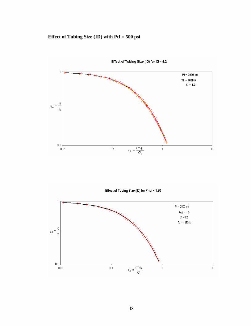
Effect of Tubing Size (ID) with Ptf = 500 psi

48

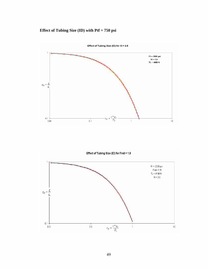
Effect of Tubing Size (ID) with Ptf = 750 psi

49

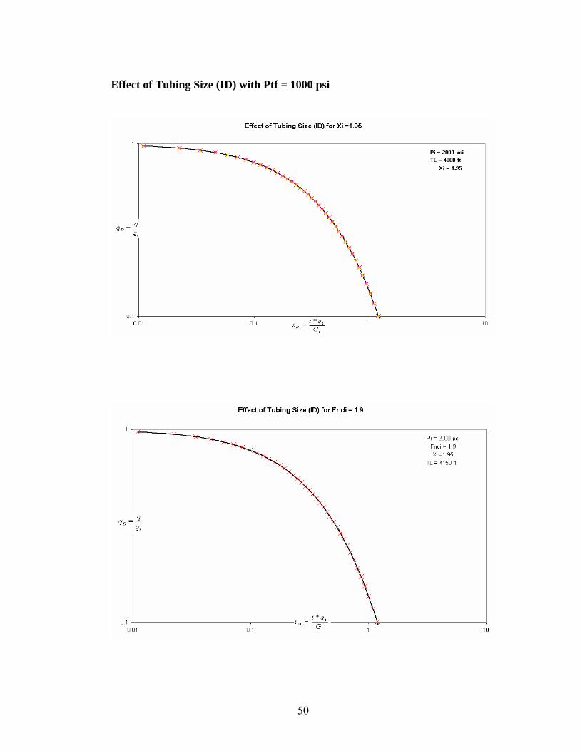
Effect of Tubing Size (ID) with Ptf = 1000 psi

50

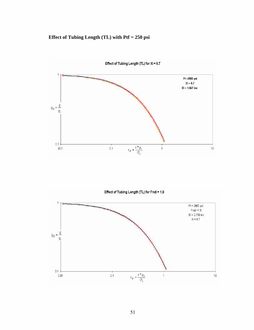
Effect of Tubing Length (TL) with Ptf = 250 psi

51

Effect of Tubing Length (TL) with Ptf = 500 psi

52

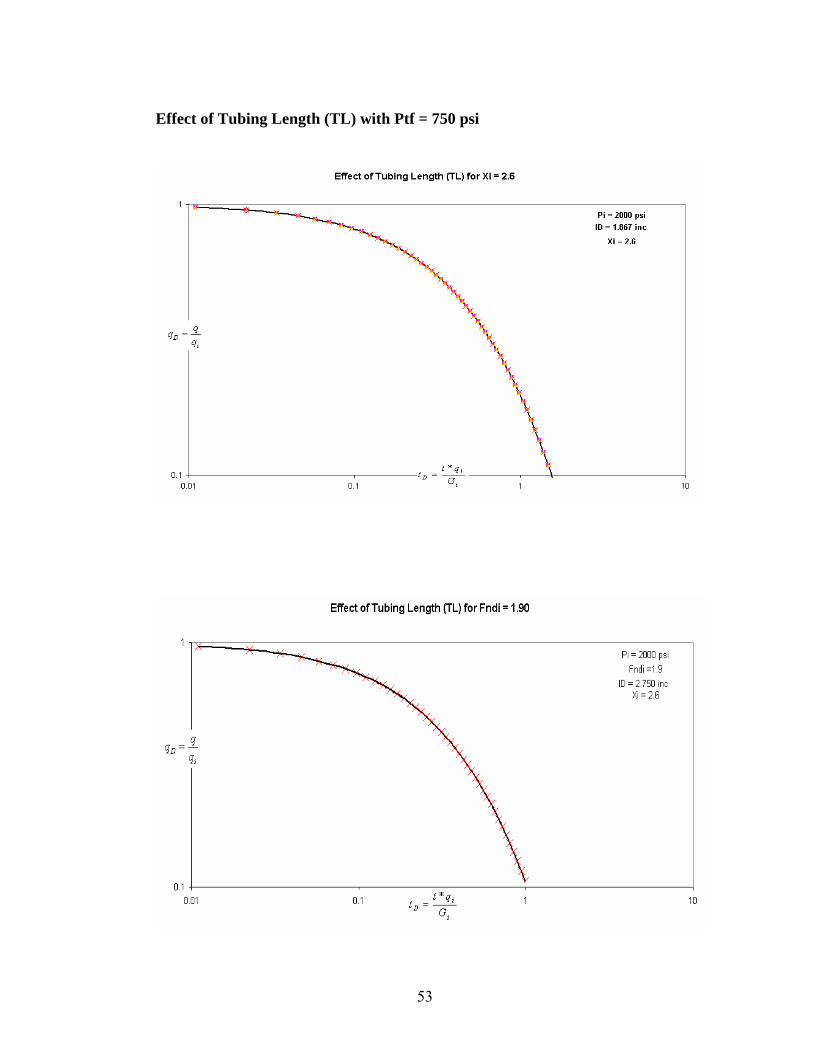
Effect of Tubing Length (TL) with Ptf = 750 psi

53

Effect of Tubing Length (TL) with Ptf = 1000 psi

54

Effect of Non- Darcy to the Type Curve Shape

Effect Xi to the Type Curve Shape

of

55

VITA

Permanent Address: 130 Glen Abbey Ln

Bachelor of Scienc ical Engineering

Master of Science D roleum Engineering July, 2007

Name: Hassan D Eljack

Morgantown, WV 26508 Education: Khartoum University-Sudan

e Degree in ChemDecember 1996

West Virginia University, Morgantown, WV/ USA egree in Pet

56