Embed Size (px)
Citation preview
Enhanced Mode ClusteringYen-Chi Chen, Christopher R. Genovese and Larry Wasserman
Department of StatisticsCarnegie Mellon University
Abstract
Mode clustering is a nonparametric method for clustering that defines clusters using thebasins of attraction of a density estimator’s modes. We provide several enhancements to modeclustering: (i) a soft variant of cluster assignment, (ii) a measure of connectivity between clusters,(iii) a technique for choosing the bandwidth, (iv) a method for denoising small clusters, and(v) an approach to visualizing the clusters. Combining all these enhancements gives us a usefulprocedure for clustering in multivariate problems.
Keywords. Kernel density estimation, nonparametric clustering, soft clustering, visualization
MSC2010. Primary: 62H30, secondary: 62G07, 62G99
1 Introduction
Mode clustering is a nonparametric clustering method (Cheng, 1995; Chazal et al., 2011; Comaniciuand Meer, 2002; Fukunaga and Hostetler, 1975; Li et al., 2007; Arias-Castro et al., 2013) with threesteps: (i) estimate the density function, (ii) find the modes of the estimator, and (iii) define clustersby the basins of attraction of these modes.
There are several advantages to using mode clustering relative to other commonly-used methods:
1. There is a clear population quantity being estimated.
2. Computation is simple: the density can be estimated with a kernel density estimator, andthe modes and basins of attraction can be found with the mean-shift algorithm.
3. There is a single tuning parameter to choose, namely, the bandwidth of the density estimator.
4. It is theoretically well understood since it depends only on density estimation and modeestimation (Arias-Castro et al., 2013; Romano et al., 1988; Romano, 1988).
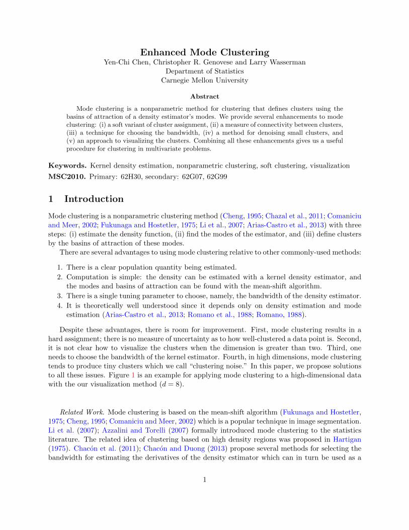
Despite these advantages, there is room for improvement. First, mode clustering results in ahard assignment; there is no measure of uncertainty as to how well-clustered a data point is. Second,it is not clear how to visualize the clusters when the dimension is greater than two. Third, oneneeds to choose the bandwidth of the kernel estimator. Fourth, in high dimensions, mode clusteringtends to produce tiny clusters which we call “clustering noise.” In this paper, we propose solutionsto all these issues. Figure 1 is an example for applying mode clustering to a high-dimensional datawith the our visualization method (d = 8).
Related Work. Mode clustering is based on the mean-shift algorithm (Fukunaga and Hostetler,1975; Cheng, 1995; Comaniciu and Meer, 2002) which is a popular technique in image segmentation.Li et al. (2007); Azzalini and Torelli (2007) formally introduced mode clustering to the statisticsliterature. The related idea of clustering based on high density regions was proposed in Hartigan(1975). Chacon et al. (2011); Chacon and Duong (2013) propose several methods for selecting thebandwidth for estimating the derivatives of the density estimator which can in turn be used as a
1
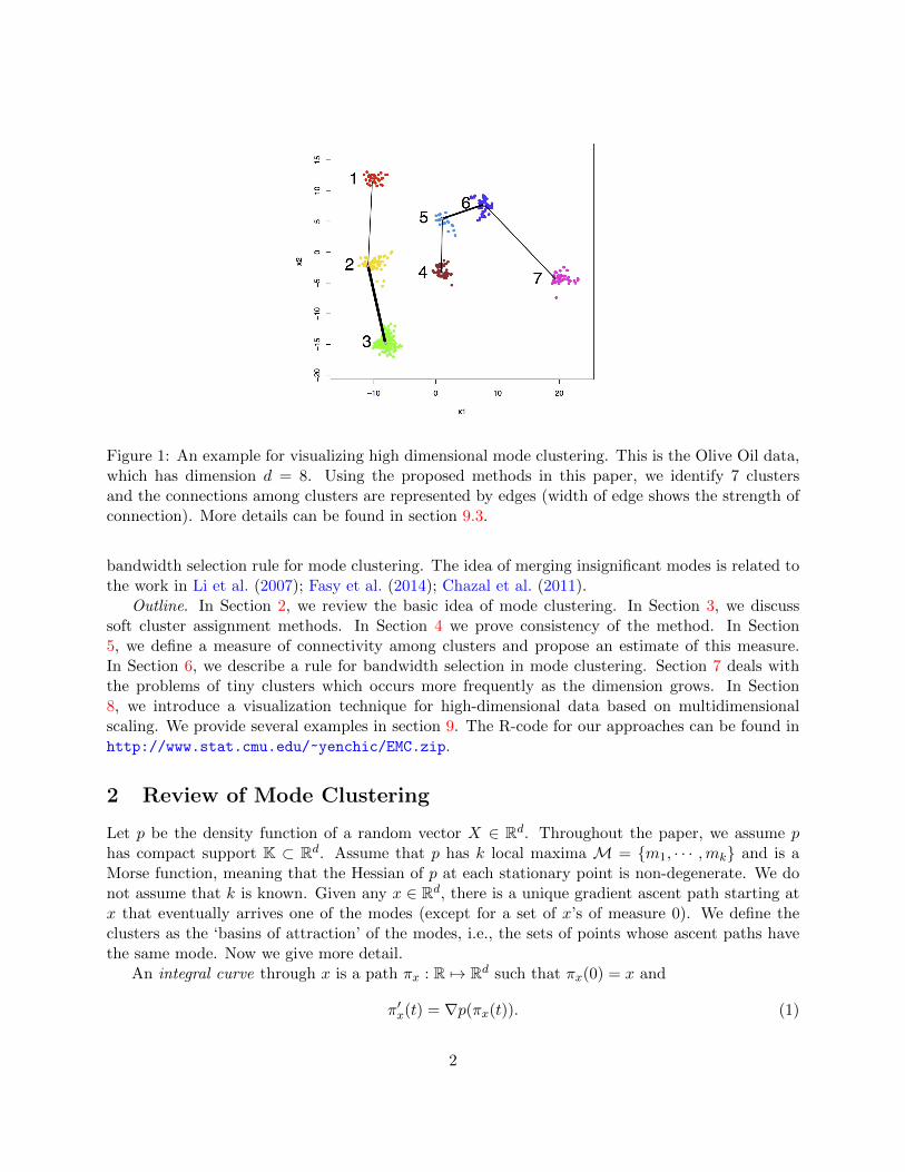
Figure 1: An example for visualizing high dimensional mode clustering. This is the Olive Oil data,which has dimension d = 8. Using the proposed methods in this paper, we identify 7 clustersand the connections among clusters are represented by edges (width of edge shows the strength ofconnection). More details can be found in section 9.3.
bandwidth selection rule for mode clustering. The idea of merging insignificant modes is related tothe work in Li et al. (2007); Fasy et al. (2014); Chazal et al. (2011).
Outline. In Section 2, we review the basic idea of mode clustering. In Section 3, we discusssoft cluster assignment methods. In Section 4 we prove consistency of the method. In Section5, we define a measure of connectivity among clusters and propose an estimate of this measure.In Section 6, we describe a rule for bandwidth selection in mode clustering. Section 7 deals withthe problems of tiny clusters which occurs more frequently as the dimension grows. In Section8, we introduce a visualization technique for high-dimensional data based on multidimensionalscaling. We provide several examples in section 9. The R-code for our approaches can be found inhttp://www.stat.cmu.edu/~yenchic/EMC.zip.
2 Review of Mode Clustering
Let p be the density function of a random vector X ∈ Rd. Throughout the paper, we assume phas compact support K ⊂ Rd. Assume that p has k local maxima M = m1, · · · ,mk and is aMorse function, meaning that the Hessian of p at each stationary point is non-degenerate. We donot assume that k is known. Given any x ∈ Rd, there is a unique gradient ascent path starting atx that eventually arrives one of the modes (except for a set of x’s of measure 0). We define theclusters as the ‘basins of attraction’ of the modes, i.e., the sets of points whose ascent paths havethe same mode. Now we give more detail.
An integral curve through x is a path πx : R 7→ Rd such that πx(0) = x and
π′x(t) = ∇p(πx(t)). (1)
2
(a) Attraction basins (b) Mean shift
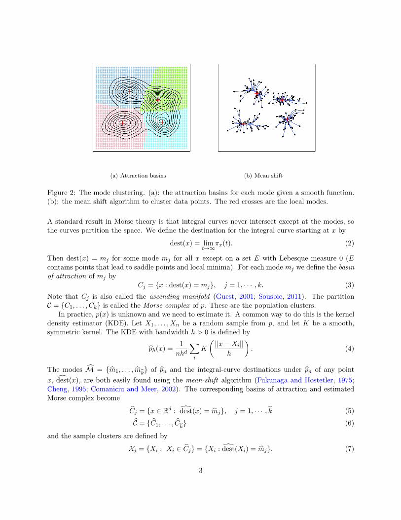
Figure 2: The mode clustering. (a): the attraction basins for each mode given a smooth function.(b): the mean shift algorithm to cluster data points. The red crosses are the local modes.
A standard result in Morse theory is that integral curves never intersect except at the modes, sothe curves partition the space. We define the destination for the integral curve starting at x by
dest(x) = limt→∞
πx(t). (2)
Then dest(x) = mj for some mode mj for all x except on a set E with Lebesque measure 0 (Econtains points that lead to saddle points and local minima). For each mode mj we define the basinof attraction of mj by
Cj = x : dest(x) = mj, j = 1, · · · , k. (3)
Note that Cj is also called the ascending manifold (Guest, 2001; Sousbie, 2011). The partitionC = C1, . . . , Ck is called the Morse complex of p. These are the population clusters.
In practice, p(x) is unknown and we need to estimate it. A common way to do this is the kerneldensity estimator (KDE). Let X1, . . . , Xn be a random sample from p, and let K be a smooth,symmetric kernel. The KDE with bandwidth h > 0 is defined by
ph(x) =1
nhd
∑i
K
( ||x−Xi||h
). (4)
The modes M = m1, . . . , mk of pn and the integral-curve destinations under pn of any point
x, dest(x), are both easily found using the mean-shift algorithm (Fukunaga and Hostetler, 1975;Cheng, 1995; Comaniciu and Meer, 2002). The corresponding basins of attraction and estimatedMorse complex become
Cj = x ∈ Rd : dest(x) = mj, j = 1, · · · , k (5)
C = C1, . . . , Ck (6)
and the sample clusters are defined by
Xj = Xi : Xi ∈ Cj = Xi : dest(Xi) = mj. (7)
3
3 Soft Clustering
Mode clustering is a type of hard clustering, where each observation is assigned to one and only onecluster. Soft clustering methods (McLachlan and Peel, 2004; Lingras and West, 2002; Nock andNielsen, 2006; Peters et al., 2013) attempt to capture the uncertainty in this assignment. This istypically represented by an assignment vector for each point that is a probability distribution overthe clusters. For example, whereas a hard-clustering method might assign a point x to cluster 2, asoft clustering might give x an assignment vector a(x) = (0.01, 0.8, 0.01, 0.08, 0.1), reflecting boththe high confidence that x belongs to cluster 2 the nontrivial possibility that it belongs to cluster5.
Soft clustering can capture two types of cluster uncertainty: population level (intrinsic difficulty)and sample level (variability). The population level uncertainty originates from the fact that evenif p is known, some points are more strongly related to their modes than others. Specifically, for apoint x near the boundaries between two clusters, say C1, C2, the associated soft assignment vectora(x) should have a1(x) ≈ a2(x). The sample level uncertainty comes from the fact that p has beenestimated by p. The soft assignment vector a(x) is designed to capture both types of uncertainty.
Remark: The most common soft-clustering method is to use a mixture model. In this approach,we represent cluster membership by a latent variable and use the estimated distribution of thatlatent variable as the assignment vector. In the appendix we discuss mixture-based soft clustering.
3.1 Soft Mode Clustering
A straightforward way to obtain soft mode clustering is to us a distance from a given point x to allthe local modes. The idea is simple: if x is close to a mode mj , the soft assignment vector shouldhave a higher aj(x). We describe a method based on level set distance in appendix B. However,converting a distance to a soft assignment vector has a problem: we need a way to choose theconversion.
We now present a direct method based on diffusion that does not require any conversion ofdistance. Consider starting a diffusion at x. We define the soft cluserting as the probability thatthe diffusion starting at x leads to a particular mode, before hitting any other mode. That is, letaHP (x) = (aHP1 (x), . . . , aHPk (x)) where aHPj (x) is the conditional probability that mode j is thefirst mode reached by the diffusion, given that it reaches one of the modes. In this case a(x) is aprobability vector and so is easy to interpret.
In more detail, let
Kh(x, y) = K
(‖x− y‖h
).
Then
qh(y|x) =Kh(x, y)p(y)∫Kh(x, y)dP (y)
,
defines a Markov process with qh(y|x) being the probability of jumping to y given that the processis at x. Fortunately, we do not actually have to run the diffusion to estimate aHP (x).
An approximation to the above diffusion process restricted to x, y in m1, . . . , mk, X1, . . . , Xn
is as follows. We define a Markov chain that has k + n states. The first k states are the estimatedlocal modes m1, . . . , mk
and are absorbing states. That is, the Markov process stops when it hits
any of the first k state. The other n states correspond to the data points X1, . . . , Xn. The transition
4
probability from each Xi is given by
P(Xi → ml) =Kh(Xi, mj)∑n
j=1Kh(Xi, Xj) +∑k
l=1Kh(Xi, ml)
P(Xi → Xj) =Kh(Xi, Xj)∑n
j=1Kh(Xi, Xj) +∑k
l=1Kh(Xi, ml)
(8)
for i, j = 1, . . . , n and l = 1, . . . , k. Thus, the transition matrix P is
P =
[I 0S T
], (9)
where I is the identity matrix and S is an n × k matrix with element Sij = P(Xi → mj) and Tis an n× n matrix with element Tij = P(Xi → Xj). Then by Markov chain theory, the absorbing
probability from Xi onto mj is given by Aij where Aij is the (i, j)-th element of the matrix
A = S(I− T )−1. (10)
We define the soft assignment vector by aHPj (Xi) = Aij .Remark: In addition to the level set distance in appendix, other distance metric such as density
distance (Dijkstra, 1959; Bousquet et al., 2004; Sajama and Orlitsky, 2005; Cormen et al., 2009;Bijral et al., 2011; Hwang et al., 2012; Alamgir and von Luxburg, 2012), diffusion distance (Nadleret al., 2005; Coifman and Lafon, 2006; Lee and Wasserman, 2010) can be applied to obtain thesoft-assignment vector.
4 Consistency
Here we discuss the consistency of mode clustering. Despite large amount of literature on theconsistency for estimating a global mode (Romano, 1988; Romano et al., 1988; Pollard, 1985),there is less work on estimating local modes.
Here we adapt the result in Chen et al. (2014b) to describe the consistency of estimating localmodes in terms of the Hausdorff distance. For two sets A,B, the Hausdorff distance is
Haus(A,B) = infr : A ⊂ B ⊕ r,B ⊂ A⊕ r, (11)
where A⊕ r = y : minx∈A ‖x− y‖ ≤ r.Let K(α) be the α-th derivative of K and BCr denotes the collection of functions with bounded
continuously derivatives up to the r-th order. We consider the following two common assumptionson kernel function:
(K1) The kernel function K ∈ BC3 and is symmetric, non-negative and∫x2K(α)(x)dx <∞,
∫ (K(α)(x)
)2dx <∞
for all α = 0, 1, 2, 3.
5
(K2) The kernel function satisfies condition K1 of Gine and Guillou (2002). That is, there existssome A, v > 0 such that for all 0 < ε < 1, supQN(K, L2(Q), CKε) ≤
(Aε
)v, where N(T, d, ε)
is the ε−covering number for a semi-metric space (T, d) and
K =
u 7→ K(α)
(x− uh
): x ∈ Rd, h > 0, |α| = 0, 1, 2, 3
.
The assumption (K1) is a smoothness condition on the kernel function and is commonly assumedto obtain the rate of convergence for the KDE to estimate derivatives of density. (K2) ensures thatthe complexity of KDE does not grow too quickly as the smoothing parameter h converges to 0. (K2)will be used for the rate in terms of L∞ metric for KDE. This condition is a common assumption(Gine and Guillou, 2002; Einmahl and Mason, 2005; Genovese et al., 2012; Arias-Castro et al.,2013; Chen et al., 2014a).
Theorem 1 (Consistency of Estimating Local Modes). Assume p ∈ BC3 and the kernel functionK satisfies (K1-2). Let C3 be the bound for the partial derivatives of p up to the third order and
Mn ≡ M be the collection of local modes of the KDE pn and M be the local modes of p. Let Kn
be the number of estimated local modes and K be the number of true local modes. Assume
(M1) There exists λ∗ > 0 such that
0 < λ∗ ≤ |λ1(mj)|, j = 1, · · · ,K,
where λ1(x) ≤ · · · ≤ λd(x) are the eigenvalues of Hessian matrix of p(x).
(M2) There exists η1 > 0 such that
x : ‖∇p(x)‖ ≤ η1, 0 > −λ∗/2 ≥ λ1(x) ⊂ M⊕ λ∗2dC3
,
where λ∗ is defined in (M1).
Then when h is sufficiently small and n is sufficiently large,
1. (Modal consistency) there exists some constants A,C > 0 such that
P(Kn 6= K
)≤ Ae−Cnhd+4
;
2. (Location convergence) the Hausdorff distance between local modes and their estimators sat-sifies
Haus(Mn,M
)= O(h2) +OP
(√1
nhd+2
).
The proof is in appendix. The assumption (M1) is very mild; it is a simple regularity conditionon the eigenvalue. The second condition (M2) is a regularity on p which requires that points withsimilar behavior (near 0 gradient and negative eigenvalues) to local modes must be close to localmodes. Theorem 1 states two results: a consistency on estimating the number of local modes and aconsistency on estimating the location of local modes. An intuitive explanation for the first result
6
is from the fact that as long as the gradient and Hessian matrix of KDE pn are sufficiently closedto the true gradient and Hessian matrix, condition (M1, M2) guarantee the number of local modesis the same as truth. Applying Talagrand’s inequality (Talagrand, 1996) so that we obtain theexponential concentration which gives the desire result. The second result follows from applyingTaylor expansion over each local modes on the gradient (since local modes have 0 gradient), thedifference between local modes and their estimators is in proportional to the error in estimatingthe gradients. The rate of Hausdorff distance can be decomposed into bias O(h2) and variance
OP
(√1
nhd+2
).
5 Measuring Cluster Connectivity
In this section, we propose a technique that uses the soft-assignment vector to measure the con-nectivity among clusters. Note that the clusters here are generated by the usual (hard) modeclustering.
Let p be the density function and C1, . . . , Ck be the clusters corresponding to the local modesm1, . . . ,mk. For a given soft assignment vector a(x) : Rd 7→ Rk, we define the connectivity ofcluster i and cluster j by
Ωij =1
2
(E(ai(X)|X ∈ Cj
)+ E
(aj(X)|X ∈ Ci
))=
1
2
∫Ciaj(x)p(x)dx∫Cip(x)dx
+1
2
∫Cjai(x)p(x)dx∫Cjp(x)dx
.(12)
Each Ωij is a population level quantity that depends only on how we determine the soft assignmentvector. Connectivity will be large when two clusters are close and the boundary between them hashigh density. If we think of the (hard) cluster assignments as class labels, connectivity is analogousto the mis-classification rate between class i and class j.
An estimator of Ωij is
Ωij =1
2
( 1
Ni
n∑l=1
aj(Xl)1(Xl ∈ Ci) +1
Nj
n∑l=1
ai(Xl)1(Xl ∈ Cj)), i, j = 1, . . . , k, (13)
where Ni =∑n
l=1 1(Xl ∈ Ci) is the number of sample in cluster Ci. Note that the estimator
Ωij might be different to Ωij up to a permutation over rows and columns. The matrix Ωij is a
summary statistics for the connectivity between clusters. We call Ω the matrix of connectivity orthe connectivity matrix.
The matrix Ω is useful as a dimension-free, summary-statistic to describe the degree of over-lap/interaction among the clusters, which is hard to observe directly when d > 2. Later we willuse Ω to describe the relations among clusters while visualizing the data.
6 Bandwidth Selection
A key problem in mode clustering (as in so much else) is the choice of the smoothing bandwidth h.Because mode clustering is based on the gradient of the density function, we choose a bandwidth
7
targeted at gradient estimation. From standard non-parametric density estimation theory, theestimated gradient and the true gradient differ by
‖∇pn(x)−∇p(x)‖22 = O(h4) +OP
( 1
nhd+2
)(14)
assuming p has two smooth derivatives, see Chacon et al. (2011); Arias-Castro et al. (2013). Acommon risk measure for density estimation is the mean integrated square errors (MISE). TheMISE can be generalized to gradient estimation by
MISE(∇pn) = E(∫‖∇pn(x)−∇p(x)‖22dx
). (15)
The rate is given by the following:
Theorem 2. [Theorem 4 of (Chacon et al., 2011)] Assume p ∈ BC3 and (K1). Then
MISE(∇pn) = O(h4)
+O
(1
nhd+2
). (16)
It follows that the asymptotically optimal bandwidth should be
h = Cn−1
d+6 , (17)
for some constant C. In practice, we do not know C, so we need a concrete rule to select it. Chaconand Duong (2013) proposes four different methods to find h: the normal reference rule (Silverman,1986; Chacon et al., 2011), cross-validation, plug-in, and smoothed cross validation. The normalreference rule (a slight modification of Chacon et al. (2011)) is
hNR = Sn ×( 4
d+ 4
) 1d+6
n−1
d+6 , (18)
where Sn is the mean of sample standard deviation along each coordinate defined in (43). Weuse this for two reasons. First, it is known that the normal reference rule tends to oversmooth(Sheather, 2004), which is typically good for clustering. And second, the normal reference rule iseasy to compute even in high dimensions.
A related risk measure for the estimator ∇pn is the L∞ norm, defined by
‖∇pn −∇p‖max,∞ = supx‖∇pn(x)−∇p(x)‖max, (19)
where ‖v‖max is the maximal norm for a vector v. The rate for L∞ is given by the followings:
Theorem 3. Assume p ∈ BC3 and (K1–2). Then
‖∇pn −∇p‖max,∞ = O(h2)
+OP
(√log n
nhd+2
). (20)
8
This result appears in Genovese et al. (2009, 2012); Arias-Castro et al. (2013); Chen et al.(2014a) and can be proved by the techniques in Gine and Guillou (2002); Einmahl and Mason(2005). This suggests selecting the bandwidth by
h = C ′(
log n
n
) 1d+6
. (21)
However, no general rule has been proposed based on this norm. The main difficulty is that noanalytical form for the big O term has been found.
Remark. Comparing the assumptions in Theorem 1, 2 and 3 give an interesting result. If weassume p ∈ BC3 and (K1), we obtain consistency in terms of MISE. If further we assume (K2), weget the consistency in terms of supremum-norm. Finally, if we have conditions (M1-2), we obtainthe mode consistency.
7 Denoising Small Clusters
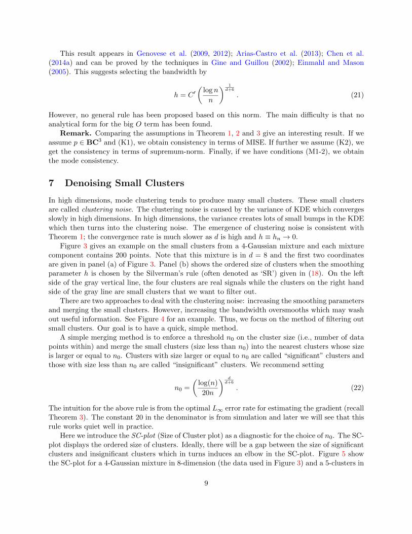
In high dimensions, mode clustering tends to produce many small clusters. These small clustersare called clustering noise. The clustering noise is caused by the variance of KDE which convergesslowly in high dimensions. In high dimensions, the variance creates lots of small bumps in the KDEwhich then turns into the clustering noise. The emergence of clustering noise is consistent withTheorem 1; the convergence rate is much slower as d is high and h ≡ hn → 0.
Figure 3 gives an example on the small clusters from a 4-Gaussian mixture and each mixturecomponent contains 200 points. Note that this mixture is in d = 8 and the first two coordinatesare given in panel (a) of Figure 3. Panel (b) shows the ordered size of clusters when the smoothingparameter h is chosen by the Silverman’s rule (often denoted as ‘SR’) given in (18). On the leftside of the gray vertical line, the four clusters are real signals while the clusters on the right handside of the gray line are small clusters that we want to filter out.
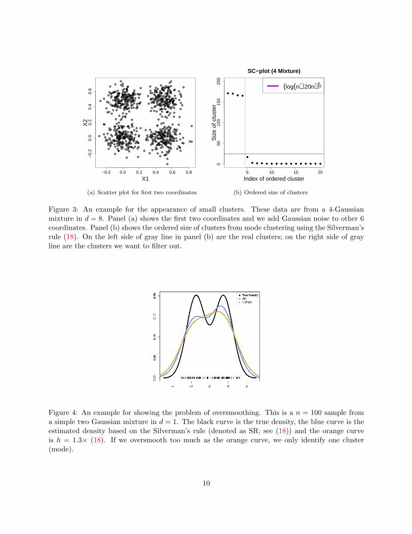
There are two approaches to deal with the clustering noise: increasing the smoothing parametersand merging the small clusters. However, increasing the bandwidth oversmooths which may washout useful information. See Figure 4 for an example. Thus, we focus on the method of filtering outsmall clusters. Our goal is to have a quick, simple method.
A simple merging method is to enforce a threshold n0 on the cluster size (i.e., number of datapoints within) and merge the small clusters (size less than n0) into the nearest clusters whose sizeis larger or equal to n0. Clusters with size larger or equal to n0 are called “significant” clusters andthose with size less than n0 are called “insignificant” clusters. We recommend setting
n0 =
(log(n)
20n
) dd+6
. (22)
The intuition for the above rule is from the optimal L∞ error rate for estimating the gradient (recallTheorem 3). The constant 20 in the denominator is from simulation and later we will see that thisrule works quiet well in practice.
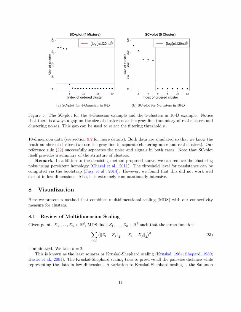
Here we introduce the SC-plot (Size of Cluster plot) as a diagnostic for the choice of n0. The SC-plot displays the ordered size of clusters. Ideally, there will be a gap between the size of significantclusters and insignificant clusters which in turns induces an elbow in the SC-plot. Figure 5 showthe SC-plot for a 4-Gaussian mixture in 8-dimension (the data used in Figure 3) and a 5-clusters in
9
−0.2 0.0 0.2 0.4 0.6 0.8
−0.
20.
00.
20.
40.
6
X1
X2
(a) Scatter plot for first two coordinates
5 10 15 20
050
100
150
200
SC−plot (4 Mixture)
Index of ordered cluster
Siz
e of
clu
ster
(log(n) 20n) dd+6
(b) Ordered size of clusters
Figure 3: An example for the appearance of small clusters. These data are from a 4-Gaussianmixture in d = 8. Panel (a) shows the first two coordinates and we add Gaussian noise to other 6coordinates. Panel (b) shows the ordered size of clusters from mode clustering using the Silverman’srule (18). On the left side of gray line in panel (b) are the real clusters; on the right side of grayline are the clusters we want to filter out.
Figure 4: An example for showing the problem of oversmoothing. This is a n = 100 sample froma simple two Gaussian mixture in d = 1. The black curve is the true density, the blue curve is theestimated density based on the Silverman’s rule (denoted as SR; see (18)) and the orange curveis h = 1.3× (18). If we oversmooth too much as the orange curve, we only identify one cluster(mode).
10
5 10 15 20
050
100
150
200
SC−plot (4 Mixture)
Index of ordered cluster
Siz
e of
clu
ster
(log(n) 20n) dd+6
(a) SC-plot for 4-Gaussian in 8-D
2 4 6 8 10 12
010
020
030
040
0
SC−plot (5 Cluster)
Index of ordered cluster
Siz
e of
clu
ster
(log(n) 20n) dd+6
(b) SC-plot for 5-clusters in 10-D
Figure 5: The SC-plot for the 4-Gaussian example and the 5-clusters in 10-D example. Noticethat there is always a gap on the size of clusters near the gray line (boundary of real clusters andclustering noise). This gap can be used to select the filtering threshold n0.
10-dimension data (see section 9.2 for more details). Both data are simulated so that we know thetruth number of clusters (we use the gray line to separate clustering noise and real clusters). Ourreference rule (22) successfully separates the noise and signals in both cases. Note that SC-plotitself provides a summary of the structure of clusters.
Remark. In addition to the denoising method proposed above, we can remove the clusteringnoise using persistent homology (Chazal et al., 2011). The threshold level for persistence can becomputed via the bootstrap (Fasy et al., 2014). However, we found that this did not work wellexcept in low dimensions. Also, it is extremely computationally intensive.
8 Visualization
Here we present a method that combines multidimensional scaling (MDS) with our connectivitymeasure for clusters.
8.1 Review of Multidimension Scaling
Given points X1, . . . , Xn ∈ Rd, MDS finds Z1, . . . , Zn ∈ Rk such that the stress function∑i<j
(‖Zi − Zj‖2 − ‖Xi −Xj‖2
)2(23)
is minimized. We take k = 2.This is known as the least squares or Kruskal-Shephard scaling (Kruskal, 1964; Shepard, 1980;
Hastie et al., 2001). The Kruskal-Shephard scaling tries to preserve all the pairwise distance whilerepresenting the data in low dimension. A variation to Kruskal-Shephard scaling is the Sammon
11
mapping which minimizes ∑i 6=j
(‖Zi − Zj‖2 − ‖Xi −Xj‖2
)2‖Xi −Xj‖2
. (24)
The Sammon mapping put more weights on the pairs with less distance.In the current paper, we use classical MDS (also known as principal coordinate analysis). The
classical MDS is to find Z1, . . . , Zn ∈ Rk that minimizes∑i,j
∣∣(Zi − Zn)T (Zj − Zn)− (Xi − Xn)T (Xj − Xn)∣∣2 . (25)
Note Zn = 1n
∑ni=1 Zi. A nice feature for classical MDS is the existence of a closed-form solution
to Zi’s. Let S be a n× n matrix with element
Sij = (Xi − Xn)T (Xj − Xn).
Let λ1 > λ2 > · · · > λn be the eigenvalues of S and v1, . . . , vn ∈ Rn be the associated eigenvectors.We denote Vk = [v1, . . . , vk] and Dk = Diag(
√λ1, . . . ,
√λk) be a k × k diagonal matrix. Then it is
known that each Zi is the i-th row of VkDk (Hastie et al., 2001). In our visualization, we constraink = 2.
8.2 Two-stage Multidimensional Scaling
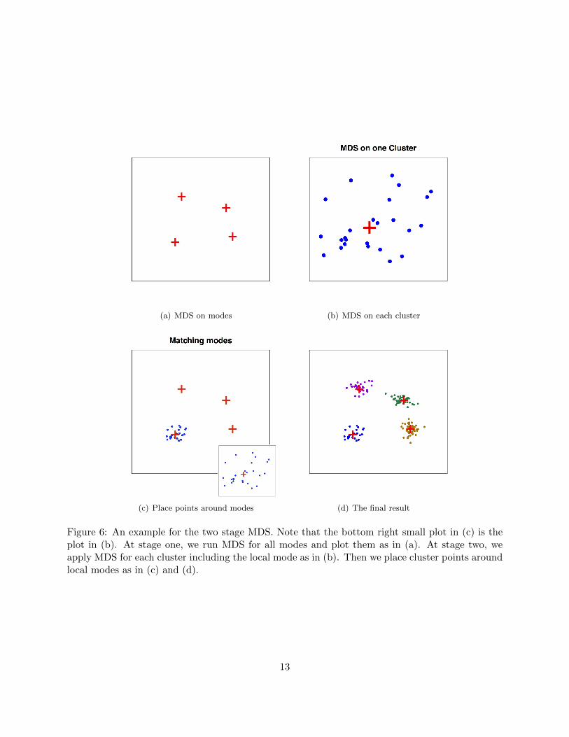
Our approach consists of two stages. At the first stage, we apply MDS on the modes and plotthe result in R2. At the second stage, we apply MDS to points within each cluster along with theassociated mode. Then we place the points around the projected modes. We scale the MDS resultat the first stage by a factor ρ0 so that each cluster is separated from each other. Figure 6 givesan example.
Recall that M = m1, . . . , mk is the set of estimated local modes and Xj is the set of data
points belonging to mode mj . At the first stage, we perform MDS on M so that
m1, . . . , mk MDS
=⇒ m†1, . . . , m†k, (26)
where m†j ∈ R2 for j = 1, . . . , k. We plot m†1, . . . , m†k.At the second stage, we consider each cluster individually. Assume we are working on the
j-th cluster and mj ,Xj are the corresponding local mode and cluster points. We denote Xj =Xj1, . . . , XjNj, where Nj is the sample size for cluster j. Then we apply MDS to the collectionof points mj , Xj1, Xj2, . . . , XjNj:
mj , Xj1, Xj2, . . . , XjNjMDS=⇒ m∗j , X∗j1, X∗j2, . . . , X∗jNj
, (27)
where m∗j , X∗j1, X
∗j2, . . . , X
∗jNj∈ R2. Then we center the points at m†j and place X∗j1, X
∗j2, . . . , X
∗jNj
around m†j . That is, we make a translation to the set m∗j , X∗j1, X∗j2, . . . , X∗jNj so that m∗j matches
the location of m†j . Then we plot the translated points X∗j1, X∗j2, . . . , X
∗jNj
. We repeat the aboveprocess for each cluster to visualize the high dimensional clustering.
Note that in practice, the above process may cause unwanted overlap among clusters. Thus,one can scale m†1, . . . , m†k by a factor ρ0 > 1 to remove the overlap.
An alternative method for visualization is to use the landmark MDS (Silva and Tenenbaum,2002; De Silva and Tenenbaum, 2004) and treats each local mode as the landmark points.
12
(a) MDS on modes (b) MDS on each cluster
(c) Place points around modes (d) The final result
Figure 6: An example for the two stage MDS. Note that the bottom right small plot in (c) is theplot in (b). At stage one, we run MDS for all modes and plot them as in (a). At stage two, weapply MDS for each cluster including the local mode as in (b). Then we place cluster points aroundlocal modes as in (c) and (d).
13
8.3 Connectivity Graph
We can improve the visualization of the previous subsection by accounting for the connectivity ofthe clusters. We apply the connectivity measure introduced in section 5. Let Ω be the matrix forthe connectivity measure defined in (13). We connect two clusters, say i and j, by a straight lineif the connectivity measure Ωij > ω0, a pre-specified threshold. Our experiments show that
ω0 =1
2× number of clusters(28)
is a good default choice. We can adjust the width of the connection line between clusters to showthe strength of connectivity. See Figure 12 panel (a) for an example; the edge linking clusters (2,3)is much thicker than any other edge.
Algorithm 1 summarizes the process of visualizing high dimensional clustering. Note that thesmoothing bandwidth h and the thresholding of cluster size n0 can be chosen by the methodsproposed in section 6. The rest two parameters ρ0 and ω0 are visualizing parameters; they are notinvolved in any analysis so that one can change these parameters on free will.
Algorithm 1 Visualization for Mode Clustering
Input: Data X = Xi : i = 1, . . . , n, bandwidth h, parameters n0, ρ0, ω0.
Phase 1: Mode clustering1. Use the mean shift algorithm for clustering based on bandwidth h.2. (Optional) Thresholding the size of each cluster by n0 and merge the small clusters to largeclusters.
Phase 2: Dimension reductionLet (mj ,Xj) : j = 1, . . . , k be the pairs of local modes and the associated data points.3. Perform MDS to each (mj ,Xj) to get (m∗j ,X ∗j ).
4. Perform MDS to modes only to get m†1, . . . , m†k.5. Place each M †j = ρ0 × m†j on the reduced coordinate.
6. Place each (mj ,Xj) around M †j by matching mj → M †j .
Phase 3: Connectivity measure7. Estimate Ωij by (13) and one of the above soft clustering methods.
8. Connect M †i , M†j if Ωij > ω0.
9 Experiments
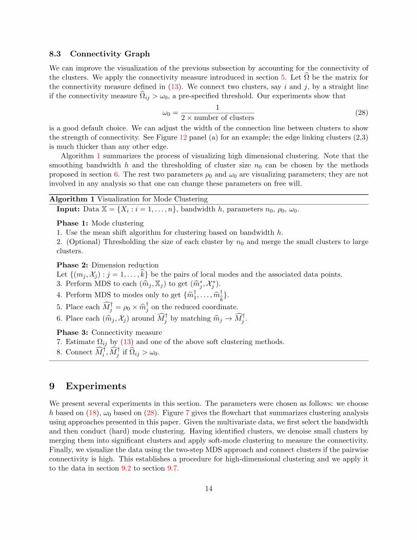
We present several experiments in this section. The parameters were chosen as follows: we chooseh based on (18), ω0 based on (28). Figure 7 gives the flowchart that summarizes clustering analysisusing approaches presented in this paper. Given the multivariate data, we first select the bandwidthand then conduct (hard) mode clustering. Having identified clusters, we denoise small clusters bymerging them into significant clusters and apply soft-mode clustering to measure the connectivity.Finally, we visualize the data using the two-step MDS approach and connect clusters if the pairwiseconnectivity is high. This establishes a procedure for high-dimensional clustering and we apply itto the data in section 9.2 to section 9.7.
14
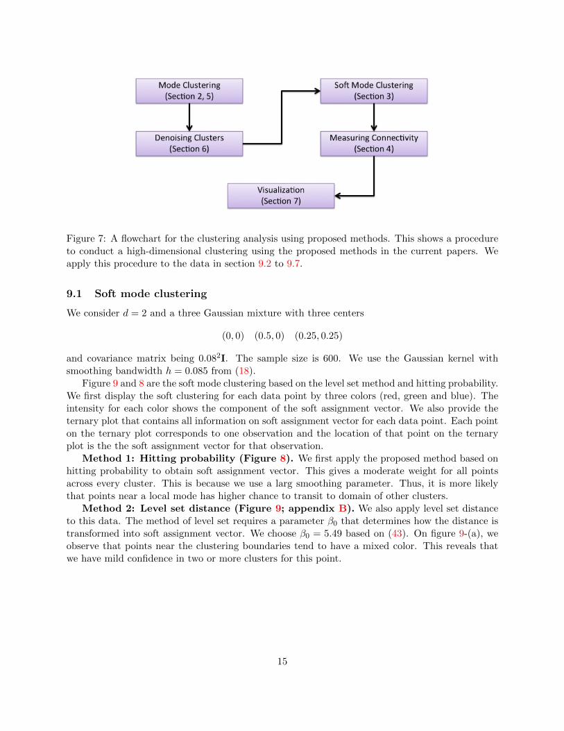
Figure 7: A flowchart for the clustering analysis using proposed methods. This shows a procedureto conduct a high-dimensional clustering using the proposed methods in the current papers. Weapply this procedure to the data in section 9.2 to 9.7.
9.1 Soft mode clustering
We consider d = 2 and a three Gaussian mixture with three centers
(0, 0) (0.5, 0) (0.25, 0.25)
and covariance matrix being 0.082I. The sample size is 600. We use the Gaussian kernel withsmoothing bandwidth h = 0.085 from (18).
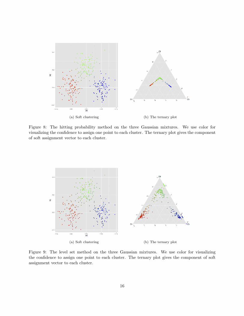
Figure 9 and 8 are the soft mode clustering based on the level set method and hitting probability.We first display the soft clustering for each data point by three colors (red, green and blue). Theintensity for each color shows the component of the soft assignment vector. We also provide theternary plot that contains all information on soft assignment vector for each data point. Each pointon the ternary plot corresponds to one observation and the location of that point on the ternaryplot is the the soft assignment vector for that observation.
Method 1: Hitting probability (Figure 8). We first apply the proposed method based onhitting probability to obtain soft assignment vector. This gives a moderate weight for all pointsacross every cluster. This is because we use a larg smoothing parameter. Thus, it is more likelythat points near a local mode has higher chance to transit to domain of other clusters.
Method 2: Level set distance (Figure 9; appendix B). We also apply level set distanceto this data. The method of level set requires a parameter β0 that determines how the distance istransformed into soft assignment vector. We choose β0 = 5.49 based on (43). On figure 9-(a), weobserve that points near the clustering boundaries tend to have a mixed color. This reveals thatwe have mild confidence in two or more clusters for this point.
15
(a) Soft clustering (b) The ternary plot
Figure 8: The hitting probability method on the three Gaussian mixtures. We use color forvisualizing the confidence to assign one point to each cluster. The ternary plot gives the componentof soft assignment vector to each cluster.
(a) Soft clustering (b) The ternary plot
Figure 9: The level set method on the three Gaussian mixtures. We use color for visualizingthe confidence to assign one point to each cluster. The ternary plot gives the component of softassignment vector to each cluster.
16
(a) The first three coordinates.
(b) Level set method (c) Hitting probability
1 2 3 4 5
1 – 0.15 0.15 0.13 0.062 0.15 – 0.04 0.05 0.023 0.15 0.04 – 0.05 0.074 0.13 0.05 0.05 – 0.165 0.06 0.02 0.07 0.16 –
(d) Matrix of connectivity
1 2 3 4 5
1 – 0.15 0.14 0.12 0.022 0.15 – 0.03 0.03 0.003 0.14 0.03 – 0.02 0.004 0.12 0.03 0.02 – 0.165 0.02 0.00 0.00 0.16 –
(e) Matrix of connectivity
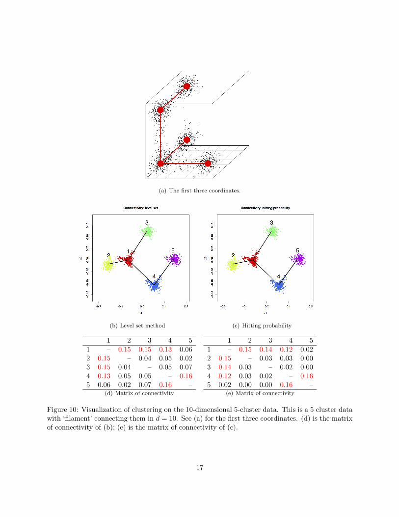
Figure 10: Visualization of clustering on the 10-dimensional 5-cluster data. This is a 5 cluster datawith ‘filament’ connecting them in d = 10. See (a) for the first three coordinates. (d) is the matrixof connectivity of (b); (e) is the matrix of connectivity of (c).
17
9.2 5-cluster in 10-D
We implement our visualization technique in the following ‘5-cluster’ data. We consider d = 10and 5 Gaussian mixture centered at the following positions
C1 = (0, 0, 0, 0, 0, 0, 0, 0, 0, 0)
C2 = (0.1, 0, 0, 0, 0, 0, 0, 0, 0, 0)
C3 = (0, 0.1, 0, 0, 0, 0, 0, 0, 0, 0)
C4 = (0, 0, 0, 0.1, 0, 0, 0, 0, 0, 0)
C5 = (0, 0.1, 0.1, 0, 0, 0, 0, 0, 0, 0).
(29)
For each Gaussian component, we generate 200 data points from σ1 = 0.01 and each Gaussianis isotropically distributed. Then we consider four “edges” connecting pairs of centers. Theseedges are E12, E13, E14, E45, where Eij is the edge between Ci, Cj . We generate 100 points froman uniform distribution over each edge and add an isotropic iid Gaussian noise to each edge withσ2 = 0.005. Thus, the total sample size is 1, 400 and consist of 5 clusters centered at each Ci andpart of the clusters are connected by a ‘noisy path’ (also called filament (Genovese et al., 2012;Chen et al., 2014a)). The density has structure only at the first three coordinates; a visualizationfor the structure is given in Figure 10-(a).
The goal is to identify the five clusters as well as their connectivity. We display the visualizationand the connectivity measures in Figure 10. We use both the level set method and the hittingprobability to compute connectivity structure. All the parameters used in this analysis is given asfollows.
h = 0.0114, n0 = 20, β0 = 25.78, ρ0 = 2, ω0 = 0.1
Note that the filtering threshold n0 is picked by the SC-plot in Figure 5 panel (b). We can use anyn0 between 233 and 1.
9.3 Olive Oil Data
We apply our methods to the Olive Oil data introduced in Forina et al. (1983). This data setconsists of 8 chemical measurements (features) for each observation and the total sample size isn = 572. Each observation is an olive oil produced in one of 3 regions in Italy and these regionsare further divided into 9 areas. Some other analyses for this data can be found in Stuetzle (2003);Azzalini and Torelli (2007). We hold out the information of the areas and regions and use only the8 chemical measurement to cluster all the data.
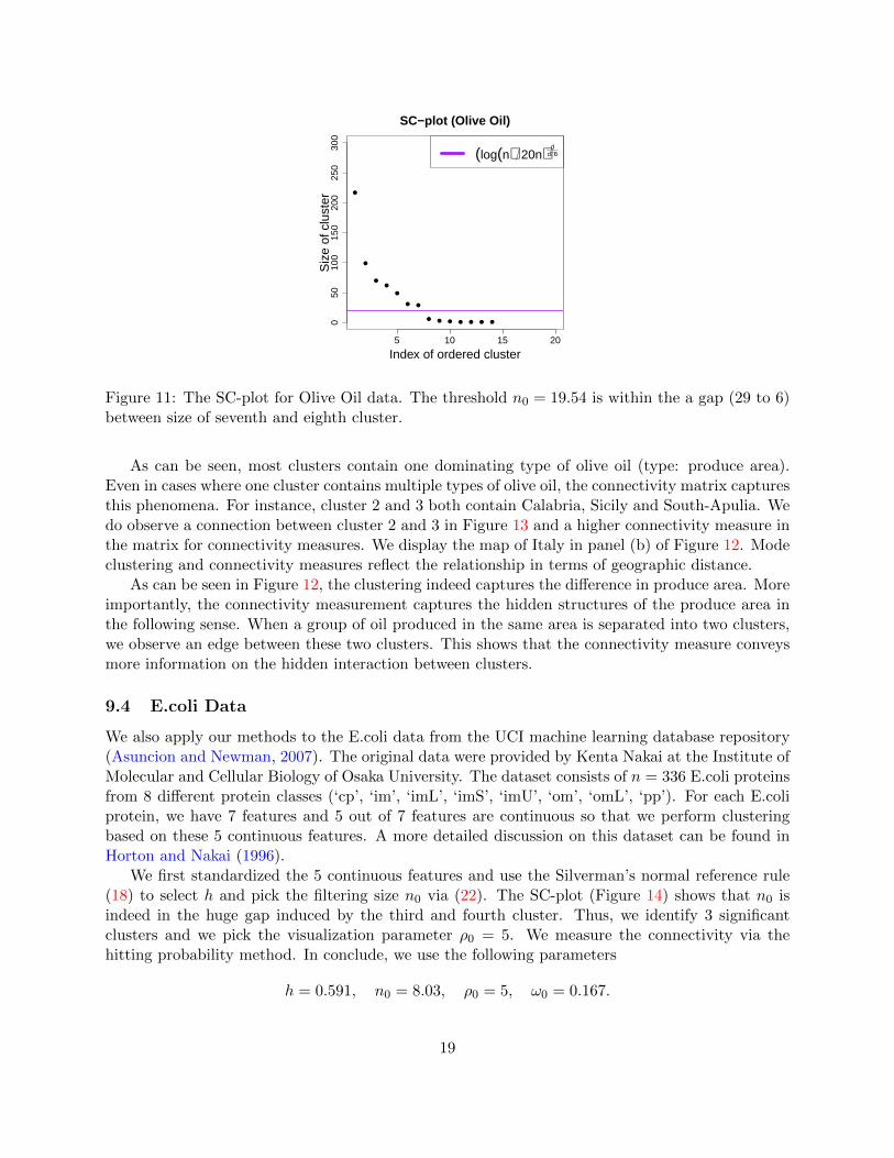
Since these measurements are in different units, we normalize and standardize each measure-ment. We apply (18) for selecting h and thresholding the size of clusters based on (22). Figure 11shows the SC-plot and the gap occurs between the seventh (size: 29) and eighth cluster (size: 6)and our threshold n0 = 19.54 is within this gap. We move the insignificant clusters into the nearestsignificant clusters. After filtering, 7 clusters remain and we apply algorithm 1 for visualizing theseclusters. To measure the connectivity, we apply the hitting probability so that we do not have tochoose the constant β0. To conclude, we use the following parameters
h = 0.587, n0 = 19.54, ρ0 = 6, ω0 = 0.071.
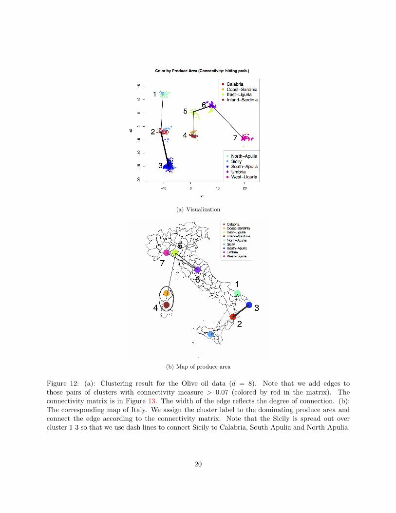
The visualization is given in Figure 12 and matrix of connectivity is given in Figure 13. We coloreach point according to the produced area to see how our methods capture the structure of data.
18
5 10 15 200
5010
015
020
025
030
0
SC−plot (Olive Oil)
Index of ordered cluster
Siz
e of
clu
ster
(log(n) 20n) dd+6
Figure 11: The SC-plot for Olive Oil data. The threshold n0 = 19.54 is within the a gap (29 to 6)between size of seventh and eighth cluster.
As can be seen, most clusters contain one dominating type of olive oil (type: produce area).Even in cases where one cluster contains multiple types of olive oil, the connectivity matrix capturesthis phenomena. For instance, cluster 2 and 3 both contain Calabria, Sicily and South-Apulia. Wedo observe a connection between cluster 2 and 3 in Figure 13 and a higher connectivity measure inthe matrix for connectivity measures. We display the map of Italy in panel (b) of Figure 12. Modeclustering and connectivity measures reflect the relationship in terms of geographic distance.
As can be seen in Figure 12, the clustering indeed captures the difference in produce area. Moreimportantly, the connectivity measurement captures the hidden structures of the produce area inthe following sense. When a group of oil produced in the same area is separated into two clusters,we observe an edge between these two clusters. This shows that the connectivity measure conveysmore information on the hidden interaction between clusters.
9.4 E.coli Data
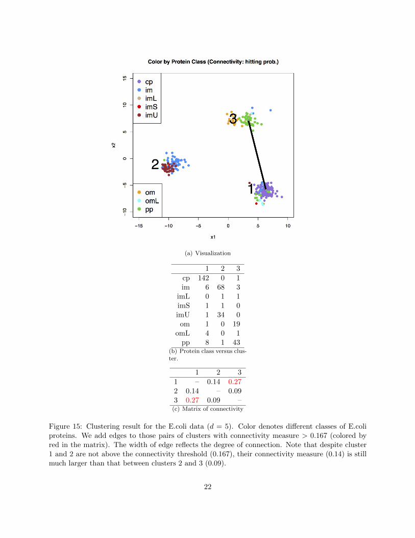
We also apply our methods to the E.coli data from the UCI machine learning database repository(Asuncion and Newman, 2007). The original data were provided by Kenta Nakai at the Institute ofMolecular and Cellular Biology of Osaka University. The dataset consists of n = 336 E.coli proteinsfrom 8 different protein classes (‘cp’, ‘im’, ‘imL’, ‘imS’, ‘imU’, ‘om’, ‘omL’, ‘pp’). For each E.coliprotein, we have 7 features and 5 out of 7 features are continuous so that we perform clusteringbased on these 5 continuous features. A more detailed discussion on this dataset can be found inHorton and Nakai (1996).
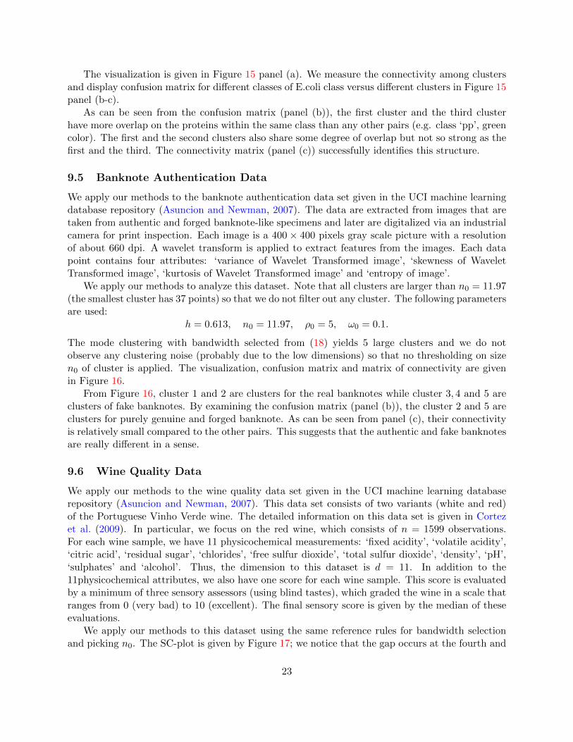
We first standardized the 5 continuous features and use the Silverman’s normal reference rule(18) to select h and pick the filtering size n0 via (22). The SC-plot (Figure 14) shows that n0 isindeed in the huge gap induced by the third and fourth cluster. Thus, we identify 3 significantclusters and we pick the visualization parameter ρ0 = 5. We measure the connectivity via thehitting probability method. In conclude, we use the following parameters
h = 0.591, n0 = 8.03, ρ0 = 5, ω0 = 0.167.
19
(a) Visualization
(b) Map of produce area
Figure 12: (a): Clustering result for the Olive oil data (d = 8). Note that we add edges tothose pairs of clusters with connectivity measure > 0.07 (colored by red in the matrix). Theconnectivity matrix is in Figure 13. The width of the edge reflects the degree of connection. (b):The corresponding map of Italy. We assign the cluster label to the dominating produce area andconnect the edge according to the connectivity matrix. Note that the Sicily is spread out overcluster 1-3 so that we use dash lines to connect Sicily to Calabria, South-Apulia and North-Apulia.
20
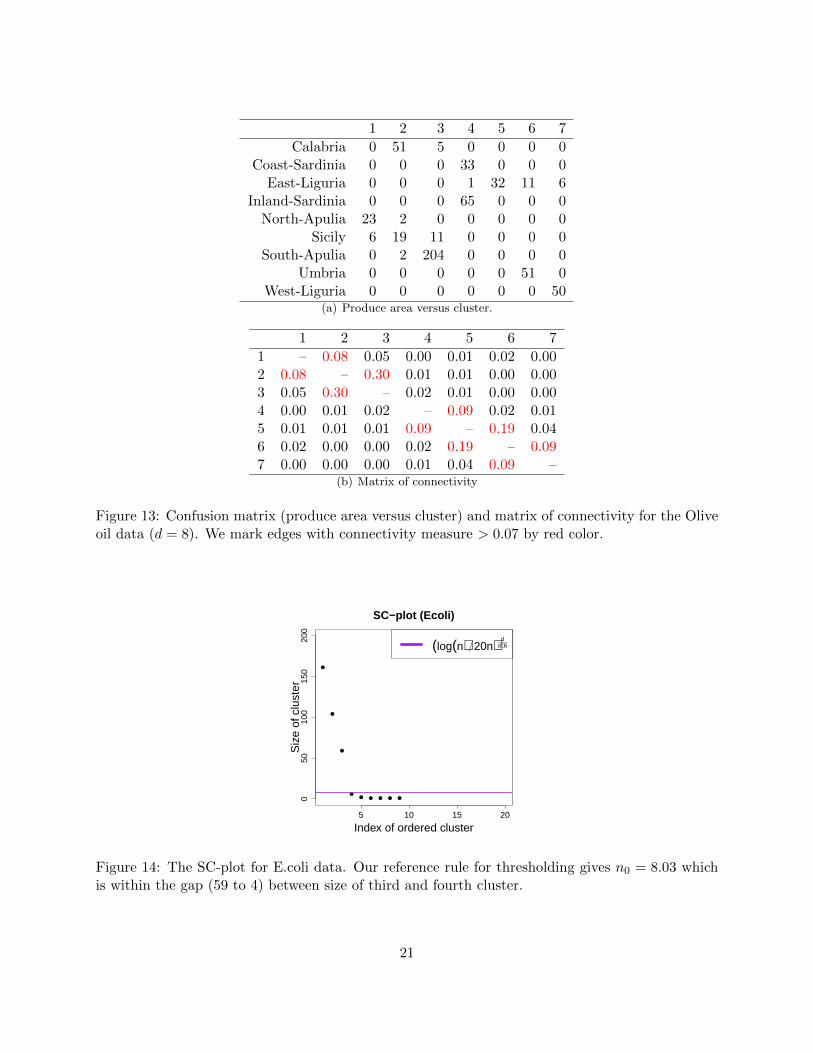
1 2 3 4 5 6 7
Calabria 0 51 5 0 0 0 0Coast-Sardinia 0 0 0 33 0 0 0
East-Liguria 0 0 0 1 32 11 6Inland-Sardinia 0 0 0 65 0 0 0
North-Apulia 23 2 0 0 0 0 0Sicily 6 19 11 0 0 0 0
South-Apulia 0 2 204 0 0 0 0Umbria 0 0 0 0 0 51 0
West-Liguria 0 0 0 0 0 0 50(a) Produce area versus cluster.
1 2 3 4 5 6 7
1 – 0.08 0.05 0.00 0.01 0.02 0.002 0.08 – 0.30 0.01 0.01 0.00 0.003 0.05 0.30 – 0.02 0.01 0.00 0.004 0.00 0.01 0.02 – 0.09 0.02 0.015 0.01 0.01 0.01 0.09 – 0.19 0.046 0.02 0.00 0.00 0.02 0.19 – 0.097 0.00 0.00 0.00 0.01 0.04 0.09 –
(b) Matrix of connectivity
Figure 13: Confusion matrix (produce area versus cluster) and matrix of connectivity for the Oliveoil data (d = 8). We mark edges with connectivity measure > 0.07 by red color.
5 10 15 20
050
100
150
200
SC−plot (Ecoli)
Index of ordered cluster
Siz
e of
clu
ster
(log(n) 20n) dd+6
Figure 14: The SC-plot for E.coli data. Our reference rule for thresholding gives n0 = 8.03 whichis within the gap (59 to 4) between size of third and fourth cluster.
21
(a) Visualization
1 2 3
cp 142 0 1im 6 68 3
imL 0 1 1imS 1 1 0imU 1 34 0om 1 0 19
omL 4 0 1pp 8 1 43
(b) Protein class versus clus-ter.
1 2 3
1 – 0.14 0.272 0.14 – 0.093 0.27 0.09 –
(c) Matrix of connectivity
Figure 15: Clustering result for the E.coli data (d = 5). Color denotes different classes of E.coliproteins. We add edges to those pairs of clusters with connectivity measure > 0.167 (colored byred in the matrix). The width of edge reflects the degree of connection. Note that despite cluster1 and 2 are not above the connectivity threshold (0.167), their connectivity measure (0.14) is stillmuch larger than that between clusters 2 and 3 (0.09).
22
The visualization is given in Figure 15 panel (a). We measure the connectivity among clustersand display confusion matrix for different classes of E.coli class versus different clusters in Figure 15panel (b-c).
As can be seen from the confusion matrix (panel (b)), the first cluster and the third clusterhave more overlap on the proteins within the same class than any other pairs (e.g. class ‘pp’, greencolor). The first and the second clusters also share some degree of overlap but not so strong as thefirst and the third. The connectivity matrix (panel (c)) successfully identifies this structure.
9.5 Banknote Authentication Data
We apply our methods to the banknote authentication data set given in the UCI machine learningdatabase repository (Asuncion and Newman, 2007). The data are extracted from images that aretaken from authentic and forged banknote-like specimens and later are digitalized via an industrialcamera for print inspection. Each image is a 400 × 400 pixels gray scale picture with a resolutionof about 660 dpi. A wavelet transform is applied to extract features from the images. Each datapoint contains four attributes: ‘variance of Wavelet Transformed image’, ‘skewness of WaveletTransformed image’, ‘kurtosis of Wavelet Transformed image’ and ‘entropy of image’.
We apply our methods to analyze this dataset. Note that all clusters are larger than n0 = 11.97(the smallest cluster has 37 points) so that we do not filter out any cluster. The following parametersare used:
h = 0.613, n0 = 11.97, ρ0 = 5, ω0 = 0.1.
The mode clustering with bandwidth selected from (18) yields 5 large clusters and we do notobserve any clustering noise (probably due to the low dimensions) so that no thresholding on sizen0 of cluster is applied. The visualization, confusion matrix and matrix of connectivity are givenin Figure 16.
From Figure 16, cluster 1 and 2 are clusters for the real banknotes while cluster 3, 4 and 5 areclusters of fake banknotes. By examining the confusion matrix (panel (b)), the cluster 2 and 5 areclusters for purely genuine and forged banknote. As can be seen from panel (c), their connectivityis relatively small compared to the other pairs. This suggests that the authentic and fake banknotesare really different in a sense.
9.6 Wine Quality Data
We apply our methods to the wine quality data set given in the UCI machine learning databaserepository (Asuncion and Newman, 2007). This data set consists of two variants (white and red)of the Portuguese Vinho Verde wine. The detailed information on this data set is given in Cortezet al. (2009). In particular, we focus on the red wine, which consists of n = 1599 observations.For each wine sample, we have 11 physicochemical measurements: ‘fixed acidity’, ‘volatile acidity’,‘citric acid’, ‘residual sugar’, ‘chlorides’, ‘free sulfur dioxide’, ‘total sulfur dioxide’, ‘density’, ‘pH’,‘sulphates’ and ‘alcohol’. Thus, the dimension to this dataset is d = 11. In addition to the11physicochemical attributes, we also have one score for each wine sample. This score is evaluatedby a minimum of three sensory assessors (using blind tastes), which graded the wine in a scale thatranges from 0 (very bad) to 10 (excellent). The final sensory score is given by the median of theseevaluations.
We apply our methods to this dataset using the same reference rules for bandwidth selectionand picking n0. The SC-plot is given by Figure 17; we notice that the gap occurs at the fourth and
23
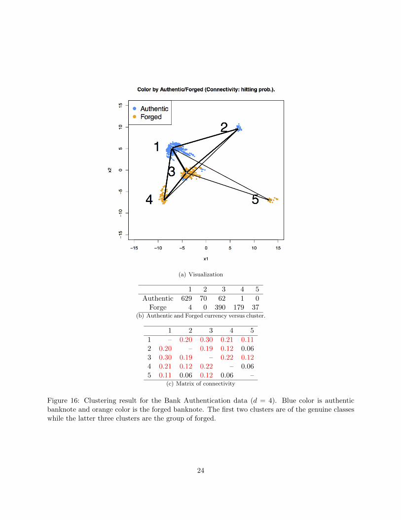
(a) Visualization
1 2 3 4 5
Authentic 629 70 62 1 0Forge 4 0 390 179 37
(b) Authentic and Forged currency versus cluster.
1 2 3 4 5
1 – 0.20 0.30 0.21 0.112 0.20 – 0.19 0.12 0.063 0.30 0.19 – 0.22 0.124 0.21 0.12 0.22 – 0.065 0.11 0.06 0.12 0.06 –
(c) Matrix of connectivity
Figure 16: Clustering result for the Bank Authentication data (d = 4). Blue color is authenticbanknote and orange color is the forged banknote. The first two clusters are of the genuine classeswhile the latter three clusters are the group of forged.
24
5 10 15 200
5010
015
020
0
SC−plot (Wine quality)
Index of ordered cluster
Siz
e of
clu
ster
(783) (log(n) 20n) dd+6
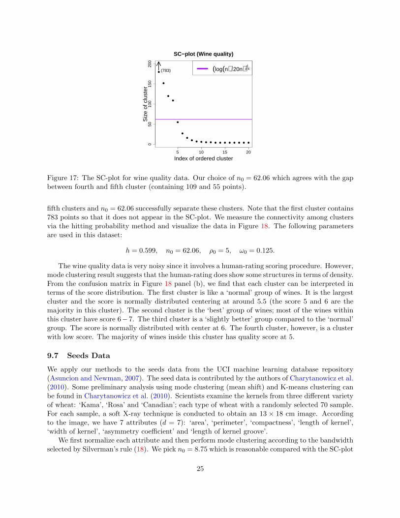
Figure 17: The SC-plot for wine quality data. Our choice of n0 = 62.06 which agrees with the gapbetween fourth and fifth cluster (containing 109 and 55 points).
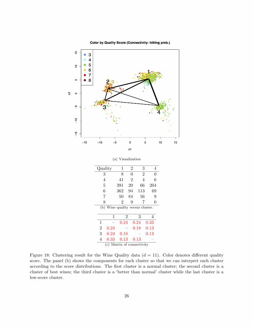
fifth clusters and n0 = 62.06 successfully separate these clusters. Note that the first cluster contains783 points so that it does not appear in the SC-plot. We measure the connectivity among clustersvia the hitting probability method and visualize the data in Figure 18. The following parametersare used in this dataset:
h = 0.599, n0 = 62.06, ρ0 = 5, ω0 = 0.125.
The wine quality data is very noisy since it involves a human-rating scoring procedure. However,mode clustering result suggests that the human-rating does show some structures in terms of density.From the confusion matrix in Figure 18 panel (b), we find that each cluster can be interpreted interms of the score distribution. The first cluster is like a ‘normal’ group of wines. It is the largestcluster and the score is normally distributed centering at around 5.5 (the score 5 and 6 are themajority in this cluster). The second cluster is the ‘best’ group of wines; most of the wines withinthis cluster have score 6− 7. The third cluster is a ‘slightly better’ group compared to the ‘normal’group. The score is normally distributed with center at 6. The fourth cluster, however, is a clusterwith low score. The majority of wines inside this cluster has quality score at 5.
9.7 Seeds Data
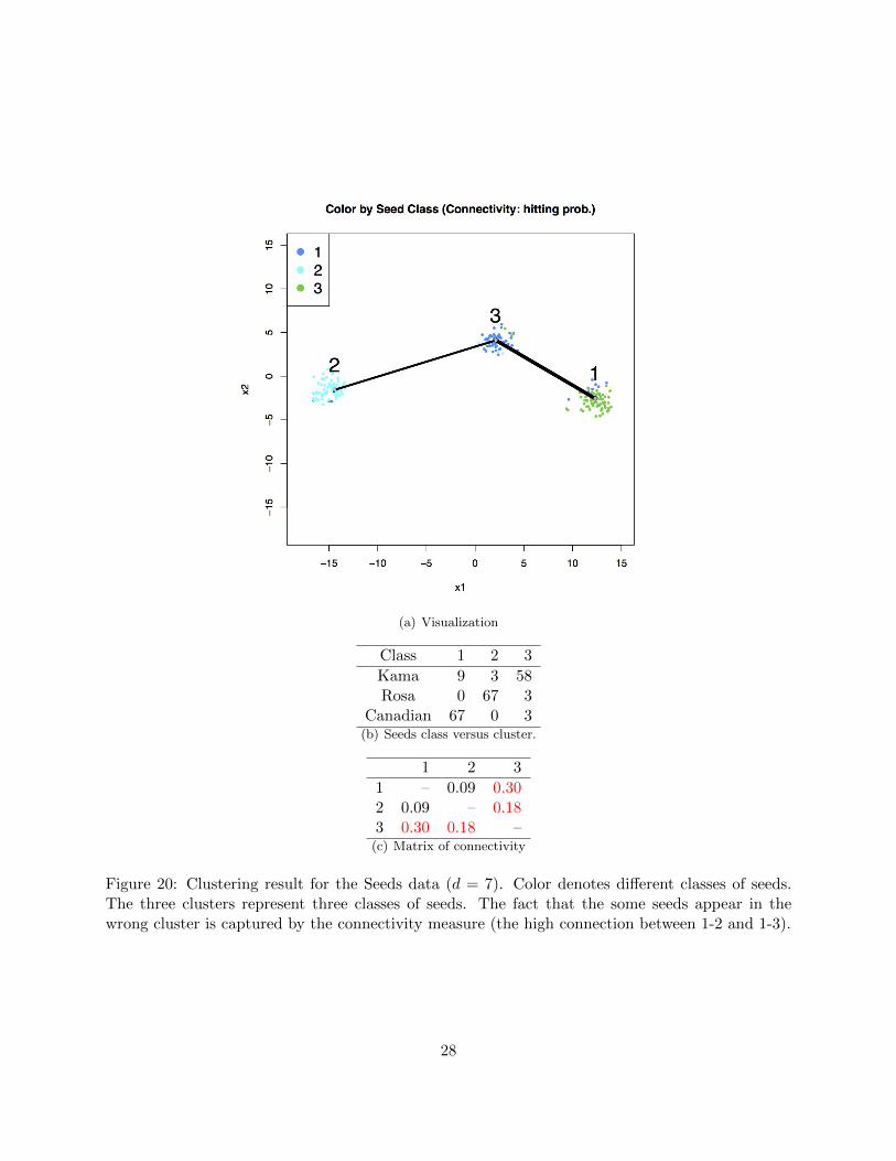
We apply our methods to the seeds data from the UCI machine learning database repository(Asuncion and Newman, 2007). The seed data is contributed by the authors of Charytanowicz et al.(2010). Some preliminary analysis using mode clustering (mean shift) and K-means clustering canbe found in Charytanowicz et al. (2010). Scientists examine the kernels from three different varietyof wheat: ‘Kama’, ‘Rosa’ and ‘Canadian’; each type of wheat with a randomly selected 70 sample.For each sample, a soft X-ray technique is conducted to obtain an 13 × 18 cm image. Accordingto the image, we have 7 attributes (d = 7): ‘area’, ‘perimeter’, ‘compactness’, ‘length of kernel’,‘width of kernel’, ‘asymmetry coefficient’ and ‘length of kernel groove’.
We first normalize each attribute and then perform mode clustering according to the bandwidthselected by Silverman’s rule (18). We pick n0 = 8.75 which is reasonable compared with the SC-plot
25
(a) Visualization
Quality 1 2 3 4
3 8 0 2 04 41 2 4 65 391 20 66 2046 362 94 113 697 50 84 56 98 2 9 7 0
(b) Wine quality versus cluster.
1 2 3 4
1 – 0.24 0.24 0.332 0.24 – 0.18 0.133 0.24 0.18 – 0.134 0.33 0.13 0.13 –
(c) Matrix of connectivity
Figure 18: Clustering result for the Wine Quality data (d = 11). Color denotes different qualityscore. The panel (b) shows the components for each cluster so that we can interpret each clusteraccording to the score distributions. The first cluster is a normal cluster; the second cluster is acluster of best wines; the third cluster is a ‘better than normal’ cluster while the last cluster is alow-score cluster.
26
5 10 15 200
2040
6080
100
SC−plot (Seeds)
Index of ordered cluster
Siz
e of
clu
ster
(log(n) 20n) dd+6
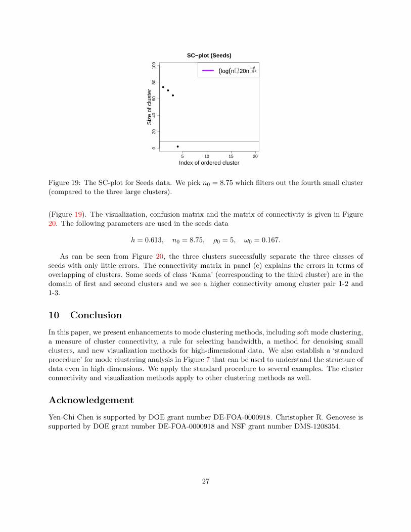
Figure 19: The SC-plot for Seeds data. We pick n0 = 8.75 which filters out the fourth small cluster(compared to the three large clusters).
(Figure 19). The visualization, confusion matrix and the matrix of connectivity is given in Figure20. The following parameters are used in the seeds data
h = 0.613, n0 = 8.75, ρ0 = 5, ω0 = 0.167.
As can be seen from Figure 20, the three clusters successfully separate the three classes ofseeds with only little errors. The connectivity matrix in panel (c) explains the errors in terms ofoverlapping of clusters. Some seeds of class ‘Kama’ (corresponding to the third cluster) are in thedomain of first and second clusters and we see a higher connectivity among cluster pair 1-2 and1-3.
10 Conclusion
In this paper, we present enhancements to mode clustering methods, including soft mode clustering,a measure of cluster connectivity, a rule for selecting bandwidth, a method for denoising smallclusters, and new visualization methods for high-dimensional data. We also establish a ‘standardprocedure’ for mode clustering analysis in Figure 7 that can be used to understand the structure ofdata even in high dimensions. We apply the standard procedure to several examples. The clusterconnectivity and visualization methods apply to other clustering methods as well.
Acknowledgement
Yen-Chi Chen is supported by DOE grant number DE-FOA-0000918. Christopher R. Genovese issupported by DOE grant number DE-FOA-0000918 and NSF grant number DMS-1208354.
27
(a) Visualization
Class 1 2 3
Kama 9 3 58Rosa 0 67 3
Canadian 67 0 3(b) Seeds class versus cluster.
1 2 3
1 – 0.09 0.302 0.09 – 0.183 0.30 0.18 –
(c) Matrix of connectivity
Figure 20: Clustering result for the Seeds data (d = 7). Color denotes different classes of seeds.The three clusters represent three classes of seeds. The fact that the some seeds appear in thewrong cluster is captured by the connectivity measure (the high connection between 1-2 and 1-3).
28
A Appendix: Mixture-Based Soft Clustering
The assignment vector a(x) derived from a mixture model need not be well defined because adensity p can have many different mixture representations that can in turn result in distinct softcluster assignments.
Consider a mixture density
p(x) =k∑j=1
πjφ(x;µj ,Σj) (30)
where each φ(x;µj ,Σj) is a Gaussian density function with mean µj and covariance matrix Σj and0 ≤ πj ≤ 1 is the mixture proportion for the j-th density such that
∑j πj = 1. Recall the latent
variable representation of p. Let Z be a discrete random variable such that
P (Z = j) = πj , j = 1, · · · , k (31)
and let X|Z ∼ φ(x;µZ ,ΣZ). Then, consistent with (30), the unconditional density for X is
p(x) =∑z
p(x|z)p(z) =∑j=1
πjφ(x;µj ,Σj) (32)
It follows that
P (Z = j|x) =πjp(x|Z = j)∑s=1 πsp(x|z = s)
=πjφ(x;µj ,Σj)∑s=1 πsφ(x;µs,Σs)
, (33)
with soft cluster assignment a(x) = (a1(x), · · · , ak(x)) = (p(z = 1|x), · · · , p(z = k|x)). Of course,a(x) can be estimated from the data by estimating the parameters of the mixture model.
We claim that the a(x) is not well-defined. Consider the following example in one dimension.Let
p(x) =1
2φ(x;−3, 1) +
1
2φ(x; 3, 1). (34)
Then by definition
a1(x) = P (Z = 1|x) =12φ(x;−3, 1)
12φ(x;−3, 1) + 1
2φ(x; 3, 1). (35)
However, we can introduce a different latent variable representation for p(x) as follows. Let usdefine
p1(x) =p(x)1(x ≤ 4)∫p(x)1(x ≤ 4)dx
(36)
and
p2(x) =p(x)1(x > 4)∫p(x)1(x > 4)dx
(37)
and note thatp(x) = πp1(x) + (1− π)p2(x) (38)
where π =∫p(x)1(x ≤ 4)dx. Here, 1(E) is the indicator function for E. Let W be a discrete
random variable such that P (W = 1) = π and P (W = 2) = 1− π and let X|W has density pW (x).Then we have p(x) =
∑w p(x|w)P (W = w) which is the same density as (34). This defined the
soft clustering assignment a(x) = (P (W = 1|x), · · · , P (W = k|x)) where
a1(x) = P (W = 1|x) = 1(x ≤ 4) (39)
29
which is completely different from (35). In fact, for any set A ⊂ R, there exists a latent representa-tion of p(x) such that a1(x) = I(x ∈ A). There are infinitely many latent variable representationsfor any density, each leading to a different soft clustering. The mixture-based soft clustering thusdepends on the arbitrary, chosen representation.
B Appendix: Method of Level Set Distance
Here, we generate a soft assignment vector based on the density level sets (Rinaldo and Wasserman,2010; Rinaldo et al., 2012; Chaudhuri and Dasgupta, 2010). The upper level set, for λ ≥ 0, is definedas
L(λ) = x : p(x) ≥ λ. (40)
As before, we use the modes to define the clusters and then use the level sets to measure closenessto the modes. Specifically, our level set method consists of the following steps.
(1) Identify the mode clusters C1, . . . , Ck.
(2) Given any x, let L ≡ Lx =y ∈ Rd : p(y) ≥ p(x)
.
(Note that x will be on the boundary of L.)
(3) Let Di = L ∩ Ci for i = 1, . . . , k.
(4) Define the distance profile
di(x) =
d(x,Di) if Di 6= ∅∞ if Di = ∅
(41)
for i = 1, . . . , k, where d(x,A) = infy∈A ‖x − y‖ is the distance from a point x to a set A.Note that di(x) = 1 if i is the cluster that x belongs to.
(5) Transform each di(x) into a soft assignment vector by
aLi (x) =exp(−β0di(x))∑ki=1 exp(−β0di(x))
(42)
so that we obtain aL(x). β0 is a contrast parameter that controls the distance-weight trans-formation; we will discuss β0 later. Note that we will have aLi (x) = aLj (x) if x is on theboundary between cluster i and j. The superscript L indicates that this assignment vector isfrom the level set method.
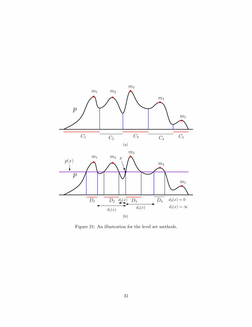
Figure 21 provides an illustration of the above process. This method measures how strongly xbelongs to each cluster. In practice, we replace the density by the KDE pn. We summarize theimplementation in Algorithm 2. Note that the contrast parameter β0 can be chosen as
β0 =1
2Sn, Sn =
1
d
d∑j=1
Sn,j , (43)
where Sn,j is the sample standard deviation along j-th coordinate. This gives a scale-free softassignment vector.
30
p
m1 m2
m3
m4
m5
C1 C2C3 C4
C5
(a)
p
m1 m2
m3
m4
m5
xp(x)
D1 D2 D3 D4d2(x)
d1(x)d4(x)
d3(x) = 0
d5(x) = ∞
(b)
Figure 21: An illustration for the level set methods.
31
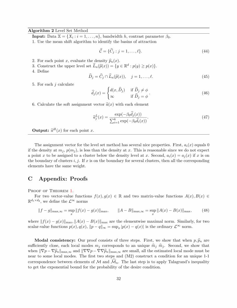
Algorithm 2 Level Set Method
Input: Data X = Xi : i = 1, . . . , n, bandwidth h, contrast parameter β0.1. Use the mean shift algorithm to identify the basins of attraction
C = Cj : j = 1, . . . , `. (44)
2. For each point x, evaluate the density pn(x).3. Construct the upper level set Ln(p(x)) = y ∈ Rd : p(y) ≥ p(x).4. Define
Dj = Cj ∩ Ln(p(x)), j = 1, . . . , `. (45)
5. For each j calculate
dj(x) =
d(x, Dj) if Dj 6= φ
∞ if Dj = φ. (46)
6. Calculate the soft assignment vector a(x) with each element
aLj (x) =exp(−β0dj(x))∑ki=1 exp(−β0di(x))
. (47)
Output: aH(x) for each point x.
The assignment vector for the level set method has several nice properties. First, ai(x) equals 0if the density at mj , p(mj), is less than the density at x. This is reasonable since we do not expecta point x to be assigned to a cluster below the density level at x. Second, ai(x) = aj(x) if x is onthe boundary of clusters i, j. If x is on the boundary for several clusters, then all the correspondingelements have the same weight.
C Appendix: Proofs
Proof of Theorem 1.For two vector-value functions f(x), g(x) ∈ R and two matrix-value functions A(x), B(x) ∈
Rd1×d2 , we define the L∞ norms
‖f − g‖max,∞ = supx‖f(x)− g(x)‖max, ‖A−B‖max,∞ = sup
x‖A(x)−B(x)‖max, (48)
where ‖f(x)− g(x)‖max, ‖A(x)− B(x)‖max are the elementwise maximal norm. Similarly, for twoscalar-value functions p(x), q(x), ‖p− q‖∞ = supx |p(x)− q(x)| is the ordinary L∞ norm.
Modal consistency: Our proof consists of three steps. First, we show that when p, pn aresufficiently close, each local modes mj corresponds to an unique mj mj . Second, we show thatwhen ‖∇p−∇pn‖max,∞ and ‖∇∇p−∇∇pn‖max,∞ are small, all the estimated local mode must benear to some local modes. The first two steps and (M2) construct a condition for an unique 1-1
correspondence between elements of M and Mn. The last step is to apply Talagrand’s inequalityto get the exponential bound for the probability of the desire condition.
32
Step 1: WLOG, we consider a local mode mj . Now we consider the set
Sj = mj ⊕λ∗
2dC3.
Since the third derivative of p is bounded by C3,
supx∈Sj
‖∇∇p(mj)−∇∇p(x)‖max ≤λ∗
2dC3× C3 =
λ∗2d.
Thus, by Weyl’s theorem (Theorem 4.3.1 in Horn and Johnson (2013)) and condition (M1), thefirst eigenvalue is bounded by
supx∈Sj
λ1(x) ≤ λ1(mj) + d× λ∗2d≤ −λ∗
2. (49)
Note that eigenvalues at local modes are negative. Since ∇p(mj) = 0 and the eigenvalues arebounded around mj , the density at the boundary of Sj must be less than
supx∈∂Sj
p(x) ≤ p(mj)−1
2
λ∗2
(λ∗
2dC3
)2
= p(mj)−λ3∗
16d2C23
,
where ∂Sj = x : ‖x−mj‖ = λ∗2dC3 is the boundary of Sj . Thus, whenever
‖pn − p‖∞ <λ3∗
16d2C23
, (50)
there must be at least one estimated local mode mj within Sj = m⊕ λ∗2dC3
. Note that this can begeneralized to each j = 1, · · · ,K.
Step 2: It is obvious that whenever
‖∇pn −∇p‖max,∞ ≤ η1,
‖∇∇pn −∇∇p‖max,∞ ≤λ∗4d,
(51)
the estimated local modes
Mn ⊂M⊕λ∗
2dC3
by condition (M2) and triangular inequality (also need Weyl’s theorem again for the eigenvalues).Step 3: By Step 1 and 2,
Mn ⊂M⊕λ∗
2dC3
and for each mode mj there exists at least one estimated mode mj within Sj = mj ⊕ λ∗2dC3
. Nowapply (49) and second inequality of (51) and triangular inequality, we conclude
supx∈Sj
λ1(x) ≤ −λ∗4, (52)
33
where λ1(x) is the first eigenvalue of ∇∇pn(x). This shows that we cannot have two estimatedlocal modes within each Sj . Thus, each mj only corresponds to one mj and vice versa by Step 2.We conclude that a sufficient condition for the number of modes being the same is the inequalityrequired in (50) and (51) i.e. we need
‖pn − p‖∞ <λ3∗
16d2C23
,
‖∇pn −∇p‖max,∞ ≤ η1,
‖∇∇pn −∇∇p‖max,∞ ≤λ∗4d.
(53)
Let ph = E(pn) be the smoothed version of the KDE. It is well-known in nonparametric theorythat (see e.g. page 132 in Scott (2009))
‖ph − p‖∞ = O(h2),
‖∇ph −∇p‖max,∞ = O(h2),
‖∇∇ph −∇∇p‖max,∞ = O(h2).
(54)
Thus, as h is sufficiently small, we have
‖ph − p‖∞ <λ3∗
32d2C23
, ‖∇ph −∇p‖max,∞ ≤ η1/2, ‖∇∇ph −∇∇p‖max,∞ ≤λ∗8d. (55)
Thus, (53) holds whenever
‖pn − ph‖∞ <λ3∗
32d2C23
,
‖∇pn −∇ph‖max,∞ ≤ η1/2,
‖∇∇pn −∇∇ph‖max,∞ ≤λ∗8d
(56)
and h is sufficiently small.Now applying Talagrand’s inequality (Talagrand, 1996; Gine and Guillou, 2002) (see also equa-
tion (90) in Lemma 13 in Chen et al. (2014a) for a similar result), there exists constants A0, A1, A2
and B0, B1, B2 such that for n sufficiently large,
P (‖pn − ph‖∞ ≥ ε) ≤ B0e−A0εnhd ,
P (‖∇pn −∇ph‖max,∞ ≥ ε) ≤ B1e−A1εnhd+2
,
P (‖∇∇pn −∇∇ph‖max,∞ ≥ ε) ≤ B2e−A2εnhd+4
.
(57)
Thus, combining (56) and (57), we conclude that there exists some constants A3, B3 such that
P((53) holds) ≥ 1−B3e−A3nhd+4
(58)
when h is sufficiently small. Since (53) holds implies Kn = K, we conclude
P(Kn 6= K) ≤ B3e−A3nhd+4
(59)
34

for some constants B3, A3 as h is sufficiently small. This proves modal consistency.
Location convergence: For the location convergence, we assume (53) holds so that Kn = Kand each local mode is approximating by an unique estimated local mode. We focus on one localmode mj and derive the rate of convergence for ‖mj −mj‖ and then generalized this rate to allthe local modes.
By definition,∇p(mj) = ∇pn(mj) = 0.
Thus, by Taylor expansion and the fact that the third derivative of pn is uniformly bounded,
∇pn(mj) = ∇pn(mj)−∇pn(mj)
= ∇∇pn(mj)(mj −mj) + o(‖mj −mj‖).(60)
Since we assume (53), this implies all eigenvalues of ∇∇pn(mj) are bounded away from 0 so that∇∇pn(mj) is invertible. Moreover,
∇pn(mj) = ∇pn(mj)−∇p(mj)
= O(h2) +OP
(√1
nhd+2
)(61)
by the rate of pointwise convergence in nonparametric theory (see e.g. page 154 in Scott (2009)).Thus, we conclude
‖mj −mj‖ = O(h2) +OP
(√1
nhd+2
). (62)
Now applying this rate of convergence to each local mode and use the fact that
Haus(Mn,M
)= max
j=1,··· ,K‖mj −mj‖,
we conclude the rate of convergence for estimating the location.
References
M. Alamgir and U. von Luxburg. Shortest path distance in random k-nearest neighbor graphs. InICML. icml.cc / Omnipress, 2012.
E. Arias-Castro, D. Mason, and B. Pelletier. On the estimation of the gradient lines of a densityand the consistency of the mean-shift algoithm. Technical report, IRMAR, 2013.
A. Asuncion and D. Newman. Uci machine learning repository, 2007.
A. Azzalini and N. Torelli. Clustering via nonparametric density estimation. Statistics and Com-puting, 17(1):71–80, 2007. ISSN 0960-3174. doi: 10.1007/s11222-006-9010-y.
A. S. Bijral, N. Ratliff, and N. Srebro. Semi-supervised learning with density based distances, 2011.
35
O. Bousquet, O. Chapelle, and M. Hein. Measure based regularization. In Advances in NeuralInformation Processing Systems 16. MIT Press, 2004.
J. Chacon and T. Duong. Data-driven density derivative estimation, with applications to nonpara-metric clustering and bump hunting. Electronic Journal of Statistics, 2013.
J. Chacon, T. Duong, and M. Wand. Asymptotics for general multivariate kernel density derivativeestimators. Statistica Sinica, 2011.
M. Charytanowicz, J. Niewczas, P. Kulczycki, P. A. Kowalski, S. Lukasik, and S. Zak. Completegradient clustering algorithm for features analysis of x-ray images. In Information Technologiesin Biomedicine, pages 15–24. Springer, New York, NY, USA NY, 2010.
K. Chaudhuri and S. Dasgupta. Rates of convergence for the cluster tree. NIPS, 2010.
F. Chazal, L. Guibas, S. Oudot, and P. Skraba. Persistence-based clustering in riemannian man-ifolds. In Proceedings of the 27th annual ACM symposium on Computational geometry, pages97–106. ACM, 2011.
Y.-C. Chen, C. R. Genovese, and L. Wasserman. Asymptotic theory for density ridges. arXiv:1406.5663, 2014a.
Y.-C. Chen, C. R. Genovese, and L. Wasserman. Generalized mode and ridge estimation. arXiv:1406.1803, 2014b.
Y. Cheng. Mean shift, mode seeking, and clustering. Pattern Analysis and Machine Intelligence,IEEE Transactions on, 17(8):790–799, 1995.
R. R. Coifman and S. Lafon. Diffusion maps. Applied and Computational Harmonic Analysis, 2006.
D. Comaniciu and P. Meer. Mean shift: a robust approach toward feature space analysis. PatternAnalysis and Machine Intelligence, IEEE Transactions on, 24(5):603 –619, may 2002.
T. H. Cormen, C. E. Leiserson, R. L. Rivest, and C. Stein. Introduction to Algorithms. The MITPress, Cambridge MA, 2009.
P. Cortez, A. Cerdeira, F. Almeida, T. Matos, and J. Reis. Modeling wine preferences by datamining from physicochemical properties. Decision Support Systems, 47(4):547–553, 2009.
V. De Silva and J. B. Tenenbaum. Sparse multidimensional scaling using landmark points. Technicalreport, Technical report, Stanford University, 2004.
E. W. Dijkstra. A note on two problems in connexion with graphs. Numerische Mathematik, 1959.
U. Einmahl and D. M. Mason. Uniform in bandwidth consistency for kernel-type function estima-tors. The Annals of Statistics, 2005.
B. T. Fasy, F. Lecci, A. Rinaldo, L. Wasserman, S. Balakrishnan, and A. Singh. Statistical inferencefor persistent homology: Confidence sets for persistence diagrams. The Annals of Statistics, 2014.
M. Forina, C. Armanino, S. Lanteri, and E. Tiscornia. Classification of olive oils from their fattyacid composition. Food Research and Data Analysis, 1983.
36
K. Fukunaga and L. D. Hostetler. The estimation of the gradient of a density function, withapplications in pattern recognition. IEEE Transactions on Information Theory, 21:32–40, 1975.
C. R. Genovese, M. Perone-Pacifico, I. Verdinelli, L. Wasserman, et al. On the path density of agradient field. The Annals of Statistics, 37(6A):3236–3271, 2009.
C. R. Genovese, M. Perone-Pacifico, I. Verdinelli, and L. Wasserman. Nonparametric ridge estima-tion. arXiv:1212.5156v1, 2012.
E. Gine and A. Guillou. Rates of strong uniform consistency for multivariate kernel density esti-mators. In Annales de l’Institut Henri Poincare (B) Probability and Statistics, 2002.
M. A. Guest. Morse theory in the 1990’s. arXiv:math/0104155v1, 2001.
J. Hartigan. Clustering Algorithms. Wiley and Sons, Hoboken, NJ, 1975.
T. Hastie, R. Tibshirani, and J. Friedman. The Elements of Statistical Learning. Springer Seriesin Statistics. Springer New York Inc., New York, NY, USA, 2001.
R. A. Horn and C. R. Johnson. Matrix Analysis. Cambridge, second edition, 2013.
P. Horton and K. Nakai. A probabilistic classification system for predicting the cellular localizationsites of proteins. In Ismb, volume 4, pages 109–115, 1996.
S. J. Hwang, S. B. Damelin, and A. O. Hero. Shortest path through random points. arXiv:1202.0045, 2012.
J. Kruskal. Multidimensional scaling by optimizing goodness of fit to a nonmetric hypothesis.Psychometrika, 29(1):1–27, 1964. ISSN 0033-3123. doi: 10.1007/BF02289565.
A. Lee and L. Wasserman. Spectral connectivity analysis. Journal of the American StatisticalAssociation, 2010.
J. Li, S. Ray, and B. Lindsay. A nonparametric statistical approach to clustering via mode identi-fication. Journal of Machine Learning Research, 8(8):1687–1723, 2007.
P. Lingras and C. West. Interval set clustering of web users with rough k-means. Journal ofIntelligent Information Systems, 2002.
G. McLachlan and D. Peel. Finite mixture models. John Wiley & Sons, Hoboken, NJ, 2004.
B. Nadler, S. Lafon, R. R. Coifman, and I. G. Kevrekidis. Diffusion maps, spectral clustering andeigenfunctions of fokker-planck operators. NIPS, 2005.
R. Nock and F. Nielsen. On weighting clustering. IEEE Transactions on Pattern Analysis andMachine Intelligence, 2006.
G. Peters, F. Crespoc, P. Lingrasd, and R. Weber. Soft clustering - fuzzy and rough approachesand their extensions and derivatives. International Journal of Approximate Reasoning, 2013.
D. Pollard. New ways to prove central limit theorems. Econometric Theory, 1985.
37

A. Rinaldo and L. Wasserman. Generalized density clustering. The Annals of Statistics, 2010.
A. Rinaldo, A. Singh, R. Nugent, and L. Wasserman. Stability of density-based clustering. Journalof Machine Learning Research, 2012.
J. P. Romano. Bootstrapping the mode. Annals of the Institute of Statistical Mathematics, 40(3):565–586, 1988.
J. P. Romano et al. On weak convergence and optimality of kernel density estimates of the mode.The Annals of Statistics, 16(2):629–647, 1988.
Sajama and A. Orlitsky. Estimating and computing density based distance metrics. In Proceedingsof the 22Nd International Conference on Machine Learning, ICML ’05, 2005.
D. W. Scott. Multivariate density estimation: theory, practice, and visualization, volume 383. JohnWiley & Sons, 2009.
S. J. Sheather. Density estimation. Statistical Science, 2004.
R. N. Shepard. Multidimensional scaling, tree-fitting, and clustering. Science, 210(4468):390–398,1980.
V. D. Silva and J. B. Tenenbaum. Global versus local methods in nonlinear dimensionality reduc-tion. In Advances in neural information processing systems, pages 705–712, 2002.
B. W. Silverman. Density Estimation for Statistics and Data Analysis. Chapman and Hall, LondonUK, 1986.
T. Sousbie. The persistent cosmic web and its filamentary structure – i. theory and implementation.Mon. Not. R. Astron. Soc., 2011.
W. Stuetzle. Estimating the cluster tree of a density by analyzing the minimal spanning treeof a sample. Journal of Classification, 20(1):025–047, 2003. ISSN 0176-4268. doi: 10.1007/s00357-003-0004-6. URL http://dx.doi.org/10.1007/s00357-003-0004-6.
M. Talagrand. Newconcentration inequalities in product spaces. Invent. Math, 1996.—
38