Embed Size (px)
Citation preview
arX
iv:0
907.
3454
v3 [
mat
h.ST
] 1
0 N
ov 2
010
The Annals of Statistics
2010, Vol. 38, No. 5, 2678–2722DOI: 10.1214/10-AOS797c© Institute of Mathematical Statistics, 2010
GENERALIZED DENSITY CLUSTERING1
By Alessandro Rinaldo and Larry Wasserman
Carnegie Mellon University
We study generalized density-based clustering in which sharplydefined clusters such as clusters on lower-dimensional manifolds areallowed. We show that accurate clustering is possible even in highdimensions. We propose two data-based methods for choosing thebandwidth and we study the stability properties of density clusters.We show that a simple graph-based algorithm successfully approxi-mates the high density clusters.
1. Introduction. It has been observed that classification methods canbe very accurate in high-dimensional problems, apparently contradictingthe curse of dimensionality. A plausible explanation for this phenomenon isthe “low noise” condition described, for instance, in Mammen and Tsybakov(1999). When the low noise condition holds, the probability mass near thedecision boundary is small and fast rates of convergence of the classificationerror are possible in high dimensions.
Similarly, clustering methods can be very accurate in high-dimensionalproblems. For example, clustering subjects based on gene profiles and clus-tering curves are both high-dimensional problems where several methodshave worked well despite the high dimensionality. This suggests that it maybe possible to find conditions that explains the success of clustering in high-dimensional problems.
In this paper, we focus on clusters that are defined as the connectedcomponents of high density regions [Cuevas and Fraiman (1997), Hartigan(1975)]. The advantage of density clustering over other methods is that thereis a well-defined population quantity being estimated and density clusteringallows the shape of the clusters to be very general. (A related but somewhat
Received July 2009; revised November 2009.1Supported by NSF Grants DMS-07-07059, DMS-06-31589, ONR Grant N00014-08-
1-0673 and a Health Research Formula Fund Award granted by the Commonwealth ofPennsylvanias Department of Health.
AMS 2000 subject classifications. Primary 62H30; secondary 62G07.Key words and phrases. Density clustering, kernel density estimation.
This is an electronic reprint of the original article published by theInstitute of Mathematical Statistics in The Annals of Statistics,2010, Vol. 38, No. 5, 2678–2722. This reprint differs from the original inpagination and typographic detail.
1
2 A. RINALDO AND L. WASSERMAN
different approach for generally shaped clusters is spectral clustering; see vonLuxburg (2007) and [Ng, Jordan andWeiss (2002)].) Of course, without someconditions, density estimation is subject to the usual curse of dimensionality.One would hope that an appropriate low noise condition would obviate thecurse of dimensionality. Such assumptions have been proposed by Polonik(1995), Rigollet (2007), Rigollet and Vert (2006), and others. However, theassumptions used by these authors rule out the case where the clusters arevery sharply defined, which should be the easiest cases, and, more generally,clusters defined on lower dimensional sets.
The purpose of this paper is to define a notion of density clusters thatdoes not rule out the most favorable cases and is not limited to sets of fulldimension. We study the risk properties of density-based clustering and itsstability properties, and we provide data-based methods for choosing thesmoothing parameters.
The following simple example helps to illustrate our motivation. We referthe reader to the next section for a more rigorous introduction. Supposethat a distribution P is a mixture of finitely many point masses at distinctpoints x1, . . . , xk where xj ∈ R
d. Specifically, suppose that P = k−1∑k
j=1 δjwhere δj is a point mass at xj . The clusters are C1 = x1, . . . ,Ck = xk.This is a trivial clustering problem even if the dimension d is very high.The clusters could not be more sharply defined yet the density does noteven exist in the usual sense. This makes it clear that common assumptionsabout the density such as smoothness or even boundedness are not well-suited for density clustering.
Now let ph = dPh/dµ be the Lebesgue density of the measure Ph obtainedby convolving P with the probability measure having Lebesgue density Kh,a kernel with bandwidth h. Unlike the original distribution P , Ph has full-dimensional support for each positive h. The “mollified” density ph containsall the information needed for clustering. Indeed, there exist constants h > 0and λ≥ 0 such that the following facts are true:
1. for all 0 < h < h, the level set x :ph(x) ≥ λ has disjoint, connectedcomponents Ch
1 , . . . ,Chk ;
2. the components Chj contain the true clusters: Cj ⊂Ch
j for j = 1, . . . , k;
3. although Chj overestimates the true cluster Cj , this overestimation is
inconsequential since P (Chj − Cj) = 0 and hence a new observation will
not be misclustered;4. let ph denote the kernel density estimator using Kh with fixed band-
width 0 < h < h and based on a i.i.d. sample of size n from P . Then,supx|ph(x)− ph(x)|=O(
√logn/n) almost everywhere P , which does not
depend on the dimension d (see Section 3.1). The bias from using a fixedbandwidth h—which does not vanish as n→∞—does not adversely af-fect the clustering.
DENSITY CLUSTERING 3
In summary, we can recover the true clusters using an estimator of thedensity ph with a large bandwidth h. It is not necessary to assume that thetrue density is smooth or that it even exists.
Our contributions in this paper are the following:
1. We develop a notion of density clustering that applies to probabilitydistributions that have nonsmooth Lebesgue densities or do not evenadmit a density.
2. We find the rates of convergence for estimators of these clusters.3. We study two data-driven methods for choosing the bandwidth.4. We study the stability properties of density clusters.5. We show that the depth-first search algorithm on the ρ-nearest neighbor-
hood graph of ph ≥ λ is effective at recovering the high-density clusters.
Another approach to clustering that does not require densities is the min-imum volume set approach [Polonik (1995), Scott and Nowak (2006)]. Ourapproach is different because we are specifically trying to capture the ideathat kernel density estimates are useful for clustering even when the densitymay not exist.
Section 2 contains notation and definitions. Section 3 contains resultson rates of convergence. We give a data-driven method for choosing thebandwidth in Section 4. Section 4.2 contains results on cluster stability.The validity of the graph-based algorithm for approximating the clusters isproved in Section 5. Section 6 contains some examples based on simulateddata. Concluding remarks are in Section 7. All proofs are in the Section 8.Some technical details are in the Appendix.
Notation. For two sequences an and bn, we write an = O(bn) andan =Ω(bn) if there exists a constant C > 0 such that, for all n large enough,|an|/bn ≤ C and |an|/bn ≥ C, respectively. If an = Ω(bn) and an = O(bn),then we will write an ≍ bn. We denote with P(E) the probability of a genericevent E, whenever the underlying probability measure is implicitly under-stood from the context. By the dimension of a Euclidean set, we will alwaysmean the k-dimensional Hausdorff dimension for some integer 0≤ k ≤ d (seethe Appendix). These sets may consist, for example, of smooth submanifoldsor even single points.
2. Settings and assumptions.
2.1. Level set clusters. In this section, we develop a probabilistic frame-work for the definition of clusters we have adopted. For ease of readability,the more technical measure-theoretic details are given in the Appendix.
Let P be a probability distribution on Rd whose support S (the smallest
closed set of P -measure 1) is comprised of an unknown number m of disjoint
4 A. RINALDO AND L. WASSERMAN
compact sets S1, . . . , Sm of different dimensions. We define the geometricdensity of P as the measurable function p :Rd 7→R given by
p(x) = limh↓0
P (B(x,h))
vdhd,(1)
where B(x, ε) is the Euclidean ball of radius h centered at x, µ is the d-dimensional Lebesgue measure and vd ≡ µ(B(0,1)). Note that, almost every-where P , p(x) =∞ if and only if x belongs to some set Si having dimensionstrictly less than d and is positive and finite if and only if x belongs to somed-dimensional set Si. In general,
∫Rd p(x)dµ(x)≤ 1 and, therefore, p is not
necessarily a probability density. Nonetheless, p can be used to recover thesupport of P , since
S = x :p(x)> 0,where for a set A⊂R
d, A denotes its closure.For λ≥ 0, define the λ-level set
L≡L(λ) = x :p(x)≥ λ,(2)
and its boundary ∂L(λ) = x :p(x) = λ. Throughout the paper, we will sup-pose that we are given a fixed value of λ < ‖p‖∞, where ‖p‖∞ ≡ supx∈Rd p(x).Often, λ is chosen so that P (L(λ))≈ 1−α for some given α. In practice, itis advisable to present the results for a variety of values of λ as we discussin Section 7.
We assume that there are k ≥ 1 disjoint, compact, connected sets C1(λ), . . . ,Ck(λ) such that
L=C1(λ) ∪ · · · ∪Ck(λ).
We will often write Cj instead of of Cj(λ) when the dependence of λ isclear from the context. The value of k is not assumed to be known. The setsC1, . . . ,Ck are called the λ-clusters of p, or just clusters. In our setting, theCj ’s need not be full dimensional. Indeed, Cj might be a lower-dimensionalmanifold or even a single point. Furthermore, if Si has dimension smallerthan d, then Cj = Si, for some j = 1, . . . , k. Thus, for any λ ≥ 0, the λ-clusters of p will include all the lower-dimensional components of S. On theother hand, if Si is full-dimensional, then there may be multiple clusters init, depending on the value of λ.
We observe an i.i.d. sample X = (X1, . . . ,Xn) from P , from which weconstruct the kernel density estimator
ph(x) =1
n
n∑
i=1
1
cdhdK
(x−Xi
h
)∀x ∈R
d,(3)
where cd ≡∫Rd K(x)dµ(x). For simplicity, we assume that the kernelK :Rd 7→
R+ is a symmetric, bounded, smooth function supported on the Euclidean
DENSITY CLUSTERING 5
unit ball. These assumptions can be easily relaxed to include, for instance,the case of regular kernels as defined in Devroye, Gyorfi and Lugosi [(1997),Chapter 10]. In particular, while the compactness of the support of K sim-plifies our analysis, it is not essential and could be replace by assuming fastdecaying tails. Further conditions on the kernel K are discussed in Section3.1.
Let ph :Rd 7→R be the measurable function given by
ph(x) =
∫
SKh(x− y)dP (y) = E(ph(x)),(4)
where Kh(x)≡ 1cdhdK(‖x‖h ). Also, let Khµ be the probability measure given
by Khµ(A) =∫AKh(x)dµ(x), for any Borel set A ⊆ R
d. Then, ph is theLebesgue density of the probability measure Ph obtained by convolving Pwith Khµ. More precisely, for each measurable set A,
Ph(A) =
∫
A
∫
SKh(x− y)dP (y)dµ(x) =
∫
Aph(x)dµ(x).
Borrowing some terminology from analysis, where the kernel K is referredto as a mollifier, we call the measure Ph and the density ph as the mollifiedmeasure and mollified density, respectively. For each h, the mollification ofP by K yields that:
1. the mollified measure Ph has full-dimensional support S ⊕B(0, h) and isabsolutely continuous with respect to µ; here, for two set A and B in R
d,A⊕B ≡ x+ y :x ∈A,y ∈B denotes its Minkowski sum;
2. the mollified density ph is of class Cα whenever K is of class Cα, with α ∈N+ ∪ ∞. (A real valued function is of class Cα if its partial derivativesup to order α exist and are continuous.)
(As a referee pointed out to us, the properties of mollified measures arerelated to the classical theory of distributions.) Mollifying P makes it betterbehaved. At the same time, Ph and ph can be seen as approximations ofthe original measure P and the geometric density p, respectively, in a sensemade precise by the following result.
Lemma 1. As h→ 0, Ph converges weakly to P and limh→0 ph(x) = p(x),almost everywhere P .
To estimate the λ-clusters of p, we use the connected components of L,that is, the λ-clusters of ph. That is, we estimate L with
L≡ Lh(λ) = x : ph(x)≥ λ.(5)
In practice, finding the estimated clusters is computationally difficult.Indeed, to verify that two points x1 and x2 are in the same cluster, we need
6 A. RINALDO AND L. WASSERMAN
to find at least one path γ ⊂ Rd connecting them such that ph(x) ≥ λ for
each x ∈ γ. Conversely, when x1 and x2 do not belong to the same cluster,this property has to be shown to fail for every possible path between them.We discuss an algorithm for approximating the clusters in Section 5. Untilthen, we ignore the computational problems and assume that the λ-clustersof ph can be computed exactly.
2.2. Risk. We consider two different risk functions.
• The level set risk is defined to be RL(p, ph) = E(ρ(p, ph, P )), where
ρ(r, q,P ) =
∫
x : r(x)≥λ∆x : q(x)≥λdP (x),(6)
and A∆B = (A∩Bc)∪ (Ac ∩B) is the symmetric set difference.• Define the excess mass functional as
E(A) = P (A)− λµ(A)(7)
for any measurable set A⊂Rd. This functional is maximized by the true
level set L; see Mueller and Sawitzki (1991) and Polonik (1995). We canuse the excess mass functional as a risk function except, of course, thatwe maximize it rather than minimize it. Given an estimate L of L basedon ph, we will then be interested in making the excess mass risk
RM(p, ph) = E(L)− E(E(L))(8)
as small as possible. Furthermore, if P has full-dimensional support, sim-ple algebra reveals that maximizing E(A) is equivalent to minimizing,
∫
A∆L|p− λ|dµ,
which is the loss function used by Willett and Nowak (2007). In this case,the minimizer L is unique. More generally, if P = P0 + P1 where P0 isthe part of P that is absolutely continuous with respect to the Lebesguemeasure, then
E(L)−E(A) =∫
A∆L|p0 − λ|dµ+ P1(L)−P1(A),(9)
where p0 =dP0dµ . It is clear that L is no longer the unique minimizer of the
excess mass functional.
2.3. Assumptions. Throughout our analysis, we assume the followingconditions.
(C1) There exist positive constants γ, C1 and ε such that
P(|p(X)− λ|< ε)≤C1εγ ∀ε∈ [0, ε).
DENSITY CLUSTERING 7
(C2) There exist a positive constant h, and a permutation σ of 1, . . . , ksuch that, for all h ∈ (0, h) and all λ′ ∈ (λ− ε,λ+ ε),
Lh(λ′) =
k⋃
j=1
Chj (λ
′),
where:(a) Ch
i (λ′)∩Ch
j (λ)′ =∅ for 1≤ i < j ≤ k;
(b) Cj(λ′)⊆Ch
σ(j)(λ′), for all 1≤ j ≤ k.
(C3) There exist a positive constant C2 such that, for all h ∈ (0, h) andλ′ ∈ (λ− ε,λ],
L(λ′) =k⋃
j=1
Cj(λ′),
where
µ(∂Cj(λ′)⊕B(0, h))≤C2h
(d−di)∨1,
and di is the dimension of the component Si of the support of P suchthat Cj(λ
′)⊆ Si.
2.4. Remarks on the assumptions. Conditions of the form (C1) or ofother equivalent forms, are also known as low noise condition or margin con-ditions in the classification literature. They have appeared in many places,such as Tsybakov (1997), Mammen and Tsybakov (1999), Baıllo, Cuesta-Albertos and Cuevas (2001), Tsybakov (2004), Steinwart, Hush and Scovel(2005), Cuevas, Gonzalez-Manteiga and Rodrıguez-Casal (2006), Cadre (2006),Audibert and Tsybakov (2007), Castro and Nowak (2008) and Singh, Scottand Nowak (2009).
This condition, first introduced in Polonik (1995), provides a way to relatethe stochastic fluctuations of ph around its mean ph to the clustering risk.Indeed, the larger γ, the smaller the effects of these fluctuations, and theeasier it is to obtain good clusters from noisy estimates of ph, for any h < h.
Conditions (C2) simply require that the level set of the mollified densityinclude the true clusters. The additional fringe Lh − L can be viewed asa form of clustering bias. Though mild and reasonable, these assumptionsare particularly important, as they imply that the estimated density ph canbe used quite effectively for clustering purposes, for a range of bandwidthvalues. This is is shown in the next simple result. Let N(λ), Nh(λ) and
Nh(λ) denote the number of λ-clusters for p, ph and ph, respectively. Noticethat we do not require p to satisfy any smoothness properties. See Section3.3 for the case case of smooth densities.
8 A. RINALDO AND L. WASSERMAN
Lemma 2. Under conditions (C2) and for all ε ∈ (0, ε) and h ∈ (0, h),on the event Eh,ε = ‖ph − ph‖∞ < ε,
Nh(λ) = Nh(λ) = k.
Condition (C3) is used to obtain establish rates of convergence for thelevel set risk and the excess mass risk. It provides a way of quantifying theclustering bias due to the use of the mollified density ph as a function ofthe bandwidth h, locally in a neighborhood of λ. In fact, if condition (C2)holds, then the clustering bias is due to the sets Lh(λ− ε)− L(λ− ε), forh ∈ (0, h) and ε ∈ [0, ε).
Lemma 3. Under conditions (C2) and (C3), for all h ∈ (0, h) and ε ∈[0, ε) such that λ− ε≥ 0,
µ(Lh(λ− ε)−L(λ− ε))≤C2hθ,(10)
where
θ =
d−max
idi +1, if max
idi > 0,
d, otherwise,
and, for some positive constant C3,
P (Lh(λ− ε)−L(λ− ε))≤C3hξ,(11)
where ξ is either ∞ or 1; in particular, ξ = 1 only if maxi di = d.
Condition (C3) is rather mild and depends only on dimension of thesupport of P . Indeed, it follows from the rectifiability property (see theAppendix for details) that if, Si is a component of the support of P ofdimension di < d, then Si has box-counting dimension di [see, e.g., Ambro-sio, Fusco and Pallara (2000), Theorem 2.104]. This implies that (C3) issatisfied for all h small enough [see also Falconer (2003)]. For clusters Cj
belonging to full-dimensional components of the support of P , (C3) followsif the sets ∂Cj(λ
′) have box-counting dimension d− 1 for all λ′ ∈ (λ− ε,λ]and if h is small enough. In fact, under these additional assumptions, it ispossible to show that the bounds in Lemma 3 are sharp in the sense that,for all λ′ ∈ (λ− ε,λ] and h ∈ (0, h), µ(Lh(λ
′)− L(λ′)) = Ω(hθ). In addition,provided that h is smaller than the minimal inter-cluster distance
mini 6=j
infx∈Cjy∈Cj
‖x− y‖,
we also obtain that P (Lh(λ− ε)−L(λ− ε)) = Ω(hξ), where ξ can only be 1or ∞.
Finally, we point out that the value of h depends on the curvature ofthe components ∂L(λ− ε) for all ε ∈ [0, ε), and on the minimal inter-cluster
DENSITY CLUSTERING 9
distance. The smaller the condition numbers [see, e.g., Niyogi, Smale andWeinberger (2008)] of these components, and the larger the inter-clusterdistance, the larger h.
Although the rates are not affected by the constants, in practice, they canhave a significant effect on the results, since they may very well depend ond. This is especially true of C1, as illustrated in Example 7 below.
2.5. A refined analysis of condition (C1). We conclude this section withsome comments on the parameter γ appearing in condition (C1), whosevalue affects in a crucial way the consistency rates, with faster rates arisingfrom larger values of γ. If S has dimension smaller than d, then, clearly,γ =∞, thus throughout this subsection we assume that P is a probabilitymeasure on R
d having Lebesgue density p.First, a fairly general sufficient condition for assumption (C1) to hold with
γ = 1 at λ can be easily obtained using probabilistic arguments as follows.Let G denote the distribution of the random variable Y = p(X) and supposeG has a Lebesgue density g which is bounded away from 0 and infinity on(λ− ε,λ+ ε). Then, by the mean value theorem, for any nonnegative ε < ε,
P(λ− ε≤ p(X)≤ λ+ ε) =G(y :y ∈ (λ+ ε,λ− ε)) = εg(λ+ η)
for some η ∈ (−ε, ε). Thus, (C1) holds with γ = 1 at λ. See also Example7 below. A more refined result based on analytic conditions is given next.Below Hd−1 denotes the (d− 1)-dimensional Hausdorff measure in R
d. Seethe Appendix for the definition of Hausdorff measure.
Lemma 4. Suppose that P is a probability measure on Rd having Lip-
schiz density p. Assume that, almost everywhere µ, ‖∇p(x)‖ > 0 and thatHd−1(x :p(x) = λ)<∞ for any λ ∈ (0,‖p‖∞). Then (C1) holds with γ = 1for each λ ∈ (0,‖p‖∞) except for a set of Lebesgue measure 0.
A further point of interest is to characterize the set of λ values for whichcondition (C1) holds with γ 6= 1. Clearly, if p has a jump discontinuity, then(C1) holds with γ =∞, for all values of λ in some interval. On the otherhand, due to the previous result, if ‖∇p‖ is bounded away from 0 and ∞ ina neighborhood of p−1(λ), then γ = 1. Thus, one could expect a value of γdifferent than 1 when ∇p does not exist or when ‖∇p‖ is infinity or vanishesin p−1(λ). See the example on page 7 in Rigollet and Vert (2006), where (C1)holds with γ < 1 if q > d and γ > 1 if q < d, the former case corresponding to‖∇p(x0)‖= 0 and the latter to limx→x0 ‖∇p(x)‖=∞. However, this wouldseem to indicate that, if p is sufficiently regular, the values of λ for whichγ 6= 1 form a negligible set of R. Lemma 4 above already shows that thisset has Lebesgue measure zero if p is Lipschitz with nonvanishing gradient.Under stronger assumptions, it can be verified that this set is in fact finite.
10 A. RINALDO AND L. WASSERMAN
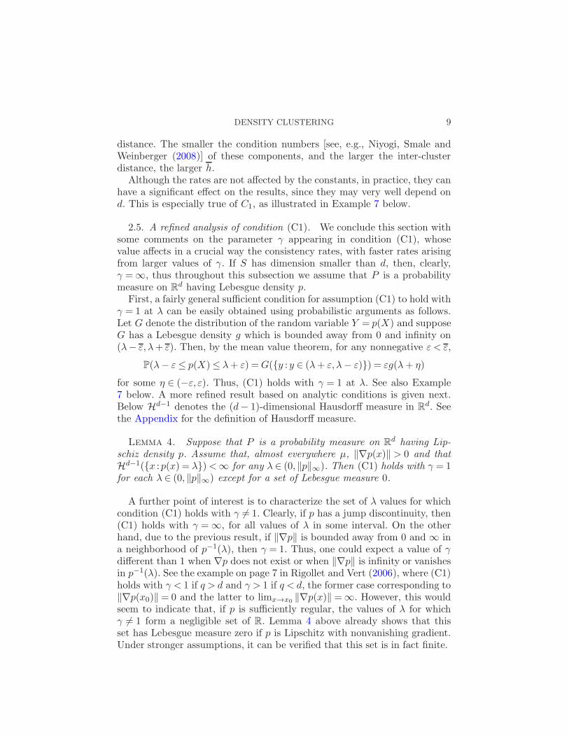
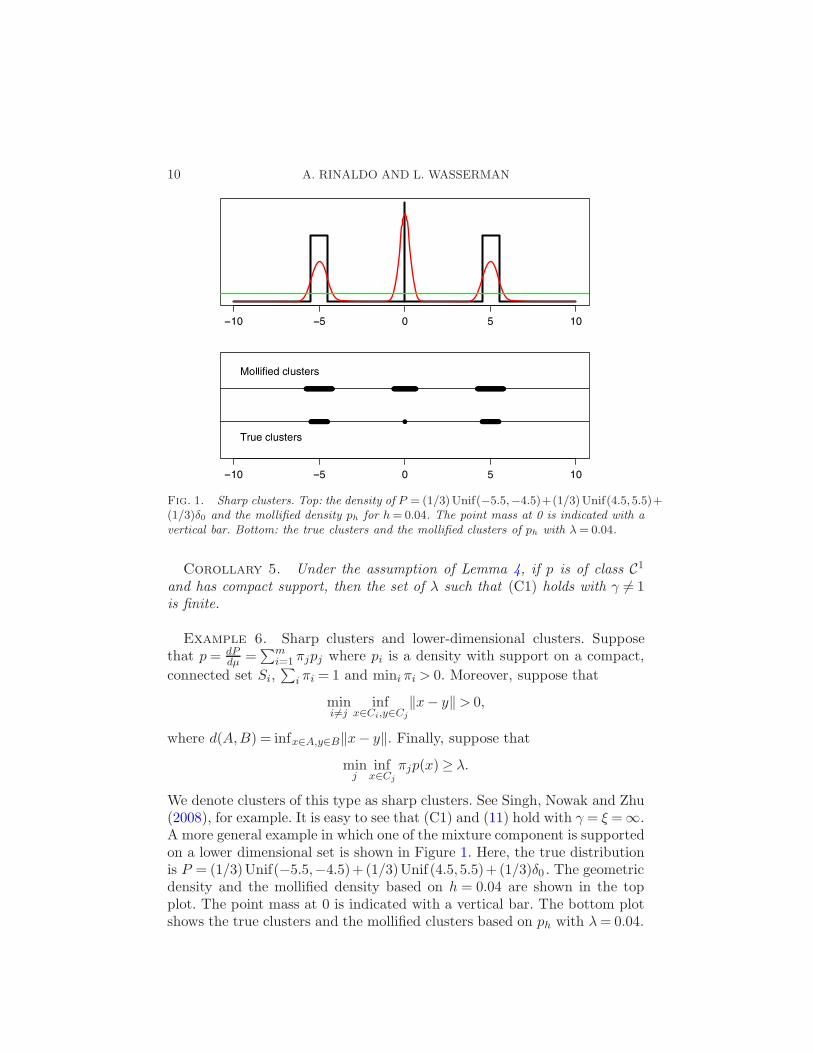
Fig. 1. Sharp clusters. Top: the density of P = (1/3)Unif(−5.5,−4.5)+(1/3)Unif(4.5,5.5)+(1/3)δ0 and the mollified density ph for h= 0.04. The point mass at 0 is indicated with avertical bar. Bottom: the true clusters and the mollified clusters of ph with λ= 0.04.
Corollary 5. Under the assumption of Lemma 4, if p is of class C1
and has compact support, then the set of λ such that (C1) holds with γ 6= 1is finite.
Example 6. Sharp clusters and lower-dimensional clusters. Supposethat p= dP
dµ =∑m
i=1 πjpj where pi is a density with support on a compact,
connected set Si,∑
i πi = 1 and mini πi > 0. Moreover, suppose that
mini 6=j
infx∈Ci,y∈Cj
‖x− y‖> 0,
where d(A,B) = infx∈A,y∈B‖x− y‖. Finally, suppose that
minj
infx∈Cj
πjp(x)≥ λ.
We denote clusters of this type as sharp clusters. See Singh, Nowak and Zhu(2008), for example. It is easy to see that (C1) and (11) hold with γ = ξ =∞.A more general example in which one of the mixture component is supportedon a lower dimensional set is shown in Figure 1. Here, the true distributionis P = (1/3)Unif(−5.5,−4.5)+(1/3)Unif (4.5,5.5)+(1/3)δ0 . The geometricdensity and the mollified density based on h = 0.04 are shown in the topplot. The point mass at 0 is indicated with a vertical bar. The bottom plotshows the true clusters and the mollified clusters based on ph with λ= 0.04.
DENSITY CLUSTERING 11
The clusters based on ph contain the true clusters and the difference betweenthem is a set of zero probability.
Example 7 (Normal distributions). Suppose that X ∼Nd(0,Σ), with Σpositive definite. Set σ = |Σ|1/2. Then (C1) holds for any 0≤ λ≤ (σ(
√2π)d)−1
with γ = 1 and C1 = Cd2σ(√2π)d, where the constant Cd depends on d
(and, of course, λ). We prove the claim only for λ= α(σ(√2π)d)−1, where
α ∈ (0,1). Cases in which α = 1 or α = 0 can be dealt with similarly. Let
W ∼ χ2d and notice that X⊤Σ−1X
d=W . For all ε > 0 smaller than
min
α
σ(√2π)d
,(1− α)
σ(√2π)d
,(12)
simple algebra yields
P (|φσ(X)− λ|< ε)
= P
(2 log
1
α− εσ(√2π)d
≤W ≤ 2 log1
α+ εσ(√2π)d
)
= 2
(log
1
α− ε(σ√2π)d
− log1
α+ ησ(√2π)d
)pd
(log
1
α+ ησ(√2π)d
)
for some η ∈ (−ε, ε) where pd denotes the density of a χ2d distribution and
the second equality holds in virtue of the mean value theorem. By a firstorder Taylor expansion, for ε ↓ 0, the first term on the right-hand side of theprevious display can be written as
2εσ(√2π)d
(1
α− εσ(√2π)d
+1
α+ εσ(√2π)d
)+ o(ε2).
Since ( 1α−εσ(
√2π)d
+ 1α+εσ(
√2π)d
)pd(log1
α+ησ(√2π)d
)≍ 1 for any ε≥ 0 bounded
by (12), the claim is proved. See Figure 2.
3. Rates of convergence. In this section, we study the rates of conver-gence in the two distances using deterministic bandwidths. We defer thediscussion of random (data driven) bandwidths until Section 4.
3.1. Preliminaries. Before establishing consistency rates for the differentrisk measures described above, we discuss some necessary preliminaries.
In our analysis, we require the event
Eh,ε ≡ ‖ph − ph‖∞ ≤ ε, ε ∈ (0, ε), h ∈ (0, h),(13)
to hold with high probability, for all n large enough. In fact, some controlover Eh,ε provides a means of bounding the clustering risks, as shown in thefollowing result.
12 A. RINALDO AND L. WASSERMAN
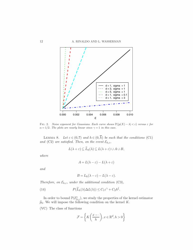
Fig. 2. Noise exponent for Gaussians. Each curve shows P(|p(X)− λ|< ε) versus ε forα= 1/2. The plots are nearly linear since γ = 1 in this case.
Lemma 8. Let ε ∈ (0, ε) and h ∈ (0, h) be such that the conditions (C1)and (C2) are satisfied. Then, on the event Eh,ε,
L(λ+ ε)⊆ Lh(λ)⊆ L(λ+ ε) ∪A∪B,
where
A= L(λ− ε)−L(λ+ ε)
and
B = Lh(λ− ε)−L(λ− ε).
Therefore, on Eh,ε, under the additional condition (C3),
P (Lh(λ)∆L(λ))≤C1εγ +C2h
ξ.(14)
In order to bound P(Ech,ε), we study the properties of the kernel estimator
ph. We will impose the following condition on the kernel K.
(VC) The class of functions
F =
K
(x− ·h
), x ∈R
d, h > 0
DENSITY CLUSTERING 13
satisfies, for some positive number A and v
supP
N(Fh,L2(P ), ε‖F‖L2(P ))≤(A
ε
)v
,(15)
where N(T,d, ε) denotes the ε-covering number of the metric space(T,d), F is the envelope function of F and the supremum is takenover the set of all probability measures on R
d. The quantities A andv are called the VC characteristics of F .
Assumption (VC) appears in Gine and Guillou (2002), Einmahl and Mason(2005), and Gine and Koltchinskii (2006). It holds for a large class of ker-nels, including, for example, any compact supported polynomial kernel andthe Gaussian kernel. See Nolan and Pollard (1987) and van der Vaart andWellner (1996) for sufficient conditions for (VC).
Using condition (VC), we can establish the following finite sample boundfor P(‖ph − ph‖∞ > ε), which is obtained as a direct application of resultsin Gine and Guillou (2002).
Proposition 9 (Gine and Guillon). Assume that the kernel satisfies theproperty (VC) and that
supt∈Rd
suph>0
∫
Rd
K2h(t− x)dP (x)<D <∞.(16)
1. Let h be fixed. Then, there exist constants L> 0 and C > 0, which dependonly on the VC characteristics of K, such that, for any c1 ≥ C and 0<
ε≤ c1D‖K‖∞ , there exists an n0 > 0, which depends on ε, D, ‖K‖∞ and the
VC characteristics of K, such that, for all n≥ n0,
P
supx∈Rd
|ph(x)− ph(x)|> 2ε≤L exp
− 1
L
log(1 + c1/(4L))
c1
nhdε2
D
.(17)
2. Let hn → 0 as n→∞ in such a way that nhdn
|loghdn|
→∞. If εn is a se-
quence such that
εn =Ω
(√log rnnhdn
),(18)
where rn =Ω(h−d/2n ), then, for all n large enough, (17) holds with h and
ε replaced by hn and εn, respectively. In particular, the term on the right-hand side of (17) vanishes at the rate O(r−1
n ).
14 A. RINALDO AND L. WASSERMAN
The above theorem imposes minimal assumptions on the kernel K and,more importantly, on the probability distribution P , whose density is notrequired to be bounded or smooth, and, in fact, may not even exist. Condi-tion (16) is automatically satisfied by bounded kernels. Finally, we remark
that, for fixed h, setting εn =√
2 lognhdnCK
for an appropriate constant CK (de-
pending on K), an application of the Borel–Cantelli lemma yields that, as
n→∞, ‖ph − ph‖∞ =O(√
lognn ) almost everywhere P .
3.2. Rates of convergence. We now derive the converge rates for the clus-tering risks defined in Section 2.2. Below, we will write CK for a constantwhose value depends only on the VC characteristic of the kernel K and onthe constant D appearing in (16).
We recall that Lemma 3 provides a way of controlling the clustering biasdue to the sets Lh(λ − ε) − L(λ − ε), uniformly over ε < ε and h < h. Infact, the parameters θ ∈ 1, . . . , d and ξ ∈ 1,∞ will determine the ratesof consistency for the excess mass and the level set risk, respectively. Specifi-cally, higher values of the parameter θ which correspond to supports of lowerdimension yield faster convergence rates for the excess mass risk. As for thelevel set risks, the case ξ =∞ is the most favorable, since it implies that theclustering bias has no effect on the estimation of level sets and dimension in-dependent rates are possible. In particular, if Cj has dimension smaller thand, then P (Ch
σ(j) − Cj) = 0, so that ξ = ∞. More generally, ξ = ∞ occurs
when L= S. Overall our results yield that, as expected, better rates for theclustering risk are obtained for distributions supported on lower-dimensionalsets.
Theorem 10 (Level set risk). Suppose that (C1), (C2), (C3) and (VC)hold. Then there exists a constant CL such that, for any h ∈ (0, h) and ε ∈(0, ε),
RL(p, ph)≤CL(εγ + hξ + e−CKnhdε2).(19)
In particular, setting
hn =
(logn
n
)γ/(2ξ+dγ)
and εn =
√logn
CKnhdn
we obtain
RL(p, phn) =O
(max
(logn
n
)γξ/(2ξ+dγ)
,1
n
).(20)
DENSITY CLUSTERING 15
If γ = ∞, then either S − L is empty or has zero Lebesgue measure,or S −L is a full dimensional set of positive Lebesgue measure. The formercases, which correspond to P having a lower-dimensional support or to sharpclusters (see Example 6), implies that RL =O( 1n). Thus, we have dimension
independent rates for sharp clusters. In the latter case, ξ = 1, so that RL
is of order O(( lognn )1/d). When γ <∞, then ξ = 1 and the risk is of order
O(( lognn )γ/(2+dγ)).In practice, there are examples in between the sharp and nonsharp cases
for probability distributions with full-dimensional support. For example, ifthere is a very small amount of mass just outside the cluster, then, techni-cally, ξ = 1 and the rate will be slow for large d. However, if this mass isvery small then we expect for finite samples that the behavior of the riskwill be close to the behavior observed in the sharp case. We could capturethis idea mathematically by allowing P to change with n and then allowingξn to vary with n and take values between 1 and ∞. However, we shall notpursue the details here.
As an interesting corollary to Theorem 10, we can show that the expectedproportion of sample points that are incorrectly assigned as clusters or noisevanishes at the same rate.
Corollary 11. Let fh =|Ih|n , where
Ih = i : sign(ph(Xi)− λ) 6= sign(p(Xi)− λ).
Then, E(fh)≤CL(εγ + hξ + e−CKnhdε2).
We now turn to the excess mass risk.
Theorem 12 (Excess mass). Suppose that (C1), (C2), (C3) and (VC)hold. Then, there exists a constant CM , independent of ε and h, such that,for any h ∈ (0, h) and ε ∈ (0, ε) with ε < λ,
RM (p, ph)≤CM (εγ+1 + hθ + e−nCKε2hd).
Thus, setting
hn =
(logn
n
)(γ+1)/(2θ+d(γ+1))
and εn =
√logn
CKnhdn,
we obtain
RM (p, ph) =O
((logn
n
)θ(γ+1)/(2θ+d(γ+1))).(21)
16 A. RINALDO AND L. WASSERMAN
When γ =∞ the excess mass risk RM is of order O( lognn )θ/d. Thus, thehigher θ, that is, the smaller the dimension of the support of P , the fasterthe rate of convergence. In particular, if P is supported over a finite set ofpoints the risk vanishes at the dimension independent rate O( lognn ). When
γ <∞, then θ = 1 and the risk is of order O(( lognn )(γ+1)/(2+d(γ+1))).
3.3. Some special cases. Here, we discuss some interesting special cases.
Fast rates for biased clusters. In some cases, we might be content withestimating the level set Lh(λ), which is a biased version of L(λ). That is, thefringe Lh(λ)−L(λ) may not be of great practical concern and, in fact, it maycontain a very small amount of mass. Indeed, we believe this is why clusteringis often so successful in high-dimensional problems. Exact estimation of thelevel sets is not necessary in many practical problems. In fact, by Lemma2, conditions (C2) guarantees that L will include L with high probability.Thus, for clustering purposes, one may consider some modifications of ourrisk functions. First, suppose we only require that the estimated clusterscover the true clusters. That is, we say there is not error as long as Cj ⊂ Cj .This suggests the following modification of our risk functions:
• RL(p, ph) =∫x : p(x)≥λ∩x : ph(x)<λ dP (x),
• RM (p, ph) = E(L)−E(Lh ∩L).
Then we have the following result, which gives faster, dimension independentrates. The proof is similar to the proofs of the previous results and is omitted.
Theorem 13. Let h ∈ (0, h) be fixed. Under (C1), (C2) and (VC), then
RL(p, ph) =O
(max
(logn
n
)γ/2
,1
n
)
and
RM (p, ph) =O
((logn
n
)(1+γ)/2).
Alternatively, one may be only interested in estimating the clusters ofthe mollified density ph, for any fixed h ∈ (0, h). Then, provided that ph issufficiently smooth (which is guaranteed by choosing a smooth kernel) andhas finite positive gradient for each point in the set ∂Lh(λ), the results inSection 2.5 show that, for all ε small enough,
µ(x : |ph(x)− λ|< ε)≤ ε.
DENSITY CLUSTERING 17
Thus, under assumptions (C2) and (VC), similar arguments to the ones usedin the proofs of Theorems 10 and 12 imply that
RL(ph, ph) =
∫
x : ph(x)≥λ∆x : ph(x)≥λdP (x) =O
(√logn
n
)
and
RM (ph, ph) = E(Lh)− E(E(Lh)) =O
(logn
n
).
In either case, we get dimension independent rates.
The smooth full-dimensional case. In the more specialized settings inwhich P has full-dimensional support and the Lebesgue density p is smooth,better results are possible. For example, using the same settings of Rigolletand Vert (2006), if p is β-times Holder differentiable, then the bias conditions(C2) are superfluous, as
‖ph − p‖∞ ≤Chβ(22)
for some constant C which depends only on the kernel K. Choosing h suchthat Chβ < ε, on the event Eh,ε, the triangle inequality yields ‖ph−p‖∞ < 2ε.Thus, for each ε < ε
2 and each h such that Chβ < ε, on Eh,ε, instead of (14),one obtains
P (Lh(λ)∆L(λ))≤C12γεγ .
Then, setting hn = (logn/n)1/(2β+d) and εn =Ω((logn/n))β/(2β+d)), we seethat RL(p, ph) is of order O((logn/n)γβ/(2β+d)), while RM (p, ph) is of orderO((logn/n)(γ+1)β/(2β+d)). These, are, up to an extra logarithmic factor, theminimax rates established by Rigollet and Vert (2006). In fact, under thesesmoothness assumptions, and since the bias can be uniformly controlledas in (22), then, by a combination of Fubini’s theorem and of a peelingargument as in Audibert and Tsybakov (2007) and Rigollet and Vert (2006),
the exponential term O(e−CKnhdε2) becomes redundant and rates withoutthe logarithmic term are possible.
4. Choosing the bandwidth. In this section, we discuss two data-drivenmethod for choosing the bandwidth that adapts to the unknown parametersγ and θ. Before we explain the details, we point out that L2 cross-validationis not appropriate for this problem. In fact, we are allowing for the casewhere P may have atoms, in which case it is well known that cross-validationchooses h= 0.
18 A. RINALDO AND L. WASSERMAN
4.1. Excess mass. We propose choosing h by splitting the data and max-imizing an empirical estimate of the excess mass functional. Polonik (1995)used this approach to choose a level set from among a fixed class L oflevel sets of finite VC dimension. Here, we are choosing a bandwidth, or, inother words, we are choosing a level set from a random class of level setsL= x : ph(x)≥ λ :h > 0 depending on the observed sample X . The stepsare in Table 1.
To implement the method, we need to compute µ(Lh). In practice, µ(Lh)can be approximated by
1
M
M∑
i=1
I(ph(Ui)≥ λ)
g(Ui),
where U1, . . . ,UM is a sample from a convenient density g. In particular, onecan choose g = pH for some large bandwidth H . Choosing M ≈ n2 ensuresthat the extra error of this importance sampling estimator is O(1/n) whichis negligible. We ignore this error in what follows.
Technically, the method only applies for λ > 0, at least in terms of thetheory that we derive. In practice, it can be used for λ= 0. In this case, E(h)becomes 1 when h is large. We then take h to be the smallest h for whichE(h) = 1.
Below we use the notation EX(·) instead of E(·) to indicate that the excessmass functional (7) is evaluated at a random set depending on the trainingset X and, therefore, is itself random. Accordingly, with some abuse of no-tation, for any h > 0, we will write EX(h) = E(Lh), with Lh the λ-level set ofph. Below H is a countable dense subset of [0, h]. The next result is closelyrelated to Theorem 7.1 of Gyorfi et al. (2002).
Theorem 14. Let h∗ = argmaxh∈H EX(h). For any δ > 0,
E(EX(h∗))−E(EX(h))≤ d(δ, κ)1 + log 2
n,(23)
Table 1
Selecting the bandwidth using the excess mass risk
1. Split the data into two halves which we denote by X = (X1, . . . ,Xn) and Z =(Z1, . . . ,Zn).
2. Let H be a finite set of bandwidths. Using X , construct kernel density estimatorsph :h ∈H. Let Lh = x : ph(x)≥ λ.
3. Using Z, estimate the excess mass functional
E(h) =1
n
n∑
i=1
I(Zi ∈ Lh)− λµ(Lh).
4. Let h be the maximizer of E(h) and set L= Lh.
DENSITY CLUSTERING 19
where the expectation is with respect to the joint distribution of the trainingand test set, d(δ, κ) = 2
κδ(1 + δ)(16γ2 + δ(7 + 16γ2)), with κ = 2 + λµ(S +
B(0, h)) and γ2 = 74 (e
4/7 − 1).
Now we construct a grid Hn of size depending on n that is guaranteed toensure that optimizing over Hn implies we are adapting over γ and θ.
Theorem 15. Suppose (C1) and (C2) hold. Let
δn(θ) =aθ/dn
2An(θ),
where an = (logn/n) and
An(θ) =2|log an|aθ/(2θ+d)
n θ2
(2θ + d)2.
Let Gn(θ) = γ1(θ), . . . , γN(θ)(θ) where γj(θ) = (j−1)δn(θ) and N(θ) is thesmallest integer less than or equal to Υn(θ)/δn(θ),
Υn(θ) =2θ2
d2Wn− 2θ
d− 1
and
Wn =log 2
logn− log logn.
Let
Hn = hn(γ, θ) : θ ∈ 1, . . . , d, γ ∈Gn(θ),where hn(γ, θ) = a
(γ+1)/(2θ+d(γ+1))n . Let L be obtained by minimizing E(h)
for h ∈Hn. Then
E(L)−E(E(L))≤O
(logn
n
)θ(γ+1)/(2θ+d(γ+1))
.
The latter theorem shows that our cross-validation methods gives a com-pletely data-driven method for choosing the bandwidth that preserves therate. Notice, in particular, that adapting to the parameter θ is equivalentto adapting to the unknown dimension of the support of P . This makes itpossible to use our method in practical problems as long as the sample sizeis large. For small sample sizes, data splitting might lead to highly variableresults in which case our bandwidth selection method might not work well.An alternative is to split the data many times and combines the estimatesover multiple splits.
When µ(L) = 0, we have that h∗ = 0. The above theorems are still validin this case. Thus, the case where P is atomic is included while it is ruledout for L2 cross-validation.
20 A. RINALDO AND L. WASSERMAN
4.2. Stability. Another method for selecting the bandwidth is to choosethe value for h that produces stable clusters, in a sense defined below. Theuse of stability has gained much popularity in clustering; see Ben-Hur, Elisse-eff and Guyon (2002) and Lange et al. (2004), for example. In the context ofk-means clustering and related methods, Ben-David, von Luxburg and Pall(2006) showed that minimizing instability leads to poor clustering. Here, weinvestigate the use of stability for density clustering.
Suppose, for simplicity, that the sample size is a multiple of 3. That is,the sample size is 3n say. Now randomly split the data into three vectors ofsize n, denoted by X = (X1, . . . ,Xn), Y = (Y1, . . . , Yn) and Z = (Z1, . . . ,Zn).(In practice, we split the data into three approximately equal subsets.)
We define the instability function as the random function Ξ : [0,∞) 7→ [0,1]given by
Ξ(h)≡ ρ(ph, qh, PZ) =
∫
x : ph(x)≥λ∆x : qh(x)≥λdPZ(x),(24)
where ph is constructed from X , qh is constructed from Y and PZ is theempirical distribution based on Z.
Rather than studying stability in generality, we consider a special caseinvolving the following extra conditions.
1. Sharp clusters. Assume that P =∑m
j=1 πjPj where∑
i πj = 1, and Pj
is uniform on the compact set Sj of full dimension d. Thus, p(z) =∑j ∆jI(z ∈ Sj) where ∆j = πj/µ(Sj). Let ∆ =minj ∆j > 0 and let ∆ =
maxj ∆j .2. Spherical Kernel. We use a spherical kernel so that
ph(z) =1
nhd
n∑
i=1
I(‖z −Xi‖ ≤ h)
vd=
P (B(x,h))
hdvd,
where vd = πd/2/Γ(d/2 + 1) denotes the volume of the unit ball and P isthe empirical measure.
3. The support of P is a standard set. Letting S = ∪mj=1Sj , we assume that
there exists a δ ∈ (0,1) such that
µ(B(z,h)∩L)≥ δµ(B(z,h)) for all z ∈ S and all h < diam(S),
where diam(S) = sup(x,y)⊂S ‖x− y‖ indicates the diameter of the set S.This property appears in a natural way in set estimation problems; see,for example, Cuevas and Fraiman (1997).
4. Choice of λ. We take λ= 0, so that L= S.
Under these settings, the graph Ξ(h) is typically unimodal with Ξ(0) =Ξ(∞) = 0. Hence, it makes no sense to minimize Ξ. Instead, we will fix a
DENSITY CLUSTERING 21
constant α ∈ (0,1) and choose
h= infh : sup
t>hΞ(t)≤ α
.(25)
Theorem 16. Let h∗ = diam(L). Under conditions 1–4:
1. Ξ(0) = 0 and Ξ(h) = 0, for all h≥ h∗;2. sup0<h<h∗
E(Ξ(h))≤ 1/2;
3. as h→ 0, E(Ξ(h))≍ hd;4. for each h ∈ (0, h∗),
D3(h∗ − h)d(n+1)Dn4 ≤ E(Ξ(h))≤ 2D1(h∗ − h)n+1Dn
2 ,
where
D1 =πd/2hd−1
∗2dΓ((d/2) + 1)
, D2 =πd/2hd−1
∗Γ((d/2) + 1)
,
D3 =δ∆πd/2
Γ((d/2) + 1), D4 =
∆δπd/2
Γ(d/2 + 1).
To see the implication of Theorem 16, we proceed as follows. Consider agrid of values H⊂ (0, h∗) of cardinality nβ , for some 0< β < 1. By Hoeffd-ing’s inequality, with probability at least 1− 1
n , we have that
suph∈H
|Ξ(h)−E(Ξ(h))| ≤wn ≡√
2 log(2n)(1− β)
n.
Replacing E(Ξ(h)) by Ξ(h) + wn and Ξ(h) − wn in the upper and lowerbounds of part 4 of Theorem 16, respectively, setting them both equal toα and then finally solving for h, we conclude that the selected h is upperbounded by
h∗ −(α−wn
2D1
)1/(n+1)
D−n/(n+1)2
and lower bounded by
h∗ −(α+wn
D3
)1/(d(n+1))
D−n/(d(n+1))4
with probability larger than 1− 1n . Thus, as n→∞, the resulting bandwidth
does not tend to 0. Hence, the stability based method leads to bandwidthsthat are quite different than the method in the previous section. Our expla-nation for this finding is that the stability criterion is essentially aimed at
22 A. RINALDO AND L. WASSERMAN
reducing the variability of the clustering solution, but it is virtually unaf-fected by the bias caused by large bandwidths.
In the analysis above, we assumed for simplicity that λ= 0. When λ > 0,the instability Ξ(h) can have some large peaks for very large h. This occurswhen h is large enough so that some mode of ph(x) is close to λ. Choosingh according to (25) will then lead to serious oversmoothing. Instead, we can
choose h as follows. Let h0 = argmaxhΞ(h) and define
h= infh :h≥ h0,Ξ(h)≤ α.(26)
We will revisit this issue in Section 6. A theoretical analysis of this modifiedprocedure is tedious and, in the interest of space, we shall not pursue it here.
5. Approximating the clusters. Lemma 2 shows that, under mild, con-ditions and when the sample size is large enough, N(λ) = Nh(λ) uniformlyover h ∈ (0, h) with high probability. However, computing the number of con-
nected components of Lh(λ) exactly is computationally difficult, especiallyif d is large. In this section, we study a graph-based algorithm for findingthe connected components of Lh and for estimating the number of λ-clustersN(λ) that is based on the ρ-nearest neighborhood graph of Xi : ph(Xi)≥ λthat is fast and easy to implement.
The idea using the union of balls of radius ρ centered at the sample pointsto recover certain properties of the support of a probability distribution iswell understood. For instance, Devroye and Wise (1980) and Korostelev andTsybakov (1993) use it as a simple yet effective estimator of the support,while Niyogi, Smale and Weinberger (2008) show how it can be utilized foridentifying certain homology features of the support.
In particular, Cuevas, Febrero and Fraiman (2000) and Biau, Cadre andPellettier (2007) propose to combine a kernel density estimation with asingle-linkage graph algorithm to estimate the number of λ-clusters [see alsoJang and Hendry (2007), for an application to large databases]. Our resultsoffer similar guarantees but hold under more general settings.
The algorithm proceeds as follows. For some h ∈ (0, h) and a given λ≥ 0:
1. compute the kernel density estimate ph;2. compute the ρ-nearest neighborhood graph of Xi : ph(Xi) ≥ λ, that is
the graph Gh,n on Xi : ph(Xi)≥ λ where there is an edge between anytwo nodes if and only if they both belong to a ball of radius ρ;
3. compute the connected components of Gh,n using a depth-first search.
The computational complexity of the last step is linear in the number ofnodes and the number of edges of Gh,n [see, e.g., Cormen et al. (2002)],which are both random.
We will show that, if ρ is chosen appropriately, then, with high probabilityas n→∞:
DENSITY CLUSTERING 23
1. the number of connected components of Gh,n, NGh (λ), matches the number
of true clusters, N(λ) = k;2. there exists a permutation of 1, . . . , k such that, for each j and j′,
Chj ⊆
⋃
x∈Cσ(j)
B(x,ρ) and
( ⋃
x∈Cσ(j)
B(x,ρ)
)∩( ⋃
x∈Cσ(j′)
B(x,ρ)
)=∅,
(27)where C1, . . . ,Ck are the connected components of Gh,n.
We will assume the following regularity condition on the densities ph,which is satisfied if the kernel K is of class C1 and P is not flat in a neigh-borhood of λ:
(G) there exist constants ε1 > 0 and Cg > 0 such that for each h ∈ (0, h), phis of class C1 on x : |ph(x)− λ|< ε1 and
infh∈(0,h)
infx∈|ph(x)−λ|<ε1
‖∇ph(x)‖>Cg.(28)
Let δh = mini 6=j infx∈Chi ,y∈Ch
j‖x− y‖ and set δ = infh∈(0,h) δh. Notice that,
under (C2)(b), δ > 0. Finally, let Oh,n denote the event in (27), which clearly
implies the event NGh (λ) = k.
Theorem 17. Assume conditions (G) and (C2) and let d∗ = dim(L).Assume further that there exists a constant C such that, for every r ≤ δ/2and for P -almost all x∈ S ∩L,
P (B(x, r))>Crdi ,(29)
where di = dim(Si), with x ∈ Si. Then there exists positive constants ρ andM , depending on d∗ and L such that, for every ρ <minδ/2, ρ, there existsa number ε(ρ) such that, for any ε < η(ρ),
P(Och,n)≤ P(Ec
h,ε) +Mρ−d∗e−Cnρd∗
,
uniformly in h ∈ (0, h).
The previous result deserves few comments. First, the constants ρ, Mand C depend on d∗. Second, assumption (29) is a natural generalizationto lower-dimensional sets of the standardness assumption used, for exam-ple, in Cuevas and Fraiman (1997). It is clearly true for components Pi offull-dimensional support that are absolutely continuous with respect to theLebesgue measure. Finally, in view of Lemma 19 [and, specifically, of theway ε(ρ, τ) is defined], Theorem 17 holds for sequences εn, hn and ρnsuch that:
24 A. RINALDO AND L. WASSERMAN
1. εn = o(1),2. supn hn ≤ h;3. supn ρn <minδ/2, ρd and εn = o(ρn).
In particular, if hn = o(1), then, following Proposition 9, the term P(Echn,εn
)
vanishes if nhdn
|loghdn|
→∞. Interestingly enough, condition (C1) does not play
a direct role in Theorem 17.We now consider a bootstrap extension of the previous algorithm, as
suggested in Cuevas, Febrero and Fraiman (2000). For any h, let X∗ =(X∗
1 , . . . ,X∗N ), denote a bootstrap sample from ph conditionally on ph ≥ λ
and let G∗n,h denote the ρ-neighborhood graph with node set X∗. Finally, let
O∗h,n be the event given in (27), except that C1, . . . ,Ck are now the connected
components of G∗h,n.
Theorem 18. Assume conditions (C2) and (G). Suppose that thereexist positive constants C and ρ such that
infh∈(0,h)
∫
Ah∩Lh(λ)ph dµ > Cρd(30)
for any ball Ah of radius ρ < ρ and center in Lh(λ). Then, for any ρ ≤minδ/2, ρ, there exists a positive number ε(ρ) such that, for each ε < ε(ρ),
P((O∗h,n)
c)≤ P(Ech,ε) +Mρ−de−CNρd ,
uniformly in h ∈ (0, h), where M and C are positive constants independentof h and ρ.
The constants C, C, ρ, and M depend on both d and S ⊕ B(0, h). Inour settings, condition (30) clearly holds if P has full-dimensional support.More generally, it can be shown that conditions (G) and (29) imply (30).
Just like with Theorem 17, using Lemma 19, it can be verified that the the-orem holds if one consider sequences of parameters depending on the samplesize such that εn = o(1), εn = o(ρn), supn ρn <maxδ/2, ρ and supn hn < h,provided that the conditions of Proposition 9 are met.
Despite the similar form for the error bounds of Theorems 17 and 18,there are some marked differences. In fact, in Theorem 17 the performanceof the algorithm depends directly on the sample size n and, in particular,on the actual dimension d∗ ≤ d of the support of P , with smaller values ofd∗ yielding better guarantees. In contrast, besides n, the performance of thealgorithm based on the bootstrap sample depends on the ambient dimensiond, regardless of d∗, and on the bootstrap sample size N . By choosing N verylarge, the expression P(Ec
h,ε) becomes the leading term in the upper bound
of the probability of the event (O∗h,n)
c.
DENSITY CLUSTERING 25
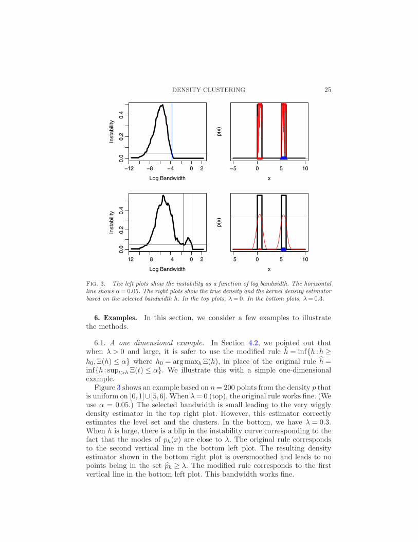
Fig. 3. The left plots show the instability as a function of log bandwidth. The horizontalline shows α= 0.05. The right plots show the true density and the kernel density estimatorbased on the selected bandwidth h. In the top plots, λ= 0. In the bottom plots, λ= 0.3.
6. Examples. In this section, we consider a few examples to illustratethe methods.
6.1. A one dimensional example. In Section 4.2, we pointed out thatwhen λ > 0 and large, it is safer to use the modified rule h = infh :h ≥h0,Ξ(h) ≤ α where h0 = argmaxhΞ(h), in place of the original rule h =infh : supt>hΞ(t) ≤ α. We illustrate this with a simple one-dimensionalexample.
Figure 3 shows an example based on n= 200 points from the density p thatis uniform on [0,1]∪ [5,6]. When λ= 0 (top), the original rule works fine. (Weuse α = 0.05.) The selected bandwidth is small leading to the very wigglydensity estimator in the top right plot. However, this estimator correctlyestimates the level set and the clusters. In the bottom, we have λ = 0.3.When h is large, there is a blip in the instability curve corresponding to thefact that the modes of ph(x) are close to λ. The original rule correspondsto the second vertical line in the bottom left plot. The resulting densityestimator shown in the bottom right plot is oversmoothed and leads to nopoints being in the set ph ≥ λ. The modified rule corresponds to the firstvertical line in the bottom left plot. This bandwidth works fine.
26 A. RINALDO AND L. WASSERMAN
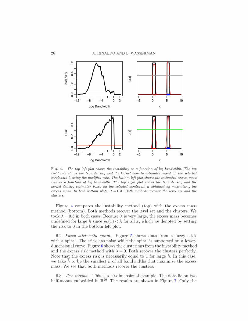
Fig. 4. The top left plot shows the instability as a function of log bandwidth. The topright plot shows the true density and the kernel density estimator based on the selectedbandwidth h using the modified rule. The bottom left plot shows the estimated excess massrisk as a function of log bandwidth. The top right plot shows the true density and thekernel density estimator based on the selected bandwidth h obtained by maximizing theexcess mass. In both bottom plots, λ = 0.3. Both methods recover the level set and theclusters.
Figure 4 compares the instability method (top) with the excess massmethod (bottom). Both methods recover the level set and the clusters. Wetook λ= 0.3 in both cases. Because λ is very large, the excess mass becomesundefined for large h since ph(x)< λ for all x, which we denoted by settingthe risk to 0 in the bottom left plot.
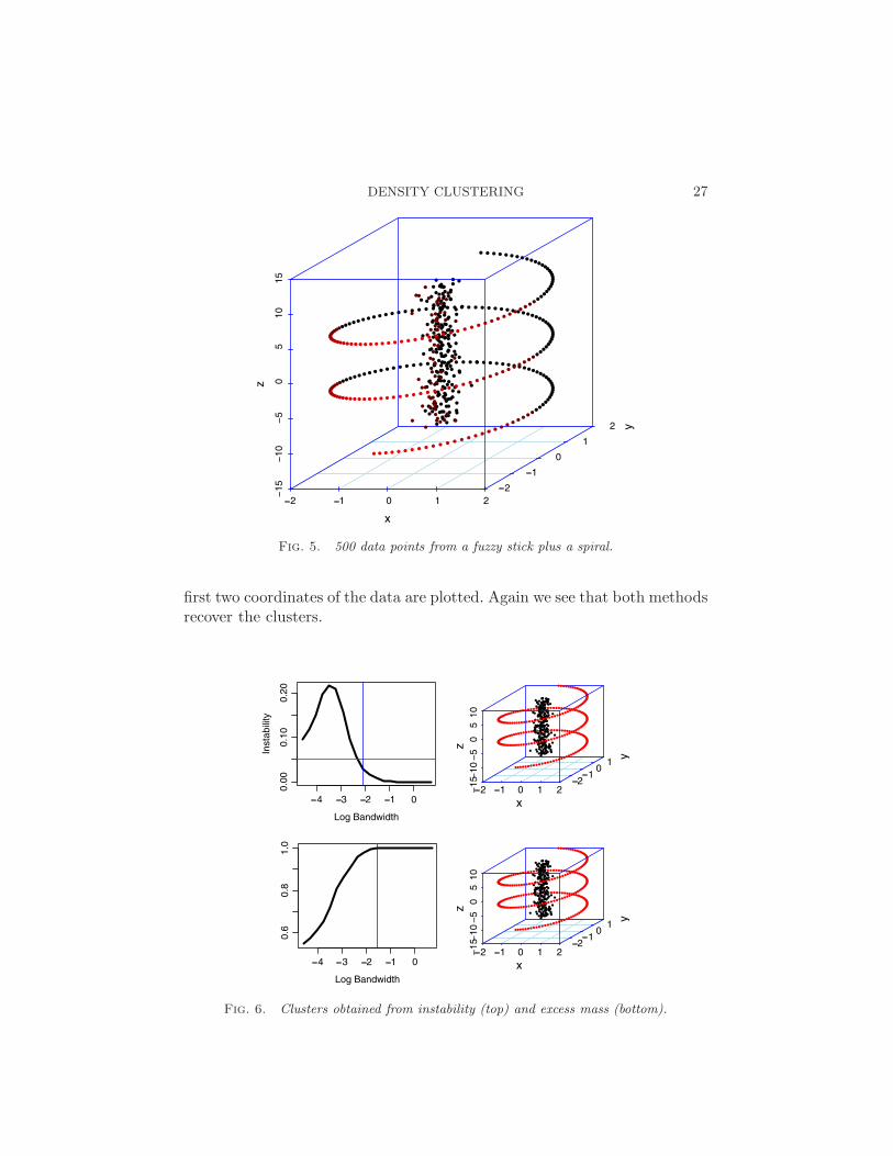
6.2. Fuzzy stick with spiral. Figure 5 shows data from a fuzzy stickwith a spiral. The stick has noise while the spiral is supported on a lower-dimensional curve. Figure 6 shows the clusterings from the instability methodand the excess risk method with λ= 0. Both recover the clusters perfectly.Note that the excess risk is necessarily equal to 1 for large h. In this case,we take h to be the smallest h of all bandwidths that maximize the excessmass. We see that both methods recover the clusters.
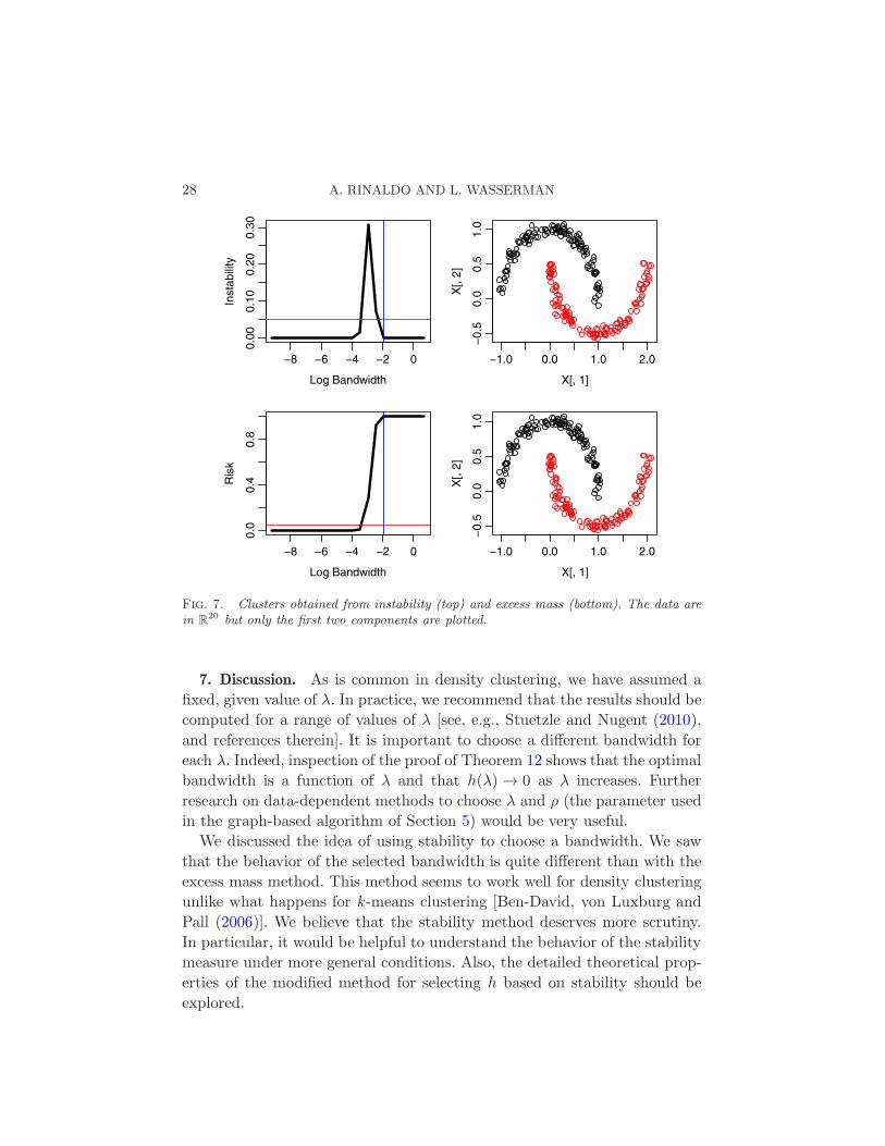
6.3. Two moons. This is a 20-dimensional example. The data lie on twohalf-moons embedded in R
20. The results are shown in Figure 7. Only the
DENSITY CLUSTERING 27
Fig. 5. 500 data points from a fuzzy stick plus a spiral.
first two coordinates of the data are plotted. Again we see that both methodsrecover the clusters.
Fig. 6. Clusters obtained from instability (top) and excess mass (bottom).
28 A. RINALDO AND L. WASSERMAN
Fig. 7. Clusters obtained from instability (top) and excess mass (bottom). The data arein R
20 but only the first two components are plotted.
7. Discussion. As is common in density clustering, we have assumed a
fixed, given value of λ. In practice, we recommend that the results should be
computed for a range of values of λ [see, e.g., Stuetzle and Nugent (2010),
and references therein]. It is important to choose a different bandwidth for
each λ. Indeed, inspection of the proof of Theorem 12 shows that the optimal
bandwidth is a function of λ and that h(λ) → 0 as λ increases. Further
research on data-dependent methods to choose λ and ρ (the parameter used
in the graph-based algorithm of Section 5) would be very useful.
We discussed the idea of using stability to choose a bandwidth. We saw
that the behavior of the selected bandwidth is quite different than with the
excess mass method. This method seems to work well for density clustering
unlike what happens for k-means clustering [Ben-David, von Luxburg and
Pall (2006)]. We believe that the stability method deserves more scrutiny.
In particular, it would be helpful to understand the behavior of the stability
measure under more general conditions. Also, the detailed theoretical prop-
erties of the modified method for selecting h based on stability should be
explored.
DENSITY CLUSTERING 29
Finally, we note that there is growing interest in spectral clustering meth-ods [von Luxburg (2007)]. We believe there are connections between the workreported here and spectral methods.
8. Proofs. Proof of Lemma 1. The weak convergence follows fromthe fact that P is a Radon measure [see, e.g., Leoni and Fonseca (2007),Theorem 2.79]. As for the second part, if x ∈ Si, where Si has Hausdorffdimension d, then p(x) = πipi(x), with pi a Lebesgue density, and the resultfollows directly from Leoni and Fonseca (2007), Theorem 2.73, part (ii). Seealso the Appendix. On the other hand if di < d, then it is necessary to modify
the arguments as follows. Since K is smooth and supported on B(0,1), there
exists a η such that K(x−yh )> η if ‖x− y‖< ηh. Set C =
ηdi+1vdicd
, where vdiis the volume of the unit Euclidean ball in R
di . Then
ph(x) =1
cdhd
∫
Si∩B(x,h)K
(x− y
h
)dP (y)
≥ 1
cdhdη
∫
Si∩B(x,ηh)dP (y)
=ηdi+1vdicdhd−di
1
vdi(ηh)diPi(B(x, ηh))
=C
h(d−di)
Pi(B(x, ηh))
vdi(ηh)di
.
As as h→ 0, Pi(B(x,η,h))
vdi (ηh)di
→ pi(x)<∞, by (39) almost everywhere Hdi , while
Ch(d−di)
→∞, thus showing that limh→0 ph(x) =∞.
Proof of Lemma 2. By assumption (C2), for any 0≤ ε < ε and 0<h< h,
Nh(λ− ε) =Nh(λ) =Nh(λ+ ε) =N(λ) = k.
On the event Eh,ε it holds that
Lh(λ+ ‖ph − ph‖∞)⊆ Lh(λ)⊆ Lh(λ−‖ph − ph‖∞),
which implies that, on the same event,
k =Nh(λ+ ‖ph − ph‖∞)≤ Nh(λ)≤Nh(λ− ‖ph − ph‖∞) = k.
Proof of Lemma 3. Recall that Kh is supported on B(0, h). For thefirst claim, it is enough to show that, for any ε ∈ [0, ε), Lh(λ−ε)−L(λ−ε) ⊆∂L(λ− ε) +B(0, h). Indeed, by (C3), µ(∂L(λ− ε)⊕B(0, h))≤C2h
θ, which
30 A. RINALDO AND L. WASSERMAN
implies (10). Thus, we will prove that, if w /∈ ∂L(λ − ε) ⊕ B(0, h), thenw /∈ Lh(λ − ε) − L(λ − ε). For such a point w, either p(w) ≥ λ − ε or, byconditions (C2), p(z) < λ − ε for every z ∈ B(w,h). Since the kernel Khas compact support, the latter case implies that ph(w) < λ − ε as well.Therefore,
w ∈ x :p(x)≥ λ− ε ∪ x :ph(x)< λ− ε= x :p(x)<λ− ε, ph(x)≥ λ− εc
= (Lh(λ− ε)−L(λ− ε))c.
As for inequality (11), it is enough to observe that the set
Ih,ε = (Lh(λ− ε)−L(λ− ε)) ∩ S
either has zero probability (because it is empty or has Lebesgue measure 0)or has positive Lebesgue measure. In the former case, we obtain ξ =∞. Inthe latter case, Ih,ε must be full dimensional, so that, by (10), µ(Ih,ε)≤C3h,
for all h ∈ (0, h). Since p is bounded by λ on Ih,ε, we obtain
P (Lh(λ− ε)−L(λ− ε)) = P (Ih,ε)≤ λC2h=C3h,
which implies that we can take ξ = 1.
Proof of Lemma 4. Since p is Lipschitz and integrable, p−1(λ) isHd−1-measurable, so the integral Hd−1(x :p(x) = λ) is well defined forλ ∈ (0,‖p‖∞), where Hd−1 denote the (d− 1)-dimensional Hausdorff mea-sure in R
d. Furthermore, we can use the coarea formula. See Evans andGariepy (1992) and Ambrosio, Fusco and Pallara (2000) for backgroundson Hausdorff measures and the coarea formula. By the Rademacher theo-rem, the set E1 of points where p is not differentiable has Lebesgue measurezero. By Lemma 2.96 in Ambrosio, Fusco and Pallara (2000), the set E2 =x :‖∇p(x)‖= 0 is such that Hd−1p−1(λ) ∩E2= 0, for all λ ∈ (0,‖p‖∞)outside of a set E3 ⊂ R of Lebesgue measure 0. Without loss of generality,below we may assume that E1 and E2 are empty. Thus, we can assume that,for any λ ∈ (0,‖p‖∞) ∩Ec
3, there exists positive numbers ε, C and M suchthat:
(i) infx∈x : |p(x)−λ|<ε ‖∇p(x)‖>C, almost everywhere-µ;
(ii) supη∈(−ε,ε)Hd−1(x :p(x) = λ+ η)<M .
Then for each ε ∈ (0, ε),
P (x : |p(x)− λ|< ε) =∫
p(x)1|p(x)−λ|<ε dµ(x)
=
∫p(x)
‖∇p(x)‖1|p(x)−λ|<ε‖∇p(x)‖dµ(x)
DENSITY CLUSTERING 31
=
∫ +ε
−ε
∫
p−1(λ+u)
p(x)
‖∇p(x)‖ dHn−1(x)du
=
∫ +ε
−ε(λ+ u)
∫
p−1(λ+u)(‖∇p(x)‖)−1 dHn−1(x)du
≤ 2λM
Cε,
where the second equality holds because ‖∇p(x)‖ is bounded away from 0on x : |p(x) − λ| < ε by (i), the third equality is a direct application ofthe coarea formula [see, e.g., Proposition 3, page 118 in Evans and Gariepy(1992)] and the last inequality follows from (i) and (ii).
Proof of Corollary 5. Following the proof of Lemma 4 and usingour additional assumption that p is of class C1, without any loss of generality,below we can assume that the set E1 and E2 are empty and we recall thatE3 has Lebesgue measure 0. Let λ /∈E3 be such that
infx∈p−1(λ)
‖∇p(x)‖> 0.
We now claim that there exists a nonempty neighborhood U of λ for which
infλ∈U
infx∈p−1(λ)
‖∇p(x)‖> 0.
Indeed, arguing by contradiction, suppose that the previous display were notverified for any neighborhood U of λ. Then there exist sequences λn ⊂R
and xn ⊂ S such that limn λn = λ, and xn ∈ p−1(λn) and ∇p(xn) = 0 foreach n. By compactness, it is possible to extract a subsequence xnk
ofxn such that xnk
→ x, for some x ∈ p−1(λ). Since p is of class C1, thisimplies that ∇p(xnk
)→∇p(x) as well. However, ∇p(xnk) = 0 for each k by
construction, while ∇p(x) 6= 0. This produces a contradiction. Thus, for eachλ that is not a critical point, one can find a neighborhood of positive lengthcontaining it and, by Lemma 4, (C1) holds at λ with γ = 1. Since, usingcompactness again, ‖p‖∞ <∞, this implies that there can only be a finitenumber of critical points for which γ may differ from 1.
Proof of Lemma 8. Since ε < ε and h < h, in virtue of (C2)(b) itholds that, on Eh,ε,
Lh(λ)⊇Lh(λ+ ε)⊇ L(λ+ ε)
and
Lh(λ)⊆ Lh(λ− ε) =L(λ− ε)∪ (Lh(λ− ε)−L(λ− ε)).
32 A. RINALDO AND L. WASSERMAN
Because L(λ+ε)⊆L(λ)⊆ L(λ−ε), the above inclusions imply, still on Eh,ε,that
Lh(λ)∆L(λ)⊆ (L(λ− ε)−L(λ+ ε)) ∪ (Lh(λ− ε)−L(λ− ε))
=A∪B,
where it is clear that the sets A and B are disjoint. Taking expectation withrespect to P of the indicators of the sets Lh(λ)∆L(λ), A and B and usingcondition (C1) and Lemma 3 yield (14).
Proof of Proposition 9. The claimed results are a direct conse-quence of Corollary 2.2 in Gine and Guillou (2002). We outline the detailsbelow. We rewrite the left-hand side of (17) as
P
∥∥∥∥∥
n∑
i=1
f(Xi)−E[f(X1)]
∥∥∥∥∥Fh
> 2εnhd
,
where
Fh =
K
(x− ·h
), x ∈R
d
and then proceed to apply Gine and Guillou (2002), Corollary 2.2. Followingtheir notation, we set t= nhdε and, since,
supf∈Fh
Var[f ]≤ supz
∫
Rd
K2
(z − x
h
)dP (x)≤ hdD,
we can further take σ2 = hdD and U =C‖K‖∞, where C is a positive con-stant, depending on h, such that σ < U/2. Then conditions (2.4), (2.5) and(2.6) of Gine and Guillou (2002) are satisfied for all n bigger than somefinite n0, which depends on the VC characteristics of K, D, ‖K‖∞, C andε. Part 2 is proved in a very similar way. In this case, we take the supre-mum over the the entire class F and we set σ2
n = hdnD and U = ‖K‖∞. Forall n large enough, condition (2.5) is trivially satisfied because hn = o(1),while equations (2.4) and (2.6) hold true by virtue of (18). The unspecifiedconstants again depend on the VC characteristics of K, D and ‖K‖∞.
Proof of Theorem 10. We can write
E(ρ(p, ph, P )) = E
(∫
Lh(λ)∆L(λ)dP ;Eh,ε
)+E
(∫
Lh(λ)∆L(λ)dP ;Ec
h,ε
),(31)
where for a random variable X defined on some probability space (Ω,F ,P)and an event E ⊂ F , E(X;E) ≡
∫Ω∩AX(ω)dP(ω). Using Proposition 9, the
second term on the right-hand side is upper bounded by
P(Eh,ε)≤Le−nCKhde2 .(32)
DENSITY CLUSTERING 33
As for the first term on the right-hand side of (31), without loss of gen-erality, we consider separately the case in which the support of P has nolower-dimensional components and the case in which it of lower dimension.The result for the cases in which the support has components of differentdimensions follows in a straightforward way.
If the support of P consists of full-dimensional sets, then, on the eventEh,ε,
∫
Lh(λ)∆L(λ)dP ≤ P (L(λ− ε)−L(λ+ ε)) +P (Lh(λ− ε)−L(λ− ε))
≤ C1εγ +C3h
ξ,
where the first inequality stems from (14) and the second from conditions(C1) and (11).
If instead P has lower-dimensional support, then, because, on the eventEh,ε, Lh ⊂ Lh(λ− ε) and because L⊂ Lh(λ− ε) by (C2)(b), we see that, onEh,ε,
∫
Lh(λ)∆L(λ)dP = 0.
We conclude that E(ρ(p, ph, P );Eh,ε) is bounded by maxC1,C3(εγ +hξ) ifthe support of P contains a full-dimensional set and is 0 otherwise. This,combined with (32), yields the claimed upper bound on the level set risk withCL = maxC1,C3,L. The convergence rates are established using simplealgebra. Notice that the choice of the sequences εn and hn does notviolate condition (18).
Proof of Corollary 11. For each i ∈ 1, . . . , n,
P(i ∈ Ih|Eh,ε)≤ P(Xi ∈ Lh∆L|Eh,ε)≤maxC1,C3(εγ + hξ)1
P(Eh,ε),
where the last inequality is due to Lemma 8. Thus,
E(|Ih|)≤n∑
i=1
P(i ∈ I |Eh,ε)P(Eh,ε) + nP(Ech)
≤ n(maxC1,C3(εγ + hξ) + P(Ech))
≤ CL(εγ + hξ + e−CKnhdε2).
Proof of Theorem 12. From (9), we have
E(L)−E(Lh) =
∫
Lh∆L|p0 − λ|dµ+P1(L)− P1(Lh),
34 A. RINALDO AND L. WASSERMAN
where p0 =dP0dµ . Since, on the event Eh,ε, Lh⊃ Lh(λ+ ε), we obtain, on the
same event,
P1(L)−P1(Lh)≤ P1(L)− P1(Lh + ε) = 0,
where the last equality is due to condition (C2)(b). Therefore,
E(L)− E(Lh)≤∫
Lh∆L|p0 − λ|dµ.
Just like in the proof of Theorem 10, we treat separately the case in whichthe support of P is of lower-dimension and the case in which it consists offull-dimensional sets. If the support of P is not of full dimension, then, onEh,ε,
E(L)− E(Lh)≤ λµ(Lh∆L)≤ λµ(Lh(λ− ε)−L(λ− ε))≤ λC2hθ
by (10). On the other hand, if the support of P has no lower-dimensionalcomponents (so that p0 = p), still on the event Eh,ε and using Lemma 8,
∫
Lh(λ)∆L(λ)|p− λ|dµ≤
∫
L(λ−ε)−L(λ+ε)|p− λ|dµ
(33)
+
∫
Lh(λ−ε)−L(λ−ε)|p− λ|dµ.
The first term on the right-hand side of the previous inequality can bebounded as follows:
∫
L(λ−ε)−L(λ+ε)|p− λ|dµ(x) =
∫
x : |p(x)−λ|<ε|p− λ|dµ(x)
≤ ε
∫
x : |p(x)−λ|<εdµ(x)
=ε
λ− ε
∫
x : |p(x)−λ|<ε(λ− ε)dµ
≤ ε
λ− ε
∫
x : |p(x)−λ|<εp(x)dµ(x)
≤ C1
λ− εεγ+1,
where the last inequality is due to condition (C1). As for the second termof the right-hand side of (33),
∫
Lh(λ−ε)−L(λ−ε)|p− λ|dµ≤ λµ(Lh(λ− ε)−L(λ− ε))≤ λC2h
θ
DENSITY CLUSTERING 35
by (10).
Thus, we conclude that E(E(L)−E(Lh);Eh,ε) is bounded by λC2hθ if the
support of P is a lower-dimensional set and by
max
λC2,
C1
λ− ε
(εγ+1 + hθ)
otherwise. Next, by compactness of S, and using (32),
E(E(L)−E(Lh);Ech,ε)≤ (1+λµ(S+B(0, h)))P(Eh,ε)≤CS(1+λ)Le−nCKhde2
for some positive constant CS , uniformly in h < h. The claimed upper boundon the excess mass risk now follows by taking CM =maxλC2,
C1λ−ε ,CS(1 +
λ)L. The convergence rates can be easily obtained by simple algebra. Noticethat the choice of the sequences εn and hn does not violate condition(18).
Proof of Theorem 14. This follows by combining the version of Ta-lagrand’s inequality for empirical processes as given in Massart (2000) withan adaptation of the arguments used in the proof of Theorem 7.1 in Gyorfiet al. (2002). For completeness, we provide the details.
Define h= arg suph∈H E(Lh), where
E(Lh) =1
n
n∑
i=1
I(Zi ∈Lh)− λµ(Lh)
and h∗ = arg suph∈H EX(Lh). Set Γ(h) = EX(Lh∗) − EX(Lh), where h ∈ H.Recall that both Lh∗ and Lh = x : ph ≥ λ, are random sets depending on
the training set X . We will bound E(Γ(h)), where the expectation is overthe joint distribution of X and Y .
We can write
E(Γ(h)|X) = E(Γ(h)|X)− (1 + δ)Γ(h)︸ ︷︷ ︸T1
+ (1+ δ)Γ(h)︸ ︷︷ ︸T2
,
where Γ(h) = E(Lh∗)− E(Lh). Note that
Γ(h) = E(Lh)− E(Lh∗)≤ E(Lh∗)− E(Lh∗) = 0.
Thus, E(T2|X)≤ 0. We conclude that
E(Γ(h)) = E(E(Γ(h)|X)) = E(E(T1|X)) + E(E(T2|X))≤ E(E(T1|X)).(34)
Now we bound E(T1|X). Consider the empirical process
Z = suph∈H
Γ(h),
36 A. RINALDO AND L. WASSERMAN
so that Z = Γ(h) and E(Γ(h)|X) = E(Z|X). We have
P(T1 ≥ s|X) = P(E(Z|X)− (1 + δ)Z ≥ s |X)
= P
(E(Z|X)−Z ≥ s+ δE(Z|X)
1 + δ
∣∣∣X).
Notice that, conditionally on X , Z = 1n suph∈H
∑ni=1 fh(Yi), where, for each
h ∈H, fh :Rd 7→R is the function given by
fh(x) = I(x ∈Lh∗)− λµ(Lh∗)− (I(x ∈ Lh)− λµ(Lh))
with ‖fh‖∞ <κ. Let σ2 ≡ E( 1n suph∈H∑n
i=1 f2h(Yi)|X) and notice that σ2 ≤
κE(suph Γ(h)|X) = κE(Z|X). Thus,
P(T1 ≥ s|X)≤ P
(E(Z|X)−Z ≥ s+ δσ2/κ
1 + δ
∣∣∣X),
which, by Corollary 13 in Massart (2000), is upper bounded by
2exp
−n((s+ δσ2/κ)/(1 + δ))2
4(4γ2σ2 +7/4κε)
.
Then, some algebra [see Problem 7.1 in Gyorfi et al. (2002)] yields the finalbound
P(T1 ≥ s|X)≤ 2exp
−ns
d(δ, κ)
,
where d(δ, κ) is given the in the statement of the theorem.
Set u= d(δ,κ)n log 2. Then
E(T1|X) =
∫ ∞
0P(T1 > s|X)ds≤ u+
∫ ∞
uP(T1 > s|X)ds
= u+2d(δ, κ)
nexp
− nu
d(δ, κ)
= d(δ, κ)1 + log 2
n.
From (34), we conclude that
E(Γ(h))≤ d(δ, κ)1 + log 2
n
and so
E(M(h))≤ E(M(h∗)) + d(δ, κ)1 + log 2
n,
DENSITY CLUSTERING 37
which implies that
E(E(h))≥ E(E(h∗))− d(δ, κ)1 + log 2
n.
This shows (23).
Proof of Theorem 15. Define rn(γ, θ) = ( lognn )θ(γ+1)/(2θ+d(γ+1)). Foreach θ, rn(γ, θ) is decreasing in θ and
rn(Υn(θ), θ)≤ 2rn(∞, θ).
Hence, infγ∈[0,Υn(θ)] rn(γ, θ)≤ 2 infγ≥0 r(γ, θ). Some algebra shows that |∂rn(γ,θ)/∂γ| ≤An(θ) for all γ and θ. Therefore, for each j, rn(γj(θ), θ) = rn(jδn(θ)+δn(θ), θ)≥ rn(jδn(θ), θ)− δn(θ)An(θ)≥ rn(γj(θ), θ)/2. Let hn = h(γ, θ). By
Theorem 12, RM (p, phn) =O((logn/n)θ(γ+1)/(2θ+d(γ+1)). Let h∗ ∈Hn mini-mize RM (p, ph) for h ∈Hn. Then RM (p, ph∗)≤ 2RM (p, phn). So,
RM (p, ph)≤ d(δ, κ)
1 + log 2
n+RM (p, ph∗)
≤ d(δ, κ)1 + log 2
n+2RM (p, phn)
= d(δ, κ)1 + log 2
n+2rn(γ, θ)
=O
(logn
n
)θ(γ+1)/(2θ+d(γ+1))
.
Proof of Theorem 16. (1) When h= 0, ph > λ=X and qh > λ=Y so that ph > λ∆qh > λ= (X,Y ). Since P has a Lebesgue density, with
probability one, dPZ puts no mass on (X,Y ) and, therefore, Ξ(0) = 0. Bycompactness of S, if h ≥ diam(S), then ‖ph‖∞ = ‖qh‖∞ = 1
hdvd, with the
supremum attained by any z ∈ S. Thus, as h → ∞, ‖ph − qh‖∞ → 0 andconsequently, Ξ(∞)→ 0.
(2) Note that
Ξ(h) = ρ(ph, qh, PZ) =
∫
ph≥λ∆qh≥λdPZ(z)
=
∫I(ph(z)≥ λ, qh(z)≤ λ)dPZ(z)
+
∫I(ph(z)≤ λ, qh(z)≥ λ)dPZ(z).
Define ξ(h) = E(Ξ(h)|X,Y ). Then
ξ(h) = ρ(ph, qh, P )
38 A. RINALDO AND L. WASSERMAN
=
∫I(ph(z)≥ λ, qh(z)≤ λ)dP (z)
+
∫I(ph(z)≤ λ, qh(z)≥ λ)dP (z)
d= 2
∫I(ph(z)≥ λ, qh(z)≤ λ)dP (z),
whered= denotes identity in distribution. Let πh(z) = P(ph(z)≤ λ) = P(qh(z)≤
λ). By Fubini’s theorem and independence,
E(Ξ(h)) = E(ξ(h))
= 2
∫
Rd
P(ph(z)≥ λ, qh(z)≤ λ)dP (z)
(35)
= 2
∫
Rd
P(ph(z)≥ λ)P(qh(z)≤ λ)dP (z)
= 2
∫
Rd
πh(z)(1− πh(z))dP (z).
Since πh(z)(1− πh(z))≤ 1/4 for all n, h and z, (2) follows.(3) Let W = (X,Y ) be the 2n-dimensional vector obtained by concate-
nating X and Y and define the event
Ah = B(Wi, h)∩B(Wj, h) =∅,∀i 6= j.Let h be small enough such that λnhdvd < 1 (trivially satisfied if λ = 0).Then, for any realization w of the vector W for which the event Ah occurs,
∫I(ph(z)≥ λ, qh(z)≤ λ)dP (z) =
2n∑
i=1
P (B(wi, h)).
By our assumptions,
2nδhdvd ≤2n∑
i=1
P (B(wi, h))≤ 2n∆hdvd.
Using the union bound, we also have
P(Ach)≤
(2n2
)(2h)dvd∆.
Thus, it follows that, for fixed n, E(ξ(h))→ 0 as h→ 0 according to
2nδhdvd ≤ E(ξ(h))≤ hdvd2∆max2dn(2n− 1),2n.(4) By the same arguments used in the proof of point (1), for all h≥ h∗,
ξ(h) = 0 almost everywhere with respect to the joint distribution of X and
DENSITY CLUSTERING 39
Y , and, therefore, E(ξ(h)) = 0. Thus, we need only to consider the case0<h≤ h∗.
Set pz,h = P (B(z,h)) and denote with Xz,h a random variable with dis-tribution Bin(n,pz,h). Then
P(ph(z) = 0) = P(Xz,h = 0) = (1− pz,h)n.
For each z ∈ S, set D(z,h) = z′ ∈ S :‖z − z′‖< h and Sh = z :D(z,h) 6=S. Furthermore, set ph,max = supz∈Sh
pz,h and ph,min = infz∈Shpz,h. Then
the expected instability can be written as
E(Ξ(h)) = 2
∫
Sh
πh(z)(1− πh(z))dP (z)
so that Ah,n ≤ E(Ξ(h))≤Bh,n, where
Ah,n ≡ 2P (Sh)(1− ph,max)n(1− (1− ph,min)
n),
Bh,n ≡ 2P (Sh)(1− ph,min)n(1− (1− ph,max)
n).
We will now upper boundBh,n/2. For the first term, we proceed as follows.There exists a sphere E =B(z0, h∗/2) such that S ⊂E. [E.g., choose any twopoints z, z′ such that ‖z−z′‖= h∗. Set z0 = (z+z′)/2.] Let A=B(z0, h∗/2)−B(z0, (h∗−h)/2). We claim that Sh ⊂A. This follows since if z ∈Ac∩S thenz ∈ B(z0, h/2) and then supz′∈S ‖z − z′‖ ≤ supz∈B(z0,h/2),z′∈B(z0,h∗/2) ‖z −z′‖= h. Thus, if z ∈ Sh then z ∈A∩ S ⊂A. Hence,
P (Sh)≤ P (A)≤∆µ(A) =∆((h∗/2)d − (h/2)d)πd/2
Γ((d/2) + 1)≤D1(h∗ − h),
where
D1 =πd/2hd−1
∗2dΓ((d/2) + 1)
.
For the second term, let z0 = argminz pz,h. Then
1− ph,min = 1−P (B(z0, h)) = P (B(z,h∗))−P (B(z0, h))
= P (B(z,h∗)−B(z0, h))≤∆µ(B(z,h∗)−B(z0, h))
≤∆(hd∗ − hd)πd/2
Γ((d/2) + 1)=D2(h∗ − h),
where D2 =πd/2hd−1
∗
Γ((d/2)+1) . The third term is bounded above by 1. Hence, Bn ≤D1D
n2 (h∗ − h)n+1.
Now we lower bound Ah,n/2. First, we claim that Sh contains the inter-section of a sphere of radius r/2 where r = h∗−h, with S. Indeed, let z ∈ Sh.Then there exists z′ ∈ S such that ‖z− z′‖ ≤ h∗ = h+ r. Let w ∈B(z′, r/2).
40 A. RINALDO AND L. WASSERMAN
By the triangle inequality, ‖w− z‖ ≥ h+ r/2. So B(z′, r/2)∩S ⊂ Sh. There-fore,
P (Sh)≥ P (B(z′, r/2)∩ S)≥∆µ(B(z′, r/2)∩ S)
≥ δ∆µ(B(z′, r/2)) =D3(h∗ − h)d,
where D3 =δ∆πd/2
Γ((d/2)+1) .
To lower bound the second term, Let z0 = argmaxz pz,h. Then
1− ph,max = 1−P (B(z0, h)) = P (B(z,h∗))−P (B(z0, h))
= P (B(z,h∗)−B(z0, h))≥∆µ((B(z,h∗)−B(z0, h)) ∩ S)
≥∆δµ(B(z,h∗)−B(z0, h)) = ∆δ(h∗ − h)dπd/2
Γ(d/2 + 1)
=D4(h∗ − h)d,
where D4 =∆δπd/2
Γ(d/2+1) . Thus, (1−phmax)n ≥Dn
4 (h∗−h)nd. For the third term,
argue as above that 1− ph,min ≤D2(h∗ −h) so the third term is larger than
1/2 when h is close enough to h∗. Hence, An ≥ D32 Dn
4 (h∗ − h)d(n+1).
Proof of Theorem 17. By our assumptions (see Section 2.1),
0< limr→0
P (B(x, r))
rdi<∞,
where di = dim(Si), for any x outside of a set of Pi measure zero. By Theorem5.7 in Mattila (1999), di is also the box-counting dimension of Si. Thus, d
∗ =maxi di. Combined with (29) this implies that, without loss of generality, wecan assume that there exist constants C > 0 and ρ > 0 such that for everyball B of radius ρ < ρ and center in L(λ), P (B)>Cρd
∗.
Let A be a covering of L(λ) with balls of radius ρ/2 and centers in L(λ),with ρ < ρ. By compactness of L, |A| ≤ Mρ−d∗ , where M depends on d∗
and L(λ) but not on ρ.
Next, by Lemma 2, on the event Eh,ε = ‖ph − ph‖∞ < ε, the set Lh
consists of k disjoint connected sets. Since ρ < δ/2, this implies, on the
same event, that NGh (λ)≥ k. Thus, on the event Eh,ε, for some ε < ε1 to be
specified below, a sufficient condition for the event Oh,n to be verified is that
every A ∈ A contains at least one point from the set Jh ≡ i : ph(Xi) ≥ λ[similar arguments are used also in Cuevas, Febrero and Fraiman (2000),Biau, Cadre and Pellettier (2007)]. We conclude that the probability of Oc
h,nis bounded from above by
P(Ech,ε) +Mρ−d∗ sup
A∈Ah
P(Xi /∈A,∀i ∈ Jh ∩ Eh,ε).
DENSITY CLUSTERING 41
Since, on the event Eh,ε the set Jhn = i :phn(Xi) ≥ λ+ ε is contained in
Jh, we further have that, for each A ∈Ah,
P(Xi /∈A,∀i ∈ Jh ∩ Eh,ε)≤ (1− P (A∩ ph ≥ λ+ ε))n,(36)
where the inequality stems from the identity among events
Xi /∈A,∀i ∈ Jh=⋂
i
phn(Xi)≥ λ+ ε ∩Ac ∪ phn(Xi)<λ+ ε,
and the independence of the Xi’s. By Lemma 19, for any fixed 0< τ < 1/2,there exists a point y ∈L(λ)∩Lh(λ+ ε) such that B(y, τρ2 )⊂A∩Lh(λ+ ε),for all ε < ε(ρ, τ). Thus,
P (A∩Lh(λ+ ε))≥ P
(B
(y,
τρ
2
))≥C
(τρ
2
)d∗
for all ε < ε(ρ, τ), where the second inequality is verified since ρτ2 < ρ. Set
ε(ρ) = minε1, ε(ρ, τ). The result now follows from collecting all the termsand the inequality (1− x)n ≤ e−nx, valid for all 0≤ x≤ 1.
Proof of Theorem 18. Let Ah be a covering of Lh(λ) by balls ofradius ρ/2 and centers in Lh(λ). By the same arguments used in the proofof the Theorem 17, the probability of the event (O∗
h,n)c is bounded by
P(Ech,ε) +Mρ−d sup
A∈Ah
P(X∗j /∈A,∀j ∩ Eh,ε),
where the probability is over the original sample X = (X1, . . . ,Xn) and thebootstrap sample X∗ = (X∗
1 , . . . ,X∗N ). Here, the value of ε < ε1 used in the
definition of the event Eh,ε is to be specified below. Because of compactness
of the support of P , M is a constant depending only d and S +B(0, h).For a set S ⊆ R
d, we denote with S⊗n the n-fold Cartesian product ofS and with P h
X∗|X=x the conditional distribution of the bootstrap sample
X∗ given X = x, with x= (x1, . . . , xn). Let En = x ∈ S⊗n :‖ph− ph‖∞ ≤ ε,where ph is the kernel density estimate based on x. Then, for each A ∈Ah,
P(X∗j /∈A,∀j ∩ Eh,ε) =EX(PX∗|X((Ac)⊗n);En),
where, if X ∼ P , EX(f(X);E)≡∫x∈E f(x)dP (x). For every x ∈ En, by the
conditional independence of X∗ given X = x,
PX∗|X=x((Ac)⊗n) =
(1−
∫A∩Lh(λ)
ph(v)dv∫ph≥λ ph(v)dv
)N
≤(1−
∫A∩Lh(λ+ε)(ph − ε)dµ
V (h, ε)
)N
,
42 A. RINALDO AND L. WASSERMAN
where
V (h, ε) =
∫
Lh(maxλ−ε,0)(ph + ε)dµ.
By Lemma 19, for any fixed τ < 1/2 and each h, there exists a point y ∈Lh(λ) ∩ Lh(λ + ε) such that B(y, τρ2 ) ⊂ A ∩ Lh(λ + ε), for all ε < ε(ρ, τ).Thus,
∫
A∩Lh(λ+ε)(ph − ε)dµ≥
∫
B(y,τρ/2)(ph − ε)dµ
=
∫
B(y,τρ/2)ph dµ− εµ
(B
(y,
τρ
2
)).
Next,
V (h, ε) =
∫
Lh(λ)ph dµ+ εµ(Lh(maxλ− ε,0)) +
∫
Lh(λ)−Lh(maxλ−ε,0)ph dµ.
Following the proof of Lemma 19, one can verify that, because of assumption(G), infh∈(0,h) µ(Lh(λ)−Lh(maxλ− ε,0))→ 0, as ε→ 0. Thus,
∫A∩Lh(λ+ε)(ph − ε)dµ
V (h, ε)≥∫B(y,τρ/2) ph dµ∫Lh(λ)
ph dµ(1 + o(1))
as ε→ 0. Then using (30) and the facts τ < 1/2 and∫Lh(λ)
ph dµ≤ 1 for each
h, we conclude that there exists a ε(ρ, τ) such that∫A∩Lh(λ+ε)(ph − ε)dµ
V (h, ε)≥Cρd
for all 0< ε < ε(ρ, τ) and for some appropriate constant C, independent ofρ and h. Thus,
PX∗|X=x((Ac)⊗n)≤ e−NCρd
and the results now follows by setting ε(ρ) = minε1, ε(ρ, τ).
Lemma 19. Assume conditions (C2) and (G). Then, for any 0< τ < 1and ρ > 0, there exists a positive number ε(ρ, τ) such that, for all ε < ε(ρ, τ),
suph∈(0,h)
supx∈L(λ)
dist(x,Lh(λ+ ε))< τρ.(37)
Proof. The claim follows by minor modifications of the arguments usedin the Appendix of Biau, Cadre and Pellettier (2007). We provide somedetails for completeness and refer to Lee (2003) for background. Because of
DENSITY CLUSTERING 43
assumption (G) and in virtue of the regular level set theorem [see, e.g., Lee(2003), Corollary 8.10], for any ε ∈ (0, ε1) and h ∈ (0, h), the set x :ph(x) =λ+ ε is a closed embedded submanifold of Rd. Let r(ε,h) be the maximalradius of the tubular neighborhood around x :ph(x) = λ + ε. Set rh =infε<ε1 r(ε,h) and notice that rh > 0 is positive for each h ∈ (0, h). Then,following the proof of Biau, Cadre and Pellettier [(2007), Proposition A.2]if ε < ε1, for any h ∈ (0, h),
supx∈∂Lh(λ)
dist(x,Lh(λ+ ε))≤C−1g ε,(38)
where Cg in the same constant appearing in (28) [see equation (A.1) in Biau,Cadre and Pellettier (2007)]. In fact, since Cg does not depend on h, (38)holds uniformly over h ∈ (0, h). Set ε(ρ, τ) = supε ∈ (0, ε1) :Cε< τρ. Thenas L(λ)⊆ Lh(λ) by (C2)(b), (37) is verified for each ε < ε(ρ, τ).
APPENDIX: THE GEOMETRIC DENSITY
In this section, we describe in detail our assumptions on the unknowndistribution P . For the sake of completeness, we provide the basic definitionsof Hausdorff measure, Hausdorff dimension, and rectifiability. We refer thereader to Evans and Gariepy (1992), Mattila (1999), Ambrosio, Fusco andPallara (2000) and Federer (1969) for all the relevant geometric and measuretheoretic background.
Let k ∈ [0,∞). The k-dimensional Hausdorff measure of a set E in Rd is
defined as Hk(E)≡ limδ↓0Hkδ (E), where, for δ ∈ (0,∞],
Hkδ (E) =
vk2k
inf
∑
i∈I(diam(Ei))
k : diam(Ei)< δ
,
where the infimum is over all the countable covers Eii∈I of E, with theconvention diam(∅) = 0. The Hausdorff dimension of a set E ⊂R
d is
infk ≥ 0 :Hk(E) = 0.Note that H0 is the counting measure, while Hd coincides with the (outer)Lebesgue measure. If k < d, we will refer to any Hk-measureable set as a setof lower-dimension. When 1≤ k < d is an integer, Hk(E) coincides with thek-dimensional area of E, if E is contained in a C1 k-dimensional manifoldembedded in R
d.The set E is said to be Hk-rectifiable if k is an integer, Hk(E)<∞ and
there exist countably many Lipschitz functions fi :Rk 7→R
d such that
Hk
(E −
∞⋃
i=0
fi(Rk)
).
44 A. RINALDO AND L. WASSERMAN
A Radon measure ν in Rd is said to be k-rectifiable if there exists a Hk-
rectifiable set S and a Borel function f :S 7→Rd such that
ν(A) =
∫
A∩Sf(x)dHk(x)
for each measurable set A⊆Rd.
Throughout this article, we assume that P is a finite mixture of prob-ability measures supported on disjoint compact sets of possibly differentintegral Hausdorff dimensions. Formally, for each Borel set A⊆ R
d and forsome integer m,
P (A) =
m∑
i=1
πiPi(A),
where π is a point in the interior of the (m−1)-dimensional standard simplexand each Pi is a di-rectifiable Radon measure with compact and connectedsupport Si, where di ∈ 0,1, . . . , d and Si ∩ Sj = ∅, for each i 6= j. Noticethat we also have maxiHdi(Si)<∞. By Theorem 3.2.18 in Federer (1969),each of the lower-dimensional rectifiable sets comprising the support of P ,can be represented as the union of C1 embedded submanifolds, almost every-where P . Thus, we are essentially allowing P to be a mixture of distributionssupported on disjoint submanifolds of different dimensions and finite sets.
Our assumptions imply that, for every mixture component Pi, there existsa Hdi-measurable real valued function pi such that such that
pi(x) =
limh→0
Pi(B(x,h))
vdihdi
> 0, if x∈ Si,
0, if x /∈ Si,
(39)
where vdi is the volume of the unit Euclidean ball in Rdi . See, for instance,
Mattila [(1999), Corollary 17.9] or Ambrosio, Fusco and Pallara [(2000),Theorem 2.83]. Indeed, pi is a density function with respect to Hdi since,for any measurable set A,
Pi(A) =
∫
A∩Si
pi(x)dHdi(x),
where Hdi denotes the di-dimensional Hausdorff measure on Rd.
We do not assume any knowledge of the probability measures comprisingthe mixture P , of their number, supports and dimensions, nor of the vectorof mixing probabilities π.
Recall that the geometric density is the extended real-valued functiondefined as
p(x) = limh↓0
P (B(x,h))
vdhd, x ∈R
d.
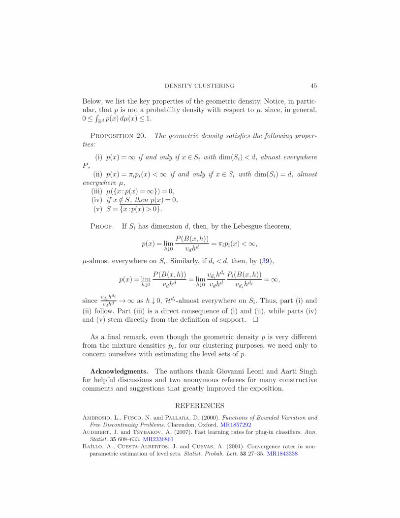
DENSITY CLUSTERING 45
Below, we list the key properties of the geometric density. Notice, in partic-ular, that p is not a probability density with respect to µ, since, in general,0≤
∫Rd p(x)dµ(x)≤ 1.
Proposition 20. The geometric density satisfies the following proper-ties:
(i) p(x) =∞ if and only if x ∈ Si with dim(Si)< d, almost everywhereP ,
(ii) p(x) = πipi(x) < ∞ if and only if x ∈ Si with dim(Si) = d, almosteverywhere µ,
(iii) µ(x :p(x) =∞) = 0,(iv) if x /∈ S, then p(x) = 0,
(v) S = x :p(x)> 0.
Proof. If Si has dimension d, then, by the Lebesgue theorem,
p(x) = limh↓0
P (B(x,h))
vdhd= πipi(x)<∞,
µ-almost everywhere on Si. Similarly, if di < d, then, by (39),
p(x) = limh↓0
P (B(x,h))
vdhd= lim
h↓0vdih
di
vdhdPi(B(x,h))
vdihdi
=∞,
sincevdih
di
vdhd →∞ as h ↓ 0, Hdi-almost everywhere on Si. Thus, part (i) and
(ii) follow. Part (iii) is a direct consequence of (i) and (ii), while parts (iv)and (v) stem directly from the definition of support.
As a final remark, even though the geometric density p is very differentfrom the mixture densities pi, for our clustering purposes, we need only toconcern ourselves with estimating the level sets of p.
Acknowledgments. The authors thank Giovanni Leoni and Aarti Singhfor helpful discussions and two anonymous referees for many constructivecomments and suggestions that greatly improved the exposition.
REFERENCES
Ambrosio, L., Fusco, N. and Pallara, D. (2000). Functions of Bounded Variation andFree Discontinuity Problems. Clarendon, Oxford. MR1857292
Audibert, J. and Tsybakov, A. (2007). Fast learning rates for plug-in classifiers. Ann.Statist. 35 608–633. MR2336861
Baıllo, A., Cuesta-Albertos, J. and Cuevas, A. (2001). Convergence rates in non-parametric estimation of level sets. Statist. Probab. Lett. 53 27–35. MR1843338
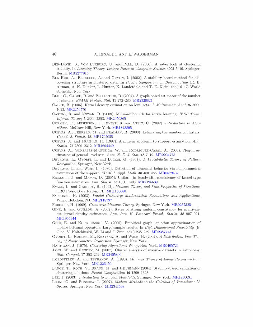
46 A. RINALDO AND L. WASSERMAN
Ben-David, S., von Luxburg, U. and Pall, D. (2006). A sober look at clusteringstability. In Learning Theory. Lecture Notes in Computer Science 4005 5–19. Springer,Berlin. MR2277915
Ben-Hur, A., Elisseeff, A. and Guyon, I. (2002). A stability based method for dis-covering structure in clustered data. In Pacific Symposium on Biocomputing (R. B.Altman, A. K. Dunker, L. Hunter, K. Lauderdale and T. E. Klein, eds.) 6–17. WorldScientific, New York.
Biau, G., Cadre, B. and Pellettier, B. (2007). A graph-based estimator of the numberof clusters. ESAIM Probab. Stat. 11 272–280. MR2320821
Cadre, B. (2006). Kernel density estimation on level sets. J. Multivariate Anal. 97 999–1023. MR2256570
Castro, R. and Nowak, R. (2008). Minimax bounds for active learning. IEEE Trans.Inform. Theory 5 2339–2353. MR2450865
Cormen, T., Leiserson, C., Rivest, R. and Stein, C. (2002). Introduction to Algo-rithms. McGraw-Hill, New York. MR1848805
Cuevas, A., Febrero, M. and Fraiman, R. (2000). Estimating the number of clusters.Canad. J. Statist. 28. MR1792055
Cuevas, A. and Fraiman, R. (1997). A plug-in approach to support estimation. Ann.Statist. 25 2300–2312. MR1604449
Cuevas, A., Gonzalez-Manteiga, W. and Rodrıguez-Casal, A. (2006). Plug-in es-timation of general level sets. Aust. N. Z. J. Stat. 48 7–19. MR2234775
Devroye, L., Gyorfi, L. and Lugosi, G. (1997). A Probabilistic Theory of PatternRecognition. Springer, New York.
Devroye, L. and Wise, L. (1980). Detection of abnormal behavior via nonparametricestimation of the support. SIAM J. Appl. Math. 38 480–488. MR0579432
Einmahl, U. and Mason, D. (2005). Uniform in bandwidth consistency of kernel-typefunction estimators. Ann. Statist. 33 1380–1403. MR2195639
Evans, L. and Gariepy, R. (1992). Measure Theory and Fine Properties of Functions.CRC Press, Boca Raton, FL. MR1158660
Falconer, K. (2003). Fractal Geometry: Mathematical Foundations and Applications.Wiley, Hoboken, NJ. MR2118797
Federer, H. (1969). Geometric Measure Theory. Springer, New York. MR0257325Gine, E. and Guillou, A. (2002). Rates of strong uniform consistency for multivari-
ate kernel density estimators. Ann. Inst. H. Poincare Probab. Statist. 38 907–921.MR1955344
Gine, E. and Koltchinskii, V. (2006). Empirical graph laplacian approximation oflaplace-beltrami operators: Large sample results. In High Dimensional Probability (E.Gine, V. Koltchinskii, W. Li and J. Zinn, eds.) 238–259. MR2387773
Gyorfi, L., Kohler, M., Krzyzak, A. and Walk, H. (2002). A Distribution-Free The-ory of Nonparametric Regression. Springer, New York.
Hartigan, J. (1975). Clustering Algorithms. Wiley, New York. MR0405726Jang, W. and Hendry, M. (2007). Cluster analysis of massive datasets in astronomy.
Stat. Comput. 17 253–262. MR2405806Korostelev, A. and Tsybakov, A. (1993). Minimax Theory of Image Reconstruction.
Springer, New York. MR1226450Lange, T., Roth, V., Braun, M. and J.Buhmann (2004). Stability-based validation of
clustering solutions. Neural Computation 16 1299–1323.Lee, J. (2003). Introduction to Smooth Manifolds. Springer, New York. MR1930091Leoni, G. and Fonseca, I. (2007). Modern Methods in the Calculus of Variations: Lp
Spaces. Springer, New York. MR2341508
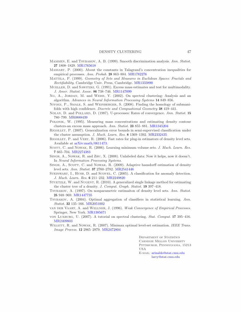
DENSITY CLUSTERING 47
Mammen, E. and Tsybakov, A. B. (1999). Smooth discrimination analysis. Ann. Statist.27 1808–1829. MR1765618
Massart, P. (2000). About the constants in Talagrand’s concentration inequalities forempirical processes. Ann. Probab. 28 863–884. MR1782276
Mattila, P. (1999). Geometry of Sets and Measures in Euclidean Spaces: Fractals andRectifiability. Cambridge Univ. Press, Cambridge. MR1333890
Mueller, D. and Sawitzki, G. (1991). Excess mass estimates and test for multimodality.J. Amer. Statist. Assoc. 86 738–746. MR1147099
Ng, A., Jordan, M. and Weiss, Y. (2002). On spectral clustering: Analysis and analgorithm. Advances in Neural Information Processing Systems 14 849–856.
Niyogi, P., Smale, S. and Weinberger, S. (2008). Finding the homology of submani-folds with high confidence. Discrete and Compuational Geometry 38 419–441.
Nolan, D. and Pollard, D. (1987). U-processes: Rates of convergence. Ann. Statist. 15780–799. MR0888439
Polonik, W. (1995). Measuring mass concentrations and estimating density contourclusters-an excess mass approach. Ann. Statist. 23 855–881. MR1345204
Rigollet, P. (2007). Generalization error bounds in semi-supervised classification underthe cluster assumption. J. Mach. Learn. Res. 8 1369–1392. MR2332435
Rigollet, P. and Vert, R. (2006). Fast rates for plug-in estimators of density level sets.Available at arXiv:math/0611473.
Scott, C. and Nowak, R. (2006). Learning minimum volume sets. J. Mach. Learn. Res.7 665–704. MR2274383
Singh, A., Nowak, R. and Zhu, X. (2008). Unlabeled data: Now it helps, now it doesn’t.In Neural Information Processing Systems.
Singh, A., Scott, C. and Nowak, R. (2009). Adaptive hausdorff estimation of densitylevel sets. Ann. Statist. 37 2760–2782. MR2541446
Steinwart, I., Hush, D. and Scovel, C. (2005). A classification for anomaly detection.J. Mach. Learn. Res. 6 211–232. MR2249820
Stuetzle, W. and Nugent, R. (2010). A generalized single linkage method for estimatingthe cluster tree of a density. J. Comput. Graph. Statist. 19 397–418.
Tsybakov, A. (1997). On nonparametric eatimaiton of density level sets. Ann. Statist.25 948–969. MR1447735
Tsybakov, A. (2004). Optimal aggregation of classifiers in statistical learning. Ann.Statist. 32 135–166. MR2051002
van der Vaart, A. and Wellner, J. (1996). Weak Convergence of Empirical Processes.Springer, New York. MR1385671
von Luxburg, U. (2007). A tutorial on spectral clustering. Stat. Comput. 17 395–416.MR2409803
Willett, R. and Nowak, R. (2007). Minimax optimal level-set estimation. IEEE Trans.Image Process. 12 2965–2979. MR2472804
Department of Statistics
Carnegie Mellon University
Pittsburgh, Pennsylvania, 15213
USA
E-mail: [email protected]@stat.cmu.edu


