Field and Lab Methods & Protocols - University of Michigan

1

Field and Lab Methods & Protocols

Kling Lab University of Michigan

Protocol version: v3.2

Updated: September 2016 – working on this now to update to v3.3 In use from: May 2015

Filename = Protocols_v3.2.docx

Last updated: 12 September 2016

2

LAST UPDATED: 5 JUNE 2015 ................................................................................................................................. 1

SECTION I - PREPARATION AND INFORMATION .......................................................................................... 5

(I-1) LOGISTICS PLANNING FOR ALASKA FIELD SEASON .......................................................................................... 5 (I-2) SUMMER PRIMER AND GENERAL INFORMATION ............................................................................................. 10

SECTION II - ALASKA FIELD OPENING AND CLOSING ............................................................................... 16

(II-1) TOOLIK FIELD STARTUP ............................................................................................................................. 16 (II-2) TOOLIK FIELD SHUT DOWN ........................................................................................................................ 29

SECTION III - ALASKA FIELD SAMPLING AND PROCESSING .................................................................. 45

(III-1) ALASKA WINTER SAMPLING ...................................................................................................................... 45 (III-2) ALASKA SUMMER SAMPLING – GENERAL .................................................................................................. 51 (III-3) DISSOLVED GAS FIELD SAMPLING PROTOCOL ........................................................................................... 60 (III-4) DIC SAMPLING PROTOCOL – NEW METHOD, 2006 - .................................................................................... 62 (III-5) OLD - DIC SAMPLING PROTOCOL WITH SERUM VIALS .............................................................................. 63 (III-6) FILTERING .................................................................................................................................................. 64 (III-7) SURFACE WATER DISCHARGE .................................................................................................................... 67 (III-8) MAGNETIC DECLINATION AND COMPASSES ............................................................................................... 70 (III-9) PROTOCOLS FOR OPERATION OF THE NEON EDDY FLUX TOWER ON TOOLIK LAKE .................................. 71 (III-11) DNA SAMPLE FROM SOILS, SEDIMENTS, EPILITHON ............................................................................... 80 (III-12) LTREB TOOLIK LAKE SURVEY – PROTOCOL FOR SUMMER 2007 ........................................................... 81 (III-14) FLOW CYTOMETER COUNTING OF BACTERIA, VIRUSES, HETEROTROPHIC NANOFLAGELLATES ............ 85 (III-15) IMNAVAIT HYDROGRID SETUP/ SHUTDOWN ........................................................................................... 87

SECTION IV - FIELD EQUIPMENT ..................................................................................................................... 90

(IV-1) PH METER .................................................................................................................................................. 90 (IV-2) CONDUCTIVITY METER .............................................................................................................................. 92 (IV-3) LIGHT METER AND SECCHI DEPTH ............................................................................................................. 93 (IV-4) DATALOGGERS ........................................................................................................................................... 98 (IV-5) SBE 19 CTD .............................................................................................................................................101 (IV-6) SCUFA I - FIELD INSTRUCTIONS, DATA DOWNLOAD AND USE WITH CTD ...............................................107 (IV-7) ISCO AUTOMATIC WATER SAMPLERS ......................................................................................................109 (IV-8) Y.E.S. UVA AND UVB SENSORS ON TOOLIK CLIMATE STATION..............................................................112 (IV-8) UV-PAR LIGHT PROFILES WITH BIOSPHERICAL C-OPS ...........................................................................113 (IV-9) HOBOS AND STOWAWAYS .........................................................................................................................115 (IV-10) TROLL – TEMP, PRESSURE, CONDUCTIVITY INSTRUMENT ........................................................................121 (IV-11) STAR-ODDI MINI TEMPERATURE SENSORS ............................................................................................123

SECTION V - LAB EQUIPMENT ...........................................................................................................................124

(V-1) BALANCES ................................................................................................................................................124 (V-2) OVENS ......................................................................................................................................................126 (V-3) MICROSCOPES ...........................................................................................................................................127 (V-4) GAS CHROMATOGRAPHS ..........................................................................................................................128 (V-5) DIONEX ION CHROMATOGRAPH ................................................................................................................133 (V-6) TURNER DESIGNS 10-AU CHLOROPHYLL FLUOROMETER .........................................................................140 (V-7) PROTOCOL FOR SHIMADZU UV-1601 .......................................................................................................141 (V-8) PROTOCOL FOR SCINT COUNTER AT TOOLIK FIELD STATION ...................................................................142 (V-9) HOW TO RECYCLE DI CARTRIDGES IN MICHIGAN ....................................................................................144 (V-10) HOW TO INSTALL SAS (V 9.2) ...................................................................................................................145

SECTION VI - LAB METHODS ..............................................................................................................................146

(VI-1) CO2 AND CH4 DETERMINATION ................................................................................................................146 (VI-2) DIC DETERMINATION (USING HGCL2 SAMPLES) ........................................................................................147 (VI-2) DIC DETERMINATION (USING THE APOLLO MODEL AS-C3) .....................................................................148 (VI-3) DOC - DISSOLVED ORGANIC CARBON DETERMINATION ...........................................................................152 (VI-4) SILICA DETERMINATION ............................................................................................................................167 (VI-5A) SOLUBLE REACTIVE PHOSPHATE (SRP) ................................................................................................169

3

(VI-5B) TOTAL DISSOLVED PHOSPHORUS (TDP) ...............................................................................................173 (VI-5C) PARTICULATE PHOSPHORUS (PP) ..........................................................................................................182 (VI-6) NITRATE / NITRITE DETERMINATION .......................................................................................................187 (VI-7) PARTICULATE CARBON AND NITROGEN -- CHN ANALYZER .....................................................................197 (VI-8) BACTERIAL PRODUCTION ..........................................................................................................................209 (VI-9) PRIMARY PRODUCTION..............................................................................................................................211 (VI-10) ALKALINITY DETERMINATION ...............................................................................................................221 (VI-11) OPA - FLUOROMETRIC AMMONIUM ANALYSIS .....................................................................................227 (VI-13) CATION DETERMINATION ......................................................................................................................235 (VI-14) DISSOLVED OXYGEN DETERMINATION..................................................................................................245 (VI-15) PHYTOPLANKTON SETTLING ..................................................................................................................246 (VI-16) GRINDING PLANTS FOR ISOTOPE ANALYSIS............................................................................................247 (VI-17) ACID WASHING AND AUTOCLAVE PROCEDURES ...................................................................................248 (VI-18) PROTOCOL FOR ANALYSIS OF TOTAL PHENOLICS ..................................................................................249 (VI-19) PROTOCOL FOR REDUCING SUGAR ASSAY ............................................................................................250 (VI-20) PROTOCOL FOR PROTEIN ASSAY ............................................................................................................251 (VI-21) PROTOCOL FOR PHENOL OXIDASE & PEROXIDASE ASSAY ....................................................................252 (VI-22) CHLOROPHYLL DETERMINATION ...........................................................................................................254 (VI-23) SEDIMENT CHLOROPHYLL DETERMINATION .........................................................................................260 (VI-24) TOTAL SUSPENDED SOLIDS & LOSS ON IGNITION PROTOCOL ...............................................................263 (V1-25) ABSORBANCE + EEM PROTOCOL AT TOOLIK ........................................................................................266 (V1-26) BIOSPHERICAL UV-VIS PROFILER ........................................................................................................269

SECTION VII - LAB DATA PROCESSING ...........................................................................................................271

(VII-1) RETURNING FROM THE SUMMER FIELD SEASON ........................................................................................271 (VII-2) FILES FOR AK AND LTER- GENERATION AND FATE .................................................................................273 (VII-3) ADDING DATA TO FILES PROTOCOL ...........................................................................................................279 (VII-4) FILE PROCESSING ......................................................................................................................................281 (VII-5) QA/QC PROTOCOL ....................................................................................................................................285 (VII-6) INSTRUCTIONS FOR PRIMER SOFTWARE .....................................................................................................287 (VII-7) SPSS PROTOCOL .......................................................................................................................................289 (VII-8) REPORTING DATA PROTOCOL ....................................................................................................................291 (VII-9) GAS FILE PROTOCOL ................................................................................................................................294 (VII-10) COMPLETING FILE WORK AT TOOLIK ...................................................................................................296

SECTION VIII – LAB MANAGEMENT.................................................................................................................297

(VIII-1) ORDERING ............................................................................................................................................297 (VIII-2) SHIPPING ...............................................................................................................................................300 (VIII-3) RADIATION SAFETY AND ORDERING PROCEDURES ...............................................................................306 (VIII-4) HAZARDOUS MATERIALS AND WASTE ..................................................................................................310 (VIII-5) PRINTERS ...............................................................................................................................................312 (VIII-6) LABEL CREATION WITH MAIL MERGE FEATURE IN WORD ...................................................................313 (VIII-7) ACCESSING THE SERVER FROM AN OFFSITE COMPUTER ........................................................................316 (VIII-8) PROTOCOL BOOK VERSIONS ..................................................................................................................319

SECTION IX - OTHER PROJECTS AND OLD PROTOCOLS .........................................................................320

(IX-1) MICHIGAN - LAKE SAMPLING, AND WATERSHED PROJECT ........................................................................320 (IX-2) FIELD SAMPLING AND PROCESSING FOR LAKE VICTORIA ..........................................................................326 (IX-3) OLD PROTOCOLS (ALL PROJECTS) ........................................................................................................332

APPENDICES .............................................................................................................................................................352

LIST OF SUPPLIERS AND VENDORS ............................................................................................................................352 ADAPTATION TO CHANGING LIGHT EXPERIMENT PROCEDURE ...................................................................................354

WALLOCOLS ............................................................................................................................................................357

TOOLIK DAILY TASK FLOWCHART ............................................................................................................................358 ACID WASHING PROTOCOL .......................................................................................................................................359 SURFACE WATER NEEDS ...........................................................................................................................................360

4

SOIL WATER NEEDS ..................................................................................................................................................361 WHEN YOU RETURN FROM THE FIELD… ....................................................................................................................362 ACIDIFYING DOC/TDN, TDP, AND CATION SAMPLES ..............................................................................................363 AMMONIUM - PHENATE METHOD ..............................................................................................................................364 AMMONIUM OPA METHOD - TOOLIK .......................................................................................................................365 AMMONIUM OPA METHOD – ANN ARBOR ...............................................................................................................366 PHOSPHORUS SRP .....................................................................................................................................................367 CHLOROPHYLL WALLOCOL FOR LTER .....................................................................................................................368 PRIMARY PRODUCTION ON-SITE COLLECTION AND INCUBATION .............................................................................369 PRIMARY PRODUCTION OFF-SITE COLLECTION AND INCUBATION ............................................................................370 PRIMARY PRODUCTION FILTERING AND COUNTING PROCEDURES ............................................................................371 PRIMARY PRODUCTION - SCINTILLATION COUNTER ..................................................................................................372 SHIMADZU GC-14A – STARTUP WALLOCOL .............................................................................................................373 GC14A – RUNNING GASES WALLOCOL ....................................................................................................................374 APOLLO DIC ANALYZER – WALLOCOL .....................................................................................................................375 STREAM RAIN EVENT SAMPLING ..............................................................................................................................376 DOC/TDN DETERMINATION ON TOC-V ...........................................................................................................377 TOC-V SOFTWARE: ANALYSIS SET-UP AND DATA PROCESSING ...............................................................................379 PH METER CALIBRATION WALLOCOL .......................................................................................................................384 DOWNLOADING HYDROLAB PROTOCOL ....................................................................................................................386 NE-14 INLET SAMPLING NEEDS ................................................................................................................................387 NE-14 LAKE SAMPLING PROTOCOL ..........................................................................................................................388 NE-14 EQUIPMENT LIST FOR START-UP .....................................................................................................................389 WINTER FIELD SAMPLING CHECKLIST ......................................................................................................................390 DOWNLOADING THE PDA .........................................................................................................................................391 NOTES FOR PHOTO-BIO EXPERIMENTS ......................................................................................................................392

5

SECTION I - Preparation and Information

(I-1) Logistics Planning for Alaska Field Season Updated 15 Dec 2014, GWK

Field Season Preparation Calendar December 1. George will be going to the LTER Exec committee meeting. Ask him to remind the Woods Hole or other PIs

about initiating the REU process for the next summer. Also remind George about getting technicians early for the next summer in AK.

January-February 1. Find out from George what he wants to talk about at the LTER meeting in late February or March – what data

must be run or analyzed? What graphs must be made? 2. Need to know who is going to the March meeting – are they presenting posters or talking? A. Get a list of names and start George arranging the plane tickets or travel. MBL will email with a list of

invitees, ask George to make sure the appropriate people are on it. That list then allows people to make travel plans with Commonwealth travel. Ask George if anyone needs to go early or stay late for special sessions.

B. Need to arrange who needs a room at Swope with the contact at The Ecosystems Center at MBL. C. Need a lab meeting to check over the student’s posters, and to remind them to get graphs to George. 3. Start the process of hiring summer technicians, because we need to know who is going to AK soon. A. Update the flyer on summer research assistants – post around campus, send to colleagues. Ask grad students

if there are good undergrads in their lab or lecture classes that would be appropriate to hire. B. Determine the cut-off dates. We know that an application deadline of March 31 is TOO LATE. We use an

application deadline of March 1, an initial decision deadline for us of March 15, and a response from applicants 1 week (2 weeks maximum) after we offer the position to them.

C. Update “frequently asked questions” on the web page. D. Place adds on list-servers (ASLO; NABS; Arctic Info (ARCUS); MSU FW email list; UROP (call them rather

than email, and ask to be put on the Summer Research Internship Database; etc.); Eco-log (ESA, only a member of ESA can place an ad – get George to do it); U-M student opportunities page (get a staff member to do it); contact U-M human resources to get a job add posted (temporary hourly position)). There are instructions and contact info in the \DOCUMENTS\Lab\Job_Applicants\ location.

E. Contact MBL and USU (Phaedra Budy) to get access to their list of applicants for their summer jobs (if we need to); share with MBL and USU anyone who is better for them.

F. Start a paper file and electronic file of all the CVs and other information from applicants. There are two files, one for REU applications and another for RA applications. These are kept in the “Arctic Current” filing cabinet in 1041A. Use the files to keep applicants notified by email of the status of the hiring process.

4. Talk with George about new main Land Water plans for the summer. Are there new projects that require new people, new equipment, or new procedures that need to be developed?

A. If any special equipment is required, it could take months to delivery (from order date) - Find out now. B. Determine what we want and then get quotes. Beware of adding your name to any list/company, you will get

a ton of calls. 5. Set up summer payment plans with UAF.

A. We used to set up summer POs with UAF. There were two kinds: 1. One PO is for the housing charges at the UAF dorm rooms. This can take a while to do, start early. The

information on contacts for housing is located in the excel file used for the last year, found at \Documents\Arctic\Field\Schedules_calendars_plans\year\ Toolik_housing_transport_YEAR.

2. For the supplies PO, contact the Departmental office staff as well as Mike Abels to make sure that nothing has changed at IAB\UAF. Amount should be $2000. This P.O. is in the form of a “contract”, and Purchasing will need to know the justification for it – ask George to print this out for you to take down to the Department to have them arrange the P.O. with Purchasing. Chances are that we can use the same P.O. number from year to year.

B. Currently we talk with Sonja or Amber to determine what the best plan for us (minimal work on our part), for the department (easy for them to follow-up and pay), and UAF (it gets done).

1. Payment plan for UAF Conference Center (dorm rooms): we have been using the department p-cards (Sonja’s card) with great success. Contact both Amber Cagwin (UAF) and Amber Stadler (EEB) and

6

have them set up the details. Once our plans are finalized, we send a reservation list (with cost estimate) to Sonja and Amber Stadler in the EEB office so that can double check the receipts. We may be asked to verify.

2. For IAB supply requests, first talk to the EEB department to find out what about their preference (if anything went wrong previously, etc). The PO number that we have set up with them in previous years should be adequate to get things going. If an updated PO is required, Kaye will set it up if the previous charge is rejected. We are going to this process because we usually do not receive the charges within the time frame of the PO contact anyway. The contacts at UAF are Mike Ables (manager), Brett Biebuyck (logistics, assistant manager), and Joe Franich (logistics helper).

March (before the LTER meeting) 1. Decide on the number of people going to Toolik and their rough time schedules. George will know whether

we have the user days to support these people. This information goes to IAB to reserve space for us at Toolik. The spreadsheet located at \Documents\Arctic\Field\Schedules_calendars_plans\ should also be sent to the LTER PI (Shaver/Rastetter) and MBL for their information.

2. Go over general plans for the upcoming year with George and make a detailed sampling schedule (file called “YEAR_Sampling_calendar”. Ask the Lakes RA for his/her schedule and coordinate on the I-series, Toolik, E5-E6 or any lakes that you wish to sample at the same time. Update the calendar for sampling sites, dates, and when people are in the field and bring this to the March meeting and give George a copy.

March - April (after the LTER meeting) {Hiring, Plane Tickets, Housing, Transport} 1. Decide on who we are going to hire. Once we have letters of recommendation we sort and rank the

applications, and then the general procedure for the top people is that if the person is in Michigan have them stop by and talk with technicians, grad students, and then after that see George. If they are out of towners, then we do a phone interview. The grad students should interview the REUs (if they will be mentoring them), otherwise technicians or George can interview REUs over the phone. We need to keep the interview process short – max 20 minutes over the phone, and max 1 hour in person. Then technicians rank candidates and share this with George, they compare notes and decide on who to hire. Two main criteria that we learn from the interviews are (1) are they outdoor people, don’t mind being cold and wet and muddy, (2) are they careful and do they pay attention to detail in the field and lab, and (3) you MUST check the references, even if undergrads have worked in our lab before.

2. Finalize the LW schedule with George. Update the ordering lists based on last year’s inventory plus last year’s orders. The order should be started using the file \Documents\Lab\Orders_ Inventories.xls -- Update for a new year using information from previous years. In other words, each year has a new file, based on the previous year’s file.

3. Make everyone decide on their dates of travel to AK. Give dates to George so he can order airline tickets from Janet or Colleen at Commonwealth Travel (George puts them on his credit card). The phone numbers are 508-548-5100 or 800-287-5103. Also indicate whether you need room reservations in Anchorage if we fly through there – Commonwealth can help with these reservations (DON’T stay at the Samovar in Anchorage…). If we travel to Fairbanks, WE make the housing reservations. Generally, we stay at the Alpine Lodge in Fairbanks.

4. Make reservations at UAF Dorms. We make as many reservations as we can at the UAF dorms because they are considerably cheaper than hotels. The template for making reservations at the UAF dorms or apartments (up to 4 people per apartment) are found in the file \Documents\Arctic\Field\Schedules_calendars_plans\YEAR\Toolik_housing_transport_YEAR. Update the tab “UAF_Reservations” and save the tab in its own Excel file. Review the UAF housing webpage, which should have current summer rates and other useful info: http://www.uaf.edu/reslife/conference/rates-1/ For a large group (greater than 8 people), contact UAF conference services to set up a contract by emailing [email protected]. Attach the UAF_Reservations file you created. Either the UAF contact (Camille Linn) will reply back within a couple of days to confirm the availability of the housing, or you can email her directly in the first place ([email protected]). For individual reservations, please fill out the individual reservation request (found at http://www.uaf.edu/reslife/conference/ConferenceReservationForm.UAF.pdf ). After you set up a contract with UAF, you should send it UNSIGNED to Sonja. She will then send it to Procurement and they will review the document, sign it, and send it to UAF.

*** NOTE: We cannot count on UAF dorms for the end of the season, as the university has already started classes.

We then need to make reservations in local hotels. Check their website for the dates they’re available for reservations.***

7

5. Take UM rad safety and lab safety courses. Make reservations for everyone new in the lab to take the U-M rad safety class and lab safety class. People can do this on their own over the web if they have a U-M unique name (ID), otherwise we need to call and vouch for them.

6. Update UAF Rad certification. Everyone in the lab needs to update their UAF rad certification by filling out the form and by taking the test. Ask the UAF RSO if there are any updates to the Rad book or to the exams – found in L:\Documents\lab\rads_haz_mat\Alaska. We then send the entire package of forms to the RSO at UAF. Information for doing all of this is under \Documents\Lab\Rads_haz_mat\year. We have to stay on top of this or nobody will register for a class or fill out a form to save their lives…

7. Arrange with UAF RSO for Rad shipping and pickup. Need to arrange with the RSO at UAF to pick up the standards for the scint counter at Toolik, and any rad that George may need in May or in early June. This is done when traveling through Fairbanks. IAB will also send up the standards or rad with their employees, but make sure it gets to Toolik in time and we know that it is coming and it is picked up by us rather than sitting in the general hazmat bin at Toolik – careful, this stuff can’t freeze! Remember that shipping any rad from Michigan to Toolik goes from UM RSO to UAF RSO.

9. Make sure George has what he needs for May sampling (check the list of THINGS TO DO NEXT YEAR from the previous year). If George is NOT going up in May, you still need to go through the list below and check. Shipping address to Toolik:

NAME IAB Toolik 757000 900 Yukon Dr BLDG-T-4 Univ. Alaska Fairbanks, Fairbanks, AK 99775-7000

Telephone numbers at IAB: Logistics (907) 474-5159; FAX (907) 474-5513; TOOLIK FAX (907) 474-7690

A. He will likely take up with him (as baggage on the plane) the CTD, and he will need pH and conductivity

meters, pH solutions, pipets, and maybe bottles, filters, DNA filtering, etc. B. Also, make sure that you contact the Lakes RA to arrange to have the Hydrolab repaired if necessary and

waiting at IAB in Fairbanks for George to take up to Toolik. It should be there several days ahead of time to account for delays in shipping (start all this early, it usually messes up somehow).

C. Make sure that the laptop is ready to go and try out the CTD with the laptop, check voltages of batteries, etc. Check to see that any cables we brought back from Toolik are set to return to Toolik if needed.

D. Make sure that we have disks of software necessary to update the desktop computers at Toolik. George will take the small external hard drive with him, so it needs to have the most recent AK files or software (Seabird, PC208, Consorts, dataloggers, etc.) on it already. Check for software updates from the web for all of these companies and instruments.

E. Order the gas cylinders for the GC at Toolik. Get 2 hydrogen, 2 helium, 2 air – specify the regulator that we want to use (breathable air versus regular air – we use regular air) (use the UAF PO). These need to be in camp when George arrives, not sitting at IAB for him to take up with him.

F. Arrange with IAB for George to pick up our warm storage items from Fairbanks to take to Toolik. DO NOT have IAB send them to Toolik before George gets there, or they will freeze.

G. Update the Toolik_InventoryAndOrdering_YEAR.xls with information from the previous year’s inventory, and being going through what needs to be ordered. Any big supplies or supplies that will take a long time to receive should be ordered in early April.

H. Create as many Field Books as possible (LW, Imnavait, etc.), at least the main Land-Water field book. Make sure to order Rite-n-Rain paper early (takes a while to get) and get Avery weatherproof labels. If you need Rite-n-Rain poly covers, order them very early.

H. Update SampleBottleLabelsYEAR.xls with our sampling schedule and estimate the supply needs for the summer. This worksheet is used to assign sortchems.

I. Use SampleBottleLabelsYEAR.xls to assign sortchems to samples and create/update the yearly akchemYEAR.xls.

J. Begin organizing files that will be used up at Toolik for the upcoming field season (make from previous year’s files).

K. Update the protocol book and especially the Wallocols if things have changed.

8

May 1. Encourage students to finalize their research plans so that we can complete the orders and shipping.

Finalize and send in orders for the summer by May 15th at the very latest. Check with George to determine which supplies are ordered on which grant number. Have the Fisher and large items shipped directly to Toolik via UAF. Email the logistics support at IAB about shipments that you are sending -- look on the TFS website or email Mike Ables to check email addresses or name of current person. Get to know the “logistics person” soon – he will be your friend, and will be the person responsible through the summer. TFS has a log of shipments posted on the web – check it.

2. Prepare equipment for the field. A. Check the list of “things to do/order/change” from last year. This list lives in a file in

\DOCUMENTS\Arctic\Field or hanging outside of George’s office. Go over the list and decide WHO IS DOING WHAT – remember that the final decisions of who is running what analysis in the field may have to wait until we see the strengths of our field crew.

B. Repair and check the operation of the following: Cap Rods; Consorts; Hobos; Stowaways; Programs for Campbell dataloggers (need new printouts); clean the storage modules. Put information into the Calibrations book and into the Calibrations computer file.

C. Add information on meters and equipment checked above into the calibration file. D. Ash GF/F filters – 450°C for 4 hours; E. Print the remaining field notebooks for the upcoming summer. Have them punched and spiral bound at

OfficeMax Impress on Ann Arbor-Saline Road (or an equivalent). They have done this for us before and have the correct equipement. Give them one week for processing (but it will probably be done within a day). Templates for all the books are found in \DOCUMENTS\Arctic\Field\Notebook.

F. Wait to print labels until May. Print them using the just-updated SampleBottleLabelsYEAR.xls file, found in L:\Documents\Arctic\Field\Labels

G. Have George go over the Essentials document and print it out (LSA printing services, spiral bound). 3. Make sure all summer help is rad trained and has all information necessary - what to bring, what to wear, general

conditions (have them check out the protocol book on “Toolik Field Station – General Information”). Also, make sure that they have read or hear about the different experiments going on up at Toolik and the type of samples they will be taking. If possible review field techniques like gas collection here in Michigan before going to the field.

4. If George did not go to Toolik in May, then by the 15th order gases for the GC from IAB support help at UAF (this is their “logistics” person). Do this more than 3 weeks before you are scheduled to go up there. Order 2 Air, 2 H2, and 2 He for each GC you are operating (ask George). Note that if George went up in May, you will have already ordered 2 of each. Be sure you have a PO first, and you know what the air needs to be (e.g., we don’t need the breathing quality air; we use regular air, and the two kinds require two different regulators).

5. Arrange dedicated coolers and boxes for shipping. Buy new ones if some were left in AK. All boxes are shipped 2nd day air from Michigan, so shipping can be done closer to date of departure if necessary. Use UPS as shipper as they have given us (Kling) a special rate, those forms are across from Geo's office – all on web now.

6. Send in Radiation Safety forms to Tracey Martinson (or current RSO). Portions of the forms are pre-filled out and located in \DOCUMENTS\Lab\Rads_haz_mat\Alaska\rad_forms_info\YEAR. George is a different user type (Authorized) than the rest of the lab and has his own form. Everyone else will need to fill out the Supervised User forms: App_Super user.doc and RAD_Blank_App_Super user.doc.

7. Make sure that everyone fills out the medical form to take with them to Toolik. Form is on the web, or ask Abels. 8. Update the forms for TFS for the reservations and registration on the Toolik Field Station website. The

registration includes requests for taxi rides from Prudhoe. If using the Dalton Express from FBX, reservations need to be made by calling them rather than checking their website (this can actually be done during the year if you can’t get them by phone, and in fact it is a good thing to do both). The information for doing this is in the \DOCUMENTS\Arctic\field\schedules\YEAR\Toolik_housing_transport.xls file. Our arrangement is to have them bill us at the end of the season.

June 1. Two weeks before you go - make sure all items are ordered, and have been shipped and are not backordered. 2. Bring a copy of last years data files and also the new LW field book and the old Calibrations book. Bring the

external hard drive with the entire, updated \DATA\Arctic directory from the Server. 3. Make this year’s file structure in the computer in Ann Arbor. There is a “blank” directory structure on George’s

computer. Make templates of all the common files (chem., gas, chl, nuts, pprods, bacprods). Bring copies to Toolik on a CD. Note that George may have already had to do this for some files in May – do not overwrite them.

9

4. Create the new files for this summer from last year’s files for all operations: including, AKCHEM, GAS, ALK, Calibrations, Discharge, Dataloggers (various), etc.

5. If we have technicians going to Toolik already here in the lab, start training them on basic operations in the field and in the lab and on the computer while they are still in Ann Arbor (e.g., calibrations, DICs, etc.).

6. At Toolik use the Essentials STARTUP section as a guide for setting up the lab – check with George if he went up in May to find out any irregularities you may encounter.

7. Make a list of the “scientific equipment” (don’t be too descriptive…) and put them in the coolers or boxes that people bring up on the plane – keep a record on the Server of these lists.

July 1. The prime responsibility of people in the lab during the summer is to support the people in the field with shipping

supplies and tracking packages. August 1. Be sure to fill in the inventory and take a copy back to AA. 2. Bring back the “for next year” list of things to do and things you will need. 3. Bring back the paper calendar that you used for the year. 4. Bring back data and equipment and send materials to warm storage in FBX as specified in the startup-

shutdown section of the protocol book. Use dedicated containers. 5. Begin running DOC samples or other samples that have been shipped to Ann Arbor. September to January 1. Make sure all samples are present and accounted for before starting to run them. 2. Check all equipment shipped back from AK immediately to see if it was damaged in transit. 3. Follow the protocols for data generation and the data-file flow chart (see below).

10

(I-2) Summer Primer and General Information

Kling Lab Fundamentals: An Introduction and Welcome Updated: 18 April 2014, GWK

I. What we do: At Toolik, we are the “Landwater group.” We have several different projects (e.g., “LTREB,” “Photochem,” “AON,” and the “LTER”), but the LTER is the main, organizing project. LTER stands for Long Term Ecological Research funded by the National Science Foundation (NSF), and there are four main groups of the Arctic LTER: (1) Landwater (us), (2) Lakes, (3) Streams, (4) Terrestrial. Our focus is to investigate the linkages between terrestrial and aquatic ecosystems with respect to the cycling and transformations of important elements in food webs (carbon, nitrogen, phosphorus). We work at both well-established sites and new sites each summer in areas near and surrounding Toolik Field Station. We sample soil water, stream water, and lake water for chemistry, biological parameters, and physical characteristics. Our work at Toolik Field Station is comprised of field sampling, sample analysis on site, and data entry, checking for quality (QA/QC), and preliminary interpretation or synthesis. Our goals every summer are to collect and analyze samples, generate valid data, and ensure that all relevant information is properly recorded.

II. What you can expect from us at Toolik:

1. An introduction to the field station, the field sites, and general lab procedures. 2. Comprehensive training that includes detailed sampling techniques, analysis procedures, and data entry. 3. George and Jason are always available to answer questions. 4. A very thorough Protocol book of everything we do. This stops us from making things up or “reinventing

the wheel”, and is an essentially part of our “long-term” research (i.e., methods and protocols can’t deviate one iota or long-term data sets become useless).

5. Exposure to and a chance to talk with world-class arctic scientists from many countries and universities. III. What you can expect from “Toolik” itself:

1. You will sample and work in all sorts of weather – at times you will be too hot, too cold, too wet, and too tired.

2. The “virtues” you were taught as a child to strive for (e.g., patience, prudence, temperance, courage…) will be routinely tested.

3. A very rare experience and opportunity to learn and do science in an amazing place – make the best of it. IV. What we expect of you:

We expect you to learn the lab function, your responsibilities, and the lab culture. It may seem like a lot at first, but most aspects are probably second nature to you already. There are 4 main categories: 1. Workplace “climate” – personal conduct and responsibilities

- Respect people’s views and respect people’s time. Help your fellow team members. - Communication is key – issues can’t be solved if they aren’t known. Openly communicate any problems to

George or Jason, or make sure they hear about it through a third party. - Social interactions can be intense in isolated field locations – remember to “do unto others …”. 2. Goal – Our goal is to do the best long-term ecological research and science we can possibly do.

3. Expectations:

- Prepare, think, and question before doing anything. If you are unsure about something, please ask someone! Remember, being an “independent” worker comes only after you have properly learned a task…

- Follow protocols exactly o We all need continuous re-training, re-visiting, and practice on methods. o There are reasons for protocols – we are not automatons, think and question why we do what we do. Ask

someone if the reason for a protocol or step is not clear. - Be careful and precise – consistency is critical - Assume responsibility to complete tasks from start to finish - Organize yourself, don’t depend on others to do it for you

11

- Communicate problems or deviations from protocols - Even though computers and local networks have made communication with the outside world easier in camp

(e.g., over cell phones), during working hours we expect you to work, not chat or IM through the day.

4. Learn the Lab Culture

- Everything we do, from sampling water to drafting emails to publishing a paper, is part of being a professional. Be engaged in the science and research, and especially in being professional in all your work and interactions.

- Act with integrity and maturity (remember that one definition of “integrity” is to do what you should, even when you don’t want to... ).

Typical day at Toolik Field Station: Room and Board:

The station provides shared dorm rooms or tents (with heaters), or you can stay in your own tent in “tent city” if you want a little privacy, as well as 3 meals a day (breakfast, lunch, dinner). The mess hall area with shelves and refrigerators of food and leftovers is accessible 24/7. We pack a lunch in the morning if we are in the field all day, and we try to schedule our sampling so that we make breakfast and dinner on time. Work:

Field work: We begin our work day after breakfast each morning. We start the day at 8:30 sharp by preparing for the field (calibrating pH meters, checking our equipment, getting personal gear together…). We leave for the field at 9 am.

Returning from the field: Once we return from the field, we unpack EVERYTHING from our backpacks (including personal items, food, etc.). The first priority is to sort out the samples. Bottle labels and field-book information are checked against one another and, if necessary, corrections are made. Some samples are processed or filtered or preserved by acidification, and all samples are stored properly until analysis or shipping. The second priority is to unpack, dry, and check the equipment and perform maintenance if needed. The third priority is to wash dirty sampling equipment (such as syringes or bottles) as soon as possible. The fourth priority is to unpack and stow any personal items (throw trash away). Finally, the backpacks are put away. This is the routine followed every time when returning from the field.

Sample processing: We run several analyses at Toolik Field Station. We break up the responsibilities by assigning each person one or more analyses. You will become the “expert” on that analysis and will be responsible for maintaining records and notes concerning the samples and data issues. You will also be responsible for cleaning up after running samples (disposing of waste, cleaning bottles and glassware), and keeping Sara and Jason posted on any problems. (1) Analyzing a sample, (2) entering the results into a spreadsheet, and (3) clean-up, are performed each day and constitute “running” or “processing” a sample. You’re not done with your analysis until you finish these three tasks. Once you finish your daily responsibilities, check with other team members and ask if they need help. If they don’t need help, or it is a one person job, please don’t hover around them – let them finish their work. Remember, “don’t turn a one-person job into a two-person screw up”. Each night we prep for the next day, and pack up what we can for the morning. Talking Science: Talking Shop: Every Tuesday evening scientists from camp or invited speakers from outside of camp give a short presentation about their work or experiences. This is an excellent opportunity to see what other people are doing up at Toolik or to hear public policy presentations. We strongly encourage you to attend these meetings. Science Saturdays: A Kling lab exclusive. Every Saturday afternoon, we meet for 1-2 hours to discuss our data. The topics are determined at least one day before the meeting, and the meeting is designed to provide a venue for each member of the lab to discuss their results and get help or feedback processing data or solving problems. When the PIs

12

(Principle Investigators, e.g., George) are in camp they often present overviews and the conceptual framework that links our science projects. Sampling Descriptions: You don’t need to memorize the previous information, or the following lists, before going to Toolik. This primer is meant to give you an idea of the kinds of samples that we collect, what we analyze at Toolik, and what is sent back to Michigan for analysis. 1. Samples collected and analyzed at Toolik Field Station: NH4 (OPA): Ammonium (o-phthaldialdehyde method) PO4 (SRP): Phosphate (soluble reactive phosphorus) Dissolved gases: CO2 and CH4 DIC: Dissolved inorganic carbon Chla: Chorophyll Bac Prods: Bacterial production measurements Prim Prods: Primary production measurements 2. Samples collected near Toolik Field Station and analyzed in Ann Arbor: TDP: Total dissolved phosphorus TDN: Total dissolved nitrogen NO3: Nitrate ALK: Alkalinity Cats: Cations – currently we analyze for Al, Ca, Mg, Na, K, Mn, Fe, Ni, Si, Sr, Zn. Ans: Anions – we analyze for Cl and SO4. PP: Particulate phosphorus PCN: Particulate carbon and particulate nitrogen Isotope-DIC: 13C-dissolved inorganic carbon Isotope Filter: particulate sample (filter/seston) collected for 13C and 15N analysis.

Toolik Field Station – General Information Updated: 18 April 2014, GWK

1. Communication: Address for receiving mail at the Toolik Field Station (TFS), operated by the University of Alaska, Fairbanks

(UAF): __ your name __ IAB Toolik 757000 900 Yukon Dr. BLDG T-4 Univ. of Alaska Fairbanks Fairbanks, AK 99775-7000

Telephone numbers at IAB: Logistics (907) 474-5159; FAX (907) 474-5513; TOOLIK FAX (907) 474-7690 Web address is: http://www.uaf.edu/toolik/ Mail is sent when the van goes to Deadhorse (1-2 times per week) and received when a shipping or NSF transport

truck comes from Fairbanks (1-2 times a week), or when the Dalton Highway transport trucks run. Mail is usually received within 2 weeks (it could be faster, but, don’t count on it). Email is the best and easiest method of communication. There are telephones at Toolik for outgoing calls – they require a calling card. Skype works well and we have a computer dedicated to Skyping, downloading pictures, and emailing. We have a lab account for work related calls, but personal calls must be placed on your own Skype account. Finally, the fax number above can be used to receive work information or important letters.

2. Weather: It can snow any day of the year; in summer it melts quickly. Normal temperatures for mid-June to mid-August are:

Daily highs = 25 to 75° F (-4 to 24° C) Daily lows = 10 to 25° F (-12 to -4° C)

13

3. What to bring: a. Essentials

1. Plane ticket (or e-ticket). Make sure the TFS fax number is the contact phone number for the return flight. 2. Driver’s license 3. Credit card 4. Cash 5. Cell phone (for calling other lab members in Fairbanks), calling card, Skype account info. 6. Proof of Insurance form (hand to camp manager upon arrival) 7. Packet that Jason sends you in May – this contains your reservation information and an envelope to keep any

receipts for work-related purchases (food during your travel to/from Toolik Field Station, etc.).

DUE TO RECENT CHANGES IN BAGGAGE FEES, WE WILL ONLY PAY FOR ONE CHECKED BAG. You can check another bag (we recommend 2 checked bags Maximum due to space limitations) but you are responsible for covering the cost.

b. Clothes -- Layering is important as the weather can change quickly and severely. You can wash your clothes once every two weeks in washer/dryer units in camp (laundry detergent is supplied). Below is a list of suggested items; bring these or their equivalents:

OUTERWEAR Rain jacket and pants (VERY IMPORTANT). Gore-tex jackets are usually sufficient, but we recommend the

PVC rain pants (thinner material rips more easily). Mosquito head net (don't go cheap here, you will regret it) or bug jacket/bug suit (bug jackets are really nice). Warm hat (ski hat) Sun hat Sunglasses Gloves (think warm; fingerless are nice for work), two sets – one lighter, one heavy Fleece or down jacket (to be worn under rain jacket when it is wet outside) Heavy work shirt (e.g., wool, flannel, heavy cotton – Carhart style) Light work shirt (2-5, long-sleeve, medium-weight fabric to repel mosquitoes) Short-sleeve or T-shirt (5-10, depending on your tolerance for dirty clothing) Heavy work pants (1-2, jeans are OK, Carhartts recommended - but we don’t get a kickback…) Medium pants (1-2, nylon quick-dry are nice for the field) Hiking pants (can double as work pants) Knee-high rubber boots (VERY IMPORTANT). We will cover the cost for these boots, but they must be left at

Toolik. If you want to keep them, you can purchase them. Hiking boots (for Sunday hikes or long treks; not required for our routine fieldwork) Tennis shoes (for around camp or exercising) Lab shoes (IMPORTANT) -- no outside shoes are allowed in labs, you must change to indoor shoes that are

clean. (1-2 pair, good choices for labs are old tennis shoes, slippers, or garden clogs; think large and easy on/off over thick socks)

Optional: Workout clothes (for running, yoga, etc.), lounge or sleeping clothes (sweatshirts, pajama pants, etc.), flip flops/sandals (helpful for around camp, Sunday hikes, and crossing rivers), swim suit or play shorts (like swimming trunks or running shorts), work shorts (for the brave).

INNERWEAR Heavy long underwear (tops and bottoms) Light long underwear (tops and bottom) Heavy socks (2-3 pair) Medium socks (enough socks for ~2 weeks) Underwear (enough for ~2 weeks)

c. Toiletries -- There is a wash-up room for brushing teeth and washing faces near the dorms, showers that can be

used twice per week and a clothing-optional sauna where you can bathe several times a week. There is a limited first aid supply at Toolik, but you will need to bring your own supply of cold medicine, prescription drugs, and so forth. Gauge the amount of supplies (e.g., toothpaste) to bring by the length of your stay at Toolik. You can buy some items if you have a scheduled day to purchase things in Fairbanks. Ask Jason if you will have time to shop.

14

There is a small general store in Deadhorse for emergency purchases (very expensive). Bring your normal travel toilet kit, including at least the following:

Towel (2; leave one in the washroom and one in the sauna) Shampoo Soap (camp provides Bronner’s soap for general use at the sauna and there is plenty of it) Toothbrush and paste Deodorant Sunscreen (we have general use sunscreen in the lab and lots of it) Chapstick Hand cream or moisturizer (working in water is very drying to your hands; available in the lab) Fingernail clippers Cold medicine, aspirin (limited medicine available in camp), and vitamins. Sore throat and cough medicine Specialty medicines or prescriptions Bug repellent (buy 1 with 100% DEET or the maximum you want to use and one with much less) – we have a

lot of bug repellent for general use. You will need to purchase your own if you have specialized or preferred brands.

d. Miscellaneous -- You can sleep in the dorm (may not be available), the Polar Tents with room dividers that are

heated (usually 2 people to a room), or in a personal tenting area. Bring the following or their equivalents: 1 sleeping bag no matter where you stay For tenting, 1 three-season sleeping bag (see weather above) or 2 one/two-season sleeping bags, black tarp (to

keep light out of tent), air mattress or thermarest, plus your normal tenting gear. 2 waterproof watches – VERY IMPORTANT - DO NOT FORGET TO BRING A WATCH FOR

FIELDWORK! Flashlight (or headlamp) and batteries (for August when the sun goes down or reading at night) Camera, charger, cards, cords, and software Waterproof bag for camera, dry sack for clothes in the field. Compass (optional; we have some available for work related uses) Pocket knife or Leatherman (IMPORTANT - pack in your checked baggage, not your carry-on) Water bottle(s) – depending if you tend to lose them… Insulated coffee mug (you will get a non-insulated mug at Toolik when you arrive) Books, Kindles, DVDs, iPods, iPads (and accessories) Laptop (make sure you have a good case or other way to protect it) Backpack/daypack for hiking Tupperware/food storage containers for salads, etc. if you prefer (plastic baggies are provided).

4. Rules for Survival (figuratively and literally) a. Vehicles – The most potentially dangerous part of the Toolik experience is driving on the haul road. This road is

used by large semi-tractor trailer trucks supplying the oil fields, and we use it to drive to field sites. The semis will go 75 mph and do not slow down or move over for anything.

When a semi is approaching you, slow down and pull to the side of the road. Speed limit is 50-55 mph for our trucks. Many times this is too fast depending on road conditions. If you are

in a truck and are uncomfortable with the speed, tell the driver to slow down, or get out and walk. Do not jump the gravel berms in the road with any speed. Slow down and crawl over them (stay in the

truck…). Vehicles are available for field work by sign-out sheet in the communications room. Some vehicles require

paperwork filled out in the truck itself, along with an operational checklist. Work vehicles owned by the LTER are used on Sundays for hiking. Other vehicles rented or owned by NSF or CPS are only for work. Never take a vehicle for personal use (i.e., use other than research and hiking with a group).

b. Weather – Toolik is not a summer-fun camp. It is in the middle of nowhere and the weather can change

rapidly to freezing conditions. Follow these precautions: Always take your rain jacket in the field with you, no matter what the weather is like at the moment.

15

Do not travel a long way from camp alone (nearby field sites are OK, within ~1 mile of Toolik Lake or the road).

If you are going in the field for the day, take food and water and a rain and warm jacket (even if it is hot and sunny).

If you travel away from camp take a compass and a map and know how to use them (remember the declination…).

Sign-out on the camp board (let camp manager know where you went, time left, expected time of return). Let Jason or George (whoever is in camp) or another member of the Kling lab know where you are going and

how long you will be there.

c. Lab Chemicals – There are both radioactive and hazardous chemicals in camp. Use caution with all chemicals. No food in rad areas. Do not place ANYTHING into a rad area unless told to do so. Do not remove anything from a rad area unless

told to do so. Know where the eye-wash stands are or where there is water available. Watch out for others doing stupid things with chemicals – stop them or help them.

d. Problems and Issues -- From time to time there are general or specific problems between camp operations and the research, or problems of a personal nature. There is a “Lead Scientist” or “Scientific Liaison” designated in camp at all times. These people are usually related to the LTER project in some way. If there are issues regarding camp policy that is negatively affecting the research, or personnel issues that you cannot easily solve, tell the Scientific Liaison what is happening, or call George, or tell Jason. There is a handbook which discusses the role of the Scientific Liaison, and answers other FAQs about Toolik - Read this! http://toolik.alaska.edu/user_guide/policies.php

e. General Etiquette -- Toolik can become a crowded place. Almost all space and most of the equipment is shared

and multi-user, there is little personal privacy, and you will likely interact with a diverse group of people daily. Please remember this and strive for tolerance in all situations.

Alcohol use is prohibited on the UAF campus, and the Toolik Field Station is considered part of the campus. However, there has been an unwritten policy whereby alcohol use is tolerated as long as it is not “obvious”. Keep all alcohol hidden when not in use (i.e., do not leave bottles of booze out on the lab counters) and clean up after yourself. Drunkenness is frowned upon and will lead to serious consequences (see the TFS handbook cited above). Other illegal drugs are, well, illegal. Treat them that way.

Remember, most of you are just starting your careers. How you conduct yourself personally and professionally at Toolik will be noted and will reflect on you for a long time to come. Make the best of this opportunity to have pride in your actions.

16

SECTION II - Alaska Field Opening and Closing

(II-1) Toolik Field Startup 16 May 2013 sef / jad

START UP Proceed in the following order unless otherwise instructed. There may be a sampling day before you get to

the bottom of this list. Check everything off as you go!

A. Warm Storage 1. In 2010, TFS decided to maintain a warm storage area at the field station. This eliminates shipping materials back

and forth to Fairbanks, but we still need to make sure that all of our items are initially marked with contents and “Kling Lab 4” or “Dry Lab” so they can be returned to their proper places in the spring. Go over the previous year’s warm storage inventory, and check it off as you find and open boxes in June. This could include (but not limited to): Chemicals, tops for ISCO autosamplers, data loggers, etc. Note that you may have to search several labs in the spring (May) to find where the stored materials are.

2. Radioactive material is still transported between UAF and TFS, make sure you emailed the RSO to meet with them and obtain the rad before leaving Michigan for Toolik.

3. In May you may need to keep warm storage materials in the lab because it is too cold outside. But in June, put all warm storage materials in the conex, or a spare room in the lab, so that you can clean the lab.

B. Conex & Lab I. THE CONEX. The conex will be crowded due to materials stored there from the lab or materials that will be

installed in the field. Sometimes we have a Polar Tent (next to Dry Lab) – the tents may or may not be left set up over winter - polar tent items are often stored on the plastic shelves that came from the polar tent; over winter these shelves are stored in the conex. Move all conex items from the lab back to the conex and arrange them as well as possible at this point – you are still just moving materials out of the main lab so it can be cleaned and set up. You will move most of the bottles, vials, waders, syringes, etc., and LATER they will all be arranged properly in the conex.

II. CLEAN THE LAB (this step takes about 1 full day for 1 person in Lab 4) 1. Move all warm storage materials and boxes received this year from Fisher or wherever into a spare room in the lab

or into the conex. If there is no room anywhere, then the first step is to match the ISCO tops with correct bottoms, close them up and put them outside under the stairs next to the conex. This will give you room in the lab to work.

2. Dust and clean the tables and shelves first – remove (or move) stuff from the shelves and counters, then wipe them down with wet paper towels or rags (basically you are moving dirt to the floor…).

3. Sweep then mop the floor, moving everything out of the way as you do this in sections (if you need to). 4. Go through all of the “knick-knacks” that people thought they could not live without last summer, which are now

just pieces of junk cluttering the lab, and put them in a box labeled “summer 20XX junk”. Save it in the conex for a while, then throw it out. This includes the leftovers in people’s personal bins.

5. Go through the “bug dope, sunscreen, gloves, nets” tubs and throw out the really old or almost empty or rotten junk. Put “good clothes for anyone” into a box and store it in the closet or conex.

6. Clean and arrange the personal bins for the summer and assign them.

C. Setting up the Lab 1. The first consideration is when you need to sample. If you must sample a lake or stream immediately, then the

priority is to prep the lab for taking samples, filtering them, preserving and then storing them. Follow this sequence to set up what you need for sampling a stream or lake (e.g., Van Dorn or clean 2 L bottles, bottle kits, pH and conductivity meter, acid bath and TMG acid for preservation, plug in a refrigerator and a drying oven for the filters, etc.). This will take 1 person half a day.

2. If you do not need to sample immediately, then the first task is to put the warm storage materials back where they belong on shelves and drawers or cabinets. Do not make the “final arrangement” of the stuff, e.g., don’t set up the pH calibration station yet, just move the supplies and instruments to where they will live for the summer.

3. Next open the boxes that were shipped this summer and put those materials where they belong. Some, like bottles, will go into the conex – do not arrange them yet, just put them in the conex out of the way. YOU MUST SAVE

17

THE PACKING SLIPS AND CHECK OFF THAT YOU GOT EVERYTHING YOU WERE SUPPOSED TO RECEIVE!

4. If you have enough experienced help, you can have a team start working on arranging the conex at the same time you are setting up the lab.

5. After all the boxes are opened and the conex more or less arranged, you can start to set up the lab (a – l below). (a) Acid bath – find and set up the board over sink, and clean out the hood (wipe it down with wet paper towels) and

the cabinet below. If there are non-acid bottles in the cabinet move them to the yellow chem cabinet at the East entrance of Lab 4. Put new bench paper inside the hood.

-- Then take the acid-bath container and the DI carboys to the Wet Lab to get DI water. Bring a new, clean 125 mL bottle and rinse then fill it with DI to ~1/2 full. One person stays and fills the carboys and rinses the other containers, while the second person returns and makes up the TMG acid. If you need to make up more acid, bring the 500 mL glass HCl bottle that has markings on it for making up TMG – this bottle lives under the hood in the cabinet. Fill the 500 mL glass bottle ½ full with D.I.

-- Make up the acid for preserving samples first. Always add Acid to Water by pouring the ~12N Trace Metal Grade HCl into the 125 mL bottle half filled with DI to make up ~6N TMG acid (or add ~250 mL TMG to the 250 mL DI in the 500 mL glass bottle). Do this with the hood on and with gloves, glasses, etc. Mark this bottle with contents, date, person. Now take several new, clean 30 mL bottles and tape them with Red and Yellow tape and label as “6N TMG HCl” and the date, and then distribute acid from the 125 mL bottle into these smaller bottles.

-- Put the 125 mL and a couple of the 30 mL bottles under the hood in the cabinet for later use. -- Once the DI carboys have returned full, make up the acid bath by filling the bath with water to the “water line”, and

then adding 12N HCl to the acid (full) line. DO NOT USE TRACE METAL GRADE ACID. Use normal ACS grade HCl, found in the cabinet under the hood.

(b) Clean out all refrigerators and freezers that we will use. The one on the deck, and the ones in the entry way

(the one on your right when facing them is the one we use most – no soil samples, just water). Wipe them down with water and paper towels. Re-label what samples go in them if that has been removed. Make bottle boxes for the inside fridge (use the Nalgene boxes the bottles arrived in and label for each analysis).

At this point, the following steps can be done in whatever order makes the most sense and depending on how much

help you have. If you have experienced help you can start them setting up the ISCO while you set up the Hobos or vice versa. Remember that getting ready to sample is still the most important task.

(c) ISCO Conditioning – See Section H. Charging batteries, running programs, finding solar panels, rinsing or acid-

washing ISCO bottles. (d) Set up the “Bottle wall” (don’t bother taping the bottles). -- Usually there are lids that need to go on bottles (e.g., 30 mL, 60 mL, 125 mL) – put on gloves and do small batches

at one time so as not to contaminate the large bag of bottles or caps. IT IS CRITICAL THAT ONCE YOU OPEN UP A BAG OF BOTTLES THAT YOU PUT ON ALL THE CAPS, NOT JUST ENOUGH CAPS FOR WHAT YOU NEED.

(e) Gas and DIC – clean and recondition syringes, makeup new sulfuric acid for the DIC, assemble DIC kits (f) Sampling syringes – tape 140s for surface waters and 60s for DIC. Throw out stiff or worn syringes. (g) HOBO Calibration – this takes a while, start the ice-bath and especially the room-temp bath early. Do it WITH

the Stowaways and other meters and especially the CTD, because that is our standard for temperature. -- check to see if new Hobo-houses need to be made, or old ones repaired. The complete HOBO calibration

instructions are in a section below. (h) Stowaway calibration

-- check on the stowaway houses (short grey PVC tubes) (i) pH meter station – buffers (old buffer is moved to the rinse bottle, new buffer in the “clean” bottle for calibration) (j) Pygmy-Gurley meter (or Marsh-McBirney or Flow-Mate discharge meter – get from streams group, checked out

on operation). (k) Dry Lab rad set up – this is usually done by the LTREB people. (l) Set up the clipboard with unassigned sortchems for the season --- AT THIS POINT everything should be ready for the first demonstration or training sampling at Toolik

Inlet ---

18

D. Computers 1. Uncover or unpack the computers in the main lab (Lab #4), Wet Lab, and Dry Lab. Move them to the side and

clean the counter well before moving them back and setting them up. 2. Check to make sure that the anti-virus installation is up to date. If not, then ask someone in the lab in Michigan

(or, use another computer that is protected) for the newest version and load that before hooking up to the internet. 3. Once you are virus protected, then the Wet Lab & Dry Lab computers can be networked back to the Download

computer in Lab 4 (but the Wet Lab & Lab 4 computers haven’t been able to recognize each other for 2+ years). To map the LTREB computer on the Download computer, click through My Computer->Tools->Map Network Drive. Then select an unused drive letter, set folder to Microsoft Windows Network->Michigan->Ltreb->C:\ and click Ok.

4. If someone has already been to Toolik in May, they will have started some of the files you need for the summer (e.g., akchem) – check with them to get the latest files. Then load the disk with this year’s templates for the rest of the files (gas, chemistry, nutrient, and other data files) onto all computers. Also update the last year’s data directory with the files brought from Michigan (\Data, \Documents, \Drawings). Just in case we still have data on the field computers that did not make it back to Michigan, do not delete the previous year’s directories (e.g., _TO_MICHIGAN_2014) just yet, but put them in the C:\Archive folder.

E. Getting ready for OPA and PO4 analyses 1. Update protocol from last year, and put up new Wallocol 2. Acid wash phosphate tubes 3. Pre-react OPA tubes

4. Get the proper spreadsheets for OPA and PO4 on the Wet Lab LW computer – double check formulae

F. Gas Chromatographs – Startup - Unless otherwise instructed, start up the Roots GC14A in the Dry Lab (not any other GCs in camp). GWK, 10 May 2012

1. Check on gas tanks to see that what you ordered is at Toolik - air, helium, hydrogen from UAF. 2. Clean the shelves and floor in the GC room (Dry or Wet Lab). 3. Place the helium and hydrogen tanks outside the lab in the holders or cage clamp them. The holders are found on

the building outside, or inside the GC room, or somewhere in the Dry Lab. 4. Place the air tank inside the GC room next to the integrator, closest to the wall, and clamp it in place. 5. Connect all regulators to outside and inside tanks, including brown standards tanks, that are found in marked

boxes for all tanks. Use teflon tape. Check all regulators for leaks using SNOOP. 6. Remove metal plugs or parafilm (it is best to use metal plugs, not parafilm) from the ends of the copper lines that

go to the outside tanks and the air tank inside. Open only the ends of the lines that attach to the outside tanks, not the inside ends. Put these in a labeled bag and store on the shelf above the integrator.

7. Open the portal in the wall and push the hydrogen and helium lines outside and down to the tanks. Connect the gas lines to the regulators. Shove plastic in the portal hole from inside the lab to seal it from the weather.

8. On the helium tank, back out the regulator then turn on the main valve. Turn in the regulator so that a very small amount of gas flows (the regulator needle should just barely move or not move at all) for a minute at most; shut off the gas flow. This purges the line to remove air so that you can connect the OXY trap (next step).

9. To connect the helium line, first remove the solid plug on the OXY trap and then attach the helium line fitting to the OXY trap. DO NOT EXPOSE THE OXY TRAP TO AIR. This is why you have turned on the helium flow slightly in the previous step. Note the OXY trap is already connected to the GC.

10. Test the entire helium line for leaks using first ~10 psi on the regulator then ~40 psi. Use SNOOP to check for leaks in the line.

11. If there are “T” connections for air and hydrogen to hook up another GC, make sure that the ends of those lines have screw fittings on them that are closed.

12. Connect the hydrogen line from outside to the water trap behind the GC (first remove the plug in the water trap). Note that the trap is already connected to the GC. Tighten all connections. Use SNOOP to check for leaks in the entire line with the gas pressure at ~20 psi. Turn off the gas flow when finished leak testing.

13. Connect the air tank line to the regulator (it should already be connected to the trap behind the GC). Use SNOOP to check for leaks in the line with a pressure at ~20 psi. Turn off the air flow when finished leak testing.

14. Turn OFF the wall circuit and plug the GC and the Chromatopac integrator into the wall (or DataShield power box). Note that the GC and chromatopac are 110v.

15. Remove the “Roots card” from its holder taped to the wall on the shelf above the chromatopac, and insert it into the front of the chromatopac.

19

15. Turn on the wall circuit then turn on the Shimadzu (lower front right) and the integrator. Hit STOP1 and STOP2 on the integrator because it starts running when it is turned on.

16. Turn on the heater button on the Shimadzu (green button, lower right), and set the column temperature to 180 degC to bake out the column overnight. Hit COL Init-Temp 80 Enter

17. On the Shimadzu, hit INJ/AUX 70 Enter to set the injector temp at 70C. Hit DET-T/TCD 100 Enter to set the detector temp to 100C. If you have questions consult the detailed operating instructions for the GC14A (hanging in the GC room, or in the Kling Lab Protocol Book on the web).

18. Turn down the helium to ~15 psi for overnight (from 40 psi used for leak checking). 19. Follow the Wallocol instructions for normal GC operation (on the top of the machine or on the wall).

G. Dataloggers at TW Weir, Toolik Inlet, Watering Plots and E5 Outlet ** Make sure most current data are downloaded. ** Record the date and time in the field book if you will be changing, interfering with, or otherwise altering the data

readings. ** For downloading instructions, look in the field equipment/datalogger download section, for wiring diagrams and

programs look in PC208\programs or \wiring_diagrams TW Weir 1. Carry up a charged car battery to power the Campbell datalogger and the ISCO. 2. Get the solar panel out of the fish tote on the way to the weir (note: in 2012 the solar panel was brought back to

camp and was not left in the fish tote). 3. Level the weir. 4. Install the Hobo on the south side of the weir. There is a piece of rebar already in the ground for the hobo house

(the house is generally left there because it gets stuck and can’t be removed). 5. If we are using a Stevens Pulse Generator, take the float out of the box and put it in place in the bucket, with the

wire cable around the pulse generator. 6. Record the stage height in mm from inside the weir – you will need to enter this into the program. 7. Place the temp/cond probe in the water above the weir. Strap it onto a rock (the one used last time is probably

close by) with electrical tape. 8. Check with Jim Laundre and/or GWK before you change the program.

(a) Change program for Table 1 *1 change from 0 to 30sec, which means it starts Table 1 which reads the weir water data (it was only running the program in Table 2 over the winter, which reads from the soil probes a few feet up the slope)

(b) *0 (zero) to log changes. The keypad should say LOG12; if it says LOG2 you did something wrong and it is not reading the first Table - do it again.

7. Currently, this program is set in conjunction with the datalogger logging the soil temperature data. If wanted, Steven’s can be moved over to the Campbell datalogger using the Toolik Inlet program as a reference.

Watering Plots (Not sampled since 2006) 1. Ask GWK or Jim Laundre if you need to change the program. There may have been a decrease in the number of

readings and thus an increase the amount of time the storage module will last over the winter. Jim usually sets this up at the start of the season in June.

2. Check the 12V battery to see if it is still good and is being charged by the solar panel. Toolik Inlet 1. Jim or our group usually sets this up at the start of the season in June – check with him to see what has been done. 2. Currently, the large gray case with the datalogger is stored in the Lab 4 (Kling) conex. 3. Take the gray case out to the standpipe and place on top. 4. Take the float out and place the wire cable around the pulse generator. 5. Secure the gray case with 3 nuts (not 4). 6. Record the stage height (on the long staff gauge attached to the standpipe). 7. Re-attach the entire datalogger box and the temp/cond probe. It is usually stored in the terrestrial trailer – ask

Jim. 8. As of 2013, we want to start leaving a hobo at Toolik Inlet for the entire summer (remove at the end of the seaon).

Make a new hobo house if needed. 9. There should be room next to the stilling well to pound a piece of rebar into the sediment to secure the hobo

house. Find a flat rock and place next to the rebar so that the hobo house rests on top of the rock. This will

20

prevent the hobo house from sinking into the sediment and will keep its location consistent even after the rebar is pounded farther into the sediment throughout the summer.

10. Install the hobo!

H. ISCO Samplers 1. Finding them

The 4 ISCO samplers (Toolik Inlet, TW Weir, Imnavait, and NE14 Outlet) can be found in the conex. The computer portion of the sampler will be with the equipment from Warm Storage. (If you have no idea what an ISCO sampler looks like, it is a tan/gray plastic cylinder, about 2 ft in diameter and about 3 feet tall and might remind you of R2-D2 from Star Wars.) Note: since 2010, the Toolik Inlet ISCO has had issues sampling properly and has been switched with the TW Weir ISCO, but neither have been relabeled.

2. Charge Batteries The batteries are in dish tubs under the metal table in the main section of the lab. The battery charger is in a basket in the “biocomplexity” office. Start charging the batteries as soon as you get to camp.

3. Battery hook up Place the battery into position behind the programming panel and connect the cord to the back of the panel just in front of the battery. The cord connects to the panel at the 2 pin male connector where the picture of the battery is.

4. Testing in the lab a. Test the ISCO in the lab before carrying it to their final destinations. b. Check the tubing, and turn the autosampler on; check program to make sure it is sampling on the correct time schedule, the tube length is correct, bottle volume is correct (500mL or 1L), etc. c. Run diagnostics. d. Place the sampling end of the tube in a bucket of water and start the program to make sure it is sampling properly. e. Start acid washing the ISCO bottles.

5. Installing in the field a. Haul all ISCO equipment to its final destination. b. Place all bottles in the circular tub and fit the tub and bottles into the bottom shell of the sampler. c. Secure the bottles in the center of the tub using the 4 large rubber bands. d. Attach battery to sampler at the 2 pin male connector where the picture of the battery is. Place battery in its

position behind the programming panel. e. Connect the solar panel cord to the panel and then to the 6-pin female connector at the back of the

programming panel and to the battery. The solar panel connects to the back of the programming face at the 6-pin female connector with the solar panel picture. (The cord splits to connect from the panel to the battery and also to the sampler.)

f. Attach the solar panel to the upright wooden board (if applicable). Make sure the panel faces upward. g. Turn on. Start the site associated time interval program.

6. Programming Please reference Section IV-7 ISCO Automatic Water Samplers for instructions on setting a program.

I. Setting up Radioisotope Use Area in Dry Lab – Updated 6 September 2012 (jad)

The room nearest the south end of the Dry Lab is the designated radioisotope area used for filtering bacterial production samples (bacprods or BP). When standing in the doorway (looking into the room), the bench on the left hand side is where all rad work (working solution prep, WS addition to samples, and filtering) should be done. This area is clearly designated by “radioactive” tape. The area beneath the window is generally used for rinsing vials and pipette tips. The bench against the same wall as the door, and the bench on the right-hand side should never have any rad items placed or stored on them. Remember, once items go in, they do not leave until they are decontaminated and tested. EQUIPMENT

Hazardous waste disposal containers Cellosolve – use an old empty bottle or get a carboy from the Haz Mat person (EMT). (waste cellusolve is

not usually generated) Scintisafe – use an old container or get a carboy from the Haz Mat person (EMT).

21

Radioactive Waste disposal containers o 5 gallon jugs (usually black) – Ask Haz Mat person to have it delivered to the dry lab. o Dry Waste – we have an old ‘burn’ garbage can that we leave directly under the counter. Get two 3

mil thick large plastic bags (OSEH approved) from the Haz Mat shack. If you do not know where they are located or what they look like, ask the Haz Mat person. Put one bag inside the other and place in the old garbage can (cover edges). There may be a supply of thick yellow trash bags in the wet lab.

Box of 7 mL mini-scintillation vials Other items listed in the “Processing Samples - Filtering Samples” section of this protocol.

Prepare to conduct wipe tests

Turn on Scintillation Counter if you have not already. There is a startup protocol posted near it. Put on your gloves, safety goggles, and lab coat (whenever you enter the rad area). Roll up the plastic bags covering the counter-top and cabinets. It can be left on the uppermost shelf. Fill the cellosolve repipettor – it is stored in the flammable cabinet, it is also called Ethylene glycol

monoethyl ether or Ethyl cellosolve (Note: some old protocols call it cellUsolve, but the bottle says cellOsolve.)

Fill the scintisafe repipettor – it is stored cleaned and dried in a marked box under the counter. Test for contamination – see instructions for performing Wipe Tests in the Redbook.

Label mini-scintillation vial tops. Wipe test the counter, filter manifolds, plastic tray holding the manifolds (usually placed over during the

winter), shelves, floor, the rad fridge, and a few areas outside of the rad area. Make sure to include a filter blank.

This is a good time to perform wipe tests on the radioisotope shipping boxes (if this has not been done already) and to fill in isotope receipt information on the rad fridge rad list (on the rad fridge).

Run wipe test filters (wet lab wipe test) While filters are running, clean the area with water or NoCount. Face masks are available for use when using

NoCount. Set-up the plastic trays and filtering manifolds and make sure that you have all of the equipment you need for

the summer (pipettes, etc). Inspect filter manifolds for wear and tear – check o-rings and tubing, especially the centermost o-ring, this

needs replacement often. Tape off the rad area and replace old tape as necessary. Enter the results of the wipe test in “isotope use log XXXX.xls”. If a particular area does not pass the wipe test, test it again (now that you have cleaned it).

PRIMARY PRODUCTION START-UP in WET LAB (prime prods) The rad area in the corner of wet lab should be set up in a similar fashion to the protocol for the dry lab. All surfaces and equipment should be wipetested before running any samples. Prepare Working Solution See pprodsXXXX.xls (where XXXX = the current year) for details on making the solution. Old Method for 50 uCi/mL Working Solution: Dilute 14C-HCO3 to make a 50uCi/mL working solution. We

normally get 5mL ampules of 1mCi/mL 14C-NaCO2H and dilute them to a volume of 100mL with 0.22um filtered, NaHCO3 aq. solution. Store working solution in 50mL amber bottles in radioactive materials refrigerator in the Wet Lab.

NON-RAD EQUIPMENT TO SET-UP: Clean Sampling Bottles

22

Get the 3 milk crates left under the shoe area in the wet lab mud room – these contain 500 mL to 1000 mL amber bottles used to collect primary production samples.

Acid wash all bottles (see acid washing protocol) After the bottles are thoroughly rinsed (~3x) with RO-DI, fill bottles about halfway with RO-DI. You will not need to acid wash the bottles again as long as they are filled with DI or sample water and are not

allowed to completely dry in between uses. Racks – check tubing and ropes Bottles – inspect that they are still in good condition and/or make more (all summer task).

PHOTOSYNTHETRONS:

a. Uncover p-trons and water bath – they live in the wet lab just outside of the marked rad area. b. Plug p-trons and water bath into a surge protector power strip. c. Fill water bath with water (from tap, or with lake water that has settled to remove sediment) d. Attach p-trons to water bath using ½” id Tygon tubing. The tubing may need to be reinforced to keep it from

kinking. Make sure the water can flow freely. Use joint tape and silicon sealant to keep tubing joints from leaking.

e. Turn on p-trons and make sure lights and fans are working; may need to replace bulbs or clean fans.

J. Climate Stations - last updated 31 July 2007, G. Kling

There are two climate stations, one on Toolik Lake and one on Lake E5. Starting in 2007, the climate station on Toolik Lake will be mainly operated by the Toolik Field Station EDC staff. The Kling lab will be available for help and consultation, as will Jim Laundre for datalogger issues. Contacts are [email protected] and [email protected] .The set-up and shutdown of both stations is very similar. The main difference is that the Lake E5 station is smaller, lighter (requires only 2-4 people to lift in and out of the water as opposed to 8 people for the Toolik Lake station), and the E5 station does not have a Kipp and Zonen radiation sensor. Therefore, in the instructions below the two stations are not always “separated” in terms of what needs to be done.

A. SET UP OF STATION AFTER ICE OUT 1. Location of equipment. First locate all of the equipment. The wind and other sensors that may have been

removed are probably in Christie Haupert’s office, or are in boxes in Lab #4 or in the terrestrial trailer (Trailer #2). If the wind sensors need to be assembled all necessary parts are in the box.

2. Location of programs, data, and wiring diagrams. These are found on Christie’s computer or on the computer in Lab #2, the dataloggers computer, and there should be a backup on the Kling “Download” computer in Lab #4, SW office room.

3. Preparation. You need to take the backpack or the Tupperware with the “datalogger tools”. This should contain a small wiring screwdriver, a large flathead screwdriver, lots of fasteners (cable ties, electrical tape), allen wrench set, storage modules, wrenches for cross-arms and other bolts, putty, instruction manuals for the climate station, wiring diagrams, and programs.

4. Attaching sensors. Attach all sensors except the Kipp and Zonen when the raft is on land. Attach the temp/humidity probe to the underside of the white radiation shield by tightening the large plastic bolt over it (hand tight). Using the tall, 8-ft step ladder, attach the wind sensor to the higher cross-bar using the allen wrench. Connect the cable. Put the wires through the opening at the bottom of the datalogger box and hook up the wires to the datalogger using the instruction manual. Once all the sensors are attached fill the hole with putty. Fasten all the loose wires to the tripod using ample tie-downs to keep them from flapping in the wind – either cable ties or black electrical tape can be used. Attach the storage module or radio if one is used. Remove the big thumb screws at the top of the power supply box and turn the on/off switch to “on” – a small red light should now be visible.

** Always attach the Kipp and Zonen radiation sensor AFTER the station is installed on the lake. 5. Programming and checking the datalogger. Make sure it is programmed correctly by checking the

current program, and by checking to see if all the sensors are operating properly and showing believable numbers. This can be done with the computer or with the keypad. Once back in the lab log on to the server and

23

check that the radio installation and transmission is working. If other people are installing instruments on the climate station (such as a thermistor chain), have them do as much work as possible while the station is on land.

6. Lake Installation. Note that you can’t install the station until the ice is nearly gone. The anchors and ropes are stored on or near the raft on land, and need to be placed in the lake when the station is towed out to its GPS location - the GPS location for the Toolik Lake station is xxxxxxxxxxxxxxxxxxxxxxxxxxxxxxxxxxxxxxxxxxxxxxxxx.

The location should be in at minimum ~16.5 m of water, and 17-20 m of water depth is better – this will depend in part on the lake level.

- The location for the Lake E5 station is basically in the middle of the lake, not too close to the fertilizer dripper.

(A) Putting the station in the water and towing it into position. In order to move the station from land and tow it out onto the lake, you need a calm lake (mornings are best, but sometimes after dinner works fine as well), about 1-1.5 hr of time for two people, and the following:

(i) ~ 7-8 people to lift the Toolik station, at least one of whom has hip waders on and a couple people need to have rubber boots on. This takes about 10 minutes once people are assembled. Move the 4 anchors OFF the raft and clear the ropes before you start walking the station toward the lake. Once one end of the station is in the lake, gather the anchors and ropes and place them on the raft, but not all in one corner – distribute the weight on the raft, and don’t tangle the anchor lines. The anchor lines should each have a small weight near the station end to keep the line below the water and out of the boat propellers

(ii) one of the small motor boats and a rope for towing the station. DO NOT use a large boat because it is too difficult to maneuver around the raft when you are installing the Kipp and Zonen radiation sensor, which sticks out over the water, and you can’t ‘fend-off’ all parts of such a big boat against bumping the sensor. We have already cracked the sensor dome once because someone didn’t believe me on this…

(iii) at least two people who can go out in the boat to install the station (iv) a small float with ~20 m of line and a weight to mark exactly where the GPS station location is once you find it

on the lake. (v) the datalogger backpack with tools and programs and a keypad, the Kipp and Zonen sensor in its box, a compass,

a broomstick or paddle, and a field book. (B) Securing the anchors. (i) Bring the GPS and slowly tow the climate station out toward the site (No GPS required for the Lake E5

installation, just dead reckoning). Once the boat is over the GPS site, check the depth with a “dive buddy” (small yellow sonar instrument) to be sure that it is 17-20 m, and quickly drop the marker float and weighted line to mark the position. It is much easier to have this location marked so that if the station drifts while you are setting the anchors you know where the correct spot is in the lake. The location should be well to the north, toward the middle of the lake, from the “Toolik Main” buoy station that the LTER Lakes crew has set up.

(ii) Orient the station so that the solar panel is roughly south and the wind-sensor cross-arm orients roughly north-south. Now take the “southeast” anchor (milk carton of rocks – check to see that they are secure) and line in the boat and motor toward the south east until the rope is stretched fully. If you go too far you will simply pull the station off the GPS spot (but, you can move it back). Drop the anchor, then motor back to the raft and take the northwest anchor (milk carton of rocks) and rope into the boat and motor to the northwest. Pull the anchor line taut (you are now pulling against the southeast anchor that you just installed). Try to keep the raft near the GPS spot, but because you are pulling against only one other line, the station will tend to drift to the west of the GPS spot – that is OK, because you still have the other anchors to install which will bring it back closer to the spot. Drop the northwest anchor when the line is taut, and motor back to the raft to pick up the third anchor. This is another rock crate or bucket anchor, and it should be taken in the boat toward the southwest. Pull the line taut and drop the anchor. The final and fourth anchor is the Danforth anchor with chain on it, and it is the shortest length of rope of all the anchors – this is because we rarely get a strong wind out of the northeast, which is the direction you will motor to stretch out this anchor line. The line should be roughly equidistant from the other two anchor lines – now you can position the raft on the southwest-northeast transect so that it is over the GPS point, and when the line is taut and the raft is positioned, drop the anchor.

(iii) Once all four anchors are dropped return to the station and take up the slack on the northeast anchor line first. This will pull all of the other anchor lines taut (if the station is far from the GPS point and its float, and no longer in 17m+ water, you can adjust the raft position by taking up some slack on any of the anchors. Now retrieve the GPS line and float that you originally used to mark the desired position of the raft.

(C) Installing the Kipp and Zonen. When the station is fixed then you can install the Kipp and Zonen - keep the instrument in its box all the way out to the raft. You will need a screw driver to loosen the metal clamps on the wooden arm that is attached to the deck and that slides out over the water. Have one person hold the back end of the raft and the other person work in the very front of the raft to install the sensor. Put the large round metal

24

sensor arm through the metal clamps and tighten them partially. Now “level” the sensor and then fully tighten the clamps. Now you can slide the wooden arm with the sensor attached out over the lake. The bottom sensor domes should be about ~50 cm off the lake surface, and should stick out past the end of the raft at least one meter. You can use shims under the wooden arm to raise and lower the height to level the sensor. Now get on the raft and pass the KZ wires into the datalogger through the bottom hole, re-putty the hole, and hook up the sensor according the your wiring diagram.

7. Wind Sensor Corrections. Once the station is in place and the KZ is installed, the wind sensor must be

calibrated for direction. Standing on the raft, point the wind vane directly down along the mast crossarm (toward the north) and hold it there (with a broomstick or paddle or equivalent). Use the keypad to check the direction readout from the datalogger, and record this direction in your field notebook. Make sure to change the execution interval to a short time period so that you can quickly get a reading on the direction (that is, you don’t have to wait 5 minutes until it updates the reading), and then don’t forget to change the interval back again when you are done. Finally, sight along the crossarm and record its deviation and direction away from magnetic north, to be used for later corrections. Be careful reading the compass with the metal station and metal boats all around. Depending on the compass, you can stand on the south side of the raft and use the mirror to line up the crossarm, then you can read the main dial of the compass to get the direction. Note that the compass will point to magnetic north, and the declination at Toolik is 29 deg to the east. You need to record what “magnetic direction” the crossarm is pointing. Then in the data file a correction is made to relate the crossarm (mast) direction back to Degrees Magnetic North (DMN), and then from the DMN back to true north. Once we have the true direction in degrees that the crossarm points, and we know what the datalogger thinks that direction is in degrees, we can correct the datalogger reading for the fact that the wind sensor was not set up to point to true north (note that this is not required for land-based stations, because there you CAN easily set-up the wind sensor to point to true north because the station is not moving around). See the diagram below for details on these corrections.

8. Final checks. Once you have all the sensors hooked up and the wind sensor direction recorded, use the keypad

or the computer to check the “*6” readouts of values from all the sensors. Make sure that all the sensors are operating correctly or at least “in the ballpark” (that is, you don’t have temperature or humidity readings of -12 or wind speeds of 125 m/sec…). Now the station is ready for use by other groups who may want to install instruments such as thermistor chains attached to the station. Finally, when you get to shore log on to the server and make sure that the radio is still transmitting data properly.

DR - Datalogger reading with vane aligned along mast

DMN - Degrees mast is from Magnetic N

DEC – Declination

Wind Dir. - Wind Direction Read from Datalogger

Corrected Wind Direction = Wind Dir - (DR - DMN - DEC)

True N Mag. N

29°

Mast

DMN =

DR=

DEC=

25

9. Summer Operation. Once the station is set up and running it is relatively maintenance free. We have lost an

anchor before in a very strong storm, so check to make sure that the station hasn’t twisted its orientation or drifted from its GPS location – this can be done from shore. At least every few weeks the station needs to be checked to make sure that the anchors are relatively taut (if the lake water level lowers then the anchor lines loosen up), none of the sensors has visible damage, the KZ instrument is still level and at the correct height above the water and away from the raft, the orientation of the crossarm and thus wind sensor has not changed substantially (it will normally drift back and forth a little when the anchors aren’t tight enough or in strong winds), and that there are no loose boards or other pieces on the station. The data recording should be checked on land from the radio transmissions, but if that is not working then you must visit the station to check that the logger is recording data properly – Lake E5 has no radio transmission. Data files from the radio transmission should be looked at each week at a minimum during the summer to check for bad sensors or strange values (best to do this at the same time that you are checking on the Toolik Land Climate Station, or other stations that you are monitoring near Toolik). If there are anomalies contact Kling and let someone in his group know that there is a problem as a first start to correcting the situation.

K. Eddy Flux Platform – startup and summer operation

Updated 13 August 2009, GWK

In July 2009 we installed a platform on Toolik Lake that measures the eddy flux of CO2 and CH4 in the air and includes basic climate and light sensors, a thermistor chain for water temperatures, and a gas equilibrator to measure dissolved CO2 and CH4 continuously. The Eddy platform on Toolik Lake will be mainly operated by Dr. Werner Eugster (ETH, Switzerland), as well as people from the AON/NEON terrestrial group (Jim Laundre and Adrian Roche, Gus Shaver is the PI). Contacts are [email protected] ; [email protected] ; [email protected] ; [email protected] ; [email protected] . The set-up and shutdown of the Eddy platform is similar to the set-up of the Toolik Lake climate station which is also on a floating raft anchored in the lake during the summer.

A. SET UP OF PLATFORM AFTER ICE OUT 1. Location of equipment. First locate all of the equipment. The wind and other sensors that may have been

removed are probably in boxes in the Winter Lab, Dry Lab, Lab #4, or in the terrestrial trailer (Trailer #2). If the wind sensors need to be assembled all necessary parts are in the box.

2. Location of programs, data, and wiring diagrams. These are found on Christie’s computer or on the computer in Lab #2, the dataloggers computer, and there should be a backup on the Kling “Download” computer in Lab #4, SW office room.

3. Preparation. You need to take the backpack or the Tupperware with the “datalogger tools”. This should contain a small wiring screwdriver, a large flathead screwdriver, lots of fasteners (cable ties, electrical tape), allen wrench set, storage modules, wrenches for cross-arms and other bolts, putty, instruction manuals for the Eddy platform, wiring diagrams, and programs.

4. Attaching sensors. Attach all sensors except the Kipp and Zonen and the CSAT sonic anemometer when the raft is on land. Attach the temp/humidity probe to the underside of the white radiation shield by tightening the large plastic bolt over it (hand tight). Using the tall, 8-ft step ladder, attach the wind sensor to the higher cross-bar using the allen wrench. Connect the cable. Put the wires through the opening at the bottom of the datalogger box and hook up the wires to the datalogger using the instruction manual. Once all the sensors are attached fill the hole with putty. Fasten all the loose wires to the tripod using ample tie-downs to keep them from flapping in the wind – either cable ties or black electrical tape can be used. Attach the storage module or radio if one is used. Remove the big thumb screws at the top of the power supply box and turn the on/off switch to “on” – a small red light should now be visible.

** Always attach the Kipp and Zonen radiation sensor AFTER the platform is installed on the lake. 5. Programming and checking the datalogger. Make sure it is programmed correctly by checking the

current program, and by checking to see if all the sensors are operating properly and showing believable numbers. This can be done with the computer or with the keypad. Once back in the lab log on to the server and check that the radio installation and transmission is working. If other people are installing instruments on the

26

Eddy platform (such as a thermistor chain), have them do as much work as possible while the platform is on land.

6. Lake Installation. Note that you can’t install the platform until the ice is nearly gone. The anchors and ropes are stored on or near the raft on land, and need to be placed in the lake when the platform is towed out to its GPS location - the GPS location for the Toolik Lake platform is Northing 2080239.143, Easting 180605.975. The location should be in at minimum ~16.5 m of water, and 17-20 m of water depth is better – this will depend in part on the lake level.

(A) Putting the platform in the water and Towing in onto the lake. In order to move the platform from land and tow it out onto the lake, you need a calm lake (mornings are best, but sometimes after dinner works fine as well), about 1-1.5 hr of time for two people, and the following:

(i) ~ 7-8 people to lift the Toolik platform, at least one of whom has hip waders on and a couple people need to have rubber boots on. This takes about 10 minutes once people are assembled. Move the 4 anchors OFF the raft and clear the ropes before you start walking the platform toward the lake. Once one end of the platform is in the lake, gather the anchors and ropes and place them on the raft, but not all in one corner – distribute the weight on the raft, and don’t tangle the anchor lines. The anchor lines should each have a small weight with them to keep the line below the water and out of the boat propellers (these weights are cable-tied on to the rope once the anchors are in place and tightened).

(ii) one of the small motor boats and a rope for towing the platform. DO NOT use a large boat because it is too difficult to maneuver around the raft when you are installing the Kipp and Zonen and Sonic sensors, which stick out over the water, and you can’t ‘fend-off’ all parts of such a big boat against bumping the sensors. We have already cracked the K&Z sensor dome once because someone didn’t believe me on this…

(iii) three people who can go out in the boat to install the platform (two stay on the boat, one on the platform) (iv) a small float with ~20 m of line and a weight to mark exactly where the GPS platform location is once you find

it on the lake. (v) the datalogger backpack with tools and programs and a keypad, the Kipp and Zonen and CSAT sensors in their

boxs, a compass, a broomstick or paddle, and a field book. (B) Securing the anchors. (i) Bring the GPS and slowly tow the Eddy platform out toward the site. Once the boat is over the GPS site, check

the depth with a “dive buddy” (small yellow sonar instrument) to be sure that it is 17-20 m, and quickly drop the marker float and weighted line to mark the position. It is much easier to have this location marked so that if the platform drifts while you are setting the anchors you know where the correct spot is in the lake. The location should be well to the north, toward the middle of the lake, from the “Toolik Main” buoy platform that the LTER Lakes crew has set up.

(ii) Orient the platform so that the solar panel is roughly south and the wind-sensor cross-arm orients roughly north-south. Now take the “southeast” anchor (milk carton of rocks – check to see that they are secure) and line in the boat and motor toward the south east until the rope is stretched fully. If you go too far you will simply pull the platform off the GPS spot (but, you can move it back). Drop the anchor, then motor back to the raft and take the northwest anchor (milk cartoon of rocks) and rope into the boat and motor to the northwest. Pull the anchor line taut (you are now pulling against the southeast anchor that you just installed). Try to keep the raft near the GPS spot, but because you are pulling against only one other line, the platform will tend to drift to the west of the GPS spot – that is OK, because you still have the other anchors to install which will bring it back closer to the spot. Drop the northwest anchor when the line is taut, and motor back to the raft to pick up the third anchor. This is another rock crate or bucket anchor, and it should be taken in the boat toward the southwest. Pull the line taut and drop the anchor. The final and fourth anchor is the Danforth anchor with chain on it, and it is the shortest length of rope of all the anchors – this is because we rarely get a strong wind out of the northeast, which is the direction you will motor to stretch out this anchor line. The line should be roughly equidistant from the other two anchor lines – now you can position the raft on the southwest-northeast transect so that it is over the GPS point, and when the line is taut and the raft is positioned, drop the anchor.

(iii) Once all four anchors are dropped return to the platform and take up the slack on the northeast anchor line first. This will pull all of the other anchor lines taut (if the platform is far from the GPS point and its float, and no longer in 17m+ water, you can adjust the raft position by taking up some slack on any of the anchors. Now retrieve the GPS line and float that you originally used to mark the desired position of the raft.

(C) Installing the Kipp and Zonen. When the platform is fixed then you can install the Kipp and Zonen - keep the instrument in its box all the way out to the raft. You will need a screw driver to loosen the metal clamps on the wooden arm that is attached to the deck and that slides out over the water. Have one person hold the back end of the raft and the other person work in the very front of the raft to install the sensor. Put the large round metal sensor arm through the metal clamps and tighten them partially. Now “level” the sensor and then fully tighten the clamps. Now you can slide the wooden arm with the sensor attached out over the lake. The bottom sensor

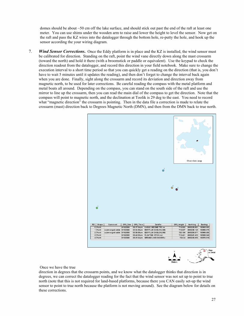
27

domes should be about ~50 cm off the lake surface, and should stick out past the end of the raft at least one meter. You can use shims under the wooden arm to raise and lower the height to level the sensor. Now get on the raft and pass the KZ wires into the datalogger through the bottom hole, re-putty the hole, and hook up the sensor according the your wiring diagram.

7. Wind Sensor Corrections. Once the Eddy platform is in place and the KZ is installed, the wind sensor must

be calibrated for direction. Standing on the raft, point the wind vane directly down along the mast crossarm (toward the north) and hold it there (with a broomstick or paddle or equivalent). Use the keypad to check the direction readout from the datalogger, and record this direction in your field notebook. Make sure to change the execution interval to a short time period so that you can quickly get a reading on the direction (that is, you don’t have to wait 5 minutes until it updates the reading), and then don’t forget to change the interval back again when you are done. Finally, sight along the crossarm and record its deviation and direction away from magnetic north, to be used for later corrections. Be careful reading the compass with the metal platform and metal boats all around. Depending on the compass, you can stand on the south side of the raft and use the mirror to line up the crossarm, then you can read the main dial of the compass to get the direction. Note that the compass will point to magnetic north, and the declination at Toolik is 29 deg to the east. You need to record what “magnetic direction” the crossarm is pointing. Then in the data file a correction is made to relate the crossarm (mast) direction back to Degrees Magnetic North (DMN), and then from the DMN back to true north. Once we have the true direction in degrees that the crossarm points, and we know what the datalogger thinks that direction is in degrees, we can correct the datalogger reading for the fact that the wind sensor was not set up to point to true north (note that this is not required for land-based platforms, because there you CAN easily set-up the wind sensor to point to true north because the platform is not moving around). See the diagram below for details on these corrections.

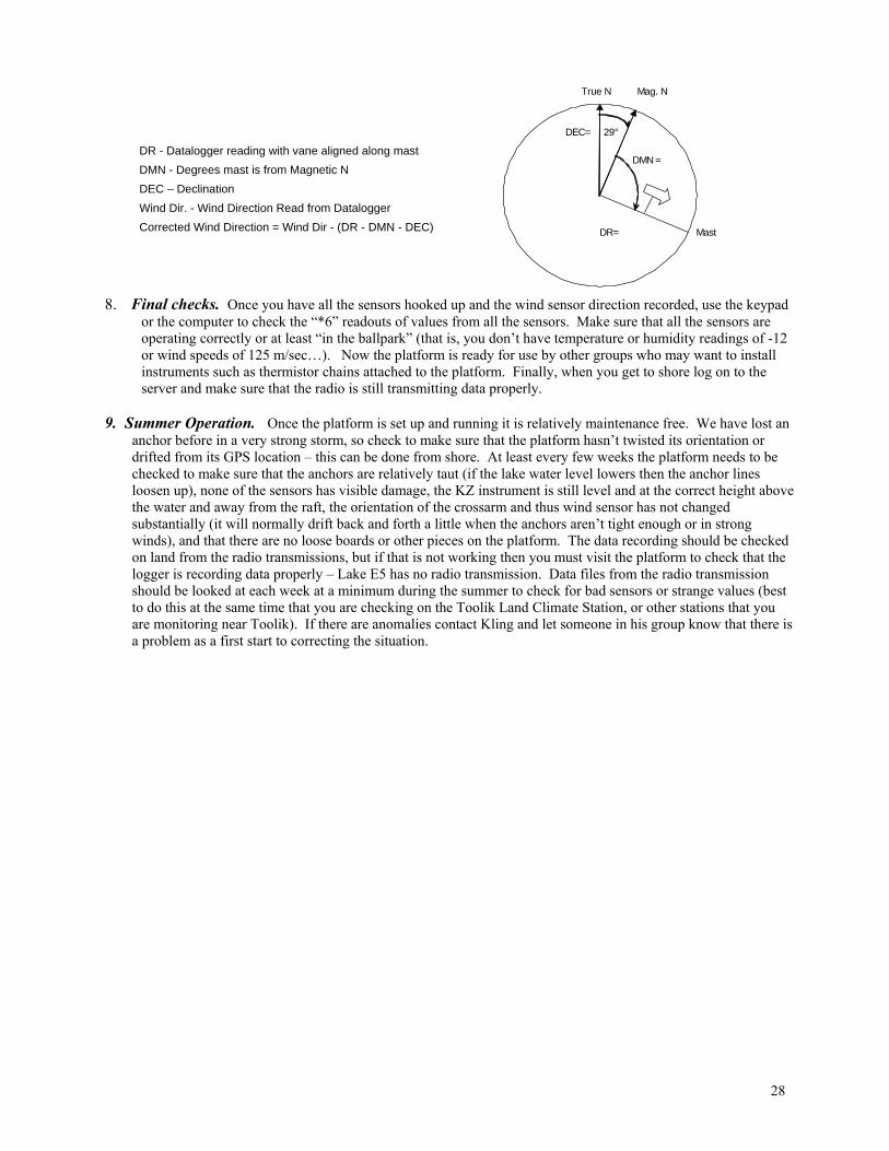
28

8. Final checks. Once you have all the sensors hooked up and the wind sensor direction recorded, use the keypad

or the computer to check the “*6” readouts of values from all the sensors. Make sure that all the sensors are operating correctly or at least “in the ballpark” (that is, you don’t have temperature or humidity readings of -12 or wind speeds of 125 m/sec…). Now the platform is ready for use by other groups who may want to install instruments such as thermistor chains attached to the platform. Finally, when you get to shore log on to the server and make sure that the radio is still transmitting data properly.

9. Summer Operation. Once the platform is set up and running it is relatively maintenance free. We have lost an

anchor before in a very strong storm, so check to make sure that the platform hasn’t twisted its orientation or drifted from its GPS location – this can be done from shore. At least every few weeks the platform needs to be checked to make sure that the anchors are relatively taut (if the lake water level lowers then the anchor lines loosen up), none of the sensors has visible damage, the KZ instrument is still level and at the correct height above the water and away from the raft, the orientation of the crossarm and thus wind sensor has not changed substantially (it will normally drift back and forth a little when the anchors aren’t tight enough or in strong winds), and that there are no loose boards or other pieces on the platform. The data recording should be checked on land from the radio transmissions, but if that is not working then you must visit the platform to check that the logger is recording data properly – Lake E5 has no radio transmission. Data files from the radio transmission should be looked at each week at a minimum during the summer to check for bad sensors or strange values (best to do this at the same time that you are checking on the Toolik Land Climate Station, or other stations that you are monitoring near Toolik). If there are anomalies contact Kling and let someone in his group know that there is a problem as a first start to correcting the situation.



DEC – Declination



True N Mag. N

29°

Mast

DMN =

DR=

DEC=

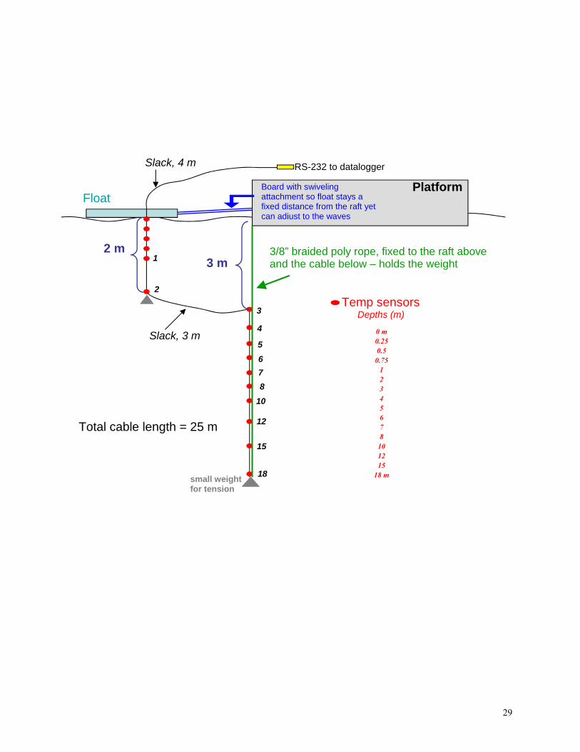
29

Float

3/8” braided poly rope, fixed to the raft above and the cable below – holds the weight

RS-232 to datalogger Slack, 4 m

Temp sensors Depths (m)

Slack, 3 m

3 m 2 m

5

4

7

6

10

8

12

15

18

3

1

2

small weight for tension

Board with swiveling attachment so float stays a fixed distance from the raft yet can adjust to the waves

0 m0.250.5

0.7512345678

101215

18 m

Total cable length = 25 m

Platform

30

(II-2) Toolik Field Shut Down FOLLOW THIS LIST EXACTLY, AND CHECK-OFF THINGS AS YOU DO THEM. Also consult the list of

responsibilities and timetable of shutdown found in the Excel file “Toolik_Shutdown_year.xls”. If you have questions do not hesitate to call or email the lab. Last revised 2014.

A. Labs - General 1. Chemicals – Leave solid chemicals in the cabinets but tape the cabinet doors shut (the winter wind shakes the

trailer and bottles could fall off the shelves). Cover all open shelves with plastic bags (but don’t put tape on the walls of Lab 4 as it pulls of the paint; use packing tape and tape onto the metal frames of the shelves).

2. Computers – Shut down, turn off, then unplug all the computers and printers. Remove all printer cartridges and put in warm storage. Carefully cover them with big plastic bags or they will be covered with dust in spring. (a) The Dell XPS (blue) and small silver HP laptops must return to Ann Arbor (the others go to warm storage).

Make sure to ship the transformers and power plugs. The computer DATA for this year MUST BE TRANSFERRED to the Download computer in Lab 4 first.

(b) There is also a cable that connects the laptops to the dataloggers. It has a nine-pin connection on each end and has an orange piece of tape on one end that says “com port”. This SC532 cable MUST RETURN TO ANN ARBOR.

3. Inventory - INVENTORY the consumables using the Inventory file on the download computer. This includes items that will need reordering and also reusable items. Transfer the inventory to the Michigan server, and make scan and bring the inventory to Ann Arbor.

NOTE: Record the volume left in a container and also any expiration dates. If there is just one box of an item, look inside to see if the box is full or not – recording “one box” of syringes when there are only 2 left in the box is less than helpful. (Note – do not get carried away with the inventory; e.g., we just need to know that there are x full boxes of GF/F filters and y opened boxes, but not how many filters are actually in the opened boxes.)

2. Move all items that may break or contain liquid from open shelves to the floor and place in buckets or plastic pans (see Section B for information on what liquids to send to warm storage). All car batteries (i.e., the ones running ISCOs or dataloggers) should be brought in an placed under the metal table in a container. Fill the batteries with DI (if they are not sealed gel types) and charge them before storing over the winter!

3. Do not store any cardboard boxes on the lab floor. We have had eye-wash stations leak and flood the lab, and the cardboard boxes were ruined. Everything has to be in a tub, basin, or plastic container.

6. For Next Year – At the end of the Inventory list, add any item that we are low on or that you think we could use for next year (If it is not obvious, please write what the item is for or why we need it).

* There is also usually a list on the wall or the filing cabinet in the office of things needed for next year – check in both labs and bring all lists back to Ann Arbor.

7. Close all the windows and lock them. Lower the blinds. 8. REMOVE ALL SODA CANS AND BEER BOTTLES FROM THE LAB. They will burst over the winter

and I don’t want to clean up the stinking mess if I come up first in the spring. 9. REMOVE ALL FOOD from the lab. 10. Clean out all refrigerators and wipe them down with wet rags – no dead fish left over the winter! Unplug the

refrigerator (bring extension cord inside the lab and fill opening in wall if necessary) and stick a piece of cardboard between the door and the fridge – duck tape into place. Secure the refrigerator on the landing outside of lab 4 (North-ish side of the lab – facing the lake).

11. Clean out and check the –80 C freezer in Lab 1 for chlorophyll or DNA samples. 12. Clean out all the drying ovens that have our filter samples or other (e.g., isotope) samples in them. Check them

for filters, desiccant pouches (store in shelves near gas kits), personal gear, and remove. If there is not another group using the drying oven, power it off.

13. Clean off the landing and put all backpacks and miscellaneous items into the conex. 14. Clean out the personal bins in the lab 4. Throw out what people do not want. 15. Clean and clearly label all hazardous waste barrels, and notify the haz mat person (the EMT in camp). Make sure

you have filled out the form located in the white TFS folders in each lab where the hazardous waste was generated.

16. Clean the lab (sweep and mop our areas) and cover open shelves and computers with large plastic bags. 17. Clean out the fume hoods – these are not storage areas for our crap. 18. Acid wash all bottles that will be used next year – store dry (no DI in the bottles) – leave enough time for bottles

to dry before you store them. 20. Sweep and mop. Remove hazardous waste. Place garbage bags over the shelves. Shutdown the Rad room.

31

21. Do not store any cardboard on the floor of the outside storage tents. Now that TFS leaves the tents up over winter it is nice for the extra room, but all tents leak. Most of the stuff in the tent in between Wet and Dry Lab was frozen-in to the floor in spring 2012, and after it thawed out the boxes are falling apart. Now there are shelves in the tent to get things off the floor – Lakes side is toward Wet Lab, Dry Lab projects on the other side. Do not leave pillows or towels uncovered. All are moldy and disgusting and ruined in spring, not to mention the exploded pop cans and other general trash – clean all this junk out before leaving TFS.

22. In the Conex, move all winter sampling gear to the front near the doors, so George can easily access it next May. 23. Remove small acid bottles from gas kits and put with other acids in a Tupperware container in the acids cabinet in

the entryway. 24. Make sure DI carboys are empty. 25. Dump all nutrient bottles and acid wash if there’s time. If not, empty the bottles, put them in a box or bag (bottles

capped) and LABEL THAT THE BOTTLES WERE NOT ACID WASHED along with the YEAR. 26. Dump the acid bath on the pad and rinse container with DI. 27. Update protocols by saving a file with an ampersand & at the beginning of the file, and place it on the Kling Lab

Server under \Documents\Lab\Protocols\_&filename. Or, write the protocol changes in the “Essentials” protocol book that returns to Ann Arbor.

Dry Lab Shutdown In the Dry Lab, we can usually keep most of our things “in place”, but we do consolidate items in the main lab

into the Eddy corner (opposite the bac prod room), and on the wall by the hood. Except for those two areas, the counter tops should be clean except for large instruments (the GC, the scint counter, the bac prod set up) or computers. If you are told by Camp that others will need space in Dry Lab during the winter, put the nice, expensive, or important items in the GC room. 1. Inventory all chemicals and supplies, including entry ways. Make sure to keep a copy of just Dry Lab inventory

before handing over one copy to be merged with Lab 4 inventory. 2. Pack chemicals going to warm storage, mark any remaining Scintisafe as “overwintered”, and box up any

miscellaneous volumetric flasks and pipettes used for DOM analysis. 3. Pack up Shimadzu UV-Vis spectrophotometer – take to warm storage. 4. Empty out, turn off, and cover bench top sterilizer (LTREB) – it now lives on the floor under the large drying

oven – cover the sterilizer with plastic. 5. Move the expensive equipment/drawers/supplies into the GC room so it can be locked over winter. Make sure

you put the expensive/important stuff in the back of the room. The laminar flow hood and the large floor centrifuge can stay in the main lab. Also, most stuff on the shelves can stay in the main lab. Check with George whether we can have space in the main Dry Lab to store some things (or not). Take pictures.

6. If the Camp says people will definitely use the Dry Lab during the winter, move remaining rolling drawers back into GC room or the bac prod room.

7. Calculate and fill out waste forms, notify Haz Mat person (camp EMT) for pick-up. 8. Shutdown and cover all computers after verifying that data has been properly backed up to servers and external

hard drives. 9. Make sure all notebooks have been scanned or photocopied - leave one photocopy in Lab 4 with general lab

copies. 10. Dust shelves, mop floor, pull down plastic over shelves. Do Not use labeling tape on the plastic covers – it

doesn’t stick through the winter – use the clear packing tape (not duct tape). 11. Clean rad area including bin and manifolds with No-Count, wipe test and re-clean if necessary (empty No-count

containers must only be disposed of in No-burn garbage containers- dry rad waste is incinerated in Fairbanks). 12. Bring in vacuum pump from under the lab and close ports in the wall. 13. Finish calculations and paperwork for rad liquid waste, dry waste, and counted samples. 14. Wipe test exterior of all rad waste containers. 15. Shut down scintillation counter if all users in camp are done with wipe tests, package rad standards to ship to

UAF. Notify the UAF RSO, and the Haz Mat personnel for final waste pick-up. 16. Make a list of WHERE STUFF IS after it has been relocated to the GC and bac prod rooms. 17. DO NOT LEAVE ANY LIQUIDS (SODA, BEER, ETC.) IN THE LAB. 18. Clean the sink area well, scraping off any soap scum or rust around the sink. Sweep and mop floor.

32

B. Warm Storage Items that cannot freeze, such as certain reagents, LCD screens in the ISCO samplers, and so forth are sent to Warm Storage over the winter. Warm storage is now in camp (not in FBX as in the past) in either the Winter Lab, the Dry Lab, or both – Camp decides, but, we must let them know that we have Warm Storage materials. We have dedicated action packers or boxes for our materials. 1. ISCO heads (not the bottom part, only the top computer part) must be put in the large boxes dedicated for them

and sent to warm storage. 2. Consort conductivity meters – the two in the big blue cases go to warm storage (the third meter goes to AA in a

small black case WITH THE POWER CABLE). 3. The Hobos, stowaways, and the Troll also stay in warm storage. Find the labeled action packer, fit them all in

there. If they don’t all fit in one box, just make sure the other box is properly labeled. 4. The Licor stays at camp, make sure the inside is DRY before storing it all winter. 5. The Shimadzu spectrophotometer in the Dry Lab, GC room, must be packed up (its box lives in the Dry Lab tent

or conex). Leave the spec cells etc. in a box in the GC room where the spec was located. If camp says that Dry Lab will be warm storage, then you don’t have to pack up the spec you can cover it and leave it on the counter in the GC room of the Dry Lab.

6. The older IBM laptop computers and the black/silver Dell go to warm storage (the blue Dell and newer HP laptop go to AA).

7. Any liquids that CANNOT freeze must be put in warm storage. This includes: (a) Liquid reagents for use in the DOM analyses (e.g., BSA, Commassie, Folin-Coltreau). (b) UNOPENED bottles of pH buffers and conductivity standards. Store in plastic bags inside the action packer.

All other pH buffers and standards can stay in camp, but keep them in the plastic trays in case they burst over winter.

(c) Standardized acids or reagents that YOU KNOW WILL BE USED NEXT YEAR. These are often specialized items that are bought with or made to have a standardized concentration. These are rare, and check with George before sending these to warm storage. * Make sure that the acids are stored in a container separately from everything else.

8. The other items that are to be stored Warm: a. Thermometers (the NIST thermometer especially!) b. Any remaining meters that are left (All Conductivity and some pH meters – See Send to Michigan Section). c. Printer cartridges (except the big Laser Jet cartridges, they are fine cold). d. Voltmeters from the office in Lab 4. e. Any pipettes that are not sent to Michigan – See Send to Michigan Section. Don’t forget about the pipettes used to acidify samples.

9. Make an inventory of what is in warm storage for the person who will open camp next year, including any pertinent details or things done differently. Scan or photocopy and bring one copy to Ann Arbor, leave one copy at Toolik. Make sure that you put the inventory on the computer and back it up to the server in Michigan.

10. All pH and conductivity meters and probes that aren’t sent to Michigan- See Send to Michigan Section. 11. PDA and downloading cables in small Tupperware – check with George because may be sent to Michigan. 12. Both discharge meters and probes (not the staffs).

C. Send to Michigan Everything labeled “return to Ann Arbor” needs to be sent back to Michigan; but, be sure to check that it is on the list

below (if not, email the lab and ask). Start assembling these items to send as early as possible to avoid the Christmas rush. If you are not sure about something, email or call the lab and ask.

The following 1st 4 items are put into the AA#1 action packer that has specially placed foam for these instruments pH meters: 1 WTW meter and all WTW probes (all else is sent to Warm Storage). The two 5mL pipettes and the repeat pipette in the Wet Lab area. 3. CF Cards that were used that summer (all others stay at Toolik) 4. One Consort conductivity meter in a small black case with the power cable (the other 2 Consorts in the blue cases go to warm storage) 5. The blue Dell and silver HP laptops and power cables and transformers – transfer data to Download computer first. 6. Downloading cables (CTD/Downloads, LiCor tupperware container) – check with George 7. Thumb drives (~5 total) 8. Any non-functioning equipment that needs to be fixed in AA

33

9. CTD and Scufa if it is in camp – check with George to see if it is to be stored Warm at Toolik or shipped back to Ann Arbor.

10. External hard drives from the LTREB and LW computers. 11. Storage Modules (SM4) for data loggers IF THEY HAVE NOT BEEN DOWNLOADED. Otherwise, store in

plastic container in the lab 4 office. DATA: see the section below on DATA for details; ALL hard copies of field books, nuts books, GC chromatograms, climate station book, external hard drive, storage modules, all need to go to AA

D. CTD-SCUFA 1. The CTD is usually shipped back to Ann Arbor at the end of the field season – check with George. Ship the CTD

with the Scufa attached, in the CTD wooden box. 2. Download all data, but do not erase the CTD memory. 3. Make sure that the CTD magnetic switch (white bar near the sensor end) is turned off. Use a rubber band to hold

it in the OFF position. 4. Add a little DI water to the pump and leave the syringe attached. 5. REMOVE the CTD yellow log and HAND CARRY IT TO ANN ARBOR. 6. Screw down the top of the box and latch the outside latches. 7. The big yellow cable (realtime cable) and the small downloading cable that is connected to the back of the main

lab computer or stored in the “CTD/LICOR Downloads” Tupperware stays in the office at Toolik (do not ship the floats or the nylon rope).

E. Data and Other Documents * Be sure to “collect” all of the data from other computers and laptops throughout camp, including data that the

REUs may have generated. 1. (a) Save all data to the external hard drive attached to the Dry Lab LTREB computer and the Lab 4 Download

computer. (b) Save all data to the C:\_to_Michigan_year directory of the Download computer, and then update all data to

the Michigan server. The Michigan server has a directory called “To_Michigan_year” as well, and everything in the “to_Michigan” directory should go in the “To_Michigan” directory on the Server.

2. HAND CARRY the external hard drives (two of them) with you back to Michigan (this means in your carry-on luggage, not in your checked baggage).

3. Data Copies -- Make Scan copies of everything except the GC chromatographs, and follow the protocol in the Table below and the description of the table. Or, scan everything and print a copy to leave at Toolik; update the server with the scans (hard copies don’t need to be brought home).

HOME (hand carried) HOME (in luggage) STAYS at TOOLIK

FIELD Books Warm Storage Inventory Copy of FIELD Books GC Chromatographs Lab Inventory NUTS Books CTD Cast Book Scan Copies of other data sources Red RAD Book External hard drives Marked-up Protocol Book Copy of Warm Storage Inventory

Description of Table above: Make Scan copies of (a) all field notebooks, (b) mini Field notebook, (c) 3-ring Rad book, (d) the Calibrations

book (for instruments, climate stations, dataloggers, etc.), and (e) all personal notebooks (brains). Make Scan copies of the nutrient, chlorophyll, and red rad books. Put all scans on the Kling Lab Server and on the external hard drives. (a) The two Nutrient books and the chlorophyll book stay at Toolik. The Scan copies are transferred to the Lab

Server in Michigan. (b) The Red Rad book stays at Toolik, and a scan is sent to the Lab Server. (c) ALL OTHER DATA BOOKS MUST BE HAND CARRIED (i.e., NOT in checked luggage) to Ann

Arbor: this includes the Field Books, Mini Field Book, and Climate Station book. (d) HAND CARRY the GC-chromatographs to Ann Arbor. (e) Bring back any protocol books that have been marked in (checked baggage is fine). (f) HAND CARRY the Warm Storage Inventory to AA, copy stays at Toolik. (g) Inventory list -- file downloaded to UM server; hard copy sent back to A2.

34

(h) List of things needed for next year (i) All packing slips, shipping receipts, the sampling calendar on the cabinet in Lab 4.

F. Gas Chromatographs 1. There are several GC’s at Toolik – The main one now is the Roots Schimadzu GC14A/B in the Dry Lab (TCD

and FID). There are also other GCs in storage in camp: (1) the Carle in the wet lab (that was used as a backup machine, and as of 2005 is broken and packed up); (2) the ECD Shimadzu 14A in the Dry Lab tent or conex (used by Kei Koba in 2000, plumbed for N2O); (3) an old Shimadzu 8A (from Breck Bowden that Jennifer King brought up in 1998 and that is missing a bracket to hold the sample injection port to the machine, but otherwise, J. King said it was fully functional).

2. General GC shutdown – Follow the instructions below. These instructions apply to ALL GCs. Note that the standards are stored in their clamps with bungies for safety -- the regulators can be left on, but make sure that the regulators are backed out, the tank valves are shut off, and the regulators are covered with cardboard boxes. The air, helium, and hydrogen tanks are sent back to UAF – notify the Camp staff to pick up the tanks (show them what to take so they don’t ship our standards to FBX…).

GC SHUTDOWN -- Usually you will only shut down the Roots GC in the Dry Lab, unless otherwise

instructed. This protocol works for all GCs and starts with the GC already running. 10 May 2012, gwk 1. Turn off the FID and TCD detectors (hit CE to stop beeping). 2. Turn off the heater (hit the green button) and then the white power button on the GC14A. 3. Turn off the chromatopac. Remove the “card” from the front of the chromatopac if it is being used and put it in its

holder taped to the wall on the shelf above the chromatopac. 4. Turn off the wall circuits and unplug the GC and the chromatopac. 5. Leave the helium running at ~10 psi so that the column can cool down properly (i.e., DO NOT shut off the helium

gas yet). This can take ~30-60 minutes, and if you are in a hurry you can also open the door to the GC for better airflow.

6. On the air tank, close the main valve and back out the regulator. 7. Disconnect the air tank line and at the regulator and put a plug in the fitting to keep air and water out of the trap

(Unscrew the connection furthest away from the regulator; that is, leave every fitting that you can on the regulator). Remove it and put the regulator in its box on the shelf.

8. Turn off the hydrogen tank and back out the regulator. Disconnect the hydrogen line at the trap (inside the GC room) and insert a plug into the water trap (have the plug ready).

9. Once the GC has cooled down, shut off the helium main valve and back out the regulator. 10. At the OXY trap, disconnect the helium line and have a plug ready to insert into the trap. 11. Disconnect the helium and the hydrogen lines at the regulators; unscrew the connection furthest away from the

regulator (that is, leave every fitting that you can on the regulator). 12. Bring both the helium and hydrogen lines (they should now be free at both ends) into the lab through the portal.

Use tape to mark the lines that they are for the “Roots GC14A” and store the lines on the table along the wall. 13. Disconnect the regulators on the outside helium and hydrogen and inside air tanks. Replace the caps, and put all

the regulators back in their appropriate boxes. Do not disconnect the fittings. 14. Close the main valves and back out the regulators on all the brown standard gas tanks. You can leave the

regulators on the tanks, but make sure that they are covered with cardboard boxes. 15. The air tank can stay in the GC room if it still has air in it. Otherwise, if it is near empty then place the air tank

outside and on the ground, next to the helium and hydrogen tanks that are in the cage. Alert IAB staff that the tanks are ready to be put on the loading dock to be backhauled to FBX.

16. If there are tank clamps outside, detach them and store them in the GC room. 17. Empty the drierite from the glass column and store the empty column in its box. 18. Tighten the drierite lid!! 19. Move the gas tank so that the GC room door can close shut. 20. Cover the GC, the chromatopac, the APC, and the tool box with plastic bags. Put a plastic bag over the shelf in

the GC room.

G. Dataloggers and ISCOs GENERAL 1. Winterizing the dataloggers at the TW Weir (us/Jim Laundre) and Toolik Inlet (TFS) – May need car batteries (if

running instruments over the winter when the solar panels are ineffective), putty, metal wire, and rebar. This may

35

entail changing the dataloggers to car battery (from Alkaline “D” size batteries), and securing the boxes for wind movement, as well as changing any programs.

2. Make sure most current data is downloaded or the storage module is going to be removed. 3. Record the date and time if you will be changing, interfering or otherwise altering the data readings. 4. Make sure that storage modules left over winter are set to stop when full (vs. continually overwriting the data). 5. Make sure dataloggers and multiplexor boxes are secure and will not move much with the wind. 6. Make sure boxes have desiccant and sufficient putty in the hole where the wires come in. 7. Make sure all wires are as hidden as possible - rumor has it that foxes and sik-siks like to chew on them. If

possible, use splicing tape to cover the ends of wires before sealing them in plastic bags 8. All ISCO heads are put in Warm Storage, and the bottoms are stored in the conex. All bottles should be acid

washed, dry, and capped before placing back in the ISCO bottom. The sample tubing should also be acid washed and dry before being coiled and placed on top of the bottles. Put the bottom with the bottles and tubing inside a trash bag and tie it shut. Then put a long piece of labeling tape across the top and write “SITE NAME ISCO BOTTOM and 24 acid washed, capped bottles and tubing YEAR” on it.

Toolik Inlet

1. Arrange with the camp staff or EDC to shut down the Toolik Inlet gauging station when the water is no longer flowing (but before freeze-up of the water in the stream).

2. Open the gray military box on the standpipe and turn off the datalogger. The logger should be attached by wires to a power supply (with batteries in it), and there is a small toggle switch on the power supply that needs to be turned to the OFF position. DO NOT DISCONNECT ANY WIRING IN THE DATALOGGER BOX.

3. The float in the standpipe needs to be raised and secured so that it is out of the water and will not freeze and be crushed over winter. To do this, lift the wire with beads on it off the pulley of the Stevens recorder (small tan box). On one side of the pulley is the weight, and that should be brought up through the hole and kept inside the gray box (don’t let the wire and weight fall down the other side where the float is located). The float on the other end of the wire needs to be brought up toward the bottom of the gray box. It is too large to fit through the hole in the bottom of the gray box, and instead a stick or bolt is placed across the hole that the wire goes down and through the connector on the float. This “suspends” the float up above the water over the winter.

4. Unless otherwise instructed by Kling lab or Jim Laundre, leave the storage module in the gray box. 5. Close the gray box and secure all of the latches. 6. There is one large black wire going out from the gray box to a small white plastic conductivity probe in the

water. This probe needs to be unfastened (it may be on a rock or on rebar driven into the stream bottom). The cable should be pulled out of the water and wrapped around the large gray box so that it won’t fall off during the winter. You can use a cable tie to keep the cable and probe together. DO NOT detach the wire from the datalogger inside the gray box – everything inside stays wired over the winter, only the datalogger power is turned off.

7. If there are problems or questions take a picture and ask the Kling lab or Jim Laundre what to do. 8. Record the time the hobo is pulled from the hobo house (download the Hobo in the lab). LEAVE THE HOBO

HOUSE ATTCHED TO THE STANDPIPE. Imnavait Weir

1. Bring the ISCO (the whole thing) and ISCO solar panel back to Lab 4. The ISCO head (computer part) is put in Warm Storage for the winter, and ISCO body lives in the conex over the winter (bottles are washed and dried).

a. The ISCO solar panel overwinters in lab 4 underneath the big metal table, or in the Lab 4 conex. b. Bring the battery back to Lab 4 to store under the metal table.

2. Consort Meter and Datalogger: c. Download the datalogger that the Consort is connected to with the computer (or the PDA). d. Disconnect the Consort meter (power off) and probe. These are brought back to Lab 4, packed into a blue

case, and sent to warm storage. LEAVE THE CABLES RUNNING FROM THE CONSORT BOX TO THE WHITE DATALOGGER BOX ALONG THE BOARDWALK.

e. Disconnect the storage module (if one is attached) after downloading the data. f. In the storage module box (above the solar panel that is attached to the boardwalk), flip the metal switch

on the black power box (right hand side of the white box) to the off position. g. Disconnect the batteries and pull the power cords into the white box – separate the red and black battery

wires so they don’t touch. DO NOT DISCONNECT ANY CABLES FROM THE DATALOGGER – LEAVE ALL DATALOGGER WIRING INTACT.

h. Make sure there are no pieces of tape along the outside seal of the white datalogger box – this will create a gap and water will enter over the winter.

36

i. Bring the Datalogger/Consort battery under the wooden box back to Lab 4 to store underneath the big metal table.

3. Lift up the boardwalk bridge and set it down on the boardwalk to the East of the stream in a secure area (but, not too close to the stream so it is not washed away in the spring snowmelt runoff event).

TW Weir: Check with Jim Laundre about the status of the dataloggers for soil temperature and moisture. In 2015 we started to remove the weir from this site – it is leaking badly and there are no other places where a new one can be installed. We may use temporary weirs during the summer from now on. The instructions below pertain to the old set-up at this site, and to the remaining dataloggers for soil temperature and moisture. 1. Record the stage height (in four places along the weir) and download all dataloggers. 2. Disconnect the car battery and pull up all wires into the white box (closest to the weir). 3. The ISCO and car batteries are brought back to camp. The car battery is stored under the metal table in Lab 4. 4. Leave the solar panel and rain gauge in the fish tote near the watering plots. Cover the solar panels with large

plastic bags and make sure any cable ends are secured against moisture. Note that in 2012, the solar panel was brought back to camp instead of being stored in the fish tote.

5. Secure the Fish tote top onto the bottom (wind will carry it far, far away if it is not secured). 6. Take out the white conductivity/temperature probe, wrap the cord loosely, and place over one of the vertical

wooden beams on the right hand side of the weir. Do the same thing with the pressure transducer. 7. Take out the float and the cable – the float and cable are stored in the wooden weir box with the gray Stevens

pulse generator (note that the Stevens Pulse generator hasn’t been used since 2010). Leave the white 5 gallon bucket attached to the weir, but make sure that there is a plastic bag stretched over it and the lid is on so that it does not fill with snow or water in the winter; or, place the bucket in the wooden weir box.

8. Leave the Steven’s pulse generator in the weir box and cover the weir box with a big garbage bag. 10. In the white box closest to the weir: Leave the datalogger and wiring in place. Cover any cable ends with a

plastic bag and tie it together with electrical tape or a cable tie. 11. Pull up the black Consort conductivity probe. 12. Disconnect and bring in the Consort conductivity meter and probe. The Consort meter and probe are placed in

the blue container and put into Warm storage for the winter. 13. Place dessicant packages in the white datalogger boxes and secure any holes with putty. 14. Record the time the hobo is pulled from the hobo house. If possible, bring the hobo house back to lab 4 to store in

the conex, but it may be stuck in the ground.

H. Climate Stations – shutdown Updated 14 Sept 2014 by G. Kling

* This protocol applies to both the Lake E5 station and the Toolik Lake station that are owned and operated by the Arctic LTER project. The E5 station should be pulled on shore next to the fertilizer barge (northeast side of the lake) before the LTER Lakes crew leaves for the summer. The Toolik Lake climate station should be pulled on shore into its winch ramp near the dock at the end of the ice-free season. Starting in 2007 this has been done by the TFS Camp Staff, after the EDC person (or equivalent) has removed the Kipp and Zonen sensor and any temperature chains or other instruments in the water. If you have questions please contact George Kling ([email protected]) for instructions.

-- As an overview of removing the climate stations, you must first bring inboard the Kipp and Zonen radiation sensor (if it exists) and disconnect it from the datalogger box. Next pull up from the lake any thermistor chains that may be installed from the raft, disconnect them from the datalogger and put them in boxes on the platform. Then you can pull up the anchors and put them on the station platform, then tow the station ashore. Finally, remove the storage module (if used), fully detach certain sensors and wires, and finally turn “off” the dataloggers and make sure the station is winterized.

-- You will need the instrument boxes from the Dry Lab or the Lab 8 tent for the Kipp and Zonen instrument and for the thermistor chain, which are placed in the boxes out on the lake before you tow the station to shore.

-- You will need two people in the boat to pull anchors and tow the station to shore, and then 2-4 people to lift and drag the Lake E5 station on shore, and 2-3 people to winch the Toolik station on to its winter resting ramp. The entire operation should take no more than 1-2 hours (not including driving time to Lake E5).

1. Data Downloading - if storage modules are used, they must be downloaded and the data checked. If the data cannot be retrieved, the module must be sent back to Ann Arbor. Check with the Landwater senior tech (now Jason) or with Jim Laundre at MBL who will have a record of what has been radioed to shore and recorded.

37

Record in a field book the date and time that the climate station is being moved or the storage module is removed, and also record the date that the storage module is removed on a piece of tape on the module itself. Please email this information to George Kling at [email protected]

2. Disconnecting the Kipp and Zonen - Use one of the small boats to move the station – the large boats are often difficult to maneuver and you run the risk of hitting the Kipp and Zonen sensor while it is overhanging the raft. Before moving the Toolik Climate station, make sure that you bring inboard the Kipp and Zonen radiation sensor hanging over the side of the platform. Keep the boat away from the side of the Kipp and Zonen, and work from the platform and not the boat. Open the Kipp and Zonen storage box and have it ready (should be marked and stored in Dry Lab or the “No Bird” tent #8. Remove any safety ropes or bungie cords from the long metal tube to which the sensor is attached, and loosen the screw clamps that fasten the tube to the tripod. This will allow you to slide the tube and the sensor over the deck of the platform (not into the boat). Now CAREFULLY move the sensor on board the station raft (not the boat) and place the sensor in the box and tape the top shut. There are two gray cables that run from the sensor into the white datalogger box and connect to the datalogger – leave the sensor in its box and leave it connected to the datalogger until you are onshore. Pull back the long metal tube and secure it so that it doesn’t interfere with towing the station. Leave that arm on the station deck over winter. Once on shore the Kipp and ZOnen is detached and put into warm storage for the winter.

3. Disconnecting the thermistor chain - There may be one or two thermistor chains (t-chains) connected to the platform. One may belong to Sally MacIntyre’s group, and it should be attached to the smaller white datalogger box on the tripod. Contact MacIntyre to have her group remove the chain BEFORE you go out to tow in the station (you don’t want others working out there at the same time, it makes everything more difficult), or get instructions from her group on how to remove the t-chain. Do not take any instructions from MacIntyre’s or any other group on any other aspect of the climate station, as it belongs to and is the responsibility of the LTER. Contact George Kling ([email protected]) or Anne Giblin ([email protected]) or Phaedra Budy ([email protected]) for any and all instructions concerning the LTER aquatic climate stations.

Have the large gray plastic box for the t-chain on the station deck (if you cannot find the gray box you can use an empty cooler). The LTER thermistor chain should have a surface float and secondary line on the raft that is attached to the t-chain at ~3 m depth. All of this material can be hoisted on to the raft to start the process. Once this surface apparatus is on the raft you can pull up the t-chain itself. It may have small weights on the line as you bring it up or at the bottom – leave these weights attached. Start to put the t-chain into the box by lowering the bottom of the chain (deepest sensors you just retrieved) into the box first, followed by the rest of the t-chain including the surface float and materials. If the surface float does not fit in the box then detach it but please keep it with the box for warm storage over winter.

4. Towing the Station - Now you are ready to move the station. There are three lines on the Lake E5 station attached to anchors, and four lines on the Toolik station that are connected to anchors or buckets or crates filled with rocks or cement at the bottom of the lake. The anchors are pulled up at the end of the year and the station is towed to shore. It is easiest to pull the anchors and tow the station in calm conditions. First unhook the station from one anchor (remove the end of the anchor rope from the cleat on the station), then follow the anchor line and take the boat out to the anchor so that you are directly above it and pull it up. After each anchor is removed, drive back to the raft and re-tie the anchor line to the station where it was tied initially, and place the anchor back on the station platform (you don’t want all those anchors and ropes in the metal boat with you). Make sure that the anchor and rope are inboard enough not to fall off the raft. DO NOT detach ropes from the anchors. Repeat for all anchors.

Now you can move the station to shore. Connect the climate station to the front of the boat with a rope and tow the station ashore (the boat is in reverse). This is the best method of towing because the “lever point” (the motor) is far away from the station and it makes it easier to maneuver. On shore you will need at least one person with hip waders to help maneuver the station when it is in deeper water. Now connect the station to the winch with a rope and winch the station up on to its raft. Ask Jeb or another TFS staff member with experience using the winch to help.

5. Shutting down the Station - (i) Unplug the Kipp and Zonen sensor from the datalogger by first unscrewing the connector on the bottom of the

datalogger box and then gently rocking the plug while pulling down (out) to disconnect it from the box. There should be a cap for the connector that lives inside the datalogger box, and replace the cap on the connector. If the cap is missing then put duct tape over the connector to keep it from becoming wet over the winter. You do not need to remove any wires inside the datalogger box. Now put the K&Z cable inside its storage box and tape it up for warm storage over the winter.

38

(ii) Follow the same procedure for the thermistor chain. Remove the connector from the datalogger box by first unscrewing and then gently rocking the plug to remove it. Then use the cap stored inside the datalogger box to seal the connector, or seal it with duct tape if the cap is missing. Place the connector end of the t-chain into its storage box and seal the box for warm storage over winter .

(iii) Turn off the datalogger by unscrewing the cover to the power supply panel in the datalogger box (two big thumb screws) and turn the toggle switch to the “off” position. Depending on which datalogger is being used, this procedure may be different – if you have questions please contact George Kling ([email protected]) or Jim Laundre ([email protected]) for instructions.

(iv) All external instruments on the climate station tripod can be left attached over winter. The only procedure for winterizing is to cover the wind sensor with a plastic bag. Use two of the big, clear plastic bags (from Camp) to cover the sensor. Gently work the plastic bag around the delicate wind vane, then gather up the excess plastic so that it doesn’t flap in the wind. We also don’t want the wind vane to be too loose inside the plastic bags and to flap in the wind. Secure the plastic to the cross arm with cable ties and duct tape. NOTE THAT COVERING THE SENSOR REQUIRE USE OF A 8-FT TALL STEPLADDER. If you are uncomfortable with this operation DO NOT PROCEED, and ask for help.

* If you are told that the wind sensor needs to be replaced or taken down, you must unplug the wind sensor wire (at the sensor itself, not in the datalogger box) and remove the wind sensor. Use the tall 8 ft. stepladder for the Toolik station, and a small stepladder (4-5 ft.) or a tall 5 gallon bucket for the Lake E5 station. You need the tools in the Dataloggers Backpack or the Tupperware box. First remove the wind vane with the small allen wrench screw on top of the sensor. Then unscrew the two large allen screws on the crossarm bracket and slip the sensor out of the bracket. Leave the bracket attached to the crossarm. Place the wind sensor in its box and put it in the EDC office, or in some other location if requested.

(iv) Cover the end of the wind sensor cable with a couple of small plastic bags and tape to exclude water. Leave the sensor cable attached inside the datalogger.

(v) Leave the rest of the climate station as is – do not remove any other sensors or any wires. (vi) Check for any damage to the station and make a note of what needs to be ordered for the following year.

6. Data Files - once the station is secured, the data file for the summer needs to be assembled, corrected, checked for errors, and then calculations need to be performed for certain variables (such as the Kipp and Zonen radiation sensor). This is done by the LTER personnel. The details of how to process the file are found on the NOTES page in the file itself. For Toolik Lake, once the file is finished send it to the Kling lab for a verification check. Once the file has been verified it can be “reformatted” to be compliant with the NSF-LTER Network Data Requirements. This reformatting is done by the Kling lab, and then the file can be posted to the TFS website (done by Christie) and to the Arctic LTER website (done by the Kling lab). The file should NOT be given to anyone before the corrections, verification, and reformatting is complete.

I. Eddy Flux Platform – shutdown Updated 25Aug2014 by M. Finnegan / G. Kling 1. Preparations - There are 4 main steps to shutting down the Eddy Flux platform: (1) removing the instruments

from the lake (t-chain, dissolved oxygen, conductivity) and instruments extended over the raft (Kipp and Zonen radiation senso); (2) retrieving the eddy platform anchor lines; (3) securing and sinking the line-power cable from shore. (4) towing the platform to shore.

CPS will need to turn off the shore power before the power cable is detached from the eddy platform (talk to the camp manager to arrange that) The instruments must be removed first, although the platform can be towed to shore before the power cable is sunk. Remember, the external instruments must be removed before the platform is towed to shore. On shore the platform can be secured to the dock / winched up on the Eddy skid. It can be easier to remove instruments and transport them back to the lab from the dock.

You will need two people minimum in the boat to detach the sensors, tow the raft, and retrieve the anchors . On shore, depending on the configuration of the winch and skids, you may need up to 4-5 people to lift the platform out of the water and onto the shore (arrange that with the Camp Manager). Allow for ~1 hour to remove the instruments, ~1 hour to sink the cable, and ~1 hour to retrieve the anchors and tow the platform to shore. Before

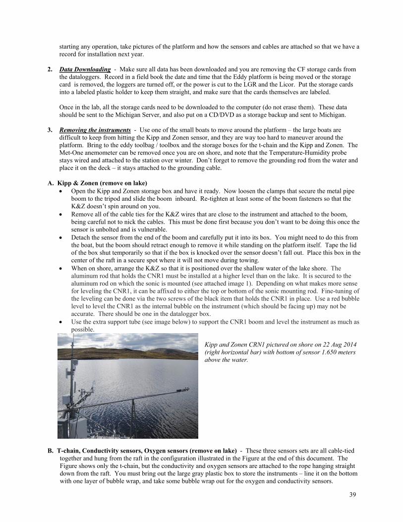
39

starting any operation, take pictures of the platform and how the sensors and cables are attached so that we have a record for installation next year.

2. Data Downloading - Make sure all data has been downloaded and you are removing the CF storage cards from

the dataloggers. Record in a field book the date and time that the Eddy platform is being moved or the storage card is removed, the loggers are turned off, or the power is cut to the LGR and the Licor. Put the storage cards into a labeled plastic holder to keep them straight, and make sure that the cards themselves are labeled.

Once in the lab, all the storage cards need to be downloaded to the computer (do not erase them). These data

should be sent to the Michigan Server, and also put on a CD/DVD as a storage backup and sent to Michigan. 3. Removing the instruments - Use one of the small boats to move around the platform – the large boats are

difficult to keep from hitting the Kipp and Zonen sensor, and they are way too hard to maneuver around the platform. Bring to the eddy toolbag / toolbox and the storage boxes for the t-chain and the Kipp and Zonen. The Met-One anemometer can be removed once you are on shore, and note that the Temperature-Humidity probe stays wired and attached to the station over winter. Don’t forget to remove the grounding rod from the water and place it on the deck – it stays attached to the grounding cable.

A. Kipp & Zonen (remove on lake)

Open the Kipp and Zonen storage box and have it ready. Now loosen the clamps that secure the metal pipe boom to the tripod and slide the boom inboard. Re-tighten at least some of the boom fasteners so that the K&Z doesn’t spin around on you.

Remove all of the cable ties for the K&Z wires that are close to the instrument and attached to the boom, being careful not to nick the cables. This must be done first because you don’t want to be doing this once the sensor is unbolted and is vulnerable.

Detach the sensor from the end of the boom and carefully put it into its box. You might need to do this from the boat, but the boom should retract enough to remove it while standing on the platform itself. Tape the lid of the box shut temporarily so that if the box is knocked over the sensor doesn’t fall out. Place this box in the center of the raft in a secure spot where it will not move during towing.

When on shore, arrange the K&Z so that it is positioned over the shallow water of the lake shore. The aluminum rod that holds the CNR1 must be installed at a higher level than on the lake. It is secured to the aluminum rod on which the sonic is mounted (see attached image 1). Depending on what makes more sense for leveling the CNR1, it can be affixed to either the top or bottom of the sonic mounting rod. Fine-tuning of the leveling can be done via the two screws of the black item that holds the CNR1 in place. Use a red bubble level to level the CNR1 as the internal bubble on the instrument (which should be facing up) may not be accurate. There should be one in the datalogger box.

Use the extra support tube (see image below) to support the CNR1 boom and level the instrument as much as possible.

Kipp and Zonen CRN1 pictured on shore on 22 Aug 2014 (right horizontal bar) with bottom of sensor 1.650 meters above the water.

B. T-chain, Conductivity sensors, Oxygen sensors (remove on lake) - These three sensors sets are all cable-tied

together and hung from the raft in the configuration illustrated in the Figure at the end of this document. The Figure shows only the t-chain, but the conductivity and oxygen sensors are attached to the rope hanging straight down from the raft. You must bring out the large gray plastic box to store the instruments – line it on the bottom with one layer of bubble wrap, and take some bubble wrap out for the oxygen and conductivity sensors.

40

Slide out the t-chain line from the floatation board and start to pull it up. Initially you can just coil the cable and the thermistors on the deck. When you get to the end of the slack (that is, just before the 3 m depth thermistor, see the diagram) you need to carefully place all the cable and sensors into the gray box.

Carefully pull up the rope and the cables together, and feed the cables and the sensors into the gray box, coiling them as you go. Leave everything attached at this point.

As you get to the conductivity sensors and especially the oxygen sensors, wrap them (don’t need to tape them) in a small piece of bubble wrap as you feed them into the gray box.

The bottom of the cable has the weight for the thermistor chain. Remove the weight and store it next to the PFD box near the boat docks. The yellow polypro rope is attached to the thermistor chain via cable ties. Cut them, and separate the rope from the thermistor chain. Once the chain is completely out of the water and coiled on deck, you can un-tie the thermistor chain rope from the eddy platform cleat.

Now you can remove the wiring for the sensors from the datalogger. Start with the conductivity probes, and remove the cables from the logger box.

Next unplug the bulkhead connector of the t-chain from the datalogger box. Wrap the male connector in plastic to keep it safe from the elements.

Place all of the wires into the gray box and tape the top of the box shut for protection. C. CSAT3 sonic anemometer (remove on lake) - the sonic is attached to a boom from the tripod, which also has a

supporting rod that is attached to the aluminum frame of the platform. Given the slow towing of the raft, the sonic can remain affixed for transport to shore as the raft receives far

more jostling during summer operation than during the tow in. When on shore, the sonic must be leveled again and the new magnetic and true directions noted as well as the

distance above the water that the center of the instrument head is at. Record this in the wiki (https://glwiki.ethz.ch/doku.php?id=40_sites:toolik_lake:fieldbook:fieldbook).

CSAT3 sonic (left horizontal arm) on shore on 22Aug2014 facing 220 degrees magnetic north (with a declination of 19 degrees, giving a true north reading of 201 degrees) and positioned 1.675 meters above the water.

D. Met-One anemometer (remove on shore)

Have the Met-One storage box ready Unplug the cable from the sensor and coil all of the wire. The wire can be double-bagged and stored on the

raft over winter so that you don’t have to unwire the sensor from the datalogger (same goes for the temperature probe, which can just be left out in its housing).

41

Remove the vane (tail fin) from the sensor with an Allen wrench and place it between the two sheets of cardboard found in the storage box. Re-tighten the Allen screw so that it doesn’t fall out.

Remove the sensor body from the mount on the tripod – the mounting bracket stays on the tripod – and place the sensor in the box with the cups in the proper places (it will only fit one way).

E. Removing Equilibrator – Disconnect according to instructions from Werner 4. Securing and sinking the power cable The power cable is attached to the platform by two cable-grippers, one of which is roped to a cleat on the platform and the other of which is roped directly to the platform’s aluminum frame. NOTE: The power cable anchor is NEVER MOVED. See figure below to see the setup and operation of the submerged power cable. A) Securing the power cable on the surfer float

Get the big Styrofoam surfboard from under Lab 4 that the power cable was attached to before the platform was out on the lake. Also bring out one of the large red floats from the Conex or under Lab 4.

Unplug the cable from the junction box on the raft. DOUBLE CHECK THAT THE POWER IS OFF! Attach the waterproof connector for storage in the lake over winter. Talk to the camp manager if you need

CPS to be involved during this process. Coil the extra cable on the platform and cable-tie or rope it together. Place the coil on top of the Styrofoam

and attach it by running wire (or rope) through the hole in the Styrofoam. Detach the power cable from the raft, and re-attach the ropes on the grippers to the big float (both grippers). Remove the power cable anchor line running straight down into the water from the eddy platform, and tie the

end to the large float, passing through the lines from the grippers. Now you have the anchor line running to the float, the power cable attached to the float, and the excess power cable sitting on top of the Styrofoam.

Release the float and the Styrofoam and check to see that it remains upright on the water (even if it tips over and spills the excess cable, we still have the cable attached to the float and anchor line).

At this point you can move the platform because it is independent from the cable, then come back with the winter line and sink the cable.

B) Sinking the power cable (can be done after the 4 directional anchors are pulled or after the eddy platform is on shore)

Get the winter line from under lab 4 (~1/4 inch white nylon line on a large wooden spool). Secure the end of the winter line to the rebar on shore, found ~50-100 ft north of the sauna. Bring the winter line out to the surfer float (while a person on shore feeds out slack on the line) Attach the winter line to the cable grippers. Make sure that both power cable anchor line and winter line are

SECURED properly on the cable grippers BEFORE you remove the attachment to the surfer.

42

Detach the line from the power cable grippers to the surfer, it will sink with both the anchor and winter line. To retrieve the power cable next season, you should only need to trace the winter line from shore to the submerged power cable.

5. Towing the Platform - Now you are ready to move the platform (after the instruments are removed and power cable is on the surfer). There are four anchor lines running away from the platform that must be removed, DO NOT REMOVE the one anchor line running straight down under the platform that is attached to the power cable. Also make sure that the grounding rod is lifted up out of the water and placed on deck – it should stay attached to the grounding cable.

With two people in the boat, untie an anchor line at the platform and start to reel it up on a spool (or on a

PVC pipe). As you reach the small weights that move the rope down out of propeller range, you can cut the cable-tie and remove the weight.

Move the boat slowly out toward the anchor, winding the line on the spool as you go. When you reach the anchor (the anchor line will be more or less straight up and down), have two people pull

the anchor out of the mud (using gloves) and put it into the boat. Return to the platform and repeat this procedure for the next anchor. When all four anchors are removed. Tow the platform back to use by securing it alongside the boat (if calm conditions) or using two fixed lines as

described in the eddy platform deployment section of the protocol. 6. Replacing LiCor 7000 scrubber contents –

Shut off power to the Licor using the main switch panel in the Nema box labeled Licor/CSAT. Locate the scrubber in the front left of the Nema box and remove the tygon tubing from both ends. Take note

of which hose goes to which port.

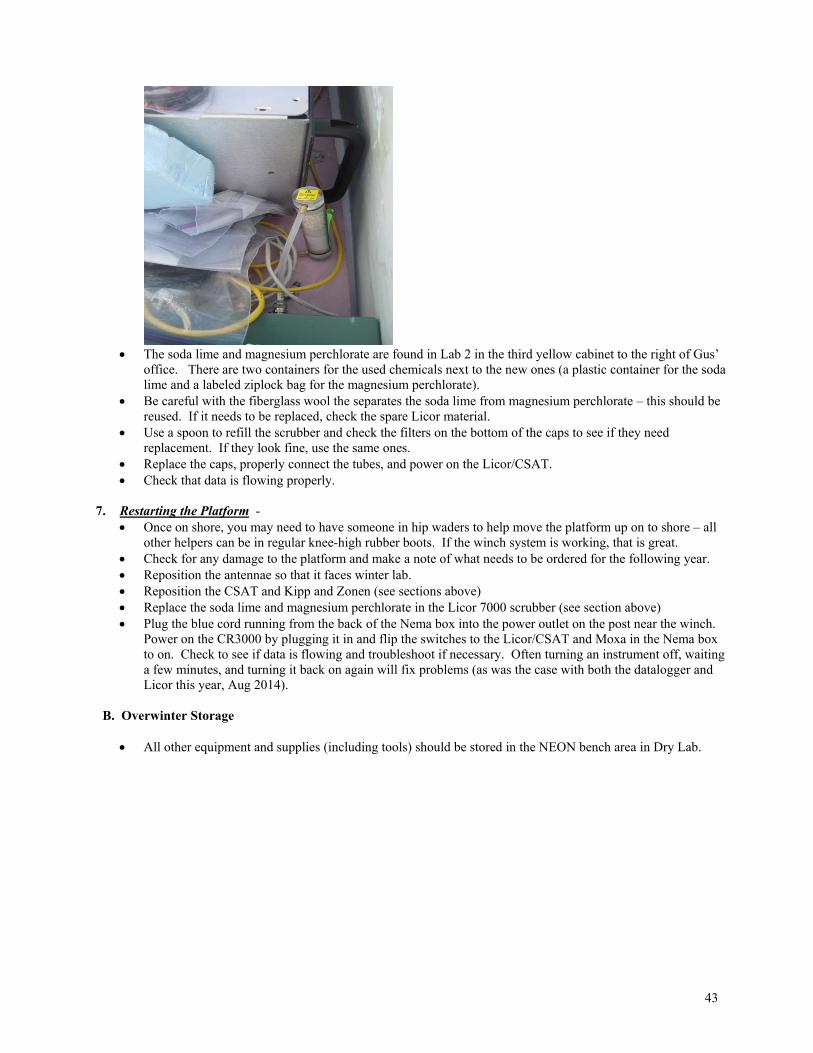
43

The soda lime and magnesium perchlorate are found in Lab 2 in the third yellow cabinet to the right of Gus’

office. There are two containers for the used chemicals next to the new ones (a plastic container for the soda lime and a labeled ziplock bag for the magnesium perchlorate).

Be careful with the fiberglass wool the separates the soda lime from magnesium perchlorate – this should be reused. If it needs to be replaced, check the spare Licor material.

Use a spoon to refill the scrubber and check the filters on the bottom of the caps to see if they need replacement. If they look fine, use the same ones.

Replace the caps, properly connect the tubes, and power on the Licor/CSAT. Check that data is flowing properly.

7. Restarting the Platform -

Once on shore, you may need to have someone in hip waders to help move the platform up on to shore – all other helpers can be in regular knee-high rubber boots. If the winch system is working, that is great.

Check for any damage to the platform and make a note of what needs to be ordered for the following year. Reposition the antennae so that it faces winter lab. Reposition the CSAT and Kipp and Zonen (see sections above) Replace the soda lime and magnesium perchlorate in the Licor 7000 scrubber (see section above) Plug the blue cord running from the back of the Nema box into the power outlet on the post near the winch.

Power on the CR3000 by plugging it in and flip the switches to the Licor/CSAT and Moxa in the Nema box to on. Check to see if data is flowing and troubleshoot if necessary. Often turning an instrument off, waiting a few minutes, and turning it back on again will fix problems (as was the case with both the datalogger and Licor this year, Aug 2014).

B. Overwinter Storage

All other equipment and supplies (including tools) should be stored in the NEON bench area in Dry Lab.

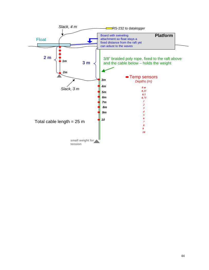
44

Float

3/8” braided poly rope, fixed to the raft above and the cable below – holds the weight

RS-232 to datalogger Slack, 4 m

Temp sensors Depths (m)

Slack, 3 m

3 m2 m

5m

4m

7m

6m

9m

8m

10

3m

1m

2m

small weight for tension

Board with swiveling attachment so float stays a fixed distance from the raft yet can adjust to the waves

0 m0.250.50.75

12345678910

Total cable length = 25 m

Platform

45

SECTION III - ALASKA FIELD SAMPLING AND PROCESSING

(III-1) Alaska Winter Sampling

A. Lab Set-up in Winter

I. Lake Sampling Field Supplies - winter II. Preparation in the lab – for winter sampling 1. Calibrate Hydrolab (see abbreviated operation manual

(http://ecosystems.mbl.edu/arc/data_doc/lakes/cpcpractice/Protocolssplit_files/Surveyor4a%20Datasounde%20Abbrev.%20Manual.htm ). This needs to be done every day for pressure (can be done on the lake), and every 3 days for pH and DO after the initial calibration.

2. Label bottles for later filtering. 3. Make sure that the Hydrolab Surveyor is fully charged.

46

B. Winter Lake Sampling

I. CHECKLIST – Lake Sampling Field Supplies updated May 2015, gwk Print this out as a checklist and follow it every day of sampling! Note there is a shorter Wallocol version at the back of the Protocol Book. Ice auger (gas, extension, 9/16” wrenches) – make sure to use the large 8” auger blade if using the CTD Shovel (medium or big aluminum scoop) Ice chopper (or re-bar) and extra safety rope to tie on end of chopper. Snow machine(s) Sled(s) (1 large and 1 small) Bungee cords, extra ropes Dive buddies (two) and spare battery, 9V Elbow-length rubber glove (optional, for use with dive buddy) Tape measure Tool kit including screw drivers, crescent wrenches, vice grips, duct tape, cable ties, etc. Ice scooper (giant strainer) Tsunami water pump, control unit, connectors, and tubing for collecting water (enough for 20 m if sampling Toolik) Action packer to store Tsunami, tubing, and control unit 12 volt battery (fully charged - put in a battery case in back rack of snow machine) Hydrolab, magnetic stir attachment, cable, and Surveyor key pad (goes in the large cooler with padding) CTD and its marked yellow rope, CTD log book Milk crate to hold 2 L bottles (nice seat for Hydrolab operator) Life jacket (seat cushion); 5 gallon bucket also makes a nice seat 2 L bottles (2 for each lake, plus 2 spares for the day) Syringes (3 of the 140 mL size, extra stopcocks) Gas syringes (enough for an ambient at each lake, plus usually two depths or a full profile at Toolik) Wash tub to fill for equilibrating gases at the surface Filters, filter holders, forceps, and small bottles if filtering in the field DIC kit for old method in glass serum vials (HgCl, 1mL syringes, bottles, caps, sharpie & pencil. Use pink needles) Field book, pencils, sharpies Bathymetric maps of the lakes Map of the Toolik region, compass or GPS Warm clothes, insulated boots, rain paints and rain jacket (for wind), hat, fingerless gloves, latex gloves First aid kit, sunscreen, and sunglasses Food and drink Backup – Geo-pump in case, plus connectors for battery operation Tubing and connection w/ 3-way for gases for Geo-pump Jack-rabbit pumps (2, for backup)

47

III. Details of Winter Lake Field Sampling 1. Pack snow machine sleds. Big cooler and auger in the long sled, action packer and Geo-pump in the small sled.

Bungee down all equipment really well. Snow machines only need 1-3 primes when cold. If they don’t start with 3, then they are flooded. Hold the throttle down with one hand and pull the starter cord with the other hand until the machine starts.

2. Use map to select location of deepest hole in the lake. 3. Shovel away snow. Unscrew the gas vent knob on ice auger. The yellow ice auger needs the choke set open (no

choke), 2-3 primes, and then keep pushing the black primer button until the engine will run without stalling. Then you are ready to drill the hole.

4. Clear hole often, at least when snow in hole covers the connector at the top of the auger. Close the vent on the gas tank, and set the auger blade away from walking paths or cover it immediately. You may have to chip away a place for the auger motor to fit in order to reach the water.

5. Use ice scooper to remove slush in hole. Let bubbles subside (dive buddy doesn’t seem to like bubbles…). 6. Take depth reading with Dive Buddy (warning, Buddy can be off by up to a meter. Take two measurements and

choose deepest sampling depth conservatively). George does this by sticking his arm in the hole up to his shoulder (well, maybe elbow). For the less hearty, an arm-length glove may be necessary.

7. Measure snow depth, ice thickness, and distance from top of ice to water. Note large refreezes. 8. Begin Hydrolab. Remove chamber and small cap on pH probe, then screw on the protective cage and lower into

water. Take barometric pressure and calibrate depth with sensors at the surface. Lower to the bottom of the hole. 9. Create a new file for each lake. Take first reading. Be sure to wait for O2 to equilibrate. This can take 5-8

minutes (it tends to go way down, then come back way up, then settle). Write down measurements in the field book, then record on the Surveyor. Take measurements each meter.

10. Put Hydrolab back in cooler, replace pH probe cap and sealed chamber. Keep cooler and action packer closed for warmth (keeps things from freezing).

11. Lower tubing to desired depth (3 m used as surface depth starting in 2003). Or drop Van Dorn bottle to that depth.

12. Set up ProActive Pump or Geo-pump on top of its case near the hole. Begin pumping (use 600 rpm setting on GeoPump). Allow Geo-pump to run for at least 2.5 minutes to clear a 16 m long tube; Proactive pump needs only 1 minute to clear the same length line. If using jack-rabbit pump, flush with at least 120 turns. Set rolled tubing as close to the ice as possible (i.e., not up on a snow bank – this helps with minimizing the gravity that the pump must overcome).

13. Use three-way attachment for filling gas and DIC syringes (no attachment needed for jack-rabbit, just stick the end of the stopcock into the tubing opening). One person can fill the syringes while another does the DIC.

14. Rinse bottles 3 times and then fill 2 L bottle with water to very top.

III. Lake Sample Processing - winter

1. Filter samples with GF/Fs and polypro filter for cations (follow normal filtering protocols found below). Note: do not use more than 700 mL for each filter or there will not be enough water for bacteria from the 2 L bottle. Follow normal filtering procedures.

2. Use ProActive pump or Geo-pump for cations (poly-pro filter) and then bacteria (500 mL). 3. Start GC, and take filters to drying oven.

48

A. Winter Runoff and Lake Sampling

I. Runoff/Lake Sampling - winter

1. First Priority 1-6. Dissolved inorganic and organic nutrients (N & P), and particulate nutrients, field temp, cond, pH. If these cannot be filtered, collect 2 L if possible (or 1 L) and freeze for later filtering.

2. Second Priority 7-8. Inorganic carbon (alkalinity), major and minor elements. If these cannot be filtered, collect ~ 500 mL of water and freeze for later filtration.

3. Third Priority 9-10. DIC and gases only done if GC is up and running, or use serum vial method for DIC. Priority Label

Color Size (mL) Sample Preserve

(L 6N TMG HCl)

Notes

1. Orange 125 mL DOC/TDN/TDP 200 L 2. White 125 mL

HDPE Inorganic Nutrients 200 L Only acidify if nutrient

lab is not running 3. Red 60 mL

LDPE NO3 Freeze Fill only 2/3 full. Goes

in Freezer. 4. Blue Plastic petri PP filter Dry Record Volume, put in

drying oven 5. White Plastic petri PCN filter Dry Record Volume, put in

drying oven 6. Temp, Cond, pH,

Date-time, discharge estimate

Measure in the field with meter if no Hydrolab

7. Blue 125 mL Alkalinity/Anions 8. Green 60 mL Cations 100 L Use 0.45 µ Polypro

filter 9. Pink 20-30 DIC 0.2 mL HgCl Filled in the field

10. 20 mL Nylon

Gases – CO2 and CH4 Filled in the field

II. Runoff/Lake Filtering -- winter Make sure that all of your bottles are taped and labeled for each sample before you start filtering.

1. Load 25 mm white filter cartridges with GF/F filters (3 filters per sample, one for particulate C and N, one for particulate phosphorus, and one for chlorophyll a – or 1 for black carbon if working on the Burn site).

2. Rinse syringe three times with sample (small volume of water, pull down plunger). 3. Shake sample bottle to suspend particulates (repeat each time you withdraw water). Always pour water from

the bottle into the back of the syringe – do not put the syringe into the sample bottle. 4. Fill a 140 mL syringe (exactly). 5. Rinse ~20-30 mL of sample through GF/F filter. 6. Uncap bottles and rinse each bottle with ~ 5 mL of sample water. 7. Fill bottles (in order of priority, given in Table. Usually save cation bottle until last because of polypro filter) 8. Stop filtering when filter becomes full or you can see much color (Filter as much water as possible to have

enough particulates for analysis). 9. Keep track of how many syringes you filter (you can use the Official, Semi-Automated Counter if you like).

Filter as many as possible (but not more than 5 or you will run out of water from a 2L bottle); (2 syringes= 280mL, 3=420, 4=560, 5=700). Collect more bottles of water if sample is very dilute in particulates.

10. When finished with a filter, push some air (gently) through the filter to remove the excess water. 11. Unscrew filter cartridge and transfer filter to plastic petri dish with forceps. 12. Record volume of water filtered on back of petri dish and in field book (if filtering in the field). 13. Begin filtering with second filter. Filter the same volume through this filter if at all possible. Once the

chemistry bottles are filled you can discard the filtered water. Place the filter in the petri dish. 14. Repeat the process with the third filter for chlorophyll. You need to filter less water for the chlorophyll than

for the particulates, but a minimum of 3 syringes (420 mL). Put the chlorophyll filter in a 15 mL Falcon tube and in a dark bag or wrap with aluminum foil and freeze. If using foil packet, fold filter in half onto itself (so no particulates wipe off onto the foil).

49

15. Rinse ~10-20 mL of sample through white polypro filter for cations. 16. Rinse cation bottle (60 mL green) with ~ 5 mL and then fill to neck. 17. Acidify all samples that require acidification. Use 6 N Trace Metal Grade HCl. General rule for surface

waters is 100 uL for 60 mL bottles of DOC/TDN, TDP, and Cations. Soil waters get half that much acid. IF NUTRIENTS CAN’T BE RUN WITHIN 2 DAYS, acidify the 125 mL bottle with 100 uL acid..

18. NO3 is stored in the freezer, all other samples go in the fridge. If can’t be frozen, acidify as with NH4/PO4. 19. Put particulate filters in a drying oven – set for 40 degC to avoid volatization of carbon (especially important

if we want to run isotopes on the particulates). If no oven is available, air dry the filters as best you can. III. Lake Bacterial DNA - see below Adapted from B. Crump in 2001. Updated 3August 2007, gwk and bcc, 12 August 2007, jlg. OVERVIEW – we use Sterivex filters (sterile, 0.22 μm) to capture bacterial DNA from lake water, stream water, soil

water, and hyporheic water samples. Use two sterivex filters per water sample, and filter up to 1L of water through each filter. A minimum volume if field filtering with syringes is ~500 mL through each filter.

** In 2003 we used ~1 ml of DEB in field and later had to add more during extraction. Be sure to use 2 ml DEB. 1. Equipment and reagents: Millipore Sterivex filters (Fisher cat#SVGP01050) Geopump and pumping apparatus (all components in triplicate if using 3-head Geopump): 1.5 m piece plus two 5

cm pieces of Geotech tubing, y-tube splitter, 10 mL stereological sterile plastic pipette, 7 4” (10.16 cm) cable ties, two 3 mL syringes, fine tip forceps, 1L plastic graduated cylinder Or 140 cc syringes with 3-way stopcock and caulking guns

30 or 60 cc syringe with 0.2-micron syringe filter – for DEB (in the past we used sterile needles attached to the 0.2-micron syringe filter to inject the DEB into the filter, but now we just use a 3-way stopcock attached to the 0.2-micron syringe filter and that works fine).

Appropriate number of 2L brown Nalgene bottles for sample collection Sterile luer plugs (Ark-plas cat#AP117LMLP0CL) or sterile 3 cc syringes to seal the in-port of the sterivex filters Cha-seal putty (Fisher cat#02-678) for sealing the outport of the sterivex filter (or syringe tips from 3 cc syringes

cut in half; use the closed end). DNA Extraction Buffer (DEB) To prepare 50 mL DEB (all solutions autoclaved, recipes below): volume solution final concentration 5 ml 1.0 M Tris-HCL (pH 8.0) 0.1 M 10 ml 0.5 M NaEDTA (pH 8.0) 0.1 M 5 ml 1.0 M Na2H2PO4 (pH 8.0) 0.1 M 15 ml 5.0 M NaCl 1.5 M 10 ml 5% CTAB 0.5% 5 ml H2O (Note: If a precipitate forms in the DNA extraction buffer, just warm it to room temperature and it will redissolve.

The DEB can be frozen in 50 mL centrifuge (Falcon) tubes until use, but it is best shipped as a liquid in 60 mL Nalgene bottles because they won’t leak, and the centrifuge tubes can leak.)

For soil water sampling: Soil sucker needles (50cm and 30cm long hollow needle with holes in last 5cm), with masterflex 6411-16

tubing attached and three-way stop cock attached to other end of tubing 140 cc syringe 1L brown Nalgene bottle for collection

For Hyporheic water sampling: Soil sippers (apx 1.5 m straw with beveled holes in last 10 cm and covered by a mesh bag resembling a

vacuum bag) Hyporehic stake (apx 1.2 m solid metal stake that slides into a solid metal pipe of comparable size) Sledge hammer Tape measure Sterile luer plugs (Ark-plas cat#AP117LMLP0CL) to seal the sipper Masterflex 96410-15 tubing attached and three-way stop cock attached to each end of tubing 140 cc syringe

50

1L brown Nalgene bottle for collection 2. Field filtering with syringes: Pull plunger out of syringe. Attach syringe to sterivex filter. Pour sample into the back of the syringe to ~140 mL line. Insert plunger and push sample through sterivex filter. Remove sterivex filter (or leave the filter on and turn the three-way stopcock on the syringe to allow plunger

removal). Repeat. Aim to get a minimum of 500 mL and up to 1L of sample water through the filter. 3. After filtering: Force all water out of filter using the syringe filled with air. Shake last few drops out of filter forcefully. Stab the filter outport into the Cha-seal, or cap the filter outport with tips from 3 cc syringes cut in half. !!Close

the outports gently so the little caps don't split!! Inject 1 mL DNA Extraction Buffer (DEB) into the filter inport. If using a needle, do not pierce the white filter

inside. (You can put all the DEB buffer in a 60 cc syringe and just use it repeatedly for each sample.) Close inport with a male luer plug or a 3 cc syringe. Be sure it is seated tightly. The syringe sometimes slips out. Freeze ASAP, store at –80ºC. If in the field, put in a small cooler with ice packs. 4. Filtering with the GeoPump (we have two GeoPumps, one is a multi-head unit): Filtering apparatus is set up as such:

Insert base of y-splitter into 1.5m piece of tubing and secure with a cable tie. Connect a 5cm piece of tubing to the branches of the y-splitter and secure each with a cable tie. Pull plunger out of each 3mL syringe an cut off just below the support tabs (where the plunger was). Insert this end into the remaining ends of the 5 cm pieces of tubing and secure with 2 cable ties each. Break off tip of pipette, while still in wrapper and remove cotton from the top with forceps. Insert this end into the other side of the 1.5m piece of tubing Wrapping a different color of tape every 20-50cm around each tubing set is helpful if using multi-head Thread tubing into head of Geo Pump at length appropriate for the area in which you will filter

Insert pipette (either new pipette or particle-free water rinsed and DI water rinsed) into sample water and allow to run through tubing completely for a few seconds for a sample rinse

Attach pre-labeled sterivex to ends of the 3mL syringes at end of tubing Place ends of tubing with filters into 1L graduated cylinder, keep ends of filters above 1L mark Make sure pump is set in correct direction (direction of switch indicated direction of flow), put on medium to

high speed Begin pumping Watch filter and when the water level reaches 1L stop pump and empty cylinder (retaining runoff = particle-free

water for rinsing). Continue filtering until filtering becomes difficult or 1L line is reached again or there is no more sample to filter Record volume filtered and remove streivex filters Follow procedure after filtering above (#3) Rinse pipettes with particle-free water then insert into particle-free water and turn on pump to rinse tubing for a

few seconds, repeat with DI water. Remove pipettes from particle free and pump air through tubing. If intending on re-using pipettes, insert into original wrappers, or discard and hang tubing to dry.

51

(III-2) Alaska Summer Sampling – General Updated 28 May 2013 sef

A. Summer Field Sampling Field Preparation Pack all of the equipment you will need the night before so that nothing will be overlooked. Use the checklists on the wall. Prepare the following items: 1. Sample bottles labeled and divided into separate ziplock bags for each site. The bottles should be labeled (site, date, and sample type (i.e. Nitrate, Cats) as well as color coded: ANALYSIS Size/Type Color Tape DOC/TDN/TDP 125ml/Translucent HDPE Orange NUTS (NH4/PO4) 125ml/Translucent HDPE White (reusable) Nitrate 60ml/Translucent LDPE Red Alk/Ans 125ml/Translucent HDPE Blue Cats 60ml/Translucent HDPE Green PP petri dish for filter Blue PCN petri dish for filter White Chla 15 mL Falcon tube/ Dark bag Green Photochem 30 ml/Amber HDPE Pink **For the PP, PCN & Chla filters be sure record the final volume filtered.** 2. DIC kit: A 1 mL plastic pipette (and one spare) put into a small whirl-pack bag (to keep acid contained) Two 30 mL bottles of ~6N H2SO4 - one bottle is a spare put into a whirlpack with the extra 1 mL syringe. Two 60 mL DIC plastic syringes (labeled as “DIC”) with 3-way stopcocks Sharpie and pencil, just in case OLD METHOD DIC kit: Sharpie permanent marker extra taped 20 mL serum bottles numerous aluminum caps with Teflon septa, inside the blue plastic filter holder case HgCl2 bottle HgCl2 syringe and needle (2) 60 mL H2O syringes (at least 2) and stopcocks (plus an extra stopcock) Crimper to fasten cap to bottle 3. Gas kit: Sharpie permanent marker 140 mL syringes with 3-way stopcocks (at least two); 60mL syringes for soil water sampling nylon syringes (more than the anticipated number of sites) extra stopcocks 4. Filtering kit: clean filter holders (do not load filters the night before - they will break) box of GF/F combusted filters forceps (2 pair) DI water to rinse filter holders Bag of extra micron polypro filters for cation sampling Caulking gun for facilitation of cation filtering, if preferred 5. Field notebook with sharpened pencils 6. pH and conductivity meters with extra pH probe, buffers, filling solution, batteries, thermometer, and DI water 7. Verify boat or vehicle arrangements, if necessary, and try to coordinate with other groups’ outings 8. Inform the nutrient chemist in advance of approximately how many samples you will need to run

52

If taking soil water samples, you will also need: 1. Steel needles and masterflex tubing for the tops 2. Temperature probe and meter 3. Thaw depth probe and meter stick or ruler 4. Well depth stick, if sampling Tussock Watershed 5. Pooling bottles and extra DI 6. 45mm GF/F filters and holders

B. Summer General Field Collection The following sampling order has proven most efficient. Be sure to write down the date and the weather conditions

for that day and the previous days, as well as any unusual conditions. 1. H2O temperature (write down the thermometer # if applicable) 2. pH

a. lakes/streams: submerse the probe tip early in the sampling period and read the final value at the end of the sampling period - note that after the pH meter turns off it takes a while to restabilize the reading.

b. soil water: let equilibrate with soil water before measuring samples. Samples need to be read quickly (once the probe is equilibrated in another, older soil water sample) because they will degas.

3. Conductivity (submerse the probe tip to let it stabilize with the water temperature before taking a reading). 4. DIC (see sampling protocol) –duplicates are taken at some sites. See individual site sampling sheets. 5. Gas samples (see gas sampling protocol) -Take ambient gas samples at each site or for a close group of sites. 6. Filtering for water chemistry -- expel 50 mL of sample water through the filter in order to rinse the filter. (Note:

if there is little water, fill the alkalinity bottle first. This will help rinse the filter and should not affect alkalinity). Rinse each bottle with a few mL of filtered water, then collect the sample. For cations, DO NOT use the GF/F filter and filter holder. Remove the GF/F filter apparatus from the syringe and replace it with a disposable polypro filter. Collect the cation sample using this filter. A caulking gun can be used with the syringe to make filtering through this smaller filter easier/faster.

* Make sure the label has the correct site number and date - THIS IS VERY IMPORTANT. Filtering priority Amount of water Label on bottle

(F=filtered, A=acidified) 1st. Nutrients 125 mL translucent HDPE bottle F if run within a day 2nd. DOC/TDN/TDP 125 mL translucent HDPE bottle F/A 3rd. NO3 40 mL in 60 mL plastic LDPE bottle FU - (frozen) (unacidified) 4th. Alkalinity/Anions 125 mL translucent HDPE bottle FU (filtered unacidified) 5th. Cations 60 mL translucent HDPE bottle F/A 6th. Particulate filters 1 filter for PP, 1 filter for CHN mL filtered= 7th. Chla filter 1 filter (GF/F) Falcon tube, dark bag/foil 8th. Photochemistry 30 ml in amber HDPE bottle F mL filtered= written in field book * GF/F combusted filters with amount H2O (in mL) filtered written on petri dish or aluminum foil packet; freeze or

dry filter at 40C. (The filter is not kept for soil waters). * Beginning in 2002 filters used for Cation samples were changed from the GF/F filter to a polypropolene filter.

The polypro filters do not contaminate the samples as did the GF/F filters.

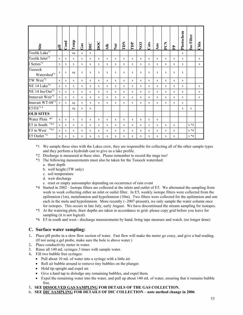
53

Sit

e p

H

Con

d

Tem

p

Gas

DIC

DO

C

Alk

Nu

t

TD

N

TD

P

NO

3

Cat

s

An

s

PC

N

PP

Ph

otoc

hem

Iso

Fil

ter

Ch

la

Toolik Lake*1 eq x x x

Toolik Inlet*2 x x x x x x x x x x x x x x x x x

I Series*2 x x x x x x x x x x x x x x x x x

Tussock Watershed*3

x x eq x x x x x x x x x x x x x

TW Weir*2 x x x x x x x x x x x x x x x x

NE 14 Lake*4 x x x x x x x x x x x x x x x x x

NE 14 Ins/Out*2 x x x x x x x x x x x x x x x x x

Imnavait Weir*2 x x x x x x x x x x x x x x x x x

Imavait WT-08*3 x x eq x x x x x x x x x x x x x

E5/E6*1,4 eq x x x x

OLD SITES

Water Plots *5 x x x x x x x x x x x x x

E5 in South *4,6 x x x x x x x x x x x x x x x x *4

E5 in West *4,6 x x x x x x x x x x x x x x x x *4

E5 Outlet *4 x x x x x x x x x x x x x x x x *4

*1 We sample these sites with the Lakes crew, they are responsible for collecting all of the other sample types

and they perform a hydrolab cast to give us a lake profile. *2 Discharge is measured at these sites. Please remember to record the stage too! *3 The following measurements must also be taken for the Tussock watershed:

a. thaw depth b. well height (TW only) c. soil temperature d. weir discharge e. reset or empty autosampler depending on occurrence of rain event

*4 Started in 2002 - Isotope filters are collected at the inlets and outlet of E5. We alternated the sampling from week to week collecting either an inlet or outlet filter. In E5, weekly isotope filters were collected from the epilimnion (1m), metalimnion and hypolimnion (10m). Two filters were collected for the epilimnion and one each in the meta and hypolimnion. More recently (~2007-present), we only sample the water column once for isotopes. This occurs in late July, early August. We have discontinued the stream sampling for isotopes.

*5 At the watering plots, thaw depths are taken in accordance to grid- please copy grid before you leave for sampling (it is not logical)

*6 E5 in south and west-- discharge measurements by hand, bring tape measure and watch. (no longer done)

C. Surface water sampling: 1. Place pH probe in a slow flow section of water. Fast flow will make the meter go crazy, and give a bad reading.

(If not using a gel probe, make sure the hole is above water.) 2. Place conductivity meter in water. 3. Rinse all 140 mL syringes 3 times with sample water. 4. Fill two bubble free syringes:

Pull about 10 mL of water into a syringe with a little air. Roll air bubble around to remove tiny bubbles on the plunger. Hold tip upright and expel air. Give a hard tap to dislodge any remaining bubbles, and expel them. Expel the remaining water into the water, and pull up about 140 mL of water, ensuring that it remains bubble

free. 5. SEE DISSOLVED GAS SAMPLING FOR DETAILS OF THE GAS COLLECTION. 6. SEE DIC SAMPLING FOR DETAILS OF DIC COLLECTION – note method change in 2006

54

7. Fill syringes and filter through 25mm GF/F and cation filters. Rinse 10-20 mL water through filter before filling bottles (if water is in short supply, fill ALK bottle first – but, see priority order for all samples). Rinse each bottle with a few mL of water before filling.

D. Surface Water Sampling Sites

1. I-SERIES -- USUALLY SURVEYED 3 TIMES PER YEAR, REMEMBER TO SAMPLE CHLA.

I Series Surface Sites Samples to take: 25 Site bags: Other stuff: Nuts I8 Headwater Discharge/Stage Alk/Ans I2 out Discharge Cats I1 out Discharge DOC/TDN/TDP I1-I3 Discharge Nitrate I2-I3 Discharge DIC I3 out Discharge PP (25mm filter) I4 out Discharge/Stage PCN (25mm filter) I4-I5 Discharge/Stage Gas I5 out Discharge/Stage Temp I5-I6 Discharge/Stage PH I6 Inlet West Discharge Conductivity I6 out Discharge/Stage Chlorophyll (25mm filter) I7 out Discharge/Stage Photochemistry I8 in Discharge/Stage I8 out Discharge/Stage I Swamp in Discharge I Swamp out Discharge I7-I9 Discharge/Stage I8-I9 Discharge/Stage MWL Discharge MWU Discharge Toolik Inlet Duplicate, discharge/stage I6 Headwater Lake Inlet Discharge I6 Headwater Lake Outlet Discharge

2. Lakes Inlets Before 2000 these were sampled frequently (1/week). In 2000, sampling was abbreviated and also included TW Weir

(see inlets above), 2003-2007 we included I8 Inlet and I8 Outlet, and by 2008 we dropped MWU; as of 2011, we started sampling I8 Inlet and I8 Outlet again; by 2012 we sampled this complete list every other week.

Lakes Inlets Surface Sites Samples to take: 6 Site bags: Other stuff: Nuts I7-I9 Discharge/Stage Alk/Ans I8-I9 Discharge/Stage Cats MWL Discharge DOC/TDN/TDP Toolik Inlet Duplicate, discharge/stage Photochemistry TW Weir Duplicate, discharge/stage Nitrate I8 Inlet Discharge/Stage DIC I8 Outlet Discharge/Stage PP (25mm filter)

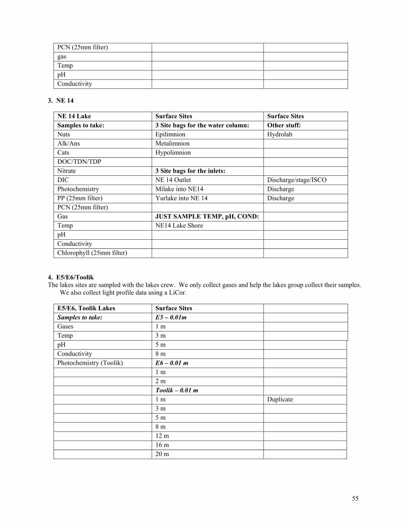
55

PCN (25mm filter) gas Temp pH Conductivity

3. NE 14

NE 14 Lake Surface Sites Surface Sites Samples to take: 3 Site bags for the water column: Other stuff: Nuts Epilimnion Hydrolab Alk/Ans Metalimnion Cats Hypolimnion DOC/TDN/TDP Nitrate 3 Site bags for the inlets: DIC NE 14 Outlet Discharge/stage/ISCO Photochemistry Milake into NE14 Discharge PP (25mm filter) Yurlake into NE 14 Discharge PCN (25mm filter) Gas JUST SAMPLE TEMP, pH, COND: Temp NE14 Lake Shore pH Conductivity Chlorophyll (25mm filter)

4. E5/E6/Toolik The lakes sites are sampled with the lakes crew. We only collect gases and help the lakes group collect their samples.

We also collect light profile data using a LiCor.

E5/E6, Toolik Lakes Surface Sites Samples to take: E5 – 0.01m Gases 1 m Temp 3 m pH 5 m Conductivity 8 m Photochemistry (Toolik) E6 – 0.01 m 1 m 2 m Toolik – 0.01 m 1 m Duplicate 3 m 5 m 8 m 12 m 16 m 20 m

56

E. Soil Water Sampling Before sampling soil water, measure: 1. Soil temperature 2. Thaw depth 3. Well depth if lysimeter is used 4. Soil moisture

F. Soil Water Sampling Sites 1. Imnavait Water Track 08

Imnavait WT08 Soil Sites Samples to take: 17 Site bags: Other stuff: Gas Imnavait WT08-01 Datalogger kit Water temp Imnavait WT08-02 Thaw depth probe Gas equil. Temp Imnavait WT08-03 Soil Moisture probe pH Imnavait WT08-04 Soil needles Conductivity Imnavait WT08-05 Soil temp probes Nuts Imnavait WT08-06 Alk/Ans Imnavait WT08-07 Cats Imnavait WT08-08 DOC/TDN/TDP Imnavait WT08-09 Nitrate Imnavait WT08-10 Photochemistry Imnavait WT08-11 DIC Imnavait WT08-12 Imnavait WT08-13 Imnavait WT08-14 Imnavait WT08-15 Imnavait WT08-16 Imnavait Weir Duplicate, discharge/stage, ISCO,

datalogger 2. Tussock Watershed Plots Sampled 1-2 times per year. Be sure to start at lowest elevation sites (TW Weir, then up the slope) and work your way up to avoid contaminating the water.

Tussock Watershed Soil Sites Samples to take: 16 Site bags: Other stuff: Gas TW1 Datalogger kit Water temp TW2 Thaw depth probe Gas equil. Temp TW3 Well depth tube pH TW4 Soil needles Conductivity TW5 Soil temp probe DIC TW6 Nuts TW7 Alk/Ans TW8 Cats TW9 DOC/TDN/TDP TW10 Nitrate TW11 Photochemistry TW12 TW13

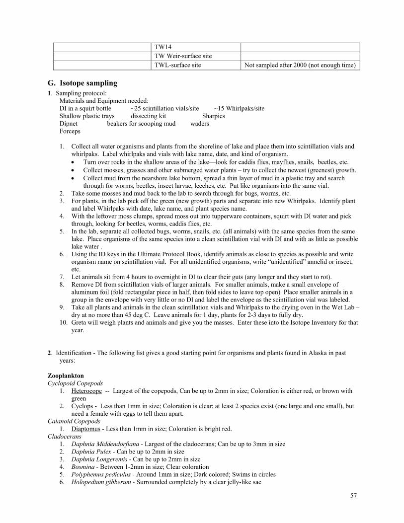
57

TW14 TW Weir-surface site TWL-surface site Not sampled after 2000 (not enough time)

G. Isotope sampling 1. Sampling protocol:

Materials and Equipment needed: DI in a squirt bottle ~25 scintillation vials/site ~15 Whirlpaks/site Shallow plastic trays dissecting kit Sharpies Dipnet beakers for scooping mud waders Forceps

1. Collect all water organisms and plants from the shoreline of lake and place them into scintillation vials and

whirlpaks. Label whirlpaks and vials with lake name, date, and kind of organism. Turn over rocks in the shallow areas of the lake—look for caddis flies, mayflies, snails, beetles, etc. Collect mosses, grasses and other submerged water plants – try to collect the newest (greenest) growth. Collect mud from the nearshore lake bottom, spread a thin layer of mud in a plastic tray and search

through for worms, beetles, insect larvae, leeches, etc. Put like organisms into the same vial. 2. Take some mosses and mud back to the lab to search through for bugs, worms, etc. 3. For plants, in the lab pick off the green (new growth) parts and separate into new Whirlpaks. Identify plant

and label Whirlpaks with date, lake name, and plant species name. 4. With the leftover moss clumps, spread moss out into tupperware containers, squirt with DI water and pick

through, looking for beetles, worms, caddis flies, etc. 5. In the lab, separate all collected bugs, worms, snails, etc. (all animals) with the same species from the same

lake. Place organisms of the same species into a clean scintillation vial with DI and with as little as possible lake water .

6. Using the ID keys in the Ultimate Protocol Book, identify animals as close to species as possible and write organism name on scintillation vial. For all unidentified organisms, write “unidentified” annelid or insect, etc.

7. Let animals sit from 4 hours to overnight in DI to clear their guts (any longer and they start to rot). 8. Remove DI from scintillation vials of larger animals. For smaller animals, make a small envelope of

aluminum foil (fold rectangular piece in half, then fold sides to leave top open) Place smaller animals in a group in the envelope with very little or no DI and label the envelope as the scintillation vial was labeled.

9. Take all plants and animals in the clean scintillation vials and Whirlpaks to the drying oven in the Wet Lab – dry at no more than 45 deg C. Leave animals for 1 day, plants for 2-3 days to fully dry.

10. Greta will weigh plants and animals and give you the masses. Enter these into the Isotope Inventory for that year.

2. Identification - The following list gives a good starting point for organisms and plants found in Alaska in past

years: Zooplankton Cyclopoid Copepods

1. Heterocope -- Largest of the copepods, Can be up to 2mm in size; Coloration is either red, or brown with green

2. Cyclops - Less than 1mm in size; Coloration is clear; at least 2 species exist (one large and one small), but need a female with eggs to tell them apart.

Calanoid Copepods 1. Diaptomus - Less than 1mm in size; Coloration is bright red.

Cladocerans 1. Daphnia Middendorfiana - Largest of the cladocerans; Can be up to 3mm in size 2. Daphnia Pulex - Can be up to 2mm in size 3. Daphnia Longeremis - Can be up to 2mm in size 4. Bosmina - Between 1-2mm in size; Clear coloration 5. Polyphemus pediculus - Around 1mm in size; Dark colored; Swims in circles 6. Holopedium gibberum - Surrounded completely by a clear jelly-like sac

58

Other Aquatic Fauna 1. Ostracods 2. Small clams – Sphaeridae (pill clams) 3. Snails - Sp. Lymnaea; Physa; Valvata (planorbid whorls) 4. Amphipods (Scuds)

Aquatic Insects 1. Trichoptera – Lymnophillidae, Grensia (sp) 2. Ephemeroptera 3. Hemiptera - Corixidae 4. Coleoptera - Gyrinidae 5. Diptera - Chironomidae (Chironomids)

Chironomini - Stictochironomus (g) Prodiamesinae - Monodiamesa (g) Chaoboridae – Chaoborus (g)

H. Field Laboratory Analysis Once back at the lab, unload all of the equipment and samples. Open up all of the kits and remove contents to dry. Be sure to put the pH probe into storage solution (KCl), and fix any malfunctioning equipment. When the equipment is dry, put it back into the tupperware boxes and leave the lids OPEN.

- Place all the samples on the counter and check to see that you have everything and that the dates are all correct.

- All samples need to have a sortchem #, site name, date, depth, analysis, filtered/acidified label (FU or FA), and volume filtered if applicable.

1. Acidify all samples that need to be preserved (DOC/TDN/TDP, Cats, and nutrients if they are being stored longer

than 1 day- nutrients are usually run the same day and do not require preservation). As of 9 July 1997, DOC/TDN/TDP and Cats are preserved using 100 L of 6N HCl TMG/60 mL of sample for surface water (previous ratio was 1L acid /mL sample, or about 60 uL per 60 mL sample – Phosphorus tends to stick less to the bottles at lower pH), and 50 L of 6N HCl TMG/60 mL of sample for soil water. The volumes are doubled for 125 mL sample bottles.

2. Store the remainder of the samples in the appropriate spot. Nitrate samples go in the freezer, filters should be placed in the drying oven for at least 24 hours, and the rest of the samples should be stored dark in the refrigerator (especially alkalinity). Nutrient samples are stored in the door/drawers in the refrigerator in Lab 4 until they have been run, double-checked for reruns, and can then be dumped, washed, and re-used.

3. Wet chemistry analyses (NH4, PO4) are run on MWF. Notify the nutrient chemist AT LEAST that day how many samples you will have by writing it on the sign-up sheet. NH4 samples need to be read on the fluorometer on TuThSa.

4. Run the gas samples (should be run within 24 hours, see GC method). 5. Enter data from field book into computer file (see below procedure).

J. Field Schedules, Data Entry, and samples from other groups 1. Field Schedule. The yearly schedule will be made up in advance and posted in Lab 4 and Dry Lab at Toolik.

Major changes to the schedule should be ok'd by George or LTER RAs. There can be absolutely no changes to the thaw depth survey dates for Tussock Watershed. We often accompany the Lakes group on lake sampling and take DIC and gas samples, as well as measure light profile data. If a lake is scheduled with the Lakes group, make sure that you verify with the Lakes RA what time they are leaving and that they know that you are going. a. Thaw Depth Survey

i. This survey must be performed on the same two days every year for Tussock Watershed: 2 July and 11 August. ii. Thaw depth is recorded for a specific transect. These transects are mapped out in the appropriate fieldbooks for Tussock Watershed and Imnavait. iii. Do the thaw survey with someone who has done it before to sample properly. iv. The Imnavait survey should be done on the same days as TW, or, very close to that time. If the 2 July or 11 Aug dates fall on a Sunday, ask for a volunteer and do the Imnavait on Saturday or Monday to reduce the time needed on Sunday.

b. I-series

59

LW samples the inlets and the outlets three times each summer. We do Chla for the inlets and outlets as well (so take the falcon tubes and extra filters – we used 47 mm GF/Cs until 2002, when we started using GF/Fs). Chla samples are stored in the -80°C freezer in Lab 1 until they can be analyzed.

c. Rain Events which cause significant increases in discharge should be sampled. If there is not an autosampler operating on TW Weir and Toolik Inlet try to sample as frequently as possible (of special interest is the rising leg of the discharge).

2. Data Entry. Open AKchemXXXX.xls. Every scheduled sampling already has sortchems assigned for all samples. After returning from the field, enter all data (time, temp, pH, cond, what analyses were collected, etc.) If you collected any unscheduled samples, you must assign sortchems to them and add them to AKchemXXX.xls. Every sample collected must have a sortchem!

3. Outside data. There are a few samples that you may receive to analyze which LW did not collect. At Toolik, we may run gas/DIC samples or Photochemistry samples we received from other groups. The Lakes group pre-assigns sortchems just like we do, so make sure to get sortchems from them, or any other group that gives you samples. Do not just assume they need to be given a sortchem.

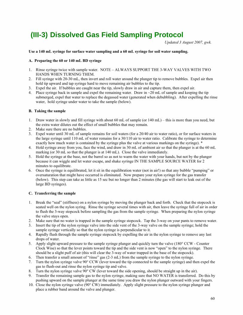
60

(III-3) Dissolved Gas Field Sampling Protocol Updated 3 August 2007, gwk.

Use a 140 mL syringe for surface water sampling and a 60 mL syringe for soil water sampling. A. Preparing the 60 or 140 mL BD syringe 1. Rinse syringe twice with sample water. NOTE – ALWAYS SUPPORT THE 3-WAY VALVES WITH TWO

HANDS WHEN TURNING THEM. 2. Fill syringe with 20-30 mL, then invert and roll water around the plunger tip to remove bubbles. Expel air then

hold tip upward and tap syringe hard to move remaining air bubbles to the tip. 3. Expel the air. If bubbles are caught near the tip, slowly draw in air and capture them, then expel air. 4. Place syringe back in sample and expel the remaining water. Draw in ~20 mL of sample and keeping the tip

submerged, expel that water to replace the degassed water (generated when debubbling). After expelling the rinse water, hold syringe under water to take the sample (below).

B. Taking the sample 1. Draw water in slowly and fill syringe with about 60 mL of sample (or 140 mL) – this is more than you need, but

the extra water dilutes out the effect of small bubbles that may remain. 2. Make sure there are no bubbles. 3. Expel water until 30 mL of sample remains for soil waters (for a 20/40 air to water ratio), or for surface waters in

the large syringe until 110 mL of water remains for a 30/110 air to water ratio. Calibrate the syringe to determine exactly how much water is contained by the syringe plus the valve at various markings on the syringe). *

4. Hold syringe away from you, face the wind, and draw in 30 mL of ambient air so that the plunger is at the 60 mL marking (or 30 mL so that the plunger is at 140 mL). Close the valve immediately.

5. Hold the syringe at the base, not the barrel so as not to warm the water with your hands, but not by the plunger because it can wiggle and let water escape, and shake syringe IN THE SAMPLE SOURCE WATER for 2 minutes to equilibrate.

6. Once the syringe is equilibrated, let it sit in the equilibration water (not in air!) so that any bubble “pumping” or oversaturation that might have occurred is eliminated. Now prepare your nylon syringe for the gas transfer (below). This step can take as little as 15 sec but no longer than 2 minutes (the gas will start to leak out of the large BD syringes).

C. Transferring the sample 1. Break the “seal” (stiffness) on a nylon syringe by moving the plunger back and forth. Check that the stopcock is

seated well on the nylon syring. Rinse the syringe several times with air, then leave the syringe full of air in order to flush the 3-way stopcock before sampling the gas from the sample syringe. When preparing the nylon syringe the valve stays open.

2. Make sure that no water is trapped in the sample syringe stopcock. Tap the 3-way on your pants to remove water. 3. Insert the tip of the nylon syringe valve into the side vent of the 3-way valve on the sample syringe; hold the

sample syringe vertically so that the nylon syringe is perpendicular to it. 4. Rapidly flush through the sample syringe stopcock by expelling the air in the nylon syringe to remove any last

drops of water. 5. Apply slight upward pressure to the sample syringe plunger and quickly turn the valve (180° CCW - Counter

Clock Wise) so that the lever points toward the tip and the side vent is now “open” to the nylon syringe. There should be a slight puff of air (this will clear the 3-way of water trapped in the base of the stopcock).

6. Then transfer a small amount of “rinse” gas (2-3 mL) from the sample syringe to the nylon syringe. 7. Turn the nylon syringe valve 90° CCW (lever toward the tip connected to the sample syringe) and then expel the

gas to flush-out and rinse the nylon syringe tip and valve. 8. Turn the nylon syringe valve 90° CW (lever toward the side opening, should be straight up in the air). 9. Transfer the remaining sample gas to the nylon syringe, making sure that NO WATER is transferred. Do this by

pushing upward on the sample plunger at the same time you draw the nylon plunger outward with your fingers. 10. Close the nylon syringe valve (90° CW) immediately. Apply slight pressure to the nylon syringe plunger and

place a rubber band around the valve and plunger.

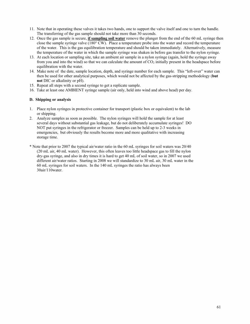
61

11. Note that in operating these valves it takes two hands, one to support the valve itself and one to turn the handle. The transferring of the gas sample should not take more than 30 seconds.

12. Once the gas sample is secure, if sampling soil water remove the plunger from the end of the 60 mL syringe then close the sample syringe valve (180° CW). Place a temperature probe into the water and record the temperature of the water. This is the gas equilibration temperature and should be taken immediately. Alternatively, measure the temperature of the water in which the sample syringe was shaken in before gas transfer to the nylon syringe.

13. At each location or sampling site, take an ambient air sample in a nylon syringe (again, hold the syringe away from you and into the wind) so that we can calculate the amount of CO2 initially present in the headspace before equilibration with the water.

14. Make note of the date, sample location, depth, and syringe number for each sample. This “left-over” water can then be used for other analytical purposes, which would not be affected by the gas-stripping methodology (but not DIC or alkalinity or pH).

15. Repeat all steps with a second syringe to get a replicate sample. 16. Take at least one AMBIENT syringe sample (air only, held into wind and above head) per day. D. Shipping or analysis 1. Place nylon syringes in protective container for transport (plastic box or equivalent) to the lab

or shipping. 2. Analyze samples as soon as possible. The nylon syringes will hold the sample for at least

several days without substantial gas leakage, but do not deliberately accumulate syringes! DO NOT put syringes in the refrigerator or freezer. Samples can be held up to 2-3 weeks in emergencies, but obviously the results become more and more qualitative with increasing storage time.

* Note that prior to 2007 the typical air/water ratio in the 60 mL syringes for soil waters was 20/40

(20 mL air, 40 mL water). However, this often leaves too little headspace gas to fill the nylon dry-gas syringe, and also in dry times it is hard to get 40 mL of soil water, so in 2007 we used different air/water ratios. Starting in 2008 we will standardize to 30 mL air, 30 mL water in the 60 mL syringes for soil waters. In the 140 mL syringes the ratio has always been 30air/110water.

62

(III-4) DIC Sampling Protocol – new method, 2006 - * This method was developed and tested in 2006 at Toolik, and has been used since 2006. The only exceptions are

when there is no GC available to run samples, and instead samples are prepared using the old protocol with serum vials that can be stored until a GC is up and running.

A. Preparation Pack the following items in your DIC kit: 1. A 1 mL plastic pipet (and one spare) put into a small whirl-pack bag (to keep acid contained) 2. Two 30 mL bottles of ~6N H2SO4 - one bottle is a spare, and should be put into a whirlpack with the extra 1 mL

syringe. 3. Two 60 mL DIC plastic syringes (labeled as “DIC”) with 3-way stopcocks 4. Sharpie and pencil, just in case

B. Sampling 1. Rinse the 60 mL H2O syringe three times with sample water. 2. Draw up ~ 60 mL of sample surface water into H2O syringe without bubbles (see gas sampling protocol

“preparing the 60 or 140 mL BD syringe”). If you are water limited, you must have exactly 20 mL water. 3. Fill the 1mL syringe with acid up to exactly one mL 4. Expel water from the 60 mL syringe through the side port (not the top) until you have exactly 20 mL remaining 5. Put tip of the 1mL acid syringe into the side port of the 3-way stopcock (the stopcock lever is toward the tip of the

stopcock) and inject all the acid into the 60 mL syringe. 6. With slight pressure pulling down on the 60 mL syringe plunger with one hand, remove the 1 mL syringe with the

other hand as you start to draw in ambient air through the side port. Note that using the side port means that all acid is drawn into the syringe (preserving the correct volume calculations).

7. As you are drawing in the air, move your finger so that it covers the tip of the stopcock. This is to prevent gas from escaping when you turn the stopcock from open to closed.

8. Draw in air until the plunger is at the 60 mL mark – you now have 39 mL air and 20 + 1 mL of water + acid. Close the stopcock while holding your finger over the tip.

7. Shake the sample for ~1-2 minutes in water of a known temperature (sample water if possible, the stream or lake).

8. Transfer the headspace gas to a dry-gas nylon syringe (see procedure detail in the gas sampling protocol). 9. Rinse the acid syringe 3x to remove excess acid in the stream or lake and place the acid syringe back into its

whirl-pack bag.

63

(III-5) OLD - DIC Sampling Protocol with serum vials This protocol was used until 2006 - now it is only used when no GC is available.

A. Preparation Pack the following items in your DIC kit: (NOTE – LEAVE ONE DIC KIT FOR THE OLD METHOD INTACT) 1. labeled 20 mL glass DIC bottles (more than the number of sites in case one breaks) 2. excess aluminum caps with Teflon septa 3. small (30 mL) plastic bottle with saturated HgCl2 (6g HgCl2 per 100mL) 4. two HgCl2 syringes (1 mL) with needles 5. two 60 mL H2O syringes with 3-way valves 6. crimper 7. permanent marker and extra labeling tape

B. Sampling 1. Fill the 1mL syringe with HgCl2 and expel bubbles. 2. Rinse the 60 or 140 mL H2O syringe three times with sample water. 3. Debubble the syringe (see Dissolved Gas Sampling protocol). 4. Draw up 140 mL (60 mL if sampling soil water) of sample surface water into H2O syringe without bubbles (see

gas sampling protocol “preparing the syringe”). Close the stopcock and leave syringe in sample water. 5. Seat the Teflon-lined cap on the sample bottle and place the cap top up on a flat working surface. Arrange the 1

mL syring and the crimper for easy access. 6. Put tip of stopcock of syringe into DIC bottle, tilt the bottle to avoid generating bubbles during filling, and flush

the bottle by letting the sample overflow the neck of the bottle. Flush at least 2 bottle volumes. 7. With 10 mL of water left in the syringe, slowly raise the syringe out of the neck of the bottle, continuing to

expel water. 6. As the last bit of water is expelled from the syringe, make sure the sample water has a positive meniscus above

the neck of the DIC bottle and the outer lip of the DIC bottle is wet. Save some water in the sampling syringe to “top-off” the meniscus if needed after adding the HgCl.

7. Insert the needle of the 1 mL syringe at least 1 inch into the sample water and add 0.2 mL of HgCl2. (0.1 mL per 10 mL sample)

8. Carefully place an aluminum cap with Teflon septa on the DIC bottle. 9. Holding the bottle in one hand (or setting the bottle on a stable surface if you must), take the crimper in the other

hand and quickly and firmly crimp down on the cap. 10. Check for bubbles, and redo if there are any air bubbles larger than 2-3mm in diameter.

C. Shipping and storage 1. The small glass DIC bottles are tough, but they will break. Line the shipping box with some soft material (paper

will do) and then pack the bottles tightly with no extra space in the box. 2. A box of DIC bottles is heavy. Only use very strong boxes, or double box the samples. 3. DIC samples should be stored dark, and cool if possible, although the Hg in the sample should be an effective

preservative. Samples will store for months without degrading. 4. There may be some bubbles that form in the bottles when they are shipped by air. If this occurs, use the sample

with the smallest bubbles for the “isotope” sample when possible.

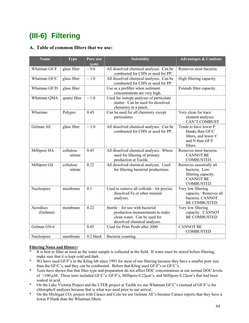
64

(III-6) Filtering

A. Table of common filters that we use:

Name Type Pore size (m)

Suitability Advantages & Cautions

Whatman GF/F glass fiber ~ 0.6 All dissolved chemical analyses. Can be combusted for CHN or used for PP.

Removes most bacteria.

Whatman GF/C glass fiber ~ 1.0 All dissolved chemical analyses. Can be combusted for CHN or used for PP.

High filtering capacity.

Whatman GF/D glass fiber Use as a prefilter when sediment concentrations are very high.

Extends filter capacity.

Whatman QMA quartz fiber ~ 1.0 Used for isotope analyses of particulate matter. Can be used for dissolved chemistry in a pinch.

Whatman Polypro 0.45 Can be used for all chemistry except particulates

Very clean for trace element analyses. CAN’T COMBUST

Gelman AE glass fiber ~ 1.0 All dissolved chemical analyses. Can be combusted for CHN or used for PP.

Tends to have lower P blanks than GF/C filters, and lower C and N than GF/F filters.

Millipore HA cellulose nitrate

0.45 All dissolved chemical analyses. Where used for filtering of primary production at Toolik.

Removes most bacteria. CANNOT BE COMBUSTED.

Millipore GS cellulose nitrate

0.22 All dissolved chemical analyses. Used for filtering bacterial productions.

Removes essentially all bacteria. Low filtering capacity. CANNOT BE COMBUSTED.

Nucleopore membrane 0.1 Used to remove all colloids - for precise dissolved Fe or other mineral analyses.

Very low filtering capacity. Removes all bacteria. CANNOT BE COMBUSTED.

Acrodiscs (Gelman)

membrane 0.22 Sterile – for use with bacterial production measurements to make clean water. Can be used for dissolved chemical analyses.

Very low filtering capacity. CANNOT BE COMBUSTED.

Gelman GN-6 0.45 Used for Prim Prods after 2000 CANNOT BE COMBUSTED

Nucleopore membrane 0.2 black Bacteria counting.

Filtering Notes and History: * It is best to filter as soon as the water sample is collected in the field. If water must be stored before filtering,

make sure that it is kept cold and dark. * We have used GF/F’s in the Kling lab since 1991 for most of our filtering because they have a smaller pore size

than the GF/C’s, and they can be combusted. Before that Kling used GF/F’s or GF/C’s. * Tests have shown that that filter type and preparation do not affect DOC concentrations at our normal DOC levels

of >100 M. These tests included GF/C’s, GF/F’s, Millipore 0.22m’s, and Millipore 0.22m’s that had been soaked in acid.

* On the Lake Victoria Project and the LTER project at Toolik we use Whatman GF/C’s (instead of GF/F’s) for chlorophyll analyses because that is what was used prior to our arrival.

* On the Michigan CO2 project with Caraco and Cole we use Gelman AE’s because Caraco reports that they have a lower P blank than the Whatman filters.

65

* Starting in 2002 we used Whatman polypro filters in Alaska for cation samples.

B. Filter Preparation 1. All glass fiber and quartz fiber filters should be combusted at 450 C for 4 hours before use (hotter and they tend

to break apart). Place filters in clean glass beakers or in clean aluminum foil and cover them with foil before placing in the muffle furnace.

2. All filters (except for bacterial counting) should be rinsed with sample water before use. A minimum of 10 mL should be used. If water is plentiful then 50 mL should be used.

C. Filtering using Millipore Swinnex (small or large) Filter Holders 1. These holders can be preloaded with filters not more than 2-3 hours prior to filtering. Using clean forceps place

the filter with the shiny side up (grid side down) on the holder. Carefully screw on the top of the filter holder finger tight. Using the 60 mL BD syringe withdraw 60 mL of water from the sample or bottle containing the unfiltered water.

2. Attach the filter holder to the syringe so that the label that says “Millipore Swinnex” is next to the syringe. 3. Push the water through the filter into one of the sample bottles. Remove the filter holder and refill the 60 mL

syringe, being careful not to touch the outflow nozzle of the filter holder. Continue and repeat until all bottles needed are filled. * Note that when the filter begins to clog do not apply too much pressure because (1) the filter may break, and

(2) the cells of phytoplankton will rupture and their contents (nutrients) will be added to the sample water that is being collected.

4. After the sample bottles are filled and the proper amount of water is passed through the filter for particulate analyses, uncouple the syringe from the holder, draw in about 10 mL of air into the syringe, attach the syringe to the holder again and blow a little air through the filter to remove excess water (this must be done gently, otherwise you may tear the filter).

5. If you are saving the filter, unscrew the filter holder and using forceps either (1) place the filter face up in a petri dish, (2) place the filter face up in a petri dish containing silica gel (if the filter cannot be dried within 3-6 hours), or (3) fold the filter in half onto itself and place the filter in an aluminum foil packet. Cover or wrap with foil the filters in the petri dishes so that they are not exposed to the light.

6. Label the petri dish or foil packet with a Sharpie and indicate Sample ID, Date, Depth, and mL filtered. 7. Rinse the filter holders with DI immediately. Holders should be acid washed every 3-5 uses (for nutrients it is

preferable to acid wash after each use if possible).

D. Filtering using a Filter Tower Using a sidearm flask, filter base, and filter tower is similar to use of the filter holders, and the same precautions apply. The connections to the vacuum pump will be self-evident (or ask someone). DO NOT suck water into the pump – make sure that the sidearm flask can hold all of the water that you put into the filter tower. In addition, water can be aspirated into the pump if the vacuum is not disconnected when pouring water out of the side-arm flask. Sometimes it helps to remove the vacuum before removing the filter from the filter base.

E. Filter Treatment and Storage Light, Heat, and Moisture are the enemies of filters. Filters for particulate or isotope analyses may be frozen. If they are not frozen then the filters must be dried in an oven or in a vacuum desiccator for a minimum of 24 hours. Drying should be at temperatures between 30-40C, and never more than 60C. Some volatile carbon compounds will start to be lost above 40C, and bulk lipid will be volatilized above 60C. Filters should be stored in the dark, and either frozen or in a drying oven or desiccator.

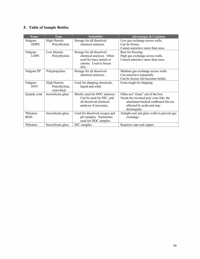
66

F. Table of Sample Bottles

Name Type Suitability Advantages & Cautions Nalgene

HDPE High Density

Polyethylene Storage for all dissolved

chemical analyses. Low gas exchange across walls. Can be frozen. Cannot autoclave more than once.

Nalgene LDPE

Low Density Polyethylene

Storage for all dissolved chemical analyses. Often used for trace metals or cations. Used to freeze NO3

-

Best for freezing. High gas exchange across walls. Cannot autoclave more than once.

Nalgene PP Polypropylene Storage for all dissolved chemical analyses.

Medium gas exchange across walls. Can autoclave repeatedly. Can be frozen, but becomes brittle.

Nalgene DOT

High Density Polyethylene, extra thick

Used for shipping chemicals, liquid and solid.

Extra tough for shipping.

Qorpak scint borosilicate glass Mostly used for DOC analyses. Can be used for DIC, and all dissolved chemical analyses if necessary.

Often not “clean” out of the box. Needs the inverted poly cone lids; the

aluminum-backed cardboard lids are affected by acids and may disintegrate.

Wheaton BOD

borosilicate glass Used for dissolved oxygen and pH samples. Sometimes used for DOC samples.

Airtight seal and glass walls to prevent gas exchange.

Wheaton borosilicate glass DIC samples. Requires caps and capper.

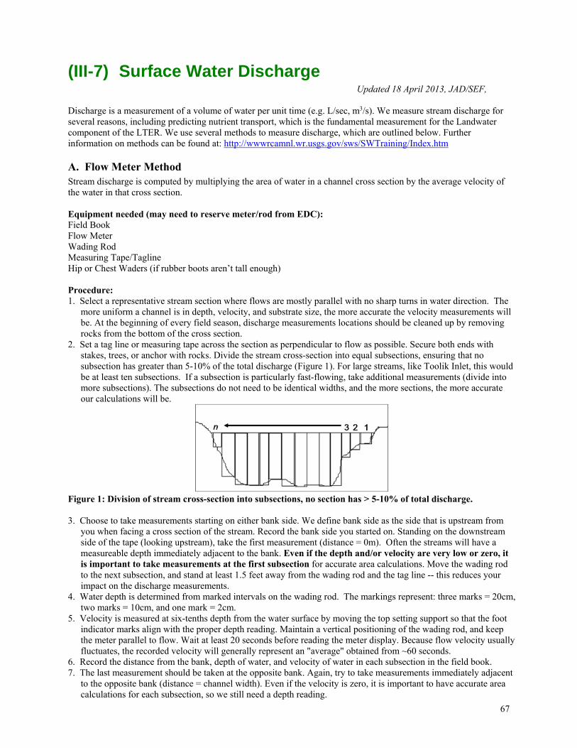
67

(III-7) Surface Water Discharge Updated 18 April 2013, JAD/SEF,

Discharge is a measurement of a volume of water per unit time (e.g. L/sec, m3/s). We measure stream discharge for several reasons, including predicting nutrient transport, which is the fundamental measurement for the Landwater component of the LTER. We use several methods to measure discharge, which are outlined below. Further information on methods can be found at: http://wwwrcamnl.wr.usgs.gov/sws/SWTraining/Index.htm

A. Flow Meter Method Stream discharge is computed by multiplying the area of water in a channel cross section by the average velocity of the water in that cross section. Equipment needed (may need to reserve meter/rod from EDC): Field Book Flow Meter Wading Rod Measuring Tape/Tagline Hip or Chest Waders (if rubber boots aren’t tall enough) Procedure: 1. Select a representative stream section where flows are mostly parallel with no sharp turns in water direction. The

more uniform a channel is in depth, velocity, and substrate size, the more accurate the velocity measurements will be. At the beginning of every field season, discharge measurements locations should be cleaned up by removing rocks from the bottom of the cross section.

2. Set a tag line or measuring tape across the section as perpendicular to flow as possible. Secure both ends with stakes, trees, or anchor with rocks. Divide the stream cross-section into equal subsections, ensuring that no subsection has greater than 5-10% of the total discharge (Figure 1). For large streams, like Toolik Inlet, this would be at least ten subsections. If a subsection is particularly fast-flowing, take additional measurements (divide into more subsections). The subsections do not need to be identical widths, and the more sections, the more accurate our calculations will be.

Figure 1: Division of stream cross-section into subsections, no section has > 5-10% of total discharge.

3. Choose to take measurements starting on either bank side. We define bank side as the side that is upstream from

you when facing a cross section of the stream. Record the bank side you started on. Standing on the downstream side of the tape (looking upstream), take the first measurement (distance = 0m). Often the streams will have a measureable depth immediately adjacent to the bank. Even if the depth and/or velocity are very low or zero, it is important to take measurements at the first subsection for accurate area calculations. Move the wading rod to the next subsection, and stand at least 1.5 feet away from the wading rod and the tag line -- this reduces your impact on the discharge measurements.

4. Water depth is determined from marked intervals on the wading rod. The markings represent: three marks = 20cm, two marks = 10cm, and one mark = 2cm.

5. Velocity is measured at six-tenths depth from the water surface by moving the top setting support so that the foot indicator marks align with the proper depth reading. Maintain a vertical positioning of the wading rod, and keep the meter parallel to flow. Wait at least 20 seconds before reading the meter display. Because flow velocity usually fluctuates, the recorded velocity will generally represent an "average" obtained from ~60 seconds.

6. Record the distance from the bank, depth of water, and velocity of water in each subsection in the field book. 7. The last measurement should be taken at the opposite bank. Again, try to take measurements immediately adjacent

to the opposite bank (distance = channel width). Even if the velocity is zero, it is important to have accurate area calculations for each subsection, so we still need a depth reading.

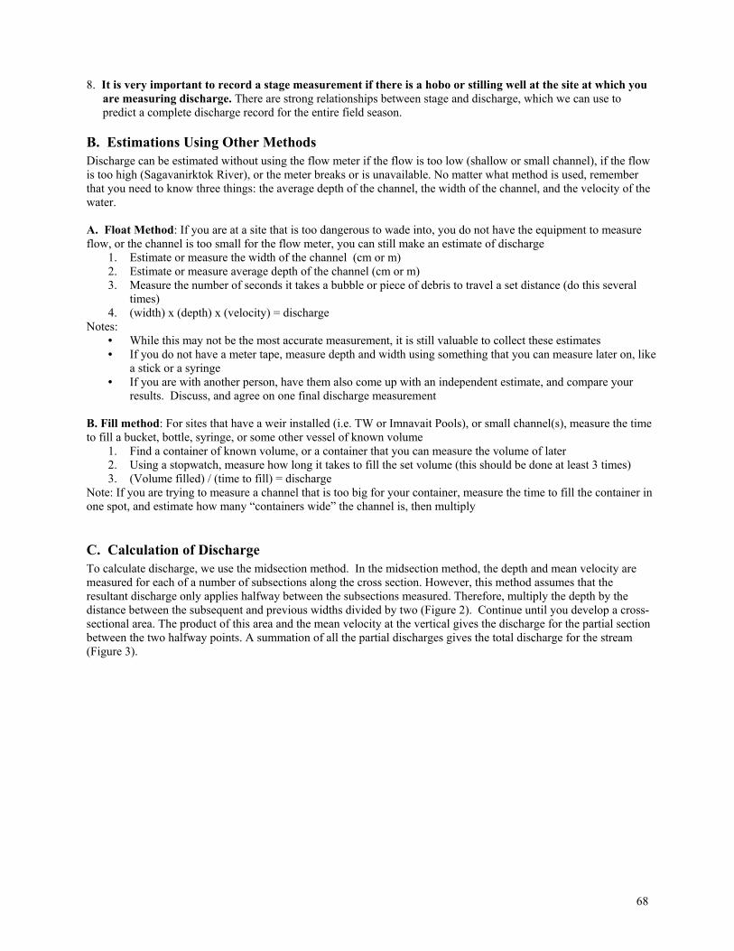
68

8. It is very important to record a stage measurement if there is a hobo or stilling well at the site at which you are measuring discharge. There are strong relationships between stage and discharge, which we can use to predict a complete discharge record for the entire field season.

B. Estimations Using Other Methods Discharge can be estimated without using the flow meter if the flow is too low (shallow or small channel), if the flow is too high (Sagavanirktok River), or the meter breaks or is unavailable. No matter what method is used, remember that you need to know three things: the average depth of the channel, the width of the channel, and the velocity of the water. A. Float Method: If you are at a site that is too dangerous to wade into, you do not have the equipment to measure flow, or the channel is too small for the flow meter, you can still make an estimate of discharge

1. Estimate or measure the width of the channel (cm or m) 2. Estimate or measure average depth of the channel (cm or m) 3. Measure the number of seconds it takes a bubble or piece of debris to travel a set distance (do this several

times) 4. (width) x (depth) x (velocity) = discharge

Notes: • While this may not be the most accurate measurement, it is still valuable to collect these estimates • If you do not have a meter tape, measure depth and width using something that you can measure later on, like

a stick or a syringe • If you are with another person, have them also come up with an independent estimate, and compare your

results. Discuss, and agree on one final discharge measurement B. Fill method: For sites that have a weir installed (i.e. TW or Imnavait Pools), or small channel(s), measure the time to fill a bucket, bottle, syringe, or some other vessel of known volume

1. Find a container of known volume, or a container that you can measure the volume of later 2. Using a stopwatch, measure how long it takes to fill the set volume (this should be done at least 3 times) 3. (Volume filled) / (time to fill) = discharge

Note: If you are trying to measure a channel that is too big for your container, measure the time to fill the container in one spot, and estimate how many “containers wide” the channel is, then multiply

C. Calculation of Discharge To calculate discharge, we use the midsection method. In the midsection method, the depth and mean velocity are measured for each of a number of subsections along the cross section. However, this method assumes that the resultant discharge only applies halfway between the subsections measured. Therefore, multiply the depth by the distance between the subsequent and previous widths divided by two (Figure 2). Continue until you develop a cross-sectional area. The product of this area and the mean velocity at the vertical gives the discharge for the partial section between the two halfway points. A summation of all the partial discharges gives the total discharge for the stream (Figure 3).

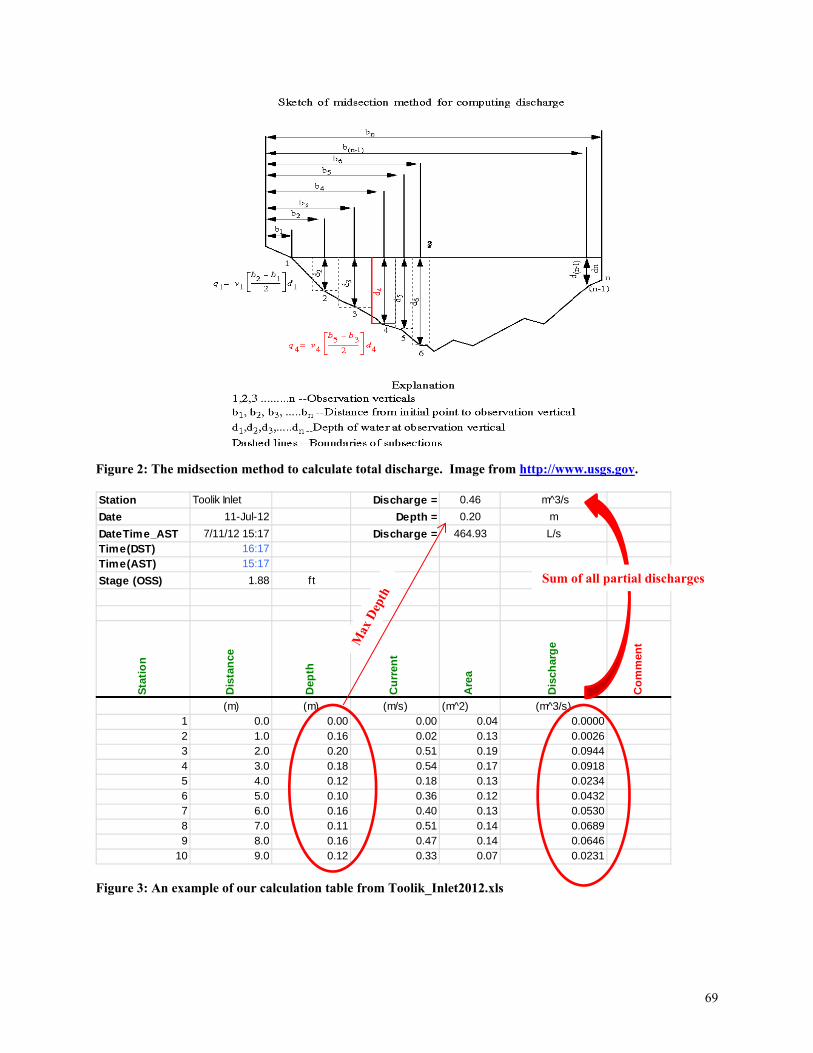
69

Figure 2: The midsection method to calculate total discharge. Image from http://www.usgs.gov.

Figure 3: An example of our calculation table from Toolik_Inlet2012.xls

Station Toolik Inlet Discharge = 0.46 m^3/s

Date 11-Jul-12 Depth = 0.20 m

DateTime_AST 7/11/12 15:17 Discharge = 464.93 L/sTime(DST) 16:17

Time(AST) 15:17

Stage (OSS) 1.88 ft

Sta

tio

n

Dis

tan

ce

Dep

th

Cu

rren

t

Are

a

Dis

char

ge

Co

mm

ent

(m) (m) (m/s) (m^2) (m^3/s)1 0.0 0.00 0.00 0.04 0.00002 1.0 0.16 0.02 0.13 0.00263 2.0 0.20 0.51 0.19 0.09444 3.0 0.18 0.54 0.17 0.09185 4.0 0.12 0.18 0.13 0.02346 5.0 0.10 0.36 0.12 0.04327 6.0 0.16 0.40 0.13 0.05308 7.0 0.11 0.51 0.14 0.06899 8.0 0.16 0.47 0.14 0.0646

10 9.0 0.12 0.33 0.07 0.0231

Sum of all partial discharges

70

(III-8) Magnetic Declination and Compasses Updated 7 August 2001, kjr

Search and Rescue Society of British Columbia From: http://www.sarbc.org/compass.html

Compasses are marked in several very different ways: The Quadrant Compass is marked 0° - 90° four times. The Military Compass is marked 0 - 6400. The Azimuth Compass is marked in 0° - 360°.

The Quadrant compasses have a scale divided into four segments of 90° each and are used primarily by surveyors for establishing base lines and datum lines. The Military compass reads in mil's. They wanted to be able to shoot a small target. The Azimuth compass measures an angle clockwise from the north. Thus, the dial on an azimuth compass is marked in degrees proceeding clockwise from the north. True North is 0° or 360°, east is 90°, south is 180° and west is 270°.

The compass does not point to True North, it points to Magnetic North. The angle that is formed by the difference between Magnetic North and True North has several names. The names tend to relate to the magnetic distractions near the compass and to the speed at which the angle changes in relation to your motion. On foot this angle is called declination, because there are usually few magnetic distractions and the distance that can be covered on foot in one or two days won't be enough for the angle to change a noticeable amount. At sea this angle is called deviation because the boat itself is a magnetic distraction and you can travel far enough in one day to put your compass out a considerable amount. In the air it is called variation because the air gap between the plane and the earth, the plane itself, temperature, and air pressure will influence a magnetic compass minute by minute enough to get you lost.

Declination is the difference in degrees between Magnetic North and True North. In North America, the line of 0° declination runs from Hudson Bay, across Lake Michigan, and down to Georgia. Along this line True North and Magnetic North are in the same direction. From any point west of this zero line, the magnetic needle points east of True North. This is easterly declination. From any point east of this line, the compass points west of True North. This is westerly declination. The coast of B.C. has a declination of about 22° east. Newfoundland has a declination of about 22° west. Earlier we were told that east is 90° from north. Vancouver and Thunder Bay are very close to the same latitude, so Thunder Bay is due east of Vancouver. However, if you were standing in Vancouver, and you could see all the way over to Thunder Bay, your compass would give you a bearing of only 68° which is north of east. But, if you were standing in Thunder Bay, taking a bearing of Vancouver, you would get a bearing of due west or 270°. How come? Vancouver and Thunder Bay are about the same latitude, but Thunder Bay is on or near the line of 0° declination while Vancouver is about 22° west of north or 22° easterly declination. National Geophysical Data Center http://www.ngdc.noaa.gov/seg/potfld/defs/dec.html

Magnetic declination is sometimes referred to as the magnetic variation or the magnetic compass correction. It is the angle formed between true north and the projection of the magnetic field vector on the horizontal plane.

For surveying practices, magnetic declination is the angle through which a magnetic compass bearing must be rotated in order to point to the true bearing as opposed to the magnetic bearing. Here the true bearing is taken as the angle measured from true North.

If west declinations are assumed to be negative while east declination are considered positive then True bearing = Magnetic bearing + Magnetic declination An example: The magnetic bearing of a property line has an azimuth of 72 degrees East. What is the true bearing of the property line if the magnetic declination at the place in question is 12 degrees West?

A magnetic declination of 12 degrees West means that magnetic North lies 12 degrees West of true North. True bearing = 72 degrees + ( -12 degrees declination ) = 72 degrees - 12 degrees declination = 60 degrees East

It should be noted that the magnetic declination becomes undefined at the North and South magnetic poles. These poles are by definition the two places where the magnetic field is vertical. Magnetic compasses become quite unreliable when the magnetic field vector becomes steeply inclined. D is defined as D = arc tangent( Y / X ). Also See Campbell Met-One Manual pages A-1 through A-3 Toolik Declination 29E

71

(III-9) Protocols for Operation of the NEON Eddy Flux Tower on Toolik Lake

Updated 9 July 2012, G. Kling, D. Carroll

A. Eddy Platform

In July 2009 we installed a platform on Toolik Lake that measures the eddy flux of CO2 and CH4 in the air and includes basic climate and light sensors, a thermistor chain for water temperatures, dissolved oxygen and conductivity sensors at two depths, and a gas equilibrator to measure dissolved CO2 and CH4 continuously. The Eddy platform on Toolik Lake will be mainly operated by the Kling lab and Dr. Werner Eugster (ETH, Switzerland). Contacts are [email protected] ; [email protected] ; [email protected] ; [email protected] ; [email protected] . The set-up and shutdown of the Eddy platform is similar to the set-up of the Toolik Lake climate station which is also on a floating raft anchored in the lake during the summer.

A. SET UP OF PLATFORM AFTER ICE OUT 1. Location of equipment. First locate all of the equipment. It was all taken from the platform and put back

into boxes in the Dry lab, but from there the warm storage gear would be put in the Winter lab. In May when the Winter lab starts to be used, the warm storage gear is redistributed to either the Dry Lab or the Wet Lab (those are the labs that are heated in May). WHEN YOU UNPACK EQUIPMENT, first take a photo of the box and how everything was assembled so that you can put it together again at the end of summer.

2. Location of programs, data, and wiring diagrams. These are found on the Dry lab main computer (LTREB computer) or on the Kling Lab server under \DATA\Arctic\Projects\Eddy_lake\year , and there should be a backup on the Kling “Download” computer in Lab #4, SW office room.

3. Preparation. You need to take the tool box and tool bag that should be stored in Dry lab under the counter in the NE corner of the main lab. This should contain a small wiring screwdriver, a large flathead screwdriver, lots of fasteners (cable ties, electrical tape), allen wrench set, wrenches for cross-arms and other bolts, putty, desiccant packs, multimeter, instruction manuals for the Eddy platform, wiring diagrams, and programs. Note that you will first be working with the platform on land, then there is some final installation (e.g., Kipp and Zonen and thermistor chain) out on the lake.

4. Attaching sensors. Attach all sensors except the Kipp and Zonen and the CSAT sonic anemometer when the raft is on land. The Temp/Humidity sensor should have overwintered on the raft.

a. Install the wind sensor, without the vane initially. Connect the sensor to the proper ports inside the datalogger box, then install the vane. Be sure to tighten the allen key on the vane tightly.

b. Install the thermistor chain and the dissolved oxygen (DO) and conductivity sensors. The cables for all three “chains” (1 thermistor chain, 2 cables for shallow and deep conductivity and 2 cables for shallow and deep oxygen sensors) need to be fastened together starting at 3 m down on the thermistor chain (after the slack to accommodate the surface float and surface thermistors, 0-2 m depth). Use electrical tape then cable ties over the tape. Make sure that the entire set of cables can be easily lowered into the water once you are out on the lake (separate the top part of the t-chain with the bottom part from 3 m down). Consult the wiring diagrams for the DO, conductivity, and t-chains.

c. Once all the sensors are attached fill the datalogger box hole with putty. Fasten all the loose wires to the tripod using ample tie-downs to keep them from flapping in the wind – either black cable ties or black electrical tape can be used. Attach the storage module or radio if one is used. Remove the big thumb screws at the top of the power supply box and turn the on/off switch to “on” – a small red light should now be visible.

** Always attach the Kipp and Zonen radiation sensor and the Sonic 3-D anemometer AFTER the platform is installed on the lake.

72

5. Programming and checking the datalogger. Check that all of the sensors you have just attached are working properly – connect to the datalogger itself and upload its program (if it has been lost in memory), and initially sync the time stamp of the datalogger to that of your computer (yes, you must first sync your computer to Greenwich Mean Time). We run the eddy flux platform on Daylight Savings Time in the summer (the same time as your watch). Note that some dataloggers like the land Met Station use Alaska Standard Time, which is one hour behind the DST in the summer. Next check that all of the sensors are providing believable numbers. If so, you can close up the datalogger box and you should not need to open it again unless you lose signals from the sensors. Once back in the lab log on to the server and check that the radio installation and transmission is working. If other people are installing instruments on the Eddy platform, have them do as much work as possible while the platform is on land.

6. Lake Installation. Note that you can’t install the platform until the ice is nearly gone and you have brought the underwater cable to the surface and put it on the larger “surfer” Styrofoam float that is stored under the W end of Lab 4. The rock anchors and ropes are stored on or near the raft on land, and the Danforth anchors should be stored under the Lab 4 building. These anchors need to be placed in the lake when the platform is towed out to its GPS location - the GPS location for the Toolik Lake platform is Northing 2080239.143, Easting 180605.975. The location should be in at minimum ~10 m of water, and 12 m of water depth is better – this will depend in part on the lake level.

(A) Finding and Installing the cable. The first thing is to locate the rope on shore to the north of the sauna which connects to the underwater cable. It is found about 50-100 feet away from the Sauna (north) and the rope is coiled along the shore and attached to a piece of rebar in the ground. Take the big surfer Styrofoam float and a red buoy with you as well as the toolkit with cable ties, and bring a boat around to the rope, make sure the rope is tight to the rebar, and then pull yourself along the line as you pull up the rope from the bottom and pull yourself out to where the cable end is located. When the rope becomes vertical you start to pull it up (it is heavy, use gloves). You will retrieve the power cable itself and the big rock anchor will stay on the bottom – DO NOT PULL UP THE ANCHOR. Once you have the cable end in the boat you can attach it to the surfer platform. The wrap a line around the float and through the hole in the float and secure that line. Now tie the cable grippers on the cable to the line on the float. Tie a second line that is attached to the red buoy through the hole in the float, so that if the cable tries to sink the float it cannot because it would also have to sink the buoy. Now coil the remaining cable and the cable end on top of the float and tie it so that it is stable and will not fall off the float. You can now leave the cable and float and go back and get the raft ready for towing.

(A) Putting the platform in the water. In order to move the platform from land and tow it out onto the lake, you need a calm lake (mornings are best, but sometimes after dinner works fine as well), about 1-1.5 hr of time for two people, and the following: (i) ~ 4-5 people with rubber boots to move the eddy platform along the ramp and into the water. This takes about 10

minutes once people are assembled. Once one end of the platform is in the lake, drag the float over to the boat dock, gather the anchors and ropes and place them on the raft, but not all in one corner – distribute the weight on the raft, and don’t tangle the anchor lines. The anchor lines should each have a small weight with them to keep the line below the water and out of the boat propellers (these weights are cable-tied on to the rope once the anchors are in place and tightened).

(ii) one of the small motor boats and a rope for towing the platform. DO NOT use a large boat because it is too difficult to maneuver around the raft when you are installing the Kipp and Zonen and Sonic sensors, which stick out over the water, and you can’t ‘fend-off’ all parts of such a big boat against bumping the sensors. We have already cracked the K&Z sensor dome once because someone didn’t believe me on this…

(iii) three people who can go out in the boat to install the platform (two stay on the boat, one on the platform). (iiii) the eddy toolbag and toolbox, the Kipp and Zonen and CSAT sensors in their boxes, a compass, a broomstick or

paddle, and a field book. (B) Towing the platform. In order to move the platform from land and tow it out onto the lake, you need a calm lake (mornings are best, but sometimes after dinner works fine as well), about 1-1.5 hr of time for two people. (i) If weather conditions are good and the lake is glassy (with light or no wind) you can tow the eddy float alongside the boat. Tie a tight line from the eddy platform to the side of the boat, and have one person hold the eddy float alongside the side of the boat. Drive the boat on the slowest speed setting and take your time. DO NOT RUSH THIS.

73

(ii) If conditions are windy, you must use 2 tow ropes to drag the float out on the lake. Do the following:

Attach one end of one tow rope to the handle on the back of the boat, run it through the metal ring, and attach the other end to the other handle.

Attach one end of the second tow rope to a cleat on the short side of the platform, pass the rope through the metal ring, and attach the other end to the opposite cleat on the short side of the platform.

You now have two “V” shaped ropes that are attached at the narrow point by the metal ring, and you can start towing the platform. The ropes should adjust their tension by sliding through the ring so that the raft tows straight. Don’t go too fast, it’s not a race to shore.

(B) Securing the anchors. (i) Slowly tow the Eddy platform out toward the site marked with the surfer float and red buoy. Once the boat is over

the power cable site and next to the surfer float, check the depth with a “dive buddy” (small yellow sonar instrument) to be sure that it is 10-12 m. If needed, you can CAREFULLY drag the power cable out to a slightly deeper depth. Remove the coiled power cable from the top of the surfer float (with two people holding it) and bring it over to the eddy platform. Attach the power cable anchor line to the eddy float, and then attach the power cable grippers to this line. You can now take the waterproof connector apart (with a large pipe wrench) and plug the power cable in the transformer box.

(ii) Take the “southeast” anchor and line in the boat and motor toward the south east until the rope is stretched fully. If you go too far you will simply pull the platform off the power cable spot (but, you can move it back). Drop the anchor, then motor back to the raft and take the northwest anchor and rope into the boat and motor to the northwest. Pull the anchor line taut (you are now pulling against the southeast anchor that you just installed). Drop the northwest anchor when the line is taut, and motor back to the raft to pick up the third anchor. It should be taken in the boat toward the southwest. Pull the line taut and drop the anchor. The final and fourth anchor is the Danforth anchor with chain on it, and it is the shortest length of rope of all the anchors – this is because we rarely get a strong wind out of the northeast, which is the direction you will motor to stretch out this anchor line. The line should be roughly equidistant from the other two anchor lines, and when the line is taut and the raft is positioned, drop the anchor.

(iii) Once all four anchors are dropped return to the platform and take up the slack on the northeast anchor line first. This will pull all of the other anchor lines taut (if the platform is far from the initial point, and no longer in 10m+ water, you can adjust the raft position by taking up some slack on any of the anchors.

(C) Installing the Kipp and Zonen. When the platform is fixed then you can install the Kipp and Zonen - keep the

instrument in its box all the way out to the raft. You will need a flathead screw driver to loosen the hose clamps that attach the sensor mounting kit to the boom. Once the sensor is installed, “level” the sensor and then fully tighten the hose clamps and set screws on the mounting kit. The bottom sensor domes should be about ~50 cm off the lake surface, and should stick out past the end of the raft at least one meter. Use the large diameter plastic PVC tube (that is attached the eddy platform ) under the boom to level the sensor. Now get on the raft and pass the KZ wires into the datalogger through the bottom hole, re-putty the hole, and hook up the sensor according the your wiring diagram.

7. Wind Sensor Corrections. Once the Eddy platform is in place and the KZ is installed, the wind sensor must

be calibrated for direction. Standing on the raft, point the wind vane directly down along the mast crossarm (toward the north) and hold it there (with a broomstick or paddle or equivalent). Check the direction readout from the datalogger, and record this direction in your field notebook. Finally, sight along the crossarm and record its deviation and direction away from magnetic north, to be used for later corrections. Be careful reading the compass with the metal platform and metal boats all around. Depending on the compass, you can stand on the south side of the raft and use the mirror to line up the crossarm, then you can read the main dial of the compass to get the direction. Note that the compass will point to magnetic north, and the declination at Toolik is 29 deg to the east. You need to record what “magnetic direction” the crossarm is pointing. Then in the data file a correction is made to relate the crossarm (mast) direction back to Degrees Magnetic North (DMN), and then from the DMN back to true north.

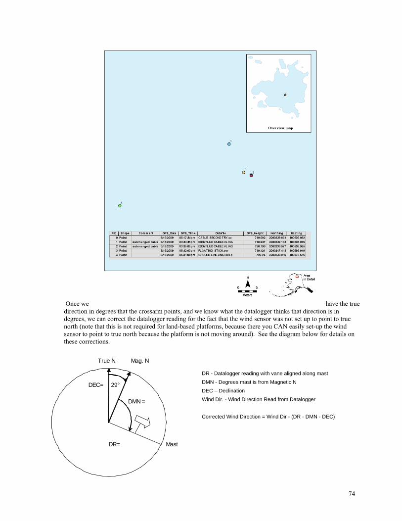
74

Once we have the true direction in degrees that the crossarm points, and we know what the datalogger thinks that direction is in degrees, we can correct the datalogger reading for the fact that the wind sensor was not set up to point to true north (note that this is not required for land-based platforms, because there you CAN easily set-up the wind sensor to point to true north because the platform is not moving around). See the diagram below for details on these corrections.



DEC – Declination



True N Mag. N

29°

Mast

DMN =

DR=

DEC=

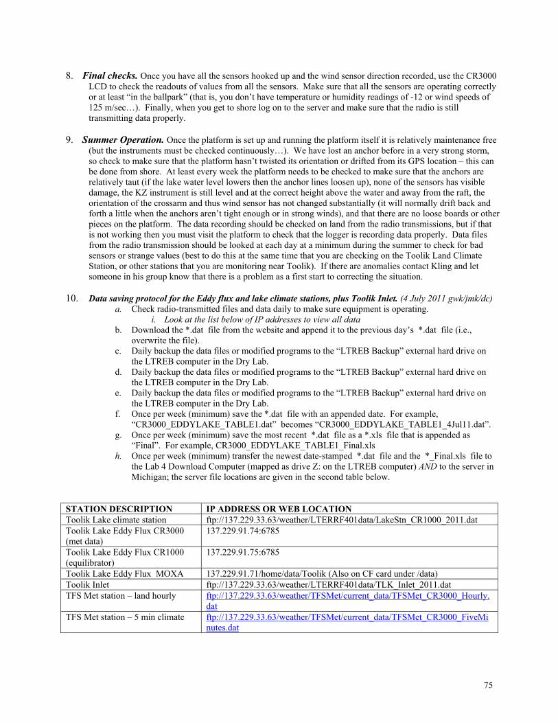
75

8. Final checks. Once you have all the sensors hooked up and the wind sensor direction recorded, use the CR3000

LCD to check the readouts of values from all the sensors. Make sure that all the sensors are operating correctly or at least “in the ballpark” (that is, you don’t have temperature or humidity readings of -12 or wind speeds of 125 m/sec…). Finally, when you get to shore log on to the server and make sure that the radio is still transmitting data properly.

9. Summer Operation. Once the platform is set up and running the platform itself it is relatively maintenance free

(but the instruments must be checked continuously…). We have lost an anchor before in a very strong storm, so check to make sure that the platform hasn’t twisted its orientation or drifted from its GPS location – this can be done from shore. At least every week the platform needs to be checked to make sure that the anchors are relatively taut (if the lake water level lowers then the anchor lines loosen up), none of the sensors has visible damage, the KZ instrument is still level and at the correct height above the water and away from the raft, the orientation of the crossarm and thus wind sensor has not changed substantially (it will normally drift back and forth a little when the anchors aren’t tight enough or in strong winds), and that there are no loose boards or other pieces on the platform. The data recording should be checked on land from the radio transmissions, but if that is not working then you must visit the platform to check that the logger is recording data properly. Data files from the radio transmission should be looked at each day at a minimum during the summer to check for bad sensors or strange values (best to do this at the same time that you are checking on the Toolik Land Climate Station, or other stations that you are monitoring near Toolik). If there are anomalies contact Kling and let someone in his group know that there is a problem as a first start to correcting the situation.

10. Data saving protocol for the Eddy flux and lake climate stations, plus Toolik Inlet. (4 July 2011 gwk/jmk/dc) a. Check radio-transmitted files and data daily to make sure equipment is operating.

i. Look at the list below of IP addresses to view all data b. Download the *.dat file from the website and append it to the previous day’s *.dat file (i.e.,

overwrite the file). c. Daily backup the data files or modified programs to the “LTREB Backup” external hard drive on

the LTREB computer in the Dry Lab. d. Daily backup the data files or modified programs to the “LTREB Backup” external hard drive on

the LTREB computer in the Dry Lab. e. Daily backup the data files or modified programs to the “LTREB Backup” external hard drive on

the LTREB computer in the Dry Lab. f. Once per week (minimum) save the *.dat file with an appended date. For example,

“CR3000_EDDYLAKE_TABLE1.dat” becomes “CR3000_EDDYLAKE_TABLE1_4Jul11.dat”. g. Once per week (minimum) save the most recent *.dat file as a *.xls file that is appended as

“Final”. For example, CR3000_EDDYLAKE_TABLE1_Final.xls h. Once per week (minimum) transfer the newest date-stamped *.dat file and the *_Final.xls file to

the Lab 4 Download Computer (mapped as drive Z: on the LTREB computer) AND to the server in Michigan; the server file locations are given in the second table below.

STATION DESCRIPTION IP ADDRESS OR WEB LOCATION Toolik Lake climate station ftp://137.229.33.63/weather/LTERRF401data/LakeStn_CR1000_2011.dat Toolik Lake Eddy Flux CR3000 (met data)

137.229.91.74:6785

Toolik Lake Eddy Flux CR1000 (equilibrator)

137.229.91.75:6785

Toolik Lake Eddy Flux MOXA 137.229.91.71/home/data/Toolik (Also on CF card under /data) Toolik Inlet ftp://137.229.33.63/weather/LTERRF401data/TLK_Inlet_2011.dat TFS Met station – land hourly ftp://137.229.33.63/weather/TFSMet/current_data/TFSMet_CR3000_Hourly.

dat TFS Met station – 5 min climate ftp://137.229.33.63/weather/TFSMet/current_data/TFSMet_CR3000_FiveMi

nutes.dat

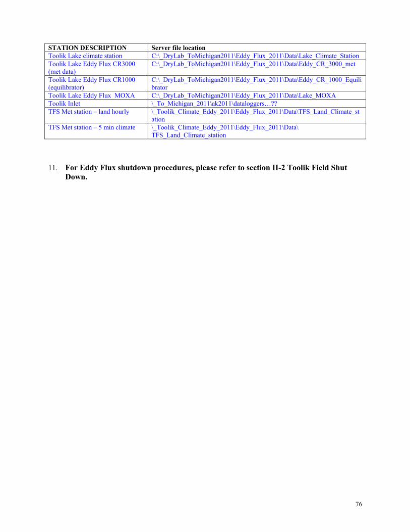
76

STATION DESCRIPTION Server file location Toolik Lake climate station C:\_DryLab_ToMichigan2011\Eddy_Flux_2011\Data\Lake_Climate_Station Toolik Lake Eddy Flux CR3000 (met data)

C:\_DryLab_ToMichigan2011\Eddy_Flux_2011\Data\Eddy_CR_3000_met

Toolik Lake Eddy Flux CR1000 (equilibrator)

C:\_DryLab_ToMichigan2011\Eddy_Flux_2011\Data\Eddy_CR_1000_Equilibrator

Toolik Lake Eddy Flux MOXA C:\_DryLab_ToMichigan2011\Eddy_Flux_2011\Data\Lake_MOXA Toolik Inlet \_To_Michigan_2011\ak2011\dataloggers…?? TFS Met station – land hourly \_Toolik_Climate_Eddy_2011\Eddy_Flux_2011\Data\TFS_Land_Climate_st

ation TFS Met station – 5 min climate \_Toolik_Climate_Eddy_2011\Eddy_Flux_2011\Data\

TFS_Land_Climate_station

11. For Eddy Flux shutdown procedures, please refer to section II-2 Toolik Field Shut Down.

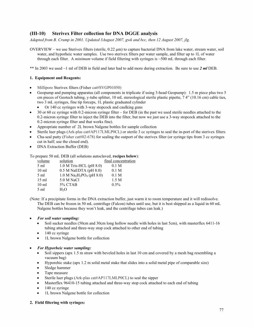
77

(III-10) Sterivex Filter collection for DNA DGGE analysis Adapted from B. Crump in 2001. Updated 3August 2007, gwk and bcc, then 12 August 2007, jlg. OVERVIEW – we use Sterivex filters (sterile, 0.22 μm) to capture bacterial DNA from lake water, stream water, soil

water, and hyporheic water samples. Use two sterivex filters per water sample, and filter up to 1L of water through each filter. A minimum volume if field filtering with syringes is ~500 mL through each filter.

** In 2003 we used ~1 ml of DEB in field and later had to add more during extraction. Be sure to use 2 ml DEB. 1. Equipment and Reagents: Millipore Sterivex filters (Fisher cat#SVGP01050) Geopump and pumping apparatus (all components in triplicate if using 3-head Geopump): 1.5 m piece plus two 5

cm pieces of Geotech tubing, y-tube splitter, 10 mL stereological sterile plastic pipette, 7 4” (10.16 cm) cable ties, two 3 mL syringes, fine tip forceps, 1L plastic graduated cylinder Or 140 cc syringes with 3-way stopcock and caulking guns

30 or 60 cc syringe with 0.2-micron syringe filter – for DEB (in the past we used sterile needles attached to the 0.2-micron syringe filter to inject the DEB into the filter, but now we just use a 3-way stopcock attached to the 0.2-micron syringe filter and that works fine).

Appropriate number of 2L brown Nalgene bottles for sample collection Sterile luer plugs (Ark-plas cat#AP117LMLP0CL) or sterile 3 cc syringes to seal the in-port of the sterivex filters Cha-seal putty (Fisher cat#02-678) for sealing the outport of the sterivex filter (or syringe tips from 3 cc syringes

cut in half; use the closed end). DNA Extraction Buffer (DEB)

To prepare 50 mL DEB (all solutions autoclaved, recipes below): volume solution final concentration 5 ml 1.0 M Tris-HCL (pH 8.0) 0.1 M 10 ml 0.5 M NaEDTA (pH 8.0) 0.1 M 5 ml 1.0 M Na2H2PO4 (pH 8.0) 0.1 M 15 ml 5.0 M NaCl 1.5 M 10 ml 5% CTAB 0.5% 5 ml H2O (Note: If a precipitate forms in the DNA extraction buffer, just warm it to room temperature and it will redissolve.

The DEB can be frozen in 50 mL centrifuge (Falcon) tubes until use, but it is best shipped as a liquid in 60 mL Nalgene bottles because they won’t leak, and the centrifuge tubes can leak.)

For soil water sampling:

Soil sucker needles (50cm and 30cm long hollow needle with holes in last 5cm), with masterflex 6411-16 tubing attached and three-way stop cock attached to other end of tubing

140 cc syringe 1L brown Nalgene bottle for collection

For Hyporheic water sampling:

Soil sippers (apx 1.5 m straw with beveled holes in last 10 cm and covered by a mesh bag resembling a vacuum bag)

Hyporehic stake (apx 1.2 m solid metal stake that slides into a solid metal pipe of comparable size) Sledge hammer Tape measure Sterile luer plugs (Ark-plas cat#AP117LMLP0CL) to seal the sipper Masterflex 96410-15 tubing attached and three-way stop cock attached to each end of tubing 140 cc syringe 1L brown Nalgene bottle for collection

2. Field filtering with syringes:

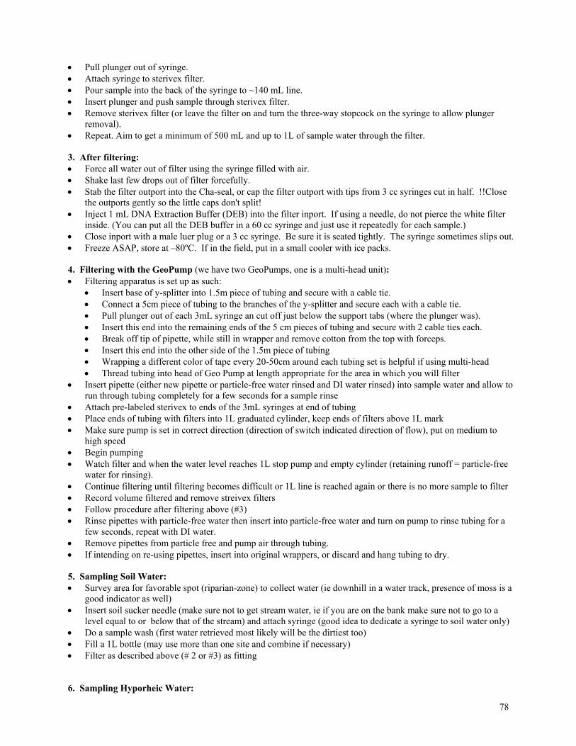
78

Pull plunger out of syringe. Attach syringe to sterivex filter. Pour sample into the back of the syringe to ~140 mL line. Insert plunger and push sample through sterivex filter. Remove sterivex filter (or leave the filter on and turn the three-way stopcock on the syringe to allow plunger

removal). Repeat. Aim to get a minimum of 500 mL and up to 1L of sample water through the filter. 3. After filtering: Force all water out of filter using the syringe filled with air. Shake last few drops out of filter forcefully. Stab the filter outport into the Cha-seal, or cap the filter outport with tips from 3 cc syringes cut in half. !!Close

the outports gently so the little caps don't split! Inject 1 mL DNA Extraction Buffer (DEB) into the filter inport. If using a needle, do not pierce the white filter

inside. (You can put all the DEB buffer in a 60 cc syringe and just use it repeatedly for each sample.) Close inport with a male luer plug or a 3 cc syringe. Be sure it is seated tightly. The syringe sometimes slips out. Freeze ASAP, store at –80ºC. If in the field, put in a small cooler with ice packs. 4. Filtering with the GeoPump (we have two GeoPumps, one is a multi-head unit): Filtering apparatus is set up as such:

Insert base of y-splitter into 1.5m piece of tubing and secure with a cable tie. Connect a 5cm piece of tubing to the branches of the y-splitter and secure each with a cable tie. Pull plunger out of each 3mL syringe an cut off just below the support tabs (where the plunger was). Insert this end into the remaining ends of the 5 cm pieces of tubing and secure with 2 cable ties each. Break off tip of pipette, while still in wrapper and remove cotton from the top with forceps. Insert this end into the other side of the 1.5m piece of tubing Wrapping a different color of tape every 20-50cm around each tubing set is helpful if using multi-head Thread tubing into head of Geo Pump at length appropriate for the area in which you will filter

Insert pipette (either new pipette or particle-free water rinsed and DI water rinsed) into sample water and allow to run through tubing completely for a few seconds for a sample rinse

Attach pre-labeled sterivex to ends of the 3mL syringes at end of tubing Place ends of tubing with filters into 1L graduated cylinder, keep ends of filters above 1L mark Make sure pump is set in correct direction (direction of switch indicated direction of flow), put on medium to

high speed Begin pumping Watch filter and when the water level reaches 1L stop pump and empty cylinder (retaining runoff = particle-free

water for rinsing). Continue filtering until filtering becomes difficult or 1L line is reached again or there is no more sample to filter Record volume filtered and remove streivex filters Follow procedure after filtering above (#3) Rinse pipettes with particle-free water then insert into particle-free water and turn on pump to rinse tubing for a

few seconds, repeat with DI water. Remove pipettes from particle free and pump air through tubing. If intending on re-using pipettes, insert into original wrappers, or discard and hang tubing to dry. 5. Sampling Soil Water: Survey area for favorable spot (riparian-zone) to collect water (ie downhill in a water track, presence of moss is a

good indicator as well) Insert soil sucker needle (make sure not to get stream water, ie if you are on the bank make sure not to go to a

level equal to or below that of the stream) and attach syringe (good idea to dedicate a syringe to soil water only) Do a sample wash (first water retrieved most likely will be the dirtiest too) Fill a 1L bottle (may use more than one site and combine if necessary) Filter as described above (# 2 or #3) as fitting 6. Sampling Hyporheic Water:

79

Find area just down stream of a riffle if possible Use sledge hammer to drive in Hyporheic stake Measure distance beneath stream by measuring to the bottom of the stream and subtracting from total length of

the stake (try to get at least 10-15cm) Remove core stake slowly and quickly insert hyporheic sipper Slowly remove outer pipe Allow sediment to re-stabilize for several minutes Attach tubing and syringe (good idea to dedicate a syringes to hyporheic water only), make take awhile to retrieve

any water, if still dry, attempt to reposition sipper by gently rocking or blowing air into sipper. May have to try several areas Fill a 1L bottle (or retrieve as much as is possible, most likely a small sample will adequately fill the filter) Filter as described above (# 2 or #3) as fitting DEB components Tris Buffer 1.0 M (pH 8.0) 100 ml ultrapure water 8.64g Tris-HCl (f.w.=157.6, Sigma cat#T5941) 5.46g Tris Base (f.w.=121.1, Sigma cat#T6066) NaEDTA 0.5 M (pH 8.0) 200 ml ultrapure water 46.525 g Na2EDTA (f.w.=372.2, Sigma cat#E5134) ~5g NaOH pellets Stir and heat solution Bring to pH 8.0 with drops of 5 M NaOH solution Phosphate Buffer 1.0 M (pH 8.0) – Prepare 2 components and combine A) 1M Na2HPO4 (dibasic, f.w.=142)

100 ml ultrapure water 14.2 g Na2HPO4

B) 1M NaH2PO4 (monobasic, f.w.=137.99) 25 ml ultrapure water 3g NaH2PO4

C) Combine 93.2 ml dibasic solution 6.8 ml monobasic solution

NaCl 5.0 M 100 ml ultrapure water 29.22 g NaCl (f.w.=58.44) CTAB 5% 100 ml ultrapure water 5g CTAB (Hexadecyltrimethyl-Ammonium Bromide, Sigma cat#H6269)

80

(III-11) DNA Sample from soils, sediments, epilithon 1. Equipment: Gloves 50 mL Falcon tubes (8 per site) Scrub brushes (2) Plastic wash basins (2) Centrifuge capable of holding 50 mL falcon tubes Corer (140cc syringe with tip cut off) Spatula 2. Sampling rock surfaces in streams or lakes – Scrubates: Choose a 2 rocks, one from a riffle and one from a run (probably best to do one at a time, unless you have several

people working at the same time) Rocks should be somewhere between dessert plate and dinner plate size (exceptions can be made if options are

limited) Be conscious of top and bottom, since each will be extracted separately. Holding rock over basin, scrub with brush in small circular motions (like brushing teeth) for several minutes to

loosen biofilm Use squirt bottle of particle-free water to rinse rock, aim for 45-50 mL of sample. Collect sample in 50 mL Falcon tube. Repeat procedure for other side of rock, being sure to rinse the basin with particle free and scrub with sponge and

then rinse again with particle free at least two more times in between samples (having two basins is helpful here) Ice immediately if in field and store in freezer until extraction 3. Sampling Bank Soils: Wearing gloves, reach under the stream bank at water level (2 separate samples one from each side of bank) Grab a few inches of soil Squeeze out excess water Put in 50 mL Falcon tube Ice immediately and store in freezer until extraction 4. Sampling Sediment: Wearing gloves, wade out into stream insert corer into stream bottom, avoiding rocks (2 separate samples, 1

upstream of riffle, one downsteam…sampling in actual riffle difficult due to rocks) Push syringe over the plunger and into sediment apx 5 cm deep In a quick and fluid motion pull out corer and bring to the surface Using plunger push out all but the top cm, pick out and discard any large pebbles Scrape into 50 mL Falcon tube using spatula Ice immediately and store in freezer until extraction

81

(III-12) LTREB Toolik Lake survey – Protocol for summer 2007 GOAL: Our goal is to characterize variability in bacterioplankton communities in Toolik lake, and to try to identify the sources of this variation. Although we have taken replicate samples before at the same location and get similar DGGE results, for example two bottles from 3 m depth at Toolik Main, we have little idea about the sources of the bacteria that we find in the middle of the lake – are they coming from deep waters, or from the inlet stream, or from the epilithon on rocks in the shallows, or from the bottom sediments? This two-day survey will help to answer these questions. Day 1. Epilimnion and Hypolimnion (Red and Green sites on attached map). This will probably take most of the day, with at least half of the day spent out on the lake. You will need at least one person (Sarah+) from the LTER crew. There are 7 sites and you will generate two water samples (surface and bottom water) and one sediment sample from each site. The exception is the Outlet Bay site where there is only one sample generated (too shallow for a deep site) – this sample should be very close to where you are definitely in the outlet “stream”, but still within the lake; we want a lake sample, not a stream sample. Procedure:

Motor to the site and check the depth. Drop an anchor to hold position. Check depth again and record in the field book. Record GPS position. Have one person do a Hydrolab cast and record data for each meter of depth (conductivity, temperature, pH,

oxygen – note that on the old LTER Hydrolab the SCUFA sensor for chlorophyll fluorescence is broken. You will need to have Jeremy check you out on the old Hydrolab the day before the survey, and it will need to be calibrated for pH and oxygen {air saturation calibration}).

The other two people should work on a different end of the boat using the large Van Dorn to collect water at 3m and 16m depth, or ~1m off bottom at the shallower sites – be sure to record the depth of the sample. We want all of the sample water to come from the same Van Dorn bottle.

o Fill two 2L bottles and one thermos from each depth. Label the sites as they are shown on the map. o Put all bottles in a cooler

Ekman dredge for bottom sediment. The easiest way to sample the dredge is to use the small 60 mL syringe “corer” that we have made for the stream surveys, and take a core of the top one cm of mud from 3 spots within the dredge. You can make a deeper core to keep the mud in the syringe, but, only use the last cm (top cm) of mud for the sample. Put all three subsamples into a 50 mL centrifuge tube just as we do in the stream surveys, then put the centrifuge tube in the cooler with the other samples. {Do not delay the Lake survey if the Ekman dredge does not come into camp in time – you can do the bottom samples on a later day}.

Return to lab for processing (14 water samples total from 7 sites) o Bacteria Production {note that if the sample collection takes a long time, the first thermos of bottom

water may have warmed up – the temperatures from surface and bottom waters will be the same from the same depths in the lake, so for example you can use 8 m depth water collected at the last site for all of the other sites that had samples from a similar depth}.

o Two Sterivex filters (1L each) with DEB added o Filter for chlorophyll (~560 mL) o TDN/DOC bottle o TDP bottle o Alkalinity bottle o Nutrients ( PO4 and NH4 ) – you must arrange this ahead of time with Amanda, so that that Sarah

and Annie know there are 14 nutrient samples coming. Day 2. Shoals and scrubate samples (pink sites on the map). This day will be shorter and can be done by two people. Collect water samples from Toolik Inlet, Camp shoal, Sauna shoal, and Rock shoal. Procedure: Motor to site, but be careful not to hit the bottom with the propeller – be sure to take oars, and, someone will need to have hip waders on as well.

82

Drop an anchor to hold position. Do a Hydrolab cast and record data for each meter of depth (conductivity, temperature, pH, oxygen). Note

that you may only get one reading at say 0.5 m depth. Use the large Van Dorn to collect subsurface water at 0.5 m depth, or just get the Van Dorn submerged.

Again, we want all sample water to come from the same Van Dorn bottle. Record the depth or the mid-point depth of the Van Dorn.

o Fill two 2L bottles and one thermos from each site o Put all samples in a cooler

Collect a two rocks for a scrubate sample from each site and put them into a ziplock bag – use roughly the same size rock that we use for scrubates in the streams. Hopefully you can reach the rock with hip waders on, or you will need to be “inventive”, especially at the Rock Shoal site (this is the site with the rock that sticks up a little bit out of the water. At the shoals close to shore you could also wade out to get rocks after returning to the dock. The rock does not have to be from the same exact spot as the water sample.

Return to lab for processing o Water samples – total of 4 sites, the three rock shoals and Toolik Inlet.

Bacteria Production Two Sterivex filters (1L each) with DEB Chlorophyll filter TDN/DOC bottle TDP bottle Alkalinity bottle Nutrients ( PO4 and NH4) – again, arrange with Amanda for the 4 nutrient samples to be

run on the following day (Friday). o Rocks

Use Sterivex filtrate to rinse rocks Collect a scrubate sample (use technique from stream survey) by combining the surface of

both rocks (don’t worry about the bottom of the rock).

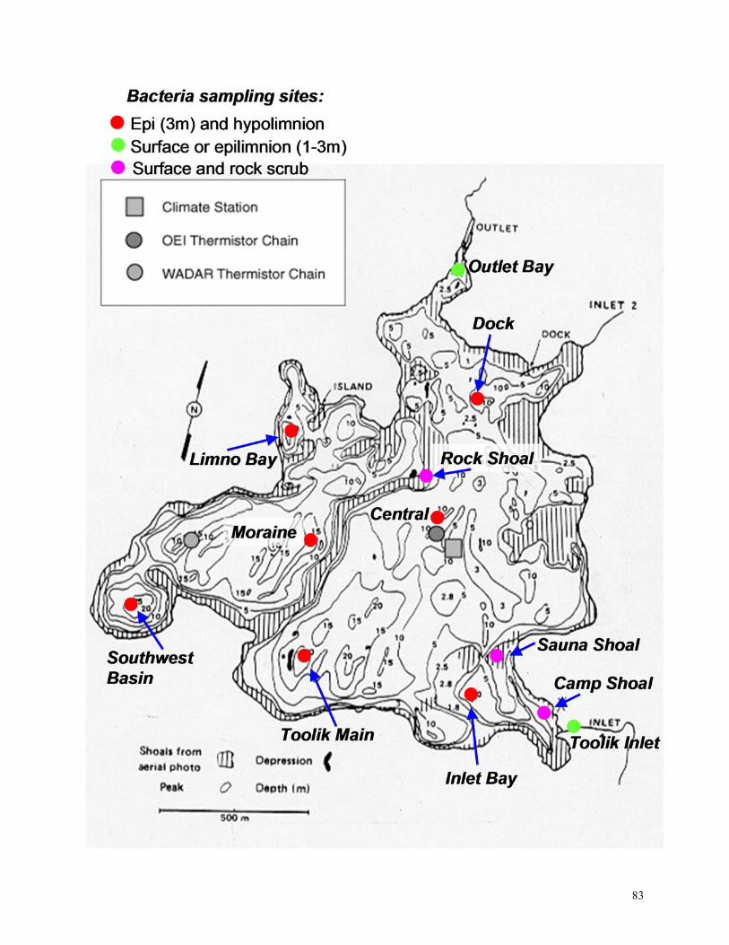
83

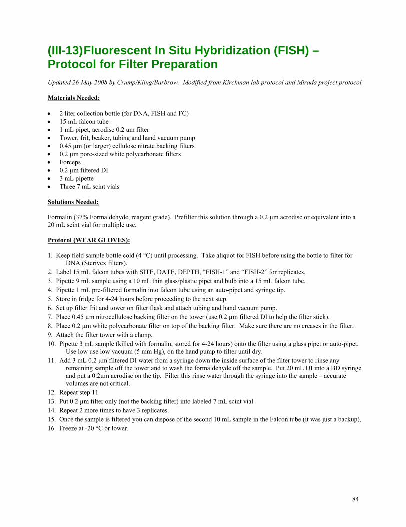
84

(III-13) Fluorescent In Situ Hybridization (FISH) – Protocol for Filter Preparation Updated 26 May 2008 by Crump/Kling/Barbrow. Modified from Kirchman lab protocol and Mirada project protocol. Materials Needed: 2 liter collection bottle (for DNA, FISH and FC) 15 mL falcon tube 1 mL pipet, acrodisc 0.2 um filter Tower, frit, beaker, tubing and hand vacuum pump 0.45 µm (or larger) cellulose nitrate backing filters 0.2 µm pore-sized white polycarbonate filters Forceps 0.2 µm filtered DI 3 mL pipette Three 7 mL scint vials Solutions Needed: Formalin (37% Formaldehyde, reagent grade). Prefilter this solution through a 0.2 µm acrodisc or equivalent into a 20 mL scint vial for multiple use. Protocol (WEAR GLOVES): 1. Keep field sample bottle cold (4 °C) until processing. Take aliquot for FISH before using the bottle to filter for

DNA (Sterivex filters). 2. Label 15 mL falcon tubes with SITE, DATE, DEPTH, “FISH-1” and “FISH-2” for replicates. 3. Pipette 9 mL sample using a 10 mL thin glass/plastic pipet and bulb into a 15 mL falcon tube. 4. Pipette 1 mL pre-filtered formalin into falcon tube using an auto-pipet and syringe tip. 5. Store in fridge for 4-24 hours before proceeding to the next step. 6. Set up filter frit and tower on filter flask and attach tubing and hand vacuum pump. 7. Place 0.45 µm nitrocellulose backing filter on the tower (use 0.2 µm filtered DI to help the filter stick). 8. Place 0.2 µm white polycarbonate filter on top of the backing filter. Make sure there are no creases in the filter. 9. Attach the filter tower with a clamp. 10. Pipette 3 mL sample (killed with formalin, stored for 4-24 hours) onto the filter using a glass pipet or auto-pipet.

Use low use low vacuum (5 mm Hg), on the hand pump to filter until dry. 11. Add 3 mL 0.2 µm filtered DI water from a syringe down the inside surface of the filter tower to rinse any

remaining sample off the tower and to wash the formaldehyde off the sample. Put 20 mL DI into a BD syringe and put a 0.2µm acrodisc on the tip. Filter this rinse water through the syringe into the sample – accurate volumes are not critical.

12. Repeat step 11 13. Put 0.2 µm filter only (not the backing filter) into labeled 7 mL scint vial. 14. Repeat 2 more times to have 3 replicates. 15. Once the sample is filtered you can dispose of the second 10 mL sample in the Falcon tube (it was just a backup). 16. Freeze at -20 °C or lower.

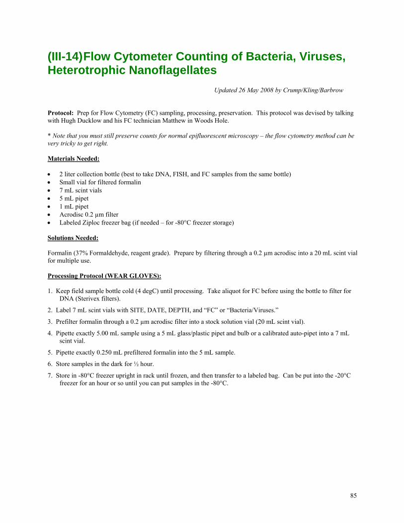
85

(III-14) Flow Cytometer Counting of Bacteria, Viruses, Heterotrophic Nanoflagellates

Updated 26 May 2008 by Crump/Kling/Barbrow Protocol: Prep for Flow Cytometry (FC) sampling, processing, preservation. This protocol was devised by talking with Hugh Ducklow and his FC technician Matthew in Woods Hole. * Note that you must still preserve counts for normal epifluorescent microscopy – the flow cytometry method can be very tricky to get right. Materials Needed: 2 liter collection bottle (best to take DNA, FISH, and FC samples from the same bottle) Small vial for filtered formalin 7 mL scint vials 5 mL pipet 1 mL pipet Acrodisc 0.2 µm filter Labeled Ziploc freezer bag (if needed – for -80°C freezer storage) Solutions Needed: Formalin (37% Formaldehyde, reagent grade). Prepare by filtering through a 0.2 µm acrodisc into a 20 mL scint vial for multiple use. Processing Protocol (WEAR GLOVES): 1. Keep field sample bottle cold (4 degC) until processing. Take aliquot for FC before using the bottle to filter for

DNA (Sterivex filters).

2. Label 7 mL scint vials with SITE, DATE, DEPTH, and “FC” or “Bacteria/Viruses.”

3. Prefilter formalin through a 0.2 µm acrodisc filter into a stock solution vial (20 mL scint vial).

4. Pipette exactly 5.00 mL sample using a 5 mL glass/plastic pipet and bulb or a calibrated auto-pipet into a 7 mL scint vial.

5. Pipette exactly 0.250 mL prefiltered formalin into the 5 mL sample.

6. Store samples in the dark for ½ hour.

7. Store in -80°C freezer upright in rack until frozen, and then transfer to a labeled bag. Can be put into the -20°C freezer for an hour or so until you can put samples in the -80°C.

86

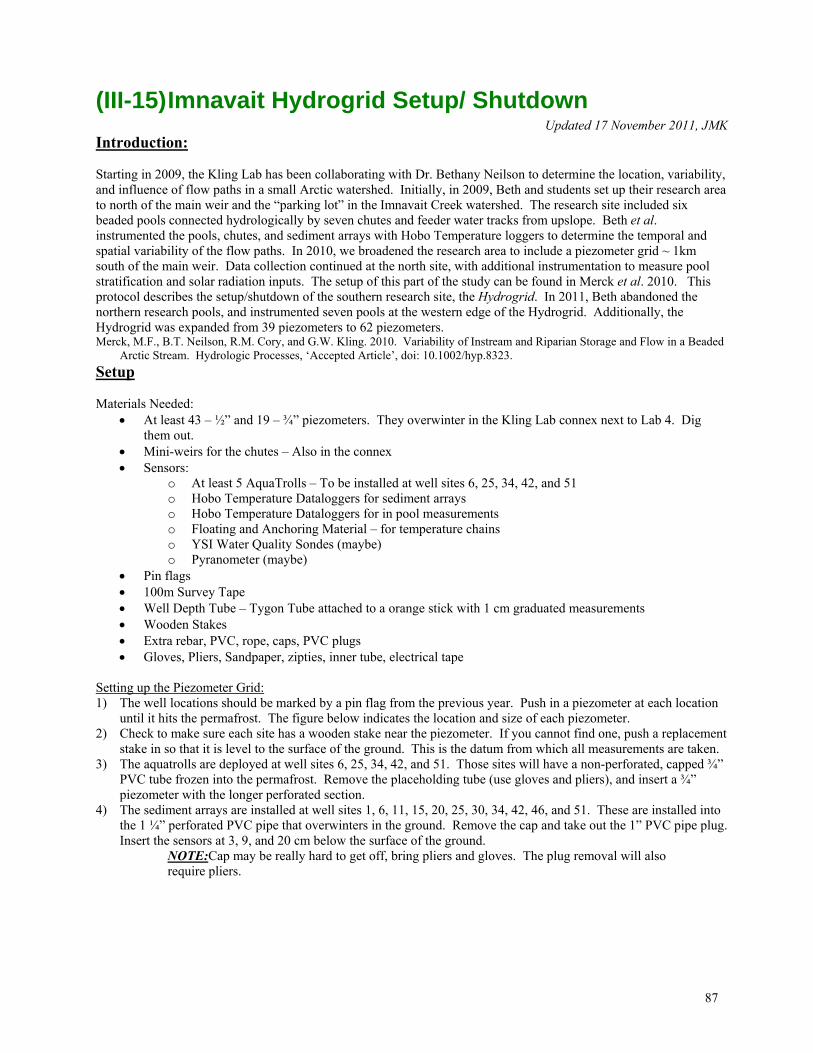
87

(III-15) Imnavait Hydrogrid Setup/ Shutdown Updated 17 November 2011, JMK

Introduction: Starting in 2009, the Kling Lab has been collaborating with Dr. Bethany Neilson to determine the location, variability, and influence of flow paths in a small Arctic watershed. Initially, in 2009, Beth and students set up their research area to north of the main weir and the “parking lot” in the Imnavait Creek watershed. The research site included six beaded pools connected hydrologically by seven chutes and feeder water tracks from upslope. Beth et al. instrumented the pools, chutes, and sediment arrays with Hobo Temperature loggers to determine the temporal and spatial variability of the flow paths. In 2010, we broadened the research area to include a piezometer grid ~ 1km south of the main weir. Data collection continued at the north site, with additional instrumentation to measure pool stratification and solar radiation inputs. The setup of this part of the study can be found in Merck et al. 2010. This protocol describes the setup/shutdown of the southern research site, the Hydrogrid. In 2011, Beth abandoned the northern research pools, and instrumented seven pools at the western edge of the Hydrogrid. Additionally, the Hydrogrid was expanded from 39 piezometers to 62 piezometers. Merck, M.F., B.T. Neilson, R.M. Cory, and G.W. Kling. 2010. Variability of Instream and Riparian Storage and Flow in a Beaded

Arctic Stream. Hydrologic Processes, ‘Accepted Article’, doi: 10.1002/hyp.8323.

Setup Materials Needed:

At least 43 – ½” and 19 – ¾” piezometers. They overwinter in the Kling Lab connex next to Lab 4. Dig them out.

Mini-weirs for the chutes – Also in the connex Sensors:

o At least 5 AquaTrolls – To be installed at well sites 6, 25, 34, 42, and 51 o Hobo Temperature Dataloggers for sediment arrays o Hobo Temperature Dataloggers for in pool measurements o Floating and Anchoring Material – for temperature chains o YSI Water Quality Sondes (maybe) o Pyranometer (maybe)

Pin flags 100m Survey Tape Well Depth Tube – Tygon Tube attached to a orange stick with 1 cm graduated measurements Wooden Stakes Extra rebar, PVC, rope, caps, PVC plugs Gloves, Pliers, Sandpaper, zipties, inner tube, electrical tape

Setting up the Piezometer Grid: 1) The well locations should be marked by a pin flag from the previous year. Push in a piezometer at each location

until it hits the permafrost. The figure below indicates the location and size of each piezometer. 2) Check to make sure each site has a wooden stake near the piezometer. If you cannot find one, push a replacement

stake in so that it is level to the surface of the ground. This is the datum from which all measurements are taken. 3) The aquatrolls are deployed at well sites 6, 25, 34, 42, and 51. Those sites will have a non-perforated, capped ¾”

PVC tube frozen into the permafrost. Remove the placeholding tube (use gloves and pliers), and insert a ¾” piezometer with the longer perforated section.

4) The sediment arrays are installed at well sites 1, 6, 11, 15, 20, 25, 30, 34, 42, 46, and 51. These are installed into the 1 ¼” perforated PVC pipe that overwinters in the ground. Remove the cap and take out the 1” PVC pipe plug. Insert the sensors at 3, 9, and 20 cm below the surface of the ground.

NOTE:Cap may be really hard to get off, bring pliers and gloves. The plug removal will also require pliers.

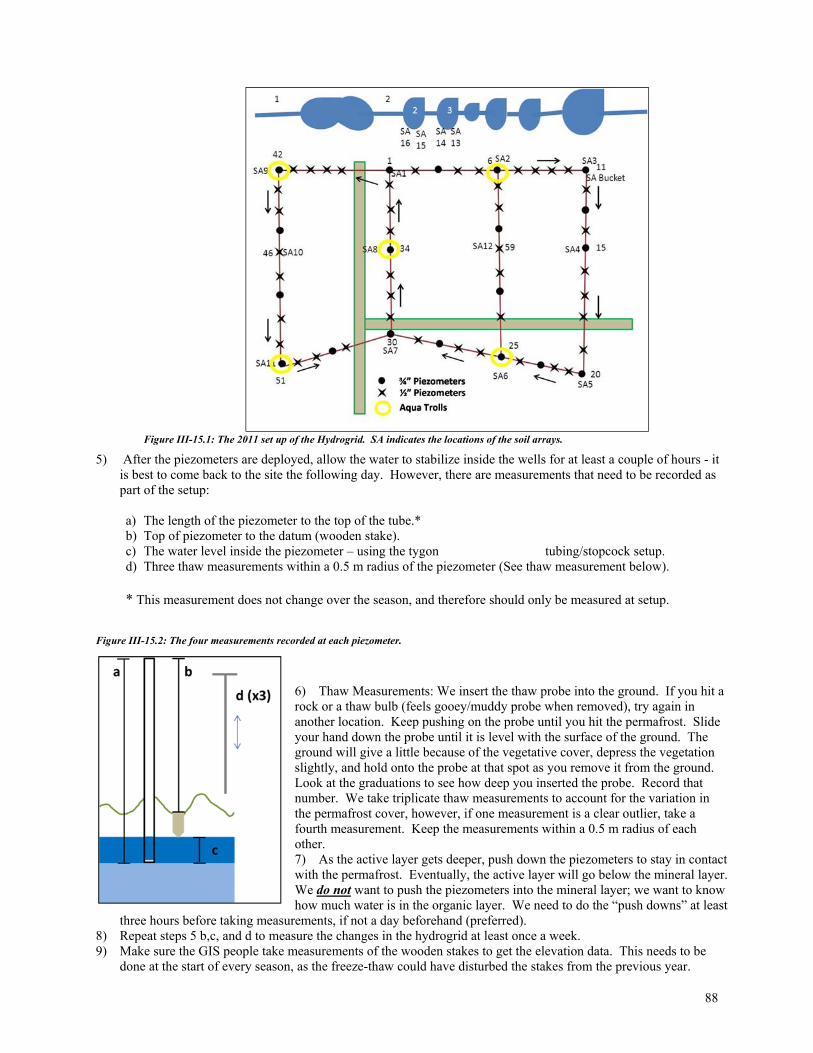
88

Figure III-15.1: The 2011 set up of the Hydrogrid. SA indicates the locations of the soil arrays.

5) After the piezometers are deployed, allow the water to stabilize inside the wells for at least a couple of hours - it is best to come back to the site the following day. However, there are measurements that need to be recorded as part of the setup:

a) The length of the piezometer to the top of the tube.* b) Top of piezometer to the datum (wooden stake). c) The water level inside the piezometer – using the tygon tubing/stopcock setup. d) Three thaw measurements within a 0.5 m radius of the piezometer (See thaw measurement below). * This measurement does not change over the season, and therefore should only be measured at setup.

Figure III-15.2: The four measurements recorded at each piezometer.

6) Thaw Measurements: We insert the thaw probe into the ground. If you hit a rock or a thaw bulb (feels gooey/muddy probe when removed), try again in another location. Keep pushing on the probe until you hit the permafrost. Slide your hand down the probe until it is level with the surface of the ground. The ground will give a little because of the vegetative cover, depress the vegetation slightly, and hold onto the probe at that spot as you remove it from the ground. Look at the graduations to see how deep you inserted the probe. Record that number. We take triplicate thaw measurements to account for the variation in the permafrost cover, however, if one measurement is a clear outlier, take a fourth measurement. Keep the measurements within a 0.5 m radius of each other. 7) As the active layer gets deeper, push down the piezometers to stay in contact with the permafrost. Eventually, the active layer will go below the mineral layer. We do not want to push the piezometers into the mineral layer; we want to know how much water is in the organic layer. We need to do the “push downs” at least

three hours before taking measurements, if not a day beforehand (preferred). 8) Repeat steps 5 b,c, and d to measure the changes in the hydrogrid at least once a week. 9) Make sure the GIS people take measurements of the wooden stakes to get the elevation data. This needs to be

done at the start of every season, as the freeze-thaw could have disturbed the stakes from the previous year.

89

Setting up the Pools: 1) When possible, we prefer to install the mini weirs early in the season. They are only useful during low to

moderate flows, otherwise they can be overtopped or the water can flow around them. The weirs should be able to fit back into their previous locations at the outflows of the pools. We want to use the same locations to minimize the damage to the tundra. Once the water flow is too high for the weirs to be useful, remove them. If you do not, they could be underwater for a long time.

2) We install a temperature chain in the center of every pool. We deploy the number and depths of the hobo temperature sensors depending on the maximum depth of the pool. Use a combination of anchors, floats, sensors, and rope/string to set up the sensors.

3) Beth may have other really cool instruments to deploy including but not limited to: sediment arrays, pyranometers, water quality sondes, pressure transducers, autosamplers, and rhodamine (not an instrument, but it can turn you pink!). Help her out to accomplish the goals of the project. It can be a lot of fun, just keep an open mind, a good sense of humor, and a lot of electrical tape!!

Shutdown of the Hydrogrid and Pools: 1) Before you remove anything from the hydrogrid, make sure that you have every datum to top of well

measurement. This will be the last time to take them for the season. 2) Remove the aqua troll sensors from well sites 6, 25, 34, 42, and 51. Record the well location, the sensor

identification number, and the time you removed the sensor in the field notebook. Insert the non-perforated, capped 3/4” PVC pipe in the place of the piezometers. Push down on the capped pipes until you hit the permafrost, leave overwinter.

3) Remove the sediment arrays from their PVC homes; insert the plugs in their place. Remember to bring some ziplock bags, as they can be wet and muddy. Double check to make sure the correct hobo identification numbers match what was recorded when the hobos were deployed.

4) Remove all of the other PVC piezometers from the hydrogrid and mark the holes with pin flags. Make a few bundles of the tubes using electrical tape to secure them, and make multiple trips. Don’t hurt yourself!!

5) Using the inflatable inner tube, raft down the pools to collect the temperature chains. This can be a lot of fun. Don’t fall in, and don’t forget to record location, the total water depth at the temperature chain location, and hobo ID numbers. We need the total depth of the pool because all other sensor depths are relative to the surface sensor.

6) Collect any other debris from the hydrogrid or the pools. Leave only the pin flags and the capped PVC pipes. Everything else will go back to camp with you.

7) When you return to camp, rinse all of the hobos and if you have time, download them. Every hobo should produce a hoboware computer file and a *.csv file. Save the data to the Kling Lab server and on a CD disc. Mail the hobos, copies of the field notebook, the data CD, and any other relevant data to Utah State.

90

SECTION IV - FIELD EQUIPMENT (updated 20 May 2012, gwk)

(IV-1) pH Meter updated 20 May 2012, gwk

-- We use several different meters to measure pH, including a Hydrolab and a Seabird CTD. Most of this protocol

works for any of the handheld meters. Check the protocol on Hydrolab and CTD calibration and operation for more information. LOOK IN THE WALLOCOLS SECTION FOR CALIBRATING DIFFERENT METERS.

A. WTW 3210 pH Meter 1. Press <Power> key to turn on the meter (red circle with line going through the top).

2. Set up buffers to bracket the sample pH that are 3 pH units apart (4.0 and 7.0 for Toolik). 3. Rinse pH electrode with DI water, then with RINSE pH 4 buffer solution (stir). 4. Remove from RINSE buffer and immerse probe in CLEAN pH 4 buffer. Stir, then let sit. 5. Press the <CAL> key. The display will show “Buffer 1” in the upper right corner. Once the reading (in mV)

is relatively stable (should be ~13.8 mV), press the <ENTER> key. The value of the first buffer will be displayed in the upper right corner. While the meter is calibrating, the display will flash “pH” in the upper left corner and show a status bar in the lower left corner. (If the reading needs to be adjusted, the pH value will be displayed; use the arrow keys to enter the correct pH.)

6. If the pH meter correctly measures the buffer, “pH” stops flashing, the status bar disappears and “Buffer 2” is displayed in the upper right corner. Press the <ENTER> key.

7. Rinse pH electrode with DI water, then with second buffer solution. 8. Immerse the pH electrode in first the RINSE then the CLEAN pH 7 buffer solution. 9. Once the reading (in mV) is relatively stable (should be ~160 mV), press the <ENTER> key. The second

buffer value is displayed in the upper right corner, and while the meter is calibrating the “pH” will flash in the upper left corner. (If the reading needs to be adjusted, the pH value will be displayed; use the arrow keys to enter the correct pH.) Then the meter will ask for Buffer 3.

10. Unless you want 3 buffers, ignore the Buffer 3 and press the <M> key to view the calibration table. This table shows the pH values of the buffers, temperature, etc. Check the slope - values around -58 mV/pH are desired. It also gives stars for the condition of the probe – 2+ stars is fine.

11. Press <F1> (continue) to make measurements. 12. Turn off meter. Rinse the probe in DI water and take into the field. 13. When returning from the field, rinse probe in DI and store in storage solution, 3M KCl.

B. Calibration of the Orion pH Meter There is a checkout procedure and a calibration procedure in the manual that lives in the pH meter case. The

checkout and setup procedures do not need to be repeated unless you want to change something or the meter is not working. After replacing the battery, all setup procedures return to default settings- you may wish to turn ‘off’ the 5 minute automatic shutoff (‘on’ is default). -- Important Notes: * For measurements of pH use buffers that bracket the expected sample pH. * For alkalinity titrations use pH 7 and pH 4 buffers. 1. Turn meter on with the ‘power’ button. Use the ‘mode’ button to set to ‘pH’ 2. If there is a pH solution filling hole on the probe body, expose it by moving the rubber band downward. 3. Remove the probe cap and rinse the probe tip with DI to remove storage solution. Place the probe in pH 7 buffer

and change the meter to mV scale. When the probe has a stable mV reading it is ready for calibration. This step is not necessary if you are recalibrating in the field, only if the probe has been stored in storage solution.

4. Return to pH mode on the meter and rinse the probe tip with a squirt bottle of pH 7 buffer, then place the probe in pH 7 buffer (NOTE: If you are in the field, you can add buffer to the probe cap and replace the cap loosely on the probe; then gently shake the probe to rinse the probe tip, remove the cap and repeat; finally, add a little buffer to the cap again and push the cap all the way onto the probe). Now the probe is ready for the first calibration step.

91

5. Press the ‘2nd’ then the ‘calibrate’ button and the meter will display a pH reading and ‘P1’ at the bottom of the screen. When the reading is stable it will display ‘ready’. Now press the arrow down button until the left digit of the pH reading is flashing. Set the correct number with the up and down arrows. If the reading is correct (for example, if it reads ‘7’) then press the ‘yes’ button. This will move the flashing digit to the right, and you can set that value in the same way. Once all three digits are set the meter will display ‘P2’ (it now is ready for the second calibration buffer).

6. Remove the probe from the pH 7 buffer and rinse with the second buffer (4 or 10) as in step #3. Adjust the reading to the proper pH as in step #4. When you hit the ‘yes’ button for the final time the meter will display the slope of the line between the two buffers. If the slope is less than 90 or greater than 110 the probe should be reconditioned. The meter will automatically switch from ‘calibrate’ to ‘measure’ and it is now ready for a sample. If you are now going into the field, cap the probe with DI water.

B. Lab Determination 1. Rinse the probe tip with sample then let the probe sit in the sample to equilibrate. After a minimum of 5 minutes,

place the probe into fresh sample water (the first sample water has degassed CO2 while the probe equilibrated, and thus the pH has changed). Wait at least one minute and until the meter displays ‘ready’ and record the pH reading and the temperature.

2. If you will be making several measurements over a short time period, leave the probe in sample water or fill the cap with sample water for storage (this reduces the time necessary to equilibrate to the low ionic strength of the sample). If measurements will not be made for more than 6 hours, store the probe in storage solution.

C. Field measurement 1. Calibrate the pH meter in the lab before going out into the field. The meter can be calibrated in the field, but only

after all buffers and probes have come to equilibrium with the field temperature. Thus it is better to calibrate the meter in the lab where everything is already at a stable temperature.

2. After calibration, fill the probe cap with DI water or surface water so that the probe can begin to equilibrate with the low ionic strength solution that will be similar to the field samples.

3. In the field, before starting any other procedures, place the pH probe in the water sample - be careful not to have the water flowing past the probe too quickly, and don’t put the probe in a backwater that is not representative of the stream or lake. On a calm day you can simply place the probe into the surface water making sure that the filling hole is not submersed, and wait at least 5 minutes to make your reading. IF YOU CANNOT MAKE A MEASUREMENT IN THE FIELD, fill two BOD bottles with sample water (see below). Let the probe equilibrate for as long as possible.

4. For soil waters, take the water sample with a syringe, rinse the pH probe, then fill a beaker with the sample and put the probe into the beaker immediately. Swirl the probe to stir the sample then take a reading as quickly as possible -- the soil water will degas rapidly and change the pH.

5. After all other sampling is finished, read the pH and record the value and the temperature.

D. Sampling in the field for later lab determination 1. In the field, fill two 60 mL BOD bottles with sample from each sampling station. Fill slowly from the bottom to

avoid air contamination using either a hand pump with tygon tubing, or an air-free syringe with a tygon end. Overfill the bottle with at least 1 bottle volume (2 if possible), replace stopper. Keep BOD bottle cool and dark.

2. In the lab, allow the BOD bottles to reach room temperature (keep them in the dark). Use a small stir bar and magnetic stirrer in the BOD bottle.

3. Place the pH probe into the first BOD bottle and let the probe equilibrate (10-15 minutes). 4. After equilibration, place the stir bar and probe into the second BOD bottle. Allow the reading to stabilize

(usually 3-5 minutes), and record the pH value and the temperature.

* Note: The probe tip may collect small air bubbles from the stirring action. If this happens, wait until the reading stabilizes and then gently shake or stir the probe tip to remove the bubbles. Record the pH of the sample when bubbles have been removed (it is usually the same).

92

(IV-2) Conductivity Meter Updated 2 April 2001

A. Conductivity Meter Operating Instructions—Orion Model 122 1) The Orion model 122 meter is very easy to operate, and requires no calibration or setup, and minimal

maintenance aside from proper handling. 2) Measurements are made by submersing the probe tip (the whole probe may be submersed), into the

water, and turning the lower dial from “off” to the center position. (The third and final position of the dial measures temperature.)

3) Wait until the temperature of the probe casing comes to equilibrium with the ambient water temperature (this could take several minutes). Once the temperatures of probe and water are the same, the conductivity reading should be stable and ready for recording. The top dial is used to adjust the scale in which the conductivity is read. Use the lowest (most sensitive) scale possible. Usually, samples will be measured and recorded in S/cm on the 1999 scale, and dilute samples or lab RO-DI water reads on the 199.9 scale (i.e., less than 200 S) .

B. Conductivity Meter Operating Instructions—YSI model 30 1) The YSI model 30 conductivity meter is very easy to operate, and requires no calibration or setup, and

minimal maintenance aside from proper handling. 2) Measurements are made by submersing the probe tip (the whole probe may be submersed), into the

water, and pressing the ON/OFF button. Temperature is displayed along with the conductivity. This meter is auto-ranging, so there is no need to change the range or scale of measurement. Pressing the ON/OFF button again turns the meter off.

3) Wait until the temperature of the probe casing comes to equilibrium with the ambient water temperature (this could take several minutes). Once the temperatures of probe and water are the same, the conductivity reading should be stable and ready for recording.

4) The MODE button toggles between 3 operating modes: Conductivity, Specific Conductance (this automatically adjusts the reading to a calculated value which would have been measured if the sample had been at 25 degrees C), and Salinity. We generally record the Conductivity along with the temperature at which the reading was made.

5) This conductivity meter can be calibrated, the temperature compensation temperature set to a value other than 25 degrees C, and the auto ranging feature can be disabled by using the ARROW UP, ARROW DOWN, MODE, and ENTER buttons. See the Operations Manual (located in the Equipment and Instrument Information file cabinet drawer) for further information on these features.

93

(IV-3) Light Meter and Secchi Depth Updated July 2012, SEF

A. Light meter A Li-Cor meter and 2 flat “2-pi” sensors, one facing up and down, and a “2-pi” deck sensor are presently being used. In the past, a spherical quantum sensor (“4-pi”), or a single flat “2-pi” sensor has been used. Make sure the meter is fully charged before taking it in the field. * NOTE: Do not touch the surface of the sensor! The sensor is delicate, it can be scratched easily, and it is very

expensive. If the sensor becomes dirty use a chem-wipe or a soft cloth to clean the sensor surface. Use On Toolik Lake: 1. The sensor should be plugged into the proper inlet on the meter because each sensor has different calibration

values. Weight should be attached to the sensor frame so that the cable hangs vertically in the water. 2. Make sure that the correct settings are entered on the meter: see “settings used for Toolik”. 3. Position yourself on the sunny side of the boat so that the shadow of the boat underwater does not affect your

reading. 4. In the data book record the time of day, the weather conditions and the type of clouds, and describe the waves on

the water surface (height of waves, glassy, whitecaps, etc.). Also record the direction of the wind (e.g., “from the inlet side of the lake” if you don’t have a compass).

5. First take a reading in air with the meter pointing straight up, NOT angled toward the sun. This reading is to insure the uniformity of conditions at the start and end of the light profile. The Li-Cor must be calibrated differently for use in air or water so this reading should not be used an accurate surface light measurement. Note that while taking a light reading the cloud cover should remain the same. If cloudiness changes during the light profile then the profile must be started again. (Sometimes you can “piece-together” different parts of the profile under different conditions, but that is difficult and requires a lot of documentation of what you did.) If conditions are calm and there are no clouds (i.e., stable) you can set the meter to integrate for 10 sec before registering a reading. However, if the conditions are unstable you must set the meter for continuous reading (1 sec) and take a “running average” in your head to record in the data book. Note that with the Licor 1000 meter you can use two sensors, one shipboard one underwater, to get a differential reading.

6. Lower the sensor just into the water for the 0 m depth reading. This may be difficult if the waves are high. If the 2-pi sensor is being used, you can alternatively put lake water on top of the sensor so that a thin film covers the sensor and then take the 0 m reading while the sensor and frame are out of the water. If you use this method, record it in the data book. Take 3 readings at each depth with 3-5 seconds between readings.

7. Continue to lower the sensor so that you have at least 7 or 8 depths recorded (if possible). Let the sensor stay at a particular depth until the meter has completed a full cycle of integration before you take the first reading.

8. If you are in any doubt as to whether the climate conditions changed during the profile, record the light values at the same depths on the way up toward the surface to see if they match with the values recorded on the way down.

9. Always record the “air” value again when you get the sensor back to the surface just to make sure that the climate conditions have not changed.

Basic Li-Cor DataLogger operation: To turn DataLogger on press the ON/OFF button once. The DataLogger has 3 input channels (I1-I3) and can be set-up to have several math channels (we currently use one called MI). To view the current reading on each of these channels press the → button to toggle through the channels. (The current settings used for work in AK are: I1 is set-up for the surface sensor, I2 is set-up for the 2p upwelling sensor and I3 is set up for the 2 pi downwelling sensor. To view the time that the DataLogger thinks that it is, use the → button to toggle through the v rows until the date and time are displayed. This will show the time in YYMMDD HHMMSS format. How to Log Data on the LiCor (last edited 2012) Note that the depth of the reading is not recorded (the LiCor does not “know” what depth it’s at- you must tell it), so it is VERY important to note in your field book the order and depth of EACH reading. Generally, we record a “Remark” with the Lake and depth every 5 meters to help keep track of the readings (instructions below).

94

1. Turn on the LiCor by pressing the <On/Off> button. 2. The top line of the display should read “View New Data.” If it does not, press <View>. The first option should be “New Data” and hit <Enter>. 3. Once the top line of the display reads “View New Data,” press the <Fct> button. The first option should be “Log Remarks.” Hit <Enter>. 4. The top line should read “Log Remarks” and right below will read “LAKE=XXXXXX.” The line under the “L” signifies it is selected. Hit either the left or right arrow key to edit the lake name. Press the <Shift> button once to choose the letter in the top left corner of a key on the number pad; press it twice to choose the letter in the bottom left corner. Do not press the <Shift> key if you want to select a number. Hit <Enter> when you are finished entering the lake name. 5. Press the down arrow to select “Depth.” Press the left or right arrow key to edit the depth. You can edit the depth with each reading, but we generally only enter the depths at 0, 5 and 10 meters. Hit <Enter> when you are finished entering the depth. 6. Scroll down with the arrow key to select “! Log Remarks!” and hit <Enter>. You must do this to save your remark. 7. You should be returned to the “View New Data” display. The bottom line should read “I1I #### S.” The “S” tells you this is the surface sensor measurement. Record this number in the fieldbook and press the right arrow key. This is the upwelling sensor measurement (“UP”). Record this number in the fieldbook and press the right arrow key. This is the downwelling sensor measurement (“DO”). Record this number in the fieldbook and hit the <Enter> key ONCE to log all three measurements. 8. Press the left arrow key twice to return to the “S” reading and move the sensors to the next depth. Repeat step 7. Remember to edit the depth at 5 and 10 meters. To view logged data hit the “Esc” button once. Toggle to “LOG DATA” using the → key and hit “Enter” twice. “View all” will appear followed by a list of data points. Scroll through this list using ↑ and ↓. Use the view button to toggle how you view this list between descriptor (setup, remark, or inst reading) HHMMSS and YYYYMMDD HHMMSS. To view the data or remarks for a given point, highlight that line and hit enter, use the ↓ key to scroll through the channels, hit ESC to return to the list. When done viewing data hit ESC until you return to the VIEW menu, toggle to NEW DATA and hit Enter. To set the configuration of the DataLogger, this should not have to be done often but it is good to check that the settings are correct from time to time, hit the Setup button. The screens of the set-up menu are moved through by hitting → key and selected using the ENTER button. The settings that are used for Toolik work, as of Summer 2003, are: Logging Logging=off Remark Prompts Prompt1= Lake Prompt2= Depth Prompt3= Notes Hardware Band= 9600 Noise Fltr= 50 Hz Clock Set to AST Channels I1= Light Descr= Surface Mult= -153.37 (this is the calibration mult determined by LiCor for this specific sensor) Label= 5M Average= 1 sec Log Routin= LR1 Calc= Mean Min Max= no TCoef= 0.0036 I2= Light Descr= Upwelling

95

Mult= -280.25 Label= 5M Average= 1 sec Log Routin= LR1 Calc= Mean MinMax= No TCoef= 1 I3= Light Descr= Downwelling Mult= -317.3 Label= 5M Average= 1 sec Log Routin= LR1 Calc= Mean MinMax= No TCoef= 1 I4= Off Math Lib ML1__= none When these settings are used the DataLogger reports light averaged over 1 sec intervals in units mol s-1 m-2. Storage: The sensor is normally stored connected to the cable and is protected by a metal and foam case. The BNC connectors are protected with small plastic scintillation vials. All connections and case should be dried prior to storage. Care and Maintenance: 1. If the sensor has not been stored connected to the cable then the connection should be lubricated with

silicon (LPS-greaseless lubricant) prior to assembly. 2. The pins on the sensor are delicate and should not be forced or twisted when the connection is being

made. 3. Clean the sensor with a mild soap solution. Do not use solvents, acids, or bases. Avoid touching the

sensor with your hands. 4. The manufacturer recommends recalibration every 2 years. Next scheduled recalibration AK sensors is

~April 2005. Downloading Stored Data on the LiCOR LI-1400 (Last Updated by CLC, 2 Feb 2014) 1. Open Hyperterminal 2. Attach 9 pin plug to LiCOR, use USB to 9 pin or other series of working cables to connect to a USB port in

Computer. Turn on LiCOR. 3. Make sure that you are in COM port 3. When USB ports are used for communications you call them COM ports.

Hyperterminal should now be able to connect/communicate with LiCOR. 4. Now that LiCOR is connected and ready to talk to Hyperterminal, press the “Call” button in Hyperterminal. 5. You are now ready to send data from LiCOR to Hyperterminal. This is the climax of the data processing: - On the LiCOR, navigate to FCT -> Print Mem - Make sure to Print All. - Scroll down and hit Print Mem! Data should be populating the screen of the computer.

- Copy all data into a .txt file, save it in the proper directory on the WET LAB USB thumbdrive and harddrive in the one in wetlab is functioning.

- Also save data as an excel spreadsheet, and save on the landwater folder on the hard drive of the computer in WET LAB.

- Disconnect LiCOR from the computer, return cables if they were borrowed, close hyperterminal. Take the USB back to Lab 4, and upload all data onto its correct location on the server.

96

The following directions are no longer used (since 2010 for HyperTerminal, and since 2013 for the 9-pin to USB) – they remain in the protocol in case HT needs to be used in the future. 1. Connect the LiCor to the computer using the gray cable in the LiCor/CTD Download Cables box and the 25 pin-to-9 pin

converter and the 9-pin to USB cable. Turn the LiCor on by pressing the On/Off button. 2. Double-click the LI1400 icon. Then choose Remote->Connect. Type in Com Port 2 when prompted. Then choose Remote-

>Receive Data and then Download: All. If this is the first time the LiCor is being downloaded for the season, name the file “initial_data_dump_YYYY” in the folder C:\_TO_MICHIGAN_2012\LAB_4\Licor\LI-1400data (ideally, before the first sampling of the season, or immediately after, clear the memory on the LiCor to ensure there’s enough space for this summer’s data – check in the archive folder to make sure the entire dataset from the previous summer is saved). After the initial download, save the file as “All_data_YYYY.txt” and keep replacing this file throughout the summer, everytime you download the LiCor.

*If the LiCor won’t connect, the only way I’ve been able to fix it is by restarting the computer. 3. After the file has downloaded, choose Remote->Disconnect. Turn off the LiCor and disconnect the cables. 4. Open the “All_data_YYYY.txt” with Excel. Create a new Excel file for each of the lakes sampled and name them

“LAKE_DDMonYY.xls”. Fill in the depths sampled and save the file(s). The following directions are right from LI-COR’s website. The cable is stored with the light meter.

Using Windows® 3.1 Terminal program to download data from the LI-1000

If you use a PC with Windows 3.11 software, there is an easy way to retrieve data from the LI-COR LI-1000 without having to use the 1000-90 communications software program available from LI-COR. Terminal (found in the Accessories program group of Windows) will work just fine. Steps for setting up HyperTerminal

1. Connect LI-1000 to one of your PC’s serial connectors using either the LI-1000-03 cable with 25-pin connector or the LI-1000-09 cable with 9-pin connector depending upon your PC’s requirements.

2. Open Terminal by double-clicking on its icon. 3. From the Settings menu select Communications (Terminal may automatically go to Settings/Communications upon

opening the program). 4. Select the appropriate Connector for your connection (Com1, Com2, Com3, or Com4). 5. Change the rest of the Communications settings to the following: Baud Rate 4800, Data Bits = 8, Stop Bits = 2, Parity =

None, Flow Control = Xon/Xoff and then select OK. 6. Save this configuration as 1000.trm using File/Save As. Note:at this point you are just saving the configuration of

Terminal. The next time you start Terminal, load this file for the appropriate configuration, this will allow you to skip steps 3-6 during future interrogations.

7. From the main Terminal menu select Transfer and then Receive Text File. Type in a file name for the data you will be transferring. This will be the file name for your data. (NOTE: you must add the extension ".txt" after your file name or Terminal will not accept it. For example, TEST.TXT)

8. Terminal will give you a blank screen with boxes at the bottom labeled Stop, Pause, Bytes:0, Receiving: (your file name). Steps for collecting LI-1000 data using Terminal

1. Turn on the LI-1000 and select the OUT button. 2. Change the baud rate to Baud=48 (for 4800) by using the up and down arrows and select ENTER. 3. Set the form to Form=H (for horizontal) by using the up and down arrows and select ENTER. 4. Set the len (for length) to len=255 by directly entering the numbers from the keypad and select ENTER. 5. Set the dump all to YES or NO (depending upon your requirements) by using the up and down arrows and select ENTER.

(selecting NO will prompt you to enter the year, month, date, hour, and minute for starting and stopping your data dump) 6. Your data will begin to dump to the Terminal program. if you have, for example, two months of data stored in you LI-

1000 and choose only to dump the last month, you may have a blank screen for a minute. The LI-1000 will scroll through all readings until it reaches the date marker you set. Upon reaching the date you set for the dump, you will see the data dump to the Terminal screen.

7. To close the data file, choose "STOP" from the Transfer menu at the bottom of the Terminal screen.

B. Secchi disc A Secchi disc measurement is routinely taken, and is required for any CTD measurements or primary productivity measurements. Secchi depth readings should be taken by the same person on all dates or lakes if possible; if not, do an intercalibration between the different observers. 1. Sufficient weight should be attached to the Secchi disc so that the disc hangs vertically in the water. 2. Position yourself on the shady side of the boat so that the reflection of the sun on the water does not affect your

reading. Note that if sunglasses are worn there should be a second reading made without sunglasses for comparison; record both readings.

97

3. Record the time of day, the weather conditions and the type of clouds, and describe the waves on the water surface (height of waves, glassy, whitecaps, etc.) and whether sunglasses were worn.

4. Lower the Secchi disc until you can no longer see it and mark the depth on the rope with your fingers. Now raise the disc until you can see it again and mark the depth on the rope with your fingers. Take the midpoint of those two depths and that is the Secchi depth that you will record.

98

(IV-4) Dataloggers

A. Programming and downloading Campbell CR10 datalogger - example For Limnology laboratory internal wave experiment using Campbell CR10, removable storage module, 10 thermistors

and SC532 interface. Written 12 Jan 99 kjr. 1. Programming the CR10 to record data Table 1 On the keypad hit ‘*1’ to enter the Table 1 program. Enter the program as follows, the notes to the right are not

entered. 01:5 Set execution interval in sec 01:P86 Do loop sets the output flag to high (so that the data will be sent to the output location) 01:10 02:P11 P11 indicates the following instructions are for Temperature 01:3 Number of reps (the number sequential channels, starting with number listed under instruction 02 (input

channel), you have with same excitation chn, storage location,multiplexor, and offset ) 02:1 Input channel (red) 03:1 Excitation channel (black) 04:1 Storage location 05:1 Multiplexor 06:0 Offset (if your thermistor has a known offset) 03:P11 Same as above, but necessary it is a different excitation channels 01:3 02:4 03:2 04:4 05:1 06:0 04:P11 Same as above, but necessary it is a different excitation channels 01:4 02:7 03:3 04:7 05:1 06:0 05:P77 Programs the CR10 to include real time in the output file 01: 1111 Year,day,hour-min,sec 06:P70 Sends the sample to the output location 01:10 Number of reps to send 02:1 Output location 07:P96 Serial Out- defines the output location 01:71 Storage module 1 Hit ‘*0’ to log the program and replace the old program in the CR10 On the keypad it should say ‘log01’, meaning that it successfully logged table 1 to the CR10 Now the CR10 is collecting data according to these specifications. After the appropriate amount of time you need to

download the data from the CR10 to the storage module and then from the storage module to the computer. 2. Downloading the data (a) Instructions on downloading from the CR10 to the storage module: (start manual data dump)

i. Connect the storage module, keyboard, and CR10 with the cable provided. ii. Enter ‘*8’ on the keypad iii. Enter ‘71’ at 01 prompt—storage module, address (1) iv. Advance to 04 prompt and then hit “1” then “A” (this starts the dump) v. Unplug storage module. Next you need to down load the data on the storage module to the computer

99

(b) Downloading to the Computer (using pc208)

i. Hook up interface to com1 (under monitor connector on a Dell) and attach storage module to the cable ii. Hit the MS dos prompt, as PC208 is a dos run program iii. At the c prompt type ‘cd pc208’ iv. At the pc208 prompt type ‘smcom’ v. Enter ‘1’ for com 1 (on Dell, but could be different for other computers, if you get a can not connect error try

the other com port number) vi. Enter ‘A’ for collect all data files vii. Insert a blank floppy diskette viii. Type ‘a:\ filename’ at the prompt (6 character max for the filename) ix. Type ‘C’ for the file format which is final storage (fs) converted to comma delimited ascii arrays x. Collects file for each time you compiled the program xi. Type ‘q’ to quit the pc 208 program xii. Type ‘exit’ to return to windows xiii. Open excel xiv. Open the file xv. Since this is not an xls file, you need to tell it how to read the file check ‘Delimited’, hit the ‘next’ key, check

the ‘comma’, hit the ‘finish’ key- xvi. You should see the data with the following columns: table, year, julian, hoursmins, sec, thermistor1,

thermistor2….thermistor10 xvii. Create column f (after sec), label it ‘time’ and make the formula= d+e/60 or ‘hoursmins’+sec/60 xviii. File save as ……..xls to c drive

(c) Downloading a storage module (sm192 or sm4m) (using pc208w) You will need a SC532 interface (black metal case about 5”x4”x1”), a blue 9pin-9pin 3 ended cable (sc12), a

25pin9pin cable, and the storage module. Connect the 25pin end of the 25-9pin cable to the RS232 end of the SC532 Connect the 9pin side of the 25-9 cable to the Com1 port on your computer (if only com2 available, you will

need to change the set up in PC208 to com2) Connect the blue 9-9pin cable to the periphery side of the SC532, connect the other end to the storage module Open PC208W Click Storage Module Choose type of storage module (mostly SM4M, but still some physically larger SM192). If necessary, change the

com port in “set up” tab Click “connect” or update status if you have just changed the storage module Look at status data- verify that the file space used is what you anticipated for the time the logger was used. On the Data Tab- make sure comma separated and autoincrement name are chosen. Click on the file name to

change to appropriate name (i.e. if you choose tw02fb it will name files tw02fb01, tw02fb02…., however if you name a file twfe02, it will name twfe02, twfe03….).

Click “Get All” Watch the name increment and the file pointer move through the file. Any place where the logger program was

changed, there will be a break in the data and the name will autoincrement up for the data following that change. Immediately open .dat file in excel and save as an excel name in the appropriate folder with the appropriate name

(i.e. tw02feb2002.xls). Rename the .dat file to the same name as the excel file. Follow the individual instructions to process the data. (d) Downloading logger with laptop in field

Open PC208W Physically Connect the datalogger to the computer.

o Note that the CR10X and the CR23X have different hookup cables. Each costs about $90 and takes 1 month to ship, so do not leave in field and do not lose.

o CR10 or CR10x - use the labeled cable (9pin to 9 pin). This cable should always be kept in the file box marked Campbell in 1041A. NEVER leave cable in the field. There must be a power source for this to work (i.e. if the battery is dead at the climate station this method will not work). Connect this cable to the end of the 3 ended blue/grey cable that is connected to the SM and the datalogger.

100

o CR23X – use the labeled cable. This cable should always be kept in the file box marked Campbell in 1041A. NEVER leave cable in the field. There must be a power source for this to work (i.e. if the battery is dead at the climate station this method will not work). Connect this cable to the RS232 port on the CR23X.

Set up - click the setup button. Map the connection by adding the correct datalogger and storage module to the com port (in 2002 the IBM thinkpad laptop is COM 1, previously this laptop had a COM2). You may name your set up (e.g. toolikcl for Toolik climate station) if you wish or just use a general one. Naming gives you the advantage of speed, saves correct file name, and file paths are saved. Choose the device you wish to access (click on it).

Connect- Click connect on the main PC208 screen. It will take a second then show you the logger time and the computer time. Compare the times to make sure the logger has been working properly.

Now you can 1) look at data in realtime, 2) download and upload a program, 3) associate a program, or 4) collect data. Mostly if you know the station is working, you will just need to collect data. However, it is also important to remember to download the program whenever you have changed it and at least once per season so you can have a record of the program back in AA.

1) Look at data real time. You must have the program associated to have labels on the graph (see 3). Click the 1 button by the 1 2 3 buttons. A graph will appear with the data in realtime (so if you only save data every hour, this is not very useful). You can change all the parameters of the graph and even have it graph previous data. Buttons 2 and 3 are for the different programs you may be using.

2) Download and upload a program. To download the program from the storage module to the laptop, use the retrieve button. Save in the PC208\programs\arctic\ and the appropriate station. Use a descriptive name that includes when it was used such as twweir_18jul_20aug2000.dld. Use Send button to send a program to the logger- be careful as this is the program that will be used (i.e. it automatically *0’s).

3) Associate Program. This allows you to look at the data realtime (with labels). Just click the button and choose the .dld.

4) Collect data. Used to collect the most recent, all, or specific data. Always check the ask for file name box. Click Collect All, Choose the file name and directory (in PC208/data/arctic/station subdirectory). Click OK. Immediately open excel and open .dat file in excel and save as an excel name in the appropriate folder with

the appropriate name (i.e. tw02feb2002.xls, where 02feb2002 is the date you downloaded the file). Look over data and make sure there are no errors in downloading (large missing sections, lots of –6999 or 6999 or 9999’s). Rename the .dat file to the same name as the excel file.

Disconnect from station

101

(IV-5) SBE 19 CTD Updated: 15 May 2014, gwk

SBE19 with Pump Conductivity, Temperature, Pressure Profiler (Depth) S/N 2880 Purchased in 1999 from Seabird instruments (425) 643-9866. Turner Scufa Fluorometer added in 2001. pH probe

added in 2003, refurbished in 2008 and replaced in 2012 and again at the end of 2013. Instrument response times: 500mS Temperature, 60mS conductivity, pressure nearly instantaneous. pH response to

63% of final value is 1 second. Scan interval 0.5 sec (2 Hz)

A. Calibrating the pH sensor on the CTD – do this each day of a cast(s): 1. Set up pH solutions for CTD - at least two solutions are required. Usually use pH 4 and pH 7, or pH 7 and pH 10.

Using all three is fine. 2. Remove the plug that powers the pump on the CTD to keep the pump from turning on during the calibration (pump

can't run in air, it uses water for lubrication and if out of water it will burn out). 3. Unscrew the metal pH guard cage from the pH probe and remove the pH storage solution bottle. 4. Hold the CTD between your legs while sitting down and TURN ON THE CTD. 5. Rinse the pH probe with DI water. 6. Raise the RINSE pH 4 buffer bottle up and over the pH probe. Swirl to rinse. 7. Raise the CLEAN ph 4 buffer bottle over the probe and move up and down to rinse. Leave this on the probe for

30-60 seconds. Record the time. 8. Rinse the probe with DI, then raise the RINSE pH 7 bottle up and over the probe. Swirl to rinse. 9. Raise the CLEAN pH 7 buffer bottle over the pH probe and move up and down to rinse. Leave this on the probe

for 30-60 seconds. Record the time. 10. Repeat for pH 10 buffer if desired. 11. Turn CTD off. 12. Place storage solution bottle back on probe and secure. 13. Place metal cage back on pH probe. 14. Plug in the pump cable. You are now ready to take water casts. 15. Record the pH calibration as a “cast” in the CTD field book! Otherwise the cast #s will be off. * Note that you can run a pH calibration in real time following the Seabird protocol found to the right and at:

http://www.seabird.com/pdf_documents/ApplicationNotes/appnote18-1Feb10.pdf

B. Prior to casting the CTD for the first time of the season: Make sure that all data are off the logger and backed up, the data have been graphed and checked and the CTD is

ready to be erased. With the CTD magnetic switch in the “off” position, hook CTD to computer with cable - five prong on one end

and with a 9 pin adapter to the other end (unscrew the black plastic cap on the CTD and pull of the black rubber end to expose the 5 prong connection). Hook the 9-pin end to the comm port.

Note that starting in 2002 we updated the software from Seabird. It is now a Windows program called SeaTerm. The same commands still apply as with the DOS program, but there are icons now to click on.

{On the laptop Start Programs MS-Dos prompt} {At the prompt change directory to the Seabird software ; type "cd\sea-bird"} {We have a SBE19 so use terminal 19; type "term19" } Hit return to connect to the CTD Type ‘DS’ to check the status of the logger and the current settings. Settings should be (i.e. set back to these if they are erased/changed)

o Narrow range conductivity (if not, reset with “CN” command o Check the time and date if it looks funny (with letters or impossible times, this indicates a problem with the

CTD and it likely needs to be sent back to Seabird for repair) o Conductivity hertz for pump initiation should be set at 2000hz. The probe measures about 2000-2800hz in

air, so this means that the pump will go on in the air after the delay time. o Pump delay time should not be shorter than 45seconds (time required to bleed the air out of the line). Set to

60 seconds. o Vmain is the battery voltage. There are 9 @ 1.5Volts, so new batteries should be around 13V. You should

change batteries when this value is 8.5 volts or less. A set of batteries should last about 20 hours.

102

o Cutoff voltage is 7.3V. Will not log data when below 7.3V. If the voltage drops below 7.3V, you will see a “stop=batsal” in the downloaded data

o Vlithium is the battery on the circuit that keeps your preferences when you change the battery. This should be above 5.0V.

o IOP is the operating current and it is fairly unique to your CTD. The Kling SBE19 CTD is 171mA and this value should not change more than 510mA in either direction. If it does, it is a sign of component failure. If you add new probes to the CTD, this value will change.

o Lwait = 0. Line wait, for older computer, always zero now. o # voltage=0 (or 2 if the SCUFA is being used- see SCUFA directions for details)

If previous casts data have been downloaded, checked, and backed-up, then you can clear the memory with “IR” command. This sets all data to zero.

“IL” to set the pointer back to the beginning. “QS” to put the ctd in the quiet state. This will happen automatically if you wait a few minutes. The CTD is now ready to be used. Just use the magnetic “on/off” switch to operate the CTD, turning it off

between each cast. Follow the Field Cast Protocol below.

C. Field Cast Protocol Equipment needed:

CTD line CTD marked rope CTD foam or floats for descent control, or smoothly lower by hand DI water to rinse probes and store Conductivity Sensor Laptop computer (optional, but take if you want to see results immediately) CTD log book to record each air and water caste Magellan GPS or way of marking your location (e.g. off climate station) Marked line and rope, plus “Dive Buddy”. Secchi disk (optional, but desired)

NORMAL DEPLOYMENT (without REALTIME):

1. Remove the DI conductivity storage tube and make sure that the pump tube is connected. Tie the end of the CTD rope to the boat.

2. Use the dive-buddy or a rope and weight to determine the depth of water (Don’t lower the CTD into the sediment).

3. Turn on the CTD and hold it in air for about 20 to 30 seconds. Record the date, time, station, and depth in the yellow log book that lives with the CTD. This will be your air cast. (Note: Prior to July 2002 we took a separate air cast and turned the CTD off between the air and water casts. Now there is NO separate air cast). Remember that the pump comes on at 60 sec or whatever time you set it for, and because the pump is water lubricated you should not let it run in the air for more than a very brief time (seconds).

4. After the air cast (20-30 sec) place the CTD in water to equilibrate the temperature sensor. Submerge the entire CTD into the water for the equilibration. Wait at least another 30 sec (1 minute total) until the pump has turned on. Now you can make the cast (next step).

5. Raise the CTD so that the ON/OFF switch is at the air-water interface to include as much of the water column as possible. Slowly and evenly lower the CTD until the floats are submerged, then let the CTD rope go slack (but still hang on to the rope). If there are no floats try to lower the CTD at a rate of 0.2 to 0.5 m/s. However, if there is a strong surface current due to wind then 0.5 to 0.75 m/s is OK.

6. Lower the CTD to ~50 cm above the maximum depth and then bring it up as quickly as possible (to save batteries and watch George sweat. Note from GWK, this only happens in Africa…). Bring the CTD to the surface and turn off the ON/OFF switch.

7. Wait for at least one minute and then repeat the procedure starting at step #3 if at the same station. 8. Information to be included in the CTD log entries:

time, cast # (first cast is 0), station, weather (wind, cloud, temperature), wave state (glass, ? cm waves, white caps), depth.

NOTE: if new station, note GPS coordinates and depth GPS from Magellan, establish waypoint, record in GPS log book And whatever else you decide to put in it (can edit the form)

IF DEPLOYING using the REALTIME function:

103

1. In realtime data mode you can view and save the data from the cast. The data are the same [where same = same number data points] in the Realtime file and the traditionally downloaded file. Therefore you can avoid the extra steps of downloading from the CTD as long as the Realtime download is without incident (no loss of connection or whatever). Do not delete the CTD data file until you have thoroughly looked at the realtime file to make sure there are no anomalies.

2. Connect the CTD to the laptop with the yellow 25 m realtime cable (or the short download cable if you just want to test)

3. Open Sea-bird seasave, then choose 'acquire and display realtime data' (DOS) or “Aquire Realtime” in the Windows version.

4. Choose whether you want to save the data to a file (yes or no on the first line). If yes, fill in the file name you want it to use. Note that the file name you type will be the file name (unlike in the after deployment download where it adds 001 to the name).

5. Choose the appropriate .con and .dsp file. Note that if you have problems it may be (1) that your .con file is not in the correct directory or (2) that you are attempting to use the incorrect .con file or (3) that the baud rate is NOT set to 600 or (4) wrong com port (IBM thinkpad is com2) or (5) that you have not reset the voltage readings after adding/removing the SCUFA (see below).

6. Hit F10 and when it says to turn on CTD, then follow instructions above starting at #3 (Normal deployment).

D. Downloading the data from CTD and display (if downloaded REALTIME just convert file using datcnv and proceed to step E.)

1. After you have completed all your casts, hook the CTD up to the computer as follows: 2. Connect the thick black cable to the CTD black cable (1 large pin, several small). Connect the 25 pin end of

the black cable to the short 25-to-9 pin gray cable. Connect the gray cable to your Serial-to-USB cable, and plug the USB port into the computer.

3. To determine what “COM port” the computer has assigned the USB adapter, open Control Panel then Device Manager, then open the “Ports (COM and LPT)” node. Your USB adapter will be listed and it will give the COM port it is using.

4. Open the SBE program SeaTerm (use the Windows SeaTerm V1.59, not the V2 program, or the DOS Term19). Choose the top tab Configure, choose the SBE 19 (not 19plus or 19plusV2 – if you don’t see SBE19 then you are using SeaTermV2 and not SeaTerm) and set the COM port to the one you just discovered.

5. Hit the “connect” button (or in DOS type DS and check the status of batteries etc.). If you just want to check the machine then hit the “status” button to show the number of casts it has taken (“ncasts = “ , remember this includes every time you turn the instrument on and off, including aborted casts) and all other info. Check that the main battery voltage “vmain =” is greater than the cutoff of 7.3 volts. If you want to upload data then skip hitting move to the next step and hit “Upload”. [In DOS type DS and check the status of batteries etc.].

6. Hit the “upload” button. It is often set to upload each cast as a separate file, or you can enter a range of casts (if you want 1 cast number enter the same number for beginning and end) – casts always start with a clean memory with cast #0, then cast#1 etc. You can change how it uploads by going to “Configure”, then SBE19 then the “header” button (or F2) lets you alter what you enter into the header file. There is also a Header Format option when you go to “Configure”. Set the header information to ask for as - Site: Date: Station: Time: Depth: Cast#: [In DOS type F9 to upload data to computer].

7. Enter the cast number number or range, ignore the “comments” box, then enter the header information when prompted.

8. You will be prompted to choose the folder in which to save the cast. At Toolik, this folder is C:\_TO_MICHIGAN_YYYY\LAB_4\CTD\hex. Name the cast with the format: LAKE_DDMonYY_XXX where DD is the date, Mon is the month, YY is the year and XXX is the cast number – cast # 1 is 001.

9. Disconnect the instrument then Exit SeaTerm (or Term19) if you are finished uploading casts. 10. Make sure that the correct “configuration” or con file is in place in the \CTD\ directory. Get it from the most

recent RMA# files from SeaBird which include a calibration. Look under \Sea-Bird\RMA#\Documentation\CON & INI files, and place the SBE19_2880.xmlcon file into the \Lab_4\CTD\CTD_parameters directory. [The XMLcon file is now the configuration file to use -- in 2010, Seabird sent us two files after they calibrated the machine, 2880.con and 2880.XMLcon. Both files will work for converting the files, and the older versions only had a 2880.con file. The .xmlcon files, written in XML

104

format, were introduced with SBE Data Processing and Seasave 7.20a. Versions 7.20a and later allow you to open a .con or .xmlcon file, and to save the configuration to a .con or .xmlcon file.]

11. Enter the SeaSave Windows program (or type ‘seasave’ in the DOS program to graph the data). 12. Hit “Archived Data” tab along the top and choose the files you just downloaded to graph to make sure you

have everything and that it seems there were no errors in the cast or downloading. You can modify the contents and variables and ranges of a graph by right-clicking and choosing “modify”. Standard parameters for Toolik can be found by opening the file \CTD\CTD_parameters\Seasave.psa. [In the old Seasave you can use the files with extensions of *.dso for graphing].

13. Open the SBEDataProcessing program (either an Icon on the desktop or go to the Windows Start button, then the Seabird programs, then the SBEDataProcessing-Win32). This will convert files to engineering units (*.cnv files). Go to RUN then ‘Data Conversion’, and then make sure that the DatCnv.psa file from this year’s \CTD\CTD_parameters\ folder is chosen, and the Input and Output directories are also correct. Make sure you include all the variables you need such as pressure (dbar), depth (m), temperature (C), conductivity (uS), voltage for the SCUFA, and descent rate (m/sec). Note that when you do convert, it adds the date from the ‘.dat’ file (which the computer records as month/day) and the year that you convert the data, so be very careful when converting old data. If you need to convert old data files, best you change the date on the computer to match the year of the data.

14. Record the name of the cnv files in the CTD log book.

E. Filtering and Aligning 1. Filtering. If the profile looks particularly jumpy (not a smooth curve), you can use the SBEDataProcessing-

Win32 program to filter and then align the data. Choose filter first and the boxes will lead you through the process; note that you will need to specify the Filter.psa file that is in the \CTD\CTD_parameters directory. Be sure to save the filtered files in the \filter directory. (If using DOS, type “filter.exe” at the seasoft prompt, then just use the filtered and aligned .cnv file and import as above). There are different methods to choose what type of filter, but for our SBE 19 we use these parameters:

Time Variable Low Pass filter A 0.25sec conductivity Low Pass filter B 2.0 sec pressure Even if the numbers are correct on the first sheet, be sure to check all the variables because it goes by the variable

order, so if you download variables in a different order, the variables will change. You must always check the .cnv file header to verify that you have filtered or aligned the correct variables. 2. Aligning. After filtering then align the filtered data files (be sure to keep track of where the filtered data files

are – they should now be in the \filter directory). Use #1 (Align CTD) in the DataProcessing program (or use “align.exe” on the filtered .cnv file in DOS). You will need to specify the AlignCTD.psu file that is in the \CTD\CTD_parameters directory. To align the SBE 19 with pump (our instrument) use the Primary Advance Temperature and Conductivity relative to pressure by 0.5 sec.

3. There is no filtering or aligning necessary for pH, so follow the same as above for Greg Tanyleke’s SBE 19 CTD with pH.

4. If you need specific conductance, compute after filtering and aligning so that the correct temperature will be used to correct the conductivity.

5. DOS Batch Processing- if you need to convert, filter, or align many files use the batch processing in the DOS program (the Windows program does batch processing automatically). Make sure that all the directories are set in the programs BEFORE YOU START. If you do not do this, you will kick yourself over and over again. It will be as messy as Emily with her first icecream birthday cake. DOS Prompt- C:\seasoft\ the to filter type Filter –ax and that will filter ALL the files in the directory that you specified in the “filter.exe” program. It is absolutely imperative that all the variable in each file be in the same order in all your .hex files (see filter above). (for example all files must have variable in order pressure temperature conductivity, NOT one with depth pressure temperature conductivity). You can also align –ax. See manual for more details.

F. Data Processing in Excel 1. Import the filtered and aligned .cnv file into an Excel worksheet with each caste on a separate sheet. Rename

the tab for the sheet so that it is the same name as the .cnv file. 2. For a template file look at \DATA\Arctic\2014\CTD\Toolik_CTD_2014, or for Africa view

\DATA\Africa\cameroon\temp_ctd\nyos\ctd_casts\Nyos_CTD_1986_2003.xls file (has a template for Greg’s CTD as well). Insert this template file into a worksheet on your new spreadseet. In addition, insert the

105

worksheet called “gravity_lat_elev” from the file. You will need this worksheet to be in each file that has CTD data for processing.

3. Insert new columns from A-M. This will put all of the “raw” cnv data and information out to the right, starting in column N. Copy the columns from the template spreadsheet starting in the A column (A-L, M stays empty).

4. Determine the air pressure. If you took a separate air cast you must determine the average value from that cast (look in the cnv file for that air cast). If you held the CTD in air at the beginning of the cast, then you must go to the raw data (to the right) and make an average for the pressure column while the CTD is in the air – watch for when the pressure starts to rise, indicating that you have put the probe in the water. Truncate the air pressure before it starts to rise and put this average value in cell A14 (or where it indicates “air pressure = “. If you did not have the probe in air, there is no air cast, or there is no climate station nearby to get the barometric pressure from, then you must estimate the pressure from elevation (see the akgas file).

5. Copy the cnv data into columns C-L where the template headings are located. You can copy starting at the first row because the formulas are to the right of the data columns (corrected pressure, temp, conductivity). You must determine where to begin the cast based on when the pressure reading is steadily going up and continues to go up. Remember that the pressure will be low while the probe is in the air, then it will increase when you put the probe into the water to equilibrate (do not be fooled and take this as the start of the cast), then it will decrease slightly as you raise the probe up to the on/off switch, then it will start to increase again as you begin lowering the probe for the cast. Copy the data (all columns) beginning with this lowering of the probe for the actual cast. You can make an additional check to see that the descent rate is positive at the start point.

6. After pasting in the data in step 5, copy down the formulas from the last three columns of calculated values (blue column headings to the right).

7. Correct the CTD calculated pressure. The spreadsheet should automatically calculate the corrected pressure, and then the corrected depth. The “gravity_lat_elev” worksheet must be in the file. In addition, you must manually change the reference of the corrected depth column to the appropriate lake in the gravity_lat_elev worksheet. In other words, if working at Toolik pick the gravity value for Toolik in the gravity_lat_elev sheet. below formula is to correct the pressure for the location of the caste. This SBE19 CTD assumes you are at Sealevel you must add back in the difference between what it already subtracted from each pressure (14.7*0.689476) and the real pressure (in the example below it is 8.9, but it will vary with the elevation of the lake and with the daily conditions, which is why we take an air reading at the beginning of the cast).

8. Now look at the bottom of the cast and remove any data that appear to be contaminated by the CTD entering the mud. Keep the cnv data intact, but remove the data in columns C-L.

9. Use this equation. Press_corr = (CTD_downloaded_pressure(dbar) + ((14.7*0.689476)-8.9)). Corrected November 2002, Where 14.7 is the psi at sealevel, 0.689476 is from psi to dbar conversion, 8.9 is an example of the average air pressure at that location - you must insert the air pressure from your climate station here or from the air-cast.

10. Calculate Depth. We use the corrected pressure to recalculate the depth. We also use the gravity for the particular latitude and elevation of the caste.

Depth_corr(m) = Press_corr(dbar) / gravity_at_site (cm/s^2) * 1000 You must calculate the gravity for your location. For example, 977.7608 is the gravity at the

latitude and elevation at L. Nyos. You can use the world average 980.65 until you can find the proper information. See the Documents\lab\protocol\gravity_at_lat_elevation.xls and insert your latitude and elevation (these calculations are in the Excel spreadsheets starting 2002).

11. The formula from the CRC chemistry and physics handbook is: =[9.780356*(1+0.0052885 sin^2 (theta) - 0.0000059 sin^2 (2*theta) * 0.003086 H] where theta is the latitude and H is the height in kilometers

12. Remove data from the top of the cast while the CTD was sitting in the water and equilibrating. You may also need to remove data from the bottom of the caste, especially if the CTD hit the bottom.

13. Graph in excel with corrected depth and pressure. ENTERING pH CALIBRATION DATA – use file CTD_pH_Calibration.xlsx

1. Each time you have a Copy the cnv file from the CTD download starting in column F on the pH_CALIBRATION tab in this spreadsheet (does not need to be filtered or aligned).

2. Click on the cell with the temperature of the cast (C4) and define the temperature range. This is usually the entire range of data if the calibration is done in the lab. Eliminate outlier temperatures (>0.5C different from the mean).

106

3. Define the input voltages starting in cell B8 from the raw CTD output - choose the data string where the values are stable for each buffer (check your recorded times to see how many seconds the buffer was measured – remember that the CTD samples at 2Hz, so one second is two lines of data).

4. Copy the output pH Slope and Offset into the Toolik_CTD file for the appropriate cast. 5. Copy the output pH Slope and Offset into the tab pH_slope_offset_graph in this spreadsheet. Add the

name_date of the pH calibration cast and check the plot.

G. SCUFA Use and Switching between CTD alone and CTD with SCUFA

1. For detailed instructions on how to attach SCUFA to CTD or how to calibrate SCUFA, see SCUFA protocol below (SCUFA Field Instructions, Data Download and use with CTD).

2. As mentioned above, if the SCUFA is being used, you must use the .con file that captures the SCUFA data.

You must also make sure that the when you connect the CTD to the laptop that status shows that the voltages read are 2. If it says 0 voltage read, the CTD will not read the voltage coming from the SCUFA. Conversely if the voltage read says 2 and you are using the CTD without the SCUFA, you may need to change it back to 0. This part was unclear to me, so try it on the surface with realtime and change if necessary, If you switch back and forth between uses with SCUFA and without SCUFA, you must change this in the CTD's program. You can change the voltages read in term19 while connected to the CTD. In term19, hit the status button (type DS at prompt), and verify that the voltages read is X (0, 2, or 4). To change type "sv0", redo the status and verify the change. Can also type sv2, or sv4 to read 2 or 4 voltages.

3. When deploying the SCUFA, be aware that the SCUFA will not have power until about 10s after the pump

goes on. Therefore, it is a good idea to hold at the surface for a longer period (an extra 30 sec after pump goes on) of time than just with the CTD operating alone.

4. When graphing or viewing data in realtime, the voltage for the SCUFA will be V0. You can change the

name from V0 to Flourometer Voltage and then you will have to change the range to -0.2 to 5 V or a smaller range if you already know what you expect. I use -0.2V as the low plotted value so that you can see the 0V readings away from the axes.

107

(IV-6) SCUFA I - Field Instructions, Data Download and use with CTD

Updated: 29 Jun-01, kjr A. Overview: The SCUFA I flourometer (Turner Design, serial number 0004) must be used with a device that supplies power and data storage. It can be used by itself in a laboratory setting using SCUFA universal power supply and scufasoft software. However, it was purchased for use with the Seabird CTD (SBE19). Our CTD is serial number 2880 and all instructions are for use with this particular CTD as the ".con" files are unique to each CTD. The SCUFA is submersible to 600m and output to CTD is 0-5V. You can enter a conversion factor into the CTD software which will convert voltage to ug/L, but we have decided to convert the voltage to ug/l ChLa after the data on the CTD are downloaded. I have altered the CTD 2880.con file by adding a voltage reading and renamed it 2880scuf.con. Use 2880scuf.con when SCUFA is attached to CTD, use 2880.con when SCUFA is NOT attached to the CTD. You may deploy the CTD and download after the cast is complete, or if depth is less than 25m, you may look at data in realtime. It is important to note that you should also download the file from the CTD even if you look at the data in realtime. Below I have outlined how to attach the SCUFA to the CTD, calibration notes, and a brief outline of how to operate and download data from the CTD (see the CTD protocol for more details there). The SCUFA I has 2 gain settings that are automatic (you do not have to and can not set them), the first setting is approximately 0-10ug/L, second setting is approx. 10-100ug/L and the third setting is over 100ug/L. Since it has such large range, it is important to set the voltage scale to accommodate your samples (to a range that reflects the values you expect) to have the best resolution possible. Currently (6/01) is it set to 0-10ug/L. To resent the voltage scale, see III below. B. Attaching the SCUFA to the CTD If the SCUFA is to be attached without the cap, then the sensor should be facing downward (where other sensors are) and approximately 2" clearance from any objects (nothing should be in its light path). Attach the SCUFA to the CTD with the 2 brackets and metal clasps. If the cap is being used, then the SCUFA should be oriented with sensor facing toward the top of the CTD and should be attached to the pump. C. Calibration of SCUFA I There are three ways to calibrate- primary standards (chla, copro), solid secondary standard (adjustable), and extracting algae from your system. All 3 would be ideal. The secondary standard is meant to be used for a routine check for drift. Primary standards are used to make sure the entire range is linear and that samples will be proportional and at least close to a "real" chla concentration. The extractions will allow you to be confident that the fluorescence to ug/L Chla is accurate for those algae in your lake (at the time you collected those algae). The solid secondary standard was purchased from Turner Designs (Rob Ellison is our contact at 408-212-4027) and calibrated to 50ug/L with a mixture of marine algae. Recently (6/01) Turner has run some tests and found that in freshwater systems, this correlates to more like 80ug/L. They are still doing some tests so, they may send us and updated number soon. To adjust solid secondary standard to desired output, use small screw driver and turn the single screw that is deeply recessed. To calibrate the SCUFA using primary and secondary standards

1. Hook up the SCUFA to a computer with scufasoft using the universal power supply and the SCUFA PC interface cable.

2. Plug in the SCUFA to the other end of the cable 3. Start scufasoft 4. Make sure that the analog icon (sign wave) is blue (blue=on, yellow/red=off), you should see the readout on

the screen. There will be no graph as that part of scufasoft has been deleted in recent updates. You will need blank water and your standards- follow the directions on page 10 of the SCUFA manual 11/27/00 edition.

D. Resetting the voltage range or changing between 1hz and 5 hz of the SCUFA Start the SCUFA using scufasoft as mentioned in "calibration section" above. Go into "analog output" and enter the appropriate numbers into the 0V and 5V, then hit "Set 0V" and "Set 5V" bottons, watch color change to make sure that it took. Sample frequency is on this same screen. These will be transferred to the SCUFA. E. SCUFA Deployment (on CTD)

108

This SCUFA has neither internal memory nor power to run without the CTD or external datalogging device (unless you are using with external power and scufasoft as in calibrations). Deployment and data acquisition are the same as for the CTD alone, please see the CTD protocol CTD protocol . It is important that you use the correct .con file and the correct .dsp file with the SCUFA attached. 2880scuf.con must be used with the scufa scufa.dsp works for display of realtime data and downloaded scufa data. The voltage for the SCUFA is called "voltage number 0"While you may alter this file, please be considerate and save as a new name (if you make specific for a project or area) so that others can alter this general template for other areas (otherwise yours will be ruined and lost forever). I have deleted all the extraneous .con files from the laptop. Also note that there is not time delay for the SCUFA response, no adjustment is required (i.e. is it not like the conductivity sensor that has a delayed response and is thus lagging the other measurements and has to be adjusted). Also remember that if you are having difficulties in seasave looking at previously recorded data, is it likely that your .con, .dat, or .hex file is in the wrong directory. Copy to correct directory and try again. This means if you make a change to a .con file, you have to recopy or you will be using the old version.

109

(IV-7) ISCO Automatic Water Samplers Updated 17 November 2011 JMK

As of 2011, the Kling group uses four ISCO Autosamplers – at Toolik Inlet, TW Weir, Imnavait Weir, and NE 14 Outlet. The machines are different models from the oldest, a 3700 model to the most recent 6700 model. In general, they all have the same mechanics and computer command structure, although they may have different interfaces. This protocol will walk through the general maintenance, install, operation, and shutdown of all ISCOs. Startup:

1) Find all of the deep cycle and motorcycle batteries under the table in Lab 4. Start charging them right away. This will give you a selection of batteries (size, attachments) to match up to the ISCOs depending on connections and location.

2) Match the ISCO heads to the ISCO bottoms. The heads were overwintering with the Warm Storage items, and should be in Lab 4 by the time you arrive. If not, ask the camp manager where to find them. The bottoms overwinter in the connex. Find them and match them to their respective ISCO heads. Each ISCO comes complete with 1) A computer head and distributor arm, 2) Power cables to attach to a battery, 3) Cables to attach to a solar panel, 4) Solar Panel, 5) A set of 24 – 500 mL bottles or 24 – 1 L bottles, 6) Bottle Lids, 7) Intake tubing and strainer, 8) Removable tray to hold the bottles (except for the NE14 ISCO) and 9) An ISCO bottom.

3) Start acid washing the ISCO bottles. There are three ISCOs that are setup for 500 mL bottles, and one set up for 1 L bottles. Make sure that you acid wash enough bottles for the deploying needs.

4) Acid wash the intake tubing. Make sure that you flush the acid many times (~5 times) with DI water. 5) If you haven’t already, find the solar panels. The Toolik Inlet solar panel remains at the inlet, and the TW Weir

panel stays in the fish tote overwinter, so don’t look around the lab for those two. The Imnavait Weir solar panel resides on the shelf under the table (where you found the batteries). The NE14 Outlet panel overwinters in the connex near the ISCO bottoms.

6) Once at least one battery is charged, you can start the diagnostics and system checks before sending the samplers out to their sites.

a. Change the pump tubing – There are model specific tubes for this in the connex b. Change the internal battery – This only needs to be done every ~3yrs, a piece of labeling tape should tell

you when the battery was last changed. c. Attach the intake tubing. Double check the length of the tube. d. Connect the battery – Power up the computer. e. Set the time and date. f. Run the computer through the system diagnostics. This checks on the distributor arm, the pump, and the

internal memory for the system. g. Check the site specific program to make sure the parameters are correct (see below). h. Put the intake tube in a 5 gallon bucket of water, and run the site specific program to ensure that it works. i. Before you put it all away to be sent to the field, make sure the connections between the battery and the

ISCO will connect. For instance, if the battery has wingnuts, make sure the cable terminals are ring terminals.

j. Pack it up for the field. 7) If you have any questions, the ISCO manuals are in the office in lab 4.

Programs: Currently, we have all of our programs time paced, without triggers. In the fish tote near TW Weir, we do have a tipping bucket to trigger the sampler, but we have not used that set up since 2008 (if not before). The general outline of a program is as follows: Program Name: “Toolik Inlet” / “TW Weir” / “NE 14 Outlet” / “Imnavait Creek” Select Units For Length: m Number of Bottles: 24 Bottle Volume is: 500 / 1000 mL Suction Line Length: xx m (site specific) Time Paced Time Between Sample Events: 4 (Toolik Inlet) / 6 (Imnavait and TW Weir) / 12 (NE14 Outlet) Hours, 0 Minutes

110

Sequential Do You Want to Run Continuously? No Sample Volume 500 / 1000 mL No Delay to Start Programming Complete Run this Program Now? Yes The ISCO will then rinse and purge the line, and then collect the first sample. Make sure to check that the sample water did flow into the correct bottle and that the bottle is full to the shoulder. The ISCO will then continue to sample the stream until all of the bottles are full or you interrupt the program. Programs can be made more complex, please see the user’s manual for further information. Stopping a Program / Viewing Data / Resetting a Program: In order to access the menu of the ISCO, press the STOP button (the red circle with an upside-down triangle inside). If you are stopping the program, this is an option in the first screen. Use the cursors until the selection is flashing, and then hit the ‘enter’ button. If the program is already stopped, continue to the next step. Using the cursors, highlight “View Report,” and then press enter. The ISCO will start cycling through the collection record. Please record this information in the field book. You need to write the bottle position (1-24) and the date and time of collection. Compare this information with your selection criteria (time interval, conductivity, discharge, etc.) and identify which bottles you want to take back to camp with you. Separate the head of the ISCO from the bottom. Cap the bottles with lids, and pull your selected bottles. Make sure you write down the bottle identification number next to the date and time of collection in the field book. This identification number is written on the bottle in sharpie on the labeling tape. DO NOT FORGET TO DO THIS STEP. Otherwise, you will return to camp, and not know which bottle is which. That is an epic fail. Dump the rest of the unwanted water from the bottles in the ISCO bottom. Rinse them with DI (use at least 1 L of DI), and replace the empty slots with the extra ISCO bottles you brought with you. You now should have 24 empty, clean ISCO bottles ready to go. Put the ISCO head back onto the bottom. Press the STOP button to access the main screen. Use the cursors to highlight ‘RUN PROGRAM,’ and press the ENTER button. This will start the program again. Check to make sure the first sample was collected properly, if so, head on back to camp. If not… well… fix it. Troubleshooting: Do not be afraid to push buttons on an ISCO. It is a remarkably robust system. If you are ever in doubt, press the STOP button. This will stop the machine from running, and always take you to the main menu. It also is the equivalent to a BACK button. Please familiarize yourself with the button functions on the ISCO before deploying them. The older ISCOs do have a different interface than what is described in this protocol. In this instance, it is very important to take the time to familiarize yourself. Problem: ISCO is not pulling water or the volume of water is not correct. 1.) Make sure the intake tubing is correctly connected to the ISCO. If it is not fully seated properly, the pump will pull air

instead of water. 2.) Check to see if the strainer is fully submerged. We usually electrical tape the strainer to a rock to weigh it down. Try

to position it so that even in the lowest flows the strainer will be submerged. If the strainer is above water, you will pump air instead.

3.) Check that the pump tubing is sitting correctly on the peristaltic heads. If it does not have the right amount of pressure, is crimped, etc., it will not work correctly.

4.) The length of intake tubing is not correctly inputted into the program. If the tubing length is longer, the pump will not pull the correct volume of water for a sample. Please make sure you measure this before you deploy the ISCO.

Problem: Battery keeps draining. 1.) Make sure you started with fully charged batteries. If you did not, it is possible that the ISCO will drain the battery

before the solar panel can recharge it. This will never work out. 2.) Check the connections between the solar panel and the battery. If they came loose, you will never charge the battery! 3.) There is no sun. This is highly unlikely, as you are IN THE ARCTIC IN THE SUMMER. Try a new battery.

111

Problem: Battery is charged, but ISCO still will not turn on. 1.) There is an in-line fuse along the cables that connect the battery to the ISCO. This prevents any surges from ruining the

computer. Check if the fuse has been blown. We should have replacements in Lab 4, or elsewhere in camp. 2.) Try a different cable to connect to the computer. If it still will not work, call Teledyne.

Deployment: Toolik Inlet – The Toolik Inlet ISCO is deployed downstream of the stream gage, on the north bank of the inlet. There is a solar panel that permanently stays mounted to a wooden post. Place the ISCO and battery on the pallet. Run the intake tubing to the inlet, and secure the strainer to a rock in a location that will stay submerged all season. Connect the solar panel and the battery to the ISCO. Make sure the bottle lids are removed, then run the program. TW Weir – The TW Weir ISCO is deployed on the western side of the weir. Before you get there, pick up the solar panel from the fish tote (at the watering plots) along the way. Set up the ISCO and battery on the pallet. Connect the solar panel to the battery, and the battery to the ISCO. This battery is also used to power the datalogger as well. The regulator for the solar panel can be found inside the enclosure. Run the intake line to the south side of the weir (just before the weir). Make sure the bottle lids are removed, then run the program. Imnavait Weir – The pallet is north of the datalogger setup at the end of the boardwalk near the main weir, place the ISCO and the battery there. Run out the intake line to the creek, and attach it to a rock with electrical tape. Make sure that it will be submerged even at low flows. The solar panel can be attached to the metal pipe near the pallet with the hose clamp on the back of the panel. Slide it over the pipe and then tighten the screw. This solar panel has a regulator attached, so directly connect the solar panel to the battery, and attach the battery to the ISCO. Make sure the bottle lids are removed, then run the program. NE 14 – Nothing is overwintered at NE14, so we have to bring it all with us on the first day. Bring the following:

1.) ISCO 2.) Intake Line with Strainer 3.) 24 – 1 L bottles with lids 4.) Cables to connect the solar panel to the ISCO 5.) Cables to connect the battery to the ISCO 6.) Solar Panel mounted on a wooden stand 7.) 12 V deep cycle car battery 8.) Small Action Packer – dedicated for NE 14, with bungee cords 9.) Small Pallet 10.) Extra rebar 11.) Rope 12.) Two extra 1L ISCO bottles full of DI Water 13.) Three extra bottle sets 14.) Patch kit for the inflatable boat 15.) Extra filters (25 mm and 47 mm), forceps, filter holders (both 25 mm and 47 mm)

Set up the pallet near the outlet of NE 14. Stake it in place with a 4 foot piece of rebar. Place the ISCO on the pallet, and place the solar panel next to the pallet pointing south. Run the intake line to the outlet, but not in the lake. Secure the strainer to a rock with electrical tape, and make sure it will be completely submerged even in low flows. Coil the extra intake line and keep it under the pallet (this prevents animals from chewing on it). Connect the solar panel to the ISCO. Connect the battery to the ISCO, and keep it in the action packer. The action packer also acts as a cache for items 12-15 - just in case. Keep the action packer behind the solar panel, near the ISCO with the bungee cords around it to keep it closed. Stake a rebar through one of the handles of the ISCO, and tie everything else together with rope. This will not prevent a bear attack, but it will keep most of our items together (this concept has yet to be field tested (thankfully)). Make sure the bottle lids are removed, then run the program. Shutdown:

ISCOs are retrieved during the last week in camp. Collect the last samples (filter for total nutrients if the wet lab is already shutdown), and pack up the ISCOs. When you get back to the lab, acid wash all of the bottles, and store a complete, dry, capped set in the bottom of each ISCO. Dry the intake line to the best of your ability (make sure there’s not any standing water in the tube), coil it, and put it on top of the bottles. Put it all inside of a large garbage bag, label the bag with the site name, indicate that the bottles are acid washed and capped, the intake line is present, and write the year on labeling tape. Store the ISCO bottoms in the connex. Make sure the ISCO head is clean and dry. Put the cables that connect to the solar panel and battery inside a ziplock bag, and store it inside the head of the ISCO. Find the Warm Storage boxes and carefully package them. Send the heads off to Warm Storage. Put the solar panels back where you found them, or prepare them for being overwintered outside (TW - inside the fish tote, Toolik Inlet - inside a garbage bag with electric tape to secure it). Place the batteries under the table in lab 4. Make sure they have secondary containers just in case they leak over winter.

112

(IV-8) Y.E.S. UVA and UVB Sensors on Toolik Climate Station.

Updated 21 May 2012, gwk and dc In June 2010 two Yankee Environmental Systems UV sensors (http://www.yesinc.com/) for UVA and UVB were installed on the Toolik Met Station. To process the data from these sensors in “realtime” for use in photochemistry experiments, see the following protocol. These sensors will be recalibrated in April of 2015 at the factory. 1. The main file is TFSMet_2012_UV_Processed.xls (year changes). The met station access is via radio link which

is dumped to ftp://137.229.33.63/weather/TFSMet/current_data/TFSMet_CR3000_FiveMinutes.dat 2. There is a link already set in the desktop folder on the Dry Lab computer. When connecting via the internet or ftp,

DO NOT USE MOZILLA - IT WILL NOT WORK. Do not set mozilla to be the default browser! There is also a TFS_Met connection established in FileZilla on the Dry Lab computer.

3. To update this file, go to the desktop folder CLIMATE DATA ACCESS and click on the link TFS Climate data 5 min.

4. This will bring up a screen for login -- the user name is gwk and the password is toolik 5. Save the *.dat file to \\DryLab_to_Michigan_2012\Ak_Photochem_2012\UV_Climate_data\. 6. Open Excel, and open the TFSMet_2012_UV_Processed file. 7. Open the TFS_Climate_data_5min.dat file FROM INSIDE EXCEL. Choose “delimited” (next) and the “comma

delimited data”. 8. Check the date and time of the last update of the TFSMet_2012_UV_Processed file (on the ‘DATA TFSMet

CR3000 5min’ tab, and then in the 5min.dat file copy from that date and time down to the most recent date and time. Insert the copied rows into the TFSMet_UV_Processed file, checking to make sure that you have the correct time stamps.

9. For the ‘Calcs_Graphs’ tab, copy down the formulas and the graphs of UV at the top should update - if not, check the ranges for the graphs.

10. Each day, update the photo experiments section in the Calcs_Graphs worksheet. Enter the date / experiment name from the photochem notebook. Update the photo time IN and OUT. People in the lab will give you the Daylight Savings time (DST, watch time), and you need to subtract one hour to get the Alaska Standard Time (AST) which is what the met station uses.

11. Then update the daily total columns for UVA and UVB (in both J/m2 and W/m2) using the met station data. Notice that the start / end time is offset by 5min due to the averaging window. In other words, for one full day you define the range at 0:05 hours (5 min past midnight) until 0:00 hrs (midnight) of that day. For 5 minute data this sould be 287 rows in the spreadsheet.

12. Finally, update the photo-period columns (J/m2 and W/m2) for when experiments were photo-exposed using the met station data and the IN and OUT times. Be sure to subtract one hour when selecting the date ranges as the met station is in AK Standard Time.

13. If there is more than one experiment on any given day you need to keep track of, then add another row and give it the same date but a different “Experiment” description.

113

(IV-8) UV-PAR Light Profiles with Biospherical C-OPS

Updated 3 April 2014, khh (R. Cory Lab) Prior to the Field Season: At the beginning of every field season check that the connections between the red cable and instrument and deckbox are all well lubricated with silicone grease (light layer). If at any point during the field season you have trouble connecting the red cable to any of the ports, relubricate these connections. This preserves the rubber seals on the connectors. DO NOT HOLD THE METAL BANDS THAT LOOK LIKE HANDLES. ONLY HOLD THE C-OPS BY THE RED TOP OR TWO BLACK VERTICAL POSTS. Day Before Use:

1. Make sure laptop and microradiometer master controller (yellow deckbox) are charged.

Day of Use: 2. Make sure you have all of these before leaving the lab:

- C-OPS UV profiling sensor - Red cable to connect yellow deckbox to C-OPS - Weights for C-OPS (inside of the C-OPS black case) - Laptop computer with software - Silver USB to RS232 connector for computer to yellow deckbox - Orange tool-box (depending which site you go to) - Backpack to haul yellow box, computer, and misc. tools - Field notebook to record date, site, data filenames, weather - 2-L chocolate nalgenes to collect water for chemistry samples at each site

At Field Site:

3. One person should start the computer. Insert the silver USB cable to the computer and the opposite side of the cable to the yellow deckbox at the port that says RS-232. Secure the cable to the yellow box.

4. The other person should remove the C-OPS from the black Biospherical protective case and start assembling the harness. Screw the fastening on the end of the red cable to the two loops on the C-OPS. Make sure all fittings connecting the cord to the C-OPS are fastened securely and that both loops are locked into the main cable.

5. Place all of the black weights on the bottom bar of the instrument (evenly in two sets of two between the washers and nuts) and secure to finger tightness. The fittings on the bottom ring should remain in place so that the weights are distributed evenly to avoid high deviations in pitch and roll. If this is not the case, use your best judgment to evenly distribute the weight.

6. Connect the main red cable to the side of the yellow deck box (to the underwater port: Port 1, or to Port 2 if Port 1 is having connectivity issues) and to the C-OPS. The connection port on the C-OPS is on the bottom of the instrument on the same side as the sensor. Screw in the cable to finger tightness. It is very important to put aside the protective cases for these connectors in a safe spot and that they remain there until sampling is complete.

7. Turn on yellow deckbox via the switch. Secure all connections before starting software. 8. Start Uprofile software. At TFS, a shortcut can be found on the desktop of the laptop. 9. Make sure the black lid is screwed on to the sensor on the C-OPS. Select one of the COM settings (which

one is correct varies depending on which USB port you use to connect the yellow box and computer, if the first one doesn’t work try the other) and select the begin “Dark Correct Launch” button. Check the two boxes titled “dnwelling irrad@z” and “Downwelling PAR@z” in top left corner of window to enable two sensors, then press “Start Correction” button.

10. Upon completion of collecting the dark spectrum, the window will show a spreadsheet. Close window and remove lid from C-OPS sensor. The person with the computer should see the realtime values jump up when the lid is removed.

11. The person with the C-OPS in hand should prepare to feed the cord into the water while the instrument descends (i.e., untangle the cord). The person with the computer should see real-time values of depth, pressure, temp, and wavelength dependent energy terms.

114

12. Lift the C-OPS into the water so that the sensor is just above the surface of the water. When you have a steady depth reading, the person with the computer should click the “tare depth” button located in the upper left area and verify that z = 0 (or very close to zero).

13. The instrument is now ready to be deployed. The two users should communicate with each other and agree on when recording should begin.

- With the sensor reading z = 0, press “start recording.” - The person with the computer should note what time recording began and log it in the field

notebook. - This person should also record the filename. - Once recording, wait ~15-20 seconds at z = 0 - Then raise the instrument out of the water for an “aircast” of ~ 15-20 seconds. - Place the instrument back at z = 0 and hold the instrument there for another 15-20 seconds - Then deploy the instrument. It is very important to be aware of how much slack is available as

putting too much tension on the cord at any point in this process can be harmful. If in a boat, try to release the instrument so that it does not descend underneath the boat.

14. During descent, the person with the computer should see an almost immediate depletion in the wavelength dependent energy terms. Be sure to check pitch and roll to make sure they are +/- 5 degrees.

15. When the instrument has reached the depth to which you want to cast, press “stop recording.” Slowly pull up the profiler. It is extremely important to be cautious when retrieving the instrument and do not let any of the instrument collide with the boat or other debris. The person with the computer can watch the depth and let the second person know when the C-OPS is getting close to the surface (e.g., ~5 m).

16. To perform a replicate downcast, repeat steps 11-16. The software should read z = 0 at original “tared depth,” so it should not be necessary to tare depth again, but if it is repeat step 12.

17. Upon completion of replicates, first turn off yellow deckbox, second disconnect any fittings to and from yellow deckbox and computer. Then perform these steps (in no particular order):

- remove weights - undo harness - place protective casings on red cord, C-OPS, and yellow-box - wrap up red cord - close software and computer - place biospherical back into carrying case

18. When returning from field, open up carrying case use a kimwipe to lightly dry the sensor. Let instrument air dry overnight.

19. Data files will automatically be exported to “Biospherical” folder located on desktop. The files will be imported into and processed in excel file: Biospherical_Water_2013.

20. Remember to charge computer and yellow deckbox if using the next day. Notes from Talking with John Morrow (Biospherical, Inc) on 16 June 11 * Look at Fig 18- note similarities and differences to our device. Red stuff = foam * C-OPS is designed to be neutrally buoyant at surface, air bladders contract, start to sink. Instrument sinks slowly at the surface, 1 cm/sec, and at 10m the bladders are ½ volume so ½ buoyancy. At 30m the instrument reaches terminal velocity, ~ 12 cm/sec. * Instrument collects data at 12 hz so 1% uncertainty at 1cm resolution * Operation: use weights and floats to get the buoyancy we want, then adjust roll (side to side) and pitch (nose down or up). The goal is to have it be level at the surface, just below surface should be close to level. The main goal is to drop it as slowly as possible, using floats and weights to control buoyancy and descent rate. * Pitch: nose down or nose up of the device. It is mostly a function of the cable, cable won’t pull or drag instrument as long as it is in the water. * Roll: weights/float left to right on threaded arm, as much weight as possible and be neutrally buoyant at the surface. * Goal is to have roll and pitch to be +/- a few degrees of zero, put device in water, adjust based on looking at software (see Fig 4.4, pg 51 for operation details). * Orange plastic calipers: measures amount of v-block projected after adjustment. Use the calipers to measure from top (side) of v-block surface to back plane surface, transfer measurement to the other side (if needed, for fine tuning, mainly needed it we have radiance sensor). The only way to hurt the instrument is to over tighten the nuts on the v-blocks! DO NOT OVER-TIGHTEN!

115

(IV-9) Hobos and Stowaways Updated 12 Sept 2012, sef

HOBOS The following instructions have been copied from Hobo_Data_Calibration_2012.xls, but should be present in every yearly hobo calibration file. Only slight edits have been made. HOW TO CALIBRATE THE HOBOS What is needed:

- 2 thick sided coolers - use the white ones or green one with the very thick sides for the ice bath. Look in the connex to find them.

- Ice -- get this from the mess hall ice machine. Carry in a 5 gal bucket - Lake water -- this is for both of the coolers. For room temp, start the day before - keep the cooler lid open

(mix before reading). For ice, start early in the day because it will take many hours for the water and sensors to come to equilibrium. The room temp will take even longer to come to equilibrium (24 hrs +).

- NIST thermometer -- found in the drawer in the main lab under the small drying oven (and pH supplies). - CTD -- this is the most accurate thermometer that we have. Use this above all other instruments as a reference

standard. - Hobo optic USB base station -- found in the tuperware marked "Stowaway/Hobo downloads", or in the box

with the Hobos on the top shelf. - Hobos -- stored in a tupperware or a box in the office - they should go to warm storage each winter, and you

might find them in the warm storage boxes. Instructions for Calibration and Launching: 1. Prepare the ice bath by filling the cooler with lake water (fill about half full) and add a lot of ice (cooler should

be about 3/4 full). This cooler can be left outside. 2. Prepare room temperature bath by filling a cooler ~3/4 full with lake water (temp will be what the lake is - bring

this cooler inside and open the lid so it can equilibrate - this will take HOURS). ** Set the computer clock to an atomic clock time (go to Google, GMT, set your computer minutes and seconds

manually). 3. Open the Excel file "Hobo_DATA_Calibration_YEAR.xls" (or Hobo_DATA_year.xls). Read the instructions,

then make sure that you have the Hobo serial numbers S/N matched up to the sites. 4. Launch all the Hobos (5 min interval - same as in the field).

Go to "Device / Launch". This will give a status screen. a. Verify the name of the logger (site location) and change if necessary. Check that battery status is

"GOOD". b. Check to measure absolute pressure and temperature 10k.

c. Set logging interval to 5 minutes (standard for I-series field measurements and calibration). Check to see if "Duration" which is number of days of memory is sufficient.

d. Set start time (launch options) to "at interval". This should start the logger at the next 5 minute interval - this is critical for all Hobos to be on the same 5 minute intervals.

5. Place an NIST thermometer in each cooler. MIX WATER well with your hand. Check to see if there is an immersion line. Use the magnifier.

6. Place the Hobos AND THE CTD into the ice cooler (it comes to stable temperature before the room temp cooler).

-In the Excel file, record date, time, and temp (NIST therm, and later the downloaded CTD temperature) when you place the Hobos in the cooler

-Record the NIST therm temp every 20 minutes for a total of 60 minutes (3 readings). The "initial reading" at zero time is no good because the instruments have not equilibrated yet.

7. Remove the Hobos from the ice bath and place them into the 'room temp' cooler -In the Excel file, record date, time, and temp (NIST therm) when you place the Hobos in the cooler -Record the NIST therm temp every 15 minutes for a total of 60 minutes (4 readings). Note that this is a higher frequency than the ice bath - it warms up or cools down more than the ice bath does. Again, the time zero reading is not taken because the instruments aren't equilibrated yet.

8. Connect the Hobos to the compter and download ("Readout") the data from each Hobo. Note that it doesn't matter which Hobo goes in which lake, except if they are named you need to change the name on the Hobo or match the name to the lake or stream.

116

9. Save the Hobo file by adding "_cal" and the year to the file name. 10. Go to File, "Export Points as Excel text…", export as single file, and export the file as a .csv file. ADD "_cal"

to the end of the file name. -Choose "Export to multiple files" only to be able to change the Directory location for the file.

-Browse to the correct directory, which should be \_To_Michigan\Dataloggers\Hobos\Raw_Data -Choose "Export to a single file"

10. Once you confirm you have readings around room temp and around 0C, (that is, the loggers work), then relaunch the Hobos to be taken into the field.

11. Use tape to label which site each Hobo goes into. How to Download the Conductivity Hobo (at NE14) to Include Specific Conductivity

1. To communicate with the conductivity hobo, you must use the Onset Waterproof Shuttle with the micro-USB cord and 2-C coupler. Attach the shuttle to the computer, align the hobo in the coupler, and open Hoboware Pro. Then squeeze the plastic arm on the coupler in order to recognize the hobo in the shuttle. At the bottom of the screen on the left-hand side, the device should read Conductivity Hobo with a serial number (it should NOT say Waterproof Shuttle at this point). 2. Download the data file (*.hobo) in the same manner as the other hobos. 3. After the data has been plotted, choose File-> Open-> then choose the data file you just created. 4. In the next window that pops up, click on “Process” (make sure Conductivity Assistance is highlighted on the left side). 5. The conductivity series should be “low range.” 6. The temperature compensation should be “Non-linear, natural water compensation.” 7. Use the factory calibration only. 8. Now plot the data again and export the file to the same folder as the original *.hobo file- add “SP_COND” to the end of the file name. 9. Open the file with Excel to make sure it saved correctly and includes specific conductivity in addition to actual conductivity.

DEPLOYING THE LOGGERS

1. Find HOBO houses in the connex – these are the PVC tubes (one large, one small) with a meter stick and eyelet attached to the PVC tubing. Most PVC tubes are labeled by site. Note that some houses MUST be placed at a particular site because of extra small tubes added for barometric Hobos (ex. Imnavait, I8 Headwaters) and additional Hobos or Trolls (NE14 Outlet), or the rebar in the field is narrower (some sites on the I-Series) or there isn’t rebar and instead there’s a thick PVC tube (I5 into I6). Before going into the field, locate extra pieces of rebar to bring in case the rebar at the site was lost during the winter. 2. Pound the rebar in as much as possible using a small sledge (and pounding cap to prevent the top of the PVC from flattening out and expanding). Place the PVC HOBO houses over the rebar left in the field. If needed, secure the PVC in place by placing rocks around it. 3. HOBO loggers are mounted onto the PVC tubing by looping the stainless steel cable around the eyelet attached to the PVC. In the field notebook, note the serial number of the logger and the time it was deployed. 4. Place the logger in the short PVC. 5. Periodically check and clean debri from the Hobo during the summer. 6. EVERYTIME YOU PASS A HOBO DURING THE SUMMER, NOTE THE TIME AND STAGE (water level read from meter stick)!!!!!

BRINGING IN THE LOGGERS AT THE END OF THE SUMMER

What is needed: Rubber mallet Something to use between a mallet and rebar (metal pipe cap…) Field Notebook Backpack and some padding/Tupperware container to safely transport the loggers back to camp.

Instructions:

1. Record the stage in the field notebook. Remove the loggers from the hobo house. Note the date/time of removal in the field notebook.

2. Remove the Hobo house from the rebar. 3. Pound the rebar in as much as possible. 4. Transport hobos back to Lab 4 and download after final calibration.

117

FINAL DOWNLOAD INSTRUCTIONS (for Hoboware Pro 2.x versions) Read through all the instructions FIRST, then start the process. 1. Set the computer clock to an atomic clock time (go to Google, GMT, set your computer minutes and seconds

manually). Leave the computer clock screen open. 2. Open the "Hobo_DATA… . xls" file and create tabs for the loggers you will download if they are not already

made. Use the pattern of header information from previous downloads. 3. Connect the Hobo Base to the USB port on the computer. Open HOBOware PRO 4. Insert the logger into the optical reader base - There is a flat key to align. Wait for the software to recognize the

logger (look at status on bottom of software page). 5. Go to DEVICE and choose "Status" -Verify the S/N of the Hobo.

-Verify the location name of the Hobo (versus where you collected it from). If it is wrong, you have a chance to change it when you launch the Hobo.

6. Go to Device and choose "Readout". Select the Hobo. * When it asks if you want to Stop before readout say YES (if it is the end of the year). If you are IN THE

FIELD, say NO, and leave the logger running. * Record the computer clock time when you hit STOP. Put this time in the tab for that logger - columns A,

B, C, rows 1 and 2, with Download Date = , and Download Time =.

* If the logger is already stopped and you are downloading again, when you hit OK it will start to readout. Note the computer (GPS, or GMT) exact time when you hit OK.

7. Save the *.hobo file by adding the year to the file name. For example, if it shows " TW_Weir.hobo ", save the file into the \Raw_Data folder as " TW_Weir_2008.hobo "-- if you are downloading multiple times a year, save the intermediate files with the exact date, e.g., "TW_Weir_9Jul08.hobo"

8. Plot the data to make sure that the logger worked (it will take you to this screen automatically after saving the *.hobo file). Make notes of problems on the tab for that logger.

9. Go to File, "Export Points as Excel text…". * Choose "Export to multiple files" at first, so that you can choose the proper Directory location for the file

(otherwise it puts it god only knows where…). * Browse to the correct directory, which should be \_To_Michigan\Dataloggers\Hobos\Raw_Data * Now choose "Export to a single file" and click on "Export" (check again to see that it is in the proper

directory, change if necessary). * Save the file as a *.csv file (which is its default), and add the year to the end of the file name and remove

any other numbers or letters the software wants to add: -- for example, if it says TW_Weir_page0.csv (or something similar), save the file exactly as

"TW_Weir_2008.csv" . This is the same file name that you used for the raw *.hobo file. -- if you are downloading multiple times a year, save the intermediate files with the exact date, e.g.,

"TW_Weir_9Jul08.csv" 10. Open the newly created *.csv file in Excel. 11. Copy the data from columns A-D in the *.csv file into the correct tab on the "Hobo_DATA_yyyy.xls" file.

The data copy should begin to the right of the calibration data which are in columns A-D.

12. Save the file into at least two different back-up locations.

QA-QC FINAL PROCEDURE FOR CHECKING AND CORRECTING DATA 1. Plot the calibration data for each sensor on each tab. 2. Using the times that the reference temperatures were read, choose several times to create an average of STABLE

READINGS from the sensor. (a) ICE BATH -- Check that the stable calibration readings make sense, especially the NIST temp in the ice

bath because the NIST is difficult to read. -If all sensors group similarly (within 0.1-0.2C) around 0.0C in the ice bath, and the NIST is off by 0.3+

C, then correct the sensors to 0.0 deg C (reliable ice bath temperature) or to the CTD value.

118

(b) OTHER TEMPS -- If you don't have a reliable NIST or reference temp, but all sensors group at one temp (e.g., 4.0C) except one that is at 3.5C, then assume 4.0C is the reference and correct the 3.5C value to be 4.0C.

-If there is an even spread of values for the sensors, say 3.8, 3.85, 3.9, 3.95, 4, 4.05, 4.1, 4.15, 4.2 deg C, then we just leave all the sensors alone because we don't really know which ones are most accurate (assuming we have no good reference temperature).

3. Add those average sensor values from each tab to the table in the "Calibration Summary" tab, and add in the reference temperatures as well.

4. Update all of the regressions and difference calculations in the Calibration Summary tab. CHECK to make sure that the regressions are good (r2 >0.999) and the differences are not large (less than 0.5-1 deg C difference from reference temps).

-If the differences are greater than 1 deg C, then the formulas are probably referencing an empty cell. Check for these and correct them.

-If the regression r2 values are less than 0.995, plot them and check for outliers or other problems. 5. Add the regression data in a formula to correct the final temperatures for each sensor in each tab. Double check

to make sure that each sensor is referencing the correct values in the Calibration Summary table. 6. Remove the formulas from the final temp calculations (hard paste the values) but save the top two rows so that

we can reuse those formulas. This will reduce the size of the file overall.

STOWAWAYS The following instructions have been copied from Stowaway_Data_Calibration_2011.xls, but should be present in every yearly stowaway calibration file. Only slight edits have been made. Note that the stowaways and hobos should be calibrated together to save time, and have more sensors with which to compare temperatures. HOW TO CALIBRATE THE STOWAWAYS See “How to Calibrate the Hobos” for a list of what equipment is needed (replacing hobo accessories with the stowaway PC download cable and noting that new stowaway batteries are located on the shelf in the Lab 4 office) and follow steps 1 & 2.

3. Open the Excel file “Stowaway_DATA_Calibration_XXXX.xls”. Read the instructions in the file (which match this document), then make sure that you have all the stowaways and their matching thermistors ready (battery, etc.)

4. Launch all the stowaways (5 min interval – same as in the field). See below. 5. Place an NIST thermometer in each cooler. Check to see if there is an immersion line. Use a magnifier. 6. Tape all the stowaway sensors together using electrical tape to make sure they are reading approximately the

same area of water. Place the bundled sensors into the ice cooler (it comes to stable temperature before the room temp cooler).

-In the Excel file, record date, time, and temp (NIST therm, and later the downloaded CTD temperature) when you place the Stowaways in the cooler. Get at least 3 temperature readings in the ice bath, each at least 30 minutes apart. The CTD needs be included in at least one of these temperature readings.

7. Remove the stowaways from the ice bath and place them into the room temp cooler, along with the NIST thermometer.

-In the Excel file, record date, time, and temp (NIST therm) when you place the Stowaways in the cooler. Get at least 3 temperature readings in the room temp bath, each at least 30 minutes apart.

8. Connect the stowaways to the computer and download (“Readout”) the data from each stowaway. -Then choose File->Export->Excel to save as a txt file. Put the data into the assigned tab in the file.

-Note that it doesn’t matter which stowaway goes into which body of water, but they need to be named appropriately.

9. Once you confirm you have readings around room temp and around 0 deg C (that is, the loggers work), Then RELAUNCH the stowaways to be taken into the field. 10. Use tape to label which site each stowaway goes into.

How to launch the stowaways (step 4 above): *Note: loggers use time from the launch computer. Also record S/N of the stowaway and the thermistor in

the file! Before you start, update the computer’s clock from the Greenwich Mean Time site (Google GMT, choose first

option, synchronize computer or do it manually)

119

1. Connect the download cable to stowaway and com 2 (you may have to check the com port connections – on the New Download computer and serial port is COM 2)

2. Open Boxcar 3.6. Click Logger and then Readout. Make sure you have the information from the readout saved before you launch.

3. Click Logger and then Launch. 4. Change Description and Interval if necessary. 5. In Advanced, uncheck overwrite old data. Set for delayed start to be an even 5 minute interval – watch the date and

AM/PM. Hit Start. 6. Disconnect stowaway after launch. Logger should be blinking.

How to download data from the stowaways (step 8 above): 1. Connect stowaway to the computer. 2. Open Boxcar 3.6, under Logger, hit Readout. Save data in the appropriate directory (either Calibration_Files or

Data_Files_XXXX in the Stowaways folder). You can view data on screen by clicking show data. 3. After downloading, logger has stopped recording. You much relaunch before use again. DEPLOYING THE LOGGERS

1. Find Stowaway houses in the connex – these are the short gray PVC tubes with a hole drilled in the top. Before going into the field, locate extra pieces of rebar to bring in case the rebar at the site was lost during the winter.

2. Pound the rebar in as much as possible using a small sledge (and pounding cap to prevent the top of the PVC from flattening out and expanding). Place the PVC Stowaway house over the rebar left in the field. If needed, secure the PVC in place by placing rocks around it.

3. Cable tie the Stowaway to the PVC house using the hole drilled at the top. Electrical tape the Stowaway to secure it to the PVC.

4. Electrical tape the black cable to the PVC so the end (the sensor) sits at the bottom of the stream. 5. Periodically check and clean debri from the PVC during the summer.

BRINGING IN THE LOGGERS AT THE END OF THE SUMMER

What is needed: Rubber mallet Something to use between a mallet and rebar (metal pipe cap…) Field Notebook Backpack and some padding/Tupperware container to safely transport the loggers back to camp. Knife to cut electrical tape

Instructions:

1. Remove the PVC house from the stream. Note the date/time of removal in the field notebook. 2. Cut the electrical tape to remove the Stowaway from the PVC. 3. Pound the rebar in as much as possible. 4. Transport Stowaways back to Lab 4 and download after final calibration.

FINAL DOWNLOAD INSTRUCTIONS 1. Set the computer clock to an atomic clock time. Leave the computer clock screen open. 2. Open the file Stowaway_DATA_.....xls. 3. Connect the stowaway to the computer. If the stowaway isn’t found, try a different connection port. 4. Open Boxcar 3.6, under Logger, select Launch.

-Verify that the logger is working – hold your fingers over the probe tip and see if the temperature goes up. If not, see a doctor. -Check the S/N – it should be the same as on the logger and in the Excel file.

5. Under Logger, click Readout. -In the Excel file tab, record the data and time of logger download.

6. Unplug the stowaway if it asks you to. 7. Check the graph to see if the logger worked. Record any problems as notes in the Excel file. 8. When the screen shows graph, click on File->Export->Microsoft Excel Spreadsheet. 9. Open the new Excel file and Copy the data into the proper tab in the Stowaway Excel file.

-Copy data to the right of the calibration data, below the Download time and date.

120

10. Before you put the stowaway away, make sure that the light has stopped blinking. It should be blinking before step 4, but not after that.

QA-QC FINAL PROCEDURE FOR CHECKING AND CORRECTING DATA

See Hobo section of the same name above for instructions on final stowaway data processing.

121

(IV-10) Troll – Temp, Pressure, Conductivity Instrument

Updated 11 June 2012, sef

The troll should be included in the same calibrations as the Hobos and Stowaways – see section IV-9 above for instructions on how to calibrate the loggers. As of 2012, the only troll the Landwater group deploys is at NE14 Outlet. Setting up the troll to log: 1. Find the connector cable in the Lab 4 office in the Tupperware labeled “Troll, Stowaway/Hobo Download.” It is black and says “In-Situ Inc. USB Troll Com” on the thick plastic part, with a red cap. Remove the cap and plug into the troll (remove the twist-off cap on the troll). 2. Open the troll software by double-clicking on the Win-Situ 5 icon on the desktop. 3. A dialog box will appear asking if you want to connect to device. Click yes. 4. Next you will be asked if you want the device time to synchronize. Click yes. 5. Click on the Logging tab (second tab from the left). Right click below the data files that are listed, if there are any, and choose “New.” Type in the log name (ex. Calibration_08Jun2012) and proceed through the following steps. a. The log type should be Linear.

b. Next you can choose the parameters you want to measure. In the left box, click the boxes of the parameters you want. In the right box, highlight a parameter to change the units it measures in using the drop-down menu at the bottom.

c. Choose the time you want the troll to begin logging. We generally do a delayed start to ensure data are logged at even time intervals (5 minutes for calibration, 10 or 30 minutes in the field- whatever allows enough memory to last the entire field season).

d. The output should be Surface Water – Depth. e. The specific gravity should be Freshwater. f. The specific conductivity compensation method should be Standard.

6. Click on the icon in the lower right corner of the cords plugged into each other to disconnect the troll. Now the troll can be unplugged from the computer and deployed! Downloading the troll: 1. Plug in the troll to the computer using the same steps as above, and open the Win-Situ 5 software. 2. A dialog box will appear asking if you want to connect to device. Click yes. 3. Click on the Logging tab. Find the data file you had created when you set up the troll to log, and right click on it. Choose “Stop” and record the time. 4. Right click on the data file again and choose “Download.” This will save the file to C:\Documents and Settings\gwk-lab\My Documents\WinSitu Data\Site Data. Copy this file to C:\To_MICHIGAN_YEAR\Lab_4\Dataloggers\Troll\Raw_Data and remove all the extra numbers at the end of the file name. 5. Return to the Win-Situ program and look at the plot of the data. Make sure everything looks right- otherwise make a note about it (in the downloaded csv file you are about to make). Click on “File” and then “Export to CSV.” This saves the *.csv file to C:\Documents and Settings\gwk-lab\My Documents\WinSitu Data\Exported Data\NE14 Outlet. Copy the file to the same Raw_Data folder as in step 4. Remove the extra numbers at the end of the file name. Open the file and make sure all the data is in there, and make any necessary notes.

122

123

(IV-11) STAR-ODDI Mini Temperature Sensors Updated September 2012, jad

We currently only have a protocol on how to download the sensors. Still need a description of how to launch and deploy them.

1. Find the 4-pin to 9-pin connector cable (should be in the star oddi box) and the 9-pin to USB connector. 2. Connect cables to the USB port on the HP laptop (right hand side) 3. Launch the SeaStar program. This program currently requires administrator privileges to open it. (see GWK

or SEF) 4. Once the program has launched, unscrew the plastic cap from the temp logger you wish to download, and

connect the 4-pin connector, lining up the “notch” 5. On the top menu bar, then click <recorder>, then click <connect>, and wait for confirmation of connection. 6. Once connected, click <recorder>, then click <retrieve data> 7. Data will be downloaded and several files will be opened. In the last window, there will be a graph and table

containing the data from the season. At the top of this window, there will be an icon that looks like a disk, click this to save the data. Be sure to save the data someplace where it will be backed up to the server in MI. (i.e., C:\DATA\Arctic\akXXXX\dataloggers\star_oddi_temploggers\rawdata

124

Section V - Lab Equipment

(V-1) Balances

A. METTLER ELECTRONIC BALANCE Model AG-245 Updated:16 Nov 10, LRY

Before using the balance, make sure the desicant in the weighing box is fresh and the balance is level. To level the balance, turn the two leveling feet at the right and left rear of the instrument until the air bubble is centered in the concentric rings of the level indicator. The level indicator is located above the right leveling foot. Although the display indicates “OFF” the balance is actually in “Standby” mode unless it has been physically disconnected from the power line. If the balance has been disconnected from power, it must be allowed to warm up for 30 minutes prior to using. In the standby mode, the default factory setting is automatic calibration using a built-in internal calibration weight; the balance automatically recalibrates itself periodically. It is also set to automatically weigh a sample as soon as it is placed on the weighing pan. However, we usually need to tare the balance after a weighing boat or paper has been placed on the weighing pan, and it is always more reassuring to see the balance display read 00.0000 at the beginning of the weighing procedure. Press the ON/OFF key briefly and the normal weight display will appear. To tare, place the weighing boat or paper--or other container--on the weighing pan, close the draft shield doors, and press the 0/T key. When the display returns to 00.0000, taring is complete. Open the draft shield, place the sample in the container on the weighing pan and close the draft shield doors. The weight of the sample will appear on the display along with an open circular symbol at the left of the display. This symbol is the stability indicator; once it fades away, the reading is stable and can be recorded. This balance has a dual range feature. Below a weight of 41 grams it is capable of weighing to 00.00000 grams. By briefly pressing the 1/10 key, you can switch between standard and semi-micro ranges. This balance can be custom programmed via internal menu to set default operating modes to be most convenient for your needs. The most important options are covered next. Please see the operating manual for all the details. To enter the menu mode, press and hold the MENU key. When the MENU key is released, the first option is displayed, “reset”. This option returns all settings back to the factory defaults. Continue to press the MENU key to step through all of the options. When you encounter an option that you would like to change, briefly press the (double arrow) key—this key cycles through the various settings available in the selected option. To change the setting, simply cycle to the next option while the desired setting is displayed. Once all desired changes have been made, press and hold the MENU key until the balance returns to the weigh mode to store your selections. To exit the menu option without saving any changes to the options, briefly press the C key. REPEATABILITY—“Repro-Set” option This option allows you to change the length of the time period during which the result must remain within the limits for it to be considered stable. For our work, we need results that are as repeatable as possible, so this option should be set to “best”. UNITS—“Unit” option and “Unit2” option This option should be set at g for grams and the second unit should be set at mg for milligrams. CALIBRATION WITH EXTERNAL WEIGHTS—“VariCal” option This option allows the balance to be calibrated with an external weight. First press and hold the Cal key. Next, use the (double arrow) key to cycle through the available weights for calibration. When the desired calibration weight is displayed press the (single arrow coming out of an open square) key. This zeros the balance and initiates the calibration procedure. The display will then flash; this is the prompt for placing the selected calibration weight on the pan. Dashes across the display indicates the procedure is in progress. When the display flashes again, remove the weight from the pan. Calibration is now complete; this is indicated with the message, “CAL done”.

125

B. OHAUS Portable Plus Top Loading Balance This balance is the “quick & dirty” alternative to the Mettler H34. It can and should be used when the 0.1 mg accuracy of the Mettler analytical balance is not necessary, as, for example, when making up most reagents. It can weigh up to 280 grams with an accuracy of +/- 0.1 gram. Two touch buttons to the right of the digital weight display are the only controls. The “on/tare” button turns the balance on with the first touch and tares or zeros the balance with each subsequent touch. The “off/mode” switch toggles between ounce and gram weighing modes with each touch. To turn the balance off this button must be held down for 2 seconds.

C. METTLER H34 Electrobalance This balance is no longer used. See previous versions of protocol book for instructions on its use. We now use the

electrobalance in Mark Hunter’s lab – please see his lab manager for proper instructions and use.

126

(V-2) Ovens Updated 16 Nov 10, LRY

A. Drying Ovens We currently have two drying ovens in use. Both are located in room 1041. The small brown colored and somewhat rusty older drying oven is used to reactivate desiccants and to de-hydrate chemicals--especially standards--before they are weighed. This oven is kept at 100 C. The large beige colored new drying oven is used to dry samples. This oven is kept at 40 C. Both of these ovens use standard 120 volt 60 hz AC current and plug into standard outlets. Each has an on-off switch and a temperature control rheostat knob. Temperature is set by changing the setting of the temperature control knob and monitoring the temperature inside the oven using a thermometer with the appropriate range.

B. THERMOLYNE 62700 Muffle Furnace The Thermolyne muffle furnace is used whenever temperatures greater than 100 C are needed. Its primary function is “ashing” or “combusting” filters, DIC serum bottles, and tubes for the TOC-5000 carbon analyzer, burning off all organic carbon. The temperature necessary for combusting carbon is 550 C, so the furnace is usually set to this temperature, except when combusting GF/F filters, (which is done at 450 C to prevent filters from becoming too brittle). The cooling fan is always on while the furnace is plugged in. The on-off switch is located at the lower left corner of the front of the furnace. A display is located above the power switch. When the furnace is first turned on, two sets of digits are visible on the display. The upper numbers are the actual temperature of the inside of the furnace. The lower digits are the set temperature. When turned on, the furnace will immediately begin to heat. Heating will continue, rising quite rapidly, until the set temperature is reached. The muffle furnace will then maintain the set temperature until it is turned off. CHANGING THE SET TEMPERATURE Just above the gray bar across the bottom of the display are 3 touch buttons. If any one of them is pushed, they all light up. The left button (arrow down) decreases the set temperature. The button on the right (arrow up) increases the set temperature. The longer these buttons are held down, the more rapid the change, starting with single digits, then by 10’s (11-20) to the next 100, then by 100’s. The middle button (incomplete loop) cycles between the available operation options. These options cannot be completely described until we obtain a replacement user’s manual; the original has been misplaced and cannot be located.

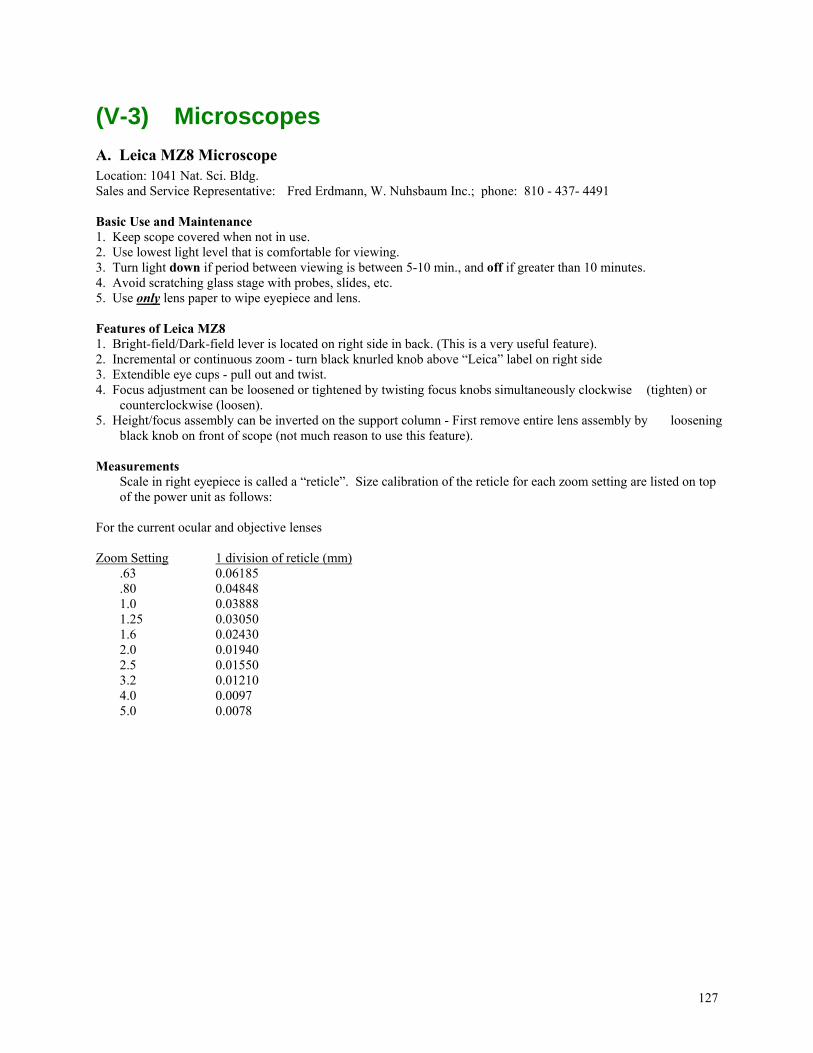
127

(V-3) Microscopes

A. Leica MZ8 Microscope Location: 1041 Nat. Sci. Bldg. Sales and Service Representative: Fred Erdmann, W. Nuhsbaum Inc.; phone: 810 - 437- 4491 Basic Use and Maintenance 1. Keep scope covered when not in use. 2. Use lowest light level that is comfortable for viewing. 3. Turn light down if period between viewing is between 5-10 min., and off if greater than 10 minutes. 4. Avoid scratching glass stage with probes, slides, etc. 5. Use only lens paper to wipe eyepiece and lens. Features of Leica MZ8 1. Bright-field/Dark-field lever is located on right side in back. (This is a very useful feature). 2. Incremental or continuous zoom - turn black knurled knob above “Leica” label on right side 3. Extendible eye cups - pull out and twist. 4. Focus adjustment can be loosened or tightened by twisting focus knobs simultaneously clockwise (tighten) or

counterclockwise (loosen). 5. Height/focus assembly can be inverted on the support column - First remove entire lens assembly by loosening

black knob on front of scope (not much reason to use this feature). Measurements Scale in right eyepiece is called a “reticle”. Size calibration of the reticle for each zoom setting are listed on top

of the power unit as follows: For the current ocular and objective lenses Zoom Setting 1 division of reticle (mm) .63 0.06185 .80 0.04848 1.0 0.03888 1.25 0.03050 1.6 0.02430 2.0 0.01940 2.5 0.01550 3.2 0.01210 4.0 0.0097 5.0 0.0078

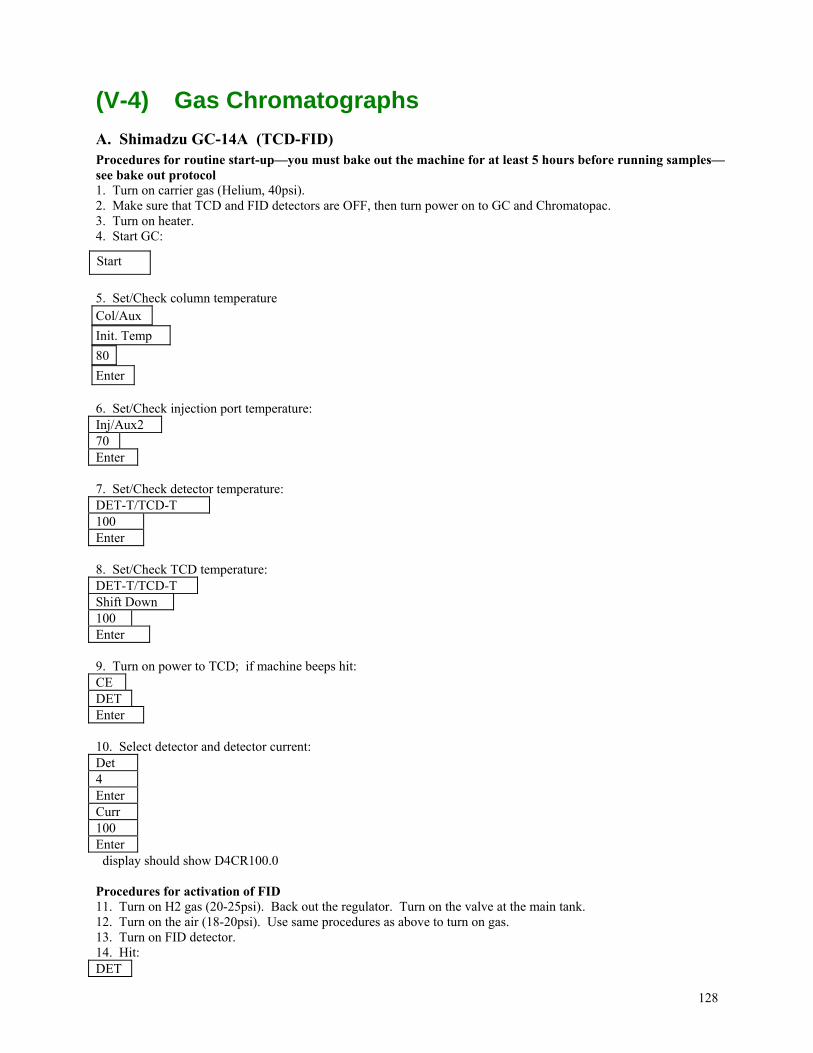
128

(V-4) Gas Chromatographs

A. Shimadzu GC-14A (TCD-FID) Procedures for routine start-up—you must bake out the machine for at least 5 hours before running samples—see bake out protocol 1. Turn on carrier gas (Helium, 40psi). 2. Make sure that TCD and FID detectors are OFF, then turn power on to GC and Chromatopac. 3. Turn on heater. 4. Start GC:

5. Set/Check column temperature Col/Aux

Init. Temp

80

Enter 6. Set/Check injection port temperature: Inj/Aux2 70 Enter 7. Set/Check detector temperature: DET-T/TCD-T 100 Enter 8. Set/Check TCD temperature: DET-T/TCD-T Shift Down 100 Enter 9. Turn on power to TCD; if machine beeps hit: CE DET Enter 10. Select detector and detector current: Det 4 Enter Curr 100 Enter display should show D4CR100.0 Procedures for activation of FID 11. Turn on H2 gas (20-25psi). Back out the regulator. Turn on the valve at the main tank. 12. Turn on the air (18-20psi). Use same procedures as above to turn on gas. 13. Turn on FID detector. 14. Hit: DET

Start

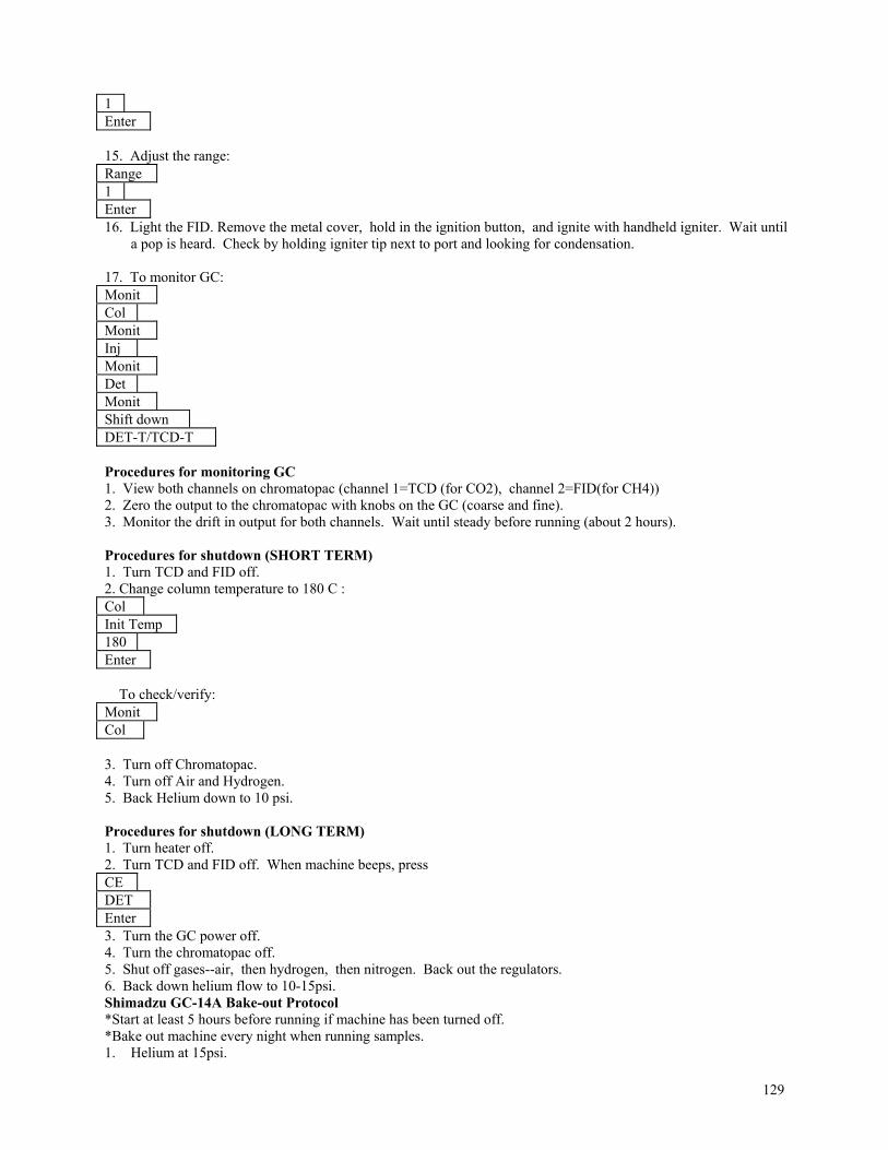
129

1 Enter 15. Adjust the range: Range 1 Enter 16. Light the FID. Remove the metal cover, hold in the ignition button, and ignite with handheld igniter. Wait until

a pop is heard. Check by holding igniter tip next to port and looking for condensation. 17. To monitor GC: Monit Col Monit Inj Monit Det Monit Shift down DET-T/TCD-T Procedures for monitoring GC 1. View both channels on chromatopac (channel 1=TCD (for CO2), channel 2=FID(for CH4)) 2. Zero the output to the chromatopac with knobs on the GC (coarse and fine). 3. Monitor the drift in output for both channels. Wait until steady before running (about 2 hours). Procedures for shutdown (SHORT TERM) 1. Turn TCD and FID off. 2. Change column temperature to 180 C : Col Init Temp 180 Enter To check/verify: Monit Col 3. Turn off Chromatopac. 4. Turn off Air and Hydrogen. 5. Back Helium down to 10 psi. Procedures for shutdown (LONG TERM) 1. Turn heater off. 2. Turn TCD and FID off. When machine beeps, press CE DET Enter 3. Turn the GC power off. 4. Turn the chromatopac off. 5. Shut off gases--air, then hydrogen, then nitrogen. Back out the regulators. 6. Back down helium flow to 10-15psi. Shimadzu GC-14A Bake-out Protocol *Start at least 5 hours before running if machine has been turned off. *Bake out machine every night when running samples. 1. Helium at 15psi.

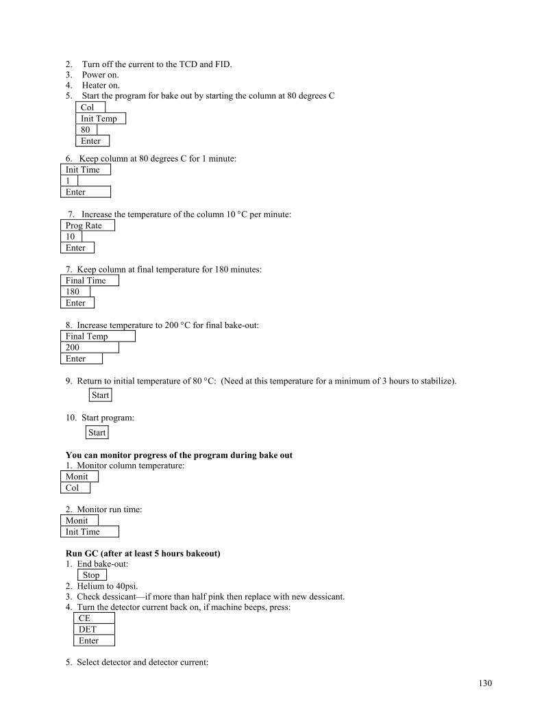
130

2. Turn off the current to the TCD and FID. 3. Power on. 4. Heater on. 5. Start the program for bake out by starting the column at 80 degrees C

6. Keep column at 80 degrees C for 1 minute: Init Time 1 Enter 7. Increase the temperature of the column 10 C per minute: Prog Rate 10 Enter 7. Keep column at final temperature for 180 minutes: Final Time 180 Enter 8. Increase temperature to 200 C for final bake-out: Final Temp 200 Enter 9. Return to initial temperature of 80 C: (Need at this temperature for a minimum of 3 hours to stabilize).

10. Start program:

You can monitor progress of the program during bake out 1. Monitor column temperature: Monit Col 2. Monitor run time: Monit Init Time Run GC (after at least 5 hours bakeout) 1. End bake-out:

Stop 2. Helium to 40psi. 3. Check dessicant—if more than half pink then replace with new dessicant. 4. Turn the detector current back on, if machine beeps, press:

CE DET Enter

5. Select detector and detector current:

Col Init Temp 80 Enter

Start

Start

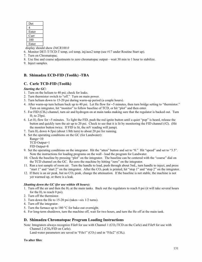
131

Det 4 Enter Curr 100 Enter

display should show D4CR100.0 6. Monitor DET-T/TCD-T temp, col temp, inj/aux2 temp (see #17 under Routine Start up). 7. Turn on Chromatopac. 8. Use fine and coarse adjustments to zero chromatopac output—wait 30 min to 1 hour to stabilize. 9. Inject samples.

B. Shimadzu ECD-FID (Toolik) -TBA

C. Carle TCD-FID (Toolik) Starting the GC: 1. Turn on the helium to 40 psi; check for leaks. 2. Turn thermistor switch to “off.” Turn on main power. 3. Turn helium down to 15-20 psi during warm-up period (a couple hours). 4. After warm-up turn helium back up to 40 psi. Let He flow for 5 minutes, then turn bridge setting to “thermistor.”

Turn on integrator, hit “monitor” to follow baseline of TCD, or hit “plot” and then enter. 5. For FID (CH4) channel, turn air and hydrogen on at main tanks making sure that the regulator is backed out. Turn

H2 to 25psi. 6. Let H2 flow for 5 minutes. To light the FID, push the red ignite button until a quiet “pop” is heard, release the

button and quickly turn the air up to 20 psi. Check to see that it is lit by monitoring the FID channel (#2). (Hit the monitor button twice. If FID is lit, the mV reading will jump).

7. Turn H2 down 4-5psi (about 1/8th turn) to about 20 psi for running. 8. Set the operating conditions on the GC (for Landwater): Range=10 TCD Output=1 FID Output=8 9. Set the operating conditions on the integrator. Hit the “atten” button and set to “0.” Hit “speed” and set to “3.5”.

Note the instructions for loading programs on the wall - load the program for Landwater. 10. Check the baseline by pressing “plot” on the integrator. The baseline can be centered with the “coarse” dial on

the TCD channel on the GC. Re-zero the machine by hitting “zero” on the integrator. 11. Run a test sample of room air. Turn the handle to load, push through about 5mL, turn handle to inject, and press

“start 1” and “start 2” on the integrator. After the CO2 peak is printed, hit “stop 1” and “stop 2” on the integrator. 12. If there is an air peak, but no CO2 peak, change the attenuation. If the baseline is not stable, the machine is not

yet warmed up, or there is a leak. Shutting down the GC (for use within 48 hours): 1. Turn off the air and then the H2 at the main tanks. Back out the regulators to reach 0 psi (it will take several hours

for the H2 to reach 0 psi). 2. Turn off the thermistor. 3. Turn down the He to 15-20 psi (takes six 1/2 turns). 4. Turn off the integrator. 5. Turn the furnace up to 180 C for bake-out overnight. 6. For long-term shutdown, turn the machine off, wait for two hours, and turn the He off at the main tank.

D. Shimadzu Chromatopac Program Loading Instructions Note: Integrators always recognize File0 for use with Channel 1 (CO2/TCD on the Carle) and File9 for use with

Channel 2 (CH4/FID on Carle). Land-water parameters are saved in “File1” (CO2) and in “File2” (CH4). To alter files:

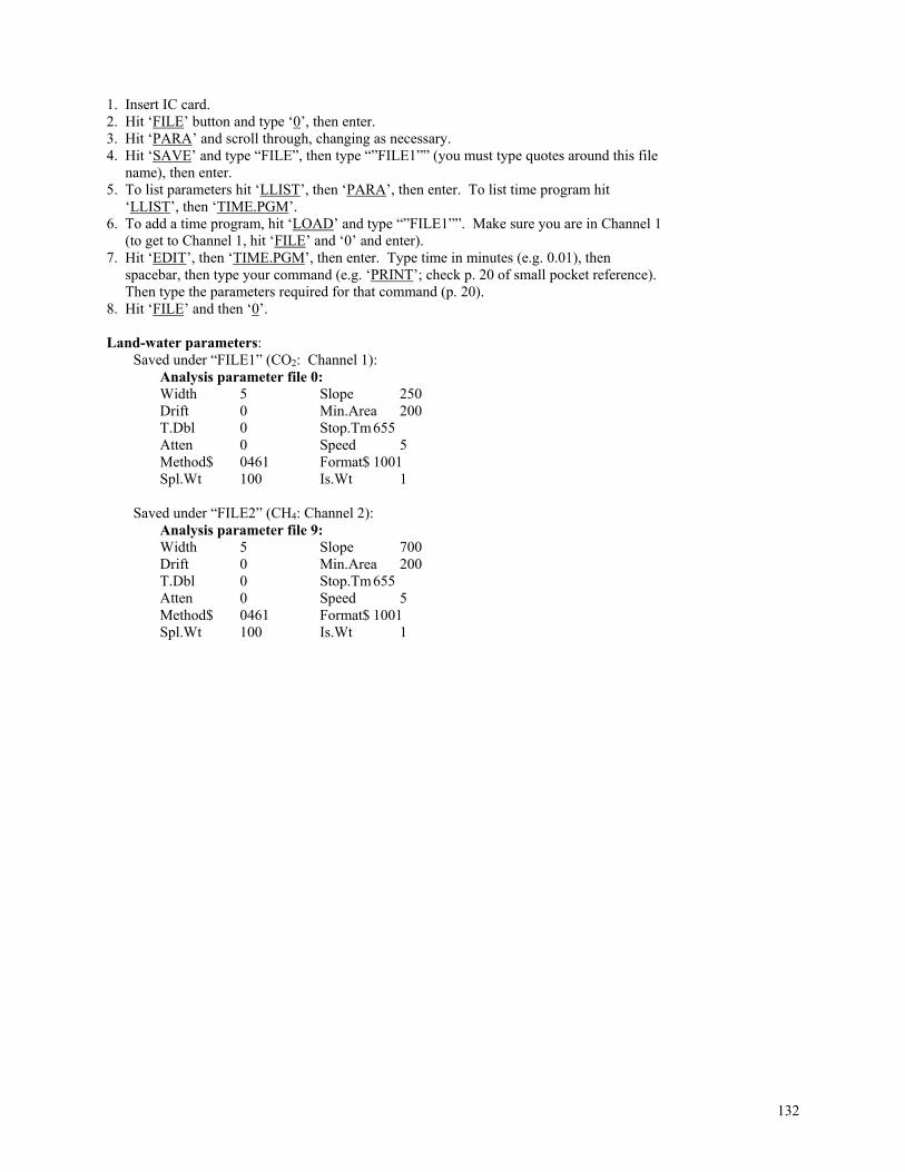
132

1. Insert IC card. 2. Hit ‘FILE’ button and type ‘0’, then enter. 3. Hit ‘PARA’ and scroll through, changing as necessary. 4. Hit ‘SAVE’ and type “FILE”, then type “”FILE1”” (you must type quotes around this file name), then enter. 5. To list parameters hit ‘LLIST’, then ‘PARA’, then enter. To list time program hit ‘LLIST’, then ‘TIME.PGM’. 6. To add a time program, hit ‘LOAD’ and type “”FILE1””. Make sure you are in Channel 1 (to get to Channel 1, hit ‘FILE’ and ‘0’ and enter). 7. Hit ‘EDIT’, then ‘TIME.PGM’, then enter. Type time in minutes (e.g. 0.01), then spacebar, then type your command (e.g. ‘PRINT’; check p. 20 of small pocket reference). Then type the parameters required for that command (p. 20). 8. Hit ‘FILE’ and then ‘0’. Land-water parameters: Saved under “FILE1” (CO2: Channel 1): Analysis parameter file 0: Width 5 Slope 250 Drift 0 Min.Area 200 T.Dbl 0 Stop.Tm 655 Atten 0 Speed 5 Method$ 0461 Format$ 1001 Spl.Wt 100 Is.Wt 1

Saved under “FILE2” (CH4: Channel 2): Analysis parameter file 9: Width 5 Slope 700 Drift 0 Min.Area 200 T.Dbl 0 Stop.Tm 655 Atten 0 Speed 5 Method$ 0461 Format$ 1001 Spl.Wt 100 Is.Wt 1

133

(V-5) Dionex Ion Chromatograph Anion Determination (Dionex ICS-1100) By JRL,JAD, October 2014, CLC March 2015 I. Overview This protocol is used to measure chloride and sulfate concentrations through ion chromatography. The method separates and measures all of the negatively charged anions present in a solution, and quantifies their concentrations based on a known standard curve.

Instrument information: Dionex ICS-1100 (purchased in December 2013, and installed March 2014) Serial Number: 14017772 Autosampler: Dionex AS-DV

Installation technician: Justin Kosewick (800) 346-6390 [email protected]

II. Supplies and reagents

A. Consumables Standards (from old protocol) 1. The anion stock standard solution is made by adding 1.1688g NaCl (biological grade) and 2.6141g

K2SO4 to 1 L of RO-DI H2O in a 1000 mL volumetric flask. The resulting stock standard solution has a concentration of 20 mM Cl and 15 mM SO4

2. Working standards are prepared from an intermediate anion stock solution of 0.5mM Cl and 0.375mM SO4. Make the intermediate stock solution by adding 25.0 mL Anion stock standard solution to a 1L volumetric flask. Bring to exactly 1000 mL volume with RO-DI water.

3. The following volumes of intermediate stock solution are added to 1 L volumetric flasks. Standard Concentration Volume of Intermediate Stock Added 0.5 M Cl / 0.375 M SO4 1ml 1.0 M Cl / 0.75 M SO4 2ml 2.0 M Cl / 1.5 M SO4 4ml

5.0 M Cl / 3.75 M SO4 10ml 10 M Cl / 7.5 M SO4 20ml 20 M Cl / 15M SO4 40ml

B. Eluent

With the purchase of the new ICS-1100, we also got eluent concentrate (cat # XXXXX). However it is possible to prepare eluent in the lab. Below is the method from the old protocol.

1. Anion eluent is a weak solution of sodium carbonate and sodium bicarbonate. The strength of the working solution is 3.5 mM Sodium carbonate plus 1.0 mM Sodium Bicarbonate. Our current method requires an eluent 4 times this concentration which is diluted with RO-DI water in the mixing manifold. Make up this 4x eluent in 8 L batches in the 8 L carboy on the sink.

2. To make 4X anion eluent, add 11.880 g Sodium Carbonate and 2.688 g Sodium Bicarbonate to a final 8 L of RO-DI H2O (see mark on 8L anion eluent carboy). First add the sodium carbonate and bicarbonate to 1 L RO-DI water in a 1 L reagent bottle and mix until reagents are completely dissolved. Then add this to 7 L of RO-DI water in the carboy and mix thoroughly (7 + 1 = 8 L).

3. All eluent must be thoroughly degassed before use on the machine. THIS INCLUDES ANY RO-DI WATER USED! Degassing is accomplished using l L pyrex reagent bottles placed in an ultra-sonicator bath under a vacuum of greater than 45 psi for 20 – 30 minutes or by placing the 1 L pyrex bottle on a stir plate with a stir bar at medium speed for 15 minutes under a vacuum. Close bottles tightly when finished and use eluent that day.

III. START-UP -- Powering on the machine and Chromeleon 1. Turn on the computer attached to the ICS-1100, make sure the blue chromeleon 7 “dongle” is inserted in a USB

port on the back of the computer. The instrument should be plugged into an ACS power backup system. 2. Turn on the ICS-1100, there is a switch in the back of the instrument near the top.

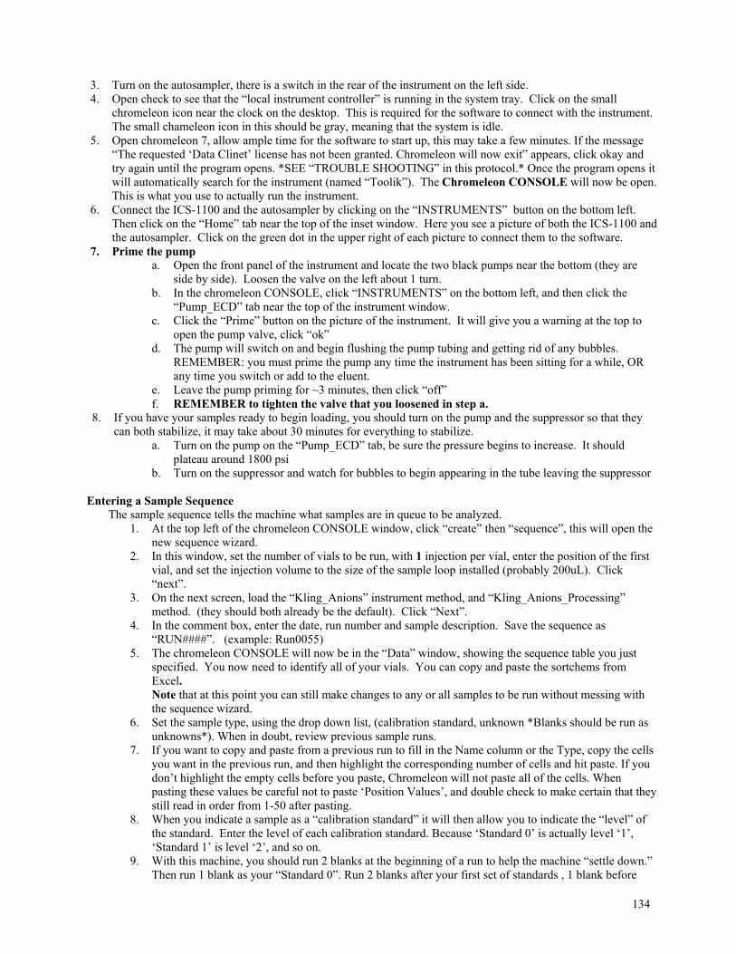
134

3. Turn on the autosampler, there is a switch in the rear of the instrument on the left side. 4. Open check to see that the “local instrument controller” is running in the system tray. Click on the small

chromeleon icon near the clock on the desktop. This is required for the software to connect with the instrument. The small chameleon icon in this should be gray, meaning that the system is idle.

5. Open chromeleon 7, allow ample time for the software to start up, this may take a few minutes. If the message “The requested ‘Data Clinet’ license has not been granted. Chromeleon will now exit” appears, click okay and try again until the program opens. *SEE “TROUBLE SHOOTING” in this protocol.* Once the program opens it will automatically search for the instrument (named “Toolik”). The Chromeleon CONSOLE will now be open. This is what you use to actually run the instrument.

6. Connect the ICS-1100 and the autosampler by clicking on the “INSTRUMENTS” button on the bottom left. Then click on the “Home” tab near the top of the inset window. Here you see a picture of both the ICS-1100 and the autosampler. Click on the green dot in the upper right of each picture to connect them to the software.

7. Prime the pump a. Open the front panel of the instrument and locate the two black pumps near the bottom (they are

side by side). Loosen the valve on the left about 1 turn. b. In the chromeleon CONSOLE, click “INSTRUMENTS” on the bottom left, and then click the

“Pump_ECD” tab near the top of the instrument window. c. Click the “Prime” button on the picture of the instrument. It will give you a warning at the top to

open the pump valve, click “ok” d. The pump will switch on and begin flushing the pump tubing and getting rid of any bubbles.

REMEMBER: you must prime the pump any time the instrument has been sitting for a while, OR any time you switch or add to the eluent.

e. Leave the pump priming for ~3 minutes, then click “off” f. REMEMBER to tighten the valve that you loosened in step a.

8. If you have your samples ready to begin loading, you should turn on the pump and the suppressor so that they can both stabilize, it may take about 30 minutes for everything to stabilize.

a. Turn on the pump on the “Pump_ECD” tab, be sure the pressure begins to increase. It should plateau around 1800 psi

b. Turn on the suppressor and watch for bubbles to begin appearing in the tube leaving the suppressor Entering a Sample Sequence

The sample sequence tells the machine what samples are in queue to be analyzed. 1. At the top left of the chromeleon CONSOLE window, click “create” then “sequence”, this will open the

new sequence wizard. 2. In this window, set the number of vials to be run, with 1 injection per vial, enter the position of the first

vial, and set the injection volume to the size of the sample loop installed (probably 200uL). Click “next”.

3. On the next screen, load the “Kling_Anions” instrument method, and “Kling_Anions_Processing” method. (they should both already be the default). Click “Next”.

4. In the comment box, enter the date, run number and sample description. Save the sequence as “RUN####”. (example: Run0055)

5. The chromeleon CONSOLE will now be in the “Data” window, showing the sequence table you just specified. You now need to identify all of your vials. You can copy and paste the sortchems from Excel. Note that at this point you can still make changes to any or all samples to be run without messing with the sequence wizard.

6. Set the sample type, using the drop down list, (calibration standard, unknown *Blanks should be run as unknowns*). When in doubt, review previous sample runs.

7. If you want to copy and paste from a previous run to fill in the Name column or the Type, copy the cells you want in the previous run, and then highlight the corresponding number of cells and hit paste. If you don’t highlight the empty cells before you paste, Chromeleon will not paste all of the cells. When pasting these values be careful not to paste ‘Position Values’, and double check to make certain that they still read in order from 1-50 after pasting.

8. When you indicate a sample as a “calibration standard” it will then allow you to indicate the “level” of the standard. Enter the level of each calibration standard. Because ‘Standard 0’ is actually level ‘1’, ‘Standard 1’ is level ‘2’, and so on.

9. With this machine, you should run 2 blanks at the beginning of a run to help the machine “settle down.” Then run 1 blank as your “Standard 0”. Run 2 blanks after your first set of standards , 1 blank before

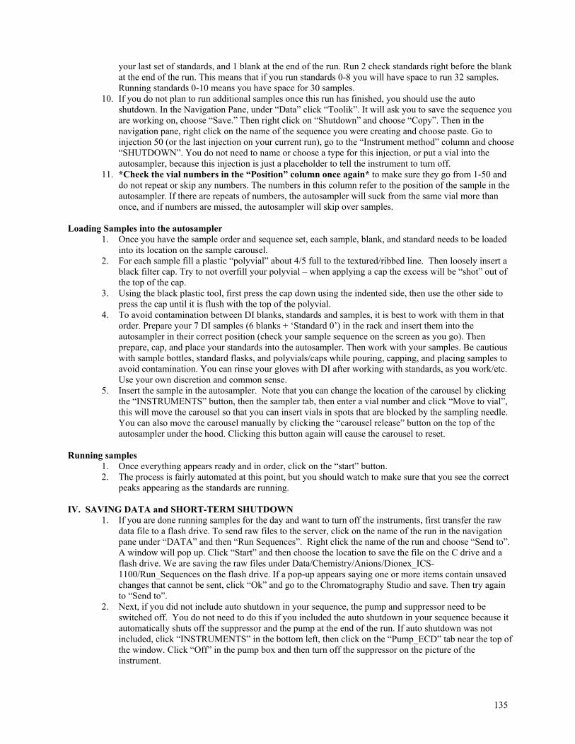
135

your last set of standards, and 1 blank at the end of the run. Run 2 check standards right before the blank at the end of the run. This means that if you run standards 0-8 you will have space to run 32 samples. Running standards 0-10 means you have space for 30 samples.

10. If you do not plan to run additional samples once this run has finished, you should use the auto shutdown. In the Navigation Pane, under “Data” click “Toolik”. It will ask you to save the sequence you are working on, choose “Save.” Then right click on “Shutdown” and choose “Copy”. Then in the navigation pane, right click on the name of the sequence you were creating and choose paste. Go to injection 50 (or the last injection on your current run), go to the “Instrument method” column and choose “SHUTDOWN”. You do not need to name or choose a type for this injection, or put a vial into the autosampler, because this injection is just a placeholder to tell the instrument to turn off.

11. *Check the vial numbers in the “Position” column once again* to make sure they go from 1-50 and do not repeat or skip any numbers. The numbers in this column refer to the position of the sample in the autosampler. If there are repeats of numbers, the autosampler will suck from the same vial more than once, and if numbers are missed, the autosampler will skip over samples.

Loading Samples into the autosampler 1. Once you have the sample order and sequence set, each sample, blank, and standard needs to be loaded

into its location on the sample carousel. 2. For each sample fill a plastic “polyvial” about 4/5 full to the textured/ribbed line. Then loosely insert a

black filter cap. Try to not overfill your polyvial – when applying a cap the excess will be “shot” out of the top of the cap.

3. Using the black plastic tool, first press the cap down using the indented side, then use the other side to press the cap until it is flush with the top of the polyvial.

4. To avoid contamination between DI blanks, standards and samples, it is best to work with them in that order. Prepare your 7 DI samples (6 blanks + ‘Standard 0’) in the rack and insert them into the autosampler in their correct position (check your sample sequence on the screen as you go). Then prepare, cap, and place your standards into the autosampler. Then work with your samples. Be cautious with sample bottles, standard flasks, and polyvials/caps while pouring, capping, and placing samples to avoid contamination. You can rinse your gloves with DI after working with standards, as you work/etc. Use your own discretion and common sense.

5. Insert the sample in the autosampler. Note that you can change the location of the carousel by clicking the “INSTRUMENTS” button, then the sampler tab, then enter a vial number and click “Move to vial”, this will move the carousel so that you can insert vials in spots that are blocked by the sampling needle. You can also move the carousel manually by clicking the “carousel release” button on the top of the autosampler under the hood. Clicking this button again will cause the carousel to reset.

Running samples

1. Once everything appears ready and in order, click on the “start” button. 2. The process is fairly automated at this point, but you should watch to make sure that you see the correct

peaks appearing as the standards are running. IV. SAVING DATA and SHORT-TERM SHUTDOWN

1. If you are done running samples for the day and want to turn off the instruments, first transfer the raw data file to a flash drive. To send raw files to the server, click on the name of the run in the navigation pane under “DATA” and then “Run Sequences”. Right click the name of the run and choose “Send to”. A window will pop up. Click “Start” and then choose the location to save the file on the C drive and a flash drive. We are saving the raw files under Data/Chemistry/Anions/Dionex_ICS-1100/Run_Sequences on the flash drive. If a pop-up appears saying one or more items contain unsaved changes that cannot be sent, click “Ok” and go to the Chromatography Studio and save. Then try again to “Send to”.

2. Next, if you did not include auto shutdown in your sequence, the pump and suppressor need to be switched off. You do not need to do this if you included the auto shutdown in your sequence because it automatically shuts off the suppressor and the pump at the end of the run. If auto shutdown was not included, click “INSTRUMENTS” in the bottom left, then click on the “Pump_ECD” tab near the top of the window. Click “Off” in the pump box and then turn off the suppressor on the picture of the instrument.

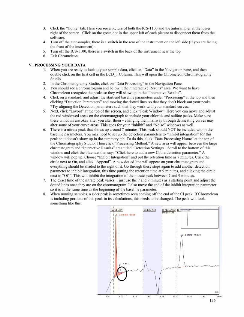
136

3. Click the “Home” tab. Here you see a picture of both the ICS-1100 and the autosampler at the lower right of the screen. Click on the green dot in the upper left of each picture to disconnect them from the software.

4. Turn off the autosampler, there is a switch in the rear of the instrument on the left side (if you are facing the front of the instrument).

5. Turn off the ICS-1100, there is a switch in the back of the instrument near the top. 6. Exit Chromeleon.

V. PROCESSING YOUR DATA

1. When you are ready to look at your sample data, click on “Data” in the Navigation pane, and then double click on the first cell in the ECD_1 Column. This will open the Chromeleon Chromatography Studio.

2. In the Chromatography Studio, click on “Data Processing” in the Navigation Pane. 3. You should see a chromatogram and below it the “Interactive Results” area. We want to have

Chromeleon recognize the peaks so they will show up in the “Interactive Results”. 4. Click on a standard, and adjust the start/end baseline parameters under “Processing” at the top and then

clicking “Detection Parameters” and moving the dotted lines so that they don’t block out your peaks. *Try aligning the Detection parameters such that they work with your standard curves.

5. Next, click “Layout” at the top of the screen, and click “Peak Window”. Here you can move and adjust the red windowed areas on the chromatograph to include your chloride and sulfate peaks. Make sure these windows are okay after you alter them – changing them halfway through delineating curves may alter some of your curve areas. This goes for your “Inhibit” and “Noise” windows as well.

6. There is a nitrate peak that shows up around 7 minutes. This peak should NOT be included within the baseline parameters. You may need to set up the detection parameters to “inhibit integration” for this peak so it doesn’t show up in the summary tab. To do this, click “Data Processing Home” at the top of the Chromatography Studio. Then click “Processing Method.” A new area will appear between the large chromatogram and “Interactive Results” area titled “Detection Settings.” Scroll to the bottom of this window and click the blue text that says “Click here to add a new Cobra detection parameter.” A window will pop up. Choose “Inhibit Integration” and put the retention time as 7 minutes. Click the circle next to On, and click “Append”. A new dotted line will appear on your chromatogram and everything should be shaded to the right of it. Go through these steps again to add another detection parameter to inhibit integration, this time putting the retention time at 9 minutes, and clicking the circle next to “Off”. This will inhibit the integration of the nitrate peak between 7 and 9 minutes.

7. The exact time of the nitrate peak varies. I just use the 7 and 9 minutes as a starting point and adjust the dotted lines once they are on the chromatogram. I also move the end of the inhibit integration parameter so it is at the same time as the beginning of the baseline parameter.

8. When running samples, a rider peak is sometimes seen coming off the end of the Cl peak. If Chromeleon is including portions of this peak in its calculations, this needs to be changed. The peak will look something like this:

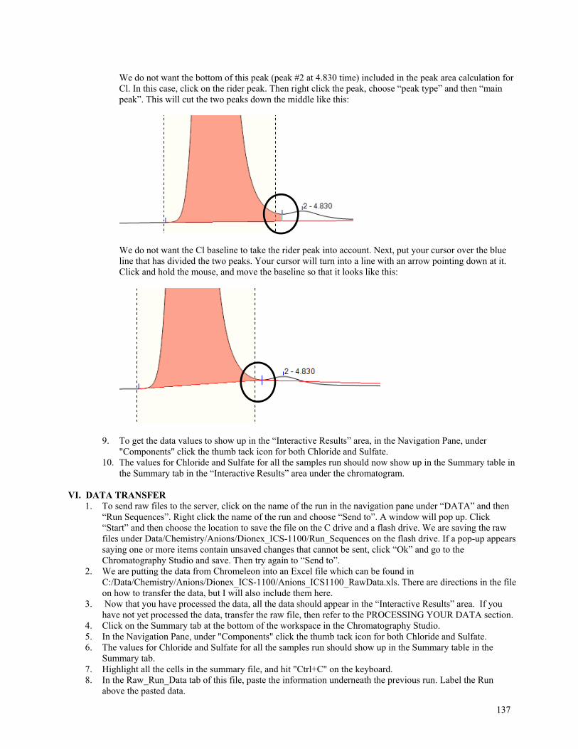
137

We do not want the bottom of this peak (peak #2 at 4.830 time) included in the peak area calculation for Cl. In this case, click on the rider peak. Then right click the peak, choose “peak type” and then “main peak”. This will cut the two peaks down the middle like this:

We do not want the Cl baseline to take the rider peak into account. Next, put your cursor over the blue line that has divided the two peaks. Your cursor will turn into a line with an arrow pointing down at it. Click and hold the mouse, and move the baseline so that it looks like this:

9. To get the data values to show up in the “Interactive Results” area, in the Navigation Pane, under "Components" click the thumb tack icon for both Chloride and Sulfate.

10. The values for Chloride and Sulfate for all the samples run should now show up in the Summary table in the Summary tab in the “Interactive Results” area under the chromatogram.

VI. DATA TRANSFER 1. To send raw files to the server, click on the name of the run in the navigation pane under “DATA” and then

“Run Sequences”. Right click the name of the run and choose “Send to”. A window will pop up. Click “Start” and then choose the location to save the file on the C drive and a flash drive. We are saving the raw files under Data/Chemistry/Anions/Dionex_ICS-1100/Run_Sequences on the flash drive. If a pop-up appears saying one or more items contain unsaved changes that cannot be sent, click “Ok” and go to the Chromatography Studio and save. Then try again to “Send to”.

2. We are putting the data from Chromeleon into an Excel file which can be found in C:/Data/Chemistry/Anions/Dionex_ICS-1100/Anions_ICS1100_RawData.xls. There are directions in the file on how to transfer the data, but I will also include them here.

3. Now that you have processed the data, all the data should appear in the “Interactive Results” area. If you have not yet processed the data, transfer the raw file, then refer to the PROCESSING YOUR DATA section.

4. Click on the Summary tab at the bottom of the workspace in the Chromatography Studio. 5. In the Navigation Pane, under "Components" click the thumb tack icon for both Chloride and Sulfate. 6. The values for Chloride and Sulfate for all the samples run should show up in the Summary table in the

Summary tab. 7. Highlight all the cells in the summary file, and hit "Ctrl+C" on the keyboard. 8. In the Raw_Run_Data tab of this file, paste the information underneath the previous run. Label the Run

above the pasted data.

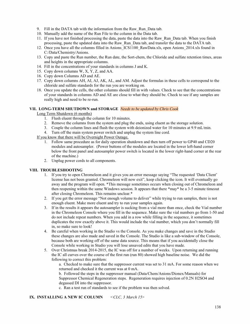
138

9. Fill in the DATA tab with the information from the Raw_Run_Data tab. 10. Manually add the name of the Run File to the column in the Data tab. 11. If you have not finished processing the data, paste the data into the Raw_Run_Data tab. When you finish

processing, paste the updated data into the Raw_Run_Data tab, and transfer the data to the DATA tab. 12. Once you have all the columns filled in Anions_ICS1100_RawData.xls, open Anions_2014.xls found in

C:/Data/Chemistry/Anions. 13. Copy and paste the Run number, the Run date, the Sort-chem, the Chloride and sulfate retention times, areas

and heights in the appropriate columns. 14. Fill in the concentrations of your standards in columns J and K. 15. Copy down columns W, X, Y, Z, and AA. 16. Copy down Columns AD and AE. 17. Copy down columns AH, AI, AJ, AK, AL, and AM. Adjust the formulas in these cells to correspond to the

chloride and sulfate standards for the run you are working on. 18. Once you update the cells, the other columns should fill in with values. Check to see that the concentrations

of your standards in columns AD and AE are close to what they should be. Check to see if any samples are really high and need to be re-run.

VII. LONG-TERM SHUTDOWN and STORAGE Needs to be updated by Chris Cook

Long Term Shutdown (6 months) 1. Flush eluent through the column for 10 minutes. 2. Remove the columns from the system and plug the ends, using eluent as the storage solution. 3. Couple the column lines and flush the system with deionized water for 10 minutes at 9.9 mL/min. 4. Turn off the main system power switch and unplug the system line cord.

If you know that there will be Overnight Power Outage, 1. Follow same procedure as for daily operation shutdown and then turn off power to GP40 and CD20

modules and autosampler. (Power buttons of the modules are located in the lower left-hand corner below the front panel and autosampler power switch is located in the lower right-hand corner at the rear of the machine.)

2. Unplug power cords to all components.

VIII. TROUBLESHOOTING 1. If you try to open Chromeleon and it gives you an error message saying “The requested ‘Data Client’

license has not been granted. Chromeleon will now exit”, keep clicking the icon. It will eventually go away and the program will open. *This message sometimes occurs when closing out of Chromeleon and then reopening within the same Windows session. It appears that there *may* be a 3-5 minute timeout after closing Chromeleon. This remains unclear.*

2. If you get the error message “Not enough volume to deliver” while trying to run samples, there is not enough eluent. Make more eluent and try to run your samples again.

3. If in the results it appears the autosampler is sucking from a vial more than once, check the Vial number in the Chromeleon Console where you fill in the sequence. Make sure the vial numbers go from 1-50 and do not include repeat numbers. When you add in a row while filling in the sequence, it sometimes duplicates the row exactly above it. This would include the vial number, which you don’t normally fill in, so make sure to look!

4. Be careful when working in the Studio vs the Console. As you make changes and save in the Studio these changes are also made and saved in the Console. The Studio is like a sub-window of the Console, because both are working off of the same data source. This means that if you accidentally close the Console while working in Studio you will lose unsaved edits that you have made.

5. Over Christmas break 2014-2015, the IC was off for a number of weeks. Upon returning and running the IC all curves over the course of the first run (run 80) showed high baseline noise. We did the following to correct this problem:

a. Checked to make sure that the suppressor current was set to 31 mA. For some reason when we returned and checked it the current was at 0 mA. b. Followed the steps in the suppressor manual (Data/Chem/Anions/Dionex/Manuals) for Suppressor Chemical Regeneration steps. Regeneration requires injection of 0.2N H2SO4 and degassed DI into the suppressor. c. Ran a test run of standards to see if the problem was then solved.

IX. INSTALLING A NEW IC COLUMN <CLC, 3 March 15>

139

The column in the IC-1100 was replaced in March of 2015, the first one being installed in March of 2014. It lasted almost exactly 100 runs before the chloride curve was getting too close to the conductivity pit that occurs between 2 and 3 minutes in retention time. Here are the directions for installing a new column and column guard in the ICS-1100.

1. Make sure that the IC is disconnected and turned OFF. Use the small wrench in the anion supplies drawer to disconnect the old guard “inlet” and column “outlet” lines.

2. Remove the protective ferrules from the NEW guard and column. *Be sure to save the new frits that come with the new guard and column.*

3. Write the install date on the outside of the NEW guard and NEW column. 4. Remove the “guard out”/”column in” line from the OLD guard and OLD column and connect it in the

same orientation to the NEW guard and NEW column. 5. Reconnect the NEW column and guard, making sure to plug the lines all the way into the guard inlet/

column outlet, and THEN twist the ferrules so that these lines are held securely in place, making sure as you do so that the guard and column are in the right order and orientation such that the “flow” mark points from the guard, to the column, to the suppressor.

6. Attach the “column out” line to the NEW column outlet, and leave the “eluent in” portion of this line disconnected from the suppressor.

7. Turn on the IC and connect to the IC using Chromeleon. Prime the pump for three minutes. 8. Stop the pump priming. Direct the “column out” line into a waste container (allow the “eluent in” end of

the line to drip into a waste beaker). 9. Turn the pump to “ON”, LEAVE THE SUPPRESSOR SET TO “OFF”. 10. Turn on “Monitor Background” conductivity in the PUMP_ECD Tab of the Chromeleon Console. Allow

the pump to move eluent through the column for 45 minutes – 1 hour, or until conductivity is constant. 11. Once baseline conductivity is flat, turn the pump to “OFF”. Leave “Monitor Background” ON.

Reconnect the “eluent in” side of the “column out” line to the suppressor, again being certain to insert the line as deep into the suppressor as possible and THEN tighten the ferrule to hold the line in place. You should see a spike in the conductivity in the plot Chromeleon console.

12. After connecting the line, turn the pump back to “ON”, and turn the suppressor to “ON”, making sure that current is set to 31 mA (suppressor box in the PUMP_ECD tab in Chromeleon Console).

13. Allow the column/pump/suppressor to move eluent through the system for at least an hour, at least until conductivity is constant. Pressure should be around 1900 psi and conductivity around 21.77 uS.

14. Turn off the machine or start a run of standards to test the new column. X. INSTALLING CHROMELEON ON A NEW COMPUTER <INCOMPLETE as of June 2015> In 2014 the computer that was being used to run the IC failed. Here are the necessary steps to back up data, deal

with software licensing, deal with data vault issues, and the ultimate software re-install. BACKING UP YOUR DATA:

1. Finish processing all files from runs that have been completed BEFORE you start the backup. 2. Double check to make sure that all of the “raw curve” data (.cmbx files in the following location:

Data/Chemistry/Anions/Dionex_ICS-1100/Run_Sequences) are backed up on you work computer hard-drive and on the Lab Server. Also back up any other files associated with data processing.

SOFTWARE LICENSING:

1. The software license for Chromeleon is automatically moved onto the computer you are using when you initially plug in the “blue dongle”. The license file, ‘Chromeleon7_156349.cmlic” was copied and placed onto the server on 17-Dec-2014 under Data/Chemistry/Anions/Dionex_ICS-1100/Manuals. The number ‘156349’ is our personal serial number of the License File. This number must match the serial number of the License Key (‘the blue dongle’) for the installation to work.

SOFTWARE INSTALL:

1. This information can be found in the Chromeleon 7.2 Installation Guide (in the Chromeleon Black Box) under Section 5.5.2 “Using an ‘Empty’ License Key and a separate License File”.

2. Install troubleshooting can be found under Section 5.6

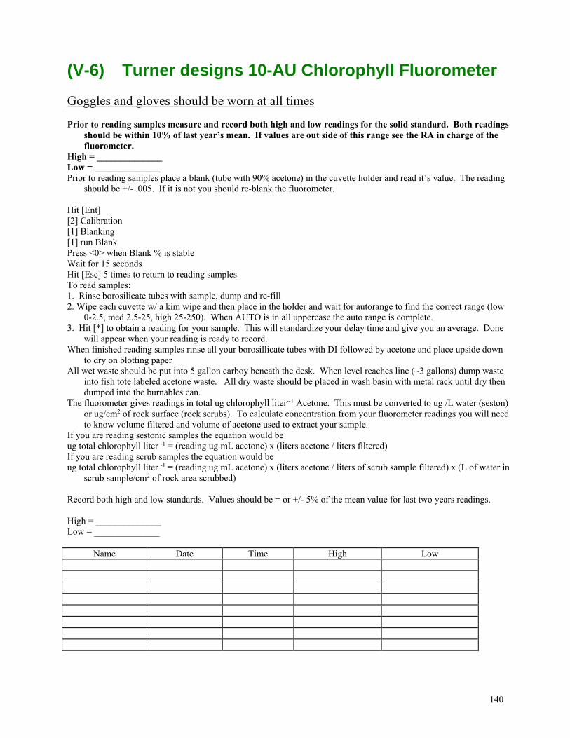
140

(V-6) Turner designs 10-AU Chlorophyll Fluorometer

Goggles and gloves should be worn at all times Prior to reading samples measure and record both high and low readings for the solid standard. Both readings

should be within 10% of last year’s mean. If values are out side of this range see the RA in charge of the fluorometer.

High = ______________ Low = ______________ Prior to reading samples place a blank (tube with 90% acetone) in the cuvette holder and read it’s value. The reading

should be +/- .005. If it is not you should re-blank the fluorometer. Hit [Ent] [2] Calibration [1] Blanking [1] run Blank Press <0> when Blank % is stable Wait for 15 seconds Hit [Esc] 5 times to return to reading samples To read samples: 1. Rinse borosilicate tubes with sample, dump and re-fill 2. Wipe each cuvette w/ a kim wipe and then place in the holder and wait for autorange to find the correct range (low

0-2.5, med 2.5-25, high 25-250). When AUTO is in all uppercase the auto range is complete. 3. Hit [*] to obtain a reading for your sample. This will standardize your delay time and give you an average. Done

will appear when your reading is ready to record. When finished reading samples rinse all your borosillicate tubes with DI followed by acetone and place upside down

to dry on blotting paper All wet waste should be put into 5 gallon carboy beneath the desk. When level reaches line (~3 gallons) dump waste

into fish tote labeled acetone waste. All dry waste should be placed in wash basin with metal rack until dry then dumped into the burnables can.

The fluorometer gives readings in total ug chlorophyll liter--1 Acetone. This must be converted to ug /L water (seston) or ug/cm2 of rock surface (rock scrubs). To calculate concentration from your fluorometer readings you will need to know volume filtered and volume of acetone used to extract your sample.

If you are reading sestonic samples the equation would be ug total chlorophyll liter -1 = (reading ug mL acetone) x (liters acetone / liters filtered) If you are reading scrub samples the equation would be ug total chlorophyll liter -1 = (reading ug mL acetone) x (liters acetone / liters of scrub sample filtered) x (L of water in

scrub sample/cm2 of rock area scrubbed) Record both high and low standards. Values should be = or +/- 5% of the mean value for last two years readings. High = ______________ Low = ______________

Name Date Time High Low

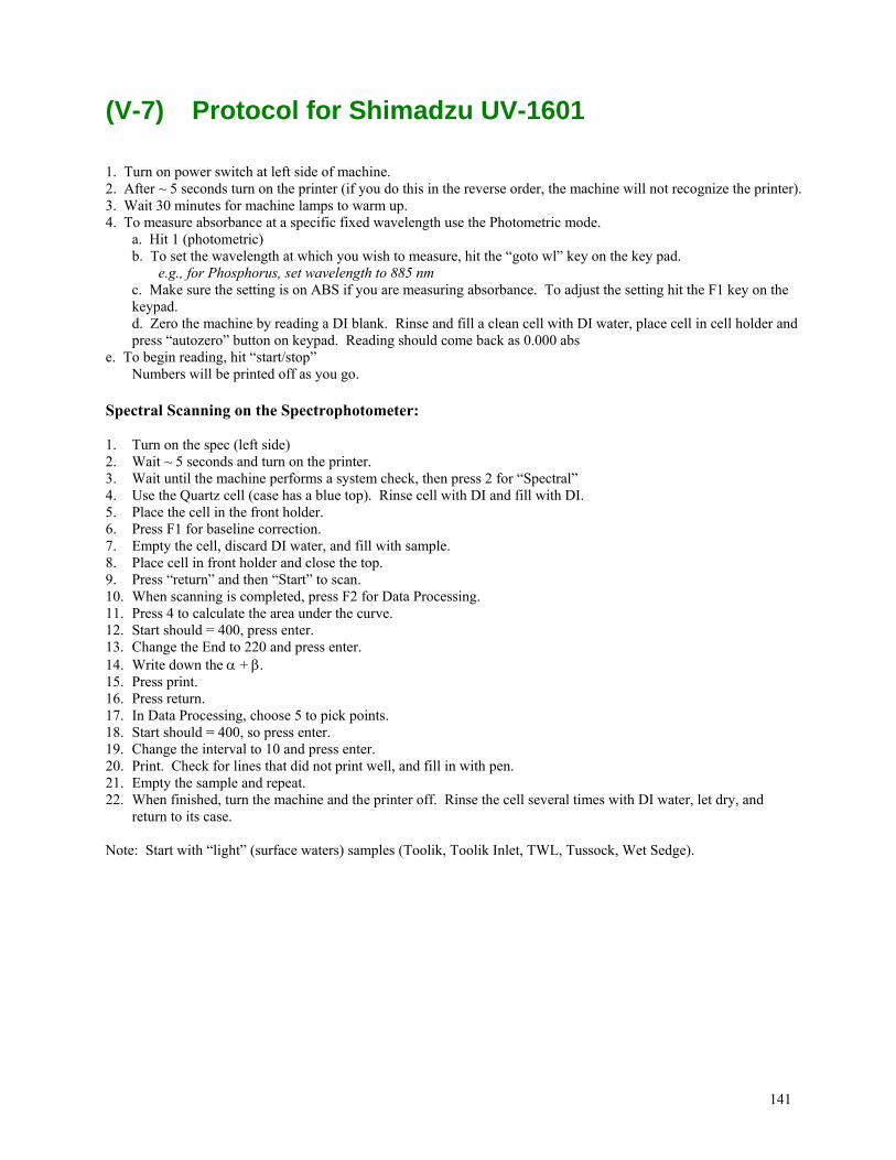
141

(V-7) Protocol for Shimadzu UV-1601 1. Turn on power switch at left side of machine. 2. After ~ 5 seconds turn on the printer (if you do this in the reverse order, the machine will not recognize the printer). 3. Wait 30 minutes for machine lamps to warm up. 4. To measure absorbance at a specific fixed wavelength use the Photometric mode. a. Hit 1 (photometric) b. To set the wavelength at which you wish to measure, hit the “goto wl” key on the key pad. e.g., for Phosphorus, set wavelength to 885 nm c. Make sure the setting is on ABS if you are measuring absorbance. To adjust the setting hit the F1 key on the

keypad. d. Zero the machine by reading a DI blank. Rinse and fill a clean cell with DI water, place cell in cell holder and

press “autozero” button on keypad. Reading should come back as 0.000 abs e. To begin reading, hit “start/stop” Numbers will be printed off as you go. Spectral Scanning on the Spectrophotometer: 1. Turn on the spec (left side) 2. Wait ~ 5 seconds and turn on the printer. 3. Wait until the machine performs a system check, then press 2 for “Spectral” 4. Use the Quartz cell (case has a blue top). Rinse cell with DI and fill with DI. 5. Place the cell in the front holder. 6. Press F1 for baseline correction. 7. Empty the cell, discard DI water, and fill with sample. 8. Place cell in front holder and close the top. 9. Press “return” and then “Start” to scan. 10. When scanning is completed, press F2 for Data Processing. 11. Press 4 to calculate the area under the curve. 12. Start should = 400, press enter. 13. Change the End to 220 and press enter. 14. Write down the + . 15. Press print. 16. Press return. 17. In Data Processing, choose 5 to pick points. 18. Start should = 400, so press enter. 19. Change the interval to 10 and press enter. 20. Print. Check for lines that did not print well, and fill in with pen. 21. Empty the sample and repeat. 22. When finished, turn the machine and the printer off. Rinse the cell several times with DI water, let dry, and

return to its case. Note: Start with “light” (surface waters) samples (Toolik, Toolik Inlet, TWL, Tussock, Wet Sedge).

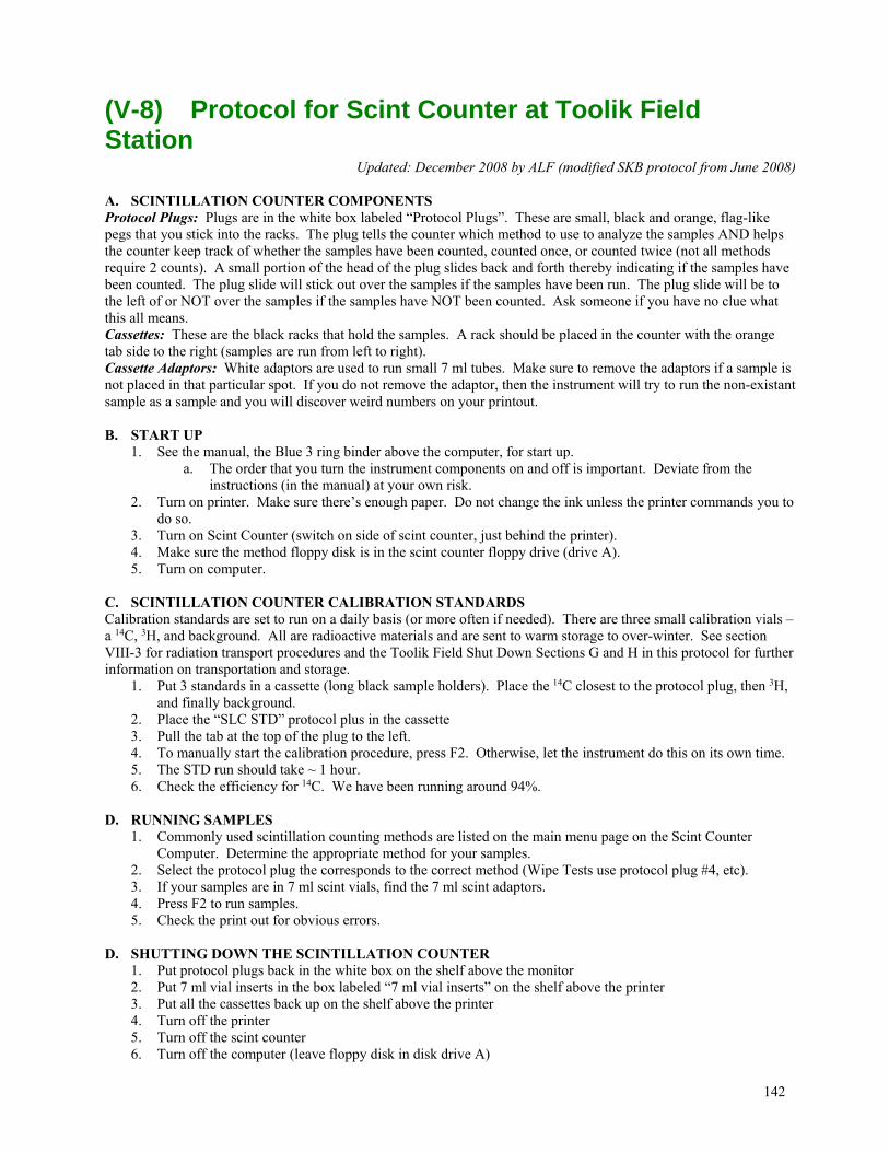
142

(V-8) Protocol for Scint Counter at Toolik Field Station

Updated: December 2008 by ALF (modified SKB protocol from June 2008) A. SCINTILLATION COUNTER COMPONENTS Protocol Plugs: Plugs are in the white box labeled “Protocol Plugs”. These are small, black and orange, flag-like pegs that you stick into the racks. The plug tells the counter which method to use to analyze the samples AND helps the counter keep track of whether the samples have been counted, counted once, or counted twice (not all methods require 2 counts). A small portion of the head of the plug slides back and forth thereby indicating if the samples have been counted. The plug slide will stick out over the samples if the samples have been run. The plug slide will be to the left of or NOT over the samples if the samples have NOT been counted. Ask someone if you have no clue what this all means. Cassettes: These are the black racks that hold the samples. A rack should be placed in the counter with the orange tab side to the right (samples are run from left to right). Cassette Adaptors: White adaptors are used to run small 7 ml tubes. Make sure to remove the adaptors if a sample is not placed in that particular spot. If you do not remove the adaptor, then the instrument will try to run the non-existant sample as a sample and you will discover weird numbers on your printout. B. START UP

1. See the manual, the Blue 3 ring binder above the computer, for start up. a. The order that you turn the instrument components on and off is important. Deviate from the

instructions (in the manual) at your own risk. 2. Turn on printer. Make sure there’s enough paper. Do not change the ink unless the printer commands you to

do so. 3. Turn on Scint Counter (switch on side of scint counter, just behind the printer). 4. Make sure the method floppy disk is in the scint counter floppy drive (drive A). 5. Turn on computer.

C. SCINTILLATION COUNTER CALIBRATION STANDARDS Calibration standards are set to run on a daily basis (or more often if needed). There are three small calibration vials – a 14C, 3H, and background. All are radioactive materials and are sent to warm storage to over-winter. See section VIII-3 for radiation transport procedures and the Toolik Field Shut Down Sections G and H in this protocol for further information on transportation and storage.

1. Put 3 standards in a cassette (long black sample holders). Place the 14C closest to the protocol plug, then 3H, and finally background.

2. Place the “SLC STD” protocol plus in the cassette 3. Pull the tab at the top of the plug to the left. 4. To manually start the calibration procedure, press F2. Otherwise, let the instrument do this on its own time. 5. The STD run should take ~ 1 hour. 6. Check the efficiency for 14C. We have been running around 94%.

D. RUNNING SAMPLES

1. Commonly used scintillation counting methods are listed on the main menu page on the Scint Counter Computer. Determine the appropriate method for your samples.

2. Select the protocol plug the corresponds to the correct method (Wipe Tests use protocol plug #4, etc). 3. If your samples are in 7 ml scint vials, find the 7 ml scint adaptors. 4. Press F2 to run samples. 5. Check the print out for obvious errors.

D. SHUTTING DOWN THE SCINTILLATION COUNTER

1. Put protocol plugs back in the white box on the shelf above the monitor 2. Put 7 ml vial inserts in the box labeled “7 ml vial inserts” on the shelf above the printer 3. Put all the cassettes back up on the shelf above the printer 4. Turn off the printer 5. Turn off the scint counter 6. Turn off the computer (leave floppy disk in disk drive A)

143

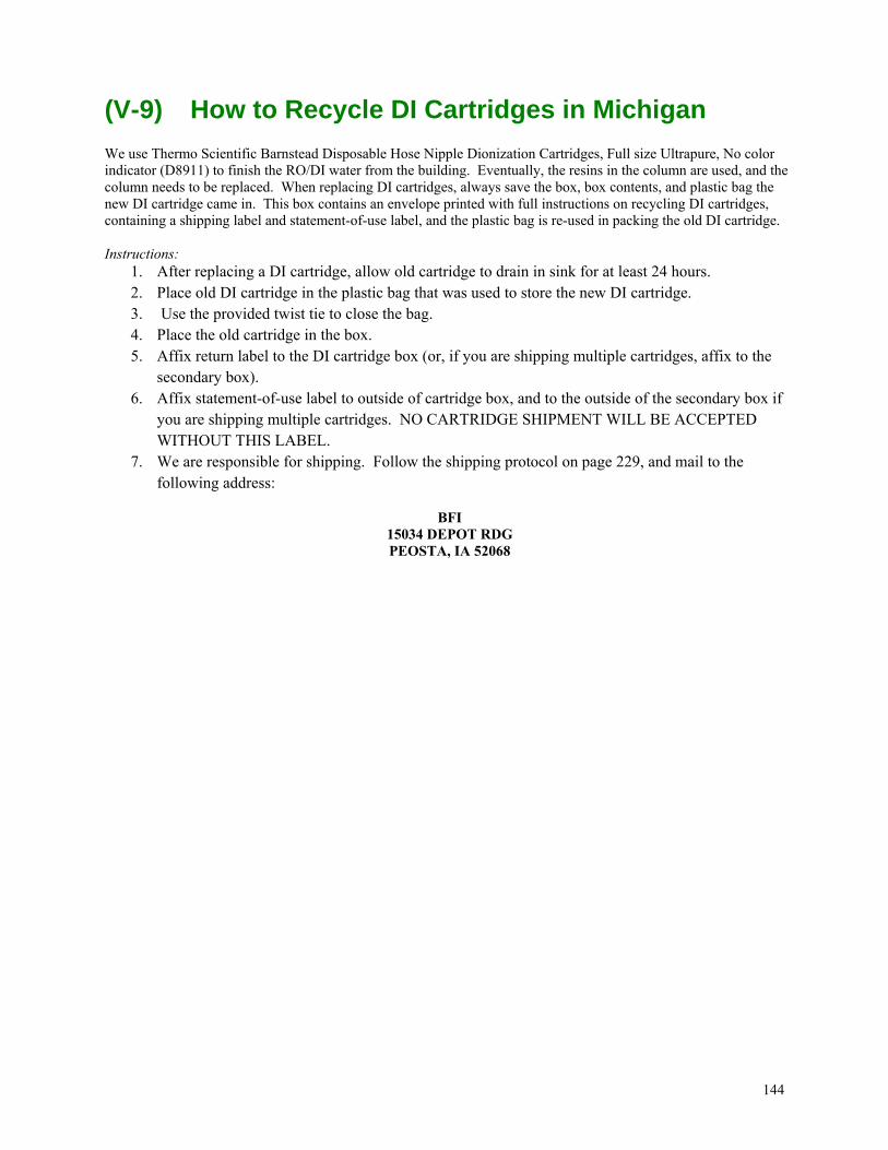
144

(V-9) How to Recycle DI Cartridges in Michigan We use Thermo Scientific Barnstead Disposable Hose Nipple Dionization Cartridges, Full size Ultrapure, No color indicator (D8911) to finish the RO/DI water from the building. Eventually, the resins in the column are used, and the column needs to be replaced. When replacing DI cartridges, always save the box, box contents, and plastic bag the new DI cartridge came in. This box contains an envelope printed with full instructions on recycling DI cartridges, containing a shipping label and statement-of-use label, and the plastic bag is re-used in packing the old DI cartridge. Instructions:

1. After replacing a DI cartridge, allow old cartridge to drain in sink for at least 24 hours. 2. Place old DI cartridge in the plastic bag that was used to store the new DI cartridge. 3. Use the provided twist tie to close the bag. 4. Place the old cartridge in the box. 5. Affix return label to the DI cartridge box (or, if you are shipping multiple cartridges, affix to the

secondary box). 6. Affix statement-of-use label to outside of cartridge box, and to the outside of the secondary box if

you are shipping multiple cartridges. NO CARTRIDGE SHIPMENT WILL BE ACCEPTED WITHOUT THIS LABEL.

7. We are responsible for shipping. Follow the shipping protocol on page 229, and mail to the following address:

BFI 15034 DEPOT RDG PEOSTA, IA 52068

145

(V-10) How to Install SAS (v 9.2)

Updated 16 Nov 2010, LRY (The following instructions no longer apply. We must get Rob or Adam to install programs as we can’t access the software distribution site anymore.) To get to the LSA software distribution site and the SAS program files, go to Start → Run, and type: \\lsa\dfs\Swdist\s\SAS Copy files, and save to: C:\Program Files\SAS To install, run the following file: Setup.exe You will then be prompted through the SAS installation process. To license SAS, you will need to run the SAS licensing wizard application. Start → All Programs → SAS → SAS 9.2 License Renewal & Utilities For “Step 1. Select a SAS installation data file”, type in the address of the “SID” text file. This file contains the license renewal information. If you can’t locate this file, go back to the LSA Software distribution files, and copy it over to your SAS program folder: Example: C:\Program Files\SAS\ SAS92_SID_Win.txt After typing in the address of the SID file (including the file name), click “Okay”. You should next see a popup window indicating that you are “licensed for the software listed below.” Click “Okay”. Next, you will need to type in the address of the SAS installation file (the .exe file). You do not need to include the file name this time. The address may automatically be filled in for you. Example : C:\Program Files\SAS\ Click “Okay”. After completing this step, you should see a popup window indicating that license renewal was successful.

146

Section VI - Lab Methods

(VI-1) CO2 and CH4 Determination A. Follow directions for the starting the GC you will use – these directions are in the GC Startup section of

the Protocol book, or are hanging near the machines. Ensure that the GC has had time to stabilize in temperature, and that the desiccant does not need to be changed.

B. Visually inspect the nylon syringes and ensure that there is no water in the sample or the stopcock, as

water has adverse affects on analysis. Clean out the water with a rolled up kimwipe. If water is inside the syringe, make a note in the computer file and run the sample.

C. Use calibrated standards to create a standard curve bracketing the range of your samples. There are

dedicated syringes for each standard concentration; these should be flushed 3 times each with the standard before filling the syringe the final time. Run at least 2 (3 is better) replicate injections of each standard. Check that replicate values are obtained for each standard, then proceed with sample analysis.

D. With the stopcock still closed, “break” the seal on the nylon syringe by pushing gently on the plunger.

Turn the valve on the GC to the “load” position. Open the nylon syringe and inject ~1/2 of the gas you have in the syringe, or at minimum ~5 cc of gas. Count for 4 seconds then turn valve on GC to “inject” and ensure that Chromatopac is running.

E. Record syringe number, sample ID information, equilibration temperature, gas:water ratio, and peak areas

in the gas book and on the chromatogram, and type this into the computer. F. Rerun any sample that follows an unusually high sample, or any other sample that you may question.

Also rerun standards at the end of a long run to ensure that the machine has not drifted during analysis.

147

(VI-2) DIC Determination (using HgCl2 samples) A. Use a clean 60 mL syringe marked as “DIC” and a long metal needle for a tip. B. Push down on the plunger with force to expel all air. Draw in 3-4 mL of 0.2N sulfuric acid. Draw in air

and slowly move the air bubble from the tail to the tip so that it removes small air bubbles. Tap the side of the syringe to remove small bubbles clinging to the rubber plunger.

C. Tap the syringe with the tip pointed upwards to force any remaining air bubbles to the top. Then expel air bubbles and acid until there is a little more than 1mL (1-1/2mL) of acid in the syringe.

D. Insert the DIC needle into the septa of the DIC vial leaving the hole in the needle just above the septa. E. Expel the acid onto the septa until there is exactly 1mL left in the syringe. There should now be a

bubble of acid on the septa covering the hole in the needle. This is a precaution to keep air out of the sample.

F. Insert needle of syringe to the bottom of the DIC bottle taking care not to bend the needle; support the bottom of the needle shaft.

G. Insert a small needle into the DIC bottle to eliminate the vacuum created while withdrawing sample. H. Slowly withdraw exactly 19 mL of water from the DIC bottle until there is a total of 20 mL of liquid in

the syringe. I. Close the three way valve so that contents of the syringe are sealed off and remove the needle from the

syringe. Be sure to grip the syringe valve so it does not come loose. **Repeat steps A-I for each syringe** J. Use nitrogen for the equilibration headspace. Make sure the regulator is backed out on the nitrogen tank.

Turn the main valve on and open the small valve. Turn up the pressure slightly until you hear a very slight hiss from the exit tube -- in general, if you hear the gas flowing it is flowing too fast. Flush for 20 seconds. Insert the DIC syringe into the exit tube and slowly fill with 40 mL of nitrogen. Be careful not to overpressurize the Nitrogen in the syringe.

K. Gently shake the syringe for 2 minutes to allow equilibration. L. Let the syringe sit for one minute in case the air became super-saturated from shaking, and to return to

temperature in case your hands warmed the syringe during shaking. M. Draw in about 10 mL of air into a nylon dry gas syringe and use that gas to flush the tip of the DIC 60

mL sample syringe. N. Open the dry gas syringe valve and then the DIC syringe valve and transfer a small amount of gas (about

1-2 mL) from the DIC syringe to the dry gas syringe. Close the DIC syringe valve, then turn the valve on the dry gas syringe and expel the gas to flush out the syringe tip and valve. Note that in operating these valves it takes two hands; one to support the valve itself and one to turn the handle.

O. Inject the gas into the dry gas syringe. Close the three-way valve of the dry gas syringe before pulling it away from the three-way valve on DIC 60 mL syringe.

**Repeat steps M-O for each syringe** N. The dry gas syringe is now ready to be injected into a gas chromatograph.

148

(VI-2) DIC Determination (using the Apollo Model AS-C3)

2 July 2013, gwk, khh Preparation

1. Check to see that there is sufficient N2 ultra pure gas (need at least 150 psi in the tank). 2. Check for sufficient phosphoric acid. Make more 10% phosphoric acid if necessary (85% phosphoric acid is

in the corrosives cabinet). First make sure you have enough 85% phosphoric acid in the 500 mL pyrex stock bottle in the hood. If not, refill that 500 mL bottle from the large 2.5 L bottle in the corrosives cabinet. Add 720 mL DI to the nearly empty 1-L phosphoric acid bottle used by the DIC analyzer. Then add 80 mL of 85% phosphoric acid from the 500 mL pyrex bottle. Measure out in graduated cylinders. Or, add 40 mL of phosphoric acid to 360 mL of DI water to “top off” the DIC Acid bottle.

3. Empty the waste container! It is mercuric chloride waste and goes in the large waste container. 4. Turn on Main Power first! (see diagram on last page, main power is circled and indicated with a “1” and is

also labeled Main Power on the front of the instrument 5. Wait 10-15 seconds then turn on LI-COR (move black rocker switch at lower left of green LI-COR

instrument from “0” to “I”). 6. Let instrument warm up for 30 minutes (up to 1 hour) – temperature on the front panel of the instrument, just

above the main power switch, should read 4-5°C.

-- While the instrument is warming up, continue with the following preparation steps –

7. Make sure that your standards or samples are equilibrated at the correct temperature – samples and standards need to be run at the temperature at which they were filled or colder (never warmer, that will create bubbles because gas is less soluble at warmer temps). Equilibration to room temp may take one hour if samples are in the fridge, so plan accordingly and remove them before turning on machine.

8. If you are running Photomineralization samples (PC) you must first equilibrate them to room temp in a dark box. Arrange the vials as you will run them (e.g., R1, R2,…) and put them in an open top box and cover it with aluminum foil. Always run the set of rep vials for the Light then the Dark (or Dark then Light or Kill and Viable) from a single Site, Date, Depth together – do not intermix samples, and do not stop the machine until you have run a complete set of Light and Dark (or Kill and Viable) vials from a single site. Run similar sites (with similar background DIC) together (e.g., Kuparuk and Imnavait and Toolik Inlet, or Sag and Toolik and Toolik Outlet together).

9. If you are running Biomineralization samples (BC) you must keep them cool (ice bath temp) while you run them. Add ice to ¾ full in three small blue coolers. Arrange the first set of 3-4 vials (a Light or Dark, Kill of Viable) you will run in one cooler, standing vertically pushed into the ice – lay Al foil on the top and then close the lid. Put the rest of the Al packets of vials in the second cooler on ice. This does not have to be kept in the fridge (thus saving space), just so the ice doesn’t completely melt. The third cooler of ice is used to restock the sample holder (ice bath). When you start your last vial from the “running cooler”, take out a new packet of 3-4 vials from the storage cooler and stand them into the ice in the running cooler. Refill the coolers with ice to keep them cold (empty the water).

10. Change the phosphoric acid bottle cap to the one with the hole in the center and put the left inlet tube into phosphoric acid (match the salt content with the standard/sample salt – for example, if you are running a seawater standard you need to use the phosphoric acid that has NaCl added to approximate the density of seawater).

11. Put the right inlet tube into sample, std, or DI -- If running samples, wait to uncap a sample tube until the computer and program are started and ready.

12. Make sure that you have D.I. rinse water, Kim Wipes to wipe the sampling tube between samples of very different chemistry, and you have parafilm to cover the tubes while running them.

Set up

1. After 30+ minutes of warming up, turn on N2 gas as follows. Open the main tank if you did not do so already to check the pressure. If necessary, set to 15 psi on the outlet gauge – THIS SHOULD ALREADY BE SET, DO NOT TOUCH THE LARGE REGULATOR KNOB. Now turn on the gas (and off at the end)

149

with the small round-knob needle valve on the outlet, then check to see if the pressure is still 15 psi. If not, adjust it slowly.

2. Turn on computer and start software by clicking on the ADIC globe icon on the left side of the screen. 3. Hit the upper left blank page button to Connect, or from the top menu bar select Control | Connect 4. Check that gas flow is ~300 mL/min (lower left of graph on screen) (it should not vary more than ~2 mL/min

during the run). 5. Open Parameters bar (middle left) and if necessary change Pump = COM 3 and LICOR = COM 4 (these

parameters should be correct already). 6. Change sample volume (Spl volume (mL) ) to desired value (0 - 1.5 mL) – start with 0.8 mL for samples,

then Hit Enter Running Samples -- Samples can be run in “batch” mode or one injection at a time

1. Determine the volume of High or Low Dummy Standard you need to match the area units for the samples you are running – use the chart on the wall. Run 8-10 Dummy standard injections on batch mode. You can change the volume partway through to adjust the areas.

2. Set up your “dark box” for warm samples or your sample holder with ice and a little water to make a sample ice bath. Be very careful not to block the area under the injector syringe and not to accidentally bump either of the power switches.

3. When switching between very different sample sites, run 1-3 Dummy Stds to match the area units you expect on the new set of vials.

4. To set-up batch processing first click on the upper left “hierarchy” icon (called “Batch Process”) (or Control | Batch Process), then you have three screens.

a. For sample measurement set the Measurement Scheme screen and set to 0.10% error. Max times of measurement = 4, Multiple measurements = 3, and Interval between to 40 sec. Make sure that scheme “name a” is highlighted in red by clicking on that row.

b. If you are running samples then the Sample list screen must have the same name for each sample (for example, “FW”), 1 sample listed (this will give 4 reps, 2 samples listed will give 8 reps), and the proper sample volume (0.8 mL).

c. Make sure that the first sample is highlighted in red before you hit the “Sample Measurement” button at the bottom of the Status of Sample box that you have open (the Batch Process Box) to start running the machine.

d. If you want to run a std curve then you must fill out the Standard Curve screen by typing in the sample volume in descending order – for example, you would type in std # 1 = 0.8 mL, std # 2 = 0.6 mL, std # 3 = 0.4 mL, and std # 4 = 0.2 mL. Make sure that all of the boxes are checked to include the standard. Check that the Scheme Adapted box has “a” in it to run 4 reps 1 time. If it is not, go back to the Measurement Scheme screen and check then highlight Scheme “a”.

e. Note that the machine will say “Valid” or “Neglect” in its output for different peaks. When in Batch mode “Neglect” indicates the first injection run for a vial. Otherwise these notes are related to the error you chose (0.1%) and can be ignored. We take all area output values and decide for ourselves what to include or not include. If the first 3 samples are really consistent, within 0.1%, then it will stop measuring and not run the 4th sample, and that is fine.

Both batch and single samples are run following the instructions below:

5. For running sealed samples, only remove one sample at a time from the dark box (room temp samples) or from the cooler (cold samples) and place it in a rack or in the sample ice bath next to the sample inlet. Invert the closed vial twice for mixing before placing in the rack or bath.

6. Uncap the vial and immediately remove the sample tube from the previous sample and put it into the vial just at the top (do NOT displace any water), and hit either the “Syringe” icon (called “Start Test”) in the upper left corner for a single sample, or the Start Measurement button in the window with your other hand.

7. The machine first rinses and draws in acid, then it draws in sample. Lower the tube into the vial as water is withdrawn until you can put the tube to the bottom of the vial without overflowing.

8. Place parafilm over the sample vial while it is running. 9. When the injection is finished (no run time in the upper left of the graph), start the stopwatch and at 40

seconds begin the next injection. When batch processing, this happens automatically. While you are waiting for 40 sec keep the clipboard up to date, and the Notepad txt file.

10. On the last injection of this vial (usually #4), as soon as the injection starts take out the next sample from the cooler and place it in the rack holder or the sample ice bath.

150

11. When the last injection of a sample is finished, have the Test Result window open, hit refresh, and record the last vial number and net area on the clipboard. Close the Result window and move the cursor to the Start Test button (single running) or the Start measurement button (batch processing). DO NOT CLICK TO START YET.

12. Remove the parafilm from the last sample, then Go To Step # 5

-- Repeat the above process for 4 reps per vial (unless told otherwise).

13. While waiting on the first sample vial, open the program Notepad and “save as” the file in the \DIC_Results folder with the name and date – e.g., “DIC_23Jun13.txt”. Minimize this file window (you will open the window repeatedly during the run). Under | Format, keep word wrap off.

14. After you are finished with all injections on a vial and the next vial is running, open the Test Results window (upper left icon pencil and notepad) to save the new data. If the window was open, click the “refresh” button.

15. In the Test Results window, type in the first ID number of the day in the lower left corner. Leave the second box blank, and the third box should read “All”. Now click “refresh”. If you don’t do this the program will output all data it has stored from the first run number, not just today’s data.

16. Click “Copy to clipboard”, then a new window opens and you click “Confirm”. Then maximize the Notepad window, click “CRTL + A” , then “CTRL + V” , then “CTRL + S” to first define all data in the txt file, then paste in the new data to replace the old data and update the new samples, and finally to save the file to the hard drive. The ID number on the bottom line of data should be a higher number than what was there before (the new data).

17. Note that you cannot start a new batch or injection with the Test Result window open – close it (x-out) first.

18. If there is a large spread between the net areas of the multiple injections of a single sample (larger than 25-30 between the smallest and largest), run a 5th injection by using the single “Start Test” method. Record this injection as the last Sample ID number and Net Area corresponding to that sample. You can run up to 7-8 injections per vial, but this should be a rare occurrence.

Shut down

There is a short-term and long-term shut down protocol (p.22 Manual). The short-term method only cleans the acid line once, while the long-term method cleans both the acid and sample lines with D.I. water. We use a combination of both methods to clean the acid and sample lines.

1. Place both acid and sample tubes in DI water bottle (this is similar to the long-term shut down procedure). 2. Change volume to 1.5 mL and “run” a sample of DI – it will draw DI for the sample and the acid. 3. Remove the sample tube from the DI (leave the acid tube in the DI) 4. Stop the run on the computer (upper left box, Connect/Disconnect) – it will remind you to put acid tube in DI

water (this is the instrument’s short-term shut down procedure 5. Let machine run it’s cleansing of the acid tube 6. Turn off the N2 gas flow first! Close the small round black knob, then the main tank knob. 7. Turn off the LICOR analyzer power (black toggle switch on bottom) 8. Wait 10 sec, then Turn off the MAIN POWER 9. Replace the solid cap (no hole) on the DIC acid bottle. Replace the lid on the D.I. bottle. 10. Open Notepad on the computer. 11. Open the Test Result Icon (top, hand and pencil), and click on the bottom right “Copy to Clipboard”. 12. Select the “confirm” button, which will put all variables into the output. 13. Paste the clipboard into Notepad (see step # 14-16 above) and save the file as “ DIC_date” with date being

in the format of “27May13”. The file name will be “DIC_27May13.txt”. This is the file you will import into Excel.

14. Save data file to the hard drive in the DIC_Results folder on the desktop. Then copy that file to a thumb drive, eject the thumb drive properly and then turn off computer or close the lid. Copy the file from your run onto the main LTREB computer.

Clean Up

1. Empty the DIC waste in the black bucket for Hg waste. 2. Clean out the DIC vials. First dump them into a waste transfer beaker, then into the large black bucket for

Hg waste. 3. Peel the labels from the vials.

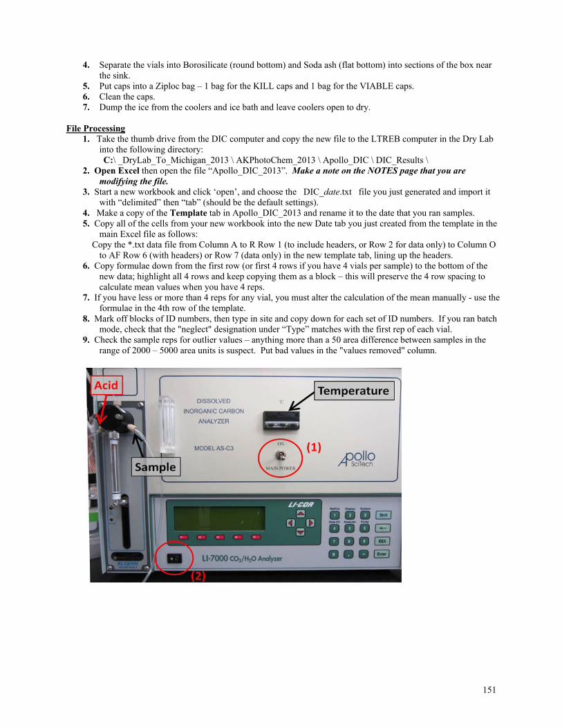
151

4. Separate the vials into Borosilicate (round bottom) and Soda ash (flat bottom) into sections of the box near the sink.

5. Put caps into a Ziploc bag – 1 bag for the KILL caps and 1 bag for the VIABLE caps. 6. Clean the caps. 7. Dump the ice from the coolers and ice bath and leave coolers open to dry.

File Processing 1. Take the thumb drive from the DIC computer and copy the new file to the LTREB computer in the Dry Lab

into the following directory: C:\ _DryLab_To_Michigan_2013 \ AKPhotoChem_2013 \ Apollo_DIC \ DIC_Results \ 2. Open Excel then open the file “Apollo_DIC_2013”. Make a note on the NOTES page that you are

modifying the file. 3. Start a new workbook and click ‘open’, and choose the DIC_date.txt file you just generated and import it

with “delimited” then “tab” (should be the default settings). 4. Make a copy of the Template tab in Apollo_DIC_2013 and rename it to the date that you ran samples. 5. Copy all of the cells from your new workbook into the new Date tab you just created from the template in the

main Excel file as follows: Copy the *.txt data file from Column A to R Row 1 (to include headers, or Row 2 for data only) to Column O

to AF Row 6 (with headers) or Row 7 (data only) in the new template tab, lining up the headers. 6. Copy formulae down from the first row (or first 4 rows if you have 4 vials per sample) to the bottom of the

new data; highlight all 4 rows and keep copying them as a block – this will preserve the 4 row spacing to calculate mean values when you have 4 reps.

7. If you have less or more than 4 reps for any vial, you must alter the calculation of the mean manually - use the formulae in the 4th row of the template.

8. Mark off blocks of ID numbers, then type in site and copy down for each set of ID numbers. If you ran batch mode, check that the "neglect" designation under “Type” matches with the first rep of each vial.

9. Check the sample reps for outlier values – anything more than a 50 area difference between samples in the range of 2000 – 5000 area units is suspect. Put bad values in the "values removed" column.

152

(VI-3) DOC - Dissolved Organic Carbon Determination Updated 10 Jan 2013, smm/sef

1. Introduction: This method uses a Shimadzu TOC-V platinum-catalyzed oxidative combustion with infrared detection to determine the amount of Total Organic Carbon (TOC), and the principles of oxidative combustion coupled with chemiluminescence to determine Total Nitrogen (TN), in aqueous samples. Our samples are filtered in the field through a Whatman GF/F filter (~0.7µm pore size), meaning we determine Dissolved Organic Carbon (DOC) and total dissolved N (TDN) in our samples. Citations: 5310B. Total Organic Carbon (TOC), Combustion-Infrared Method. 1995. Standard Methods for the

Examination of Water and Wastewater 19th Ed. EPA Method 415.1. Organic Carbon, Total (Combustion or Oxidation). Methods for the Chemical

Analysis of Water and Wastes (MCAWW) (EPA/600/4-79/020) Instrument Model numbers and Shimadzu Contacts: Shimadzu TOC-VCPH (S/N 417503900) ASI-V (S/N 41669180) TN Module (S/N 40726417) Shimadzu Instruments

7102 Riverwood Drive Columbia, MD 21046 Customer Service: (800) 477-1227 Website: www.shimadzu.com Billing Code – 234700, Shipping Code – 14

High Sensitivity Rep – Keith Long, (800) 477-1227 x1915, [email protected] Good Website for advice: http://www.ssi.shimadzu.com/TOC_VirtualAdvisor/TOCVA.htm 2. Summary of Procedures – setting up the run files and the machine:

1. See file C:\DATA\Chemistry\DOC\Doc2012.xls, access the Data tab. Use this list as a reference while inventorying the DOC/TDN samples to sort them by the curve they should be run with (Surface, Low Soil, or High Soil).

2. Access the Daily Entry Sheet tab of C:\DATA\Chemistry\DOC\DocFileVI.xls and use it to print the Daily Entry Sheet, a schedule of the samples that make up a given run on the TOC-V DOC/TN analyzer. The Daily Sample Schedule tab is accessed and the Daily Entry Sheet is imported.

3. Access the DOC_TDN_ALL tab and import the Daily Sample Schedule. 4. Append the run number and sequence-in-run information to the daily sample schedule, and check and revise

as necessary the dilution values. 5. Save the updated DocFileVI.xls to both C:\\ and L:\\ drives. 6. In Excel, open the file C:\TOC3201\Data\Import\Template_TBL.txt. 7. Copy the specific sample information for the current run from the ‘DOC_TDN_ALL’ tab to the appropriate

blank spaces in Template_TBL.txt, and save the file as xxxx_tbl.txt, where xxxx is the sequential and unique run number for ALL runs done on this machine.

8. In the TOC_V software on the DOC computer, import the file xxxx_tbl.txt and use it to make a TOC-V run schedule.

9. Load samples, standards and rinses as specified by the run schedule, and analyze on the TOC-V instrument for DOC and TDN.

10. TOC-V analysis generates 2 files: TOC_ xxxx.t32 (which contains the run schedule information and some analysis results), and TOC_xxxx.pkt (which contains all of the raw peak area data, by individual injection). Export TOC_xxxx.t32 as a TOC_xxxx.txt file. All three files are saved onto a thumb drive, and then copied to both C:\\ and L:\\ drives of your work computer.

153

11. Open TOC_xxxx.txt in Excel. Copy all run data from this file into the file C:\TOC3201\Data\TOC_TN_data.xls.

12. SAS program ‘DOC_V_1of4_Condensed.sas’ is used to condense the individual injection data into a single mean value for DOC and a single mean value for TDN per vial (Sample, Standard or Rinse). SAS programs are located here: C:\DATA\Chemistry\DOC\doc_pgms\Use With DocFile_VI.xls

13. SAS program DOC_V_2of4_Concentrations.sas is used to calculate concentrations of DOC and TDN on a run-by-run basis, based on the standards analyzed in that run and the mean peak area values generated by the program DOC_V_1of4_Condensed.sas. The results of these analyses are written to DocFileVI.xls. Standard curve statistics appear in the ‘curve’ tab of this file.

14. ‘Bad’ standards can be excluded manually, and the program DOC_V_2of4_Concentrations.sas re-run, to recalculate the standard curve and concentrations.

15. The ‘report’ tab is used to generate a final report for each run which contains standard curve statistics and all final concentrations for DOC and TDN.

3. Reagents/Consumables: Platinum Catalyst – We order this from Shimadzu (P/N 638-60116). One bottle is sufficient to fill one combustion

tube. More info on part numbers and consumables can be found in the binders located above the instrument. 4. Associated Files: Before any sample is poured, there is some basic file work to prepare for a run. We use the following files throughout the process of running DOC/TDN samples: DocFileVI.xls -- Repository for processed DOC data stored by run vial and sortchem #, and intermediate files and macros for formulating Daily Entry Sheets and Sample Schedules, divided into the following tabs:

Notes Runs Daily Entry Sheet Daily Sample Schedule DOC_TDN_ALL Curve Report Dilution value Machine blanks

Note that this file must be in *.xls format because the SAS programs will not work with *xlsx. DOC_TN_SASFREE.xls -- A backup file for calculating the concentration of DOC/TDN without the use of the SAS statistical program. This file is more time consuming to use, but there is full control of the output and intermediary steps. TOC_TN_data.xls -- Repository for raw data from TOC-V, stored by injection value; this is the file sent to SAS for statistical analysis, reduction to a single value per run vial, and final concentrations calculated based on the standards run with each analysis. Note that this is an *.xls file and tabs can only support ~60,000 rows. For this reason (and because we’re limited by row numbers for the same reason in the DocFiles), it’s easiest to just dedicate tabs to a year’s samples (2012 was Data_6, 2013 will be Data_7, etc). Create a new DocFile for each Data tab (2013 will be DocFileVII.xls). Template_TBL.txt -- This is a template file used to construct xxxx_tbl.txt in the proper format for importing to the TOC-V. xxxx_tbl.txt (xxxx is the run number) -- This is a text-format file which contains the specific run data--sample, standard, blank and rinse information--from DocFileVI.xls; it is used to import this data to TOC_xxxx.t32. TOC_xxxx.t32 (xxxx is the run number) -- This is the TOC-V run schedule, a list of samples, standards, blanks, rinses that make up an analysis run (the ‘Daily Sample Schedule).

154

TOC_xxxx.txt (xxxx is the run number) -- This is a .txt file to which specific run analysis data from run xxxx (sample, standard, blank and rinse information stored by injection) is imported. This file is used to transfer this data to the file TOC_TN_data.xls. DocTnAllData.xls – Using a SAS program, this file compiles all the sample data. DOC and TDN values are on separate tabs, and each DOC file (I through VI) has its own tabs. DOC_VI_1of4_Condensed.sas takes the raw peak area data from the multiple injections per vial (sample, standard or rinse), statistically evaluates them, and then condenses them to a single representative value per vial (sample, standard or rinse). DOC_VI_2of4_Concentrations.sas takes this condensed data and uses the standard and blank values to construct a standard curve per analysis run, then uses this curve to calculate the concentrations of samples in that run. DOC_VI_3of4_Averages.sas averages sample DOC values (duplicates, replicates) and outputs all data to DocTnAllData.xls. TN_VI_3of4_Averages.sas averages sample TDN values (duplicates, replicates) and outputs all data to DocTnAllData.xls. 5. Stock Solution and Working Standards: The Stock standard (highest concentration) solution should be made fresh at the start of each season, and stored in the sample refrigerator. All stock and working standard solutions are made with acidified Reverse Osmosis Distilled water RO-DI (because our samples are acidified – the solutions need to be acidified to at least pH ~4 so that all inorganic carbon is converted to CO2). A. Acidified RO-DI

1. If the same flask will be used to make more acidified RO-DI H2O, it should first be rinsed 4 times with RO-

DI water. In all other cases the flask should be acid washed and rinsed the usual 8 times with RO-DI H2O. 2. Pour about 3-4 mL of 6N trace metal grade (TMG) HCl into a clean 10 mL beaker. 3. Use a pipette with a clean 1 mL tip (rinse pipette tip four times with RO-DI H2O) to add 1mL of 6N TMG

HCl to a clean 2L volumetric flask partially filled with RO-DI water: 1 mL (6N trace metal grade HCl) / 2 L (RO-DI)

4. Fill volumetric flask to appropriate volume with standard and RO-DI water and mix thoroughly.

B. Stock Solutions We make 2 separate stock solutions: K-H-P and urea.

1. The K-H-P stock standard solution is made by weighing out exactly 1.2764 g of potassium hydrogen phthalate (K-H-P) and dissolving it in acidified RO-DI water in a 1L volumetric flask to a volume of exactly 1L.

2. Because K-H-P absorbs moisture (which increases its weight), it is stored in the desiccator and must be completely desiccated when weighed on the Mettler balance.

3. Prepare to weigh chemicals by adding fresh silica gel to the trays in the weighing chamber. Make sure the trays do not interfere with the movement of the weighing pan.

4. Weigh out an excess of the 1.2764 g needed, and place in a small, clean glass beaker. Place in a drying oven at 105 ºC for 4 hours to completely evaporate any residual water molecules.

5. Return beaker to weighing chamber and transfer chemical to a tared weigh pan. The weight should be stable because of the silica desiccant in the chamber.

6. Carefully and quickly remove excess K-H-P and again allow weight reading to stabilize. Repeat, removing or adding K-H-P and allowing to stabilize until the exact weight is reached.

7. Take your time and be very exact; the accuracy of up to 2 months of analyses depends upon this dilution of exactly 1.2764 g of K-H-P.

8. It is equally important to fill the volumetric flask to exactly 1.00L. a. It is safest to add the last few mLs of water with a squirt bottle or a syringe, which has been acid

washed and rinsed.

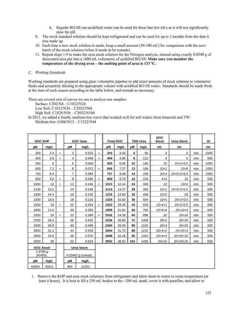
155

b. Regular RO-DI (un-acidified) water can be used for these last few mLs as it will not significantly raise the pH.

9. The stock standard solution should be kept refrigerated and can be used for up to 2 months from the date it was made up.

10. Each time a new stock solution is made, keep a small amount (50-100 mL) for comparison with the next batch of the stock solution (when it needs to be remade).

11. Repeat steps 1-9 to make the urea stock solution for the Nitrogen analysis, instead using exactly 0.0240 g of desiccated urea put into a 1000 mL volumetric of acidified RO-DI. Make sure you monitor the temperature of the drying oven – the melting point of urea is 133 ºC.

C. Working Standards

Working standards are prepared using glass volumetric pipettes to add exact amounts of stock solution to volumetric flasks and accurately diluting to the appropriate volume with acidified RO-DI water. Standards should be made fresh at the start of each season according to the table below, and remade as necessary. There are several sets of curves we use to analyze our samples: Surface: C202/N4 – C1012/N24 Low Soil: C1012/N24 – C2032/N64 High Soil: C1828/N56 – C3052/N104 In 2012, we added a fourth, medium-low curve that worked well for soil waters from Imnavait and TW: Medium-low: C606/N12 – C1522/N44

DOC KHP DOC Urea Final DOC TDN Urea DOC Stock Urea Stock DI

µM mg/L µM mg/L µM mg/L µM mg/L mL mL mL

200 2.4 + 2 0.024 = 202 2.42 4 56 4 5 into 1000

400 4.8 + 4 0.048 = 404 4.85 8 112 4 5 into 500

500 6 5 0.060 505 6.06 10 140 10 10+2+0.5 into 1000

600 7.2 + 6 0.072 = 606 7.27 12 168 10+2 10+5 into 1000

700 8.4 7 0.084 707 8.48 14 196 10+4 10+5+2+0.5 into 1000

800 9.6 + 8 0.096 = 808 9.70 16 224 4+4 10 into 500

1000 12 + 12 0.144 = 1012 12.14 24 336 10 10+5 into 500

1100 13.2 14 0.168 1114 13.37 28 392 10+1 10+5+2+0.5 into 500

1200 14.4 16 0.192 1216 14.59 32 448 10+2 20 into 500

1300 15.6 18 0.216 1318 15.82 36 504 10+3 20+2+0.5 into 500

1500 18 + 22 0.264 = 1522 18.26 44 616 10+4+1 25+2+0.5 into 500

1800 21.6 28 0.336 1828 21.94 56 784 10+4+4 20+10+5 into 500

2000 24 + 32 0.384 = 2032 24.38 64 896 20 20+20 into 500

2200 26.4 36 0.432 2236 26.83 72 1008 20+2 20+25 into 500

2400 28.8 40 0.480 2440 29.28 80 1120 20+4 25+25 into 500

2600 31.2 44 0.528 2644 31.73 88 1232 20+4+2 25+25+5 into 500

2800 33.6 48 0.576 2848 34.18 96 1344 20+4+4 20+20+20 into 500

3000 36 52 0.624 3052 36.62 104 1456 20+10 20+20+25 into 500

DOC Stock Urea Stock 1.2764 g (KHP)/L 0.02402 g (Urea)/L

µM mg/L µM mg/L

50000 600.5 800 11201

1. Remove the KHP and urea stock solutions from refrigerator and allow them to warm to room temperature (at

least 4 hours). It is best to fill a 250 mL beaker to the ~200 mL mark, cover it with parafilm, and allow to

156

warm up to room temperature. Using a beaker will cut down on the hours required to warm up the large volume of stock solution.

2. When a new set of standards is prepared the set should be run against an old set of standards, which were saved for comparison. Pour old standards into 4 tubes for each concentration (or into clean, labeled 60mL Nalgene bottles if you want to save a larger volume). When you compare the new and old standards use only 2 tubes of each concentration. Save the other 2 in case the standards made are incorrect (and you have to run the comparison again). If standards are good (see QAQC section for criteria) discard the remaining old standards.

3. Clean and label (with concentration, date, and operator) volumetric flasks which will be dedicated for diluting and storing the working standards. a. If the concentration of new standard is the same as the previous standard, the flask should be rinsed 4 times with RO-DI water. b. In all other cases the flask should be acid washed and rinsed the usual 8 times with RO-DI.

4. Prepare a clean area for the dilution procedure and set out volumetric pipettes, volumetric flasks, pipette pumps or bulbs, KimWipes, and a clean squirt bottle with fresh RO-DI water.

5. Select the appropriate volumetric pipette and rinse it 2 times with stock solution from the 250 mL beaker. 6. Use rinsed pipette to accurately add stock solution from the 250 mL beaker to each appropriate volumetric flask

according to your plan. As each addition is made, check it off on a checklist to make sure that you deliver the correct amounts to the flasks. a. When all additions have been successfully completed, fill all flasks with acidified RO-DI water to within about 5 mL of the etched calibration line. b. Use the squirt bottle or an acid washed syringe to carefully add acidified RO-DI water to the calibration line of each volumetric flask (the bottom of the meniscus right on the line). Take your time and remember to wait a minute or two to allow all the water to drain down the inside of the flask neck before adding the last bit of water. c. Mix each working standard flask thoroughly only after it has been filled to the proper volume as a small amount of liquid may leak out around the ground glass stopper while mixing.

7. Working standards can be stored on the counter at room temperature near the TOC instrument. 6. Analysis Set-Up: A. Creating a Daily Entry Sheet

1. Update the DocFileVI.xls from the L:\\ drive to the C:\\ drive 2. Open ‘DocFileVI.xls’ in C:\DATA\Chemistry\DOC

a. Enable Macros b. Do not update links

3. Go to the next available cell in column E on the ‘Daily Entry Sheet’ tab. 4. Type in the sortchem numbers. You only need to include the number after the year of the sortchem and the

dash (i.e. the sample 2011-0065 can be entered as “65”). After all samples have been entered, click on the first cell you entered in column D and click on the “Get Site Info” button to pull over the full sortchems and site info from the “Inventory” tab. This means the “Inventory” tab needs to be updated with all sample information. If you do not have an electronic copy of the samples you want to run, hand-type in the sortchems, site names, and dates into the appropriate cells.

5. In Column A, copy and paste the numbers 1-70; in Column B, type in the next page number for the next 70 cells; in Column C, copy the formula from the cell above or type in the numbers 21-90 to identify the cup numbers; and in Column D, type in the project that the samples are associated with (e.g. AK2010, Burn2010, TK2010, Photo2010, etc).

6. We run 70 samples per run. If there are less than 70 samples in the run, add blank lines to compensate (must have 70 lines total).

7. Click on the ‘Print Daily Entry Sheet’ button, located in the upper right. a. Enter the page number to print. b. Click on ‘OK’. c. Check over the preview, correct all mistakes b. If pages are off, spacing is incorrect and row height will need to be adjusted. c. If changes have been made, close the file to save changes, and repeat

step a. d. Click on ‘Print’. e. Use the printout for getting and organizing the samples for the run.

157

B. Creating a Daily Sample Schedule (TOC-V Sample Run Table)

1. In the DOCFileVI.xls, go to the ‘Daily Sample Schedule’ tab. 2. Click the ‘Import Daily Entry Sheet’ button, located in the upper left.

a. Enter the page number to import. b. Click on ‘OK’.

3. In the “Review” menu, choose to unprotect the sheet. In column U, titled Curve, type in the standard curve that will be run with the samples (low, medium, high), and copy down for the entire run. This will fill in the correct standards for the run.

4. Go to the ‘DOC_TDN_ALL’ tab. 5. Click the ‘Import Daily Sample Schedule’ button, located in the upper left.

a. Scan down the rows; the new schedule should be at the bottom. b. Delete all blank rows added in section A.5.a.1 above, but leaving rinses and end standards. c. In column B, number sequentially from 1 to 101. d. In column A, enter the run number. e. Check that the field dilutions are correct (column J) and enter any lab dilution values (column K).

i. Enter 1 in all rows without lab dilutions (column K). f. Save file on the C:\\ and L:\\ drives

6. In Excel, open the text file ‘Template_TBL.txt’, located in C:\\TOC3201\Data\Import. (Make sure *.* is selected as file type)

a. Select ‘Delimited’ – click ‘Next’. b. Select ‘Tab’ – click ‘Finished’.

7. From DocFileVI.xls, copy the data in column D ‘SampleName/SortChem’ for the run that was just entered on the ‘DOC_TDN_ALL’ tab.

a. Paste the copied data into column D of the ‘Template_TBL.txt’ file. b. Verify that the pasted data matches with the data in column C.

8. Select ‘Save As’ from the ‘File’ menu. c. Enter the file name as ‘xxxx_tbl.txt’, where xxxx is the run number (sequentially increased by 1

from the previous run) d. Make sure the ‘save as type’ is text tab delimited e. Click ‘Save’ then click ‘Yes’

9. Close the file; if asked to save changes, click ‘No’ 10. Save the file xxxx_tbl.txt to a thumb drive, and transfer to the DOC computer folder,

C:\TOC3201\Data\Import. The table is now ready to be imported to the TOC-Control V software (see section 6.C)

C. Import Daily Sample Schedule (TOC-V Sample Table) to TOC-V Analyzer

1. On the DOC computer, open the TOC software (TOC-Control V). 2. In the TOC-Control V main window, click on ‘Sample Table Editor’ icon; the user dialogue box is displayed;

click ‘OK’ (no user name or password). 3. From the ‘File’ menu select ‘New’ 4. Click on the ‘Sample Run’ icon; click ‘OK’ 5. Click on the System dropdown menu, and select the desired system (typically DOC-TN); click ‘OK’ 6. In the ‘Save as’ window, enter the file name as ‘TOC_xxxx’.t32’, where xxxx is the run number

(sequentially increased by 1 from the previous run); click ‘Save’ 7. On the blank Sample Table, select the first cell in the column ‘Type’.

a. From the ‘Edit’ menu select ‘Import’. b. Double click on the run table that is to be imported (should be same run number as that used for the

file name); the sample table will automatically fill in. 8. Check sample table to make sure all is correct; then click on the ‘File’ menu and select ‘Save’.

D. Manually Programming the Sample Run Table via TOC-V software:

1. Follow stops 1-6 of section 6.C above (at this point, the empty sample run table should be displayed; the background monitor window must be closed to edit the Sample Run Table).

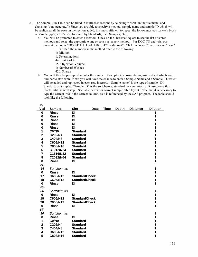
158

2. The Sample Run Table can be filled in multi-row sections by selecting “insert” in the file menu, and choosing “auto generate.” (Since you are able to specify a method, sample name and sample ID which will be replicated all the rows in the section added, it is most efficient to repeat the following steps for each block of sample types, i.e. Rinses, followed by Standards, then Samples, etc.)

a. You will be prompted to enter a method: Click on the “browse” square to see the list of stored methods and select the appropriate one or construct a new method. For DOC-TN analysis, our current method is “DOC-TN_1_1_44_150_1_420_calib.met”. Click on “open;” then click on “next.”

i. In order, the numbers in the method refer to the following: 1: Dilution 1: Determinations 44: Best 4 of 4 150: Injection Volume 1: Number of Washes 420: Sparge

b. You will then be prompted to enter the number of samples (i.e. rows) being inserted and which vial number to start with. Next, you will have the chance to enter a Sample Name and a Sample ID, which will be added and replicated in each row inserted. “Sample name” is the type of sample: DI, Standard, or Sample. “Sample ID” is the sortchem #, standard concentration, or Rinse; leave this blank until the next step. See table below for correct sample table layout. Note that it is necessary to type the correct info in the correct column, as it is referenced by the SAS program. The table should look like the following:

Inj. Vial Sample Site Date Time Depth Distance Dilution

0 Rinse DI 1 0 Rinse DI 1 0 Rinse DI 1 0 Rinse DI 1 0 Rinse DI 1 1 C0/N0 Standard 1 2 C202/N4 Standard 1 3 C404/N8 Standard 1 4 C606/N12 Standard 1 5 C808/N16 Standard 1 6 C1012/N24 Standard 1 7 C1516/N32 Standard 1 8 C2032/N64 Standard 1 0 Rinse DI 1

21-44 Sortchem #s 1 0 Rinse DI 1 17 C606/N12 StandardCheck 1 18 C606/N12 StandardCheck 1 0 Rinse DI 1

45-66 Sortchem #s 1 0 Rinse DI 1 19 C606/N12 StandardCheck 1 20 C606/N12 StandardCheck 1 0 Rinse DI 1

67-90 Sortchem #s 1 0 Rinse DI 1 1 C0/N0 Standard 1 2 C202/N4 Standard 1 3 C404/N8 Standard 1 4 C606/N12 Standard 1 5 C808/N16 Standard 1

159

6 C1012/N24 Standard 1 7 C1516/N32 Standard 1 8 C2032/N64 Standard 1 0 Rinse DI 1 0 Rinse DI 1 0 Rinse DI 1 0 Rinse DI 1 0 Rinse DI 1

c. After entering this information, click on “next;” click on “next” again; then click on “finish.” The

following window displays a sample table and a schematic diagram of the sample carousel with the occupied positions colored blue. Click on “OK.” The selected number of rows will then be filled in, sequentially, as specified above.

d. This process is repeated until the entire Sample Run Table has been filled. 9. Next, type in the Sample ID information. All information that is unique to a row, e.g. sortchem #s, must be

entered manually. Because this software is rather primitive, the process is not easily streamlined and is the most tedious part of setting up a run. NOTE: YOU CANNOT COPY AND PASTE TEXT. For reasons unknown, in the next window any text that has been copied and pasted will not be displayed, and you will be forced to return to the previous Sample Run Table window and re-type it. Don’t worry about changing the vial (position number) in this window; the only time a vial number can be changed is in the “Sparging/Acid Addition” window (see section H below).

10. Once the table is completely filled in, save it to the hard drive. 7. Routine Machine Start-up:

1. Make sure sufficient compressed Ultra Zero Air is available for TOC analysis and dry air for TN analysis. A full run takes over 36 hours, and requires 600 psi dry air and 300 psi ultra zero air; change cylinders before starting the run if necessary.

a. Currently we are using a Domnick Hunter Ultra-Zero Air generator fed by building compressed air to supply what is needed for TOC and TN analysis. However, it requires a dry air compressed gas cylinder to operate its automatic cycling (as building air does not have sufficient pressure to do this).

i. Turn on building air to supply the Ultra-zero air generator. ii. Turn on the dry compressed air; set the regulator at 80 – 100 psi.

iii. Turn on (i.e., plug in) the Ultra-zero air generator. 2. Fill the RO-DI bottle to the right of the autosampler. 3. Make sure there is sufficient 2N HCl in the acid container to the left of the TOC-V. 4. Open the front of the TOC instrument and check the humidifier water level (front reservoir); water level

should be between low and high. 5. Check the drain reservoir (located behind the humidifier reservoir) water level; it needs to be completely full.

There is an attached tube for the purpose of filling. 6. In 2012, we also started emptying the water trap. Remove the top panel and disconnect the tubes to the glass

vial that rests on all of the tubing and is full of water) and empty the water into a beaker. Replace the tubes. 7. Turn on main TOC module (switch on front) and TN module (switch on right side; power is on when the top

of switch is pushed in). 8. Open TOC-V software. We are using the DOC-TN system. 9. Click on “File” and select “New.” Then select “Sample Run” icon. 10. The General Information screen will appear; select the correct system from the dropdown menu (usually

DOC_TN) and click on “ok.” 11. Name the file by clicking on “Save As,” calling up the last file run, and increasing the sequential number by

1. An empty Sample Run table will appear. Refer to section 6.C to import a Sample Run Table OR refer to section 6.D to manually enter sample information.

12. To establish communication between the software and instrument, click on “Connect” (the yellow lightning bolt button) and then select “use settings on the PC.” The analyzer will then begin its initialization procedure.

13. The status of the instrument detectors can be monitored by clicking on “Instrument” menu and selecting “Background Monitor.” The background monitor is displayed. There are three tabs (TDC, TN, ASI) that each display the baseline parameters (position, fluctuation and noise) of each detector and other properties,

160

such as the temperature of the dehumidifier and TC furnace. The software will notify you when the baseline is stable enough to start a run. After a cold start, the baseline should take approximately 2-6 hours to stabilize, but, it could also take two days. When the machine has already been running, it should take much less time. The Background Monitor must be closed prior to opening a Sample tray window.

14. After the machine has stabilized, click on “Instrument,” then select “Maintenance,” and then select “Perform Zero Point Detection;” click on “Start.” Click on “Close” when completed.

15. When you are ready to start running samples, load the sample carousal (see section 8 below), mount the loaded sample tray in the auto sampler and place the plastic cover over the sample tray. The auto sampler will automatically move the tray to the correct starting position.

16. Click on the box with the green light symbol to start the run. A “Standby” window will appear; click “Shut Down Instrument,” then click “Standby” (this will make the instrument shutdown when the run is complete).

17. Next, the “Sparging/Acid Addition” window will appear; here is where you will enter/change vial numbers (i.e. the location on sample carousel) as needed. The display will show a schematic diagram of the sample carousel with all positions programmed into the run table colored blue. Remember that DI Rinses are position 0. Do not use the “Enter” key to click to the next row, as this will take you to the next window, not the next cell; use the down arrow key instead. NOTE: THIS IS THE ONLY TIME VIAL (POSITION) NUMBERS CAN BE ADDED OR ALTERED. Click on “ok” after correctly entering all vial position numbers.

18. Finally, the “Start ASI Measurement” screen will appear; un-check “External Acid Addition” then click on “Start” if everything has been entered and set-up correctly; otherwise, click on “Cancel” if you need to go back and change anything before starting the run.

19. You can monitor run measurements in real time by opening the Sample Window. To open, place cursor in the row of the sample table that contains the desired sample; then, select Sample Window from the View menu. The dropdown menu on the Sample Window allows you to display either only the peak of the current injection, or all injection peaks for the selected sample.

20. At the end of a run, to close the “Sample Run” window, you must abort communication between the instrument and the TOC-V program. Click on the yellow lightning bolt symbol, and check the ‘Abort Communication’ box. Click ‘OK’.

8. Loading the Sample Carousel:

1. Samples are acidified (done in the field) and run in 24 mL glass sample vials. To prepare vials for running: a. Carefully remove all parafilm from used sample tubes. b. Empty tubes and rinse 6 times with RO-DI water. c. Roll-up the rinsed (dry) tubes in heavy-duty aluminum foil, folding foil over tops and bottoms of

tubes before rolling up (40 tubes/roll). Or, use heavy-duty aluminum trays and cover the tops with foil.

d. Combust covered tubes in muffle furnace at 550C for 4 hours to burn off all residual carbon. e. Store combusted tubes, in the aluminum foil, in a drawer or covered cabinet until used.

2. Prior to pouring, samples need to be sonicated for 10 minutes to re-dissolve any flocculation that may have occurred during sample storage. If flocculation is common, you may be acidifying the samples too much because you will get more condensation reactions at pH 3 than you will at pH 4. A single run of 70 samples can be done in two batches.

3. Fill each clean vial at least ½ full with sample or standard, and cover with a square of parafilm. The volume is dependent on how many injections and of what volume you use.

4. The sample carousel holds 93 vials. We program 5 DI rinses into the run file at the beginning of the run, 1 DI rinse every time we switch between sample types (e.g., check standards to samples), and 5 DI rinses at the end of the run. RO-DI water is drawn from a rinse water reservoir, position 0. Make sure the reservoir is full. See section 6.D.b for current sample arrangement.

10. Processing the Output of a TOC-V run: A. Processing TOC-V output of a run set up following preceding protocol, using a run schedule downloaded from

‘DocFileVI.xls’

1. Open the TOC software (TOC-Control V) b. Double click on ‘Sample Table’ c. Select ‘OK’

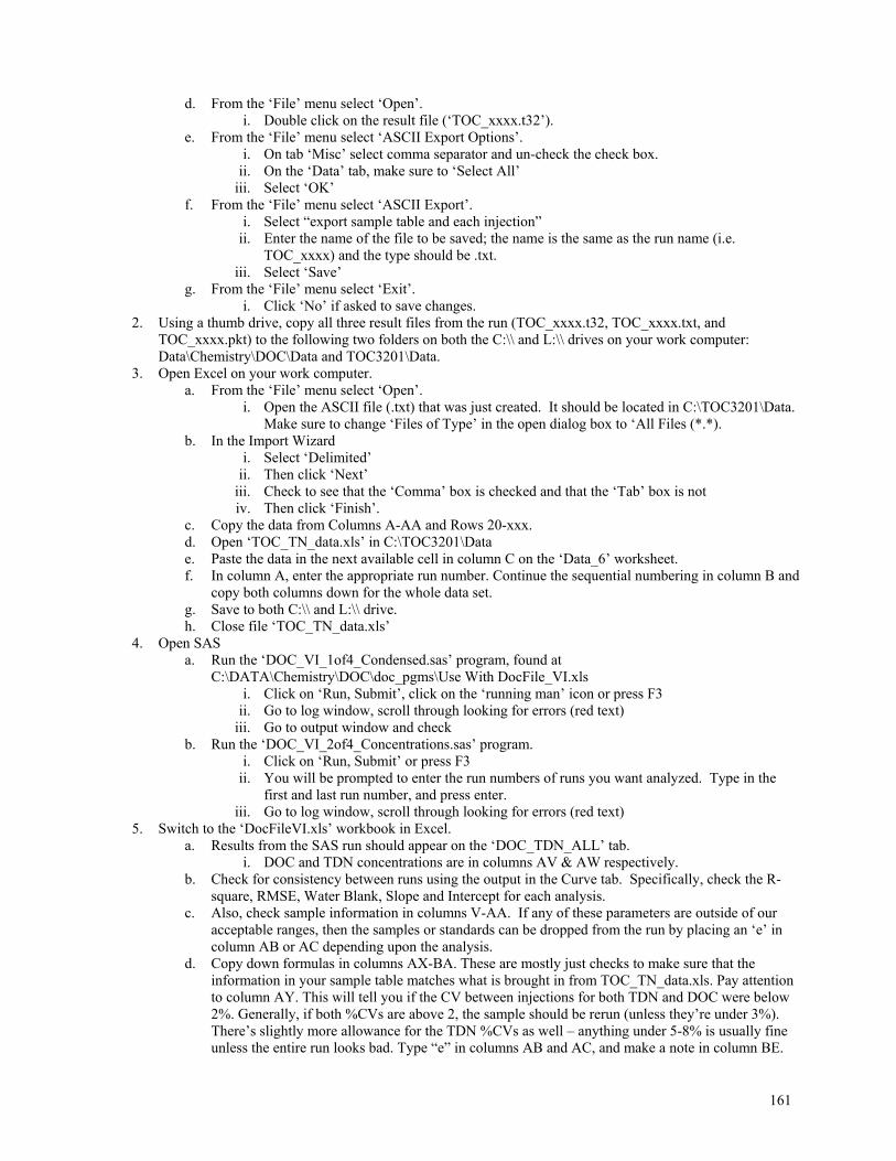
161

d. From the ‘File’ menu select ‘Open’. i. Double click on the result file (‘TOC_xxxx.t32’).

e. From the ‘File’ menu select ‘ASCII Export Options’. i. On tab ‘Misc’ select comma separator and un-check the check box.

ii. On the ‘Data’ tab, make sure to ‘Select All’ iii. Select ‘OK’

f. From the ‘File’ menu select ‘ASCII Export’. i. Select “export sample table and each injection”

ii. Enter the name of the file to be saved; the name is the same as the run name (i.e. TOC_xxxx) and the type should be .txt.

iii. Select ‘Save’ g. From the ‘File’ menu select ‘Exit’.

i. Click ‘No’ if asked to save changes. 2. Using a thumb drive, copy all three result files from the run (TOC_xxxx.t32, TOC_xxxx.txt, and

TOC_xxxx.pkt) to the following two folders on both the C:\\ and L:\\ drives on your work computer: Data\Chemistry\DOC\Data and TOC3201\Data.

3. Open Excel on your work computer. a. From the ‘File’ menu select ‘Open’.

i. Open the ASCII file (.txt) that was just created. It should be located in C:\TOC3201\Data. Make sure to change ‘Files of Type’ in the open dialog box to ‘All Files (*.*).

b. In the Import Wizard i. Select ‘Delimited’

ii. Then click ‘Next’ iii. Check to see that the ‘Comma’ box is checked and that the ‘Tab’ box is not iv. Then click ‘Finish’.

c. Copy the data from Columns A-AA and Rows 20-xxx. d. Open ‘TOC_TN_data.xls’ in C:\TOC3201\Data e. Paste the data in the next available cell in column C on the ‘Data_6’ worksheet. f. In column A, enter the appropriate run number. Continue the sequential numbering in column B and

copy both columns down for the whole data set. g. Save to both C:\\ and L:\\ drive. h. Close file ‘TOC_TN_data.xls’

4. Open SAS a. Run the ‘DOC_VI_1of4_Condensed.sas’ program, found at

C:\DATA\Chemistry\DOC\doc_pgms\Use With DocFile_VI.xls i. Click on ‘Run, Submit’, click on the ‘running man’ icon or press F3

ii. Go to log window, scroll through looking for errors (red text) iii. Go to output window and check

b. Run the ‘DOC_VI_2of4_Concentrations.sas’ program. i. Click on ‘Run, Submit’ or press F3

ii. You will be prompted to enter the run numbers of runs you want analyzed. Type in the first and last run number, and press enter.

iii. Go to log window, scroll through looking for errors (red text) 5. Switch to the ‘DocFileVI.xls’ workbook in Excel.

a. Results from the SAS run should appear on the ‘DOC_TDN_ALL’ tab. i. DOC and TDN concentrations are in columns AV & AW respectively.

b. Check for consistency between runs using the output in the Curve tab. Specifically, check the R-square, RMSE, Water Blank, Slope and Intercept for each analysis.

c. Also, check sample information in columns V-AA. If any of these parameters are outside of our acceptable ranges, then the samples or standards can be dropped from the run by placing an ‘e’ in column AB or AC depending upon the analysis.

d. Copy down formulas in columns AX-BA. These are mostly just checks to make sure that the information in your sample table matches what is brought in from TOC_TN_data.xls. Pay attention to column AY. This will tell you if the CV between injections for both TDN and DOC were below 2%. Generally, if both %CVs are above 2, the sample should be rerun (unless they’re under 3%). There’s slightly more allowance for the TDN %CVs as well – anything under 5-8% is usually fine unless the entire run looks bad. Type “e” in columns AB and AC, and make a note in column BE.

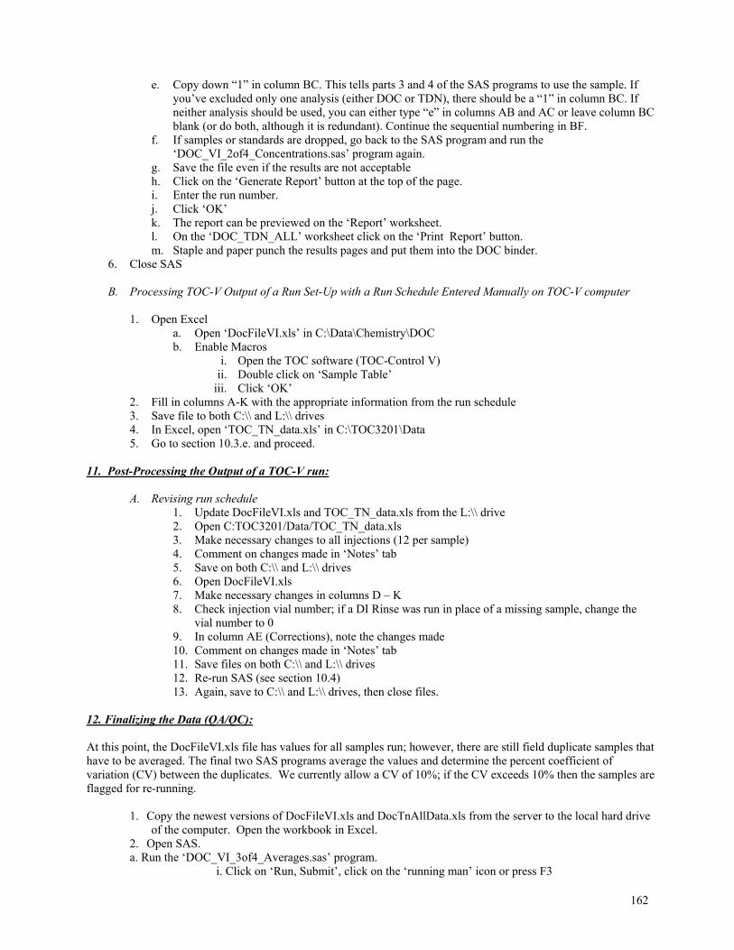
162

e. Copy down “1” in column BC. This tells parts 3 and 4 of the SAS programs to use the sample. If you’ve excluded only one analysis (either DOC or TDN), there should be a “1” in column BC. If neither analysis should be used, you can either type “e” in columns AB and AC or leave column BC blank (or do both, although it is redundant). Continue the sequential numbering in BF.

f. If samples or standards are dropped, go back to the SAS program and run the ‘DOC_VI_2of4_Concentrations.sas’ program again.

g. Save the file even if the results are not acceptable h. Click on the ‘Generate Report’ button at the top of the page. i. Enter the run number. j. Click ‘OK’ k. The report can be previewed on the ‘Report’ worksheet. l. On the ‘DOC_TDN_ALL’ worksheet click on the ‘Print Report’ button. m. Staple and paper punch the results pages and put them into the DOC binder.

6. Close SAS

B. Processing TOC-V Output of a Run Set-Up with a Run Schedule Entered Manually on TOC-V computer 1. Open Excel

a. Open ‘DocFileVI.xls’ in C:\Data\Chemistry\DOC b. Enable Macros

i. Open the TOC software (TOC-Control V) ii. Double click on ‘Sample Table’

iii. Click ‘OK’ 2. Fill in columns A-K with the appropriate information from the run schedule 3. Save file to both C:\\ and L:\\ drives 4. In Excel, open ‘TOC_TN_data.xls’ in C:\TOC3201\Data 5. Go to section 10.3.e. and proceed.

11. Post-Processing the Output of a TOC-V run:

A. Revising run schedule 1. Update DocFileVI.xls and TOC_TN_data.xls from the L:\\ drive 2. Open C:TOC3201/Data/TOC_TN_data.xls 3. Make necessary changes to all injections (12 per sample) 4. Comment on changes made in ‘Notes’ tab 5. Save on both C:\\ and L:\\ drives 6. Open DocFileVI.xls 7. Make necessary changes in columns D – K 8. Check injection vial number; if a DI Rinse was run in place of a missing sample, change the

vial number to 0 9. In column AE (Corrections), note the changes made 10. Comment on changes made in ‘Notes’ tab 11. Save files on both C:\\ and L:\\ drives 12. Re-run SAS (see section 10.4) 13. Again, save to C:\\ and L:\\ drives, then close files.

12. Finalizing the Data (QA/QC): At this point, the DocFileVI.xls file has values for all samples run; however, there are still field duplicate samples that have to be averaged. The final two SAS programs average the values and determine the percent coefficient of variation (CV) between the duplicates. We currently allow a CV of 10%; if the CV exceeds 10% then the samples are flagged for re-running.

1. Copy the newest versions of DocFileVI.xls and DocTnAllData.xls from the server to the local hard drive of the computer. Open the workbook in Excel.

2. Open SAS. a. Run the ‘DOC_VI_3of4_Averages.sas’ program.

i. Click on ‘Run, Submit’, click on the ‘running man’ icon or press F3

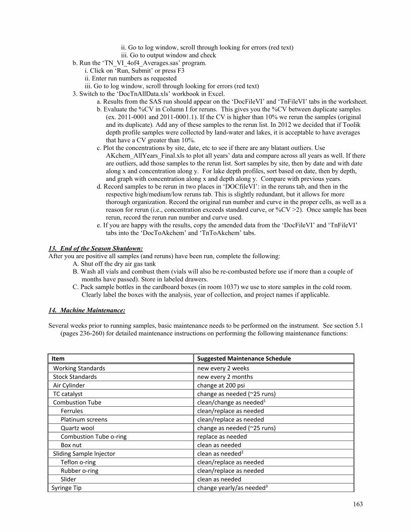
163

ii. Go to log window, scroll through looking for errors (red text) iii. Go to output window and check

b. Run the ‘TN_VI_4of4_Averages.sas’ program. i. Click on ‘Run, Submit’ or press F3 ii. Enter run numbers as requested iii. Go to log window, scroll through looking for errors (red text)

3. Switch to the ‘DocTnAllData.xls’ workbook in Excel. a. Results from the SAS run should appear on the ‘DocFileVI’ and ‘TnFileVI’ tabs in the worksheet. b. Evaluate the %CV in Column I for reruns. This gives you the %CV between duplicate samples

(ex. 2011-0001 and 2011-0001.1). If the CV is higher than 10% we rerun the samples (original and its duplicate). Add any of these samples to the rerun list. In 2012 we decided that if Toolik depth profile samples were collected by land-water and lakes, it is acceptable to have averages that have a CV greater than 10%.

c. Plot the concentrations by site, date, etc to see if there are any blatant outliers. Use AKchem_AllYears_Final.xls to plot all years’ data and compare across all years as well. If there are outliers, add those samples to the rerun list. Sort samples by site, then by date and with date along x and concentration along y. For lake depth profiles, sort based on date, then by depth, and graph with concentration along x and depth along y. Compare with previous years.

d. Record samples to be rerun in two places in ‘DOCfileVI’: in the reruns tab, and then in the respective high/medium/low reruns tab. This is slightly redundant, but it allows for more thorough organization. Record the original run number and curve in the proper cells, as well as a reason for rerun (i.e., concentration exceeds standard curve, or %CV >2). Once sample has been rerun, record the rerun run number and curve used.

e. If you are happy with the results, copy the amended data from the ‘DocFileVI’ and ‘TnFileVI’ tabs into the ‘DocToAkchem’ and ‘TnToAkchem’ tabs.

13. End of the Season Shutdown: After you are positive all samples (and reruns) have been run, complete the following:

A. Shut off the dry air gas tank B. Wash all vials and combust them (vials will also be re-combusted before use if more than a couple of

months have passed). Store in labeled drawers. C. Pack sample bottles in the cardboard boxes (in room 1037) we use to store samples in the cold room.

Clearly label the boxes with the analysis, year of collection, and project names if applicable. 14. Machine Maintenance: Several weeks prior to running samples, basic maintenance needs to be performed on the instrument. See section 5.1

(pages 236-260) for detailed maintenance instructions on performing the following maintenance functions: Item Suggested Maintenance Schedule

Working Standards new every 2 weeks

Stock Standards new every 2 months

Air Cylinder change at 200 psi

TC catalyst change as needed (~25 runs)

Combustion Tube clean/change as needed1

Ferrules clean/replace as needed

Platinum screens clean/replace as needed

Quartz wool change as needed (~25 runs)

Combustion Tube o‐ring replace as needed

Box nut clean as needed

Sliding Sample lnjector clean as needed2

Teflon o‐ring clean/replace as needed

Rubber o‐ring clean/replace as needed

Slider clean as needed

Syringe Tip change yearly/as needed3

164

Halogen Scrubber change yearly4

CO2 Absorber (soda lime) change yearly

NOx Absorber (TN module) change yearly5

Detector Window (TN module) clean yearly

Catalyst (TN module‐ozone gen.) replace after 2000 h operation

Ozone Generator (TN module) replace after 8000 h operation6

Oil Filter (Zero Air Generator) replace yearly

Carbon Filter (Zero Air Generator) replace after 2 m operation

Particulate Filter (Zero Air Generator) replace yearly

2000 hr ~ 40 runs 8000 hr ~ 160 runs

1 Combustion tubes can be clean and reused so long as there are no chips on the bottom. However, note that the glass

bottoms can be ground down with a belt sander to prolong their lifespan. 2 Clean with DI and Q-tip 3 Have a backup syringe on hand, as it can take weeks to receive a new one 4 When tube becomes black/oxidized. 5 Set a warning generation value of 8000 runs in the Maintenance History dialog box (see section 5.5.3 in the

instrument manual). Must be performed by a Shimadzu rep. Changing the Combustion tube

1. Cool the machine by turning the furnace off. Select: Options

Select: Instrument Conditions Select: TOC tab Check: Furnace ON (click on the box so the “X” is removed) 2. Remove the top of the machine and open the front of the machine. 3. Allow the machine to cool for several hours. 4. When cool the combustion tube can be removed.

a. First loosen the compression nut at the bottom of the tube (do not remove the nut). b. While holding on to the bottom of the tube, remove the screw holding the injector slider in place. c. Still holding the tube remove the other two knurl screws which hold the injector assembly in place. d. Carefully remove the injector assembly from the top of the tube. e. Using an Accuwipe hold the top of the tube and lift the tube out of the furnace. Place tube in some sort of

holder (i.e. test tube rack). 5. Inspect and clean the injector slider and the injector. Remove the two o-rings from the injector assembly and

clean, replace if necessary (the rings will be flatten over time). 6. Inside of the injector assembly is an o-ring that grips the top of the combustion tube, if the tube does not fit tight

in the assembly replace the o-ring. 7. Rebuild the combustion tube, follow the instructions in the manual. Important: use only 115mm of catalyst.

Clean the used tube and screens with DI. Do not use a bottle brush. 8. Putting the combustion tube back into the machine.

a. Apply a thin layer of grease around the top of the tube. b. Hold on to the top of the tube with a Accuwipe and lower the tube through the furnace and slide the bottom

of the tube in to the compression nut. Seat the tube then lift it up 1/8 inch and tighten the nut. c. Press the injector assembly back on to the top of the tube. Replace the two screws which hold the injector

assembly in place. d. Replace the screw which connects the injector slider. e. Loosen the compression nut at the bottom of the combustion tube.

9. Turn the furnace on. Select: Options

Select: Instrument Conditions Select: TOC tab Check: Furnace ON (click on the box so the “X” appears)

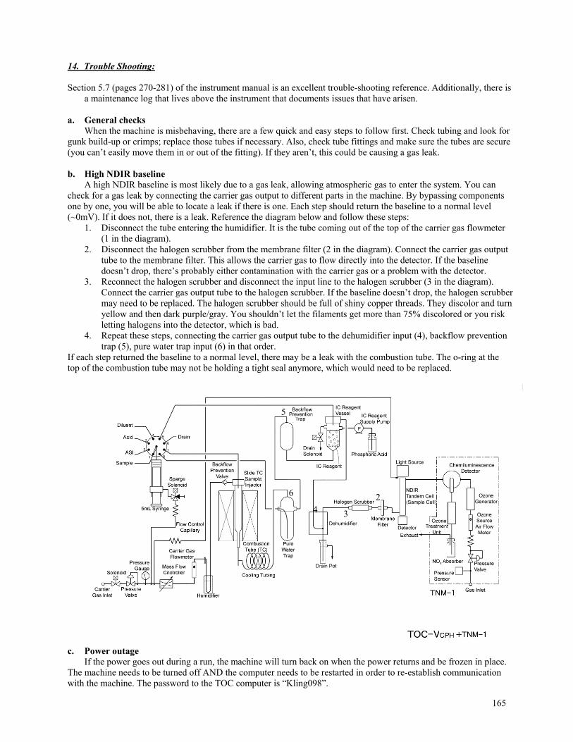
165

14. Trouble Shooting: Section 5.7 (pages 270-281) of the instrument manual is an excellent trouble-shooting reference. Additionally, there is

a maintenance log that lives above the instrument that documents issues that have arisen. a. General checks When the machine is misbehaving, there are a few quick and easy steps to follow first. Check tubing and look for gunk build-up or crimps; replace those tubes if necessary. Also, check tube fittings and make sure the tubes are secure (you can’t easily move them in or out of the fitting). If they aren’t, this could be causing a gas leak. b. High NDIR baseline A high NDIR baseline is most likely due to a gas leak, allowing atmospheric gas to enter the system. You can check for a gas leak by connecting the carrier gas output to different parts in the machine. By bypassing components one by one, you will be able to locate a leak if there is one. Each step should return the baseline to a normal level (~0mV). If it does not, there is a leak. Reference the diagram below and follow these steps:

1. Disconnect the tube entering the humidifier. It is the tube coming out of the top of the carrier gas flowmeter (1 in the diagram).

2. Disconnect the halogen scrubber from the membrane filter (2 in the diagram). Connect the carrier gas output tube to the membrane filter. This allows the carrier gas to flow directly into the detector. If the baseline doesn’t drop, there’s probably either contamination with the carrier gas or a problem with the detector.

3. Reconnect the halogen scrubber and disconnect the input line to the halogen scrubber (3 in the diagram). Connect the carrier gas output tube to the halogen scrubber. If the baseline doesn’t drop, the halogen scrubber may need to be replaced. The halogen scrubber should be full of shiny copper threads. They discolor and turn yellow and then dark purple/gray. You shouldn’t let the filaments get more than 75% discolored or you risk letting halogens into the detector, which is bad.

4. Repeat these steps, connecting the carrier gas output tube to the dehumidifier input (4), backflow prevention trap (5), pure water trap input (6) in that order.

If each step returned the baseline to a normal level, there may be a leak with the combustion tube. The o-ring at the top of the combustion tube may not be holding a tight seal anymore, which would need to be replaced.

c. Power outage If the power goes out during a run, the machine will turn back on when the power returns and be frozen in place. The machine needs to be turned off AND the computer needs to be restarted in order to re-establish communication with the machine. The password to the TOC computer is “Kling098”.

1

2

34

5

6

166

15. History and Tests a. Adding Acid Does the amount of acid added to a sample effect the DOC concentration? In 1997 the amount of acid added to a DOC sample in the field was changed from 1 µL 6N acid per 1 mL sample for surface water (that is, 60 µL acid per 60 mL bottle) to 100 µL 6N acid per 60 mL bottle. This is doubled to 200 µL acid per 125 mL sample bottle. For soil waters (less buffered so they need less acid), we now use half this amount, 50 µL 6N acid per 60 mL sample bottle and 100µL acid per 125 mL sample bottle. A number of tests were conducted to establish what effect this would have on the DOC concentrations of a sample. From these tests it was determined that the amount of acid added has little or no effect on the results. The SigmaPlot file ‘docacidtest5.JNB’ found in the folder ‘e:\Drawings\lab\doc’ is a graphical representation of this data. b. Old vs. New Standards Do the standards over the course of a few weeks degrade? When a new set of standards are prepared, the old standards should be run with them once for comparison. This is an essential check to see if the new standards were accurately made and to see if the old standards have degraded. Usually the lower level standards are good for about 2 months and then may start to degrade, but the values of old versus new standards are usually quite close. QAQC

In 2012 we noticed a lot of variation between DOC and TDN in Lakes-group versus Landwater-group collected Toolik depth profiles, the following protocol was devised to pinpoint where this variation is coming from. There are multiple steps during the sample process at which point we could add (or detect) variation: 1. Collection 2. Filtration 3. Bottling 4. Machine variation within runs 5. Sample variation 6. Machine variation between runs Before running these samples on the DOC/TN analyzer, make sure that the following are true:

a) The Shimadzu has been running pretty consistently for several runs (good standard curves, check standards, etc.)

b) You haven’t just run higher concentration samples. There is a fair amount of carryover, and we don’t want that influencing anything.

1. To test for variation due to COLLECTION: Lakes OR Land-Water collects water at a depth (1m). They then re-collect water from the same depth (1m) and filter these samples using their own filtration method. (This is essentially our current method of duplicates: two samples collected from the same depth, but from a different drop of the van Dorn.) These samples would then get analyzed side by side on the Shimadzu. 2. To test for variation due to FILTRATION: One group collects ONE sample at the specified depth (1m). LW and Lakes both filter this water using their respective methods, so that there are two samples. These samples would get analyzed side by side on the Shimadzu. 3. To test for variation due to BOTTLING: One sample bottle from the specified depth (1m). Filter into one 60 mL, then continue to filter into a separate 60 mL, so that you have two 60 mL that have “the same” water. These samples would then be analyzed side by side on the Shimadzu 4. To test for GENERAL SAMPLE VARIATION Collect sample from the specified depth (1m) and filter into one 60 mL (or larger) bottle. Then, run the same sample twice in a row on the Shimadzu. 5. To test for variation in the MACHINE THROUGHOUT THE RUN (drift): Collect water from one depth. Filter into one 60 mL (or larger) bottle. Run the sample twice in one run, once at the beginning of the run, and once at the end of the run. 6. To test for variation in the MACHINE BETWEEN runs Collect one sample from specified depth (1m). Filter it into one 60 mL bottle. Run it once in one run, and then another time in a different run and look for variation.

167

(VI-4) Silica Determination Dissolved silica is determined on water that has been filtered but not acidified. This usually comes from the bottles labeled “anions”. A. Reagents and Standards All solutions should be made in the fume hood. 1. Reagents a. 5% NaMoO4 solution: 25 g NaMoO4 + 7 mL concentrated H2SO4 to 500 mL total volume b. 50% H2SO4 c. SnCl2 stock solution: [Stock: 40 g SnCl2 per 100 mL concentrated HCl] add SnCl2 to the acid not acid into SnCl2 d. SnCl2 working solution (made daily): 1 mL of stock SnCl2 to a total volume of 100 mL e. Standard stock solution: 0.188 g Na2SiF6 /L which is a final concentration 1 mole Si/mL 2. Standards must be made up prior to the day of running and stored in a refrigerator. A good range of standards is as

follows: 0, 2, 5, 10, 20, 40, 80, 200 mole Si/L. 3. Reagents should also be prepared ahead of time. Sodium molybdate must be made before the running day and

stored in a dark bottle. Concentrated stannous chloride (SnCl2) must also be made ahead of time and stored in the refrigerator.

B. Spectrophotometer setup 1. Turn on the spec (Hitachi, at Univ. Michigan) and let it warm up for at least 5 minutes, but a half hour is better. 2. Select the test you want to run. Choose the test menu option (number 6) and hit enter. 3. Choose number 1 (load test) and then hit enter. 4. Load the silica test by choosing number 2 and hit enter (you will see other silica tests on the menu; these tests use

different parameters). The parameters used for test number 2 are as follows: Sample Num 1 WL (nm) 870.0 Init Delay (sec) 1 Hi Limit 9999 Lo Limit 0.000 Unit Label UM Curve Type 1st Order Num Stds 6 Curve Mode New Baseline System Response Medium Lamp Change WL (nm) 340.0 Vis Lamp On UV Lamp Off Text Print On 5. In order to look at the test parameters or change the number and concentration of standards, go to the options menu

by hitting the return key (you will change the number and concentration of the standards used according to the concentrations of your samples).

6. To set the number of standards, choose number 4 (num stds). Then enter the number of standards you want to run and hit enter.

7. To change the concentrations of the standards you will run, go to curve data (number 6) and hit enter. Then change each standard concentration as necessary.

8. Escape out of the setup screen by hitting the forward key on the keypad. 9. Before starting to run, you must zero the spec. Do this by placing two 1 cm cells filled with DI water into each cell

holder, one of which is the reference cell, near the back of the machine and one of which is the sample cell, near

168

the front of the machine. Close the sliding top door and hit the auto zero key. Take out the sample cell, but leave the reference cell. This will remain in place for the duration of your sample running.

C. Running standards and samples Running Standards 1. Take the standards and reagents out of the refrigerator and allow them to warm up to room temperature. 2. Pour Na-molybdate and H2SO4 into two 20 mL scint vials with screw-on caps. 3. Remember to make up the SnCl2 by pipetting 1 mL of the concentrated solution into a 100 mL volumetric flask

partially filled with DI H2O with a glass pipette. (Do all of this under a hood). Top off the DI H2O in the flask to exactly 100 mL of solution. Mix the solution.

4. Pour the diluted SnCl2 into a 20 mL scint vial. 5. Place all three vials into the wooden sample tray in the following order: Na-molybdate, H2SO4, SnCl2. * NOTE: Set up your standards and samples in the sample tray before you begin running. This will minimize the

confusion in running samples. The easiest way to run the samples is in multiples of eight. Run a set of standards to check the curve before beginning your samples: 1. Number small scint vials consecutively, depending on how many standards you will run. 2. Add exactly 2 mL of each standard into the vials (increasing in concentration) and record the vial number and

concentration. Don’t forget to run a blank; your first standard (number 1) will be DI H2O. 3. Set the vials in the sample rack and set up a time sheet to keep track of when to add the reagents and read the

sample. Below is an example of how to set up your time sheet (for four standards). Sample Na-Molybdate H2SO4 SnCl2 Read 1 12:00 12:15 12:16 12:31 2 12:02 12:17 12:18 12:33 3 12:04 12:19 12:20 12:35 4 12:06 12:21 12:22 12:37 4. Use a different pipette for each reagent. Label them appropriately so as not to confuse them. 5. Start adding reagents to your standards when your digital watch reads 12:00 (for the example above). Add 0.2 mL

Na-molybdate, wait 15 minutes and then add 0.5 mL H2SO4, and then wait one minute before adding 0.1 mL SnCl2. Lightly shake the vials after adding each reagent. Cross out times on your time sheet when you have completed each step.

6. Read your sample’s absorbance at the appropriate times by pouring the entire contents of each vial into a clean, dry cell. Place the cell into the slot inside the spec, making sure that you place it the same way each time (there is usually a faint letter ‘G’ in an upperhand corner of the cell. Make sure it faces the same direction each time you place it in the spec). Slide the top closed and hit the start key on the keypad.

7. After the reading is complete (it will only take a few seconds), clean the cell. Dump the waste in an appropriate container (do not put it down the sink) and rinse the cell with DI H2O three times. Then remove as much water as possible from the cell by forcefully shaking it. Go on to the next reading.

8. When you have finished reading all your standards run a regression on the absorbencies to check the r2 value. If it is greater than or equal to 0.9990, start running your samples.

9. A set of standards should also be run at the end of all your samples for each day you are running! Running samples: 1. Samples should be obtained from bottles labeled ‘anions.’ Shake each bottle before opening and then pour a small

amount into the anion bottle lid. Pipette 2 mL out of the lid and put into small scint vials. 2. Samples are run in the same fashion as the standards. You may, however, want to run more than eight samples at a

time. In order to achieve maximum output per time, start your ninth sample immediately after you read your first sample in the spec. For example, if you were following the time table shown above, you would add Na-Molybdate to sample 9 at 12:32.

3. The samples can be read right after the standard curve is finished. Fill the appropriate cuvette with your sample, wipe the cuvette with a Kim-Wipe to remove anything that interferes with the light path, and read the absorbance by pressing “start”.

169

(VI-5a) Soluble Reactive Phosphate (SRP) Updated 3 December 2012, SEF

The Kling lab analyzes phosphorus content in samples by targeting three different fractions: Soluble Reactive Phosphate (SRP), Total Dissolved Phosphorus (TDP) and Particulate Phosphorus (PP). All of the methods eventually measure P in the form of soluble reactive phosphate (inorganic). Organic and particulate forms are converted to inorganic forms through one of two steps, (1) persulfate oxidizes the organic phosphorus to inorganic forms (for TDP); or (2) acid hydrolysis splits the organic phosphorus and converts it to inorganic phosphorus (for PP). The resultant solutions from TDP and PP are then analyzed with SRP method, in which the molybdate acid react with the reducing ascorbic acid to form a blue-colored solution, which is measured on a spectrophotometer at a wavelength of 885 nm. Citations: Murphy, J. and J.P Riley. 1962. A modified single solution method for the determination of phosphate in

natural waters. Anal. Chim. Acta 27:31-36. Instrument Models/Contacts: Toolik Field Station- Cary 50 Scan UV-VIS Spectrophotometer Varian Customer Service: (650) 213-8000 Web Site: http://www.varianinc.com/ A. REAGENTS

SRP requires the following reagents, all of which are prepared by the Nutrient RA: Ammonium Molybdate Solution, Sulfuric Acid Solution, Antimony Potassium Tartrate Solution, Ascorbic Acid Solution, and a Color Reagent (see Total Dissolved Phosphorus protocol for details on these reagents).

B. STANDARDS Working standards range from 0.05 – 5.0µM P and are prepared by the Nutrient RA. Two sets of standards are prepared for each sample run, 10 mL of standard per tube. Ask the Nutrient RA which standards are used for PO4 (there are separate bottles dedicated for the PO4 and OPA analyses).

C. SAMPLE PREPARATION 1. Determine which samples are going to be run. 2. Talk to the person responsible for the OPA analysis to determine what time the nutrient bottles will be

available for you. This is necessary because nutrients (PO4 and NH4) are collected in the same bottle. In general, you will prepare your PO4 samples (will use the bottles) while the OPA person is prepping their tubes.

3. Transport samples from the refrigerator in the entryway of Lab 4 to the Wet lab. 4. Calibrate the pipette you are going to be using (there is a dedicated 5mL pipette used for the SRP analysis).

Record the total mass of water dispensed from the pipette five times. Record the calibration information on the front page in the PO4 nutrient book (stays on shelf above computer in Wet Lab). Adjust the pipette as needed to dispense 5.0mL of liquid.

5. Create a run sheet by entering the sample information into the “PO4 Template” tab in the akPO4_YEAR.xls file. Note that each sample has a corresponding tube number, and the Inventory tab needs to be periodically updated to be referenced by the PO4 Template tab.

6. Print the run sheet (this will help you keep the samples in order). 7. Verify the sample information on the bottles and make sure they match your run sheet (this can be done

while pipetting samples). If the bottle and your run sheet information do not match, correct the information on one or both and notify whoever that akchem needs to be updated.

8. Arrange samples in order on the Wet Lab chemistry bench. 9. Using a DI triple rinsed and sample rinsed pipette tip, pipette 10 mL of each standard into two tubes (two

tubes, each with 10 mL of standard). At the end of every run, two check standards and a blank are run (e.g. DI, 0.05, 0.1µM), so prepare two additional tubes with 10 mL of standard per tube.

10. If the samples were acidified (ex. early season backlogged samples), the standards need to be acidified using the same sample to acid ratio.

170

11. Using a DI triple rinsed and sample rinsed pipette tip, pipette 10 mL of sample into two sample tubes (two tubes, each with 10 mL of sample). This will allow for duplicate sips to the spec per tube.

12. Add 1000 µL mixed reagent to the two sets of standards and the other tubes (100µL of mixed reagent / 1 mL of sample). VORTEX THE TUBES IMMEDIATELY AFTER ADDING MIXED REAGENT. Do not add reagent to all the tubes and then vortex; add the reagent to a tube, vortex it, place it back in the rack and repeat for all tubes.

13. Cover with saran wrap and leave in the light for 30 minutes to 3 hours.

D. SAMPLE ANALYSIS 1. Check that the software (Advance Read) is set to the proper wavelength – 885nm. 2. Rinse the spectrophotometer’s tubing with DI by inserting the sipper tubing into a beaker of DI and hitting

“flush.” Repeat until the machine stabilizes, usually after 3-5 cycles. 3. Zero the machine on DI, without any reagent. 4. Set up the program so you can run all of the tubes in your run. 5. Press “Start.” 6. Vortex the first tube of the zero standard. 7. Place tubing into the first tube and press the “start” button on the spectrophotometer pump. You can also hit

any key when prompted for the first tube or click on the “fill and read” button. 8. Click the “start” button once more so that there are a total of two readings for the first tube. Write the values

down on the run sheet (the computer file generated by the software cannot keep track of sample information and is essentially useless, so we MUST keep track of values on the run sheet).

9. Continue vortexing and analyzing until you have read all of the tubes twice. 10. When finished, select “save data as” from the SimpleRead menu. Save it in the Kling folder in

DDMMMYY_runXX.rtf format. 11. Pour tubes out into phosphorus waste. Rinse tubes once with DI and pour into waste. Rinse tubes 3X with DI

and place upside down in designated area by sink (NOT in the Nutrient RA’s drying area). Trouble Shooting: 1. If the spectrophotometer pumps the samples through, but fails to read the sample, click “read” in the

SimpleRead program. 2. If the spectrophotometer fails to pump the sample, yet provides a reading, try again. Do not use the first

reading. 3. If there are bubbles present in sipper tube, contact the Nutrient RA (he/she will need to replace tube). In

2011, there were constantly bubbles in the line, so we constantly had to clear them by pinching the tube above the sipper.

E. DATA PROCESSING

1. Copy the raw data file and the Nutrient RA’s standard curve files from the spec computer onto the wet lab computer. Place a backup copy on the download computer.

2. Open the akPO4_YEAR.xls file. In the PO4_Std_Curves tab, fill in the run information (run number, date, standard concentrations). Copy the equations from the previous run in columns D through N. Enter the standard readings recorded on the run sheet in columns O through R. Enter any notes about the standards in column W.

3. Use the arrows in column D, rows 1 and 2, to select the run you just entered. Check the plots to the right. Look at the R2 to check if it’s good (~0.99), and look at the other graphs for a comparison of the analysis slope and intercept over time.

4. Copy the sample data from PO4 Template tab and hard-paste into columns C through H on the PO4 tab. Enter the run number (starting with 1.01, 1.02 and so on; start with a new integer on the next run, e.g. 2.01). Enter sample and check standard readings recorded on the run sheet into columns M through P.

5. Check the formulas in columns J-K and columns S through Z to ensure they are correct, and drag them down to include the newly added data. Add any pertinent notes in column AA.

6. Using the graph and scroll bar at the top of the worksheet, look at the replication between sucks and vials for each sample.

a. We do not throw out data points unless there is a valid reason. b. The first and last sample replicate occasionally have carry over and/or bubbles… look carefully c. Note that the y-scale changes as you scroll down – what may see like a large graphical difference

may actually be quite small.

171

7. Look at the check standards to make sure there isn’t a large drift throughout the analysis; the values are within range of the concentrations from the standard curve. If they are not close, you may have to redo the run.

8. Plot up data, and make sure you get the data double checked while at Toolik Field Station. 9. Any time you work in the akPO4_YEAR.xls file, or make changes in the raw data files, update them on the

computer in Lab 4. If the computers are networked, drag the files from the Wet Lab computer and replace them on the Lab 4 computer; if they are not networked, save files to a flash drive and update them on the Lab 4 computer. ALWAYS RECORD NOTES in the Notes tab of the file you worked in, describing what you did.

F. END OF SEASON

1. Make sure all data have been double-checked and the Lab 4 computer has the most recent versions of all files.

2. Before Wet Lab is shut down, make sure any samples that need to be rerun have been. A sample needs to be rerun if there is high variation among sips (CV of ~30% or greater), it has a negative value, or it has an unlikely value (compare to previous years’ data by site).

3. Rinse tubes as usual. Place in the acid bath outside Wet Lab for at least 3 hours. When removing from the acid bath, dump acid in tubes back into the bath. Rinse tubes 8 times with DI. After the tubes are dry, cover with saran wrap and place in designated area next to the chemistry bench until the next year.

4. Bring all pipettes back to Lab 4. Place all other Landwater items on the shelves above the computer. Cover the shelves with plastic.

5. Make sure all files have been updated on the Lab 4 computer. Shut down the Wet Lab computer and unplug. Cover with plastic.

G. FINAL QA/QC After all the data entries have been double-checked, and the akchem_YYYY file has been finalized (double-checked and site information is updated), it is time to embark upon the delightful process of QA/QC. This procedure is VERY IMPORTANT, and should not be taken lightly.

1. In the akPO4_YYYY.xls file, first update the Inventory tab. Assuming all the sortchems are in akchem_YYYY.xls (from every project that was worked on that summer), it is easiest to just copy the sortchem, site, date, time, depth, distance, elevation for every sample directly from akchem and paste into the Inventory tab. Now you have the most updated sample information.

2. Once you are sure the Inventory has all the information necessary (check for any missing values, like time and depth), update the Data tab. Use index-match to pull the site, date, time, depth, distance information from the Inventory tab, matching with the sortchems in the Data tab. Do not do this for the check standards because they obviously will not have sample information in the Inventory tab.

3. Once you have updated the site, date, time, depth, and distance, then “hard paste” these values into place. (Copy all the values, and then choose “paste special” and click “values.”)

4. On the Data tab, go through each individual formula and make sure that it is referencing the correct cells and returning the correct information. This can be time consuming, but it is important that these formulas are correct. If you are unsure about a certain formula, check with someone else before assuming it is OK.

5. Once checked, copy down all formulas for all cells where that formula is used. 6. Next, look at the standard curves in the PO4_Std_Curves tab and see if there are “bad” curves. Use the

arrows in the upper left corner to scroll through the runs and check the curves in the plot directly to the right. Also check the other plots at the top of the screen and look for runs that had uncharacteristic slopes or intercepts. If a standard curve clearly does not fit with the other runs (does not fall within normal variability), the samples run with the curve should be looked at extra closely for suspect values (if the whole run wasn’t rerun anyway). Finally, check the R-squared values for the curves (we want at least 0.99 ideally) and look for any notes that suggest a curve shouldn’t be used.

7. Update the Summary tab using the instructions at the top of the tab. Sometimes it is difficult to decide which rerun to use, especially if the person doing the QAQC is not the person who originally ran the analysis. Checking through the reruns generally entails checking back through the raw data in the PO4 tab to figure out why a sample was rerun and whether the original value should be used. MAKE NOTES explaining why a sample was rerun and which value should be used (or both). Common reasons for reruns include negative values, unexpectedly high values, high %CVs among sample readings, high %CVs between duplicates, bad standard curves, or bad sample readings due to machine errors.

172

8. Copy the data in the Summary tab (all columns) and hard paste into the QAQC tab. Sort by site name. Make scatter plots for each site (concentration on y-axis, date on x-axis) and look for outliers. It’s useful to compare to the previous year’s (or years’) data if unsure about “normal” values for a site. Keep in mind that some sites (like soil water or thermokarsts) experience greater variability and higher concentrations. If a value looks like an outlier, look at the PO4 tab for any notes about the sample or an explanation for the unexpected value. If the value needs to be removed, replace the value with a “.” and make notes (including the original concentration) in the Summary tab.

9. After checking through the data and updating the Summary tab, copy the data into the For_AKChem tab. There are instructions at the top of the tab.

173

(VI-5b) Total Dissolved Phosphorus (TDP) Updated 29 May 2013, SMM

1. Introduction: The Kling lab analyzes phosphorus content in samples by targeting three different fractions: Soluble Reactive Phosphate (SRP), Total Dissolved Phosphorus (TDP) and Particulate Phosphorus (PP). All of the methods eventually measure P in the form of soluble reactive phosphate (inorganic). Organic and particulate forms are converted to inorganic forms through one of two steps, (1) persulfate oxidizes the organic phosphorus to inorganic forms (for TDP); or (2) acid hydrolysis splits the organic phosphorus and converts it to inorganic phosphorus (for PP). The resultant solutions from TDP and PP are then analyzed with SRP method, in which the molybdate acids react with the reducing ascorbic acid to form a blue-colored solution, which is measured on a spectrophotometer at a wavelength of 885 nm. Citations: Menzel, D.W. and N. Corwin. 1965. The measurement of total phosphorus in seawater based upon the

liberation of organically bound fractions by persulfate oxidation. Limnol. Oceanogr. 10:280-282. Instrument Models/Contacts: Ann Arbor – Alpkem Flow Solutions (FS) 3000 AutoAnalyzer OI Analytical Customer Service: (800) 336-1911 Web Site: http://www.oico.com A. REAGENTS

1. Stock Ammonium Molybdate Solution Ammonium Molybdate……………………………………………………48g (NH4)6Mo7O24 4H2O (FW 1235.95) Dissolve 48g of ammonium molybdate in 800mL of deionized water in a 1L glass pyrex bottle. Dilute to 1,000mL with deionized water. Store in the glass pyrex bottle with orange cap in the refrigerator. Stable until a precipitate forms.

2. Stock Sulfuric Acid Solution, 5N

Sulfuric Acid, concentrated ……………………………………………….140mL H2SO4 (FW 98.08) Slowly add 140mL analytical reagent quality sulfuric acid to 750mL of deionized water in a glass Pyrex bottle. When cool, bring up to 1,000mL with deionized water in the bottle. Store in refrigerator. Stable indefinitely.

3. Stock Antimony Potassium Tartrate Solution

Antimony Potassium Tartrate……………………………………………..1.2g K(SbO)C4H4O6 1/2H2O (FW 333.94) Dissolve 1.2g analytical reagent antimony potassium tartrate in 500mL deionized water in a Pyrex bottle. Mix and fill with DI to the 1,000mL line on the Pyrex bottle. Store in the refrigerator. Stable until a precipitate forms.

4. Stock Ascorbic Acid Ascorbic Acid ……………………………………………………………..2.16g C6H8O6 (FW 176.13) Dissolve 2.16g of ascorbic acid into 70mL of deionized water in a 100ml volumetric flask. Bring up to

100mL with deionized water. Make fresh daily.

5. Color reagent

Stock Sulfuric Acid 100 mL Stock Antimony Potassium Tartrate Solution 25 mL Stock Ammonium Molybdate Solution 25 mL Stock Ascorbic Acid 50 mL **Dowfax 2 mL

174

Combine these reagents in the above order in the dedicated 1-LmL amber bottle and stir after each addition using the magnetic stir plate. Only add the Dowfax reagent after the color reagent has been degassed. Prepare fresh daily. **Dowfax is only added when using the autoanalyzer for analysis (although it might help any tubing)

6. Persulfate Digestion Reagent Potassium Persulfate……………………………………………………………4.5g K2S2O8 (FW 270.33) Dissolve 4.5g of potassium persulfate in 70ml of deionized water in a 100ml volumetric flask with magnetic stirbar. Place on a stirplate and stir for at least an hour. Pull the stirbar up (but not quite out) of the flask using a magnet. Dilute to 100ml with deionized water. Make fresh daily.

B. STANDARD PREPARATION

1. Stock Standard 2000µM P Potassium Monobasic Phosphate………………………………………………0.2722g KH2PO4 (FW 136.09) Dissolve 0.2722g pre-dried potassium monobasic phosphate in 700mL deionized water in a 1L volumetric flask. Bring up to 1,000mL with deionized water. Store in the refrigerator. Stable for months.

2. Intermediate Stock Solution 4µM P

Stock Standard 2000µM P……………………………………………………...2mL Using a glass volumetric pipette, add 2 mL of stock solution into 700mL deionized water in a 1L volumetric flask. Bring up to 1,000mL with deionized water. Store in the refrigerator. Make fresh biweekly.

3. Organic Stock Standard 500µM P

D-Glucose 6-Phosphate…………………………………………………………0.1411g C6H12O9PNa (FW 282.1) Dissolve 0.1411g desiccated D-Glucose 6-Phosphate in 700ml deionized water in a 1L volumetric flask. Use a magnetic stir bar, because the compound takes a long time to dissolve in water. Bring up to 1,000ml with deionized water. Store in the refrigerator. Stable for months. **After we started running samples in early 2013, we consulted with the Lakes group and they use ATP disodium trihydrate (FisherSci BP413-25). In the future, this might be both less expensive, and less difficult to dissolve. Dan White also recommends using it fresh, because it is a hydrate. There are smaller bottles available through Fisher: 1g bottle: A30030-1.0; 5g bottle: A30030-5.0

4. Intermediate Stock Solution 4µM P Organic Stock Standard 500µM P ……………………………………………...8ml

Pipette 8ml of stock solution into 700ml deionized water in a 1L volumetric flask. Bring up to 1,000ml with deionized water. Store in the refrigerator. Make fresh biweekly.

5. Working Standards Organic working standards range from 0.05 – 5.0µM P and are prepared using the microstep dilutor. These standards are prepared in 7.5ml volumes (directly in the digestion tubes), are acidified with 10µl 6N Trace Metal Grade HCl and are digested with 187µl of digestion reagent. Prepare three sets for each run and autoclave with the samples. Inorganic standards should be run along with organic standards before any samples are run to make sure our digestion process is working sufficiently.

175

C. SAMPLE PREPARATION

1. Reacidification of samples – a few days before (or right before) the samples are to be run add 100µl 6N HCl/ 60ml samples to each sample bottle. Mix the bottle thoroughly. Return the samples back to the cold room after reacidification. Once samples have been acidified once, they do not need to be reacidified again if rerunning.

2. Sonication - samples are sonicated in a sonic bath for 10 minutes prior to being poured into digestion tubes. Both the reacidification and sonication aid to separate any potential phosphate compounds that may have

formed in solution. Sonicate samples again if they are being rerun. 3. We have the capability to run 192 samples per run, but we usually run 60 samples per run to reduce the

possibility of reruns due to drift or human error (running out of reagent, not putting all the tubes in, etc.). 4. Transfer XXXX_TDP_InventoriesandRunLogs.xls (where XXXX is the year of analysis) from the server at:

L:\DATA\Chemistry\Nutrients\TDN_TDP\TDP\Inventory_Logs_Tables to the local hard drive, or make a new file from a template of the previous year.

5. Check to see if the Inventory Tab has the inventory from that sampling year. If not, update with information from that year’s akchem (ensure this is up-to-date).

6. On the Paste-Cut Tab, type in the sortchem numbers of the 60 bottles that you selected in column K. 7. Use an Index formula to look up the other information (Site, Date, Time, etc.) from the Inventory Tab. 8. Highlight cells S1:AD90 on the Paste-Cut tab. Click on File → Print… and when the dialog box opens, select

print selection. This prints a digestion log sheet for the samples you are digesting. 9. Create a new tab in the workbook. Name the tab TDPXX-YY, where XX is the year and YY is the

run #. For example, TDP08-01 would be the first run in 2008. Copy the information in columns A5:H144 on the Paste-Cut Tab and paste it in the new tab.

10. Save TDP_DigestionLog_XXXX.xls on the local hard drive and the server. 11. Save the new tab on a jumpdrive/thumbdrive, the local hard drive, and the server as a text delimited (.txt) file

named the same as the tab (TDP08_01.txt). 12. Copy this file from the jumpdrive onto the computer that runs the Alpkem. 13. Using an electronic balance pour out 7.5ml +/- 0.05 (7.5g) of sample, directly into a dry acid washed

digestion tube. The tubes used for digestion are the 16 x 100 mm borosilicate tubes with a PTFE-faced rubber lined phenolic cap. These tubes fit the sample tube racks used by the auto-analyzer, eliminating the need to transfer the sample to a sample vial prior to determination. To acid wash the tubes, first dump the waste into a waste container, rinse once with DI and dump the waste into the waste container. Rinse twice more with DI, then scrub the tubes with 10% HCl and a tube brush. Then, soak the tubes for at least three hours in a 10% HCl acid bath. Finally, rinse with DI eight times and let air dry upside down.

14. To each tube add 187µl of persulfate digestion reagent (25µl reagent / 1 ml sample) and cap tightly. The amount of digestion reagent used is ~ ¼ of what was used in the past. Experimentation has shown that this is a sufficient enough concentration for complete digestion of phosphorus samples.

15. Cap the vials after adding reagent. Using the electronic balance, weigh the vials. Record their weight before autoclaving them.

16. For autoclaving, make sure you use metal tube racks, because the plastic racks can melt. Put racks in a secondary container (there’s a bin on the cart that is used to transport the racks) and wheel them to the first floor autoclave. Normally there is a user log located near the autoclave, so make sure to fill that out. Currently, we digest the samples on CYCLE 2 – liquids, 122C/ 250F for 30 minutes. [In the past, we have had to use the second floor autoclave because it was the only one that could be programmed for 117C/243F for a 90-minute duration, but this autoclave was replaced in 2012. Prior to this, we used an autoclave at 105C but that autoclave has been replaced and 117C is the lowest we can get. Using heat resistant gloves, remove the samples from the autoclave. Use a cart to take them back to the lab. Allow the sample tubes to cool before running.

17. Once samples are cool enough to handle, re-weigh the vials, and record their masses. This will allow you to calculate a dilution factor, which accounts for the fact that some of the water evaporates during autoclaving. If the sample has lost more than 0.3 mL (0.3 g), add DI to bring it within 0.3 g of its original volume. This ensures that there is enough sample for the needle to suck twice, if necessary.

**There is an online autoclave safety training course sponsored by OSEH, it is mandatory for all users

take. Visit oseh.umich.edu, course BLS013w Additional note: samples are split into Surface and Soil water. Surface samples are run first and generally

have lower phosphate concentrations.

176

D. SAMPLE ANALYSIS

1. ALPKEM FS3000 AUTOANALYZER CONFIGURATION The set up of the Alpkem Autoanalyzer is very amenable to modification. The user can increase/decrease the rate of sample analysis by changing the tubing types, the sample loop, and time of sample suction. In general, as time between suction and time entering the flow cell increases, the analysis gains resolution due to a longer reaction time. Currently, we use the Winflow version 4.1 as the operating/analysis software. a. Tubing and cartridge configuration We Use Alpkem Recommends 1. Carrier yellow-blue red-red 2. To Waste green-green green-green 3. Color Reagent white-black orange-orange 4. Debubbler orange-white not used 5. DI/Dowfax not used white-white b. Injection loop → 300µl or 400µl c. Wavelength → 885nm d. Heater → 37 °C e. Sample rate → Depends upon your sample loop size f. When only one channel is being used replace the single green/green tube (connected to the waste port)

with two green/green tubes joined with a ‘T’ connector. g. In the past, both channels have been setup for phosphorus analysis in order to compare channel variation.

Typically, one channel was always higher then the other - for now there is no explanation.

2. ALPKEM FS3000 AUTOANALYZER STARTUP (Approx. 2 hours)

a. Remove any reagents, standards and/or samples that are going to be used from the refrigerator. For organic standards, you can pour what you need into a vial, and allow it to warm to room temperature, rather then letting the volumetric flask warm up.

b. Turn on the timer that the auto-analyzer is plugged into. Plug the dilutor and sampler into the wall outlets. Allow the sampler to pass through its startup procedure.

c. Open the WinFlo auto-analyzer program on the computer by clicking on the desktop icon. You must open WinFlo after the alpkem has been turned on.

d. Check the conductivity of the RO/DI. If the conductivity reading is satisfactory, fill a 4L wash container three times to allow 12L of DI to flow through the filter before use. Rinse the two dedicated 2.5L glass containers (old HCl bottles) with RO/DI three times. Then fill the containers to the neck. Next, degas the RO/DI by using a rubber stopper large enough to fit into the mouth of the bottle and the lab vacuum. To aid in degassing, the bottles should be placed on stir plates and stirred while under vacuum. Two bottles can be degassed at a time.

e. Check the waste containers to see if they need to be emptied. The waste in the 2-liter containers should be emptied into the 5-gallon plastic carboy kept underneath the bench.

f. Empty the 4L wash containers, rinse with distilled deionized water, and then fill the containers with degassed RO/DI. A typical TDP run uses more than 4 L of DI, so fill both of the 4L containers. You may need to degas another batch of water, after pouring the first batch into the containers. Also, empty the RO/DI water in the squirt bottles and refill with fresh RO/DI water.

g. Examine the pump tubing to make sure it is not permanently creased or crinkled, or excessively worn. If any lines look overly worn, replace with new pump lines of the same color (indicating the tube id). If you pump water through and there appears to be a small air bubble that appears at regular intervals at the exit end of the pump, the tube may also need to be replaced. Depending on the use of the machine the pump tubing is replaced every 3-4 weeks. The new tubing will be broken in after a few hours of use. If you change tubing, let the machine pump DI for through the system for a few hours. The tubes (grn/grn) connected to the wash and waste may need to be replaced before the others. Typically, when these tubes begin to wear out the amount of time it takes a sample to be drawn into the machine increases, you may need to adjust the timing within the methods in WinFlow (See Alpkem/WinFlow Manual).

h. Snap the pump plates into place. i. Using the WinFlow software start both pumps.

177

j. While the analyzer is warming up prepare the color reagent (there is labeled dedicated glassware for each reagent).

k. Degas the Ammonium Molybdate Working Reagent (color reagent) in a manner similar to the degassing of the RO/DI. Replace the rubber stopper used to degas the water with a slightly larger one.

l. If you are using the auto-dilutor to make standards, this is a good time to begin. (See Section D4). If you already have standards, continue on to step 13.

m. Import or create your sample table into Winflow. To import a sample table from Excel, save the table as a tab delimited table (.txt) with the sample format as in Winflow. Click on File → Import… and browse to find the excel file. Or create the sample table in Winflow by clicking File → New, and type in the information (See section D3 for more information). Regardless of how the file was created, save it as XXX#####.rst, where XXX is the analysis and ##### is the next available run number (found on the clipboard on top of the autosampler). Save this file on the local hard drive in the dedicated folder, for example, a TDP file would be saved as: C:/Winflow/Tables/TDP/TDP00231.tbl.

n. Click on the Start Analysis button to start an analysis, open your sample table, and hit enter to confirm the name of the results file (same naming criteria as in step m). Make sure to save the results file in the results folder: C:/Winflow/Results/TDP/ Click on the “Play” button in order to monitor the baseline. So begin an analysis, but do not “fast forward,” because this will start the autosampler. Check to make sure that the Serial communication values are reasonable: You want your SAM to have a gain of 2 and a percentage that changes by only 0.1% over an hour, and is relatively consistent from run to run (in 2013, it was around 69%). You want the REF to have a gain of 1 and a percent that doesn’t change (in 2013, it was 100%). If these values are not as listed above, stop the run, rewind, and press play again. If the problem persists, you will have to do some troubleshooting (see section below). If the color reagent line isn’t connected to the color reagent bottle, do so now. Load the standards and samples into the racks in the autosampler (to match the sample table).

o. After 30-60 minutes the baseline should have stabilized. The baseline is “stable” when the amplitude ranges between 0 -250 Absorbance Units, and the baseline hasn’t increased or decreased by more than 200 units over the course of 300 seconds. If it isn’t stabilizing, check to see if the reagents are being properly pumped. Occasionally, an air bubble will become trapped in the flowcell. To clear the bubble, pinch and release the waste line going from the flowcell to the waste container (hold about 5 seconds). This will dislodge the air bubble/bubbles.

p. Once the baseline is relatively stable, samples may be run. To aid in baseline stabilization, run an analysis of a known standard, 4-6 times. Check that the shapes of the peaks are typical for the chosen standard and that the heights of the peaks are similar. Repeat as needed. Another technique similar to this is to include at the beginning of the run 4-6 replicates of a known standard right after the “Sync Peak.” If these peaks are not O.K., the run can be stopped. This technique also seems to condition the machine (perhaps it is coating the flow cell). Either method is valid, but the second method will only be successful if you remember to include the standards into the sample table.

q. The analyzer is now ready for running samples. Put in the little red tab so that the autoanalyzer will stop running after all samples have been run. Allow 5 minutes for each vial that will be run (look at the last number on the sample table and multiply by 5) and add a little extra time, just to be sure.

Trouble Shooting:

a. If there is a lot of drift in the output of the Alpkem, you can “clean” it by placing the carrier line and color reagent line in a 2N NaOH solution. Pump the cleaning solution through the system for 15 minutes. After 15 minutes, connect the carrier line and color reagent line to the wash container. Turn both pumps to the high-speed setting and let run for 5 minutes. After 5 minutes, turn the pumps to the low speed setting.

**WARNING!! Cleaning of the system in this manner appears to remove a coating from the flowcell. Though this may seem to be desirable, it may not be – because the flowcell will be re-coated at the beginning of the run which initially results in a large amount of drift.** b. Run the cleaning solution through the system as needed. c. Another option (suggested by Tim the Oi Rep in 2013) is to clean with 0.1N HCl. Place all of the

tubes into the HCl solution and run for 15 minutes. Then rinse with water for at least 20 minutes. d. If your Serial Communications (SC) values do not have the right ratio, and you get an oddly flat,

steadily increasing baseline, there are several things that could be occurring: i. There is a bubble in the flow cell. To clear the bubble, pinch and release the waste line

going from the flowcell to the waste container (hold about 5 seconds). This will dislodge

178

the air bubble/bubbles. If this doesn’t work, remove the flowcell from the module, and pass water through the lines using a syringe.

ii. If this doesn’t work, check the lamp to see if it’s working properly. If both SAM and REF have gains of 128, it either means that the lamp is out, or that you need a new photodiode array (hopefully not though – one was replaced in 2013).

iii. If it seems a part is malfunctioning, use both units to try and pinpoint where the problem lies. Systematically go through and swap out one part at a time: replace the filter with a backup and see if that fixes the problem. If that doesn’t work, put the old filter back in, and switch out the lamp for a new one. If still no luck, put the old lamp back in and try a different flow cell, etc. We also have two modules, so it is possible to see if the whole module is malfunctioning by taking all the parts of one and putting them in the other and seeing if it solves the problem (as of 2013 however, it seems as though there may be a problem with one of the modules.)

3. ALPKEM FS3000 AUTOANALYZER SAMPLE TABLES

a. The sample table governs the order in which the samples are processed. b. Most of the sample tables will have a similar structure composed of four parts: 1. The first item run is used as a “Sync” peak, which is used by the computer to synchronize the output

to the sample table. A relatively high concentration is used for the Sync peak (10 µM for example), and it’s good to use the same concentration for each run in order to compare numbers. A large deviation from “normal” numbers may mean the machine is not functioning properly.

2. Next, the first set of standards are processed, and a standard curve and R2 value are generated by the software. For some reason, the new software will not allow calibrants (designated with a C) to be run after unknowns (designated with a U, which is used for samples). During post-processing, all standards need to be changed to C in the Type column.

3. The heart of the sample table consists of the samples. Samples are grouped in sets of ten and are separated by a blank, a baseline, a check standard, and another baseline. Blanks are pulled from the DI reservoir, but they are treated as an unknown sample with a peak height. Baselines are different because, although they too are pulled from the DI reservoir, they are the datum to which the software compares all subsequent peak heights. They do not have a peak height.

4. In the middle of the samples, there is usually a second standard curve. 5. At the end of the samples, the first sample of each group of ten is run again. This replication allows

us to calculate the repeatability of the analysis. If the coefficients of variation are consistently greater than 10% for a run, we usually rerun the entire set of samples (See QA/QC section).

6. Finally, after all the samples have been analyzed, the final set of standards is run. Table 1. A partial example of a typical sample table.

Cup Name Type R Dil Wt Vial Comment 112 Sync SYNC 1 1 1 4

0 Blank BLNK 1 1 1 4 0 Baseline RB 1 1 1 4 0 Blank BLNK 1 1 1 4

101 Cal 0 um C 1 1 1 4 102 Cal 0.05 uM C 1 1 1 4 103 Cal 0.10 uM C 1 1 1 4 104 Cal 0.20 uM C 1 1 1 4 105 Cal 0.50 uM C 1 1 1 4 106 Cal 1.00 uM C 1 1 1 4 107 Cal 2.00 uM C 1 1 1 4 108 Cal 5.00 uM C 1 1 1 4

0 Blank BLNK 1 1 1 4 0 Baseline RB 1 1 1 4 0 Blank BLNK 1 1 1 4

201 Barrel Water U 1 1 1 4 202 Barrel Water U 1 1 1 4 203 Barrel Water U 1 1 1 4

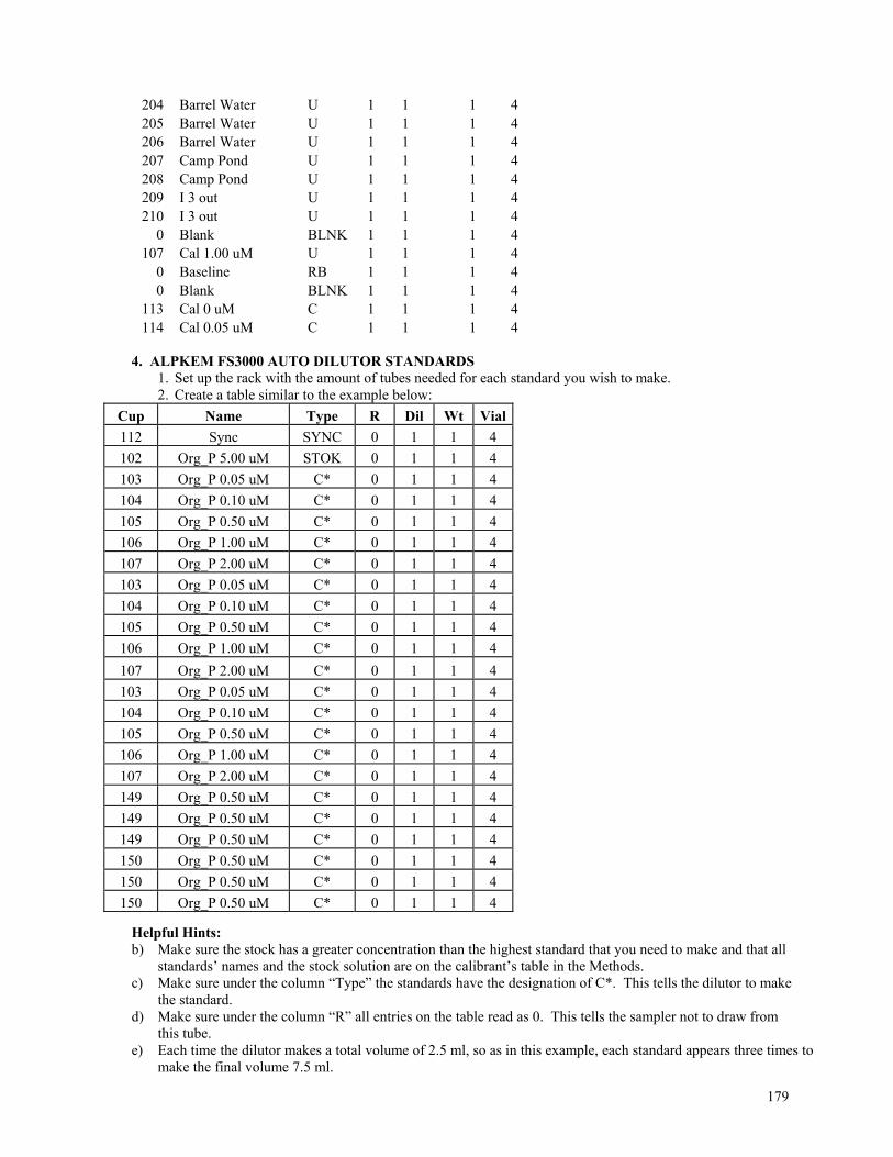
179

204 Barrel Water U 1 1 1 4 205 Barrel Water U 1 1 1 4 206 Barrel Water U 1 1 1 4 207 Camp Pond U 1 1 1 4 208 Camp Pond U 1 1 1 4 209 I 3 out U 1 1 1 4 210 I 3 out U 1 1 1 4

0 Blank BLNK 1 1 1 4 107 Cal 1.00 uM U 1 1 1 4

0 Baseline RB 1 1 1 4 0 Blank BLNK 1 1 1 4

113 Cal 0 uM C 1 1 1 4 114 Cal 0.05 uM C 1 1 1 4

4. ALPKEM FS3000 AUTO DILUTOR STANDARDS

1. Set up the rack with the amount of tubes needed for each standard you wish to make. 2. Create a table similar to the example below:

Helpful Hints: b) Make sure the stock has a greater concentration than the highest standard that you need to make and that all

standards’ names and the stock solution are on the calibrant’s table in the Methods. c) Make sure under the column “Type” the standards have the designation of C*. This tells the dilutor to make

the standard. d) Make sure under the column “R” all entries on the table read as 0. This tells the sampler not to draw from

this tube. e) Each time the dilutor makes a total volume of 2.5 ml, so as in this example, each standard appears three times to

make the final volume 7.5 ml.

Cup Name Type R Dil Wt Vial

112 Sync SYNC 0 1 1 4

102 Org_P 5.00 uM STOK 0 1 1 4

103 Org_P 0.05 uM C* 0 1 1 4

104 Org_P 0.10 uM C* 0 1 1 4

105 Org_P 0.50 uM C* 0 1 1 4

106 Org_P 1.00 uM C* 0 1 1 4

107 Org_P 2.00 uM C* 0 1 1 4

103 Org_P 0.05 uM C* 0 1 1 4

104 Org_P 0.10 uM C* 0 1 1 4

105 Org_P 0.50 uM C* 0 1 1 4

106 Org_P 1.00 uM C* 0 1 1 4

107 Org_P 2.00 uM C* 0 1 1 4

103 Org_P 0.05 uM C* 0 1 1 4

104 Org_P 0.10 uM C* 0 1 1 4

105 Org_P 0.50 uM C* 0 1 1 4

106 Org_P 1.00 uM C* 0 1 1 4

107 Org_P 2.00 uM C* 0 1 1 4

149 Org_P 0.50 uM C* 0 1 1 4

149 Org_P 0.50 uM C* 0 1 1 4

149 Org_P 0.50 uM C* 0 1 1 4

150 Org_P 0.50 uM C* 0 1 1 4

150 Org_P 0.50 uM C* 0 1 1 4

150 Org_P 0.50 uM C* 0 1 1 4

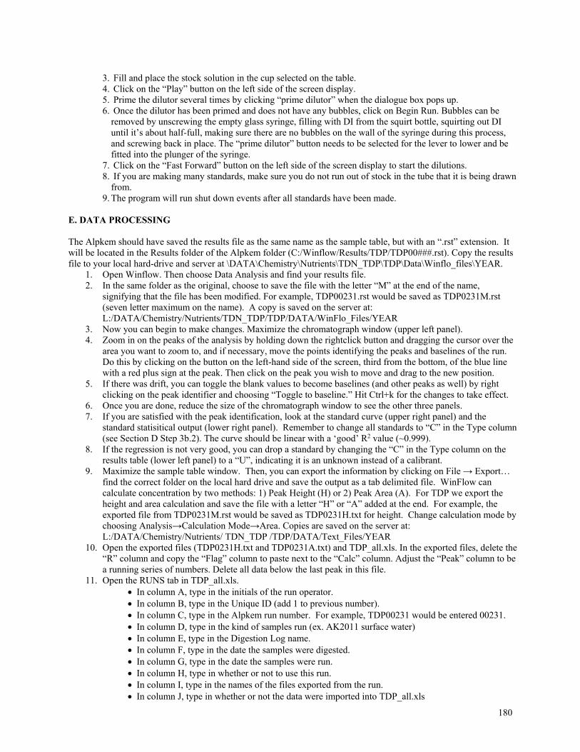
180

3. Fill and place the stock solution in the cup selected on the table. 4. Click on the “Play” button on the left side of the screen display. 5. Prime the dilutor several times by clicking “prime dilutor” when the dialogue box pops up. 6. Once the dilutor has been primed and does not have any bubbles, click on Begin Run. Bubbles can be

removed by unscrewing the empty glass syringe, filling with DI from the squirt bottle, squirting out DI until it’s about half-full, making sure there are no bubbles on the wall of the syringe during this process, and screwing back in place. The “prime dilutor” button needs to be selected for the lever to lower and be fitted into the plunger of the syringe.

7. Click on the “Fast Forward” button on the left side of the screen display to start the dilutions. 8. If you are making many standards, make sure you do not run out of stock in the tube that it is being drawn

from. 9. The program will run shut down events after all standards have been made.

E. DATA PROCESSING The Alpkem should have saved the results file as the same name as the sample table, but with an “.rst” extension. It will be located in the Results folder of the Alpkem folder (C:/Winflow/Results/TDP/TDP00###.rst). Copy the results file to your local hard-drive and server at \DATA\Chemistry\Nutrients\TDN_TDP\TDP\Data\Winflo_files\YEAR.

1. Open Winflow. Then choose Data Analysis and find your results file. 2. In the same folder as the original, choose to save the file with the letter “M” at the end of the name,

signifying that the file has been modified. For example, TDP00231.rst would be saved as TDP0231M.rst (seven letter maximum on the name). A copy is saved on the server at: L:/DATA/Chemistry/Nutrients/TDN_TDP/TDP/DATA/WinFlo_Files/YEAR

3. Now you can begin to make changes. Maximize the chromatograph window (upper left panel). 4. Zoom in on the peaks of the analysis by holding down the rightclick button and dragging the cursor over the

area you want to zoom to, and if necessary, move the points identifying the peaks and baselines of the run. Do this by clicking on the button on the left-hand side of the screen, third from the bottom, of the blue line with a red plus sign at the peak. Then click on the peak you wish to move and drag to the new position.

5. If there was drift, you can toggle the blank values to become baselines (and other peaks as well) by right clicking on the peak identifier and choosing “Toggle to baseline.” Hit Ctrl+k for the changes to take effect.

6. Once you are done, reduce the size of the chromatograph window to see the other three panels. 7. If you are satisfied with the peak identification, look at the standard curve (upper right panel) and the

standard statisitical output (lower right panel). Remember to change all standards to “C” in the Type column (see Section D Step 3b.2). The curve should be linear with a ‘good’ R2 value (~0.999).

8. If the regression is not very good, you can drop a standard by changing the “C” in the Type column on the results table (lower left panel) to a “U”, indicating it is an unknown instead of a calibrant.

9. Maximize the sample table window. Then, you can export the information by clicking on File → Export… find the correct folder on the local hard drive and save the output as a tab delimited file. WinFlow can calculate concentration by two methods: 1) Peak Height (H) or 2) Peak Area (A). For TDP we export the height and area calculation and save the file with a letter “H” or “A” added at the end. For example, the exported file from TDP0231M.rst would be saved as TDP0231H.txt for height. Change calculation mode by choosing Analysis→Calculation Mode→Area. Copies are saved on the server at: L:/DATA/Chemistry/Nutrients/ TDN_TDP /TDP/DATA/Text_Files/YEAR

10. Open the exported files (TDP0231H.txt and TDP0231A.txt) and TDP_all.xls. In the exported files, delete the “R” column and copy the “Flag” column to paste next to the “Calc” column. Adjust the “Peak” column to be a running series of numbers. Delete all data below the last peak in this file.

11. Open the RUNS tab in TDP_all.xls. In column A, type in the initials of the run operator. In column B, type in the Unique ID (add 1 to previous number). In column C, type in the Alpkem run number. For example, TDP00231 would be entered 00231. In column D, type in the kind of samples run (ex. AK2011 surface water) In column E, type in the Digestion Log name. In column F, type in the date the samples were digested. In column G, type in the date the samples were run. In column H, type in whether or not to use this run. In column I, type in the names of the files exported from the run. In column J, type in whether or not the data were imported into TDP_all.xls

181

In column K, type in any relevant notes about the run. Finally, type in any relevant notes in column L.

12. Open the Raw_Data tab in TDP_all.xls. Copy the information from the exported files into columns L through W. Copy column N into column D. Copy down column A to continue the series. In column B, type in the Alpkem file name. In column C, type in the Unique ID from the RUNS tab. Look up the identifiers in columns E through I (Site, Date, Time, etc.) from the Sortchem in the

AKchem inventory. Type “Yes” or “No” into column J to identify if the information should be used for each individual

sample. In column AD, type in any notes about the sample (especially if you are not planning to use the

data). 13. See the Notes tab of TDP_all.xls for processing instructions, but make sure to update the blue DATA tab by

dragging down the formulas in columns A-U. At some point you will have to assign a curve number to the data (column B), but first copy the standard curve data into the appropriate standard curve files. Make sure to use the height and area values that account for dilution. Use Special Paste to transpose the “values only” of any standards in column Q into the HT_1_Std_Curve tab (light blue) and column S into the Area_1_Std_Curve tab (pale yellow). Then, drag down the formulas in the standard curve tabs and look at the graphs to make sure that the curves look good. Then, check the r2 values and determine which curve (area or height) is statistically a better fit. Fill in a1 or h1 in column V of the data tab, depending on the answer. Also assign each curve a number (generally 1, 2, or 3) and fill in the appropriate curve number in column B of the data tab. To do this, count the number of samples run, and pick whichever curve has the closest 0 standard to that sample. Finally, copy down the formulas in columns W to AC to get the final concentrations of the samples run.

14. Save the file on the local hard-drive and the server at \DATA\Chemistry\Nutrients\TDN_TDP\TDP\Data\TDP_all.xls

15. See the Notes tab of TDP_all.xls for additional processing instructions (like how to handle the data so that you can put it into AKChem. )

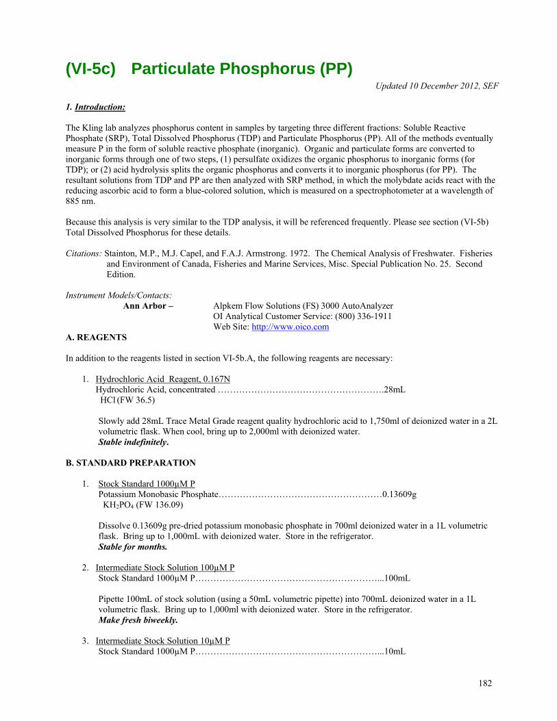
182

(VI-5c) Particulate Phosphorus (PP) Updated 10 December 2012, SEF

1. Introduction:

The Kling lab analyzes phosphorus content in samples by targeting three different fractions: Soluble Reactive Phosphate (SRP), Total Dissolved Phosphorus (TDP) and Particulate Phosphorus (PP). All of the methods eventually measure P in the form of soluble reactive phosphate (inorganic). Organic and particulate forms are converted to inorganic forms through one of two steps, (1) persulfate oxidizes the organic phosphorus to inorganic forms (for TDP); or (2) acid hydrolysis splits the organic phosphorus and converts it to inorganic phosphorus (for PP). The resultant solutions from TDP and PP are then analyzed with SRP method, in which the molybdate acids react with the reducing ascorbic acid to form a blue-colored solution, which is measured on a spectrophotometer at a wavelength of 885 nm. Because this analysis is very similar to the TDP analysis, it will be referenced frequently. Please see section (VI-5b) Total Dissolved Phosphorus for these details. Citations: Stainton, M.P., M.J. Capel, and F.A.J. Armstrong. 1972. The Chemical Analysis of Freshwater. Fisheries

and Environment of Canada, Fisheries and Marine Services, Misc. Special Publication No. 25. Second Edition.

Instrument Models/Contacts: Ann Arbor – Alpkem Flow Solutions (FS) 3000 AutoAnalyzer OI Analytical Customer Service: (800) 336-1911 Web Site: http://www.oico.com A. REAGENTS In addition to the reagents listed in section VI-5b.A, the following reagents are necessary:

1. Hydrochloric Acid Reagent, 0.167N Hydrochloric Acid, concentrated ……………………………………………….28mL HCl (FW 36.5)

Slowly add 28mL Trace Metal Grade reagent quality hydrochloric acid to 1,750ml of deionized water in a 2L volumetric flask. When cool, bring up to 2,000ml with deionized water. Stable indefinitely.

B. STANDARD PREPARATION

1. Stock Standard 1000µM P Potassium Monobasic Phosphate………………………………………………0.13609g KH2PO4 (FW 136.09) Dissolve 0.13609g pre-dried potassium monobasic phosphate in 700ml deionized water in a 1L volumetric flask. Bring up to 1,000mL with deionized water. Store in the refrigerator. Stable for months.


Stock Standard 1000µM P……………………………………………………...100mL Pipette 100mL of stock solution (using a 50mL volumetric pipette) into 700mL deionized water in a 1L volumetric flask. Bring up to 1,000ml with deionized water. Store in the refrigerator. Make fresh biweekly.


Stock Standard 1000µM P……………………………………………………...10mL

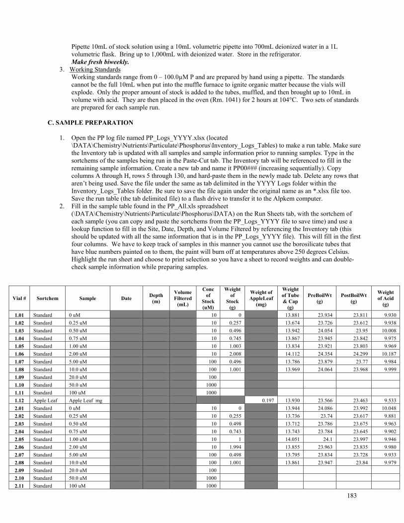
183

Pipette 10mL of stock solution using a 10mL volumetric pipette into 700mL deionized water in a 1L volumetric flask. Bring up to 1,000mL with deionized water. Store in the refrigerator. Make fresh biweekly.

3. Working Standards Working standards range from 0 – 100.0µM P and are prepared by hand using a pipette. The standards

cannot be the full 10mL when put into the muffle furnace to ignite organic matter because the vials will explode. Only the proper amount of stock is added to the tubes, muffled, and then brought up to 10mL in volume with acid. They are then placed in the oven (Rm. 1041) for 2 hours at 104°C. Two sets of standards are prepared for each sample run.

C. SAMPLE PREPARATION

1. Open the PP log file named PP_Logs_YYYY.xlsx (located \DATA\Chemistry\Nutrients\Particulate\Phosphorus\Inventory_Logs_Tables) to make a run table. Make sure the Inventory tab is updated with all samples and sample information prior to running samples. Type in the sortchems of the samples being run in the Paste-Cut tab. The Inventory tab will be referenced to fill in the remaining sample information. Create a new tab and name it PP00### (increasing sequentially). Copy columns A through H, rows 5 through 130, and hard-paste them in the newly made tab. Delete any rows that aren’t being used. Save the file under the same as tab delimited in the YYYY Logs folder within the Inventory_Logs_Tables folder. Be sure to save the file again under the original name as an *.xlsx file too. Save the run table (the tab delimited file) to a flash drive to transfer it to the Alpkem computer.

2. Fill in the sample table found in the PP_All.xls spreadsheet (\DATA\Chemistry\Nutrients\Particulate\Phosphorus\DATA) on the Run Sheets tab, with the sortchem of each sample (you can copy and paste the sortchems from the PP_Logs_YYYY file to save time) and use a lookup function to fill in the Site, Date, Depth, and Volume Filtered by referencing the Inventory tab (this should be updated with all the same information that is in the PP_Logs_YYYY file). This will fill in the first four columns. We have to keep track of samples in this manner you cannot use the borosilicate tubes that have blue numbers painted on to them, the paint will burn off at temperatures above 250 degrees Celsius. Highlight the run sheet and choose to print selection so you have a sheet to record weights and can double-check sample information while preparing samples.

Vial # Sortchem Sample Date Depth

(m)

Volume Filtered

(mL)

Conc of

Stock (uM)

Weight of

Stock (g)

Weight of AppleLeaf

(mg)

Weight of Tube & Cap

(g)

PreBoilWt (g)

PostBoilWt (g)

Weight of Acid

(g)

1.01 Standard 0 uM 10 0 13.881 23.934 23.811 9.930

1.02 Standard 0.25 uM 10 0.257 13.674 23.726 23.612 9.938

1.03 Standard 0.50 uM 10 0.496 13.942 24.054 23.95 10.008

1.04 Standard 0.75 uM 10 0.745 13.867 23.945 23.842 9.975

1.05 Standard 1.00 uM 10 1.003 13.834 23.921 23.803 9.969

1.06 Standard 2.00 uM 10 2.008 14.112 24.354 24.299 10.187

1.07 Standard 5.00 uM 100 0.496 13.786 23.879 23.77 9.984

1.08 Standard 10.0 uM 100 1.001 13.969 24.064 23.968 9.999

1.09 Standard 20.0 uM 100

1.10 Standard 50.0 uM 1000

1.11 Standard 100 uM 1000

1.12 Apple Leaf Apple Leaf mg 0.197 13.930 23.566 23.463 9.533

2.01 Standard 0 uM 10 0 13.944 24.086 23.992 10.048

2.02 Standard 0.25 uM 10 0.255 13.736 23.74 23.617 9.881

2.03 Standard 0.50 uM 10 0.498 13.712 23.786 23.675 9.963

2.04 Standard 0.75 uM 10 0.743 13.743 23.784 23.645 9.902

2.05 Standard 1.00 uM 10 1 14.051 24.1 23.997 9.946

2.06 Standard 2.00 uM 10 1.994 13.855 23.963 23.835 9.980

2.07 Standard 5.00 uM 100 0.498 13.795 23.834 23.728 9.933

2.08 Standard 10.0 uM 100 1.001 13.861 23.947 23.84 9.979

2.09 Standard 20.0 uM 100

2.10 Standard 50.0 uM 1000

2.11 Standard 100 uM 1000

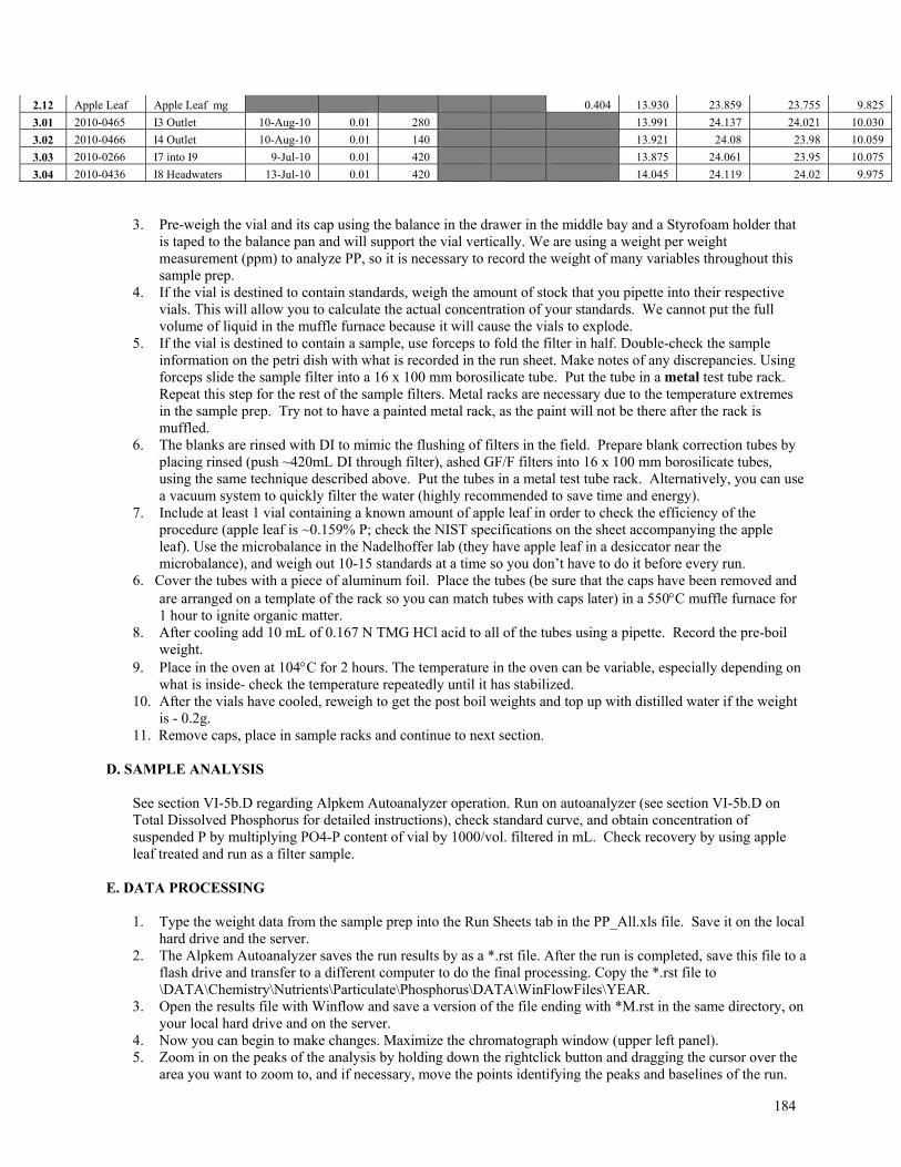
184

2.12 Apple Leaf Apple Leaf mg 0.404 13.930 23.859 23.755 9.825

3.01 2010-0465 I3 Outlet 10-Aug-10 0.01 280 13.991 24.137 24.021 10.030

3.02 2010-0466 I4 Outlet 10-Aug-10 0.01 140 13.921 24.08 23.98 10.059

3.03 2010-0266 I7 into I9 9-Jul-10 0.01 420 13.875 24.061 23.95 10.075

3.04 2010-0436 I8 Headwaters 13-Jul-10 0.01 420 14.045 24.119 24.02 9.975

3. Pre-weigh the vial and its cap using the balance in the drawer in the middle bay and a Styrofoam holder that

is taped to the balance pan and will support the vial vertically. We are using a weight per weight measurement (ppm) to analyze PP, so it is necessary to record the weight of many variables throughout this sample prep.

4. If the vial is destined to contain standards, weigh the amount of stock that you pipette into their respective vials. This will allow you to calculate the actual concentration of your standards. We cannot put the full volume of liquid in the muffle furnace because it will cause the vials to explode.

5. If the vial is destined to contain a sample, use forceps to fold the filter in half. Double-check the sample information on the petri dish with what is recorded in the run sheet. Make notes of any discrepancies. Using forceps slide the sample filter into a 16 x 100 mm borosilicate tube. Put the tube in a metal test tube rack. Repeat this step for the rest of the sample filters. Metal racks are necessary due to the temperature extremes in the sample prep. Try not to have a painted metal rack, as the paint will not be there after the rack is muffled.

6. The blanks are rinsed with DI to mimic the flushing of filters in the field. Prepare blank correction tubes by placing rinsed (push ~420mL DI through filter), ashed GF/F filters into 16 x 100 mm borosilicate tubes, using the same technique described above. Put the tubes in a metal test tube rack. Alternatively, you can use a vacuum system to quickly filter the water (highly recommended to save time and energy).

7. Include at least 1 vial containing a known amount of apple leaf in order to check the efficiency of the procedure (apple leaf is ~0.159% P; check the NIST specifications on the sheet accompanying the apple leaf). Use the microbalance in the Nadelhoffer lab (they have apple leaf in a desiccator near the microbalance), and weigh out 10-15 standards at a time so you don’t have to do it before every run.

6. Cover the tubes with a piece of aluminum foil. Place the tubes (be sure that the caps have been removed and are arranged on a template of the rack so you can match tubes with caps later) in a 550C muffle furnace for 1 hour to ignite organic matter.

8. After cooling add 10 mL of 0.167 N TMG HCl acid to all of the tubes using a pipette. Record the pre-boil weight.

9. Place in the oven at 104C for 2 hours. The temperature in the oven can be variable, especially depending on what is inside- check the temperature repeatedly until it has stabilized.

10. After the vials have cooled, reweigh to get the post boil weights and top up with distilled water if the weight is - 0.2g.

11. Remove caps, place in sample racks and continue to next section.

D. SAMPLE ANALYSIS

See section VI-5b.D regarding Alpkem Autoanalyzer operation. Run on autoanalyzer (see section VI-5b.D on Total Dissolved Phosphorus for detailed instructions), check standard curve, and obtain concentration of suspended P by multiplying PO4-P content of vial by 1000/vol. filtered in mL. Check recovery by using apple leaf treated and run as a filter sample.

E. DATA PROCESSING

1. Type the weight data from the sample prep into the Run Sheets tab in the PP_All.xls file. Save it on the local hard drive and the server.

2. The Alpkem Autoanalyzer saves the run results by as a *.rst file. After the run is completed, save this file to a flash drive and transfer to a different computer to do the final processing. Copy the *.rst file to \DATA\Chemistry\Nutrients\Particulate\Phosphorus\DATA\WinFlowFiles\YEAR.

3. Open the results file with Winflow and save a version of the file ending with *M.rst in the same directory, on your local hard drive and on the server.

4. Now you can begin to make changes. Maximize the chromatograph window (upper left panel). 5. Zoom in on the peaks of the analysis by holding down the rightclick button and dragging the cursor over the

area you want to zoom to, and if necessary, move the points identifying the peaks and baselines of the run.

185

Do this by clicking on the button on the left-hand side of the screen, third from the bottom, of the blue line with a red plus sign at the peak. Then click on the peak you wish to move and drag to the new position.


7. Once you are done, reduce the size of the chromatograph window to see the other three panels. 8. If you are satisfied with the peak identification, look at the standard curve (upper right panel) and the

standard statistical output (lower right panel). Change all standards to “C” in the Type column to designate the measurement was from a calibrant (standard- the new software won’t let you run calibrants after “unknown” samples so the Type must be altered later). The curve should be linear with a ‘good’ R2 value (~0.99) but this curve was created under the assumption that the standards were perfectly made (i.e., exactly 1.00uM or 5.00uM) but they weren’t. The true concentrations will be calculated later, so a ‘good’ R2 isn’t necessarily expected.

9. If the regression is not very good, you can drop a standard by changing the “C” in the Type column on the results table (lower left panel) to a “U”, indicating it is an unknown instead of a calibrant. This can also be determined at a later step.

10. Export the information by clicking on File → Export… find the correct folder on the local hard drive and save the output as a tab delimited file. WinFlow can calculate concentration by two methods: 1) Peak Height (H) or 2) Peak Area (A). For PP we export the height calculation and save the file with a letter “H” added at the end. For example, the exported file from PP0231M.rst would be saved as PP00231H.txt for height. Change calculation mode by choosing Analysis→Calculation Mode→Area. Copies are saved at \DATA\Chemistry\Nutrients\Particulate\Phosphorus\DATA\Text Files\YYYY

11. Open the exported file (PP00231H.txt) and PP_All.xls. In the exported file, delete the “R” column and copy the “Flag” column to paste next to the “Calc” column. Adjust the “Peak” column to be a running series of numbers. Delete all data below the last peak in this file.

12. In the DATA tab in PP_All.xls, paste the information from the text file – from the Peak column through the Flag column – into columns J through R.

13. Type the subsequent run number in column A. 14. Place Y or N in columns D through G if the vial is usable, contains a sample or a standard, or is a half filter.

(Half of the PP filter may be used/missing if the PCN does not get a value the first time when running the PCN filters.)

15. Drag down the formulas from columns S through AF. 16. Copy and paste the appropriate information from the Run Sheets tab and the DATA tab into the Standard

Curves tab. After looking at the curves (adjust the run number in cell B1), assign which curve you want to reference in column B in the DATA tab. Usually, we assign curve 1 and curve 2, which is an average of the curves run (so 4 curves total – curve 1 is run before and after the first half of samples and curve 2 run before and after the second half of samples). There is generally a lot of drift in this analysis, and each curve is assigned to half of the samples.

17. Drag the formulas down in columns AH:AO. 18. Copy the formulas in columns AP:AX for any apple leaf standards run. Change the weight in column AQ to

whatever you were running in that vial to calculate the %efficiency. We shoot for 100% but there is generally some variability (+/- 10%, usually on the + side) due to errors while weighing, etc.

19. Make sure to double-check the values calculated for samples that were run twice (the first vial of each column in the sample rack is rerun near the end of the run) – if there are large differences (greater than 0.05uM), re-examine the run.

20. Also double-check the concentrations for the blanks (column AE) and make sure they aren’t high (compare to the average concentration in cell H2).

F. FINAL QA/QC

1. After all the samples have been run, update the Inventory tab with the most up-to-date sample information. If you found any discrepancies between the run sheet and what was in the Inventory, make sure you look into those and make changes in the appropriate files. This will update the sample information in the DATA tab because it references the Inventory tab.

2. Update the Summary tab to begin the final QA/QC. Copy the data in AH:AO in the DATA tab, and paste the values in the Summary tab into columns A through H. Sort by sortchem, and delete all non-samples. Drag the formulas down in columns I through M. Double check to make sure the formula are averaging the correct values for instances in which there are double sucks on either the duplicate or the original sample IN ADDITION to the duplicate or original sample.

186

3. The %CV column will only calculate the variation for two samples (replicates or duplicates) but not for more than 2 (like when a sample has a replicate AND a duplicate). Scan through these values and look at any that are greater than 10%. There is a place to mark to check a sample and make notes in columns N and O. Ideally, all %CVs would be less than 10%, but this is particularly unlikely for field duplicates because they’ve gone through entirely separate processes (filtering, sample prep, etc). Make sure to consider the actual sample concentrations as well. Low concentrations may show a high %CV but the actual differences in concentration are very small (less than 0.1uM). Investigate large %CVs to try to uncover other issues- maybe a standard curve was mis-assigned or a sample was actually half a filter but that wasn’t designated in the DATA tab. Also note that some samples typically show more variation between field duplicates, like Imnavait Weir.

4. After any necessary changes have been made (make sure to re-update the DATA/Summary tabs), copy the data in the Summary tab through column M and hard-paste in the QAQC tab. Sort by site name, then date, and make graphs for each site. Check for outliers. Look at previous years’ data to get a better idea for what is “expected” for a site. If a value seems high (or low), check the DATA tab and Run Sheets tab for an indication of why the sample may have that concentration. There could be a note that the sample was dropped on the floor, for example, which would excuse removing its value and replacing with a “.” MAKE NOTES OF ANY CHANGES.

5. Finally, update the To_AKChem tab from the QAQC tab (columns A:L). Update the appropriate files (akchem_YYYY or akchem_allyears_final) with the values according to protocol.

187

(VI-6) Nitrate / Nitrite Determination Updated: JML 28 May 2015 1. Introduction: This analysis uses nitrogen segmented flow and a commercially available cadmium reactor coil to determine the amount of nitrate and nitrate in surface and soil waters. The cadmium reduces the nitrate species to nitrite forms, and determines the concentration of nitrite by colorimetric analysis. If you desire to obtain the concentration of nitrate and nitrite separately, samples must be analyzed twice, once with the cadmium coil (nitrate+nitrite) and once without the coil (nitrite only). Nitrate concentrations can then be calculated as the difference between the two analyses. For Toolik surface water (and many other systems), nitrite concentrations are negligible, so we only analyze our samples once with the column. Citations: Oi analytical, 4500-NO3- F. Automated Cadmium Reduction Method. 1995. Standard Methods for the Examination of Water and Wastewater 19th Ed. EPA Method 353.3. Methods for the Chemical Analysis of Water and Wastes (MCAWW) (EPA/600/4-79/020) Armstrong, F.A., C.R. Stearns, J.D. Strickland. 1967 The measurement of upwelling and subsequent Biological

processes by means of the Technicon AutoAnalyzer and associated equipment. Deep Sea Research 14:381. Instrument Models/Contacts: Ann Arbor – Alpkem FS3100 AutoAnalyzer, purchased November 2013 OI Analytical Customer Service: (800) 336-1911, usually we talk to Tim Smith Sales (check part #, prices): (800) 653-1711 Web Site: http://www.oico.com Astoria Pacifica (tubing and reducing coils) Web Site:ezkem.com (tubing and reducing coils) 2. Before starting analysis: a. Check chemical closet for all chemicals used in this analysis. Make sure there is enough to account for all

samples being run and order what is needed. b. Place a small amount (~5 grams) of the compounds being used to make the stock standards in beakers covered

with aluminum foil in the drying oven overnight. c. Check the desiccant near the balance. It may need to be reactivated before weighing the standard compounds.

(167degrees C in the muffle furnace) d. Replace all tubing on the autoanalyzer. Order any tubing in low supply. Make sure to check that all tubing is

connected properly, even tubing inside autodilutor. e. Run DI water through all lines and check for any leaks at the autosampler, autodilutor, and autosampler. 3. Reagents: a. Imidazole buffer (NEW REAGENT 2014) Dissolve 6.81 g imidazole in DDW and dilute to 900 ml. pH adjust to 7.5 with concentrated hydrochloric acid (in 2014 I found it takes one disposable dropper-full, plus

about 15-20 drops to get the pH to 7.5. Life undetermined - should be stable for long period. Store in NO3 Chemicals Cupboard. b. Color Reagent Add 100 mL concentrated H3PO4 and 10 g sulfanilimide to 750 mL DDW and dissolve completely.

Add 0.5 g N-1-napthylethylenediamine dihydrochloride and dissolve. Dilute to 1000 mL with DDW and dissolve. Store in 1 L pyrex bottle wrapped in foil; refrigerate; good until develops a pink color. c. Cupric sulfate solution

Dissolve 10 g CuSO4.5H2O in 500 mililiters of distilled water (0.08 M, 2% w/v cupric sulfate solution).

Life undetermined - should be good indefinitely.

188

d. 10 % v/v Hydrochloric Acid Add 50 mL concentrated HCl to 450 mL DDW. Store in glass bottle. Good indefinitely. 4. Standard Preparation a. Stock Solutions 1. Nitrate Standard – 1000 µM

Dissolve 0.08499 g pre-dried (105 C for one hour) sodium nitrate (NaNO3) in 1000 mL DI

(1000µM). Refrigerate. Stable indefinitely.

2. Nitrite Standard - 1000µM

Dissolve 0.069 g pre-dried (105 C for one hour) sodium nitrite (NaNO2) in 1000 mL DI (1000µM).

Refrigerate. Stable indefinitely. b. Working Standards

Working standards range from 0.10 – 10.0µM N (Nitrate) and 10.0 µM N (Nitrite). They are prepared using the OI Analytical MS Autodilutor. Each individual standard should have enough volume to run three sets of standards for each sample run. Do this by diluting the same standard in a test tube multiple times (2.5 mL X 4 dilutions, See section 7D). If the Autodilutor cannot be used or is not functioning properly, standards will need to be prepared volumetrically (volumetric pipettes in volumetric flasks, for best accuracy).

5. Sample Preparation: Nitrate samples are preserved by freezing, and must be thawed completely before running. We have the capability to run 240 samples per run, but we usually run 80 samples per run to reduce the possibility of reruns due to drift or human error (running out of reagent, not putting all the tubes in, etc.).

A. Fill a 2.5 L bottle (labeled degassed DI) with DI water then degas on stir plate until no more bubbles are produced (section 6).

B. Select all samples to be run (maximum of ~80) out of the freezer and space them out on plastic trays to thaw (these are currently on the cabinets of the second bay). Current year nitrate samples are stored in the refrigerator in room 1041 and 1037. Additionally, a small electric fan (room 1041) can be used on the samples to decrease thaw time.

C. Sort out and copy nitrate inventory for appropriate sample year from the server (DATA\Arctic\akXXXX\chem\ XXXX_SampleInventory). Then Paste into NO3_Runsheet_XXXX on the NO3_inventory tab.

D. Copy the excel sheet labeled TEMPLATE in NO3_Runsheet_XXXX and re-label the copied sheet with the run number (Run number increases numerically, check clipboard near autoanalyzer or NO3_XXXX file for the previous run number).

E. Type sortchems of the samples that are going to be run into the blank cells in the NAME column, starting at sample 1. The site name and other sample information will fill itself in.

F. Adjust end the end of the runsheet for the length of each specific run so that there are no duplicates or empty cells in the entire run. Each run should have a 0.40 uM check standard every ten samples, a set of standards at the beginning, after 40 samples, and at the end of the run.

G. Once the runsheet is filled out, copy all of the blue text that is outlined in the runsheet and paste it into a Sample Table in WinFlow. Save the sample table with the same run number used in NO3_Runsheet_XXXX.

H. After the run is set up in WinFlow, the cadmium coil can be reactivated if necessary (See section 6). 6. Cadmium Reactor Coils: While it is possible to make reductor columns in the lab, we have been purchasing Open Tube Cadmium Reactors (OTCR) from either OI Analytical (model #: A000897) or Astoria Pacifica (model #: 303-0500-24) or, in 2014, EZ-Kem. Purchasing the premade coils reduces the exposure to cadmium to the environment, and more importantly, to ourselves. However, you are still using acids and other dangerous chemicals, so wear eye protection, a lab coat, and gloves.

189

Before any analysis, it is necessary to prereact the coil with 10% HCl (to strip the cadmium of buildup) and CuSO4 solution (to reactivate the cadmium). Once the process is started do not expose the inside of the coil to air, it will reduce the reduction efficiency (and you’ll have to do this all over again):

A. Fill three dedicated 10 mL syringes with 10mL of 10% HCl, CuSO4, and 20 mL of imidazole buffer solution.

B. Attach a luer tip adapter into one end of the OTCR. C. Place the tube at the opposite end of the OTCR into a waste beaker. D. Quickly attach the HCl syringe and push the liquid through. It should take less than 3 seconds to

complete this step. E. Swap out that syringe for the imidazole buffer and quickly flush through the column F. Attach the CuSO4 syringe to the adapter. Slowly push CuSo4 through the column. Push enough

through that you see it come out the other side, then allow it to sit in the column for 1-2 minutes. Then slowly push through the remaining CuSO4. This process needs to be slow enough to regenerate the column, but not so slow that you over-react the column.

G. Replace the copper sulfate syringe with the imidazole buffer syringe and flush with buffer. You should see black flocculate coming out of the column.

H. Quickly reattach the ends of the column, so that it’s not exposed to air, then hook it up in line with the instrument once you’re ready to run/have established a good baseline.

NOTE: The Brij-35 surfactant is not good for the column, and the Brij is added to the mixed reagent, which flows in line after the sample has gone through the column. Avoid putting the column on if you’re flushing the system with Brij 35 (when you first start up the instrument).

7. Sample Analysis:

A. ALPKEM FS3100 AUTOANALYZER CONFIGURATION The set up of the Alpkem Autoanalyzer is very amenable to modification. The user can increase/decrease the rate of sample analysis by changing the tubing types, the sample loop, and time of sample suction. In general, as time between suction and time entering the flow cell increases, the analysis gains resolution due to a longer reaction time. Currently, we use the Winflow version 4.2 as the operating/analysis software. The speed and flow direction of the IPC pump (High Precision Multichannel Depsensor) can be altered to desired flow rates and directions. Currently for nitrate, the IPC is set up to flow counter clockwise (designated as a negative direction) at a speed setting of -40. Flow direction may be changed by pressing the escape button (two opposite pointing arrows), and speed may be increased or decreased using the two settings arrow buttons at the top right of the IPC. The Valve Inject time in WinFlow settings must be adjusted as the speed of the IPC and sample tubing length are changed. The Valve Inject time is currently set at 98.000 seconds with the current sample tubing length and IPC set at -40. To adjust the Valve Inject time, first allow the autosampler to suck up a significant amount of air, and record the amount of time it takes for the air bubble to pass through the sample line and reach the valve. Then open the Method Editor tab in the main screen of WinFlow and click the stopwatch icon on the lefthand side of the window and enter the recorded time in the appropriate valve inject cell. All tubing should be properly labeled with its intended purpose.

1. Tubing and cartridge configuration We Use Alpkem Recommends a. Carrier (Degased water) black-black black-black b. Sample pull (To Waste) purple-black green-green c. To Wash (DI) purple-black(not pumped) not used d. Color Reagent black-black white-white e. Buffer yellow-yellow yellow-yellow f. Debubbler red-red white-white g. Nitrogen Pillow black-black Black-black 2. Injection loop – 400µl 3. Wavelength – 540 nm 4. Sample mixing loop – 2 mL 5. Sample rate – 2 minutes per sample

190

* The reason for using different tubing (both the debubbler and sample pull have a larger diameter than those recommended by Oi) is to get better peak resolution and fewer bubbles. By having a larger diameter on the debubbler tubing, the bubbles are able to move at a faster rate, reducing the bubbles that overpower the debubbler and flow through the flow cell.

B. ALPKEM FS3100 AUTOANALYZER STARTUP (Approx. 3 hours)

1. Turn on the power strip that the autoanalyzer and the autosampler are plugged into. 2. Check the conductivity of the RO/DI. If the conductivity reading is satisfactory, fill one of the 4L wash

containers three times times to allow 12L of DI to flow through the filter before use. 3. Rinse the dedicated 2.5L glass containers (old HCl bottles) with DI three times. Then, fill the containers to

below the neck. Next, degas the DI by using a rubber stopper large enough to fit into the mouth of the bottle and the lab vacuum. To aid in degassing, the bottles should be placed on stir plates while under vacuum. Two bottles can be degassed two at a time.

4. Open the WinFlow auto-analyzer program on the computer by clicking on the desktop icon. 5. Check the waste containers to see if they need to be emptied. The waste in the 2L containers should be

emptied into the labeled 5-gallon plastic carboy kept in the cabinet underneath the bench. 6. Empty the 2L wash container, rinse with DI, and then fill the container with degassed DI, taking care to

splash or aerate the water as you pour. Also, empty the DI water in the squirt bottles, rinse three times and refill with fresh DI water.

7. Hook up pump tubing Examine the pump tubing to make sure it is not permanently creased or crinkled, or excessively worn. If any lines look overly worn, replace with new pump lines of the same color (indicating the tube id). Depending on the use of the machine the pump tubing is replaced every 8-10 weeks (In 2014 the machine was run for several months and the pump tubing was not replaced). The new tubing will be broken in after a few hours of use. If you change tubing, let the machine pump DI for through the system for a few hours. To hook up the tubing, stretch the area between the colored nodules across the platen. The platen arrow indicates the direction that the flow is going. For reagents and the wash line, the flow should be away from the reagent bottles and towards the mixing coils and autosampler. For the sample pull and waste tubing, the flow should be away from the instrument and into a wash bottle.

8. Snap the pump platens into place by placing the platen notches in one side and then snapping in the other side. Start with the tension adjuster at a 45 degree angle, then start the pump. Unhook each tube from their respective reagents, and watch as a bubble moves through. Find the spot at which the bubble moves forward in the tube (instead of being pulled backward) and then go three clicks tighter. This allows for the proper tension on each tube. The tension adjusters may not all be at exactly the same spot.

9. If you are using the auto-dilutor to make standards, this is a good time to begin. (See section 6D). If you already have standards, continue on to step 12.

10. Reactivate the OTCR (Section 5) if necessary. If the efficiency in the previous run was below 95%, reactivate the OTCR.

11. Open NO3_Runsheet_XXXX and copy the created run into WinFlow, save the table as NIT00###.tbl, where ### is the next available run number (found on the clipboard on top of the autosampler). Save this file on the local hard drive in the dedicated folder, for example, a nitrate table would be saved as: C:/Winflow/Tables/Nitrate/NIT00231.tbl.

12. Connect the reagent line to the color reagent bottle, and connect the buffer line to the imidazole buffer solution bottle.

13. Fill the nitrogen pillow with nitrogen gas, and attach it to the autoanalyzer. The nitrogen pillow can be filled in Jim Lemoine’s lab using his nitrogen tank. A fitting for the tank that will plug into the nitrogen pillow is located below the autoanalyzer in the drawer labeled Alpkem Gas Bags. Nitrogen pillows should be filled once and then pressed to empty, then filled again before use.

14. Attach the OTCR to the mixing column. 15. Click on the Collect data button (top button on the left –hand side, a white square with 2 blue squiggly

lines) to start an analysis, choose your sample table and methods, and choose to save the results file (same naming criteria as in step 13) in C:/Winflow/Results/Nitrate/ . Click on the “Play” button in order to monitor the baseline. Begin an analysis, but do not “fast forward,” this would start the autosampler.

16. At this time, open the Serial Communications Window within the Window drop-down menu. Check the values in Ch 1. You should see “Sam ##.##% @ Gain# Ref ##.##% @ Gain#”. The Sam Gain# to Ref Gain# should be a 1 to 1 ratio, in 2014 we had 55%@16 and 80% at 16. Shoot for those values, and if you get a higher ratio, flick the tubing to try to eliminate bubbles and then restart the run . The highest

191

gain level is 128 and is undesirable. As soon as the analysis is started, Winflow obtains a percentage of light value in the middle of the percentage range for both the sample and reference photodiode, which means Winflow sets the gain level to achieve light percentages between 50 and 70. Record these values in NO3_2014.xls in the RUNS tab. See step f in Trouble Shooting & Maintenance for more on this topic.

17. After 2 hours the baseline should have stabilized (amplitude ranges between 0-250 micro Absorbance Units). If the noise is larger than 500 uAU, don’t start the instrument, instead work to get a better baseline. If the baseline is noisy, check to see if the reagents are being properly pumped. Occasionally, a bubble will become trapped in the flowcell. To clear the bubble, pinch and release the waste line going from the flowcell to the waste container (hold about 5 seconds). This will dislodge the helium bubble/bubbles. Also flicking the line going from the debubbler to the flow cell helps. If the bubble is persistent, unhook the line right before the debubbler and hook up a syringe with DI+Brij. Quickly push the water through the line, while loosening the tension on the waste line (so you’re pushing with the syringe while simultaneously pushing the tension adjuster down). This will hopefully flush any bubbles from the line. Reapply the tension to the waste tube and hook the tubing back up. You’ll see a spike in the BL, but hopefully noise will be reduced and the line will run flat.

18. While the baseline is stabilizing and the samples have completely thawed, the samples should be sonicated for 10 minutes. There are Styrofoam molds with holes cut through to hold the bottles in the sonicator. After sonicating, the samples can be poured into tubes (more than halfway full). The first tube of each column should be about three-quarters full because these tubes are sampled twice. Check the data on the sample bottles with the printed run sheet. Place the standard and sample tubes into the autosampler racks as dictated by the sample table.

19. Click on the “fast forward” button. Watch the sync peak, the efficiency test, and the first set of standards to ensure a good start for your run. Stop the analysis if any results (from sync, efficiency, or standard curve) are not what you were expecting.

20. Let the analyzer run the remaining samples.

Trouble Shooting & Maintenance: a. If there is a lot of drift in the output of the alpkem you can “clean” it with 10% HCl, by placing the

carrier line, color reagent line and buffer line in the cleaning solution. MAKE SURE THE COIL IS NOT ATTACHED. Prolonged exposure to HCl can ruin the coil. Pump the cleaning solution through the system for 15 minutes. After 15 minutes connect the carrier line and color reagent line to the wash container. Turn both pumps to the high-speed setting and let run for 5 minutes. After 5 minutes turn the pumps to the low speed setting.

**WARNING!! Cleaning of the system in this manner appears to remove a coating from the flowcell. Though this may seem to be desirable, it may not be – because the flowcell will be re-coated at the beginning of the run which initially results in a large amount of drift.** b. Run the cleaning solution through the system as needed. c. Check the color reagent to ensure pink coloration has not occurred. If it is already pink, there is

contamination. Contamination Sources and Victims:

Acid Bath (Test Tubes) DI System (Reagents/DI) Dirty Glassware (Standards) Backflushing (Tubing)

d. If the sampler arm does not sample (i.e., draw in water), try the following: 1. Tighten the four screws closest to the valve. 2. Remove the entire valve module and tighten all screws and tube connections.

Check for kinks in the tubes. 3. Use a syringe to push DI through the tubes and check for leaks/blockages. 4. Remove the black gear box from the valve and disassemble the valve. Clean all

parts with cotton swabs located in the drawer under the autoanalyzer. Grease the shaft piece with silicone oil.

e. If the baseline will not stabilize, remove the cadmium column from the system and run DI/reagents for several hours. This helps condition all tubing and reduce noise.

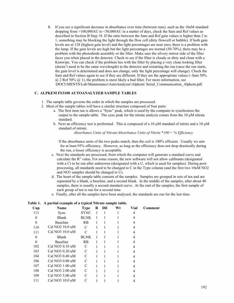
192

f. If you see a significant decrease in absorbance over time (between runs), such as the 10uM standard dropping from >100,000AU to <50,000AU in a matter of days, check the Sam and Ref values as described in Section B Step 18. If the ratio between the Sam and Ref gain values is higher than 2 to 1, something may be blocking the light through the flow cell (dirty flowcell or bubble). If both gain levels are at 128 (highest gain level) and the light percentages are near zero, there is a problem with the lamp. If the gain levels are high but the light percentages are normal (50-70%), there may be a problem with the photodiode assembly or the filter. Make sure the silvery mirror side of the filter faces you when placed in the detector. Check to see if the filter is cloudy or dirty and clean with a Kimwipe. You can check if the problem lies with the filter by placing a very clean looking filter (doesn’t need to be the same wavelength) in the detector and restarting the run (once the run starts, the gain level is determined and does not change; only the light percentage will change). Check the Sam and Ref values again to see if they are different. If they are the appropriate values (~Sam 50% @ 2 Ref 50% @ 1), the problem is most likely a bad filter. For more information, see \DOCUMENTS\Lab\Maintenance\AutoAnalyzer\Alpkem\ Serial_Communication_Alpkem.pdf.

C. ALPKEM FS3100 AUTOANALYZER SAMPLE TABLES

1. The sample table governs the order in which the samples are processed. 2. Most of the sample tables will have a similar structure composed of four parts:

a. The first item ran is allows a “Sync” peak, which is used by the computer to synchronize the output to the sample table. The sync peak for the nitrate analysis comes from the 10 μM nitrate standard.

b. Next an efficiency test is preformed. This is composed of a 10 μM standard of nitrite and a 10 μM standard of nitrate.

Absorbance Units of Nitrate/Absorbance Units of Nitrite *100 = % Efficiency If the absorbance units of the two peaks match, then the coil is 100% efficient. Usually we aim

for at least 95% efficiency. However, as long as the efficiency does not drop drastically during the run, a lesser efficiency is acceptable.

c. Next the standards are processed, from which the computer will generate a standard curve and calculate the R2 value. For some reason, the new software will not allow calibrants (designated with a C) to be run after unknowns (designated with a U, which is used for samples). During post-processing, all standards need to be changed to C in the Type column (and the first two 10uM NO2 and NO3 samples should be changed to U).

d. The heart of the sample table consists of the samples. Samples are grouped in sets of ten and are separated by a blank, a baseline, and a second blank. In the middle of the samples, after about 40 samples, there is usually a second standard curve. At the end of the samples, the first sample of each group of ten is run for a second time.

e. Finally, after all the samples have been analyzed, the standards are run for the last time. Table 1. A partial example of a typical Nitrate sample table.

Cup Name Type R Dil Wt Vial Comment 111 Sync SYNC 1 1 1 4

0 Blank BLNK 1 1 1 4 0 Baseline RB 1 1 1 4

110 Cal NO2 10.0 uM C 1 1 1 4 111 Cal NO3 10.0 uM C 1 1 1 4


102 Cal NO3 0.10 uM C 1 1 1 4 103 Cal NO3 0.20 uM C 1 1 1 4 104 Cal NO3 0.40 uM C 1 1 1 4 106 Cal NO3 0.80 uM C 1 1 1 4 107 Cal NO3 1.00 uM C 1 1 1 4 108 Cal NO3 2.00 uM C 1 1 1 4 109 Cal NO3 5.00 uM C 1 1 1 4 111 Cal NO3 10.0 uM C 1 1 1 4

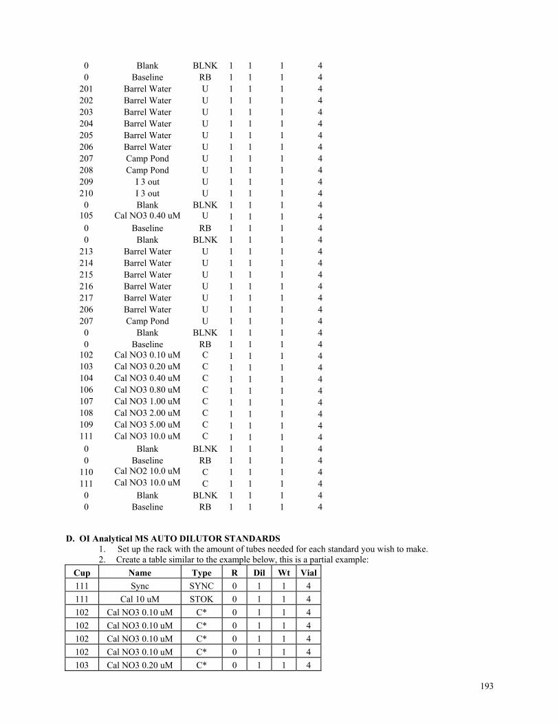
193


201 Barrel Water U 1 1 1 4 202 Barrel Water U 1 1 1 4 203 Barrel Water U 1 1 1 4 204 Barrel Water U 1 1 1 4 205 Barrel Water U 1 1 1 4 206 Barrel Water U 1 1 1 4 207 Camp Pond U 1 1 1 4 208 Camp Pond U 1 1 1 4 209 I 3 out U 1 1 1 4 210 I 3 out U 1 1 1 4

0 Blank BLNK 1 1 1 4 105 Cal NO3 0.40 uM U 1 1 1 4

0 Baseline RB 1 1 1 4 0 Blank BLNK 1 1 1 4

213 Barrel Water U 1 1 1 4 214 Barrel Water U 1 1 1 4 215 Barrel Water U 1 1 1 4 216 Barrel Water U 1 1 1 4 217 Barrel Water U 1 1 1 4 206 Barrel Water U 1 1 1 4 207 Camp Pond U 1 1 1 4


102 Cal NO3 0.10 uM C 1 1 1 4 103 Cal NO3 0.20 uM C 1 1 1 4 104 Cal NO3 0.40 uM C 1 1 1 4 106 Cal NO3 0.80 uM C 1 1 1 4 107 Cal NO3 1.00 uM C 1 1 1 4 108 Cal NO3 2.00 uM C 1 1 1 4 109 Cal NO3 5.00 uM C 1 1 1 4 111 Cal NO3 10.0 uM C 1 1 1 4


110 Cal NO2 10.0 uM C 1 1 1 4 111 Cal NO3 10.0 uM C 1 1 1 4


D. OI Analytical MS AUTO DILUTOR STANDARDS

1. Set up the rack with the amount of tubes needed for each standard you wish to make. 2. Create a table similar to the example below, this is a partial example:

Cup Name Type R Dil Wt Vial

111 Sync SYNC 0 1 1 4

111 Cal 10 uM STOK 0 1 1 4

102 Cal NO3 0.10 uM C* 0 1 1 4

102 Cal NO3 0.10 uM C* 0 1 1 4

102 Cal NO3 0.10 uM C* 0 1 1 4

102 Cal NO3 0.10 uM C* 0 1 1 4

103 Cal NO3 0.20 uM C* 0 1 1 4

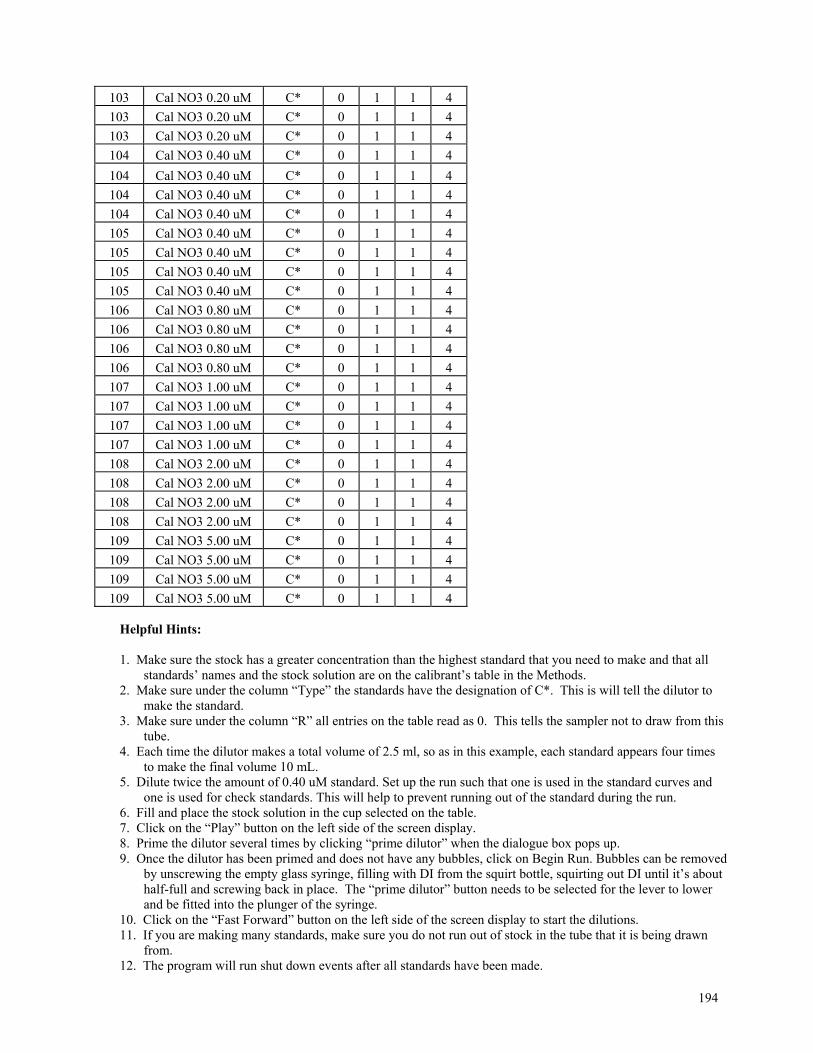
194

Helpful Hints: 1. Make sure the stock has a greater concentration than the highest standard that you need to make and that all

standards’ names and the stock solution are on the calibrant’s table in the Methods. 2. Make sure under the column “Type” the standards have the designation of C*. This is will tell the dilutor to

make the standard. 3. Make sure under the column “R” all entries on the table read as 0. This tells the sampler not to draw from this

tube. 4. Each time the dilutor makes a total volume of 2.5 ml, so as in this example, each standard appears four times

to make the final volume 10 mL. 5. Dilute twice the amount of 0.40 uM standard. Set up the run such that one is used in the standard curves and

one is used for check standards. This will help to prevent running out of the standard during the run. 6. Fill and place the stock solution in the cup selected on the table. 7. Click on the “Play” button on the left side of the screen display. 8. Prime the dilutor several times by clicking “prime dilutor” when the dialogue box pops up. 9. Once the dilutor has been primed and does not have any bubbles, click on Begin Run. Bubbles can be removed

by unscrewing the empty glass syringe, filling with DI from the squirt bottle, squirting out DI until it’s about half-full and screwing back in place. The “prime dilutor” button needs to be selected for the lever to lower and be fitted into the plunger of the syringe.

10. Click on the “Fast Forward” button on the left side of the screen display to start the dilutions. 11. If you are making many standards, make sure you do not run out of stock in the tube that it is being drawn

from. 12. The program will run shut down events after all standards have been made.

103 Cal NO3 0.20 uM C* 0 1 1 4

103 Cal NO3 0.20 uM C* 0 1 1 4

103 Cal NO3 0.20 uM C* 0 1 1 4

104 Cal NO3 0.40 uM C* 0 1 1 4

104 Cal NO3 0.40 uM C* 0 1 1 4

104 Cal NO3 0.40 uM C* 0 1 1 4

104 Cal NO3 0.40 uM C* 0 1 1 4

105 Cal NO3 0.40 uM C* 0 1 1 4

105 Cal NO3 0.40 uM C* 0 1 1 4

105 Cal NO3 0.40 uM C* 0 1 1 4

105 Cal NO3 0.40 uM C* 0 1 1 4

106 Cal NO3 0.80 uM C* 0 1 1 4

106 Cal NO3 0.80 uM C* 0 1 1 4

106 Cal NO3 0.80 uM C* 0 1 1 4

106 Cal NO3 0.80 uM C* 0 1 1 4

107 Cal NO3 1.00 uM C* 0 1 1 4

107 Cal NO3 1.00 uM C* 0 1 1 4

107 Cal NO3 1.00 uM C* 0 1 1 4

107 Cal NO3 1.00 uM C* 0 1 1 4

108 Cal NO3 2.00 uM C* 0 1 1 4

108 Cal NO3 2.00 uM C* 0 1 1 4

108 Cal NO3 2.00 uM C* 0 1 1 4

108 Cal NO3 2.00 uM C* 0 1 1 4

109 Cal NO3 5.00 uM C* 0 1 1 4

109 Cal NO3 5.00 uM C* 0 1 1 4

109 Cal NO3 5.00 uM C* 0 1 1 4

109 Cal NO3 5.00 uM C* 0 1 1 4

195

E. ALPKEM FS3100 AUTOANALYZER SHUTDOWN

1. Once all samples have been run and the run is completed, the autoanalyzer will reverse flow and change pump speed to 10 (or -10). When this occurs, remove the cadmium coil and fill the coil with imidazole buffer. Screw the ends of the coil together tightly and store until its next use.

2. Disconnect the color reagent and buffer lines from their designated bottles and reconnect them to the carrier bottle.

3. Change the flow direction and speed back to what it was set at during the run (usually -40) and allow carrier to pump through the carrier, color reagent, and buffer lines for at least 10 minutes.

4. Disconnect carrier, color reagent, and buffer lines from the carrier bottle and leave them unconnected. 5. Allow autoanalyzer to continue pumping for 10 more minutes to air out the system. 6. While carrier and air are being pumped through the system, make sure the run is saved and the files are

exported before shutting the power off. 7. After the system has aired out stop the pump and turn off the system at the power strip.

8. DATA PROCESSING The Alpkem should have saved the results file as the same name as the sample table, but with an “.rst” extension. It will be located in the Results folder on the Alpkem computer (C:/Winflow/Results/Nitrate/NIT00###.rst). Copy the results file your local hard-drive and server at \DATA\Chemistry\Nutrients\Inorganic\Nitrate\Alpkem_Data\WinFlo Results\YEAR.

1. Find the results file and double-click to open it. This will open Winflow. Then choose Data Analysis and find your results file.

2. In the same folder as the original, choose to save the file with the letter “M” at the end of the name, signifying that the file has been modified. For example, NIT00231.rst would be saved as NIT0231M.rst (seven letter maximum on the name). A copy is saved on the server when all changes have been made at:

L:/DATA/Chemistry/Nutrients/Inorganic/Nitrate/Alpkem_Data/WinFlo Results/YEAR 3. Now you can begin to make changes. Maximize the chromatograph window (upper left panel). 4. Zoom in on the peaks of the analysis by holding down the rightclick button and dragging the cursor over the

area you want to zoom to, and if necessary, move the points identifying the peaks and baselines of the run. Do this by clicking on the button on the left-hand side of the screen, third from the bottom, of the blue line with a red plus sign at the peak. Then click on the peak you wish to move and drag to the new position.


6. Once you are done, reduce the size of the chromatograph window to see the other three panels. 7. If you are satisfied with the peak identification, look at the standard curve (upper right panel) and the standard

statisitical output (lower right panel). Remember to change all standards to “C” in the Type column (see Section C Step 2c). The curve should be linear with a ‘good’ R2 value (~0.999).

8. If the regression is not very good, you can drop a standard by changing the “C” in the Type column on the results table (lower left panel) to a “U”, indicating it is an unknown instead of a calibrant.

9. Export the information by clicking on File → Export… find the correct folder on the local hard drive and save the output as a tab delimited file. WinFlow can calculate concentration by two methods: 1) Peak Height (H) or 2) Peak Area (A). For nitrate we only export the height calculation and save the file with a letter “H” added at the end. For example, the exported file from NIT0231M.rst would be saved as NIT0231H.txt. Copies are saved on the server at:

L:/DATA/Chemistry/Nutrients/Inorganic/Nitrate/Alpkem_Data/WinFlo Export/YEAR 10. Open the exported files (NIT0231H.txt) and N03_all.xls in Excel. In the exported height file, delete the “R”

column and copy the “Flag” column to paste next to the “Calc” column. Adjust the “Peak” column to be a running series of numbers. Delete all data below the last peak in this file.

11. Open the RUNS tab in NO3_NEW2014.xls. In column A, type in the subsequent number. This is an ongoing record of the number of runs in

this file. In column B, type in the initials of the run operator. In column C, type in the Alpkem run number. For example, NIT00231. In column D, type the date the analysis was run.

196

In column E, enter the table number from the YEARInventoryAndRun.xls file. For example, NIT08-01.

Column F identifies if the run contained samples or was a test. This was important when SAS was used to determine sample concentrations, but is not anymore.

In column G, type in the results file name (NIT0231.rst). In column H, type in the export file name (NIT0231H.txt). In column I, type in whether or not to use this run. In column J, type in the Sam photodiode values from the beginning of the run. In column K, type in the Ref photodiode values from the beginning of the run. Finally, type in any relevant notes in column L.

12. Open the Raw_Data tab in NO3_NEW2014.xls.

In column A, type the run number from the Runs Tab. Copy the information from the exported file into columns J through O and columns S through U. Copy the Name information (Column L) into the Sortchem column (column B). Type in the name of the exported file in column I. Look up the identifiers in columns C through G (Site, Date, Time, etc.) from the Sortchem in the

AKchem inventory. Type “Yes” or “No” into column H to identify if the information should be used for each individual

sample. Column V is intentionally left blank, so do not delete it. Column W is an ongoing count of the rows, so drag down the column so that each new data point

has a number. Column X contains any notes about the sample.

13. Save file on the local hard drive and on the server at: L:/DATA/Chemistry/Nutrients/Inorganic/Nitrates/NO3_all.xls

14. See the Notes tab of NO3_all.xls for additional processing instructions.

197

(VI-7) Particulate Carbon and Nitrogen -- CHN Analyzer Updated 21 March 2013, SMM

1. Introduction: The CHN analyzer is used to determine the carbon, hydrogen, and nitrogen content of solid and liquid samples. The sample is combusted and all of the elements are transformed into their gaseous forms. The carbon (in the form of carbon dioxide), hydrogen (in the form of water vapor), and nitrogen (NOx is reduced by copper to N2) are passed through an infrared detector to determine concentration. The machine is normally left on when running more samples within several days. Prepping the machine consists of purging the columns with He gas. Citation: Patterson, RK. 1973. Automated Pregl-Dumas Technique for Determining Total Carbon, Hydrogen,

and Nitrogen in Atmospheric Aerosols. Analytical Chemistry 45(3): 605-609. Instrument Models/Contacts: Ann Arbor (Rm. 1051, Nat. Sci. Building): Perkin-Elmer 2400 series 1 CHN Analyzer Serial #: 241N3112101 http://www.perkinelmer.com/

P.E. Service Representative: Dave Hook 1-800-762-4000 (roaming, but works on series 1) Cathy O’Grady X 3335 Ordering same number as above. Can check prices online (see Ordering Protocol)

A. Sample preparation

1. Printed sample sheets (called “traysheets”) are prepared using information from akchem_YYYY.xls Open CHNtraysheet_wholefilters_YYYY.xls (DATA\Chemistry\Nutrients\Particulate\CHN\). Open the akchem_YYYY.xls, where YYYY is the year the samples were collected. Copy sample information from akchem_YYYY.xls into the tab called akchem_YYYY. Follow the instructions for preparing a “printable_traysheet” in the

CHNtraysheet_wholefilters_YYYY.xls workbook. Print out a traysheet. Pull out the samples that are to be pelletized and pelletize the samples (see instruction #3 in this

section below) Place the pellet in the well that corresponds to the information in the “printable_traysheet” that

you printed out. 2. Weighed particulate material for standards (or soil). See instructions for using AD 6 autobalance in the

“Standard Preparation” section of this protocol. The microbalance is very sensitive – Check with someone who has done this and get them to show you how to do it.

Weigh out particulate material into tin capsules (4x6mm or 5x8mm) and record to the nearest microgram (0.001mg).

Fold over top and continue folding and compressing until capsule is as small as feasible. The smaller the pellet the better because there will be less chance of the sample hanging up during injection.

Store in a drying oven at less than 40º C or over silica gel in a desiccator. 3. Filtered particulate material (filters). Prior to 2005, the filters were cut in half (attempts were made to have

the same amount of material on each half of the filter). Currently (post-2005), we pelletize the entire filter. To pelletize:

Clean workspace and forceps with ethanol Place filter on tin disk and roll into a tube Crimp the ends of the tube using forceps Pelletize the tin + filter using the filter press in room 1037.

Do not touch the filter or foil with anything except clean forceps. The pelletized sample is stored in a plastic sample holder (microwell plate) until ready for analysis. Store the sample holder in a desiccator over silica gel until ready for analysis. Prior to 2005, the sample inlet and sample tray holes did not match (the

198

sample inlet was smaller) and expanded pellets would get stuck. If samples were stored for more than a week, they required re-pressing. Now the sample tray hole is the smaller of the two, so this is not as much of a concern (but still check this to make sure that the pellet hasn’t expanded too much).

4. Indicate on the traysheet with a “P” or “X” that filter was pressed. If filter is missing, note with an “M”. 5. Place the completed traysheet in the current CHN Run volume 3-ring binder under the traysheet tab. The

binder is located on the counter near the machine. Past volumes are shelved in the back bay of 1037.

B. Standard (K-factor) and Blank Preparation Standards Acetanilide is used for making standards in this analysis, and standards are referred to heretofore as a “K-factors”. Prior to January 1998, the weight used for K-factors was 0.5 mg to 0.7 mg, but on suggestion of the service rep this was changed to current value 1.8-2.2 mg acetanilide). Prior to 2005, Prof. Martin’s Cahn electrobalance was used. Currently, the micro-balance in Knute Nadelhoffer’s lab is used (AD 6 autobalance). Note that we have also used the autobalance in Mark Hunter’s lab, and you need to get instructions from his lab on its use.

Instructions for the AD-6 autobalance (Nadelhoffer lab): Note : The balance has two pan arrests which are normally raised. The pan arrests must be in the raised position prior to loading or unloading. The blue knob at the base of the balance is used to lower or raise the pan arrests. The standard/sample pan is on the left and the reference pan is on the right. To calibrate: 1. Remove all samples from the sample and reference pans and close the doors. Lower pan arrests. Set

‘range’ to 2mg. 2. Press ‘autotare’ and wait until integration (“Int) is complete. 3. Press ‘range’ until “200mg” appears on the left display. 4. Raise pan arrest and place calibration weight (100 mg; stored in drawer at the bottom of the balance) on

the sample pan. Close doors. 5. Lower pan arrests, wait for balance to stabilize and type 100.00 on the numeric keypad. Press ‘calib’,

and calibration is complete. Standard weights are recorded on the sample traysheet printouts, and standards are stored in the corresponding microplate well. For each run, you will need to weigh enough standards for the conditioning run (5 K-factors; see step 12 of CHN Analysis Operation section ), one K-factor per every 10 samples, plus a few extra. To weigh a standard or soil (note that the filters are not weighed, just pressed and put into the CHN): 1. Raise pan arrests. Make sure there is a counter weight (i.e. sample pedestal and tin) on the reference

pan. 2. Place empty tin boat in sample pedestal and fan out the edges with forceps. Place on sample pan. Close

doors, and lower pan arrests. 3. Press ‘autotare’ and wait until “Int” is complete. The balance is now zeroed. 4. Raise pan arrests and remove the sample pedestal and tin boat from pan. 5. Fill tin boat with approximately 1.8-2.2 mg of acetanilide using the dedicated small chemical scoop(s)

on top of the glass plate. Weigh the standard + tin (not rolled). Record this weight (‘weight 1’) on the standard traysheet (see below).

6. Raise pan arrests. Remove sample pedestal/tin boat from balance, and roll into a ball (using forceps). Make sure acetanilide is not leaking out.

7. Re-weigh the rolled standard + tin and record the weight (‘weight 2’). Allow time for weight to stabilize. Some acetanilide is usually lost during the rolling process. Use the rolled standard + tin weight (‘weight 2’) for weight that you enter in the CHN Analyzer.

Blanks For soil samples, blanks consist of pelletized empty tins. For filter samples, blanks consist of pelletized GF/F filters (see ‘Sample Preparation’ for pelletizing instructions) that have been muffled at 450 ºC for 4 hours. A run of 50 samples requires 5 blanks for the conditioning run, one blank per every 10 samples, plus a few extra (total= 10+). Store blanks in appropriate microplate wells, as indicated by the sample traysheets. Or, designate a tray specifically for blanks.

199

When running samples, look back at previous years’ data to get a sense of what the appropriate blank values should be.

In 2012, there was some difficulty with consistently high blanks. Old filters were recombusted, and that seemed to decrease the blank values for C and N. The best blanks seemed to be newly purchased filters that were combusted for the first time. These gave the most consistent and lowest blank values. Limit of Detection (LOD) and Method Detection Limit (MDL) In 2012 we calculated a limit of detection and a method detection limit that involved using the concentration of K-factors from a single run to calculate a percent LOD (See CHN_2012.xls). In 2014 we standardized these calculations and the description and equations are found in the CHN_2014.xls file on the ‘LOD’ tab. To calculate these values, make sure that sometime during the course of using the machine, you run: (a) At least one batch of 7 apple leaf standards or K-factors as samples (or both for good measure). This will allow you to calculate the standard deviation of the concentration of these samples and then a limit of detection. MDL = (standard deviation of concentration) x (critical value) The critical value is calculated according to Standard Methods for the Examination of Water and Waste Water, 19th ed., p. 1-11, and is 3.14 for 7 replicates (6 degress of freedom) for a 1-sided t test with a 99% confidence interval (see http://fshn.ifas.ufl.edu/faculty/mrmarshall//fos4310/t_dist.gif) for a more complete description. This gives you a percent of C, H, or N that you can detect. You can also calculate a limit of detection based on the weight of the standards you run, and essentially with this method you are standardizing to 1 mg of std and determining “if I had 1 mg of sample, I could detect x ug of C or H or N”. Note that this gives the same relative value as the approach above with % (see CHN_2014.xls, tab ‘LOD’). (b) A second approach is to run a series of samples with smaller and smaller masses to determine at what point the machine cannot distinguish between samples (the machine counts are the same). This provides a lower limit of detection. Because it can be difficult to weigh out very small amounts of std, it is easier to apply this method by comparing sample or std counts to the counts determined for blanks. We have three kinds of blanks – (1) machine blank, which is what the machine reports with no sample injected, (2) empty tin boats, and (3) blank filters. The actual blank we use for samples is a combination of these three parts of the “blank”. Compare the blank values to the sample values to see what level of counts is needed to “exceed” the blank and detect a sample. For example, if you have 15 counts for every 1 ug of C determined for a std, and your blank value is 30 counts, then you would need to have at least 2 ug C in your sample before you were above the background of a blank and could detect the sample. Note that while this is an empirical calculation, it does not take into consideration the variance of your counts (only uses averages). This is why the minimum amount that can be detected is less than the limits of detection calculated using the Standard Methods approach of running the same standard multiple times to get a variance.

C. Getting Started: Changing the Reduction and Combustion columns. There are extra quartz columns located in boxes above the pellet press in room 1037. Materials for the columns are stored in the Nadelhoffer lab (Kraus 1051), either in the vacuum dessicator or in the cabinets above the CHN machine. If you cannot find them, ask Jim. Before you decide to run the machine, make sure that there are chemicals stocked, and if not order more. You need about 1.5-2 bottles of copper to begin with, and (depending on the volume of the bottles) one bottle of the silver tungstate and the EA1000. We “share” materials with other labs, and the materials that are stocked in the Nadelhoffer lab can be used, but they will need to be reordered (so essentially you replace what you use). Additionally, there are tin boats (used for K-factors) and well trays located in the drawer labeled “Kling Lab” to the left of the autobalance. Also check to make sure that the helium tank still has helium in it, above a PSI of 500, and order more He if necessary. Also make sure to have pressed about 1.5 to 2 trays of samples before running, as it is difficult to press and run when the machine is first online.

Reduction column: The column usually lasts for ~150 samples or 2 days when running every day. As of 2009, we change the column after ~140 runs (70 runs/day: a conditioning run, 50 samples, and a K-factor and blank after every 10 samples) to prevent sample loss. See CHN_2009.xls for cost analysis of this decision. In 2012, one reduction column lasted for over 300 runs, however the majority of these samples had very small N concentrations. The nitrogen values will skyrocket (but not C values) when the reduction column is oxidized.

200

YOU MUST HAVE SOMEONE DEMONSTRATE THE CHANGING OF A COLUMN BEFORE ATTEMPTING IT YOURSELF.

Materials: Gloves for your oily hands, new quartz column, quartz wool, vortex with blue foam adaptor, ring stand, funnel with neck that fits into column opening, glass rod (for ramming wool into place), and piece of wire (for ramming wool into place). Chemicals: Copper, Copper Oxide General Instructions: See Section 4-6, Filling and Installing Tubes, in the 2400 Series II CHNS/O Analyzer User’s Manual. It is located in a blue 3-ring binder next to the machine. Fill column in the fume hood. 1. Follow the manual diagram for appropriate amounts of copper and copper oxide and locations of quartz

wool. (See final page of CHN protocol) 2. The silver gauze is generally re-used after conditioning (see METHOD 2 for Conditioning Silver Gauze

on page 4-9 in the manual) as is the copper diffuser. 3. Check o-rings. Replace o-rings if they are stiff or cracked; otherwise, they can be re-used. In general, o-

rings are replaced when replacing the combustion column or when the leak test fails. 4. Check the filters at the top and bottom of the column; replace if filters are dirty. 5. Use the vortex (set at 1000) and gentle tapping while rotating the column to pack the copper. A thin disk

of quartz wool separates the copper and copper oxide. Use gentle tapping to pack the copper oxide. 6. The copper diffuser is placed on top and the silver gauze at the bottom.

To replace the top filter, snap the column holding unit into place, place the filter on top of the reduction column, and begin to raise into position. This can be a frustrating step. Another option is to place filter on finger and then try and stuff filter into the hole above the reduction column. Then make adjustments using forceps.

Combustion column: Lasts for about 600-1000 samples. Both the Nitrogen and Carbon values will shoot up drastically. Materials: Gloves for your oily hands, new quartz column, quartz wool, ring stand, funnel with neck that fits into column opening, glass rod (for ramming wool into place), piece of wire (for ramming wool into place). Chemicals: EA-1000, silver tungstate on magnesium oxide, and silver vanadate (these are nasty; exercise caution when working with them) General Instructions: See Section 4-6, Filling and Installing Tubes, in the 2400 Series II CHNS/O Analyzer User’s Manual. It is located in a blue 3-ring binder next to the machine. Fill Column in fume hood. 1. Follow the “Filling Procedure” instructions in the manual and refer to the diagram for appropriate

amounts of EA-1000, silver tungstate on magnesium oxide, silver vanadate, and locations of quartz wool.

2. The EA-1000 and silver tungstate on magnesium oxide will need to be placed in a muffle furnace and pre-heated to ~900 oC for 10-30 minutes prior to use to remove any traces of moisture and carbon.

3. The silver gauze is generally re-used after conditioning (see METHOD 2 for Conditioning Silver Gauze on page 4-9 in the manual). The vial receptacle is re-used after it has been emptied and cleaned.

4. Replace the o-rings. 5. Check the filters at the top and bottom of the column; replace if filters are dirty. Note: the vial receptacle (ash trap) needs to be emptied and cleaned every time the reduction column is

replaced. If it is full, replace it with a new one.

D. CHN analyzer operation If the machine is turned-off it will reset to default values. You must re-enter the date (dd-mm-yy), the run counters (use the tally sheet to estimate), the operator ID (1), and you must reset T2 to 5.00s.

1. Instrument Run Log. The run log is kept in a white 3-ring binder near the machine. Fill this out each time!

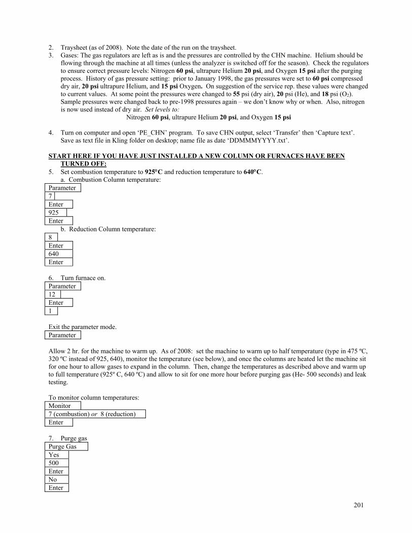
201

2. Traysheet (as of 2008). Note the date of the run on the traysheet. 3. Gases: The gas regulators are left as is and the pressures are controlled by the CHN machine. Helium should be

flowing through the machine at all times (unless the analyzer is switched off for the season). Check the regulators to ensure correct pressure levels: Nitrogen 60 psi, ultrapure Helium 20 psi, and Oxygen 15 psi after the purging process. History of gas pressure setting: prior to January 1998, the gas pressures were set to 60 psi compressed dry air, 20 psi ultrapure Helium, and 15 psi Oxygen. On suggestion of the service rep. these values were changed to current values. At some point the pressures were changed to 55 psi (dry air), 20 psi (He), and 18 psi (O2). Sample pressures were changed back to pre-1998 pressures again – we don’t know why or when. Also, nitrogen is now used instead of dry air. Set levels to:

Nitrogen 60 psi, ultrapure Helium 20 psi, and Oxygen 15 psi 4. Turn on computer and open ‘PE_CHN’ program. To save CHN output, select ‘Transfer’ then ‘Capture text’.

Save as text file in Kling folder on desktop; name file as date ‘DDMMMYYYY.txt’. START HERE IF YOU HAVE JUST INSTALLED A NEW COLUMN OR FURNACES HAVE BEEN

TURNED OFF: 5. Set combustion temperature to 925C and reduction temperature to 640C.

a. Combustion Column temperature: Parameter 7 Enter 925 Enter

b. Reduction Column temperature: 8 Enter 640 Enter 6. Turn furnace on. Parameter 12 Enter 1 Exit the parameter mode. Parameter Allow 2 hr. for the machine to warm up. As of 2008: set the machine to warm up to half temperature (type in 475 ºC, 320 ºC instead of 925, 640), monitor the temperature (see below), and once the columns are heated let the machine sit for one hour to allow gases to expand in the column. Then, change the temperatures as described above and warm up to full temperature (925º C, 640 ºC) and allow to sit for one more hour before purging gas (He- 500 seconds) and leak testing. To monitor column temperatures: Monitor 7 (combustion) or 8 (reduction) Enter 7. Purge gas Purge Gas Yes 500 Enter No Enter

202

8. Leak check the mixing chamber and combustion zone once operating temperatures are reached. Diagnostic 2 ‘gas’ 1 ‘leak test’ 1 ‘mixing chamber’ Enter Diagnostic 2 ‘gas’ 1 ‘leak test’ 2 ‘combustion’ Enter START HERE WHEN MACHINE IS IN GAS SAVER MODE. 9. Turn off gas-saver mode. Parameter 22 2 “Off” Enter 10. Purge gases; Helium for 120 seconds; “No” for Oxygen purge. Purge Gas Yes 120 Enter No Enter 11. Adjust carousel sample tray to 1 and reset Runs to 1 (see more about Auto run below) Autorun 4 “Reset” 12. If you are starting with a NEW combustion column, run several apple leaf standards to help burn out whatever

may be on the column. 13. Conditioning run. At the start of run, use the following sequence: 3 blanks or enough blanks to reproduce from

the mean within- see below, then K1, Blank, K1, Blank, K1, Blank, K1, K1, K1. a. Blanks. Check to see if machine has equilibrated by running 3 blanks (tin or filter blanks depending on

sample type) or until they reproduce from the mean within: C + 30, H +100, N + 16

For Blanks: Auto Run 1 “1B” Enter 2 “Option 2”

b. K-factors. Check that the machine is calibrated properly by running standards as K-factors. Place a pre-weighed standard sample in the receptacle. The theoretical acetanilide weight percent is stored in S1. Enter the correct weight of the standard sample in mg (+ 0.001mg).

For K factors: Auto Run

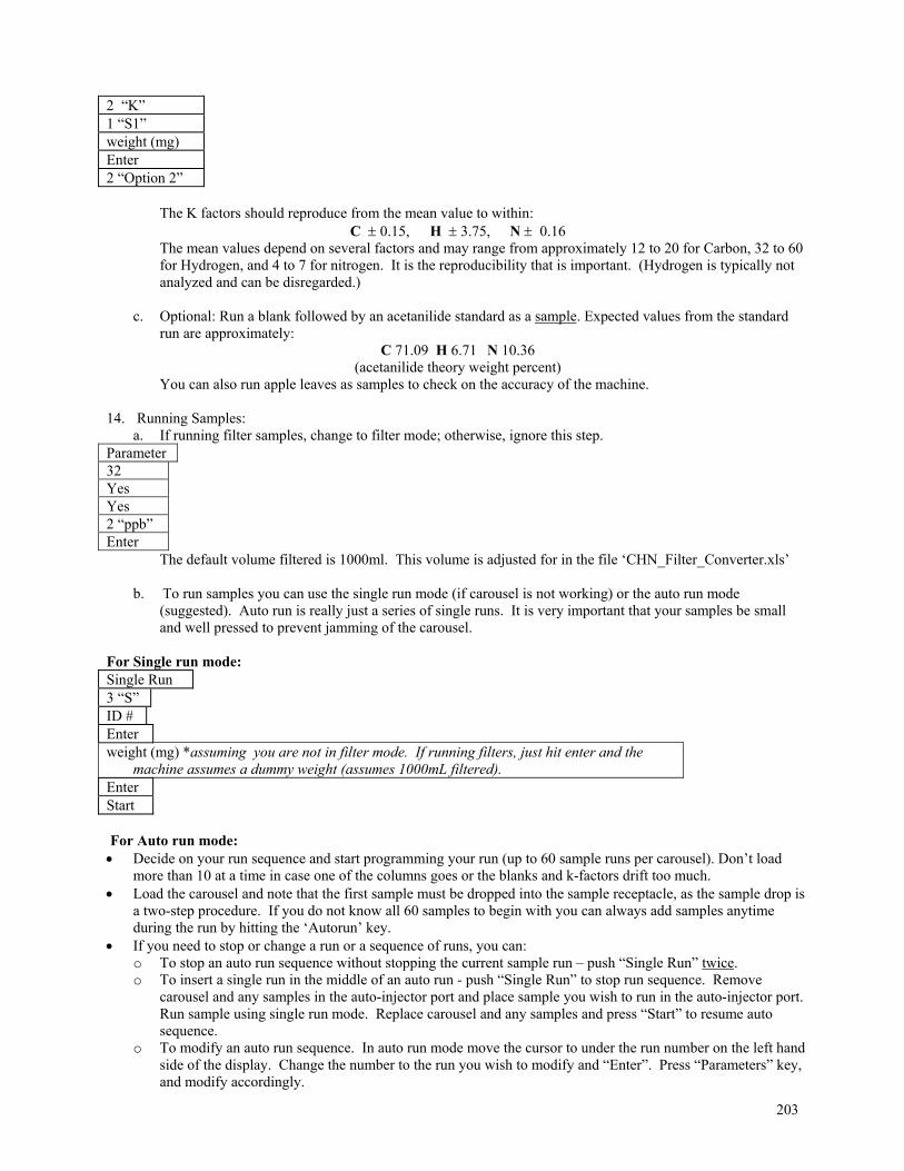
203

2 “K” 1 “S1” weight (mg) Enter 2 “Option 2”

The K factors should reproduce from the mean value to within:

C 0.15, H 3.75, N 0.16 The mean values depend on several factors and may range from approximately 12 to 20 for Carbon, 32 to 60 for Hydrogen, and 4 to 7 for nitrogen. It is the reproducibility that is important. (Hydrogen is typically not analyzed and can be disregarded.)

c. Optional: Run a blank followed by an acetanilide standard as a sample. Expected values from the standard

run are approximately: C 71.09 H 6.71 N 10.36

(acetanilide theory weight percent) You can also run apple leaves as samples to check on the accuracy of the machine.

14. Running Samples:

a. If running filter samples, change to filter mode; otherwise, ignore this step. Parameter 32 Yes Yes 2 “ppb” Enter

The default volume filtered is 1000ml. This volume is adjusted for in the file ‘CHN_Filter_Converter.xls’ b. To run samples you can use the single run mode (if carousel is not working) or the auto run mode

(suggested). Auto run is really just a series of single runs. It is very important that your samples be small and well pressed to prevent jamming of the carousel.

For Single run mode: Single Run 3 “S” ID # Enter weight (mg) *assuming you are not in filter mode. If running filters, just hit enter and the

machine assumes a dummy weight (assumes 1000mL filtered). Enter Start For Auto run mode: Decide on your run sequence and start programming your run (up to 60 sample runs per carousel). Don’t load

more than 10 at a time in case one of the columns goes or the blanks and k-factors drift too much. Load the carousel and note that the first sample must be dropped into the sample receptacle, as the sample drop is

a two-step procedure. If you do not know all 60 samples to begin with you can always add samples anytime during the run by hitting the ‘Autorun’ key.

If you need to stop or change a run or a sequence of runs, you can: o To stop an auto run sequence without stopping the current sample run – push “Single Run” twice. o To insert a single run in the middle of an auto run - push “Single Run” to stop run sequence. Remove

carousel and any samples in the auto-injector port and place sample you wish to run in the auto-injector port. Run sample using single run mode. Replace carousel and any samples and press “Start” to resume auto sequence.

o To modify an auto run sequence. In auto run mode move the cursor to under the run number on the left hand side of the display. Change the number to the run you wish to modify and “Enter”. Press “Parameters” key, and modify accordingly.

204

o If you accidentally hit the incorrect sample type button (e.g. “1B” for blank instead of “2S” for standard) when entering your run, press “Autorun” to escape. Then, reenter correct information.

If you need to print the run data (due to printing problems during the run), Auto run 4 3 to print data or 2 to print run list

NOTE: Sample ID may include alpha-numeric characters. Alpha characters are obtained by entering a period followed by its numeric position in the alphabet ( a=“.01”, b=“.02” j=“.10”, etc.).

15. Run a blank and a K-factor every 10 samples. If you want to really double check the functioning of the machine,

run an apple leaf standard as a sample after the k-factor. 16. At the end of a run, turn on Gas Saver mode. . Parameter 22 1 “On” Type date MM-DD-YYYY Enter Enter 16. Complete Instrument Run log sheet in white binder. END OF THE SEASON SHUTDOWN: Turn off instrument power (switch located on right side of machine). Turn off printer. Close the nitrogen, oxygen and

helium gas tanks.

E. Data Processing 1. Turn on computer sitting on top of the CHN machine and open ‘PE_CHN’ program found on the desktop. To

save CHN output, select ‘Transfer’ in the menu bar, then ‘Capture text’. Save as text file in Kling folder on desktop; name file as date ‘DDMMMYYYY.txt’. DO THIS BEFORE STARTING THE RUN EACH DAY!!

2. Text files are converted to Excel files using a macro written by Jim LeMoine in the file ‘CHN_Filter_Converter.xls’ located in L:\DATA\Chemistry\Nutrients\Particulate\CHN. This file converts CHN raw output from the Perkin Elmer 2400 Series II Elemental Analyzer into useable data. The converter works for data output from the Filters setting that includes water concentration and volume of 1000 mL (see Parameter 32 on the CHN machine to convert between standard and filter output setting). The conversion occurs through two Macros found in the Tools\Macro menu. The Macro named Module1.Reformat converts the raw output to a list of data. The Macro Module2.Reformat separates the list of data by sample type: Samples, Blanks, Acetanilide calibration factors, Apple Leaf Standards, and NRCS E Soil standards. Do the following to convert your data: 1) Open your text file of data from the elemental analyzer (choose tab and space delimited options when

opening the file) 2) Copy the data from cell A1 to the end of the text file; To do so click on cell A1 and press

CTRL+SHIFT+END followed by CTRL+C 3) Paste the data in the 'Raw worksheet beginning cell A2 or append to the bottom of the existing data in the

'Raw' worksheet (note: as an alternative you can open the text file in Notepad or Wordpad, select all the data with CTRL+A, paste it into the 'Raw' worksheet cell A2 or append it to the 'Raw' worksheet. If you use this method be sure to select Column A of the new data and convert the text to columns with tab and space delimiters before proceeding. The data aren't automatically pasted into columns if they are copied from Notepad or Wordpad)

4) Navigate to the menu Tools\Macro\Macro..., select Module1.Reformat, and click Run. If the macro fails to run, check to make sure there isn’t any junk (e.g. “print list…”) in the text output from the CHN machine. Delete any non-data text

5) Select the 'List' worksheet to view the data. 6) Highlight Column D and press CONTROL+F to find BLANK. Replace all of them with BLK. The

Module2.Reformat Macro cannot recognize BLANK. Similarly, K-Factors must be called 'K1', Apple Leaf

205

Standards must be called 'A', and E soil standards must be called 'E'. All other Sample IDs will be put in the Samples worksheet. Look through the data to ensure that values were put in the appropriate columns. Sometimes irregular spacing in the raw data results in incorrectly listed values. Copy and paste the correct values where necessary.

7) Navigate to the menu Tools\Macro\Macro..., select Module2.Reformat, and click Run 8) You can now adjust the figures for each of the worksheets to better view the data.

3. Converted and formatted CHN output files are cut and pasted from ‘CHN Filter Converter.xls’ into ‘CHN_YYYY.xls’, found in C:\DATA\Chemistry\Nutrients\Particulate\CHN. From 2008 onward, there will be a yearly file for all the CHN runs for that year. 1) Paste formatted sample data, found in the ‘Samples’ worksheet in the ‘CHN Filter Converter.xls’ file, into

column G of the worksheet ‘Raw_Samples’ and below the existing data. 2) Make sure formulas in columns A through F are pasted down, and that the sample year is typed in cell B1.

(NOTE: The formula in column A that concatenates the sort-chem and sample year is not perfect, so double-check to make sure all the sort-chems are correct! For example, if there were samples from more than one year in a run, you must adjust the sort-chems manually to include the proper date. Also, if sample is a duplicate, you must manually adjust sort-chem. Check the traysheet for all sample information related to each run)

3) Paste blank data, found in the ‘Blanks’ worksheet in the ‘CHN Filter Converter.xls’ file, into 'Raw_blanks' worksheet

4) Paste K-factor data, found in the ‘K-factors’ worksheet in the ‘CHN Filter Converter.xls’ file, into 'Raw_K_Factors' worksheet.

5) Transfer notes for each run to Notes column in each run worksheet. 6) Make sure to note any samples lost to a spent combustion or reduction column in the ‘bad column?’ column. 7) Final sample values (µg/L) are calculated in worksheet ‘Sample_calculations’. 8) When all samples have been run, copy and hard paste sample info and CHN values to the ‘Summary’ tab.

Remove outliers from this page during the QAQC process. 9) To QAQC, copy sortchem etc. and C, N, and C:N ratio data into a new tab and sort based on site name (then

by depth, then by date). Go through different sites and make graphs. Look for points that are particularly high or particularly low within a site. Also look to see if the C:N ratio makes sense. If it’s particularly variable within a site, it’s likely that the concentrations are low. Also do QAQC on the blanks and K-factors. Make plots of blanks and K-factors (there should be space for this in the file) just to make sure things look generally good for a run.

10) When you’re certain that the data has been properly looked through, transfer to akchemYYYY.xls and akchem_allyears_final.xls if possible

11) Check the NOTES page in the CHN_YYYY.xls file for more detailed instructions.

F. Calculations New Method (filter mode ON):

If filter mode is on, the output from the CHN analyzer gives the results in both g C or g N per L and ppb (note: ppb= ug/L if the water density is 1 g/cm3). 1L the default Vf value in the CHN output, and is corrected for the true Vf by multiplying with the ratio of 1000mL/Vf mL in the following equation:

[ ___g-C/ L] * [1000 mL/ ___volume filtered (mL)] * [1 mol-C/12.01 g-C] = ___mol C/L Old Method (filter mode OFF):

If filter mode is off, the output from the CHN analyzer gives the results as percent of the entered weight value; therefore, it is necessary to convert these percentages into M concentrations. Example: You have filtered 90 mL of water through a 25mm GF/F filter. The filters used to be cut in half and the two halves analyzed separately. If you suspect that the concentration of C or N is high, enter a weight of 0.2 mg when entering the sample weight. This weight is used as a convenience only (a “dummy weight”).

The output results are given as 82.96% C and 9.97% N for this sample. To calculate the g-C: [%C/100] * [0.2mg] * [1000 g/mg] = 0.8296 * 0.2 * 1000 = 165.92 g-C If the filter was cut in half and the two halves analyzed separately, then sum up the g C for both halves.

To calculate the final M concentrations: [318.76 g-C] * [1 mol-C/ 12.01 g-C] * [1000 mL/ 1 L] * [1/90 mL] = 295 M

206

F. Troubleshooting Symptom Checkerratic background/ background will not reproduce gas purge, leak check, gas tanks low in pressure

(<500psi), combustion column vial receptacle full of spent tin causing poor gas flow patterns

leak check fails check column seals, check injection port for stuck

samples or debris on sealing surfaces, check valve seats (see manual for exact procedures)

K-Factors not reproducing check background for fluctuations, check

acetanilide standard weights for accuracy

Nitrogen results/background rapidly increase between runs

check reduction column usage (generally replaced approximately every 150 samples + standards/k factors)

Printer jams release paper platen and un-jam

Error message 20 excessive drift check carrier gas flow, this message often occurs

when the machine has been shut down and idle

Error message x/x/x change reduction column/change combustion column/ empty vial receptor

These messages occur as a result of run counters set by the operator and are a warning that it may be time to perform the indicated operation. The machine will continue to operate properly if nothing is done but be aware that conditions may change.

zero or negative results sample did not drop, check injection valve to see if

stuck, insufficient sample

Sudden high blanks, not combustion or red tubes Contamination in machine- check Bimba Valve.

G. Manuals CHN instrument manuals are kept on the counter next to the machine. Microbalance manuals are kept in

top drawer to the left of the microbalance.

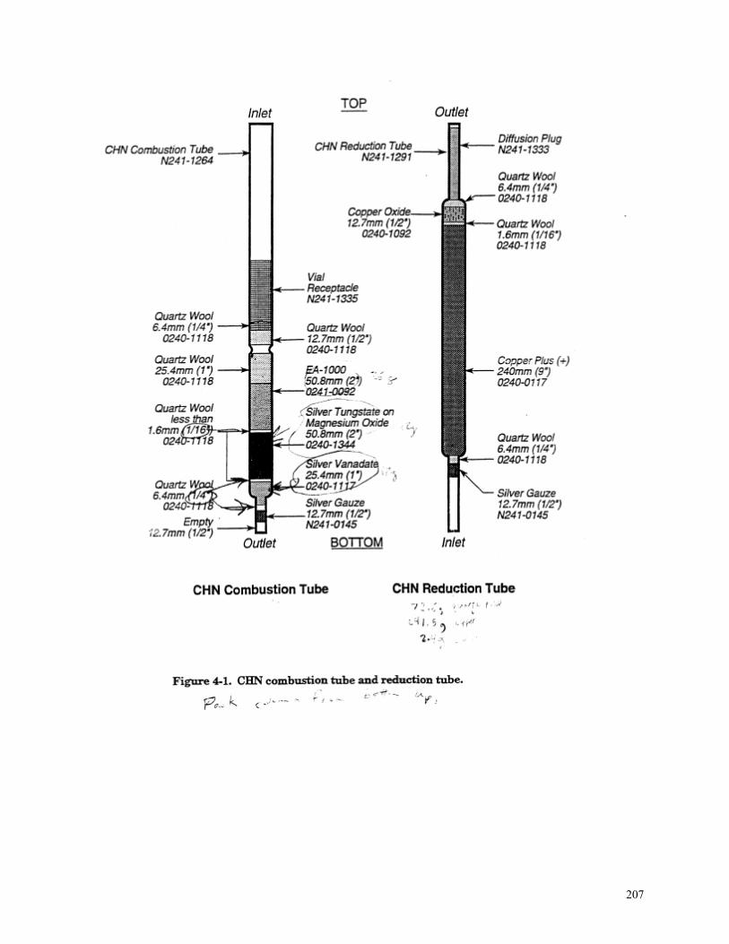
207

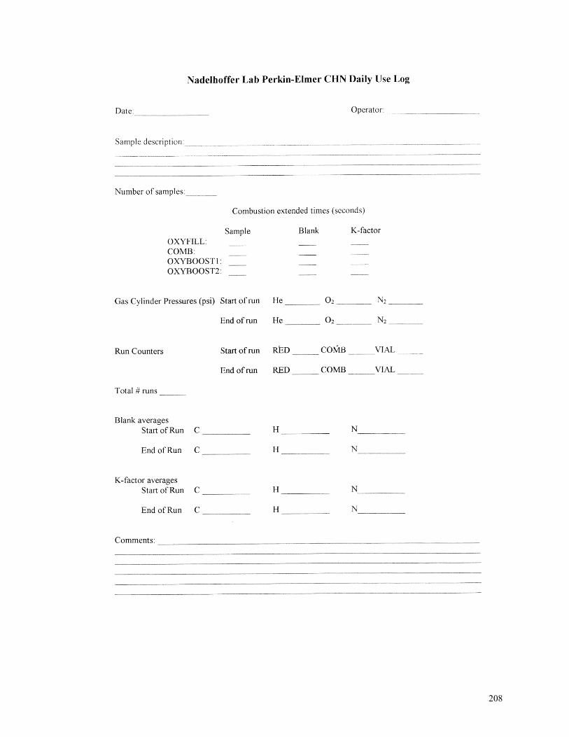
208

209

(VI-8) Bacterial Production Updated by Kristi Judd (April 2001); modified by Heather Adams and G. Kling (January 2008)

BACTERIAL CELL PRODUCTION FROM 14-C LEUCINE INCORPORTATION

A. Supplies 1. 20 mL plastic scintilation vials 2. 10 mL pipette and bulb (or 10 mL autopipet) 3. Eppendorf pipettes - 1 mL and tips; 200 L and tips 4. Hamilton syringe - 25 L 5. Sterile syringe needles 6. Filters - Millipore 0.22 m, 25 mm Nitrocellulose 7. Filtration manifold 8. Vacuum set-up 9. Forceps 10. m sterile disposable filter unit (or equivalent) 11. ice/ice bucket 12. squirt bottles 13. 7 mL plastic scintillation vials 14. waste container 15. rubber gloves 16. 3 mL BD syringe for adding TCA (or, use an old 1 mL autopipet)

B. Solutions 1. 50% TCA, cold. ~200 mL needed for 12 samples (48 vials with 3 reps and 1 kill per sample) 2. m filtered DI, 1-2 mL needed for isotope dilution 3. m filtered lake water or DI, (filtered through 2 filters) 100 mL per 12 samples, cold 4. cellusolve 5. scintillation cocktail 6. leucine stock solution: activity- ~315 mCi / mmol this will vary by bottle - be sure to record the activity into

the yearly akBacProds excel file. Also, if you change bottles mid-season, note the date in the file. Activity ~ 0.1 mCi / mL concentration ~ 0.32 mol / mL working solution (WS): 15 L stock solution + 810 L 0.2 m filtered DI = 825 L working solution

- insert thin sterile needle with a 0.22 μm sterile filter on the end into stock solution rubber cap. This relieves the pressure and keeps the vial sterile

- use another sterile needle with 25 L Hamilton syringe attached to withdraw the stock solution - add 50 L WS per each 10 mL sample (600 L / 12 samples) Record rad usage every time WS is made - make WS fresh at least daily when required.

C. Protocol 1. Pipette replicate 10 mL water samples into four 20 mL scint vials (also incubate some vials with filtered DI

water) Note that falcon tubes may also be used if you are working in the lab and there are no field operations..

2. Add 1 mL cold 50% TCA to killed control tubes (the fourth tube in a series of four) with a needle and syringe and mix well. You must wait at least 1 minute for the bacteria to be killed before adding the rad-leucine. Add leucine to all the other samples and then finally return and add leucine to the killed controls.

3. Add 50 L 14-C working solution to each sample, first recording the Start Time. Shake the vials or tube rack gently after every 6-12 additions (no lids, don’t shake the sample out of the vial). Record the End Time. Then add lids and invert all tubes to mix well. Save an aliquot of WS for count testing).

4. Incubate at in situ temperature in the dark (using thermos of water or incubator) for 1-3 hrs. Can also be incubated in the lake at depth, no need to keep them dark.

5. Remove from fridge or lake and add 1 mL 50% TCA (with needle and syringe) to kill the first three vials. Record Kill Time. Gently shake rack to mix.

210

6. Place 0.22 m Millipore filters on the clockface manifold. The most efficient method is to squirt clockface with DI water and place filter down with paper spacer on top. Spacers will curl, and can be easily removed with forceps. Make sure filters are centered.

7. Hook manifold up to vacuum pump. Two manifolds may be used at once. Turn on vacuum pump and screw down the top until a seal is formed. This is evident by a change in the sound of the pump. Adding a spacer under the blue screw handle allows you to get a good vacuum with the top off (useful when you are rinsing the filters after the top is off). DO NOT OVERTIGHTEN!

8. Pour sample water through 0.2 m Millipore filters (on filter unit). 9. Rinse clockface cups with ~5 mL cold 0.2 m filtered lake water (or DI). 10. Turn off vacuum and release pressure by turning the valve on the tubing connector to pump. 11. Add 5 mL cold, 5% TCA. 12. Leave TCA in each sample cup on the clockface to extract for 5 minutes. 13. Apply vacuum. 14. Rinse each filter with ~5 mL 5% TCA (can use a squirt bottle). 15. Remove filter unit top. Here you may need to add the spacer and tighten the face slightly to maintain vacuum. 16. Rinse filter with ~5 mL cold 5% TCA using a squirt bottle, paying particular attention to rinsing edges. 17. Transfer filter to 7 mL scintillation vial 18. Add 1 mL Cellusolve to each scint vial. Let filter dissolve overnight. Leave the top slightly ajar. 19. Add 4 mL scint cocktail for a 7 mL vial (add 10 mL scintillation cocktail for 20 mL vial). 20. Count (make sure that Toolik scint counter is set to mode 4 for 14C). Also, with the filter manifold using a white plastic tubing restrictor thingy (very scientific term) under the blue screw handle allows you to get a good vacuum with the top off (useful when you are rinsing the filters after the top is off). I would recommend using it or using a sawed-off 10 mL plastic centrifuge tube as a spacer so that you can screw the top onto the hollow bottom part of the filter apparatus and get a vacuum with the top off. Otherwise getting the excess TCA off is nearly impossible and very frustrating. If kill controls are high, be sure to make up a new solution of 50% TCA and take fresh into the field. Try to keep acid as cold as possible, mix after adding, and be sure to wait at least 1 minute before adding the rad. Adding the acid with a syringe and needle helps to deliver the acid in a faster and more turbulent manner, increasing the speed of mixing in the sample to kill bacteria. A 5 or 10 mL syringe works best, as does the smaller diameter (higher gauge) needle. To make 50% w/v TCA: (note that this is a weight-to-volume solution). In a fume hood and wearing goggles, lab coat, and rubber gloves: Add ~500-600 mL DI water to a new bottle of 500 g trichloroacetic acid (in the original glass bottle), replace lid, and mix slowly until dissolved (may take minutes but not hours). Note that the solution will become warm or very warm. Pour this TCA solution into a dedicated graduated cylinder and bring total volume to 1 L (this may take another 50-100 mL). Carefully pour the solution into a dedicated and labeled 1 L amber HDPE bottle and refrigerate until use. -- To dilute to 5%, pour 100 mL of 50% TCA into a dedicated graduate cylinder and bring volume up to 1 L. Pour into a dedicated and labeled 1 L amber HDPE bottle and refrigerate until use. To make 50% w/w TCA: (note that this is a weight-to-weight solution – we do not do this!). In a fume hood and wearing goggles, lab coat, and rubber gloves: Add 500 mL DI water (which is 500 g assuming water is 1g/mL) to a new bottle of 500 g trichloroacetic acid (in the original glass reagent bottle), replace lid, and mix slowly until dissolved, which may take some time (minutes but not hours). Note that the solution will become warm or very warm. Carefully pour solution into dedicated and labeled 1 L amber HDPE bottle and refrigerate until use. To dilute to 5%, pour 100 mL of 50% TCA into dedicated graduate cylinder and bring volume up to 1 L. Pour into dedicated and labeled 1 L amber HDPE bottle and refrigerate until use.

211

(VI-9) Primary Production

Updated 17 April 2008, ALF Method Summary: Primary production is determined by uptake of 14C labeled bicarbonate in the particulate fraction and conversion into carbon assimilation (Wetzel and Likens 2000). Samples for Chlorophyll a and alkalinity and measurements of pH, conductivity, light, and temperature are collected in addition to the primary production samples. The LTER follows a modified version of the Wetzel and Likens (2000) method for 14C-bicarbonate. Several methods are presented here, two of which differ only slightly. The section listed first describes the most common method used for the determination of primary production, the in-lake diel incubation. The in-lake method is used for samples collected from Toolik, E 05, E 06, and the I-series lakes. Because of logistical constraints, the I-series lakes are incubated in Toolik Lake instead of the sample collection lake. For all other lakes, samples are incubated in-situ. Finally, the photosynthetrons (see photosynthetron section of this protocol) were used as part of M.A. Evans’s dissertation (2007) work (also see Evans et al. 2008) and are not normally used by the Arctic LTER in the determination of primary production. Method Notes – significant changes made to the protocol and why: - Prior to 2000, 0.45 um Millipore HA cellulose filters were used for primary production analysis. Tests comparing these to the Gelman GN-6 filters currently used show no difference. - Fertilization of lakes E 05 and E 06 caused an increase in biomass filtered and necessitated that subsamples of a known volume be taken from samples at these sites. From 2002 to 2004, this procedure was used as necessary. From 2005 onward, the entire sample was filtered through two filters in equal volumes. Both filters were placed in the same mini-scintillation vial and counted as one sample. - Prior to 2006, the working solution was 50 Ci/mL and 100 L was added per sample. This was the result of an inadvertent experiment where 3 times the amount of working solution was added to the sample. We did not observe a similar increase in our resulting estimates of primary production. It was determined that the working solution had forced the sample to conditions of carbon limitation because of the shift in pH (WS pH ~ 9). Therefore, we increased the activity of the working solution and reduced the volume added to a sample. References: Steeman Nielsen, E.. 1951. Measurement of the production of organic matter in the sea by means of carbon-14.

Nature. 167:846-685. Wetzel, R.G., and G.E. Likens. 2000. Limnological analyses. 3rd edition, Springer. Miller, M. C., G. R. Hatter, P. Spatt, P. Westlake, and D. Yeakel. 1986. Primary production and its control in Toolik

Lake, Alaska. Arch. Hydrobiol. 74: 97-131. Evans, M.A., S. MacIntyre, and G.W. Kling. 2008. Internal wave effects on photosynthesis: Experiments, theory,

and modeling. Limnol. Oceanogr. 53(1), 2008, 339-353. Evans, M.A. 2007. Phytoplankon Ecology of Arctic Lakes. Ph.D. Dissertation, Univerisity of Michigan, Ann Arbor,

Michigan, United States of America.

212

A. For incubation in the field (lake) – In situ incubations Avoid exposure of samples to light! Equipment needed Sample collection:

Field Notebook VanDorn bottle LiCor Light Meter Hydrolab (Lakes group) and/or CTD 500 mL amber HDPE bottles 2 clear 70 mL culture flask for each depth 1 dark 70 mL culture flask for each depth (must be darkened so NO light gets in) Tarp (to cover you while you inoculate samples)

Secondary Containment Primary Production Field Kit - Eppendorf Repipettor set to 50 L 2-4 new 2.5 mL Epi-tips in whirl pack labeled “clean” “Dirty” whirl pack for used “dirty” 2.5 mL Epi-tips (labeled “radioactive”) New latex gloves (use gloves that fit your hand well) in “clean” disposable bag “Dirty” disposable bag for used gloves (labeled “radioactive”) Glass Scintillation vial with Working Solution (no more than 10 ml at a time): 50 L of 100 Ci/ml of 14C-HCO3 to each 70 mL sample bottle. Incubation racks with weights on bottom (with racks set to sampling depths). Floats for holding racks (if not already deployed)

Collecting Samples for processing

Dark box large enough to hold incubation racks Field Notebook to notate time and date of removal (end incubation time)

Processing Samples - Filtering Samples

Filter manifold (millipore, 12 positions with extension towers) Filters (Gelman GN-6, 25 mm diamater, 0.45 um pore size) Forceps Filled RO-DI carboy Latex gloves 7 mL Mini-scintillation vials (1/sample i.e. 3/depth) Rinse bottle with DI H2O Extra fine and regular point Sharpie

Sample counting

Box to incubate samples (the original mini-scintillation vial box works very well). Cellusolve (1 ml/sample) Scint-safe (5 ml/sample) 1 mL repipettor 5 mL repipettor Latex gloves Scintillation counter

Radioactive stock and working solution

Stock from manufacturer is 14C-bicarbonate, 2 mCi/mL Working solution. Make up non-rad solution of 20 mM NaHCO3 adjusted with NaOH to pH 9.5

213

Use the non-rad working solution to dilute the stock to the Working Solution of 100 uCi/mL We add 50 uL of the rad Working Solution to a 70 mL flask for the incubations.

Preparing to Sample Packing for the field: Rules for radioisotope use are followed. Make sure your rad is secured in primary and secondary containment

(the scintillation vial is the primary, the rad kit is the secondary, and we often put those into a third container). The night before you sample: In Lab 4: Get things together so that you do not forget them in the morning rush… -The Biocomplexity/LTER lakes field notebook. -Depth reader (check that it is working) -LiCor - Check, download it if you have not already, and pack it up in the shiny spy case. -VanDorn – Check, make any repairs, set next to LiCor. -We usually take gases and POM/DIC isotopes (for E 05/E 06) – make sure that is prepped. -CTD (ask George), prepare it for use (download it, calibrate pH, bring floats, depth reader) In Wet Lab: - Prepare amber bottles and place in milk crates or next to the backpack you are taking. + Empty out any water in the bottles BEFORE you go out to sample (reduces weight). - Find the blue/gray organizer and arrange your sample (culture) bottles. + Check that labels are readable. + Check dark bottles for holes in your covering. + Bring extra for sampling the deep chlorophyll max (DCM, if there is one) or in case you need an extra

bottle. -Make sure you plenty of extra good caps. Rule of thumb: count out how many caps you need

and grab a few more handfuls. We have two types of bottles – Corning (orange caps) and Falcon (white caps). We have two different types of bottles and caps right now – we have found through trial and error that the white and orange caps are not interchangeable.

-Racks – check that the bottle holding tubing is good. Replace any worn or broken tubing. Set the racks at the correct depths (what you will be sampling). Occasionally, the ropes need to be measured off again to make sure they are close to our sampling depth. Make sure the knots are tied well and will hold.

-Tarp – put it next to your pack or you will forget it. Morning that you are sampling: -Pack field kit -Pack sampling gear -Get everyone else to hurry up and get out in the field!! Sample collection Water is collected by the Lakes crew with a VanDorn sampler. Water at each depth is poured into one 500 mL – 1 L amber HDPE bottles. Each bottle is filled approximately 1/3rd full of sample, the cap is replaced and the bottle inverted several times to rinse. Chemistry, algal, zoop, bacteria, etc, and a hydrolab cast are done at the same time as sample collection. While the hydrolab is cast, we perform a LiCor cast and collect for gases (CH4 & CO2), 13C-DIC, and Isotope POM. 1) Record the date and general weather conditions. 2) For each depth, record the time, light, temperature, and conductivity. 3) Pour sample water from each desired depth into a 500 mL to 1000 mL amber bottle. 4) Fill each bottle 1/3rd full of sample, replace the cap and invert the bottle, and dump out. This is one rinse. 5) Rinse the bottle again. 6) Fill the amber bottle to the top and cap. 7) Make sure the label on the bottle corresponds with the lake and depth sampled. If using the synthetron method,

you will need to know the collection depth temperature (nice to have written on the bottle). 8) If you are using the synthetron method, keep the samples cool and in the dark and return to the lab as quickly as

possible. Follow the instructions in “Incubation using photosynthetron” section of this protocol. 9) If incubating samples in the lake, continue with instructions below. Sample preparation

214

If doing sample preparation in the field, work under a tarp to avoid light exposure. Wait until all depths are collected so that you can minimize the time that you are actively using the radioactive working solution. Work quickly, but do not rush. Your priority is always to keep your rad secure. 1) Set up your work area in the bottom of the boat and under a tarp. Make sure everything is secure. 2) Put your gloves on – they are hard to get on once your hands are wet. 3) Double check the labels on your culture flasks (your flasks are not ‘rad’ until inoculated). 4) For each bottle, you will fill three culture flasks. Two are not covered to allow light in (“light” bottles) and one is

taped, painted, or wrapped with heat shrink tubing to prevent light exposure (“dark” bottle). 5) Rinse culture flask twice with sample water making sure to rinse all sides of the bottle by tipping in each of the

four directions (back, forward, side, side). 6) Fill culture flask with sample up to the neck of the bottle. It is often easiest to fill up to the top, then hold your

three bottles (2 light, one dark) and tip to allow water out. When you feel a bubble enter the bottle, stop. 7) Repeat until samples from all depths are poured into their appropriate 3 culture flasks. 8) Let everyone in the boat know that you are about to open up the rad container. Ask them to minimize movement

and quiet down. 9) Add 5 uCi of 14C – HCO3 into each culture flask (50 uL of 100 uCi/mL working solution). Lightly touch the side

of the flask with your pipette tip so that you do not ‘splash’. 10) Repeat #9 until working solution is added to all flasks. 11) Secure your working solution. 12) Put your used pipette tip into a dirty bag. 13) Place caps on flasks loosely so that all flasks are covered, then tighten each cap. 14) Cap culture flasks tightly and check the cap for splitting along the seams. 15) Invert the flask 2 times to mix the working solution and sample. 16) Hook culture flask on to the rack that corresponds to their sample depth (flasks should be on the TOP of the rack

as it hangs in the water). Load the rack, bottom up so that you can put the racks into the lake as soon as possible (make sure the tarp overhangs the boat.

17) Put weight on bottom of string of racks so they will hang vertically in the water. 18) If working in the lab:

Put string of racks into dark box. Take racks out to Toolik main.

19) Lower racks into lake, hook and tie-up to float. Record exact time of deployment. 20) Record day’s rad use on rad tracking sheet. 21) Incubate for 24 h (+/- 1.5 h). 22) Enter sampling information into the “sample sheets” tab in pprodsYEAR.xls (where YEAR is the year). - Copy down appropriate columns in “Data in situ” - Write on the Notes page!! 23) In “isotope use log YEAR.xls”, fill in the Activity used colums and check that information is correct. Sample processing Samples are tracked from lake to filter station to scintillation counter by the use of a primprod #. Each year a letter (a,b,c…) that is easy to write is selected and samples are numbered starting with 1, then 2, then 3, and so forth. For example, we used the letter ‘s’ in 2005, so the first sample filtered was “s1”. This saves us from having to write the year and full sample info on each mini-scint vial cap. The two light bottles are labeled A and B and the dark bottle is labeled bottle C. Using our example, the first light bottle filtered in 2005 was “s1 A”. The inventory/numbering list is kept in: pprodsYEAR.xls (where YEAR is the year) in the “sample sheets” tab. Preparing to collect samples from the field 1) Check the “sample sheets” tab in pprodsYEAR.xls for the vial #s. 2) Put on your lab coat, glasses, and gloves and enter the marked rad area. 3) Label the tops of mini-scintillation vials with vial #. 4) Prepare your filtering manifolds by placing filters in the filter position and seal manifold by tightening the top

screw. 5) Announce to users in the lab that you will need to use the small suck in about 15-30 minutes and that they cannot

change over to the big suck while you are working (if you notice a change in the vacuum, yell at someone). 6) Remove your gloves, glasses, and coat. 7) Get your dark box ready. 8) Get your field notebook (don’t try to remember the time – we always screw up when we try).

215

Collecting Samples 1) When incubation time is complete, pull-up the racks, and put the entire rack or remove each flask and place into a

dark box. If sampling Toolik, go out 10-15 minutes prior to the time you want to collect. For E 05 and E 06, go out ½ hour before.

2) Return to lab as quickly as possible. 3) Record the vial # for each sample (lake, depth, date/time in and out, and light or dark bottle and the minimum

info. Needed to track samples). 4) Turn on small suck. 5) Turn valve so that the line is open to the filter manifolds. 6) Check trap and tubing leading up to manifold. 7) Stopper unused positions on the filter manifold. 8) Apply vacuum to filter manifold. Dispense each sample sequentially into each of the filter positions of the filter

manifold. Rinse each flask twice with 5-10 mL of RO-DI water after dispensing sample. 9) After a filter has been vacuumed almost dry, rinse filter and column with DI water 2x. 10) Apply vacuum just till dry. Place filters in separate mini-scintillation vials. Cap lightly with appropriately

labeled top. Leave tops loose so filter can dry completely. 11) Repeat 4-7 till all samples are filtered. 12) Dispose of rad waste in rad waste containers. 13) Rinse filter manifold with DI water, dispose of this rinse in the 30 gallon liquid rad waste drum. 14) Thoroughly rinse all equipment (2 times) and put it away. 15) Record rad disposal on rad tracking sheet. 16) When filters are dry (at least 24 hours), follow “Sample counting” procedures. Sample counting 1) Add 1-mL of cellusolve to each mini-scintillation vial (where gloves, coat, glasses). 2) Swirl cellusolve so that it covers the filter. 3) Add cellusolve to your other samples so that the filters have time to dissolve. 4) Check your filters, they should be almost dissolved (we used to let samples sit overnight with cellusolve), then

add scinti-safe. 5) Add 5-mL of scinti-safe to each mini-scintillation vial. 6) Securely cap the mini-scintillation vial and invert two times. 7) Let sit in the dark 1-2 days (minimum 24 hours). 8) Count on scintillation counter using a 14C program. Count each vial for 5-10 min. Record counts per minute and

time counted. 9) Enter results into pprodsYEAR.xls. Data Processing – under construction Primary production is calculated from the uptake of 14C labeled bicarbonate, dissolved inorganic carbon (DIC, normally calculated from sample pH, conductivity, alkalinity, and temperature). To calculate photosynthesis-irradiance curves, data on sample Chlorophyll a and incubation light level are also needed. Primary production is calculated as:

P=C*a*1.06/(R*h) Where: P = primary production in umol/(L hr) C = sample DIC in umol/L a = sample assimilation of of 14C (dmp) 1.06 accounts for the discrimination against the heaver 14C vs. 12C R = total activity of 14 C added to sample (dpm) h = length of incubation (hours) DIC (C in above formula) can be measured directly or can be calculated from sample pH, conductivity, alkalinity, and temperature using formulas from the gas files (ask GWK if you want more details). In practice, we use duplicate light bottles and a single dark bottle at each depth and particulate 14C samples are counted twice. Data (especially the duplicate counts) should be checked for outliers. Thus:

216

a = [average(LB)-average(DB)]*DF*Q Where: LB = scint counter counts of light bottles with outliers removed DB = scint counter counts of dark bottles with outliers removed DF = dilution factor = (sample volume – volume of 14C solution added)/volume filtered

Q = any quench factor or counting inefficiency of the scint counter We dilute commercially obtained 14C stock solutions to a 50 uCi/ml working solution that is then used to label primary production samples, thus the activity of 14C added to the sample is: R = WSa*WSv*2220000 Where: WSa = working solution activity (uCi/ml), generally 50 uCi/mL WSv = working solution volume (mL) 2220000 = conversion from uCi to dpm

B. Photosynthetron - Background and Use Photosynthetron Vendor: UCSB Lamp Vendor: Cool-Lux Summary: The photosynthetron is used to determine the photosynthetic capacity of phytoplankton. The photosynthetron is used to expose a sample to different light conditions, at a constant temperature, in order to model the relationship between light and primary production. The eventual goal is to be able to incubate a sample in the photosynthetron, develop the a P/I curve, and determine the primary production of the sample using your developed curve and the light measurements performed on a lake. The photosynthetron has 21 positions for 20 mL scintillation vials. It is connected to a water bath set to the temperature of the sample collection depth. The light (energy) reaching the samples is adjusted by the use of filters that can be placed between the photosynthetron reflector and the sample vial (more below). References: Evans, M.A., S. MacIntyre, and G.W. Kling. 2008. Internal wave effects on photosynthesis: Experiments, theory,

and modeling. Limnol. Oceanogr. 53(1), 2008, 339-353. Evans, M.A. 2007. Phytoplankon Ecology of Arctic Lakes. Ph.D. Dissertation, Univerisity of Michigan, Ann Arbor,

Michigan, United States of America. Light Distribution: The light level in each of the 21 incubation positions is affected by two factors; the distribution of light coming from the reflector below the incubation block, and any filters which may have been placed beneath each incubation position. The light distribution coming from the reflector can be changed by moving the location at which the center of the light beam strikes the reflector. If the “hot spot” is near the lamp, the light distribution at each of the incubation positions will be more nearly equal than if the “hot spot” strikes the reflector farther away from the lamp. Note that generally, you will want an uneven light distribution in order to generate a P/I curve. I suggest that during the initial setup, you first measure the light levels at each position without any of the “neutral density” filters in place. Try moving the angle of the lamp to get a light distribution which most nearly suits your needs. Once you have found the best distribution, lock the lamp in place and then add the light filters as needed. The light filters come in two densities. One passes approximately 50% and the other approximately 10% of the light. You can stack the filters to get other values (e.g. 10% * 50% = 5%). If no filters are being used, there is a sheet of glass that can be used to provide at least a little more temperature control by conducting some heat from the bottom of the incubation vials to the aluminum block.

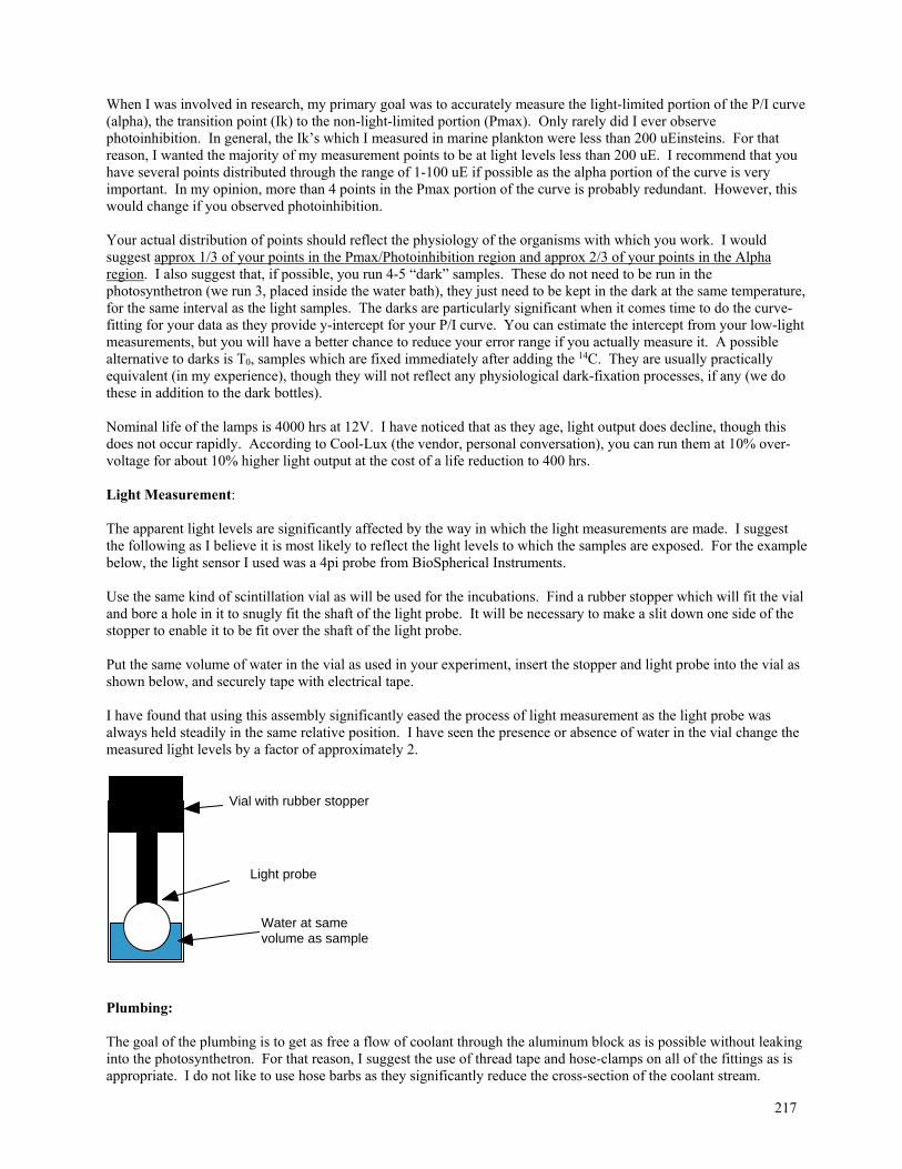
217

When I was involved in research, my primary goal was to accurately measure the light-limited portion of the P/I curve (alpha), the transition point (Ik) to the non-light-limited portion (Pmax). Only rarely did I ever observe photoinhibition. In general, the Ik’s which I measured in marine plankton were less than 200 uEinsteins. For that reason, I wanted the majority of my measurement points to be at light levels less than 200 uE. I recommend that you have several points distributed through the range of 1-100 uE if possible as the alpha portion of the curve is very important. In my opinion, more than 4 points in the Pmax portion of the curve is probably redundant. However, this would change if you observed photoinhibition. Your actual distribution of points should reflect the physiology of the organisms with which you work. I would suggest approx 1/3 of your points in the Pmax/Photoinhibition region and approx 2/3 of your points in the Alpha region. I also suggest that, if possible, you run 4-5 “dark” samples. These do not need to be run in the photosynthetron (we run 3, placed inside the water bath), they just need to be kept in the dark at the same temperature, for the same interval as the light samples. The darks are particularly significant when it comes time to do the curve-fitting for your data as they provide y-intercept for your P/I curve. You can estimate the intercept from your low-light measurements, but you will have a better chance to reduce your error range if you actually measure it. A possible alternative to darks is T0, samples which are fixed immediately after adding the 14C. They are usually practically equivalent (in my experience), though they will not reflect any physiological dark-fixation processes, if any (we do these in addition to the dark bottles). Nominal life of the lamps is 4000 hrs at 12V. I have noticed that as they age, light output does decline, though this does not occur rapidly. According to Cool-Lux (the vendor, personal conversation), you can run them at 10% over-voltage for about 10% higher light output at the cost of a life reduction to 400 hrs. Light Measurement: The apparent light levels are significantly affected by the way in which the light measurements are made. I suggest the following as I believe it is most likely to reflect the light levels to which the samples are exposed. For the example below, the light sensor I used was a 4pi probe from BioSpherical Instruments. Use the same kind of scintillation vial as will be used for the incubations. Find a rubber stopper which will fit the vial and bore a hole in it to snugly fit the shaft of the light probe. It will be necessary to make a slit down one side of the stopper to enable it to be fit over the shaft of the light probe. Put the same volume of water in the vial as used in your experiment, insert the stopper and light probe into the vial as shown below, and securely tape with electrical tape. I have found that using this assembly significantly eased the process of light measurement as the light probe was always held steadily in the same relative position. I have seen the presence or absence of water in the vial change the measured light levels by a factor of approximately 2.

Plumbing: The goal of the plumbing is to get as free a flow of coolant through the aluminum block as is possible without leaking into the photosynthetron. For that reason, I suggest the use of thread tape and hose-clamps on all of the fittings as is appropriate. I do not like to use hose barbs as they significantly reduce the cross-section of the coolant stream.

Vial with rubber stopper

Light probe

Water at same volume as sample

218

The aluminum blocks are threaded to accept 1/4” NPT fittings. Should the cooling blocks attached to the sides of the incubation block ever leak, you can disassemble them, clean and reseal with silicon rubber or type II Permatex (flexible). The coolant circulated through the blocks should be compatible with anodized aluminum. Other specs: Fuse: AGC-2 Lamp: FOS-008, 12V 75W – Cool-Lux, Inc. (www.cool-lux.com) Lamp should be turned on ~30 minutes before start of incubation or light measurement as output can vary when first

turned on. Sample size: For a 20 mL scintillation vial, I would recommend approx 3-5 mL sample size. A larger sample size will have a larger light-gradient through the sample. Collect the water sample. Place in some sort of repeating dispenser. Add working reagent and mix thoroughly. Dispense into all sample vials, including darks and T0 (Tzeroes). T0 vials should already contain an appropriate fixative or should be immediately filtered. We usually filter the T0 immediately and allow them to filter while completing the rest of the procedure. Keep all vials in a light-tight container until ready to load into p-tron.

Collect Rts. These are very small samples, usually 100 L, of the sample/C14 mix made above. Usually something like 10 ul is adequate. They should be placed directly into scintillation cocktail and capped immediately. These are used to determine the concentration of C14 in the sample mix.

Load the samples onto the p-tron, and incubate for 60-90 minutes. At the end of the incubation, remove the vials and either fix immediately or return to the dark box and fix or filter as soon as possible. It is not necessary to have the caps on the scint vials during the incubations. In some ways it is an advantage to not have them on as it saves capping and uncapping time, which reduces handling time and helps produce more consistent results. However, this requires that the vials be labeled. It also somewhat increases the possibility of spills, though, in my experience, it never was a problem. If you are filtering rather than acidifying and drying your samples, be sure to rinse each vial and put the rinse water through its respective filter, and then to rinse the filter to wash off any non-fixed 14C. I would guess that an appropriate rinse solution for your samples would be fresh water with some sodium bicarbonate added. The amount probably is not too critical as long as it is significantly more concentrated than the amount of 14C bicarbonate you added to the samples. I used to tell the students who worked with me that the best thing they could do for the quality of their data was to work on their consistency. If they scratched their ear after loading their first sample, they should scratch their ear after loading every sample. That was perhaps a little extreme. However, what I was trying to tell them was that often consistency was more important than perfection. In the case of the dark samples above, the reality is that they will be exposed to some light during handling. However, though this exposure should be minimized, it is not critical as long the light samples are exposed to the same amount of light during handling. The effect of the handling process will disappear when the darks are subtracted from the lights.

219

C. Incubation using photosynthetron Equipment

biospherical light wand (to check light levels – do this BEFORE you run samples). 500 mL flask for mixing sample 14C bicarbonate solution Gloves Repeating dispenser or 10-mL pipette 24 20 mL glass scintillation vials Dark box Photosynthetron Filter manifold (Millipore, 12 positions) Gelman GN-6 filters (25 mm diamater, 0.45 um pore size) Forceps Rinse bottle with DI H20 – it helps to have two Filled carboy with RO-DI 30 7 mL mini-scintillation vials 1 mL pipette 100 L fixed pipette 7 mL pipette Cellusolve Scintisafe Scintillation Cocktail

Sample collection

1) Before you go into the field a) Check photosynthron cooling system and turn on. Set to what lake temperature should be. b) Turn on p-tron light and let warm-up for 30 min. Make light readings in each photosynthron position.

Adjust light as needed. Record final light readings. 2) Sample collection is the same as for incubation in the field. Only about 200 mL of water is needed for a p-

tron run 3) Return to lab.

Sample preparation and incubation

1) Adjust cooling system temperature to match measured lake temperature at sampling depth. 2) Place filters in 3 positions of the filter manifold, stopper all other positions. Attach vacuum pump.

Avoid exposure of samples to light. 3) Place 300-mL of sample in a flask. 4) Add 2 ml of 50 Ci/mL 14C – HCO3). 5) Mix thoroughly. 6) Dispense 10-mL of sample/14C solution into each of 24 20-mL scintillation vials. Keep in dark. 7) Dispense 10-mL of sample/14C solution into each of the 3 filter positions of the filter manifold. 8) Dispense 100-ul of sample/14C solution into each of 3 mini-scintillation vials, add 7-mL scint-safe. Cap

vials. Record the vial numbers as unfiltered sample. 9) Apply vacuum to filter manifold. Rinse filters with DI H2O. Apply vacuum just till dry. Place filters in

separate mini-scintillation vials. Record vial numbers as the initial (T0) samples. 10) Place 21 of the 20-mL scintillation vials in the photosynthron. Record the position of each vial. 11) Place the other 3 20-mL scintillation vials in the dark and record their numbers. 12) Record time. 13) Incubate samples for 60-90 minutes. 14) While samples are incubating:

Place 12 filters on filter manifold and arrange 12 more for fast loading. Arrange 24 mini-scintillation vials for fast loading. Check that there is enough rinse solution in rinse bottle for all filters.

Sample processing

1) After 60-90 minutes: remove vials from photsynthetron to dark box, record exact time. 2) Filter vials 1-12 in position 1-12 of the filter manifold. Rinse vials twice with DI H2O. Apply vacuum. Rinse filter once with DI H2O and reapply vacuum.

220

3) Place filters in mini-scintillation vials. Record what sample went in which mini-scintillation vial. 4) Repeat 18 and 19 with vials 13-24 (22-24 are the dark vials). 5) Let filters dry with tops off. 6) Dispose of rad waste in rad waste containers. 7) Rinse filter manifold with DI water, dispose of this rinse in rad waste. 8) Thoroughly rinse all equipment and put it away. 9) Record days rad use and disposal on rad tracking sheet. 10) When filters are dry, tighten caps on scint vials. 11) Count according to same procedure as for field incubates samples

221

(VI-10) Alkalinity Determination 15 December 2014 JAD/JML

Alkalinity is the measure of the buffering capacity of water. Alkalinity results from any dissolved species

(usually weak acid anions) that can accept and neutralize protons. The milliequivalents (meq) of acid necessary to neutralize the hydroxyl (OH-), carbonate (CO3

2-), bicarbonate (HCO3-), and any silicate ions or dissolved organic

acids (with pKa values near the endpoint of the titration) in water is referred to as “total alkalinity”. In practice, we have mainly carbonate ions in our waters which are buffering acid, and thus we are measuring “carbonate alkalinity”. We measure the alkalinity of a sample by titrating with hydrochloric acid (HCl) until the point at which buffering ions have been neutralized with acid (the equivalence point); we determine this point by monitoring pH. We graph pH (y-axis) against volume (mL)of acid added (x-axis), and alkalinity is equivalent to the amount of acid used at the point where pH is changing fastest and the slope of the graph is the steepest (i.e., the “inflection point”), or in other words where the second derivative of the curve is zero.

IMPORTANT: The Kling lab purchased a new autotitrator in the fall of 2014 to replace the old Tim800 system. This protocol contains information pertaining to the old Tim800 system and the new TIM865, because some parts are interchangeable. Be aware that some older info may not apply to the new system.

Alkalinity Auto-Titrator Alkalinity Titrator – Radiometer Analytical Machine : TIM865 Titration Manager, (5mL burette), SAC80 Sample Changer, pH electrode GK 273920B

(~$130.00). Purchased new Titration manager December 2014 Company phone number: note that radiometer is now part of Hach Software : Titramaster85 OVERVIEW OF ANNUAL RUN PROCEDURE 1. Setup alkalinity titrator. 2. Sort samples. 3. Run tap water on titrator (about 8-10 vials to test basic operation and repetition). 4. Reset the TimTalk sample number to 1 at the beginning of each run year. Run standards prior to running any

samples to ensure everything is working properly. 5. Start to run samples with appropriate check standard for each run (see detailed method below). 6. Process samples and input into Alks_YYYY.xls (where YYYY is equal to the year that the samples were

collected). 7. QA/QC all sample titrations, and re-run high samples (with lower volume or dilutions; see QA/QC and Rerun

sections below) or any samples that seem abnormal, that were run on the wrong method, or for which the titration was stopped in the middle (usually due to a software problem).

8. Shut down alkalinity titrator (see Annual Shutdown section). 9. Copy alkalinity values from Alks_YYYY.xls to to Akchem_YYYY.xls file (remember that the AKchem unit is

µeq/L); send results to appropriate groups (i.e., LTER Lakes). ANNUAL STARTUP

Uncover and set up sample changer Turn on power (switch in back).

2. Connect pH electrode (type GK273920) to TIM865 and arrange the cord so it will not become caught on the sample changer. Note that the cord comes up through the ring of samples from below the sample changer. Rinse outside of probe and fill with 4M KCl to 0.5 cm below the filling hole, the company recommends also adding a small amount of KCl crystals to maintain KCL saturation in the probe. When probe is not in use, keep the filling hole covered with parafilm.

3. Put acid dispenser into correct slot on the autotitrator above a waste beaker. Flush DI then titrant acid through lines (see Detailed Instructions for Alkalinity Titrator Method), looking for any particulates, clogs, or big air bubbles. Make sure the final flushes are with the appropriate acid concentration for the method you are using.

ANNUAL SHUTDOWN 1. Remove acid titrant bottle from auto-burette and replace with DI bottle. Flush system completely with DI and

leave DI bottle on auto-burette for long-term storage. Flush the system by going to SETUPBURETTE and clicking FLUSH.

222

2. Remove titrant dispenser from the autosampler, place with auto-burette, and turn “off” auto-burette (switch in back). Cover auto-burette with plastic and leave on bench.

3. Remove pH probe from auto-sampler, unplug pH probe from Titralab865, place probe tip in storage cap (filled with storage solution), and wrap with parafilm (around the hole where you put the filling solution in, and the storage cap). Store in cupboard labeled “Alkalinity Supplies” in Alkalinity bench. Electrode should be stored upright and in its original box (instructions for care and maintenance are in the box).

4. Unplug auto-sampler. Leave stirrer as it is. Wrap with plastic and store auto-sampler on Alkalinity bench.

SORT ALKALINITY SAMPLES INTO RUN ORDER 1. Alkalinity samples are unacidified and stored in the coldroom until they are ready to be sorted or run. 2. Inventory samples when they arrive from Toolik by playing “bottle bingo” and using the ‘Alkalinity Inventory’

column in the Data\Arctic\Chemistry\Inventory_YYYY.xls file, or the AK_Sample_Master_YYYY.xls file. 3. Copy the Alkalinity inventory into the ‘Inventory’ tab in the Alkalinities_YYYY.xls file. 4. Sort samples into cardboard trays by method, determined by anticipated alkalinity concentration. Methods

control the amount of acid dispensed per injection (more for HIGH method, less for ULLOW), and also the concentration of the acid, plus the maximum amount of acid added per titration. If site is not listed below, look up site on previous Alks_YYYY file to see what methodology was used.

SITE METHODOLOGY (see also Method_Determination.xls in C:\\Data\Chemistry\Alkalinity):

5. If sample cannot be found in Method_Determination.xls or a previous Alkalinity_YYYY.xls file, first check the conductivity of the site and match it up to the closest known sample of similar conductivity, then use that method. If you have enough water or there is no conductivity, test the site by running ~20 mL of the sample using LOW or MEDIUM methodology in a small cup.

I. STANDARD PREPARATION Stock solution- 20 meq/L = 20,000 µeq/L NaHCO3 (Sodium Bicarbonate)

Place NaHCO3 in a beaker, and place in a desiccator for 24 hours (DO NOT place in 105°C drying oven as the NaHCO3 melting point is 60°C, and this temperature will alter its chemistry). Weigh out 1.680 g NaHCO3. Dissolve in a 1000 mL volumetric flask. [Note: You can make standards using Sodium Carbonate (Na2CO3) , but you must dry the reagent first in a 105°C drying oven for 24 hours (melting point is 851°C)].

The following standard concentrations should be used for specified methods: HIGH 1200 µeq/L (60 mL stock solution → 1000mL volumetric) MEDIUM 600 µeq/L (30 mL stock solution → 1000mL volumetric) LOW 50 µeq/L (2.5 mL stock solution → 1000mL volumetric) ULLOW 20 µeq/L (1 mL stock solution → 1000mL volumetric)

Making Standards

HIGH method: -Fog 02 Lake -S Lakes -NE Lakes -N2C & N2F -N 01 Lake -S 06 & S 07 Lakes -Shrew River N. -Thermokarsts

MEDIUM method: -Toolik Lake -Toolik Inlet -Inlet Series I1-8 (incl. I8 HW) -Lakes I6-I 8 (incl. I Swamp) -E 01 Lake -Green Cabin Lake -Watering Plot Barrel Water -Shrew Tributary & River -North Lake -Luna Lake

LOW method: -Kuparuk (sites 7 and greater) -E 05 & E 06 -Lakes I1-I5 - Dimple Inlet & Outlet -Dimple Lake -Perched Lake

ULTRA LOW (ULLOW) method: -Imnavait -Tussock Watershed (TW) -Watering Plots -Birthday Creek

223

1. For the each standard, place a clean cup on scale, and press Tare. Using a pipette, add the appropriate volume of 20,000 eq/L stock solution. If done correctly, the mass should be 1:1 of the volume. If you add too little or too much stock, you can calculate the new standard concentration using cross multiplication (C1V1=C2V2). Formulas to calculate the exact concentration of a standard are found in the “Notes” tab of the Alks_YYYY.xls file.

2. Carefully pour the stock solution into a 1 L volumetric flask. Rinse the cup several times with DI and pour into the volumetric.

3. Fill the volumetric flask full to the 1 L mark with DI water. Use a squirt bottle when the water gets close to the 1 L mark.

4. Allow standards to sit overnight before using in analysis without stoppers in. This is necessary because water comes out of the tap overly carbonated, and this affects the pH readings. The standard must be allowed to equilibrate with the air.

II. CHANGING ACID

When running the alkalinity analysis, the acid will need to be replaced in order to keep up with the amount of samples generated; acid is also changed between LOW/ULLOW, MED, and HIGH methods. 1. Make new acid

Prepare new hydrochloric acid at appropriate concentration (0.005N for LOW/ULLOW, 0.02N for MED, and 0.1N HIGH). We currently purchase 0.1N and 0.02N HCl , so no dilution is necessary for MED and HIGH titrants. For 0.005N HCl, dilute 50 mL of 0.1N HCl in 1000mL DI.

2. Changing the acid Unscrew the cap of current acid bottle, wipe the acid off the tube connected to the cap with a Kimwipe. Leave the cap off to allow the lines to drain Remove the acid delivery tip from the sample changer arm and place in the stand over the waste beaker. Using TIM865, go to titrant tab(2nd tab over on screen) Burrette Functions (option 7) Press flush (option 3) to drain burrette and titrant lines. When burette is done emptying, unscrew the tube connected to the burrette. Use a needle point syringe to

suck out the remaining acid. This will create a large bubble that will draw out smaller bubbles in the tubing. Put cap on new titrant, and press flush again. This may have to be done more than once in order to

completely fill the lines. Check the lines for any air bubbles. If any bubbles remain, press the empty option and then the fill option

until all lines no longer have air bubbles. If a bubble persists flick the line or pinch it for a few seconds to build pressure and for the bubble out.

3. Run check standards Run at least four cups of standard to make sure the old acid is completely flushed out of the system. If the

values of all four continue to sequentially increase or decrease, run more standards until values stabilize. DETAILED INSTRUCTIONS FOR ALKALINITY TITRATOR 1. Open Titramaster (double click icon in center of monitor)

The program will ask for a user and a password USER: kling, PASSWORD: kling011.

2. Calibrate the pH electrode:

Check that electrode filling solution in pH probe is filled to the bottom of the filling hole with 4M KCl filling solution, add KCl crystals. BE SURE TO LEAVE THE FILLING HOLE UNCOVERED WHILE MEASURING pH FOR CALIBRATION AND FOR SAMPLES. pH will begin to drift if the filling hole is covered! This has been a problem in previous years

To calibrate the probe, go to probe tab (3rd tab over) Check to make sure the calibration setup (Option 2) is set to calibrate with the 4.0 buffer first, and then the

7.0 buffer. Pour buffers into designated 4.0 and 7.0 buffer sampler cups and place 4.0 buffer in slot 1 and 7.0 buffer into

slot 2. Remove the acid delivery tube from the arm and place in the waste beaker. press Calibrate Probe (Option 1) Date and time should update, and sensitivity should be between 97-103%. Update ‘Run_Summary’ tab in the Alkalinity_YYYY.xls file with pH calibration sensitivity reading.

3. Enter sample order into Alks_YYYY.xls

224

Set up the Excel file, located in Data\Arctic\Chemistry\Alkalinity\Alks_YYYY.xls. This is usually most convenient to do while the electrode is calibrating. Refer to the ‘Setting Up Alks_YYYY.xls’ section below.

4. Clear bubbles in the burette line: This is done both to remove bubbles from line, and also because the acid in the tube will become diluted as it

sits in the DI rinse cup. Remove the acid delivery tube from the arm and place in the waste beaker. Under SETUP, select BURETTE, then EMPTY IN BEAKER. Wait until the burette has fully emptied. Unscrew the green nut on top of the burette, and insert a needle-point syringe (should be in drawer) through

the top of the burette, and suck out the remaining acid; this pulls a large bubble through the line which removes any small bubbles. Alternate filling (click FILL) and emptying (click EMPTY IN BEAKER) the burette until all bubbles are clear from line.

When you are satisfied that all bubbles have been cleared, Select CLOSE. Return acid delivery tube to position in the sample changer arm.

5. Set up the autosampler tray: Sample water MUST be at room temperature in order to properly determine alkalinity, so the samples should

be taken out of the refrigerator at least ½ hour before they are run. YOU MUST SHAKE SAMPLES AND STANDARDS BEFORE POURING in case there are mineral

precipitates at the bottom. Make sure all the cups are clean (rinsed 5-6 times with DI) and dry. Measure samples and standards by placing a cup on balance and pressing ‘tare’. Pour approximately 40 mL

of sample or standard into cup, and record mass (volume determined by assuming a 1g= 1 mL relationship). Again, refer to ‘Setting up Alk_YYYY.xls file’ section for further details.

Standards: Fill cups 1 and 2 with 38-42 mL of NaHCO3 standard solution of the appropriate concentration for the

current method. Record the mass of the standard (in grams) in the “Sample Volume” column in “Alks_YYYY.xls” file.

Samples: Use the same method as with standards, except fill cups with sample. In cups 3-13, pour ~40 mL of sample. Leave at least 10mL of water in the bottle for HIGH, MEDIUM,

and LOW methods, and at least 20mL for ULLOW method. This way, if the run is bad there is enough water to re-run the samples. Record the mass of the sample (in grams) under the “Sample Volume” in “Alks_YYYY.xls” file.

Sample cups 14 and 15 are always rinse cups of RO/DI water. Re-fill before the start of each run. 6. Enter sample info into Titramaster:

From the Alks_YYYY.xls file, copy the sortchem numbers and weights. In Titramaster, under the FILE menu select SAMPLE STACK. Then, under EDIT select PASTE. (note

that you CANNOT just use ctrl+v, you have to select EDIT then PASTE) Verify samples information copied correctly into SAMPLE STACK. Under FILE, select SAVE, then

select EXIT. If you do not select SAVE, it will use the last sample stack. All samples should be set to printout after each is run.

7. Check that open method is the correct one: Under FILE, select EDIT METHOD, or on the autotitrator itself, select EDIT METHOD. The current

method used is Continuous IP. In 2015, we had drift problems with the titrator and probe that would not allow for accurate or precise check standard values. Therefore, continuous IP should be used to decrease the effect of the probe drift.

8. Start the run: In the first tab on TIM865, select Check “Sequence SAC” Then click the first tab, Start Sequence and the

run will begin. After the first 10-20 minutes, check the machine to make sure that standards have run correctly (within ~5%

of the standard value). If not, stop the run. If you do not see the graph on the screen, see Trouble Shooting immediately.

SETTING UP THE Alks_YYYY.xls FILE 1. The yearly Alkalinity file can be found L:\DATA\Chemistry\Alkalinity\Alks_YYYY.xls Make sure the

Alkalinity inventory, found on the ‘Inventory’ tab, is updated from L:\DATA\Arctic\akYYYY\Akchem_Inventory_YYYY.xls (or AkChem_YYYY.xls).

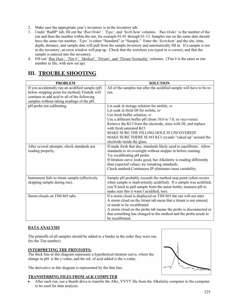
225

2. Make sure the appropriate year’s inventory is in the inventory tab. 3. Under ‘RadIP’ tab, fill out the ‘Run Order’, ‘Type’, and ‘SortChem’ columns. ‘Run Order’ is the number of the

run and then the number within the run, for example 01-01 through 01-13. Samples run on the same date should have the same run number. ‘Type’ is either “Standard” or “Sample.” Enter the ‘Sortchem’ and the site, time, depth, distance, and sample date will pull from the sample inventory and automatically fill in. If a sample is not in the inventory, an error window will pop up. Check that the sortchem you typed in is correct, and that the sample is entered into the inventory.

4. Fill out ‘Run Date’, ‘Tim #’, ‘Method’, ‘Titrant’, and ‘Titrant Normality’ columns. (Tim # is the same as run number in file, with new set up)

III. TROUBLE SHOOTING

PROBLEM SOLUTION If you accidentally run an acidified sample (pH below stopping point for method) Timtalk will continue to add acid to all of the following samples without taking readings of the pH.

All of the samples run after the acidified sample will have to be re-run.

pH probe not calibrating.

Let soak in storage solution for awhile, or Let soak in fresh DI for awhile, or Use fresh buffer solution, or Use a different buffer pH (from 10.0 to 7.0, or vice-versa) Remove the KCl from the electrode, rinse with DI, and replace with fresh saturated KCl MAKE SURE THE FILLING HOLE IS UNCOVERED! MAKE SURE THERE IS NO KCl crystals “caked up” around the electrode inside the glass.

After several attempts, check standards not reading properly.

If made fresh that day, standards likely need to equilibrate. Allow standards to sit overnight without stopper in before running. Try recalibrating pH probe. If titration curve looks good, but Alkalinity is reading differently than expected values, try remaking standards. Check method-Continuous IP eliminates most variability

Instrument fails to titrate sample (effectively skipping sample during run).

Sample pH probably exceeds the method stop point (often occurs when sample is inadvertently acidified). If a sample was acidified, you’ll need to pull sample from the anion bottle; measure pH to make sure this it wasn’t acidified, too).

Storm clouds on TIM 865 tabs If a storm cloud is displayed on TIM 865 the run will not start. A storm cloud on the titrant tab mean that a titrant is not entered, or needs to be recalibrated A storm cloud on the probe tab means the probe is disconnected or that something has changed in the method and the probe needs to be recalibrated.

DATA ANALYSIS The printoffs of all samples should be added to a binder in the order they were run (by the Tim number). INTERPRETING THE PRINTOFFS: The thick line in this diagram represents a hypothetical titration curve, where the change in pH is the y-value, and the mL of acid added is the x-value. The derivative in this diagram is represented by the thin line. TRANSFERRING FILES FROM ALK COMPUTER After each run, use a thumb drive to transfer the Alks_YYYY file from the Alkalinity computer to the computer

to be used for data analysis:

226

Copy the files to 2 locations: o C:\DATA\Chemistry\Alkalinity (then into the appropriate folder). Don’t forget to backup onto the L:\ drive,

too!

ENTERING DATA INTO Alks_YYYY.xls In the “Rad_IP” tab, manually enter data from the printoff into the spreadsheet columns titled ‘Starting pH’, ‘IP

pH’ (the pH at equivalence point), ‘Acid (mL)’ (amount of acid added at equivalence point), and ‘Alk (meq)’. No data is manually entered into the ‘AlkCalc (µeq/L)’ or the ‘Dbl Chk’ columns; instead, copy down formulas.

The ‘AlkCalc_(µeq/L)’ column calculates the equivalence point using the following formula: ((Titrant Normality) * (mL Acid Added)) / (mL Sample Volume)

If this value does not match the value under the ‘alk_(umeq/L),’ then the message “ERROR” will appear in the ‘Dbl Chk’ column. This message means that some of the above values must have been entered incorrectly, there was an error with instrument/software, or the equivalence point was incorrectly identified.

Determine if a sample needs to be re-run (see “QA/QC” section below) or calculated using Gran Calculations (see below). Note in the appropriate column in the “Rad_IP” tab if a sample needs to be either re-run or calculated using Gran calculations. Maintain a current list of samples to re-run by copying sample information into the “Re-run” tab.

Copy all newly entered run info, notes and data to the Alks_YYY_for_alks_computer.xls file to the full Alks_YYYY.xls file.

Gran Calculations o It is preferable to use the IP to determine alkalinity. However, sometimes the program fails to identify an

equivalence point, and it is difficult to “eyeball it,” usually due to noise in pH readings. In such cases, you can calculate the equivalence point using Gran calculations. From Wetzel and Likens Limnological Analyses: The accumulation of protons is calculated as the product the hydrogen ion (H+) concentration and the sum of the sample volume, plus the titrant volume. The accumulation of protons is referred to as the 1st Gran function (F1) . F1 is very slow as pH>5, due to bicarbonate buffering, but the accumulation of protons becomes rapid and linear below pH=4, where bicarbonate buffering is exhausted. The volume of acid required to reach the equivalence point is determined by the extrapolation of the linear portion of the plot (between pH 4 and 3.5).

F1 = (Volume of sample + Volume of acid) * 10 –pH

Using only the data where pH <4, regress F1 as the independent variable versus the volume acid added as the X-variable:

X-intercept = -1 * Y-intercept / Slope Alkalinity (meq/L) = (Normality of acid) * (X-intercept, L) / (Sample volume, L)

o In the “Rad_Gran” tab, auto-paste sample information by clicking on the “Paste Sample Info” box. o Click on the “Multiple Data Fetch” box to import curve data; this imports data into the tab “RadGranData”;

don’t do anything with data in that tab! That tab is referenced by functions in the “Rad_Gran” tab. o Sometimes you will get an error message “Curve file is missing!” If you get this message erroneously, there

are several things to check. Make sure that 1) the curve file is consistently named in the Alk_YYYY file and in the Timtalk program, 2) the curve file has been uploaded from the Alk computer to the computer you are currently using, and 3) all samples that are listed on the left side of the “Rad_Gran” tab actually have been run and have curve files (if the sample was never run, but remains in the list, this screws up the macro; delete that sample info in the “Rad_Gran” tab only).

o The titration curve, first derivative and F1 are automatically graphed. Use the spinners adjacent to the graph to select a particular sample to examine, or type in the row number.

Determine the best fit line for the linear portion of F1; use the Vt high and Vt low spinners (fine tuning to the left, coarse to the right) to adjust the line in order to achieve the highest r2 . When you are satisfied with the fit, click the “Paste Results” box.

QA/QC : There are several levels of QAQC. The first step occurs while you are running samples. Check standards should fall within +/- 5 ueq/L of calculated concentration for ULTRALOW and LOW methods,

and +/- 10 ueq/L. Sometimes the first curve is bad, especially when changing methods or using ULTRALOW or LOW methods. Proceed if the second check standard falls within range.

After a sample has run, inspect its curves. Certain runs require further examination:

227

o If samples have fewer than 5 points before or after the inflection point, try re-running on another methodology to produce more accurate results. See “RE-RUNS” section below for details.

o Two problems arise using the ULTRALOW methodology: Alkalinity in soil samples will sometimes be below the detection limit. If so, the alkalinity cannot

be determined, and the only data in alks.xls file will be the starting pH. Often in ULTRALOW methodology, no equivalence point is chosen; values must be determined by

eye. This occurs because the low alkalinity values make it difficult for the program to determine the true equivalence. The equivalence point must be recalculated using the TimTalk program.

The next step of QAQC is to have a second party double-check your data entry. The person should also make sure they agree with any eye-balled inflection points. If they determine a curve is questionable or bad, they should flag the curve by filling in "Do not use" or "examine" in the appropriate column of the Rad_IP tab; otherwise they should fill in that column with "RadIP" or "Gran" (if there is a lot of noise in the pH readings). Samples will be sorted by this column in the next steps of QAQC.

The final steps of QAQC occurs once all the samples are run for the year.

o After all Alks have been run for the season and double-checked, paste columns A through H from Rad_IP tab to Alk_Summary tab.

o Copy down formulas in columns I through V. o Sort by column I, and delete all samples that return "do not use" in column I. o Sort by column B, then C. Delete all standards. o Manually go through remaining samples. Make sure duplicates are calculated properly, and that any samples

returning "examine" in column I are okay to use (re-examine curves). o Look at CV’s of duplicate samples. Examine duplicates with high CV’s. o When you are certain only "good" runs remain and that values are correct, copy and hardpaste the

Alk_summary tab into the For_akChem tab. o Sort by alkalinity values, and delete duplicate sortchems (they should not have any data associated with them

because it was averaged in the Alk_Summary tab). Sort by Site, Date and Depth, and perform QAQC to look for outliers. Outliers should be designated as "do not use" in column AF of the Rad_IP tab, and the reason recorded in the Notes column of that tab.

RE-RUNS Sometimes you will need to re-run a sample. Note in column AE of the Rad_IP tab in the alks file if a sample is

to be rerun, and also copy the sample information over to the Re-runs tab. To adequately submerge the pH probe, the analysis requires 40 mL of sample; however, we only collect 60 mL.

This leaves <20 mL of sample for subsequent runs. This issue can be addressed by diluting samples to 40 mL wit h DI, or using small cups. GWK has determined that using small cups is preferable to diluting, but both methods work (see Alks_2008.xls for results of a Small Cups versus Dilution Experiment).

Choose the appropriate method to run the sample on (remember, you are effectively halving the alkalinity; a good rule of thumb is to run a small-volume of sample using the next lower method.

Place small cups in styrofoam holders. Pour approximately 20ml of sample in to each cup (make sure to run a check standard in a small cup, as well).

Dilute to bring volume to 20ml , if absolutely necessary. Record the pre-dilution sample volume.

(VI-11) OPA - Fluorometric Ammonium Analysis Updated 9 Jan 2013 by SEF

228

References: Holmes, R. M., J. W. McClelland, D. M. Sigman, B. Fry, and B. J. Peterson. 1998. Measuring 15N-NH4+ in marine,

estuarine and fresh waters: an adaptation of the ammonia diffusion method for samples with low ammonium concentrations. Marine Chemistry. 60: 235-243.

Holmes, R.M., A. Aminot, R. Kerouel, B.A. Hooker, and B.J. Peterson. 1999. A simple and precise method for measuring ammonium in marine and freshwater ecosystems. Can. J. Fish. Aquat. Sci. 56: 1801-1808.

INTRODUCTION The determination of ammonium in arctic waters is difficult both in terms of preserving the sample and achieving consistent, reliable results during sample analysis. Concentrations are usually very low and require a very sensitive method. For these reasons, the Arctic LTER began to use the OPA method for ammonium determination instead of the indophenol blue (Solorzano) method in 2001 (a brief history of this shift is described below). The OPA method uses a fluorometric method modified from Holmes et al. (1999). The method described here is modified from the Protocol B-1 (previous protocol version) & the LTER lakes protocol. Note that the calculation method described in the Holmes et al. papers is wrong; the correct modification is described below. Through the summer of 1998, the indophenol blue (Solorzano) method for ammonium determination was used by the Arctic LTER. Comparisons between the Solorzano and OPA methods were performed in the summers of 1999-2001. During those years, ammonium samples were analyzed by both the phenate and OPA methods. The Solorzano method results are used as the final data values for samples through 2000 (more of the samples were run using the Solorzano method). In 2001, the majority of samples were run using the OPA method and the final data values reported are the results of the OPA analysis. GENERAL COMMENTS Safety -- Gloves, a lab coat, and safety glasses should be worn when dealing with OPA. The OPA chemicals are

treated as hazardous waste. Contamination & Problems Always use ammonia-free water for all reagents. Get the water from the DI unit immediately prior to use (or

use the DI that the Nutrient RA has set aside specifically for chemical analysis). Make absolutely sure the DI used to make the standards is also used for the blanks. The tubes are pre-reacted with OPA working reagent (WR). Initially, you may need to do this several times

before running samples (surface is ‘sticky’ with NH4). NEVER ACID WASH THESE TUBES once the season starts.

If you suspect that a sample tube is contaminated, follow the pre-reaction procedures. DO NOT ACID WASH!

Accuracy Calibrate the pipette with each use. Check calibration by weighing the desired amount on the balance and adjusting the pipette as needed.

Keep a record of the calibrations in the OPA notebook (kept above the computer in Wet Lab). Apparatus & supplies 25 mm x 150 mm borosilicate culture tubes 4 liter amber bottles (fisher # 028846b) 6/case (to hold the WR) REAGENTS The Nutrient Research Assistant (Nut RA) prepares the reagents, standards, and sets up the fluorometer. If there are problems with any of these items, ask the Nut RA. The following will make 48 liters of Working Reagent and 4 liters of Borate Buffer. Reagent Formula Amount Sigma cat # sodium sulfite 250 g S 4672 sodium borate 2.5 kg S 9640 orthophthadialdehyde 100 g P 1378 ethanol 2.5 L a. Borate Buffer (BB): Follow the directions for preparing the working reagent, but do not add the sodium sulfite or the OPA reagents. b. Sodium Sulfite: Dissolve 2.0g of sodium sulfite into 200mL of deionized water in a 250mL volumetric flask. Dilute to 250mL with deionized water.

229

c. Orthophthadialdehyde (OPA): Dissolve 8g of OPA into 200mL of ethanol (keep this solution as dark as possible), shake vigorously until OPA dissolves. d. Working Reagent (WR):

i. Dissolve 160g of sodium borate into 3L of deionized water in a 4L amber bottle (pre-react bottle – if first time making WR, make a small amount initially to pre-react the bottles, dump, and then make the intended amount - or if the bottle was previously used for WR rinse with DI), cap, and shake vigorously until your arms are tired, then rest, then do it some more. There will be a precipitate in this solution because at this level, the solution is supersaturated.

ii. Add 20mL of sodium sulfite reagent, cap and mix. iii. Add 200mL of OPA reagent, cap and mix. iv. Add deionized water until the bottle is nearly full (about 1 inch from the top), cap and mix. v. Let age for at least a few days if possible, and then the WR is ready to use.

vi. Working reagent appears to be stable for months, and its blank fluorescence decreases over time, so it is best to make WR in large batches and let it age. We make WR batches of about 4 L in 1 gallon brown Nalgene bottles (these bottles actually hold about 4.4 L).

PROCEDURE: The Landwater group uses the standard addition method and also runs the standard curve prepared by the Nutrient RA. We continue to run the standard addition method because we collect surface and soil water samples. Therefore, we have a wide range in concentrations and matrix effects are strong with our soil water samples. Essentially, matrix effects result in concentrations that are either higher or lower than what you would expect (it is hard to know whether it is actually higher or lower). Matrix effects are the result of other compounds (such as humic acids) in a sample that interfere with the OPA reaction OR react with the OPA reagent. OPA reacts with amino acids; however, the addition of sodium sulfite to the working reagent results in OPA preferentially reacting with the ammonium in a sample. Therefore, the fluorescence observed by the reaction of a sample with the OPA working reagent is directly related to the concentration of ammonium in a sample. However, some background fluorescence is observed in the sample (without OPA) and the working reagent. A buffer is used to estimate the background fluorescence of the working reagent (the buffer does not contain the sodium sulfite or OPA). In order to specify the fluorescence associated with the OPA and ammonium reaction, the sample is run with a) only the buffer added, b) with only working reagent added, and c) with several standard spikes + working reagent. In addition, sample water and DI react different with the OPA reagent and buffer. Therefore, a DI+buffer and a DI+working reagent is also run and subtracted from each sample fluorescence (see calculations section below). As of 2010, we have also begun taking a time zero reading for a more accurate blank estimate (as we cannot be certain there is no NH4 in the DI…). Note that the buffer tubes must never have working reagent added to them! General Set-up The OPA standard curves are used as a between-run comparison. . The check standards provide a measure of the ‘actual’ quality of our run. We run 3 replicates of DI and buffer (DI+BF) and 3 replicates of DI and working reagent (DI+WR, 3 reps = 3 different vials). These are run at the beginning of each run along with the standard curve prepared by the nutrient RA. The nutrient curve consists of a standard plus the working reagent (same ratio as sample to working reagent used for the samples). Note that if the samples have been acidified, you will also need to acidify the standards using the same sample to acid ratio. Below is a typical run print-out (BF=buffer, WR=working reagent, STD=standard):

RUN: 21

WHO: AER Ratio (sample in ml : WR in ml): 4 : 8

Doubled Checked

Date: 17Aug07 Time Reagent Added __________

Date Read _________

Time Read __________

Tray SortChem Site Date BF Sample Spike 1 Spike 2 Time Zero

1 DI + BF

1 DI + BF

1 DI + BF

230

1 DI + WR

1 DI + WR

1 DI + WR

2 STD 0.05

2 STD 0.10

2 STD 0.25

2 STD 0.50

2 STD 0.75

2 STD 1.00

1 2007-0657 Toolik Inlet 17-Aug-07

2 2007-0657.1 Toolik Inlet 17-Aug-07

3 2007-0658 I8 Inlet 17-Aug-07

4 2007-0659 Milkyway Upper 17-Aug-07

Pre-reacting tubes (do this at the beginning of the summer or if you think the tube is contaminated) Tubes are color-coded so that there are four tubes for every sample #: blue (sample + BB = BF), white (sample + WR), pink (sample + WR + low spike), and red (sample + WR + high spike). REMEMBER!! Ask the nutrient RA which borate buffer and working reagent you can use to pre-react your tubes. Pre-reacting the buffer (blue) tubes (DI+buffer, Sample+buffer tubes):

1. Turn on the fume hood in the dark room. 2. Inspect the tubes. If they seem very dirty, rinse with a small amount of borate buffer and dump into the

labeled OPA hazardous waste container. 3. Add 10 mL buffer to the tube, cap, and shake. Let the tubes sit with buffer for at least 3 hours (24 hours is

best; days to weeks is fine). 4. Dump the buffer after 3+ hours. 5. Add 10 mL of buffer, shake, and dump into a labeled OPA hazardous waste container. 6. Add another 10 mL buffer. 7. Store in the dark until use.

Pre-reacting working reagent (WR) tubes (standards, DI+WR, and samples – white, pink, and red labels):

1. Turn on the fume hood in the dark room. 2. Inspect the tubes. If they seem very dirty, rinse with a small amount of pre-reactant (diluted working

reagent—1 part WR: 3 parts DI) and dump into the labeled OPA hazardous waste container. 3. Add 10 mL pre-reactant to the tube, cap, and shake. Let the tubes sit with pre-reactant for at least 3 hours (24

hours is best; days to weeks is fine). 4. Dump the pre-reactant after 3+ hours. 5. Add 10 mL of pre-reactant, shake, and dump into a labeled OPA hazardous waste container. 6. Add another 10 mL pre-reactant. 7. Store in the dark until use.

Tubes Preparation for Sample Analysis (do this each time before running samples) The sample tubes need to be prepped prior to running samples. Each vial will still contain reagent and sample from your previous run (remember, we do not acid wash tubes). This is performed in the dark room (room with fluorometers) in the Wet lab. There is a hood in the wet lab dark room, turn it on (knob is on the wall) to reduce the fumes associated with the procedure.

1. Pour out reagent/sample in tubes from previous run into the appropriate waste container. If the waste container is full, ask the Nut RA to properly dispose of the container and get a new one.

2. Rinse all tubes with DI, then ~4 mL of buffer and empty into waste (leave these tubes empty for now). Running the Samples The nutrient RA prepares standard curves and reagents on Mondays, Wednesdays, and Fridays. Samples are run within 1-2 days of collection. If they cannot be analyzed within 1-2 days, they are preserved with ~100 µL of 6N TMG-HCl. Remember, the standards need to be acidified if the samples are acidified. Running the Samples Part I: Getting organized

231

12. Determine which samples are going to be run. 13. Transport samples from the refrigerator in the entryway of Lab 4 to the Wet lab. 14. Talk to the person responsible for the PO4 analysis to determine what time the nutrient bottles will be

available for you. This is necessary because nutrients (PO4 and NH4) are collected in the same bottle. In general, the PO4 person will prepare his/her PO4 samples (will use the bottles) while you are prepping your tubes. After he/she has finished, you can take the bottles.

15. Calibrate the repeat pipette before you use it and record the calibration information on the front page in the OPA nutrient book and enter into akNH4_YEAR.xls.

16. Create a run sheet by entering the sample information into the “NH4 Template” tab in the akNH4_YEAR.xls file. Note that each sample has a corresponding tube number. Periodically update the Inventory tab in the NH4 file because the NH4 Template tab references the Inventory to get site information.

17. Print the run sheet (this will help you keep the samples in order). 18. Arrange samples in order on the Wet Lab chemistry bench. 19. Verify the sample information on the bottles and make sure they match your run sheet (this can be done

while pipetting samples). If the bottle and your run sheet information do not match, correct the information on one or both and notify whoever that akchem needs to be updated.

Running the Samples Part II: Starting the reaction Standard curve :

9. Add 4 mL of DI to the 3 DI+buffer tubes and the 3 DI+WR tubes (6 tubes total; 24 mL DI total). 10. Add 4 mL of prepared standard into each the corresponding tube. We run a curve with the 0.05 M, 0.1

MM,M, 0.75M, and 1M standards prepared by the nutrient RA. We have dedicated vials for each standard. Rinse each vial with the appropriate standard once before filling it with that standard. Make sure you use the standards for OPA (there are separate bottles for the PO4 and OPA analyses).

Samples: In addition to running samples, run at least 2 check standards per run. We run 0.05 and 0.25 M standards in the same fashion that we would run a sample (4 different tubes per sample).

12. Change your pipette tip and rinse 3 times with DI and 1 time with water from your first sample. 13. Add 4 mL sample to each row of tubes (the blue, white, pink, and red) to the appropriate numbered tube

(check your run sheet). 14. Place the caps on the tubes. Between each row (when you switch to a different sample), rinse the pipette 3 times with DI and 1 time with

sample water. You do not need to rinse if you are using the same sample. You MUST rinse if you switch samples.

16. Spike all of the pink (3rd tube from the left) tubes with 25 L of 50 M stock and recap the tubes. This is the low spike addition. Do this for all samples making sure you are adding the spike to the correct tubes.

17. Spike all of the red (4th tube from the left) tubes with 100 L of 50 M stock and recap the tubes. This is the high spike addition. Do this for all samples making sure you are adding the spike to the correct tubes. In the Wet Lab dark room:

18. Add 8 mL borate buffer to all blue vials (first tube on the left; NEVER EVER add OPA to the blue BF tubes), recap and vortex.

19. Add 8 mL WR to each white tube. After adding the WR, recap, vortex , wipe with Kimwipe, and place in fluorometer to obtain a time zero reading (see next section on reading samples). Use the reading from 20 seconds after placing tube in the fluorometer, unless the reading stablilizes before that.

20. Add 8 mL WR to all pink and red tubes, recap and vortex. 21. Keep all tubes in the dark for 18-24 hours. Tubes are generally kept in a large ‘dark’ box under the counter

in the dark room in the wet lab. Running the Samples Part III: Reading the Samples in the dark room Samples are read on a Turner Designs 10-AU field fluorometer wth optical kit No. 10-303 (Holmes et al. 1999). Read the tubes by columns (all BF, all samples+WR, all samples+low spike+WR, then samples+high spike+WR). This will reduce the time it takes for the fluorometer reading to stabilize.

22. Turn on fluorometer at least 20 minutes prior to use to allow it time to warm up. 23. Read the samples after incubating for ~18-24 hours. 24. Vortex tube and wipe the outside with a Kimwipe before reading.

232

25. Insert the tube into the fluorometer. 26. Place our specially made ‘cap’ on top of the tub to minimize outside light interference. 27. Wait for the value to stabilize or press the * key (it will take an average of readings) 28. Record the value on the run sheet. 29. After you have run all samples, simply leave the sample+reagent in the tubes. Throw away all of your

Kimwipes and put samples back into the Kling dark box. Leave the box under the counter in the Wet Lab dark room.

Running the Samples Part IV: Entering the results into akNH4_YEAR.xls Enter the date, the run number, the operator (you), and a summary of the day’s run in the Notes page. Make sure to notate whether you used a new bottle of OPA or anything else that may have been slightly different.

30. Staple the run sheet into the OPA Nutrient Book (located above Landwater computer in the wet lab). 31. Enter the sample curve information into the “OPA_Std_Curves” tab. 32. Copy down formulas where indicated. 33. Enter sample and check standard information into the “OPA_NH4” tab. 34. Copy down formulas where indicated. 35. Enter notes, save file and update on Lab 4 computer (if the computers are networked, simply drag file to right

location on Lab 4 computer; otherwise save on flash drive and copy onto Lab 4 computer). Running the Samples Part V: QA-QC results in akNH4_YEAR.xls

36. Check the average buffer (DI+buffer; column M) in the “OPA_Std_Curves” tab; it should be similar to previous runs. If it is variable, talk to the Nutrient RA. This could also be a result of using a different bottle of buffer (and why it is good to indicate when you use a different bottle).

37. Compare the DI+WR reagent (column Z) in the “OPA_Std_Curves” tab to previous runs. This is often more variable than the DI+buffer. However, it should be below 1. If not, talk to the Nutrient RA. This could also be a result of using a different bottle of working reagent (and why it is good to indicate when you use a different bottle).

38. Compare the estimated slopes across time (graph on top left) in the “OPA_Std_Curves” tab. The slope should be rather consistent. It is normally a little high at the beginning of the season or if newer working reagent is used. It should settle down in 1-2 weeks.

39. Check the sample information in the “OPA_NH4” tab. Make sure that any information marked on your run sheet is also entered into the excel spreadsheet. Note any major changes in the Notes column and/or Notes page (in general, a note specific to a sample is located in the OPA_NH4 tab notes column (column BE) and major notes (run summary, etc) are kept on the “Notes” tab.

40. Check that data are entered correctly. Someone other than the original data-enterer should double-check all data entry

41. Check the sample, spike 1, and spike 2 fluorescence values. Spike 1 and spike 2 should not be the same (if so, you may have spiked both samples with the same standard). Spike 2 should be higher than spike 1 and spike 1 should be higher than the sample. If there was an analytical error, that sample will need to be re-run.

42. Update your sample inventory. Make sure to indicate whether a sample has been run, needs to be re-run, and/or whether the sample was acidified.

43. Plot sample values with previous years’ data and look for outliers. Any sample that has a negative value or an unlikely value compared with previous years needs to be rerun.

Running the Samples Part VI: End of Season Procedures

44. After you are sure all samples have been run (including reruns), you are ready to shutdown Wet Lab. Bring all pipettes back to Lab 4. Place all other Landwater items on the shelves above the computer. Cover the shelves with plastic.

45. Make sure all files have been updated on the Lab 4 computer. Shut down the computer and unplug. Cover with plastic.

46. Pour all liquid in the OPA test tubes into OPA waste. Rinse with DI and empty into waste. Store in the covered box, capped and empty, under the counter in the dark room.

FINAL QA/QC After all the data entries have been double-checked, and the akchem_YYYY file has been finalized (double-checked and site information is updated), it is time to embark upon the delightful process of QA/QC. This procedure is VERY IMPORTANT, and should not be taken lightly.

233

10. In the akNH4_YYYY.xls file, first update the Inventory tab. Assuming all the sortchems are in

akchem_YYYY.xls (from every project that was worked on that summer), it is easiest to just copy the sortchem, site, date, time, depth, distance, elevation for every sample directly from akchem and paste into the Inventory tab. Now you have the most updated sample information.

11. Once you are sure the Inventory has all the information necessary (check for any missing values, like time and depth), update the OPA_NH4 tab. Use index-match to pull the site, date, time, depth, distance information from the Inventory tab, matching with the sortchems in the OPA_NH4 tab. Do not do this for the check standards because they will not have sample information in the Inventory tab.

12. Once you have updated the site, date, time, depth, and distance, then “hard paste” these values into place. (Copy all the values, and then choose “paste special” and click “values.”)

13. On the OPA_NH4 tab, go through each individual formula and make sure that it is referencing the correct cells and returning the correct information. This can be time consuming, but it is important that these formulas are correct. If you are unsure about a certain formula, check with someone else before assuming it is OK. There are descriptions of the formulas in the Notes tab for reference.

14. Once checked, copy down all formulas for all cells where that formula is used. 15. Next, look at the standard curves in the OPA_Std_Curves tab and see if there are “bad” curves. Use the

arrows in the upper left corner to scroll through the runs and check the curves in the plot directly to the right. Also check the other plots at the top of the screen and look for runs that had uncharacteristic slopes or intercepts. If a standard curve clearly does not fit with the other runs (does not fall within normal variability), the samples run with the curve should be looked at extra closely for suspect values (if the whole run wasn’t rerun anyway). Finally, check the R-squared values for the curves (we want at least 0.99 ideally, but down to 0.95 is normal for OPA) and look for any notes that suggest a curve shouldn’t be used.

16. Update the Summary tab using the instructions at the top of the tab. Sometimes it is difficult to decide which rerun to use, especially if the person doing the QA/QC is not the person who originally ran the analysis. Checking through the reruns generally entails checking back through the raw data in the OPA_NH4 tab to figure out why a sample was rerun and whether the original value should be used. MAKE NOTES explaining why a sample was rerun and which value should be used (or both). Common reasons for reruns include negative values, unexpectedly high values, spiking samples incorrectly, high %CVs between duplicates, bad standard curves, or bad sample readings due to machine errors.

17. Copy the data in the Summary tab (all columns) and hard paste into the QAQC tab. Sort by site name. Make scatter plots for each site (concentration on y-axis, date on x-axis) and look for outliers. It’s useful to compare to the previous year’s (or years’) data if unsure about “normal” values for a site. Keep in mind that some sites (like soil water or thermokarsts) experience greater variability and higher concentrations. If a value looks like an outlier, look at the OPA_NH4 tab for any notes about the sample or an explanation for the unexpected value. If the value needs to be removed, replace the value with a “.” and make notes (including the original concentration) in the Summary tab.

18. After checking through the data and updating the Summary tab, copy the data into the Summary_Hardpaste tab. There are instructions at the top of the tab.

Calculations The calculations for OPA ammonium can be confusing. Please try to follow along. A. Blanks. Regardless of using or not using standard additions and matrix effects, the following applies for determining our best estimate of a true blank (since that cannot be determined in theory -- agreed upon between Giblin, Kling, Field, Wallace on 4 Jan 2005). 1. DI+WR (DI water plus Working Reagent) 2. DI+BF (DI water plus Borate Buffer) 3. Sample+BF (Sample plus Borate Buffer) 4. Sample+WR (Sample or spike plus WR)

234

To calculate the blank corrected Sample or Spike +WR (4), you subtract the effect of the WR (DI+WR) (1), and then subtract the effect of natural fluorescence (Sample+Borate) (3). However, because the effect of Borate alone is in both the DI+WR and the Sample+Borate, you need to correct for the double counting by adding back the DI+Borate (2). This gives the formula of 4 - 1 - 3 + 2. In practice the DI_BF is very low, and for years where we don't have it we can simply take the average of the years that we do have it and apply that average. {Other ways of expressing the formula are 4 - (1) - (3-2), which should be equal to 4 - (1+3-2), and equal to 4-1-3+2.} Time-zero blank correction is equal to 4 – (time zero reading) – 3 + 2. B. Sample calculations. The original calculations in the Holmes et al. papers are incorrect and should be ignored. You can calculate final values using (1) a DI-based standard curve, or (2) a standard additions method curve [the standard addition method is a commonly used analytical method for instances where matrix effects are high], or (3) a spike and calculating a matrix effect. We use either (1) or (2), and not (3) although it is included for completeness. 1. Currently, Lakes group runs standard curves with DI and calculates the sample concentration following the normal

procedure with standard curves: x = (y-b)/m (derived from y = mx + b), where x = DI Standard Curve NH4 concentrations in μM y = Avg Sample-corrected rfu (raw fluorescence units), where ‘corrected’ is described above in “blanks” b = DI Standard curve intercept m = DI Standard curve slope 2. Landwater currently uses standard additions due to the high matrix effects in soils waters, and those calculations

are as follows: x = -b , where x = final concentration μM b = the intercept of the regression of y = mx + b, where x = time 0 corrected rfu of the sample and sample+spikes (at least 2 spike levels) y = amount of spike added in μM. m = the slope of the regression of y = mx + b as described for b above. See Useful Notes below for years 2010/2011 for a description of this calculation. 3. Matrix effects may be calculated in several different ways. The original calculation (corrected from Holmes) is shown in (a), where F = fluorescence and rfu blank corrected is defined above. (a) ME = ((F sample+spike – F sample) – (Fstd spike – Fstd 0)) / (F sample+spike – F sample), and Fsample corrected = F sample rfu blk corrected + [F sample rfu blk corrected * (ME)] However, you may also calculate the matrix effect using one of these methods. In the LW spreadsheets we calculate all three (they rarely match, probably due to slight formula configurations and to the variable in the overall OPA test especially when there are large matrix effects). We tend to rely on (b) if we do anything. (b) Matrix Effect % = ((NH4_DI_uM - NH4_Spike_uM)/NH4_DI_uM)*100 (c) Matrix Effect_Difference In Slope = ((Slope_DI_Curve) - (Slope_Spike_Curve))*100 (d) Matrix Effect_fromSlope = (-1*(Spike_Slope - DI_Slope)/Spike_Slope)*100 C. Method Detection Limit The detection limit for this method should be determined daily. If the detection limits are consistent for a couple of weeks, then it will be necessary to perform this task weekly. Spike DI water with 2-3 times the estimated instrument detection limit. This should be around 0.2 to 0.3 M. (Use the 0.2 or 0.3 M standard as the spike.) Run 7 spikes as samples after the standard curve has been run. Calculate the method detection limit (MDL) by

MDL= [t(7, 0.01) * s] Where t=t statistic for 7 reps (t=3.14) with 99% confidence and s=standard deviation of the calculated concentration. Alternative Method for Detection Limit Determination (if you do not have the information described above). An alternative method for determining the detection limit uses the blank standard deviation (see the Standard Methods for the examination of water and wastewater for full description; we use the product of 3*Standard Deviation of the blanks as the detection level estimate). We currently use a detection limit of 0.1 M for all years (see below for outlier years). Calculations are performed on a yearly basis then compared to previous years. All information is originally compiled in a year’s OPA file (akNH4_YEAR.xls) and copied into:

235

L:\DATA\Arctic\SUMMARIES\Nutrients\Nutrients_DetLimit_2000_2006.xls and outlier years are determined using a SAS program (L:\DATA\Arctic\SUMMARIES\Nutrients\DetLimit_OPA.sas). If a particular year is an outlier year (blanks were consistently higher/lower), then the detection limit calculated in akNH4_YEAR.xls is used. USEFUL NOTES (see previous versions of protocol book for old protocols used prior to 2003). 2002-2005: Samples were run with a ratio of 8 mL sample to 8 mL working reagent. 2005: Experiments - While most of our samples have low concentrations, the soil waters we collect occasionally over-

range. To test whether we should be diluting a sample before we perform the OPA analysis, we collected water from Toolik Inlet and ran several variations of sample “dilutions” (all of which had been performed by Toolik RA’s at some point). These “dilutions” included (1) no manipulation, (2) “pre-diluted” samples (sample to working reagent ratio, S:WR, was decreased), (3) “post-diluted” samples (DI was added to the sample after incubation with WR), and (4) samples were “post-diluted” two times (after incubation with WR). Samples that were run with the same S:WR ratio were approximately 60% of the “pre-diluted” samples (S:WR ratio modified) indicating that diluting samples after incubation with WR did not change the results. Subsequent tests in 2006 (very quick, little data), demonstrated that no more than 2 “post-dilutions” can be made on a sample.

2006: We purchased 13 mm x 100 mm borosilicate tubes with caps to run the OPA analysis. Borosilicate glass, as long as pre-reacted at the beginning of the year, did not significantly change the OPA results. The advantage to this approach is that we do not have to pour samples into a different tube to run the sample. The reaction takes in the tube and you simply place it into the fluorometer, thus eliminating handling and contamination effects. We began to run check standards on a regular basis (standards that are run like the samples – this is different than how we run our regular standards).

We ran a lot of method tests in 2006. The S:WR ratio was tested (1:2, 1:3, and 1:4 ratios) and we decided to consistently use a 1:2 S:WR ratio (actual was 2 mL:4 mL). Additional tests were performed to determine the appropriate incubation time (~18-20 hours is typical), whether vortexing the sample prior to reading helps to improve consistency, and different machine comparisons (Cody’s versus the wet lab).

2007: We began using larger 25mm x 150mm borosilicate tubes (15 ml) to increase the fluorometric pathlength (and hopefully our sensitivity). We used the same 1:2 ratio, but increased volumes to 4 mL sample and 8 mL WR. We consistently ran check standards. In general, the check standard should be similar to our expected sample concentrations.

2010/2011: During the 2010 and 2011 field seasons, Time 0 readings were recorded for all samples. This consisted of reading the fluorescence of a standard or sample immediately after working reagent was added. The procedure entailed adding working reagent to the standard or sample (no buffer, no spikes) vial, vortexing, kimwiping, placing the vial in the fluorometer, and reading the fluorescence after about 20 seconds. In most cases, the fluorescence stabilized even before 20 seconds.

The sample concentration calculations using Time 0 readings are simple. The Time 0 reading theoretically should represent both the natural fluorescence of the working reagent and the natural fluorescence of the standard/sample water itself. Therefore, the only blank that needs to be subtracted is the Time 0 fluorescence. This fluorescence should be subtracted from the sample with no spike, as well as the low and high spike samples. Then, using the standard addition method of plotting the spike concentrations against the corrected spike fluorescences, the sample concentration is equal to the negative of the intercept (see section on standard additions). The DI standard curve is not used.

The concentrations obtained from this method of calculation resulted in only 2 negative values within all of the 2010 samples and 3 negative values in 2011, as summarized above.

The fact that the Time 0 method gives similar results to the buffer corrected method could be evidence that these are both accurate methods for determining NH4 concentrations.

The final NH4 concentration should use the Time 0 calculation if it is a positive value; if it is negative, the buffer corrected standard addition calculation should be used if positive; if it is negative, the DI curve calculation should be used

(VI-13) Cation Determination Updated February 2015 JAD

Inductively-coupled plasma optical emission spectroscopy (ICP-OES) is a method used for the detection of a wide suite of elements. Aqueous samples are fed through a high-energy, high-temperature plasma of argon as a nebulized

236

spray where the electrons of all the elements are excited to a higher state. As the spray moves away from the high-energy plasma, the electrons return to their original valence shell and emit energy at wavelengths specific to each element. A spectrometer reads the intensity of the energy released at these very specific wavelengths. Machine: Inductively Couple Plasma Optical Emission Spectrometer (ICP-OES) Series: Optima 8000 DV New in 2012 PE technician: Rick Berlin ([email protected]) Location: 2548 Dana Building. Computer: username: Soils-Lab Password: 5oilsLab2548 The new Optima 8000 is a shared instrument with the Burton lab. It is important to keep in good communication with the Burton lab manager and students using the machine to keep a schedule. In 2014 The Burton manager was Michelle (Shelly) Hudson ([email protected]) and was the primary contact from their lab for setting up time to use the machine. When there is high demand for the machine we have used a shared google calendar to make a schedule. NOTE: This protocol contains information for the old and new ICP-OES system and may still need additional updates. Not everything in this document may apply to the current system. Method History:

2005: George, Amanda, and Katy decided to reduce the number of elements run. No longer running B,Co,Li,P,Rb, and V. Half-way through the samples, we switched from the Blum laboratory ICP-OES to an instrument owned by Don Zak , located in the Soils Class lab. Prior to 2005, sample concentrations were calculated in excel through a complicated process. After a comparison with the machine calculated values and excel calculated values, we decided to use the sample concentrations output by the WinLab32 software (the ICP-OES software). No longer prepare mixed stock standard; mixed stock standard is ordered instead of purchasing individual elements (give time for delivery). 2008: George and Amanda decided to drop Ni because is does not run well in our current set-up.

I. Setting Up the ICP-OES Pre-Setup

Contact Allen Burton’s lab manager to determine when the instrument is available. We also share the ICP with the Burton lab in SNRE and it may be used by the soil ecology lab too (taught by Don Zak).

Put together a sample inventory. Check instrument parts and consumables (stored in 1037). Create an order list. In general, the Kling lab

purchases consumables (e.g. tubing) and instrument parts that we don’t want dirtied (purge windows, torch, injector, etc).

Order supplies ahead of time (at least one week in advance) – see DATA\Chemistry\Cations\Supplies\IcpOes_Supplies.xls for the list of supplies and vendors.

If necessary, clean removable parts: torch, bonnet, injector, purge windows, spray chamber, gem-tips. Generally, parts are soaked in 4% HNO3 then rinsed with DI. See Chapter 5 of the instrument manual for detailed instructions. This hasn’t been as much of a problem since we have a dedicated “Kling Torch” and torch mount now. Our torch tends to stay WAY cleaner than the burton lab’s torch.

Check vent filters. Consumables:

Gases: o Liquid argon – used for plasma generation (210 L tank usually lasts 12-15days of use, or ~120 torch

hours) o Ultra-high purity (UHP) nitrogen – NOT used anymore with the Optima 8000 o Liquid nitrogen – used as shear gas and purge gas (210 L tank usually lasts for 6 or 7 days ore about 60

torch hours) → Special notes: Check the gas tanks the day before you plan to use the instrument. Place an order to

Cryogenic Gases if necessary. Liquid gas tanks are delivered next day. Specify room delivery to Dana 2548. Let Cyrogenics know that it is important that tank level gauges function properly, and tell them that the liquid tanks are for gas use. The Cryogenics delivery person will hook up new liquid Argon and Nitrogen tanks. Full tanks will often vent and make a “wooshing” sound that can be alarming at first.

237

This is normal. Wait until the ICP software initiates to adjust the pressure on new liquid tanks. There is backpressure from the instrument that needs to be dispersed before you can properly adjust the regulator. Monitor the tank pressure, especially on new gas tanks. If pressure drops, open the pressure-builder valve until pressure builds back up in the tank. DO NOT LET THE PRESSURE BUILD TOO HIGH (greater than 350 PSI) it will trip the safety release valve and again make a LOUD, startling venting sound.

Wash liquid – 2% TMG nitric acid:

o ~28.4 mL of 70% TMG HNO3 into 971.6 mL RO-DI Sample tubes – 15 mL polypropylene centrifuge tubes (autosampler rack can hold 149 tubes, positions 9-

157) o You need at least 10 mL of sample for the ICP. Samples must be acidified.

Standard tubes – 50 mL polypropylene centrifuge tubes (rack can hold 8 tubes, positions 1-8) Pump tubing (replace when worn; clear tubing tends to need replacing more than opaque tubing):

o Red-red – clear tubing on ICP pump o Black-black – clear tubing on ICP pump o Red-red – opaque tubing on autosampler o Purple-white – opaque tubing on autosampler

Standards We purchase pre-mixed standards in varying cation concentrations and serial dilute them. For our calibration curve, we order a Special Mix (see DATA\Chemistry\Cations\Supplies\IcpOes_Supplies.xls), and for check standards we order a Trace Metal Drinking Water (CRM-TMDW) mix and a River Sediment B mix (CRM-RS B) from High Purity Standards. Use a repipettor to prepare standards.

See C:\DATA\Chemistry\Cations\Protocols\Cation_Standard_Preparation.xls for detailed instructions on diluting stock standards and final concentration values.

For 2012, 2013, 2014 our Special mix was Product: SM-2251-005, $263.00 Be sure to allow at least a week from when you order this until it is delivered.

Sample Tubes and Labels Use mail merge function in Microsoft Word to create labels for sample tubes.

o Open last year’s C:\DATA\Chemistry\Cations\Labels\Cation_YYYY_Labels.xls file and Save As with current year.

o Paste current year’s inventory into Sheet 1. Sort inventory according to how you have sorted the samples (usually by water type, e.g. soil or surface, and project).

o Open last year’s C:\DATA\Chemistry\Cations\Labels\ Cation_YYYY_Labels.doc file, and Save As with current year.

o Proceed with mail merge, and print onto waterproof Avery labels. Pour 10-12 mL of sample into labeled 15mL centrifuge tubes and refrigerate. Be sure to label cation tube trays with run date and run number. Additionally, it is helpful to label with

sample bottle tray number in case you have to rerun (and re-pour) samples.

II. Running the ICP-OES 1. Sample & Schedule Preparation

Take standards and samples out of the refrigerator to warm up to room temperature. Prepare sample run list, the sample information file, using DATA\Chemistry\Cations\ Schedules_Inventories\

Cation_YYYY_Schedules.xls (each run gets a separate tab, with columns for A/S location and Sorthchem #). The sample information file is created in conjunction with the YYYY_Inv worksheet in the CATION_YYYY.xls file (see “About the CATION_YYYY.xls file” in this protocol).

Save a copy of Cation_YYYY_schedule.xls on a thumb drive. Place the poured sample vials, the 2% HNO3, and the thumb drive with your sample schedule in a gray bin to

bring to the Soils Teaching lab. 2. ICP-OES DAILY START UP

a. First check over the instrument, inspect the torch and purge windows, check the waste container, inspect tubing on the rinse and sample pump.

b. Turn on BOTH the liquid Ar and liquid N2 tanks. The regulators should already be set at 80psi. Verify that the internal tank pressure (the valve that is part of the tank itself) is greater than 80psi, but lower than 350psi. If tank pressure is too low, open the “Pressure builder valve”.

c. Turn on the chiller unit, there is a power switch in the back on the right hand side.

238

d. Turn on the Optima 8000 by flipping the switch on the back, there are two settings for this switch, if you don’t flip it all the way to on, the spec component will not power up, so make sure to flip the switch all the way when you are turning on the instrument.

e. Turn on the PC and log on. Name: Soils-Lab Password: 5oilsLab2548 (case-sensitive) f. After the computer has finished starting up all the way, open the excel file called “ICP tracking” and

enter in the info for the day’s run (name, date, lab, #of samples, etc) g. Connect the tubing for the autosampler rinse, it is important to do this before you open the winlab

software. h. Open Winlab32 software (should be on the desktop). Wait for software to go through all of its

initialization steps. It will verify its connections to the torch, the spec, and the autosampler to make sure everything is operational.

3. CONNECTING AND FLUSHING TUBING

Autosampler (pump runs counterclockwise) Red-red goes from the wash bottle to the autosampler Purple-white runs from the autosampler to the waste

ICP pump (the pump runs clockwise) Black-black should run from the autosampler to the nebulizer Red-red runs from the nebulizer to the waste

While plasma is stabilizing, flush tubing for at least 5 minutes with wash liquid (2% nitric acid) or RO-DI water. Be sure the wash tubing is submerged before turning on the autosampler pump.

The autosampler pump is controlled through Options>Autosampler. To turn on/off the pump, select the appropriate button (e.g., “Pump always on”) and click “Okay”

o When starting up and rinsing use “Pump always off” and “pump always on” o DON’T FORGET: before running a sample sequence, switch to “Pump on while probe in rinse

loc.” You can’t switch pump modes during a run. The sample needle location is controlled through Analysis>Autosampler. You can choose to raise or lower

the needle, or move it to the rinse location. Make sure the sample drain tubing is pumping the waste from the spray chamber. Flow should be steady and

segmented. Check tubing for wear or irregular flow. Replace worn tubing (tubing is generally changed every 3-4 runs; if

you are running a lot of samples back-to-back, you may have to change the tubing more often. Clear tubing typically needs to be replaced more frequently than opaque tubing).

If replacing tubing, prepare sample introduction and drain tubing by gently stretching before placing on the pump. Tubing will need to be broken in before use – place on the pump and allow the pump to run while waiting for the plasma to stabilize. For wash tubing, prep the tubing by applying a very small amount of silicon oil.

4. ALIGN THE TORCH:

Once the plasma is warm, you will need to align the torch before running samples. The align view procedure is performed before each analysis in order to track the instrument performance over time and indicate whether a problem exists in the sample introduction.

Place the 1 ppm Mn standard in position #1 (1/2 concentration Special Mix standard) Click “Manual” icon on the tool bar In the box next to “A/S Location” type 1 and click “Go to A/S Location”. The autosampler should move to

#1 and begin sampling from the 1 ppm Mn standard Click “Tools” > “Spectrometer control” With “Radial” selected click “Align View” In the “Read delay” box type in 30 and click “OK” Click the “Results” icon in the toolbar (or “Tools” > “Results”) and when the align procedure is complete

record the maximum intensity in the log book. In the “Spectrometer Control” window select “Axial” and click “Align View” Change the “Read delay” to 0 and click “OK” Again, when the procedure is complete record the max intensity In the “Manual Control” window click “Go to wash”. Close the “Spectrometer Control” and “Manual Control” windows

239

5. LOADING/EDITING A METHOD Methods are the backbone for running the ICP-OES. Methods control:

o What elements are being analyzed o What wavelengths to look at o How long to run the pump for rinses and samples o Calibration curves and check standard concentrations and run frequency

Methods are stored in a Microsoft Office Access Database file (.mdb) in the C:\pe\gwk-lab\Methods folder. Start a new method file each year, and name it Methods_YYYY.mdb

To open in Winlab32: click on the “Method” icon on the tool bar (or “File” > “Open” >“Method”). Select the method you would like to use or edit (for a typical run, use the previous run’s method) and click “OK”

To save method: “File”>”Save As” Run#_DDMMMYY To edit method click the “MethodEd” icon on the tool bar (or “Tools” > “Method Editor”) Below are the most commonly changed parameters in a method. If not mentioned, leave as default. See the

manual for any parameters/tabs not discussed here. “Spectrometer” tab: “Define Elements” tab

o You can look at up to 250 wavelengths at once o To add a new wavelength click on “Periodic table” and select the element o From the “Wavelength” drop down menu select the wavelength of interest o Once you select the wavelength it will be immediately entered in the method o To delete an element select the row and hit delete key

“Settings” tab o “Delay Time” controls how long the samples are run through the machine before a reading is taken.

Should be between 30-90 sec. o “Replicates” controls the number of readings taken for each sample. Computer will then average

these readings into a single value. Default is 3; we set it for 5 readings. “Sampler” tab: “Peristaltic Pump” tab

o Sample flow rate - 1.5 mL/min o Flush time - 30 sec.

“Autosampler” tab o Wash should be done between samples o Wash for between 45-90 sec at 1.5 mL/min

“Calibration” tab: “Define Standards” tab

o Enter in the names of your standards in the “ID” column and their location in the autosampler racks in the “A/S Location” column. Use 50 mL centrifuge tubes for standards and place in slots 1-8.

“Calib Units and Concentrations” o In “Calib Units” column change the units to match your standards o For each standard ID put in the appropriate concentration of each standard for each element in your

standards. o NOTE: if you do not enter a concentration for a particular element/standard, the instrument will not

measure that element for that particular standard. You can drop standards from a curve after a run during re-processing.

6. RUNNING CALIBRATION STANDARDS

Make sure that you have loaded a method Load sample information

o Open Cation_YYYY_schedule.xls in Excel o Click on the SamInfo icon in Winlab32 o Under the A/S location, enter the autosampler location (first sample location is 9). o Under Sample ID, enter the sortchem numbers of the samples you will be running (copy from

Cation_YYYY_schedule.xls file)

240

o Click on File and select Save As > Sample Info File in the drop menu. o In the pop-up window, save the Sample Info File (.sif) as Run#_DDMMMYY. Make sure you save

the information in the correct directory (see Data Management section below) Load standards into positions 1-8 (depending on number of standards run). The locations of standards are

defined in the method. The same A/S position can be used for different standards (don’t’ forget to switch them!!!).

Click on the Auto tab at the top of the screen. o There are two tabs at the bottom : “Set up” and “Analyze” o Select the “Set up” window o Make sure the sample info file you just set up is selected in the “Sample Information Name” box,

otherwise browse to find correct file. Click the “Browse” button next to select “Results Data Set Name”. Select directory C:\\pe\gwk\Results\ and name the file Run#_DDMMMYY

o Check the Auto Export box. The Export template used should be C:\pe\gwk-lab\Designs\Ak_cats.xpt

o The Auto Shutdown should NOT be scheduled…yet o Click on the “Analyze” tab to move to the Analyze window o Click on “Calibrate” to run the calibration standards only. o Open the Calib, Spectra, and Results windows using the buttons in the top panel. It is best to stay

and monitor the system for errors or instrument failures during the calibration period. 7. RUNNING SAMPLES

Load samples during torch alignment and calibration procedures. Double check that your sample information file and loaded samples match.

If the calibration curves look okay (most RSQ values are >0.999, except for K and Na which often are 0.998), prepare to run samples.

After calibtration , remove standard tubes and replace with check standard tubes (locations defined in the Method).

If the run will extend well into the night, enable the Auto Shutdown: o Click on the Set Up tab in the Automated Analysis Control dialogue box. o Click on the “Set” button next to “Auto Shutdown: Not Scheduled”

Check the box next to “Shutdown” Select “At the end of automated analysis”

Check the “including terminations caused by error” box Check the box next to “Wash Before Shutdown”

Select “Multiple” o Enter zero for the position of wash, 1 minute o Enter a location for a vial of RO-DI (usually 8), rinse for 5 minutes o Click OK

Check the box next to “Turn off plasma and pump” Click on the Analyze tab in the Automated Analysis Control dialogue box.

o Click on “Analyze Samples” (don’t click “Analyze All”; this will re-run the calibration curve in addition to the samples).

Manual Shutdown: o After your sequence is completed allow the pump to rinse for 5 minutes o After rinsing with liquid, run air through the machine for 5 minutes to drain the tubing. o Once drained, turn off both pumps and unclamp all the tubing

Turn off autosampler pump through Options>>Pump select “Pump always off” Turn off the ICP pump by clicking “Pump” in the “Plasma control” window

o Turn off the plasma by toggling the Off/On switch to Off o Wait 5-10 minutes for the Plas, Aux, and Neb buttons to switch from green to grey

Remove check standards and samples. Inspect sample vials to make sure that all samples have been run. Close the software (may take a couple minutes). Turn off all gasses at the tank and record gas tank levels. Reorder tanks if necessary. If you are not going to be using the machine in the next 48 hrs. turn off the spectrometer and the recirculator. Fill out the sheet in the logbook to document your activity and make note of any problems with the machine.

If there are any major problems, let the Zak lab know.

241

III. DATA PROCESSING About the CATION_YYYY.xls file:

The results of the cation analysis are stored in the CATION_YYYY.xls file where the YYYY is the year of sample collection (NOT the year samples are analyzed).

Many tabs exist in the CATION_YYYY.xls file. Red tabs require manual entry. Orange tabs are output from the SAS program. Below is an explanation of each tab in the CATION_YYYY.xls file: o NOTES: Generally, notes about the file go on this page, and notes about a particular run go on the

Run_Info page. o Run_Info: Information page with run number, date run, results file location, mixed standard, and daily

run summary. o RawData: Data from the .csv file is copied and pasted into this worksheet. The first four columns must

be entered manually and are necessary to run the SAS programs. If data must be removed from the SAS analysis, an “e” is placed in the “Excluded” column. The final column is a Notes column for any information on a particular sample/analyte.

o YYYY_Inv: Yearly inventory of samples. Includes run information. This worksheet is used to prepare the Sample Information file (Cation_YYYY_Schedules.xls) and to keep track of samples that have been run, need to be run, or need to be re-run. This page is used by the SAS program to update sample identifiers the “Output to AKChem” tab.

o SAS_RunGood: SAS output of average recovery for check standards and comparison to average sample concentrations. This worksheet is used to determine if a run needs to be reprocessed (see Re-proceessing Procedure section below) or if the run should be re-run. SAS output is placed into columns A-M. Columns N-Q are manually copied down (formulas in excel) and columns R-W are manually entered.

o SAS_CheckStds: SAS output of check standard recoveries, detection limit calculation, and average recovery by check standard. This worksheet can be used to track instrument performance over the course of a single run.

o CheckStds_Info: Check standard concentrations and averages of sample concentrations for the year (excel formulas). Information in this worksheet is used by the SAS program.

o SAS_CatsDups: SAS output file of samples and duplicate samples. SAS output is placed into columns A-F. Columns G – K must be copied or manually entered. This worksheet is used to view sampling error. Also included is an indication if samples are above the highest standards used in the analysis.

o Output_to_Akchem: SAS output of the final sample concentrations (duplicates are averaged) by sortchem. Sample identifiers pulled from the YYYY_Inv sheet. Use this worksheet to copy the results directly into akchemYYYY.xls.

o Standard_Info: Concentrations of analytes in the mixed stock standard. Yearly standard concentrations are included in this worksheet as a running log.

o SAS_DL: SAS output of the detection limit, by run, calculated from the RO-DI check standards run with each sample set. Results from this worksheet are used by SAS to calculate final values that are reported in the LTER metadata.

o ME: The results of a matrix effect test performed in 2006. The test was run as a side experiment to test the instrument; therefore, care should be taken with any interpretations from the data. Nonetheless, the tab remains in the file should there ever be an additional test (extra gas and standards after running samples).

Other Files Used During Processing: DATA\Chemistry\Cations\SASfiles\Cations_YYYY.sas – Averages samples and finalizes data. NOTE:

Must be updated for each new CATION_YYYY.xls file! Go through the code and make sure file names are changed to correspond with the current year.

Cation_QAQC.xls – QAQC excel file used to graph DL’s over time and graph results. Output from QAQC.sas program is stored here.

Processing Procedure:

1. Open CATION_YYYY.xls a. Summarize the run (instrument performance, troubleshooting procedures, any problems

encountered) in the Run_Info tab in CATION_YYYY.xls. b. Update any changes to YYYY_Inv.

242

c. In the RawData tab, fill in the run number of your recent run in column A, the run date of the run in column B, and copy down the formula in column C.

2. Select File >Open> C:\pe\gwk-lab\Reports\Run#_ddmmmyy.csv a. Copy everything except for the header row. b. Paste into the next available row and columns E – AJ in the RawData tab in CATION_YYYY.xls. c. Enter an “e” in the Excluded column (column D) if a sample or analyte needs to be removed from

the SAS analysis. You may need to do this if a sample was run (not sucked) or an analyte needs to be reprocessed for any reason.

3. Open SAS. a. Select File > Open Program > C:\DATA\Chemistry\Cations\SASfiles\Cations_YYYY.sas b. Run the SAS program. Check log to make sure that no errors were encountered.

4. Check CATION_YYYY.xls to make sure the data was properly placed into excel. a. Use the SAS_RunGood tab to determine if samples need to be reprocessed. b. Check SAS_CheckStds and SAS_DL for changes in instrument performance over the run. c. Check the sample information in SAS_CatsDups for samples flagged for re-runs due to poor CV’s

and/or values exceeding the highest standard. d. Check the Output_to_akchem worksheet for any missing values. Missing values (other than P and

Ni which we no longer run) may indicate the sample saturated the purge window and may need to be re-run on a different view.

5. If you need to reprocess the data, see the REPROCESSING DATA section in this protocol. 6. If you are happy with the results, results from Output_to_akchem can be copied into the yearly akchem file.

Usually the final results are not transferred until all runs have been completed and all processing is finished. Re-processing Procedure

1. Reprocess data when you need to drop standards or adjust the ranges or wavelengths of spectra. 2. Open WinLab32 Off-Line software. 3. Examining spectra: (Viewing spectra also helps determine if samples are within or out of range of the

samples and visually can assist in determine if the instrument is performing properly): a. Click on the Examine button in the top panel to view spectra by run. b. Click on the Data button, then ‘select data set’. You can pick and choose which elements or

samples to examine. IF you select all, you can scroll between elements using the arrows at the bottom of the window, and can examine individual spectra by clicking on the checked boxes next to each sample. Double-click on the ‘Visible’column header to check or uncheck all the boxes.

c. Check that peak heights and ranges are correct. Adjust if necessary by clicking on the Method tab and dragging down to “Set Peak Wavelength” or “Adjust Wavelength”.

4. Dropping or adding calibration standards: a. Select the Method for the run you want to reprocess by clicking on the Method button in the top

panel (exactly the way you would load the method to run your samples). b. Click on the MethEd button to make any modifications. Modify a curve by selecting the

“Calibration tab”, then “Calib Units and Concentrations”. To drop a standard, simply delete the concentration.

c. Save your changes by clicking on File > Save As > Method. i. Add “_Rep” to the end of the method name to indicate the run was reprocessed (always

keep a copy of your original method). d. Click on the Reproc button in the top panel. e. Browse for “Data Set To Reprocess”. Select the Results (.mdb) file you want to reprocess. The

loading list with appear in the table. Click on the Run#_DDMMMYY you want to reprocess. f. Browse for “Reprocessed Data Set” and select the Results file to which you want to save

reprocessed data. Save as Run#_DDMMMYYYY_Rep to indicate that the data is reprocessed. g. Highlight the samples that you want to reprocess.

i. The SHIFT button on your keyboard will highlight everything between the first and last cell selected.

ii. The CTRL button your keyboard can be used to select discontinuous sample selections. h. Click on the “Reprocess” button. i. Open the Results tab at the top of your screen to view the results. j. NOTE: If you are not happy with the results, you MUST delete the reprocessed data file that you

just created by deleting it in the Data Manager software. See the instructions below for how to open

243

the Data Manager. Additionally, If you need to reprocess a run several times, you must select Analysis > New Calibration to clear the previous calibration.

5. To export the results to a .csv format that you can open in excel, you need to use the Data Manager. a. Open the Data Manager by selecting File > Utilities > Data Manager.

i. The Data Manager software can be used to store files more efficiently. We have not yet utilized this software on our computer systems, but it is useful for files that are not longer in use. You can pack the file (compress the file) and archive if it will not be used on a regular basis. The file compression can be reversed by using the Restore function.

b. To export a file, select the file name by clicking on the “Library Name” button. Select your file from the list in the pop-up window.

c. Select the file name that appears in the white window. 6. Click on Export.

a. In the Data Export Wizard dialogue box, click on “Use Existing Design” and select Ak_Cats.xpt from the pop-up window.

b. Click on Open. c. Select Finish (you do not have to go through all of the settings if you selected an existing design). d. Click on the “Export Data” button at the top of the dialogue box. e. Click Finish.

7. If you did not want to export the file (you were not happy with the reprocessing results), select the reprocessed results file as described above.

a. Click “Delete”. Your file is deleted. i. NOTE: If you do not delete the file and decide to try to reprocess the file again, the new

reprocessed results will be appended to the end of the original reprocessing file if you do not change the reprocessed file name.

8. Select File > Exit to close the Data Manager. 9. Select File > Exit to close the WinLab32 – Off-Line software. Click OK. 10. Follow the instructions in PROCESSING PROCEDURE to enter the reprocessed results.

IV. QAQC

There are several levels of QAQC. 1. Run level:

a. Calibration curve: Curves for each element should be >.999 (except K and Na, >.998). b. Check standards: Check standard recovery should fall within 90-110%, and should not dramatically

decline or increase over the course of a run. See Section 9 Troubleshooting for solutions to poor recovery.

i. The “SAS_RunGood” tab shows the average check standard recovery, and flags an element in a run if it exceeds recovery limits.

ii. The “SAS_CheckStds” tab shows the check standard recovery over the course of a run, and is used to determine if the recovery is increasing or decreasing over time.

2. Sample level: a. Post-run, examine tubes to make sure samples were sucked. b. Check out the sample average, max and min values on the “SAS_RunGood” tab. c. If CV values exceed 5%, “check” will be indicated in column “QAQC_CHECK CV>5%” (you

have to copy down the formula). d. Look at ReRun_High_Stds column in the “SAS_CatsDups” tab. If the sample value exceeds the

high standard, it will be indicated by “ReRun_High”. The percent difference over the highest standard is calculated in the “%_Over_High_Std” column (you have to copy down the formula). In general, because of the linearity of the calibration curves, we do not rerun samples if they exceed the highest standard unless there is reason to suspect there was something wrong with the reading (e.g. contamination).

e. Copy data over from the Output_to_Akchem tab to the “QAQC” tab. Sort min to max by each element. Sample sites should group together somewhat. Next sort by site/date/depth. Again, sites should not exhibit extreme variation in cation concentrations. Trends or outliers can be determined by graphing.

Transferring Data to AKChem (and other files)

1. After you have run all samples for the year and performed QAQC, you need to transfer data to AkChem.

244

2. Prior to transferring data, update the “YYYY_Inv” tab with the finalized site identifiers, and rerun the SAS program to update the “Output_to_Akchem” tab.

3. Use index-match or vlookup to transfer data from “Output_to_AKChem” to the AKChem yearly file. V. TROUBLE-SHOOTING

IF… TRY… You have generally poor recovery of check standards

Reprocess run, and see if dropping a standard from the calibration curve improves percent recovery. If no: Repour check standards, or Clean the torch, injector, gem tips, spray chamber, and axial purge window (see Chapter 5 of the manual for maintenance instructions), or Check tubing, particularly black-black sample introduction tubing, or Check to make sure sample is being introduced properly by the opening up the spray chamber and observing the spray pattern (use DI). Make sure assembled spray chamber is not leaking. Also check to make sure argon tank is not low, and the argon tubing and fittings are not leaking, which affects sample introduction.

Gas tank pressure drops.

Open pressure builder valve. Check to make sure pressure gauge is not faulty (see log book for gas usage hours). Check to make sure regulator fitting is not leaking. Check argon quick release fitting and tubing on the instrument. Check the argon tube fitting on the spray chamber.

Winlab32 software error messages or glitches

Don’t click on anything during warm-up initiation (~3 minutes), otherwise software will freeze. For error messages, check to see if there is a solution in the Winlab software manual. If no: Restart program. Restart computer. Restart spectrometer (leave off for one entire minute before turning on).

245

(VI-14) Dissolved Oxygen Determination 1. Setup the Hach digital titrator as follows:

* Push in on the piston release button and slide the button back toward the handle of the titrator. Insert a thiosulfate cartridge into the end of the titrator by holding the titrator with the numbers facing you and the flat edges of the cartridge end are parallel to the ground. Turn the cartridge about 1/8th turn to make sure that it is seated well.

* Push in the piston release button and slide the button toward the end of the titrator. This will move the piston into the cartridge. Remove the cartridge cap and insert the tip.

2. Record the site, date, BOD bottle number and its corresponding depth. Add the entire contents of a BOD sample bottle to a small, clear flask. Use a squirt bottle to add about 5 mL of tap or distilled water to the BOD bottle and swirl the bottle. Add this rinse water to the flask and place the flask on a white background.

3. Hold the titrator AWAY from the sample flask and above a waste beaker. Turn the small knob to the right of the number dial in order to flush the titrator tip and remove bubbles. Touch the end of the tip with a wipe to remove any excess thiosulfate. Reset the titrator to zero using the large knob at the left of the number dial. Place the titrator tip into the sample flask and add about 20 digits of 0.20 N thiosulfate (20 digits is appropriate if the sample is from surface water and was in a 60 mL BOD bottle) and then swirl the flask to mix the sample and thiosulfate. Continue this procedure until the sample becomes a light straw or yellow color. NOTE that for bottom water samples with low oxygen values, the light straw color will be reached more quickly and with fewer digits of thiosulfate added.

4. Add 3 drops of starch to the sample. The sample will turn a muddy brown-blue color. Continue to add thiosulfate slowly while swirling until the color turns a lighter blue. Now you are very close to the endpoint and you should record the number of digits added for reference. Add only one or two digits of thiosulfate at a time until the sample becomes clear. Record the number of digits added. Wait for at least one minute to see if a faint color ‘comes back’ to the sample. If it does, add more thiosulfate to make the sample clear. Record the final digits added.

5. Discard the sample and rinse the flask at least three times with tap or distilled water. Rinse the outside of the titrator tip.

6. Begin a new sample starting at step #2. 7. Calculation: 800 Hach digits = 1.0 ml; thiosulfate cartridges are 0.20 N. * The mg/L of O2 in the sample is equal to (digits) x (0.01) x (mL of sample / 200).

246

(VI-15) Phytoplankton Settling A. Settling (Sample settling and volume reduction): 1. Mix the amber sample bottle thoroughly and pour 250 mL of sample into a clean, dry, labeled, 250 mL graduated

cylinder. If there is less than 250 mL, record the total volume of sample, and rinse the sample bottle with 5 mL of DI water and pour into the graduated cylinder.

2. Cover the graduated cylinder with aluminum foil and place in a dark place (top shelf of large storage cabinet in the lab). Let settle undisturbed for 5 or more days.

3. Gently siphon the water from the top of the graduated cylinder until 10-15 mL of sample remains (be careful not to stir or mix the bottom water). Pour the 10-15 mL of concentrated sample into a labeled scintillation vial with a poly seal cap. Rinse the graduated cylinder twice with ~ 4mL of DI water and add to the vial. If formalin was not added previously, add the 3 drops now, and add Lugols if the sample is not a tea colored

4. Store settled samples in a dark place, until analysis or sent/delegated to another lab. *Note: Siphoning may be done with a hand vacuum pump, using a disposable glass pipette on the end of a 2 ft. latex

tubing connected to a one gallon reservoir.

247

(VI-16) Grinding plants for Isotope analysis 22 May 2003 ama

We use the Wiley 8300 Mill in Don Zak’s lab, or the Mill in Knute’s lab. 1. If the plant is large (grasses, long stems, etc.) break it up in its bag so you have pieces that are about 1 inch in

length or shorter. 2. Pour the plant material into the stainless steel canister with the steel balls and close the lid it tightly. 3. Place the canister into the mill and tighten it down. 4. Set the time for 1 minute and turn the mill on. 5. While it is grinding, label a vial with the lake name, date, species name (or plant type) and reference number.

Mark a “Y” in the column “sample ground?” on the inventory sheet for that year. 6. When it has finished grinding, remove the canister from the mill and unscrew the lid. Pour out the steel balls onto

a Kim wipe or into a dish, being careful to not pour out the plant material. 7. Pour the ground plant material into the vial, using a funnel with the tip cut off. Use a metal spatula to scrape the

sides, top, and bottom of the canister to remove as much plant material as possible. 8. Spoon about a serving spoon full of sand into the canister (fill about 1/3 of the canister), return the steel balls to

the canister, tighten the lid, place the canister in the mill, and run for 1 minute. 9. Remove the canister, pour out the sand and balls into a dish, move the balls to a Kim wipe, and dump the sand

into the sediment disposal bucket. 10. Rinse out the canister, balls, funnel, dish, and spatula with tap water. Wipe and dry out with a paper towel and

then use the compressed air to dry completely. 11. When cleaning the canisters for the last time each day, remove the o-ring and dry the lid completely with the

compressed air and dry the o-ring with a Kim wipe and then return the o-ring to its position in the lid. The canisters will rust if they are even damp.

12. Weigh the plant samples on Ray Barbehenn’s 0.001 mg balance. We need the accuracy to 0.001 mg for Marshall Otter at MBL to run them. Ask Mark to email Ray about when is a good time to use the balance, and then have Mark go with you to train you on the balance. Ray may want to train you also.

13. Take with you to use the balance: glass plate, forceps, metal scoop, tin cylinders, Kim Wipes, 96 well tray, 96 well tray sheet, and list of samples to record weights.

14. Calibrate the balance, according to Mark’s (or Ray’s) instructions**. Clean off all tools with a Kim Wipe and place them on the clean glass surface. Carefully pick up one of the tin canisters, tap it lightly on a wet Kim Wipe to reduce any static cling, and then place it in the weighing pan. Close the door on the balance and when the reading stabilizes record the cylinder weight on your sample list sheet.

15. Use the small spatula to scoop out a plant sample and place it in the tin cylinder. Place a second scoop of plant sample into the cylinder. You may have to add a third scoop because of the different density plants you will be measuring out.

16. Squeeze the tin cylinder shut with the forceps and then fold the closed end over so that when the cylinder is laying on its side the closed end makes a shape that is easy to pick up with the forceps.

17. Pick up the cylinder with the sample in it, tap it on the wet paper towel, place it on the balance pan, close the door, wait for the reading to settle and then record the weight of the cylinder and sample.

18. Note that if the total weight is greater than 20 mg you will have to start over with another cylinder or recalibrate the balance on the higher setting. The goal is to get at least 4-5 mg of sample in the tin cylinder. If you have more than 5 mg of sample, it’s ok, but if you get less than 4 mg of sample in that cylinder you’ll have to start over with that sample.

19. Take the sample off the balance pan and fold the “handle” portion down. Fold the sample end down on the closed end so that you are folding the cylinder in thirds. Turn the folded cylinder ¼ of a turn and then fold the cylinder in thirds again, making those folds perpendicular to the first folds. Squish up the folded tin and sample into a more spherical shape. Be careful not to squish it too much either in the folding stage or the sphere “squishing” stage so that the cylinder breaks and the contents spill out.

20. Place the tin and sample sphere into the next well in the 96 well tray and record its location in the 96 well tray sheet.

21. Wipe off all utensils and the glass surface between samples. 22. When you have finished weighing your samples turn off the balance.

248

(VI-17) Acid Washing and Autoclave Procedures Updated November 2010 by LRY

A. Acid Washing Laboratory chemistry is only as good as the glassware you use. Cutting corners when cleaning glassware only costs you more time in the long-run when analyses need to be repeated due to contaminated glassware. In order to maintain quality chemical analysis, certain glassware washing procedures must be followed: 1. All chemical analysis must be done with acid washed glassware, preferably dedicated glassware where applicable

(i.e.: autoanalyzer). 2. When you have finished with a piece of glassware, rinse it out with DI then fill it with DI for storage until acid

washing can be done. You are responsible for washing glassware you dirty! 3. There is one acid bath, located in the fume hood in 1041. It is filled with 10% hydrochloric acid, which should be

changed periodically for use with general purpose glasswear (every 2 months or when visibly dirty). Glassware should be well rinsed before being placed in the acid bath, and should not stay in the acid for a prolonged time (>1 day).

4. The acid bath must be changed prior to washing tubes for a low level nutrient analysis (TDN, TDP), and is NOT to be used for washing general purpose glasswear during that time. In addition, low level analysis tubes must be well rinsed with 10% hydrochloric acid from a squirt bottle before they are put in the bath (see acid washing Wallocol hanging near sink in 1041 for further instructions). Do not leave these tubes in the acid for a prolonged period (>1 day) as the white write-on area will begin to dissolve and contaminate the acid.

5. After glassware has soaked in the acid for at least 5 minutes, it is ready for rinsing. Use the RODI water (from cartridge) at a rate of >1 liter per minute to rinse. All glassware should be rinsed at least 6 times to ensure all the acid is removed (if contamination is still a problem for low level analysis rinsing 8 times may be necessary).

6. Invert glassware on a clean piece of bench paper to dry. When dry, carefully cover glassware with foil or Saran wrap (low level analysis tubes) while avoiding contamination, and then put glassware away in its appropriate location.

B. Autoclave You MUST be certified as an autoclave user prior to using the autoclave!!! Ed Grant typically administers an autoclave class at the beginning of each semester (if there is no class scheduled, email Ed to let him know you need to take the course, and he will schedule one once enough people are interested). The autoclave is located on the first floor of the natural science building (Room 1012). Place items to be sterilized in the autoclave and set the desired time for sterilization. Close the door, and turn crank to seal the sterilization chamber. Select liquids or solids and then push start. The autoclave will now sterilize everything inside. Be sure to record your usage on the clip-board next to the autoclave, so that the next person will know when the autoclave will be available. Be careful when you first open the door to the autoclave after a run as hot steam, often contaminated with nasty stuff, usually exits. Stand back and let this vent before reaching in to retrieve your sterilized glassware/samples.

249

(VI-18) Protocol for Analysis of Total Phenolics Updated: JMK 4 October 2010

Folin-Ciocalteau Method 1. Introduction: This colormetric assay uses the reaction between polyphenolics and Folin-Ciocalteau Reagent to determine the concentration of phenolics in surface and soil waters. The spectrophotometer measures the absorbance at 760 nm. Citations: Waterman, P. G. and S. Mole. 1994. Analysis of Phenolic Plant Metabolites.

Blackwell Scientific Publications. Boston. pp. 81-84. Instrument Models/Contacts: Shimadzu UV-Vis1601 Spectrophotometer Customer Service: 1800-477-1227 x1710 www.shimadzu.com 2. Reagents: a. Sodium Carbonate Dissolve 20 g Na2CO3 in DDW and dilute to 100 ml.

Make sure this stays at room temperature, as the solution recrystallizes when cold.

b. Folin-Ciocalteu Reagent We purchase this from Fisher (Catalog # ICN19518690). Below is the directions to make it if necessary. To a 1 L round bottom flask add 700 mL Milli-Q water, 100 g tungstate, 25g phosphomolybdic acid, 10 mL conc. HCl and 50 mL 85% orthophosphoric acid. Reflux for 10 h, cool and add 150 g lithium sulphate. Use glass beads during reflux period to avoid bumping. Add a few drops of liquid bromine so that the final reagant is yellow, not green. Biol off the excess bromine from the open flask. Dilute to 1L with Milli-Q water.

3. Standard Preparation a. Humic Acid Stock Solution DOC ranges for surface and soil waters is 400-2000 uM, surface waters were greater than 750 uM only twice in 2003.

Use 1000 uM as the highest standard. 3.0275 g of humic acid in 250 mL (1000 mol). Humic Acid standard is 39.01% C Refrigerate. Stable indefinitely.

b. Working Standards

50 umol = 5 ml of 1000 mol standard into 100 ml of DI 25 umol = 2.5 ml of 1000 mol standard into 100 ml of DI 15 umol = 1.5 ml of 1000 mol standard into 100 ml of DI 10 umol = 1 ml of 1000 mol standard into 100 ml of DI 5 umol = 0.5 ml of 1000 mol standard into 100 ml of DI 2 umol = 0.2 ml of 1000 mol standard into 100 ml of DI 1 umol = 0.1 ml of 1000 mol standard into 100 ml of DI 0.5 umol = 0.05 ml of 1000 mol standard into 100 ml of DI

4. Sample Preparation: 1. Add 10 mL of sample water (and blank = DI water (milli Q) and 500µL of Folin-Ciocalteau reagent to a 15mL

test tube and vortex. 2. After 1 min and before 8 min, add 1500 µL of the sodium carbonate solution, vortex and record the time as t=0. 3. After 1 h record the absorbance at 760nm.

250

(VI-19) Protocol for Reducing Sugar Assay

Updated 30 January 2006 by HEA Adapted from MCC (microcrystalline cellulose) reducing sugar assay from the Lab of Bob Sinsabaugh, July 1994, modified by Kristi Judd, 2001, for soil and surface waters from arctic tundra. A. Sample Collection: Filter samples through 0.22m filters and freeze. B. Chemical Analysis

1. Prepare glucose standards. For arctic soil and surface waters use standards between 0 and 50 M (however some soil waters may be greater than 50 M; surface waters range from 5-15 M).

2. Prepare Solution A: 25 g sodium carbonate (anhydrous), 25 g potassium sodium tartrate, 25 g sodium

bicarbonate, 200 g anhydrous sodium sulfate dissolved in 1 L of solution (this should be enough reagent to do ~100 samples plus standards).

3. Prepare Solution B: 15% (w/v) cupric sulfate pentahydrate with 1-2 drops of reagent grade sulfuric acid

added per 100 mL of solution (this should be enough for at least 200 samples plus standards). 15% (w/v) is 15g in 100 mL H2O.

4. Prepare Arsenomolybdate reagent: dissolve 26.5 g (NH4)6Mo7O24-4H2O (amonium molybdate) in 450 mL

of distilled water, add 21 mL of reagent grade sulfuric acid. Dissolve 3.0 g Na2HasO4-7H2O (sodium arsenate) in <~25 mL and add to reagent; bring volume to 500 mL. This reagent is light sensitive, so store it in an amber bottle. (This is enough 200 tubes). **Note this solution forms a yellow precipitate if it is heated too high- remake if the ppt forms. Nelson (1944) recommends incubating at 37 degrees C for 24 to 48 hours.

5. Pipette 2.5 mL of sample into 15 mL screw-cap polypropylene centrifuge tubes (if you will be using a 1 cm

spec cell, 1 mL of sample and reagents can be used. Use of a 5 cm cell requires 2.5 mL of each). Use replicate tubes for samples and standards.

6. Add 2.5 mL of copper reagent to each tube. Shake vigorously (or vortex). Copper reagent is prepared fresh

each time as follows: Mix 100 mL of solution A with 4 mL of solution B (this is enough for about 36 tubes). 7. Place tubes in a dri-bath heater or water bath and boil for 20 minutes. 8. Cool tubes in fridge for ~30 min. Add 2.5 mL of arsenomolybdate reagent to each tube. Shake vigorously.

Considerable effervescence will occur, so mix slowly. 9. Wait 5-24 hours (the reaction is supposed to occur immediately and be stable for 48 hours, however I have

found that color formation can be slow) and read absorbance at 510 nm. Original Reference: Nelson N. 1944. A photometric adaptation of the Somogyi method for the determination of glucose. Journal of Biological Chemistry 153:375-380.

*** sensitivity can be increased four-fold by reading at 660 nm, but may increase effect of variation in reagent blank, reoxidation of cuprous oxide, etc.

251

(VI-20) Protocol for Protein Assay Supplies: Bradford Reagent (Sigma B 6916) Store at 2-8 degrees C Note: This protocol is based off of the “Micro 2 mL Assay Protocol” found in the Bradford Reagent Product

Information, but has been modified for arctic tundra soil and surface waters (K. Judd 2002). It could also be done as a well plate assay.

1. Make protein standards using BSA. Standards should be made just prior to running samples. BSA comes in 1

mg/mL 1 mL ampules. Transfer the entire 1 mL into a 100 mL volumetric using a syringe to wash the sides of the ampule. The concentration is now 10 mg/L. Using this stock, add X mL to a 100 mL volumetric and fill with DI water.

X mL of 10 mg/L Final Conc. (mg/L) 1.0 0.1 2.5 0.25 5.0 0.50 7.0 7.00 10 10.00 2. Turn on Spec, set to 595 nm, and let the spec warm up for about 30 minutes. 3. Add 6 mL of sample to 10 mL falcon tubes. Run duplicates on all samples. 4. Add 1.5 mL of Bradford reagent to each tube in set of six and let incubate for 6-10 minutes in the dark. (The goal

is to be able to read each sample within a similar time span). 5. Transfer samples to a 5 cm cuvette and measure absorbance at 595 nm. 6. Return to step 4 for the next set of 6 samples. Plot absorbance vs. protein concentration of standards and determine protein concentration of samples by comparing absorbance values to the standard curve.

252

(VI-21) Protocol for Phenol Oxidase & Peroxidase Assay

updated 9 July 2007, by gwk Soils and surface waters 1. Prepare 5 mM solution of L-3,4-dihydroxyphenylalanine (DOPA) in DI water. 0.1972 g L-DOPA in 200 mL

water. Make fresh daily. (Can use a graduated cylinder for volumes) 2. Prepare 0.3% H2O2 by adding 2 mL of 3% H2O2 stock to 18 mL DI water for a final volume of 20 mL. Or, if

using 35% H2O2 stock, add 0.1714 mL (171.4 L) to 19.8286 mL of DI water. (Use Pipets for volumes) 3. Phenol oxidase assay: place 2.0 mL of sample water (or suspension if from soils) in 2.0 mL of L-DOPA solution

into a 15 mL Falcon tube. Use 2 mL of DI water and 2 mL of sample solution as a background control (for each sample). Make 4 analytical replicates for each sample and 2 replicates for the controls.

4. Peroxidase assay: Place 2.0 mL of sample water (or suspension if from soils), 2.0 mL of L-DOPA, and 0.2 mL of

0.3% H2O2 into a 15 mL Falcon tube. For the controls, use 2.0 mL of sample, 2.0 mL of DI, and 0.2 mL of 0.3% H2O2 as a background for each sample. Make 4 analytical replicates for each sample and 2 replicates for each control.

5. Vortex all tubes and place in a platelet mixer at 20 degrees C for 1 hour. This can be done on the shaker table at

Toolik. Record the temperature of the room where the shaking is occurring. The incubation time is not critical, but should not vary by more than 20 minutes unless you test the results for longer or shorter times.

6. For tubes with soil samples or very heavy particulates, centrifuge all tubes and withdraw 2.0 mL of supernatant. 7. Measure the absorbance at 460 nm using distilled water to zero the spectrophotometer. 8. Compare activity as mol substrate converted per hour per g organic matter of sample (or per gram of sample

water) using absorbances as follows: Phenol Oxidase: OD = Sample ABS – Control ABS Activity (mol/h/g) = OD/(1.66/mol)(incubation time, h)(g sample/mL of sample homogenate) (* if surface water, the g sample/mL homogenate = 1.0 and can be ignored) Peroxidase: OD = Sample ABS – Control ABS – (OD for phenol oxidase) Activity (mol/h/g) = OD/(1.66/mol)(incubation time, h)(g sample/mL of sample homogenate) (* if surface water, the g sample/mL homogenate = 1.0 and can be ignored) REAGENTS: 1. L-DOPA. Total Amount Needed is equal to (# of samples) x (32). If you have 10 samples you need 320 mL.

Amount to weigh out = g 0.0986 0.12325 0.1479 0.1725 0.1972 0.2218 0.2465 0.2711 0.2958 0.3204 0.3451

To make up volume = mL 100 125 150 175 200 225 250 275 300 325 350 2. H2O2. Total Amount Needed is equal to (# of samples) x (1.6). If you have 10 samples you need 16 mL. * use this with 3% stock || * use this when you have 35% stock

Final Volume needed, mL = 10 15 20 25 10 15 20 25 Final Percent H2O2 needed = 0.3 0.3 0.3 0.3 0.3 0.3 0.3 0.3

Initial Stock Percent H2O2 = 3 3 3 3 35 35 35 35 Volume of Initial H2O2, mL = 1 1.5 2 2.5 0.086 0.129 0.171 0.214

253

Volume of DI required = 9 13.5 18 22.5 9.914 14.871 19.829 24.786

254

(VI-22) Chlorophyll Determination Updated August 2012, LEW

1. Introduction This method uses an acetone extraction to lyse and remove chlorophyll from cells that were filtered from a known volume of water. The fluorescence from the extract corresponds to the amount of chlorophyll a in the sample. Starting in 2004 at Toolik both Lakes and Landwater started using an acidification step to this method to account for influence of phaeophytin (note that Landwater used this earlier as well). Citations: EPA Method 445.0, Arar, J and G. B. Collins. In Vitro Determination of Chl a and Pheo a in

Marine and Freshwater Algae by Fluorescence. Revision 1.9, 1997

Strickland, J.D.H. and T.R. Parsons. 1972. A Practical Handbook of Seawater Analysis

Instrument Models/Contacts: Ann Arbor – Turner 450 and 111 Fluorometers Turner Customer Service: (877) 316.8049 Web Site: http://www.turnerdesigns.com/ Toolik Field Station- Turner Designs 10-AU Fluorometer Turner Customer Service: (877) 316.8049 Web Site: http://www.turnerdesigns.com/ 2. Chlorophyll Method A. REAGENTS 1. 90% Buffered Acetone Solution Pure Acetone ....................................................................................................................... 900 mL Magnesium Carbonate (MgCO3) ............................................................................................ 1 mg Deionized Water ................................................................................................................. 100 mL 2. ~0.3 N HCl Acid Concentrated Hydrochloric Acid (12N) ............................................................................... 24 mL Deionized Water ................................................................................................................. 976 mL B. STANDARD PREPARATION Concentrated chlorophyll standards are available from Fisher Scientific (Cat# NC9090787). These are used in Woods Hole before the season to calibrate the solid standards that we use at the Toolik Field Station. Below are the average values from the Turner Designs 10-AU for the past three years:

Year Average Low Standard Value Average High Standard Value 2009 7.5 69.4 2010 7.2 69.1 2011 8.3 78.5

The standards should read within +/- 10% of the readings that are posted above the fluorometer. Notify the Nutrient RA if the solid standard readings are higher or lower than the posted readings. C. SAMPLE PREPARATION

1. At each sampling site, filter a known volume of water through a Whatman GF/F 47mm or 25mm filter. a. Usually we filter 420-560 mL (3-4 140mL syringes) of surface water, don’t try and filter more

because then we will have to dilute samples (we don’t like to dilute!!). 2. While removing the filter from the filter cartridge, keep it shaded (with your hand or body to block the sun)

and quickly place the filter into a labeled 15 mL falcon tube. Quickly put the filter in a dark bag with an ice pack, so that it remains cool and dark. Keep the dark bag inside your backpack to reduce its exposure to the sun and heat.

255

3. Once you return from the field, wrap the filters in aluminum foil to prevent light exposure, and place them in the –80°C freezer in Lab 1 for at least 24 hours and up to 4 months. We leave the filters in the freezer until there are enough to compose a run (~10-20 filters).

a. For ease of sample location, we wrap all the tubes from one day in the aluminum foil and label the foil with sites and the date.

D. SAMPLE ANALYSIS

Personal Protection Equipment: Please use eye protection, gloves, and the ventilation system as prolonged exposure to acetone may cause health problems.

1. Fluorometer Setup and Operation

We currently use two fluorometers. At Toolik Field Station we use the Turner Designs AU-10, and in Ann Arbor we use the Turner 450. This section briefly describes the startup and operation for each. Additionally, at the end of this protocol are the operating procedures for the Turner 111, although we do not use it as frequently as the other two.

A. At Toolik Field Station - Turner Designs Fluorometer 10-AU The Turner Designs Fluoromter 10- AU is located in the Wet Lab at Toolik Field Station. This fluorometer should already be calibrated and ready for use. Do not try to configure this machine without consulting the Nutrient RA, who is responsible for the maintenance and general well being of this machine.

Helpful Websites/Notes: Turner Designs Fluorometer 10-AU (see links at bottom of this page for PDFs of FAQ, background info, scope of applications, etc. http://www.turnerdesigns.com/t2/instruments/10au.html Quick Start Manual for 10-AU http://www.turnerd3esigns.com/t2/doc/manuals/10au_manual.pdf Frequently asked questions about Fluorometry (Good Background Info)

THE DAY BEFORE A RUN

1. Place ice around the dark room acetone (with MgCO3) container in the wet lab. 2. Determine the number and sortchems of the samples that are going to be run. Create an inventory. 3. Place samples in a cooler and move them to the wet lab. 4. In the dark room, add 10 mL cold 90% acetone (with MgCO3) to each falcon tube. Avoid direct light. 5. Extract the chlorophyll for ~24 hours (20-26 hr range) in cold and absolute dark. Cover the falcon

tubes with aluminum foil. The best place to keep the tubes is in a cooler with frozen ice packs and the lid closed, as keeping them in a freezer or refrigerator may lead to spark ignition of the vapors.

THE DAY OF A RUN 6. Check to see if the AU-10 fluorometer is on, if it is not, press the red button at front of unit and allow

to warm up for 20 minutes. 7. Make sure the windows in the room are covered, and that the door is mostly closed to limit light

exposure. 8. Ensure that the snorkel ventilation system is on and operating correctly. (This is the red vacuum-like

thing that hangs from the ceiling; the switch is in front of you.) 9. First run an acetone blank (90% acetone with MgCO3). The reading should be close to zero. If it is

not, hit ‘enter’, select ‘calibrate’, ‘run blank’. If it still fails to read near zero, contact the Nutrient RA. 10. Always check the solid standards with each run. Place the standard with its standard holder into the

fluorometer after taking out the regular borosilicate tube holder. The old solid standard can also be read using the new standard holder. Wait two minutes for reading to stabilize, press ‘*’ to read average and record values for both the high and low standards on the sheet above fluorometer. To switch between the two, simply turn 180 degrees till solid slides into place. The standards should read +/- 10% the mean values from this or the previous year. If the standards read outside of the above ranges, notify the Nutrient RA. When finished reading standards, remove standard and standard holder and put the borosilicate tube holder back in place to read samples.

11. Record the volume filtered from the falcon tube. The tube may be the only place that information in written!!

256

12. Decant sample into 10 mL borosilicate 13x100 mm tube. Avoid the transfer of any pieces of the filter, and rinse the tube once with sample. Wipe the outside of the tube with a kim-wipe.

13. Place the tube in the fluorometer, and replace metal cap. 14. Hit the ‘*’ key, record the value when readout says ‘done’. 15. Dilute if sample over-ranges.

The following steps account for the presence of phaeophytin. These steps are time sensitive, so please plan accordingly.

16. Acidify sample in borosilicate tube by adding 100 µL of 0.1N HCl (low volume of stronger acid minimizes dilution of the sample).

17. Cover the tube with saran wrap, place your finger over the top, and mix by inversion. 18. Wait 60 seconds, while waiting, read the total chlorophyll of the next sample. 19. Read the acidified fluorescence as follows:

a. Wipe the outside of tube with a kimwipe. b. Return the borosilicate tube to fluorometer, and replace the metal cap. c. Hit the ‘*’ key 75 seconds after adding acid. d. Record this value when the fluorometer screen reads ‘done’ or stabilizes.

B. At University Of Michigan - Turner 450 Fluorometer The Turner 450 Fluoromter located in the Kling Lab, Room 1041, in the Natural Sciences building. The fluorometer aperture screens and light filters can be found in the drawer labeled “Cuvettes” in the second research bay. This machine should be calibrated using standard dilutions prepared from a commercially obtained chlorophyll a standard. Because fluorometer readings are quite stable, calibration with standards is required only once per year or when components such as the light source and filters are replaced.

1. Move the POWER switch to the up position (in the rear of the instrument). Allow the machine to warm

up for 15 minutes. 2. Introduce the cuvette with sample, choose a GAIN setting that will provide at least 3 digits on the

display (2000 = max reading). Remove the sample. 3. Introduce a cuvette with solvent blank into the chamber. Set the reading to 0.00 using the ZERO

control knob. Remove the blank. 4. Return the sample cuvette to the chamber. 5. Record both the GAIN setting and the reading for each sample.

Tips on using the Turner 450 If possible, choose a GAIN setting that will suffice for all of your samples. You must re-zero the display with a solvent blank every time you change the GAIN. For low GAIN settings, it is OK to use several cuvettes of same type. For high GAIN settings, you

should compare readings from several cuvettes with solvent blank to repeated readings from the same cuvette before you decide whether variation between cuvettes is acceptable.

The SPAN control is for convenience only. It can be used to change the display to match the concentration of a known standard. Because it introduces another factor in the readings, it is probably simpler and safer not to use this feature. Keep the SPAN knob turned all the way to the left and tape it in place to avoid accidental movement of the knob.

The following chart is an example of the calibration done in 1999. Each year a new regression should be completed for calibration.

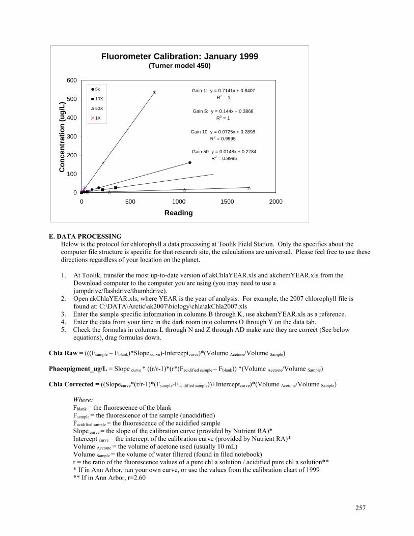
257

E. DATA PROCESSING

Below is the protocol for chlorophyll a data processing at Toolik Field Station. Only the specifics about the computer file structure is specific for that research site, the calculations are universal. Please feel free to use these directions regardless of your location on the planet. 1. At Toolik, transfer the most up-to-date version of akChlaYEAR.xls and akchemYEAR.xls from the

Download computer to the computer you are using (you may need to use a jumpdrive/flashdrive/thumbdrive).

2. Open akChlaYEAR.xls, where YEAR is the year of analysis. For example, the 2007 chlorophyll file is found at: C:\DATA\Arctic\ak2007\biology\chla\akChla2007.xls

3. Enter the sample specific information in columns B through K, use akchemYEAR.xls as a reference. 4. Enter the data from your time in the dark room into columns O through Y on the data tab. 5. Check the formulas in columns L through N and Z through AD make sure they are correct (See below

equations), drag formulas down. Chla Raw = (((Fsample – Fblank)*Slope curve)-Interceptcurve)*(Volume Acetone/Volume Sample) Phaeopigment_ug/L = Slope curve * ((r/r-1)*(r*(Facidified sample – Fblank)) *(Volume Acetone/Volume Sample) Chla Corrected = ((Slopecurve*(r/r-1)*(Fsample-Facidified sample))+Interceptcurve)*(Volume Acetone/Volume Sample)

Where: Fblank = the fluorescence of the blank Fsample = the fluorescence of the sample (unacidified) Facidified sample = the fluorescence of the acidified sample Slope curve = the slope of the calibration curve (provided by Nutrient RA)* Intercept curve = the intercept of the calibration curve (provided by Nutrient RA)*

Volume Acetone = the volume of acetone used (usually 10 mL) Volume Sample = the volume of water filtered (found in filed notebook)

r = the ratio of the fluorescence values of a pure chl a solution / acidified pure chl a solution** * If in Ann Arbor, run your own curve, or use the values from the calibration chart of 1999 ** If in Ann Arbor, r=2.60

Fluorometer Calibration: January 1999(Turner model 450)

Gain 1: y = 0.7141x + 0.8407

R2 = 1

Gain 5: y = 0.144x + 0.3868

R2 = 1

Gain 10 y = 0.0725x + 0.2898

R2 = 0.9995

Gain 50 y = 0.0148x + 0.2784

R2 = 0.9995

0

100

200

300

400

500

600

0 500 1000 1500 2000

Reading

Co

nc

en

tra

tio

n (

ug

/L)

5x

10X

50X

1X

258

***Note that in 2007, we changed our method of calculating Chla: we no longer include the intercept of the calibration curve in our calculations. The intercept column in the Data tab of the file should be left blank to account for this change!!!

6. QA/QC the data. This involves comparing samples from one site over time, or comparing blanks, etc. 7. Save the file on the local hard drive and the Download computer. 8. Once back in Ann Arbor (congrats on another successful field season), complete the QA/QC process:

a. Double Check the data b. Check for outliers c. Summarize the data on the Summary Tab d. Enter data into AkChemYEAR.xls

3. Standard Operating Procedures for the Turner Model 111 Fluorometer Infrequently used equipment and DMF Protocol Sources: Operating and Service Manual: Model 111 Fluorometer, G.K. Turner Associates 1970 A Practical Handbook of Seawater Analysis, J.D.H. Strickland and T.R. Parsons, 1972 1. Startup

a) Move the POWER switch to the up or on position b) Hold the START switch in the up position for 3 or 4 seconds. Release. c) Open sample door and check that U.V. source is on and that filter is in place. d) Allow 2 minutes warm up time (15 minutes if fluorometer has been moved recently).

2. Operation

a) Introduce first sample into the sample chamber. b) Close sample door and read dial on top of fluorometer. If reading is greater than 100 or less than about 10

fluorometer units, use the RANGE SELECTOR lever ( 1X, 3X, 10X, 30X) to set light intensity so that reading falls well within the 0-100 range on dial.

c) Introduce a solvent blank into the sample chamber. Turn BLANK knob until dial reads zero. You will need to reset zero using a blank every time you change the intensity range.

d) Return first sample to the chamber and read fluorescence from the dial. The fluorometer reading will continue to fluctuate by about +/- ¼ of a dial division after it stabilizes.

3. Calibration Most recent calibration: October 1996 Dilutions of a chl a standard dissolved in DMF were used to calibrate the instrument (0.5, 1, 5, 10, 15, 20, 25, 30, and 45g/L. Readings were recorded using ranges 1X, 3X, and 10X. According to the operating manual, fluorescence readings are very stable and calibration only needs to be checked every couple of years; but, our machine is old and has been moved frequently, so more frequent calibration is necessary. For pure chlorophyll standards, the equations are as follows: 1X: g/L = (reading + 0.24043)/ 2.236065 r2 = .999 3X: g/L = (reading + 0.692081)/ 6.281283 r2 = .997 10X: g/L = (reading - 0.453425)/ 17.62466 r2 = .999 4. Chlorophyll Determination This method involves the use of DMF (dimethyl formamide) as a solvent. The main advantage of using DMF is that grinding the filter is not necessary. Disadvantages are that DMF is more toxic and more expensive than acetone or methanol. a) Filter a known volume of sample water (typically 50 to 100 ml) onto GFF or GFC filters. Use low vacuum

pressure to avoid bursting the algal cells. b) Fold filter and place in a small amber vial with 7 mL of DMF. Make sure filter is submerged in solvent. c) Place in freezer for approximately 12 hours

259

d) Heat vials in 65C water bath for 15 minutes. Allow vials to cool before handling. e) Agitate for 15-20 seconds on a shaker table. Pour contents of vial into a graduated centrifuge tube. Rinse filter

inside vial and inside vial walls with DMF. Shake for 5 seconds. Pour into centrifuge tube. Repeat rinse. f) Record centrifuge tube volume and then centrifuge for 10 minutes at medium speed. g) Pour contents of tube into a cuvette and read on fluorometer. h) Add one drop of 10% HCl to the cuvette, mix and read again. i) Dispose of DMF waste in a labeled container. 5. Calculations Before chlorophyll can be determined, the amount of fluorescence due to pheophytin (chl breakdown products) must be subtracted from overall fluorescence. a) chla fluorescence = 2.24(initial reading - reading after acid) b) use chla fluorescence in the appropriate equation in Calibration section to find g/L chla in extract (g/L chla in extract)(mL extracted)/ (mL filtered) = final chla concentration (g/L).

260

(VI-23) Sediment Chlorophyll Determination Updated Jan 2011, by LRY

1. Introduction This protocol has been modified from the protocol s written specifically for compliance with the Battelle CW/QAPP (Giblin, Tucker); modifications may be warranted for other projects. This protocol is for high water content sediments, hence the use of 100% acetone rather than the traditional 90%. References: Strickland, J.D.H. and T.R. Parsons. 1972. A Practical Handbook of Seawater Analysis. Fisheries Research Board of

Canada, Ottawa. 310pp. Sun, Mingyi, R.C. Aller, C. Lee. 1991. Early diagenesis of chlorophyll-a in Long Island Sound sediments: A

measure of carbon flux and particle reworking. J. of Mar. Res., 49, 379-401. 2. Sediment Chlorophyll Method A. SUPPLIES

1. Spectrophotometer 2. 50‐ml polypropylene centrifuge tubes (e.g. Falcon tubes) NOT polystyrene; acetone will “melt”

polystyrene 3. Cell disruptor (e.g. Probe‐type sonicator) 4. Cooler with ice 5. 7 mL glass test tubes, 2 per sample +

B. REAGENTS 1. 100% Acetone

2. 90% Buffered Acetone Solution (used for regular chla analysis)

Pure Acetone ............................................................................................... 900 mL

Magnesium Carbonate (MgCO3) ...................................................................... 1 mg

Deionized Water .......................................................................................... 100 mL

3. ~0.6 N HCl Acid (or 0.3N HCl) Concentrated Hydrochloric Acid (12N) ......................................................... 48 mL

Deionized Water .......................................................................................... 952 mL

B. SAMPLE PREPARATION

1. Place 5 cubic cm of sediment core into a 50‐ml centrifuge tubes and securely cap. You can measure the 5 cc’s using a cut‐off syringe. You can “calibrate” this by weighing the amount of water the syringe holds.

2. Wrap tubes in foil and freeze immediately (or store tubes in a dark place). Samples should be kept in the dark and frozen until extracted. Normal freezer is fine for short term. We leave the filters in the freezer until there are enough to compose a run (~10‐20 filters). For ease of sample location, we wrap all the tubes from one day in the aluminum foil and label the foil with sites and the date.

C. SAMPLE ANALYSIS

261

Personal Protection Equipment: Please use eye protection, gloves, and the ventilation system as prolonged exposure to acetone may cause health problems. THE DAY BEFORE A RUN

20. Put acetone on ice in cooler to chill. 21. Determine the number and sortchems of the samples that are going to be run. Create an inventory. 22. Place samples in a cooler and move them to the wet lab. Allow to thaw, but not to warm. 23. In the dark room, add 35 mL 100% acetone to each tube. It is best if you can use a repipettor for this

to get accurate volumes. Automatic Pipetman or Finpipets (and the like) tend not to work well and don’t give consistent volumes with acetone because the surface tension is so low. In a pinch a graduated cylinder will do, but be careful in your measurements.

24. NOTE: if you have a sonicator bath or a sonicating probe available, sonicate with probe sonicator for 30 seconds. Hold the centrifuge tube in a plastic beaker with ice . The probe gets hot, and we want to keep the sample chilled. ALWAYS USE EARPLUGS WHEN OPERATING THE SONICATOR. If you don’t have a sonicator it is OK, just make sure you extract for at least 16 hours (24 max) and try to be as consistent as possible with the extracation times.

25. Cap the tubes and put back on ice immediately. Extract for ~16-24 hours in the cold and absolute dark; starting the procedure in the afternoon and finishing up the next morning usually works. Cover the falcon tubes with aluminum foil. The best place to keep the tubes is in a cooler with frozen ice packs and the lid closed, as keeping them in a freezer or refrigerator may lead to spark ignition of the vapors. Resuspend the sediments a couple of times (at least shake up again the next morning; we want full extraction).

THE DAY OF A RUN

1. Check to see if the spectrophotometer is on; allow it to warm up for 20 minutes. 2. After extraction, spin the tubes down in a tabletop centrifuge (a refrigerated centrifuge is better; or a

tabletop centrifuge put in the cold room TEMPORARILY) for about 10 min at max speed if using the tabletop version (if using a bigger, higher rpm centrifuge, do not exceed the specs for your centrifuge tubes.) It doesn’t take too much spinning, and shorter spin times are preferable to a longer time because we don’t want the samples to warm up. Keep samples on ice until they are ready to be read on the spectrophotometer, and be careful not to resuspend the fine sediment.

3. Make sure the windows in the room are covered, and that the door is mostly closed to limit light exposure.

4. Ensure that the snorkel ventilation system is on and operating correctly. (This is the red vacuum-like thing that hangs from the ceiling; the switch is in front of you.)

5. Blank the spectrophotometer. Zero the spec with 90% acetone at 750 nm and check the zero at 665 nm, unless you have a baseline correction feature (750 nm is the turbidity blank). The reading should be close to zero. If it is not, hit ‘enter’, select ‘calibrate’, ‘run blank’. If it still fails to read near zero, contact the Nutrient RA.

6. When ready to run, pipette two 4-ml subsamples into clean 10 mL borosilicate 13x100 mm tubes (clean out the tube with DI and then a quick squirt of acetone; it is best if you can have batch of dry tubes going for the samples). One tube will be read as is, the other tube will be acidified. Wipe the outside of the tube with a Kimwipe.

7. Work in batches of about 10 samples. Acidify the second tube of each pair, using 25 µl 0.6N HCL per 4 ml sample (also okay to use 50 uL of the 0.3N HCl we use for the water column), and mix carefully. Don’t contaminate; cover the tube with saran wrap or parafilm, place your finger over the top, and mix by inversion. Let the acidified samples react for at least 3 minutes, but no more than 5 minutes. NOTE: Keep the tubes for acidified and unacidified samples separate.

8. While the acidified samples are reacting, measure the extinction of the extracts in the first tube at 750 and 665 nm and record.

9. Read the acidified samples at 750 nm and 665 nm and record. Footnotes: 1. We use 100% acetone instead of 90% because the sediment section contains an amount of water that lowers

the concentration of the acetone. This should be taken into account and the volume of acetone adjusted accordingly; acetone concentrations less than 90% may not give full extraction. For Battelle contract work through 2001 at least, however, we do not want to change the protocol.

262

2. Use a cooler with ice, not a refrigerator. There is a safety issue with acetone fumes building up in a closed

refrigerator, such that the spark of a motor coming on and off could ignite it.

3. For sediments, pigment concentrations are usually reported in terms of volume (cc or ml) of sediment. However, sometimes it may be needed in terms of dry weight of sediment. This may be calculated from porosity measurements made on another subsample of the same sediments. You should know the porosity anyway to correct volume of extractant.

4. If you have it, take a separate sample for wet-dry and figure out how much water you added with your

sediment. Your final volume would be 35 mL + the water. If you didn’t or can’t do this just use 39 for all, the relative concentrations will be the same. Porosity of surface sediments is usually about 90%.

D. CALCULATIONS

Subtract each 750 nm reading from the corresponding 665 nm reading, and use the following equations to calculate chl a and phaeopigments (see methods in Strickland and Parsons): Chla (mg/m3) = (26.7(665o - 665a) * v)/ (V * l) Phaeopigment (mg/m3) = (26.7 ((1.7 * 665a) - 665o)) * v)/(V * l)

Where: 665o = extinction before acidification665a = extinction after acidification v = volume in ml of acetone used for extraction (and porewater see note 4) V = volume in cc of sediment extracted 3 l = path length of the cuvette.

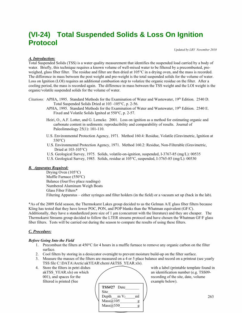
263

(VI-24) Total Suspended Solids & Loss On Ignition Protocol

Updated by LRY November 2010

A. Introduction:

Total Suspended Solids (TSS) is a water quality measurement that identifies the suspended load carried by a body of water. Briefly, this technique requires a known volume of well-mixed water to be filtered by a precombusted, pre-weighed, glass fiber filter. The residue and filter are then dried at 105°C in a drying oven, and the mass is recorded. The difference in mass between the post weight and pre-weight is the total suspended solids for the volume of water. Loss on Ignition (LOI) requires an additional combustion step to volatize the organic residue on the filter. After a cooling period, the mass is recorded again. The difference in mass between the TSS weight and the LOI weight is the organic/volatile suspended solids for the volume of water. Citations: APHA, 1995. Standard Methods for the Examination of Water and Wastewater, 19th Edition. 2540 D.

Total Suspended Solids Dried at 103 -105°C, p. 2-56. APHA, 1995. Standard Methods for the Examination of Water and Wastewater, 19th Edition. 2540 E.

Fixed and Volatile Solids Ignited at 550°C, p. 2-57.

Heiri, O., A.F. Lotter, and G. Lemcke. 2001. Loss on ignition as a method for estimating organic and carbonate content in sediments: reproducibility and comparability of results. Journal of Paleolimnology 25(1): 101-110.

U.S. Environmental Protection Agency, 1971. Method 160.4: Residue, Volatile (Gravimetric, Ignition at 550°C)

U.S. Environmental Protection Agency, 1971. Method 160.2: Residue, Non-Filterable (Gravimetric, Dried at 103-105°C)

U.S. Geological Survey, 1975. Solids, volatile-on-ignition, suspended, I-3767-85 (mg/L): 00535 U.S. Geological Survey, 1985. Solids, residue at 105°C, suspended, I-3765-85 (mg/L): 00530

B. Apparatus Required: Drying Oven (105°C) Muffle Furnace (550°C) Balance (four/five place readings) Numbered Aluminum Weigh Boats Glass Fiber Filters* Filtering Apparatus – either syringes and filter holders (in the field) or a vacuum set up (back in the lab). *As of the 2009 field season, the Thermokarst Lakes group decided to us the Gelman A/E glass fiber filters because Kling has tested that they have lower POC, PON, and POP blanks than the Whatman equivalent (GF/C). Additionally, they have a standardized pore size of 1 μm (concurrent with the literature) and they are cheaper. The Thermokarst Streams group decided to follow the LTER streams protocol and have chosen the Whatman GF/F glass fiber filters. Tests will be carried out during the season to compare the results of using these filters. C. Procedure: Before Going Into the Field

1. Precombust the filters at 450°C for 4 hours in a muffle furnace to remove any organic carbon on the filter surface.

2. Cool filters by storing in a desiccator overnight to prevent moisture build-up on the filter surface. 3. Measure the masses of the filters are measured on a 4 or 5 place balance and record on a printout (see yearly

TSS file C:\DATA\Arctic\akYEAR\chem\AkTSS_YEAR.xls). 4. Store the filters in petri dishes with a label (printable template found in

akTSS_YEAR.xls) on which an identification number (e.g. TSS09-001), and spaces for the recording of the site, date, volume filtered is printed (See example below).

TSS#27 Date_______ Site________________Depth___m Vf_____ml Mass@105_________gMass@550_________g

264

In the Field/Filtering 1. Record in the field book the identification number of the filter and the volume of water that was filtered. Also

record this information on the petri dish label. Keep the filter in this dish until you get back to lab.

2. If you do not want to filter in the field, take a 2L sample of the water back to the lab and us a vacuum set up to filter the water. Remember to record the filter number and volume filtered.

In the Lab 1. Place the filter(s) into a numbered, pre-weighed aluminum weigh boat(s). Record both the filter number and

the weigh boat identification in a lab book. 2. Place the weigh boat(s) into the 105°C drying oven (use the Nadelhoffer oven in 1050; the muffle furnace

does not reliably maintain temperatures this low) for at least twelve hours. Cover the boat(s) with a sheet of aluminum foil to prevent foreign material from falling onto the filter surface.

3. Place the boat(s) into a desiccator to cool. Record the weight of the room temperature filter + weigh boat. 4. Place the boat(s) into a preheated and stabilized, 550°C muffle furnace for two hours. 5. Cool filters + weigh boat(s). Depending on the muffle furnace demand at camp, either a) remove hot filter +

weigh boats, and allow them to cool in a GLASS desiccator, or b) turn off furnace and cool filter + weigh boat(s) in furnace. Once filters are cool enough to handle, record the room temperature weight of the filter + weigh boat.

6. Discard the filter. D. Calculations: Four measurements are required to calculate total suspended sediments (TSS) and loss on ignition (LOI) or organic content.

1. This method relies on six measurements:

(a) Tare weight of the dry, pre-combusted, numbered, unused filter (Wfilt, mg) (b) The volume of water raw water filtered in the field or lab (Vfilt, ml) (c) Tare weight of the dry and empty weighing tin (Wtin, mg) (d) Tare weight of the 105oC dried tin plus used filter (Wdry, mg) (e) Tare weight of the 550oC combusted tin plus used filter (Wcomb, mg) (f) Tare weight of the combusted, empty tin (Wpost, mg)

2. The six measurements are used to make the following calculations

(a) TSS = (Wdry – Wtin - Wfilt) / (Vfilt/1000) in mg TSS/L (b) LOI = (Wdry – Wcomb) / (Vfilt/1000) in mg LOI/L

(c) Weighing check = (Wpost – Wtin) / (Wtin)] * 100 or % change in tin weight

3. Notes

(a) LOI is roughly equivalent to organic content and can be multiplied by 0.45 to obtain an estimate of organic C content.

(b) Once the combusted filter has been successfully weighed and the data are safely recorded, the

combusted filters can be discarded and the aluminum weighting tins can be recycled for a new run.

(c) The weighing check is suggested as a partial check on weighing discrepancies and as a way to monitor for unusual changes in pan weights, especially when these pans are used repeatedly.

E. Tests

265

20 May 2009 Jen Kostrzewski performed a “Brittleness Test,” where three Gelman A/E filters and three Whatman GF/F filters were precombusted for 4 hours at 450°C, and combusted again at 550°C for two hours. The purpose of the test was to see how each type of filter held up at the listed heat intensities. The test by nature is subjective, and this should be taken into consideration in the evaluation of the results. If the researcher is careful (i.e. does not fumble too much with the forceps) both filters were fine. However, the A/E filters were more brittle than the GF/F’s. Amanda Field concurred with this conclusion. Both Jen and Amanda think the filter should be removed from the petri dish as soon as possible, because the majority of filter breakup occurred during the attempts to remove the filter from the dish. If we want to keep the filter in the petri dish while in the desiccator, we should buy larger dishes than our 47mm petris.

266

(V1-25) Absorbance + EEM Protocol at Toolik Detailed information on parameters and troubleshooting can be found in the Cory Lab Fluoromax-4 and Ocean Optics SOPs. Before getting started

Make sure all your samples and blank water are close to room temperature. Have ready DI water from the Big Lebowski, two quartz cuvettes, gloves, kimwipes. Do not ever touch the cuvette without gloves on. Change gloves frequently to avoid contaminating the cuvette surface.

Instrument Start Up

Make sure the computer and ALL peripheral devices are turned off, DO Not turn on the Fmax4 with any other device on!

Turn on the power switch on the Fluoromax‐4 fluorometer (Fmax4), on the lower right side towards the back, wait 1 minute.

Make sure the Ocean Optics UV‐Vis (spec) is NOT connected to the computer by its USB cable. The spec will be damaged if you connect via the usb cable before connecting the power (i.e. connect power first).

Power on the Ocean Optics spec (flip the wall circuit switch from ‘off’ to ‘on’).

After powering on the Ocean Optics spec, connect its USB cable to the front of the computer.

Power on the computer and the monitor (buttons on front).

While the instruments warm up for 20 minutes, take one cuvette to the DI, holding it tightly at the top of the cuvette and rinse it with DI water 20‐30 times getting the inside and outside of the cuvette with DI. Place cuvette in the plastic rack on the Fmax4 and repeat with the 2nd cuvette.

Open the Fmax4_logbook.xlsx file, fill out 1st two columns for today’s date (you will add more soon) Software Activation and Daily Instrument Checks

Double click on the FluorEssenceV3 icon on the desktop to activate the software

Click the ‘Experiment Menu’ ( ), found in the upper right corner of the toolbar (takes a few seconds to appear after starting the software)

Wait for the system to initialize (normally takes about 1‐3 minutes ‐ machine will make noise).

When the “Main Experiment Menu” is showing, and if the Fmax4 has been on 20+ minutes, then perform a lamp scan: o Click on ‘Spectra’ excitation next, then load the Lamp scan file from C:\Data\Chemistry\Fluorescence\Fluoromax4\Scans\Lamp.xml, click open

o Enter the filename in the data identifier box “LYYMMDD” e.g. L110525 for lamp scan 25 May 11 o Click run (lower right) o When prompted, click browse and go to: C:\DATA\Chemistry\Fluorescence\Fluoromax4\2011_Data, then save file as YYMMDD.opj, click save, and then click ok.

o In Fmax4_logbook.xlsx, fill in the project filename you just saved. o Maximize the lamp scan graph and use the red, bullet shaped cursor tool to make sure peak of the lamp scan is at 467 +/‐ 0.5 nm (you can right click, copy and paste info to excel file). Record the peak position and intensity of the lamp scan in the Fmax4_logbook.xlsx file. If peak is outside this range, get help calibrating excitation.

Raman scan: o Fill cuvette with DI from the Big Lebowski, wipe all sides with kimwipe, open Fmax4 door, with cuvette

in right hand, pull back tab in lower left corner of cuvette holder, insert cuvette Q Facing You, gently release the metal tab (don’t let it snap back on the cuvette!).

o Spectra’ emission next, load the Raman scan file from C:\Data\Chemistry\Fluorescence\Fluoromax4\Scans\Raman.xml click open

o Enter the filename in the data identifier box “RYYMMDD” o Click ‘run’ o Make sure the Raman peak is at 397 +/‐ 0.5 nm, record the peak position and intensity of the Raman

scan in the Fmax4_logbook.xlsx file. If peak is outside this range, get help calibrating emission.

Cuvette scan: o With cuvette containing DI still in the Fmax4 sample chamber

267

o Spectra’ emission next, then load the Cuvette scan file from C:\Data\Chemistry\Fluorescence\Fluoromax4\Scans\Cuvette.xml click open

o Enter the filename in the data identifier box “CYYMMDD”. o Click run. o Make sure there is no clear peak, should be a flat noisy line of average intensity between 20,000‐

40,000 units, IF NOT, rinse cuvette and repeat. Remove the cuvette from Fmax4 chamber by pulling back the metal tab with your middle finger (don’t let the metal slide or rub on the cuvette), place it in the Ocean Optics spec chamber‐ use this cuvette as the absorbance blank for the rest of the day.

o Fill 2nd cuvette with DI from the Big Lebowski and place it in the Fmax4 sample chamber.

o Click ‘Previous Experiment Setup’ ( , found in the upper right corner of the toolbar) to repeat the cuvette scan with the second cuvette

o Click run and let the software auto‐increment the filename. o Record the approx. mean intensity in the Fmax4_logbook.xlsx file. If there is a peak, or high background

intensity, rinse the cuvette again multiple times and repeat the scan. o Save and close the Fmax4_logbook.xlsx file.

Ocean Optics spec: double click on the Spectra Suite icon on the desktop to start the software o Place a clean cuvette containing DI in the sample holder (Q Facing You) o Close the Graph(A) (click on the x in the top left corner of the graph itself) o Make sure that the Strobe/Lamp Enable box at the top of the screen is unchecked. o File New Absorbance measurement; click next. o Check the box to enable the Strobe/Lamp. o Click Set automatically button once, wait 5 seconds click it again. o Set the Scans to Average to 20 and the Boxcar Width to 20. o Click next to see yellow light bulb (reference) screen. o With the clean cuvette containing DI in the sample holder (Q Facing You), press the large

yellow light bulb button to collect a reference spectrum. o Click next to see the dark light bulb (dark reference) box. o Uncheck the Strobe/Lamp Enable box. Wait a couple of seconds for the lamp to turn off. You

should hear a click. o Click the gray light bulb button and the dark spectrum preview will appear, should be ~1500

units. o Check the Strobe/Lamp enable box. o Click Finish. o The screen will now show a flatish blue line centered around zero (on the y axis). o Then click the Scale graph to fill window button (2nd from left on toolbar above graph). o Save the reference (blank) spectrum by clicking the save icon ( on the toolbar above the

graph). Do NOT save from the File menu! o Select the file type (tab delimited, no header) o Click the browse button and browse to

C:\DATA\Chemistry\Absorbance\OceanOpticsUSB4000\2011_Data Save the blank as BYYMMDD, click Save and then click Close.

o Leave the cuvette with DI in it in the sample holder‐ cover lightly with parafilm when NOT blanking the spec.

SAMPLE ANALYSIS:

Rinse the Fmax4 cuvette out with sample three times (filling at least ½ per rinse), fill quartz cuvette at least ¾ full with sample but don’t overfill! Gently wipe cuvette surface with kimwipe and place it in the plastic cuvette rack on the Fmax4. Put lid on sample bottle.

First blank the spec: remove the parafilm from the DI‐containing cuvette in the spec, then click the yellow lightbulb icon. Remove the blank cuvette and place it on top of the spec. o Place the sample cuvette in the spec (Q Facing You), click scale graph to window (second

button from left).

268

o Save the sample spectrum by clicking the save icon ( on the toolbar above the graph). Do NOT save from the File menu!

o Check that file type is still: tab delimited, no header. o Enter the PhotoNum as the filename, click on the mini‐graph in the box, then click Save and

then click Close. o Now place sample cuvette into the Fmax4 sample chamber, and then put the blank back in

the Ocean Optics and cover it with parafilm.

Go to the Fmax4 software to collect a sample EEM: 3D, load the Water_EEM scan file from C:\Data\Chemistry\Fluorescence\Fluoromax4\Scans\Water_EEM.xml, open o Change the data identifier to the filename (PhotoNum), click run. o (Every Monday, run a blank EEM on a cuvette containing DI named: BYYMMDD). o While EEM is running, open AkPhotochem_2011.xls, record all sample information from the Master List:

If the bottle or bag has no PhotoNum, consult the Master List and find the pre‐assigned #, or assign one if none exists and write information on the Master List (site,date, sortchem, etc.).

Make sure to change the F_blank file name in the spreadsheet every Monday when a new blank EEM is run.

To run Abs + EEMs continuously, it is a little different than running samples for the 1st time each day. To run the next sample Abs + EEM, repeat the process as above with these differences: o If running replicates of the same sample, just rinse 3x with the sample o If running a new sample, rinse cuvette ~ 10x with DI, then 3x with sample o When saving the absorbance spectrum, just enter the filename in the box, click on graph, then click

save and close. No need to browse, the directory is already set, but check to make sure the file type is always “tab delimited, no header”.

o To run the next EEM just click ‘Previous Experiment Setup’ ( , just to the right of the symbol) and make sure to enter the PhotoNum, then click run.

POWER DOWN: NOTE that if you will be running samples within about 4 hours it is ok to leave the lamp on in the Fluoromax – but it is BEST to get all of your samples ready and run at the same time because it is hard on the lamp to turn it on and off.

Fmax4:

When done running samples, go to file batch export, click on ASCII, then when the box pops up, select all the data objects, then click ok, then select this folder to export the data: C:\Data\Chemistry\Fluorescence\Fluoromax4\2011_Data

Close the FluorEssenceV3 software (yes save if/when prompted) and turn off the power on the Fluoromax.

Ocean Optics spec:

uncheck the Strobe/Lamp Enable box.

Exit the software.

Unplug the USB cable between the Ocean Optics UV/Vis and the computer FIRST.

AFTER the USB cable is DISCONNECTED, then flip the switch to off on the wall circuit.

Rinse the cuvette that contained sample 20 times with DI, empty the blank cuvette. Place both cuvettes in the plastic cuvette rack on top of the Fmax4, cover cuvettes with a kimwipe.

Rose Cory -- [email protected] Office: 919-966-3529 Lab: 919-962-5808 (one of Rose’s students may be able to help out if Rose is not there, ask for Katie or Collin)

269

(V1-26) Biospherical UV-VIS Profiler July 2011

This needs to be checked by Collin and Rose and updated for 2012

21. The day before planned use, make sure laptop computer and microradiometer master controller (yellow box) are fully charged.

22. C-OPS check list. Make sure you have all of these before leaving lab: - C-OPS UV profiling sensor - Red cable connecting yellow box to C-OPS - Weights for C-OPS - Laptop computer - USB to RS232 connector for computer to yellow-box - Orange tool-box (depending which site you go to) - Backpack to haul yellow box, computer, and misc. tools - Field notebook to record date, site, data filenames, weather

23. Once at the field site, one person should start up the computer and connect it to the yellow box. The other

person should open up the biospherical protective case and start assembling the harness. Make sure all fittings are fastened securely and that both loops are locked into the main cable.

24. Place all the weights on the instrument and secure to finger tightness. The fittings on the bottom ring should remain in place so that the weights are distributed evenly to avoid high deviations in pitch and roll. If this is not the case, use your best judgment to evenly distribute the weight.

25. Connect the main red cable to the yellow deck box (to the underwater port) and to the biospherical. Screw in the cable to finger tightness. It is very important to put aside the protective cases for these connectors in a safe spot and that they remain there until sampling is complete.

26. Turn on Yellow Box. All connections must be secured before starting software. 27. Start Uprofile software. A shortcut can be found on the desktop. 28. Accept the parameters titled COM7 and command the software to begin a “dark correct launch.” Ensure that

the black lid is screwed on at this point. If accessible, place another piece of black fabric over the black lid to minimize light penetration (possibly use photochem bag). Check two boxes in top left corner of window to enable two sensors, then press launch.

29. Upon completion of collecting the dark spectrum, close window and remove lid. 30. At this point, the person with the biospherical in hand should prepare to feed the cord into the water while the

instrument descends (ie, untangle the cord). The person with the computer should see real-time values of depth, pressure, temp, and wavelength dependent energy terms.

31. Lift the biospherical into the water so that the depth sensor is just above the surface of the water. When you have a steady depth reading, the person with the computer should “tare depth” and verify that z = 0.

32. The instrument is now ready to be deployed. The two users should communicate with each other and agree on when recording should begin. When the sensor reads z = 0, press “start recording.” The person with the computer should note what time recording began and log it in the field notebook. Once recording, wait a few seconds at z = 0 and then take the instrument completely out of the water for an “aircast” of ~ 20 seconds.

33. Place the instrument back at z = 0 and deploy the instrument. It is very important to be aware of how much slack is available as putting too much tension on the cord at any point in this process can be harmful. If in a boat, try to drop the instrument so that it does not descend underneath the boat.

34. During decent, the person with the computer should see almost immediate depletion in the wavelength dependent energy terms (don’t know what the technical term is for this unit) µW/(cm²nm). Be sure to check pitch and roll to make sure they are +/- 5 degrees.

35. When the instrument has reached terminal velocity, press “stop recording.” Slowly pull up the profiler. It is extremely important to be cautious when retrieving the instrument and absolutely not let any of the instrument collide with the boat or other debris.

36. To perform a replicate downcast, repeat steps 10 -15. The software should read z = 0 at original “tared depth,” so it should not be necessary to tare depth again.

37. Upon completion of replicates, turn off yellow box, disconnect any fittings to and from yellow box and computer. Then perform these steps (in no particular order):

- remove weights - undo harness - place protective casings on red cord, biospherical, and yellow-box

270

- wrap up red cord - close software and computer - place biospherical back into carrying case

38. When returning from field, open up carrying case and towel dry biospherical and weights. Remove cap from

sensor and dry sensor. Let air dry overnight. 39. Data files will automatically be exported to “Biospherical” folder located on desktop. The files will be

imported into and processed in excel file: Biospherical_Water_2011. 40. Remember to charge computer and yellow box if using the next day.

Notes from Talking with John Morrow (Biospherical, Inc) on 16 June 11 - Look at Fig 18- note similarities and differences to our device. Red stuff = foam - C-OPS- designed to be neutrally buoyant at surface, air bladders contract, start to sink at 10m: bladders ½ volume so ½ buoyancy 30m = terminal velocity. It sinks slowly at the surface = 1 cm/s, Deeper ~ 12 cm/s - Instrument collects data at 12 hz so 1% uncertainty at 1cm resolution - Operation: use weights and floats to get the buoyancy we want, then adjust roll (side to side) and pitch (nose down or up). The goal is to have it be level at the surface, just below surface should be close to level. The main goal is to drop it as slowly as possible, using floats and weights to control buoyancy and descent rate. - Pitch: nose down or nose up of the device. It is mostly a function of the cable, cable won’t pull or drag instrument as long as it is in the water. - Roll: weights/float left to right on threaded arm, as much weight as possible and be neutrally buoyant at the surface. - Goal is to have roll and pitch to be +/- a few degrees of zero, put device in water, adjust based on looking at software (see Fig 4.4, pg 51 for operation details). - Orange plastic calipers: measures amount of v-block projected after adjustment. Use the calipers to measure from top (side) of v-block surface to back plane surface, transfer measurement to the other side (if needed, for fine tuning, mainly needed it we have radiance sensor). -- The only way to hurt the instrument is to over tighten the nuts on the v-blocks! DO NOT OVER-TIGHTEN!

271

SECTION VII - LAB DATA PROCESSING

(VII-1) Returning from the Summer Field Season Updated 12 September 2016 by gwk, jad

A. General Rules and Procedures Usually we return from the field at the beginning of the semester (end of August or start of September). We need to organize the samples, data, and equipment that we used or produced from the recently finished field season to have it in working and usable order. Below is a brief overview of the major tasks that need to be completed. It is important to remember that most of these individual tasks cannot be completed in a single day. This list is organized to create a general path to follow, but it is non-linear (you do not have to proceed from step 1 to 2 to 3 and so forth – check with George on the order you are taking). Some steps require other information before they can be started, e.g., we need the inventory of Lakes samples before actually sorting the samples), meaning that you need to read through the entire list first and get started on certain tasks that require information before beginning. Also, ask George if he or collaborators need any particular data first to help prioritize tasks.

1.) Unpacking. Check with your shipping information to make sure that all of the boxes arrived to Ann Arbor. Check the shipping manifest log generated at Toolik, and if you are missing any, check the tracking number on www.ups.com.

2.) Put all of the sample boxes in the cold room until you can sort the bottles. Put nitrates in the freezer. 3.) Open all of the coolers, boxes, Tupperware, etc. to let them air out. 4.) Clean and dry any field equipment; then put it away in its proper spot. If any equipment was damaged, try to

get it sent away for repairs right away. 5.) Email the Lakes RA (Dan White) for the final hydrolab data files and an inventory of the samples that (s)he

will be sending for Alkalinities, DOC/TDN, and CATS analyses. Remember we need metalimnion depths for the I-Series samples, and, he may send samples later in September if a project operates into the Fall.

6.) Email any other collaborator for other data files or copies of notebooks needed such as: AKBurn chemistry files, hydrolab files, field book copies, LTREB files, Thermokarst files, etc.

7.) File Updates and Migration. Compare the files on the external hard drive brought back from Toolik to those on the server in the \_To_Michigan Folder. Open every folder (Chemistry, Biology, Discharge, etc.) to make sure all of the files (#s and names) were transferred correctly from Alaska. You don’t need to open each individual file. Note that this should be done on only one computer by one person. Do this all in one sitting.

8.) Once you are comfortable with all of the files being present in the \_To_Michigan Folder on the server, you should copy the entire directory to your local hard drive – this might take minutes to hours.

9.) First, check that the \AK20xx\ folder has the same directories on the local hard drive and in the \_To_Michigan folder you just copied from the server.

10.) Second, on the local hard drive migrate files from the \_To_Michigan folder to the \DATA\Arctic\AK20xx folder. You need to do this with George on one computer (because this is the time you make sure that you still have the directories you want, and because he will know where he wants the different “Project” files. Do steps 10 and 11 together with George.

11.) Also copy any other directories you have updated locally (e.g., \Data\Arctic\Projects…) to the server. All data for other local computers should be taken from the Server.

12.) Once the \AK20xx folder is updated, then archive the \_To_Michigan folder on the server and on the local hard drive.

13.) Checking Data. Start double checking the data from the field books, the scint counts, and all other primary sources from the field season against the AK_Sample_Master_year file. Note that we double check every original field book we have. Other projects are responsible for double checking the field books they have – we do not double check the scans of another project’s field book. We finish bottle bingo before we update AK_Sample_Master and send it out to other projects (don’t send out Sample_Master too soon…).

14.) Create an inventory of what samples were taken in Alaska (start from the Sample_Master file). Use the previous year’s inventory file as a template (found at C:\DATA\Arctic\akYYYY\chem \ YYYY_AK_Chem_Inventory.xls). Copy in the sortchems and site info (site, date, depth) to the inventory file. The cells marked with an “x” in the sample master indicate that a sample was collected for that specific chemistry analysis. Print inventories for use in Bottle Bingo. Note that most years we separate inventories by major projects (LandWater, Lakes, LTREB, Photo, etc.).

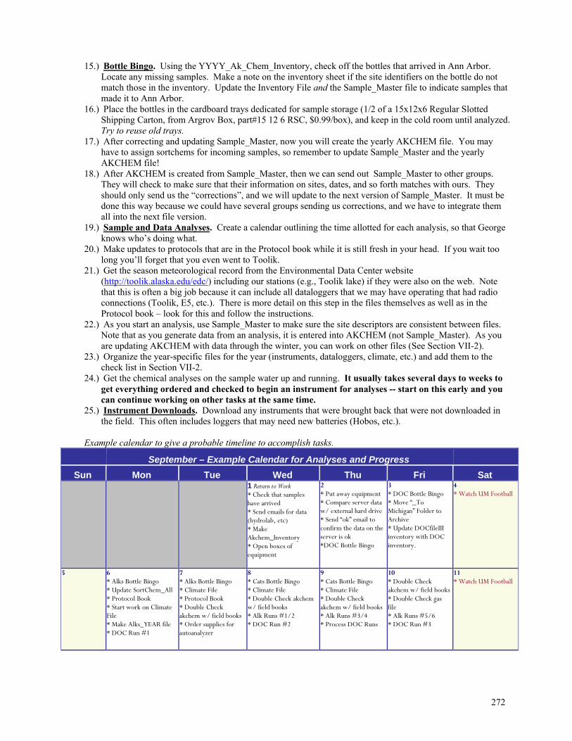
272

15.) Bottle Bingo. Using the YYYY_Ak_Chem_Inventory, check off the bottles that arrived in Ann Arbor. Locate any missing samples. Make a note on the inventory sheet if the site identifiers on the bottle do not match those in the inventory. Update the Inventory File and the Sample_Master file to indicate samples that made it to Ann Arbor.

16.) Place the bottles in the cardboard trays dedicated for sample storage (1/2 of a 15x12x6 Regular Slotted Shipping Carton, from Argrov Box, part#15 12 6 RSC, $0.99/box), and keep in the cold room until analyzed. Try to reuse old trays.

17.) After correcting and updating Sample_Master, now you will create the yearly AKCHEM file. You may have to assign sortchems for incoming samples, so remember to update Sample_Master and the yearly AKCHEM file!

18.) After AKCHEM is created from Sample_Master, then we can send out Sample_Master to other groups. They will check to make sure that their information on sites, dates, and so forth matches with ours. They should only send us the “corrections”, and we will update to the next version of Sample_Master. It must be done this way because we could have several groups sending us corrections, and we have to integrate them all into the next file version.

19.) Sample and Data Analyses. Create a calendar outlining the time allotted for each analysis, so that George knows who’s doing what.

20.) Make updates to protocols that are in the Protocol book while it is still fresh in your head. If you wait too long you’ll forget that you even went to Toolik.

21.) Get the season meteorological record from the Environmental Data Center website (http://toolik.alaska.edu/edc/) including our stations (e.g., Toolik lake) if they were also on the web. Note that this is often a big job because it can include all dataloggers that we may have operating that had radio connections (Toolik, E5, etc.). There is more detail on this step in the files themselves as well as in the Protocol book – look for this and follow the instructions.

22.) As you start an analysis, use Sample_Master to make sure the site descriptors are consistent between files. Note that as you generate data from an analysis, it is entered into AKCHEM (not Sample_Master). As you are updating AKCHEM with data through the winter, you can work on other files (See Section VII-2).

23.) Organize the year-specific files for the year (instruments, dataloggers, climate, etc.) and add them to the check list in Section VII-2.

24.) Get the chemical analyses on the sample water up and running. It usually takes several days to weeks to get everything ordered and checked to begin an instrument for analyses -- start on this early and you can continue working on other tasks at the same time.

25.) Instrument Downloads. Download any instruments that were brought back that were not downloaded in the field. This often includes loggers that may need new batteries (Hobos, etc.).

Example calendar to give a probable timeline to accomplish tasks.

September – Example Calendar for Analyses and Progress

Sun Mon Tue Wed Thu Fri Sat 1 Return to Work

* Check that samples have arrived * Send emails for data (hydrolab, etc) * Make Akchem_Inventory * Open boxes of equipment

2 * Put away equipment * Compare server data w/ external hard drive * Send “ok” email to confirm the data on the server is ok *DOC Bottle Bingo

3 * DOC Bottle Bingo * Move “_To Michigan” Folder to Archive * Update DOCfileIII inventory with DOC inventory.

4 * Watch UM Football

5

6 * Alks Bottle Bingo * Update SortChem_All * Protocol Book * Start work on Climate File * Make Alks_YEAR file * DOC Run #1

7 * Alks Bottle Bingo * Climate File * Protocol Book * Double Check akchem w/ field books * Order supplies for autoanalyzer

8 * Cats Bottle Bingo * Climate File * Double Check akchem w/ field books * Alk Runs #1/2 * DOC Run #2

9 * Cats Bottle Bingo * Climate File * Double Check akchem w/ field books * Alk Runs #3/4 * Process DOC Runs

10 * Double Check akchem w/ field books * Double Check gas file * Alk Runs #5/6 * DOC Run #3

11 * Watch UM Football

273

(VII-2) Files for AK and LTER- Generation and Fate General Rules for Working with Files Updated: September 2016 jad, gwk

In the Excel file for each analysis, make NOTES in the notes column and on the notes sheet when altering files or about an individual datum point, an abnormal nutrient run, or anything unusual. Make sure that these notes follow the data (i.e., if merging in with akchem, be sure to merge the notes about those data). Notes such as “I screwed up” are not as helpful as “I added twice the acid – 40uL/60ml sample instead of 20uL –kjr date”.

Make sure nobody else is concurrently working with the file. Upload the most recent file from the server. Work on the file on your local computer, then when finished backup the file to your local external hard drive.

Only after that can you copy the file to the server - then email the group when you have finished altering a file. Have data double checked by someone other than original data enterer. Do not make your own “rules” about data checking without consulting others. Always make a note about exactly

how you decided that values were questionable or should be removed. Then check your rationale with George. This is a reminder as everyone is tempted to think “well, this is so obvious, I will NEVER forget.”

All files should have notes page.

B. Primary Files -- PRINT OUT AT THE BEGINNING OF EVERY FALL

1. AkchemYEAR.xls - \\Data\Arctic\akXXXX\chem\akchemXXXX.xls Started in the field data are entered at Toolik by various persons from the yearly Field Book. Eventually to contain all chemical and physical data about our field sites. Some alks, ions, light, chla, and physical data will come from Lakes LTER web files (ask Geo if you do not know web address). When data do not originate in our lab, it must be noted in the “source” column (be sure to do this when downloading web files). If we run samples for some other group or project, you will have to obtain the basic information from them (we like to have elevation, temp, ph, cond from every site). If data are entered in field, then have someone else double check in AA. Sortchem numbers are assigned in the field and written on the bottles and petri dishes in the field. Also, be sure to check discharge units as these are commonly in error. Every spring, this file will go on Arctic LTER website as YEAR_akchem_Kling.xls.

2. AkPO4YEAR.xls- \\Data\Arctic\akXXXX\nutrients\akPO4XXXX.xls Started in the field, the data are entered by the person who runs the phosphates (SRP) at the

end of each day (or the next day). Running nuts in the field is difficult and frustrating, be sure to put lots of notes in the file (i.e. “saw air bubble while reading” to explain a really high value). Raw data are stored in the akPO4 notebook and include phosphates run on the spectrophotometer. Double check in AA carefully, people often decide not to use a duplicate in an average in the field, but make sure that all decisions are sound and explainable and that all data are in the file (whether used for average or not) so you do not have to go searching for the data later. These data are copied into the akchem file for web publication.

3. AkNH4YEAR.xls - \\Data\Arctic\akXXXX\nutrients\akNH4XXXX.xls

Started in the field, the data are entered by the person who runs the ammoniums (OPA) at the end of each day (or the next day). Running nuts in the field is difficult and frustrating, be sure to put lots of notes in the file (i.e. “Lots of color in water” to explain a really high value). Raw data are stored in the akNH4 notebook and include ammoniums run with the OPA method on the fluorometer. Double check in AA carefully, people often decide not to use a duplicate in an average in the field, but make sure that all decisions are sound and explainable and that all data are in the file (whether used for average or not) so you do not have to go searching for the data later. These data are copied into the akchem file for web publication.

4. AkgasYEAR.xls-\\Data\Arctic\akXXXX\gas\akgasXXXX.xls

Started in the field with data from GC output. Usually George and one other person run gas and DIC samples in field. If not run on Shimadzu GC, then it should be noted in the file.

Who √√ _______ Done?____ Who Final______Done?____

Who √√ _______ Done? ____ Who Final _____ Done? ____

Who √√ _______ Done? ____ Who Final ______Done? ____


274

Other important notes include if there was suspected water in the sample or why a sample was run twice. See section VI-1 for protocol on running samples. In the gas file, make sure to copy down all the formulae after you have completed entering the data. Frequently, these formulae are altered when cutting and pasting in the file. After all samples are run and all data double checked, CO2, CH4, and DIC values will be entered into akchem and appear on the website as part of that file.

5. LicorYEAR.xls-\\Data\Arctic\akXXXX\Licor\LicorXXXX.xls

Started in the field with raw data from the LICOR profiles from Toolik, E 05, E 06 lake sampling. The output is integrated into this final file. In the Licor file, we paste the logged data into preassigned columns, and the formulae are copied down to calculate the light attenuation coefficients. Similar to the gas file, make sure the formulae are correctly referencing the proper cells to ensure the correct output. This file will be double checked in Ann Arbor to check QA\QC.

6. BacProdYEAR.xls- \\Data\Arctic\akXXXX\biology\bacprods\bacprodXXXX.xls Started in the field with the scintillation counter output from the bacterial production incubations. The data should be double checked by a different person that the original enterer. Make sure the formulae are copied down correctly and are referencing the accurate cells to calculate the production numbers. This file is published to the LTER website each spring as YEAR_bacprods_Kling.xls.

7. AkchlaYEAR.xls- \\Data\Arctic\akXXXX\biology\chla\akchlaXXXX.xls This file is started in the field with the output from the cholorphyll analysis. The data should

be double checked at Toolik, but if not, it needs to be checked by another person other than the original data enterer in Ann Arbor. The formulae need to be check for proper referencing, and then the final data are put into a file named YEAR_Chla_Kling.xls for web publication.

8. I_Series_YEAR_Q.xls-- \\Data\Arctic\akXXXX\Discharge\Iseries\I_Series_XXXX_Q.xls The creation of this file starts in the field. The primary person responsible for discharge

enters the data values for depth, distance, and velocity. The file contains formulae to calculate discharge using the midpoint method. Also included in this file are the hobo output for water temperature and stage. Once back in Ann Arbor, the individual rating curves for all the inlet streams are determined and continuous discharge is calculated based on that relationship. This file is not published to the web, but is used to calculate solute loading and water budgets.

9. Imnavait_Discharge_YEAR.xls—

\\Data\Arctic\akXXXX\Discharge\Imnavait\Imnavait_Discharge_XXXX.xls Prior to 2010, the Imnavait discharge was the responsibility of Kane and Hinzman. However,

the task was undertaken by the Kling group in 2010. A hobo data logger was installed to measure water temperature and depth, and a consort conductivity data logger tracked changes in specific conductivity. This file calculates the rating curve and subsequent continuous discharge values. Similar to the I Series discharge file, this is not published to the web, but is used to calculate solute loading and water budgets.

10. Toolik_Inlet_YEAR.xls-

\\Data\Arctic\akXXXX\Discharge\ToolikInlet\Toolik_Inlet_XXXX.xls The creation of this file starts in the field. The primary person responsible for discharge enters the data values for depth, distance, and velocity. The file contains formulae to calculate discharge using the midpoint method. Once back in Ann Arbor, the yearly rating curve is determined and continuous discharge is calculated based on that relationship. This file is published to the web (YEAR_Toolik_Inlet_Kling.xls), and is used to calculate solute loading and water budgets. The yearly discharge is also copied into the Toolik_Inlet_QTC file that contains all discharge from 1992 to the present. See notes in that file for direction.

11. TWweirxxxx.xls- \\Data\Arctic\akXXXX\Discharge\TWWeir\TWweirXXXX.xls







275

Files generated from datalogger at weir that records water temp, conductivity, and stage height (up to 2001 measured with a Steven’s logger) at TW Weir. Files are downloaded in the field by a member of the Kling Lab or by Jim L. They are in “.dat” format and should then be opened into excel and merged together into twweirxxxx.xls. The columns to the right of the water conductivity are soil measurements and only used by Jim L and are moved to the “soil” tab. The discharge is calculated from the stage height (see below “Processing datalogger files” for detailed directions) in the qpw file xxxxtwweir.wb3 in akyear\discharge\tw\ directory.

12. Thaw_Surveys_YEAR.xls- \\Data\Arctic\akXXXX\Soils\Thaw\Thaw_Surveys_XXXX.xls The thaw surveys for the Tussock Watershed and Imnavait hillslope are recorded in this file.

The data are usually double checked in the field, but if they are not, they need to be checked in Ann Arbor. This annual data set is incorporated as a part of the TRENDS from Toolik, and needs to be updated in the summary file. These summary files go onto the Arctic LTER website.

13. AkTSS_YEAR.xls- \\Data\Arctic\akXXXX\Chem\AkTSS_XXXX.xls This file is primarily dedicated to the Thermokarst project, but other sites may be included. It

is started before we leave for the field. The TSS filters need to be precombusted and weighed before any sampling can occur (see section VI-13). The mass values are entered into this file. After the field season, the dried filters are weighed, combusted, and weighed again to get the total suspended solids and the loss on ignition values. These are entered into this file as well. This file is not web published.

14. CTD Folders\File- \\Data\Arctic\akXXXX\CTD

These folders contain the files generated from CTD profiles taken during the field season. Please see sections IV-5 and IV-6 for processing and production.

15. Hydrolab Files- \\Data\Arctic\akXXXX\Dataloggers\Hydrolab The hydrolab files are created by the Lakes RA. We need the data for the physical data used

in the akchem and gas files. Throughout the season try to get this data from the Lakes RA, but email him\her once you are back to Ann Arbor to get the final file. Add the temperature, conductivity, pH, and dissolved oxygen data into the akchem file for web publication, and the temperature, conductivity and pH into the gas file to calculate final gas values.

16. Licor Raw Files- \\Data\Arctic\akXXXX\Licor\RAW These data are downloaded from the Licor 1400 in the field and copied into the

LicorYEAR.xls file. The .txt files are saved as a backup. See #5 above. 17. Climate Files (multiple files) - \\DATA\Arctic\akXXXX\dataloggers\Toolik_Lake etc.

The creation of this file starts in the field. The primary person responsible for discharge enters the data values for depth, distance, and velocity. The file contains formulae to calculate discharge using the midpoint method. Once back in Ann Arbor, the yearly rating curve is determined and continuous discharge is calculated based on that relationship. This file is published to the web (YEAR_Toolik_Inlet_Kling.xls), and is used to calculate solute loading and water budgets. The yearly discharge is also copied into the Toolik_Inlet_QTC file that contains all discharge from 1992 to the present. See notes in that file for direction.

18. Ak_Chem_Inventory.xls - \\Data\Arctic\akXXXX\Chem\Ak_Chem_Inventory.xls

File has inventory columns to the far right, this will be double checked in AA and will be used to make inventories for each analyses. Never write over the inventory columns with values or anything else. VII-1

19. Alks_YEAR.xls- \\Data\Chemistry\Alkalinity\Alks_XXXX.xls This file is created in Ann Arbor to contain the formulas to calculate the alkalinity of our

samples. Copy the previous year’s file, rename it correctly, delete out the old data, and double check that the formulas are accurate. Please reference the notes in this file for










276

direction for use. Once the file is QAQC’d, the data needs to be put into the gas file for final calculations. Also, if we ran any other groups Alks, we need to send that data out.

20. CATIONS_Year.xls- \\Data\Chemistry\Cations\Cations_XXXX.xls This file is created in Ann Arbor to contain the formulas to calculate the concentrations of

cations in our samples. Copy the previous year’s file, rename it correctly, delete out the old data, and double check that the formulas are accurate. Please reference the notes in this file for direction for use.

21. ANIONS_YEAR.xls- \\Data\Chemistry\Anions\Anions_XXXX.xls This file is created in Ann Arbor to contain the formulas to calculate the concentrations of

anions in our samples. Copy the previous year’s file, rename it correctly, delete out the old data, and double check that the formulas are accurate. Please reference the notes in this file for direction for use.

22. TDP_YEAR.xls - \\Data\Chemistry\Nutrients\TDN_TDP\TDP\Data\TDP_calculations.xls This file is created in Ann Arbor to contain the formulas to determine the concentration of

total dissolved phosphorus in our samples. Copy the previous year’s file, rename it correctly, delete out the old data, and double check that the formulas are accurate. Please reference the notes in this file for direction for use.

Once you are satisfied with the year’s TDP values, the data is moved into the TDP_ALL.xls

file which contains the concentrations for all TDP samples the Kling Lab has run. 23. DOCfileIV.xls – \\DATA\Chemistry\DOC

File started in Ann Arbor. Samples from field are brought back to Ann Arbor and are run by Mark & Jen over the Fall/Winter. Jen is largely in charge of the files while Mark runs the samples. The raw data generated on the Shimadzu TOC machine are peak areas of the samples and standards. These raw data are converted to uM DOC, and averaged in the SAS programs Doc_IV_1of4_Condensed.pgm, Doc_IV_2of4_Concentrations.pgm, Doc_IV_3of4_Averages.pgm, and TN__IV_4of4_Averages.pgm. For details on this process see section VI-3. The final values (in uM) are stored in DocTnAllData.xls and are added to akchem after double checking.

24. CHN_YEAR.xls - \\DATA\Chemistry\Nutrients\Particulate\CHN This file is created in Ann Arbor to contain the formulas to determine the concentration of

total dissolved phosphorus in our samples. Copy the previous year’s file, rename it correctly, delete out the old data, and double check that the formulas are accurate. Please reference the notes in this file for direction for use. See section VI-7 for more information. Once you are satisfied with the year’s CHN values, the data are added to akchem.

25. NO3_YEAR.xls - \\DATA\Chemistry\Nutrients\Inorganic\Nitrate This file is created in Ann Arbor to contain the formulas to determine the concentration of

nitrate in our samples. This is a multiyear file, so amend the next run after the previous runs. Please reference the notes in this file for direction for use. For more information, please see section VI-6. Once you are satisfied with the year’s NO3 values, the data are added to akchem.

26. Protocol Book Updates -\\DOCUMENTS\Lab\Protocols

Throughout the season, handwritten notes were recorded in the protocol book at Toolik regarding any change to the current protocol. These changes need to be incorporated into the new version of the lab protocols.

D. Summary Files Once the yearly files have gone through QAQC process, the data in many files are incorporated into secondary, “Summary” files that are useful for looking at long-term trends. Below is a list of the major files that fit in this category; however, this is not a comprehensive list, as there are always new additions every year.








277

#1 Akchem_AllYears.xls - \\DATA\Arctic\SUMMARIES\AKCHEM

All of the akchem files are consistent with the number and order of the headers, so just copy the entirety of the year’s data and amend it to the bottom of this file. Update the notes page.

#2 Analysis Summaries

As mentioned in the previous sections, if the analysis has a summary file, you need to update it with the new data for the year. Examples: CHN_All.xls, TDP_All.xls, TDN_All.xls, etc.

#3 Other Projects Summary Files \\DATA\Arctic\PROJECTS\Burn_SGER_study \\DATA\Arctic\PROJECTS\DOM_Photochemistry \\DATA\Arctic\PROJECTS\Eddy_Lake \\DATA\Arctic\PROJECTS\LTREB

The chemical data need to be distributed into other project files as well. For example, the Burn chemistry file needs to be updated similar to akchem, with all analyses entered. This is more difficult because not all analyses are completed at UM, so communication with collaborators is key. Other potential summary files include LTREB, Photochem, etc.

#4 Toolik_Inlet_1991_Present_QTC.xls -- \\DATA\Arctic\SUMMARIES\Discharge\Toolik_Inlet This file contains the discharge records, rain events, and annual volumes from the past years. Add the current year’s data and update the summary tabs. See the notes in the file for further direction.

#5 I-Series Discharge Summary -- \\DATA\Arctic\SUMMARIES\Discharge\I_Series This file contains the I Series discharge from all previous years. We don’t always collect enough data for good rating curves within one year, so this file allows us to assemble a multi-year composite curve for all of the sites along the I Series. See the notes in the file for further direction.

#6 Loading Files \\DATA\Arctic\SUMMARIES\Discharge\Imnavait \\DATA\Arctic\SUMMARIES\Discharge\Toolik_Inlet \\DATA\Arctic\PROJECTS\Burn_SGER_study \\DATA\Arctic\PROJECTS\Thermokarst These files combine the discharge and the chemistry data for Toolik Inlet, Imnavait Weir, and NE14 Outlet to determine the solute loading for their respective catchments. They have the same format, and are very large in size due to the number of formulae involved. Don’t forget to double check those formulae for accuracy. See the notes in the file for further direction.

*********************************************************************************

Archive files – No longer used: 13. isoinvYEAR.xls- \\Data\Arctic\akXXXX\Biology\Isotopes\IsoinvXXXX.xls

In the field data are entered by persons doing isotopes, in the last few years the organism have been collected, identified, dried, pressed by Leuke’s team (Greta) while we do the DIC and filtering for particulates. Upon returning to AA, the yearly information is added to Data\arctic\summaries\biology\isotopes\arctic_isotopes.xls and each sample is given a reference number (you use a red tape and put the number on the sample). Samples are stored in the dark cabinets adjacent to the DOC machine. Samples are run at MBL, USU, or at UM. When data are returned, they are entered into arctic_isotope.xls.

14. PprodsYEAR.xl- \\Data\Arctic\akXXXX\Biology\Pprods\PprodsXXXX.xls s Between 2001 and 2009, the Kling lab was responsible for obtaining the primary production

values for Toolik, E05, and E06 lakes. This task has been returned to the LTER Lakes RA. We are not responsible for maintaining these files. However, we do need to send alkalinity values to the Lakes RA so they can calculate the final data.

17. Datalogger Raw File- \\Data\Arctic\akXXXX\Dataloggers

278

All of these files are created during the field season. The respective dataloggers are downloaded throughout the season and are collated in their final files (see above). These files are saved as a backup.

23. TNfile.xls-\\Data\Chemistry\Nutrients\TDN_TDP\TDN\TNfile.xls This file was used to collate all the total dissolved nitrogen concentrations, but since 2003 our

TDN is included in our DOC file since both are analyzed on the same machine. All TDN values are double checked and then added to akchem.

279

(VII-3) Adding Data to Files Updated: 21 Feb 2012

By: sef

This protocol describes the steps to take when adding data to a file, and especially applies for instances of adding chemistry values to a file by matching sortchems. During this process, it is important not to overwrite existing data that is either not present in the file you are adding data from or is inexplicably different from your file.

1. Check that the site name, date, time, and depth are consistent between the two files. If the file you are adding data to is AKChem_AllYears_Final.xls and your file has different information, update your file so it matches AKChem_AllYears_Final. If you are adding values to a different file, first use AKChem_AllYears_Final to double-check the site information and update your file, and the file you’re adding the data to, if necessary. Site information can be checked using the following steps:

a. In your file, add columns next to site name, date, time, and depth to bring in the same information from AKChem.

b. Use Index-Match to match sortchems between the files and index site name, date, time, and depth from AKChem.

c. A quick way to look for differences between the files is to add another column and use the Exact function. This can tell you if two cells contain exactly the same information (if they are different, the cell will say “FALSE”). If they don’t match exactly, trust AKChem.

d. For drastic changes (such as changing a site name from “New Slump” to “LTER 900” and NOT changing “E5” to “E 05”), include a note in your file that has the old and new information.

e. If there is information in your file that is not in AKChem (such as a date for a sample), add it to AKChem and include a note.

f. If no information can be found in AKChem for a sortchem that should be in AKChem (i.e. is not a Burn , LTREB, etc. sample) ask the lab manager or George about it. It may need to be added to AKChem or the data may need to go into a different file (such as AKBurn).

2. Load your data into the new file. The most important part of this step is not to erase data that is already present in the new file that you are adding data to, but not in the file you are pulling data from. It is also important to check for large differences in values if the new file already contains data for a sample(s).

a. In the new file, add a column for the data you want to bring in. b. Use Index-Match to match sortchems between the files and index the data you want to bring in from

your file. Hardpaste the data and change all “#N/A” to “.”. c. Once again, you can add another column and use the Exact function to check for differences in

values. However, chances are that the two values will not be exactly the same. For example, in AKChem values often get truncated to a certain decimal place and may also be rounded. If your data wasn’t manipulated in the same way, the values will be different. Additionally, you may know that your new values will be different because a calculation method was changed for example. Instead, you can add another column and use the following formula: IF(AND(A1=".",B1="."),".",ABS(A1-B1)) Where column A is the data that is already in the file and column B is the data you have just added. After dragging this formula down for all rows, hardpaste and sort all data by this column. This will allow you to easily see how the original and new values differ, and also where there is not data in one of the two columns because the formula column will show “#VALUE!”. If there are large differences in values (such as 2uM original, 20uM new), investigate why to make sure the new value is correct.

d. If there are sortchems that already had data in the new file, but there are no data in your file, double-check the appropriate source files to make sure that is not an error. It may be that we did not analyze that sample in Ann Arbor and instead received the data from MBL or elsewhere, and the files that contain the data should be located. At the very least, make sure no data are overwritten with “.” and keep the values already present in the file.

e. For samples that already have data in the new file, and not in your file you’re pulling data from, copy and paste that data into the column that has the data you just added. This is especially easy to do if the data is sorted by the column created in step 2c.

f. Rename the column that has the data you just added, plus any data already in the file that shouldn’t be overwritten, to be the same as the original column. Delete the original column and any other columns you created.

280

3. MAKE NOTES. In the file you are adding data to, make notes explaining what you did. Include the location and file name of the file you pulled data from and also why you needed to add the new data. Note if all values changed, or only those that were run in Ann Arbor, and all other data was retained. In the file you pulled data from, also write a note about where you added the data.

281

(VII-4) File Processing

A. Downloading Datalogger Files -- see above in protocol book

B. Processing Datalogger Files See general Datalogger downloading for downloading loggers and saving .dat files. 1. Watering Plot

-Make a copy of the last years file in the data\arctic\akxxxx\dataloggers\watering plot\we200xdata.xls and place in this years directory, rename to this year and erase data. -Open all the .dat files in Excel and merge all .dat files onto a blank (copy of last year) .xls file -There will be one table for temperature profiles and one table for soil moisture profiles. Copy the data so that it is on one line for one date and time, and in the same sequence as the last year’s file. -Remove all the –6999, and 6999 data; look at the graph and investigate any other data that look suspicious. -If necessary, rearrange the data in the new xls file with this years .dat data so that it will easily copy into the we200xdata.xls file. If you do it correctly, you will not have to remake all the graphs. -Merge this file with the multi year file in the data\arctic\summaries\soils\wateringplots directory. Update the name of this file to include the year you just added (i.e. we1998_2002data.xls)

2. Climate stations

a. Toolik Lake 1998 t/rh/wind, 1999 added radiometer, 2000

-open a new blank .xls file and open all .dat files as comma delimited. Copy these into the blank xls file for t/rh/wind and another file for radiometer data. Delete redundant data (if files overlap in date). Look for gaps in data and if present see if you missed a .dat file or if something else happened.

-Copy previous years 3 files from

1. data\arctic\akxxxx\dataloggers\tooliklake\t_rh_wind\tlk99t_rh_wind.xls and 2. … tooliklake\radiometer\kippzonen99data.xls and 3. … tooliklake\tlk99climate.xls

Rename to this year and save into this years directories. -Copy the data from the above made t/rh/wind file into the new yearly t/rh/wind file. Do the same for

the radiometer data. Check the date formula; for decimal year, you may have to change the divisor from the /366 (in 2000) to /365 for 2001.

-Change the graphs to reflect the number of rows in the new file. Look at graphs and delete all bad data

(-6999, 6999, and points that are obviously not correct) making notes of what you deleted and why you think it is bad.

-Look at the field book and copy in any notes related to the datalogger data (time that the station was

worked on, started or stopped, observations, gps readings, etc.) -Wind direction correction Enter the offset that was used in the datalogger program. Enter the manual compass reading of the

climate station mast that should have been done sometime each season. This reading is usually from magnetic north, if it is not, you will have to correct it to read from Mnorth for the formula in this worksheet to work properly. The declination at Toolik is 29 degrees at this time.

-Copy in radiometer data into the same file. Copy all notes associated with each file (from the field

book, or any observations that you had). Note any changes in equipment or program in the file.

282

-Copy yearly file into the multi year file tlk1998_2000climate.xls in the qpw\arctic\climate\lake\toolik change file name to include the year you just added -For graphs, copy this years data into spw\arctic\climate\tlk1998_2000climate.spw Add the plots for the current data onto the file; use the data row only xxxx to xxxx to add only the year

you want. Rename the file to reflect the year you just added.

b. E5

2000 t/rh/wind Same as for Toolk Lake, but since the station was just started, there was no need yet to start spw file. Will have to do that in 2001.

c. Tussock and Toolik Main (land) climate stations These are terrestrial stations and Jim L is in charge of these stations. Download data from web or email Jim L if not yet on web. Add to folder xxxxxx and update files xxxxx and xxxxxx.

3. Discharge a. # 16 TW Weir After the Toolik season ends, you should have the datalogger data from the TW Weir. See field protocol for

datalogger downloading instructions on downloading files in the field. Follow instructions below to calculate and correct discharge from yearly stage height data and to update the yearly files.

Use files twweirxxxx.xls, xxxxtwdish.wb3 (e.g. 98twdisch.wb3) in yearly discharge/tw folder, twflume.wb3 (should be in data\arctic\summaries\discharge\tw and also copied onto a tab of the xxxtwdish.wb3 file), and SAS program twflume_q.pgm (in MSAS folder).

i. Copy last year’s twweirxxxx.xls and xxxxtwdischarge.wb3 files to this year’s folder and add new datalogger data

from the .xls (which is from the .dat files). Note that the .xls file may have been done in the field. If not, there are 2 different program “tables” or “ID”’s that you can use to sort the data into Q and soil probe and place in appropriate tabs in the xls file. At this point, only Jim L. analyzes the soil data- we keep it but do nothing with it. From the Q tab of the .xls sheet, copy data to appropriate columns of .wb3 file under the H2O_data tab. For upcoming years, the .wb3 file can be converted to an .xls file. It has many formula that need to be preserved (not always the same formula all the way down the column), so do not convert past years to .xls format, unless formula can be preserved.

There are two corrections (or at least, I find it easiest to correct the data this way). The corr_1 is to correct the baseline of the DL stageheights so that there are no negative numbers. The corr_2 is to make the DL discharges close to the discharges we measured by hand.

-Corr_1 Look at the DL stage ht graph. Correction 1 is used to make the logger baseline zero. If you notice it is consistently 10mm below zero then add 10mm in the corr_1 column. With the Steven’s logger, these corrections may be in many phases (i.e. not just one correction per year).

ii. Use this formula to convert the datalogger stage height data to discharge in wb3 file. We used the below formula for 1998, 1999, and 2000 data, found in file data\summaries\discharge\tw\twflume.wb3.

Discharge (m^3/s)= -0.00001920 + 0.000059072*stageht + 0.000040498*stageht^2 +

0.000000723*stageht^3; with stage height in cm. The following equation might have been used for pre-1998. However, it must be checked before applying. Discharge (m^3/s)= -0.000020719 + 0.000059620*stageht + 0.000040444*stageht^2 + 0.000000724*stageht^3; with stage height in cm. This equation is designed for stage height<20 cm, which is usually the case for TW Weir. If TW weir has stage

height>20, consider rerunning the SAS twflume_q.pgm and change the SAS stage height < 20 to whatever is necessary. The formula was calculated in 1999 with all previous data. It will been to be recalculated every other year and if there are any changes to equipment, weir, etc.

iii. Add the measured discharge and stage height from akchem. Make it as close to the hour as possible. Remember

that the DL is on GPS time that is one hour different from normal watch time.

283

iv. Copy data to stage corr_2 tab and look at relationship between DL Q and measured Q. - Look for big jumps in the cumulative stage height. This could mean that there was a problem (something was stuck

or moved, or the wire slipped off the pulse counter). - Use measured Q to correct DL stage height - 1997-99 results indicate that there is a clear relationship between measured Q and DL stage height; the relationship

between measured stage and DL stage is not as reliable, especially at low stage heights. - use stage corr_2 tab: fill in all columns from data_h20 tab as indicated on top of spreadsheet - change all corrections to zero and then go back an see what corrections you need to make the calculated and

measured discharges the same - do this for both right before and right after the beginning stage height was changed - For example if you have a measured discharge for 1230 and the beginning stage was changed at 1200, use the

1230pm discharge to make a correction factor for both beginning stage heights (so 1200 and 1230) - copy measured Q data to both 1200 and 1230 (in example above) - sort by measured Q - see if there is a consistent correction factor or a pattern; graph 1999- For correction factor 2, I have decided to integrate as corrections are so different. There was a problem with the

data. -I noticed that in many places the beginning stage height changed, but the cumulative did not go back to zero and the

DL stage ht was not the beg stage ht (right when you change it, it should read about zero for the cum stage ht and the stage ht=beginning stage ht or very close)

-I corrected this by assuming that there was some sort of error while Kristi was entering the new beginning stage height. I talked to Mandy and she remembers there being problems with the stage height datalogger input and it not taking the new beginning stage height. I recieved emails from Kristi during the field season that reflected this same problem.

- Where there was no change in "cum" or "stage ht", but a new "begin" stage height, I put the original beginning stage height back and marked it in the notes column of the page.

You could tell this was correct as the discharges went back to having smooth changes whereas with the entered "incorrect" beg stage height, there were very large jumps in Q that were not associated with rain events.

v. Copy data back to data_h2o sheet and finish graph to right. vi. Look at graphs to make your conversion and corrections are adequate. Make any further adjustments that may be

required (so far, every year has been slightly different, so I can not give more detailed information- just use your best judgment).

vii. Update file twdisch_1991_1999.xls and change name to include the year you just added. viii. Give copies of graphs to Geo (and make sure that after you discuss them that they go in the manilla file folder

next to his refrigerator that is marked “hydrology” and tell him to update his files. b. Toolik Inlet Can download the file from the web. Jim may need some files from you if you downloaded in the field and did not

give to him. Update our file xxxxxx.xls 4.Processing other files akchem- double check column- make sure all lines have been double checked, if they have not, do it now. In spring when you are adding data from our lab, add data from web files. Start to add the chemistry web files by making a file of all the chemistry web data- copy last years from

Data\arctic\LTER_files\chemistry\summaries\year. Make a new year file and download all the chla and physical/chemical data from the LTER Lakes site. Make sure each site only has one line (i.e. merge the chla and physical/chemical data). Now copy the lakes data for the sites that we sampled (E5, E6, Toolik, any survey) into the yearly akchem. It is very IMPORTANT to indicate the file in the “source” column of akchem- look at previous years to get an idea of all the info you should put her (i.e. t, ph, light, cond from tlkph01.dat on Lakes website). Sometimes not all the data are ready by spring or on the web, make a note of what is missing and contact the appropriate RA to get a status update.

C. Updating web files How to ADD DATA and DOCUMENT files to the LTER Land-Water Webpage The following instructions are also in the “LTER Webpage” binder

284

A copy of the LW webpage is in ARCTIC: documents/arctic/web pages/backup_currentwebpage folder. It is

important to update this folder with any changes you make to the webpage (this does not include adding or updating data files to pre-existing directories).

1. Protocol linked to the LTER LW website is our Klinglab protocol saved as a pdf file with name lw_protocol.pdf.

The lw_protocol.pdf is then copied to GWK's biology account. Rapid filer load profile biology choose public choose html choose research -- replace old lw_protocol.pdf with new lw_protocol.pdf.

2. If you want to add a whole new directory to the web. You will have to add a directory to the data_doc\lanwater directory

3. If you want to add or update data or document files to pre-existing directories (eg. chemistry, discharge, soils, climate, etc. ), follow the below directions. These instructions and pertinent emails are in the black binder in 1041A called LTER Webpage. It is important that you update the first page in this binder.

a. Look at a web file to see the order of the data, file naming convention, and header titles that are being used for your

file. All our data and document files are in: ARCTIC: documents/arctic/web pages/data_files ARCTIC: Documents/arctic/web pages/document_files

b. If UPDATING, remember to increase the version number by 1 in the data file and note it in the documentation file archive use section. In the documents/arctic/web pages/data_files directory will need to rename the data file that is being replaced with the new name to indicate the version number. For example if the file you are replacing was version 01, save the version 01 as 2001lwchemv01.dat. Then you will put the version 2 on web just as you would any other file (i.e. do not call it v02-- just use the normal naming procedure)

c. Use the above format (from #1) and save data in Excel as a .csv (comma separated variables" following our naming convention (eg. 2001lwchem.dat). To save a file as .dat Save as choose .csv for file type select appropriate directory type name with " " (eg. "2001lwchem.dat").

d. Open the most current .doc file associate with these .dat files (eg. 2001lwchem.doc). You MUST change: (1) File Name (2) Year (3) Others (add or subtract persons as appropriate) (16) Format of data file: File Name: VERY IMPORTANT! (19) Archival use: if updating be sure to ADD the new version information Look over the description and experimental design and update if necessary (eg. Water added to the watering plots

increased to 150 gallons/day starting June 21, 2001). e. Now that you have save into the appropriate directories on our computers, you must transfer these files to the dryas

server (MBL). Rapid filer load profile choose lterdata copy the new data files with .dat extension into this directory (note

that if you are updating, you should overwrite the previous version) Change directories to arc\data_doc\lanwater Add the new document files here. Close rapid filer. f. Now that the files are on dryas, you must initiate the program that links the data and document files to the webpage. Open Internet Explorer (as of May 2001 the program does not work with Netscape) http:/ecosystems.mbl.edu/ARC/data_doc/buildcgi.htm Enter the username: geo Enter the password: lwlterum9 Enter the directory that you put the .doc file into. The directory is relative to arc/data_doc. For example,

lanwater\chemistry. It will now link every file in that directory (so not just those that you added). It will give you a list of the everything it linked. Print this list and add it to this binder under the appropriate tab.

g. On the first page in the binder, add the files (write by hand) that you added, the date and the version.

285

(VII-5) QA/QC Protocol Updated: 03 APR 01

By: cdw

A. Gas Samples 1. Go though field book and verify that all samples collected in field have been recorded correctly in both the gas

book and the gas computer file. As you check each date, verify that all equilibration temperatures match the values recorded in the field book.

2. Once you have verified the values in the computer, check the quality of your standard curves. The correct way to run the regression is with the area of your standard being the independent variable and the concentration of your standard as the dependent variable; let the regression compute the y-intercept. You should have an R-squared value which is at least 0.999. If your R-squared value is less than 0.999, then you must graph the standard curve and delete the outlying points.

3. Using the x-coefficient and the constant of your regression, plug in the area of your standards and calculate the Y-hat value in the following manner:

PCO2_HS = {(peak area) (x-coefficient)} + constant The results should be close to the concentrations of your standards. If not, your regression is off. Often when a

high (10,000 ppm) standard is used, low concentration values will be off because the slope of your regression is slightly weighted towards higher concentrations. As a result, you often have to calculate a second standard curve for your low range samples (such as ambient air samples). To do this, follow the above procedure, but force the curve through zero (this is acceptable because nitrogen blanks give zero for a peak on the GC, hence there is no machine blank) and check your low range Y-hat values and see if they are any closer to the actual concentration of your standards. If the values are still off, delete the high standards from the curve, and only use the lower values for the curve (still forcing the curve through zero).

3. Once you have a good standard curve for low and high samples, use the above formula to calculate your sample concentrations, using values from the appropriate curve.

4. Sort your samples by concentration and compare the values from date to date, and from site to site. If you find any negative values, or extremely high values go back and check the field book for notes on that sample, check the gas book for possible problems analyzing the sample, and if nothing is found flag the sample and show the results to George. Often these outlying samples can be found quickly by graphing the sample concentrations in Quattro Pro or Reflex by site or date.

B. Dissolved Organic Carbon Samples 1. Before you run any DOC samples, invert the bottle a few times and check for any particulates or fungal growth in

the sample, as these will plug the lines in the DOC machine. If samples have particulates present, first try sonicating the sample for several hours. If this does not remove the particulates, try adding a small amount of NaOH. If this does not work, the sample must be filtered onto a pre-weighed ashed filter. Dry the filter in the drying oven and then reweigh the filter. If there is at least 100 g of particulates present on the filter, analyze the filter on the CHN machine. The reason for this is that all of the samples are filtered in the field, so the particulates or fungal growth could have decreased the DOC concentration in the sample during formation.

2. Need to establish the new criteria. (Each sample should be analyzed on two different runs (days), using different standard curves. The DOC calculation program then averages these and gives the relative percentage difference between duplicate runs. Flag any samples that have percent differences greater than 2.5% for a third run if there is enough sample.)

3. Finally sort the samples by site and concentration of DOC. Look for outliers, or any number that looks unusual. This may be real or an error, consult field book and any other notes to try and determine the problem. If no problem is obvious, flag the sample and discuss it with George.

C. General Chemistry 1. Be familiar with the analysis you are running. If you haven’t done it before, go through it with someone who has.

This is what is known as being “checked out” on a method. No one can run analysis without being checked out on a method. During the analysis look for anything strange that may signal an error or contamination.

2. If possible run samples at least two times, with two different standard curves. The two runs should replicate to within 2-3 % or the analysis should be done a third time.

286

3. Finally sort the samples by site and concentration. Look for outliers, or any number that looks unusual. This may be real or an error, consult field book and any other notes to try and determine the problem. If no problem is obvious, flag the sample and discuss it with George.

D. AkChemQaQc.xls File 1. This program lets the user view multiple years of data based on the LTER code and variable desired (i.e. DOC,

DIC, TDP, etc.). Currently, this program only function with seven variables, though these variables can be changed.

2. Input variable information on the QaQcSummary sheet. The results can be viewed on the small graph at the top of the page. Pressing the ‘Print’ button will print the graph out to the default printer. Set the default printer to the color Epson Stylus attached to the computer Annie.

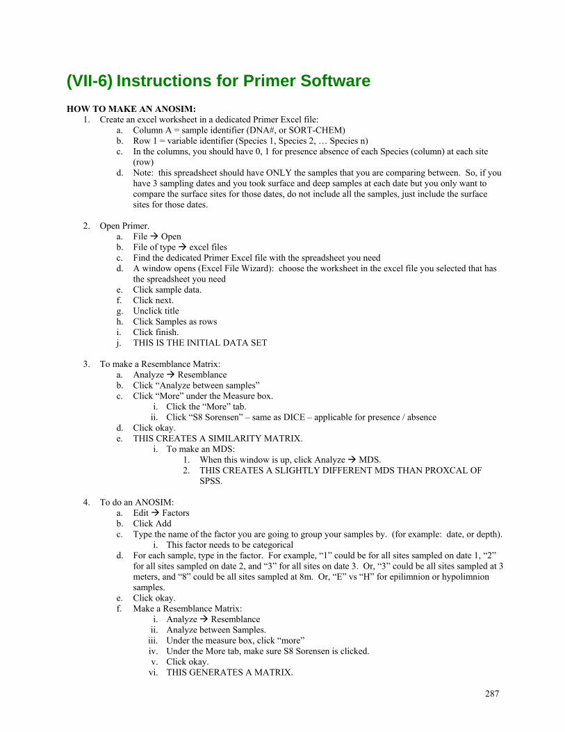
287

(VII-6) Instructions for Primer Software HOW TO MAKE AN ANOSIM:

1. Create an excel worksheet in a dedicated Primer Excel file: a. Column A = sample identifier (DNA#, or SORT-CHEM) b. Row 1 = variable identifier (Species 1, Species 2, … Species n) c. In the columns, you should have 0, 1 for presence absence of each Species (column) at each site

(row) d. Note: this spreadsheet should have ONLY the samples that you are comparing between. So, if you

have 3 sampling dates and you took surface and deep samples at each date but you only want to compare the surface sites for those dates, do not include all the samples, just include the surface sites for those dates.

2. Open Primer.

a. File Open b. File of type excel files c. Find the dedicated Primer Excel file with the spreadsheet you need d. A window opens (Excel File Wizard): choose the worksheet in the excel file you selected that has

the spreadsheet you need e. Click sample data. f. Click next. g. Unclick title h. Click Samples as rows i. Click finish. j. THIS IS THE INITIAL DATA SET

3. To make a Resemblance Matrix:

a. Analyze Resemblance b. Click “Analyze between samples” c. Click “More” under the Measure box.

i. Click the “More” tab. ii. Click “S8 Sorensen” – same as DICE – applicable for presence / absence

d. Click okay. e. THIS CREATES A SIMILARITY MATRIX.

i. To make an MDS: 1. When this window is up, click Analyze MDS. 2. THIS CREATES A SLIGHTLY DIFFERENT MDS THAN PROXCAL OF

SPSS. 4. To do an ANOSIM:

a. Edit Factors b. Click Add c. Type the name of the factor you are going to group your samples by. (for example: date, or depth).

i. This factor needs to be categorical d. For each sample, type in the factor. For example, “1” could be for all sites sampled on date 1, “2”

for all sites sampled on date 2, and “3” for all sites on date 3. Or, “3” could be all sites sampled at 3 meters, and “8” could be all sites sampled at 8m. Or, “E” vs “H” for epilimnion or hypolimnion samples.

e. Click okay. f. Make a Resemblance Matrix:

i. Analyze Resemblance ii. Analyze between Samples.

iii. Under the measure box, click “more” iv. Under the More tab, make sure S8 Sorensen is clicked. v. Click okay.

vi. THIS GENERATES A MATRIX.

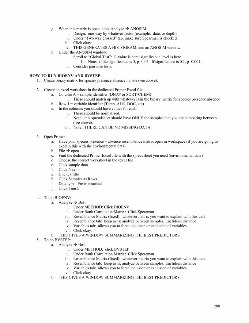
288

g. When this matrix is open, click Analyze ANOSIM. i. Design: one-way by whatever factor (example: date, or depth).

ii. Under “Two way crossed” tab, make sure Spearman is checked. iii. Click okay. iv. THIS GENERATES A HISTOGRAM, and an ANOSIM window.

h. Under the ANOSIM window: i. Scroll to “Global Test”: R value is here, significance level is here.

1. Note: if the significance is 5, p=0.05. If significance is 0.1, p=0.001. ii. Consider pairwise tests.

HOW TO RUN BIOENV AND BVSTEP:

1. Create binary matrix for species presence absence by site (see above). 2. Create an excel worksheet in the dedicated Primer Excel file:

a. Column A = sample identifier (DNA# or SORT-CHEM) i. These should match up with whatever is in the binary matrix for species presence absence

b. Row 1 = variable identifier (Temp, ALK, DOC, etc) c. In the columns you should have values for each.

i. These should be normalized. ii. Note: this spreadsheet should have ONLY the samples that you are comparing between

(see above). iii. Note: THERE CAN BE NO MISSING DATA!

3. Open Primer

a. Have your species presence – absence resemblance matrix open in workspace (if you are going to explain this with the environmental data).

b. File open c. Find the dedicated Primer Excel file with the spreadsheet you need (environmental data) d. Choose the correct worksheet in the excel file e. Click sample data f. Click Next g. Unclick title h. Click Samples as Rows i. Data type: Environmental j. Click Finish

4. To do BIOENV:

a. Analyze Best i. Under METHOD: Click BIOENV

ii. Under Rank Correlation Matrix: Click Spearman iii. Resemblance Matrix (fixed): whatever matrix you want to explain with this data iv. Resemblance tab: keep as is; analyze between samples, Euclidean distance v. Variables tab: allows you to force inclusion or exclusion of variables

vi. Click okay. b. THIS GIVES A WINDOW SUMMARIZING THE BEST PREDICTORS.

5. To do BVSTEP: a. Analyze Best

i. Under METHOD: click BVSTEP ii. Under Rank Correlation Matrix: Click Spearman

iii. Resemblance Matrix (fixed): whatever matrix you want to explain with this data iv. Resemblance tab: keep as is; analyze between samples, Euclidean distance v. Variables tab: allows you to force inclusion or exclusion of variables

vi. Click okay. b. THIS GIVES A WINDOW SUMMARIZING THE BEST PREDICTORS.

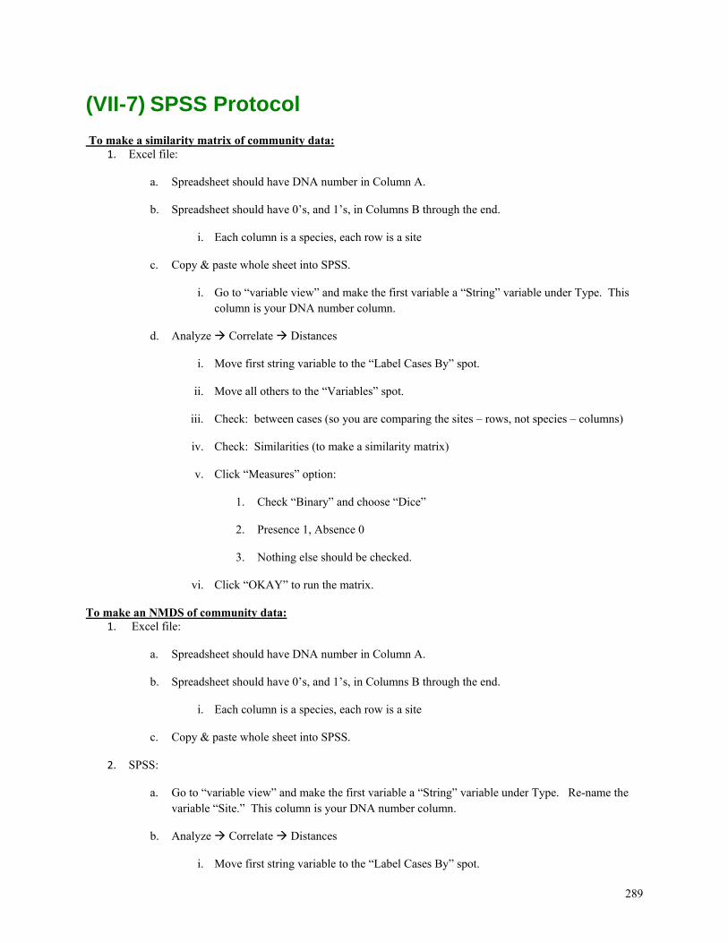
289

(VII-7) SPSS Protocol To make a similarity matrix of community data:

1. Excel file:

a. Spreadsheet should have DNA number in Column A.

b. Spreadsheet should have 0’s, and 1’s, in Columns B through the end.

i. Each column is a species, each row is a site

c. Copy & paste whole sheet into SPSS.

i. Go to “variable view” and make the first variable a “String” variable under Type. This column is your DNA number column.

d. Analyze Correlate Distances

i. Move first string variable to the “Label Cases By” spot.

ii. Move all others to the “Variables” spot.

iii. Check: between cases (so you are comparing the sites – rows, not species – columns)

iv. Check: Similarities (to make a similarity matrix)

v. Click “Measures” option:

1. Check “Binary” and choose “Dice”

2. Presence 1, Absence 0

3. Nothing else should be checked.

vi. Click “OKAY” to run the matrix.

To make an NMDS of community data: 1. Excel file:

a. Spreadsheet should have DNA number in Column A.

b. Spreadsheet should have 0’s, and 1’s, in Columns B through the end.

i. Each column is a species, each row is a site

c. Copy & paste whole sheet into SPSS.

2. SPSS:

a. Go to “variable view” and make the first variable a “String” variable under Type. Re-name the variable “Site.” This column is your DNA number column.

b. Analyze Correlate Distances

i. Move first string variable to the “Label Cases By” spot.

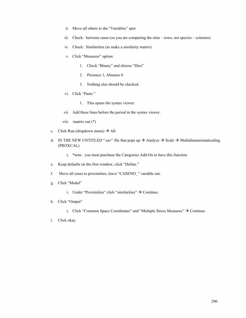
290

ii. Move all others to the “Variables” spot.

iii. Check: between cases (so you are comparing the sites – rows, not species – columns)

iv. Check: Similarities (to make a similarity matrix)

v. Click “Measures” option:

1. Check “Binary” and choose “Dice”

2. Presence 1, Absence 0

3. Nothing else should be checked.

vi. Click “Paste.”

1. This opens the syntax viewer.

vii. Add these lines before the period in the syntax viewer:

viii. /matrix out (*)

c. Click Run (dropdown menu) All

d. IN THE NEW UNTITLED “.sav” file that pops up Analyze Scale Multidimensionalscaling (PROXCAL)

i. *note: you must purchase the Categories Add-On to have this function

e. Keep defaults on the first window, click “Define.”

f. Move all cases to proximities, leave “CASENO_” variable out.

g. Click “Model”

i. Under “Proximities” click “similarities” Continue.

h. Click “Output”

i. Click “Common Space Coordinates” and “Multiple Stress Measures” Continue.

i. Click okay.

291

(VII-8) Reporting Data Protocol Updated: 19 May 2014, gwk

Several things need to be done when providing data to people outside the lab, or within the lab to graduate students. Data may be requested from someone who sent samples to the lab for analysis or it may just be a general request for data we have. This protocol generally applies to reporting chemistry values, but may be applied to other data as well. 1. Data should be organized in an Excel spreadsheet. The first tab in the spreadsheet should be titled “Notes” with

the following column headings in bold: Date, Who, Notes. The person creating the file should describe why the file was created in this section.

2. Make sure all data has been hard-pasted and the file does not contain links to other files. Not everyone has our files and they can’t access any information in a linked file.

3. The machine information and errors should be reported in the file on the “Notes” tab. In order to be cited properly in publication, specify when the samples were run and on what machine. The errors associated with the machine and with sample replication (if done) should also be noted. Below are examples of the information that should be included when reporting values.

4. George needs to look through all data leaving the lab. This is to double-check that the above points have been completed and to ensure that the data being reported is acceptable (i.e., no negative values, makes sense as far as we can tell, etc.).

* NOTES ON INSTRUMENT, ERRORS, AND REPORTING SIGNIFICANT FIGURES: DOC/TDN DATA: Instrument After 2004, samples were run on a Shimadzu TOC-V CHP with a TDN module. Before 2004, samples were run on a Shimadzu TOC-5000. Errors The machine makes 5 injections of a single sample and calculates a mean value and a CV% for those 5

injections. This "machine" CV% ranges from <1% to about 4%. The CV% of duplicate standards run on two different machine operating days is about 5% for both DOC and TDN. This should be the maximum variation because it is calculated across runs on different days rather than within a single run. In other words, although we report DOC to the 1 uM decimal place, and TDN to the 0.1 uM decimal place, the differences between two single samples should be considered to be "real" if they are greater than 5% of the sample value. If you have true field replicate samples, then consider the differences between the averages of those replicates to be "real" when some statistical convention (P value) is reached.

Reporting DOC = Dissolved Organic Carbon, micro moles per liter; Report to the nearest whole number value (e.g., 445, not 445.2). We assume the sample was filtered and acidified, meaning that there is no inorganic or particulate C in the sample. TDN = Total Dissolved Nitrogen, micro moles per liter; Report to the nearest tenth of a whole number (e.g., 12.1 but not 12.14). The TDN values include all dissolved forms of nitrogen in the sample - we assume the sample has been filtered, meaning that the values are total DISSOLVED nitrogen.

GAS (CO2, CH4) DATA: Instrument After ~1992 samples were run on a Shimadzu GC14 or GC14A with a TCD and FID detector and using

a poropak Q column. The machines are plumbed to run both CO2 and CH4 on the same injection of sample gas. Column temperature is set at 80 degC, Injector temp is 70 degC, and Detector temp is 100 degC.

Before 1992, samples were run on a Carle GC with a poropak Q column. Errors The machine blank is very low, determined by injecting pure N2 gas and having no detection of CO2 or

CH4. The lowest limit of detection is well below our normal sample range of >300 ppmv CO2 and >1 ppmv CH4. The average CV% for running duplicate standards is <3% for CO2 and <2% for CH4 over the range of CO2 400-20,000 and CH4 2-2,000. Field duplicates have typically higher CV% values, especially for CH4 because of its lower solubility. For example, in the summer of 2013 the duplicate samples taken in Toolik Lake had an average CV of 3.2% for CO2 and 7.8% for CH4. In May 2014, the duplicate samples taken in a profile of 6 depths under ice in Toolik Lake had an average CV of 1.2% for CO2 and 6.8% for CH4.

292

Reporting CO2 = The partial pressure of CO2, PCO2 in micro atmospheres of pressure (µatm, equivalent to parts per million by volume), should be reported to the nearest whole number (e.g., 380 µatm, not 380.2). The concentration of CO2 in the water in micro moles per Liter of water should be reported to one decimal place (e.g., 40.1 µmol/L, not 40.12). CH4 = The partial pressure of CH4, PCH4 in micro atmospheres of pressure (µatm, equivalent to parts per million by volume), should be reported to one decimal place (e.g., 10.1 µatm, not 10.12). The concentration of CH4 in the water in micro moles per Liter of water should be reported to three decimal place (e.g., 0.052 µmol/L, not 0.0524).

TDP/SRP/PP: Instrument All phosphorus samples run in Ann Arbor are analyzed on an Alpkem Flow Solutions 3000. SRP analyzed at Toolik Field Station are analyzed on a Cary 50 Scan UV-VIS Spectrophotometer. Method The Total Dissolved Phosphorus (TDP) is initially digested with potassium persulfate (Mendzel and

Corwin, 1965). The Particulate Phosphorus is digested with the acid hydrolysis method (Stainton et al., 1972). The digested liquid is then run on the autoanalyzer using the Automated Ascorbic Acid Reduction Method 4500-P (APHA, 1995).

Error The average limit of detection on the FS3000 is 0.05 uM phosphate. The CV% between runs is less than 10%, usually around 5%.

Reporting TDP: Total Dissolved Phosphorus, micro moles per liter; Report to the nearest hundredth of a whole number. The TDP values include all dissolved forms of phosphorus in the sample - we assume the sample has been filtered, meaning that the values are total DISSOLVED phosphorus. SRP: Soluble Reactive Phosphorus, micro moles per liter; Report to the nearest hundredth of a whole number. PP: Particulate Phosphorus, micro moles per liter; Report to the nearest hundredth of a whole number.

NITRATE DATA: Instrument All nitrate samples run in Ann Arbor are analyzed on an Alpkem Flow Solutions 3000. Method The samples are kept frozen until analysis, and analyzed using the Automated Cadmium Reduction

Method 4500-NO3 (APHA, 1995). Error The average limit of detection on the FS3000 is 0.10 uM nitrate. The CV% between runs is less than

10%, usually around 5%. Reporting Nitrate, micro moles per liter; Report to the nearest hundredth of a whole number. The method that we

use actually determines both Nitrate and Nitrate, however, we have demonstrated that the nitrite levels in our samples are very low, and considered non-existent.

CATION DATA: Instrument The cations (Ca, Mg, Na, K, Si) are determined using a Perkin Elmer Inductively Couple Plasma Optical

Emission Spectrometer (ICP-OES) Optima 4300 DV. Method Please see Section VI-13 for a complete methods description. Errors Limits of detection for 2009-2010 were: Ca – 0.07 uM, Mg – 0.21 uM, Na – 0.04 uM, K – 0.03 uM, and

Si - 0.10 uM. Reporting Most elements can be reported to the nearest 10 nanomoles/Liter (e.g., 1.15 µM Ca, Mg, Na, or K). ALKALINITY DATA:

Instrument After 1998 samples were run on a Radiometric Auto Titrator (Tim 800 Titration Manager, ABU900

Autoburette (5 mL), SAC80 Sampler, Germany). Before 1998 peotentiometric titrations were performed using an Orion pH meter and electrode. Method We measure total alkalinity on filtered samples (stored dark and cold once we receive them) by

potentiometric titration usuing HCl in an open container. Samples are shaken well before being poured and weighed to determin volume titrated, in order to caputer any particulate inorganic carbon that may have precipitated in the bottle during storage.

Typically from 25-200 individual points on the titration curve are measured, waiting until the pH is stable before adding the next increment of acid. The instrument software determines the final equivalency point (inflection point of a graph of acid added and pH where the second derivative of the

293

line is zero), and we check a printout of the titration curve by hand to verify the inflection point. If the inflection point cannot be determined (e.g., the sample alkalinity is very low), then we use the method of Gran to estimate the alkalinity. Although we do not report the acid neutralization capacity (ANC, which can be negative if the sample is acidic), we can calculate it using the method of Gran for any sample that we analyze - if you require this number, please let us know. In other words, although we report Alk to the 1 uEq/L decimal place, the differences between two single samples should be considered to be real if they are greater than 2-3 uEq/L for samples <50 uEq/L and 5-10 uEq/L for samples greater than 50 uEq/L.

Errors The average CV% between duplicate standards within a run is ~3% and the average % difference between the actual and measured standard concentration is abot 4% - e.g., a 100 uEq/L standard is really 100 +/- 4 uEq/L. The average CV% between duplicate samples (which included field and processing variation) is less than 10% for values 20 uEq/L or lower, and ~2% for values greater than 20 uEq/L. If you have replicate samples, then consider the differences between the averages to be “real” when some statistical convention (P value) is reached. Report the Alk value to the nearest whole number, that is, report 452, and not 452.5 uEq/L.

Reporting “Alkalinity” is the total dissolved alkalinity in micro equivalents of charge per liter (or umol/L of HCO3- if you prefer to think of it that way). In most samples this is due to the carbonate alkalinity; test on samples from near Toolik lake show that burrering capacity from DOC is very low, less than 2-10% of total alkalinity.

294

(VII-9) Gas File Protocol Edited December 2011

1. Checking Gas File Samples with Chromatograph print-outs A. Samples are entered in the “data” tab in four columns bracketed by purple columns. The four sample

columns are named CO2 Area, CH4 Area, CO2-AMB Area and CH4-AMB Area. CO2 Area and CH4 Area must be checked against the hard copy and the two Ambient column are decided by the person running samples. See # 2

B. The Sample values can be found on the hard copy after peaks that are labeled with syringe numbers. The first set of numbers following the labeled peaks will be CO2 and the numbers with pen marks will correspond to the file. Following another set of peaks are the numbers for CH4.

C. Occasionally a sample may be rerun in which case the person running gases will have to decide which number to take. The number in the file will then either be the original or the rerun number and either is appropriate. If you suspect the wrong number has been chosen, ask someone for verification.

2. Checking to make sure the correct ambient are applied to samples a. On longer sampling days when multiple ambients are taken, the ambient should be averaged and then

applied to every sample from that day as long as there are no outliers. If there are outliers (150 uatm or more difference) then the weather on that day should be checked in the field notebooks. If a different weather front moved in that can explain the difference in concentrations, then ambient should be applied by nearest time. If the weather was consistent for the whole sampling day then the outliers can be removed from the average.

b. Ambients should only be averaged for the same sampling events. For instance, on some days Toolik lake samples were taken and gas samples were taken on inlets. Only Toolik ambients should be averaged and applied to Toolik samples and only inlet ambients should be averaged and applied to inlet samples. If any ambients don’t look good, an expception can be made and you can use ambients from other sites.

c. On sampling days that cover great distances (Kuparuk Survey or Lakes Survey) the ambients cannot be averaged because they are taken too far apart. In these instances apply the ambient nearest by time to each sample.

3. Checking Gas File Standards with Chromatograph print-outs A. Standards are generally run at the beginning or ending of runs. In the file they are located in the

standards tab and can be six or eight rows labeled CO2 1, CO2 2, CH4 1, CH4 2 and so on. B. The standards run are nominally 400 ppmv CO2/2 ppmv CH4, 5000 ppmv CO2/20 ppmv CH4, 20,000

ppmv CO2/200 ppmv CH4 and occasionally 50,000 ppmv CO2/2000 ppmv CH4. Similarly to samples, they have peaks on the print-outs that should be labeled and the following two sets of numbers will be CO2 and then CH4.

C. Generally, there are three standard curves for each standard so that each standard will have three separate values. In some cases there are more than three if the person running gases felt they needed more curves. Occasionally a standard curve will look bad and need to be rerun. In this situation the bad curve should be labeled and will not be entered in the file and an additional curve will be run to replace it.

4. Checking Gas File against Ak Chem to make sure there is agreement

A. Open a new tab called Names_Corr in the gas file and copy the columns from the data tab into there. The copied columns should include Run Number, Type (DIC/GAS), Syringe #, SortChem, Site, Date, Time, Depth (m), Distance (km), Elev(m), T-eq(C), Cond (uS/cm) and pH.

B. Then using the Index function, retrieve all of the equivalent columns in Ak Chem and put them in a different grouping next to the group that was pasted previously from the “data” tab in the gas file.

C. Copy the headers once more and then use the exact function for all of the cells below and let excel tell you whether the gas file data and the Ak Chem indexed data matches. Cells that match should read TRUE and those that don’t should read FALSE.

D. Sort by each column so that all of the exact functions returning false are at the top. Then go through and investigate why the gas file and Ak Chem disagree. Make appropriate corrections and then paste into yet another grouping at the end of the new tab. It may be necessary to refer to field notebooks to decide which file’s information is correct. This final grouping is what will eventually be pasted back into the gas file because it is verified as being correct.

295

E. In the event that Ak Chem information is found to be wrong, be sure to go back into that file and make appropriate corrections.

5. Moving gas information into AkChem

a. Copy data from the data tab (hard paste) into the Toakchem tab. Paste the site,date, time depth, sortchem, CO2uM, CH4 uM, CO2 uatm, CH4 uatm.

b. Then sort by type in the Toakchem tab (Gas,DIC, AMB). Delete that ambients samples. Delete the CH4 samples for the DIC samples because DIC samples have converted all carbon to CO2. Therefore CH4 measurements don’t make sense.

c. Merge the Gas and DIC values by sortchem so that each sortchem will have Site, Date, Time, Depth, DIC uM, CO2 uM, CH4 uM, CO2 uatm, CO2 uatm. Then the data for duplicates (ex. 0938 and 0938.1) must be averaged. Finally move all of the Data into AKchem using index match functions.

296

(VII-10) Completing File Work at Toolik Updated 1 November 2012

At the beginning of the summer, it is imperative that the PIs for each project explain the file structure and

responsibilities to everyone working in our labs. The PIs need to be in agreement when relating their expectations for the files, so it is clear to the RAs/grad students exactly what should be done. Also, the importance of making notes in the Notes tab of files should be stressed- this really helps us figure out what has been done in a file, especially ones that we (the Kling lab) didn’t work on all summer.

We could try posting lists in the labs with the file names, where the most up to date file is located (e.g. AKchem is on the Lab 4 computer and AKchem_LTREB is on the Dry Lab computer), who is responsible for the file, who double-checks the data, who backs the files up, etc. Also maybe include a chart with dates that can be checked off when the file has been updated, or some variation of that.

The AKchem project files should remain separate during the summer. By the end of the summer, we should all have a clear understanding of who will double-check them and send the final, completely updated file to the other projects. We think that in the future, it makes more sense for the other project members to double-check their own files (ideally very soon after the field season ends) and send us the final versions before we compile them into our yearly AKchem file. We had the copies to double-check the files, but because we often were not the ones involved in the sampling or experiments, it was somewhat difficult to double-check thoroughly.

Saturday sampling needs to be minimal to allow more time for catch-up. Also, Science Saturday needs to be re-imagined (ideas coming soon....) but it seems like a brief "file report" at the beginning of Science Saturday would be helpful and add accountability.

File work should be built into the schedule. Maybe try working on files in the morning on lighter sampling days (and non-nutrient days) to make sure it gets done before going into the field.

297

SECTION VIII – LAB MANAGEMENT Updated November 2010 by LRY

(VIII-1) Ordering

A. Placing an Order

All orders under $5000 are placed using one of two systems: Bioorders or Marketsite. Marketsite is a university-wide system, and preferred if the order is being shipped to Michigan and the vendor is one the university strategic suppliers. You will login as a “browse only” user via Wolverine Access, add items to your cart, and an authorized person (“assignee”) will complete the order using MPathways. You can also price check using Marketsite. We use Bioorders for purchases that are either being shipped to Toolik, or being ordered from a specialty supplier. Bioorders is a departmental system, and as such we can get updates on orders by contacting Sheila Dunn or Jackie Glebe, who will follow up with the vendor. Both systems require that you are an approved user. GWK must approve you as an orderer and email Sheila with your uniqname. Ordering with the Bio-Orders system on Footprints

1. Navigate to http://request.umich.edu/biology/bioorders (link also posted on EEB website) 2. Log in with your Kerberos password 3. Select “Submit request”. 1. Select your department; MCDB, EEB, or Biology. 4. 2. In the description box enter “ATTN: (your name) Kling Lab Room 1041. 5. Select Vendor, Shipment Method (usually “regular”), and Building (Kraus). 6. Selecting the item will open the item information window (titled Edit Dependent Fields) 7. After completing the item information, select “GO” to save it to the request. 8. After entering all items, complete the Short Code, Course Number, and Radioactive items information. 9. You may now add attachments by clicking “Attach files” 10. Additional users may receive email notifications about this request by entering their email addresses in the

“addresses” field. 11. You MUST now click on “GO” to save and finalize the request. 12. Your confirmation of request and summary will automatically be e-mailed to you. Print these, and file it (see

“Filing Order Requests” section below). Ordering with Marketsite See http://www.procurement.umich.edu/mmarketsite_howto.html for detailed instructions on how to order from Marketsite. After requesting the order, print the Order Requisition page, and file it (see “Filing Order Requests” section below). Filing Order Requests Ordering paperwork lives in the small “Ordering” file cabinet outside the lab manager’s office in 1041. There is a hanging file folder labeled Current Orders. Within this file are subfolders labeled “Orders Ann Arbor” (for Michigan lab orders), “YYYY Field supplies to Ann Arbor” (for stuff shipped to A2 but eventually going to Toolik), and “YYYY To Toolik” (orders shipped directly to Toolik). Within the “YYYY To Toolik” folder are subfolders for each current grant (e.g. LTER, LTREB, Thermokarst, etc.). Place the order request summary printout in the appropriate folder. Receiving Orders When you receive your order, check if it is complete. You will need to document that you have received the order in two places: Biorders (if the order was made through Bioorders) and in the ordering file.

a. First, log on to Bioorders home page and click on the pencil icon corresponding to your order. A new page will open that will allow you to update the status of the order. Scroll down to the Delivery Status

298

box, and click on the “Order is complete “ box, or if the order is only partially complete, click on the boxes next to the individual items you received. Click the Save icon to complete the form.

b. Locate the order confirmation printout in the “Orders YYYY” file folder. Staple the invoice or packing slip to this sheet, record the date received, and move printout to the file folder “YYYY Orders Received”. Additionally, if the order is chemical in nature, record the date received on the bottle, along with your initials.

c. If you are receiving orders in Toolik, it is unlikely that you will have the time or energy to organize your packing slips by grant. Record date received, if the order was complete, and place the invoices in an envelope. Return the envelope to Ann Arbor, and place the packing slips in a separate folder labeled “YYYY Packing Slips from Toolik”.

Orders Greater Than $5000: If an order total is more than $5000 the university requires the purchasing department to obtain quotes or "bids" from at least 3 different sources or "vendors" if possible. Sole Source: Sometimes an item is sold by only one vendor (for example, a new autosampler for the Shimadzu carbon analyzer). If there is only one source for an item, or if the new equipment has to be compatible with existing equipment, the rather lengthy bid process is obviously pointless; in this case it is necessary to provide the purchasing department with a written statement justifying the "sole source" claim. George will write a sole source justification for you if the situation arises. The next step is to take the sole source justification and all necessary purchasing information to the EEB secretary, who has access to the departmental credit card. The secretary acts as a mediary between us and the purchasing department, providing our purchasing agent, Sandra Romanchuk (http://www.procurement.umich.edu/contacts.php), with all of the information she requires to approve our purchase. If Ms. Romanchuk needs additional information, she will ask the secretary, and the secretary pass along the question to the orderer. Once the purchase has been approved, Ms. Romanchuk will issue a Purchase Order (PO) number to the secretary, who will then place the order. It is important to work closely with the secretary throughout this process to ensure that you are quickly informed of all status changes as well as any difficulties that may arise. Multiple Sources--Out on Bid: If the item is sold by several vendors and we have no basis to submit a sole source justification, it will have to "go out on bid." This means the purchasing department wants to obtain price quotes or bids from several sources, so they can make a choice based mainly on lowest cost. The best and quickest way to get this done is to again work closely with Lisa. She knows the system and she knows the people in purchasing, so she is the best person to handle this part of the process. Provide Lisa with the following information and then allow her to interact with the purchasing department to do all that is necessary to obtain a PO number:

1. Item name, manufacturer, and manufacturer's model number. 2. Names, addresses, phone and fax numbers of 3-4 vendors (if possible) who sell this item, and each vendor's

individual catalog number for the item. Ask Lisa to keep you updated on all status changes as well as any difficulties that may arise so you can do your

part to help everything progress quickly and smoothly. About Strategic Suppliers: Fisher Scientific is the university’s primary strategic supplier. The university has established a relationship with Fisher Scientific as a sole provider for everything Fisher sells, including chemicals. This means that if Fisher sells what we need, we must order if from them unless using another source can be justified because of lower cost, higher quality, greater compatibility, etc. Fisher has also agreed to price match other vendors. We are given substantial discounts on items most commonly ordered, and many things listed in the Fisher catalog as being available only by the case are available to us in smaller quantities. Orders placed before noon for in-stock items at their Chicago warehouse are delivered to the Natural Science Building by noon of the next day. If an item is not in stock at Chicago, but we need it the next day, Fisher will have it sent next day Federal Express or UPS if this service is requested when the order is placed; we will, however, be charged for the next-day shipping expense.

On-site Fisher Customer Service Representative: Sue Lidak Customer Service Email: [email protected] For assistance with orders, call: (734) 615-6767

299

C. Ordering Compressed Gas Cylinders Cryogenic Services

12620 Southfield Detroit, MI 48223 Phone (313) 835-5513

Fax (313) 835-3562 All gas cylinders used for the carbon analyzer, gas chromatograph, ion chromatograph, and CHN analyzer are ordered from Cryogenic Services. Call to order. You will need to indicate the type of gas, the shortcode on which to order the tank, the building/room number for delivery. All gases we currently use are normal stock items except for the combination CO2 and CH4 gas standards used with the gas chromatograph. Information on the gases we regularly order can be found in the file C:\DOCUMENTS\Lab\Orders_Inventories\ Lab_A2_Supplies.xls. If it is necessary to order special order compressed gases, call Cryogenic Services to make certain they can supply what is needed with the desired accuracy in the time period required (for example, ultra zero grade air requires about 2-3 weeks for delivery). Information on available gases and current pricing can be found by browsing on Marketsite. Gas cylinders are delivered to individual labs. Orders placed by Wednesday will be delivered the following Friday as long as the gas(es) ordered are in stock. If the need is urgent, Cryogenic Services can arrange a special delivery for an extra fee. When a tank is delivered, file the invoice in the “YYYY Orders Received” folder in the Ordering file cabinet in 1041. We are responsible for returning empty cylinders. It is important to return empty gas cylinders ASAP because the account is charged a daily rental fee for as long as we have the cylinder. Cylinders should arrive with perforated tags indicating “full”, “in-use”, and “empty.” Rip off the perforated portion to indicate the status of the cylinder. All spent cylinders must be labeled "EMPTY." They will be picked up by the same folks who deliver the full cylinders.

300

(VIII-2) Shipping

A. Domestic Shipping Updated November 2010 by LRY

UPS is our preferred shipping company. To ship a package domestically:

1. Navigate to the website https://www.campusship.ups.com

2. The screen should now have the UPS logo and clearly state UPS CampusShip at the top. You cannot go through the regular UPS webpage for this. There should be a box that asks you to “Please log in”.

a. User ID: gwk b. Password: ask GWK or a senior technician

3. In the “Begin Your Shipment” box:

a. Under Address Information: My UPS Address Book > Select the appropriate address in the drop down menu box:

i. If shipping to Michigan, select UM lab. ii. If shipping to Toolik, select Lab4 at Toolik

b. Under Shipper: Leave default i. Use the default address - “My Location Address” (Contact will show “Kling Lab”)

c. Ship From: same as 3a. d. Do NOT select the “Schedule a Pickup” box if you are shipping from Michigan. There is a charge

for the scheduled pickup. Simply put the packages in the UPS bin near the loading dock before 6:30 pm.

e. Payment Information: should state UPS Account 1F9909.

4. Under Shipment Information: a. Service > Select service from the drop down menu (we can ship ground from Michigan, select 2-day

air from Toolik unless told otherwise). b. Packing>Select package type from the drop down menu (generally this is “Your Packaging”) >

select number of packages (if you select more than 1, skip the next step). c. Package 1 Weight > enter weight of package > entered declared value (if needed). The shipping

scale is located in Sheila Dunn’s office. d. Shortcode > click on Search > enter the % sign in the top box > click on Search > scroll down the

search results and select the appropriate shortcode (ask which grant to use – all Kling grants start with Kling-…..).

e. Select Print shortcode on shipping label as bar code. f. Click on “Ship Now” (button is under the box, on the right).

5. If you had entered more than 1 package, the next screen will ask you to fill in the weight for each package.

a. Follow part 4d to select shortcode for each package.

6. Under Quantum View Notify: verify that [email protected] and any other applicable email addresses are entered and all email options are checked.

7. Complete information as indicated on the “Schedule a Pickup” page.

8. After verifying that all other information is correct, select View/Print Label button.

9. Print label and receipts (print 2 copies of the receipts).

a. When in Michigan, place receipt in the “YYYY Shipping” folder, located in the Ordering file cabinet outside the lab manager’s office in 1041.

b. At Toolik, place the receipts in the “Return to Michigan” folder (with other shipping receipts).

301

10. Place the label in UPS clear envelope (with adhesive on back) and place on package. Envelopes are found in the Shipping Supplies cabinet to the right of the front secretary’s desk in the EEB office.

B. International Shipping -- UPS International shipping is done via UPS. Special international shipping papers are needed and are available at the Dispensary. In addition to the shipping papers a Customs Commodity Declaration--available at the Dispensary--also needs to be filled out and photocopied 3x. The original form is attached to the shipping papers, 2 copies are placed inside the package and 1 copy is kept for laboratory records. Examples of these forms correctly filled out are included in a section at the end of this notebook. Federal Express will pick up packages for international shipment as part of their daily pick-up at 3:00 PM; special arrangements are not needed. If computer discs are included in a shipment, be sure to note this on the Customs Commodity Declaration form. Failure to do this will result in an additional delay.

D. International Shipping-- Air Freight It is also possible to ship internationally via two categories of air freight, over-the-counter small packages and commercial (or general) air freight. Shipping via over-the-counter small packages can be used to ship (of course) small packages—which for some reason are not classified as “excess baggage”—on the same flight as the accompanying people. However, this method is usually more costly than designating the packages “excess baggage.” The value limit, per package, is $1250. Weight and size limits are 70 pounds and L+W+H=90”, respectively. It is necessary to have 5 copies of an invoice for each package. The invoice must contain the following information: 1) description of each item including its value; 2) the name, address, phone and fax numbers of the shipper; 3) the name, address, phone and fax numbers of a contact at the destination. In 1994 there was a $10 charge for preparation of the airbill and the following weight classes (with example prices from Detroit to Entebbe) were dedicated: 1 - 22 lbs……………..…….$100. 23 - 44 lbs………………….$150. 45 - 70 lbs………………….$205. Commercial air freight is for large packages; they are shipped on air freight planes as available, with a total transit time from drop-off to pick-up at destination of 3 - 7 days. Shipping is from airport to airport only. The maximum weight for a single package is 500 pounds; maximum size is LxWxH = 65”x 45”x 34”, but if H and W are less, L can be longer, up to 201” when WxH = 5”x 5”. The following cost examples are from Detroit to Entebbe, 1994, but serve to illustrate the dedicated size categories. Weights are for the total shipment which can consist of several packages which individually weigh < 500 pounds. 1 - 100 lbs………...…………$9.10/lb

101 - 220 lbs…………...……$8.29/lb 221 - 661 lbs……...…………$6.41/lb 662 - 1,103 lbs………….…...$3.51/lb >1,103 lbs…………………....$2.95/lb The very bad thing about international shipping via commercial air freight is the complicated paperwork involved; detailed instructions are beyond the scope of this manual (and would probably change before this method would again be used). The following will give one a taste of the level of hassle involved. To ship via commercial air freight from the USA it is necessary to have: 1) 3 copies of the customs department certification of value and invoice of goods or 3 copies of a commercial invoice, either of which must include specific descriptions of each item shipped, its quantity, value and country of origin, and 2) the import license number and validation date of the party the goods are being shipped to. It is also necessary to check with the counsel in the country of destination to determine what documentation they require to have the shipment clear customs and be

302

released to the recipient of the shipment. It is also necessary to have made arrangements to have someone at the destination airport available to make inquiries about the shipment and to shepherd the packages through customs and transport them from the airport. If items must be shipped via commercial air freight, call the appropriate airline and ask for current information.

C. Excess Baggage-International and national When sending equipment and supplies along with people for fieldwork in Alaska or overseas, it is usually necessary to ship items in additional boxes along with personal luggage on the same plane as the people. These extra packages are termed excess baggage. Shipping charges for excess baggage are based on size (L+W+H) and weight, divided into the following classes (the example costs included are based on shipping from Detroit Metro Airport to Entebbe, Uganda, Africa in 1994): SIZE (L+W+H) WEIGHT COST < 62”....................................< 70 lbs...................................$135. 63-80”...................................< 70 lbs...................................$270. 81-115”.................................< 70 lbs...................................$405. < 62”..................................71-99 lbs...................................$405. 63-80”.................................71-99 lbs...................................$675. 81-115”...............................71-99 lbs...................................$810. 81-115”.................................> 99 lbs.............................add $135. charge for overweight to base rate of $810. + $405. for every 22# over 99# Dangerous goods are not permitted in excess baggage. Each box should be sturdy and well taped and, if at all possible, within the L+W+H=62” and 70 lbs restrictions (see cost column). If this is not possible, exploit the necessary size and weight class as much as possible. It is advisable to seal individual items within the shipping box in zip-lock plastic bags because the shipping boxes may be left outside exposed to the elements for undetermined periods of time. Each box should be numbered and a complete and accurate list constructed of the contents of each box. Include a copy of the appropriate list inside each box and keep two additional copies with whoever is accompanying the boxes through customs.

E. Shipping Dangerous Goods -- Domestic Compressed gas of any type and most chemicals are considered dangerous goods. Any radioactive substance is also considered dangerous. The shipment of all radioactive items must be done by Radiation Services. For further information on shipping radioactive items call Radiation Safety Service at 764-4420. The shipment of dangerous but not radioactive goods is best done via Federal Express. It is a complicated and tedious procedure but it is possible to accomplish if one possesses sufficient patience and tenacity. Special shipping documents are required, along with an additional “Shippers Declaration for Dangerous Goods” form. There are also very strict requirements for labeling and packaging which must be complied completely and exactly. Federal Express has a 50 point “Dangerous Goods Acceptance Checklist” which a package must pass to be accepted for shipment. A copy of this checklist is included in a section at the end of this notebook. It is necessary to know various classifications, as established by the federal government, of the goods to be shipped. These include: “proper shipping name”, “class or division”, “UN or ID number”, “packing instructions”, “authorization”, and if applicable, “packing group” and “subsidiary risk”. Most of this information can be found in the “Hazardous Waste Manual” published by the U of M. A copy can be found in the vicinity of the catalogs, next to the “Radiation Safety Manual.” Sheila Dunn, in the Dispensary, is our building safety officer and is an excellent source of the most up-to-date information. If she doesn’t have it, she will be able to tell you who to call to get it.

303

I have specified Federal Express for shipping dangerous goods because their people are the most knowledgeable and helpful. The appropriate number to call for information about shipping dangerous goods is 1-800- GO FEDEX, ext. 1666. When you call, have specific questions ready to ask, and be prepared to give them whatever information you have, especially the quantity, including weight and/or volume amounts and concentration, the material’s class or division category and UN or ID number. It is helpful to follow their “Dangerous Goods Acceptance Checklist” point by point. Ask Sheila about any points you are not sure of, then get prepared and call the Federal Express help number for answers to any remaining questions. Examples of correctly completed shipping documents and the “Shipping Declaration for Dangerous Goods” are included in a section at the end of this notebook. When everything is ready to ship, but before sealing the package, call the local Federal Express office and tell them you want to arrange a dangerous goods shipment. They will either schedule a pick-up time or ask you to bring the package to their office.

F. Shipping Dangerous Goods – International The good news here is that it is not more difficult to send dangerous goods internationally; it is just a little more inconvenient. No additional information is needed, but it is necessary to fill out a different shipping document, a 7-copy airport to airport air waybill (which must be filled out using an electric typewriter), and a commercial invoice. Examples of these forms correctly filled out are included in a section at the end of this notebook. You will need to provide Federal Express with 3 copies of the commercial invoice, so photocopy it x4 and keep a copy for laboratory records. Arrangements must be made in advance to deliver the package to the Detroit Metro Airport Federal Express office for processing, or to schedule a special pick-up (cost $12.50 in 1996). Federal Express will also need to give you a rate (price) quote and provide you with a “rate quote number” which is needed to complete the airport to “airport air waybill.” It is a good idea to call well in advance of when you want to ship so they can provide you with all current information and required forms. The address and phone number of the Detroit Metro Federal Express office: 11401 Metro Airport Center Drive Suite 100, Building K (313) 955-8800 It should be noted that Federal Express does not deliver everywhere in the world; thus it may be necessary to use another service. For example, DHL is the courier service used in Uganda. G. FedEx Example Shipping Form ‐ US Airbill Use the FedEx US Airbill for all FedEx Express shipments within the US except FedEx SameDay and FedEx Collect on Delivery (C.O.D.), which have their own airbills. Prepare shipments online with ShipManager. See additional information about FedEx Stamp, hundredweight pricing and multiple-package shipments. Call 1.800.GoFedEx (1.800.463.3339) to order pre-printed, peel-and-stick airbills.

304

1. Sender Information 2. Internal Billing Reference 3. Recipient Information 4. Service

5. Packaging 6. Special Handling 7. Payment 8. Required Signature

1. Sender Information Enter your shipping information. This includes the address you are shipping from, your name, your phone number, and your FedEx Account Number. If you need a FedEx Express account number, register for one now.

2. Internal Billing Reference You may assign any internal billing numbers or codes here. The first 24 characters will will appear in your invoice.

3. Recipient Information Fill in the details for your shipping destination. This includes Recipient name, address, and phone number. FedEx cannot deliver to P.O. boxes or to P.O. box ZIP codes in the US

4. Service Indicate which of the US Express or US Express Freight services you are using. If no service is marked, we will send your shipment via FedEx Priority Overnight®, or FedEx 1DaySM

Freight (as appropriate). 5. Packaging

Indicate the packaging you are using, or mark "other" if you are using your own packaging. 6. Special Handling

Mark "Yes" or "No" to indicate whether your shipment contains Dangerous Goods. If yes, as per attached shipper’s declaration, include two copies of a Shipper’s Declaration for Dangerous Goods. This is also where you can choose other special handling options including "Hold at FedEx Location" or Saturday Service (when applicable). Note: If you would like us to hold the shipment at a FedEx Location for pickup, select the appropriate Hold at FedEx Location option box, and write the FedEx location address on the address line of the Recipient information. Addresses are available at Dropoff Locator.

7. Payment Bill To - If billing to sender, recipient or third party, include the payer's FedEx Express account number.

Credit Card - If paying by credit card, write the credit card number and expiration date. FedEx accepts these credit cards: American Express, Carte Blanche, Diners Club, Discover Card, MasterCard, Optima, and VISA. Cash - If paying by cash or check, payment is requested at time of shipment.

8. Required Signature Sign here if you want a courier to deliver your shipment even if no one is there to accept it.

NOTE: This option isn't available if the shipment contains regulated commodities such as dangerous goods, alcohol or pharmaceuticals.

305

Internal Billing Information To help with your records, use this optional area for your internal shipping numbers or codes. We'll print the first 24 characters of this code on your invoice.

306

(VIII-3) Radiation Safety and Ordering Procedures Updated: 02 April 2001

By: MZB Laboratory Work Procedures with Radioactive Materials

A. Purchase and Sources Radioactive source material for conducting experiments is purchased in coordination with Radiation Safety Services

(RSS) of the University of Michigan, which has on file an authhorization agreement with the Kling lab as to the nature of experiments we are likely to conduct, the type or specific isotopes of radioactive materials we would like to use (e.g. 14C, 35S), and the amount of radioactive material we are allowed to have on hand to conduct experiments.

To Purchase Radioactive material: 1) Check the lab agreement to confirm that we have authorization for the desired isotope and a description of the

proper experimental procedures on record. Secondly, check that the amount to be purchased, along with our current inventory, does not exceed our authorized possession quantity. If you are shipping RAD directly to Alaska, the maximum amount that can be shipped from UM is 5 mCi bicarbonate per box. We have a 10 mCi bicarbonate shipping limit to our lab (as of 28 Apr 04), so you may need to put in two orders of 5 mCi bicarbonate each if you want a total of 10 mCi to be sent to Alaska.

2) Determine a stock number, unit, quantity of that unit, and estimated cost of the isotope from the desired supplier. The University has special purchase agreements with Fisher/ICN and Sigma-Aldrich, so it is less expensive and a much easier procedure to purchase radioisotopes from one of these two sources; Fisher/ICN is the first choice. a) To order from Fisher/ICN: Call our local Fisher rep at 5-6767 and get a price for and check on the availability of the radioisotope you are purchasing. Next call Radiation Safety Services to get a clearance code (see step 3 below) and then fill out and submit the special Fisher Scientific/University of Michigan “ICN Radioactive Requisition Form”. This form is available from Fisher b) To order from Sigma-Aldrich: Call Sigma at 1-800-365-2535 and get a price for and check on the availability of the radioisotope you are purchasing. You will need to give them the following account number—49447796. Next call Radiation Safety Services to get a clearance code (see step 3 below) and then fill out and submit a departmental order form (see ordering protocol for more detailed information on this procedure if necessary); be sure to indicate in the proper field that this is a rad order and also include the clearance code obtained from RSS as an extra line in the description field of the order form. Sheila will obtain a P.O. number and fax the order to Sigma-Aldrich.

3) Obtain a clearance code for the purchase by calling Radiation Safety Services (4-4420). They will ask for the following information: Authorized User name (George Kling), laboratory delivery address, the isotope you are going to purchase, the isotope’s activity, the supplier and catalog number and the UM short code and our order number (gkxxxx). Copy the clearance code they give you as it must be included on the order.

4) All radioactive material is first shipped to: Radiation Safety Services

University of Michigan 1239 Kipke Drive

Ann Arbor MI 48109-1010 ATTN: Dr. George Kling

RSS will make sure the shipment arrives intact, without leaking, and will call us to make arrangements to bring the package to our lab.

B. Receipt of radioactive material 1) Although RSS receives all shipments of radioactive material before they are forwarded to us, we are still

responsible for conducting a radiation survey on the contents of the package. We are to determine whether there is any loose contamination within the shipping carton by taking wipes on the inside of containers and on packing material. The isotopes we are likely to order are all low energy beta emitters which means that we must count the wipes with a scintillation counter to detect loose contamination at low but significant quantities. We are also responsible for accountability of all material we have in our possession.

2) Accountability - Start a log sheet for each new isotope receipt by filling out a blank form xxx which are kept in our three ring binder for radiation safety records. Include all appropriate dates, quantities, vendor numbers, vendors etc.

307

3) Check for contamination internal to the package - While opening the package, conduct a wipe survey ( see section D.1 below) using good radiation practices (wear gloves, lab coat, protective eye wear) in a properly marked work area (e.g. under the rad hood). a) Take a wipe with a filter paper (Whatman qualitative paper filters) on each container and place each into a

labeled scintillation vial. b) Take a wipe on the inside of the shipping package and on the packing material and place into a labeled

scintillation vial. c) Add scintillation cocktail to each vial and count on the scintillation counter on the forth floor. Include a

background sample wipe for comparison. d) If loose activity is detected (ie., the measured activity on one or more of the wipes is equal to or greater than

three times the background value), contact the Radiation Safety Group for instructions. e) Record all results on the wipe survey log sheet and the new inventory log sheet in the three ring binder.

Initial, annotate, and date the count results and add to the record book. f) If no contamination of packing materials is found, they can be disposed of only after the radiation labeling

has been obliterated in accordance with University of Michigan and Federal regulations.

C. Use of radioactive material during experiments 1) When performing experiments with radioactive isotope tracers, all work will be conducted in authorized work

areas. Prudent work practices should be followed. Wear gloves, lab coat and protective eye wear. Provide secondary containment and absorbent material in case of potential spills. Only place radioactive liquid waste into containers provided by the Radiation Safety Group. Dry waste (paper towels , absorbent mats) is collected in waste drums, and sharps (spent flame sealed vials, needles, etc.) are collected in a special sharps container.

2) Record the amount of isotope used on the appropriate record sheet in the log book (volume and activity used). 3) Upon completion of experiment conduct a wipe survey of the surrounding work space (counter, floor, door).

Place wipes in labeled scintillation vials, add scintillation cocktail and count wipes and a background wipe on the scintillation counter on the forth floor. If loose activity is detected (three times the background value), contact the Radiation Safety Group for instructions.

4) Record all wipe results on the wipe survey log sheet in the three ring binder. Initial, annotate, and date the count results and add to the record book.

D. Routine safety monitoring and surveys Monthly wipe surveys are required in all dedicated radiation areas when isotopes have been in use. If no experiments involving radioactive materials was performed through out a month (e.g. everyone was in Africa or Alaska), a wipe survey is not required, however, a notation must be entered into the log indicating this was the case. 1) Wipe surveys are performed by taking a filter paper (Whatman qualitative paper filters) and wiping the surface of

an object, counter, floor, etc. to collect loose surface material or dirt. The approximate surface area to wipe for routine comparison is 100 cm2.

2) Place each wipe into a labeled scintillation vial (either 20mL or 7mL vials may be used) and add scintillation cocktail to each vial (15mL or 5ml).

3) Count each vial for one minute with the B_Channel (14C or 35S) on the scintillation counter on the forth floor. Include a background sample wipe for comparison.

4) If loose activity is detected (three times the background value), contact RSS for instructions. 5) Record all results on the wipe survey log sheet in the three ring radiation safety document binder. Initial,

annotate, and date the count results and add to the record book.

E. Disposal of waste materials Arrangements for disposal of radioactive waste materials is made through RSS. A waste manifest form is filled out indicating the volume and approximate activity of the waste. A wipe survey must be conducted on the external surfaces of each container for disposal. The survey must be documented in the three ring radiation safety document binder and a copy available with the containers for the radiation safety technicians to indicate the survey was completed. Special tags are affixed to each container.

F. Safety training An introductory class on radiation safety is provided by RSS. All University of Michigan personnel are required to attend this class and pass an exam prior to working with radioactive materials. Attendance at this

308

class is scheduled through the radiation safety group. Yearly, a laboratory refresher session is required. The refresher session usually consists of reading a handout and signing a document that you have reacquainted yourself with the necessary rules and regulation. Additional topics or notices from the safety group may be discussed as necessary.

G. Ordering Radioisotope for use at Toolik Field Station Updated: 11 April 2008 By: ALF ORDERING RADIOISOTOPE

Important people to remember: RSO at UM = Mark Driscoll Senior OSEH Rep at UM = Dennis Palmieri RSO at UAF= Tracey Martinson, Ph.D.

George is the authorized user at the University of Michigan and UAF Ordering Information

o User Name: George Kling o Radionuclide: 14C L-Leucine o Activity: 250 uCi o Delivery Location (gift to UAF – we may be able to order directly through UAF, but need to work

out the money flow – how we pay for it): Tracey Martinson, Ph.D., RSO 1000 University Ave Room 155, University of Alaska Fairbanks, Fairbanks, AK 99709

o Vendor: Sigma – Aldrich o Catalog#: L5770 (specify 250 uCi; 100 uCi/ml; specific activity varies from 258 to over 300

mCi/mmol) Call Vendor for pricing and availability:

o Contact at Sigma-Alrich: estimated cost $797, 1-2 weeks Brian Dulle ([email protected]); 1-800-325-4581

o Fisher estimated cost = $890 o MP Biomedical estimated cost = $918.05

Call RSS (734-764-4420) Provide RSS with information from step #2 (above). You will receive a clearance code

Clearance code: Contact Dennis Palmieri ([email protected]) and tell him you are ordering rad to be sent to UAF. Once you have a clearance code, you can place the order with your selected vendor. Ask vendor (if have not already) for an estimated time of receipt (and tell Dennis and Tracey this). Rad material goes from UM RSO to UAF RSO to us. Contact Dennis Palmieri ([email protected]) and tell him you are ordering rad to be sent to UAF. Notify RSO at UAF of the purchase and desire to have the material transferred from UM to UAF. Indicate purchase and transfer in our rad book in the lab at Michigan.

TRANSPORTING MATERIAL FROM UAF TO TOOLIK FIELD STATION

We arrange the transport of radioactive material to TFS with the RSO at UAF, we have two types: 1. Unused radioisotope from previous year that has overwintered in warm storage. 2. New radioisotope ordered in the current year (See acquiring rad section of this protocol). RECEIVING RADIOACTIVE MATERIALS

Follow procedures for receiving radioactive material as outlines in the UAF Redbook. TRACKING RADIOISOTOPE RECEIPT, USE, DISPOSAL, AND TRANSFER

Document any transaction with radioisotope using “isotope use log XXXX.xls”. Document your usage and disposal when you use the radioisotope – do not rely on ‘remembering’. Keep a record of your rad use in the field notebook WHEN you use it.

309

Clean the rad area after each use Wipe tests are conducted on a weekly basis (pick a day and do it consistently; this is not required, but things

get dusty at Toolik and it is better to be on the safe side). At the end of the summer, print the forms at put in the redbook in the wetlab.

310

(VIII-4) Hazardous Materials and Waste Updated: May 2013 SEF

A. General Information The U of M department of Occupational Safety and Environmental Health (OSEH) considers anything you would not be willing to drink or eat as hazardous waste. Thus, everything we do in the lab which involves chemicals generates hazardous waste. We must be prepared to contain any waste generated, and then we must dispose of it properly. NOTE: Radioactive materials are an entirely separate class of chemicals and are not included in this section (see section VIII-3). All hazardous waste must be

1. collected in an appropriate container, 2. accurately and completely labeled, and 3. properly stored and disposed of when the container is full.

Important contact information:

OSEH Contact Info: http://www.oseh.umich.edu/ (734) 647-1143

Central Campus OSEH representative: Erik McClellan

(734) 936-3039

B. Collecting Hazardous Waste Official OSEH waste disposal instructions:

http://www.oseh.umich.edu/pdf/Chemical_Waste_Bulletin.pdf OSEH provides us with waste containers and hazardous waste labels free of charge. We are responsible for requesting both containers and waste labels (best time to do this is when we schedule a pickup). Containers we commonly use include: 1 gallon plastic jugs for liquid waste; 5 gallon white plastic buckets for solid waste, including rags and paper; and 5 gallon plastic carboys for large volume liquid waste. Liquid containers should be placed on a secondary container, i.e. a plastic tray with lip. Most of the hazardous waste we generate is liquid, and for the volume we generate, the 1 gallon jug is usually sufficient. It is important to keep liquid waste as segregated as possible. Do not mix two or more different kinds of waste together; instead, use a separate jug for each. However, there are times when it is impossible to keep waste segregated. For example, when running the Technicon AutoAnalyzer, two or more different chemical analyses (each with 2-4 separate reagents) are combined during analysis into a single waste stream. In this instance, because of the relatively large volume of same-mixture liquid waste generated, the AutoAnalyzer is connected to small waste jugs that are emptied into a single 5 gallon carboy. In general, when making up reagents or standards, it is good laboratory practice to cover the work surface with absorbent bench paper and gather all the necessary equipment, including waste containers, paper towels, kim-wipes and disposable gloves. Work involving toxic or irritating powders and/or solvents or preservatives which produce toxic fumes should be done under the exhaust hood. NOTE: Waste containers must be kept closed unless actively adding or removing waste. Funnels cannot be left in waste containers. They must be removed immediately after use and the container lid closed/sealed. Empty chemical containers: Empty non-hazardous chemical containers should be triple rinsed and defaced. Rinse water should be added to the appropriate hazardous waste container. The rinsed containers can then be placed in a regular trash bin, glass disposal bin, or recycling bin. If the chemical is acutely hazardous (e.g. cadmium metal, compounds of arsenic, lead or mercury, any organic solvent), the container should be rinsed again with 10% HCl. Solvent rinses should be collected for disposal in the appropriate hazardous waste container. If the rinsed container that contained acutely hazardous materials is to be discarded, it should be added to the appropriate hazardous solid waste container.

311

Any gloves, tissues, paper towels, absorbent paper, etc., which have come in contact with any acutely hazardous chemical should be added to the appropriate hazardous solid waste container. Disposable gloves used to protect the hands while mixing non-actutely hazardous chemicals such as acids, solvents, acid washing glassware, etc., can simply be rinsed in the sink and then discarded in a regular trash bin.

C. Labeling Hazardous Waste Hazardous waste containers MUST be properly labeled. Labels are attained from OSEH (request extras each time you schedule a waste pickup). We store extra labels in the Chemical Hygiene Binder, found on the shelf outside the lab manager’s office in 1041. Hazardous waste labels should be filled out and adhered to the waste jug, bucket, or carboy prior to waste collection. You will need to fill out “Name,” “Room Number,” “Building,” “Accumulation Start Date,” and “Chemical Description”. Do not abbreviate the chemical description!

D. Scheduling Waste Pickup We are responsible for calling OSEH to schedule hazardous waste pickups: (734) 763-4568 NOTE: Waste containers cannot be kept for more than 90 days past the Accumulation Start Date. Contact OSEH-HazMat for pickup within 60 days of the accumulation start date. OSEH-HazMat will make every attempt to pickup waste within 1 week of scheduling and arrange for proper disposal. We store full waste containers awaiting pickup on a cart near the north door of 1041. Take care not to place reactive chemical waste containers (e.g. acids and bases) near one another! Liquid containers must be placed on a secondary tray. Waste containers of 1 gallon and smaller must be placed in a secondary cardboard box, sealed, and properly labeled. Prior to scheduling a waste pickup, we must fill out a Waste Manifest form. Extra forms are stored in the Chemical Hygiene Binder, found on the shelf outside the lab manager’s office in 1041. Follow directions on back of the Waste Manifest to properly complete the form. Make sure to sign and date the certification statement, otherwise waste will not be picked up! Do not forget to fill in the Manifest Tracking # on the labels of every hazardous waste container that is being picked up. Also, make a photocopy of the Waste Manifest form and put the copy in the appropriate section in the Chemical Hygiene Binder (Section 12 – Disposal of Waste Materials).

312

(VIII-5) Printers Updated 03 Feb 2011 by LRY

A. Adding a networked departmental printer

1. Open the “Printer and Faxes” utility. 2. Click on “Add Printer”, and then click “next”. 3. Choose “local printer attached to this computer”. 4. Click to “Create a new port”, and choose TCP/IP port from the dropdown menu. 5. Enter the port name (i.e. network address).

The network addresses / hostnames for department printers are as follows:

Room 2060 Grad Lounge: eeb-2060-4250.eeb.lsa.umich.edu eeb-2060-4350.eeb.lsa.umich.edu

Room 1300:

eeb-1300-4250.eeb.lsa.umich.edu EEB office: eeb-mainoffice.biology.lsa.umich.edu

EEB office:

eeb-2019-color.eeb.lsa.umich.edu

6. If you have correctly typed in the address, a window will pop up with the heading “Completing the Add Standard TCP/IP Printer Port Wizard”. If you do not see this window, go back a step and make sure you typed in the address correctly. Otherwise, click “Finish”.

7. Select the driver for the printer. HP LaserJet 4350 PS should work for any of the three departmental printers. If it does not show up in the list for Windows XP, use the “Windows update” button. Windows Update may take several minutes.

8. In the next window, choose a local name for the printer (something you can identify it by). 9. Choose whether or not to make printer the default printer. 10. DO NOT SHARE the printer!

B. Adding a local printer connected to a lab computer 1. Open the “Printer and Faxes” utility. 2. Click on “Add Printer”, and then click “next”. 3. Choose “local printer attached to this computer”. 4. Select “create a new port,” and choose “local port”. 5. Enter the printer address: eeb-[service tag of computer connected to printer].eeb.lsa.umich.edu 6. Select the driver for the printer. If it does not show up in the list for Windows XP, use the

“Windows update” button. Windows Update may take several minutes. 7. In the next window, choose a local name for the printer (something you can identify it by). 8. Choose whether or not to make printer the default printer. 9. DO NOT SHARE the printer!

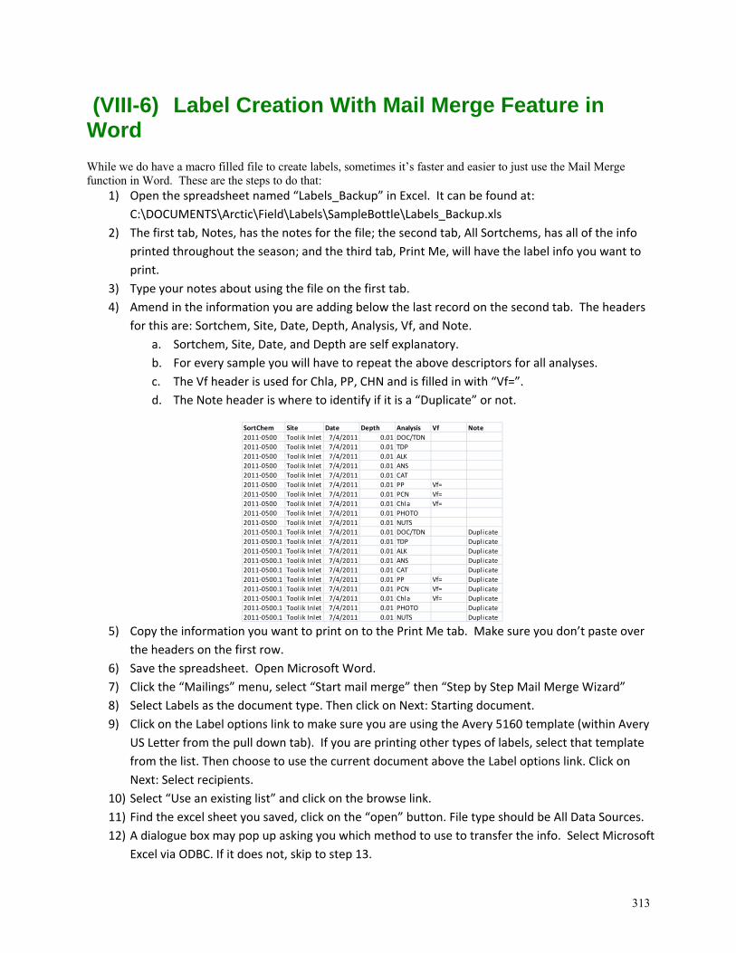
313

(VIII-6) Label Creation With Mail Merge Feature in Word While we do have a macro filled file to create labels, sometimes it’s faster and easier to just use the Mail Merge function in Word. These are the steps to do that:

1) Open the spreadsheet named “Labels_Backup” in Excel. It can be found at:

C:\DOCUMENTS\Arctic\Field\Labels\SampleBottle\Labels_Backup.xls

2) The first tab, Notes, has the notes for the file; the second tab, All Sortchems, has all of the info

printed throughout the season; and the third tab, Print Me, will have the label info you want to

print.

3) Type your notes about using the file on the first tab.

4) Amend in the information you are adding below the last record on the second tab. The headers

for this are: Sortchem, Site, Date, Depth, Analysis, Vf, and Note.

a. Sortchem, Site, Date, and Depth are self explanatory.

b. For every sample you will have to repeat the above descriptors for all analyses.

c. The Vf header is used for Chla, PP, CHN and is filled in with “Vf=”.

d. The Note header is where to identify if it is a “Duplicate” or not.

5) Copy the information you want to print on to the Print Me tab. Make sure you don’t paste over

the headers on the first row.

6) Save the spreadsheet. Open Microsoft Word.

7) Click the “Mailings” menu, select “Start mail merge” then “Step by Step Mail Merge Wizard”

8) Select Labels as the document type. Then click on Next: Starting document.

9) Click on the Label options link to make sure you are using the Avery 5160 template (within Avery

US Letter from the pull down tab). If you are printing other types of labels, select that template

from the list. Then choose to use the current document above the Label options link. Click on

Next: Select recipients.

10) Select “Use an existing list” and click on the browse link.

11) Find the excel sheet you saved, click on the “open” button. File type should be All Data Sources.

12) A dialogue box may pop up asking you which method to use to transfer the info. Select Microsoft

Excel via ODBC. If it does not, skip to step 13.

SortChem Site Date Depth Analysis Vf Note

2011‐0500 Toolik Inlet 7/4/2011 0.01 DOC/TDN

2011‐0500 Toolik Inlet 7/4/2011 0.01 TDP

2011‐0500 Toolik Inlet 7/4/2011 0.01 ALK

2011‐0500 Toolik Inlet 7/4/2011 0.01 ANS

2011‐0500 Toolik Inlet 7/4/2011 0.01 CAT

2011‐0500 Toolik Inlet 7/4/2011 0.01 PP Vf=

2011‐0500 Toolik Inlet 7/4/2011 0.01 PCN Vf=

2011‐0500 Toolik Inlet 7/4/2011 0.01 Chla Vf=

2011‐0500 Toolik Inlet 7/4/2011 0.01 PHOTO

2011‐0500 Toolik Inlet 7/4/2011 0.01 NUTS

2011‐0500.1 Toolik Inlet 7/4/2011 0.01 DOC/TDN Duplicate

2011‐0500.1 Toolik Inlet 7/4/2011 0.01 TDP Duplicate

2011‐0500.1 Toolik Inlet 7/4/2011 0.01 ALK Duplicate

2011‐0500.1 Toolik Inlet 7/4/2011 0.01 ANS Duplicate

2011‐0500.1 Toolik Inlet 7/4/2011 0.01 CAT Duplicate

2011‐0500.1 Toolik Inlet 7/4/2011 0.01 PP Vf= Duplicate

2011‐0500.1 Toolik Inlet 7/4/2011 0.01 PCN Vf= Duplicate

2011‐0500.1 Toolik Inlet 7/4/2011 0.01 Chla Vf= Duplicate

2011‐0500.1 Toolik Inlet 7/4/2011 0.01 PHOTO Duplicate

2011‐0500.1 Toolik Inlet 7/4/2011 0.01 NUTS Duplicate

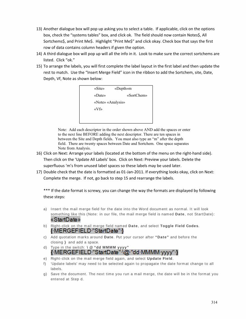
314

13) Another dialogue box will pop up asking you to select a table. If applicable, click on the options

box, check the “systems tables” box, and click ok. The field should now contain Notes$, All

Sortchems$, and Print Me$. Highlight “Print Me$” and click okay. Check box that says the first

row of data contains column headers if given the option.

14) A third dialogue box will pop up will all the info in it. Look to make sure the correct sortchems are

listed. Click “ok.”

15) To arrange the labels, you will first complete the label layout in the first label and then update the

rest to match. Use the “Insert Merge Field” icon in the ribbon to add the Sortchem, site, Date,

Depth, Vf, Note as shown below:

«Site» «Depth»m

«Date» «SortChem»

«Note» «Analysis»

«Vf»

Note: Add each descriptor in the order shown above AND add the spaces or enter to the next line BEFORE adding the next descriptor. There are ten spaces in between the Site and Depth fields. You must also type an “m” after the depth field. There are twenty spaces between Date and Sortchem. One space separates Note from Analysis.

16) Click on Next: Arrange your labels (located at the bottom of the menu on the right‐hand side).

Then click on the ‘Update All Labels’ box. Click on Next: Preview your labels. Delete the

superfluous ‘m’s from unused label spaces so these labels may be used later.

17) Double check that the date is formatted as 01‐Jan‐2011. If everything looks okay, click on Next:

Complete the merge. If not, go back to step 15 and rearrange the labels.

*** If the date format is screwy, you can change the way the formats are displayed by following

these steps:

a) Insert the mail merge field for the date into the Word document as normal. It will look something like this (Note: in our file, the mail merge field is named Date, not StartDate):

b) Right-click on the mail merge field named Date, and select Toggle Field Codes.

c) Add quotation marks around Date. Put your cursor after “Date” and before the

closing } and add a space. d) Type in the switch: \@ “dd MMMM yyyy”

e) Right-click on the mail merge field again, and select Update Field. f) ‘Update labels’ may need to be selected again to propagate the date format change to all

labels. g) Save the document. The next time you run a mail merge, the date will be in the format you

entered at Step d.

315

18) Click on the Edit individual labels to make one final check. A dialogue box may pop up. Choose to

merge all records. Scroll to the end of the document to make sure you aren’t printing any

extraneous labels.

19) Print.

20) These word files do not need to be saved every time new labels are printed. Files only need to be

saved after changing the date format.

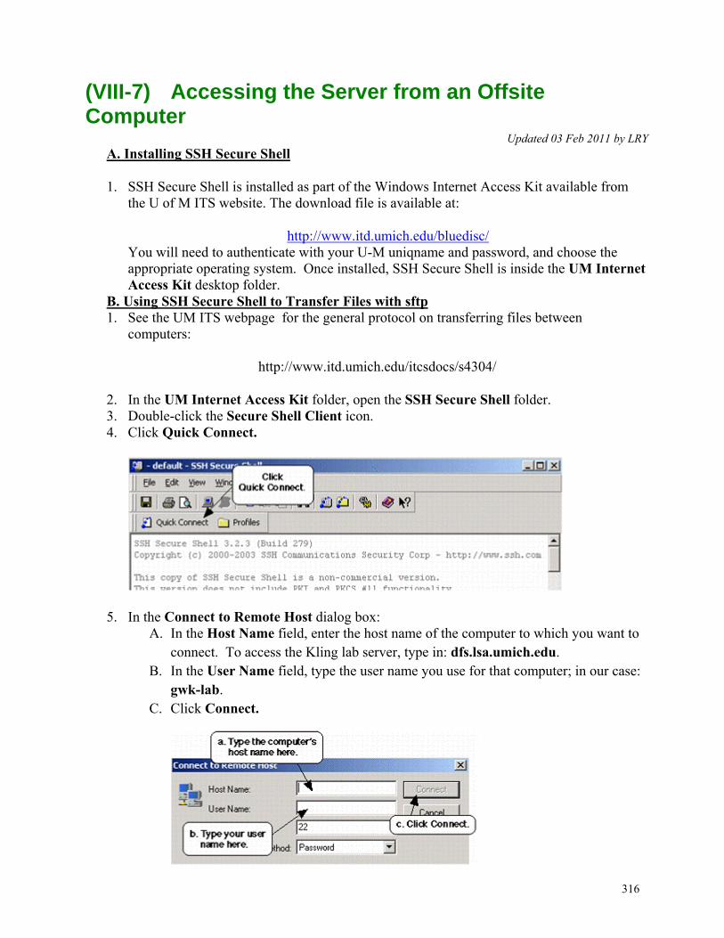
316

(VIII-7) Accessing the Server from an Offsite Computer

Updated 03 Feb 2011 by LRY A. Installing SSH Secure Shell

1. SSH Secure Shell is installed as part of the Windows Internet Access Kit available from the U of M ITS website. The download file is available at:

http://www.itd.umich.edu/bluedisc/ You will need to authenticate with your U-M uniqname and password, and choose the appropriate operating system. Once installed, SSH Secure Shell is inside the UM Internet Access Kit desktop folder.

B. Using SSH Secure Shell to Transfer Files with sftp 1. See the UM ITS webpage for the general protocol on transferring files between

computers:

http://www.itd.umich.edu/itcsdocs/s4304/

2. In the UM Internet Access Kit folder, open the SSH Secure Shell folder. 3. Double-click the Secure Shell Client icon. 4. Click Quick Connect.

5. In the Connect to Remote Host dialog box: A. In the Host Name field, enter the host name of the computer to which you want to

connect. To access the Kling lab server, type in: dfs.lsa.umich.edu. B. In the User Name field, type the user name you use for that computer; in our case:

gwk-lab. C. Click Connect.

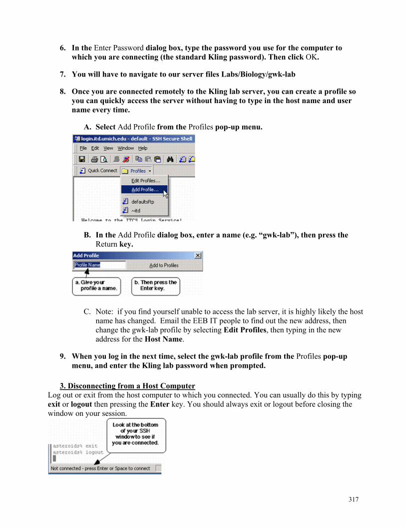
317

6. In the Enter Password dialog box, type the password you use for the computer to which you are connecting (the standard Kling password). Then click OK.

7. You will have to navigate to our server files Labs/Biology/gwk-lab

8. Once you are connected remotely to the Kling lab server, you can create a profile so you can quickly access the server without having to type in the host name and user name every time.

A. Select Add Profile from the Profiles pop-up menu.

B. In the Add Profile dialog box, enter a name (e.g. “gwk-lab”), then press the Return key.

C. Note: if you find yourself unable to access the lab server, it is highly likely the host name has changed. Email the EEB IT people to find out the new address, then change the gwk-lab profile by selecting Edit Profiles, then typing in the new address for the Host Name.

9. When you log in the next time, select the gwk-lab profile from the Profiles pop-up menu, and enter the Kling lab password when prompted.

3. Disconnecting from a Host Computer

Log out or exit from the host computer to which you connected. You can usually do this by typing exit or logout then pressing the Enter key. You should always exit or logout before closing the window on your session.

318

4. Exiting SSH

1. From the File menu, select Exit. 2. If you are using a dial-up connection, be sure to close your modem connection when you

have finished using it.

WARNING! Your computer account will continue to accrue dial-in charges for as long as you have an open dial-up connection to the Internet.

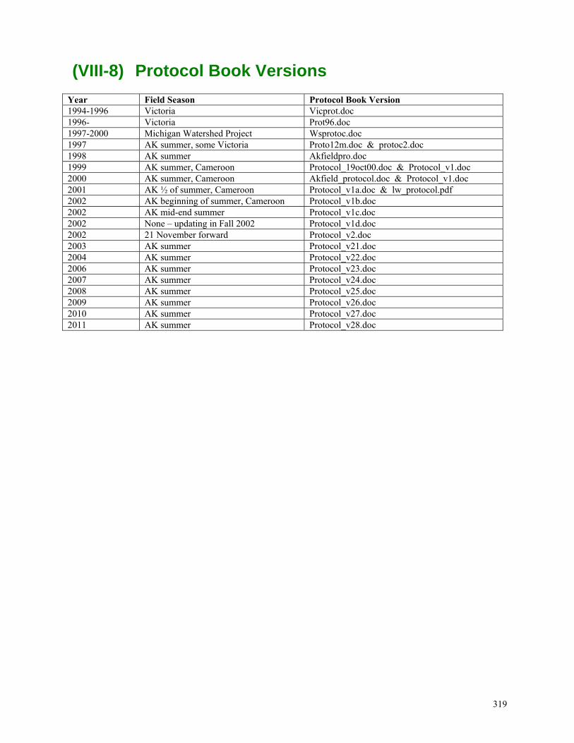
319

(VIII-8) Protocol Book Versions Year Field Season Protocol Book Version 1994-1996 Victoria Vicprot.doc 1996- Victoria Prot96.doc 1997-2000 Michigan Watershed Project Wsprotoc.doc 1997 AK summer, some Victoria Proto12m.doc & protoc2.doc 1998 AK summer Akfieldpro.doc 1999 AK summer, Cameroon Protocol_19oct00.doc & Protocol_v1.doc 2000 AK summer, Cameroon Akfield_protocol.doc & Protocol_v1.doc 2001 AK ½ of summer, Cameroon Protocol_v1a.doc & lw_protocol.pdf 2002 AK beginning of summer, Cameroon Protocol_v1b.doc 2002 AK mid-end summer Protocol_v1c.doc 2002 None – updating in Fall 2002 Protocol_v1d.doc 2002 21 November forward Protocol_v2.doc 2003 AK summer Protocol_v21.doc 2004 AK summer Protocol_v22.doc 2006 AK summer Protocol_v23.doc 2007 AK summer Protocol_v24.doc 2008 AK summer Protocol_v25.doc 2009 AK summer Protocol_v26.doc 2010 AK summer Protocol_v27.doc 2011 AK summer Protocol_v28.doc

320

SECTION IX - OTHER PROJECTS and OLD PROTOCOLS

(IX-1) Michigan - Lake sampling, and Watershed Project

A. Preparation 1. Reserve the department van a week in advance 2. Prepare all gear the day before, follow lists for Alaska, as the kits are the same 3. The morning of sampling, load small filter holders with GF/F combusted filters, and start GC. 4. Before leaving ensure that you have the boat valves and plugs as well as the key to the gate at Third Sister Lake. 5. When sampling Blind Lake, space is limited so prepare accordingly. 6. For Third Sister Lake, follow the same procedure as for Blind Lake, except use the aluminum boat locked up at the

lake, and sample only the main station.

B. Necessary Equipment 1. Inflatable boat, aluminum oars, anchor and rope, boat pump 2. Three one-liter bottles for each sample site and depth 3. 250 mL amber bottle for phytoplankton sampling, and Lugol’s solution 4. pH meter and/or 60 mL BOD bottles for in lab pH determination 5. conductivity meter 6. oxygen meter and probe 7. light meter and sensor 8. chemistry sample bottles (two 60 mL HD bottles for alkalinity and cations, one 30 mL for anions) 9. one loaded filter holder for each site and depth 10. DIC and gas sampling kit, and pH and conductivity. meters (see above, from Alaska sampling) 11. spare filters and holders The main station is sampled first, after rowing out and anchoring: One person begins sampling the surface waters,

while the other begins the oxygen and light profiles. The profile is then sampled at depths 5, 10, 15, and 20 meters with a hand crank peristaltic pump with tygon

tubing. Successful mastery of the three-way stop cocks is necessary for bubble free sampling (i.e., practice before going into the field).

C. Efficient sampling order 1. After tygon is thoroughly rinsed (>75 pump turns with 15m hose), fill 1L sample bottles 2. Sample phytoplankton and add lugols 3. Take water for pH reading (If taking 60 mL BOD bottles for pH, do so now, slowly) 4. Fill 60 mL syringes ( for gas and DIC, these must be bubble free) 5. Use the bubble free for gas equilibration and DIC 6. The remaining syringes are used for alk/cats/ans, using 10 mL for an initial filter rinse, and 5 mL rinse in each

bottle 7. Read the pH meter if stable, and record 8. Repeat sampling for each sample depth, then “Michael, row your boat ashore” 9. Now sample the true inlet and outlet (Due to space constraints in the boat, keep the sample bottles for the Inlet and

Outlet separate and in the van).

D. Phytoplankton Sampling 1. Phytoplankton samples are collected in clean, labeled 250 mL amber plastic bottles. 2. In shallow waters, the bottle is rinsed once with sample water, then filled to the “shoulder”. 3. In deep waters, rinse a tygon tube twice of length sufficient to reach the bottom of the upper mixing layer by

lowering the tube slowly, pinching off the surface end of the tube, retrieving the tube from depth, then releasing

321

the surface end of the tube allowing it to drain. The sample is collected in the same way except that the sample is drained into the collection bottle.

4. In the field, add Lugol’s until the sample is “tea colored” ( ~ 4 mL / 250 mL sample). 5. In the lab, add buffered formalin solution. Either add 1.5 mL to the entire 250 mL, or add 3 drops of formalin after

the settling procedure (described below).

E. Back at the Laboratory 1. Acidify cation samples, and place cation, anion, and alk samples in the cold room. 2. Remove gas syringes from the gas kit, and insure that the stopcocks are dry. 3. Remove and dry all field equipment, and rinse tygon tubing with building DI water. 4. Using vacuum apparatus, filter 2 chlorophyll, PP, and PN from each site on AE filters. from the 1 liter bottles. see

Filtering

F. Sampling Protocols for Michigan Watershed Project-Lysimeter, Surface, and Ground waters

Lysimeter Samples 1. Sampling Lysimeters

There are two types of lysimeters within the Watershed project: A larger, white lysimeter placed in the Pellston Plain (PP) and the Experimental Forest (EF); and a thinner, clear variety found within the microcosm chambers of the CO2 experiment (MC).

The EF and PP lysimeters have a green plastic tube running the length of the lysimeter, from which water is drawn, and a black tube which extends just into the top, and is used for drawing suction and sampling headspace. The ends of the tubes currently have a plastic O-ring which crimps them to hold suction, and a fail-safe stopper (golf tee) in the end.

The MC lysimeters have a thin clear tube running to the base of the lysimeter, and a larger Tygon piece for headspace sampling and vacuum administration. Both ends have a valve which can be combined and manipulated to form a closed system, or a semi-open system for sampling and equilibration bubbling.

a. APPLYING VACUUM -- The lysimeters vacuums should be applied at least the day before sampling, but

not more than three days. EF and PP: Remove the stopper from the end of the black tube and connect the pump. Release the O-ring and pump to ~50 psi vacuum (some gauges read in centibars). Replace the O-ring and remove the pump. MC: Connect the hand pump to the stop-cock (a one-way stop-cock in most cases) of the thicker, Tygon tubing. Ensure that the stop-cock at the end of the thin tubing is closed, and the valve connected to the pump is open. Draw a vacuum, then close the stop-cock, and remove the pump. In some cases, the vacuum on the shallow lysimeters was drawn by pulling one volume of a 60 mL syringe, then closing the valve (this was effective in the Nov-97 sampling, but the actual amount of vacuum was not known).

b. TO MEASURE VACUUM -- Vacuum is to be measured before sampling.

EF and PP: Remove the stopper from the end of the black tube and connect the hand-held pump. Release the O-ring and record the vacuum pressure within the lysimeter. Re-crimp the tube, replace the O-ring, and remove the pump to maintain vacuum. MC: Place the small pump and connection to the top of the lysimeter, open the stop-cock and record the vacuum, re-close the stop-cock and remove the pump

c. TO SAMPLE GASES -- The first sample taken from a lysimeter is a gas sample for dissolved CO2 and CH4.

It is taken from the headspace of the lysimeter after active bubbling. The bubbling serves to equilibrate the dissolved gases within the headspace and water. This is done with micro-pumps which circulate headspace air into the tube leading down to the base of the lysimeter. Pump for four minutes, then let set one minute before taking a headspace sample. Crimp the tubing while disconnecting the pump, and connect both tubes to the three way on a nylon syringe. To ensure that a fresh sample is taken from the headspace, first flush the headspace tube by drawing the “dead headspace” volume within the tubing, and expelling this air into the “water sampling” tube (to not loose sample volume or vacuum). The actual volume to flush depends on the depth of the lysimeter, hence the length of the tubing (5-10 mL in the MC, and 10-20 mL of headspace in the

322

PP and EF). Then take the final headspace sample for GC analysis (7-10 mL within the MC, and 14-20 mL for the PP and EF). To take a sample of appropriate volume against the vacuum, one hand must keep the syringe plunger pulled back, and the other hand turns the three-way, then crimps the hose. Turn the stopcock’s “off” position towards the syringe body and then remove the syringe. (Note that if the lysimeter had a strong remaining vacuum, the gas inside the nylon syringe will be under-pressured and when you release the plunger the volume will decrease). Record the site number, and mark the sample as a lysimeter headspace. (Note: Proper manipulation of the 3-way stopcock is essential for gas sampling - make sure that you practice using the 3-way to avoid release of sample or vacuum).

d. WATER SAMPLE COLLECTION-- Bubble-free lysimeter water should now be sampled from the tube

extending to the bottom of the lysimeter. The bubble-free methodology limits degassing of the sample for a proper DIC sample. MC: connect a clean syringe to the thin tube which extends to the lysimeter base. Pull suction on the syringe until water starts to come into the syringe. When water begins entering the syringe, manipulate the three-way to expel all of the excess air from the syringe. Now release the vacuum on the system and immediately, steadily, but slowly finish drawing up the remaining water. Watch the thin tubing for air bubbles indicating that the lysimeter is dry. Stop taking sample immediately before those bubbles reach the syringe. READ AND RECORD the total volume of sample water within the lysimeter. EF and PP: Use the same procedure as for MC, but attach the syringes directly to the “green” tubing. Keep track of the order of the syringes drawn, and take the DIC from the first syringe.

2. The current method for small volume DIC measurement was developed Nov 97, and is subject to change:

a. Preparing the DIC vials: i. To a five mL volume DIC vial, add 20 �L of Mercuric Chloride and 75 �L of 6 N Sulfuric Acid. ii. Cap the vials with teflon septa and aluminum caps. iii. Tape or label the vials, and remove the center portion the cap. Weigh each bottle (recommended to three

decimal places)--record the weight, and its respective vial number. 3. DIC Field sampling:

Draw a vacuum on the vials in the field using a syringe and a small needle. Carefully stick the needle into the septum, and draw two syringe “volumes” from the vial. After the second volume is taken, keep the syringe plunger pulled back, as you remove the evacuated vial from the needle.

The sample is taken directly from the bubble-free lysimeter sample. Attach a small needle on the end of the three way, and purge the air from the three-way and needle until droplets of sample come from the needle tip.

With the needle tip pointing upwards, place the vial (which is upside down) onto the needle, so the needle tip is just above the surface of the teflon septum. The sample will get “sucked” into the evacuated vial, and the sample water will fill above the needle tip, thereby reducing gas exchange after ambient equilibration. Once the vial is ½ full (about 2 mL), turn the stopcock in a downward position (turning the sample flow off, and allowing a flow path from the ambient air to the vial still containing vacuum.)

The ambient air will bubble into the vial until at pressure equilibrium with the atmosphere. Immediately, pull the needle from the vial, and shake the vial to mix the acid, sample and poison. Keep the samples as cold and dark as possible until the time of analysis, when they should be at room

temperature. 4. Running the DIC samples

The samples have been run on Don Zak’s Gas Chromatograph. A small volume (approx .6 mL) of the DIC headspace gas is extracted with a Hamilton syringe, then turn off the “on/off flow regulator.” The plunger is then depressed to .4 mL. Immediately before a rapid injection in the GC septum and sample loop, the needle valve is opened to equilibrate the pressure within the syringe to 1 atm, and ensure a .4 mL sample injection. The samples are set against standards run within the lab, and entered into the spreadsheet to calculate DIC based on the temperature of running, and the water to headspace ratio. This ratio is determined by weighing the sample before running, and assuming 1 g/ 1mL water. This value is subtracted from an average value of the volume of the vials (determined from an average of 8 vials to be 4.89 mL). The initial headspace CO2 and CH4 concentration will be the ambient values of the site collected.

323

5 Use the remaining water for various chemistry samples, taken by priority basis. DOC’s are the first priority, and should have at least five mL of filtered sample. Samples for pH, ICP, alkalinity, and other EAGL lab analysis will depend on the volume of water available. All samples are filtered and poisoned when appropriate.

6. If there is enough water for a pH measurement, it should be taken immediately after the DIC, because it may

change quickly over time. Use a small amount of sample water to rinse the pH probe, then place the probe in the appropriate sample receptacle. There have been many different sample receptacles for pH reading, including: a clean beaker (with and without stirring have been done); a small “sealable” vial with stir-bar used to limit the effects of degassing, and to limit the amount of sample used; and filling the storage cap of the pH probe with the sample. In all cases, the soil water will degas rapidly and change the pH, so take the reading soon after stabilization.

Surface Water Sampling (Lakes and Streams) 1. PREPARATION -- The pH meter should be calibrated following the procedure below shortly before reaching the

first sample site. Note that these instructions are specifically for the Orion pH meters, but many of the sampling “tips” apply to all instruments.

a. Calibration of pH meter -- there is a checkout procedure and a calibration procedure in the manual that lives in

the pH meter case. The checkout and setup procedures don’t need to be repeated unless you want to change something or the meter is not working. To calibrate with two buffers follow the section on “calibration with 2 or more buffers” (p. 37). Use buffers that bracket the expected sample pH. i. Turn meter on with the ‘power’ button. Use the ‘mode’ button to set to ‘pH.’ ii. Expose the filling hole on the probe body by moving the rubber band downward (note: There are two

types of pH probes currently used by the Kling lab. One uses a refillable liquid and has a open hole, which this protocol is written for. The other lacks a hole, and is completely submersible--when using this probe, ignore protocol written for the other).

iii. Remove the probe cap and rinse the probe tip with DI to remove storage solution. Place the probe in pH 7 buffer and change the meter to mV scale. When the probe has a stable mV reading it is ready for calibration. This step is not necessary if you are recalibrating in the field, only if the probe has been stored in storage solution.

iv. Return to pH mode on the meter. If you are calibrating with beakers in the lab or van then start by rinsing the probe tip with pH 7 buffer, then adding pH 7 buffer to a clean beaker and placing the beaker on a stir plate. If you are calibrating in the field, add pH 7 buffer to the probe cap and replace the cap loosely on the probe. Gently shake the probe to rinse the probe tip. Remove the cap and repeat. Add a little buffer to the cap again and push the cap all the way onto the probe. Now the probe is ready for the first calibration step. NOTE that the meter can only be calibrated after all buffers and probes have come to equilibrium with the field or lab temperature. Because field temperatures often change rapidly, it is better to calibrate the meter in the lab where everything was stored the previous night and is already at a stable temperature. NOTE also that the probe should be calibrated according to the field measurement conditions; that is, if you don’t stir the samples in the field, or place them in moving water, don’t stir them for the calibration.

v. Press the ‘2nd’ then the ‘calibrate’ button and the meter will display a pH reading and ‘P1’ at the bottom of the screen. When the reading is stable it will display ‘ready’. Now press the arrow-down button until the left digit of the pH reading is flashing. Set the correct number with the up and down arrows. If the reading is correct (for example, if it reads ‘7’) then press the ‘yes’ button. This will move the flashing digit to the right, and you can set that value in the same way. Once all three digits are set the meter will display ‘P2’ (it now is ready for the second calibration buffer).

vi. Remove the probe cap and rinse with the second buffer (4 or 10) as in step #3. Adjust the reading to the proper pH as in step #4. When you hit the ‘yes’ button for the final time the meter will display the slope of the line between the two buffers. If the slope is less than 90 the probe should be reconditioned. The meter will automatically switch from ‘calibrate’ to ‘measure’ and it is now ready for a sample.

vii. After calibration, fill the probe cap with DI water or sample water so that the probe can begin to equilibrate with the low ionic strength solution that will be similar to the field samples.

2. SAMPLING -- The following sampling order has proven most time efficient. Remember to write down the date

and the weather conditions for that day and the previous days, as well as any unusual conditions. Once a sample site is reached it is best if two people work independently on the following tasks:

324

A. PERSON #1 - pH, DIC, Gas, temperature, and conductivity

i. pH measurement -- Place the pH probe tip in the water at the site and allow to equilibrate. Submerse the probe tip early in the sampling period and read the final value at the end of the sampling period. Note that if the pH meter has just been turned on then it takes a while to stabilize. Make sure that the probe is in non-stagnant water, but not in a “fast flowing” section, and that the probe “hole” is not submersed (a gel probe may be used, which does not have a hole, and can be submersed completely). The EAGL lab may prefer to measure pH from a large sample bottle placed on a stir plate. Also place the conductivity probe tip in the water.

IF YOU CANNOT TAKE A pH MEASUREMENT IN THE FIELD, THEN --

a) In the field, fill two 60 mL BOD bottles with sample from each sampling station. Fill slowly from the bottom to avoid air contamination using either a hand pump with Tygon tubing, or an air-free syringe with a Tygon end. Overfill the bottle with at least 1 bottle volume (2 if possible), replace stopper. Keep BOD bottle cool and dark.

b) In the lab, allow the BOD bottles to reach room temperature (keep them in the dark). Use a small stir bar and magnetic stirrer in the BOD bottle.

c) Place the pH probe into the first BOD bottle and let the probe equilibrate (10-15 minutes). d) After equilibration, place the stir bar and probe into the second BOD bottle. Allow the reading to

stabilize (usually 3-5 minutes), and record the pH value and the temperature. * NOTE: The probe tip may collect small air bubbles from the stirring action. If this happens, wait until the

reading stabilizes and then gently shake or stir the probe tip to remove the bubbles. Record the pH of the sample when bubbles have been removed (it is usually the same).

ii. GAS and DIC sample water collection.

a) Fill two 140mL syringes with bubble free water. Place one of the syringes back into the water to keep it

at temperature -- this will be used for a DIC. b) Expel water from one of the bubble-free syringes until 110 mL remains. Hold into the wind and draw in

30 mL of ambient air. Equilibrate by shaking for two minutes in the water to maintain the original temperature. Let set for one minute in the water, then transfer the headspace gas into a nylon syringe (see below). Take an ambient air sample. Record the syringe numbers, and water temperature.

c) TRANSFER THE GAS SAMPLE i) Make sure that no water is trapped in the syringe stopcock. ii) Break the “seal” (stiffness) on a nylon syringe by moving the plunger back and forth. Keep about

10 mL of air in the syringe to flush the 3-way stopcock before sampling the gas from the sample syringe. The the valve on the nylon syringe should be closed.

iii) Insert the tip of the nylon syringe valve into the side vent of the 3-way valve on the sample syringe; hold the sample syringe vertically so that the nylon syringe is perpendicular to it.

iv) Open the nylon syringe valve (90° CCW) and flush the 3-way valve by expelling all the gas in the nylon syringe.

v) Apply slight pressure to the sample syringe plunger and turn the valve (180° CCW) from close to open quickly, there should be a slight puff of air.

vi) Then transfer a small amount of gas (1-2 mL) from the 60mL sample syringe to the nylon syringe. vii) Turn the nylon syringe 90° CCW and then expel the gas to flush-out the syringe tip and valve. viii) Turn the nylon syringe 90° CW. ix) Transfer the remaining gas from the sample to the nylon syringe, making sure that NO WATER is

transferred. x) Close the nylon syringe valve (90° CW) immediately. Apply slight pressure to the nylon syringe

plunger and place a rubber band around the valve and plunger. xi) Note that in operating these valves it takes two hands, one to support the valve itself and one to turn

the handle. The transferring of the gas sample should not take more then 30 seconds. xii) Once the gas sample is secure, remove the plunger from the end of the 60mL syringe then close the

sample syringe valve (180° CW). Place a temperature probe into the water and record the temperature of the water. This is the gas equilibration temperature and should be taken as soon as possible.

325

xiii) At each location or sampling site, take at least one air sample in a nylon syringe (again, hold the syringe away from you and into the wind) so that we can calculate the amount of CO2 initially present in the headspace before equilibration with the water.

xiv) Make note of the date, sample location, depth, and syringe number for each sample. xv) This “left-over” water can then be used for other analytical purposes, which would not be affected

by the gas-stripping methodology (not any carbon species samples).

d) Take a DIC sample using the other bubble free syringe (see below). The EAGL lab may also sample a “sigma CO2 ”, which is not filtered. i) Label the proper glass bottle (20 or 30 mL for surface waters) with date, station, depth. ii) Have the poison (saturated HgCl2), caps, and crimpers ready to go. iii) Use the bubble-free syringe to fill the DIC vial--filling slowly along the sides to reduce degassing.

Overfill the bottle with at least twice the bottle volume of sample. Make sure that the bottle has a positive meniscus of water above the bottle rim. (Note: EAGL lab generally filters this water; make sure that the filter is free of air bubbles, and that there is enough bubble free sample water to both saturate the filter and overfill the bottle.)

iv) Add 0.1 mL HgCl2 per 10 mL of sample; carefully place cap/septum on; and clamp.

iii. Measure and record the conductivity, temperature, and check for pH meter stabilization. (Note: The pH meter may take longer to completely equilibrate at the first site, but should be relatively quick after that.) Record the pH when stable.

B. PERSON #2 - filtering for water and particulate samples, DOC

i. Fill a two liter beaker or bottle with representative sample water, and return to the vehicle for filtering. ii. FILTER -- label all bottles with site and date before starting to filter. Rinse the filter initially with at least

20-30 mL of sample water. Fill each bottle individually and cap the bottle when finished before moving on to the next bottle. Do not apply excessive force to the filter as it becomes clogged; it is best to use a new filter.

iii. Prepare a particulate filter for CHN analysis. Sample water is passed through a 25mm ashed (450C for 2 hours), GF/F filter. At least 360 mL of sample should be passed through the filter. The filter is removed with forceps and placed in a disposable petri dish. Label the dish and record the volume filtered. Rinse the filter cartridge with DI water between sample sites. The filters are placed in a drying oven upon returning to the lab.

iv. Prepare DOC samples -- filter 20 mL of water into a 20 mL glass scintillation vial for a DOC sample. This should be done using the filtrate of the particulate filter.

v. Acidify or preserve samples. DOC samples are acidified with 1 �L of 6N HCl per mL of sample. Cation samples are preserved with nitric acid. All samples should be kept cold and dark. When sampling stream sites at culverts, always sample the upstream side of the road.

3. Groundwater sampling

Groundwater sampling proceeds exactly as the surface water sampling described above, except that the well water is monitored initially for temperature to make sure that we are sampling true groundwater and not water that was held in a storage tank. These storage tanks can be pretty large, and it may take many minutes for the tank to be drawn down and the temperature of the water coming directly from the ground and not the tank to stabilize. Once the temperature has stabilized, sampling proceeds following the surface water sampling.

326

(IX-2) Field Sampling and Processing for Lake Victoria

A. Packing List for Field 1. PCO2 and DIC Box

a. Instructions for sampling b. several 30 mL nylon syringes fitted with 2-way nylon valves c. rubber bands d. 3 or 4 60 mL plastic syringes fitted with 3-way valves e. 2 (at least) hose connectors for sampling from the van Dorn into the syringes, these also have 3-way valves

attached. f. extra 3-way valves g. solution of saturated mercuric chloride (HgCl2) h. 1 mL syringes and 18 G needle for injecting mercuric chloride i. serum vials for DIC, with label tape on them j. serum stoppers (Teflon stoppers with aluminum caps) k. cap crimper l. Sharpie marker m. pencil n. Whirlpacks

2 Filtration Box

a. Instructions for filtering b. Aluminum foil for filters c. 1 box of GF/F filters (precombusted) 4.7 cm diameter d. 1 box of GF/F filters (precombusted) 2.5 cm diameter e. 60 mL syringe with 3-way valve for measuring water (you can use the ones from the DIC kit if you need

more) f. 5 large Swinnex filter holders g. 12 small Swinnex filter holders h. 2 pairs of forceps i. petri dishes (for silica gel and chlorophyll filters) j. Aluminum foil for petri dishes k. small bottle of 6N HCl for preserving filtered water for nutrient analysis if necessary l. Sharpie Marker m. pencil n. label tape o. Field Book

3. Nalgene Bottles (with label tape on them)

For each depth sampled you need: a. 3-30 OR 60 mL bottles for filtered water: 1 for cations, 1 for anions and 1 for alkalinity (Note the volume for

the alkalinity samples since you titrate them directly in this bottle) b. 1-250 mL dark bottle for filtered water c. 1-500 mL dark bottle for unfiltered water d. 1-1L dark bottle for unfiltered water (this is the container from which you take the water for filtering)

4. CTD Box

a. CTD b. 2-500 mL bottles of DI water c. small wrench for shackle d. instructions

5. Other required equipment:

a. CTD line b. CTD buoys or foam for descent control c. computer (optional, but take it if many casts are to be made and the CTD might run out of memory)

327

d. CTD log book (or Ecosystems Program Field book) e. Magellan GPS and extra battery pack f. Bottom Line Depth Finder (especially in new transect) g. Secchi disk

B. Field Sampling - Chemistry and Physics ** Order of work: One person should get the hydrolab ready as the station is being approached. Keep the cap on the

sensors until the ship is anchored. Remove the cap, screw on the stirrer, and submerse the probe in water so it can begin to equilibrate.

1. Chemistry * For each depth do the following in this order:

a. Take the PCO2 samples (see sampling protocol) b. Take DIC samples (see sampling protocol) c. Rinse and then fill one 500 mL bottle and one 1 L bottle with unfiltered water. d. Save the 500 mL bottle for lab analyses requiring unfiltered water. This water is used for other analyses (Si,

TN, and TP). e. Water will then be filtered from the 1 L bottles into 4 bottles as follows: 1-60 mL bottle, labeled for alkalinity (the accurate volume filtered into this bottle must be recorded). 1-60 mL bottle, labeled for cations 1-60 mL bottle, labeled for anions 1-250 mL bottle, labeled as filtered water to be used for lab analyses.

* Note that each bottle must be labeled with Site, date, depth, alk (or whatever) and whether it is filtered (F) or unfiltered (UF) or acidified (for example, F-HCl means filtered with HCl added).

f. The filters: 2-25 mm filters and 1-47 mm filter are kept and the volumes noted on the foil packets. These are put in the drying oven at 40 degrees C upon return from the field. The water samples kept dark and cool and then refrigerated upon return from the field.

To filter: There are several numbered Swinnex filter holders in the field boxes. These can be preloaded with GF/F filters not more than 1-2 hours prior to filtering. For each depth you will need 2-25 mm filters and 1-47 mm filter.

a. Using the 60 mL BD syringe withdraw 60 mL of water from the 1 L bottle containing the unfiltered water. b. Attach one of the small Swinnex filters to the syringe so that the label that says “Millipore Swinnex” is next

to the syringe. c. Rinse each of the bottles EXCEPT the alkalinity bottles with about 20 mL of water. d. Remove the filter holder and refill the 60 mL syringe. Filter the next 60 mL through the filter into one of the

appropriate bottles. By this time 120 mL has been filtered through the first filter. e. Change to the second small filter holder and fill the other two 60 mL bottles the same way. f. Using the large filter holder (47 mm filter) fill the 250 or 500 mL bottle with filtered water. Keep track of

the amount of water that is passed through the filter. You can get at least 240 mL and more frequently 300 mL through the large filter. 240 mL is just enough for replicates of these three nutrients; the remaining water should be used for TDN and TDP. If more water is needed to run these TDN and TDP analyses then filter more into the 500 mL bottle.

* When you are finished with one depth there should be 4 bottles of filtered water and 3 filters. Put the two small filters into separate foil packets that are labeled with date, site, depth, and amount filtered. Using the 2 forceps carefully fold the filters in half, making sure not to touch them with anything except the forceps. Put the large filter into a petri dish with drierite and label with date, site, depth, and amount filtered (this filter is for Chla and should be stored immediately in the dark).

Filters for Stable Isotope Measurements In some instances filters will be collected for stable isotope measurements of particulate organic material. We use pre-ignited quartz filters (ignited at 550 C for 4 hours; Whatman QM/A). The water filtered through these filters should not be used for any chemical analyses. Filter at least 240 mL through the filter, although the more material on the filter, the easier it will be to analyze. Fold the filter in half and store in a foil packet with the appropriate label. Dry as per usual filters and store at 40 C. 2. Physics - CTD, Light meter, Secchi disc, and Hydrolab

a. CTD:

328

i. Equipment needed: - CTD - CTD line - CTD foam for descent control (hopefully arrives Dec. ‘94) - DI water - computer (optional, but take if many casts to be made) - CTD log book (or Ecosystems Program Field book) - Magellan GPS - Bottom Line Depth Finder (especially in new transect) - Secchi disk ii. Pre-Checklist - download and initialize CTD prior to field trip (check status for battery power) - portable computer battery charged - sufficient DI water

b. Field sampling - taking a CTD cast NOTE: Between any field or air cast allow at least one minute before turning on the CTD again

i. take an air cast at the maximum within 30 minutes of any cast (turn on for about 20 to 30 seconds) ii. prior to a cast, make sure the DI conductivity storage tube has been removed and the pump tube

connected iii. turn on the CTD and place into the water, note the time CTD turned on and record in logbook iv. wait about 1 minute (at least 40 seconds) and bring CTD up to the ON/OFF switch and slowly, evenly,

and smoothly lower CTD. Until arrival of good CTD foam to control buoyancy attempt to lower at a rate of at most 0.5 m/s. However, if a strong surface current due to wind then 0.5 to 0.75 m/s OK.

v. bring up the CTD as quickly as possible, turn off the ON/OFF switch. THAT’S IT! vi. Information to be included in the CTD log entries: time, cast # (first cast is 0), station, weather (wind,

cloud, temperature), wave state (glass, height of waves (cm), white caps, etc.) ** NOTE: if new station, record GPS coordinates and depth from BOTTOMLINE Depth sounder. GPS from

Magellan, establish waypoint, record in GPS log book. c. Downloading and Processing Protocol

NOTE: * ALL SEA-BIRD PROGRAMS RUN IN DIRECTORY C:\SEASOFT * ALL CUSTOM (made by JOSE) PROGRAMS RUN IN DIRECTORY

C:\SEASOFT\CTDPROG * Commands for using XtreeGold (XTG) in general work for either the DOS or Windows XTG versions

i. Connect cable from CTD I/O port to computer COM port. ii. Go to directory SEASOFT. iii. Type ‘term19’ at the prompt.

Press F3 to check status of the CTD: (a) Check for accuracy of date and time (see page 9 in manual if need to change) (b) Check for the battery voltage which is VMAIN and must be above the minimum of 5.8 Volts (note

this is also given in status report). If voltage is below 6.5 Volts change the batteries. iv. Press F9 to upload the data.

A prompt for a filename is given. Use a three letter code for the month and 2 digits for the day; e.g. aug21 for august 21. After entering this filename the computer uploads data from the CTD with that prefix and sequentially numbers the profiles using the last two characters starting with 00. * After upload is complete press F10 to exit program term19.

v. Type ‘XTG’ (xtree gold) at the prompt. * Split the screen with F8. * Press F and type “*.hex”. This will choose all the CTD hexadecimal files using the filespec

command. * Compare the uploaded computer data with the log of CTD casts made in the field. If there is a

discrepancy in the number of casts between the two, rectify. Note that the HEX files have headers which give the time and date at which the cast was made. Use this.

vi. To separate aircasts from the water profiles: (a) There is a directory labeled “HEX” which is where all of the water casts hex files will be stored.

Also under “HEX” is a subdirectory entitle “AIRCASTS” which is where all of the aircasts hex files will be stored:

329

(b) While you are still in XTG tag all of the aircast files. This is done by pressing “t” beside each file that is an aircast. You will need to look in the log book to match up the files. You then move them to the “AIRCASTS” subdirectory by pressing “CTRL M”. This will move all of the tagged files at one time. Using the F2 key to ‘point’ indicate the directory you want to move these files to. (AIRCASTS)

(c) The remaining HEX files should be water column profiles; copy them to the HEX directory. “CTRL T” will tag all of the remaining *.hex files and “CTRL C” can then be used to copy them to the HEX directory.

vii. Quality Control - Water Profiles and Air Casts You should still have a copy of the water profile HEX files in the “SEASOFT” directory. If you don’t, then they should be copied back to that directory. Water Profiles

(a) Exit xtg (press ‘q’). (b) Get to \seasoft directory. (c) Type seasave which is a graphics program to look at HEX profiles. (d) If inshore work use Buv-Pilk.DSP (display configuration) or if deep water use (Bugaia.DSP) or

custom make your own. The configuration file is always VICTORIA.CON which should never change.

(e) Select a file to view in the top line by pressing “enter” to choose the file. (f) Press F10 to view, a plot appears. Press <CTRL> F1 to exit plot. (g) Press ENTER when file is highlighted and use direction arrows to choose next profile to view.

Check all profiles. (h) If all profiles have no anomalies. If have anomalies, such as no profile plotted (probably an air

cast and check air casts made at a similar time to see if it is a water profile), if have spurious points in the profile there may have been a data transfer error, try to re-upload the profiles and check the spurious ones to see if corrected.

(i) Clear all HEX profiles from directory SEASOFT by going back to “XTG”. (j) Again use F (filespec) to choose only the *.HEX files. “CTRL T” is used to tag all of the files

and “CTRL D” will delete all of the tagged files. Air Casts

(a) Copy all aircasts to directory SEASOFT with XTG. (b) Exit XTG and type ‘datcnv’ at the seasoft prompt. Make sure that configuration file is

Victoria.con and that the ‘both upcast and downcast’ option is used. (c) Press ‘ESC’ to exit datcnv. (d) Type ‘datcnv -ax’ (space between v and -) and all of the HEX files in the directory are

converted to ASCII. (e) In XTG use the editor (press ‘V’ to view a file) and scroll through all the aircasts which should

contain values between approximately -0.9 and -1.5 for the air pressure. These ASCII files will have the extension *.CNV.

viii. Saving data and ending (a) IF EVERYTHING IS OK MAKE COPIES OF THE HEX PROFILES TO AT LEAST TWO

FLOPPIES. (b) Then type ‘term19’ at the seasoft prompt (c) Press F8 to initialize the CTD, you are prompted if you are sure you would like to do this potentially

very sorrowful act. Be sure that you are. Hit ‘y’ and the data in the CTD is zapped away (alas). (d) Term 19 automatically exits after this action. Type term19 again to make sure that you have

initialized the CTD (i.e. no casts and all free data space). ix. If any questions, consult the two manuals as they are both actually quite decent. x. Rename all the casts as appropriate and enter into the LOTUS 123 worksheet CTDLOG.WK3 (The

CTD LOG also contains the atmospheric pressure measurements which you will enter after the next step when you convert the hexadecimal files (*.HEX) to ASCII files (*.CNV).) This requires that if not a regularly sampled station (i.e. not a fixed station give GPS coordinate, time, date, weather and condition notes).

FOR ADVANCED PROCESSING SEE BELOW: xi. Run ‘DATCNV’ with the “downcast only” option for water column profiles.

Run ‘DATCNV’ with the “up and down cast” option for air casts.

330

NOTE #1: If you type ‘datcnv -ax’ the -ax switch will convert all the *.HEX which is in the C:\SEASOFT directory to *.CNV files automatically, in the manner that the DATCNV option is configured at the time of the command. Therefore for air casts, run DATCNV to make sure or change the option to “up and down cast”, and similarly if converting water column casts make sure or change option to “down cast only”.

NOTE #2: The -ax switch after any of the commands below result in all input files with the appropriate extension having the file operation performed on them which are in the directory C:\SEASOFT.

xii. Put the aircast *.CNV files in the appropriate directory. Update the CTDLOG.WK3 123 (in

C:\SEASOFT\CTDPROG\INF) worksheet by entering the appropriate air casts. (NOTE: I choose the aircast as the predominant pressure recorded, there is usually a bit of atmospheric pressure fluctuation). After the aircasts have been placed in the aircast directory and atmospheric pressures transferred to the CTD log, the aircasts are no longer used. Print out the last page of the CTD log to keep the most recent version with you. Update the file FILEINFO.WK3 (in the same directory as CTDLOG) which basically asks for the same information. The final column ‘distance’ is for transects that are made and if it is just routine sampling enter a zero in the final column. This information is used for running all the custom programs (prescorr.for, ctdgroup.for, surfrctd.for, profoffs.for). Make an ASCII file from the new casts added to correct for pressure (call it something with the extension *.INF which stands for CTD INFO FILE).

xiii. Two more operations must be run on the water column *.CNV files. Run ‘filter -ax’ which forces the response function of the conductivity sensor to match the response function of the temperature sensor. Then run ‘alignctd -ax’ which advances the temperature relative to pressure 0.5 sec since the time constant (i.e. the time for the thermistor to record the ambient temperature) is of order 0.5 sec. (NOTE: if you now view the header of the *.CNV file you will see that the filter and alignctd tasks have been added to the header). Now transfer the *.CNV water column files to the appropriate directory.

xiv. Run ‘asciiout -ax’ on the *.CNV water column files which simply gets rid of all the header info and prepares the casts for the program prescorr.for. Put *.ASC in directory. Transfer *.ASC to directory CTDPROGS.

xv. Run custom program ‘prescorr’ (in c:\seasoft\ctdprog\) and you will be prompted for the *.INF info file you created in step 5 (make sure the *.INF file was transferred from c:\seasoft\ctdprog\inf to c:\seasoft\ctdprog\). The CTD casts are now corrected for pressure and have the extension *.PRS. Save files to PRS directory and also copy *.PRS files to the SEASOFT directory and rename extension from *.PRS to *.ASC.

xvi. Run ‘asciiin -ax’ on the *.ASC files which gives the files a header which is required to run the next processing step derive. Run ‘derive -ax’ which determines the depth in meters, the salinity, and the density. Rename the *.CNV files after derive to *.PRF short for profiles. Put in the appropriate directory. The remaining programs are all custom programs and are explained below and they run solely with the info files (*.inf) and the complete water column profiles (*.PRF).

d. Light meter

A Li-Cor Spherical Quantum Sensor (4-pi) is presently being used, and there is a 2-pi sensor to be used as backup. Note that while taking a light reading the cloud cover should remain the same. If cloudiness changes during the light profile then the profile must be started again. Alternatively you can set-up the meter so that it uses the 2-pi sensor at the surface and takes a differential reading with the 4-pi sensor at depth. Weight should be attached to the sensor frame so that the cable hangs vertical in the water. * Record the time of day, the weather conditions and the type of clouds, and describe the waves on the

water surface (height of waves, glassy, whitecaps, etc.)

c. Secchi disc A Secchi disc measurement is routinely taken, but is most especially required for any CTD measurements

and primary productivity measurements. Sufficient weight should be attached to the Secchi disc so that the disc is not suspended at an angle. Note that if sunglasses are worn there should be a second reading made without sunglasses for comparison.

* Record the time of day, the weather conditions and the type of clouds, and describe the waves on the water

surface (height of waves, glassy, whitecaps, etc.), and whether sunglasses were worn. All “new” secchi readers should be field calibrated to Moses, the master reader.

331

d. Hydrolab sampling Prior to each field trip the Hydrolab is checked and calibrated for temperature, pH, and DO as described in

the instruction manual. Depth is zeroed on site. Oxygen samples should be taken for Winkler titrations for cross comparisons with the Hydrolab meter. The most stable variables, such as conductivity, should be read and recorded first at each depth, followed by the variables such as oxygen that take a long time to come to equilibrium. * Note that the Redox measurement is not routinely used, although we do record the value. * The order of variables measured is usually: Depth, Redox, Conductivity, Temperature, pH, Oxygen. * Note that the time spent allowing for the probes to come to equilibrium at the new depth is dependent on

how much the variable of interest has changed since the last depth reading. For example, if you in the upper water column, oxygen levels will not change very much with depth, and so the time spent waiting for equilibration can be shortened. If, however, you are at the chemocline or thermocline, then usually all of the variables will be changing rapidly with depth and you will need to wait longer for the readings to reach equilibrium.

* Note that you if you are particularly interested in a variable you should return to that setting on the Hydrolab and take a final reading just before moving to the next depth.

C. Returning From the Field 1. The unfiltered water and filtered water should be refrigerated (filtered water has priority). Ammonium samples

should be dealt with immediately (note that letting the sample sit too long after the reagents have been added may decrease the reliability of the test).

2. 1 L of 6 N HCl is added for every 1 mL of sample in the cation bottle (so about 60 L total). Note that the water for DOC analyses will be taken out of the cation bottle.

3. Put the filters in foil packets in the drying oven at 40 C upon return from the field. Make sure that there is a sign on the oven door asking other users not to increase the temperature!

4. Open all boxes and meters to let the hydrolab, light meter, ropes, etc. dry out. Mold and wet connections are a problem in the tropics. We need to make sure everything is dry. You can also put the meters (not the probes) in a drying oven at low heat between 25-35 C (always less than 40 C max).

332

(IX-3) OLD PROTOCOLS (all projects) OLD PROTOCOLS – DO NOT USE!

A. Old protocols no longer used at Toolik

1. Start-Up

WATERING PLOT EXPERIMENT 1. Preparing the pump engine. The engine is stored inside near the front of the Kling conex box. It does not have gas or oil, so

you must add oil and gas. It takes regular gas (i.e. not an oil/gas mixture as it mixes internally). Look inside the gas tank to make sure that it is not filled with sediment. If needed, rinse it out with gas (or with water followed by alcohol). Check the spark plug and replace the spark plug with a new one if needed. Test start the engine and let it run for at least 5 min (in camp). If engine does not work, check for crud at the bottom of the float valve which keeps the float from seating, so gas keeps flowing and floods the engine (requires taking everything apart which is difficult – find somebody who knows small engine repair). Mid-year, check for water in the gas and float.

2. Check the fish tote (These used to be 6 roughneck trash cans) left at the site. Stretch the watering hose (black with holes in it – should be stored in the fish tote) in an “S” shape above the experimental watering plot labeled W1-W6 (i.e., not over the control plots!! Watering plot is immediately to the left of the center boardwalk looking at the lake). Fish tote should be filled every third day. As needed, repair liner around the top edge of fish tote with duck tape.

3. Connecting the pump. This is a two-person job. Bring a large pipe wrench (just in case), the PVC cleaner and adhesive (if repairing), tarpaulin (to contain cleaner/adhesive), and two walkie-talkies. Use a boat to bring the pump over to location. Place pump next to the lake on the pallet on top of the heavy yellow containment tarp (the pallet and tarp are on a small hill above the lake — move it closer to the lake edge). The yellow containment unit is there to catch any oil or gas and prevent it from entering the lake and is a BLM requirement. Place the pump so that the port labeled ‘suction’ faces North and the port labeled ‘discharge’ faces the hill (it will be connected to the tubing going up to the plots). The two pipe pieces you will need are just above the pump on the little hill. The piece with the right angle bend on one end connects onto the ‘suction’ port and the filter end of the pipe lays submerged at the edge of the lake. The other piece of pipe connects to the port labeled ‘discharge’ and connects to the tubing uphill from the pump. The yellow tarpaulin goes over the pump when it is not in use to prevent rusting.

4. Starting and priming the pump. Send one person up the hill with one walkie-talkie. When the person arrives at the top, start the engine. To start the engine, turn the metal On/Off switch below the gas tank to “on”, turn the choke (round red metal dial on uphill side of pump) on, turn throttle (the silver metal lever on the top of the engine) to middle, pull the handled-cord until the engine turns over and then turn choke off quickly. If this does not work, try moving the choke to different positions. Let pump warm up for a couple of minutes and then turn throttle to low. After the engine is running you need to prime the pump. The priming uses the exhaust system to create a suction to get the water from the lake to the pump. Move the yellow lever (located near the suction port) to horizontal and then close the exhaust pipe with the handle for ~10 seconds. In the priming of the pump, water will spit out at you with a loud noise while you are holding the exhaust pipe closed. When primed, release the exhaust pipe lever and return the yellow lever to its vertical position. If the pump doesn’t prime on the first try you may need to try this priming procedure several times and possibly closing the exhaust pipe for a longer period. Once the pump is primed, check with the uphill person - the water should arrive there in a minute or so. The pressure should be >60 psi or the pump may not work.

5. Filling the fish tote. Fill the fish tote. It takes ~24.538 minutes to fill the fish tote (note that I have not verified this – gwk). When the fish tote is full, have the uphill person call down to the person at the pump to turn it off. Turn the pump switch below the gas tank to “off”. When the pump has cooled, cover it with the yellow tarpaulin and place rocks at edges so it does not blow off. If you cover the pump while it is hot it will burn holes in the yellow tarp.

6. Fixing leaks. Often the pump is clearly pumping, but water is not reaching the top of the hill. With the pump running, have the person at the top walk back down the hill along the pipe to check for leaks. Mark them and then shut the pump off and repair the leak. The fixed joint can be tested again in ~10 minutes in order to find the next leak in the pipe. You do not have to wait overnight before turning the pump back on to check for more leaks.

2. Shut-Down

OLD PROTOCOLS – DO NOT USE!

WATERING PLOT EXPERIMENT 1. Bring pipe wrenches and two people and two walkie-talkies. 2. Disconnect hoses and put them in the fish tote. Leave them at the site (according to Amanda or Chris’ ructions). 3. Run the pump engine out of fuel or siphon fuel out. 4. Unhook the coupler HALFWAY UP THE HILL first (there may be more than one coupler on the pipe), and then uncouple the

pipe at the bottom next to the pump. Let pipe water drain and then unscrew from pump with pipe wrench.

333

5. Unscrew the pipe going to the lake and place both pipe sections up on the hill (in a place that looks safe from rolling etc.). Do

not cut the pipes! 6. Carry the engine to outside the lab and drain the oil by unscrewing the square-headed screws on the very bottom of the engine

block (there is one on each side just above the hole in the framing), collect oil in pan (ask Scott for help and about oil disposal). Ask the camp staff where you can dispose of the used oil.

7. Put the engine inside the camp’s CONEX box (ask Scott or Chad for help) and cover with tarpaulin.

CLIMATE STATION – LEAVING ANCHORS IN THE LAKE In past years the anchors and the lines have stayed out in the lake over winter, but the lines need to be attached to a buoy and the buoy sunk ~3m under the surface with an anchor. Sinking the float keeps it out of the depth range that will be frozen in the winter. If you sink the float, use the depth finder and an appropriate length of rope (depth is around 20m at Toolik Main station). Connect the rope to the buoy and then connect the three anchor ropes to the buoy as well. Drop the weight and check that the buoy is ~3 m below the lake surface. The ice won’t be 3 m thick, but, the lake level can drop considerably at the end of the year. Retrieving Anchors left in the Lake. If the anchors were kept in the lake over winter, first find the orange buoy sunk ~3m deep about 50m to the NE of Toolik Main; hopefully you will have a GPS coordinate, but otherwise you can line up the stakes on land. Retrieve the buoy, anchor, and three attached ropes. Put small buoys on each of the three ropes, and take the big orange buoy, its rope and its anchor back to camp.

B. Oxygen Meters updated 03-APR-01 MZB

1. YSI Model 55 Dissolved Oxygen Meter

OLD PROTOCOLS – DO NOT USE! * The YSI hand-held dissolved oxygen meter consists of three components: 1) the meter, 2) an oxygen sensing

probe, and 3) the cable which connects the two. Our cable is about 50 ft long and is marked with color electrical tape at 1-M intervals.

* The cable is permanently connected to the meter at one end and the oxygen sensing probe at the other end. The entire assembly has to be returned to the manufacturer for repair if any of the parts fail.

* The sensor probe consists of a pair of electrodes in a reservoir of electrolyte solution--the probe filling solution--sealed with a delicate semi-permeable membrane. The membrane is held in place with a rubber o-ring. The membrane must be replaced periodically, a relatively easy procedure.

* The D.O. probe MUST ALWAYS be stored in a moisture-saturated environment. Such an environment is provided by the port located on the side of the top of the hand held meter. This hole is sized so that the probe head with o-ring fits snuggly when pushed into place and makes a very tight seal. A small sponge has been placed at the bottom of this hole; it should always be kept moist to provide the perfect environment for storage of the probe’s membrane and for probe calibration.

1. Replacing the Probe Membrane * Unscrew and remove the probe guard. Carefully remove the o-ring and remove and discard the old

membrane. Keep and re-use the rubber o-ring unless it is brittle and cracked. Empty the reservoir and flush several times with de-ionized water before flushing once and then filling the reservoir with the “probe filling” solution. This is most conveniently done with a 30 mL disposable syringe fitted with a large bore blunt-tip needle or a 3” long piece of slender plastic or tygon tubing. While adding solution, get rid of any air bubbles lurking in the fluid reservoir of the probe. Once all air bubbles have been removed, keep adding fluid until it is bulging up over the top. The new membrane needs to be floated on top of the solution, drawn tight and wrinkle-free over the end of the electrode, and held in place with the o-ring. The membrane must be attached wrinkle-free without trapping any air bubbles underneath. If ANY air bubbles are visible below the membrane, the procedure must be repeated. It is also important not to touch the surface of the membrane with your fingers other than at the edges.

* The above procedure is most easily accomplished if the membrane is cut to the approximate size (leave about 1/4” border around the end of the probe) in advance and pre-wetted with some of the electrolyte filling solution. It is

334

also a big help if you can find someone else to assist you by holding the probe while you slide the membrane into position, stretch it over the opening and anchor it with the o-ring.

* Flush the entire probe well with tap water to rinse off all of the KCl solution which will severely corrode the stainless steel portion of the probe. Replace the probe guard.

* Membranes, o-rings, rubber gaskets and probe filling solution are all standard Y.S.I. supplies; they can be ordered through Fisher Scientific. Two types of membranes are available, standard and high sensitivity. We always use the standard membranes. The high sensitivity membranes are for accurately measuring very low oxygen concentrations.

* The probe filling solution can be easily made in the lab. It is just a saturated solution of potassium chloride in DI water with a drop or two of Kodak Foto-Flow added as a surfactant to aid in the wetting of the membrane.

2. Replacing the Batteries * The D.O. meter is powered by six “AA” size batteries. It is best to use high quality alkaline batteries for

electronics. The batteries are held in the handle portion of the meter. They are accessed by unscrewing the knob at the bottom or base of the meter, directly under the cable attachment. A dime works well in the plastic slot on the head of the knob. The instrument automatically checks the battery condition and performs a series of self-diagnostic tests each time it is turned on. The LCD display will read “LOW BAT” if batteries need to be replaced.

3. Calibration

(a) Check the sponge at the bottom of the probe storage/calibration port, making sure it is wet. Add water to completely moisten it if necessary and replace probe inside port.

(b) Turn the instrument on by pressing the on/off switch at the top of the handle of the meter. Wait for temperature and DO readings to stabilize before proceeding—usually takes about 15 minutes.

(c) To enter the calibration menu, use two fingers to simultaneously press and release the “up arrow” and “down arrow” keys on the handle of the meter

(d) The display will first prompt you to enter the local altitude (in hundreds of feet above sea level; eg. Enter “12” for 1200 feet. To change the value displayed, use the up arrow key to increase and the down arrow key to decrease the value displayed. Press the “enter” key to store the correct value. Now the word ”CAL” should appear at the lower left corner of the display, the calibration value should be at the lower right corner of the display, and the current DO reading should be visible on the main display

(e) Once the DO reading remains stable, press the “ENTER” button again. Now the display will prompt you to enter the salinity of the water to be measured. This will always be “0” for us. Again, use the up arrow and down arrow keys to increase/decrease the displayed value until it is correct—again, “0” for us—and press “ENTER” again, to store the value.

(f) The meter is now calibrated and ready for use.

Important notes: Leave the instrument on from the time it is calibrated until you are done taking measurements with it. Once it is

turned off, it will take about 15 minutes to warm up and give stable readings and it will have to be re-calibrated. This instrument is most accurate when calibrated at a temperature within 10 deg C of the sample temperature.

2. ORION Model 57 Dissolved Oxygen Meter

OLD PROTOCOLS – DO NOT USE! The Orion dissolved oxygen meter consists of three components: 1) the meter, 2) an oxygen sensing probe, and 3) the cable which connects the two. Our cable is about 100 ft long and is marked with color electrical tape at 1-M intervals. The cable has waterproof multi-conductor connectors at each end. It is most convenient to leave the probe connected to the cable at all times; the other end of the cable should be connected to the meter only when in use. Handle the connectors with care; they are somewhat delicate, the weakest links. The cable should always be stored wound around the cable reel.

335

The sensor probe consists of a pair of electrodes in a reservoir of electrolyte solution--the probe filling solution--sealed with a delicate semi-permeable membrane. The membrane is held in place with a rubber o-ring. The membrane must be replaced periodically, a relatively easy procedure. The D.O. probe MUST ALWAYS be stored in a moisture saturated environment. It is convenient to use a 50 mL plastic bottle with the top cut off so that the bottle fits snugly around the probe. The bottom of the modified plastic bottle is layered with several folded kim-wipes which are kept soaked with DI water. 1. Replacing the Probe Membrane

Remove and discard the old membrane. Keep and re-use the rubber o-ring unless it is brittle and cracked. Empty the reservoir and flush several times with de-ionized water before flushing once and then filling the reservoir with the “probe filling” solution. This is most conveniently done with a 30 mL disposable syringe fitted with a large bore blunt-tip needle or a 3” long piece of slender plastic or tygon tubing.

On one side of the probe, approximately 1/3 of the length from the membrane end, is a 1/4” diameter port

sealed with a black rubber gasket. This gasket is used like a pump to remove air bubbles from the electrolyte reservoir of the probe. After filling with probe solution, before attaching the membrane, hold the probe membrane-end-up and use the eraser end of a pencil to pump the gasket--push it in with the eraser and when it rebounds back, push it in again. Continue pumping the gasket in this manner and adding more fluid as needed until you are sure all air bubbles have been removed. Keep adding fluid until it is bulging up over the top. The new membrane needs to be floated on top of the solution, drawn tight and wrinkle-free over the end of the electrode, and held in place with the o-ring. The membrane must be attached without introducing air bubbles underneath. If ANY air bubbles are visible below the membrane, the procedure must be repeated. It is also important not to touch the surface of the membrane with your fingers other than at the edges.

The above procedure is most easily accomplished if the membrane is cut to the approximate size (leave about

1/4” border around the end of the probe) in advance and pre-wetted with some of the electrolyte filling solution.

Membranes, o-rings, rubber gaskets and probe filling solution are all standard Y.S.I. supplies; they can be

ordered through Fisher Scientific. Two types of membranes are available, standard and high sensitivity. We always use the standard membranes. The high sensitivity membranes are for accurately measuring very low oxygen concentrations and require a special calibration procedure.

The probe filling solution can be easily made in the lab. It is just a saturated solution of potassium chloride

in DI water with a drop or two of Kodak Foto-Flow added as a surfactant to aid in the wetting of the membrane.

2. Replacing the Batteries

The D.O. meter is powered by two “C” size batteries. It is best to use high quality alkaline batteries for electronics.

The back of the meter must be removed (4 screws with plastic washers) to access the batteries. The “extra

battery holders” (as well as a switch and a port on the front of the meter) are used in conjunction with an optional stirrer which we do not have.

The condition of the batteries is checked by turning the selector switch of the right side of the front of the

meter to the “red line” position. The batteries are fine if it is possible to adjust the meter needle to the red line position on the meter display with the “red line” adjustment knob.

3. Calibration Calibration procedures are included in the operating instructions printed on the back of the D.O. meter and are

repeated here. (a) With the selector switch in the “off” position, use the screw in the center of the meter face (above the

“stirrer/charger” port) to adjust the needle to read “0.” This adjusts the meter’s mechanical movement. (b) Next turn the selector switch to the “red line” position. For proper functioning, the membrane covering the

end of the D.O. probe must be fully polarized. This requires an electrical current, and full polarization can take up to 15 minutes. This means that once the meter has been mechanically adjusted and the selector

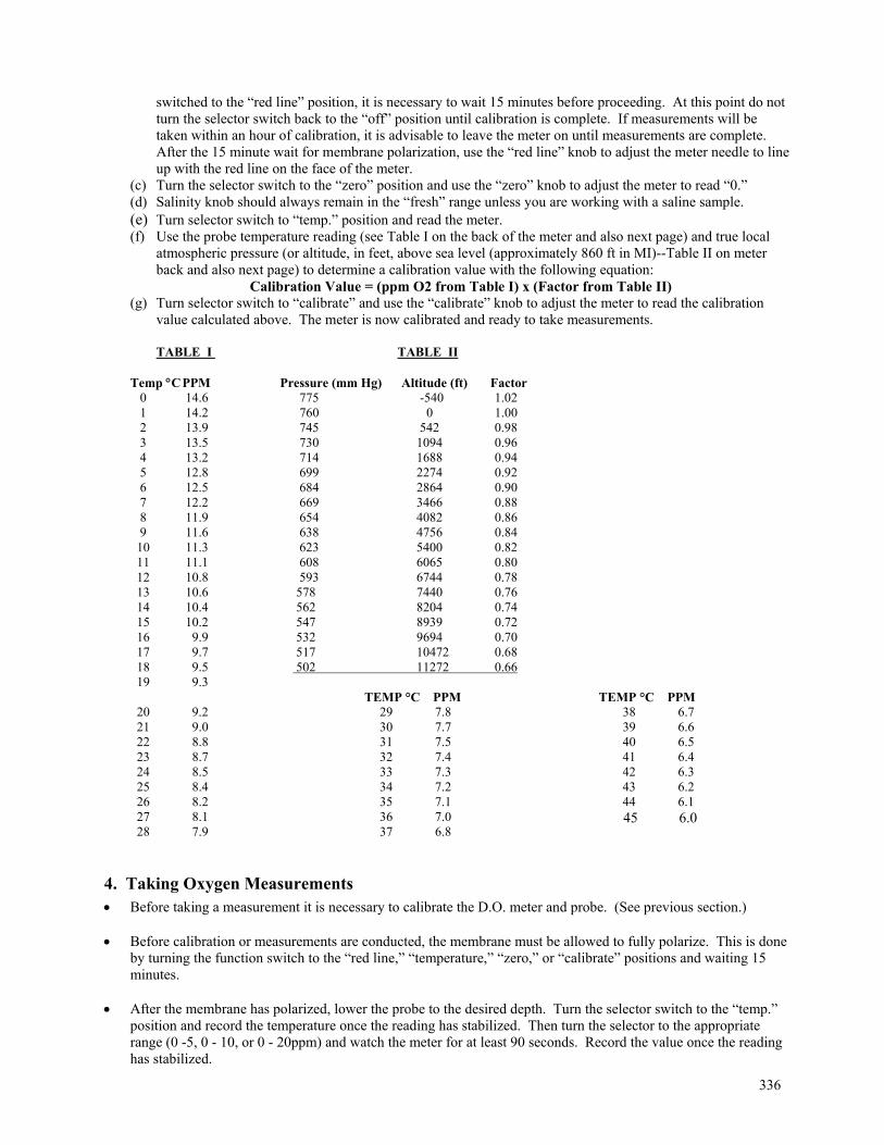
336

switched to the “red line” position, it is necessary to wait 15 minutes before proceeding. At this point do not turn the selector switch back to the “off” position until calibration is complete. If measurements will be taken within an hour of calibration, it is advisable to leave the meter on until measurements are complete. After the 15 minute wait for membrane polarization, use the “red line” knob to adjust the meter needle to line up with the red line on the face of the meter.

(c) Turn the selector switch to the “zero” position and use the “zero” knob to adjust the meter to read “0.” (d) Salinity knob should always remain in the “fresh” range unless you are working with a saline sample. (e) Turn selector switch to “temp.” position and read the meter. (f) Use the probe temperature reading (see Table I on the back of the meter and also next page) and true local

atmospheric pressure (or altitude, in feet, above sea level (approximately 860 ft in MI)--Table II on meter back and also next page) to determine a calibration value with the following equation:

Calibration Value = (ppm O2 from Table I) x (Factor from Table II) (g) Turn selector switch to “calibrate” and use the “calibrate” knob to adjust the meter to read the calibration

value calculated above. The meter is now calibrated and ready to take measurements.

TABLE I TABLE II Temp C PPM Pressure (mm Hg) Altitude (ft) Factor 0 14.6 775 -540 1.02 1 14.2 760 0 1.00 2 13.9 745 542 0.98 3 13.5 730 1094 0.96 4 13.2 714 1688 0.94 5 12.8 699 2274 0.92 6 12.5 684 2864 0.90 7 12.2 669 3466 0.88 8 11.9 654 4082 0.86 9 11.6 638 4756 0.84 10 11.3 623 5400 0.82 11 11.1 608 6065 0.80 12 10.8 593 6744 0.78 13 10.6 578 7440 0.76 14 10.4 562 8204 0.74 15 10.2 547 8939 0.72 16 9.9 532 9694 0.70 17 9.7 517 10472 0.68 18 9.5 502 11272 0.66 19 9.3 TEMP °C PPM TEMP °C PPM

20 9.2 21 9.0 22 8.8 23 8.7 24 8.5 25 8.4 26 8.2 27 8.1 28 7.9

29 7.8 30 7.7 31 7.5 32 7.4 33 7.3 34 7.2 35 7.1 36 7.0 37 6.8

38 6.7 39 6.6 40 6.5 41 6.4 42 6.3 43 6.2 44 6.1 45 6.0

4. Taking Oxygen Measurements Before taking a measurement it is necessary to calibrate the D.O. meter and probe. (See previous section.) Before calibration or measurements are conducted, the membrane must be allowed to fully polarize. This is done

by turning the function switch to the “red line,” “temperature,” “zero,” or “calibrate” positions and waiting 15 minutes.

After the membrane has polarized, lower the probe to the desired depth. Turn the selector switch to the “temp.”

position and record the temperature once the reading has stabilized. Then turn the selector to the appropriate range (0 -5, 0 - 10, or 0 - 20ppm) and watch the meter for at least 90 seconds. Record the value once the reading has stabilized.

337

Remember to turn the selector switch to the “off” position after the final measurement has been recorded. IMPORTANT NOTE: Proper technique is crucial to obtaining an accurate and reproducible measurement. It is vital that the membrane is always in contact with “new water.” This means the probe must be constantly and gently jigged--moved steadily and consistently up and down with a 4-10” stroke--the entire time you are waiting for the reading to stabilize. Failure to do this will result in an inaccurate measurement. The meter will fail to stabilize; instead it will slowly decline as the measurement process gradually depletes oxygen in the water surrounding the membrane.

B. Uploading and Downloading OEI and WADAR Units

OLD PROTOCOLS – DO NOT USE! Updated: 29 April 2004, cdw NOTE that these OEI and WADAR temperature loggers were used from ~1999-2004, and are no longer used. * "Standard watch time" is taken from the GPS unit at Toolik, which should be very accurate and very repeatable.

Set your own watch to this std time before starting to upload or download the instruments. Also, set the clock on the computer to the GPS/standard watch time as well (be careful to frequently check the computer clock and date -- set the clock immediately before working with the units).

1. OEI Units (Page numbers indicated are from the instruction manuals) (a) To Program and Start logging: For each datalogger unit, record the following Table in the yellow logbook (make these headings columns, not

rows as they are listed below). Clock set time -- from the std time Deploy Date/Time Retrieve Date/Time Location Serial # Depth of deployment Name of Log file Name of Data file End Clock Time (from the std time) End Logger Time (from the data logger unit) Time DIFF (difference between the end clock time and the end logger time) Instructions:

i. Plug interface into a serial port in the computer. ii. Plug antenna into the interface. If interface power does not come on, replace batteries or plug the interface

into the wall w/AC adapter. iii. Place logger label-side down on antenna, probe to ‘cut’ side of antenna (opposite cable). iv. Go to DOS prompt, then to C:\WCOMM directory. v. Type comm com1 [enter]. It gives back "9311". It is only when you have the 9311 prompt that you can

communicate with the unit (see ** below if unit does not respond). Type in the following commands IN THIS ORDER. status (enter) -- Typing in "status" at the prompt checks for cleared/saved data, checks the serial

number and start time/date (p. 12) reset (enter) Yes -- This ERASES all data, so if you have not downloaded and copied the files,

you should follow the “To Download” instructions below. label Name Depth Deployment Number (enter) For example “Label Toolik 12m 01” date 07/24/1998 09:59:05 Press enter at an exact known GPS time, and enter this into the first

column in the data book [GPS/clock set time]. Format is Month/Day/Year, Hour/Minute/Second. Entering the zero's before single digit numbers is optional (p. 8).

channels temp (enter) if using a temperature/pressure OEI then type “temp press”.

338

sample 00:00:10 (enter) sets the sampling interval to 10sec, if using a temp/press unit set this to 20sec. Here you need all the zeros.

start 07/24/1998 08:00:00 (enter) You can make the start time and date in the past, and the unit will start recording immediately. Then you can check to be sure it is recording data before you place it in the lake. Write start date and time in the logbook.

stop 08/30/98 08:00:00 (enter) This sets the stop time, it will either stop then, or it will stop when it is full. The default for the unit is to stop when it is full rather than to over-write existing data. THE STOP TIME MUST BE LATER IN TIME THAN WHEN THE UNIT WILL BE FULL -- for example, with a 10 sec sample interval the temp only units will fill in ~15 days, and you should set the stop time to be longer than 15 days (20 days is fine).

log c:\wcomm\logfile\'filename' (enter) Choose the filename according to the naming convention discussed later in this document. When you press enter, the program writes everything that you type and the computer responses after that to the logfile. Write Log filename in the logbook.

status Hit 'enter' at an exact, known GPS time. This sends the information about this particular deployment start and stop time, etc., to the log file. Note if the logger time is the same as the GPS time. If it is even a second off, note this in the book as “reads GPS +1s” or whatever the logger time is relative to GPS time.

** If the unit is not talking to the computer, check the following:

1. Is it plugged in? This plug is located between the halves of the unit, and unplugs the internal batteries. NOTE THAT IF YOU UNPLUG THIS BEFORE DOWNLOADING AND SAVING DATA, ALL DATA WILL BE LOST, FOREVER (i.e., the memory is volatile).

2. If it was plugged in, and if you have downloaded and saved the data, then unplug the unit, let it sit a few min, plug in and try again;

3. The reset button is under the address, lower left of the unit. Place a magnet over the reset area (can also put magnet under top half of the unit) and this will get it going again.

File Naming Criteria for OEI Units S2703L01 (where “S" is for Serial number, 2703 is the serial number, L is the code (see below) and “01” is the

deployment number or the number of times the unit has been put out into the field. Codes include: A=Data file for AK L=Logfile for AK T=Test C=Calibration G=Log file for other lakes M=Mono Lake _ = Other lake data files ** Reminder: You MUST write a log file in the log book. (b) To Download:

i. Clean and dry the units. ii. Connect interface and antenna as described above. iii. Go to DOS c:\wcomm iv. Type comm com1 (enter), it will return with >9311. ENTER THE FOLLOWING COMMANDS:

status !Press enter at an exact, known GPS time! Record the known GPS date and time and the logger date and time in the log book under “End GPS time” and “End Logger time” columns. If you make a mistake, just type Status again - this command does not erase data or stop the unit from recording data.

download c:\wcomm\data\'filename' (enter) The data will now start to download, you can always download it again (until you hit reset). See file naming criteria below. Record filename in log book.

quit (enter) v. Repeat 1-4 for each unit (or if you want you can look at each file first, check that it is OK following the

instructions below, and then proceed to the next unit). vi. View and copy data. Go to c:\dosshell (enter) This is the dos file manager. Tab to the directory tree,

arrow to \wcomm, type “+” to expand directory, arrow to \wcomm\data, tab to file on right, arrow to the data file, press F9 to view. Page down to check all data and the dates. Hit ESC to return.

vii. If the data file is OK, save the data to a floppy and a zip disk (or two different floppies). F8 to copy, change to directory A:\ or E:\ and label according. Alt + File to Exit (type c: to get back to the C drive).

339

viii. To redeploy the units, go to part A of these instructions. Contacts: Sally MacIntyre (UCSB) (805) 893-5501 George Kling (UM) (734) 647-0894, lab -0898, FAX -0884, [email protected] The following two people are at the OEI company - ask them for help after asking Sally or George: erik@oei-

inc.com or [email protected] 2. WADAR Units (a) To Start Logging: Before you even touch the units, make sure the DOS clock is set to GPS time (C:\date and C:\time). Check the dos clock again immediately before you begin up or downloading. Instructions:

i. Clean and dry the units before opening. Open WaDaR w/tool if you can't unscrew it with your fingers (hold unit upside down so that any water around the opening does not fall into the unit). Dry the O-ring before fully unscrewing.

ii. Pull out board enough to get to pin connector and the battery connector. iii. Plug-in the battery within the Wadar unit. Check the voltage on the pins on the back of the board behind the

copper prongs - should be between 7.0-7.4 (7.3 nominal) (Battery type=3.6V lithium, 2 Amp hrs, AA size -- note that this is not a normal AA battery, so do not try to use a normal AA).

**Use 9v during data downloading only** The 9V battery externally powers the logger while downloading to save the internal batteries. If hooked up during programming, it sends a spike that looks like an “end-of-file” mark that stops data recording.

iv. Hook up to COM1 in back of computer, thru adapters, hook-up AA battery and clip within the WaDaR unit. v. Set or check DOS Clock to std time from the GPS time (via your watch). C:\time. If it is ok, then just hit

return. vi. Go to c:\wadar and type wtl.exe [return] vii. Instrument file Name : wtl.var [return] viii. Go to SETUP ix. Set Date and Time. These set the computer date and time. Check against your STD time watch. The

computer gives the first time stamp for the datalogger unit -- you do not have to pick the start and stop time as in the OEI's.

x. Pick sampling schedule= 60 sec (at this rate the memory will last about 45 days). DO NOT PRESS ENTER UNTIL YOU KNOW THE EXACT GPS TIME! When you press Enter, the unit begins collecting data. If you mess up, stop the data recording by resetting the sampling schedule at step 10.

xi. Record sampling start time and date (exactly when you press Enter!) in the logbook. xii. Go to VERIFY – Gives temperature at 2 second interval for 20 seconds, then it goes to the interval that you

set. End VERIFY with the Escape key. xiii.Unplug unit from the computer. Wipe it off, remove dirt and lint from the o-ring, then apply a small amount

of stopcock grease (use sparingly). Wipe off the excess grease and Finger Tighten the unit cap Only! (b) To Download: !Disable the screen-saver on the computer!

i. Go to c:\wadar and type wtl.exe and instrument file name wtl.var ii. Go to TRANSFER on WADAR software (select COM Port if it has changed - it will remember the last com

port you selected). iii. Plug in 9V battery on the computer cable. iv. Hook-up WADAR unit to the computer through the interface as above. v. Choose Offload Raw Data from the menu (ignore the computer time statement) Give a Filename e.g., W0007A01.RAW where W=WADAR, 0007 is S/N with 0 in first place if the S/N

has only three digits, A is for Alaska, and 01 is deployment number. YOU MUST Record the Std Watch Time when you hit enter! ** Do not let computer screen go off, or to other power saving features -- disable power saving features on the

computer, like a monitor power or screen saver (the CCS computer at Toolik only has a screen saver).

340

vi. Check the data file to make sure that it is complete and looks good. If you only get 6 or 7 blocks (vs 1000 when memory is full), then something is wrong and you should press ESC key and then go to EMERGENCY OFFLOAD - Give filename as above with the extension *.off This ignores all end-of-file characters and goes to end of memory whether there are data there or not. Then check this data file. Record in the log book if you must do an emergency offload for one or more of the units.

vii. If redeploying: make a backup on two separate floppies or on a zip disk and a floppy, then go to SETUP, pick sampling interval; this resets the unit, and it starts logging data again (see instructions above).

viii. If not redeploying: then make 2 separate floppy copies (or 1 zip disk plus 1 floppy) and unplug the unit and the Wadar battery, and seal (does not need stopcock grease as is described above).

DO NOT USE THE WRENCH FOR TIGHTENING - FINGERS ONLY. ix. You can use convert to ENG.Units, then choose OHMS to get the data into an easier format to work with.

Call the file *.res, as this is giving you the resistance. Note that the calibration constants are entered at a later stage in the processing, and you ignore the calibration constants that are in the software. You can also convert directly to temperature by choosing "engineering units". Call the file e.g., W0007aeu

(IX-4) Nutrient Determination –Technicon Autoanalyzer OLD PROTOCOLS – DO NOT USE! The methods in this section were developed using a Technicon Autoanalyzer. Currently, these analyses are being performed on a Alpkem Flowsystem 3000 autoanalyzer. Because of differences in the two systems the methods are slightly different. For example, 20ml of sample were digested for TDP analysis in the past, now only 7.5ml of sample are used. As the methods in this section are adapted to the Alpkem autoanalyzer the new methods will be updated in section (IV-5).

A. Autoanalyzer Operation START UP: 1. Check the run log to see how the machine is working. 2. Check the waste containers below the autoanalyzer (AA) to make sure they do not need to be emptied. The

colored waste in the bucket should be emptied into the large blue plastic carboy and the waste water jug can be emptied into the sink

3. Dump out distilled water in the rinse container connected to the pump and in the small containers with the reagent lines (leave the lines in the container and dump the water into the waste beaker). Also, dump the distilled deionized water in the squirt bottle. Refill all with fresh distilled deionized water. Add ~10 drops of Westco (formerly Levor) to the DDW for the P-channel and several drops of Brij to the N-channel DDW (fill the ~500mL container).

4. Make sure the sampler probe is in the rinse receptacle, and that the rinse receptacle is full with RO/DI. 5. Stretch pump lines over the end plates. Examine the pump tubing to make sure it is not permanently creased or

crinkled, or excessively worn. If any lines look too worn, replace with new pump lines of the same color (indicating the tube id).

6. Put pump platen on pump and snap into place. 7. Turn on pump (switch is on left side). 8. Turn on bulbs in colorimeters to warm up. 9. Plug the heater for the phosphorus channel into the wall outlet. 10. Turn on chart recorder. Check the pen response by switching the scale on top of the colorimeter to “full” and

“zero” scale. Also make sure there is sufficient paper to last through the run. 11. Make up new reagents (there is labeled dedicated glassware for each step): a. Phosphorus i. For Persulfate digesting method Ascorbic Acid Reagent Make FRESH EACH DAY!

1. Dissolve 9.0 g ascorbic acid (pre-weighed vials) in ~ 400mL DDW 2. Add 25 mL acetone (in freezer) and dilute to 500 mL in the volumetric flask. Pour this solution into the

reagent bottle. 3. Add ~10 drops wetting agent (Westco 021-s000-01, formerly Levor) Ammonium Molybdate Working Reagent Make FRESH EACH DAY! Combine:

341

150 mL sulfuric acid solution, 4.9 N 45 mL ammonium molybdate solution 15 mL antimony potassium tartrate solution

ii. For Acid hydrolysis method (can also see Stainton et al. 2nd ed., below are the recalculated so you can use the

same concentration solutions as in the persulfate method above). Ascorbic Acid Reagent Make FRESH EACH DAY! Dissolve 9g ascorbic acid in 360 mL DDW. Add 10 drops wetting agent (Westco 021-s000-01). Ammonium Molybdate Working Reagent Make FRESH EACH DAY! Combine: 132 mL sulfuric acid solution, 4.9 N 38.3 mL ammonium molybdate solution 10 mL antimony potassium tartrate solution 25 mL DDW

b. Nitrate/Nitrite Reagents are stable and do not need to be prepared daily. Check color reagent to make sure it is not pink by pouring a small amount into a beaker. If it is pink, replace with

new reagent. For reagent formulas, see the nitrate/nitrite analysis instructions. 12. Put reagent lines into reagent bottle tops. Use Accuwipes and be careful not to touch the lines with your fingers. 13. After about 10 minutes, check lines again. Make sure all reagents are flowing smoothly. Make sure that the

bubbles are evenly spaced. 14. After ensuring that there are no bubbles entering the line leading up to the cadmium column, turn the cadmium

column switch to “on”. Occasionally a bubble exits the valve when it is turned to the “on” position, watch for this and be prepared to disconnect the cadmium column and let the bubble escape before it enters the column.

15. Make sure no bubbles are stuck in the flow cell. Lift the lid and check the line coming up from the flowcell for bubbles. It should be clear (full of liquid). If it’s not, flick the bubbles through the line. Then pinch the line closed for a second and let it go. This should suck a big bubble through the flow cell. Wait about 20 seconds. You should see the bubble leaving the line. If it is a large bubble with no little bubbles attached, all is well. Otherwise repeat this procedure. Make sure that the bubble is being sucked steadily through the line. Otherwise check the outlet of this line and its connection through the pump.

16. Adjust the baseline on the colorimeters if necessary to bring the pens onto scale. The nitrate/nitrite channel is fairly stable and the baseline should be adjusted to about 10 on the recorder. The phosphorus channel tends to drift downward slowly. Adjust the baseline to about 15 on the recorder. Allow about 10 minutes for the recorder to warm up. The baselines should start to get steadier. Once they are relatively stable, samples may be run. If it is necessary to get the pens into range, the slit width or the standard calibration knobs may be adjusted. Do so carefully and judiciously! The slit widths are VERY sensitive. Only adjust them a minute amount. The standard calibration setting will affect the sensitivity of the run.

Persulfate TDP or PP 9.5 - 9.8 Acid PP 2.75 Persulfate TDN 4.3 - 4.5 17. Fill up your 4 mL sample vials and insert into tray. Position one (1) should be even with the rinse receptacle and

red line. Turn on the sampler. After a rinse interval, the sample tray should move clockwise and the probe should begin sampling at position 1. The probe samples for 80s and rinses for 120s.

18. Label the chart recorder paper with the date, initials, and “tray 1”. 19. Check the standard curve (should be run first; stop the recorder in the rinse after the last standard in the curve has

run so that you do not lose any samples if the standard calibration needs to be changed or if the autoanalyzer is not working properly) and verify that the r^2 is 0.99... and that the highest peak does not run off the chart paper. If necessary, change the standard calibration and rerun the curve.

20. Check the column efficiency (Nitrate/Nitrite peaks should be .99). If column efficiency is low, replace the column or reactivate coil and start the run again.

21. Start daily log book entry in blue notebook. AUTOANALYZER MONITORING: Each Time Sampler Moves:

342

-Verify that the probe is in either the rinse or the sample, as appropriate. -If the probe is stuck on the edge of the container, IMMEDIATELY lift and move it into the container. Push it into

place. Any air that gets into the system and is too much to be removed by the debubbler will both trash the cadmium column and cause air bubbles to get caught in the flow cell, obscuring peaks.

-Check the chart recorder peaks and make sure they look smooth and normal. If anything is awry, stop the sample probe in the next rinse cycle by turning the sampler power off. This way you won’t lose more than a few samples before the problem is fixed. If you stop the sampler be sure to make a note of what happened on the chart recorder paper.

AT LEAST EVERY 20 MINUTES: -Check the distilled deionized water in the rinse receptacle container that is connected to the pump. If it is less than

2/3 full, refill it by pouring more DI in from the squirt bottle. Be sure not to let the tubing suck up any air during or after refilling (for the same reasons as above).

-Check the reagent lines and make sure they are well below the surface. Add more reagent if necessary. -Check the lines running through the coils and columns. Look for uniform distances between bubbles, correct bubble

shapes...be sure nothing looks unusual. -Check the chart recorder paper to be sure it is not getting bunched up or too near the end(No. feet remaining is on the

right side); keep it in a roll on the floor or pause to reload the paper. -Check the baselines to be sure they are not drifting off the chart paper. If they have drifted substantially you can

adjust the baseline by rotating the baseline knob on the colorimeter. Record the baseline change on the chart recorder paper.

-Keep track of how many samples are left on the sampler tray. Be prepared to turn off the sampler in the rinse cycle following the last sample, again to avoid bringing air into the system if the sampler attempts to sample an empty vial. Air in the sample line ruins the cadmium column (if the 10-turn coil is in use, it will need to be reactivated), and a new coil must be used if air is in the column.

BETWEEN TRAYS -Label the chart recorder paper appropriately. -Check the waste jugs to make sure they do not need to be emptied. If the water overflow container is full, pour

contents down the sink and replace the jug. If the waste container in the bucket is full empty it into the large blue receptacle. If the receptacle is becoming full ask Mark or Sheila for another. Make sure Mark labels all waste receptacles appropriately as part of the proper disposal.

-Check the baseline. -Check all lines again to make sure that everything appears normal. Check that the cadmium column did not get

contaminated with air bubbles. -Check new standard curve at start of tray as in start up procedure. AUTOANALYZER SHUT DOWN: 1. After the last sample has been taken, stop the sampler in the rinse cycle by pressing the power off button. 2. Let reagents and the rinse water flow through the system for 10 minutes. 3. Once a good baseline has been reached on the chart recorder, turn off the chart recorder, label the paper, and

roll it up for later reading. Place the pen caps on the chart recorder pens. 4. Turn off the colorimeter lights. 5. Turn off the cadmium column. 6. Take the rinse lines out of the reagent bottles (be careful not to touch them with fingers) and place in the filled

distilled deionized water rinse bottle. Continue running the pump for 10 minutes to completely rinse the reagent lines. ON FRIDAY, or every 5 days of running, place all lines in 10% HCl and pump for 10 minutes, then place in DDW rinse and pump for an additional 10 minutes.

7. Pour the leftover ascorbic acid down the sink and rinse the bottle three times with DDW. 8. Pour any leftover mixed reagent into the waste receptacle. Rinse the reagent bottle three times with DDW. 9. If there is color reagent or ammonium chloride buffer left, seal the reagent bottles with Parafilm. Replace the

caps and place the leftover reagents on the shelf above the autoanalyzer. If there is very little reagent left, dump it into the autoanalyzer waste jug and acid wash the bottles.

10. Once the lines have all been rinsed for at least 10 minutes, shut off the pump. 11. Unplug the heater for the phosphorus channel. 12. Undo the pump platen and remove. 13. Remove one end of the pump tubes from the end plate to relax the tubes.

343

14. Check the waste bottles to see if they need to be replaced. Dump the water from the rinse water overflow jug down the sink. If you replace a waste receptacle be sure to label it “autoanalyzer waste”.

15. Make sure all activities of the day are recorded in the blue log notebook (i.e. how many trays you ran, what the samples where run for (TDN, TDP), if you changed any tubing or settings, if there were any problems, etc.).

B. SRP Determination-Molybdenum Method

OLD PROTOCOLS – DO NOT USE! 1. REAGENTS a. Ascorbic Acid Reagent Dissolve 9.0 g U.S.P. quality ascorbic acid in approximately 400 mL distilled-deionized water (DDW). Add 25 mL acetone and dilute to 500 ml. Add ~10 drops wetting agent (WESTCO 021-s000-01 to replace LEVOR 1V). Stable for 1 week at 4 degrees C. For best results prepare daily. b. Sulfuric Acid Solution (4.9 N) Add 137 mL analytical reagent quality sulfuric acid (H2SO4) to ~750 mL DDW (slowly).

When cool dilute to 1000 mL with DDW. Stable indefinitely. c. Antimony Potassium Tartrate Solution

Dissolve 3.0 g analytical reagent antimony potassium tartrate (K(SbO)C4H4O6.1/2H2O) in 900 mL DDW.

Mix and dilute to 1000 ml. Store in a dark plastic bottle in the refrigerator. This solution is stable until a precipitate forms. d. Ammonium Molybdate Solution

Dissolve 40.0 g analytical reagent quality ammonium molybdate ((NH4)6Mo7O24.4H2O) in 900 mL DDW.

Mix and dilute to 1000 ml. Store in a dark plastic bottle in the refrigerator. Stable until a precipitate forms. e. Ammonium Molybdate Working Reagent Combine: 150 mL Sulfuric Acid Solution, 4.9 N 45 mL Ammonium Molybdate Solution 15 mL Antimony Potassium Tartrate Solution Eliminate any turbidity by continued mixing. Prepare daily, preferably with reagents that have reached room temperature.

2. STANDARDS a. Stock Solution Dissolve 0.8787 g pre-dried (105 degree C for one hour) potassium monobasic phosphate (KH2PO4) in 1000 mL

DDW (0.2 g PO4 - P/liter).

Add 1 mL chloroform as a preservative. Store in a dark bottle and refrigerate. Stable for many months. b. Intermediate Stock Solution Dilute 10 mL of stock solution to 1000 mL with DDW (2 mg PO4 - P/liter).

Add 1 mL chloroform as a preservative. Store in a dark bottle and refrigerate. Stable for many weeks, but for greatest accuracy, make fresh every 10 days. c. Daily Stock Solution Dilute 20 mL of intermediate stock solution to 200 mL with DDW (0.2 mg PO4 - P/liter).

Prepare daily.

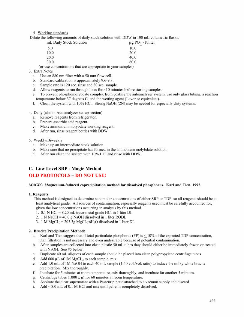
344

d. Working standards Dilute the following amounts of daily stock solution with DDW in 100 mL volumetric flasks: mL Daily Stock Solution g PO4 - P/liter

5.0 10.0 10.0 20.0 20.0 40.0 30.0 60.0 (or use concentrations that are appropriate to your samples) 3. Extra Notes a. Use an 880 nm filter with a 50 mm flow cell. b. Standard calibration is approximately 9.6-9.8. c. Sample rate is 120 sec. rinse and 80 sec. sample. d. Allow reagents to run through lines for ~10 minutes before starting samples. e. To prevent phosphomolybdate complex from coating the autoanalyzer system, use only glass tubing, a reaction

temperature below 37 degrees C, and the wetting agent (Levor or equivalent). f. Clean the system with 10% HCl. Strong NaOH (2N) may be needed for especially dirty systems. 4. Daily (also in Autoanalyzer set-up section) a. Remove reagents from refrigerator. b. Prepare ascorbic acid reagent. c. Make ammonium molybdate working reagent. d. After run, rinse reagent bottles with DDW. 5. Weekly/Biweekly a. Make up an intermediate stock solution. b. Make sure that no precipitate has formed in the ammonium molybdate solution. c. After run clean the system with 10% HCl and rinse with DDW.

C. Low Level SRP - Magic Method

OLD PROTOCOLS – DO NOT USE! MAGIC: Magnesium-induced coprecipitation method for dissolved phosphorus. Karl and Tien, 1992. 1. Reagents: This method is designed to determine nanomolar concentrations of either SRP or TDP, so all reagents should be at

least analytical grade. All sources of contamination, especially reagents used must be carefully accounted for, given the low concentrations occurring in analysis by this method.

1. 0.1 N HCl = 8.20 mL trace-metal grade HCl in 1 liter DI. 2. 1 N NaOH = 40.0 g NaOH dissolved in 1 liter RODI. 3. 1 M MgCL2 = 203.3g MgCL2

.6H2O dissolved in 1 liter DI. 2. Brucite Precipitation Method: a. Karl and Tien suggest that if total particulate phosphorus (PP) is < 10% of the expected TDP concentration,

than filtration is not necessary and even undesirable because of potential contamination. b. After samples are collected into clean plastic 50 mL tubes they should either be immediately frozen or treated

with NaOH. See #5 below. c. Duplicate 40 mL aliquots of each sample should be placed into clean polypropylene centrifuge tubes. d. Add 600 L of 1M MgCL2 to each sample, mix. e. Add 1.0 mL of 1M NaOH to each 40 mL sample (1:40 vol./vol. ratio) to induce the milky white brucite

precipitation. Mix thoroughly. f. Incubate for 5 minutes at room temperature, mix thoroughly, and incubate for another 5 minutes. g. Centrifuge tubes (1000 x g) for 60 minutes at room temperature. h. Aspirate the clear supernatant with a Pasteur pipette attached to a vacuum supply and discard. i. Add ~ 8.0 mL of 0.1 M HCl and mix until pellet is completely dissolved.

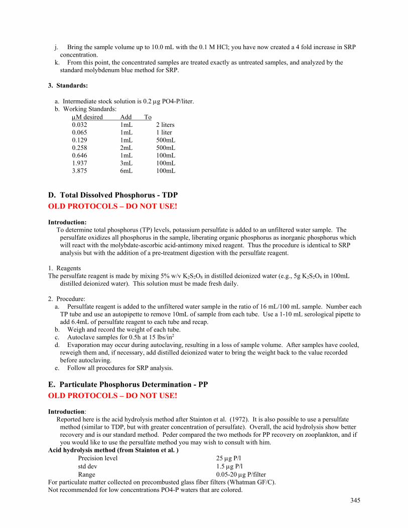
345

j. Bring the sample volume up to 10.0 mL with the 0.1 M HCl; you have now created a 4 fold increase in SRP concentration.

k. From this point, the concentrated samples are treated exactly as untreated samples, and analyzed by the standard molybdenum blue method for SRP.

3. Standards: a. Intermediate stock solution is 0.2 g PO4-P/liter. b. Working Standards: M desired Add To 0.032 1mL 2 liters 0.065 1mL 1 liter 0.129 1mL 500mL 0.258 2mL 500mL 0.646 1mL 100mL 1.937 3mL 100mL 3.875 6mL 100mL

D. Total Dissolved Phosphorus - TDP

OLD PROTOCOLS – DO NOT USE! Introduction: To determine total phosphorus (TP) levels, potassium persulfate is added to an unfiltered water sample. The

persulfate oxidizes all phosphorus in the sample, liberating organic phosphorus as inorganic phosphorus which will react with the molybdate-ascorbic acid-antimony mixed reagent. Thus the procedure is identical to SRP analysis but with the addition of a pre-treatment digestion with the persulfate reagent.

1. Reagents The persulfate reagent is made by mixing 5% w/v K2S2O8 in distilled deionized water (e.g., 5g K2S2O8 in 100mL

distilled deionized water). This solution must be made fresh daily. 2. Procedure: a. Persulfate reagent is added to the unfiltered water sample in the ratio of 16 mL/100 mL sample. Number each

TP tube and use an autopipette to remove 10mL of sample from each tube. Use a 1-10 mL serological pipette to add 6.4mL of persulfate reagent to each tube and recap.

b. Weigh and record the weight of each tube. c. Autoclave samples for 0.5h at 15 lbs/in2 d. Evaporation may occur during autoclaving, resulting in a loss of sample volume. After samples have cooled,

reweigh them and, if necessary, add distilled deionized water to bring the weight back to the value recorded before autoclaving.

e. Follow all procedures for SRP analysis.

E. Particulate Phosphorus Determination - PP

OLD PROTOCOLS – DO NOT USE! Introduction: Reported here is the acid hydrolysis method after Stainton et al. (1972). It is also possible to use a persulfate

method (similar to TDP, but with greater concentration of persulfate). Overall, the acid hydrolysis show better recovery and is our standard method. Peder compared the two methods for PP recovery on zooplankton, and if you would like to use the persulfate method you may wish to consult with him.

Acid hydrolysis method (from Stainton et al. ) Precision level 25 g P/l std dev 1.5 g P/l Range 0.05-20 g P/filter For particulate matter collected on precombusted glass fiber filters (Whatman GF/C). Not recommended for low concentrations PO4-P waters that are colored.

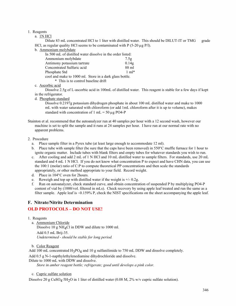
346

1. Reagents a. 1N HCl Dilute 83 mL concentrated HCl to 1 liter with distilled water. This should be DILUT-IT or TMG grade

HCl, as regular quality HCl seems to be contaminated with P (5-20g P/l). b. Ammonium molybdate In 500 mL of distilled water dissolve in the order listed: Ammonium molybdate 7.5g Antimony potassium tartrate 0.14g Concentrated Sulfuric acid 88 ml Phosphate Std 1 ml* cool and make to 1000 ml. Store in a dark glass bottle. * This is to control baseline drift c. Ascorbic acid Dissolve 2.5g of L-ascorbic acid in 100mL of distilled water. This reagent is stable for a few days if kept

in the refrigerator. d. Phosphate standard Dissolve 0.2197g potassium dihydrogen phosphate in about 100 mL distilled water and make to 1000

mL with water saturated with chloroform (or add 1mL chloroform after it is up to volume), makes standard with concentration of 1 mL = 50 g PO4-P

Stainton et al. recommend that the autoanalyzer run at 40 samples per hour with a 12 second wash, however our

machine is set to split the sample and it runs at 24 samples per hour. I have run at our normal rate with no apparent problems.

2. Procedure a. Place sample filter in a Pyrex tube (at least large enough to accommodate 12 ml). b. Place tube with sample filter (be sure that the caps have been removed) in 550C muffle furnace for 1 hour to

ignite organic matter. Include tubes with blank filters and empty tubes for whatever standards you wish to run. c. After cooling and add 2 mL of 1 N HCl and 10 mL distilled water to sample filters. For standards, use 20 mL

standard and 4 mL 1 N HCl. If you do not know what concentration P to expect and have CHN data, you can use the 100:1 (molar) ratio of C:P to compute theoretical PP concentrations and then scale the standards appropriately, or other method appropriate to your field. Record weight.

d. Place in 104C oven for 2hours. e. Reweigh and top up with distilled water if the weight is +/- 0.2g. f. Run on autoanalyzer, check standard curve, and obtain concentration of suspended P by multiplying PO4-P

content of vial by (1000/vol. filtered in mLs). Check recovery by using apple leaf treated and run the same as a filter sample. Apple leaf is ~0.159% P, check the NIST specifications on the sheet accompanying the apple leaf.

F. Nitrate/Nitrite Determination

OLD PROTOCOLS – DO NOT USE! 1. Reagents a. Ammonium Chloride Dissolve 10 g NH4Cl in DDW and dilute to 1000 ml.

Add 0.5 mL Brij-35. Undetermined - should be stable for long period. b. Color Reagent Add 100 mL concentrated H3PO4 and 10 g sulfanilimide to 750 mL DDW and dissolve completely.

Add 0.5 g N-1-napthylethylenediamine dihydrochloride and dissolve. Dilute to 1000 mL with DDW and dissolve. Store in amber reagent bottle; refrigerate; good until develops a pink color. c. Cupric sulfate solution

Dissolve 20 g CuSO4.5H2O in 1 liter of distilled water (0.08 M, 2% w/v cupric sulfate solution).

347

Undetermined - should be good indefinitely. d. 10 % v/v Hydrochloric Acid Add 100 mL concentrated HCl to 900 mL DDW. Store in glass bottle. Good indefinitely. 2. Preparation of Reductor Columns Prepare 8 columns at a time. Will take approximately 3-4 hours. Do this under the hood and put lab bench absorbent paper down under your working area. Wear gloves. (I wear double gloves) a. Wash several grams of course cadmium filings (99.9% purity) with 10% HCl in a beaker or flask and rinse

well with DDW(using the funnel apparatus in the fume hood). b. Decant rinse water. c. Add CuSO4 solution to the filings and swirl until the blue color disappears.

d. Let stand for 15-20 minutes. e. Rinse at least 12 times with DDW, being careful to avoid exposing the cadmium filings to the air. f. Decant rinse water. g. Add NH4Cl to the cadmium filings.

h. Prepare the glass tubing for packing. The glass tubing, connectors and glass wool should soak in NH4Cl for several minutes to rid air bubbles, this is especially important for te glass wool. Place a small amount of glass wool into one end of the tubing and stop with the connector. Prepare all columns before adding the cadmium (for ease in process).

i. Pack a piece of glass tubing (8 to 9 cm long; 3.5 mm ID) with the cadmium in NH4Cl solution. It is very

important that the cadmium does not have contact with the air, if it does, you must start over again. For this reason, there is an intricate procedure to try to keep the cadmium in the NH4Cl solution. For best results, fill a

syringe with NH4Cl solution. Place the syringe on the connector end of the tube. Fill the tube with NH4Cl

solution and keep a small amount of pressure on the syringe so that some NH4Cl solution is coming out. Place

the open end of the tube into the tubing at the bottom of the funnel apparatus, trying to make sure that the funnel apparatus has NH4Cl solution in it. Open the clamp for a second and let the tube fill with cadmium. Tap sides of

glass tube to compact the cadmium. Fill another syringe with NH4Cl solution and connect it to a connector

(connector should have glass wool in it). Push syringe so NH4Cl solution buffer is slowly coming out of the

connector. Next part requires two people- 1person holds the filled tube and disconnects it from the funnel apparatus while slowly pushing the NH4Cl solution up tube. The other person takes the syringe/connector and

connects it to the top of the filled tube while pushing the buffer up the connector. j. Keep prepared columns submerged in NH4Cl solution until use. When you have finished making the column,

quickly transfer it to a vial filled with NH4Cl for storage. AVOID EXPOSURE OF THE CADMIUM TO AIR AND TO YOURSELF.

3. Standards a. Stock Solution (Nitrate Standard) Dissolve 7.218 g pre-dried (105 C for one hour) potassium nitrate (KNO3) in 1000 mL DDW (1 g N/liter).

Add 1 mL chloroform as a preservative. Refrigerate. Stable indefinitely. b. Intermediate Stock Solution Dilute 10 mL of stock solution to 1000 mL with DDW (10 mg N/liter). Add 1 mL chloroform as a preservative. Refrigerate. Stable for many weeks, but for greatest accuracy make fresh every 10 days. c. Working Standards Dilute the following volumes of intermediate stock solution with DDW in 100 mL volumetric flasks. mL intermediate stock solution mg NO3 - N/liter

1 0.1 2 0.2 5 0.5 10 1.0

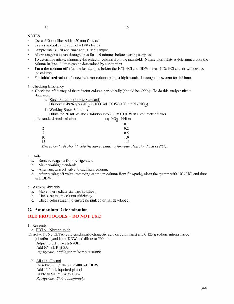
348

15 1.5 NOTES Use a 550 nm filter with a 50 mm flow cell. Use a standard calibration of ~1.00 (1-2.5). Sample rate is 120 sec. rinse and 80 sec. sample. Allow reagents to run through lines for ~10 minutes before starting samples. To determine nitrite, eliminate the reductor column from the manifold. Nitrate plus nitrite is determined with the

column in-line. Nitrate can be determined by subtraction. Turn the column off after the last sample, before the 10% HCl and DDW rinse. 10% HCl and air will destroy

the column. For initial activation of a new reductor column pump a high standard through the system for 1/2 hour. 4. Checking Efficiency a. Check the efficiency of the reductor column periodically (should be ~99%). To do this analyze nitrite

standards: i. Stock Solution (Nitrite Standard) Dissolve 0.4926 g NaNO2 in 1000 mL DDW (100 mg N - NO2).

ii. Working Stock Solutions Dilute the 20 mL of stock solution into 200 mL DDW in a volumetric flasks. mL standard stock solution mg NO2 - N/liter

1 0.1 2 0.2 5 0.5 10 1.0 15 1.5 These standards should yield the same results as for equivalent standards of NO3.

5. Daily a. Remove reagents from refrigerator. b. Make working standards. c. After run, turn off valve to cadmium column. d. After turning off valve (removing cadmium column from flowpath), clean the system with 10% HCl and rinse

with DDW. 6. Weekly/Biweekly a. Make intermediate standard solution. b. Check cadmium column efficiency. c. Check color reagent to ensure no pink color has developed.

G. Ammonium Determination

OLD PROTOCOLS – DO NOT USE! 1. Reagents a. EDTA - Nitroprusside Dissolve 1.86 g EDTA (ethylenedinitrilotetraacetic acid disodium salt) and 0.125 g sodium nitroprusside

(nitroferricyanide) in DDW and dilute to 500 ml. Adjust to pH 11 with NaOH. Add 0.5 mL Brij-35. Refrigerate. Stable for at least one month. b. Alkaline Phenol Dissolve 12.0 g NaOH in 400 mL DDW. Add 17.5 mL liquified phenol. Dilute to 500 mL with DDW. Refrigerate. Stable indefinitely.

349

c. Sodium Hypochlorite Dilute 15 mL Chlorox (commercial bleach, 5.25% sodium hypochlorite) to 500 mL with DDW. Use bleach that is less than 3 months old. Prepare daily. 2. Standards a. Stock Solution Dissolve 0.3819 g pre-dried (105 C for 1 hour) NH4Cl in DDW and dilute to 1000 mL (100 mg N/liter).

Add 1 mL chloroform as a preservative. Prepare monthly and store in refrigerator. b. Intermediate Stock Solution Dilute 10 mL stock solution to 1000 mL with DDW (1 mg N/liter). Add 1 mL chloroform as a preservative. Prepare every 10 days. Refrigerate. c. Working Standards Dilute the following volumes of intermediate stock solution with DDW in 100 mL volumetric flasks. mL Intermediate Stock Solution g NH4 - N/liter

0.5 5 1 10 2 20 3 30 4 40 5 50 3. Notes a. Use a 630 nm filter with a 50 mm flow cell. b. Use a standard calibration of 7.50. c. Allow reagents to run through lines for ~10 minutes before starting samples. d. If tygon tubing gets discolored due to metal hydroxide build-up, rinse with a strong complexing agent like

oxalic acid. 4. Daily a. Remove reagents from refrigerator. b. Prepare sodium hypochlorite reagent. c. Make working standards. d. After run, clean the system with 10% HCl and rinse with DDW. 5. Weekly/Biweekly a. Make intermediate standard solution. 6. Monthly a. Make EDTA - Nitroprusside reagent. b. Make stock solution.

H. Total Dissolved Nitrogen - TDN

OLD PROTOCOLS – DO NOT USE! 1. Reagents Same as nitrate/nitrite, but replace Ammonium Chloride Reagent (NH4Cl) with Mixed Buffer:

a. Mixed Buffer For 1 liter volumetric flask (note at present dedicated glassware is 2 liters-so double this) Mix 101 mL of 1N NaOH, 30.9 g H3BO3 and 10 g NH4Cl in a 1000 mL volumetric flask.

Dilute to 1000 mL with DDW. Add 0.5 mL Brij-35 Refrigerate; buffer is stable for months.

350

b. TDN Reagent Dissolve 14.80 g K2S2O8 and 4.40 g NaOH in 500 mL DDW. Make fresh. Use 5 mL reagent per 45 mL sample. c. TDP Reagent Dissolve 22.4 g K2S2O8 in 500 mL DDW. Make fresh. Use 5 mL reagent per 45 mL sample. 2. Preparation of Mixed Standards In 200 mL volumetric flasks mLs P daily stock g/l mLs NO3 working stock mg/l N Mixed Standard 1 10 10 2 .1 Mixed Standard 2 20 20 4 .2 Mixed Standard 3 40 40 10 .5 Mixed Standard 4 60 60 20 1.0 Note-you can also include a lower (no lower than 5ug/l P and 0.05 mg/l N) or higher standard depending on your own

samples. 3. If you are preparing standards for TDP and TDN analyses: a. Make standards as above. b. Prepare 4 vials for each standard, two with TDN reagent and two with TDP reagent. Pour 20 mL (20.0g) of

standard into an acid washed dry vial. Add 2.2 mL of either TDN or TDP reagent as appropriate. Record standards, vial numbers and weights on autoanalyzer standard sheets.

c. Fill at least 4 vials with DDW for reagent blanks. Add 2.2 mL TDN reagent to two of the vials and 2.2 mL TDP reagent to the other two. Record vial numbers and weights on autoanalyzer standard sheets.

d. Also make up a set of NO2 standards (for testing column efficiency) and add TDN reagent to them. Record vial numbers and weights on autoanalyzer standard sheets.

e. Autoclave standards for 90 minutes at 105 degrees C. 4. Preparation of Samples a. Samples with persulfate reagents added in the field i. Pour sample into an acid washed dry vial. ii. Record vial number and weight of vial (with cap) + sample on sample inventory list. iii. Autoclave at 105 C for 90 minutes on liquids cycle. iv. After autoclaving, let vials cool and weigh them. Add DDW to bring vials which have lost more than + 0.3 g of

weight during autoclaving back to volume. b. Frozen samples i. Remove samples from freezer and thaw. ii. Add 2 l of 6N ultrapure HCl per mL of sample. Invert several times to mix. iii. Let sit in cold room for 48 hours. iv. Pour 20 mL (20.0 g) of sample into each of two acid washed dry vials. Add 2.2 mL TDN reagent to one and 2.2

mL TDP reagent to the other. v. Record vial numbers and weights on sample inventory list. vi. Autoclave at 105 C for 90 minutes on liquids cycle. vii. After autoclaving, let vials cool and weigh them. Add DDW to bring vials which have lost more than + 0.2 g of

weight during autoclaving back to volume. viii. If any floculent precipitate forms, filter the sample onto a precombusted glass fiber filter and save in a desiccator

for later CHN analysis. c. Samples in cold room without preservative i. Add 2 l of 6N ultrapure or TMG HCl per mL of sample. Invert several times to mix. ii. Let sit in cold room CAP DOWN for 48 hours. iii. Pour sample into an acid washed dry vial. iv. Record vial numbers and weights on sample inventory list.

351

v. Autoclave at 105 C for 90 minutes on liquids cycle. vi. After autoclaving let vials cool and weigh them. Add DDW to bring vials which have lost more than + 0.2 g of

weight during autoclaving back to volume. d. Samples preserved with acid Start at number 4 on the frozen sample instructions.

Reference Stainton, M. P., M. J. Capel, and F. A. J. Armstrong. 1972. The chemical analysis of fresh water. Fisheries and

Environment Canada, Fisheries and Marine Service, Misc. Special Publication No. 25. Second Edition. OLD PROTOCOLS – DO NOT USE!

352

Appendices

List of Suppliers and Vendors Updated: January 2011 by LRY

UNIVERSITY OF MICHIGAN PROCUREMENT SERVICES: Website: http://www.finance.umich.edu/procurement Email: [email protected] Address: 7071 Wolverine Tower 3003 South State Street Ann Arbor, MI 48109-1282 Phone: (734) 764-8212 (8:00 a.m. to 4:30 p.m.) Fax: (734) 647-0733 or (734) 615-6235 UNIVERSITY OF MICHIGAN STRATEGIC SUPPLIERS: Visit M-Marketsite or the following website for a comprehensive list of strategic suppliers: http://www.finance.umich.edu/procurement/howtobuy/universitycontracts/ups?s=&cat=&status= Strategic suppliers we most frequently use: Fisher Scientific (U of M campus) Connie Brindle or Denise Smith, Customer Service

Phone: (734) 622-0413 Fax: (734) 622-0532 E-mail: [email protected]

Sigma Chemical Company P.O. Box 14508 St. Louis, MO 63178 (800) 325-3010 - to order (800) 325-5052 - to fax order (800) 325-8070 - customer service (800) 325-5832 - technical service Cryogenic Gases 12620 Southfield Detroit. MI 48223

(313) 835-5513 – all customer service (313) 835-3562 – fax Office Max 13301 Stephens Road Warren, MI 48089 (800) 264-7370 – order, customer service (800) 264-7366 – to fax order Aldrich Chemical 1001 West Saint Paul Avenue Milwaukee, WI 53233 (800) 558-9160 - all customer service (800) 962-9591 - fax orders (800) 231-8327 - technical service

================================================================================ OTHER FREQUENTLY USED VENDORS: Aldrich Chemical 1001 West Saint Paul Avenue Milwaukee, WI 53233 (800) 558-9160 - all customer service (800) 962-9591 - fax orders (800) 231-8327 - technical service Account Number: 324-000 Alltech 2051 Waukegan Road Deerfield, IL 60015-1889

(800) 255-8324 - orders (800) 337-6583 - technical support Account Number: MI 327 Alpkem (O-I Analytical) P.O. Box 9010 151 Graham Road College Station, TX 77842-9010 www.oico.com (800) 336-1911 – customer support (409) 653-1711 – orders: ask for Melanie, ext. 514 (409) 690-0440 – fax

353

Sales Rep: Scott Hazard, phone: (517) 783-1711, fax: (517) 783-4908

Account - 1057800 Ben Meadows Company 190 Etowah Industrial Court Canton, GA 30114 www.benmeadows.com (800) 241-6401 - all customer service (800) 628-2068 - fax orders Account Number: 0267365 Boise Cascade Office Products 13301 Stephens Road Warren, MI 48089 (800) 264-7370 – order, customer service (800) 264-7366 – to fax order Campbell Scientific 815 W. 1800 N. Logan, UT 84321-1784 www.campbellsci.com (435) 753-2342 – all customer service (435) 750-9540 – fax to Doug Bryson, Technical

Service (435) 750-9671 – fax for orders—Order Entry, Kim CMS (aka Curtin Matheson Scientific, Inc.) 1225 N. Michael Drive Wood Dale, IL 60191-1019 (800) 650-0650 Account Number: 099045 Cole-Parmer Instrument Company 7425 North Oak Park Avenue Niles, IL 60714 (800) 323-4340 Account Number: 051792-53 Cryogenic Gases 12620 Southfield Detroit. MI 48223 (313) 835-5513 – all customer service (313) 835-3562 – fax Contract Number: 500402 Dionex Corp. P.O. Box 3603 1228 Titan Way Sunnyvale CA 94088-3603 (800) 346-6390 – customer service (408) 736-4476 – fax for ordering (248) 546-5144 – Phil Martin, Technical Rep Customer Number - 2620 Elemental Microanalysis, Ltd. P.O Box 722 Mason, OH 45040

(513) 754-0103 - all customer service (513) 754-0105 - fax Forestry Suppliers, Inc. P.O. Box 8397 Jackson, MS 39284 (800) 647-5368 - orders (800) 543-4203 - fax orders (800) 752-8460 - customer service (800) 430-5566 - tech support ( 601) 354-3565 - international sales Account Number: 209048 Fluka Chemical Corp. 980 South 2nd St. Ronkonkoma, NY 11779-7238 (800) 358-5287 - orders and tech support (800) 441-8841 - fax Account Number: 324-000 Giangarlo Scientific 162 Steuben Street Pittsburgh, PA 15220 (412) 922-8850 (810) 278-2726 - local office Graphic Controls P.O. Box 1272 Buffalo, NY 14240 (800) 669-1535 - all customer service (800) 347-2420 - fax Account Number: 00360784 Hach Company P.O. Box 389 Loveland, CO 80539 (800) 227-4224 - all customer service Account Number: 117014 Hydrolab 12921 Barnet Road Austin, TX 78727 (800) 949-3766 (512) 255-3106 - fax ISCO 4700 Superior Street Lincoln, NE 68504 (800) 228-4373 – phone (402) 465-3022 - fax Kipp and Zonen (a division of Sci-Tec) 125 Wilbur Place Bohemia, N.Y. 11716 www.sci-tec.com (800) 645-1025 (516) 589-2068 – fax KPSI (Pressure Systems, Inc.)

354

34 Research Drive Hampton, VA 23666 www.kpsi.com (800) 328-3665 – customer support (757) 865-8744 - fax Li-Cor 4421 Superior Street P.O. Box 4425 Lincoln, NE 68504 (402) 467-3576 (402) 467-0630 - Carla, service Millipore Corporation 80 Ashby Road Bedford, MA 01730-2271 (800) 645-5476 - all customer service Account Number: 3420-180523 NEN (New England Nuclear) 549 Albany Street Boston, MA 02118-2512 www.nenlifesci.com (800) 551-2121 – customer service (617) 482-1380 - fax customer number - 22880 O-I Analytical (Alpkem) P.O. Box 9010 151 Graham Road College Station, TX 77842-9010 www.oico.com (800) 336-1911 – customer support (409) 653-1711 – orders: ask for Melanie, ext. 514 (409) 690-0440 – fax Sales Rep: Scott Hazard, phone: (517) 783-1711,

fax: (517) 783-4908 Account - 1057800 Orion Research, Inc. 529 Main Street Boston, MA 02129 (800) 225-1480 – all customer service (978) 927-3932 - fax Omega Engineering, Inc. P.O. Box 2284 Stamford, CT 06906 (800) 826-6342 - sales (800) 622-2378 - customer service Account Number: 013762 Perkin-Elmer (aka P-E)

761 Main Avenue Norwalk, CT 06859 (800) 762-4002 - all customer service Account Number: 066570-0017 Radiometer 810 Sharon Drive Westlake, OH (800) 998-8110 – all customer service (choose “customer service” to place orders; inside

sales: Gina, ext. 299) Sea-Bird Electronics, Inc. 1808 136th Place NE Bellevue, WA 98005 (425) 643-9866 – customer service (Matt Pillsbury,

ext. 220) (425) 643-9954 - fax Shimadzu Instruments 7102 Riverwood Drive Columbia, MD 21046 (800) 477-1227 – customer service – technical

support: Michael Green, ext. 1397; John Fetters, ext.1446

(410) 381-6781 - fax Account Number: Billing code – 234700 Shipping code - 14 Sigma Chemical Company P.O. Box 14508 St. Louis, MO 63178 (800) 325-3010 - to order (800) 325-5052 - to fax order (800) 325-8070 - customer service (800) 325-5832 - technical service Account Number: 204356991 VWR Scientific Products 800 East Fabyan Pkwy. Batavia, IL 60510 www.vwrsp.com (800) 932-5000 – customer service (630) 879-6718 - fax (800) 431-4132 ext. 6303 (Mark Napierkowski –

sales rep) Westco (supplies for AutoAnalyzer) 12 Precision Rd. Danbury CT 06810 (800) 445-07 (Technical Assistance--ask for Tony; he

knows his stuff)

Adaptation to changing light experiment procedure Updated: Aug 9, 2000 By: Mary Anne Evans

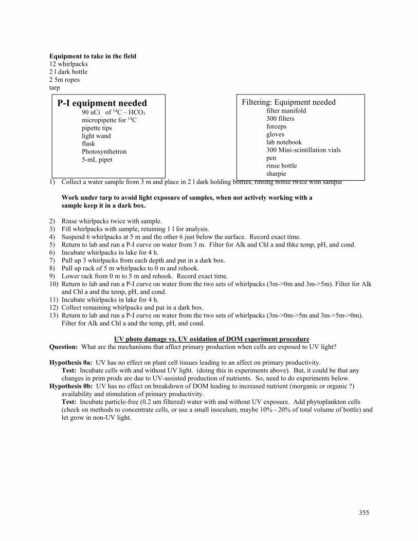
355

Equipment to take in the field 12 whirlpacks 2 l dark bottle 2 5m ropes tarp 1) Collect a water sample from 3 m and place in 2 l dark holding bottles, rinsing bottle twice with sample

Work under tarp to avoid light exposure of samples, when not actively working with a sample keep it in a dark box.

2) Rinse whirlpacks twice with sample. 3) Fill whirlpacks with sample, retaining 1 l for analysis. 4) Suspend 6 whirlpacks at 5 m and the other 6 just below the surface. Record exact time. 5) Return to lab and run a P-I curve on water from 3 m. Filter for Alk and Chl a and thke temp, pH, and cond. 6) Incubate whirlpacks in lake for 4 h. 7) Pull up 3 whirlpacks from each depth and put in a dark box. 8) Pull up rack of 5 m whirlpacks to 0 m and rehook. 9) Lower rack from 0 m to 5 m and rehook. Record exact time. 10) Return to lab and run a P-I curve on water from the two sets of whirlpacks (3m->0m and 3m->5m). Filter for Alk

and Chl a and the temp, pH, and cond. 11) Incubate whirlpacks in lake for 4 h. 12) Collect remaining whirlpacks and put in a dark box. 13) Return to lab and run a P-I curve on water from the two sets of whirlpacks (3m->0m->5m and 3m->5m->0m).

Filter for Alk and Chl a and the temp, pH, and cond.

UV photo damage vs. UV oxidation of DOM experiment procedure Question: What are the mechanisms that affect primary production when cells are exposed to UV light? Hypothesis 0a: UV has no effect on plant cell tissues leading to an affect on primary productivity. Test: Incubate cells with and without UV light. (doing this in experiments above). But, it could be that any

changes in prim prods are due to UV-assisted production of nutrients. So, need to do experiments below. Hypothesis 0b: UV has no effect on breakdown of DOM leading to increased nutrient (inorganic or organic ?)

availability and stimulation of primary productivity. Test: Incubate particle-free (0.2 um filtered) water with and without UV exposure. Add phytoplankton cells

(check on methods to concentrate cells, or use a small inoculum, maybe 10% - 20% of total volume of bottle) and let grow in non-UV light.

Filtering: Equipment needed filter manifold 300 filters forceps gloves lab notebook 300 Mini-scintillation vials pen rinse bottle sharpie

P-I equipment needed 90 uCi of 14C – HCO3

micropipette for 14C pipette tips light wand flask Photosynthetron 5-mL pipet

356

Equipment: 18 whirlpack bags foil to cover 6 whirlpack bags UV-B blocking cover 48 uCi of 14C – HCO3 2 l dark bottles micropipette for 14C pipette tips algal concentrators bucket 0.2 um filter capsules pump for filtering 2 mL pipette for plankton pipette tips p-tron vials p-trons light wand

1) Filter 12 l of Toolik lake water through 0.2 um filters. Rinse and fill 18 whirlpacks. 2) Cover 6 of the full whirlpacks with foil. 3) Tie up bags at the dock in the sun with 6 under UV-B blocking cover. Record time. 4) Incubate for 24h.

Work under tarp to avoid light exposure of samples, when not actively working with a sample keep it in a dark box.

5) About 15 min before the incubation time is up, collect 3.6 l of Toolik lake water and concentrate phytoplankton using 10 um mesh to a final vol. of 360 ml.

6) Retrieve 3 light and 3 dark bag. 7) Pool water form each treatment (dark and light) in a 2 l dark bottle rinsing bottle twice with treated water. 8) Add 180 mL of concentrated plankton to each bottle. 9) Place 150 mL of light treatment water, with algae, in a flask and run a P vs. I curve on it. 10) Filter 600 mL of water algal mixture for chl a, retaining 60 mL of filtrate for alk. analysis. 11) Take temp., cond., and pH of mixture. 12) Repeat steps 10-12 with dark treated water. 13) 48 h after the water was set to oxidize, repeat steps 6-13 with 24 h water

357

Wallocols The following pages contain wallocols used in Alaska and in Ann Arbor.

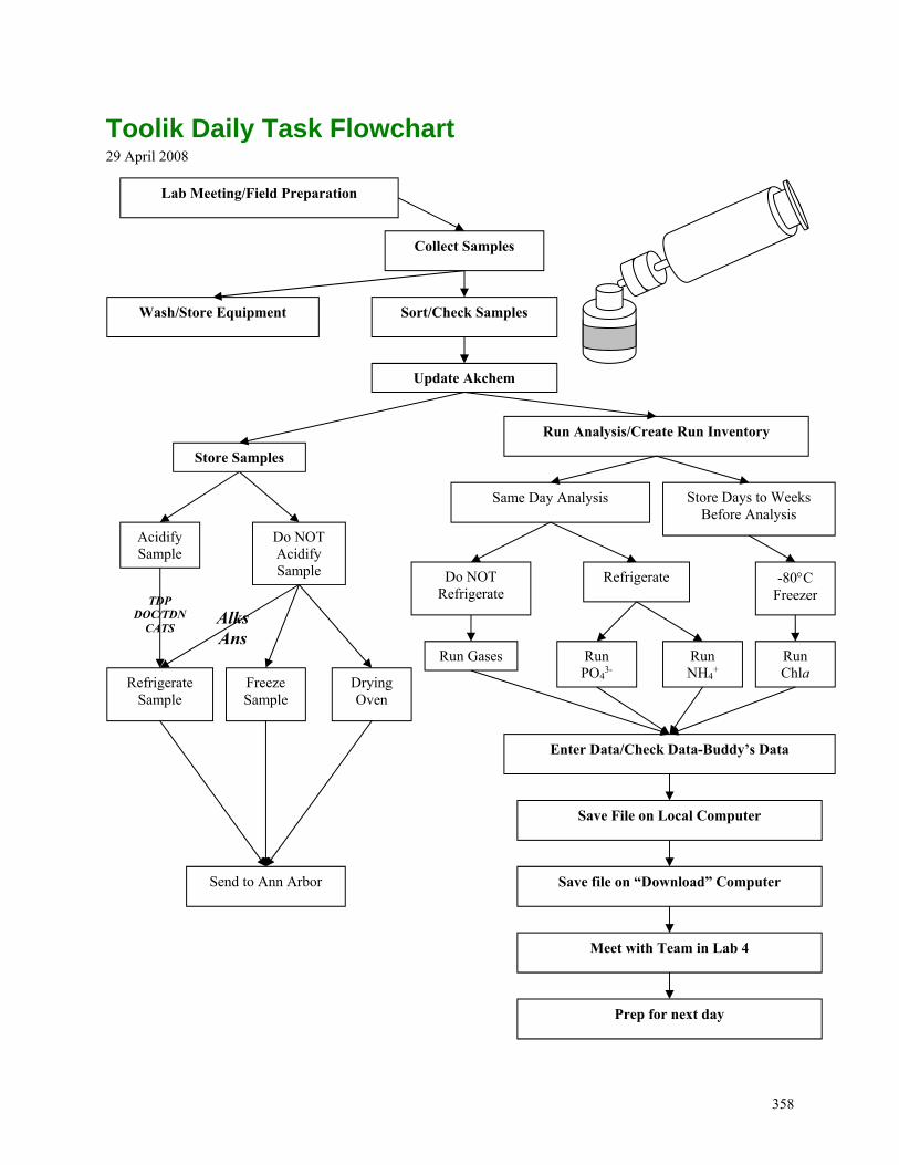
358

Toolik Daily Task Flowchart 29 April 2008

Sort/Check Samples

Freeze Sample

Refrigerate Sample

Acidify Sample

Wash/Store Equipment

Collect Samples

Lab Meeting/Field Preparation

Update Akchem

Run Gases

Store Samples

Run Analysis/Create Run Inventory

-80C Freezer

Same Day Analysis

Run PO4

3- Run NH4

+ Run Chla

Enter Data/Check Data-Buddy’s Data

Save File on Local Computer

Save file on “Download” Computer

Meet with Team in Lab 4

Prep for next day

Send to Ann Arbor

Drying Oven

Do NOT Acidify Sample

Store Days to Weeks Before Analysis

Refrigerate Do NOT Refrigerate TDP

DOC/TDN CATS

Alks Ans

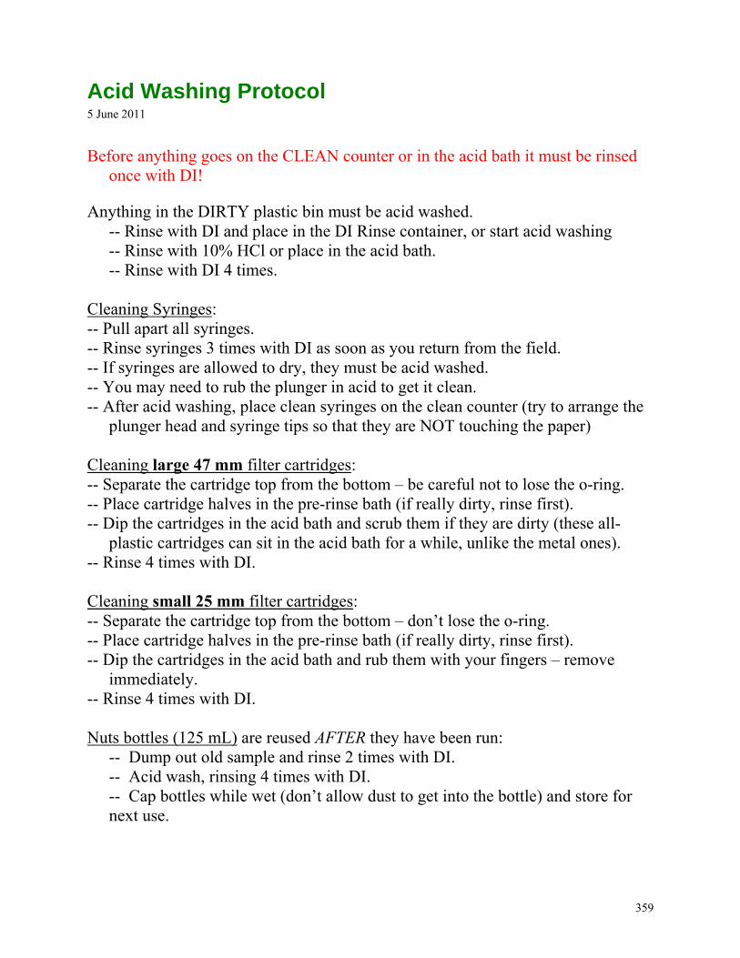
359

Acid Washing Protocol 5 June 2011

Before anything goes on the CLEAN counter or in the acid bath it must be rinsed

once with DI! Anything in the DIRTY plastic bin must be acid washed. -- Rinse with DI and place in the DI Rinse container, or start acid washing

-- Rinse with 10% HCl or place in the acid bath. -- Rinse with DI 4 times. Cleaning Syringes: -- Pull apart all syringes. -- Rinse syringes 3 times with DI as soon as you return from the field. -- If syringes are allowed to dry, they must be acid washed. -- You may need to rub the plunger in acid to get it clean. -- After acid washing, place clean syringes on the clean counter (try to arrange the

plunger head and syringe tips so that they are NOT touching the paper) Cleaning large 47 mm filter cartridges: -- Separate the cartridge top from the bottom – be careful not to lose the o-ring. -- Place cartridge halves in the pre-rinse bath (if really dirty, rinse first). -- Dip the cartridges in the acid bath and scrub them if they are dirty (these all-

plastic cartridges can sit in the acid bath for a while, unlike the metal ones). -- Rinse 4 times with DI. Cleaning small 25 mm filter cartridges: -- Separate the cartridge top from the bottom – don’t lose the o-ring. -- Place cartridge halves in the pre-rinse bath (if really dirty, rinse first). -- Dip the cartridges in the acid bath and rub them with your fingers – remove

immediately. -- Rinse 4 times with DI. Nuts bottles (125 mL) are reused AFTER they have been run: -- Dump out old sample and rinse 2 times with DI. -- Acid wash, rinsing 4 times with DI.

-- Cap bottles while wet (don’t allow dust to get into the bottle) and store for next use.

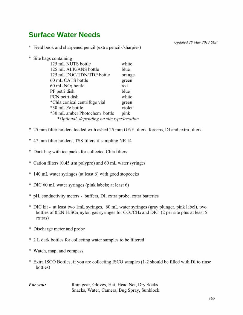
360

Surface Water Needs

Updated 28 May 2013 SEF * Field book and sharpened pencil (extra pencils/sharpies) * Site bags containing 125 mL NUTS bottle white 125 mL ALK/ANS bottle blue

125 mL DOC/TDN/TDP bottle orange 60 mL CATS bottle green 60 mL NO3 bottle red PP petri dish blue PCN petri dish white *Chla conical centrifuge vial green *30 mL Fe bottle violet *30 mL amber Photochem bottle pink *Optional, depending on site type/location * 25 mm filter holders loaded with ashed 25 mm GF/F filters, forceps, DI and extra filters * 47 mm filter holders, TSS filters if sampling NE 14 * Dark bag with ice packs for collected Chla filters * Cation filters (0.45 m polypro) and 60 mL water syringes * 140 mL water syringes (at least 6) with good stopcocks * DIC 60 mL water syringes (pink labels; at least 6) * pH, conductivity meters - buffers, DI, extra probe, extra batteries * DIC kit - at least two 1mL syringes, 60 mL water syringes (gray plunger, pink label), two

bottles of 0.2N H2SO4, nylon gas syringes for CO2/CH4 and DIC (2 per site plus at least 5 extras)

* Discharge meter and probe * 2 L dark bottles for collecting water samples to be filtered * Watch, map, and compass * Extra ISCO Bottles, if you are collecting ISCO samples (1-2 should be filled with DI to rinse

bottles) For you: Rain gear, Gloves, Hat, Head Net, Dry Socks Snacks, Water, Camera, Bug Spray, Sunblock

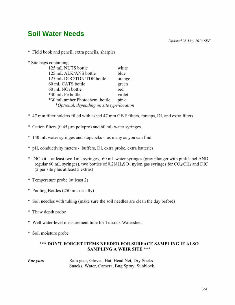
361

Soil Water Needs

Updated 28 May 2013 SEF

* Field book and pencil, extra pencils, sharpies * Site bags containing 125 mL NUTS bottle white 125 mL ALK/ANS bottle blue

125 mL DOC/TDN/TDP bottle orange 60 mL CATS bottle green 60 mL NO3 bottle red *30 mL Fe bottle violet *30 mL amber Photochem bottle pink *Optional, depending on site type/location * 47 mm filter holders filled with ashed 47 mm GF/F filters, forceps, DI, and extra filters * Cation filters (0.45 m polypro) and 60 mL water syringes. * 140 mL water syringes and stopcocks - as many as you can find * pH, conductivity meters - buffers, DI, extra probe, extra batteries * DIC kit - at least two 1mL syringes, 60 mL water syringes (gray plunger with pink label AND

regular 60 mL syringes), two bottles of 0.2N H2SO4, nylon gas syringes for CO2/CH4 and DIC (2 per site plus at least 5 extras)

* Temperature probe (at least 2) * Pooling Bottles (250 mL usually) * Soil needles with tubing (make sure the soil needles are clean the day before) * Thaw depth probe * Well water level measurement tube for Tussock Watershed * Soil moisture probe

*** DON’T FORGET ITEMS NEEDED FOR SURFACE SAMPLING IF ALSO SAMPLING A WEIR SITE ***

For you: Rain gear, Gloves, Hat, Head Net, Dry Socks Snacks, Water, Camera, Bug Spray, Sunblock

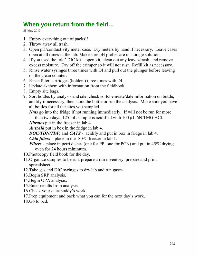
362

When you return from the field… 28 May 2013

1. Empty everything out of packs!! 2. Throw away all trash. 3. Open pH/conductivity meter case. Dry meters by hand if necessary. Leave cases

open at all times in the lab. Make sure pH probes are in storage solution. 4. If you used the ‘old’ DIC kit – open kit, clean out any leaves/trash, and remove

excess moisture. Dry off the crimper so it will not rust. Refill kit as necessary. 5. Rinse water syringes three times with DI and pull out the plunger before leaving

on the clean counter. 6. Rinse filter cartridges (holders) three times with DI. 7. Update akchem with information from the fieldbook. 8. Empty site bags. 9. Sort bottles by analysis and site, check sortchem/site/date information on bottle,

acidify if necessary, then store the bottle or run the analysis. Make sure you have all bottles for all the sites you sampled. Nuts go into the fridge if not running immediately. If will not be run for more

than two days, 125 mL sample is acidified with 100 L 6N TMG HCl. Nitrates put in the freezer in lab 4. Ans/Alk put in box in the fridge in lab 4. DOC/TDN/TDP, and CATS - acidify and put in box in fridge in lab 4. Chla filters – place in the -80ºC freezer in lab 1. Filters - place in petri dishes (one for PP, one for PCN) and put in 45ºC drying

oven for 24 hours minimum. 10. Photocopy field book for the day. 11. Organize samples to be run, prepare a run inventory, prepare and print

spreadsheet. 12. Take gas and DIC syringes to dry lab and run gases. 13. Begin SRP analysis. 14. Begin OPA analysis. 15. Enter results from analysis. 16. Check your data-buddy’s work. 17. Prep equipment and pack what you can for the next day’s work. 18. Go to bed.

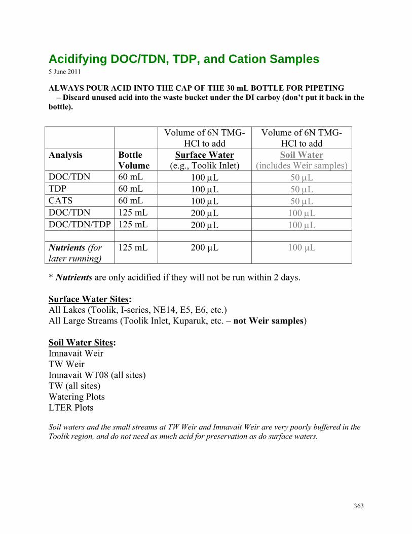
363

Acidifying DOC/TDN, TDP, and Cation Samples 5 June 2011 ALWAYS POUR ACID INTO THE CAP OF THE 30 mL BOTTLE FOR PIPETING – Discard unused acid into the waste bucket under the DI carboy (don’t put it back in the bottle).

Volume of 6N TMG-HCl to add

Volume of 6N TMG-HCl to add

Analysis Bottle Volume

Surface Water (e.g., Toolik Inlet)

Soil Water (includes Weir samples)

DOC/TDN 60 mL 100 L 50 L TDP 60 mL 100 L 50 L CATS 60 mL 100 L 50 L DOC/TDN 125 mL 200 L 100 L DOC/TDN/TDP 125 mL 200 L 100 L Nutrients (for later running)

125 mL 200 µL 100 µL

* Nutrients are only acidified if they will not be run within 2 days. Surface Water Sites: All Lakes (Toolik, I-series, NE14, E5, E6, etc.) All Large Streams (Toolik Inlet, Kuparuk, etc. – not Weir samples) Soil Water Sites: Imnavait Weir TW Weir Imnavait WT08 (all sites) TW (all sites) Watering Plots LTER Plots Soil waters and the small streams at TW Weir and Imnavait Weir are very poorly buffered in the Toolik region, and do not need as much acid for preservation as do surface waters.

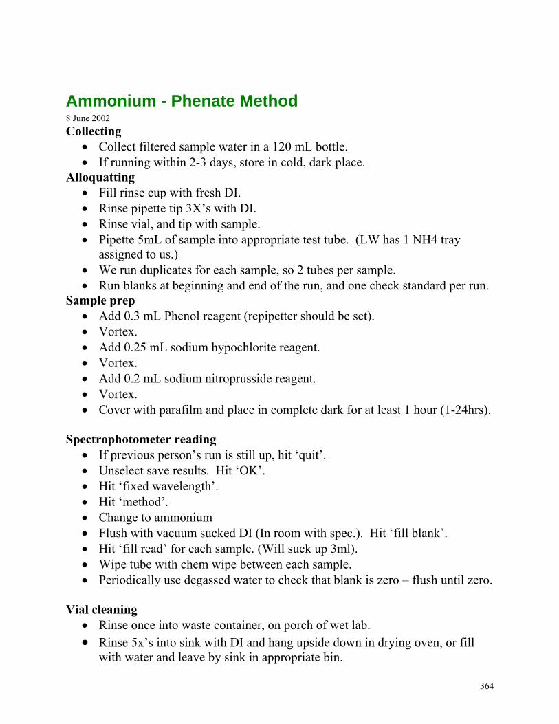
364

Ammonium - Phenate Method

8 June 2002

Collecting Collect filtered sample water in a 120 mL bottle. If running within 2-3 days, store in cold, dark place.

Alloquatting Fill rinse cup with fresh DI. Rinse pipette tip 3X’s with DI. Rinse vial, and tip with sample. Pipette 5mL of sample into appropriate test tube. (LW has 1 NH4 tray

assigned to us.) We run duplicates for each sample, so 2 tubes per sample. Run blanks at beginning and end of the run, and one check standard per run.

Sample prep Add 0.3 mL Phenol reagent (repipetter should be set). Vortex. Add 0.25 mL sodium hypochlorite reagent. Vortex. Add 0.2 mL sodium nitroprusside reagent. Vortex. Cover with parafilm and place in complete dark for at least 1 hour (1-24hrs).

Spectrophotometer reading

If previous person’s run is still up, hit ‘quit’. Unselect save results. Hit ‘OK’. Hit ‘fixed wavelength’. Hit ‘method’. Change to ammonium Flush with vacuum sucked DI (In room with spec.). Hit ‘fill blank’. Hit ‘fill read’ for each sample. (Will suck up 3ml). Wipe tube with chem wipe between each sample. Periodically use degassed water to check that blank is zero – flush until zero.

Vial cleaning

Rinse once into waste container, on porch of wet lab. Rinse 5x’s into sink with DI and hang upside down in drying oven, or fill

with water and leave by sink in appropriate bin.

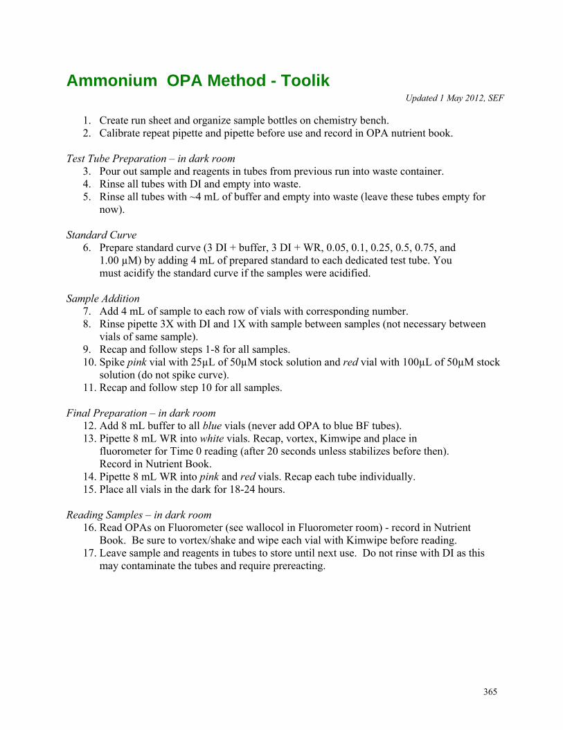
365

Ammonium OPA Method - Toolik

Updated 1 May 2012, SEF

1. Create run sheet and organize sample bottles on chemistry bench. 2. Calibrate repeat pipette and pipette before use and record in OPA nutrient book.

Test Tube Preparation – in dark room

3. Pour out sample and reagents in tubes from previous run into waste container. 4. Rinse all tubes with DI and empty into waste. 5. Rinse all tubes with ~4 mL of buffer and empty into waste (leave these tubes empty for

now).

Standard Curve 6. Prepare standard curve (3 DI + buffer, 3 DI + WR, 0.05, 0.1, 0.25, 0.5, 0.75, and

1.00 µM) by adding 4 mL of prepared standard to each dedicated test tube. You must acidify the standard curve if the samples were acidified.

Sample Addition 7. Add 4 mL of sample to each row of vials with corresponding number. 8. Rinse pipette 3X with DI and 1X with sample between samples (not necessary between

vials of same sample). 9. Recap and follow steps 1-8 for all samples. 10. Spike pink vial with 25µL of 50µM stock solution and red vial with 100µL of 50µM stock

solution (do not spike curve). 11. Recap and follow step 10 for all samples.

Final Preparation – in dark room

12. Add 8 mL buffer to all blue vials (never add OPA to blue BF tubes). 13. Pipette 8 mL WR into white vials. Recap, vortex, Kimwipe and place in

fluorometer for Time 0 reading (after 20 seconds unless stabilizes before then). Record in Nutrient Book.

14. Pipette 8 mL WR into pink and red vials. Recap each tube individually. 15. Place all vials in the dark for 18-24 hours.

Reading Samples – in dark room

16. Read OPAs on Fluorometer (see wallocol in Fluorometer room) - record in Nutrient Book. Be sure to vortex/shake and wipe each vial with Kimwipe before reading.

17. Leave sample and reagents in tubes to store until next use. Do not rinse with DI as this may contaminate the tubes and require prereacting.

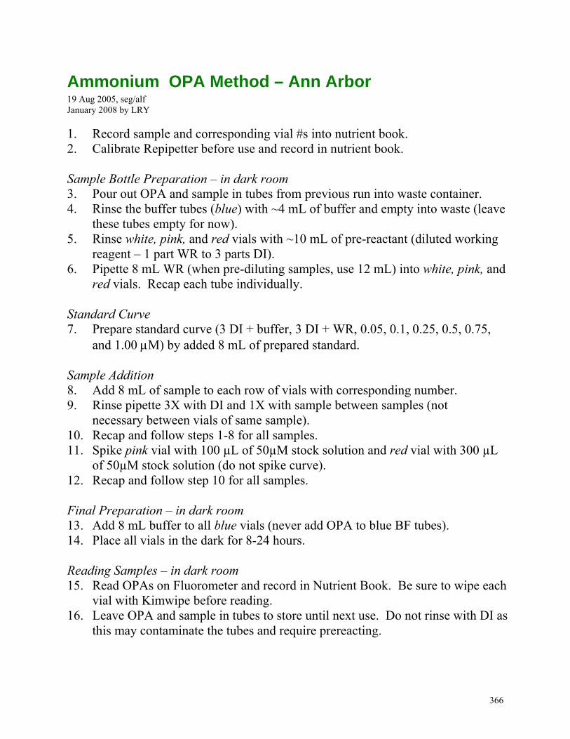
366

Ammonium OPA Method – Ann Arbor

19 Aug 2005, seg/alf January 2008 by LRY

1. Record sample and corresponding vial #s into nutrient book. 2. Calibrate Repipetter before use and record in nutrient book. Sample Bottle Preparation – in dark room 3. Pour out OPA and sample in tubes from previous run into waste container. 4. Rinse the buffer tubes (blue) with ~4 mL of buffer and empty into waste (leave

these tubes empty for now). 5. Rinse white, pink, and red vials with ~10 mL of pre-reactant (diluted working

reagent – 1 part WR to 3 parts DI). 6. Pipette 8 mL WR (when pre-diluting samples, use 12 mL) into white, pink, and

red vials. Recap each tube individually. Standard Curve 7. Prepare standard curve (3 DI + buffer, 3 DI + WR, 0.05, 0.1, 0.25, 0.5, 0.75,

and 1.00 M) by added 8 mL of prepared standard. Sample Addition 8. Add 8 mL of sample to each row of vials with corresponding number. 9. Rinse pipette 3X with DI and 1X with sample between samples (not

necessary between vials of same sample). 10. Recap and follow steps 1-8 for all samples. 11. Spike pink vial with 100 µL of 50µM stock solution and red vial with 300 µL

of 50µM stock solution (do not spike curve). 12. Recap and follow step 10 for all samples. Final Preparation – in dark room 13. Add 8 mL buffer to all blue vials (never add OPA to blue BF tubes). 14. Place all vials in the dark for 8-24 hours. Reading Samples – in dark room 15. Read OPAs on Fluorometer and record in Nutrient Book. Be sure to wipe each

vial with Kimwipe before reading. 16. Leave OPA and sample in tubes to store until next use. Do not rinse with DI as

this may contaminate the tubes and require prereacting.

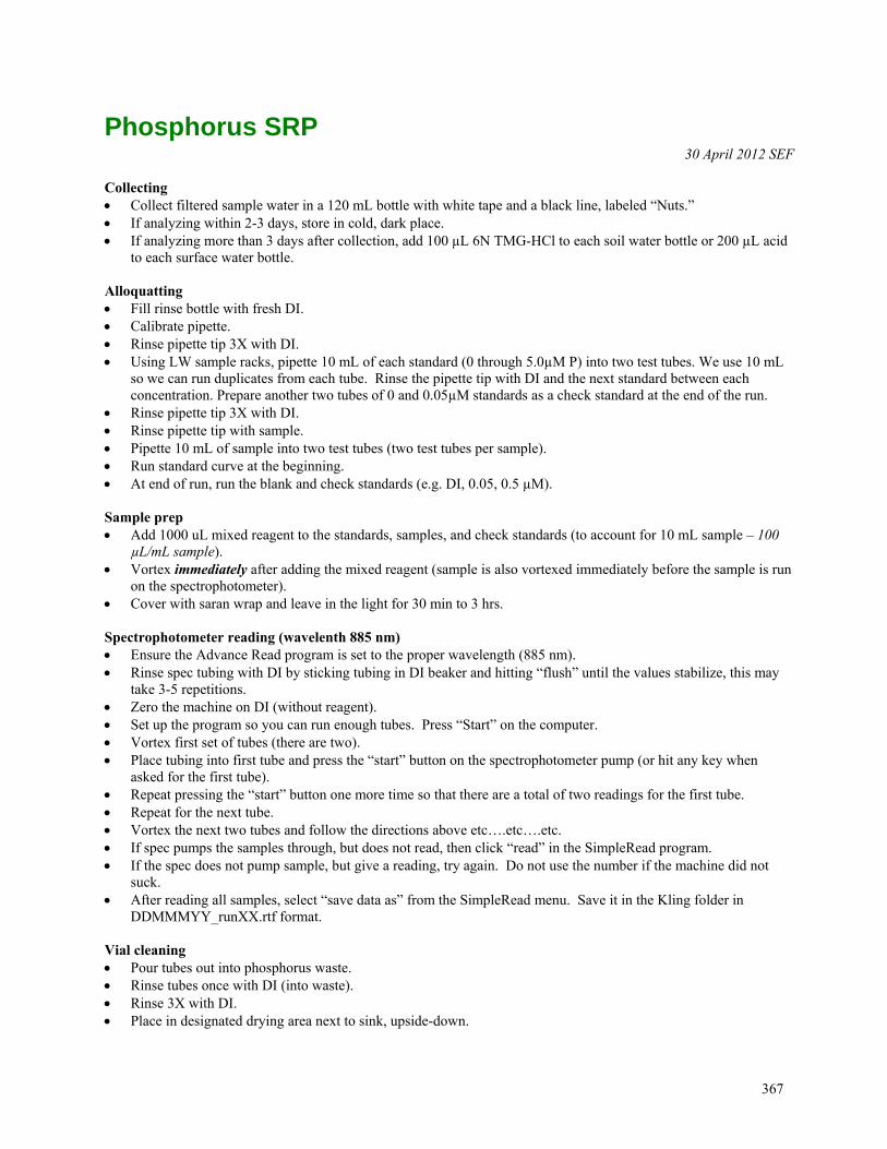
367

Phosphorus SRP 30 April 2012 SEF

Collecting Collect filtered sample water in a 120 mL bottle with white tape and a black line, labeled “Nuts.” If analyzing within 2-3 days, store in cold, dark place. If analyzing more than 3 days after collection, add 100 µL 6N TMG-HCl to each soil water bottle or 200 µL acid

to each surface water bottle. Alloquatting Fill rinse bottle with fresh DI. Calibrate pipette. Rinse pipette tip 3X with DI. Using LW sample racks, pipette 10 mL of each standard (0 through 5.0µM P) into two test tubes. We use 10 mL

so we can run duplicates from each tube. Rinse the pipette tip with DI and the next standard between each concentration. Prepare another two tubes of 0 and 0.05µM standards as a check standard at the end of the run.

Rinse pipette tip 3X with DI. Rinse pipette tip with sample. Pipette 10 mL of sample into two test tubes (two test tubes per sample). Run standard curve at the beginning. At end of run, run the blank and check standards (e.g. DI, 0.05, 0.5 µM). Sample prep Add 1000 uL mixed reagent to the standards, samples, and check standards (to account for 10 mL sample – 100

µL/mL sample). Vortex immediately after adding the mixed reagent (sample is also vortexed immediately before the sample is run

on the spectrophotometer). Cover with saran wrap and leave in the light for 30 min to 3 hrs. Spectrophotometer reading (wavelenth 885 nm) Ensure the Advance Read program is set to the proper wavelength (885 nm). Rinse spec tubing with DI by sticking tubing in DI beaker and hitting “flush” until the values stabilize, this may

take 3-5 repetitions. Zero the machine on DI (without reagent). Set up the program so you can run enough tubes. Press “Start” on the computer. Vortex first set of tubes (there are two). Place tubing into first tube and press the “start” button on the spectrophotometer pump (or hit any key when

asked for the first tube). Repeat pressing the “start” button one more time so that there are a total of two readings for the first tube. Repeat for the next tube. Vortex the next two tubes and follow the directions above etc….etc….etc. If spec pumps the samples through, but does not read, then click “read” in the SimpleRead program. If the spec does not pump sample, but give a reading, try again. Do not use the number if the machine did not

suck. After reading all samples, select “save data as” from the SimpleRead menu. Save it in the Kling folder in

DDMMMYY_runXX.rtf format. Vial cleaning Pour tubes out into phosphorus waste. Rinse tubes once with DI (into waste). Rinse 3X with DI. Place in designated drying area next to sink, upside-down.

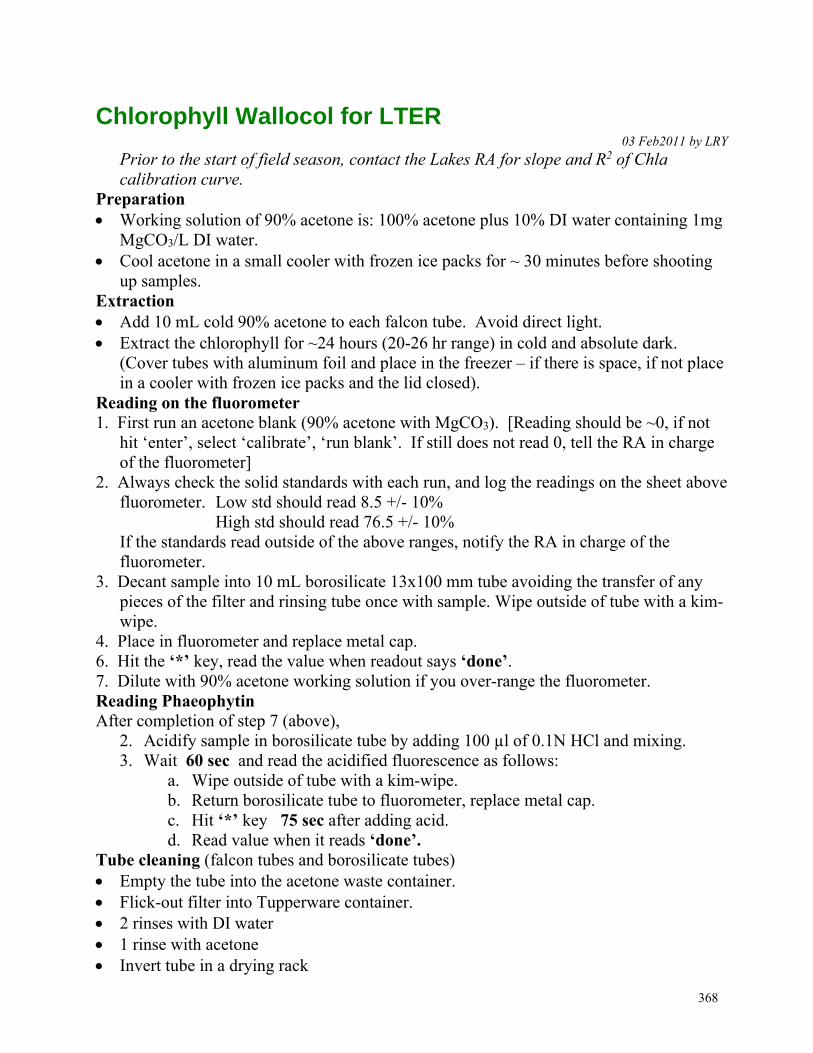
368

Chlorophyll Wallocol for LTER 03 Feb2011 by LRY

Prior to the start of field season, contact the Lakes RA for slope and R2 of Chla calibration curve.

Preparation Working solution of 90% acetone is: 100% acetone plus 10% DI water containing 1mg

MgCO3/L DI water. Cool acetone in a small cooler with frozen ice packs for ~ 30 minutes before shooting

up samples. Extraction Add 10 mL cold 90% acetone to each falcon tube. Avoid direct light. Extract the chlorophyll for ~24 hours (20-26 hr range) in cold and absolute dark.

(Cover tubes with aluminum foil and place in the freezer – if there is space, if not place in a cooler with frozen ice packs and the lid closed).

Reading on the fluorometer 1. First run an acetone blank (90% acetone with MgCO3). [Reading should be ~0, if not

hit ‘enter’, select ‘calibrate’, ‘run blank’. If still does not read 0, tell the RA in charge of the fluorometer]

2. Always check the solid standards with each run, and log the readings on the sheet above fluorometer. Low std should read 8.5 +/- 10%

High std should read 76.5 +/- 10% If the standards read outside of the above ranges, notify the RA in charge of the

fluorometer. 3. Decant sample into 10 mL borosilicate 13x100 mm tube avoiding the transfer of any

pieces of the filter and rinsing tube once with sample. Wipe outside of tube with a kim-wipe.

4. Place in fluorometer and replace metal cap. 6. Hit the ‘*’ key, read the value when readout says ‘done’. 7. Dilute with 90% acetone working solution if you over-range the fluorometer. Reading Phaeophytin After completion of step 7 (above),

2. Acidify sample in borosilicate tube by adding 100 µl of 0.1N HCl and mixing. 3. Wait 60 sec and read the acidified fluorescence as follows:

a. Wipe outside of tube with a kim-wipe. b. Return borosilicate tube to fluorometer, replace metal cap. c. Hit ‘*’ key 75 sec after adding acid. d. Read value when it reads ‘done’.

Tube cleaning (falcon tubes and borosilicate tubes) Empty the tube into the acetone waste container. Flick-out filter into Tupperware container. 2 rinses with DI water 1 rinse with acetone Invert tube in a drying rack

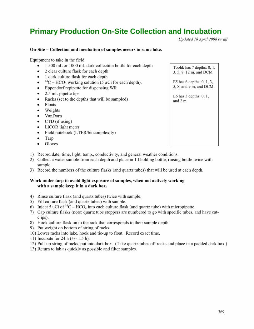
369

Primary Production On-Site Collection and Incubation Updated 18 April 2008 by alf

On-Site = Collection and incubation of samples occurs in same lake. Equipment to take in the field

1 500 mL or 1000 mL dark collection bottle for each depth 2 clear culture flask for each depth 1 dark culture flask for each depth 14C – HCO3 working solution (5 Ci for each depth). Eppendorf repipette for dispensing WR 2.5 mL pipette tips Racks (set to the depths that will be sampled) Floats Weights VanDorn CTD (if using) LiCOR light meter Field notebook (LTER/biocomplexity) Tarp Gloves

1) Record date, time, light, temp., conductivity, and general weather conditions. 2) Collect a water sample from each depth and place in 1 l holding bottle, rinsing bottle twice with

sample. 3) Record the numbers of the culture flasks (and quartz tubes) that will be used at each depth. Work under tarp to avoid light exposure of samples, when not actively working

with a sample keep it in a dark box. 4) Rinse culture flask (and quartz tubes) twice with sample. 5) Fill culture flask (and quartz tubes) with sample. 6) Inject 5 uCi of 14C – HCO3 into each culture flask (and quartz tube) with micropipette. 7) Cap culture flasks (note: quartz tube stoppers are numbered to go with specific tubes, and have cat-

clips). 8) Hook culture flask on to the rack that corresponds to their sample depth. 9) Put weight on bottom of string of racks. 10) Lower racks into lake, hook and tie-up to float. Record exact time. 11) Incubate for 24 h (+/- 1.5 h). 12) Pull-up string of racks, put into dark box. (Take quartz tubes off racks and place in a padded dark box.) 13) Return to lab as quickly as possible and filter samples.

Toolik has 7 depths: 0, 1, 3, 5, 8, 12 m, and DCM E5 has 6 depths: 0, 1, 3, 5, 8, and 9 m, and DCM E6 has 3 depths: 0, 1, and 2 m

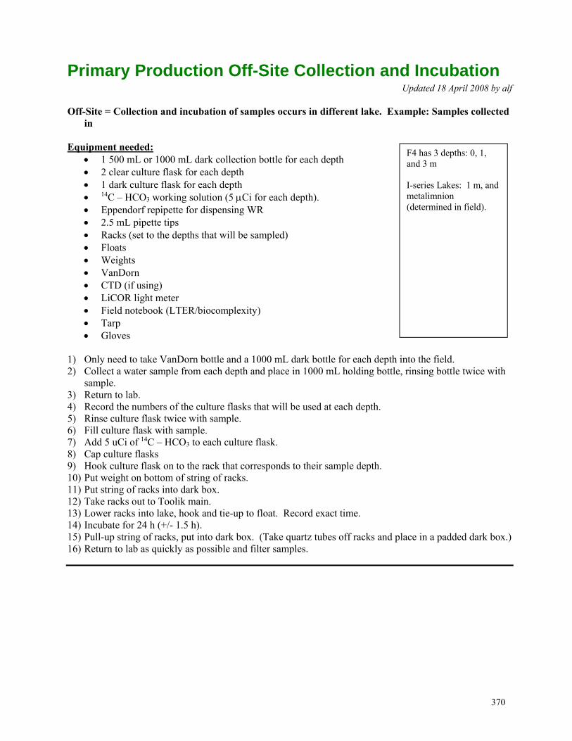
370

Primary Production Off-Site Collection and Incubation Updated 18 April 2008 by alf

Off-Site = Collection and incubation of samples occurs in different lake. Example: Samples collected

in Equipment needed:

1 500 mL or 1000 mL dark collection bottle for each depth 2 clear culture flask for each depth 1 dark culture flask for each depth 14C – HCO3 working solution (5 Ci for each depth). Eppendorf repipette for dispensing WR 2.5 mL pipette tips Racks (set to the depths that will be sampled) Floats Weights VanDorn CTD (if using) LiCOR light meter Field notebook (LTER/biocomplexity) Tarp Gloves

1) Only need to take VanDorn bottle and a 1000 mL dark bottle for each depth into the field. 2) Collect a water sample from each depth and place in 1000 mL holding bottle, rinsing bottle twice with

sample. 3) Return to lab. 4) Record the numbers of the culture flasks that will be used at each depth. 5) Rinse culture flask twice with sample. 6) Fill culture flask with sample. 7) Add 5 uCi of 14C – HCO3 to each culture flask. 8) Cap culture flasks 9) Hook culture flask on to the rack that corresponds to their sample depth. 10) Put weight on bottom of string of racks. 11) Put string of racks into dark box. 12) Take racks out to Toolik main. 13) Lower racks into lake, hook and tie-up to float. Record exact time. 14) Incubate for 24 h (+/- 1.5 h). 15) Pull-up string of racks, put into dark box. (Take quartz tubes off racks and place in a padded dark box.) 16) Return to lab as quickly as possible and filter samples.

F4 has 3 depths: 0, 1, and 3 m I-series Lakes: 1 m, and metalimnion (determined in field).

371

Primary Production Filtering and Counting Procedures Updated 18 April 2008 by alf

Equipment needed:

Filter manifold Filters Forceps Gloves Lab notebook Mini-scintillation vials Rinse bottle with DI H2O Filled RO-DI caboy Samples Pen Sharpie

Avoid exposure of samples to light. 1) Label the tops of mini-scintillation vials with a sharpie to indicate date and

sample #. 2) Fill in sample information on sample tracking book 3) Place filters in position in the filter manifold. Seal filter manifold (do not over

tighten, make sure parts are aligned right) stopper any unused positions. Attach vacuum pump.

4) Add DI water to a filter position to check for leaks 5) Apply vacuum to filter manifold. Dispense each sample sequentially into each of

the filter positions of the filter manifold. Rinse each vial twice with 5-10 mL of DI water after dispensing sample.

6) Once the filter is dry or almost dry, rinse filter and column with DI water. 7) Apply vacuum just till dry. Place filters in separate mini-scintillation vials. Cap

lightly with appropriately labeled top. Leave tops loose so filter can dry completely.

8) Repeat 4-7 till all samples are filtered. 9) Dispose of rad waste in rad waste containers. 10) Rinse filter manifold once with DI water, dispose of this rinse in rad waste. 11) Thoroughly rinse all equipment in the lake and put it away.

372

Primary Production - Scintillation Counter Updated 18 April 2008 by alf

Equipment needed Filter (Sample) Scintillation counter Cellusolve Scintisafe 1 mL pipette 5 mL pipette

1) Add 1-mL of Cellusolve to each mini-scintillation vial containing a

sample filter (see filtering protocol). 2) Let sit over night. 3) Add 5-mL of Scintisafe to each mini-scintillation vial. 4) Let sit in dark 1-2 days. 5) Load samples into white adapters and into scintillation counter trays

with the orange tag to your right. - If you do not fill all spaces, remove adapters – if adapters are left in, the scintillation counter will try to count that location. 6) Place the protocol tag on the left side of the scintillation counter tray. 7) Push the ‘flag’ of the protocol tag so that the part that moves hangs

further over the tray. 8) Load samples + sample tray into the right half of the scintillation

counter with the flag closest to the median and the orange side of the tray facing the outside wall of the right side of the scintillation counter.

9) Close lid, cover with black material, and keep the room DARK (this scintillation counter has a little light leak).

10) Count on scintillation counter using a 14C program. Count each vial for 5-10 min. Record counts per minute.

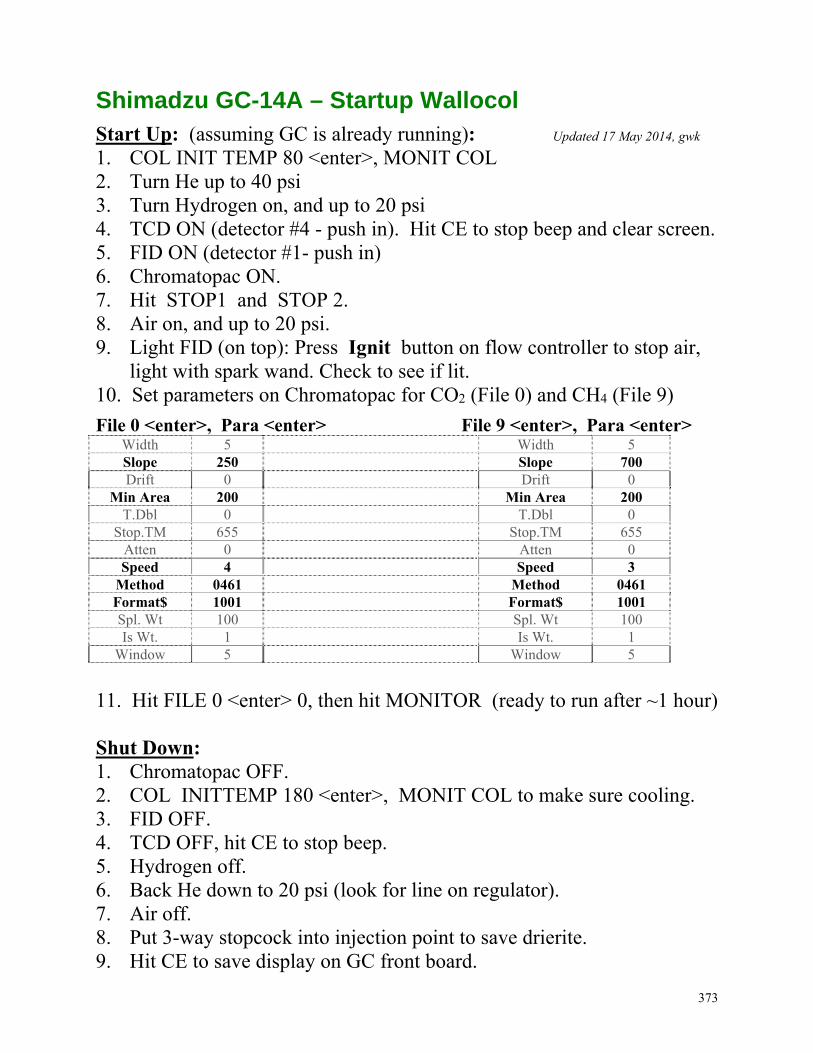
373

Shimadzu GC-14A – Startup Wallocol Start Up: (assuming GC is already running): Updated 17 May 2014, gwk 1. COL INIT TEMP 80 <enter>, MONIT COL 2. Turn He up to 40 psi 3. Turn Hydrogen on, and up to 20 psi 4. TCD ON (detector #4 - push in). Hit CE to stop beep and clear screen. 5. FID ON (detector #1- push in) 6. Chromatopac ON. 7. Hit STOP1 and STOP 2. 8. Air on, and up to 20 psi. 9. Light FID (on top): Press Ignit button on flow controller to stop air,

light with spark wand. Check to see if lit. 10. Set parameters on Chromatopac for CO2 (File 0) and CH4 (File 9)

File 0 <enter>, Para <enter> File 9 <enter>, Para <enter> Width 5 Width 5 Slope 250 Slope 700 Drift 0 Drift 0

Min Area 200 Min Area 200 T.Dbl 0 T.Dbl 0

Stop.TM 655 Stop.TM 655 Atten 0 Atten 0 Speed 4 Speed 3

Method 0461 Method 0461 Format$ 1001 Format$ 1001 Spl. Wt 100 Spl. Wt 100 Is Wt. 1 Is Wt. 1

Window 5 Window 5

11. Hit FILE 0 <enter> 0, then hit MONITOR (ready to run after ~1 hour) Shut Down: 1. Chromatopac OFF. 2. COL INITTEMP 180 <enter>, MONIT COL to make sure cooling. 3. FID OFF. 4. TCD OFF, hit CE to stop beep. 5. Hydrogen off. 6. Back He down to 20 psi (look for line on regulator). 7. Air off. 8. Put 3-way stopcock into injection point to save drierite. 9. Hit CE to save display on GC front board.

374

GC14A – Running Gases Wallocol Updated 17 May 2014, gwk

1. Complete the Start-up Wallocol sequence. 2. Check the drierite tube – if ¼ or more pink, change the drierite. 3. Label printout at top with Date, Samples, GC operator and Run#. 4. Open AKGAS_YEAR.xls file on laptop to record data. 5. Run standards: 3 reps each of low (ambient) and medium for surface

waters, plus high stds for soil waters. 6. To inject std or sample, turn switch to LOAD (left), inject sample,

turn switch to INJECT, then hit START1 and START2. 7. After the first set of 3 std reps have been run, press STOP1 and

STOP2. 8. While the chromatopac is printing, flush the drierite and sample loop

with the next highest std, and the switch to INJECT – you are not recording this std, but it will help flush the column at the level of the next standard. Repeat 2x. Wait for last peak to clear.

9. Run higher set of standards. Repeat step 8. 10. If stds are OK, run samples (see Step #6). Make sure to flush the

sample loop and column with room air if you will begin with “low range” samples.

11. Write the syringe # next to each sample peak on chromatogram. 12. Print areas (hit STOP1, STOP2) after every 15 samples to avoid

running out of memory on the Chromatopac (= lost data). 13. Repeat step 6 to begin next sample batch. 14. If the run is very long, analyze standards at end (2 reps). Tips from the Top: 1. Check the syringe tip for water. Dry with rolled up kimwipe. If water

is inside the syringe, note this in the gas book. 2. Always support the 3-way stopcocks and especially the luer-lock

injection port with both hands – the port is very fragile (i.e., if you break it there is not a replacement...).

3. Inject the sample slowly down to 5 mL remaining (if possible) and wait 4 seconds until turning the valve to inject. This will result in fewer pressure variations and better reproducibility.

APOLLO DIC ANALYZER -- Wallocol 2 July 2013, gwk, khh

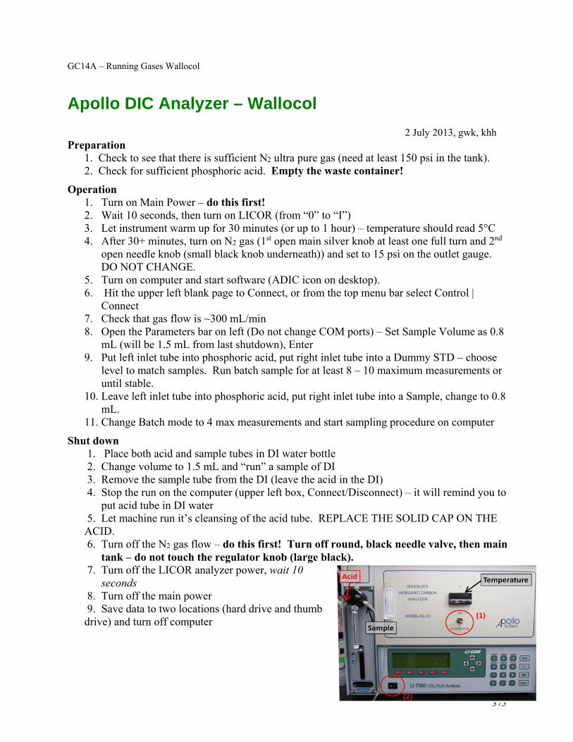
375

GC14A – Running Gases Wallocol

Apollo DIC Analyzer – Wallocol

2 July 2013, gwk, khh Preparation

1. Check to see that there is sufficient N2 ultra pure gas (need at least 150 psi in the tank). 2. Check for sufficient phosphoric acid. Empty the waste container!

Operation 1. Turn on Main Power – do this first! 2. Wait 10 seconds, then turn on LICOR (from “0” to “I”) 3. Let instrument warm up for 30 minutes (or up to 1 hour) – temperature should read 5°C 4. After 30+ minutes, turn on N2 gas (1st open main silver knob at least one full turn and 2nd

open needle knob (small black knob underneath)) and set to 15 psi on the outlet gauge. DO NOT CHANGE.

5. Turn on computer and start software (ADIC icon on desktop). 6. Hit the upper left blank page to Connect, or from the top menu bar select Control |

Connect 7. Check that gas flow is ~300 mL/min 8. Open the Parameters bar on left (Do not change COM ports) – Set Sample Volume as 0.8

mL (will be 1.5 mL from last shutdown), Enter 9. Put left inlet tube into phosphoric acid, put right inlet tube into a Dummy STD – choose

level to match samples. Run batch sample for at least 8 – 10 maximum measurements or until stable.

10. Leave left inlet tube into phosphoric acid, put right inlet tube into a Sample, change to 0.8 mL.

11. Change Batch mode to 4 max measurements and start sampling procedure on computer

Shut down 1. Place both acid and sample tubes in DI water bottle 2. Change volume to 1.5 mL and “run” a sample of DI 3. Remove the sample tube from the DI (leave the acid in the DI) 4. Stop the run on the computer (upper left box, Connect/Disconnect) – it will remind you to

put acid tube in DI water 5. Let machine run it’s cleansing of the acid tube. REPLACE THE SOLID CAP ON THE ACID. 6. Turn off the N2 gas flow – do this first! Turn off round, black needle valve, then main

tank – do not touch the regulator knob (large black). 7. Turn off the LICOR analyzer power, wait 10

seconds 8. Turn off the main power 9. Save data to two locations (hard drive and thumb drive) and turn off computer

376

Stream Rain Event Sampling

28 March 2007 by ALF

For ISCO rain event sampling: NUTS, DOC/TDN, TDP, NO3, ANS, ALK, CATS, no gases/DIC.

Field Notebook and pencil Laptop or PDA kit Clear garbage bag to protect laptop 140 mL water syringes (for chemistry) 60 ml water syringes (for gas/DIC) 25 mm filter holders with ashed filters with extra filters, forceps, and filter holders. Cation filters DI water to clean out ISCO bottles 3-5 clean ISCO bottles Extra pencils and sharpies Labeled bottles Extra sampling bottle kits/bags

For “live” rain even sampling (all of above plus…): Sample for all chemistries, gases, and DIC.

Nylon gas syringes for gas and DIC (2 syringes plus 4 extra) DIC kit (H2SO4, 1 cc syringe) pH and conductivity meters (buffers, DI, extra probe, extra battery).

For people: Rain-gear, gloves, hat, dry socks, head-net or bug jacket, water, snacks, camera, bug spray. Rain Event Sampling:

Before you leave: 1) Prepare bottles (NUTS, DOC/TDN, TDP, NO3, ANS, ALK, CATS).

a. Check handwritten sortchem inventory sheet BEFORE assigning new sortchems. i. ISCO samples: Assign a rain event (RE) number for ISCO samples. Check the list on

the wall in lab 4 for the next available RE number. ii. “Live” samples: use standard naming convention (do NOT assign RE#)

iii. Make labels using Toolik_SampleBottleLabels2007.xls. 2) Check that laptop/PDA battery is working. 3) Toolik Inlet and TW Weir: ask for a list of the ~ date/time of bottles to be collected.

In the field:

1) Download the datalogger (either ISCO at IMN Weir or Campbells at TI and TW Weir). a. At IMN Weir (1000 ml bottle ISCO)

i. Use the laptop to determine which bottles to sample. Save the text file and the graph (data).

1. Write down the bottle position, date AND time (when that bottle was filled), and bottle number.

2. Filter for both PCN and PP (all chemistry, no gas/DIC). b. Toolik Inlet and TW Weir (500 ml bottle ISCOs)

i. Determine the bottles that are closest to the ideal date/time. ii. Filter only for PCN (all chemistry, no gas/DIC).

c. At a minimum, select a bottle representing a period of time during the ascent, peak, and descent of the stage height.

2) Take a live sample for NUTS, DOC/TDN, TDP, NO3, ANS, ALK, CATS, gases, and DIC, a. Do NOT take a duplicate sample.

377

DOC/TDN DETERMINATION ON TOC-V

A. Routine Start-Up:

1. Make sure sufficient compressed ultra zero air is available for TOC analysis and dry Air for TN analysis. A full run takes over 36 h and requires 600 psi dry air and 300 psi ultra zero air; change cylinders before starting the run if necessary.

2. Turn on main TOC module (switch on front) and TN module (switch on right side; power on when top of switch is pushed in).

3. Open TOC-V software. We are using the DOC-TN system. 4. Click on “File” and select “new.” Then select “Sample Run.” 5. The General Information screen will appear; select the correct system (usually DOC_TN) and click on

“ok.” Name the file by clicking on “save as,” calling up the last file run, and increasing the sequential number by 1. An empty run file form will appear.

6. Click on “connect” (the lightning symbol) and then select “use settings on PC.” The analyzer will then begin its initialization procedure.

7. After initialization is complete, click on “Instrument,” then select “Maintenance,” and then select “Perform Zero Point Detection;” click on “Start.” Click on “Close” when completed.

8. Click on “Instrument,” then select “Maintenance,” and then select “Replenish IC Solution”; click on “Start.” Click on “Close” when completed.

9. Instrument status can be monitored by clicking on “Instrument” and selecting “Background Monitor.”

B. Loading the Sample Carousel:

1. Samples should be pre-acidified and are run in 24 mL sample vials. These vials should be filled at least ½ full and covered with parafilm.

2. The sample carousel holds 93 vials. Samples are not placed in the following positions: 30, 54, 72, 85, and 93 to eliminate the possibility of sample contamination from the sparge needle.

3. Current protocol calls for placing 2 check standards at the start of the run, in positions 1 and 2. They are followed by 36 samples (if running a full tray) in positions 3-38. Positions 39-52 are used for the standards which are loaded in duplicate, in ascending order. Positions 53-90 are used for samples, followed by 2 more check standards in positions 91 and 92. The check standards should have a concentration similar to the concentration of most samples. (DI rinses before the first check standards, after the last check standards and before and after the series of standards in the middle of the run are programmed into the run file on the computer and use DI water drawn from a rinse water reservoir, position 0.)

C. Manually Programming the Sample Run Table via TOC-V software:

1. The empty sample run table should be displayed in the monitor. The Background Monitor window must be closed.

2. The table can be filled in multi-row sections by selecting “insert” and choosing “auto generate.” (Since you are able to specify a method, sample name and sample ID which will be replicated for each row in the section added, it is most efficient to add samples one group at a time, i.e. standards, samples, blanks.)

3. You will first be prompted to enter a method: Click on the browse square to see the list of stored methods and select the appropriate one or construct a new method. Click on “open;” then click on “next.” You will then be prompted to enter the number of samples (rows) being inserted and what vial number to start with. Then you will have the chance to enter a sample name and a sample ID which will be added and replicated in each row inserted. After this information has been entered, click on “next;” click on “next” again; then click on “finish.” The next view includes a sample table and a schematic diagram of the sample carousel with the occupied positions colored blue. Click on “OK.” The selected number of rows will then be filled in, sequentially, as specified above.

4. This process is repeated until the entire Sample Run Table has been filled in. 5. All information that is unique to a row must next be entered manually. Because this software is rather

primitive, the process is not easily streamlined and is the most tedious part of setting up a run. At this

378

time you cannot change the vial (position) number. The only time a vial number can be changed is via the “Sparging/Acid Addition” screen (see below.)

6. Once the table is completely filled in, save it. Then save it (as TOC_xxxx.t32) in C/TOC3201/data, C/data/chemistry/DOC/data, and L/TOC/3201/data.

7. When you are ready to start running these samples click on the green light symbol to start the run. You will then be prompted through the following sequence:

8. “Standby” screen—choose “Shut Down Instrument,” then click on “standby.” 9. “Sparging/Acid Addition” screen—enter/change vial numbers (location on sample carousel) as needed.

The display will show a schematic diagram of the sample carousel with all positions programmed into the run table colored blue. Correct any vial numbers that are wrong. THIS IS THE ONLY TIME VIAL (POSITION) NUMBERS CAN BE ADDED OR ALTERED. Click on “ok” after correctly entering all vial position numbers.

10. “Start ASI Measurement” screen—un-check “External Acid Addition,” then click on “Start” if everything has been entered and set-up correctly; or click on “Cancel” if you need to go back and change anything before starting the run.

379

TOC-V Software: Analysis Set-up and Data Processing

I. Overview File list and descriptions: DocFileIII.xls----------Repository for processed DOC data stored by run vial/sortchem, and intermediate files and macros for formulating Daily Entry Sheets and Sample Schedules, divided into the following tabs:

Notes Runs Daily Entry Sheet’ Daily Sample Schedule’ TOCdata-DOCfinal’ Curve Report Dilution value Machine blanks

TOC_TN_data.xls--------------Repository for raw data from TOC-V, stored by injection value—this is the file sent to SAS for:statistical analysis, reduction to a single value per run vial, and final concentrations calculated based on the standards run with each analysis. Template_TBL.txt--------------This is a template file used to construct xxxx_tbl.txt in the proper format for importing to the TOC-V. xxxx_tbl.txt (xxxx is the run number)--This is a text-format file which contains the specific run data--sample, standard, blank and rinse information--from DocFileIII.xls; it is used to import this data to TOC_xxxx.t32. TOC_xxxx.t32 (xxxx is the run number)-----------This is the TOC-V run schedule, a list of samples, standards, blanks, rinses that make up an analysis run (the ‘Daily Sample Schedule). TOC_xxxx.txt (xxxx is the run number)-----------This is a text-format file to which specific run analysis data from run xxx --sample, standard, blank and rinse information stored by injection--is imported. This file is used to transfer this data to TOC_TN_data.xls. DOC_III_1of4_Condensed.sas & DOC_III_2of4_Concentrations.sas—These are SAS programs. DOC_III_1of4_Condensed.sas takes the raw peak area data from the multiple injections per vial (sample, standard or rinse), statistically evaluates them, and then condenses them to a single representative value per vial (sample, standard or rinse). DOC_III_2of4_Concentrations.sas takes this condensed data and uses the standard and blank values to construct a standard curve per analysis run, then uses this curve to calculate the concentrations of samples in that run.

II. Summary of Procedure

1. C:DocFileIII.xls is updated from L:DocFileIII.xls 2. The Daily Entry Sheet tab of C:DocFileIII.xls is accessed and used to print the Daily Entry Sheet, a

schedule of the samples that make up a given run on the TOC-V DOC/TN analyzer. 3. The Daily Sample Schedule tab is accessed and the Daily Entry Sheet is imported. 4. The TOCdata_DOCfinal tab is accessed and the Daily Sample Schedule is imported 5. Run number and sequence-in-run information is appended to the daily sample schedule and dilution

values are checked and revised as necessary. 6. The updated DocFileIII.xls is saved to both C and L drives

380

7. The Template_TBL.txt file is accessed. It is a template of a TOC-V run table, complete except it has blank spaces to receive specific sample information.

8. The specific sample information for a given run is copied from the TOCdata_DOCfinal tab to the appropriate blank spaces in Template_TBL.txt and it is saved as (run number)tbl.txt

9. (run number)tbl.txt is imported into the TOC-V software and used to make a TOC-V run schedule. 10. Samples, Standards and Rinses are loaded as specified by the run schedule and analyzed on the TOC-V

for DOC and TN 11. TOC-V analysis generates 2 files, TOC(run number).t32 which contains the run schedule information

and some analysis results, and TOC_(run number).pkt which contains all of the raw peak area data, by individual injection. These files are saved to both C and L drives.

12. TOC(run number).t32, the TOC-V output file, is translated into a .txt file with the same name and imported into Excel. All run data from this file is copied into TOC_TN_data.xls

13. SAS program ‘DOC_III_1of4_Condensed.sas’ is used to condense the individual injection data into a single mean value for DOC and a single mean value for TN per vial (sample, standard or rinse).

14. SAS program DOC_III_2of4_Concentrations.sas is used to calculate concentrations of DOC and TN on a by run basis, based on the standards analyzed in that run and the mean peak area values generated by DOC_III_1of4_Condensed.sas. The results of these analyses are written to DocFileIII.xls. Standard curve statistics appear in the ‘curve’ tab of this file.

15. ‘Bad’ standards can be excluded and DOC_III_2of4_Concentrations.sas re-run to recalculate the standard curve and concentrations.

16. The ‘report’ tab is used to generate a final report for each run which contains standard curve statistics and all final concentrations for DOC and TN.

III. Instructions A. Creating Daily Entry Sheet for finding and organizing samples for a run

1. Open the TOC software (TOC-Control V) a. Click on ‘Sample Table Editor’ b. Click ‘OK’ (no password) 2. Drag DocFileIII.xls from the L drive to the C drive 3. Open Excel 4. Open ‘DocFileIII.xls’ in C:\DATA\Chemistry\DOC a. Enable Macros b. Do not update links 5. Click on the ‘Daily Entry Sheet’ tab a. Click the ‘Print Daily Entry Sheet’ button, located in the upper right.

1. If there are less than 70 samples in the run, add blank lines to compensate (must have 70 lines total).

b. Enter the page number to print. 1. Click on ‘OK’. 2. Check over the preview, correct all mistakes

a. If pages are off, spacing is incorrect and row height will need to be adjusted. b. If changes have been made, close the file to save changes c. Repeat A. above 3. Click on ‘Print’.

c. Use the printout for getting and organizing the samples for the run.

B. Creating Daily Sample Schedule (TOC-V Sample Table)

1. Click on the ‘Daily Sample Schedule’ tab 2. Click the ‘Import Daily Entry Sheet’ button, located in the upper left. a. Enter the page number to import. b. Click on ‘OK’. 3. In Excel, click on the ‘TOCdata-DOCfinal’ tab 4. Click the ‘Import Daily Sample Schedule’ button, located in the upper left.

a. Scan down the rows--the new schedule should be at the bottom.

381

b. Delete all blank rows added in section A.5.a.1 above, leaving rinses and end standards. c. In column B, number sequentially from 1 to 101

d. In column A, enter the run number. e. Check that the field dilutions are correct (column J) and enter any lab dilution values (column K)

i. Enter 1 in all rows without lab dilutions (column K) f. Click on the ‘Save C’ button. i. Select to replace the file by clicking ‘Yes’.

g. Click on the ‘Save L’ button. i. Select to replace the file by clicking ‘Yes’. 5. In Excel, open the text file ‘Template_TBL.txt’, located in C:\TOC3201\Data\Import. (Make sure *.* is selected as file type) a. Select ‘Delimited’ – click ‘Next’. b. Select ‘Tab’ – click ‘Finished’.

c. From DocFileIII.xls, copy the data in column D ‘SampleName/SortChem’ for the run that was just entered on the ‘TOCdata-DOCfinal’ tab.

i. Paste the copied data into column D of the ‘Template_TBL.txt’ file. ii. Verify that the pasted data matches with the data in column C.

d. Select ‘Save As’ from the ‘File’ menu. i. Enter the file name as ‘xxxx_tbl.txt’, where xxxx is the run number ii. Make sure the ‘save as type’ is text tab delimited iii. Click ‘Save’ then click ‘Yes’

iv. Close the file; if asked to save changes, click ‘No’

C. Send Daily Sample Schedule (TOC-V Sample Table) to TOC-V Analyzer (and save on Drives C and L)

1. Switch to the TOC program. a. From the ‘File’ menu select ‘New’. b. Click on ‘Sample Run’

i. Click ‘OK’ c. Select the system--it should match the analysis; it is governed by the method.

i. Click ‘OK’ d. Enter the file name as ‘TOC_xxxx’.t32’ i. Click ‘Save’ e. On the sample table select the first cell in the column ‘Type’. i. From the ‘Edit’ menu select ‘Import’.

1.) Double click the ‘Import’ folder 2.) Then double click on the run table that is to be imported--the sample table should automatically be filled in. 3.) Check sample table to make sure all is correct

ii. From the ‘File’ menu, select ‘Save’. 1.) From the ‘File menu select ‘Save as’ and save to TOC-V analyzer drive N (N:\TOC3201\data) 2.) From the ‘File’ menu select ‘Save as” and save to L drive (L:\TOC3201\Data)

2. Close the TOC program and Excel--the table is now ready to be used by the TOC-V.

D. Processing the Output of a TOC-V run: I. Processing TOC-V output of a run set up following preceding protocol, using a run schedule downloaded from ‘DocFileIII.xls’

1. Copy both result files from the run (TOC_xxxx.t32 and TOC_xxxx.pkt) to C:\Data\Chem\DOC\Data, C:TOC3201/Data and L:\TOC3201\Data

2. Open Excel a. Open ‘DocFileIII.xls’ in C:\DATA\Chemistry\DOC i. Enable Macros 3. Open ‘TOC_TN_data.xls’ in C:\TOC3201\Data

382

4. Open SAS a. Load programs ‘DOC_III_1of4_Condensed.sas’ & ‘DOC_III_2of4_Concentrations.sas’ by opening these files which are located in C:\DATA\Chemistry\DOC\doc_pgms

5.. Open the TOC software (TOC-Control V) a. Double click on ‘Sample Table’

i. Select ‘OK’ In TOC-Control V b. From the ‘File’ menu select ‘Open’. i. Double click on the result file (‘TOC_xxxx.t32’). c. From the ‘File’ menu select ‘ASCII Export Options’.

i. On the first three tabs make sure that all of the check boxes are checked. ii. On tab ‘Misc’ select comma separator and un-check the check box.

d. Select ‘OK’ 6. From the ‘File’ menu select ‘ASCII Export’.

a. Enter the name of the file to be saved--the name is the same as the run name and the type should be *.txt. b. Select ‘Save’ (make sure it is saved to both C and L drives as a .txt file).

7. From the ‘File’ menu select ‘Exit’. a. Click ‘No’ if asked to save changes.

8. Switch to Excel a. From the ‘File’ menu select ‘Open’.

i. Open the ASCII file (.txt) that was just created. It should be located in C:\TOC3201\Data. Make sure to change ‘Files of Type’ in the open dialog box to ‘All Files (*.*).

9. In the Import Wizard a. Select ‘Delimited’ b. Then click ‘Next’ c. Check to see that the ‘Comma’ box is checked and that the ‘Tab’ box is not d. Then click ‘Finish’.

10. Copy the data from Columns A-AB and Rows 21-xxx. 11. Switch to the ‘TOC_TN_data.xls’ workbook on L drive.

a. Paste the data in the next available cell in column B on the ‘Data’ worksheet. b. In column A, enter the appropriate run number and copy down.

c. From the ‘File’ menu select ‘Save’. d. From the ‘File’ menu select ‘Save as’ and save a copy to the L drive (C:\TOC3201/Data)

12. Close file ‘TOC_TN_data.xls’ 13. Switch to SAS a. Run the ‘DOC_III_1of4_Condensed.sas’ program.

i. Click on ‘Run, Submit’, click on the ‘running man’ icon or press F3 ii. Go to log window, scroll through looking for errors (red text) iii. Go to output window and check b. Run the ‘DOC_III_2of4_Concentrations.sas’ program. i. Click on ‘Run, Submit’ or press F3 ii. Enter run numbers as requested iii. Go to log window, scroll through looking for errors (red text)

14. Switch to the ‘DocFileIII.xls’ workbook in Excel. a. Results from the SAS run should appear on the ‘TOCdata-DOCfinal’ worksheet.

i. DOC and TN concentrations are in columns AV & AW respectively. b. Check for consistency between runs using the output in columns AJ – AU. Specifically, check that R-square, RMSE, Water Blank, Slope and Intercept for each analysis. These results are in columns AJ-AU. c. Also, check sample information in columns X-AC. If any of these parameters are outside of our acceptable ranges, then the samples or standards can be dropped from the run by placing an ‘E’ in column AD or AE depending upon the analysis. d. If samples or standards are dropped, go back to the SAS program and run the ‘TN_DOC_Conc.sas’ program again. e. Save the file even if the results are not acceptable

i. Click on the ‘Save C’ button. 1.) Select to replace the file by clicking ‘Yes’.

ii. Click on the ‘Save L’ button.

383

2.) Select to replace the file by clicking ‘Yes’. f. Click on the ‘Generate Report’ button at the top of the page.

i. Enter the run number. ii. Click ‘OK’ iii. The report can be previewed on the ‘Report’ worksheet.

iv. On the ‘TOCdata-DOCfinal’ worksheet click on the ‘Print Report’ button. g. Staple and paper punch the results pages and put them into the DOC binder. h. Close SAS

II. Processing TOC-V output of a run set up with a run schedule entered manually on TOC-V computer A. Open Excel 1. Open ‘DocFileIII.xls’ in C:\Data\Chemistry\DOC a. Enable Macros

B. Open the TOC software (TOC-Control V) 1. Double click on ‘Sample Table’ 2. Click ‘OK’ C. Fill in columns A-K with the appropriate information from the run schedule D. Save file to both C and L drives

E. In Excel, open ‘TOC_TN_data.xls’ in C:\TOC3201\Data F. Go to section VI., line D. and proceed.

III. Post-Processing the Output of a TOC-V run:

A. Revising run schedule 1. Update DocFile III.xls and TOC_TN_data.xls from the L drive 2. Open C:TOC3201/Data/TOC_TN_data.xls 3. Make necessary changes to all injections (12 per sample) 4. Comment on changes made in ‘Notes’ tab 5. Save on both C and L drives 6. Open C:DocFile III.xls 7. Make necessary changes in columns D – I 8. Check injection vial number—If a DI Rinse was run in place of a missing sample, change the vial

number to 0 9. In column AE (Corrections), note the changes made 10. Comment on changes made in ‘Notes’ tab 11. Save files on both C and L drives 12. Re-run SAS (see section VI-H) 13. Again, save to C and L drives, then close files.

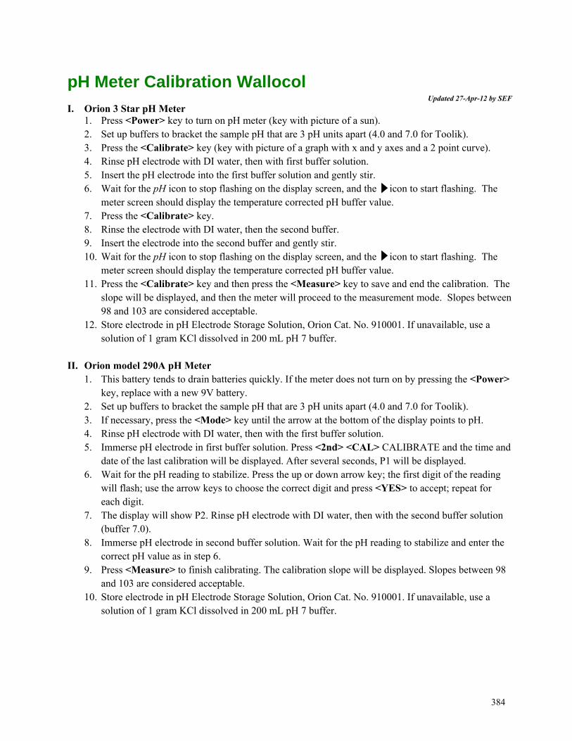
384

pH Meter Calibration Wallocol Updated 27-Apr-12 by SEF

I. Orion 3 Star pH Meter 1. Press <Power> key to turn on pH meter (key with picture of a sun). 2. Set up buffers to bracket the sample pH that are 3 pH units apart (4.0 and 7.0 for Toolik). 3. Press the <Calibrate> key (key with picture of a graph with x and y axes and a 2 point curve). 4. Rinse pH electrode with DI water, then with first buffer solution. 5. Insert the pH electrode into the first buffer solution and gently stir. 6. Wait for the pH icon to stop flashing on the display screen, and the icon to start flashing. The

meter screen should display the temperature corrected pH buffer value. 7. Press the <Calibrate> key. 8. Rinse the electrode with DI water, then the second buffer. 9. Insert the electrode into the second buffer and gently stir. 10. Wait for the pH icon to stop flashing on the display screen, and the icon to start flashing. The

meter screen should display the temperature corrected pH buffer value. 11. Press the <Calibrate> key and then press the <Measure> key to save and end the calibration. The

slope will be displayed, and then the meter will proceed to the measurement mode. Slopes between 98 and 103 are considered acceptable.

12. Store electrode in pH Electrode Storage Solution, Orion Cat. No. 910001. If unavailable, use a solution of 1 gram KCl dissolved in 200 mL pH 7 buffer.

II. Orion model 290A pH Meter 1. This battery tends to drain batteries quickly. If the meter does not turn on by pressing the <Power>

key, replace with a new 9V battery. 2. Set up buffers to bracket the sample pH that are 3 pH units apart (4.0 and 7.0 for Toolik). 3. If necessary, press the <Mode> key until the arrow at the bottom of the display points to pH. 4. Rinse pH electrode with DI water, then with the first buffer solution. 5. Immerse pH electrode in first buffer solution. Press <2nd> <CAL> CALIBRATE and the time and

date of the last calibration will be displayed. After several seconds, P1 will be displayed. 6. Wait for the pH reading to stabilize. Press the up or down arrow key; the first digit of the reading

will flash; use the arrow keys to choose the correct digit and press <YES> to accept; repeat for each digit.

7. The display will show P2. Rinse pH electrode with DI water, then with the second buffer solution (buffer 7.0).

8. Immerse pH electrode in second buffer solution. Wait for the pH reading to stabilize and enter the correct pH value as in step 6.

9. Press <Measure> to finish calibrating. The calibration slope will be displayed. Slopes between 98 and 103 are considered acceptable.

10. Store electrode in pH Electrode Storage Solution, Orion Cat. No. 910001. If unavailable, use a solution of 1 gram KCl dissolved in 200 mL pH 7 buffer.

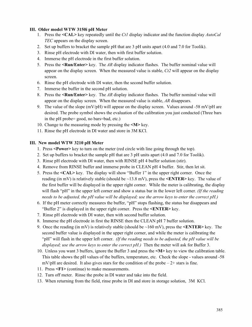
385

III. Older model WTW 3150i pH Meter 1. Press the <CAL> key repeatedly until the Ct1 display indicator and the function display AutoCal

TEC appears on the display screen. 2. Set up buffers to bracket the sample pH that are 3 pH units apart (4.0 and 7.0 for Toolik). 3. Rinse pH electrode with DI water, then with first buffer solution. 4. Immerse the pH electrode in the first buffer solution. 5. Press the <Run/Enter> key. The AR display indicator flashes. The buffer nominal value will

appear on the display screen. When the measured value is stable, Ct2 will appear on the display screen.

6. Rinse the pH electrode with DI water, then the second buffer solution. 7. Immerse the buffer in the second pH solution. 8. Press the <Run/Enter> key. The AR display indicator flashes. The buffer nominal value will

appear on the display screen. When the measured value is stable, AR disappears. 9. The value of the slope (mV/pH) will appear on the display screen. Values around -58 mV/pH are

desired. The probe symbol shows the evaluation of the calibration you just conducted (Three bars in the pH probe= good, no bars=bad, etc.)

10. Change to the measuring mode by pressing the <M> key. 11. Rinse the pH electrode in DI water and store in 3M KCl.

III. New model WTW 3210 pH Meter 1. Press <Power> key to turn on the meter (red circle with line going through the top).

2. Set up buffers to bracket the sample pH that are 3 pH units apart (4.0 and 7.0 for Toolik). 3. Rinse pH electrode with DI water, then with RINSE pH 4 buffer solution (stir). 4. Remove from RINSE buffer and immerse probe in CLEAN pH 4 buffer. Stir, then let sit. 5. Press the <CAL> key. The display will show “Buffer 1” in the upper right corner. Once the

reading (in mV) is relatively stable (should be ~13.8 mV), press the <ENTER> key. The value of the first buffer will be displayed in the upper right corner. While the meter is calibrating, the display will flash “pH” in the upper left corner and show a status bar in the lower left corner. (If the reading needs to be adjusted, the pH value will be displayed; use the arrow keys to enter the correct pH.)

6. If the pH meter correctly measures the buffer, “pH” stops flashing, the status bar disappears and “Buffer 2” is displayed in the upper right corner. Press the <ENTER> key.

7. Rinse pH electrode with DI water, then with second buffer solution. 8. Immerse the pH electrode in first the RINSE then the CLEAN pH 7 buffer solution. 9. Once the reading (in mV) is relatively stable (should be ~160 mV), press the <ENTER> key. The

second buffer value is displayed in the upper right corner, and while the meter is calibrating the “pH” will flash in the upper left corner. (If the reading needs to be adjusted, the pH value will be displayed; use the arrow keys to enter the correct pH.) Then the meter will ask for Buffer 3.

10. Unless you want 3 buffers, ignore the Buffer 3 and press the <M> key to view the calibration table. This table shows the pH values of the buffers, temperature, etc. Check the slope - values around -58 mV/pH are desired. It also gives stars for the condition of the probe – 2+ stars is fine.

11. Press <F1> (continue) to make measurements. 12. Turn off meter. Rinse the probe in DI water and take into the field. 13. When returning from the field, rinse probe in DI and store in storage solution, 3M KCl.

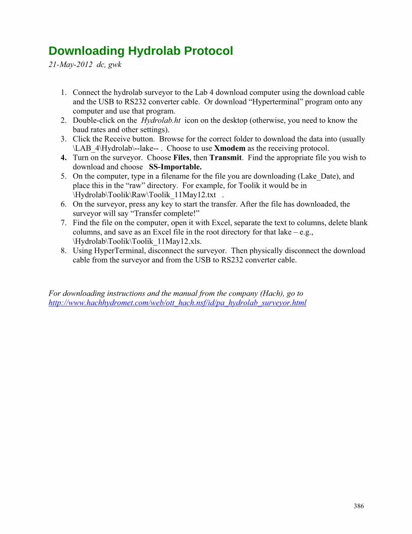
386

Downloading Hydrolab Protocol 21-May-2012 dc, gwk

1. Connect the hydrolab surveyor to the Lab 4 download computer using the download cable and the USB to RS232 converter cable. Or download “Hyperterminal” program onto any computer and use that program.

2. Double-click on the Hydrolab.ht icon on the desktop (otherwise, you need to know the baud rates and other settings).

3. Click the Receive button. Browse for the correct folder to download the data into (usually \LAB_4\Hydrolab\--lake-- . Choose to use Xmodem as the receiving protocol.

4. Turn on the surveyor. Choose Files, then Transmit. Find the appropriate file you wish to download and choose SS-Importable.

5. On the computer, type in a filename for the file you are downloading (Lake_Date), and place this in the “raw” directory. For example, for Toolik it would be in \Hydrolab\Toolik\Raw\Toolik_11May12.txt .

6. On the surveyor, press any key to start the transfer. After the file has downloaded, the surveyor will say “Transfer complete!”

7. Find the file on the computer, open it with Excel, separate the text to columns, delete blank columns, and save as an Excel file in the root directory for that lake – e.g., \Hydrolab\Toolik\Toolik_11May12.xls.

8. Using HyperTerminal, disconnect the surveyor. Then physically disconnect the download cable from the surveyor and from the USB to RS232 converter cable.

For downloading instructions and the manual from the company (Hach), go to http://www.hachhydromet.com/web/ott_hach.nsf/id/pa_hydrolab_surveyor.html

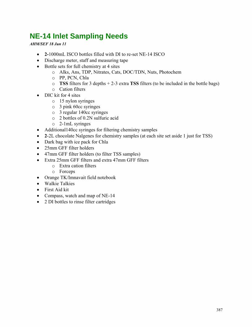
387

NE-14 Inlet Sampling Needs AHM/SEF 18 Jun 11

2-1000mL ISCO bottles filled with DI to re-set NE-14 ISCO Discharge meter, staff and measuring tape Bottle sets for full chemistry at 4 sites

o Alks, Ans, TDP, Nitrates, Cats, DOC/TDN, Nuts, Photochem o PP, PCN, Chla o TSS filters for 3 depths + 2-3 extra TSS filters (to be included in the bottle bags) o Cation filters

DIC kit for 4 sites o 15 nylon syringes o 3 pink 60cc syringes o 3 regular 140cc syringes o 2 bottles of 0.2N sulfuric acid o 2-1mL syringes

Additional140cc syringes for filtering chemistry samples 2-2L chocolate Nalgenes for chemistry samples (at each site set aside 1 just for TSS) Dark bag with ice pack for Chla 25mm GFF filter holders 47mm GFF filter holders (to filter TSS samples) Extra 25mm GFF filters and extra 47mm GFF filters

o Extra cation filters o Forceps

Orange TK/Imnavait field notebook Walkie Talkies First Aid kit Compass, watch and map of NE-14 2 DI bottles to rinse filter cartridges

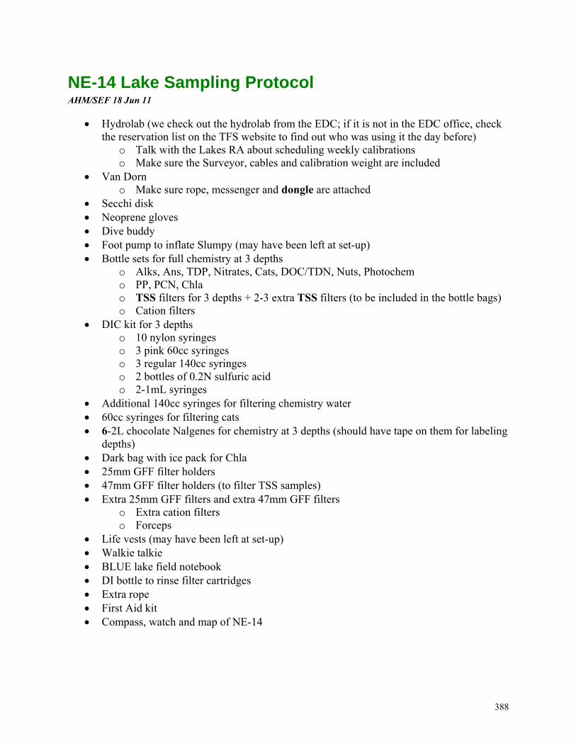
388

NE-14 Lake Sampling Protocol AHM/SEF 18 Jun 11

Hydrolab (we check out the hydrolab from the EDC; if it is not in the EDC office, check the reservation list on the TFS website to find out who was using it the day before)

o Talk with the Lakes RA about scheduling weekly calibrations o Make sure the Surveyor, cables and calibration weight are included

Van Dorn o Make sure rope, messenger and dongle are attached

Secchi disk Neoprene gloves Dive buddy Foot pump to inflate Slumpy (may have been left at set-up) Bottle sets for full chemistry at 3 depths

o Alks, Ans, TDP, Nitrates, Cats, DOC/TDN, Nuts, Photochem o PP, PCN, Chla o TSS filters for 3 depths + 2-3 extra TSS filters (to be included in the bottle bags) o Cation filters

DIC kit for 3 depths o 10 nylon syringes o 3 pink 60cc syringes o 3 regular 140cc syringes o 2 bottles of 0.2N sulfuric acid o 2-1mL syringes

Additional 140cc syringes for filtering chemistry water 60cc syringes for filtering cats 6-2L chocolate Nalgenes for chemistry at 3 depths (should have tape on them for labeling

depths) Dark bag with ice pack for Chla 25mm GFF filter holders 47mm GFF filter holders (to filter TSS samples) Extra 25mm GFF filters and extra 47mm GFF filters

o Extra cation filters o Forceps

Life vests (may have been left at set-up) Walkie talkie BLUE lake field notebook DI bottle to rinse filter cartridges Extra rope First Aid kit Compass, watch and map of NE-14

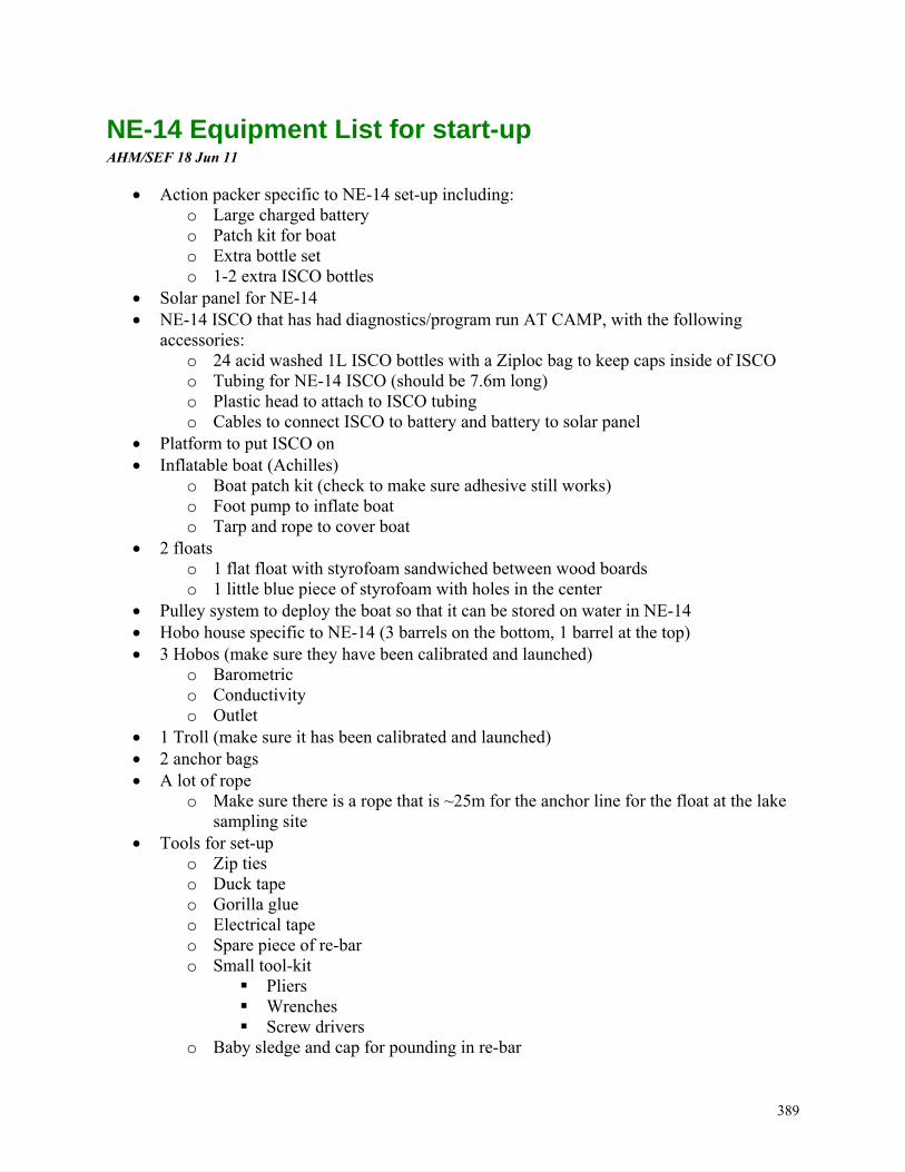
389

NE-14 Equipment List for start-up AHM/SEF 18 Jun 11

Action packer specific to NE-14 set-up including: o Large charged battery o Patch kit for boat o Extra bottle set o 1-2 extra ISCO bottles

Solar panel for NE-14 NE-14 ISCO that has had diagnostics/program run AT CAMP, with the following

accessories: o 24 acid washed 1L ISCO bottles with a Ziploc bag to keep caps inside of ISCO o Tubing for NE-14 ISCO (should be 7.6m long) o Plastic head to attach to ISCO tubing o Cables to connect ISCO to battery and battery to solar panel

Platform to put ISCO on Inflatable boat (Achilles)

o Boat patch kit (check to make sure adhesive still works) o Foot pump to inflate boat o Tarp and rope to cover boat

2 floats o 1 flat float with styrofoam sandwiched between wood boards o 1 little blue piece of styrofoam with holes in the center

Pulley system to deploy the boat so that it can be stored on water in NE-14 Hobo house specific to NE-14 (3 barrels on the bottom, 1 barrel at the top) 3 Hobos (make sure they have been calibrated and launched)

o Barometric o Conductivity o Outlet

1 Troll (make sure it has been calibrated and launched) 2 anchor bags A lot of rope

o Make sure there is a rope that is ~25m for the anchor line for the float at the lake sampling site

Tools for set-up o Zip ties o Duck tape o Gorilla glue o Electrical tape o Spare piece of re-bar o Small tool-kit

Pliers Wrenches Screw drivers

o Baby sledge and cap for pounding in re-bar

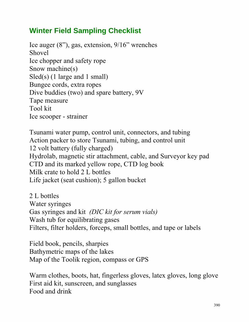
390

Winter Field Sampling Checklist

Ice auger (8”), gas, extension, 9/16” wrenches Shovel Ice chopper and safety rope Snow machine(s) Sled(s) (1 large and 1 small) Bungee cords, extra ropes Dive buddies (two) and spare battery, 9V Tape measure Tool kit Ice scooper - strainer Tsunami water pump, control unit, connectors, and tubing Action packer to store Tsunami, tubing, and control unit 12 volt battery (fully charged) Hydrolab, magnetic stir attachment, cable, and Surveyor key pad CTD and its marked yellow rope, CTD log book Milk crate to hold 2 L bottles Life jacket (seat cushion); 5 gallon bucket 2 L bottles Water syringes Gas syringes and kit (DIC kit for serum vials) Wash tub for equilibrating gases Filters, filter holders, forceps, small bottles, and tape or labels Field book, pencils, sharpies Bathymetric maps of the lakes Map of the Toolik region, compass or GPS Warm clothes, boots, hat, fingerless gloves, latex gloves, long glove First aid kit, sunscreen, and sunglasses Food and drink

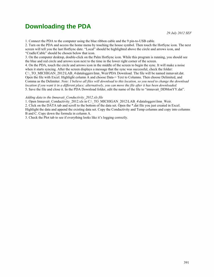
391

Downloading the PDA 29 July 2012 SEF

1. Connect the PDA to the computer using the blue ribbon cable and the 9 pin-to-USB cable. 2. Turn on the PDA and access the home menu by touching the house symbol. Then touch the HotSync icon. The next screen will tell you the last HotSync date. “Local” should be highlighted above the circle and arrows icon, and “Cradle/Cable” should be chosen below that icon. 3. On the computer desktop, double-click on the Palm HotSync icon. While this program is running, you should see the blue and red circle and arrows icon next to the time in the lower right corner of the screen. 4. On the PDA, touch the circle and arrows icon in the middle of the screen to begin the sync. It will make a noise when it starts syncing. After the screen displays a message that the sync was successful, check the folder: C:\_TO_MICHIGAN_2012\LAB_4\dataloggers\Imn_Weir\PDA Download. The file will be named inmavait.dat. Open the file with Excel. Highlight column A and choose Data-> Text to Columns. Then choose Delimited, and Comma as the Delimiter. Note: I believe all files will download to this location, so you need to change the download location if you want it in a different place; alternatively, you can move the file after it has been downloaded. 5. Save the file and close it. In the PDA Download folder, edit the name of the file to “imnavait_DDMonYY.dat”. Adding data to the Imnavait_Conductivity_2012.xls file 1. Open Imnavait_Conductivity_2012.xls in C:\_TO_MICHIGAN_2012\LAB_4\dataloggers\Imn_Weir. 2. Click on the DATA tab and scroll to the bottom of the data set. Open the *.dat file you just created in Excel. Highlight the data and append the existing data set. Copy the Conductivity and Temp columns and copy into columns B and C. Copy down the formula in column A. 3. Check the Plot tab to see if everything looks like it’s logging correctly.

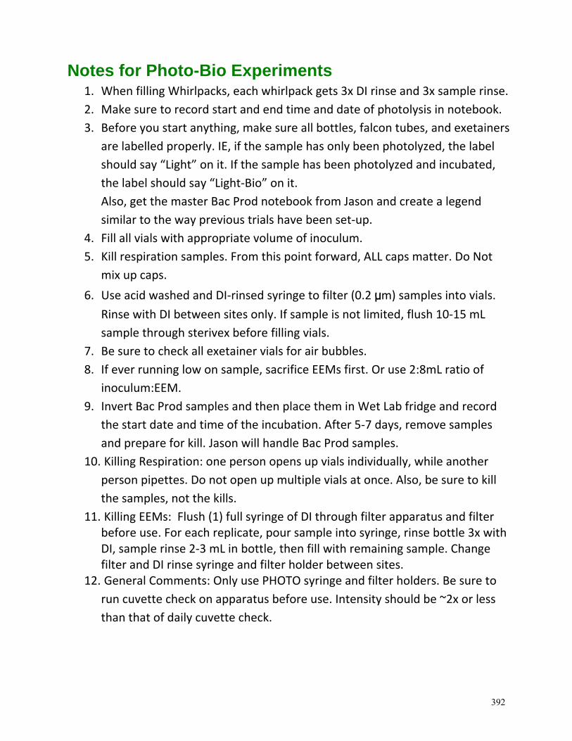
392

Notes for Photo-Bio Experiments 1. When filling Whirlpacks, each whirlpack gets 3x DI rinse and 3x sample rinse.

2. Make sure to record start and end time and date of photolysis in notebook.

3. Before you start anything, make sure all bottles, falcon tubes, and exetainers

are labelled properly. IE, if the sample has only been photolyzed, the label

should say “Light” on it. If the sample has been photolyzed and incubated,

the label should say “Light‐Bio” on it.

Also, get the master Bac Prod notebook from Jason and create a legend

similar to the way previous trials have been set‐up.

4. Fill all vials with appropriate volume of inoculum.

5. Kill respiration samples. From this point forward, ALL caps matter. Do Not

mix up caps.

6. Use acid washed and DI‐rinsed syringe to filter (0.2 μm) samples into vials.

Rinse with DI between sites only. If sample is not limited, flush 10‐15 mL

sample through sterivex before filling vials.

7. Be sure to check all exetainer vials for air bubbles.

8. If ever running low on sample, sacrifice EEMs first. Or use 2:8mL ratio of

inoculum:EEM.

9. Invert Bac Prod samples and then place them in Wet Lab fridge and record

the start date and time of the incubation. After 5‐7 days, remove samples

and prepare for kill. Jason will handle Bac Prod samples.

10. Killing Respiration: one person opens up vials individually, while another

person pipettes. Do not open up multiple vials at once. Also, be sure to kill

the samples, not the kills.

11. Killing EEMs: Flush (1) full syringe of DI through filter apparatus and filter before use. For each replicate, pour sample into syringe, rinse bottle 3x with DI, sample rinse 2‐3 mL in bottle, then fill with remaining sample. Change filter and DI rinse syringe and filter holder between sites.

12. General Comments: Only use PHOTO syringe and filter holders. Be sure to

run cuvette check on apparatus before use. Intensity should be ~2x or less

than that of daily cuvette check.

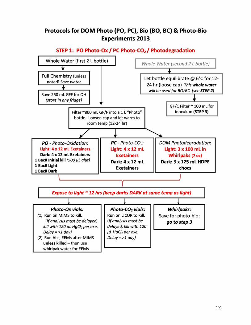
393

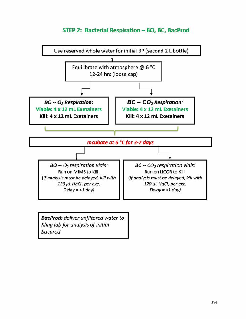
394

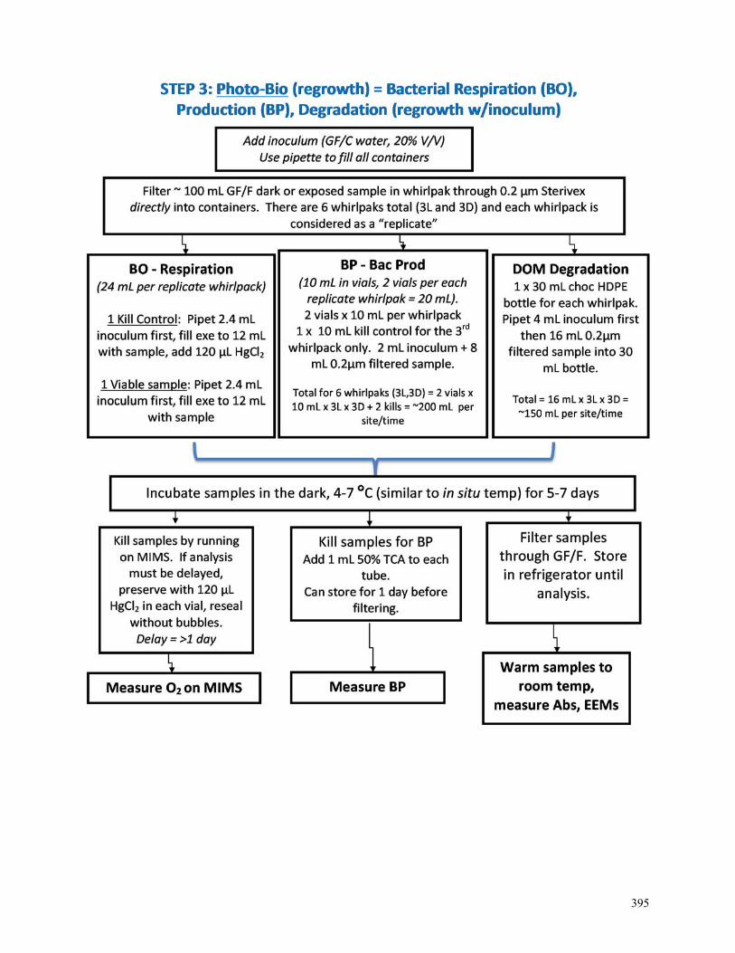
395

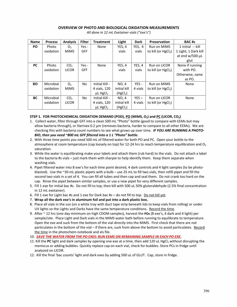
396

OVERVIEW OF PHOTO AND BIOLOGICAL OXIDATION MEASUREMENTS All done in 12 mL Exetainer vials (“exe’s”)

Name Process Analysis Filter Treatment Light Dark Preservation BAC #s

PO Photo oxidation

O2 MIMS

Yes ‐ GFF

None YES, 4 vials

YES, 4 vials

Run on MIMS to kill (or HgCl2)

1 initial ‐‐ kill1 Light, 1 Dark kill at end w/500 µL

glut

PC Photo oxidation

CO2 LICOR

Yes ‐ GFF

None YES, 4 vials

YES, 4 vials

Run on LICOR to kill (or HgCl2)

None if running with PO.

Otherwise, same as PO.

BO Microbial oxidation

O2 MIMS

No Initial Kill ‐4 vials, 120 µL HgCl2

NO, 4 initial kill (HgCl2)

YES ‐4 vials

Run on MIMS to kill (or HgCl2)

None

BC Microbial oxidation

CO2 LICOR

No Initial Kill ‐4 vials, 120 µL HgCl2

NO, 4 initial kill (HgCl2)

YES –4 vials

Run on LICOR to kill (or HgCl2)

None

STEP 1. FOR PHOTOCHEMICAL OXIDATION DEMAND (POD), PO (MIMS, O2) and PC (LICOR, CO2) 1. Collect water, filter through GFF into a clean 500 mL “Photo” bottle (good to compare with EEMs but may

allow bacteria through), or Sterivex 0.2 µm (removes bacteria, harder to compare to all other EEMs). We are checking this with bacteria count numbers to see what grows up over time. IF YOU ARE RUNNING A PHOTO‐BIO, then you need ~800 mL GFF filtered into a 1 L “Photo” bottle.

2. With three time points you need 500 mL of filtered water for both PO and PC. Open your bottle to the atmosphere at room temperature (cap loosely on top) for 12‐24 hrs to reach temperature equilibration and O2 saturation.

3. While the water is equilibrating make your labels and attach them (rub hard) to the vials. Do not attach a label to the bacteria #s vials – just mark them with sharpie to help identify them. Keep them separate when washing vials.

4. Pipet filtered water into 8 exe’s for each time point desired, 4 dark controls and 4 light samples (to be photo‐blasted). Use the ~30 mL plastic pipets with a bulb – use 25 mL to fill two vials, then refill pipet and fill the second two vials in a set of 4. You can fill all tubes and then cap and seal them. Do not crank too hard on the cap. Rinse the pipet between similar samples, or use a new pipet for very different samples.

5. Fill 1 exe for initial bac #s. Do not fill to top, then kill with 500 uL 50% gluteraldehyde (2.5% final concentration in 12 mL exetainer).

6. Fill 1 exe for Light bac #s and 1 exe for Dark bac #s – do not fill to top. Do not kill yet. 7. Wrap all the dark exe’s in aluminum foil and put into a dark plastic box. 8. Place all vials in the sun (on a white tray with duct tape strip beneath lids to keep vials from rolling) or under

UV lights so the Lights and Darks have the same temperature conditions. Record the time. 9. After ~ 12 hrs (one day minimum on high CDOM samples), harvest the POs (8 exe’s, 4 dark and 4 light) per

sample/site. Place Light and Dark vials in the MIMS water bath before running to equilibrate to temperature. Open the exe and suck from the bottom of the vial directly into the MIMS. First check that there are not particulates in the bottom of the vial – if there are, suck from above the bottom to avoid particulates. Record the time in the photochem notebook and xls file.

10. SAVE THE WATER FROM THE PO EXES: RUN EEMS ON REMAINING SAMPLE IN EACH PO EXE. 11. Kill the PC light and dark samples by opening one exe at a time, then add 120 uL HgCl2 without disrupting the

meniscus or adding bubbles. Quickly replace cap on each vial, check for bubbles. Store PCs in fridge until analyzed on LICOR.

12. Kill the final ‘bac counts’ light and dark exes by adding 500 uL of GLUT. Cap, store in fridge.