Endogenous growth and changing sectoral composition in advanced economies

Lugi Bonatti (Università di Bergamo)

Giulia Felice

(Università di Pavia)

# 162 (02-04)

Dipartimento di economia politica e metodi quantitativi

Università degli studi di Pavia Via San Felice, 5

I-27100 Pavia

Febbraio 2004

Luigi Bonatti* and Giulia Felice**

Endogenous growth and changing sectoral composition in advanced economies

ABSTRACT

Despite the striking evidence of the changing sectoral composition in employment and output shares

characterizing the growth process, structural change is usually disregarded in growth modeling. In contrast,

we focus on how structural change can affect aggregate growth by presenting a two-sector model with a

“progressive” industry (“manufacturing”), which exhibits endogenous technological progress and produce

both for consumption and for investment, and a technologically “stagnant” industry (“services”), which

produces only for consumption. Within this framework, we show under what conditions on preferences

perpetual growth can be generated. In particular, the paper demonstrates that positive long-term growth is

possible even if what households spend on services tends to increase more than proportionally than their total

consumption expenditure, namely when preferences are non-homothetic. This is at odds with previous

literature arguing that Baumol’s “asymptotic stagnancy” applies when the stagnant industries supply final

products. Moreover, the paper does not limit its attention to the balanced growth path: numerical examples

illustrate how the transition path displays the regularities which appear to characterize the structural

dynamics in advanced economies.

KEY WORDS: Balanced growth, structural change, non-homothetic preferences.

JEL CLASSIFICATION NUMBERS: O41. *University of Bergamo <luigi.bonatti@unibg.it> **University of Pavia <gfelice@unipv.it>

1

1 INTRODUCTION

There is a striking evidence that dramatic changes in the sectoral output and employment shares occur

during any development and growth episode. In particular, a sharp increase in service-sector employment

share to the detriment of manufacturing has taken place in industrialized economies during the last fifty

years. This notwithstanding, growth theoreticians usually treats the economy as if its sectoral composition

were constant for very long periods. In general, this literature does not provide an adequate framework for

explaining structural change and its implication for aggregate growth. In contrast, this paper aims at

modeling the changing sectoral composition that characterizes the economic dynamics of the advanced

countries by developing a two-sector endogenous-growth framework.

This model has two main features that are crucial for explaining the structural change which is peculiar

to the growth process in the advanced economies. On the supply side, we assume that there is a

“progressive” industry (“manufacturing”), which exhibits endogenous technological progress and produce

both for consumption and for investment, and a technologically “stagnant” industry (“services”), which

produces only for consumption.1 The stagnant industry uses an input (physical capital) that is produced by

the progressive industry, thus benefiting indirectly by the possible improvements in total factor productivity

(TFP) achieved in the latter. On the demand side, we consider both homothetic and non-homothetic

consumers’ preferences, so as to analyze the consequences for the growth process of different hypotheses on

the evolution of final demand. This formal set-up is especially suited to study how aggregate growth is

affected by the interaction between technological progress, which is generated endogenously and has a

stronger positive impact on the manufacturing sector, and the demand for services, which tends to increase—

other things being equal—more than proportionally than total expenditure in consumption. To our

knowledge, indeed, no other growth model—even among those recent theoretical contributions dealing with

sectoral changes (see Echevarria, 1997; Laitner, 2000; Kongsamut et al. 2001)—captures the joint effect of

1 The “progressive” sector can be identified with manufacturing sector, with the possible inclusion of some service

branches (Transport, Communications, Financial services)., which have experienced radical changes in their production

processes because of the massive introduction of information and communication technologies (ICT). One can include

in the “stagnant” sector the remaining branches of services. A distinction along similar lines was proposed (but at the

early stage of the ICT revolution) by Baumol (1967) and Baumol et al. (1985).

2

non-homothetic preferences and endogenous technological progress having an uneven impact on different

industries’ TFP.

An important result of our paper is that positive long-term growth is possible even if what

households spend on services tends to increase more than proportionally than their total consumption

expenditure, namely when their preferences are non-homothetic. Even in this case, indeed, the model shows

that asymptotic stagnancy can occur only if an excessively large portion of what households spend on

consumption is devoted to the service. This is at odds with previous literature arguing that Baumol’s

“asymptotic stagnancy” applies when the stagnant industries supply final goods or services.2

However, one may claim that the study of the asymptotic properties of such economic system can

provide useful insights on the direction towards which it will proceed as long as preferences and

technologies are not subject to major changes, but that for any practical purpose what really matters is its

behavior along the transition path. In this spirit, we present two numerical examples where we show that

starting from an initial employment share of the manufacturing sector in overall employment greater than its

long-run equilibrium share, the gradual shift of employment shares towards the service sector is

accompanied by rates of growth of output and capital stock that are higher in the service sector than in

manufacturing. Moreover, along this transition path, the relative price of the service is growing and the

economy’s GDP tend to grow at a higher rate than along the balanced growth path of the economy: the

gradual shift of labor towards the service sector is accompanied by a decline in the aggregate rate of growth.

In other words, the pattern resulting from these numerical examples seems to be consistent with the stylized

facts both in the case where preferences are assumed to be homothetic and in the case with non-homothetic

preferences, although the latter case appears to be more relevant in the light of empirical estimates showing

an income elasticity of demand greater than one for the services and lower than one for the manufactured

goods.

This paper is organized as it fallows. Section 2 presents the main stylized facts about structural change

and briefly reviews some theoretical and empirical contributions. Section 3 presents the model. Section 4

2 Oulton (2001) shows that Baumol’s stagnationist conclusion does not apply when the stagnant industries supply

intermediate products.

3

characterizes the equilibrium path of the economy. The case with homothetic preferences is analyzed in

section 5, while the case with non-homothetic preferences is treated in section 6. Section 7 concludes.

2 MOTIVATIONS

Stylized facts

We present some stylized facts that may help understanding the changes in sectoral composition that

have occurred in the advanced countries, together with their implications for aggregate growth.

1. It is typically observed in industrialized economies a first phase of increase in manufacturing and

services shares to the detriment of agriculture, followed by a second phase characterized by the sharp

increase in the services share in overall employment to the detriment of manufacturing. Looking at

Table 1 in the Appendix, we see that starting, at the beginning of last century, from an employment

share of 27.1% in France, 16% in Italy, 26.2% in Germany, 43.1% in the UK and 31.4% in the US,

services have reached in 1990 respectively a share of 64.6% in France, 59,7% in Italy, 58.7% in

Germany, and about 70% in the US and in the UK. Among services, the initially weightiest and then

ever growing activities have been the “wholesale and retail trade, restaurants and hotels” and the

“community, social and personal services”, with a share—respectively--of 20% and 30% in overall

employment. The activities showing the sharpest increase, starting from very low levels, are the

“finance, insurance, real estate and business services”, in contrast with the quasi-constant levels of

“transport, storage and communications”.3

2. As pointed out by some recent papers (Easterly, 1999; O’ Mahony and Van Ark, 2003), the

aggregate income and productivity growth rates are not constant. The growth rates of GDP and

productivity have decreased since the second half of the 1970s in industrialized economies,

compared with their values in the previous decades. As Table 4 in the Appendix shows, GDP growth

has decreased, in most of the industrialized economies, from yearly rates well above 4% in the

3 See Table 7 and 8 in Borzaga and Villa (1999). As for some recent evidence about structural dynamics of

employment, see also Castells and Aoyama (1994), Wieczorek (1995), Oecd (1994, 2000), Martinelli and Gadrey

(2000), Schettkat and ten Raa (2001). In 1998, the services share in overall employment reached 70.7% in France,

64.1% in Italy, 62.1% in Germany, 71% in the UK and 73.8% in the US (see Table 3.2 in Oecd, 2000).

4

decades before 1970, to rates about 2% in the post-1970 period. The trend of aggregate productivity

appears to be similar.4 In the US both the rates have risen since the mid 90’s, while there is no

evidence of a similar recovery in the EU countries (see for productivity first line of Table 5 in the

Appendix).5

3. The services share in total expenditure remains constant or rises slightly as income grows, when

expressed in real terms (constant prices), while it is sharply increasing when measured in nominal

terms (current prices). Table 2 in the Appendix shows the evolution of the service share in total GDP

over the period 1957-1978, and the evolution of the services share in total expenditure6 (in real and

nominal terms), for the US, the UK and France: in real terms, the shares in total GDP and in total

expenditure remained constant, except for the US where they both increase, whereas in nominal

terms all the three countries exhibit a massive increase.7 In more recent analysis focused on the

US (see Appelbaum and Schettkat, 1999; Mattey, 2001), it is presented evidence of increasing

relative prices of services, together with an increasing share of services in nominal product, while the

share of services in real output is shown to be more or less constant until the mid-1970s and to be

increasing since then.8

4. The relative price of services increases with income. As mentioned before, the services share is

growing more in nominal terms than in real ones. This is explained by the positive correlation

4 For a general discussion on these trends, see OECD (1994a), OECD (1994b), OECD (1995, in particular Table 2.3

and 2.4).

5 See also Table 2 and Table 4 in Mc Guckin and Van Ark (2003); Table I.1 and Table I.3 in Oecd (2002).

6 The difference is given by the final expenditures of government, included in the service share in total GDP, excluded

in the share of services in total expenditure.

7 In 1998, the services share in nominal value added for the three countries is about 70% (Oecd, 2000, in particular

Table 3.8). The same evidence is provided by Summers (1985) in his cross-sectional analysis carried out over 39

countries in 1975 on the relationship between real (inflation adjusted) per capita GDP and share of services in total real

GDP expenditure and in total nominal GDP expenditure. The results obtained by Summers corroborate what Fuchs

(1968), Baumol (1967, 2001) and Kuznets (1971) argued: the share of services in nominal output increases more than

the share of services in real output (see also Echevarria, 1998, and—for specific countries—Inman, 1985).

8 For contrasting results, see Falvey and Gemmel (1996).

5

between the price of services and GDP, as come out from the cross-sectional and longitudinal

analysis presented by Kravis et al. (1983) and from the cross-sectional evidence presented by

Summers (1985). Moreover, it is also confirmed in the more recent analysis cited in the point above.9

5. Services are more labor intensive than manufacturing. The capital intensity (capital per hour worked)

in 2000 is lower in most of the service sectors, with the exceptions of “transport and

communication” and of “financial services” in some countries (the US, and slightly, France and

Netherlands), as O’Mahony and Van Ark (2003) have pointed out.10 This is true despite the fact that

the pace of capital accumulation appears to be faster in services than in manufacturing. Looking at

Table 3 in the Appendix, one can see that before 1973 trends in capital accumulation were similar in

industry and services. After 1973 they diverged sharply in a number of countries, with capital

accumulation slackening in manufacturing and being maintained in services (see Glyn, 1997, 2001).

6. The income elasticity of demand is estimated to be above unity for most of the service branches and

for services as an aggregate. The same elasticity is sharply below unity for manufacturing branches

and for the whole sector (see Curtis and Murthy, 1998; Rowthorn and Ramaswamy, 1999; Inman in

Oecd, 2000; Möller, 2001).11

7. The recent empirical evidence reaches a general consensus in pointing out the negative productivity

differential of most of the service branches compared with manufacturing ones (see Kravis et al.,

1983; Summers, 1985; Sakuray, 1995; Rowthorn and Ramaswamy, 1999; Inman in Oecd, 2000).12

We can see from Table 5 in the Appendix that the growth rates of productivity in services are lower

9 For the correlation between prices and productivity, see Rowthorn and Ramaswami (1999). According to them, the

relative price of services increases because their productivity grows more slowly.

10 See in particular Table II.6. A similar evidence is reported also by Mohnen and ten Raa (2001) for Canada.

11 Kraving et al. (1983) and Summers (1985) find income elasticity of demand for services slightly different from unity

for the sector as a whole (in contrast they are far above unity for some branches). Falvey and Gemmel (1996), extending

Summers (1985), reach similar conclusions. In the same papers, services as a whole appear to be highly price inelastic.

Price rigidities are also found by Curtis and Murthy (1998), Inman in Oecd (2000) and Möller (2001), although the

evidence on the existence of price rigidities appears to be less univocal than on income elasticity.

12 For specific countries see also Inman (1985), Mohnen and ten Raa (2001); while for comparisons among

industrialized countries of sectoral productivity in the long run (1913-1987), see Maddison (1991, Table 5.13).

6

than in manufacturing with the exception of branches like “Transport and Communications” and

“Finance”.13

Theoretical literature

As we already pointed out, despite the stylized facts presented above, growth modeling has not

generally focused on structural change.14 The long-run dynamics is generally analysed along the balanced

growth path, where all the relevant variables grow at constant rates and the system is not supposed to change

in its sectoral composition. The omission of structural change and the priority given to balanced growth

analysis probably depends on the acceptance of the so-called “Kaldor facts”15 as a good description of the

behavior of aggregate variables in the long run by most of the growth literature (including endogenous

growth theory).

Some recent papers (Meckl, 2000; Foellmi and Zweimüller, 2002) seek to reconcile the Kaldor facts

(in particular, steady aggregate growth) with the existence of structural change. They derive a dynamic

equilibrium characterized by continuous structural change: in both these models, the driving force behind

structural change is the difference in the income elasticity of demand across sectors, while technological

progress is uniform across the sectors producing the final products. In other words, the changing sectoral

composition of the economy originates only from non-homothetic preferences. This approach makes the

structural change neutral with respect to aggregate growth, but--at the same time--it ignores another

fundamental force driving structural dynamics, namely the fact that sectors differ in their permeability to

technological progress. Under this respect, our model differ from these papers because of our attempt of

accounting for both forces underlying structural change.

13 Although the existence of a productivity bias in favor of manufacturing is widely accepted, it is not evident whether

this differential will be preserved in the future, when ICT will increasingly affect the services sector. In this respect, a

consequence of the application of ICT is the possibility of separating production and consumption for many service

activities, increasing their “stockability” and “transferability”. For evidence and discussions on the impact of ICT on

sectoral productivities, see Petit and Soete (1997), Mattey (2001), Triplett (2003), O’ Mahony and van Ark (2003).

14 Among the noteable exceptions, one can cite Pasinetti (1984), Reati (1998), Metcalfe (2000), Montobbio (2001),

Aoki and Yoshikawa (2001).

15 That is, per capita output grows at a rate that is roughly constant, the capital-output ratio is roughly constant, the real

rate of return to capital is roughly constant, the share of labour and capital in national income are roughly constant.

7

In contrast with this approach, some other recent papers (Echevarria, 1998; Kongsamut et al., 2001)

argue that the long-run economic dynamics has to be analyzed out of the balanced growth path. In particular,

Kongsamut et al. find a knife-edge condition on parameters which must be satisfied for a generalized

balanced growth path (GBGP) to exist, characterizing it as a path which features a constant real interest rate

but a time-varying allocation of inputs across sectors. It is worth noting that along this GBGP the relative

prices and the growth rates of GDP, productivity and final expenditure are time varying. Also in this

model—as in those previously discussed--structural change is driven by non-homothetic preferences, but the

case of sector-specific (exogenous) technological progress is taken into account. Moreover, structural change

vanishes asymptotically as the economy approaches its balanced growth path. Therefore, the possibility of

analyzing the changing sectoral composition of the economy relies on the existence of the GBGP, which in

its turn depends on very particular combinations of values of the parameters entering both the utility and the

production function. In contrast, our approach introduces endogenous technological progress and does not

hinges on special assumptions on the parameters values in order to deal with the changing sectoral

composition of the economy.

Finally, one should consider Oulton (2001), where it is shown that Baumol’s stagnationist argument

does not hold when services are used as intermediate products. This approach is consistent with the literature

identifying the cause of services expansion in the increasing demand for services as intermediate products

(see Stanback, 1979; Gershuny and Miles, 1983; Momigliano and Siniscalco, 1986; Petit and Soete, 1997;

Klodt, 1997). However, consensus has not yet been reached about the relative weight of the use of services

as intermediate products in the overall growth of the services sector (see Russo and Schettkat, 2001),16 while

it is widely recognized the importance of physical capital as an input in most service industries, which is a

feature that is captured by our model.

3 THE MODEL

We consider an economy in discrete time with an infinite time horizon. This economy is assumed to

have two sectors of market activity (manufacturing and services). The manufactured good, which is the

numéraire of the system (its price is set to be one), can be both consumed and used for investment purposes.

16 For a recent review of the literature of the shift to services, see Schettkat and Yocarini (2003).

8

The service can be only consumed. Moreover, consistently with the Baumol’s distinction between

“progressive” and “stagnant” sectors, we assume that there is (endogenous) technological progress only in

the manufacturing sector. Finally, all markets are assumed to be perfectly competitive.

Households

For simplicity and without loss of generality, it is assumed that the population is constant and that

each household contains one adult working member of the current generation. Thus, there is a fixed and large

number (normalized to be one) of identical adults who take account of the welfare and resources of their

actual and perspective descendants. Indeed, following Barro and Sala-i-Martin (1995), this intergenerational

interaction is modeled by imaging that the current generation maximizes utility and incorporates a budget

constraint over an infinite future. That is, although individuals have finite lives, the model considers

immortal extended families (“dynasties”).17 The current adults expect the size of their extended family to

remain constant, since expectations are rational (in the sense that they are consistent with the true processes

followed by the relevant variables). In this framework in which there is no source of random disturbances,

this implies perfect foresight.

Again for simplicity and without loss of generality, it is assumed that all households--being the

firms’ owners--are entitled to receive an equal share of the firms' net profits and that bequests are

accidental.18

Households decide in each t what fraction of their labor income and gross returns on wealth to spend

on consumption rather than on buying corporate bonds. Simultaneously, they decide how to allocate their

consumption expenditure over the manufactured good and the service. Hence, the representative household’s

problem amounts to deciding a contingency plan for CMt, CSt and Bt+1 in order to maximize:

17 As Barro and Sala-i-Martin (1995, p. 60) point out, “this setting is appropriate if altruistic parents provide transfers to

their children, who give in turn to their children, and so on. The immortal family corresponds to finite-lived indiiduals

who are connected via a pattern of operative intergenerational transfers that are based on altruism”.

18 In other words, it is ruled out the existence of actuarially fair annuities paid to the living investors by a financial

institution collecting their wealth as they die: the wealth of someone who dies is inherited by some newly born

individual.

9

∑∞

=+

tsSsMs

t-s )(CC γη εθ , 0<θ<1, 0<η<1, 0<γ<1, ε≥0, (1)

subject to

StMttttSttMt1t )Br1(WCPCB ππ ++++≤+++ , B0 given, (2)

where CMt and CSt are, respectively, the manufactured good and the service consumed by the representative

household in period t, Bt are corporate bonds with maturity in period t and issued in t-1, θ is a time-

preference parameter, ε can be interpreted as the amount of service that is produced at home, Pt is the price

of the service (the units of manufactured good that are necessary to buy one unit of service), Wt is the wage

rate (the quantity of labor supplied by each household is assumed to be fixed and set to be one), rt is the one-

period market rate of interest, and πMt and πSt are the net profits generated in period t, respectively, by the

manufacturing firms and the service-producing firms. It is worth to note that in the special case where ε=0

the period-utility function is Cobb-Douglas, while for ε>0 preferences are not homothetic: in the latter case,

the elasticity of the demand for the service with respect to the household’s consumption expenditure is more

than unitary, while the elasticity of the demand for the manufactured good with respect to the household’s

consumption expenditure is less than unitary.

Manufacturing firms

The manufactured good is denoted by YMt and is produced by a large number (normalized to be one)

of identical firms according to the technology

1,0 ,KLAY -1MtMttMt <<= ααα (3)

where At is a variable measuring the state of technology, KMt is the capital installed in the manufacturing

sector (capital can be interpreted in a broad sense, inclusive of all reproducible assets) and LMt is labor

employed in the manufacturing sector. It is assumed that At is a positive function of the stock of capital

existing in the manufacturing sector: αMtt KA = .19 Furthermore, consistently with Frankel (1962), it is

supposed that although At is endogenous to the economy, each firm takes it as given, since a single firm

19 Consistently with this formal set-up, one can interpret technological progress as labor augmenting.

10

would only internalize a negligible amount of the effect that its own investment decisions have on the

aggregate stock of capital.

The period net profits πMt of a manufacturing firm are given by:

MttMttMtMt )Br(1-LW-Y +=π , (4)

where BMt are the bonds with maturity in period t and issued by a manufacturing firm in t-1 to finance its

investment expenditure in that period.

Service-producing firms

The output of a service-producing firm is denoted by YSt and is produced by a large number

(normalized to be one) of identical firms according to the technology

1,0 ,KLY -1StStSt <<= βββ (5)

where KSt is the capital installed in the service sector and LSt is labor employed in the service sector.

The period net profits πSt of a service-producing firm are given by:

SttSttSttSt )Br(1-LW-YP +=π , (6)

where BSt are the bonds with maturity in period t and issued by a service-producing firm in t-1 to finance its

investment expenditure in that period.

Investment

The process of installing new capital and adapting the existing production facilities to the new

machinery and equipment reduces the manufactured good available for consumption purposes and for adding

to the stock of capital. One may think of this adjustment cost indifferently as if the producers of the

manufactured good must divert resources from production in order to assist the capital users in installing the

new capital, or as if some manufactured good is used up in the process of installing the new capital. Since

firms finance their investment costs c(Iit,Kit) by issuing debt, one has:

c(Iit,Kit)=Iit+it

2it

KI

=Bit+1, i=M,S, (7)

where investment costs are assumed to be the sum of gross investment Iit and adjustment costs, that are a

quadratic function of Iit and a decreasing function of Kit.

The capital stock installed in each sector evolves according to

11

Kit+1=Iit+(1-δ)Kit , 0≤δ≤1, Ki0 given, i=M,S, (8)

where δ is a capital depreciation parameter.

Firms’ objective

In t, a firm chooses ∞=tsisL and ∞=tsisI in order to maximize its discounted sequence of net profits:

,

)r1(tss

1tvv

is∑

∏

∞

=

+=

+

π i=M,S, (9)

subject to (5), (6) and (7), where 1)r1(t

1tvv =+∏

+=.

Markets equilibrium

Equilibrium in the product markets requires, respectively,

YMt= CMt+IMt+Mt

2Mt

KI +ISt+

St

2St

KI (10)

and

YSt= CSt. (11)

Equilibrium in the labor market requires

1=LMt+LSt. (12)

Equilibrium in the asset market requires

BMt+BSt=Bt. (13)

4 CHARACTERIZATION OF THE GENERAL EQUILIBRIUM PATH

Households’ optimal behavior

One can solve the intertemporal problem of the representative household by maximizing

∑∞

=+++++++

tsSssMs1sSsMsssssSsMs

t-s ]CP-C-B-)Br1(W[)(CC ππχεθ γη with respect to CMt, CSt, Bt+1

and χt, and then by eliminating the multiplier χt, thus obtaining:

12

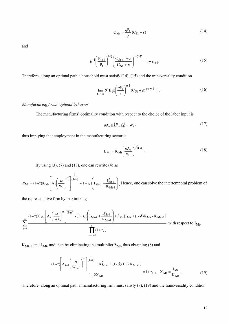
)C(P

C Stt

Mt εγ

η+= (14)

and

.r1C

CP

P1t

--1

St

1St-1

t

1t1-+

++ +=

++

γηη

εεθ (15)

Therefore, along an optimal path a household must satisfy (14), (15) and the transversality condition

.0)C(P

Blim 1-St

1-t

tt

t=+

+∞→

ηγη

εγ

ηηθ

(16)

Manufacturing firms’ optimal behavior

The manufacturing firms’ optimality condition with respect to the choice of the labor input is

t1-

Mt-1

Mtt W LKA =ααα , (17)

thus implying that employment in the manufacturing sector is:

)-1(1

t

tMtMt W

AKL

αα

= . (18)

By using (3), (7) and (18), one can rewrite (4) as

++

=

1-Mt

21-Mt

1-Mtt

)-(11

ttMtMt K

II)r(1-

WAK)-1(

ααααπ . Hence, one can solve the intertemporal problem of

the representative firm by maximizing

∑∏

∞

=

+=

+

+

++

++

tss

1tvv

1MsMsMsMs1-Ms

21-Ms

t-Mss)-(1

1

sMs

)r1(

]K-)K-1(I[KI

I)r(1-Ws

AK)-1( δλαααα

with respect to IMt,

KMt+1 and λMt, and then by eliminating the multiplier λMt, thus obtaining (8) and

Mt

MtMt1t

Mt

1Mt2

1Mt

)-(11

1t1t

KI

X ,r12X1

)2X)(1-1(XW

A)-1(

≡+=+

+++

+

+++

+ δαααα

. (19)

Therefore, along an optimal path a manufacturing firm must satisfy (8), (19) and the transversality condition

13

0

)r1(

)KX21(lim

s

1tvv

MsMss

=

+

+

∏+=

∞→. (20)

Service-producing firms’ optimal behavior

The service-producing firms’ optimality condition with respect to the choice of the labor input is

t1-

St-1

Stt W LKP =βββ , (21)

thus implying that employment in the manufacturing sector is:

)-1(1

t

tStSt W

PKL

ββ

= . (22)

By using (5), (7) and (22), one can rewrite (6) as

++

=

1-St

21-St

1-Stt

)-(11

ttStSt K

II)r(1-

WPK)-1(

ββββπ . Hence, one can solve the intertemporal problem of

the representative firm by maximizing

∑∏

∞

=

+=

+

+

++

++

tss

1tvv

1SsSsSsSs1-Ss

21-Ss

t-Sss)-(1

1

sSs

)r1(

]K-)K-1(I[KI

I)r(1-Ws

PK)-1( δλββββ

with respect to ISt, KSt+1

and λSt, and then by eliminating the multiplier λSt, thus obtaining (8) and

St

StSt1t

St

1St2

1St

)-(11

1t1t

KI

X ,r12X1

)2X)(1-1(XW

P)-1(

≡+=+

+++

+

+++

+ δββββ

. (23)

Therefore, along an optimal path a service-producing firm must satisfy (8), (23) and the transversality

condition

0

)r1(

)KX21(lim

s

1tvv

SsSss

=

+

+

∏+=

∞→. (24)

General equilibrium path

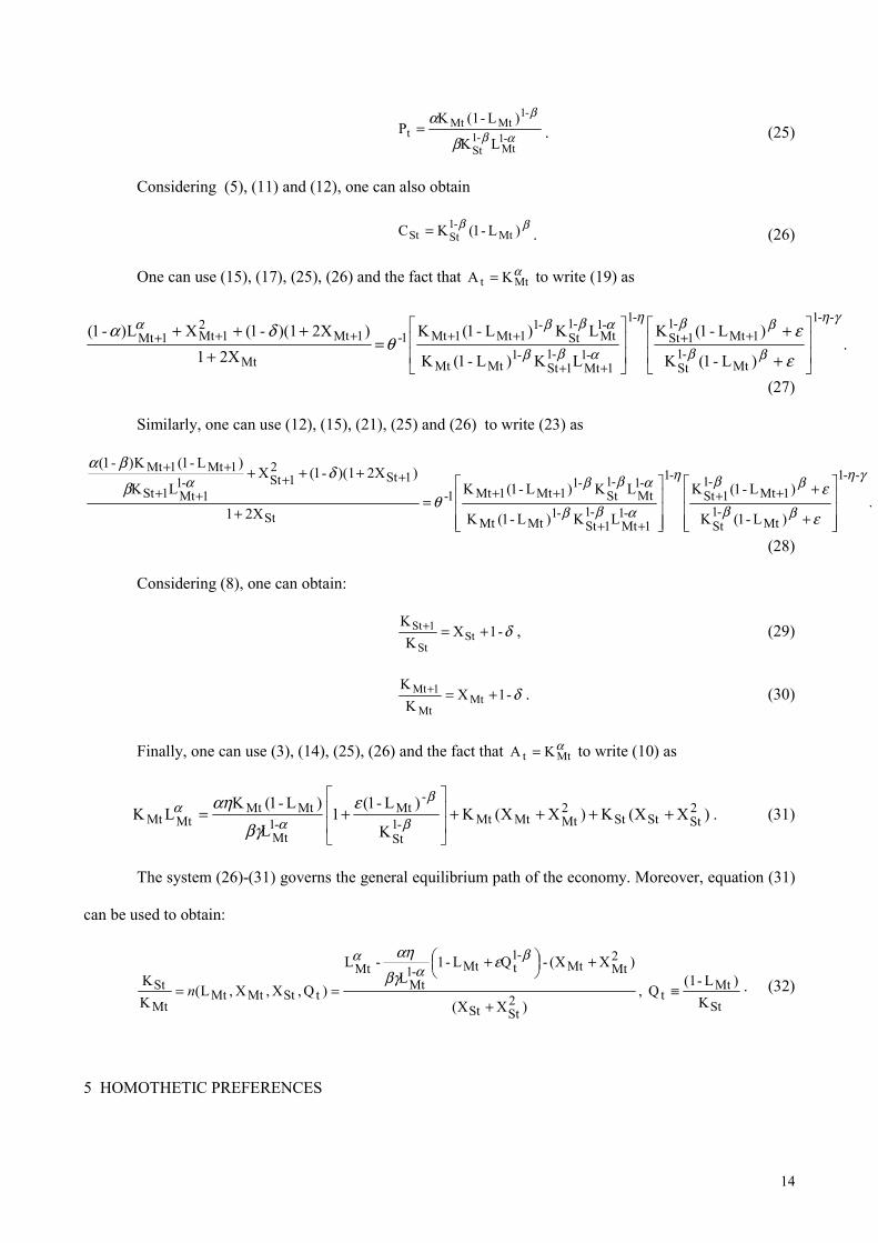
Considering (12), (17), (22) and the fact that αMtt KA = , one can obtain

14

αβ

β

β

α-1Mt

-1St

-1MtMt

tLK

)L-(1KP = . (25)

Considering (5), (11) and (12), one can also obtain

ββ )L-1(KC Mt-1

StSt = . (26)

One can use (15), (17), (25), (26) and the fact that αMtt KA = to write (19) as

.)L-1(K

)L-1(K

LK)L-1(K

LK)L-1(K2X1

)2X)(1-1(XL)-1(--1

Mt-1

St

1Mt-1

1St-1

-11Mt

-11St

-1MtMt

-1Mt

-1St

-11Mt1Mt1-

Mt

1Mt2

1Mt1Mtγη

ββ

ββη

αββ

αββα

ε

εθ

δα

+

+

=

++++ ++

++

+++++

(27)

Similarly, one can use (12), (15), (21), (25) and (26) to write (23) as

.)L-1(K

)L-1(K

LK)L-1(K

LK)L-1(K

2X1

)2X)(1-1(XLK

)L-1(K)-1(--1

Mt-1

St

1Mt-1

1St-1

-11Mt

-11St

-1MtMt

-1Mt

-1St

-11Mt1Mt1-

St

1St2

1St-11Mt1St

1Mt1Mt γη

ββ

ββη

αββ

αββα

ε

εθ

δβ

βα

+

+

=+

+++++

++

++++

++

++

(28)

Considering (8), one can obtain:

δ-1XK

KSt

St

1St +=+ , (29)

δ-1XK

KMt

Mt

1Mt +=+ . (30)

Finally, one can use (3), (14), (25), (26) and the fact that αMtt KA = to write (10) as

)XX(K)XX(KK

)L-1(1

L

)L-1(KLK 2

StStSt2MtMtMt-1

St

-Mt

-1Mt

MtMtMtMt ++++

+=

β

β

αα ε

βγ

αη. (31)

The system (26)-(31) governs the general equilibrium path of the economy. Moreover, equation (31)

can be used to obtain:

StMt

t2StSt

2MtMt

-1tMt-1

MtMt

tStMtMtMtSt

K)L-(1

Q ,)XX(

)XX(-QL-1L

-L

)Q,X,X,L(KK

≡+

+

+

==

βα

α εβγ

αη

n . (32)

5 HOMOTHETIC PREFERENCES

15

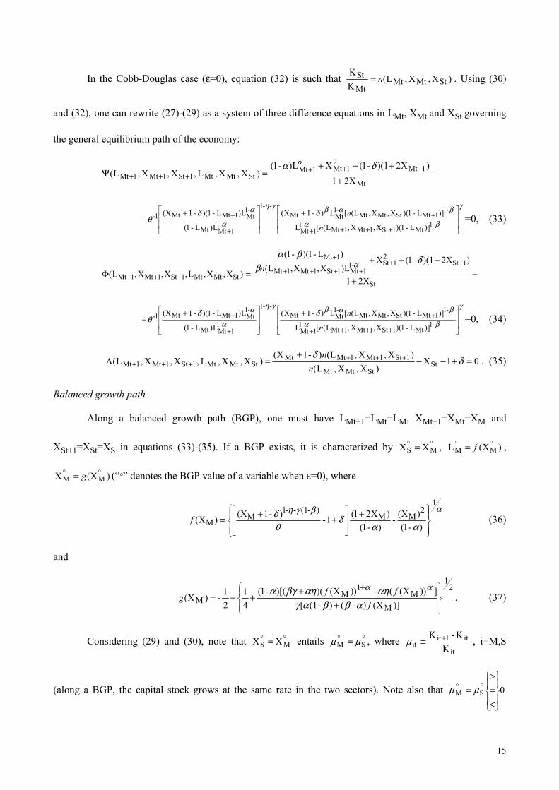
In the Cobb-Douglas case (ε=0), equation (32) is such that )X,X,L(KK

StMtMtMt

St n= . Using (30)

and (32), one can rewrite (27)-(29) as a system of three difference equations in LMt, XMt and XSt governing

the general equilibrium path of the economy:

−+

+++=Ψ +++

+++Mt

1Mt2

1Mt1MtStMtMt1St1Mt1Mt 2X1

)2X)(1-1(XL)-1()X,X,L,X,X,L(

δα α

γ

βα

βαβγη

α

α δδθ

+

+−

++++

+

+

+-1

Mt1St1Mt1Mt-1

1Mt

-11MtStMtMt

-1MtMt

--1

-11MtMt

-1Mt1MtMt1-

)]L-1)(X,X,L([L

)]L-1)(X,X,L([L)-1X(

L)L-1(

L)L-1()-1X(

n

n =0, (33)

−+

+++=Φ

++++++

+

+++St

1St2

1St-11Mt1St1Mt1Mt

1Mt

StMtMt1St1Mt1Mt 2X1

)2X)(1-1(XL)X,X,L(

)L-1)(-1(

)X,X,L,X,X,L(δ

ββα

αn

γ

βα

βαβγη

α

α δδθ

+

+−

++++

+

+

+-1

Mt1St1Mt1Mt-1

1Mt

-11MtStMtMt

-1MtMt

--1

-11MtMt

-1Mt1MtMt1-

)]L-1)(X,X,L([L

)]L-1)(X,X,L([L)-1X(

L)L-1(

L)L-1()-1X(

n

n =0, (34)

01X)X,X,L(

)X,X,L()-1X()X,X,L,X,X,L( St

StMtMt

1St1Mt1MtMtStMtMt1St1Mt1Mt =+−−

+=Λ +++

+++ δδ

nn . (35)

Balanced growth path

Along a balanced growth path (BGP), one must have LMt+1=LMt=LM, XMt+1=XMt=XM and

XSt+1=XSt=XS in equations (33)-(35). If a BGP exists, it is characterized by °° = MS XX , )X(L MM°° = f ,

)X(X MM°° = g (“°” denotes the BGP value of a variable when ε=0), where

αβγη

ααδ

θδ

12

MM)-(1--1

MM )-1(

)X(-)-1(

)X21(1-)-1(X)X(

+

++=f (36)

and

21

MM

1M

M )]X()-()-(1[]))X((-))X(())[(-1(

41

21-)X(

++

++=+

fff

gαββαγ

αηαηβγα αα. (37)

Considering (29) and (30), note that °° = MS XX entails °° = SM µµ , where it

it1itit K

K-K +≡µ , i=M,S

(along a BGP, the capital stock grows at the same rate in the two sectors). Note also that 0SM

<=>

= °° µµ

16

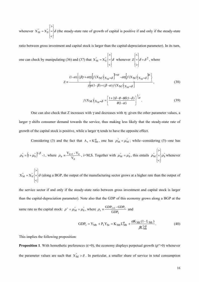
whenever δ

<=>

= °°SM XX (the steady-state rate of growth of capital is positive if and only if the steady-state

ratio between gross investment and capital stock is larger than the capital-depreciation parameter). In its turn,

one can check by manipulating (36) and (37) that δ

<=>

= °°SM XX whenever 2Z δδ +

>=<

, where

[ ] [ ][ ]δ

αδ

αδ

αββαγ

αηαηβγα

=

=+

=

+

+

≡M

MM

XM

XM1

XM

)X()-()-(1

)X(-)X()()-1(Z

f

ff, (38)

αδ αθ

δθδθδ1

XM )-1()-(1--21

)X(M

+==f . (39)

One can also check that Z increases with γ and decreases with η: given the other parameter values, a

larger γ shifts consumer demand towards the service, thus making less likely that the steady-state rate of

growth of the capital stock is positive, while a larger η tends to have the opposite effect.

Considering (3) and the fact that αMtt KA = , one has °° = MM µρ ; while--considering (5)--one has

( ) 1-1-1

SSβ

µρ °° += , where it

it1itit Y

Y-Y +≡ρ , i=M,S. Together with °° = SM µµ , this entails °°

<=>

SM ρρ whenever

δ

<=>

= °°SM XX (along a BGP, the output of the manufacturing sector grows at a higher rate than the output of

the service sector if and only if the steady-state ratio between gross investment and capital stock is larger

than the capital-depreciation parameter). Note also that the GDP of this economy grows along a BGP at the

same rate as the capital stock: °° == SM µµρ , where t

t1tt GDP

GDP-GDP +≡ρ and

αα

βα

-1Mt

MtMtMtMtSttMtt

L

)L-(1KLKYPYGDP +=+= . (40)

This implies the following proposition:

Proposition 1. With homothetic preferences (ε=0), the economy displays perpetual growth (ρ°>0) whenever

the parameter values are such that δ>°MX . In particular, a smaller share of service in total consumption

17

expenditure (smaller γ) and a larger share of manufacturing in total consumption expenditure (larger η) can

contribute to generate a positive steady-state rate of growth.

Finally, considering (25) and (32), one has ( ) 1-1 Mβ

µω °° += , where t

t1tt P

P-P +≡ω . Note that

0

<=>

°ω whenever δ

<=>

= °°SM XX (the steady-state rate of growth of the relative price of the service is

positive if and only if the steady-state ratio between gross investment and capital stock is larger than the

capital-depreciation parameter).

The transition path: a numerical example

As a numerical example, let α=0.6, β=γ=0.7, δ=0.008, ε=0, η=0.3 and θ=0.851797. Given these

parameter values20, one can show that there exists a unique BGP21 characterized by 28.0LM š and

0096.0XX SM ≈= °° , thus entailing 0016.0MSM ≈== °°° ρµµ , 00049.0S ≈°ρ and 0011.0≈°ω . Furthermore, by

linearizing (33)-(35) around )X,X,(L SMM°°° , one can show that the linearized system is saddle-path stable,

since the characteristic roots are: σ1≈0.8923, σ2≈1.3062+0.1421i and σ3≈1.3062-0.1421i. The unique path

converging to )X,X,(L SMM°°° is governed by

t11MMt ZeL-L σ=° , (41)

t12MMt ZeX-X σ=° , (42)

20 The values of the parameters η and γ entering the utility function have been chosen looking at the expenditure shares

for the two sector as reported by Mattey (1997), Oecd (2000), Business Statistic of the US (2002). These expenditure

shares include government expenditure. The parameter α—entering the production function of the progressive sector--

is consistent with the evidence reported in the Survey of Current Business (2003) for US. A larger value is assigned to

the corresponding parameter entering the production function of the stagnant sector (β), so as to account for the

evidence showing that this sector is more labor intensive (see O’Mahony and Van Ark, 2003; particularly Table II.6).

These parameters values are in line with those chosen by Kongsamut et al. (2003) in their examples.

21 The existence and the uniqueness of the BGP are guaranteed by the following facts: i) both f(XM) and g(XM) are continuous and monotonically increasing in XM for XX0 M ≤≤ , where X is that value of XM such that f(XM)=1; ii) g(XM)-XM<0 at XM=0 and g(XM)-XM>0 at XX M = , and iii) g’>1 for XXX M ≤≤ , where 0X > is that value of XM such that g(XM)=0.

18

t13SSt ZeX-X σ=° , (43)

where

≈

4725.01386.03965.0

eee

3

2

1 are the characteristic vectors associated with the stable root σ1, Z is a constant to be

determined, 2

12M0M0

1-M0M0

S0

M0S0 X-X-L-1L

KK

41

21-X

+++= αα

βγαη

βγαη is obtained from (31) and

S0

M0KK is given.

Recalling that δµ −= MtMt X and δµ −= StSt X , equations (41)-(43) tell us that--whenever

°> MM0 LL --both µMt and µSt are larger along the transition path than along the BGP. Moreover--along the

transition path--µSt tends to be larger than µMt: along this path, the capital stock tends to grow at a faster rate

in the service sector than in the manufacturing sector when the share of the manufacturing sector on total

employment tends to decline. Finally, the combined effect of a declining share of the manufacturing sector

on total employment and of µSt>µMt may imply that for some t ρSt≥ρMt.

Obviously, the value that LM0 must assume along the path converging to the BGP depends on the

initial condition S0

M0KK . In particular, it is apparent that °= MM0 LL

and °° === SS0MM0 XXXX

whenever

6.0KK

KK

SM

S0M0 ≈

=

° (the system is at its steady state starting from period 0 if the initial value of the ratio

between the capital stock installed in the manufacturing sector and the capital stock installed in the service

sector is equal to its steady-state value, which is approximately equal to 0.6). One can also check that

0SM

S0M0

S0M0M0

KK

KK

KKL >°

=∂

∂ (44)

(as the initial value of the ratio between the capital stock installed in the manufacturing sector and the capital

stock installed in the service sector tends to be larger than its steady-state value, also the initial value of the

share of the manufacturing sector on total employment tends to be larger than its steady-state value). Finally,

one can easily check that

0SM

S0M0

S0M0

M0S0

KK

KK

KK

)X-X( >°

=∂

∂

(45)

19

(as the initial value of the ratio between the capital stock installed in the manufacturing sector and the capital

stock installed in the service sector tends to be larger than its steady-state value, the initial value of the gross

investment-installed capital ratio tends to be larger in the service sector than in the manufacturing sector).

For instance, take °

>≈

SM

S0M0

KK6592.0

KK . Given this initial condition, one has °>≈ MM0 L3.0L and

XS0≈0.03347>XM0≈0.016626> °° = SM XX . Furthermore--in a neighborhood of the BGP--one has:

-)-X1()-X1)(X-X()-(1-)-X1)(X-X( M2-

SSS01-

SMM00 δδβδωω ββ ++++=

≈++

+ )L-)(L-X1()-X1(

L)-1(

)L-(1)-(1- M0M1M

1-S

MMδδαβ β

0.00492, (46)

≈+

++= °

M

M0M1MMM0MM0

L

)L-)(L-X1(X-X

δαρρ 0.0039356, (47)

≈+

++= °

)L-(1

)L-(L)-X1(-)X-(X)-X1()-1(

M

M0M1-1

SSS0

-SSS0

ββ δβ

δβρρ 0.009727, (48)

≈+

+=° )L-)(L-X1(

)-()L(L

)-(L--1-X-X- M0M1M2

MM

MMM00 δ

αβααβααρρ

0.0097298. (49)

We have from equation (46) that the relative price of the service tends to grow along a transition path

characterized by a declining employment level in the manufacturing sector. In addition, one can see by

comparing (47) and (48) that along such a path the output of the service sector may grow at a higher rate than

the output of the manufacturing sector. Finally, equation (49) shows that along this transition path the

economy’s GDP may increase at a higher rate than along the BGP: the economy’s rate of growth tends to

decline over time as the share of the two factors of production used in the manufacturing sector shrinks.

6 NON-HOMOTHETIC PREFERENCES

As ε>0, one can use (32) to rewrite (27)-(30) as a system of four difference equations in LMt, XMt,

XSt and Qt governing the general equilibrium path of the economy:

20

-2X1

)2X)(1-1(XL)-1()Q,X,X,L,Q,X,X,L(

Mt

1Mt2

1Mt1MttStMtMt1t1St1Mt1Mt +

+++=Ω +++

++++δα α

γ

βα

βαβγη

β

β

α

α δε

εδθ

+

+

+

+−+++++

+++

+-1

Mt1t1St1Mt1Mt-1

1Mt

-11MttStMtMt

-1MtMt

--1

-1tMt

-11t1Mt

-11Mt

-1MtMt1-

)]L-1)(Q,X,X,L([L)]L-1)(Q,X,X,L([L)-1X(

)L-1(

Q)L-1(

L)L-1X(

nn

Q=0, (50)

-2X1

)2X)(1-1(XL)Q,X,X,L(

)L-1)(-1(

)Q,X,X,L,Q,X,X,L(St

1St2

1St-11Mt1t1St1Mt1Mt

1Mt

tStMtMt1t1St1Mt1Mt +

+++

=Γ++

+++++

+

++++

δβ

βααn

γ

βα

βαβγη

β

β

α

α δε

εδθ

+

+

+

+−+++++

+++

+-1

Mt1t1St1Mt1Mt-1

1Mt

-11MttStMtMt

-1MtMt

--1

-1tMt

-11t1Mt

-11Mt

-1MtMt1-

)]L-1)(Q,X,X,L([L)]L-1)(Q,X,X,L([L)-1X(

)L-1(

Q)L-1(

L)L-1X(

nn

Q=0, (51)

0)Q,X,X,L(

)Q,X,X,L()-1X(-)-1X()Q,X,X,L,Q,X,X,L(1t1St1Mt1Mt

tStMtMtStMttStMtMt1t1St1Mt1Mt =++=Θ

++++++++ n

nδδ , (52)

0Q)L-1()-1X(-Q)L-1()Q,X,L,Q,L( 1tMtStt1MttStMt1t1Mt =+=Σ ++++ δ . (53)

Balanced growth paths

Along a BGP, one must have LMt+1=LMt=LM, XMt+1=XMt=XM, XSt+1=XSt=XS and Qt+1=Qt=Q in

equations (50)-(53). If a BGP exists, it is characterized by δ>= *M

*S XX , )X(L *

M*M f= , )X(X *

M*M g= ,

Q*=0 whenever Z<δ+δ2, and by δ== *S

*M XX , δ==

MXM*M )X(L f ,

*S

*M

K

)L-(1Q* = ,

)-1)(L-(1)-1(LK

K*M

*M

*S*

M βααβ

= , [ ] 1)-(1

-*M

-*M

2*M

1-*M

1-*M2*

M*S

)L-1()-1())(L-1)((

-)L-1(

-)(L)L-1(

--)(LKβ

β

αβ

α

βα

αεηβδδγ

εαηεβγδδ

+

=

whenever Z≥δ+δ2 (“*” denotes the BGP value of a variable when ε>0), where f(XM), g(XM), Z and

δ=MXM )X(f are given, respectively, by (36), (37), (38) and (39) 22.

22 Given the definition of Qt

≡

St

Mtt K

)L-(1Q , one can easily see that there cannot exist a BGP characterized by

*M

*S XX = , )X(fL *

M*M = , )X(X *

M*M g= , Q*=0 whenever Z≥δ+δ2. In this case, indeed, one would

have δ≤= *M

*S XX , entailing 0*

M*S ≤µ=µ , which is inconsistent with the fact that both )X(fLLlim *

M*MMtt

==∞→

and

0*QQlim tt==

∞→ must hold. Moreover, to see that there cannot exist a BGP characterized by fixed levels of KMt and

KSt whenever Z<δ+δ2, consider that

[ ] 0)L-1()-1(

))(L-1)((-

)L-1(-

)(L

)L-1(--)(L)(K

-*M

-*M

2*M

1-*M

1-*M2*

M1-*

S <+

=β

αβ

α

βαβ

αεη

βδδγεαηε

βγδδ if Z<δ+δ2, where

21

By comparing the case with ε=0 to the case with ε>0, one can see that whenever Z<δ+δ2 (which

tends to be satisfied when γ is small and/or η is large) the economy with homothetic preferences and the

economy with non-homothetic preferences share the same BGP, that is characterized by perpetual growth

( )0 ,0 ,0 *S

**S

*M

*M

* >ρ>ω>µ=µ=ρ=ρ . In contrast, whenever Z>δ+δ2, the economy with ε=0-displays a

negative steady-state rate of growth ( )0 ,0 ,0 *S

**S

*M

*M

* <ρ<ω<µ=µ=ρ=ρ , while the economy with ε>0 has a

BGP along which the levels of capital and output are fixed in both sectors ( )0**S

*M

*S

*M

* =ω=µ=µ=ρ=ρ=ρ .

Hence, one can conclude that, even in the case where the elasticity of demand for the service with respect to

the household’s consumption expenditure is greater than one (ε>0), the economy displays perpetual growth

if the share of total consumption expenditure devoted to the manufactured good is not too small. In other

words, even with non-homothetic preferences, asymptotic stagnancy can occur only if an excessively large

portion of what households spend on consumption is devoted to the service.

Intuitively, one can think that when final demand is not too much unbalanced towards the product of

the stagnant industry, a virtuous circle can be ignited, whereby growing market production of both the

manufactured good and the service makes progressively less relevant the fixed amount of service that is

produced at home. Thanks to this virtuous circle, the elasticity of demand for each of the two goods

approaches asymptotically one, thus avoiding that aggregate growth could vanish in the long run because of

the structural burden of increasing labor and capital shares getting used in the stagnant sector. Finally, note

that a negative steady-state rate of growth can be ruled out when ε>0: in this case, indeed, a path

characterized by a strictly negative rate of growth cannot be a BGP, since--in a shrinking market economy—

the elasticity of the two goods with respect to the household’s consumption expenditure would increasingly

diverge, thus progressively unbalancing the composition of final demand.

This discussion can be summarized by the following proposition:

Proposition 2. With non-homothetic preferences (ε>0), the economy displays perpetual growth (ρ*>0)

whenever the parameter values are such that Z<δ+δ2 and asymptotic stagnancy (ρ*=0) whenever the

parameter values are such that Z≥δ+δ2 In particular, a smaller share of service in total consumption

δ==MXM

*M )X(L f .

22

expenditure (smaller γ) and a larger share of manufacturing in total consumption expenditure (larger η) can

contribute to avoid asymptotic stagnancy.

Note that--when the economy is asymptotically stagnant-- *ML depends neither on the parameters of

the households’ period-utility function nor on the parameter of the service-producing firms’ production

function. Indeed, the steady-state share of the manufacturing sector on total employment increases with the

steady-state rate of interest (1/θ-1): other things being equal, the marginal profitability of capital must be

boosted in the manufacturing sector by employing more workers in order to accommodate a higher rate of

interest. Similarly, *ML increases with the capital-depreciation parameter (δ): the gross rate of return on

capital investment in the manufacturing sector must be higher in order to accommodate a faster capital

depreciation. Note also that--in the case where Z≥δ+δ2-- *ML increases with the share of labor on the income

generated in the manufacturing sector (α) and that the steady-state ratio between the capital stock installed in

the manufacturing sector and the capital stock installed in the service sector increases with *ML . In contrast,

both *MK and *

SK are sensitive to the parameters of the households’ period-utility function. In particular—

still in the case where Z≥δ+δ2--everything that (other things being equal) induces the households to devote a

larger fraction of their consumption expenditure to the manufactured good (higher η or ε, lower γ) leads to

larger *MK and *

SK , thus boosting *MY and *

SY .

The transition path: a numerical example

As a numerical example, let α=2/3, β=γ=0.8, δ=0.05, ε=0.1, η=0.2 and θ=0.93. Given these

parameter values, one has Z≥δ+δ2, and -the unique BGP is characterized by 25859.0L*M ≈ ,

05.0XX *S

*M == , 33453.0K*

M ≈ and 47958.0K*S ≈ , thus entailing 6976.0

KK

*S

*M ≈ . Furthermore, by linearizing

(26)-(29) around )K,K,X,(L *S

*M

*M

*M , one can show that the linearized system is saddle-path stable, since the

characteristic roots are: ξ1≈0.99167, ξ2≈0.8723, ξ3≈1.22847+0.2078i and ξ4≈1.22847-0.2078i. The unique

path converging to )K,K,X,(L *S

*M

*M

*M is governed by

23

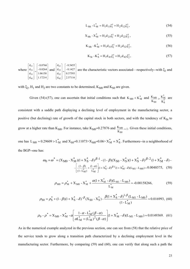
t2122

t1111

*MMt dHdHL-L ξξ += , (54)

t2222

t1211

*MMt dHdHX-X ξξ += , (55)

t2322

t1311

*MMt dHdHK-K ξξ += , (56)

t2422

t1411

*SSt dHdHK-K ξξ += , (57)

where

≈

17214.106150.1

0264.0-0766.0-

dddd

41

31

21

11

and

≈

57116.237593.0

1427.0-5455.0-

dddd

42

32

22

12

are the characteristic vectors associated—respectively--with ξ1 and

with ξ2, H1 and H2 are two constants to be determined, KM0 and KS0 are given.

Given (54)-(57), one can ascertain that initial conditions such that *MM0 KK < and

*S

*M

S0

M0KK

KK > are

consistent with a saddle path displaying a declining level of employment in the manufacturing sector, a

positive (but declining) rate of growth of the capital stock in both sectors, and with the tendency of KSt to

grow at a higher rate than KM0. For instance, take KM0≈0.27876 and 1KK

S0

M0 ≈ . Given these initial conditions,

one has *MM0 L29609.0L >≈ and XS0≈0.11073>XM0≈0.06> *

S*M XX = . Furthermore--in a neighborhood of

the BGP--one has:

-)-X1()-X1)(X-X()-(1-)-X1)(X-X( *M

2-*S

*SS0

1-*S

*MM0

*0 δδβδωω ββ ++++=

≈++

+ )L-)(L-X1()-X1(

L

)-1(

)L-(1

)-(1- M0M1*M

1-*S*

M*M

δδαβ β 0.0048575, (58)

≈+

++=*M

M0M1*M*

MM0*MM0

L)L-)(L-X1(

X-Xδαρρ -0.00158266, (59)

≈+

++=)L-(1

)L-(L)-X1(-)X-(X)-X1()-1(

*M

M0M1-1*

S*SS0

-*S

*SS0

ββ δβ

δβρρ 0.016993, (60)

≈+

+= )L-)(L-X1(

)-()L(L

)-(L--1-X-X- M0M1

*M2*

M*M

*M*

MM0*

0 δαβα

αβααρρ 0.0149369. (61)

As in the numerical example analyzed in the previous section, one can see from (58) that the relative price of

the service tends to grow along a transition path characterized by a declining employment level in the

manufacturing sector. Furthermore, by comparing (59) and (60), one can verify that along such a path the

24

output of the service sector may grow at a higher rate than the output of the manufacturing sector. Again,

equation (61) shows that along this transition path the economy’s GDP may increase at a higher rate than

along the BGP: as along the transition path considered in the Cobb-Douglas case, the economy’s rate of

growth tends to decline over time as the share of the two factors of production used in the manufacturing

sector shrinks.

7 CONCLUSIONS

The massive reallocation of resources among sectors and, in particular, the reallocation from

manufacturing to services in the industrialized economies which have characterized the latest decades, has

induced us to develop a model that can account for these impressive evidence. This formal set-up has

permitted to study how aggregate growth is affected by the interaction between technological progress,

which is generated endogenously and has a stronger positive impact on the manufacturing sector, and the

demand for services, which tends to increase—other things being equal—more than proportionally than total

expenditure in consumption.

Indeed, we have presented two numerical examples where it is shown that starting from an initial

employment share of the manufacturing sector in overall employment greater than its long-run equilibrium

share, the gradual shift of employment shares towards the service sector is accompanied by rates of growth

of output and capital stock that are higher in the service sector than in manufacturing. Moreover, along this

transition path, the relative price of the service is growing and the economy’s GDP tend to grow at a higher

rate than along the balanced growth path of the economy: the gradual shift of labor towards the service sector

is accompanied by a decline in the aggregate rate of growth. In other words, the pattern resulting from these

numerical examples seems to be consistent with the stylized facts.

In addition, we have shown within this analytical framework that positive long-term growth is

possible even if what households spend on services tends to increase more than proportionally than their total

consumption expenditure, namely when their preferences are non-homothetic: perpetual growth cannot take

place only if an excessively large portion of what households spend on consumption is devoted to the

service. This implies that tastes and attitudes of households may have relevant consequences for the long-

term growth performances of an economy by affecting the composition of consumers’ demand. More in

25

general, one may conclude that every factor affecting the composition of final demand can influence long-

term growth. Such important conclusion suggests an interesting extension of this paper: introducing public

demand for final products in order to model its effects on growth via its impact on the composition of final

demand.

REFERENCES

Aoki, M. and H. Yoshikawa. (2001). “A New Model of Economic Fluctuations and Growth,” Discussion

papers.

Appelbaum, E. and R. Schettkat. (1999). „Are Prices Unimportant? The changing structure of the

industrialized economies,” Journal of Post Keynesian Economics, 21, 3, 387-398.

Barro, Robert J. and Xavier Sala-i-Martin. (1995). Economic Growth. New York: McGraw-Hill.

Baumol, William J. (1967). “Macroeconomics and Unbalanced Growth: the Anatomy of Urban Crisis,”

American Economic Review, 57, 415-426.

Baumol, W.J., S. Batey Blackman and E.N. Wolff. (1985). “Unbalanced growth revisited: asymptotic

stagnancy and new evidence,” American Economic Review, 75, 4, 806-17.

Baumol, W.J. (2001). “Paradox of the services: exploding costs, persistent demand.” In Thijs ten Raa and

Ronald Schettkat (eds.), The Growth of Service Industries. Elgar.

Borzaga, C. and P. Villa. (1999). “Flessibilità e terziario,” Mimeo.

Business Statistics of the US. (2002).

Castells, M. and Y. Aoyama. (1994). “Paths Towards the Informational Society: Employment Structure in G-

7 Countries, 1920-1990,” International Labour Review, 133, 1, 5-33.

Curtis, D.C.A. and K:S.R Murthy. (1998). “Economic Growth and Restructuring: a test of unbalanced

growth models 1977-1992,” Applied Economic Letters, 5, 777-780.

Easterly, W. and L. Ross. (2001). “It’s Not Factor Accumulation: Stylized Facts and Growth Models,” World

Bank.

Echevarria, C. (1997). “Changes in sectoral composition associated with economic growth,” International

Economic Review, 38, 431-452.

Ercolani, P.(1994). “La terziarizzazione dell’occupazione. Analisi delle cause e dei problemi aperti,”

Quaderni di ricerca, 54. Univ. degli Studi di Ancona.

Erdem, E. and A. Glyn. (2001). “Employment Growth, Structural Change and Capital Accumulation.” In

Thijs ten Raa and Ronald Schettkat (eds.), The Growth of Service Industries. Elgar.

Falvey, R. and N. Gemmel. (1996). “Are Services Income-Elastic? Some New Evidence,” Review of Income

and Wealth, 42, 3, 257-269.

26

Foellmi, R. and J. Zweimüller. (2002). “Structural change and the kaldor facts of economic growth,” Cepr

Discussion Paper, N. 3300.

Frankel, Marvin. (1962). “The Production Function in Allocation and Growth: A Synthesis,” American

Economic Review, 52, 995-1022.

Fuchs, V.R. (1968). The service economy. NBER. New York: Columbia University Press.

Gershuny, J. and I.D. Miles. (1983). The new service economy. The transformation of employment in

industrial society. London: Frances Pinter.

Glyn, A. (1997). “Does Aggregate Profitability Really Matter?,” Cambridge Journal of Economics, 21, 593-

619.

Hill T.P. (1977). “On goods and services,” The Review of Income and Wealth, 23, 4, 314-339.

Inman, R. ed. (1985). Managing the Service Economy. Cambridge University Press.

Klodt, H. (1997). “The transition to the service society: prospects for growth, productivity and employment,”

Kiel W.P., N.839.

Kongsamut, P., S. Rebelo and Xie Danyang. (2001). “Beyond Balanced Growth,” Review of economic

studies, 68, 869-882.

Kravis, I.B., A. Heston and R. Summers. (1983). “The share of services in economics growth.” In Adams G.

F. and B. G. Hickman (eds.), Global econometrics: essey in honour of Lawrence Klein. Boston: MIT.

Kuznets, S. (1971). Economic Growth of Nations. Cambridge: Belknap Press.

Laitner, J. (2000). “Structural change and economic growth,” Review of Economic Studies, 67, 545-561.

Maddison, A. (1991). Dynamic Forces in Capitalist Development. Oxford: Oxford Univ. Press.

Martinelli, F. and J. Gadrey. (2000). L’economia dei servizi. Bologna: il Mulino.

Mattey, J. (2001). “Will the new information economy cure the cost disease in the USA?.” In Thijs ten Raa

and Ronald Schettkat (eds.), The Growth of Service Industries. Elgar.

Mc Guckin, R.H. and B. van Ark. (2001). Performance 2000: Productivity, Employment and Income in the

World’s Economies. The Conference Board.

Meckl, J. (2000). “Structural change and Generalized Balanced Growth,” Econometric Society World

Congress 2000 Contributed Papers, N. 0233.

Metcalfe, S. (2000). “Restless Capitalism: Increasing Returns and Growth in Enterprise Economies,” CRIC

W.P.

Montobbio,F. (2001). “An evolutionary model of industrial growth and structural change,” Stuctural change

and economic dynamics, 13, 387-414.

Möller, J. (2001). “Income and Price Elasticities in Different Sectors of the Economy: an Analysis of

Structural Change. for Germany, the UK and the USA.” In Thijs ten Raa and Ronald Schettkat (eds.), The

Growth of Service Industries. Elgar.

Mohnen, P., ten Raa, T. (2001). “Productivity Trends and Employment across Industries in Canada.” In Thijs

ten Raa and Ronald Schettkat (eds.), The Growth of Service Industries. Elgar.

27

Momigliano F. and D. Siniscalco. (1986). “Mutamenti nella struttura del sistema produttivo e integrazione

tra industria e terziario.” In Luigi Pasinetti (eds.), Mutamenti strutturali del sistema produttivo. Integrazione

tra industria e settore terziario. Bologna: Il Mulino.

O’Mahony, M. and B. van Ark. (2003). EU Productivity and Competitiveness: An Industry Perspective.

Luxembourg : Office for official publications of the European Communities.

OECD (1994a).The OECD Jobs Study. Paris: Oecd.

OECD (1994b). The OECD Jobs study: Investment, Productivity and Employment. Paris: Oecd.

OECD (1995). The OECD Jobs Strategy: Technology, Productivity and Job creation. Paris: Oecd.

OCSE (2000). Employment Outlook. Paris: Ocse.

OECD (2002). Economic Outlook. Paris: Oecd.

Pasinetti, L. (1984). Dinamica strutturale e sviluppo economico. Torino: Utet.

Petit, P. and L. Soete. (1997). “Technical change and employment growth in services: analytical and policy

challenges,” Nota di lavoro, 46. Milano: FEEM.

Oulton, N. (2001). “Must the Growth Rate Decline? Baumol’s Unbalanced Growth Revisited,” Oxford

Economic Papers, 53, 605-627.

Reati, A. (1998). “A Long-Wave Pattern for Output and Employment in Pasinetti’s Model of Structural

Change,” Economie Appliquée, 2, 29-77.

Rowthorn, R. and R. Ramaswami. (1999). “Growth, Trade and Deindustrialization,” IMF Staff Papers, 46, 1,

18-40.

Russo, G. and R. Schettkat.(2001). “Structural economic dynamics and the final product concept.” In Thijs

ten Raa and Ronald Schettkat (eds.), The Growth of Service Industries. Elgar.

Sakurai, N. (1995). “Structural change and employment: empirical evidence for 8 OCSE countries,” Science

Technology Industry, 15, 133-177.

Schettkat, R. and L. Yocarini. (2003). “The shift to services: a review of the literature,” IZA DP, N. 964.

Schettkat, R. and Thijs ten Raa. (2001). The Growth of Service Industries. Edward Elgar. Cheltenam, UK.

Stanback T.M. (1979). Understanding the service economy: employment, productivity location. Baltimore:

The Johns Hopkins University Press.

Summers, R. (1985). “Services in the international economy.” In R. Inman (ed.), Managing the Service

Economy, Cambridge University Press.

Survey of Current Business. (2003), 83, 10.

Triplett, J. (2003). “Baumol’s disease” has been cured: IT and Multifactor productivity in US services

industries. Paper presented at XV Villa Mondragone International Economic Seminar on “Markets, growth

and global governance”. CEIS – Univ. Roma Tor Vergata. July 2-3, 2003.

Wieczorek, J. (1995). “Sectoral trends in world employment and the shift toward services,” International

Labour Review, 134, 2, 205-226.

28

APPENDIX

Table 1. Sectoral employment shares. Agriculture Manuf. Services Agriculture Manuf. Services

France Germany1901 41.4 31.5 27.1 1907 33.9 39.9 26.2 1949 29.6 33.1 37.3 1950 22.1 44.7 33.2 1960 22.0 36.9 41.1 1960 13.8 47.7 38.5 1970 13.3 38.7 47.9 1970 8.5 48.4 43.1 1980 8.6 35.4 56.0 1980 5.2 42.8 52.0 1990 6.1 29.2 64.6 1990 3.5 39.1 57.4 Italy Japan 1901 61.7 22.3 16.0 1906 61.8 16.2 22.0 1951 43.9 29.5 26.7 1950 48.3 22.6 29.0 1960 32.2 36.2 31.6 1960 32.6 29.7 37.6 1970 19.6 38.4 42.0 1970 17.4 35.7 46.9 1980 13.3 36.9 49.2 1980 10.4 35.3 54.2 1990 8.7 31.6 59.7 1990 7.2 34.1 58.7 UK US 1901 13.0 43.9 43.1 1900 40.4 28.2 31.4 1951 5.0 47.4 47.6 1950 12.8 31.5 55.7 1961 3.7 48.4 47.9 1960 8.6 30.6 60.8 1970 3.2 44.1 52.7 1970 4.4 33.0 62.6 1980 2.6 37.2 60.3 1980 3.5 29.9 66.6 1990 2.1 28.7 69.2 1990 2.8 25.7 71.5 Sources: OECD, Job Study, 1994.

Table 2. Changes in Services Shares over time. France, UK., US. Shares of Services in private consumption. Services in GDP At current prices At constant prices At current prices At constant pricesFrance 1959-60 28.9 36.3 31.3 38.0 1977-78 37.5 37.7 37.9 36.5 UK 1957-58 22.8 35.2 39.5 51.6 1967-68 29.4 33.6 43.8 50.5 1977-78 31.6 33.2 47.6 49.7 US 1947-48 31.4 39.6 33.2 42.4 1957-58 38.4 41.5 44.9 49.6 1967-68 42.2 43.6 48.8 50.8 1977-78 45.6 45.5 49.7 49.0 Source Kravin-Heston-Summers (1983)

29

Table 3. Manufacturing and services capital stock growth (average annual % changes) 1960-64 1963-68 1968-73 1973-78 1979-83 1983-88 1988-93France Man 6.1 5.6 6.4 3.4 2.0 2.0 2.2 Ser 7.6 6.2 4.3 3.6 4.8 Ger Man 7.9 6.0 5.5 2.0 1.4 1.2 2.1 Ser 6.7 5.9 6.2 4.6 4.5 Italy Man 8.4 4.7 4.9 5.1 3.8 2.5 2.7 Japan Man 16.5 12.8 13.7 5.8 5.2 5.9 7.7 Ser 14.9 9.4 7.6 11.9 9.9 UK Man 3.9 3.8 3.3 2.3 1.7 1.4 0.9 Ser 4.4 3.0 2.6 3.8 4.5 US Man 2.7 5.1 4.0 4.1 3.5 2.0 2.5 Ser 4.7 3.7 4.2 4.7 3.3 Source Glyn (1997)

Table 4. GDP growth. GDP growth 1960-73 1974-95 France 5.4 2.2 Ger 4.4 2.6 Italy 5.3 2.4 Japan 9.4 3.2 UK 3.2 1.8 EC 12 4.8 2.2 US 4.3 2.5 Source Table 2.3, ILO (1996)

Table 5. Annual labour productivity growth by sector. EU-15 US 1979-90 1990-95 1995-01 1979-90 1990-95 1995-01 Total Economy 2.2 2.3 1.7 1.4 1.1 2.3 Agr., Forestry, Fish. 5.2 4.8 3.3 6.4 1.7 9.1 Mining, quarrying 2.9 13.1 3.5 4.4 5.1 -0.2 Manufacturing 3.4 3.5 2.3 3.4 3.6 3.8 Elect., gas, water 2.7 3.6 5.7 1.1 1.8 0.1 Construction 1.6 0.8 0.7 -0.8 0.4 -0.3 Distributive trade 1.3 1.9 1.0 1.8 1.5 5.1 Transport 2.8 3.8 2.3 3.9 2.2 2.6 Communications 5.2 6.2 8.9 1.4 2.4 6.9 Financial services 2.2 1.0 2.8 -0.7 1.7 5.2 Business services 0.7 0.7 0.3 0.1 0.0 0.0 Community, social, personal serv. -0.3 0.4 0.3 1.2 0.9 -0.4 Public Ad., Education, Health 0.6 1.1 0.8 -0.4 -0.8 -0.6 Source: Table 1.4b in O’Mahony-Van Ark (2003)

30

Dipartimento di economia politica e metodi quantitativi Università degli studi di Pavia

List of the lately published Technical Reports (available at the web site: "http://economia.unipv.it/Eco-Pol/quaderni.htm").

Quaderni di Dipartimento # Date Author(s) Title 144 06-02 I.Epifani Exponential functionals and means of neutral

A.Lijoi to the right priors I.Pruenster

145 06-02 P.Bertoletti A note on third-degree price discrimination and output

146 12-02 P.Berti Limit theorems for predictive sequences of L.Fratelli random variables P.Rigo

147 01-03 A. Lijoi Practicable alternatives to the Dirichlet I. Pruenster process

148 02-03 A. Lijoi Extending Doob's consistency theorem to Pruenster nonparametric densities S.G.Walker

149 02-03 V.Leucari Compatible Priors for Causal Bayesian G.Consonni Networks 150 02-03 L. Di Scala A Bayesian Hierarchical Model for the

L. La Rocca Evaluation of a Web Site G.Consonni

151 02-03 G.Ascari Staggered Prices and Trend Inflation: Some Nuisances

152 02-03 G.Ascari How inefficient are football clubs? P.Gagnepain An evaluation of the Spanish arms race

153 03-03 P.Dellaportas Categorical data squashing by C.Tarantola combining factor levels

154 05-03 A. Lijoi A note on the problem of heaps Pruenster

155 09-03 P.Berti Finitely additive uniform limit theorems P.Rigo 156 09-03 P.Giudici Web Mining pattern discovery C.Tarantola 157 09-03 M.A.Maggi On the Relationships between

U.Magnani Absolute Prudence M.Menegatti and Absolute Risk Aversion

158 10-03 P.Bertoletti Uniform Pricing and Social Welfare 159 01-04 G.Ascari Perpetual Youth and Endogenous Labour

N.Rankin Supply: A Problem and a Possible Solution