The Determination and Development of Sectoral Structure

by

Henri L.F. de Groot*

Free University of Amsterdam

Department of Spatial Economics

De Boelelaan 1105

1081 HV Amsterdam

The Netherlands

Tel.: (+31) 20 444 6095

Fax.: (+31) 20 444 6004

E-mail: hgroot@econ.vu.nl

Abstract.

The development over time of sectors in terms of value added and employment has

common characteristics in all economies. We develop a simple Ricardian multi-sector

general equilibrium model that allows for (i) non-unitary income elasticities, (ii)

different paces of technological progress per sector, and (iii) endogenously determined

technological progress per sector. A model with these ingredients allows us to

replicate the sectoral developments that are found empirically, and which are shown

to be the outcome of an interplay between factors of demand and supply. Under

reasonable assumptions, deindustrialization is shown to be a natural and

unavoidable consequence of increases in the wealth of nations.

JEL-codes: O11, O41

Key-words: sectoral change, endogenous growth, deindustrialization

* This paper is based on my Ph.D. research performed at the Department ofEconomics and CentER for Economic Research at Tilburg University. I would like tothank Jeroen van den Bergh, Henk van Gemert, Richard Nahuis, Michiel de Nooij,Thijs ten Raa, Ton van Schaik, and Sjak Smulders for useful comments on earlierversions of this paper. The usual disclaimer applies.

- 1 -

The Determination and Development of Sectoral Structure

by Henri L.F. de Groot

Abstract.

The development over time of sectors in terms of value added and

employment has common characteristics in all economies. We develop a

simple Ricardian multi-sector general equilibrium model that allows for

(i) non-unitary income elasticities, (ii) different paces of technological

progress per sector, and (iii) endogenously determined technological

progress per sector. A model with these ingredients allows us to

replicate the sectoral developments that are found empirically, and

which are shown to be the outcome of an interplay between factors of

demand and supply. Under reasonable assumptions,

deindustrialization is shown to be a natural and unavoidable

consequence of increases in the wealth of nations.

1. Introduction

Developments in the sectoral composition of countries share several

common characteristics. Most pronounced in terms of sectoral changes are

the reallocations of labour that take place as countries grow richer.

Countries typically start with a large agricultural sector and end up with a

large service sector. In the meantime, manufacturing employment follows a

hump-shaped pattern. Developments in sectoral shares measured in GDP at

constant prices are much less pronounced. The share of manufacturing in

GDP measured at constant prices remains roughly constant. The

agricultural share shows some tendency to decline, whereas the service

sector has gradually increased its share. This latter change has taken place

despite the continuously rising relative prices of services.1 The existence of a

1 There is a rich and mainly descriptive literature on the development of sectoral sharesthat we do not discuss here. This literature goes back to, amongst others, Chenery andSyrquin (1975) and Kuznets (1966). This literature has attempted to find normal patterns inthe development of economies over time. We refer here to Van Gemert (1985) for an extensiveoverview and discussion of this literature as well as an empirical test of the normal-patternhypothesis. The main emphasis in this paper is on theoretical models aiming to explain the

- 2 -

strong link between the degree of economic maturity and the structure of

employment was already pointed out by Sir William Petty in 1691 and

restated by Clark (1957, p. 492) when he wrote that ‘A wide, simple and far-

reaching generalisation ... [is that] as time goes on and communities become

more economically advanced, the numbers engaged in agriculture tend to

decline relative to the numbers in manufacture, which in their turn decline

relative to the numbers engaged in services’. How can these tendencies be

explained and reconciled? This is the central question that we will address

in this paper.

A topic that has gathered particular attention in the debate on

sectoral developments is which factors are responsible for the observed

drastic decline in manufacturing employment in the last 25 years. This

decline, often referred to as deindustrialization, has recently been discussed

in relation to increased unemployment in Europe and increased income

inequality in the USA. At least five basic explanations for this experience of

deindustrialization are available. The first relies on differences in

productivity growth on a sectoral level. If productivity in the manufacturing

sector is relatively fast-growing, less and less labour is required to produce a

given relative amount of products. For this explanation to be relevant, goods

produced in the broad sectors defined above need to be relatively bad

substitutes. A second explanation relies on the operation of Engel’s law. If

the income elasticities of the demand for goods produced in different sectors

are unequal, the share of the sector producing the goods with the highest

income elasticity has a tendency to increase as countries grow richer. A

third explanation relies on the integration of the South and the North,

resulting in the South specializing towards low-skilled labour-intensive

manufacturing goods. Fourthly, and related to the third explanation,

changing ‘endowments’ can play a role. Assuming, for example, that services

are relatively skill-intensive and that the accumulation of skills is a

particularly fast process in OECD countries may explain why OECD

countries specialize in (tradeable) services and are experiencing a decline in

manufacturing employment. Finally, outsourcing (or contracting out) of

activities previously carried out within the manufacturing sector but now

performed in the service sector or abroad may be part of the explanation (see

empirical tendencies that we observe.

- 3 -

for example Feenstra and Hanson (1995) and De Groot (1998)).2

In a seminal theoretical contribution on the macroeconomics of

unbalanced growth, Baumol (1967) studied the consequences of differences

in productivity growth rates between sectors (known as differential

productivity growth) for macroeconomic developments. Differential

productivity growth rates are labelled as ‘forces so powerful that they

constantly break through all barriers erected for their suppression’ (Baumol

(1967, p. 415)). Based on a simple Ricardian model with only two sectors,

one stagnant with zero productivity growth and one progressive with positive

productivity growth, he concludes that the cost per unit of the stagnant

sector will rise without limitation. This creates a tendency for demand to

shift in favour of goods produced in the progressive sector. If, however,

goods from different sectors are bad substitutes, more and more labour

must be transferred to the non-progressive sector. Which tendency

ultimately dominates in the determination of the sectoral composition of the

economy depends on the evolution of consumers' preferences as income

increases. The macroeconomic growth rate will ultimately tend to converge

to the growth rate of the stagnant sector. The implications of this very

simple model have become to be known as the ‘cost disease of stagnant

services’.

One of the objections which can be raised against Baumol's model is

that its main focus is on supply factors (i.e., differential rates of productivity

growth). Although Baumol considers the special cases in which (i)

consumers spend constant shares of their income on all categories of goods

available, and (ii) relative demand in volume terms for both goods categories

is constant, he does not discuss in detail the importance of demand factors.

Pasinetti (1981, p. 69) stresses the importance of considering both factors of

demand and supply for a good understanding of macroeconomic sectoral

2 Recent empirical contributions on the driving forces behind deindustrialization areRowthorn and Ramaswamy (1997) and Saeger (1997). Based on a panel of 21 industrialcountries, the first two authors argue that there is evidence for a non-linear relationshipbetween per capita income and the manufacturing share of employment. Furthermore, theyconclude that the manufacturing share of employment is significantly affected by the tradebalance in manufactured goods. They find little evidence of an important role of North-Southtrade in explaining the decline in manufacturing employment. A similar exercise is performedby Saeger. Based on panel data for OECD countries, he examines the relationship betweendeindustrialization and productivity growth, Dutch disease, human capital accumulation,and trade flows. Differential productivity growth and the Dutch disease account for about40% of deindustrialization in the majority of countries, while about 25% is explained byNorth-South trade.

- 4 -

developments when he argues that ‘... to pretend to discuss technical

progress without considering the evolution of demand would make it

impossible to evaluate the very relevance of technical progress and would

render the investigation itself meaningless. Increases in productivity and

increases in income are two facets of the same phenomenon. Since the first

implies the second, and the composition of the second determines the

relevance of the first, the one cannot be considered if the other is ignored’.

This point was taken seriously by, for example, Quibria and Harrigan

(1996). They extended the model of Baumol by introducing a constant

elasticity of substitution utility function. Their simple model allows them to

replicate what they consider to be the stylized facts of sectoral

developments, namely the rising relative prices of service goods, a rising

share of service employment in total employment, a rising share of services

in the value share of national income (in current prices), and a non-

increasing share in the national real product. To arrive at these results, they

assume the presence of differential productivity growth and a substitution

elasticity of demand between services and manufacturing goods that is less

than unity.

Although these simple two-sector models give interesting insights in

the role of factors of demand (i.e. preferences) and supply (i.e. technological

progress) in shaping sectoral structures, they are by definition not capable

of capturing the type of sectoral development processes described at the

beginning of this introduction. So in order to capture and explain these

developments, multi-sectoral (i.e., more than two-sector) models are needed.

In addition, the previously discussed models are simple one-factor models.

Some recent attempts have been undertaken to fill these gaps. Most

complete in this are Echevarria (1997) and Kongsamut, Rebelo and Xie

(1997).3 Again focusing on the regularities with respect to the growth process

and the associated reallocation of labour, they develop three-sector models

including capital as a factor of production. Their dynamic general

equilibrium models are characterized by (i) different and non-unitary income

elasticities of demand for goods from the distinguished sectors during the

3 Three-sector models with only one production factor are developed in Cornwall andCornwall (1994), and Rowthorn and Ramaswamy (1997). Both studies are able to replicaterich dynamics of structural change, but lack a clear and simple system of demand equationsderived from optimizing consumer behaviour. In addition, the study by Rowthorn andRamaswamy does not consider relative price changes. The importance of price effects inshaping sectoral structures is considered (explicitly) by Schettkat and Appelbaum (1997).

- 5 -

transition to the long-run equilibrium of the model, and (ii) differences in the

exogenously given rate of technological progress on a sectoral level. A

combination of these two elements results in models characterized by rich

dynamics in structural change that are able to replicate empirically observed

dynamics. The sectoral economic growth rates of labour productivity are

given exogenously and attention is restricted to models where the elasticity

of substitution between goods from different sectors is unity in the long-run

equilibrium, implying constant sectoral employment shares and shares in

nominal GDP in the long-run.

Given this state of affairs, the main goal of this paper is to develop a

simple Ricardian model that allows us to understand part of the

developments that take place on a sectoral level. We abstain from trade-

based explanations of the observed trends and instead focus on differential

productivity growth and increased maturity as potential candidates for

explaining observed trends in sectoral developments. The model that we

develop allows for non-unitary income elasticities of demand, non-unitary

substitution elasticities between goods from different sectors, differential

productivity growth (i.e., different paces of technological progress on a

sectoral level), and endogenously determined technological progress on a

sectoral level resulting from learning by watching. Previously performed

studies that develop Ricardian models (in particular, Baumol (1967),

Matsuyama (1992), and Quibria and Harrigan (1996)) are shown to be

special cases of the general model developed in this paper. Compared to

other existing studies (e.g., Gundlach (1994), and Rowthorn and

Ramaswamy (1997)) our model has the advantage that it is derived from a

well-specified system of demand-equations that is derived from optimizing

consumer behaviour with clearly specified utility functions.

This paper proceeds as follows. Section 2 illustrates the developments

in sectoral shares, employing the OECD International Sectoral Data Base

(1997). The similarity of the trends for the countries under consideration

suggests that structural factors are at play. We develop a simple Ricardian

model in section 3 that allows us to explain how developments as described

in section 2 may come about as the outcome of an interplay between factors

of demand and supply. To get a good feeling for the fundamental

mechanisms that are at play, we present a two-sector version of the model

in section 4. In section 5 we discuss the characteristics of a multi-sector

variant of the model. This will be done against the background of the

- 6 -

empirically found regularities. We conclude in section 6.

2. Empirical evidence

In this section, we briefly present and discuss some trends in sectoral

developments in advanced countries. These trends are well-established in

the literature (see for example Maddison (1991 and 1995), Van Ark (1996),

Echevarria (1997), and Kongsamut, Rebelo and Xie (1997)). Our empirical

investigation covers three countries (USA, Germany, and Japan)4 and three

sectors (agriculture, manufacturing and the service sector) over the period

1960-1995. Data were taken from the OECD International Sectoral Data

Base (1997). We refer to the OECD (1997) for details on sectoral composition

and construction of the data. The agricultural sector contains ISIC group 1

and includes hunting, forestry and fishing. Manufacturing contains ISIC

group 3 (a broad aggregate of manufacturing industries). The service sector

contains ISIC group 6 (wholesale and retail trade, restaurants and hotels),

group 8 (finance, insurance, real estate and business services) and group 9

(community, social and personal services).5

4 We deliberately restrict the attention to these large and relatively closed economies inthe hope that we can safely assume that developments are only to a small extent the result ofexternal developments and are not strongly related to patterns of specialization. Othercountries included in the ISDB are France, Italy, United Kingdom, Canada, Australia,Belgium, Denmark, Finland, Netherlands, Norway, and Sweden. From the inspection ofpatterns of development of small open economies, one can conclude that patterns ofspecialization play a sometimes important role in explaining developments of sectoral sharesof these countries. In the Netherlands, for example, the 1980s have witnessed an increase inthe GDP-share at constant prices of the agricultural sector which is likely to be due to relativespecialization. Furthermore, developments in energy-intensive sectors were strongly influ-enced by the oil-crisis in the 1970s, whereas developments in the construction sector arestrongly influenced by population growth and reconstruction after World War II. Since thesedevelopments are to a large extent the result of period-specific shocks, we omitted thesesectors from the analysis.

5 We omitted the transport- and communication sector from the aggregate of the servicesector for reasons of heterogeneity. The communication sector is among the fastest growingsectors (in terms of labour productivity). This holds true for all countries. This sector couldtherefore, in our opinion, better be considered as a high-tech (manufacturing) sector than aservice sector (Baumol, Blackman and Wolff (1989) label this kind of sectors as‘technologically progressive’). The distinction they make between technologically progressiveand stagnant activities is based on intrinsic attributes of activities like the ease ofstandardization and the ease of formalizing the production process in a set of easily replicableinstructions.

- 7 -

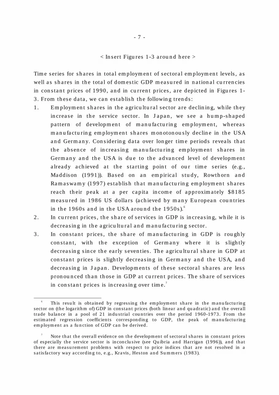
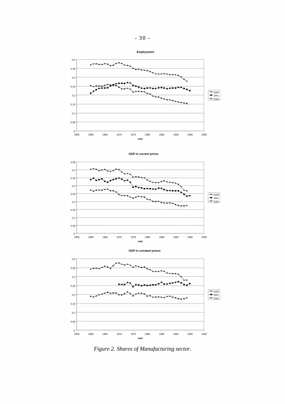
< Insert Figures 1-3 around here >

Time series for shares in total employment of sectoral employment levels, as

well as shares in the total of domestic GDP measured in national currencies

in constant prices of 1990, and in current prices, are depicted in Figures 1-

3. From these data, we can establish the following trends:

1. Employment shares in the agricultural sector are declining, while they

increase in the service sector. In Japan, we see a hump-shaped

pattern of development of manufacturing employment, whereas

manufacturing employment shares monotonously decline in the USA

and Germany. Considering data over longer time periods reveals that

the absence of increasing manufacturing employment shares in

Germany and the USA is due to the advanced level of development

already achieved at the starting point of our time series (e.g.,

Maddison (1991)). Based on an empirical study, Rowthorn and

Ramaswamy (1997) establish that manufacturing employment shares

reach their peak at a per capita income of approximately $8185

measured in 1986 US dollars (achieved by many European countries

in the 1960s and in the USA around the 1950s).6

2. In current prices, the share of services in GDP is increasing, while it is

decreasing in the agricultural and manufacturing sector.

3. In constant prices, the share of manufacturing in GDP is roughly

constant, with the exception of Germany where it is slightly

decreasing since the early seventies. The agricultural share in GDP at

constant prices is slightly decreasing in Germany and the USA, and

decreasing in Japan. Developments of these sectoral shares are less

pronounced than those in GDP at current prices. The share of services

in constant prices is increasing over time.7

6 This result is obtained by regressing the employment share in the manufacturingsector on (the logarithm of) GDP in constant prices (both linear and quadratic) and the overalltrade balance in a pool of 21 industrial countries over the period 1960-1973. From theestimated regression coefficients corresponding to GDP, the peak of manufacturingemployment as a function of GDP can be derived.

7 Note that the overall evidence on the development of sectoral shares in constant pricesof especially the service sector is inconclusive (see Quibria and Harrigan (1996)), and thatthere are measurement problems with respect to price indices that are not resolved in asatisfactory way according to, e.g., Kravis, Heston and Summers (1983).

- 8 -

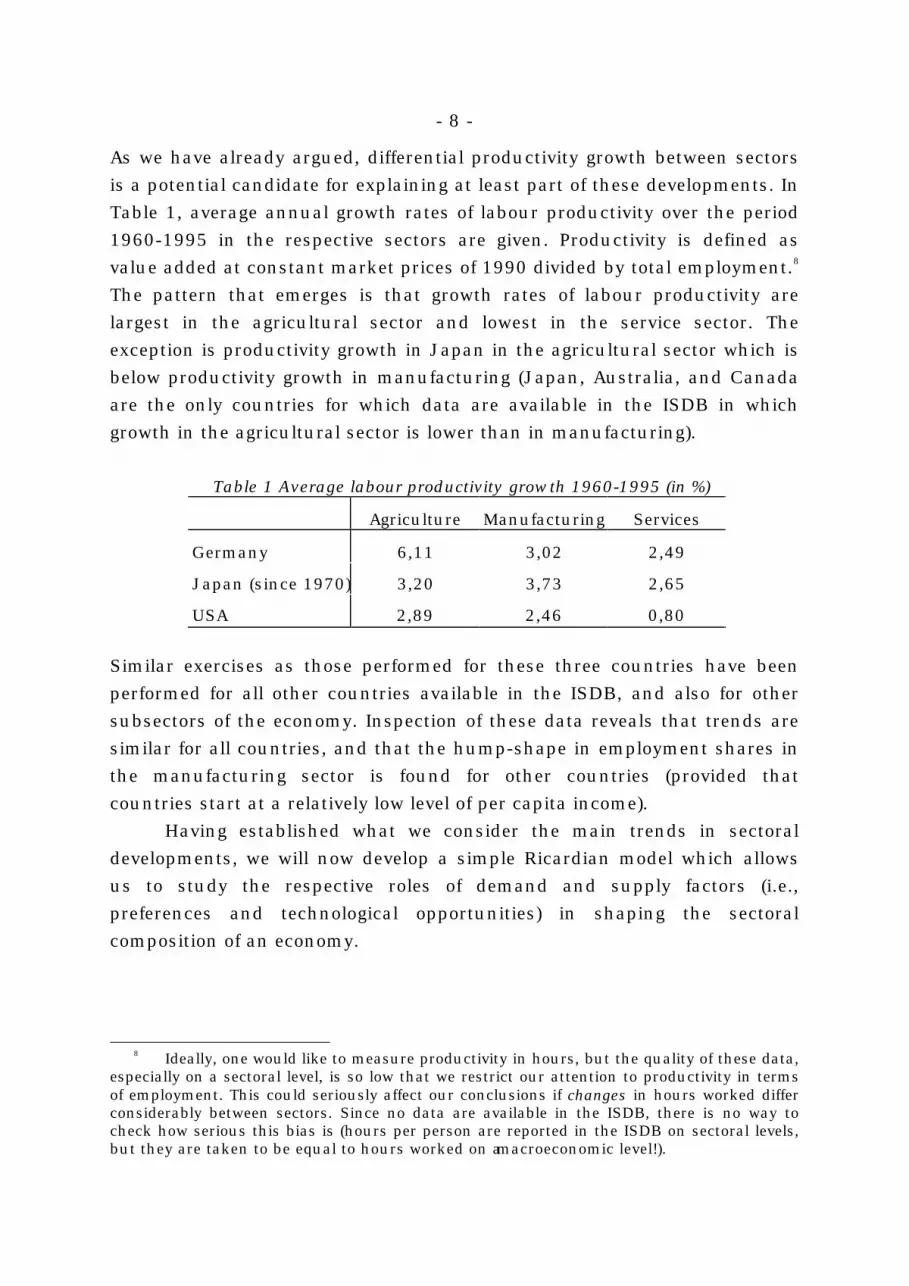
As we have already argued, differential productivity growth between sectors

is a potential candidate for explaining at least part of these developments. In

Table 1, average annual growth rates of labour productivity over the period

1960-1995 in the respective sectors are given. Productivity is defined as

value added at constant market prices of 1990 divided by total employment.8

The pattern that emerges is that growth rates of labour productivity are

largest in the agricultural sector and lowest in the service sector. The

exception is productivity growth in Japan in the agricultural sector which is

below productivity growth in manufacturing (Japan, Australia, and Canada

are the only countries for which data are available in the ISDB in which

growth in the agricultural sector is lower than in manufacturing).

Table 1 Average labour productivity growth 1960-1995 (in %)

Agriculture Manufacturing Services

Germany 6,11 3,02 2,49

Japan (since 1970) 3,20 3,73 2,65

USA 2,89 2,46 0,80

Similar exercises as those performed for these three countries have been

performed for all other countries available in the ISDB, and also for other

subsectors of the economy. Inspection of these data reveals that trends are

similar for all countries, and that the hump-shape in employment shares in

the manufacturing sector is found for other countries (provided that

countries start at a relatively low level of per capita income).

Having established what we consider the main trends in sectoral

developments, we will now develop a simple Ricardian model which allows

us to study the respective roles of demand and supply factors (i.e.,

preferences and technological opportunities) in shaping the sectoral

composition of an economy.

8 Ideally, one would like to measure productivity in hours, but the quality of these data,especially on a sectoral level, is so low that we restrict our attention to productivity in termsof employment. This could seriously affect our conclusions if changes in hours worked differconsiderably between sectors. Since no data are available in the ISDB, there is no way tocheck how serious this bias is (hours per person are reported in the ISDB on sectoral levels,but they are taken to be equal to hours worked on a macroeconomic level!).

- 9 -

3. A simple model

In this section, we develop a model of an economy that consists of S

production sectors, indexed i=1,…,S. Production in these sectors takes place

under perfect competition and there is only one factor of production, namely

labour (L), which is fully employed. We normalize the amount of labour at

100 so that we can conceive sectoral employment shares as percentage-

shares in total employment. Consumer preferences are such that goods from

all sectors are consumed. Income elasticities of demand may differ for goods

from different sectors due to the presence of differing subsistence

requirements. Labour productivity grows with a rate that is partly

exogenous and partly depends on the scope for learning by watching. We

will characterize the solution of the model in terms of the allocation of

labour over the production sectors of the economy.

The objective of the representative consumer in our model is specified

as

max where andC

1/

i=1

S

i i i i i ii

S

i

C = a C C ) < 1, 0, C > C 0, a( - ,ρ

ρ ρ ρ∑ ∑

≠ ≥ =

=1

1 (1)

where C is the consumption index, Ci is the consumed amount of goods from

sector i, Ci is the subsistence requirement of consumption, and ai is a

distribution parameter. In the absence of subsistence requirements, 1/(1-ρ)

is the elasticity of substitution between goods from different sectors. The

budget constraint corresponding to this problem is

C P = C P wL Y,Ci=1

S

i Ci∑ ≤ ≡ (2)

where PC is the macroeconomic price index, PCi is the price of a good

produced in sector i, w is the nominal wage rate which is equal for workers

in all sectors, and Y is nominal income. Four remarks with respect to the

choice of the utility function deserve attention. Firstly, the introduction of

subsistence requirements in the utility function is an easy way of allowing

for non-unitary income elasticities of demand that can differ between

sectors. Secondly, a minor disadvantage of a utility function with

subsistence requirements is that it is undefined for levels of Ci lower than

Ci , and marginal utilities go to infinity as Ci approaches Ci from above (e.g.,

Echevarria (1997)). This problem is not serious, assuming as we will do that

countries are sufficiently advanced that they can fulfil their subsistence

- 10 -

requirements (i.e., C h Li i/ 0∑ < , where hi0 is the productivity level at time

t=0). Thirdly, there is no need to assume Ci to be non-negative on

theoretical grounds, but it gives these values a simple interpretation as

subsistence requirements (e.g., Deaton and Muellbauer (1980)). Finally, in

the special case in which ρ→0, the utility function boils down to a Stone-

Geary utility function.9

Formulating the Lagrangian corresponding to optimization problem (1)

and performing standard optimization yields demand for goods from sector i

as a function of prices (see Appendix)

i i

1

-1Ci

i

j=1

S

Cj j

j=1

S

Cj

1

-1Cj

j

C = C +P

a

Y - P C

PP

a

.ρ

ρ

∑

∑(3)

The income elasticity of demand can be derived as

∂∂

∑ ∑

i

i

ij=1

S

Cj

1

-1Cj

Ci

i

j j=1

S

Cj j

C

Y

Y

C =

Y

C PP

P

a

a+ Y - P C

.ρ

(4)

This expression reveals how sectoral demand changes if nominal income Y

increases with one percent, keeping everything else constant. If there are no

subsistence requirements, income elasticities are equal to one. The income

elasticity of good i is larger when its subsistence requirement is smaller. A

larger subsistence requirement of good j lowers the income elasticity of good

i.

Producers of the consumption goods operate under perfect

competition and produce with a constant returns to scale technology, only

using labour which has labour productivity hi . The production function 9 To be more precise, evaluating equation (1) at ρ→0 by taking logs on both sides andapplying l'Hôpital's rule reveals that the optimization problem in the case where ρ→0 boilsdown to

( )max . . .C

i=1

Sa

i i C i Cii

S

i

iC = C C s t CP C P wL∏ ∑− = ≤=1

With no subsistence requirements, a Stone-Geary utility function becomes a standard Cobb-Douglas utility function. We refer to Klump and Preissler (1997) for an extensive discussionon the characteristics of various forms of CES-functions that are used in the literature.

- 11 -

thus looks like

i i iC = h L . (5)Due to perfect competition, the price of the consumption good of sector i

equals

Pw

hCii

= . (6)

From this point onwards we take the wage rate as numeraire (w=1 so Y=L).

Finally, we propose the following ‘engine of growth’ describing the

development of labour productivity

( )dh

dth g h g Li i i i i i= = + ξ , (7)

where gi is the exogenously given part of the rate of technological progress.

The parameter ξ captures in a stylized way the importance of ‘learning by

watching’ in each sector (compare Matsuyama (1992)). This is the most

simple way of incorporating an element of endogenous growth in the model.

In this view, growth (partly) occurs because of workers working together and

becoming better in producing by looking at each other’s productive

performance. The scope for learning, and thus for growth, is in this view

determined by the amount of people working together in a particular sector.

Knowledge results as an unintended by-product of producing. We use the

term learning by watching instead of learning by doing since in our engine of

growth, it is the number of workers that can learn from each other that

matters for growth, and not the mass of products produced by these

workers. This distinction is important for the following reason. One of the

arguments put forward by Baumol (1967) as to why (exogenous) growth in

manufacturing is persistently larger than in services is that scale effects are

operating in this sector. It is important to be precise on the meaning of scale

in this context. Scale may matter in the sense that the volume of production

matters for growth (implying that learning by doing matters), but it may also

matter in the sense that the number of producers is a driving force behind

growth (implying that learning by watching matters). In this paper, we take

the latter approach.

- 12 -

The model is now complete and we can establish the allocation of

labour over sectors as a function of sectoral productivity levels by

substituting the production function (5) and the price-equation (6) into the

demand-equation (3)

ii

ii i

j=1

Sj

j

j=1

S

j j

L = Ch

+ h a

L -C

h

h a

.−−

−−

−−

−−

∑

∑

ρρ ρ

ρρ ρ

1

1

1

1

1

1

(8)

The complete model is now essentially reduced to equations (7) and (8) and

we can study the characteristics of the model in more detail. This will be the

topic of the next two sections.

4. The two-sector version of the model

In this section, we consider the model in a two-sector context (S=2). This

serves two goals. First, it gives a feeling for the basic forces that are at play

in shaping the sectoral composition of economies. This will be useful for

understanding the developments in a multi-sector version (i.e. more than

two) of the model which will be discussed in section 5. Secondly, it makes

clear that existing two-sector Ricardian models on growth and sectoral

structure developed previously can be seen as special cases of the model

developed in this section.

Starting from equation (8), we can derive employment shares in a two-

sector economy as

11

1

1

1

2

2

2 1L = Ch

+ h a

L -Ch

+Ch

h a + h a

, L = L - L .11

1

1

1

11

1

1

12

12

1

1

−−

−−

−−

−−

−−

−−

ρ

ρ ρρ

ρ ρρ

ρ ρ

(9)

The number of cases we can now analyze is large, depending on the

assumptions with respect to (i) the presence of subsistence requirements

(Ci ), (ii) the presence of (differentiated) exogenous technological progress

( gi ), (iii) the presence of learning by watching (captured by ξi), and (iv) the

elasticity of substitution between goods of the two sectors (which is related

to ρ). Table 2 gives a classification of previous studies by Baumol (1967),

- 13 -

Matsuyama (1992), and Quibria and Harrigan (1996), and of the two

additional cases we will explicitly consider in this section.10 The analysis of

additional cases is deliberately restricted to the two basic cases of Stone-

Geary preferences (ρ→0), and CES-preferences in which we allow for both

exogenous and endogenous technological progress (assuming away the

existence of subsistence requirements for simplicity). Discussion of the other

cases one can consider does not yield additional insights as they are

straightforward combinations of the two basic cases we present.

Table 2 Classification of cases in the two-sector variant of the model

Ci =0, ξi=0 Ci >0, ξ

i=0 Ci =0, ξ

i>0 Ci >0, ξ

i>0

ρ→0 Baumol (1967) This section - Matsuyama(1992)11

ρ<0 Quibria and Harrigan(1996)

- This section -

ρ→-∞ Baumol (1967)12 - - -

In the case of a Stone-Geary utility function (ρ→0), we can describe the

development of sectoral labour shares over time by taking the derivative of

10 Table 2 does not contain a classification on the basis of exogenous growth rates. In allcases that we consider we assume that the exogenous growth rates are positive and differentbetween the two sectors under consideration, unless otherwise stated.

11 Matsuyama (1992) looks at a very special case in that he assumes (i) a Stone-Gearyutility function, (ii) exogenous growth in both sectors to equal zero, (iii) an agricultural sectorwhich has a positive subsistence requirement and no technological progress, and (iv) amanufacturing sector which has endogenous technological progress, but no subsistencerequirements. This combination of assumptions results in a constant sectoral allocation oflabour. Matsuyama was well aware of the specificity of his assumptions and acknowledgesthat his result depends on the absence of growth in the agricultural sector and theassumption of a Stone-Geary utility function. This will be further explained in the remainderof this section.

12 Due to the choice of the utility function in our model, we obtain the result thatconsumption shares in constant prices are equal (Ci=Cj) under Leontief-preferences (ρ→-∞).This result would not obtain once instantaneous utility would be specified as

( )[ ]ai Ci Ci−∑

ρ ρ1/

. In this case, however, expenditure shares would be equal in the case of

Cobb-Douglas preferences ( )ρ → 0 .

- 14 -

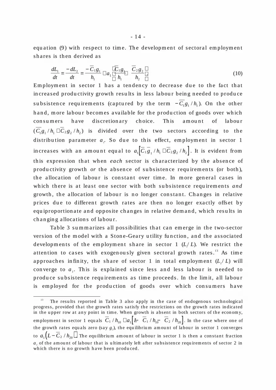
equation (9) with respect to time. The development of sectoral employment

shares is then derived as

dL

dt

dL

dt

C g

ha

C g

h

C g

h1 2 1 1

11

1 1

1

2 2

2

=−

=−

+ +

. (10)

Employment in sector 1 has a tendency to decrease due to the fact that

increased productivity growth results in less labour being needed to produce

subsistence requirements (captured by the term − C g h1 1 1/ ). On the other

hand, more labour becomes available for the production of goods over which

consumers have discretionary choice. This amount of labour

(C g h C g h1 1 1 2 2 2/ /+ ) is divided over the two sectors according to the

distribution parameter ai. So due to this effect, employment in sector 1

increases with an amount equal to [ ]a C g h C g h1 1 1 1 2 2 2/ /+ . It is evident from

this expression that when each sector is characterized by the absence of

productivity growth or the absence of subsistence requirements (or both),

the allocation of labour is constant over time. In more general cases in

which there is at least one sector with both subsistence requirements and

growth, the allocation of labour is no longer constant. Changes in relative

prices due to different growth rates are then no longer exactly offset by

equiproportionate and opposite changes in relative demand, which results in

changing allocations of labour.

Table 3 summarizes all possibilities that can emerge in the two-sector

version of the model with a Stone-Geary utility function, and the associated

developments of the employment share in sector 1 (Li/L). We restrict the

attention to cases with exogenously given sectoral growth rates.13 As time

approaches infinity, the share of sector 1 in total employment (L1/L) will

converge to a1. This is explained since less and less labour is needed to

produce subsistence requirements as time proceeds. In the limit, all labour

is employed for the production of goods over which consumers have

13 The results reported in Table 3 also apply in the case of endogenous technologicalprogress, provided that the growth rates satisfy the restrictions on the growth rates indicatedin the upper row at any point in time. When growth is absent in both sectors of the economy,

employment in sector 1 equals [ ]C h a L C h C h1 10 1 1 10 2 20/ / /+ − − . In the case where one of

the growth rates equals zero (say g2), the equilibrium amount of labour in sector 1 converges

to ( )a L C h1 2 20− / . The equilibrium amount of labour in sector 1 is then a constant fraction

a1 of the amount of labour that is ultimately left after subsistence requirements of sector 2 inwhich there is no growth have been produced.

- 15 -

complete free choice.

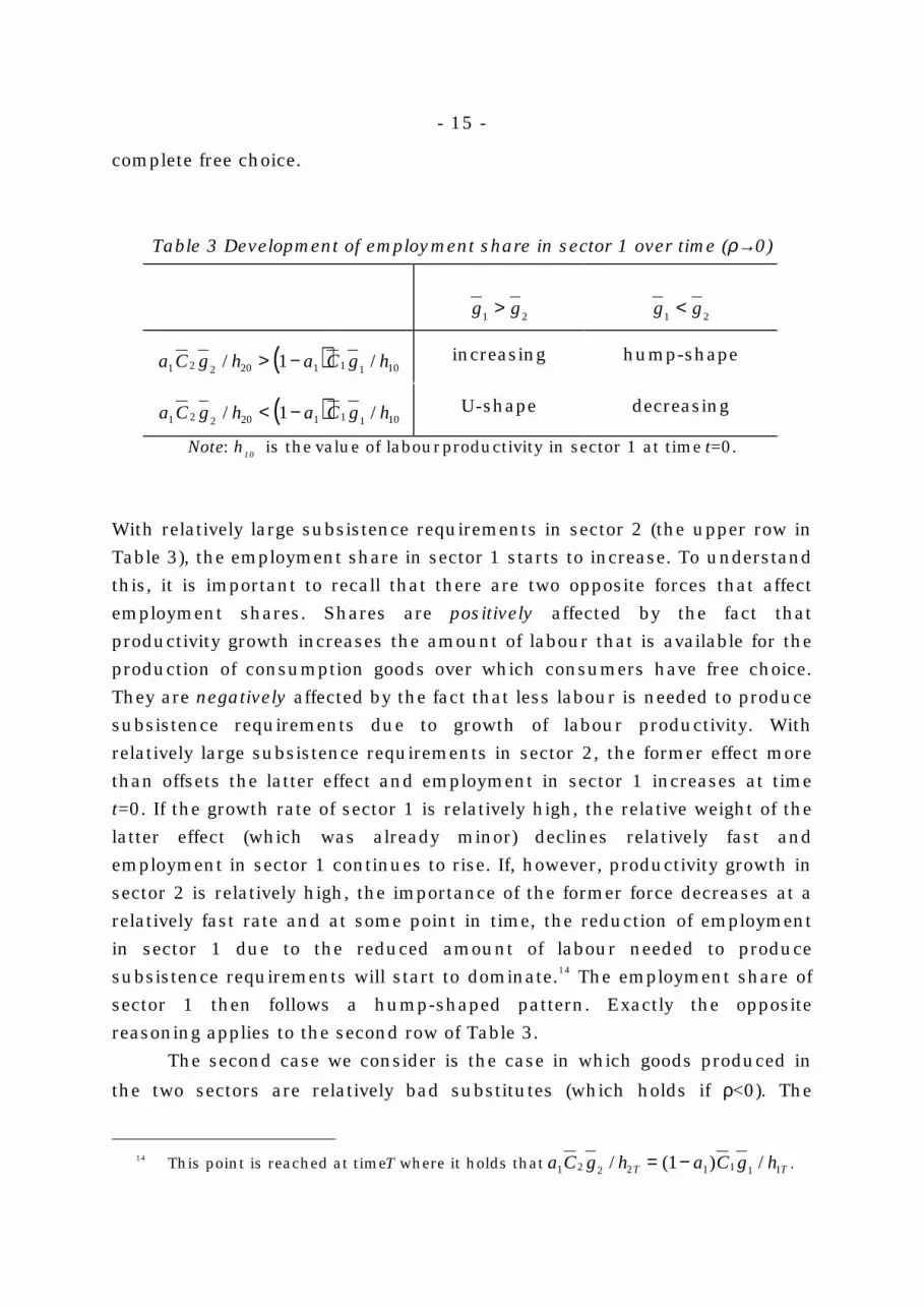
Table 3 Development of employment share in sector 1 over time (ρ→0)

g g1 2> g g1 2

<

( )a C g h a C g h1 2 2 20 1 1 1 101/ /> − increasing hump-shape

( )a C g h a C g h1 2 2 20 1 1 1 101/ /< − U-shape decreasing

Note: h10 is the value of labour productivity in sector 1 at time t=0.

With relatively large subsistence requirements in sector 2 (the upper row in

Table 3), the employment share in sector 1 starts to increase. To understand

this, it is important to recall that there are two opposite forces that affect

employment shares. Shares are positively affected by the fact that

productivity growth increases the amount of labour that is available for the

production of consumption goods over which consumers have free choice.

They are negatively affected by the fact that less labour is needed to produce

subsistence requirements due to growth of labour productivity. With

relatively large subsistence requirements in sector 2, the former effect more

than offsets the latter effect and employment in sector 1 increases at time

t=0. If the growth rate of sector 1 is relatively high, the relative weight of the

latter effect (which was already minor) declines relatively fast and

employment in sector 1 continues to rise. If, however, productivity growth in

sector 2 is relatively high, the importance of the former force decreases at a

relatively fast rate and at some point in time, the reduction of employment

in sector 1 due to the reduced amount of labour needed to produce

subsistence requirements will start to dominate.14 The employment share of

sector 1 then follows a hump-shaped pattern. Exactly the opposite

reasoning applies to the second row of Table 3.

The second case we consider is the case in which goods produced in

the two sectors are relatively bad substitutes (which holds if ρ<0). The

14 This point is reached at time T where it holds that a C g h a C g hT T1 2 2 2 1 1 1 11/ ( ) /= − .

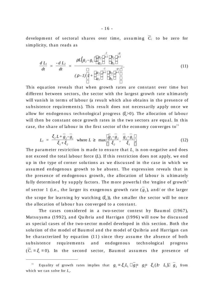
- 16 -

development of sectoral shares over time, assuming Ci to be zero for

simplicity, than reads as

( )d L

dt =

- d L

dt =

L g - ga

a

h

h

( - 1) 1+a

a

h

h

.1 2

2

-1

-12

1

-

-12

1

2-1

-12

1

-

-12

1

ρ

ρ

ρρ

ρ

ρρ

ρ

1

(11)

This equation reveals that when growth rates are constant over time but

different between sectors, the sector with the largest growth rate ultimately

will vanish in terms of labour (a result which also obtains in the presence of

subsistence requirements). This result does not necessarily apply once we

allow for endogenous technological progress (ξi>0). The allocation of labour

will then be constant once growth rates in the two sectors are equal. In this

case, the share of labour in the first sector of the economy converges to15

12 2 1

1 2

1 2

2

2 1

1

L = L+ g - g

+ L

g - g,

g - g.

ξξ ξ ξ ξ where max≥

(12)

The parameter restriction is made to ensure that L1 is non-negative and does

not exceed the total labour force (L). If this restriction does not apply, we end

up in the type of corner solutions as we discussed in the case in which we

assumed endogenous growth to be absent. The expression reveals that in

the presence of endogenous growth, the allocation of labour is ultimately

fully determined by supply factors. The more powerful the ‘engine of growth’

of sector 1 (i.e., the larger its exogenous growth rate ( g1 ), and/or the larger

the scope for learning by watching (ξ1)), the smaller the sector will be once

the allocation of labour has converged to a constant.

The cases considered in a two-sector context by Baumol (1967),

Matsuyama (1992), and Quibria and Harrigan (1996) will now be discussed

as special cases of the two-sector model developed in this section. Both the

solution of the model of Baumol and the model of Quibria and Harrigan can

be characterized by equation (11) since they assume the absence of both

subsistence requirements and endogenous technological progress

(Ci i= =ξ 0). In the second sector, Baumol assumes the presence of

15 Equality of growth rates implies that g L g g L L g1 1 1 1 2 2 1 2= + = = − +ξ ξ ( ) from

which we can solve for L1.

- 17 -

exogenous technological progress, which is absent in the first sector ( g1 0= ,

g2 0> ). The two cases he then considers in order to describe the

development of sectoral shares are (i) a case with unitary elasticity of

demand and constant relative outlays (ρ→0; i.e. Cobb-Douglas preferences),

and (ii) a case where relative output is constant (ρ→-∞; i.e. Leontief

preferences). In case (i), the sectoral shares of labour remain constant

whereas the output ratio (C1/C2=h1L1/h2L2) declines to zero as time passes. In

the second case, labour will ultimately be fully employed in the first sector of

the economy. Quibria and Harrigan (1996) study the intermediate case in

which the elasticity of substitution between goods from different sectors is

between zero and one. The basic results they arrive at were already

discussed in this section. More and more labour will be allocated towards

the slowly growing service sector until ultimately all labour is employed in

this sector. The relative prices of services will rise without bound.

Matsuyama (1992) incorporates an element of endogenous growth in a

two-sector model with an agricultural and a manufacturing sector (say

sector 1 and 2, respectively).16 His basic model is characterized by constant

shares of labour. This result is due to his very specific parametrization of

the model. His economy is characterized by (i) the absence of technological

progress in the agricultural sector (g1=0), (ii) endogenous growth in the

manufacturing sector (ξ2>0), and (iii) a Stone-Geary utility function (ρ=0)

with subsistence requirements in the agricultural sector (C1 0> ) and no

subsistence requirements in the manufacturing sector (C2 0= ). It is

immediately evident from equation (10) that in such a specific case,

employment shares are constant over time. This is not considered as a

problem by Matsuyama since the main focus in his paper is not on the

dynamics of structural change, but on the effects of an increase in the

(exogenously given and non-growing) productivity of the agricultural sector

for growth in the manufacturing sector. It is clear from equation (9) that an

increase in the productivity level of the agricultural sector (h1) which has a

16 The basic Ricardian model of Matsuyama differs from our model in two respects. First,Matsuyama employs production functions with diminishing returns to scale with respect tolabour. Compared to our way of modelling, this does not affect the basic results arrived at (ina closed economy setting). Secondly, he assumes consumers to have an intertemporal utilityfunction with a subjective discount rate. Again, this does not affect the comparability of hisresults with the results in this paper and is only of importance for the welfare evaluation inhis paper.

- 18 -

positive subsistence requirement releases labour that will be employed in

the dynamic manufacturing sector. Since this sector is characterized by

learning by watching in the model of Matsuyama, growth will increase in

this sector. This is the basic result arrived at by Matsuyama in the closed

economy version of his model.17

5. The model in a multi-sector context

Although the simple two-sector version of the model as discussed in the

previous section gives insights in the basic forces shaping the sectoral

composition of economies, this model does not allow us to replicate the

typical dynamics that characterize the sectoral developments of

industrialized economies. For this aim,we have to resort to a multi-sectoral

version of the model. As in the previous section, our analysis will start with

considering the Stone-Geary utility function (ρ→0) as a special case to gain

some further insights in the working of the model and the processes that are

at play. In turn, we will generalize to the case of CES-preferences (for

simplicity, we assume away subsistence requirements). Again, all other

cases that we can distinguish are straightforward combinations of these two

basic cases. We conclude this section by presenting some numerical

experiments with a three-sector version of the model. The aim of these

exercises is to mimic part of the empirically found trends described in

section 2.

17 In addition, he shows that a negative relation between growth and agriculturalproductivity prevails in a small open economy. This is due to the fact that a small openeconomy that experiences a productivity improvement in the agricultural sector will specializemore in the production of agricultural goods, taking away labour from the manufacturingsector and depressing the growth rate of the economy. Finally, he also considers thedynamics of structural change by allowing for non-unitary elasticities of substitution. Due tothe assumed absence of growth in the agricultural sector, Matsuyama has to assumeagricultural goods to be relatively good substitutes for manufacturing goods in order to beable to explain the declining share of agricultural employment. Both the assumption ofagricultural growth being lower than manufacturing growth and the assumption of goodsubstitutability between goods from broadly defined sectors seems at odds with empiricalevidence.

- 19 -

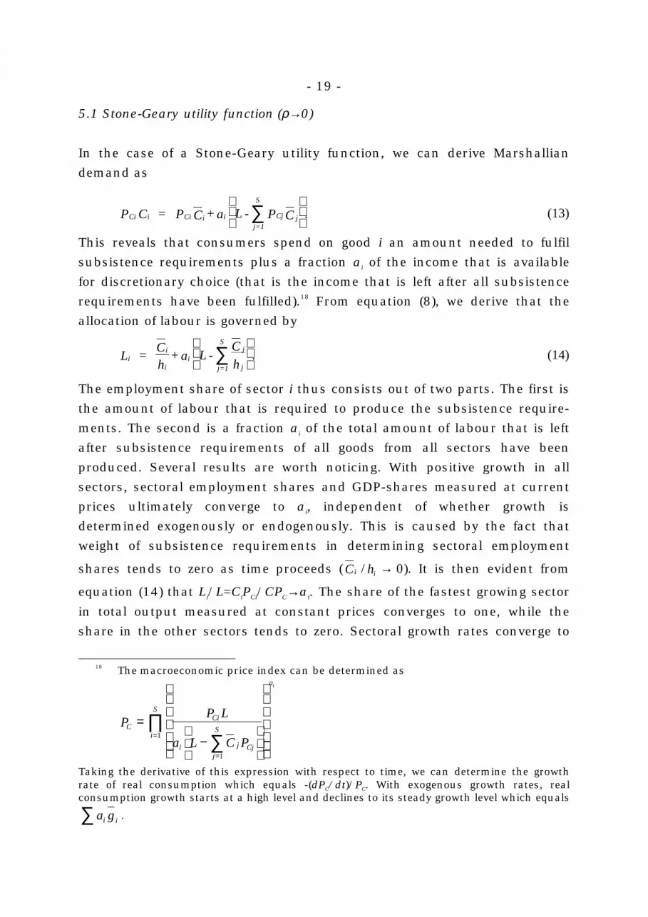
5.1 Stone-Geary utility function (ρ→0)

In the case of a Stone-Geary utility function, we can derive Marshallian

demand as

Ci i Ci i ij=1

S

Cj jP C = P C + a L - P C .∑

(13)

This reveals that consumers spend on good i an amount needed to fulfil

subsistence requirements plus a fraction ai of the income that is available

for discretionary choice (that is the income that is left after all subsistence

requirements have been fulfilled).18 From equation (8), we derive that the

allocation of labour is governed by

ii

ii

j=1

Sj

jL =

Ch

+ a L -C

h.∑

(14)

The employment share of sector i thus consists out of two parts. The first is

the amount of labour that is required to produce the subsistence require-

ments. The second is a fraction ai of the total amount of labour that is left

after subsistence requirements of all goods from all sectors have been

produced. Several results are worth noticing. With positive growth in all

sectors, sectoral employment shares and GDP-shares measured at current

prices ultimately converge to ai, independent of whether growth is

determined exogenously or endogenously. This is caused by the fact that

weight of subsistence requirements in determining sectoral employment

shares tends to zero as time proceeds (C hi i/ → 0). It is then evident from

equation (14) that Li/L=CiPCi/CPC→ai. The share of the fastest growing sector

in total output measured at constant prices converges to one, while the

share in the other sectors tends to zero. Sectoral growth rates converge to

18 The macroeconomic price index can be determined as

PP L

a L C PC

Ci

i j Cjj

S

a

i

S

i

=−

=

= ∑∏

1

1

Taking the derivative of this expression with respect to time, we can determine the growthrate of real consumption which equals -(dPC/dt)/PC. With exogenous growth rates, realconsumption growth starts at a high level and declines to its steady growth level which equals

a gi i∑ .

- 20 -

g a Li i i+ ξ . Relative prices of the slowest growing sector tend to infinity, while

those of the fastest growing sector tend to zero. Income elasticities

ultimately all converge to one.

So far, attention has been restricted to the long-run in which

employment shares are constant and income elasticities of demand equal

one. However, for long periods during the transition to a situation with

constant employment shares income elasticities may be unequal to one. In

particular, the income elasticity of demand of the sector with the lowest

(largest) initial subsistence requirement starts at a level larger (smaller) than

one. In the light of the deindustrialization debate, we are particularly

interested in the short-run behaviour of employment shares. It is easily

derived that these shares are not constant and may behave non-

monotonously. This is seen by taking the derivative of equation (14) with

respect to time which results in

d L

dt =

C g

ha

C g

h.

i i i

ii

j=1

Sj j

j

− + ∑ (15)

This equation reveals that with positive growth rates, employment shares in

all sectors indeed converge to a constant since C hi i/ tends to zero as time

proceeds. Let us now restrict the attention to a three-sector version of the

model (S=3), and consider the case in which the subsistence requirement of

goods from the first sector (say the agricultural sector) is largest, while that

from the third sector (say the service sector) is zero. The rate of technological

progress is assumed to be largest in the first sector and lowest in the third

sector. Assuming that at t=0 it holds that [ ]a C g h C g h C g h2 1 1 1 2 2 2 2 2 2/ / /+ > ,

employment in the manufacturing follows a hump-shaped pattern. The

interpretation of this condition is the same as in section 4 and relies on the

fact that sectors become larger due to the fact that more labour becomes

available for the production of consumption goods over which consumers

have free choice, while sectors become smaller due to the fact that less

labour is needed to produce subsistence requirements. Similarly, we can

derive that employment in the service sector is continuously increasing,

while agricultural employment initially strongly declines. In other words, if

relatively much labour is required initially to produce the subsistence

requirement of the good produced in sector 1 and this sector is

characterized by large productivity growth, so much labour is freed up

initially that the employment share in both the second and the third sector

- 21 -

start to increase. Ultimately, all employment shares converge to their long-

run shares (ai).

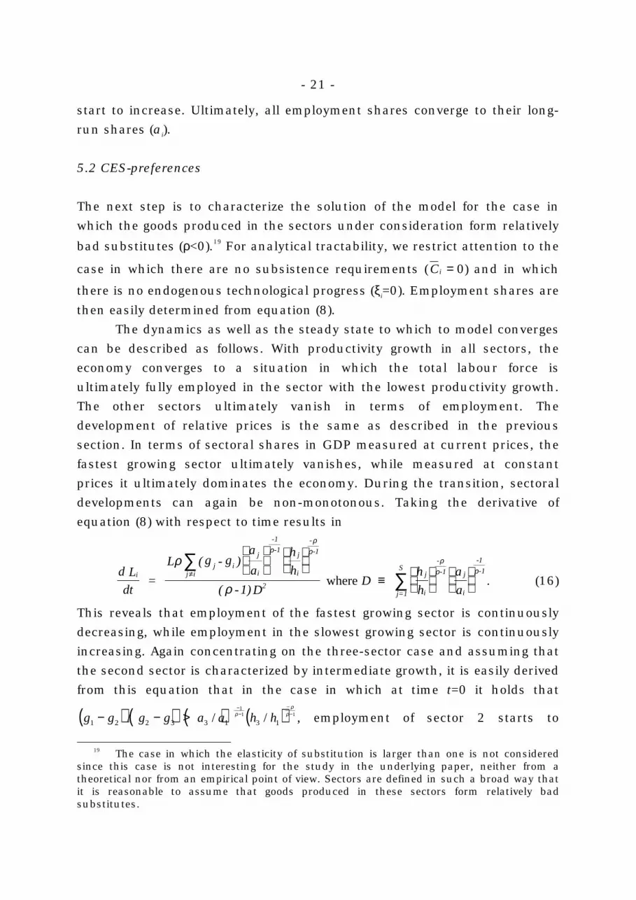
5.2 CES-preferences

The next step is to characterize the solution of the model for the case in

which the goods produced in the sectors under consideration form relatively

bad substitutes (ρ<0).19 For analytical tractability, we restrict attention to the

case in which there are no subsistence requirements (Ci = 0) and in which

there is no endogenous technological progress (ξi=0). Employment shares are

then easily determined from equation (8).

The dynamics as well as the steady state to which to model converges

can be described as follows. With productivity growth in all sectors, the

economy converges to a situation in which the total labour force is

ultimately fully employed in the sector with the lowest productivity growth.

The other sectors ultimately vanish in terms of employment. The

development of relative prices is the same as described in the previous

section. In terms of sectoral shares in GDP measured at current prices, the

fastest growing sector ultimately vanishes, while measured at constant

prices it ultimately dominates the economy. During the transition, sectoral

developments can again be non-monotonous. Taking the derivative of

equation (8) with respect to time results in

d L

dt =

L ( g - g )a

a

h

h

( -1)D D

h

h

a

a.

i j ij i

-1

-1j

i

-

-1j

i

2j=1

S-

-1j

i

-1

-1j

i

ρ

ρ

ρρ

ρρ

ρ ρ≠∑

∑

≡

where (16)

This reveals that employment of the fastest growing sector is continuously

decreasing, while employment in the slowest growing sector is continuously

increasing. Again concentrating on the three-sector case and assuming that

the second sector is characterized by intermediate growth, it is easily derived

from this equation that in the case in which at time t=0 it holds that

( ) ( ) ( ) ( )g g g g a a h h1 2 2 3 3 1 3 1

11 1− − >

−−

−−/ / /ρρ

ρ , employment of sector 2 starts to

19 The case in which the elasticity of substitution is larger than one is not consideredsince this case is not interesting for the study in the underlying paper, neither from atheoretical nor from an empirical point of view. Sectors are defined in such a broad way thatit is reasonable to assume that goods produced in these sectors form relatively badsubstitutes.

- 22 -

increase. At some point in time it reaches a top and ultimately converges to

zero. This result reveals that the development of sectoral employment shares

can behave non-monotonously in a world in which there are sectoral

productivity differentials and goods are relatively bad substitutes. In

particular, if differential productivity growth between the agricultural and

manufacturing sector is large relative to differential productivity growth

between manufacturing and the service sector, manufacturing employment

will follow a hump-shaped pattern (otherwise all labour would be reallocated

towards the service sector from the outset).

Let us now introduce endogenous technological progress. The

previous analysis has made clear that as long as growth rates are not

equalized, employment shares are changing. This continues until in the

limiting case the two fast-growing sectors have vanished. By endogenizing

growth rates, they may converge. This occurs if employment shares are such

that the differences in exogenously given productivity differentials are

compensated by endogenously determined productivity differentials which

are due to different scopes for learning by watching. In general, convergence

of growth rates obtains once sectoral employment shares satisfy (provided

that all ξ's are positive)

i

ij=1

S

j j=1

Sj

j

ij=1

S

j

L =

L - g1

+ g

1.

∑ ∑

∑ξ ξ

ξ ξ

(17)

A meaningful solution requires that 0<Li<L. If this restriction is not satisfied,

we end up in corner solutions in which some sector takes over the whole

economy in terms of employment and is still characterized by a lower growth

rate than the other sectors. If there is no learning by watching in one sector

(say in sector j (ξj=0)), growth rates will converge when employment shares in

the other sectors equal ( )L g gi j i i= − / ξ . These exercises reveal that in the

presence of endogenous growth, the allocation of labour is ultimately fully

determined by supply factors. Previously derived results that the labour

force is ultimately fully employed in one sector when goods are bad

substitutes hence depend on the assumption of the absence of endogenous

technological progress on a sectoral level. Once learning by watching is

introduced, a minimal sectoral scale in terms of employment is required to

be and to remain a fast-growing sector.

- 23 -

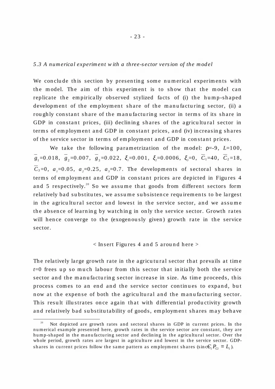
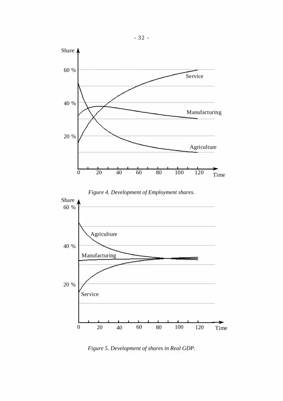
5.3 A numerical experiment with a three-sector version of the model

We conclude this section by presenting some numerical experiments with

the model. The aim of this experiment is to show that the model can

replicate the empirically observed stylized facts of (i) the hump-shaped

development of the employment share of the manufacturing sector, (ii) a

roughly constant share of the manufacturing sector in terms of its share in

GDP in constant prices, (iii) declining shares of the agricultural sector in

terms of employment and GDP in constant prices, and (iv) increasing shares

of the service sector in terms of employment and GDP in constant prices.

We take the following parametrization of the model: ρ=-9, L=100,

g1=0.018, g2 =0.007, g3 =0.022, ξ1=0.001, ξ2=0.0006, ξ3=0, C1=40, C2 =18,

C3 =0, a1=0.05, a2=0.25, a3=0.7. The developments of sectoral shares in

terms of employment and GDP in constant prices are depicted in Figures 4

and 5 respectively.20 So we assume that goods from different sectors form

relatively bad substitutes, we assume subsistence requirements to be largest

in the agricultural sector and lowest in the service sector, and we assume

the absence of learning by watching in only the service sector. Growth rates

will hence converge to the (exogenously given) growth rate in the service

sector.

< Insert Figures 4 and 5 around here >

The relatively large growth rate in the agricutural sector that prevails at time

t=0 frees up so much labour from this sector that initially both the service

sector and the manufacturing sector increase in size. As time proceeds, this

process comes to an end and the service sector continues to expand, but

now at the expense of both the agricultural and the manufacturing sector.

This result illustrates once again that with differential productivity growth

and relatively bad substitutability of goods, employment shares may behave 20 Not depicted are growth rates and sectoral shares in GDP in current prices. In thenumerical example presented here, growth rates in the service sector are constant, they arehump-shaped in the manufacturing sector and declining in the agricultural sector. Over thewhole period, growth rates are largest in agriculture and lowest in the service sector. GDP-shares in current prices follow the same pattern as employment shares (since C P Li Ci i= ).

- 24 -

non-monotonously (recall that we do not need endogenous growth nor

subsistence requirements for this result). Due to the presence of

endogenous growth, the growth rates ultimately converge to the

(exogenously given) growth rate of the service sector. When growth rates

have converged, relative prices are constant and employment shares have

converged to values that are fully determined by supply side factors. This

result is in contrast with models with only exogenously given technological

progress. Those models predict that the slowest growing sector ultimately

dominates the whole economy in terms of employment. The roughly

constant/slightly increasing share of manufacturing in GDP in constant

prices results from a parameter choice in the model (in particular the choice

of subsitence requirements) that results in an income elasticity of demand

for manufacturing goods which is close to one. The specific result that

sectoral shares in real GDP converge to 1/3 is due to the particular choice of

the utility function (see footnote 12). Inspection of the shares of agricultural

and service goods in GDP in constant prices reveals that despite increasing

prices of services relative to agricultural goods, the share of services in real

GDP increases relative to the share of services. This result is due to the fact

that the subsistence requirement for agricultural goods is large, which

results in a low income elasticity of demand (without subsistence

requirements, declining relative prices result in increasing relative shares in

real GDP).

To conclude, the simple numerical experiment with the model

performed in this section has revealed that the sectoral developments

described in section 2 can roughly be replicated with our simple Ricardian

model. Non-unitary income elasticities and differing growth rates on a

sectoral level are crucial and sufficient elements in explaining these

developments.

6. Conclusions

This paper has developed a simple Ricardian general equilibrium model that

allows us to determine the sectoral composition of an economy as the

outcome of factors of supply and demand. Differential productivity growth

rates, non-unitary income elasticities and non-unitary substitution

elasticities between goods from different sectors were considered as

- 25 -

important explanatory factors in empirically observed sectoral changes. The

model allowed for the presence of endogenously determined rates of

technological progress resulting from the presence of learning by watching.

Previously developed two-sector Ricardian models on growth and

sectoral structure of Baumol (1967), Matsuyama (1992), and Quibria and

Harrigan (1996) were shown to be special cases of our model. With goods

from different sector being relatively bad substitutes, differential

productivity growth results in declining employment shares in fast growing

sectors (agriculture) and increasing employment shares in slowly growing

sectors (services). Differential productivity growth was also shown to suffice

for explaining the empirically observed hump-shaped development of the

share of manufacturing employment. In particular, if the growth rate of the

fast-growing agricultural sector is sufficiently large compared to the other

growth rates, so much labour may be released initially from this sector that

all other sectors may become larger in terms of employment. This effect is

reinforced once we allow for income elasticities in the agricultural sector

that are smaller than one. Ultimately, only the slowest growing sector will

increase in size at the expense of all other sectors. The result that slow-

growing sectors ultimately dominate the whole economy was shown not to

arise necessarily once allowance is made for endogenously determined

technological progress as a result of learning by watching. We may then

arrive in a situation in which sectoral growth rates converge and sectoral

employment shares converge to constants (which are unequal to zero or

one).

In the end, we can draw the conclusion that the empirical stylized

facts on sectoral developments can basically be replicated by a simple

Ricardian model in which we do not have to rely on trade-related

explanations for sectoral developments. This is not to deny that trade-based

explanations have some role to play in explaining sectoral compositions of

economies. Countries that have a comparative advantage in a particular

sector as a result of for example differences in endowments will specialize in

production in these sectors. We wanted to emphasize, however, that

changes in sectoral compositions which are experienced by all countries can

simply be the resultant of differential productivity growth, non-unitary

income elasticities, and relatively bad substitutability between goods from

different sectors. The recently observed deindustrialization can hence be an

inherent and unavoidable part of the development of maturing economies.

- 26 -

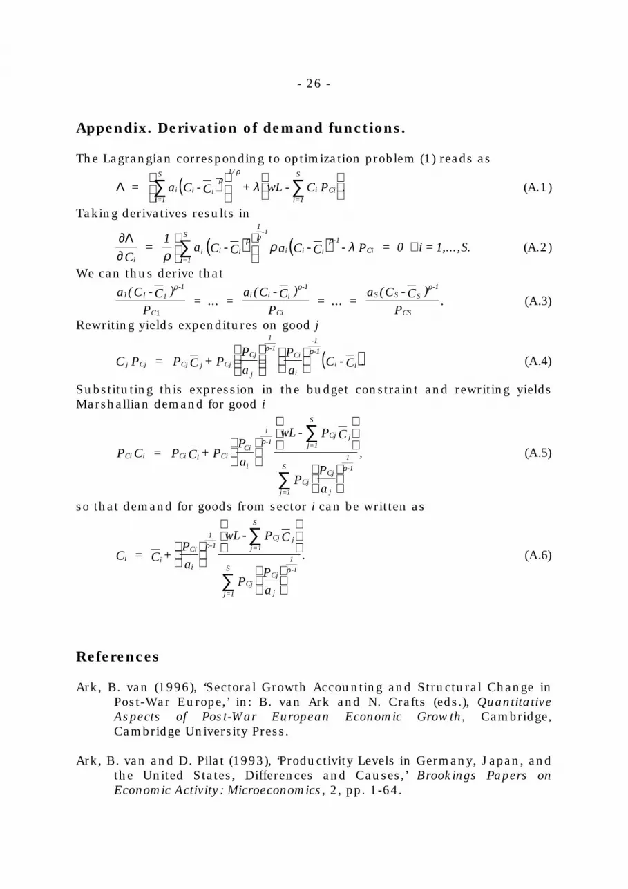
Appendix. Derivation of demand functions.

The Lagrangian corresponding to optimization problem (1) reads as

( )Λ = a C - C + wL - C P .

1/

i=1

S

i i ii=1

S

i Ci

ρρ

λ∑ ∑

(A.1)

Taking derivatives results in

( ) ( )∂Λ∂

∀∑

i

1-1

i=1

S

i i i i

-1

i i CiC

= 1

a C - C a C - C - P = 0 i = 1,...,S.ρ

ρ λρρ ρ

(A.2)

We can thus derive that

1 1 1-1

C

i i i-1

Ci

S S S-1

CS

a (C - C )

P = ... =

a (C - C )

P = ... =

a (C - C )

P.

ρ ρ ρ

1

(A.3)

Rewriting yields expenditures on good j

( )j Cj Cj j Cj

1

-1Cj

j

-1

-1Ci

ii iC P = P C + P

P

a

P

aC - C .

ρ ρ

(A.4)

Substituting this expression in the budget constraint and rewriting yieldsMarshallian demand for good i

Ci i Ci i Ci

1

-1Ci

i

j=1

S

Cj j

j=1

S

Cj

1

-1Cj

j

P C = P C + PP

a

wL - P C

PP

a

,ρ

ρ

∑

∑(A.5)

so that demand for goods from sector i can be written as

i i

1

-1Ci

i

j=1

S

Cj j

j=1

S

Cj

1

-1Cj

j

C = C +P

a

wL - P C

PP

a

.ρ

ρ

∑

∑ (A.6)

References

Ark, B. van (1996), ‘Sectoral Growth Accounting and Structural Change inPost-War Europe,’ in: B. van Ark and N. Crafts (eds.), QuantitativeAspects of Post-War European Economic Growth, Cambridge,Cambridge University Press.

Ark, B. van and D. Pilat (1993), ‘Productivity Levels in Germany, Japan, andthe United States, Differences and Causes,’ Brookings Papers onEconomic Activity: Microeconomics, 2, pp. 1-64.

- 27 -

Baumol, W. (1967), ‘Macroeconomics of Unbalanced Growth: The Anatomyof Urban Crisis,’ American Economic Review, 57, pp. 415-426.

Baumol, W., S. Blackman, and E.N. Wolff (1989), Productivity and AmericanLeadership: The Long View, Cambridge, MA, MIT Press.

Chenery, H. and M. Syrquin (1975), Patterns of Development, 1950-1970,London, Oxford University Press.

Cornwall, J. and W. Cornwall (1994), ‘Growth Theory and EconomicStructure,’ Economica, 61, pp. 237-251.

David, P.A., (1991), ‘Computer and Dynamo: The Modern ProductivityParadox in a Not Distant Mirror,’ in: OECD (1991), Technology andProductivity: The Challenge for Economic Policy, Paris, OECD.

Deaton, A. and J. Muellbauer (1980), Economics and Consumer Behavior,Cambridge, Cambridge University Press.

Dollar, D. and E.N. Wolff (1993), Competitiveness, Convergence, andInternational Specialization, Cambridge, MA, MIT Press.

Echevarria, C. (1997), ‘Changes in Sectoral Composition Associated withEconomic Growth,’ International Economic Review, 38, pp. 431-452.

Feenstra, R.C. and Hanson (1995), Foreign Investment, Outsourcing andRelative Wages, NBER Working Paper, 5121, Cambridge, MA.

Gemert, H. van (1987), Orde en Beweging in de Sectorstructuur, Groningen,Wolters-Noordhoff.

Groot, H.L.F. de (1998), The Macroeconomic Consequences of Outsourcing,CentER Discussion Paper, 9843, Tilburg.

Gundlach, E. (1994), ‘Demand Bias as an Explanation for StructuralChange,’ Kyklos, 47, pp. 249-267.

Klump, R. and H. Preissler (1997), How Exactly does the Elasticity ofSubstitution Influence Economic Growth?, Discussion Paper Universitätof Ulm, Ulm.

Kongsamut, P., S. Rebelo, and D. Xie (1997), Beyond Balanced Growth,CEPR Discussion Paper, 1693, London.

Kravis, I., A. Heston, and R. Summers (1983), ‘The Share of Services inEconomic Growth,’ in: F.G. Adams and B. Hickman (eds.), GlobalEconometrics: Essays in Honor of Lawrence R. Klein, Cambridge, MA,MIT Press.

- 28 -

Kuznets, S. (1966), Modern Economic Growth, New Haven, Yale UniversityPress.

Maddison, A. (1991), Dynamic Forces in Capitalist Development, Oxford,Oxford University Press.

Maddison, A. (1995), Monitoring the World Economy 1820-1992, Paris, OECDDevelopment Centre Studies.

Matsuyama, K. (1992), ‘Agricultural Productivity, Comparative Advantage,and Economic Growth,’ Journal of Economic Theory, 58, pp. 317-334.

Nelson, R.R., and G. Wright (1992), ’The Rise and Fall of AmericanTechnological Leadership: The Postwar Era In Historical Perspective,’Journal of Economic Literature, 30, pp. 1931-1964.

Pasinetti, L.L. (1981), Structural Change and Economic Growth, A TheoreticalEssay on the Dynamics of the Wealth of Nations, Cambridge,Cambridge University Press.

Pilat, D. (1996), Labour Productivity Levels in OECD Countries: Estimates forManufacturing and Selected Service Sectors, OECD EconomicsDepartment Workings Papers, 169, Paris.

Quibria, M.G. and F. Harrigan (1996), ‘Demand Bias and StructuralChange,’ Kyklos, 49, pp. 205-213.

Rowthorn, R. and R. Ramaswamy (1997), Deindustrialization: Causes andImplications, IMF Working Paper, WP/97/42, Washington.

Saeger, S.S. (1997), ‘Globalization and Deindustrialization: Myth and Realityin the OECD,’ Weltwirtschaftliches Archiv, 133, pp. 579-608.

Schettkat, R. and E. Appelbaum (1997), Are Prices Unimportant? TheChanging Structure of the Industrialized Economies, Working PaperOnderzoeksschool Arbeid, Welzijn, Sociaal Economisch Bestuur,97/10, Utrecht.

Summers, R. and A. Heston (1991), ‘The Penn World Table (Mark 5): AnExpanded Set of International Comparisons, 1950-1988,’ QuarterlyJournal of Economics, 106, pp. 327-368.

- 29 -

Employment

0

0,05

0,1

0,15

0,2

0,25

0,3

0,35

0,4

1955 1960 1965 1970 1975 1980 1985 1990 1995 2000

year

GERJPNUSA

GDP in current prices

0

0,02

0,04

0,06

0,08

0,1

0,12

0,14

1955 1960 1965 1970 1975 1980 1985 1990 1995 2000

year

GERJPNUSA

GDP in constant prices

0

0,01

0,02

0,03

0,04

0,05

0,06

1955 1960 1965 1970 1975 1980 1985 1990 1995 2000

year

GERJPNUSA

Figure 1. Shares of Agricultural sector

- 30 -

Employment

0

0,05

0,1

0,15

0,2

0,25

0,3

0,35

0,4

1955 1960 1965 1970 1975 1980 1985 1990 1995 2000

year

GERJPNUSA

GDP in current prices

0

0,05

0,1

0,15

0,2

0,25

0,3

0,35

0,4

0,45

1955 1960 1965 1970 1975 1980 1985 1990 1995 2000

year

GERJPNUSA

GDP in constant prices

0

0,05

0,1

0,15

0,2

0,25

0,3

0,35

0,4

1955 1960 1965 1970 1975 1980 1985 1990 1995 2000

year

GERJPNUSA

Figure 2. Shares of Manufacturing sector.

- 31 -

Employment

0

0,1

0,2

0,3

0,4

0,5

0,6

1955 1960 1965 1970 1975 1980 1985 1990 1995 2000

year

GERJPNUSA

GDP in constant prices

0

0,1

0,2

0,3

0,4

0,5

0,6

1955 1960 1965 1970 1975 1980 1985 1990 1995 2000

year

GERJPNUSA

Figure 3. Shares of Service Sector.

GDP in current prices

0

0,1

0,2

0,3

0,4

0,5

0,6

1955 1960 1965 1970 1975 1980 1985 1990 1995 2000

year

GERJPNUSA

- 32 -

0 20 40 60 80 100 120

60 %

40 %

20 %

Agriculture

Manufacturing

Service

Time

Share

Figure 4. Development of Employment shares.

0 20 40 60 80 100 120

60 %

40 %

20 %

Agriculture

Manufacturing

Service

Time

Share

Figure 5. Development of shares in Real GDP.