Impacts of Fuel Subsidy Rationalization on Sectoral Output

Impacts of Fuel Subsidy Rationalizationon Sectoral Output and Employment

in Malaysia

NOORASIAH SULAIMAN, MUKARAMAH HARUN,AND ARIEF ANSHORY YUSUF

¤

Large allocations for fuel subsidies have long put the Government ofMalaysia’s budget under great strain. Using a computable general equilibrium(CGE) model, this paper evaluates the impact of fuel subsidy rationalizationon sectoral output and employment. Employment is classified intooccupational categories and skill levels. Fuel subsidies were measuredusing the disaggregation of prices for petrol, diesel, and other fuel products.Findings show that removing fuel subsidies would hit economic performancethrough high input costs, specifically for industries closely attached to thepetroleum refinery sector. The manufacturing sector has the largest reductionin output and employment. Nevertheless, high- and medium-skilled laborforces experience increased demand. To increase economic efficiency, thesavings from the removal of fuel subsidies should be put toward policies suchas sales tax reduction. This study provides useful information for policymakers in evaluating or updating current subsidy policies to reduce economiclosses.

⁄Noorasiah Sulaiman (corresponding author): Center for Sustainable and Inclusive Development Studies,The National University of Malaysia. E-mail: [email protected]; Mukaramah Harun: Universiti UtaraMalaysia College of Business. E-mail: [email protected]; Arief Anshory Yusuf: Center forSustainable Development Goals Studies, Padjadjaran University. E-mail: [email protected] for this paper was supported by the Project of Economy and Environment Program for SoutheastAsia (EEPSEA-2011). We thank the managing editor and the anonymous referees for helpful commentsand suggestions. The Asian Development Bank recognizes “China” as the People’s Republic of China.

This is an Open Access article published by World Scientific Publishing Company. It is distributed underthe terms of the Creative Commons Attribution 3.0 International (CC BY 3.0) License which permits use,distribution and reproduction in any medium, provided the original work is properly cited.

March 23, 2022 1:10:17pm WSPC/331-adr 2250008 ISSN: 0116-11052ndReading

Asian Development Review, Vol. 39, No. 1, pp. 315–348DOI: 10.1142/S0116110522500081

© 2022 Asian Development Bank andAsian Development Bank Institute.

https://dx.doi.org/10.1142/S0116110522500081

https://dx.doi.org/10.1142/S0116110522500081

Keywords: computable general equilibrium model, employment, fuel subsidy,sectoral output, subsidy removal

JEL codes: H29, E23, E24, D58

I. Introduction

The high level of uncertainty over future global oil prices, which are more

influenced by international market conditions than domestic factors, places a domestic

economy in a very precarious position. An increase in fuel prices affects government

spending on fuel subsidies in many countries, including Malaysia. The latest data

reveal that government spending on fossil fuel subsidies has cost Southeast Asia

$17 billion (International Energy Agency 2017). The fuel subsidy has been identified

as the primary cause of Malaysia’s ballooning fiscal deficit, which threatens to make

the country’s economic position unsustainable (Economic Planning Unit [EPU] 2010).

Besides straining the budget, as the fuel subsidy continually raises the issue of

fiscal balance (Anand et al. 2013), the subsidy boosts the demand for fossil fuels and

discourages energy efficiency (Liu and Li 2011), leading to negative environmental

impacts (Li, Shi, and Bin 2017) and fuel smuggling (Asian Development Bank 2016).

Also, the fuel subsidy, which was primarily created to help the poor, has benefited the

wealthy population more. The poorest 20% of the population get only 7% of

the subsidy’s benefit, while the wealthiest 20% receive a disproportionate 43%

(del Granado, Coady, and Gillingham 2012).

Rapid industrialization has led to the domination of fuel usage in the industrial

sector, which has made Malaysia the third-largest energy consumer in Southeast Asia

(International Energy Agency 2015). Therefore, when the managed-float mechanism

for fuel prices comes into effect, fuel usage for all economic activities would be

based on market rates, which means those economic activities would be exposed to

high fluctuating costs. High-cost burdens those domestic sectors that are dependent

upon fuel and other energy products in their production processes. Thus, sectors

that are characterized by large shares of fuel-based inputs would be significantly

affected. Subsequently, decision-making concerning production activities will be

influenced too.

The impact of oil price hikes on commercial and industrial users includes

increased production costs (Middle East Economic Survey 2016). For example, in

Saudi Arabia, the Saudi Cement Company expected annual production costs to rise by

$18 million due to the removal of fuel subsidies (Trade Arabia 2015). Energy price

increases caused by subsidy reforms highlight that cost increases occur both directly

316 ASIAN DEVELOPMENT REVIEW


and indirectly (Rentschler, Kornejew, and Bazilian 2017). Notably, energy-intensive

manufacturing firms experience substantial changes to their cost structures, with

adverse implications for profitability (Bazilian and Onyeji 2012).

Such implications can have knock-on effects on economic activity, employment,

and eventually on households (Kilian 2008). Although producers can pass on the

cost to their consumers, the output is reduced due to increased production costs.

Furthermore, employment decisions are impacted as high production costs lead to

reduced desirability for producing more output, which lowers the demand for

employment. Rentschler, Kornejew, and Bazilian (2017) highlight that cost increases

(both direct and indirect) do not necessarily reflect competitiveness losses since firms

have various ways to mitigate and pass on price shocks. Initially, high fuel prices are

often associated with low output and, in turn, low employment. Moreover, the high

costs of goods and services discourage spending by households and the government,

leading to lower economic growth.

Malaysia’s fiscal capacity runs at an unsustainable level as subsidies to maintain

low fuel prices constitute a huge portion of the government’s annual budget. The

country must run a fiscal deficit when excessive spending on subsidies has to support

rising fuel prices. When the crude oil price hovers between $65 and $85 per barrel

under normal circumstances, the estimated fuel subsidy is between 9 billion ringgit

(RM) and RM11 billion per annum (EPU 2008). When the crude oil price peaked in

2008 at more than $100 per barrel, the Malaysian government’s total fuel subsidy was

RM15 billion (EPU 2008).

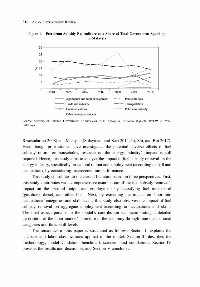
Figure 1 shows that the petroleum subsidy comprised a large percentage of

public spending in Malaysia from 2004 to 2010, ranging from a low of 10.1% to a

high of 26.4% in 2008. It is more than the combined total spending on agriculture and

rural development, health, and housing, which are all critical to the country’s

development. The fiscal deficit, which was about 2.7% in 2007, climbed rapidly to

7.0% in 2009 as a result of the global oil price spike and its impact on the cost of fuel

subsidies (EPU 2010). The large substitution effect of the petroleum subsidy can be

seen by comparing it to other sectors. In other words, it indicates that a potentially high

amount of savings from a cut in the petroleum subsidy can be utilized for other policy

priorities that can have potentially more benefit for the Malaysian people.

Subsidy reforms and their impact have been thoroughly examined in developed

and developing countries (Clements et al. 2014). These studies have emphasized

welfare effects by looking at the distributional impact of fuel subsidy reform on

households. These investigations have been conducted in developing countries

(del Granado, Coady, and Gillingham 2012) such as Indonesia (Yusuf and

IMPACTS OF FUEL SUBSIDY RATIONALIZATION 317


Resosudarmo 2008) and Malaysia (Solaymani and Kari 2014; Li, Shi, and Bin 2017).

Even though prior studies have investigated the potential adverse effects of fuel

subsidy reform on households, research on the energy industry’s impact is still

required. Hence, this study aims to analyze the impact of fuel subsidy removal on the

energy industry, specifically on sectoral output and employment (according to skill and

occupation), by considering macroeconomic performance.

This study contributes to the current literature based on three perspectives. First,

this study contributes via a comprehensive examination of the fuel subsidy removal’s

impact on the sectoral output and employment by classifying fuel into petrol

(gasoline), diesel, and other fuels. Next, by extending the impact on labor into

occupational categories and skill levels, this study also observes the impact of fuel

subsidy removal on aggregate employment according to occupations and skills.

The final aspect pertains to the model’s contribution via incorporating a detailed

description of the labor market’s structure in the economy through nine occupational

categories and three skill levels.

The remainder of this paper is structured as follows. Section II explains the

database and labor classifications applied in the model. Section III describes the

methodology, model validation, benchmark scenario, and simulations. Section IV

presents the results and discussion, and Section V concludes.

Figure 1. Petroleum Subsidy Expenditure as a Share of Total Government Spendingin Malaysia

Source: Ministry of Finance, Government of Malaysia. 2011. Malaysia Economic Reports 2004/05–2010/11.Putrajaya.



II. Data

This study uses the 2005 Malaysia Input–Output (IO) Table consisting of 120

industries and commodities (Department of Statistics Malaysia 2010). We disaggregated

the subsector of petroleum refinery into three types of fuel commodities: petrol, diesel,

and other fuel products (liquified petroleum gas, coke, and gas), thus bringing the total to

122 industries (see Table A1 of the Appendix). The disaggregation is based on the

Malaysian Standard Industrial Classification (Department of Statistics Malaysia 2000),

while the fuel share is based on the National Energy Balance (Energy Commission

2005). The disaggregation is in line with the subsidy provided according to fuel products,

Table 1. Database of the Computable General Equilibrium Model

Sector

Producer Investor Household Export Government

Extension Matrix 1–122 1 1 1 1

Basic flows ofintermediateinputs,domestic

122� 122 V1dom V2dom V3dom V4dom V5dom

Basic flows ofintermediateinputs, import

122� 122 V1imp V2imp V3imp V4imp V5imp

Taxes 1� 122 V1tax V2tax V3tax V4tax V5tax

Labor Occupationalcategory

9� 122 V1lab

Skill levels 3� 122

Capital 1 V1cap

Land 1 V1lnd

Other costs 1 V1oct

V1dom ¼ domestic intermediate goods, V2dom ¼ domestic investment, V3dom ¼ household domesticconsumption, V4dom ¼ domestic production on export, V5dom ¼ domestic government expenditure,V1imp ¼ imported intermediate good, V2imp ¼ investment on imported capital, V3imp ¼ householdconsumption on import, V4imp ¼ imported goods, V5imp ¼ government expenditure on import,V1tax ¼ taxes on producer, V2tax ¼ taxes on investor, V3tax ¼ taxes on household, V4tax ¼ taxes onexport, V5tax ¼ taxes on government expenditure, V1lab ¼ labor, V1cap ¼ capital, V1lnd ¼ land, andV1oct ¼ other costs.Source: Noorasiah Sulaiman and Mukaramah Harun. 2015. “Valuing the Impact of RationalizingMalaysia’s Fuel Subsidies on its Macroeconomic Performance.” In Economy-Wide Analysis of ClimateChange in Southeast Asia: Impact, Mitigation and Trade-Off, edited by A.A. Yusuf, Arvin Hermanto, A.R.Irlan, K. Ahmad, N. Sulaiman, and M. Harun, pp. 146–201. Los Banos: WorldFish and Economy andEnvironment Program for Southeast Asia.



i.e., petrol for passenger vehicles, and diesel and other fuel products for non-passenger

vehicles.

Table 1 presents the database that comprises production, primary factors, and

final demand components, as well as detailed labor variables. The rows in the matrix

represent the supply side. In particular, the table presents linkages among economic

activities such as the relationships among production value, production cost, selling

price, market clearing conditions for the commodity, primary inputs, other macro

indicators, and the price index.

This study develops and includes an extension of the employment matrix,

according to occupations and skills in the Malaysia IO Table, to analyze the impact of

fuel subsidy removal on employment across subsectors. Employment data are obtained

from the Labour Force Survey 2005 (Department of Statistics Malaysia 2006).

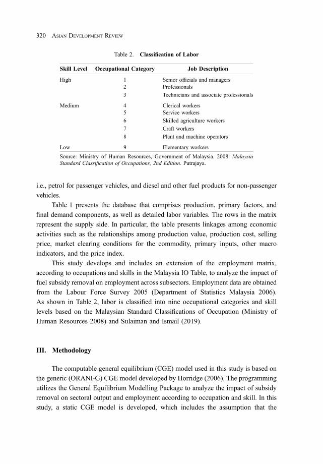
As shown in Table 2, labor is classified into nine occupational categories and skill

levels based on the Malaysian Standard Classifications of Occupation (Ministry of

Human Resources 2008) and Sulaiman and Ismail (2019).

III. Methodology

The computable general equilibrium (CGE) model used in this study is based on

the generic (ORANI-G) CGE model developed by Horridge (2006). The programming

utilizes the General Equilibrium Modelling Package to analyze the impact of subsidy

removal on sectoral output and employment according to occupation and skill. In this

study, a static CGE model is developed, which includes the assumption that the

Table 2. Classification of Labor

Skill Level Occupational Category Job Description

High 1 Senior officials and managers2 Professionals

3 Technicians and associate professionals

Medium 4 Clerical workers5 Service workers

6 Skilled agriculture workers

7 Craft workers

8 Plant and machine operators

Low 9 Elementary workers

Source: Ministry of Human Resources, Government of Malaysia. 2008. MalaysiaStandard Classification of Occupations, 2nd Edition. Putrajaya.



subsidy will be returned to the economy, so that aggregate employment remains

constant. Thus, the analysis focuses on the structural implications of subsidy removal

on sectoral output and employment growth.

The model is calibrated according to subsidy removal by fuel types, whereas

employment is based on occupation and skill. The inclusion of occupation and skill

into the Malaysia IO Table, and thus into the CGE model, allows the in-depth

realization of the impact of fuel subsidy removal on output and employment growth.

In analyzing the impact of the labor market in the CGE model, further assumptions are

made (Meagher, Adams, and Horridge 2000). The demand side of the labor market

assumes that labor by occupational type is demanded by industry according to constant

elasticity of substitution (CES) functions. Meanwhile, the supply side assumes that

labor is supplied according to the constant elasticity of transformation functions.

Thus, both labor demand and supply are supposed to be in equilibrium. Similar labor

skills are assumed substitutable among industries, and relative wage rates are assumed

to adjust to clear labor markets by occupation.

Since a fuel price increase is an endogenous variable, it would not directly affect

output and employment among industries. The subsidy’s removal would indirectly

affect production. As this study analyzes subsidy removal on fuel commodities, removal

of the subsidy would increase cost in terms of transportation due to diesel and other fuel

products used for non-passenger vehicles. Output and employment would remain high

in moderately competitive industries, with both falling in the least competitive ones.

The cost saving from subsidy removal is assumed as aggregate tax revenue from all

indirect taxes. The cost-saving return to households via cash transfer alleviates the

increased cost of living, specifically among low-income households. Household spending

would increase as a result of the cash transfer, resulting in higher aggregate demand.

Therefore, growth in aggregate demand would impact output and employment

among subsectors of the economy. The price elasticities of demand are expected not to

respond to fuel demand in the short run because the endogenous shock of the fuel price

increase has a smaller impact on demand for fuel products from economic subsectors

and households.

Nevertheless, demand for fuel can be elastic, as all inputs can be changed in the

long run. In developing countries, cash transfer programs are now more prevalent,

both as long-term poverty alleviation measures and to lessen the adverse effects of

certain types of reforms that may impact the poor. It has been successful to use these

transfers to reform fuel subsidies. Yusuf (2018) found that cash transfers funded by

cost savings in fuel subsidies minimize disparity in Indonesia more than other

approaches.



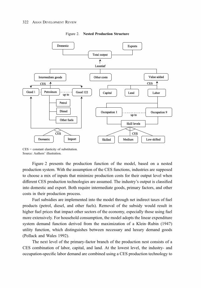
Figure 2 presents the production function of the model, based on a nested

production system. With the assumption of the CES functions, industries are supposed

to choose a mix of inputs that minimize production costs for their output level when

different CES production technologies are assumed. The industry’s output is classified

into domestic and export. Both require intermediate goods, primary factors, and other

costs in their production process.

Fuel subsidies are implemented into the model through net indirect taxes of fuel

products (petrol, diesel, and other fuels). Removal of the subsidy would result in

higher fuel prices that impact other sectors of the economy, especially those using fuel

more extensively. For household consumption, the model adopts the linear expenditure

system demand function derived from the maximization of a Klein–Rubin (1947)

utility function, which distinguishes between necessary and luxury demand goods

(Pollack and Wales 1992).

The next level of the primary-factor branch of the production nest consists of a

CES combination of labor, capital, and land. At the lowest level, the industry- and

occupation-specific labor demand are combined using a CES production technology to

Figure 2. Nested Production Structure

CES = constant elasticity of substitution.Source: Authors’ illustration.



obtain the occupation-aggregated labor input. Labor by occupational categories is

represented by occupation 1 to occupation 9 and then classified into three skill levels.

The labor market extension in the CGE modeling techniques relies on the

strength of its capacity to consider available information on the structural linkages

between industries, occupations, and skills. Therefore, the model has a significant

feature of disaggregated employment into occupational categories and skill levels to

examine the impact of distributed labor demand and the output production across

industries by three types of fuel products.

A. Impacts of Fuel Subsidy Removal

The demand function is contingent on the impacts of energy disaggregated into

diesel, petrol, and other fuel. Specified as follows, the elasticity of demand in a

constant estimation with a range of parameters is

c ¼ b": ð1ÞTherefore, we can express that as

Δc ¼ "(B1 � B0): ð2ÞMeanwhile, the impact of household utilization is determined by the equation

Δc ¼ C1 � C0, ð3Þwhere Δc is the change in energy consumption when the fuel price increases; " is the

long-run price elasticity of energy demand; B0 and C0 indicate the price of energy and

its consumption before the subsidy removal policy, respectively. The B1 and C1 refer

to the price of energy and its consumption after the subsidy removal policy.

B. Employment Impacts

It is assumed that all production factors are variable. Producers can rent capital

and land in the agriculture sector. Intermediate inputs of capital and land are assumed

fixed between industries. Production specifications for the model are nested. Demand

for inputs for each industry ( j ) is determined by the cost-minimizing function subject

to Leontief ’s production function in equation (4). Inputs in the production structure

are composite commodities (i) (hþ 1, s), intermediate inputs, and other costs (hþ 2).



Therefore, the production function is

LeontiefI 1iyT 1iy

( )

¼ T 1j Aj, ð4Þ

where

I 1iy is an effective input for good i for current production in industry j,

Aj is the level of activity for industry j, and

T 1y and T 1

j are the coefficients for technological change.

Based on equation (5), composite commodity I 1iy is used in every industry with a

combination of export and import goods based on the CES technology. Primary input

I 1(hþ1, x)j also includes a combination of labor, capital, and land integrated based on the

CES technology. The CES technology refers to the combination of exported and

imported commodities, which explains that these two sources are imperfect substitutes

for input demand that vary according to relative price changes:

I 1iy ¼ CESx¼1, 2, 3I 1(hþ1, x)j

T 1(hþ1, x)j

( )

i ¼ 1, . . . , h (h is differential in production),

j ¼ 1, . . . , h (h is differential in industries):ð5Þ

The CES specification allows for an inter-labor replacement for the primary factors’

composite and intermediate inputs, depending on price changes relative to skill level.

In the input demand function, the production of each industry’s output level and the

input price (excluding the composite labor demand) are exogenous factors.

Consequently, minimizing costs can be solved with the input functions in the form

of percentage change by choosing the following equation:

I 1ij , I1(ix)j, I

1(hþ1, x)j, I

1(hþ1, 1, n)j: ð6Þ

To minimize,

Xh

i¼1

X2

x¼1

P1(ix)jI

1(ix)j þ

Xn

n¼1

P1(hþ1, 1, n)jI

1(hþ1, 1, n)j

þX3

x¼2

P1(hþ1, 1, x)jI

1(hþ1, 1, x)j þ P1

hþ2I1hþ2, j: (7)

I 1ij is the demand for effective intermediaries and primary inputs for industry j;

I 1(ix)j is the demand for intermediate inputs for import and export in industry j;

I 1(hþ1, x)j is the demand for primary factor input for industry j, including the capital,

labor, and L;

I 1(hþ1, 1, n)j is the demand for labor for types of skill levels for industry j;



P1(ix)j is the price for the intermediate input of import and export;

P1(hþ1, 1, n)j is the price for the primary factor s for industry j; and

P1hþ2 is the price for other costs.

The function of demand for primary factors in equation (8) exhibits an increase

in industry j, following the average cost of labor, capital, and land, and causing

replacement factors:

I 1(hþ1, s)j ¼ yj � �1(hþ1, s)j p1

(hþ1, s) �X

x

F 1(hþ1, s)jp

1(hþ1, s)j

!

þ c1j þ c1hþ1, j

þ c1(hþ1, s)j �X

x

F 1(hþ1, s)c

1(hþ1, s)j): (8)

F 1(hþ1, s) is the share of labor, capital, and land for the payment of primary factor inputs

in industry j.

Equation (9) is a demand function of labor according to skill level. It also

includes changes in technical variables. In the absence of technological changes, an

increase in labor price for specific skills relative to other skilled labor costs will

increase the consumption of such labor more slowly than other labor:

I 1(hþ1, 1, r)j ¼ x(hþ1, 1)j � δ1(hþ1, 1, r)j p1(hþ1, 1, r)j �

X

r

F 1(hþ1, 1, r)jp

1(hþ1, 1, r)j

!

þ c1(hþ1, 1, r)j � �1(hþ1, 1)j c1(hþ1, 1, r)j �

X

r

F 1(hþ1, 1, r)jp

1(hþ1, 1, r)j

!

,

j ¼ 1, . . . , h: (9)

F 1(hþ1, r) is the share of costs for labor (at a skill or occupational level).

This can be explained as

F 1(hþ1, 1, r)j ¼

P1(hþ1, 1, r)jI

1(hþ1, 1, r)j

Pnr¼1 P

1(hþ1, 1, r)jI

1(hþ1, 1, r)j

: ð10Þ

δij denotes the elasticity of substitution between imported goods. Meanwhile, domestic

goods are the input for the production in industry j. Therefore, this specifies that if the

cost of any one source increases, it will cause a relative decrease in the input demand

of that particular source.

C. The Closure

The conditions give the closure of the model on the (i) government balance and

(ii) saving–investment balance. The government balance follows the condition that



saving is endogenously determined as the difference between the government’s

disposable income and total expenditure. The saving–investment balance condition

requires that investment is saving-driven, with gross fixed investment that derives

from the sum of aggregate saving. The real exchange rate can be flexible, while gross

saving and interest rates are fixed in nominal terms.

Government consumption and public transfers to households are fixed.

Furthermore, investment, the nominal exchange rate, government saving, and real

investment expenditure are also considered endogenous. Labor at three skill levels

and nine occupational types are mobile across subsectors, and capital supply is

exogenously fixed. Endogenous factor prices clear the corresponding labor and capital

markets, so there is no unemployment model. The model results must be considered

short term since the model is static with a fixed total factor supply.

D. Parameter and Model Validation

This study sets out the parameters of the model. The parameters are Armington

elasticities between domestic and imported commodities for different CES functions

for intermediate-use investment demand and household demand obtained from the

Global Trade Analysis Project (2008). The parameters also include commodity-

specific export elasticities, constant elasticity of transformation between domestic and

export supply commodities from the ORANI-G model (Horridge 2006), and the

elasticities of substitution between labor types by skill level utilized from the literature

(Meagher, Adams, and Horridge 2000). Sensitivity analysis is done for each elasticity

parameter, and the results show that the models are not sensitive to the value for

different parameters.

The model’s calibration is accomplished by a validation test to verify database

construction, specifying the equations and closure of the model. The model establishes

a validation test for the implementation of the CGE model (Horridge 2006). First, this

study has performed the nominal and real homogeneity tests. The test considers the

system of equations, and economic agents respond to the changes according to the

relative prices, not the absolute price level. The results imply that if all exogenous

nominal variables of the model change, then all endogenous nominal variables will

also change, while real variables remain unchanged. Likewise, if all real exogenous

variables of the model change, then all real endogenous variables will change, while

nominal variables remain unchanged.

Second, the model should pass a conditional balance equal to gross domestic

product (GDP) from the income and expenditure sides. Thus, the percentage changes



in GDP are uniform. Third, the zero-profit condition test is performed with the total

cost of output equal to the total sale of commodities.

E. Benchmark Scenario and Simulations

The model simulation is outfitted with CES production and utility functions, with

indirect taxation affecting inputs, and consumption as the subsidy is removed through

the increase in prices. As an endogenous variable, the percentage change in prices can

be used to simulate the impacts of different policy scenarios in the CGE model

(Horridge 2006). Moreover, the endogenous variable of the price is used to determine

a subsidy removal on the fuel commodities.

For efficiency in fuel consumption and real cost for the industry, this study

developed a benchmark scenario used as a baseline for the model. The benchmark of

the scenario is based on the price increase for petrol and diesel from the Means of

Platts Singapore, which is a calculation of petrol prices done by a company based in

Singapore called Platts. The retail prices of petrol and diesel in Malaysia are

determined through the automatic price mechanism, ensuring that the difference

between retail and actual prices is borne by subsidies and sales tax exemptions

(EPU 2005).

In this study, we calculate the price changes in petrol and diesel as practiced in

Malaysia. As shown in Table A2 of the Appendix, the price increases in petrol and

diesel are considered as the base case and alternative scenarios. For petrol, the

subsidized rate is RM1.62 per liter. Without the subsidy, the actual cost would be

RM2.45 per liter. Hence, the government is bearing 83 sen: 59 sen in foregone taxes

and 24 sen in subsidies.1 On the other hand, the retail price is RM1.28 per liter for

diesel, but the actual cost is RM2.07 per liter. Thus, the subsidy is 59 sen per liter

with a foregone tax of 20 sen per liter. Besides, the unsubsidized price for other fuels

(e.g., liquified petroleum gas) is higher (i.e., RM2.39 per kilogram), but the retail price

is only RM1.45 per kilogram, and the subsidy is 94 sen (EPU 2005).

The level of price increase in fuel products affects government spending on

subsidies. Based on this situation, the fuel subsidy will be markedly higher, especially

when the fuel price per barrel has increased remarkably. The alternative scenario

considers the largest price increase to reflect the highest percentage when the subsidy

is removed. Table A2 of the Appendix shows that when the increase in fuel is larger

than $100 per barrel, the subsidized petrol and diesel are RM2.70 and RM2.58 per

1The Malaysian ringgit is divided into 100 sen.



liter, respectively, representing 30% and 40% of the subsidy removal. Table 3 presents

two scenarios that are examined in this study. In each scenario, three different

simulations are designed (i.e., for petrol, diesel, and other fuels). In the base case

scenario, the subsidy removal starts with a 10% increase in prices; the simulation of

fuel products can be seen in SIM1 (petrol), SIM2 (diesel), and SIM3 (other fuels). The

minimum 10% removal in subsidy per liter is chosen as the base model benchmark to

observe the general impact. It is represented by a minimum subsidy removal of 25 sen

per liter of fuel consumed for petrol, diesel, and other fuels.

Furthermore, it is crucial to examine the extent to which the policy instrument of

subsidy is fully removed to ensure a competitive market. Without the subsidies, the

prices for petrol and diesel are higher by 30% and 40%, respectively. Prices with those

subsidies correspond to the largest amount that the government commits for subsidies.

IV. Results and Discussion

The results on the impact of demand for labor are analyzed in two stages. First,

the macroeconomics scenario is discussed for the selection of macro variables. At the

macro level, by conducting each simulation, employment growth is determined

according to occupational categories and skill levels. At the sectoral level, labor is

Table 3. Subsidy Removal Simulations for Petrol, Diesel, and Other Fuels

Simulation Base Case Scenario Description

SIM1 f0tax_s(“C44aPetrol”) 25 sen per liter subsidy removal foris increased by 10% all users of petrol

SIM2 f0tax_s(“C44bDiesel”) 25 sen per liter subsidy removal foris increased by 10% all users of diesel

SIM3 f0tax_s(“C44cOthFuel”) 25 sen per liter subsidy removal foris increased by 10% all users of other fuel products

Simulation Alternative Scenario Description

SIM1 f0tax_s(“C44aPetrol”) RM1.32 per liter subsidyis increased by 30% removal for all users of petrol

SIM2 f0tax_s(“C44bDiesel”) RM1.70 per liter subsidy removalis increased by 40% for all users of diesel

SIM3 f0tax_s(“C44cOthFuel”) RM1.32 per liter subsidy removalis increased by 30% for all users of other fuel products

RM ¼ Malaysian ringgit, SIM ¼ simulation.Source: Authors’ calculations based on data from the Department of StatisticsMalaysia, Government of Malaysia. 2010. Malaysia Input–Output Tables 2005.Putrajaya.



aggregated into the employment rate to determine the impact of subsidy removal on

employment growth. Similarly, at the subsector or industrial level, subsidy removal is

analyzed based on the type offuel product to examine the impact on employment and output

growth. Price elasticities of demand for fuels at the sectoral level are also estimated.

A. Key Results

Table 4 presents the base case scenario and the alternative scenario of subsidy

removal for selected macro variables and employment by occupation type and skill

level. The impacts of each scenario can be seen in the aggregate employment level by

occupational category and skill level. The base case scenario assumes a price increase

of 10% for each fuel commodity. In contrast, the alternative scenario is based on fuel

price increases of 30% (petrol) and 40% (diesel and other fuels). In both scenarios, the

results for all simulations (SIM1: petrol, SIM2: diesel, SIM3: other fuel products)

indicate that the price has increased for all users.

As the table shows, the fuel subsidy’s reduction by 10% of the fuel price

increase positively impacts macroeconomic variables for GDP, exports, and imports.

GDP (in real terms) increases by 0.05% for SIM1 and SIM2, whereas for SIM3, it

increases by 0.04%. Similar results are obtained for the alternative scenario, where the

subsidy reductions are 30% (petrol) and 40% (diesel and other fuels) of the fuel price

increase. GDP increases by 0.139% (SIM1), 0.185% (SIM2), and 0.119% (SIM3).

Likewise, the increase in exports rises from 0.244% with a 10% fuel subsidy reduction

to 0.721% with the fuel subsidy’s full removal (SIM1), from 0.258% to 1.007%

(SIM2), and from 0.205% to 0.608% (SIM3). The gain in imports also increases from

0.243% with a 10% fuel subsidy reduction to 0.73% with the fuel subsidy’s full

removal (SIM1), from 0.256% to 1.030% (SIM2), and from 0.204% to 0.613%

(SIM3). A similar study by Solaymani and Kari (2014) also found that removing

energy subsidies increases real GDP. However, total exports and imports decline,

which is the opposite of the results obtained from this study.

On the other hand, household consumption and government expenditure are

impacted negatively under the base case and the alternative scenarios. Household

consumption under a 10% fuel subsidy reduction falls by 0.035%, 0.036%, and

0.043% for SIM1, SIM2, and SIM3, respectively. Similarly, government expenditure

drops by 0.132%, 0.139%, and 0.111%, respectively. Nevertheless, both variables

show a larger contraction for the alternative scenario (full subsidy removal). The larger

decline in household consumption indicates that the cash transfer program does not

fully compensate for a higher cost of living due to the rising prices of goods and

services brought about by the increase in fuel prices.



Table

4.Key

ResultsforSelectedMacro

Variables(%

)

BaseCaseScenario

AlternativeScenario

Macroecon

omic

Variable

SIM

1SIM

2SIM

3SIM

1SIM

2SIM

3

GDP(real)

0.05

10.05

30.04

30.13

90.18

50.119

Hou

seho

ldexpend

iture

�0.035

�0.036

�0.029

�0.103

�0.143

�0.088

Gov

ernm

entexpend

iture

�0.132

�0.139

�0.111

�0.387

�0.537

�0.327

Exp

orts

0.24

40.25

80.20

50.72

11.00

70.60

8Im

ports

0.24

30.25

60.20

40.73

01.03

00.61

3

Skill

Level

Employm

entbyOccupation

High

1.Seniorofficialsandmanagers

0.17

00.18

00.14

30.50

60.71

00.42

72.

Professionals

0.16

40.17

30.13

80.48

70.68

20.41

0

3.Techn

icians

andassociate

profession

als

0.12

00.12

70.10

10.35

60.49

70.30

0

Total

0.45

40.48

00.38

21.34

91.88

91.13

4

Medium

4.Clericalworkers

0.15

80.16

70.13

30.46

90.65

70.39

65.

Service

workers

0.18

10.19

10.15

20.53

70.75

20.45

2

6.Skilledagricultu

reworkers

0.15

20.16

10.12

80.45

30.63

40.38

1

7.Craftworkers

0.12

60.13

30.10

60.37

30.52

10.31

4

8.Plant

andmachine

operators

0.119

0.12

60.10

00.35

20.49

20.29

7Total

0.73

60.77

80.61

92.18

43.05

61.52

6

Low

9.Elementary

workers

0.15

00.15

80.12

60.44

40.62

10.37

4

GDP¼

grossdo

mestic

prod

uct,SIM

¼simulation.

Sou

rce:Autho

rs’calculations

basedon

datafrom

theDepartm

entof

StatisticsMalaysia,Gov

ernm

entof

Malaysia.20

10.M

alaysia

Inpu

t–Outpu

tTables

2005

.Putrajaya.



All results rely upon the assumption of providing extra revenue to households

through cash transfers to lower the cost of living. The results highlight that Malaysia’s

budget is distributing the cash transfers otherwise to other production factors.

A positive sign for real GDP implies that the fuel subsidy’s removal would reduce the

government’s budget and positively affect productive sectors. Specifically, the removal

of the diesel subsidy has a larger impact, as shown by SIM2, compared to the removal

of the subsidy for petrol (SIM1) and other fuels (SIM3).

Table 4 also shows that the aggregate demand for labor (the employment aspect)

has recorded positive signs by occupational categories and skill levels. In the base case

scenario, employment expansion for all types ranges from 0.100% to 0.191%; under

the alternative scenario, it ranges from 0.297% to 0.752%. Specifically, diesel subsidy

removal (SIM2) would significantly impact aggregate employment expansion for all

skill levels and occupational categories. Furthermore, the service worker category

experiences significant employment expansion.

B. Output and Employment Effects

Rationalizing fuel subsidies would have a significant impact on industries. In the

second stage of focusing on output and employment growth by type of industry, capital

growth and technical change are constant when production costs increase. With a

larger subsidy removal for fuel commodities, the additional cost to industry will

directly affect output and labor usage. On the other hand, an industry with a relatively

high rate of return will attract investment and enjoy a relatively high capital growth

rate. As a result, a relatively low percentage of employment growth is achieved for a

given rate of output growth. Also, for labor-intensive industries, employment

expansion will increase labor productivity.

Since this study concentrates on the mitigation scenario to see the maximum

impact of subsidy removal, the alternative scenario is given priority in the discussions.

Hence, the relative growth (both positive and negative) in the base case scenario

would always be a benchmark to examine the mitigation’s impact in general. Thus, the

relative growth rates in the alternative scenario are quite similar to those in the base

case scenario. For all simulations, subsidy removal shows a contraction in output and

employment for most of Malaysia’s economic subsectors. The output and employment

contractions range from 0.005% to 0.582% and from 0.011% to 3.951% for the base

case scenario. Moreover, the alternative scenario registers larger contractions from

0.025% to 2.425% for output and from 0.051% to 14.484% for employment.

Figure 3 presents the output and employment effects for each scenario according

to subsectors based on the findings for SIM1, SIM2, and SIM3. Within the agriculture



Figure 3. Agriculture Sector: Output and Employment

Source: Authors’ calculations based on data from the Department of Statistics Malaysia, Government of Malaysia.2010. Malaysia Input–Output Tables 2005. Putrajaya.



sector, the oil palm subsector shows the largest contraction in output and a significant

reduction in employment for all the simulations in the base case scenario. Similar

results are obtained for the alternative scenario. All simulations have a larger impact

on output and employment, with the largest contraction belonging to SIM2 (petrol).

It shows a contraction of 1.141% for output and 2.505% for employment. However, the

forestry and logging subsector have the largest contractions in employment at 0.678%

(SIM1), 0.717% (SIM2), and 0.569% (SIM3). Thus, despite the adverse impact of

subsidy removal, there are also some positive impacts on output and employment.

A positive impact on output and employment can be seen in subsectors such as

vegetables, food crops, other agriculture, other livestock, paddy, fruits, poultry, and

rubber. For all simulations in the alternative scenario, the growth in output ranges from

0.029% to 1.721%, while employment growth ranges from 0.430% to 4.062%.

The findings indicate that employment growth is relatively larger than the output

growth for all simulations in the alternative scenario.

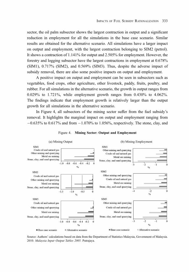
In Figure 4, all subsectors of the mining sector suffer from the fuel subsidy’s

removal. It highlights the marginal impact on output and employment ranging from

�0.635% to 0.617% and from �1.070% to 1.056%, respectively. The stone, clay, and

Figure 4. Mining Sector: Output and Employment




sand quarrying subsector is the most affected, followed by the metal ore and other

mining and quarrying subsectors. The alternative scenario shows a reduction in output

and employment from 0.012% to 1.282% and from 0.555% to 3.620%, respectively.

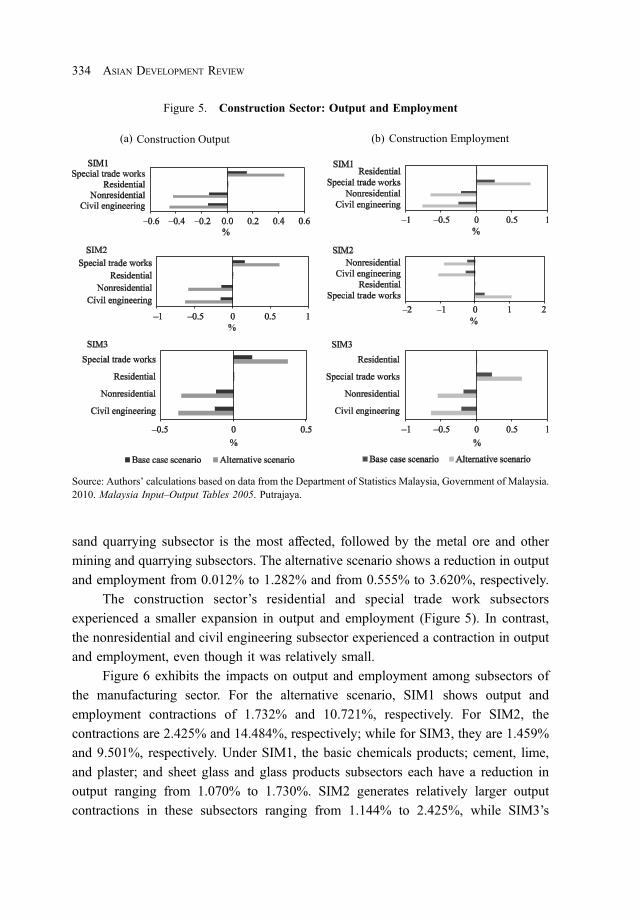
The construction sector’s residential and special trade work subsectors

experienced a smaller expansion in output and employment (Figure 5). In contrast,

the nonresidential and civil engineering subsector experienced a contraction in output

and employment, even though it was relatively small.

Figure 6 exhibits the impacts on output and employment among subsectors of

the manufacturing sector. For the alternative scenario, SIM1 shows output and

employment contractions of 1.732% and 10.721%, respectively. For SIM2, the

contractions are 2.425% and 14.484%, respectively; while for SIM3, they are 1.459%

and 9.501%, respectively. Under SIM1, the basic chemicals products; cement, lime,

and plaster; and sheet glass and glass products subsectors each have a reduction in

output ranging from 1.070% to 1.730%. SIM2 generates relatively larger output

contractions in these subsectors ranging from 1.144% to 2.425%, while SIM3’s

Figure 5. Construction Sector: Output and Employment




Figure 6. Manufacturing Sector: Output and Employment




contractions range from 1.040% to 1.459%. In terms of employment, the contractions

range from 2.596% to 10.721% (SIM1), from 3.647% to 14.484% (SIM2), and from

2.184% to 9.501% (SIM3).

Expansions in output for all simulations of the alternative scenario were

registered for the following subsectors: semiconductor devices, tubes, and circuit

boards; TVs, radio receivers, transmitters, and associated goods; domestic appliances;

industrial machinery, measuring, checking, and industrial process equipment; soap,

perfumes, cleaning, and toilet preparations; office, accounting, and computing

machinery; electric lamps and lighting equipment; electrical machinery and apparatus;

and ship, boat building, and bicycles. These industries are all associated with

multinational companies and/or foreign direct investment. The output expansion was

largest for SIM2, ranging from 1.918% to 5.973%, followed by SIM1 (from 1.363% to

4.231%) and SIM3 (from 1.146% to 3.551%). The employment growth was largest for

SIM1, ranging from 5.024% to 9.827%, followed by SIM2 (from 7.034% to 13.906%)

and SIM3 (from 4.232% to 8.242%).

Fuel products show a significant contraction, both in output and employment,

particularly in the full subsidy removal (i.e., alternative) scenario. For both the base

case and full subsidy removal scenarios, the subsectors of petrol, diesel, and other fuel

products suffer large contractions in output and employment in each simulation.

Observing the full subsidy removal scenario, for SIM1, these industries experience

output reductions ranging from 0.856% to 1.177%, while for employment, the decline

ranges from 7.857% to 10.721%. SIM2 shows the largest effects, with contractions

ranging from 1.208% to 1.604% for output and from 11.002% to 14.484% for

employment. A similar result is obtained for SIM3, with output and employment

reductions ranging from 0.719% to 1.040% and from 6.618% to 9.501%, respectively.

Overall, these results imply that subsidy removal increases the price of fuels so that the

cost of production increases, indicating a decline in output and employment in fuel

product industries and among manufacturing subsectors.

Finally, for the service sector, subsectors closely related to petroleum refining

exhibit a larger impact on output and employment for all simulations in the alternative

scenario (Figure 7). The subsectors include other private services, restaurants, air

transport, land transport, port and airport operation, water transport, electricity and gas,

and waterworks. For those subsectors, output and employment decline under SIM1

from 0.323% to 1.585%, from 0.457% to 2.228% (SIM2), and from 0.271% to

1.333% (SIM3). Large declines are recorded in the output of other private services,

with contractions of 1.585% (SIM1), 2.228% (SIM2), and 1.333% (SIM3). Similarly,

for restaurants, the reductions in output are 1.277% (SIM1), 1.799% (SIM2), and



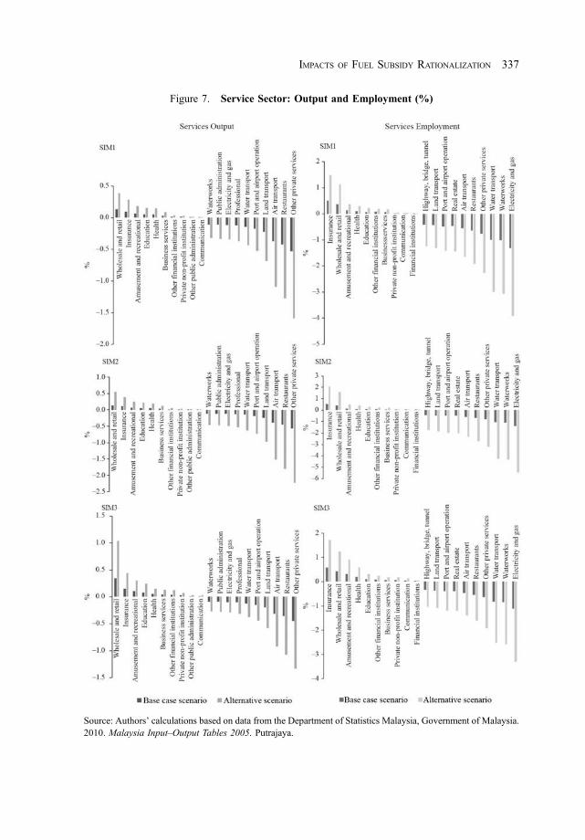
Figure 7. Service Sector: Output and Employment (%)




1.333% (SIM3). Among the transportation sector, air transport and land transport are

the most affected subsectors in output reduction for all alternative scenarios in

this study.

Furthermore, all simulation results register even larger contractions in

employment. The subsectors of electricity and gas and waterworks register the largest

reductions in employment. For electricity and gas, the declines are 3.910% (SIM1),

5.472% (SIM2), and 3.297% (SIM3); while for waterworks, the reductions are 3.065%

(SIM1), 4.323% (SIM2), and 2.576% (SIM3) (Figure 7). The results are similar for the

subsectors of water transport, other public services, restaurant, air transport, real estate,

port and airport operation services, land transport and highways, and bridge and tunnel

operations, with each subsector experiencing a significant contraction in employment

for all simulations.

From the results obtained, a few inferences are formed. Based on the scenario

analysis, first, the findings reveal that SIM2 (diesel) has a larger impact on the output

and employment contraction than SIM1 and SIM3 for both the base case and

alternative scenarios. It is supported by the fact that the government-borne subsidy for

diesel is substantially larger than for petrol and other fuels. Specific subsectors,

especially those under the manufacturing sector, are affected the most when the

subsidy is removed. Notwithstanding, fuel subsidy reforms significantly influenced

sectoral output through increased production costs due to an increase in the prices of

intermediate inputs (Rentschler, Kornejew, and Bazilian 2017). Furthermore, the larger

contribution in both domestic and imported inputs shows that intermediate input is the

major component of total factor productivity growth for the manufacturing sector

(Sulaiman 2012). Also, the manufacturing sector is supported by upstreaming (as

consumers) and down-streaming industry (as suppliers) linkages (Sulaiman and Fauzi

2017), implying that those manufacturing subsectors deal with the transportation of

intermediate inputs and finished products from the supplier to the consumers.

Second, in general, both scenarios (base and alternative) indicated that all sectors

experience either a contraction or expansion in output and employment, particularly

both are larger for the manufacturing sector. A contraction in output usually reduces

the need for employment, and vice versa in the case of output and employment

expansion. The subsectors most influenced by multinational firms’ production

experience an increase in output and employment. As mentioned, the semiconductor

devices; tubes, circuit boards, TVs, radio receivers, and transmitters associated goods;

and measuring, checking, and industrial process equipment subsectors all have

substantial ties to foreign producers (i.e., multinational corporations). On the other

hand, output and employment contractions are experienced by local producers. Oil and



fats; clay and ceramics; sheet glass and glass products; basic chemicals; and cement,

lime, and plaster are examples of locally produced goods. These findings are

corroborated by Sulaiman, Rashid, and Hamid (2012), who revealed that multinational

corporations are more efficient in utilizing both domestic and imported inputs than

local manufacturers.

Third, this study found a larger contraction in output for subsectors closely

related to the fuel sector, both in the manufacturing and service sectors. The findings

are comparable to that of an Indonesian study that reached the same conclusion (Yusuf

and Resosudarmo 2008). Furthermore, the study observed that fuel subsidy removal

tends to increase the price of industrial outputs that are highly dependent on fuel such

as in the transportation, energy, fishery, and industrial sectors. Increased production

costs result from rising oil prices for commercial and industrial customers (Middle

East Economic Survey 2016). Increases in energy prices from subsidy reforms result

in direct and indirect cost increases (Rentschler et al. 2017). Thus, subsectors that used

more energy, in particular, would have a significant impact on their cost structures

(Bazilian and Onyeji 2012).

Fourth, the alternative scenario shows the contraction in the employment rate is

greater than that in output. This finding is rational because firms will react by not

hiring new workers rather than reducing their production units. Thus, to cover the cost

of a price increase due to a subsidy removal, firms would prefer to minimize labor

compared to reducing the output produced, implying that the decline in the labor used

would adversely impact the output. Similarly, expansion in employment growth is

larger than the output growth even though it is not as big as the contraction, resulting

in a moderate impact on the distribution of employment across industries.

Such consequences may have repercussions for economic activity, jobs, and,

ultimately, households (Kilian 2008). Even though producers can pass on the cost

to their customers, the industry’s output is being reduced as production costs rise

(Harun et al. 2018). Therefore, employment decisions must be carefully considered

because high production costs reduce the desire to produce more output, depressing

the employment rate. According to Rentschler, Kornejew, and Bazilian (2017), cost

increases (both direct and indirect) may not indicate competitiveness losses because

firms have a variety of techniques to manage and pass on price shocks. Initially, high

fuel prices are often associated with lower output and, as a result, lower employment.

Furthermore, high prices for goods and services deter household and government

spending, resulting in slower economic growth.

Finally, based on the analysis presented, it is notable that when the revenues from

subsidy removal policies are channeled back into the economy via payments to



households, the resulting increase in demand will stimulate the economy. In Malaysia,

studies such as Solaymani and Kari (2014) and Loo and Harun (2020) identified the

harmful effects that would come from the implementation of the fuel subsidy reform

and urged for mitigating measures. The study found that the integration of a transfer of

government income to rural households would increase pro-poor growth and reduce

the negative impacts on all households’ real incomes with a slight improvement.

Specifically, Loo and Harun (2020) emphasized that (i) cash transfers are needed to

cope with the underlying high price resulting from the high fuel consumption price,

and (ii) the vulnerable—primarily low-income households and the poor—are the ones

hit hardest. Cash transfers are particularly preferable in the short term, where extended

time is needed for behavioral change, while developmental investments have

long-term benefits.

C. Sensitivity Analysis

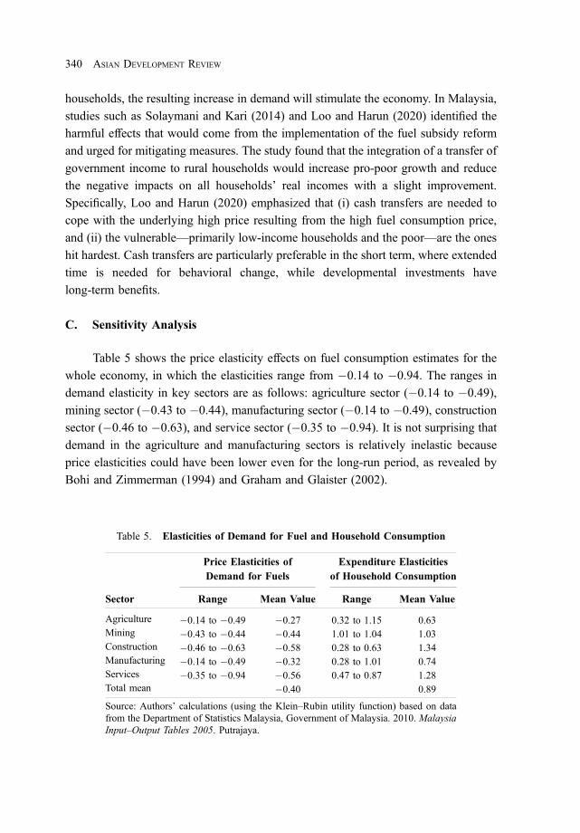
Table 5 shows the price elasticity effects on fuel consumption estimates for the

whole economy, in which the elasticities range from �0.14 to �0.94. The ranges in

demand elasticity in key sectors are as follows: agriculture sector (�0.14 to �0.49),

mining sector (�0.43 to �0.44), manufacturing sector (�0.14 to �0.49), construction

sector (�0.46 to �0.63), and service sector (�0.35 to �0.94). It is not surprising that

demand in the agriculture and manufacturing sectors is relatively inelastic because

price elasticities could have been lower even for the long-run period, as revealed by

Bohi and Zimmerman (1994) and Graham and Glaister (2002).

Table 5. Elasticities of Demand for Fuel and Household Consumption

Price Elasticities ofDemand for Fuels

Expenditure Elasticitiesof Household Consumption

Sector Range Mean Value Range Mean Value

Agriculture �0.14 to �0.49 �0.27 0.32 to 1.15 0.63Mining �0.43 to �0.44 �0.44 1.01 to 1.04 1.03Construction �0.46 to �0.63 �0.58 0.28 to 0.63 1.34Manufacturing �0.14 to �0.49 �0.32 0.28 to 1.01 0.74Services �0.35 to �0.94 �0.56 0.47 to 0.87 1.28Total mean �0.40 0.89

Source: Authors’ calculations (using the Klein–Rubin utility function) based on datafrom the Department of Statistics Malaysia, Government of Malaysia. 2010. MalaysiaInput–Output Tables 2005. Putrajaya.



However, prior studies found that long-run price elasticities tend to be much

higher than in the short run due to the three crucial conclusions on the sensitivity of

price changes on fuel demand in the long run (Graham and Glaister 2002, Plante

2014). First, behavioral responses to cost changes occur over time, implying demand

has a larger impact than short-run elasticity. Second, the range of responses included

changes by vehicle type and location decisions. Third, policy options are more

comprehensive in the long run.

Under the linear expenditure (Klein–Rubin) system, the elasticity of marginal

utility of income is estimated, which shows that the long-run household expenditure

elasticities for the whole economy are relatively larger, ranging from 0.28 to 1.15. In

contrast, the mean value ranges from 0.63 to 1.34. This result is in line with prior

studies that have reported income elasticity of fuel consumption in the range of 0.6–1.6

(Graham and Glaister 2002).

The subsidy removal minimizes deadweight losses in the economy by

incorporating an efficient fiscal policy to give a complete result (Plante 2014).

Remarkably, the Government of Malaysia has distributed the savings from

rationalizing fuel subsidies in the form of a direct cash assistance program to

low-income groups to mitigate fuel price increase (e-BR1M 2018). The program

provides RM500 ($159) in cash aid to households with a monthly income of RM3,000

($953) or below. Even though the cash transfer program is not a popular practice, it

can save about 70% of the government’s current expenses on fuel subsidies and benefit

low-income groups, while the benefits of fuel subsidies are biased toward high-income

groups.

V. Conclusions

The simulations investigate the impact of fuel price increases on macroeconomic

variables, sectoral outputs, and employment. In addition, the disaggregation of fuel

commodities into petrol, diesel, and other fuel products has enabled examining the

impact of price increases for these fuel commodities separately according to industry.

The subsidy removal and subsequent increase in fuel prices will reduce selected

sectors’ activities in the Malaysian economy. Still, a reduction in the general sales tax

has an expansionary impact on the broader segments of the economy. This effect will

more than compensate for the contractionary impact, resulting in a positive net gain for

the overall economy. On the other hand, removing fuel subsidies can have immediate

negative effects on macroeconomic indicators like GDP through an increase in the cost



of production, a rise in the consumer price index, and a reduction in employment.

Nevertheless, the net macroeconomic impact is positive when revenue from the

subsidy removal is given back to the economy through cuts in the general sales tax.

It indicates that the pre-reform fuel pricing policy has distorted resource allocation.

Therefore, a departure from such a policy reform would be the right move toward

having a more efficient economy.

The contraction in output is larger in the manufacturing sector due to increased

diesel prices versus petrol and other fuels. It is not surprising because a larger

proportion of the government’s fuel subsidy expenditure goes to diesel rather than

petrol and other fuels. However, negative impacts, such as increased production costs

due to higher fuel prices, would be more than offset by the positive impacts of

government revenue reallocation. Most subsectors exhibit a drop in output due to an

increase in the cost borne by all users. Some producers have no choice concerning the

consumption of petroleum products; they will not reduce their use and thus, their cost

of production will increase, resulting in contractions in industry output. Nonetheless,

some industries experience a positive impact on output and employment.

Furthermore, the distributional impacts across different types of labor vary and

are much larger than impacts on output. Hence, the results show that the effect of

subsidy removal would be felt much more by unskilled labor, such as service workers

and elementary workers, compared to skilled labor. On the other hand, the most

uniform impact across workers implies that the distributional impact of the reform

would be neutral. Under the subsidy rationalization program, the Government of

Malaysia has planned for a gradual subsidy removal for other subsidized items, primarily

food (e.g., wheat flour, cooking oil, sugar, and rice). This is because it accounts for a

sizable portion of the operating expenditure in Malaysia’s national budget.

An estimated RM25 billion worth of subsidies is allocated in the budget

annually, depending on price changes. The sugar subsidy was eliminated on

26 October 2013, and the rice subsidy was completely removed on 1 November

2015. On 1 November 2016, the government announced that the cooking oil subsidy

would be phased out (Ministry of Finance Malaysia 2018). All of these actions are part

of the subsidy rationalization program, necessitating further analysis and future

research.

This study, therefore, suggests that the design of subsidy removal has to include

mitigating measures that address the well-being of the Malaysian people, especially

from the perspective of employment. Awell-designed subsidy rationalization program

would not only increase the acceptance level of the reform but underpin sustainable

economic development. Regarding the fuel subsidy rationalization that has been



focused on in this study, the integration of a cash transfer program would strengthen

economic performance by increasing real GDP growth, aggregate output, and

employment, and by improving the trade balance.

References

Anand, Rahul, David Coady, Mohammad Adil, Thakoor Vimal, and James P. Walsh. 2013.“The Fiscal and Welfare Impacts of Reforming Fuel Subsidies in India.” InternationalMonetary Fund Working Papers 13/128.

Asian Development Bank. 2016. “Fuel Smuggling: 12 Things to Know.” https://www.adb.org/news/features/fuel-smuggling-12-things-know (accessed 15 October 2019).

Bazilian, Morgan, and Ijeoma Onyeji. 2012. “Fossil Fuel Subsidy Removal and InadequatePublic Power Supply: Implications for Businesses.” Energy Policy 45 (C): 1–5.

Bohi, Douglas R., and Mary B. Zimmerman. 1994. “An Update on Econometrics Studies ofEnergy Demand.” Annual Review of Energy 9 (1): 105–54.

Clements, Benedict, David Coady, Stefania Fabrizio, Sanjeev Gupta, and Baoping Shang. 2014.“Energy Subsidies: How Large Are They and How Can they Be Reformed?” Economicsof Energy and Environmental Policy 3 (1): 1–17.

del Granado, Francisco J. A., David Coady, and Robert Gillingham. 2012. “The UnequalBenefits of Fuel Subsidies: A Review of Evidence for Developing Countries.” WorldDevelopment 40 (11): 2234–48.

Department of Statistics Malaysia, Government of Malaysia. 2000. Malaysian StandardIndustrial Classification. Putrajaya.

_____. 2006. Labour Force Survey 2005. Putrajaya._____. 2010. Malaysia Input–Output Tables 2005. Putrajaya.e-BR1M. 2018. Initial Portal. https://ebr1m.hasil.gov.my/ (accessed 23 January 2018).Economic Planning Unit, Prime Minister’s Office, Government of Malaysia. 2005.

Socioeconomic Indicators 2005. Putrajaya._____. 2008. Socioeconomic Indicators 2008. Putrajaya._____. 2010. Tenth Malaysia Plan 2011–2015. Putrajaya.Energy Commission, Ministry of Energy, Green Technology and Water, Government of

Malaysia. 2005. National Energy Balance. Putrajaya.Global Trade Analysis Project. 2008. “GTAP 7 Data Base.” Department of Agricultural

Economics, Purdue University. https://www.gtap.agecon.purdue.edu/databases/v7/(accessed 11 March 2016).

Graham, Danie J., and Stephen Glaister. 2002. “The Demand for Automobile Fuel: A Survey ofElasticities.” Journal of Transport Economics and Policy 36 (1): 1–25.

Harun, Mukaramah, Siti Hadijah Che Mat, Wan Roshidah Fadzim, Shazida Jan Mohd Khan,and Mohd Saifoul Zamzuri Noor. 2018. “The Effects of Fuel Subsidy Removal on InputCosts of Productions: Leontief Input–Output Price Model.” International Journal ofSupply Chain Management 7 (5): 529–34.



Horridge, Mark J. 2006. ORANI-G: A Generic Single-Country Computable GeneralEquilibrium Model. Centre for Policy Studies, Monash University.

International Energy Agency. 2015. Southeast Asia Energy Outlook 2015: World EnergyOutlook Special Report. Paris.

_____. 2017. Southeast Asia Energy Outlook 2017: World Energy Outlook 2017 SpecialReport. Paris.

Kilian, Lutz. 2008. “The Economic Effects of Energy Price Shocks.” Journal of EconomicLiterature 46 (4): 871–909.

Klein, Lawrence R., and H. Rubin. 1947. “A Constant Utility Index of the Cost of Living.”Review of Economic Studies 15 (2): 84–87.

Li, Yingzhu, Xunpeng Shi, and Su Bin. 2017. “Economic, Social, and Environmental Impactsof Fuel Subsidies: A Revisit of Malaysia.” Energy Policy 110 (C): 56–61.

Liu, Wei, and Hong Li. 2011. “Improving Energy Consumption Structure: A ComprehensiveAssessment of Fossil Energy Subsidies Reform in China.” Energy Policy 39 (7): 4134–43.

Loo, Sze Ying, and Mukaramah Harun. 2020. “The Assessment of Direct AgriculturalInvestment and Cash Transfer on Households in Malaysia: An Evidence of CompensationMechanism for Fuel Subsidy Removal.” International Journal of Business and Society21 (1): 300–12.

Meagher, Gerald A., Philip D. Adams, and Mark J. Horridge. 2000. “Applied GeneralEquilibrium Modeling and Labour Market Forecasting.” CoPS Working Paper No. IP-76.

Middle East Economic Survey. 2016. “Riyadh Cuts Fuel Subsidies, Petchem Producers Countthe Cost.” http://archives.mees.com/issues/1618/articles/53472.

Ministry of Finance, Government of Malaysia. 2011. Malaysia Economic Reports 2004/05–2010/11. Putrajaya.

_____. 2018. Estimated Federal Expenditure. http://www.treasury.gov.my/index.php/bajet/anggaran-perbelanjaan-persekutuan.html (accessed 22 January 2018).

Ministry of Human Resources, Government of Malaysia. 2008. Malaysia StandardClassification of Occupations, 2nd Edition. Putrajaya.

Plante, Michael. 2014. “The Long-Run Macroeconomic Impacts of Fuel Subsidies.” Journal ofDevelopment Economics 107 (C): 129–43.

Pollack, Robert A., and Terrence J. Wales. 1992. Demand System Specification and Estimation.New York: Oxford University Press.

Rentschler, Jun, Martin Kornejew, and Morgan Bazilian. 2017. “Fossil Fuel Subsidy Reformsand Their Impacts on Firms.” Energy Policy 108 (C): 617–23.

Solaymani, Saeed, and Fatimah Kari. 2014. “Impacts of Energy Subsidy Reform on theMalaysian Economy and Transportation Sector.” Energy Policy 70 (C): 115–25.

Sulaiman, Noorasiah. 2012. “An Input–Output Analysis of the Total Factor ProductivityGrowth of the Malaysian Manufacturing Sector, 1983–2005.” Jurnal Ekonomi Malaysia46 (1): 147–55.

Sulaiman, Noorasiah, and M. Ahmad Fauzi. 2017. “Identifying Key Sector of EmploymentPotential in Malaysia.” International Journal of Applied Business and EconomicResearch 15 (8): 577–93.



Sulaiman, Noorasiah, and Rahmah Ismail. 2019. “Re-Aligning the Needs of Manpower for theVision 2020: The Case of the Manufacturing Sector in Malaysia.” International Journalof Business and Management Science 9 (3): 407–23.

Sulaiman, Noorasiah, Zakariah Rashid, and Khalid Hamid. 2012. “Productivity Improvement inthe Utilization of Domestic and Imported Inputs in Resource and Non-Resource-BasedIndustries: 1983–2005.” International Journal of Management Studies 19 (1): 87–114.

Trade Arabia. 2015. “Energy Price Hike to Cost Saudi Cement $18M.” http://www.tradearabia.com/news/CONS_297717.html.

Yusuf, Arief. 2018. “The Direct and Indirect Effect of Cash Transfers: The Case of Indonesia.”International Journal of Social Economics 45 (5): 793–807.

Yusuf, Arief, and Budy Resosudarmo. 2008. “Mitigating Distributional Impact of Fuel PricingReform: The Indonesian Experience.” ASEAN Economic Bulletin 25 (1): 32–47.



Appendix

TableA1.

Subsectorsof

theMalay

sian

Econom

y

No.

Sectoran

dSubsector

Agriculture

1Paddy

29Other

food

processing

60Rub

berprod

ucts

2Foo

dcrop

s30

Animal

feed

61Plastic

prod

ucts

3Vegetables

31Wineandspirits

62Sheet

glassandglassprod

ucts

4Fruits

32Softdrinks

63Clayandceramics

5Rub

ber

33Tob

acco

prod

ucts

64Cem

ent,lim

e,andplaster

6Oilpalm

34Yarnandcloth

65Con

creteandotherno

n-metallic

minerals

7Flower

plants

35Finishing

oftextiles

66Iron

andsteelprod

ucts

8Other

agricultu

re36

Other

textiles

67Basic

precious

andno

n-ferrou

smetals

9Pou

ltryfarm

ing

37Wearing

apparel

68Castin

gof

metals

10Other

livestock

38Leather

indu

stries

69Structuralmetal

prod

ucts

11Forestryandlogg

ing

39Foo

twear

70Other

fabricated

metal

prod

ucts

12Fishing

40Saw

millingandplaningof

woo

d71

Indu

strial

machinery

Mining

41Veneersheets,plyw

ood,

etc.

72General-purpo

semachinery

13Crude

oilandnaturalgas

42Builders’

carpentryandjoinery

73Special

purposemachinery

14Metal

oremining

43Woo

denandcane

containers

74Dom

estic

appliances

15Stone,clay,andsand

quarrying

44Other

woo

dprod

ucts

75Office,accoun

ting,

compu

tingmachinery

16Other

miningandqu

arrying

45Paper,paperprod

ucts,andfurnitu

re76

Electricalmachinery

andapparatus

Con

struction

46Pub

lishing

77Other

electrical

machinery

17Residential

47Printing

78Insulatedwires

andcables

18Non

-residential

48Petrolprod

ucts

79Electriclamps

andlig

htingequipm

ent

19Civilengineering

49Dieselprod

ucts

80Sem

i-cond

uctordevices,circuitbo

ards,etc.

20Special

tradeworks

50Other

fuel

prod

ucts

81TV,radioreceivers,transm

itters,etc.

Man

ufacturing

51Basic

chem

icals

82Medical,surgical

&orthop

edic

appliances

21Meatandmeatprod

uctio

n52

Fertilizers

83Measuring

,checking

,etc.

22Preservationof

seafoo

d53

Paintsandvarnishes

84Optical

instruments,etc.

23Preservationof

fruitsandvegetables

54Pharm

aceutical,chem

ical,etc.

85Watches

andclocks

Con

tinued.



Table

A1.

Con

tinued.

No.

Sectoran

dSubsector

24Dairy

prod

uctio

n55

Soap,

perfum

es,cleaning

,etc.

86Motor

vehicles

25Oils

andfats

56Other

chem

ical

prod

ucts

87Motorcycles

26Grain

mills

57Tires

88Shipandbo

atbu

ilding,

bicycles,etc.

27Bakeryprod

ucts

58Rub

berprocessing

89Other

transportequipm

ent

28Con

fectionery

59Rub

berglov

es90

Other

manufacturing

91Recyclin

g10

1Portandairportop

erationservices

112

Researchanddevelopm

ent

Service

102

Highw

ay,bridge,andtunn

elop

eration

113

Professional

92Electricity

andgas

103

Com

mun

ication

114

Businessservices

93Waterworks

104

Banks

115

Pub

licadministration

94Who

lesale

andretailtrade

105

Financial

institu

tions

116

Edu

catio

n95

Accom

mod

ation

106

Insurance

117

Health

96Restaurants

107

Other

financialinstitu

tions

118

Defense

andpu

blic

order

97Landtransport

108

Realestate

119

Other

public

administration

98Water

transport

109

Ownershipof

dwellin

gs12

0Private

non-profi

tinstitu

tion

99Airtransport

110

Rentalandleasing

121

Amusem

entandrecreatio

nal

100

Rentalandleasing

111

Com

puterservices

122

Other

privateservices

Sou

rce:

Departm

entof

StatisticsMalaysia,

Gov

ernm

entof

Malaysia.

2010

.MalaysiaInpu

t–Outpu

tTables

2005

.Putrajaya.



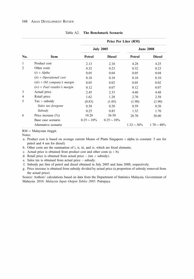
Table A2. The Benchmark Scenario

Price Per Liter (RM)

July 2005 June 2008

No. Item Petrol Diesel Petrol Diesel

1 Product cost 2.13 2.10 4.28 4.252 Other costs 0.32 0.23 0.32 0.23

(i)þ Alpha 0.05 0.04 0.05 0.04(ii)þ Operational cost 0.10 0.10 0.10 0.10(iii)þ Oil company’s margin 0.05 0.02 0.05 0.02(iv)þ Fuel retailer’s margin 0.12 0.07 0.12 0.07

3 Actual price 2.45 2.33 4.60 4.484 Retail price 1.62 1.28 2.70 2.585 Taxþ subsidy (0.83) (1.05) (1.90) (1.90)

Sales tax foregone 0.58 0.20 0.59 0.20Subsidy 0.25 0.85 1.32 1.70

6 Price increase (%) 10.20 36.50 28.70 38.00Base case scenario 0.25� 10% 0.25� 10%

Alternative scenario 1.32� 30% 1.70� 40%

RM ¼ Malaysian ringgit.Notes:a. Product cost is based on average current Means of Platts Singaporeþ alpha (a constant: 5 sen for

petrol and 4 sen for diesel).b. Other costs are the summation of i, ii, iii, and iv, which are fixed elements.c. Actual price is obtained from product cost and other costs (aþ b).d. Retail price is obtained from actual price� (taxþ subsidy).e. Sales tax is obtained from actual price� subsidy.f. Subsidy per liter of petrol and diesel obtained in July 2005 and June 2008, respectively.g. Price increase is obtained from subsidy divided by actual price (a proportion of subsidy removed from

the actual price).Source: Authors’ calculations based on data from the Department of Statistics Malaysia, Government ofMalaysia. 2010. Malaysia Input–Output Tables 2005. Putrajaya.



Documents

Impacts of Fuel Subsidy Rationalization on Sectoral Output