Embed Size (px)
Citation preview

CRASH MODIFICATION FACTORS: FOUNDATIONAL
ISSUES
Ezra Hauer, University of Toronto (retired), 35 Merton Street, Apt. 1706, Toronto, ON,
M4S3G4. 416 483 4452, [email protected]
James A. Bonneson, Kittelson and Associates, Inc., Portland, OR 97205,
Forrest Council, UNC Highway Safety Research Center, 730 MLK Jr. Blvd, Chapel Hill, NC
27599-3430, Phone: 919-962-0454, Email: [email protected]
Raghavan Srinivasan, UNC Highway Safety Research Center, 730 MLK Jr. Blvd, Chapel Hill,
NC 27599-3430, Phone: 919-962-7418, Email: [email protected]
Charles Zegeer, UNC Highway Safety Research Center, 730 MLK Jr. Blvd, Chapel Hill, NC
27599-3430, Phone: 919-962-7801, Email: [email protected]
Word Count of Paper: 5962
3 Figures and 5 Tables
1

ABSTRACT
Crash Modification Factors (CMFs) are listed in the Highway Safety Manual (HSM) and other authoritative publications. Using these one cannot distinguish between predictions of safety effect that can be made confidently and are likely to lead to correct decisions and those that can easily be wrong. Nor can one know how transferable are past research results to decisions about future actions to be implemented in different circumstances. The conceptual framework described in this paper aims to provide guidance for future research about CMFs and to meta-analyses thereof. The central claim is that CMFs are random variables and not universal constants that apply everywhere and at all times. The smaller the standard deviation of a CMF the more confident can be the related decision-making. Therefore, the aim of research about CMFs is to reduce their standard deviations. Ways to do so efficiently are indicated. The requisite theory and equations are provided.
2
CRASH MODIFICATION FACTORS: FOUNDATIONAL
ISSUES
INTRODUCTION
An entire volume of the Highway Safety Manual (1) is about CMFs. An authoritative
handbook containing a multitude of CMF estimates is in its second edition (2). A web site
providing users with current CMF estimates (3) is maintained by the FHWA. A guide on how to
estimate good CMFs has been recently published (4). In view of these, a paper on foundational
issues may seem to be coming too late. The motivation for writing it is threefold.
First, there is the issue of efficiency in decision-making. CMFs serve to predict the safety
effect of actions (interventions, treatments, countermeasures, choice of design, choice of traffic
control, etc.). These predictions influence implementation decisions. The decisions will be
correct if the current mean CMF estimate corresponds sufficiently closely to the CMF that would
materialize in the circumstances of in which the contemplated action would be implemented; if
the two CMFs are not close the decision may be incorrect. References 1, 2 and 3 do not provide
information about how closely the two CMFs might correspond. As a result one cannot know
whether decisions to implement or not to implement some action are likely to be right, or
whether a substantial proportion will be wrong. For a profession and for society this is an
undesirable state of affairs. To remedy it a change in the commonly held but deficient point of
view about CMFs is necessary.
Second, there is the matter of research about CMFs. The way one thinks about CMFs has
far-reaching implications about how research about CMFs is to be done, what needs to be
researched, and about what information the researcher has to report. If the CMF is thought to be
a constant that is estimated by the weighed mean of available research results then what matters
is the standard error of that mean. This is what is most often reported in the literature. However,
if the CMF is considered to be a random variable then what matters for decision making is the
standard deviation of its distribution. The standard error of the weighted mean can be reduced by
replication. However, to reduce the standard deviation of the CMF distribution one has to make
3

the CMF a function of the variables and of the circumstances that affect its magnitude. A correct
view of CMFs is a prerequisite for productive research.
Third, there is the question of transferability. Whenever some future action is
contemplated, one must rely on CMF estimates that come from experience with similar actions
implemented in the past and elsewhere. How well can one trust these to predict the potential
safety effect of the future action now under consideration? Legitimate doubts about the
transferability of CMFs easily morph into misuse and non-use based on the ‘not invented here’
pseudo-rationale. We need to measure the confidence with which CMFs based on past research
can be transferred to predict the safety effect of future actions. To define such a measure, one has
to have a realistic view of CMFs.
Much of the next section is based on (5) and some of what follows on is based on
ongoing work aimed at measuring the value of future research projects (6). Notation will be
introduced where needed and a glossary provided at the end.
WHAT ARE CMFS AND HOW THEY ARE USED.
When the implementation of some action is contemplated one needs to know what change in
crash frequency it is expected to cause. The action could be to illuminate a presently unlit road,
to reduce the legal BAC, to use an 800 m radius instead of a 600 m one, etc. In each case the
comparison is of (at least) two courses of action to be denoted ‘a’ and ‘b’. In the above examples
‘a’ may stand for ‘illuminate’, ‘reduce BAC’, and ‘use 800m radius’ while ‘b’ stands for ‘leave
unlit’, ‘keep BAC’, and ‘use 600 m radius’. The comparison is always of the expected target
crash frequency with the action implemented denoted by μa, against the expected target crash
frequency prevailing under identical conditions but without the action implemented, denoted by
μb. Research results usually report estimates of the ratio μa/μb. This ratio is the Crash
Modification Factor or Function (CMF) of implementing ‘a’ instead of ‘b’ to be denoted by
θ(a,b) or, when the context is clear by θ. Thus,
CMF for implementing ' a' insteadof ' b ' ≡θ (a , b)≡ Expected (target ) crashes with ' a'
Expected (target ) crashes∈identical conditionsbut with' b ' ≡μa
μb 1
When implementing ‘a’ instead of ‘b’ reduces the expected target crash frequency then θ(a,b)<1.
4
The main use of the estimate θ(a , b) of θ(a,b) is for predicting what we expect to be the
safety effect of doing ‘a’ instead of ‘b’ in some specific circumstance. Transposing terms in
equation and adding the caret to signify ‘estimate’,
μa=μb× θ(a ,b) 2
The safety effect of implementing ‘a’ instead of ‘b’ is usually measured by the expected
change in the number of target crashes (by severity). The estimate of this expected change is:
μb−μa= μb×[1−θ (a , b )] 3
Clearly θ(a , b) is needed for the prediction of safety effect.
THE CENTRAL CLAIM: CMFS ARE RANDOM VARIABLES
Guidance about what θ(a , b) to use to predict the future expected safety effect of
implementing ‘a’ instead of ‘b’ comes from past experiences; that is, from research about the
safety consequences of similar actions implemented in the past and elsewhere.
To illustrate, suppose that the question is whether to illuminate a certain access-
controlled road in Colorado. To decide we need the θ(illuminate, do not illuminate) that will
apply in the future to this specific road, with its climate, geometry, vehicles, users, traffic, and
illumination design. To keep the illustration simple, imagine that there are only two past research
studies about the safety effect of illumination on access-controlled roads; one from Arizona
based on data from 1992-1995 in which the estimated CMF for night-time injury crashes was
0.75 with a standard error (s) of ±0.04, and the other from British Columbia with data from
2001-2006 in which the estimated CMF was 0.62 with s=± 0.06. If ‘A’ stands for Arizona, ‘B’
for British Columbia, and ^ for “estimate”, θA=0.75±0.04 and θB=¿0.62±0.06. If that is the
information we have, what should we use for θ(illuminate, do not illuminate) in equation to
predict the safety effect of illuminating this Colorado road?
This question entails the main elements of the situation. There is no reason to believe that
the action called ‘illumination’ has the same effect on safety everywhere and at all times. The
effect may depend on the specifics of the illumination design, on the traits of the illuminated
roads, the traits of their road users, on traffic volume, twilight duration, latitude etc. That is, one
should not assume that θ(a, b) is a universal constant which has the same value always and
5
everywhere. Rather, it should be viewed as a random variable the value of which depends on a
host of factors. I will refer to these factors taken together as the ‘circumstances’ of
implementation.
Since θ(a,b) is a random variable it has a probability distribution with a mean and a
variance. For some actions the θ(a,b) may vary little from one implementation to another and
therefore the variance will be small; for other actions the variance may be large. How large is the
variance of θ(a,b) is an empirical question and ways to answer it will be described.
Thinking of θ as a random variable allows us to correctly frame the question of
‘transferability’.
The issue is this: In a cost-effectiveness or cost-benefit framework, decisions are based
on expected consequences. This is why, to predict the future safety effect by equation we use θ,
the current estimate of the expected value of θ as based on past research. The problem is that the
θ based on the past implementations in Arizona and British Columbia is not the θ of the future
safety effect of illuminating the road in Colorado. The difference between the θ and θ determines
whether the decision about illuminating the road in Colorado is right or wrong. Thus, concern
about transferability amounts to concern about how well the θ based on past implementations
predicts the θ of a future implementation. When past research indicates that whenever ‘a’ was
implemented instead of ‘b’ approximately the same θ was found, the issue of transferability
should not arise. Transferability concerns are real when the difference between θ and θ is often
large. Thus, concern about transferability arises whenever the variance of θ is large and/or when
θis not a good estimate of the mean θ; it arises irrespective of whether the future application is in
a different country, city, project, or time period.
WHAT CAN BE OBSERVED AND WHAT WE NEED TO KNOW.
Past research produces the estimates of θ, the . For the Arizona-British Columbia
illustration these are shown in the two tiers of Figure 1.
Figure 1
In the lower tier are the θ s-the estimates based on past research. Thus, e.g., the arrow for
the Arizona estimate (θA ¿is placed at 0.75 on the θ scale. The estimates are surrounded by
6

brackets of ±one standard error. The values on this axis are computed from data and are therefore
‘observable’. The upper tier of Figure 1 shows the parameters θA and θB; those are what the
estimates in the lower part would converge to if estimation could be repeated many times under
identical conditions. Since this cannot be done, these values are never known and
‘unobservable’; this is why they are shown as if they were behind a cloud.
There is no reason to think that the circumstances of the illumination projects in Arizona
and British Columbia were the same. Nor is there reason to believe, that the safety effect of
illumination did not depend on these circumstances. This is why the two parameters θA and θB in
the upper tier are separate; the difference between them is attributed to the difference in
circumstances.
For simplicity, Figure 1 shows only two θs that correspond to the two θ s from the two
past research studies. In principle, however, there could be many such research studies, each
with its θ. Each unit within each research study may have its own θ (see, e.g., section 10.2 in
(7)). These θs would have a probability distribution with a mean (E{θ}) and a standard deviation
(σ{θ}).
The other differences visible in Figure 1 is between the unobservable parameter θA and its
estimate θA and also between θB and θB. These ‘statistical’ differences are due to limitations of
data, estimation method and sample size.
Now the circle can be closed. The setting is that of making a decision about some future
action that has safety consequences. For that purpose we need to predict the θ of that future
action. The assumption is that that the future will be similar to the past. If so, the θ for the future
action will be one of the values from the probability distribution of past θs the standard deviation
of which is σ{θ}. For decision-making it is best to assume that the θ of the future action is the
current estimate θ of E{θ}, the mean of past experiences. The θ has a standard error to be
denoted by s{θ}. The σ{θ} and s{θ} are two different constructs. While σ{θ} is an aspect of
reality, namely, how variable are the CMFs from one circumstance to another, the s{θ}
measures the uncertainty of an estimate and thus, indirectly, the quality of data. If s{θ } and also
σ{θ} are small, then equation can be confidently used to predict the safety effect of
implementing ‘a’ instead of ‘b’. If s{θ } and/or of σ{θ} are large, then predictions by equation
7

can be insufficiently accurate. A prediction of θ is insufficiently accurate when some likely-to-
occur values of θ lead to the ‘Implement’ decisions while other likely-to-occur values lead to the
opposite decision. Decisions based on insufficiently accurate predictions are in danger of being
wrong. It follows that rational decision-making about actions that have safety consequences
require three estimates: the current estimate θ of E{θ}, it standard error s{θ }, and an estimate of
σ{θ}. While the ‘implement’ vs. ‘do not implement’ decision is based on θ, both s{θ } and σ {θ }
are needed to know whether the decision can be made with confidence.
The usual sources of CMFs are (1), (2) and (3). These list θ s and sometimes their s{θ }.
None give estimates of σ{θ}. When there are several past studies about the safety effect of some
action, θ is the average of several results and therefore the s{θ } can be small. This may lead the
user to the erroneous belief that the safety effect of that action is sufficiently well known and the
decision based on it is likely to be correct. In truth, only when the user also has an estimate of
σ{θ} can a correct assessment be made. This state of affairs requires remedy.
ESTIMATING θ , s{θ}, AND {σ θ}
How θ is estimated depends on what information is available. Two estimators will be explored
below.
A simple estimator of θ and its s{θ}
Suppose that from past research we have the unbiased and independent estimates
θ1 , θ2 ,⋯ , θi ,⋯ , θn and their standard errors are ±s1, ±s2, …, ±si, …,±sn . The weighted average of
these estimates is the linear combination ∑1
n
(w i /∑1
n
wi) θi in which wi is the (non-normalized)
weight of the i-th estimate. The variance of this linear combination is ∑1
n
(w i /∑1
n
wi)2
VAR {θi }.
This variance is smallest (see, e.g.,7, p. 193) when wi is proportional to 1/VAR {θ i}. When this
weight is used, the variance of the weighted average is 1/∑1
n
¿¿¿¿ . Replacing VAR {θi } by si2,
Weighted Average≡ θ=∑1
n 1/s i2
∑1
n
1/ si2
θi 4
8

V A R {θ }≡ s2{θ }= 1
∑1
n
1 /si2 5
To illustrate the use of these equations the computations using the Arizona and British Columbia
data are in .
Table 1
The shaded part of the table contains the data. The next three columns show the
computation of the weights. The weighted contribution of each θ is in the last column and their
sum, the weighted average is 0.71. The variance of θ is estimated to be 1/903=0.0011 and
s {θ }=√1/903=± 0.03 .
A more efficient estimator of θ and its s{θ}
If richer information about the estimates θ1 , θ2 ,⋯ , θi ,⋯ , θn was available, a somewhat more
efficient estimator of θ can be used. Suppose that for each result we have estimates
μa , V A R { μa } , μb∧V A R {μb}. Using equations 6.3 and 6.4 of (7),
θ (a , b )≅
μa
μb
1+V A R {μb }
μb2
≅μa
μb6
V A R {θ (a ,b ) }≅ θ2¿ 7
To illustrate, suppose that the data in the shaded part of Table 2 are available. Using
equations 6 and 7 the entries in the last two columns were computed. Now θ=0.71 is computed in
the same way as θ (a , b ) in equation 6 except that the appropriate column sums are used; similarly
s{θ} is the square root of the expression in equation 7 again using the corresponding column
sums.
9
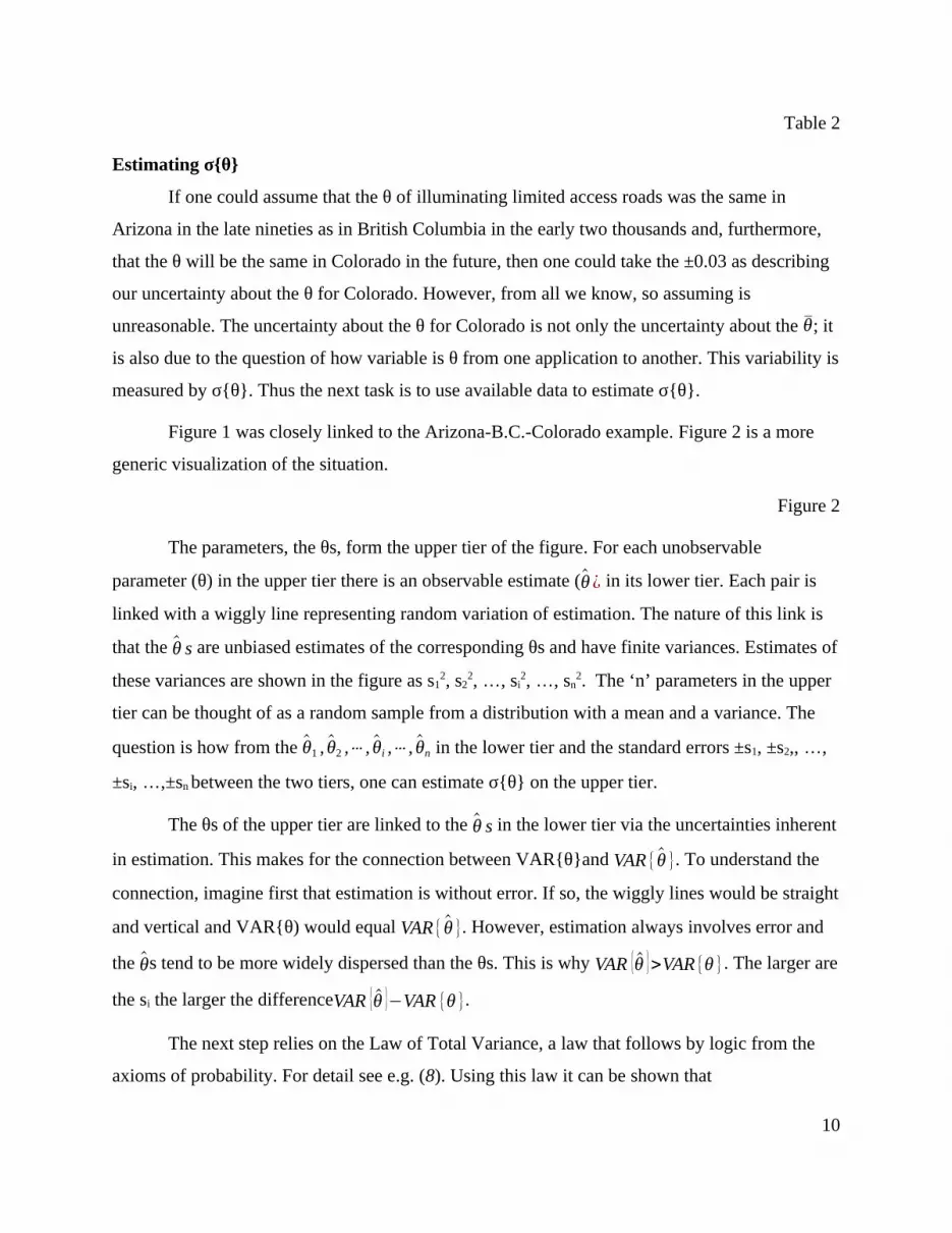
Table 2
Estimating σ{θ}
If one could assume that the θ of illuminating limited access roads was the same in
Arizona in the late nineties as in British Columbia in the early two thousands and, furthermore,
that the θ will be the same in Colorado in the future, then one could take the ±0.03 as describing
our uncertainty about the θ for Colorado. However, from all we know, so assuming is
unreasonable. The uncertainty about the θ for Colorado is not only the uncertainty about the θ; it
is also due to the question of how variable is θ from one application to another. This variability is
measured by σ{θ}. Thus the next task is to use available data to estimate σ{θ}.
Figure 1 was closely linked to the Arizona-B.C.-Colorado example. Figure 2 is a more
generic visualization of the situation.
Figure 2
The parameters, the θs, form the upper tier of the figure. For each unobservable
parameter (θ) in the upper tier there is an observable estimate (θ ¿ in its lower tier. Each pair is
linked with a wiggly line representing random variation of estimation. The nature of this link is
that the θ s are unbiased estimates of the corresponding θs and have finite variances. Estimates of
these variances are shown in the figure as s12, s2
2, …, si2, …, sn
2. The ‘n’ parameters in the upper
tier can be thought of as a random sample from a distribution with a mean and a variance. The
question is how from the θ1 , θ2 ,⋯ , θi ,⋯ , θn in the lower tier and the standard errors ±s1, ±s2,, …,
±si, …,±sn between the two tiers, one can estimate σ{θ} on the upper tier.
The θs of the upper tier are linked to the θ s in the lower tier via the uncertainties inherent
in estimation. This makes for the connection between VAR{θ}and VAR {θ }. To understand the
connection, imagine first that estimation is without error. If so, the wiggly lines would be straight
and vertical and VAR{θ) would equal VAR {θ }. However, estimation always involves error and
the θs tend to be more widely dispersed than the θs. This is why VAR {θ }>VAR {θ }. The larger are
the si the larger the differenceVAR {θ }−VAR {θ }.
The next step relies on the Law of Total Variance, a law that follows by logic from the
axioms of probability. For detail see e.g. (8). Using this law it can be shown that
10

VAR {θ }}=VAR {θ }−E {VAR {θ|θ }} 8
The first term on the right-hand-side of equation 8 is the variance of the estimates on the
lower tier of Figure 2; the second term is the average of the variances with which the θ s are
estimated. Were it true that the weighted average θ was the same as E{θ} we could estimate
VAR{θ} by V :
V={∑1
n
(θ i−θ )2
n∨(n−1)−∑
1
n
si2
nif positive
0 otherwise
9
Dividing by n-1produces unbiased estimates, while dividing by n is more efficient.
However, inasmuch as the weighted average θ is not the same as E{θ}, i.e., θ has a
positive variance (the estimate of which is in equation ), it has to be added to the mix. Denote the
expected value of the squared difference θ-θ by VAR*(θ). We estimate VAR*{θ} by:
V A R¿ {θ }=V +V A R {θ }=V+ 1
∑1
n
1 /si2 10
In equation 10 we replaced V A R {θ } by the expression in equation 5. When the more efficient
estimator of θ is used it should be replaced by the expression in equation 7.
To illustrate, Arizona-British Columbia data are used again in Table 3.
Table 3 about here
For the data in Table 3 we have V=¿ 0.0048-0.0026=0.0022. Since V A R {θ }=1/903=0.0011,
V A R ¿ {θ }=0.0033 and σ ¿ {θ }=√0.0033=±0.06. It is worth noting that in the first edition of the
Highway Safety Manual (1) V is not used to describe the uncertainty about θ. In this illustration
the HSM would list a variance which is about one third of the correct value.
At this point the story can be summarized and its lessons highlighted. To predict the
expected safety effect in the Colorado illumination project we should use θ=0.71in equation 3.
Considering that this θ will likely be somewhere within ±2 standard errors of 0.71 (σ ¿ {θ }=0.06,
2×0.06=0.12), the corresponding range is about 0.59-0.83. The θ at which at the value of the
11

crash reduction predicted by equation 3 equals the opportunity cost of implementing ‘a’ instead
of ‘b’ is called the ‘break-even θ’. The size of the break-even θ varies from project to project and
depends on the expected number of target crashes, on the amount society is willing to pay to save
a target crash, and on the prevailing opportunity cost of capital. If the break even θ in the
Colorado project is less than 0.59 (i.e., at least a 41% reduction in target crashes is required), and
because θ will most likely be larger, it is almost certain that the ‘do not illuminate’ decision will
prove to be correct. Similarly, if the break even θ for the Colorado project is above 0.83, the
decision is also clear: ‘Illuminate’. However, if the break-even value of θ in the Colorado project
is in the 0.59-0.83 range, there is a chance that the decision based on θ=0.71will prove to be
incorrect (i.e. that the cost will exceed the safety benefit). The narrower is the θ ± 2 σ¿{θ } range
the lesser is the chance of making incorrect decisions. The smaller the chance of making
incorrect decisions, the larger will be the value of the crash reductions attained. It follows that
the aim of research is to reduce σ*{θ}.
The Arizona-British Columbia-Colorado story was only an illustration. The general
framework is now clear. Equation is used to predict the safety effect of doing ‘a’ instead of ‘b’.
To predict best, one should use θ for θ (a ,b ) in equation . θ is the weighted average of past
research findings. How θ and its standard error s{θ } can be computed is shown in equations 4
and 5 or 6 and 7. The θ used to predict the safety effect is not the θ that will materialize in a
future project. Whether the ‘implement or do not implement’ decision will be right or wrong
depends on the difference between θ and θ . How large the difference might be is measured by
σ*{θ}=√VAR¿{θ }. The requisite estimators are in equations 9 and 10.
When ±2 σ¿{θ} makes for a narrow range around θ, decisions can be made confidently
and no new research is needed. When for many decisions the range is so wide that it covers the
break-even value of θ, there is a good chance for the decisions to be incorrect. In this case, new
research to reduce σ*{θ} may be needed. How to do effective CMF research is discussed next.
HOW TO DO EFFECTIVE CMF RESEARCH
To reduce the chance of wasting resources by making bad decisions one must reduce the
VAR*{θ}. As shown in equation 10, VAR*{θ} is the sum of two components. One component,
VAR{θ}, measures the uncertainty about how different is the weighted mean of past results (θ)
12
from the mean E(θ). The more studies are done, the more θ s go into the determination of θ, the
lesser is VAR{θ}. The other component, V, reflects the variability of θs which is due to
differences in the ‘circumstances’; that is, how different will the θs tend to be from one instance
of implementation to another. The variance due to this source cannot be reduced by doing more
and more studies; it can be reduced only by determining how the θs depend on this or that
circumstance of implementation. These two options for reducing the VAR*{θ} will be examined
separately.
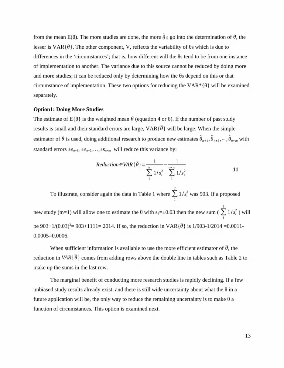
Option1: Doing More Studies
The estimate of E{θ} is the weighted mean θ (equation 4 or 6). If the number of past study
results is small and their standard errors are large, VAR{θ} will be large. When the simple
estimator of θ is used, doing additional research to produce new estimates θn+1, θn+2 ,⋯ , θn+m with
standard errors ±sn+1, ±sn+2,…,±sn+m will reduce this variance by:
Reduction∈VAR {θ }= 1
∑1
n
1/si2
− 1
∑1
n+m
1/s i2 11
To illustrate, consider again the data in Table 1 where ∑1
2
1 /si2 was 903. If a proposed
new study (m=1) will allow one to estimate the θ with s3=±0.03 then the new sum ( ∑1
3
1 /si2 ) will
be 903+1/(0.03)2= 903+1111= 2014. If so, the reduction in VAR{θ} is 1/903-1/2014 =0.0011-
0.0005=0.0006.
When sufficient information is available to use the more efficient estimator of θ, the
reduction in VAR {θ } comes from adding rows above the double line in tables such as Table 2 to
make up the sums in the last row.
The marginal benefit of conducting more research studies is rapidly declining. If a few
unbiased study results already exist, and there is still wide uncertainty about what the θ in a
future application will be, the only way to reduce the remaining uncertainty is to make θ a
function of circumstances. This option is examined next.
13

Option 2: Making θ a Function of Circumstances
Suppose that several past study results already exist but that VAR*{θ} is still too large. Now one
must ask: “Why did the same kind of action have such diverse safety effects? Can one divide the
extant research results into groups that differ in some variable such that within each group
VAR{θ} will be smaller? The Arizona-B.C. hypothetical example will be developed further to
show how making θ a function of a variable can reduce VAR{θ}.
The latitude of Phoenix is 33.5º N and of Vancouver 49.2º N. Can it be that a part of the
difference between θArizona=0.75 and the θB.C .=0.62 ( ) is due to the difference in light
conditions associated with latitude? Two data points are not a sufficient for speculating about
why the θs estimates seem to differ. However, there is research suggesting that the safety effect
of illumination may depends on geographical latitude (see, e.g., 9). The question could be
answered by estimating θ at a few more latitudes. If the resulting relationship will seem regular,
then one can estimate how θ depends on latitude and thereby reduce VAR{θ}.
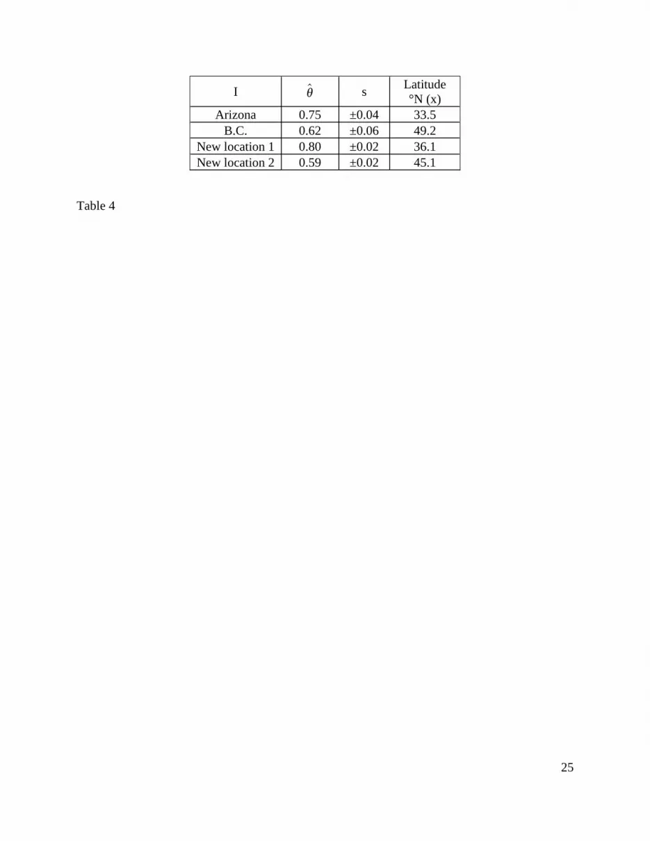
Suppose that such new research was done at two more locations. Both the old and the
new results are shown in Table 4.
Table 4 about here
Figure 3 is based on the entries of Table 4. The two new estimates seem to confirm the
speculation that the further north is the road the larger is the safety effect of illuminating it.
Assuming that E {θi }=α+ β x i where α and β are unknown constants and xi is the Latitude for
study i, a regression line was fitted to these data points by ordinary least squares. (While the use
of weighted least squares would be more appropriate, it would complicate matters, perhaps
unnecessarily.) Now the estimate of E{θi} is θi=α+ β x i where α∧ β are estimates of α and β.
With the data in Table 4, θi=1.18−0.0120 x i.
Figure 3 about here
The benefit in variance reduction is now plain to see. If latitude was not used as a
variable, estimation of VAR{θ} would be based on the average squared difference between the
solid circles (the θ s) in Figure 3 and the weighted mean - dotted horizontal line. However, when
the influence of latitude is considered, the squared differences are those between the solid circles
14
and the empty circles (the θi s ¿ on the fitted regression line. Because the fitted line comes closer
to the data points than the horizontal line, the squared differences will now be much smaller.
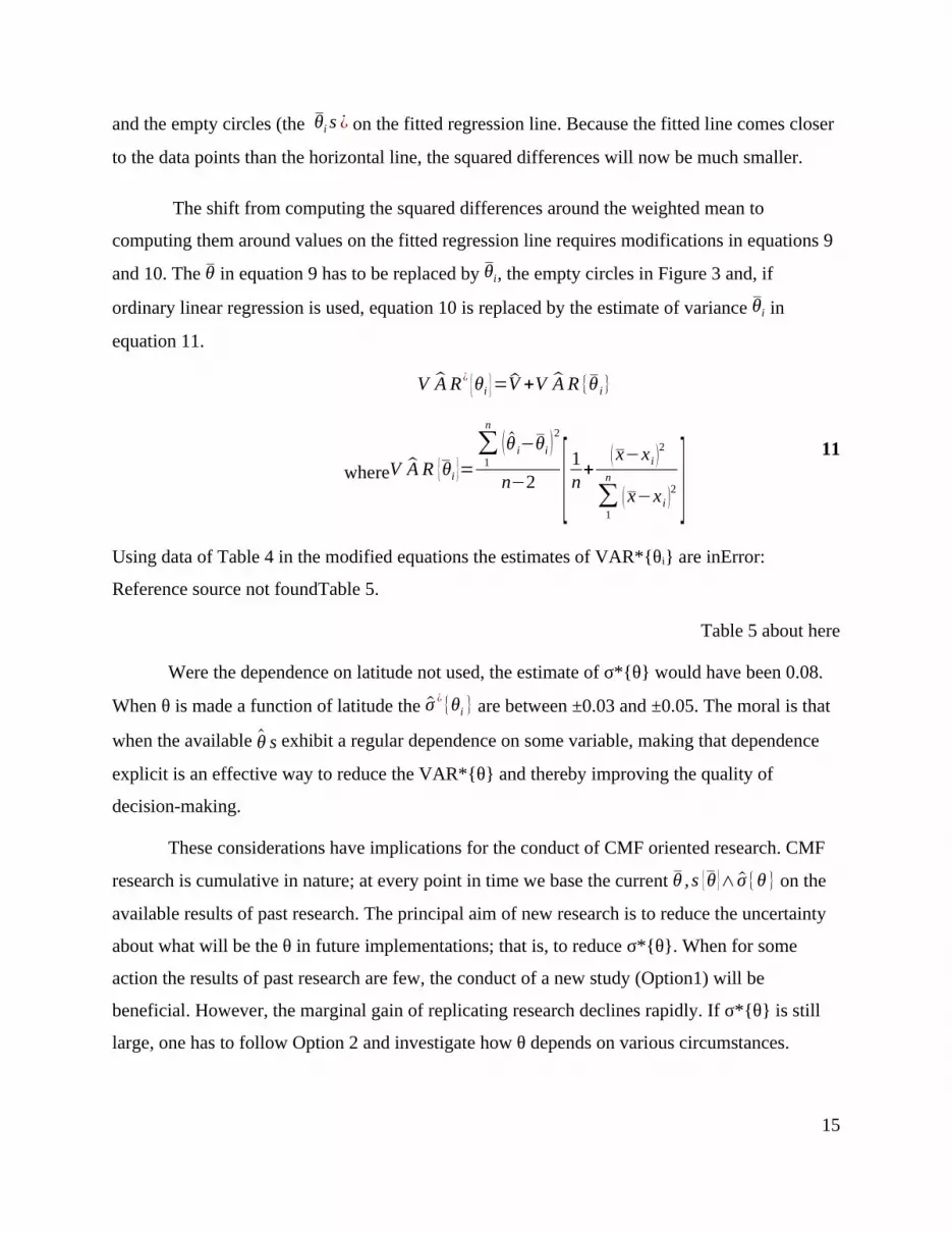
The shift from computing the squared differences around the weighted mean to
computing them around values on the fitted regression line requires modifications in equations 9
and 10. The θ in equation 9 has to be replaced by θi, the empty circles in Figure 3 and, if
ordinary linear regression is used, equation 10 is replaced by the estimate of variance θi in
equation 11.
V A R ¿ {θi }=V +V A R {θ i}
11whereV A R {θi }=
∑1
n
(θ i−θi )2
n−2 [ 1n+
( x−x i )2
∑1
n
( x−x i )2 ]
Using data of Table 4 in the modified equations the estimates of VAR*{θi} are inError:
Reference source not foundTable 5.
Table 5 about here
Were the dependence on latitude not used, the estimate of σ*{θ} would have been 0.08.
When θ is made a function of latitude the σ ¿{θi } are between ±0.03 and ±0.05. The moral is that
when the available θ s exhibit a regular dependence on some variable, making that dependence
explicit is an effective way to reduce the VAR*{θ} and thereby improving the quality of
decision-making.
These considerations have implications for the conduct of CMF oriented research. CMF
research is cumulative in nature; at every point in time we base the current θ , s {θ }∧ σ {θ } on the
available results of past research. The principal aim of new research is to reduce the uncertainty
about what will be the θ in future implementations; that is, to reduce σ*{θ}. When for some
action the results of past research are few, the conduct of a new study (Option1) will be
beneficial. However, the marginal gain of replicating research declines rapidly. If σ*{θ} is still
large, one has to follow Option 2 and investigate how θ depends on various circumstances.
15
Such an investigation is possible only when the same kind of action is implemented in
varying circumstances. This usually requires the use of several past research results the
circumstances of which are known and differ. It follows that for Option 2 to be viable it is
imperative that a rich set of potentially important circumstances be reported in every future
evaluation research. Only then will it be possible to make CMFs into functions of variables.
Some such ‘important circumstances’ are easy to fathom; those pertaining to geometry,
traffic, speed etc. It would be useful to compile a short list of such items to guide researchers in
the next few years. Other circumstances may not be evident at the time the research is done but
could emerge later, especially if large and unexplained variances will persist.
Those who wrote the first edition of the Highway Safety Manual (1) faced the question of
whether a separate CMF should be provided for the same action when taken in different
circumstances (such as when roads differed by number of lanes, speed limit, or when location
was ‘urban’ or ‘rural’). Their usual choice was to list separate CMFs for each circumstance. This
question should now be examined more systematically. Using the tools and approach provided
here one should ask whether the CMF of some action is a function of some variable and, if yes,
what that function is. Research guided by this question will effectively reduce the uncertainty
about the safety effect of actions.
SUMMARY OBSERVATIONS
The need to use a θ arises when the safety consequences of a future action are
contemplated. Guidance about that future θ comes from research about the consequences of
similar actions taken in the past. Past actions of the same kind were not identical and were taken
in a variety of circumstances. Therefore, their effect on safety can be expected to be similar but
not identical. That is, the past θs are not all the same; they are random variables from a
distribution that has a mean, and a variance.
The equations needed to estimate the mean and the variance of θ are provided. As raw
material for estimation serve past estimates of θ and their standard errors. Evaluation research
that does not ensure that the estimates of θ are unbiased and does not report their standard error
is of no use.
16

What the θ for the future action will be is unknown; it can be any value from the
aforementioned distribution. Still, our best prediction of what that future θ will be is the current
estimate of the mean of past θs. If the variance of θ around this mean is small, our prediction will
likely to be close to the mark and the decision based on it correct. However, if the variance of the
past θs is large then decisions based on the estimated mean of past θs may be systematically
incorrect. The danger of making systematically incorrect decisions is acute when the break-even
θ is within few standard deviations of this mean.
When the danger of making incorrect decisions is substantial, the conduct of new
research should be considered. The aim of such new research is to reduce the variance of the θs
and thereby to diminish the chance of making bad decisions. There are two ways to reduce the
variance of the θs. When for a certain action little research has been done in the past, a new and
accurate estimate of θ may help to reduce the variance. However, if several past estimates of θ
are available and their variance is still large, then adding more estimates will be of little help. In
this case the task is to make θ a function of those circumstances that cause the diversity.
Presently available sources of CMFs give an estimate of the mean θ and of its standard
error. They do not provide estimates of σ{θ}. This may mislead and requires remedy. When the
standard error of the estimated mean is tolerably small the user may be led to the belief that the
safety effect of future actions can be confidently predicted, that the decision based on the
prediction is likely to be correct, and that no more research about this CMF is needed. All three
beliefs are incorrect. Only if an estimate of σ{θ}is listed can the user assess the chance of the
decision to be right.
Today’s decisions are based on information extracted from the accumulation of past
research results. For tomorrow’s research to contribute to future research cumulation, its results
must be reported in the requisite detail. As a minimum it must contain the relevant estimates of θ
and their standard errors; but preferably the estimates of μa , VAR {μa }, μb∧VAR {μb }. In addition it
must contain information about the relevant circumstances of implementation. Relevant
circumstances are those that might materially affect the θ. Only then will subsequent researchers
be in the position to make θ a function of circumstances; only then will we substantially diminish
the chance of making incorrect decisions.
17

GLOSSARY
Greek
σ(θ) Standard deviation of the random variable θ
θ(a,b) The CMF for implementing ‘a’ instead of ‘b’
θ Estimate of E{θ}
μ Expected number of (target) crashes.
Latin
^ Caret above denotes ‘estimate’
a and b Action (intervention, countermeasure, treatment, decision etc.)
E{θ} Expected value of θ
s{.} Standard error of {.}
VAR{θ} Variance of the random variable θ
REFERENCES
1. AASHTO, Highway Safety Manual, 2010
2. Elvik,R., Hoye, A., Vaa, T., Sorensen, M. The Handbook of Road Safety Measures.
Emerald Group Publishing, Bingley, UK, 2009
3. FHWA, Crash Modification Factor Clearinghouse, http://www.cmfclearinghouse.org/, accesed on 06 April 2011.
4. Gross, F, Persaud, B.N., and Lyon, C., A Guide to Developing Quality Crash Modification Factors, FHWA-SA-10-032, FHWA, U.S. Department of Transportation, 2010.
5. Hauer, E., Accident modification functions in road safety. Proceedings of the 28th Annual
Conference of the Canadian Society for Civil Engineering, London, Ontario, 2000.
6. Hauer, E., Estimating the Mean and Variance of CMFs and how they can be changed by
new research. ‘Second Report’ prepared for the Highway Safety Research Center at the
University of North Carolina and Appendix D of Task 1 report, NCHRP Project 17-48 –
Development of a Strategic National Highway Infrastructure Safety Research Agenda.
2011.
18

7. Hauer, E., Observational before-after studies in road safety. Pergamon (currently
Emerald), 1997
8. http://en.wikipedia.org/wiki/Law_of_total_variance. Accessed on April 14, 2011.
9. M. Koornstra, F. Bijleveld, M. Hagenzieker. The Safety Effects of Daytime Running
Lights. SWOV Institute for Road Safety Research, R-97-36.Leidschendam, The
Netherlands, 1997.
Figure 1
19

Figure 2
20

Figure 3
21

θ s s2 1/s2 Weights
Contributions to mean
Arizona 0.75 ±0.04 0.0016 625 0.69 0.519B.C. 0.62 ±0.06 0.0036 278 0.31 0.191
Sums 903 1 θ=¿0.710
Table 1
22

μb μa V A R { μb } V A R { μa } θ (a ,b ) s{θ(a , b)}
Arizona 999.6 751.0 1798.6 751.0 0.75 0.04B.C. 400.0 249.0 798.0 249.0 0.62 0.06Sums 1399.6 1000.0 2596.6 1000.0 0.71 0.03
Table 2
23

θ s (θ−θ )2 s2
Arizona 0.75 ±0.04 0.0016 0.0016
B.C. 0.62 ±0.06 0.0081 0.0036
Averages V A R {θ }=¿ 0.0048* E {VAR {θ|θ }}=0.0026
*Using the sample variance, not the bias-corrected sample variance.
Table 3
24
I θ s Latitude °N (x)
Arizona 0.75 ±0.04 33.5B.C. 0.62 ±0.06 49.2
New location 1 0.80 ±0.02 36.1New location 2 0.59 ±0.02 45.1
Table 4
25

V A R ¿{θi } ±σ ¿{θi }Arizona 0.0023 0.05
B.C. 0.0025 0.05New location 1 0.0016 0.04New location 2 0.0014 0.03
Average 0.0020 0.04
Table 5
Figure captions
Figure 1. What can be observed and what we want to know
Figure 2. Parameters and their estimates.
Figure 3. Linear regression to the data in TABLE
26
Table captions
TABLE 1. Illustration of Computations (Invented Data)
TABLE 2. Illustration of Computations (Invented Data)
TABLE 3. Illustration of computations
TABLE 4. Two new estimates (Invented data)
TABLE 5. Estimates of VAR{θi}
27