Improving Freeway Crash Prediction Models Using Disaggregate Flow State Information

http://www.virginiadot.org/vtrc/main/online_reports/pdf/20-r15.pdf

NANCY DUTTA, Ph.D. Graduate Research Assistant MICHAEL D. FONTAINE, Ph.D., P.E. Associate Director

Final Report VTRC 20-R15

Standard Title Page - Report on Federally Funded Project 1. Report No.: 2. Government Accession No.: 3. Recipient’s Catalog No.: FHWA/VTRC 20-R15

4. Title and Subtitle: 5. Report Date: Improving Freeway Crash Prediction Models Using Disaggregate Flow State Information

January 2020 6. Performing Organization Code:

7. Author(s): Nancy Dutta, Ph.D., and Michael D. Fontaine, Ph.D., P.E.

8. Performing Organization Report No.: VTRC 20-R15

9. Performing Organization and Address: Virginia Transportation Research Council 530 Edgemont Rd Charlottesville, VA 22903

10. Work Unit No. (TRAIS): 11. Contract or Grant No.: 112913

12. Sponsoring Agencies’ Name and Address: 13. Type of Report and Period Covered: Virginia Department of Transportation 1401 E. Broad Street Richmond, VA 23219

Federal Highway Administration 400 North 8th Street, Room 750 Richmond, VA 23219-4825

Final 14. Sponsoring Agency Code:

15. Supplementary Notes: This is an SPR-B report. 16. Abstract:

Crash analysis methods typically use annual average daily traffic as an exposure measure, which can be too aggregate to capture the safety effects of variations in traffic flow and operations that occur throughout the day. Flow characteristics such as variation in speed and level of congestion play a significant role in crash occurrence and are not currently accounted for in the American Association of State Highway and Transportation Officials’ Highway Safety Manual. This study developed a methodology for creating crash prediction models using traffic, geometric, and control information that is provided at sub-daily aggregation intervals. Data from 110 rural four-lane segments and 80 urban six-lane segments were used. The volume data used in this study came from detectors that collect data ranging from continuous counts throughout the year to counts from only a couple of weeks every other year (short counts). Speed data were collected from both point sensors and probe data provided by INRIX.

The results showed that models that used data aggregated to an average hourly level reflected the variation in volume and speed throughout the day without compromising model quality. Crash predictions for urban segments underwent a 20% improvement in mean absolute deviation for total crashes and a 9% improvement for injury crashes when models using average hourly volume, geometry, and flow variables were compared to the model based on annual average daily traffic. Corresponding improvements over annual average daily traffic models for rural segments were 11% and 9%. Average hourly speed, standard deviation of hourly speed, and differences between speed limit and average speed had statistically significant relationships with crash frequency. For all models, prediction accuracy was improved across all validation measures of effectiveness when the speed components were added. The positive effect of flow variables was true irrespective of the speed data source. Further investigation revealed that the improvement achieved in model prediction by using a more inclusive and bigger dataset was larger than the effect of accounting for spatial/temporal data correlation. For rural hourly models, mean absolute deviation improved by 52% when short counts were added in comparison to the continuous count station only models. The respective value for urban segments was 58%. This means that using short count stations as a data source does not diminish the quality of the developed models. Thus, a combination of different volume data sources with good quality speed data can lessen the dependency on volume data quality without compromising performance. Although accounting for spatial and temporal correlation improved model performance, it provided smaller benefits than inclusion of the short count data in the models.

This study showed that it is possible to develop a broadly transferable crash prediction methodology using hourly level

volume and flow data that are currently widely available to transportation agencies. These models have a broad spectrum of potential applications that involve assessing safety effects of events and countermeasures that create recurring and non-recurring short-term fluctuations in traffic characteristics. 17 Key Words: 18. Distribution Statement: Crash modeling, safety performance function, speed No restrictions. This document is available to the public

through NTIS, Springfield, VA 22161. 19. Security Classif. (of this report): 20. Security Classif. (of this page): 21. No. of Pages: 22. Price: Unclassified Unclassified 61

Form DOT F 1700.7 (8-72) Reproduction of completed page authorized

FINAL REPORT

IMPROVING FREEWAY CRASH PREDICTION MODELS USING

DISAGGREGATE FLOW STATE INFORMATION

Nancy Dutta, Ph.D.

Graduate Research Assistant

Michael D. Fontaine, Ph.D., P.E.

Associate Director

In Cooperation with the U.S. Department of Transportation

Federal Highway Administration

Virginia Transportation Research Council

(A partnership of the Virginia Department of Transportation

and the University of Virginia since 1948)

Charlottesville, Virginia

January 2020

VTRC 20-R15

ii

DISCLAIMER

The contents of this report reflect the views of the authors, who are responsible for the

facts and the accuracy of the data presented herein. The contents do not necessarily reflect the

official views or policies of the Virginia Department of Transportation, the Commonwealth

Transportation Board, or the Federal Highway Administration. This report does not constitute a

standard, specification, or regulation. Any inclusion of manufacturer names, trade names, or

trademarks is for identification purposes only and is not to be considered an endorsement.

Copyright 2020 by the Commonwealth of Virginia.

All rights reserved.

iii

ABSTRACT

Crash analysis methods typically use annual average daily traffic as an exposure

measure, which can be too aggregate to capture the safety effects of variations in traffic flow

and operations that occur throughout the day. Flow characteristics such as variation in speed

and level of congestion play a significant role in crash occurrence and are not currently

accounted for in the American Association of State Highway and Transportation Officials’

Highway Safety Manual. This study developed a methodology for creating crash prediction

models using traffic, geometric, and control information that is provided at sub-daily

aggregation intervals. Data from 110 rural four-lane segments and 80 urban six-lane segments

were used. The volume data used in this study came from detectors that collect data ranging

from continuous counts throughout the year to counts from only a couple of weeks every other

year (short counts). Speed data were collected from both point sensors and probe data provided

by INRIX.

The results showed that models that used data aggregated to an average hourly level

reflected the variation in volume and speed throughout the day without compromising model

quality. Crash predictions for urban segments underwent a 20% improvement in mean absolute

deviation for total crashes and a 9% improvement for injury crashes when models using average

hourly volume, geometry, and flow variables were compared to the model based on annual

average daily traffic. Corresponding improvements over annual average daily traffic models for

rural segments were 11% and 9%. Average hourly speed, standard deviation of hourly speed,

and differences between speed limit and average speed had statistically significant relationships

with crash frequency. For all models, prediction accuracy was improved across all validation

measures of effectiveness when the speed components were added. The positive effect of flow

variables was true irrespective of the speed data source. Further investigation revealed that the

improvement achieved in model prediction by using a more inclusive and bigger dataset was

larger than the effect of accounting for spatial/temporal data correlation. For rural hourly

models, mean absolute deviation improved by 52% when short counts were added in

comparison to the continuous count station only models. The respective value for urban

segments was 58%. This means that using short count stations as a data source does not

diminish the quality of the developed models. Thus, a combination of different volume data

sources with good quality speed data can lessen the dependency on volume data quality without

compromising performance. Although accounting for spatial and temporal correlation

improved model performance, it provided smaller benefits than inclusion of the short count data

in the models.

This study showed that it is possible to develop a broadly transferable crash prediction

methodology using hourly level volume and flow data that are currently widely available to

transportation agencies. These models have a broad spectrum of potential applications that

involve assessing safety effects of events and countermeasures that create recurring and non-

recurring short-term fluctuations in traffic characteristics.

1

FINAL REPORT

IMPROVING FREEWAY CRASH PREDICTION MODELS USING

DISAGGREGATE FLOW STATE INFORMATION

Nancy Dutta, Ph.D.

Graduate Research Assistant

Michael D. Fontaine, Ph.D., P.E.

Associate Director

INTRODUCTION

The 2017-2021 Virginia Strategic Highway Safety Plan set a fatality goal for the state of

zero fatalities (Virginia Department of Transportation [VDOT], 2017). To achieve this goal of

saving lives and reducing motor vehicle crashes and injuries, Virginia aims to expand the use of

data-driven, systemic safety management approaches. Crashes are complicated events that are

influenced by multiple factors, including roadway geometry, driver behavior, traffic conditions,

and environmental factors. The influence of those factors on traffic crashes cannot be fully

understood without detailed information not only on the crash itself but also on its surrounding

circumstances. There is a continuing need to evolve and improve analytic methods to increase

the understanding of crash causal factors, identify locations with possible safety concerns, and

assess the effectiveness of safety improvement alternatives.

The American Association of State Highway and Transportation Officials’ (AASHTO)

Highway Safety Manual (HSM) serves as a national resource that provides standard scientific

techniques and knowledge to help transportation officials make informed decisions regarding

road safety (AASHTO, 2010; AASHTO, 2014). The core of the predictive methodology used in

the HSM is the use of safety performance functions (SPFs). An SPF is a mathematical

relationship that models the frequency of crashes by severity and accounts for geometric and

traffic control factors that influence crashes on specific types of roads. For practical reasons,

base SPFs often use a concise functional form and include only limited numbers of variables

(such as annual average daily traffic [AADT] and segment length).

The HSM provides professionals with a much-needed resource in which current

knowledge, techniques, and methodologies to estimate future annual crash frequency and

severity are presented. Despite that, there are some limitations of using the SPFs recommended

in the HSM. One drawback of using AADT for predicting crashes is that it can be interpreted as

a quantity measure but it cannot be used to assess the quality of flow. Quality of flow is related

to the variation in flow parameters such as speed or density on a much shorter time interval, such

as hours or minutes, as compared to the yearly variation in volume used for HSM SPFs. Since

AADT is the average number of vehicles per day over an entire year, hourly, daily, and seasonal

variations in traffic volume are averaged out. It is generally assumed that crash rates for

highways vary with flow state, but the relationship among flow, speed, and crashes is not simple.

The customary use of AADT in safety analysis may be too aggregate to capture how variation in

the flow affects the occurrence of highway crashes.

2

A study of the relationship between crashes and flow state requires reliable and detailed

information on crashes and disaggregated traffic flow data, which are often complicated by

sparse detector coverage and the quality of available data. Volume data are collected by each

state from both a limited set of continuous count stations that collect data continuously

throughout the year and short count stations that collect data periodically for shorter time

intervals. The quality of continuous count data is very high, even though the total number of

stations is limited. On the other hand, the short count stations have a broader coverage but the

quantity of data available from them is much less. Both of these issues can be crucial since

current crash models depend on volume data. One way to address this concern is to add other

variables in the modeling process that capture the variation in traffic, such as speed. Private

sector probe data theoretically provide 24-hour temporal coverage and broad network coverage

spatially. As availability and reliability of observed traffic data significantly affect the accuracy

of crash predictions, using probe data, which has better network coverage, might be a useful way

to improve the availability of data. Another important consideration in crash modeling is the

presence of spatial and temporal correlation in crashes. The HSM-recommended methodology

does not acknowledge correlation in data. This issue may be even more acute when

disaggregated data are used.

PURPOSE AND SCOPE

Current safety prediction methodologies look only at annual measures of exposure and do

not account for changes in traffic flow over the course of a day. As a result, these methods do

not do a good job capturing the safety impacts of projects that improve traffic operations but do

not change overall exposure, such as incident management programs, dynamic hard shoulder

running, or active traffic management. Given VDOT’s recent emphasis on deploying operations

projects, there is a need to develop better methods to analyze these projects so that safety impacts

can be assessed more accurately and safety performance can be better predicted. The specific

objectives of this study were as follows:

1. Determine whether sub-daily crash predictions models can provide better safety

predictions than AADT-based models and which time aggregation interval provides

the best predictions.

2. Determine if inclusion of traffic state variables improves predictions.

3. Evaluate different sources of speed data and assess the change in quality of crash

prediction models based on the data source used. This has implications for how

models that rely on speed data can be deployed widely.

4. Investigate whether the data from non-continuous count stations can be used to

generate quality predictions. This has implications for whether continuous volume

data are required to generate sub-annual predictions, which could affect whether

models can be applied widely.

5. Investigate whether accounting for spatial and temporal correlations creates

significant improvements in the crash prediction models.

3

The scope of this study was limited to two common configurations of basic freeway

segments in Virginia: two-lane rural freeway directional segments, and three-lane urban freeway

directional segments. These cross sections were selected because they are the most common

freeway segment type in Virginia and relationships between flow state and safety are expected to

be more uniform on limited access freeways than on arterials. It is expected that the models

developed in this study will require more data and analytical effort to apply, but they could be

used strategically on projects where changes in flow by time of day are expected in order to

improve the overall accuracy of safety estimates for those projects.

METHODS

Literature Review

Relevant online databases such as TRID and the VDOT Research Library database were

searched to identify relevant literature on disaggregated crash modeling, the relationship between

crashes and geometric variables, the relationship between crashes and traffic flow parameters,

and statistical methodologies used for crash modeling with and without data correlation.

Data Collection and Preparation

For this task, volume, speed, and geometry data were collected for two-lane directional

rural freeway segments and three-lane directional urban freeway segments from 2011-2017 using

VDOT data systems. The characteristics of the data sources and how they were processed for

use in safety modeling are discussed here.

Volume Data

VDOT’s traffic data collection program includes more than 100,000 traffic roadway

segments where data are collected and traffic estimates produced. There are more than 400

continuous count stations across the state, 140 of which are on the interstates. The continuous

count stations collect data 24 hours a day, 365 days a year. VDOT also has short count stations

throughout the state in an effort to ensure that at least some data exist for all roads maintained by

VDOT, even if they are not collected continuously in real time. Short count durations range

from 48 hours to longer periods less than 1 year. Even though the data derived from continuous

count stations are of high quality, the spatial coverage of these stations is limited. Although the

short count stations cover a broader area, the quantity of data available from them is less than for

the continuous count stations.

First, the locations of traffic detectors were identified using the detector database

maintained by VDOT’s Traffic Engineering Division (TED) and the VDOT GIS integrator. For

rural two-lane segments, 110 count stations were used (31 continuous count, 79 short count); for

urban six-lane segments, 80 count stations were used (24 continuous count, 56 short count). For

all of the continuous count stations, only the time periods in which volume data met the quality

threshold set by VDOT were included in the dataset, resulting in a loss of 16% of data for the

4

rural segments and 9% of data for the urban segments after screening. The short count stations

collect data periodically, so average volumes were determined using all data collected at each

station, which is less than an entire year’s worth of data.

Geometry Data

Geometric and traffic control information was also extracted from several databases.

Information such as number of lanes, speed limit, shoulder width, median type, rural/urban

designation, etc., was gathered for the study segments. VDOT also provided a database

containing horizontal curvature (HC) and vertical curvature (VC) information for each segment.

The start and end mile marker positions for these segments were used to match them with the

selected freeway segments for this analysis. The VC data were calculated using the difference in

slope and length of curve and expressed in the form of percent grade. HC was expressed using

length of curve, presence of curve as a percentage of segment length, and radius of curve.

Length of curve and radius of curve for each segment were directly available in the dataset.

Identification of Freeway Segments

Only homogeneous basic freeway segments that had volume data and were free from

ramps or interchanges were considered for modeling. Endpoints of analysis sections were

initially defined such that each freeway segment had no entry/exit ramps within 0.5 miles of the

start/end of the segment. Next, it was important to define a segment surrounding each count

station so that conditions were homogeneous for the entire length. The number of lanes, lane and

shoulder width, speed limit, median type, and median width were used to define the geometric

homogeneity of the segment. If the station was on a link with homogeneous characteristics that

was greater than 2 miles in length, a buffer of a maximum of 1 mile upstream and 1 mile

downstream of the actual location of the detector was created to reduce the likelihood that traffic

conditions varied substantially from those of the location of the count station. The product of

this task was the identification of a series of basic freeway segments with homogeneous traffic

and geometric conditions that contained a detector station.

Speed Data

Speed data were collected from two sources: (1) the available continuous count stations,

along with volume data for the entire study period; and (2) INRIX, at 15-minute and hourly

intervals. INRIX is a private sector company that processes GPS and fleet probe data to estimate

speeds, which are reported spatially using traffic message channel (TMC) links. TMC links are

spatial representations developed by digital mapping companies for reporting traffic data and

consist of homogeneous segments of roadways. VDOT currently uses INRIX data to support a

variety of performance measurement and traveler information applications, and several

evaluations have supported the accuracy of the travel time data for freeways (Haghani et al.,

2009).

Using the latitude and longitude information of TMCs from INRIX, it was possible to

match the location of the identified freeway segments and corresponding TMCs. INRIX

provides confidence scores for each 1-minute interval travel time, with a confidence score of 30

representing real-time data and scores of 10 and 20 representing historic data during overnight

5

and daytime periods, respectively. About 73% of the data for rural segments and 71% of the

data for urban segments had a confidence score of 30. For the purposes of this analysis, no

threshold was set for the confidence scores and both real-time and historic speed data were

averaged for use in model development.

Crash Data

Crash data for all segments were obtained from the VDOT Roadway Network System

(RNS). The data included detailed information on crash location and date, crash type, severity,

number of vehicles involved, etc. For all the segments, crash information was also collected

from 2011-2017. For this analysis, the researchers examined total crashes as well as fatal and

injury crashes.

Statistical Approach to Crash Prediction Modeling

A range of factors must be considered when developing crash prediction models. Relevant

issues include selection of data structure, contributing variables, type of regression method used,

technique used for modeling, and model selection and validation. The statistical analysis used to

develop the crash prediction models in this study is described here.

Selection of Data Structure

Traditionally, most crash frequency models have used aggregated information with

relatively large time scales (e.g., yearly) rather than detailed, time-varying data in smaller time

scales (e.g., hourly, daily, or weekly). Because of the adoption of larger time scales, temporal

variation of some explanatory variables such as hourly traffic variation or inclement weather is

often lost. Depending on how the data are being collected and used, different data formats can

be used. Cross-sectional data are observed at a single point of time for several study sites. When

this data format is used, the interest lies in modeling how particular sites are performing at a

certain point of time (Washington et al., 2010). The problem with this approach is that by

analyzing only a "snapshot" of longitudinal data, it is possible to overlook the simultaneous

correlation between crashes and their contributing factors. If multiple years of data are available

for study sites, it is possible to use a panel data format. The key feature of panel data is that the

same sites appear repeatedly. This data structure makes it possible to capture a collective effect

of the omitted variables in regression analysis (Washington et al., 2010). If a common

correlation pattern in crash frequencies exists across the segments over the analysis period, the

pattern can lead to more accurate model estimation compared to the cross-sectional data.

Because of these benefits, the crash data used in this study were analyzed as panel data.

Selection of Model Form

Overview

Since crashes are non-negative and characterized by overdispersion (the variance of

crashes is greater than the mean), negative binomial regression has become the most common

method for developing SPFs and is also the recommended modeling approach in the HSM

(AASHTO, 2010; Lord and Mannering, 2010; Milton and Mannering, 1996). In a negative

6

binomial regression model, the probability of roadway entity i having yi crashes per time period

is defined as follows (Washington et al., 2010):

𝑃(𝑦𝑖) = 𝑒𝑥𝑝(−𝜆𝑖) ∗ 𝜆𝑖

𝑦𝑖

𝑦𝑖 !

𝜆𝑖 = 𝑒𝑥𝑝(𝛽𝑋𝑖 + 휀𝑖)

where

yi = the number of crashes for segment i in year t

β = a vector of the estimable parameters

Xi = a vector of the explanatory variables

exp (εi) = a gamma-distributed error term with mean 1 and variance α.

It should be noted that λ is an indication of the expected number of crashes on segment i. If one

had used a Poisson model and did not have explanatory variables Xi, then λ i would simply be the

estimated mean of crashes observed on the segment. The addition of this term allows the

variance to differ from the mean as follows:

VAR (𝑦𝑖) = E ((𝑦𝑖) [1+ αE(𝑦𝑖) ] = E(𝑦𝑖) + αE(𝑦𝑖) 2

Another popular method for modeling disaggregated data is zero inflated models. Zero

inflated models have been developed to handle data characterized by a significant number of

zeros, or more zeros than one would expect in a traditional Poisson or negative binomial /

Poisson-gamma model. These models operate on the principle that the excess zero density that

cannot be accommodated by a traditional count structure is accounted for by a splitting regime

that models a crash-free versus a crash-prone propensity of a roadway segment (Lord and

Mannering, 2010; Washington et al., 2010).

If the probability of a data point being zero is π and the probability of it being non-zero is

(1 – π), then the probability distribution of the zero-inflated negative binomial (ZINB) random

variable 𝑦𝑖 can be written as follows:

𝑃𝑟(𝑦𝑖 = 𝑗) = {𝜋𝑖 + (1 − 𝜋𝑖)𝑔(𝑦𝑖 = 0) 𝑖𝑓 𝑗 = 0(1 − 𝜋𝑖)𝑔(𝑦𝑖) 𝑖𝑓 𝑗 > 0

where πi is the logistic link function and g(yi) is the negative binomial distribution given by the

following:

𝑔(𝑦𝑖) = 𝑃𝑟(𝑌 = 𝑦𝑖| 𝜇𝑖, 𝛼) = ⌈(𝑦𝑖+ 𝛼−1)

⌈(𝛼−1)⌈(𝑦𝑖+1) (

1

1+ 𝛼𝜇𝑖)

𝛼−1

(𝛼𝜇𝑖

1+ 𝛼𝜇𝑖)

𝑦𝑖

As temporal data aggregation becomes more disaggregate, it is a reasonable expectation

to have a larger number of 0 crash observations in each interval. As a result, this study

developed crash prediction models using both the negative binomial form and the ZINB form.

7

Vuong Test

Since both negative binomial and ZINB forms were tested, the model forms needed to be

compared to determine which option was superior. The use of the Vuong test statistic (V) has

been proposed for non-nested models to compare the fitness of zero inflated models versus that

of regular count models (Vuong, 1989). The test statistic is calculated as follows:

𝑉 =𝑚 ̅̅̅̅ ∗ √𝑁

𝑆𝑚

where

𝑚𝑖 = 𝑙𝑜𝑔[𝑓1 (𝑦𝑖)

𝑓2 (𝑦𝑖)]

N = number of observations

𝑚 ̅̅ ̅ = mean of 𝑚𝑖

𝑆𝑚= standard deviation of 𝑚𝑖

𝑓1, 𝑓2 = two competing models.

V has a standard normal distribution, and the test has three possible outcomes:

1. If the absolute value of V is less than 1.96 for a 0.95 confidence level, then neither

model is preferred by the test result.

2. If V is a large positive value, then Model 1 is preferred.

3. If V is a large negative value, then Model 2 is preferred.

This test was used to select which model form was appropriate for the dataset.

Selection of Modeling Technique

Generalized Linear Models (GLMs)

GLMs are extensions of traditional regression models that allow the mean to depend on

the explanatory variables through a link function and the response variable to be any member of

a set of distributions called the exponential family (e.g., normal, Poisson, binomial) (McCullagh

and Nelder, 1991). In a GLM, each outcome Y of the dependent variables is assumed to be

generated from the exponential family. The mean, μ, of the distribution depends on the

independent variables, X, through the following:

𝐸(𝑌) = 𝜇 = 𝑔−(𝑋𝛽)

where

E(Y) = the expected value of Y

Xβ = the linear predictor, a linear combination of unknown parameters β

g = the link function.

8

The unknown parameters, β, are typically estimated using the maximum likelihood method. This

method estimates model parameters by selecting those that maximize a likelihood function that

describes the underlying statistical distribution assumed for the regression model. For a negative

binomial regression model, the likelihood function can be described as follows:

𝐿 (𝜆𝑖) = ∏𝛤 (𝑦𝑖+(

1

𝛼))

𝑦𝑖! 𝛤 (1

𝛼)

𝑖 . [𝛼𝜆𝑖

1+𝛼𝜆𝑖 ]

𝑦𝑖

. [1

1+𝛼𝜆𝑖 ]

1/𝛼

where

Γ(x) = the gamma function

variance = α

λ = the mean

𝑦𝑖 = the number of crashes per period for roadway segment i.

Models in this study were initially estimated using a GLM.

Spatial and Temporal Correlation and Generalized Linear Mixed Models (GLMMs)

A common phenomenon in crash data is overdispersion, meaning that the variance of the

data exceeds the mean. Overdispersion is usually attributed to unobserved heterogeneity. Motor

vehicle crashes are highly complex processes influenced by various contributing factors, so it is

nearly impossible to collect all the data that describe factors that contribute to a crash and its

resulting injury severity. As a result, the impacts of these unobserved factors on the likelihood of

a crash cannot be adequately captured solely by the explanatory variables in the model, leading

to the unobserved heterogeneity problem (Lord and Mannering, 2010; Mannering and Bhat,

2014).

Traditionally, most crash frequency models have used a cross-sectional data format.

Since this format overlooks the correlation between crashes and their contributing factors over

time, it is not suitable for studies where multiple years of data are available for each study site.

Panel data permit identification of variations across individual roadway segments and variations

over time. Accommodation of observation-specific effects also mitigates omitted-variables bias

by implicitly recognizing segment-specific attributes that may be correlated with control

variables. The time-series nature of multiyear data as used in this study presents serial

correlation issues. In a similar vein, there can be spatial correlation space because roadway

entities that are in close proximity may share unobserved effects. This again sets up a correlation

of disturbances among observations and results in the associated parameter estimation problems.

Both overdispersion and serial correlation needs to be addressed in a modeling

framework to produce efficient estimates. Although regular negative binomial models account

for overdispersion, they do not allow for location-specific effects or serial correlation over time

for clustered crash counts. In recent years, mixed effect models have gained popularity among

researchers because of their ability to handle both overdispersion and correlation. They are

usually called GLMMs because they use the common distributions associated with the GLM

such as Poisson, negative binomial, or zero inflated models and also account for data structures

in which observations cluster within larger groups (Hausman et al., 1984). GLMMs were also

9

used in this study to determine whether accounting for spatial and temporal correlation

significantly improved crash prediction models.

The dataset for this study was composed of multiple segments for rural and urban

highways where data had been collected for 7 years, which introduced correlation in the data that

came from a combination of spatial considerations (data from different VDOT districts in

Virginia) and temporal considerations (average hourly data for 7 years).

The random effects model can introduce random location-specific or time-specific effects

into the relationship between the expected numbers of crashes and the covariates of an

observation unit i in a given time period t (Hausman et al., 1984). The GLMM model structure

is as follows:

𝑦𝑖|𝑏 ≈ 𝐷𝑖𝑠𝑡𝑟 [𝜇𝑖,𝜎2

𝑤𝑖]

𝑔 (𝜇) = 𝛽𝑋 + 𝑏𝑍 + 𝛿

where

𝑦𝑖 = dependent variable

b = random effects vector

Distr = a specified conditional distribution of y given b

µ= the conditional mean of y given b, 𝜇𝑖 is its i-th element

𝜎2 = the variance or dispersion parameter

w = the effective observation weight vector (𝑤𝑖 = the weight for observation i)

g(µ) = link function that defines the relationship between the mean response µ and the

linear combination of the predictors

X = fixed effects design matrix of independent variables

β = fixed-effects vector

Z = random-effects design matrix of independent variables

δ = residuals (Mussone et al., 2017).

The model for the mean response µ is as follows:

𝜇 = 𝑔−1 (�̂�)

where

𝑔−1 = inverse of the link function g(µ)

�̂� = linear predictor of the fixed and random effects of the generalized linear mixed

effects model.

In the simplest terms, the mixed effect model used in this study can be defined as

follows:

10

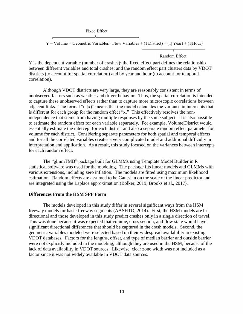
Y is the dependent variable (number of crashes); the fixed effect part defines the relationship

between different variables and total crashes; and the random effect part clusters data by VDOT

districts (to account for spatial correlation) and by year and hour (to account for temporal

correlation).

Although VDOT districts are very large, they are reasonably consistent in terms of

unobserved factors such as weather and driver behavior. Thus, the spatial correlation is intended

to capture these unobserved effects rather than to capture more microscopic correlations between

adjacent links. The format “(1|x)” means that the model calculates the variance in intercepts that

is different for each group for the random effect “x.” This effectively resolves the non-

independence that stems from having multiple responses by the same subject. It is also possible

to estimate the random effect for each variable separately. For example, Volume|District would

essentially estimate the intercept for each district and also a separate random effect parameter for

volume for each district. Considering separate parameters for both spatial and temporal effects

and for all the correlated variables creates a very complicated model and additional difficulty in

interpretation and application. As a result, this study focused on the variances between intercepts

for each random effect.

The “glmmTMB” package built for GLMMs using Template Model Builder in R

statistical software was used for the modeling. The package fits linear models and GLMMs with

various extensions, including zero inflation. The models are fitted using maximum likelihood

estimation. Random effects are assumed to be Gaussian on the scale of the linear predictor and

are integrated using the Laplace approximation (Bolker, 2019; Brooks et al., 2017).

Differences From the HSM SPF Form

The models developed in this study differ in several significant ways from the HSM

freeway models for basic freeway segments (AASHTO, 2014). First, the HSM models are bi-

directional and those developed in this study predict crashes only in a single direction of travel.

This was done because it was expected that volume, cross section, and flow state would have

significant directional differences that should be captured in the crash models. Second, the

geometric variables modeled were selected based on their widespread availability in existing

VDOT databases. Factors for the lengths, offset, and type of median barrier and outside barrier

were not explicitly included in the modeling, although they are used in the HSM, because of the

lack of data availability in VDOT sources. Likewise, clear zone width was not included as a

factor since it was not widely available in VDOT data sources.

11

Model Selection and Validation

Model Selection

This study generated a number of potential models, and it was necessary to select the best

model based on goodness of fit (GOF) and model efficiency. In order to measure the model fit,

the 𝜌𝑐2 statistic was used based on the loglikelihood of the selected model and the constant only

model:

𝜌𝑐2 = 1 −

𝐿𝐿(𝛽)

𝐿𝐿(𝐶)

where

(𝛽) = the log-likelihood at convergence

𝐿𝐿(C) = the log-likelihood with the constant only model.

A perfect model has a likelihood equal to 1. The closer the value is to 1, the more variance the

estimated model is explaining (Washington et al., 2010).

An analysis of variance (ANOVA) comparing the negative binomial and ZINB models

was used to test which distribution fit the model better. ANOVA, which is readily available

using R software, gives a list of a number of other GOF measures.

When the models are compared, it is important to have a consistent methodology to select

a model from a series of models that have been developed for each technique. A popular method

for model selection is the Akaike information criterion (AIC) (Akaike, 1974). The AIC offers an

estimate of the relative information lost when a given model is used to represent the process that

generated the data and is calculated as follows:

AIC = −2LL + 2p

where p = the number of estimated parameters included in the model. A lower value of AIC

indicates a better model.

The Bayesian information criterion (BIC) is a criterion for model selection among a finite

set of models. It is based in part on the likelihood function and is closely related to the AIC.

The BIC also uses a penalty term for the number of parameters in the model. The penalty term is

larger in the BIC than in the AIC. The BIC is given by the following:

BIC = −2ln(L) + k*ln(n)

where

n = number of observations

k = the number of free parameters to be estimated

12

L = the maximized value of the likelihood function for the estimated model (Schwarz,

1978).

Model Validation

An objective assessment of the predictive performance of a particular model can be made

only through the evaluation of several GOF criteria. The GOF measures used to conduct

external model validation included mean absolute prediction error (MAPE), MAD, and mean

squared prediction error (MSPE) (Washington et al., 2010). In addition, cumulative residual

(CURE) plots were examined to check the functional form of the model. Residuals are defined

as the differences between the observed and fitted values of the response; when plotted

cumulatively, they demonstrate the suitability of a regression model. The data in the CURE plot

are expected to oscillate about 0. Any large jumps between residuals indicate areas where there

may be outliers in the data.

Model building used a random selection of 70% of the available data; the remaining 30%

was used for testing and validation. The calculation of the GOF measures was based on the

following equations:

𝑀𝑒𝑎𝑛 𝐴𝑏𝑠𝑜𝑙𝑢𝑡𝑒 𝑃𝑟𝑒𝑑𝑖𝑐𝑡𝑖𝑜𝑛 𝐸𝑟𝑟𝑜𝑟 (𝑀𝐴𝑃𝐸) = ∑ |𝑌𝑚𝑜𝑑𝑒𝑙− 𝑌𝑜𝑏𝑠𝑒𝑟𝑣𝑒𝑑

𝑌𝑜𝑏𝑠𝑒𝑟𝑣𝑒𝑑|𝑛

𝑖=1

𝑀𝑒𝑎𝑛 𝐴𝑏𝑠𝑜𝑙𝑢𝑡𝑒 𝐷𝑒𝑣𝑖𝑎𝑡𝑖𝑜𝑛 (𝑀𝐴𝐷) = ∑ |𝑌𝑚𝑜𝑑𝑒𝑙− 𝑌𝑜𝑏𝑠𝑒𝑟𝑣𝑒𝑑|𝑛

𝑖=1

𝑛

𝑀𝑒𝑎𝑛 𝑆𝑞𝑢𝑎𝑟𝑒𝑑 𝑃𝑟𝑒𝑑𝑖𝑐𝑡𝑖𝑜𝑛 𝐸𝑟𝑟𝑜𝑟 (𝑀𝑆𝑃𝐸) = ∑ (𝑌𝑚𝑜𝑑𝑒𝑙− 𝑌𝑜𝑏𝑠𝑒𝑟𝑣𝑒𝑑)2𝑛

𝑖=1

𝑛

where

𝑌𝑚𝑜𝑑𝑒𝑙 = predicted crash frequency

𝑌𝑜𝑏𝑠𝑒𝑟𝑣𝑒𝑑 = observed crash frequency

n = sample size.

Since AADT-based models predict annual crashes whereas hourly volume models predict

hourly crashes, there was a need to look at GOF measures using a consistent time scale. For

hourly level predictions, the summation of hourly predictions was used to generate annual

predicted numbers of crashes for the GOF calculations so comparisons could be consistent. The

average hourly volume data were computed by averaging data for each available hour for each

site, so there were always 24 hours of data available for each year and each site for validation.

For the validation of raw hourly data, high-quality volume and speed data were not always

available for all 24 hours of every single day. To deal with this issue, crash predictions were

calculated using all hours with valid data. The hour-by-hour predictions produced by these valid

hours were then averaged and multiplied by 365 to convert predictions to an annual value for

each hour of the day. This essentially assumed that missing hours are set equal to the value of

the average hourly crash prediction for that hour at that site and provides a consistent basis for

comparison between the model forms.

13

Experimental Design for Developing Crash Prediction Models

A three-stage process was used for developing crash prediction models and making

decisions about variables and model form using the procedures discussed earlier. The three

stages were as follows:

1. initial investigations of data aggregation intervals and influence of flow parameters

2. assessment of the effects of different speed data sources using continuous count stations

3. examination of short count stations and effects of spatial and temporal correlation.

The following sections discuss the major steps in each stage.

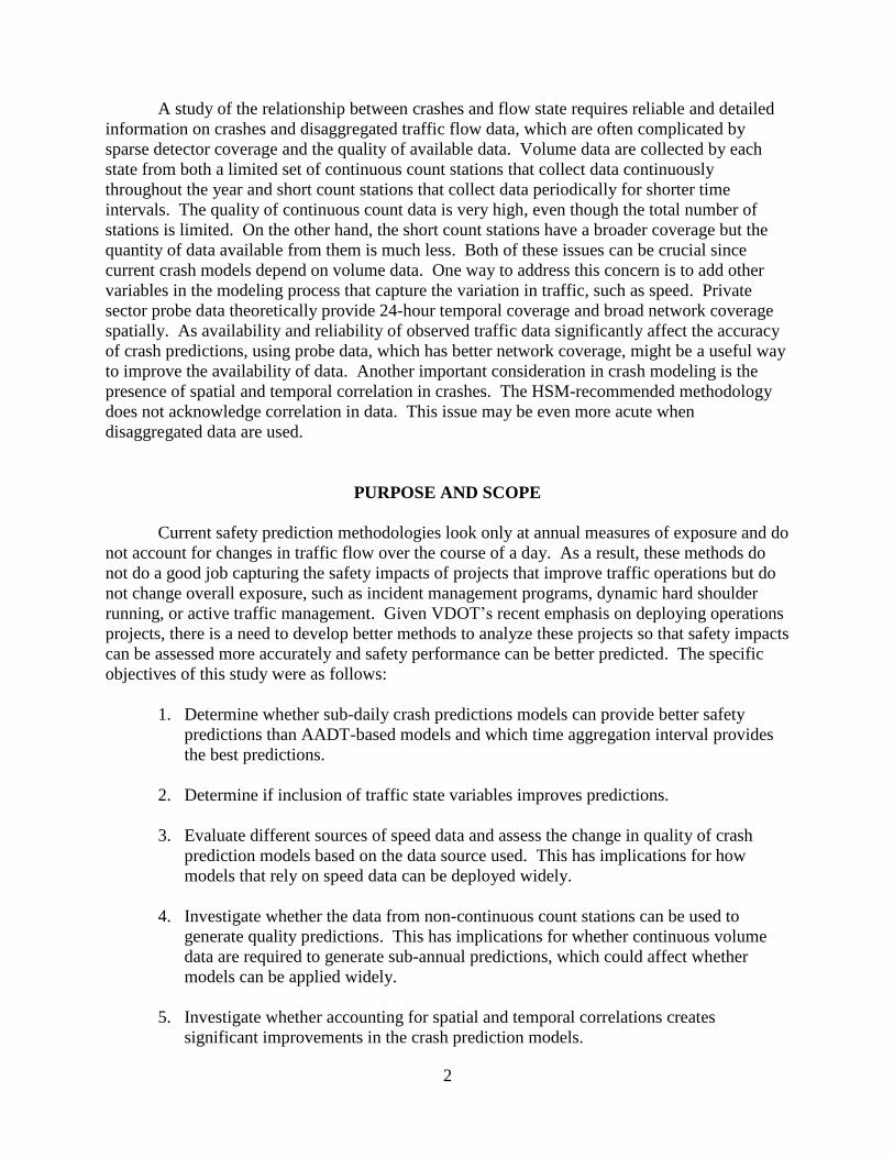
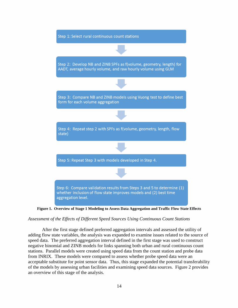
Step 5: Repeat Step 3 with models developed in Step 4. Initial Investigations of Data Aggregation Intervals and Influence of Flow State Variables

The first stage involved ascertaining which temporal data aggregation interval produced

the best crash prediction models and determining whether inclusion of flow parameters improved

the models. Figure 1 provides an overview of how the statistical concepts discussed earlier were

applied to investigate these issues. These initial investigations used the four-lane rural freeways

to test these concepts since they generally had the most consistent geometric cross sections. Two

basic regression model forms were evaluated as part of this stage:

1. models using volume, segment length, and geometric variables

2. models using volume, segment length, geometric variables, and traffic flow parameters.

Each of these model forms was estimated using negative binomial and ZINB models to

assess relative performance. Volume was examined at four aggregation intervals:

1. raw hourly volume, as observed each day at the site

2. average 15-minute volume, expressed as an average volume for each 15 minutes of the

day for each site over each year

3. average hourly volume, expressed as an average volume for each hour of the day for

each site over each year

4. AADT.

Quality of flow variables were summarized at the same time interval as the corresponding

volume variable. The models were compared to one another and with the AADT model to

determine how the predictions differed from a typical HSM-like model. To be consistent with

the HSM, length was used as an offset variable in the models.

Models generated through the process summarized in Figure 1 were compared to assess

which combination of data aggregation interval and predictive variables produced the best

results. The results of this investigation then informed development of the second stage of model

generation.

14

Figure 1. Overview of Stage 1 Modeling to Assess Data Aggregation and Traffic Flow State Effects

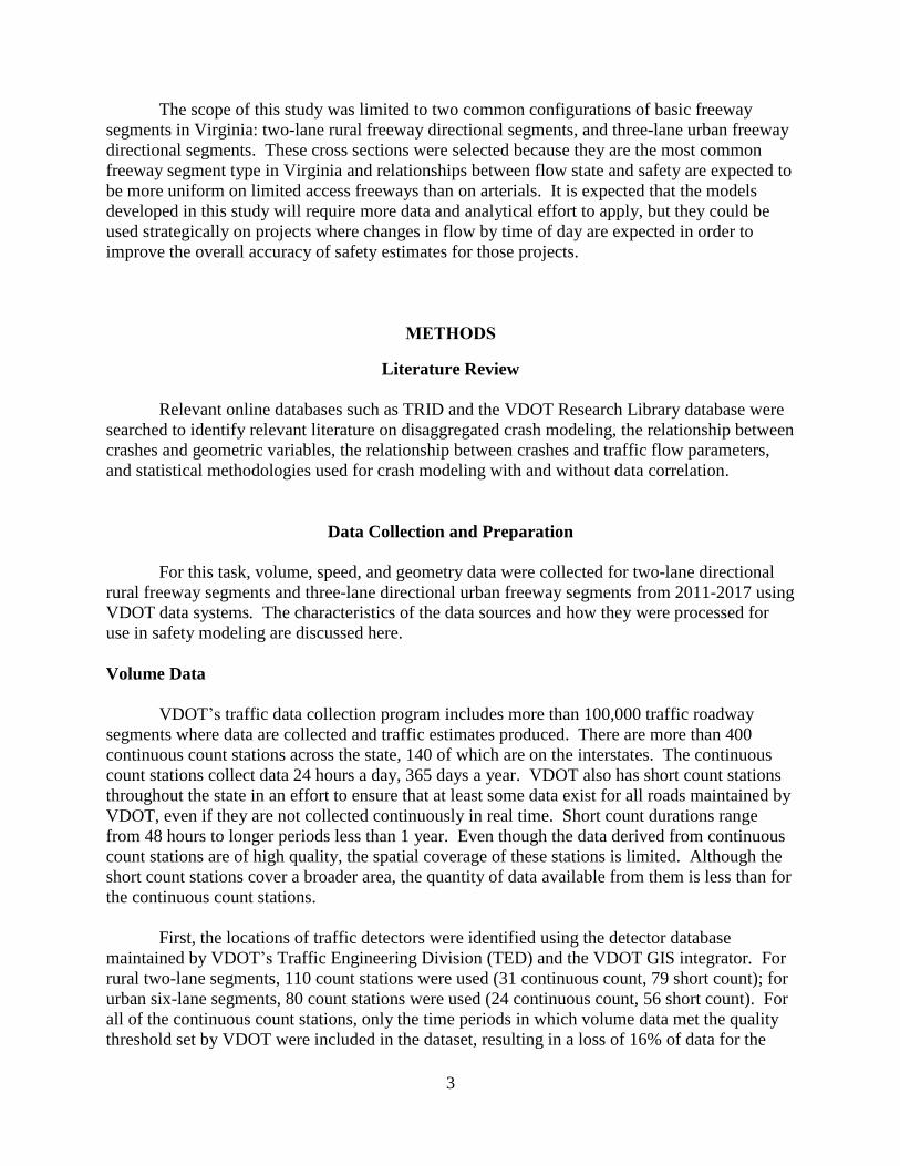
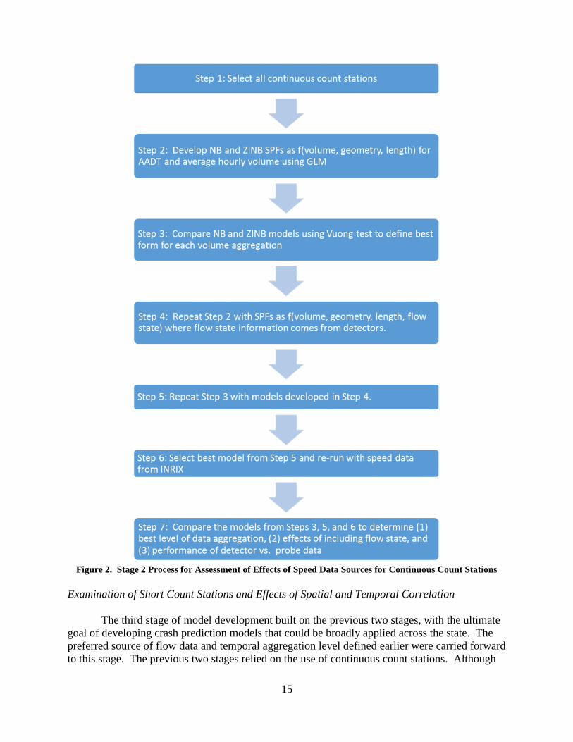
Assessment of the Effects of Different Speed Sources Using Continuous Count Stations

After the first stage defined preferred aggregation intervals and assessed the utility of

adding flow state variables, the analysis was expanded to examine issues related to the source of

speed data. The preferred aggregation interval defined in the first stage was used to construct

negative binomial and ZINB models for links spanning both urban and rural continuous count

stations. Parallel models were created using speed data from the count station and probe data

from INRIX. These models were compared to assess whether probe speed data were an

acceptable substitute for point sensor data. Thus, this stage expanded the potential transferability

of the models by assessing urban facilities and examining speed data sources. Figure 2 provides

an overview of this stage of the analysis.

15

Figure 2. Stage 2 Process for Assessment of Effects of Speed Data Sources for Continuous Count Stations

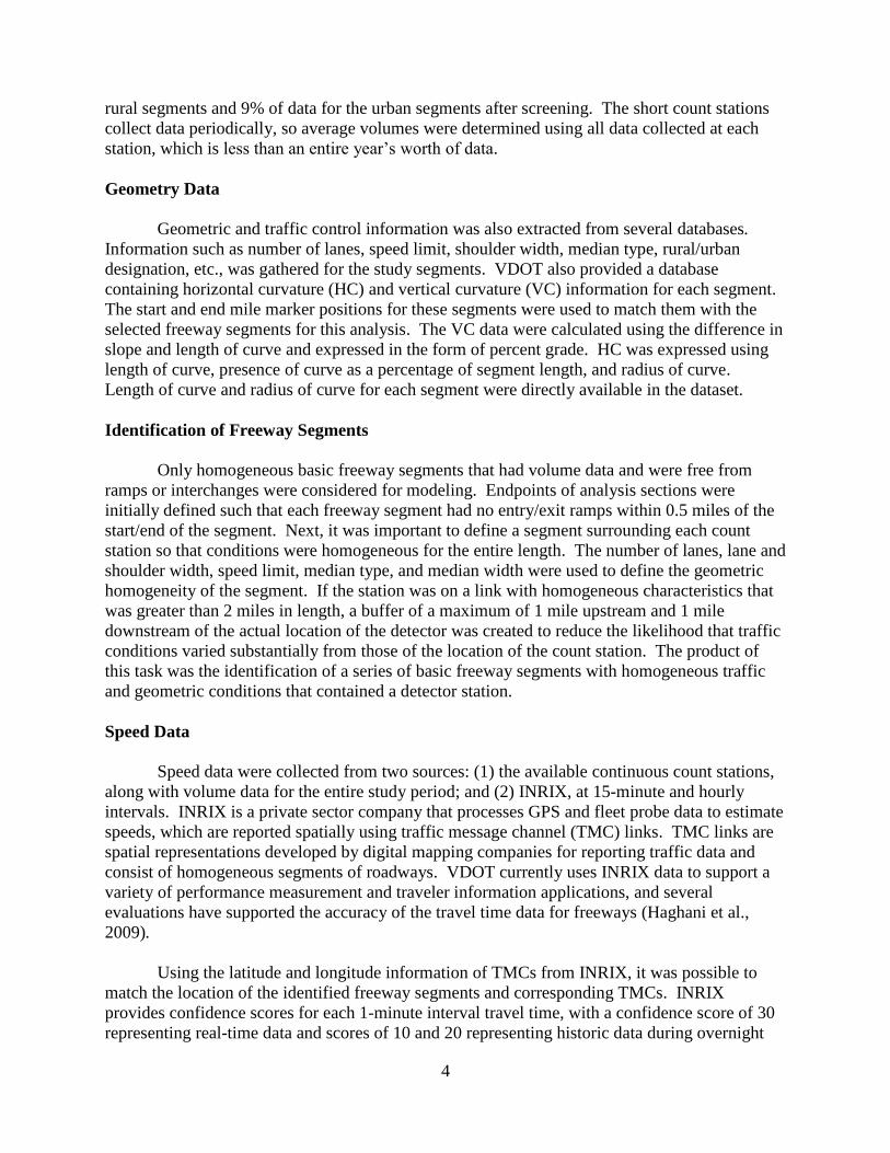
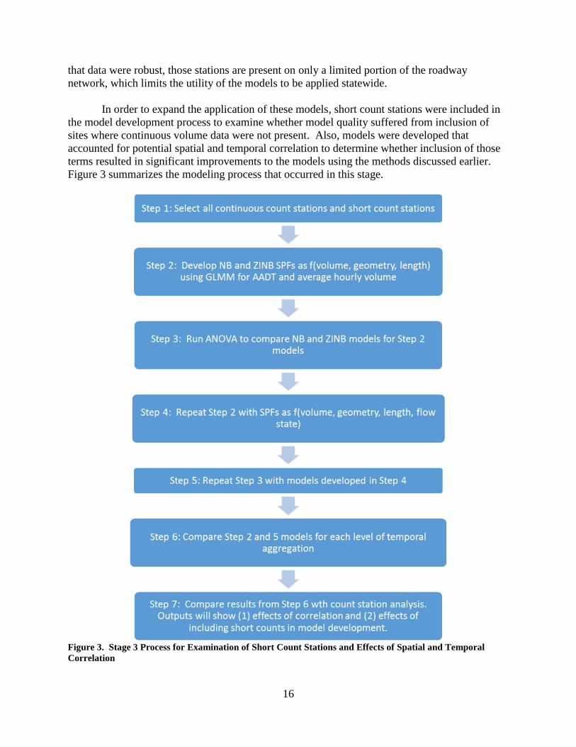
Examination of Short Count Stations and Effects of Spatial and Temporal Correlation

The third stage of model development built on the previous two stages, with the ultimate

goal of developing crash prediction models that could be broadly applied across the state. The

preferred source of flow data and temporal aggregation level defined earlier were carried forward

to this stage. The previous two stages relied on the use of continuous count stations. Although

16

that data were robust, those stations are present on only a limited portion of the roadway

network, which limits the utility of the models to be applied statewide.

In order to expand the application of these models, short count stations were included in

the model development process to examine whether model quality suffered from inclusion of

sites where continuous volume data were not present. Also, models were developed that

accounted for potential spatial and temporal correlation to determine whether inclusion of those

terms resulted in significant improvements to the models using the methods discussed earlier.

Figure 3 summarizes the modeling process that occurred in this stage.

Figure 3. Stage 3 Process for Examination of Short Count Stations and Effects of Spatial and Temporal

Correlation

17

Selection of Preferred Models

Following the completion of the three stages of modeling, preferred models were selected

that provided the best predictions accounting for the following:

level of temporal data aggregation

inclusion of flow state variables

use of continuous versus short counts

use of probe versus continuous count station data

inclusion of spatial/temporal correlation.

RESULTS AND DISCUSSION

Literature Review

Crash prediction models are very useful tools in highway safety, given their potential for

determining both the frequency of crash occurrence and the contributing factors that could be

addressed by transportation policies or site interventions. This section highlights existing studies

on sub-annual crash trends and discusses the issues associated with data availability and

correlation.

Relationship Between Crashes and Hourly Exposure

Studies of relationships between crashes and traffic characteristics can be divided into

two categories: aggregated studies, in which the units of analysis represent counts of crashes or

crash rates for specific time periods (typically months or years), and disaggregated analysis,

where the units of analysis are the crashes themselves and traffic flow is represented by

parameters of the traffic flow at the time and place of each crash. Disaggregate models typically

use data based on average hourly observations of crash rates and traffic flow.

Ivan et al. (2000) concluded that there was evidence that the hourly volume explains

much of the variation in highway crash rates. They focused on using hourly data from 17 rural,

two-lane highway segments in Connecticut with varying land use patterns. Single-vehicle and

multi-vehicle crashes were modeled separately. Time of day was significant for both types of

crashes but in different ways. Single-vehicle crashes occurred most often in the evening and at

night. On the other hand, multi-vehicle crashes were more likely to occur during daylight

conditions at midday and during the evening peak period.

Persaud and Dzbik (1993) developed crash prediction models at both the macroscopic

level (in crashes per unit length per year) and the microscopic level (in crashes per unit length

per hour) using the GLM approach with a negative binomial error structure. Crash, road

inventory, and traffic data for approximately 500 freeway sections in Ontario, Canada, were

obtained for 1988 and 1989. Microscopic models showed a decreasing slope in regression lines

as hourly volume increased, perhaps capturing the influence of decreasing speed as congestion

formed. This is in contrast to the macroscopic model, which showed increasing slopes.

18

Perhaps the most extensive evaluation of this subject was an 8-year study of eight

sections of four-lane interurban road in Israel (Ceder and Livneh, 1982). Single-vehicle crash

rates were very high for flow rates below 250 vehicles per hour (vph). The multiple-vehicle

crash rates were more diverse, with one-half of the sites showing a substantial increase in crash

rates for flow rates greater than about 900 vph, and the remaining sites showing little change,

with increases in hourly traffic volumes. When the two crash types were combined, the results

were dominated by the data for multiple-vehicle crashes. More specifically, those study sections

that encompassed a broad range of traffic volumes had a U-shaped relationship when crash rates

were plotted as a function of hourly volume; the minimum rate occurred near 500 vph. The

remaining four sites, three of which did not have hourly volumes in excess of 1,000 vph, did not

show an increase in crash rates as hourly volumes increased.

Relationship Between Crashes and Flow Parameters

When the flow of traffic along a freeway is considered, three parameters are of

considerable significance: speed and density (which describe the quality of service experienced

by the stream) and volume (which measures the quantity of the traffic and the demand on the

highway facility). Similar flows could be attributed to different combinations of density and

speed, leading to different levels of safety. Speed is an important descriptor of traffic operations

that has an effect on crash severity and frequency, but this variable is difficult to capture

accurately in aggregate models that use AADT to predict annual crashes. The speed distribution

may also play an important role since variance in speed is higher for lower traffic flows than for

more congested conditions. By introducing parameters such as speed, density, or

volume/capacity (v/c) ratio in addition to traffic volume, crash analysis could take into account

the effect of traffic operations on safety.

Solomon (1964) studied the relationship between crashes on two-lane and four-lane

roadways and a number of factors. From an analysis of 10,000 crashes, Solomon concluded that

crash severity increased rapidly at speeds in excess of 60 mph and the probability of fatal injuries

increased sharply above 70 mph. He found a U-shaped relationship between vehicle speed and

crash risk, where crash rates were lowest for travel speeds near the mean speed of traffic. Crash

risk then increased as a vehicle traveled significantly above or below the mean speed of

prevailing traffic. Solomon’s work is often cited as the source of the 85th percentile speed rule

for setting speeds.

Harkey et al. (1990) also replicated the U-shaped relationship between speed and crashes

on urban roads. The researchers compared the police–estimated travel speed of 532 vehicles

involved in crashes over a 3-year period to 24-hr speed data collected on the same section of

non–55 mph roads in areas of Colorado and North Carolina. To address partially the concerns of

earlier studies and make the crash and speed data more comparable, their analysis was limited to

non-intersection, non-alcohol, and weekday crashes.

Empirical examination of the relationship between flow, density, speed, and crash rate on

selected freeways in Colorado by Kononov et al. (2011) suggested that as flow-density increases,

the crash rate initially remains constant until a certain critical threshold combination of speed and

density is reached. Once this threshold is exceeded, the crash rate rises rapidly. The rise in crash

rate may be caused by flow compression without a notable reduction in speed; resultant

19

headways are so small that drivers find it difficult or impossible to compensate for errors and

avoid a crash. The researchers calibrated SPFs for corridor-specific safety that relate crash rate

to hourly volume density and speed.

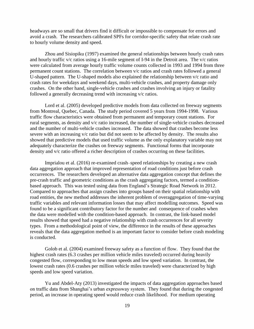
Zhou and Sisiopiku (1997) examined the general relationships between hourly crash rates

and hourly traffic v/c ratios using a 16-mile segment of I-94 in the Detroit area. The v/c ratios

were calculated from average hourly traffic volume counts collected in 1993 and 1994 from three

permanent count stations. The correlation between v/c ratios and crash rates followed a general

U-shaped pattern. The U-shaped models also explained the relationship between v/c ratio and

crash rates for weekdays and weekend days, multi-vehicle crashes, and property damage only

crashes. On the other hand, single-vehicle crashes and crashes involving an injury or fatality

followed a generally decreasing trend with increasing v/c ratios.

Lord et al. (2005) developed predictive models from data collected on freeway segments

from Montreal, Quebec, Canada. The study period covered 5 years from 1994-1998. Various

traffic flow characteristics were obtained from permanent and temporary count stations. For

rural segments, as density and v/c ratio increased, the number of single-vehicle crashes decreased

and the number of multi-vehicle crashes increased. The data showed that crashes become less

severe with an increasing v/c ratio but did not seem to be affected by density. The results also

showed that predictive models that used traffic volume as the only explanatory variable may not

adequately characterize the crashes on freeway segments. Functional forms that incorporate

density and v/c ratio offered a richer description of crashes occurring on these facilities.

Imprialou et al. (2016) re-examined crash–speed relationships by creating a new crash

data aggregation approach that improved representation of road conditions just before crash

occurrences. The researchers developed an alternative data aggregation concept that defines the

pre-crash traffic and geometric conditions as the crash aggregating factors, termed a condition-

based approach. This was tested using data from England’s Strategic Road Network in 2012.

Compared to approaches that assign crashes into groups based on their spatial relationship with

road entities, the new method addresses the inherent problem of overaggregation of time-varying

traffic variables and relevant information losses that may affect modelling outcomes. Speed was

found to be a significant contributory factor for the number and consequence of crashes when

the data were modelled with the condition-based approach. In contrast, the link-based model

results showed that speed had a negative relationship with crash occurrences for all severity

types. From a methodological point of view, the difference in the results of these approaches

reveals that the data aggregation method is an important factor to consider before crash modeling

is conducted.

Golob et al. (2004) examined freeway safety as a function of flow. They found that the

highest crash rates (6.3 crashes per million vehicle miles traveled) occurred during heavily

congested flow, corresponding to low mean speeds and low speed variation. In contrast, the

lowest crash rates (0.6 crashes per million vehicle miles traveled) were characterized by high

speeds and low speed variation.

Yu and Abdel-Aty (2013) investigated the impacts of data aggregation approaches based

on traffic data from Shanghai’s urban expressway system. They found that during the congested

period, an increase in operating speed would reduce crash likelihood. For medium operating

20

speeds, the changes in operating speed did not have substantial effects on crash occurrence

probability. For free-flow periods, increases in operating speed further increased the probability

of crashes.

Garber and Ehrhart (2000) analyzed the effect of speed, flow, and geometric

characteristics on crash rates for different types of Virginia highways. Based on this study, all of

the models showed that under most traffic conditions, the crash rate tends to increase as the

standard deviation of speed increases. The effect of the flow per lane and mean speed on the

crash rate varied with respect to the type of highway.

Wang et al. (2018) developed different models to estimate crash frequency using annual

daily traffic and annual hourly traffic. The study segments were from three expressways in

Orlando, Florida, and included basic freeway segments, merging segments, and weaving

segments. They found that the logarithm of volume, the standard deviation of speed, the

logarithm of segment length, and the existence of a diverge segment were significant variables in

the models. Weaving segments had higher daily and hourly crash frequencies than merge and

basic freeway segments.

Effect of Correlation on Crash Prediction Models

Statistical methods that incorporate a panel data structure have gained popularity because

of their capacity to address both time-series and cross-sectional variations. McCarthy (1999)

employed fixed-effects negative binomial models to examine fatal crash counts using 9 years of

panel data for 418 cities and 57 areas in the United States. A negative binomial regression with

cross-sectional data using the same dataset could not capture the interaction among crashes and

variables properly. Noland (2003) used fixed-effects negative binomial and random-effects

negative binomial (RENB) models to investigate the effects of roadway improvements on traffic

safety using 14 years of data for all 50 U.S. states. A RENB model was found to be more

suitable than the conventional negative binomial model. In the RENB model, the joint effects of

the unobserved variables are assumed to follow certain distributions along the spatial and

temporal dimensions.

Another popular methodology that has been advocated in recent years is a random-

parameter negative binomial model. Three years of crash data for two-lane, two-way urban

roads in Florida were examined to assess the effect of road-level factors on crash frequency

across different regions (Han et al., 2018). A Poisson lognormal model, a hierarchical random

intercept model, and a hierarchical random parameter model were compared. The result showed

that the hierarchical random parameter model outperformed the Poisson lognormal model and

the hierarchical random intercept model. Rather than treating the intercept term as the only

random component, as with the RENB model, the random-parameter negative binomial model

allows each estimated parameter to vary across individual observations, thus including the

unobserved heterogeneity along the spatial and temporal dimensions.

Li et al. (2018) used a mixed effect negative binomial regression model and a back-

propagation neural network model to consider bus crashes. The performance of the mixed-effect

negative binomial model showed that it is advantageous to use a mixed effects modeling method

to predict crash counts in practice because it can take into account the effects of specific factors.

21

Another analysis using data from an urban road segment in Turin, Italy, also favored the use of

mixed effect models (Mussone et al., 2017). Data from 2006-2012 were used, and traffic flows

and weather station data were aggregated in 5-minute intervals for 35 minutes across each crash

event. Two different approaches, a back-propagation neural network model and a mixed effect

model, were used. The researchers concluded that the mixed effect model performed well and

was easier to interpret. The mixed effect models combine two popular methodologies for

modeling repeated measurements of crash data: fixed effects and random effects models. They

are also widely accepted for their ability to handle both spatial and temporal correlation in data.

Data Collection and Preparation

Data Summary

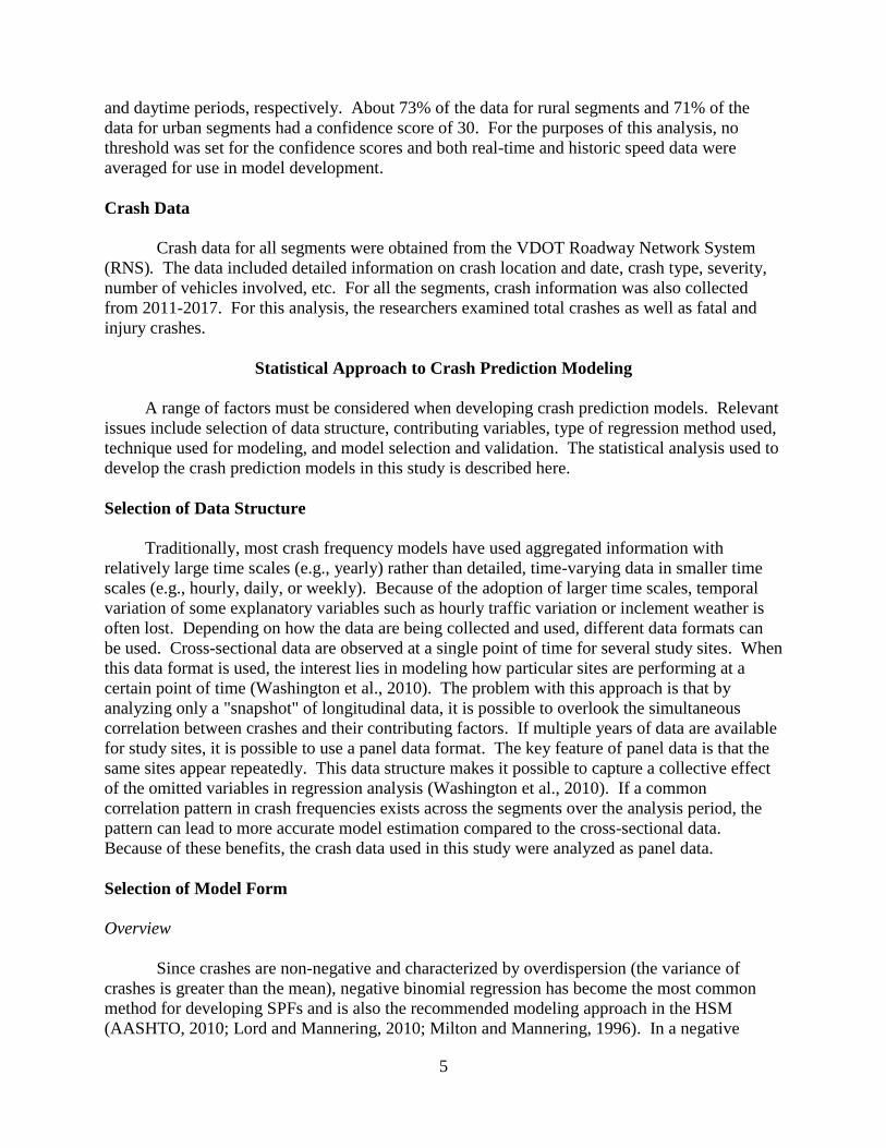
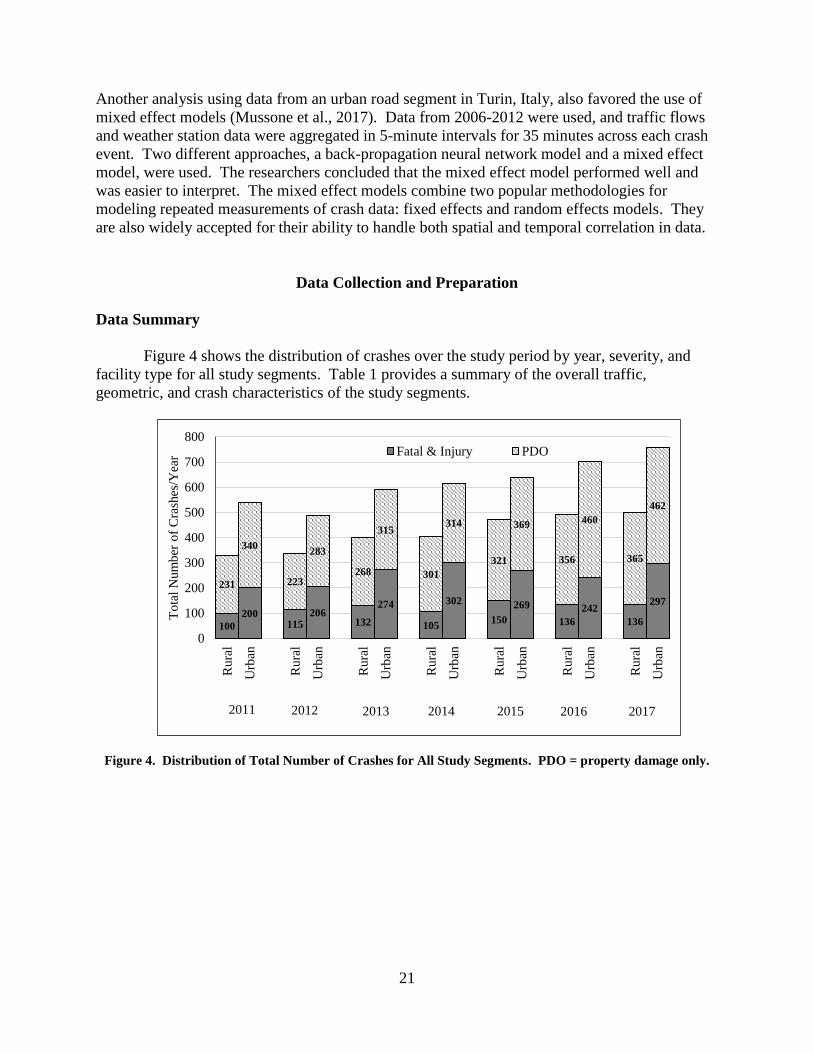
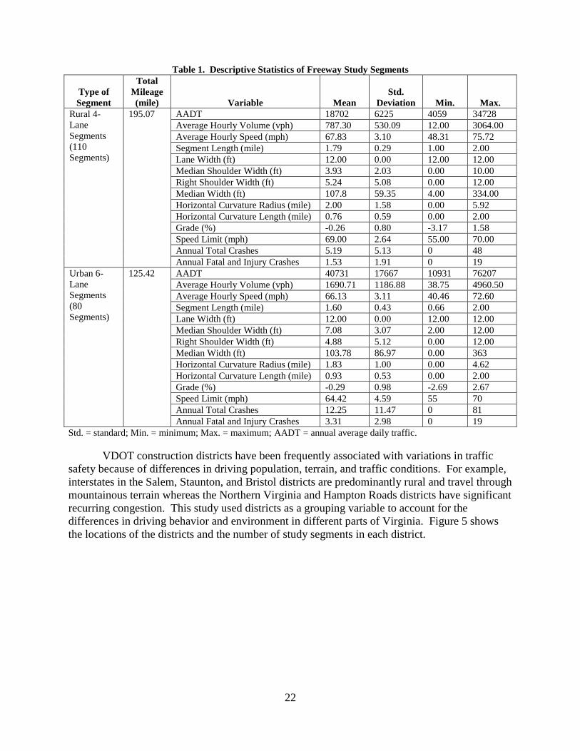
Figure 4 shows the distribution of crashes over the study period by year, severity, and

facility type for all study segments. Table 1 provides a summary of the overall traffic,

geometric, and crash characteristics of the study segments.

Figure 4. Distribution of Total Number of Crashes for All Study Segments. PDO = property damage only.

100

200115

206132

274

105

302

150

269

136

242

136

297

231

340

223

283

268

315

301

314

321

369

356

460

365

462

0

100

200

300

400

500

600

700

800

Rura

l

Urb

an

Rura

l

Urb

an

Rura

l

Urb

an

Rura

l

Urb

an

Rura

l

Urb

an

Rura

l

Urb

an

Rura

l

Urb

an

To

tal

Num

ber

of

Cra

shes

/Yea

r Fatal & Injury PDO

2011 2012 2013 2014 2015 2016 2017

22

Table 1. Descriptive Statistics of Freeway Study Segments

Type of

Segment

Total

Mileage

(mile)

Variable

Mean

Std.

Deviation

Min.

Max.

Rural 4-

Lane

Segments

(110

Segments)

195.07 AADT 18702 6225 4059 34728

Average Hourly Volume (vph) 787.30 530.09 12.00 3064.00

Average Hourly Speed (mph) 67.83 3.10 48.31 75.72

Segment Length (mile) 1.79 0.29 1.00 2.00

Lane Width (ft) 12.00 0.00 12.00 12.00

Median Shoulder Width (ft) 3.93 2.03 0.00 10.00

Right Shoulder Width (ft) 5.24 5.08 0.00 12.00

Median Width (ft) 107.8 59.35 4.00 334.00

Horizontal Curvature Radius (mile) 2.00 1.58 0.00 5.92

Horizontal Curvature Length (mile) 0.76 0.59 0.00 2.00

Grade (%) -0.26 0.80 -3.17 1.58

Speed Limit (mph) 69.00 2.64 55.00 70.00

Annual Total Crashes 5.19 5.13 0 48

Annual Fatal and Injury Crashes 1.53 1.91 0 19

Urban 6-

Lane

Segments

(80

Segments)

125.42 AADT 40731 17667 10931 76207

Average Hourly Volume (vph) 1690.71 1186.88 38.75 4960.50

Average Hourly Speed (mph) 66.13 3.11 40.46 72.60

Segment Length (mile) 1.60 0.43 0.66 2.00

Lane Width (ft) 12.00 0.00 12.00 12.00

Median Shoulder Width (ft) 7.08 3.07 2.00 12.00

Right Shoulder Width (ft) 4.88 5.12 0.00 12.00

Median Width (ft) 103.78 86.97 0.00 363

Horizontal Curvature Radius (mile) 1.83 1.00 0.00 4.62

Horizontal Curvature Length (mile) 0.93 0.53 0.00 2.00

Grade (%) -0.29 0.98 -2.69 2.67

Speed Limit (mph) 64.42 4.59 55 70

Annual Total Crashes 12.25 11.47 0 81

Annual Fatal and Injury Crashes 3.31 2.98 0 19

Std. = standard; Min. = minimum; Max. = maximum; AADT = annual average daily traffic.

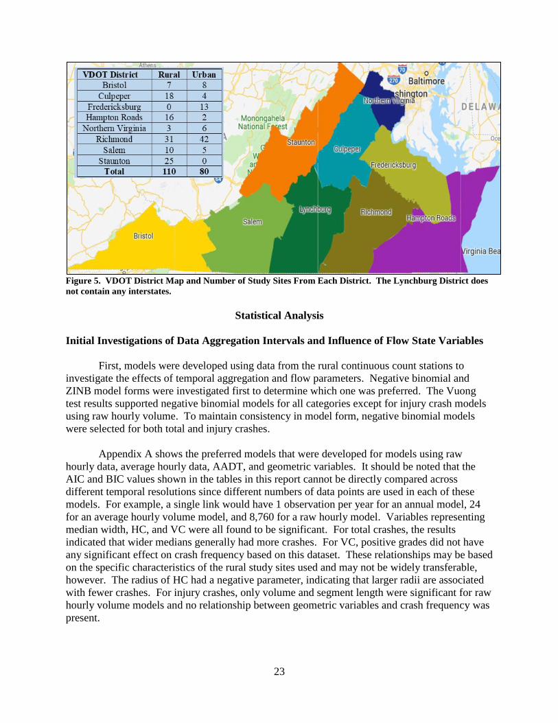
VDOT construction districts have been frequently associated with variations in traffic

safety because of differences in driving population, terrain, and traffic conditions. For example,

interstates in the Salem, Staunton, and Bristol districts are predominantly rural and travel through

mountainous terrain whereas the Northern Virginia and Hampton Roads districts have significant

recurring congestion. This study used districts as a grouping variable to account for the

differences in driving behavior and environment in different parts of Virginia. Figure 5 shows

the locations of the districts and the number of study segments in each district.

23

Figure 5. VDOT District Map and Number of Study Sites From Each District. The Lynchburg District does

not contain any interstates.

Statistical Analysis

Initial Investigations of Data Aggregation Intervals and Influence of Flow State Variables

First, models were developed using data from the rural continuous count stations to

investigate the effects of temporal aggregation and flow parameters. Negative binomial and

ZINB model forms were investigated first to determine which one was preferred. The Vuong

test results supported negative binomial models for all categories except for injury crash models

using raw hourly volume. To maintain consistency in model form, negative binomial models

were selected for both total and injury crashes.

Appendix A shows the preferred models that were developed for models using raw

hourly data, average hourly data, AADT, and geometric variables. It should be noted that the

AIC and BIC values shown in the tables in this report cannot be directly compared across

different temporal resolutions since different numbers of data points are used in each of these

models. For example, a single link would have 1 observation per year for an annual model, 24

for an average hourly volume model, and 8,760 for a raw hourly model. Variables representing

median width, HC, and VC were all found to be significant. For total crashes, the results

indicated that wider medians generally had more crashes. For VC, positive grades did not have

any significant effect on crash frequency based on this dataset. These relationships may be based

on the specific characteristics of the rural study sites used and may not be widely transferable,

however. The radius of HC had a negative parameter, indicating that larger radii are associated

with fewer crashes. For injury crashes, only volume and segment length were significant for raw

hourly volume models and no relationship between geometric variables and crash frequency was

present.

24

Next, models were created by adding flow parameters such as v/c ratio, speed, and

density to the models selected in the previous step. The parameters for the preferred models with

flow parameters included are shown in Appendix B. The percentage of heavy vehicles was also

considered a variable, but it did not have any significant effect on crash frequency in this dataset.

Initially, speed, density, and v/c ratio were all tested in the model. While the models were being

developed, it was found that the v/c ratio was often an unreliable indicator of traffic flow state

since incidents, work zones, or other events might restrict flow at the site. This created a

situation where observed speeds might be low but the corresponding v/c ratio was also low.

Inclusion of the v/c ratio often resulted in counterintuitive parameter signs, so it was removed

from further consideration. After different combinations of volume, speed, and density variables

were examined, it was observed that only speed and density had a logical and statistically

significant relationship when they were used one at a time with volume or when they were both

used in the same model without a volume component. This finding is not surprising since traffic

flow theory indicates that all three variables are related, so their presence in the same model

violates assumptions of parameter independence. Since volume was deemed an important

measure of exposure and speed is more widely available than density, models that used volume

in conjunction with speed were selected as the best alternative.

For all models developed, speed was negatively related to crashes, meaning that lower

average speed was correlated with higher crash frequency. Lower average speeds indicated the

presence of congestion, so this relationship was intuitive. The negative relationship with speed

and injury crashes seems counterintuitive since higher speeds are generally associated with more

severe injuries. This result could be due to how injury was defined and the type of data used for

modeling. Fatal and injury crashes were combined in this category and ranged from a crash

being fatal to a minor injury that did not require any physician or hospital visit. Disaggregating

the injury crash data further by injury severity was not feasible because of the impact on sample

sizes available at each injury level, however. This relationship also might be specific to this

particular dataset. This analysis was based on rural continuous count station data where the

maximum hourly volume observed was 3,822 vph across two lanes. Thus, these results may be

driven by the fact that this dataset was dominated by locations that often experienced speeds near

free flow and a broader variation in traffic speeds was not expected.

Model Comparison

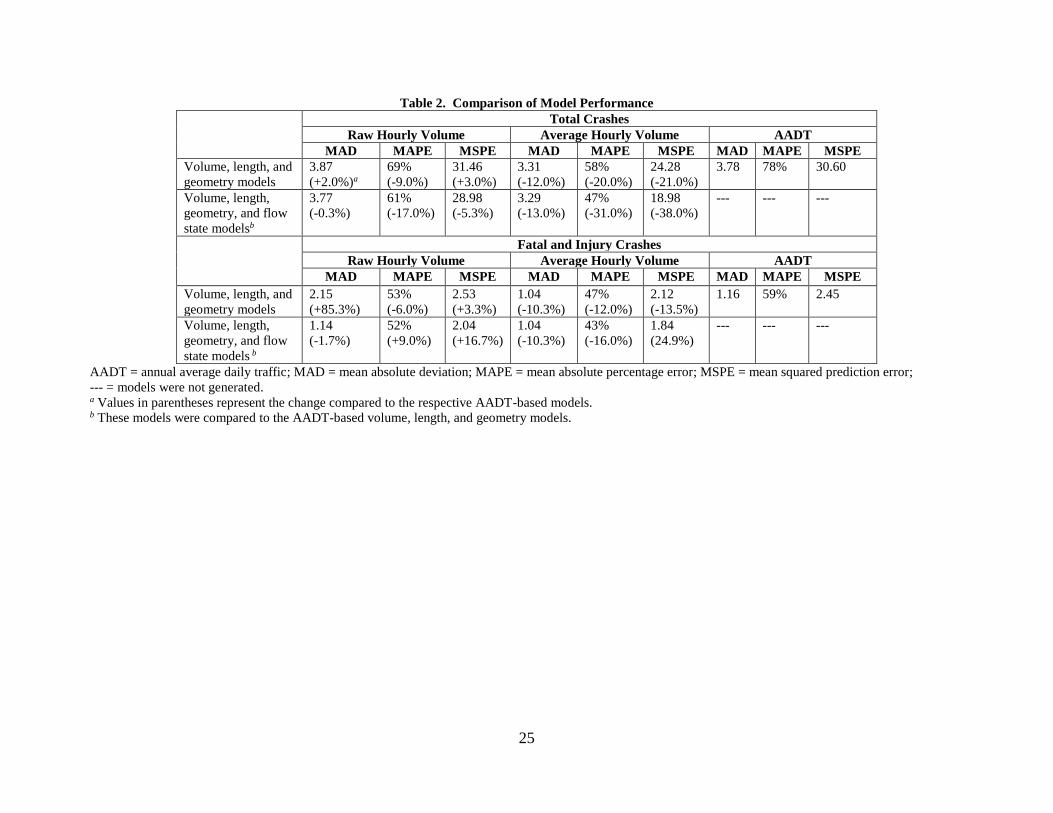
The performance of the preferred raw hourly and average hourly models was contrasted

to the AADT-based models to determine if more disaggregate models improved crash

predictions. For all models, data from 2016 and 2017 were used as the validation dataset. Table

2 shows the comparison among these models. The AADT models did not include speed as a

variable because averaging speed data over 1 year did not capture the effect of speed on traffic

conditions and crashes on an hourly level. For comparison purposes, the volume, flow, and

geometry models were compared to the AADT-based volume and geometry models.

25

Table 2. Comparison of Model Performance

Total Crashes

Raw Hourly Volume Average Hourly Volume AADT

MAD MAPE MSPE MAD MAPE MSPE MAD MAPE MSPE

Volume, length, and

geometry models

3.87

(+2.0%)a

69%

(-9.0%)

31.46

(+3.0%)

3.31

(-12.0%)

58%

(-20.0%)

24.28

(-21.0%)

3.78 78% 30.60

Volume, length,

geometry, and flow

state modelsb

3.77

(-0.3%)

61%

(-17.0%)

28.98

(-5.3%)

3.29

(-13.0%)

47%

(-31.0%)

18.98

(-38.0%)

--- --- ---

Fatal and Injury Crashes

Raw Hourly Volume Average Hourly Volume AADT

MAD MAPE MSPE MAD MAPE MSPE MAD MAPE MSPE

Volume, length, and

geometry models

2.15

(+85.3%)

53%

(-6.0%)

2.53

(+3.3%)

1.04

(-10.3%)

47%

(-12.0%)

2.12

(-13.5%)

1.16 59% 2.45

Volume, length,

geometry, and flow

state models b

1.14

(-1.7%)

52%

(+9.0%)

2.04

(+16.7%)

1.04

(-10.3%)

43%

(-16.0%)

1.84

(24.9%)

--- --- ---

AADT = annual average daily traffic; MAD = mean absolute deviation; MAPE = mean absolute percentage error; MSPE = mean squared prediction error;

--- = models were not generated. a Values in parentheses represent the change compared to the respective AADT-based models. b These models were compared to the AADT-based volume, length, and geometry models.

26

For both the raw and average hourly volume models for total crashes, prediction accuracy

improved as speed variables were added, but the raw hourly models for fatal and injury crashes

gave a mixed result in comparison to the AADT-based model. For these models, the raw hourly

volume and geometry model performed worse than the AADT model in terms of MAD and

MSPE. Results were similar for injury crashes for raw hourly models as well. This result was

likely influenced by the missing data in the raw volume dataset. Ideally, all sites would have

100% hourly data availability. Unfortunately, 23% of the raw hourly data in the validation

dataset did not meet quality control standards and thus were not used to generate predictions.

The prediction accuracy improved significantly for both total and injury crashes when

average hourly data were used. In this case, the average volume calculation helped to smooth

out the discrepancies created by missing raw hourly data. This model consistently performed

better than the AADT-based model for all measures of effectiveness (MOEs). The flow

parameter models showed the highest improvement for all MOEs compared to the AADT-based

model with volume, length, and geometric variables. MAD, MAPE, and MSPE decreased by

13%, 31%, and 38%, respectively, for total crashes and 10%, 16%, and 25%, respectively, for

injury crashes.

Based on the results of preliminary analysis, raw data models were discarded from further

consideration. Gaps in data availability created problems with model predictions, which

worsened performance relative to AADT models. As a result, the next step focused on the use of

average hourly data. The preliminary analysis also showed that inclusion of flow state in crash

prediction models had a beneficial effect, so those variables were subjected to further

examination in the next step.

Assessment of the Effects of Different Speed Sources Using Continuous Count Stations

In the second stage of analysis, the dataset was expanded to include both the rural four-

lane and urban six-lane segments with continuous count station data. In this case, average 15-

minute and average hourly volumes were compared to AADT models, and the quality of

predictions generated using point sensor and INRIX data was compared.

As with the previous stage of the analysis, initial investigations focused on whether

negative binomial or ZINB model forms were preferred. The Vuong test results showed that in

general, negative binomial models performed better than the zero inflated models with respect to

AIC value, variable significance, and sign of estimated coefficients. Appendix C documents the

results from the Vuong test. For the average 15-minute dataset, the volume and geometry model

for fatal and injury crashes for rural segments was the only category where the Vuong test results

preferred the zero inflated model over the negative binomial form. For average hourly data,

negative binomial models outperformed the zero inflated models for both rural and urban

segments, irrespective of crash type. To maintain consistency in model form, negative binomial

models were used for both total and injury crashes.

Volume and Geometry Models

Appendix D shows the model parameters for the volume and geometry models for all

levels of temporal aggregation. For urban segments, the only statistically significant geometric

variable was median width for all levels of aggregation and crash type. The segments with curve

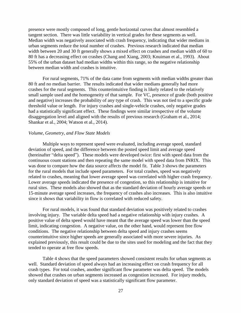
27

presence were mostly composed of long, gentle horizontal curves that almost resembled a

tangent section. There was little variability in vertical grades for these segments as well.

Median width was negatively associated with crash frequency, indicating that wider medians in

urban segments reduce the total number of crashes. Previous research indicated that median

width between 20 and 30 ft generally shows a mixed effect on crashes and median width of 60 to

80 ft has a decreasing effect on crashes (Chang and Xiang, 2003; Knuiman et al., 1993). About

55% of the urban dataset had median widths within this range, so the negative relationship

between median width and crashes is intuitive.

For rural segments, 71% of the data came from segments with median widths greater than

80 ft and no median barrier. The results indicated that wider medians generally had more

crashes for the rural segments. This counterintuitive finding is likely related to the relatively

small sample used and the homogeneity of that sample. For VC, presence of grade (both positive

and negative) increases the probability of any type of crash. This was not tied to a specific grade

threshold value or length. For injury crashes and single-vehicle crashes, only negative grades

had a statistically significant effect. These findings were similar irrespective of the volume

disaggregation level and aligned with the results of previous research (Graham et al., 2014;

Shankar et al., 2004; Watson et al., 2014).

Volume, Geometry, and Flow State Models

Multiple ways to represent speed were evaluated, including average speed, standard

deviation of speed, and the difference between the posted speed limit and average speed

(hereinafter “delta speed”). These models were developed twice: first with speed data from the

continuous count stations and then repeating the same model with speed data from INRIX. This

was done to compare how the data source affects the model fit. Table 3 shows the parameters

for the rural models that include speed parameters. For total crashes, speed was negatively

related to crashes, meaning that lower average speed was correlated with higher crash frequency.

Lower average speeds indicated the presence of congestion, so this relationship is intuitive for

rural sites. These models also showed that as the standard deviation of hourly average speeds or

15-minute average speed increases, the frequency of crashes also increases. This is also intuitive

since it shows that variability in flow is correlated with reduced safety.

For rural models, it was found that standard deviation was positively related to crashes

involving injury. The variable delta speed had a negative relationship with injury crashes. A

positive value of delta speed would have meant that the average speed was lower than the speed

limit, indicating congestion. A negative value, on the other hand, would represent free flow

conditions. The negative relationship between delta speed and injury crashes seems

counterintuitive since higher speeds are generally associated with more severe injuries. As

explained previously, this result could be due to the sites used for modeling and the fact that they

tended to operate at free flow speeds.

Table 4 shows that the speed parameters showed consistent results for urban segments as

well. Standard deviation of speed always had an increasing effect on crash frequency for all

crash types. For total crashes, another significant flow parameter was delta speed. The models

showed that crashes on urban segments increased as congestion increased. For injury models,

only standard deviation of speed was a statistically significant flow parameter.

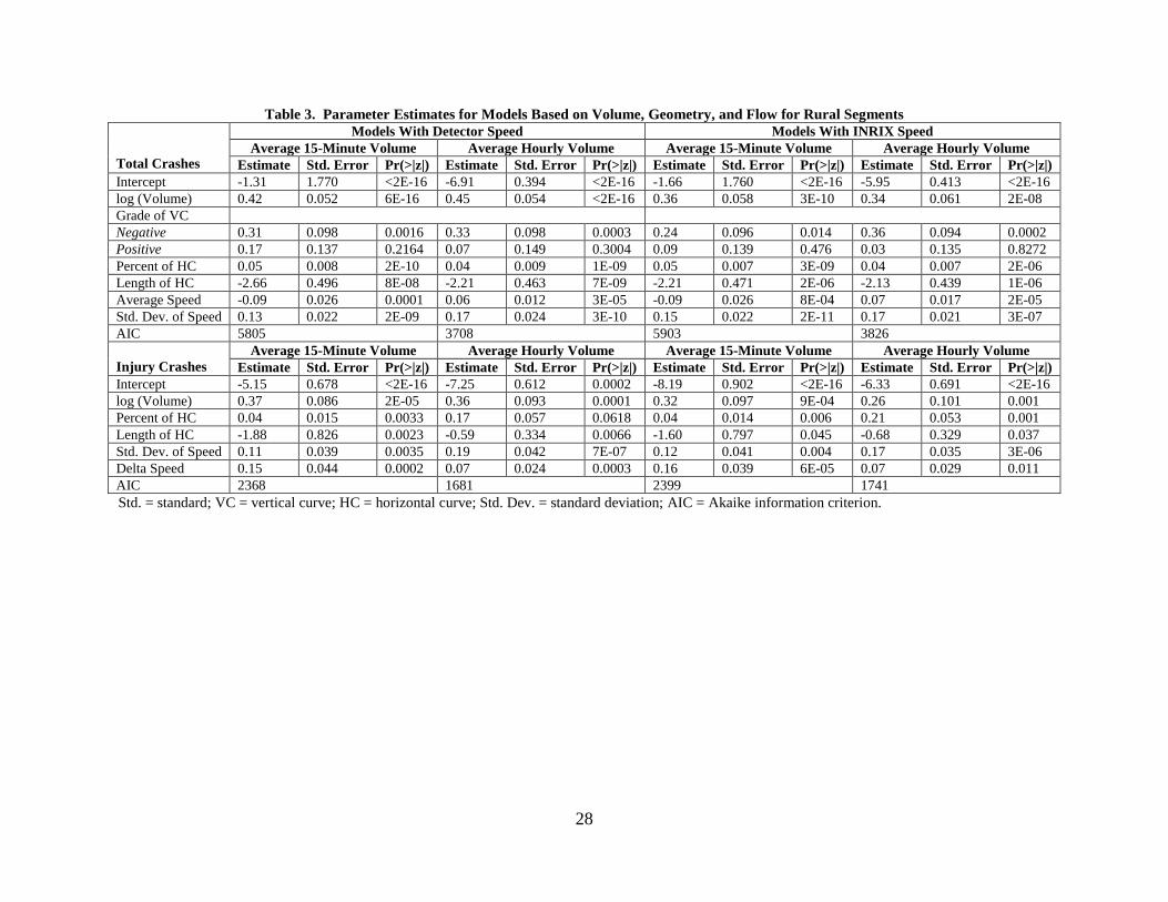
28

Table 3. Parameter Estimates for Models Based on Volume, Geometry, and Flow for Rural Segments

Total Crashes

Models With Detector Speed Models With INRIX Speed

Average 15-Minute Volume Average Hourly Volume Average 15-Minute Volume Average Hourly Volume

Estimate Std. Error Pr(>|z|) Estimate Std. Error Pr(>|z|) Estimate Std. Error Pr(>|z|) Estimate Std. Error Pr(>|z|)

Intercept -1.31 1.770 <2E-16 -6.91 0.394 <2E-16 -1.66 1.760 <2E-16 -5.95 0.413 <2E-16

log (Volume) 0.42 0.052 6E-16 0.45 0.054 <2E-16 0.36 0.058 3E-10 0.34 0.061 2E-08

Grade of VC

Negative 0.31 0.098 0.0016 0.33 0.098 0.0003 0.24 0.096 0.014 0.36 0.094 0.0002

Positive 0.17 0.137 0.2164 0.07 0.149 0.3004 0.09 0.139 0.476 0.03 0.135 0.8272

Percent of HC 0.05 0.008 2E-10 0.04 0.009 1E-09 0.05 0.007 3E-09 0.04 0.007 2E-06

Length of HC -2.66 0.496 8E-08 -2.21 0.463 7E-09 -2.21 0.471 2E-06 -2.13 0.439 1E-06

Average Speed -0.09 0.026 0.0001 0.06 0.012 3E-05 -0.09 0.026 8E-04 0.07 0.017 2E-05

Std. Dev. of Speed 0.13 0.022 2E-09 0.17 0.024 3E-10 0.15 0.022 2E-11 0.17 0.021 3E-07

AIC 5805 3708 5903 3826

Injury Crashes

Average 15-Minute Volume Average Hourly Volume Average 15-Minute Volume Average Hourly Volume

Estimate Std. Error Pr(>|z|) Estimate Std. Error Pr(>|z|) Estimate Std. Error Pr(>|z|) Estimate Std. Error Pr(>|z|)

Intercept -5.15 0.678 <2E-16 -7.25 0.612 0.0002 -8.19 0.902 <2E-16 -6.33 0.691 <2E-16

log (Volume) 0.37 0.086 2E-05 0.36 0.093 0.0001 0.32 0.097 9E-04 0.26 0.101 0.001

Percent of HC 0.04 0.015 0.0033 0.17 0.057 0.0618 0.04 0.014 0.006 0.21 0.053 0.001

Length of HC -1.88 0.826 0.0023 -0.59 0.334 0.0066 -1.60 0.797 0.045 -0.68 0.329 0.037

Std. Dev. of Speed 0.11 0.039 0.0035 0.19 0.042 7E-07 0.12 0.041 0.004 0.17 0.035 3E-06

Delta Speed 0.15 0.044 0.0002 0.07 0.024 0.0003 0.16 0.039 6E-05 0.07 0.029 0.011

AIC 2368 1681 2399 1741

Std. = standard; VC = vertical curve; HC = horizontal curve; Std. Dev. = standard deviation; AIC = Akaike information criterion.

29

Table 4. Parameter Estimates for Models Based on Volume, Geometry, and Flow for Urban Segments

Total Crashes

Models With Detector Speed Models With INRIX Speed

Average 15-Minute Volume Average Hourly Volume Average 15-Minute Volume Average Hourly Volume

Estimate

Std.

Error

Pr(>|z|)

Estimate

Std.

Error

Pr(>|z|)

Estimate

Std.

Error

Pr(>|z|)

Estimate

Std.

Error

Pr(>|z|)

Intercept -10.59 0.755 <2E-16 -4.87 0.347 <2E-16 -7.64 0.665 <2E-16 -4.81 0.338 <2E-16

log (Volume) 0.55 0.051 <2E-16 0.34 0.048 9E-13 0.58 0.052 <2E-16 0.32 0.048 9E-12

Median Width -0.21 0.167 <2E-16 -0.22 0.366 <2E-16 -0.15 0.208 <2E-16 -0.28 0.278 <2E-16

Std. Dev. of Speed 0.08 0.009 <2E-16 0.13 0.012 <2E-16 0.11 0.013 <2E-16 0.16 0.111 <2E-16

Delta Speed 0.11 0.013 <2E-16 0.05 0.006 <2E-16 0.03 0.011 0.0002 0.02 0.009 1.4E-05

AIC 7709 4264 8407 4887

Injury Crashes

Average 15-Minute Volume Average Hourly Volume Average 15-Minute Volume Average Hourly Volume

Estimate

Std.

Error

Pr(>|z|)

Estimate

Std.

Error

Pr(>|z|)

Estimate

Std.

Error

Pr(>|z|)

Estimate

Std.

Error

Pr(>|z|)

Intercept -11.14 1.34 <2E-16 -6.62 0.594 <2E-16 -8.07 1.16 <2E-16 -6.07 0.539 <2E-16

log (Volume) 0.51 0.089 1E-08 0.36 0.079 6E-07 0.44 0.088 6E-07 0.32 0.072 8E-06

Median Width -0.13 0.128 1E-10 -0.25 0.123 <2E-16 -0.17 0.146 2E-06 -0.19 0.135 <2E-16

Std. Dev. of Speed 0.07 0.017 2E-05 0.17 0.013 <2E-16 0.12 0.018 3E-10 0.15 0.009 <2E-16

AIC 3274 2059 3515 2328

Std. = standard; Std. Dev. = standard deviation; AIC = Akaike information criterion.

30

Model Comparison

Next, the developed models were compared. Model comparisons provide a check on

whether flow parameters improve model performance as expected. They also show how

different levels of data aggregation affect the performance. Finally, they show whether the

model performance is significantly different depending on the source of speed data. For all

models, irrespective of type of facility, type of crash, or level of data aggregation, the highest

prediction accuracy was achieved across all validation MOEs when speed components were

added to the model.

Tables 5 and 6 show the comparison of performance among the models developed for

rural and urban sites, respectively. Even though the average 15-minute volume models

performed better than the AADT-based model most of the time, there were certain models

(injury models for urban segments) that were worse than the AADT models. It is possible that at

a 15-minute level, data are too noisy to capture the true relationship between crashes and flow

parameters. Likewise, inaccuracies in time stamps of crash reports could influence results at that

level. The prediction accuracy improved significantly for all models when average hourly data

were used. In this case, the aggregation interval was neither too disaggregated to capture the

random nature of crashes nor too aggregated to lose the variation in traffic.

For the rural hourly volume, geometry, and flow models, MAD, MAPE, and MSPE

improved by 11%, 33%, and 29%, respectively, when continuous count stations were used as the

speed data source and 10%, 28%, and 17%, respectively, when INRIX speed data were used.

For the urban models, similar trends were observed where MAD, MAPE, and MSPE improved

by 20%, 22%, and 38%, respectively, for detector data and 20%, 19%, and 32% for INRIX data.

In both cases, these models were compared to AADT-based volume and geometry models. Even

though models using INRIX data performed slightly worse than the models based on continuous

count data, they were still far better than AADT-based models.

Because of the random nature of crash occurrence, the 15-minute data had too much

variability to generate useful models. Similarly, aggregated models that rely on AADT may fail

to capture variations in traffic flow that could influence safety. Another very important finding

was that speed variables played a significant role in model performance irrespective of their

source. Since current models rely only on volume, quality of volume data dictates the quality of

the model. This step showed that INRIX data can be used as an alternate source for speed data

without reducing the quality of crash prediction models. Models developed using INRIX data

performed similarly to the models using speeds from continuous count stations during model

validation. For all crash types and model categories, INRIX models consistently outperformed

AADT models. This provided a strong basis for using INRIX data along with historic volume

distributions from short count stations in the next step.

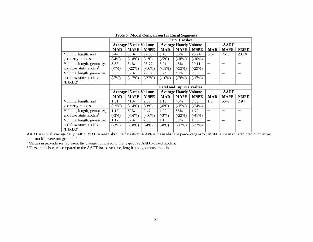
31

Table 5. Model Comparison for Rural Segmentsa

Total Crashes

Average 15-min Volume Average Hourly Volume AADT

MAD MAPE MSPE MAD MAPE MSPE MAD MAPE MSPE

Volume, length, and

geometry models

3.47 58% 27.88 3.45 58% 25.24 3.62 76% 28.18

(-4%) (-18%) (-1%) (-5%) (-18%) (-10%)

Volume, length, geometry,

and flow state modelsb

3.37 54% 23.77 3.21 43% 20.11 ─ ─ ─

(-7%) (-22%) (-16%) (-11%) (-33%) (-29%)

Volume, length, geometry,

and flow state models

(INRIX)b

3.35 59% 22.07 3.24 48% 23.5 ─ ─ ─

(-7%) (-17%) (-22%) (-10%) (-28%) (-17%)

Fatal and Injury Crashes

Average 15-min Volume Average Hourly Volume AADT

MAD MAPE MSPE MAD MAPE MSPE MAD MAPE MSPE

Volume, length, and

geometry models

1.31 41% 2.86 1.13 40% 2.23 1.2 55% 2.94

(+9%) (-14%) (-3%) (-6%) (-15%) (-24%)

Volume, length, geometry,

and flow state modelsb

1.17 39% 2.47 1.09 33% 1.72 ─ ─ ─

(-3%) (-16%) (-16%) (-9%) (-22%) (-41%)

Volume, length, geometry,

and flow state models

(INRIX)b

1.17 37% 2.83 1.1 38% 1.85 ─ ─ ─

(-3%) (-18%) (-4%) (-8%) (-17%) (-37%)

AADT = annual average daily traffic; MAD = mean absolute deviation; MAPE = mean absolute percentage error; MSPE = mean squared prediction error;

--- = models were not generated. a Values in parentheses represent the change compared to the respective AADT-based models. b These models were compared to the AADT-based volume, length, and geometry models.

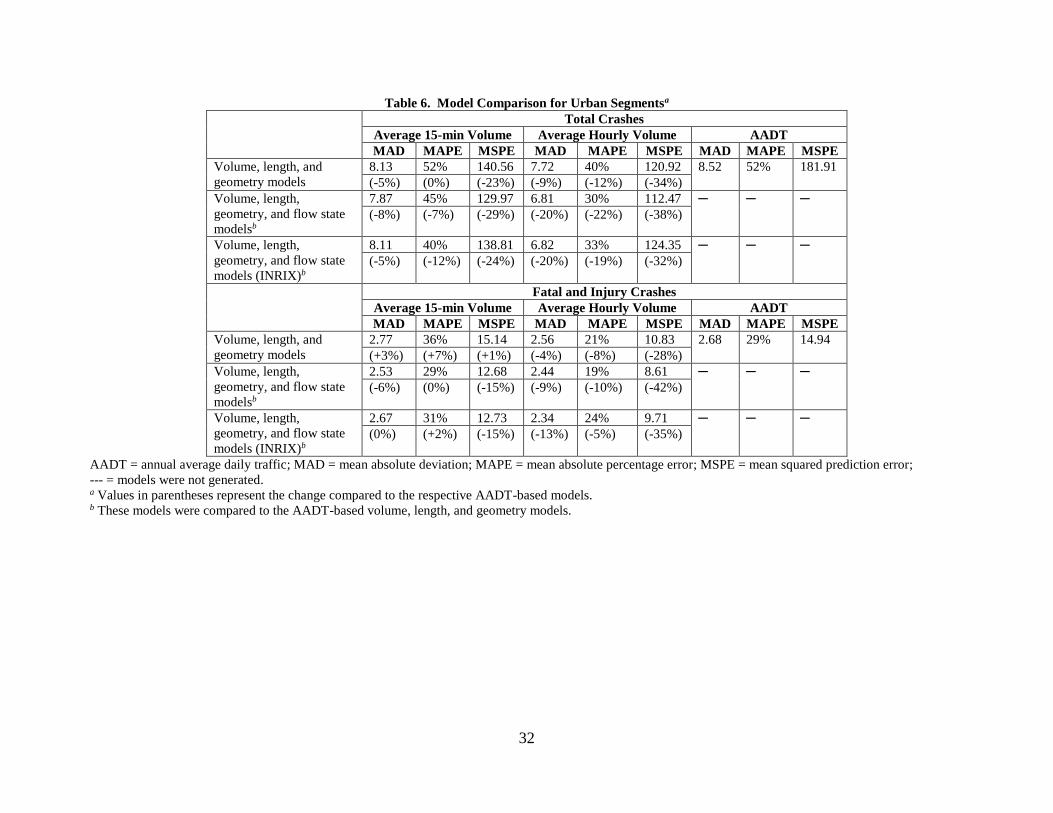
32

Table 6. Model Comparison for Urban Segmentsa

Total Crashes

Average 15-min Volume Average Hourly Volume AADT

MAD MAPE MSPE MAD MAPE MSPE MAD MAPE MSPE

Volume, length, and

geometry models

8.13 52% 140.56 7.72 40% 120.92 8.52 52% 181.91

(-5%) (0%) (-23%) (-9%) (-12%) (-34%)

Volume, length,

geometry, and flow state

modelsb

7.87 45% 129.97 6.81 30% 112.47 ─ ─ ─

(-8%) (-7%) (-29%) (-20%) (-22%) (-38%)

Volume, length,

geometry, and flow state

models (INRIX)b

8.11 40% 138.81 6.82 33% 124.35 ─ ─ ─

(-5%) (-12%) (-24%) (-20%) (-19%) (-32%)

Fatal and Injury Crashes

Average 15-min Volume Average Hourly Volume AADT

MAD MAPE MSPE MAD MAPE MSPE MAD MAPE MSPE

Volume, length, and

geometry models

2.77 36% 15.14 2.56 21% 10.83 2.68 29% 14.94

(+3%) (+7%) (+1%) (-4%) (-8%) (-28%)

Volume, length,

geometry, and flow state

modelsb

2.53 29% 12.68 2.44 19% 8.61 ─ ─ ─

(-6%) (0%) (-15%) (-9%) (-10%) (-42%)

Volume, length,

geometry, and flow state

models (INRIX)b

2.67 31% 12.73 2.34 24% 9.71 ─ ─ ─

(0%) (+2%) (-15%) (-13%) (-5%) (-35%)

AADT = annual average daily traffic; MAD = mean absolute deviation; MAPE = mean absolute percentage error; MSPE = mean squared prediction error;

--- = models were not generated. a Values in parentheses represent the change compared to the respective AADT-based models. b These models were compared to the AADT-based volume, length, and geometry models.

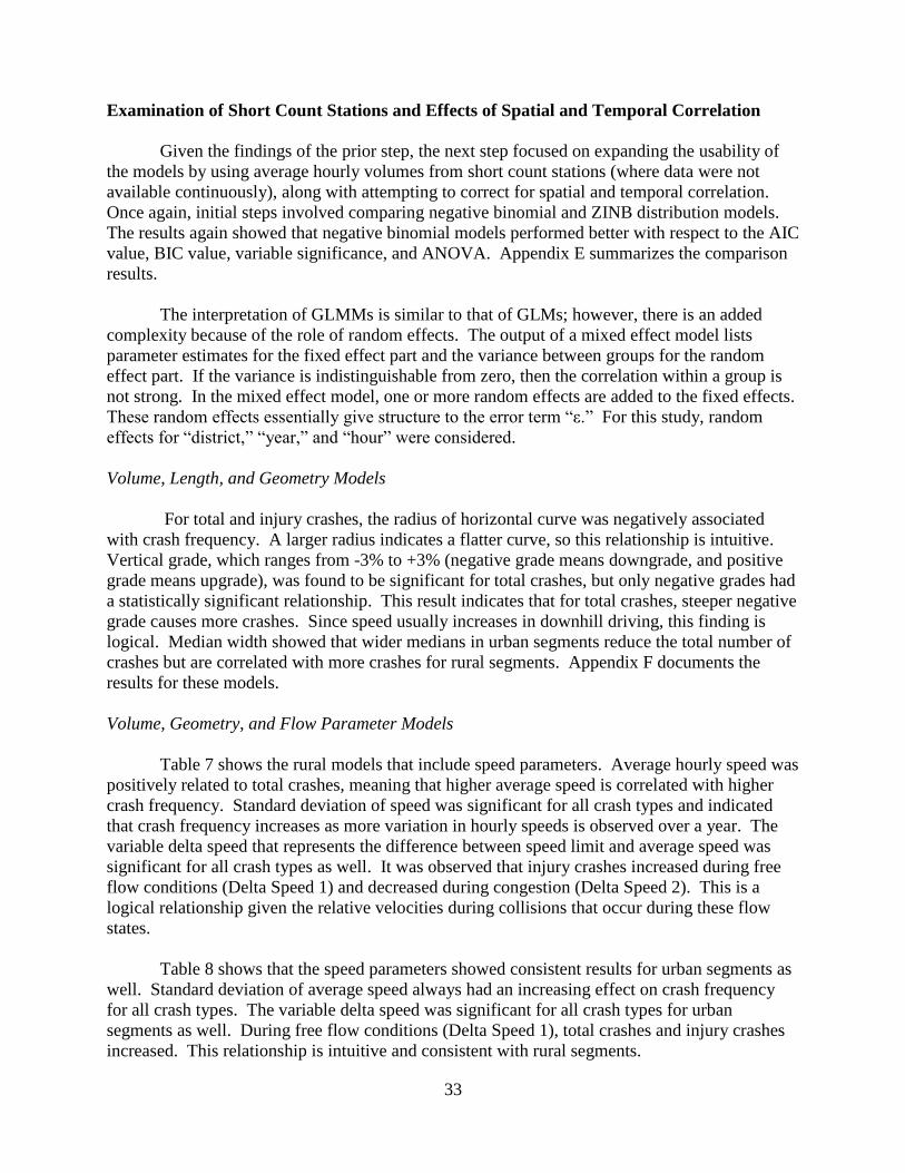
33

Examination of Short Count Stations and Effects of Spatial and Temporal Correlation

Given the findings of the prior step, the next step focused on expanding the usability of

the models by using average hourly volumes from short count stations (where data were not

available continuously), along with attempting to correct for spatial and temporal correlation.

Once again, initial steps involved comparing negative binomial and ZINB distribution models.

The results again showed that negative binomial models performed better with respect to the AIC

value, BIC value, variable significance, and ANOVA. Appendix E summarizes the comparison

results.

The interpretation of GLMMs is similar to that of GLMs; however, there is an added

complexity because of the role of random effects. The output of a mixed effect model lists

parameter estimates for the fixed effect part and the variance between groups for the random

effect part. If the variance is indistinguishable from zero, then the correlation within a group is

not strong. In the mixed effect model, one or more random effects are added to the fixed effects.

These random effects essentially give structure to the error term “ε.” For this study, random

effects for “district,” “year,” and “hour” were considered.

Volume, Length, and Geometry Models

For total and injury crashes, the radius of horizontal curve was negatively associated

with crash frequency. A larger radius indicates a flatter curve, so this relationship is intuitive.

Vertical grade, which ranges from -3% to +3% (negative grade means downgrade, and positive

grade means upgrade), was found to be significant for total crashes, but only negative grades had

a statistically significant relationship. This result indicates that for total crashes, steeper negative

grade causes more crashes. Since speed usually increases in downhill driving, this finding is

logical. Median width showed that wider medians in urban segments reduce the total number of

crashes but are correlated with more crashes for rural segments. Appendix F documents the

results for these models.

Volume, Geometry, and Flow Parameter Models

Table 7 shows the rural models that include speed parameters. Average hourly speed was

positively related to total crashes, meaning that higher average speed is correlated with higher

crash frequency. Standard deviation of speed was significant for all crash types and indicated

that crash frequency increases as more variation in hourly speeds is observed over a year. The

variable delta speed that represents the difference between speed limit and average speed was

significant for all crash types as well. It was observed that injury crashes increased during free

flow conditions (Delta Speed 1) and decreased during congestion (Delta Speed 2). This is a

logical relationship given the relative velocities during collisions that occur during these flow

states.

Table 8 shows that the speed parameters showed consistent results for urban segments as

well. Standard deviation of average speed always had an increasing effect on crash frequency

for all crash types. The variable delta speed was significant for all crash types for urban

segments as well. During free flow conditions (Delta Speed 1), total crashes and injury crashes

increased. This relationship is intuitive and consistent with rural segments.

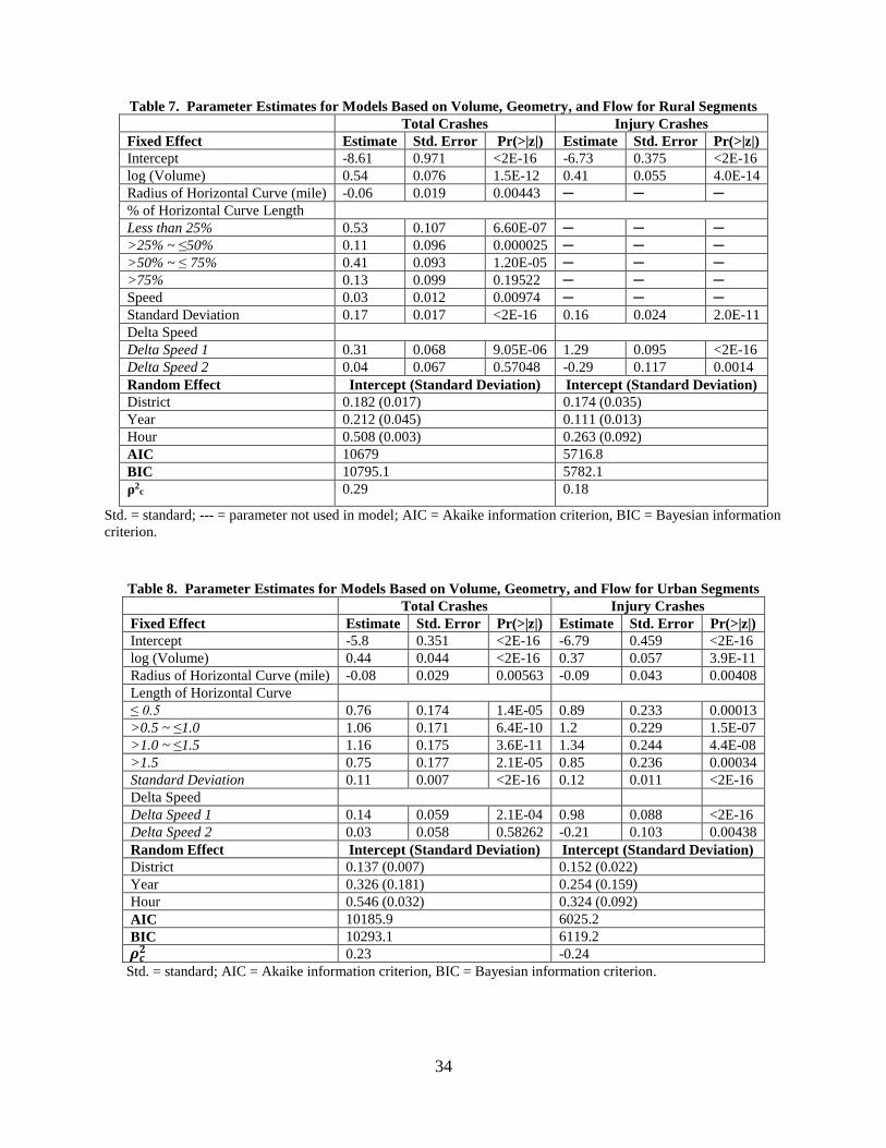
34

Table 7. Parameter Estimates for Models Based on Volume, Geometry, and Flow for Rural Segments

Total Crashes Injury Crashes

Fixed Effect Estimate Std. Error Pr(>|z|) Estimate Std. Error Pr(>|z|)

Intercept -8.61 0.971 <2E-16 -6.73 0.375 <2E-16

log (Volume) 0.54 0.076 1.5E-12 0.41 0.055 4.0E-14

Radius of Horizontal Curve (mile) -0.06 0.019 0.00443 ─ ─ ─

% of Horizontal Curve Length

Less than 25% 0.53 0.107 6.60E-07 ─ ─ ─

>25% ~ ≤50% 0.11 0.096 0.000025 ─ ─ ─

>50% ~ ≤ 75% 0.41 0.093 1.20E-05 ─ ─ ─

>75% 0.13 0.099 0.19522 ─ ─ ─

Speed 0.03 0.012 0.00974 ─ ─ ─

Standard Deviation 0.17 0.017 <2E-16 0.16 0.024 2.0E-11

Delta Speed

Delta Speed 1 0.31 0.068 9.05E-06 1.29 0.095 <2E-16

Delta Speed 2 0.04 0.067 0.57048 -0.29 0.117 0.0014

Random Effect Intercept (Standard Deviation) Intercept (Standard Deviation)

District 0.182 (0.017) 0.174 (0.035)

Year 0.212 (0.045) 0.111 (0.013)

Hour 0.508 (0.003) 0.263 (0.092)

AIC 10679 5716.8

BIC 10795.1 5782.1

ρ2c 0.29 0.18

Std. = standard; --- = parameter not used in model; AIC = Akaike information criterion, BIC = Bayesian information

criterion.

Table 8. Parameter Estimates for Models Based on Volume, Geometry, and Flow for Urban Segments

Total Crashes Injury Crashes

Fixed Effect Estimate Std. Error Pr(>|z|) Estimate Std. Error Pr(>|z|)

Intercept -5.8 0.351 <2E-16 -6.79 0.459 <2E-16

log (Volume) 0.44 0.044 <2E-16 0.37 0.057 3.9E-11

Radius of Horizontal Curve (mile) -0.08 0.029 0.00563 -0.09 0.043 0.00408

Length of Horizontal Curve

≤ 0.5 0.76 0.174 1.4E-05 0.89 0.233 0.00013

>0.5 ~ ≤1.0 1.06 0.171 6.4E-10 1.2 0.229 1.5E-07

>1.0 ~ ≤1.5 1.16 0.175 3.6E-11 1.34 0.244 4.4E-08

>1.5 0.75 0.177 2.1E-05 0.85 0.236 0.00034

Standard Deviation 0.11 0.007 <2E-16 0.12 0.011 <2E-16

Delta Speed

Delta Speed 1 0.14 0.059 2.1E-04 0.98 0.088 <2E-16

Delta Speed 2 0.03 0.058 0.58262 -0.21 0.103 0.00438

Random Effect Intercept (Standard Deviation) Intercept (Standard Deviation)

District 0.137 (0.007) 0.152 (0.022)

Year 0.326 (0.181) 0.254 (0.159)

Hour 0.546 (0.032) 0.324 (0.092)

AIC 10185.9 6025.2

BIC 10293.1 6119.2

0.23 -0.24

Std. = standard; AIC = Akaike information criterion, BIC = Bayesian information criterion.

𝝆𝒄𝟐

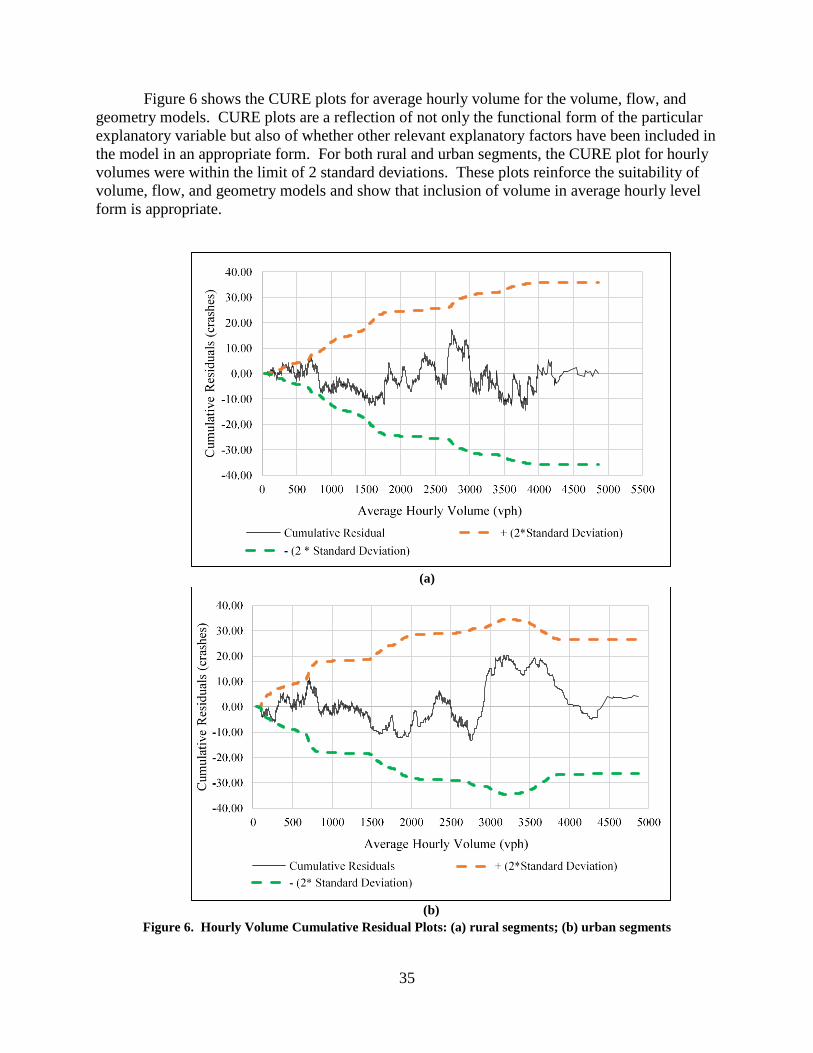
35

Figure 6 shows the CURE plots for average hourly volume for the volume, flow, and

geometry models. CURE plots are a reflection of not only the functional form of the particular

explanatory variable but also of whether other relevant explanatory factors have been included in

the model in an appropriate form. For both rural and urban segments, the CURE plot for hourly

volumes were within the limit of 2 standard deviations. These plots reinforce the suitability of

volume, flow, and geometry models and show that inclusion of volume in average hourly level

form is appropriate.

Figure 6. Hourly Volume Cumulative Residual Plots: (a) rural segments; (b) urban segments

(a)

(b)

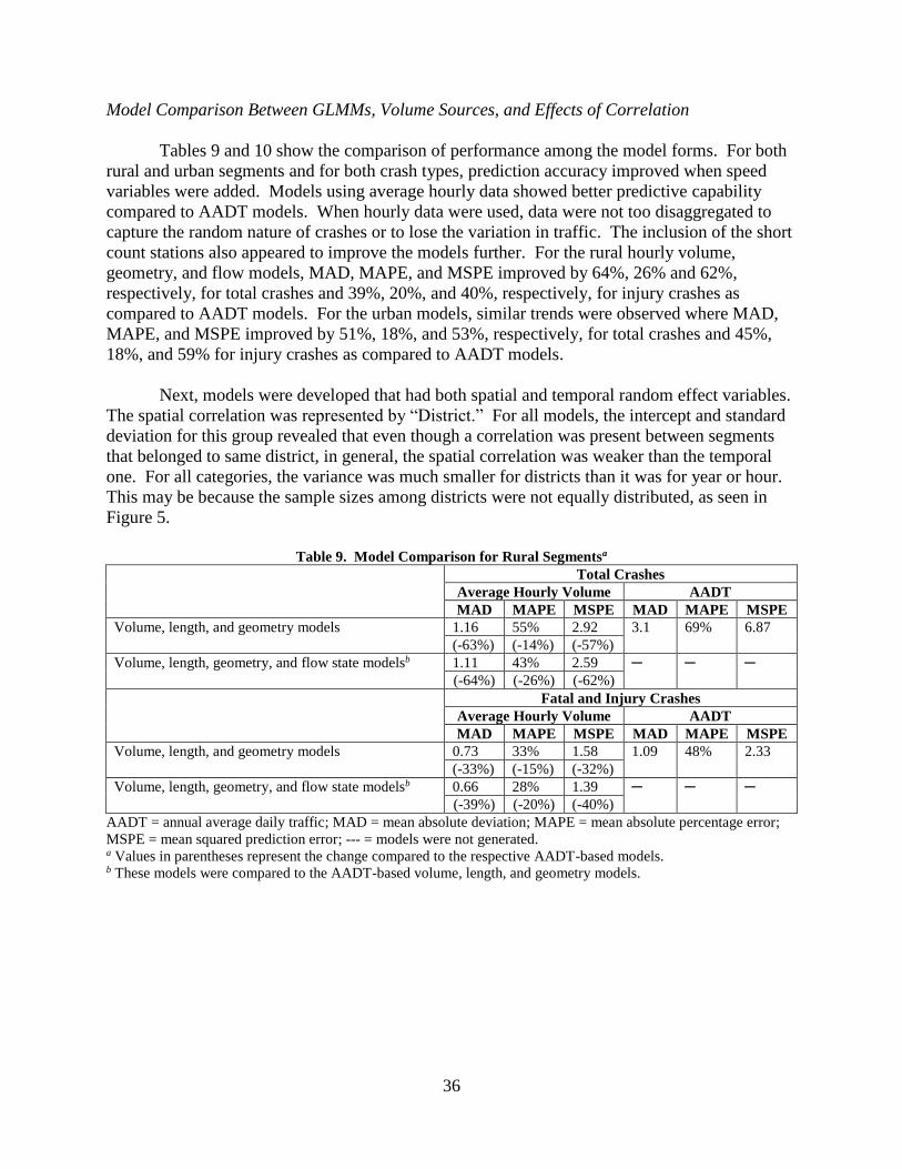
36

Model Comparison Between GLMMs, Volume Sources, and Effects of Correlation

Tables 9 and 10 show the comparison of performance among the model forms. For both

rural and urban segments and for both crash types, prediction accuracy improved when speed

variables were added. Models using average hourly data showed better predictive capability

compared to AADT models. When hourly data were used, data were not too disaggregated to

capture the random nature of crashes or to lose the variation in traffic. The inclusion of the short

count stations also appeared to improve the models further. For the rural hourly volume,

geometry, and flow models, MAD, MAPE, and MSPE improved by 64%, 26% and 62%,

respectively, for total crashes and 39%, 20%, and 40%, respectively, for injury crashes as

compared to AADT models. For the urban models, similar trends were observed where MAD,

MAPE, and MSPE improved by 51%, 18%, and 53%, respectively, for total crashes and 45%,

18%, and 59% for injury crashes as compared to AADT models.

Next, models were developed that had both spatial and temporal random effect variables.

The spatial correlation was represented by “District.” For all models, the intercept and standard

deviation for this group revealed that even though a correlation was present between segments

that belonged to same district, in general, the spatial correlation was weaker than the temporal

one. For all categories, the variance was much smaller for districts than it was for year or hour.

This may be because the sample sizes among districts were not equally distributed, as seen in

Figure 5.

Table 9. Model Comparison for Rural Segmentsa

Total Crashes

Average Hourly Volume AADT

MAD MAPE MSPE MAD MAPE MSPE

Volume, length, and geometry models 1.16 55% 2.92 3.1 69% 6.87

(-63%) (-14%) (-57%)

Volume, length, geometry, and flow state modelsb 1.11 43% 2.59 ─ ─ ─

(-64%) (-26%) (-62%)

Fatal and Injury Crashes

Average Hourly Volume AADT

MAD MAPE MSPE MAD MAPE MSPE

Volume, length, and geometry models 0.73 33% 1.58 1.09 48% 2.33

(-33%) (-15%) (-32%)

Volume, length, geometry, and flow state modelsb 0.66 28% 1.39 ─ ─ ─

(-39%) (-20%) (-40%)

AADT = annual average daily traffic; MAD = mean absolute deviation; MAPE = mean absolute percentage error;

MSPE = mean squared prediction error; --- = models were not generated. a Values in parentheses represent the change compared to the respective AADT-based models. b These models were compared to the AADT-based volume, length, and geometry models.

37

Table 10. Model Comparison for Urban Segmentsa

Total Crashes

Average Hourly Volume AADT

MAD MAPE MSPE MAD MAPE MSPE

Volume, length, and geometry models 1.92 35% 47.92 2.98 47% 79.43

(-36%) (-12%) (-40%)

Volume, length, geometry, and flow state modelsb 1.45 29% 36.95 ─ ─ ─

(-51%) (-18%) (-53%)

Fatal and Injury Crashes

Average Hourly Volume AADT

MAD MAPE MSPE MAD MAPE MSPE

Volume, length, and geometry models 1.09 12% 4.58 1.69 26% 8.82

(-36%) (-14%) (-48%)

Volume, length, geometry, and flow state modelsb 0.93 8% 3.63 ─ ─ ─

(-45%) (-18%) (-59%)

AADT = annual average daily traffic; MAD = mean absolute deviation; MAPE = mean absolute percentage error; MSPE = mean squared prediction error;

--- = models were not generated. a Values in parentheses represent the change compared to the respective AADT-based models. b These models were compared to the AADT-based volume, length, and geometry models.

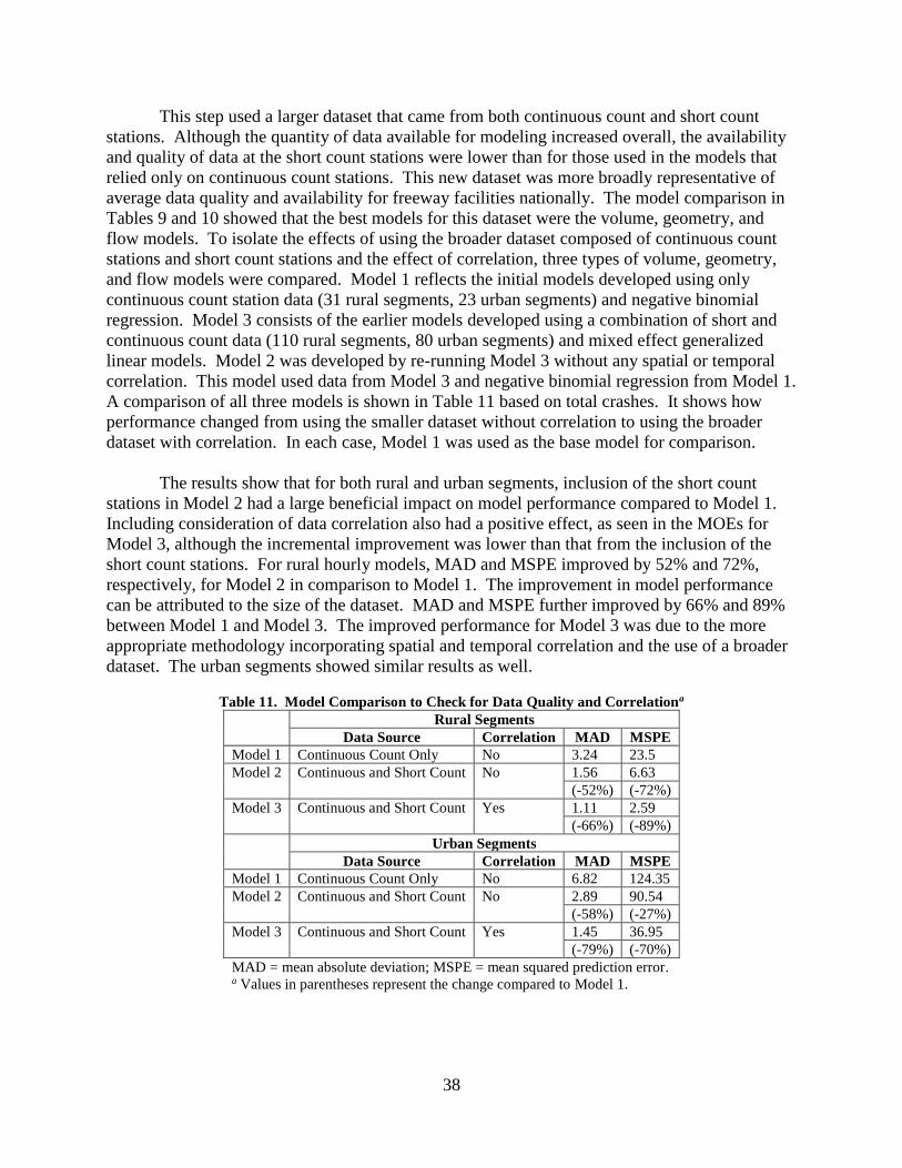
38

This step used a larger dataset that came from both continuous count and short count

stations. Although the quantity of data available for modeling increased overall, the availability

and quality of data at the short count stations were lower than for those used in the models that

relied only on continuous count stations. This new dataset was more broadly representative of

average data quality and availability for freeway facilities nationally. The model comparison in

Tables 9 and 10 showed that the best models for this dataset were the volume, geometry, and

flow models. To isolate the effects of using the broader dataset composed of continuous count

stations and short count stations and the effect of correlation, three types of volume, geometry,

and flow models were compared. Model 1 reflects the initial models developed using only

continuous count station data (31 rural segments, 23 urban segments) and negative binomial

regression. Model 3 consists of the earlier models developed using a combination of short and

continuous count data (110 rural segments, 80 urban segments) and mixed effect generalized

linear models. Model 2 was developed by re-running Model 3 without any spatial or temporal

correlation. This model used data from Model 3 and negative binomial regression from Model 1.

A comparison of all three models is shown in Table 11 based on total crashes. It shows how

performance changed from using the smaller dataset without correlation to using the broader

dataset with correlation. In each case, Model 1 was used as the base model for comparison.

The results show that for both rural and urban segments, inclusion of the short count

stations in Model 2 had a large beneficial impact on model performance compared to Model 1.

Including consideration of data correlation also had a positive effect, as seen in the MOEs for

Model 3, although the incremental improvement was lower than that from the inclusion of the

short count stations. For rural hourly models, MAD and MSPE improved by 52% and 72%,

respectively, for Model 2 in comparison to Model 1. The improvement in model performance

can be attributed to the size of the dataset. MAD and MSPE further improved by 66% and 89%

between Model 1 and Model 3. The improved performance for Model 3 was due to the more

appropriate methodology incorporating spatial and temporal correlation and the use of a broader

dataset. The urban segments showed similar results as well.

Table 11. Model Comparison to Check for Data Quality and Correlationa

Rural Segments

Data Source Correlation MAD MSPE

Model 1 Continuous Count Only No 3.24 23.5

Model 2 Continuous and Short Count No 1.56 6.63

(-52%) (-72%)

Model 3 Continuous and Short Count Yes 1.11 2.59

(-66%) (-89%)

Urban Segments

Data Source Correlation MAD MSPE

Model 1 Continuous Count Only No 6.82 124.35

Model 2 Continuous and Short Count No 2.89 90.54

(-58%) (-27%)

Model 3 Continuous and Short Count Yes 1.45 36.95

(-79%) (-70%)

MAD = mean absolute deviation; MSPE = mean squared prediction error. a Values in parentheses represent the change compared to Model 1.

39

Since current models such as those in the HSM rely only on volume, the quality of

volume data dictates the quality of the model. The analysis showed that using short count

stations as a data source does not diminish the quality of developed models if speed-related

variables are also used in the model. This means that a combination of different volume data

sources with good quality speed data can lessen the dependency on the quality of the volume

data without compromising performance. Since short count stations are more common, this

finding also indicates that this approach can be applied broadly across transportation networks.

CONCLUSIONS

Models that incorporated speed along with volume provided better performance than models

that used other combinations of flow variables. Multiple flow parameters were investigated,

including heavy vehicle percentage, v/c ratio, speed, and density. Only speed and density

had a logical and statistically significant relationship when they were combined with volume.

Since speed is more widely available than density, models that used volume in conjunction

with speed were selected as the best alternatives.

For all models, prediction accuracy was improved across all validation MOEs when the

speed components were added vs. when the speed components were not added. Speeds from

both continuous count stations and probe data provided similar results.

Models using raw hourly data were inferior to models using other levels of aggregation. The

raw hourly models were influenced by the missing data in the dataset. About 23% of the raw

hourly data in the validation dataset did not meet quality control standards and thus could not

be used to generate predictions. These models did not have a better prediction capability in

comparison to AADT models.

Using averages of available data in each hour improved the model performance significantly

over AADT models. The average volume calculation helped to smooth out the discrepancies

created by missing raw hourly data. Models based on average 15-minute data did not always

perform better than AADT models. For both rural and urban segments, models based on

average hourly data outperformed the AADT-based models across all MOEs. For total

crashes on urban segments, models using hourly volume, geometry, and flow variables

showed 20%, 22%, and 38% improvement in MAD, MAPE, and MSPE, respectively, as

compared to the AADT-based model. Corresponding improvements for rural segments were

11%, 33%, and 29%. The added benefit is that average values are more easily predicted for

future conditions than the distributions of data.

Models developed using both short count and continuous count station data outperformed

those using only continuous count stations. For rural hourly models, MAD and MSPE

improved by 52% and 72%, respectively, when short counts were added in comparison to

continuous count only models. The respective values for urban segments were 58% and

27%.

40

Inclusion of spatial and temporal correlation improves model fit, but the district-level spatial

correlation effect is weaker than the temporal one. For all categories, the variance is much

smaller for districts than it is for year or hour. Although the temporal correlation was

stronger than the spatial one, the variance in data explained by yearly correlation was smaller

than the hourly correlation. When the models that accounted for correlation were compared

to the models that used the same dataset but no correlation, MAD and MSPE improved by

14% and 17%, respectively, for rural segments and 21% and 43%, respectively, for urban

segments. Although accounting for correlation improved model performance, it provided

smaller benefits than inclusion of the short count data in the models for rural sites. Spatial

correlation benefits were larger for urban locations.

RECOMMENDATIONS

1. VDOT’s TED should begin pilot testing the models developed in this study to analyze two-

lane rural and three-lane urban freeway segments where projects are expected to impact the

quality of traffic flow. The models created in this study can be immediately applied to any

potential rural two-lane or urban three-lane freeway segment projects. As an initial pilot, the

TED could begin using these models to compare alternatives on freeway segments that are

expected to influence speeds or hourly volume distributions. In cases where little variation in

flow is expected, analysts should weigh the tradeoffs between the level of effort to conduct

the analysis and the anticipated improvement in accuracy of predictions for a specific

application. Comparisons between predictions made using the hourly models and AADT

models should be made to assess whether conclusions would change if the hourly models

were used.

2. The Virginia Transportation Research Council (VTRC), in conjunction with VDOT’s TED,

should expand this research effort to examine other freeway facility types. This study

examined only basic freeway segments for three-lane urban freeways and two-lane rural

freeways. Given the positive results found in this study, additional models should be

developed for freeway interchange areas and other freeway cross sections. Expansion to

those other facilities may be more complex and require additional data elements. For

example, interchange analysis will require additional data on merging and diverging traffic

and ramp configuration.

IMPLEMENTATION AND BENEFITS

Implementation

For Recommendation 1, VDOT’s TED will apply the models shown in Tables 7 and 8

when a safety analysis of hourly level data on freeway segments is required. This will occur

upon publication of this report. Since these models are applicable only for two-lane rural and

three-lane urban freeway segments, the potential pilot testing may be limited in scope. Findings

41

from these pilot tests will be compiled by the TED and VTRC and used to inform future research

conducted as part of Recommendation 2.

For Recommendation 2, VTRC and the TED will discuss relative need, availability of

data, and potential applications of the models for various freeway cross sections and elements.

Based on this discussion, VTRC would initiate a second phase of research if the results from

Recommendation 1 merited further development of this technique.

Benefits

The benefit of implementing Recommendation 1 is to gain more field experience with the

applications of the models developed in this study. Since the models proposed in this study will

require more effort to apply on the part of the analyst, there is a potential that more time would

be required to perform an analysis than to use traditional SPFs. Lessons learned about

applications and projects where these techniques were beneficial will help further define use

cases where this more detailed level of analysis is appropriate.

The benefits of implementing Recommendation 2 will be an ability to improve the

quality of freeway crash predictions by including operational characteristics in the analysis over

the entire freeway system. Although it is difficult to quantify the monetary benefit of this

improvement, better crash predictions should result in better evaluations of countermeasures and

more accurate identification of locations where operational improvements could improve safety.

ACKNOWLEDGMENTS

The authors thank Simona Babiceanu and Dan Dunnavant from VDOT’S TED for their

assistance in data collection for this study. The authors also thank the members of the technical

review panel: In-Kyu Lim (TED), John Miller (VTRC), Stephen Read (TED), and Kamal

Suliman (Northern Region Operations).

REFERENCES

Akaike, H. A New Look at the Statistical Model Identification. IEEE Transactions on

Automatic Control, Vol. 19, No. 6, 1974, pp. 716-723.

American Association of State Highway and Transportation Officials. Highway Safety Manual,

1st Edition. Washington, DC, 2010.

American Association of State Highway and Transportation Officials. Highway Safety Manual,

1st Edition Supplement. Washington, DC, 2014.

42

Bolker, B. 2019. Getting Started With the GlmmTMB Package, 2009. https://cran.r-

project.org/web/packages/glmmTMB/vignettes/glmmTMB.pdf. Accessed December 16,

2019.

Brooks, M.E, Kristensen, K., Van Benthem, K.J., Magnusson, A., Berg, C.W., Nielsen, A.,

Skaug, H.J., Machler, M., and Bolker, B.M. GlmmTMB Balances Speed and

Flexibility Among Packages for Zero-Inflated Generalized Linear Mixed Modeling. The

R Journal, Vol. 9, No. 2, 2017, pp. 378-400.

Ceder, A., and Livneh, M. Relationships Between Road Accidents and Hourly Traffic Flow -I;

Analysis and Interpretation. Accident Analysis & Prevention, Vol. 14, No. 1, 1982, pp.

19-34.

Chang, G., and Xiang, H. The Relationship Between Congestion Levels and Accidents.

Maryland State Highway Administration, College Park, 2003.

Federal Highway Administration. Traffic Monitoring Guide, 2016.

https://www.fhwa.dot.gov/policyinformation/tmguide/tmg_fhwa_pl_17_003.pdf.

Accessed December 16, 2019.

Garber, N.J. The Effect of Speed, Flow and Geometric Characteristics on Crash Rates for

Different Types of Virginia Highways. VTRC 00-R15. Virginia Transportation Research

Council, Charlottesville, 2000.

Golob, T.F., Recker, W.W., and Alvarez, V.M. Freeway Safety as a Function of Traffic Flow.

Accident Analysis and Prevention, Vol. 36, No. 6, 2004, pp. 933-346.

Gonzales, D., and Fontaine, M.D. Impacts of the I-77 Variable Speed Limit System on Speed and

Crash Characteristics During Low Visibility Conditions. VTRC 19-R6. Virginia

Transportation Research Council, Charlotttesville, 2018.

Graham, J.L., Harwood, D.W., O’Laughlin, M.K., Donnell, E.T., and Brennan, S. NCHRP

Report 794: Median Cross-Section Design for Rural Divided Highways. Transportation

Research Board, Washington, DC, 2014.

Haghani, A., Hamedi, M., and Sadabadi, K.F. 2009. I-95 Corridor Coalition Vehicle Probe

Project: Validation of INRIX Data July-September 2008. University of Maryland,

College Park. https://i95coalition.org/wp-content/uploads/2015/02/I-95-CC-Final-

Report-Jan-28-2009.pdf?x70560. Accessed December 16, 2019.

Han, C., Huang, H., Lee, J., and Wang, J. Investigating Varying Effect of Road-Level Factors

on Crash Frequency Across Regions: A Bayesian Hierarchical Random Parameter

Modeling Approach. Analytic Methods in Accident Research, Vol. 20, 2018, pp. 81-91.

43

Harkey, D.L., Robertson, H.D., and Davis, S.E. Assessment of Current Speed Zoning Criteria.

Transportation Research Record: Journal of the Transportation Research Board, No.

1281, 1990, pp. 40-51.

Hausman, J., Hall, B.H., and Griliches, Z. Econometric Models for Count Data With an

Application to the Patents-R & D Relationship. Econometrica, Vol. 52, No. 4, 1984, pp.

909-938.

Imprialou, M.M., Quddus, M., Pitfield, D.E., and Lord, D. Re-Visiting Crash-Speed

Relationships: A New Perspective in Crash Modelling. Accident Analysis and

Prevention, Vol. 86, 2016, pp. 173-85.

Ivan, J.N., Wang, C., and Bernardo, N.R. Explaining Two-Lane Highway Crash Rates Using

Land Use and Hourly Exposure. Accident Analysis and Prevention, Vol. 32, 2000, pp.

787-95.

Jenior, P., Dowling, R., Nevers, B., and Neudorff, L. Use of Freeway Shoulders for Travel-

Guide for Planning, Evaluating, and Designing Part-Time Shoulder Use as a Traffic

Management Strategy. FHWA-HOP-15-023. Federal Highway Administration,

Washington, DC, 1016.

Khan, G., Bill, A., Chitturi, M., and Noyce, D. Safety Evaluation of Horizontal Curves on Rural

Undivided Roads. Transportation Research Record: Journal of the Transportation

Research Board, No. 2386, 2013, pp. 147-57.

Knuiman, M., Council, F., and Reinfurt, D. Association of Median Width and Highway

Accident Rates. Transportation Research Record: Journal of the Transportation

Research Board, No. 1401, 1993, pp. 70-82.

Kononov, J., Lyon, C., and Allery, B. Relation of Flow, Speed, and Density of Urban Freeways

to Functional Form of a Safety Performance Function. Transportation Research Record:

Journal of the Transportation Research Board, No. 2236, 2011, pp. 11-19.

Li, L., Wenfang, T., Yuqi, M., Xiyuan, Z., and Rujing, G. Traffic Accident Analysis With or

Without Bus Priority. In 2018 International Conference on Civil and Hydraulic

Engineering, IOP Publishing, Dalian, China, 2018.

Lord, D., Manar, A., and Vizioli, A. Modeling Crash-Flow-Density and Crash-Flow-V/C Ratio

Relationships for Rural and Urban Freeway Segments. Accident Analysis and

Prevention, Vol. 37, No. 1, 2005, pp. 185-99.

Lord, D., and Mannering, F. The Statistical Analysis of Crash-Frequency Data: A Review and

Assessment of Methodological Alternatives. Transportation Research Part A: Policy

and Practice, Vol. 44, No. 5, 2010, pp. 291-305.

44

Mannering, F.L., and Bhat, C.R. Analytic Methods in Accident Research: Methodological

Frontier and Future Directions. Analytic Methods in Accident Research, Vol. 1, No. 1,

2014, pp. 1-22.

Mccarthy, P.S. Public Policy and Highway Safety: A City-Wide Perspective. Regional Science

and Urban Economics, Vol. 29, 1999, pp. 231-244.

McCullagh, P., and Nelder, J.A. Generalized Linear Models. Journal of the Royal Statistical

Society. Series A (Statistics in Society), Vol. 154, No. 2, 1991, pp. 361-364.

Milton, J.C., and Mannering, F.L. The Relationship Between Highway Geometrics, Traffic

Related Elements and Motor Vehicle Accidents. Washington State Department of

Transportation, Olympia, 1996.

Mussone, L., Bassani, M., and Masci, P. Back-Propagation Neural Networks and Generalized

Linear Mixed Models to Investigate Vehicular Flow and Weather Data Relationships

With Crash Severity in Urban Road Segments. In Transport Infrastructure and Systems,

Dell’Acqua and Wegman (Eds.). The Taylor Group, London, 2017.

National Highway Traffic Safety Administration. Early Estimate of Motor Vehicle Traffic

Fatalities in 2017. Washington, DC, 2017.

Noland, R.B. Traffic Fatalities and Injuries: The Effect of Changes in Infrastructure and Other

Trends. Accident Analysis and Prevention, Vol. 35, 2003, pp. 599-611.

Persaud, B., and Dzbik, L. 1993. Accident Prediction Models for Freeways. Transportation

Research Record: Journal of the Transportation Research Board, No. 1401, 1993, pp.

55-60.

Schwarz, G. Estimating the Dimension of a Model. The Annals of Statistics, Vol. 6, No. 2,

1978, pp. 461-464.

Shankar, V., Chayanan, S., Sittkariya, S., Ulfarsson, G., Shyu, M-B, and Juvva, N.K. Median

Crossover Accident Analyses and the Effectiveness of Median Barriers. Washington

State Transportation Center, Olympia, 2004.

Shankar, V., Mannering, F., and Barfield, W. Effect of Roadway Geometrics and Environmental

Factors on Rural Freeway Accident Frequencies. Accident Analysis and Prevention, Vol.

27, No. 3, 1995, pp. 371-389.

Solomon, D. Accidents on Main Rural Highways Related to Speed, Driver & Vehicle. U.S.

Department of Commerce/Bureau of Public Roads, Washington, DC, 1964.

Tegge, R.A., Jo, J., and Ouyang, Y. Development and Application of Safety Performance

Functions for Illinois. Illinois Center of Transportation, Springfield, 2010.

45

Virginia Department of Transportation. Virginia Strategic Highway Safety Plan 2017-2021.

Richmond, 2017.

Vuong, Q. H. Likelihood Ratio Tests for Model Selection and Non-Nested Hypotheses.

Econometrica, Vol. 57, No. 2, 1989, p. 307.

Wang, L., Abdel-Aty, M., Wang, X., and Yu, R. Analysis and Comparison of Safety Models

Using AADT, Hourly Traffic, and Microscopic Traffic. Accident Analysis & Prevention,

Vol. 111, 2018, pp. 271-79.

Washington, S.P., Karlaftis, M.G., and Mannering, F.L. Statistical and Econometric Methods

for Transportation Data Analysis. 2nd Edition. Chapman and Hall/CRC, Boca Raton,

FL, 2010.

Watson, D.C., Al-kaisy, A., and Anderson, N.D. Examining the Effect of Speed, Roadside

Features, and Roadway Geometry on Crash Experience Along a Rural Corridor. Journal

of Modern Transportation, Vol. 22, No. 2, 2014, pp. 84-95.

Yu, R., and Abdel-Aty, M. Developing Safety Performance Functions for a Mountainous

Freeway. 16th Road Safety on Four Continents Conference, Beijing, China, 2013.

Zegeer, C., Stewart, R., Reinfurt, D., Council, F., Neuman, T., Hamilton, E., Miller, T., and

Hunter, W. Cost Effective Geometric Improvements for Safety Upgrading of Horizontal

Curves. Federal Highway Administration, Washington, DC, 1990.

Zhou, M., and Sisiopiku, V. Relationship Between Volume-to-Capacity Ratios and Accident

Rates. Transportation Research Record: Journal of the Transportation Research Board,

No. 1581, 1997, pp. 47-52.

46

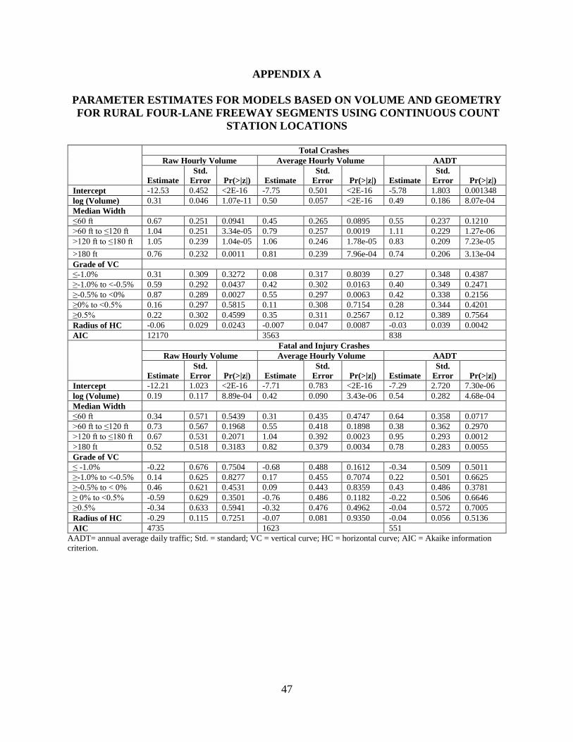
47

APPENDIX A

PARAMETER ESTIMATES FOR MODELS BASED ON VOLUME AND GEOMETRY

FOR RURAL FOUR-LANE FREEWAY SEGMENTS USING CONTINUOUS COUNT

STATION LOCATIONS

Total Crashes

Raw Hourly Volume Average Hourly Volume AADT

Estimate

Std.

Error

Pr(>|z|)

Estimate

Std.

Error

Pr(>|z|)

Estimate

Std.

Error

Pr(>|z|)

Intercept -12.53 0.452 <2E-16 -7.75 0.501 <2E-16 -5.78 1.803 0.001348

log (Volume) 0.31 0.046 1.07e-11 0.50 0.057 <2E-16 0.49 0.186 8.07e-04

Median Width

≤60 ft 0.67 0.251 0.0941 0.45 0.265 0.0895 0.55 0.237 0.1210

>60 ft to ≤120 ft 1.04 0.251 3.34e-05 0.79 0.257 0.0019 1.11 0.229 1.27e-06

>120 ft to ≤180 ft 1.05 0.239 1.04e-05 1.06 0.246 1.78e-05 0.83 0.209 7.23e-05

>180 ft 0.76 0.232 0.0011 0.81 0.239 7.96e-04 0.74 0.206 3.13e-04

Grade of VC

≤-1.0% 0.31 0.309 0.3272 0.08 0.317 0.8039 0.27 0.348 0.4387

≥-1.0% to <-0.5% 0.59 0.292 0.0437 0.42 0.302 0.0163 0.40 0.349 0.2471

≥-0.5% to <0% 0.87 0.289 0.0027 0.55 0.297 0.0063 0.42 0.338 0.2156

≥0% to <0.5% 0.16 0.297 0.5815 0.11 0.308 0.7154 0.28 0.344 0.4201

≥0.5% 0.22 0.302 0.4599 0.35 0.311 0.2567 0.12 0.389 0.7564

Radius of HC -0.06 0.029 0.0243 -0.007 0.047 0.0087 -0.03 0.039 0.0042

AIC 12170 3563 838 Fatal and Injury Crashes

Raw Hourly Volume Average Hourly Volume AADT

Estimate

Std.

Error

Pr(>|z|)

Estimate

Std.

Error

Pr(>|z|)

Estimate

Std.

Error

Pr(>|z|)

Intercept -12.21 1.023 <2E-16 -7.71 0.783 <2E-16 -7.29 2.720 7.30e-06

log (Volume) 0.19 0.117 8.89e-04 0.42 0.090 3.43e-06 0.54 0.282 4.68e-04

Median Width

≤60 ft 0.34 0.571 0.5439 0.31 0.435 0.4747 0.64 0.358 0.0717

>60 ft to ≤120 ft 0.73 0.567 0.1968 0.55 0.418 0.1898 0.38 0.362 0.2970

>120 ft to ≤180 ft 0.67 0.531 0.2071 1.04 0.392 0.0023 0.95 0.293 0.0012

>180 ft 0.52 0.518 0.3183 0.82 0.379 0.0034 0.78 0.283 0.0055

Grade of VC

≤ -1.0% -0.22 0.676 0.7504 -0.68 0.488 0.1612 -0.34 0.509 0.5011

≥-1.0% to <-0.5% 0.14 0.625 0.8277 0.17 0.455 0.7074 0.22 0.501 0.6625

≥-0.5% to < 0% 0.46 0.621 0.4531 0.09 0.443 0.8359 0.43 0.486 0.3781

≥ 0% to <0.5% -0.59 0.629 0.3501 -0.76 0.486 0.1182 -0.22 0.506 0.6646

≥0.5% -0.34 0.633 0.5941 -0.32 0.476 0.4962 -0.04 0.572 0.7005

Radius of HC -0.29 0.115 0.7251 -0.07 0.081 0.9350 -0.04 0.056 0.5136

AIC 4735 1623 551

AADT= annual average daily traffic; Std. = standard; VC = vertical curve; HC = horizontal curve; AIC = Akaike information

criterion.

48

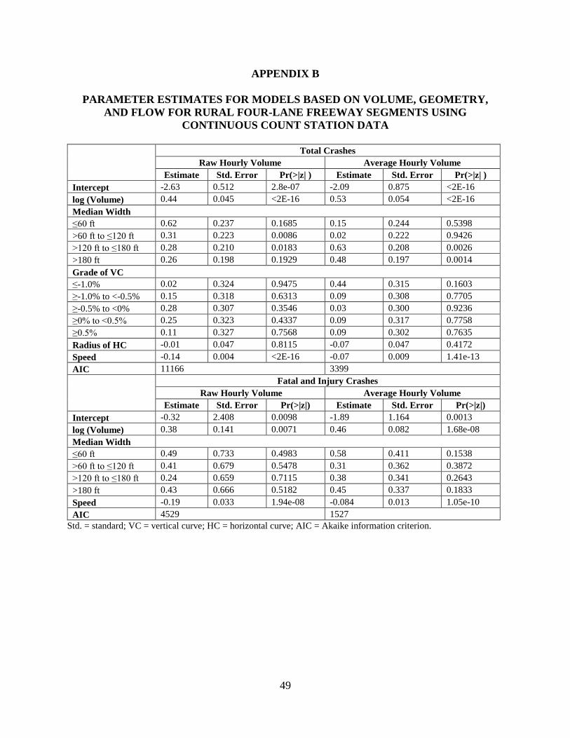
49

APPENDIX B

PARAMETER ESTIMATES FOR MODELS BASED ON VOLUME, GEOMETRY,

AND FLOW FOR RURAL FOUR-LANE FREEWAY SEGMENTS USING

CONTINUOUS COUNT STATION DATA

Total Crashes

Raw Hourly Volume Average Hourly Volume

Estimate Std. Error Pr(>|z| ) Estimate Std. Error Pr(>|z| )

Intercept -2.63 0.512 2.8e-07 -2.09 0.875 <2E-16

log (Volume) 0.44 0.045 <2E-16 0.53 0.054 <2E-16

Median Width

≤60 ft 0.62 0.237 0.1685 0.15 0.244 0.5398

>60 ft to ≤120 ft 0.31 0.223 0.0086 0.02 0.222 0.9426

>120 ft to ≤180 ft 0.28 0.210 0.0183 0.63 0.208 0.0026

>180 ft 0.26 0.198 0.1929 0.48 0.197 0.0014

Grade of VC

≤-1.0% 0.02 0.324 0.9475 0.44 0.315 0.1603

≥-1.0% to <-0.5% 0.15 0.318 0.6313 0.09 0.308 0.7705

≥-0.5% to <0% 0.28 0.307 0.3546 0.03 0.300 0.9236

≥0% to <0.5% 0.25 0.323 0.4337 0.09 0.317 0.7758

≥0.5% 0.11 0.327 0.7568 0.09 0.302 0.7635

Radius of HC -0.01 0.047 0.8115 -0.07 0.047 0.4172

Speed -0.14 0.004 <2E-16 -0.07 0.009 1.41e-13

AIC 11166 3399

Fatal and Injury Crashes

Raw Hourly Volume Average Hourly Volume

Estimate Std. Error Pr(>|z|) Estimate Std. Error Pr(>|z|)

Intercept -0.32 2.408 0.0098 -1.89 1.164 0.0013

log (Volume) 0.38 0.141 0.0071 0.46 0.082 1.68e-08

Median Width

≤60 ft 0.49 0.733 0.4983 0.58 0.411 0.1538

>60 ft to ≤120 ft 0.41 0.679 0.5478 0.31 0.362 0.3872

>120 ft to ≤180 ft 0.24 0.659 0.7115 0.38 0.341 0.2643

>180 ft 0.43 0.666 0.5182 0.45 0.337 0.1833

Speed -0.19 0.033 1.94e-08 -0.084 0.013 1.05e-10

AIC 4529 1527

Std. = standard; VC = vertical curve; HC = horizontal curve; AIC = Akaike information criterion.

50

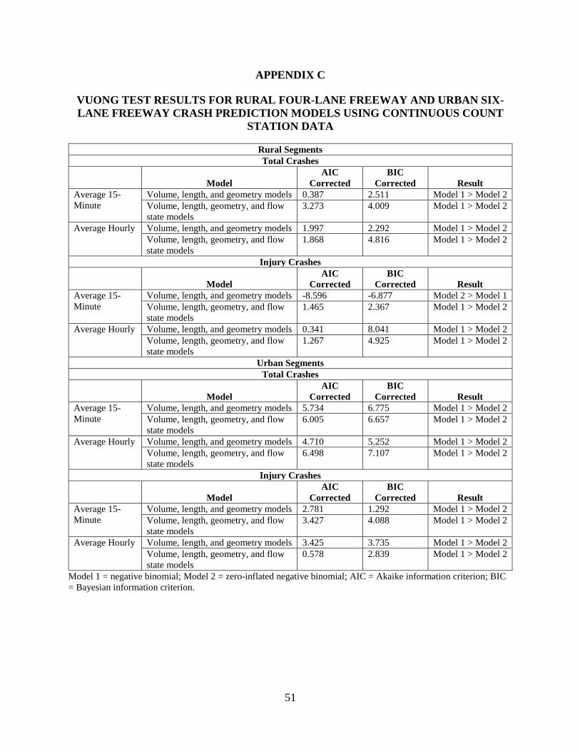
51

APPENDIX C

VUONG TEST RESULTS FOR RURAL FOUR-LANE FREEWAY AND URBAN SIX-

LANE FREEWAY CRASH PREDICTION MODELS USING CONTINUOUS COUNT

STATION DATA

Rural Segments

Total Crashes

Model

AIC

Corrected

BIC

Corrected

Result

Average 15-

Minute

Volume, length, and geometry models 0.387 2.511 Model 1 > Model 2

Volume, length, geometry, and flow

state models

3.273 4.009 Model 1 > Model 2

Average Hourly Volume, length, and geometry models 1.997 2.292 Model 1 > Model 2

Volume, length, geometry, and flow

state models

1.868 4.816 Model 1 > Model 2

Injury Crashes

Model

AIC

Corrected

BIC

Corrected

Result

Average 15-

Minute

Volume, length, and geometry models -8.596 -6.877 Model 2 > Model 1

Volume, length, geometry, and flow

state models

1.465 2.367 Model 1 > Model 2

Average Hourly Volume, length, and geometry models 0.341 8.041 Model 1 > Model 2

Volume, length, geometry, and flow

state models

1.267 4.925 Model 1 > Model 2

Urban Segments

Total Crashes

Model

AIC

Corrected

BIC

Corrected

Result

Average 15-

Minute

Volume, length, and geometry models 5.734 6.775 Model 1 > Model 2

Volume, length, geometry, and flow

state models

6.005 6.657 Model 1 > Model 2

Average Hourly Volume, length, and geometry models 4.710 5.252 Model 1 > Model 2

Volume, length, geometry, and flow

state models

6.498 7.107 Model 1 > Model 2

Injury Crashes

Model

AIC

Corrected

BIC

Corrected

Result

Average 15-

Minute

Volume, length, and geometry models 2.781 1.292 Model 1 > Model 2

Volume, length, geometry, and flow

state models

3.427 4.088 Model 1 > Model 2

Average Hourly Volume, length, and geometry models 3.425 3.735 Model 1 > Model 2

Volume, length, geometry, and flow

state models

0.578 2.839 Model 1 > Model 2

Model 1 = negative binomial; Model 2 = zero-inflated negative binomial; AIC = Akaike information criterion; BIC

= Bayesian information criterion.

52

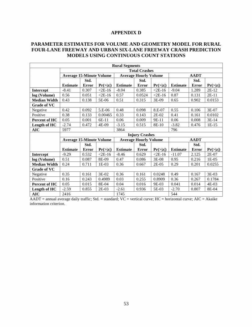
53

APPENDIX D

PARAMETER ESTIMATES FOR VOLUME AND GEOMETRY MODEL FOR RURAL

FOUR-LANE FREEWAY AND URBAN SIX-LANE FREEWAY CRASH PREDICTION

MODELS USING CONTINUOUS COUNT STATIONS

Rural Segments

Total Crashes

Average 15-Minute Volume Average Hourly Volume AADT

Estimate

Std.

Error

Pr(>|z|)

Estimate

Std.

Error

Pr(>|z|)

Estimate

Std.

Error

Pr(>|z|)

Intercept -8.41 0.307 <2E-16 -8.04 0.385 <2E-16 -9.04 1.289 2E-12

log (Volume) 0.56 0.051 <2E-16 0.57 0.0524 <2E-16 0.87 0.131 2E-11

Median Width 0.43 0.138 5E-06 0.51 0.315 3E-09 0.65 0.902 0.0153

Grade of VC

Negative 0.42 0.092 5.E-06 0.48 0.098 8.E-07 0.55 0.106 3E-07

Positive 0.38 0.133 0.00465 0.33 0.143 2E-02 0.41 0.161 0.0102

Percent of HC 0.05 0.001 6E-11 0.06 0.009 9E-11 0.06 0.008 3E-14

Length of HC -2.74 0.472 4E-09 -3.15 0.515 8E-10 -3.82 0.476 1E-15

AIC 5977 3864 796

Injury Crashes

Average 15-Minute Volume Average Hourly Volume AADT

Estimate

Std.

Error

Pr(>|z|)

Estimate

Std.

Error

Pr(>|z|)

Estimate

Std.

Error

Pr(>|z|)

Intercept -9.29 0.532 <2E-16 -8.46 0.629 <2E-16 -11.07 2.125 2E-07

log (Volume) 0.51 0.087 8E-09 0.47 0.086 3E-08 0.95 0.216 1E-05

Median Width 0.24 0.711 1E-03 0.36 0.667 2E-05 0.29 0.201 0.0255

Grade of VC

Negative 0.35 0.161 3E-02 0.36 0.161 0.0248 0.49 0.167 3E-03

Positive 0.16 0.243 0.4989 0.03 0.255 0.8909 0.36 0.267 0.1784

Percent of HC 0.05 0.015 8E-04 0.04 0.016 9E-03 0.041 0.014 4E-03

Length of HC -2.59 0.855 2E-03 -2.61 0.936 5E-03 -2.70 0.807 8E-04

AIC 2416 1745 544

AADT = annual average daily traffic; Std. = standard; VC = vertical curve; HC = horizontal curve; AIC = Akaike

information criterion.

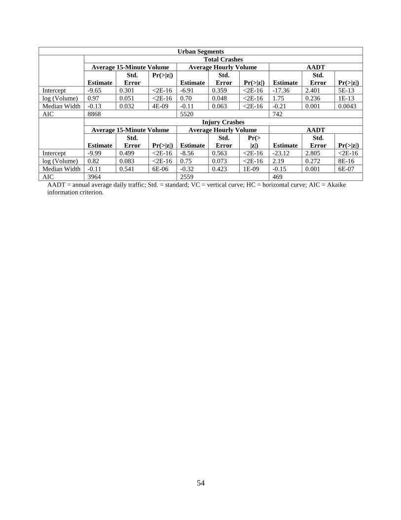
54

Urban Segments

Total Crashes

Average 15-Minute Volume Average Hourly Volume AADT

Estimate

Std.

Error

Pr(>|z|)

Estimate

Std.

Error

Pr(>|z|)

Estimate

Std.

Error

Pr(>|z|)

Intercept -9.65 0.301 <2E-16 -6.91 0.359 <2E-16 -17.36 2.401 5E-13

log (Volume) 0.97 0.051 <2E-16 0.70 0.048 <2E-16 1.75 0.236 1E-13

Median Width -0.13 0.032 4E-09 -0.11 0.063 <2E-16 -0.21 0.001 0.0043

AIC 8868 5520 742

Injury Crashes

Average 15-Minute Volume Average Hourly Volume AADT

Estimate

Std.

Error

Pr(>|z|)

Estimate

Std.

Error

Pr(>

|z|)

Estimate

Std.

Error

Pr(>|z|)

Intercept -9.99 0.499 <2E-16 -8.56 0.563 <2E-16 -23.12 2.805 <2E-16

log (Volume) 0.82 0.083 <2E-16 0.75 0.073 <2E-16 2.19 0.272 8E-16

Median Width -0.11 0.541 6E-06 -0.32 0.423 1E-09 -0.15 0.001 6E-07

AIC 3964 2559 469

AADT = annual average daily traffic; Std. = standard; VC = vertical curve; HC = horizontal curve; AIC = Akaike

information criterion.

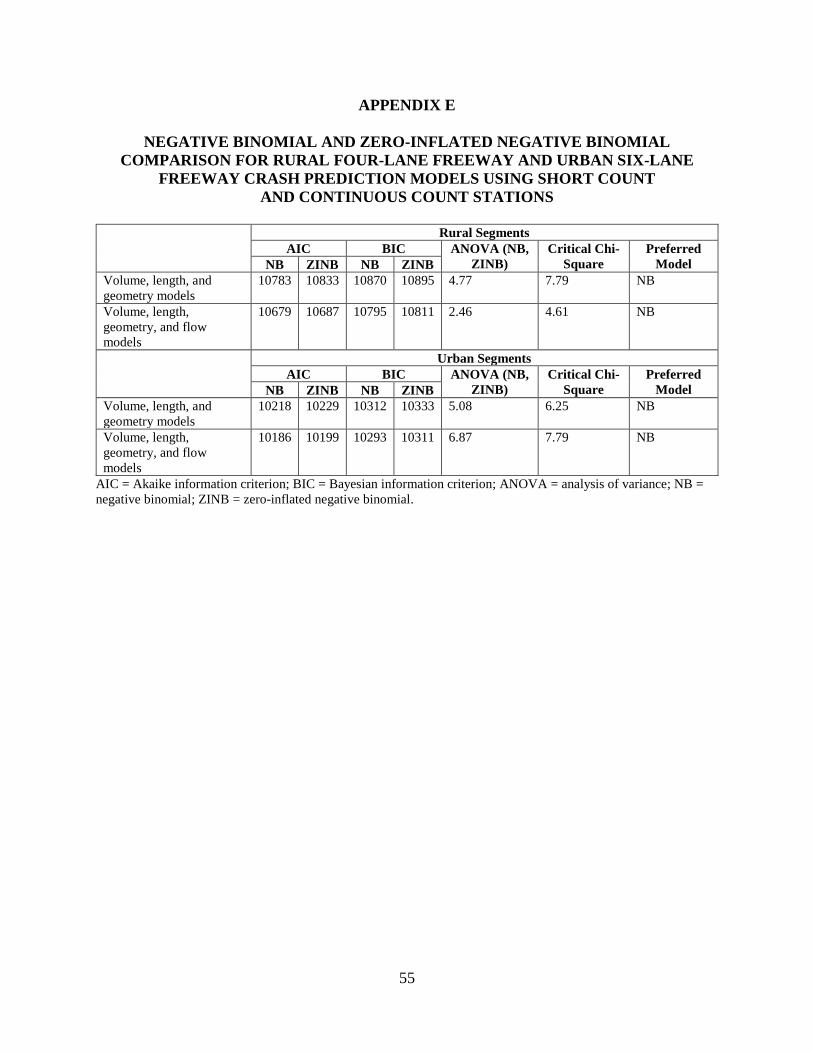
55

APPENDIX E

NEGATIVE BINOMIAL AND ZERO-INFLATED NEGATIVE BINOMIAL

COMPARISON FOR RURAL FOUR-LANE FREEWAY AND URBAN SIX-LANE

FREEWAY CRASH PREDICTION MODELS USING SHORT COUNT

AND CONTINUOUS COUNT STATIONS

Rural Segments

AIC BIC ANOVA (NB,

ZINB)

Critical Chi-

Square

Preferred

Model NB ZINB NB ZINB

Volume, length, and

geometry models

10783 10833 10870 10895 4.77 7.79 NB

Volume, length,

geometry, and flow

models

10679 10687 10795 10811 2.46 4.61 NB

Urban Segments

AIC BIC ANOVA (NB,

ZINB)

Critical Chi-

Square

Preferred

Model NB ZINB NB ZINB

Volume, length, and

geometry models

10218 10229 10312 10333 5.08 6.25 NB

Volume, length,

geometry, and flow

models

10186 10199 10293 10311 6.87 7.79 NB

AIC = Akaike information criterion; BIC = Bayesian information criterion; ANOVA = analysis of variance; NB =

negative binomial; ZINB = zero-inflated negative binomial.

56

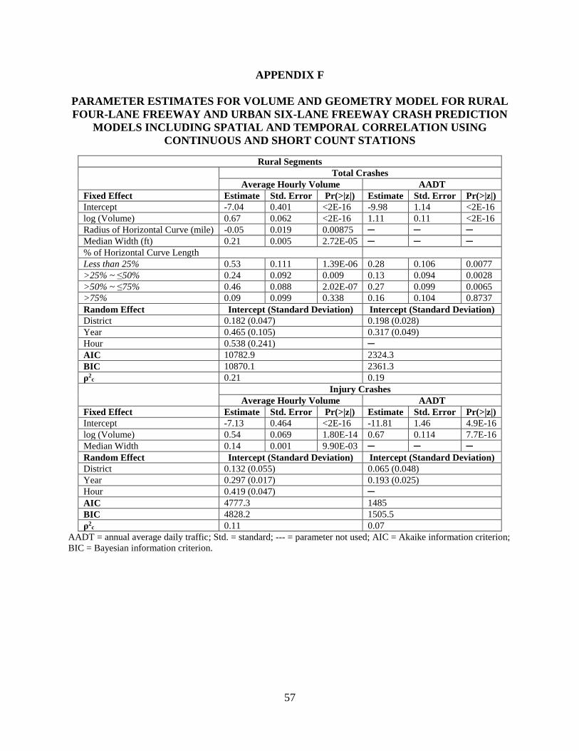
57

APPENDIX F

PARAMETER ESTIMATES FOR VOLUME AND GEOMETRY MODEL FOR RURAL

FOUR-LANE FREEWAY AND URBAN SIX-LANE FREEWAY CRASH PREDICTION

MODELS INCLUDING SPATIAL AND TEMPORAL CORRELATION USING

CONTINUOUS AND SHORT COUNT STATIONS

Rural Segments

Total Crashes

Average Hourly Volume AADT

Fixed Effect Estimate Std. Error Pr(>|z|) Estimate Std. Error Pr(>|z|)

Intercept -7.04 0.401 <2E-16 -9.98 1.14 <2E-16

log (Volume) 0.67 0.062 <2E-16 1.11 0.11 <2E-16

Radius of Horizontal Curve (mile) -0.05 0.019 0.00875 ─ ─ ─

Median Width (ft) 0.21 0.005 2.72E-05 ─ ─ ─

% of Horizontal Curve Length

Less than 25% 0.53 0.111 1.39E-06 0.28 0.106 0.0077

>25% ~ ≤50% 0.24 0.092 0.009 0.13 0.094 0.0028

>50% ~ ≤75% 0.46 0.088 2.02E-07 0.27 0.099 0.0065

>75% 0.09 0.099 0.338 0.16 0.104 0.8737

Random Effect Intercept (Standard Deviation) Intercept (Standard Deviation)

District 0.182 (0.047) 0.198 (0.028)

Year 0.465 (0.105) 0.317 (0.049)

Hour 0.538 (0.241) ─

AIC 10782.9 2324.3

BIC 10870.1 2361.3

ρ2c 0.21 0.19

Injury Crashes

Average Hourly Volume AADT

Fixed Effect Estimate Std. Error Pr(>|z|) Estimate Std. Error Pr(>|z|)

Intercept -7.13 0.464 <2E-16 -11.81 1.46 4.9E-16

log (Volume) 0.54 0.069 1.80E-14 0.67 0.114 7.7E-16

Median Width 0.14 0.001 9.90E-03 ─ ─ ─

Random Effect Intercept (Standard Deviation) Intercept (Standard Deviation)

District 0.132 (0.055) 0.065 (0.048)

Year 0.297 (0.017) 0.193 (0.025)

Hour 0.419 (0.047) ─

AIC 4777.3 1485

BIC 4828.2 1505.5

ρ2c 0.11 0.07

AADT = annual average daily traffic; Std. = standard; --- = parameter not used; AIC = Akaike information criterion;

BIC = Bayesian information criterion.

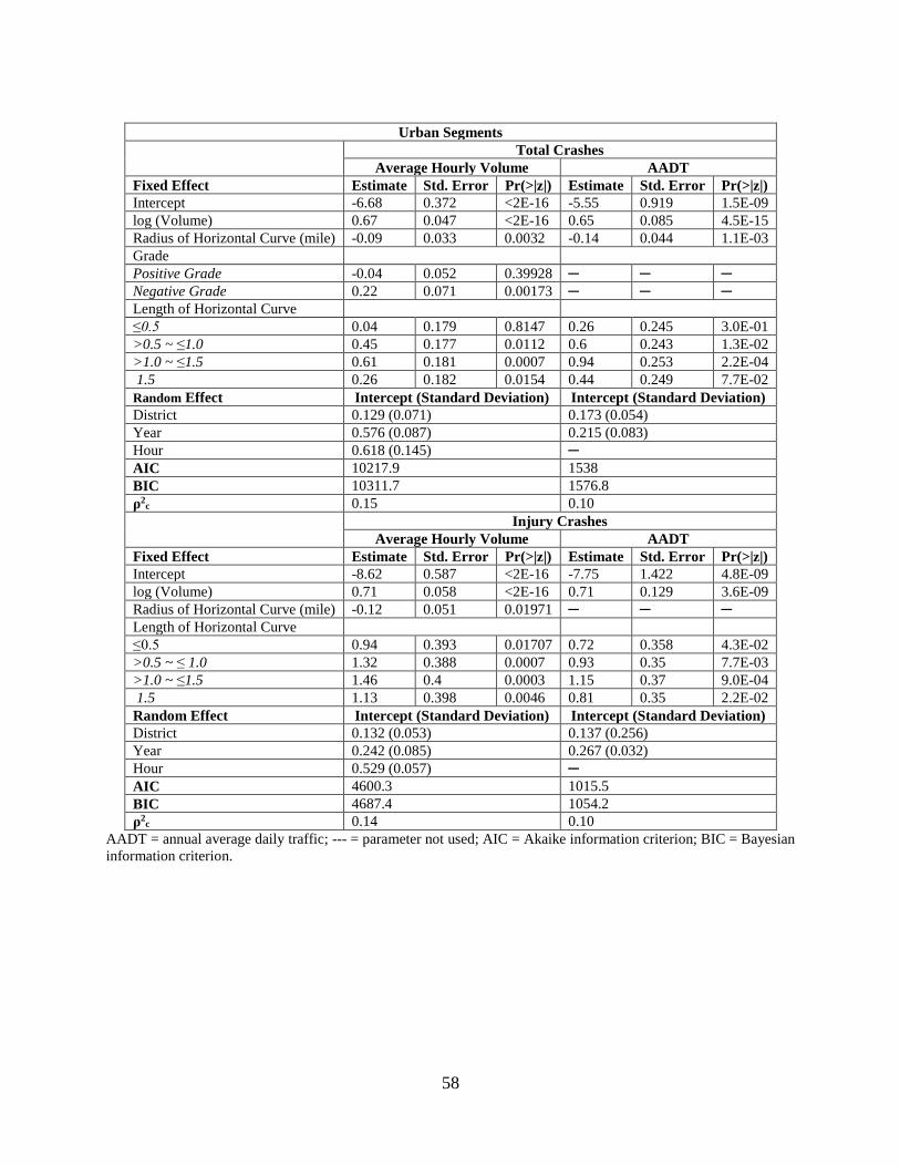
58

Urban Segments

Total Crashes

Average Hourly Volume AADT

Fixed Effect Estimate Std. Error Pr(>|z|) Estimate Std. Error Pr(>|z|)

Intercept -6.68 0.372 <2E-16 -5.55 0.919 1.5E-09

log (Volume) 0.67 0.047 <2E-16 0.65 0.085 4.5E-15

Radius of Horizontal Curve (mile) -0.09 0.033 0.0032 -0.14 0.044 1.1E-03

Grade

Positive Grade -0.04 0.052 0.39928 ─ ─ ─

Negative Grade 0.22 0.071 0.00173 ─ ─ ─

Length of Horizontal Curve

≤0.5 0.04 0.179 0.8147 0.26 0.245 3.0E-01

>0.5 ~ ≤1.0 0.45 0.177 0.0112 0.6 0.243 1.3E-02

>1.0 ~ ≤1.5 0.61 0.181 0.0007 0.94 0.253 2.2E-04

1.5 0.26 0.182 0.0154 0.44 0.249 7.7E-02

Random Effect Intercept (Standard Deviation) Intercept (Standard Deviation)

District 0.129 (0.071) 0.173 (0.054)

Year 0.576 (0.087) 0.215 (0.083)

Hour 0.618 (0.145) ─

AIC 10217.9 1538

BIC 10311.7 1576.8

ρ2c 0.15 0.10

Injury Crashes

Average Hourly Volume AADT

Fixed Effect Estimate Std. Error Pr(>|z|) Estimate Std. Error Pr(>|z|)

Intercept -8.62 0.587 <2E-16 -7.75 1.422 4.8E-09

log (Volume) 0.71 0.058 <2E-16 0.71 0.129 3.6E-09

Radius of Horizontal Curve (mile) -0.12 0.051 0.01971 ─ ─ ─

Length of Horizontal Curve

≤0.5 0.94 0.393 0.01707 0.72 0.358 4.3E-02

>0.5 ~ ≤ 1.0 1.32 0.388 0.0007 0.93 0.35 7.7E-03

>1.0 ~ ≤1.5 1.46 0.4 0.0003 1.15 0.37 9.0E-04

1.5 1.13 0.398 0.0046 0.81 0.35 2.2E-02

Random Effect Intercept (Standard Deviation) Intercept (Standard Deviation)

District 0.132 (0.053) 0.137 (0.256)

Year 0.242 (0.085) 0.267 (0.032)

Hour 0.529 (0.057) ─

AIC 4600.3 1015.5

BIC 4687.4 1054.2

ρ2c 0.14 0.10

AADT = annual average daily traffic; --- = parameter not used; AIC = Akaike information criterion; BIC = Bayesian

information criterion.