Integrated modelling and numerical treatment of freeway flow

Integrated modelling

and numerical treatment

of freeway flow

Panos G. Michalopoulos and Jawkuan Lin zyxwvutsrqponmlkjihgfedcbaZYXWVUTSRQPONMLKJIHGFEDCBA

Department of Civil Engineering, University of Minnesota, Minneapolis, Minnesota 55455,

USA

Dimitrios E. Beskos

Department of Civil Engineering, University of Patras, Patras, Greece

(Received September 1986; revised February 1987)

The effectiveness of macroscopic dynamic freeway flow models at both

uninterrupted and interrupted flow conditions is tested. Model

implementation is made by finite difference methods developed here

for solving the system’s governing equations. These schemes are more

effective than existing numerical methods, particularly when generation

terms are introduced. The modelling alternatives and numerical solution

algorithms are compared by employing a data base generated through

microscopic simulation. Despite the effectiveness of the proposed

numerical treatments, substantial deviations from the data at interrupted

flows are still noticeable. In order to improve performance when flow

is interrupted, we develop a modelling methodology that takes into

account the ramp-freeway interactions so that all freeway components

are treated as a system. We show that the coupling effects of the merging

traffic streams are significant. Finally, the incremental benefits of using

the more sophisticated high-order continuum models are assessed.

Keywords: macroscopic traffic flow dynamics, traffic simulation, free-

way modelling, free way flow

Introduction

Despite the need for improved macroscopic modelling

and anlysis of freeway dynamics, relatively little progress

can be reported in more than a decade. The most widely

known dynamic formulations can be characterized as

either simple continuum’ or high-order continuum.*”

The simple continuum formulation is based only on the

conservation equation, which is supplemented by a quasi-

static equation of state (i.e., an equilibrium flow-density

relationship) for determining density, flow, and speed in

time and space. In the high-order continuum models pure

dynamic effects are introduced by the momentum equ-

ation, which takes into account the effects of inertia and

acceleration of the traffic mass; thus, in the high-order

formulation the governing equations include (a) the

conservation and (b) the momentum. Despite this theoret-

ical improvement, a field experiment in Canada7 did not

reveal satisfactory agreement of the two existing high-

order continuum models with real data, and similar

performance problems were reported in a simpler experi-

ment.8 Furthermore, although the high-order continuum

models were introduced long ago, comparisons with the

much simpler continuum formulation are still lacking; i.e.,

despite the theoretical appeal of high-order models their

superiority over the simple continuum alternative has not

been verified experimentally.

In this paper all continuum models are implemented to

simple uninterrupted and interrupted flow situations in

order to test their performance and assess the incremental

benefits of the more sophisticated high-order alternatives.

Initially, the only available solution algorithm is em-

ployed for numerical implementation of the high-order

models; subsequently more efficient and accurate al-

gorithms are developed. In the absence of an existing

methodology for implementing the simple continuum

model, three alternatives are introduced. Despite the

improved performance of the high-order models when the

new numerical treatment is employed, substantial devi-

ations from data at interrupted flow conditions are still

noticeable. Similar deviations were also realized with the

simple continuum models. In order to improve perfor-

0307-904X/87/060447-1 l/$03.00

0 1987 Butterworth Publishers Appl. Math. Modelling, 1987, Vol. 11, December 447

Integrated modelling and numerical treatment of freeway flow: zyxwvutsrqponmlkjihgfedcbaZYXWVUTSRQPONMLKJIHGFEDCBAP. G. Michajopoulos et al.

mance when flow is interrupted, we introduce a new modelling methodology that takes into account the ramp- freeway interactions, so all freeway components are treated as a system. This improvement suggests simulta- neous solution of the state equations corresponding to the freeway and the ramps. It appears that the coupling effects of the merging traffic streams are important, and the gains from the high-order modelling are not as significant, especially at moderate to congested flows. Finally, it is confirmed that, as suggested in the recent literature,4 further improvements can be realized when discontinuous equilibrium speed-density relationships are employed or when the step size is reduced.

Background

The two most widely known high-order dynamic models are those of Payne’ and Phillips5*6 Both of these models, referred to as high-order model 1 and 2, respectively, from here on, can be rewritten in the following common form:

ak c?q z+z=g

; + a(u, k) g + /I@, k) g = 4(u, k)

(1)

where k = k(x, t) is the traffic density, q = q(x, t) is the traffic flow, u = u(x, t) is the space mean speed, g = g(x, t) is the generation rate, t stands for time, and x denotes distance along the road. In high-order model 1, u, /I, and 4 are defined as follows:

6 k) = n B(u, k) = f ; 4(u, k) = - ; [u - u,(k)]

where T= a constant time delay (reaction time), u,(k) =

the equilibrium speed, and v = - gdu,(k)/dk).

In high-order model 2 one has

1 @ u(u, k) = u + k au /I@, k) = ; $

$(u, k) = l[uJk) - U] + E (Ui - U)

where

P = ku2(o,Z + 0.15~:~~)

z&l + 1.8~~)

i = A(k) = ul(k, - k)

L,CC, k - C,(k, - zyxwvutsrqponmlkjihgfedcbaZYXWVUTSRQPONMLKJIHGFEDCBA41

ui = ui(x, t) is the speed of the entering flow

j= X’

s g(x, r) Ax

X,-l

t, = t, + n At

t, = starting time

z = k/(ko - k) At = time increment

ud = uf is the mean desired (free flow) speed cd = standard deviation of the desired speed distri-

bution (about 5 mph) k, = jam density u1 = proportionality (headway-speed) constant

(N 15 mph)

Equation (4) gives the density at t + At if the density at t is known. The derivation of the speed at t + At is obtained from equation (2), which is first written in finite-difference form and subsequently solved with respect to u;+‘; i.e.,

C, = high-density relaxation constant (- 1) C, = low-density relaxation constant (N 10) L, = average effective car length = l/k,

Sinks or sources are taken into account in the conservation equation (equation (1)) by the generation term.

‘j “+ l = uj” + At +(u;, kj”) - a($, k;) ” ,,“ ;-’ 4 zyxwvutsrqponmlkjihgfedcbaZYXWVUTSRQPONMLKJIHGFEDCBA

J

- p@J?, k,?) ky;x; kj” Vj

J 1

Implementation of each method to a particular situation requires solution of the governing equations specified by the model. Due to the nonlinearity of the governing equations (equations (1) and (2)), analytical solutions are precluded except in the simple continuum formulation (equation (1) only). In this latter case, the method of characteristics can be employed for deriving speed, flow, and density graphically or analytically at relatively simple situations. However, when discontinuous equilibrium relationships, generation terms, or initial and boundary conditions are introduced, numerical solutions should be sought even in the simple continuum formulation. Such solutions are developed in later sections.

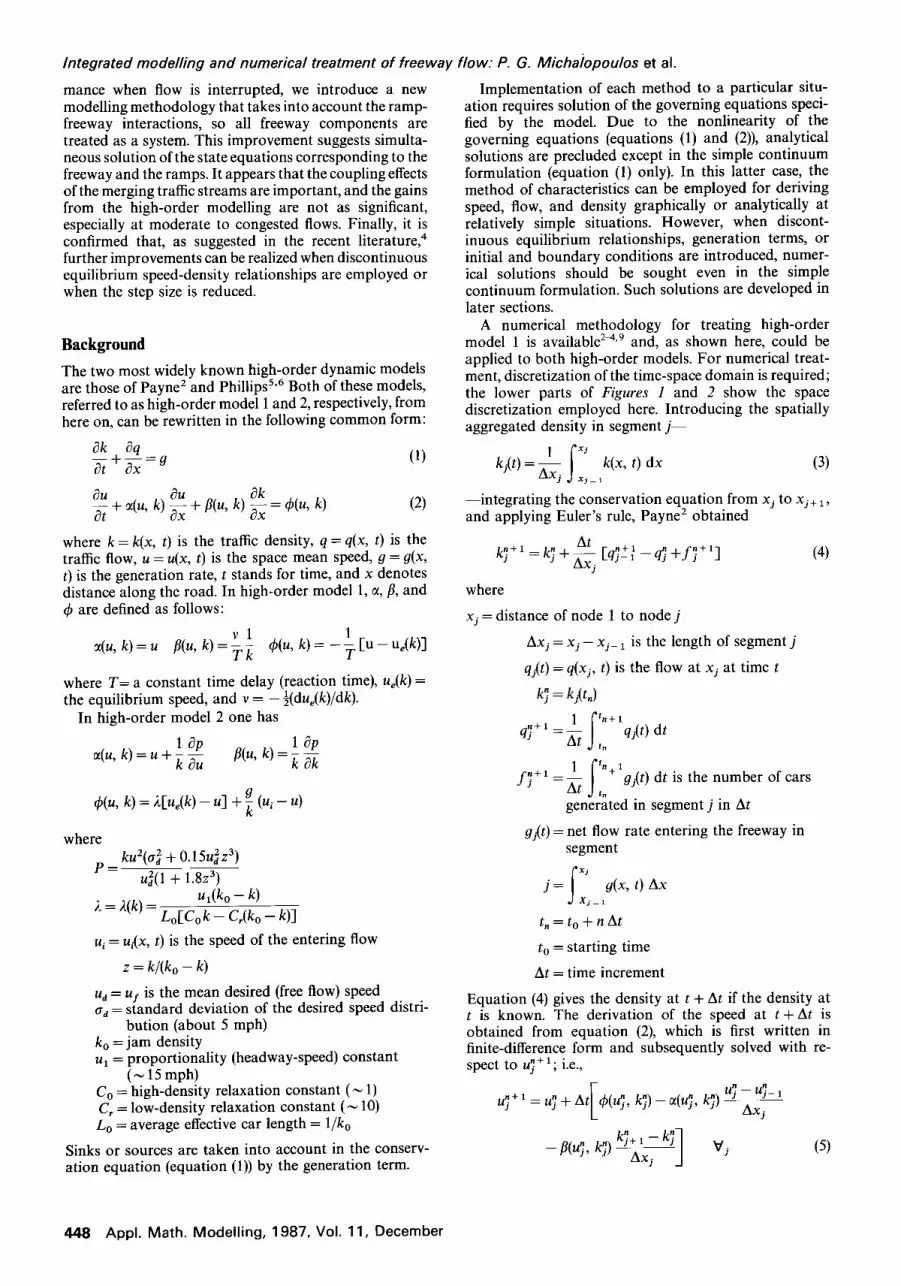
A numerical methodology for treating high-order model 1 is available2A,9 and, as shown here, could be applied to both high-order models. For numerical treatment, discretization of the time-space domain is required; the lower parts of Figures 1 and 2 show the space discretization employed here. Introducing the spatially aggregated density in segment j-

k,(r) = k Xj

k(x, t) dx (3) 1 s Xj_I

-integrating the conservation equation from xj to xj+ 1,

and applying Euler’s rule, Payne’ obtained

k;+‘=k;+& [qj”+;-q4i”+fj”+l]

J

where

xj = distance of node 1 to node j

Axj = xj - xj_ 1 is the length of segment j

qj(t) = q(xj, t) is the flow at xj at time t

k; = k,(t,)

qJ+‘=; s fn+ zyxwvutsrqponmlkjihgfedcbaZYXWVUTSRQPONMLKJIHGFEDCBA1

qAt) dt fn

,;+l J& s ln+l g,(t) dt is the number of cars

gene&ed in segment j in At

g,(t) = net flow rate entering the freeway in segment

(5)

448 Appl. Math. Modelling, 1987, Vol. 11, December

q, (Vehlhrl

3000

F

40 a0 120 160 200 240

30.5 m

,,, zyxwvutsrqponmlkjihgfedcbaZYXWVUTSRQPONMLKJIHGFEDCBAH (100’)

I/

qa I I I

I 0 1’ I -1 1

I ; ,000,10, II’ (

I t 0 0 0 I 20 1

I 1 I I I I 1 /, I I /I zyxwvutsrqponmlkjihgfedcbaZYXWVUTSRQPONMLKJIHGFEDCBAL I

I 2 ‘/ IO II 12 ” 20 21

Geometries 607 m

(2000’) i

Figure 7 Arrival patterns and geometries for uninterrupted flow

testing (case 1)

q, (Veh/hr)

t

3000

t

- INTRAS Generated

80 100

---

120

“,er Speclfmd

0 I I I 1 I

44-u t

L_ --

I I I

-

I 20 40 60 140 160

I_ 180 200 220 (Set)

q,(Veh/hr)

914 m

tzq

( 3000’ 1

I a, I I ” I I I I ” 1 I

Figure 2 Input patterns and geometries for interrupted flow (severe

congestion, case 2)

Before using equation (4), we estimate the flow at t + At

from the relation

q;+l = +J zyxwvutsrqponmlkjihgfedcbaZYXWVUTSRQPONMLKJIHGFEDCBAQj (6) In addition to equations (4H6), the solution of the

governing equations requires defining the initial and boundary conditions, which depend on the particular situation under consideration. The latter correspond to the arrival and departure flow patterns; downstream,

Integrated modelling and numerical treatment of freeway flow: P. G. Michalopoulos et al.

boundary flow is rarely known in practical applications, so we can assume that kj” = kj”I: if the flow conditions

downstream are lighter than those at the downstream boundary J at all times. Otherwise downstream conditions must be specified to allow upstream propagation of downsteam disturbances. Finally, it can be demon- strated’ that to obtain solutions within the admissible range [O< kJ < k,] and [0 <n; cur], we must have

AxjfAt > uf = free flow speed. This restriction ensures that equation (4) does not result in negative densities.

Before concluding this section, we note that the above numerical treatment was employed in the FREFL03 and TRAFLO” simulation programs. In these programs the length L of the merging (or diverging) areas is ignored; i.e., it is considered too small with respect to the roadway. Thus the FREFLO program3 implies that L = 0. This simplification is removed in later sections, where the actual merging volumes and generation rates are not

According to the aforementioned solution algorithm,23439 we can avoid excessively high-density values by restricting the input flow #?: to segment j when

assumed known but they are calculated as part of the

necessary so that ky+’

solution.

< k,. Finally, when speed tends to exceed its maximum (or minimum) value, the latter must be imposed on the solution. The last two modifica- tions demonstrate a weakness of the solution algorithm, which is removed by the numerical schemes developed here. A final adjustment in both models is to set k; slightly greater than zero when, from the solution, /$ = 0; otherwise, speed would become infinite (equation (2)). A similar adjustment to speed should be made in Phillips’ model when kj” - k, becomes zero.

Test situations

The effectiveness of the models and numerical methods was determined through implementation to several exemplary situations (test sites) representing both uninterrupted and interrupted flow conditions. Due to space limitations the results from only two representative test sites under both light and heavy flow conditions are presented here. These sites represent only single-line flow in order to avoid distortion of true model performance, which could be introduced by lane changing. Unsatis- factory model performance, even under such simple conditions, would imply that there is little reason to expect better results as the number of lanes increases. (Multilane modelling results are included elsewhere.’ ‘) Due to the lack of real detailed data under uninterrupted and interrupted flow conditions, we judged model effectiveness by comparing the results against those obtained from microscopic simulation. A recently developed, well- documented, tested and calibrated microscopic simulation program called INTRAS12 was employed for this purpose. Microscopic simulation for generating a data base was further justified by the need to allow demands to fluctuate sufficiently over a controlled and often wide range in relatively short intervals. Finally, generation of the data base by controlling the geometries and initial and boundary conditions allowed simple intuitive inspection of the results.

The geometries and arrival flow patterns for each test site, corresponding to uninterrupted and interrupted flow,

Appl. Math. Modelling, 1987, Vol. 11, December 449

integrated modelling and numerical treatment of freeway flow: P. G. Michalopoulos et al.

are shown in Figures 1 and 2. In case 1 (Figure 1) arrival flow starts at about one third of capacity and gradually increases to the maximum flow rate (capacity), where it remains for some time and then gradually decreases to its initial level. In case 2 (Figure 2) merging flows are introduced for a short time, resulting in congestion; following this, demands drop substantially for quick dissipation. Finally, the geometries of cases 3 and 4 are the same as in cases 1 and 2, respectively; however, in cases 3 and 4 the demand conditions are uniformly lighter by 30% from the patterns of Figures 1 and 2. In all cases, freeway sections were assumed empty initially, and a capacity value of 2500 passenger cars per hour per lane was employed. Further, it was assumed that during the simulation no downstream disturbances occur, so at the downstream boundary k; = k;I:. These assumptions were only made fore easy qualitative inspection of the results. We initially determined model performance by visual inspection, which we carried out by plotting q, k, or u versus x and t. In addition, the deviations of the basic flow variables from the simulated data during each 10-s increment were found, and subsequently the mean square error (MSE)13 and mean absolute error (MAE) were computed and used in the comparisons. In this manner model (and/or solution algorithm) effectiveness was assessed quantitatively. Finally, from k, total travel time was computed, and its percentage difference (at the end of simulation) from the INTRAS estimate was calculated.

Preliminary testing

Initially, the existing numerical treatment9 and high- order formulations presented in the second section were implemented to the test sites of the third section. The results were subsequently compared to the INTRAS generated data for evaluating the effectiveness of the existing numerical methodology. In high-order models 1 and 2, Payne’? and Phillips’5,6 suggested values of the parameters were adopted, respectively. Further, the Greenshields14 equilibrium speed-density relationship was initially adopted, and more sophisticated models4 were used in subsequent testing. Implementation of the aforementioned numerical methodology9 in the selected test sites resulted in mixed model performance. More specifically, it was found that the error indices of both models in the heavy-demand interrupted flow case (case 2) are large. For instance, the MAE of density corresponding to high-order models 1 and 2 in case 2 was 17.20 and 17.05 veh/mi, respectively; in the remaining cases (1, 3, and 4) this error ranged from 5.5 to 8.1 veh/mi. Similar large deviations in the other three measures of effectiveness were observed in case 2, as shown in ~01s. 1 and 2 of Table 1; this table presents the error indices obtained in case 2 by applying 10 modelling and numerical treatment combinations.

Qualitative comparisons revealed that in the congested interrupted flow case the first high-order model resulted in more severe congestion than data indicated; furthermore, this congestion was unreasonably prolonged. On the other hand, in the second high-order model, congestion did not propagate upstream of the entrance ramp; i.e., it was stationary as long as ramp flow was high. Consequently, when the ramp input reduced to zero, congestion dissipated very rapidly.

In summary, we conclude that during the initial testing both high-order models performed satisfactorily except in heavy interrupted flow conditions. The poor model performance in this case could be attributed to defici- encies on either the numerical treatment or the modelling itself. Both possibilities were explored, and the results are presented next.

Proposed numerical treatment

Simple continuum model

The lack of purely dynamic effects in the simple continuum formulation suggests that this alternative should be more appropriate at heavy flow conditions. Since numerical methods for implementing this model are still lacking, three alternatives representing increasingly higher accuracy levels were developed and are presented here. The high level of accuracy is needed for capturing the effects of shocks that are inherent in the conservation equation. The numerical methods presented next proved to be the most successful among several alternatives and were specifically designed to treat systems of conservation equations of the form

k, + zyxwvutsrqponmlkjihgfedcbaZYXWVUTSRQPONMLKJIHGFEDCBACWI, = 9 (7)

where k = k(x, t) is the dependent variable, g = g(x, t) is a known function, and the subscripts indicate differentiation.

Equation (7) is identical to Equation (l), and in the

simple continuum model it must be supplemented by an equilibrium flow-density relationship. There are two general families of numerical methods that can be employed for solving conservation equations similar to the one at hand; these families can be characterized as either shock capturing or shock fitting. The latter require predictor-corrector or iteration schemes in conjunction with a centered finite-difference algorithm. In an earlier experiment l5 shock-fitting methods did not prove to be more effective than the much simpler shock-capturing ones; for this reason, the latter are employed in this study. A simple interpretation of the better performance of the shock-capturing methods is that they tend to smooth shocks so that discontinuities disappear. This seems to be more consistent with the actual behavior of traffic where real shocks (corresponding to mathematical discontinuities in k, q, or u) would imply decleration at zero time and distance.

In the numerical methodology of this and subsequent sections, calculation of q, k, and u refers to the nodes of the discretized time-space domain as opposed to Payne’s treatment in which these values are spatially aggregated; however, conversion to the latter is straigtforward. The spatial discretization employed here is shown in Figure 3. As the figure suggests, the nodes are placed in the center of each segment so that speed, flow, and density represent the average of the segment. This is also needed for avoiding zero generation rates when the nodes coincide with the beginning and ending of the merging area.

The simplest numerical treatment employs a finite- difference scheme specifically designed to solve one- dimensional, time-dependent, compressible flows con- taining strong shocks. This scheme provides a stable difference approximation,i5 and it is of first-order accuracy with respect to At, i.e., O(At); the solution of


Table 7 Error indices corresponding to the interrupted flow heavy demand combinations (case 2)

Case 2 (Heavy flow condition)

Density 17.20 17.05 12.54 14.17 11.75 11.46 12.28 11.04 10.47 9.47

(veh/mi) s ii’

946.7 838.9 320.3 455.7 270.1 261 .l 306.5 232.0 243.9 187.0 ?

Speed 6.59 7.67 6.73 7.36 6.47 6.34 6.84 6.02 5.09 4.64 ?

(m/h) 2 95.10 115.9 85.6 104.1 77.6 75.0 86.3 65.8 55.1 42.2 5

Flow 467.0 418.9 361.2 381.8 355.0 369.8 382.2 50.5 382.4 341.1 “s

(veh/h) 386 759 357 514 234 302 262 357 226 031 246 522 265 150 219068 273 431 215807

: x ?

TTT 100.67 93.19 89.20 90.24 89.55 84.83 85.01 89.96 78.18 82.79 (veh-min)

:

PD -20.6% -12.4% -7.6% -8.9% - 8.0% -2.3% -2.6% -8.5% -5.7% -0.1% f

=?

*HOM = High-order model.

TSCM = Simple continuum model. :

f Discontinuous equilibrium speed-density model employed; Greenshields model employed in columns 1-8. b

**MOE = Measure of effectiveness. 0

_ -. - ._ _ ._ _. _. ^. _ _ - ._. - ._ _.-__-. . . . . --I I .- .- - _ - ._ -.


Direction of Travel

Figure 3 Space discretization for the new numerical treatment

equation (1) is obtained from

+ g (gjn+ 1 + sy- 1) w (8)

,;+I = u,(ky + ‘) (9)

$+I = ki”“$” (10)

where zyxwvutsrqponmlkjihgfedcbaZYXWVUTSRQPONMLKJIHGFEDCBAkJ = k(xj, t,), G = G(k) = ku, implying GJ = k;u;,

gy = g(xj, t,), and the remaining notation is as in the

second section. The quantity U; is obtained from kj”,

because when employing the conservation equation

alone, we assume that U; = u,(kJ). For instance, if Green-

shields’14 model is adopted, u,(kj”) = u,(l - k,“/kJ.

The second numerical treatment is similar to the first

but is more accurate in the sense that it contains second-

order terms. Consequently, the results obtained from this

treatment should be closer to those that would have been

obtained from the analytical solution. According to the

second-order scheme:l 5

k;+l =; (k,?,, + kj”_l)- &G&G:_,)

- 2 {BY+ l,z(G;+ I - G;)

- Bj”- l,z(Gjn - G;_ ,)} zyxwvutsrqponmlkjihgfedcbaZYXWVUTSRQPONMLKJIHGFEDCBA

+$(gy+l +&l) vj (11)

where B = B(k) is the Jacobian of G(k) with respect to k;

i.e.,

Also

B;+ l/z = +@,?+ 1+ By) and

Bj”- 1,2 = $(Bj” + Bj”_ 1)

As before $+I = u,(ky+‘) and L$+’ = kj+luy+‘, and for

Greenshields14 model we can easily see that B(k)

= ur( 1 - 2k/k,).

In order to get even closer to the analytical solution,

we developed a fourth-order scheme based on Reddy.16

However, that higher-order accuracy does not necessarily

imply closer agreement with the field data, since the

conservation equation alone is generally insufficient for

a complete description of flow. As the order of accuracy

increases, shocks become sharper due to the closer

agreement with the analytical solution; however, due to

the finite time required for deceleration (or acceleration),

sharp shocks are unlikely. After some experimentation

the following fourth-order accuracy scheme was

developed :

kj”+ ‘s4 = $(kj”+ 1,2 + kj”- 1,2)

-$((G;: ;/,,3 - G;_t,3j,4s3) + +(Gj”;;;;J

- G;+;j,4,‘) - &(Gjn$;//;J - G;‘,3/;J)}

_ Bi”_ l,2(@+ 11232 _ G?_‘1/2,2 J 11 I>

-- 1’* (;)2{B;+ l,z(G,?+ I - G;)

- Bi”- l,2(Gi” - G;_ ,)>

+$ ; 2{B;+,,,(G;,, ( > - G;, 1) - Bj”_ 3,2(GJ?_ 1 - G;_ ,)}

+~(S:+l+Y;-1) I+j (12)

where k; + 1 si = the order of accuracy corresponding to k;;

i = 1, 2, 3, 4; i.e., kj”+ 1,4

k1+lS3

implies fourth-order accuracy,

third-order, etc.

k;+ 1’4*1 =; (k;+ 1,2 + k,?- 1,2)

+; 2 (Gin+ 1,2 - GJ- 1,2)

kJ+3/4J = f (k,? , 1,2 + kjn- l,2) f ; g

( )

(G,?+ 1,2

- Gj” - 1,2)

k’ !+“2.2+;& (G;;;/;.l _Gj” ‘+/;J) 1

k'f + 3’4,3 = ; (k;, 1,2 + kj”_ 1,2) - ; (kj”, 3,2 + k,?_,,,) .l

+a ; (G;++fj;,2 - G33;.‘)

+; ; (G;+ 1,2 - G;- 1,2)

;4 & (G;+ 3,2 - Gy- 3,2) --

k?+2’3,2=k;+~~(G;::::.l .I

_ G?+ l/3,1 J 112 )

kj”+ 1,2 = S; + k,?+ 1)

kj”- 1,2 = Sk,‘_ 1 + k;)

GJ;;/;‘3 = G(k;=;/;,3) = k;;;/;,3u,(k;=,“i;“.3)

G,“~$$’ = G(k;::/isl)= k;~$Ju,(k;~#$l) etc.

High-order models

In the fourth section it was concluded that the perfor-

mance of the high-order modelling alternatives could



possibly be improved by a more accurate solution al-

gorithm. The algorithms presented next appear to be

more effective, especially at congested interrupted flow

conditions.

Considering Payne’s mode1,2-4 we can rewrite the

momentum equation as follows:

.,+[;.‘+;J;dklX= +-u,(k), (13)

which has the solution

q” =- ; ($+1 +ujn_1)- & CD;+1 -+1,

At +y ($+I ++J

where

s; = - + [u; - u,(kJ)]

UY = u(xj, tJ # ue(kj”)

dk ’ zyxwvutsrqponmlkjihgfedcbaZYXWVUTSRQPONMLKJIHGFEDCBA1 j

(14)

(15)

(16)

Thus the proposed solution for Payne’s model consists of

equations (8), (lo), and (14). When the equilibrium u-k

model is defined, the second term of the right side of

equations (15) and (16) can be determined. For instance,

from Greenshields’14 model and the relationship

1 due(k) 1 uf ‘=-? dk -Zk,

it follows that

f s

f dk = k i 2 In(k) zyxwvutsrqponmlkjihgfedcbaZYXWVUTSRQPONMLKJIHGFEDCBA0

Therefore equation (15) becomes

(17)

(18)

(19)

If the equilibrium relationship u,(k) is discontinuus or

other than Greenshields,14 then equation (18) changes. If

the analytical derivation is too complex, numerical calcul-

ation of v and the left side of equation (18) can be easily

performed. Summarizing the proposed numerical so-

lution we first find us” from equation (14), and then

comp;te k;+ ’ from equation (8). Flow is then obtained

from equation (10).

Similarly, the momentum equation in Phillips’ model

can be written as

ut+[j(u+;:) du+[(&) dk].=& (20)

The proposed numerical solution of equation (20) is

where 0; = au; + bkj”

(21)

. 1 dPl”

b=qk(j 4 = $(u:, ky) = S’y = -I;(U,(k,?) - z$) + &(Ui,’ - ~7)

17 = A(ky) is defined in equation (2)

As in Payne’s model, following computation of the speed

(equation (21)), we find density and flow from equations

(8) and (lo), respectively.

Remember that at the upstream boundary, speed and

density are defined by the arrival flow, whereas if no

downstream disturbances exist we can assume that UT+ ’

= uJ_~ and kJ n+l = k;_ 1 Vn; otherwise, the downstream

boundary conditions must be specified. Further note that

the new solution algorithm, unlike the existing one, does

not give excessively high values of speed and density as

long as AxfAt > ur; i.e., free flow speed and jam density do

not have to be imposed externally. Finally, it can be easily

seen that any equilibrium model, whether in discrete or

continuous form, can easily be incoporated in the numer-

ical treatment presented here. However, care must be

exercised at points of discontinuity to ensure single values

of speed at the vicinity of such points.

Test results

Implementation of the new numerical methods for

uninterrupted flow and light interrupted flow suggested

only minor performance gains. However, the new solution

treatment improved the performance of high-order

models substantially in the high-demand interrupted flow

case. Most interestingly, the simple continuum model

performed equally well or, in the high-demand cases,

better than both high-order models. This suggests that

unless improvements to the momentum equation are

made, employment of the high-order models only in-

creases the computational effort.

Some of the above conclusions can be verified quantita-

tively in ~01s. 3 and 4 of Table 1, where the error indices for

heavy interrupted flow are presented. From the table we

see that the new solution treatment improved perfor-

mance of both high-order models drastically. For in-

stance, in high-order model 1 the MAE of the density

drops from 17.20 to 12.54 veh/mi (~01s. 1 and 3) and, in

high-order model 2, from 17.05 to 14.17 veh/mi (~01s. 2

and 4). Further, in total travel time (TTT) the percentage

errors of models 1 and 2 were reduced from 20.6 to 7.6 %

and from 12.4 to 8.9%, respectively. Qualitatively, the

improvements can be seen in Figure 3, which suggests that

with the new solution algorithm density estimates are

much closer to the data during the period of congestion.

Further, congestion in model 1 dissipates faster, which

agrees better with the data. The test results also revealed

small differences among the three solution algorithms

(order 1, order 2, and order 4) of the simple continuum

model. This suggests that the first-order algorithm is

sufficient, even though the higher-order ones are more

appropriate for following shock developments. Column 5

of Table 1 shows the error indices corresponding to the

simple continuum model implemented by the first-order

accuracy algorithm. The error levels suggest that despite

the improved numerical treatment, the simple continuum

model performs better than high-order models at heavy

interrupted flows. For instance, density MAE in the

simple continuum model is 11.75 veh/mi, and the corre-

sponding values of the high-order models are 12.54 and zyxwvutsrqponmlkjihgfedcbaZYXWVUTSRQPONMLKJIHGFEDCBA

APP~. Ma th. Mode lling , 1987, Vol. 11, December 453


14.17 veh/mi. In addition to the quantitative comparisons, qualitative verification of the conclusions concern- ing the simple continuum model were made in all cases by detailed visual inspection of the zyxwvutsrqponmlkjihgfedcbaZYXWVUTSRQPONMLKJIHGFEDCBAq, k, and u estimates as before.

Even though the test results confirmed improved performance of the high-order models with the proposed numerical treatment, especially at interrupted flows, later figures suggest that the error increases substantially during this period for all models. Thus modelling improvements are considered next in an effort to further improve model performance.

Integrated ramp-freeway modelling

To this point we have considered the modelling of interrupted flow only on the state equations of the freeway. The effects of ramps were taken into account by the generation terms in these equations. This modelling is incomplete in the sense that the behavior of the merging flow and its effects on the mainstream are missing. When the coupling effects between ramp and freeway flow are not taken into account, the freeway and its ramp compo- nent are not treated as a system. For instance, it appears that when congestion sets in, upstream freeway flow should not only be constrained from density considerations alone but also from the evasive nature of the merging maneuvers. Thus, an integrated treatment that considers both the freeway and the ramp as a system should offter an improvement.

With these observations in mind, we can begin modelling by considering the governing equations of the freeway and the ramp and solving them simultaneously. We can obtain a solution numerically by the methods of the fifth section. The only complication appears on line AB (Figure 4), which is an internal boundary. Conditions at this boundary are time varying and depend on the flow in the merging area (point M) as well as the ramp demand. We established the upper limit for flow at AB as a function of flow at M - 1 (Figure 4) experimentally by using the INTRAS” program, and we determined maximum flow rates crossing line AB by assuming very high ramp demands (1800 veh/h) and gradually increasing freeway flow at the upstream boundary (node 1).

This experiment was repeated to obtain maximum entering rates for one-, two-, and three-, lane freeways; the results are shown in Figure 5. Before using Figure 5, we

must determine flow conditions within the merging area. We do this by comparing density at M with a threshold value kth; this value was established at 106 veh/mi when only the right freeway lane is considered, 86.6 veh/mi/lane when flow is aggregated on the right two freeway lanes, and 73.8 veh/mi/lane when flow is aggregated over three

DIrectIon of Travel

Figure 4 Space discretization for integrated modelling zyxwvutsrqponmlkjihgfedcbaZYXWVUTSRQPONMLKJIHGFEDCBA

0 2000 4000

58 k$ k& (,_,cl,

q,:., .,,(Veh/Hr) ‘&J Max flerg Flow)

(Veh/Hr)

I

80

40 i

n

” ’ 1.1 n

400 800 1. 1200 %-1 60 100 140 180

kM

(Veh/Hr)

3b: k:< kth, $,.,% h $.,qr, SC k,$ k,,, Wehltlile)

Figure 5 Maximum allowable ramp and freeway flows in the merging area

lanes. When freeway flow is uncongested (i.e., when kL

< kth), we find the upper limit qkmax of the boundary condition at E (Figure 4) from Figure 5(a) by entering

value of q2_ 1 on the horizontal axis. The actual flow at E

is therefore given by q:+l = min{q&,, , q;_ 1}. Figure

S(a) applies up to a critical upstream freeway flow f,, measured just upstream of the merging area at node M - 1. Thus, as long as k’& < kth and q’& 1 <f, (

= 1100 v/h for one-lane main flow), we find qgma, from q&_ 1 by entering the appropriate curve in Figure 5; as the future suggests, 930 < qn Emax < 1750 veh/h. If the merging length (line AB) is 100 ft, these limits translate to maximum generation rates of 49 100 to 92 400 veh/h/mi. The critical valuesf, for two- and three-lane aggregate analysis are shown at the top of Figure 5.

When upstream freeway flow at M - 1 exceedsf, and ramp inflow qi- 1 is below a critical value r, = 930 veh/h, then line CD (Figure 4) rather than AB should be treated as an internal boundary. In this case the flow at CD is given by q$J1 = min{q”,_ 1 max, q$- *l, where the maximum flow qb-l max is given by Figure 5(b). Further, merging Ilow is not restricted, since at M flow is uncongested; i.e., q;+ 1 = q; _ 1. As Figure 5(b) suggests, in this

case 4L - 1 max varies from 1100 to 2400 veh/h in the right lane. Figure 5(b) also gives qk_ 1 max at two- and three- lane situations. When both upstream freeway how qk- 1

and ramp flow at E - 1 tend to exceed their critical levelsf, and rE, respectively, while flow at M is uncongested, then both nodes M - 1 and E are treated as internal bound- aries so that qgJl =f, and qk+ ’ = r, as long as this situation persists.

When a downstream distrubance, specified by a restriction at the boundary J (Figure 4), causes congestion to propagate up to the merging area (i.e., when kL 2 kth),

then line AB should again be treated as an internal boundary. In this case, maximum flow conditions at E,

4: max, are given by density kL in the merging area

according to Figure .5(c) and qg+ ’ = min{q; max, qE_ l}.


In summary, the integrated treatment in the merging

area as derived by experimenting with INTRAS is as

follows:

Step 1:

Step 2:

Start at time zyxwvutsrqponmlkjihgfedcbaZYXWVUTSRQPONMLKJIHGFEDCBAt = 0 (n = 0) and set initial flow and

density of nodes 1 and J and 1 to E as specified.

Is kk > k,,? If Yes, flow at M is congested; set

maximum allowable ramp flow qEmax from knM in

Figure 5(c) and go to Step 4. If No, flow at

merging point is uncongested; go to Step 3.

Is q’& 1 <f,? If Yes, set maximum allowable

ramp flow qnEmax from qL _ 1 in Figure 5(a). If

No, maximum allowable ramp flow = qgmax

= r, = 930 veh/h.

Set q;+’ = min{q;,,,, q;_ 1}.

Calculate the generation term at node M from

&+ ’ = q;+ 1 jAx.

Compute k;+l for nodes 1 to E - 1 from

equation (8). Flow at E was set in Step 4.

Is k% 2 k,,? If Yes, compute kg’l for nodes 1 to

J from equation (8) then go to Step 11. If No, go

to step 8. zyxwvutsrqponmlkjihgfedcbaZYXWVUTSRQPONMLKJIHGFEDCBAIS q;_ 1 < r,? If Yes, maximum allowable free-

way flow qL- 1 max can be obtained by entering

q;_ 1 into Figure 5(b). If No, maximum allow-

able freeway flow qL_ 1 max = f,.

Set q$Jl =min{, qnM_lmax, qLez}.

Compute k,?’ ’ for nodes 1 to M - 2 and for

nodes M to J - 1 from equation (8). Flow at M

was set in Step 9.

Calculate u;+ ’ according to the model em-

ployed (i.e., from equations (9), (14), or (21))

and qJf’ from equation (10)

If the analysis period is over, stop. Otherwise,

sett=t+At(n=n+l)andreturntoStep2.

Step 3:

Step 4:

Step 5:

Step 6:

Step 7:

Step 8:

Step 9:

Step 10:

Step 11:

Step 12:

Uet& I zyxwvutsrqponmlkjihgfedcbaZYXWVUTSRQPONMLKJIHGFEDCBA150

100

I

-p+yyy/:~p,.) 0 1000 3000 0 1000 2000 3000

01 I (Set), 01 I Gac), 0 50 LOO 150 200 0 50 100 150 200

<a) (b)

(c) (d)

Figure 7 Density MAE variation of each modelling alternative and

numerical treatment

Implementation of the above treatment for heavy

interrupted flow test gave remarkable quantitative and

qualitative improvements. These can be seen in Figure 6,

which reveals a close agreement with the data during the

merging influence period (t = 120-l 80 s). Further, Figure

6 suggests better performance of the simple continuum

model. The improvements of integrated modelling can

also be visualized in Figures 7(a)-7(c), which depict the

density MAE variation during the entire simulation

period for each model and treatment. Finally, Figure 7(d)

clearly shows that the error of the simple continuum

model (SCM) is lower than both high-order models.

Quantitatively, we can verify the above findings by

inspecting the error indices of the integrated treatment

shown in ~01s. 6-8 of Table 1. For instance, in high-order

models 1 and 2 the integrated treatment reduces the MAE

of density by 9.3 % and 13.4 %, respectively, compared to

the improved solution algorithm (~01s. 3,4,6, and 7). The

overall improvement over the existing solution algorithm

is more sizable (34.1% and 28.1%, respectively). Natur-

ally, during the merging influence period the improve-

ments of the integrated treatment are more dramatic, and

they range from 18.3 to 40.2 %, as shown in Table 2.

integrated modeling and numerical treatment of freeway flow: P. G. Michalopoulos et al.

“.ahlrl I

150 t

I zyxwvutsrqponmlkjihgfedcbaZYXWVUTSRQPONMLKJIHGFEDCBA

70-80(Sec)

1

190-200 (Set)

IO0 100 Further improvements

0 ,SFt>

0 1000 2000 3000 0 1000 2000 3000

Simple Continuum

______. High Order ,'lodel 1

~~~'-'~~-'~~ High Order node1 2

Figure 6 Continuum modelling results obtained from the integrated

treatment

So far a simple equilibrium speed-density relationship was

employed14 to test the various models and numerical

methods. Naturally, this relationship should affect model

performance. In an earlier experiment Payne4 demon-

strated that a discontinuous equilibrium relationship

improved model performance. This result was also veri-

fied in this study by deriving the best u-k relationship

from the data and implementing it to each modelling

alternative and test site combination. This relationship for

the interrupted flow case is shown in Figure 8. Note that

despite this improvement our previous conclusions con-

cerning modelling and algorithm performance were not

altered. Further, the simple continuum model benefited

most by the improved u-k model, and the benefit in high-

order models was marginal in the congested interrupted


Integrated modeling and numerical treatment of freeway flow: P. G. Michalopoulos et al. zyxwvutsrqponmlkjihgfedcbaZYXWVUTSRQPONMLKJIHGFEDCBA

Tab/ e 2 Density MAE and percent improvement during the merging influence period (120-180s)

Algorithm Existing Proposed

Numerical numerical

treatment treatment lntregrated modelling

Model (1) (2) (3) (4) (5) (6)

MAE

(veh/mi)

MAE

(veh/mi)

% improvement

over (1)

MAE (veh/mi)

% improvement

over (2)

% improvement

over (1)

High-order

model 1

High-order

model 2

Simple

continuum

model

23.6 17.55 25.6 % 14.34 18.3% 39.2%

27.8 21.43 22.9% 16.64 22.4% 40.2%

15.59 12.77 22.1 % zyxwvutsrqponmlkjihgfedcbaZYXWVUTSRQPONMLKJIHGFEDCBA

. .*

60

;i- ,4,C , &‘,T ,2$X, (:hK/Mi)

0 20 40 60 60 100 120 (VehlKm)

figure 8 Discontinuous u-k relationship employed in the heavy

interrupted flow case

flow case. The test results of the improved u-k model for the simple continuum model are shown in ~01s. 9 and 10 of Table 1. We can see the order of magnitude of the improvement by comparing ~01s. 5, 9, and 8, 10, respectively.

In a final attempt to obtain further improvements we reduced the step size by one half to At = 0.5 s and Ax = 5Oft, and found that the error indices were reduced substantially; i.e., algorithm accuracy improved by 40-45 %.

Conclusions

If one is willing to accept the validity and limitations of the experimentation described here, then the following conclusions can be drawn:

(1)

(2)

(3)

At uninterrupted flows model performance is about the same regardless of flow conditions or the numerical treatment employed. However, at interrupted flows substantial differences can be introduced; i.e., proper model and numerical treatment selection are important. Even though qualitative differences between the two high-order models were detected, their overall performance was about the same regardless of interruptions. Recall, however, that the potential of Phillips’ mode15*6 was not fully tested due to insufficient data for optimal parameter identification. The proposed numerical treatment substantially improved the performance of both high-order models at interrupted flows, especially under congested conditions.

(4)

(5)

(6)

The integrated modelling combined with the proposed numerical treatment further improved the performance of all models. The effectiveness of the simple continuum formulation cannot be easily surpassed at heavy interrupted flow conditions, whereas at uncongested flows no significant differences from the high-order model were detected. This makes the simple continuum model more attractive due to its relative simplicity. When the equilibrium u-k relationship was adjusted according to the data, high-order model performance improved. However, the improvement in the simple continuum model was more drastic. In this case the simple model outperformed both high-order alternatives even at light flow conditions.

Despite the better performance of the simple continuum model, the high-order formulations cannot casu- ally be dismissed, because they take into account flow properties that are, in principle, significant (acceleration and inertia). It therefore appears that further improvements in the high-order models could alter the above findings.

The finite-difference methods employed in the solution of the governing equations are the simplest and most efficient computationally. Another alternative is the finte element method (FEM), which is more complex but allows treatment of nonorthogonal systems; i.e., it is capable of treating freeways with more complex geo- metric characteristics, such as sharp curves. Since, however, these are rather uncommon in most facilities, finite element analysis only adds complexities. Recent algorithm development and experimentation with such methods’7-19 did not reveal higher accuracy, at least for segments where free flow speed is not affected by restricted geometries (high horizontal or vertical curvatures).

In addition to better understanding of the inner workings of traffic, we can use the continuum models simulation, control, and analysis of situations where simple demand-capacity considerations are insufficient. The relative simplicity of the numerical treatments presented here allows model implementation in microcomputers. This was accomplished recently by the prepar- ation of an interactive menu-driven macroscopic freeway simulation program. 20221 The ramp proper, acceleration, deceleration, and auxiliary lanes are treated in an integrated fashion by the program; i.e., their governing



equations are added to those of the freeway proper and solved simultaneously as a system. Ramp metering is considered by treating the stop line as an internal boundary.

Before concluding, we note that the merging flow treatment presented here refers only to short merging areas (i.e., areas represented by a single Ax increment). The merging dynamics for longer merging areas are being developed, and results should appear in the near future.

Acknowledgement

This research was supported by NSF Grant CEE 8210189. Preliminary testing and validation was performed by Mr. Y. Yamauchi, who is currently with the Japan Highway Corporation, Tokyo, Japan.

References

Lighthill, M. H. and Whitham, G. B. On kinematic waves. II. A

theory of traffic flow on long crowded roads, zyxwvutsrqponmlkjihgfedcbaZYXWVUTSRQPONMLKJIHGFEDCBAProc. Roy. Sot. A,

1955,229, 317-345

Payne, H. J. Models of freeway traffic and control, Proc. Math.

Public System, Simulation Council, 1971, 1, 51-61

Payne, H. J. FREFLO: A macroscopic simulation model of freeway

traffic: Version I-User’s guide, ESSCOR Report ES-R-78-1,1978

Payne, H. J. Discontinuity in equilibrium freeway traffic flow,

Tramp. Res. Rec., 1984, 971, 14&146

Phillips, W. F. A new continuum model for traffic flow, Ufah State

Univ., Report DOT-RC-82018, Logan, Utah, 1979

Phillips, W. F. A new continuum traffic model obtained from

kinetic theory, IEEE Tram Automat. Control, 1978, AC-23,

1032-1036

Derzko, N. A., Ugge, A. J. and Case, E. R. Evaluation of a dynamic

freeway flow model using field data, Tramp. Res. Rec., 1983, 905,

52-60

8

9

10

11

12

13

14

15

16

17

18

19

20

21

22

Hatter, E., and Hurdle, H. F. Discussion on FREFLO, Transp. Res.

Rec., 1979, 722, 75-76

Payne, H. J. Macroscopic simulation for urban traffic management:

, the TRAFLO model, general technical specifications, supplement:

Macroscopic freeway model, Technical Report ESSCOR, Rept. ES-

R-BOOI-2, San Diego, 1978

Liebcrman, E. B. er al. Macroscopic simulation for urban traffic

management: The TRAFLO model, Vol. I-5# FHW A Reporf,

DOT-FH-II-9369, 1980

Michalopoulos, P. G., Beskos, D. E. and Yamauchi, Y. Multilane

traffic flow dynamics: Some macroscopic considerations, Tramp.

Res. 1984, 18B, 377-395

Wicks, D. A. and Lieberman, E. B. Development and testing of

INTRAS, a microscopic freeway simulation model, Vol. l-4,

FHW A Report, DOT-FH-11-8502, 1980

Lindgren, B. W. Statistical theory, Macmillan, New York, 1976

Greenshields, B. D. A study of traffic capacity, Proc. Hwy. Res.

Board, 1934, 14,448477

Michalopoulos, P. G., Beskos, D. and Lin, J. Analysis ofinterrupted

traffic flow by the finite difference methods, Tramp. Res. 1984,18B,

409-42 1

Reddy, A. S. Higher order accuracy finite difference schemes for

hyperbolic conservation laws, Znf. J. Num. Meth. Eng., 1982, 18,

1018-1029

Michalopoulos, P. G. and Beskos, D. E. Improved modelling and

numerical treatment of freeway flow, Proc. 9th Znr. Symp. on

Transportation and Traffic Theory, Delft Univ. of Technology, 1984,

89-111

Michalopoulos, P. G., Beskos, D. E. and Okutani, I. Finite element

analysis of freeway dynamics, Eng. Anal. 3, 85-93

Michalopoulos, P. G. and Beskos, D. E. An application of the finite

element method in traffic signal analysis, Mech. Res. Comm., 1984,

11, 185-190

Michalopoulos, P. G. and Lin, J. KRONOS IV: An interative

freeway simulation program for personal computers, Proc. ASCE

Nat. Conf on Microcomputers in Urban Transporation, San Diego,

1985, 33G342

Michalopoulos, P. G. A dynamic simulation program for personal

computers, Transp. Res. Rec., No. 971, 68-79

Beskos, D. E., Michalopoulos, P. G. and Lin J. Analysis of traffic

flow by finite element method, A& Math. Modelline. 1985. 9.


Documents

Integrated modelling and numerical treatment of freeway flow