Technical Session FourCrash Avoidance

Chairman; Robert Nicholson, United States

Accident Avoidance: An Analysis of Inherent Vehicle and System ResponseDifferences Between Cars and Commercial Vehicles: Are DevelopmentsWidening the Performance Gap?

Marcus A. Jacobson,Former Chief Engineer,The Automobile Association,United Kingdom

AbstractMajor differences in basic accident avoidance char-

acteristics are almost inevitable when one comparestypical private cars with various other cases of motor-driven road vehicles-and tlrey are becoming moremarked. The search for ever lower air resistance hasresulted irt low profile cars with fairly large areas ofcurved and steeply sloping glass, front and rear.When encountering low lying or drift ing banks of fog

or evcn early morning mist, the truck driver, generallysitt ing above such low banks of translucent fog, wil l

be able to see reasonably clearly the general layout ofthe road ahead, as well as the shapes of tall ishvehicles in front and to the side. He may, however,fail to notice the car in front and ride over it,crunching it in the processr for its driver, unable tosee where he is and whether there are other vehiclesahead of him, wil l tend to put on his brakes-andthey wil l be fast acting.

Braking performance of trucks is not as good asthat of cars even when the respective $y$tems areworking perfectly.

The very real benefits to cotltnercial vehicles whichcould be provided by anti-lock brakitrg, in terms of

better braking under adverse conditions and, aboveall, improved vehicle stabil ity and directional controlduring ernergellcy braking, have beeu well understood,but rclatively iew have been litted to cotntnercialvehicles, whereas it will not be long before some formof anti-lock braking will become available on highpriced cars as well as modestly priced mass prodr-rced

small cars. 'Ihis

wil l soon create an etrtirely new

situation, in which the car driver can stop his vehiclein a controlled and safc manner, no matter w]tat theweather, road or traffic conditions are or how rirshlyor inexpertly thc driver reacts to them, whereas vel'y

few truck drivers wil l have the benefit of suchtechnological quick-reacting devices.

For the wide range of possible surface textures, l.he

tyre-to-road grip of bus and truck tyres wil l be around

2/3 or 3/4 that provided by car tyres itrtetrded for

Westcrn Europe. The minimum braking distance wil l,

therefore, be l59o to 2ZV0 longcr. In the foreseeable

future there is l i tt le change of this basic performancegap being closed.

Current TrendsRoad haulage, in its widest sense, is experiencing

considerable and ever increasing competit ive pres-

sures. Hence operators wil l try to squeezc in an extra

Ioad or a longer trip whenever the opportunity ariscs.

Thc new motto is "Tittre is Money" and since vehicles

have "to earn their keep", many operators tend to

keep their .vehicles on the road, even whcn prudent

preventive maintenance is called for.Five key iactors, arising from the need to meet ever

tighter schcdules, regardless of weather and road

conditions, are affecting the transport scene:

More powerful engines and developments in

transmissions and suspension allow trucksand coaches to rcach attd maintain quite highroad speeds-also moderate gradietrts do nolonger significantly slow them down' Onmany busy cross country roads in the UK,car drivers, therefore, f ind it ever morediff icult to overtakc without taking chatrces.Thcrc are considerably more of the heavierand larger trucks about tltan only a decadeago-in particular there has been a markedincrease in the nuntber of articulated lorries,

which in thc UK and many parts of Europe

have taken over from the railways as theprincipal load carriers.An ever increasing rate of utilisation ofmotorways and interl inking main roads andthe hcavy loads carried has resulted in therapid collapse of road surfaces and countlessnumbers of repair sections. In order to keep

traffic flowing on motorways and dual car-riageways whilc repairs are being carried out,many of them have been given contrallowsections. which create new accident hazards.

rirF

l .

2.

3 .

377

EXPERI]VIENTAL

Although motorway$ are inherently saferthan othcr roads, when accidents do occur,they tend to be more spectacular, with trucksand coaches crushing cars caught up inmultiple shunts.A significant number of heavy trucks movein tight convoy formatiorr at speed, on trunkroads as well as through built up arcas. Thistends to irritate car drivers. for it makes itdifficult, ii not impossible, to overtake byleap-frogging trucks onc at a time. It is notgenerally appreciated that such "appall ing

bchaviour" by the truck drivers is a deliber-ate and defensive reaction to defeat orga-nised crime. For single high value loads,ranging from registered mail or cash deliveryto such readily disposable cargoes as ciga-rettes and spirits, attract thc "vil lains".

Driving in tight convoy formation tends tofrustrate the well-established hi jacking tech-nique of infi l trating, oftcn in broad daylight,a car. van or I'ast truck in front and anotherimrnediately behind the vehicle singled outfor a hi-jack. The average truck driver has,undoubtedly and inevitably, beconre less tol-erant of other motorists suddently appearingout of his blind quarter*instinctively he wil lno longer yield ground. This is quite apartfrorn the fact that hard braking might causehis load to shift or $lew the vehicle, particu-larly so when the roads are wet and slipperyand when spray interferes with his rcarwardfield of vision.

Some Basic ConsiderationsWhat applies to the UK, need not necessarily be of

equal rclcvance in the rest of the developed world, noteven all of Hurope, for thc following reasons:

Britain has a very changeable climate and this cancause road traffic hazards to arise suddenly andunexpectedly. Though these hazards may be l imitcd inspread, in intensity, duritt ion and location, they can

and do cause serious disturbances to safe traffic f lowrates.

The methods and frequency of the Police enfbrcinglegal l imits on speed, vehicle loading and propermaintenance, as well as the penalties for f louting theLaw of the Land, are $uch that many operatorsconsider being caught and consequently f ined to be nomore than a sporting risk-and worth takirlg.

There is l i tt le prospect o[ better driver cducation-or exhortations by Police and Government spokes-mcn-improving the behaviour of ull drivers and notjust a /bw and therctry rrrinimise the accident riskduring the rnost hazardous cornbination of fast f low-ing traffic suddenly experiencing such changes in

378

SATFTY VEHICLES

visibility as may be caused by swirling fog, heavyrain, fall ing snow and spray frorn trucks and coaches.For it is a well-documented fact that, like lemrnings,many drivers have just one thought then-to get totheir destination as fast as possible.

The fact that much of the trunk route network ischronically overloaded tbr prolonged periods is notuniquely a UK problem, nor are the morning rushhours with a reverse flow when millions of peopleIeave work in the latc aftcrnoon and cvening.

All future road building projects, dcsign of vehiclesand safety legislation ought to bear that in mind.Above all, we should, if at all practicable, make thesystems of all classes of vehicles compensate forhuman fail ings and not improvc one group of vehiclesto suclr an extent a$ to nake them rclatively "super

saf'e", while the others remain largely unchanged.Ma,ior di.fferences in basic uccident avoidance char-

acteristi$ ure ulmost inevitable when one c()mpsrestypical private rurs with various other classes ofmotor-driven road vehicles, ranging from highly ma-noeuvrable two wheelers to often relatively cumber-some farm machinery, from vans or light trucks to"juggernauts",-nol

forgetling double decker busesand higlt-speed hng disluntt: coaches.

The key differences are in the fields of:

1. Driver's f ield of vision,2. Conspicnity,3. Manoeuvrabil ity,4. Stability, particularly under adverse condi-

tions caused by wind and weather and thosecaused by variations in loading,

5. Occupantprotect ion,6- Load shifl ing restraints,7. Strrrctural integrity in various forms of acci-

dent,8. Accelcrating power,9. Brakingperfbrmance,10. Handling characteristics.

The Driver's Field of Vision andConspicuity

The scarch for even lower air resistance has resultedin low profi le cars with fairly large areas of curvedand stecply sloping glass, front and rear, slenderpil lars and maxirnttnl amount of sidc window glass. Ingeneral, the faster the vehicle, the lower its silhouetteand hence, l ike a motorcyclist, such very fast cars caneasily be missed by othcr motoris;t i;, unless they arealerted by thc enginc noise of the irpproaching fastmover. Whcre hedges fringe a typical cross countryroad, these readily screen such vchicles from view.whcreas one caln see that there is a high sided van,truck or coach rounding a bend and take appropriateaction-steering and,/or slowing down-to avoid acoll ision or scrape.

4.

5 .

SECTION 4. TECHNICIAL SESSIONS

There are further effects of steeply sloping awindscreen:

l. The driver cannot see the four corners of hisvehicle,

2. The low roof l ine severely restricts the dri-ver's f iclct of vision allround: so he canreadily miss signals from a high sided truckor touring coach moving alongside,

3. Such curved laminated or toughened glassareas tend to lead to image distortion, unde-sirable reflections and glare, distracting anddisoricntating the driver, particularly so un-der bad weather conditions.

With an ever increasing use of non-rigid plastics toabsorb or, at least, soften some ol' shock loadsimposed on the occupants, should bodily colttactoccur during a coll ision, there wil l inevitably be somemigration of plasticizer vapours towards the freesurface arrd escape through it. These wil l then depositthemselvcs as a v(ry tcnacious thin layer orr the insideof thc glass areas. The rate and amount of build upof such undesirable thin fi lms is accelerated by anincrease of temperature of the surf'ace of the plastic;the steeper the slope of the glass, the more ol' ahot-housc wil l be gencrated inside the car by strongsunlight.

Smoking has a similar effect, for it wil l result in ath in f i lm of a n icot ine deposi t ; such a n icot ine f i lmwi l l be addi t ivc to that duc to thc in s i tu f ina l andprogressive curing of thc plastic ancl/or irclhcsivcs usedin the manufacture and trirnming of a car or acommercia l vehic le 's cab.

When a $trong beam of light strikes a glass withsuch a thin fi lnr coating the inside, it results in asimilar prismatic glare effect as that due to a slnearfrom an ineffective or sil icone loaded wiper blade onthe outside of a windscreen with caked-on dirt. Ascries of haloes wil l then surround the shapes seenthrough the glass. It may create a distinct safetyhazard not only at night with oncorning trafficcausing glare, though its l ights are on dipped beam,but also when thc sun is low and near the horizon. orwhen the full beam ol' a truck approaching from therear, after passing through the rear window, strikesthe steeply raked front screen, turning it into atwo-way mirror, with the driver of the sports carbeing blinded by the glare and unable to see out.

Jusl aboul the worsl situation ol:urs when encoun-tering low lying or driJ'ting banks o_f tttg or even earlyrnorning rnist, The truck driver, generally sittingab(tve su<:h low banks of translutent .foe, will be ableto see reasonably clearU lhe general layout of theroad ahead, as well as lhe shapes o.[ tallish vehidts infrttnt and to the .side; this tna! enc()urcrge him not toreduce his speed draslically. He may, however, fuil to

notice the sports car in .front and ride over it,crunching il in the process, .f'or its driver, unable tosee where he is und whelher tJtere are other vehiclesahead of him, will tend to put on his brakes and theywill be fast acting.

The converse is also not uncommon-the classicunder-ride case. The clriver of the sports car, unableto see far ahead in adverse weathcr. wil l have beenclosely following the red rear l ights of the vehicle infront of hirn. The front of the car can easily getwedged unclcr the tail end of a truck when the truckdriver urrexpectedly and suddenly brakes hard.

The rnodern forv,ard contol truck or coach, withthe driver sitling high u1t und well forward, givesmuch belter vision-lhough nol Io the intmediate rearo.f sttch a vehicle. This is a particular boon underconditions o.f low lying .fos, rsin or fallinE snow.There is less of the disorientalion caused b_v lhe thin

film deposits on lhe inside of the glass, for thewindsc'reen has little rake.

Differences in Stopping DistancesThe bettcr I 'orward visibil i ty, given to a truck driver

by rnodern dcsign trcnds, allows him to see dangerfurther ahead and thereby compensates in some meas-ure for the truck's inherently inferior braking whencomparing it with a nrodern car. But, when it comesto sideways vision, he docs not have that plus factor.

This is most noticeable in the case ol' double deckerbuses. Also a new type of long distance touring coachis gain ing popular i ty ; i t t r ies to combine thc mer i ts ofsingle deck and double deck designs, yet is sufficientlyIow not Io be inconvenienced by hcight restriction.s oflow br idges or road tunnels. In order to maximise thecarrying capacity and profitabil ity of such a coach,the dr iver is madc to s i t unusual ly low down; h is f ie ldof vision can be inferior to that of a car driver's-andthis could wcll be an cxplanation frtr some of themhaving become involved in spectacular rnulti-vehicleaccidents in poor v is ib i l i ty .

Despite considerable e.f.forts over the past decade bybrake s1.,slem suppliers and tyre manu.furturer.\' lotlose lhe Tterformanre E(tp, it still rernains a fac:t thateven lhe most advanced ftucks cunnot be hraked lo astop in lhe same dislanrc as ju.tl about any .f'amily car.

Added to this are two further factors;

l. The truck driver, conscious of the dangers tohimsel f -and other$ in the cab- i l thc loadhc carries wcrc [o brcirk loose and,/or penc-trate through the thin partit ion protecting hisback, wil l, sensilrly under these circum-

, s lances, not necessar i ly apply maximumbrake pedal push right I 'rom the start of hisattcrrpt at stopping.

2. Whert such a t ruck runs in to a car , then theremaiuing kineti{r energy can be quite consid-

3'�79

EXPERIMENTAL SAFETY VEHICLES

erable, sufficient to push the much lightervehicle a considerablc distance. Cmshing andnrangling of the car wil l be an inevitable

, consequence if there is not enough spacebetween an obstruction ahead and the car sopushed along, despitc thc car's wheels beingfully locked.

Discrepancy in braking performance is unlikely tobe dramatically reduced hy technologj<:ul develop-ments currenlll in hilnd.

Whereas at least some motorists appreciate thatthere might be inherent problems shortld the driver ofa fully laden articulated truck be forced into a crashstop I'rom over 60 rnph, few realise that it might beeven more difficult for the truck drivcr to achieve astraight-l ine pull up in a short distatrce if the trailercarries no load or only a very l ight one, particularly ifthat is located well forward.

In all situations involving efttergency braking .fromspeeds above about 30 mph, sensihly even weightdistribulion is important in the case of cars, but moreso where trucks are concerned, particularly when thereis a towed trailer, be il draw-bur or semi-trailer.

Braking: The Present State of the ArtIt is worth remembering, when rcviewing the cur-

rent state ol braking systerns of mill ions ol vchicles inregular use on our roads, that it costs a good deal ofmoney, effort and time to t'ully develop effectivemodern systems and see them adopted by a vehicle ortrailer manufacturer; thereafter they tend to have arelatively long service life and it takes many years todevelop and evaluate a system which is significantlybetter and which finds acceptance by manufacturersand operators. A good example is the case of anti-lock braking:

The polential and very real henefils whit:h c:ould beprovided by anti-lock braking, in terms of betterbraking under adverse conditions qnd, above all,improved vehicle stabilit), and diret:tional control dur-ing emergency braking, have heen understood eversince the pioneering work of the TRRL and theirencouraEement oJ' UK vehit:le and component manu-

facturers some 15 to 20 years ago. The potentialbenefits were shown to the industry, l ikely users, theAutlrorit ies, Members of Parliament and the rnedia-and that included spectaculirr demonstration on heavyarticulated vehicles as well. So why lrave they notbeen morc widely used?

Quitc apart from the economic factor-currently itadds another f 3,000 to f 4,500 ($4.800 to $7,200) tothe cost of a tractor-trailer combination-there rnaywell be technical problems; for it requires that bolfttractor and trailer must bc equipped with fully com-patible systems. ln practice this means dedicatedtractor-trailer combinations.

380

Generally, it is still .fairly rare in the UK und muchof Europe to have twmprehensive technological co-ordinatit)n hetween lrutk and trailer rtakers at thedesign antl devektpment stages. This omission rnust beseen against thc background of many commercialvehicle and trailer makerri finding it difficult tosurvive in a market where f'or several years a 3-590 to4090 ovcrcapacity has been the norm and adoptingcost cutting the prcferred method ol' staying in busi-ness. It is not well known that despite that lhe UK issellin7 a good example lrt the rest oJ' Eurttpe. Forilhout 20,000 to 22,000 anti-lor:k braking systents havebeen instulled on its heavy goods vehicles, mainly onsuch high risk or dangerous cargo vehicles as J'uel andpetro-chemical tankers and some -fire engines. Most ofthe installed anti-lock systems are retrofit ones.

When it comes to cars, it wil l not bc long beforeseveral competitors wil l follow the recent example setby Ford of Europe of making some form of anti-lockbraking available not only to those buying rclativelyexperrsive cars, but acro$$ their model range, rightdown to modestly priccd mass produced small cars.

This will soon create an entirely new situation, inwhich the car driver can stop his vehicle in acontrolled and sqfe manner, no ffiatler what theweulher, road or traffie: c'onditions qre or how rashlyor inexpertly the rlriver re(tcts Io lhem. ()n the otherhand, very few truck drivers will have the benefit ofsuch technological ttruick-reacting devices.

All anti-lock systems are designed to enable avehicle to be braked in a straight l ine from a highspeed and keep all of its full length inside a 3 l/2 mto 4 m wide lane during braking and when coming torest. But not all systems allow the drivcr to steer andtake avoiding action whilc Ihc driver applies full brakepedal pressure.

The aim for comnercial vehicles, int:luding articu-lated ones and truck-draw-bar trailer combinationsshould be lo retain steerability during emergencybraking under all road surface conditions, inclndin7"split p", rulled snow and othttr ntugh wintry situa-tions. It is not an eas! task-s.fter all, several of theanti-lock systems .fitted to car and their light comrner-cial derivatives cannol meet such a crilerion either.

Visualisation o1' thc sequence of event,$, includingthe rclative rnovements and the paths followcd by thetruck and its trailer during thc braking and accidentavoidance steering manoeuvre, can play a major rolein shortening dcvclopment time and high-lightingshortcornings and limitations of one sysitcm cornparedto another. Computer Aids to Engineering (CAE) maygo a long way in convincing potential customers andpossibly even Government Departrnents, but, ofcourse, verillcation by actual physical testing will stillbe necessary*and to-date no agreernents have beenreached regarding realistic tcst procedures and an

SECTION 4. TECHNICAL SESSIONS

internationally acceptable set of manoeuvres andbraking performance values.

So, in the rneantime, the majority of commercialvehicle manufacturers design and build to jusl meetthe currently mandatory brake performance tests asset oul in particular National Type Approval Regula-tions. By their very nature, these wil l be a compro-mise, reflecting the old-established srate-of -thc-art.

Whereas, these days, no car maker could hope toget by-and actually sell his cars in the competit ivemarket place-if the performance ol' his brakingsystem were not very substantially better than theminiurunr laid clown in such Rcgulations, this does notnecessarily apply to comrnercial vehicles.

The not unreasonable fear of what adverse mediacomments could do to the sales prospects of a newmodel has done a great deal to "improve the breed"of cirr.$. For there is no shortage ol' motoring journal-

ists who are prepared to wear a flat or two on thetyres of a new car model they are evaluating, just toestablish how good, bad or indifferent the car'sstopping characteristics really are.

Heavy commercial vehicles are made in muchsmaller numbers and are not generally maclc availablefor such "evaluation" and far fewer journalists arercally capable or interested in fully testing them.

The Importance of Load SensingBrake Force Limiters

Car makers have done a great deal to achievebetter, more level ride suspension, minimised bounceand wavyness in the interest of directional stabil ity-and there are nowadays few, if any, makes with apronounced '*front end dive" during hard trrakingfrom high speed. Also they have come to accept thatthey must provide reliable and fool proof brake lorcelimiters to the rear wheels.

It is, of course, relatively easy and not costly toincorporate such dcvicc$ into the quick-acting all-hydraulic braking system, as fitted to a modern car,ancl thereby prcvent premature and undesirable lock-ing up of the rcar wheels as weight transfer occursduring hard braking. Without such devices thcrc isalways the risk of the vehicle slewing when the rearwheels lock up before thc front ones, for it is afundamental feature of vehicle dynamics that themole vertical load is applied to a roll ing tyre, the lessprone the road wheel is to lock up during heavybraking; also when a wheel locks up, then all thesideways guidance forces developed by the tyre sud-denly disappear.

Compared lo commercial vehicles, the basic proh-lems are eusier Io resolve on curs, because the ratio o-foverall weight of a car when fully luden, right up tothe manufac'turer's limil, Io its unladen condition is ofthe order o l l .5 : l to 1.8:1.

This ratio tends Io be 3:I to 3.6:I for heavycorn nrcrcia I ve hicles'.

It is even more, when considering a truck-draw-bar trailer combination, for it could then be anythingu p t o 8 : 1 .

A variety of systems have been evolved by truckand trailer rnanufacturers, which can modulate thecompressed air pressure to actuate the brakes onindividual axles to allow for such a very wide range ofpossible Ioading c-ortdit ions. But the rnajority ofsystems are not ir l l that satisfactory in service, partlybecause they need more routine maintenance, but alsofor two othcr reasons:

t. Most trucks and trailers corne from differentmanufacturers-and they often do not havethe sanre component supplier,

Z. Emf:ty trailers have a distinct tendency torhythmically bounce on their springs, forthese were designed for maximum ratherthan minimum axle loading-and it is virtu-ally impossible to achievc a proper brakeef' lbrt control on a bouncing axlc.

Ideally both the tractor snd trf,iler should beequipped with a Jully cornpatible anti-lot:k brakingsjstem which rapidly responds to d.ynamic movemenlsof individual axles on their suspension as well ds slaticaxle loading. Currentl"y this is still lhe exception ratherthan the norm.

An early udoption of anti-lock braking systems forat least the tracter unit of a tractor-semi lrailercomhination is a logical developmenl lo ensure im-provements over current truck braking perJ'ormance.

But it should be remembered that the anti-lockbraking system does, generally, not give a shorterbraking distance on a dry road surface than thecurrent standard types of non anti-lock braking sys-tems when thc tractor-trailer combination is carryingmaximum load and whel all the axles carrv their fullshare of vertical loading.

Steerability and Handling Stability ofTractor-Trailer Units

This involve$ so malny very cornplex dynamic inter-actions that some over-simplif ications are called for,to appreciate the principal behaviour patterns ofcurrent tractor-trailer combinations, including somewith a fornr ol anti-lock braking:

Steerabil ity and handling stabil ity can be roughlydividcd into for.rr main categories.

The vehicle response characteristics are very similarfor the following operating conditions:

l. Severe braking on a straight stretch of dryroad,

2. Moderate to hard braking when the com-bined unit straddles a section of road where

3 8 1

EXFERIMENTAL

part has a "grippy" surface and the rest amuch lower tyre-to-road grip,

3. Moclerate braking on a slippery road surface.

Category 1:The wheels on the lraclor's front axle lock first:The cornbined unit remains stable, brakes in a

straight line and cannot be steered.

Category 2:The wheels on the tructor's drivinp axle or axles

Iock first:The fraclor-trailer combination becomes unstable to

the point of initiating jack knifing. The driver mayfeel the onset of this just in time and, by easing offhis brake pedal, then bc ablc to minimise this inher-ently dangerous instabil ity to iust a large swervc;residual controllabil i ty on damp or wet roads can bemaintained if thc driver applies only moderate brak-ing.

Category 3:All the wheels on the trador lock simultaneouslv-

those on the trailer still roll:The tractor-trailer combination is unsteerable, the

trailer wil l swing up to l0 degrees out of l ine.

Catcgory 4:The wheels on the lrailer's axles lock up-but not

those on the tractor:The combined unit remains steerable, the trailer will

swing out of l ine. The lower the tyre-to-road grip orthe weight carried by these traiier axles, the larger theangle of the trailer swing. Also the higher the initialroad speed and/or the rate of deceleration of thevehiclc, the greater wil l be the trailer swing.

If, .for one reason or another, the braking e.ffortdistribution between individual tractor axles andwheels is such that the tractor will start to yaw orswing from side to side under heuvy braking, then thetructor-trailer cornbination becomes unslable.

The undersirable behaviour of the tractor duringhard braking may be cluc to the dynamic mr)vementof twin rear axles, whcrc fittcd, on thcir suspensionand/or too slow a response of the braking system torapidly changing conditions-and that can happeneven with early types of anti-lock braking .systems.Poor maintenance can produce the same effect.

Braking in a Bend on a Wide RoadOnly a few years ago, having to apply brakes

suddenly while ncgotiating a bend at speecl used togive real concern to car drivers, lor it could causc thecars to either carry on in a straight l inc, tangential tothe curve, or spin out of control. But steady progresswith tyres and particularly with thc latest types ofanti-lock braking systerns wil l substantially raisc thesafety margin and accident avoidance potential ofcars.

382

SAFETY VEHICLES

Path deviation during emergency braking can al-ready occur with tractor-trailcr cornbinations whilethey are bcing braked f'rom fairly modest speeds,particularly on damp or wet roads, it wil l be morepronounced when braking from higher speeds. ,4nunladen lractor-trailer comhinution is more ilt risk ofthat thdn one c'urr.ying a load-and the way suchIttads are distrihuled over the axles can have aconsiderable in flttence.

Four basic conditions exist:

l. The lrauor-trailer combination hus no anti-. lock hruking: Tractor-trailer combination

moves into the opposing traffic lane,2. An anti-lock hruking systern is ./'iued trt the

semi-trailer only: Similar response to case l,3. The lrilL:tor hus anti-lock hraking, the trailer

has not; Tractor remains stable, trailermoves into opposing traffic lane,

4. Tractor and semi-trailer huve compatibleanti-lock braking: Tractor-trailer combina-tion remains stable. no path cleviation,-shoftest braking distance.

Design ImprovemeRts to the Tractor-Trailer Coupling

Improvemcnts to the fifth wheel coupling, includingstrengthening, have virtually eliminatcd the dreadedphenomenon of the trailer breaking free dr.rl ing orfollowing cmcrgency braking and continuing on pastthe tractor. But in a tractor-trailer combination with-out anti-lock braking and with the tractor bcing ashort wheel base type and the load conccntrated at therear of the trailer, it is then not uncommon for thetractor to nose dive during emergcncy braking, due tothc front axle locking up, and the rear of the tractorjacking up, l i ft ing its rear wheels clcrrr off the road.This may or may not be accornpanied by jack knifing,even a roll over.

Trailer Swing and Jack Knife DangerJack knifing occurs only under sjcvcre braking

conditions. Trailer swing, on the other hand, canoccur under both high speed towing and brakingcondi t ions.

None ol the patented anti-jack knife solutions cantotally clirninate trailer swing while the tractor-trailercombination travels at speed, particularly if the trailercarries only a l ight load-or uone at all. Such devices,including the Hope anti-jack knife system, can, how-ever, often inhibit the orrset of jack knifirrg or, atleast, minimise its severity.

Some quite ingenious systemri have been evolved tomininrise the tendency of l ightly loadcd or emptydraw-bar trailers swinging from side to siclc whilebeing towed at speed. But, under emergency braking,these have little eff'ect on overall directional srabilitv

SECTION 4. TECHNICAL SESSIONS

of the truck-draw-bar trailer combination. for thetra i lcr wi l l s t i l l swing out of l ine.

The only effective way to prevent thc dangers l istedabove is to equip hoth the towing and the towedvelricle with a compatible and very quick-acting micropro(:essor controlled anti-lock braking syslern.

Problems Associated with Anti-LockBraking Systems

Some currerlt types of truck brakes, though looselydescribed as of' the *'anti-lock typc", have proved farfronr satisf 'actory in actual service. There are a num-ber of reasons for that;

I. The moving parts of the complex brakingsystem react too slowly in resporrse to rapidlychanging input signals,The movcment of axles on their suspensionor of indcpendently sprung wheels rrray bcsuch as to scnd false signals to the electronicand/or pneumatic controls which regulatethe admission of compressed air to actuateor mornentarily frcc individual brakes. Whensevere braking is called for on a stretch ofpot holed, broken up or loose surfaced road,the performance of such an anti-lock brakinglayout can be most disappointing; the sametends to apply to braking on very unevenroads ancl t ltose covered in rutted strow,Unacceptable and unpredictably variable de-lay in systern response to sensor input signalsmay be due to the "st ick ing" of actuat ingmechanisms; this frequency occurs in coldwintry conclit ions and where corrosion hasset in.Under conditions of rain splash, slush andsnow as well as high humidity-which maybe due to Inist and fog-sotne systems areprone to suffer from contact corrosion and/or short circuiting on whcel rotation scnsors.The effect is that some sensots may then failto "report" to tlrc systeltt 's electronic brain,Inabil ity of electrical and electrotric compo-nents to survive the arduous in-service shockloads, vibratiotts and scvere temperaturefluctuations,Electrostatic and EMI (Electro Magnetic In-terference) eff'ects, which may originate fromwithin the truck or the trailer's refrigerationplant, powerful radio frequency signals froma variety of statirlnary or nrobile transmittcrsif the source is close cnough,-when travel-l ing in close proximity to other vehicles evensome CB (Citizcn Band) radio chatter can be

troublesone. It is trowadays technically pos-

sible to e.f.fectivell screen the complicated

anti-lock sy$tem against most of these unde-

sirable stray input$, fiurge currents and inter-ference-but this costs money.

7. Early applications of anti lock brakes suf-' fered from cornponents giving unacceptably

short in-service l i l 'e, largely due to costcutting and indifferent to poor quality.

Al l th is-and the unfor tunate h is tory of 'some heavytruck anti-lock braking systems fir i l ing so spectacu-larly in the USA about a decade ago-calls for betterengineering allround, a fhil safe approach to thesyste ln, sc l f moni tor ing and possib ly dupl icat ion of 'sorne parts of the systern. It rnay be easier to solvesome of the problems by adopting rnulti-disc ratherthan drum brakes.

Cornmercial Vehicle General BrakingCharacteristics

Cars and their derivatives use a fairly simple andinherently self balancing hydraulic system, activatedby direct applicatiorr of pcdal prcssurc, which on allmodern cars is suitably assisted by a vacuum orhydraulic servo.

Howevsl, all-hydraulic brakes are not the norm fortrucks. For l ight trucks-up to about 7 l/2 GYW-apncrrmatic over hydraulic system is sometimes used.

The majority of trucks and buses are fitted withdrum brakes, actuated by cronrpressed air via l inkagesand these require regular and more frequent mainte-nance to keep them in perfect balance than do discbrakes fitted to cars.

The tnodern car braking slslem can achieve maxi-mum bruking efficiency in u srtrull fraction of asecond, for, unlike the systems used on trucks andbuses, it has practically no lost motion in its mecha-nisms and does not require a substantial transfer ofworking fluid (compressed air), nor a complex systemof valves to regulate the flow of the working fluid.

But in |rucks and buses there will inevitably alwaysbe a deluy between Ihe driver phtsic'ull-v depressing thebrake pedal and the vehit:le's hrakes becoming Jullyeffective, In many tractor-trailer conhinations andwhere a truck pulls u draw-bar trailer, such a delayperiod will be quite noticeable-and it cun take aset'ond or two before peak brake per.formance isachieved.

Coefficient of FrictionIt is conveniently assurnsd that the two friction

coefficients which determine the ratc of decelerationol' a moving vehicle remain constant throughout thebraking opcration. It is dernonstrably not true forrapid braking from about 60 mph or above. Onefriction coefficient is that between the rotating metaldrum or disc and the friction l ined component whichis anchored to a non-rotating part of the vehicle; theother is that between the road surface and the tyre,which may or may not be rotating.

.,

*

3 .

4.

6 .

383

EXPERIMENTAL SAFETY VEHICLES

It takes a measurable amount of time before thebrake linings and the metal I'aces they rub againstreach the minimum temperature to allow them todevelop their peak friction value, whiclr may thendrop slightly and reach a plateau value.

It takes longcr to bring the mass of a truck's largecast iron brake drum to the required rnetal tcmpera-ture than it does to stabil ise the disc of a car.

Prolonged application of drum brakes can cause aprogressive fall ofi in this friction value, in somecases this may be followed by a sudden and dramatic"brake lade".

Now that many c:ountries have banned the use ofaslreslos in .friction materials, a new situation hasarisen. Many truck and coach operalors will hetempled lo fit reildily available cheaper service andreplacemenl purts, often originating from sourceswhich still use asbestos. Sometimes such asbestos-based friction linings develop a higher friction coeJfi-cienl than the OEM .fitments, hut this can be asundesirahle as when they develop a ktwer value. It is,lherefore, nol uncotnmon to J'ind that previously wellbalanced brake systems on a truck-trailer c:ombinationIhereufter tend to be seriously out of balance whenemergency braking is applied.

Repair garages are unlikely to refer to standardquality control tests for friction materials; thoughbetter than none, these tests are very basic, briel 'and,likc the standard low speed brake perforrnance dyna-mometer, unlikcly to give a full representation ofwhat is likely to occur under real life operatingconditions.

The tyre-to-road grip is much more variable, largelydue to (a) the weather and (b) tra.f.fic polishing andwear of the road surface; it is likely to vary subsl(tn-tially across the width of a traJfic lane. lt is quitecommon to find in the UK and Europe that repeatedheavy truck traffic has created grooving, which inturn may hold rain water and thereby cause one ofthe pre-conditions for aquaplaning, the other beingspeed.

In really hot weather, the repeated passing ofheavily laden trucks may cause the asphalt to "flow"

like viscous treacle ahead of and under the rollingtyre; acting l ike a sticky lubricant, this can, inemergerlcy situations, lead to extended braking dis-tances. Under wet road conditions, such a truck tyrewill plough through quite deep water, parting it anddisplacing it as a powerful spray with an astonishingrange, most of it to the side.

Fundamental Differences Between Carand Truck Tyres

Because of the very much higher loading of theircontact area, truck tyres tend not to be so disturbedby dcep water as many low protile car tyres are.

384

The trend for ever lower profile car tyres isre-introducing problems which had been successfullytackled before their advcnt-namely low level ofvehicle controllability when travelling at speed on rainsoaked or snow and slush covered roads. fbr underthose conditions the area of contact with the roadprovided by low profile car tyres is reduced to only afew percent of what it is when the road is dry.

When this "floating off" starts, the effectiveness ofanti-lock braking, where fitted, is greatly reduced*and any form of accident avoidance possibility maybe lost .

However, both car (tnd truck tyres are at theirworst when the roads have just a thin film ofmoisture, which can range from morning mist and fogto black ice and meh water on top of hurd packedsnow. For it results in a very poor lyre-to-road gripand hence affects accelerating and braking potrer, aswell as steering and staying with the selecled path.Despite considerable and sustained development workby lhe tyre makers to uchieve better damp und icegrip, there rs, within the .foreseeable Juture, noprospecl of a technical breakthrough-not even dmarked improvement.

It is a basic fact of vehicle dynamics that the lowerthe downward-acting forces on a tyre-be they due tostatic weight carried, dynamic weight transfer dLrringmanoeuvring and/or braking, or aerodynamics-theless will be the control forces which such a tyre canprovide, particularly thosc which determine whetherthe vehicle can bc steered predictably.

This explains why a fully laden trailer will "track"

as though running on rails and why the same trailerwhen not carrying a load will oflen tend to develop anoutward drift in a tight bend or snake when beingtowed at speed.

In addition, there is the question of the "grip-

piness" of the tyre on the road. For lhe wide range ofpossible surface lextures, including traffic polished,broken and uneven or pot holed ones, those withIoose gravel t:overing, dry, wet, damp, packed snowor combinulions o.f these, the tyre-to-ro(rd grip o.f husand truck tyres will be around 2/3 to 3 /4 thatprovided by car tyres intended Jor Western Europe.The rcasons for this performance difference are thevery different design and constructiorr cherracteristicsof car and commercial vehicles respectively and differ-ences in rubber compounding.

In the foreseeable future there is tiitle chsnce o.f thisbasic performance gap being closed, particularly aslong as the all too prevalcnt-though little publi-cised-practice continues that, in order to be able tosecure a sales contract, a "slight adjustment" is madeby truck or trailer supplier on the final choice oftyres-which usually means substituting second line

SECTION 4. TECHNICAL SESSIONS

for first line tyres; these may also have a slightlynarfower section.

In commercial vehicles, the loads carried per tyreand hence the internal air pressures are several t imesthat applicable to car tyres, therefore these tyre$ mustbe given must greater sidcwall stif l fness and morereinfiorcing plies allround.

AIso in a modern car tyre the flexing under load, beit due to acceleration, braking or sideways forcescoming into play during changes in direction from thestraight-ahead steady progress, plays a major role ingiving enhanccd tyre-to-road grip characteristics.

Car tyres destined for the West European marketsare, generally, optimised to givc good wet grip perfor-mance, a quiet ride and high comfort level, even ifthat means some sacril ' ice in terms of very highmileagc being achievable. The designed-in perfor-mance characteristics of truck and bus tyres, particu-larly so in the case of second line tyres, come in thereverse order of priorit ies.

In praclice the e/J'eil of all these .factors is that,even if lhe lruck or bus were Io be equipped with abraking system equally as effective as thal of themodern European type cilr, the shortest brakingdistunce athievahle would be I5Vo ttt 22Vo greilterlhan that oj the car under dry road .surface corrditionsat speeds u1t to about 50 mph lo 60 mph. And to-datetruck.s do not have such idt:al brakin7 slstems.

AI higher initial speeds and when the roads areslippery, the differentes in the shortest possible brak-ing dislances to a complete stop are greater still.

These are fundamental facts and unlikety to changein the next decade.

Spray GenerationConsiderable irnprovements can be achieved by

shrouding the wheels down to near hub trcight andlining such wheel arches with textured material whichthcn dissipates some of the kinetic energy of the highvelocity spray or jets of displaced water as they leavethe periphery of the texturcd tyre trcad. While itcannot do much about deep water displaced sidewaysas a bow wave when travell ing at speed and the spraythis generatcs as high velocity jets of warer mix wirhentrained air to form spray, it can deal with theconsiderable amount of surface water scooped up bythe tyre tread and convert it into a steady strearn ofwater directed to leave the trail ing end of $uch ashroud with much diminished velocity.

It is possible to reduce by about 35Vo to 50o/o thevision obscuring effects caused by spray from trucksand coaches; but it complicatcs brake cooling androutine maintenance, adds a l itt le weight and costsmoney, hence is not l ikely to be adopted by operatorsuntil cornpelled to do so by Regulations or theirInsurers.

Enforcing safety standards costs money, so does tovoluntarily fit spray suppressors. The effects of de-controlling a substantial sector of the commercialvehicle fleet-in the UK it is buses and coaches, in theUSA it rnay cover an even wider range-can onlyworsen the situation, for it encourages competitiveoperators to do the bare minimum the Law dcmandsof them; few will, therefore, care about a nuisancecaused-after all it will affect others only. Addirion-ally there is some evidence that several operators haveresorted to cutting back on preventive maintenance;-and fitting cheaper second line tyres and cheap brakereplacement parts fall into that category too.

Compatability Problems of Tractor-Trailer Brake Systems

While the peculiar way US truckers operate doesnot generally apply in Europe, it does have somerelevance, as others may wish to follow it.

US truckers,-a large number of whom are selfemployed and own one or two "bobtails"-large andpowerful sleeper tractor units-traverse the States,picking up a load here, dropping it off where calledfor and picking up another trailer or two as theyprogress. In terms of weight carried per axle andgeneral brake performance, these tractors and trailersfrequently are not even of similar or compatible types.The degree of braking effort matching of tractors andtrailers of such comhined units, to give optimumretardation and good directional stability whilst brak-ing, can, therel'ore, leave a good deal to be desired,for their inhercnt perlormance characteristics can varyfrom one "rig" to another. The rig may be a"bobtail", which frequently is a three axle tractorunit, a four or five axle tractor-semi trailer combina-tion, a Western Double, having five or six axles, inwhich a close coupled draw-bar trailer is attached tothe rear of the semi trailer, to say nothing of the evenlonger seven axle Rocky Mountain Double and thenine axle Turnpike Double, in which the trailers areeach 26 to 28 ft long; a few States allow triples, eachtrailer of up to 28 ft lcngrh and in Michigan State 16axled vehicles are not uncommon.

Though the trucks which lravel long distances rightacross Europe and on to the Middle East and the CulfStates are generally large tractor-semi trailer combina-tions, with a few Western Double or even RockyMountain type units thrown in where local Icgislationpermits their use, there are also a considerable num-ber of two or three axled rigids towing one or twotrailers behind them.

There will be difficulty in achieving oprimum brak-ing performance even on uniformly well surfacedstraight-line motorway sections. For it is not easy toget proper matching of the performance of themutiplicity of compressed air brake actuating cylin-

385

EXPERIMENTAL SAFETY VEHICLES

ders, their control valves and pressure modulatingdevices to suit a// possible combiuations of load androad surface grip conditions; additionally, under hardbraking, there are thc performance variations ofdiiierent brake lining naterials, including fade prone-ness of some.

When it comes to braking in a bend or wheresurlace irregularitiesr unevenness and differences intyre-to-road grip across the width of the carriagewayoccur, the problems are even greater.

Three Air Line Versus Two Air LineBraking Systems

As if this were not enough, a practice has arisen inwhich the UK has for a number of years been out ofstep with the rest of' Europe-and it may take afurther 7 to l0 years hefore these "odd" tractor andsemi trailer units are being phased out of regularcirculation.

It just does not make sense for the UK vehiclemakers and./or operators to go it alone, even thoughsome operators may, from time to time, express apreference for the three compressed air brake linearrangement rather than the two compressed air brakeline $ystem, which is the European norm.

In practice it is all too ea$y for an incorrectcoupling of a trailer and tractor unit to occur wheneither are to the UK standard.

An impropcr functioning of the trailer braking, andhence possible trailer swing, are, therefore, thc likelyconsequences. In cxtreme cases, it can lead to a jack

knife situation, primarily when the trailer is onlylightly loaded or empty. For one must never forgetthat, apart from Company owned dedicated tractor-trailer combinations. there are a substantial numberof loose trailers crossing the Channel in either direc-tion.

Not long ago the UK Department of Transport, theSMMT and other interested groups issued publicitymaterial which the Department called "three into twocan go", to tell truck drivers how to modify theirtractor or trailer and/or introduce special pneumaticancl electrical couplings to allow them to operate witheithcr three or two air l ines. Unl'ortunately the leafletassumed a degree of litaracy which is hardly thehallmark of foreign or many Brit ish truck drivers.

In the case of a two-line tractor towing a three-linesemi trailer, there should be no real problem, thetrailer's blue (secondary) air l ine is simply left uncon-nected. In the case of a three-line tractor towing atwo-line trailer, provision has to be made for thetractor's secondary brakes to operate the trailerbrakes-otherwise a mall 'unction of the (main) servisebrake on the tractor would mean that the trailerbrakes could also not be applied.

386

If the truck driver remembers to have a fourthcoupling handy and so assembles it that the secondaryline pressurc can be fed back i l l to thc service l ine,then all is well.

If he does not, then the sort of catastrophicrun-away accident can take place, which so enragesthe media and pressure groups that they forthwith callfor the banning of foreign truck drivers and/or heavygoods vehicles in thcir towns and villages.

Differences Between UK Constructionand Use Regulations nnd EECDirectives

The major difference between these two is that, inthe case of articulated vehicles, the EEC BrakingDirectives do rrol require the trailers to bc fitted witha secondary braking sy$tcrn, for it is quite logicallyargued that a trailer cannot run on the road unlcsscoupled to a towing vehicle and that, provided theprime mover and trailer braking system respectivelyare each protected against a failure in the other, acoupled outl ' i t has, in effect, a dual braking system.

The tractor, which may at t irnes run without atrailer being attached to it, must, however, have asecondary brake.

Five additional features are required by the EEClegislation, aimed at preserving satisfactory breakingperformance of the tractor-trailer cornbination in theevent of partial or total failure of the (primary)service brake, or a leak in the connector or part of thesy$tcm or rupture of the air l ine supplying it.

There are basically three braking systems currentlyin regular u$e on our roads:

L The traditional UK system,2. The mixed UK-EEC system,3. The EEC systern as operated in e.g. W.

Germany.

Just what does it all nrean in a typical four axlearticulated truck with a tractor unit having onesteerod and one driving axle?

ln the traditional UK system, only the steered frontaxle of the tractor and both the trailer axles arebraked when the secondary fiystem conles into play.This leads to loss of steerabil ity of the combined unit.

In the mixed UK-EEC system all four axles wouldbe braked. Whilst this rnay result irr a shortcr brakingdistance, the driver would be unable to steer out of apotential collision.

In the West German (EEC) system the secondarybraking system would nol itpply brakes on the steeredfront axle, thereby giving the driver the abil ity tocontrol the movement of his "rig" and avoid obstruc-tions as he approaches them.

SECTION 4. TECHNICAL SESSIONS

Of equal significant is that, when it comes topark ing:

In both the traditional UK and the mixed UK-EECsysterns the brakes wil l only be applied to the twotractor axles and none to the trailer.

In the West German (HEC) system both the drivingaxle of the t ractor and the two axles o l lhe t ra i lerhave their brakes applied by cornpressed air. In strongwinds or uncler slippery road conditions, this mayhelp to hold the combined unit or the trailer againstan involuntary dr i f t .

Also whcrr ir trailer complying with the EEC regula-tions is Ieft on site. i.e. is disqonnected from thetractor unit, i ts compressed air reservoirs immediatelyapply the trailer brakes; this can be a valuable safetyfeature when, for one rea$on or another, a trailerbecomcs disconnected from its towing vchicle or hasto be temporarily dropped off.

Primary and Secondary BrakePerformance

Modern private cars have an all-hydraulic secondarybrake system. Should the primary circuit fail, thisgives a much better perfonnance and shorter brakingdistance than the all-rnechanical handbrake of oldcould ever hope to provide.

Since frucks could wreak havoc if there were apartial, let alone a total failure of the main (service)brake, some provision I 'or a reliable secondary brak-ing systern is essential.

Braking performance of trucks is not os good asthat o.f cars, when lhe respective systetns ure workingperJbctly, but there is even fftore a discrepuncy whenthe primar.y brake has failed und the driver has to relyon the sec:ondar! ltraking sllstetn.

For there is a consideruhle difference in brakingperformance when comparing the commercial vehi-cle's secondary with its service or main brake.

It is a nrandatory test requirement under ECEReg l3 that in both ihc laden and the unlirdencondition the commercial vehicle must be capable ofbeing stopped by the service brake within a brakingdistance of no more than 5l m (168 ft) from an init ialspeed ol' 50 mph and 7l m (234 ft) from 60 rnph.When there is a partial l 'ai lure in eithcr the tractor ortrailer l ine and the secondary brake comes intooperation, then the corresponding distances must notexceed 93 m (307 fr) and 133 m (439 ft).

These minimum bruke slstem requiremenls maywell be marginul when the driver has lo brake hard toa stop from 65 to 70 mph, let alone from the highermaximum speed which heavy trucks can and doachieve.

Even the latest amendments to the European Brak-ing Regulation ECE 13 only demand that the tractorunit main brakes do not run out of their stored

working fluid (compressed air) for about 23 secondsalter the brake pedal is applied and that the secondarybrakes wil l sti l l pcrlorm adequately after up to Ifull-stroke applications ol' the brakc pedal.

In the case of the towed vehiclc, the compressed airreservoir capacity need only be capable of ensuringthat the trailcr brakes wil l function for at least 15seconds.

European vs. UK Heavy Truck andCoach Driving Techniques

Partly to compensate for marked differences interrain, some Europcan operators tend to rely on anauxil iary retarder being fitted to thcir hcavy trucksand particularly to touring coaches; these devices wil lstabil ise their speed on long downhil l descents. Orrepopular device is an eddy current clcctric rcrerrcler,which can relieve the service brakes ol' much ol' theeffort requirecl in controll ing the vehicle's speed. Thedriver can modulate the degree of retardation over afairly wide range by a simple hand control of arhcostat type-not unlike the controls on trams andelectric tube trains-and, by anticipating the roadconditions ahead, progressivcly slow down the vehicleto a crawl without ever touching his scrvice brake.

The degree of maximunt rate of retardation whichcan lte achieved by this meuns is about one third ofthat which truck and coach drivers would ttorrrtttllyobtain by applying regular braking, or ahout one sixthoI lhe ntaximum which run be achieved under idealcondilions on a dry level road when upplying Jullemergencj braking.

For coaches and rigids, it is convenient to locate theeddy current retarder to operate via thc drive l ine, byoffering a stcady "drag", i.e. the brakes as such arenot actuated.

ln the case of articulated vehicles. it is morecommon to have a pnCumatic assistance counterpArt,be it vacuum or compressed air actuated, which canbe made to act on one of the non-driven lrailer axles.It is then not uncommon for sonre typcs of retardersto apply the trailer brakes in a similar nanner to apartial application of thc hand brake. This demandsthat such trailers be fitted with more fade-resistantfriction l inings than are the norm on UK built trailers.

Sotne of the apparently "inexplicable" run-awaytouring coach accidents which occur, from time totirne, on mountain routes may be due to the followingcombinations of circumstances;

Wlii lst on a nornlal run over a familiar route,where he can anticipate when and where to slowdown, the driver hardly ever applies the service brake.For hc can achieve progressivc deceleration by usingthe retarder only. This lack of use then causes themechanical parts of the service brake mechanism to bestiff to the point of partial seizure due to corrosion. It

387

EXPERIMENTAL SAFETY VEHICLES

has been established on a number of occasions thatthis is what actually happened and that the operatorswere unaware of the "creeping malfunction" of theservice brake system, for it is perfectly possible to letthe retarder perform the braking function.

When the driver finds that he has lo slow downmore quickly on a twisty or steep scenic route andtherefore apltlies lhe main service hrake, il may eilher

fail to respond, or, more likely, the braking efJ'ortmay be uneven, causing the vehicle lo slew out ofconlrol and plunge over a precipice.

Though it is claimed as a distinct commercialbenefit to fleet operators, it is false economy to"save" by extending the lif'e of the brake linings andconcentrate instead on the utilisation of the electricretarders.

AIso, r/ an electric retarder is retro-fitted to avehicle that has a basically well-bulanc:ed foundationbraking system, it could readily lead lo overbruking ofthe driven axle and hence introduce directional insta-bility, partit:ularly when applying, in a bend, emer-gency braking via the service bruke in addilion to thatalready provided by the re{arder.

The Lack of Harmonisation of TruckRegulations

There is no international agreement yet on manykey design and performance standards. Thc various

countrics of the EEC, not to mention othcr Europeancountries and other major producers and users ofcommercial velricles, all have quite a way to go beforeeven such relatively sirnple hut basic dimensions asmaximum length, weight and permitted load per axleare fully standardised. The reasons fbr this lack ofharmonisation are mainly political rather than techni-cal-not least among$t thenr having to please pressuregroups in each soversigrr state; these can range fromenvironmentalist to manufacturers lobbies.

The UK. in an effort to come in line with the restof the EEC, increased in May 1983 the maximumweight l imit from 32.5 to 38 tonnes and the minimumnumber of axles for that load from four to five. ButItaly and the USSR permit 40 tonnes; it is 42 tonnesin Holland, 44 tonnes in f)enmark, 48 tonncs inFinland, 50 tonnes in Norway and 51.4 tonnes inSweden.

When it comes to truck and draw-bar trailer combi-nations or road trains, the picture is even moreconfused. The UK has stayed at the 32.5 tonne limit.In thc majority ol other European countries, with thesole exception of the USSR, the weight l imit for aroad train is not less thirn that l'or an articulatedlorry. In fact it is 44 tonnes in ltaly and 50 tonnes inHolland.

388

The road haulers have long been lobbying for a 40tonne limit for articulerted lorries throughout Europeand 44 tonnes for road trains.

Contrary to popular perception, allowing heavierIorries on UK roads does not rnean longer vehicles.They will not take up rrlorc road space than thosecomplying with the olcl UK Construction and UseRegulations-nor will they cause more road damage,for the load will be carried by more axles. It isgenerally relatively easier and economic:allj more at-tractive Io fit to these "juggernau[s"-where they willbe of most henqfit-Ihe by no rneans cheap hul latesttechnolo7y and often quile complex electronic anti-loc:k brakinE systems and betler axle movement con-trols.

Such vehicles inherently command a higher unitprice tag, since it has been demonstrated that, Iakenover a period of two years or more, they can give abetter return on money invested, for thcy tend to bemore efficient on a basis of cost per ton-mile of goodsdelivered.

Heavier vehicles are likely to be given better all-round safety features than lighter ones. Also there willbe fewer vehiclcs on the road to carry the same loadnhence the likelihood of traffic conflict situationsarising is reduced.

The Roundabout "Squeeze"However, there remains a basic traffic flow prob-

lem which will not be affected by improvements to thesuspension and braking systcms; it is the "jockeying"

for the best position at sharp turns, traffic islands androundabouts. Some car drivers tend to deliberatelysqueeze their carrj in between moving trucks onroundabouts and motorway slip roads. lt demon-strates a selfishness by car drivers and, above all, afundanrental lack of appreciation of the inhcrenthandling limitations which apply to trucks, buses andcoachcs.

There are detail differences, in terms of wheelbaseand overhang, betwcen various makes of trucks andcoaches, between articulated lorries-which predomi-nate in the UK-and the rigid truck towing a draw-bar trailer of a length comparable to the towing truck,which is favoured by many freight operalorri on theContinent.

But they all "sweep" a much larger proportion ofavailable road space than a car docs. However much acoach or truck driver may wish to avoid pushing anovertaking car off the road or squeezing it against anobstruction, there is very little he can do to prevent it,once hc has committed his vehicle to negotiate such arelatively tight bend.

It is really up to the car driver to hold back untilcoach or truck and trailer are again fully on thestraieht section of the road.

SECTION 4. TECHNICAL SESSIONS

Any action by the car driver which might cause thetruck driver to brake suddenly is l ikely to cause sometrailer snaking, which would aggravate the situationfurther.

Articulated Trucks: Critical Speeds atTypical UK Roundabouts

There are some speeds which lead to a rapid and

irreversible Ioss of control by the driver; this ofteu

occurs without the drivcr being aware of it even whilst

it happens. For typical UK sized roundabouts these

crit ical speeds, which lead to the trailer in an articu-lated truck rising off the tyres on the inside of thecurve and then tipping right over, tend to be as low as

25 mph on the traditional roundabout and only 12

mph on a mini roundabout. The exact valucs depend

on the radius of the island. ln practice, a band of

about 3mph either side of this calculable critical speed

can lead to a trailer overturning.Snow, slush, heavy rain and strong cross winds

and, above all, the way a driver cuts a corner, tend to

modily the exact values of these critical speeds. The

tighter the bend, the lower the actual values of these

crit ical speeds.

Overturning TrucksVarious attempts have been made to improve the

stability of high sided vehicles in curves and whensubjected to strongly gusting winds. But all haveproved too costly or impracticable.

ConclusionsCurrently, the level of advanced technology applied

to commercial vehicles, from light trucks to roadtrains, from local buses to long distance touring

coaches, is about a decade behind that to be found onmany ma$s-produced cars-and the new generation offamily cars wil l have "nra$tcrmindri" to co-ordinateautorratically and electronically many of the thinkingand vehicle control furtctions, thereby giving suchvehicles a greatly enhanced accidcnt avoidance capa-bil ity. But all this wil l nol minimise the risk of suchcars and their occupants being badly mauled bycommercial vehicles, which have none of thcse quick-acting devices.

While no one wants to trold back technical develop-ments on private cars, the issue must be addressed bya/l concerned with road sal'ety of whether this wil lfurther widen the already substantial gap in terms ofaccidcnt avoidance capabil ity which exists betweencars and the vast maiority ol ' commercial vehicles.

Is it really desirable to concentrate so much re-search funding and technological effort towards mak-ing cars go ever faster, have better traction andbasically "idiot prool'" braking and possibly evenincorporate a form of proxirnity radar to trigger ofthe braking function, while leaving most commercialvehicles with somewhat dated "state of the art"braking and suspension systems and no effective spraysuppression dcvicc.c?

Should not some of the resources be redirected tomake coaches and commercia l vehic les bet terequipped to cope with the ever more demandingrequirements of fast moving road traffic:? Resources-and that means rnoney and skil lcd pcople-are notunlimited.

ln the end, it may well become the responsibil i ty ofpolit icians rather than engineers to influcnce the orderof priorit ies. Could onc not begin with making theexisting road network, road junctions arrd round-abouts safer for heavy goods transport?

An Investigation of SelectedAvoidance Research Datafile

Mark L. Edwards,National Highway Traffic SafetY

Vehicle Design Characteristics Using the Crash

Administration,United States

AbstractProblem identification efforts have been hampered

in the field of crash avoidance research by the lack ofa database tailored to the information requirements ofthis approach to crash prevention and injury rcduc-tion. A prototype database clcsigned to overcome thedel'iciencies of existing crash databases has recentlybeen developed. Initial analyses of the information

contained in this database suggest it is a viable sourceof intbrmation for identifying problems in the general

area of crash avoidance research.

IntroductionCrash data have traditionally functioned as a source

of information for identifying highway safety prob-lems, assessing their magnitude, developing potentialsolutions, and evaluating their effectiveuess. Perhapsthe bcst known analyses of crash datir havc been thosewhich have enhanced our understanding of the crash-worthiness design characteristics oI motor vehicles andtheir role in injury production. The knowledge derived

389

EXPERIMENTAL

from these investigations has ultimately led to thedevclopment of a number of improvements in vehicledesign, which have in turn led to reductions in theseverity of injuries sustained in motor vehiclc crashes.

Efforts to employ existing crash data in support ofsimilar activit ies in the field of crash avoidancercscarch have proven less successful, in part becauseexisting crash databases have been developed to sat-isfy the information needs of crashworthiness re-search, which differ somewhat frorn those of crashavoidance. In general, currently available databaseshave been found to be deficient in one or nrore of thefollowing respectsr

Slse-Available databases do not contain enoughobservations to permit meaningful analyscs ol'therelationship between specific vehicle design cltar-acteristics and particular types of crashes.Representatiyeness-Many of' thc crashes in exist-ing databases are old, and thus do not reflect thecrash cxpcrience of currently manufactured vehi-c l es.Content-Available databases contain l itt le if anydata indicative of the movements of involvedvehicles immediately prior to crash.

Any of thcse dcficiencies is sufficient to obviate theutil i ty of a givcn database l 'or crash avoidance re-search. A lack of information concerning thc precrashmovefirents of vehicles does, however, represetrt themost significant shortcoming. Without this informa-tion, it is diif icrrlt to use crash data to explore therelationship between specific vchicle design character-istics and crash propensity. lt is also diff icult to

Table 1. CARDflle data elements.

SAFETY VEHICLES

establish a precise estimate of the degree to which aproposed improvernent in vchicle design rrright affectcrash involvement. For example, without some knowl-edge o[ precrash movcments, one cannot exarnine therole of rearward field of view in crashes preceeded bya lane change maneuver. Similarly, the potential valueof improvements in the detectabil ity of' f 'ront turnsignals cannot be assessed without knowing one vehi-cle was turning left in lront of another immediatelyprior to cra$h.

In an attempt to overcome these and other short-comings in existing crash databascs, NHTSA's Officeof Crash Avoidance Research recently undcrtook aneffort to develop a crash database specifically gearedto the information needs of crash avoidance re$earch.The specil ic objectives of this effort were tot

l. Identify the information requirements for acrash avoidance database.

2, Identil 'y a $ourcc of crash information whichcould satisfy these information requirements.

3. Develop a prototype version of the database.

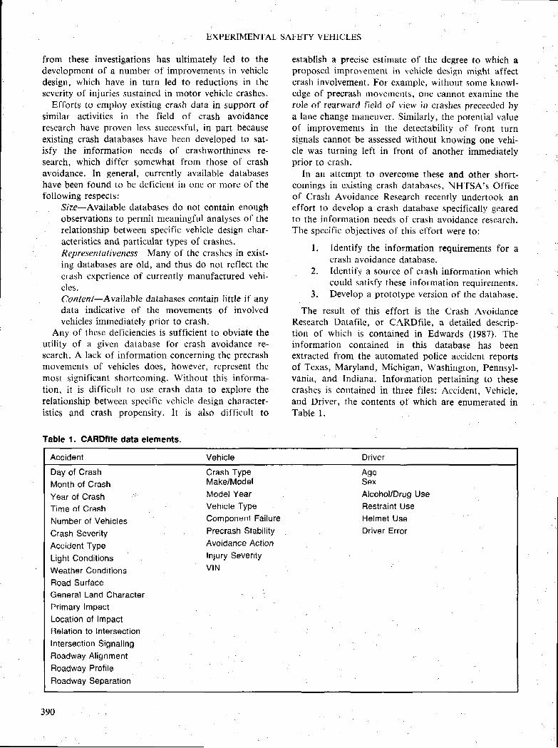
The result of this effort is the Crash AvoidanceResearch Datafilc, or CARDfile, a derailed descrip-tion of which is contained in Edwards fl987). Theinformation contained in this database has beenextracted from the automated police accident rcportsof Texas, Maryland, Michigan, Washington, Pennsyl-vania, and Indiana. Information pertaining to thesecrashcs is containcd in three fi les: Accident, Vchicle,and Driver, the contents of which are enulnerated inTable l .

Accident Vehicle Driver

AgeSex

Day of CrashMonth of CrashYear of CrashTime of CrashNumber of Vehic les

Crash SeverityAccident TypeLight ConditionsWeather ConditionsRoad SurfaceGeneral Land CharacterPrimary lmpactLocation of lmpactRelation to lntersectionIntersection SignalingRoadway AlignmentFloadway ProfileRoadway Separation

Crash TypeMake/ModelModel YearVehicle Type

Component Failure

Precrash Stabil ity

Avoidance ActionInjury SeverityV IN

Alcohol/Drug UseRestraint UseHelmet UseDriver Error

390

SECTION 4. TECHNICAL SESSIONS

Perhaps the most unique data element contained inCARDfile is Accident Type, which is used to describethe precrash movements of vehicles involved in eachof the crashes contained in the database. A total of 43accident type codes exist, describing not only theoverall movement patterns associated with the crash,but the specific movements of each involved vehicle.The coding scheme employed is based on workoriginally accomplished by Perchonok (1972) andTerhune (1983). As has been indicated, this informa-tion is of particular importance to crash avoidauceresearch because it makes possible the developmentand testing of hypotheses related to the role ofspecific vehicle design characteristics in crash involve-ment. For example, using CARDfile, it is possible toexamine the frequency with which vehicles ecluippedwith amber turn signals are struck in the rear endwhile turning, and compare this involvement to thefrequency with which vehicles equipped with red turn

signals are struck in similar situations. As anotherexample, it would be possible to exarnine the extent towhich vehicles equipped with front wheel drive areinvolved in rollover crashes. In fact, any vehiclecharacteristic common to a particular make and

model of vehicle can be evaluated with respect to itsinvolvenrent in a particular typc o[ cras]r and com-pared with the involvernent experience of vehicles with

different or similar characteristics.

CARDfile CharacteristicsAt prcscnt, CARDfile contains data on slightly

fewer than 4,000,000 crashes involv ing a lmost7,000,000 vehicles, which represents the police re-ported crash experience for the most recent threeyears of data available. A summary of the three year

crash experience (1983-1985) for each of the states inthis database is presented in Table 2. In total, thecrash data containcd in CARDfile repre$ents slightly

more than 2090 of the nation's annual police rcportedcrash experience.

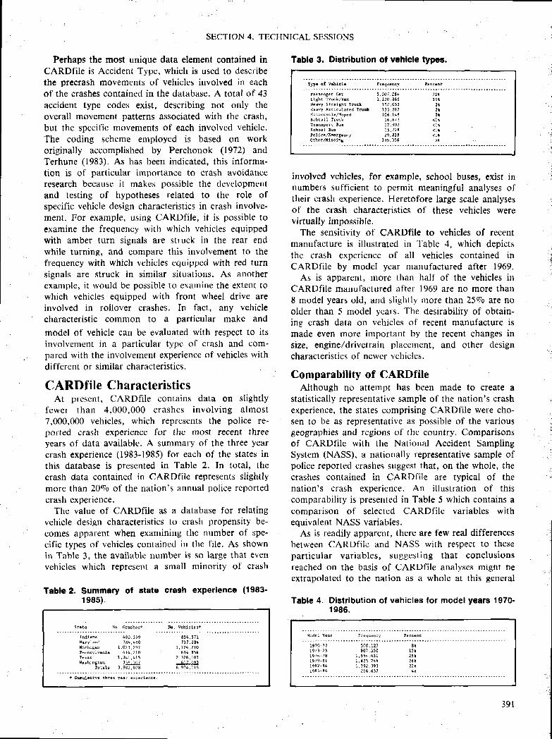
The value of CARDfile as a database for relatingvehicle design characteristics to crash propensity be-comes apparent when examining the number of spe-cif ic types of vehicles cotttained in the f i le. As shownin Table 3, the available number is so large that even

vehicles which represent a small minority of crash

Table 2. Summary ol state crash experience (1983'1 e85).

involved vehicles, for example, school buses, exisf innumbers sufficient to perrnit meaningful analyses oftheir crash experience. Heretofore large scale analysesof the crash characteristics of these vehicles werevirtually impossible.

The sensitivity of CARDfile to vehicles of recentmanufacture is i l lustrated in Table 4, which depictsthc crash experience of all vehicles contained inCARDiile by model year manufacturecl after 1969.

As is apparent, more than half of the vehicles inCARDfile manufactured after lg69 are no more than8 rnodel years old, and slightly more than 2590 are noolder than 5 model ycars. The desirabil ity of obtain-ing crash data on vehicles of recent manufacture ismade even more important by the recent changes insize, engine/drivetrain placement, and other designcharacteristics of newer vehicles.

Comparability of CARDfileAlthough no attempt has been made to create a

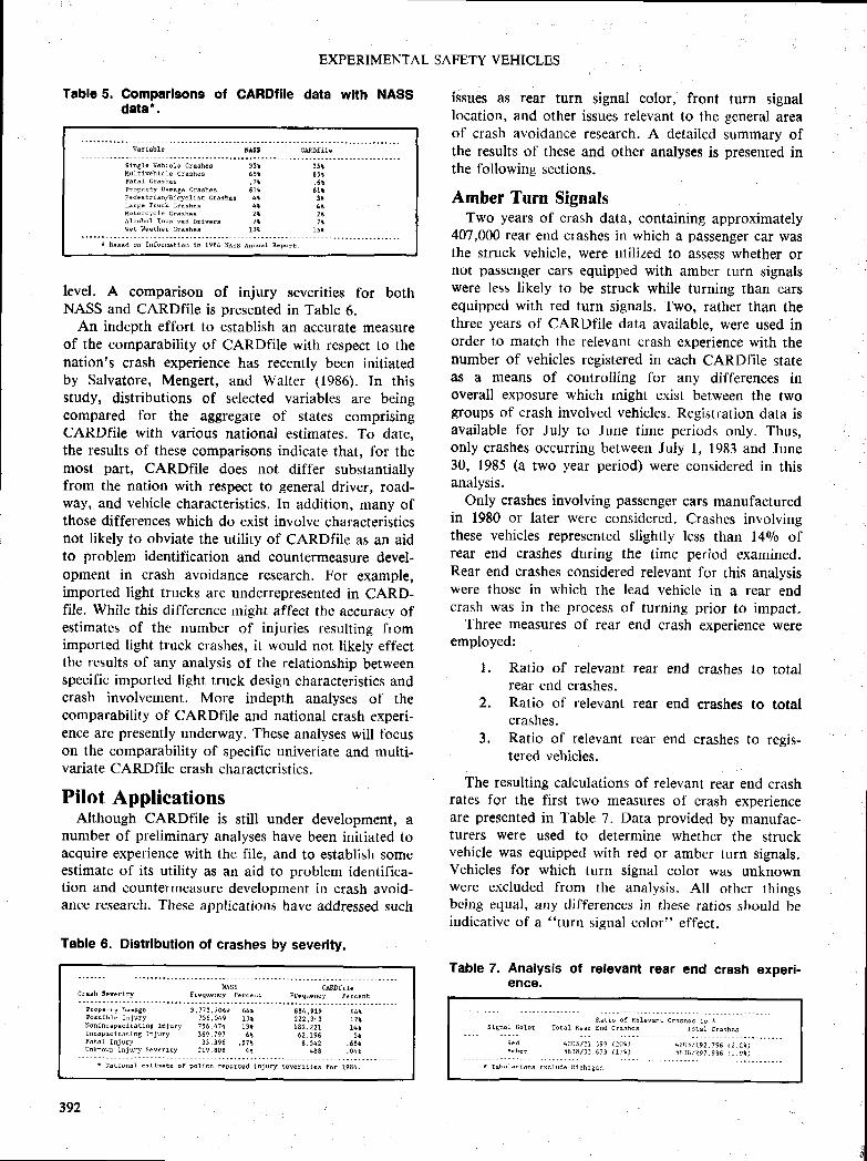
statistically representative sample of the nation's crashexperience, the states comprising CARDfile were cho-$en to be as representative as possible of the variousgeographies and rcgions of the country. Comparisonsof CARDfile with the Nationitl Accident SamplingSysteilr (NASS), a nationally representative sample ofpolice reported crashes suggest that, on the whole, thecrashes contained in CARDiile are typical of thenation's crash experience. An il lustration of thiscomparabil ity is presented in Table 5 which contains acomparison of selected CARDfile variables withequivalent NASS variables.

As is readily apparent, there are few real differencesbetween CARI)fi lc and NASS with respect to thesepart icu lar var iables, suggest ing that conclus ionsreached on the basis of CARDfile analyses mlght beextrapolated to the nation as a whole at this general

Table 4. Dlstrlbution of vehicles for model years 1970-1 986.

Table 3. Distribution ol vehlcle typ€s.

lT::1.1::::i:Prr rcn8. r c r r 5 ,OA1 ,284 72 \L t 8 h t r r u c k ^ i n I , 1 2 0 , 8 6 6 1 6 rH.s ry S t r r l th r Truc l 15?,os l 2 tH e s r y A r r l c u l a t e d l r u c l 1 1 5 , 2 8 7 2 sH o r o r c y c l . / H o F c d 1 0 6 , 1 4 8 2 tB o b t s i l T r u ( k 1 6 , 6 7 1 < 1 rTr i f , cpor r Buc 11 ,902 . i l r

s . h o o l B u ' 1 ! . 7 1 8 4 1 tPo l I r . /FnarEEn y ?g ,B lE < l r0 t h s r / H t E 6 t n t 1 1 5 , 1 5 6 5 r

Sta to No. Ctssh€s* No. vsh tc lss*

E 5 { , 5 7 rt l 7 , 1 8 L

7 , 7 Z 4 , Z L O6 9 . , 6 5 4

2 , 1 2 6 , I 0 3-Eu.tlt6 , S 3 4 , 1 1 3

H o d . t Y c r r r r . q u c n c y F c f c c f r t

, io ),1 9 7 3 - ) !t916 78I 9 7 9 - E II 9 8 2 - E 4l q B 5 - 8 6

391

EXPERIMENTAL SAFETY VEHICLES

Var iab le MSS CNDf t Is

Stn t le v€h lc le Crashss 35 t 3 ! lUu l t tv€h lc le c rsches 6s t 65 iF r r a l C l l r h e r , 7 , . 6 tPro ! . r ty DFhstF CrashBs 611 61 tFedest r tsn /Stcyc l l s r c rschcr 41 3 tLs IEe Truc l Cr t r rhcr 4 i 4 tMo lorcyc I c Cr r rhdr 2 { 2 t rcoh . r Invo tvsd Dr tvs rs 7N Jr[€ i Hsathsr Crashes 13 t 15*

* Bsssd on ln fo rna t lon 1n 1984 NAss Asnu l l R .po l r .

Table 5. Comparleone of GAHDflle data with NASSdate*.

level. A comparison of injury severities for bothNASS and CARDfile is presented in Table 6,

An indepth effort to establish an accurate measureof the comparability of CARDfile with respect to thenation's crash experience has recently been initiatedby Salvatore, Mengert, and Walter (1986). In this$tudy, distributions of selected variables are beingcompared for the aggregate of states comprisingCARDfile with various national estimates. To date,the results of these comparisons indicate that, for themost part, CARDfile does not diff'er substantiallyfrom the nation with respect to general driver, road-way, and vehicle characteristics. In addition, many ofthose differences which do exist involve characteristicsnot likely to obviate the utility of CARDfile as an aidto problem identification and countermeasure devel-opment in crash avoidance research. For example,imported light trucks are underrepresented in CARD-file. While this difference might affect the accuracy ofestimates of the number of injuries resulting fromimported light truck crashes, it would not likely eff'ectthe results of any analysis of the relationship betweenspecific imported light truck design characteristics andcrash involvement. More indepth analyses of thecomparability of CARDfile and national crash experi-ence are presently underway. These analyses will focuson the comparability of specific univeriate and mutti-variate CARDfile crash characteristics.

Pilot ApplicationsAlthough CARDfile is still under development, a

number of preliminary analyses have been initiated toacquire experience with the file, and to establish someestimate of its utility as an aid to problem identifica-tion and countermeasure development in crash avoid-ance research. These applications havs addressed such

Table 6. Distrlbutlon of crashes by severity,

issue$ as rear turn signal color, front turn signallocation, and other issues relevant to the general areaof crash avoidance research. A detailed summary ofthe results of these and other analyses is presented inthe following sections.

Amber Turn SignalsTwo years of crash data, containing approximately

407,000 rear end crashes in which a passenger car wasthe struck vehicle, were ulilized to asse,$s whether ornot passenger cars equipped with amber turn signalswere less likely to be struck while turning than carsequipped with red turn signals. Two, rather than thethree years of CARDfile data available, were used inorder to match the relevant crash experience with thenumber of vehicles registered in each CARDfile stateas a means of controlling for any differences inoverall exposure which might exist between the twogroups of crash involved vehicles. Registration data isavailable for July to June time periods only. Thus,only crashes occurring between July l, 1983 and June30, 1985 (a two year period) were considered in thisanalysis.

Only crashes involving pas$enger cars manufacturedin 1980 or later were considered. Crashes involvingthese vehicles represented slightly less than 14rlo ofrear end crashes during the timc period examined.Rear end crashes considered relevant for this analysiswere those in which the lead vehicle in a rear endcrash was in the proces.s of turning prior to impact.

Three measures of rear end crash experience wereemployed:

Ratio of relevant rear end crashes to totalrear end crashes.Ratio of relevant rear end crashes to totalcrashes.

3. Ratio of relevant rear end crashes to rcsis-tered vehicles.

The resulting calculations of relevant rear end crashrate$ for the first two measures of crash experienceare presented in Table 7. Data provided by manufac-turers were used to determine whether the struckvehicle was equipped with red or amber turn signals.Vehicles for which turn signal color was unknownwere excluded from the analysis. All other thingsbeing equal, any differences in these ratios should beindicative of a "turn signal color" effect.

Table 7. Analysis ot relevant rear end crash experi-ence.

l �

2.

NAss cNDfi l€

: : : : : : : t : : i : l . . . . . . . . . . . : : : : T : : ' * * - " . F * q u s n c v l e r c € n r

Plop. r ry Danet€ 3 , )12 , )66* 64 i 684 , !19P o r r i b r n I n j u r y J 3 6 , n 4 9 l t t Z Z 2 , r 4 rN a n i n f a p s c l E s E l i l A I s ] u r y 7 7 6 , 4 7 4 t 3 r t B r , ? Z lI l c l p r c l i r r i n 8 I n j u r y 3 6 9 , 1 9 7 6 t 6 2 , 1 9 6F i r n r t n j u r y 3 3 , J 9 6 , j 7 t 8 , 5 4 2thknoh ln ju ry sever lEy 219,808 4 i 496

1 7 114 i5r

.6 ! r

392

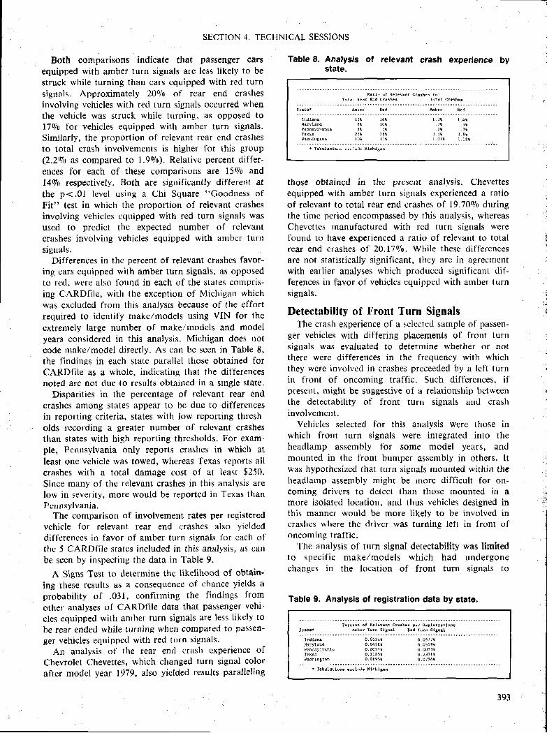
SECTION 4. TECHNICAL SESSIONS

Both comparisons indicate that passenger cars

equipped with amber turn signals are less l ikely to bestruck while turning than cars equipped with red turn

sigrrals. Approximately 20Vo of rear end crashesinvolving vehicles with red turn signals occurred whenthe vehiclc was struck while turning, as opposed tol79o for vehicles equipped with amber turn signals.Similarly, the proportion of relevant rear cnd crashesto total crash involvements is higher for this group(2-2Vo as compared to 1.9070). Relative percent differ-ences for each of these comparisons are l59o and

l49o respectively. tsoth are significantly different atthe p<.01 level using a Chi Square "Coodness ofFit" test in which the proportion of relevant crashesinvolving vehicles cquipped with red turn signals was

used to predict thc expected number ol relevantcrashes involving vehicles equipped with amber turnsignals.

Differences in the percent of relevant crashes favor-ing cars equipped with amber turn signals, as opposedto red, were also found in each of the states compris-ing CARDfile, with the exception of Michigan whichwas excluded from this analysis because of the effortrequired to identify make/models using VIN for theextremely large number o[ make,/models and modelyears considered in this analysis. Michigan does notcode make/rnodel directly. As catr be seen in Table 8,the findings in each state parallel those obtained forCARDfile as a whole, indicating that the differencesnoted are nof due to results obtained in a single state.

Disparit ies in the percentage of relevant rear endcrashes among states appear to be due to differencesin reporting criteria, states with low reporting thresh-olds recording a greater number of relevant crashesthan states with high reporting thresholds. For exam-ple, Pennsylvania only reports crashes in which atleast one vehicle was towed, whereas Texas reports allcrashes with a total damage cost of at least $250.Since many of the relevant crashes in this analysis arelow in severity, more would be reportccl in Texas thanPennsylvania.

The comparison of involvement rates per registeredvehicle for relevant rear end crashes also yielded

differences in favor of amber turn signals I 'or each ofthe 5 CARDfile states included in this analysis, as canbe seen by inspecting the data in Table 9.

A Signs Test to determine thc likelihood of obtain-

ing thesc results a$ a collsequence of chance yields a

probabil ity of .031, confirrning the findings from

other analyses of ClARDfile data that passenger vehi-

cles equipped with amber turn signals are less l ikely to

be rear ended while turnitrg when compared to passen-

ger vehicles equipped with red turn signals.

An analysis of the rear encl crash cxperience of

Chevrolet (lhevettes, which changed turn signal color

after model year I979, also yiclded results paralleling

Table 8. Analysis of releyant crash experience bystate.

those obtained in the present analysis. Chevettesequipped with amber turn signals experienced a ratio

of relevant to total rear end crashes of l9.70Vo duringthe time period encompassed by this atralysis, whereasChevettes rnanufacturcd with red turn signals werefound to have experienced a ratio of relevant to totalrear end crashes of 20.1790. While these dil lerencesare not statistically significant, thcy are in agreementwith earlier analyses which produced significant dif-ferences in favor of vehicles equipped with amber turnsignals.

Detectahility of Front Turn SignnlsThe crash experience oI a sck'cted sample of passen-

ger vehicles with differing placements of front turnsignals was evaluated to determine whether or notthere were differences in the lrequency with whichthey were involvcd in crashes preceeded by a left turnin front of oncoming traffic. Such differences, ifpre$ent, might be suggestive of a relationship betweenthe detectabil ity of front turn signals and crashinvolvement.

Vehicles selected for this analysis were those inwhich front turn signals were integrated into theheadlamp assembly for some model years, andmounted in the front bumper assembly in others. Itwas hypothesized that turn signals mounted within theheadlarnp assembly might be more diff icult for on-coming drivers to detect than those mounted in amore isolated location, and thus vehicles designed inthis manner would be more l ikely to be involverl incrashes where thc clrivcr was turning left in frottt ofoncoming traffic.

The analysis of turn signal detectability was limitedto speci f ic make/models which had undergonechanges in the location of front turn signals to

RaEio o f RaI€v inE c r { rher Eo:Tor :n l R . { r E f rd Cr$hcr ToEAI Cr+*hr r

s r6Ee* Mbsr Rsd hbsr Red

; ; ; ; ; " i i ; i ; ; " " "

i ; ; i ; ;H r r y l l n d 8 $ I 0 r . 7 t . 9 tP . n n 5 y l v r n l d 2 t 3 r . 2 r . 3 iT c x l r 2 3 r 2 6 1 3 . I $ 3 . 8 i

1r:11:'r::r 1:: ll: ....... l.ilt ].11t .,..* T r b u h E t a n r E x c l u d E M l c h t 8 i f r

Table 9. Analysls ol registration data by state.

;:;;:;; ;; ;:i:;:;; ;;:;;:: ;:; ;;;:;;;;i;;;: : : : : : . . . . . . . . . . T::: l : : : : ir : i i : i l : : : :1T::.

I n d t r M 0 . 0 1 2 4 1 0 . 0 t 7 / rM F r y l s n d 0 . 0 4 5 8 1 0 . 0 t t 9 rr s n n s y l v 8 h { a 0 , 0 0 5 7 r o . 0 0 7 l rT s x s s o , ? l 8 5 t o . ? r l t r$ € B h t n t t a h 0 . 0 6 9 5 l d , d 7 2 6 r

393

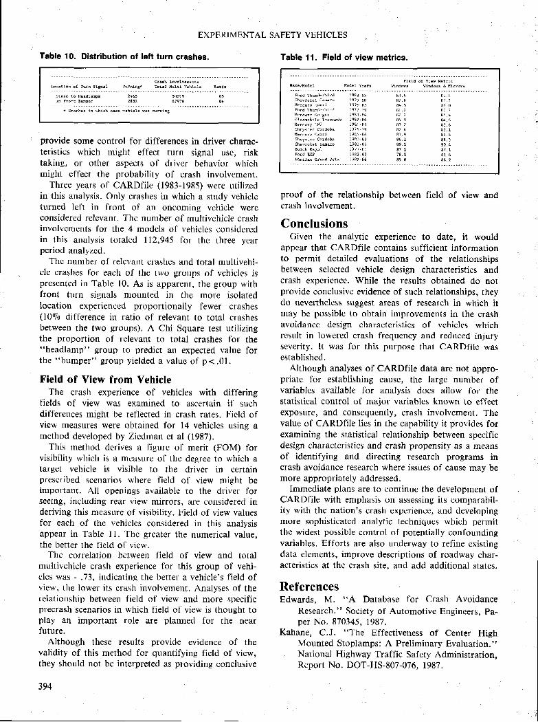
EXPERIMENTAL SAFETY VEHICLES

Table 10. Dlstribution of left turn crashes.

h c { E 1 6 n o l T u r n S l B n a I T u Y f i l s E * T o l l l X u l L t V c h l c l c

Clor t To lh ld l lmp l 2465 50019 .05In Fron t BMpcr 2d1? 62976 ,O4

provide some control for differences in driver charac-teristics which might effect turn signal use, risktaking, or other aspect$ of driver behavior whichmight effect the probability of crash involvernent.

Three years oi CARDfile (1983-1985) were uti l izedin this analysis. Only crashes in which a study vehicleturned left in lront of an oncoming ve]ricle wereconsidered relevant. The nunrber of multivehicle crashinvolvcments for the 4 models o[ vehicles cronsideredin this analysis totaled llZ,945 for the three yearperiod analyzcd.

The number of relcvant crashes and total multivehi-cle crashe,r for each of the two groups of vehic-les ispresented in Table 10. As is apparent, the group withfront turn signals mounted in the more isolatedlocation expericnced proportionally fewer crashes(1090 dii lerence in ratio of relevant to total crashesbetween the two groups). A Chi Square test utilizingthe proportion of relevant to total crashes for the"headlamp" group to predict an expected value forthe "bumper" group y ie lded a value of p<.01.

Field of View from YehicleThe crash experience of vehicles with differing

fields of view was exarnined to ascertain if suchdifferences rnight be reflected in crash rates. Ficld ofview measures were obtained for 14 vehicles using amethod developed by Zicdman et al (1987).

This method dcrives a figure of merit (FOM) forvisibil i ty which is a measure of the degree to which atarget vehicle is visible to the driver in certainprescribed scenarios where field of view might beimportant. All openings availablc to the driver forseeing, including rear view mirrors, are considered inderiving this measure of visibil i ty. Field of view valuesfor each of the vehicles considered in this analysisappear in Table I l. Thc grcater the numerical value,the berter the f ield of vicw.

The correlation between lield of view and totalmultivehicle crash experience for this group of vehi-cles was -.73, indicating the better a vehicle's f ield ofview, the lower its crash involvernent. Analyses of therelationship between field of view and more specificprecrash scenarios in which field of view is thought toplay an important role are planned for the nearfuture.

Although these results provide evidence of thevalidity of this method for quantifyine field of view,they should not be interpreted as providing conclusive

394

Table 11. Fleld of view metrics.

proof of the relationship between field of view andcrash involvement.

ConclusionsCiven the analytic experience to date, it would

appear that CARDfile contains sufficient informationto permit detailed evaluations of the relationshipsbetween selected vehicle design characteristics andcrash experience. While the results obtained do notprovide conclusive evidence of such relationships, theydo nevertheless suggest areas of researsh in which itmay be possible to obtain improvements in the crashavoidancc design characteristic$ of vehicles whichresult in lowered crash frequency and reduced injuryseverity. lt was for this purpose that CARDfile wasestablished.

Although analyses of CARDfile data are not appro-priate for establishing cause, the large number ofvariables available for analysis does allow Ibr thestatistical control of rnajor variables known to effectexposure, and consequently, crash involvcment. Thevalue of CARDfile lies in the capability it provides forexamining the statistical relationship between specificdesign characlcristics and crash propensity as a rneansof identifying and clirecting research programs incrash avoidance research where issrres of cause may bemore appropriately addressed.

Immediate plirns are to continue the development ofCARDfile with emphasis on assessing its comparabil-ity with the nation's crash experience, and developingmore sophisticated analytic techniqucs which permitthe widest possible control of potentially confoundingvariables. Efforts are also underway to refine existingdata elements, improve descriptions of roadway char-acteristics at the crash site. and add additional states.

ReferencesEdwards. M. "A Database for Crash Avoidance

Research." Society of Automotive Engineers, Pa-per No. 870345, 1987.

Kahane, C.J. "The Effectiveness of Center HighMounted Stoplamps: A Preliminary Evaluation."National Highway Traffic Safety Administrarion,Report No. DOT-HS-807-076, 1987.

Frc ld e f V lsp f le t r l cXsk€/Mod€ l Mddc l Yc ! r ' v tndowr Htndows E Mt r !6 ! j

F u I d T h u u d r f b l f d 1 9 8 3 - 8 5 E l , 4 8 5 . 6c h c v l o l c l c l n r f o 1 9 7 9 - 8 0 8 7 , E 8 / . 3b E r E u r . l C ^ F r i 1 9 7 9 - 8 3 8 4 . 5 8 1 . 0F o r d T h u n d c r h i r d 1 9 7 1 - 7 9 8 I . 2 A 2 . 7H c r . u r y c o u E 8 r 1 9 E l . E 4 8 2 . 2 4 6 , 4o l d r h o h i l a T a r o r u d o 1 9 8 2 - E 4 8 n . 9 8 4 , 6U P r N U r y L N 7 I 9 8 I - 8 3 8 3 . 2 8 3 . 6C h r y e l e r c o r d o b { I 9 7 5 - 7 t 8 2 . 6 8 3 . Ix c r c u r y c l p r l 1 ! g ! - 8 6 B t , g 8 ! . JchryF lc r Cordobs I e80 E l E6. I EE, lC h e v r o l e t C M a r o 1 9 8 2 - 8 5 8 9 . 1 9 0 . LE u r c l R c f r l l g / / - H ] E 7 1 8 t . 1F o r d H ? 1 9 8 2 - 8 1 7 8 . 8 8 1 . 6l o n l r d c G r l n d P r t x 1 ! 8 r - 4 6 8 5 , 6 8 8 . 2

Perchonok, K. "Accielent Cause Analysis." NationalHighway Traffic Safety Administration, ContractNo . DOT-HS-053 - l - 109 , 1972 .

S a l v a t o r e , S . , M e n g e r t , P . , a n d W a l t e r , R ."CARDfile l)atabase Representativeness-PhaseI : General Character is t ics inc luding Populat ions,Vehicles, Roads, and Fatal Acciclcnts." Transpor-tat ion Systems ( icr r ter , 1986.

Study in Avoidflnce of Road AceidentsAccident-Relevant Driving Manoeuvres

F. KramerrN. Shakeri-Nejad,G. Schockenhoff, et. al. , iTechnische Universitat,

W. Hauschild,MAN Technologie CmbH; ;:Ber l in .Federal Republic of Germany

AhstractOn the basis of control loop components, it is

explained which occurrcnccs ol' accident-relevatrt driv-ing rnanoeuvres can lead to road accidents. Thesemanoeuvres are simulated with the aid ol ' the drivingdynamics s imulat ion model MEDYNA. In extremesituations, the variatiorrs in the vehicle parameters

lead to an unstable behaviour, which at; a ruleprecedes an accident, mcaning that l intit values and/or area$ representing the criterion for study of anaccident, or rather, of its avoidance, can be estab-lished. The accident-rclcvrrnt driving manoeuvres, thedescribed quantit ies of thc irctions introduced by thedriver, such as braking, accelerating atrd steering, aswcll as the spectrum of vehicle-spccific paranteters arededuced fronr the analysis of the material provided bythe accident research group of Medizitrische Hoch-schule Hannover and Technische Universitdt Berlin(MHH/TUB). The init ial results on the avoidabil itystudy, which were achieved in a research work spon-sored by the Bundesan$talt f i ir StraBenwesen! arepresented,

Presentation of the Prohlem andApproach to AvoidabilityConsiderations

All activit ies in the field of vehicle safety are carriedout frorn the aspcct of influencing the accidentoccurrence. The followiflg questions therefore arise inconsiderations on the avoidabil ity of accidents:

SECTION 4. TECHNICAL SESSIONS

Terhune, K. "CALAX: A Coll ision Taxonomy forResearch and Traf f ic Records." Journal ofSafety Research, Vol . 14, pp. l3-20, 1983.

Zicdman, K. Final Bricfing: Dcvclopment of Figuresof Merit lor Motor Vehicle Conspicuiry andVisibil i ty Subsystems. National Highway TrafficSafety Adnr in is t rat ion, Contract No. DTNII22-84-CO7098. Apr i l , 1986.

with the Aid of Computer Simulation of

how do accidents come about (rcsearch intoaccident causes)?

r what circumstances lead to accidents andwhal parameters can be used to describethese circumstances'l

. how can thc circumstatrces which cause acci-dents be avoided; i .e . , what value must thepararneter not be allowed to assume?

The answers to these questions incvitably lead tothe neccssity of atralysing the accidcnt occurrence withregard to its causes, and of followirtg thc cleveloptnentol' accidents, so that the scnsitivity and liniitations ofthe parameters describing the actual state can bedetermined by introducing a widely applied variationof thcsc parameters (F ieure l ) .

The accident occurrencc only includes a negativeselection of all those cascs in which an accident-relevant driving nranosuvre did not lead to the nraster-ing of a crit ical situation, but resulted in an accidentin the form of incurrcd damages atrd injuries' respec-tively. Those case$ in which accident-relevant drivingmanoeuvre$ were able to be mastcred are near-accidents, but these are not included in any compila-tion of accident data (even though every driver of anlotor vehicle can report fronr lr is own expcrience onone or another near-accident). In our study on theavoidabil ity of accidents we are dealing, ltowever,with the question of what conditions lead to theoccurrerlce or non-occurrense o[ an accident when acrit ical situation ari$e$-i.e., what parameters dirt in-guish irn accidcnt-relevant driving manocuvre frotn apre-crash phase?

Iirom this, we can conclude that indications ofaccident-relevant clriving manoeuvres can be deducedfrom an analysis of the accidettt occurtence but thatthe questions concerning the tnastering of a crit icalsituation can only be answered by sirnulation of theaccident-relevant driving manoeuvres. This can, how-ever, only be carried out usirtg individual cases asexamples. To do this, it is necessary to deducedevelopment patterns of accident-rclcvant driving ma-

395

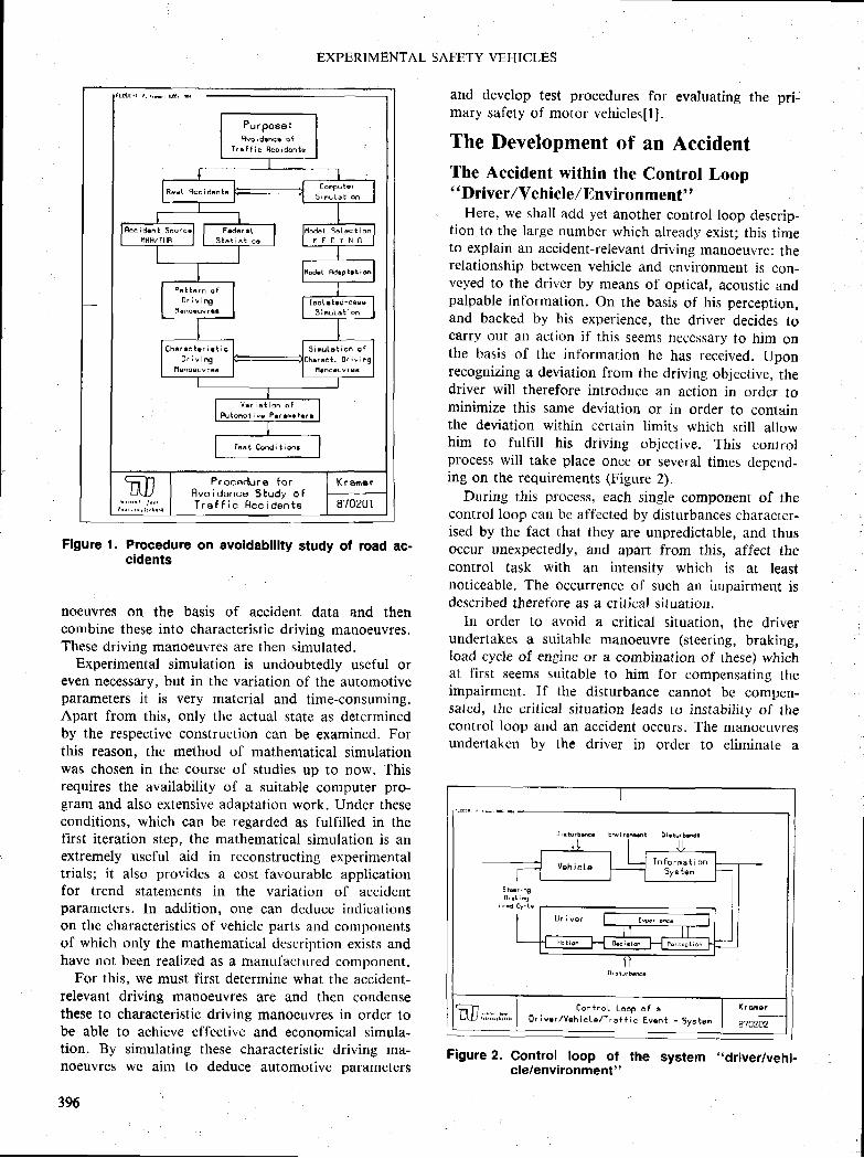
Procadu re f o rF l vo i dance S tudy o fT r a f f i c R c c i d e n t s

Pu r poee rBvq idmcq o f

T r g f f i c f f c c i d e n t e

I rot r t .d-crssS i n u L e t i o n

5 i n u L o t i o n o f

v s r i s t i o n o fH u t o m o t i v e P . r . n . t r . r

fsst Condi t ionr

EXPERIMENTAL SAFETY VEHICLES

Flgure 1. Procedure on avoldablllty study ol road ac-cidentg

noeuvres on the basis of accident data and thencombine these into characteristic driving rrlanoeuvres.These driving manoeuvres are then simulated.

Experirnental simulation is undoubtedly uscful oreven neces$ary, but in the variation of the automotiveparameters it is very material and time-consuming.Apart from this, only the actual state as detcrrninedby the respective construction can be examined. Forthis reason. the method of mathematical simulationwas chosen in the course of studies up to now. Thisrequires the availability of a suitable computer pro-gram and also extensive adaptation work. Undcr theseconditions, which can be regarded as fulfilled in thefirst, iteration step, the mathematical simulation is anextremely useful aid in reconstructing experinrentaltrials; it also provides a co$t-favourable applicationfor trend statements in the variation of accidentparameters. ln addition, one can deduce indicationson the characteristics of vehicle parts and componentsof which only the mathematical description exists andhave not been realized as a manufactured component.

For this, we must first determine what the accident-relevant driving manoeuvres are and then condensethese to characteristic driving manocuvres in order tobe able to achieve effective and economical simula-tion. By simulating these characteristic driving ma-noeuvres we aim to deduce automotive parameters

396

and develop test procedures for evaluating the pri-mary sal'ety of motor vehiclesIl].

The Development of an AccidentThe Accident within the Control Loop" Driver/Veh icle/ Flnvironment"

Here, we shall add yet another control loop descrip-tion to the large numbcr which already exist; this t imeto explain an accident-relevant driving manoeuvrc; therelationship between vehicle and environment is con-veyed to the driver by means of optical, acoustic andpalpable information. On the basis of his perception,and backed hy his experience, the driver decides tocarry out an action if this seerns neccssary to him onthe hasis of the information he has received. Uponrecognizing a deviation frorn the driving objective, thedriver will therefore introcluce an action in order tominimize this same deviation or in order to containthe deviation within ccrtain l inrits which sti l l allowhim ro fulf i l l his driving objective. This conlrolprocess will take place once or several times depcnd-ing on the requirements (Figure 2).

During this process, each single component of thecontrol loop can lre affected by disturbances character-ised by the fact that they are unpredictable, and thusoccrur unexpectedly, and apart from this, affect thecontrol task with an intensity which is at leastnoticeable. The occurrencc of such an impairment isdcscribed therefore as a critical situation.

ln order to avoid a crit ical situation, the driverundertakes a suitable manoeuvre (stcering, braking,load cycle of engine or a combination of these) whichat f irst seems suitable to him for compcnsating theimpairrnent. If the disturbance cannot be compen-sated, the crit ical situation leads to instabil ity of thecontrol loop and an accident occurs. The manoeuvresundertaken by the driver in order to eliminate a

Figure 2. Control loop of the $ystem .,driver/vehi-cle/environment"

I LJ I ^ f o r * . t i o .Y e n r c t e S y e t e m

0r iv6r l----E*.;---]-Tr-rc . t , o n f 0 . < , . , o n f f e " . . * p t , o .

C o n t r o l L o o p o f e0 r i v c r . / V e h i c L e / T r s f f i c E v e o t - S y e t e '

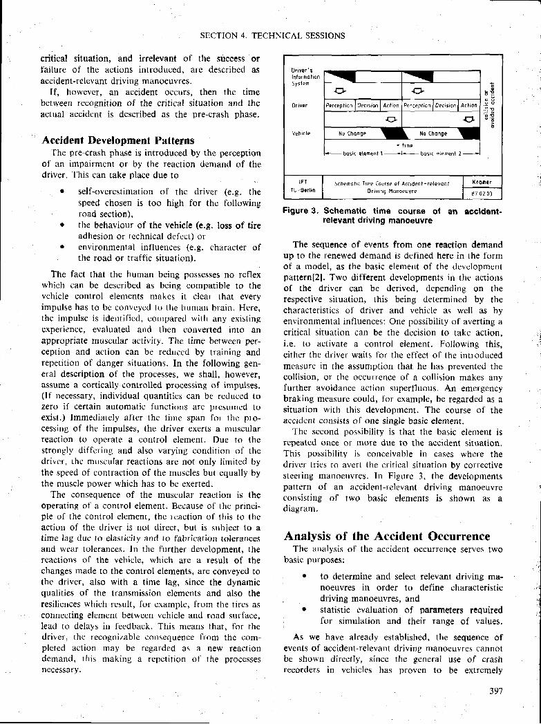
SECTION 4. TECHNICAL SESSIONS

critical situation, and irrelevant of the success orfailure of the actions introduced, are describcd asaccidertt-relevant driving manoeuvres.

lf, however, an accident occurs, then the timebetween recognition of the critical ,situation and theactual accident is described as the pre-crash phase.

Accident Development PatternsThe pre-crash phase is introduced by the perception

of an impairmcnt or by the reaction denrand of thedriver. This can take place due to

t self-overestirnation of the driver (e.g. thespeed chosen is too high for the following

' road section),t the behaviour of the vehicle (e.g. Ioss of t ire

adhesion or technical dcfcct) orr environrnental influences (e.g. chirracter of

the road or traffic situation).

The fact that the humau being possesses no reflexwhich can be described as being compatible to thevehicle control elements makcs it clear that everyimpulse has to bc convcyed to the human blain. Here,the impulse is identi l iccl, compared with any existingexperience, evaluated and then converted into anappropriate muscular activity. The time between per-ception and action can be reduccd by training andrepetit ion of danger situirt ions. In the following gen-eral description of the processes, we shall, however,assume a cortically-controlled proccssing of impulses.(lf rrecessary, individual quantit ies can be reduced tozero i[ certain automatic lunctions arc prcsumed toexist.) Immediately al 'ter fhe tirnc span for rhc pro-cessing of the impulses, the driver exerts a muscularreaction to operate a control element. Due to thestrongly diffcring aud also varying condition of thedrivcr, thc mr.rscular reactions are not only l imited bythe speed of contraction of the muscles but equally bythe muscle power which has to be exerted.

'fhe consequence of the muscular reaction is the

operating of a control element. Because of the princi-ple oi ' the control element, thc rcaction of this to theaction of the driver is not direct, but is subject to atime lag due to elasticity and to fahrication tolerancesand wear tolerances. ln the further developmentn thereactions of the vehicle. which are a result of thechanges made to the control elements, are conveyed tothe driver, also with a time lag, since the dynamicqualit ie$ of the transmission elemcnts and also theresil iences which result, for example, from the tires asconnecting element between vehicle and road surface,lead to delays in feedback. This means that, for thedriver, the recognizable corrsequence from thc com-pleted action may be regarded as a new reactiondemand, th is making a rcpct i t ion of the processesnecessary.

Figure 3. Schematlc time course ol an aecldent-relevant driving manoeuvre

The sequence of events from one reaction demandup to the renewed demand is defined here in the formof a model, as the basic elernent of the developmentpattern[2]. Two different developments in the actionsof the driver can be derived, depending on therespective situation, this being determined by thecharacteristics ol ' driver and vehicle as well as byenvironmental intluences: One possibil i ty of averting acrit ical situation can be the decision to take action,i.e. to activate a control element. Following this,either the driver waits l 'or the el'fect of the irrtroducedmcasurc in the assumption that he has prevented thecoll ision, or the occurrence of a coll ision makes anyfurther avoidance action superfluous. An emergencybraking measure could, for example, be regarded as asituation with this development. The course of theaccident consists ol 'one single basic element.

The second possibil i ty is that the basic element isrepeated once or more due to the accident situation.This possibil i ty is conceivable in cases whcre thedriver tries to avert the crit ical situation by correctivesteering manoeuvres. In Figurc 3, the developmentspattern of an accident-relcvant driving manoeuvreconsisting of two basic elements is shown as adiagranr.

Analysis of the Accident OccurrenceThe analysis of the accident occurrence serves two

basic purposes:

. to determine and select relevant driving ma-noeuvres in order to define characteristicdriving manoeuvres, and

. statistic evaluation of pf,rameters requiredfor simulation and their range of values.

As we have already established, the sequence ofevents of accident-relevant driving manoeuvres cannotbe shown directly, since the general use of crashrecorders in vehicles has proven to be extremely

Or iver ' sIn fo rmol rdnS y s l e m

0r iver

Veh i t te

. o d

bosir eleFent

E E+ +

Percept ron | 0ec is ion I Ar t ion Per rep t ion | Oecrs ion I Ac t ion

+ +No [ndngo L No [ndngE

. . . . .* t tm€

r t e l e

I F I

I U - B G r l i n5(hef to l i t I tme [ourse o f A( ( iden l - re levon l

0 r i Y r n g H o n o e u v r e

KroDer

87 02 0 l

397

EXPERIMENTAL SAFETY VEHICLES

problematic, mainly for legal reasons. For this ieason,the clevelopments have to be derived from the pre-crash phase of docurnented accidents. This necessarystep of equating an accident-relevant driving ma-noeuvre with the course of a pre-crash phase can beregarded as permissible, due to the presurnption thatthe same cour$e of action is taken by the driver fromthe init ial situation up to aversion of the accident, or,in the second case, up to the acciderrt actuallyhappening.

From the Accident-relevant DrivingManoeuvre to the Characteristic DrivingManoeuvre

In the Federal Republic of Germany, all accidentsreported to the police are compiled in the forrn of atable in the so-called Bundes-Statistik-this is thenumerical data on the road traffic accidents which isevaluated and published by the Statistisches Bunde-samt (Federal Statistics Oftice)[3]. In thcse statisticsthe traffic accidents are differentiated into seven typesand these are divided into two groups: within cityboundaries (intra-urban) and outside of city bound-aries (extra-urban) and also with regard to theirseverity. On the basis of this, it is possiblc todetcrmine, in ecorromical terms, the costs resultingfrom injuries in the various types ol accident, whichcan be shown in comparison to each other. Since,however, more detailed circumstances and informa-tiorr on the course of the accidents-which we shall gointo in more detail-are lacking, actual analysis ofaccident occurrences is based on the considerablymore detailed documention material on accidentsprovided by the accident research group MHH/TUB(financed by the Bundcsanstalt fr ir StraBenwesen).

The correlation of thesc two scts of material bymeans of the common criteria: type of' accident andseverity of injury (expressed as costs resulting frominjuries), for the purposes of comparative study, as

Figure 4. Di$tribution of the economic costs resull lnglrom Inluries in 1984 (intra-urban)

398

Figure 5. Distribution of the economic co$ts resultingfrom injuries in l9B4 (extra-urban)

-

well as a limitation to the accident year 1984 makes itpossible to establish the relevant type of accidentinsidc and outside of city boundaries. Figures 4 arrd 5show the percentual distribution of the costs resultingfrom injuries in various types of accidents inside andoutside of city boundaries. Despite the considerabledifference in the number ol ' cases recorded (Bundes-

stati$tik 1984: 416,232, MHH/TUB-material 1984: 646injured persons) and the philosophy conccrning datacollection practised at this time, but which has mean-while been revised, by the accident research groupMHH/TUB (mainly $erious accidents were recorded),the correlation between the respective clsfinit ions canbe considered as sufficiently exact. The comparisonquite clearly allows the conclusion to be made that

r inside city boundaries, the categories of acci-dents caused by "crossing pedestrians" and"junction,/crossing" are prevalent, and

r in areas outside of' ciLy boundaries the cate-gories o1' acciderrt "driving accident" and"longitudinal-traffic accident" cau$c thehighest costs re$ulting from injuries.

The further statistical evaluation was based on totalmaterial comprising 2,753 accidents. However, inorder to be able to ensurc a comparable safetystandard, the accident material had to be leveled outand older vehiclcs (up to the year o[ construction1972) eliminated; apart from this, only four types ofvehicle of an cxemplary character werc selected.

ln an evaluation of the remaining accidents materialwith a total of 290 accidents, the respectivc actions ofthe driver, such as steering and braking, can becoordinated with the relevant types of accident; thevehicle reactions swerving and deceleration, which canbe determined from accident marks, serve as compari-son and control quantit ies. Engine-load cycles couldnot be established as driver activity in the acciclentmaterial. Apart from this, the evaluation includes the

f i d

= r r i i l f f i i! /A l Y / .4= * l r / /A l l s

ircident TZp.

1 Dr iy ing Tro f f i c

2 T ! r n o f f T r o f l i r

I J u n ( t i o n / t f o s s i n q

4 G o i n g A r r o s s r P c d )

6 L o ^ q , l u d i n o l T r s l f i c

l ? 1 4 5 6 7Ai l de f t Type

tcc ident dAtq *or . r r I s to t i s t i s fher apntp1p i l f f ihan t tgg

IF IfU-Srrtin

Eronomi( ln jury Cosis in 19E4(exfrd - urbsnl

K r o m e f

87 02 05

.9

Aftident TIF

1 Dr iY inq T fo f f i c

? Tufn o f t T ro f f i (

1 J !ncr ,on / L ro t i lnE

{ 6 o i n q A ( f o s s l P { d I

5 T r o t f l c i n F e s i

6 L o r q r t u d i n q l T r o l t i (

? 0 thers

Aridrnt doto ' ""r .* l - ' l stor i rr i r rhes sund+loni f f i naartul

: l V /A l V tn i i- | v/At r//A = i

IFTTU - Ber l in

Ecdnonic Injury Cosls in i984( i n t r o - u r b o n )

Xra m er

I'I 02 0t

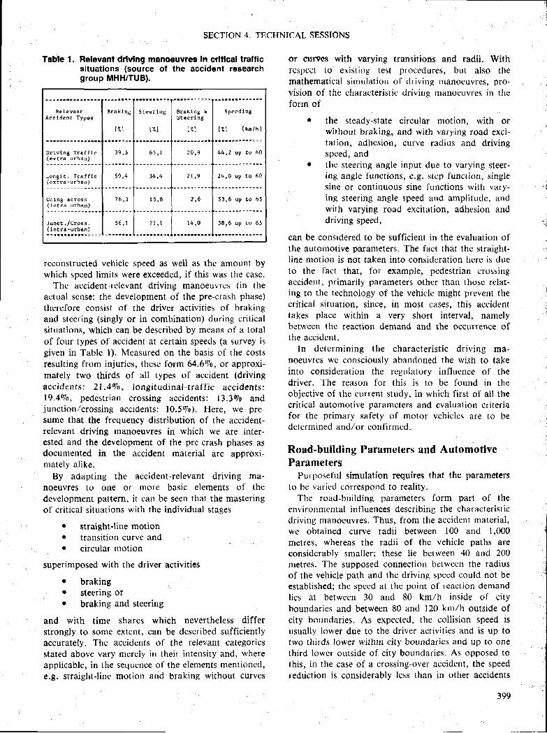
S t e e r l n g

t l l

B r a k l n g &S t e e r l n g

l r l

S p e e d l n g

t 1 l [ k 6 / h ]

6 5 , 1D r i v l n B T r a f f l c( e x E r a - u r b a n )

L o n B i t , T r a f f l c( e x t r a - u r b a n )

C o i n B a c r o s s

I l::::::::::lJ u n c t . / c r o s s .

I 1:::::::::: I

59,4 14,4

1 n o 4 4 , 2 u p t o 6 0

2 4 , 0 u p t o 6 0

2 , 6 5 3 , 6 u p t o 6 5

l 4 , 0 3 8 , 6 u p t o 6 5

SECTION 4. TECHNICAL SESSIONS

Table 1. Relevant drlvlng mano€uvrea In crltlcal trafficsituations (source of the accident researchgroup MHH/TUB).

reconstructed vehiclc speed as well as the amount bywhich speed limits were exceeded, if this was the case.

The accident-rclevant driving manoeuvreri (in theactual scnse: the development of the pre-crash phase)

therefore con$ist of the driver activit ies of brakingand steering (singly or in combination) during criticalsituations, which can be describcd by means of a totalof four types of accident at certain speeds (a survey isgiven in Table 1). Measured on the basis of the costsresulting from injuries, these form 64.690, or approxi-mately two thirds of all types of accident (driving

accidents: 2 l .4Vo, longi tudinal - t raf f ic acc idents:19.4Vo, pedestrian crossing accidents: 13.390 andjunction,/crossing accidentsl 10.590). Here, we pre-sume that the frequency distribution of the accident-relevant driving manoeuvres in which we are inter-ested and the development of the prc-crash phases asdocumented in the accident material are approxi-mately a l ike.

By adapting the accident-relevant driving ma-noeuvres to one or more basic elements of thedevelopment pattern, it can be seen that the masteringof crit ical situations with the individual stages

r $traight-line motion. transition curvc andr circular motion

superimposed with the driver activities

r brakingr steering or. braking and steering

and with time shares which nevertheless differstrongly to somc extent, can be described sufficientlyaccurately. The accidents of the relevant categoriesstated above vary merely in their intensity and, where

applicable, in the sequence ol the elements mentioned,e.g. straight-l ine motion and braking without curves

or curves with varying transitions and radii. Withrespect to ex is t ing test procedure$, but a lso themathematical simulation oI driving manoeuvres, pro*vision of the characteristic drivins manoeuvres in theform of

. the steady-state circular motion, with orwithout braking, and with varying road exci-tation, adhesion, curve radius and drivingspeed, and

r the steering angle input clue to varying steer*ing anglc frrnctions, c.g. stcp functiorr, singlesine or continuous sine functions with vary-ing steering angle speed and amplitude, andwith varying road excitation, adhesion anddriving speed,

can be considered to be sufficient in the evaluation ofthe automotive parameters. The fact that the straight-l ine motion is not taken into consideration here is dueto the facl that, for example, pedestrian crossingaccident, primarily parameters other than those relat-ing to the technology of the vehicle might prevent thecrit ical situation, since, in most cases, this accidenttakes place within a very short interval, namelybetween the reaction demand and the occurrence ofthe accident.

ln determining the characteristic drivirrg ma-noeuvres we consciously abandoned the wish to takeinto consideration the regulatory influence of thedriver. The reason for this is to be found in theobjective of the currert stutly, in which first of all thecrit ical automotive paramcters and evaluation criteriafor the primary safety of motor vehicles are to bedetermined and,/or confirmed.

Road-building Parameters and AutomotiveParameters

Purposel'ul simulation requires that the parameters

to be varied correspond to reality.Ttre road-building parameters form part of the

environrnental influences describing the characteristicdriving manoeuvres. Thus, from the accident material,we obtained curve radii between 100 and I,000metres, whereas the radii of the velticle paths areconsiderably smaller; these lie between 40 and 200metres. The supposed connection between the radiusof the vehicle path and the driving speed could not beestablished; the speed at the point of reactiotr demandlics at between 30 and 80 km/h inside of cityboundaries and between 80 and 120 km/h outside ofcity boundaries. As expected, the coll ision speed isusually lower due to the driver activit ies and is up totwo thirds lower witlt in city boundaries and up to oDethird lower outside of city boundaries. As opposed tothis, in the case of a crossing-over accident, the speedreduction is considerably less than in other accidents

399

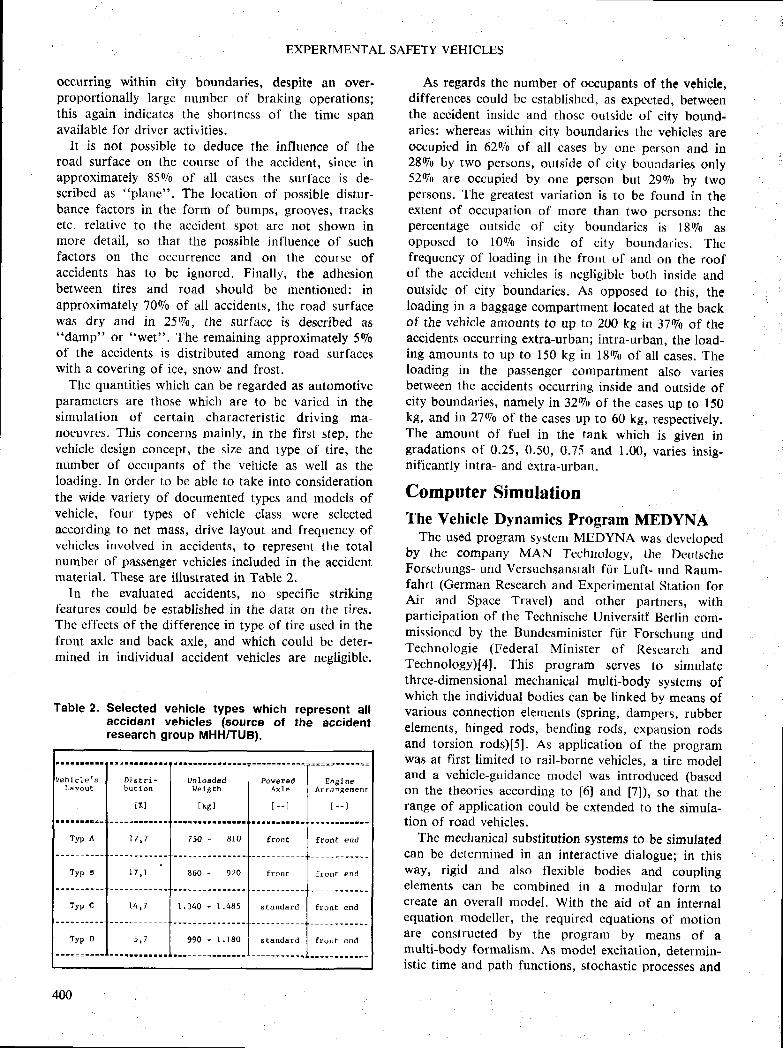
EXPERIMENTAL SAFETY VEHICLES

occurring within city boundaries, despite an over-proportionally large number of braking operations;this again indicates the shortness of the time spanavailable fior driver activities.

It is not possiblc to deduce the influence of theroad surface on the course of the accident. since inapproximately 8590 of all cases the surfacc is de-scribed as "plitne". The location of possible distur-bance factors in the form of bumps, grooves, tracksetc. relative to thc accident spot are not shown inmore detail, so that the possible influence of suchfactors on the occurrence and on the course ofaccidents has to be ignored. Finally, the adhesionbetween tires and road should be mentioned: inapproximately 70ulo of all accidents, the road surfacewas dry and in 25Vo, the surlace is described as"damp" or "wet". The remaining approximately 590of the accidents is distributed among road surfaceswith a covering of ice, snow and frost.

The quantities which can be regarded as automotiveparameters are those which are to bc varicd in thesimulation of certain characteristic driving ma-noeuvres. This concerns mainly, in the firsf step, thevehicle design concept, the size and type of tire, thenumber of occupants of the vehicle as well as theloading. In order to be able to take into considerationthe wide variety of documented types and models ofvehicle, four types of vehicle class were selectedaccording to net mass, drive layout and firequency ofvehicles involved iu accidents, to represent the totalnumber of passenger vchicles included in the accidcntmaterial. These are illustrated in Table 2.

ln the evaluated accidents, no specific strikingfeatures could be established in the data on the tires.The effects of the difference in type of tire uscd in thefront axle and back axle, and which could be deter-mined in individual accident vehicles are negligible.

Table ?. Selected vehicle types which represent allaccident vehicles (source ol the accidentresearch group MHH/TUB).

As regards the number of occupants of the vehicle,differences could be established, as expected, betweenthe accident inside and those outside of city bound-aries: whereas within city boundaries the vehicles areoccupied in 62o/o of all cases by one person and in2890 by two persons, outside of city boundaries only52r/o are occupied by one person but 29go by twoper$ons. The greatest variation is to be tbund in theextent of occupation of more than two persons: thepercentage outside of city boundaries is lSVo asopposed to l09o inside of city boundaries. Thefrequency of loading in the front of and on the roofof the accident vehicles is negligible both inside andoutside of city boundaries. As opposed to this, theloading in a baggage compartment locatecl at the backof the vehicle anrounts to up to 200 kg in 37Wo of theaccidents occurring extra-urban; intra-urban, the load-ing amounts to up to 150 kg in lSgo of all cases. Theloading in the passengcr compartment also variesbetween the accidents occurring inside and outside ofcity boundaries, namely in 3290 of the cases up to 150kg, and in 27Vo of the cases up to 60 kg, respectively.The amount of fuel in the tank which is given ingradations of 0.25, 0.50, 0.75 and 1.00, varies insig-nificantly intra- and extra-urban.

Computer SimulationThe Vehicle Dynamics Program MEDYNA

The used prograrn system MEDYNA was developedby the company MAN Technology, the DeutscheForschungs- und Versuch$anstalt fiir Luft- und Raum-fahrt (German Research and Expcrimental Station forAir and Space Travel) and other partners, withparticipation of the Technische Universitt Berlin com-missioncd by the Bundesminister ftir Forschung undTechncllogie (Federal Minister of Research andTechnoloey)[4]. This program serves to simularethree-dimensional mechanical multi-body systems ofwhich the individual bodies can be linked by means ofvarious connection elenrents (spring, dampers, rubberelements, hinged rods, bending rods, cxpansion rodsand torsion rods)[S]. As application of the programwas at first limited to rail-borne vehicles, a tire modeland a vehicle-guidancc model was introduced (basedon the theories according to [6] and [7]), so that therange of application could be extended to the simula-tion of road vehicles.

Thc mechanical substitution systems to be simulatedcan be determined in an interactive dialogue; in thiswfly, rigid and also flexible bodies and couplingelements can be combined in a modular form tocreate an overall model. With the aid of an internalequation modeller, the required cquations of motionare conslructed by the program by means of amulti-body fbrmalism. As model excitation. determin-istic time and path functions, stochastic processe$ and

Unloadedl.re t I th

t k6 l

D l s t r i -bu t lon

t [ ]

E n g I d eA r r d n B e m e n t

t - - l

f ron t end

f r o n t € n d

I t a n d a r d f ron t end

s t a n d a r d f r o n t e n d

400

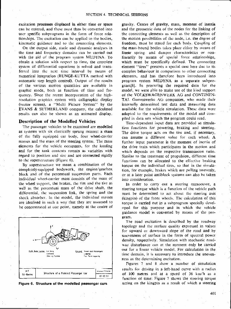
SECTION 4. TECHNICAL SESSIONS

excitation processes displaced in either time or spacecan be entered, and these must then bc converted intouscr specific subprograms in the form of force rela-tionships. The excitation can be applied to the bodies,kincmatic guidance and to the connecting elements.

On the output side, static and dynamic analyses inthe time and frequency domains can be carried outwith the aid of the program $y$tem MEDYNA. Toobtain a solution with respect to time, the completesystem of differential equations is solved and trans-ferred into the next time interval by means ofnumerical integration (RUNGE-KUTTA method withautomatic step length control). Output oi the resultsof the various motion quantit ies are available ingraphic mode, both as function of t ime and fre-quency. Since thc recent incorporation of the high-rcsolution graphics system with call igraphic display(vector screen), a "Multi Picture System" by theEVANS & SUTHERLAND company, the calculatedresults can also be shown as an anirnated display.

Description of the Modelled VehiclesThe passenger vehicles to be examined are modelled

as systems with six elastically sprung masses; a massof the fully equipped car body, four wheel-carriermasse$ and the mass of the steering system. The masselements for the vehicle occupants, for thc loadingand for the tank contents remain as variables withregard to position and size and are connected rigidlyto the superstructure (Figure 6),

By superstructure we mean a combination of thecompletely-equipped bodywork, the engine./gearboxblock and of the percentual suspension parts. Eachindividual wheel-carrier ma.ss consists of the mass ofthe wheel support, the brakes, the rim and the tire aswell as the percentual mass of the drive shaft, thedifferential, the suspension link, the spring and theshock absorber. ln the model, the individual massesare idealised in such a way that they are assumed tobe concentrated at one point, namely at the centre of

gravity. Centre of gravity, mass, moment of inertiaand the geometric data of the nodes for the l inking ofthe connccting elements as well as the description ofthe motion possibil i t ies of the node, i.e. the degree offreedom, must be stated for each body. Coupling ofthe mass-bound bodies takes place either by means ofl inear spring- and darnper characteristics or non-linearily by means of special force relationships,which must be specifically defined. The connectingelement "tires" presents a special case here due to itscomplex behaviour in comparisotr to other connectingelements. and has thercl'ore been introduced intoprogram system MEDYNA as a separate subpro-gram[8]. In procuring the required data for themodel, we were able to make use of the kind supportOf thE VOLKSWACENWERK AG ANd CONTINEN-TAL Gummiwerke AG companies, who made theirinternally determined test data and measuring dataavailable for the vehicle simulation. These data wereadapted to the requirements of the tnodel aud conr-piled in data sets which the program could read.

Time-dependent input data are provided as simula-tion functions for powering, braking and steering.The drive torque acts on the tire and, if necessary,can assume a different value for each wheel. Afurfher input parameter is the moment of inertia ofthe drive train which participates in the motion andwhich depcnds on the respective transmission ratio.Similar to the treatment of propulsion, different t imefunctions can be allocated to the efl 'ective brakingtorque on the individual t ires, so that in the simula-tiorr, for example, brakes which are pull ing unevenly,or at a later point antiblock $ystems can also be takeninto consideratiort.

ln order to carry out a steering manoeuvre, asteering torque which is a function of the vehicle path

must be determined to act about the steering axis(kinepin) of the front wheels. The calculation of thistorque is carried out in a subprogram specially devel-oped for this purpose and in which the vehicleguidance model is converted by means of the pro-gram.

The road excitation is described by the roadwaytopology and the surface quality expressed in valuesfor upward or downward slope of the road and byunevenness of surface in the form of spcctral power

density, respectively. Simulatictn with stochastic road-way disturbance can at the moment only be carriedout for a l inear vehicle model. For calculation in thetime domain, it is necessary to introduce the uneven-ness as the determining excitation.

Figures 7 and I show a number of simulation

results for driving in a left-hand curve with a radiusof 100 metres and at a speed of 36 km/h as afunction of t ime: Figure 7 shows the steerirtg torqueacting on the kingpin as a result of which a ste€ring

!!lll!q!-!Elq: tor sody poy!!j! orivrr ond pos$nq.ri4 Hheels Luqqogestoor,ro 5rrhf i Fuel Tonk lopdri t t

I F TTU'Ber l in Struciure of o l,, lodeted Possenger tor

87 02 08

Figure 6. Structure of the modelled passenger cars

401

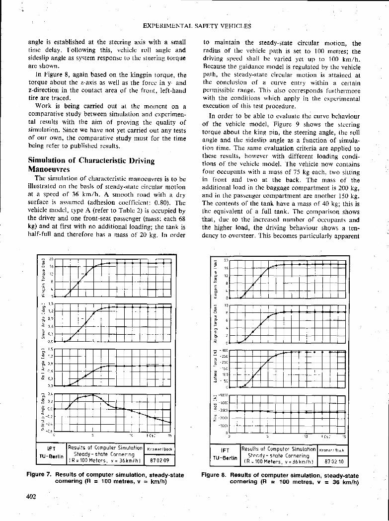
EXPERIMENTAL SAFETY VEHICLES

angle is established at the steering axis with a smalltimc delay. Following this, vehicle roll angle andsideslip angle as system response to the steering torqueare shown.

In Figure 8, again based on the kingpin torque, thetorque about the z-axis as well as the force in y- andz-direction in the contact area of the front. Ieft-handtire are traced.

Work is being carried out at the momcnt on acomparative study between simulation and experimen-tal results with the aim of proving the quality ofsimulation. Since we have not yet carried out any te$tsof our own, the comparative study must for the timebeing refer to published results.

Simulation of Characteristic DrivingManoeuvres

The simulation of characteristic manoeuvres is to beillustrated on the basis of steady-state circular motionat a speed of 36 km/h. A smooth road with a drysurface is assumed (adhesion coefficient: 0.80). Thevehicle rnodel, type A (refer to Table 2) is occupied bythe driver and one front-seat passenger (mass: each 68kg) and at first with no additional loading; the tank ishalf-full and therefore has a mass of 20 ke. In order

Figure 7. Results of computer simulatlon, steady-statecornering (R = 100 metres, v = km/h)

M2

to maintain the steady-state circular motion. theradius of the vehicle path is set to l(-)0 metres; thedriving speed shall be varied yet up to 100 km/h.Because the guidance model is regulated by the vehiclepath, the steady-state circular motion is attainecl atthe conclusion of a curve entry within a certainpermissible range. This also corresponds furthermorewith the conditions which apply in the cxperimentalexecution of this test procedure.

In order to be able to evaluate the curve behaviourof the vehicle model, Figure 9 shows the steeringtorque about the king pin, the steering angle, the rollangle and the sideslip angle as a function of simula-tion time. The same evaluation criteria are applicd tothese results, however with different loading corrdi-t ions of the vehicle model. The vehicle now containsfour occupants with a mass of 75 kg each, two li i tt ingin front and two at the back. The mass of theadditional load in the baggage compartmenr is 200 kg,and in the passenger compartment are another 150 kg.The contents of the tank have a mass of 40 kg; this isthe equivalent of a full tank. The comparison showsthat, due to the increased number of occupants andthe higher load, the driving behaviour shows a ten-dency to oversteer. This becomes particularly apparent

- ? 0

zL 1 6

F g

=.EY 0

- 1 0Ezu 8

g b

E

q o

- - 1 0 01

i - ? o o

_ - r s oE - 1 0 0=: j - 5 0

- -5000

; -4ooo

: -looo

.: 2000

-1000

I F TTU -Ber l in

Resu l ts o f Computer S imu lo t ionS l e o d y - s t o t e C o r n e r i n g

( R = 1 0 0 M e t e r s , v = 3 6 k m / h )

X r o m e r / B o c k

87 02 10

Figure 8. Rosults ol computer simulation, steady-statecornering (R = 100 metres, v = 36 km/h)

2g

1 6

1 ?

I

L

0

1 , 2

) , 9

) , 6

) . 1

, 2

, 9

a 0,1.

3 n "

=

G -o. t

Ez .

a=

- 1 ,

3 r

4 0 ,

3 v ,

0,

r 1 ,

; "6 U l

q 0

tFTTU-Ber l in

Results of [omouter Simulot ionSteody - s lo le Corner ing

( R = 1 0 0 M e l e r s , v = 3 6 k m / h )

K t d m e r , / B o c k

87 02 09

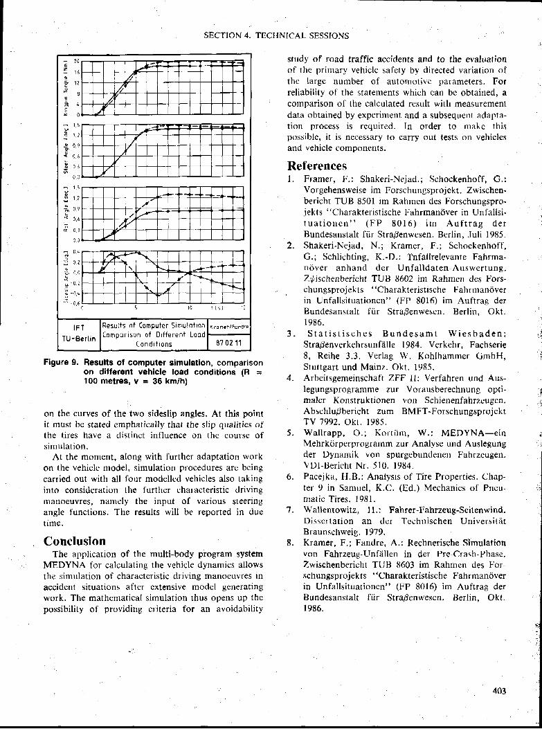
E

B r zo

4 ,

sr 0

T 1 , 5

< 0 6

e u r

0 . 0

n 1 , 5

3 n q

E 0 J

J | )

2 0,1,

* n r

S - 0 , 1

i ; - 0 , 6

I

-l\

l--

I ttlt, /r

I

7f

I F TTU -Ber l in

Resutts of Computer Simulot ionCompor ison o f D i f fe ren t Lood

I o n d i t i o n s

K . s n € f , l F o n d r l

87 02 11

SECTION 4. TECHNICAL SESSIONS

Flgure 9. Results ol computer simulation, comparisonon different vehlcle load conditions (R =100 metres, v = 36 km/h)

on the curves of the two sideslip angles. At this pointit must be stated emphatically that the slip qualities ofthe tires have a distinct influence on the course ofsinrulat ion.

At the moment, along with further adaptation workon the vehicle model, simulation procedures are bcingcarried out with all four modelled vehicles also takinginto consideration the f'urther characteristic drivingmanoeuvres, namely the input of various steeringangle functions. The results will be reported in duet ime.

ConclusionThe application of the multi-body program system

MEDYNA for calculating the vehicle dynamics allowsthe simulatiorl of characteristic driving manoeuvres inaccident situations after extensive ntodel generatingwork. The mathernatical simulation thus opens up thepossibil i ty of providing criteria for an avoidabil ity

study of road traffic accidents and to the evaluationof t lte prinrary vehiclc salety by directed variation ofthc large number of autonrotivc parameters, Forreliabil i ty of the statements which can be obtained, acornparison of the calculated result with measurementdata obtained by experiment and a subsequent adapta-tion proce$s is required. ln order to makc thispossiblc, it is necessary to carry out tests on vehiclesand vehicle components.

Referencesl. Framer, F.: Shakeri-Nejad.; Schockenhoff, G.:

Vorgehensweise im Forschurrgsprojekt. Zwischen-bericht TUB 8501 im Rahrnen des Forschungspro-jekts "Charakteristische Fahrmanriver in Unl'allsi-t u a t i o n e n " ( F P 8 0 1 6 ) i m A u f t r a g d e rBundesanstalt fi ir Strapenwesen. Berlin, Juli 1985.

2. Shakeri-Nejad, N.; Kramer, F.; Schockerthoff,G.; Schlichting, K.-D.: Tnfallrelevante Fahrma-ndver anhand der Unfal ldaten-Auswertung.Z'y'ischenbericht TUB 8602 im Rahmen des Fors-

, chungsprojekts "Charakteristische F-ahrmanciverin Unfallsituationen" (FP 8016) im Auftrag derBundesanstalt fi ir StraBenwesen. Berlin, Okt.l98fr .

3 . S t a t i s t i s c h e s B u n d e s a m t W i e s b a d e n ;StraBenverkehrsunfiil le 1984. Verkehr, Fachserie8, Reihe 3.3. Verlag W. Kohlhammer CmbH,Stuttgart und Mainz. Okt. 1985.

4- Arbeitsgemeinschaft ZFF lI: Verfahren und Aus-legungsprogramme zur Vorausberechnung opti-maler Konstruktionen von Schienenfahrzeugen.AbschluBbericht zum BMFT-ForschungsprojektTV 7992. Okr. 1985.

5. Wal lrapp, O.; Kort i i rn, W.: MEDYNA-einMehrkcirperprogramm zur Analyse und Auslegungder Dynamik von spurgebundenen Fahrzeugerr.VDl-Bericht Nr. 510. 1984.

6. Facejka, H.B.: Analysis of Tire Properties. Chap-ter 9 in Samuel, K.C. (Ed.) Mechanics of Pneu-matic Tires. l98l .

1. Wallentowitz, H.: Fahrer-Fahrzeug-Seitenwind.Dis.scrtat ion an der Technischen Universi t i i tBraunschweig. 1979.

8. Kramer, F.; Fandre, A.: Rechnerische Simulationvon Fahrzeug-Unfdllen in der Pre-Crash-Phase.Zwischenbericht TUtl 8603 im Rahmen des For-schungsprojekts "Charakteristische Fahrmanciverin Unfallsituationen" (FP 8016) im Auftrag derBundesanstalt fi ir Stradenwesen. Berlin. Okt.1986.

403

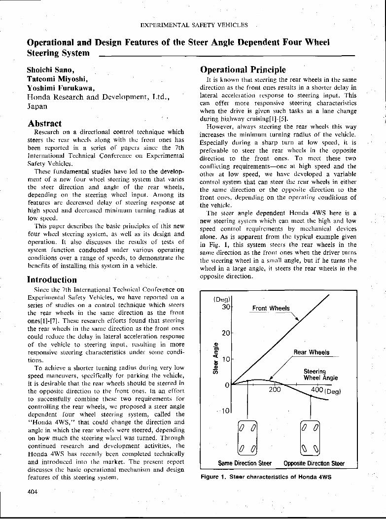
EXPERIMENTAL SAFETY VEH ICLES

Design Features of the Steer Angle Dependent Four WheelOperational andSteering System

Shoichi Sano,Tateomi Miyoshi,Yoshimi l 'urukawa.Honda Research and Development, Ltd.,Japan

AbstractResearch on a directional control technique which

steers the rear wheels along with the front ones hasbeen reported in a series of papers since the 7thInternational Technical Conference on ExperimentalSafety Vehicles.

These I'undamental studies have led to the develop-ment of a new I'our whcel steering system thal. variesthe steer direction and anglc of the rear wheels,depending on the steering wheel input. Among itsfeatures are decreased dclay of steering response athigh speed and decreascd minirnurn turning radius atlow speed.

This paper describes the basic principles of this newfour wheel steering sy$tem, as well as its design andoperat ion. I t a lso d iscusses the resul ts of ' tcsts ofsystem I'unction conducted under various operatingconditions over a range of speeds, to dernonstrate thebenefits of install ing this system in a vehicle.

IntroductionSince the 7th Intcrnatiorral Tcchnical Conference on

Expcrimental Safety Vehicles, we have reported on aseries of studies on a control technique which steersthc rear wheels in the same direction as the frontones[]-[71. These research efforts found that steeringthe rear wheels in the same direction as the frotrt onescould reduce the delay in lateral acceleration response

of the vehicle to steering input, resulting in moreresponsive steering characteristics under sornc condi-t ions.

To achieve a shorter turning radius during very lowspeed maneuvers, spccifically for parking the vehicle,it is desirable that the rear wheels should be steered inthe oppositc direction to the front ones. In an effortto successfully combine these two requirements forcontroll ing the rear wheels, we proposed a steer angledependent I 'our wheel steering system, called the"Honda 4WS," that could change the direction andanglc in which the rear wheels were steered, depettdingon how much thc steering wheel was turued. Thror.rghcontinued research and development activit ies, theHonda 4WS has recently bccn completed technicallyand introduced into the market. The present reportdiscusses the basic operational nrechanisrn and designfeatures of this steering system.

404

Operational PrincipleIt is known that steering the rear wheels in the same

direction as the front ones results in a shorter delay inIateral accelcration rcsponse to steering input. Thiscan offer rnore responsive steering characteristicswhen the drive is given such tasks as a lane changeduring highway cruisingil l-[5].

However, always steering the rear wheels this wayincreases the minimum turning radius of the vehicle.Especially during a sharp turn at low speed, it isprelbrable to steer the rear wheels in thc oppositedirection to the front ones. To meet these twoconflicting requirements-one at high speed and theother at low speed, we have developed a variablecontrol system that can steer the rear wheels in eitherthe same direction or the opposite direction to thefront ones, depending on the operating conditions ofthe vehicle.

The stcer angle dependent Honda 4WS here is anew steering systcm which can meet the high arrd lowspeed control rcquircrrrents by mechanical devicesalone. As is apparent from the typical example givenin Fig. 1, this sy$tem steers the rear wheels in thesame direction as the I'ront ones when the driver turnsthe steering wheel in a snrall angle, but if he turns thewheel in a large angle, it steers the rear wheels in theopposite direction.

Front Wheels

(Deg)30

Rear Wheels

SteeringWheel Angle

.400 (o*g)

* 1 0

$ame $teer

-eE tE

l t o(l)ovt

Steer

mt lN-!l

Opposite Direction

mt lV3

Dhection

Figure 1. Steer characteristics of Honda 4WS

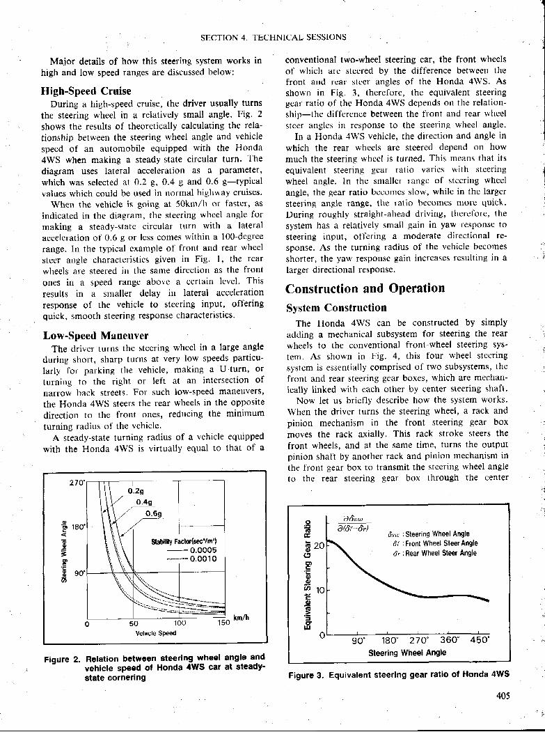
SECTION 4. TECHNICAL SESSIONS

Major details of how this steering sy$tem works inhigh and low speed ranges are discussed below:

High-Speed CruiseDuring a high-speed cruise, the driver usually turns

the steering wheel in a relatively small angle' Fig. 2shows the results of theorctically calculating the rela-tionship between the steering wheel angle and vehiclespeed of an automobile equipped with the Honcla4WS when making a steady-state circular turn. Thediagram uses lateral acceleration as a parameter'which was selected at 0.2 g, 0.4 g and 0'6 g-typicalvalues which could be used in trortnal highway cruises.

When the vehicle is going at 50km/h or faster' asindicated in the diagram, the steering wheel attgle formaking a steady-state circular turn with a lateralaccelcration of 0.6 g or less comes within a 1O0-dcgreerange, In the typical example of front and rear wheelsteer angle characteristics given in Fig. l, the rearwheels are steered in the same direction as the front

ones in a speed range abovc a certaitr level. This

results in a smaller delay iu lateral accelerationresponrie of the vehicle to steeritrg input, offeringquick, $mooth steering response characteristics'

Low-Speed ManeuverThe driver turns the steering wheel in a large angle

during short, sharp turns at very low speeds particu-

larly for parking the vehicle, making a U-turn, or

turning to the right or left at an intersection of

narrow back streets. For such low-speed malleuvets'the Honda 4WS steers the rear wheels in the oppositedirection to the front oues, reducing the minimum

turning radius of the vehicle.A steady-state turning radius of a vehicle equipped

with the Hottda 4WS is virtr.rally equal to that of a

Figure 2. Relation between steerlng wheel angle and- vehicle speed ot Honda 4WS car at steady'state cornering

conventional two-wheel steering car, the front wheels

of which are steered by the difference between thefront and rear siteel angles of the Honda 4WS. Asshown in Fig. 3, therel'ore, the equivalent steeringgcar ratio of the Honda 4WS depends otr the relation-

ship-the difference between the front atrd rear wheel

stcer angles in response to the steeritrg wheel angle.

In a Honda 4WS vehicle, the direction and angle in

which the rear wlreels are steercd depend on how

much the steering wheel is turned. This meatrs that its

equivaletrt steering gear rit l io varies with steering

wheel angle. ln the smaller rangc of steeritrg wheel

angle, the gear ratio becc'rrnes slow, while in the larger

steering angle range, thc ratio becomes more quick'

During roughly straight-ahead driving, thereforc, the

system has a relatively small gain in yaw response to

steering input, offering a moderate directional re-

sponse. As the turning radius of the vehicle becomes

shorter, the yaw response gain increases resulting in a

Iarger directional response.

Construction and Operation

System ConstructionThe Honda 4WS can be cottstructed by simply

adcling a mechanical subsystem for steering the rear

wheels to the cotrventional front-wheel steering sys'

tem, As shown in Fig. 4, this four wheel stccring

systcm is essetrtially comprised of two subsystems, the

front and rear steerirtg gear boxes, which are tnechan-

ically linked with each other by center steering shaft'

Now let us brielly describe how the system works'

When the driver turtrs the steering wheel, a rack and

pinion mechanism in the front steering gear box

moves the rack axially. This rack stroke steers the

front wheels, and at the same time, turns the outputpinion shal't by auother rack and pinion mechanism in

the front gear box to tran$mit the steerilrg wheel angle

to thc rear steering gear box through the center

Figure 3. Equivalent steering gear ratio of Honda 4W$

405

s- rgO'

oEFIE so'U'

Slablllty Factor(e€c'/m'l- o.ooo5---- .- .0.0010

50 100Vehicle Speed

fro rmlt

dsr' ;Steering Wheel Anglerlt ; Front Wheel Steer Angledr ;Rear Wheel Steer Angle

10

90' 180" 270" 360' 450'Steering WheelAngle

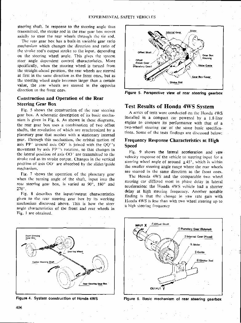
EXPERIMENTAL SAFETY VEHICI-ES

steering shaft. In response to the steering angle thustransfi l i tted, the stroke rod in the rear gear box rnovcsaxially to steer the rear wheels through thc tie rod.

The rear gear box has a built- in variable gear ratiomechanism which changes the direction and ratio ofthe stroke rod's output stroke to the input, dependingon the steering wheel anglc. This givcs the $ystemsteer angle depelrclent control characteristics. Morespecifically, when the steering wheel is turned f'romthe straight-ahead position, the rear wheels are steeredat first in the same direction as the front ones, but asthe steering wheel angle becomes larger than a certainvalue, the rear wheels are steered in the oppositedirection t0 the front ones.

Construction flnd Operation of the RearSteering Gear Box

F'ig. 5 shows the construction of the rear steeringgear box. A schematic description of its basic mecha-nism is given in Fig. 6. As shown in these diagrams,the rear gear box uses a combination of two offsetshafts, the revolution of which are synchronized by aplanetary gear that meshes with a stationary internalgear. Through this mechanism, the orbital motion ofax is PP' around axis OO' is jo ined wi th the QQ"smovement by axis PP"s rotation, so that changes inthe lateral position of axis OO' are transmitted to thestroke rod as its stroke output. Changes in thc vcrticalposition of axis OO' are ahsorbed by the slider/guidemechanism.

Fie. 7 shows the operation of the planetary gearwhen the turning angle of the shaft, input into therear steering gear box, is varied as 90o, l80u and270".

Fig. I describes the input/output characteristicsgiven to the rear steering gear lrox by its workingmechanism discussed above. This is how the steerangle characteristics of the front and rear wheels inFig. I are obtained.

Figure 5. Perspective vlew of rear steering gearbox

Test Results of Honda 4WS SystemA serics of tests were conductcd on the Honcla 4WS

installed in a compact car powered by a 1.8-literengine to compare its performance with that of atwo-wheel steering car ol' the same basic specifica-tions. Soure of the tests findings are clissussed below:

Frequency Response Characteristics at HighSpeed

Fig. 9 shows the lateral acceleration and yawvelocity respon$ie of the vehicle to steering input for asteering wheel angle of around +45', which is withinthe smaller steering angle range where the rear wheelsare steered in the same direction as the front ones.

The Honda 4WS and the cornparable two wheelsteering car differcd most in phasc dclay irr lateralacceleration: the Honda 4WS vehicle had a shorterdelay at high steering frequency. Another notablefinding is that thc changc in yaw rate gain withHonda 4WS is less than with two wheel steering up toa high steering frequcncy

Ollset Shaft //'

Otfeai_ Pinion G6ar /{Planetary Goar)

Gadr BoxHousing

\ $l'!gfq!'d6

NPUT X J

i .Sllnternal Gear (Ftx€d)

(4]Slider

/ illGutde/ t -

OUTPUT Y

Front SteerlngGear Box

/r; .'rI\,)T

Ctrier Steerin$ Shatt /-

fi,,\ {

\

Figure 4. System construction of Honda 4WS

406

Figure 6. Basic mechanism of rear steering gearbox

SECTION 4. TECHNICAL SESSIONS

Figure 7. Operation of rear steering gearbox

Output Y

| -\-

O-O's Movementby P-P's Rotation

Combined Movementof Outout

' -ir P-P's Orbital Motion

t _ /t r '

ttt

tt

Figure 8. Input/output characteristic$ of rear steeringgearbox

Flgure L Vehicle steering response characteristics

Lane-Change Test at High-SpeedIn this tcst, thc driver was requested to steer the

vehic le in such a manncr that the posi t ion of i ts centerof gravity would lbllow as closely as possible thedesire path marked with an objective line on the testcourse surlace as described in Fig. 10.

The difference between the two test vehicles insteering re$pon$e during an example lane change isshown in Fig. I l. In this particular example, theHonda 4WS vehicle had smaller anrplitudes of lateralacceleration, yaw vclocity and roll angle-

Turns at Very Low-SpeedA U-turn tesr was conducted at very low speed with

the steering wheel set at the nraximum steering wheelangle. tsecause of its minimum turning radius, some0.5 rneters shorter than the two-wheel steering car, asshown in Fig. 12, the Honda 4WS vehicle could makeU-Turn in a test course I meter narrower than theminimum course width required by the other test car.Of course, these results wil l vary slightly with thewheelbase, track and other specifications rtf the vehi-cle in which the steering system is installed.

ConclusionIn the foregoing sections, we have described the

operational and design features of the steer angledependent Honda 4WS.

The Honda 4WS offers both steering ease at hiehspeed and good maneuverability at low speed by

Figure 10. Course layout of lane-change test

LEtoral Acceleration0 4

0.2

0

0

-s0

Ptresr Ddey o'

Sx+o - l00km/h

stsring Frequency lHr)

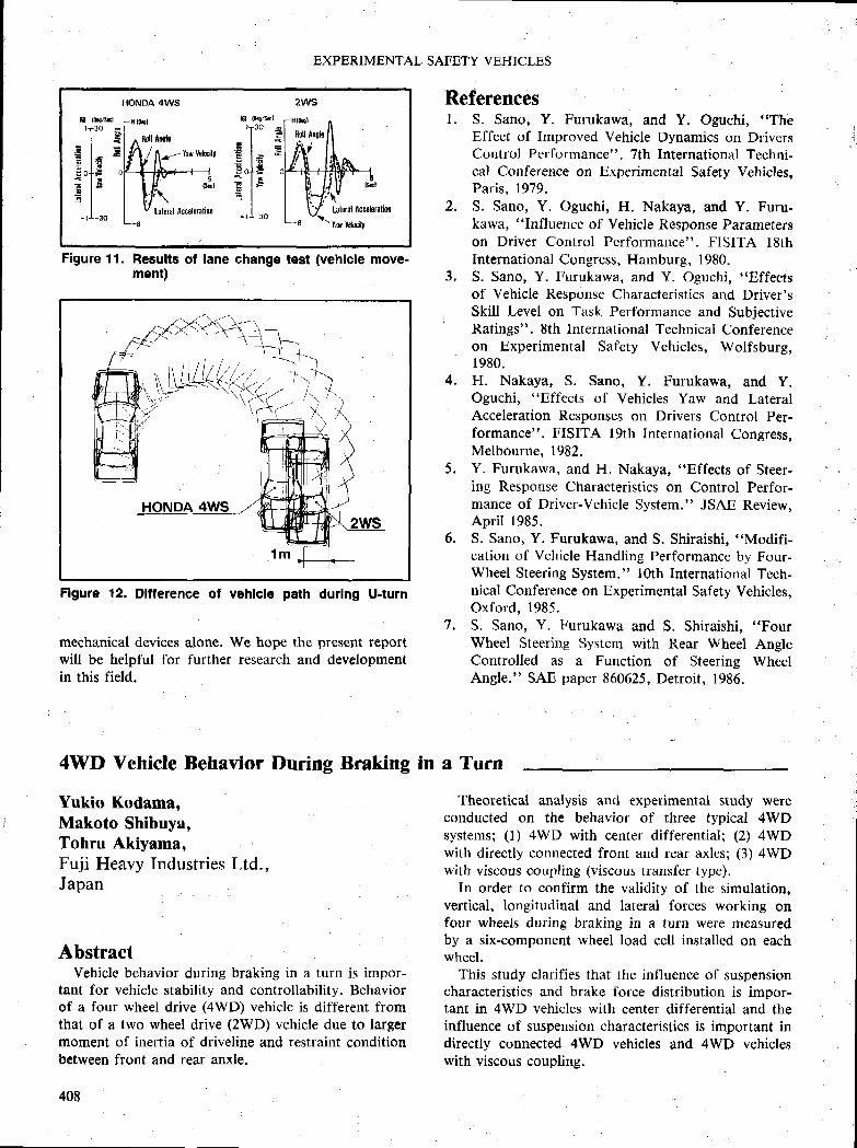
EXPERIMENTAL SAFETY VEHICLES

Referencesl. S. Sano, Y. Furukawa, and Y. Oguchi, "Thb

Effect of Improved Vehicle Dynamics on DriversControl Performance". 7th International Techni-cal Conference on Experimental Safety Vehicles,Paris. 1979.S. Sano, Y. Oguchi, H. Nakaya, and Y. Furu-kawa, "Influence of Vehicle Response Parameterson Driver Control Performance". FISITA lSthlnternational Congress, Hamburg, 1980.S. Sano, Y. Furukawa, and Y. Oguchi, "Effects

of Vehicle Response Characteristics and Driver'sSkill Level on Task Performance and SubjectiveRatings". 8th lnternational Technical Conferenceon Experimental Safety Vehicles, Wolfsburg,1980.H. Nakaya, S. Sano, Y. Furukawa, and Y.Oguchi, "Effects of Vehicles Yaw and LateralAcceleration Responses on Drivers Control Per-formance". FISITA l9th International Congress,Melbourne, 1982.Y. Furukawa, and H. Nakaya, "Effects of Steer-ing Response Characteristics on Control Perfor-mance of Driver-Vehicle System." JSAE Review,April 1985.S. Sano, Y. Furukawa, and S. Shiraishi, "Modifi-

cation of Vehicle Handling Performance by Four-Wheel Steering System." l0th International Tech-nical Conference on Experimental Safety Vehicles,Oxford, 1985.S. Sano, Y. Furukawa and S. Shiraishi, "Four

Wheel Steering System with Rear Wheel AngleControlled as a Function of Steering WheelAngle." SAE paper 860625, Detroit, 1986.

Theoretical analysis and experimental study wereconducted on the behavior of three typical 4WDsystems; (l) 4WD with center differential; (2) 4WDwith directly connected front and rear axles; (3) 4WDwith viscous coupling (viscous transfer type7.

In order to confirm the validity of the simulation,vertical, longitudinal and lateral forces working onfour wheels during braking in a turn were measuredby a six-component wheel load cell installed on eachwheel.

This study clarifies that the influence of suspensioncharacteristics and brake force distribution is impor-tant in 4WD vehicles with center differential and theinfluence of suspension characteristics is important indirectly connected 4WD vehicles and 4WD vehicleswith viscous coupling.

z.

Figure 11. Results of lane change test (vehicle move-ment)

HONDA 4WS

Flgure 12. Dlfference ot vohlcle path durlng U-turn

mechanical devices alone. We hope the present reportwill be helpful for further research and developmentin this field.

3 .

4.

6.

7 .

4WD Yehicle Behavior During Braking in a Turn

Yukio Kodama,Makoto Shibuya,Tohru Akiyama,Fuji Heavy Industries Ltd.,Japan

AbstractVehicle behavior during braking in a turn is impor-

tant for vehicle stability and controllability. Behaviorof a four wheel drive (4WD) vehicle is different fromthat of a two wheel drive (ZWD) vehicle due to largermoment of inertia of driveline and restraint conditionbetween front and rear anxle.

408

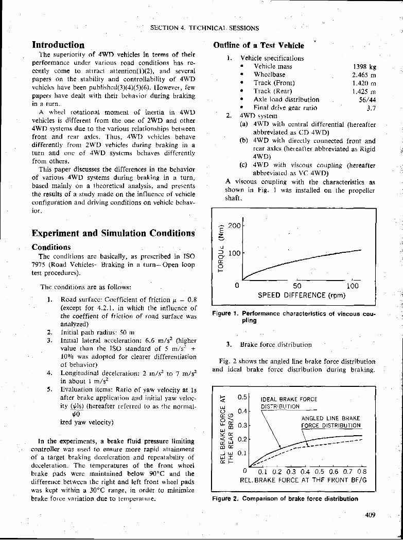
SECTION 4. TECHNICAL SESSIONS

IntroductionThe superiority of 4WD vehicles in terms of their

performancc under various road conditions has re-cently come to attract attention(lX2), and severalpapers on the stability and controllability of 4WDvehicles have been published(3)(4X5X6). However, l 'ewpapers have dealt with their behavior during brakingin a turn.

A whcel rotational moment of inertia in 4WDvehicles is different from the one of 2WD and other4WD systcms due to the various relationships betweenfront and rear axles. Thus, 4WD vchicles behavedifferently from 2WD velricles during braking in aturn and orre of 4WD systems behaves diffcrentlyfrom others.

This paper discusses the differences in the behaviorof various 4WD systems during braking in a turn,based mainly on a thcoretical analysis, and prescntsthe results of a study made on the influence of vehicleconfiguration and driving conditions on vehicle behav-ior.

Experiment and Simulation ConditionsConditions

Thc conditions are basically, as prescribed in ISO7975 (Road Vehicles-Braking in a turn-Open looptest procedures).

The conclit ions are as follows:

l. Road surf'ace: Coefficient of friction p = 0.8(except for 4.2.1. in which the influence ofthe coeffient of friction of road surface wasanalyzed)

Z. In i t ia l path radius: 50 m3. Init ial lateral acceleration: 6.6 m/s? thigher

value than the ISO standard of 5 m,/sr +I09o was adopted for clearer differentiationof behavior)Longitudinal deceleration: 2 m/sz to 7 m/s2in about I m,/szEvaluation items: Ratio of yaw velocity at lsafter brake application and init ial yaw veloc-itv (r/ ls) (hereafter referred to as the normal-

,t,Oized yaw velocity)

In the experiments, a brake fluid pressure limitingcontroller was used to ensure more rapid attflinmentof a target braking deceleration and repeatability ofdeceleration. The temperatures of the front wheelbrake pads were maintained below 90'C and thedifferencc between the right and left front wheel padswas kept within a 30"C range, in order to minimizebrake folce variation due to temperature.

Outline of a Test Vehicle

l. Vehiclespecifications. Vehicle massr Whcclbaser Track (Front)r Track (Rear)r Axle load distribution. Final drive gcar ratio

Z. 4WD system(a) 4WD with central differential (hereafrer

abbreviated as CD 4WD)(b) 4WD with directly connected front and

rear axles (hereafter abbreviated as Rigid4WD)

(c) 4WD with viscous coupling (hereafterabbreviated as VC 4WD)

A viscous coupling with the characteristics asshown in Fig. I was installed on the propellershaft.

-z'J

f

EoF

200

100

0 50 100SPEED DIFFERENCE (rpm)

Figure 1. Performance characteristics of viscous cou-pt ing

3. Brake force distribution

Fig. 2 shows the angled line brake force distributionand ideal brake force distribution during braking.

1398 kg2.465 m1.420 ml.425 m

56/443 . 7

4,

5 .0.5

d

H * ooo >I H o :: c E< { 0 . 2f f r Jd ( t sJ I J U . I

E F

o 6. I o,z 0.3 0.4 o.s 0.6 o.z 0.8REL. BRAKE FORCE AT THE FRONT BFIG

IDEAL BRAKE FORCED I S T R I B U ' I I O N

ANGLED L INE BRAKEFORCE DISTRIBUTION

Figure 2. Comparison of brake lorce distrlbutlon

409

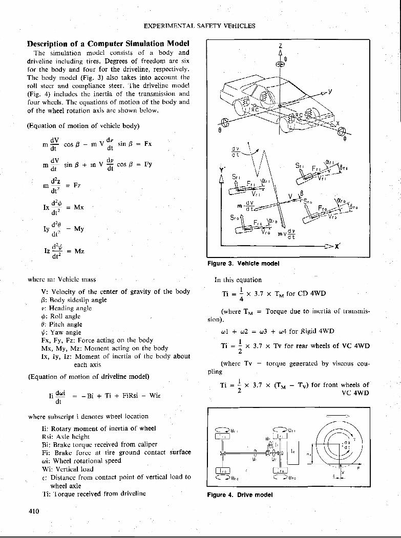
EXPERIMENTAL SAFETY VEHICLES

Description of a Computer Slmulatiort ModelThe simulation modcl consists of a body aqd

driveline including tires. Degrees of freedom are sixfor the body and four for the driveline, respectively.The body model (Fig. 3) also takes into account theroll steer and compliance steer. The driveline model(Fig. a) includes the inertia of the transmission andfour wheels. The equations of motion of the body and

of the wheel rotation axis are shown below.

(Equation of motion of vehicle body)

dVm - -dt

dVm -

(lt

dzzm ^

dt'

, dtdl x -

dr'

, d2otY

d,t

- d?rl,E ---:

dt'

c o s P - * U * 4 s i n B : P x

s i n B + m V

= F z

= M x

- M y

= M z

* q . o * F : F y

where ml Vehicle mass

V: Velocity of the center of gravity of the body

B: Body sideslip angler,: Heading anglef: Roll angled: Pitch anglery': Yaw angleFx, Fy, Fz: Force acting on the bodyMx, My, Mz: Moment acting on the bodylx, ly, Iz: Moment of inertia of the body about

each axis

(Equation of motion of driveline model)

ri 4q! : -Bi + Ti + FiRsi - wiedt

where subscript i denotes wheel location

Ii: Rotary moment of inertia of wheelRsi: Axle heightBi: Brake torque received from caliperFi: Brake force at tire ground coRtact surface

c,ri; Wheel rotational sPeedWi: Vertical loade : Distance from contact point of vertical load to

wheel axleTi: Torque received from driveline

4 1 0

Figure 3. Vehlcle model

In this equationI

T i = . x 3 . 7 x T . f o r C D 4 W D4

(where Tu = Torque due to inertia of transmis-sion).

ul + 0)Z = c.r3 + o/ for Rigid 4WDI

Ti = : x 3,7 x Tv for rear wheels of VC 4WD2

(where Tv : torque generated by viscous cou-pling

T i : x 3.7 x (Tr,,a - Ty) for front wheels ofVC 4WD

Figure 4. Drlve model

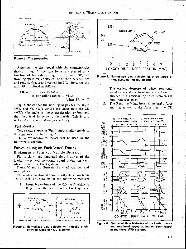
Flgure 5. Tlre propertles

Assuming the tire model with the characteristicsshown in Fig. 5, the side force is expressed as afunction of tire sideslip angle a, slip ratio SR, tiretraveling speed Vi, coefficient of friction between tireand road surface p and vertical load W. Here, the slipratio SR is defined as follows.

S R = I - R e o i / V i c o s aRe: Tire rolling radius = Yi/ui

(when SR - 0)

Fig. 6 shows that the side slip angles for the Rigid4WD and VC 4WD vehicle are larger than the CD4WD's slip angle in higher deceleration region, andthat they tend to verge to the inside. This is alsoreflected in the normalized yaw velocity.

Test ResultsTest results shown in Fig. 7 show similar trends to

the simulation results in F'ig. 6.The above-mentioned model

following discussion.

Forces Acting on Each Wheel DuringBraking in n Turn and Vehicle Behavior

Fie. I shows the simulated time histories of theloads, forces and rotational speed acting on eachwheel in the tl lree 4WD systems.

Figure l0 and ll i l lustrate the wheel load cell andan amplif ier.

The studies mentioned above clarify the characteris-tics of each 4WD system in the following manner:

l. Front brake force of the CD 4WD vehicle islarger than the one of other 4WD systems.

Flgure 6. Normallzed yaw velocity vs. sideslip angleof three types of 4WO systems

SECTION 4. TECHNICAL SESSIONS

be used in the

RIGID 4WD VC 4WD_4-#o

o r z B 4 s 6 7LONGITUDINAL DECELERATION (m/sz)

Figure 7. Normallzed yaw velocity ol three types of4WD systems (measurement)

' The earliest decrease of wheel rotationalspeed occurs at the front inner wheel due toabsence of a constraining force between thefront and rear axles.

2. The Rigid 4WD has lower front brake forceand higher rear brake force than the CD

Flgure 8. Simulated time historles of the loads, forcesend rotational $peed acting on each wheelin the three 4WD systems

4 l l

1 .5

-Crr6 r.o

p

J t no _ -z

o l ? 3 4 5 6 7t ONGItUDTNAL DECELERATION(rills?)LONGITUDINAt DECEIERATT0N(m/s')

3.0 4,5 0 1.5 3.0 4.5

5

00

1 .5

3,0

A

2

4

2

0

1 .5 3 .0 4 .5TIML (s l

CD 4WD

l . c J

( ! ) FRONT INNER WHEEL I3 ) REAR INNER WHEEL

€) FRONT OUTER WHEEL i I ] REAR OUTER WHEEL

R I G I D 4 W D

r Z4 Oz =

a r *

z ! - l iI d :

F

= 9 8

Its

E 5 ;I ? - E _

E H a

= zd - -F 6

F Y

O

o 2

< Ez o

l . i ' 1 k d

B E * d

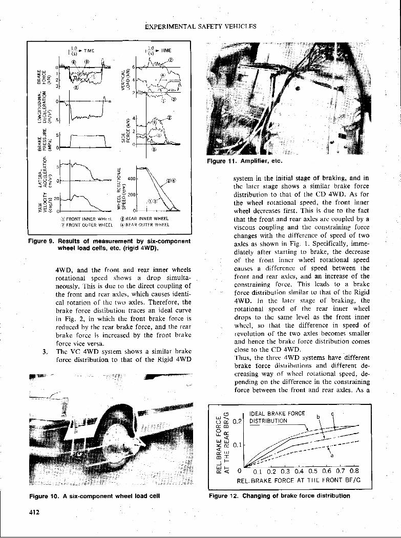
1 4 ut H +H y l

--!z+ a= t sF SF Y

o u ] ^z C ) <9 H 5

U

=H B a{ U L

E f f Ez

trJ E

< u ]

d O FJ { 5

FF

O D

= 9 F{ U ;> > +

EzoE ^A CE i

t , ri ; U= UB 6

( . I FRONT INNER WHEEL (O REAR INNER WHEEL(4FRONT OUTER WHEEL ( { . )REAR OUTER WHEEL

EXPERIMENTAL SAFETY VEHICLES

Figure 9. Hesults of measurement by six-componentwheel load cells, etc. (rigid aWD).

4WD. and the front arrd rear inner wheelsrotational speed shows a drop simulta-neously. This is due to the direct coupling ofthe front and rear axles, which causes identi-cal rotation of the two axles. Therefore, thebrake force distibution traces an ideal curvein Fig. 2, in which the front brake force is

reduced by the rear brake force, and the rear

brake force is increased by the front brakeforce vice versa.

3. The VC 4WD systemfbrce distribution to

mfi i f f i i , - , r i l r , , i | l lillF--'-.ti4'trril.ryryrri

Figure 10. A six-component wheel load cell

412

system in the initial stage of braking, and in

the lal.er stage shows a similar brake force

distribution to that of the CD 4WD. As for

the wheel rotational speed, the front innerwheel decreases first. This is due to the fact

that the front and rear axles are coupled by aviscous coupling and the constraining force

changes with the difference of speed of two

axles as shown in Fig. l. Specifically, imme-

diately al 'ter starting to brake, the decrease

of the f'ront intrer wheel rotational speed

cau$es a difference of speed between thefront and rear axles, and an increase of theconstraining force. This leads to a brake

force distribution similar to that of the Rigid

4WD. In thc latcr stage of braking, the

rotational speed of the rear intrer wheel

drops to the same level as the front innerwheel, so that the difference in speed ofrcvolution of the two axles becomes smallerand hence the brake force distribrrtion comesclose to the CD 4WD.Thus, the three 4WD systems have differentbrake force distributions and different de-creasing way of wheel rotational spced, de-pending on the difference in the constrainingforce between the front and rear axles. As a

shows a similar brakethat of the Rigid 4WD

Figure 11. Amplif ier, etc.

(5uJ \.

t r mP su trJ! { f f{t r U JM I

JlrJ FE {

IDEAL BRAKE FORCE

0.? D I S T R I B U T I O N

0 . 1

o o r 0 .2 0 .3 0 .4 0 .5 0 .6 0 .7 0 .8

REL. BRAKE FORCE AT THE FRONT BF /G

Figure 12. Changlng of brake lorce distributlon

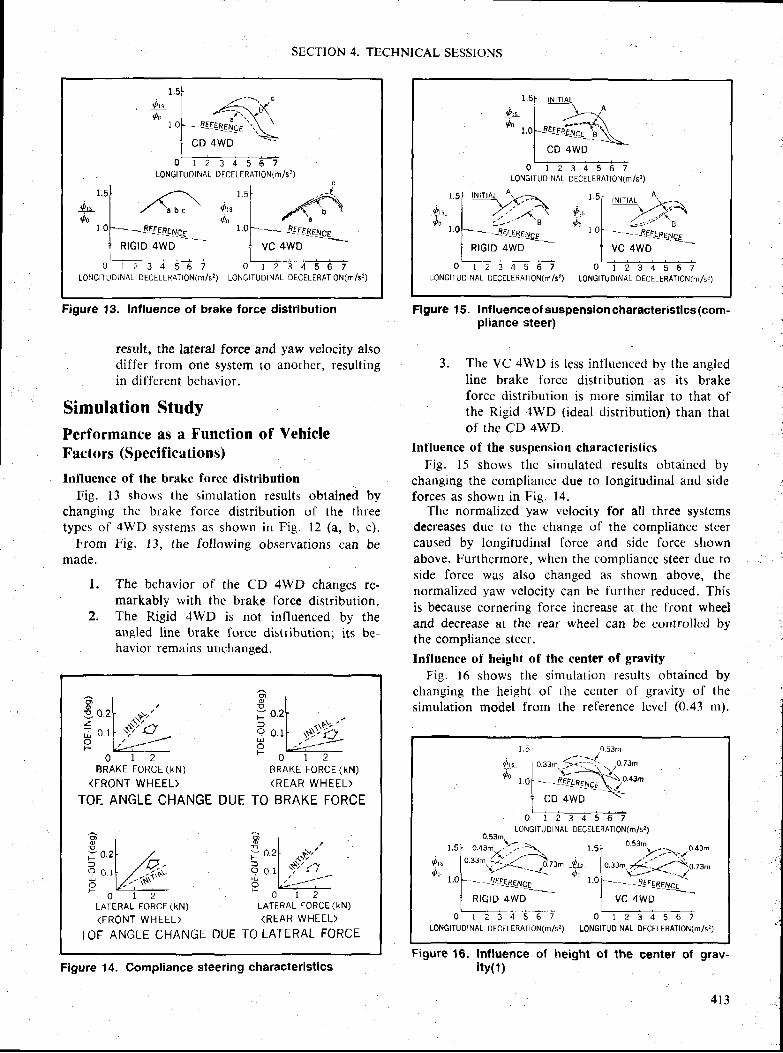
f r r,tn

LONGITUDINAL DECELERATION(T i l5?)

4-#b

i , tQa

t t"f ^| f l \ . o

t. 0 f ----- _ f_r1 g4_5lya_E_

L5'_*'0 1 2 3 4 5 6 7

L0NGITUDINAL DECLLLRATI0N(m/s?)L0NGI I [ ,D lNAL DECELERATI0N(m/s?)

. \ . , c

r . K

Figure 13. Influence of brake force distrlbution

SECTION 4. TECHNICAL SESSIONS

result, the lateral force and yaw velocity alsodiffer from one system to another, resultingin different behavior.

Simulation StudyPerformance fls fl Function of VehicleFactors (Specifications)

Influence of the brake force distributionFie. 13 shows the simulation results obtained by

changing thc brake force distribution of the threetypes ol' 4WD systems as shown in Fig. 12 (a, b, c).

From Fig. 13, the following observations can bemade.

l. The behavior of fhe CD 4WD changes re-markably with the brake force distribution.

Z. The Rigid 4WIl is not influenced by theangled line Lrrake force distribution; its be-havior- remains unchanged.

Figure 15. Inlluenceof suspensloncharacteristacs(com-pliance steer)

3. The VC 4WD is less influenced by the angledline brake force distribution as its brakeforce distribution is more similar to that ofthe Rigid 4WD (ideal distribution) than thatof the CD 4WD.

Influence of the suspension characterislicsFig. l5 shows the sinrulated results obtained by

changing the compliance due to longitudinal and sideforces as shown in Fig. 14.

The normalized yaw velocity for all three systemsdecreases dr.rc to the change of the compliance steercaused by longitudinal force and side force shownabove. Furthcrmore, when the compliancc steer due toside force was also changed as shown above, thenormalized yaw velocity can be further reduced. Thisis because cornering force increase at the front wheeland decrease at the rear wheel can be controlled bvthe compliance steer.

Influence of heighl of the center of gravity

Fig. l6 shows the s imulat ion resul ts obta ined bychanging the height ol the centcr of gravity of thesimulation model from the reference level (0.43 m).

Figure 16. Influence ofity(1)

grav-

4 1 3

l5 [ t t ' l t r tnL

a' i -]-_:i

* r. o f - r-.i-ru-;-'^;5t1| - - - - - - :+*

1i111_0 r 2 3 4 5 6 7

L0NGITUDINAL DECELERATI0N(m/s?)

*u,"1 -i4h* t o1- at'r-+rorr"---

L1''"iY1_0 r z 2 4 5 6 7

LONGITUDINAL DECELERAIION(m/s?) LONGIIUDINAL DECELERAIION(m/s?)0 l 2 3 4 5 6 7

o

I \J. lz

o@

E

E 0.2lq 0 1

Fl

nF

Do9 n r

o n l

oE

fg 0 .1a

'+V'

,+f"d

0 1 ?BRAKE FORCE (KN)

{FRONT WHEELi

TOE ANGLE CHANGE

0 t ?BRAKE FORCE (KN)( R E A R W H E E L )

DUE TO BRAKE FORCE

LATERAL FORCE (KN)( F R O N T W H E E L )

rOE ANGLE CHANGE

LATERAL [ORCE (kN)( R E A R W H E E L )

TO LATERAL FORCEDUE

t 2

Figure 14. Compliance steering chalacteristicsheight of the center ot

.€

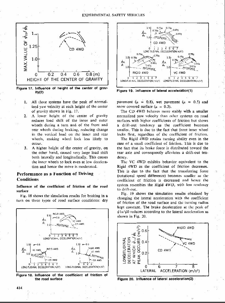
.soUJfJ

}<{E

1. -

1 . 2 5

1 . 0

0 o.2 0.4 0.6 0.8 (m)HEIGHT OF THE CENTER OF GRAVITY

EXPERIMENTAL SAFETY VEHICLES

Figure 17. Influence of height of the center of grav'ity(2)

l. All three systems have the peak of normal-ized yaw velocity at each height of the centerof gravity shown in Fig. 17.

2. A lower height of thc center of gravityreduces load shift of the inner and outer

:' wheels during a turn and of the front andrear wheels during braking, reducing changein the vertical load on the inner and rcarwheels, making wheel lock less likely tooccur,

3. A higher height of the center of gravity, onthe other hand, caused very large load shiftboth laterally and longitudinally. This causesthe inner wheels to lock even at low decelera-tion and hence the move is moderated.

Performance fls A F-unction of Driving

Conditions

Influence of the coefficient of friction of the roadsurface

Fie. 18 shows the simulation results for braking in aturn on three types of road surface conditions; dry

Figure 18. Inlluence of the coefficientthe road surface

4t4

0 1 2 3 4 5

4-(,o

LONGITUDINAL DECELERATI0N(m/st) L0NGITUDINAL DECELERATI0N(m/s?)

Figure 19. Inlluence of lateral acceleration(1)

pavement (p = 0.8), wet pavement (p - 0.5) andsnow covered surface (r, : 0.3).

The CD 4WD behaves more stably with a smallernormalized yaw velocity than othcr systems on roadsurfaces with higher coefl'icients of friction but showsa dril't-out tendency as the coefficient becomessmaller. This is due to the fact that front inner wheellocks first, regardless of the coefficient of friction.

The Rigid 4WD retains turning ability even in thecase of a small coefficient of friction. This is due tothe fact that its brake force is distributed toward therear axle and con$equently alleviates a drift-out ten-dency.

The VC 4WD exhibits behavior equivalent to theRigid 4WD as the coefficient of friction decreases.This is due to the fact that the transferring force(rotational speed difference) becomes smaller as thecoefficient of friction is decreased and hence thesystem resembles the Rigid 4WD, with less tendencyto drift-out.

Fig. 19 shows the simulation results obtained bychanging the lateral acceleration with the coefficientof friction of the road surface and the turning radiuskept con';tant. The brake deceleration at the peak of{tls/rtt0 rcduces according to the lateral acceleration asshown in Fig. 20.I

!-+.

l-l,'"'Yy*/y '-- ' \ , 'vc'+wo

- - -o-*u-ro-.-r- -']",=j_o

o* o1 , 0

0LONGITUDINAL DECELERATI0N(fl /s?)

RIGID

1 .5

4wD #n4,,

, ,0

LoNGITUDINAL DECELERATI0N(m/sr)LONGITUDINAL DECELERATI0N(m/s2)

RIGID 4WD

f y" o*o-\ terrnrry",

F-'cn +wo

.\RIGID 4WD

0 6 7 8LATERAL ACCELERATION (m/s2)

k o o. € 5J Z

* ] ; . n

E = s E o oO < I ( )

= E H 8 O'E 3 = E9 H E H

Figure 20. lnfluence of lateral acceleration(z)of lriction of

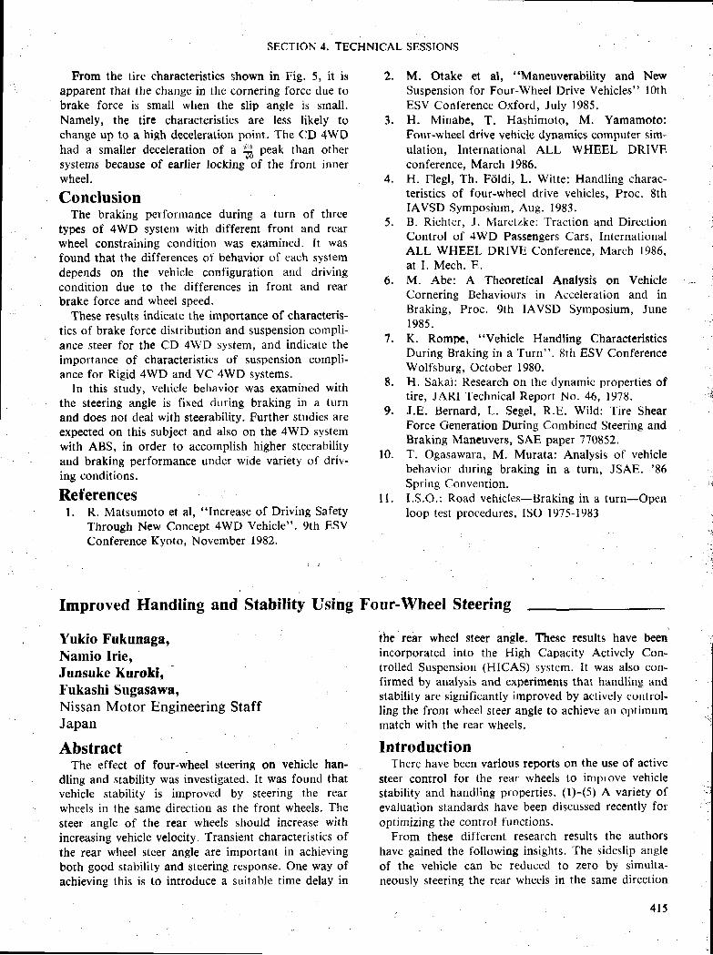
From the tire characteristics shown in Fig. 5, it isapparent that the change in thc cornering force due tobrake force is small when the slip angle is small.Namely, the tire characteristics are less likely tochange up to a high deceleration point. The CD 4WDhad a smaller deceleration of a !I* peak than othersystem$ because of earlier locking of the front innerwheel.

ConclusionThe braking performance during a turn of three

types of 4WD system with different front and rearwheel constraining condition was examined. It wasfound that the differences of behavior of each systemdepends on the vehicle configuration atrd drivingcondition due to the differences in front and rearbrake force and wheel speed.

These results indicate the importance of characteris-tics of brake force distribution and suspension compli-ance steer for the CD 4WD system, and indicate theimportance of characteristics of suspcnsion compli-ance for Rigid 4WD and VC 4WD systems.

ln this study, vehicle behavior was examined withthe steering angle is fixed during braking in a turnand does not deal with steerability. Further studies areexpected on this subject and also on the 4WD systemwith ABS, in order to accomplish higher steerabilityand braking performance under wide variety of'driv-ing conditions.

Referencesl. R. Matsumoto et al, "Increase of Driving Safety

Through New Concept 4WD Vehicle". gth ESVConference Kyoto, November 1982.

Improved Handling and Stability Using

Yukio Fukunaga,Namio lrie.Junsuke Kurokl,

"'

Fukashi Sugasawa,Nissan Motor Engineering StaffJapan

AbstractThe effect of four-wheel steering on vehicle han-

dling and stability was investigated. It was found thatvehicle stability is improved by steering the rearwheels in the same direction as the front wheels. Thesteer angle of the rear wheels should increase withincreasing vehicle velocity. Transient characteristics ofthe rear wheel steer angle are important in achievingboth good stability and steering response. One way ofachieving this is to introduce a suitable time delay in

SECTION 4. TECHNICAL SESSIONS

M. Otake et al, "Maneuverability and NewSuspension for Four-Wheel Drive Vehicles" lOthESV Conl'erence Oxford, July 1985.H. Minabe, T. Hashimoto, M. Yamamoto;Four-wheel drive vehicle dynamics computer sim-ulation, International ALL WHEEL DRIVEconference. March 1986.H. Flegl, Th. Fdldi, L. Witte: Handling charac-teristics of four-wheel drive vehicles. Proc. 8thIAVSD Symposium, Aug. 1983.B. Richter, J. Maretzkc: 'Iraction and DirectionControl of 4WD Passengers Cars, InternationalALL WHEEL DRM Conf'erence, March 1986,at L Mech. E.M. Abe: A Theoretical Analysis on VehicleCornering Behaviours in Acceleration and inBraking, Proc. 9th IAVSD Symposium, June1985.K. Rompe, "Vehicle Handling CharacteristicsDuring Braking in a Turn". 8th ESV ConferenceWolfsburg, October 1980.H. Sakai: Research on the dynamic properties oftire, JARI Technical Report No. 46, 1978.J.E. Bernard, L. Segel, R.E. Wild: Tire ShearForce Generation During Combined Steering andBraking Maneuver$, SAE paper 770852.T. Ogasawara, M. Murata: Analysis of vehiclebehavior during braking in a turn, JSAE. '86

Spring Convention.I.S.O.; Road vehicles-Braking in a turn-Openloop test procedures, ISO 1975-1983

Four-Wheel Steering

the rear wheel steer angle. These results have beenincorporated into the High Capacity Actively Con-trolled Suspension (HICAS) sy$tcm. It was also con-firmed by analysis and experiments that handling andstability are significantly improved by actively control-Iine the front wheel steer angle to achieve an optimummatch with the rear wheels.

IntroductionThcrc have been various reports on the use of active

steer control for the rear wheels to improve vehiclestabil ity and handling properties. (l)-(5) A variety of

evaluation standards have been discussed recently for

optimizing the control functions.From these different research results the authors

have gained the following insights. The sidcslip angle

of the vehicle can be reduced to zero by simulta-neously steering the rear wheels in the same direction

t

J .

4.

I

6.

1

8.

9.

10 .

i l .

4 1 5

EXPERIMENTAL SAFETY VEHICLES

as the front wheels and in proportion to their steerangle. The result will be improved vehicle stability andbetter lateral acceleration response. On the otherhand, this will also cause the yaw rate response todeteriorate. Transient sideslip will occur in the oppo-site direction from that of a two-whccl-steering sys-tem, which will be disconcerting to the driver.

The authors have attempted to overcome theseproblems by focusing on the transient characteristicsof steer angle control. Several different types oftypical steer angle control functions have been intro-duced to resolve the problems noted above. Theireffectiveness in improving vehicle stability and han-dling properties has been confirmecl throush simula-tion analysis and experimentation.

Definition of Four-Wheel SteeringThe steady-state sideslip angle of a vehicle, B, can

be reduced to zero by controlling the rear wheel steerangle according to the following procedure.

Kr = #: H#+"'"4#In this equation, Kr is the ratio of the rear wheel steerangle relative to that of the front wheels and it variesaccording to the vehicle velocity, V. This idea isil lustrated in Fig. l.

Reducing the sideslip angle to zero has both ergo-nomic and dynamic aspect$. In terms of ergonomics,the vehicle will be easier to steer because it willconstantly proceed in the I'orward direction withoutany sideslip. As for the motion dynamics involved,less energy will be requircd to turn the vehicle when itenters a turn from a straight-l ine course. This wil lmean improved stability along with better yaw andlateral motion convergence.

The second aspect is explained in more detail inreference to Fig. 2. When a front-wheel-steering(zWS) vehicle turns, its nose generally points increas-ingly toward the center of the turn as the vehiclevelocity increases. This is illustrated in (i) and (ii) inthe figure. The large centripetal force needed forturning at high speed is obtaincd by means of thelarge sideslip angle and the increased side force of thetires. In other words, wheu a vehicle enters a rurnfrom a straight-line course through a series of stepsteering inputs, it is necessary to turn the vehicle usingF until the vehicle assumes a stable condition.

In contrast to this, the rear wheels of a four-wheel-steering (4WS) vehicle are steered in the same direc-tion (phase) as the front wheels, which increases theslip angle of the rear tires. This recluces the sideslipangle of the vehicle and provides large centripetalforce. To turn a vehicle with 4WS, it is only necessaryto turn the tires, which have a small moment ofinertia, irrstead of turning the vehicle body with itslarge moment of inertia. Since this requires much lessenergy, it allows easier convergence of yaw motion.

Steering the rear wheels according to Eq. (l)achieves good stability in intermediate and high speedranges, however, it does not always provide a thvor-able steering sensation. This is because it tends toproduce a strong understeer characteristic and itcauses yaw response to deteriorate.

Steering the rear wheels in the opposite direction(phase) of the front wheels at low speed improvesmaneuverability. However, it is better to treat maneu-verability separate from handling and stability sincetheir respective aims are diff'erent.

Analysis Using a Mathematical ModelAnalytical Model

A two-wheel model like that illustrated in Fig. 3was employed in the analyses. The front and rearwheel control functions, Af and Ar, are given in the

Large pl

Figure 2. Felationshlp between centripetal force (F)

( l )

(rm/n)

o o

E f iE 4 0 .E E9 o

o s O-g r

g E H o6 9 - o _

T 9 . 9 rf E

'8 ": E o - *s oE

Figure 1. Rear wheel steer angle relative to that of

4 1 6

front wheels (sideslip angle = 0) and sideslip angle (B)

n : (Y+v r)

Flgure 3. Two-wheel steerlng model

form of transfer functions relative towheel angle, as shown in Fig. 4.

The basic equations are given below.M c = F f + F rlo =aFf - bFrFf = Cf [6f - (ara' + ]i )/VJFr : Cr [6. - (-b,p + v)/VJ6 i : ( d / N ) . ( l + A f )6r : (0/N),Ar

the steering

From Eqs. Ql - Q), the vehiclens response relativeto the steering wheel angle is given as follows:

steering wheel angle

Here,

lateral acceleration

steering wheel angle

V [ ( l +60-dr ]

con2 (l +r,S) (8)=ts,. TI;inEffi-

- (on/r,rr)2 (S2 + 2frolrs + orr2)=o, ' f f ig )

B t =

B z =

(10)

(l r)

(12)

( l3 )

Tr n = v

tl2 =

f n =

bf - -5 2 -

2V

K s =

I- =

t1

(Cf + Cr)I + lazcf + b2Cr)M (14)

zf .ffiefcr(l + KsvT

t(l +6f1+fl arl '� ( l 5)

t ( l+6 f ) -6 r l I ( l+0 f l +H I ' t

bc f -F(

Crf

aMV

' * ) (16)

(17)

(21(3)(4)(5)(6)(7)

( l + d O - 6 r

( l + d f t - ( 9 m .

Using these equations, a comparison was made ofthe four typical control methods noted below in aneffort to determine what phase characteristic shouldbe given to the rear wheel steer angle control. Aninvestigation was al$o made of the vehicle characteris-tics obtained with control merhod (E) in whichfirst-order advance control was applied to the front aswell as the rear wheels.

Control methods(A) Front-wheel steering(B) Proportional steering control for rear wheels(C) First-order delay control for rear wheels(D) First-order advance control for rear wheels(E) First-order advance control for both front

and rear wheels

The control functions for each method are given inTable l. The 4WS methods are compared below usingthe front-wheel steering system characteristics (A) asthe baseline.

SECTION 4. TECHNICAL SESSIONS

yaw rate

f ( l + KsVz)

v2 111 + 60 - 6rl

lrc,V - ;

Vehicle

cherect6risticB

0 :N :

6 f ;

6 r iri, :f i :

Sleering wheel engle

Steering gear ralio

Front wheel steer angle

Rear wheel ste6r angle

Yew rate

Lateral G

Figure 4. Block dlagram of simulation model

4t7

EXPERIMENTAL SAFETY VEHICLES

Table 1. Control functlone.

FunotionsControl svstem Ar Ar

(A) front- wheet steoring (- ) 0 0

(B) Proportlonat (----r 0 K,

(C) I st. order detay (--- ) 0 K,/(l +T,.s)

(D) I st - order advance (-.- ) 0 K'-Tr'S

(E) Front and rear wheel (-.- ) K*Tr'S Kt-T,'S

Proportional Steering Control (B)With this method the steer angle ol the rear wheels

is controlled in proportion to that of the front wheels.The rear wheel control function, Ar, is equal to Kr(rear wheel steer angle/front wheel steer angle) in Eq.(l). The step response characteristics obtained forvarious Kr values are shown in Fig. 5-(B). The Krvalue of 0.35 in this figure is equivalent to zerosteady-state sideslip in Eq. (l).

As the rear wheel steer angle is increased theovershoot of the yaw rate is reduced and improvedstability is obtained. The results indicate thar rhe risetime characteristic for lateral acceleration is also

improved. On the other hand, the rise time for theyaw rate is delayed and a large phase delay occurs inthe yaw rate, as can be seen in Fig. L

These results were also made clear by analysis. InEqs. (9), (13) and (15), c,.r2 decreases as the rear wheelangle (6r) increa$es, and there is a correspondingincrease in fr. This means that the phase delay inlateral accelcration is reduced, resulting in improvedresponse and stability (Fie. 6-a).

On the other hand, the yaw rate response is reducedbecause of the phase delay in the frequency character-istics (Fig. 6-b). This occurs on account of the factthat l/r1 becomes larger as 6r increases, which isevident from Eqs. (8) and (17). The reason for this isthat vehicles are generally designed with an understeercharacteristic such that bCr/aCf > l.

While the sideslip angle decreases under a steady-state condition. its transient value increases in theopposite direction from that of front-wheel steering,which is disconcerting to the driver. This signifies thatgreater lateral acceleration is being generated than theyaw rate and that there is a strong tendency for aparallel shift in the lateral direction (Fie. 5-(B)).

To reduce this feeling of disconcertion, it is neces-sary to decrease 6r which is what happens whensteady-state sideslip is generated. This means that a

Steedng whccl angl€

Beer wheel sl6er angl6

Yaw ral6

Lilersl ecc€lgrEffon

$ldesnp angh

0l5 ($ec) t

At=Kr(Kr= 0 , 0. I 75, 0. 35)

(B) Proportional

(Sec) I

Ar=0 .35 , / (1 *T r 'S )(rr= 0 , 0.05, 0.10, 0. l5)

.- (c)- lst- order delay

11=ll, t$-Tt ' S(rr= 0 , 0.015, 0.030, 0.045)

(D) lst- order advance

Tr=0.45

Figure 5. Step response with the steBrlng characteristics

4 1 8

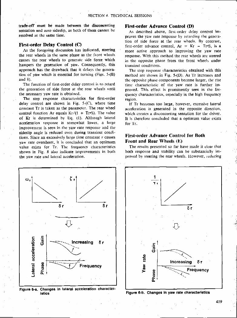
SECTION 4. TECHNICAL SESSIONS

trade-off must be made between the disconcertingsensation and zero sideslip, as both of them cannot beresolved at the same time.

First-order Delry Control (C)As the foregoing discussion has indicated, steering

the rear wheels in the same phase as the front wheelscauses the rear wheels to generate side force whichhampers the generation of yaw. Consequently, thisapproach has the drawback that it delays the genera-tion of yaw which is essential for turning (Fies. 5-(B)and 8).

The function of first-order delay control is to retardthe generation of side force at the rear wheels untilthe necessary yaw rate is obtained.

The step respon$e characteristics for first-orderdelay control are shown in Fig. 5-(C), where timeconstant Tr is taken as the parameter. The rear wheelcontrol function Ar equals Kr/(l + TrS). The valueof Kr is determined by Eq. (l). Although lateralacceleration response is somewhat lower, a largeimprovement is seen in the yaw rate re$ponse and thesideslip angle is reduced even during transient condi-tions. Since an excessively large time constant r causesyaw rate overshoot, it is concluded that an optimumvalue exists for Tr. The frequency characteristicsshown in Fig. 8 also indicate improvements in boththe yaw rate and lateral acceleration

Figure 6-a. Ghangee ln lateral scceleratlon charactel'letlcs

Flrst-order Advance Control (D)As described above, first-order delay control im-

proves the yaw rate response by retarding the genera-tion of side force at the rear wheels. By contrast,first-order advance control. Ar = Kr - Tr.S. is amore active approach to improving the yaw rateresponse. With this method the rear wheels are steeredin the oppo$ite phase from the front wheels undertransient conditions.

The step response characteristics obtained with thismethod are shown in Fig. 5-(D). As Tr increases andthe opposite phase components become larger, the risetime characteristic of the yaw rate is further im-proved. This effect is prominently seen in the fre-quency characteristics, especially in the high frequencyregion.

If Tr becomes too large, however, excessive lateralacceleration is generated in the opposite direction,which creates a disconcerting sensation for the driver.It is therefore concluded that a optimum value existsfor Tr.

First-order Advance Control for BothFront nnd Rear Wheels (E)

The results presented so far have made it clear thatboth response and stability can be substantially im-proved by steering the rear wheels. However, reducing

*+._---

+tr.9Go0)(J(,(E

(E

oN

._trftt(5 6 r

8G-cq

Frequency

+.Erg(5

oG'

EL O

tg-co.

increasing 6 r

Frequency

Figure 6-b. Changes in yaw rate characterlstlcs

419

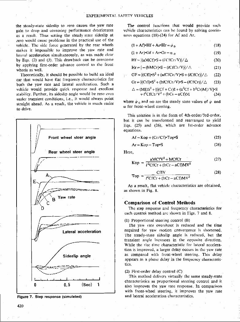
EXPERIMENTAL SAFETY VEHICLES

the steady-state sideslip to zero causes the yaw rategain to drop and cornering performance deterioratesas a result. Thus setting the steady-stal.e sideslip ateero would cause problems in the practical use of thevehicle. The side force generated by the rear wheelsmakcs it impossible to improve the yaw rate andlateral acceleration simultaneously, as was made clcarby Eqs. (2) and (3). This drawback can be overcomeby applying first-order advance control to the frontwheels as well.

Theoretically, it should be possible to build an idealcar that would havc flat frequetrcy characteristics forboth the yaw rate and lateral acceleration. Such avehicle would provide quick response and excellentstability. Further, its sideslip angle would be zero evenunder transient conditions, i.e., it would always pointstraight ahead. As a result, the vehicle is much easierto drive.

Front wheel steer angle

Rear wheel steer angle

0 . 5 (Sec) I

Figure 7. $tep response (simulated)

420

The control functions that would provide suchvehicle characteristics can be found by solving contin-uous equations (18)-(2a) for Af and Ar.

( l +Af) 'Hf +ArHr:po

( l +Ar ) 'Gf +ArGr :a o

111= [(aMCf).S + (f CfCr/V)]/A

Hr: [- (bMCr).S - (ICfCr/V) j/A

(18)

(1e)

(20)

(21)

6p = [(Cfl).S2 + (afCfCr/V).S + (dcfcr)]/A (22)

61= [(CrI)'S2 + (bBCfCr/V).S - (SCfCr)J/A (23)

a = (MI)S? + t[(Cf + Cr)I + 1a2Cf + U2Cr;tU1ZV1.S+ FCfCt/v2 + (bCr - aCf)M (24)

where rir s and ao are the steady state values of rir ando tbr front-wheel steering.

This solution is in the form of 4th-order/3rd-order,but it can be transformed and rearranged to yieldEqs.(25) and (26), which are lst-order advanceequations.

Af = Kop + (CrlCf).Top.S (25)

Ar=Kop-Top.5

Here,

aMCfVz+bBCfCr (27'�)

(28)

Kop - fzcfcr+(bCr-aCf)MVz

CilVTop=ffi

As a result, flat vehicle characteristics are obtained,as shown in Fig. 8.

Comparison of Control MethodsThe step response and frequency characteristics for

each control method are shown in Figs. 7 and 8.

(l) Proportional steering control (B)The yaw rate overshoot is reduced and the time

required lbr yaw motion convergence is shortened.The steady-state sideslip angle is reduced, but thetransient angle increases in the opposite direction.While the rise timc characteristic for lateral accelera-tion is irnproved, a larger delay occurs in the yaw ratea$ compared with front-wheel steering. This delayappears as a phase delay in the frequency characteris-tics.

(2) First-order delay control (C)This method delivers virtually the same steady-state

characteristic$ as proportional steering control and italso improves the yaw rate response. In comparisonwith front-wheel steering, it improves the yaw rateand lateral acceleration characteristics.

(26)

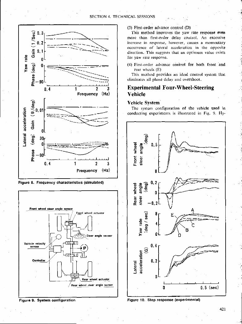
SECTION 4. TEC-HNICAL SESSIONS

(3) First-order advance control (D)This method improves the yaw rate response even

more than first-order delay control. Arr excessiveincrease in response, however, causes a momentaryoccurrence of lateral acceleration in the oppositedirection. This suggests that an optimum valuc existsfor yaw rate response.

(4) First-order advance control for both front andrear wheels (E)

This method provides an ideal control system thateliminates all phase delay and overshoot.

Experimental Four-Wheel-SteeringVehicle

Vehicle SystemThe system configuration of the vehicle used in

conducting experiments is illustrated in Fie. 9. Hy-

o(q

Io

0 . 4 1 2 3Frequency (Hz)

c.9G'

goaoa

(E

ofit

Go

; ; 0 . 0 1

=(E(t

0

E 3ors o f

Io r

E -totil

1 2 3Frequency (Hz)

Figure 8. Frequency characteristics (simulated)

Front rvhe€l Bt6€rwheel acluator

angle sensor

Rear wheel ectuatol

Reef iheel steer angle sensor

il)31."'

L

Figure 9. System configuration

E',oT'

o o -P 6F 6c ( t )o o

fl th

$ H 3 'EH -O

ooo g 'E -L d i

F €( E v

ts

E so

6 bE Er E OJ $

0 . 5

II:l

0 . 4

0 . 2

0

,lf-:z>- '+

E\//-/'?€:-i45=-a=-E+-+-/{'\ c

0. 5 (sec)

Figure 10. Step response (experimental)

421

t 0 . 3oah

.EO r E6 ( J 0B ^ 0.o tril> - o

3

s -s0(Il.tro-

0 . 0 2 [

rI

o .o tF

I0L

0 [

I-90 L

t-

t0 . 4

0 . 4

1 2 3Frequency (Hz)

-'t

1 2 3Frequency (Hz)

E loE

t r -. 9 *E c; ' 6t ( 5ooo ^- E ' |( E O

B goJ o

ahG.tro-

EXPERIMENTAL SAFETY VEHICLES

Figure 11. Frequency characteristics (experimental)

draulic actuators are providcd at both the front andrear wheels. Based on the vehicle velocity and steerangle signal$, the controller calculates the optimumcontrol signals for controlling the front and rearwheel steer angles.

Experimental ResultsThe step response and frequency characteristics are

shown in Figs. l0 and ll. Good agreement is seenwith the simulated rcsr.rlts given in Figs. 7 and 8.

The best yaw rate rise time characteristic is obtainedwith first-order advance control for both front andrear wheels, followed by first-order advance andfirst-order delay control in that order.

Lateral acceleration shows a two-stage rise charac-teristic, with front and rear wheel advance controlproviding the best performance in both stages. Withfirst-order advance control there is a momenl.ary delayin the initial rise stagc, but large lateral acceleration isobtained in the second stage owing to the generationof the yaw rate.

422

Table 2. $ublectlve evaluetlon of four-wheel steerinEcontrol.

Control

systemDescriptlon

{B) Proportlonal

Although hlgh stability ls obtain€d, a

dlsconcerting lateral shift occurs when the

vehicle is steered.

O, ls t -orderdelay

High levels of stabllity and response ar€

obtained. Vehicle behavior ls natural.

, . l s t - o r d e r(D)advancs

Exceptlonally good response is obtained whlchprovides crisp, sharp $teerlng. High gain ls

al$o felt,

(E) Ftont and

rear wheel

Good balance of stablllty and response at hlgh

levels, Steering characterlstlcs are natural

and accurate tracklng faithful to the driver'$

Intentlon is ohtained.

The results of a subjective evaluation of stabilityand steering response are given in Fig. 12 ancl briefsummaries of the evaluators' comments are given inTable 2-

The results indicate that stability was greatly im-proved by steering the rear wheels in the same phaseas the front wheels. When the same amount ofcontrol (proportional amounts) was applied, somedifference was seen depending upon how the transientyaw rate characteristic was given, however, the differ-ence between systems was very small.

The evaluation of steering respon$e improved asmore control was applied to cause the tire side forceto be increasingly generated in the direction of thetransient yaw rate (same phase for front wheels andopposite phase for rear wheels). Thus first-orderadvance control was evaluated the highest among therear wheel control methods.

The front and rear wheel advance control methodprovided a good balance of stability and response athigh levels. Because it kept the vehicle's sideslip angleto zero at all t imes (i.e. thc vchicle was constantlypointed straight ahead), the evaluators commentedthat the vehicle was easy to drive and that it providedaccurate tracking performance.

Development of HICAS SystemSystem concept

The High-Capacity Actively Controlled Suspension(HICAS) system has been built around the first-orderdelay control method (C) described before.

The results of thc authors' research to date haveclarified the following poinrs:{6)

r The frequency characteristics for the steerangle and steering force are virtually thesame.

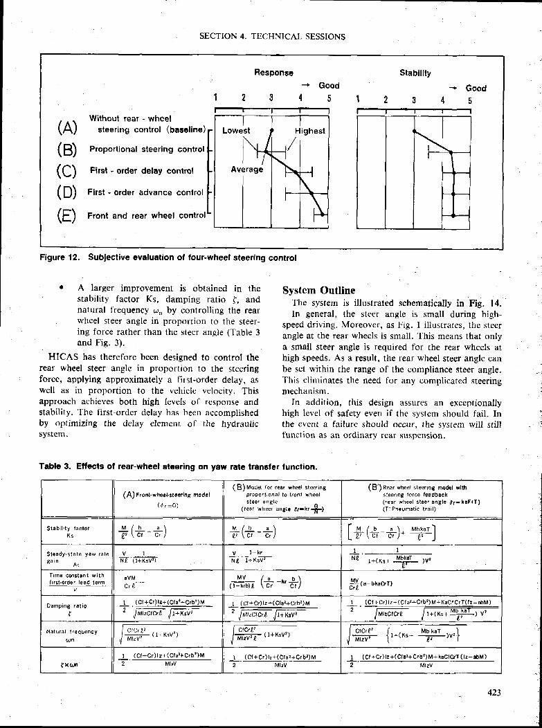
SECTION 4, TECHNICAL SESSIONS

Response

2 3

Stabll ity

Good

4 5Good

4 5

(A)(B)(c)(D)(E)

Without rear - wheelsteering control (baseline)

Proportional steering control

First - order delay control

First - order advance control

Front and rear wheel control

Highest

Figure 12. $ubiective evaluation of four-wheel steering control

A larger improvement is obtained in thestability factor Ks, damping ratio f, andnatural frequency <,r,, by controlling the rearwheel steer angle in proportion to the steer-ing force rather than the steer angle (Table 3and Fig. 3).

HICAS has therefore been designed to control therear wheel steer angle in proportion to the steeringforce, applying approximately a first-order delay, aswell as in proportion to the vehicle velocity. Thisapproach achieves both high levels of response andstabil ity. The first-order delay has heen accomplishedby optimizing the delay element ol ' the hydraulicsystem.

Table 3. Effects of rear-whcel eteering on yew rete trensfer function.

System OutlineThe system is i l lustrated schematically in Fig. i4.In general, the steer angle is small during high-

speed driving. Moreover, as Fig. I i l lustrates, the steerangle at the rear wheels is snall. This means that onlya small steer angle is required for the rear wheels athigh speeds. As a result, the rear wheel steer angle canbe set within the range of the compliance steer angle.This eliminates the need for any complicated steeringmechanism.

In addition, this design assures an exceptionallyhigh level of safety even if the system should fail. Inthe evcnt a failurc should occur, the system lvil l sti l lfunction as an ordinary rear suspension.

(A) Front. wtreet.staering model

( d r =O)

( B) t"toa"t {or rear.rh€€l steeringpropottiohal to f/ont wheelS t e e r A n g t e

( rear wheer ang la a r=kr f t )

(B') nearwheet-steering modsl wlthsteering torce leedback( r€ar whee l s teer an8 l6 d r -ksFtT)(T : Pn€umat ic t ra i l )

S tab i l i t y lac to rK 5

M / b a \

7 \ c t - c , /M / b a \! , ' \ c t

- c t i [+t+-+). -,rr*]

S t e a d y . S t d t a y d w r a t eg a i n

V 1NT' ( l+KsvT

y l - k rj|*T' t+i;Vr-

1 lNo r+(xs+ iH- )vr

T i m 6 c m s t E n t w i t hf i rs t .o rder lead t6 rm

svM-Cr g- ch (+-"*) ffit"-tt"ctrl

Dampin8 rd t iO

{I2

(Cf +Cr ) l z+(Cf d '+Crb ' � ) M

,[W trK'vilI (C f+Cr) l r+ (CtE2+crb2)M

" ltatcrw 1;x'v,

I (C f +Cr ) tz + ( C f a?+Crbz) M +KaCf CrT( l z - sM)

tr'c,c't F^JF\r-Natura l f requency

Q)n f iF-- (t+Ksvl) ffi

f Xartl

I (C f+Cr) lz+(Cfa t+Crb t )M I (Cf+Cr)h+(Cfd t+Crbr )M I (Ct+c/)12+(cla?+crb?)M+kacfcrT ( l r -sbM)MhV MhV 2 MlzV

o -s " -c

E -6

ah

c . E oE G \

, g lr ! s

f l IE G( r r

Four - wheel - steeting vehicleFront - wheel . steering vehicle

0 .002

0 . 0 1 5

0 . 0 0 1o 'o fo'r l

0-

^--+',----

: ; - - ' ' - - - - - = - - - - ' . . . - - - = _ : _ i - .

50 r00 r50 200Vehic le veloci ty I km/h ]

EXPERIMENTAL SAFETY VEH ICLES

Figure

Thiscontrolsystem.

13. Stabil ity factor and vehicle response gain

system is called an active compliance steersystem and it plays a vital role in the HICAS

Figure 15. Double-valve steerlng gear

force generated by the hydraulic cylinder and therigidity of the insulators, hydraulic pre$sure is fedback to control the rear wheel steer angle (6r) inaccordance with Eq. (29) given in Fie. l4' As a result,the rear wheel steer angle obtained is virtually propor-tional to the lateral acceleration.

Electronic Conlroller. The rear wheel steer angle iscontrolled relative to the vehisle velocity. As shown inFig. 17, the steer angle increases as the vehicle velocityincreases. This is accomplished by means of a bypassvalve whictr is controlled by an electronic controller.The controller operates according to the signal re-ceived from a vchicle velocity sensor. This makes itpossible to raise thc vehicle's natural stability factoras the vehicle velocity increases, thereby improvingvehicle stability.

The steering gear ratio is set at a small 13.3, whichprovides an improved yaw rate gaitr in low andintermediate speed ranges. The stability factor in thelow-speed region where the rear wheels are not steeredis also set on the small side at about 0.001 s2lm2. Thiscontributes to better vehicle handling properties at lowand intermediate speeds.

As a result, precise steering controllability is ob-tained at low speeds and also excellent vehicle stabilityis provided in the high speed range.

r ; i ' i i ' i . i

i t , ; , r i + i i r r .

System StructureHydraulic Syslems. Two hydraulic systems are em-ployed, with one providing hydraulic pressure forpower steering at the front wheels and the other used

for steering the rear wheels. The hydraulic pump is

built with a tandem structure.

Rear Wheel Steer Control Actuator. The hydraulic

control valve for the rear wheels has a double-valve

structure, as i l lustrated in Fie. 15. The valve construc-

tion is the same as that of the power steering valve at

the front wheels, though the two valves differ in theirperformance characteristics.

Thc hydraulic pressure is controlled proportional tothe steering force, and it is transferred to the hydrau-lic cylinder with a first-order time lag characteristic.The compact hydraulic cylinder presses against therubber insulators that are installed where the suspen-sion is attached to the vehicle body. Through the

Figure 14. Outllne of rear-wheel actlve compllancesteer system wlth steering lorce feedback(HrcAs)

Controlva l ve

AElectronlcl-1controller L+

vehicle

uvarauricffi

F"'�ffi"Velocitysen$or

Actua torcon$tant E

o, =# ... (2s)

Figure 16. Hydraulic cyllnder

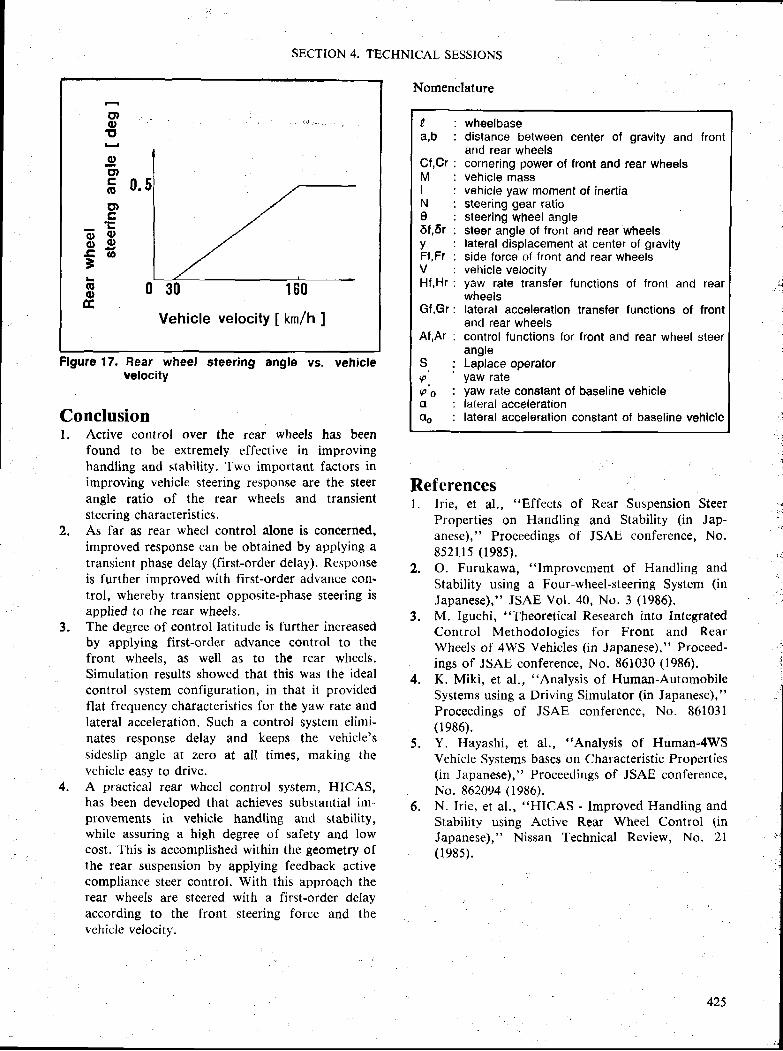
Flgure 17. Bear wheel steering anglevelocitY

grott

ggtc(E

g)gL

? i o.r-r O

B

ooIE

0.

0 30 160

Vehicle velocity I km/h ]

SECTION 4. TECHNICAL SESSIONS

vehicle

Nomenclature

Referencesl. Irie, et al., "Effects of Rear Suspension Steer

Properties on Handling and Stability (in Jap-anese)," Proceedings of JSAE conference, No.8521 l5 (1985) .O. Furukawa, "Improvement of Handling andStability using a Four-wheel-steering System (inJapane$e)," JSAE Vol. 40, No. 3 (1986).M. Iguchi, "Theoretical Research into IntegratedControl Methodologies for Front and RearWheels of 4WS Vehicles (in Japanese)," Proceed-ings of JSAE conference, No. 861030 (1986).K. Miki, et al., "Analysis of Human-AutomobileSystems using a Driving Simulator (in Japanese),"Proceedings of JSAE conference, No. 861031(1986).Y. Hayashi, et al., "Analysis of Human-4WSVehicle Systems bases on Characteristic Properties(in Japanese)," Proceedings of JSAE conference,No. 862094 (1986).N. Irie, et al., "HICAS - Improved Handling andStability using Active Rear Wheel Control (inJapanese)," Nissan Technical Review, No. 2l(1e85).

2.

Conclusionl. Active control over the rear wheels has been

found to be extremely effective in improvinghandling and stability. Two important factors inimproving vehicle steering reiiponse are the steerangle ratio of the rear wheels and transientsteering characteristics.As far as rear wheel control alone is concerned,improved response can be obtained by applying atransient phase delay (first-order delay). Responseis further improved with first-order advance con-trol, whereby transient opposite-phase steering isapplied to the rear wheels.The degree of control latitude is further increasedby applying first-ordcr advance control to thefront wheels. as well as to the rear wheels.Simulation results showed that this was the idealcontrol system configuration, in that it providedflat l'requency characteristics for the yaw rate andlateral acceleration. Such a control $ystem elimi-nates response delay and keeps the vehicle'ssideslip angle at zero at all t imes, making thevehicle easy to drive.A practical rear wheel control system, HICAS,has been developed that achieves substantial im-provements in vehicle handling and stability,whilc assuring a high degree of safety and lowcost. This is accomplished within the geometry ofthe rear suspension by applying feedback activecompliance steer control. With this approach therear wheels are $teered with a first-order dclayaccording to the front steering force and thevehicle velocity.

2.

3 .3.

4.

4.

5 .

6.

xa,b

CI,CrMINe6r,6rvFI,FTVHf ,H r

Gf,Gr

Af,Ar

SF ,9 oCI

oo

wh€elbasedistance between center of gravity and frontand rear wheelscornering power of front and rear wheelsvehicle massvehicle yaw moment of inertiasteering gear ratiosteering wheel anglesteer angle of front and rear wheelslateral displacement at center of gravityside force of front and rear wheelsvehicle velocityyaw rate transfer functions of front and rearwheelslateral acceleration transfer functions of frontand rear wheelscontrol functions for front and rear wheel steerangleLaplace operatoryaw rateyaw rate constant of baseline vehiclelateral acceleraiionlateral acceleration constant of baseline vehlcle

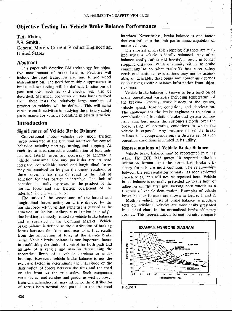
Objective Testing for Yehicle Brake Balance Performance

T.A. Flaim,J.S, Smith,General Motors Current Product Engineering,United States

AbstractThis paper will describe GM technology for objec-

tive measurement of brake balance. Facilities will

include the road transducer pad and torque wheel

instrumentation. The need for multiple approaches to

brake balance testing will be defined. Limitations ofpast methods, such as skid checks, wil l also be

described. Statistical properties of data bases derived

from these test$ for relatively largc numbers ofproduction vehicles will be defined. This will assist

other research activities in studying the primary safetyperformance for vehicles operating in North America.

IntroductionSigrrificance of Vehicle Brake Balance

Conventional motor vehicles rely upon frictionforces generated at the tire road interface for control

behavior including starting, turning, and stopping. At

each tire to road contact, a combination of longitudi-nal and lateral forces are necessary to generate a

vehicle maneuver. For any particular tire to road

interface, controllable Iateral and longitudinal forces

may be sustained as long as the vector resultant of

these forces is less than or equal to the l imit ofadhesion for that particular interface. The limit ofadhesion is usually expressed as the product of the

normal force and the friction coefficient of the

interface, i.e., L :mu X N.The ratio of the vector sum of the lateral and

longitudinal forces acting on a tire divided by the

normal force acting on that same tire is defined as theadhesion uti l ization. Adhesion uti l ization in straightl ine braking is directly relatcd to vehiclc brakc balanceand is regulated in the Common Market. Vehicle

brake balance is defined as the distribution of brakingforces between the front and rear axles that resultsfrom the application of force at the service brakepedal. Vehicle brake balance is one important factorin establishing the limits of control for both path andattitude of a vehicle and also in determining thetheoretical limits of a vehicle deceleration uuderbraking. However, vehicle brake balance is rtot theexclusive factor in determining the magnitude or the

distribution of forces between the tires and the road

on the front vs the rear axles. Such exogenousvariables as road camber and grade, as well as power

train characteristics, all may influence the distributionof fbrces both normal and parallel to the tire road

426

EXPERIMENTAL SAFETY VEHICLES

interface. Nevertheless. brake balance is one factorthat can influence the limit perfortnance capability ofmotor vehicles.

The shortest achievable stopping distances are real-ized when a vehicle is ideally balanced. Any otherbalance configuration will inevitably result in longerstopping distances. While unanimity within the brakecommunity' as to what tradeoffs best meet safetyneeds and customer expectations may not be achiev-able, or desirable, developing any consen$us dependsupon having credible balance information from objec-tive tests.

Vehicle brake balance is known to be a function ofmany operational variables including temperature ofthe braking elements, work history of the $ystem,vehicle speed, loading condition, and deceleration.The challenge for the brake engineer is to select acombination of foundation brake and system compo-nents that best meets the customer's needs over thebroad range of operating conditions to which thevehicle is exposed. Any measure of vehicle brakebalance that comprehends only a discrete set of suchoperating conditions is limited in its utility.

Representations of Vehicle Brake BalanceVehicle brake balance may be represented in many

ways. The ECE Rl3 annex l0 required adhesionutilization format, and ths normalized brake effi-ciency formats are most common. The relationshipsbetween the representation formats has been reviewedelsewhere (l) and will not be repeated here. Vehiclebrake balance is normally presented up to the limit ofadhesion on the first axlc locking both wheels as afunction of vehicle deceleration. Examples of vehiclebrake balance formats are shown in figures I and 2.

Multiple vehicle tests of brakc balance or multipletests on individual vehicles arc most easily ptesentedin a cloud chart in the normalized brake efficiencyformat. This representation format permits compari-

EXAMPLE FISHBONE DIAGRAMtff

go

flt

f r 7 0H mE s oo8 4 0A

il

20

t0

00.0 0.1 0.2 0.3 rt.4 0.5 0.8 0-7 0.8 0.0

Figure I

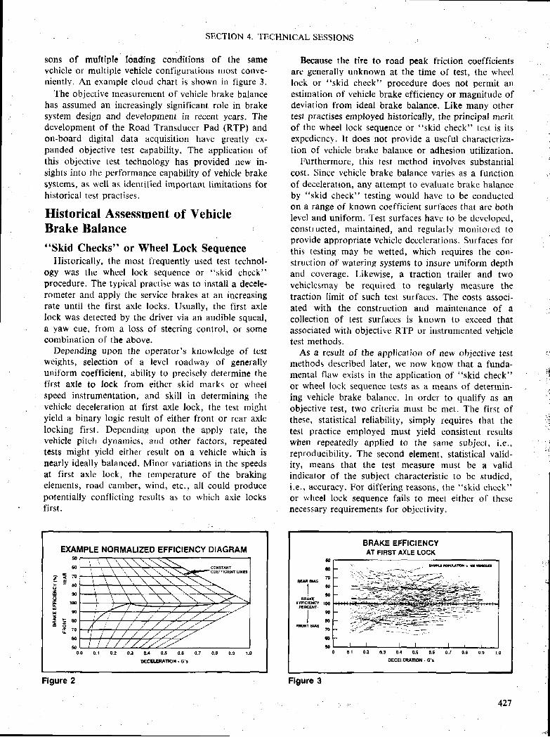
SECTION 4. TECHNICAL SESSIONS

sons of multiple loading conditions of the samevehicle or multiple vehicle configurations mo$t conve-niently. An example cloud chart is shown in I ' igure 3.

The objective measurement of vehicle brake balancehas assurned an increasingly significant role in brakesystem design and development in recent years. Thedevelopment of the Road Transducer Pad (RTP) andon-board digital data acquisit ion have greatly ex-panded objective test capabil ity. the application ofthis objective test technology has provided new in-sights into the performance capability of vehicle brakesystems, as well as identified important limitations forhistorical test practises.

Historical Assessment of VehicleBrake Balance"Skid Checks" or Wheel Lock Sequence

Historically, the most lrequently used test technol-ogy was the wheel lock sequence or "skid check"procedure. The typical practise was to install a decele-rotneter and apply the service brakes at an increasingrate unti l the first axle locks. Usually, the first axlelock was detected by the driver via an audible squeal,a yaw cue, from a loss of steering corrtrol, or somecombination of the above.

Depending upon the operator's knowledge of testweights, selection of a levcl roadway of generallyuniform coefficient, ability to precisely determine thefirst axle to lock from eithcr skid marks or wheelspeed instrumentation, and skil l in determining thevehicle deceleration at first axle lock, the test nrightyield a binary logic result of either front or rear axlelocking first. Depending upon the apply rate, thevehicle pitch dynamics, and other factors, repeatedtests might yield either result on a vehicle which isnearly ideally balanced. Minor variations in the speedsat f irst axle lock, the temperature of the brakingelements, road camber, wind, etc., all could producepotentially confl icting results as to which axle Iocksfirst.

Eecause the tire to road peak friction coefficientsare generally unknown at the time of test, the wheellock or "skid check" procedure does not permit anestimation of vehicle brake efficiency or magnitude ofdeviation from ideal brake balance. Like many othertest practises employed historically, the principal meritof the wheel lock $equence or "skid check" tcst is itsexpediency. It does not provide a useful characteriza-tion of vehicle brake balance or adhesion utilization.

Furthermore, this test method involves substantialcost. Since vehicle brake balance varies as a l'unctionof deceleration, any attempt to evaluate brake balanceby "skid check" testing would have to be conductedon a range of known coefficient surfaces that are bothlevel and uniform. Test surfaces have to be developed,conf;tructed, nraintained, and regularly monitorcd toprovide appropriate vehicle decelerations. Surfaces forthis testing may be wetted, which requires the con-struction of watering systems to insure uniform depthand coverage. Likewise, a traction trailer and twovehiclesrnay be required to regularly measure thetraction limit of such test surfaces. The costs associ-ated with the construction and maintenance of acollection of test surfaces is known to exceed thatassociated with objective RTP or instrumented vehicletest methods.

As a result of the application of new objcctive testmethods described later. we now know that a funda-mental flaw exists in the application of "skid check"or wheel [ock sequence tests as a means of determin-ing vehicle brake balance. ln order to qualify as anobjective test, two criteria rnust be met. The first ofthese, statistical reliability, simply requires that thetest practice employed must yield consistent resultswhen repeatedly applied to the same suhject, i.e.,reproducibility. The second element, statistical valid-ity, means that the test measure must be a validindicator of the subject characteristic to be studied,i.e., accuracy. For differing reasons, tlte "skid check"or wheel lock sequence fails to meet either of thesenecessary requirements for objectivity.

EXAMPLE NOHMALIZED EFFICIENCY DIAGRAM5{l

s

E E ' oE

* E O

E g oF ' -u S

E = *@ oF 7 0

60

500.0 0,r 0-e 0,3 0,4 0-5 0-a o.7 0.8 0.9 1.0

Flgure 2

BRAKE EFFICIENCYAT FIRST AXLE LOCK

3

60

roFUtrc

l mIi s

BMXEEncrEH 100+tExr-

l sII E

* f f i *

to$

0 0.r 0,2 0,3 0,4 0.5 0.6 n,1 0,8 0.9 1.0

Flgure 3

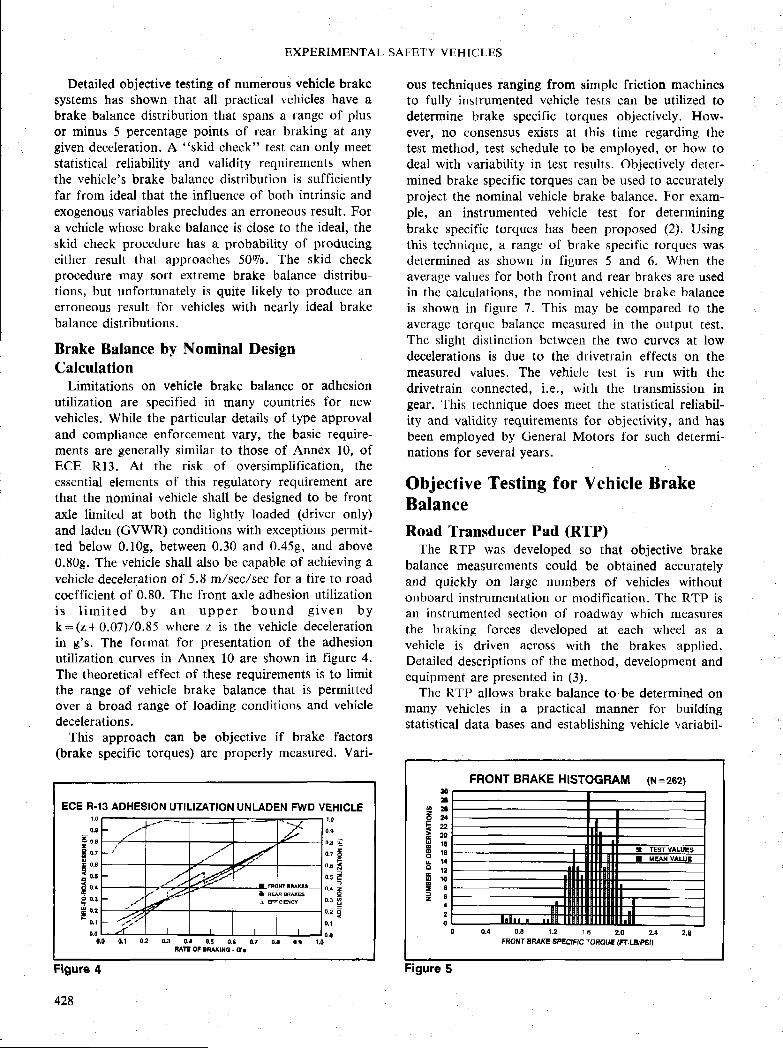
EXPERIMENTAL SAFETY VEHICT,ES

Detailed objective testing of numerous vehicle brakesystems has shown that all practical vehicles have abrake balance distribution that spans a range o[ plusor minus 5 percentage points of rear braking at anygiven deceleration. A "skid check" test can only meetstatistical reliability and validity requirements whenthe vehiclens brake balancc distribution is sufficientlyfar from ideal that the influence of both intrinsic andexogenous variables precludes an erroneous result. Fora vehicle whose brake balance is close to the ideal, theskid check procedure has a probability oi producingeither result that approachcs 5090. The skid checkprocedure may sort extreme brake balance distribu-tions, but unfortunately is quite likely to produce anerroneous result for vehicles with nearly ideal brakebalance distributions.

Brake Balance by Nominal DesignCalculation

Limitations on vehicle brake balance or adhesionutilization are specified in many countries for newvehicles. While the particular details of type approvaland compliance enforcement vary, the basic require-ments are generally similar to those of Annex 10, ofECE Rl3. At the risk of oversimplification, theessential elements of this regulatory requirement arethat the nominal vehicle shall be designed to be frontaxle limited at both the lightly loaded (driver only)and laden (GVWR) conditions with exceptions permit-ted below 0.10g, between 0.30 and 0.459, and above0.809. The vehicle shall also be capable of achieving avehicle deceleration of 5.8 m/sec/sec for a tire to roadcoefficient of 0.80. The front axle adhesion utilizationi s l i m i t e d b y a n u p p e r b o u n d g i v e n b y1q:(z+0.07)/0.85 where z is the vehicle decelerationin g's. The format for presentation of the adhesionutilization curves in Annex 10 are shown in figure 4.The theoretical effect of these requirements is to limitthe range of vehicle brake balance that is permittedover a broad range of loading conditions and vehicledecelerations.

This approach can be objective if brake factors(brake specific torques) are properly measured. Vari-

ous techniques ranging from simple friction machinesto fully instrumented vehicle tests can be utilized todetermine brake specific torques objectively. How-ever, no consensus exists at this time regarding thetest method, test schedule to be employed, or how todcal with variability in tcst results. Objectively deter-mined brake specific torques can be used to accuratelyproject the nominal vehicle brake balance. For exam-ple, an instrumented vehicle test for determiningbrake specific torques has been proposed (2). Usingthis technique, a range of brake specific torques wasdetermined as shown in figures 5 and 6. When theaverage values for both front and rear brakes are usedin the calculations, the nominal vehicle brake balanceis shown in figure 7. This may be compared to theaverage torque balance measured in the output test.The slight distinction between the two curves at lowdecelerations is due to the drivetrain effects on themeasured values. The vehicle test is run with thedrivetrain connected, i.e., with the transmission ingear. This technique does meet the statistical reliabil-ity and vatidity requirements for objectivity, and hasbeen employed by Ceneral Motors for such determi-nations for several years.

Objective Testing for Vehicle BrakeBalance

Road Transducer Pad (RTP)The RTP was developed so that objective brake

balance measurements could bc obtained accuratelyand quickly on large numbers of vehicles withoutonboard instrumentation or modification. The RTP isan in$trumented section of roadway which measuresthe braking forces developed at each wheel as avehicle is driven acros$ with the brakes applied.Detailed descriptions of the method, development andequipment are presented in (3).

The RTP allows brake balance to be determined onmany vehicles in a practical manner for buildingstatistical data bases and establishing vehicle variabil-

ECE R.l3 ADHESION UTILIZATION UNI-ADEN FWD VEHICLEr,00,9

E o.t-r 0.4q

E o'uF n .I 0.3

f rn t0.1

EF

M II

- ,..8,J EFICIEXfl

- t'/t

1.0

0.9

0.8 5

o.r Eo.e fi=0.5 r-

0.4 zo

0." fr0,2 4

0.1

0 . 0 r n | | | | l d . d

o0 (lt 0.1 43 0.r 0,5 0.6 0.7 0.r 0-i t.0BATE OF ERAKlxc - c'!

Flgure 4

30B

4 2 66 2 .l ne a oH 1 8E 1 6E l,lo . .u 1 0

i al o

420

FHONT BHAKE HISTOGRAM (il=z6z)

a

l i l r i I

0.4 0.8 1.2 1-6 LO 2,1FFOI{T BRAXE SPECIFIC TOROU€ {Fr-LE/PSI}

Figure 5

428

SECTION 4. TECHNICAL SESSIONS

ity. Since no modification is required, customer vehi-cles and vehicles under durability assessment can bemeasured without disruption of vehicle hardware.

Objective brake balance assessnlent can be per-formed accurately and efficiently. Since actual roadforces are measured, knowledge of dynamic tireradius is not required. Vehicle measurements arelimited to a series of "snapshots" as the vehicles passover the transducers,

Instrumented Vehicle TestsInstrunrented vehicle testing has been used success-

fully by General Motors to objectively measure brakebalance. Torque wheels combined with other systemtransducers, and onboard digital data acquisit ionhardware, permit a complete vehicle brake systemanalysis to be performed relatively quickly. With thismethod, instrumented wheels replace the normal vehi-cle wheels and torque developed during braking ismeasured at each wheel. Since the torque transducersare rotating, slip ring dcvices arc cmployed to couplethe instrumerrted wheels to data acquisition equipmentresiding onboard the vehicle. Measurements are madeat various decelerations and analyzcd to objectivelyassess brake balance through the entire brake apply.Axle lock sequence for various tire-road friction levelsand braking efficiencies are easily calculated from thedata.

Dynamic wheel torque measurements and loadedtire radii are u$ed to compute road f'orces at eachwheel. Four sensors mea$ure individual wheel veloci-ties and a fifth wheel at the rear of the car measuresvehicle speed. Other instrunrentation is included tomeasure hydraulic pressures, brake temperatures andpedal apply force. Data is acquired by equipmenthoused in the passenger compartment.

Instrumented vehicles can provide objective assess-ments of total brake system performance. Efficiencyand axle lock sequence for all road friction coeffi-cients are easily obtained from proper analysis oftorque wheel tests on a single high I 'r iction surface.

Brake balance assessment requires knowledge of dy-namic tire radius because whcel torques rather thanactual road forces irre nteasured. An array of customtransducers must be acquired, maintained and in-stalled on test vehicles which makes the method lesspractical than the RTP for measuring large numbersof vehiclcs for statistical analyses. However, thismethod with its accurate and rather extensive results isoften required for in-depth investigations of totalbrake system performance on development vehicles.

Correlntion Between Torque Wheels and theRTP

To evaluate the statistical validity of the RTP andthe use of torque whecl/digital data acquisition meth-ods for brake balance assessrnent. a series of testswere conducted on a vehicle equipped with fullinstrumentation including torque wheels, pedal forceand line pressure transducers, and event marker pho-tocell detectors. A series of constant decelerationsnubs were made over the RTP while the digital dataacquisition system sirnultaneously recorded the wheeltorques. A dynamic rolling radius correction wasmade to the torque wheel data for conversion to roadforce. The brakc balance determined from both theRTP and the converted torque wheel data is shown infigure 8. Here one can see general agreement over abroad range of vehicle decelerations between the twotest techniques.

Statistical analysis of the brake balance measure-ments revealed an average difference of 0.05 percent-age points with a standard deviation of 0.744 percent-age point$. Perfect agreement between the twomethod,r would have produced an average differenceof 0 and a finite standard dcviation due to randomerror only.

DiscussionThe selection of a particular objective test method

to employ for vehicle brake balance testing is more a

HEAH BRAKE HISTOGRAM

4

35

&

25

m

r5

r0

5

0

(N = 262)

I TEETVALUES

I UEdVALUE

l l l t , . ,r . , l l ,h. I .

tr4 ttt 1-2 '1.8 z0 24

NEAN ERAXE SPECIFIC YOFOUE (FT-LBPSI)

Figure 6

BHAKE BALANCE COMPAHI$ONAVG MEASURED vs. PFEDICTED Avc

=sGg

E*

" f" f" f

:l0.4 0.6

OECEL€fiAnOfl. G t

I

Figure 7

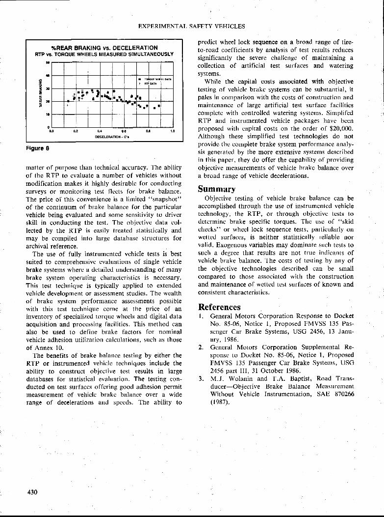
%REAH BHAKING vs. DECELERATIONRTP vs. TOROUE WHEELS MEASURED SIMULTANEOUSLY

50

atlo=J 3 0tE

H 2 0rr

10

00.0

I TOI

+ f f i

wE wt

t

il !

af + i r ' {

I

5.ta ) It - t r I

I

Flgure I

EXPERIMENTAL SAFETY VEHICLES

matter of purpose than technical accuracy. The abilityof the RTP to evaluate a number of vehicles withoutmodification makes it highly desirable for conductingsurveys or monitoring test fleets for brake balance.The price of this convenience is a limited "snapshot"

of the continuum of brake balance for the particularvehicle being evaluated and some sensitivity to driverskill in conducting the test. The objective data col-lected by the RTP is easily treated statistically andmay be compiled into large database structures forarchival reference.

The use of fully instrumented vehicle tests is bestsuited to comprehensive evaluations of single vehiclebrake systems where a detailed understanding of tnanybrake system operating characteristics is ncccssary.This test technique is typically applied to extendedvehicle development or a$$essment studies. The wealthof brake system performance assessments possiblewith thi$ test technique come at the price of aninventory of specialized torque wheels and digital dataacquisition and processing facilities. This method canalso be used to define brake factors for nominalvehicle adhesion utilization calculations. such as thoseof Annex 10.

The benefits of brake balance testing by either theRTP or instrumented vehicle techniques include theability to construct objcctive test results in largedatabase$ for statistical evaluation. The testing con-ducted on te$t surfaces offering good adhesion permitmeasurement of vehicle brake balance over a widerange of decelerations and speeds. The ability to

predict wheel lock sequence on a broad range of tire-to-road coel'ficients by analysis of test results reducessignificantly the severc challcngc of maintaining acollection of artificial test surl'aces and wateringsystems.

While the capital costs associated with objectivetesting of vehicle brakc systems can be substantial, itpales in compari$on with the co$ts of construction andmaintenance of large artificial test surface facilitiescomplete with controlled watering systems. SimplifedRTP and instrumented vehicle packages have beenproposed with capital costs on the order of $20,000.Although these simplified test technologies do notprovide the complete brake system performance analy-sis generated by the more extensive systems describedin this paper, they do offcr the capability of providingobjective measurements of vehicle brakc balance overa broad range of vehicle decelerations.

SummaryObjective testing of vehicle brake balance can be

accomplished through the use of instrumented vehicletechnology, the RTP, or through objective tests todetermine brake specific torque$. The use of "skid

checks" or wheel lock sequence tests, particularly onwetted surfaces, is neither statistically reliable norvalid. Exogenous variables may dominate such tests tosuch a degree that results are not true indicants ofvehicle brake balance. The costs of testing by any ofthe objective technologies described can be srnallcompared to those associatcd with the constructionand maintenance of wetted test surfaces of known andconsistent characteristics.

ReferencesI. General Motors Corporation Response to Docket

No. 85-06, Notice l, Proposed FMVSS 135 Pas-senger Car Brake Systems, USG 2456, 13 Janu-ary, 1986.

2. General Motors Corporation Supplemental Re-sponse to Docket No. 85-06, Notice l, ProposedFMVSS 135 Passenger Car Brake Systems, USG2456 part ll l, 3l October 1986.

3. M.J. Wolanin and T.A. Baptist,ducer-Objective Brake BalanceWithout Vehicle Instrumentation,( r e87).

Road Trans-MeasurementsAE 870266

SECTION 4. TECHNICAL SESSIONS .

Antilock System PerformaRce Under Winter Conditions-lVhat Should BeRequired?

Olle Nordstriim,Swedish Road and Traffic Research Institute,Sweden

AbstractIn Sweden accidents due to loss of $tability and

steerability caused by braking with locked wheels to alarge extent occur on icy roads in the winter. It istherefore essential that antilock systems that areexpected to eliminate this type of accidents perfiormwell under these circum$tances. In order to establishsuitable test methods and realistic performance levelsinvestigations have been made both with passengercars and commercial vehicles including heavy trailers.

Stability and steerability in terms of staying withinlane boundaries with restricted steering wheel correc-tions and braking performance in terms of brakingefficiency related to a reference performance in termsof lateral friction, locked wheel friction, optimumfriction (ECE/EEC) or friction according to the ISOTR 8349 method have been considered as primarysaf-ety criteria.

These investigations are described and the resultssummarized. As winter performance test methods thefollowing are discussed and recommended togetherwith suggested rninimum performance

r J-turn braking performance test on ice. split friction test with very low friction on

one sider straight line braking on ice. Transition from low friction to high friction

surface

IntroductionIn Sweden the necessity of driving under winter

conditions with very low road adhesion can be cx-pected from the middle of October to the end of Aprilor approximately six months of the year. Not onlyhomogeneous low friction but also asymmetric socalled split friction and transitions from low to highfriction or the opposite are frequently met during thewinter period.

Safe braking under these conditions is for obviousreasons a serious problem. Strrdded tyres have beenfound to be one effective way of raising the safetylevel and is widely used on passenger cars in wintertime. They are also to some extent used on trucks buthardly on heavy trailers. Even with studs the frictionlevel can be below 0.2 and the risk of wheel lockingwith Ioss of steering control and stability duringbraking is considerable during emergency braking.

Antilock braking systems with good performanceunder these conditions can therefore be expected togive a significant reduction in traffic accidcnts wherebraking is involved.

The Swedish Road Safety Office, The SwedishBoard for Technical Development and other Swedishorganizations interested in traffic saf'ety research havetherefore sponsored several projects with the aim toinvestigate what can be expected from vehiclesequipped with antilock systems in terms of stability,steerability and braking performance. The SwedishRoad and Traffic Research Institute (VTI) has beenactive in most of these projects.

This paper summarizes investigations during fivewinterperiods from 1980-1986 and presents proposalsfor antilock system test procedurcs and requirernents,the aim of which is to ensure good braking perfor-mance under winter conditions.

These tests are to be regarded as proposed comple-mentary winter service requirements to be added tothe rnore general requirernents in the ECE/EECregulations.

Antilock System Tests Under WinterConditions Carried Out hy VTI

Test proceduresThe following antilock system test procedures have

been studied

steerability tests on ice comprisingl ) J- turn brak ing2) Braking in a steady state turn3) Single lane change braking

. split friction test defined as straight linebraking with one side of the vehicle on ahigh frictiorr surface and the other side on alow friction surface (ice)

I straight line braking test on icer transition from low to high friction and the

opposite with ice as low fiiction surface

The steerability and split friction tests evaluatedifferent aspects of steerability and stability andbraking efficiency while the two rernaining test typesprimarily evaluates braking efficiency.

The conclusion from these studies is a recommenda-tion to include the following winter $ervice approvaltests for anti lock systems.

Driver controlled J-turn test on iceSplit friction test with one very low frictionsurfaceSrraight line braking test on ice

l ' : i| : t

il

,J:F;

3.

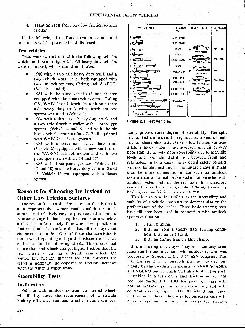
EXPERIMENTAL SAFETY VEHICLES

4, Transition test from very low friction to highfriction.

In the following the different test procedures andtest results will be presented and discussed.

Test vehiclesTests were carried out with the following vehicles

which are shown in figure 2.1. All heavy duty vehicleswere air braked. with S-cam drum brakes.

| 1980 with a two axle heavy duty truck and atwo axle drawbar trailer both equipped withtwo antilock systems, Girling and WABCO.(Vehicle I and 5)

. l98l with the same vehicles (l and 5) nowequipped with three antilock systems, GirlingGX. WABCO and Bosch. In addition a threeaxle heavy duty truck with Bosch antilocksystem was used. (Vehicle 3)

. 1984 with a three axle heavy duty truck anda two axle drawbar trailer with a prototypesystem. (Vehicle 4 and 6) and with the six

, heavy vehicle combinations 7-12 all equipped, with wABCo antilock syritems.

r 1985 with a three axle heavy duty truck(Vehicle 2) equipped with a new version ofthe WABCO antilock system and with two

' passenger cars. (Vehicle 14 and 15)| 1986 with three passenger cars (Vehicle 16,

l7 and 18) and the heavy duty vehicles 2 and13. Vehicle 13 was equipped with a Bosch

r SYSt€m'

Reasons for Choosing Ice Instead ofOther Low Friction Surfaces

The reason for choosing ice as test surface is that itis a representative winter road condition that isdurable and relatively easy to produce and maintain.A disadvantage is that it requires temperatures below0"C. lt has unfortunately till now not been possible tofind an alternative surface that has all the importantcharacteristics of ice. One of these characteristics isthat a wheel operating at high slip reduces the frictionof the ice for the following wheels. This means thaton ice the front wheels can get higher friction than therear wheels which has a destabilizing effect. Onwetted low friction surfaces for test purposes theeffect is normally the opposite as friction increaseswhen the water is wiped away.

Steerability Tests

JustificationVehicles with antilock systems on steered wheels

will if they meet the requirements of a straightbraking efficiency test and a split friction test cer-

432

TEST VEHICTES TEST TIEIGHTKG

TEST VEHICLES IEST IIEIGHKG

r f f^/-fi{ ro:bEr

,-{--------l3LO_F

4frd

5dEr:rfF,- r--r

5 f f i

I

l 0

,61_E:+H

Vehicler0 ?0

length n

6500-13000

96m-22700

t580{t

108{n

12000-33000

16300

17000-51400

t3000-28500

I 5000-36400

20500-51400

70000-51400

22000-664m

50900

ffim nttuEl 4

t 5

t 6

r 7at0l tm tvilr 198!

, fih-==1s t$Ei=t@

rflw 7s

l 2 l5 -1520

1600- l9z0

t58{t

1580- 1840

1640-r8t0

Figure 2.1 Test vehlcles

tainly posse$s some degree of steerability. The splitfriction test can indeed be regarded as a kind of hiehfriction steerability test. On very low friction surfacesa bad antilock system may, however, give either verypoor stability or very poor steerability due to high sliplevels and poor slip distribution between front andrear axles. ln both cases the expected safety benefitswill not be obtained and in the unstable case it mighteven be more dangerous to use such an antilocksystem than a normal brake system or vehicles withantilock system only on the rear axle. lt is therefbreessential to test the steering qualities during emergencybraking on low friction in a special test.

This is also true for trailers a$ the steerability andstability of a vehicle combination depends also on theperformance of the trailer. Three basic steering testshave till now been used in connection with antilocksystem evaluation:

I. J-turn braking.2. Braking l'rom a steady state turning condi-

tion (Braking in a turn).3. Braking during a single lane change

J-turn braking a$ an open loop constant step steerinput test for passenger cars with antilock systems wasproposed by Sweden at the 1974 ESV congress. Thiswas the result of a research program carried outmainly by the Swedish car industries SAAB SCANIAand VOLVO but in which VTI also took active part.

Braking in a turn on a high friction surface hasbeen standardized by ISO for passenger cars withnormal braking systems as an open loop test withconstant steering input. TUV Rheinland has testedand proposed this method also for passenger cars withantilock systems. In order to assess the steering

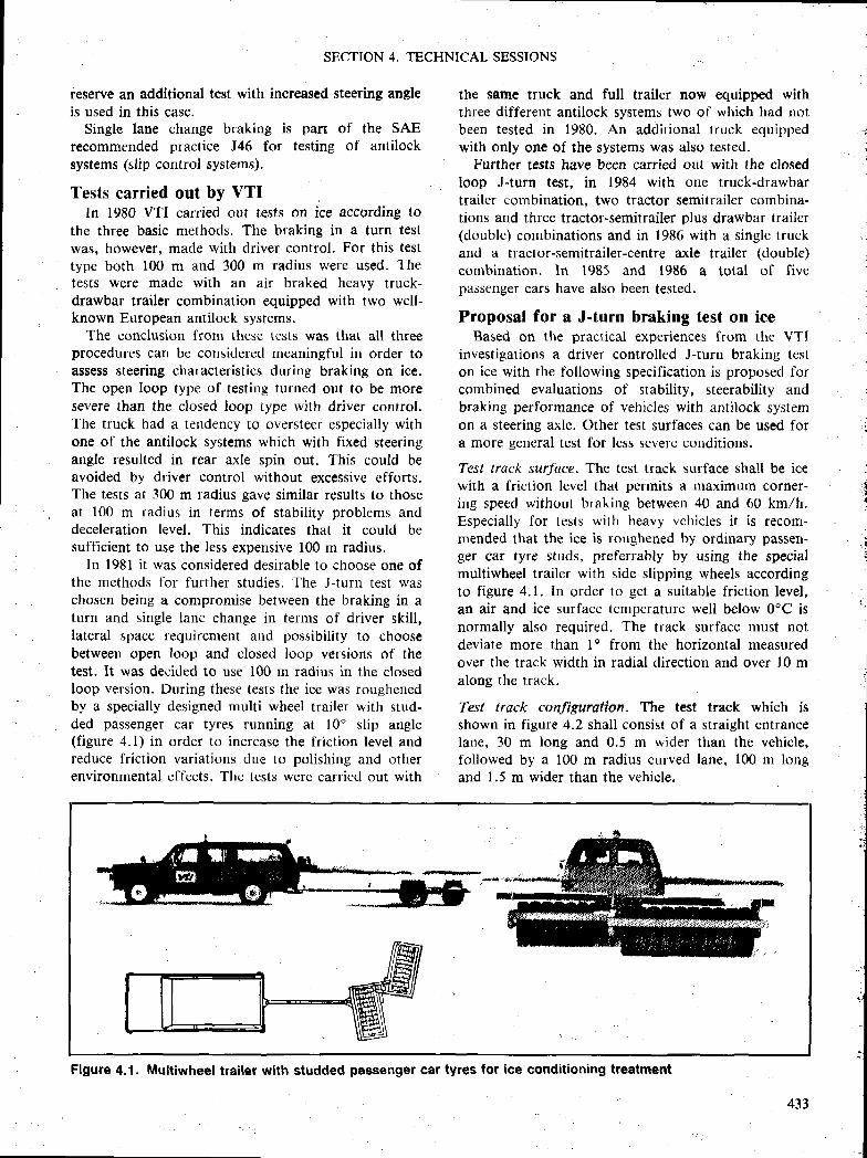
SECTION 4. TECHNICAL SESSIONS

reserve an additional test with increased steering angleis used in this case.

Single lane change braking is part of the SAErecommended practice J46 for testing of antilocksystems (slip control systems).

Tests cflrried out by VTIIn 1980 VTI carried ouf tests on ice according to

the three basic methods. The braking in a turn testwas, however, made with driver control. For this testtype both 100 m and 300 m radius were used. Thete$ts were made with an air braked heavy truck-drawbar trailer combination equipped with two well-known European antilock systems.

The conclusion from these tests was that all threeprocedures can be considered meaningful in order toassess steering characteristics during braking on ice.The open loop type of testing turned out to be moresevere than the closed loop type with driver control.The truck had a tendency to oversteer especially withone of the antilock systems which with fixed steeringangle resulted in rear axle spin out. This could beavoided by driver control without excessive efforts.The tests at 300 m radius gave similar results to thoseat 100 rn radius in terms of stability problems anddeceleration level. This indicates that it could besufficient to use the less expensive 100 m radius.

ln l98l it was considered desirable to choose one ofthe methods for further studies. The J-turn test waschosen being a compromise between the braking in aturn and single lane change in terms of driver skill,lateral space requirement and possibility to choosebetween open loop and closed loop versions of thetest. It was decided to use 100 m radius in the closedloop version. During these tests the ice was roughenedby a specially designed multi wheel trailer with stud-ded passenger car tyres running at 10" slip angle(figure 4.1) in order to increase the friction level andreduce friction variations due to polishing and otherenvironmental effects. The tests were carried out with

the same truck and full trailer now equipped withthree different antilock systems two of which had notbeen tested in 1980. An additional truck equippedwith only one of the systems was also tested.

Further tests have been carried out with the closedloop J-turn test, in 1984 with one truck-drawbartrailer combination, two tractor semitrailer combina-tions and three tractor-semitrailer plus drawbar trailer(double) cornbinations and in 1986 with a single truckand a tractor-semitrailer-centre axle trailcr (double)combination. In 1985 and 1986 a total of fivepassenger cars have also been tested.

Proposal for a J-turn hraking test on iceBased on the practical experiences from the VTI

investigations a driver controlled J-turn braking teston ice with the following specification is proposed forcombined evaluations of stability, steerability andbraking performance of vehicles with antilock systemon a steering axle. Other test surfaces can be used fora more general test for less severe conditions.

Test track surJace. The test track surface shall be icewith a friction level that permits a maximum corner-ing speed without hraking between 40 and 60 km/h.Especially for tests with heavy vchiclcs it is recorn-nrended that the ice is roughened by ordinary passer)-ger car tyre studs, preferrably by using the specialmultiwheel trailer with side slipping wheels accordingto figure 4.1. In order to get a suitable friction level,an air and ice surlhce tenperature well below OoC isnormally also required. The track surface must notdeviate more than I o from the horizontal measuredover the track width in radial direction and over l0 malong the track.

Test track conJiguration. The test track which isshown in figure 4.2 shall consist of a straight entrancelane, 30 m long and 0.5 m wider than the vehicle,followed by a 100 m radius curved lane, 100 m longand 1.5 m wider than the vehicle.

:It

Figure 4.1 . Multiwheel trailer with studded passenger car tyres lor lce conditioning treatment

433

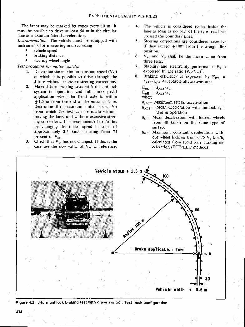
EXPERIMENTAL SAFETY VHHICLES

The lanes may be marked by cones wery l0 m. ltmust be possible to drive at least 50 m in the circularIane at maximum lateral acceleration.Instrumentation. "the vehicle must be equipped withinstruments for measuring and recording

r vehicle speedr braking distancer steering wheel angle

Test procedure for motor vehiclesl. Determine the maximum constant speed (V*)

at which it is possible to drive through theJ-turn without excessive steering corrections.

2. Make J-turn braking tests with the antilocksy$tem in operation and full brake pedalapplication when the front axle is within1 1.5 m from the end of the entrance lane.Determine the maximum initial speed Vofrom which the test can be made withoutleaving the lane, and without excessive steer-ing corrections. It is recommended to do thisby changing the initial speed in steps ofapproximately 2.5 km/h starting from 75percent of V*.

3. Check that VM has not changed. If this is thecase use the new value of V*n as reference.

The vehicle is considered to be inside theIane as long as no part of the tyre tread hascrossed the boundary lines.Steering corrections are considered excessiveif they exceed 1 180' from the straight lineposition.Vy and Vo shall be the mean value fromthree tests.Stability and steerability performance E, isexpressed by the ratio (Vo,/V"n)2.Braking efficiency is expressed by Eev =ao,-rla"r,r Acceptable alternatives are;

EBr- : il1ys/ayEse : a,'rs/auwherea"p1 : Maximum lateral accelerationitaLs: Mean deceleration with antilock sys-

tem in operationf,l = Mean deceleration with locked wheels

from 40 km/h on the same type ofsurface

fle = Maximum constant deceleration with-out wheel locking from 0.75 Vo km,/h,calculated from Front axle braking de-celeration (ECE/EEC method)

4.

{

6 .

7 .

8 .

Yehicle Hidth + 1.5 m

Yehicle r ldth + 0,5 m

Brake appllcation line

Figure 4.2. J-turn antllock brakinE test with driver control. Test track configuration

434

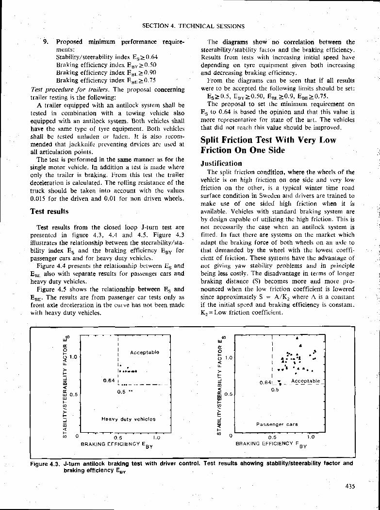
SECTION 4. TECHNICAL SESSIONS

9. Proposed minimum performance require-ments;Stability/steerability index E, > 0.64Braking efficiency index 8r"40.50Braking efficiency index E"r20.90Braking efficiency index E"s>0.75

Test procedure for trailers. The proposal concerningtrailer testing is the following:

A trailer equipped with an antilock system shall betested in combination with a towing vehicle alsoequipped with an antilock system. Both vehicles shallhave the same type of tyre equipment. Both vehiclesshall be tested unladen or laclerr. It is also recom-mended that jackknife preventing devices are used atall articulation points.

The t€st is performed in the same manner as for thesingle motor vehicle. In addition a test is made whereonly the trailer is braking. From this test the trailerdeceleration is calculated. The rolling resistance of thetruck should be taken into account with the values0.015 for the driven and 0.01 for non driven wheels.

Test results

Test results from the closed loop J-turn test arepresented in figure 4.3, 4.4 and 4.5. Figure 4.3illustrates the relationship between the steerabil ity / sta-bility index Es and the braking efficiency Eut forpassenger cars and for heavy duty vehicles.

Figure 4.4 presents the relationship lretween E* andEr. also with separate results for passenger cars andheavy duty vehicles.

Figure 4.5 shows the relationship between Er andEuu. The results are from passenger car tests only asfront axle deceleration in the curve has not been madewith heavy duty vehicles.

The diagrams show no correlation between thesteerability,/stability lactor and th€ braking efticiency.Rcsults frorn tests with increasing initial speed havedepending on tyre equipment given both increasingand decreasing braking efficiency.

From the diagrams can be scen that if all resultswere to be accepted the following limits should be set:

E*40.5 , Eu" 20 .50 , Eut20 .9 , EBF>0.75.The proposal to set the minimum requirement on

E, to 0.64 is based the opinion and that this value ismore ref)resentative for state of the art. The vehiclesthat did not reach this value should be improved.

Split Friction Test With Very LowFriction On One SideJust i f icat ion

The split friction condition, where the wheels of thevehicle is on high friction on one side and very lowfriction on the other, is a typical winter time roadsurface condition in Sweden and clrivers are trained tomake use of one sided high friction when it isavailable. Vehicles with standard braking system areby design capable of util izing thc high friction. This isnot necessarily the case whcn an antilock system isfitted. ln fact there are systems on the rnarket whichadapt the braking force of both wheels on an axle tothat demanded by the wheel with the lowest coeffi-cient of friction. These systetns have the advantage o[not giving yaw stability problems and in principlebeing less costly. The disadvantage in terms of longerbraking distance (S) becomes more and more pro-nounced when the low friction coefficient is loweredsince approxirnately S : A/K2 where A is a constantif the initial speed and braking efficiency is constant.K" : Low friction coefficient,

aLIJ I

II

j Acceptau te

i .l r r r r * rI

0 .64 r

0 .5 ' .

Heavy du t y veh l c l es

uJtroE r . oI

IJ

dl

fi o.sulFa

JflF6

a

l al r

r ^ i j : . i r ' :I . . I '

l r r t ' r ^ . .I '

0 .641 v , - Agcaptab lg -0 .5

P a s s e n g e r c a r s

TEoFr-r Lo{L

tsJo

f f o sIIJF-U)

_=dl{6 o o .5

BRAKTNG EFF IC IENCY EBYl . o 0 ' 5

B R A K I N G E F F T C T E N C Y E B Y1 . O

Figure 4.3. J-turn antllock braking te$t with driver control. Test results showlng stability/steerabillty factor andbraking efiiciency E*

435

oU

Fo

F=={tUu o . 5aJ)

=Jdt{tr)

o

(h

U.EoF

q r . 0

trdt

14 0.5UFvt

F

J(tl.(Fo o

A c c e o t a b l e

0 .84 l_ - .

n a

H e a v y d u t y v e h i d l g s

r . 0 2 . oB R A K I N G E F F T C T E N C Y E B L

1 .o 2 .0B R A K I N G E F F I C I E N C Y E B L

A c c e p t a b l e0.64 L- . . . ' : " ' ' ' i : : ' "_ _

0 ,9

P a s s e n g e t c a r s

EXPERIMENTAL SAFETY VEHICLES

Figure 4.4. J.turn antilock braking test with driver control.braking etficiency EBL

In figure 5.1 the braking distance from 50 km/h isshown as a function of the low friction coefficientwhen 5 m/sz can be achieved on the right frictionsurface and the braking efficiency is 10090. lt can beseen that at a friction coefficient of 0.1 the brakingdistance is 95 m for a system adapting to the lowcoefficient (select low system) compared to 3? m for asystem with individual wheel control. Antilock sys-tems with these characteristics are not desirable onroads where split friction conditions with very lowfriction can be expected. ln order to check splitfriction braking performance, thc low friction coeffi-cient should be as low as possible.

Tests carried out by VTI '

VTI has performed tests on split friction surfaceswith ice as low friction surface having peak and

, Test results showing stability/steerability factor and

locked wheel friction coefficients 0.1 with standardtyres and sand bonded to the ice with water as highfriction surface giving a friction coefficient of about0,6 (fieure 5.2). The test speed was 50 km,/h. Asshown in the figure, antilock braking tests wereperlbrmed also on the low and high friction surfacesfor reference purpose. Part of the test program alsoincluded measurement of the friction coell'icients K,and K, according to ECE/ECE regulations. This wasdone with front axle braking without wheel locking.

Passenger cars, heavy trucks and truck trailer com-binations with comrnercially available systems andalso one prototype system (see figure 2.1) have bccntested. The systems represent different control strate-gies from "select low" that adapts to the low frictionto individual whcel control.

ResultsIn figure 5.3 the braking ratio Z.* obtained in the

split lriction test is compared to the optimum brakingratio defined as (2, + Zr)/2- The braking ratios Z,and Z, are those obtained by antilock braking tests onthe high and low friction surfaces with the vehicle inquestion. Braking ratio is defined as the mean deceler-ation divided by gravity acceleration (9.81 m/$2).

It can be seen that the select low system has abraking efficiency of only 27 percent of the optimumbraking ratio compared to values between 75 ancl 90percent for systems with a higher degree of individuatwheel control. ln figure 5.4 the braking ratio Z. iscompared to a minimum required braking ratia (4Zz+Z)/5 proposed by E. Pctersen from WABCO. Thetested vehicles with select low antilock systems did notmeet this requirement. ln figure 5.S te$t results arecompared with the ECE/EEC requirement Z3>0.75(4K2 +IKJ/S. The ECE/EEC requirement was easierto meet fhan that from WABCO.

v,UtroFoL

=

EUlr,ho

F

_f6

F6

1 .O

0 . 5

IIl . , .t a

; . .o.o+ h.""ptrut"

0 . 7 5

P a s s e n g e t c a r s

N E

B R A K I N G E F F I C I E N C Y E - ^

Figure 4.5. J-turn antilock braking test wlth drivercontrol. Test results showing stability/steerability factor and braking efficiencyE"-

436

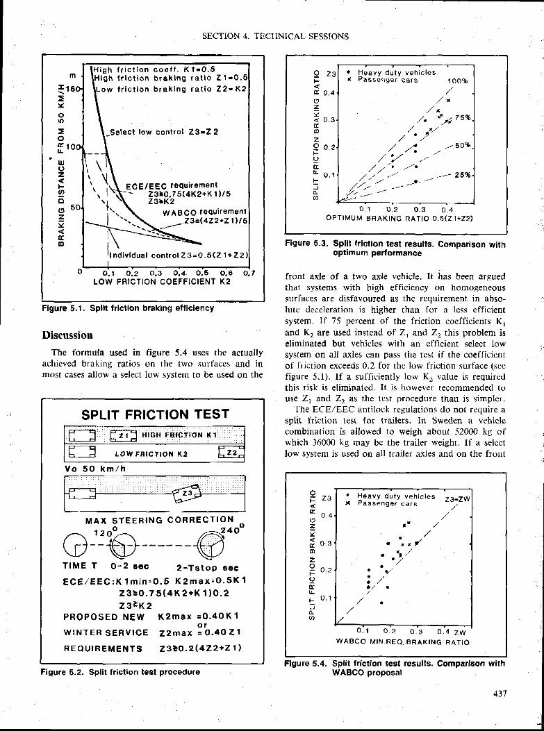
{ r=votO

Eor 1lrJ(Jz{2o(9=vtr6

o,B o,7K 2LOW FHICT ION COEFFIC IENT

f r i c t i o n c o e f f . K 1 . O . 5l r l c t i o n b r a k l n g r a t l o Z 1 - 0 .

f r l c t i o n b r a k l n g r a t i o Z 2 - K ?

t low contro l l3-22

' . ] r - \ EcE/EEc requirement\ \ | \ i"- ' idr*o,f st+xa+K 1 )/s' \ t

\ t \ Z g r K a

I t r \ wABco requ i remen tI \ \ Y Y n g V v

| - ' - - \

_ZgE(4Zz+Zlr tE

r f nd i v l dua f con t ro l Z3=Q.5 (Z1+Zz

Flgure 5.1. Spllt lrlctlon braking elficiency

SECTION 4. TECHNICAL SESSIONS

Discussion

The formula used inachieved braking ratiosmosf cases allow a select

figure 5.4 uses the actuallyon the two surfaces and inlow system to be used on the

Figure 5.3. Split friction test re$ults. Comparison withoptlmum performance

front axle of a two axle vchicle. It has been arguedthat systems with high efficiency on homogeneoussurfaces are disfavoured as the requirement in abso-Iute deceleration is higher than fior a less efficientsystem. If 75 percent of the friction coefficients K,and K, are used instead of Z, and Z, this problem iseliminated but vehicles with an efficient select lowsystem on all axles can pass the test if the coefficientof friction exceeds 0.2 for the low friction surface (seefigure 5.1). lf a sufficiently low K, value is requiredthis risk is eliminated. It is however recommended touse Z, and Z2 a$ the test procedure than is simpler.

The ECE/EEL- anti lock regulations do not require asplit friction test for trailers. In Sweden a vehiclecombination is allowed to weigh about 52000 kg ofwhich 36000 kg may be the trailer weight. lf a selectlow system is used on all trailer axles and on the front

Figure 5.4. Split friction test resufts. Comparlson withWABCO proposal

g z s

cE 0 .4

' H e a v y d u t y v e h i c l e sx P a s s e n g e r c a r s 1 o o %

/ ' *. / *

'/ ' irt7s%/ l /. . + -

,/ //,/ /'i ,- ,/ 50%

, / / * ' -'/ t

"' "tt

/ ' r ' - t - -s 25%,'r' ,' -t'

----, / / / - J/ / / r J

zv{ O . 3

oza o . EF

ICEr o . 1tJ

u)o . 1 0 . 2 0 . 3 0 . 4

O P T I M U M B R A K I N G R A T I O O . 5 ( 2 1 + 2 2 )

SPLIT FRICTION TE$THtGiH:FR:!CrfoH t ( ' !

LOW FR|CT|OT{ K2 |Fzz

V o 5 O k m / h

M A X S T E E R I N GC O R R E C T I O N240(J

Tl t tnE T O-2 scc 2 - T s t o p s e c

E C E / E E C : K 1 m i n = O . 5 K 2 m a x = O ' 5 K 1Z $ r O . 7 5 ( 4 K 2 + K 1 ) O . 2z 3 r K 2

P R 0 P O S E D N E w K 2 m a x = o ' 4 o K l

w f NTER SERVTCE Z lmax 3b .oo z t

R E Q U I R E M E N T S Z 3 I O . 2 ( 4 2 . 2 + Z 1 I

Grjb @

Figure 5.2. Split fr iction test procedure

t r 2 3t ^ ,

=g

f o .s(D

1= o . 2F

IEt!

L o 1

o

o . 1W A B C O M I N . R E Q . B R A K I N G R A T I O

o . 2 O . 3 O . 4 Z W

. Heavy du ty veh ic les ZB_ZINx Passenger cars , /

I

a

a./

431

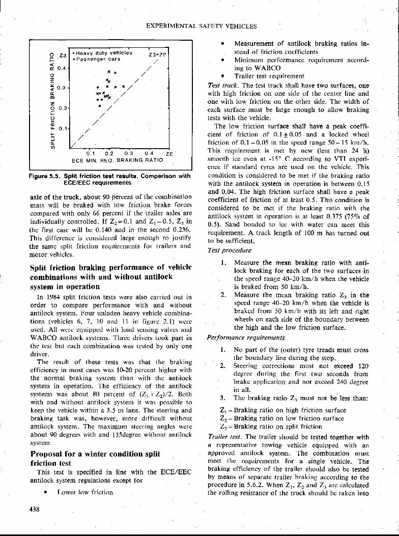
q z 3F

cE o .4(,=I o . t(Itrlzg o . 2F

I(IL O . 1

F

(L6

' H 6 a v y d u t y v e h i c l e s z g - Z Ex P a s s e n g e r C a r s , /

' x * /

\ , r /t t x * /

1'*ror- ,/a a ^

, /' /

//

,/,/

o . 1 0 . 2 0 3 0 . 4 Z EECE MIN . REO. BF IAK ING RATIO

EXPERIMENTAL SAFETY VEHICLES

Figure 5.5. Split friction test result$. Comparison withECE/EEC requirements

axle of the truck, about 90 percent of the combinationmass will be braked with low friction brake forcescompared with only 66 percent if the trailer axles areindividual ly control led. I f Z2=0.1 and Zr:0.5, Zt inthe first case will be 0.140 and in the second 0.236.This difference is considered large enough to justify

the samc split friction requiretnents for trailers andmotor vehicles.

Split friction braking performance of vehicle

combinations with and without antilock

system in operation

In 1984 split friction te$t$ were also carried out inorder to compare performance with and withoutantilock system. Four unladen heavy vehicle combina-t ions (vehicles 6, 7, l0 and l l in f igure 2.1) wereused. All were equipped with load sensing valves andWABCO antilock systems. Three drivers took part inthe test but each combination was tested by only onedriver.

The result of these test$ was that the brakingefficiency in most cases was 10-20 percent higher withthe normal braking $ystcm than with the antilocksystem in operation. The efficiency of the antilocksystems was about 80 percent of (Zt+Zz)/z. Bothwith and without antilock system it was possible tokeep the vehicle within a 3.5 m lane. The steering andbraking task was, however, more difficult withoutantilock system. The maximum steering angles wereabout 90 degrees with and l35degree without antilocksystem.

Proposal for a winter condition splitfriction test

This te$t is specified in line with the ECE/EECantilock system regulations except for

r Lower low friction

r Measurement of antilock braking ratios in-stead of friction coefficients

r Minimum performance requirement accord-ins to WABCO

r Trailer test requirementTest track- The test track shall have two surfaces, onewith high friction on one side of the center line andone with low friction on the other side. The width ofeach surface must be large enough to allow brakingtests with the vehicle.

The low friction surface shall have a peak coeffi-cient of friction of 0.110.0-5 and a locked wheelfr ict ion of 0.1-0.05 in the speed range 50- 15 km/h.This requirement is met by new (less than 24 h)smooth ice even at -15' C according to VTI experi-ence if standard tyres are used on the vehicle. Thiscondition is considcrcd to be met if the braking ratiowith the antilock sy$tem in operation is between 0.15and 0.04. The high friction surface shall have a peakcoefficient of friction of at least 0.5. This condition isconsidered to be met if the braking ratio with theantilock system in operation is at least 0.375 (75V0 of0.5). Sand bonded to ice with water can meet thisrequirement. A track length of 100 m has turned outto be sufficient.Test proc:edure

l. Measure the mean braking ratio with anti-lock braking for each of the two surfaces inthe speed range 40-20 km,/h when the vehicleis braked from 50 km/h.

2. Measure the mean braking ratio Z. in thespeed range 40-20 km/h when the vehicle isbraked lrom 50 krtr/h with its left and rightwheels on each side of the boundary betweenthe high and the low friction surfhce.

Peffi rmance requirements

l . No part of the (outer) tyre treads must crossthe boundary line during the stop.Steering corrections must not exceed 120degree during the first two seconds frombrake application and not exceed 240 degree

3. The braking ratio Zl must not be less than:

Zr:Braking ratio on high triction surfaceZr: Braking ratio on low friction surfaceZr: Braking ratio on split friction

Trailer les/. The trailer should be tested together witha representative towing vehicle equipped with anapproved antilock system. The combination mustmeet the requirements for a single vehicle. Thebraking efficiency of the trailer should also be testedby means of separate trailer braking according to theprocedure in 5.6.2. When Zr, Trand Z, are calculatedthe rolling resistance of the truck should be taken into

?,.

SECTION 4. TECHNICAL SESSIONS

account with the values 0.015 for driven and 0.01 fornon driven wheels.

Straight Line Braking on Ice

Just i f icat ionStraight line braking on a homogeneous surface is

the classic and basic way of testing the brakingperformance of vehicles. The ECEIEEC antilockbraking regulations prescribe straight line low frictiontests. The friction level is however allowed to be ashigh as 0.4. A test on ice is therefore regarded as auseful winter service approval requirement.

Tests carried out by VTIStraight line antilock braking tests on ice have been

made in comparison with

r locked wheel brakinr. best driver control brakingr peak friction measured with single axle brak-

ing according to ECE/EEC antilock regula-tionStandard reference tyre friction coefficientmeasured with the Swedish constant slip(13-15 percent) friction test vehicles BV lland BV 12 (see figure 6.1 and 6.2) neasuredat 40 and 20 km/h. BV ll had a 4.00-8 tyreand BV 12 a 5.60 - l5 PIARC "Europe"

tyre both with rib tread, in accordance withISO TR 8349 on friction measurement.

Tests were carried out with the followine vehicleswhich are shown in figure 2.1.

r 1980 with a two axle heavy truck and a twoaxle drawbar trailer both equipped with twoantilock systems, Girl ing and WABCO. (Ve-hicle I and 5)

r l98l with the same vehicles (l and 5) nowequipped with three anti lock systems, Girl ingGX. WABCO and Bosch. In addition a threeaxle truck with Bosch antilock system wasused. (Vehicle 3)

| 1984 with a three axle truck and a two axledrawbar trailer with a prototype system.(Vehicle 4 and 6)

r 1985 with a three axle truck (Vehicle 2)equipped with a new vcrsion o[ the WABCOantilock $ystem and with two passenger cars,Audi and Honda.

r 1986 with three passenger cars, Audi, FordScorpio and Volvo.

Tests have been made from initial speeds rangingfrom 70 to 35 km/h for trucks and trailers and. forpassenger cars from I l0 to 50 km/h.

Most of the fests have been done in the temperaturerange -5"C to -20"C but tests have also been made

near OoC and down to -30oC. Except in 1980 the testshave been made on ice roughened by the specialmultiwheel trailer with studded passenger car tyresshown in figure 4.1. The treatment results in asomewhat higher and more uniform friction andreduces polishing eflfects which tend to lower thefriction.

ResultsThe results are $ummarized in figure 6.3, 6.4, 6.5,

6.6 and 6.7.From the figures can be seen that as a rule the

braking efficiency with antilock systems is higher thanwith locked wheels and higher than best drivcr perfor-mance. In tests with laden and unladen vehicles theunladen vehicles tend to get higher deceleration butnot necessarily higher braking efficiency based onpeak value.

The 75 percent efficiency required by ECE/EECregulations is not always met on ice by antilocksystems lbr heavy vehicles. For the tested passeng€rcars with and without studs the efficiency is close to100 percent.

Longitudinal friction coefficients obtained with thereference tyres on friction test vehicles BV ll and BV12 according to the constant slip method gave thesame values as the peak friction coefficients obtainedby single axle braking according to ECE Regulation13 both for a truck and a passerUler car with standardtyres (0.17).

DiscussionAccording to Annex l0 in ECE regulation 13 it is

for normal brakes allowed to have a braking effi-cicncy of 50 percent at a friction coefl' icient of 0.2. Itcould therefore be debated il' the efficiency require-ments on antilock systems on ice should be as high as75 percent of the peak friction coefficient. The testresults indicate that 90 percent of thc locked wheelfriction could be a more suitable requirement. Alocked wheel test is also the simplest and leastexpensive alternative. ln order to avoid stability prob-lems the locked wheel braking tcst$ on ice arerecommended to be done from an initial speed of 40km/h.Proposal for a straight ahead braking teston ice

Based on the field test experience and theoreticalconsiderations the following test is proposed.

Test surlurc.' The test surface should be ice with alocked wheel friction of 0.1 + 0,05 or a peak frictionof 0,20 + 0.05 measured with the test vehicle itself orthe friction test vehicle BVI I or equivalent equipment.Roughness of the ice by means cf the special multi-wheel trailer according to figure 4. 1 is recommended.The air and ice surface temperature should be belowzerooC, pret'errably between -5 and -l5oC.

439

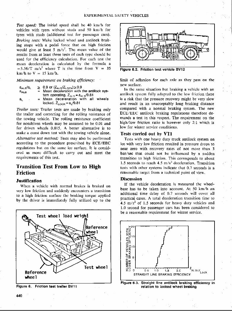
EXPERIMENTAL SAFETY VEHICLES

Test speed: The initial speed shall be 40 km/h forvehicles with tyres without studs and 50 km/h fortyres with studs (additional test for passenger cars).

Braking /ests.' Make locked wheel and antilock brak-ing stops with a pedal force that on high frictionwould give at least 5 m/s?. The mean value of theresults from at least three tests of each type should beused for the efficiency calculation. For each test themean deceleration is calculated by the formula a:5.56/T m./sz where T is the time from V : 35km/h to V : 15 km/h.

Minimum requirement on braking efficiency:

aALs/aL > 0.9 or (Z^.*/Z.."J>0.9dars = Mean deceleration with the antilock sys-

tem operating. ZnLs = aars/9.81aL = Mean decelerat ion with al l wheels

locked" Zrocx = aL/9.81

Trailer /es/s.' Trailer tests are made by braking onlythe trailer and correcting for the rolling rcsistance ofthe towing vehicle. The rolling resistance coefficientfor nondriven wheels may be assumed to be 0.01 andfor driven wheels 0.015. A better alternative is tomake a coast down test with the towing vehicle alone.Alternative test method: Tests may also be performedaccording to the procedure prescribed bv ECE/EECregulations but on the same ice surface. It is consid-ered as more difficult to carry out and meet therequirements of this test.

Transition Test From Low to HighFrictionJustification

When a vehicle with normal brakes is braked onvery low friction and suddenly encounters a transitionto a high friction surface the braking torque appliedby the driver is immediately fully utilized up to the

erencet

Test wheelReferencewheel

Figure 6. Frlctlon teet trailer BVl1

MO

Figure 6.2. Friction test vehicle BVl2

limit of adhesion for each axle as they pass on thenew surface.

In the same situation but braking a vehicle with anantilock system tully adapted to the low fristion thereis a risk that the pressure recovery might be very slowand result in an unacceptably long braking distancecompared with a normal braking $ystem. The newECE/EEC antilock braking regulations therefore de-mands a test in this rcspect. The requirement on thehigh/low friction ratio is however only 2:l which islow for winter service conditions.

Tests carried out by VTITests with one heavy duty truck antilock system on

ice with very low friction resulted in pressure drops tonear zero with recovery rates of not more than 3bar/sec that could not be influenced by a suddentransition to high friction. This corresponds to about1.5 seconds to reach 4.5 m/sz deceleration. Transitiontests with other systems indicate that 0.7 seconds is areasonable target from a technical point of view.

DiscussionIf the vehicle deceleration is measured thc wheel'

base has to be taken into account. At 50 km/h anadditional time delay of 0.7 seconds will cover allpractical cases. A total deceleration transition time to4.5 m/sz of 1.5 seconcls for heavy duty vehicles and1.0 second for passenger cars has been considered tobe a reasonable requirement for winter service.

>?

tsz= g- o lf / , i 'U ; iJ r lo -

i l z '> g, , {dsS sSHz . J o 0 . s 1 . 0 i . s 2 . 0 A L S / Z L . " k

STRAIGHT L INE BRAKING EFF IC IENCY

Figure 6.3. Straight l ine anti lock braking efficiency inrelation to locked wheel braking

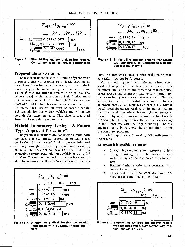
SECTION 4. TECHNICAL SESSIONS

Figure 6.4. Straight line antilock braking test results.Comparison with test driver performance

Proposed winter serrice testThe test shall be made with full brake application at

a pressure that corresponds to a deceleration of atleast 5 m/s? starting on n low friction surface whichmust not give the vehicle a higher deceleration than1.5 m/sz with the anti lock system in operation. Thevehicle speed at the transition to high friction mustnot be less than 50 km,/h. The hieh friction surfacemust allow an antilock braking deceleration of at least4.5 m/sz. This cleceleration must be reached within1.5 seconds for heavy duty vehicles and within 1.0seconds for passenger cars. This time is measuredfrom the front axle transition time.

Hybrid Laboratory Testing-A FutureType Approval Procedure?

The practical difficulties are considerable from bothtechnical and economical aspects in obtaining testtracks that give the desired friction characteristics andare large enough for safe high speed and corneringtests. In fact they are so large that th€ ECEIEECregulations regard peak friction coefficients up to 0.4at 40 to 50 km/h as low and do not specify speed orslip characteristics of the tyre/road adhesion. Further-

Flgure 6.5. Stralght l ine anti lock braking test reeults.Comparison with ECE/EEC friction coeffi-cient

(ZRLs/Keur . | ) too

o , l 7 l o , 1 70 , 1 5 / O , 1 7o , 1 7 1 o , 1 7

e.ry-tffi

tuFigure 6.6. Straight llne antilock braklng test results

with standard tyres. Comparlson with fric-tion test treiler BVl1

more the problems connected with brake lining char-acteristics must not be forgotten.

For antilock systems with electric wheel speedsignals these problems can be eliminated by real timecomputer simulation of the tyre/road characteristics,brake torque characteristics and vehicle motion dy-namics including wheel speed sensor signals. The realvehicle that is to be tested is connected to thecornputer through an interface so that the simulatedwheel speed signals are received by its antilock systemcontroller and the wheel brake cylinder pressure$measured by sensors on each wheel are fed back tothe computer. During the test the vehicle is stationaryin the laboratory with the engine running. The testengineer has only to apply the brakes after startingthe computer program.

This technique has been used by VTI with promis-ing results.

At present it is possible to simulate;

Straight braking on a homogeneous surfaceStraight braking on a split friction surfacewith steering corrections based on yaw mo-tlon

r Braking during steady state cornering withconstant steer inputJ-turn braking with constant steer input ap-plied at the same time as the brakes

Figure 6.7. $traight line antilock braking test resultswith standard tyres. Comparison with fric-tion test vehicle BVl2

I

i

I

a

a

(zets /ZDriuur) 1oo

ft------ltc'_fd

rrlttr+:#

, 078 /0 ,073, o 7 7 l O , O 6 9

0 , 1 1 6 / 0 , 0 8 0

107

e

q=5

/Ti-L{F:-;rEl

/-rf,tFDcF

TTI

fr##.ry-t{F::::#

(Zor_s /KEcE) 1oo

5 0 1 0 1

0 , 1 7 / 0 , 1 6 t 0 51 0 6o , ? 7 l o , 2 o

o , 1 6 / 0 , 1 7 940 , 1 1 / 0 , 0 9 J l 2 3

1 0 70 , 1 7 1 Q , 2 374o , 1 5 / 0 , 1 4

( t o r s /K rv r r ) t oo5 0 1 0 0

o , 1 7 1 0 , 1 6

1 5 / 0 , 1 60 , 1 7 / 0 , 1 8

€niltCF.#.fTI_LfuJ

441

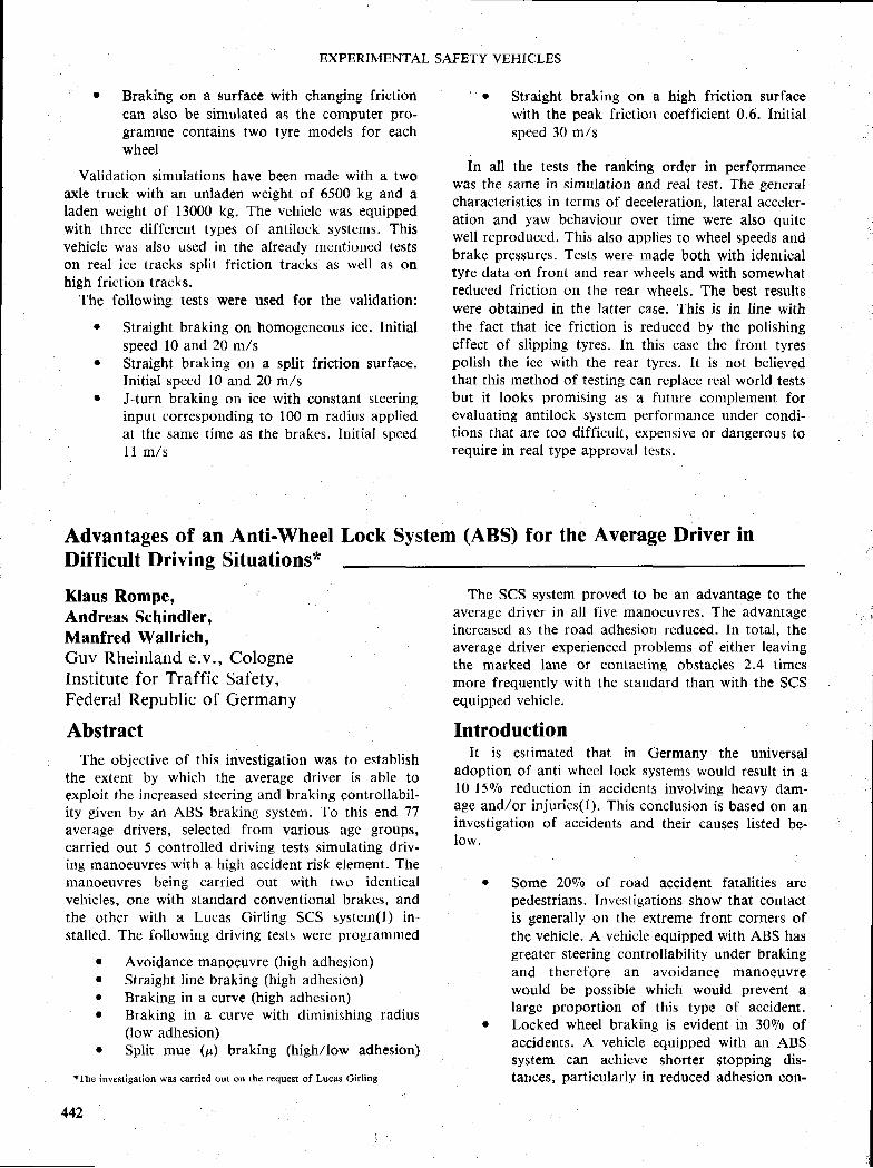
EXPERIMENTAL SAFETY VEHICLES

r Braking on a surface with changing frictioncan also be simulated as the computer pro-gramme contains two tyre models for eachwheel

Validation simulations have been made with a twoaxle truck with an unladen wcight of 6500 kg and aladen weight of 13000 kg. The vehicle was equippedwith three different types of antilock systems. Thisvehicle was also used in the already mentioned testson real ice tracks split friction tracks as well as onhigh friction tracks.

The following tests were used for the validation:

r Straight braking on homogeneous ice. Initialspeed l0 and 20 m/s

r Straight braking on a split friction surface.Initial speed l0 and 20 m/s

. J-turn braking on ice with constant steeringinput corresponding to 100 m radius appliedat the same time as the brakes. Initial spcedl l m/s

r Straight braking on a high friction surfacewith the peak friction coefficient 0.6. Initialspeed 30 m/s

In all the tests the ranking order in performancewas the same in simulation and real test. The generalcharactcristics in terms of deceleration. lateral acceler-ation and yaw behaviour over time were also quitewell reproduced. This also applies to wheel speeds andbrake pressures. Tests were made both with identicaltyre data on front and rear wheels and with somewhatreduced friction on the rear wheels. The best resultswere obtained in the latter case. This is in line withthe fact that ice friction is reduced by the polishingeffect of slipping tyres. In this case the front tyrespolish the icc with the rear tyres. lt is not believedthat this method of testing can replace real world testsbut it looks promising as a future complement fbrevaluating antilock system performance under condi-tions that are too difficult, expensive or dangerous torequire in real type approval tests.

Advantages of an Anti-WheelDifficult Driving Situations*

Klaus Rompe,Andreas Schindler,Manfred Wallrich.Guv Rheinland e.v., CologneInstitute for Traffic Saf'ety,Federal Republic of Germany

Lock System (ABS) for the Average Driver in

AbstractThe objective of this investigation was to establish

the extent by which the average driver is able toexploit the increased stccring and braking controllabil-ity given by an ABS braking system. To this end 77average drivers, selected from various agc groups,carried out 5 controlled driving tests simulating driv-ing manoeuvres with a high accident risk element. Themanoeuvres being carried out with two identicalvehicles, one with standard conventional brakes, andthe other with a Lucas Cirl ing SCS system(l) in-stallcd. The following driving tests were programmed

r Avoidance manoeuvre (high adhesion)r Straight l ine braking (high adhesion). Braking in a curve (high adhesion)r Braking in a curve with diminishing radius

(low adhesion)Split mue (s.) braking (high/low adhesion)

iThe invesl.igation was carried out on thc request of Lucas Cirling

442

The SCS system proved to be an advantage to theaverage driver in all live manoeuvres. The advantageincreased a$ the road adhesion reduced. In total, theaverage driver experienced problems of either leavingthe marked lane or contacting obstacles 2.4 timesmore frequently with the standard than with the SCSequipped vehicle.

IntroductionIt is esLimated that in Germany the universal

adoption of anti whccl lock systems would result in al0-150/o reduction in accidents involving heavy dam-age and/or injurics(l). This conclusion is based on aninvestigation of accidents and their cau$e$ li$ted be-low.

. Some 2090 of road accident fatalities arepedestrians. Investigations show that contactis generally on the extreme front corners ofthe vehicle. A vehicle equipped with ABS hasgreater steering controllability r.rnder brakingand therefore an avoidance manoeuvrewould be possible which would prevent alarge proportion of this type of accident.

r Locked wheel braking is evident in 30tr/o ofaccidents. A vehicle equipped with an ABSsystem can achieve shorter $topping dis-tances, particularly in reduced adhesion con-

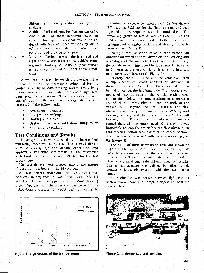
SECTION 4. TECHNICAL SESSIONS

ditions, and thereby reduce this type ofaccident.

r A third of all accidents involve one car only.About 50Vo of these acciclents occur oncurves, this type of accident would be re-duced with ABS equipped vehicles by virtueof the ability to retain litsering control under

I conclitions of braking in a curve.r Varying adhesion between the left hand and

right hand wheels leads to the vehicle gyrat-ing under braking. An ABS equipped vehicleis far easier to control under these condi-tions.

To evaluate the extent by which the average driveris able to exploit the increased steering and brakingcontrol given by an ABS braking systeut, five drivingmanoeuvres were deviscd which simulated high acci-dent potential situations. These manoeuvres werecarried out by the team of average drivers andconsisted of the fbllowine(2):

r Avoidance manoeuvrer Straight line brakingr Braking in a curver Braking in a curve with diminishing radiusr Split mue (p) braking

Test Conditions and Results77 average drivers were selectecl by an independent

marketing company in thc UK. The selected driverswere ol' varying age and driving experietrce, andapproxirnately a third were female. All had experiencewith Ford Escorts, the vehicle selectcd for the testprogramrne.

The te$t drivers were divided into 3 age groups(Figure l), mo$t being in the 26-40 group.

All test drivers unclcrtook the five driving ma-noeuvres in sequence in two Ford Escort XR 3 ivehicles, the one equipped with standard brakingsystem (std car), and the other with the Lucas Girl ing"Stop-Control-Systcm"(3) (SCS car). In order to

oc

o

sF

1 8 - 2 5 2 6 - 4 0 4 1 - 6 0 A g e g r o u p

Figure 1. Age groups Of the test personnel

minimise the experience factor, half the test drivers(37) used the SCS car for the first test run, and thenrepeated thc test sequence with the standard car. Therernaining group of test drivers carried out the testprogramme in the reverse order. Both vehicles wereinstrumented to enable braking and steering inputs tobe measured (Figure 2).

During a familiarisation drive in each vehicle, anobserver informed the test driver on the working andadvantages of the anti wheel lock system. Eventuallythe test driver was instructed by tape recorder to drivein 5th gear at a speed of 45 rnph into the first testmanoeuvre (avoidance test) (Figure 3).

On entry into a 3 m wide lane, the vehicle actuateda trip mechanism which released an obstacle, adummy child, sited 35 m from the entry and hiddenbchind a wall on the left hand side. This obstacle wasprojected into thc path of thc vehicle. With a con-trolled timc delay, the same mechanism triggered asecond child dummy obstacle into the path of thevehicle 20 m beyond the first obstacle. The firstobstacle cor.rld only tre avoided by a steering andbraking action, and the second obstacle by fullbraking only. The sit ing of the obstacles being ar-ranged that, with an entry speed of 45 nrph, it wasimpossible to stop the car before the first obstacle, sothat steering action was essential to avoid contact.The road surface was wet with an adlresion of plo +

0.8 (fieure 4).The result of these comparison tests are shown on

Figure 5. The upper part shows the total driving testswith the standard car, irnd the lower part the safi letcsts with SCS car. The two halves are divided toshow the crit ical and sal'e driving situation results.The crit ical situation was defined by either vchiclecontact witlt thc obstacles, or with the lane rnarkercones.

No distinction was drawn between light contactwith a marker cone and complete departure from themarked lane.

EXPERIMENTAL SAFETY VEHICLES

H

HHt

t : 4 5 m P h€

Trip mechanism

Fo - O,B

1 5 m

t

Figure 3. Avoldance manoeuvre (wet roads)

The test drivers recorded a total of 86 criticalsituation results, 47 with the standard car and 39 withthe SCS car. From these results it can be deduced thatthe driver of the standard car is more prone to acritical situation by a factor 1.2. This low factor doesnot give a significant statistical advantagc to theaverage driver with the SCS equipped vehicle. Thatthe average driver in this driving rnanoeuvre had arelatively small advantage from the SCS system was,in part, due to incorrect decision, or too slow reactionto the driving situation, so that the full potential ofthe SCS sy$tem was not always exploited.

The initial reaction time to take eppropriate actionis critical for the successful completion of this steer-ing/braking manoeuvre. Shorrld the reaction time ofthe test driver exceed 1.75 s, then the remaining

braking distance available is insufficient to avoid acollision with the obstaclc il ' the entry speed of 45mph is achieved.

The entry speed for the second test (straight linebrakine) (Figure 6) was tixed at 45 mph. On entry

safe situations

E scs, s tdcr i t ical s i tuat ions

N std

W scs

Tests with the std car

Tests with the SCS car

q ld c r i t . _ 47 = 1 .21SCS cri t .

- 39

- "

Flgure 5. Crit lcal situations in avoidance manoeuvreFigure 4. Avoidance manoeuvre

444

,ffi.,

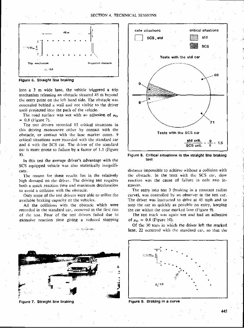
4 5 m

f - f r ' t ' It l

- t l, . - 4 5 h o h c l l- + d l l

t l| , ! . . r r r . | .

Trlp mschaniEm

-{rI i

IP r o j e c t e d o b s t a c l e

rr" - O,8

SECTION 4. TECHNICAL SESSIONS

Figure 6. Straight l ine braking

into a 3 m wide lane, the vehicle triggered a tripmechanism releasing an obstacle situated 45 m beyondthe entry point on the lclt hand side. The obstacle wasconcealed bchind a wall and not visible to the driveruntil projected into the path of the vehicle.

The road surface was wet with an adhesion of po= 0.8 (F igure 7) .

The test drivers recorded l5 crit ical situations inthis driving manoeuvre either by contact with theobstacle. or contact with the lane marker cones. 9crit ical situations were recorded with the standard carand 6 with the SCS car. The driver of the standardcar i$ more prone to failure by a factor of 1.5 (Figure

8) .

ln this test the average driver's advantage with the

SCS equipped vehicle was also statistically insignifi-

cant,The reason for these results l ies in the relatively

high demand on tlte driver. ' fhe driving test requiresboth a quick reaction time and maximum deceleration

to avoid a coll ision with the obstacle.CJnly some of the test drivcrs were able to uli l ize the

available braking capacity oi the vchicles.

All the collisions with the obstacle which wererecorded in the standard car, occurred in the l ' irst run

of the test. Four of the test clrivers failed due to

excessive reaction time giving a reduced stopping

ftd{1hffi ' ,r"sir

Figure 8. Crit ical situations in the straight l ine brakingtest

distance impossible to achieve without a coll ision withthe obstacle. In the tests with the SCS car, slowreaction was the cause of failurc in only two in-stances.

The entry into test 3 (braking in a constant radittscurve), was conlrolled by an observer in the test car.The driver was instructed to drive at 45 mph and tostop the car as quickly as possible on entry, keepingthe car within the cone markcd lane (Figure 9).

The test track was again wet and had an adhesionof P6 = 0.8 (Figure l0).

Of the 30 tests in which the driver left the markedlane, 22 occurred with the standard car, so that the

i

ili{

;{{

.MMs�ffifffl

safe

nsituations

SCS, std

critic

ffiW

al situations

std

SCS

Tests with the std car

Tests with the SCS car

std crlt.*= t . u

SCS crit.

a

t .v , . a ! F h E

| ._:

Fc'o '8

a , .t -

a / '

. f l

/ .

Figure 9. Braking in a curveFigure 7. Straight l ine braking

EXPERIMENTAL SAFETY VEHICLES

Figure 10. Braking ln a curve

average driver was more prone to failure in thestandard car by a factor of 2,'15 (Figure ll).

All the test drivers in the standard car who left themarked out lane, lost control due to locked frontwheels.

Whilst the tests I to 3 were on a wet surface butwith a relatively high adhesion (pa : 0.8), the tests 4and 5 were carried out on a section of the test trackwith a special low adhesion surface (pci = 0.28 - 0.35)apart from the difference in adhesion between tests 4and 3, the curvc of test 4 was of a progressively

Figure 12. Braking in a curve wlth a tightening radius

tightening radius (Figure l2). The driver again re-ceived instructions from the observer to brake hard toa standstill on entry into the test area

In this driving manoeuvre only one driver of thestandard car out of 77, was able to stop the carwithout leaving the lane. All the other drivers skiddedout of the lane with locked front wheels. 66 driverslocked all four wheels.

In the SCS car. 28 test drivers also touched themarkcr cones or left the lane, however only 2 driverscompletely Ieft the marked lane, the other 26 driversonly disturbed two or three of the marker coneswithout leaving the marked lane. However, since thedefinition of a critical situation includes contact witha marker cone, the average driver is more prone to

Figure 13. Crit ical sltuations by braking in awith a tlghtening radius

IIII

I

mI

/{n. o r5 (Bridport)

r a l

safe

nsi tuat ions

SCS, s td

cr i t i ca l s i tua t ions

Nffi

s td

scs

Te$ts with the std car

Tests with the SCS car

std crlt. 22 = 2.75SCS crit.

Flgure 11. Crit ical situations in braklng in a bend

safe situations

l-l scs, sto

cri t ical si tuations

N std

ffi scs

Tests with the std car

Tests with the SCS car

qlqg4r - !9 -- z.ttSCS crit. 28

446

curve

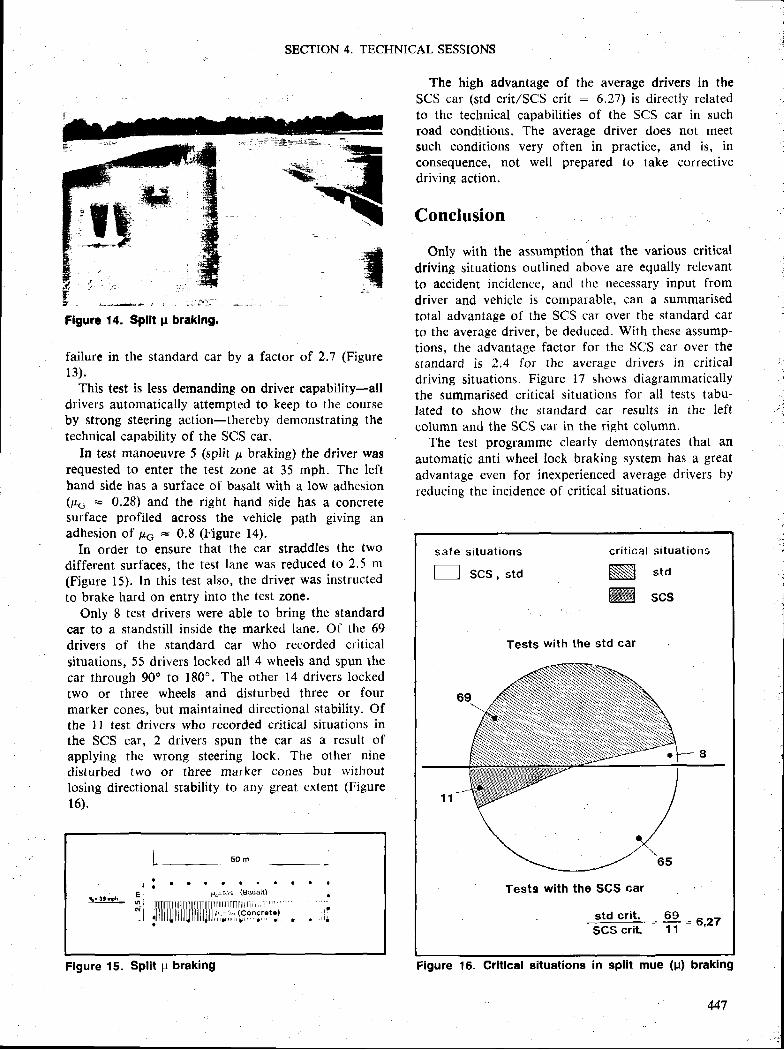
SECTION 4. TECHNICAL SESSIONS

failure in the standard car hy a factor of 2.1 (FieureI 3).

This test is less demanding on driver capability-alldrivers automatically attempted to keep to the courseby strong $teering action-thereby demonstrating thetechnical capability of the SCS car.

In test manoeuvre 5 (split p braking) the driver wasrequested to enter the test zone at 35 mph. The lefthand side has a surface ol basalt with a low adhesion(pc * 0.28) and the right hand side has a concretesurface profiled across the vehicle path giving anadhesion of po = 0.8 (Figure l4).

In order to ensure that the car straddles the twodifferent surfaces, the test lane was reduced to 2.5 m(Figure l5). In this test also, the driver was instructedto brake hard on entry into the test zone'

Only 8 test drivers were able to bring the standardcar to a standstill inside the marked lane. Of the 69drivers of the standard car who recorded criticalsituations, 55 drivers locked all 4 wheels and spun thecar through 90o to 180'. The other 14 drivers lockedtwo or three wheels and disturbed three or fourmarker cones, but maintained directional stability. Ofthe I I test drivers who recorded critical situatiorrs inthe SCS car, 2 drivers spun the car as a result ofapplying the wrong steering lock. The other ninedisturbed two or three marker cones but withoutlosing directional stability to any great extent (Figurel6).

The high advantage of the average drivers in theSCS car (std crit/SCS crit : 6.27) is directly relatedto the technical capabilities of the SCS car in suchroad conditions. The average driver does not meetsuch conditions very often in practice, and is, inconsequence, not well prepared to take correctivedriving action.

Conclusion

Only with the assumption that the various critical

driving situations outl ined above are equally relevant

to accident incidence, and the necessary input l 'rom

driver and vehicle is comparable, can a summarisedtotal advantage of the SCS car over the standard carto the average driver, be deduced. With these a$sump-tions, the advantage factor for the SCS car over thestandard is 2.4 lor the average drivers in crit icaldriving situations. Figure l7 shows diagrammaticallythe summarised crit ical situations for all tests tabu-lafed to show the standard car result$ in the left

column and the SCS car in the right column.The test programme clearly demonstrates that an

automatic anti wheel lock braking system has a great

advantage even for inexperienced average drivers by

rcducing the incidence of crit ical situations.

Flgure 14. Spllt p braklng.

I s o t

F"'o.rs (Basalt}

J l l l l l l l l l l l T T l l l i i l t i t r ' ' .t r ,= tc (Concrs te )

i l r l i i l ' l , l r I

t- i6 rh

Flgure 15. SPlit ;r braking

s a f e s i t u a t i o n s

f__l scs, "tdcr i t i c

NW

al s i tuat ions

std

scs

Tests with the std car

Tests with the SGS car

s ld_c r i t =E=a .z t$CS cr i t . 11

Figure 16. Crlt lcal situations in $plit mue (U) braklng

EXPERIMENTAL SAFETY VEHICLES

Figure 17. $ummarised critical situations with bothvehicles

Anti-Lock Brakes for Passenger Cars and tight Trucks

Robert H. Munson,Director, Automotive Safety Office,Ford Motor Company,United States

Good morning. My name is Bob Munson and I amthe Director of the Automotive Safety Office of theFord Motor Company. My purpose in bcing heretoday is to acquaint you witlr the rjtatus of anti-lockbrake programs at Ford. As perhaps some of youknow, Ford was the first automobile company tomake electronic four-wheel anti-lock brakes availablein the North American markct. This actually goesback to 1984 when four-whecl anti-lock systems wereoffered on some 1985 Lincoln models.

Today I want to discuss several topics relating toFord's anti-lock brake system program. I will touchbriefly on Ford's history of involvement with anti-Iock brakes. I will also discuss the nature andperformance of the $ystems currently available in ourNorth American products. And finally, I'll give you

448

The early introduction of such systems on a univer-sal basis would effect a considerable reduction in boththe severity and number of road accidents. Consider-ation now needs to be given to the question of howcan the vehicle driver be given adequate training inorder that he is able ro fully utilize the potential ofABS system$ to pl'omote greater safety on the roads.

Reference

K. Langwieder, Der Froblemkreis Bremsen in derUnfallforshung VII. p-Symposium, Oct. l986K. Rompe, A. Schindler, M. Wallrich, Compari-son of the Braking Performance Achieved byAverage Drivers in Vehicles with Standard andAnti Wheel Lock Brake Systems, SAE paper87033sA. Thomas, A. Yardley, The Lucas Girling "Stop

Control System," International Engineering Sym-posium, 1985

an outline of our forward model plans for anti-lockbrakes.

Let me turn first to our current truck programs.An electronic rear wheel anti-lock system supplied

by Kelsey-Hayes is standard on all l9B7 Ford F-serieslight trucks and Bronco vehicles, with anticipatedcombined sales of about 700,000 units.

The Kelsey-Hayes $ystem in our 1987 light trucksprevents rear wheel lock-up at all but the lowestspeeds. Controlling rear wheel lock-up is especiallydifficult in light trucks with conventional brakesbecause there are large differences in the load on therear tires between loaded and unloaded conditions. Aslong as the rear tires continue to roll, they providesome lateral friction which keeps the vehicle trackingand helps the driver maintain control. According torecently released NH'ISA research papers, keeping thevehicle from getting sideways in emergency situationsmay reduce the chances of overturning.

Four-wheel systems have been available on expen-sive Europe&n luxury and performance passenger car

l .

z.

3 .

v,

.9o=ooo

o

SECTION 4. TECHNICAL SESSIONS

models for serreral years. Our aim has been to developa more broadly affordable, state-of-the-art system.

Ford's first production anti-lock system was thet'Sure-Track" rear wheel system. Ford offered theSure-Track rear-wheel anti-lock system on some pas-senger car models as an option as far back as 1968.This option was subsequently dropped in the late 70'sfor want of customer interest.

Ford has been working since l98l with ITT Tevesto develop a practical four-wheel antilock system forour products. As I mentioned a moment ago, we firstoffered the Teves system on our 1985 Lincoln Conti-nental and Mark VII cars. This system was providedas standard equipment on our 1986 Lincoln Continen-tal and Mark VII. This year it is also standardequipment on the 1987 Thunderbird Turbo Coupe.

I'm sure that most of you are familiar with theconcept of anti-lock brakes, but let me give a briefreview of the essentials. Anti-lock brake systems aredesigned to prevent wheel lock-up during braking onmost road surfaces. A four-wheel sy$tem provides thedriver with greater steering control under braking inwet or icy conditions and can also reduce stoppingdistance, especially on slippery surfaces. The anti-lockfunction responds when the driver apptics enoughbrake pressure to lock the wheels. The system moni-tors wheel speed and spin-down rates to sense impend-ing wheel lock. When impending lock-up is sensed fora given wheel, line pressure to that wheel is reducedand modulated. In both the Ford two- and four-wheelsystems, electronic sensing and processing makes itpossible to cycle the system 12 to 15 times a second tokeep the wheels near the peak of the mu/slip curve.

Reliability is obviously a very important consider-ation in the design of any brake system. The Ford-Teves four-wheel system uses redundant dual micro-processors and three separate braking circuits; oneeach for the two front wheels and one for the rearwheels. The software in both our two- and four-wheelsystems incorporates fault checking which can detectproblems with the anti-lock system, and if necessary,isolate it from the rest of the system, leaving a fullyfunctional brake system.

The generally understood advantage of anti-lockbrakes is that they largely eliminate the loss of lateralstability caused by locked wheels that can lead toloss-of-control accidents.

It can be shown that anti-lock improves lateralstability. The cornering force falls off rapidly as thewheels begin to lock and when the wheels are fullyIocked (10090 slip), the cornering force is close tozero. By preventing lock-up, the anti-lock systemmaintains reasonably high levels of cornering force.

Four-wheel systems such as the Ford-Teves systemcan also provide a substantial improvement in straightline braking pcrformance. The rapid cycling keeps the

wheels close to the optimcurve,

point on the mu/slip

In one test we made on a wet pavement, the peakmu was at about 20Vo slip. The Teves system controlsslip to keep it close to the point that produces peakmu. The result is a useful improvement in theeffective mu on most surfaces.

When we tested for the maximum average brakingdeceleration from various speeds on different sur-faces, the deceleration was higher with anti-lock on allof the surfaces; but the advantage is greater on themore slippery surfaces. On hard, packed snow, fiorexample, four-wheel anti-lock results in a 30Vo in-crease in deceleration.

The microprocessor algorithms that control theanti-lock function in both two- and four-wheel sys-tem$ are very sophisticated. These routines analyze theraw wheel speed data to detect incipient wheel lock-upand send signals to the pressure control valves toprevent lock-up from occurring. The Teves systemincorporates algorithms to estimate the surface muand calculate optimum slip. It is only in recent yearsthat microprocessors with the necessary speed andcapacity have been available in economic productionquantities.

But make no mistake about it. the four-wheelsystems in production today are still expensive. Never-theless. the installed cost to Ford of the four-wheelsystems is considerably less expensive than the sameproduct would have been just a few years ago. Andwe expect to bring the price down substantially in thefuture as the volume goes up. Several factors havecolne together in the last few years to make it possibleto begin to offer high performance anti-lock systemson a broader basis.

The first, and perhaps most important, is theavailability of reliable and relatively inexpensive mi-croprocessors.

Second is the ongoing engineering developmentwork carried out by ITT Teves, Kelsey-Hayes andothers. In particular, the development of inexpensivehigh speed solenoid valves for pressure regulation wasan important breakthrough. It is the combination ofthese valves with a microprocessor that makes thehigh cycle rates possible.

And the third factor is that people are more safetyconscious now than they were a few years ago. This istrue, not only of people in the industry, but ourcustomers as well. I might also add that the verypositive encouragement and support of Ford was amajor factor in stimulating the suppliers' engineeringdevelopment that led to current production systems.

The key to broader availability of state-of-the-artanti-lock systems is getting the cost down to the pointwhere it can be offered on low- and medium-pricedcars without turning them into high-priced cars. There

449

EXPERIMENTAL SAFETY VEHICLES

is a three-way synergy between engineering develop-ment, price and demand for a product that operatesto drive costs down. As interest in the product growsand the number of units sold increases. t'urtherdevelopment is stimulated and the cost decreases. Thisfurther increases sales, resulting in further decreases incost, and so forth.

This process is already beginning to operate. Weanticipate that an increasingly sophisticated and safetyconscious buying public will demand state-of-the-artanti-lock systems.

Right now our plans call for increasing availabilityof anti-lock systems on passenger cars and lighttrucks. We plan to have rear wheel anti-lock systemsas standard equipment on all of our light trucks by

Yisual Performance Characteristics in Vehicles

Haruhiko lizuka,Keiichiro Yabuta,Hiroshi Tsuda, et fl|.,Nissan Motor Engineering Staff,Japan

AbstractAlmost all of the information required to drive a

vehicle is obtained through the eyes. Instrumentsconvey information on vehicle conditions and theirvisibility is of primary importance. A study is con-ducted on two aspects of visibility in vehicles.

(i) Readability of instruments(ii) Perception of objects in forward field of

vision when reading instruments.

Experiments are conducted to analyze quantitativelythe effects of display parameters, environment, andage on the above factors in order to produce instru-mentation which is easy for older drivers to read. Theparameters chosen are display brightness, charactersize, distance between the eye and display, andlocation of the display. The subjects are separatedinto two groups, one in their twenties and the other intheir fifties. All have visual acuity of 0.7 or above.Each test run consists of a 20 min. adaptation timefollowed by the visual task. A Landolt's Ring is usedas the display character and subjects are asked toindicate whether the Landolt Rings opens to the leftor right by operating a hand-held two-way switch.

IntroductionSenior citizens (aeed 65 years and older) in the

more advanced nations of North America and Europe

450

1990. And we expect that four-wheel systems will beavailable on our 1990 medium-sized cars and perhapson some smaller cars as well by the mid 1990's. Wealso plan to eventually introduce four-wheel systemson our light trucks. By the mid-1990's state-of-the-art,four-wheel electronic anti-lock $y$tems should beavailable on most of Ford's U.S. and Europeanpassenger cars and domestic light trucks.

To conclude, I would like to emphasize the pointthat at Ford we regard anti-lock brakes in a verypositive way, not as somcthing we must reluctantlyaccept as inevitable. We believe thar anti-lock brakesprovide a meaningful sal'ety benefit which our cus-tomers will come to demand and whose developmentwe will continue to pursue.

accounted for approximately llt/o of the overallpopulation in these countries in the l9B0s. It appearsthat this figure will continue to increase annually. lnJapan, too, a sudden aging will occur, achieving thepresent percentage of about l5Vo of Western nationsin the year 2000. Predictions are that this figure willthen reach approximately 20a/o by 2020.

Parallel to this trend, the number of senior citizenspossessing a driver's license, as well as the number ofaccidents these people cause, appear to be on the rise.The physical reactions of olcl-aged drivers has sud-denly become, as a consequence, a matter demandingurgent attention.

With advancing years, a driver's physical abilitieschange. This change involves a decrease in visual,auditory and motor functions. Among these, the lossof visual acuity is said to be exceedingly fast.

The driver of an automobile generally shifts his orher attention repeatedly while driving, from the roadahead, to objects on the road and the variousreadouts on the dashboard. In doing so, the drivermust conducf a series of frequent eye focalizationactions. It is known that among the visual capacities,deterioration of the focal regulation function isknown to begin, and accelerate rapidly, from themiddle 40s.

This paper examines the factors involved in visualrecognition by older drivers when rcgulating the focusof vision in response to objects in the visual fieldahead and objects within the vehicle. The optimumconditions, from the older driver's viewpoint, ofvisual displays are also clarified. For this research, apanel of drivers in their 50s was selected to representsenior drivers.

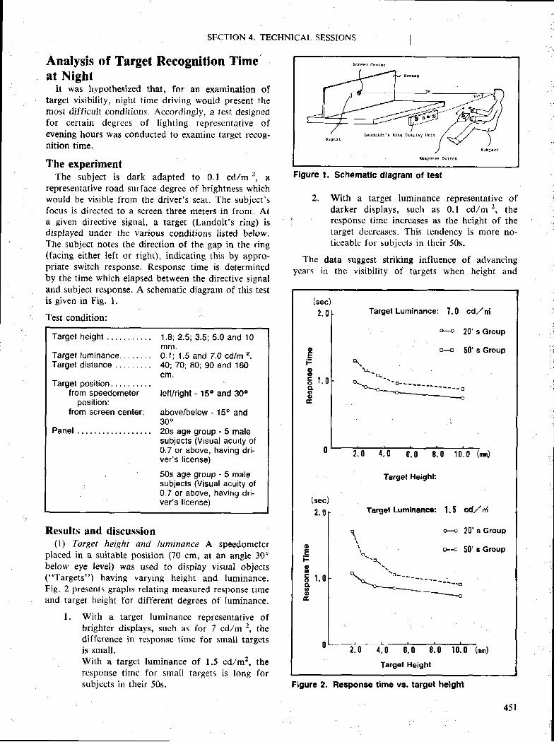
SECTION 4. TECHNICAL SESSIONS

Analysis of Target Recognition Time ,at Night

It was hypothesized that, for an examination oftarget visibility, night time driving would present themost difficult conditions. Accordingly, a test designedfor certain degrees of lighting representative ofevening hours was conducted to examine target recog-nition time.

The experimentThe subject is dark adapted to 0.1 cd/mz, a

representative road surface dcgrec of brightness whichwould be visible from the driver's seat. The subject'sfocus is directed to a screen three meter$ in front. Ata given directive signal, a target (Landolt's ring) isdisplayed under the various conditions listed below.The subject notes the direction of the gap in the ring(facing either left or right), indicating Lhis by appro-priate switch response. Response time is determinedby the time which elapsed between the directive signaland subject response. A schematic diagram of this testis given in Fig. l.

Test condition;

Target height . 1 .8; 2.5; 3.5; 5.0 and 10mm.

Target luminance. 0.1; 1.5 and 7,0 cd/m 2.Target d is tance 40;70;80;90 and 160

cm,Target position

from speedometer left/right - 15o and 30oposition:

from screen centgr: above/below - 150 and300

Panel . 20s age group - 5 malesubjects (Visual acuity of0.7 or above, having dri-ver's l icense)

50s age group - 5 malesubjects (Visual acuity of0.7 or above, having dri-ver's l icense)

Results and discussion(l) Target height and luminance A speedometer

placed in a suitable position (70 cm, at an angle 30obelow eye level) was used to display visual objects('*Targets") having varying height and luminance.Fig. 2 presents graphs relating measured response timeand target height for different degrees of luminance.

l. With a target luminance repre$entative ofbrighter displays, such as for 7 cd/m z, thedifference in response time for small targetsis small.With a target luminance of 1.5 cdlmz, theresponse time for small targets is long lorsubjects in their 50s.

Figure l. Schematlc diagram of test

2. With a target luminance representative ofdarker displays, such as 0. I cdlm 2, theresponse time increases as the height of thetarget decreases. This tendency is more no-ticeable for subjects in their 50s.

The data suggest striking influence of advancingyears in the visibility of targets when height and

1

' t

(sec)

2 . 0

Target Luminance: 7.0 cd/ f i

o+ 20 's GrouP

rl-{ 50'e Groupqr

b

d - i -- \ o . - u - - - * - - - - - - * - - - o

8 . 0 8 . 0 10.0 (mm)

Target HeiEht:

Target Lumlnance: t.5 cd,/nl

o.+ 20 's Group

r-tr 50' s Group

4.0 8 .0 8 .0 10 .0 (mm)

Target Height

oE

oo

E t . oo-ng,E,

2 . 0

Figure 2. Response tlme vs. target helght

451

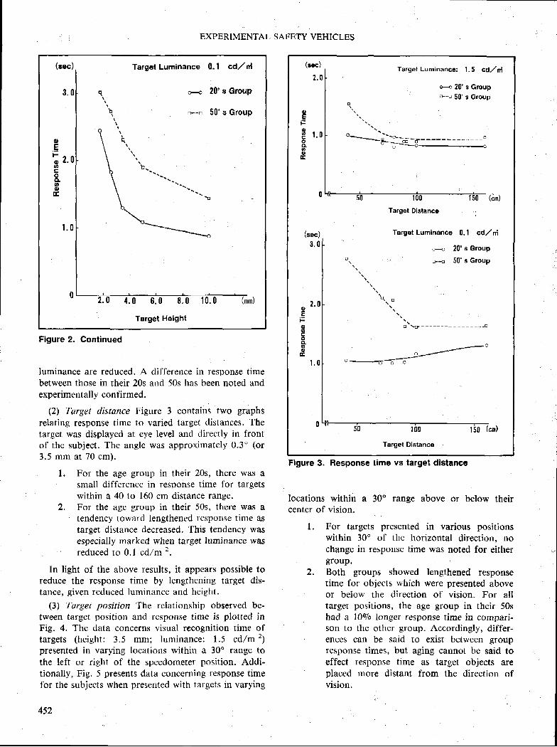
EXPERIMENTAL SAFETY VEHICLES

(eec)

3 . 0

Target Luminance 0. I cd,/ rl

20' s Group

50 's Group

1 0 . 0

o-{

r-tr

o.E' " , 2.0coCLootr

4 . 0 6 . 0 8 . 0

Targel Height

Figure 2. Continued

(aec)

1 . 0

(sec)3 . 0

Target Distance

Targgt Luminsnce 0,1 cd,/n

..'.* 20's Group

u-{ 50' s Group

EE

Fscoo6oE

o * * * - - - - - - - - - - - - - - - - J

Terg€t Distanc6

Target Luminance: l. 5 cd,/nl

o< 20' s Groupo-+ 50' s Group

Flgure 3. Response time vs target dlstance

Iuminance are reduced. A difference in response timebetween those in their 20s and 50s has heen noted andexperimentally confirmed.

(2) Tqrget distance Figure 3 contains two graphs

relating response time to varied target distances. Thetarget was displayed at eye level and directly in frontof the subject. The angle was approximately 0.3" (or

3.5 mm at 70 cm).

1. For the age group in their 20s, there wa$ asmall difference in resf)onse time for targetswithin a 40 to 160 cm distance range.

2. For the age group in their 50s, there was atendency toward lengthened rcsponse time astarget distance decreased. This tendency wasespecially marked when target luminance was

reduced to 0.1 cd/m 2.

In light of the above results, it appears possible toreduce the response time by lengthening target dis-talrce, given reduced luminance and height.

(3) Target position The relationship observed be-tween target position and response time is plotted inFig. 4. The data concerns visual recognition time oftargets (heieht: 3.5 mm; luminance: 1.5 cdlm 2;

presented in varying locations within a 30" range tothe left or right of the speedometer position. Addi-tionally, Fig. 5 presents data concerning response timefor the subjects when presented with targets in varying

452

locations within a 30o range above or below theircentcr of vision.

I. For targets presented in various positionswithin 30" of the horizontal direction, nochange in response time was noted for eithergroup.

2. Both groups showed lengthened responsetime fbr objects which were presented aboveor below the direction of vision. For alltarget positions, the age group in their 50shad a l09o longer response time in compari-son to the other group. Accordingly, differ-

i ences can be said to exist between groupre$pon$e times, but aging cannot be said toeffect response time as target objects areplaced more distant from the direction ofvision.

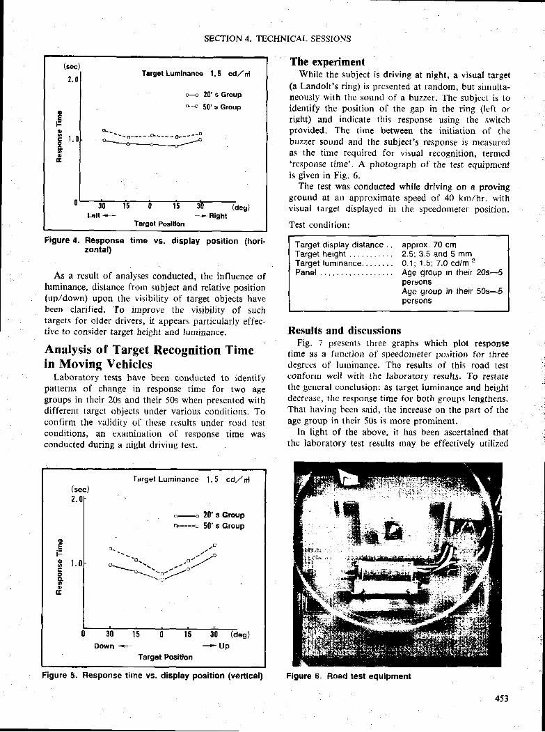
(sec)

2 . 0Targst Luminance 1, 5 cd,/nl

Lsn + * RighrTarget Poeition

o< 20,s GroupD-{ S0, s Group

o*_ _^

- \ r r d - - - - + * - - - * - - - f

U

(des)

SECTION 4. TECHNICAL SESSIONS

Figure 4. Hesponse time vs. display position (hori-zontal)

As a result of analyses conducted, the influence ofluminance, distance I'rom subject and relative position(up/down) upon the visibility of target objects havebeen clarified. To irnprove the visibility of suchtargets for older drivers, it appears particularly effec-tive to consider target height and luminance.

Analysis of Target Recognition Timein Moving Vehicles

Laboratory tests have been conducted to identifypatterns of change in response time for two agegroups in their 20s and their 50s when presented withdifferent target objects under various conditions. Toconfirm the validity of these results under road testconditions, an exarnination of response time wasconducted during a night driving test.

The experimentWhile the subject is driving at night, a visual target

(a Landolt's ring) is presented at random, but sirnulta-neously with the sound of a buzzer. The subject is toidentify the position of the gap in the ring (left orrieht) and indicate this response using the switchprovided. The time between the initiarion of thebuzzer sound and the subject's response is measuredas the time required for visual rccognition, termed'response time'. A photograph of the test equipmentis given in Fig. 6.

The test was conducted while driving on a provingground at an approximate speed of 40 km/hr. withvisual target displayed in the speedometer position.

Test condition:

Target display distance . , approx. 70 cmTarget height . 2.5; 3.5 and 5 mmTarget luminance, 0.1; 1,5; 7.0 cd/m 2

Panel . Age group in their 20s-5personsAge group in their 50s-5persons

Results and discussionsFig. 7 presentsi three graphs which plot response

time as a function of speedornetel position for threedegrees of luminance. The results oI this road testconform well with the laboratory results. To restatethe general conclusion; as target luminance and heightdecrease, the response time for both groups lengthens.That having been said, the increase on the part of theage group in their 50s is more prominent.

ln light of the above, it has been ascertained thatthe laboratory test results may be effectively utilized

Target Luminance l . 5 cd,/ f i(sec)

2.

Q-----LJ

20' a Group50' s Group

l s 0 1 5 30 (des;+ U pDown +

Target Position

Figure 5. Hesponse time vs. display position (vertical) Flgure 6. Hoad test equipment

453

EXPERIMENTAL SAFETY VEHICLES

Target Lumlnance lcd,/ rn (sec) Targel Luminance t. 5 cd/ ti(sec)

- ?q't Group I noao TeerF{ 50' s Group J

= if,, :3131fi | LaboratorY rest

H 20' s Group '1

r--r 50, s Group fRoad Test

(H 20 's Group I .D{r sll, * Group f

LaboratorY Test

oF

i 2 . 0ootroCLU'o

E

tr,

t \ ***i.

5 . 0

Target Height

(mm)5 . 0

Target Height(mm)

Target Luminance: 0. 1 cd,/ rt,l - 20's Group I Roao tesr\. *- 50' s Group j

\ Hr 20' s Grouo'l- \ llaboretory T€stI, i. ++ 50' s Group J

' n \

ttt

A r b

\\\\Nk

\

5.0 hrn)

Targ€l Height

(sec)

3 . 0

Figure 7. Responee time vs. display po$ltlon

to clarify the target conditions useful in improving thevisibility of such objects for older drivers.

Analysis of Conditions FacilitatingVisibility

Standard response timeIn order to determine the target conditions which

facilitate visibility, it is necessary to determine astandard response time. This is the maximum intervaljudeed to be acceptable between target recognitionand the switch manipulating response.

454

For the purpose of this investigation, the timeduring daylight driving when attention is focused onthe speedometer, and the time to respond by switchare calculated separately, and the total value of thetwo has been set as the standard response time.

In order to avoid having the drivsrs become self-conscious, they were told of other objectives. Bymeans of a road test utilizing installed eye cameras,the time during which driver focus is on the speedom-eter is recorded, and an average time period deter-mined. In the present study, this was found to be 0.7sec. Next, a Landolt's ring is displayed while attention

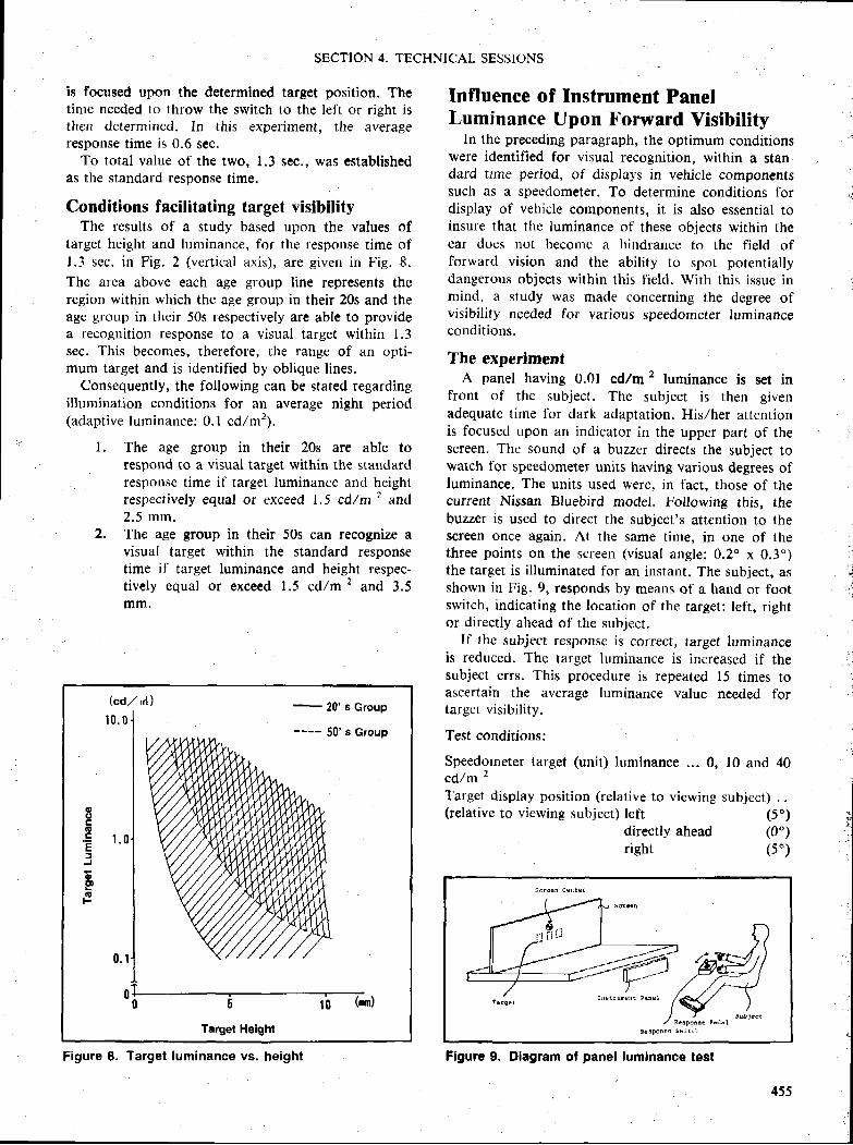
SECTION 4. TECHNICAL SESSIONS

is focused upon the determined target position. Thetime needed to throw the switch to the left or right isthen determined. In this experiment, the averageresponse time is 0.6 sec.

To total value of the two, 1,3 sec., was establishedas the standard response time.

Conditions facilitating target visibilityThe results of a study based upon the values of

target height and luminance, for the response time of1.3 sec. in Fig. 2 (vertical axis), are given in Fig. 8.The area above each age group line represents theregion within which the age group in their 20s and theage group in their 50s respectively are able to providea recognition response to a visual target within 1.3sec. This beconles, therefore, the range of an opti-mum target and is identified by oblique lines.

Consequently, the following can be stated regardingillumination conditions for an average night period(aclaptive luminance: 0.1 cdlm2).

l. The age group in their 20s are able torespond to a visual target within the standardresponsc time if target luminancc and heightrespectively equal or exceed 1.5 cd/mz and2.5 mm.

2. The age group in their 50s can recognize avisuaI target within the standard response

: time if target luminance and height respec-tively equal or exceed 1.5 cd/m ? and 3.5mm'

Influence of fnstrument PanelLuminance Upon Forward Visibility

In the preceding paragraph, the optimum conditionswere identified for visual recognition, within a stan-dard tirne period, of displays in vehicle componentssuch as a spee'dometer. To determine conditions tordisplay of vehicle components, it is also essential toinsure that the luminance of these objects within thecar does not become a hindrance to the field offorward vision and the ability to spor potentiallydangerous objects within this field. Wirh rhis issue inmind, a $tudy was made concerning the degree ofvisibility needed for various speedometer luminanceconditions.

The experimentA panel having 0.01 cdlm 2 luminance is set in

front of the subject. The subject is then givenadequate time for dark adaptation. His/her atrenrionis focused upon an indicator in the upper part of thescreen. The sound of a buzzer directs the $ubject towatch lor speedometer units having various degrees ofluminance. The units used werc, in fact, those of thecurrent Nissan Bluebird model. Following this, thebuzzer is used to direct the subject's attention to thescreen once again. At the same time. in one of thethree points on the screen (visual angle: 0.2o x 0.3')the target is il luminatecl for an instant. The subject, asshown in Fig. 9, responds by means of a hand or footswitch, indicating the location of the target: left, rightor directly ahead of the subject.

If the subject response is correct, target luminanceis reduced. The target luminance is increased if thesubject errs. This procedure is repeated 15 times toascertain the average lurninance value needed fortarget visibility.

Test conditions:

Speedometer target (unit) luminance 0, l0 and 40cd,/m z

Target display position (relative to viewing subject) . .(relative to viewing subject) left

directly aheadright

(5")(0")(5")

ResponFc lk i t rh

Flgure 9. Dlagrem of panel lumlnance test

- 20' s Group

--- - 50 's Group

ooc(E

E 1 . 0E5

6E.E

Target Helght

Figure 8. Target luminance vs. height

EXPERIMENTAL SAFETY VEHICLES

Results and discussionFig. l0 indicates the relationship obtained between

speedometer luminance and the target luminance dif-ferential required for visibility. The difference be-tween target and screen luminance is termed theluminance differential threshold region.

For both the 20- and 50-year-age groups, as speed-ometer luminance is raised, the luminance thresholdregion also rises. It is easily understood that itbecomes more difficult to notice the target. Conse-quently, given night driving conditions, reduced lumi-nance of the speedometer and other devices facilitatesrecognition of obstacles within the forward visualfield.

ConclusionThe data obtained from the preceding examination

of the factors involved in object visibility for subjectsin their 20s and 50s leads to the following conclu-sions:

Object luminance, height, display distanceand position all int-luence visual recognition.The 50-year-age group, compared to theyounger group, is greatly influenced by tar*get luminance and height.If target height and luminance are increased,visual respon$e time decreases. This suggeststhat improvement in prompt recognition is

Hans-Joachim Schmidt-ClausenTechnical University Darmstadt,Federal Republic of Germany

AbstractBased on the European- and US low-beam situa-

tion, tests were made about the recognition distancefor pedestrians. The following parameters were inves'tigated

shape of the headlamPsmounting height of the headlamPsinclination of the headlamPsreflectance factor of pedestrians.

IntroductionStarting from the measured contrast of pedestrians

in the streets during nighttime, in dynamic experi-ments in the street the recognition distance for pedes-trians illuminated by low-beam headlamps was mea-sured. During the tests several parameters werechanged.

456

possible. Conversely, this leads to increaseddifficulty in recognizing obstacles in the for-ward visual field. Accordingly, the determi-nation of optimum object conditions forolder drivers requires careful considerationof both trade offs in determining optimalconditions.

3. While the present work employed 50-year-oldsubjects in the 'senior' age group, it will benecessary to analyze data for even oldersubjects.

Pedestrians in the StreetIn Figure I schematically a twolane road is shown

as seen by a car driver. The pedestrians are at a

distance of d : 50 m in front of the car, illuminatingthe street by mcans of low-beam hcadlamps. C shows

the cut-off-line of the two headlamps, correctly aimed

with a mounting height of h : 65 cm.Z describes the border Iines to zone III in the

European regulations. A is the area of an overheadsign, B of a shoulcler mounted sign at 50 m distance.The Figure shows that the pedestrians are mainlyilluminated by the light in-between "C" and "2"

(dotted area). This area is without legal requirements.

Light-Distribution of Headlampsln Figure 2 arrd 3 the vertical illumination distribu-

tion for two diflerent types of headlamps are shown.The distribution is measured through the points 75Rand B50L o[ the European regulations.

In Figure 2 the light-distribution for a typicalEuropean low-beam headlamp is shown, in Figure 3for a SB-headlamp.

l .

z.

Recognition of Pedestrians During Nighttime Traffic

0 .07

0.08

0 .05

0.04

0t 0Target Luminance

T'o

(1,(ttr(E

.EEt

h

=tl

:EalE to

Adaptive Luminance 0.0l cd,/ n1

- 20 ' s Group*-n 50' s Group

cd/fi)

Figure 10. Visibility vs. target luminance

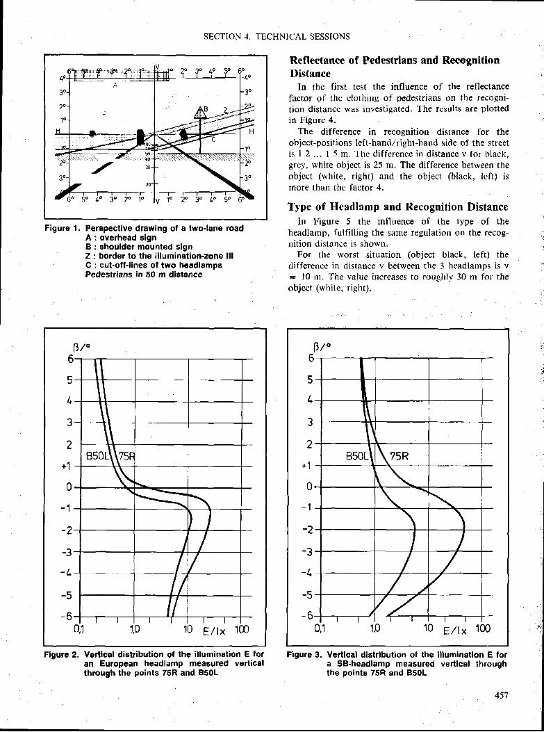
SECTION 4. TECHNICAL SESSIONS

Reflectance of Pedestrians and Recognitionllistance

In the first test the influence of the reflectancefactor of the clothing of pedestrians on the recogni-tion distance was investigated, The results are plottedin Figure 4.

The difference in recognition distance for theobject-positions left-hancl/right-hand side of the streetis I 2 ... I 5 m. The difference in distance v for black.grey, white object is 25 m. The difference between theobjcct (white, right) and the object (black, Ieft) ismore than the factor 4.

Type of Headlamp and Recognition DistanceIn Figure 5 the influence of the type of the

headlamp, fulfilling the same regulation on the recog-nition distance is shown.

For the worst situation (object black, left) thedifference in distance v between the 3 headlamps is v= l0 m. The value increases to roughly 30 m for theobject (white, right).

Figure 3. Vertical distribution ot the illumlnatlon E fora SB-headlamp measured vertical throughthe points 75R and B50L

Figure l. Perspectlve drawing of a two-lane roadoverhead slgnehoulder mounted signborder to the illuminatlon-zone lllcut-off-lines ol two headlamps

Pedestrians in 50 m dletance

Figure 2. Vefilcal distribution of the illumination E foran European headlamp measured verticalthrough the points 75R and B50L

ABzc

f i;

. ii'tI

\

\\

\\

asor\\zsr

\

- \I

I /II /

l/tl

F/o6r

5

/-

3

2

+1

0

- 1

-?

-3

- L

-5

- 60,1 1,0 10 E/ tx 1m

F/"6--r

5

L

3

2

+ 1

0- 1

-2

-3

-1.

-5

- 60,1 10 10 E/ tx 100

\

IBs0il\ zsn

\ \

\

\ \

/

/ /

//

I

/r/

457

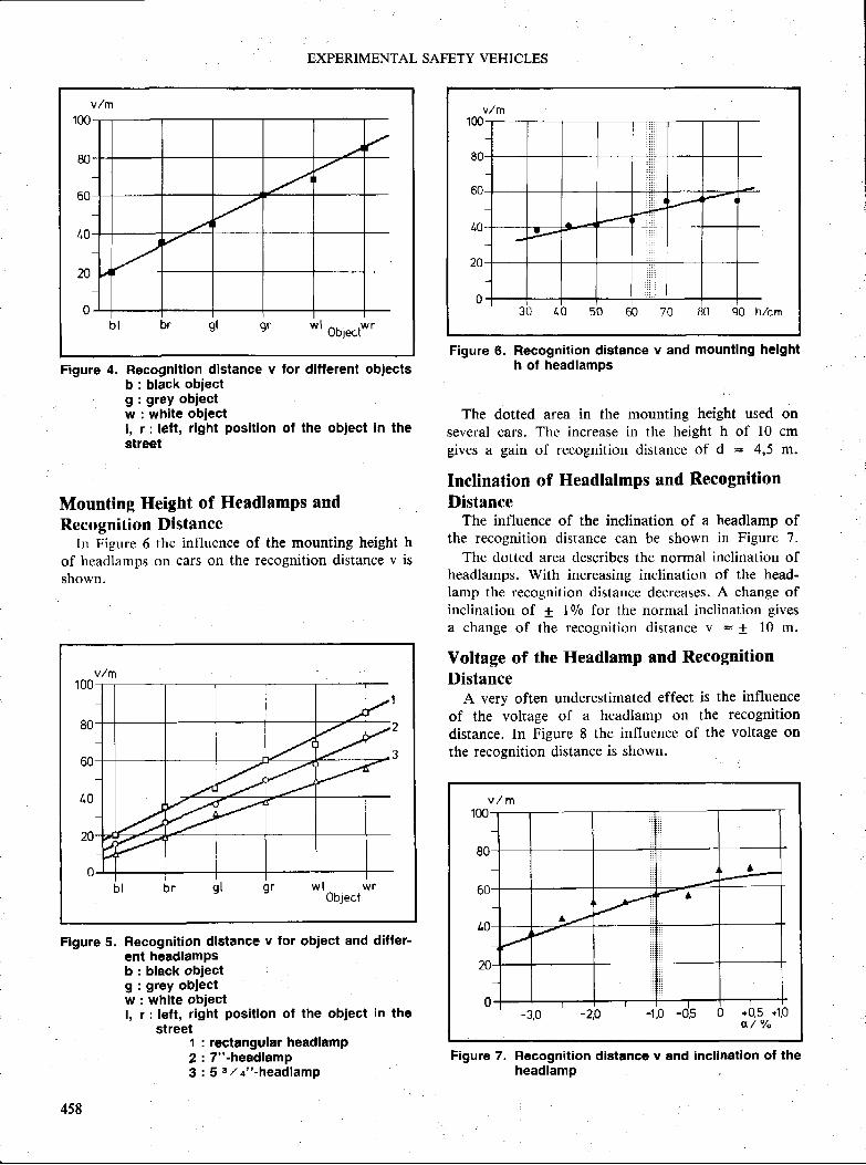
EXPERIMENTAL SAFETY VEHICLES

100

80

60

t o

20

0

Figure 4. Recognition distance v for different obiectsb : black obiectg : grey obiectw : white obiectl, r : l€ft, right position of the obiect in thestreet

Mounting Height of Headlamps nndRecognition Distance

In Figure 6 thc influcnce of the mountine height h

of headlamps on cars on the recognition distance v is

shown.

100

80

60

40

Flgure 5. Recognition dletance v for obiect and differ'ent headlampsb : black obiectg : grey ohlectw : white obiectl, r : left, right posltlon of the obiect in the

' street1 : rectangular heedlamP2 : 7"'headlamP3 : 5 s . z r " - h e a d l a m p

60

lr0

20

090 h/cm

Figure 6. Recognition distance v and mounting heighth ol headlamps

The dotted area in the mounting height used onseveral cars. Thc increase in the height h of l0 cmgives a gain of recognition distance of d = 4,5 m.

Inclination of Headlalmps and RecognitionDistance

The intluence of the inclination of a headlamp ofthe recognition distance can be shown in Figure 7.

The dotted area describes the normal inclination ofheadlamps. With increasing inclination of the head-lamp the recognition distance decreases. A change ofinclination of + l Vo for the normal inclination givesa change of the recognition distance v E t l0 m.

Voltage of the Headlamp nnd RecognitionDistance

A very often underestimated effect is the influenceof the voltage of a headlamp on the recognitiondistance. ln .b-igure 8 the influence of the voltage onthe recognition distance is shown.

Figure 7. Fecognition distance v and lncllnatlon of theheadlamp

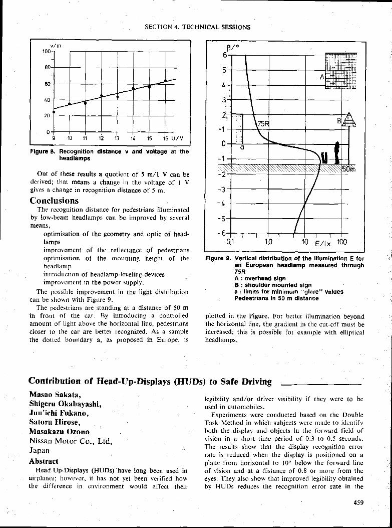
100- r

80

60

LO

20

01 0 1 1 1 2 1 3 1 L 1 5 1 6 U / V

SECTION 4. TECHNICAL SESSIONS

Figure 8. Recognition distance v and yoltage at theheadlamps

Out of these results a quotient of 5 m/l V can bederived; th&t means a change irr the voltage of I Vgives a change in recognition distance of 5 m.

ConclusionsThe recognition distance for pedestrians illuminated

by low-beam headlamps can be improved by severalmeans.

optimisation of the geometry and optic of head-Iampsimprovement of the reflectance of pedestriansoptimisation of the mounting height of theheadlampintroduction of headlamp-leveling-devicesimprovement in the power supply.

The possible improvement in the light distributioncan be shown with Figure 9.

The pedestrian$ are standing at a distance of 50 min front of the car. By introducing a controlledamount of light above the horizontal line, pedestrianscloser to the car are better recognized. As a sanrplethe dotted boundary a, as proposed in Europe, is

Flgure 9. Vertical distribution of the illumination E foran European headlamp measured through75RA : overhead elgnB : shoulder mounted signa : limits for minimum "glare" valuesPedesFians In 50 m distance

plotted in the Figure. For betrer illumination beyondthe horizonral line, the gradient in thc cut-off must beincreased; this is possible for example wirh ellipricalheadlamps.

iI

i n

Contribution of Head-Up-Displays (HUIls) to Safe DrivingMnsao Sakata.Shigeru Okabayashi,Jun' ichi Fukano.Satoru Hirose,Masakazu OzonoNissan Motor Co., Ltd,Japan

AbstractHead-Up-Displays (HUDs) have long

airplanes; however, it has not yet beenthe difference in environment would

been used invcrificd howaffcct their

legibil i ty and/or driver visibil i ty if they were to beused in automobile$.

Experiments were conducted based on the DoubleTask Method in which subjects were made to identifyboth the display and objects in the forward l ield ofvision in a short t ime period of 0.3 to 0.5 seconds.The results show that the display recognition errorrate is reduced when the display is positioned on aplane from horizontal to l0o below the forward l ineof vision and at a distance of 0.8 or more from theeyes. They also show that improved legibil i ty obtainedby HUDs reduces the recognition error rate in the

5

lr,

3

2

+l

04

It\-2-

10 E/tx 100

459

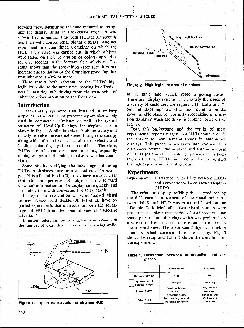
EXPERIMENTAL SAFETY VEHICI,ES

forward view. Measuring the time required to recog-nize the display using an Eye-Mark-Cam0ra, it wasshown that recognition time with HUD is 0.2 secondsless than with conventional digital displays. Anotherexperiment involving tinted Combiner on which theHUD is projected was carried out, in which subjectswere tested on their perception of objects appearingfor 0.27 seconds in the forward field of vision. Theresult shows that the recognition error rate does notincrease due to tinting of the Combiner providing thattransmittance is 4090 or more.

These results both substantiate the HUDs' highlegibility while, at thc same time, proving its effective-ness in assuring safe driving from the standpoint ofenhanced driver attention to the front view.

IntroductionHead-Up-Displays were first installed in military

airplanes in the 1940's. At present they are also widelyused in commercial airplanes as well. The typicalstructure of Head-Up-Displays for airplane use isshown in Fig. l. A pilot is able to both accurately andquickly perceive the external scene through the canopyalong with information such as altitude, velocity andlanding point displayed on a combiner. Therefore,HUDs are of great assistance to pilots, especiallyaiming weapons and landing in adverse weather condi-tions.

Some studies verifying the advantages of usingHUDs in airplanes have been carried out. For exam-ple, Naish(l) and Fischer(2) et al. have made it clearthat pilots can perceive both objects in the forwardview and information on the display more quickly andaccurately than with conventional display panels'

In regard to recognition of superimposed visualsources, Neisser and Becklen(3), (4) et al. have re'ported experiments that indirectly supports the advan-tages of HUD from the point of view of "selective

attention".In automobiles, number of display items along with

the number of older drivers has been increasing while,

Figure 1. Typical constructlon of alrplane HUD

_Slraight- loruard line

Windshi€ld

Figure 2. Hlgh leglblllty area of displays

at the same time, vehicle speed is getting faster.Thereforen display $ystems which satisfy the needs ofa variety o[ customers are required. H. Izuka and Y.Seko et al.(5) reported what they found to be themost suitable place for correctly recognizing informa-tion displayed when thc driver is looking lbrward (seeFig 2).

Both this background and the results of theseexperimental reports suggest that HUD could providethe answer to new demand trends in automotivedisplays. This paper, which takes into considerationdifferences between the airplane and automotive usesof HUD (as shown in Table l), presents the advan-tages of using HUDs in automobiles as verifiedthrough experimental investigatious.

ExperimentsExperiment l. Difference in legibility between HUDs

and conventional Head-Down-Displays(HDDs)

The effect on display leeibility that is produced bythe difference in movement of the visual point be-tween HUD and HDD was examined based on the"Double Task Method". Two visual sources wereprojected in a short time period of 0.48 seconds. Onewas a pair of Landolt's rings which was projected ona screen, and was meant to corrcspond to objccts inthe forward view. The other was 2 digits of randomnumbers, which correspond to the display. Fig. 3shows the setup and Table 2 shows the conditions ofthe experiment.

Teble 1. Difference between automobiles and gir.planes.

Automobileg

Near

Abrupt ly

Hoad, bui ldings,

v e h i c l e s ,

pedest ians, etc.

Not spocial ly t rained

Gradual ly

Sky, c louds

runways,

airplanes, etc.

Wel l t rained

and ski l led

Distanca df view

Appealance ol

obiects in view_

Forward view

460

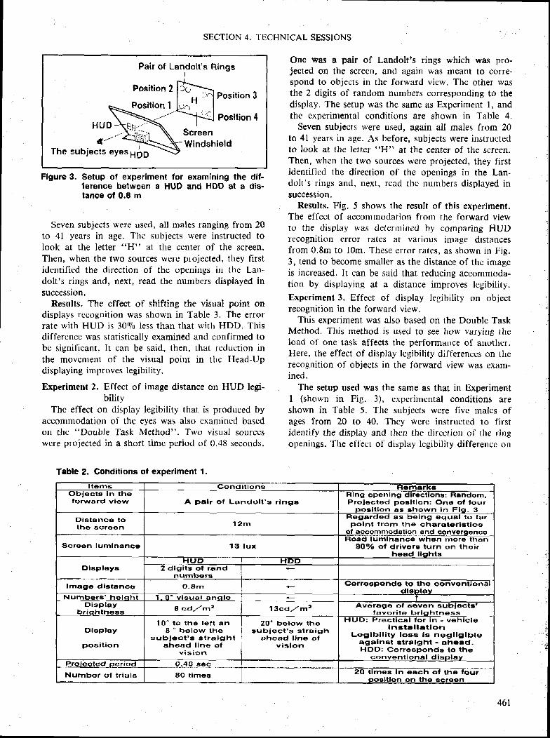
Pair of Landolt 's Rings

Foeition 2

Fosition 1Position 3

Position 4

ScreenWindshield

The subiects eyesppg

SECTION 4. TECHNICAL SESSIONS

Flgure 3. Setup of experiment for examining the dif-ference between a HUD and HDD at a dis-tance of 0.8 m

Seven subjects were used, all males ranging from 20to 4l years in age. The subjects were instructed tolook at the letter "H" at the center of the screen.Then, when the two sources were projected, they firstidentified the direction of the openings in thc Lan-dolt's rings and, next, read the numbers displayed insuccession.

Results. The effect of shifting the visual point ondisplays recognition was shown in Table 3. The errorrate with HUD is 3090 less than that with HDD. Thisdifference was statistically examined and confirmed tobe significant. lt can be said, then, that reduction inthe movement of the visual point in thc Head-Updisplaying improves legibility.

Experiment 2. Eftect of image distance on HUD legi-bility

The effect on display legibility that is produced byaccommodation of the eyes was also examined basedon the "Double Task Method". Two visual sourceswere projected in a short time period of 0.48 seconds.

One was a pair of Landolt's rings which was pro-jected on the scrccn, ancl again was meant to corre-spond to objects in the forward view. The other wasthe 2 digits of random numbers corresponding to thedisplay. The setup was the same as Experiment l, andthc cxpcrimental conditions are shown in Table 4.

Seven subjects were used, again all males from 20to 4l years in age. As before, subjects were instructedto look at the letter *'H" at the center of the screen.Then, when the two sources were projected, they i irstidenti l ' ied the direction of the openings in the Lan-dolt 's rings and, next, read the numbers displayed insuccession.

Results. Fig. 5 shows the result of this experiment.The effect of accommodation from the forward viewto the display was deterrnined by comparing HUDrecognition error rates at various image distancesfrom 0.8m to l0m. These error rates, as shown in Fig.3, tend to become smaller as the distance of the imageis increased. It can be said that reducing accommoda-tion by displaying at a distance irnproves legibil i ty.

Expcriment 3. Effect of display legibil i ty on objectrecognition in the forward view.

This experiment was also based on the Double TaskMethod. This method is used to see how varying theload of one task affects the performarrce of another.Here, the effect of display lcgibil i ty differences on therecognition of objects in the forward view was exam-ined.

The setup used was the same as that in ExperimentI (shown in Fig. 3), experimental conditions areshown in Table 5. The subjects were five rnales ofages from 20 to 40. They were instructed to firstidentify the display and then the direcriorr of the ringopenings. The ell 'ect of display lcgibil i ty differencc on

Table 2. Gonditions of experlment 1.

It6firs Gondl t lorrs FlemarkaLrE!€|c:tA In th€

lo rward v iow A pa l r o f Lando l t ' s r l ngsRIng op6ning dl rEct long: Random,Prolectod posl t ion; One of four

poa l t l on 6a ahowr1 I n F l g . 3

Diatanc6 toths scroon 12rn

Flogarded aa belng equal to farpolnt l ror t l t l ro c l . r6rEter let ice

of accommodal ion and convergonco

Screon lumlnsnce 1 3 l u xRoad lumlnanca when more than

8096 of dr ivere turn on theirl r6ed I lohts

Dlsplayet-t L, Lt HDD

2 dig i ts of rs l rdn r r m h a r r

lmage dletancs O . 8 m Gorrgspq64a to th€ conv€r'rtlonaldl61'lay

H r r h h a r G ' h a l d h a - O - v a s u a l a n o l 6D i $ p l a y

br iah lnca I cd/rnz l 3 c < l / m eAv6rag6 of a$v€n B|Jblect8'

favor i te b r lsh tness

Dleplay

posi t ion

l 0 ' t o t h 6 l e t t a n8 " be low t he

BUblect 'E Etra ig l - r tahead l l ne o f

v is ior . |

20 " be low t hegub iec t ' s s t r a i gh

ahead l ln€ oty l $ l on

t- | rJrJ: Fract lc€| t tor In - venlc lctl r rats l lEt iot ' r

Leg lb l l i t y l oss i s neg l l g l b l oagalnat atra lg l ' r t - Eh€Ed.HFD; Corroeponde to tho

conven t i one l d l s6 l avO .48 sec

Numbor o f t r i a l s 8O t imes 20 t l r t r€E In each of th€ tourooglt lon on the scr66n

461

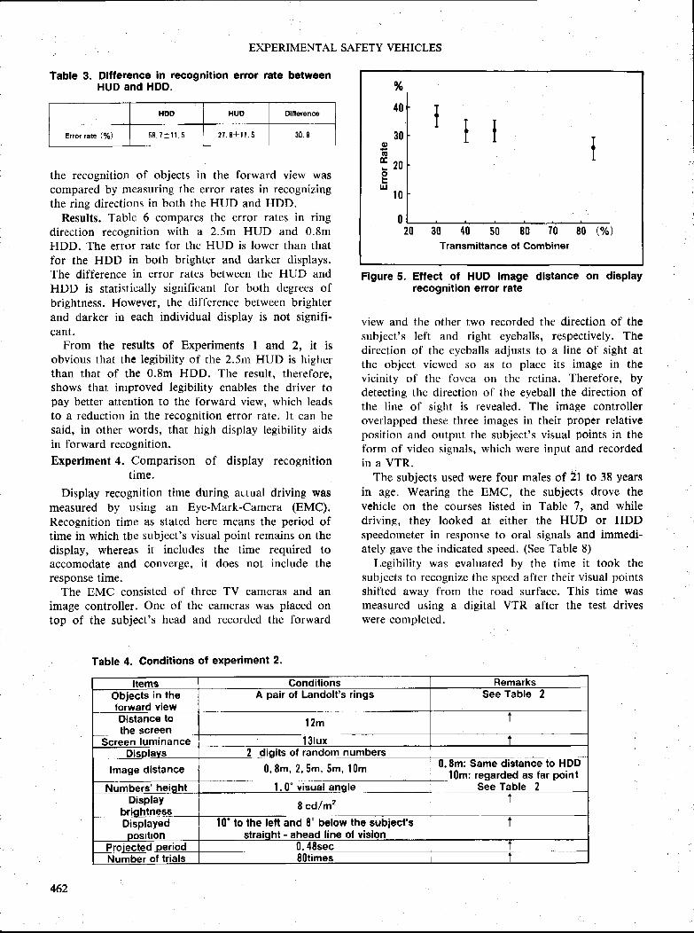
EXPERIMENTAL SAFETY VEHICLES

Table 3. Dlflerence In recognition error rete betweenHUD and HDO.

the recognition of objects in the forward view wascompared by measuring the error rates in recognizingthe ring directions in both the HUD and HDD.

Results. Table 6 compares the error rates in ringdirection recognition with a 2.5m HUD and 0.8mHDD. The error rate for the HUD is lower than thatfor the HDD in both brighter and darker displays.The difference in error rates between the HUD andHDD is statistically significant for both degrees ofbrightness. However, the difl 'crence hetween brighterand darker in each individual display is not signifi-cant.

From the results of Experiments I and 2, it isobvious that the leeibility of the 2.5m HUD is higherthan that of the 0.8m HDD. The result, therefore,shows that improved legibility cnables the driver topay better attention to the forward view, which leadsto a reduction in the recognition error rate. lt can besaid, in other words, that high display legibility aidsin forward recognition.Experiment 4. Comparison of display recognition

time.

Display recognition time during actual driving wasmeasured by using an Eye-Mark-Camera (EMC).Recognition time as stated here means the period oftime in which the subject's visual point remains on thedisplay, whereas it includes the time required toaccomodate and converge, it does not include theresponse time.

The EMC consisted of three TV cameras and animage controller. One of the cameras was placed ontop of the subject's head and recorded the forward

Table 4. Conditions ol experiment 2'

%

40

30gG

T z ogt!

l 0

20 30 40 s0 60 t0 80 P/o)Transmiltance ol Combiner

Flgure 5. Effect of HUD lmage dlstance on dirplayrecognitlon error rate

view and the other two recorded the direction of thesubject's left and right eyeballs, respectively. Thedirection of the eyeballs adjusts to a line of sight atthe object viewed so as to place its image in thevicinity of the fovea on the retina. Therefore, bydetecting the direction of the eyeball the direction ofthe line of sight is revealed. The image controlleroverlapped these three images in their proper rclativeposition and output the subject's visual points in theform of video signals, which were input and recordedin a VTR.

The subjects used were four males of 2l to 38 years

in age. Wearing the EMC, the subjects drove thevehicle on the courses l isted in Table 7. and whiledriving, they looked at either the HUD or HDDspeedometer in response to oral signals and immedi-ately gave the indicated speed. (See Table 8)

Legibility was evaluatcd by the time it took thesubjects to recognize the speed after their visual pointsshifted away from the road surface. This time wasmeasured using a digital VTR after the test driveswere completed.

Items Gonditions RemarksObiects in thetorward view

A pair of Landoll 's rings See Table 2

Distance tothe screen

Screen luminance

l 2 m t

l S lux_ Displavs

lmage distance

2 digits of random numbers

0 . 8 m , 2 . 5 m , 5 m , 1 0 m-0.8m:

si-nie o-iitince to t-too_-l0m: regarded as far point

See Table 2Numbetg 'he iqh t 1. 0" visual anEleDisPlaY

brightnessDisplaYedoosition

I cdlm2t

l0' to ttre lett and 8' below th6 subioct'sstraiqht - ahead line ol vislon

t

Proiected period U.4dsecNumber of trials Rlltiilree

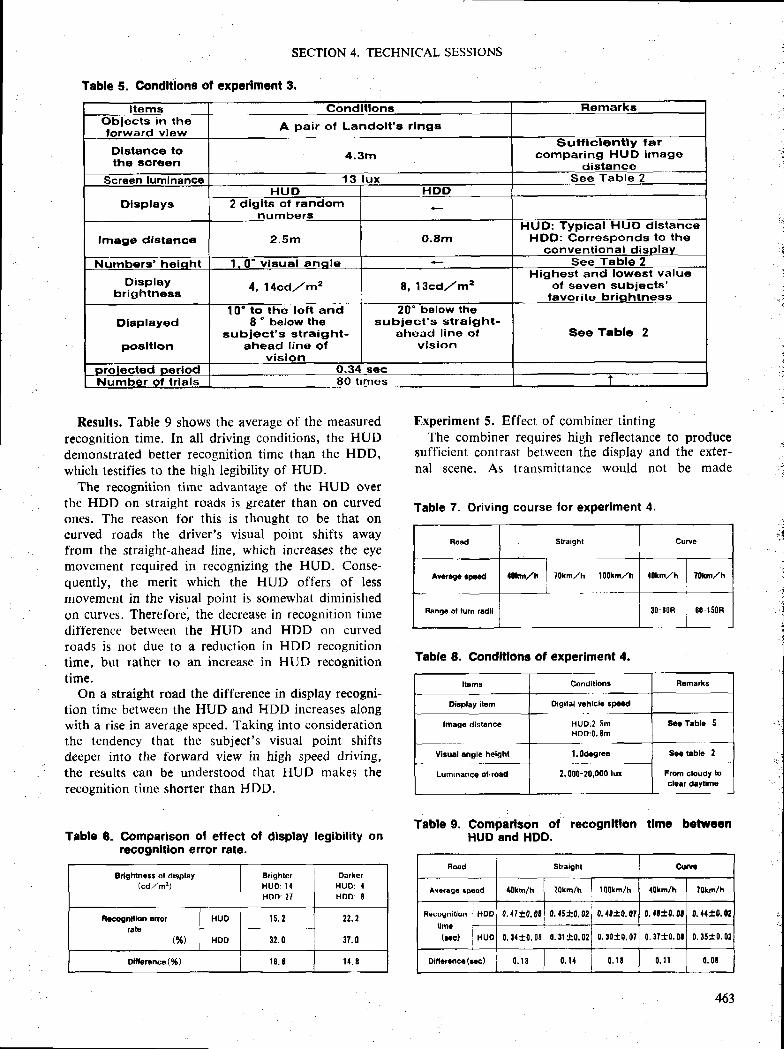
SECTION 4. TECHNICAL SESSIONS

Table 5. Gondlilons of experlment $,

I t ems Condltlons RemarksOblects in th€lorward viaw A pair of Landolt 'e r lngs

Dlatanc€ toth6 scrosn

4 .3mSuff lelently tar

compar ing HUD lmagodi$tsnce

Screcn lumlnence 1 3 l u x See Tab le 2

DlsplayaH U D H O O

2 dlgits of randomn r r m h e r l l

lmage distsnce 2 . 5 m O.8mHUD: Typ lca l HUD d is tance

HDD: Corresponds to theconvent iona l d isp lav

N r r m h a r q ' l r a i a h l I - 0 - v lsua l anq l€ See Table 2

Displaybrightnesa 4, lilcd,/mz 8, l3cd,/mu

Highes t and lowest va lueol seven subjects'

fevori t€ briqhtness

Dloplayed

poaltlon

10" to the left andI

" betow theEubl€ct 's straight-

ahead l ins ofv is lon

20' below thesub lec t ' s g t ra lgh t -

ahead l ine o fv is ion

8ee Tsbb 2

orolectsd oerlod o.34 a€cNumber o f t r la ls 8O t imes t

Results. Table 9 shows the average of the measuredrecognition time. In all driving conditions, the HUDdemonstrated better recognitiort time than the HDD,which testifie$ to the high legibility of HUD.

The recognition time advantage of the HUD overthe HDD on straight roads is greater than on curvedones. The reason for this is thought to be that oncurved roads the driver's visual point shifts awayfrom the straight-ahead line, which increases the eyemovement required in recognizing the HUD. Conse-quently, the merit which the HUD offers of lessmovement in the visual point is somewhat diminishedon curves. Therefore, the decrease in recognition timedifference between the HUD and HDD otr curvedroads is not due to a reduction in HDD recognitiontime, but rather to an increase in HUD recognitiontime.

On a straight road the difference in display recogni-tion time between the HUD and HDD itrcreases alongwith a rise in average speed. Taking into considerationthe tendency that the subject's visual point shiftsdeeper into the forward view in high speed driving,the results can be understood that HUD nrakes therecognition time shorter than HDD.

Table B. Gomparison of ettect of dlsplay legibility onrecognltlon error rate.

Experiment 5. Effect of combiner tintingThe combiner requires high reflectance to produce

sufficient contrast between the display and the exter-nal scene. As transmittance would not be made

Table 8. Condftlons of experiment 4.

Table 9. Comparlron of recognltlon tlme betweenHUD and HDD.

e 4

Table 7. Driving course for experlment 4.

Boad Sifeighi

l0krn./lt | 70km,zh l00km,ztt

Cury6

fwrfo iFaid

HEng6 ol lurn rEdll

lokn,/h | ?0tm,/h

30-80R 80-1$0R

lloma Cdndltionr Femarks

Dirpley itam Digilal Yohicl€ EPc{d

HUD:2 .5mHDD:0. Em_

l:T*':-2' 000-20,000 lux

lffiago distdnce

Vlsul angle height

au-,""."a-O*

8eo Table 5

See rabl6 I

From cloudy toclgar daylima

Bdghlnaas ol di$play(cdlm?)

Brighlet

HUo: l 1HDD: 27

DarkerH U D : {HDD: E

Hacognltion onor |

,uo

(9{) r HDo__

t t ' t

32 .0

22.2

3t. 0

Diffsrunce(%) r t . t 1 { . E

Fdad Stralghi Cut|

AYsaEgo rp€od {0km/h ?0ttrl76 I 00km/h {0km/h ?qkn1h

Fecognltlonuma(ro)

HOO 0, {rf,o.0t0, t5*0.02 0. {tt0.0t 0. frt0.0f 0. tft0, 02

lrup 0,c { t0 ,080.3t t0,0t 0. r0 t0 .070. 3t*0,0l 0. t5t0. 0I

Dlllcroncr (r.c) 0 . l 3 0. t1 0 ,u 0 . l l 0 , 0 l

463

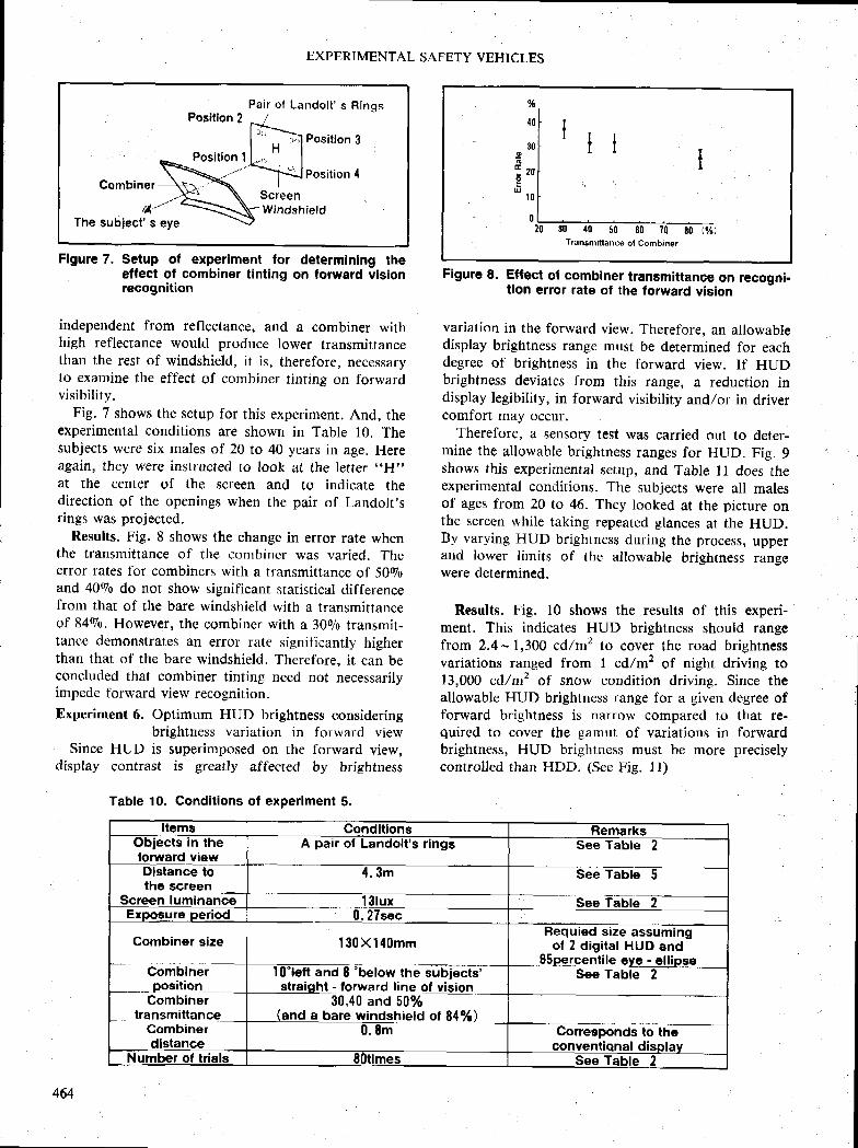
Pai r o l Lando l t ' s R ingsPosition ?

Position I

Positlon 3

Position 4Combiner

,N-'-The subject' s eye

$creenWindshield

EXPERIMENTAL SAFETY VEHICLES

Flgure 7. Setup of experiment for determlnlng theeffect of combiner tinting on forward vlsionrecognition

independent from reflectance, and a combiner withhigh reflectance would produce Iower transmittancethan the rest of windshield, it is, therefore, necessaryto examine the effect of cornbiner tinting on fbrwardvisibil i ty.

Fig. 7 shows the setup for this experiment. And, theexperimental conditions are shown in Table 10. Thesubjects were six males of 20 to 40 years in age. Hereagain, they were instructed to look at th€ letter ,,H"

at the center of the screen and to indicate thedirection of the openings when the pair of Landolt 'srings was projected.

Results. Fig. 8 shows the change in error rate whenthe transrnittance of t lre combiner was varied. Theerror rates for combiners with a transmittance of 50goand 4090 do not show significant statistical differencefrom that of the bare windshield with a transmittanceof 8490. However, the combiner with a 30go transmit-tance demonstrates an error rate significantly higherthan that of the bare windshield. Therefore, it can beconcluded that combiner tinting need not necessarilyimpede forward view recognition.

Experiment 6. Optimum HUD brightness consideringbrightness variation in forward view

Since HUD is superimposed on the forward view,display contrast is greatly affected by brightness

Table 10. Conditions of experlment 5.

Figure 8. Efiect of comblner transmittance on recogni.tlon error rate of the forward vision

variation in the forward view. Therefore, an allowabledisplay brightness range mu$t be determined for eachdegree of brightness in the forward view. If HUDbrightness deviatcs lrom this range, a reduction indisplay legibility, in forward visibility and/or in drivercomfort may occur.

Theretbre, a sensory test was carried out to deter-mine the allowable brightness ranges for HUD. Fig. 9shows this experimental setup, and Table I I does theexperimental conditions. The subjects were all malesof ages from 20 to 46. They looked at the picture onthe screen while taking repeatcd glances at the HUD.By varying HUD brightness during the process, upperand lower lirnits of the allowable brightness rangewere determined.

Results. Fig. 10 shows the results of this experi-ment. This indicates HUD brightness should rangefrom 2.4*1,300 cdlm2 to cover the road brightnessvariations ranged from I cd/mz of night driving to13,000 cd/mz of $now condition driving. Since theallowable HUD brightness range for a given degree offorward brightness is narrow compared to that re-quired to cover the gamut of variations in forwardbrightness, HUD brightness must be more preciselycontrolled than HDD. (See Fie. lI)

o

E

Eq

Item$ Conditions RemarksObiect$ in thelorward view

A pair of Landolt 's rings See Table 2

Distance tothe screen

Screen luminencG

m See rTEe--T-

l Slux See Tiul6--?-Eroosure oeriod 0.27sec

Combiner size

Comuinei-____position_

Combinertransmittance_

Gombinerdistance

l30X140mm

l|l-'left- 6nd 6 "below th; suE]ects,-

straight - lorward line g|llqiql-go,qo .no bo%-

-(and a bare windshield ot 84%)

0 . 8 m

Hequied size assumingof 2 digital HUD and

. S5pelgenti le e1e__4rj!!pgeSee Table 2

- Torresponoi io ttreconveniional disnlav

Number ol trials Slltimes See Table 2

464

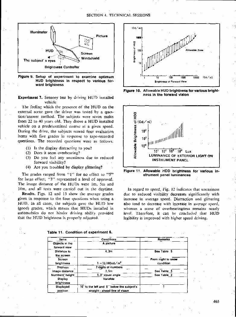
lllumlnator

H U D

t--t;T Picture

-f,Screen

- Windshietd

Brightne$$ Controlfer

The subject'r lr"- T

Flgure 9. Setup of experiment to examine optlmum

SECTION 4. TECHNICAL SESSIONS

HUD brightness in respect to various for.ward brightness

Experiment 7. Sensory test by driving HUD installedvehicle

The feeling which the presence of the HUD on theexternal scene gave the driver was tested by a ques-tion/answer method. The subjects were seven malesfrom 22 to 40 years old. They drove a HUD installedvehicle on a predeterrnined course at a given speed.During the drive, the subjects scored four evaluationitems with five grades in response to tape-recordedquestions. The recorded questions were a$ follows;

(l) Is the display distracting to you?(2) Does it seem overbearing?(3) Do you feel any uneasiness due to reduced

forward visibility?(4) Are you troubled by display glittering?

The grades ranged from "1" for no effect to tt5tt

for large effect; "3" represented a level of approval.The irnage distance of the HUDs were lm, 5m andlOm, and all tests were carricd out in the daytime.

Results. Figs. 12 and 13 show the average gradesgiven in response to the four questions when using aHUD. ln all cases, the subjects gave the HUD low(good) grades, which means that HUDs installed inautomobiles do not hinder driving ability providedthat the HUD brightness is properly adjusted.

Table 11. Condition of experiment 6.

o

E

.E

o

Brighlnoss ol Fomard Vlew

Flgure 10. Allowable HUD brightness lor varloue brlght-ness in the lorward vlelon

strument panel luminances

In regard to speed, Fig. 12 indicates that uneasinessdue to reduced visibility decreases significantly withincrease in average speed. Distraction and glitteringalso tend to decrease with increase in average speed,whereas a sense of overbearingness remains nearlyIevel. Therefore, it can be concluded that HUDlegibility is improved with higher speed driving.

,,,,l|'rrrttiilllll

ooI

E Gd,/o]t

E ro'-cg t t t l

lq

fi roo(E

!e 1 0 1 l 0 ? 1 0 3 , | 0 4 L u x

LUMINANCE OF EXTERIOR LIGHT ONINSTRUMENT PANEL

Figure 11. Allowable HDD brightness for varlous in-

Items Conditione FlemarksObiecls in the

__ torward vieryDistence tothe screen

A piclure

l . 3 m See Table 5

Screenbriohtness I -10.000cd,/mz

Flom nighl to Bnolcondilion

Disptays-_ _lmage distance -_

Numb6rs' heighl - _DisplEy

briohtness

_ 2_A_tgits ol nurfiber$? . 5 m

"_vigual angle _ _Variable

l0; to the lett and S " b"l.* th6 s"biectb

strEiqht - ahead line ol Yl$lon

ESee Table 2

1

465

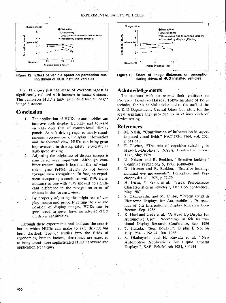
EXPERIMENTAL SAFETY VEHICLES

Flgure 12. Effect of vehicle speed on perception dur'ing drives of HUD In$talled vehicles

Fig. 13 shows that the sense of overbearingness issignificantly reduced with increase in image distance.This reinforces HUD's high legibility effect at longerimage distances.

ConclusionThe application of HUDs to automobiles can

improve both display Iegibility and forward

visibility over tlritt of conventional displaypanels. As safe driving requires nearly simul-taneous rccognition of display informationand the forward view, HUDs can bring greatimprovement in driving safety, especially inhigh-speed driving.Adjusting the brightness of display images isconsidered very important. Although com-biner transmittance is less than that of wind-

shield glass (84V0), HUDs do not hinder

forward view recognition. In fact, an experi-ment comparing a combiner with 8490 trans-mittance to one with 4090 showed no signifi-cant difference in the recognition error ofobjects in the forward view.

By properly adjusting the brightness of dis-play images and properly setting the size andposition of display images, HUDs can beguaranteed to never have an adverse el'f'ecton driver sensitivities.

Through these experiments and analyses the contri-bution which HUDs can make to safe driving hasbeen clarified. Further studies into the fields ofergonomics, human factors, electronics are expectedto bring about more sophisticated HUD hardware andapplication techniques.

Figure 13. Effect of image distances on perceptionduring drives ol HUD installed vehicles

AcknowledgementsThe authors wish to extend their gratitude to

Professor Toyohiko Hatada, Tokyo Institutc of Poly-technics, for his helpful advice and to the staff of' theR & D Department, Central Glass Co. Ltd., for thegreat assistance they provided us in various kinds ofdevice testing.

Referencesl. M. Naish, "Contribution of information in super-

imposed visual fields" NATURE, 1964, vol. 202,p.641-646

2. E. Fischer, "The role of cognitive switching inHead-Up-Displays", NASA Contractor report3137, May 1979

3. U. Neisser and R. Becklen, "Selective looking"Cognitive Psychology 5, 1975, p.480-494

4. D. Littman and R. Becklen, "Selective looking,minimal eye movements", Perception and Psy-chophysics 20, 1976, p.77-79

5. H. Izuka, Y. Seko, et al. "Visual PerformanceCharactcristics in vehicles", llth ESV confcrence,May 1987

6. S. Okabayashi, and M. Chiba, "Recent trend inElectronic Displays for Automobiles", Proceed-ings of 6th International Display Research Con-ference, Sep. 1986

7. K. Hori and Ueda et al. "A Head Up Display forAutomotive Use", Proceedings of 6th Interna-tional Display Research Conference, Sep. 1986

L T. Hatada, "Seiri Kogaku", O plus E No. 56July 1984 - No.74, Jan. 1986

9. S. Okabayashi and H. Kawata et al. "New

Automotive Applications for Liquid CrystalDisplays", SAE, Feb/March 1984, 840144

l .

2.

3 .

(Large el lect)

5

o: l

3 (allowable)

E

o

H 2&

lDistraclionOveibearing

!'Uneasines6 due lo reduced visibil i lylTroubled by display glittering

=________-_-____ -_..-Dg-':r:---::$*-�----t

--_.----*- l ' -*q

25 70 100

Average Speed (kmlh)

I(No effect)

(Large eflect)

5

o6 1a3(allowable)

E gob .o.

I

lDlstraction(lOverbearingvUnedslnoss dud lo rednced YisibilitylTroubled by dibPl6Y glittering

i-.�rj:-,...q:#

(Noe6ecr) I 5 10lmage Oistance (m)

466

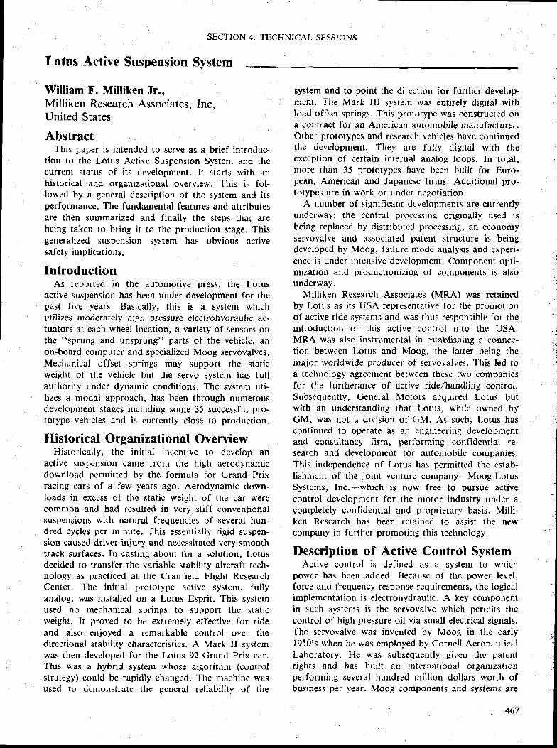
SECTION 4. TECHNICAL SESSIONS

Lotus Active Suspension System

William F. Milliken Jr.,Milliken Research Associates, fnc,United States

system and to point the direction for further develop-ment. The Mark III system was entirely digital withload offset springs. This prototype was constructed ona contract for an American automobile manufacturer.Other prototypes and research vehicles have continuedthe development. They are fully digital with theexception of certain internal analog loops. In total,more than 35 prototype$ have been built for Euro-pean, American and Japanese firms. Additional pro-totypes are in work or under negotiation.

A number of significant development$ are currentlyunderway; the ccntral processing originally used isbcing replaced by distributed processing, an economyservovalve and associated patent structure is beingdeveloped by Moog, failure mode analysis and experi-ence is under intensive development. Component opti-mization and productionizing of components is alsounderway.

Milliken Research Associates (MRA) was retainedby Lotus as its USA representative l'or the promotionof active ride systems and was thus responsible for theintroduction of this active control into the USA.MRA was also instrumental in establishing a connec-tion between Lotus and Moog, the latter being themajor worldwide producer of servovalves. This led toa technology agreernent between these two companiesfor the furfherance of active ride/handling control.Subsequently, General Motors acquired Lotus butwith an understanding that Lotus, while owned byCM, was not a division of GM. As such, Lotus hascontinued to operate as an engineering developmentand consultancy firm, performing conlidential re-search and development for automobile companies.This independence of Lotus has permitted the estab-lishment of the joint venture company-Moog-LotusSystems, lnc.*which is now free to pursue activecontrol development for the motor industry under acompletely confidential and proprietary basis. Milli-ken Research has been retained to assist the newcompany in furthcr promoting this technology.

Description of Active Control SystemActive control is defined as a system to which

power has been added. Because of the power level,force and frequency response requirements, the logicalimplementation is electrohydraulic. A key componentin such systems is the servovalve which permits thecontrol of high pressure oil via small electrical signals.The servovalve was invented by Moog in the early1950's when he was employed by Cornell AeronauticalLaboratory. He was subsequently given thc patentrights and has built an internationirl organizationperforming several hundred million dollars worth ofbusiness per year. Moog components and systems are

AbstractThis paper is intended to serve as a brief introduc-

tion to the Lotus Active Suspension System and thecurrent status of its development. It ritart$ with anhistorical and organizational overview. This is fol-lowed by a general description of the system and itsperformance. The fundamental features and attributesare then summarized and finally the steps that arebeing taken to bring if to the production stage. Thisgeneralized suspension system has obvious activesafety implications.

IntroductionAs reported in the automotive press, the Lotus

active suspension has been under development for thepast five years. Basically, this is a system whichutilizes moderately high pressure electrohydraulic ac-tuator$ at each wheel location, a variety of sensors onthe "sprung and unsprung" parts of the vehiclen anon-board computer and specialized Moog servovalves,Mechanical offset springs may support the staticweight ot the vehicle but the servo system has fullauthority under dynamic conditions. The system uti-lizes a modal approach, has been through numerousdevelopment stages including some 35 successful pro-totype vehicles and is currently clo$e to production.

Historical Organizational OverviewHistorically, the init ial irrcentive to develop an

active suspension came from the high aerodynamicdownload permitted by the formula for Grand Prixracing cars of a few years ago. Aerodynamic down-loads in excess of the $tatic weight of the car werecommon and had resulted in very stiff conventionalsuspensions with natural frequencies of several hun-dred cycles per tninute. This essentially rigid suspen-sion caused driver injury and necessitated very smoothtrack surfaces. In casting about for a solution, Lotusdecided to transfer the variahlc stabil ity aircraft tech-nology as practiced at the Cranfield Flight ResearchCenter. The init ial prototype active system, fullyanalog, was installed on a Lotus Esprit. This systemused no mechanical springs to support the staticweight. It proved to be extremely efl'ective for rideand also enjoyed a remarkable control over thedirectional stability characteristics. A Mark II systemwas then developed for the Lotus 92 Crand Prix car.This was a hybrid system whose algorithrn (corrtrolstrategy) could be rapidly changed. The machine wasused to demonstratc the seneral reliabilitv of the

467

EXPERIMENTAL SAFETY VEHICLES

preeminently used in high performance aircraft, mis-siles, the space shuttle, robots and for many othermilitary and industrial uses.

The Moog valve, by design and internal feedback,is closely a linear flow-control device. Its frequencyresponse characteristic is in the hundreds of cycles persecond range and full flow is reached in two-tenmilliseconds in typical automotive active systems.

A typical active suspension system utilizes a numberof transducers at each wheel and also lateral andIongitudinal accelerometers on the 'nsprutrg mass"C.G. of the vehicle. These signals are fed into a smallsoftware package typically powered by a 600 milliampbattery (and standby) which is completely separatefrom the vehicle electrical system. The software pack-age contains servo amplifiers, filter networks, signalconditioning circuits, an 8-bit microcomputer andover 100 operational amplifiers.

Orr the hydraulic side there is an engine drivenpump with control system pressure on the order of2500 psi, accumulators, oil cooler, filters and doubleacting actuators at each wheel location. Package-wise,the installation at the wheel Iocation is comparable toor smaller than that of a conventional suspensionsystem.

The microcomputer is programmed with the rideand handling algorithms. These algorithms are theresult of extensive development by Lotus/Cranficldbased on theoretical and experimental consideratious.Several hundred algorithms have been explored in thedevelopment.

The overall $y$tem response is flat to over 2O Hz.Essentially the system enables complete separation ofbocty and whccl motions, i.e., eliminates the designcompromise between ride and handling. In essence,the suspension is a fully generalized one, capable ofany interconnections, desirable nonlinearities, etc. Al-though the frequency response is approaching theharshness range, sotne rubber is still utilized for thecontrol of higher frequency harshness.

PerformanceThe performance of these active systems is truly

remarkable and can only be fully appreciated by ademonstration. Since the body motion is separatelycontrollable from the acceleration inputs, it is possible

to call for no roll or pitch under any mancuver.Specifically, the vehicle can be made to roll outwardor inward or remain level. Similarly, the antipitch

characteristics are fully under control and the vehiclecan be given 10090 pitch compensation or even havean over-compensation in which the nose of the carrises under braking. Because of the ability to rapidlychange the roll and pitch characteristics, a prototypeactive system is an excellent device for determiningwhat the human driver desires in the way of body

468

motion. Experience to date, indicates drivers univer-sally prefer no roll (thus eliminating the roll transient)and prefer a small amount of dive under heavybraking. With antilock, it seems likely zero pitchwould be desirable. With zero roll, camber changes onthe wheels are eliminated and this plus thc morenearly constant force between the tire and road haveresulted in an increase in maximum lateral accelera-tion on the order l5o/0. It is perfectly possible toadjust the over-understeer properties by a controlaccessable to the driver en route. With a nonrollingvehicle, full wheel travel is retained in even thc mostsevere turn, which markedly improves rough roadcornering. Maintaining zero roll and eliminating theroll mode, results in improved directional responsecharactcristics and improved controllability through-out the speed range. The roll mode appears as auseless and extraneous form of motion since experi-ence with activc vehicles demonstrates that the rollingmotion does not contribute to skid warning as hereto-fore assunred.

Crash avoidance and active safety are improved byan order of magnitude due to:

r Increase in maximum lateral accelerationr Elimination of cxtraneous vehicle ride mo-

tions due to rough roads and maneuveringr Elimination of coupling between ride and

handling, hence control simplification. Optimized directional control response and

handling characteristicsI Improved control and directional damping at

rhe limitLarge discrete bump$ and road waves are com-

pletely "swallowed" by the active suspension providedtheir amplitude is not in excess of maximum $uspen-sion travel. The active suspension lends itself to largetravel and progressive nonlinear approach to maxi-mum travel. The behavior of the active suspension onrough roads is one of its more remarkable features.Subjectively, the ride improvement is very great andcorrespond$ to objective measurement.

The system is able to distinguish between an aidingload on the wheel or the converse. This featureenables an economy of power. Extensive use can bemacle of electronic system technology, as for example,in the application of filters to control various vibra-tional modes. Thc fiilters increase the order of thesystem and a 20th order system is common andpractical. Tirelground contact forces are made mnchmore constant by effectively reducing the "unsprung

mass" of the road wheels. Automatic height andattitude leveling are, of course, available. The me-chanical design of the suspension is greatly simplifiedsince geometric compromiscs are no longer necessary.The wheels, for example, can be supported tiomsimple trailing arms with improved packaging.

SECTION 4. TECHNICAL SESSIONS

One of the most dramatic advantages of the activesy$tem is the reduction in testing and developmenttime for satisl'actory ride and handling. This was welland initially illu,itratcd on the race car application inwhich the vehicle could be "setup" in the space of acouple of laps, whereas it is not uncommon with aconventional suspension to use an entire practiceperiod. Fast updating of ride and handling require-ments in response to market changes is entirelypractical. With a good onboard instrumentation sys-t€m it is possible to explore on a subjective/objectivebasis, various ride and handling ritrategie$. Experienceindicates up-front design costs are more than offset byreduced development time.

Summary of Features and AttributesBelow is a concise summary of the features and

attributes of the Lotus active suspension and controlsystem:

l. Addition of Powera. Selectivity with load direction

2. Computer Controla. Sensed-motion variables inputb. High-order control strategy

3. Computer Flexibility., a. Nonlinearities

b. Manual and automatic adjustmentsc. Algorithm changes (program)

4. Computer Enables:a. Feedback controlb. Electronic system technology(l) Sophisti-

cated filters5. A Completely Generalized Sy$tem

a. Avoids design compromises of conven-tional suspensions

5. Can be implemented with mechanicat springsfor static load or no springs. Full servoauthority in both cases.

Some Attributes of Active Suspensionl . Body and Wheel Control Independent

a. Elimination of roll modeb. Separation of ride and handling; individ-

ual optimizatir:n2- More Constant Tire/Ground Contact Forces

a. Improve response and dampingb. Enhanced ride and road holding

3. Body Attitude Control to Accelerationsa. Large effective wheel travel

4. Progressive Nonlinear Approach to Limit orTravel

5. Manual or Automatic Height and AttitudeLeveling

6. Vibration Control by Selective Filtering7. Design and Operational Control of Direc-

tional Response and Trim

Development Time and Cost FactorsL Simplified Mechanical Design; Improved

Packaging2. Standardized Hydraulic Components3. Testing and Development Time Drastically

Reduced4. Fast Updating as Requirements Change5. Rapid Subjective/Objective Evaluation6. Up-Front Dcsign Costs Offset by Above

Items

Steps Toward Production SystemsMoog-Lotus Systems, Inc., has beer-r formed to

facilitatc;

. Further development of experimental systems(Lotus)

. Further economy servoyalve development(Mooe)

r Further computer/electronic/algorithm devel-opment (Lotus/Cran field)Production components (Morlg)

ServovalvesHydraulicsElectronics

. Systems integration technique (Moog/Lotus/Cranfield)

I Field servicing

Thus the plan is to offer complete active capabil-ity-design, development, production and $ervicc-atautomotive cost levels.

Future DevelopmentsMoog-Lotus believe that "[ull active control of all

vehicle dynamics" is inevitable in the future. This wil linc lude:

r Active su$pensionr Active four-wheel steer. Active traction and braking

469

EXPERIMENTAL SAFETY VEHICLES

Adapting Radar to the Automotive EnviroRment

John lV. Davis,Radar Control Systems Corporation,United States

AbstractRecent developments in short range radar technol-

ogy should soon make vehicle radar a reality. Areview will be given of the scheme and approach usedfor radars operating in a complex environment. Thedifficulties encountered in developing vehicle radarand the headway control logic that provides a safedriving margin will also be covered. Operation of asensitive radar in a high-clutter environment will behighlighted, as well as the techniques involved inmaking it work. The methods used for radar accidentprevention and the impact automotive radar will haveon drivers and society will be discussed.

IntroductionOur goal has been to develop a small vehicle radar

system that would actively increase driving safety.Highway safety can be improved electronically byincreasing drivers' awareness and by helping them tomaintain safe driving margins. Radar will help driversmitigate and prevent many avoidable accidents.

To achieve a high level of performance, many radarand vehicle factors had to be considered. The level ofdriving hazard had to be established, and the criticalmoment it became dangerous had to be determined. Asystems approach was carefully selected and lurtherdeveloped to achieve our goal. Operating a short-range radar in a complex vehicular environmentrequired new technology. Many techniques and uniquedesigns were needed to $olve the problems associatedwith operating a vehicle radar system.

This radar system was implemented, road tested,and developed to make it a practical reality. Driverswith radar-equipped vehicles will soon have a newinstrument to increase their safety, and that givesthem a better chance of avoiding accidents. This newcollision avoidance technology will save many livesand reduce injuries. ln doing $o it will gencrate a realsavings for drivers, insurance companies, and society.

Recent Developments in AutomotiveRadar

New Radar Technology wfls Needed forVehicles

New technology had to be developed for vehicleradar that covers many disciplines-from the small,shaped-beam antenna that transmits 3 mw of powerto the specialized signal conditioning circuits, micro-controller and automatic radar braking system. A new

470

approach was taken, and new parameters had to beestablished. The vehicle radar system needs a sensitiv-ity greater than -100 DBC to work well, even thoughthe radar environment limits the useful sensitivity to amuch lower level. The dynamic and linear operatingrange of the system had to be over 75 DB to handlethe radar signals accurately. Such high gain andsensitivity were necessary even though they createdadditional problcms and the need for many newcircuits to handle the signals in the radar returns. Allthc details of this new technology cannot be coveredhere, but the following should provide a betterunderstanding of vehicle radar technology.

The design for vehicle radar starts with a goodantenna and microwave system that can detect small,complex targets. The antenna beam has to be sized,shaped and steered appropriately to cover a vehicle'schanging headway. The detected signal is usuallydistorted as a result of complex multitarget returns.The signal, however, contains all the needed informa-tion such as closing rate, range, direction, signalcoding, interference, and other data needed by theradar system.

Assuming that we have all the radar data, it mustbe conditioned and processed to determine how manyfeet (or seconds) a driver needs for accident preven-tion. Then the radar's external information is com-bined with the vehicle's internal data components(vehicle speed, steering, acceleration, stopping, etc.)plus the driver inputs to have all the inputs to makethe radar system operational. We refer to all theinternal vehicle and driver inputs as driving monitorsor driving modifications (DMs), which describes theirfunction. If a radar system were in free space lookingat a target ten miles away, no system modificationwould be necessary. However, in the ever-changingvehicle radar environment, where small and largeobjects are constantly passing nearby at variousspeeds, a different solution was needed and devel-oped. The vehicle radar system design had to beadapted to the environment as well as to the vehicleu$age.

Once the radar, vehicle and driver inputs areavailable, they are conditioned and then combined ina digital-analog processor. After this data is in themicroprocessor, the system can be programmed to fitthe vehicle's driving situation to achieve the appropri-ate outputs for the driver.

The main output of the vehicle radar system is toalert the driver-who is the vehicle's ultimate safetydevice. The radar warning system is designed to keepthe driver safer and to actively warn him in dangeroussituations. Radar braking system (RBS) technologywas developed to further demonstrate the radar's

SECTION 4. TECHNICAL SESSIONS

capability to logically stop the vehicle. This new radartechnology and developments should soon make colli-sion avoidance radar a production reality"

Yehicle Rndar Performnnce Must beEffective

An effective vehicle radar system should benefit thedriver in several different ways. However, regardlessof how good a radar system is, it has limitations.Accidents will still occur in both controllable anduncontrollable situations. Radar-equipped vehicles willbe taking on a very complex problem, and in spite ofthe fact that it may greatly improve safety, the radarwill stil l be blamedn in many cases, for not beingadequate. Regardless of these criticisms, the overallsafety benet'its anticipated for radar collision avoid-ance may be as high as 40 percent and this alone willjustify production. This high percentage may beachievable simply because distracted drivers are themajor cause of accidents, and they obviously need anactive system to make them safer drivers.

The ideal vehicle radar system would always alertthe driver in time to avoid a collision. However, inreal-world traffic situations, this is not always possi-ble. Curving roadways, cross traffic, and many otherfast-changing situations make it physically impossihtein many situations for the radar to always give thedriver the time and distance needed for stopping. Butalerting the driver just one second (e.g. 73 feet at 50MPH) before impact can often provide enough timeto steer around an ob.stacle, or at lea$t allow someadditional braking time. The system can provideseconds in many situations that may give drivers theextra lime they need.

Some of the safety benefits a vehicle radar systemcan provide are:

Radar will be constantly on guard to act as asafety back-up for distracted drivers.

Radar should prevent many sideswipe accidents,especially when the road is straight or turns left.

Radar can help drivers establish and maintainsafer driving margins in traffic situations.

Radar can respond very quickly in accident situa-tions to alert drivers.

Radar, to be truly effective, must perform wellenough to gain the driver's confidence. To be mosteffective and meaninglul for a driver, the systemshould communicate in the same manner as a passen-ger would warn an unsafe driver. A passenger knowswhen fl driver is unsafe and he will respond accord-ingly. If a driver is careless, a passenger may saysomething; if a collision is immincnt, he may yell. Theradar warning system should also communicate itsmeasured level or intcrpretation of the hazardous

situation and alert the driver in words and statements.The system can now say "look out," "be careful,"and alert the driver in appropriate situations.

The primary control for vehicle safety will alwaysbe in the hands of the driver. However. when a driveris not paying attention, the radar will be working forhim in many critical situations. This means it shouldnot miss too many opportunities to avoid preventableaccidents; yet it must not disturb the driver orpassenger needlessly. Therefore, the output of theradar warning system should be tocused toward keep-ing the driver attentive in hazardous and dangeroussituations and alerting him to take action. Collisionavoidance radar now looks very promising because ofwhat it can do for drivers.

The Difficult Environment for VehicleRadar

The Yehicle Radar EnvironmentThe complex, moving environment the vehicle radar

sees, and must operate in, poses many difficulties forreliable and optimum system performance. With asmall high-gain antenna mounted two feet above thcroadway, many nearby objects must and will be seenby the radar system. Radar energy bounces aroundwhen it hits nearby objects, much like water from anozzle would bounce back from a nearby object. Asensitive radar will see the road, cars, posts and anyother nearby and distant objects in the radar beam.Some small, poorly shaped radar objects (referred toas targets) are hard to see. Other targets are verylarge, and some large targets can be seen miles away.The necessary dynamic operating range of the systemmust, therefore, be great to see both small and largetargets. For this reason, many ships switch to low-power radar systems when they are coming intoharbor. Many vehicle radar systems can only see orrespond to larger target$ at clo$e range. A goodshort-range radar system must detect smaller targetsand also work well when large targets are blindinglyclose. A radar can blind itself by its own rerurn.

All of rhese environmental difficulties are mani-fested one way or another as signal problems such asdistortion, saturation, multipath, multitarget, multi-bounce, and multiple returns. Other related problemsare false alarms, radar blinding, electrical interfer-ence, road noises, vehicle noise, bounce and vibratian,weather, and similar phenomena.

These environmental problems are some of theprimary reasons why vehicle radar has been such achallenge to develop. Regardless of environmentalrestrictions, it is very important for a system torecover all the information available in the radarsignal. The difficulties of exrracring the informationfrom a weak, saturated or distorted return signal have

471

EXPERIMENTAL SAFETY VEHICLES

caused vehicle radar designers to look for alternatesolutions.

It was for this and other reasons that a dopplersystem was selected over the pulse and frequencymodulation approaches. The doppler signal providesmore direct information than other radar approachestried, and it has the primary component of closingrate. New circuits and designs were developed for thevehicle radar system to help resolve the environmentalradar problems.

Roadway Environment Should ImproveThe road performance of the vehicle radar antenna

and the circuits that back it up must be very good inorder to see smaller radar targets. The major factor inany vehicle radar system will be how well the radarsees and recognizes the weaker targets. Some objects,at times, appear almost invisible to the radar. Thenormal signal strength range or radar cross-section ofthese radar returns now varies about 50 DB. Somepoor radar targets can be improved with ease, butdetecting a small child will always be a challenge forany radar system.

Roadways are now enhanced with all types of visualaids to help the driver's vision. Radar visibility canalso be enhanced by adding a radar reflecting deviceor material to existing vehicles and roadside markers.Visible light and radar images are comparable inmany ways. Radar returns respond somewhat likelooking at yourself in a mirror. A slight turn of themirror and your image disappears, even though youcan still see the mirror. Radar returns don't suddenlydisappear like the visual image, but they do becomevery weak in many cases.

As vehicle radar becomes a reality, vehicles mayhave improved radar cross-sections, or they may beaugmented with one or more radar reflectors toenhance their radar irnage. It takes a very smallchange to make poor radar targets many times stron-ger, especially at higher frequencies. A radar systemshould still be able to perform in the present automo-tive environment. However, when the roadway envi-ronment is improved for radar, it will be better fordrivers as well.

The Headway Control SchemeThe Headway Control Logic

In simple term$, the hcadway control zone repre-sents the space or distance a driver needs in front ofhis vehicle to stop it or regain control. Since vehiclesare always turning in various ways as they are driventhrough both a moving and stationary environment,this complex motion must be taken into account in allradar driving situations.

One of the keys to collision avoidance is a schemeor algorithm that can always distinguish between a

472

safe or dangerous driving situation. fhe degree ofsafety or danger can be thought of as a measure ofhazard level (HZL). The critical hazard levcl isdetermined by the total value of all the major factorsin the algorithm. Additionally, the dynamic algorithmallows us to differentiate between many differenthazard /evels. With the control zone scheme, the radarsystem can determine any hazard level within thecontrol zone, while disregarding radar targets outsideof the zone.

The major components used in the control zone logicare:

Range (R). This is a measurement of the distancefrom the radar to the object it sees, referred to as thetarget. Range, in feet, is weightcd at about 5090 ofthe value of the algorithrn. (Line R, Figurc l)

Closing Rate (CR). The closing rate is the relativespeed difference between you and the target, whichmay be moving or $tationary. The closing rate, inMPH, is weightcd at about 3390 ot the value ot thealgorithm. (Line CR, Figure l)

Vehicle Speed (VS). The vehicle speed is how fastthe vehicle is moving on the road. Vehicle speed, inMPH, is weighted at about l7v/o of the value of thealgorithm. (Line VS, Figure l)

Driving Modifiers {DMs). These modifying factorshave to do with the operation of the vehicle, and withwhat the driver is doing in traffic. Since the radarenvironment is constantly changing, the DMs arespecifically applied to adapt the radar's control zonelogic to fit these vehicle driving situations. Specifi-cally, the DMs include factors such as turning as afuncfion ot' vehicle speed, slow closing rates andvehicle speeds, the status of the brake pedal (whetherthe driver is braking or not), and target direction.These inputs, along with other processor-generatedmodifiers, are used to fine tune the algorithm in orderto yield the appropriate output for any driving sce-nario. All the DMs, as weighted, fifly range from+ lSVo to - 30q0 in the algorithm. When thc vehicleis going straight in a normal situation, the DM valueis usually zero.

The Headway Control Algorithm. When the ordi-nate value units of the range R, closing rate CR andvehicle speed VS are choscn separately and then addedtogether, the total will yield the value of the hazardIevel. (Please refer to Figure l, page 7.) Hazard levelsare considered safe under 400 units and dangerousabove 400 units. (The DM value has been omitted forclarity.) The formula for the HZL is: HZL : R +CR + VS t Uf,t. For working examples let DM =0 .

The Dynamic Safety MarginA safer driving margin can be maintained if several

key factors are controlled. To establish an appropriate

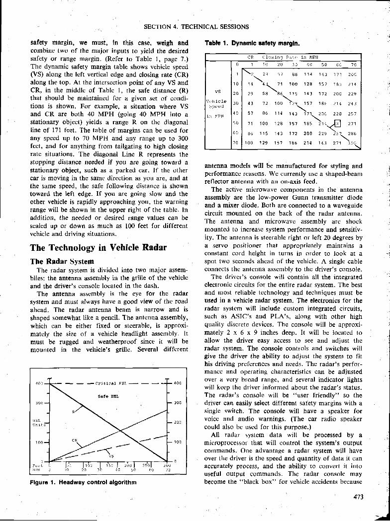
SECTION 4. TECHNICAL SESSIONS

safety margin, we must, in this case, weigh andcombine two of the major inputs to yield the desiredsafety or range margin. (Refer to Table l, page 7.)The dynamic safety margin table shows vehicle speed(VS) along the left vertical edge and closing rate (CR)along the top. At the intersection point of any VS andCR, in the middle of Table l, rhe safe distance (R)that should be maintained for a given set of condi-tions is shown. For example, a situation where VSand CR are both 40 MPH (going 40 MPH into astationary object) yields a range R on thc diagonalline of l7l feet. The table of margins can be used forany speed up to 70 MPH and any range up to 300feet, and for anything from tailgating to high closingrate situations. The diagonal Line R represents thestopping distance needed if you are going toward astationary object, such as a parked car. If the othercar is moving in the same direction as you are, and atthe same speed, the safe following distance is showntoward the Ieft edge. If you are going slow and theother vehicle is rapidly approaching you, the warningrange will be shown in the upper right of the table. Inaddition, the needed or desired range values can bescaled up or down as much as 100 feet for differentvehicle and driving situations.

The Technology in Vehicle Radar

The Radar SystemThe radar system is divided into two major assem-

blies: the antenna assembly in the grille of the vehicleand the driver's console located in the dash.

The antenna assembly is the eye for the radarsystem and must always have a good view of the roadahead. The radar antenna beam is narrow and isshaped somewhat like a pencil. The antenna assembly,which can be either fixed or steerable, is approxi-mately the size o1' a vehicle headlight assembly. ltmust be rugged and weatherproof since it will bemounted in the vehicle's grille. Several different

- c r l f i c a l l | ? ' L -

S a f e H U L

HZLU n i t s

-Y--(-,.F V5

Flgure 1. Headway control algorithm

Table 1. Dynamlc satety margln.

antenna models will be manufactured for styling andperformance reasons. We currently use a shaped-beamreflector antenna with an on-axis feed.

The active microwave components in the antennaassembly are the low-power Cunn transmitter diodeand a mixer diode, Both are connected to a waveguidecircuit mounted on the back of the radar antenna.The antenna and microwave assembly are shockmounted to increase system performance and sensitiv-ity. The antenna is steerable right or left Z0 degrees bya servo po,ritioner that appropriately mainf ains aconstant cord height in turns in order to look at aspot two seconds ahead of the vehicle. A single cableconnects the antenna assembly to the driver's console.

The drivcr's corrsole will contain all the integratedelectronic circuits for the entire radar system. The bestand most reliable technology and techniques must beused jn a vehicle radar system. The electronics for theradar system will include custom integrated circuits,such as ASIC's and PLA's, along with other highquality discrete devices. The console will be approxi-mately 2 x 6 x 9 inches deep. It will be located toallow the driver easy access to see and adjust theradar system. The console controls and switches willgive the driver the ability to adjust the system to fithis driving preferences and needs. The radar's perfor-mance and operating characteristics can be adjustedover a very broad range, and several indicator lightswill keep the driver infbrmed about the radar's status.The radar's console will be "user friendly" so thedriver can easily select different safety margins with asingle switch. The console will have a speaker forvoice and audio warnings. (The car radio speakercould also be used for this purpose.)

All radar system data will be processed by amicroprocessor that will control the system's outputcommands" One advantage a radar system will haveover the driver is the speed and quantity of data it canaccurately process, and the ability to convert it intouseful output commands. The radar console maybecome the "black box" for vehicle accidents because

C R C l o : ; i n g f t a L * l n M P H

V S

Vr :h i c Ie

i n M P H

1

1 0

2 0

l 0

4 0

5 0

0 I 1 0 2 0

r o o 1 ? 9 1 5 7 1 8 6 2 1 4 1 4 3 z i j i o

\ 2 2 9 5 7 8 6 I 1 4 I 4 3 1 7 1 2 0 0

1 4 4 \ 7 1 1 0 0 1 2 8 1 \ 7 ] 8 5 7 1 4\

2 9 s 8 8 6 1 r 5 r 4 3 1 7 2 2 0 0 2 2 9

; , 7 2 , ' u u \ r u 1 5 7 r e 6 2 1 4 2 4 3

5 1 8 6 1 ' l 4 , o : \ r r - 2 0 0 2 ? B z s l

7 1 1 0 0 1 2 8 t 5 7 ' U , \

rJ6 r 'r5 r4., 1'tz roo i l-+rt-:; t

473

EXPERIMENTAL SAFETY VEHICLES

it will have all the radar and vehicle data in non-volatile memory. All external inputs and internalvehicle data are scanned 50 times a second, thenprocessed, stored and used by the sy$tem. The systemwill also continually test itself for operational failuresand alert the driver if necessary. The radar, with amicropr'ocessor that can be programmed to fit variousdriver preferences, will be a dynamic instrument thatwill extend a driver's capahility. We have manypatent$ pending covering the technology used in ourradar system. Vehicle radar required many designinnovations to overcome all the problems and to makeit work well, especially at low power.

A good practical test for a vehicle radar system canbe conducted on any roadway or city street. Trafficcongestion is an ideal situation for a radar sy$tembecause the target vehicle is close and directly ahead.Standard car$ can be seen beyond 300 feet and even apoor target like the beetle-shaped Volkswagsn can beseen beyond 200 feet in many situations. A vehicleradar system may prctvide drivers the extra margin ofsafety they need to make safer driving possible.

Figure 2 shows a functional block diagram of thevehicle radar system. The radar signal processor canbe either analog-digital or microprocessor bascd. Ahost computer can be connected through an RS-232serial port to communicate directly with the radar'smicroprocessor. For details about the radar system'sspecifications, please refer to Table 2.

Collision Avoidance for Drivers andSocietyThe Impact of Active Prevention

Automakers are doing many things to make vehiclessafer. Seatbelts, airbags, and improved braking sys-tems are now available. Governmental agencies andinsurance companies are doing everything possible toimprove driver awareness. Today's cars and highways

Figure 2. Vehicle radar system functional block dia-gram

414

are much better than 40 years ago, but speeds arehigher and roadways are more complex. Driving hasbeen made easier and more convenient, but somethingmore will still be needed as long as accidents occur.Although passive devices can reduce injuries, thisapproach will not prevent accidents or reduce theirnumber. An active collision avoidance system invehicles could prevent or mitigate accidents. A colli-sion avoidance system could easily pay for itself if itprevents just one accident.

Apparently, what the driver need.r now is help-help to prcvent accidents before they happen. Colli-sion avoidance is active prevention, which means itwill do some or all of its work befbre the collision.With collision avoidance to alert the driver, he willhave a better chance to lessen the severity of acci-dents. This lifesaving radar instrument will save livesand be unduly criticized if it doesn't. Drivers may relyon their radar for protection in many unrealisticsituations. Vehicle radar systems should be able toestablish their own worth and safety limitations withinone or two years. Regardless of the criticisms, radarshould prove to be a very substantial safety improve-ment.

Table 2. Summary of vehlcle rader speclflcetions.

OFERAIING I'REQUENCY

TIIAN$MITTED R.F. POWER

MODULATION BANDWIMH

SYSTEM SEN$ITTVITY

ANTENNAIleamwidthlJidelobeeSiEStssring

OPERATING RANGE

AMIIICUOUS RANGE

CLOSING EATE CAFASILI�T

VEHICLE INPI.NSpeedl\re angletsrnking

DRIVING MODIFIERS

DEIVEE INPUITPrcgramsSereitiviry lewlrDrivs eelectio

SYSTEM PROCESSORMicroprmessorSyst+m ClekCycle llatsROM lRAIr{

POWER INPLNE

COMMUNICATION PORT

SYSTEM 8E$PONSE TIME

SYSTEM OTIIFUTSAudio StahlcntsVirul IndietoreBraking (RBS)

24.15 GHz

3 mw typical

I MHr

$6 DBC

50 0-3 DB-22 DBI minimum, 04 .

20o left/right

r-900 feet

6O00 feet

.l-200 MPI{

r-r00 MPH35o leturiFhto{Von 12VDC

8 bryical

423

80885 MHU7 M S8 K3 2 K

16 wattd typi€l

BS 232, 9600 bpe

100 MS typical

sIproportidnhl

End

1""*'" ' l

I;;J115t_i_f

-{**l-

I;;Jl'*'* |

l;* I1t5

lil;;]' t** '* ' l

la

SECTION 4. TECHNICAL SESSIONS

The vehicle radar system is also perceived as aninstrument to help drivers maintain better control oftheir driving safety. If drivers paid attention anddrove more carelully at all t imes, coll ision avoidanceequipment wouldn't be as effective. Drivers will neverbe able to pay attention at all t imes-even when theyshould. The vehiclc rirdar could be the catalyst thatmakes driving, and drivers, safer. Coll ision avoidancetechnology could make a big difference because it willhelp the driver directly.

Thcre are now good reasons to believe that theimmediate benefits of vehicle radar will make it areality. It can be demonstrated that a vehicle radarsystem may be able to reduce the consequences ofaccidents by 5090. This would double driving safety,and thereby result in significant savings to insurancecompanies and drivers. Insurance companies couldreduce insurance premiums 2590 and sti l l maintaintheir level ol ' earnings.

We predict that once radar systems are massproduced, they should cost between $400 and $700each, depending on model and driver options. Ini-tially, the consumer cost of a radar system in a newluxury vehicle is estimated to be higher at about $700to $900. Let us assume that in 1989 a new luxury carwil l cost $24.000 and the vchicle raclar wil l cost about$800 extra. Also assume the owner keeps his vehiclefor four years and then resells it. The owner's yearlyinsurance premium of $800 may be reduced byapproximately 250/0, thereby resulting in a savings of$200 every year, or $800 over a four-year period. This$800 insurance savings will have completely paid farthe radar system. We also assume that the radarsystem will be worth at least $400 after four years,which means the owner will be $400 ahead over thefour-year periocl.

Objective Directional Response Testing(Written only paper)

Dennis T. KunkelRonald L. Leffert,Ceneral Motors Current Engineering andManufacturing Services Staff,United States

AbstractThis paper $ummarizes the technology and mcthod-

ology used at General Motors for the objectivemeasurenlent of vehicle directional response character-istics. It serves to update previous publications regard-ing this subject and presents inl 'ormation on new testprocedures that have not previously been published.

During this same four-year period, the insurancecompany could save an additional l59o or gl20 peryear, or a total of $480 over four years. Based on thisexample, the radar owner would save 9400 and theinsurance company $480 ol'er four years. That is apossible $880 savings for the driver and insurancecompany in four years, and the radar system shouldlast l0 to 15 years.

These assumptions may be conservative for severalreasons. The cost o[ a new radar system may quicklydrop to $600. lt is believed that radar systems in usedvehicles will command a premium ol'perhaps 80s/o to9090 of their new cost. The vehicle radar would,therefore, have a greater value to the second ownerbecause of its accident reduction capabil ity and lowerinsurance premiums. If one typical accident can beavoided over a five-year span, the radar's cost wouldbe recovered many times over. The net savings gener-ated by a vehicle equipped with radar could besignificant every year, regardlcss of its age.

There may be other important benefits for societythat may re.sult from the use of radar-equippedvehicles. These benefits could include less trafficcongestion because of fewer accidents, and a reduc-tion in the number of additional larres needed duringpeak hours. Computer-controlled interval spacingtechnology is already in the radar system. The result-ing roadway efficiency, and greater overall drivingsafety, could make radar a real value to society.Radar-equipped vehicles can give drivers the iretivehelp they need to prevent many avoidable accidents.The vehicle radar system could make a differencebecause it can focus the driver's attention to keep himin touch with his driving. Pcople wil l have greaterpeace of mind knowing that their radar-equippedvehicles make them safer drivers.

Trends noted from statistical analysis of productionvehicle performance data are also discussed.

IntroductionVehicle directional response characteristics, driver

skil l . and road,/environmental irrf lucnces are the threeprimary factors that comprise the active safety perfor-mance of motor vehicles. These factors can bc vicwedas forming a simple closed-loop model of vehicleoperation (Figure l), where the vehicle interacts withthe road surface and environment, rlnd the drivercloses the loop through application of inputs to thevehicle. based on cues obtained from both the vehicleand the road system. Of these thrce factors, onlyvehicle directional response characteristics are quanti-

475

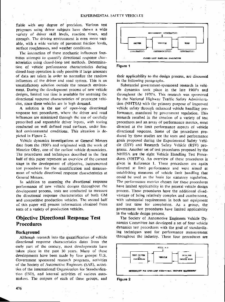
EXPERIMENTAL SAI.'ETY VEHICLES

fiable with any degree of precision. Various testprograms using driver subjects have shown a widevariety of driver skill levels, reaction times, andstrength. The driving environment is even more vari-able, with a wide variety of pavement friction levels,surface roughnesses, and weather conditions.

The interaction of these stochastic inflrrences frus-trates attempts to quantify directional response char-acteristics using closedJoop test methods. Determina-tion of vehicle performance characteristics duringclosed-loop operation is only possible if large amountsof data are taken in order to normalize the randominfluences of the driver and road system. This is anunsatisfactory solution outside the research environ-ment. During the development process of new vehicledesigns, limited test time is available for assessing thedirectional response characteristics of prototype vehi-cles, since these vehicles are in high demand.

A solution is the use of open-loop directionalresponse test procedure$, where the driver and roadinfluences are minimized through the use of carefullyprescribed and repeatable driver inputs, with testingconducted on well defined road surfaces, under lim-ited environmental conditions. This situation is de-picted in Figure 2.

Vchiclc dynamics investigations at General Motorsdate from the 1930's and originated with the work ofMaurice Olley, one of the earliest vehicle dynamicists.The procedures and techniques described in the firsthalf of this paper represent an overview of the currentstage in the development of objectivc, instrumentedtest procedures for the quantification and measure-ment of vehicle directional response characteristics atGeneral Motors.

In addition to assessing the directional responseperformance of new vehicle desigrrs throughout thedevelopment process, tests are conducted to measurethe directional response characteristics of both GMand competitive production vehicles. The second halfof this paper will present information obtained fromtests of a variety of production vehicles.

Objective Directional Response TestProcedures

BackgroundAlthough research into the quantification of vehicle

directional response characteristics dates from theearly part of the century, most developments havetaken place in the pa$t 30 years. Many of thesedevelopments have been made by four groups: U.S.Government sponsored research programs, activitiesof the Society of Automotive Engineers (SAE), activi-ties of the lnternational Orgarrization for Standardiza-tion (ISO), and internal activities of various auto-makers. The outputs of each of these groups, and

4t6

wrmHffiT ( smcEA.StIc)

(sscffiTrcl (DETERI'iIIISTrC) (afocHNTIC)

(Id5ED_I{DP lffiLTre EVALUATIOTI

Figure 1

their applicability to the design process, are discussedin the following paragraphs.

Substantial government-sponsored research in vehi-cle dynamics took place in the late 1960's andthroughout the 1970's. This research was sponsoredby the National Highway Traffic Safety Adminislra-tion (NHTSA) with the primary purpose of improvedvehicle safety through enhanced vehicle handling per-formance, mandated by government regulation. Thisresearch resulted in the creation of a variety of testprocedures and an array of performance metrics, mostdirected at the limit performance aspects of vehicledirectional respon$e. Some of the procedures pro-duced by these studies are the tests and performancegoals proposed during the Experimental Safety Vehi-cle (ESV) and Research Safety Vehicle (RSV) pro-grams. Another set of te$t procedures proposed by theNHTSA are the eight Vehicle Handling Test Proce-dures (VHTP's). An overview of thcsc procedures isgiven in Reference l. These proceclures are againdirected at limit perl'ormance and were aimecl atestablishing measures of vehicle limit handling thatcould be used as the basis for statutory regulation.The perfornrance metrics chosen for these procedureshave limited applicability in the general vehicle clesignprocess. These procedures have the additional disad-vantage of being relatively complex and cumbersome,with substantial requirements in both test equipmentand test time for completion. As a group, thegovernment test procedures have limited applicabilityin the vehicle design process.

The Society of Automotive Engineers Vehicle Dy-namics Committee has dcveloped a set of four vehicledynamics test procedures with the goal of stanclardiz-ing techniques used for performance measurementthroughout the industry. These fbur procedures are

till"oDolrg? ?oE opff-I# trftmrohAl, ffi6F0fl88 tGtfltEGtT

Figure 2

b-

SECTION 4. TECHNICAL SESSIONS

currently in draft form(2) and have been validated bya number of manufacturers and independcnt organiza-tions as providing representative data. The proposedtest procedures are the constant radius method, theconstant steering wheel angle method, the constantspeed method, and the constant throttle method.These procedures all measure steady state directionalresponse properties of a vehicle and employ similarperformance metrics. The last of the proceduresmeasures transient response properties as well and isvirtually jdentical to orre of the starrdard te$t flroce-dures used by General Motors (the Control RcsponseTest, discussed below).

The International Organization for Standardization(ISO) Vehicle Dynamics and Road Holding AbilitySubcommittee (Tfl 22/SC 9) has also developed aseries of vehiclc dynamics test$. These tests aregenerally directed at methods for measuring vehicleresponses on test tacilities available in Europe, wherelarge skid pads are less available than they arc in theUnited States. One of the procedures (ISO 4138) is anaccepted lnternational Standard(3) and is similar tothe constant radius test method contained in SAEXJ266. The remaining procedures (ISO/DP 7401),relating to the measurement of transient directionalresponse characteristics, are in dratl form(4). Theprocedures are basically conducted on straight roadsand emphasize the evaluation of perforrnance in thefrequency domain. An exception is the step input test,which is similar to the SAE constant throttle test andthe control re$ponse test ur;cd by GM.

The last major source of technology for the quanti-fication of directional response characteristics is themanufacturers themselves. The procedures and facili-ties used by General Motors are described in thefollowing paragraphs.

Data Acquisition Equipment IThe testing nccds of a vehicle manufacturer are

different than those of a research organization. TheIatter can afford the time to design ancl fabricatespecial transducers to suit the particular requirementsof a specific vehicle and can carel'ully instrument avehicle with numerous individual transducers. ln addi-tion to instrurnentation time. test turnaround time isalso a minor constraint in the research environment,with testing of a vehicle taking days or weeks tocomplete.

For the vehicle manufacturer, overall test time forobjective performance measurement must be rnini-mized due to thc high demand for prototype vehicles.This need to nrinimize test t ime has led to thedevelopment of specialized test and data acquisit ionequipment. This equipment has evolved into compact,modularized packages that can be quickly installed ina vehicle.

For most testing, four equipment modules are used:a data acqr.risit ion system, a transducer and signalconditioning module, an instrumented steering wheel,and a velocity transducer. This equipment is generalpurpose and can be applied to a variety of tests. Withthe modular equipment, a vehicle can be fully instru-mented and ready for test in less than one hour.

The data acquisition sy$tsm which has been devel-oped consists of a commercially available IBM PCcompatible microcomputer, equipped with additionalcommercially available cards to configure it for use asa data acquisit ion device. A custom l2 volt DC powersupply card completes the package, enabling thesystem to be operated from a standard vehicle electri-cal system. The system has thc following specil'ica-tions: 702 kB RAM, two 360 kB floppy disk drives,512 kB non-volati le bubble memory, and the capabil-ity of monitoring up to l6 analog data channels, withanalog-to-digital signal conversion. Digital samplingrates of 40 samples per second or less are used for alltests, as this sampling rate has been determined toprovide the desired accuracy without the need to take(and reduce) excessive anrounts ol 'data.

The transducer and signal conditioning modulecontains nlost transducers used in standard tests: afree gyroscope, used for measuring vehicle roll angle;a yaw rate gyroscope; a lateral accelerometer; and aforc-aft accelerometer. The package also contains allnecessary power sul:plies and signal conditioning to

suflport these transducers plus other standard trans-ducers (steering wheel angle, steering wheel torque,and vehicle velocity). The module does not use astabil ized platforrn for the accelerometers, as stabi-l ized platforms have been found to require excessivemaintenance when used in routine testing. Errorsresulting from vehicle roll and pitch motions arecorrected during data processing.

Two different instrumented steering wheel modulesare available for use in different types of testing. Bothof these modules require the removal of the produc-tion steering wheel. One steering wheel has the capa-bil ity of measuring steering wheel attgle and incorpo-rates adjustable stecring stops to enable repeatablestep $teer inputs to be made. Thc other steering wheelmeasures both steering wheel angle and steeringtorque.

The velocity transducer module currently employedis a standard tifth wheel. which has beeu found to beaccurate and durable in the production test environ-ment.

The complete instrumentation package which ltasbeen developed weighs approximately 60 kg and hasan operating current draw of approximately l0 A.

General Motors TestsAs stated above, the test needs of a manufacturer

are different lrom those of a research organization.

477

EXPERIMENTAL SAFETY VEHICLES

Directional response tests used by a manufacturermust be relatively routine and not overly complex, sothat vehicle testing can be accomplished expeditiously.

Objective directional response tests used by GeneralMotors are intended to quantity the performance ofvehicles to permit comparison of the directional re-sponse characteristics of new vehicle designs with thecharacteristics of existing vehicles. The procedurescurrently in use are directed at the quantification ofboth limit and sub-limit performance and have foundincreasing application in the CM design process. Theavailability of objective test information permits vehi-cles to be measured quantitatively throughout thedesign process.

The following objective tests are discussedpaper:

r Control Response Test. Frequency Response Testr Maximum Lateral Acceleration Test

On-Center Handlirrg TestLift-Dive TestCenter of Gravitv Test

Control Response TestThe control response test is a fixed control test (i.e.

- vehicle path is not defined) run at highway speed(Iffi km/h). This test speed was selected in order tomagnify vehicle performance differences as much aspossible, consistent with constraints imposed by testfacility size and test safcty. This test can be run to thelimits of vehicle performance in relative safety. Thetest procedure is virtually identical to tho$e containedin SAE XJ266 (constant throttle test) and ISO/DP7401 (step steer test), which are both based on theGM procedure. The test consists of a series ofstep-like steering inputs of increasing magnitude ap-plied from an initial condition of zero steering wheelangle and 100 km/h forward velocity. In each testrun, the steer input is held until steady-state turningconditions are established, then quickly removed. Thetest provides information on steady-state turning per-formance as well as transient characteristics bothentering and exiting a turn.

Because the vehicle path is not defined in thisopen-loop procedure, a large test surface is required.General Motors is able to run this tcst year-round,with the 67 acre Vehicle Dynamics Test Area at theMilford Proving Ground in Michigan permitting test-ing during the spring, summer, and fall months, and asimilar, smaller facility located at the Desert ProvingCround in Arizona permitting tests to be conductedduring the winter months.

A complete control response test consists of 30 ormore test runs, hall in each turn direction. Steeringwheel angle increments used range from 2 ] degrees tol0 degrees. During the test, the follow-ing vehicle

478

motion variables are continuously monitored: forwardvelocity, steering wheel anglc, roll angle, yaw velocity,fore-aft acceleration, and lateral acceleration.

The specific metrics evaluated are: understeer gradi-ent, roll gradient, sideslip gradient, steering sensitiv-ity, yaw velocity response time, and lateral accelera-tion response time. This test is utilized extensively inthe development process.

Frequency Response TestThe frequency response test provides gain and

phase relationships in the frequency domain describ-ing the dynamic response of a vehicle to steeringwheel angular displacement. The test procedure usedis similar to that described in the random inputmethod in the ISO/DP 7401 test procedure. The testis conducted at specified con$tant speeds (typically 100and 140 km/h) on a straight, three-lane road, withvehicle steer excitation using a broadband pseudo-random steering input. The steer input used is at'swept-$ine" input, comprising steer input frequenciesfrom near-Dc to the maximum frequency which thetest driver is capable of achieving. The swept-sineinput has been chosen to in$ure adequate input poweracross all steer frequencies.

During the test, steering wheel angle, yaw velocity,lateral acceleration, and roll angle are continuouslyrecorded. The recorded data are processed through adigital spectrum analyzer to define the spectral con-tent of each signal.

The transfer functions describing the yaw velocity,lateral acceleration and roll angle responses to asteering angle excitation are obtained for each testsegment and ensemble averaged for the entire test.The test is conducted within a lateral accelerationlimit of 0.4 g. The vehicle gains are normalized withsteering wheel angle.

Maximum Lateral Acceleration TestThe maximum lateral acceleration test measures the

maximum steady-state cornering capability of a vehi-cle on a constant radius circular cour$e. The testcourse used is similar to that specified in the constantradius part of the SAE XJ266 test procedure and tothat specified in the ISO 4138 test procedure. Thepurpo$e of the test is much different than thc SAEand ISO tests, however, and concentrates only on thevehicle's limit performance characteristics. The singletest metric is maximum lateral acceleration. The test isrun by driving the vehicle at the maximum speedattainable on a fixed radius circle, while still remain-ing on the circle. The test is run under driver control.This is one of the few closedJoop objective testsperformed by General Motors, and is somewhatdriver-sensitive.

During the test, vehicle velocity and yaw rate arecontinuously monitored. When these two variables are

this

a

I

a

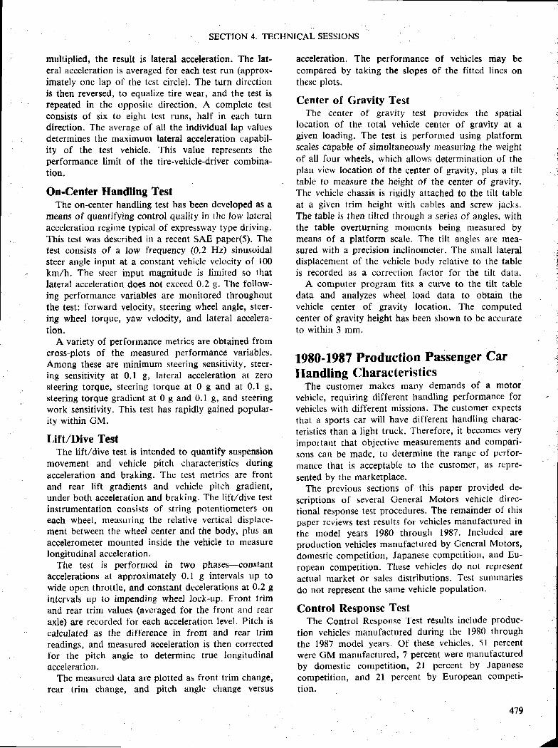
SECTION 4. TECHNICAL SESSIONS

multiplied, the result is lateral acceleration. The lat-eral acceleration is averaged for each test run (approx-imately one lap of the test circle). The turn directionis then reversed, to equalize tire wear, and the test isrepeated in the opposite direction. A complete testconsists of six to eight test runs, half in each turndirection. The average of all the individual lap valuesdetermines the maximum lateral acceleration capabil-ity of the test vehicle. This value represents theperformance limit of the tire-vehicle-driver combina-tion.

On-Center Handling TestThe on-center handling test has been developed as a

means of quantifying control quality in the low lateralacceleration regime typical of expressway type driving.This test was described in a recent SAE paper(S). Thetest consists of a low frequency (0.2 Hz) sinusoidalsteer angle input at a constant vehicle velocity of 100km/h. The steer input magnitude is limited so thatlateral acceleration does not exceed 0.2 g. The follow-ing performance variables are monitored throughoutthe test: forward velocity, steering wheel angle, $teer-ing wheel torque, yaw velocity, and lateral accelera-tion.

A variety of performance metrics are obtained fromcross-plots of the measured performance variables.Among these are minimum steering sensitivity, steer-ing sensitivity at 0.1 g, lateral acceleration at zerosteering torque, steering torque at 0 g and at 0.1 g,steering torque gradient at 0 g and 0.1 g, and steeringwork sensitivity. This test has rapidly gained popular-ity within GM.

Lift/Dive TestThe lift/dive test is intended to quantify suspension

movement and vehicle pitch characteristics during

acceleration and braking. The test metrics are frontand rear lift gradients and vehicle pitch gradient,under both acceleration and braking. The lift/dive ter;tinstrumentation consists of string potentiometers oneach wheel, rneersuring the relative vertical displace-ment between the wheel center and the body, plus anaccelerometer mounted inside the vehicle to measurelongitudinal acceleration.

The test is performed in two phases-constantaccelerations at approximately 0.1 g intervals up towide open throttle, and constant decelerations at 0.2 g

intervals up to impending wheel lock-up. Front trimand rear trim values (avcraged for the front atrd rearaxle) are recorded for each acceleration level. Pitch iscalculated as the difference in front and rear trimreadings, and measured acceleration is then correctedfor the pitch angle to determine true longitudinalaccelcration.

The measured data are plotted as front trim change,rear trim change, and pitch angle change versus

acceleration. The performance of vehicles may becompared by taking the slopes of the fitted lines onthese plots.

Center of Gravity TestThe center of gravity test provides the spatial

location ol the total vehicle center of gravity at agiven loading. The test is performed using platformscales capable of simultaneou.rly measuring the weightof all four wheels, which allows determination of theplan view location of the center of gravity, plus a tilttable to measure the height of the center of gravity.The vehicle chassis is rieidly attached to the tilt tableat a given trim height with cables and screw jacks.The table is then tilted through a .series of angles, withthe table overturning moments being measured bymeans of a platform scale. The tilt angles are mea-sured with a precision inclinometer. The small lateraldisplacement of the vehicle body relative to the tableis recorded as a correction factor for the tilt data.

A computer program fits a curve to the tilt tabledata and analyzes wheel load data to obtain thevehicle center of gravity location. The computedcenter of gravity height has been shown to be accurateto within 3 mm.

1980-1987 Production Passenger CarHandling Characteristics

The custonrer makes many demands of a motorvehicle, requiring different handling performance forvehicles with different missions. The customer expectsthat a sports car will have dilterent handling charac-teristics than a Iight truck. Therefore, it becomes veryimportant that objective measurements and compari-sons can be made, to determine the range of perfor-mance that is acceptable to the customer, as I'epre-sented by the marketplace.

The previous sections of this paper provided de-scriptions of several General Motors vehicle direc-tional response test procedures. The remainder of thispaper reviews test results for vehicles manufactured inthe model years 1980 through 1987' Included areproduction vehicles manufactured by Gcneral Motors,domestic competition, Japanese competition, and Eu-ropean competition. These vehicles do not reprcsentactual market or sales distributions. Test summariesdo not represent the same vehicle population'

Control Response TestThe Control Response Test results include produc-

tion vehicles manufactured during the 1980 throughthe 1987 model years. Of these vehicles, 5l percentwere GM manufactured, 7 percent were manufacturedby domestic competition, 2l percent by Japanesecompetition, and 2l percent by European competi-tion.

l479

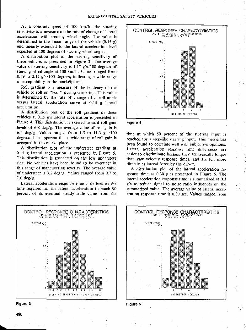
EXPERIMENTAL SAFETY VEHICLES

At a constant speed of 100 km/h, the steeringsensitivity is a measure of the rate of change of lateralacceleration with steerirrg wheel angle. The value isdetermined in the linear range of the vehicle (0.15 e)and linearly extended to the lateral acceleration levelexpected at 100 degrees of steering wheel angle.

A distribution plot of the steering sensitivity ofthese vehicles is presented in Figure 3. The averagevalue of steering sensitivity is 1.17 g'sl100 degrees of$teering wheel angle at 100 km/h. Values ranged from0.59 to 2.17 g's/lM degrees, indicating a wide rangeof acceptability in the marketplace.

Roll gradient is a measure of the tendency of thevehicle to roll or "lean" during cornering. This valueis determined by the rate of change of a roll angleversus lateral acceleration curve at 0.15 g lateralacceleration.

A distribution plot of the roll gradient of thesevehicles at 0.15 g's lateral acceleration is presented inFigure 4. This distribution is skewed toward roll gainlevels of 6-8 deg/g. The average value of roll gain is6.4 deg/g. Values ranged from 1.5 to ll.3 g's/100degrees. It is apparent that a wide range of roll gain isaccept€d in the marketplace.

A distribution plot of the understeer gradient at0.15 e lateral acceleration is presented in Figure 5.This distribution is truncated on the Iow understeerside. No vehicles have been found to be oversteer inthis range of maneuvering severity. The average valueof understeer is 3.2 deg/g. Values ranged frorn 0.7 to7.0 deg/s.

Lateral acceleration response time is defined as thetime required for the lateral acceleration to reach 90percent of its eventual steady $tate value from the

GOfiV'Ir]ROL HESFONSE CHARAGT EHIS]=flGS1 9 8 0 _ 8 7 F R O I J U C T I O N P A S S E N G E R C A R s

R O L L G A I N ( D E G . / G )

PE RCE NTACE4 0

? 4 6 I t 0

R O L L G A I N ( D E C , / G )

Figure 4

time at which 50 percent of the steering input isreached for a step-like steering input. This metric hasbeen found to correlate well with subjective opinions.Lateral acceleration response time differences areeasier to discriminate because they are typically longerthan yaw velocity response times, and are felt moredirectly as lateral force by the driver.

A distribution plot of the lateral acceleration re-sponse time at 0.30 g is presented in Figure 6. Thelateral acceleration response time is surnmarized at 0.3g's to reduce signal to noise ratio influences on thesummarized value. The average value of lateral accel-eration response time is 0.39 sec. Values ranged from

CON]TRQL RFSFOII\.I] g,E GHARAGTETF{I$TI]C$1 S 8 0 - 8 7 p f t 0 D U C r 0 N F A 5 5 t ^ N c E R C A F S

: i t i l - R N c t ; l N l ; T t v | l y ( c - i , / 1 0 0 O t c . )

P E R C E N T A G EJO

0 . 6 0 . 8 1 . 0 1 . ? 1 . 4 1 . 6 1 . 8

S T E E R I N G S E N S I T I V I T Y ( G _ S , / 1 O O O E G )

Figure 3

GON]THOL IRIE$FMfr{SE CHARAffi TEHI$IJ-rcS] 9 8 0 - T i 7 P H O I ] U C T I O N P A S S T N G E R C A R S

U N D E R S T E I R ( O h ( ; , / ( ] )

P I R C E N T A 6 EJ O

2 J 4 5

U N D E R S T E E R ( D E G l 6 )

Figure 5

\

480

SECTION 4. TECHNICAL SESSIONS

0.23 to 0.77 sec. Short lateral acceleration responsetimes are perceived as better.

Frequency Response TestThe Frequency Response Test results include pro-

duction vehicles manufactured during the 1983through the 1987 model years. Of these vehicles, 33percent were GM manufactured, 9 percent were man-ufactured by domestic competition, 33 percent byJapanese competition, and 25 percent by Europeancompetition, Many of these vehicles are equipped withoptional handling suspensions and tires.

Lateral acceleration bandwidth is the liequency atwhich the lateral acceleration response of the vehicleis reduced by 3 decibels. A distributicn plot of thelateral acceleration bandwidth of these vehicles ispresented in Figure 7. The average value of lateralacceleration bandwidth is 0.99 Hertz. Values rangedfrom 0.66 to 1.32 Hertz. High lateral acceierationbandwidths are perceived as better.

Yaw velocity bandwidth is the frequency at whichthe yaw velocity response of the vehicle is reduced by3 decibels. A distribution plot of the yaw velocitybandwidth of these vehicles is presented in Figure 8.The average value of yaw velocity bandwidth is 2.8Hertz. Values ranged from 2.1 to 3.5 Hertz. Again,high yaw velocity bandwidths are perceived as betterif the yaw damping is acceptable.

The peak to steady state yaw velocity ratio yields ameasure of the damping of the vehicle yaw velocityresponse. A distribution plot is presented in Figure 9.The average value of the peak to steady state yawvelocity ratio for these vehicles is 1.4, ranging froml.l to 2.1. Low ratios are perceived as better if theyaw velocity bandwidth is acceptable.

Figure 7

Both the yaw velocity and roll responses of vehiclesexhibit a peaked frequency response. The ratio of thefrequencies at which the corresponding peaks occurcan be used to indicate roll-yaw velocity coupling invehicles with lightly damped roll modes. A distribu-tion plot of the peak roll-yaw velocity frequencyratios is presented in Figure 10. The average value forthese vehicles is 2.0, ranging from I to 4. Valueshigher than I are perceived to be better for vehicleswith lightly damped roll modes.

It has been noted in the literature that subjectiveopinions of vehicle handling improve when the phasedifference between yaw velocity and lateral accelera-tion is reduced. This pararneter can be determinedfrom the frequency re$ponse test result$. The actualparameter is the average phase angle difference be-tween the yaw velocity and lateral acceleration be-tween 0.2 Hertz and the latcral acceleration band-width of the vehicle. A distribution plot of the phasedifferences measured is presented in Figure ll. Theaverage value for these vehicles is 17 degrees. The

.. . ;

DEECTiOI{AL COi!I|ROL FREQUEiTCV RESPOT{$E 0t"{AfiAclERtslftos9 8 1 8 - F A S s F , ( , l l ^ r r

L A I I F A I A C ( : T I T R A I O N E A N O W I O I H ( H 2 )

PEFCINT^GE4 0

50

? 0

i o

0

ffi

ffiffiHilli:l ::::::i:tiil!:: .:i:l l ] : : : . . t l

Fi:,,,,,,:,t;lffi:" "":r1 m

ffi ffi# iii,,,, ,,,,i1*.,,- Ht;,,, :: ::;:.::.:.t t . l

r " ^ : " " , , r . r " , - o n . n u ' , n u i ,

GONTHOL RE$FON{SE CHAHAGTEHISTOES] 9 8 0 - 8 7 P R O D U C T L O N P A S S E N G E R C A R S

L A T E R A T A C C E L E R A T J O N F E 5 F O N S E T I M T ( 5 E C . )

PERCENT AGE4 0

0 . 2 0 0 . ? i r

I A T I . H A I

0 . . 1 0

A { i t .

Figure 6

DfiECTlqNAL Cofi,{lfF0rL. [-FlEQl-JElA,lCY RESPOf{SE CIIARACTEFNiT|GS1 ! 8 0 6 / F A ! 5 t t u c E F C A R S

Y A W V F , L d C T Y E A N b W I O I H ( H 2 )

PERCENIACE4 0

30

20

r 0

0

Figure I

481

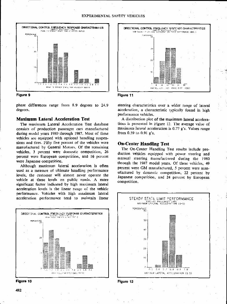
DIRECTEfiIAL CONTTHOL FHEQ{JEhICY RESPOI{SE CHARACTEHISTICSI g E O - E / F A S S L N C I R C A F S

F E A X T O S T E A D Y S T A T E I A W V E L O C I T Y R A T I O

F E R C T N T A 6 IJO

1 . 0 r r r . 2 r J 1 4

P E A ( T O S T E A O Y

EXPERIMENTAL SAFETY VEHICLES

Figure I

phase differences range from 8.9 degrees to 24.9degrees.

Maximum Lateral Accelemtion TestThe maximum Lateral Acceleration Test database

consists of production passenger car$ manufacturedduring model years 1980 through 1987. Most of thesevehicles are equipped with optional handling suspen-sions and tires. Fifty five percent of the vehicles weremanufactured by General Motors. Of the remainingvehicles, 3 percent were domestic competition, 26percent were European competition, and 16 percentwere Japanese competition.

Although maximum lateral acceleration is oftenused as a measure of ultimate handling performancelevels, the customer will almost never operate thevehicle at these levels on public roads. A moresignificant factor indicated by high maximum lateralacceleration levels is the linear range of the vehicleperformance. Vehicles with high maximum lateralacceleration performance tend to maintain linear

Flgure 10

482

DHECll0ohlAL coNTRoL FRrEO{jEhrfiV HESFffihrsE Clt.iAHACtfERtStftosyAw vELoc I Ty-L A rER!l*'iA', JiH*ff tii I ii,Tr'' o, r.r*rr.,, or.,

PERCEN I ACI4 0

Figure 11 :

steering characteristics over a wider range of lateralacceleration, a characteristic typically found in highperformance vehicles.

A distribution plot of the maximum lateral accelera-tions is presented in Figure 12. The average value ofmaximum lateral acceleration is 0.77 g's. Values rangefrom 0.59 to 0.91 g's.

On-Center Hnndling TestThe On-Center Handling Test results include pro-

duction vehicles equipped with power steering andmanual steering manufactured during the l9B0through the 1987 model years. Of these vehicles, 49percent were GM manufactured, 5 percent were man-ufactured by domestic competition, 22 percent byJapanese competition, and 24 percent by Europeancompetition.

i i lr i

DtREo rf |ohlArL c@r{rHor F,HFrp,rJflryFEyrcFiti'fl.iTT GFTARACTEF

F E F I E N I A G E ." "1I1 k f f i

,ol ffiI i:,{,11ffirffif#[h;;iilllii:'iii# w- 'rij.li i::i:::: ,,,.ra il#,ffir[rii]r'xiiiii+lir:l:iffi ffil[i{+ i+ii l# r:ri;ii iiffi ffiffi

.ffiiffi ;,H ffiffiffir Lr : , ,1 1, , : ;^" ' , ; ,0 ,1, i , ' ,1 ' , ] '

'u

S T E A D Y S T A T E L I M I T P E R F O R M A N C E1 9 8 0 - 8 7 P A S S E N G t h - C A R t

M A X I M U M L A I L R A L A C C E L E R A I I O N ( 6 _ 5 )

P E R C E N T A C E

0 , 5 0 , 6 a . / D I 0 . 9 r . O

M A X I M U M L A T T R A L A C C h I L R A I I O N ( G - 5 )

Flgure 12

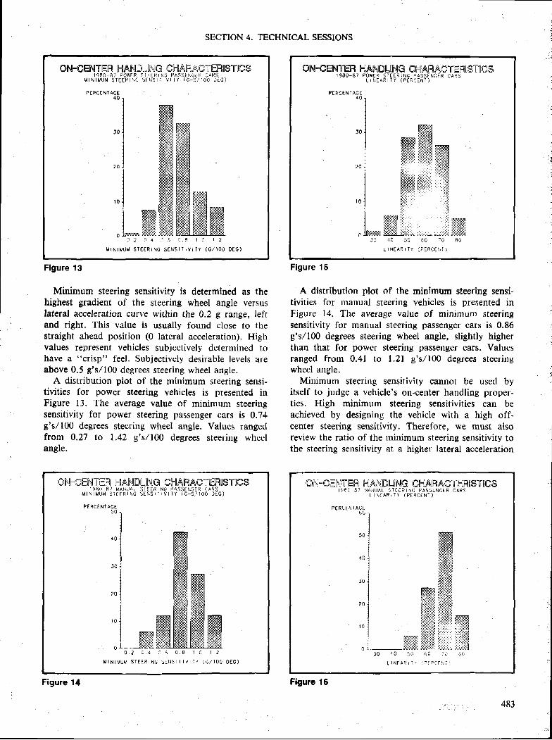
SECTION 4. TECHNICAL SESSIONS

Flgure 13

Minimum steering sensitivity is determined as thehighest gradient of the steering wheel angle versuslateral acceleration curve within the 0.2 g range, leftand right. This value is usually found close ro thestraight ahead position (0 lateral acceleration). Highvalues represent vehicles subjectively determined tohave a "crisp" feel. Subjectively desirable levels areabove 0.5 g's/100 degrees steering wheel angle.

A distribution plot of the minimum steering sensi-tivities for power steering vehicles is presented inFigure 13. The average value of minimum steeringsensitivity for power steering passenger cars is 0.74g's/100 degrees steering wheel angle. Values rangedfrom 0.27 to 1.42 g'sl100 degrees steering wheelangle.

ON*CENTEH !.{ANDL[NG CHAHACTERO$TICS1 9 E O - 8 7 P O W E R S T t E R I i ] C F A S S F N G E R C A R S

L i N T A F I T Y ( F T R C E N T )

PERCE N I ACE4 A

JO

2 0

t 0

Figure 15

A distribution plot of the minimum steering sensi'tivities for manual steering vehicles is presented inFigure 14. The ayera1e value of minimum steeringsensitivity for manual steering passenger cars is 0.86g's/100 degrees steering wheel angle, slightly higherthan that for power steering passenger cars. Valuesranged from 0.41 to l.2l g's/100 degrees steeringwheel angle.

Minimum steering sensitivity cannot be used byitself to judge a vehicle's on-center handling proper-ties. High minimum steering sensitivities can beachieved by designing the vehicle with a high off-center steering sensitivity. Therefore, we must alsoreview the ratio of the minimum steering sensitivity tothe steering sensitivity at a higher lateral acceleration

ON-OENTEH HANDLilD'IG GHAR/\GTEHISTICS1 9 8 0 _ 8 7 P O W E R 5 I L T R I N G P A 5 5 L N G L H ( : A R S

M I N I M U M S T E E R I N C 5 I N 5 T I V I ] Y ( G _ : ; / 1 0 i . ] D L G )

PERCE N TAGE4 0

ffiffiffi

gffi ffS$fl

ffi# H:ff

,l^in,o'',1*

{DF,I-GED'JTEH HANDLIFJG GHAHACTEH0STICS] 9 8 0 8 7 M A N I . J A t S T t E R I N C P A S S E N C E R C A R S

M I N ] M U M 5 ] F F R I N G S E N 5 I T I V I T Y ( C _ 5 , / 1 O O D E C )

P E R C T N T A 6 L5 0

r 0

0 ffi0 . ? 0 . 4 0 . 6 0 . 8 1 . 0 1 2

M I N I M U M S T E E R I N G 5 L N 5 I I V I T Y ( G / ] O ODEG )

Figure 14

ON{-GEF{TER HAFJDLINJG CHAIRAGTHIHOSIIIG$] 9 8 0 8 7 M A N U A L 5 T E E R I N G I J A S S L N I j L R c A H 5

I I N T A R I T Y ( P I R C E N T )

P E R C E N T A C E6 0

50

4 0

l 0

2 0

1 0

0

Flgure 16

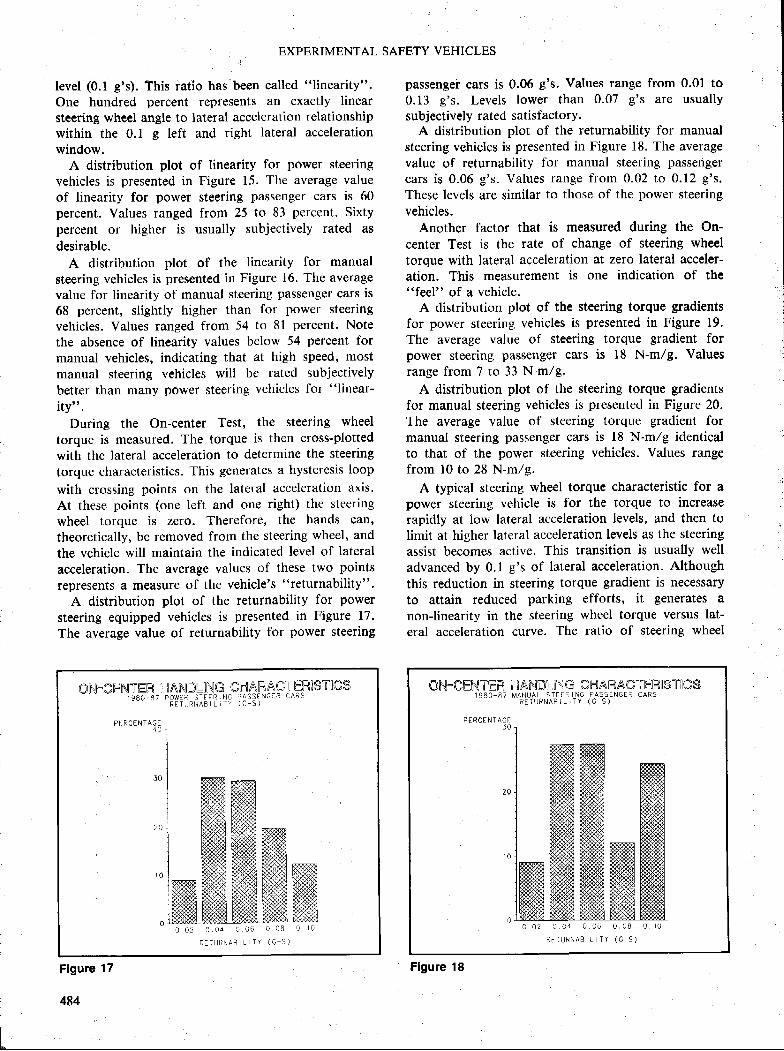
EXFERIMENTAL SAFETY VEHICLES

level (0.1 g's). This ratio has been called "linearity".

One hundred percent represents an exactly linearsteering wheel angle to lateral acceleration relationshipwithin the 0.1 g left and right lateral accelerationwindow.

A distribution plot of linearity for power steeringvehicles is presented in Figure 15. The average valueof linearity for power steering passenger cars is 60percent. Values ranged from 25 to 83 percent. Sixtypercent or higher is usually subjectively rated asdesirable.

A distribution plot of the linearity for manualsteering vehicles is presented in Figure 16. The averagevalue for linearity of manual steering passenger cars is68 percent, slightly higher than for power steeringvehicles. Values ranged from 54 to 8l percent' Notethe absence of linearity values below 54 percent formanual vehicles, indicating that at high speed, mostmanual steering vehicles will be rated subjectivelybetter than many power steering vehicles for "linear-

ity".During the On-center Test, the steering wheel

torque is measured. The torque is then cross-plottedwith the lateral acceleration to determine the steeringtorque characteristics. This generates a hysteresis loop

with crossing points on the lateral acceleration axis'At these points (one left and one right) the steeringwheel torque is zero. Therefore, the hands can'theoretically, be removed from the steering wheel, andthe vehicle will maintain the indicated level oI lateralacceleration. The average values of these two pointsrepresents a measure of the vehicle's "returnability"'

A distribution plot of the returnability for powersteering equipped vehicles is presented in Figure 17.The average value of returnability for power steering

a)fi{-GfrlilJTEH I iI,A$,1]DL[F{C GHiAH AFTERI$I| tlffi $t g 8 0 - 8 7 t r O W L t s , _ r - f F f t . \ 6 r r n S : i E \ C F E C ^ H : l

R E T I ] R N A E I L I T Y ( C _ 5 )

P F R C E N T A G I4 0

J O

? o

passengei cars is 0.06 g's. Values range from 0.01 to0.13 g's. Levels lower than 0.07 g's are usuallysubjectively rated satisfactory.

A distribution plot of the returnability for manualsteering vehicles is presented in Figure 18. The averagevalue of returnability for manual steering passengercars is 0.06 g's. Values range fiom 0.02 to 0. 12 g's.These levels are similar to those of the power steeringvehicles.

Another factor that is measured during the On-center Test is the rate of change of steering wheeltorque with lateral acceleration at zero lateral acceler-ation. This measurement is one indication of the"feel" of a vehicle.

A distribution plot of the steering torque gradientsfor power steering vehicles is presented in Figure 19.The average value of steering torque gradient forpower steering pas$enger cars is t8 N-m/g. Valuesrange from 7 to 33 N-m,zg.

A distribution plot of the steering torque gradientsfor manual steering vehicles is presented in Figure 20.The average value of steering torque gradient formanual steering passenger cars is l8 N-m/g identicalto that of the power steering vehicles. Values rangefrom l0 to 28 N-m,/g.

A typical steering wheel torque characteristic for apower steering vehicle is for the torque to increaserapidly at low lateral acceleration levels, and then tolimit at higher lateral acceleration levels as the steeringassist becomes active. This transition is usually welladvanced by 0.1 g's of lateral acceleration. Althoughthis reduction in steering torque gradient is necessaryto attain reduced parking efforts, it generates anon-linearity in the steering wheel torque versus lat-eral acceleration curve. The ratio of steering wheel

m$$:eE$,$lrEH Ii ll,A,lNlDl lllNlG ffihHi\LRl\crHHllslf ucs1 9 8 0 - 8 7

P E R C E N T A C FJ O

M A N I J A I S T F F R I N G F A 5 5 E N 6 E R C A R SR E T U R N A B I L I T Y ( C S )

0 l

Figure 17

484

Flgure 18

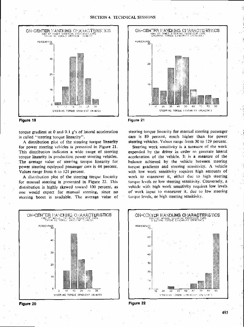
SECTION 4. TECHNICAL SESSIONS

ch{ " c.: ENTEH }-N,ANlrD[-.r]rNlG CH Ar'.r /\ r-]T EHI $]f I (0 $r 1 1 8 0 . 8 ' p J w t t ! T E E F T \ 6 l r ^ : j L : : \ t ; L r ( A { : l

S I L L I i I N C I O R O I J E C R A D I I N T ( N - M , / C )

P E R C E N T A 6 E4 0

. r i 0 t b , ) 0

S T E E R I N C T O R Q U E G R A { J I

ffiffiFS#

ffimt5 ,10

ENT (N.M, /C

Flgure 19

O)D\I]-{CEN\IT EIIX E-I,AND[ j]INIffi (C[ N AR A(DTEMIFJTIG$r g 8 0 t l 7 p o w E R S T t t R r N L p A 5 5 E N 6 t R r j A R 5S I E E R I N G I O R O U E L I N E A R ] T Y ( F I R C I - N T )

P E R C E N I A G Lt 0

r 0 2 0 l 0 4 0 5 0 6 0 7 t ) 8 0 9 0

S T E E R I N G T O R O U E L I N E A R I T Y ( P E R C E N I )

Figure 21

torque gradient at 0 and 0.1 g's of lateral accelerationis called "steering torque linearity".

A distribution plot of the steering torque linearityfor power steering vehicles is presented in F'igure 21.This distribution indicates a wide range of steeringtorque linearity in production power steering vehicles.The average value of steering torque linearity forpower steering equipped passenger cars is 44 percent.Values range from 6 to l2l percent.

A distribution plot of the steering torque linearityfor manual steering is presented in Figure 22. Thisdistribution is highly skewed toward 100 percent, asone would expect for manual steering, since nosteering boost is available. The average value of

steering torque Iinearity for manual steering passengercars is 89 percent, much higher than lbr powersteering vehicles, Values range from 30 to 129 percent.

Steering work sensitivity is a measure of the workexpended by the driver in order to generate lateralacceleration of the vehicle. It is a measure of thebalance achieved by the vehicle between steeringtorque gradients and steering sensitivity, A vehiclewith low work sensitivity requires high amounts ofwork to maneuver it, either due to high steeringtorque levels or low steering sensitivity. Conversely, avehicle with high work sensitivity requires low levelsof work input to maneuver it, due to low steeringtorque levels, or high steering sensitivity.

CFil*OEF'IIIEH I 1I,A\L\]IDLON,Jffi {Gr'{ AR AA]TEH] 9 8 0 - 8 7 M A N L J A L 5 I L L R I N G P A I i 5 E N C E R C A R 5

S I L L R I N C T ( ) F O U I C R A D I N T ( N - M , / G )

ilsTm$

P E R C E N T A C E50

5 1 0 1 5 ? o ? 5 3 0

S T E E R I N G T O R O U E G R A O I T N T ( N _ M , / G )

Flgure 20

OFrI-OED\0TLEH HANIIDLING OHAHACTEH0$-Iffi$1 ! } 8 0 _ 8 7 M A N U A L S I E E R I N G P A S S E N G E R C A R S

5 I L L R I N C T O R O I ' E I I N T A R I T Y ( P E R C E N T )

PERCE NT AG E7 0

6 0

50

4 0

30

2 0

1 0

0? 0 J 0 4 0 5 0 6 0 7 n 8 0 9 0

5 T E E R I N C T O R O I J E I . ] N f A R T f ( P L H C L N ] )

Flgure 22

485

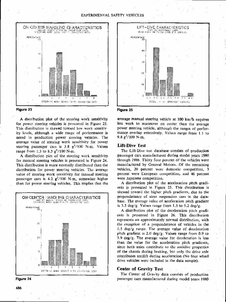
EXPERIMENTAL SAFETY VEHICLES

fr)n{ -c EN T tE R r-il A\ t},t ID[_[R{ G 0[---i A H AC TER I S,T0CS1 9 8 0 - 8 7

S T I I R I N GP O W I ] I I 5 T I F R N G F A S 5 E N C E R C A f t S

w o R E 5 L N 5 l I l V l l Y ( c i r ? / 1 0 0 t J [ 6 )

PERCEN IAGE4 0

Figure 23

A distribution plot of the steering work sensitivityfor power steering vehicles is presented in Figure 23.This distribution is skewed toward low work sensitiv-ity levels, although a wide range of performance isnoted in production power $teering vehicles. Theaverage value of steering work sensitivity for powersteering passenger cars is 3.8 g2ztoo N-m. Valuesrange from 1.3 to 8.5 g2l100 N-m.

A distribution plot of the steering work sensitivityfor manual steering vehicles is presented in Figure 24.This distribution is more normally distributed than thedistribution for power steering vehicles. The averagevalue of steering work sensitivity for manual steeringpassenger cars is 4.2 E2/100 N-m, somewhat higherthan for power steering vehicles. This implies that the

ON-CEhilTEHI S 8 0 - 8 7

S I L E R I N G

I iI,ANIDI .ilINIG ffi h.XAtR/\GI-HIfi ilSTOffiSM A N U A L 5 l L L I I ] N G P A 5 S L N G L F I C A R Sw o R K S E N S T T T V T T Y ( G . . 2 / 1 0 0 0 t c )

PERCENT AGE4 0

Flgure 24

L I F T - D I V E C H A R A C T E R I S T I C S_ 1 $ d 0 - 8 6 P A 5 5 E \ 6 E q C A R SD E C E L E R ^ I o \ t r ' - C r '

c o A D E \ T ( D F G , / G )

PERCEti]AGE

Figure 25

average manual steering vehicle at 100 km/h requiresless work to maneuver on center than tne averagepower steering vehicle, although the ranges of perfor-mance overlap extensively. Values range from l.l to9.8 g2ltoo tt-m.

Lift-Dive TestThe Lift-Dive test database consists of production

passenger cars manufactured during model years 1980through 1986. Thirty four percent of the vehicles weremanufactured by General Motors. Of the remainingvehicles, 20 percent were domestic competition, 3percent were European competition, and 46 percentwere Japanese competition.

A distribution plot of the acceleration pitch gradi-ents is presented in Figure 25. This distribution isskewed toward the higher pitch gradients, due to thepreponderance of strut suspension cars in the data-base. The average value of acceleration pitch gradientis 3.3 deglg. Values range from 1.3 to 5.2 deg/g.

A distribution plot of the deceleration pitch gradi-ents is presented in Figure 26. This distributionrepresents an approximately normal distribution, withthe exception of a preponderance of vehicles in the1.5 deg/g range. The average value of decelerationpitch gradient is 2.0 dee/e. Values range from 0.9 to3.9 deg/g. The average value for deceleration is Iessthan the value for the acceleration pitch gradients,since both axles contribute to the antidive propertiesof the chassis during braking, but only the drive axlecontributes antilift during acceleration (No four wheeldrive vehicle$ were included in the data sample).

Center of Gravity TestThe Center of Cravity data consists of production

pas$enger cars manufactured during model years 1980

486

SECTION 4. TECHNICAL SESSIONS

L I F T * D I V E C H A R A C T E R I S T I C S1 3 8 0 _ 8 6 P A 5 5 E N C E R C A R S

A C C E L E R N T I O N P I I C H C R A O I E N T ( D E G , / G )

PERCE NTAGE30

Flgure 26

VEHOGIIE L;EI{T.ELft O]F ffiRAVITV [ilFIGH.1 9 8 0 * 8 7 P R O D U C I I O N P A S S I N G E R C A R S

CURB WEIGHIPBCBTACE

{o

ffiffi

ffiffiffiffiffi[S ffi fl:j[+'1 F+,1['1.r,; 3 ;CSNTER OF CRAVITT HT (D)

Figure 27

through 1987. Twenty percent of the vehicles weremanufactured by General Motors. Of the rernainingvehicles, 15 percent were dome$tic competition, 29percent were European competition, and 36 percentwere Japanese competition.

A distribution plot of the center of gravity heightsis presented in Figure 27. The averag€ value of vehiclecenter of gravity height is 520 mm. Values range from437 mm to 589 mm.

Summary rr

This paper documents the usefulness of openJooptest procedures in the measurement of vehicle direc-tional response characteristics. The development ofdirectional response test procedures in the U,S. wasdiscussed. An overview of some of the objective testprocedures used by General Motors for the assessmentof vehicle directional response characteristics wasprovided, together with a discussion of the keyperformance metrics obtained from these tests, Astatistical analysis of test clata for 1980 through 198?model year production vehicles was performed, notingaverages and ranges for these performance metrics.

Referencesl. Ervin, R.D., Fancher, P.S., and Segel, L., "Re-

finement and Application of Open-Loop LimitManeuver Response Methods", SAE 730491, May1973.

2. Anon., "Passenger Car and Light Truck Direc-tional Control Response Test Procedures", Pro-posed SAE Recommended Practice XJ266.

3. Anon., "Road Vehicles - Steady State CircularTest Procedure", lnternational $tandard ISO4138.

4. Anon., "Road Vehicles - Lateral Transient Re-spon$e Test Procedure$", ISO/DP 7401 DraftProcedure, November 1984.

5. Norman, K.D., "Objective Evaluation of On-Center Handling Performance", SAE 840069,February 1984.

The Ergonomics of Driver Information Systems for Maintained Safety(lYritten only paper)D. Southhall,M.K. Twiss.Institute for Consumer Ergonomics,United Kingdom

. :Abstract

The development of a safe vehicle must recognizethe requirement to maintain that level of safety forthe design life of the vehicle. Whilst secondary safety,

i,e. occupant protection is to a large part determinedby the design team, primary safety, i.e. accidentavoidance. has in the past been the ultimate responsi-bility of the owner,/driver.

In recent years with new developments this situationhas begun to change with the provision by themanufacturer of systems to aid accident avoidance:antilock braking is perhaps the most obvious example.

This paper propo$es that another important aspectof primary safety where the motor manufacture can

487

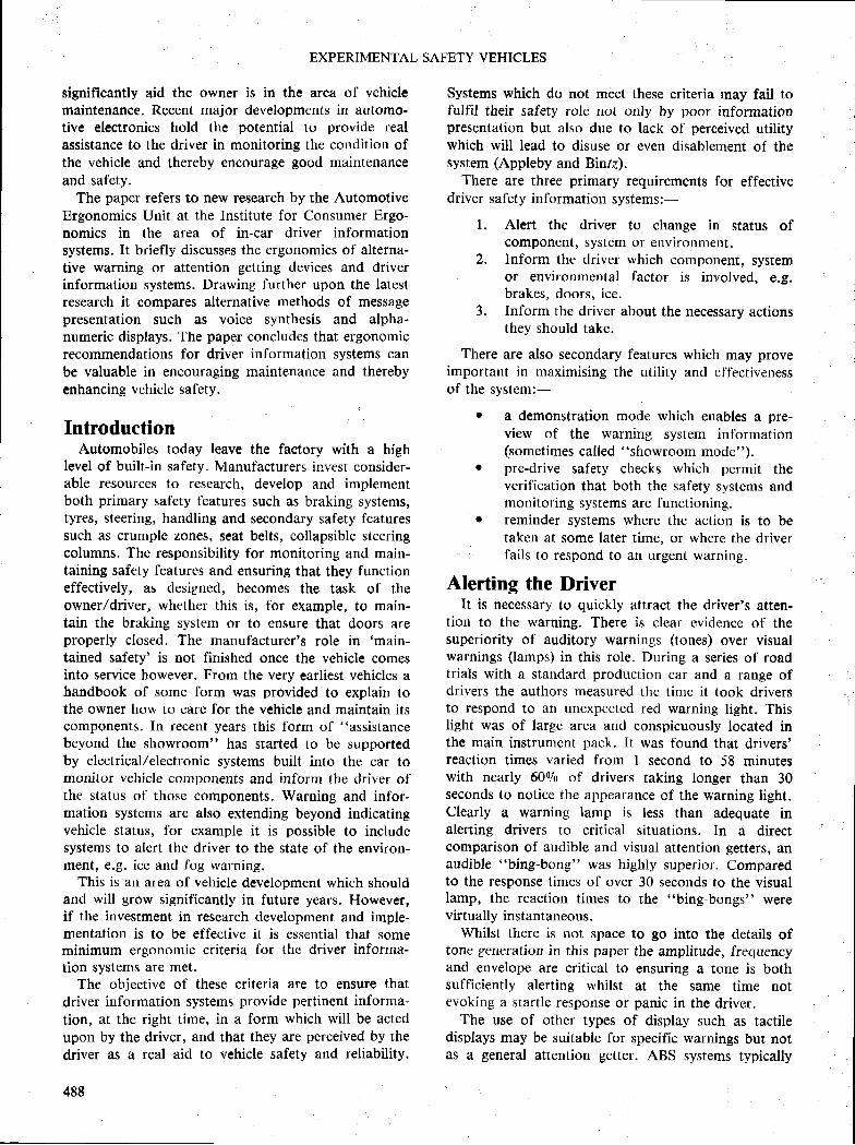
EXPERIMENTAL SAFETY VEHICLES

significantly aid the owner is in the area of vehiclemaintenance. Recent major developments in automo-tive electronics hold the potential to provide realassistance to the driver in monitoring the condition ofthe vehicle and thereby encourage good maintenanceand safety.

The paper refers to new research by the AutomotiveErgonomics Unit at the lnstitute for Consumer Ergo-nomics in the area of in-car driver informationsystems. It briefly discusses the ergonomics of alterna-tive warning or attention getting devices and driverinformation system$. Drawing further upon the latestresearch it compares alternative methods of messagepresentation such as voice synthesis and alpha-numeric displays. The paper concludes that ergonomicrecommendations for driver information systems canbe valuable in encouraging maintenance and therebyenhancing vehicle safety.

IntroductionAutomobiles today leave the factory with a high

level of built-in safety. Manufacturers invest consider-able resources to research, develop and implementboth primary safety features such as braking systems,tyres, steering, handling and secondary safety featuressuch as crumple zones, seat belts, collapsible steeringcolumns. The responsibility for monitoring and main-taining safety features and ensuring that they functioneffectively, as designed, becomes the task of theowner,/driver, whether this is, for example, to main-tain the braking system or to ensure that doors areproperly closed. The manufacturer's role in 'main-

tained safety' is not finished once the vehicle comesinto service however. From the very earliest vehicles ahandbook of some form was provided to explain tothe owner how to care for the vehicle and maintain itscomponents. In recent years this lorm of "assistance

beyond the showroom" has started to be supportedby electrical/electronic systems built into the car tomonitor vehicle components and inform the driver ofthe status of those components. Warning and infor-mation systems are also extending beyond indicatingvehicle status, for example it is possible to include$ystems to alert the driver to the $tate of the environ-ment, e.g. ice and fog warning.

This is an area of vehicle development which shouldand will grow significantly in future years. However,if the investment in research development and imple-mentation is to be effective it is essential that someminimum ergonomic criteria for the driver informa-tion sy$tems are met.

The objective of these criteria are to ensure thatdriver information systems provide pertinent informa-tion, at the right time, in a form which will be actedupon by the driver, and that they are perceived by thedriver as a real aid to vehicle safety and reliability.

488

Systems which do not meet these criteria may fail tofulfil their safety role not only by poor informationpresentation but also due to lack of perceived utilitywhich will Iead to disuse or even disablement of thesystem (Appleby and Binfe).

There are three primary requirements for effectivedriver safety information systems;-

L Alert the driver to change in status ofcomponent, system or environment.

Z. Inform the driver which component, systemor environmental factor is involved, e.E,brakes, doors, ice.

3. lnform the driver about the necessary actionsthey should take.

There are also secondary features which may proveimportant in maximising the utility and et'f'ectivenessof the system:-

I a demonstration mode which enables a pre-view of the warning system information(sometimes called "showroom mode").

r pre-drive safety checks which permit theverification that both the safety systems andmonitoring systems are functioning.

r reminder systems where the action is to betaken at some later time, or where the driver

, fails to respond to an urgent warning.

Alerting the DriverIt is necessary to quickly attract the driver's atten-

tion to the warning. There is clear evidence of thesuperiority of auditory warnings (tones) over visualwarnings (lamps) in this role. During a series of roadtrials with a standard production car and a range ofdrivers the authors measured the time it took driversto respond to an unexpected red warning light. Thislight was of large area and conspicuously located inthe main instrument pack. It was found that drivers'reaction times varied from I second to 58 minuteswith nearly 6090 of drivers taking longer than 30seconds to notice the appearance of the warning light.Clearly a warning lamp is Iess than adequate inalerting drivers to critical situations. In a directcomparison of audible and visual attention getters, anaudible "bing-bong" was highly superior. Comparedto the response times of over 30 seconds to the visuallamp, the reaction times to the "bing-bongs" werevirtually inrrtantaneous.

Whilst there is not space to go into the details oftone generation in this paper the amplitude, frequencyand envelope are critical to ensuring a tone is bothsufficiently alerting whilst at the same time notevoking a startle response or panic in the drivcr.

The use of other types of display such as tactiledisplays may be suitable for specific warnings but notas a general attention getter. ABS systems typically

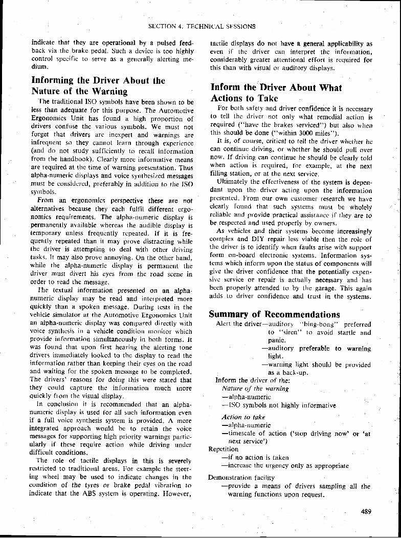
SECTION 4. TECHNICAL SESSIONS

indicate that they are operational by a pulsed feed-back via the brake pedal. Such a device is too highlycontrol specific to serve as ir generally alerting me-dium.

Informing the Driver Ahout theNature of the Warning

The traditional ISO symbols have been shown to beIess than adequate for this pulpose. The AutonrotiveErgonomics Unit has found a high proportion ofdrivers confuse the various symbols. We mu$t notforget that drivers arc inexpert and warnings areinfrequent so they cannot learn through experience(and do not study sufficiently to recall infbrrnationfrom the handbook). Clearly more informative meansare required at the time of warning presentation. Thusalpha-numeric displays and voice synthesized messagesmust be considered, preferably in addition to the ISOsymbols.

From an ergonomics perspective these are notalternatives because they each fulfil different ergo-nomics requirements. The alpha-numeric display ispermanently available whereas the audible display istemporary unless frequently repeated. lf it is fre-quently repeatecl than it may prove distracting whilethe driver is attempting to deal with other drivingtasks. It may also prove annoying. On the other hand,while the alpha-numeric display is permanent thedriver must divert his eyes from the road scene inorder to read the message.

The textual information presented on an alpha-numeric display may be read and intcrpreted morequickly than a spoken message. During tests in thevehicle simulator at the Automotive Ergonomics Unitan alpha-numeric display was compared directly withvoice synthesis in a vehicle condition monitor whichprovide information sirnultaneously in both forms. Itwas found that upon first hearing the alcrting tonedrivers immediately looked to thc display to read theinformation rather than keeping their eyes on the roadarrd waiting for the spoken message to be cornpleted.The drivers' reasons for doing this were stated thatthey could capture the information much morequickly from the visual display.

In conclusion it is recommended that an alpha-numcric display is used fbr all such information evenif a full voice synthesis system is provided. A moreintegrated approach would be to retain the voicemessages for supporting high priority warnings partic-ularly if these require action while driving underdifficult conditions.

The role of tactile displays in this is severelyrestricted to traditional areas. For example the steer-ing wheel may be used to indicate changes in thecondition of the tyres or brake pedal vibration toindicate that the ABS system is operating. However,

tactile displays do not have a general applicability aseven if thc driver can interpret the infprmationnconsiderably greater attentional effort is required forthis than with visual or auditory displays.

Inform the Driver About WhatActions to Take

For both sal'ety and driver confidence it is necessaryto tell the driver not only what remedial action isrequired ("have the brakes serviced") but also whcnthis should be done ("withirr 3000 miles").

It is, of course, critical to tell the driver whether hecan continue driving, or whcther he should pull overnorv. If driving can continue he should be clearly toldwhen action is required, for exarnple, at the nextfil l ing station, or at the next $ervice.

Ultimately the eff'ectiveness ol' the system is depen-dant upon the driver acting upon the informationpresented. F'rom our own customer research we haveclearly found that such system$ must be wholelyreliable and provide practical assistance if they are tobe respected and used properly by owners.

As vehicles and their systems become increasinglycomplex and DIY repair less viable then the role ofthe driver is to identify when faults arise with $upportform on-board electronic systems. Information sys^tems which inform upon the status of components willgive the driver confidence that the potentially expen-sive service or repair is actually necessary and hasbeen properly attended to by the garage. This againadds to driver confidence and trust in the systems.

Summary of RecommendationsAlert the driver-auditory "bing-bong" preferred

to "siren" to avoid startle andpanrc.

-auditory preferabteIieht.

-warning l ight shouldas a back-up.

to warning

be provided

Inform the driver of the;Nature of the warning-alpha-nurneric*lSO symbols not highly informative

Action to take-alpha-numeric-timescale of action ('stop driving now' or .at

next service')Repetition

-if no action is taken-increase the urgency only as appropriate

Demonstration facility-provide a means of drivers sampling all the

warning functions upon request.

489

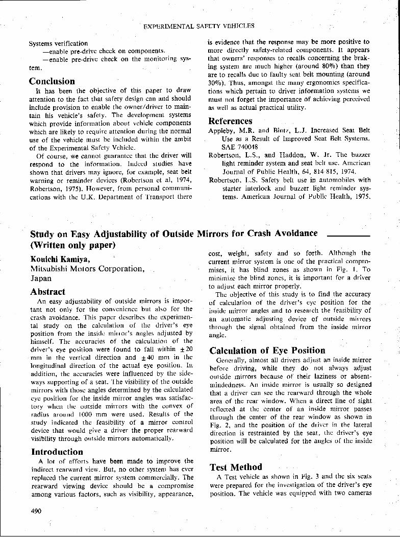
Systems verification-enable pre-drive check on components.-enable pre-drive check on the monitoring sys-

tem.

ConclusionIt has been the objective of this paper to draw

attention to the fact that saiety design can and shouldinclude provision to enable the owner/driver to main-tain his vehicle's safety. The development systemswhich provide information about vehicle componentswhich are likely to require attention during the uormaluse of the vehicle must be included within the ambitof the Experimental Safety Vehicle.

Of course, we cannot guarantee that the driver willrespond to the information. lndeed studies haveshown that drivers may ignore, for example, seat beltwarning or reminder devices (Robertson et al, 1974,Robertson, 1975). However, from personal comtnuni-cations with the U.K. Department of Transport there

Study on Easy Adjustability of Outside(Written only pflper)

Kouichi Kamiya,Mitsubishi Motors Corporation,Japan

AbstractAn easy adjustabil ity of outside mirrors is impor-

tant not only for the convenience but also for the

crash avoidance. This paper describes the experimen-tal study on the calculation of the driver's eyeposition frorn the insidc mirror'$ angles adiusted byhimself. The accuracies of the calculation of thedriver's eye position were found to tall within t 20mm in the vertical direction and 140 mm in thelongitudinal direction of the actual eye position. Inaddition, the accuracies were influetrced by the side-ways supporting of a seat. The visibil i ty of the outsidemirrors with those angles determined by the calculatedeye position for the inside mirror angles was satisfac-tory when the outside mirrors with the convex ofradius around 1000 rnm were used. Results of thestudy indicated the feasibility of a mirror controldevice that would give a driver the proper rearwardvisibility through outside mirrors automatically.

IntroductionA lot ol' efforts have been made to improve the

indirect rearward view. But, no other system has everreplaced the current mirror system commercially. Therearward viewing device should be a cotnpromiseamong various factors, such as visibility, appearance,

490

EXPERIMENTAL SAFETY VEHICLES

is evidence that the response may be more positive tomore directly safety-related components. lt appearsthat owners' responses to recalls concerning the brak-ing system are much higher (around 8090) than theyare to recalls due to faulty seat belt mounting {around30Vo). Thus, amongst the many ergonomics specifica-tions which pertain to driver information systems wemust not forget the importance of achieving perceivedas well as actual practical utility.

ReferencesAppleby, M.R. and Bintz, L.J. Increased Seat Belt

Use as a Result of Improved Seat tselt Systems.sAE 740048

Robertson, L.S., and Haddon, W. Jr. The buzzerlight reminder system and seat belt use. AmericanJournal of Publ ic Health, 64, 814-815, 1974.

Robertson, L.S. Safety belt use in automobiles withstarter interlock and buzzer light remindcr sys-tems. American Journal of Public Health. 1975.

Mirrors for Crash Avoidance

cost, weight, safety and so forth. Although thecurrent mirror system is one of the practical compro-mises, it has blind zones as $hown in Fig. I. Tominimize the blind zoncs, it is important for a driverto adjust each mirror properly.

The objective of this study is to find the accuracyof calculation of the driver's eye position for theinside mirror angles and to research the feasibility ofan automatic adjusting device of outside mirrorsthrough the signal obtained from the inside mirrorangle.

Calculation of Eye PositionCenerally, almost all drivers adiust an inside mirror

before driving, while they do not always adjustoutside mirrors because of their laziness or absent-mindedness. An inside mirror is usually so designedthat a driver can see the rearward through the wholearea of the rear window. When a direct line of sightreflected at the center of an inside mirror passes

through the cetrter of the rear window as shown inFig. 2, and the position of the drivcr in the lateraldirection is restrainted by the seat, the driver's eyeposition wil l bc calculated for the angles of the insidemirror.

Test MethodA Test vehicle as shown in FiS. 3 and the six seats

were prepared for the investigation of the driver's eyeposition. The vehicle was equipped with two cameras

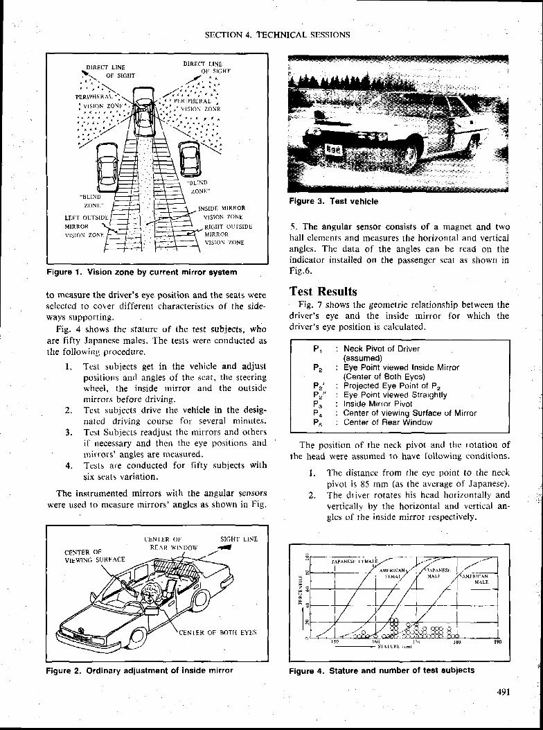
DlRll(lT I, lNlrOI I S IGHT

. . B L I N D

7.ONF:"*II LINI]

zoNt i "INSIDI I MIRROR

vlsloN zoNtLEFT OI]TSIDI

MIRROR

VISI ( ]N ZONFRI(iHT Otl] 'SlDIrMIRROR

VI$ ION ZONE

SECTION 4. TECHNICAL SESSIONS

Figure 1. Vision zone by current mirror eystem

to measure the driver's eye position and the seats weresclected to cover different characteristics of the side-ways supporting.

Fig. 4 shows the stature of the test subjects, whoare fifty Japanese males. The tests were conducted asthe following procedure.

l. Test subjects get in the vehicle and adjustpositions ancl angles of the $cat, the stecringwheel. the inside mirror and the outsidemirrors before driving.

2" Test subjccts drive the vehicle in the desig-nated driving course for several minutes.

3. Test Subiects readjust the mirrors and othersif necessary and thcn the eye positions atrdmirrors' angles are measured.

4, Tests are conducted for fifty subjects withsix seats variation.

The instrumented mirrors with the angular sensorswere used to measure mirrors' angles as shown in Fig.

{flr.rir'fffiffiW@$!

5. The angular sensor consists of a magnet and twohall elements and measures the horizontal and verticalangles. The data of the angles can be read on theindicator installed on the pa$senger seat as shown inFie.6.

Test ResultsFig. 7 shows the geometric relationship between the

driver's eye and the inside mirror I'or which thedriver's eye position is calculated.

The position of the neck pivot and the rotation ofthe head were assumed to have I'ollowing conditions.

l. The distance from the eye point to the neckpivot is 85 mnr (as the average of Japanese).

2. The driver rotates his head horizontally andvertically by the horizontal and verticirl an-

, gles of the inside mirror respectively.

JAP^NEST: tsLMAI.I

r l , 1 6 l lS I A I L : R I t ( m )

Fz!*

E

1Figure 4. Stature and number of test subiects

Flgure 3. Test vehicle

P l

P2

Pr'P,"P3P4P5

: Neck Pivot of Driver(assumed)

: Eye Point viewed Inside Mirror(Center of Both Eyes)

: Projected Eye Point of P": Eye Point viewed Straightly; lnside Mirror Fivot: Center of viewing Surface of Mirror: Center of Flear Window

CI,NTER OFR I A R W I N D O W

SIGHT L INE

ICENTER OFVIL.WING SLJRFACE

CENI 'ER OF BOTH EYES

Flgure 2. Ordinary adjustment of Inside mirror

491

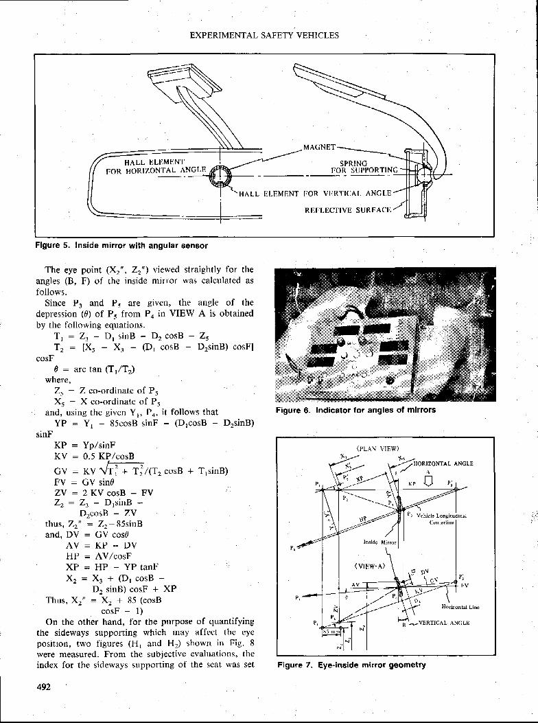
EXPERIMENTAL SAFETY VEHICLES

HALL T.]LIIMENTH()RIZONTAL ANGLE

SPRINGFOR ST]PPORTINC

IJI,I IMI]NT IIOR VIJRTICAL ANCI,E

R|IFLECTM ruOOoa,trtl

Figure 5. Inside mirror with angular sensor

The eye point {Xr", Zr") viewed straightly for theangles (8, F) of the inside mirror was calculated asfollows.

Since Pl and P{ are given, the angle of thedepression (d) of P. from Po in VIEW A is obtainedby the I'ollowing equations.

T, : Zt - f)t sinB - Dr cosB - Z5Tr : [Xj - Xl - (D, cosB - DrsinB) cosF]

cosFd : arc tan (T,/Tr)

where,Zs : Z co-ordinate of P5Xs : X co-ordinate of P5

and, using the given Yr, P4, it follows thatYP = Yr - 85cosB sinF - (DrcosB - DrsinB)

sinFKP = Yp/sinFKV : 0.5 KP/cosB

: rv Vrl + T:/$zcosB + T'sinB): GV sind: 2 K V c o s B - F V

- ZJ D's inB *

DtcosB - ZVth'tf,s, Zr" - Zz- 85sinBand, DV : CV cos0

A V : K P " . D VHP : AV/cosFXP * HP - YP tanFXz : Xr + (Dt cosB -

Dt sinB) cosF + XPThus, Xr" : Xr * 85 (cosB

cosF - l )On the other hand, for the purpose of quantifying

the sideways supporting which may affect the eyeposition, two figures (Ht arrd H2) shown in Fig. 8were measured. From the subjective evaluations, theindex for the sideways supporting of the scat was set

492

Inside Mirror

(vrFw.A)

Pr Vchicle Longitudinal

B;VERTTCAL ANCLE

Figure 7. Eye-inside mirror goometry

GVFVzvz2

Figure 6. lndicator for angles of mirrors

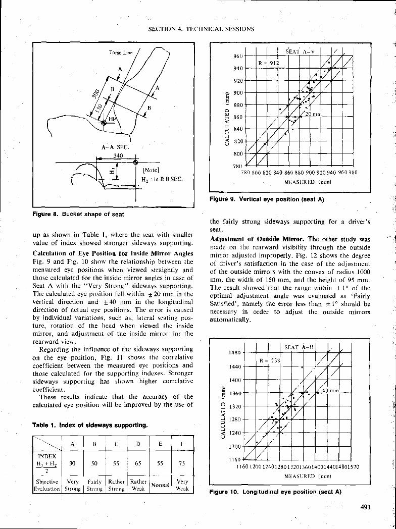
SECTION 4. TECIHNICAL SESSIONS

A--A SEC.

B B SEC.

Figure 8. Bucket shape of seat

up as shown in Table l, where the seat with smallervalue of index showed stronger sideways supporting.

Calculation of Eye Position for Inside Mirror AnglesFig. 9 and Fig. l0 show the relationship between themeasured eye positions when viewed straightly andthose calculated for the inside mirror angles in case olSeat A with the "Very Strong" sideways supporting.The calculated eye position I 'ell within 120 mrn in thevertical direction and t 40 mm in the longitudinaldirection of actual eye positions. The error is causcdby individual variations, such as, lateral seating pos-ture. rotation of the head when viewed thc insidemirror, and adjustment of the inside mirror for therearward view.

Regarding the influence of the sideways supporting

on the eye position, Fig. I I shows the correlative

coefficient between the measured eye positions andthose calculated for the supporting indexes. Stronger

sideways supporting has shown higher correlativecoefficient.

These results indicate that the accuracy of the

calculated eye position wil l be improved by the use of

Table 1. Index of sldeways supportlng.

the fairly strong sideways supporting for a driver'sseat.Adjustment of Outside Mlror. The other study wasmade on the rearward visibility through the outsidemirror adjusted improperly. Fie. l2 shows the degreeof driver's satisfaction in the case of the adjustrnentof the outside mirrors with the convex of radius 1000mm, the width of 150 mrn, and the height of 95 mm.The result showed that the rangc within +lo of theoptimal adjustmcnt angle was evaluated as 'Fairly

Sat isf ied' , namely the error less than +l 'should benecessary in order to adjust the outside mirrorsautomatically.

l

.t

, . . i

. !

"+!4

-E

trlF.{JpU,l{()

96t l

940

920

900

880

860

840

820

800

780

MEASLIREfJ (mrn)

780 800 820 840 860 880 900 920 940 960 980

Flgure g. Vertical eye position (seat A)

A B c D E F

INDEXH r + H r

230 50 5 5 65 55 7 5

SbiectiveIlvr lu a t ion

VeryStrong

Fair lySt rong

Rathe r

S t r ong

RatherWrak

NormaVeryWclk

;!F{t

U-J4U

1 4 8 0

I 440

l 400

l 360

1 3 2 0

1 2 8 ( )

t240

I 200

l r 6 0l l 60 I?00 1240 I 280 1320 I3601400144014801520

MF.ASI. iRED (nrnt)

Flgure 10. Longitudinal eye position ($eat A)

493

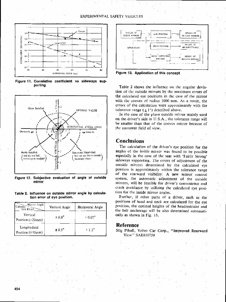
I

0 . 9

zH 0.8

E 0.6

F-

X n.s

o 0.4

0 3

EXPERIMENTAL SAFETY VEHICT,ES

Figure 11. Correlatlve coefficientporting

vs sideways $up-

Figure 12. Subjective evaluation of angle ol outsidemirror

Table ?. Influence on outside mlrrot angle by calcula-tion error ol eye position.

Table 2 shows the influence on the angular devia-tion of the outside mirrors by the maximum errors ofthe calculated eye positions in the case of the mirrorwith the convex of radius 1000 mm. As a result, theerrors of the calculation were approximately with thetolerance range (+ l") described above.

In the case of the plane outside mirror mainly usedon the driver's side in U.S.A., the tolerance range wil lbe smaller than that of the convex mirror because ofthc narrower field of view.

ConclusionsThe calculation of the driver's eye position for the

angles of the inside mirror was found to be possibleespecially in the case of the $eat with 'Fairly Strong'sideways $upporting. The errors of adjustment of theoutside mirrors detcrrnined by the calculated eyeposition is approximatcly within the tolerance rangeof the rearward visibility. A new mirror controlsystem, the automatic adjustment of the outsidemirrors, wil l be l 'easible for driver's convenience andcrash avoidalce by utilizing the calculated eye posi-tion for the inside mirror angles.

Further, if other parts of a driver, such as thepositions of head and neck are calculated for the eyeposition, the optimal heights of the headrestraint andthe belt anchoragc will he also determined automati-cally as shown in Fig. 13.

ReferenceStig Pihall, Volvo Car Corp., "Improved Rearward

View" SAEgt0759

AN(;LI |S OF

INSII 'E ] \ { IRR0RHYI: POSITION

APPLICA] ION

III

HEAD POSITIONHF: ICHT OF

HE ̂ T)RF5TR AINT

ANGLIS 0]

Figure 13. Application of this concept

IJ

IQuite Satisfied

Outwards - 2

OPTIMAL VALUE

HORIZOT]TAL ANGLE (TJFG)

Z ?, l i lwards,

z' SomewhatUnsatisftedFairly #sfied \\rr

F/ anri do not feel \

-----l

\necessity to readjustrl

€

tCr

/ bt t can ,ce the t l in imum\

\ necessarY vision

I

cii.i,r;: -Y il-'"' nnshtion Error-----r-

Vert ical

Posit ion (t20mm)_

Longitudinal

Posit ion (rr40rnm)

Vertical Angle Horizontal Angle

+ 0 ,go t 0 .070

t 0 . 5 0 ! l . z n

494

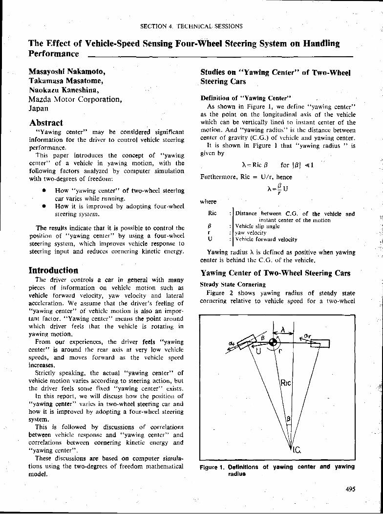
SECTION 4. TECHNICAL SESSIONS

The Effect of Yehicle-Speed Sensing Four-Wheel Steering System on HandlingPerformanre

Masayoshi Nnkamoto,Takamasa Masatome,Naokazu KaneshinaMazda Motor Corporation,Japan

Abstract"Yawing center" may be considered significant

information for the driver to control vehicle steeringperformance.

'fhis paper introduces the concept of "yawing

center" of a vehicle in yawing motion, with thefollowing factors analyzed by computer simulationwith two-degrees of freedom:

a How "yawing center" of two-wheel steeringcar varies while running.

I How it is improved by adopting four-wheelsteering system.

The results indicate that it is possible to control theposition of "yawing center" by using a four-wheelsteering system, which improves vehicle response tosteering input and reduces cornering kinetic energy.

IntroductionThe driver controls a car in general with many

pieces of information on vehicle motion such asvehicle forward velocity, yaw velocity and lateralacceleration. We assume that the driver's feeling of"yawing center" of vehicle motion is also an impor-tant factor. "Yawing center" means the point aroundwhich driver feels that the vehicle is rotatine in

From our experiences, the driver feels "yawing

center" is around the rear axis at very low vehiclespeeds, and moves forward as the vehicle speedincreases.

Strictly speaking, the actual "yawing center" ofvehicle motion varies according to steering action, butthe driver feels some fixed "yawing center" exists.

ln this report, we will discuss how the position of"yawing center" varies in two-wheel steering car andhow it is improved by adopting a four-wheel steeringsystem.

This is followed by discussions of correlationsbetween vehicle response and "yawing center" andcorrelations between cornering kinetic energy and"yawing center",

These discussions are based on computer simula-tions using the two-degrees of freedom mathematicalmodel.

Studies on "Yawlng Center" of Two-WheelSteering Cars

Definit ion of "Yawing Center"As shown in Figure l, we define "yawing center"

as the point on the longitudinal axis of the vehiclewhich can be vertically lined to instant center of themotion. And "yawing radius" is the distance betweencenter of gravity (C.C.) of vehicle and yawing center.

It is shown in Figure I that "yawing radius " isgiven by

I = R i c F f o r l F l < l

Furthermore, Ric = U/r, hence

l = 4 urwhere

Ric

pf

U

, f Dir,"n". between C.G. of the vehicle and1 inslant cenrer of the motion

; I Vehicle slip angle: I yaw velocity: I Vehicle forward velocity

\ j

: .l

+ t

Yawing radius \ is defined as positive when yawirrgcenter is behind the C.G. of the vehicle.

Yawing Center of Two-Wheel Steering CarsSteady State Cornering

Figure 2 shows yawing radius of steady statecornering relative to vehicle speed for a two-wheel

Figure 1. Oellnltlons ofradlus

yawlng and yawing

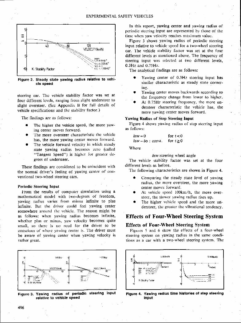
EXPERIMENTAL SAFETY VEHICLES

In this report, yawing center and yawing radius ofperiodic steering input are represented by those of thetime when yaw velocity reaches maximum value.

Figure 3 shows yawing radius of periodic steeringinput relative to vehicle speed for a two-wheel steeringcar. The vehicle stability factor was set at the fourdifferent levels as mentioned above. The frequency ofsteering input was selected at two different levels,0.3H2 and 0.75H2.

The analytical findings are as follows:

I Yawing center of 0.3H2 steering input hassimilar characteristic as steady $tate corner-ing.

I Yawing center moves backwards according to, the frequency change from lower to higher.o At 0.75H2 steering frequency, the more un-

dersteer characteristic the vehicle has, themore yawing center moves forward.

Yawing Radius of Step Steering InputFigure 4 shows yawing radius of step steering input

as follows:

6sw:0 fo r t<06sw:6o : const. for t>0

Where

6sw:steering wheel angleThe vehicle stability factor was set at the four

different levels as before.The following characteristics are shown in Figure 4.

I Comparirtg the steady state level of yawingradirrs, the more oversteer, the more yawingcenter moves forward.At vehicle speed lO0km/h, the more over-steer, the slower yawing radius rises up.The higher vehicle speed and the more un-dersteer, the greater the vibrational tendency.

Effects of Four-Wheel Steering System

Effects of Four-Wheel Steering SystemFigurcs 5 and 6 show the effects of a four-wheel

steering system on yawing radius in the same condi-tions as a car with a two-wheel steering system. The

M5 K'O ---

Flgure 4. Yewing radius time historles ol step steeringInput

Figure 2. Steady state yawing radius relatlve to vehi-cle speed

steering car. The vehicle stability factor was set at

four cliffercnt levels, ranging from slight understeer to

slight oversteer. (See Appendix ts for full details of

vehicle specifications and the stability factor.)

The findings are as follows:

I The higher the vehicle speed, the more yaw-

ing center moves forward.I The more oversteer characteristic the vehicle

has, the more yawing center moves forward.o The vehicle forward velocity in which steady

state yawing radius becotnes zero (called"Tangent Speed") is higher for greater de-grees of understeer.

These findings are considered to be coincident withthe normal driver's feeling of yawing center of con-ventional two-wheel steerins cars.

Periodic Steering Input

From the results of computer simulation using amathematical model with two-degrees of freedom,yawing radius varies from minus infinite to plus

infinite. But the driver could feel yawing centersomewhere around the vehicle. The reason might beas follows: when yawing radius becomes infinite,whether plus or minus, yaw velocity becomes quite

small. so there is no need for the driver to beconscious of where yawing center is. The driver mustbe aware of yawing center when yawing velocity israther great.

Figure 3. Yawing radius ot perlodlcrelative to vehicle sPeed

I

steerlng inPut

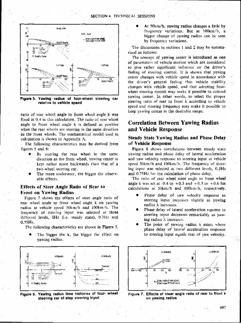
SECTION 4. TECHNICAL SESSIONS

k=01 tixed

1=Hsrxie o!Fr rHLffi illlP or n dt ffi,

Flgure 5. Yawing radius of four-wheel steering earrelative to vehlcle speed

ratio of rear wheel angle to front wheel angle k wasfixed at 0.4 in this calculation. The ratio of rear wheelangle to front wheel angle k is defined a.s positivewhen the rear wheels are steering in the same directionas the front wheels. The mathematical model used incalculation is shown in Appendix A.

The following characteristics may be derived fromfigures 5 and 6:

r By steering the rear wheel in the samedirection as the front wheel, yawing center iskept rather more backwards than that of atwo-wheel steering car.

t The more understeer, the bigger the observ-able effects.

Effects of Steer Angle Ratio of Rear toFront on Yawing Radius

Figure 7 shows the effects of steer angle ratio ofrear wheel angle to front wheel angle k on yawingradius at vehicle speed 50km/h and lO0km/h. Thefrequency of steering input was selected at threedifferent levels, OHe (i.e. steady state), 0.3H2 and0.75H2.

The following characteristics are shown in Figure 7.

I The bigger the k, the bigger the effect onyawing radius.

7

a/5 [-{

Figure 6. Yawing radius tlme histories of four' wheelsteering car of step steering input

I At 50km/h, yawing radius changes a little byfrequency variations. But at 100km/h, abigger change of yawing radius can be seenby frequency variations.

The discussions in sections I and 2 may be summa-rized as follows:

The concept of yawing center is introduced as oneof parameters of vehicle motion which are consideredto give rather significant influence on the driver'sfeeling of steering control. It is shown that yawingcenter changes with vehicle speed in accordance withthe driver's general feeling that vehicle stabilitychanges with vehicle speed, and that adopting four-wheel steering system may make it possible to controlyawing center. In other words, to select the propersteering ratio of rear to front k according to vehiclespeed and steering frequency may make it possible tokeep yawing center in the desirable range.

Correlation Between Yawing Radiusand Vehicle Response

Steady State Yawing Radius and Phase Delayof Yehicle Response

Figure I shows correlations between steady stateyawing radius and phase delay of lateral accelerationand yaw velocity response to steering input at vehiclespeed 50km/h and lO0km/h. T'he frequency of steer-ing input was selected at two different levels, 0.3H2and 0.75H2 for the calculation of phase delay.

The ratio of rear wheel steer angle to front wheelangle k was set at -0.4to +0.3 and +0.3 to +0.6 forcalculations at 5Okm/h and l00km,/h, respectively.

I Phase delay of yaw velocity response tosteering input increases slightly as yawingradius \ increases.

. Phase delay of lateral acceleration reponse tosteering input decreases remarkably as yaw-ing radius \ increascs.

I The point of yawing radius X exists wherephase delay of lateral acceleration responseto steering input equals that of yaw velocity.

Figure 7. Etlecte of steer angle ratlo of rear to front kon yawing radlus

497

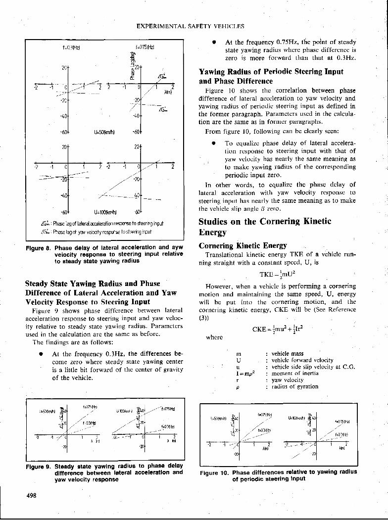
EXPERIMENTAL SAFETY VEHICLES

f=01(l-h)

U=1m0fiih)

l6L : Fhme lag of lalerat xceteration resporse io sleerinq input

lGl,, : Pfnse lag of yal velocity response io steenng input

Flgure 8. Phase delay of lateral acceleration and ayw- velocity response to steering input relativeto steady state Yawing radius

Steady State Yawing Radius and PhaseDifference of Lateral Acceleration and YawVelocity Response to Steering Input

Figure 9 shows phase difference between lateralacceleration response to steering input and yaw veloc-ity relative to steady state yawing radius. Parametersused in the calculation arc the same as before.

The findings are as follows:

t At the frequency 0.3H2, the differences be-

come zero where steady state yawing centeris a little bit forward of the center of gravity

of the vehicle.

.--..--"i=ortru

f=0t(fL)

t At the frequency 0.?5H2, the point of steadystate yawing radius where phase difference iszero is more forward than that at 0.3H2.

Yawing Radius of Periodic Steering Inputand Phase Difference

Figure l0 shows the correlation between phasedifference of lateral acceleration to yaw velocity andyawing radius of periodic steering input as defined inthe former paragraph. Parameters used in the calcula-tion are the same as in former paragraphs.

From figure 10, following can be clearly seen:

I To equalize phase clelay of lateral accelera-tion response to steering input with that ofyaw velocity has nearly the same meaning asto make yawing radius of the correspondingperiodic input zero.

In other words, to equalize the phase delay oflateral acceleration with yaw velocity response to

steering input has nearly the same meaning as to makethe vehicle slip angle P zero.

Studies on the Cornering KineticEnergyCornering Kinetic Energy

Translational kinetic energy TKE of a vehicle run-ning srraight with a

THTljlTd, u, is

L

However. when a vehicle is performing a corneringmotion and maintaining the same speed, U, energywill be put into the cornering motion, and thecorncring kinetic energy, CKE will be (See Reference(3))

C6p=]muz+l lrzwhere

vehicle massvehicle forward velocityvehicle side slip velocity at C.C.moment of inertiayaw velocityradius of gyration

mUuI = m p 2tp

Flgure 9. Steady state yawing radius to phase delayditference between latersl acceleratlon andyaw velocity response

Figure 10. Phase differences relatlve to yawing radlusol Periodic steering lnput

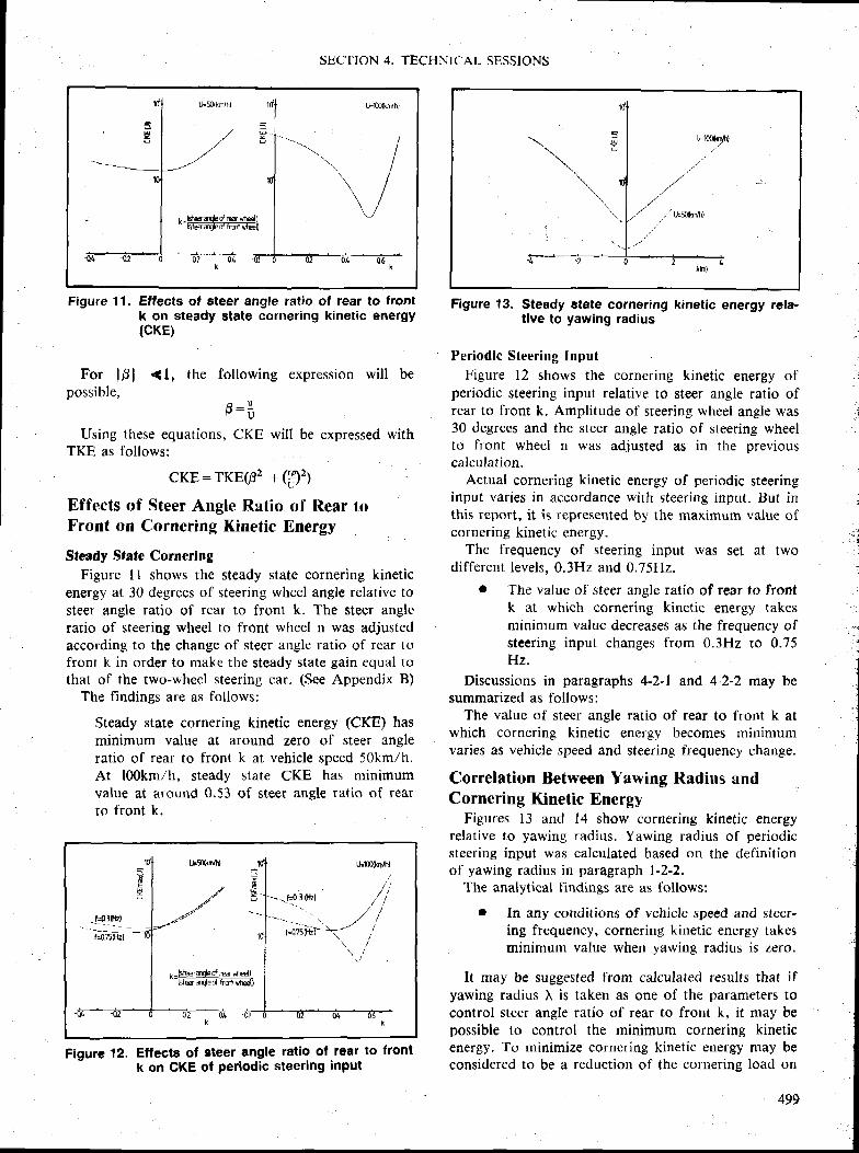
SECTION 4, TECHNICAL SESSIONS

Figure 11. Effects of eteer angle ratio of rear to frontk on steady Btate cornering kinetic energy(cKE)

For lPl {1, the following expression will bepossible,

0 : iUsing these equations, CKE will be expressed with

TKE as follows:

CKE:rKE(62 +(p1

Effects of Steer Angle Ratio of Rear toFront on Cornering Kinetic Energy

Steady State CorneringFigure I I shows the steady state cornering kinetic

energy at 30 degrees of steering wheel angle relative tosteer angle ratio of rear to front k. The steer angleratio of $teering wheel to front wheel n was adjustedaccording to the change of steer angle ratio of rear tofront k in order to make the steady state gain equal tothat of the two-whecl steering car. (See Appendix B)

The findings are as follows;

Steady state cornering kinetic energy (CKE) hasminimum value at around zero of steer angleratio of rear to front k at vehicle speed 50km/h.At loOkm/h, steady state CKE has minimumvalue at around 0.53 of steer angle ratio of rearto front k.

Figure 13, Steady $tate cornering kinetic energy rela-tlve to yawing radius

Periodic Steering InputFigure 12 shows the cornering kinetic energy of

periodic steering input relative to steer angle ratio ofrear to front k. Amplitude of steering wheel angle was30 degrees and the steer angle ratio of steering wheelto front wheel n was adjusted as in the previouscalculation.

Actual cornering kinetic energy of periodic steeringinput varies in accordance with steering input. But inthis report, it is represented by the maximurn value ofcornering kinetic energy.

The frequency of steering input was set at twodifferent levels, 0.3H2 and 0.75H2.

r The value of steer angle ratio of rear to frontk at which cornering kinetic energy takesminimum value decreases as the frequency ofsteering input changes from 0.3H2 to 0.75Hz.

Discussions in paragraphs 4-2-l and 4-2-2 may besummarized as follows:

The value of steer angle ratio of rear to front k atwhich cornering kinetic energy becomes minimumvaries as vehicle speed and $teering frequency change.

Correlation Between Yawing Radius andCornering Kinetic Energy

Figures l3 and 14 show cornering kinetic energyrelative to yawing radius. Yawing radius of periodicsteering input was calculated based on the definit ionof yawing radius in paragraph l-2-2.

The analytical findings are as follows:

I In any conditions of vehicle speed and steer-ing frequency, cornering kinetic energy takesminimum value when yawing radius i$ zero.

It may be suggested from calculated results that ifyawing radius \ is taken as one of the parameters tocontrol steer angle ratio of rear to front k, it may bepossible to control the minimum cornering kineticenergy. To minimize corncring kinetic energy may beconsidered to be a reduction of the cornering load on

Figure 12. Ellects of eteer angle ratio of-rear to front- k on CKE ol periodic steering input

499

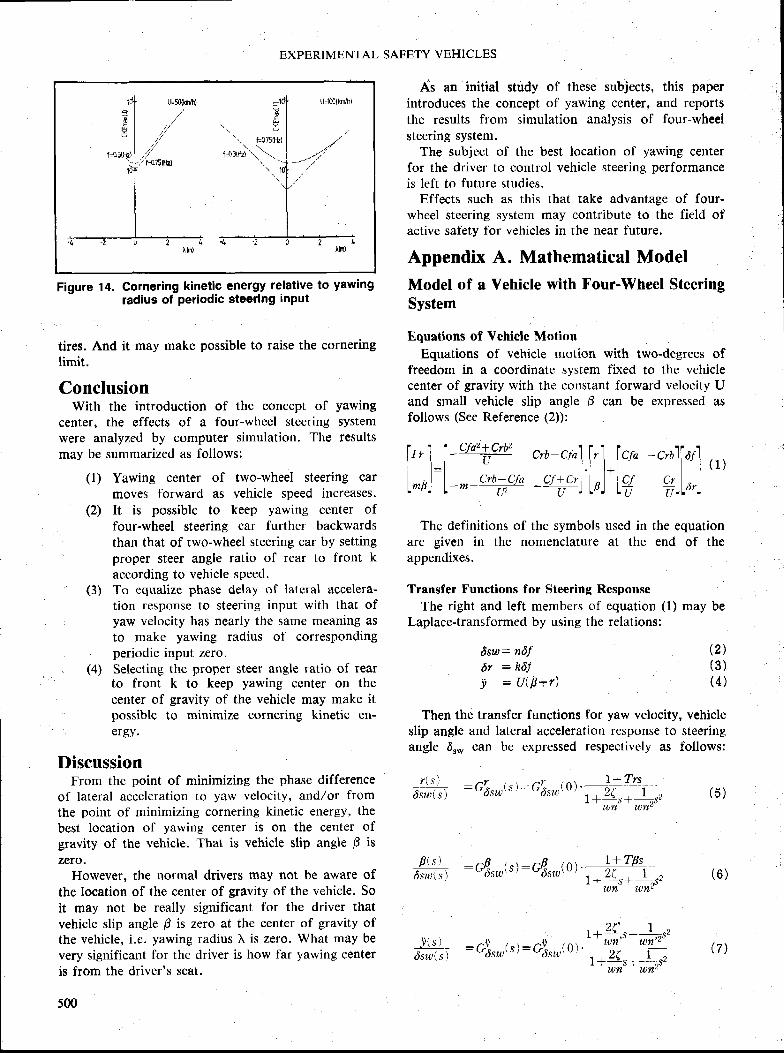
Figure 14. Cornering kinetic energy relative to yawingradius of Periodic steerlng input

tires. And it may make possible to raise the corneringlimit.

ConclusionWith the introduction of the concept of yawing

center, the effects of a four-wheel steering systemwere analyzed by computer simulation. The resultsmay be summarized as follows:

(l) Yawing center of two-wheel steering carmoves forward as vehicle speed increases.

(2) It is possible to keep yawing center offour-wheel steering car further backwardsthan that of two-wheel steering car by setting

' proper steer angle ratio of rear to front kaccording to vehicle speed.

(3) To equalize phase delay of lateral accelera-tion response to steering input with that ofyaw velocity has nearly the same meaning asto make yawing radius of correspondingperiodic input zero.

(4) Selecting the proper steer angle ratio of rearto front k to keep yawing center on thecenter of gravity of the vehicle may make itpossible to minimize cornering kinetic en-

' ergy'

DiscussionFrom the point of minimizing the phase difference

of lateral acceleration to yaw velocity, and/or from

the point of minimizing cornering kinetic energy, the

best location of yawing center is on the center ofgravity of the vehicle. That is vehicle slip angle B is

zeto-However, the normal drivers may not be aware of

the location of the center of gravity of the vehicle. So

it may not be really significant for the driver that

vehicle slip angle B is zero at the center of gravity ofthe vehicle, i.e. yawing radius tr is zero. What may bevery significant for the driver is how far yawing centeris from the driver's seat.

500

EXPERIMENTAL SAFETY VEHICLES

f ( . s )dsur(.s )

"r(s ) _dszp(.s )

As an initial study of these subjects, this paperintroduces the concept of yawing ccnter, and reportsthe results from simulation analysis of four-wheelsteering system.

The subject of the best location of yawing centerfor the driver to control vehicle steering performanceis left to future studies.

Effects such as this that take advantage of four-wheel steering system may contribute to the field ofactive safety for vehicles in the near future.

Appendix A. Mathematical Model

Model of a Yehicle with Four-Wheel SteeringSystem

Equations of Vehicle MotionEquations of vehicle motion with two-degrees of

freedom in a coordinate system fixed to the vehiclecenter of gravity with the constant forward velocity Uand small vehicle slip angle F can be expressed asfollows (See Reference (2));

The definitions of the symbols used in the equationare given in the nomenclature at the end of theappendixes.

Transfer Functions for Steering ResponseThe right and left members of equation (l) may be

Laplace-transformed by using the relations;

6sw= ndf6r -- kdf! = U(B+r)

Then the transfer functions for yaw velocity, vehicleslip angle and lateral acceleration response to $teeringangle d.* can be expressed respectively as follows;

1,,,1:lW c'D-cr'l f'l*f.t" -.*lf"l ,,,l*B) L-*-qfftu utf)tn) Ltr ?ll'l

(2 )(3 )(4 )

/ " r .$) _7r , - , . . rorr (0, ;_ ] i t * f ,d.itGl

-L'd.sxo\'l ' t' r_f_s_r_.,s.

: rL (c) : r - . r { (o) . l+TPs- r ' ' . t . $ t r o \ r / - " d . s t t r ' " i . 2 ( II + -=Sf :;.$"

utn 'u)nl

r+-2{ ' . r+ I ,os,=Gj.rr i . t )=4.ru,(or '

. * [ t *=

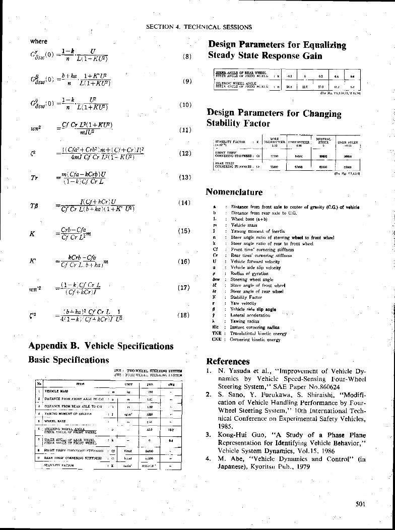
SECTION 4. TECHNICAL SESSIONS

where

cSsu(o)

utn2

r-p^ ,n, _b*fra. 1*K'4*d.$r{ r ' " ' n L( l+KU)

n f r , ^ \ l - h Utr6rrt,u/ : n

'Tfr+@

_ 7 - h . un L ( . I+K | l )

cf cr L|(7+KUz)mIU

t)

Tr

TB

_ | ( Cfaz + Crbz ) m + ( C.f + Cr) I\2AmI Cf Cr L2(11KU)

Crb-Cfa=:;-;---H|lLJ LT L"

IfhCrb-Cfa:

c f c , L .b ' , , po1*

( l - h 'C f C r L(Cf+kCr)I

- ( b - l ha , \ 2 C f C r L . 74r .7-k ' t ' Cf + kf r ) I U

Appendix B. Vehicle SpecificationsBasic Specifications

ff

IbLmIn

ctCrUucEry6f6rKrpvRic

TKECKE

: Dietance from frcnt ule to center of gravity (C.G.) of vehicleDistance from rerr axle to C.G.Wheel base (a+b)

Vehicle rnass

Yawing moment of inertlaSteer angle ratio of Bteering wheel to front wheelSteer angle ratio of rcar to front wheelFront t ires' comcring stiffnessRear tires' cornering stiffnesrVehicle forward Yelocity

Vrhi<:le side slip vrlrxityRadius of gyration

Steering wheel angleSteer angle of front whelSteer angle of rear wheelStrbility Factor

Yaw velocity

Vehicle side slip angleLateral accelerntion

Yawing tadius

Instanl .u.n"ri* a*'*Translational kinetic energyCotnering kinetic energy

( 1 6 )

(17)

( 1 8 )

zws : TwO-WfiEEL SmERING SlEfttl4wS I FOI-IR.WI]UEL STtUlttNc SYSTEI,I

Design Parameters for Equalizing( 8 ) Steady State Response Gain

(e )

( r0)

( 1 1 )

( r2)

{13 )

( 14 )

( ls)

Design Parameters for ChangingStability Factor

Nomenclature

Referencesl . N. Yasuda et al., "Improvement of Vehicle Dy-

namics by Vehicle Speed-Sensing Four^WheelSteering System," SAE Paper No.860624

2. S. Sano, Y. Furukawa, S. Shiraishi, "Modifi-

cation of Vehicle Handling Performance by Four-Wheel Steering System," lOth lnternational Tech-nical Conference on Experimental Safety Vehicles,1985 .

3. Kong-Hui Guo, "A Study of a Phase PlaneRepresentation for Identifying Vehicle Behavior,"Vehicle System Dynamics, Vol.l5, 1986

4. M. Abe, "Vehicle Dynamics and Control" (inJapanese), Kyoritsu Pub., 1979

@EB.AI{CI.E OF REAT WTEEI!ffiER ANGLE ol-lnohlT ffiEE_L__j I

STEEEINd WHEEL .'NCL[ -. .-.STEER AI"CLE OF FBONT WIIEEL

-0.2 0 0,1 0,1 0.G

s,4 22,0 l ? ,6 tx.2 a.a

(For Fig. ?,8,9,10,11,1r,13,1{)

6ffi

I (Cf+kCr)U=dFTi',b+ka)i#

xo I ._

ftEil UMT 2W8 aws

r i vEHlcLE t{^sst -

I I OISTANCE Frct FmIT dLE TO C.C- : r

I I DIETANCE FROM REAR AXLE m C.C. : b----T------1 I

yAWING XOHf,NT Ot lNfl.r,A : Il -

I I wtrEEI, a sE----1.-- . ...--6 $rEDftlNG WrtDEt scrE

STET:R AN(II,I] (}ts FBI)NT WHEEL

? ETIEB Ati.CI]E OF BEAF WHEEL : K]

$T};HR ̂ N(|LE OF FRI.)NT WHEEL

j_lll"iT llhr:s (r)R\r:RrN(i srrFtsNEss : ct

I REAR TIRT:$'CORNERINC STIFFNESS : CT

StABrLrtY t.^fr)B : K

xs l2s0

r .0l

krm'

l ,&

lffi

tr.61

n.o r3.8

o l- ' 1

& m l

0.4

N/d

€7{m

d . s 5 x r d '

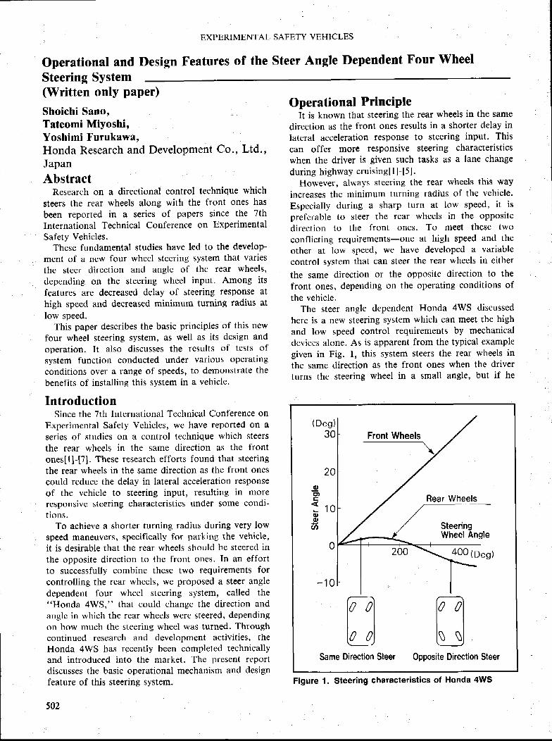
EXPERIMENTAL SAFETY VEHICLES

Design Features of the Steer Angle Dependent Four WheelOperational andSteering System(Written only paper)

Shoichi Sflno,Tateomi Miyoshi,Yoshimi Furukawa,Honda Research and Development Co., Ltd.,

Japan

AhstractResearch on a directional control technique which

steers the rear wheels along with the front ones hasbeen reported in a series of papers since the 7thInternational Technical Conference on ExperimentalSafety Vehicles.

These fundamental studies have led to the develop-ment of a new four wheel steering system that variesthe steer direction and angle of the rear wheel$,depencling on the steering wheel input. Among itsfeatures are decreased delay of steering response athigh speed and decreased minimum turning radius atlow speed.

This paper describes the basic principles of this newfour wheel steering system, as well as its design andoperation. It al$o discusses the results of tests ofsystem function conducted under various operatingconditions over a range of speeds, to demonstrate thebenel'its of installing this system in a vehicle.

IntroductionSince the 7th lnternational Technical Conf'erence on

Experimental Safety Vehicles, we have reported on a

series of studies on a control technique which steers

the rear wheels in the same direction as the front

ones$l-[7]. These research efforts found that steering

the rear wheels in the same direction as the front ones

could reduce the delay in lateral acceleration response

of the vehicle to steering input, resulting in more

responsive steering characteristics under some condi-tions.

To achieve a shorter turning radius during very low

speed maneuvers, specifically for parking the vehicle,

it is desirable that the rear wheels should be steered in

the opposite direction to the frorrt ones. In an effortto successfully combine these two requirements for

controlling the rear wheels, we proposed a steer angle

dependent four wheel steering system, called the"Honda 4WS," that could change the direction and

anglc in which the rear wheels were steered, dependingon how much the steering wheel was turned. Throughcontinuecl research and development activities, theHonda 4WS has recently been completed technicallyand introduced into the market. The present reportdiscusses the basic operational mechanism and designfeature of this steering system.

502

Operational PrinciPteIt is known that steering the rear wheels in the same

direction as the front ones results in a shorter delay in

lateral acceleration response to steering input. This

can offer more responsive steering characteristics

when the driver is given such tasks as a lane change

during highway cruisineI I ]-[5].However, always steering the rear wheels this way

increases the minimum turning radius of the vehicle'

Espccially during a sharp turn at low speed, it is

prefcrable to steer the rear wheels in the opposite

direction to the front ones. To meet these two

conflicting requirement$-one at hieh speed and the

other at low speed, we have developed a variable

control system that can steer the rear wheels in either

the same clirection or the oppositc direction to the

front ones, depending on the operating conditions of

the vehiclc.The steer angle dependent Honda 4WS discussed

here is a new steering $ystem which can meet thc high

and low speed control requirements by mechanical

devices alone. As is apparent from the typical examplegiven in Fig. l, this system steers the rear wheels in

the same direction as the front ones when the driver

turns the steering wheel in a small angle, but if he

( D e g )30

20-gcttE

J 1 0(l)oU,

0

- 1 0

Same

Front Wheels

TAVr)

Direction

Rear Wheels

SteeringWheel Angle

.400 (o*s)

Tn)t lt!_E

0pposite DirectionSteer Steer

Figure 1. Steering characteristics of Honda 4WS

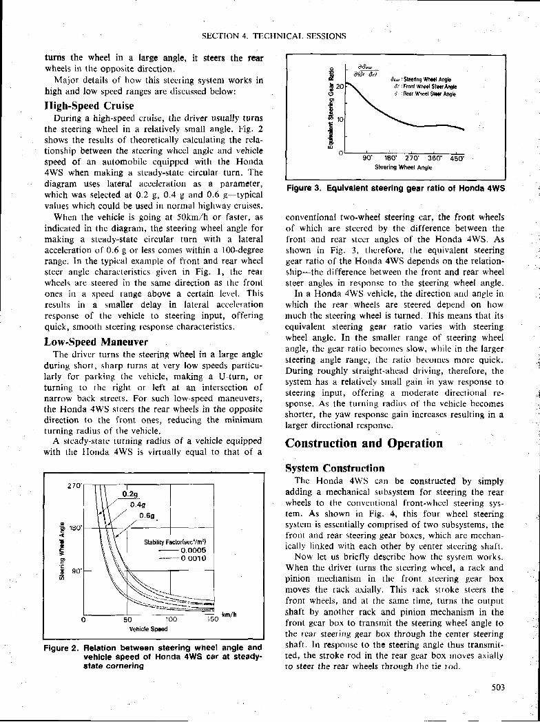
SECTION 4. TECHNICAL SESSIONS

turns the wheel in a large angle, it steers the rearwheels in the opposite dircction.

Major details of how this steering system works inhigh and low speed ranges are discussed below:

High-Speed CruiseDuring a high-speed cruise, the driver usually turns

the steering wheel in a relatively small angle. Fig. 2shows the results of theoretically calculating the rela-tionship between the steering wheel angle and vehiclespeed of an automobile equipped with the Honda4WS when making a steady-state circular turn. Thediagram uses Iateral acceleration as a parameter,which was selected at 0.2 g, 0.4 g and 0.6 g-typicalvalues which could be used in normal highway cruises.

When the vehicle is going at 50km/h or faster, asindicated in the diagram, the steering wheel angle formaking a steady-state circular turn with a lateralacceleration of 0.6 g or less comes within a 10O-degreerange. In the typical example of front and rear wheelsteer angle characteristics given in Fig. l, the rearwheels are steered in the samc direction as the frontones in a speed range above a certain level. Thisresults in a smaller delay in lateral accele rationresponse of tlre vehicle to steering input, offeringquick, smooth steering response characteristics.

Low-Speed ManeuverThe driver turns the steering wheel in a large arrgle

during short, sharp turns at very low speeds particu-larly for parking the vehicle, making a U-turn, orturning to the right or left at an interscction ofnarrow back streets. For such low-specd maneuvers,the Honda 4WS steers the rear wheels in the oppositedirection to the front ones, reducing the minimumturning radius of the vehicle.

A steady-state turning radius of a vehicle equippedwith the Honda 4WS is virtually equal to that of a

.goc

E,tBoc.;oovt

50 100vehicle Sp€€d

Figure 2. Relation between steering wheel angle andvehicle speed ot Honda 4WS car at steady-alate cornering

conventional two-wheel steering car, the front wheelsof which are steered by the diflerence between thefront and rear steer angles of the Honda 4WS. Asshown in Fig. 3, t lrerefore, the equivalent steeringgear ratio of the Honda 4WS depends on the relation-ship-the difference between the front and rear wheel$teer angles in response to the steering wheel angle.

In a Honda 4WS vehicle, the direction and angle inwhich the rear wheels are steered depend on howmuch the steering wheel is turned. This means that itsequivalent steering gear ratio varies with steeringwheel angle. In the smaller range of steering wheelangle, the gear ratio becomes slow, whilc in the Iargersteering angle range, the ratio becomes more quick.During roughly straight-ahead driving, therefore, thesystem has a relatively small gain in yaw response tosteering input, offering a moderate directional re-sponse. As the turning radius of the vehicle becomes$horter, the yaw response gain increases resulting in aIarger directional response.

Construction and Operation

System ConstructionThc Honda 4WS can be constructed by simply

adding a mechanical subsystem for steering the rearwheels to the conventional front-wheel steering sys-tem. As $hown in Fig. 4, this four wheel steeringsystem is essentially comprised of two subsystems, thefront and rear $tcering gear boxes, which arc mcchan-ically l inked with each other by center steering shaft.

Now let us briefly describe how the system works.When the driver turns the steering wheel, a rack andpinion mechanism in the front steering gear boxmoves the rack axially. This rack stroke steers thefront wheels, and at the same time, turns the outpufshaft by another rack and pinion mechanism in thefront gear box to transmit the steering wheel angle tothe rear steerinH gear box through the center steeringshaft. In re$ponsc to the steering angle thus transmit-ted, the stroke rod in the rear gear box moves axiallyto st€er the rear wheels throrrgh the tie rod.

20ds& : Steeting Wh6€l Angh

d/ rFffil Wh€el Stdef AdEilad, : Rear Wheel $toor Angle

Steering Wheel Angle

Flgure 3. Equlvalent steerlng gear ratio of Honda 4WS

503

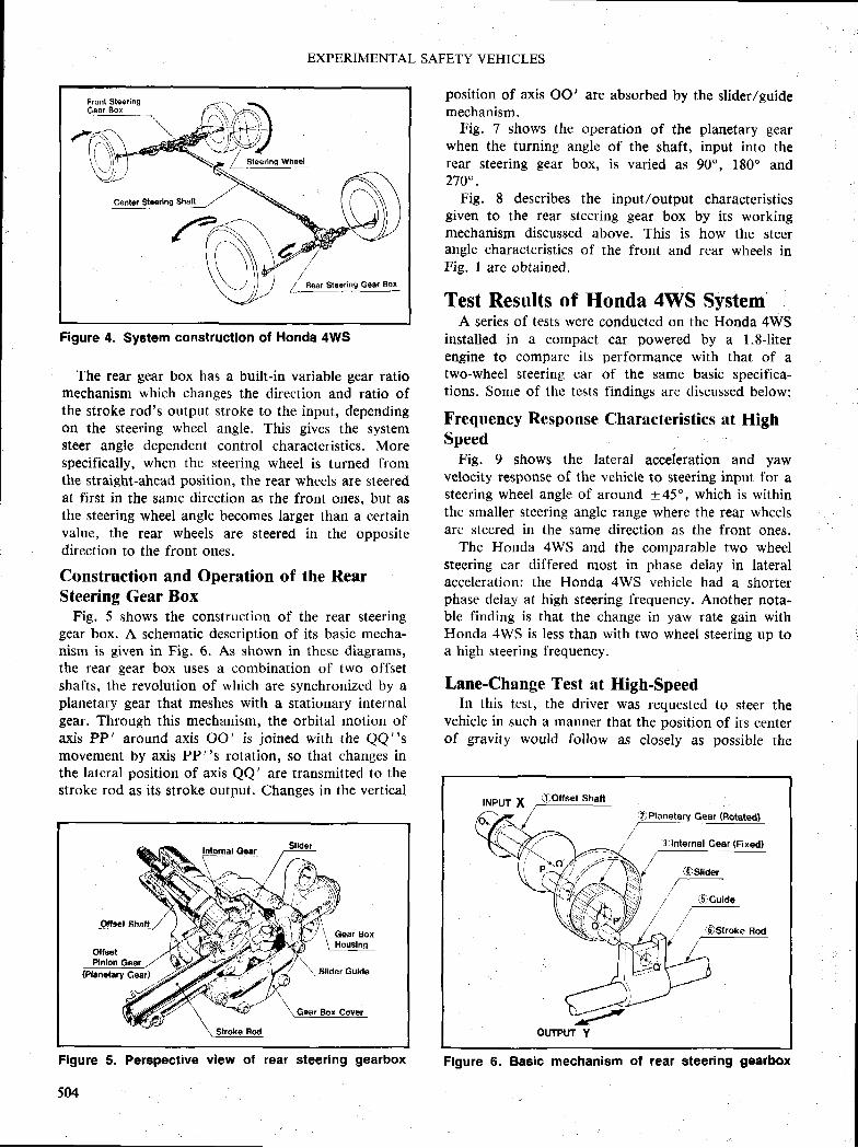
EXPERIMENTAL SAFETY VEHICLES

Figure 4. System constructlon of Honda 4WS

The rear gear box has a built-in variable gear ratiomechanism which changes the direction and ratio ofthe stroke rod's output stroke to the input, dependingon the steering wheel angle. This gives the systemsteer angle dependent control characteristics. Morespecifically, when the steering wheel is turned fromthe straight-ahead position, the rear wheels are steeredat first in the same direction as the front ones, but asthe steering wheel angle becomes larger tharr a certainvalue, the rear wheels are steered in the oppositedirection to the front ones.

Construction flnd Operation of the RearSteering Gear Box

Fig. 5 shows the construction of the rear steeringgear box. A schematic description of its basic mecha-nism is given in Fig. 6. As shown in these diagrams,the rear gear box uses a combination of two offsetshafts, the revolution of which are synchronized by aplanetary gear that meshes with a stationary internalgear. Through this mechanism, the orbital motion ofaxis PP' around axis OO' is joined with the QQ"smovement by axis PP"s rotation, so that changes inthe latcral position of axis QQ' are transmitted to thestroke rod as its stroke output. Changes in the vertical

_Otts6t Shsft

OffeolPlnlon

Gear Box

S,lder Gulde

Flgure

position of axis OO' are absorbed by the slider/guidemechanism.

Fig. 7 shows the operation of the planetary gearwhen the turning angle of the shaft, input into therear steering gear box, is varied as 90", 180" and270".

FiS. 8 describes the input/output characteristicsgiven to the rear steering gear box by its workingmechanism discussed above. This is how the steerangle characteristics of the front and rear wheels inFig. I are obtained.

Test Results of Honda 4WS SystemA series of tests were conducted on the Honda 4WS

installed in a compact car powered by a 1.8-literengine to compare its performance with that of atwo-wheel steering car of the same basic specifica-tions. Some of the tests findings are discussed below:

Frequency Response Characteristics at HighSpeed

Fig. 9 shows the lateral acceleration and yawvelocity response of the vehicle to steering input for asteering wheel angle of around + 45" , which is withinthe smaller steering angle range where the rear wheelsare steered in the same direction as the front ones.

The Honda 4WS and the comparable two wheelsteering car differed most in phase delay in lateralacceleration: the Honda 4WS vehicle had a shorterphase delay at high steering fi'equency. Another nota-ble finding is that the change in yaw rate gain withHonda 4WS is less than with two wheel steering up toa high steering frequency.

Lane-Change Test at High-SpeedIn this test, the driver was requested to steer the

vehicle in such a manner that the position of its centerof gravity would follow as closely as possible the

INPUT X

6)stder

' iSlcuido

$;Stroke Rod

OUTPUT Y

504

5 . Perepective view of steerlng gearbox Flgure 6 . Baelc mechanism ot steeringgearbox

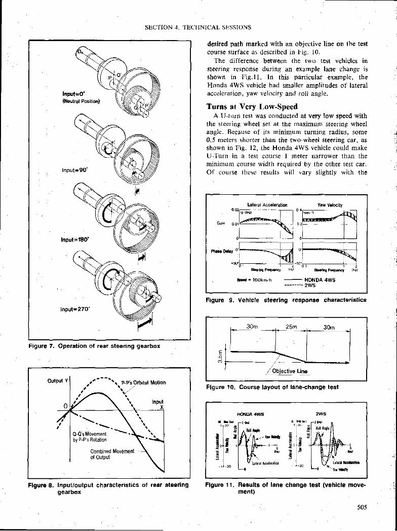
SECTION 4. TECHNICAL SESSIONS

Figure 7. Operation of rear steering gearbox

Flgure L lnput/output characteri$tics of rear steerlnggearbox

desired path marked with an objective line on the testcourse surface as described in Fig. 10,

The difference between the two test vehicles insteering response during an example lane change is .,ishown in Fig.l L In this particular example, theHonda 4WS vehicle had smaller amplitudes of lateralacceleration, yaw velocity and roll angle.

Turns at Very Low-SpeedA Ulurn test was conducted at very low speed with

the steering wheel set at the maximum steering wheel :angle. Because of its minimum turning radius, some .i0.5 meters shorter than the two-wheel steering car, a$ ;shown in Fig. 12, the Honda 4WS vehicle could make iU-Turn in a te$t course I meter narrower than the l

minimum course width required by the other test car. ,Of course these results wil l vary slightly with the

Lateral Accoleration

Gain 0,01

0

0 . 4

0 ?

Plraro Hay

0 1Srarltrg Flfiffiy lHzl Se*liq Fra$Hrct (Hr)

Enrd - looknrih ----_- l$[On

+WS

YEw Velocity

[[ilil[

Flgure 9. Vehicle steerlng response characteristics

Eul(r)

/ Objectivg Line

Figure 10. Course layout of lane-change test

Flgure 11. Results ol lane change test (vehicl6 move-ment)

t

2WS

I ioql

Soll Angla

16l lDq/sclI r 3 0

l - E

E l - =E " f $ d= L E- l

1 r - J d

HC}IUOA 4VIAi

E it|/srll r3o e

I - 6

E l =F l = 4

fi.+I o= l rf l- l

- r r - lo

545

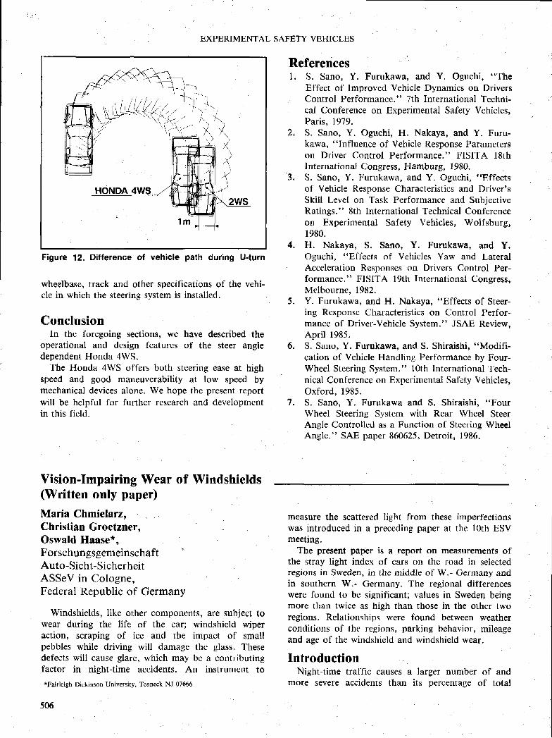
EXPERIMENTAL SAFETY VEHICLES

wheelbase, track and other specifications of the vehi-cle in which the steering system is installed.

Conclusionln the foregoing sections, we have described the

operational and design features of the steer angledependent Honda 4WS.

The Honda 4WS offers both steering ease at highspeed and good maneuverability at low speed bymechanical devices alone. We hope the present reportwill be helpful lbr further research and developmentin this field.

Vision-Impairing Wear of Windshields(Written only paper)

Maria Chmielarz,Christian Groetzner,Oswald Hflase*,ForschungsgemeinschaftAuto-Sicht-SicherheitASSeV in Cologne,Federal Republic of Germany

Windshields, like other components, are subject towear during the life of the car; windshield wiperaction, scraping of ice and the impact of smallpebbles while driving will damage the glass. Thesedefects will cause glare, which may be a contributingfactor in night-time accidents. An instrument to*Fairleigh Dickiflson University, Teaneck NJ 07666

506

Referencesl. S. Sano, Y. Furukawa, and Y. Oguchi, "The

Effect of Improved Vehicle Dynamics on DriversControl Performance." 7th International Techni-cal Conference on Experimental Safety Vehicles,Paris. 1979.S. Sano, Y. Oguchi, H. Nakaya, and Y. Furu-kawa, "Influence of Vehicle Response Farameterson Driver Control Performance." FISITA lSthlnternational Congress, Hamburg, 1980.S. Sano, Y. Furukawa, and Y. Oguchi, "Effects

of Vehicle Response Characteristics and Driver'sSkill Level on Task Perfonnance and SubjectiveRatings." 8th lnternational Technical Conferenceon Experirnental Safety Vehicles, Wolfsburg,1980.H. Nakaya, S. Sano, Y. Furukawa, and Y.Oguchi, "Effects of Vehicles Yaw and LateralAcceleration Responses on Drivers Control Per-formance." FISITA l9th International Congress,Melbourne. 1982.Y. Furukawa, and H. Nakaya, "Effects of Steer-ing Response Characteristics on Control Perfor-mance of Driver-Vehicle System." JSAE Review,April 1985.S. Sano, Y. Furukawa, and S. Shiraishi, "Modifi-

cation of Vehicle Handling Performance by Four-Wheel Steering System." 10th International Tech-nical Confierence on Experimental Safety Vehicles,Oxford. 1985.S. Sano, Y. Furukawa and S. Shiraishi, "Four

Wheel Steering System with Rear Wheel SteerAngle Controlled as a Ilunction of Steering WheelAngle." SAE paper 860625, Detroit, 1986.

measure the scattered light from these imperfectionswas introduced in a preceding paper at the l0th ESVmeeting.

The present paper is a report on measurements ofthe stray light index of cars on the road in selectedregions in Sweden, in the middle of W.- Cermany andin southern W.- Germany. The regional differenceswere found to be significant; values in Sweden beingmore than twice as high than those in the other tworegions. Relationships were found between weatherconditions of the regions, parking behavior, mileageand age of the windshield and windshield wear.

IntroductionNight-time traffic causes a larger number of and

more severe accidents than its percentage of total

2.

3 .

4.

{

6.

7 .

Figure 12. Diflerence of vehicle path during U-turn

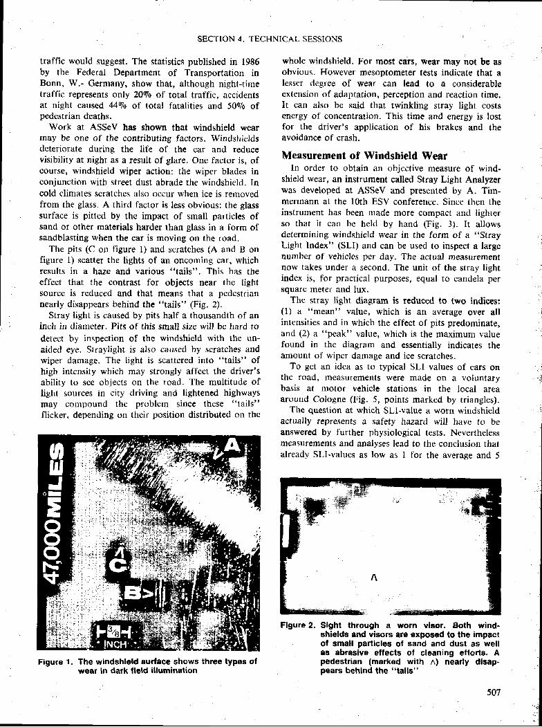
SECTION 4. TECHNICAL SESSIONS

traffic would suggest. The statistics published in 1986by the Federal Department of Transportation inBonn, W.- Cermany, show that, although night-timetratfic represents only 2090 of total traffic, accidentsat night caused 44r/o of total fatalities and 50go ofpedestrian deaths.

Work at ASSeV has shown that windshield wearmay be one of the contributing factors. Windshieldsdeteriorate during the life of the car and reducevisibility at night as a result of glare. One factor is, ofcourse, windshield wiper action: the wiper blades inconjunction with street dust abrade the windshield. Incold climates scratches also occur when ice is rernovedfrom the glass. A third factor is less obvious: the glasssurface is pitted by the impact of small particles ofsand or other materials harder than glass in a form ofsandblasting when the car is moving on the road.

The pits (C on figure l) and scratches (A and B onfigure l) scatter the tights of an oncoming car, whichresults in a haze and various "tails". This has theeffect that the contrast for objects near the lightsource is reduced and that means that a pedestriannearly disappears behind the "tails" (Fig. 2).

Stray light is caused by pits half a thousandth of aninch in diameter. Pits of this small siee will be hard todetect by inspection of the windshield with the un-aided eye. Straylight is also caused by scratches andwiper damage. The light is scattered into "tails" ofhigh intensity which may strongly affect the driver'sability to see objects on the road. The multitude oflight sources in city driving and lightened highwaysmay compound the problem since these "tails"

flickern depending on their position distributed on the

Figure 1. The windshleld surface shows three types ofwear in dark field illumination

whole windshield. For most cars, wear may not be asobvious. However mesoptometer tests indicate that alesser degree of wear can lead to a considerableextension of adaptation, perception and reaction time.It can also be said that twinkling stray light costsenergy of concentration. This time and energy is lostfor the driver's application of his brakes and theavoidance of crash.

Measurement of Windshield Wearln order to obtain an objcctive measure of wind-

shield wear, an instrument called Stray Light Analyzerwas developed at ASSeV and presented by A. Tim-mermann at the lOth ESV conference. Since then theinstrument has been made more compact and lighterso that it can be helcl by hand (Fig. 3). It allowsdetermining windshield wear in the form of a "Stray

Light Index" (SLI) and can be used to inspect a largenumber of vehicles per day. The actual measurementnow takes under a second. The unit of the stray lightindex is, for practical purposes, equal to candela perSquare meter and lux.

The stray light diagram is reduced to two indices:(1) a "mean" value, which is an average over allinrensities and in which the effect of pits predominate,and (2) a "peak" value, which is the maximum valuefound in the diagram and essentially indicates theamount of wiper darnage and ice scratches.

To get an idea as to typical SLI values of cars onthe road, measurcments were made on a voluntarybasis at motor vehicle stations in the local areaaround Cologne (Fig. 5, points marked by triangles).

The question at which Sl,I-value a worn windshieldactually r€presents a safety hazard will have to beanswered by further physiological tests. Neverthelessmeasurements and analyses lead to the conclusion thatalready Sll-values as low as I for the average and 5

Flgure 2. Slght through a worn vleor. Both wind-shielde and visors are exposed to the impactof small particles of sand and dust as welles abrasive effecte of cleaning eftorts. Apedestrian (marked with n) nearly dimp-pears behind the "tails"

:,

507

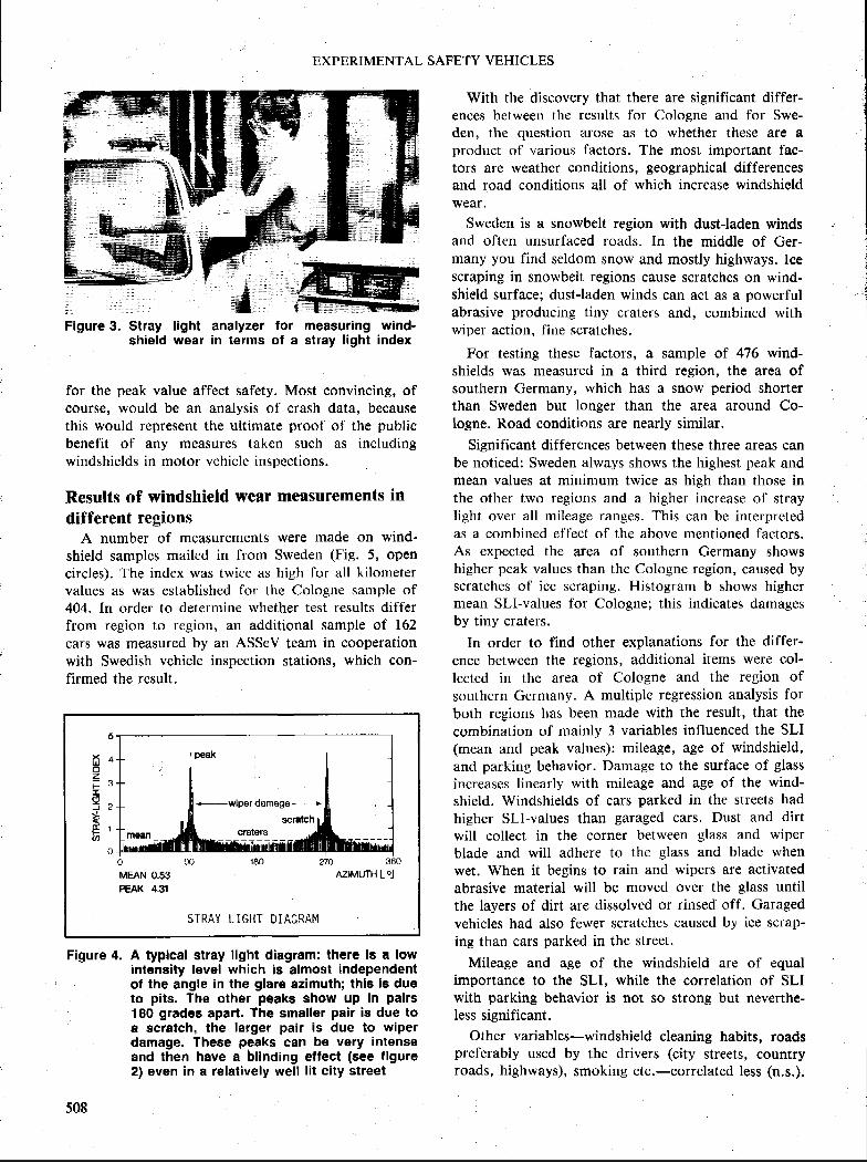
EXPERIMENTAL SAFE'TY VEHICLES

Figure 3. Stray l ight analyzer for measuring wind-shield wear in terms of a stray l ight index

for the peak value affect safety. Most convincing, ofcourse, would be an analysis of crash data, becausethis would represent the ultimate proof of the publicbenefit of any measures takcn such as includingwindshields in motor vehicle inspections.

Results of windshield wear meflsurements indifferent regi0ns

A number of measurements were made on wind'shield samples mailed in from Sweden (Fig. 5, opencircles). The index was twice as high for all kilometervalues as was established for the Cologne sample of404. In order to determine whether test results differfrom region to region, an additional sample of 162cars was measured by an ASSeV team in cooperationwith Swedish vehicle inspection stations, which con-firmed the result.

Figure 4. A typlcal stray light diagram: there ls a lowintensity level which is almost independentof the angle in the glare azimuth; thls le due

, to pits. The other peaks show up in pairslB0 grades apart. The smaller pair is due toe scrateh, the larger pair is due to wiperdamage. These peaks can be very intenseand then have a blinding effect (see figure2) even in a relatively well lit city street

With the discovery that there are significant differ-ences between the results for Cologne and for Swe-den, the question arose as to whether these are aproduct of various factors. The mosl important fac-tors are weather conditions, geographical differencesand road conditions all of which increase windshieldwear.

Sweden is a snowbelt region with dustladen windsand often unsurfaced roads. In the middle of Ger-many you find seldom snow and mostly highways. Icescraping in snowbelt regions cause scratches on wind-shield surface; dust-laden winds can act as a powerfulabrasive producing tiny craters and, combined withwiper action, fine scratches.

For testing these factors, a sample of 476 wind-shields was measured in a third region, the area ofsouthern Germany, which has a snow period shorterthan Sweden but longer than the area around Co-logne. Road conditions are nearly similar.

Significant differences between these three areas canbe noticed: Sweden always shows the highest peak andmean values at minimum twice as high than those inthe other two regions and a higher increase of' straylight over all mileage ranges. This can be interpretedas a combined effect of the above mentioned factors.As expected the area of southern Germany showshigher peak values than the Cologne region, caused byscratches of ice scraping. Histogram b shows highermean Sll-values for Cologne; this indicates damagesby tiny craters.

In order to find other explanations for the differ'

ence between the regions, additional items were col'lected in the area of Cologne and the region of

southern Germany. A multiple rcgression analysis for

both regions has been made with the result, that the

combination of mainly 3 variables influenced the SLI(mean and peak values): mileage, age of windshield,and parking behavior. Damage to the surface of glass

increases Iinearly with mileage and age of the wind-shield. Windshields of cars parked in the streets had

higher Sll-values than garaged cars. Dust and dirtwill collect in the corner between glass and wiperblade and will adhere to the glass and bladc whenwet. When it begins to rain and wipers are activatedabrasive material will be moved over the glass until

the layers of dirt are dissolved or rinsed off. Garagedvehicles had also fewer $cratches caused by ice scrap-ing than cars parked in thc street.

Mileage and age of the windshield are of equalimportance to the SLI, while the correlation of SLIwith parking behavior is not so $trong but neverthe-less significant.

Other variables-windshield cleaning habits, roadspreferably used by the drivers (city streets, countryroads, highways), smoking etc.-correlated less (n.s.).

N A

z; 3-= ?+l E rFth

o

p€ak

--wlperdamage+

scrEtch

mean _ *ffi*__ __":a=l'__ _ _1ffi-=- ____

MEAN 0.Sg AZTMUTH [o]PEAK 4.31

STRAY LIGHT DIAGRAM

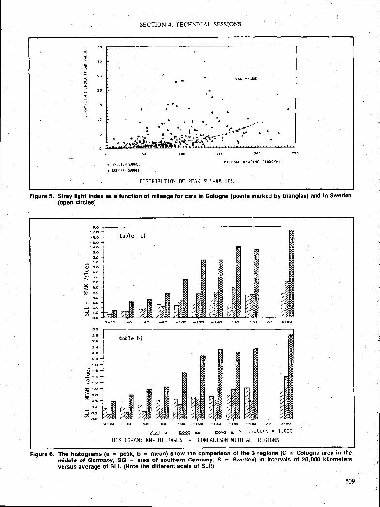
__ 15

JJ

> 3 0

L- ? 5

l{Hzl z oEo

fI t 4

. E

r 0

1 0 0 1 5 0

o sxtDISH $AlfLE HILPT'E RuolNG t l000KHt

a C0lOGltE SMPLE

DISTRIBUTION OF PEAK 5L I -VALUES

PFAI( VALI.JEo 6

a

o"I

^ t a

6

a A

" n t 1 A " ^ " " A

o A A l

,^ " . . o"^ .q i " " .^ - )+{ . ^ .

o o

SECTION 4. TECHNICAL SESSIONS

Figure 5. Stray llght lndEx as a lunctlon of mlleage for cars in Cologne (points marked by triangles) and in $weden(open circles)

Figure 6. The histogram$ (a = peak, b = mea[) show the cOmparleon ot the 3 regions (C = Cologne area in the- middle of-Germany, SG = area of southern Germany, S = Sweden) in intervals of 20,000 kilometersversus average of SLl. (Note the diflerent scale ot SLlt)

tab le a )

1 E , O

1 7 , O

| 6 . 0

t 3 , o

l 4 , o

i 5 . o

r 2 . d

o r o - o

= s - o

. E e , oa - o

* . . o

H ..oa . o

I t . o

s 2 . O

d t ' D

5,O

2,t

2.6

2 , 4

2 . 2

2 , O

t . E

o 1 . 6=> 1 , 2

z t . o

t ! d.6E

o . 6I

o . 4

J O . 2

o.oo - m - 4 o - G 6 4 0 - 1 m

@ c E S t

H I S T O G R A M : K M _ ] N T E R V A L S

- t zt t - t 5 -1 6 -1 tEt / / >rBo

to E f f i t I k i lometers x . l ,000

C O M P A R i S O N l . I I T H A L L R E 6 I O N S

t a b l e b )

509

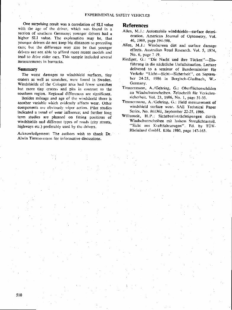
EXPERIMENTAL SAFETY VEHICLES

One surprising result was a correlation of SLI valuewith the age of the driver, which was found in asection of southern Germany; younger drivers had ahigher SLI value. The explanation may be, thatyounger drivers do not keep big distances to precedingcars; but the difference may also be that youngerdrivers are not able to afford more recent models andtend to drive older cars. This sample included severalmea$urements in barracks.

SummaryThe worst damages to windshield surfaces, tiny

craters as well as scratches, were fbund in Sweden.Windshields of the Cologne area had fewer scratchesbut more tiny craters and pits in contrast to thesouthern region. Regional differences are significant.

Besides mileage and age of the windshield there isanother variable which evidently aff'ects wear. Othercomponent$ are obviously wiper action. Pilot studiesindicated a trend of wear influence; and further longterm studies are planned on fitting positions ofwindshields and different types of roads (ciry streets,highways etc.) preferably used by the drivers.

Acknowledgement: The authors wish to thank Dr.Alwin Timmermann for irrformative discussions.

ReferencesAllen, M.J.: Automobile windshields-surface deteri-

oration. American Journal of Optometry, Vol.46, 1969, page 594-598.

Allen, M.J.: Windscreen dirt and surface damageeffects. Australian Road Research. Vol. S, 1974,No. 6, page 7-19.

Riediger, G.: "Die Nacht und ihre Tiicken"-Ein-ftihrung in die niichtliche Unfallsituation. Lecturedelivered to a seminar of Bunclesminister fiirVerkehr "Licht-Sicht-Sicherheit", on Septem-ber 24-25, 1986 in Bergisch-Gladbach, W.-Germany.

Timmermann, A./Cehring, G.: Oberfliichenschidenan Windschurzscheiben. Zeitschrift fiir Verkehrs-sicherheit . Vo[. 23, 1986, No. l , page 3l-35.

Timmermann, A.,/Cehring, G.; Field measurement ofwindshield surface wear. SAE Technical paperSeries, No. 861361, September 22-25, 1986.

Wil lumeit , H.P.; Sichtbeeintr i icht igungen durchWindschutzscheiben mit hohem Streulichtanteil."Sicht aus Kraftfahrzeugen". Ed. by TUV-Rheinland CmbH. Koln 1980, page 147-163.

510