Correlated Linear Response Calculations of the C6 Dispersion Coefficients of Hydrogen Halides

Brill Academic PublishersP.O. Box 9000, 2300 PA Leiden,The Netherlands

Computing Letters (CoLe)

vol. 3, no. 2-4, 2007, pp. 399-421ISSN 1574–0404

Correlated Linear Response Calculations of the C6

Dispersion Coefficients of Hydrogen Halides

Stephan P. A. Sauer‡1 and Ivana Paidarova†2

‡Department of Chemistry, University of Copenhagen,Universitetsparken 5, DK-2100 København Ø, Denmark

†J. Heyrovsky Institute of Physical Chemistry, ASCR, v.v.i.,Dolejskova 3, Praha 8, 182 23 Czech Republic

Received 23 June, 2007; accepted 27 August, 2007

Abstract: Three correlated linear response theory methods – the second order polarizationpropagator approximation (SOPPA), the second order polarization propagator approxima-tion with coupled cluster singles and doubles amplitudes, SOPPA(CCSD), and multiconfig-urational self-consistent field (MCSCF) linear response theory – were used to determine theelectric dipole polarizabilities at imaginary frequencies of the hydrogen halides HX (withX = F, Cl, Br and I). The dynamic polarizabilities were subsequently used to calculatethe C6 dispersion coefficient for a pair of interacting HX molecules via numerical integra-tion of the Casimir-Polder formula. The dependence of the polarizabilities, their frequencydependence and C6 coefficients on the one-electron basis set, the level of correlation andzero-point vibrational corrections was studied. Furthermore it was investigated whetherrelativistic effective core potentials (RECP) could be employed in such calculations. It wasfound that SOPPA(CCSD) and MCSCF calculations with large active spaces using basissets of at least double augmented quadruple zeta quality give comparable results whichin particular for SOPPA(CCSD) are in close agreement with the available experimentalvalues. Furthermore it could be shown that the results of the RECP calculations are inclose agreement with the all electron calculations.

Keywords: hydrogen halides, C6 dispersion coefficients, van der Waals coefficients, po-larizability at imaginary frequencies, SOPPA, SOPPA(CCSD), MCSCF linear responsefunction, relativistic effective core potentials, zero-point vibrational averaging

PACS: 31.15.Ar, 31.15.Md, 31.25.-v, 31.25.Nj, 31.30.Jv, 31.70.-f, 33.15.Kr, 34.20.Gj

1 Introduction

The dispersion-energy coefficients which govern the interaction energy of nonpolar species at longseparation (see e.g. [1, 2, 3, 4, 5, 6, 7]) are of great interest for atomic and molecular physics inparticular at low temperature. Accurately calculated values of dispersion coefficients are neededfor, e.g., the interpretation of experiments concerning total and differential cross-sections from low-angle scattering [8]. The anisotropic part of the dispersion interaction energy plays an importantrole in, e.g., molecular dynamics simulations of molecules, where the mutual orientation has to betaken into account [9], or in molecular modelling of crystal structures [10].

1Corresponding author. E-mail: [email protected]. URL: http://fyskem.ki.ku.dk/sauer2E-mail: [email protected]

400 S.P.A. Sauer and I. Paidarova

The long-range asymptotic part of the weak interaction of van der Waals complexes is deter-mined by the electric polarizability. While the asymptotic induction energy can be calculated fromstatic multipole polarizabilities and multipole moments, the dispersion energy is described in termsof dispersion coefficients which are related to the dynamic multipole polarizabilities at imaginaryfrequencies via integration in the Casimir-Polder formula [4].

A. D. Buckingham has published two seminal review articles on this topic [11, 12] which havebeen and still are an important source of inspiration for many researchers including us [13, 14,15, 16, 17, 18, 19]. We decided therefore to contribute to this special issue in honour of A. D.Buckingham with a study of C6 dispersion coefficients using correlated linear response methods.The emphasis of the study is on basis set and zero-point vibrational averaging effects as well as thepossible usage of relativistic effective large-core potentials, but in particular on the performance ofthe second order polarization propagator methods, SOPPA and SOPPA(CCSD). This is thus thefirst application of the SOPPA(CCSD) method to the calculation of dispersion coefficients.

2 Theoretical Background

Wormer and co-workers [20, 21, 22, 23, 24, 25, 26, 27, 28] expand the second order dispersionenergy between two diatomic molecules A and B as

ΔEABdisp(θA, φA, θB , φB , R) =

∑LA,LB ,L

ΔELALBL(R) ALALBL(θA, φA, θB , φB) (1)

where ALALBL(θA, φA, θB , φB) is an angular function [21], which can be defined in terms of thenormalized spherical harmonics functions Y M

L (θ, φ) as

ALALBL(θA, φA, θB , φB) =∑M

(LA LB LM −M 0

)√4π

2LA + 1Y M

LA(θA, φA)

√4π

2LB + 1Y −M

LB(θB , φB)

(2)The expansion coefficients ΔELALBL(R) are given as

ΔELALBL(R) = −∑

n

CLALBLn

Rn(3)

In case of the dipole-dipole dispersion interaction this leads to six C6 coefficients, of which, however,only four are independent

C0006 =

23

(C‖,‖ + 2C⊥,‖ + 2C‖,⊥ + 4C⊥,⊥

)(4)

C0226 =

23

√5

(C‖,‖ + 2C⊥,‖ − C‖,⊥ − 2C⊥,⊥

)(5)

C2026 =

23

√5

(C‖,‖ − C⊥,‖ + 2C‖,⊥ − 2C⊥,⊥

)(6)

C2206 =

23

1√5

(C‖,‖ − C⊥,‖ − C‖,⊥ + C⊥,⊥

)(7)

C2226 =

10√14

C2206 (8)

C2246 =

545

C2206 (9)

The coefficients C0226 and C202

6 become equal, if the molecules A and B are the same. Instead ofthe anisotropic coefficients C022

6 to C2246 one often reports dimensionless anisotropy factors γLALBL

n

C6 coefficients of hydrogen halides 401

defined as

γLALBLn =

CLALBLn

C000n

(10)

The coefficients C‖,‖, C⊥,‖, C‖,⊥ and C⊥,⊥ can be obtained from electric dipole polarizabilitiesαA/B of the two molecules via integration over imaginary frequencies3 ıω according to the Casimir-Polder formula [4]

C‖,‖ =12π

∫ ∞

0

αA‖ (ıω) αB

‖ (ıω) dω (11)

C⊥,‖ =12π

∫ ∞

0

αA⊥(ıω) αB

‖ (ıω) dω (12)

C‖,⊥ =12π

∫ ∞

0

αA‖ (ıω) αB

⊥(ıω) dω (13)

C⊥,⊥ =12π

∫ ∞

0

αA⊥(ıω) αB

⊥(ıω) dω (14)

where αA/B‖ and α

A/B⊥ are the components of the polarizability tensor parallel and perpendicular

to the molecular axis of molecule A or B, respectively. The isotropic polarizability α and thepolarizability anisotropy κ of a diatomic molecule can be defined as

α =13

(α‖ + 2α⊥

)(15)

κ = α‖ − α⊥ (16)

The definition in equation (1) should be distinguished from the ”LLM” definition in termsof associated Legendre functions as employed by Langhoff, Gordon and Karplus [7] and others[29, 30, 31, 32, 33, 34, 35, 36, 37]. However, the following simple relations connect the ”LLL”coefficients of Wormer and co-workers to the CAB , ΓBA and ΔAB coefficients of Langhoff, Gordonand Karplus [7] or the C6, γ200

6 and γ2206 coefficients of Meyer [30]

C0006 = CAB = C6 (17)

γ2026 =

√5 ΓBA =

√5 γ200

6 (18)

γ2206 =

1√5

ΔAB =1

3√

5γ2206 (19)

The Casimir-Polder integrals, equations (11) - (14), are typically evaluated numerically eitherwith a transformed Gauss-Legendre scheme [38] or with a Gauss-Chebyshev quadrature [25]. Inthe present study we have employed the latter approach with a grid of 10 imaginary frequencies[25].

Components of the frequency dependent polarizabilities for imaginary frequencies,

αij(ıω) = 2∑n�=0

(E

(0)n − E

(0)0

)〈Ψ(0)

0 | μi | Ψ(0)n 〉〈Ψ(0)

n | μj | Ψ(0)0 〉

(�ω)2 +(E

(0)n − E

(0)0

)2 (20)

can in general be obtained from linear response functions [39] or polarization propagators [40, 41,42, 43, 44, 45, 46, 47]

αij(ω) = −〈〈μi; μj〉〉ω (21)

= μTi

(E[2] − �ωS[2]

)−1

μj (22)

3The frequency ω is taken to be always real here.


The Hessian E[2], metric matrix S[2] and the property gradient vectors μj are defined as

E[2] = 〈Ψ(0)0 | [h†, [H(0), h]] | Ψ(0)

0 〉 (23)

S[2] = 〈Ψ(0)0 | [h†, h] | Ψ(0)

0 〉 (24)

μj = 〈Ψ(0)0 | [h†, μj ] | Ψ(0)

0 〉 (25)

where H(0) is the unperturbed Hamiltonian of the system and {hn} denotes a complete set of exci-tation and de-excitation operators, arranged as column vector h or as row vector h. Completenessof the set of operators {hn} means that all possible excited states |Ψ(0)

n 〉 of the system must begenerated by operating on |Ψ(0)

0 〉, i.e. hn|Ψ(0)0 〉 = |Ψ(0)

n 〉.In principle the polarizability for imaginary frequencies could be obtained with this formalism

by using complex arithmetic [48, 49]. However, this can be avoided by a moment expansion of thepolarizability [21, 23, 50]

αij(ω) =∞∑

k=0

(�ω)kμT

i

(E[2]

)−1

λk (26)

where the vectors λk are given as

λ0 = μj (27)

λk = S[2](E[2]

)−1

λk−1 = S[2]Xk−1 (28)

The k-th moment is then obtained by solving the set of linear equations for Xk

E[2]Xk = λk (29)

in a reduced space [51, 52]. The Hessian matrix in the reduced spaces of the k-th and all previousmoments is finally diagonalized to give a set of pseudostates which can be used to calculate thepolarizability for the imaginary frequencies according to equation (20) [50].

The frequency dependence of the polarizability is often also written in the following form

αij(ω) =∞∑

k=0

Sij(−2k − 2) ω2k (30)

where Sij(−2k − 2) are the even dipole oscillator strength sum rules.A variety of approximate linear response or polarization propagator methods have been derived

[47]. In SOPPA [53, 54] a Møller-Plesset perturbation theory expansion of the wave function [55, 56]is employed

|Ψ(0)0 〉 ≈ N

(|ΦSCF〉 + |Φ(1)〉 + |Φ(2)〉 . . .

)(31)

= N

⎛⎝1

4

∑aibj

(1)κabij |Φab

ij 〉 +∑ai

(2)κai |Φa

i 〉 + . . .

⎞⎠

where |Φai 〉 and |Φab

ij 〉 are Slater determinants obtained by replacing the occupied orbitals i and j inthe Hartree-Fock determinant |ΦSCF〉 by the virtual orbitals a and b; (1)κab

ij , (2)κai , are the so-called

Møller-Plesset correlation coefficients and N is a normalization constant. The set of operators {hn}consist of single and double excitation and de-excitation operators. All matrix elements involvingsingle (de-)excitation operators in equations (23) – (25) are then evaluated to second order in the


fluctuation potential, which is the difference between the instantaneous interaction of the electronsand the averaged interaction as used in the Hartree-Fock approximation. Matrix elements withsingle and double (de-) excitation operators are evaluated to first order and pure double (de-)excitation matrix elements only to zeroth order. With this definition of SOPPA only the singleexcited terms in the second order correction to the wavefunction are needed. The SOPPA methodgives excitation energies and transition moments correct to second order [57, 58, 59], whereasresponse functions like the frequency dependent polarizability are correct through second order[53], meaning that in addition to all second-order terms also some higher-order terms are included.The SOPPA response function, however, is not the response of a second-order wavefunction [60].

In the SOPPA(CCSD) method [17] the Møller-Plesset correlation coefficients (1)κabij and (2)κa

i

are replaced in all SOPPA matrix elements by the corresponding coupled cluster singles and dou-bles amplitudes τab

ij and τai , whereas in the earlier CCSDPPA method [61, 62] only some of the

Møller-Plesset correlation coefficients were replaced. Although SOPPA(CCSD) is based on a CCSDwavefunction, it is still only correct through second order and not the linear response of a CCSDwavefunction [63]. Since the MP2 correlation coefficients are the result of the first iteration forthe CCSD amplitudes, the CCSD amplitudes give a more accurate description of the connecteddoubles contribution to electron correlation. Thus it is often found that SOPPA(CCSD) give abetter description of electron correlation than SOPPA [17, 18, 19, 64, 65, 66, 67, 68, 69, 70, 71, 72,73, 74, 75, 76, 77, 78, 79, 80].

Truncating, on the other hand, the wavefunction in equation (31), after the SCF determinant|ΦSCF〉 and keeping only single excitation and de-excitation operators in the set of operators {hn}one obtains the time-dependent Hartree-Fock method (TDHF) [81] also know as random phaseapproximation (RPA) [82, 83] or SCF linear response function [39].

In MCSCF response theory [39] the reference state is approximated by a MCSCF wavefunction

|Ψ(0)0 〉 ≈ |ΦMCSCF 〉 =

∑i

|Φi〉Ci0 (32)

where {|Φi〉} are configuration state functions. The set of operators {hn} contains in addition tothe non-redundant single excitation and de-excitation operators, i.e. the so-called orbital rotationoperators [84], state transfer operators {R†,R}, which are defined as

R†n = |Φn〉〈ΦMCSCF| (33)

where |Φn〉 =∑

i |Φi〉Cin are the orthogonal complement states of the MCSCF reference state.In this study we have used complete active space (CAS) [85] wavefunctions in the MCSCF linearresponse calculations. Throughout the paper we use for the description of an active space the nota-tion [86] (nA1 nB2 nB1 nA2), where nΓ is the number of orbitals in the irreducible representation Γof the C2v point group. Furthermore we will denote a CASSCF calculation by CAS(activeorbitals).

The methods described above are all based on the Born-Oppenheimer approximation. Thereforethey can be used to calculate polarizabilities of diatomic molecules for a given internuclear distanceR. However, in order to compare with experiment one should at least assume, that the twomolecules are in their vibrational ground states and use the polarizability tensors αv=0

ij for thevibrational ground state |Θv=0,J (R)〉,

αv=0ij = 〈Θv=0,J | αij(R) | Θv=0,J〉 (34)

in the Casimir-Polder integrals, equations (11) - (14). The vibrationally averaged polarizability isoften expressed as the sum of the polarizability at an equilibrium geometry, Re, and a zero-point-vibrational correction (ZPVC)

αv=0ij = αij(Re) + ΔαZPV C

ij (35)


For diatomic molecules the vibrational wavefunctions can be obtained numerically by the Cooley-Numerov technique [87] as solution of the one-dimensional Schrodinger equation

{− �

2

2μ

(d2

dR2+

J(J + 1)R2

)+

e2

4πε0

ZKZL

R+ E0(R)

}| Θv,J 〉 = Ev,J | Θv,J〉 (36)

where J is the rotational quantum number and E0(R) is the electronic energy. The vibrationalaveraging in equation (34) can then be carried out numerically, if one calculates the polarizabilitypointwise as a function of the internuclear distance R.

Significant computational savings can be obtained, if one only treats the valence electronsexplicitly, which then move in the effective field of the nuclei and of the core electrons. This is theidea of pseudopotentials or effective core potentials [88, 89, 90, 91, 92]. The effective Hamiltonianfor the n valence electrons and N nuclei can then be defined as

H(0)eff = − �

2

2me

n∑i

∇2i +

n∑i<j

e2

4πε0rij+ Vcv + Vcpp +

N∑a<b

QaQbe2

4πε0Rab(37)

where Qa is the effective charge number of the core a, i.e. the nuclear charge number of nucleus aminus the number of core electrons of this nucleus, and Vcv and Vcpp are the core valence and corepolarization potentials. In the Stuttgart-Dresden-Bonn (SDB) energy-consistent pseudopotentials[92, 93], used in this work, the spin-orbit averaged core valence pseudopotential is defined as

Vcv =n∑i

N∑a

(− Qae2

4πε0rai+

lmax∑l=0

∑k

Alke−αlkr2ai

l∑m=−l

| Ylm〉〈Ylm |)

(38)

where Ylm are the spherical harmonics functions and Alk and αlk are the adjustable parameters ofthe pseudopotential which can be obtained by fitting to calculated total valence energies. In theSDB pseudopotentials [93] the reference data were obtained from calculations including the scalarrelativistic mass-velocity and Darwin operators. The resulting pseudopotentials include thus scalarrelativistic effects and are thus also denoted as relativistic effective core potentials (RECP).

3 Computational Details

All calculations of frequency dependent polarizabilities for imaginary frequencies were carried outwith the DALTON 2.0 program [17, 28, 50, 51, 52, 94, 95]. The calculation of the C6 disper-sion coefficients via a Gauss-Chebyshev quadrature with 10 grid points, as described in reference[25], and angular momentum re-coupling techniques were done with the DISPER program ofWormer [20, 21].

Experimental equilibrium geometries [96], Re=0.09169 nm (HF), 0.12746 nm (HCl), 0.14145nm (HBr), and 0.16090 nm (HI) were used in the single point calculations. For the numericalcalculation of zero point vibrational corrections to the C6 tensor elements of the HF, HCl and HBrdimers we used the RKR potential curve of [97] for HF and the ab initio potential curves of [98] andof [99] for HCl and HBr, respectively. First, for each immaginary frequency used in the Casimir-Polder summations, equations (11) - (14), we have calculated the polarizabilities αij(ıω) pointwiseas function of the internuclear distance R in the vicinity of the equilibrium geometry. For eachimaginary frequency the polarizabilities were then averaged by use of the vibrational wavefunctionsobtained as solution of the one-dimensional Schrodinger equation, (36), by the Cooley-Numerovtechnique [87]. Finally, the zero-point vibrational averaging corrected polarizabilities were used inthe Casimir-Polder summation instead of equilibrium values.


The convergence of the polarizabilities and C6 coefficients with the basis set size was studiedfor HF, HCl and HBr using the series of Dunning’s multiple-aug-cc-pVXZ (X=T, Q and multiple= d, t) basis sets [100, 101, 102, 103, 104, 105] as well as Sadlej’s polarized basis sets [106] eitherin their original form or in a totally uncontracted form.

In addition, for HCl and HBr the all-electron calculations are compared with results obtainedusing relativistic effective large-core potentials (RECP). For HI we have only carried out RECPcalculations. The Stuttgart-Dresden-Bonn (SDB) RECPs [93] were used together with the series ofaugmented correlation consistent basis sets, SDB-aug-cc-pVXZ, of Martin and Sundermann [107]for Br and I. The additional functions in the double and triple augmented basis sets were generatedin the usual way. For Cl we have made similar extension to the Dunning basis sets without explicitoptimization of the exponents or coefficients. Dunning basis sets of corresponding quality wereused for H in the RECP calculations.

The choice of the active spaces for the MCSCF calculations was based on the natural orbitaloccupancy numbers obtained in MP2 calculations [108, 109]. Only valence orbitals and additionalvirtual orbitals were included in the active spaces. Our largest active spaces were (8441) for HF,(8552) for HCl and (9552) for HBr and HI, which means that at least 3 correlating orbitals foreach occupied orbital were included in the active space.

Table 1: HF dimer: dependence of the C6 dispersion coefficients on the basis set and polarizationpropagator method (all values in atomic units).

SOPPA SOPPA(CCSD) CAS(8441)

Basis set C0006 γ202

6 γ2246 C000

6 γ2026 γ224

6 C0006 γ202

6 γ2246

aug-cc-pVDZ 17.58 4.17 2.91 16.59 3.82 2.62 16.19 3.73 2.54aug-cc-pVTZ 19.79 3.31 1.56 18.73 3.08 1.44 18.77 2.95 1.30aug-cc-pVQZ 20.20 3.02 1.24 19.13 2.85 1.17 19.27 2.78 1.09aug-cc-pV5Z 20.18 2.96 1.18 19.14 2.80 1.12 19.39 2.73 1.05d-aug-cc-pVDZ 21.00 3.07 1.22 19.60 2.85 1.13 18.91 2.85 1.17d-aug-cc-pVTZ 20.76 2.95 1.14 19.54 2.78 1.08 19.56 2.64 0.97d-aug-cc-pVQZ 20.44 2.94 1.14 19.32 2.78 1.09 19.48 2.70 1.02t-aug-cc-pVDZ 21.02 3.02 1.18 19.62 2.81 1.10 18.92 2.81 1.14t-aug-cc-pVTZ 20.76 2.98 1.16 19.55 2.81 1.10 19.56 2.67 0.98t-aug-cc-pVQZ 20.44 2.94 1.15 19.31 2.79 1.10 19.47 2.71 1.02Sadlej 21.37 3.14 1.23 19.84 2.92 1.15 19.06 2.92 1.19Sadlej uncont. 20.50 2.94 1.15 19.37 2.77 1.09 19.58 2.69 1.01

4 Results and Discussion

4.1 Basis set convergence study

Several studies of the basis set dependence of the static polarizability calculated with correlatedmethods were recently published [18, 19, 110, 111, 112, 113, 114] for some of the hydrogen halides.The optimal basis sets with respect to size and accuracy are probably the home-made basis setsby Maroulis [110, 113], which however are difficult to generalize. The other studies, on the otherhand, were based on either Dunning’s correlation consistent basis sets [18, 19, 111, 112] or Sadlej’spolarized basis sets [18, 111, 114]. Paidarova and Sauer [19] have extend earlier studies by consid-


16.0

17.0

18.0

19.0

20.0

21.0

22.0

C6

aug-cc-pVXZdaug-cc-pVXZtaug-cc-pVXZSadlej


HF

Figure 1: C6 coefficient for HF-HF as function of the basis set and method. For each methodthe C6 coefficient (in atomic units) is plotted against the basis in the order aug-cc-pVDZ, aug-cc-pVTZ, aug-cc-pVQZ, aug-cc-pV5Z, d-aug-cc-pVDZ, d-aug-cc-pVTZ, d-aug-cc-pVQZ, t-aug-cc-pVDZ, t-aug-cc-pVTZ, t-aug-cc-pVQZ, Sadlej and uncontracted Sadlej. Triangles, squares andcircles correspond to single, double and triple augmentation of the basis set, respectively. Thecrosses correspond to the Sadlej basis sets.

2.5

2.7

2.9

3.1

3.3

3.5

3.7

3.9

4.1

4.3

4.5



HF

Figure 2: γ2026 coefficient for HF-HF as function of the basis set and method. For details of the

symbols see the caption of Figure 1.


ering also the static polarizability at twice and four times the equilibrium internuclear distance.The general conclusion is that the d-aug-cc-pVQZ basis set gives well converged results for thestatic polarizability.

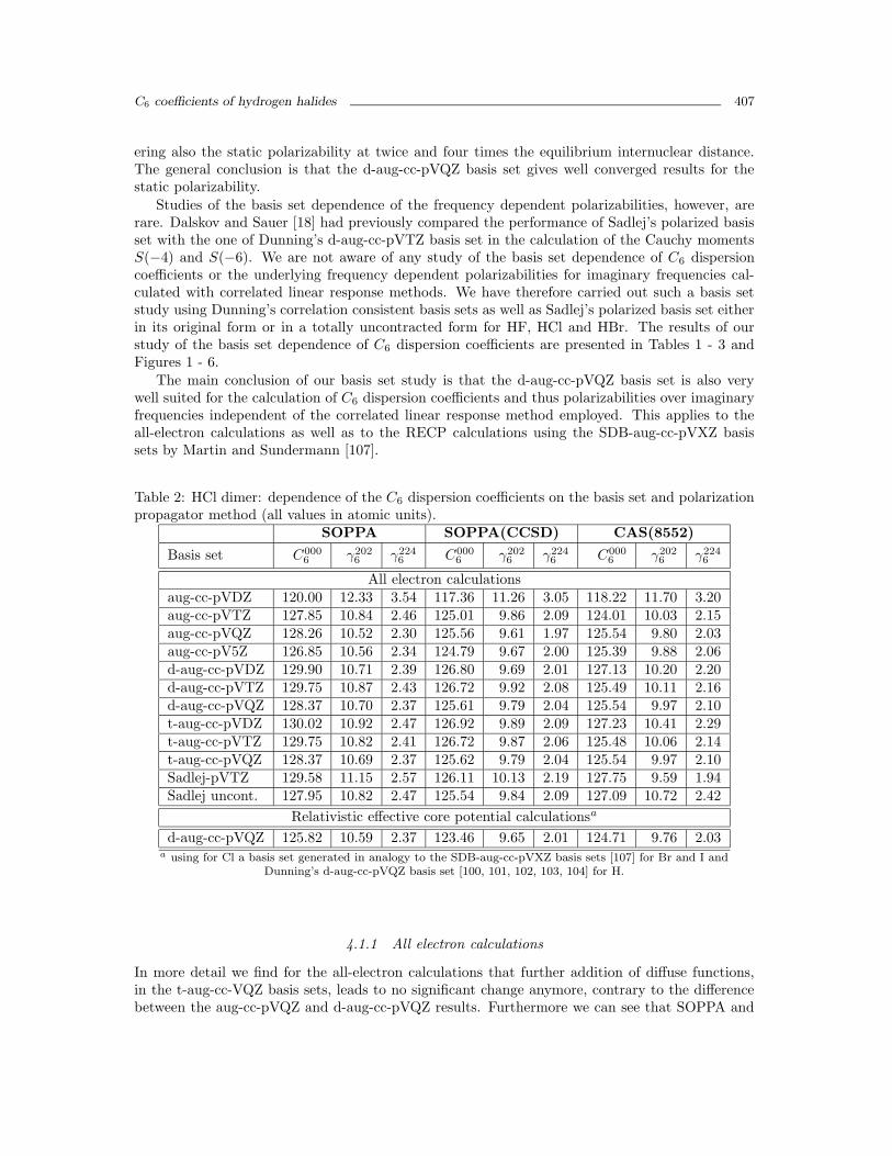
Studies of the basis set dependence of the frequency dependent polarizabilities, however, arerare. Dalskov and Sauer [18] had previously compared the performance of Sadlej’s polarized basisset with the one of Dunning’s d-aug-cc-pVTZ basis set in the calculation of the Cauchy momentsS(−4) and S(−6). We are not aware of any study of the basis set dependence of C6 dispersioncoefficients or the underlying frequency dependent polarizabilities for imaginary frequencies cal-culated with correlated linear response methods. We have therefore carried out such a basis setstudy using Dunning’s correlation consistent basis sets as well as Sadlej’s polarized basis set eitherin its original form or in a totally uncontracted form for HF, HCl and HBr. The results of ourstudy of the basis set dependence of C6 dispersion coefficients are presented in Tables 1 - 3 andFigures 1 - 6.

The main conclusion of our basis set study is that the d-aug-cc-pVQZ basis set is also verywell suited for the calculation of C6 dispersion coefficients and thus polarizabilities over imaginaryfrequencies independent of the correlated linear response method employed. This applies to theall-electron calculations as well as to the RECP calculations using the SDB-aug-cc-pVXZ basissets by Martin and Sundermann [107].

Table 2: HCl dimer: dependence of the C6 dispersion coefficients on the basis set and polarizationpropagator method (all values in atomic units).



6 γ2246 C000

6 γ2026 γ224

6 C0006 γ202

6 γ2246

All electron calculationsaug-cc-pVDZ 120.00 12.33 3.54 117.36 11.26 3.05 118.22 11.70 3.20aug-cc-pVTZ 127.85 10.84 2.46 125.01 9.86 2.09 124.01 10.03 2.15aug-cc-pVQZ 128.26 10.52 2.30 125.56 9.61 1.97 125.54 9.80 2.03aug-cc-pV5Z 126.85 10.56 2.34 124.79 9.67 2.00 125.39 9.88 2.06d-aug-cc-pVDZ 129.90 10.71 2.39 126.80 9.69 2.01 127.13 10.20 2.20d-aug-cc-pVTZ 129.75 10.87 2.43 126.72 9.92 2.08 125.49 10.11 2.16d-aug-cc-pVQZ 128.37 10.70 2.37 125.61 9.79 2.04 125.54 9.97 2.10t-aug-cc-pVDZ 130.02 10.92 2.47 126.92 9.89 2.09 127.23 10.41 2.29t-aug-cc-pVTZ 129.75 10.82 2.41 126.72 9.87 2.06 125.48 10.06 2.14t-aug-cc-pVQZ 128.37 10.69 2.37 125.62 9.79 2.04 125.54 9.97 2.10Sadlej-pVTZ 129.58 11.15 2.57 126.11 10.13 2.19 127.75 9.59 1.94Sadlej uncont. 127.95 10.82 2.47 125.54 9.84 2.09 127.09 10.72 2.42

Relativistic effective core potential calculationsa

d-aug-cc-pVQZ 125.82 10.59 2.37 123.46 9.65 2.01 124.71 9.76 2.03a using for Cl a basis set generated in analogy to the SDB-aug-cc-pVXZ basis sets [107] for Br and I and

Dunning’s d-aug-cc-pVQZ basis set [100, 101, 102, 103, 104] for H.

4.1.1 All electron calculations

In more detail we find for the all-electron calculations that further addition of diffuse functions,in the t-aug-cc-VQZ basis sets, leads to no significant change anymore, contrary to the differencebetween the aug-cc-pVQZ and d-aug-cc-pVQZ results. Furthermore we can see that SOPPA and


117.0

119.0

121.0

123.0

125.0

127.0

129.0

131.0

C6


SOPPA SOPPA(CCSD)

HCl

CAS(8552)

Figure 3: C6 coefficient for HCl-HCl as function of the basis set and method. For details of thesymbols see the caption of Figure 1.

9.0

9.5

10.0

10.5

11.0

11.5

12.0

12.5



HCl

Figure 4: γ2026 coefficient for HCl-HCl as function of the basis set and method. For details of the



SOPPA(CCSD) exhibit a very similar basis set dependence with SOPPA often showing slightlylarger changes, whereas the basis set dependence of the CAS results is different, at least for HFand HCl.

For the aug-cc-pVXZ series we could carried out calculations up to the pentuple zeta level andfind that the differences between the between X = Q and X = 5 results for C6 are only 0.5% orless for HF, 1.1% or less for HCl and 0.8% or less for HBr. The largest effects are observed in theCAS(8441) calculation for HF and in the SOPPA calculations for HCl and HBr. Also the aug-cc-pVXZ basis sets show a different convergence pattern for C6 of HF and HCl with the cardinalnumber X than the double and triple augmented basis sets.

Table 3: HBr dimer: dependence of the C6 dispersion coefficients on the basis set and polarizationpropagator method (all values in atomic units).



6 γ2246 C000

6 γ2026 γ224

6 C0006 γ202

6 γ2246

All electron calculationsaug-cc-pVDZ 187.34 20.61 6.11 183.09 18.72 5.18 184.36 19.78 5.67aug-cc-pVTZ 217.85 18.62 4.23 212.47 16.61 3.46 210.55 17.56 3.88aug-cc-pVQZ 221.05 17.80 3.82 215.79 15.88 3.13 216.15 16.63 3.40aug-cc-pV5Z 219.39 17.84 3.87 215.57 15.93 3.15 217.19 16.66 3.40d-aug-cc-pVDZ 202.83 19.89 5.14 198.05 18.00 4.32 198.73 19.01 4.77d-aug-cc-pVTZ 220.09 18.48 4.13 214.48 16.53 3.41 212.32 17.51 3.83d-aug-cc-pVQZ 221.51 17.90 3.85 216.18 15.98 3.17 216.44 16.72 3.44t-aug-cc-pVDZ 203.36 21.10 5.75 198.58 19.17 4.87 199.24 20.16 5.34t-aug-cc-pVTZ 220.54 18.37 4.08 214.91 16.42 3.35 212.75 17.41 3.78t-aug-cc-pVQZ 221.49 17.89 3.85 216.17 15.98 3.16 216.45 16.72 3.44Sadlej-pVTZ 220.63 17.05 3.53 215.73 14.98 2.81 219.48 14.39 2.57Sadlej uncont. 219.94 17.29 3.67 215.81 15.25 2.93 218.40 16.19 3.23

Relativistic effective core potential calculationsa

aug-cc-pVQZ 218.88 17.63 3.78 214.12 15.57 3.03 214.89 16.41 3.34d-aug-cc-pVTZ 221.97 17.61 3.73 216.88 15.48 2.97 215.95 16.44 3.35d-aug-cc-pVQZ 220.04 17.61 3.76 215.19 15.57 3.02 215.81 16.41 3.33t-aug-cc-pVTZ 222.00 17.60 3.73 216.91 15.48 2.97 215.95 16.40 3.33t-aug-cc-pVQZ 220.11 17.59 3.75 215.26 15.54 3.01 215.88 16.38 3.32

a using for Br the SDB-aug-cc-pVXZ basis sets [107] and Dunning’s basis set [100, 101, 102, 103, 104] for H.

Finally it is interesting to note, that the calculations with the fully uncontracted Sadlej basisset of triple zeta quality [106], denoted by crosses in Figures 1 - 6, provide results in reasonableagreement with the converged results of the series of Dunning basis sets. The agreement is bestfor HF, where all components are good reproduced with all three response methods. For HCl andHBr the best agreement is only obtained with SOPPA(CCSD) and in the later case also only forthe isotropic C6 coefficient.


180.0

185.0

190.0

195.0

200.0

205.0

210.0

215.0

220.0

225.0C

6

aug-cc-pVXZ daug-cc-pVXZ taug-cc-pVXZ Sadlej

SOPPA SOPPA(CCSD)

HBr

CAS(9552)

Figure 5: C6 coefficient for Hbr-Hbr as function of the basis set and method. For details of thesymbols see the caption of Figure 1.

13.0

14.0

15.0

16.0

17.0

18.0

19.0

20.0

21.0

22.0

aug-cc-pVXZ daug-cc-pVXZ taug-cc-pVXZ Sadlej


HBr

Figure 6: γ2026 coefficient for Hbr-Hbr as function of the basis set and method. For details of the



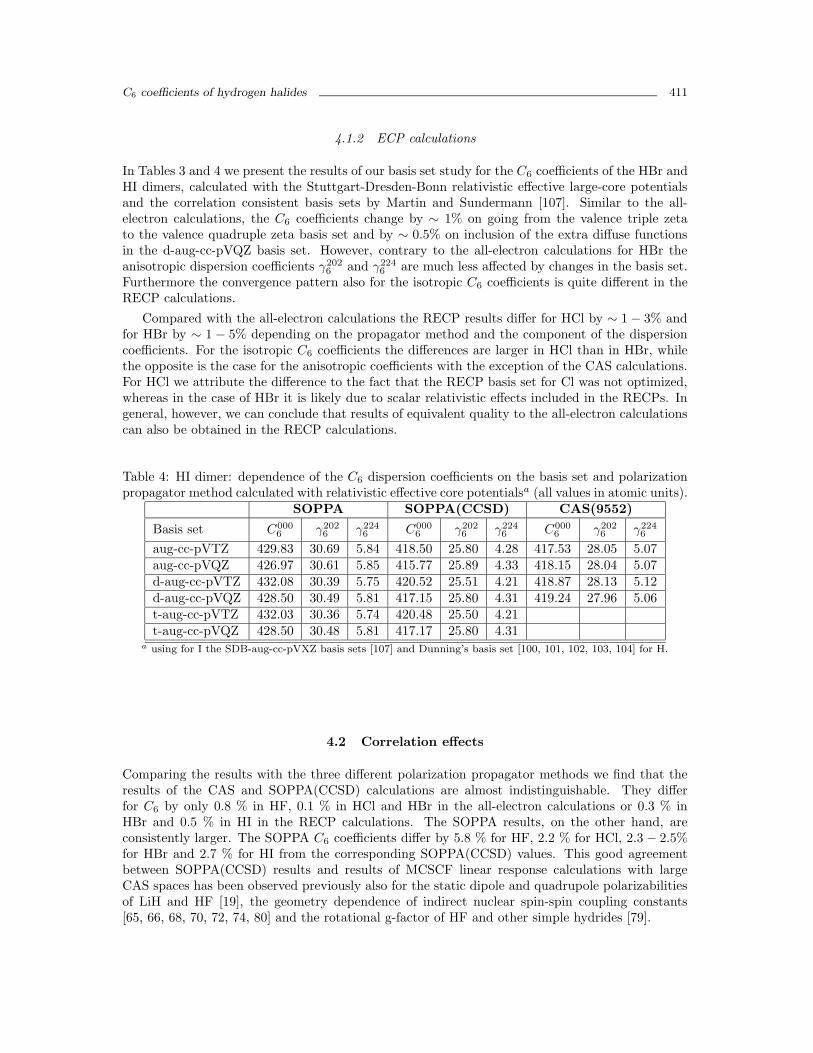
4.1.2 ECP calculations

In Tables 3 and 4 we present the results of our basis set study for the C6 coefficients of the HBr andHI dimers, calculated with the Stuttgart-Dresden-Bonn relativistic effective large-core potentialsand the correlation consistent basis sets by Martin and Sundermann [107]. Similar to the all-electron calculations, the C6 coefficients change by ∼ 1% on going from the valence triple zetato the valence quadruple zeta basis set and by ∼ 0.5% on inclusion of the extra diffuse functionsin the d-aug-cc-pVQZ basis set. However, contrary to the all-electron calculations for HBr theanisotropic dispersion coefficients γ202

6 and γ2246 are much less affected by changes in the basis set.

Furthermore the convergence pattern also for the isotropic C6 coefficients is quite different in theRECP calculations.

Compared with the all-electron calculations the RECP results differ for HCl by ∼ 1 − 3% andfor HBr by ∼ 1 − 5% depending on the propagator method and the component of the dispersioncoefficients. For the isotropic C6 coefficients the differences are larger in HCl than in HBr, whilethe opposite is the case for the anisotropic coefficients with the exception of the CAS calculations.For HCl we attribute the difference to the fact that the RECP basis set for Cl was not optimized,whereas in the case of HBr it is likely due to scalar relativistic effects included in the RECPs. Ingeneral, however, we can conclude that results of equivalent quality to the all-electron calculationscan also be obtained in the RECP calculations.

Table 4: HI dimer: dependence of the C6 dispersion coefficients on the basis set and polarizationpropagator method calculated with relativistic effective core potentialsa (all values in atomic units).



6 γ2246 C000

6 γ2026 γ224

6 C0006 γ202

6 γ2246

aug-cc-pVTZ 429.83 30.69 5.84 418.50 25.80 4.28 417.53 28.05 5.07aug-cc-pVQZ 426.97 30.61 5.85 415.77 25.89 4.33 418.15 28.04 5.07d-aug-cc-pVTZ 432.08 30.39 5.75 420.52 25.51 4.21 418.87 28.13 5.12d-aug-cc-pVQZ 428.50 30.49 5.81 417.15 25.80 4.31 419.24 27.96 5.06t-aug-cc-pVTZ 432.03 30.36 5.74 420.48 25.50 4.21t-aug-cc-pVQZ 428.50 30.48 5.81 417.17 25.80 4.31

a using for I the SDB-aug-cc-pVXZ basis sets [107] and Dunning’s basis set [100, 101, 102, 103, 104] for H.

4.2 Correlation effects

Comparing the results with the three different polarization propagator methods we find that theresults of the CAS and SOPPA(CCSD) calculations are almost indistinguishable. They differfor C6 by only 0.8 % in HF, 0.1 % in HCl and HBr in the all-electron calculations or 0.3 % inHBr and 0.5 % in HI in the RECP calculations. The SOPPA results, on the other hand, areconsistently larger. The SOPPA C6 coefficients differ by 5.8 % for HF, 2.2 % for HCl, 2.3 − 2.5%for HBr and 2.7 % for HI from the corresponding SOPPA(CCSD) values. This good agreementbetween SOPPA(CCSD) results and results of MCSCF linear response calculations with largeCAS spaces has been observed previously also for the static dipole and quadrupole polarizabilitiesof LiH and HF [19], the geometry dependence of indirect nuclear spin-spin coupling constants[65, 66, 68, 70, 72, 74, 80] and the rotational g-factor of HF and other simple hydrides [79].


Table 5: HF: best results for the static polarizability α, polarizability anisotropy κ, sum rulesS(−4) and S(−6) of HF and C6 dispersion coefficients of the HF dimer using the all-electron d-aug-cc-pVQZ basis sets in comparison with previous results and experimental values (all values inatomic units).

Method Ref. Geom. α κ S(−4) S(−6) C0006 γ202

6 γ2246

SOPPA this work Re 5.88 1.19 14.58 62.37 20.44 2.94 1.14SOPPA(CCSD) this work Re 5.68 1.18 13.83 58.87 19.32 2.78 1.09SOPPA(CCSD) this work ZPVA 5.79 1.35 14.63 65.23 19.78 3.07 1.31CAS(8441) this work Re 5.61 1.11 12.32 45.43 19.48 2.70 1.02CAS(8441) this work ZPVA 5.71 1.29 12.99 49.94 19.94 3.01 1.24SOPPA [16] Re 5.90MBPT [26, 115] Re 20.75 3.50 1.61CCSD(T) [113] Re 5.60 1.14Experiment [116, 117] 5.60 14.40 68.96 19.0

Table 6: HCl: best results for the static polarizability α, polarizability anisotropy κ, sum rulesS(−4) and S(−6) of HCl and C6 dispersion coefficients of the HCl dimer using the all electrond-aug-cc-pVQZ basis sets in comparison with previous results and experimental values (all valuesin atomic units).


6 γ2246

SOPPA this work Re 17.54 1.77 70.19 395.79 128.37 10.70 2.37SOPPA(CCSD) this work Re 17.29 1.64 68.14 377.03 125.61 9.79 2.04SOPPA(CCSD) this work ZPVA 17.34 1.72 68.53 380.38 126.09 10.11 2.17CAS(8552) this work Re 17.16 1.58 65.57 351.31 125.54 9.97 2.10SOPPA [16] Re 17.47CCSD(T) [110] Re 17.39 1.63Experiment [116, 117] 17.39 67.12 389.3 130.4

[118] 1.96±0.67[119] 1.55±0.20

4.3 Zero-point-vibrational corrections

For the HF, HCl and HBr dimers we have investigated the changes of the C6 coefficients on takinginto account the zero-point vibrational averaging corrections (ZPVC) to the dynamic polarizabili-ties. In addition we have generated vibrationally averaged values of the static polarizability tensorand the S(−4) and S(−6) sum rules. In several test calculations we have found that in the vicinityof the equilibrium geometry the shape of the α(ıω)(R) curve is almost independent on the methodand basis set considered here. Consequently, it is no surprise that the ZPVA corrections to the C6

coefficients, α and κ are identical for the SOPPA(CCSD) and MCSCF approaches as illustratedfor HF and HBr in tables 5 and 7. Larger differences between the SOPPA(CCSD) and MCSCFresults are only observed for the S(−4) and S(−6) sum rules.

In absolute values the ZPVA corrections to the C6 coefficients are with about 1.6 a.u. largest


Table 7: HBr: best results for the static polarizability α, polarizability anisotropy κ, sum rulesS(−4) and S(−6) of HBr and C6 dispersion coefficients of the HBr dimer using the d-aug-cc-pVQZor SDB-d-aug-cc-pVQZ basis sets in comparison with previous results and experimental values (allvalues in atomic units).


6 γ2246

All electron calculationsSOPPA this work Re 24.21 2.27 118.92 813.08 221.51 17.90 3.85SOPPA(CCSD) this work Re 23.87 2.03 116.18 785.16 216.18 15.98 3.17SOPPA(CCSD) this work ZPVA 24.00 2.30 117.83 804.02 217.70 17.04 3.57CAS(9552) this work Re 23.70 2.02 111.59 727.29 216.44 16.72 3.44SOPPA [16] Re 24.19MBPT4 [120] Re 23.98 1.84

Relativistic effective core potential calculationsSOPPA this work Re 24.20 2.18 119.37 833.47 220.04 17.61 3.76SOPPA(CCSD) this work Re 23.86 1.92 115.94 793.31 215.19 15.57 3.02SOPPA(CCSD) this work ZPVA 23.99 2.18 117.64 814.45 216.74 16.62 3.41CAS(9552) this work Re 23.76 1.90 113.45 765.88 215.81 16.41 3.33CAS(9552) this work ZPVA 23.89 2.16 114.91 782.85 217.38 17.53 3.75Experiment [116, 117] 23.74 116.9 827.9 216.6

[119] 2.50±0.6

Table 8: HI: best results for the static polarizability α, polarizability anisotropy κ, sum rules S(−4)and S(−6) of HI and C6 dispersion coefficients of the HI dimer using the relativistic effective corepotential SDB-d-aug-cc-pVQZ basis sets in comparison with previous results and experimentalvalues (all values in atomic units).


6 γ2246

SOPPA this work Re 36.32 2.65 234.47 2041.41 428.50 30.49 5.81SOPPA(CCSD) this work Re 35.72 2.18 227.35 1942.97 417.15 25.80 4.31CAS(9552) this work Re 35.64 2.18 223.95 1908.11 419.24 27.96 5.06CCSD(T) [121] 36.27 2.57DK-CCSD(T) [114] 36.56 1.84Experiment [121] 34.8±0.5

for HBr and smallest for HF (0.5 a.u.), which amounts to 0.5% (HCl) or 2% (HF). Numericallythe effect is also larger for C000

6 than for the dimensionless factors γ2026 (0.3 - 1.1) and γ224

6 (0.1 -0.4), whereas the order is reversed for the per cent changes due to the smallness of the γ factors.For the polarizability and its frequency dependence we can see that in absolute terms the ZPVcorrections are largest for HBr and smallest for HCl, although per cent wise they are larger for HFthan for HBr. Furthermore they increase in absolute values and per cent wise from the isotropicpolarizability (0− 2%) to the anisotropy (5− 14%) and from the S(−4) (1% or 6%) to the S(−4)(1%, 3% or 11%) sum rules.


For HBr we have carried out the vibrational averaging calculations with our all-electron andRECP results for the polarizabilities. The ZPV corrections obtained at the SOPPA(CCSD) levelwith both approaches are identical.

4.4 Relativistic corrections

In several recent studies [122, 123, 114] the importance of relativistic corrections to the dipolepolarizabilities of hydrogen halides have been investigated. These studies were partly stimulatedby the large discrepancy between the old literature value of uncertain origin [121] for the polar-izability anisotropy in HI and the result of highly accurate non-relativistic calculations publishedby Maroulis [121]. Norman et al. [122] as well as Pecul and Rizzo [123] employed the relativisticfour-component TDHF method and found that relativistic effects are very small for the polariz-abilities of hydrogen halides, the differences between relativistic and non-relativistic results are atmost 3% at the TDHF level. Norman et al. [122] could also show that the relativistic effects onthe polarizabilities of hydrogen halides can be reproduced using either the scalar Douglas-Kroll ap-proximation or the same RECPs as employed in the present study. This is in contrast to our earlierfindings [124] for the rotational g-factor of the hydrogen halides, where the results of relativisticfour-component TDHF calculations for HBr and HI could not be reproduced by a perturbativetreatment via non-relativistic calculations with the mass-velocity and Darwin operator as pertur-bation. Ilias et al. [114] finally studied simultaneously electron correlation as well as scalar andspin-orbit relativistic effects on the polarizability of HI. They could confirm the earlier findingthat scalar relativistic effects are small and could furthermore show that this applies also to thespin-orbit effects. Based on these studies we can safely assume that all relativistic effects on theC6 dispersion coefficients are recovered in our RECP calculations.

For HBr we find thus that the scalar relativistic effects included in the RECPs have no effecton the isotropic static polarizability but change the anisotropy by about 5%. The changes in theisotropic C6 coefficient are about 1 a.u. or 0.5−1% and numerically smaller but per cent wise largerfor the anisotropy factors γ6. Finally the scalar relativistic correction to the frequency dependenceof the polarizability, i.e. S(−6), is about 10 - 20 a.u. or 1 − 3%.

4.5 Comparison with previous calculations and experiment

In Tables 5 to 7 we compare our best results with earlier results for the static polarizabilities, i.e. thehighly accurate non-relativistic CCSD(T) results for HF, HCl and HI by Maroulis [113, 110, 121],the non-relativistic MBPT4 calculation for HBr by Sadlej [120] and the scalar relativistic CCSD(T)calculation for HI by Ilias et al. [114], as well with the experimental based values for the isotropicpolarizabilities, their frequency dependence and the isotropic C6 coefficients of HF, HCl and HBrby Kumar and Meath [116, 117], which are obtained from an effective dipole oscillator strengthdistribution fitted to experimental values. The agreement between our calculations, in particularat the SOPPA(CCSD) level, and these reference values is in general very good.

In more detail we find that the agreement between our equilibrium geometry SOPPA(CCSD)or CAS(8441) results for the static polarizability and the CCSD(T) results of Maroulis [113] isexcellent, although slightly better for the CAS(8441) calculations. Large differences are, however,observed between our results and the earlier MBPT values of the dispersion coefficients by Rijks andWormer [26, 115]. Comparing with the experimental results by Kumar and Meath [116, 117] we findthat our vibrationally averaged SOPPA(CCSD) or CAS(8441) results for the static polarizabilityshow also good agreement with a slightly better performance of CAS(8441) again. However, theexperimental frequency dependence, i.e. the S(−4) and S(−6) sum rules, as well as the isotropicC6 coefficients are much better reproduced at the SOPPA(CCSD) level. The differences betweenthe vibrationally averaged SOPPA(CCSD) results and the experimental values are at most 5%.


Also for HCl we find that our SOPPA(CCSD) results for the static polarizability at equilibriumdistance are in almost perfect agreement with the CCSD(T) results by Maroulis [110]. The sameholds for the vibrationally averaged SOPPA(CCSD) result in comparision with the the experimen-tal based value by Kumar and Meath [116, 117]. The differences in both cases are less than 1%.Furthermore our vibrationally averaged SOPPA(CCSD) value for S(−4), S(−6) and C000

6 is closeto the experimental value with differences in the range of 2 − 3%.

In the case of HBr we find that the RECP SOPPA(CCSD) results are closer to the experimentalvalues than the non-relativistic results. Otherwise we see the pattern from HF and HCl repeatedwith excellent agreement between our SOPPA(CCSD) results and the results of the non-relativisticMBPT4 calculation [120] for the static polarizability or the experimental values [116, 117]. Thedeviation from the MBPT4 results is only 0.1 to 0.2 a.u. for the isotropic and anisotropic polariz-ability which amounts to less than 1% for α. Per cent wise the differences between the vibrationallyaveraged RECP SOPPA(CCSD) results and the experimental values for α (1%), S(−4) (< 1%),S(−6) (2%) and C000

6 (< 1%) are even smaller than for HCl.For HI we can only compare with the non-relativistic [121] and scalar relativistic CCSD(T)

calculations of the static polarizability [114]. The agreement with out RECP calculations is ingeneral good (about 2% for α), but best at the SOPPA level for the isotropic polarizability and atthe SOPPA(CCSD) or CAS(9552) level for the anisotropy.

Significantly larger deviations from the reference and experimental values are observed inthe SOPPA calculations which implies that the usage of Coupled Cluster amplitudes in theSOPPA(CCSD) method represents an important improvement also for the calculation of C6 co-efficients as it was earlier shown to be the case for polarizabilities and NMR spin-spin couplingconstants [17, 18, 19, 64, 65, 66, 67, 68, 69, 70, 71, 72, 73, 74, 75, 76, 77, 78, 79, 80].

5 Conclusion

We have carried out correlated linear response calculations of the C6 dispersion coefficients fordimers of hydrogen halides and of the static and frequency dependent polarizabilities of themonomers employing the SOPPA, SOPPA(CCSD) and MCSCF method. Several aspects of thecalculations such as the basis set, zero-point vibrational corrections and the usage of relativisticeffective core potentials were investigated.

We find that in order to obtain well converged results for the frequency dependent polariz-abilities and C6 coefficients one has to employ at least basis sets of d-aug-cc-pVQZ quality inall-electron as well as relativistic effective core potential calculations.

Furthermore we find that the results of all-electron calculations using this basis set can verywell be reproduced with RECP calculations employing corresponding valence basis sets. Thegood performance of the relativistic pseudopotentials for calculating dynamical polarizabilities isvery encouraging for their further use. Besides the simplification of the calculations due to thereduction of the number of electrons, they account for scalar relativistic effects. In agreementwith earlier studies we have seen that for the hydrogen halides studied here (with the exceptionof HI) the relativistic effects are not so significant that they could be visible in the basis set andmethod convergence studies. However, for molecules containing heavy atoms, the inclusion ofscalar relativistic contributions will be important.

We find also that the zero-point vibrational corrections obtained in the MCSCF or SOPPA(CCSD)calculations are identical for the static polarizabilities and the C6 coefficients and amount to about2%. However, larger differences between SOPPA(CCSD) and MCSCF results are observed for theS(−4) and S(−6) sum rules and thus for the frequency dependence of the polarizability, wherethe ZPVC can amount to up to 11%. On the other hand are the ZPVC results obtained in theall-electron or RECP SOPPA(CCSD) calculations virtually identical.


Finally, we can see that SOPPA(CCSD) and MCSCF linear response calculations with largeactive spaces give very similar results for the static polarizabilities. However, larger differences areobserved for the C6 coefficients and in particular for the frequency dependence of the polarizabilityas given by the S(−4) and S(−6) sum rules. Consequently we find very good agreement betweenour SOPPA(CCSD) and MCSCF equilibrium results and the results of earlier MBPT4 or CCSD(T)calculations. In comparison with the experimental based values for the C6 coefficients and S(−4)and S(−6) sum rules, on the other hand, of our vibrationally averaged SOPPA(CCSD) resultsperform much better than the MCSCF results with deviations between less than 1% for HBr andat most 5% for HF at the SOPPA(CCSD) level. This implies that SOPPA(CCSD) is a very wellsuited for calculations of polarizabilities in the vicinity of the equilibrium geometry, whereas multi-reference methods should be applied in calculations over larger intervals of internuclear distancesas discussed e.g. in our earlier study [19]. This is in contrast to the SOPPA results which showsignificantly larger deviations from the reference values. The use of the Coupled Cluster amplitudesin the SOPPA(CCSD) method is thus crucial for the calculation of C6 coefficients.

Acknowledgment

The authors wish to thank Dr. P. E. S. Wormer for making his DISPER program available to us.SPAS acknowledges support from the Carlsberg Foundation, the Danish Natural Science ResearchCouncil and the Danish Center for Scientific Computing. IP acknowledges support from the GrantAgency of the Academy of Sciences of the Czech Republic, grant no.IAA401870702.

References

[1] F. London, Z. Physik. Chem. B. 11, 222-251 (1930).

[2] H. Margenau, Rev. Mod. Phys. 11, 1–35 (1939).

[3] F. London, J. Phys. Chem. 46, 305–316 (1942).

[4] H. B. G. Casimir and D. Polder, Phys. Rev. 73, 360-372 (1948).

[5] M. Karplus and H. J. Kolker, J. Chem. Phys. 41, 3955-3961 (1964).

[6] A. Dalgarno, Adv. Chem. Phys. 12, 143-166 (1967).

[7] P. W. Langhoff, R. G. Gordon, and M. Karplus, J. Chem. Phys. 55, 2126-2145 (1971).

[8] G. C. Maitland, M. Ribgy, E. B. Smith, and W. A. Wakeham. Intermolecular Forces. Claren-don Press, Oxford, 1981.

[9] T. Kihara. Intermolecular Forces. Wiley, New York, 1978.

[10] M. P. Allen and D. J. Tildesley. Computer Simulation of Liquids. Clarendon Press, Oxford,1987.

[11] A. D. Buckingham, Adv. Chem. Phys. 12, 107-142 (1967).

[12] A. D. Buckingham, P. W. Fowler, and J. M. Hutson, Chem. Rev. 88, 963–988 (198).

[13] S. P. A. Sauer, G. H. F. Diercksen, and J. Oddershede, Int. J. Quantum Chem. 39, 667-679(1991).

[14] S. P. A. Sauer, J. R. Sabin, and J. Oddershede, Phys. Rev. A. 47, 1123-1129 (1993).


[15] M. J. Packer, S. P. A. Sauer, and J. Oddershede, J. Chem. Phys. 100, 8969-8975 (1994).

[16] M. J. Packer, E. K. Dalskov, S. P. A. Sauer, and J. Oddershede, Theor. Chim. Acta. 89,323-333 (1994).

[17] S. P. A. Sauer, J. Phys. B: At. Mol. Opt. Phys. 30, 3773-3780 (1997).

[18] E. K. Dalskov and S. P. A. Sauer, J. Phys. Chem. A. 102, 5269-5274 (1998).

[19] I. Paidarova and S. P. A. Sauer, Adv. Quantum Chem. 48, 185-208 (2005).

[20] P. E. S. Wormer. PhD thesis, Katholieke Universiteit Nijmegen, The Netherlands, 1975.

[21] F. Visser, P. E. S. Wormer, and P. Stam, J. Chem. Phys. 79, 4973-4984 (1983).

[22] F. Visser, P. E. S. Wormer, and P. Stam, J. Chem. Phys. 81, 3755 (1984).

[23] F. Visser and P. E. S. Wormer, Mol. Phys. 52, 923-937 (1984).

[24] F. Visser, P. E. S. Wormer, and W. P. J. H. Jacobs, J. Chem. Phys. 82, 3753-3764 (1985).

[25] W. Rijks and P. E. S. Wormer, J. Chem. Phys. 88, 5704-4714 (1988).

[26] W. Rijks and P. E. S. Wormer, J. Chem. Phys. 90, 6507-6519 (1989).

[27] P. E. S. Wormer and H. Hettema, J. Chem. Phys. 97, 5592-5606 (1992).

[28] H. Hettema, P. E. S. Wormer, P. Jørgensen, H. J. Aa. Jensen, and T. Helgaker, J. Chem.Phys. 100, 1297-1302 (1994).

[29] G. A. Victor and A. Dalgarno, J. Chem. Phys. 50, 2535-2539 (1969).

[30] W. Meyer, Chem. Phys. 17, 27-33 (1976).

[31] Ph. Coulon, R. Luyckx, and H. N. W. Lekkerkerker, J. Chem. Phys. 71, 3462-3466 (1979).

[32] A. J. Thakkar, H. Hettema, and P. E. S. Wormer, J. Chem. Phys. 97, 3252-3257 (1992).

[33] D. Spelsberg, T. Lorenz, and W. Meyer, J. Chem. Phys. 99, 7845-7858 (1993).

[34] P. E. S. Wormer, H. Hettema, and A. J. Thakkar, J. Chem. Phys. 98, 7140-7144 (1993).

[35] H. Hettema, P. E. S. Wormer, and A. J. Thakkar, Mol. Phys. 80, 533-548 (1993).

[36] U. Hohm, Chem. Phys. 179, 533-541 (1994).

[37] V. Magnasco and M. Ottonelli, J. Mol. Struct. (Theochem). 469, 31-40 (1999).

[38] R. D. Amos, N. C. Handy, P. J. Knowles, J. E. Rice, and A. J. Stone, J. Phys. Chem. 89,2186-2192 (1985).

[39] J. Olsen and P. Jørgensen, J. Chem. Phys. 82, 3235-3264 (1985).

[40] J. Linderberg and Y. Ohrn. Propagators in Quantum Chemistry. Academic Press, London,1973.

[41] J. Oddershede, Adv. Quantum Chem. 2, 275-352 (1978).

[42] P. Jørgensen and J. Simons. Second Quantization-Based Methods in Quantum Chemistry.Academic Press, New York, 1981.


[43] J. Oddershede. Introductory polarization propagator theory. In G. H. F. Diercksen andS. Wilson, editors, Methods in Computational Molecular Physics, pages 249–271. D. ReidelPubl. Co, Dordrecht, 1983.

[44] J. Oddershede, P. Jørgensen, and D. L. Yeager, Comput. Phys. Rep. 2, 33-92 (1984).

[45] J. Oddershede, Adv. Chem. Phys. 69, 201-239 (1987).

[46] J. Oddershede. Response and propagator methods. In S. Wilson and G. H. F. Diercksen,editors, Methods in Computational Molecular Physics, pages 303–324. Plenum Press, NewYork, 1992.

[47] S. P. A. Sauer and M. J. Packer. The ab initio calculation of molecular properties otherthan the potential energy surface. In P. R. Bunker and P. Jensen, editors, ComputationalMolecular Spectroscopy, chapter 7, pages 221–252. John Wiley and Sons, London, 2000.

[48] P. Norman, D. M. Bishop, H. J . Aa. Jensen, and J. Oddershede, J. Chem. Phys. 115,10323-10334 (2001).

[49] P. Norman, A. Jiemchooroj, and B. E. Sernelius, J. Chem. Phys. 118, 9167-9174 (2003).

[50] P. W. Fowler, P. Jørgensen, and J. Olsen, J. Chem. Phys. 93, 7256-7263 (1990).

[51] P. Jørgensen, H. J. Aa. Jensen, and J. Olsen, J. Chem. Phys. 89, 3654-3661 (1988).

[52] J. Olsen, H. J. Aa. Jensen, and P. Jørgensen, J. Comput. Phys. 74, 265-282 (1988).

[53] E. S. Nielsen, P. Jørgensen, and J. Oddershede, J. Chem. Phys. 73, 6238-6246 (1980).

[54] K. L. Bak, H. Koch, J. Oddershede, O. Christiansen, and S. P. A. Sauer, J. Chem. Phys.112, 4173-4185 (2000).

[55] C. Møller and M. S. Plesset, Phys. Rev. 46, 618-622 (1934).

[56] J. A. Pople, J. S. Binkley, and R. Seeger, Int. J. Quantum Chem. Symp. 10, 1-19 (1976).

[57] J. Oddershede and P. Jørgensen, J. Chem. Phys. 66, 1541-1556 (1977).

[58] J. Oddershede, P. Jørgensen, and N. H. F. Beebe, Int. J. Quantum Chem. 12, 655-670(1977).

[59] J. Oddershede, P. Jørgensen, and N. H. F. Beebe, J. Phys. B. 11, 1-15 (1978).

[60] J. Fagerstrom and J. Oddershede, J. Chem. Phys. 101, 10775-10782 (1994).

[61] J. Geertsen and J. Oddershede, J. Chem. Phys. 85, 2112-2118 (1986).

[62] J. Geertsen, S. Eriksen, and J. Oddershede, Adv. Quantum Chem. 22, 167-209 (1991).

[63] H. Koch and P. Jørgensen, J. Chem. Phys. 93, 3333-3344 (1990).

[64] R. D. Wigglesworth, W. T. Raynes, S. P. A. Sauer, and J. Oddershede, Molec. Phys. 92,77-88 (1997).

[65] R. D. Wigglesworth, W. T. Raynes, S. P. A. Sauer, and J. Oddershede, Molec. Phys. 94,851-862 (1998).


[66] S. P. A. Sauer, C. K. Møller, H. Koch, I. Paidarova, and V. Spirko, Chem. Phys. 238,385-399 (1998).

[67] T. Enevoldsen, J. Oddershede, and S. P. A. Sauer, Theor. Chem. Acc. 100, 275-284 (1998).

[68] S. Kirpekar and S. P. A. Sauer, Theor. Chem. Acc. 103, 146-153 (1999).

[69] R. D. Wigglesworth, W. T. Raynes, S. Kirpekar, J. Oddershede, and S. P. A. Sauer, J. Chem.Phys. 112, 736-746 (2000).

[70] R. D. Wigglesworth, W. T. Raynes, S. Kirpekar, J. Oddershede, and S. P. A. Sauer, J. Chem.Phys. 112, 3735-3746 (2000).

[71] S. P. A. Sauer and W. T. Raynes, J. Chem. Phys. 113, 3121-3129 (2000).

[72] M. Grayson and S. P. A. Sauer, Mol. Phys. 98, 1981-1990 (2000).

[73] P. F. Provasi, G. A. Aucar, and S. P. A. Sauer, J. Chem. Phys. 115, 1324-1334 (2001).

[74] S. P. A. Sauer, W. T. Raynes, and R. A. Nicholls, J. Chem. Phys. 115, 5994-6006 (2001).

[75] L. B. Krivdin, S. P. A. Sauer, J. E. Peralta, and R. H. Contreras, Magn. Reson. Chem. 40,187-194 (2002).

[76] A. Ligabue, S. P. A. Sauer, and P. Lazzeretti, J. Chem. Phys. 118, 6830-6845 (2003).

[77] V. Barone, P. F. Provasi, J. E. Peralta, J. P. Snyder, S. P. A. Sauer, and R. H. Contreras, J.Phys. Chem. A. 107, 4748-4754 (2003).

[78] S. P. A. Sauer and L. B. Krivdin, Magn. Reson. Chem. 42, 671-686 (2004).

[79] S. P. A. Sauer, Adv. Quantum Chem. 48, 468-490 (2005).

[80] P. F. Provasi and S. P. A. Sauer, J. Chem. Theory Comput. 2, 1019-1027 (2006).

[81] P. W. Langhoff, S. T. Epstein, and M. Karplus, Rev. Mod. Phys. 44, 602-644 (1972).

[82] A. D. McLachlan and M. A. Ball, Rev. Mod. Phys. 36, 844-855 (1964).

[83] D. J. Rowe, Rev. Mod. Phys. 40, 153-166 (1968).

[84] T. Helgaker, P. Jørgensen, and J. Olsen. Molecular Electronic Structure Theory. Wiley,Chichester, 2000.

[85] B. O. Roos. The complete active space self-consistent field method and its application inelectronic structure calculations. In K. P. Lawley, editor, Ab Initio Methods in QuantumChemistry - II. Advances in Chemical Physics, pages 399–445. John Wiley & Sons Ltd.,Chichester, 1987.

[86] A. Rizzo, T. Helgaker, K. Ruud, A. Barszczewicz, M. Jaszunski, and P. Jørgensen, J. Chem.Phys. 102, 8953-8966 (1995).

[87] J. W. Cooley, Math. Comp. 15, 363 (1961).

[88] M. Krauss and W. J. Stevens, Ann. Rev. Phys. Chem. 35, 357-385 (1984).

[89] W. C. Ermler, R. B. Ross, and P. A. Christiansen, Adv. Quantum Chem. 19, 139-182 (1988).


[90] O. Gropen. Methods in Computational Chemistry, volume 2. Plenum, New York, 1988.

[91] M. Dolg. Modern Methods and Algorithms of Quantum Chemistry, volume 2 of NIC Series.Julich Research Center, Julich, 2000.

[92] M. Dolg, U. Wedig, H. Stoll, and H. Preuss, J. Chem. Phys. 86, 866-872 (1987).

[93] A. Bergner, M. Dolg, W. Kuchle, H. Stoll, and H. Preu, Mol. Phys. 80, 1431-1441 (1993).

[94] M. J. Packer, E. K. Dalskov, T. Enevoldsen, H. J. Aa. Jensen, and J. Oddershede, J. Chem.Phys. 105, 5886-5900 (1996).

[95] C. Angeli, K. L. Bak, V. Bakken, O. Christiansen, R. Cimiraglia, S. Coriani, P. Dahle, E. Dal-skov, T. Enevoldsen, B. Fernandez, C. Hattig, K. Hald, H. Heiberg, T. Helgaker, H. Hettema,H. J. Aa. Jensen, D. Jonsson, P. Jørgensen, S. Kirpekar, W. Klopper, R. Kobayashi, H. Koch,A. Ligabue, O. B. Lutnæs, K. V. Mikkelsen, P. Norman, J. Olsen, M. J. Packer, T. B. Ped-ersen, Z. Rinkevicius, E. Rudberg, T. A. Ruden, K. Ruud, P. Salek, A. Sanchez de Meras,T. Saue, S. P. A. Sauer, B. Schimmelpfennig, K. O. Sylvester-Hvid, P. R. Tayler, O. Vahtras,D. J. Wilson, and H. Agren. Dalton, a molecular electronic structure program, Release 2.0,http://www.kjemi.uio.no/software/dalton/dalton.html, 2005.

[96] F. C. De Lucia, P. Helminger, and W. Gordy, Phys. Rev. A. 3, 1849-1857 (1971).

[97] G. Di Lonardo and A. E. Douglas, Can. J. Phys. 51, 434-445 (1973).

[98] J. W. Wright and R. J. Buenker, J. Chem. Phys. 83, 4059-4068 (1985).

[99] M. Cızek, J. Horacek, A.-Ch. Sergenton, D. B. Popovic, M. Allan, W. Domcke, T. Leininger,and F. X. Gadea, Phys. Rev. A. 63, 62710 (2001).

[100] T. H. Dunning Jr., J. Chem. Phys. 90, 1007-1023 (1989).

[101] R. A. Kendall, T. H. Dunning, and R. J. Harrison, J. Chem. Phys. 96, 6796-6806 (1992).

[102] D. E. Woon and T. H. Dunning Jr., J. Chem. Phys. 98, 1358-1371 (1993).



[105] A. K. Wilson, D. E. Woon, K. A. Peterson, and T. H. Dunning Jr., J. Chem. Phys. 110,7667-7676 (1999).

[106] A. J. Sadlej, Coll. Czech. Chem. Commun. 53, 1995-2016 (1988).

[107] J. M. L. Martin and A. Sundermann, J. Chem. Phys. 114, 3408-3420 (2001).

[108] H. J. Aa. Jensen, P. Jørgensen, H. Agren, and J. Olsen, J. Chem. Phys. 88, 3834-3839 (1988).

[109] H. J. Aa. Jensen, P. Jørgensen, H. Agren, and J. Olsen, J. Chem. Phys. 89, 5354 (1988).

[110] G. Maroulis, J. Chem. Phys. 108, 5432-5448 (1998).

[111] O. Christiansen, C. Hattig, and J. Gauss, J. Chem. Phys. 109, 4745-4757 (1998).

[112] M. Pecul and A. Rizzo, J. Chem. Phys. 116, 1259-1268 (2002).

[113] G. Maroulis, J. Mol. Struct. (Theochem). 633, 177-197 (2003).


[114] M. Ilias, V. Kello, T. Fleig, and M. Urban, Theo. Chem. Acc. 110, 176-184 (2003).

[115] W. Rijks and P. E. S. Wormer, J. Chem. Phys. 92, 5754 (1990).

[116] A. Kumar and W. J. Meath, Can. J. Chem. 63, 1616-1630 (1985).

[117] A. Kumar and W. J. Meath, Mol. Phys. 54, 823-833 (1985).

[118] E. W. Kaiser, J. Chem. Phys. 53, 1686-1703 (1970).

[119] D. W. Johnson and N. F. Ramsey, J. Chem. Phys. 67, 941-947 (1977).

[120] A. J. Sadlej, Theor. Chim. Acta. 81, 45-63 (1991).

[121] G. Maroulis, Chem. Phys. Lett. 318, 181-189 (2000).

[122] P. Norman, B. Schimmelpfennig, K. Ruud, H. J. Aa. Jensen, and H. Agren, J. Chem. Phys.116, 6914-6923 (2002).

[123] M. Pecul and A. Rizzo, Chem. Phys. Lett. 370, 578-588 (2003).

[124] T. Enevoldsen, T. Rasmussen, and S. P. A. Sauer, J. Chem. Phys. 114, 84-88 (2001).

Documents

Correlated Linear Response Calculations of the C6 Dispersion Coefficients of Hydrogen Halides