Embed Size (px)
Citation preview
voiuMETRIC PROPERTIES AND VIRIAL COEFFICIENTS
OF THE METHANE-ETHYLENE SYSTEM, USING
THE TECHNIQUE OF ISOCHORIC CHANGES
OF PRESSURE WITH TEMPERATURE
By
HENRY GRADY MCMATH, JR, II
Bachelor of Science Louisiana Polytechnic Institute
· Ruston, Louisiana January, 1961
Master of Science Louisiana Polytechnic Institute
Ruston, Louisiana June, 1962
Submitted to the Faculty of the Graduate School of the Oklahoma State University
in partial fulfillment of the requirements for the degree of
DOCTOR OF PHILOSOPHY May, 1967
VOLUMETRIC PROPERTIES AND VIRIAL COEFFICIENTS
OF THE METHANE-ETHYLENE SYSTEM, USING
THE TECHNIQUE OF ISOCHORIC CHANGES
OF PRESSURE WITH TEMPERATURE
Thesis Approved:
a O lk,11c-: z-· Dean of the Graduate School
ii
01\LAHOMA STP.TE UNIVERSITY LIBRARY
JAN lo 1968
PREFACE t :.;u:-1 . ··•,• .,,. .-·· .••. , _, •.• ·~ - •. • • ••c.r...-n.• . .• ..,. , "'· •"- '\':•: . . -,•-n:,.:.r,
An isochoric PVT apparatus was developed for the determination
of precise volumetric data, Compressibility factor data was taken
for methane, ethylene, and four intermedia te mixtures: and virial
coefficients were derived from the data, Uy comparing the results
of the above aeterminations with empirical equations of state, improve-
ments to the equations were indicated,
Appreciation is expressed for the advice and direction of the
members of the Doctoral Committee, Professors 1'., J, Bell,
w. C. Edmister, J, H, Erbar, and R, U. Freeman, Tne guidance of
Professor W, C. Edmister, the author's major adviser, has been
especially helpful,
The financial support of the National Science Foundation and
the Petroleum Research Fund of the American Chemical Society is
acknowledged ,
The author is particularly grateful to his wife. Sara, ano to
his parents in Arkansas for their understanding and encouragement
throughout the duration of this work.
TABLE OF CONTENTS
Chapter
I, INTRODUCTION ... , .... -. • • • • • •
II. PREVIOUS PVT INVESTIGATIONS • • • • • • • • • • • • •
A. General Comments Regarding PVT Determinations • B. Constant Volume-Variable Mass Apparatus • . • • c. Constant Mass-Variable Volume Apparatus • • • • D, Variable Volume-Variable Mass (The Burnett
Apparatus) • • • • • • • • • • • • • • • . • E, Constant Volume-Constant Mass Apparatus • • • • F, Existing PVT Data for Methane and Ethylene • •
111, THEORETICAL CONSIDERATIONS • • • • • • • • • • . • 0 • •
A, General Comments Regarding Equations of State • B, The Virial Equation of State • 0 • • • • • • • c. Virial Coefficients • • • • • • • • • • • • • • D. Empirical Equations of State • • • • • • • . •
IV, EXPERIMENTAL APPARATUS. , , ' . . I f e O I • • • . . . A, Description of Equipment • • • • • • • • • • • B, Advantages and Disadvantages of the Isochoric
Apparatus • • • • • • • • • • • • • • • • • • c. Characterizing Equations for the Apparatus • • D, Some Experimental Difficulties • • • • • • • •
v. EXPERIMENTAL PROCEDURE • • • • • • • • • • • • • • • • •
A. General Experimental Details • • • . • • • • • B, Preparing Apparatus for Taking a Data Point • • c. Taking a Data Point • • • • • • . • • • • • 0 ~
D. Preparing Apparatus for Next Data Point • • • . E. Combining of Data to Isotherms and Isochors • • F. Special Procedure for the Two-phase Region • •
• • •
• . • • • • • • •
• • • • • • • • •
' • •
ft • • • • • • • • • • •
0 0 0
• • •
• • 0
0 • • • • 0
• • •
• • • • • . " • • • • • • • • • • •
Page
1
3
3 7 8
13 16 21
24
24 26 27 34
43
43
68 70 72
75
75 84 85.
86 88 90
VI, PRESENTATION AND CALCULATIONAL TREATMENT OF EXPERIMENTAL DATA • • • • • • • • • • • • • • • • ' • • • • ff • e Cl • e e O 9 2
A, Presentation of Data • • • • • • • , , • • • • • • • 92 B, Theoretical and Calculational Analysis of Data ••• 114 C, Error Analysis of Data • • ••••••••••••• 156
iv
Chapter Page
VII, CONCLUSIONS AND RECOMMENDATIONS • • • eoaoee ' ' 8 "
•• 165
A, B.
Calculational. • I t 0 ti • 0 8 0 • • • • • • • Experimental •••••••• , ••••••• ,
• • • 165 ••• 168
A SELECTED BIBLIOGRAPHY • • • • • • • • • • C, e I 9 I • • • • 9 • • • 173
APPENDIX
A, THERMOMETRY STANDARDS AND THERMOCOUPLE CALIBRATIONS • • • • 177
B, SAMPLE CALCULATION OF PRESSURE • • • o • • • e • • • • o • 181
C, OPERATING CHARACTERISTICS OF THE TEXAS INSTRUMENTS BAROMETER , , • • • , , • • , • • • • • • • , , • • • • • • 185
D, CALIBRATION OF BOURDON GAGES • •" • e I I t • • • • • • • • • 187
SAMPLE CALCULATION OF VOLUME RATIO VD/VB, • • • • e • • ·o • 189
F, SAMPLE CALCULATION OF A COMPRESSIBILITY FACTOR • • • • • • • 194
G, FUNDAMENTAL CONSTANTS AND MIXTURE COMPOSITIONS ••• • • • • 200
H, CALCULATION OF EFFECT OF TEMPERATURE ON THE BOMB
J,
K,
VOLUME ~ , , , , , • , , , , • . • • I .I I e O 9 I I I I I
RUSKA PISTON GAGE CALIBRATION DATA. • • • • • • • • • •
DETERMI~TION OF BOMB JACKET.·. PRESSURE REQUIRED FOR ELIMINATION OF PRESSURE DISTORTION. , • , , ••• • • •
•• 203
•• 205
• 0 208
L, ACCELERATION DUE TO GRAVITY AT STILLWATER, OKLAHOMA 0 • • • 214
M, ESTIMATION OF INTERACTION SECOND VIRIAL COEFFICIENTS. • • • 215
N, DERIVATION OF CHARACTERIZING EQUATIONS FOR THE APPARATUS •• 220
NOMENCLATURE • • • e I I I I I I e I 9 e I o I I I G O I I I O e (I e 233
V
LIST OF TABLES
Table Page
I. Summary of Literature Volumetric Data for Methane I e e e 8 e 22
II.
III,
IV.
Summary of Literature Volumetric Data for Ethylene.
Effect of Cryostat Temperature on the Ethylene Glycol Solution Temperature ••• , ••••••• , •••
Methane-Ethylene Compressibility Factor Data, • • •
• • • • • 23
• • • • • 53
• • • • • 93
V, Methane-Ethylene Data, Smoothed to Isochors • • • • • • • • • 99
VI, ~omparison of Methane Virial Coefficients • • • • • • • • • • 103
VII. Comparison of Ethylene Virial Coefficients • • • • • • • • • • 106
VIII. Methane-Ethylene Second Virial Coefficients, Uncorrected fol;' Composition • • , • • , • • • • • • • • • • • • • • . • • 108
IX, Methane-Ethylene Second Virial Coefficients, Corrected for Composition , • • • • • , • • • • • • • • • • , • • • • 109
x. Methane-Ethylene Third Virial Coefficients. 0 • • • • • • • 0 113
XI. Methane,,-Ethylene Interaction Second Virial Coefficients 0 0 0 115
XII, Linear Combining Rule Estimation of n12 • • • • I • 0 0 I 0 0 118
XIII, Square Root Combinini Rule Estimation of B12 ••••••••• 120
XIV, Lorentz Combining Rule Estimation of B12 ••• , ••••••• 122
xv.
XVI,
XVII,
XVIII.
• • Linear Square Root Combining Rule Estimation of B12
Comparisons of Compressibility Factors Versus Equations
• • • 124
of State. , , , • , • , , •• , • , • , •• , , ••• • • 0 127
s,cond Virial Coefficients From Equations of State 0 • • • • • 140
Third Virial Coefficients From Equations of State • • • • • • 147
vi
Table Page
XIX. Estimated Fractional Errors I e e I • I • e f I • I I I t I • 158
xx. Results of Error Analysis . . . . . . . . . . . . . . . ' •• 159
B-1, Data for Pressure Calculation t I e I t I t I I I I I I I I • 184
D-I. Calibration of Reference Bourdon Gages •••••• , • • • • • 188
J>-11. Calibration of Crosby Bourdon Gage •• , , , , • • • • • • • • 188
1-1. l>eta, Before Expansion, for Determination of Volume ~tio •• 190
1-11. Det•, Aftel' hpMli9R, fe! Q!l::@BliRl1;ign gf Volume Ratio. • • 190
I-III, Tabulation of Volµm~ ._tios . . . . ~ . . . . . . • • • • • • 193
r•I, Data for Cempf@lliBlli~J Factor Calculation--First .Iteration • • • • , • • • , • • • • , , • , , • • • • • , • 194
F-Il. Calculated Compressibility Factors--Results of First IteraCi9D , •••••••••••••••••••••••• 197
r-111. Data for Compreaaibility Factor Calculation-.. second
r-1v.
J-1.
J-11.
K•l,
K-11.
K-III,
N-1,
Iteration • • • • • • • , , , • • • • • • • • • • • , • , , 197
Calculated Compressibility Factors--Results of Second Iteration • • • , • • • • • • • • • • • • • • • • • • • • • 197
Composition.Analysis of Mixtures, • • • • . . . . . • • • • • , 199
lluakaMa•• Calibration Data • • • • • • • • • • • • • • • • , 201
lluska Gage Specifications I I I I W I I I I I I I I I I t I • 206
Methane-Nitrogen Interaction Coefficients
Ethylene-Ethane Interaction Coefficients.
• • • • • • • • • • 207
• • • • • • • • • , 217
Ethylene-Propane Interaction Coefficients • • • • • • • • • • 218
Voluaes and Volume Ratios for Capillary Corrections • • • • • 226
vii
Figure
1.
LIST OF FIGURES
Schematic Diagram of Apparatus for Isochoric Heating and Cooling • , • , • • • • • • • • , • , • • • • •
Page
• • • • • 44
2, Jacketed Bomb Assembly , , • , •••••••••••••••• 57
3. Diagram of Automatic Temperature Control System, •••••• * 61
4. Thermocouple Circuit Diagram , ••••••••••••• , •• 64
5. Diagram of K-3 Potentiometer and Galvanometer. • * • • • e • • 65
6. Experimental Second Vi rial Coefficients Versus Temperature • • 110
7. Experimental Second Virial Coefficients Versus Composition • • 111
a. Second Vi rial Coefficients from BWR Equation • • • . • • • . • 144
9. Second Vi rial Coefficients from Edmister Generalized BWR Equation • • • • • • • • • • • • • • • • • • • • • • • • • • 145
10. Second Virial Coefficients from RK Equation. , .•• , • • • • 0 146
11. Third Virial Coefficients from BWR Equation. • • • • • • Q • • 150
12, Third Virial Coefficients from Edmister Generalized BWR Equation • • • • • • • • • • • • • • • • • • • • • • • Q •• 151
13, Third Virial Coefficients from RK Equation •••••s•e• • 152
14, Compressibility Factor Comparisons for Methane . . . . . ' " • 161
15. Vapor Phase Compressibility Factor Comparisons for Ethylene •• 164
K-1. Drawing of Bomb and Surrounding Jacket • • • • • • • • • • • • 208
K-2. Free Body Diagram Across Section of Bomb • • • • • • • e • • •' 209
N-1. Schematic Diagram of Cryostat and DPI Cell . . . . ' • • • • • 221
viii
LIST OF PLATES
Plate Page
I. Double~walled Vessel With Upper Chamber. , , , • • • • • • • 49
II. Major Components of Cryos~at--Pisassembled View ••••••• 52
III. Internal Arrangement of Cryostat •••••••••••••• 54
ix
CHAPTER I
INTRODUCTION
This investigation was undertaken with a two-fold objective:
1) the design and construction of an experimental facility for the
determination of precise Pressure-Volume-Temperature (PVT) data for
a fluid• and the subsequent operation of the facility to obtain such
data for a selected binary mixture; 2) a comparison of the resultant
data with existing virial coefficient data and with equations of
state. The purpose of the comparison was to emphasize the need for
further equation of state improvements and to recommend future methods
for such improvements.
Volumetric data are of industrial interest in process design
calculations. The data are also of value in the calculation of derived
properties such as the thermodynamic quantities enthalpy and entropy,
and in the further development of generalized methods for estimating
thermodynamic properties from a minimum of direct data.
In the experimental determination of PVT (or compressibility
factor) data it is generally necessary to have a simultaneous knowledge
of the following five quantities: pressure, temperature• composition,
mass, and volume. Of these five quantities, the latter two are generally
the most troublesome to measure; and their resultant measurement is
frequently the least accurate. This characteristic led to the design
and operation of a PVT apparatus that requires no direct experimental
1
'2
measurement of either of the two quantities mass or volume, The apparatus
is of the isochoric (constant volume-constant mass) type, and was
operated at temperatures from 77 to 20°F, with pressures from 260 to
2400 psia, The apparatus is described herein,
In the study of compressibility factor data from the virial
coefficient and equation of state approach, it was desirable to select
for study a system whose pure component properties ,have been previously
reported in the literature. It was further desirable to make a prac-
tical contribution by reporting mixture data on a system that has not been
previously studied. This led to the selection of the methane-ethylene
binary system. Methane and ethylene and their mixtures are of industrial
importance and are encountered frequently in the petrochemical industry.
Although both methane and ethylene have been widely studied, no experimental
investigation of the methane-ethylene binary system has been reported in
the literature.
CHAPTER, II
PREVIOUS PVT INVESTIGATIONS
In this chapter various types of PVT investigations, past and
present, are discussed. These involve experimental measurements on
apparatus classified as follows:
1) constant volume-variable mass
2) constant mass-variable volume
3) variable volume-variable mass
4) constant volume-constant mass
These types of apparatus will be discussed in this order. The
constant volume-constant mass apparatus of Michels (37, 47) is quite
similar to the isochoric apparatus reported in this thesis; thus
special emphasis is placed on this apparatus.
For each type of apparatus, the operating conditions, accuracies,
and specific applications are stated. Lastly, a survey is given of
PVT determinations for methane and for ethylene.
A. General CoDIJllents Regarding PVT Determinations
The early studies of the effects of pressure and temperature on the
volume of a confined gas were made at pressures and temperatures not
greatly removed from ambient conditions.
One of the earlier investigations of PVT behavior of a confined
fluid at extreme conditions of pressure and temperature was reported by
3
4
Amagat (1) in 1893. Amagat made accurate determinations of the isotherms
of carbon dioxide over the temperature range O to 250°C, with pressures ,as
high as 3000 atmospheres. The importance of PVT data was emphasized by
this work, and the field has progressed rapidly throughout the present
century.
As stated above, the variables associated with the experimental
determination of PVT data are pressure, volume, mass, temperature. and
composition. Before discussing in detail the various types of PVT
apparatus, several introdU:ctory comments regarding the determination of
these five quantities are in order.
Measurement of Pressure
The pressure is determined precisely by means of the pressure
balance, or dead weight piston gage. The dead weight gage principle
is simple, consisting of a cylinder with an accurately fitted piston
which is loaded by weights. Oil is injected into the cylinder beneath
the piston until the load is balanced. The mass of the loading weights
and the known piston area are sufficient to determine the pressure, making
the necessary corrections.
Gages of th.is general nature may be calibrated quite accurately
.over wide ranges of pressure; instruments having an absolute accuracy
of one part in 10,000 parts are commercially available.
Dead weight gages have been discussed adequately in the literatureo
In particular, gages and their characteristics have been discussed by
Keyes (28), Bridgman (8) 1 and Johnson et al (27).
5
Determination of Volume
The determination of volume and mass is done separately in some
cases. In others only the ratio, mass/volume, is determined. ~
If the volume of an apparatus is to be separately determined, this
is commonly done in two ways. The first method involves the direct
weighing of the volumetric portion of the apparatus when filled with
a fluid of precisely known density, such as water or triple-distilled
mercury. The second method involves the charging of the apparatus to
a high pressure with a known mass of gas whose PVT properties have
previously been established, and measuring the pressure and tempera-
ture. The density of the gas is determined from the known PVT properties
of the gas and is then combined with the mass to determine the volumec
Determination of Mass
The mass of sample may similarly be determined in one of two ways¢
The first method involves the direct determination by weighing. If
the sample is a gas, the weighing must usually be done in a light-
weight thin-walled glass pipet if high accuracy is to be obtained.
This necessitates the prtsssure of the gas being approximately one
atmosphere; thus a relatively large volume is required. The second
method assumes that the PVT properties of the sample are established
along some reference isotherm (frequently near ambient conditions).
Further, the volume of the apparatus must be accurately known. The
sample is then charged to the apparatus at high pressure and allowed
to come to equilibrium at the temperature of the reference isotherm,
whereuppn the pressure of the sample is measured. The pressure and
temperature of the sample are then combined with the known volume and
the properties of the reference isotherm to yield the mass.
Measurement of Temperature
The primary standard for temperature measurement is the platinum
resistance thermometer. Such instruments may be calibrated with a
precision of 0.001 degree, and the platinum metal has a high order of
stability for several years. Thermometers are calibrated by the
National Bureau of Standards (NBS) at several fixed temperatures, and
a resulting practical working scale, known as the International Practi
cal Centigrade Scale (65) is established,
Composition Determinations
For most investigations the composition is varied only in the
sense that samples of different fixed composition are studied in a
similar manner. In this manner the composition parameter becomes
established. Composition determinations are commonly carried out by
chromatographic or mass spectrometry methods, with compositions being
frequently reported to 0,1%. The accuracy is dependent upon the
number and type of components present. For binary mixtures higher
accuracies may be obtained with very careful work. In the experi
mental determinations reported in this thesis, the samples were
blended and were analyzed by mass spectrometry before being
received.
The four types of apparatus will be considered in more detail
in the following.
6
7
B. Constant Volume-Variable Mass Apparatus
The Bean Apparatus
An apparatus of the constant volume-variable mass type was reported
by Bean (3) in 1930. An unknown mass of gas was expanded in successive
increments from a high pressure bomb of known volume into a cali-
brated buret at roughly atmospheric pressure, where the volumetric
properties of the gas were presumed known. The mass of gas at each
step of the procedure was determined by summing the increments of mass.
The compressibility of the gas in the high pressure bomb was
determined at each step of the procedure by measuring the pressure and
temperature and from a knowledge of the bomb volume and the calculated
sample mass. The mass of the gas in the buret was determined from the
known volume of the buret, the pressure of the gas in the buret (near
atmospheric), and the known low pressure compressibility of the gas.
A series of runs consisted of charging the bomb initially to a
high pressure and measuring the pressure and temperature. A small
increment of the gas was then expanded into the calibrated buret and
its pressure and temperature measured to determine the mass of the
incremento Then the pressure and temperature of the sample in the
bomb were again measured, and the second increment was expanded into the
pipeto In this manner the compressibilities were determined along an
isotherm.
It would have been equally feasible, at each successive increment,
to determine the pressure and temperature inside the high pressure
bomb at several different levels of temperature, thus determining the
data at constant densities as well as along an isotherm. This was not
8
done in the original Bean apparatus as the apparatus operated in a water
bath, and only temperatures near ambient were tllaintained,
There was no provision in this apparatus to make an independent
check of the mass. The accuracy of.the mass determination obviously
depends upon the knowledge of the compressibility near atmospheric
pressure. All errors made in this step will be reflected, since the
incremental masses are directly summed to obtain the total mass. This
factor is one of the disadvantages of the apparatus.
Bloomer (7) reports data on natural gases accurate to Oc1% at
pressures up to 1000 psi and temperatures near ambient for an apparatus
pf this type.
The Solbrig-Ellington Apparatus
A similar apparatus was reported by Solbrig and Ellington (64)
at the Institute of Gas Technology. This apparatus further permitted
the independent check on the sample mass, as the mass was determined
both before it was charged into the high pressure vessel and as it was
released from it, Data was taken at constant density at several
different temperatures before expanding a portion of the sample into
the measuring buret. This reduced the effort for a given amount of data.
This apparatus has been applied to hydrogen-methane and hydrogen-ethane
mixtures 9 and the data have a reported accuracy of 0.1%. The appara-
tus is applicable for the temperature range -300 to +300°F 9 for
pressures up to 3000 psi.
c. Constant Mass-Variable Volume Apparatus
Since the early work of Amagat (1) with a constant mass-variable
9
volume apparatus, several apparatus of this type have been reportedo
The Michels Original Cryostat
The original Michels cryostat was described by Michels and
Gibson (40} in 1928. The gas under investigation was contained within
a glass piezometer, the piezometer being contained within a steel
pressure vesselo The glass piezometer consisted of a large reservoir
and several small reservoirs connected by narrow capillaries. A platinum
wire was sealed through each of these capillaries, and all capillaries
made contact with a second platinum wire wound around the outside of
' the capillary and connected to leadso The piezometer volumes above
each of these contacts were calibrated by weighing with mercury. The
steel vessel contained mercury for compressing the gas in the piezo-
meter» the remainder of the fluid being oilo Pressure was applied to
the oil, forcing the mercury up inside the piezometer and compressing
the gas until the mercµry surface made contact with the platinum
wireso Contact was indicated by a drop in the electrical resistance
of the platinum wire wound around the capillaryo
The fixed mass of gas was determined separately by expanding the
entire sample into a large piezometer and measuring the normal volume of
the gas at 25°C and a pressure of one atmosphereo
A series of runs consisted of charging the apparatus to the de-
sired density and measuring the pressure and temperature at a known
volume. The density of the sample was then varied by injecting or
withdrawing oil from the system until the next selected volume was
arrived at, whereupon the pressure and temperature were again
10
measured. In this manner isothermal data for a fixed amount of mass were
taken. After an isotherm had been established, the above series of
measurements could be repeated at other temperatures.
This apparatus was operational over the temperature range Oto
150°C and at densities as high as 200 Amagat.l/
The above apparatus was limited in range of applica~ion, howevero
For higher densities the apparatus had the disadvantage that either
the final volumes of the sample must be very small or the initial
volume must be very large. The first disadvantage would cause inaccurate
density measurements, the second would necessitate a large bulky appa-
ratus for withstanding high pressures.
The Michels Improved Cryostat
The above disadvantages led to the alteration of the apparatus so
that it could operate as high as 3000 atmospheres. The improved appa-
ratus was described by Michels, Michels, and Wouters (43). In this
design the piezometer was filled to an initial pressure of 20 to 50
atmospheres, and the amount of gas was determined under pressure.
This assumed that data were available from a previous source for the
pressure range 20 to 50 atmospheres.
The top portion of the piezometer containing the electrical con-
tacts was similar to the original cryostat. The bottom half was
altered to allow the piezometer to be filled under pressure and to
1/ Characteristically, the Dutch and German workers express volumetric properties in Amagat units. The Amagat volume of a given amount of sample is obtained by dividing the actual volume of sample by the corresponding volume at 0°C and one atmosphere. The Amagat density is defined as the reciprocal of the Amagat volume.
11
provide a contact for the determination of the normal volume 0 Other
general features of the original cryostat were preserved.
This apparatus was applicable in the pressure range 70 to 3000
atmospheres and at temperatures from O to 150°C. The apparatus was ·,
claimed by the authors to have an accuracy of one part in 2000 parts
at 3000 atmospheres, with higher accuracy at pressures lower than
3000 atmospheres.
In both the priginal and later MichErls~piezometers the sample
mass was ultimately determined by measuring the pressure and tempera-
ture of the sample in a known volume and by combining the measurements
with the known PVT relations of the gas under those conditions. In
the technique described below the sample mass is determined by direct
weighing in a glass pipet.
The Beattie Apparatus
In the constant mass-variable volume apparatus used by Beattie (4)
in 1934 a known amount of sample (determined by direct weighing) was
placed within a glass liner or pipet of accurately known volume. The
glass pipet was inverted and placed within a pressure vessel, which
was so constructed as to allow a space between the pipet and the
pressure vessel. The pipet was provided with a thin glass tip which
confined the sample to the known volume. At the beginning of a
series of runs the space between the pressure vessel and pipet was
filled with mercury, and the tip of the inverted pipet was snapped off.
During the course of a series of runs more mercury was injected into
the inverted pipet via a volumetrically calibrated·spoke device. The
decrease in the original pipet volume was given by the amount of mercury
displaced through the spoke device, the necessary corrections to the
density of mercury being made.
12
A "blank run" (using a gas with known compressibility factors) was
first made for a series of pressures at each bomb temperature to determine
the effect of pressure and temperature on the apparent volume of the
pressure vessel, including the confining mercury. This was one advantage
of the method. The apparatus operated in the temperature range Oto
325 °C and at pressures from 10 to 500 atmospheres. Compressibilities
of a substance could be determined along isochors as well as isotherms.
The overall uncertainty in the compressibility data ranged from 0.3%
at the lower pres.sures and temperatures to O .1 to O. 2% at the higher
pressures and temperatures.
An apparatus after the design of Beattie has been in recent use
by Douslin et al (17) on fluorocarbons, hydrocarbons, and their binary
mixtures, This apparatus has a temperature range of from Oto 350°C
and an operating pressure as high as 400 atmospheres, The overall
accuracy in the compressibility measurements is reported to be ··0.03%
at the lowest temperature and pressure and 0.3% at the highest temper
ature and pressure.
Also, a Beattie type apparatus has been constructed at the Univer
sity of Texas (25). The operating temperature range is reported as
35 to 225°C, with pressures from 6 to 310 atmospheres, An accuracy
of 0,1 to 0,3% in the compressibility measurements is realized.
Other accurate versions of constant mass-variable volume type
apparatus have been repqrted by Doolittle, Simon, and Cornish ·(15)
and by Connolly and Kandalic (13).
13
Do Variable Volume-Variable Mass {The Burnett Apparatus)
The Burnett (9) apparatus was introduced in 1936, and is a
variable volume-variable mass apparatus. This apparatus provides an
accurate means of determining the volumetric properties of a gas
without making volume or mass meas~rements; only the measurement of
pressure and temperature is required, The apparatus is equally appli-
cable to pure components or to mixtures.
As will be discussed below, the Burnett apparatus is interrelated
with the isochoric apparatus of this work, as the densities for the
isochoric runs are calculated from the experimental data from the
Burnett apparatuso
General Principl~s of the Burnett Apparatus
Essentially the apparatus consists of two high pressure chambers,
connected through an expansion valve, The volumes may be referred to
as VI and VII' respectively,, The bombs are enclosed in a constant
temperature medium. Chamber I is initially filled to a pressure p0 ,
with the expansion valve being closed and chamber II evacuatedo The
pressure p0 is determined; then the expansion valve is opened and the
gas allowed to expand into chamber II. After the attainment of thermal
equilibrium the expansion valve is closed, chamber II is evacuated,
and the new pressure p1 in chamber I is determined. The pressure
measurement, expansion, and evacuation are repeated, the result after r
expansions being p0 , p1, p2, ••• , pr-l' Pr• along an isothermo
By making a simple material balance it may be shown that the
ratio p /2 may be determined from 0 0
14
lim p+O r
r Po p N •r Z
0
(II-1)
Here z0 is the compressibility factor of the gas at p0 , and N is an
apparatus constant, determined experimentally1 and defined as
Once p /Z bas been determined for·a particular 0 0
run the compressibility factor Zr may be calculated from
r Po prN • - Z Z r
0
Here Zr is the compressibility factor at the pressure Pr•
(II-2)
No correction for the effect of temperature on the bomb volumes
is required, as the expansions are made isothermally. The apparatus
constant N is sliahtly temperature dependent, and must be determined
at each isotherm of the pressure expansions. Thus the accuracy of
the Burnett apparatus depends primarily upon the measurement of two
quantities--pressure and temperature. the apparatus is potentially
most applicable to gases having a linear compreHibiU,ty isotherm;
however, it may be applied to any gas. Measurements with a calculated
maximum error of 0.15% over a wide range of temperature and pressure
have been reported by Canfield et al (10).
the Burnett apparatus has come into prominence within the last
10-15 years (7 1 48 1 531 62, 63). Miller et al (48) determined com-
pressibilities near room temperature at pressures up to 4000 psia for
helium-nitrogen mixtures. Pfefferle, Goff, and Miller (53) applied a
Burnett apparatus at 30°c, at pressures up to 120 atmospheres, to the
determination of compressibilities of helium, nitrogen, and carbon
dioxideo Silberberg, Kobe, and McKetta (63) reported compreseibility
factor isotherllll of isopentane from SO to 200°C at pressures up to
65 atmospperes. Bloomer (7) reported compressibility isotherms,
near ambient temperature. of two natural gases at pressures up to
1000 psia using a Burnett apparatus. Canfield et al (10) studied
the helium-nitrogen system at temperatures from Oto -140°C and at
pressures ranging up to 10.000 psi,
The OSU Burnett Apparatus
15
The Burnett apparatus at Oklahoma State University consists of two
s,tainless steel bombs• of approximately the same volume (85 cc' s each) •
located in a constant temperature air bath. The bombs are of the same
design as the jacketed bomb used for the isochoric apparatus of this
worko The bombs are separated from the pressure measuring device by
a differential pressure indicator (DPI) cell.
The apparatus is designed for use at room temperature and above.
Since no low temperatures are involved, no limitations arise due to
the DPI cell, The DPI cell is thus situated directly alongside the high
pressure bombs in the air bath, The bomb volumes are maintained con
stant by filling the jackets with high-pressure oilo The apparatus
was used for studies of the methane-ethylene system and for estab
lishing the reference isotherm for the isochoric- apparatus reported
hereino
The pressure measuring equipment is connected between the Burnett
apparatus and the isochoric apparatus so as to serve for either appa
ratus by the proper valving arrang~mento
16
E. ·constant Volume-Constant Mass Apparatus
The Apparatus of Goodwin
A modified Reichsanstalt apparatus!/ has been described by
Goodwin (22) for the determination of PVT and specific heat data of
hydrogen. This constant volume-constant mass apparatus consists of
a heavy-walled copper pipet situated in a cryostat and connected
through stainless steel capillary tubing to a null pressure detector
(or DPI cell). The null pressure detector, connecting valves, and
tubing are at room temperature. No temperature control arrangement is
provided for the null pressure detector and connecting valves, and
their volumes are calibrated independently.
An experimental run consists of the measurement of a sequence of
pressure versus temperature points beginning at the lowest temperature.
The total mass of sample is determined by releasing the total quantity
of confined fluid into a calibrated volumetric system and measuring
P, v, and Tat about normal conditions. Finally, the copper pipet
volume must be known in order to compute the density of the gas,
The normal (25°C) pipet volume is first determined by expanding a gas
with known PVT properties (in this case, hydrogen) into the calibrated
volumetric system, the necessary corrections being made. The pressure
and temperature dependence of the pipet volume is then calculated by
conventional equations.
ll The term Reichsanstalt apparatus is d.erived from PVT work done by Holborn et al (24) at the Physikalische Technische Reichsanstalt, Berlin, around 1920.
The copper pipet is situated inside an evacuable copper can, the
copper can being inside of and soldered to a protected refrigeration
tank containing liquid hydrogen refrigerant. The PVT data taken with
this apparatus was for parahydrogen from 16 to 100°K and at pressures
from 2 to 350 atmospheres.
The Isochoric Apparatus of Michels
The constant mass-variable volume cryostats of the design of
Michels have been previously discussed in this chapter. Although
suitable to the measurement of properties of fluids to high densities,
this equipment was applicable only at temperatures of 0°C and above
largely due to the freezing of the mercury or oil which confined the
sample.
To allow operation at lower temperatures, a new type apparatus
was constructed (37, 47), In this case the sample (at high pressure
and low temperature) was separated from the oil of the pressure
measuring device by a DPI cell, connected.· through a fine capillary
and placed in a thermostat outside the low temperature cryostat, The
DPI cell contained a thin diaphragm whose null or zero position was
detected electronically, As the DPI cell was always operated in its
null position the DPI cell volume, and thus the total volume of the
sample, remained constant,
A series of runs consisted of charging the system to a high den-.
sity and observing the pressures corresponding to a series of selected
temperature levels, The density of the sample remained constant
since the sample mass and volume remained unchanged, ln order to
17
18
uniquely determine the volumetric properties of the sample along the
isochoric path it was sufficient to know values of three quantities-
pressure. temperature, and density. The pressure and temperature of the
sample were directly measured during the course of the experiment; the
density, however, was determined indirectly as follows.
The volumetric properties of the sample were presumed known from
an independent source at s9me ~eference temperature level. Reference
temperatures of 25 and 0°C wete used by Michels, The cryostat was
initially charged and allow~d to equilibrate at the reference tempera
ture, whereupon the exact values of temperature and pressure were
measured. From the reference temperature and pressure, and from a
knowledge of the.volumetric pro~erties along the reference isotherm,
the density of the sample was determined.
After all desired points were taken along an isochor the cryostat
~as brought back to the reference temperature level, and a small
amount of sample mass was vented from the system, thus lowering the
dens~ty. After equilibrium was achieved, the temperature and
pressure were again measured, and the new lower value of density was
computed from the known volumetric properties along the reference iso
therm. The above procedure was repeated.
In this manner, volumetric properties along a series of isochoric
pa~hs were determined. For many applications it is convenient if the
data are available along an isotherm; for this reason the same series
of temperature levels was selected along each isochor so that the
final results could be presented in both isothermal as well as iso
choric form.
19
In principle there ~re three corrections which 1p.ust be made to the
experimental data. These are: 1) the change in volume of the bomb
with internal pressure, 2) the change in volume of the bomb due to
temperature changes, and 3) the mass correction for the small amount
of sample trapped in the DP! cell outside the low temperature cryostat~
The volume change due to internal pressure was determined experi
mentally. The method (36) involved calculating the change in inside
volume from the measured change in external volumeo The effect of
temperature on the bomb volume was calculated from the dimensions of
the bomb and the experimentally determined linear temperature coeffi
cient of the material.
The DP! cell was located outside the cryostat, because the oil
from the pressure balance would freeze if subjected to the low tempera
tures. Thus, corrections must be made for the amount of gas sample in
the DPI cell and interconnecting capillariese As the volumetric
properties of the sample were presumed known at the reference tempera
ture, it was convenient to maintain the DP! cell thermostat at or near
the reference temperature. A simple mass balance shows that the
correction may be made from two quantities--!) the volumetric
properties of the sample confined in the DP! cell, and 2) the ratio
of the volume of the DP! cell to the volume of the bomb.
To facilitate determining the volume ratio between the cells,
Michels placed a valve between the DP! cell and the bomb. The
cryostat was brought to the reference temperature, the connecting
valve opened, and the system charged to abou; one atmosphere with a
sample of known volumetric properties. The exact pressure and
temperature of the bomb were noted, and the valve was closed. The DPI
cell only was then charged to a high pressure, and its pressure and
temperature carefully noted. The interconnecting valve was then
openedp allowing the gas to expand into the bomb, and the final
20
pressure was.noted. The knowledge of the two different pressures before
the expansion and after the expansion, combined with the known volu
metric properties of the gas, are sufficient to calculate the required
ratio from a mass balance.
The correction for the amount of gas in the capillary was
determined from scale drawings of the apparatus.
An apparatus of this design has the advantage that no direct
determination of either mass or volume of the sample is necessary. TQ.e
accuracy of the technique is ultimately limited only by the accuracy
of measurement of temperature and pressure, and by the accuracy of
the volumetric data of the sample along the reference isotherm. The
temperature and pressure may be accurately determined without undue
difficulty. The dependence of this technique on the reference iso
therm, measured by an independent method, dictates that the technique
can 0 in the limiting case~ never be made more accurate than is the
related independent method of obtaining the reference isotherm.
Depend~ng upon the design of the cryostat, the characteristic
that only one data point is taken at each temperature level can cause
the data taking to proceed at a slow rate. It is mandatory that the
cryostat be completely lined out at the next temperature level before
the data point is taken. Types of apparatus that operate along an
isotherm (such as those of Beattie and of Burnett) do not have this
objectionable feature.
The apparatus was operational over the temperature range 25 to
-180°C and at pressures from five to 1000 atmospheres. The reported
accuracy of the determina,tions was given as one part in 10,000 parts.
21
This apparatus has been further discussed by Levelt (32) in an
investigation of the volumetric properties of argon in the gaseous and
liquid phases at temperatures from -25 to -155°C, pressures from five to
1000 atmospheres. T~is work is reported by Michels, Levelt, and
De Graaff (41). The compressibility isotherms of air.w~re determined
with this apparatus at -25 to -155°C at pressures up to 1000 atmos
pheres (densities up to 560 Amagat units) and. were reported by Michels,
Wassenaar, Levelt, and De Graaff (46).
Fo Existing PVT Data for Methane and Ethylene
Experimental Data for Methane
Tqe volumetric properties of the methane system have been exten
sively reported. The system has been studied from -170°C (-274°F)
to +350°C (+650°F) and at pressures as high as 1000 atmospheres.
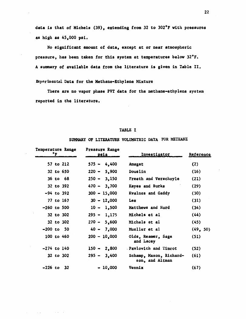
Most experimental data is reported above the critical temperature
(-115.8°F); the work of Mueller et al (49, 50), Vennix (67), and
Pavlovich and Timrot (52) extends below the critical temperature. A
summary of volumetric data for methane is given in Table I.
Experimental Data for Ethylene
The ethylene system has not been as widely studied as has
methane, one reason being that its critical temperature (+49.8°F)
is not far removed from ambient conditions. An extensive source of
22
data is that of Michels (39) 1 extending from 32 to 302°F with pressures
as high as 45 1 000 psi.
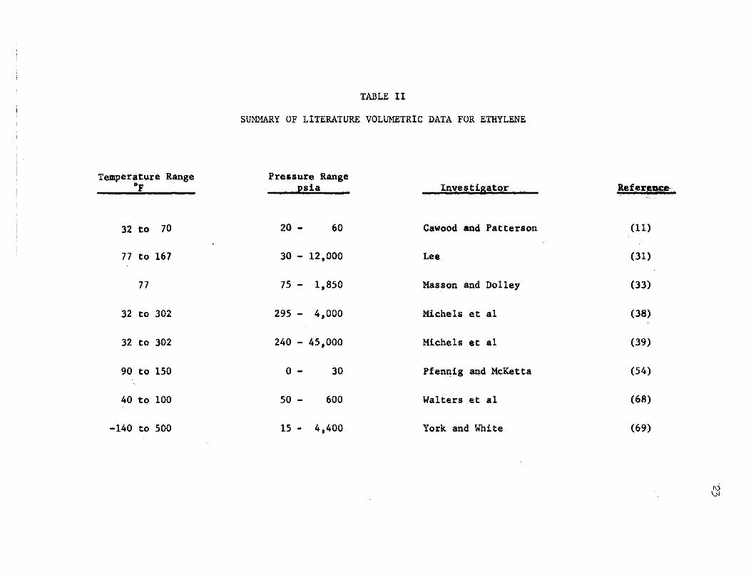
No significant amount of data, except at or near atmospheric
pressure, has been taken for this system at temperatures below 32°F.
A summary of available data from the literature is given in Table 11.
Experimental Data for the Methane-Ethylene Mixture
There are no vapor phase PVT data for the methane-ethylene system
reported in the literature.
TABLE I
SUMMARY OF LITERATURE VOLUMETRIC DATA FOR METHANE
Temperature lange Pressure Range OF psi a Investigator Reference
57 to 212 575 - 4,400 Amagat (2)
32 to 650 220 - 5,900 Douslin (16)
36 to 68 250 - 3,150 Freeth and Verschoyle (21)
32 to 392 470 - 3,700 Keyes and Burks (29)
-94 to 392 300 - 15,000 Kvalnes and Gaddy (30)
77 to 167 30 - 12,000 Lee (31)
-260 to 500 10 - 1,500 Matthews and Hurd (34)
32 to 302 295 - 1,175 Michels et al (44)
32 to 302 270 - 5 1 600 Michels et al (45)
-200 to 50 40 - 7,000 Mueller et al (49, 50)
100 to 460 200 - 10,000 Olds, Reamer, Sage (51) and Lacey
-274 to 140 150 - 2,800 . Pavlovich and Timrot (52)
32 to 302 295 - 3,400 Schamp, Mason, Richard- (61) son, and Altman
-226 to 32 - 10,000 Vennix (67)
Temperature Range OF
32 to 70
77 to 167
77
32 to 302
32 to 302
90 to 150
40 to 100
-140 to 500
TABLE II
SUMMARY OF LITERATURE VOLUMETRIC DATA FOR ETHYLENE
Pressure Range p_sia
20 - 60
30 - 12,000
75 - 1,850
295 - 4,000
240 - 45,000
0 - 30
50 - 600
15 - 4,400
In~ettigator
Cawood and Patterson
Lee
Masson and Dolley
Michels et al
Michels et al
Pfennig aQ.d McKetta
Walters et al
York and White
Reference.
(11)
(31).
(33)
(38)
(39)
(54)
(68)
(69)
I\) \>l
CHAPTER III
THEORETICAL CONSIDERATIONS
In this chapter all theoretical relationships underlying the
treatment of the experimental data (Chapter VI) are presented.
As stated in Chapter I, one of the goals of this thesis is to
emphasize the need for further development of an equation of state,
This is done by comparing experimental virial coefficients and
compressibility factors versus empirical equations of state. For
this reason primary emphasis in this chapter is given to the virial
equation of state and to empirical equations of state, These
.equations are discussed with respect to both pure components and
to mixtures. In addition, several methods are presented for
estimating virial coefficients.
A, General Comments Regarding Equations of State
In the most gen~ral terms an equation of state mathematically
relates the pressure, volume, temperature, and composition of a
substance. For a constant composition process only a relationship
between pressure, volume, and temµerature is necessary.
There have been many attempts to represent the volumetric be
havior of substances, but no equation has been entirely successful
in accurately representing actual gas behavior over the complete
range of conditions of practical interest,
24
The simplest equation of state is the so-called "perfect gas"
equation, i.e., PV = RT. Here P = absolute pressure, V = molar
volume, R = the ideal gas constant, and T = temperature, degrees
absolute. No gases exactly obey this equation; however, real gases
approach this relationship at low pressures.
25
Volumetric properties of gases and vapors are frequently expressed
in terms of the compressibility factor, z, defined as the ratio of the
actual specific gas volume, V, to the perfect gas volume RT/P. Only two
of the quantities P, V, and Tare independent; thus the compressibility
factor may be considered to be a function only of T and P for a
constant composition system.
Equations of state generally are of the closed-form type, con
taining several constants which are determined empirically. Such
equations may be made fairly accurate by proper determination of the
constants. In their present state of development, however, these
equations may lead to serious error if used in the treatment and
interpretation of compressibility data from a fundamental (virial
coefficient) standpoint, A more theoretical relationship is necessary.
The desired relationship is furnished by the virial equation of state.
This equation is of fundamental significance, and may be derived from
first principles, using the formulations of statistical mechanics.
As the virial equation forms the theoretical basis for a substantial
portion of the work reported herein it will be discussed in the
following section; a detailed discussion of closed-form equations
of state will be delayed until Section D, below.
26
B. Jlte Virial Eguation of State
The virial equation of state is an open-ended expression of the form
Z • 1 + B(T)/V + C(T)/V~ + D(T)/Vl + • • • (III;..l)
where for a pure component the coefficients B(T). C(T). D{T), • • • t
are the second, third, fourth, ••• etc., virial coefficients, which are
functions of temperature only.
The complete derivation of Equation III-1 is given in Chapter II!
of reference (23). This procedure considers interactions between all
possible configurations of particles, both pairwise and higher-ordered
interactions. The derivation is quite lengthy, and will not be pre
sented here.
The virial equation may be given either as the open-ended series
in reciprocal volume (as above) or as an open-ended series in
pressure. The reciprocal volume series is said to be the Leiden form of
the virial equation. The coefficients are said to be the Leiden virial
coefficients.
The power series in pressure is given below, and is termed the
Berlin form of the virial equation.
Z = 1 + B' (T)P + C' (T)P2 + D' (T)P·J + • • • (III-2)
Here the coefficients are termed the Berlin virial coefficients, and
are also functions of temperature only. The Berlin form was used
extensively by the early German workers for representing volumetric
properties of a gas, while the Leiden form was used in The Netherlands.
The Leiden form has the advantage of having theoretical signi-
ficance, Also, fewer terms are usually required in the Leiden form
than in the Berlin form to obtain the same degree of fit to a given
set of data. Only the Leiden form will be considered in the following
discussions.
The virial equation of state for a mixture may also be determined
from theoretical considerations, and the result, given below, is
analogous to Equation III-1 for a pure component.
Z • l + B (T)/V + c· (T)/V2 + D (T)/VJ +, m mm mm mm • • (III-3)
Here the subscript m refers to a mixture. The virial coefficients
are functions of both temperature and of the composition of the mixture.
Methods of determining viriai coefficients are given in the
following section; also relationships between mixture virial coeffi-
cients and the coefficients for pure components are discussed.
c. Virial Coefficients
In this thesis second virial coefficients are determined graphi-
cally by the following rearrangement of Equation III-1.
(Z - l)V • B(T) + C(T)/V + D(T)/v2 -+ • • • (III-4)
Here (Z - l)V is plotted versus (1/V) along an isotherm. The intercept
at infinite volume (1/V ~ O) equals the second virial coefficient,
After B(T) is known, C(T) may also be determined graphically from
the expression
lim [(Z - l)V - B(T)]V • C(T) (1/V~)
(III-5)
28
For the fourth virial coefficient, using previously determined
B(T) and C(T) values,
lim [(Z - l)V2 - B(T)V - C(T) JV• D(T) (1/V-+O)
(Ill-6)
This procedure is referred to as the slope-intercept method, and
has been employed extensively by previous investigators. This procedure
is very sensitive to inaccuracies in the experimental data, especially
in the low density region. The advantage of the procedure is that
coefficients so determined (for pure components) are functions of
temperature only.
Virial Coefficients of Mixtures
For mixtures, virial coefficients may similarly be determined
by the slope-intercept method. The second, third, and fourth virial
coefficients are determined from Equation III-3 according to the
expressions
lim (1/V -+0)
m
(Z - l)V • B (T) m m m
[(Z - l)V - B (T)]V • C (T) m m m m m
1 i.m [ (Z - l)v! - Bm (T)Vm - Cm (T) ]Vm • Dm_(T) (1/V +O) m
m
(IU-7)
(IIl-8)
(111-9)
As stated previously the virial coefficients in this case are
functions of both temperature Jnd of the composition of the mixture.
29
It has been shown by Mayer (35) that the virial coefficients for
a mixture of N components may be expressed as
N N B (T) = m l l (IU-10)
i j
C (T) • m
(III-11)
In this case xi, xj• and~ are the mole fractions, respectively, of
species i, j, and kin the mixture. The coefficient Bii(T) represents
the second virial coefficient for i in its pure state. The term B .• (T) lJ
represents the interaction between molecules of species i and j, and
is sai.d to be the second interaction or cross coefficient between i
. and j. Similar comments apply to the .terms in Equation III-11. Here
Cijk(T) represents ternary interactions between molecules i, j, and k.
If i = j = k, the resulting c111 r.epresents the third virial coe~fi
cient for component i in its pure state.
It is important to note that, although the virial coefficients
on the left side of Equations III-10 and III-11 are functions of both
temperature and composition, the coefficients on the right side
(including the cross coefficients) are functions of temperature only.
For a binary mixture Equations III-10 and III-11 take the form
B (T) m (III-12)
30
(111-13)
Here it la aaaumacl that 112 • 121' and that Cijk 11 the aame for all
permutationi of the indicea.
Empirical llelation1hip1 for Predicting VS.rial Coefficient,
Methods of predicting virial coefficients are al•o of interest and
will be considered in the following. The prediction of interaction
second vitial coefficient, (for binary ayat ... ) will receive particular
attention.
One method fo~ estimating second virial coefficients is baaed on
Pitzer'• modified theorem of correapond'-111 atatea (55). Here a
characterizing parameter,~, ii defined by the reduced vapor preaaure
,: at Tl.• 0.1. The expreaaion ii aa follows
0 w • - (log •a+ 1.oo)Ta. 007 (III-14)
ln this expression TR and PR are the reduced temperature (T/Tc) and
~educed presaure (P/Pc)• respectively, and~ 1• termed the accentric
factor. A simple fluid is defined as one having w • o.o; thus w is
a measure of the deviation from a limp~e fluid. Tbe compressibility
factor la then given by the relationship
Z • z0 + •' (111-15)
where z0 • t~ compre11ibility factor for a simple fJuid
z• • the compresaibility factor correction for deviation from a aimple fluid.
31
Based upon thi1 generalized data, an analytical expre11ion for the
f-BPc) reduced second virial coefficient wa1 al10 pre1ented by Pitzer. • ITc
The expression 11 a1 follow•
BP c . 0 1445 . 0 07 (0.33 • 0.46CA1l b • RTC • • + • 3 CAI • TR 'J
(III-16)
_ (o.13as + o.so .. ~- (2·0121 + o.097c.o~ _ (2·0073c.o~ T2 .. T3 TS
R · I It
Another mean• of estimating virial coefficient• wa1 presented by
Prausnitz (56, 57). Thia work con,iata of a auitable extension to
mixtures of.Pitzer'• (55) aeneraliaed result•, and ia deacribed as follows.
For a pure coaponent i the 1econd virial coefficient is given as
where V and T repreaent the component's critical volume and cii cii
temperature, re1pectively, and c.oii 11 the accentric factor. The
function e8 is given in tabular form.
The interaction 1econd virial coefficient Bij is given by
The parameters V , T , and c.oij characterize the interactions cij cij
(111-17)
(III-18)
between dissimilar 1pecie1; combining rules are given by Prausnitz
for estimating these parameter,.
The third virial coefficients were also given by Prausnitz; these
coefficients are given in the form of a graph and are somewhat less
32
accurate than the results for second virial coefficients.
The direct estimation of the interaction second virial coefficient
B12 from the virial coefficients B11 and B22 is also considered here.
In principle B12 may be calculated from a selected mathematical combina
tion of B11 and B22 , and the result substituted into Equation III-12
to yield B (T)o As a test of the combining rule, the calculated value m
of B (T) is then compared with the experimental value. m
In addition to being of theoretical interest a reliable combining
rule of this type would be of utility in engineering calculationso If
mixture second virial coefficients could be accurately determined,
compressibility factors of the mixture could also be calculated to
moderate pressures by use of the truncated form of the virial equation
(using only the second virial coefficient). Of even greater importance,
however, increased knowledge of combining rules could be used to
provide additional insight into the development of an improved equation
of state for mixtures. Several such combining rules for.B12 are presented
below.
The·linear combination of B11 and B22 has the form
(III-19)
Substituting B12 from Equation III-19 into Equation III-12, Bm takes
the simplified form
(III-20)
The square !.2.2! combination is given as
(III-21)
Substituting this equation into Equation III-12, there results
2 8m • (xl ' 811 + x2 l:s22 )
'.
(III-22)
The above two combining rules are the simplest expressions that
could be expected to provide a reasonable estimation of B12 • In
addition, two slightly more complex expressions are considered below.
The Lorentz combination for B12 is
3 B12 • [(B )1/3 + (B )1/3] /8
11 ,22 (III-23)
With this combining rule no simplification is obtained if Equation
III-23 is substituted into Equation III-12, Thus the value of B12
is calculated from Equation III-23, and the numerical result is
substituted directly into Equation III-12 to obtain B. m
The linear square root rule was considered only because it is
similar in mathematical form to the Lorentz combination. As far as
is known to the author this particular mathematical form has not been
previously used for equation of state combinations of this type.
The rule is
(III-24)
As was the case with the Lorentz combining rule, no simplification is
obtained by substituting this equation into Equation III-12.
In Chapter VI results are given for testing the four above com-
33
bining rules versus the experimental methane-ethylene virial coefficients.
One additional method will be considered for making empirical
estimates of virial coefficients, This method involves calculating
virial coefficients directly from the virial form of empirical equations
of state. The procedure will be described in Section D.
D. Empirical Equations of State
Empirical equations of state wer~ mentioned briefly, above.
Such equations are very numerous; in this work it is not proposed
to present a large number of equations as examples. Moreover, three
of the most important equations of state were selected for evaluation
versus the experimental data. These equations are 1) the Benedict-
Webb-Rubin (BWR) equation(~), 2) the Edmister generalized form of the
BWR equation (20), and 3) the Redlich-Kwong (RK) equation (58). The
equations will be discussed in this order.
The BWR Equation
The BWR equation is an eight constant relationship expressing
pressure or compressibility factor as a function of density (reciprocal
volume). The form of the equation is a power series ending with an
exponential density term, the coefficients of density being functions
of temperature. The equation is written as
co 2 3 P = RTd + (B RT - A - ---2)d + (bRT - a)d
o o T
(III-25)
where d = density.
In terms of compressibility factor the equation has the form
A C Z = 1 + (B - ...2. - .....2-)d + (b - ..!..)d2
o RT RT3 RT (III-26)
The empirical constants A, B, C, a, b, c. Y, and a are detero O 0
mined·for a specific compound from PVT, critical, and vapor pressure
data, This equation was developed primarily for hydrocarbons and
their mixtures, and provides a satisfactory representation of
35
experimental data for densities up to about twice the critical density.
For application to mixtures, the constants are determined from the
corresponding constants for the pure components by the relationships
N
B = l xiB 0 m i 0 i
(Linear)
N 3 B = l xixj [(B ) 113 + (B ) 1/ 3] /8
om ij oi oj
N 2 A = [ l x (A ) 1121
om i 1 oi
N 2 C = IX (C )1/2]
om i i oi
C = m
a = m
a. = m
(Lorentz)
(III-27)
Here the subscript m refers to properties of the mixture, and i refers
to properties of component i of the mixture, present at composition
xi. Although these rules are based on statistical mechanical con
siderations, they must be regarded as somewhat empirical, Both the
linear and Lorentz forms for B are frequently used. In some cases 0 m
these mixing rules have been shown to fit the experimental data for
mixtures almost as well as the original equation of state fits the
pure component data,
The BWR equation.may be rearranged into open-endedvirial form
as follows. The exponential term in Equation III-26 may be expanded
into a infinite power series, giving
36
2 2 2d~ 3d6 exp (-yd ) • l - yd + :J.f- - J.f- + • • • (III-28)
Substituting Equation III-28 into Equation III-26 and rearranging
according to increasing powers of d (reciprocal volume), there results
A C Z = l + (B - ...2. - ...2...) d + (b - !.. + ...S..) i
o RT RT3 RT RT3 ·
2 6 + ,2 d5 _ cy d + RT 2RT3
(III-29)
• • •
Comparing corresponding terms of Equations IIl-29 and III-1, the
second and third virial coefficients are given by the BWR equation as
B(T) = B 0
C(T) = b
A C 0 0 -----RT RT3
(III-30)
(III-31)
It i1 to be noted that. due to the mathematical form of the BWR
equation, the third and fourth virial coefficients (and al10 other
higher ordered coefficients) are missing from Equation 111-29.
This equation was selected for theoretical analy1i1 a1 it aives
an indication of the accuracy and application obtainable from rela-
tively complex equations of state.
The Edmister Generalized Form of the BWI. Equation
The Edmister gen~ralized form (20) of the BWI. equation presents
the eight constants in the equation in terms of Pitzer'• (55)
modified theorem of corre1pondina 1tate1. Here Equati_on III-26 ii
aiven in reduced form as
A' C'' Z • 1 + (B' • .J!. - .S.)p + (b' - £!.)p2
o e 83 e
37
(III-32)
where
• reduced density, e is defined as T/Tc • reduced temperature, and
B' A' c• b' a' c', a', and y' are reduced con1tants, o• o• o• • •
The reduced constants were determined from the oriainal BWB. con•
stants for 12 hydrocarbons by plottina them ver1us ~. obtainina
straiaht line,, the equations of the1e line• are given as
B' • 0.1306 0
A'• 0,35 • 0.30~ 0
C' • 0.10 + 0,40w 0
b' • 0,031 + 0,081.11
a' • 0,036 + 0,161.11 (III-3.3)
c' • 0,042 + 0,105w
a'a' • 0,0000875
y' • 0,049 - 0,05w
The specific constants are determined from these reduced constants
by the expressions
R2T4
C • C' Ci
oi 0 p (III-34) Ci
R2T2
bi ... b' Ci
p2 Ci
R3T3
a • a' Ci
i p2 Ci
a • a' 1
C • C 1 i .
Additional relationships similar to Equations III-33 above, but
giving the red~ced constants as functions of critical compressibility
factor Zc• were also developed b_y Edmister (~O). These relationships
are not.utilized in this work, however. -
39
Due; to the manner 'in which the reduced constants (Equations III-33)
were determined, it was unnecessary to develop new combining rules for
mixtures. From Equations III-33 and III-34 specific constants may be
determined; these constants are combined for mixtures using the .•
original BWR combining rules (Equations III-27).
In a similar manner the second and third virial coefficients for
the generalized equation are given by the same expressions as before
(Equations III-30 and III-31).
By evaluation of this equation the applicability of a generalized
relationship is demonstrated. At the same time an opportunity is
afforded to compare a aeneralized equation directly with a similar
equation for a s~ecific compound, Jthe equations differing only in the
40
value of the constants, The comparison of the two equations, both against
each other and against the experimental data, gives indications of
future methods for improving the equations,
The RK Equation
The RK equation is a two constant relationship of the form
a
with the two constants a and b given as
0 4278 R2T 2•5 • C
a = -------------P C
0.0867 RT C
b =--... p--c
(III-35)
(III-36)
For application, the equation is frequently used in the equivalent form
(III-37)
where
2 0,4278 A =
p T2,5 c R
B = 0,0867 (III-38) Pc TR
BP h. - = z
This equation was developed primarily for use at temperatures above
the critical.
For mixtures, the constants a and bare combined according to the·
relations
41
(III-39)
whereas the constants A and Bare determined from
N A • I xiAi m i
N (lII-40)
B • I xiB1 m i
The virial form of the equation is obtained as follows. Equation
III-35 is written as
1 1 a 1 2 1 P • RT -~ ) - l/2 (y") (----) (III-41)
V1-!. T l+.2. V V
1 1' Expanding the terms ~ b) and ~ .. b) into an infinite series, and
i-v i+v rearranging terms, the RK equation may be written as
(III-42)
• • •
Comparing corresponding terms between Equation III-42 and
Equation III-1, the second and third virial coefficients are given
for the RK equation as
a B(T) • b • l/2
RT
42
(III-43)
C(T) • b2 + ab RT3/2
As contrasted to the BWI. equation, all higher-ordered virial
coefficients are present in this expansion. This equation differs
further from the BWI. equation in that the constants a and bare
functions only of the critical properties of the components; the BWR
constants are somewhat dependent upon the range of data covered.
In the past the RIC equation has found application where highest
accuracy was not required, and where relative ease of computation was
desired.
No further attempt to discuss equations of state will be made
at this point. A wide variety of publications and thermodynamics
texts is.readily available; in particular, applications of equations
of state are discussed by Dodge (14) and by Edmister (19).
CWTEI. IV
IXPII.IHDTAL APPARATUS
The physical description ancl operating characteristics of the
experimental equipment are presented in this chapter, Mathematical
equations that cbaract•riae the apparatus are preeented, and the
advantages and di1aclvantages of the apparatus are diJcusaed.
A, Description qf Baui,-nt
General operating features of the entire syat• will be di.acussed
first, before- the detailed cle1criptions of each section of tbe apparat~s.
General Description of ~pparat,u~
The apparatus to be described is of the constant volume-constant
mass {isochoric) type,, which type of apparatus for PVT measurements
has been discussed in Chapter II, Thia particular apparatus is
.similar in design to that of Michels (47), the principal difference
being in the constant temperature bath, The ttichels cryostat used
a stirred liquid t~ insur~ thermal equilibrium; the·present design I
uses an air tbermoatat,
The apparatus is •hown achematically in Figure 1; connections to
the interrelated Burnett apparatu1--are also shown in this figure, . '
The apparat~a ccnasi1t1 of· a double-walled air thermostat containing
a jacke·ted conata~t dume cell, The controlled temper.ature region
I oj r-----, {;)\ DPI READOUT I I 'y rnm;;:i GAS
~-i><>-c::=>....«>cl-------:--,G~A~S,------~---1 i' I l""t~~j I BOURDON GAGE .. ,. I GAS
-- - -ELECTRICAL-WIRE
/ I I L _____ _.J VAC-'"'-'-----·-··---
t,
( TO BURNETT APPARATUS EXHAUST ~
'~ - -,,; .-------C~c-=--1-.l-!..---l~========jl - - 01 L : / / I // .Fl !IlVT I I I I I 71 r- I · I
I i ..,-· OEWAR VESSEL
II f .r CONTROLLED TEMPERATURE \ 1 EVACUATED CHAMBER I 1 •. ,.. ETHYLENE GLYCOL SOLUTION
jQ' , iltl -- REFRIGERATION COILS MANOMETER ; I j Ii'. - DOUBLED WALL COPPER VESSEL
~ I l ; - CONTROLLABLE l!ICUIJM. CNMIIIER • - . i D C..4)o_O.--+o-bc-GAS SUPA..Y - t. AIR BLOWER-.._ ~
> ! ;. •11 ; · ,,,._ L [I ,,.-AIR DUCT I . ~ ~ . .. ,-, I t I• . ID I
~ 1~1 c~I ; TEMPERATURE CONSTANT
- <i' ~ ...._ i REGION VOLUME
VA,
';!/ ~; CONTIIDU..ED JACKETED
SCREW PUMP RUSKA PISTON GAGE 1, ! CELL ~ n ~I r ~~ . ' I II ETHYLENE GLYCO n . . BAFFLE-\. 1 . CIRCULATING PUM
L p
~L l.~--------·im -~ ~= .. _===== __ ===-====-=II
GAS COMPRESSOR AIR THERMOSTAT
Figure 1
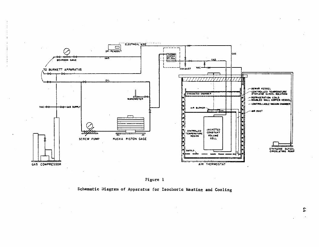
Schematic Diagram of Apparatus for Isochoric Heating and Cooling
~ ~
of the thermostat, containing the constant volume cell, consists of
a recirculating air stream whose temperature is controlled by the
addition of a small amount of heat through an electronic temperature
regulating.device. The double-walled vessel is placed in a dewar
vessel, containing a constant temperature refrigerated liquid such
as ethylene glycol, the liquid serving as a heat sink for the
thermostat.
The pressure of the sample is determined by means of the Ruska
Instrument Corporation piston gage. The oil of the pressure balance
system is separated from the gas sample by the thermostated differen
tial pressure indicator (DPI) cell.!/ This cell consists of two
chambers, separated by a flexible metal diaphragm, the zero position
of which is detected electronically and indicated by the DPI readout.
45
The DPI cell is placed outside the air thermostat because the high
pressure oil would solidify if subjected to the prevailing low tempera-
tures. The DPI cell was continuously maintained at a temperature
slightly above ambient; a temperature of approximately 95°F was found
to be practical. An interconnecting valve was placed outside the air
thermostat between the DPI cell and bomb. The necessary balancing
pressure of the oil is generated by the screw pump.
A hand-operated gas compressor is used for charging the cell and
its surrounding pressure jacket to the desired pressures, the nominal
!/ The jacketed constant volume cell will be referred to as the "bomb", whereas the differential pressure indicator cell will be termed the "DPI cell," The controlled.temperature region of the air thermostat will be referred to as the ''cryostat,"
value of pressure being indicated on the bourdon gage, The pressure
jacket around the bomb is used to offset any change of bomb volume
due to the stresses set up by the internal sample pressure. The gas
sample is injected into the main chamber of the bomb through the gas
line shown leading into the top of the bomb. Gas is injected into the
surrounding pressure jacket of the bomb via the gas line leading into
the bottom of the bomb.
Provision is made for subjecting the necessary portion of the
apparatus to the vacuum system. The temperatures of the cryostat and
DPI cell are determined by calibrated thermocouples.
46
A run consists of charging the bomb and DPI cell to a high
density and observing the pressures corresponding to a pre-selected
series of temperature.levels. Since the mass and volume are constant,
the run thus follows an isochor, or constant density path. At any
point on the isochor the simultaneous knowledge of the three quantities
pressure, temperature, and density is sufficient to determine the vol
umetric properties at that temperature and pressure. The density is
determined as follows.
A reference temperature of 77°F is established; along this isotherm
the compressibility of the sample has been independently determined
from the Burnett apparatus. Each isochoric run includes the reference
isotherm as the upper temperature; at this temperature the pressure,
temperature, and density are simultaneously known, and the value of
. 11 density for.the entire iaochor may thus be determined,
Additional i.sochors are run, at successively decreasing densities.
The density for each i1ocbor is established at the beginning of each ,..
run by e~austing a small amount of the sample to the atmosphere.
The same series of temperature levels js selected along each isochor
so that the final results may be given as either isothermal or iso-
c.horic data. Temperatures of 77, 60, 40, and 20°F were used in this
work.
A small correction is zequired for the amount of sample in the
DPI cell. A mass balance., given in Appendix N, shows that this
correction requires the value of the ratio of the volume of the DPI
cell to the volume of the bomb. It is convenient if this ratio fs
determined when the DPI cell.and bomb are at the same temperature.
· To determine the volume ratio the system is rinsed with a gas
of known volumetric properties, evacuated, and the cryostat
temperature is ,adjuited.to that of the DPI cell (95°F)~ The valve'
between the bomb and DPI cell is closed, and the DPI cell only is
charged with a sample of the same gas. After equilibrium has been
attained the DPI cell pressure is measured, and the temperatures
of both bomb and DPI cell are measured.
47
2/ . - As will be shown later, the value so calculated at the reference
isotherm is not a true density, but a run constant. The difference is due to the volume of gas in the DPI cell and capillary lines. Only the run constant is required in the calculations along the isochor; the true density exists as a constant known fraction of the run constant, and could be simply calculated if desired.
The valve is then opened, and the sample allowed to expand into
the bomb, The system is allowed to equilibrate, and the final
pressure and the temperatures of both volumes are measured. The
48
known volumetric properties of the sample at each of the above pressures
allow the volume ratio to be calculated,
A small correction for the amount of gas in the capillary line is
also required, This correction is discussed in Appendix N.
For all values of pressure, the jacket pressure must be continu
ously maintained at the proper value to eliminate the effect of
internal pressure on the bomb volume, This correction is discussed
in Appendix K. The effect of temperature on the bomb volume must be
considered, This correction is calculated from the dimensions of the
bomb and the linear temperature expansion coefficient for the
material; the equation is derived in Appendix H.
Additional details of specific sections of the apparatus are
given in the following.
Cryostat
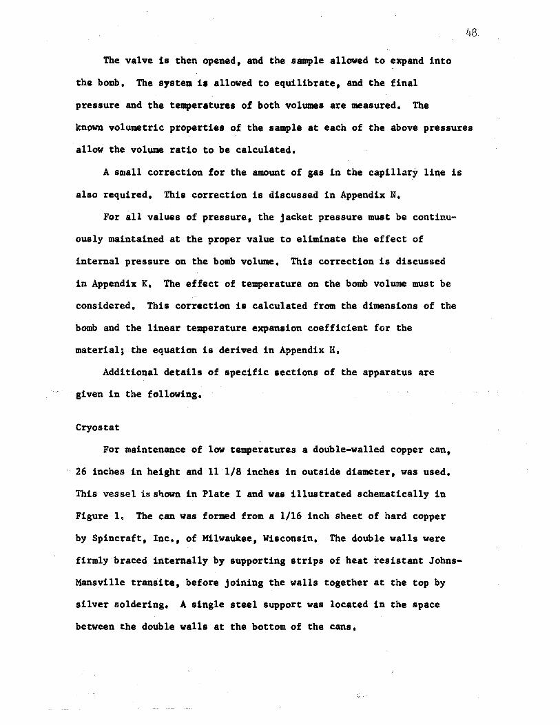
For maintenance of low temperatures a double-walled copper can,
26 inches in height and 11 1/8 inches in outside diameter, was used.
This vessel is shown in Plate I and was illustrated schematically in
Figure 1. The can was formed from a 1/16 inch sheet of hard copper
by Spincraft, Inc., of Milwaukee, Wisconsin. The double walls were
firmly braced .internally by supporting strips of heat resistant Johns
Mansville transite, before joining the walls together at the top by
silver soldering. A single steel support was located in the space
between the double walls at the bottom of the cans.
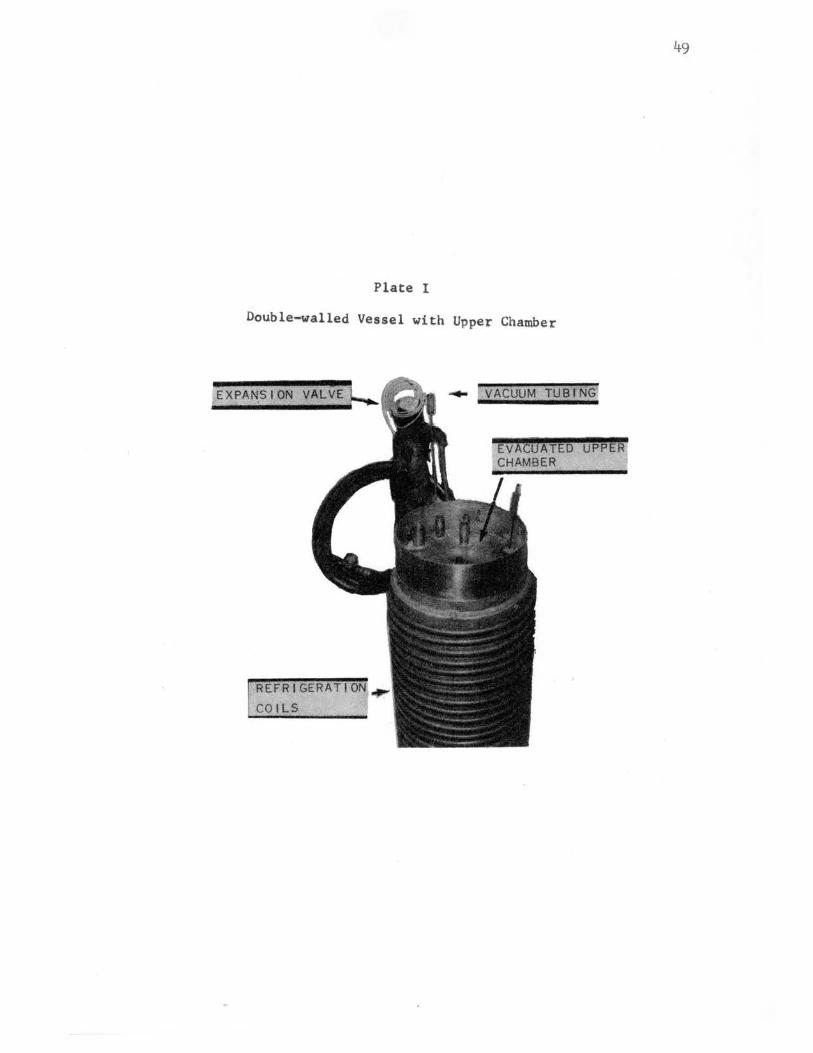
Plate I
Double-walled Vessel with Upper Chamber
EXPANSION
REFRIGERATION..
COILS
.... VACUUM TUBING
49
R
50
A 1/8 inch OD stainless steel vacuum line was silver soldered
between the double walls of the can and connected to the vacuum system.
An absolute pressure of.approximately 25 microns was maintained in the
space between the outer surface of the inside wall and the inner sur-
face of the outside wall. All walls of the vessel were plated with
nickel and then polished. The plating and polishing of the walls
and the maintenance of a vacuum between the walls thus insured the
desired small amount of heat transfer by conduction and radiation
through the annular space.
An evacuated upper chamber waa fitted into the mouth of the
double-walled cans. This chamber was formed from stainless steel
and was then nickel plated and polished to minimize radiation. heat
transfer. The chamber was evacuated and sealed at an .absolute
pressure of about one micron. The upper portion of the evacuated
chamber serves as a container for a refr:lgerating medium such as . .
liquid nitrogen or a mixture of dry ice and iao-octane,
The heat sink for the cryostat was maintained by an ordinary
Freon-12 closed loop refrigeration system. Twenty turns of 1/2 inch
OD refrigeration type copper tubing were concentrically wrapped and
soldered around the outer surface of the outside wall of the double-
walled cans. These coils served as the evaporator for the refri-
geration system. The double-walled vessel with refrigeration coils was
then placed inside a stainless steel dewar (Sulfrian Model No. SJ-2, 76
liter, 13 inches inside diameter). The outer wall of the steel dewar
was insulated from the surrounding with a layer of fibre-1lass
insulating material. A four-inch thick section of styrofoaa inaulating
material was fitted into the top of the dewar, to further minimize
51
heat transfer between the surroundings and the cryostat. A disassembled
view of the insulated dewar, double-walled copper can, and bomb is shown
in Plate II.
The space between the outside wall of the double-walled vessel
and the inside wall of the dewar was filled with approximately three
gallons of ethylene glycol solution which could be circulated by an
external centrifugal pump (Figure 1), The solution consisted of 60%
by volume commercial "Prestone" antifreeze and 40% by volume water,
thus providing a liquid with a freezing point of approximately -50°F,
The refrigeration system used a PAR 1/3 HP refrigeration compressor
unit~ The 1/2 ton Freon-12 expansion valve (Plate I) was .adjusted
so as to provide a suction side pressure of about zero psig to the
compressor and a discharge side pressure of about 120 psig.
The compressor was allowed to run continuously, reaching equi
librium with the surroundings~and with the particular temperature of
the cryostat. The temperature of the ethylene glycol solution was
affected by ambient temperature and by the level of the cryostat
temperature. Any changes in ambient temperature were gradual and
thus did not markedly upset the temperature control. The effect of
the cryostat temperature on the ethylene glycol solution temperature
(Table III) gives an indication of the rate of heat transfer between
these two regions. The change in ethylene glycol solution temperature
is considerable, and is indicative of conduction heat transfer to
the ethylene glycol solution through the upper portion of the cryostat,
This has a small effect on the temperature control inside the cryostat.
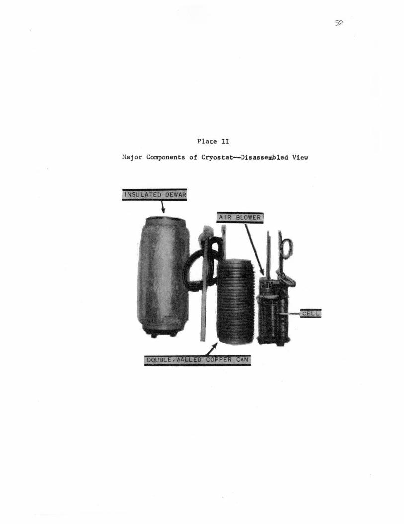
52
Plate II
Major Components of Cryostat--Disassembled View
INSUL~TEO DEWAR
CELL
DOUBLE. CAN
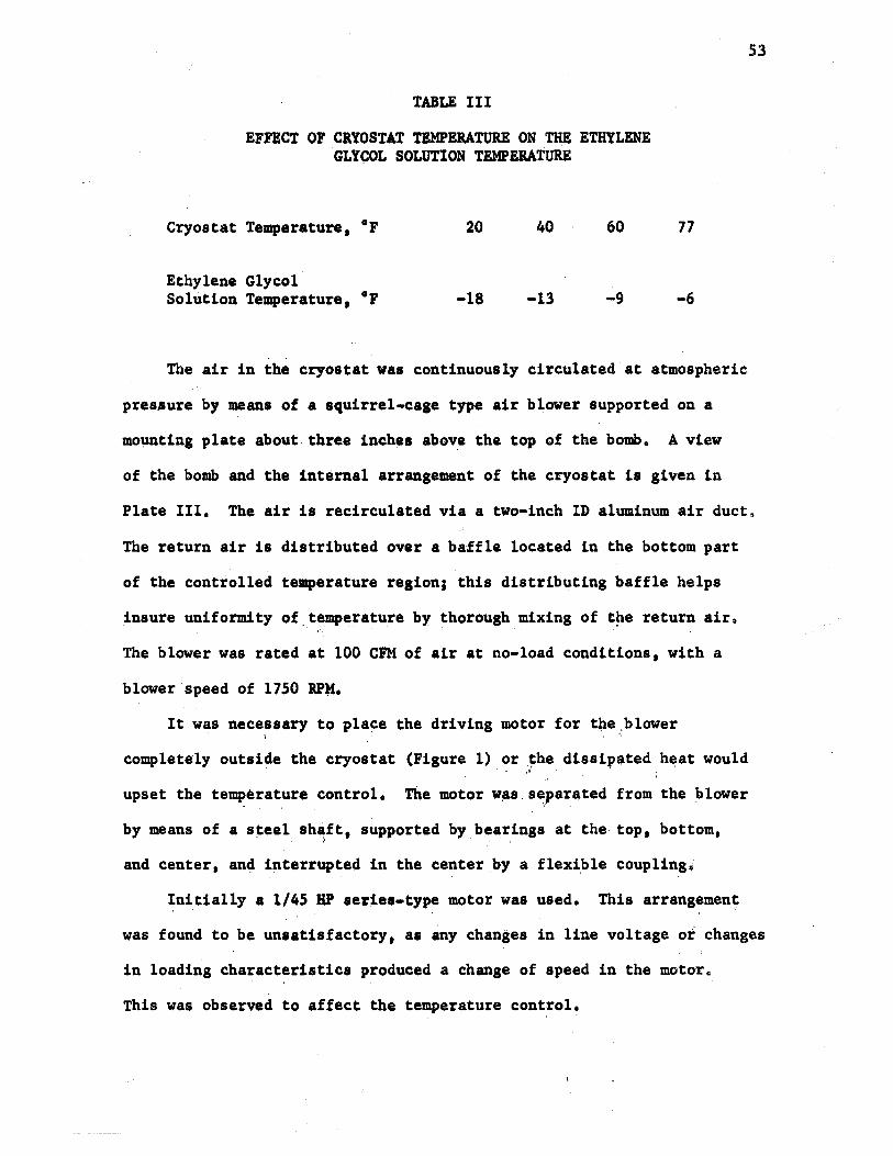
TABLE III
EFFECT OF CRYOSTAT TEMPERATURE ON THE ETHYLENE GLYCOL SOLUTION TEMPERATURE
Cryostat Temperature, °F
Ethylene Glycol· Solution Temperature, 0 P
20
-18
40 · 60
-13 -9
77
-6
The air in the cryostat was continuously circulated.at atmospheric
pressure by •ans of a squirrel-cage type air blower supp.orted on a
mounting plate about three inches above the top of the bomb. A view
of the bomb and the internal arrangement of tbe cryostat is given in
53
Plate III. The air is recirculated via a two-inch ID aluminum air duct.
The return air is distributed over a baffle located in the bottom part
of the controlled temperature region; this distributing baffle helps
insure uniformity of_temperature by thorough mixing of t~e return air. •.'
The blower was rated at 100 CFM of air at no-load conditions, with a
blower speed of 1750 RP".
It was necessary to place the driving motor for t~e.blower . \ ' •\
completely outside the cryostat (Figure 1) or .~he dissi~ated heat would .. ,.; .
upset the temperature control. .. '
The motor w~s.separated from the blower ~ ' . '
by means of a s~eel sh~ft, supported by.bearings at the top, bottom, . . ~ . . ' '
and center, and i~terrupted in the center by a flexi.ble coupling.
Initially a 1/45 HP series-type motor was used. Th;l.s arrangement
was found to be unsatisfactory, as any changes in line voltage or changes
in loading characteristics produced a change of speed in the motor.
This was observed to affect the temperature control.
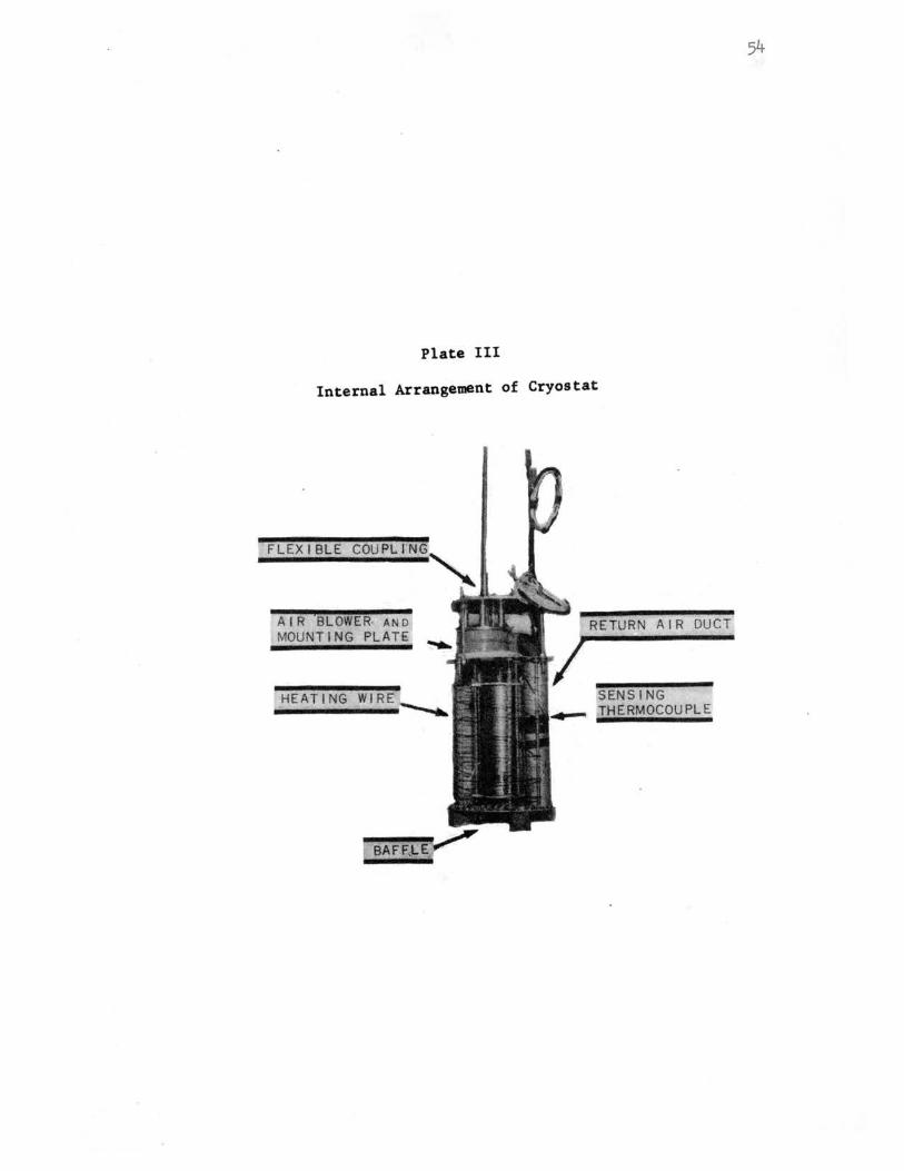
Plate III
Internal Arrangement of Cryostat
A IR BLOWER- AND MOUNTING PLATE
_HEATING WIRE
AIR DUCT
SENSING JHERMOCOUPLE
54
This motor was thus replaced by a 1/15 HP constant speed hystere-
sis synchronous motor. This unit had a rated speed of 1800 RPM, and
was observed periodically with a stroboscope to operate precisely at
rated speed, both at full load and at no load.
No convenient method to measure the rate of air circulation was
available, but it was thought to be somewhat less (perhaps by a factor ! .,
of 50%) than the rated circulatton rate at no load (100 CFM) due to
the pressure drop through the return air duct and across the air
distribution baffles.
The bomb is shown in Plate III resting on alumiJium supports
approximately two inches above the distribution air baffleo
The optimum control of temperat~re is achieved by removing only
a small amount of heat from the system via the heat sink and by adding
a corresponding small amount of heat through a temperature controller.
The control heater consisted of approximately 45 feet of nichrome wire
(Driver.Company "Tophet A" size 40) having a resistance of 20 ohmsn
This control wire was supported in the main circulating air stream by
55
vertical glass rods (Plate III) which were located concentrically around
the bomb. The entire amount of heat to the cryostat was added through
these control heaters, no auxiliary heaters being used. The automatic
temperature controller for the process will be described presentlyo
The location of the sensing thermocouple was quite important in
the control of temperature, The thermocouple was located in the return
air duct, located vertically about midway in the duct. It was found
helpful to lag the bare thermocouple lightly with a thin piece of
absorbent cotton. With this arrangement the temperature of the cryostat
could be maintained constant to within+ 0.02°K for a period of four ,, -
to six hours, sufficiently long to make a corresponding equilibrium
reading of pressure and temperature.
All high pressure valves in that portion of the apparatus between
the bomb and the DPI cell were lS,000 psi 1/8 inch Ermeto-type valves
(High Pressure Equipment Co.). The valves have a freely rotating
stem and turn easily under maximum pressure. All tubing, unions,
and tees were Autoclave Engineering Company "Tubeline" series.
The Jacketed Bomb
The bomb was fabricated from type 303 stainless steel in the OSU
Research Apparatus Development Laboratory. An assembly drawing of the
bomb is shown in Fiaure 2. The bomb assembly is .circular in cross
sectioo and is formed from three parts--a lower part, an upper part,
and the jacket. The upper and lower parts were welded together at
.. A and. B, and the welds were ma~ined flush. to the cyli'-der walls.
This portion of .the bomb was then tested with oil to 15,000 psi.
After pressure testing, this inner portion of the bomb was inserted
into the pressure jacket and was welded at C and D. These welds were
then machined flush to tae wall, and the jacket portion of the bomb
was pressure tested with oil to 15 1 000 psi. Seats for Ruska connectors
were provided for the tubing connections for both inner bomb volume and
jacket volume. The internal di•nsions of the completed bomb assembly
·are such that the outer jacket pressure P0 should be 0.8024 times the
inner pressure Pi for the elimination o.f volume changes due to wall
stresses. This relationship is developed in Appendix K.
S6
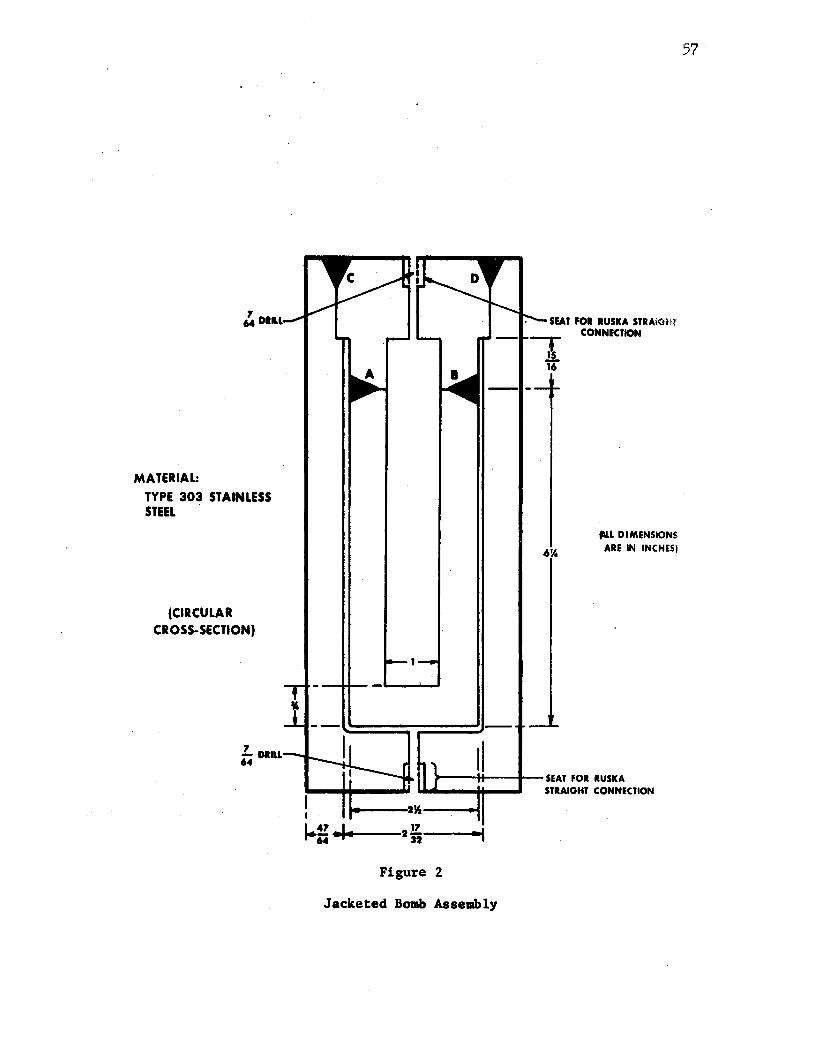
'4 DIILL
MATERIAL: TYPE 303 STAINLESS STEEL
(CIRCULAR CROSS-SECTION)
i4 DIILL
SEAT FOR RUSKA STRAl<:HH CONNECTION ---r
16
,6%
fill DIMENSIONS ARE IN INCHES)
>---+1~-,._-SEAT FOR RUSKA STRAIGHT CONNECTION
I
I_!!~• 2.!t--.....,. ~.4 32
Figure 2
Jacketed Bomb Assembly
57
The DPI Cell and Thermostat
The DPI cell is of Ruaka design (Cat. No. 2413), The cell
consists of two pressure chambers separated by a thin stainless steel
diaphragm, The diaphragm deflecta vertically as a result of any
differential pressure, and the deflection positions a core within a
differential transformer coil located within the upper pressure
chamber, The coil-core relationship causes an electrical output which
is a function of the diaphragm displacement. The electrical output
is detected and indicated by an electronic null indicator, or readout
box (Ruska Cat, No, 2416),
The DPI cell will withstand a maximum overpressure of 15,000 psi.
The cell and readout bo~ arrangement can detect a differential pressure
of 0,0002 psi.
For purposes of establishing the zero reference point of the DPI
cell and readout box, an oil filled open-end manometer was connected
into the oil system between the DPI cell and the Ruska piston gage
(Figure l), Tne manometer was constructed from approximately 30
inches of 7 DDD OD soft glass tubing. A short end was sealed with
epoxy resin into a standard high-pressure valve. By means of a
cathetometer, the exact point on the vertical section of the manometer
was located to correspond with the height of the diaphragm inside
the DPI cell, This point was marked for future reference,
The zero shift of the DPI cell with operating pressure was deter
mined by Ruska, and a calibration curve was furnished by them. This
correction is on the order of two to three parts per million parts,
In order to measure the temperature of the thermostated DPI cell,
a calibrated copper-constantan adjustable pipe clamp thermocouple
(Conax Cat, No. CL-64-CC) was clampled around the DPI cell near the
bottom of the cell in the section where the sample was confine4,
Several turns of refrigeration-type 1/4 inch OD copper tubing were then
clamped around the cell and pipe clamp thermocouple, and provision was
made to circulate controlled temperature water through the copper coils.
The entire DPI cell, thermocouple, and copper tubing were placed
inside an insulated thermostated box (illustrated schematically in
Figure 1). The outer walls of the thermostated box were made of
transite; the transite walls were then lined on the inside with sections
of one-inch thick styrofoam,
59
The controlled temperature water to the copper coils was circulated
via a constant temperature circulating system (Precision Scientific
Company), This unit uses a mercury-in-glass regulating mechanism
and is designed to circulate a liquid at a rate of three GPM at a
six foot head, Using tap water as a heat sink, this bath would main
tain a constancy of circulated water temperature of 0,05°F for
several hours, depending on the temperature changes of the surrounding
room.
The DPI cell and surrounding thermostat were maintained at a con
stant temperature for all values of temperature of the bomb; thus, no
change in the cell zero point with tempe"rature must be considered. It
is convenient to maintain a temperature sli'ghtly above ambient condi
tions; in this case 95°F was used,
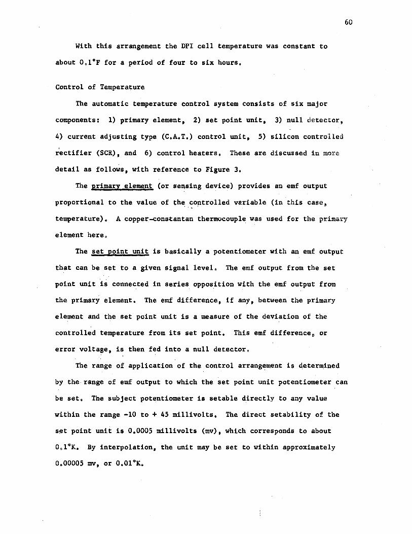
60
With this arrangement the DP! cell temperature was constant to
about 0.1°F for a period of four to six hours.
Control of Temperature
The automatic temperature control system consists of six major
components: 1) primary element, 2) set point unit, 3) null detector,
4) current adjusting type (C.A.T.) control unit, 5) silicon controlled
' rectifier (SCR), and 6) control heaterso These are discussed in more
detail as follows, with reference to Figure 3.
The primary elemenE, (or sensing device) provides an emf output
proportional to the value of the controlled variable (in this case, '' .. '
temperature). A copper.-constantan thermocouple was used for the primary
element here.
The set point unit is basically a potentiometer with an emf output
that can be set to a given signal level. The emf output from the set
point unit is connected in series opposition with the emf output from
the primary element. The emf difference, if any, between the primary
element and the set point unit is a measure of the deviation of the
controlled temperature from its set point. This emf difference, or
error voltage, is then fed into a null detector.
The range of application of the control arrangement is determ.ined
by the range of emf output to which the set point unit potentiometer can
be set. The subject potentiometer is setable directly to any value
within the range -10 to+ 45 millivolts. The direct setability of the
s~t point unit is 0.0005 millivolts (mv), which corresponds to about
0.1°K. By interpolation, the unit may be set to within approximately
0,00005 mv, or 0.01°K.
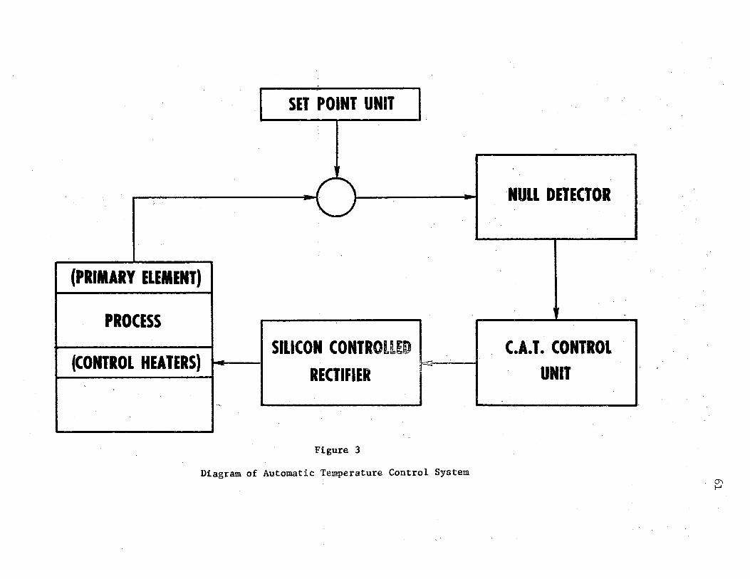
r .
SET POINT UNIT
' --:' .. _.
(PRIMARY ELEMENT)
PROCESS SILICON CONTRO"llED
(CONTROL HEATERS) - -
RECTIFIER ..
.
. ..
Figure 3
Diagram of Automatic Temperature Control System
NULL DOECTOR
C.A. T. CONTROL · UNIT
O"I I--'
62
The null detector is a high gain, high sensitivity, microvolt
amplifier, It detects any error voltage from the set point unit and
amplifies it to a level suitable for use as an input to the control unit,
The null detector for this system is a Leeds and Northrup electronic
DC null detector (Cat, No, 9834-2), This unit contains a variable
sensitivity and a readout scale for the error voltage.
The control unit is a Leeds and Northrup s.eries 60 C,Ao'I, model*
This unit has three modes of control action (proportional, reset, and
rate controls), and its function- is to provide continuous corrective
control action based on the size, rate of change, and duration of the
error voltage, It does this by providing an output current (0 to 5
milliamps DC) which is proportional to the input heat requirement
for the controlled temperature process, This output current goes to
the final control device, which is a silicon controlled rectifier-unito
It was necessary to ground electrically this portion of the
temperature control system, For this purpose a 1/2 inch diameter
solid copper rod was driven 10 feet into the earth, and was connected
to an insulated 12-gauge copper lead-in wire, This wire served to
ground only the electrical gear in the Thermodynamics Laboratoryo
The SCR is a Fincor power package (Model No. 1200-2.2-llA) -manufactured exclusively for the Leeds and Northrup Co, This unit
produces an AC output voltage that is proportional to the DC current
from the C,A,T. control unit, This output voltage supplies current to
the process control heaters, and may range from zero to 110 volts.
For a particular application, the minimum and maximum values of the
SCR output are adjusted by means of potentiometers in the circuit.
For this application, the output voltage varies linearly from zero to
a maximum of 40 volts,
Measurement of Temperature
For the determination of temperature of the sample in the bomb, a
calibrated copper-constantan thermocouple was fastened to its outside
surface. The thermocouple was calibrated over the temperature range
-40 to +9~°F versus an NBS platinum resistance thermometer.
The temperature of the sample in the DPI cell (nominally 95°F) was
determined by the copper-constantan thermocouple fastened to the outside
surface of the DPI cell. The thermocouple was calibrated over the
temperature range 80 to 115°F versus the NBS thermometer. Illustrations
of the potentiometer and thermocouple circuitry are given in Figures 4
and 5.
The potentiometer is a Leeds and Northrup type K-3 universal
potentiometer, with a scale range of zero to 1.6110 volts. The scale
may be read directly to 0.0005 mv, and may be read by interpolation to
within 0.0001 mv. For this application 0.0001 mv is roughly equivalent
to 0,002°K. The galvanometer is a standard Leeds and Northrup DC
galvanometer with self-contained lamp and scale reading device.
The accuracy of the potentiometer is 0.0005 mv or,0,01°K.
The accuracy of the thermocouple calibrations for the bomb and for
the DPI cell is estimated at 0.01 to 0.02°K, or roughly equivalent to
the accuracy of the potentiometer. Details on the NBS thermometer and
the thermocouple calibrations are given in Appendix A.
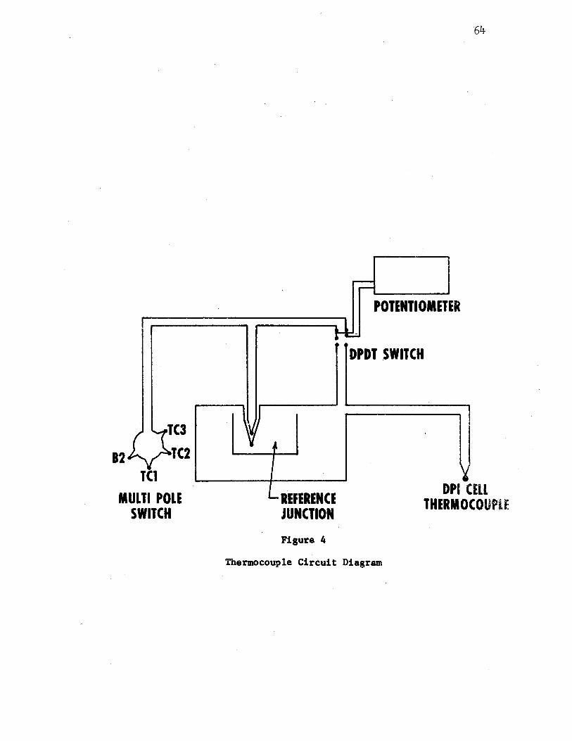
B2 TCl
MULTI POLE SWITCH
64
POTENTIOMETER
REFERENCE JUNCTION
Fiaure 4
DPDT SWITCH
Thermocouple Circuit Diagram
DPI CELL THERMOCOUPU
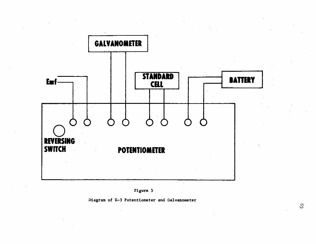
E•f--
0 .. REVERSING
SWITCH
GALVANOMETER
STANDARD CBL
POlENTIOMnn
Figure 5
Diagram of K-3 Potentiometer and Galvanometer
IATIEIY
~ \Ji
It is necessary to make a mass correction for the small amount
of the sample contained in the capillary tube, as discussed pre
viouslyo For this purpose the average temperatures of different
sections of the capillary are required. To estimate the average
temperatures, three copper-constantan thermocouples (TCl, TC2, and
TCJ--Figure 4) were fastened at equidistant intervals along the
length of the tubeo Standard thermocouple charts were used to deter
mine the temperatures from these thermocouples. The ambient
temperature of the laboratory was determined from standard mercury
in-glass thermometers, which were certified to be accurate to Oo05°F.
Measurement of Pressure
As stated previously, the gas sample is separated from the high
pressure oil system by the DPI cell. The oil pressure is generated
with the screw pump and is measured with the Ruska piston gage. The
instrument has a stated accuracy of one part in 10,000 parts over the
range six - 12,140 psi, with the calibration being directly traceable
to NBSo The calibration data and specifications .for the gage are
presented in Appendix Jo A sample calculation of a pressure point is
given in Appendix B.
Although the assembled apparatus was satisfactorily tested at
pressures up to 12,000 psia, data was taken only to pressures of
66
2400 psia. In the derivation of virial coefficients by the slope
intercept procedure it is important to have a considerable amount of
data in the low pressure region. Points at higher pressures have little
effect on the determination of virial coefficients by this procedure.
The oil used in the system is a specially developed oil with a
density of 0.85 grams/cc and a viscosity of 160 S~U at 2,5°C. A head
correction of o.031 psi per vertical inch of oil head is given by
Ruska for use in making head corrections.
Standard Ruska 1/8 inch needle valves (Cat No. 2005) were used
throughout the Ruska equipment.
A 16,000 psi Acco Helicoid bourdon gage with 200 psi subdivisions
67
was mounted on the screwpump. Two alternate bourdon gages were connected
into the gas,, side of the high pressure sys temi. These bourdon gages
were used principally during the charging of the bomb, and were valved
off from the system after the charging was completed. These two gages
are 1) a 20 9000 psi XFO Maxisafe gage with 200 psi subdivisions, and
2) a Crosby AIH 5,000 psi ~age with. SO psi subdivisions, For .clarity
the Crosby AIH 5,000 psi gage is omitted from Fi~ure l. All three of '.
the above bourdon gages were calibrated versus the Ruska piston gage.
The calibrations. are given in Appendix D, . '
Barometric pressure was determined qy means of a Texas Instfumeut:s t ' • L. •
servo-nulling pressure gage, The instrument has an a.ccuracy of 0.015%;
operating characteristics and calibration of the gage .are presented in
Appendix C,
Auxilia~y Apparatus
The vacuum system consisted of a mechanical pump (WelchScientific)
and a eve ~1pe VMF-10 diffusion pump. .The V!a-10 p~ has an ul t1111:a.t~
-6 rated fressure of 10 millimete~s ~ercury. . '
The McLeod gage is a Virt~s ?oO millimeter r~nge unit. The gage
was located so as to be able to measure the absolute pressure at any '· .
68
portion Qf the apparatus connected to the vacuum system,
A Gaertner cathetometer was used for all vertical measurementso By
means of a verni~r scale. attachment 1 this instrument could be read
di.rectly to OoOOS centimeters. The instrument was used for making all ·. 1'
vertical measurements associated with the cal~bration of the apparatuso
The _gas compressor is a 15 1 000 psi hand operated pump (Autoclave
Engineers)o This unit was used both for charging the sample into the
celle and also for injecting gas into the jacket itselfo The pump is a ..
po~~tive. displacement 1 ·reciprocating piston type with displacement per
stroke of Ooll5 cubic inc~es.
Bo Advantages and Disadvantages of the Isochoric Apparatus
The chief advantage of the apparatus is that, given the volumetric
properties of the sample along the reference is.otherm (77°F), the. vol-
umetric properties at lower temperatures may be determined solely from
the experimental measurement of pressure and temperatureo The temperature .\
may be determined to within Oo02°K,· and the pressure may be determined
to one part in 10,00.0 partso
Due to the insulating effect of the gas-filled pressure jacket
surrounding the bomb, the temperature fluctuations in the air bath
(±Oo02°K) are largely damped ou~ before affecting the inner sample
temperature. By observing the pressure fluctuations inside the cell,
it was estimated that the actual temperature fluctuations of the
sample were approximately± 0,01°K1 or roughly one-half the fluctua-
tions in the air bath.
It is of practical interest to measure the volumetric properties
of mixtures within the two-phase and the subcooled liquid regionso
For many types of PVT apparatus (such as the Burnett apparatus) this
is difficult 9 due to possible non-equilibrium conditions prevailing in
the mixturec For the isochoric apparatus, an isochor may be cooled
directly into the liquid or two-phase regions, without additional
complicatiot1s o
The use of the air bath, rather than the liquid bath (as used by
Michels) 9 introduces the disadvantage of a long period of time required
to obtain equilibrium following a change of temperatureo This is due
to the relatively low overall heat transfer coefficient between the
circulating air and the bombo Also, the insulating effect of the
surrounding pressure jacket further complicates this effecto As the
data are taken isochorically, rather than isothermally 9 only one data
point is taken between temperature changes.
Each successive isochor is r,un as nearly as possible at the same
levels of temperature as the previous run. With the most careful
work& it is yet necessary to make a small temperature correction in
combining the volumetric observations to obtain final densities for
each isothermo
Any inaccuracies in the compressibility factors of the refereuce
isotherm will introduce corresponding inaccuracies into the isochoric
datao For this reason the accuracy of the isochoric data cannot be
greater than the accuracy of the reference isotherm compressibility
factorso
69
70
c. Characterizing Equations for the Apparatus
All equations that characterize the apparatus are developed in
App~ndix No The equations will be briefly s':1mmarized in the following~
To determine the isochoric run constant D the cryostat is charged.
and all.owed to reach equiliprium at 77°F t · and the temperatures and
pressures of all portions of the system are measuredo The run co11.stm:1t !
is then determined from
D = [F(TB - 95) + o.003868]DBT + o.,01263 DD +
0.01537 o5 + 0 0 01511 D4 + 0.003794 (D3 + D2) + (N-20)
0.003273 D1
DBT is.the density of the sample in the bomb at 77°F (determined from
the compressibility factor from the reference isotherm). The quantities
D00 D59 D4 e D3 P D2, and D1 are densities representing the correction for
the amount of sample in the DPI cell and exposed capillary line. The
function F(T8 - 95) is the correction for the effect of temperature on
the bomb volume.
The quantity Dis constant along the isochor. From a knowledge of
D~ the compressibility factors at other temperatures along the isochor
are determined from
p F(TB - 95) + 0.003868 ZBT = (irf) [ DEN ]
BT (N-21)
where
DEN= D - 0.01263 DD - 0.01537 D5 •
{N-22)
The densities D0, n5 , D4, o3, o2, and D1 involve the unknown
compressibility factors ZD' z5 , z4, z3, z2, and z1 at the temperatures
T09 T59 T4, T3, T2, and Tl' respectively. These temperatures lie
approximately in the rang~ from ambient temperature to 0°F. Since
the terms involving these densities are relatively small compared to
71
the other terms, Equations N-20 and N-21 are first solved using the
approximation z0 = z5 = z4 = z3 = z2 = z1 = unity. From the assumptions
a value of D may be calc~lated at the reference isotherm from
Equation N-20; · then _values of ZBT may be calculated over the experi
mental temperature range of 77 to 20°F, using Equation N-21. From these
calculated values more accurate values of z0 , z5 , z4, z3, z2, and z1 may
be interpolated and used to recalculate values of D and ZBT from
Equations N-20 and N-21.
This iterative procedure is continued until no significant cha~ge
in the calculated value of D and ZBT ~c~urs, Since the terms involving
D09 D59 D4, D3, D2, and D1 are small, normally aQout two iterations are
sufficient for this convergence. A sample calculation is given in
Appendix F.
Do Som~.~xperimental Difficulties
The Heat Sink Temperature
Initially it was desired to maintain temperatures from ambient down
to about the sublimation temperature (-78°C) of dry ice. A mixture
of dry ice and liquid iso-octane was used as a heat sink in the space
between the outer wall of the copper can and the inner wall of the
dewar. This arrangement was found to be unsatisfactory for periods
of time in excess of about two hours; as the dry ice: began to sublime,
considerable temperature gradients formed in the cold liquid, up
setting the temperature control.
The installation of the mechanical refrigeration system with
copper evaporator coils helped considerably in elimating these tempera=·
ture gradients. A thermistor-operated on-off unit was initially
placed in the compressor circuit, controlling the temperature of the
refrigerant ethylene glycol solution; howeverP the on-off cycle of the
refrigeration unit was observed to upset the temperature control
system. The on-off control unit was thus abandoned, and the refrigera=
ti.on unit was allowed to operate continuously. This arrangement was
found to provide the most satisfactory heat sink.
Vibrations in the Blower Shaft
The excessive length (about 20 inches) of shaft between the air
blower and motor was found to cause pronounced vibrations in the shaft.
To overcome this problem it was necessary to support the shaft at the
top with a close-fitting "oil-lite'' type bronze bearingp and at the
bottom and center by steel roller bearings. Between the center and
73
upper bearings the shaft was interrupted by a steel flexible universal-
joint type coupling.
Temperature Control
Considerable difficulty was encountered in the temperature control
of the cryostat due to small voltage fluctuations within the automatic
temperature control. system. These fluctuations were principally du~ to I • \'
two separate factors: lJ the relatively high inherent electrical
"noise" in the primary temperature circuit, and 2) the instability
of the automatic reference junction compensa~or. These diJturbances
are discussed as follows.
-T~ electrical noise in the circuit results in improper corrections
being made to the output voltage to the final control device. With
reference to Figure 3 9 the emf output from the set point unit is
connected in series opposition ~i th t~e gener.ated thermocouple emf.
The emf difference is continuously monitored, and is used to determi~e
the output control voltage. For the range of temperatur!! encountered ,:
in this work the generated thermocouple emf was between -0.2 and +1.2
mv. When compared to this relatively low value of emf 9 the electrical
no~se level in the primary circuit was sufficiently high to affect
the proper operation of the entire temperature control system. The
problem of the inherently high electrical noise level in the system
was never eliminated. Temperature control of within ;t0~02°K could be
achieved with this arrangement.
The automatic reference junction compensator between the sensing
thermocouple and the set point unit was observed to be sensitive 1:·o
rapi~ fluctuations in ambient temperature. A flu~tuation in ambient
temperature caused by opening a door into the main laboratory was
observable almost immediately on the null detecting device. This
problem was largely overcome by insulating the automatic reference
junction compensator with fibre glass insulation. Also, the installa
tion of additional air. conditioning equipment helped damp out rapid
changes in the ambient temperature.
Elimination of High Pressure Leaks
Considerable effort was required to elimi.nate all leaks in the
gas s14e portion of the system. S_eparate portions of the system were
successively isolated and charged to a high pressureo The pressure
was then measured and the system allowed to stand for 24 to 48 hours 9
whereupon the pressure was remeasured. These tests were quite time
consum.ing 9 and were further complicated by any day-to-day change in
ambient temperature, especially in the portions of th, appara~us
containing the exposed capillaries. All leaks were eliminated.
74
CHAPTER V
EXPERIMENTAL PROCEDURE
The preliminary adjustments to the automatic temperature. control
system are discussed at the first of this chapter, as this phase of the
experimental work was quite important.
This is followed by a discussion of the experimental details of
the measurement of pressure and temperature. Considerable attention
is given to the operati,on of the Ruska piston gage.
Nextl) the preparation of the apparatus for taking a data point
is discussed 9 followed by the details of the actual ~aking of the data
point and the lining out of the apparatus for the next data pointo
Lastly 9 the experimental determination of isochoric volumetric
properties in the two-phase region is discussed.
Ao General Experimental Details
Adjusting Automatic Temperature Control System to the Process
The automatic temperature control system is illustrated schemat-
ically in Figure 3. The control unit uses three modes of control
action--proportional, reset, and rate modes of control. The combined
settings for these modes of control establish the characteristics of the
heat input to the cryostat; the proper setting of each particular mode
of control action is determined separatelyo
7--5_ 1' ..
The proper setting for the pro2ortional mode of control was first
determined. For the determination of this setting, the reset and rate
modes of control were set to zero. The "proportional band" setting
is a measure of the amount that the controlled variable (temperature)
must change (from its set point position) in order to produce a full
scale change in the output voltage to the control hea_ters.
In adjusting the proportional band it is desirable to start with
a fairly wide setting and thel!- d_ecrease the setting in a stepwise
fashion until the optimu~ value is reachec;l. It is generally desirable
to use a relatively nar~ow proportional band, thus making the
temperature control system sensitive to small temperature variationso
16
At each succe.ssively lower setting of the proportional band 11 small
"upsets" were thrown in.to the process by slightly moving the l,evel
of the set point temperature. If the effect of such an upset caused • I
;·
the controlled temperature to "cycle" excessivelY,, the proportional
band setting was too narrow. The optimum setting is the lowest value
that may be continuously used without introducing a cycling tendency
into the pr~~ess.
For this applJcation a proportional band of al:>out 40% ;was
found- to be adequate. There was no observable cha11:ge in the
reqt1ired proportional band with the level of tempe;rature; thu.s the
40% setting was used exclusively.
After selecting the proper propor~ional b~nd, the setting for
the !!l!. mode of control action was determined. Here the proportional
band was maintained at its 40% position and the reset control action
remained at zero. Rate control setting involves the proper determination
of the "rate time," expressed in minutes. The effect of rate control
action is to produce a magnitude of change in the output voltage
77
that is proportional to the rate of deviation of the controlled temper
ature from the set pointo
The proper procedure for determining the rate time setting is to
increase the rate time setting (in a stepwise fashion) from its zero
positiono At each setting an upset is manually introduced into the
process to detect any tendency to cycle. The rate time should be set
as high as possible without inducing cycling. In this case the rate
action was observed to introduce some cycling tendency at low rate.
times of Oo05 to 0.10 minutes. This was indicative that 0 due to the
physical nature of the processt rate action was undesirable. Accord=
ingly the rate time setting was permanently turned back to its zero
position.
After selecting the proper settings for proportional band and
rate time 0 the setting for the reset mode of control was determinedo
In reset control 9 ~he rate of change of the control voltage is con
tinuously proportional to the magnitude of the deviation of the con=
trolled temperature from its set point. The "reset rate" is expressed
in repeats per minutep ioeo 9 the number of times per minute that the
effect of the proportional control is repeated by the control action.
Reset action is connnonly used for temperature control application 9
and imparts a stability to the process.
The reset rate should be as high as practical without causing the
controlled variable to cycle continuously. A reset rate of from 0.1
to Oo3 repeats per minute was found to be adequate for this
78
application, after the process had become completely "lined outo" During
the period of time when the system was rapidly approaching thermal equi-
librium (after a set point change.), reset rates as high as 1.0 repeat/
minute were used with the 40% proportional band setting. In this case
the higher reset rate helped significantly in stabilizing the process
and in bringing the process to equilibrium more quickly. The reset
rate was then gradually decreased to Ool to 0.3 repeats per minute 9
when the system had attained equilibrium.
The variable sensitivity of the null detector (Figure 3) has a
maximum setting of ten units. The proper setting is that in which the
output control voltage is as steady as possible, considering all
upsets encountered by the entire control system. A setting of 7.5 to
8.5 units was found to be optimum. Initially the maximum setting of_
ten units was used; occasionally, however, this setting was observed
to produce an increased fluctuation in the control voltage, resulting
in instability of the system.
AcUustment of DPI Cell Temperature
In general 9 very little attention was required for this portion
of the systemo Since the insulated lead-in lines from the circulating
water bath would absorb a small amount of heat from the surroundings
(depending upon the ambi_ent te~perature) it was periodically necessary . .
to adjust the set point tempera_ture of the water bath. Regulation of
the temp.erature level was accomplished by simply adjusting a leveling
screw in the mercury-in-glass mechanism.
79
Operation of the Ruska Piston Gage and DPI Cell
Periodically, it was necessary to check the zero position of
the DPI cell and readout. The.oil-filled reference manometer for this
purpose was described in Chapter IV. The procedure is given as follows.
After bleeding the oil system and making certain that no air was
present, the gas side of the DPI cell was opened to the atmosphere via
the exhaust valve (Figure 1). With the DPI readout set at a low
sensitivity value, the oil of the pressure balance system was main
tained at about one atmosphere pressure via the screw pump, and the
valve to the reference manometer was opened,
The oil was brought to the reference mark of the manometer, and the
DPI readout was zeroed ~t low sensitivity by means of the "zero adjust"
knob. The sensitivity was then increased to its normal operating
range (about 3/4 maximum sensitivity) and the readout was more finely
zeroed. After the zeroing procedure was completed, the isolating
valve between the manometer and the high pressure system was closed.
The shift of the DPI cell zero point with operating temperature
did not have to be considered, as the DPI cell remained at the same
temperature level for all values of the cryostat temperature. As a
high overpressure of the DPI cell might tend to shift the zero point,
the DPI cell was always overpressured from the same side (the oil side),
and the overpressure was held to within 100 psi in most cases.
The zero point was redetermined each time the entire system was
opened to the at~osphere; generally this occurred each time a new
sample was charged to the system. Any change in the zero point was
observed to be negligible,
Initially~ in the determination of a pressure 9 the valves between
the screw pump and Ruska piston gage were closed (Figure l); then the
DPI cell was balanced at low sensitivity versus the screw pumpo The
necessary balancing pressure of the oil was then read as accurately as
possible from the calibrated bourdon gage atop the screw pump; and the
DPI c.ell 9 containing the high pressure oil 9 was also valved off.
The screw pump was then brought back to atmospheric pressure!)) aud
the valve to the piston gage opened. Proper masses were added to the
piston gage 9 and the gage balanced versus the screw pumpp until the
same oil balancing pressure as above was indicated by the calibrated
bourdon gage 0
The pressure of the oil of the piston gage was then approxi.mately
equal to the oil pressure of the isolated DPI cell; thus the valve
separating the piston gage and the DPI cell was opened carefully. The
approximate balance was then indicated by the readout box. At this
point the masses of the piston gage were set in rotation 8 with the
readout box remaining set at low sensitivity.
By increasing the readout box sensitivity 9 with the masse~ in
rotation 9 it could be determined whether mass needed to be added or
subtracted from the piston gage. In general the masses of O.Ol
pound and below were directly placed on (or taken from) the gage 9
without stopping the rotation.
For masses larger than 0.01 pound it was necessary to use the
following procedure in adjusting the amount of mass o The DPI (~ell
(mt approximate balance) was valved off, the rotation of the masses
w,i.;; stopped 9 and the masses on the gage were lowered with the sc.rew
80
pump. After the necessary adjustments to the amount of mass were made,
the masses were again raised, the valve to the DPI cell was reopened,
and approximate balance was again confirmed on the readout box. The
masses were then placed in rotation again.
81
As the DPI cell was balanced at each value of sensitivity setting,
the sensitivity was increased and the above balancing procedure repeated.
The DPI cell was assu~d to be completely balanced, and .the pressure
point was taken, whenever the DPI readout was maintained at balance for
fifteen minutes at normal operating sensitivity (3/4 maximum) with the
masses being in rotation. The pressure was always determined at 3/4
maximum sensitivity, since the DPI zero point was determined at this
setting.
The point was taken with the line on the rotating sleeve weight
corresponding as nea~ly as possible with the engraved reference mark on
the index post of the piston gage.
The piston gage temperature was then read and recorded to the
nearest 0,1°C, and a reading was made of the Texas Instruments baro
meter and its temperature.
The calculational procedure for the pressure determination,
including corrections for the head of oil, gives the absolute pressure,
psia, at the level of the diaphragm of the DPI cell. The sample
calculation of an experimental pressure point is presented in
Appendix B.
Measurement of Temperature
The following temperatures were measured with thermocouples,
using the K-3 potentiometer.
1) TD' the temperature of the DP! cell
2) TBT' the temperature of the bomb
3) · T3, T2• and T1, the temperatures along the capillary tube.
A diagram of the thermocouple circuit and potentiometer is given
. in Figures 4 .and 5; _the. thermocouple calibrations are discussed in
Appendix A. The temperatures TD and TBT were determined both before
and after a pressure measurement, and an average value was taken.
The potentiometer standard cell was zeroed before each indivi
dual measurement, and normal balancing procedures were followed with
the potentiometer.
The temperatures T4 and T5 were determined from ordinary mercury
in-glass thermometers.
Volume Ratio Calibration
The significance of the ratio of the volume of the DP! cell to the
. volume of the bomb has been discussed previously. The experimental
details of this determination will be given below,
82
This determination requires that a gas of known volumetric properties
be available. Airco prepurified nitrogen was used in this case; specifi
cations and purities for thi_s gas are presented in Appendix E. Also
it was convenient if the ratio was determined with the bomb and DPI
cell at the same temperature; the cryostat was thus adjusted to a
temperature of 95°F.
The entire gaseous portion of the system, including the gas
compressor, was successively evacuated (to 100 microns or less) and
rinsed with the nitrogen; finally the interconnecting valve between
the bomb and the DPI cell was closed and the gas compressor was filled
with the nitrogen,
The DPI cell was then charged to about 2500 psio After equili=
brium was attained the pressure of the gas in the DPI cell was
measured with the piston gage, and the small residual gas pressure in
the bomb (about 100 microns) was measured with the McLeod gage.l/
Temperatures of all portions of the system were read and recorded» and
the barometric pressure was noted. The interconnecting valve was then
opened 9 allowing the nitrogen to expand into the bomb.
After the system had again reached equilibrium the pressure was
determined on the piston gage; from this reading the proper bomb jacket
pressure was determined 9 and gas to this pressure was admitted to the
pressure jacket. The calibrated 5 9 000 psi Crosby bourdon gage was
used to determine the jacket pressure.
After the bomb had again attained equilibrium~ the system pressure
was again determined 9 and all temperatures were measured. The barometer
was again read and recordedo
From the above readings and the known volumetric properties of
the nitrogen 9 the volume ratio v0 /VB was then determined from Equation
N=lOo After several such calibrations the average value (VD/VB=
0001263) was determinedo A sample calculation is given in Appendix Eo
,.LI Caution must be exercised in the use of the glass McLeod gage~ especially when one portion of the system is open to the McLeod gage and the other portion of the system is under a pressureo For safety an auxiliary needle valve was placed between the McLeod gage and the systemo The valve remains closed unless the gage is being u.sedo
Bo lfepa~ing Apparatus for Taking a Data Point
Estimation of .Charging Pressures
In the treatment of the experimental data, the isochoric com
pressibility .factors are presented as isotherms. In the theoretical
treatment of the data the points along the isotherm should 9 for
convenience 0 be spaced at approximately equal intervals of density.
As the cell is charged for each isochor to a known pressure (as
indicated by the bourdon gage), rather than to a known density, the
required charging pressure may only be estimated.
In this series of measurements the Redlich-Kwong equation of
state was used to estimate the charging pressures required to produce
compressibility factors at equally spaced values of density. The com=
pressibility factor Z was first calculated as a function of pressure
84
P along an isotherm. Secondly9 the compressibility factor was calculated
as a function of the density along the same isotherm. Two plots we,re
then made--one of Z versus P 9 the second of Z versus density. The
calculated compressibilities corresponding to evenly spaced values of
density were read from the first plot; then the pressures corresponding
to each of these values of compressibility factor were read from the
second plot. The pressures so determined were used as the experimental
charging pressures for the isochoric determinations.
The same procedure was .used for each system studied. For the
four intermediate mixtures the conventional mixing rules (Equation
III-39) were used. It should be emphasized that any inaccuracies in
the RK equation do not affect the accuracy of the experimental
measurements. This proced,ure only represents a simple approximation
for spacing the compressibility factors equally with respect to
density.
Cha.rging Procedure
Prior to charging the system for an isochoric measu~ement 9 the
gas compressor was rinsed, evacuated, and filled with the sample
from the gas supply bottles. The entire gaseous portion of the
system was then rinsed and evacuated, and the cryostat temperature
was adjusted to the reference temperature (77°F). With the
interconnecting valve remaining open the DPI cell and bomb were
charged to the pre-selected initial pressureo The required pressure
for the jacket of the bomb was determined (as described in Appendix K)
and.was admitted to the jacket. This pressure was measured with the
5000 psi calibrated bourdon gage.
c. Taking a Data Poi~~
After the bomb had been allowed to line out for about ten hours 9
a data point was taken. The actual taking of the data point
requires
. 1) determination of the temperature of all portions of the systemP
2) measurement of the system gage pressure 9 and
3) measurement of the barometric pressure.
The operation of the pressure and temperature measuring apparatus
was discussed above. Details of the operation of the Texas Instruments
barometer are given in Appendix c.
86
The total time required for determination of the pressure with the
piston gage was from 30 minutes to one hour. Due to this expiration
of time the temperat~res were determined both before and after the
pressure measurement, and the average value taken.
The data point at the reference temperature was used to c.ompute
the run constant 9 D9 for that isochor, using Equation N-200 The
measurements at the other temperature levels on that isochor were
in Equation N-21 to compute the compressibility factor at that tempen:aturee
Do Preparing Apparatus for Next Data Point
After completing the .taking of a data point 11 the temperature of
the cryostat was changed to the next value as follows.
The sensitivity of the null detector portion of the control system
was set to a low value (about three units), and the set point unit was
set at the proper value corresponding to the desired temperatureo The
reset. rate of the control unit was increased from its normal operating
value of ab~ut Oo2 repeats per minute to a higher value of loO repea.t
per mim.llteo The proportional band setting was unchanged from its normal
operating value of 40%. With these settings, the control system
exhibited an increased stability during the period that the circu=
lating air temperature was changing rapidly.
As the air temperature began t.o closely approach the set point
temperature (as indicated by the null detector) the null detector
sensitivity was increased in a stepwise fashion, allowing time for
the system to stabilize after each sehsitivity increase. With each
sensitivity increase the reset rate was decreased 9 also in a stepwise
manner, until the normal reset rate setting was again reached.
87
A considerable time was required for changing temperatures within
the bomb itself. After the set point temperature was changed by 20°F
the circulating air would restabilize within an hour; the temperature
of the sample within the bomb, how~ver, required a much longer period.
The most sensitive test of constancy of temperature within the inner
portion of the bomb was the pressure change as indicated by the DPI
readout. Experimental observations of the DPI readout after a 20°F
temperature change indicated that about six to eight hours were required
for complete equilibrium to be attained. It was desirable to take the
data according to a regular schedule; hence it was decided to take one
single data point each 12 hours. This schedule allowed roughly two
hours for taking the data point and changing the temperature of the
circulating air to the next level; the remaining ten hours were utilized
for o~taining equilibrium inside the bomb.
Expansion to the Next Isochor
The above procedure was continued until all temperature levels
on the isochor had been covered. The experimental procedure for the
first isochor had then been completed. The density for the next isochor
was obtained by exhausting slowly a small portion of the sample to the
atmosphere 1 via the exhaust valve.
In this case there are two convenient temperatures at which this
expansion may be made.
1) The bomb may be returned to the starting temperature of the
reference isotherm (77°F) and the expansion of the sample to the
second isochor made at this temperatureo
2) Alternately the expansion may be made at the existing lower
temperature (20°F); the second isochor is then run in the reverse
direction of the first. starting at 20°F and increasing the temperature
stepwise to 77°F, thus including the reference isotherm as the last
point on the isochor.
Several attempts were made to raise the temperature to 77°F
from 20°F before making the expansion, These attempts showed that
the apparatus was more difficult to resta~ilize after this large
change in temperature. This was thought to be due to the insulating
effect of the gas in the surrounding pressure jacket, Thus, the
second 9 fourth (and all even-numbered) isochors were determined
starting from 20°F and increasing the temperature to 77°F. The
first, third, fifth (and all odd-numbered) isochors were determined
in the normal manner, starting at 77°F and decreasing the temperature
to 20°F. The temperature at which the expansion is made has no effect
on the data;lf the only requirement is that the reference isotherm be
included on the isochor,
Isotherms
The temperature levels along each isochor were maintained as
closely as possible to the even temperature levels 77• 60, 40, and
b£1 .. wt&
l/ An exception is made for the case ·of the two-phase region, See Section F, below.
88
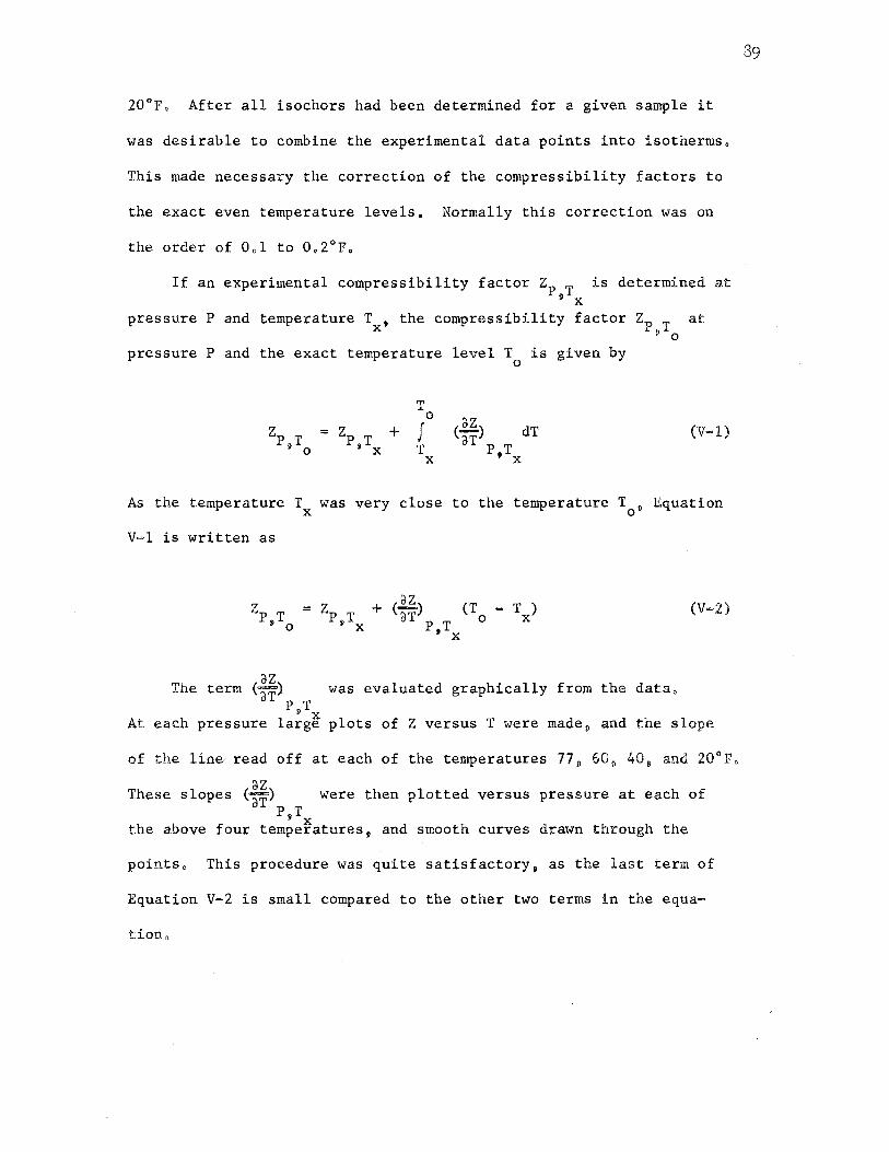
20°Fo After all isochors had been determined for a given sample it
was desirable to combine the experimental data points into isothermso
This made necessary the correction of the compressibility factors to
the exact even temperature levels. Normally this correction was on
the order of Ool to 0.2°F.
If an experimental compressibility factor ZP T is determined at 9 X
,pressure P and temperature T, the compressibility factor Z at X PpT
pressure P and the exact temperature level T is given by 0
..... ...
J 0
T X
(E) dT aT p T
t X
0
(V-1)
As the temperature T was very close to the temperature T, Equation X 0
V-1 is written as
= Zp T + (li) (T - T ) » X ar p T O X
t X
(V-2)
The term <H,) was evaluated graphically from the datao P9 T
X At each pressure large plots of Z versus T were made 9 and the slope
of the lin~ read off at each of the temperatures 77 9 60 9 40 9 and 20°F.
az These slopes ("'a'T) were then plotted versus pressure at each of P9 T
X the above four temperatures, and smooth curves drawn through the
points. This procedure was quite satisfactory, as the last term of
Equation V-2 is small compared to the other two terms in the equa-
tion.
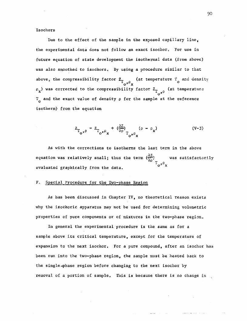
90
Isochors
Due to the effect of the sample in the exposed capillary line,
the experimental data does not follow an exact isochor. For use in
future equation of state development the isothermal data (from above)
was also smoothed to isochors. By using a procedure similar to that
above 9 the compressibility factor ZT (at temperature T and density o'Px 0
p) was corrected to the compressibility factor ZT (at temperature X o'p
T and the exact value of density p for the sample at the reference 0
isotherm) from the equation
z T ,P
0
(V-3)
As with the corrections to isotherms the last term in the above
equation was relatively small; thus the term(~) ilp T
o'Px evaluated graphically from the data.
F. Special Procedure for the Two-phase Region
was satisfactorily
As has been discussed in Chapter IV, no theoretical reason exists
why the isochoric apparatus may not be used for determining volumetric
properties of pure components or of mixtures in the two-phase region.
In general the experimental procedure is the same as for a
sample above its critical temperature, except for the temperature of
expansion to th,e next isochor, For a pure compound, after an isochor has
been run into the two-phase region, the sample must be heated back to
the single..phase region before changing to the next isochor by
removal of a portion of sample, This is because there is no change in

the sample pressure with the expansion in the two-phase region; thus
there is no way to ascertain from the pressure measurements when the
desired density has been reached. For a mixture this expansion must
also be made in the single-phase region, to avoid composition changes
of the sample.
91
CHAPTER. VI
PRESENTATION AND CALCVLATIONAL TIIATMENT OF EXPERIMENTAL DATA
In this chapter the experimental compressibility factor data from
the isochoric measurements is presented. The data for methane, ethylene,
and four intermediate mixtures covers the range 260 to ~400 psia at
temperatures of 20, 40, 60, and 77°F. For the pure ethylene, the
measurements extend into the two-phase i:egion. The 77°F data repre
sents the reference isother• from the Burnett apparatus.
The compressibility factors were compared versus the BWR equa~
tion (6) and the Edmister generalized form of the BWR equation (20).
The second apd third Leiden virial coefficients were derived by the
slope-intercept method, and were used to calculate interaction second
virial coefficients. Th.e experimental second and third virial coeffi
cients were compared versus the BWR equation (both original and
generalized forms) and the RK equation (58). Four empirical rules
were evaluated for estimating B12 from the pure component virial
coefficients B11 and B22 •
A. Presentation of Data
Volumetric Data
The experimental compressibility factor data is shown in Tables IV
and V, The reference isotherm (77°F) data from the Burnett apparatus
92
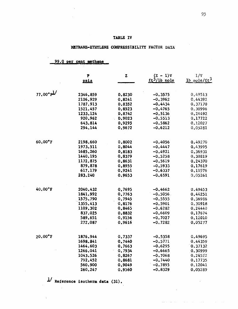
93
TABLE IV
METHANE-ETHYLENE COMPRESSIBILITY FACTOR DATA
99,0 per cent methane
p z (Z - l)V 1/V psi a ft3 /lb mo.!!_ ~.J.t3.
11.00°~1 2346.859 0.8230 -0.3575 o.i.9513 2106.929 0.8241 -0.3962 0~44392 1787.913 0.8352 -0.4434 0937170 1521.457 0.8523 -0.4765 0~30996 1233.124 0.8742 -0.5136 0.24492 920.962 0.9023 -0.5513 0.17722 643.814 0.9295 -0.5862 0.12027 294.144 0.9672 -0.6212 0~05281
. 60 0 00°F 2198.660 0,8002 -0.4056 0.49270 1973.511 0,8044 -0.4447 0&43995 1685.260 0,8183 -0.4921 0.36931 1440.195 0.8379 -0.5258 0,30819 1172.875 0,8631 -0,5619 0.24370
879,878 0,8955 -0.5933 0.17619 617.179 0.9241 -0.6337 0.11976
283.240 0,9653 -0.6591 0.05261
40,00°F 2040.432 0,7695 -0.4662 0.49453 184_1.992 0.7763 -0,5056 0.44251 . 1575.790 0.7945 _.0.5555 0,36986 1355.413 0,8176 -0.5901 0.30918 1109,302 0.8465 -0.6282 0.24440
837,025 0,8832 -0,660.9 0,17674 589,651 0.9156 -0.7027 0.12010 272,087 0,9616 -o. 7282 0,05277
20,00°F 1876.944 0,7337 -0.5358 0,49695 1698.841 0,7440 -0.5771 0.44359 1464,603 0,7663 -0.6295 0.37132 1266,041 0,7934 -0.6665 0.30999 1043.526 ·o.s261 -0.7068 0.24522
792.452 0.8681 -0.7440 0.17735 560.900 0,9049 -0.7895 0.12041 260,247 0,9560 -0.8329 0,05289
!/ Reference isotherm data (31),
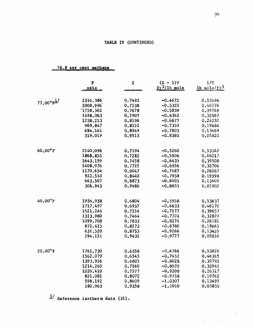
94
TABLE IV (CONTINUED)
78,8 per cent methane
p z (Z - l)V 1/V psi a ft3/lb mole 11?, ipole/ft3
77,00°p!/ 2316,386 0.7492 -0.4672 0.53684 2008,996 0,7538 -0 .• 5320 0.46276
·"''1758,562 0,7678 -0.5839 0.39769 '1498,063 0,7907 -0,6362 0.32897 1238.213 0~8196 -0.6877 0,26232 969.847 0,8552 -0.7350 0.19684 694,161 0,8949 -0.7803 0.13469 319,019 0,9513 -0.8360 0.05820
60,00°F 2140.096 0,7194 -0.5260 o.53342 1868.855 o. 7282 -0.5906 0.46017 1643.159 0.7458 -0.6435 0.39508 1408,976 0,7725 -0.6956 0,32706 1170,654 0.8047 -0.7487 0.26087
922.510 0,8440 -0.7958 0.19598 663,507 0,8873 -0.8405 o.13409 306,943 0,9486 -0.8855 0.05802
40,00°F 1956,938 0.6804 -0.5958 o.53637 1717.497 0,6937 -0.6633 0,46170 1521,246 0.7154 -o. 7177 0,39657 1313.980 0,7464 -o. 7724 0.32829 1099.708 0,7833 -0,8276 0,26181
872.425 0,8273 -0.8780 0.19665 631.520 0.8753 -0.9266 o.13455 294~121 0,9431 -0,9777 0,05816
20.00°F 1761,730 0,6358 -0.6766 0,53826 1562.079 0,6545 -0.7452 0,46365 1393.956 0,6805 -0,8028 0.39792 1214,260 0,7160 -0,8620 0.32945 1026,410 0,7577 -0.9208 Oa26317 821,081 0,8072 -0.9758 0.19762 598,192 0,8609 -1.0307 0.,13499 280,963 0,9358 -1.1oro 0.05833
!I Reference isotherm data (31).
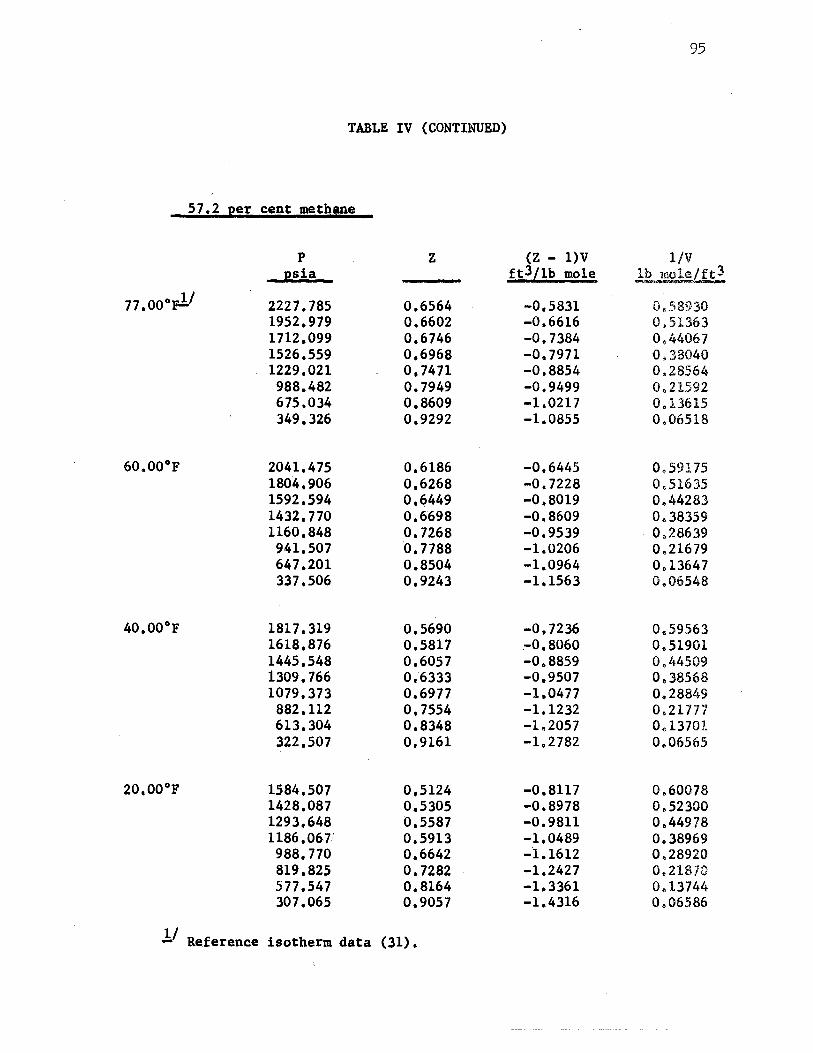
95
TABLE IV (CONTINUED)
57.2 per cent methane
p z (Z - l)V 1/V psi a ft3/lb mole lb mole/ft3 -
n.00°rl1 2227.785 0.6564 -0.5831 0.58930 1952.979 0.6602 -0.6616 0.51363 1712.099 0.6746 -0.7384 0.44067 1526.559 o.6968 -o. 7971 0.38040 1229.021 o. 7471 -0.8854 0.28564 988.482 0.7949 -0,9499 0.21592 675.034 0.8609 -1.0217 0013615 349.326 0.9292 -1.0855 0.06518
60.00°F 2041.475 0.6186 -0.6445 0.59175 1804,906 0,6268 -o. 7228 0.51635 1592,594 0,6449 -0.8019 0.44283 1432. 770 0,6698 -0.8609 0.38359 1160,848 0,7268 -0,9539 0.28639 941.507 0. 7788 -1.0206 0.21679 647,201 0.8504 -1,0964 o.13647 337.506 0,9243 -1.1563 0.06548
40,00°F 1817.319 0,5690 -o. 7236 Oc59563 1618.876 0.5817 -0,8060 0@51901 1445.548 0,6057 -0.8859 0.44509 1309,766 0,6333 -0,9507 0.38568 1079,373 0.6977 -1.0477 0.28849
882,112 0,7554 -1.1232 0.21777 613.304 0.8348 -1.2057 Ocl3701 322.507 0,9161 -1.2782 0.06565
20,00°F 1584,507 0,5124 -0.8117 0.60078 1428.087 0,5305 -0.8978 0.52300 1293,648 0,5587 -0.9811 0.44978 1186,06T 0,5913 -1.0489 0.38969 988. 770 0.6642 -1.1612 0.28920 819,825 0,7282 -1.2427 0.21870 577,547 0.8164 -1.3361 0013744 307.065 0.9057 -1.4316 0.06586
ll Reference isotherm data (31).
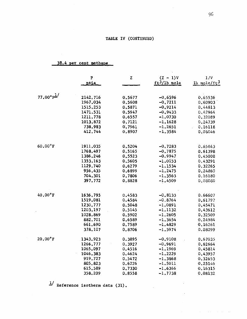
TABLE IV (CONTINUED)
38.4 per cent methane
p z (Z - l)V 1/V psi a ft3/lb mole lb mole/ft3
77 .ooop!/ 2l42.716 o .• 5677 -0.6596 0,65536 1967.034 0.5608 -o. 72ll 0~60903 1515,253 0.5871 -0,9214 o.44813 1471.531 0,5947 -0,9433 0. l;,2964 12ll. 778 0.6557 -1~0730 0.32089 1013~872 o. 7121 -1.1628 0.24739
738.983 o. 7961 -1.2651 0.16118 412.744 0,8907 -1.3584 0.08046
60,00°F 1911.035 0,5204 -o. 7283 0.65843 1768.497 0.5165 -0.7875 0.61398 1386.246 0,5523 -0.9947 0.45008 1353.163 0.5605 -1.of53 0.43291 1129.740 0,6279 -1.1534 0.32265
9.56.435 0.6899 -1.2475 0.24860 704,301 0.7806 -1.3563 0~16180 397. 772 0,8828 -1.4509 0.08080
40.00°F 1636.795 0.4583 -0,8133 0.66607 1519,081 0.4584 -0.8764 o.61797 1230. 777 0.5048 -1.0891 0.45471 1203.197 0.5145 -l. ll32 0.43612 1028.869 0.5902 -1.2605 0.32509 882.701 0,6589 -1.3654 0.24984 661,690 0.7589 -1.4829 0,16261 378.107 0,8706 -1.5974 0.08099
20,00°F 1343.923 0.3895 -0.9108 0.67035 1266.777 0,3927 -0.9691 o.62664 1065,097 0.4516 -1.1969 0.45814 1046.383 0.4624 -1.2229 0.43957 919.727 0,5472 -1.3868 0.32653 805.823 0.6226 -1.5011 0.25146 615.589 0.7330 -1.6366 0.16315 358,209 0.8558 -1. 7738 0.08132
1/ Reference isotherm data {31).
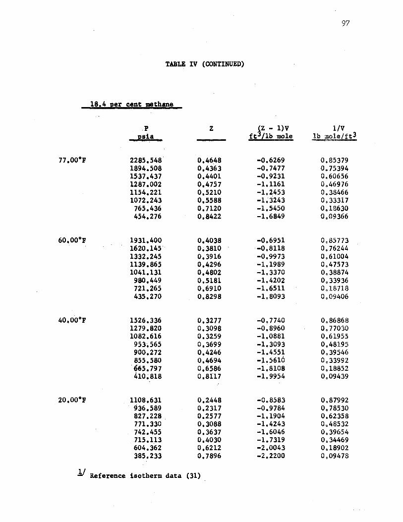
97
TABLE IV (CONTINUED)
18.4 per cent methane
p z iz • l)V 1/V psi a ft /lb mole lb mole/ft3
11.00•1 2285.548 0.4648 -0.6269 0.85379 1894.508 0.4363 -o. 7477 o. 75394 1537 .437 0.4401 -0.9231 0.60656 1287.002 0.4757 -1.1161 0.,46976 1154.221 0.5210 -1.2453 0.38466 1072.243 o.5588 -1~3243 0033317
765.436 0.1120 -1.5450 0.18630 454.276 0.8422 -1.6849 o.09366
60.00°1 1931.400 0.4038 -0.6951 0.85773 1620.145 0,;·3810 -0.8118 0.76244 1332.245 o.3916 -0.9973 0.61004 1139.865 0.4296 -1.1989 0.47573 1041.131 0.4802 -1.3370 0.38874 980.449 0.5181 -1.4202 0,33936 721.265 0.6910 -1.6511 0.18718 435.270 0.8298 -1.8093 0.09406
40.00°1 1526.336 0.3277 -0.7740 0.86868 1279.820 0.3098 -0~8960 o. 77030 1082.616 0.3259 -1.0881 0.61955 953.565 0.3699 -1.3093 0.48195 900.272 o.4246 -1.4551 0.39546 855.580 0.469.4 -1.5610 0.339-92
'665.797 o.6586 -1.8108 0.18852 410~818 0.8117 -1.99,54 0.09439
20.00°r 1108.631 0.2448 -0.8583 0.87992 936.589 0.2317 -0.9784 0.78530 827.228 0.2577 -1.1904 0.62358 771.330 0.3088 -1.4243 o .• 48532 742.455 0.3637 -1.6046 0.39654
. 715.U3 0.4030 -1.7319 o.34469 604.362 0.6212 -2.0043 0.18902 385.233 0.7896 -2.2200 0.09478
!/ Reference isotherm data (31)
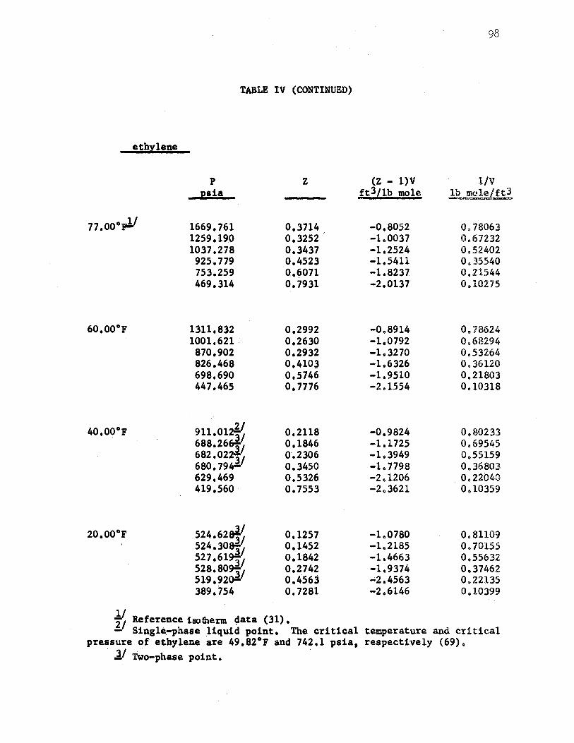
98
TABLE IV (CONTINUED)
ethylene
p z (Z - l)V 1/V psi a ft3/lb mole lb mole/ft3
11.00°p!/ 1669.761 0.3714 -0.8052 0,.78063 1259.190 0.3252 -1.0037 0.67232 1037.278 0.3437 -1.2524 0.52402 925.779 o.4523 -1.5411 Os35540 753.259 o,.~011 -1.8237 0.21544 469.314 0.7931 -2.0137 0.10275
60.00°F 1311.832 0.2992 -0.8914 Oe78624 1001,621 . 0.2630 -1.0792 0068294
870,902 0.2932 -1.3270 0.53264 826.468 0,410~ -1.6326 0.36120 698,690 0,5746 -l,9510 0.21803 447,465 O, 7776 -2.1554 0.10318
40,00°F 911,0l~ 0,2118 -0.9824 0080233 688,26~ 0,1846 -1,1725 0.69545 682.02 3/ 0.2306 -1.3949 0055159 680. 791.r" 0,3450 -1.7798 0.36803 629.469 0.5326 -2.1206 0.22040 419.560 0.7553 -2.3621 0010359
20,00°F 524.62e¥t 0.1257 -1.0780 0.81109 524.30~ 0,1452 -1.2185 0.70155 527,61 3/ 0,1842 -1.4663 0.55632 528,80~ 0,2742 -1.9374 0.37462 519,92 0.4563 ..;2.4563 0.22135 389,754 0,7281 -2.6146 0.10399
t' Reference ia>therm ~ata (31) , ll Single~phase .liquid point, The critical temperature and critical
pressure of ethylene are 49,82°F and 742.1 psia, respectively (69). · lf T'7o-phase point. ·
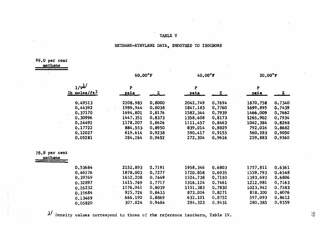
TABLE V
METUANE ... ETHYLENE DATA, SMOOTHED TO ISOCHORS
. 99.0 per cent methane
60.00°F 40.00°F 20.00°1
11v!' p p p lb moles/ft3 psia z psia z psi.a z
0.49513 2208.985 0.8000 2042.749 0.7694 1870.758 0.7340 o.44392 1989.944 0.8038 1847.183 0,7760 1699.895 0.7439 0,37170 1694,801 0,8176 1582,344 0,7939 1466.009 0,7662 0,30996 1447.351 0.8373 1358.408 0,8173 1265.902 o.7934 0.24492 1178.207 0,8626 1111.457 0.8463 1042.384 0.8268 0, 17722 884.553- 0,8950 839.014 0,8829 792.016 0,8682 0,12027 619,614 0.9238 . 590,417 0,9155 560,283 o.9oso 0.05281 284.264 0,9652 272.304 0,9616 25.9,883 0,9560
78.8 per cent methane
0,53684 2152.893 0,7191 1958.346 0,6803 1757 .811 0,6361 0,46276 1878.003 o. 7277 1720.858 0.6935 1559.793 0.6548 0,39769 1652.208 0,7449 1524.738 o. 7150 1393.693 0,6806 0.32897 1415.769 o. 7717 1316.124 0.7461 1212.981 o. 7163 0.26232 1176,041 0,8039 1101.383 0.7830 1023.942 0.7583 0,19684 925. 724 0.8433 873.004 0,8271 818.300 0,8076 0.13469 -- 666. 190 0.8869 632.101 0.8752 597.093 0,8612 0,05820 307.824 0.9484 294.323 0.9431 280.385 Oa9359
!/·Density values correspond to those of the reference isotherm, Table IV. '° '°
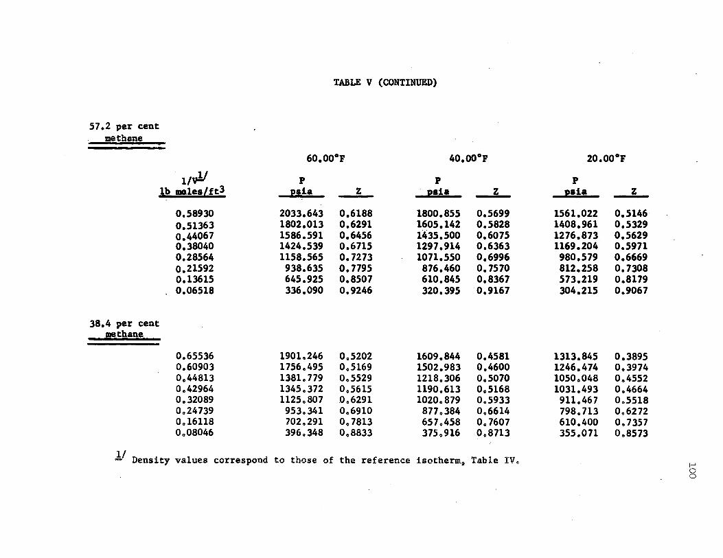
TABLE V (CONTINUED)
S7.2 per cent methane
60.00°!' 40.00°1' 20.00°,
. 11v!I p p p lb mAles/ft3 psi a z · psia z psi a z
O.S8930 2033.643 0.6188 1800.855 0.5699 1561.022 0.5146 o.51363 1802.013 0.6291 1605.142 0.5828 1408.961 0.5329 o.44067 1586.591 0.6456 1435.500 0.6075 1276.873 0.5629 0.38040 · 1424.539 0.6715 1297.914 0.6363 1169.204 0.5971 0.28564 1158.565 0.7273 1011.550 0.6996 980.579 0.6669 0.21592 938.635 0.7795 876.460 o. 7570 812.258 0.7308 0.13615 645.925 0.8507 610.845 0.8367 573.219 o.8179 o.06518 336.090 0.9246 320.395 0.9167 304.215 0.9067
38.4 per cent methane
o.65536 . 1901.246 005202 1609.844 0.4581 1313.845 0.3895 0.60903 1756.495 0.5169 1502.983 0.4600 1246.474 0.3974 0.44813 13810 779 005529 1218.306 005070 1050.048 004552 0.42964 13450372 0.5615 1190.613 0.5168 1031.493 0.4664 0.32089 1125c807 0.6291 1020.879 0.5933 911.467 0.5518 0.24739 953.341 0.6910 877.384 0.6614 7980 713 0.6272 0.1611s 702.291 0.7813 657.458 0.7607 610.400 007357 o.oso46 396.348 0.8833 375.916 · 0.8713 355.071 0.8573
1/ - Density values correspond to those of the reference isotherm, Table IVe I--' 0 0
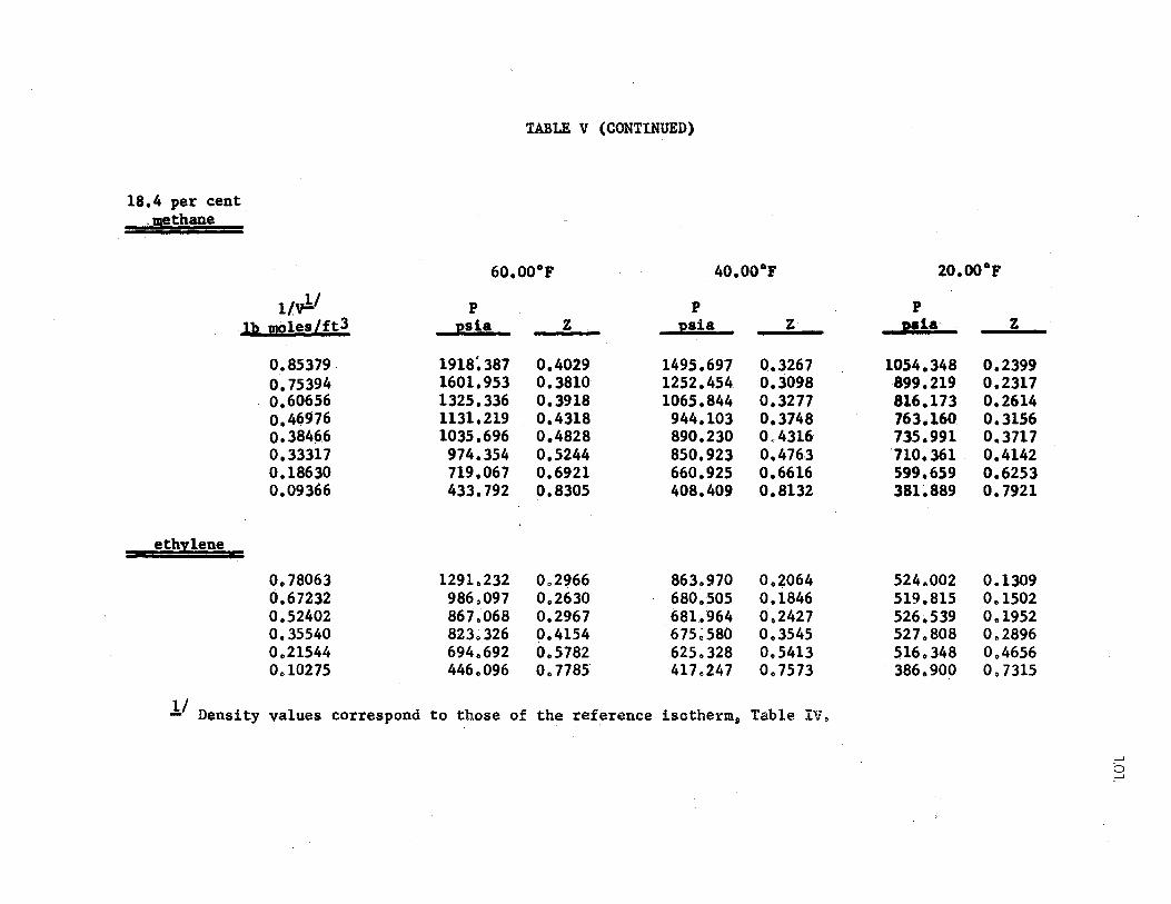
TABLE V {CONTINUED)
18.4 per cent .methane
60.00°F 4o.oo°F 20.00°F
11v!' p p p
.lb moles/ft3 --l!!!• - _Z_ - -----1:t1.ia. z _c__Hl&' z
o.85379 1918:387 0.4029 1495.697 0.3267 10S4.348 0.2399 o. 75394 1601.953 0.3810 1252.454 0,3098 899.219 0.2317 o.60656 1325.336 0,3918 1065,844 0.3277 816.173 0,2614 o.U.976 1131,219 0.4318 944.103 0,3748 763.160 0.3156 o.384~6 1035,696 0,4828 890,230 0.4316 735.991 0.3717 0.33317 974.354 0.5244 850.923 0.476-3 ·110.361. 0.4142 0.18630 719.067 0.6921 660.925 o.6616 599.659 0.6253 0,09366 433.792 0.8305 408.409 0.8132 381.889 0.7921
ethylene
o.78063 1291,232 002966 863 .• 970 0,2064 524.002 0.1309 0,67232 986.097 0,2630 680,505 0,1846 519,815 0.,1502 0.52402 867 .068 0.2967 681 .• 964 0,2427 526.539 0,1952 0.35540 823.326 9.4154 675~580 0.3545 527.808 0~2896 0.21544 694.692 0.5782 625.328 0,5413 516.348 0,4656 0,10275 446.096 o. 7785 417.247 0.7573 . 386.900 0,7315
!/ Density values correspond to those of the reference isotherm, Table IV. ' .
I-' 0 I-'
102
is shown in Table IV, Table IV represents the data before smoothing to
exact isochors; in Table V the data (at 60, 40, and 20°F) has been
smoothed to the densities of the reference isotherm. The data was
smoothed to isocho~s, as isochoric data is frequently used in equation
of state development, All calculations reported herein, however, were
based on the data of Table IV,
An error analysis of the data is given in Section C below, and a
sample cal~ula,tion of a compressibility·fac~or is presented .in
Appendix F, . I
Second Vir:t.al Coefficients
' . Leiden, s~cond vi rial coef ficienu"' were determined from the d$t:a
using the.dope.intercept techniq1.1e, desc;:ribed previously. I ' .,
Initially, values of B(T) w~re determine~ at each temperature as
intercepts on a plot of (Z - l)V ~ersus 1/V (Equation III-4). These ' ; . ' ;.~ ·.. '
initial values of B(T) were improved somewhat in the determination of
third virial'coefficieno. This is explained as follows, According . i, ..
to Equation lII-5 plots:·of [Z - l)V - B(T))V versus 1/V were constructed, . .
the intercept being the third viri~l ~~efficient. At each .temperature \ i.
several values of B(T) were assumed, using the initial value of B(T)
.as a starting value, The ~djustment:.s ~o B~T) were made in step~is~
fashion,with increme~ts of 0,001 ~t3/1b.~ole, (approximately 0.06 3 . ·h,•'·.
cm /gm mole), · i:t was found that a smau·.~djustment in B(T) resulted· ·
in ''a consid~rable change iu the function l(Z -· l)V - B(T) ]Vo This
pro~edure was coptinued until the value· of B(T) was determined.that
would produce the most linearity of, the f~nction [ (Z .. l)V - B(T).]V \ : .
at low 4e:;i~ities, The maximum revision in B(T) from the initial value
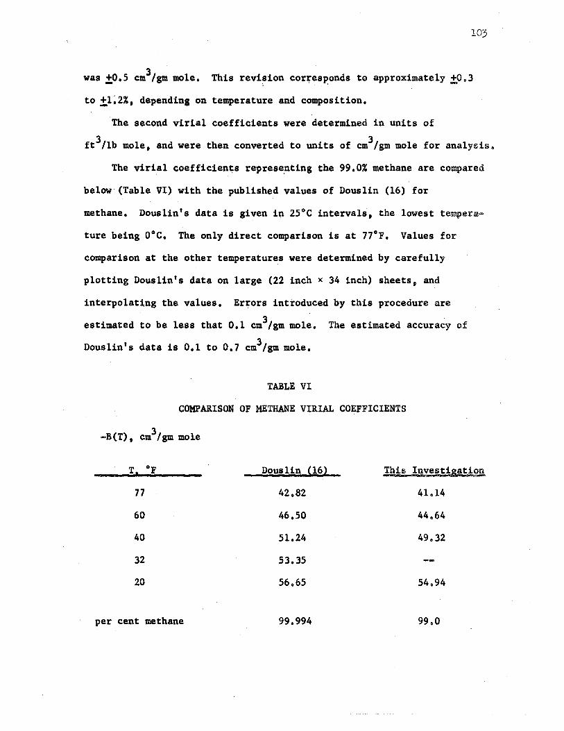
103
was +o.5 cm3 /gm. mole. - ' This revision cor;esponds to approximately ±,0.3
.. . l '
to ±1.2%, depending on temperature and composition.
The second virial coefficients were determined in units of
ft3/lb mole, and were then converted to units of cm3/gm. mole for analysiso
The virial coefficien~s represe.nting the 99.0% methane are compared
below (Table VI) with the published values of Douslin (16) for
methane. Douslin's data is given in 25°C intervals, the lowest tempera=
ture being 0°C, The only direct comparison is at 77°F, Values for
comparison at the other temperatures were determined by carefully
plotting Douslin's data on large (22 inch x 34 inch) sheets, and
interpolating the values. Errors introduced by this procedure are
3 estimated to be less that 0,1 cm /gm mole. The estimated accuracy of
Douslin's data is 0,1 to 0,7 cm3/gm. mole.
TABLE VI
COMPARISON OF METHANE VIRIAL COEFFICIENTS
-B(T), cm3/gm. mole
T OF
77
60
40
32
20
per cent methane
Douslin (16)
42.82
46,50
51.24
53.35
56.65
99.994
This Investigation
41.14
44,,64
49.32
54.94
99.0
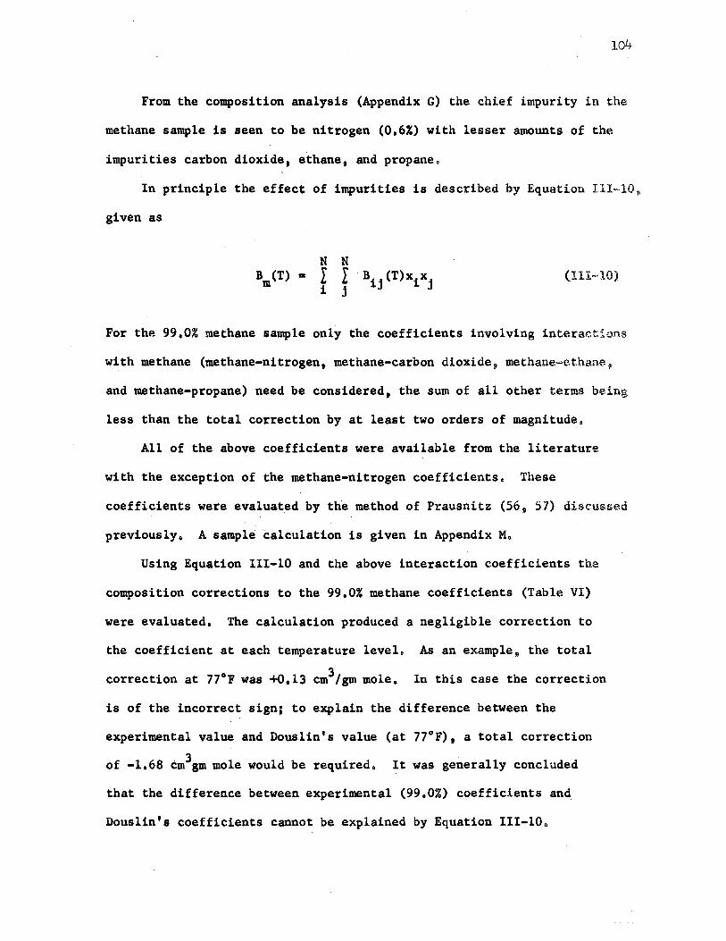
104
From the composition analysis (Appendix G) the chief impurity in the
methane sample is seen to be nitrogen (0.6%) with lesser amounts of the
impurities carbon dioxide, ethane, and propane.
In principle the effect of impurities is described by Equation 111=10~
given as
N N B (T) • m r r
i j (111=10)
For the 99.0% methane sample only the coefficients involving interactions
with methane (methane-nitrogen, methane-carbon dioxide, methane-ethane~
and methane-propane) need be considered, the sum of all other terms being
less than the total correcti.on by at least two orders of magnitude.
All of.the above coefficients were available from the literature
with the exception of the methane-nitrogen coefficients. These
coefficients were evaluated by the method of Prausnitz (56 9 57) discussed
previously. A sample calculation is given in Appendix M.
Using Equation III-10 and the above interaction coefficients the
composition corrections to the 99.0% methane coefficients (Table VI)
were evaluated, The calculation produced a negligible correction to
the coefficient at each temperature level. As an example 9 the total
correction at 77°F was +0.13 cm3/gm mole. In this case the correction
is of the incorrect sign; to explain the difference between the
experimental value and Douslin's value (at 77°F), a total correction
of -1.68 cm3gm mole would be required. It was generally concluded
that the difference between experimental (99.0%) coefficients and.
Douslin's coefficients cannot be explained by Equation III-10.
105
From the above comparisons the experimental cqefficients are con~
sistently higher (algebraically) than Douslin's values by an average
3 of approximately 1,8 cm /gm mole, Considering the accuracy of Douslin's
values, the e~perimental coefficients are estimated to be accurate to '' .. '' 3
approximately 1,5 cm /gm mole,
For the calculational analysis of the virial coefficient data
(Section B) the pure component virial coefficients :a11 (methane) and
B22 (ethylene) are combined empirically to obtain estimates of the
methane-ethylene interaction coefficient B12 • In order to make reli=
able. tests of these empirical rules it was desired to avoid intro-
ducing any uncertainty due to differences in thepure component
coefficients, Accordingly, the virial coefficient data of Douslin
was used to represent the pure methane, both for second and third
virial coeffici~nts,
The ethylene virial coefficients were also determined by the slope=
intercept method, The critical temperature of ethylene is 49.82°F (69);
thus it was seen (Table IV) that a considerable portion of the low
temperature ethylene data (at 20 and 40°F) consists of points in the
two-phase region. At these sub-critical temperatures the slope-
intercept procedure proved unsatisfactory, and the virial coefficients
could not be determined, A plot of the function (Z - l)V versus
1/V exhibits pronounced curvature through the two-phase region, making
extrapolation to the origin impossible.
As the 77 and 60°F isotherms lie close to the critical isotherm,
these points also exhibit a certain degree of curvatureo This is
to be expected. It was possible, however, to determine the virial
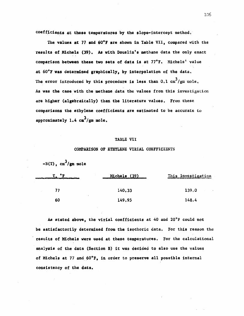
:)..06
coeff.:f.cients at these temperatures by the slope-intercept method.
The values at 77 and 60°F are shown in Table VII, compared with the
results of Michels (39)., As with Douslin's methane data the only exact
comparison between these two sets of data is at 77°F. Michels' value
at 60°F was determined graphically, by interpolation of the data.
The error introduced by this procedure is less than 0.1 cm3/gm mole.
As was the case with the methane data the values from this investigation
are higher (algebraically) than the literature values. From these
comparisons the ethylene coefficients are estimated to be accurate to
approximately 1.4 cm3/gm mole,
TABLE VII
COMPARISON OF ETHYLENE VIRIAL COEFFICIENTS
-B(T), cm3/gm mole
77
60
Michels (39)
140,33
149.95
This Investiga~!.2..~
139.0
148.4
As stated above, the virial coefficients at 40 and 20°F could not
be satisfactorily determined from the isochoric data. For this reason the
results of Michels were used at these temperatures. For the calculational
analysis of the data (Section B) it was decided to also use the values
of Michels at 77 and 60°F, in order to preserve all possible internal
consistency of the data.
The second virial coefficients for the four intermediate mixtures
were determined by the elope-intercept procedure. The impurit~es in
the int.ermediate mixture, are all hydrocarbons that are similar in
characteristics to the methane and ethylene. The largest impurity is
the 0,41 propane that is present in the 78.81 methane/20.7% ethylene . '
mixture. The correction for the impurities was made using Equation
III-10. For this correction the required interaction coefficients
are available in the literature, with the exception of the ethylene
ethane and ethylene-propane coefficients. These coefficients were
estimated from the method of Prausnitz; the total correction ranges
from +o,69 to +1,70 cm3/am mole. The resultant coefficients are
shown in Tables VIII and IX• both before and after making the com-
position corrections,
107
The second virial coefficients from Table IX (corrected for impur
ities) are illustrated graphically in Figures 6 and 7. In Figure 6
the virial coefficients are plotted versus temperature at constant
composition; in Figure 7 the coefficients are plotted versus compost-
tion at constant temperature,
Third Virial Coefficients
Leiden type third virial coefficients were determined, using
the slope-intercept technique (Equation III-5). The derivation of
third virial coefficients is similar to that of second virial coeffi;..
cients in that the initial estimate of the third coefficient is
further improved via deriving fourth virial coefficients, and adjusting . '
thirds to obtain reasonable fourths. In each case slightly different ' ' J '
.values of. C(T) (in s'teps of ±() 1 005 ft6 /lb mole 2, or approximately
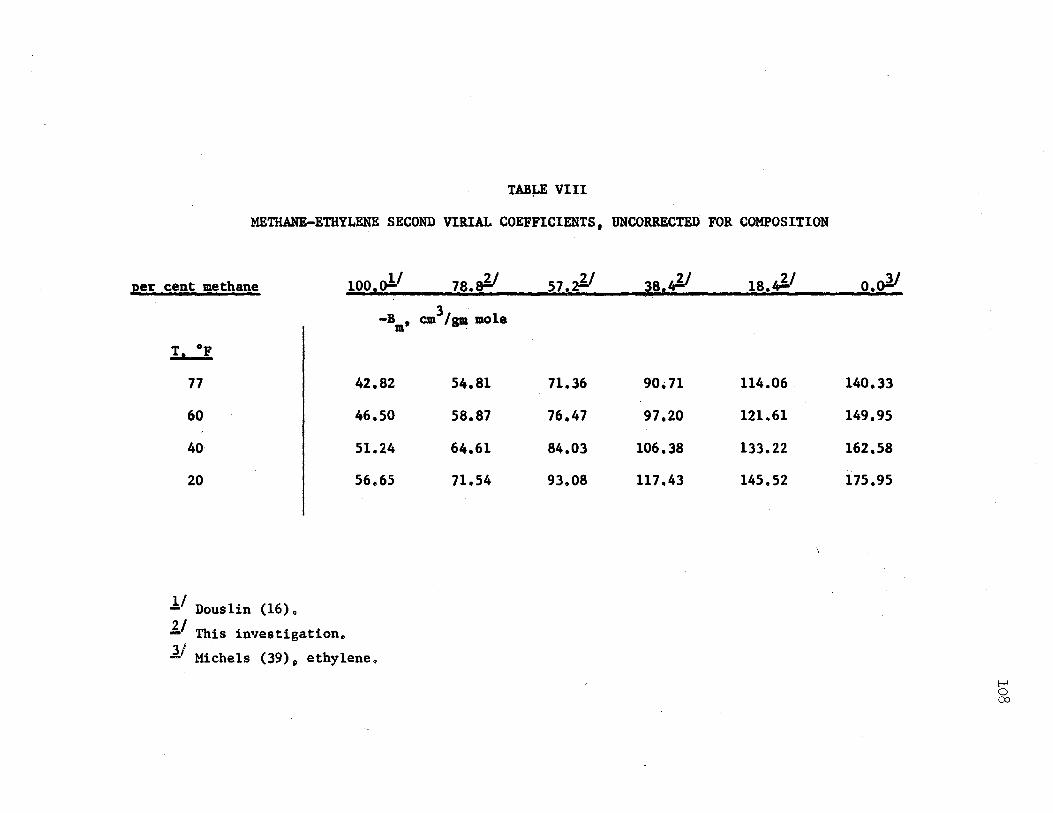
TABJ,E VIII
METHANE-ETHYLENE SECOND VIRIAL COEFFICIENTS, UNCORRECTED FOR COMPOSITION
per cent methan~ 100.o!' 78.a!' 57.~/ 38.t).I 1s.,.3.'~-- .~J!.ol' 3 -B I cm /gm mole m -
I T °F a.....:..
I 77 42.82 54.81 71.36 90.71 114.06 140.33
60 I 46.50 58.87 76.47 97.20 121~61 149.95
40 I 51.24 64.61 84.03 106.38 133.22 162.58
20 I 56.65 71.54 93.08 117.43 145e52 175.95
1.1 Douslin (16).
l.l This investigation.
11 Michels (39)p ethyleneo
I-' 0 00
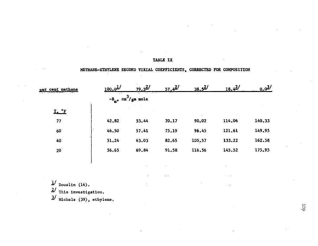
TABLE IX
METHANE-ETHYLENE SECOND VIRIAL COEFFICIENTS, CORRECTED FOR COMPOSITION
ger cent methane 100.o!-' 79.?)/ 57.,.Y 38.# 1s,,l./ 3 -Bm' cm /gm mole
I T °F ~
77 42.82 53.44 70.17 90.02 114.06
60 46.50 57.41 75.19 96.45 121,61
40 51.24 63.03 82.65 105.57 133.22
20 I 56.65 69.84 91.58 116.56 145.52
1/ Douslin (16).
l:l This investigation.
1./ Michels (39)~ ethylene.
o.ol.l
140.33
149.95
162.58
175.95
I-' 0
'°
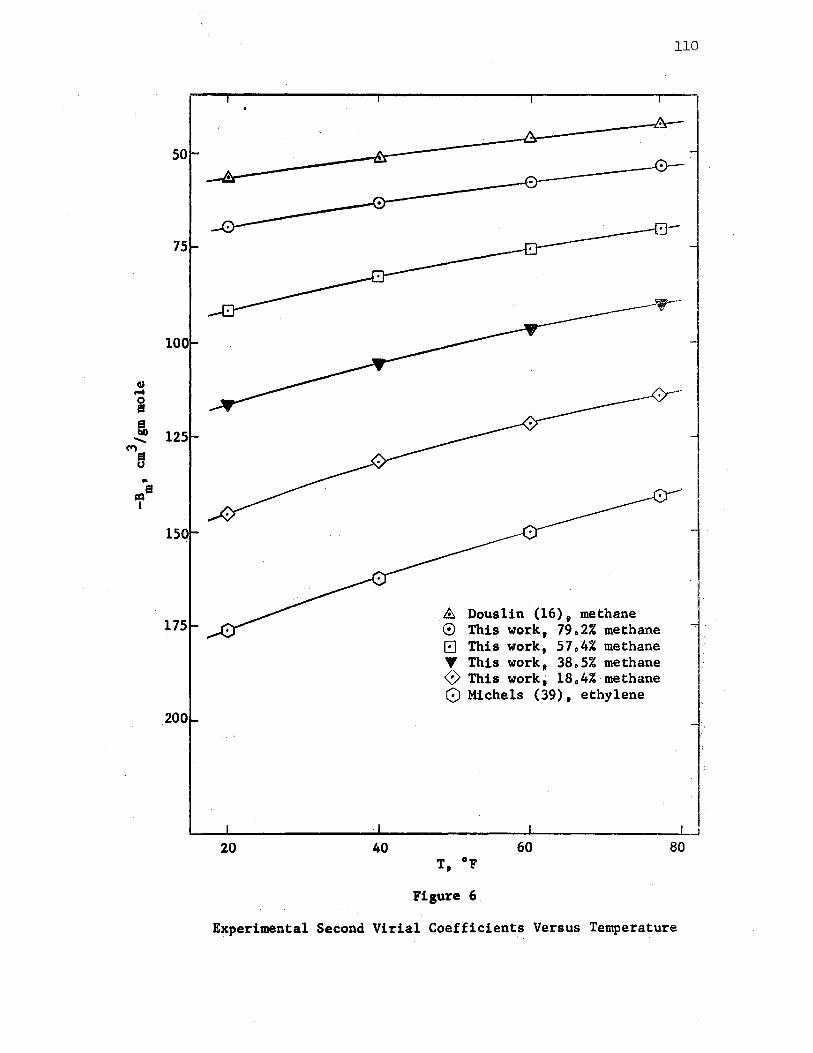
50
75
100
QI .... j m,
125 ....... ~
B .. ~s I
150
175
200
-----~
20 40
110
~-----&_____ --&,-
v,--··
& Douslin (16) 9 methane · 0 This work., 79. 2% methane 0 This work, 57.4% methane T This work, 38.5% methane 0 This work; 18.4% methane SJ Michels (39), ethylene
60 T, °F
Figure 6
80
Experimental Second Virial Coefficients Versus Temperature
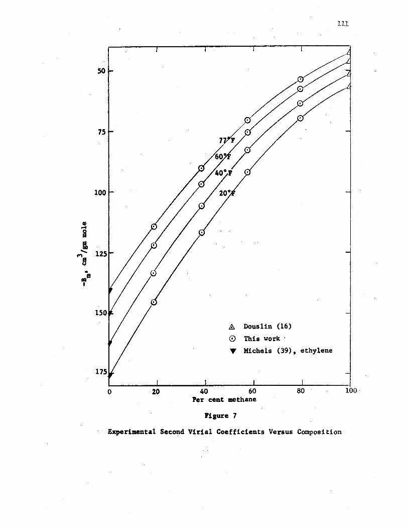
so
75
100
IU ... a I ...... 125 MB •
"4s I
150
175
0 20
& Douslin (16)
0 This work '
~ Michels (39), ethylene
40 60 80 Per cent methane
Figure 7
111
100
Experimental Second Virial Coefficients Versus Composition
2 6 2 0.2 >e 10 cm /p mole )were aaaumed at each temperature, using the
o~iginal value as an initial eatimate.
Due to conaider~ble acatter of the values of the term
[(Z - l)v2 • B(T)V - C(T)JV in the plot versus 1/V it was difficult
to determine reliable value• of thefourtb virial coefficients. By
proper choice of the third virial coefficient, the values of the
f.uriction [ (Z - ·l)v2 - B(T) V - C(T) ]V were determined which exhibited ' . ·... ' . .. . the most syatematic variation with both t~mperature and compositio~.
Although this method was valuable in improving the third virial
.coefficients, the reaulting f~urtb,virial coefficients exhibited
CO?Siderable scatter. Thus the fourth virial coefficients are not
reported,
The maximum adju1tme11t to the third virial coefficients by this
procedure was 2.0 ,c 102 cm6/gm mole2• This value corresponds to
roughly 2.0 to a.oz, depending on temperature and composition. The
absolute accuracies of the third virial coefficients are difficult to
evaluate, as theae coefficients are quite sensitive to errors in both
compressibility factor data and second virial coefficients.
112
In principle, correction for impurities in the third virial
coefficients can be made by use of Equation III-11. This correction was
not made in this case, as a sufficiently reliable means is not avail-
able for estimating the interaction third virial coefficients.
Values of the third ~ria~ coefficie~t are presented in Table x. . . 6 2
The values were determined in units of ft /~b mole, and were then
converted. to cm6/gm mole2 for analysis.
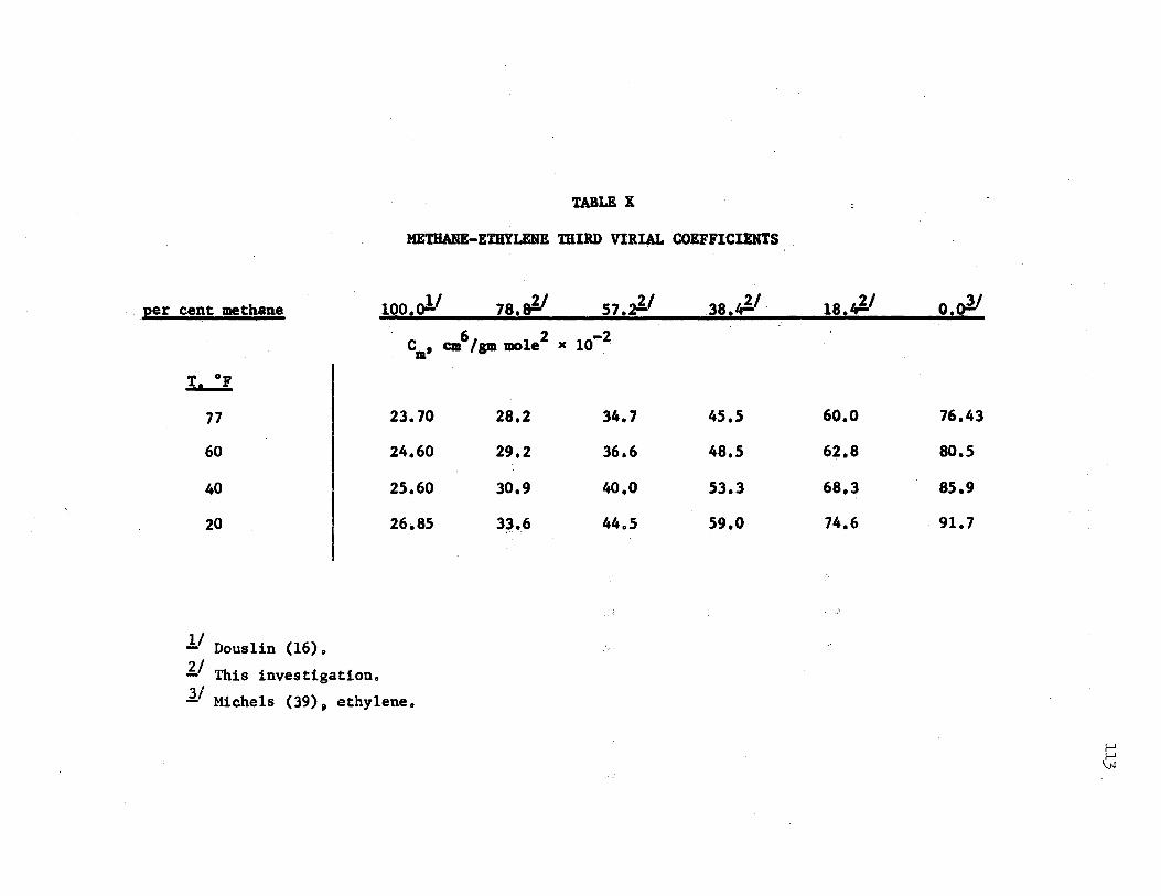
TABLE X
METHANE-ETHYLENE THIRD VIRIAL COEFFICIENTS
per cent methane 100.o!' ~~~~
78.a!' 57 .iJ=.I 38.t).I
c., cm6 /gra mole2 x 10-2
I T °F :.a......:..
77 23.70 28.2 34.7 45.S
60 I 24.60 29.2 36.6 48.S
40 I 25.60 30.9 40.0 S3.3
I 20 26.85 33.6 44.5 59.0
ll Douslin (16) o
1:/ This investigationo
l/ Michels (39) 9 ethyleneo
18.,/:./
60.0
62.8
68.3
74.6
o.o1'
76.43
80.S
85.9
91.7
I-' I-' \.N
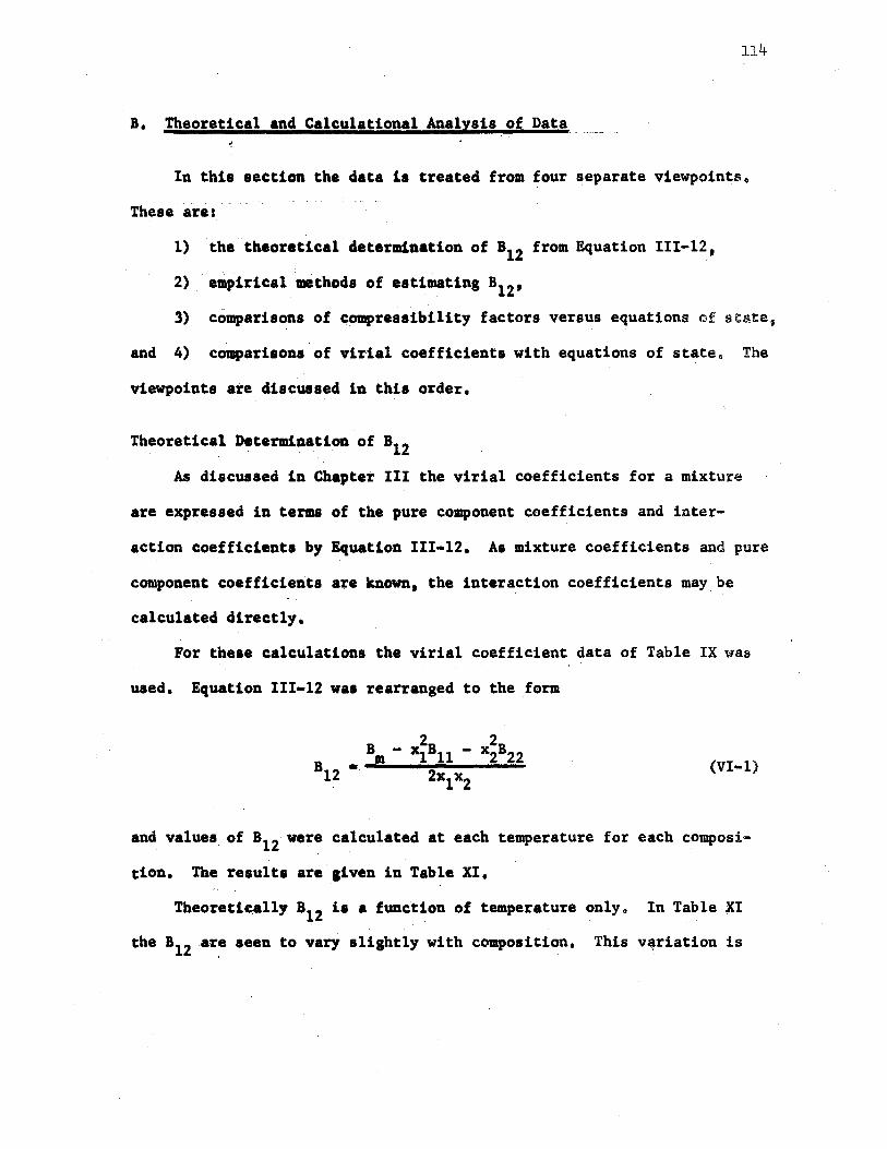
114
B. Theoretical and Calculational Analysis of Data
In this section the data is treated from four separate viewpoints.
These· are:
1) the theoretical determination of B12 from Equation III-12,
2).· empirical.methods of estimating B12 ,
3) comparisons of compressibility factors versus equations of state,
and 4) comparisons of virial coefficients with equations of state. The
viewpoints are discussed in this order.
Theoretical Determination of B12
As discussed in Chapter III the virial coefficients for a mixture
are expressed in terms of the pure component coefficients and inter-
action coefficients by Equation III-12. As mixture coefficients and pure
component coefficients are known, the interaction coefficients may be
calculated directly.
For these calculations the virial coefficient data of Table IX was
used. Equation III-12 was rearranged to the form
(VI-1)
and values. of a12 were calculated at each temperature for each composi
tion. The results are given in Table XI.
Theoreti~ally B12 is a function of temperature only. In Table XI
the B12 are seen to vary slightly with composition. This v~riation is i
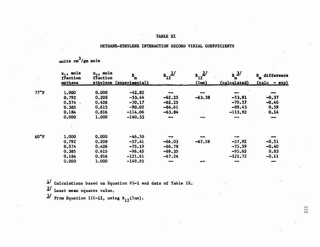
TABLE XI
METHANE-ETHYLENE INTERACTION SECOND VIRIAL COEFFICIENTS
units cm3 /gm mole
x1, mole fraction 11l8thane
x2, mole B B 1( B ?:I· B ll B difference fraction m 12 12 m m · ethylene (experimental) ~~~~lms) (calculated) · · (calc - exp)
77°F 1.000 0.000 -42.82 --
60°F
0.792 0.574 0.385 0.184 0.000
1.000 0.792 0.574 0.385 0.184 0.000
0.208 0.426 o.615 0.816 1.000
0.000 0.208 o.426 00615 0.,816 1.000
,;.53.44 -62.25 -70.17 -62.25 -90.02 -64.61
-114.06 -63.84 -140.33 --46.50 ---57.41 -66.03 -75.19 -66.78 -96.45 -69.35
-121.61 -67.24 -149.95
ll Calculations based on Equation VI-1 and data of Table IX.
ll Least mean squares value.
l/ From Equation III-12, using B12 (lms).
-63.38 -53.81 -0 .. 37 -10.s1 . -0.40 -89.43 o.s,
-113.92 0.14
--67.59 -57.92 -0.Sl
-75.59 -0.40 -95.62 0.83
-121.12 -0.11
I-' I-' \Jl .
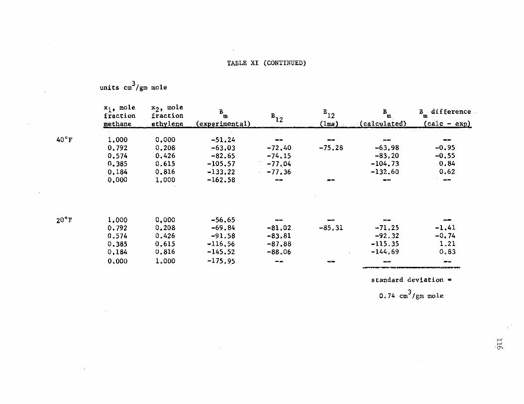
TABLE XI (CONTINUED)
units cm3/gm mole
x1 , mole fraction methane
40°F 1.000
20°F
o.792 0.574 0.385 0.184 0,000
1.000 0.792 0.574 0,385 0,184 0.000
x2 , mole d·f f ti B B B12 B B 1 ference rac on m 12 m m ethylene (experimental} (lms) (calculated) (calc - exp)
0.000 -51.24 0.208 -63.03 -72.40 -75.28 0.426 -82.65 -74.15 o.615 -105.57 -77.04 0,816 -133.22 -77.36 1.000 -162.58
0.000 -56.65 0.208 -69,84 -81.02 -85.31 0.426 -91.S8 -83.81 0.615 -116.56 -87.88 0,816 -145.52 -88.06 1.000 -175.95
-63.98 -0.95 -83.20 -0.55
-104.73 0.84 -132.60 0.62
-71.25 -1.41 -92.32 -0.74
-115.35 1.21 -144.69 0.83
standard deviation=
0.74 cm3/gm mole
1--' 1--' CJ'\
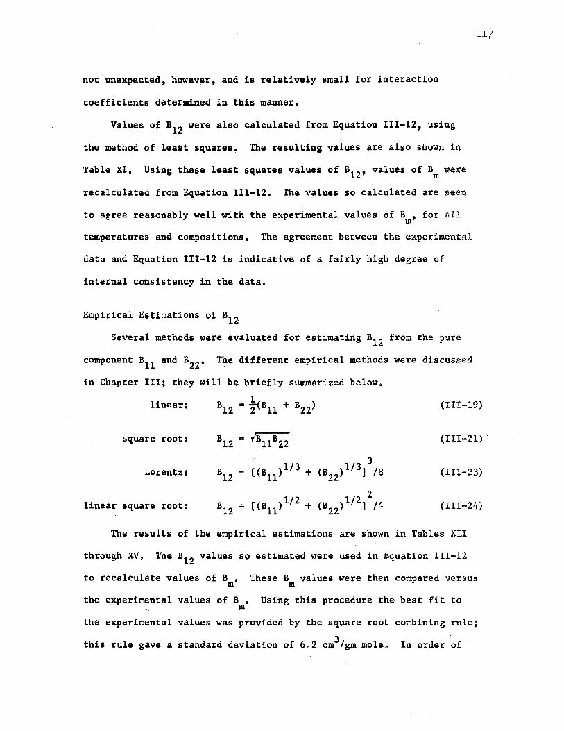
not unexpected, however, and is relatively small for interaction
coefficients determined in this manner.
Values of B12 were also calculated from Equation III-12, using
the method of least squares. The resulting values are also shown in
Table XI. Using these least squares values of B12 , values of Bm were
recalculated from Equation III-12. The values so calculated are seen
to agree reasonably well with the experimental values of B • for all m
temperatures and compositions, The agreement between the experimental
data and Equation III-12 is indicative of a fairly high degree of
internal consistency in the data.
Empirical Estimations of B12
Several methods were evaluated for estimating s12 from the pure
component B11 and s22 • The different empirical methods were discussed
in Chapter III; they will be briefly sunnnarized belowo
117
linear: Bl2 1 = 2(Bll + B22) (III-19)
square root: 812 = {BllB22 (III-21)
3 Lorentz: Bl2 = [(Bll )1/3 + (B )1/3) /S (III-23) 22
2 linear square root: Bl2 = [(Bll )1/2 + (B )1/2} 14 (III-24) 22
The results of the empirical estimations are shown in Tables XII
through XV. The B12 values so estimated were used in Equation III-12
to recalculate values of B, These B values were then compared versus m m
the experimental values of B. Using this procedure the best fit to m
the experimental values was provided by the square root combining rule;
this rule gave a standard deviation of 6.2 cm3/gm mole. In order of
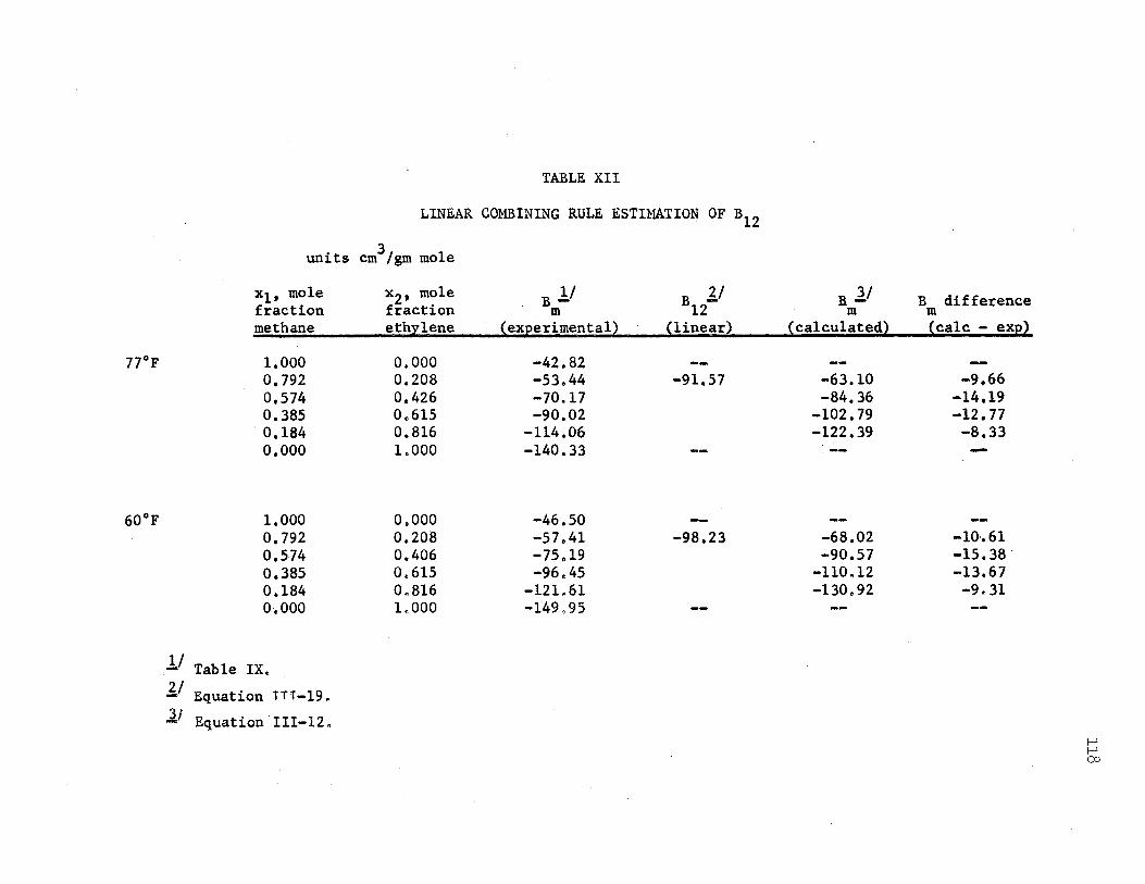
77°F
60°F
TARLE XII
LINEAR COMBINING RULE ESTIMATION OF B12
3 units cm /gm mole
x1 , mole fraction methane
1.000 0.792 0.574 0.385
. o.184 0.000
1.000 0,792 0.574 0.385 o.184 0.000
1/ Table IX.
l/ Equation TTT-19A 3 - 1 Equation III-120
x2 mole 1/ 2/ 3/ ' B - · B - B - B difference fraction m 12 m m
ethylene · ~xperimental) {linear) {calculated) (calc - exp)
0.000 0.208 0.426 0.615 0.816 1.000
0,000 0.208 0.406 0.615 0.816 1.000
-42.82 -53.44 -70.17 -90.02
-114.06 -140.33
-46.50 -57.41 -75019 -96.45
-121.61 -149095
-91.57
--
-98,23
-63.10 -9.66 -84.36 -14.19
-102.79 -12,77 -122.39 -8.33
. --
-68.02 -10·.61 -90.57 -15.38·
-110.12 -13.67 -130.92 -9.31
I-' I-' 00
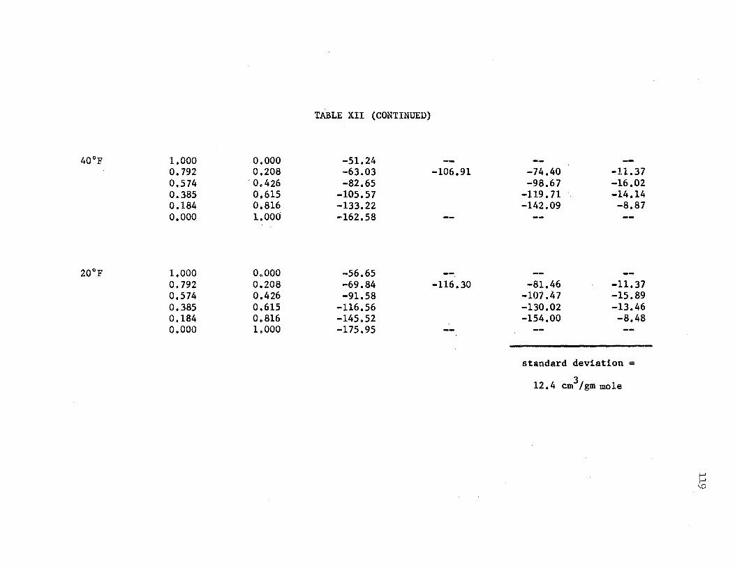
TABLE XII (CONTINUED)
40°F 1.000 0.000 -51.24 0.792 0.208 -63.03 0.574 o.426 -82.65 0.385 0.615 -105.57 0.184 0.816 -133.22 0.000 1.000 -162.58
20°F 1.000 0.000 -56.65 0.792 0.208 -69.84 0,574 0.426 -91.58 0.385 o.615 -116.56 0.184 0.816 -145.52 0.000 1.000 -175.95
-106.91
-116.30
-74.40 -11.37 -98.67 -16.02
-119. 71 -14.14 -142.09 -8.87
-81.46 -11.37 -107.47 -15.89 -130,02 -13.46 -154.00 -8.48
standard deviation=
3 12.4 cm /gm mole
I-' I-' \.0
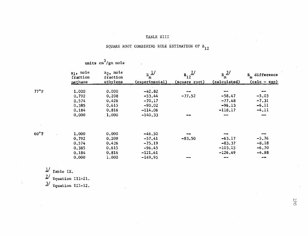
77°F
60°F
TABLE XIII
SQUARE ROOT COMBINING RULE ESTIMATION OF B12
3 units cm /gm mole
x1, mole fraction methane
1/ Table IX.
1,000 0.792 0,574 0,385 0,184 0,000
1,000 0,792 0.574 0.385 o.184 0.000
1/ Equation III-21.
ll Equation III-12.
x2, m?le B 1/ B 1/ B ll B difference fraction m 12 m m ethylene (experimental) (square root) (calculated) (calc - exp)
0,000 0,208 0,426 0,615 0.816 1.000
0.000 0.208 0,426 o.615 0.816 1.000
-42,82 -53,44 -70.17 -90,02
-114,06 -140,33
-46.50 -57.41 -75.19 -96.45
-121.61 -149,95
-77 ,52 -58.47 -5,03 -77 ,48 -7.31 -96.13 -6,ll
-118.17 -4.11
-83.50 -63,17 -5.76 -83.37 -8,18
-103.15 -6.70 -126.49 -4.88
f--' !\)
0
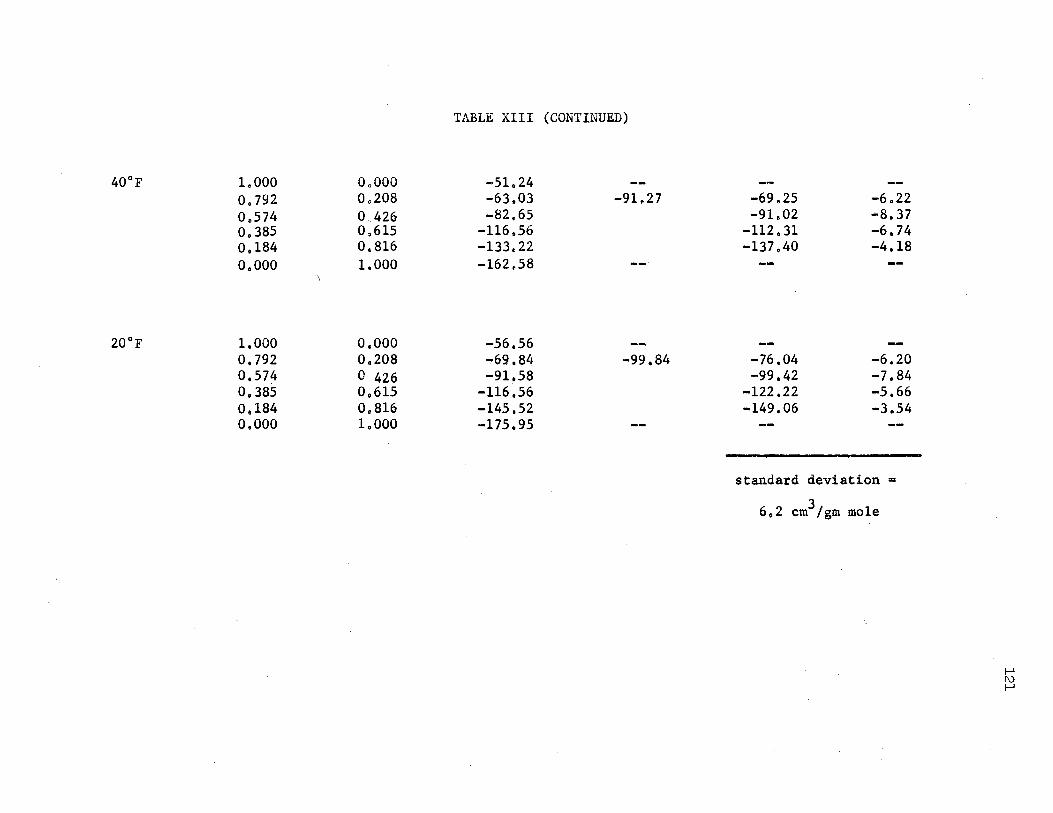
TABLE XIII (CONTINUED)
40°F 1.000 OoOOO -51.24 0.792 Oa208 -63.03 -91.27 o.574 O 426 -82.65 0.385 0.615 -116.56 o.184 0.816 -133.22 0.000 1.000 -162.58
20°F 1,000 0.000 -56.56 0.792 0.208 -69.84 -99.84 0.574 0 426 "."'91.58 0.385 0.615 -116 .56 o.1s4 0.816 -145.52 0.000 1.000 -175.95
-69.25 -6.22 -91.02 -8.37
-112. 31 -6.74 -137.40 -4.18
-76.04 -6.20 -99.42 -7.84
-122.22 -5.66 -149.06 -3.54
standard deviation=
3 6.2 cm /gm mole
f-l I\) f-l
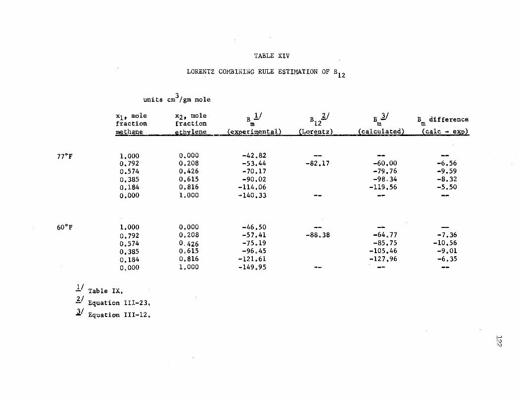
77°F
60°F
TABLE XIV
LORENTZ COMBINING RULE ESTIMATION OF B12
units cm3/gm mole
x1, mole fraction methane
1,000 0,792 0.574 0,385 o.184 0,000
1.000 o.792 0,574 0,385 0,184 0.000
1/ Table IX.
1:.,/ Equation III-23.
ll Equation III-12.
x2, mole B !/ B 1:./ B 1/ B difference fraction m 12 m m ethylene (experimental) (Lorentz) (calculated) (calc - exp)
0.000 0.208 0,426 0,615 0.816 1.000
0.000 0.208 0,426 Oo615 0,816 1.000
-42.82 -53.44 -70.17 -90.02
-114.06 -140,33
-46.50 -57.41 -75.19 -96.45
-121.61 -149.95
-82.17
-88.38
-60,00 -6.56 -79.76 -9.59 -98,34 -8.32
-119,56 -5.50
-64.77 -7.36 -85. 75 -10,56
-105.46 -9.01 -127.96 -6.35
I-' f\) f\)
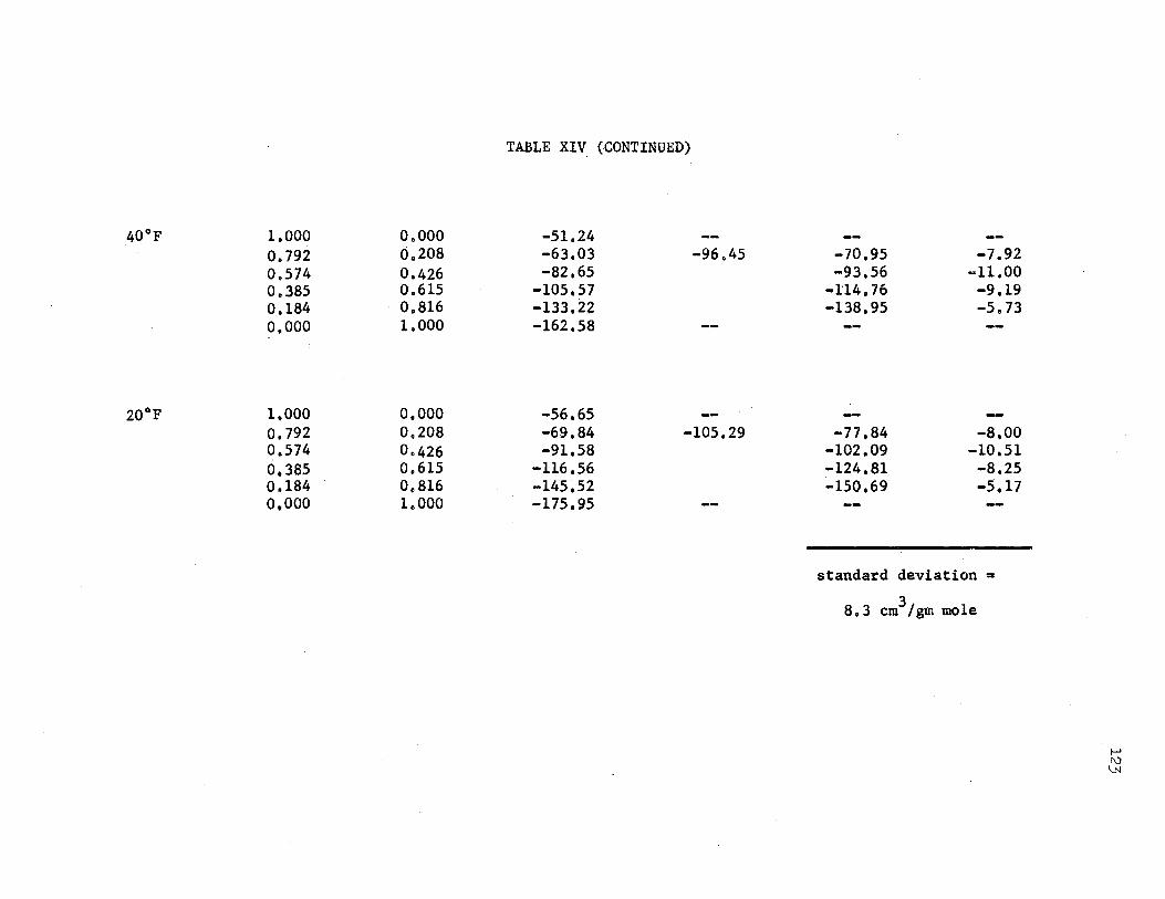
TABLE XIV (-CONTINUED)
40°F 1,000 0.000 -51.24 o.792 0,208 -63,03 -96.45 0,574 0,426 -82,65 0,385 0.615 -105.57 0,184 0,816 -133.22 0.000 1,000 -162.58 --
20°F 1,000 0.000 -56,65 --0.792 0.208 -69,84 -105,29 0,574 0.426 -91,58 0,385 0,615 -116.56 0,184 0,816 -145,52 0.000 1.000 -175.95
-70,95 -7.92 -93,56 -11.00
-114, 76 -9,19 -138,95 -5.73 -- ... -
-77 ,84 -8,00 -102,09 -10.51 -124,81 -8.25 -150,69 -5.17
standard deviation•
8,3 cm3/gm mole
I-' ('J
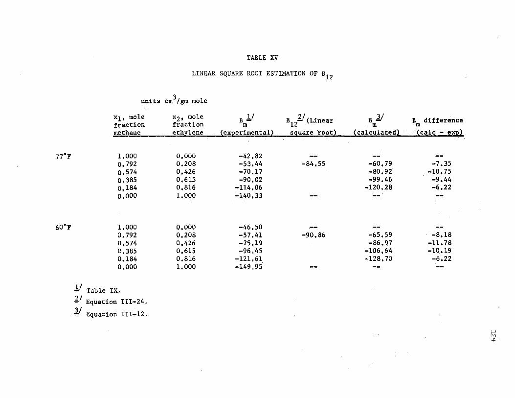
77°F
60°F
TABLE XV
LINEAR SQUARE ROOT ESTIMATION OF B12
units cm3/gm mole
x1, mole fraction methane
1.000 o.792 o.574 o.385 o.1s4 0.000
1,000 0.792 0,574 0.385 0.184 0.000
1/ Table IX.
1:./ Equation III-24. 3/ - Equation III-12.
x2 mole 1/ 2/ . 3/ ' B - B - (Linear B - B difference fraction m 12 . · m m ethylene (experimental) square root) (calculated) ·(calc - exp)
0.000 0.208 0,426 0.615 0.816 1.000
0.000 0.208 0.426 0.61s 0,816 1.000
-42,82 -53.44 -84.55 -70,.17 -90,02
-114.06 -140,33
-46,50 -57.41 -90.86 -75.19 -96.45
-121.61 -149.95
-60,79 -7.35 -80,92 -10.75 -99,46 -9.44
-120.28 -6.22
-65.59 -8.18 -86,97 -11. 78
-106,64 -10.19 -128.70 -6.22
f-' I\)
+
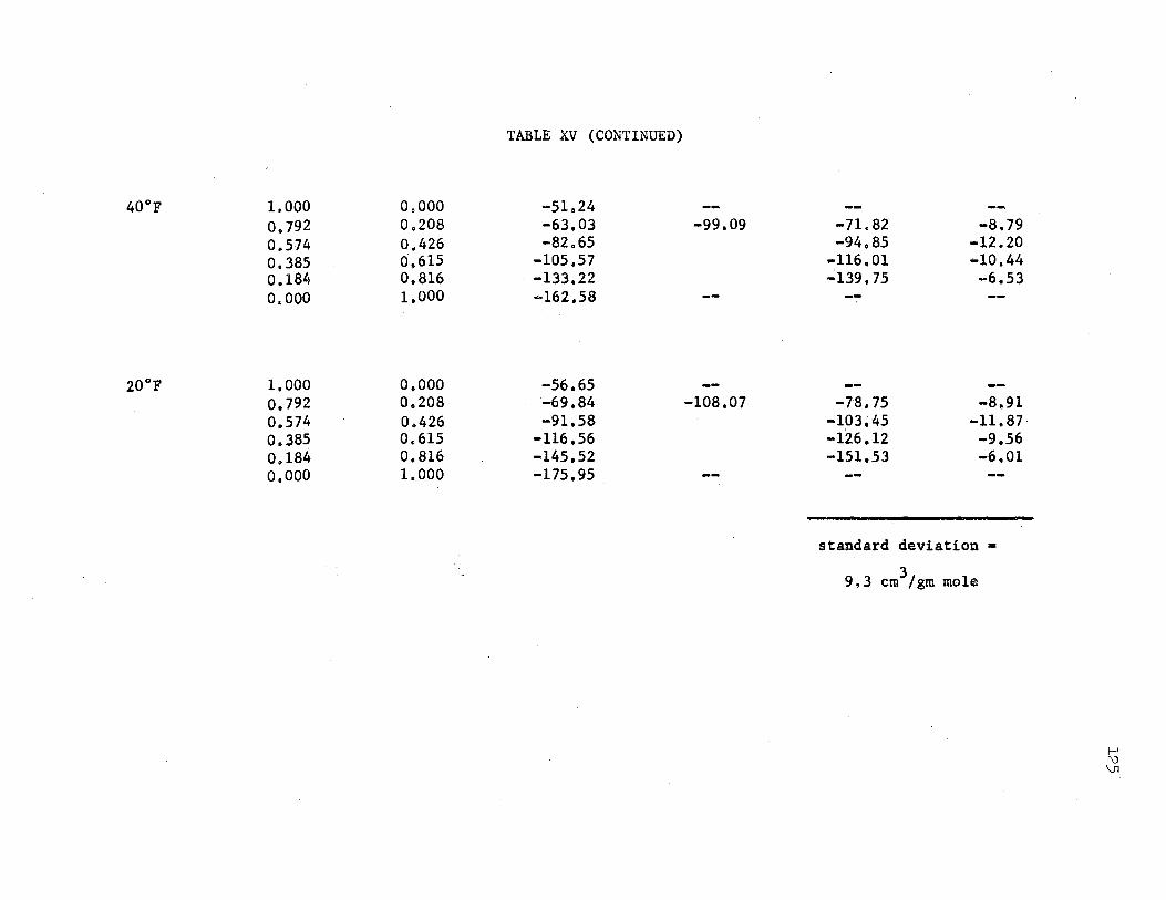
TABLE XV (CONTINUED)
40°F 1.000 0.000 -51.24 o. 792 0.208 -63.03 o.574 o.426 -82.65 0.385 0,615 -105.57 0.184 0.816 -133,22 0.000 1.000 -162.58
20°F 1.000 0.000 -56.65 o.792 0.208 -69.84 0.574 0~426 -91.58 0.385 0.615 -116.56 0,184 0.816 ... 145,52 0.000 1.000 -175,95
-99.09
-.--108.07
-71.82 -8.79 -94.85 -12.20
.-116.01 -10.44 ~139.75 -6.53
-78. 75 -8.91 -103,45 -11.87 -126.12 -9.56 -151,53 -6,01
standard deviation=
3 9.3 cm /gm mole
I-' !\) \J1
126
increasing standard deviations the remaining three methods are arranged
3 · 3 as Lorentz (8,3 cm /gm mole), linear square root (9.3 cm /gm mole), and
linear (12.4 cm3/gm mole) •. The poor fit given by the linear method is not
surprising, as this method represents an oversimplification.
Comparisons of Compressibility Factors Versus Equations of State
The experimental compressibility factors (Table IV) were compared
versus the BWR equation and the Edmister generalized BWR equation. The
results are shown in Table XVI.
For the BWR equation the constants, in English units, as tabulated
by Benedict et al (5) were used for the hydrocarbons. For the 99.0%
methane sample the constants for carbon dioxide as tabulated by Eakin
and Ellington (18) were used, For the mixtures the constant B was 0 m
determined by the linear combining rule, For use in the generalized
BWR equation the accentric factor for ethylene was required. This value
was determined from the definition (Equation I~I-14), using the vapor
pressure data of York and White (69). The resulting value was w = +0.087.
From Table XVI it is seen that both of the equations generally
predict compressibility factors that are lower than the experimental
values. For the 99,0% methane sample and the four intermediate mixtures
the generalized BWR equation provides a slightly better fit than does
the original BWR equation, For the ethylene sample the original BWR
equation provides the better fit, Considering all of the data points
together, the standard deviat.ions from the experimental compressibility
factors are given as 0,015 for the generalized BWR equation and 0.022
for the original equation,
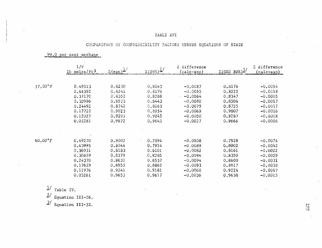
TABLE XVI
COMPARISONS OF COMPRESSIBILITY FACTORS VERSUS EQUATIONS OF STATE
_99, 0 per c~ metha,!:_e_
1/V , l/ 2 Z difference 3 Z difference .lb molt:s/ft3_,_,,~--~l£Xp)- . __ u= ,_ Z ill}:@1:/ =~£tl!::~) · Z(GEN BWR);_/ (calc-exp)
77,00°F 0049513 0,8230 0,8143 -0.0087 0.8176 -0.0054 o.44392 0.8241 0.8176 -0.0065 0.8222 -0.0019 0.37170 0.8352 0.8288 -0.0064 0.8347 -0.0005 0,30996 0.8523 0,8443 -0.0080 0.8506 -0.0017 0.24492 0,8742 0.8663 -0.0079 0.8725 -0.0017 0.17722 0,9023 0,8954 -0.0069 0.9007 -0.0016 0.12027 0,9295 0.9245 -0.0050 0.9287 -0.0008 0.05281 0,9672 0. 9645 -0.0027 0.9666 -0,0006
60,00°F 0.49270 0,8002 0.7894 -0.0108 0. 7928 -0.0074 0.43995 0,8044 0,7954 -0.0089 0.8002 -0.0042 0,36931 0,8183 0,8101 -0,0082 0,8161 -0.0022 0,30819 0.8379 0.8285 -0.0094 0.8350 -0,0029 0.24370 0.8631 0,8537 -0.0094 0.8600 -0.0031 0.17619 0,8955 0.8862 -0,0093 0.8917 -0,0038 o.11976 0 ., 9241 0,9181 -0.0060 0.9224 -0.0017 0.05261 0.9653 0.9617 -0.0036 0. 9638 -0.0015
1/ Table IV,
1./ Equation III-26.
1/ Equation III-32. I-' i\) --.J
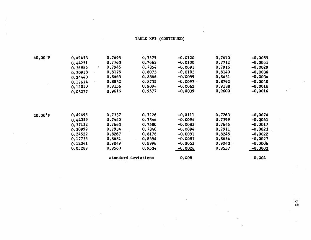
TABLE XVI (CONTINUED)
40.00°F 0.49453 0.7695 o. 7575 -0.0120 0,44251 0.1763 0,7663 -0.0100 0,36986 0,7945 0.7854 -0.0091 0~30918 0.8176 0.8073 -0,0103 0.24440 o.8465 0,8366 -o.·0099 o.17674 0,8832 0.8735 -0.0097 0.12010 0,9156 0.9094 -0.0062 0,05277 0.9616 0.9577 -0.0039
20.00°F 0,49695 0.7337 0.7226 -0.0111 0.44359 0,7440 0,7346 -0.0094 0,37132 0,7663 0.7580 -0.0083 0.30999 o. 7934 0,7840 -0.0094 0.24522 0,8267 0,8176 -0.0091 0,17735 0,8681 0,8594 -0.0087 0,12041 0,9049 098996 -0.0053 0,05289 0.9560 0.9534 -0.0026
standard deviations o.ooa
0,7610 0.7712 0.7916 0,8140 0,8431 0,8792 0,9138 0,9600
o. 7263 0,7399 o. 7646 o. 7911 0,8245 0,8654 0,9043 0,9557
-0.0085 -0.0051 -0.0029 -0.0036 -0.0034 -0.0040 -0.0018 -0.0016
-0.0074 -O.Q041 -0.0017 -0,0023 -0.0022 -0.0027 -0.0006 -0.0003 -
0.094
I-' !\) 00
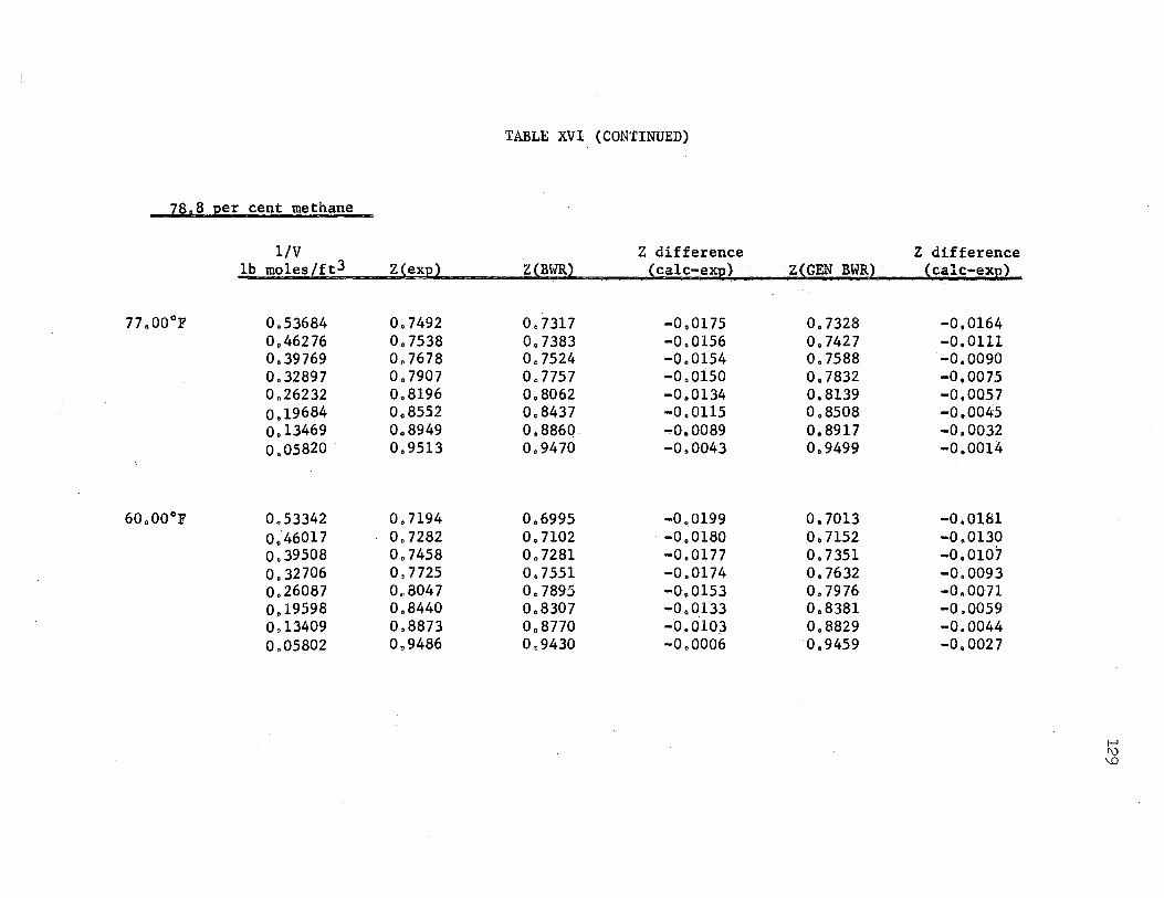
TABLE XVI (CONTINUED)
78.8 per cent methane
1/V Z difference Z difference lb moles/ft3 Z(exp) Z(BWR) (calc-exp) · Z{GEN BWR) (calc-exp)
77.00°F 0.53684 0.7492 0.7317 -0.0175 0.7328 -0,0164 0.46276 0.7538 0.7383 -0.0156 0.7427 -0.0111 0.39769 0.7678 0.7524 -0.0154 o. 7588 -0.0090 0.32897 0.7907 o. 7757 -0.0150 0.7832 -0.0075 0.26232 0.8196 0.8062 -0.0134 0.8139 -0,0057 0.19684 o.8552 o.8437 -0.0115 0.8508 -0.0045 o.13469 0.8949 0.886Q. -0.0089 0.8917 -0.0032 0.05820 . 0.9513 o.9470 -0.0043 0.9499 -0.0014
60.00°F 0.53342 o. 7194 0.6995 -0~0199 0,7013 -0.0181 o.46017 0.7282 o. 7102 -0.0180 o. 7152 -0.0130 0.39508 0.7458 o. 7281 -0.0177 0.7351 -0.0107 o.32706 o. 7725 0.7551 -0.0174 o. 7632 -0.0093 0.26087 0.8047 0.7895 -0.0153 0.7976 -0.0071 0.19598 0.8440 0.8307 -0.0133 o.8381 -0.0059 0.13409 0.8873 o.ano -0.0103 0.8829 -0.0044 0.05802 0.9486 0.9430 -0.0006 0.9459 -0.0027
I-' I\) '-.0
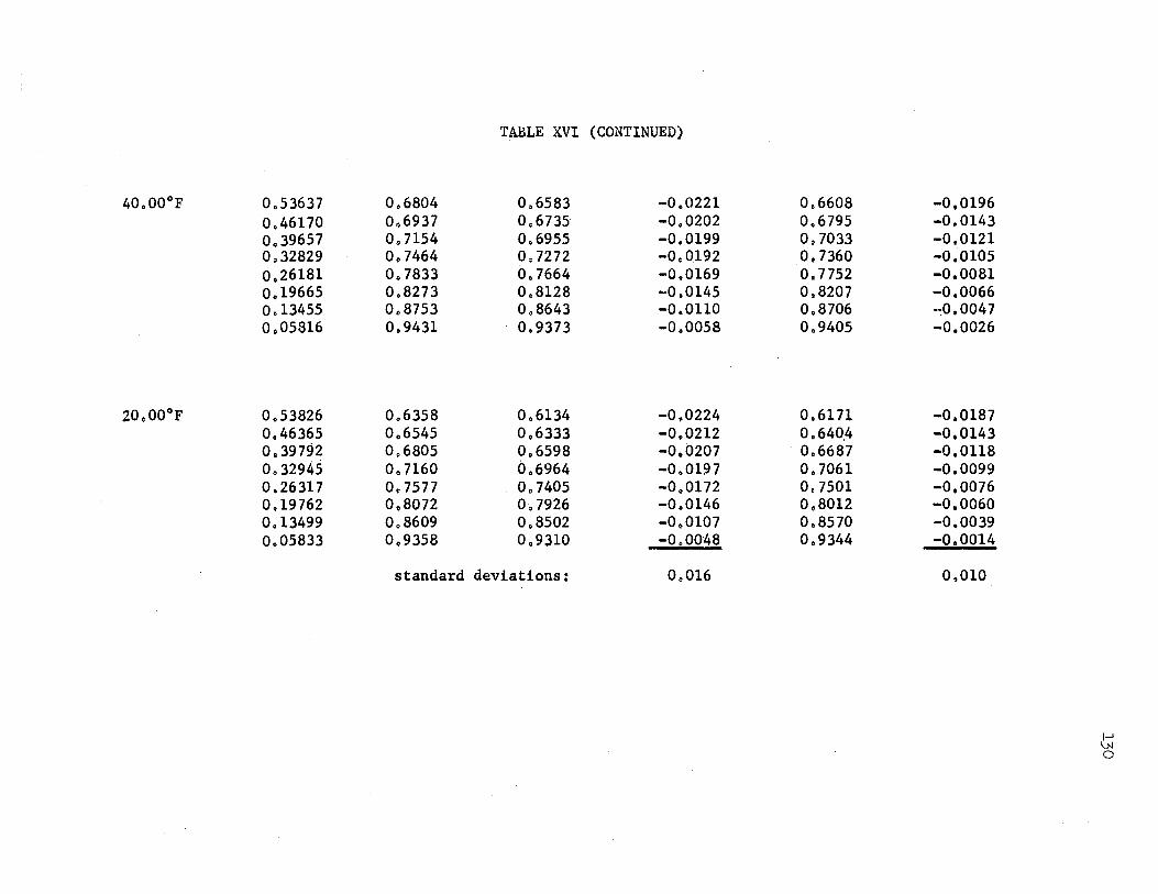
TABLE XVI (CONTINUED)
40.00°F 0.53637 0.6804 0.6583 -0.0221 0.46170 o.6937 o.6735 -0.0202 o.39657 o. 7154 0.6955 -0.0199 0.32829 0.7464 o. 7272 -0.0192 0.26181 0.7833 0.7664 -0.0169 0.19665 0.8273 0.8128 -0.0145 0.13455 o.8753 0.8643 -0.0110 o.oss16 0.9431 0.9373 -0.0058
20.00°F o.53826 0.6358 0.6134 -0.0224 0.46365 o.6545 o.6333 -0.0212 0.39792 0.6805 0.6598 -0.0201 0.32945 o. 7160 0.6964 -0.0197 o.26317 o. 7577 0.7405 -0.0172 0.19762 0.8072 0.7926 -0.0146 0.13499 0.8609 0.8502 -0.0107 0.05833 0.9358 0.9310 -0.0048
standard deviations: 0.016
0.6608 0.6795 0,7033 0,7360 0.7752 0.8207 0.8706 0.9405
0.6171 0.640.4 0.6687 0.7061 0,7501 0.8012 0.8570 0.9344
-0,0196 -0.0143 -0.0121 -0.0105 -0.0081 -0.0066 -:0.0047 -0.0026
-0.0187 -0.0143 -0,0118 -0.0099 -0,0076 -0.0060 -0.0039 -0.0014
0.010
I-' \.N 0
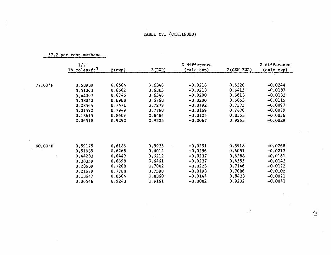
57.2 per cent methane
1/V lb moleslft3
77 .00°F 0.58930 0.51363 o.44067 0.38040 0.28564 0.21592 0.13615 0.06518
60.00°F 0.59175 o.51635 0.44283 0.38359 0.28639 0.21679 0.13647 0.06548
TABLE XVI (CONTINUED)
Z difference Z difference Z(exo) Z(BWR) (calc-exp) Z(GEN BWR) (calc-exp)
o.6564 0.6346 -000218 0.6320 -0.0244 0.6602 0.6385 -0.0218 0.6415 -0.0187 o.6746 0.6546 -0.0200 o.6613 -0.0133 o.6968 o.6768 -0.0200 o.6853 -0.0115 o. 7471 0.7279 -0.0192 o. 7375 -0.0097 0.7949 o. 7780 -0.0169 0.7870 -0.0079 0.8609 0.8484 -0.0125 0.8553 -0.0056 0,9292 009225 -0.0067 0.9263 -0.0029
o.6186 0.5935 -0.0251 0.5918 -0.0268 0.6268 0.6012 -0.0256 0.6051 -0.0217 o.6449 0.6212 -0.0237 o.6288 -0.0161 0.6698 o.6461 -0.0237 o.6555 -0.0143 o. 7268 0.7042 -0.0226 o. 7146 -0.0122 0. 7788 0.7590 -0.0198 0.7686 -0.·0102 0.8504 0,8360 -0.0144 0,.8433 -0.0071 0.9243 0.9161 -0.0082 0.9202 -0.0041
I-' \.N I-'
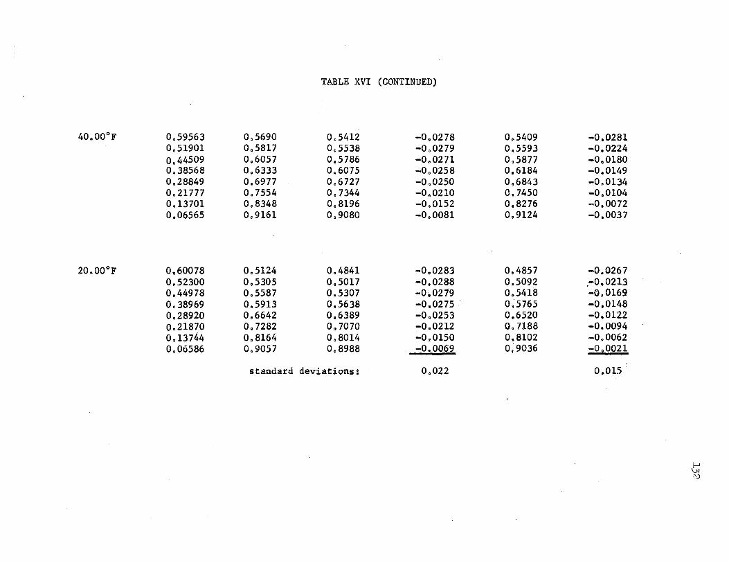
TABLE XVI (CONTINUED)
40.00°F 0.59563 0.5690 0.5412 -0.0278 0.51901 o.5817 0.5538 -0.0279 0.44509 0.6057 0.5786 -0.0271 0.38568 0.6333 0.6075 -0.0258 0.28849 0.6977 0.6727 -0.0250 0.21777 0.7554 0.7344 -0.0210 0.13701 o.8348 0.8196 -0.0152 0.06565 0.9161 0.9080 -0.0081
20.00°F 0.60078 0.5124 0.4841 -0.0283 0.52300 0.5305 0.5017 -0.0288 0.44978 0.5587 0.5307 -0.0279 0.38969 0.5913 0.5638 -0.0275 . 0.28920 0.6642 0.6389 -0.0253 0.21870 0.7282 0.1010 -0.0212 o.13744 0.8164 0.8014 -0.0150 0.06586 0.9057 0.8988 -0.0069
standard deviations: 0.022
0.5409 0.5593 0.5877 0.6184 0.6843 0.7450 0,8276 o.9124
o.4857 OS092 0.5418 0.5765 0.6520 0.7188 0.8102 0;9036
-0.0281 -0.0224 -0.0180 -0.0149 -0.0134 -0.0104 -0.0072 -0.0037
-0.0267 .-0.0213 -0.0169 -0.0148 -0.0122 -0.0094 -0.0062 -0.0021
0.01s
I-' \J.J I\)
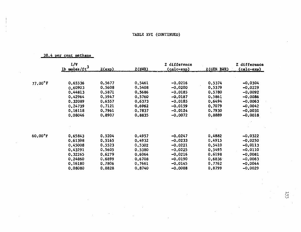
TABLE XVI (CONTINUED)
38.4 per cent methane
1/~ 3 Z difference Z diffe~ence lb 1DOles/ft Z{exp) Z(BWR) (calc-exp) Z(GEN BWR) (calc-exp)
77,00°F o.65536 Q.5677 0,5461 -0.0216 0.5374 -0.0304 0,60903 0,5608 0.5408 -0.0200 0,5379 -0.0229 o.44813 0,5871 0,5686 -0.0185 0,,5780 -0.0092 o.42964 0,5947 0.5760 -0.0187 o.5861 -0.0086 0.32089 0.6557 o.6373 -0.0185 0,6494. -0.0063 0.24739 o. 7121 0.6962 -0.0159 0.1019 -0 .. 0042 0·.16118 o.7961 0.7837 -0.0124 o. 7930 -0~0031 0~08046 0,8907 0,8835 -0.0012 0.8889 -0.0018
60,00°F 0,658~3 0.5204 o.4957 -0.0247 o.4882 -0,0322 0~61398 0.5165 o.4932 -0.0233 o.4915 -0.0250 o.4soos 0.5523 0,5302 -0.0221 0,5410 -0.0113 o.43291 o.5605 o.5380 -0.0225 0,5495 -0.0110 0.32265 0.6279 0,6064 -0.0216 0,6198 -0.0081 0.24860 0,6899 0.6708 -0.0190 0.6836 -0.0063 o.16l80 0.7806 0,7661 -0.0145 0,7762 -0.0044 0.08080 0,8828 0,8740 -0.0088 0.8799 -0.0029
~ \JJ
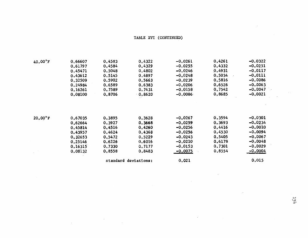
TABLE XVI (CONTINUED)
40.00°F o.66607 0.4583 0.4322 -0.0261 0.61797 o.4584 0,4329 -0.0255 o.45471 o.5048 0.4802 -0.0246 o.43612 0.5145 0.4897 -0,0248 0.32509 0.5902 0.5663 -0.0239 0.24984 0.6589 0.6383 -0.0206 0.16261 o. 7589 0.7431 -0.0158 0.08100 0,8706 - o. 8620 -0.0086
20.00°F 0,67035 0.3895 0,3628 -0.0267 0,62664 0.3927 0.3668 -0.0259 0045814 0.4516 0.4260 -0.0256 0.43957 0.4624 0.4368 -0.0256 0.32653 o.5472 o.s229 ... 0.0243 0.25146 o.6226 0.6016 -0.0210 0,16315 0.7330 0.7177 -0.0153 0,08132 o.ssss 0.8483 -0.0075
standard deviations: 0.021
o.4261 0.4332 0.4931 0.5034 o.ss16 o.6526 0,7542 o.8685
0.3594 o. 3693 0.4416 0.4530 o.s4os 0,6178 0.7301 o.sss4
-0.0322 -0,0251 -0.0117 -0.0111 -0.0086 -0.0063 -0,0047 -0.0021
-0.0301 -0.0234 -0.0010 -0.0094 -0.0067 -0.0048 -0.0029
....:.Q.:0004
0.015
I-' \)',I
+-
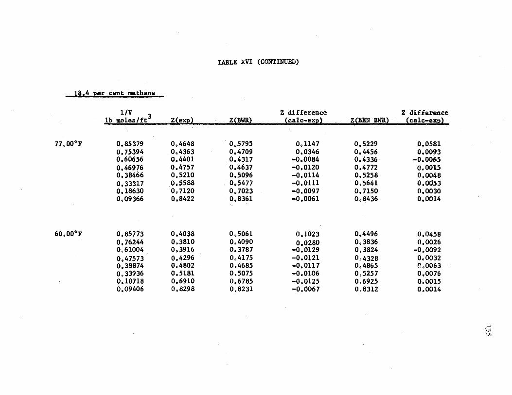
TABLE XVI (CONTINUED)
1824 per cent.methane
1/V 3 Z difference Z difference lb moles/ft Z(exp) Z(BWR) (calc-exp} Z(BEN BWR) (calc-exp)
77.00°F o. 85379 0.4648 0.5795 0.1147 0.5229 o.os81 o.75394 0.4363 004709 0.0346 o.4456 0.0093 o.60656 o.4401 . 0.4317 -0.0084 0.4336 -0.0065 0.46976 0.4757 0.4637 -0.0120 0.4772 0,,0015 0.38466 0.5210 0.5096 -0.0114 0.525'8 0.0048 0.33317 o.5588 0.5477 -0.0111 0.5641 0.0053 0.18630 0.1120 0.7023 -0.0097 0.7150 0.0030 0.,09366 0.8422 0._8361 -0.0061 o.8436 0.0014
60 0 00°F 0.85773 0.4038 0.5061 0.1023 0.4496 0.0458 o.76244 0.3810 0.4090 o.02so 0.3836 0.0026 0.61004 0.3916 .0.3787 -0.0129 0.3824 -0.0092 o.47573 0.4296 0.4175 -0.0121 0.4328 060032 o.38874 0.4802 0.4685 -0.0117 0.4865 0.0063 o.33936 o.51s1 0.5075 -0.0106 0~5257 0.0076 0.18718 o.6910 o.6785 -0.0125 0.6925 0.0015 0.09406 o. 8298 0.8231 -0.0067 0.8312 0.0014
I-' \.N \Jl
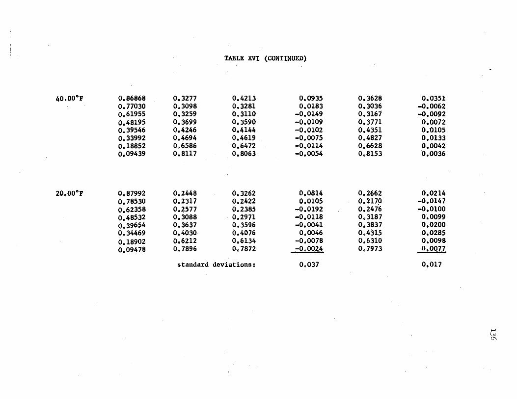
TABLE XVI (CONTINUED)
40.00°F 0.86868 003277 0.4213 0.0935 0.3628 0.0351 0.11030 0.,3098 0.3281 0.0183 0.3036 -0.0062 o.61955 0.3259 0.3110 -0.0149 0.3167 -0.0092 o.48195 003699 003590 -O.O;l.09 0.3171 0.0012 0.39546 o.4246 0.4144 -0.0102 o.4351 0.0105 0.33992 o.4694 0.4619 -0.0075 o.4827 0.0133 o.1ss52 0.6586 · o.6472 -0.0114 0.6628 0.0042 0.09439 0.8117 0.8063 -0.0054 0.8153 ·0.0036
20.00°1 0.87992 0.2448 0.3262 o.os14 0.2662 0.0214 o. 78530 0.2317 0.2422 0.0105 0.217~ -0,0147 o.62358 0.2577 0.2385 -0.0192 0.2476 -0.0100 o.48532 0.3088 • 0~2971 -0.0118 0.3187 0.0099 o.39654 0.3637 0.3596 -0.0041 0.3837 0.0200 0.34469 o.4030 0.4076 0.0046 0.4315 0.0285 0.18902 0.6212 o.6134 -0.0078 0.6310 0.009s 0.09478 0.7896 o .• 7872 -0,0024 0.7973 0.0077
standard deviations: 0.037 0.017
t: O'\
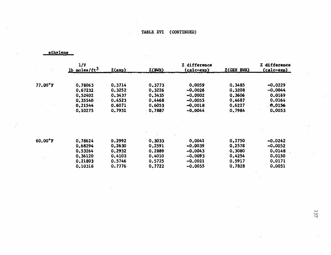
ethylene
77.00°F
60,00°F
TABLE XVI (CONTINUED)
1/V Z difference Z<difference lb moles/ft3 Z(exp) · Z{BWR) (calc-expl Z(GEN BWR) {calc-exp)
0 .. 78063 0.3714 · 0.3773 0.0059 0 .. 3485 -0.0229 0,67232 0.3252 0.3226 -0.0026 0.3208 -0.0044 0.52402 0.3437 0,3435 -0.0002 0.3606 0,0169 0,35540 0,4523 0.4468 -0.0055 o.4687 0,.0164 0,21544 0.6071 o.60S3 -0.0018 0.6227 --O.OlS6 o.1oi75 0.7931 0,7887 -0.0044 0.7984 0.0053
0.78624 0.,2992 0.3033 0.0041 0.2150 -0.0242 o.68294 0.2630 0.2591 -0.0039 0.2578 -0.0052 0.53264 0.,2932 0.2889 -0.0043 0.3080 0,0148 0.36120 o.4103 0.4010 -0.0093 0,4254 o.01so 0.21803· 0.5746 0.5725 -0.0021 0.,5917 0.0111 0.1031s o. 7776 0.1122 -0.0055 0.7828 0.,0051
f-' \..N '3
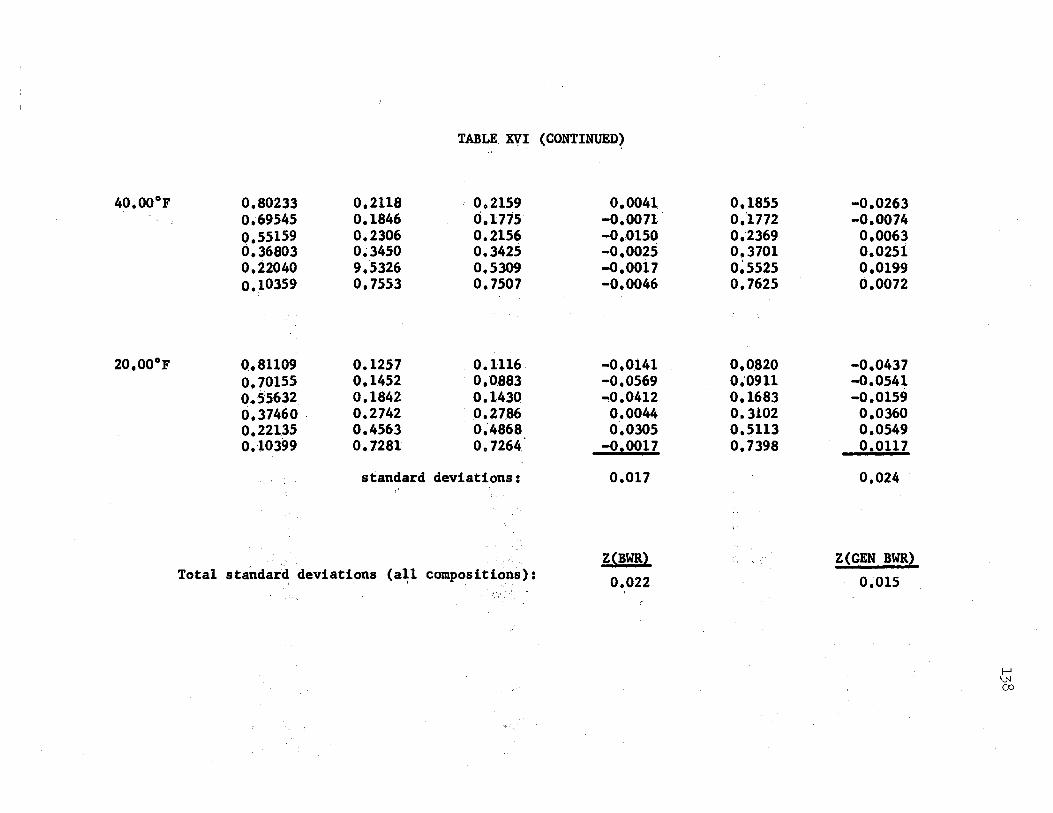
40.00°F
20.00°F
TABLE XVI (CONTINUED)
0.80233 0.2118 0.2159 o.69545 o.1846 0.1775 o.ss1s9 0.2306 0.2156 0.36803 0~3450 0.3425 0.22040 9.5326 0.5309 0.10359 0.7553 o.1so1
0.81109 0.1257 0.1116. o.101ss o.14s2 0.0883 0.5'5632 0.1842 0.1430 o.37460 . 0.2742 . 0.27,86 0.22135 0.4563 0.4868 0.10399 0,7281 0.7264
standard deviations:
Total standard deviations (a~l compositions):
0.0041 -0.0011 -0.,0150 -0.0025 -0.0011 -0.0046
-0.0141 -0.0569 -0.0412
0.0044 0.0305
-0,0017
0.011
Z(BWR)
0.022
o.1sss 0.1.112 0.-2369 0.3701 0~5525 0.7625
0.0820 0.0911 0.1683 0.3102 0.5113 0.7398
-0.0263 -0.0074
0.0063 o.02si 0.0199 0.0072
-0.0437 -o.0541 -0.0159
0.0360 0.0549
_0.0117
0,024
Z(GEN BWR)
0.015
I-' \J,J 00
Comparisons of Ezperi•ntal Second Vi.rial Coefficients with Equations of State
139
In Table XVII the experimental aeconcl virial coefficients are com
p~r~d with the coefficient, from the BWll equation, the Edmister generalized
form ot'· the BWll equation, ad the U. equation.
For the original and the generalized forma of the BWR equation both ,·
linear and Lorentz combining rulea for B0 were used. For all equations
the coefficient, were calculated in units of ft3/lb mole, and were then 3 . . .
converted to· cm / gm mole for anal71is. ~e tabulated e.xperimental
coefficients correspond to those in Table IX, corrected.for impurities. '
To make a direct comparison, therefore, the mixing rules for a two~, . '
component system were applied in all of the above equations.
The Edmister ge~eralized form of the BWll equation is seen to provide
a better.fit than the other equations teated. Usin• the linear combining
rule for B0 , the standard deviation from the 24 experimental data points
was 3.14 cm3/gm. mole. Using the original BWR equation the corresponding
standard deviation was S,99 cm3/gm mole (linear B0 ), and for. the RK
equation a val\18 of 7, 37 cm3 /gm mole1 resulted.
The agreement of the generalized BWll equation is quite good,
although the value of 3.14 cm3gm/mole is larger than the estimated
error of the experimental virial coefficients (1,5 cm3/gm mole), Both
for the generalized and original forms of the BWR equation the linear
combination rule for B appears to be slightly better than the Lorentz . 0
rule, The difference in standard deviations between the two combining
rules is small, however (0,08 cm3,im mole for the general~zed form, and
0.10 cm3/gm .,1e for the original form) and does not.represent a signi
ficant improv,..-nt.
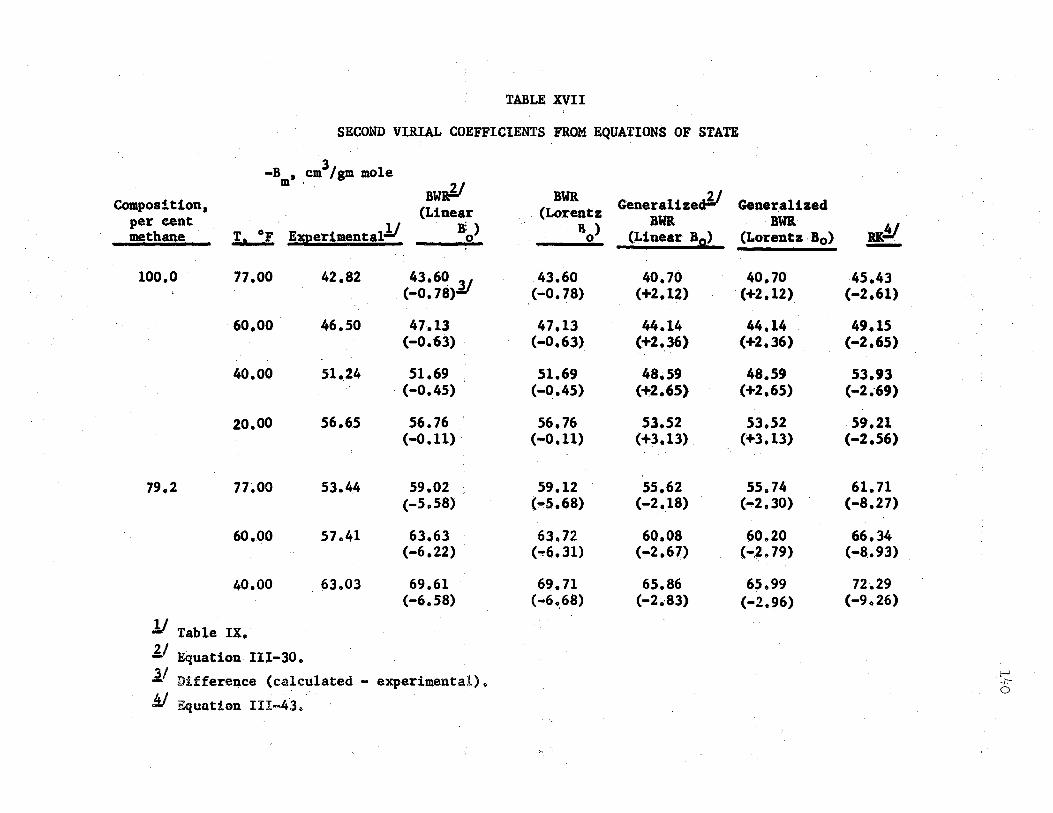
TABLE XVII
SECOND VIRIAL COEFFICIENTS FROM EQUATIONS OF STATE
-B, cm3/gm mole m ..
Bwal' Composition, BWR Generalizect!' Gener,alized (Linear (Lorentz per cent '.[~ hl,e_ri_menJ:al.!/ B!) '8 ) BWR BWB. ' !I
methane 0 0 (Lineai- . B0) (Loreutz.B0 ) u. -100.0 11.00 42.82 43.60 A/ 43.60 40.70 40.70 45.43
(-0. 78) (-0. ~8) (+2.12) (+2.12) (-2.61)
60.00 46.50 47.13 47.13 44.14 44,14 49.15 (-0.63) (-0.63) (+2.36) (+2.36) (-2.65)
40.00 51,24 51.69 · 51.69 48,59 48.59 53,93 (-0.45) (-0~45) (+2.65) (+2.65) (-2.·69)
20.00 56.65 56.76 56.76 53.52 53,52 59.21 (-0.11) (-0.11) (+3.13) (+3.13) (-2.56)
79.2 77.00 53.44 59,02 59,12 55,62 55.74 61.71 (-5.58) (-5.68) (-2,18) (-2.30) (-8.27)
60 •. 00 57.41 63,63 63.72 60,08 60.20 66,34 (-6.22) (--6. 31) (-2.67) (-.2. 79) (-8.93)
40.00 63.03 69.61 69. 71 65.86 65.99 72.29 (-6.58) (-6.,68) (-2.·83) (-2.96) (-9.26)
J/ Table IX, 2/ ' - Equation III-30.
1/ Differe~ce (calculated - experimental). i--' +"
if Equation III-43~ 0
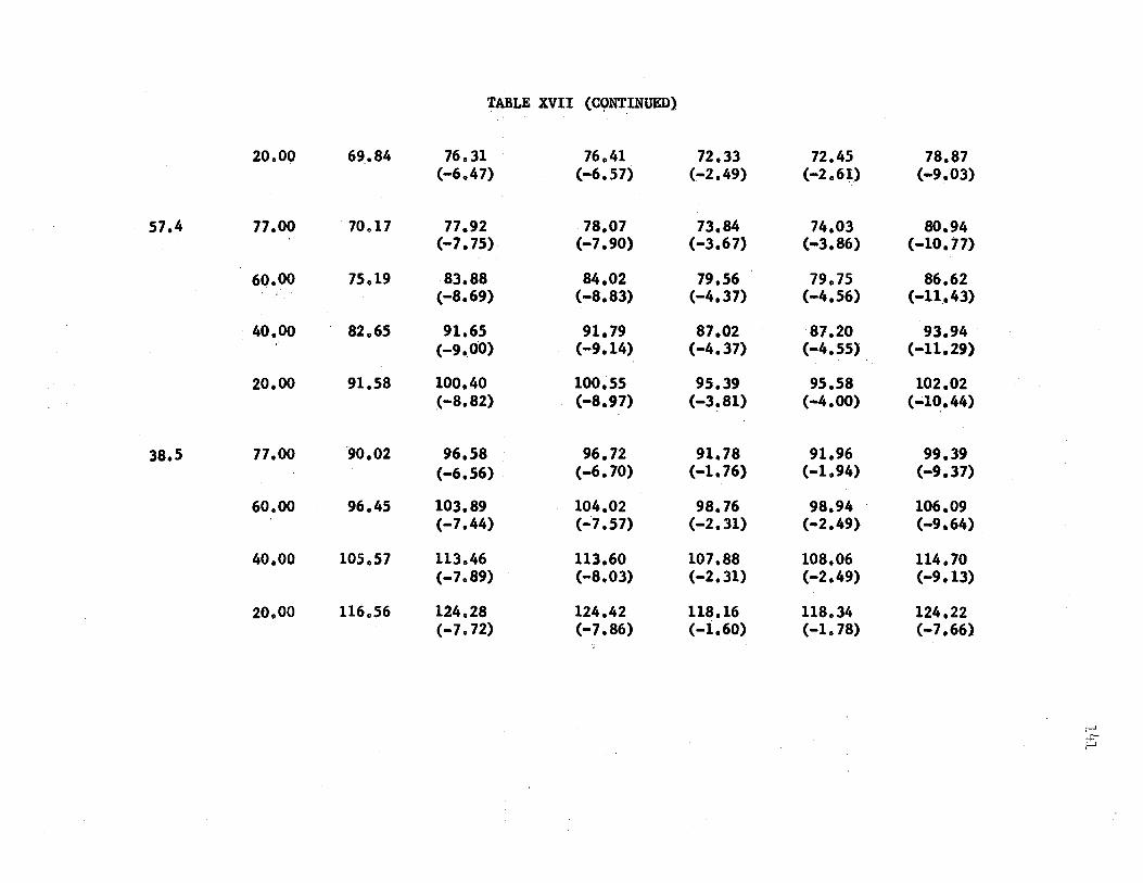
TABLE XVII (CQNT.INUED)
20000 69.84 76.31 76.41 (-6.47) (-6.57)
57.4 77.00 70~17 77.92 78.07 (-7. 75) (-7.90)
60.00 75019 83.88 84.02 (.;..8.69) (-8.83)
40.00 82.65 91.65 91.79 (-9 •. 00) (-9.14)
20.00 91.58 100.40 100.s5 (-8.82) (-8.97)
38.5 n.oo -90.02 96.58 96.72 (-6.56) (-6.70)
60.00 96.45 103.89 104.02 (-7.44) (.;.7 .57)
40.00 105.57 113.46 113.60 (-7 .89) (-8.03)
20.00 116.56 124028 124.42 (-7.72) (-7, 86)
72.33 72.45 (-2.49) (-2.61)
73.84 74.03 (-3.67) (-3.86)
79.56 79.75 (-4.37) C-4.56)
87.02 87.20 (-4.37) (-4.55)
95.39 95.58 (-3.81) (-4.00)
91.78 91.96 (-1. 76) (-1.94)
98.76 98.94 (-2.31) (-2.49)
107.88 108.06 (-2.31) (-2.49)
118.16 118.34 (-1.60) (-1. 78)
78.87 (-9.03)
80.94 c-10. 77)
86.62 (-11.43)
93.94 (-11.29)
102.02 (-l~.44)
99.39 (-9.37)
106.09 (-9.64)
114.70 (-9.13)
124.22 (-7 .66)
f-' +'" f-'
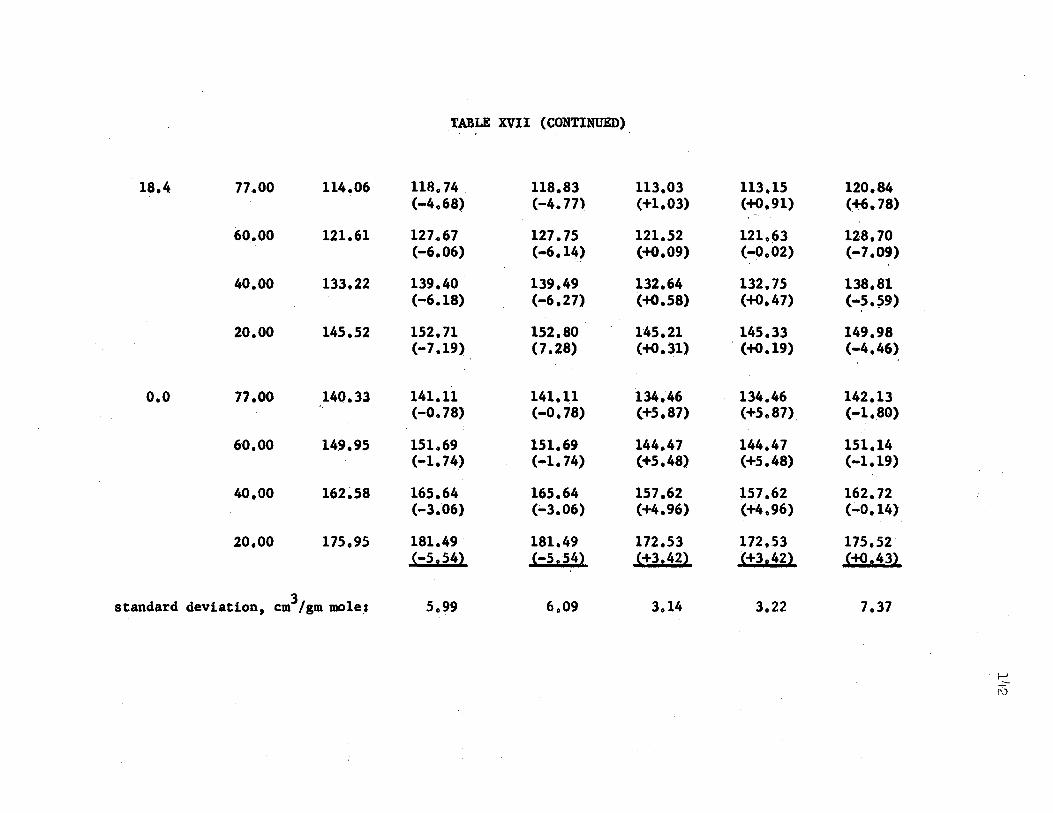
. TABLE XVII (CONTINUED)
18.4 77.00 114.06 118.74 118.83 113.03 113.15 120.84 (-4.68) (-4. 77) (+l.03) (-f-0.91) (~.78) .. ,
60.00 121.61 127 .• 67 127.75 121.52 121.~3 128.70 (-6.06) (-6.14) (+o.09) (-0.02) (-7.09)
40.00 133.22 139.40 139.49 132.64 132.75 138.81 (-6.18) (-6.27). (+o.58) (+o.47) (-5.~9)
20.00 145.52 152.71 152.80 145.21 145.33 149.98 (-7.19) (7.28) (+o.31) . (+o.19) (-4.46)
o.o 11.00 14Q.33 141.11 141.11 134.46 134.46 142.13 ... (-0. 78) (-0. 78) (+5.87) (+5.87) (-1._80)
60.00 149.95 151.69 151.69 144.47 144.47 151.14 (-1. 74) (-1. 74.) (+5.48) (+5.48) (-1.19)
40.00 162~58 165.64' 165.64 157.62 .157.62 162.72 (-3.06) (;..3.06) (+4.96) (+4.96) (~0.14)
20.00 175.95 181.49 181.49 172.Sl 172.53 11s.s2· (-5.54) (-5.54) {+3.42) (+3.42) (+o.431
standard deviation, cm3/gm mole, S.99 6.09 3.14 3.22 7.37
I--'
~
The experimental virial coefficients are compared graphically versus
the three equations of state in Figures 8, 9t and 10. Due to the small
difference between linear and Lorentz forms of B, only the linear form 0 .
Comparisons of Experimental Third Virial Coefficients with Equations of State
In Table XVIII the experimental third virial coefficients· are
compared with the above three equations of state.
The expressions for the third virial coefficient from these equations
are given by Equations III-31 and III-43. For both forms of the BWR
equation the third virial coefficient is independent of the linear and
Lorentz combining rules, as the constant B does not appear in the 0
expression.
The experimental third virial coefficients were not corrected for
impurities. In order to make a direct comparison with equations of state,
therefore• the mixing rules were written so as to include the impurities.
This procedure involves expanding the mixing rules to N terms (N being
the number of components in the system), each term containing a composi-
tion term and a pure component constant, From Appendix G the maximum
value of N = 4 for both the 57.2% methane and the 78.8% methane system.
As with the second virial coefficients the overall fit of the Edmister
generalized form of the BWR equation is better than that of the other
equations, For the 24 experimental points the standard deviations were
6 2 2 6 2 cm /gm mole (generalized BWR), 3.7 x 10 cm /gm mole
(o.riginal 2 6 2 BWR), and 12 0 8 x 10 cm /gm mole (RK). In Figures 11, 12,
and 13 the experimental coefficients are compared graphically versus
coefficients from the equations of state.
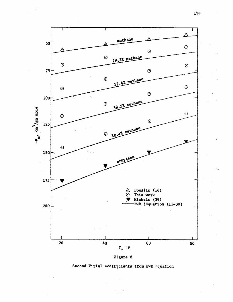
50
·100
cu .... a e,
125 ' ri-,s u •
r:Qs I
150
175
200
20 40
methane
/J::i. Douslin (16) 0 This work T Michels (39)
--BWR (Equation III-30)
T °F • Figure 8
60
Second Virial Coeff~chnts from BWR Equation
144
0
80
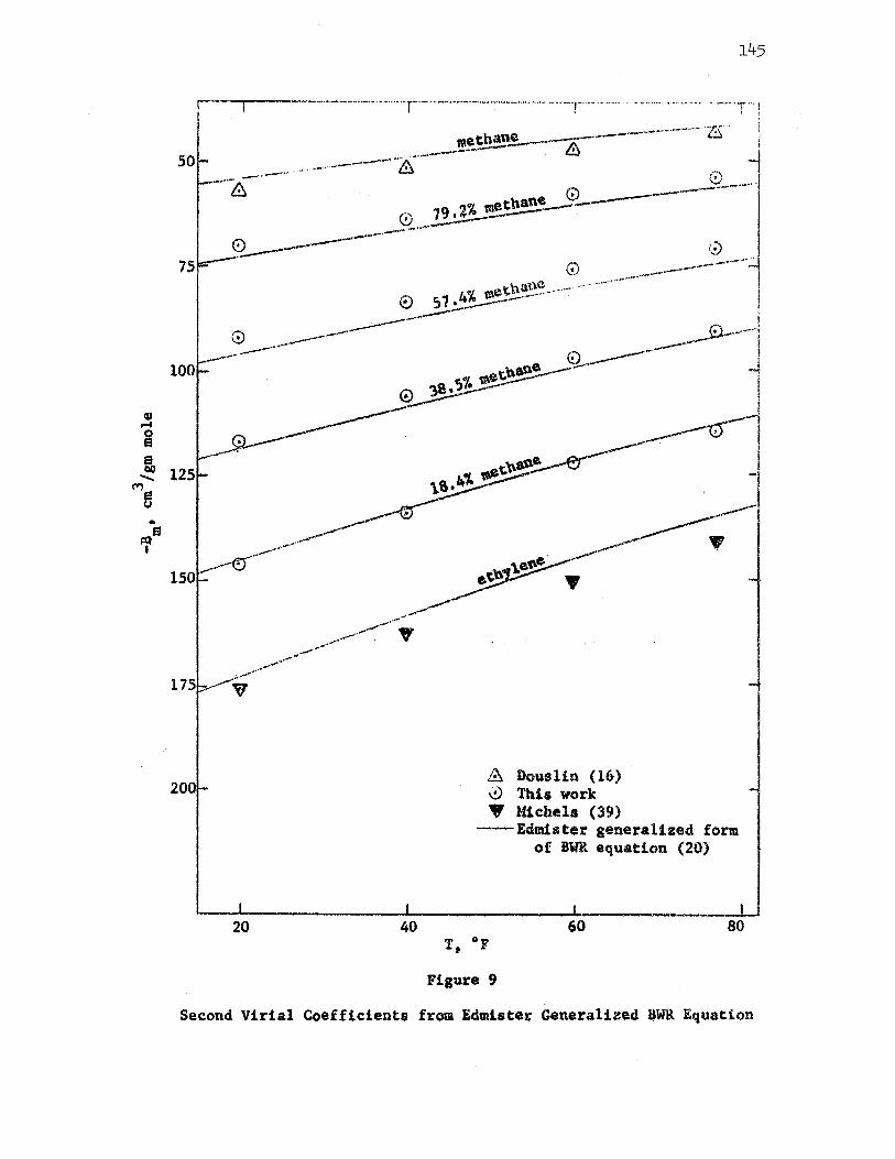
Qt .... 0 a
I ..... ('fl a
... r:Qs I
50
100
125
-
175
200
20 40
& Douslin (16) 0 1.'bis work Y Michels (39)
--Edmister generalized form of Bw:R equation (20)
T °F • Figure 9
60 80
Second Virial Coefficients from Edmister Generalized UWR Equation
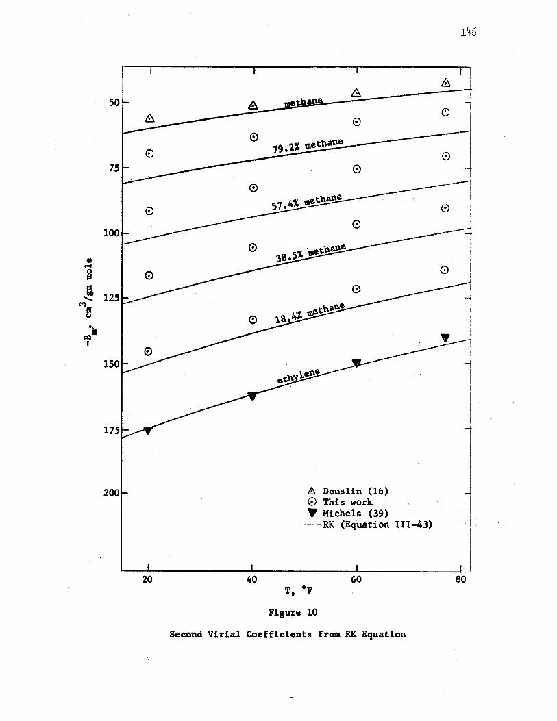
so
75
100
a, .... a I 125 ......
C"l e ....
r4s I
150
200
20
A
0
40
&
0
79 • 21 methane
0
A Douslin (16) 0 This work Y Michels (39)
--RK (Equation III-43)
60 T, °F
Figure 10
Second V:lr:lal .Coefficients from RK Equation
146
£
0
0
80
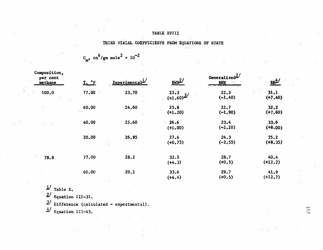
TABLE XVIII
THIRD VIRIAL COEFFICIENTS FROM EQUATIONS OF STATE
6 2 -2 C, cm /gm mole x 10 m ,
Composition, Generalized~/ per cent
ExperimentalY BwaJ:/ metha~ _L__~ BWR
100.0 11.00 23.70 25.3 11 22.3 (+1.60) (-1.40)
60.00 24.60 25.8 22.7 (+1.20) c~1.901
40.00 25.60 26.6 23.4 (+1.00) (-2.20)
20.00 26.85 27.6 24.3 (+o. 75) (-2.55)
78.8 11.00 28.2 32.5 28.7 (+4.3) (+o.5)
60.00 29.2 33.6 29.7 (+4.4) (+o.5)
!/ Table x. 1:./ Equation III-31.
ll Difference (calculated - experimental)o 4/ . . . - Equation III-43.
BK!/ -31.1
(+7.40)
32.2 (+7.60)
33.6 (+8.00)
35.2 (+8.35)
40.4 (+12.2) .
41.9 (+12. 7)
f-' +
----..]
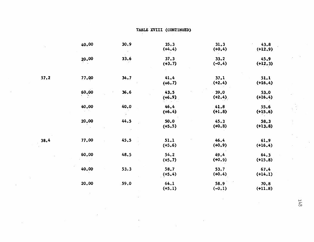
TABLE XVIII (CONTINUED).
40.00 30o9 35o3 31.3 43.8 (+4.4) {+o.4) {+12.9)
20.00 33.6 37.3 33.2 45.9 {+3.7) (-0.4) (+12.3)
57.2 77.QO 34.7 41.4 37.1 51.1 (+6. 7) .(+2.4) (+16.4)
60.00 36.6 43.5 39.0 53.0 ,,-(+6.9.> {+2.4) (+16.4)
40.00 40.0 46.4 41.8 55.6 (+6.4) (+1.8l (+15.6)
20.00 44.5 50.0 45.3 58.3 (+5.5) c+o.-s> (+13.8)
.38.4 77.00 45.5 51.1 46.4 61.9 (+,5.6) (+o.9) (+16.4)
60000 48.5 54.2 49.4 64.3 (+5. 7) (+o.9) (+15.8)
40.00 53o3 58.7 53.7 67.4 ~+5.4) (+oe4} (+14.1)
20.00 59.0 64.1 58.9 70.8 {+Sol) (-Ool) (+11.8)
f-' ..[::-00

T~LE XVIII (CONTINUED)
18,4 77000 60,0 63.4 (+3.4)
60.00 62.8 68.0 (+S.2)
40.00 68.3 74.6 (+6.3)
20.00 74.6 82.6 (+8.0)
o.o 11.00 76.43 77.27 (+o.84)
60.00 80,5 83.7 (+3.2)
40.00 · 85 •. 9 92.6 (+6. 7)
20.00 91.7 103.6 (+11.9) -
6 2 -2 standard deviation, cm /gm mole x 10 : 3.7
58.6 (-1.4)
63.l . (+o.3)
69.4 (+1.1)
77.0 (+2.4)
72.65 <~3.78) ....
78.8 (-1.7)
87.4 (+1~5)
97.8 (+6.1)
2.1
74.8 (+14.8)
77.8 (+15.0)
81.6 (+13.3)
85.9 (+11.3)
88.48 (+12.05)
92.1 (+11.6)
96.7 (+10.8)
101.8 (+10.1)
12.8
1--' -i:::\.0
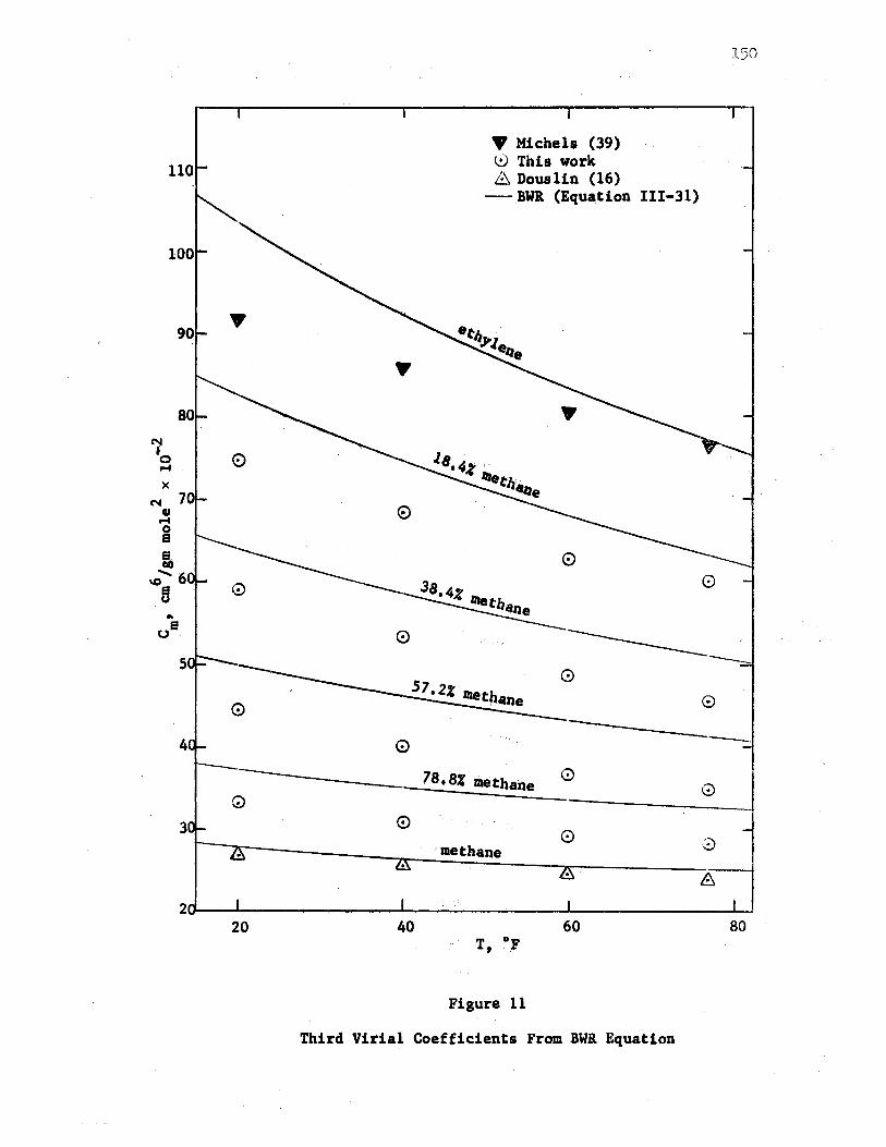
110
100
N I 0 ~
X
90
80
N 70 QI ~ s I
'° ........ 6 B .. us
0
Q
20
T Michels (39) 0 This work 6 Douslin (16)
- BWR (Equation III-31)
0
150
0
0 ------]8.8% methane 0
0
0 0 0 methane 8 8
40 60 80 T, °F
Figure 11
Third Virial Coefficients From BWR Equation
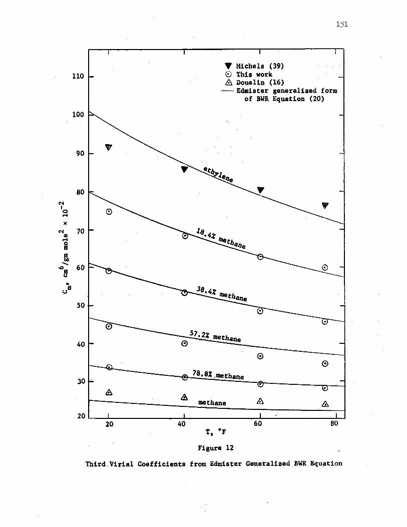
151
110 -
T Michels (39) (:) This work
N
'o .... X
100
90
80
N 70 G) .... i ~
,s:,' 60 B
so
40
30
20
Ii:). Douslin (16) - Edmister generalized form
of BWR Equation (20)
57' 2% IDeth 0 . ane
78 ,8%amethane
methane
Figure 12
Third .. Virial Coefficients from Edmister Generalizedl3WR Equation
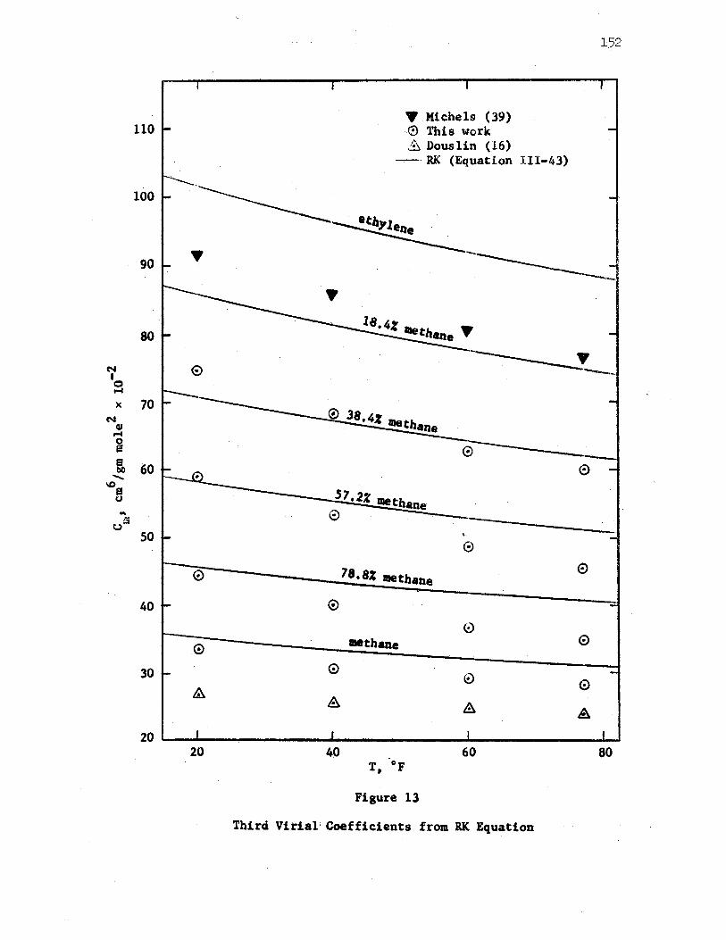
152
Y Michels (39) 110 0 This work
~ Douslin (16) -. - RK (Equation III-43)
100 ---------~ ene ·
90 • •
• 80
18.4% llleth • •ne
N e ~ I 0 ... X 70
N QI .... s 0 I ....... 60 0
'° 9 S 1, 2% Ille thane "' 0 s
t.> 50 ..
e 0 78,8% methane 0
40 0
0
0 •thane 0
30 0 © 0 & A A A
20 20 40 60 80
T ·oF • Figure 13
Third Virial' Coefficients from RK Equation·
153
General Remarks on Equation of State Comparisons
For the compressibility factor comparisons it was seen that the
generalized BWR equation provides a better overall fit to the data than
does the original BWR equation. For the pure component points the
aeneralized equation provide• the better fit to the methane data, while
the original BWR equation provides a better fit to the ethylene data.
The fact should be emphasized, however, t~at the above comparison, repre-
sent only one binary system over a fairly narrow temperature range. The
generalized equation should be tested for other binary systems before
additional conclusions can be reached.
The objective of the compari1ona was to determine and emphasize the
need for further work on methods of improving equations of state. One
criteria for an equation .of state is the accurate prediction of virial
coefficient,. For this reason, experimental virial coefficients were
compared directly versus coefficients predicted by equations of state.
For the second virial coefficients (Table XVII) the original BWB.
equation provided the best fit to the pure component data. Considering
pure component and mixture data together, however, the generalized
BWR equation provided the best fit. This difference is due in large
part to the form of the mixing rules (Equations III-27), Although
based on theoretical considerations these rules are still somewhat
empirical.
For the third virial coefficients (Table XVIII) the generalized
BWR equation provided the best fit, both for the pure components and
for the mixtures. For the pure component points the standard deviations
2 6 2 2 6 2 were 3,04 x 10 cm /gm mole (generalized BWB.), 5,04 x 10 cm /gm mole
154
(original BWR), and 9.66 x 102 cm6/gm mole2 (RK), Considering all points
together the standard deviations were also lowest for the generalized equa-
For both the second and the third virial coefficient comparisonsp
the fact should be pointed out that the constants for the original BWR
equation wer.e determined largely from compressibility factor data;
the equation was then expanded into virial form. A small adjustment iri the
constants could produce a relatively latge change in the calculated vir:lal
coefficient.
From the above comparisons several approaches were suggested for
future equation of state improvements, These approaches are presented
in the following.
Comments on Further Improvements of Equations of State
One criteria in the development of a closed-form equation of state
is that it should accurately predict the second and third virial
coefficientso Ideally the equation would accurately predict higher-
ordered coefficients also, but these coefficients are seldom available for.
comparison. With this approach in mind several arguments may be given'
in favor of the BWR (generalized or original) form of equation rather
than the RK form.
The second and third virial coefficients in the BWR equation have
the form
A C B(T) = B ....2. -2.
o - RT - RT3 (III-30)
C(T) = b - ..!. + ....£.. RT RT3
(III-31)
155
It is important here that the constants B, A, and C appear in 0 0 0
Equation III-30 whereas the different constants b, a, and c appear
in Equation III-31. For this reason the constants B, A, and C 0 0 0
may be adjusted to fit experimental second virial coefficients with-
out any effect on the expression for the third virial coefficients,
and conversely¢
For the RK equation the second and third virial coefficients are
given as
B(T) b -a
= RT3/2
(III-liJ)
C(T) b2 + ab =
RTJT2
The second virial coefficient contains only two constants, and appears
to be an oversimplification, even if the expression were fit directly
to second virial coefficient data, In addition, the third virial
coefficient is uniquely dependent upon the constants chosen for the
second coefficient.
It is of further importance that the BWR expressions for B(T) and
C(T) do not contain the constants a and y. It would be possible to
determine the six constants in Equations III-30 and III-31 from virial
coefficient data (either experimental or generalized values). The
equation could then be recombined into the normal closed form, .given
below.
156
A C Z • 1 + (B - ..2. - ..;.2...)d + (b - .!..)d2
o RT RT3 RT (III-26)
5 cd2 · 2 2 + .!!! d + - 3 (l + yd ) exp (-yd ) RT RT
In this equation the remaining unknown constants a and y could be
determined by regression analrsis so as to produce the best fit to a
set of compressibility factor data.
In principle both the ·generalized form and the original form
of the BWR equation could be evaluated in this manner. The primary
goal 1 however, is the development of an improved equation that would
be of value from an engineering standpoint, particularly for binary
and multicomponent mixtureso For this purpose the gener~lized form
would have greater application,
c. Error Analysis of Data
In this section the accuracy of the data and of the isochoric
apparatus is examined from two different viewpoints. These are:
1) making mathematical estimates of the error of the isochoric apparatus
from the estimated errors of each measured quantity (such as temperature
and pressure), and 2) ·· comparing th~ resultant data directly with
corresponding values from the literature. These two approaches are
discussed in this order.
Estimated Experimental Error
Estimates of the experimental error in the compressibility factors
were made by the method of propagation of errors (60)~ This method
enables the.estimation of the error in a function of directly measured
quantities, provided that individual errors may be established for
157
each of the directly measured quantities. As described· prev:f.ously the
isochoric compressibility factors ZBT are determined from Equation N~-H
after first determining the isochoric run constant D from Equation. N-200
For this calculation estimates were made of the error in each of the
measured quantities in these equations. The errors in these quantities
were then combined to estimate the resultant error in the compressibility
factors ZBTo
Fractional errors were estimated for the measured quantities in the
equations as ts shown in Table XIX.
The most important remaining factors are the measured pressure and
temperature of the sample inside the bomb, the determination of the
1sochoric run constant D, and the correction for the sample in the DPI
cell and exposed capillary line. The correction for the sample in the
capillary line and DP! cell is given by the terms 0.01263 DD' 0.01537 n50
etcop in the equations. Errors of 0,01% in the pressure measurements
and 0.02°K in the temperature TB of the sample inside the bomb were used
in the calculationsa The error in the run constant Dis dependent upon
the error in the compressibility factor from the reference isotherm.
The run constant is also affected by errors due to the capillary line.
In order to make error calculations it is necessary to assume
errors in the reference isotherm. Three different fractional errors
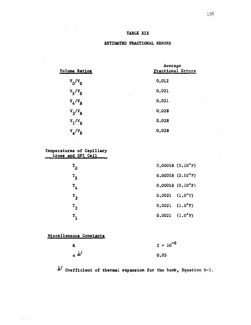
TABLE XIX
ESTIMATED FRACTIONAL ERRORS
Average Volume Ratioa Fractional Errors
VD/VB 0.012
VS/VB 0.021
V4/VB 0.0~1
V3'VB 0.02a
Vl/VB 0,028
V/VB 0.02a
Temperatures of Capillary Lines and DPI Cell
TD 0.0001a (0.10°F)
TS 0.0001a (0.10°F)
T4 0.00018 (O,l0°F)
Tl 0.0021 (l.0°F)
T2 0.0021 (l.0°F)
Tl 0.0021 (l .0°F)
Miscellaneous Constants
R
a. ll o.os
ll Coeffic.ient of thermal expansion for the bomb, Equation H-5~
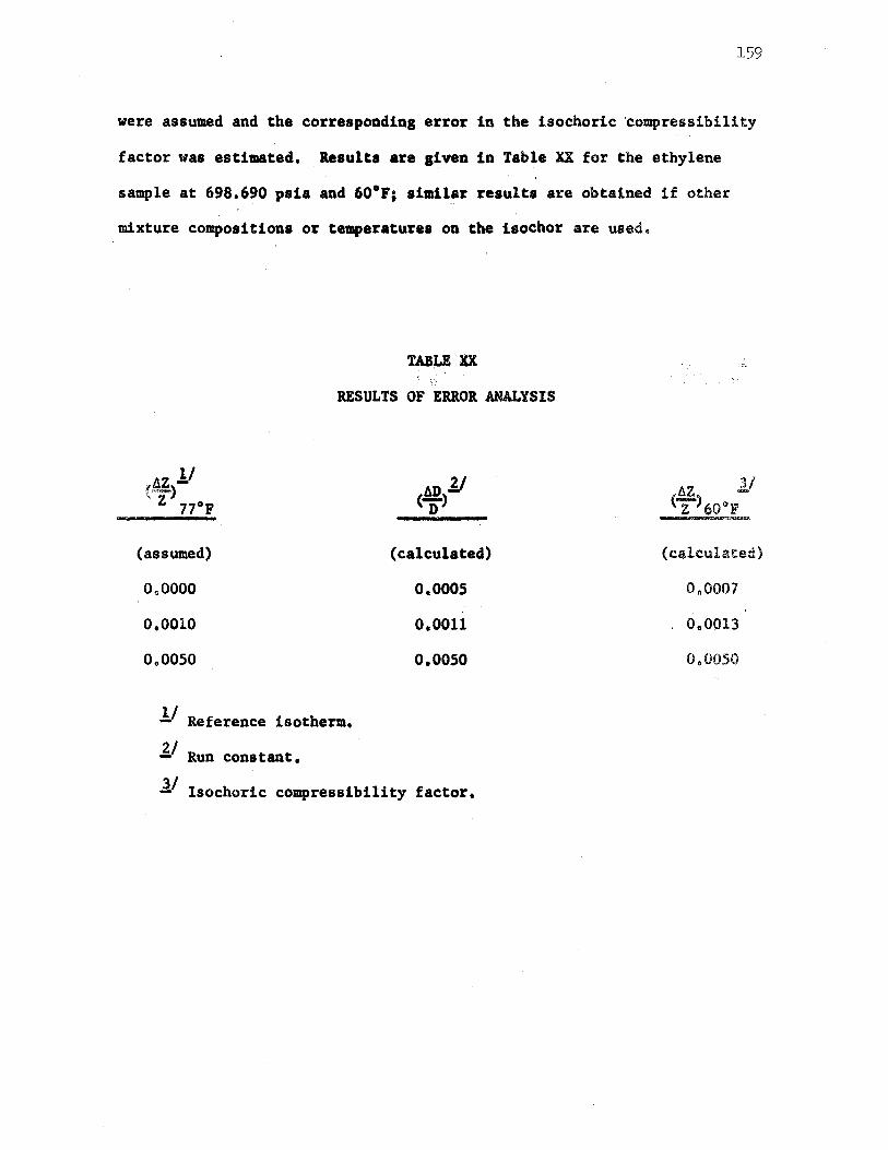
159
were assumed and the corresponding error in the isochoric ·compressibility
factor was estimated, Results are given in Table XX for the ethylene
sample at 698,690 paia and 60°F; similar results are obtained 1£ other
mixture compositions or temperatures on the isochor are used.
TAB;LE ··xx
RESULTS OF ERROR ANALYSIS
,l1Z 1/ ·'""""") ,. Z 77oF
(assumed)
0.0000
0.0010
000050
ll Reference isotherm,
1:./ Run constant.
ADY (-)
D
(calculated)
o.ooos
0.0011
o.ooso
J/ lsochoric compressibility factor,
tiz ll (Z)60°F --
(c$lculated)
0.0007
0.0013
o.ooso
160
As an estimate of the limiting accuracy of the isochoric apparatus
an error of zero was assumed in the reference isotherm, The correspond-
ing fractional error in the run constant was 0,0005, and the error in
the isochoric compressibility factor was 0.0007. In this case
essentially all of the error (both in the run constant determination
and in the final compressibility factor) was shown to be due to errors
•'. contributed by the sample in the capillary line and DPI cell,
The assumption of a fractional error of 0.0010 in the reference
isotherm produced an error of 0.0011 in the run constant, with a
final fractional error of 0.0013 in the compressibility factor. The
error in this case was attributed approximately equally to errors in
the reference isotherm and errors caused by the capillary line. The
assumed errors of 0.01% and 0,02°K in the pressure measurement and
bomb temperature, respectively, have only a small effect here.
For the assumed fractional error of 0,0050 in the reference iso-
therm the error in the run constant and final compressibility factor
was essentially all attributed to the reference isotherm error. These
calculations illustrate the fact that the accuracy of the isochoric
apparatus will never exceed the accuracy of the compressibility factor
from the reference isotherm.
Comparisons with Published Methane Data
In Figure 14, the methane data of Table IV are compared with the
published data of Mueller et al (50) and Matthews and Hurd (34)
The data of Mueller were taken over the interval -200 to +50°F,
with pressures from 40 to 7000 psia. The compressibility data is
stated to be accurate to 0.13%. By using a large sheet of graph
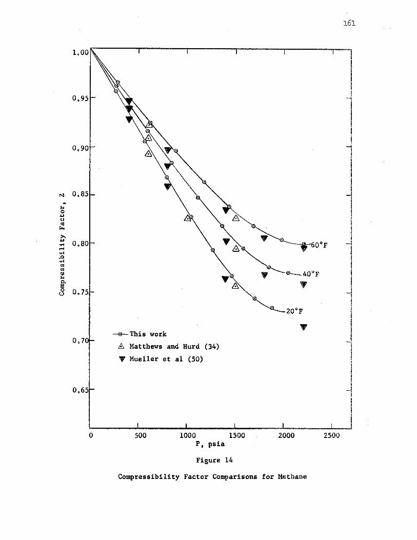
161
1.00
0.95
0.90 ~ I N o.ss .. ""'
I 0 .... 0 CII
i:<,
>. .... Oo80 ' 60°F ""
1 ~ .... ..0
"" ti) ti)
cu ""' ~ 0 0.75 u
20°F
• -s- This work 0.10
&-, Matthews and Hurd (34)
I ~ Mueller et al (50)
0.65 1 0 500 1000 1500 2000 2500
P, psia
Figure 14
Compressibility Factor Comparisons for Methane
162
paper the data was interpolated to the temperatures 60, 40~ and 20°F.
The maximum error introduced by the interpolation procedure was estimated
as 0.1%; the errors in the interpolated data points are thus 0.2% or
less.
The superheated methane data of Matthews and Hurd cover the temper
ature range -260 to. +500°F, with pressures from 10 to 1500 psia. These
data represent a compilation of the data of Kvalnes and Gaddy (30)
and of Olds, Reamer. Sage, and Lacey (51). The data of Kvalnes and
Gaddy cover the temperature range -70 to +200°C, with pressures from
300 to 15 1 000 psia. The data are reported accurate to 0.2%. The
temperatures of the Sage and Lacey data (+100 to +460°F) are highet:
than the temperatut:es of this investigation; the corresponding
pressures are from 200 to 10,000 psia, with the ~eported accuracy of
the data being 0.2%. From an examination of Figure 14 the data of
Mueller et al and Matthews and Hurd are seen to be in agreement to
within the stated accuracy (0.2%) from both sources.
From a large plot similar to Figure 14 the above literature values
were compared at even values of pressure with the data of this investi
gation. For the Matthews and Hurd data 17 corresponding data points
were compared at pressures up to 1500 psia (the limit of the Matthews
and Hurd data). For each pair of points the data of this investiga
tion were consistently higher than the literature values, with the
average deviation being 0.7%.
For the comparison with the Mueller data, the 24 data points of
this investigation were higher in each case than the literature values.
The average deviation was approximately 0.7%.
163
Comparisons with Published Ethylene Data
In Figure 15 the vapor-phase ethylene data from Table IV are com
pared with the literature data of Walters et al.(68) and York and White
(69) o,
The data of Walters cover the range +20 to +100°F, with pressures
from 50 to 600 psia, The data are presented in the form of an equation,
which has an estimated accuracy of 0.25%. The data of York and White
cover the range -140 to +500°F, with pressures from 14.7 to 4400 psia •.
These data represent an interpolation and extension of the data of
Michels (38). An.accuracy of 0,3% is claimed by York and White, From
Figure 15 the literature values from the two sources are seen to agree
within the accuracy (0.25 to 0.3%) claimed by both investigators.
Using a large plot similar to Figure 15 these literature values
were compared at even values of pressure with the data of this investi
gation, In all cases the data of this investigation were higher than
the literature data, The average difference between compressibility fac
tors was approximately 0,6%. The York and White data above 600 psia were
not used in this direct comparison, as these data below 77°F represent
an extrapolation by York and White of the data of Michels.
The pronounced curvature of the 60°F isotherm in the region 700 to
1200 psia deserves some comment. The curvature arises since the points
are in the neighborhood of the critical point (49.82°F, 742.l psia).
Considering the accuracy of the published literature data and the
differences between the literature data and the data of this investiga
tion, the following conclusion can be made, The data of this investiga
tion appear high by as much as 0.4 to 0.5% for methane, and are high
by 0.3 to 0.4% for ethylene,
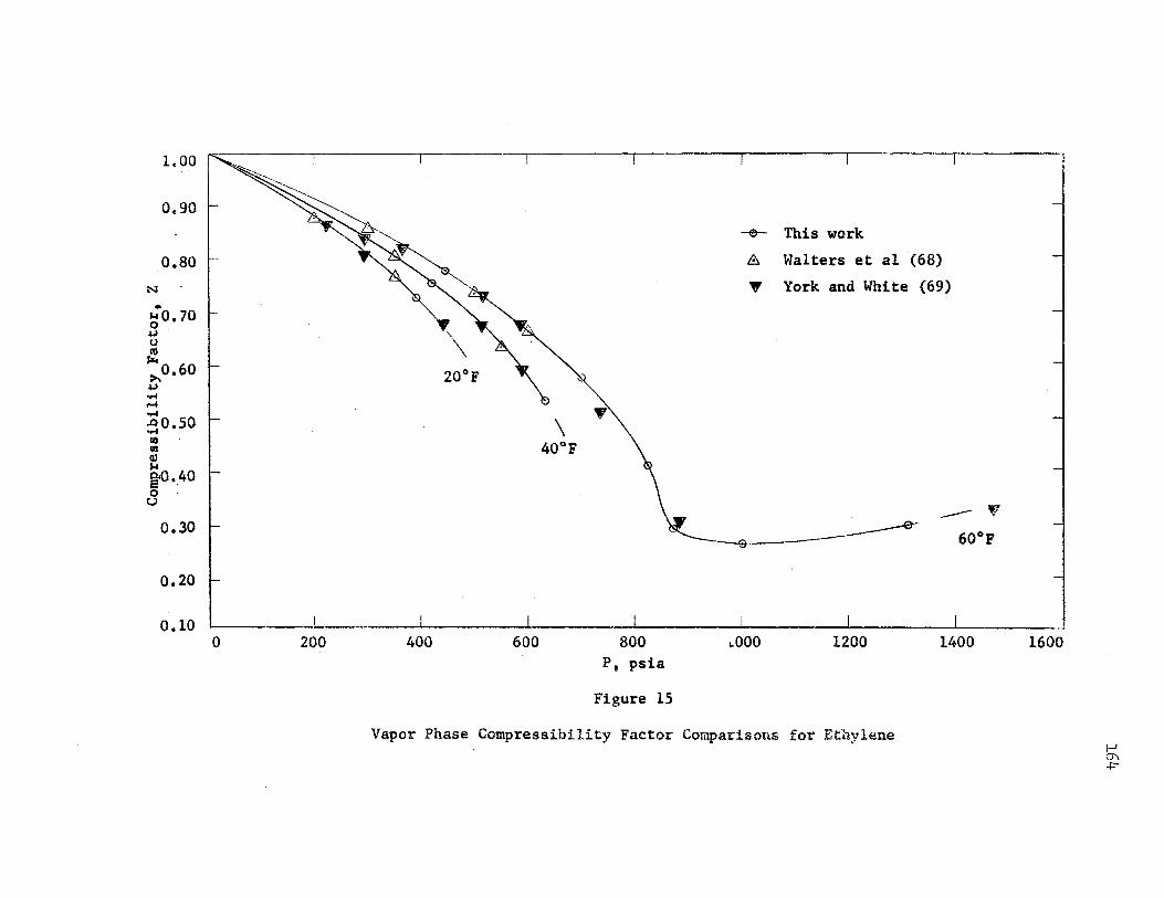
1.00
0.90
0.80
N
~·o. 10 ,I.I ' ti
:! :>,.0.60 ,I.I .... .... .... ao.so re re a, k i<>-.40 0 u
0.30.
0.20
0.10 0 200
\ 40°F
400 600 800 P, psia
Figure 15
--e- This work
A Walters et al {68)
'T Yo.rk and White (69)
~ooo 1200
. .--- V
60°F
1400
Vapor Phase Compressibility Factor Comparisons for Ethylene
1600
I-' O"\ -i::-
CHAPTER VII
CONCLUSIONS AND RECOMMENDATIONS
The purposes of this investigation were:
1) to develop and operate an experimental PVT apparatus for the determination of precise volumetric data for a binary system,
2) to compare the resultant data with existing virial coefficients and equations of state in an effort to determine and emphasize the need for further work on methods of improving these equations.
Experimental data were taken for the methane-ethylene binary system,
and virial coefficients were derived. The data were compared with
equations of state and with theoretical virial coefficient relationships.
Conclusions and recommendations from this investigation are summarized
in the following,.
A. Calculational
Conclusions
1. The experimental compressibility factors were compared versus the (
original BWR equation and the Edmister generalized BWR equation. The
standard deviations from the experimental values were determined to be
0.015 for the generalized BWR equation and 0,022 for the original BWR
equation.
2. Experimental second and third virial coefficients for the
methane-ethylene system were compared with the BWR equation (6), the
Edmister generalized form of the BWR equation (20), and the RK
166
equation (58), The Edmister generalized form fits this syst~m,better than
do the other two equations tested, For second virial coefficients,
standard deviations from the experimental data are summarized as BWR
(5.99 cm3/gm mole), generalized BWR (3,14cm3/gm mole), and RK (7.37 cm3/
gm mole). For third vi rial coefficients, the resultant standar.d deviations
2 6 2 , 2 6 2 are BWR(,3. 7 x 10 cm /gm mole ) , generalized BWR{2, l x 10 cm /gm mole ) ,
and RK(l2.8 x 102 cm6/gm mole2),
3, For each of the six systems· investigated, the reference isotherm
data from the Burnett apparatus (31) was used. The densities for the
isochoric., runs were determined directly from the reference isotherm.
Indications are that this data is somewhat high; the data is subject
to a later revision,
4. No accurate methods were found for the estimation of the inter-
action coefficient B12 from the pure component coefficients. The
estimated values were used in Equation III-12 to recalculate values
of B; the resulting B were compared versus the experimental B. Of m m . •., m
the methods tested the square root method (Equation III-21) gi~es the
lowest standard deviation (6,2 cm3/gm mole) from the experimental B. m
5. Least squares values of the interaction coefficient B12 were
determined by fitting Equation III-12 to the experimental data. The
values of Bm were then recalculated using the least squares B12 • The
B so calculated agree with the experimental coefficients to within m
the estimated accuracy (1.5 cm3/gm mole) of the coefficients. The
standard deviation from the experimental data was 0,74 cm3/gm mole
over the entire range of temperature and composition, This method
is quite useful in evaluating the internal consistency of the data.
167
6. The above conclusions indicate the need for further development
of an equati~n of stat~. For practicality in calculations and for
maximum utility in the application to mixtures, the equation should be
generalized and in closed form,· To conform with theoretical considera-
tions, the equation should be expressable in "open-ended" form, and the
resultant second and third. virial coefficients should agree with
experimental data.
7. The derivation of virial coefficients by the slope-intercept
method was discussed in Chapter III, In this investigation a modifica-1
tion to the method was used in which the original approximation to the
second coefficient was significantly improved upon in the derivation
of third virial coefficients. This procedure has been used by previous
investigators, but its use has not been extensive. The method is
sufficiently useful to be re-emphasized at this point.
Recommendations
1. Additional calculational work should be undertaken toward
the development of an improyed equation of state. The developmental
procedure outlined below should be tested on a preliminary basis,
using only selected systems for which data is available over an
extended range of conditions.
a) The second and third virial coefficients in the
BWR equation (Equation III-30 and III-31) should be
fitted to experimental pure component virial coefficients,
thus evaluating the constants B, A, C, b, a, and c. 0 0 0
b) Using the above values of the constants, the re
maining constants a and y should then be determined by
fitting the closed form BWR equation (Equation III-26)
to the experimental compressibility factor data.
c) The resulting BWR constants shoul.d then be
generalized by plotting versus w, as was done by
Edmister in the present genera,lized form of the BWR
equation~
2. The new generalized equation should be tested against mixture
compressibility factor data, using the standard mixing rules (Equation
III-27). No attempt should be made to improve upon the mathematical
form of these mixing rules, however, until definite values are
established for the constants for pure components.
3. Programs undertaken to develop improved equations of state
should be concentrated only on the generalized BWR eq~ation mentioned
above. The two-constant RK equation has the disadvantage that the
.second and third virial coefficients (Equations III-43) are not
independent 9 as both equations contain both of the constants a and bo
Conclusions
1. The isochoric method is satisfactory for the experimental
determination of compressibility factors. The only significant
requirement is that the reference isotherm be established from an
independent source. The apparatus is suited to determinations in
the gaseous or two-phase region; this particular apparatus was
168
satisfactorily operated over the temperature range 77 to 20°F, with
pressures from 260 to 2400 psia.
2. The long time required to attain thermal equilibrium between
successive experimental points is an inherent disadvantage of the
procedure< During normal operation, data is taken at the rate of
one point per 12 hour period; thus,in order to take a significant
amount of data a period of several months is required.
Recommendations
lo For future use in equation of state and virial coefficient
work, additional data should be taken with the apparatus. A binary
hydrocarbon system is preferable for study, as the resultant data
would be of greatest value for comparisons with equations of state.
2. If the data is to be used primarily in the derivation and
analysis of virial coefficients. primary emphasis should be placed
on the region 100 to 3000 psia. Experimental data taken outside
this range has little effect on the determination of virial coefficients
by the slope-intercept method. The reference isotherm temperature (77°F)
is satisfactory for the upper limit of temperature. The lower tempera
ture limit, however, should be extended. A lower temperature of -50°F
is recommended; this temperature would provide a considerably larger
temperature range, thus allowing a more thorough theoreti.cal analysis
of the resultant data.
3. For the pure components as well as the mixtures, samples of
the highest purity should be obtained. Analyzed mixtures of "prep
grade" gases are readily available from commercial suppliers.
·. 170
For future use of the apparatua ·. the following modifications are
recomnended ••
4a Using the existing •chanica~ refrigeration system (containing . ,, .
Fi'eon-12) the appa~a~ua may be operated as low as Oto 10°Fo · This
·operating range could be.extended •• low as -50°F or below by using a
system containing a different .refrigerant such as Freon 22 (BaP. -41.4°F)
or poaaibly Freon 13 (1.P. •l14·.6°F) • A closed loop system of this . . . . .
type has the advantage of .both convenience and economy as compared
.to liquid nitrogen•CQoled ayatema.
s. As a circulating liquid in the annular apace containing the
copper refrigeration coils, the use of the 601 ethylene glycol/401 :
water solution should be continued. The flammability Characteristics
of other frequently used liquids, such as i·ao-pentane or iao-octane,
make their use undesirable.
6. If the attainment of temperatures aignifica,ntly below -S0°F
is desired, the use of liquid nitrogen (B.P. -322°1!') should be
attempted. The direct use of acetone and dry ice (sublimation
po~nt .. 112°F).for_lo11g periods of ti• was found to give poor tempera
ture control inside the cryostat, Thia was due to considerable
thermal gradients that occurred in the acetone solution.
1. One source · of ~xper.imental error was ,the DPI · cell, which
contained a small amount of gu and was loc·ated outside · the low
temp~rature cryostat (Figure 1,.Chapter IV). Thia particular type
J>PI cell was designed for operating temperature no lower than +40°F.
consideration should be given to replacing this cell with a cryogenic
type cell, which could be placed directly inside the cryostat. Such
171
cryogenic cells have recently been developed by Ruska, and are similar
to the Ruska cell used in the present investigation. With the cryogenic
cell situated inside the low-temperature cryostat it would still be
necessary to separate the fluid in the upper portion of the DPI cell
frotn the oil in the Ruska gage by means of a high pressure mercury
u-tube. The fluid in the DPI cell must have a freezing point below
the lowest temperature investigated. For this application methyl
cyclopentane (freezing point -224°F) is recommended.
8. In this investigation the DPI cell and the bomb were connected
via 1/8 inch OD stainless steel tubing.· As the inner volume of this
tubing is significant, the tubing should be replaced by 1/16 inch
OD tubing.
9. In the present apparatus the measuring thermometer and thermo
couple were located in the controlled temperature air bath 9 immediately
adjacent to the bomb. For increased accuracy in temperature measure
ments, it is recommended that a calibrated platinum thermometer be
installed inside the bomb. The mounting of this thermometer inside
the bomb (Figure 2, Chapter IV) could be accomplished by using special
packing glands developed by the Conax Corporation 9 Buffalo, New Yorko
The glands may be.mounted through the wall with ordinary 1/4 inch
NPT mounting threads, and will withstand temperatures as low as
=300°F at working pressures up to 10,000 psi,
A metal-enclosed platinum thermometer is available from the Leeds
and Northrup Company (Catalog No. 8160) that would likely serve for
this application for temperatures as low as -40°F. For much wider
ranges of application (-436° to +900°F) platinum resistance tempera
ture sensors are available from the Sostman Company,
172
Cranford, New Jersey. These sensors have a reported temperature stability
of 0,001°C and could easily be calibrated over the desired working range
The entire platinum thermometer and packing gland assembly could
thus be mounted into the bomb through its top part. This would require
a modification to the upper part of t~e bomb due to the 7/64 inch drill
and due also to the seat for the Ruska connector.
lOo The bottom and center bearings on the steel blower shaft
(Plate III, Chapter IV) should be replaced by bearings designed for
continuous operation at lower temperatures,
llo As mentioned previously, the temperature control inside the
cryostat was affected by rapid fluctuations in the laboratory air
temperature. For future work the apparatus should be located so that
temperature control of approximately±. 1°F could be attained in the
immediate vicinity of the cryostat,
A SELECTED BIBLIOGRAPHY
1. Amagat, E. H., &s• Si!• ,!l Phys. ll, 68 (1893).
2. Amagat, E. H, ,. Annales ,!!!. Chimie (5), ,ll., 353, (1881).
3. Bean, Hos., J.. Research, National Bureau of Standards, vol i (1930) 0 .·
4 •. Beattie, J. A., !£2.5.• A!!• !Sfs.• Arts !s!.• ~. 389 (1934) • . ,
5. Benedict, M~, G •. B. Webb, and L. c. Rubin,~. Eng, Progress ~- 419 (1951).
6, Benedict, M., G. B. Webb, and L. c. Rubi1!', J.• . .£!!!!!• Phys. !, 334 ,(1940).
7. Bloomer, o. T, 9 Institute .21.2!!. Technology Research Bulletin .!le Institute of Gas Technology, Chicago, Illinois (1952).
8. Bridgman, P, w., "The Physics of High Pressure", G. Bell and Sons, Ltd., London (1958).
9. Burnett, E. s., .:!.• .Ael?l• Mechanics l§., A-136 (1936)0
10. Canfield, Fo B., T. W. Leland, and R, Kobayashi, Advano Cry. Ee&• !e 146, Plenum Press, New York (1963).
11. Cawood, W0 , and H, s. Patterson,:!•~. §.2.5.. (London), Part 1, 619 (1933).
12. Condon, E. u., and H. Odishaw, "Handbook of Physics", McGraw-Hill Book Company, New York (1958),
13. Connally, J. F., and G. A. Kandalic, Phys. Fluids l., 463 (1960).
140 Dodge, B, F,, "Chemical Engineering Thermodynamics", McGrawHill Book Co,, Inc., New York (1944).
15. Doolittle, A. K., I. Simon, and R. M. Cornish, AI.ChE Journal .2,, 150 (1960).
173
174
16. · Douslin, D. R., "Progress in International Resear.ch on Thermodynamic and Transport Properties." Papers of the Symposium on Thermophysical Properties, 2nd, Princeton, N. J., (1~62), 135.
17. Douslin, D.R., R. T, Moore, J.P. Dawson, and G. Waddington, J.• ~. Ch~m. §.25.. §.2., 2031 (1958) o
18. Eakin, B. E,, and R. T. Ellington, Papers of the Symposium on Thermal Properties, Purdue University, Lafayette, Indiana, (1959), 1950
19. Edmister, w. c., "Applied Hydrocarbon Thermodynamics", Gulf Publishing Company, Houston, Texas (1961).
20. Edmister, w. c,, Private Communication, MaY. 11, 1966.
21. Freeth, Fo A., and T. T. H. Verschoyle, !£2S.• Royal .§.2.5., .!J.Q!, 453 (1931) 0
22. Goodwip, R. D., .:!.• Research, National Bureau of Standards, vol .§i.£9
231 (1961).
23. Hirschfelder, J. o., C, F. Curtis, and R. B. Bird, "Molecular Theory of Gases and Liquids'' 11 John Wiley and Sons, Inc., New York (1964).
24. Holborn, L., and H. Schultze, Annalen .2!I. Physik iZ., 1089 (1915).
25. Hsu, c. c., and J. J. McKett·a, .:!, • .£!:!.!!!• Eng. ,!?.!!!.2., 45 (1964).
26. International Congress of Pure and Applied Chemistry, 18th, Montreal, Quebec, 1961.
27. Johnson, D. P., J. L. Cross, J. D. Hill, and H. A. Bowman, !rul• Eng • .£!!!!!• i2,, 2046 (1957).
28. Keyes, F. G., .f!.2.5.• ,a. As.!!• ~§.Si. • .§!, 505 (1933).
29. Keyes, F. Go, an.d H, G. Burks, .:!.• .!!!• Chem. !2£.• i2_.., 1403 (192 7) •
30. Kvalnese Ho M., and V. L. Gaddy,.:!.•.!!!• .9!.!.!!• 12£• ,al, 394 (1931).
31. Lee, R. c., Private Communication, July 19, 1966.
32. Levelt, J.M. H., Doctorate Thesis, University of Amsterdam (1958).
33. Masson, I., and L. G. F. Dolley, E!.2S.• Royal !2£.• 103A, 524 (1923).
34. Matthews, c. J •• and c. o. Hurd, Tr ans. AIChE ,!!, 55 '(1946).
35. Mayer, J. E.' .:!.• Phyt; o ~. ,il, 71 (1939).
175
36. Michels, A,• Annalen .2!!. Physik .zl, 577 (1924).
37. Michels• A,' B. Blaisse, and J. Hoogschagen, ~.2., 565 (1942).
38. Michels, A,• J, DeGruyter, and F, Niesen, Physic..!l.., 346 (1936).
39. Michels, A.• and M,, Geldermans, Physica .2., 967 (1942).
40. Michels, A.• and R, o. Gibson, Annalen.!!!.£. Physik !Z., 850 (1928).
41. Michels, A,• J, M, Levelt, and w. DeGraaff, Physica l,i, 659 (1958).
42. Michels, A.' R. J, Lunbeck, and G. J, Walkers, Physica .!l, 801 (1951)~
43. Michels, A., c. Michels, and H, Wouters, ~. Roy al §.2.s.• .!2J.!, 214 (1935).
44. Michels, A. t and G, w. Nederbragt, Physica 1, 1001 (1935).
45. Michels, A.' and G, w. Nederbragt, Phxsica 1., 569 (1936).
46. Michels, A., T. Wass~naar, J, M. Levelt, and W, DeGraaff, !22!• §.s!o !!!.• ~. 381 (1954) o
47. Michels, A,, T, Wassenaar, and Th, N, Zwietering, Physica ~. 67 (1952).
'
48. Miller, J. E,, L. Stroud, and L, W, Brandt, .:!.• ~. Ens. D,tta l, 6 (1961).
490 Mueller, W0 H,, Doctorate Thesis, The Rice Institute, Houston, Texas (1959),
so. Mueller, w. H., T. W0 Leland, Jr., and R, Kobayashi, AIChE Journal l, 267 (1961).
51. Olds, R. H., H. H. Reamer, B. H. Sage,. and w. H. Lacey, £!!.2.• EE£• Chem. 35, 922 (1943). -·-
52. Pavlovich, N. v., and D. L. Timrot, Teploinergetika l, 69 (1958)e
53. Pfefferle, W, c., Jr., J, A, Goff, and J. G. Miller,.:!.• fh!.!!l• Phys• ll, 509 (1955).
54. Pfennig, H. w., and J. J, McKetta, !!l• .!!!.•~.No. 11, 309 (1957).
55. Pitzer, K. s., D. z. Lippman, R, F, Curl, Jr., c. M. Huggins, and D. E, Patersen, .:!• .2• .£b!m• !£s.• 11.., 3427 (1955).
56. Prausnitz, J.M., AIChE Journal ,l, 3 (1959).
57. Prausnitz, J.M., and R. D, Gunn, AIChE Journal i, 430 (1958).
58. Redlich, o., and J. N. S, Kwong, £!!!!!, !!!.• .!!!, 233 (1949).
59, Rossinni, F, D., F, T. Gucker, Jr., H, L, Johnson, L. Pa~ling, and G. W, Vinal, J., 5!• .9!!!11 !2£• J.!i, 2699 (1952).
176
60, Scarborough, J. L,, "Numerical Mathematical Analysis", 4th edition, · The Johns Hopkins Press, Baltimore, Maryland (1958).
61. Schamp, H, W,, Jr., E. A, Mason, A, C, B, Richardson, and A. ~ltman, Phys. Fluids !• 329 (1958).
62, Schneider, w. G., Can. l• Research 27B, 339 (1949).
63, Silberberg, I, H,, K, A. Kobe, and J, J. McKetta, l• Chem, Eng, R!.S.!i, 314 (1959).
64, Solbrig, C, w., and R. T. Ellington, .9!!!.• Eng. Progress §Iel?.• ~~ries .a.2,, No. 44, 127 (1963),
65. Stimson, H, F., l• Research, National Bureau of Standards, vol §l!, No. 3 (1961),
66, Timoshenko, s,, "Strength of Materials, Part II, Advanced Theory and Problems!', 3rd edition,. 1), Van Nostrand Company, Princeton, New Jersey (1957),
67. Vennix, Alan J., Doctorate Thesis, Rice University, Houston, Texas (1.966).
68 •. Walters, R. J,, J, H, Tracht, E, B, Weinberger, and J. K, Rodgers, .£1!!!!. Eng. Progress 3.Q.~ 511 (1954).
69. York, Ro, and E,. F, White, Trans. AIChE !!.2., 227 (1944).
APPENDIX A
THEIMOMETRY STANDARDS AND TBEBMOCOUPLE CALIBRATIONS
Calibration of Thermocouples
The copper-constantan thermocouple B2 was connected to the potentio-! I .
meter through a double pole-double throw (DPDT) swi~ch as is illustrated . ·,
in Figure 4. The thermocouple and J>.latinum resistance thermometer
were situated in the c~~stat (Figure 1), directly beside the bombo To ' . '
further insure thermal equilibriµm between the thermocouple and thermo-
meter, a small glass container was filled with liquid iso-octane, and . '
the thermocouple and platinum thermometer were immersed into the liquid
at a distance of separation of about one inch, ....
The thermoco_uple was calibrated at approximately 40°F increments
over the temperature range -40 to +95°~. Twent~ readings· of thermocouple ,,
!!
output (mv) ·versus thermometer resistance (absoiute ohms) were made at
each successive temperature level. The calibration is expressed over
the above temperature.range as,
T°F = 29.382 + 45o938(POT) - 0 1 49224(POT) 2 + 0 0 59268(POT) 3 (A-1)
w~ere POT• t~e thermocouple·output, mv, with reference to an ice bath.
The accuracy of the calibration is estimated-as 0.01 to o.02°i.
The DPI cell thermocouple was connected to the potentiomet~r as
shown in Figure 4. For purposes of calibration, the thermocoupl~
177
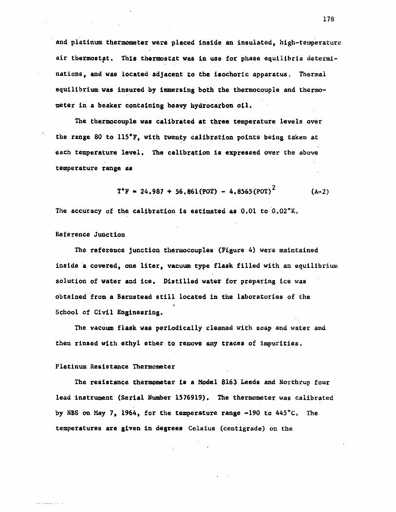
178
and platinum thermometer were placed inside an insulated, high-temperature
air thermost,t. This thermostat was in use for phase equilibria determi
nations, and was located adjacent to the isochoric apparatus, Thermal
equilibrium was insured by immersing both the thermocouple and thermo
meter in a beaker containing heavy hydrocarbon oil.
The thermocouple was calibrated at three temperature levels over
the range 80 to 115°F1 with twenty calibration points being taken at
each temperature level. The calibr•tion is expressed over the above
temperatu.re range as
T°F • 24.987 + S6.86l(POT) - 4.8565(POT) 2 (A-2)
The accuracy of the calibration is estimated as 0.01 to 0.02°K.
Reference Junction
The reference junction thermocouples (Figure 4) were maintained
inside a covered, one liter, vacuum type flask filled with an equilibrium
solution of water and iceo Distilled water for preparing ice was
obtained from a Barnstead still located in the laboratories of the
School of Civil Engineering.
The vacuum flask was periodically cleaned with soap and water and
then rinsed with ethyl ether to remove any traces of impuritieso
Platinum Resistance Thermometer
The resistance thermometer is a Model 8163 Leeds and Northrup four
lead instrument (Serial Number 1576919). The thermometer was calibrated
by NBS on May 71 1964, for the temperature range -190 to 445°C. The
temperatures are given in degrees Celsius (centigrade) on the
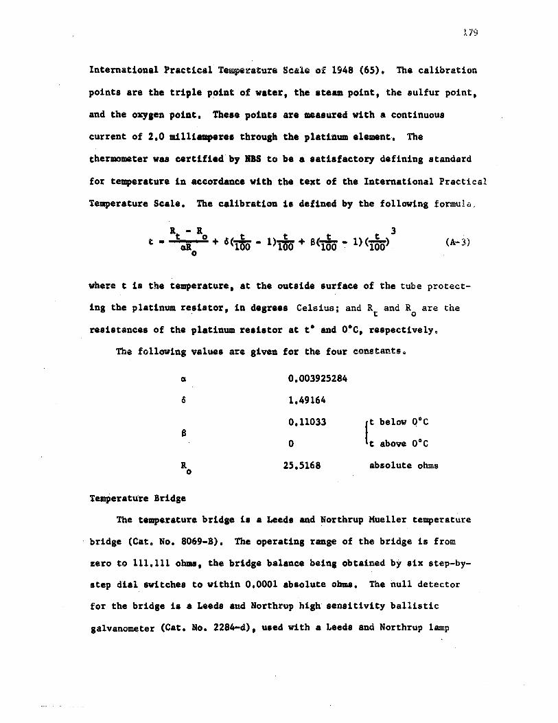
179
International Practical Temperature Scale of 1948 (65). The calibration
points are the triple point of water. the steam point. the sulfur point,
and the oxygen point, These pointe are measured with a continuous
current of 2,0 IDf.lliaaaperes throup the platinum element-, The
thermometer waa certified bJ IBS to be a satisfactory defining standard
for temperature in accordance with the text of the International Practical
Temperature Scale, The calibration is defined by the following formul6,
(A-3)
where tis the temperature. at the outside surface of the tube protect-
ing the platinum re~istor. in degrees Celsius; and Rt and R0 are the
resistances of the platinum resistor at t• and o•c. respectively.
The following values are given for the four constantso
Cl 0,003925284
cS 1,49164
0, 11033 r below 0°C 8
0 t above o•c
R 25,5168 absolute ohms 0
Temperature Bridge
The temperature bridge is a Leeds and Northrup Mueller temperature
bridge (Cat, No, 8069-B), The operating range of the bridge is from
zero to 111,111 ohms• the bridge balance being obtained by six step-by-
step dial switches to within 0,0001 absolute ohms, The null detector
for the bridge ia a Leeds and Northrup high sensitivity ballistic
1alvanometer (Cat. Ro, 2284-d), used with a Leeds and Northrup lamp

180
and scale reading device (Cat. No. 2170), The galvanometer was located
atop a concrete vibration-free pedestal which was sunk into the earth.
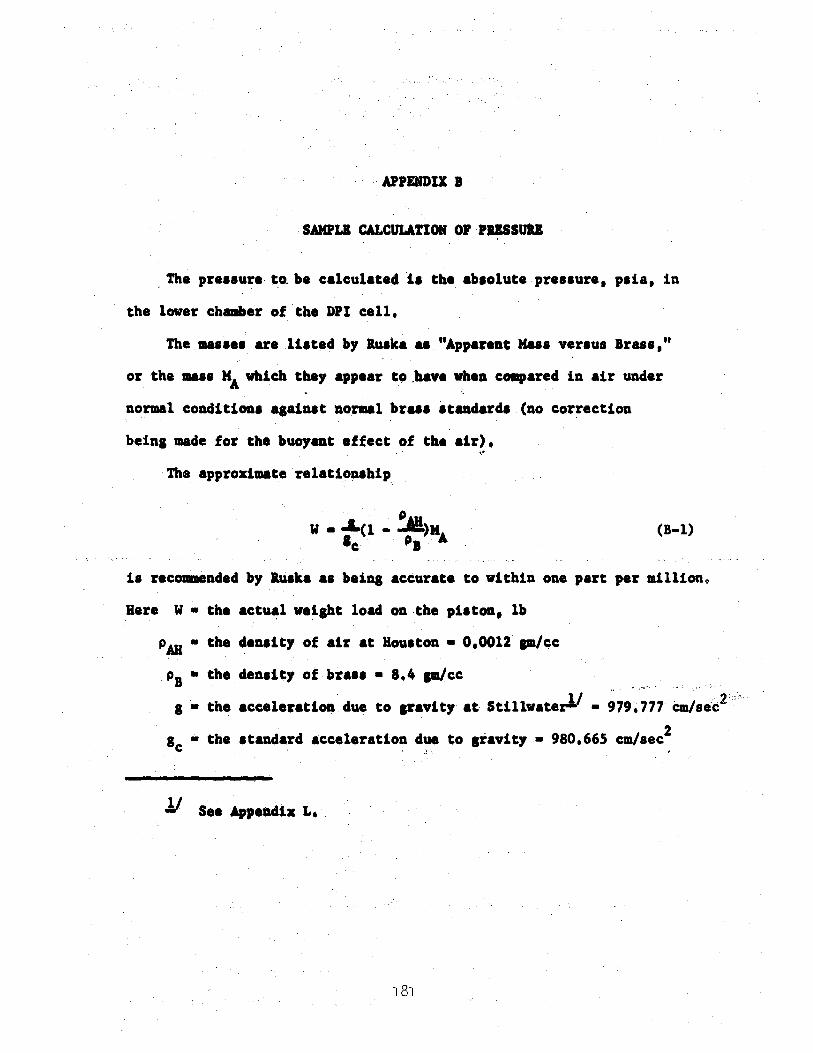
APPINDIXB
SANPLI CALCULATIOlC OFPUSSUU
. The preHure to. be calculated ia the ab1olute pre11ure, paia, in
the lower chamber of the l>Pl cell.
The ma•••• are lilted by llu1ka a• "Apparent Haas versus Brass,"
or the mass MA which they appear t.o .have when compared i1', air under
normal condition, againat no.rmal braH 1tandard1 (no correction
being made for the buoyant effect of the air),
The approximate relation1hip
. p. W • .&.(1 • .::A!)N
le ·. . PB .~
•I
(B-1)
is recommended by au1ka as being accurate to within one part per million~
Here W • the actual weight load on.the pi1ton, lb
p.AB • the denaity of air at Hou1ton • 0,0012 gm/cc
P1 • the density of bra11 • 8.4 aa/cc
g • the acceleration clue to aravity at Stillwater!' • ;79. 777 cm/sec:.2
g • the atandard acceleration clue to gravity• 980,665 cm/sec2 C · · i,
!I See Appeaclix L.
181
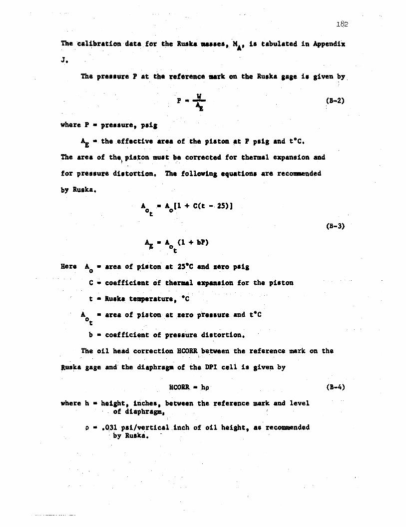
182
. .
The e_al~bration data . for the &uska u11ea ,. HA, 1• tabulated . in Appendix
J.
The pre1alire Pat the reference urt on the lluaka gage ia given bJ.
·. w P ·-...
where P • pressure, p1i1.
Ag •the effective area of the piston ~t P psig and t•c.
The area of the. pi1.ton 111118t be corrected for thermal expansion and . .. .. . . ~ . .
for pressuie distortion. The followin1 equationa are reco111Dended
by lluska.
A0 • A0 [1 + C(t. • 25) J t . .
~ • A0 (1 + bP) . . .. t . '
Here A0 • area of piston at 2s•c a~ sero psig
. C • coefficient of ther111l e:apans~on for the piston ·. . · ... . ·.:.
t • lluska temperature, •c
A0 • area of pistOII at zero pres1ure and t•c t
b • coefficien.t of pressure distortion.
'
.(B-2)
(B-3)
The oil head correction BCOll be.tween the reference mark on the
1t.us~a .gage and the diaphragm of the DPI cell'is give~ by
BCOlll • hp·
where h · • beight • inches, between the reference mark and leve.l . of diaphragm,
p • .0;31 psi/vertical inch of oil height, as recoanended : by lluska. -
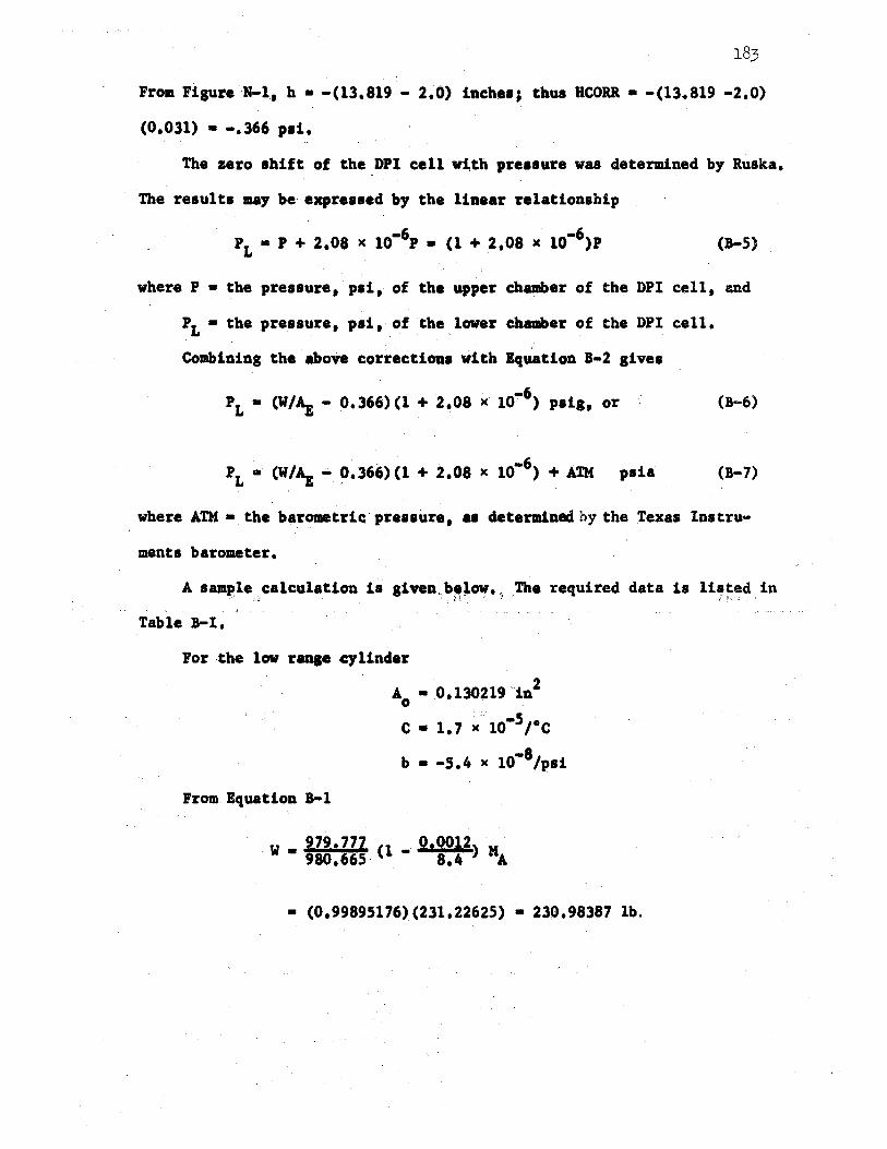
From FigQre N-1., h • -(13.819 - 2.0) inches; thus HCORR • -(13,819 -2,0)
(0.031) • -.366 psi,
The zero shift of the DPl cell wi.th pre1&ure was determined by Ruska.
The results may be expressed by the linear relationship
(B-5)
where P • the pressure, psi, of the upper ch~er of the DPI cell, and
PL• the pressure, psi, of the lower Chamber of the DPI cell.
Combining the above corrections with Equation B-2 gives
. ·. ' -6 PL• (W/Ag - 0.366)(1 + 2.08 x 10 ) psig, or (B-6)
PL• (W/Ag -~.366)(1 + 2.oa x 10-6) + ATM psia (B-7)
where ATM • the barometric;· pressure, as determined by the Texas lnstru-
ments barometer.
A sam~le calculation is given_b~~ow. ;, _The required data 1s listed in
Table B-1,
For the low range cylinder
From Equation B-1
A0 • 0,130219 in2
c • 1.1 x 10-51°c
b • -5,4 x 10⁻⁸/psi
W 979,777 (l _ o,:~!2~ M • 980,665 1 A
• (0,99895176)(231,22625) • 230,98387 lb.
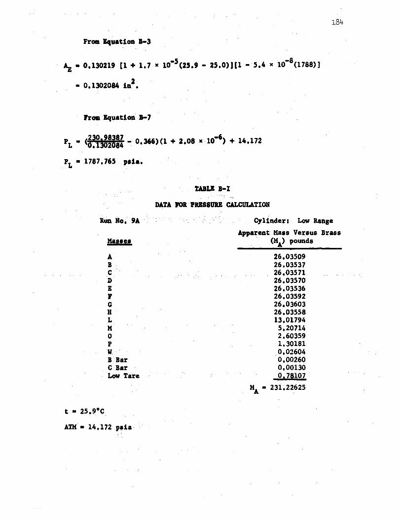
184
From Equation B-3
Ag. 0.13021, c1 + 1.1 x 10⁻⁵c2s., - 2s.0))[1 - s.4 x 10-8(1788)1
• 0,1302084 in2•
Prom Equation 1-7
PL• 1787.765 p1ia,
Run No. 9A
t • 25,9°c
MaHel
A B C D E r G B L M 0 p w B Bar C Bar Low Tare
ATM• 14.172 p11ia
TAil.i B•I
DATA roa·PUSSUU CALCULATION
Cylinder: Low Range
Apparent Mass Versus Brass · (MA) pounds
26.03509 26.03537 26,03.571 26.03570 26,03536 26.03592 26.03603 26 .• 03558 13.01794 5,20714 2.60359 1030181
.0,02604 0.00260 0.00130 o, 78107 .
MA• 231,22625
APPENDIX C
OPERATING CHARACTERISTICS or THE TEXAS INSTRUMENTS BAROMETER
A Texas Instruments servo-nulling precision pressure gage (Model
No. 141A) was used for determining barometric pressure.
This gage consists of a zero to 100 c11t-Hg range fused (low hysteres~s)
quartz bourdon tube contained within a capsule. A small mirror is
suspended from the lower portion of the bourdon tube, An optical trans-
ducer is mounted on a gear which ~ravels concentrically around the
s,uspended mirror. Light reflected from the mirror falls on a pair of
balanced photocells which are connected to a microammeter readout scale.
A closed-loop motor-driven aervo ayatem continuously accomplishe~ the
nulling by aut.omatically positioning the gear so that the microammeter
reading_is zero.
The tube has full scale rotation of 100 degrees, and the corre
sponding position of the gear is digitally presented on a counter
readout. The null position is constantly maintained for minute vari-
ations in the pressure being measured. The counter reading may then be ' '
multiplied by a scale factor (determined by calibration) to determine
the gage pressure. As this instrument is used exclusively for the
measurement of absoiute pressure, .the capsule surrounding the bourdon
tube is permanently evacuated.
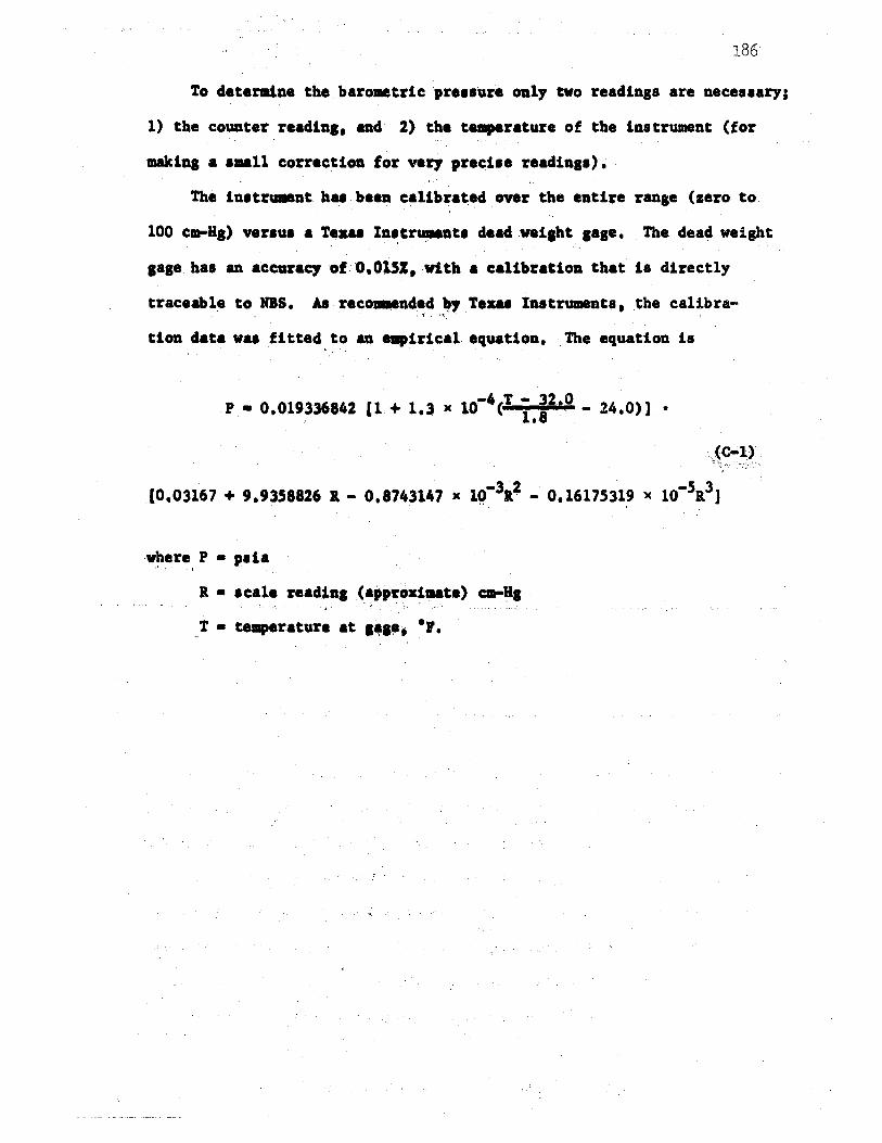
186
To determine the barometric pre11ure oaly two readings are necessary;
1) the counter reading, ad 2) tbe temperature of.the instrument (for
making a ••11 correction for very precise readings).;
The i111trU11Bnt. bas been calU,ra~e, ·. o,,er the entire range (zero to
100 cm-Hg) versu1 a Texaa Iastr11119at1 dead vel1ht gage. The dead weight ' ' I . ' '
gage has an accunc, of o.OUI, with a calibration that is directly
traceable to NBS. Aa.recomieacled 1'-, Texas Iutruments, the calibra-~ • • '/' ',, • I
tion data wu fitted.to an -,lrlcal equation. The equation ls
P • 0.019~36842 [1.+ 1.3 x 10·4~T i.:2,0 - 24.0)] •
co.03161 + 9.9358826 a - o.&743147 x 10·31.i - o.1,11s319 x 10·5a31 . . .. '
where P • p1la ,, ... '' .
. R • scale reacllng (app~ox~ute) ca-Ila .~ r-.
.. T.• temperature at•••• •r.
APPENDIX D
CALIBRATION OF BOURDON GAGES
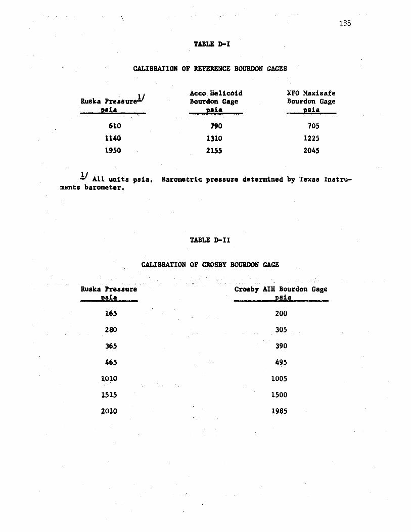
TABLE D-1
CALIBRATION OF REFERENCE BOURDON GAGES
Ruska Pressure!' psi a
610
1140
1950
Acco Helicoid Bourdon Gage
p•ia
790
1310
215S
XFO Maxisafe Bourdon Gage
psi a
705
1225
2045
188
!/ All units psia, Barometric pressure determined by Texas Instruments barometer.
Ruska Pressure psia
165
280
365
465
10~0
1515
2010
TABLED-II
CALIBRATION OF CllOSBY BOUIDON GAGE
Crosby AIH Bourdon Gage psi a
200
305
390
495
1005
1500
1985
APPENDIX E
SAMPU ~TIOB.01' VOLUME IATIO VD/VB
The determination of the ratio of the v~lume VD of the DPI cell
to the volume v1 of the bomb was .discussed in Chapter IV. A sample
calculation of this ratio is given as follows .•
Before the expansion the temperature at each section of the
apparatus was determined, and the pressure P0 at the diaphragm of
·the DPI cell was •aeured. Pre1&ures for each section of the
apparatus were corrected for heads of gas udng Equations N-14
through N-16 1 and the corresi,onding compressibility factors for the
. nitrogen were determined from the literature. values of Michels (42) e
·. Airco prepurified nitroge~·:.,as used. The i-esults. are tabulated
as follows.
!I The prepurified nitrogen was ob_tained from a local supplier, The maximum oxygen content was given as 0.001%, and the moisture content was 0.0012% with a trace of argon. The remainder was nitrogen. ·
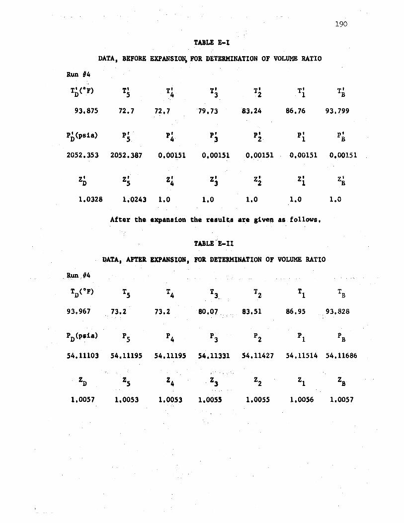
190
TABLE E-I ;
DATA, BEFORE EXPANSION, FOB. DETERMINATION OF VOLUME RATIO
Run 14
Tj,(°F) T' 5 T' _4 T' 3 T' 2 T' 1 T' B
93,875 72.7 72.7 79.73 ·a3.24 86,76 93,799
P0(psia) P' 5 P4 P' 3 P' 2 P' 1 P' B
2052.353 2052.387 0,00151 o.001s1 O,OQ1S1 0.00151 0,00151
Z' D Z' s Z4 z• 3 z• 2 z• 1 z• ·B
1.0328 1.·()243 1,0 1.0 1.0 1.0 1.0
After the expansion the results az:e giveii as.follows.
TABLE··"E-II
l)ATA, AFTER EXPANSION, 101 DETDKINATION OF VOLUME RATIO
B.un.#4
TD(OF) TS T4 Tl T2 Tl TB
93.967 73,2 73.2 . ao.97 ..... 83.51 86.95 .. _93.828
PD(psia) PS P4 pl p2 pl PB
54,11103 54.11195 54.11195 54.11331 54.11427 54.11514 54.11686
ZD z s Z4 . Z3 ·Z 2 zl ZB
1,0057 1,0053 1,0053 1,0055 1.ooss 1,0056 1,0057
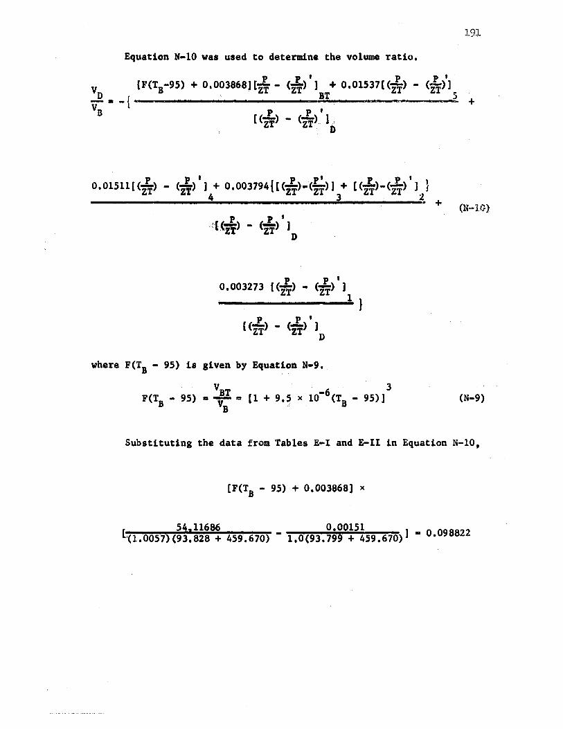
191
Equation N-10 was used to determine the volume ratio.
p p ' p p ' vo cr<TB-95> + o.003s6a1 cw - <zt> 1 + 0.01531c <z'T> - <u> 1 _ • -{ -------------B,..T ...... _______ .,.;.5 + VB p p '
l <TT> - <TT> l , . D
p P I P ·. P' P P ' l o.Ol511[(ZT) - <-zT> ] + 0,003794{[<-zT>-<-zT>] + C<u>·<rt> ] J
4 3 2 -----------------------------------------------~ +
p p ' .t((-) - (-zT) )
·Zt D
p p I
0.003213 c <u> - <rt> 1 ________________ 1 }
p p ' c <u> - <w> 1 D
where F(T8 - 95) is given by Equation N-9.
F(T8 - 95) 3
[l + 9,5 x 10⁻⁶(TB - 95)]
(N-10)
(N-9)
Substituting the data from Tables E-I and E-II in Equation N-10,
[F(TB - 95) + 0,003868) x
54,11686 0.00151 Lc1.oos7) (93.828 + 459.670) - 1.0(93. 799 + 459.670) 1 • 0•098822
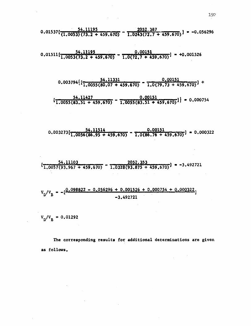
192
· 54.11195 . 2052.387 0•01537 lc1.oos3)(73.2 + 459.670) - 1.02¥3(72.7 + 459.670)) • - 0•056296
54.11195 01001S1 ·J +o 001526 o.OlSll[l.0053(73.2 + 459.670) • 1.0(72,7 + 459,670) • •
{ s4.11331 0.00151 o.oo3794 C1.0055(ao.01 + 459.670) - 1.0(79.73 + 459.610> 1 +
54.11427 0.00151 } [1.0055(83.51 + 459,670) • 1.0055(83.51 + 459,670)] • o.ooo754
54.11514 . 0,00151 0•003273l1.0056(86.95 + 459.670) - 1.0(86.76·+ 459.670)) • 0•000322
54.11103 2052.353 [1.0057(93.967 + 459.670) - 1.0328(93.875 + 459,670)) • - 3•492121
V /V = -[0.098822 - 0.056296 + 0.001526 + 0.000754 + 0.000322] D B -3.492721 . .
The corresponding results for additional determinations are given
as follows.
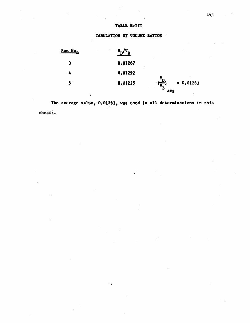
Run No.
TABLE E•Ill
TABULATION or VOLUME RATIOS
VD/VB
0.01267
0.012,2
0.0122s
193
• 0,01263
The average value, 0.01263, wa, used in all determinations in this
thesis .•
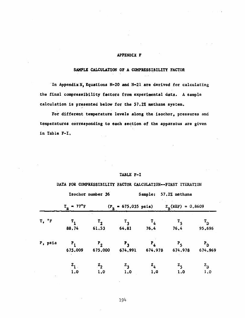
APPENDIX F
SAMPLE CALCULATION or A COMPRESSIBILITY FACTOR . .
··1n Appendix N, Equations N-20 and N•21 are derived for calculating
-the final compressibility factors from experimental d~t.8:• A sample
calculation is presented below for the 57.2% methane system.
For di~ferent temperature levels along the isochor, pressures and
temperatures corresponding to each se~tion of the apparatus are given
in Table F-I.
TABLE F•I
DATA FOR COMPRESSIBILITY FACTOR CALCULATION--FIRST ITERATION
Isochor number 36 Sample: 57.2% methane
T • 77°F B (P8 • 675.,035 psia) z8(REF) .. 0,8609
T, °F Tl T2 Tl T4 TS TD 88.74 61.Sj 64.81 76.4 76.4 95.696
P, psia pl p2 P3 P4 PS PD 675.009 675.000 674,991 674.978 674,978 674.969
z1. .z2 Z3 Z4 ZS ZD
1.0 1.0 1.0 1.0 1.0 1.0
194
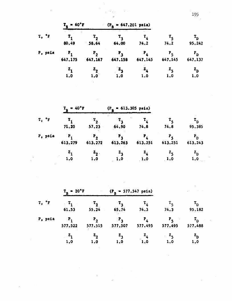
195
T1 • 60°F (P8 • 647,201 psia)
T °F t Tl T2 Tl T4 TS TD 80.49 · S8.64 64,00 74.2 74,2 95,242
P, psia '1 p2 P3 P4 PS PD 647.175 647 .167 647.158 647,145 647.145 647.137
z1 Zz Z3 Z4 ZS ZD
1.0 1.0 1.0 1,0 1.0 1.0
T • 40°F B (P1 • 613.305 psia)
T °F t Tl T2· T3 T4 T5 TD 71,20 57.23 64.90 74.8 74,8 95,385
P, psia pl p2 P3 P4 PS PD 613.279 613,272 613,263 613,251 613,251 613.243
zl Z2. Z3 Z4 ZS ZD
1.0 1,0 1.0 1,0 1,0 1.0 .
t 8 • 20°F (P8 • 577~547 psia)
T, °F Tl T2 T3 T4 TS TD 61.53 55.24 65,74 74.3 74.3 95,182
P, psia pl p2 P3 P4 PS TD 577.522 577,515 577,507 577,495 577,495 577,488
zl z2 Z3 Z4 ZS ZD 1,0 1,0 1.0 1.0 1.0 1.0
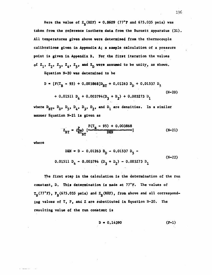
196
Here the value of z8(REF) • 0,8609 (77°F and 675,035 psia) was
taken from the reference isotherm data from the Burnett apparatus (31),
All temperatures given above were determined from the thermocouple
calibration, given in Appendix A; a ~ample calculation of a pressure . . .
point is given in Appendix B, For the fir1t iteration the values
of z1, z2, z3, z4, z5, and z0 were assumed to be unit~, as shown.
Equation N-20 was determined to be
D • [F(T1 • 9S) + 0,003868]DBT + 0,01263 DD+ 0,01537 D5
(N-20) + 0,01511 D4 + 0,0~3794(D3 + D2) + 0,003273 D1
• I • .
where DBT' DD' D5, D4, D3, D2, and D1 are densities, In a similar
manner Equation N•21 ia given as
where
. . p F(T8 • 9S) + 0,003868 ~T • (if~T [ DIN ]
DEN• D - 0,01263 DD• 0,01537 D5 -
0,01Sl1 »4 • 0,00379,4 (D3 + D2) - 0,003273 D1
(N-21)
(N-22)
The first 1tep in the calculation is the determination of the run
constant, D, Thia detendnation is made at 77°F, The values of
t 8(77°F), P8(675,03S psia) and z8(REF), from above and all correspond
ing values of T, P1 and Z are substituted in Equation N-20, The
resulting value of the run constant ii
D • 0,14390 (F-1)
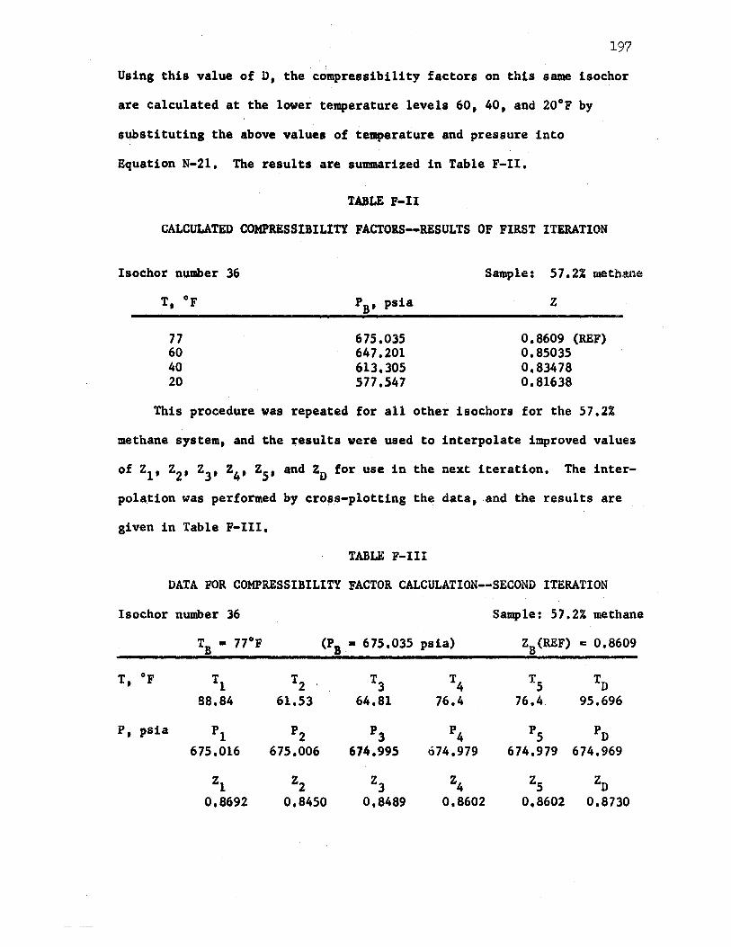
197
Using this value of D, the compressibility factors on this same isochor
are calculated at the lower temperature levels 60, 40, and 20°F by
substituting the above values of temperature and pressure into
Equation N-21. The results are summarized in Table F-II.
TABLE F-II
CALCULATED COMPRESSIBILITY FACTORS••RESULTS OF FIRST ITERATION
Isochor number 36
T, °F
77 60 40 20
Sample: 57,2% methane
PB' psia Z
675.035 647.201 613.305 S17 .S47
0,8609 (REF) 0.85035 0.83478 0,81638
This procedure was repeated for all other isochors for the 57.2%
methane system, and the results were used to interpolate improved values
of z1, z2, z3, z4, z5, and z0 for use in the next iteration. The inter
polation was performed by cross-plotting the data, and the results are
given in Table F-III.
TABLE F-III
DATA FOR COMPRESSIBILITY FACTOR CALCULATION--SECOND ITERATION
lsochor number 36 Sample: 57.2% methane
T • B
77°F (PB• 675.035 psia) ZB(REF) = 0,8609
T °F t Tl T2 T3 T4 TS TD 88.84 61.53 64.81 76.4 76.4 95.696
P, psia l\ p2 P3 P4 PS PD 675.016 675.006 674.995 674.979 674.979 674.969
zl z2 z3 Z4 ZS ZD
o.8692 0,8450 0,8489 0,8602 0.8602 0,8730
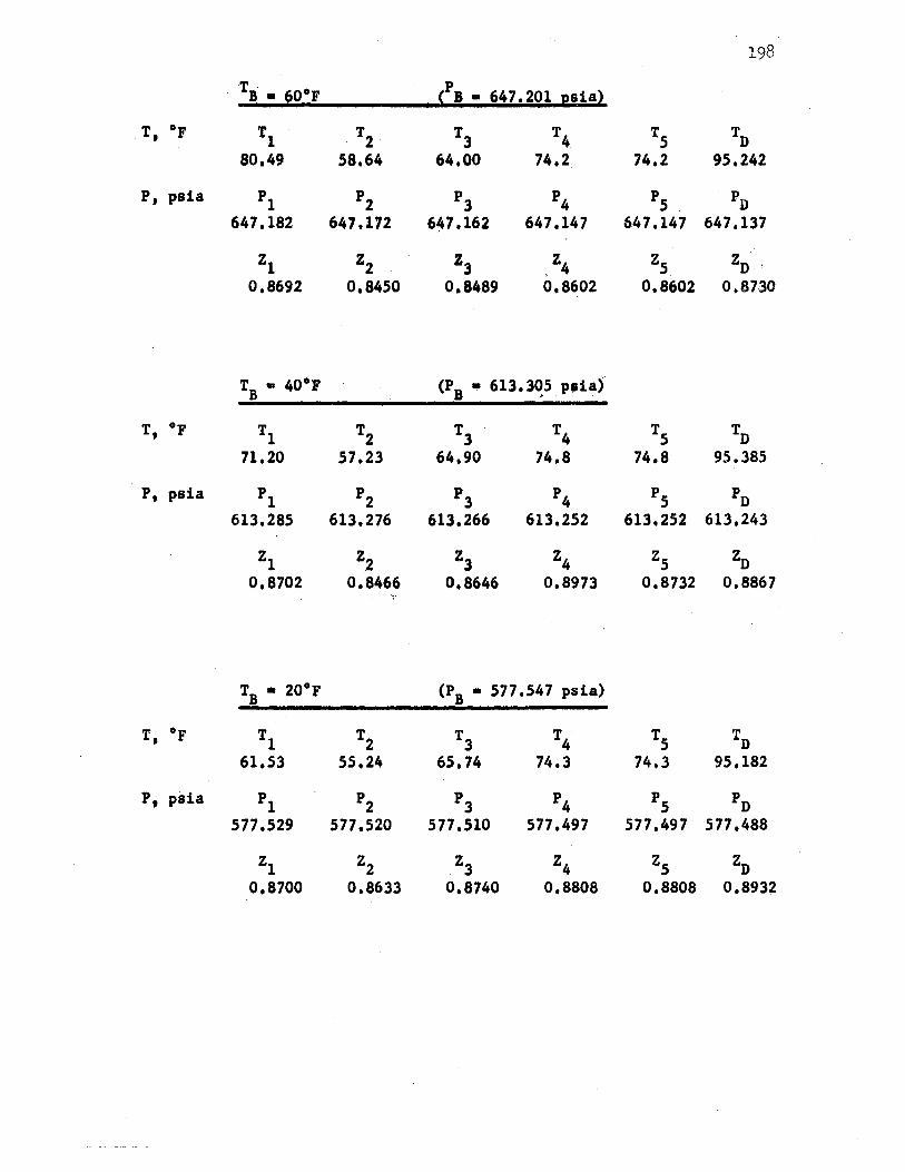
198
TB• 60°F p
( B • 647,201 psia)
T °F . . Tl . T2 T3 T4 TS TD 80,49 58,64 64,00 74,2 74,2 95,242
P, psia pl p2 pl P4 PS PD 647.182 647.172 6,7.162 647.147 647,147 647.137
zl z2 Z3 , Z4 ZS ZD , 0,8692 0,8450 0,84.89 0,8602 0,8602 0,87,30
T • 40°F B (PB• 613,3~5 pJi~j
T •r • Tl T2 Tl T4 TS TD 71,20 57.23 64.90 74.8 74,8 95.385
P, psia pl p2 pl P4 PS PD 613.285 613.276 613,266 613.252 613.252 613,243
zl z2 Z3 Z4 ZS ZD
0,8702 0,8466 0,8646 0,8973 0,8732 0,8867
T • 20°F B (P8 • 577,547 psia)
T •p • Tl T2 Tl T4 TS TD 61.53 55.24 65.74 74,3 74,3 95.182
P, psia pl p2 pl P4 PS PD 577,529 577,520 577,510 577,497 577,497 577,488
zl z2 Z3 Z4 ZS ZD
0,8700 0,8633 0,8740 0,8808 0,8808 0,8932
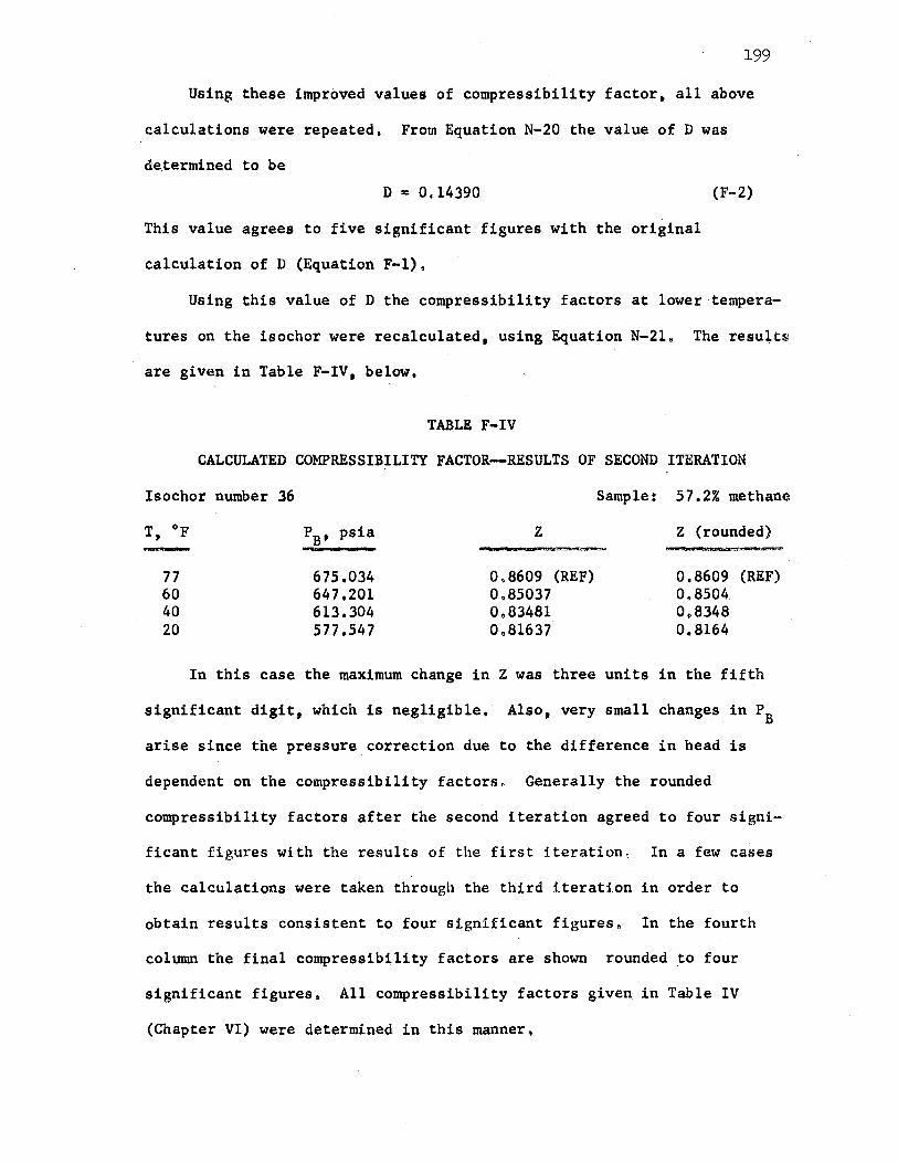
199
Using these improved values of compressibility factor. all above
calculations were repeated, From Equation N-20 the value of D was
de.termined to be
D == 0,14390 (F-2)
This value agrees to five significant figures with the original
calculation of D (Equation F-1).
Using this value of D the compressibility factors at lower tempera-
tures on the isochor were recalculated, using Equation N-21. The resu!ts
are given in Table F-IV, below.
TABLE F-IV
CALCULATED COMPIU:SSIBILITY FACTOR--RESULTS OF SECOND ITERATION
Isochor number 36 Sample: 57.2% methane
T, °F PB' psia z Z (rounded) -- -· UAW.: J:bc.:$
77 675.034 0.8609 (REF) 0.8609 (REF) 60 647.201 0,85037 0.8504. 40 613.304 0.83481 0~8348 20 577.547 0.81637 0.8164
In this case the maximum change in Z was three units in the fifth
significant digit, which is negligible. Also, very small changes in PB
arise since the pressure correction due to the difference in head is
dependent on the compressibility factors. Generally the rounded
compressibility factors after the second iteration agreed to four signi-
ficant figures with the results of the first iteration, In a few cases
the calculations were taken through the third iteration in order to
obtain results consistent to four significant figures. In the fourth
column the final compressibility factors are shown rounded to four
significant figures. All compressibility factors given in Table IV
(Chapter VI) were determined in this manner.
APPENDIX G
FUNDAMENTAL CONSTANTS AND MIXTURE COMPOSITIONS
The latest defined value of the universal gas constant R is given
(59) as 82,0567 cm3 -atm/deg K-mole, Converting this value to
engineering units, R = 10.731496 (psia - ft 3)/(lb mole 0 R).
The most recent (65) definition of absolute temperature is expressed
as T(°K) = t(°C) + 273,150. Converting this expression directly to the
absolute Rankine scale gives T( 0 R) = t(°F) + 459,670.,
The six gas samples used in this investigation were blended and
analyzed by the donor, Phillips Petroleum Company~ Bartlesville,
Oklahoma. The samples were Phillips "pure grade<" The Phillips'
analyses were performed by mass spectrometry and were reported to the
nearest 0,1 mole per cent, The 99.9% ethylene sample and the 99.0%
methane sample were independently analyzed by gas chromatography in the
laboratories of the School of Chemical Engineering. For each of the
components in the two samples the results of these independent analyses
differed by less than O ,.1%. Results of the entire analysis are given
in Table G-I below; all molecular weights were based on the Carbon 12
International Scale of Atomic.Weights (26).
200
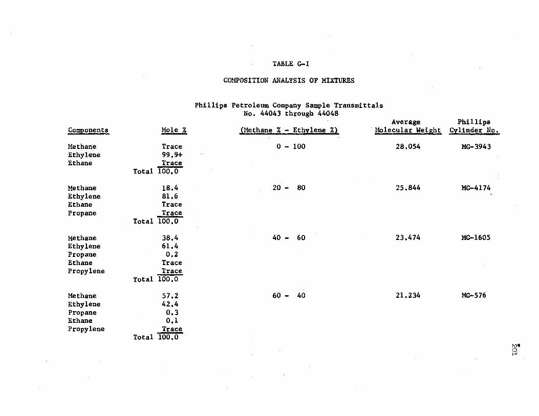
Components _t!ole %
Methane Trace Ethylene 99.9+ Ethane Trace
Total 100.0
Methane 18.4 Ethylene 81.6 Ethane Trace Propane Trace
Total 100.0
Methane 38.4 Ethylene 61.4 Propane 0.2 Ethane Trace Propylene Trace
Total 100.0
Methane 57,2 Ethylene 42.4 Propane 0.3 Ethane 0,1 Propylene Trace
Total 100.0
TABLE G-I
COMPOSITION ANALYSIS OF MIXTURES
Phillips Petroleum Company Sample Transmittals No, 44043 through 44048
(Methane% - Ethylene%)
0 - 100
20 - 80
40 - 60
60 - 40
Average Molecular Weight
28.054
25.844
23.474
21.234
Phillips Cylinder No,
MG-3943
MG-4174
MG-1605
MG-576
I\)' 0 f-'
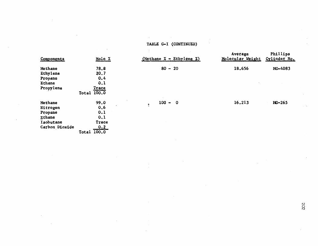
·Components Mole% -Methane 78.8 Ethylene io.1 Propane 0.4 Ethane 0.1 Propylene Trace
Total 100.0
Methane 99.0 Nitrogen 0.6 Propane 0.1 Ethane 0.1 Isobutane Trace Carbon.Dioxide 0,2
Total 100.0
TABLE G-I (CONTINUED)
(Methane% - Ethylene%)
80 - 20
100 - 0
Average Molecular Weight
18.656
16.213
Phillips Cylinder No.
MG-4083
MG-265
I\)
2
APPENDIX H
CALCULATION OF EFFECT OF TEMPERATURE ON THE BOMB VOLUME
The effect of temperature on the bomb volume is determined by
assuming the inner volume of the bomb (Figure 2) to be a cylinder of
circ·umference CBT and length LBT at. temperature T8 (°F).
The volume VBT at temperature T8 is thus given by
(H-1)
and the volume VB at 95°F is
(H-2)
where CB and LB represent the circumference and length, respectively,
at 95°F,
The effect of temperature on the circumference and length of the
inner volume is expressed by
-1 Here a is the coefficient of thermal expansion, (°F) ,
203
(H-3)
204
The expressions for CBT and LBT may be substituted into Equation H-1
to give
Dividing Equation H-4 by Equation H-2 gives
VBT 3 - • [l + e1(TB - 95)]
VB
The value of Cl for type 303 austenitic steel (Oto 600°F) is
(H•4)
(li-5)
: -6 0 -1 9,5 x 10 ( F) • Substituting this value into Equation H-S gives
-6 3 [l + 9,5 x 10 (TB - 95)] • F(T8 - 95) (N-9).
APPENDIX J
RUS1CA PISTON GAGE CALIBRATION DATA
The Ruaka piston gage is a dual range instrument (model 2400HL}.
The instrument usea two piston-cylinder combinations (low range 6 -
2428 psi; high range 30 - 12,140 psi). Ruska calibrated the gage
versus a Ruska laboratory master dead weight gage (No, 7544) which was
itself calibrated to an accuracy of one part in 10,000 parts versus
an NBS controlled-clearance piston. The NBS identification numbers
for the calibration are P6694A/2.6/161365 and P6694B/2.6/161365.
The instrument uses a total of 32 type-303 stainless steel
loading weights, their masses being determined by Ruska. The final
mass calibratio.n data is given in Table J-I. The calibration is
reported to a precision of one part .in 50,000 for masses greater than
O.l pound, one part in 20,000 for masses 0.01 to 0.1 pound, and
one part in 10,000 for masses 0.001 to 0.01 pound. Additional gage
specifications are given in Table J-II, and a sample pressure calcula
tion is given in Appendix B.
205
Designation
Low Tare High Tare
A B C D E F G H I J K L M N 0 p
Q R s T u V w X A A B C D D E F
TABLE J-I
RUSKA MASS CALIBRATION DATA
Calibration--Pressure Gage Masses Calibrat~on date 3-22-63 Ruska Serial No. 10381 Job No. A3567/C2630
30 psi
1000 1000 1000 1000 1000 1000 1000 1000 1000 1000 1000 500 200 200 100 50 20 20 10 5 2 2 l 0,5 0.2 0.2 0.1 0.05 0,02 0,02 0,01 0,005
6 psi
200 200 200 200 200 200 200 200 200 200 200 100
40 40 20 10 4 4 2 1 0,4 0.4 0;2 0.1 0.04 0,04 0,02 0.01 0,004 0,004 0,002 0,001
206
Apparent Mass versus Brass (MA) pound:._
o. 78107 0.78107
26,03509 26,03537 26,03571 26,03570 26.03536 26,03592 26.03603 26.03558 26,03563 26,03608 26,03568 13.01794
5,20714 5, 20715 2,60359 1,30181 0,52072 0,52074 0,26035 0,13020 0,05208 0,05209 0,02604 0,01302 0,005203 0 005202 0,002601 0,001301 0,000520 0,000521 0,000260 0,000130
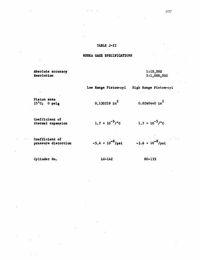
207
TABLE J•ll
RUS1CA GAGE SPECIFICATIONS
Absolute accuracy 1:10,000 Resolution 5:1,000 1000
Piston area 25°c;· 0 psig
Coefficient of thumal expansion
CoefficJ,ent of pressure distortion
Cylinder No,
Low Range Piston-cyl High Range Piston-cyl,
0,130219 in2 0.0260440 1112
1. 7 x 10⁻⁵ re
-s -5.4 x 10 /psi -8 -3.6 x 10 /psi
LC-142 HC-133
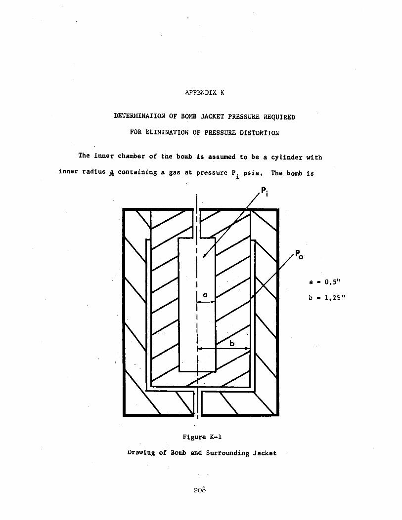
APPENDIX K
DETERMINATION OF BOMB JACKET PRESSURE REQUIRED
FOR ELIMINATION OF PRESSURE DISTORTION
The inner chamber of the bomb is assumed to be a cylinder with
inner radius.! containing a gas at pressure Pi psia, The bomb is
a. o.s"
b • 1,2511
Figure K-1
Drawing of Bomb and Surrounding Jacket
208
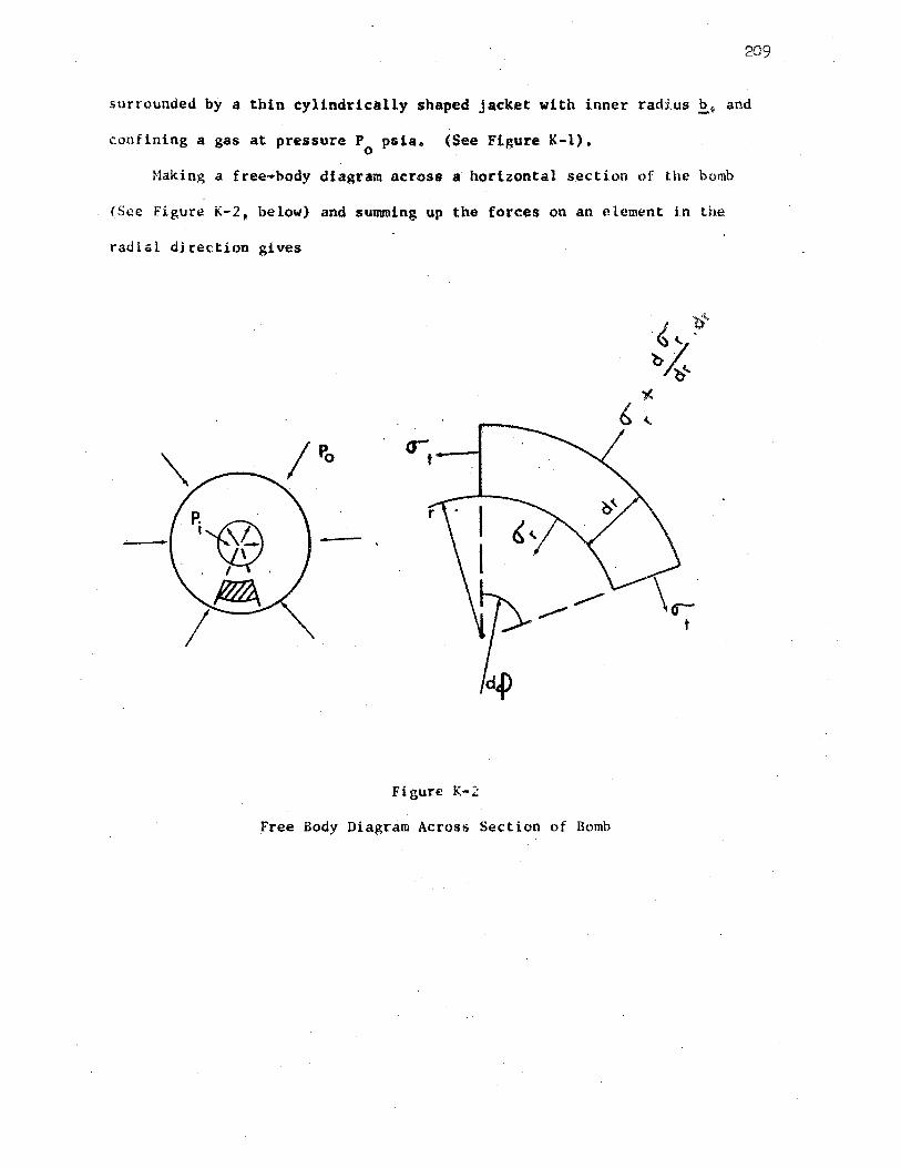
209
surrounded by a thin cylindrically shaped jacket with inner radius~. and
confining a gas at pressure P psia. (See Figure K-1). 0
Making a free•body diagram across a horizontal section of the bomb
(See Figure K-2, below) and summing up the forces on an element in the
radial direction gives
P.~ '¢ -fl/IA.
I
Figure K-2
Free Body Diagram Across Section of Bomb
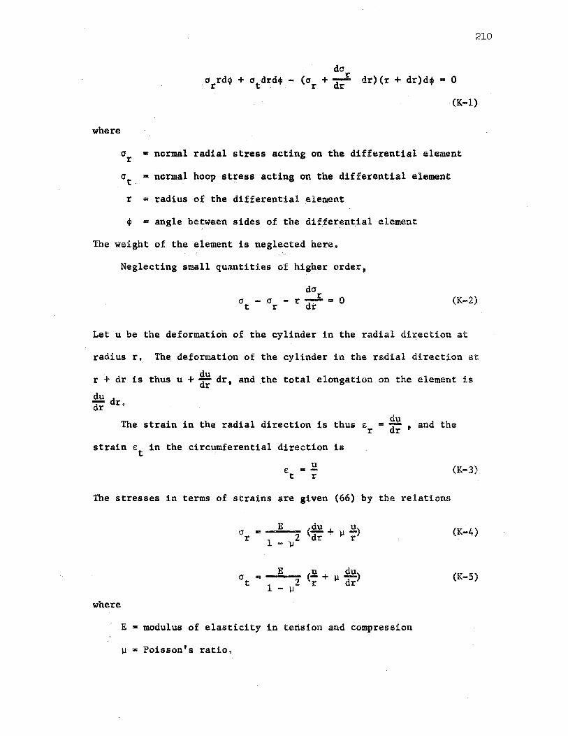
do arrdt + atdrd, - (a + -..I. dr)(r + dr)d+ • O r dr
210
(K-1)
where
or • normal radial stress acting on the differential element
at.• normal hoop stress acting on the differential element
r = radius of the di£ ferential .element
cj) • angle between sides of the differential element
The weight of the element is neglec·ted here ..
Neglecting small quantities of higher order,
do r a -a -r- 111 0
t r di' (K-2)
Let u be the deformation of the cylinder in the radial direction at
radius r. The deformation of the cylinder in the radial direction at
du r + dr is thus u + dr dr, and the total elongation on the element is
du dr dr. du The strain in the radial direction is thus e = -- , and the r dr
strain et in the circumferential direction is
u e ·• -t r
The stresses in terms of strains are given (66) by the relatio11s
where
(J = r
E (~+ .!!.) . 2 dr µ r
1 - µ
- .... E...,__ (.!!. + ~) 0 t • 2 r µ dr
1 - µ
E = modulus of elasticity in tension and compression
µ•Poisson's ratio.
(K-3)
(K-4)
(K-5)
211
Substituting Equations K-4 and K-5 into. Equation K-2, the following
equation results
(K-6)
which may be solved to give
(K-7)
Here c1 and c2 are constants to be .determined from the following condi
tions on the inner and outer surfaces of the bomb,
E 2CC1(l.+ l!} - c2
1 - ll_ a ... I I ]
r 1 - l!
2 r
E 2 [Cl (1 + l!) + c2 l - H (K-8) (J ... 2 ] t
l - l! r
(a ) • -P r b o r=
(a) • -P r i r•a
Solving for c1 and c2 gives
(K-9)
(K-10)
Substituting Equations K-9 and K-10 into Equatio~ K-7 gives the deforma-
tion of the cylinder as
u. (K-11)
The deformation 'i. due to the axial stresses aL must be added to the
deformation given by Equation K-11
e: ·-.!:La u E L
212
(K-13)
Here e:u is the axial strain. uL is of opposite sign to u in Equation
K-11 above, as it is in opposite direction to the deformation u. The
total deformation from both Equations K-11 and K-13 is
u ... l -E
a2p - b2P 2b2(P p) (P a2 - p b2) µ i · or+ (1 + ~)a i - o • 1 _ J;!. i o
(b2 _ a2) E (b2 _ a2) r E (b2 _ a2) r
(K-14)
At the inner radius r = a this deformation must be zero.
u = 0 at r • a (K-15)
This gives
(K-16)
which may be rearranged to
2 2 P ... a (1 - 2µ) + b (1 + µ) • P
0 b2(2 - µ) i (K-17) .
213
For a• 1/2", b • 1 1/4", andµ• 0,3 (for type 303 stainless steel),
Equation K-17 becomes
(K-18)
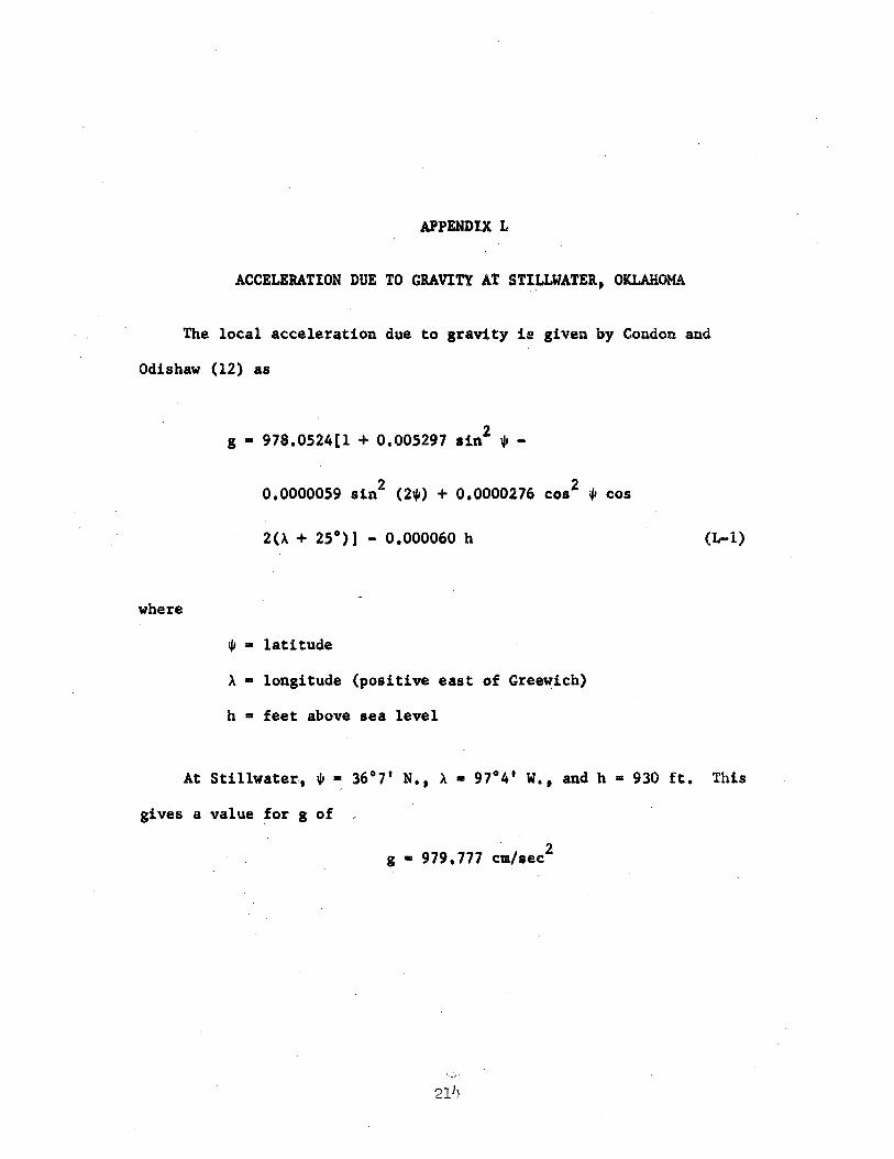
APPENDIX L
ACCELERATION DUE TO GRAVITY AT STILLWATER, OKLAHOMA
The local acceleration due to gravity h given by Condon and
Odishaw (12) as
2 g • 978.0524[1 + 0.005297 sin ~ -
0,0000059 sin2 (2~) + 0,0000276 cos2 ~ cos
2(A + 25°)) - 0,000060 h (L-1)
where
~ • latitude
A• longitude (positive east of Greewich)
h • feet above sea level
At Stillwater, ip '"'. 36°7' N,, ;\, • 97°4' W,, and h • 930 ft. This
gives a value for g of /
. . 2 g • 979,777 cm/sec
214
APPENDIX M
ESTIMATION OF INTERACTION SECOND VIRIAL COEFFICIENTS
In correcting the experimental second virial coefficients for
impurities (Chapter VI) it was necessary to estimate interaction second
virial coefficients B12 for the following molecular pairs: 1) methane
nitrogen, 2) ethylene-ethane, and 3) ethylene-propane. The
estimations were made using the method proposed by Prausnitz (56, 57).
Sample calculations are given below.
Sample Calculation of Methane-Nitrogen Coefficient
The following equation was presented in Chapter III.
(III-18)
The combining rules for e~timating the interaction parameters V 0 cij
T , and wij were given by Prausnitz as cij
215
(M-1)
216
where the temperature correction factor kij is presented graphically as
a function of the ·critical volume ratio V /V , . c1 Cj
Denoting methane by subscript i and nitrogen by subscript j, th~.re .
results
V • l.S7e!/ Ci
V • 1.443 cj
V • -21(1~578 + 1,443) • l,SlOS cij
V /V • 1,578/1,443 • 1.09 Ci Cj . , .
(&Ii• 0,013
(&)j = 0.04 . l
(&)ij = 1<0.013 + 0.04) • 0,0265
From Figure l of reference (56), using a value of V /V of 1,09, Ci . Cj
Tc • 226, 71 j
1/ In the following calculations all units will be £t3/lb mole, psia, and 0 R unless otherwise stated,
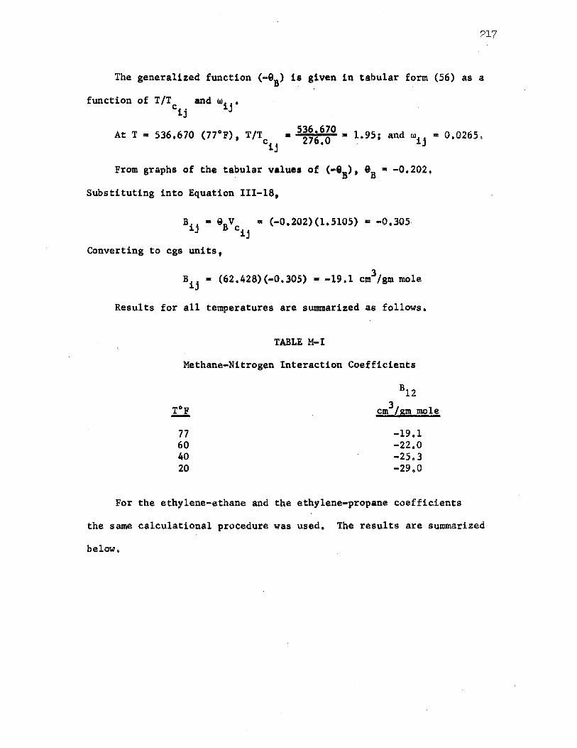
217
The generalized function (-Q8) is given in tabular form (56) as a
function of T/T and w1· j' cij
At T • 536,670 (77°F), T/Tcij • 5~~6~~0 • l.9S; and ooij • 0,0265.
From graphs of the tabular values of (-88), 98 • -0.202,
Substituting into Equation III-18,
Bij • 9BVcij • (-0,202)(1.5105) • -0,30~
Converting to cgs units,
3 Bij • (62.428)(-0,305) • -19,l cm /gm mole.
Results for all temperatures are sUD111arized as follows.
TABLE M-I
Methane-Nitrogen Interaction Coefficients
T°F -77 60 .40 20
-19.1 -22.0 -25.3 -29.0
For the ethylene-ethane and the ethylene-propane coefficients
the same calculational procedure was used, The results are summarized
below.
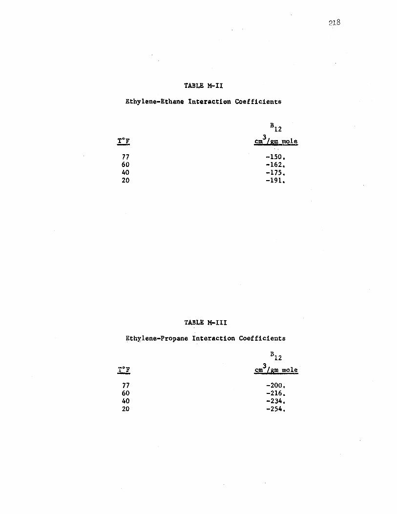
TABLE M-II
Ethylene-Ethane Interaction Coefficients
T°F -77 60 40 20
TABLE M-III
3 .s,m /gm mole
-150. -162. -175. -191.
Eth)'.:lene-Propane Interaction Coefficients
T°F -77 60 40 20
3 cm /gm mole
-200. -216. -234. -254.
218
The results for the ethylene-ethane and ethylene-propane
coefficients are markedly lower (alge~~aically) than the results for
the methane-nitrogen coefficients. This difference is to be
expected• however. and is largely due to the fact that the critical
temperatures of ethylene, ethane~ and propane are considerably higher
than those for methane and nitrogen.
219
APPENDIX N
DERIVATION OF CHARACTERIZING EQUATIONS FOR THE APPARATUS
Det.ermination of the Volume Ratio VD/VB
The determination of the volume ratio was discussed in Chapter IV.
The equition for this ratio is developed in the following.
Basically, the bomb and DPI cell are allowed to reach equilibriumt
the interconnecting valve between the two cells is closed, and the bomb
is rinsed with nitrogen and evacuated, The DPI cell is rinsed and is
then filled to about 2500 psia with the nitrogen,
The temperatures and pressures of all portions of the system are
measured and the interconnecting valve is then opened, After the gas is
allowed to equilibrate throughout the system, the temperatures and
pressures of all portions of the system are again measured. This
information is sufficient to determine the volume ratio as is discussed
below.
The dimensioned schematic diagram of the cryostat and DPI cell is
shown in Figure N-1; the following quantities are defined with reference
to this figure,
VBT = volume of bomb at T°F
= volume of bomb at 95°F
= volume of DPI cell and capillary tubing contained within the DPI celi thermostat at 95°F,
220
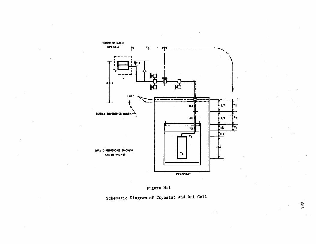
THERMOSTATED DPI CELL I.. Vs ·1 • -......-..v 4
I r----,
Vo L.....1""11 . 8.0 I!~~ ----' .
I l.067~-
+ ---RUSKA REFERENa MAR~
(All DIMENSIONS SHOWN ARE IN INCHES)
----------- T
~-'•
'• I
CRYOSTAT
Figure N-1
I
Schematic Dia~ram of Cryostat and DPI Cell
I T • J/8
'J/1
0 ~ 10.0
,_J_
,,
Vz
'I I
f\) f\) I-'
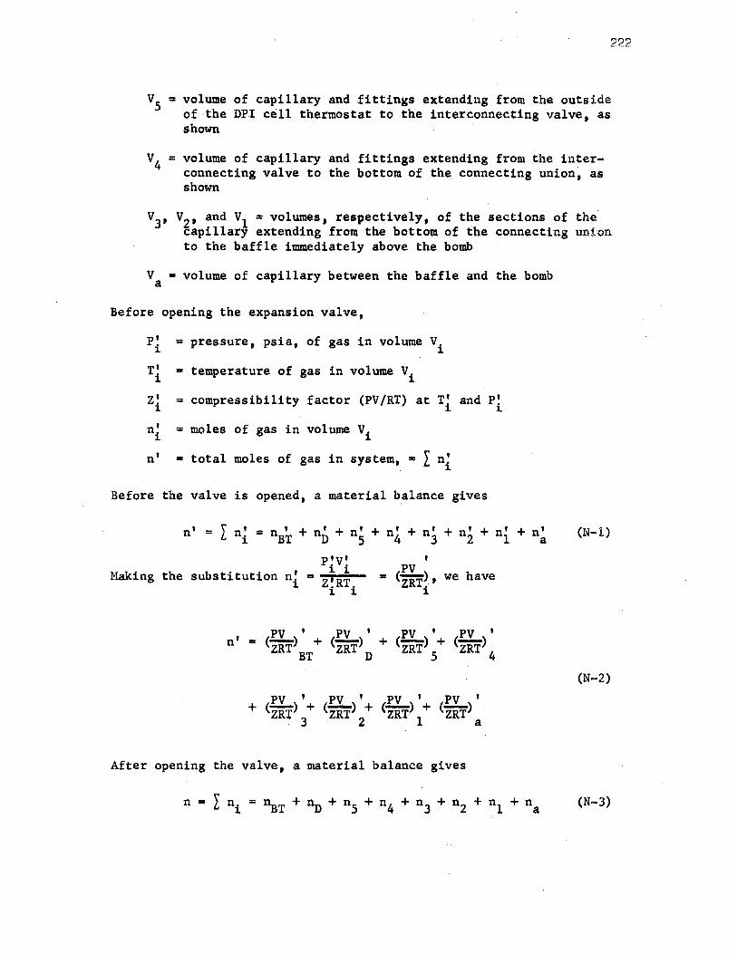
222
v5 = volume of capillary and fittin¥s extending from the outside of the DPI cell thermostat to the interconnecting valve, as shown
v4 = volume of capillary and fittings extending from the interconnecting valve to the b.ottom of the connecting union~ as shown
v3,. v2, and v1 • volumes, respectively, of the sections of the capillary extending from the bottom of the connecting union to the baffle immediately above the bomb
V = volume of capillary between the baffle and the bomb a
Before opening the expansion valve,
P' = pressure, psia, of gas in volume vi i
T' = temperature of gas in volume Vi i
Z! = compressibility factor (PV/RT) at T1 and P' 1 1
n' i = moles of gas in volume vi
n' = total moles of gas in system, = l ni
Before the valve is opened, a material b,alance gives
n' = \' n! = n' + n' + n' + n' + n' + n' + n' + n' l 1 BT D 5 4 3 2 1 a
Pi.Vi Making the substitution n' • -.~-
i z1RTi ' PV
• CzRT), we have i
n' = PV ' PV I PV I PV 1
<zRT) + <zRT) + <zRT) + <zRT) BT D 5 4
PV ' PV I PV ' PV ' + (ZRT) + <zRT) + <zRT) + (ZRT)
· 3 2 1 · a
After opening the valve, a mate.rial balance gives
(N-1)
(N-2)
(N-3)
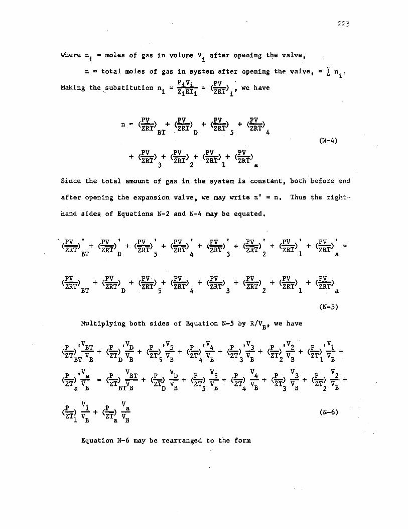
223
where n1 • moles of gas in volume Vi after opening the valve:
n = total moles of gas in system after opening the valve, = l n. • l.
PjVi PV · Making the substitution n. = = (ZRT)i, we have
1. ZiRTi
PV PV PV PV n · = (ZRT) + (ZRT) + (ziff) + (ZRT)
BT· D 5 4 (N-4)
PV PV PV PV + <zRT) + <zRT) + <zRT) + <zRT)
3 2 1 a
Since the total amount of gas in the system is constant, both before and
after opening the expansion valve, we may write n' = n. Thus the right-
hand sides of Equations N-2 and N-4 may be equated.
-- PV ' PV ' PV ' PV ' PV ' PV ' PV ' PV ' (ZRT) + <zRT) + (ZRT) + <zRT) + {ZRT) + <zRT) + (ZRT) + <zRT) "'
BT D 5 4 3 2 1 a
PV PV PV PV PV PV PV PV (ZRT) + (ZRT) + <zRT) + <zRT) + <zRT) + (ZRT) + (ZRT) + (ZRT)
BT D . S 4 3 2 1 a
(N-5)
Multiplying both sides of Equation N-5 by R/VB' we have
c'f-) 'VBT + p 'VD p ,vs P ,v4 P ,v3 P 'v2 P ,vl <rr> v + <zr> v + <rr> v + <zt> v + <zr> v + <zr> v + ZTBT VB D B 5 B 4 B 3 B 2 B 1 B
p 'Va V p VD p vs p V4 p VJ P v2 <zr> v = cL> -E + <n> v + <n> v + <zr> v + <rr> v + <zr> v +
a B ZTBTVB D B 5 B 4 B 3 B 2 B
(N-6)
Equation N-6 may be rearranged to the form
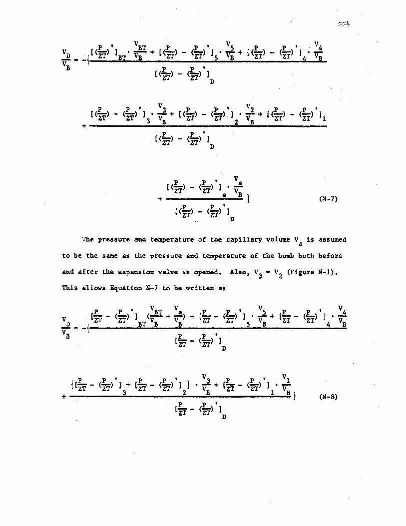
P , V V V v t <-> l • ...!! + c cLzT> - cLzT> ' 1 s. ,....Bs + cc!..> - c!..> ' J • ...! _j2, • -{ ZT BT VB _ v: ZT ZT 4 VB VB p p '
c <u> - <u> 1 D
p p ' · c <zt> - <iT> 1
D
p p ' Va c <zt> - <rt> l; v";
+ } p p ' [ <rt> - <rt> ]
D
(N-7)
224
The pressure and temperature of the capillary volume V is assumed a
to be the same as the pressure and temperature of the bomb both before
and after the expansion valve is opened. Also, v3 = v2 (Figure N-1).
This allows Equation N-7 to be written as
. p p , VT V p p , v5 p p , V4 v ·· lZT - <rt> 1 BT <v: + v;> + Cz'T - <rt> l 5 • v;- + lz'T - Cz'T) l 4 • v; ..E.=-{----------..::;..---------------------------------VB p p ' .
[if - <rt> 1 D
p p ' p p ' V 3 p p ' Vl {[TT - <zt> l + Czt - <rt> l } • v + lzf - <rr> l • v +----------~3 ...... __________ 2 ____ B _____________ 1 _____ B}
p p ' Crt - <TT> l
D
(N•8)
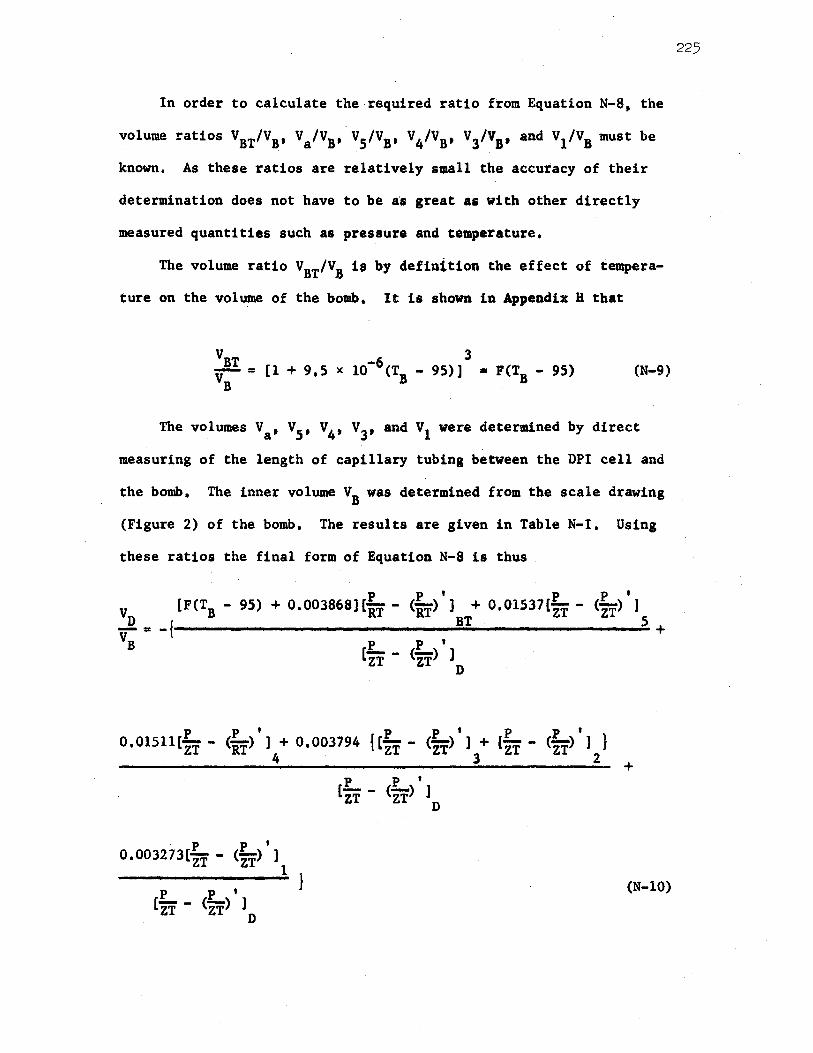
In order to calculate the required ratio from Equation N-8, the
volume ratios V8T/V8, Va/VB, v5/VB' v4tv8, v3/v8, and V1/v8 must be
known. As these ratios are relatively small the accuracy of their
determination does not have to be a's great as with other directly
measured quantities such as pressure and temperature.
The volume ratio v8T/V8 is by definition the effect of tempera
ture on the volume of the bomb. It is shown in Appendix H that
VBT 3 VB = [l + 9,5 x l0-6(TB - 95)] • F(TB - 95) (N-9)
The volumes Va• v5 , v4, v3, and v1 were determined by direct
measuring of the length of capillary tubing between the DPI cell and
the bomb, The inner volume VB was determined from the scale drawing
(Figure 2) of the bomb, The results are given in Table N-I. Using
these ratios the final form of Equation N-8 is thus.
p p ' p p ' V [F(TB - 95) + 0.003868][RT - (RT) ] + 0,01537[ZT - Czf) ] ~ = -{--------------B-T __________ S + VB p p '
lzr - <u> 1 D
P P' P P' P P' o.01s11c"iT - <if> 1 + 0.003194 { c"iT - <u> 1 + err - <rr> 1 l
4 · · 3 2
p . p t
o.003213czf - <zr> 1 _________ 1}
p p ' £TT - <zt> l
D
+
(N-10)
225
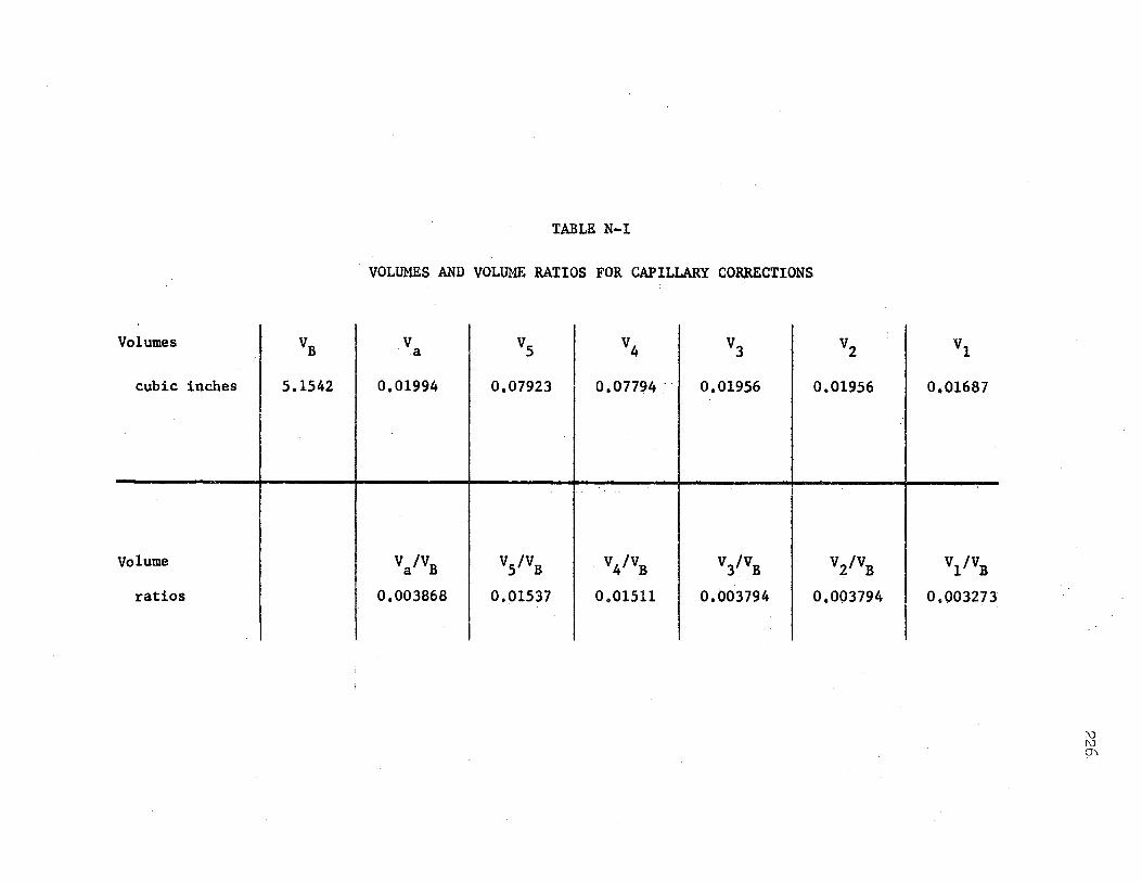
Volumes VB
cubic inches 5.1542
Volume
ratios
TABLE N-I
. VOLUMES AND VOLUME RATIOS FOR CAPILLARY CORRECTIONS
V .. a
0,01994
Va/VB
0,003868
vs
0.07923
VS/VB.
0,01537
v4 I v3
0~01194- I 0.01956
V4/VB
0.01511
ViVB
0.003794
v2
0.01956
V/VB
0,003794
vl
0,01687
Vl/VB
0,003273
I\) I\) O'\
227
Equation N-10 was used in this work to determine the volume ratio.
A sample calculation is given in Appendix E,
p p ' The smaller terms in the expression such,as 0,015ll[ZT - (ZT) ] • 4
represent the correction for the quantity of gas·tn the interconnecting
capillary, In order ·to evaluate these terms it is necessary that the
compressibility factors z5, z4, z3, z2, and z1 be known. For the
volume ratio calibration these compressibili.ty factors are also
determined from the known volumetric properties of nitrogen,
It is worthwhile to point out that the ratio VD/VB is a constant
for the apparatus and does not change with temperature or with each
particular sample as different isochors are being run,
After the volume ratio determination has been completed, the
interconnecting valve is allowed to remain open for all further com-
pressibility determinations with the apparatus,
Pressure Corrections for Differences in Vertical Height
The pressure as determined at the reference mark of the Ruska
piston gage (Figure N-1) is corrected by the factor -0.366 psi (discussed
in Appendix B) to yield the pressure at the level of the diaphragm of
the DPI cell, The pressure correction for the head of gas between the
diaphragm level and each separate section of the high pressure gas system
is discussed as follows.
The pressure correction 6P between any two points 1 and 2,
separated by a vertical displacement h 1 is given by
h pdh. L f pdh
gc o (N-11)
where p • the density of the gas between points 1 and 2,and
g/g = the correction to local acceleration due to gravity, C
If the density is assumed to be constant over the interval ht
Equation N-11 may be written as
228
AP • ~h (N-12) gc .
P(MW} The density of a gas is given by p • ZRT • Comb:1,ning this express:i.f>n
with Equation N-12, it is seen that
/J.P • hP(MW) L (12) 3ZRT le
where AP• the pressure correction, psi
(N-13)
h = the vertical displacement between the two points, inches
P • pressure, psia
MW• the molecular weight of the gas
T = temperature, 0 R
With reference to Figure N-1, it is seen that the pressure P5 of
the gas in the capillary volume v5 may be calculated from a knowledge
of the pressure PD at the diaphragm, and the expression
Cl 6.0(MW) = PD + 1728 Z RT
5 5
(N-14)
Similar expressions for the pressures at volumes v4 , v3• v2, and v1
of the capillary are given by
229
P • P [l + 9.002(MW) .&...] 3 4 1728 z3RT3 le
(N-15)
In each case the vertical distance to the centroid of each particular
section is used.
Finally the pressure PB at the centroid of the bomb is given by
· p • p [l + 11.SOO(MW) · .L] B 1 1728 ZBRTB gc
(N-16)
In the application of the above equations (Equations N-14 through
N-16) for the calculation of pressure corrections, it is seen that
these corrections are very small. In the application of Equations
N-10, N-20, and N"'.'2.1• the above equations are utilized.
Development of Equations for the Compressibility Factors
As was discussed in Chapter IV, the volumetric properties of the
sample along each isochoric path are determined by utilizing the known
volumetric. properties of the sample at the reference temperature.
The cryostat is maintained at 77°F, the system is rinsed and
evacuated, and is then charged to the desired dens~ty with the sample.
After equilibrium has been attained the temperatures and pressures of
all portions of the system are measured.
230
Since the interconnecting valve of the system is open, Equation
N-4, derived previously, applies:
PV PV PV PV n • <zat> + <zat> + <zat> + <zat> +
BT D 5 4
(N-4)
PV. PV PV PV <zat>- + <zat> + <za.T> + <zaT>
3 2 1 a
Dividing both sides of Equation N-4 by VB gives
n P VBT p VD p vs p V4 -= tzRT> v + <zRT> v + <za.T> v + <zaT> v + VB BT B D B S B 4 B
(N-17) P v3 P v2 P vl p V a
<zRT> v + <zRT> v + <za.T> v + (ZRT) -3 B 2 B 1 B a VB
The expr~ssion for VBT/VB has been given in Equation N-9. The
value for VD/VB is known from calibration, using Equation N-10. Values VS V4 V3 V2 Vl Va
of the volume ratios v• v• v• v• v• and V are given in Table N-Io B B B B B B
Equation N-17 may thus be written as
D - n - -= - V . B
p p VD <zRT> [F(T8 - 95) + 0.003868] + <zaT> v +
BT D B
p p p p 0.01537 (ZRT) + 0.01511 (ZRT) + 0,003794 [ (ZT) + Czr) ] +
5 4 3 2
p 0.003273 <.zaT>
1 (N-18)
The quantity D (defined, as n/VB) was mentioned in Chapter IV. Dis
not a true density, but a run constant, since the number of moles n
applies to the entir~ syst~n.i, including the DPI cell, whereas VB
231
•.
represents the volume of the bomb only. Although Dis not a true density
it does have a constant value along an iaochor since the total number of
moles n of the system and the volume VB remain constant, In the
equations th,-t follow, the overall density for the entire system
(including the· DPI cell) is not required. . '
A more .convenient form of Equation N-18 is obtained by making the
substitutions
p = D ~ZRT) D D
p • D .(ZRT)
s 5
p • D4 {N-19) (ZRT)
4
p • D (ZRT)
. 3 3
( p :\ • D m' 2 . 2
The quantities DBT' ~D' n5 , n4, D3, n2, and D1 a;~ true densities
by definition, and are not to be confused with the quantity D, With
these substitutions, Equation N-18 thus becomes
D • [F(TB - 95) + 0.003868]DBT + 0.01263 DD+ 0,01537 D5
(N-20)
232
Equation N-20 was the form used in this work for the determination
·of the quantity D from the reference isotherm.
For the determination of comp,reBSibility factors along the iso-
chor at lower temperatures, it is convenient to rearrange Equation
N-20 to the form
p F(T~ '"". 95) .+ 0.003868 ZBT .. (RT) [ DEN ]
. BT (N-21)
Here DEN represents the denominator of the expression in brackets
and is given by
DEN. D - 0001263 DD - .0.01537 Ds ~ o.01511 D4 ~
00003794 (D3 + D2) - 0.003273 Dl (N-22)
The quantity D appears in the denominator of Equation N-21. Thus
corresponding values of PBT and TBT (the preBSure and temperature in
.the bomb) are sufficient to calculate the compressibility factor ZBT
for any point on the isochor, Equation N-21 was the form used in.
this work for the experimental determination of cpmpressibility factorsc
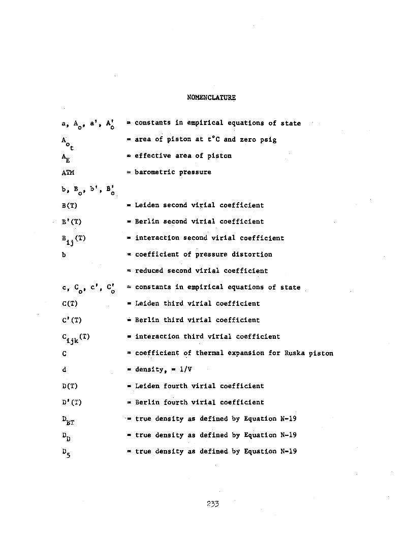
NOMENCLATURE
a, A ' a' A' • constants in empirical equations of state 0 t 0
A = area of piston at t°C and zero psig ot
~ • effective area of piston
ATM = barometric pressure
b, B , b' B' 0 ' 0
-B(T) • Leiden second vi~ial coefficient
B' (T) = Berlin second virial coefficient
• interaction second virial coefficient
• coefficient of pressure distortion
• reduc.ed second virial coefficient
c, C , c' C' 0 ' 0
= constants in empirical equations of state
C(T) • Leiden third virial coefficient
C' (T) • Berlin third virial coefficient
Cijk(T) • interaction third virial coefficient
C = coefficient of thermal expansion for Ruska piston
d •density,• 1/V
D(T) • Leiden fourth virial coefficient
D' (T) = Berlin fourth virial coefficient
DBT ·• true density as defined by Equation N-19
DD • true density as defined by Equation N-19
DS = true density as defined by Equation N-19
233
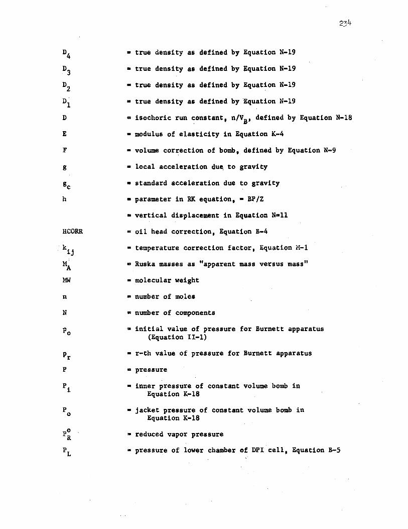
E
F
g
HCORR
n
N
p 0
• true density as defined by Equation N-19
• true density as defined by Equati.on N-19
• true density as defined by Equation N-19
• true density as defined by ·,Equation N-19
• isochoric run ~onstant, n/v8• defined by Equation N-18
• modulus of elasticity in Equation K-4
• volume correction of bomb, defined by Equation N-9
• local acceleration du~ to gravity
• standard acceleration due to gravity
• parameter in RK equation,• BP/Z
• vertical displacement in Equation N•ll
= oil head correction, Equation B-4
• temperature correction factor, Equation M-1
• Ruska masses as "apparent mass versus mass"
• molecular weight
• number of moles
• number of components
• initial value of pressure for Burnett apparatus (Equation II-1)
• r•th value of pressure for Burnett apparatus
• pressure
• inner pressure of, constant volume bomb in Equation K-18
• jacket pressure of constant volume bomb in Equation K-18
• reduced vapor pressure
• pressure of lower chamber of DPI cell, Equation B-5
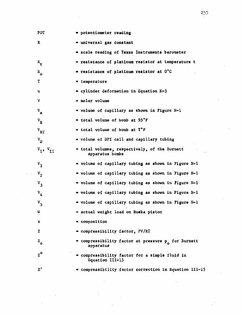
POT
R
Rt
R 0
T
u
V
V a
VB
VBT
VD
VI' VII
vl
v2
v3
V4
vs w
X
z
z 0
zo
Z'
• potentiometer reading
• universal gas constant
• scale reading of Texas Instruments barometer
• resistance of platinum resistor at temperature t
• resistance of platinum resistor at 0°C
• temperature
• cylinder deformation in Equation K-3
• molar volume
• volume of capillary as shown.in Figure N-1
• total volume of bomb at 95°F
• total volume of bomb at T°F
• volume of DPI cell and capillary tubing
= total volumes, respectively, of the. Burnett apparatus bombs
• volume of capillary tubing as shown in Figure N-1
• volume of capillary tul;>ing as shown in Figure N-1
• volume of capillary tubing as shown in Figure.N-1
• volume of capillary tubing as shown in Figure N-1
• volume of capillary tubing as shown in Figure N-1
= actual weight load on Ruska piston
• composition
•. compressibility factor,. PV/RT
= compress~bility factor at pressure p for Burnett 0 apparatus
= compressibility factor for a simple fluid in Equation III-15·
235
• compressibility factor correction in Equation III-15
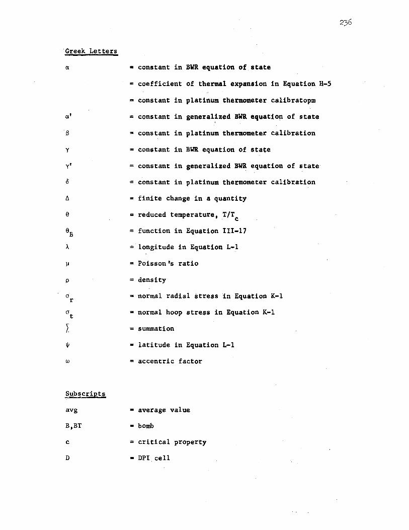
Greek Letters
a
a'
y
y'
µ
p
w
Subscripts
avg
B,BT
C
D
• constant in BWR equation of state
= coefficient of thermal expansion in Equation H-5
= constant in platinum thermometer calibratopm
= constant in generalized BWll equatfop of state
= constant in platinum thermometer calibration
= constant in BWR equation of sta{e
= constant in generalized JWR equation of state·
= constant in platinum thermometer calibration
= finite change in a quantity
• reduced temperature, T/Tc
= function in Equation 111~17
= longitude in Equation L-1
= Poisson's ratio
= density
= normal radial stress in Equation K-1
= normal hoop stress in Equation K-1
= summation
= latitude in Equation L-1
= accentric factor
= average value
• bomb
= critical property
= DPI cell
237
E • effective
i, j, k • component• of a mixture.
m • mixture
r • number of expansion for Burnett apparatus (Equation 11•1)
B. • reduced property
s, 4, 3, 2, l • propertiea of expo1ed . .-pparatus 1ectiona s. 4, 3, 2 and l, respectively (l'i1ure 1-1)·
Superscri_pts
' • property of apparatus before opening expansion value
VITA
Henry Grady McMath, Jr.
Candidate for the Degree of
Doctor of Philosophy
Thesis: VOLUMETRIC PROPERTIES AND VIRIAL COEFFICIENTS OF THE METHANE-ETHYLENE SYSTEM, USING THE TECHNIQUE OF ISOCHORIC CHANGES OF PRESSURE WITH TEMPERATURE
Major Field: Chemical Engineering
Biographical:
Personal Data: Born in El Dorado, Arkansas, January 29, 1939• the son of Henry Grady and Fannie Lou McMath. Married to Sara F. Adcox of El Dorado, Arkansas, on July 2, 1960,
Education: Attended elementary school in Strong, Arkansas; attended high school in Strong, Arkansas and El Dorado, Arkansas, graduating from El Dorado High School in 1956; received the Bachelor of Science degree in Chemical Engineering from Louisiana Polytechnic Institute in January, 1961; received the Master of Science degree in Chemical Engineering from Louisiana Polytechnic Institute in June, 1962; completed the requirements for the Doctor of Philosophy degree at Oklahoma State University in May, 1967.
Professional Experience: Employed in the Technical Service Department of Monsanto Chemical Company the summers of 1960 and 1961, Currently on active duty with the United States Air Force, serving as Project Officer, Ultra-Energy Concepts, Air Force Rocket Propulsion Laboratory', Edwards AFB, California.