Embed Size (px)
Citation preview

MoDOT
TE 5092 .M8A3 no.90-4
RI COOPERATIVE HIGHWAY RESEARCH PROGRAM
FINAL REPORT
DETERMINATION OF AASHTO DRAINAGE COEFFICIENTS
MISSOURI HIGHWAY AND TRANSPORTATION DEPARTMENT FEDERAL HIGHWAY ADMINISTRATION
90-4
Property of
MoDOT TRANSPORTATION LIBRARY
DETERMINATION OF AASHTO DRAINAGE COEFFICIENTS
STUDY 90-4
Prepared for
MISSOURI HIGHWAY AND TRANSPORTATION DEPARTMENT
by DAVID N. RICHARDSON WILLIAM J. MORRISON
PAUL A. KREMER KEVIN M. HUBBARD
DEPARTMENT OF CIVIL ENGINEERING UNIVERSITY OF MISSOURI - ROLLA
ROLLA, MISSOURI
in cooperation with U.S. DEPARTMENT OF TRANSPORTATION
FEDERAL HIGHWAY ADMINISTRATION
June 1996
The opinions, findings and conclusions expressed in this publication are not necessarily those of the Federal Highway Administration.
I IIIIIIII IIII Ill/ ll]ij1~li1]~~f 11111 1111111111111 RD0009047

I I I I I I I I I I I I I I I I I I I
ii
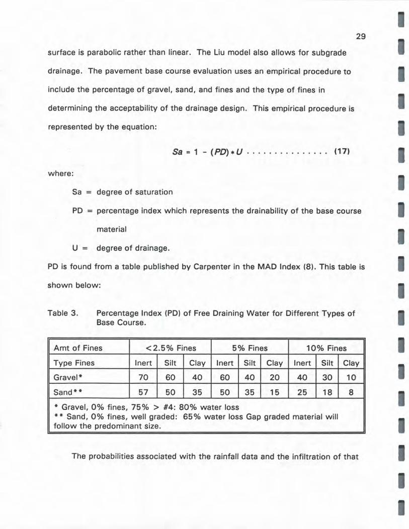
EXECUTIVE SUMMARY
This study was conducted to determine the drainage (m) coefficients of
granular bases and subbases for use in the 1986 AASHTO Guide pavement design
method. The project entailed a review and compilation of published literature,
laboratory testing, analysis of results, and preparation of this report.
One existing method which is used to determine drainage coefficients was
examined, and two potential strategies for development into a new method were
explored.
Use of the AASHTO Guide method necessitates the determination of: 1) the
Percent Time of Saturation of the pavement structure, and 2) the Quality of
Drainage of the base and subbase. With these, the m-coefficients are found from
a table. Unfortunately, little direction was given in regard to the determination of
the necessary input data that is necessary in order to use the table.
Carpenter developed a method to determine m-coefficients which can be
easily implemented by use of software called DAMP. Carpenter provided a method
to determine the Percent Time of Saturation for the pavement structure, and the
Quality of Drainage of the combined base and subgrade. DAMP does not lead to
reasonable results if one subscribes to the theory that the Road Test pavement
drainage was "Fair." The whole idea of the use of m-coefficients is to rate any
pavement's drainage relative to that at the Road Test . Better drainage should be
"Good" or "Excellent," worse drainage should be "Poor" or "Very Poor." Also, the
effect of freeze-thaw cycles and frost heave is not emphasized. The extrapolation
of the Thornthwaite method of regional moisture available to the conditions in the
iii
pavement structure is of concern. Also, the manner in which the time of
saturation for various environmental conditions is calculated is arbitrary. However,
it is recognized that at the present time there are no practical working solutions to
this dilemna, and that the time of saturation procedure in DAMP is a significant
step forward, and it or some modification should be used until a more
fundamentally sound, user-friendly method can be developed.
The TTI Integrated Model of the Climatic Effects on Pavements was
evaluated with the idea that it could be used to determine environmental effects on
granular base/subbase materials, which would lead to the calculation of m
coefficients. Unfortunately, the scheme· was unsuccessful because of limitations in
the TTI model. First, the model requires a minimum of 100 input variables, many
of which are not easily obtained and must be assumed. Model output is sensitive
to the magnitude of some of these input values. Secondly, the model has a low
sensitivity to variables that are thought to be important to the derivation of m
coefficients. Third, the program is somewhat cumbersome. And most
importantly, the output parrots the input base course modulus. This is a fatal flaw
and rendered the program unusable for purposes of drainage coefficient
determination as envisioned in this study.
The materials under study included two sources of crushed stone and two
gravels. All materials were selected, sampled, and delivered to UMR by MHTD
personnel. The primary tests performed were: 1) resilient modulus testing at a
low and high degree of saturation to assess the moisture sensitivity of the
materials, and 2) permeability and effective porosity to assess the drainage
I
I I I I I I I
I
I
I I I I I I I I I I I I I I I I I I
iv
characteristics of the materials.
Two gradations of granular material were used in the resilient modulus
testing: one followed the midpoint of the MHTD Type 1 gradation (MHTD Middle)
acceptance band, and the other was the so-called New Jersey (NJ) open-graded
gradation. An additional gradation (OGS) was used in the permeability portion of
the study, along with the MHTD Middle and the NJ. The aggregates were also
tested for specific gravity, plasticity index (Pl), moisture-density relationships, and
relative density.
Particle shape/surface texture tests were performed on the four aggregates.
The measured angularities of the two stones were about the same, and were more
angular than the two gravels, which were about equal. The difference in
angularity/texture was not great between the crushed stones and the gravels.
Resilient modulus (Eul test results were required for use in the TTI method
and in the new method developed in this study. The tests were run on all four
aggregates using two gradations, two compactive efforts, and two degrees of
saturation, with replications. Fourteen combinations of confining pressure and
cyclic applied deviator stress were used for each specimen in the test sequence.
The results of the testing indicated the Eu increases with a lower
degree of saturation. The average percent loss in k1 (intercept of the Eu - bulk
stress plot) due to increased saturation was 31 %. This information was used in
the development of the m-coefficients. The data showed that the drained open
graded moduli were greater than the undrained dense-graded moduli . An increase
in degree of saturation acted to lower k1 and raise k2 (slope of the Eu - bulk stress

V
plot) of the granular material, and to lower subgrade support, all of which acted to
lower the E9
of the granular material.
Permeability of base material is required input for DAMP, TTI Integrated
model, and the method developed in this study. Permeability data are necessary in
order to calculate the time-to-drain for base layers. The rigid wall constant head
test procedure was used for the NJ and OGS open-graded materials, while the
dense-graded specimens were tested in a triaxial compression chamber (flexible
wall, constant head).
Permeabilities estimated from the Moulton equation significantly
underestimated the observed values by an average of seven times . A review of
the data on which the Moulton equation is based reveals potential problems with
air blockage, effect of end conditions, and possibly incorrect use of specific gravity
data, all of which would lead to falsely low values.
I
I
The gravels exhibited slightly greater permeabilities than the crushed stones, I but not statistically so at the 0.05 level.
On the average, the effective porosities of the dense-graded and open-
graded materials were about 27% and 68% of the total porosities, respectively.
The dense-graded effective porosity is considerably smaller than the open-graded
value, which is to be expected because of the finer pore sizes in the dense-graded
material.
Overall, the permeabilities of the dense-graded materials were significantly
lower by several orders of magnitude than the open-graded materials (average of
0.8 vs 1014 ft/day).
I
I

I
I I
I
I I I I I I I I I I I
vi
A regression equation to estimate permeability was developed by combining
the results from several studies found in the literature with the results of this
study. The equation had an adjusted-R2 = 0.900. The equation is considered
accurate in the range of 0. 1 to 1000 ft/day.
Although the Moulton equation significantly underpredicts permeability, it
may be the equation of choice because field conditions may render the base layer
less permeable than what would be predicted with good quality laboratory testing.
A new method of calculation of drainage coefficients was developed. In
essence, m-coefficients were calculated as a ratio of the layer coefficient of Road
Test granular base material under a given drainage and climate condition to the
layer coefficient under Road Test site conditions. The layer coefficients were
calculated from resilient moduli. The resilient moduli were calculated with the
program KEN LA YER under varying conditions. By changing subgrade and base
moisture conditions for a given time of year, the moduli were varied. The base
material moisture sensitivity (effect on k1 and k2 ) was determined in part by the
resilient modulus laboratory testing of granular materials. The result of the above
analysis was the creation of a Quality of Base Drainability table (based on time-to
drain to 85 percent saturation), a Quality of Subgrade Drainability table (based on
subgrade permeability, position of water table, flooding potential, presence of
impermeable layers, potential for water seepage, and so forth), a Quality of
Pavement Drainage table (based on the previous two tables), a Climate Condition
table (based on estimated season lengths), and finally, an m-coefficient table
(based on Quality of Pavement drainage and Climate Condition).

vii
A regression equation was developed to assist in the estimation of
compacted dry density in order to estimate permeability with the Moulton equation
and the UMR equation. The equation had an adjusted-R2 = 0. 729.
A sensitivity analysis was performed. The most important variables in
regard to m-coefficient calculation were climate condition, base drainability, and
subgrade drainability. These, in turn, affected base thickness calculation
significantly.
In comparison of Missouri sites to the Road Test site, in a regional sense
actual data indicates that most of Missouri is in a climatic zone that is rated as
having a greater time of saturation, so a given paveme.nt in Missouri should fare
worse (from moisture-related problems) and therefore should have m-coefficients
less than 1 .0, unless something is done to improve the pavement drainage.
Conversely, for a situation where any water that enters the base is quickly
removed laterally and where the soil drains well and does not supply water from
the surrounding soil or side hill wet weather springs and so forth, then an
expectation of a 10 to 20% improvement in pavement performance would be
reasonable. For a somewhat lesser quality of subgrade drainage with a highly
drainable base, a 10% credit may be more realistic. And, going with the belt-and
suspenders approach, there is the option of supplying a drainable section with no
reduction in pavement thickness.
I
I I I I I I I
I I I I I I I I I I I
viii
TABLE OF CONTENTS PAGE
EXECUTIVE SUMMARY . . . . . . . . . . . . . . . . . . . . . . . . . . . . . . . . . . . . . . . ii
TABLE OF CONTENTS ....................................... viii
LIST OF FIGURES ........................................... xii
LIST OF TABLES I • • • I I I I I I I I I I I I I I I I I I I I I I I I I I I I I I I I I I I I I I xiv
INTRODUCTION . . . . . . . . . . . . . . . . . . . . . . . . . . . . . . . . . . . . . . . . . . . 1 GENERAL . . . . . . . . . . . . . . . . . . . . . . . . . . . . . . . . . . . . . . . . . . . 1 OBJECTIVES AND SCOPE . . . . . . . . . . . . . . . . . . . . . . . . . . . . . . . 4
DATA PROCUREMENT .............. . ....................... 5 GENERAL . . . . . . . . . . . . . . . . . . . . . . . . . . . . . . . . . . . . . . . . . . . 5
. SOIL SURVEYS ........ . · . . . . . . . . . . . . . . . . . . . . . . . . . . . . . . 5 MATERIAL PHYSICAL, THERMAL, AND MOISTURE
PROPERTIES/DAT A . . . . . . . . . . . . . . . . . . . . . . . . . . . . . . . . 5 CLIMATOLOGICAL DAT A . . . . . . . . . . . . . . . . . . . . . . . . . . . . . . . . 5 UNBOUND GRANULAR MATERIAL DRAINABILITY PROPERTIES . . . . . 6 PAVEMENT STRUCTURAL PROPERTIES . . . . . . . . . . . . . . . . . . . . . . 6 PAVEMENT SECTION GEOMETRY . . . . . . . . . . . . . . . . . . . . . . . . . . 7
ALTERNATIVE METHODS FOR DETERMINATION OF DRAINAGE COEFFICIENTS ...................................... . GENERAL .......................................... . 1986 AASHTO METHOD ............................... .
8 8 9
General . . . . . . . . . . . . . . . . . . . . . . . . . . . . . . . . . . . . . . . . 9 Standards for Quality of Drainage . . . . . . . . . . . . . . . . . . . . . . 9 Time-to-Drain Calculations . . . . . . . . . . . . . . . . . . . . . . . . . . . 10 Flexible Pavement Drainage Coefficients (m) .............. .
Relation to Quality of Drainage .................. . Effects of Varying Moisture Levels ................ .
DAMP ............................................ .
11 11 12 15 15 16 16 21 23 25 25 26 26
General ....................................... . Drainage Coefficient Determination .................... .
Drainage Layer Characteristics and Base Drainage Times .. Percent Time of Saturation ..................... . Subgrade Drainage ........................... . Quality of Drainage .......................... . AASHTO Drainage Coefficient Selection ............ .
TII I I I I I I I I I I I I I I I I I I I I I I I I I I I I I I I I I I I I I I I I I I I I I I I
General I I I I I I I I I I I I I I I I I I I I I I I I I I I I I I I I I I I I I I I I

ix
Precipitation Model . . . . . . . . . . . . . . . . . . . . . . . . . . . . . . . . 28 Infiltration and Drainage Model . . . . . . . . . . . . . . . . . . . . . . . . 28 Climatic-Materials-Structural Model . . . . . . . . . . . . . . . . . . . . . 30 CRREL Frost Heave and Thaw Settlement Model . . . . . . . . . . . . 30
MATERIAL TYPES AND SOURCES . . . . . . . . . . . . . . . . . . . . . . . . . . . . . . 32
LABORATORY INVESTIGATION . . . . . . . . . . . . . . . . . . . . . . . . . . . . . . . . 33 GENERAL ........................................... 33 EXPERIMENT AL GRADATIONS . . . . . . . . . . . . . . . . . . . . . . . . . . . . 33 GRADATION CURVE SHAPE/POSITION . . . . . . . . . . . . . . . . . . . . . . 34 PARTICLE SHAPE/TEXTURE . . . . . . . . . . . . . . . . . . . . . . . . . . . . . . 34 SPECIFIC GRAVITY . . . . . . . . . . . . . . . . . . . . . . . . . . . . . . . . . . . . 36 SCREENING . . . . . . . . . . . . . . . . . . . . . . . . . . . . . . . . . . . . . . . . . 37 SPECIMEN FABRICATION . . . . . . . . . . . . . . . . . . . . . . . . . . . . . . . . 37 MOISTURE - DENSITY RELATIONSHIP . . . . . . . . . . . . . . . . . . . . . . . 38 RESILIENT MODULUS . . . . . . . . . . . . . . . . . . . . . . . . . . . . . . . . . . 38
General ........................................ 38 Equipment . . . . . . . . . . . . . . . . . . . . . . . . . . . . . . . . . . . . . . 39 Test Variables . . . . . . . . . . . . . . . . . . . . . . . . . . . . . . . . . . . 41
Stress State . . . . . . . . . . . . . . . . . . . . . . . . . . . . . . . . 41 Degree of Saturation . . . . . . . . . . . . . . . . . . . . . . . . . . 42 Degree of Compaction . . . . . . . . . . . . . . . . . . . . . . . . . 42 Particle Shape/Surface Texture . . . . . . . . . . . . . . . . . . . 44
Testing Scheme . . . . . . . . . . . . . . . . . . . . . . . . . . . . . . . . . . 44 Test Procedure . . . . . . . . . . . . . . . .. . . . . . . . . . . . . . . . . .. . . 44
PERMEABILITY . . . . . . . . . . . . . . . . . . . . . . . . . . . . . . . . . . . . . . . 46 General ........................................ 46 Testing Concerns . . . . . . . . . . . . . . . . . . . . . . . . . . . . . . . . . 49
Air Blockage . . . . . . . . . . . . . . . . . . . . . . . . . . . . . . . . 49 Movement of Fines . . . . . . . . . . . . . . . . . . . . . . . . . . . 50 Excessive Gradients . . . . . . . . . . . . . . . . . . . . . . . . . . . 50 Direction of Flow . . . . . . . . . . . . . . . . . . . . . . . . . . . . . 51 Off-Target Density . . . . . . . . . . . . . . . . . . . . . . . . . . . . 52
Rigid Wall Permeameter . . . . . . . . . . . . . . . . . . . . . . . . . . . . . 52 Equipment . . . . . . . . . . . . . . . . . . . . . . . . . . . . . . . . . 52 Procedure . . . . . . . . . . . . . . . . . . . . . . . . . . . . . . . . . . 58
Flexible Wall Permeameter . . . . . . . . . . . . . . . . . . . . . . . . . . . 61 Equipment . . . . . . . . . . . . . . . . . . . . . . . . . . . . . . . . . 61 Procedure . . . . . . . . . . . . . . . . . . . . . . . . . . . . . . . . . . 61
POROSITY . . . . . . . . . . . . . . . . . . . . . . . . . . . . . . . . . . . . . . . . . . 62 EFFECTIVE POROSITY . . . . . . . . . . . . . . . . . . . . . . . . . . . . . . . . . . 66
RES UL TS OF THE LABORATORY INVESTIGATION . . . . . . . . . . . . . . . . . . . 68 AS-RECEIVED GRADATIONS . . . . . . . . . . . . . . . . . . . . . . . . . . . . . . 68
I
I
I
I
I
I
I
I I
X
EXPERIMENTAL GRADATIONS ............................ 68 GRADATION CURVE SHAPE/POSITION . . . . . . . . . . . . . . . . . . . . . . . 69 MOISTURE-DENSITY RELATIONSHIPS AND SPECIFIC GRAVITIES ..... 74 PARTICLE SHAPE AND SURFACE TEXTURE . . . . . . . . . . . . . . . . . . . 75 PLASTICITY OF FINES . . . . . . . . . . . . . . . . . . . . . . . . . . . . . . . . . . 76 RESILIENT MODULUS . . . . . . . . . . . . . . . . . . . . . . . . . . . . . . . . . . . 76 ST A TISTICAL ANALYSIS . . . . . . . . . . . . . . . . . . . . . . . . . . . . . . . . 81 PERMEABILITY, POROSITY, AND EFFECTIVE POROSITY ........... 87
Open-Graded Materials . . . . . . . . . . . . . . . . . . . . . . . . . . . . . 87 Dense-Graded Materials . . . . . . . . . . . . . . . . . . . . . . . . . . . . . 96
ESTIMATION OF PERMEABILITY . . . . . . . . . . . . . . . . . . . . . . . . . . . . . . . 105
RESULTS OF MODELS EVALUATION . . . . . . . . . . . . . . . . . . . . . . . . . . . . 114 TTI INTEGRATED MODEL . . . . . . . . . . . . . . . . . . . . . . . . . . . . . . . 114 DAMP ............................................ 116 CONTRAST BETWEEN THE INTEGRATED PROGRAM AND DAMP . . . . 120
DRAINAGE COEFFICIENT DETERMINATION . . . . . . . . . . . . . . . . . . . . . . . 122 GENERAL . . . . . . . . . . . . . . . . . . . . . . . . . . . . . . . . . . . . . . . . . . 122 AASHO ROAD TEST . . . . . . . . . . . . . . . . . . . . . . . . . . . . . . . . . . 122 DETERMINATION OF AASHTO DRAINAGE COEFFICIENTS-UMR
METHOD ...................................... 124 General Methodology . . . . . . . . . . . . . . . . . . . . . . . . . . . . . . 124 Quality of Base Drainage . . . . . . . . . . . . . . . . . . . . . . . . . . . 131 Subgrade Quality of Drainage . . . . . . . . . . . . . . . . . . . . . . . . 134 Pavement Structure Quality of Drainage . . . . . . . . . . . . . . . . . 134
DEVELOPMENT OF M-COEFFICIENT TABLE . . . . . . . . . . . . . . . . . . . 136 Reasonableness . . . . . . . . . . . . . . . . . . . . . . . . . . . . . . . . . 146
MO DAMP SENSITIVITY ANALYSIS - . . . . . . . . . . . . . . . . . . . . . . . . . . . . . 148 M-Coefficient Analysis . . . . . . . . . . . . . . . . . . . . . . . . . . . . . 148
SUMMARY AND CONCLUSIONS . . . . . . . . . . . . . . . . . . . . . . . . . . . . . . . 152
RECOMMENDATIONS . . . . . . . . . . . . . . . . . . . . . . . . . . . . . . . . . . . . . . 163
FUTURE RESEARCH NEEDS . . . . . . . . . . . . . . . . . . . . . . . . . . . . . . . . . . 164
ACKNOWLEDGEMENT ..................................... 165
REFERENCES 166
APPENDIX A . . . . . . . . . . . . . . . . . . . . . . . . . . . . . . . . . . . . . . . . . . . . 175 REQUIRED INPUT FOR TII MODEL . . . . . . . . . . . . . . . . . . . . . . . . . 175
xi
APPENDIX 8 ............................................. 180
USE OF DAMP MANUAL ..................................... 181 GENERAL ........................................... 181 USE OF DAMP DATA FILES .............................. 181 INTERACTIVE DAMP INPUT SELECTION ...................... 182 SUMMARY REQUIREMENTS FOR DAMP INPUT ................. 182
Pavement Geometry ............................... 182 Layer Thicknesses ................................ 183 Layer Densities ................................... 183 Base Course Gradation and Specific Gravity ............... 183 Subgrade Drainability/Permeability ...................... 183 Other Input Variables .............................. 184
DRAINAGE COEFFICIENT OUTPUT SCREEN ................... 185
APPENDIX C ............................................. 186 MODAMP MANUAL .................................... 186 GENERAL ........................................... 187 LOADING MODAMP AND CLIMATOLOGICAL DATA SPREADSHEETS . 187
Software and Hardware ............................. 187 Loading ........................................ 187
MO DAMP DISPLAY .................................... 188 Permeability of the Drainage Layer ..................... 188 Slope Factor .................................... 189 Thickness of Base ................................. 189 Subgrade Drainability .............................. 189 Time-to-Drain/Quality of Base Drainage .................. 191 Quality of Pavement Drainage ........................ 192 Time of Saturation ................................ 192 Climate Condition ................................. 193 Drainage Coefficients .............................. 193
APPENDIX D ............................................. 194 I
I I
I I I I I I I I
I
I I
xii
LIST OF FIGURES 1. Recommended m-values as a function of the Quality of Drainage and
the Exposure to Saturation (after Seeds and Hicks (4)) . . . . . . . . . . . . 14 2. Moulton Nomograph for Estimation of Base Course Permeability . . . . . 17 3. Integrated Program Flowchart . . . . . . . . . . . . . . . . . . . . . . . . . . . . . 27 4. Semilog Plot of Three Experimental Gradations . . . . . . . . . . . . . . . . . 35 5. Resilient Modulus Testing Equipment . . . . . . . . . . . . . . . . . . . . . . . . 40 6. Rigid Wall Permeameter . . . . . . . . . . . . . . . . . . . . . . . . . . . . . . . . . 53 7. Schematic of Rigid Wall Permeameter Test Station . . . . . . . . . . . . . . . 55
. 8. Field Gradient . . . . . . . . . . . . . . . . . . . . . . . . . . . . . . . . . . . . . . . . 60 9. Flexible Wall Permeameter Test Station . . . . . . . . . . . . . . . . . . . . . . 63 10. Schematic of Flexible Wall Permeameter Test Station . . . . . . . . . . . . . 64 11. Gradations Used in the Industry-wide Permeability Algorithm . . . . . . . . 72 12. Typical Vibratory Table Test Result . . . . . . . . . . . . . . . . . . . . . . . . . 77 13. Compaction Curves for MHTD Base Rock . . . . . . . . . . . . . . . . . . . . . 78 14. Typical Bulk Stress - Resilient Modulus Relationship . . . . . . . . . . . . . . 79 15. Relationship Between Experimentally Derived Factors (k1 and k2 ) for
the Theta Model . . . . . . . . . . . . . . . . . . . . . . . . . . . . . . . . . . . . . . 84 16. . Effect of Degree of Saturation and Aggregate Source on Resilient
Modulus ............................................ 85 17. Effect of Gradation, Degree of Saturation, and Compactive Effort on
Resilient Modulus . . . . . . . . . . . . . . . . . . . . . . . . . . . . . . . . . . . . . 86 18. Typical Constant Head Rigid Wall Permeameter Test Result . . . . . . . . . 89 19. Relationship of Porosity and Effective Porosity . . . . . . . . . . . . . . . . . . 93 20. FHWA 0.45 Power Paper Plot of Experimental Gradations . . . . . . . . . . 94 21. Plot of Individual Percent Retained for NJ and OGS Gradations . . . . . . 95 22. Relationship of Porosity and Permeability . . . . . . . . . . . . . . . . . . . . . 97 23. Relationship of Effective Porosity and Permeability . . . . . . . . . . . . . . . 98 24. Relationship of Observed Permeability and Estimated Permeability for
Open-Graded Materials . . . . . . . . . . . . . . . . . . . . . . . . . . . . . . . . . . 99 25. Relationship of Observed Permeability and Estimated Permeability for
Dense-Graded Materials .................................. 103 26. Relationship of Observed Permeability and Estimated Permeability for
Several Studies ....................................... 111 27. Relationship of Observed Permeability and Permeability Estimated by
Moulton Equation ..................................... 112 28. Relationship of Observed Permeability and Permeability Estimated by
the UMR Equation ..................................... 113 29. Variation of Subgrade Resilient Modulus Through the Year ......... 127 30. Six Climate Zones in the United States ....................... 129 31. Average AASHO Road Test Cross-Section .................... 138 32. Relationship of Road Test Resilient Modulus and Deviator Stress for
Three States of Moisture Content .......................... 142 33. Resilient Modulus Seasonal Variation With Variations in Base and
Subgrade Drainability ........ . .............. . ........... 145
xiii
C1. Typical MODAMP Screen ................................ 190
I I I I
I

1.
I 2.
3.
4. 5. 6. 7. 8. 9. 10. 11 . 12. 13. 14. 15. 16. 17. 18. 19. 20. 21. 22. 23.
24. 25. 26. 27. 28. 29. 30. 31. 32. 81. C1. C2.
xiv
LIST OF TABLES Recommended mi Values for Modifying Structural Layer Coefficients of Untreated Base and Sub-base Materials in Flexible Pavements . . . . . 13 AASHTO Quality of Drainage Using Calculated Base and Subgrade Drainability Values . . . . . . . . . . . . . . . . . . . . . . . . . . . . . . . . . . . . . 25 Percentage Index (PD) of Free Draining Water for Different Types of Base Course . . . . . . . . . . . . . . . . . . . . . . . . . . . . . . . . . . . . . . . . . 29 Material Types and Sources . . . . . . . . . . . . . . . . . . . . . . . . . . . . . . 32 Test Sequence for Granular Specimens of Base/Subbase Material . . . . . 43 Testing Variable Scheme . . . . . . . . . . . . . . . . . . . . . . . . . . . . . . . . . 44 As-Received Gradations . . . . . . . . . . . . . . . . . . . . . . . . . . . . . . . . . 68
· Experimental Gradations . . . . . . . . . . . . . . . . . . . . . . . . . . . . . . . . . 69 Gradation Shape Results . . . . . . . . . . . . . . . . . . . . . . . . . . . . . . . . . 70 Experimental Gradation Slopes . . . . . . . . . . . . . . . . . . . . . . . . . . . . . 71 Usefulness of Individual Particle Sizes in Prediction of Permeability . . . . 73 Specific Gravity and Moisture Density Data . . . . . . . . . . . . . . . . . . . . 74 Particle Shape/Texture Results . . . . . . . . . . . . . . . . . . . . . . . . . . . . . 75 Atterberg _Limits of the Base Materials .................. · ..... 76 Resilient Modulus Test Data ................... ·. . . . . . . . . . . 82 Statistical Significance of Testing Variables to Resilient Modulus . . . . . 87 Results of Rigid Wall Permeameter Permeability Testing . . . . . . . . . . . 90 Typical Set of Data for a Rigid Wall Permeameter Test . . . . . . . . . . . . 91 Results of Flexible Wall Permeameter Permeability Testing . . . . . . . . . 100 Effect of Material Variables on Permeability . . . . . . . . . . . . . . . . . . . 104 Data Used in the Permeability Predictive Equation . . . . . . . . . . . . . . 107 Drainage Coefficient Sensitivity Anaysis for DAMP . . . . . . . . . . . . . . 119 Recommended Drainage Coefficients for Flexible Pavements for Untreated Base and Subbase Materials . . . . . . . . . . . . . . . . . . . . . . 125 MODAMP Quality of Drainage . . . . . . . . . . . . . . . . . . . . . . . . . . . . 125 Climate Condition Season Lengths . . . . . . . . . . . . . . . . . . . . . . . . . 128 Zone - Climate Condition Relationships . . . . . . . . . . . . . . . . . . . . . . 130 Determination of Climate Condition for Several Missouri Sites . . . . . . 131 Required Permeabilities for Quality of Drainage Levels . . . . . . . . . . . . 132 Quality of Subgrade Drainage . . . . . . . . . . . . . . . . . . . . . . . . . . . . 135 Input Values for KENLA YER Analysis . . . . . . . . . . . . . . . . . . . . . . . 140 Drainage Coefficient Sensitivity Analysis for MODAMP . . . . . . . . . . . 149 Thickness Sensitivity Analysis for MODAMP . . . . . . . . . . . . . . . . . . 150 Subgrade Drainability Input Information . . . . . . . . . . . . . . . . . . . . . . 184 Quality of Subgrade Drainage . . . . . . . . . . . . . . . . . . . . . . . . . . . . 191 Required Drainage Times for Quality of Drainage Levels . . . . . . . . . . 192

I I

I
I
I
GENERAL
1
INTRODUCTION
The 1986 AASHT0 1 Guide (1) recommends that consideration be given to
the inclusion of the concept of pavement drainage into the design of pavement
structures. The benefits of positive drainage of pavements is well documented in
the literature and there seems to be an increasing trend toward the use of
internally drained pavements.
Seeds and Hicks (2) and the AASHTO Guide list the moisture-induced
pavement problems associated with lack of pavement structure drainage. These
include asphalt stripping, loss of asphalt stiffness, unbound granular base strength
and stiffness loss, erosion of cement-treated base, subgrade strength and stiffness
loss, and subgrade distress induced by volumetric change.
Mathis (3) and Mann (4) have summarized the trends in the use of various
types of pavement drainage designs. Both stabilized and unstabilized drainable
bases are increasingly being used. The non-stabilized materials tend to be 4 to 6 in
thick with a dense-graded subbase underneath, which acts as a filter to prevent
contamination of the open-graded base by the subgrade. The drainage base
aggregates are usually crushed and include some finer fractions for stability under
construction traffic.
This report involves the determination of AASHTO pavement design method
drainage coefficients for several highway materials commonly specified by the
Missouri Highway and Transportation Department (MHTD). The study was made
1 American Association of State Highway and Transportation Officials

2
at the request of the MHTD Research Advisory Committee. The project was
executed by personnel from the University of Missouri-Rolla (UMR) Department of
Civil Engineering.
Based on the results of the AASH02 Road Test, a pavement design method
has been developed. This is commonly known as the AASHTO method(1 ). In the
application of the method, the highway designer determines a "structural number"
(SN) by knowledge of such factors as designed traffic level, subgrade support,
desired reliability, and desired terminal serviceability. The magnitude of the SN
reflects the degree to which the subgrade must be protected from the effects of
traffic. For example, a relatively high SN would indicate that a thick or stiff
pavement structure would be necessary to protect the subgrade from failing or
causing pavement structure failure. Once the SN is calculated, it becomes
necessary to determine the manner in which the SN will be achieved, i.e., what the
required thicknesses and quality of each pavement layer should be. This is done
by solving the following equation:
where:
SN = structural number
a1,a2,a3 = layer coefficients for the surface, base, and subbase layers,
respectively
drainage coefficients of the base and subbase, respectively.
2American Association of State Highway Officials

I
3
D1 ,D2,D3 = thickness of surface, base, and subbase layers, respectively.
Drainage coefficients are essentially modifiers of the layer coefficients, and
take into account the relative effects of pavement structure internal drainage on
performance of the pavement.
Determination of the layer coefficients is addressed under a separate
contract in a second report submitted concurrently with this study (5).
Examination of Eq. 1 indicates that the thickness of any particular layer is,
to a significant extent, dependent upon the layer drainage coefficient. Hence, an
accurate determination of drainage coefficients can have a significant economic
impact in regard to the design of the pavement structure .
As originally used in the AASHO Road Test results, layer coefficients were
actually regression coefficients which were the result of relating layer thicknesses
to road performance under the conditions of the Road Test. The problem is to
translate the Road Test findings to other geographic areas where the construction
materials and climate are different. Drainage coefficients must be determined in
order to use Eq. 1 for design purposes.
It should be noted that by definition the m2 and m3 coefficients only address
the effects of drainage in the unbound granular base and subbase, respectively .
They do not address the effects of moisture in the asphalt-bound layer(s), other
stabilized layers, or the subgrade. The effects of moisture in the subgrade should
be addressed during calculation of the effective subgrade modulus in the design
phase of a given project.
4
OBJECTIVES AND SCOPE
This study entailed the determination of flexible pavement drainage
coefficients (m-coefficients) for MHTD materials. This included procurement of
existing soil, pavement material, and climatological data, the performance of
drainability and moduli testing for four unbound granular base materials, and
analysis of an existing method of m-coefficient determination to evaluate the effect
of the above factors on pavement performance. The method developed by
Carpenter (6) was evaluated and is termed herein the "DAMP" method. Also, a
study performed at the Texas Transportation Institute (7) in regard to moisture and
temperature effects beneath pavements looked promising in regard to being
adaptable to the determination of drainage coefficients. This method is referred to
as the TTI method. A third method was also developed as a part of this study. A
recommendation was to be made as to the choice of method. The report includes
a method suitable for use in routine design which will enable the designer to solve
Eq. 1 and hence obtain the desired layer thicknesses.

I I
I I
DATA PROCUREMENT
GENERAL
Five types of existing data were necessary to evaluate the m-coefficient
methods of determination. These were 1) routine soil properties and location, 2)
soil and material thermal/moisture-related properties, 3) climatological data, 4)
pavement material structural properties, 5) unbound granular material drainability
properties, and 6) MHTD typical pavement geometry information.
SOIL SURVEYS
5
Routine soil properties suitable for classification purposes were obtained
from USDA county soil maps. In the future, this material can be supplemented
with data from MHTD construction projects as necessary and if available. These
data were used in the estimation of subgrade drainability for any particular site and
were used in both the DAMP and TTI methods.
MATERIAL PHYSICAL, THERMAL, AND MOISTURE PROPERTIES/DATA
Certain material physical, thermal, and moisture properties and data were
necessary as input for the TTI method. These values were located in the literature
rather than actually obtained from testing the materials. From climatological data,
I moisture available to the soil in any given area was calculated.
I
CLIMATOLOGICAL DATA
Climate moisture availability was necessary for use in the DAMP method.
These data were in the form of mean monthly temperatures, mean monthly rainfall
data, and latitudes for various areas across the state. The TTI model required
additional data: mean monthly wind speed, averages of monthly maximum and

minimum air temperatures, number of wet days per month, number of
thunderstorms, and percentage of sunshine. U.S. Weather Bureau Data Summary
Sheets were the source of such information.
UNBOUND GRANULAR MATERIAL DRAINABILITY PROPERTIES
In the development of the m-coefficients, it was necessary to compute
drainage times for various unbound base materials in given situations. The data
required for calculation of drainage times includes two laboratory-derived
properties: permeability and effective porosity.
6
Four sources of aggregate were tested for their permeability and effective
porosity characteristics and various index properties. The sources of aggregate
included two crushed stones and two gravels representing various particle shapes.
Each of the four aggregate types had one gradation prepared with an amount of
fines as allowed in the MHTD section 208 specifications, and two open-graded
gradations for a total of three gradations per source. For each gradation, the dry
unit weight was determined. The specific gravity, liquid limit, and plasticity index
of each of the four aggregate types was also determined.
PAVEMENT STRUCTURAL PROPERTIES
Resilient modulus data for each of the pavement layer materials were
necessary as input for the TTI method. This information for asphalt surface and
bituminous base mixes and for the dense-graded unbound base were obtained from
the companion project that was executed by UMR for the MHTD, which deals with
the determination of AASHTO layer coefficients. The resi lient modulus (E.gl values
for all possible subgrade soils came from estimates based on group index
I I
I
I
7
classifications derived from county soil maps or other sources.
The resilient modulus (E5g) of unbound granular base materials was
necessary in computing m-coefficients. In conjunction with the study that was a
companion to this report, one open and one dense gradation were tested using
each of the four aggregate types as mentioned in the previous section. Testing at
two degrees of saturation was valuable in assessing the moisture sensitivity of
these materials. This information was helpful in the determination of the m
coefficients developed in this study.
PAVEMENT SECTION GEOMETRY
To assess the hydraulic capacity of the drainage layers, it was necessary to
have information regarding typical cross grades, ranges of longitudinal grades, layer
thicknesses, and pavement widths. This information was obtained from the
MHTD.

I
I
8
ALTERNATIVE METHODS FOR DETERMINATION OF DRAINAGE COEFFICIENTS
GENERAL
Two methods were explored for possible use in the determination of m
coefficients. The DAMP method is an adaptation of the Moisture Accelerated
Distress (MAD) identification system which was published by FHWA (8). It is also
a mod_ification of the basic method in the AASHTO Guide (1 ). Carpenter
postulated that the MAD system could be adapted for use in determining AASHTO
drainage coefficients. The other method that the UMR project team evaluated was
an integrated computer model for the estimation of moisture and temperature
effects on pavements. This program was developed by the Texas Transportation
Institute. It was hypothesized at UMR that there might have been some promise in
adapting this integrated model to the problem of determination of drainage
coefficients. Because layer (a) coefficients can be related to resilient modulus
values, and because drainage (m) coefficients are modifiers of a-coefficients, then
m-coefficients could simply become a ratio of base material modulus (adjusted for
differences in response to environmental effects) to a normal unadjusted base
modulus. These environmental effects could even be site-specific because of such
localized effects as rainfall, temperature, solar radiation, soil type, topography, and
so forth . Both methods required laboratory testing of granular base materials and
the location of soil survey information and certain climatological data. The DAMP
system has the advantage of simplicity and requires less input when using it. The
TTI method offers the possibility of being more accurate because it considers
actual changes in the pavement subgrade and structure .
9
1986 AASHTO METHOD
General
Appendix DD of the 1986 AASHTO Guide ( 1) describes the development of
the drainage coefficients to be used in the 1986 flexible and rigid pavement design
procedures. Seeds and Hicks (2) also described the development of the drainage
coefficients, couched in the same words. The presumption is that Seeds and Hicks
were the authors of Appendix DD of the 1986 Guide.
Standards for Quality of Drainage
Seeds and Hicks discussed the standards for quality of drainage and suggest
the following time-to-drain to a degree of drainage of 50% (they incorrectly termed
this as time to reach 50% saturation).
Quality of Drainage
Excellent
Good
Fair
Poor
Very Poor
Recommended (hrs)
2
24
168
720
Does not drain
No discussion was provided in the paper that might allow the reader to evaluate
the basis for the recommended times-to-drain. Also, the categorization of the
Quality of Drainage ("Excellent", "Good", "Fair", "Poor", "Very Poor") was not
discussed, except that calculations for the Road Test indicated a time-to-drain to
50% degree of drainage as about 120 to 240 hours. A reference was made to the
FHWA Highway Subdrainage Design manual by Moulton (9), but Moulton is silent
I
I
I I
I I
10
on the topic. Others, such as Carpenter (8) have suggested the following time-to-
drain to 85% saturation for heavy pavement structures (fL_g., interstate) with
significant truck traffic:
Quality of Drainage
Satisfactory
Marginal
Unacceptable
Time-to-Drain Calculations
Recommended (hrs)
<5
5-10
>10
Seeds and Hicks present a table (Table DD.1 in the 1986 Guide) that
summarizes the results of calculations of time-to-drain a base layer to a purported
50% saturation. The material properties of the base are said to be taken from the
AASHO Road Test materials. The FHWA Highway Subdrainage Design manual by
Moulton is referenced as the method used to calculate the values in the table. It is
clear, however, that Seeds and Hicks have calculated the time-to-drain to a degree
of drainage of 0. 50 rather than 50% saturation. Also, the table values for porosity
are obviously effective porosity, not total porosity.
Table DD.1 lists 10 days to drain a 12 in. thick base 12 feet wide with a
porosity of 0.015 to 50% saturation. Actually, this base would take approximately
255 hours to drain to 96% saturation when calculated using Moulton's procedures.
This includes the assumption that 0.015 was effective porosity, not porosity. It
never would reach 50% saturation or even 85 % saturation unless subjected to a
prolonged time where air drying could occur. However, a degree of drainage of
0.5 would be obtained in 255 hours or approximately 10 days. Also, for the given

11
permeabilities, the "porosity" values correspond to effective porosities in Moulton's
Fig. 30, which shows the permeability--effective porosity relationship. Thus, the
conclusion is that the table is for 0.5 degree of drainage, not 50% saturation, and
that the "porosity" values are actually effective porosity.
Flexible Pavement Drainage Coefficients (m)
Introduction. The development of drainage coefficients for flexible pavement (m
coefficient) is discussed in Appendix DD of the 1986 AASHTO Guide. If the base
course layer coefficient (a) is multiplied by some factor (called drainage
coefficient), there is a corresponding increase or decrease in the thickness of the
pavement layer while the structural number (SN) is maintained as a constant (Eq.
1). Seeds and Hicks plotted the change in surface thickness so obtained vs the
assumed drainage coefficients. This plot can be called the "SN constant plot."
Relation to Quality of Drainage. Seeds and Hicks then looked at a method to relate
drainage coefficients to quality of drainage of the granular base course. They
selected a theoretical mechanistic analysis. AASHO Road Test material data was
used to establish the asphalt concrete modulus = 500,000 psi, the aggregate base
modulus = 30,000 psi, and the roadbed soil modulus = 3,000 psi. These
conditions were said to correspond to a drainage coefficient of 1.0. These
modulus values were entered into a public domain multilayered elastic system
analysis computer program called ELSYM5 ( 10). Surface deflections were
calculated by ELSYM5.
The base modulus was then set at 10,000 psi, 20,000 psi, and 40,000 psi
and the surface thickness was adjusted to maintain the same surface deflection .
I
12
This yielded a set of incremental changes in surface thickness associated with
each base modulus. These constant surface deflection incremental changes were
used to enter the SN constant plot to obtain drainage coefficients associated with
the different base modulus values.
A graph of the base moduli vs their associated drainage coefficients
demonstrated a nearly straight line. This line was extrapolated to 50,000 psi to
obtain the following values:
Base Modulus
50,000 psi
40,000 psi
30,000 psi
20,000 psi
10,000 psi
Drainage Coefficient
1.4
1.2
1.0
0.7
0.4
Effects of Varying Moisture Levels. An attempt was made to quantify the effects
of varying moisture levels that may occur over the course of a calendar year. The
discussion on this topic was brief and is quoted in its entirety. "However, it is
recognized that these values would vary also with the percent of time the
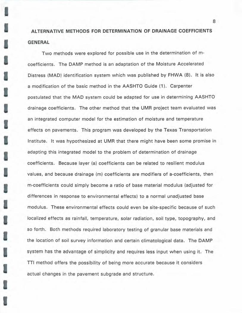
pavement structure is exposed to moisture levels approaching saturation. Fig. 8
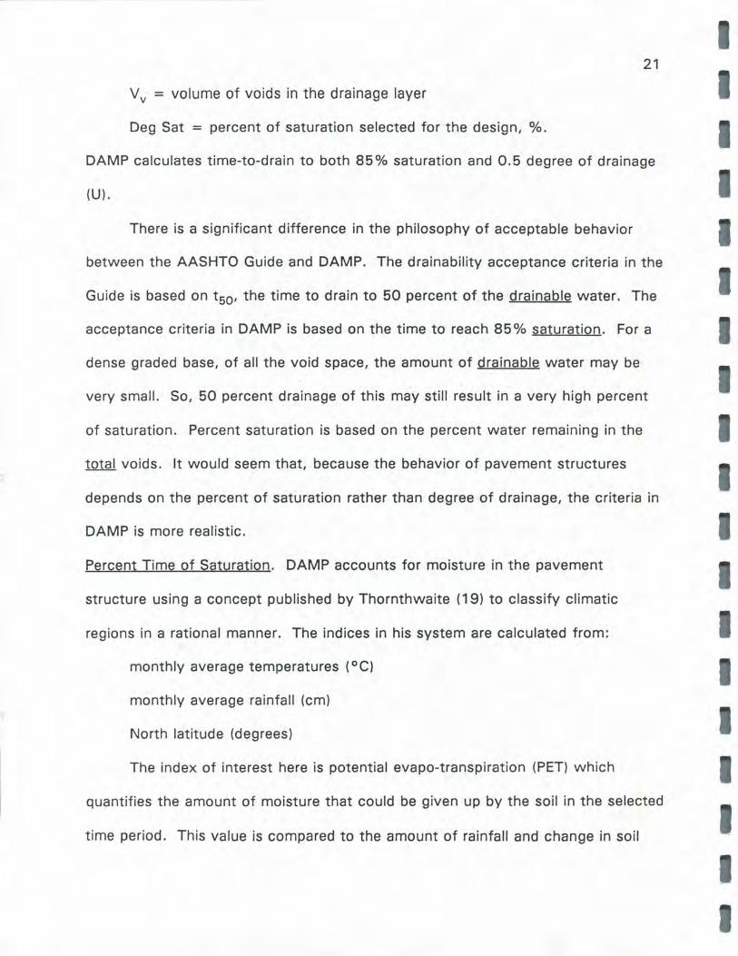
summarizes the approach for considering the variation in m-value with percent of
time the structure is in or near a saturated condition." Their Fig. 8 is included in
I this report as Fig. 1 .
I
This figure was stated to be the source of the m-value table presented in the
1986 AASHTO guide presented herein as Table 1. However, interpretation of the
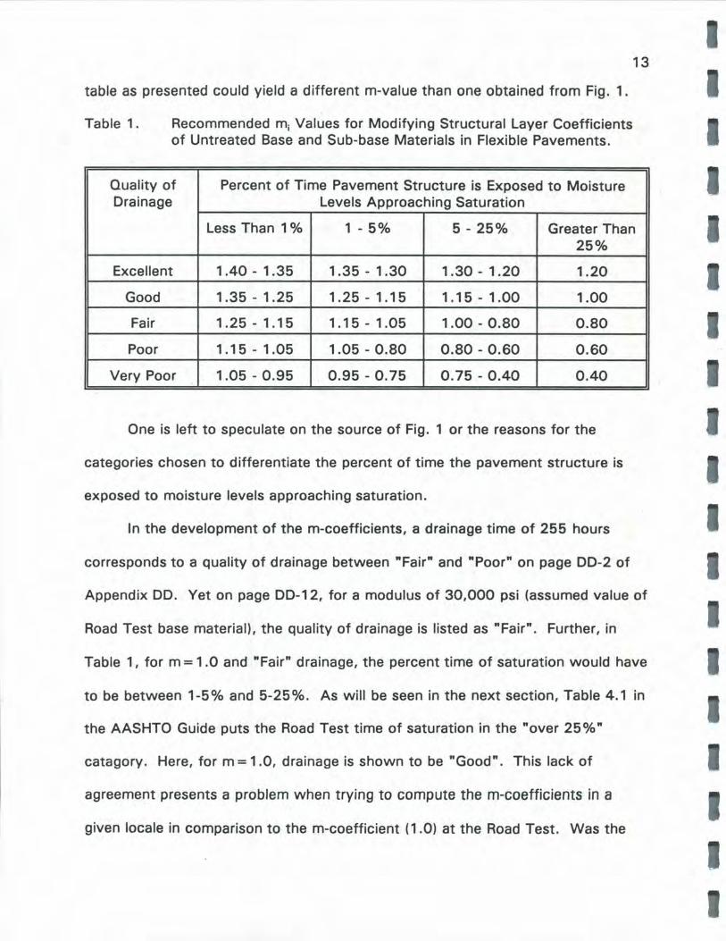
table as presented could yield a different m-value than one obtained from Fig. 1.
Table 1 . Recommended mi Values for Modifying Structural Layer Coefficients of Untreated Base and Sub-base Materials in Flexible Pavements.
Quality of Percent of Time Pavement Structure is Exposed to Moisture Drainage Levels Approaching Saturation
13
Less Than 1 % 1 - 5% 5 - 25% Greater Than 25%
Excellent 1.40 - 1.35 1.35 - 1.30 1.30-1.20 1.20
Good 1.35 - 1.25 1.25-1.15 1.15 - 1.00 1.00
Fair 1.25 - 1.15 1.15 - 1.05 1.00 - 0.80 0.80
Poor 1.15 - 1.05 1.05 - 0.80 0.80 - 0.60 0.60
Very Poor 1.05 - 0.95 0.95 - 0.75 0.75 - 0.40 0.40
One is left to speculate on the source of Fig. 1 or the reasons for the
categories chosen to differentiate the percent of time the pavement structure is
exposed to moisture levels approaching saturation.
In the development of the m-coefficients, a drainage time of 255 hours
corresponds to a quality of drainage between "Fair" and "Poor" on page 00-2 of
Appendix DD. Yet on page 00-12, for a modulus of 30,000 psi (assumed value of
Road Test base material), the quality of drainage is listed as "Fair". Further, in
Table 1, for m = 1.0 and "Fair" drainage, the percent time of saturation would have
to be between 1-5% and 5-25%. As will be seen in the next section, Table 4.1 in
the AASHTO Guide puts the Road Test time of saturation in the "over 25%"
catagory. Here, for m = 1.0, drainage is shown to be "Good". This lack of
agreement presents a problem when trying to compute the m-coefficients in a
given locale in comparison to the m-coefficient (1.0) at the Road Test. Was the

D') -+' C a,
E C ., 0 >
C +'
Cl. C L.
L. :,
0 +' C - (/'J
""C a, .c
I +' °' 0 ·-a, :r: L. L. 0 0 ... u
CD L. :, OJ ., 0 :, a. - X C
> Lu I E
I
2.0
Quality of
1.5 Drainage
Excellent
Good
1.0 Fair
Poor 0.5
Very Poor
0.0 1 1-5 5-25 >25
Percent of Time Structure is Near Saturation
Fig.1. Recommended m-Values cs a Function of
the Quality of Drainage and Exposure to
Sctu ration.
14

Road Test drainage Good? Fair? Poor? This is discussed further in the next
section.
DAMP
General
15
Carpenter has written an interactive computer program (Drainage Analysis
and Modelling Program (DAMP)) (11) designed to perform a drainage analysis of
pavement structures. DAMP basically takes the FHWA Highway Subdrainage
Design Manual (9) written by Moulton and computerizes the calculations.
Carpenter added sections on recent geocomposite fin drains and filter fabrics and
procedures for selection of m-coefficients. For m-coefficient determination, DAMP
considers base drainage capacity, subgrade drainage capacity, and climatological
data. The data necessary for these considerations include: subgrade soil drainage
characteristics, granular base width/thickness/cross-slope/longitudinal
grade/density/effective grain size/percent passing the #200 sieve, average monthly
precipitation and temperature, and latitude. Additionally, DAMP considers surface
infiltration, meltwater, roadway geometrical inflow/outflows, edge drain capacities,
and filtration criteria. The data necessary for these calculations include: weather
data, pavement type/thickness, transverse joint or crack spacing, number of
longitudinal joints, transverse joint or crack length, number of layers in the
pavement, thickness and density of each layer, permeability of subgrade, heave
rate of subgrade, and cross sections of the roadway right-of-way.
DAMP has the capability of performing many sorts of drainage-related
activities. However, in terms of the selection of drainage (m) coefficients, only the

I
I
I I
I
I
16
topic titled "Drainage Coefficient Determination" is presented.
Drainage Coefficient Determination
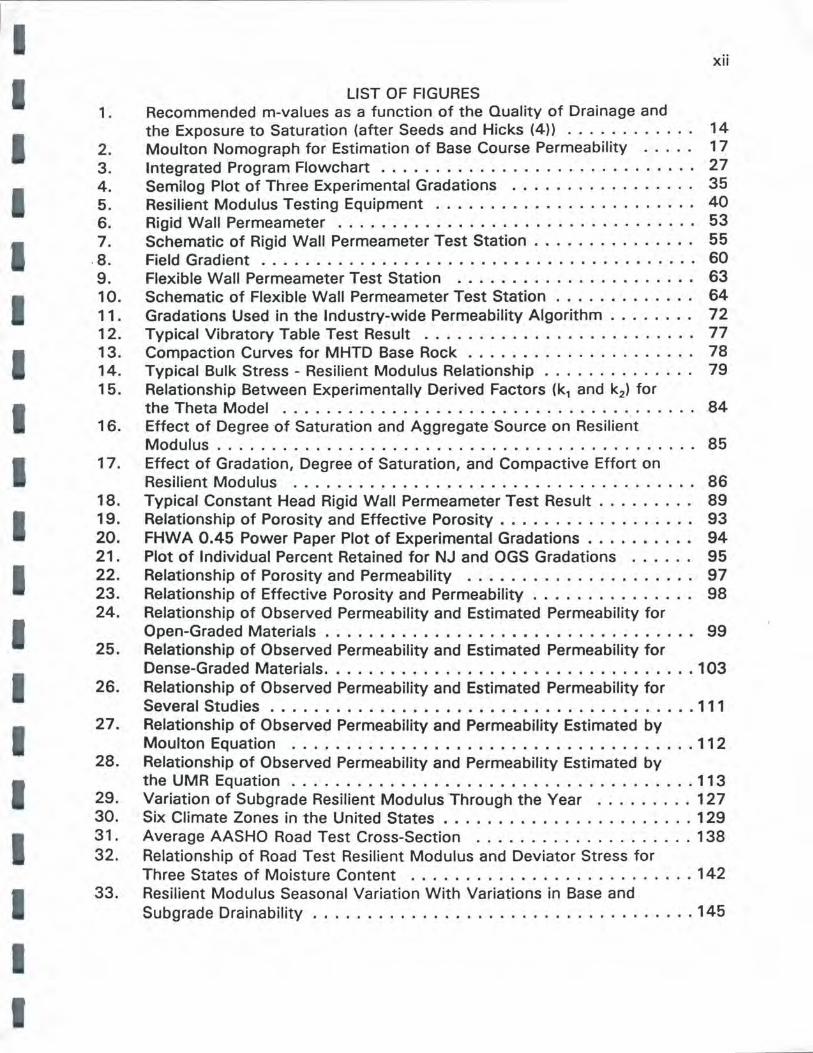
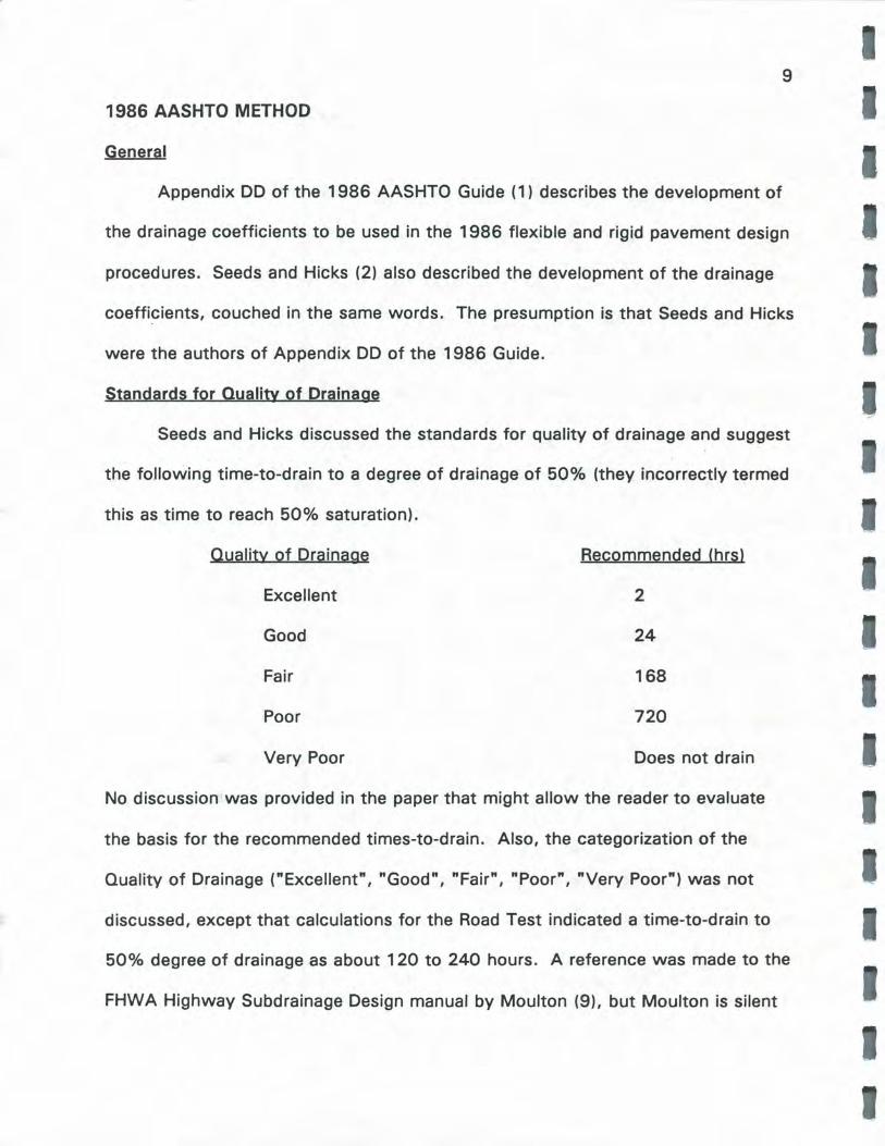
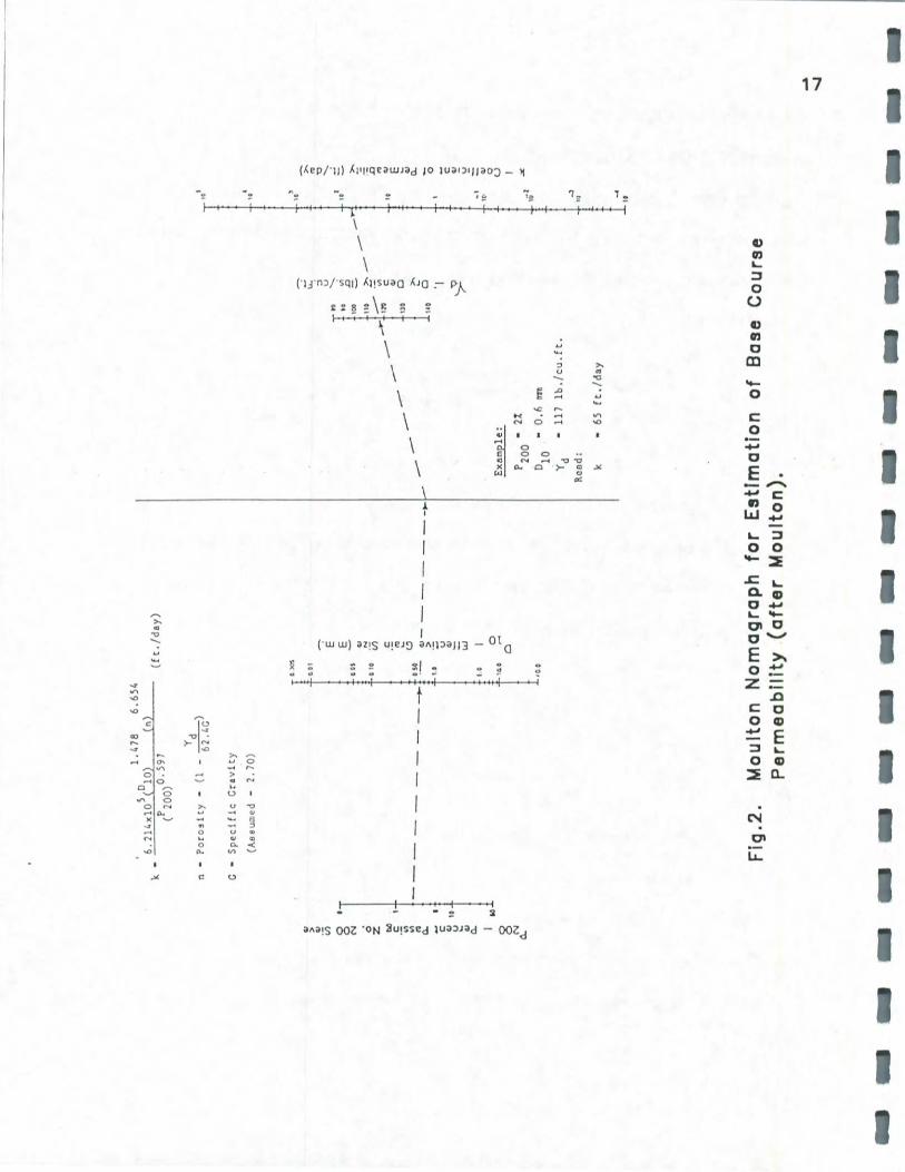
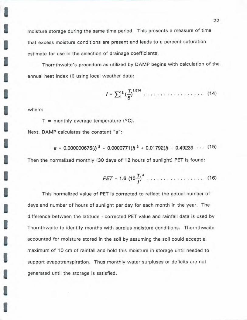
Drainage Layer Characteristics and Base Drainage Times. The permeability of the
drainage layer is computed by DAMP using the relationship from Moulton which
was based upon permeability tests reported in the literature ( 12-17). This
relationship is:
6.214x10⁵(D101·478)(n 6·654)
kd = . . . . . . . . . . . . . . (2) p2000.597
where:
kd = permeability of the drainage layer, ft/day
D10 = drainage layer's effective (10 percent passing) particle size, mm
P 200 = amount of the drainage layer material passing the #200 sieve, %
n = porosity of the drainage layer material.
where:
n = 1 Yd - -- ......... . .......... (3)
YwG•
where:
yd = compacted dry unit weight, pcf
G. = apparent specific gravity
Yw = unit weight of water.
Fig. 2 depicts the nomograph that Moulton provided in his manual.
DAMP calculates time for drainage using the relationships developed by
., > ., ii
) 8 •
N 0 z bO
C
: ,
'iii ... Ill
0..
-I
C: ~
10
., 0.. I
'° 8 N
0.
.
1.4
78
6
.654
6.2
14
xl0
5(0
10)
(n)
(ft,
/day
) k
• p
)0.5
97
(
200
yd
n
• P
oro
alt
y
• (l
-
62
.4G
)
G •
S
pecif
ic
Gra
vit
y
(Aae
umed
•
2, 7
0)
-----
-----... '·"
" O
OI
E
E
ooi
- ., N
O 1
0 V
) .c: Ill
0~
t3 ., _
> --
·-e -
-_
_ ,_
to
~
w
,., 0
,~,
.....
a
10.
0
.. IO
100
'10
u... :,
u ' vi .D
-_
_ .j.,
;;-.~
----
"' C: C1I
a ----
------
Exa
mpl
e:
p200
•
2X
010
•
0,6
rra
n
yd
•
117
lb./
cu
.ft.
Rco
d:
k •
65
ft./
day
\JO
~
uo
a ·, '-J
Fl g
. 2.
Mo
ult
on
N
om
ag
rap
h
for
Es
tim
ati
on
o
f B
as
e
Co
urs
e
Pe
rme
ab
ilit
y
(aft
er
Mo
ult
on
).
' ,, ' 10
, IO
.., " .,
:,... "' 'O
':-
:,...
.D "' ., E
~ ., C
L 0 C: ., '=
I(•
CV
0 u I
,~· l
.:J
C
.J
"' ... "
.... -.J

I I I I I I
I I I
I
18
Casagrande and Shannon ( 18). The assumptions made for this analysis included
1) the subgrade is impermeable and 2) the base course is saturated when drainage
begins . To facilitate the solution, they defined three dimensionless quantities, U,
T, and S. The degree of drainage, U is:
U = Drained cross sectional area ( of drainable voids) Total cross sectional area (of drainable voids)
. . . . . . (4)
The time factor, T is:
tkdH T = -- ......••.•..•..•...•. (5)
n L2 B
where:
t = time for drainage for U to be reached, days
kd = permeability of the base course, ft/day
H = thickness of the drainage layer, ft
L = length of the drainage path, ft
= w/1 +(gfsJ2
where:
w = width of drained area on same cross slope, ft
g = longitudinal grade
sc = cross slope
c = geometrical constant (defined later).
and from Strohm, et fil. ( 17):
19
n,, = v.VWD = 1 - [ yd (1 +GsWJ] . . . . . . . . . . . . (6) T G8 *62.4
where:
n8
= effective porosity
Vwo = volume of water drained from the sample
. Vr = total volume of the sample
yd = dry density, pcf
G5 = apparent specific gravity
W8
= water content of the sample after 24 hours of drainage, %.
DAMP, however, determines effective porosity (n8 ) by means of a statistical
correlation with measured permeabilities (kd) published by Moulton which was
based upon work reported by Barber ( 13) and Strohm et al. ( 17):
n,, = 0.027 kJ·234
The slope factor S is:
(7)
H H 5 = Ltancx = LS · · · · · · · · · · · · · · · · · · (B) d
where:
H = thickness of the base course, ft
L = length of the drainage path, ft
Sd = slope = (Sc 2 + g2)0.5
a = angle of the drainage path with horizontal, degrees.
Using these three dimensionless coefficients, DAMP computes the time
I
I I I I
factors with the following Casagrande-Shannon relationships and geometry.
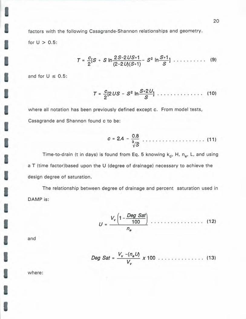
for U > 0.5:
T = c[S + S In 2S-2US+1 _ s2 In S+1] 2 (2-2~(S+1) S
and for U ::5 0.5:
20
(9)
c 2 S+2U T= -[2US - S In ] .............. (10) 2 S
I where all notation has been previously defined except c. From model tests,
I I I I I
I I I
Casagrande and Shannon found c to be:
C = 2.4 - 0.8
TS ( 11)
Time-to-drain (t in days) is found from Eq. 5 knowing kd, H, ne, L, and using
a T (time factor)based upon the U (degree of drainage) necessary to achieve the
design degree of saturation.
The relationship between degree of drainage and percent saturation used in
DAMP is:
u = v. (1-°7o;at) ................ 1121
ne
and
V -(n ~ Deg Sat = v 8 x 100 . . . . . . . . . . . . . . ( 13)
Vv
where:
21
V v = volume of voids in the drainage layer
Deg Sat = percent of saturation selected for the design, %.
DAMP calculates time-to-drain to both 85% saturation and 0.5 degree of drainage
(U).
There is a significant difference in the philosophy of acceptable behavior
between the AASHTO Guide and DAMP. The drainability acceptance criteria in the
Guide is based on t 50, the time to drain to 50 percent of the drainable water. The
acceptance criteria in DAMP is based on the time to reach 85% saturation. For a
dense graded base, of all the void space, the amount of drainable water may be
very small. So, 50 percent drainage of this may still result in a very high percent
of saturation. Percent saturation is based on the percent water remaining in the
total voids. It would seem that, because the behavior of pavement structures
depends on the percent of saturation rather than degree of drainage, the criteria in
DAMP is more realistic.
Percent Time of Saturation. DAMP accounts for moisture in the pavement
structure using a concept published by Thornthwaite (19) to classify climatic
regions in a rational manner. The indices in his system are calculated from:
monthly average temperatures (°C)
monthly average rainfall (cm)
North latitude (degrees)
The index of interest here is potential evapo-transpiration (PET) which
quantifies the amount of moisture that could be given up by the soil in the selected
time period. This value is compared to the amount of rainfall and change in soil
11 I
I I I
22
moisture storage during the same time period. This presents a measure of time
that excess moisture conditions are present and leads to a percent saturation
estimate for use in the selection of drainage coefficients.
Thornthwaite's procedure as utilized by DAMP begins with calculation of the
I annual heat index (I) using local weather data:
I '= ~2 (;>1.514 . . . . . . . . . . . . . . . . . . (14)
I I I
where:
T = monthly average temperature (°C).
Next, DAMP calculates the constant "a":
a = 0.000000675(~ 3 - o.oooon1 (~ 2 + o.01792(~ + 0.49239 (15)
I Then the normalized monthly (30 days of 12 hours of sunlight) PET is found:
I I I I I I I I I
T " . PET= 1.6 (10-) . . . . . . . . . . . . . . . . . (16) I
This normalized value of PET is corrected to reflect the actual number of
days and number of hours of sunlight per day for each month in the year. The
difference between the latitude - corrected PET value and rainfall data is used by
Thornthwaite to identify months with surplus moisture conditions. Thornthwaite
accounted for moisture stored in the soil by assuming the soil could accept a
maximum of 10 cm of rainfall and hold this moisture in storage until needed to
support evapotranspiration. Thus monthly water surpluses or deficits are not
generated until the storage is satisfied.

23
DAMP approximates percent saturation time from the monthly water surplus
and storage data using the following scheme:
1 . Frozen period - When the average monthly temperature is below freezing, no contribution to saturation can be made regardless of moisture conditions. 2. Surplus period following the winter, Zone A (northeast portion of USA) - The soil will be continually saturated during this period, with a contribution from frost heave. In Zone A all months with a surplus following a winter period will contribute to the saturation time. 3. Surplus period following the winter, Zone B (zone below A) - Here the spring thaw phenomenon is not critical. There may be periods where the soil is not totally saturated, and these may accurately correspond to dry days in the "rain and dry" day sequences. In Zone B, include the first month and one-fourth of remaining months having surplus as contributing to the saturation time . . 4. Surplus following a recharge which does not follow a frozen period - Here one-fourth of the months in the surplus period should contribute to the saturation time. 5. Utilization period following a surplus - During this period, the evaporation potential exceeds rainfall, and the storage moisture is being depleted. The soil is going from saturated to a dry condition over the period. The initial month may have a portion during which it is close to saturation. Include one-fourth of all months during this period which have a storage exceeding 7.5 cm, representing wet months with rain. 6. Utilization after a recharge which did not lead to a surplus - None of the time in this moisture state contributes to saturation time. 7. Recharge leading to a surplus - The final months when the storage moisture is close to full (saturation) may contribute to saturation. Include one-fourth of all months which have storage values above 7.5 cm. 8. Recharge leading to no surplus - This period will contribute little moisture. Include none of the time during this period toward saturation time. 9. Deficit - During this time, there is no water available at all, and if there were to be rainfall, it could evaporate before entering the soil. Include none of this period in the saturation time.
The sum of the months that DAMP includes for saturation purposes is
divided by 12 to determine a "Percent Time of Saturation" for the given climate.
Subgrade Drainage. The source for soil drainage classification of subgrades is the
I

I 24
County Soil Survey produced for most counties under the direction of the Soil
Conservation Service. The county soil surveys contain several categories of data
related to soil drainage (20) such as runoff, internal soil drainage, and soil
permeability. This information is combined with knowledge of the underlying
geological formation, slope of the land, and location of the soil with regard to
elevation/position in the topography to determine the soil drainage classification in
the county soil survey that is used by DAMP. The soil drainage classification is
I given in each soil description (rather than in the many tables) in the county soil
I I I
I I I I I I
survey. Soil drainage classifications include very poorly drained, poorly drained,
somewhat poorly drained, moderately well drained, well drained, somewhat
excessively drained, and excessively drained.
DAMP accounts for the contribution that the subgrade makes to drainage of
the pavement structure by employing a concept introduced by Hole (21) termed
Natural Drainage Indices of Soil. Bodies (NDI). The NDI arbitrarily assigns the value
of + 1 to well drained soils, -10 to excessively drained soils, and + 2.5 to + 10 to
the range of soils classed as moderately well drained to very poorly drained.
DAMP classifies the NDI numbers as follows:
NDI Classification
-10 to <-2 Good
-2 to 2.5
> 2.5 to 10
Fair
Poor
These descriptive classifications are used to enter the quality of drainage table
discussed next. Quite simply, one uses the terms "Good, Fair, or Poor" to describe
25
the contribution of the soil to the Quality of Drainage. A soil classified as "Good"
will actually improve the performance of the granular layer, a "Fair" soil will not
augment the base layer drainage, but will not detract from performance, while a
"Poor" soil will actually provide a source of water to the structure.
Quality of Drainage. The drainage time of the granular base (time to 85 %
saturation) and the subgrade drainage (good, fair, poor) discussed above are used
to enter Table 2 to determine "Quality of Drainage".
Table 2.
Subgrade Drainability (NOi)
Good -10to-2
Fair -2 to 2.5
Poor> 2.5
AASHTO Quality of Drainage Using Calculated Base and Subgrade Drainability Values.
Base Drainability (to 85 % saturation)
Excellent Good Fair Poor Very Poor s. 5 hrs 5-30 hrs 30-100 hrs 100-200 hrs 200+ hrs
Excellent Excellent Good Fair Very Poor
Excellent Good Fair Poor Very Poor
Fair Fair Poor Very Poor Very Poor
AASHTO Drainage Coefficient Selection. The "Quality of Drainage" and "Percent
Time of Saturation" are the inputs to the 1986 AASHTO drainage (m) coefficient
table (Table 1 ). These drainage coefficients are then used in the AASHTO
structural number equation (Eq. 1 ).
Thus, the column is selected by going through the Thornthwaite PET
analysis, and the row is selected by combining the effects of base drainability (time
to 85% saturation) and subgrade contribution (good, fair, poor drainage).
I I I I I I I I I I I I I I I I I I
26
Carpenter also recommends that the drainage coefficient should be adjusted
up or down within the range in each cell of Table 1 depending on certain features
of the pavement structure. Increased m-values are allowed by the presence of
edge drains and a working drainage layer. Decreased m-values result from a
bathtub-type structure.
Further evaluation of DAMP is given in the section "Results of Models
Evaluation."
TTI
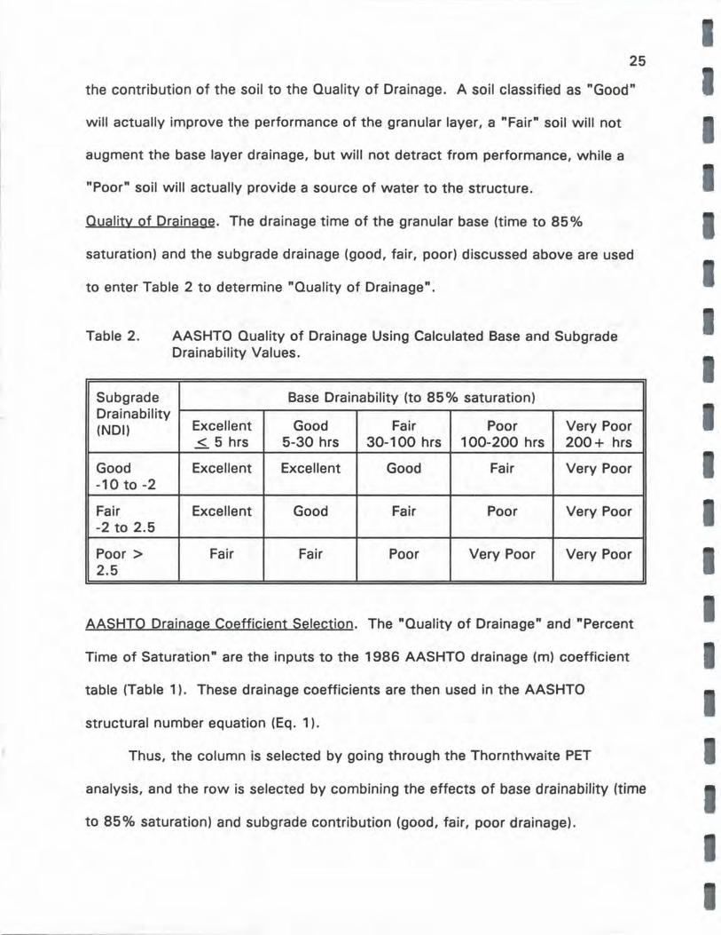
General
Titled the "Integrated Model of the Climatic Effects on Pavements" (7), this
method produced by the Texas Transportation Institute combines into a single
program several component models that had been developed independently. The
component models include the Precipitation Model, the Infiltration and Drainage
Model, the Climatic-Materials-Structural Model, and the CAREL Frost Heave-Thaw
Settlement Model. A flow chart of the integrated model is included in Fig. 3. The
component models were developed over a period of several years for use on main
frame computers. In combining these models, the authors eliminated portions of
the original programs, substituted some methods of computation, and suppressed
some of the orginal output. The program was provided in a compiled form and as
such was not available for examination. It is not clear from the documentation
which links exist between the various programs and exactly what data is passed
from program to program.

PRECIP MODEL
Input 2 Pavement Geometry Physical and Thermal
Material Properties Initial Soil Suction Profile Initial Soil Temp. Profile Heat Transfer Coeff. Rainfall Intensity Coeff. Pavement Infiltration
Parameters
ID Model
CRREL MODEL
Output
Soil Temp. Profile with Time Soil Suction Profile with Time Frost Penetration with Time Thaw Depth with Time Surface Heave with Time Degree of Drainage with Tim Dry & Wet Probabilities of
Base Course . Adequacy of Base Course
Design
Output
CMS MODEL
Asphalt Stiffness with Time Base & Subbase Mod. with Time Subgrade Mod. with Time Climatic Data
27
Fig.3. Integrated Program Flowchart (after Lytton, et al.).

I I I I
I I
I I I I I I I I I I I
28
Precipitation Model
The Precipitation Model (PRECIP) was described by Liang and Lytton (22) as
a deterministic algorithm that uses recorded data to simulate rainfall patterns that
are used for infiltration and drainage calculations. Stochastic processes and
random methods are employed to analyze past climatological data, and to estimate
and predict the effects of the environment on the performance of pavement with
specified confidence levels. This description by the authors includes the statement
"the effects of the environment on the performance of pavement." However, the
model only produces a simulation of rainfall patterns to a given confidence level.
The model considers both convective and frontal types of rainfall. Convective
rainfall generally occurs in a brief intense thunderstorm. Frontal rainfall may be
steady and of longer durations. Long duration rainfall is associated with more
water entering the pavement structure. See Fig. 3 for the relationship of the
PRECIP program to the whole.
Infiltration and Drainage Model
The Infiltration and Drainage Model (ID) was written by Lytton and Liu (23)
and evaluates the pavement base course drainage, the probabilities associated with
the rainfall data, the infiltration analysis, and the resulting probabilities of having
either a wet or dry base course. That is, each day of the month is declared either
a day when the base is saturated to greater than 85% or a day when it is drier.
The drainage output describes the degree of drainage and corresponding times
using a model developed by Liu, Jeyapalan, and Lytton (24). This model is very
similiar to the Casagrande-Shannon model with the exception that the phreatic
surface is parabolic rather than linear. The Liu model also allows for subgrade
drainage. The pavement base course evaluation uses an empirical procedure to
include the percentage of gravel, sand, and fines and the type of fines in
determining the acceptability of the drainage design. This empirical procedure is
represented by the equation:
Sa = 1 - ( PD) * U . . . . . . . . . . . . . . . ( 17)
where:
Sa = degree of saturation
29
PD = percentage index which represents the drainability of the base course
material
U = degree of drainage.
PD is found from a table published by Carpenter in the MAD Index (8). This table is
shown below:
Table 3. Percentage Index (PD) of Free Draining Water for Different Types of Base Course.
Amt of Fines <2.5% Fines 5% Fines 10% Fines
Type Fines Inert Silt Clay Inert Silt Clay Inert Silt Clay
Gravel* 70 60 40 60 40 20 40 30 10
Sand** 57 50 35 50 35 15 25 18 8
* Gravel, 0% fines, 75 % > #4: 80% water loss * * Sand, 0% fines, well graded: 65 % water loss Gap graded material will follow the predominant size.
The probabilities associated with the rainfall data and the infiltration of that
I

I
I I I
I I I I I I I I I
30
rainfall into the pavement structure are combined with the drainage times to
produce an estimate of the probibility of the amount of time the base course is
saturated. The method for establishing the probability of having a wet or dry base
course involves several steps in which the probability of a number of events and/or
conditions are established and then are combined by multiplication, addition, and/or
subtraction to obtain the final result.
Climatic-Materials-Structural Model
The Climatic-Materials-Structural Model (CMS) was written by Dempsey, .et
.a.l. (25) and uses sunshine percentage, wind speed, air temperature, and solar
radiation to find the temperature profile in the pavement structure.
CAREL Frost Heave and Thaw Settlement Model
The CAREL Frost Heave and Thaw Settlement Model (CAREL) was written
by Berg, Guymon, and Johnston (26) and provides a measure of frost heave using
a coupled heat and moisture flow mathematical model. The CAREL model uses the
temperature profile found by the CMS model.
The Integrated Model requires a minimum of 100 input variables to operate.
These are listed in Appendix A.
The exact number of variables is dependent upon the number of layers of
the pavement system modeled. There is great flexibility in the Integrated Model
that allows accurate models of many different pavement structures.
The source of the input data depends upon the location and design of the
pavement structure. Given this information, the user can construct the necessary
finite element sketch to define the pavement layers. The weather data published
31
under the title of "Local Climatological Data, Monthly Summary" by NOAA is
sufficient to complete the weather data input. The users manual for the Integrated
program offers suggestions for much of the more obscure input requirements.

I I I I I I I I I I I I I I I I I I I
32
MATERIAL TYPES AND SOURCES
All unbound aggregates in the study were MHTD approved materials. The
materials were selected and sampled by MHTD personnel. Two Type 1 crushed
stone base aggregates were studied, and were selected by MHTD personnel to
give a wide range of particle shape and texture. Additionally, in a companion
project (29), two Type 2 gravel materials (re-graded to Type 1 specifications) were
tested for resilient modulus. Test results for these two materials are also included
in this report. The materials, sources, and identification are shown in Table 4.
Table 4. Material Types and Sources.
Nomenclature Material Sources Location
DR-12 Type 1 crushed Burlington Mertens Quarry Millersburg limestone
DR-13 Type 1 crushed Jefferson City Smith Quarry Rolla dolomite
DR-14 Type 2 Crowley Ridge gravel Delta Dexter base Aggregates
DR-15 Type 2 Black River gravel base Williamsville Poplar Stone Co. Bluff
Note: All sources are located in Missouri
GENERAL
33
LABORATORY INVESTIGATION
The principal properties to be determined for unbound granular base
materials were the 1) resilient modulus at a low and high degree of saturation to
assess moisture sensitivity, 2) permeability, and 3) effective porosity to assess
drainability. However, performance of other tests and procedures were necessary
in order to conduct the primary tests and to analyze the results. These other
procedures included sieve analyses, gradation formulation, specific gravity
determination, moisture-density relationship testing, particle shape/texture testing,
and plasticity of fines determination. These operations are outlined below.
EXPERIMENTAL GRADATIONS
The experimental gradations utilized in this study were: 1) a curve situated
midway between the upper and lower limits of the allowable gradation
specification band for MHTD Type 1 unbound base material ("MHTD Middle"); 2)
the New Jersey (NJ) open gradation; and 3) the PennDOT OGS open gradation.
All three gradations were used in the permeability portion of the study, while the
MHTD Middle and the New Jersey were used in the resilient modulus (Egl part of
the study. These gradations were used for both the two crushed stones and the
two gravels. At the finer size end, the MHTD Middle gradation was extended to
include a controlled amount passing the #200 sieve, which was 8%. This value
was chosen because: 1) it matched one of the gradations used in the layer
coefficient study which is the companion project to the present study; and 2) this
was approximately the same percentage as both as-delivered gradations of the
I I I I I I I I I I I I I I I I I I I
34
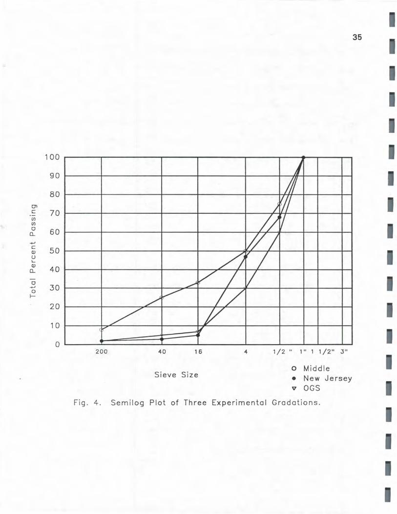
Type 1 aggregates supplied by MHTD for this project. The MHTD Middle, New
Jersey, and OGS gradations are shown in Fig. 4.
GRADATION CURVE SHAPE/POSITION
An analysis was performed to determine the effect of gradation upon
permeability and the effect of the interaction of gradation and degree of saturation
on resilient modulus. The most promising methods were later tried in the
development of the predictive permeability multiple regression equations. To
accomplish this, there was a need to characterize the gradations so that a single
value of gradation "modulus" would represent the shape and position of the
gradation curves. Nine different methods were tried and are described in detail in
Volume I of the companion study to this report (27).
PARTICLE SHAPE/TEXTURE
Numerous test methods have been devised to quantify particle shape and/or
texture. These can be divided into direct methods (those that result in
measurement or aspects of individual particle shape or texture) and indirect
methods (those that measure some sort of bulk aggregate property, such as void
content, which is related to particle shape/texture). Recent evaluations of these
methods were reported by Kandhal fil al, (28) at NCAT (National Center for
Asphalt Technology). There are several methods available which can be used in
lieu of the standard test, ASTM D 3398 (29), which is somewhat cumbersome to
perform. Kandhal fil al. recommended the National Aggregate Association's (NAA)
proposed method (A or B) for fine aggregate (30). Both of these are indirect
methods of particle shape determination.
35
I
I
100
90
80 CJ)
C 70 Cl)
Cl)
0 60 Q_
+' C
50 (l)
u L (l)
40 Q_
0 +' 30 0 I-
20
1 0
j /;, r
) w // I
/// /) '/
~ // V / ~ //
/ y (b"' ~
I
0 200 40 16 4 1/2 II 1 II 1 1 /2 11 .3 II
I 0 Middle Sieve Size • New Jersey
V OGS
Fig. 4. Semilog Plot of Three Experimental Gradations.
I
I I I I I I I I I I I I I I I I I I I
36
In this study, the (-) #8 to ( +) #100 sieve size material of each gradation
was tested using NAA Method A. The method is given in Appendix A of Volume I
of the layer coefficient study. For the ( +) #4 size, the aggregates were tested in
accordance with ASTM D 3398. This method is also given in the previously
mentioned Volume I. The results of both methods were used in developing the
permeability regression equations discussed later in the "Results" section of this
report. Photographs of the NAA test device and the D 3398 equipment are shown
in Figs. 9 and 10 of Volume I of the layer coefficient study.
SPECIFIC GRAVITY
Aggregate fractions of each of the three gradations were separated at the
#4 and #100 sieve sizes and tested in accordance with AASHTO T85-88 (31) and
T84-88 (32) for the ( + )#4 material and the (-)#4 to ( + )#100 material. These data
were necessary for use in the degree of saturation and porosity calculations.
Weighing was performed on a scale readable to the nearest 0.1 g. Weighted
averages of apparent specific gravities were used to calculate the specific gravity
for each gradation of each of the four aggregates as follows:
G=------10_0 ____ ~ % Passing #4 + % Retained #4 . . . . . . . . . . (18)
ASG ASG
where:
G = apparent specific gravity, weighted average
ASG = apparent specific gravity of each fraction.
SCREENING
All aggregates were shaken in an air dry state through the appropriate
screens in a Gilson shaker. A dust baffle/cover was designed to restrict the
movement of particles in order to minimize problems with incorrect sizes of
material being retained on any given sieve.
Upon shaking, the split material was stored in 20 gal plastic cans with lids
until the aggregate was needed for specimen fabrication.
SPECIMEN FABRICATION
37
Specimens for unbound granular base were fabricated as follows: Each
specimen was produced by taking the indicated amount of material for each sieve
size in accordance with the experimental gradation previously discussed. Each
layer was proportioned separately. The largest particle size in the gradation was
approximately 5/8 in. Thus, the specimen diameter was greater than six times the
maximum particle size, in accordance with AASHTO T-XXXC91 (33) (flexible wall
resilient modulus), and permeability method ASTM D 5084. For the triaxial-type
specimens (resilient modulus/flexible wall permeability), the 4 in diameter 8 in high
specimens were compacted in 1 in lifts with a Dayton air hammer in a split
aluminum mold lined with a nitrile rubber membrane. Various membrane materials
and thicknesses were tried, including 0.012 and 0.025 in latex and nitrile rubber.
It was found that during compaction the thinner membranes would tear, especially
the latex, even if two membranes were used. A 0.06 in thick nitrile rubber
membrane was the minimum that was sufficiently rugged . The AASHTO
specification limits membrane thickness to 0.08 in. A vacuum of approximately 20
I
I I I I I I
I
I I
I I I I I I I I I I I I I I I I I I I
38
in was applied to the specimen prior to removing the split mold. The specimen
was compacted directly on the triaxial cell pedestal. A more complete description
of the specimen fabrication process is included in Ref. 27.
The 1 O in diameter rigid wall permeameter specimens were also compacted
in 1 in lifts with the air hammer.
MOISTURE - DENSITY RELATIONSHIP
In order to choose target densities for compaction of resilient modulus and
permeability specimens, standard and modified proctor tests were performed in
accordance with AASHTO T-99 (34) and T-180 (35). Additionally, the maximum
density of the open-graded gradations were determined via the vibratory table
method, ASTM D 4253 (36). For each of the four aggregates, a double amplitude
~ dry density curve was obtained in accordance with the dry method to obtain the
optimum power setting. This power setting was then used for the determination
of the density utilizing the wet method. The vibratory table is shown in Fig. 3 of
Volume II of the layer coefficient study where a more complete description of the
test method and equipment is given.
RESILIENT MODULUS
General
The relationship between repeated applied stress and the resulting strain of
unbound granular base materials is most commonly defined by the resilient
modulus test. This test was performed by subjecting a compacted specimen to an
all-around confining pressure and then applying a vertical cyclic load. Total applied
load (a1 ), displacement resulting from the load, and confining pressure (a3 ) were
39
monitored. The applied load and confining pressure were varied to achieve a range
of stress states which should represent the expected stress states in actual
pavement structures. The specimen was encased in a flexible membrane and
tested in a triaxial cell. Fifteen combinations of confining (cell) pressure and cyclic
applied (deviator) stress were used for each specimen .
. The procedure that was followed in this study is essentially in conformance
with the 1991 Interim AASHTO method of test (33). The test procedure is also
essentially in conformance with SHRP Protocol P46 (37). One notable exception is
that the AASHTO stress state sequence (not the SHRP) was followed. However,
as per Claros fil fil. (38), a1/a3 ratios were not allowed to exceed three in order to
prevent possible excessive specimen straining.
A more complete discussion of the test equipment and procedure is given in
Ref. 27.
Equipment
The testing equipment setup is shown in Fig. 5. The equipment consisted of
an MTS electrohydraulic load system, a triaxial chamber capable of housing a 4 in
diameter specimen while subjected to cyclic loads, and a data acquisition system.
Load was measured with an internal 1000 lb capacity load cell and deformation
was measured with two L VDT'S mounted externally to the cell. This type of
measuring system is allowed in the AASHTO method and is recommended in the
SHRP method. Minimum resolution of the vertical LVDT's and the load cell met
the AASHTO standard. Actual minimum deformations and loads during the testing
were kept at least ten times the minimum resolutions to assure confidence in the
I I I
I I
I I
I I
I
I I
I I I
I I I I I I I I
40
Fig.5. Resilient Modulus Testing Equipment.
41
test results. Air was used as the confining fluid instead of water in order to
protect the internal load cell. Triaxial cell pressure and back pressure were
controlled via a Geotest control panel. The Research Engineering triaxial cell that
was used had several advantages. First, the chamber cylinder wall could be placed
after the loading piston is brought into contact with the specimen. Also, end caps I could be purged of air very easily by the unique design of the caps.
Test Variables
Although the effect of the degree of saturation was of primary interest, four
test parameters were controlled as independent variables.
Stress State. As previously mentioned, several variables affect the modulus of
granular materials. Stress state is considered to be the most important. As in
shear strength, the more confined a granular material is, the higher will be the
modulus. In the field, confinement is supplied by the layer underneath the granular
material, the granular material itself in the lateral (tangential and radial) (u2 and u3)
direction, the overburden above the point of interest, and the momentary load from
a vehicle. In a triaxial test, the difference between total vertical stress (u,) and u 3
is called the deviator stress or stress difference (ud). Cell pressure supplies the
lateral confinement to the specimen (u2 and u 3). A small static load (0.1 ud)
supplies the "overburden" pressure, and cyclic deviator stress (0.9 ud) supplies the
"vehicle" momentary stress. All of the stresses combined are known as the bulk
stress:
I
I I
I
I I I
42
= Ud + 3u3 •••••••••••••••••••••••••••••••• (19)
For each specimen, resilient modulus was determined at 14 stress states in which
effective confining pressure ranged from 2 to 20 psi and ud varied from 2 to 40
psi. This resulted in a range of bulk stress from 8 to 100 psi. This was considered
I adequate to cover the range of stress states likely to be encountered in practice.
I
I I I I I I
I I I I
The testing sequence and stress state schedule is shown in Table 5. Thus, E0 =
Degree of Saturation. In general, an increased water content will cause modulus
to decrease. Several reasons are given for explanation of this behavior. These are:
1) decrease in modulus of subgrade, thus a decrease in granular layer bulk stress;
2) reduction of apparent cohesion; 3) reduction of effective overburden pressure if
the base is below the water table; and 4) increase in positive pore pressure under
quick loads. Several degrees of saturation (0 S) have been put forth as break
points in behavior. Base materials are considered to be relatively "dry" at degrees
of saturation 60 percent and less (39). AASHO Road Test granular base materials
suffered a marked increase in distress above 85 percent saturation. In the present
study, each material was tested at two degrees of saturation: approximately 60%
and 100%. This variable was explored with the idea that a change in modulus due
to changes in saturation could lead to the development of m-coefficients. Resilient
behavior has been shown to deteriorate above 80 to 90 percent saturation (40).
Degree of Compaction. As previously discussed, modulus generally increases with
higher levels of compaction. Two levels of compactive effort were evaluated for
each material and gradation. For the dense gradation, specimens were compacted

Table 5 . Test Sequence for Granular Specimens of Base/Subbase Material.
Phase Sequence Deviator u, Confining CT1/CT3 0 No. of No. Stress Pressure Repetitions
(c,d)(psi) * (psi) ** Specimen 1 15 35 20 1.75 75 1000 Conditioning
2 10 30 20 1.5 70 50
3 20 40 20 2.0 80 50
4 30 50 20 2.5 90 50
5 40 60 20 3.0 100 50
6 10 25 15 1.67 55 50
7 20 35 15 2.33 65 50
8 30 45 15 3.0 75 50
Testing 9 5 15 10 1.5 35 50
10 10 20 10 2.0 40 50
11 20 30 10 3.0 50 50
12 5 10 5 2.0 20 50
13 10 15 5 3.0 25 50
14 5 8 3 2.67 14 50
15 2 4 2 2.0 8 50
Note: 1psi = 6.9kPa * Cyclic loads = 0.9 c,d; constant contact loads = 0. 1 c,d ** For all stress states the minimum number of repetitions necessary is 50. The
maximum is determined as per the AASHTO procedure and was redetermined for each confining pressure.
to 100% standard and 100% modified proctor densities. For the New Jersey
gradations, in most cases, one level of compaction corresponded to the maximum
index density via vibratory compaction (wet method), while the second level of
density usually corresponded to an impact-type of compaction, such as 100%
43
I

standard proctor.
Particle Shape/Surface Texture. As stated earlier, the effect of particle
shape/surface texture is not well-defined. Two crushed stones and two gravels
were chosen to delineate the effect of particle shape/surface texture.
44
I Testing Scheme
The testing scheme involved the following variables: four sources of
aggregate, two compactive efforts, two gradations, and two degrees of saturation
I for a total of 32 "tests". Each test was run with duplicate specimens. The testing
scheme is shown in Table 6.
I I I
Table 6. Testing Variable Scheme.
Crushed Stone Gravel
DR-12 DR-13 DR-14 DR-15
Mid. NJ Mid. NJ Mid. NJ Mid. NJ
CEL 0 S = 60 X X X X X X X X
0 S = 100 X X X X X X X X
CEH 0 S = 60 X X X X X X X X
05 = 100 X X X X X X X X
Note: Mid. = middle of MHTD Type 1 gradation band NJ = New Jersey gradation CEL = lower compactive effort CEH = higher compactive effort 0 S = 60 or 100% saturated X = combination of variables was utilized
Test Procedure
The resilient modulus testing procedure involved the following steps:
45
specimen compaction; assembly of the triaxial cell; consolidation; specimen
conditioning at a given stress state; load application through 14 additional stress
states at 60% saturation; backpressure saturation to 100% saturation;
consolidation; and load application through 14 stress states at 100% saturation .
After the load application at 100% saturation step, the dense-graded specimens
were tested for permeability. As a final step, the specimens were allowed to drain
overnight in order to calculate their effective porosities.
The specimens were compacted in eight layers of equal thickness with a
hand-held air hammer. The material was compacted at the optimum moisture
content (which was about at 60% saturation) into a split mold. After cell
assembly and consolidation , the specimen was conditioned with 1000 repetitions.
The various stress states and loads were then applied as per Table 4. The number
of load applications varied from 50 to 200, depending on the number of
applications necessary to meet the AASHTO modulus repeatability requirements .
Load and deformation data were taken for every load application over the
entire sequence, but only the last five repetitions were used for calculation of
resilient modulus.
The load duration for each repetition was 0.1 sec followed by 0.9 sec rest.
The stress pulse shape was haversine in nature. Repeated load equipment
deflection was determined on an aluminum dummy specimen and was subtracted
from total deflections for each stress state. Initially, calibration of the load cell and
LVDT's was performed before each test, but the interval was increased upon
determining that the drift in calibration was insignificant. The change in specimen
I
I
I I
height was constantly monitored. None of the specimens approached the
maximum allowable permanent strain of 5%.
In an effort to determine the effect of drainability on pavement bases, the
tests at 60% saturation were performed in a drained condition while the 100%
saturation tests were run in an undrained state.
PERMEABILITY
General
46
The ability of a pavement structure to drain water rapidly is partly a function
of the permeability of the various layer materials of its structure. Thus, for proper
design, knowledge of the permeability of the materials, especially of the granular
base layer, is necessary.
Even though permeability is expressed in, say, ft/day (the same as velocity),
the two are not necessarily equal. The permeability "ft/day" is a contraction of ft3
per day/ft2 as derived from Darcy's Law:
0 = ki A ................................. . ........ . (20)
where:
0 = discharge, ft3
k = permeability, ft/day
i = hydraulic gradient, ft/ft
A = cross-sectional area of discharge, ft 2•
Rearranging, 0/ A = ki
and V = 0/A (V = velocity, ft/day)
thus V = ki

47
So, velocity is equal to the product of permeability and gradient. If the gradient is
unity, then V = k. But, at any other gradient, they are not equal. For many
granular pavement base situations, gradients are 0.2 to 1.0, so velocity is usually a
fraction of permeability.
Traditionally, the determination of permeability of granular base materials
involves the assumption that Darcy's Law is in effect. For this to be true, the
underlying assumptions are that the material is 100% saturated, the flow is
laminar, and the discharge is proportional to the hydraulic gradient. Additionally, in
laboratory testing, for proper flow conditions to exist, the largest material particle
should not be excessively large in relation to the total cross-sectional diameter of
the permeameter. Typically, testing procedures impose limits so that the maximum
particle size does not exceed 10 times the specimen diameter for rigid wall
permeameters, or 6 times the specimen diameter for flexible wall permeameters.
The permeability of granular materials is a function of pore size distribution,
pore continuity, and pore shape. These are affected by grain size distribution,
particle shape, and relative density. Permeability is also a function of the degree of
saturation, specimen mineralogical composition, and nature of the permeant. This
last factor is to a certain extent affected by the viscosity, unit weight, and
chemical composition of the permeant. For coarse grained materials under normal
circumstances, due to the large volumes of water involved, tapwater is used as the
permeant, and the interaction of particle mineralogical composition and permeant
chemical nature is considered negligible. Thus, in a practical sense, the significant
variables in permeability testing of granular materials are particle size gradation,
I I
I
I
48
particle shape, degree of saturation, relative density, mineralogical composition of
the fines (~, plasticity index) and permeant temperature (which affects the
viscosity and unit weight of the permeating water). Porosity (the ratio of volume
of voids to total volume) is related roughly to permeability, and is used in various
drainability algorithms. Porosity is a function of relative density, specific gravity
and , indirectly, particle shape. In general, permeability increases with a more open
gradation (less fine material, described variously as minus #4, minus #16, or minus
#200 sieve sizes), a more angular particle shape (although, at least one study has
shown the opposite to be true (41 )), a higher degree of saturation, a lower relative
density, a higher temperature (lower viscosity), a lower mineralogical activity (~.
a lower Pl) and, in a crude way, a higher porosity.
One of two types of testing methods are usually employed in the
determination of permeability in the laboratory: one in which the flow driving head
is constant, and, alternately, one in which it is variable (decreasing, or falling). The
constant head method is usually applicable to materials with permeabilities greater
than 2 to 3 ft/day (about 10 x 10·4 cm/sec). In constant head tests, the flow is
measured. For low permeability materials, the flow may be too small to measure
accurately, and thus the falling head method is employed. The dimensions of the
apparatus can be adjusted so the measurement of head and time can be carried out
over a range of permeabilities. However, the falling head test is more sensitive to
errors (such as small leaks) because of the small amounts of permeant involved.
Thus, the constant head method is preferred.
Two different permeameters are available for testing the permeability of base
49
material: rigid wall and flexible wall. Rigid wall permeameters are generally less
costly and less complex in operation, can handle relatively large flow rates, and
probably are the more common type. The major disadvantages are potential
leakage along the permeameter wall/specimen interface, the large sample size
required, the potential for difficulties in successful specimen saturation and the
limitation in available head that can be applied. The major advantages of flexible
wall permeameters are the ability to seal the permeameter wall/specimen interface,
the ability to back pressure saturate, and the ability to apply larger heads.
Disadvantages of flexible wall permeameters are complex operation, cost of large
(4 to 6 in) diameter triaxial chamber equipment, and difficulty in specimen
compaction. In general, the constant head test in a rigid wall permeameter can be
used successfully with open-graded specimens, while the constant head test in a
flexible permeameter is more applicable to dense-graded specimens.
Testing Concerns
Air Blockage. In some studies ( 15-17, 41), submergence of the specimen has
been the method of bringing the specimen to a saturated condition. Unfortunately,
for some gradations, it is nearly impossible to fill all voids using this method. Non
water filled voids in the granular material are air filled. These bubbles tend to block
the flow of water, reducing the measured permeability. The air can be present in
an initially non-saturated specimen, or can be carried into the specimen by the
permeant, either as air bubbles or by air coming out of solution. Air can also
accumulate in the testing apparatus plumbing. Air accumulation can be detected
by plotting several successive permeability tests under identical conditions against
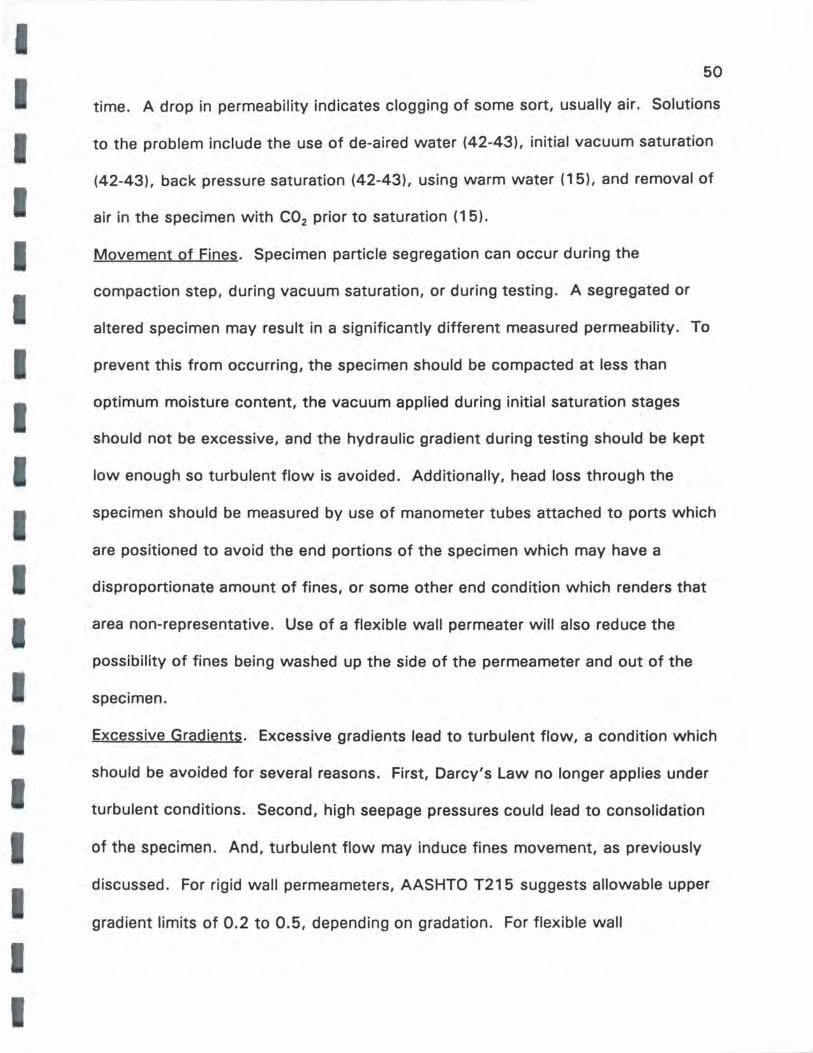
I
50
time. A drop in permeability indicates clogging of some sort, usually air. Solutions
to the problem include the use of de-aired water (42-43), initial vacuum saturation
(42-43), back pressure saturation (42-43), using warm water (15), and removal of
air in the specimen with CO2 prior to saturation ( 1 5).
Movement of Fines. Specimen particle segregation can occur during the
comp_action step, during vacuum saturation, or during testing. A segregated or
altered specimen may result in a significantly different measured permeability. To
prevent this from occurring, the specimen should be compacted at less than
optimum moisture content, the vacuum applied during initial saturation stages
should not be excessive, and the hydraulic gradient during testing should be kept
low enough so turbulent flow is avoided. Additionally, head loss through the
specimen should be measured by use of manometer tubes attached to ports which
are positioned to avoid the end portions of the specimen which may have a
disproportionate amount of fines, or some other end condition which renders that
area non-representative. Use of a flexible wall permeater will also reduce the
possibility of fines being washed up the side of the permeameter and out of the
specimen.
Excessive Gradients. Excessive gradients lead to turbulent flow, a condition which
should be avoided for several reasons. First, Darcy's Law no longer applies under
turbulent conditions. Second, high seepage pressures could lead to consolidation
of the specimen. And, turbulent flow may induce fines movement, as previously
discussed. For rigid wall permeameters, AASHTO T215 suggests allowable upper
gradient limits of 0.2 to 0.5, depending on gradation. For flexible wall

51
permeameters, ASTM D 5084 recommends using the gradient expected in the
field, which may range from less than 1 and up to 5. Recognizing that low
gradients will lead to very long testing times, D 5084 ties recommended gradient
to permeability: the lower the permeability, the higher the allowable gradient. For
materials with permeabilities of 0.3 to 3 ft/day (1 x 1 o·4 to 1 x 1 o·3 cm/sec), the
maximum recommended gradient is 5. Moulton says that, in a practical sense,
even at relatively low gradients, coarse graded materials may exhibit turbulent
behavior at gradients similar to those in the field. Thus, the coefficient of
permeability would not be a true Darcy coefficient, but would represent the desired
design situation for estimation of seepage flow. Excessive hydraulic gradients can
be detected by plotting discharge vs. gradient. Darcy's Law says that these two
variables are directly proportional and that permeability is the coefficient of
proportionality, or slope of the line. If at some point the slope begins to decrease
with increasing gradient, somet_hing is inhibiting flow. This could be the onset of
turbulent flow. Alternately, permeability could be plotted against gradient. A drop
in permeability would indicate a problem.
Direction of Flow. There are several concerns in regard to the direction of flow of
the permeant relative to the specimen. First, in the field, flow is horizontal and
thus runs parallel to the planes of compaction. In the laboratory, specimens are
usually tested with flow running perpendicular to the planes of compaction. Thus,
all things being equal, laboratory measured permeability should give conservative
(lower) values. One study (44) has shown permeability values for the horizontal
direction to be 1 .1 to 1 .8 times greater than in the vertica l direction for dense-

I
I
52
graded materials. The more fines, the more stratification, and the larger the
difference between horizontal and vertical permeabilities. Thus, in practice an
open-graded material will be less affected by stratification. However, the whole
concept may be moot because in a pavement structure a 4 to 6 in drainage layer
most likely will be placed in one lift.
Secondly, in laboratory testing, flow can be vertically upward or downward.
Downward would help prevent specimen expansion, but may even density the
material. Upward flow will assist in washing air bubbles out of the specimen, but
will tend to decompact the specimen. Upward expansion can be prevented by a
spring and perforated plate holding down the specimen. Thus, upward flow is the
preferred direction.
Off-Target Density. In a range of possible densities, the permeability of a given
material can vary from one to 20 times. This tendency is reduced as the range of
particle sizes narrows. Specimens can be inadvertently tested at densities that are
significantly different than what is intended. This can happen by incorrectly
fabricating the specimen, or through expansion or densification during the test, as
discussed earlier. Strohm m ru. ( 17) have shown that being off the target density
by 1 % can lead to a difference of measured permeability of 32% at a gradient of
0.2. In a 10 in (25.4 cm) diameter specimen, a height differential of 1 /8 in will
render a difference in density of about 2%. A change in height as a consequence
of testing can be detected by measuring the initial and final heights.
Rigid Wall Permeameter
Equipment. In this study, the open-graded materials were tested in the rigid wall

53
Fig.6. Rigid Wall Permeameter.
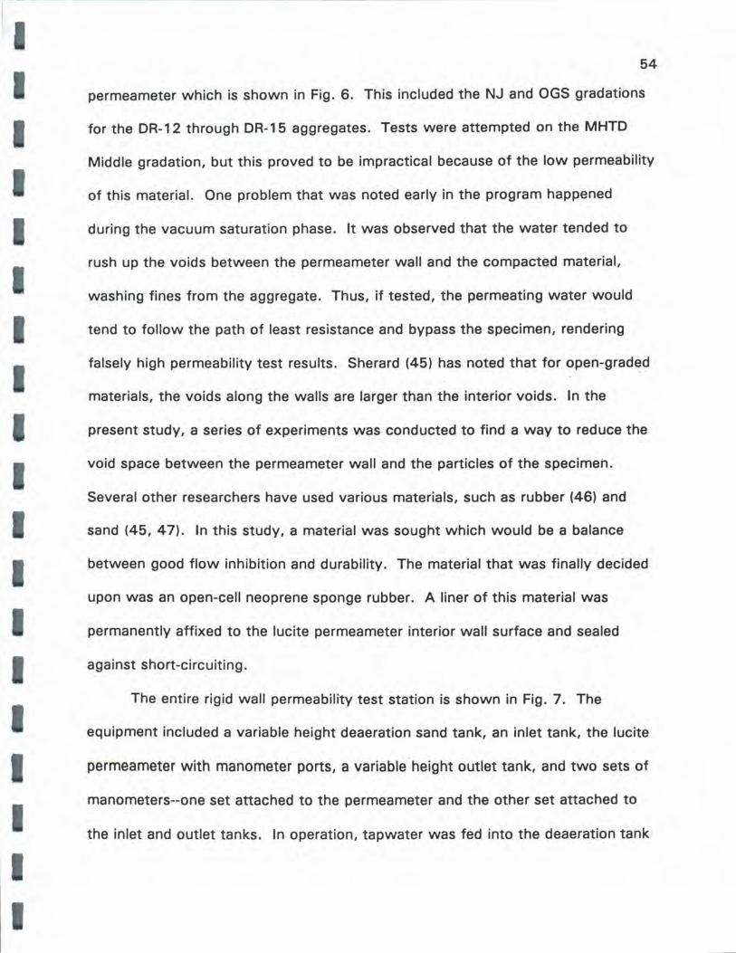
54
permeameter which is shown in Fig. 6. This included the NJ and OGS gradations
for the DR-12 through DR-15 aggregates. Tests were attempted on the MHTD
Middle gradation, but this proved to be impractical because of the low permeability
of this material. One problem that was noted early in the program happened
during the vacuum saturation phase. It was observed that the water tended to
rush up the voids between the permeameter wall and the compacted material,
washing fines from the aggregate. Thus, if tested, the permeating water would
tend to follow the path of least resistance and bypass the specimen, rendering
falsely high permeability test results. Sherard (45) has noted that for open-graded
materials, the voids along the walls are larger than the interior voids. In the
I present study, a series of experiments was conducted to find a way to reduce the
void space between the permeameter wall and the particles of the specimen.
Several other researchers have used various materials, such as rubber (46) and
sand (45, 47). In this study, a material was sought which would be a balance
between good flow inhibition and durability. The material that was finally decided
upon was an open-cell neoprene sponge rubber. A liner of this material was
permanently affixed to the lucite permeameter interior wall surface and sealed
against short-circuiting.
I
The entire rigid wall permeability test station is shown in Fig. 7. The
equipment included a variable height deaeration sand tank, an inlet tank, the lucite
permeameter with manometer ports, a variable · height outlet tank, and two sets of
manometers--one set attached to the permeameter and the other set attached to
the inlet and outlet tanks. In operation, tapwater was fed into the deaeration tank
VA
RIA
BL
E
HEI
GH
T O
UTL
ET
TAN
K
'7
"
\.I A
ST
E_
.._
__
_,
BLE
EDER
V
AL
VE
TD
BLE
EDER
V
AL
VE
INLE
T
TA
NK
,.
Fig
. 7
. S
chet
rto.
tic
o
f R
igic
l \J
a.ll
P
erM
ea
Me
ter
Te
st
Sta
. tio
n.
VA
RIA
BL
E
HEI
GH
T D
EAER
AT!
ON
TA
NK
. s·~ND
:,
-......
.:-
---B
AC
KF
LO
\./
LIN
E
<J1
<J1
I 56
which functioned in two ways. First, the water was introduced into the freeboard
above the sand bed. Here, upon depressurization, air was allowed to come out of
solution and rise to the top of the body of water and escape. The water itself
permeated downward through the sandbed. Most of the remaining air bubbles
I were trapped in the top portion of the sand bed. Periodically, the sand bed was
backflushed and stirred to remove bubbles. The gradient in the permeameter was
varied by raising or lowering the outlet tank; the driving head was the difference in
I I I
I
I I
elevation between the inlet and outlet tanks. To get a truer measurement of
permeability, the difference in readings in the two permeameter manometer tubes
were used as a measure of the driving head. This removed the problems
associated with effects at the top and bottom surfaces of the specimen, where
disturbance, smearing, and fines collection can alter the measured specimen
permeability. Flow was collected from the outlet tank and measured with a
graduated cylinder. Flow rate was calculated from time interval readings taken
with a stopwatch. Temperature was measured at the inlet and outlet tanks; the
average was used for temperature corrections to permeability calculations.
The permeameter was a 10 in diameter lucite cylinder, with manometer
ports approximately 10 in apart. The compacted specimen was 12 in in height. At
either end of the specimen was a perforated aluminum plate with an adjacent #200
screen to limit fines loss. The ability to see the specimen during saturation and
permeability testing proved to be very helpful in determining specimen behavior.
The effects of vacuum application and release, various flow rates, trapped air,
buildup of air, specimen disturbance, and so forth were observed. This ability is
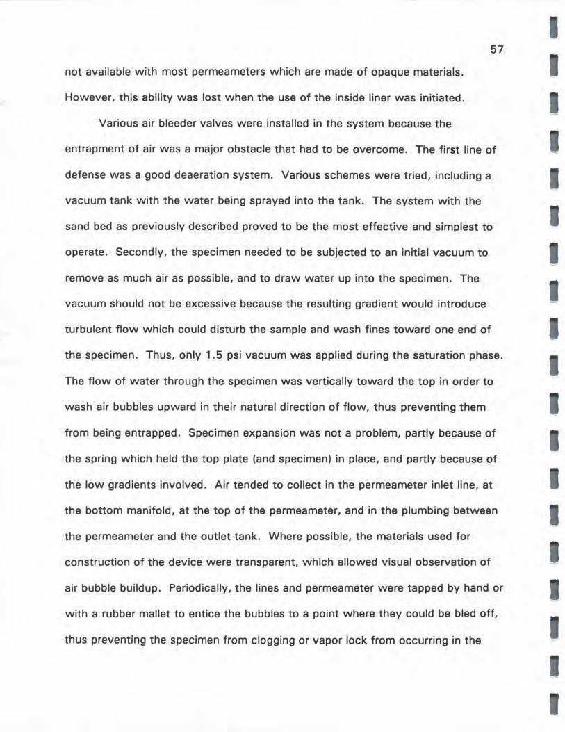
57
not available with most permeameters which are made of opaque materials.
However, this ability was lost when the use of the inside liner was initiated.
Various air bleeder valves were installed in the system because the
entrapment of air was a major obstacle that had to be overcome. The first line of
defense was a good deaeration system. Various schemes were tried, including a
vacuu_m tank with the water being sprayed into the tank. The system with the
sand bed as previously described proved to be the most effective and simplest to
operate. Secondly, the specimen needed to be subjected to an initial vacuum to
remove as much air as possible, and to draw water up into the specimen. The
vacuum should not be excessive because the resulting gradient would introduce
turbulent flow which could disturb the sample and wash fines toward one end of
the specimen. Thus, only 1.5 psi vacuum was applied during the saturation phase.
The flow of water through the specimen was vertically toward the top in order to
wash air bubbles upward in their natural direction of flow, thus preventing them
from being entrapped. Specimen expansion was not a problem, partly because of
the spring which held the top plate (and specimen) in place, and partly because of
the low gradients involved. Air tended to collect in the permeameter inlet line, at
the bottom manifold, at the top of the permeameter, and in the plumbing between
the permeameter and the outlet tank. Where possible, the materials used for
construction of the device were transparent, which allowed visual observation of
air bubble buildup. Periodically, the lines and permeameter were tapped by hand or
with a rubber mallet to entice the bubbles to a point where they could be bled off,
thus preventing the specimen from clogging or vapor lock from occurring in the
I
I
I
58
plumbing.
Procedure. Each specimen was compacted into the permeameter at a slightly drier
than-optimum moisture content. This moisture content was found to be necessary
in order to prevent fines migration during compaction. The specimens were
compacted in 12 layers of one in thickness using an air hammer and steel plate.
Final compacted height was measured; it was measured again after completion of
the permeability testing to calculate any specimen expansion or densification. The
I specimen was subjected to 1.5 psi vacuum for 15 minutes, then deaired water
was introduced at the base. After water was observed to flow into the outlet
tank, testing was initiated. Each specimen was subjected to five increasingly
higher test gradients. The flows and times were repeated five times at each
gradient. The gradients ranged from 0.02 to 0.6, which covered the expected
range of gradients in the field up to turbulent flow. The expected gradient in the
field was calculated as follows:
I
D1 +D2 +(S • \IV) = .•............... (21)
w
where:
0 1 = maximum anticipated surface layer thickness
0 2 = base layer thickness
S = slope of base
W = base width.
This assumes that water has completely filled the pavement up to the pavement
surface at the centerline joint. For a 1 5 in asphalt layer over 6 in granular subbase
59
at a cross-slope of 3/16 in per ft and a 14 ft lane width, the maximum expected
gradient at total saturation of a very thick pavement would be 0. 14. Average
gradients would be considerably less than this. The permeabilities calculated in
this study were limited to gradients of less than 0. 1 to assure that laminar flow
conditions existed. The concept is shown in Fig. 8.
Hydraulic gradient Y.S. flow rate was plotted to check for turbulent flow.
During calculation of permeability, the permeability values for all gradients up to
0.1 were averaged; however, any value of permeability which was suspected of
being under turbulent conditions was not used in order to assure compliance with
Darcy's Law.
Temperature readings at the inlet and outlet tanks were averaged.
Calculated permeabilities were corrected to 20°C.
Permeability was calculated as follows:
k = Ql R/Ath ................... (22)
where:
k = coefficient of permeability at 20°C, ft/day
Q = volume of flow, cu ft
L = distance between manometer ports, ft
Rt = temperature correction factor to 20°C
A = cross-sectional area of the specimen, sq ft
t = time interval, days
h = head loss through specimen, ft.
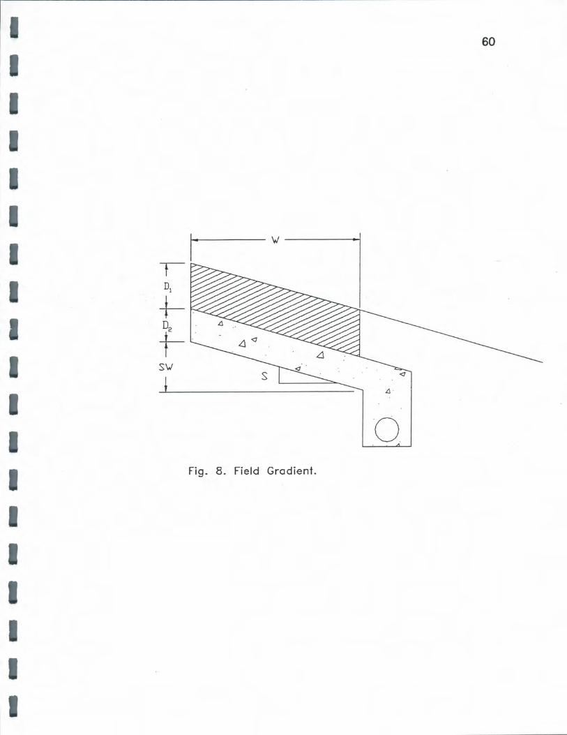
60
I
I I
1· t
D1
I +- -D .
f-S'v/
<J
t Ll
I ·o I F. 8 Field Gradient. 19. .
I
I

61
Gradient was kept constant by keeping the difference in elevation between the
outlet and inlet tank water levels constant. Gradients were adjusted by raising or
lowering the outlet tank. Calculations of permeability utilized the change in
permeameter manometer levels. The inlet and outlet tank manometer readings
were used as a check to see if the permeameter manometer readings were
behaving normally.
Flexible Wall Permeameter
Equipment. The permeability of the dense-graded materials was too low for these
materials to be used in the rigid wall permeameter because of available applied
head limitations of the equipment. Thus, a flexible wall permeameter was used for
testing the MHTD Middle gradation. Actually, the equipment used was the cyclic
triaxial apparatus used for resilient modulus testing. After the cyclic loading used
in the modulus testing was completed, the specimen was subjected to permeability
testing. The equipment and specimen fabrication has been discussed in previous
sections. Special perforated aluminum manifolds were machined to replace the
more traditional porous stones at each end of the specimen in order to assure that
sufficient flow would be applied to the specimen. Also, the porous stones tended
to break during the vibratory compaction of the specimen during fabrication.
Number 200 screen was placed at the specimen ends to reduce the chance of
fines migrating out of the specimen during fabrication and testing.
Procedure. Upon completion of the resilient modulus testing, the specimen was in
a saturated and consolidated condition. The procedure found in ASTM D 5084-90
was then followed for permeability testing. Tap water was used as the permeant.

I
62
For materials with permeabilities of 0.28 to 0.028 ft/day, hydraulic gradients of
five or less are recommended. This was achieved in the testing program by
limiting the cell pressure to 3 psi above back pressure, and the head pressure to
1.5 psi above back pressure for the 8 in high specimens. And, effective confining
pressure never exceeded 3 psi at one end of the specimen and 1.5 psi at the other
end.
The test equipment is shown in Fig. 9. A schematic of the system is
depicted in Fig. 10. As can be seen, back pressure is applied to the top of the
specimen and a higher pressure (head pressure) is applied to the specimen bottom,
forcing water flow upwards. Back pressure and head pressure are achieved
principally by applying air pressure to water-filled burettes. Flow through the
specimen is measured in both the inflow (head pressure) and outflow (back
pressure) burettes. These were essentially equal in the testing program. The time
interval over which the flow takes place is also recorded. Eq. 22 was used to
calculate permeability. The head loss (h) was the average of the initial and final
inflow burette plus head pressure readings minus the average of the initial and final
outflow burette plus backpressure readings. The final calculated permeability was
the average of five test runs.
POROSITY
In the estimation of permeability, it is useful to use porosity as a predictor,
although a high porosity does not necessarily mean a correspondingly higher
permeability. Porosity is calculated in accordance with Eq. 3, rep.eated here:
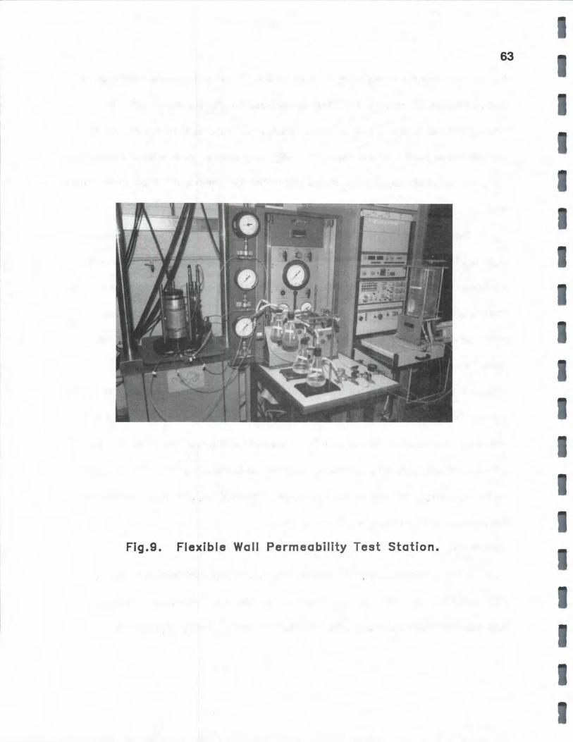
63
Fig.9. Flexible Wall Permeability Test Station.
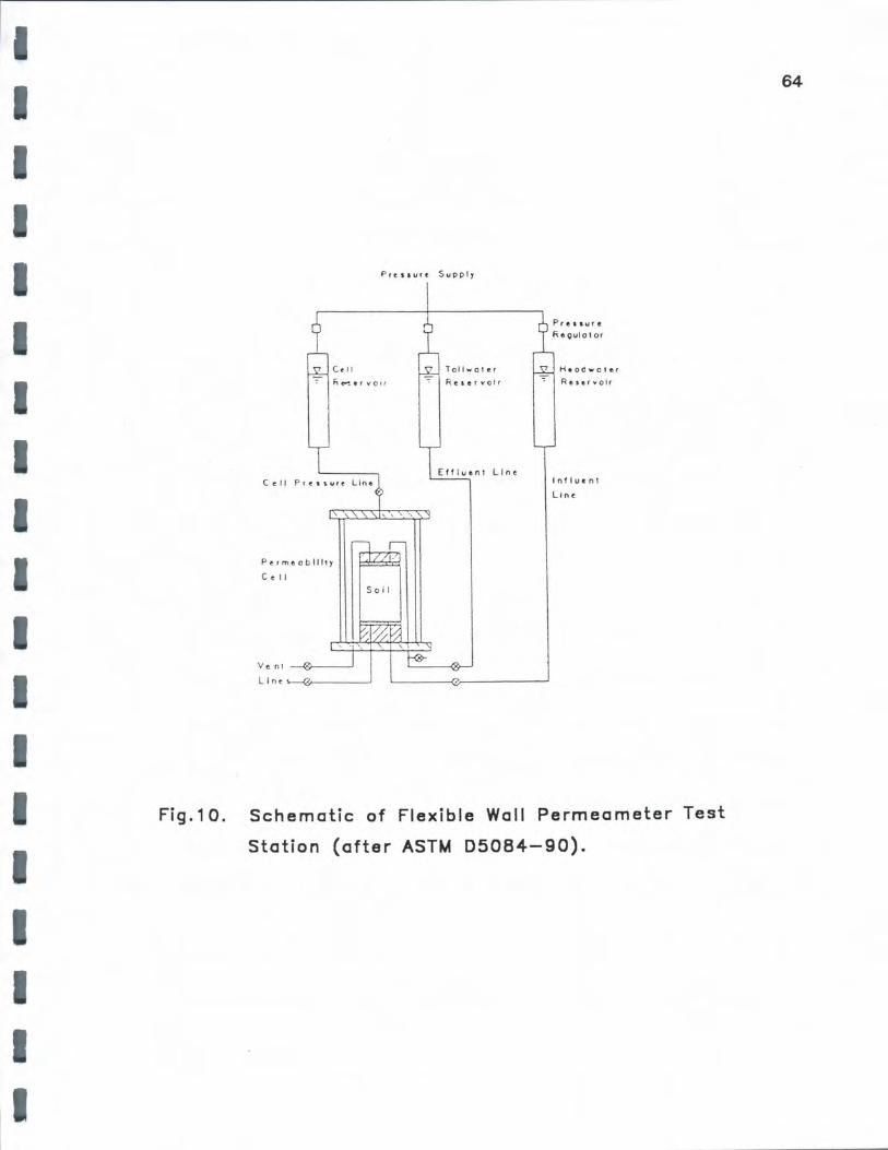
I I
I
I
I I
I
Fig.10.
Pr e 1 .aurt. S up p l y
C t 11
F;_ e""'!. • f VO Ir
Tollwoler
R e , ervo l r
Permeo b lll t y
C C 1 1
V e n 1 -----<<>----~
L I n c >--«>------'
Heod w oler
Rfl s e.r volr
Inf I u • n t
L i n t
Schematic of Flexible Wall Permeameter Test
Station (after ASTM 05084-90).
64
65
fJ = 1 _ Yd G• Yw
The question arises as to whether to use bulk or apparent specific gravity. Both
values are readily available from the same test procedure. A case can be made for
using bulk specific gravity as follows. When water is added to granular material,
water penetrates voids in the particles, filling them to the surface. Drainability
studies have shown that this void space is not available to conduct water through
the compacted granular material. Only the voids between the particles have a
possibility of being available. Thus calculation of porosity, in a practical sense,
should be based on the particles having no particle voids communicating to the
particle surface -- a condition described by bulk specific gravity, which is defined
as dry weight divided by bulk particle volume. Examination of Eq. 6 leads to the
conclusion that porosities calculated using bulk specific gravity (BSG) will be
smaller than porosities calculated with apparent specific gravity (ASG) which uses
the non-water penetrating particle volume in its definition. Unfortunately, many
studies that are reported in the literature do not specify which type of specific
gravity was used in the porosity calculations. It was assumed that apparent
specific gravity is used in the Moulton equation (Eq. 2). Examination of Eq. 2
indicates that the use of BSG would lead to lower predicted permeabilities. The
concept of effective porosity, which takes all this a step further, is explained in a
later section.
The value of specific gravity used in the porosity calculation can significantly
alter the results. Values of specific gravity seen in practice range from BSG's of
66
2.45 to ASG's of 2.80. Thus, calculated porosities can vary from 11. 7 to 27. 7%
I for a compacted unit weight of 135 pcf. It follows that an accurate value for
specific gravity is necessary for an accurate calculation of porosity.
I I
EFFECTIVE POROSITY
As previously discussed, time-to-drain calculations require data for the
effective porosity data for the material that is draining. Effective porosity is the
ratio of the volume of voids that can be drained under gravity to the total volume
of base material. It has been shown ( 16) that for open-graded materials, the
effective porosity can be close to the calculated porosity, but for dense-graded
base materials, the effective porosity can be quite small. The water that is
essentially nondrainable is water that is held in the pores by capillary action or
water films on the aggregate particle surfaces. The equation (Eq. 6) for effective
porosity is essentially the traditional porosity equation, with the term that
represents the solid volume being increased for the nondrainable water. The
equation is repeated below:
After permeability testing is complete, the water content remaining after 16 hr
drainage under gravity conditions is determined. This water content is w.. Here,
the apparent specific gravity should be used, not the bulk specific gravity, because
I w. reflects all the water remaining including the water in the particle pores. Thus,
the smaller particle volume (as calculated by use of apparent specific gravity)
should be used in the above equation. Even after 24 hr drainage, for dense-
I
67
graded, highly compacted base material with a fines content as low as 5%,
effective porosity can approach zero (17). A low TJ. directly affects drainage times.
Additionally, the mineralogical type of fines affects effective porosity much as it
does permeability (13). The more active the fines, the lower the effective porosity.
68
RESULTS OF THE LABORATORY INVESTIGATION
I AS-RECEIVED GRADATIONS
I
I
The as-received gradations of the four granular materials are shown in Table
7.
Table 7. As-Received Gradations.
Sieve Percent Passing Size
DR-12 DR-13 DR-14 DR-15
1 in 100 100 100 100
1/2 in 96 83 72 83
#4 68 50 46 50
16 -- 26 37 26
40 24 18 17 12
100 12 13 2 5
200 8 7 1 4
EXPERIMENTAL GRADATIONS
The three experimental gradations were the MHTD Middle, the New Jersey
(NJ), and the OGS. These are shown in Table 8. The NJ and the OGS were used
in the rigid wall permeameter permeability testing, while the Middle and the NJ
were used in the resilient modulus portion of the study. Only the Middle was
tested for permeability with the flexible wall permeability procedure because of
equipment limitations.
69
Table 8. Experimental Gradations.
Sieve Size % Passing
Middle NJ OGS
3 in. 100 100 100
1 1/2 100 100 100
1 100 100 100
3/4 (95) (95) (91)
1/2 75 68 60
3/8 (63) (58) (48)
#4 50 47 30
8 (40) (20) (16)
16 33 5 7
30 (28) (4) (6)
40 25 3 5
50 (22) (2.5) (4)
100 (16) (2.5) (3)
200 8 2 2
( ) = estimated from semilog plot
GRADATION CURVE SHAPE/POSITION
In an attempt to determine the effect of gradation on permeability, values for
gradation curve shape/position were required. Nine different methods were tried.
Sieve size data from all three experimental gradation curves were used for
calculation of various parameters; the parameters were then used in the
development of the multiple regression models for permeability to see which
method increased the accuracy of the model the most. The nine methods or
parameters were as follows: fineness modulus (FM), coefficient of uniformity (Cul,

I I I I I I I I I I I I I I I I I I I
70
coefficient of skew (Cz), surface fineness (SF), specific surface factor (SSF),
-(SF/SSF), Hudson's A, slopes-of-gradation-curve (mn-nl, and the percent passing
individual sieves. The results are shown in Table 9. These parameters are
discussed more fully in Volume I of this report. The slopes-of-gradation-curve
method was altered from that described in Volume I to better match the natural
break points of the experimental gradation curves. Thus the slopes of each curve
were determined between the 1 in and #4 sieve, the #4 and #16 sieves, and the
#16 and #200 sieves. The results of these calculations are shown in Table 10.
Table 9. Gradation Shape Results.
Middle NJ OGS
FM 4.53 5.66 5.95
cu 82.6 5.29 8.47
CZ 1.19 0.21 0.25
SF 1588 1938 1929
SSF 294.4 65.8 76.3
SF/SSF 5.40 29.4 25.3
A 4.55 3.36 3.07
Mn-n 94.3, 78.0, 100.0, 132.1, 138.9 192. 7, 105.5,
16.7 27.8
3/4", #4, 16, 200 95, 50, 33, 8 95, 47, 91, 30, 5, 2 7, 2
71
Table 10. Experimental Gradation Slopes.
Gradation M,.4 M4.1e M,e-200
Middle 94.3 78.0 138.9
NJ 100.0 192.7 16.7
OGS 132.1 105.5 27.8
For the permeability testing, none of the single curve shape/position
parameters was significant to the model. However, percent passing certain
individual sieves was significant. In terms of individual particle sizes, the effect of
gradation on permeability was ascertained as follows. As will be discussed more
fully later, a model was developed to represent the permeability results of several
other studies in addition to the results of the present study to give a more
generally applicable equation to predict permeability. All gradations used in the
model are shown in Fig. 11. Because grain size distribution is linked to the pore
volume available to transmit water, a method was developed to relate the two.
This was done by determining how close the percent passing on each sieve size
was to the percent passing for the densest possible gradation. The maximum
density gradation was estimated by use of 0.45 power FHWA paper, commonly
used in asphalt gradation work. For each gradation, the maximum density line
(MDL) was drawn in accordance with the method given in Volume I of the
companion report to this study (27). Next, the vertical distance (in percent
passing) between the MDL and the percent passing gradation line on each sieve
was found and converted to a percent of total possible distance. This
measurement was determined for each of the base rock gradations and was
I

I I I
I I I I I I I I I
I
I I
bl)
t:: •r-4 rt.I l1l IC
11.. ,+,)
~ Q) t.) J-4 Q)
11.. -IC ,+,)
0 ~
100
90
80
70
60
50
40
30
20
10
0
72
200 100 50 30 16 B 4 3/B" 3/4" 1 1/2"
Sieve Size
Fig. 11. Gradations of Materials Used in the Permeability Model Development.

73
correlated with permeability. Pearson's correlation coefficients (R) were
calculated. The results are shown in Table 11 . The particle sizes that were most
effective in predicting permeability were (individually) the #4, #8, and 3/8 in
sieves, as well as the D10 size. This information proved useful in the development
of the permeability model as discussed later in this report. Although the #200
sieve did not indicate a high individual correlation, it was found to be helpful in the
model development.
Table 11. Usefulness of Individual Particle Sizes in Prediction of Permeability.
Material k Percent Difference Between Maximum Density Line and Gradation Line (ft/day)
3/8 in #4 #8 #16 #30 #50 #100 #200 D,o (mm)
MHTD 0.8 8.7 0.2 8.1 25.9 47.4 57.1 60.0 14.3 0.092 Middle
S&G 1.2 0.2 5.1 0.4 19.0 53.3 63.6 1.2 33.3 0.16
Cr. 372 29.0 28.0 24.3 18.5 10.5 14.3 30.0 28.6 0.20 Gravel
MHTD 820 15.9 6.0 45.9 81.5 78.9 85.7 80.0 71.4 1.7 NJ
Cr. 1073 38.9 41.0 35.7 47.6 46.7 45.4 37.5 50.0 0.94 Stone
MHTD 1158 27.3 37.5 54.3 72.0 66.7 69.2 70.0 71.4 1.5 OGS
S&G 18,144 38.9 69.2 71.4 66.7 60.0 54.5 50.0 33.3 3.9
S&G 21,546 63.0 89.7 92.9 100 100 100 100 100 7.0
R -- 0.773 0.893 0.839 0.644 0.572 0.435 0.487 0.444 0.944
S&G = Sand and Gravel (ref. 41) Cr. Gravel = Crushed gravel (ref. 17) Cr. Stone = crushed stone (ref. 17)
I I I I I I I I I I I I

I I I I I I I I I I I I I I I I I
I
MOISTURE-DENSITY RELATIONSHIPS AND SPECIFIC GRAVITIES
Moisture-density relationship and specific gravity information were
determined in regard to the three test gradations for each of the four granular
materials. The data is shown in Table 12.
Table 12. Specific Gravity and Moisture Density Data.
74
T-99 T-180 D4253 Material Gradation Sp. Gravity
ASG BSG MOD OMC MOD OMC MOD OMC (pcf) (%) (pcf) (%) (pcf) (%)
DR-12 Middle 2.69 2.53 136.5 7.0 137.6 7.4 -- --OGS 2.69 2.53 -- -- -- -- 127.6 10.3
NJ 2.69 2.53 -- -- 131.2 9.0 121.1 12.2
DR-13 Middle 2.78 2.55 138.3 7.7 141.0 5.9 -- --OGS 2.78 2.55 -- -- -- -- 124.6 12.2
NJ 2.78 2.55 -- -- 135.2 8.3 124.1 13.0
DR-14 Middle 2.65 2.52 132.5 7.8 134.5 6.7 -- --OGS 2.65 2.52 -- -- -- -- 123.0 10.8
NJ 2.65 2.52 125.8* 7.3 122.8 10.3 121.3 12.0
DR-15 Middle 2.65 2.41 134.4 7.6 136.9 6.1 -- --OGS 2.65 2.41 -- -- -- -- 112.2 13.8
NJ 2.65 2.41 109.5* * 8.9 -- -- 114.3 14.0
Note: T-99 = Standard proctor T-180 = Modified proctor D4253 = Vibratory table *E0 specimen compacted with vibratory hammer to refusal. This value was used as the maximum target value for the High Compactive effort specimens. * * T-99, T-180, and D4253 densities were very close. To get a wider difference in values a peak vibratory density achieved with a different surcharge weight was used.
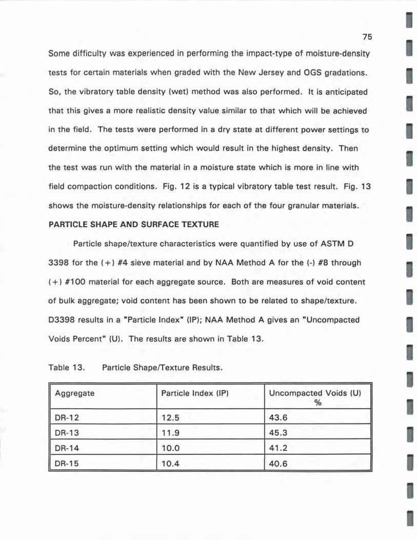
75
Some difficulty was experienced in performing the impact-type of moisture-density
tests for certain materials when graded with the New Jersey and OGS gradations.
So, the vibratory table density (wet) method was also performed. It is anticipated
that this gives a more realistic density value similar to that which will be achieved
in the field. The tests were performed in a dry state at different power settings to
determine the optimum setting which would result in the highest density. Then
the test was run with the material in a moisture state which is more in line with
field compaction conditions. Fig. 12 is a typical vibratory table test result. Fig. 13
shows the moisture-density relationships for each of the four granular materials.
· PARTICLE SHAPE AND SURFACE TEXTURE
Particle shape/texture characteristics were quantified by use of ASTM D
3398 for the ( +) #4 sieve material and by NAA Method A for the (-) #8 through
( +) #100 material for each aggregate source. Both are measures of void content
of bulk aggregate; void content has been shown to be related to shape/texture.
03398 results in a "Particle Index" (IP); NAA Method A gives an "Uncompacted
Voids Percent" (U). The results are shown in Table 13.
Table 13. Particle Shape/Texture Results.
Aggregate Particle Index (IP) Uncompacted Voids (U) %
DR-12 12.5 43.6
DR-13 11.9 45.3
DR-14 10.0 41.2
DR-15 10.4 40.6
I I

I I I I I
76
Round, smooth particles give IP's of 6 or 7, while angular, rough particles result in
values of more than 15. The range of IP's of the aggregates in this study was
10.0 to 12.5. The Particle Index was determined for the coarse aggregate fraction
of each gradation and the Uncompacted Voids content was determined for the fine
aggregate fraction.
Looking at Particle Index and especially the Uncompacted Voids values, the
crushed aggregates were somewhat more angular than the gravels, as expected,
but the ranges were limited.
PLASTICITY OF FINES
The results of the Atterberg Limits testing are shown in Table 14. All four
I aggregates were essentially non-plastic in nature.
I I I I I I I I
1•
Table 14. Atterberg Limits of the Base Materials.
Aggregate Liquid Limit Plasticity Index
DR-12 16 NP
DR-13 18 NP
DR-14 22 NP
DR-15 19 NP
RESILIENT MODULUS
Resilient modulus tests were performed on two crushed stone aggregates
(DR-12 and DR-13) and two gravels (DR-14 and DR-15) at two degrees of
saturation (aproximately 60 and 100%), two compactive efforts (low and high),
two gradations (MHTD Middle and New Jersey), and 14 stress states, with
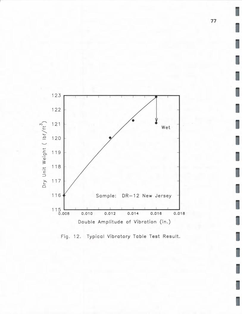
77
123
122
,........_ 1 21 rr)
-+-J ~ Wet
.......__ ~
..0 120 ....._,,
+' ...c 1 1 9 O"l
(l)
3: +' 1 1 8 C:
::J
>- 1 1 7 I...
0
1 1 6 Sample: DR-12 New Jersey
1 1 5 0.008 0 .010 0.012 0.014 0.016 0.018
Double Amplitude of Vibration (in.)
Fi g . 1 2 . Ty pi ca I Vi b rat o ry Ta b I e Test Res u It.
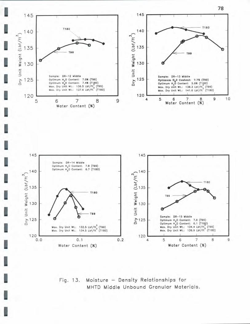
I I I I I I I I I I I I I I I I I I I
145
140
-'-.. ..... :3 1 35
; 130
C ::::J
~ 125 0
120 5
145
,......_ 140
+' -'-.. ..... :3 135
+' ..c Cl'
; 130
C: ::::J
~ 125 .... 0
120 0.0
T180
'
Semple: DR-12 Middle Optimum H20 Content : 7 .OX (T99) Optimum H20 Content: 7 .4!1: (T\80) Mo x. Dry Unit Wt. : 136.5 Lbf/ft
3 (T99)
Mo x. Dry Unit Wt.: 137 .6 Lbf/ft (T180)
6 7 8 Water Content (%)
Sample : DR-14 Middle Optimum H
20 Content: 7 .8 (T99)
Optimum H20 Content: 6.7 (T180)
T180
TIIII
Mo x. Dry Unit Wt. : Mo x. Dry Unit Wt. :
J 132.5 Lbf/ft
3 (T99)
134 .5 Lbf/ft (T180)
9
,-.. I")
+' .... ......... ....
145
140
:3 135
+' .r. Cl
.iii 130 3;
C ::::J
>- 125 .... 0
120
,...... 140 I")
+' .... ......... .... ..0
.:::, 1 35 +' .r. C7' Q)
3; 130
C ::::J
~ 125 0
4
Sample: DR-13 Middle Optimum H
10 Content: 7 .7",(, (T99)
Optimum H20 Content : 5.9% (T\80) t.Aox . Dry Unit Wt.: 138.3 Lbf/ft3 (T99) t.Aox . Dry Unit Wt. : 141.0 Lbf/fl (T1BO)
5 6 7 8 9 Water Content (%)
Sample: DR-15 Middle Optimum H20 Content: 7 .6 (T99) Optimum H20 Content : 6.1 (T18jl) Mox. Dry Unit Wt. : 134 .'4 Lbf/ft3 (T99) Mox. Dry Unit Wt. : 136.9 Lbf/ft (T1 80)
78
10
120 '-~~ ...... ~~ ...... ~~ ...... ~~---~~ ...... 0 . 1 0.2 4 5 6 7
Water Content (%) Water Content (%)
Fig. 13. Moisture - Density Relationships for
MHTD Middle Unbound Granular Materials.
8 9
~
en a.
'-"
en :::,
:::, "'O 0 ~
~
C: Q)
en Q)
0:::
1 0 100
Bulk Stress (psi)
Fig . 14. Typical Resilient Modulus Test Results.
79
I
I I
I
I
I

I I I I I I I I I I I I I I I I I I I
80
duplicate samples, for a total of 896 tests. Because the same 14 stress states and
the two degrees of saturation were used for each specimen, there were 32
specimens. The testing sequence for each specimen is shown in Table 5. Fig. 14
is a typical plot of bulk stress ~. resilient modulus. Each data point is
representative of one stress state. As can be seen, modulus increases with an
increase in stress state. The classic equation of the line (known as the "theta
model") is:
or
where:
log E(l = log k 1 + k2 log 0 ............... (23)
E(l = k1
e*• . . . . . . . . . . . . . . . . . . . . (24)
k1 = intercept of Eu at 0 = 1 psi, log-log plot
k2 = slope of line, log-log plot.
The results of all resilient modulus testing are tabulated in Table 15.
Fig. 15 shows the relationship of coefficients k1 and k2 as reported by Rada
and Witczak (40), with the results of the present study also plotted. As can be
seen, the results of the present study data fall in the range that has been reported
elsewhere.
The effect of increased degree of saturation is shown in Fig. 16. The
general trend is a loss of Eu as the degree of saturation increases from a moist
state to a saturated state. This is similar to the trend reported by others
(2,40,59,60). As will be discussed later, the loss of k1 due to an increase in
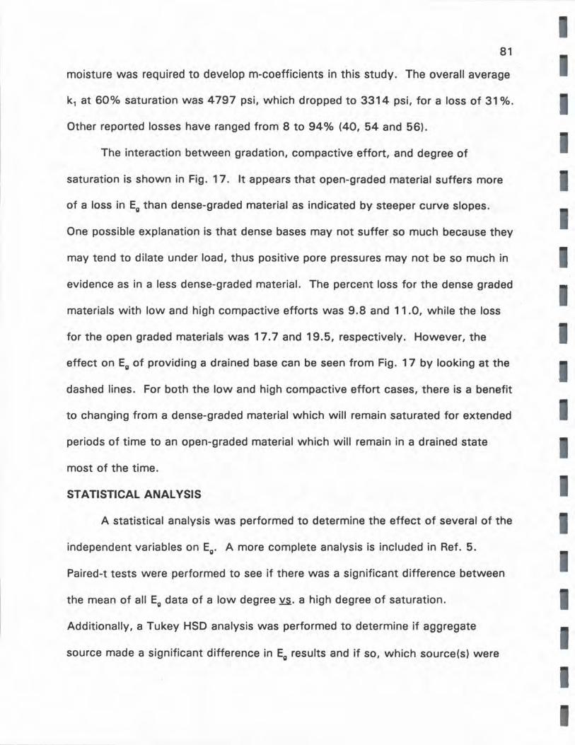
81
moisture was required to develop m-coefficients in this study. The overall average
k1 at 60% saturation was 4797 psi, which dropped to 3314 psi, for a loss of 31 %.
Other reported losses have ranged from 8 to 94% (40, 54 and 56).
The interaction between gradation, compactive effort, and degree of
saturation is shown in Fig. 17. It appears that open-graded material suffers more
of a loss in Eg than dense-graded material as indicated by steeper curve slopes.
One possible explanation is that dense bases may not suffer so much because they
may tend to dilate under load, thus positive pore pressures may not be so much in
evidence as in a less dense-graded material. The percent loss for the dense graded
materials with low and high compactive efforts was 9.8 and 11.0, while the loss
for the open graded materials was 17. 7 and 19.5, respectively. However, the
effect on Eg of providing a drained base can be seen from Fig. 17 by looking at the
dashed lines. For both the low and high compactive effort cases, there is a benefit
to changing from a dense-graded material which will remain saturated for extended
periods of time to an open-graded material which will remain in a drained state
most of the time.
STATISTICAL ANALYSIS
A statistical analysis was performed to determine the effect of several of the
independent variables on Eg. A more complete analysis is included in Ref. 5.
Paired-t tests were performed to see if there was a significant difference between
the mean of all Eg data of a low degree Y..S., a high degree of saturation.
Additionally, a Tukey HSD analysis was performed to determine if aggregate
source made a significant difference in Eg results and if so, which source(s) were
I
I I
I
I I I I I
I

----
----
----
----
---
Ta
ble
15
. R
esi
lien
t M
od
ulu
s T
est
Dat
a.
Mat
eria
l G
rada
tion/
CE
D
ry D
ensi
ty (
pcf)
M
AD
D
Tar
get
As-
test
ed
(pcf
) (%
)
DR
-12
Mid
(lo
w)
13
6.5
1
36
.4
13
8.9
9
8.2
DR
-12
Mid
(lo
w)
13
6.5
1
36
.4
13
8.9
9
8.2
DR
-12
Mid
(hi
gh)
13
7.6
1
38
.4
13
8.9
9
9.6
DR
-12
Mid
(hi
gh)
13
7.6
1
38
.4
13
8.9
9
9.6
DR
-12
NJ
(low
) 12
1.1
12
0.5
1
31
.2
91
.8
DR
-12
NJ
(low
) 12
1.1
12
0.5
1
31
.2
91
.8
DR
-12
NJ
(hig
h)
13
1.2
1
27
.7
13
1.2
9
7.3
DR
-12
NJ
(hig
h)
13
1.2
1
27
.7
13
1.2
9
7.3
DR
-13
Mid
(lo
w)
13
8.3
1
38
.2
14
1.0
9
8.0
DR
-13
Mid
(lo
w)
13
8.3
1
38
.2
14
1.0
9
8.0
DR
-13
Mid
(hi
gh)
14
1.0
1
39
.5
14
1.0
9
8.9
DR
-13
Mid
(hi
gh)
14
1.0
1
39
.5
14
1.0
9
8.9
DR
-13
NJ
(low
) 12
4.1
12
5.9
1
35
.2
93.1
DR
-13
NJ
(low
) 12
4.1
12
5.9
1
35
.2
93.1
DR
-13
NJ
(hig
h)
13
5.2
13
4.1
13
5.2
9
9.2
DR
-13
NJ
(hig
h)
13
5.2
13
4.1
13
5.2
9
9.2
DR
-14
Mid
(lo
w)
13
2.5
13
1.1
13
5.4
9
6.8
DR
-14
Mid
(lo
w)
13
2.5
13
1 .1
1
35
.4
96
.8
DR
-14
Mid
(hi
gh)
13
4.5
1
34
.4
13
5.4
9
9.3
DR
-14
Mid
(hi
gh)
13
4.5
1
34
.4
13
5.4
9
9.3
DR
-14
NJ
(low
) 1
22
.8
121.
1 1
25
.8
96
.2
DR
-14
NJ
(low
) 1
22
.8
121.
1 1
25
.8
96
.2
DR
-14
NJ
(hig
h)
12
5.3
12
4.1
12
5.8
9
8.6
DR
-14
NJ
(hig
h)
12
5.3
1
25
.0
12
5.8
9
9.3
DR
0S
at.
k,
(%)
(psi
)
92.1
6
1.4
3
04
0
92.1
1
00
2
95
8
98
.4
62
.5
38
28
98
.4
10
0
37
58
69
.3
59
.6
43
07
69
.3
10
0
19
40
90
.5
53
.1
51
34
90
.5
10
0
27
06
91
.3
63
.8
42
12
91
.3
10
0
36
06
95
.2
59
.8
83
12
95
.2
10
0
59
18
78
.3
63
.8
34
70
78
.3
10
0
28
24
97
.5
58
.8
31
64
97
.5
10
0
29
97
85
.9
58
.6
44
43
85
.9
10
0
3401
96
.8
67
.2
54
68
96
.8
10
0
57
93
84
.7
58
.2
66
18
84
.7
10
0
45
04
94
.7
55.1
7
63
9
97
.4
10
0
35
69
k2
0.8
5
0.8
6
0.8
2
0.8
0
0.7
2
0.9
0
0.7
4
0.9
2
0.7
6
0.8
0
0.5
8
0.6
2
0.81
0.8
2
0.9
0
0.8
6
0.6
0
0.6
8
0.6
4
0.6
7
0.5
6
0.7
2
0.5
3
0.7
4
Eg(
psi)*
8=
10
21
,52
2
21
,42
8
25
,29
5
23
,43
7
22
,86
5
15
,58
4
27
,89
0
22
,50
8
24
,23
8
22
,75
2
31
,96
7
24
,39
0
22
,40
7
18
,65
8
25
,42
8
21
,96
3
17
,68
8
16
,27
8
23
,86
9
27
,09
6
24
,30
9
23
,36
9
25
,88
4
19
,84
0
CX)
I\.)
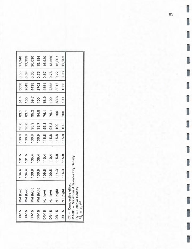
DR
-15
Mid
(lo
w)
13
4.4
1
31
.5
13
6.9
DR
-15
Mid
(lo
w)
13
4.4
1
31
.5
13
6.9
DR
-15
Mid
(hi
gh)
13
6.9
1
35
.4
13
6.9
DR
-15
Mid
(hi
gh)
13
6.9
1
35
.4
13
6.9
DR
-15
NJ
(low
) 1
09
.5
11
0.4
1
15
.8
DR
-15
NJ
(low
) 1
09
.5
11
0.4
1
15
.8
DR
-15
NJ
(hig
h)
11
4.3
1
15
.8
11
5.8
DR
-15
NJ
(hig
h)
11
4.3
1
15
.8
11
5.8
CE
=
Com
pact
ive
eff
ort
M
AD
D =
M
axim
um A
ttain
able
Dry
Den
sity
DR
=
R
elat
ive
Den
sity
* E
g =
k 1
91<2.
---
96
.0
83.1
5
1.4
96
.0
83.1
1
00
98
.9
95
.2
59
.7
98
.7
94
.5
10
0
95
.3
76.1
5
8.9
95
.3
76.1
1
00
10
0
10
0
63
.6
10
0
10
0
10
0
--
50
58
0
.55
26
45
0
.69
44
98
0
.65
27
02
0
.75
45
54
0
.57
23
58
0
.76
30
12
0
.72
13
38
0
.96
17
,94
6
12
,95
5
20
,09
0
15
,19
4
16
,92
0
13
,56
9
15
,80
7
12
,20
3 --
00
(.,.)
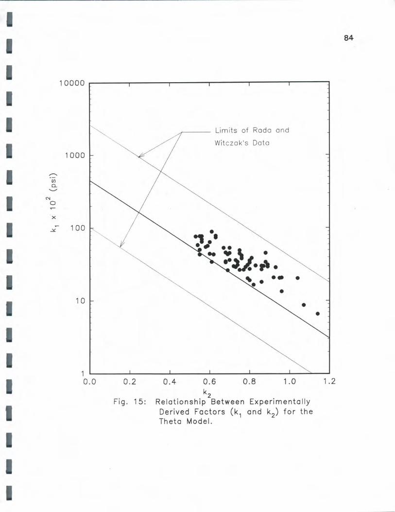
I I I I I I I I I I I I I I I I I I I
,.--....
VJ 0...
'--""
N 0 ,..-
X
~
~
1000
100
1 0
1 0.0 0.2
Fig. 15:
0 .4
Lim its of Rado and
Witczok 's Data
• ., .• . - .. .. . \ . .. ~:J. ....
0.6 0.8
k2
•• • •
1 .0
•
Relationship Between Experimentally Derived Factors (k 1 and k2 ) for the Theta Model.
84
•
1 .2
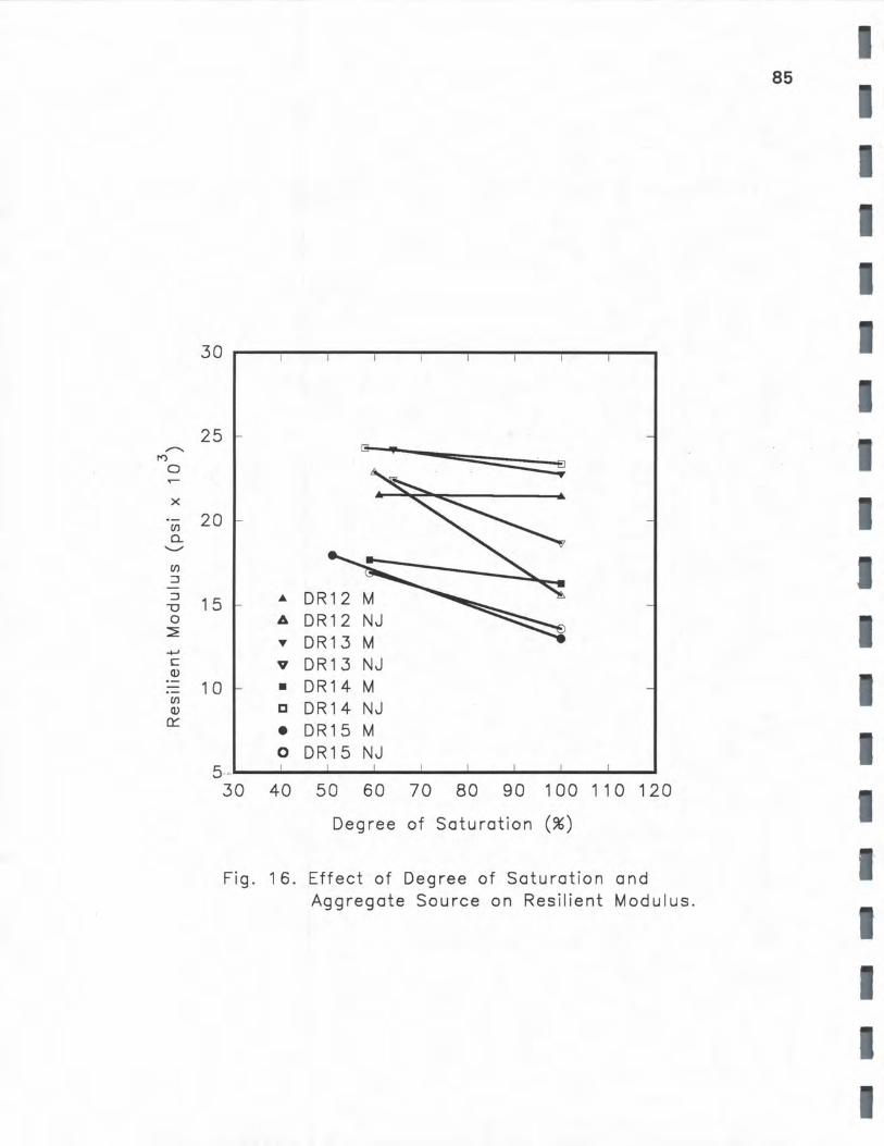
85
I
30
I 25 ,,....._ 13---- •
I")
0 ..--
X I Ul 20 0.. ...__,,
Ul :::::,
:::::, 1 5
.... DR12 ""'O 0 6 DR12 NJ I ~
DR13 M ... ......, C V DR13 NJ Q)
10 • DR14 M Ul
DR14 NJ Q) C 0:: • DR15 M
I 0 DR15 NJ 5 30 40 50 60 70 80 90 100 11 0 1 20
Degree of Saturation (%)
Fig. 1 6. Effect of Degree of Saturation and Aggregate Source on Resilient Modulus.
I
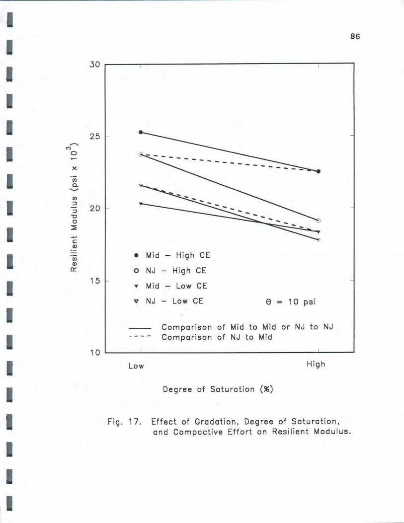
I I I I I I I I I I I I I I I I I I
1•
......... ~
0 -X
U)
0. -U) ::,
::, -0 0 ~
4,J
C: Q)
U) Q)
a::
86
30 ~-------------------------------------------,.------
25
20
• Mid
0 NJ 15
Mid ~
V NJ
- High CE
- High CE
- Low CE
- Low CE e - 10 psi
Comparison ·of Mid to Mid or NJ to NJ Comparison of NJ to Mid
10 1.-----........ ----------------------------------l.-----~ Low High
Degree of Saturation (%)
Fig. 17. Effect of Gradation, Degree of Saturation, and Compactive Effort on Resilient Modulus.
87
significantly different. The results are shown in Table 16. As can be seen, degree
of saturation was significant to differences in Eg at the 0.05 level, and the
interaction of gradation and saturation was significant at the 0.088 level.
Reduction in Eg came from increasing the saturation from 60 to 100%, and having
a saturated, dense-graded material as opposed to a drained, open-graded material.
Table 16. Statistical Significance of Testing Variables to Resilient Modulus.
Eg at 8 = 1 O psi (psi)
Condition Maximum Minimum Difference Significance at 0.05 level
All Mixture~:
0 Saturation, low~. 22,706 19,452 3164 yes high
Gradation and 22,704 20,442 2262 yes at 0.088 saturation: open level graded drained ~. dense graded undrained
PERMEABILITY, POROSITY, AND EFFECTIVE POROSITY
Open-Graded Materials
Permeability tests were performed on specimens of the four aggregates (DR-
12 through DR-15) which were graded in accordance to the two open gradations:
NJ and OGS. Duplicate specimens were tested for each gradation in the rigid wall
permeameter. The target test density was the result of the lower of the two
compactive efforts which corresponded to approximately 100% T-99 maximum
density. Each specimen was tested three to five times each at up to eight
I
I
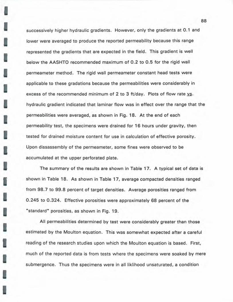
I 88
successively higher hydraulic gradients. However, only the gradients at 0.1 and
lower were averaged to produce the reported permeability because this range
represented the gradients that are expected in the field. This gradient is well
below the AASHTO recommended maximum of 0.2 to 0.5 for the rigid wall
permeameter method. The rigid wall permeameter constant head tests were
applicable to these gradations because the permeabilities were considerably in
excess of the recommended minimum of 2 to 3 ft/day. Plots of flow rate Y.§.
hydraulic gradient indicated that laminar flow was in effect over the range that the
permeabilities were averaged, as shown in Fig. 18. At the end of each
permeability test, the specimens were drained for 16 hours under gravity, then
tested for drained moisture content for use in calculation of effective porosity.
Upon dissassembly of the permeameter, some fines were observed to be
accumulated at the upper perforated plate.
The summary of the results are shown in Table 17. A typical set of data is
I shown in Table 18. As shown in Table 17, average compacted densities ranged
from 98. 7 to 99.8 percent of target densities. Average porosities ranged from
0.245 to 0.324. Effective porosities were approximately 68 percent of the
"standard" porosities, as shown in Fig. 19.
I I
All permeabilities determined by test were considerably greater than those
estimated by the Moulton equation. This was somewhat expected after a careful
reading of the research studies upon which the Moulton equation is based. First,
much of the reported data is from tests where the specimens were soaked by mere
submergence. Thus the specimens were in all liklihood unsaturated, a condition
,,.-..... u Q) (/)
N
E u
" -E ......__,,
>-_...., u 0 Q)
>
0.20
0.15
0.1 0
0 .05
0.00 --------------------0.0 0. 1 0.2 0.3 0 .4 0.5
Hydraulic Gradient
Fig. 18 . Typical Constant Head Rigid Wall Permeameter Test Result.
0.6
89

-I ll
I
I I I I
I
•
I I I I
Table 17. Results of Rigid Wall Permeameter Permeability Testing.
Material Gradation Dry Density (pcf) Target ,, * * "· * *
Hydraulic % Gradient*
Target As-Tested
DR-12 NJ 121.1 119.0 98.3 0.291 0.209 0.025-0.1
NJ 121.1 120.9 99.8 0.280 0.215 0.021-0.1
avg 99.0 0.286 0.212
DR-12 OGS 127.6 126.1 98.8 0.249 0.173 0.023-0.1
OGS 127.6 127.5 99.9 0.240 0.164 0.027-0.1
avg 99.4 0.245 0.169
DR-13 NJ 124.1 122.4 98.6 0.294 0.180 0.023-0.1
NJ 124.1 123.8 99.8 0.286 0.198 0.025-0.1
avg 99.0 0.290 0.189
DR-13 OGS 124.6 123.0 98.7 0.291 0.190 0.027-0.1
OGS 124.6 123.8 99.4 0.286 0.185 0.021-0.1
avg 99.0 0.289 0.188
DR-14 NJ 122.8 121.1 98.6 0.268 0.161 0.022-0.1
NJ 122.8 122.4 99.6 0.260 0.173 0.029-0.1
avg 99.1 0.264 0.167
DR-14 OGS 123.0 121.5 98.8 0.265 0.161 0.023-0.1
OGS 123.0 122.9 99.9 0.257 0.163 0.021-0.1
avg 98.9 0.261 0.162
DR-15 NJ 114.3 112.7 98.6 0.318 0.230 0.022-0.1
NJ 114.3 112.9 98.8 0.317 0.234 0.022-0.1
avg 98.7 0.318 0.232
DR-15 OGS 112.2 110.9 98.9 0.329 0.242 0.029-0.1
OGS 112.2 112.8 100.6 0.318 0.238 0.017-0.1
avg 99.8 0.324 0.240
* Additional tests were conducted at higher gradients. * * Estimated permeability based on ASG using Moulton Equation
90
k (Hiday)
Est.** Test
244 402
188 1178
216 790
72 552
57 783
64 668
264 402
219 773
242 588
204 1048
181 1027
192 1038
140 228
115 889
128 559
109 948
88 938
98 943
444 955
434 1730
439 1342
461 1613
362 2746
412 2180
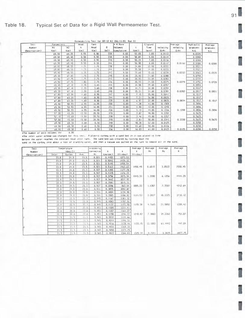
91 -
Table 18. Typical Set of Data for a Rigid Wall Permeamet er Test.
Per11,eabJl11u Test for 00-12 NJ (06/11 / 93 Qun 3)
Je s: t nano11ete<s Heao T.int: . I Pore ( ! •psed Mveraqe "'-/df..UI IC lh,er~qe N...,.ber HI H2 h He>d a lvoluaes l 1 , .. vetoc, HJ veloct tt.J qr~d1en1 qr~tent
<Oesc '1 o 1 1 on> <c•) <c• > <c• > <c ,.> <•I> u•ula11ve <sec> (a1n l 0.11'1 0 .1A1 h,t h,L
I 69. 90 69. 35 0. 55 0. 90 239 0.00 52.09 3.00 0 . 0112 0. 0229 69 . 90 69. 10 0 . 50 0. 90 238 0 . 00 50 . 81 5.00 0.0111 0. 020S 69. 90 69. 10 0. 50 0 . 90 2,0 0.00 50. 21 7.00 0.0 11 6
.. 0. 0208
69. ':a 69. "!O 0 . 50 a. 3a 1" 0 .00 50. 90 2. 00 0 .011 7 0 . 0116 0.0108 0. 0208
2 69 €G 68. 55 1. 25 I 1.70 138 0 . 00 21. 0, 11. 00 0 . 02)] 0.0511 o9. eo 66. S5 '- ,5 I I. 70 111 0. 00 15. so ! ., . 00 0.0233 0. C52 I 69. 90 ,6. 55 I. "5 I. 70 ] ... ] 0.00 ?5.cO !5 co C. 0230 0.0?32 0.050 0 . 05}5
3 l9 . 50 57.&0 I. 70 2. 70 :i,o 0.00 ,O. 90 ~ 1. 00 0 . 0?80 0 . 070il 69 . 50 67. 75 ·- ."S 1. 70 2,2 0.00 10. 93 13. 00 0. 02E2 0. Cl?~
69 . 50 67. 70 I. BG 1. 70 136 0.00 20. 93 ] ~. GO 0.0775 0 . 0279 0 . 075G 0. 0729 1 69. ,o 07. IC l . JO 3. 60 2« 0 .00 I< . 99 2':!.00 0 . OJS? 0 . 095'!
69. 30 67. 10 I 2. ?tJ ) . 60 238 0. 00 11 . 71 JO.OD 0 . 0,91 0 . 0317 69. JO 67 . 10 : . 20 3. 60 2,0 0.00 15 . 21 31. 00 0 . o,s, 0.0392 0. 0917 0 .0931
5 67. 80 63 . 20 <. 60 8. 90 2'7 0.00 J. 15 35.00 o . oa1! 0. IS !7
67.80 63.10 1 . 60 8. 90 111 0 .00 7. 21 36.00 0. 0225 0. 1917 67 . 80 6). 20 ~. 60 8 . 90 239 0 .00 6. 97 37. 00 0 . 0835 0.0831 0 . 1917 0 . 1917
6 65. 50 58. 55 6. S5 16 . 00 230 0.00 • . 28 11.00 0. 1)09 0 . ?896
65. 50 58. 55 6. 95 16 . 00 251 0 . 00 1. 90 12 . 00 0. 1218 0. 2896
65 . 50 SB . 55 6. ~:, 16.00 226 0.00 1. 12 11. 00 0 . I ])6 0. 1298 0 . 1896 0. 2696
J 50 . 10 13 . JO I~. SO 39 . 50 770 0.00 l. 87 <8. 00 0 .2 291 0. 5615
5; . 10 '3.60 11 . 50 J~ . ~a 139 0 . 00 2. 16 1,.00 0.1)57 0. 5625
57 . 00 13 . 50 !'J. so 39. 50 710 0.00 1. 8 I 50 . 00 0 . 1311 0. 2330 0 . 5615 0. 5625
8 69 . 90 69. 30 ,) . 60 0. 30 218 0. 00 '18. 28 57. 00 0 . 0125 0 . 0150
69. 90 69 . 30 0. 60 0. '30 230 0.00 11 . 60 59.00 0.0126 0. 0250
69. 90 69. 30 o . 60 0. 90 136 0.00 16 . 03 61.00 0 .01 25 0. 0125 0. 0250 0. 0250
a:lhe nuaoer of pore volu111es "" 6. 00 •TN' 1n le1 u.a1er scheae u.iS ch.inqed lor 1h1 s 1es1. M plc1s11c C,irbo~ ullh c1 sM'\d bed in 11 uc1s otc1ced 19 1tne t>elor• the, u,iter re.aches 1he conslc1n1 head 1nle1 1c1n~. The Scln.d bed u.as cre c1ted b4 rc11n1nq doun 1"e
Sclnd 1n the c.arb<X.I into c1bou1 cl 1001 of s1c1nd1nQ u.:ner, .and 1hen cl v.acuu• uu pulled on 1he 1c1n~ to reaove cltr 1n 1he sc1nd.
Tes, Teiaper.at ur e VISCOS I I~ fwer.aqe Averc1qe Aver.aqe Aver .aqe
N1.1t1ber (deo CI correct 10 l l l Qn 0< K
<Deserio, 10n) In lei Out let Ava. Q, (( • l' Se>C) (f ll'dcl!J) Cl 1.1dau >
I 23.0 21 . 0 13. s 0 . 921 0. '193 12 73. SJ
23 . 0 21 . 0 13. 5 o. 921 0.5012 1129.32
23. 0 21. 0 23. 5 0. 921 0 . 5115 1158. 51
23. 0 21. 0 23 . S 0. 92 1 0. 5163 1163 . 62 1150.19 0.6815 3. 0522 7030.15
2 22.5 21. 0 23. J 0. 927 0 . 1155 11 77 . 78
22. 5 21. 0 13. 3 0 . 917 0.1119 1176.11
22. 5 21 . 0 2) . 3 0. 927 0 . 3796 1075. 91 1113 . 31 I. 3590 6. 1256 '111 . 29
3 22.0 21 :; 1). 3 0. n1 0. 3661 1037 . 92
22. 0 11 5 1]. 3 0. 927 0. 3581 1015.11
22. 0 11 . 5 23. 3 0. 927 0. 3396 961. 51 1005 . 22 I. 6307 7. )502 121 2. 61
1 n. o 11 0 23. 0 0. 931 0. 3855 1092 . 87
21. 0 21 0 ?) 0 0. 931 0 . 1001 I 131 . 90 21. 0 ! ~. 0 :J. 0 0. 331 0. 3905 11 06. S1 1111. 53 1.2827 10 . )315 2110. 12
5 11.0 12. 5 '?7.] 0. 919 0. 1167 11 81. 32
22. 0 n 5 ~? . ) 0. 91~ 0. 1083 1157 .16 12. 0 22. 5 ?2.] 0 . 919 0. 1137 11 72.SS 1170. 36 i . l66'5 21. 9891 1209. 12
6 ,____ 21. 0 ?2. D n .o a . 951 0. '309 11? I. 11
21.0 11. 0 ?'J. 0 0. ~53 a. 1107 1161. 27 22. a 22 . 0 ;? 0 0. ~5) 0 . 1398 1216. 77 1210. e2 7 . 3863 31. 2261 751.07
7 11. 5 i I. 'i !I ., 0. 965 0. 3532 1111 1,6
I! . 5 ii 5 !I 1 IJ. '3~5 0 . 1011 111<\ . J I
ii. 5 21. ' .. 'i !J. ~f.'5 0.1016 I 1'8. 16 1133. 15 !]. 1003 61. 111 2 117. 01
a 21. 5 ? I 5 11. 5 0.%5 0 . 1831 13-S9 . i3
11 5 11. 5 : l. 'i 0. ~65 0 . 1850 1)71 . 79
? l. ~ 21 . 5 ?! 5 0. 965 0 . 181? 1366 . &J 1370. )1 0. 70 11 J . 3025 6137.'. 7') -
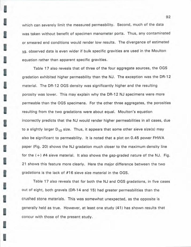
I
92
which can severely limit the measured permeability . Second, much of the data
was taken without benefit of specimen manometer ports. Thus, any contaminated
or smeared end conditions would render low results. The divergance of estimated
vs. observed data is even wider if bulk specific gravities are used in the Moulton
equation rather than apparent specific gravities.
Table 17 also reveals that of three of the four aggregate sources, the OGS
gradation exhibited higher permeability than the NJ. The exception was the DR-12
material. The DR-12 OGS density was significantly higher and the resulting
porosity was lower. This may explain why the DR-1 2 NJ specimens were more
permeable than the OGS specimens. For the other three aggregates, the porosities
I resulting from the two gradations were about equal. Moulton's equation
incorrectly predicts that the NJ would render higher permeabilities in all cases, due
to a slightly larger 0 10 size. Thus, it appears that some other sieve size(s) may
also be significant to permeability. It is noted that a plot on 0.45 power FHWA
I I
paper (Fig. 20) shows the NJ gradation much closer to the maximum density line
for the ( +) #4 sieve material. It also shows the gap-graded nature of the NJ. Fig .
21 shows this feature more clearly. Here the major difference between the two
gradations is the lack of #16 sieve size material in the OGS.
Table 17 also reveals that for both the NJ and OGS gradations, in five cases
out of eight, both gravels (DR-14 and 15) had greater permeabilities than the
crushed stone materials. This was somewhat unexpected, as the opposite is
generally held as true. However, at least one study (41) has shown results that
concur with those of the present study.
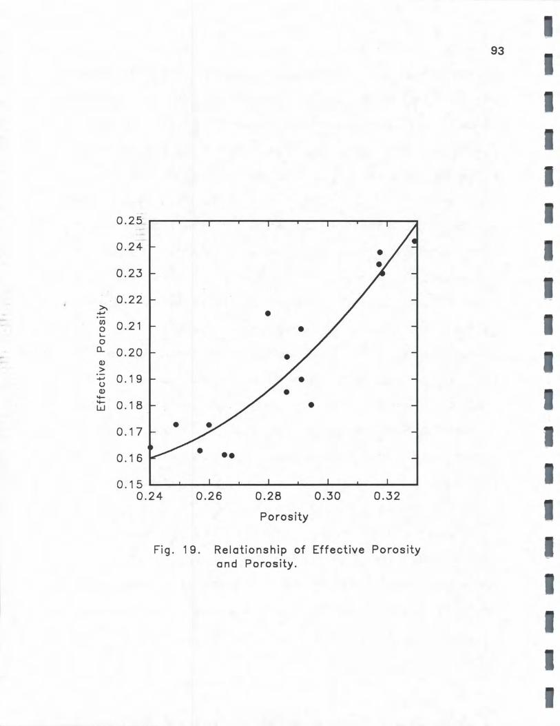
>-+'
U)
0 I...
0 Cl..
Q)
> +' u Q)
'+-'+-w
0.25
0.24
0.23
0.22
0.21
0.20
0.19
0.18
0.17
0.16
0.15 0.24 0.26 0.28 0.30 0.32
Porosity
Fig. 19. Relationship of Effective Porosity and Porosity.
93
I
I
/1 94
I
100 ,, . . --,, /
,I /
90 -LJ
I 80
Tl I Fl/ I
d I I , J I
I~ ., -IVI u A. 11 II U I 11 -, I I I ~ "1 n lC I IJ
I I
' _,._ -- . / I I \ - - - ._,._ . - -
70 '-' .... 'y L.. " .,
I I C, .::, LY ~ " . , I ~ .., r IP ,, -,, I .lou, lo..- kc- 0\/
,.--._ , / I - - - - -J
~
I ....__,, 60
CJ)
C:
~/ / I U/
u7 / ,, / I
" / , . / , Cf)
50 / 1,
Cf) / , ,
0 /I ,
0... 40 I/ I ,
/ I ,
/ I ,
0 / I ,
~
0 30 I-
/ J
/ I J , • , I I
20 ,,, , , ,
I I I/ , I/
10 " • I -
I 0 ,
200 50 JO 18 II 4 J/11 In J/4 In 1 In 1.50 In J In 100 1/2 In
Sieve Sizes • Middle
(0.45 Power) • New Jersey
I A. OGS
Fig. 20. FHWA 0.45 Power Paper Plot of Experimental Gradations.
I I I
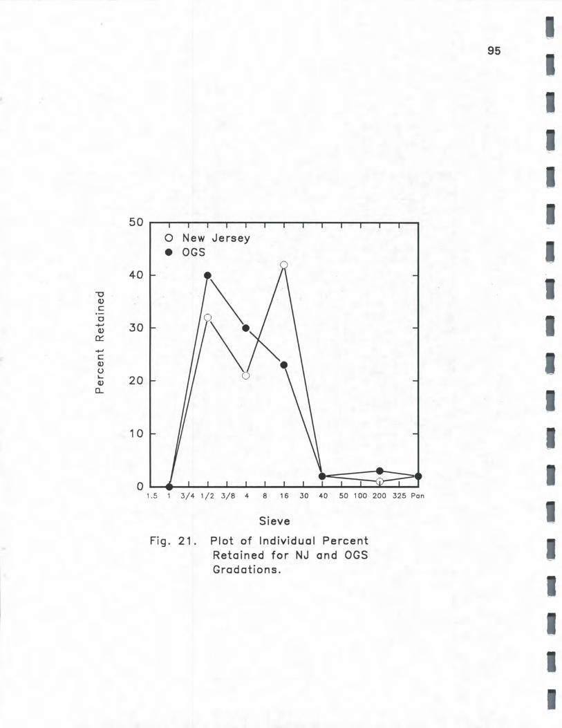
50
40
-0 Cl) C ·-C +' 30 Cl)
a::: +' C Cl)
0 lo.. 20 Cl)
a..
0 New Jersey
• OGS
1.5 1 3/4 1/2 3/8 4 8 16 30 40 50 100 200 325 Pan
Sieve
Fig. 21. Plot of Individual Percent Retained for NJ and OGS Gradations.
95
I
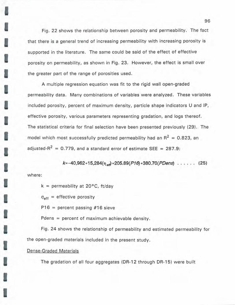
96
Fig. 22 shows the relationship between porosity and permeability. The fact
I that there is a general trend of increasing permeability with increasing porosity is
supported in the literature. The same could be said of the effect of effective
porosity on permeability, as shown in Fig. 23. However, the effect is small over
I
I
I
the greater part of the range of porosities used.
A multiple regression equation was fit to the rigid wall open-graded
permeability data. Many combinations of variables were analyzed. These variables
included porosity, percent of maximum density, particle shape indicators U and IP,
effective porosity, various parameters representing gradation, and logs thereof.
The statistical criteria for final selection have been presented previously (29). The
model which most successfully predicted permeability had an R2 = 0.823, an
adjusted-R2 = 0. 779, and a standard error of estimate SEE = 287.9:
k=-40,962+15,284(n8,J +205.89(P16) +380.70(PDens) . . . . . . (25)
where:
k = permeability at 20°C, ft/day
/Jett = effective porosity
P16 = percent passing #16 sieve
Pd ens = percent of maximum achievable density.
Fig. 24 shows the relationship of permeability and estimated permeability for
the open-graded materials included in the present study.
Dense-Graded Materials
The gradation of all four aggregates (DR-12 through DR-15) were built
~
>. 0
"U ........... +-' '+-'--"
>. +-'
..0 0 Q)
E I... Q)
Cl..
• 2500
2000
• 1500
• 1000 •• • •
• 500
•• •
0 0.24 0 .26 0.28 0.30 0.32
Porosity
Fig. 22 . Relationship of Permeability and Porosity.
97

98
I 3000
I • 2500 ->.
. a, 'C
........... 2000 +' 111-1 ......... >. +' •.-1 1500 -•.-1 ,c cd Q)
I s 1000 J-4 Q) • ll.! •
I 500 • •
I 0 0.16 0.18 0.20 0.22 0.24
Effective Porosity
Fig. 23. Relationship of Permeability and Effective Porosity.

.a C
2500
2000
CD 1500 E L. CD
Q.
"D 1 000 CD > L. CD m .a 500 0
•
• •
•• .. o---~~__._~~~--~~~"'--~~__,_~~~...i
0 500 1000 1500 2000 2500
Estimated Permeability (ft/day)
Fig.24. Relationship of Observed Permeability and Estimated Permeability for Open- Graded Materials.
99
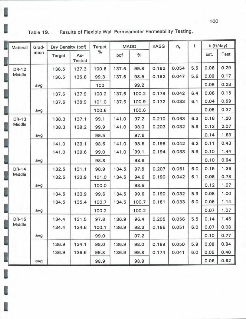
100
Table 19. Results of Flexible Wall Permeameter Permeability Testing.
Material Grad- Dry Density (pcf) Target MADD nASG n. i k (ft/day)
ation % pcf % Est. Test Target As-
Tested
DR-12 136.5 137.3 100.6 137.6 99.8 0.182 0.054 5.5 0.06 0.29
Middle 136.5 135.6 99.3 137.6 98.5 0.192 0.047 5.6 0.09 0.17
avg 100 99.2 0.08 0.23
137.6 137.9 100.2 137.6 100.2 0.178 0.042 6.4 0.06 0.15
137.6 138.9 101.0 137.6 100.9 0.172 0.033 6.1 0.04 0.59
avg 100.6 100.6 0.05 0.37
DR-13 138.3 137.1 99.1 141.0 97.2 0.210 0.063 6.3 0.16 1.20 Middle
138.3 138.2 . 99.9 141.0 98.0 0.203 0.032 5.8 0.13 2.07
avg 99.5 97.6 0.14 1.63
141.0 139.1 98.6 141.0 98.6 0.198 0.042 6.2 0.11 0.43 ,
141.0 139.6 99.0 141.0 99.1 0.194 0.033 5.9 0.10 1.44
avg 98.8 98.8 0.10 0.94
DR-14 132.5 131.1 98.9 134.5 97.5 0.207 0.061 6.0 0.15 1.36 Middle
132.5 133.9 101.0 134.5 94.6 0.190 0.042 6.1 0.08 0.78
avg 100.0 98.5 0.12 1.07
134.5 133.9 99.6 134.5 99.6 0.190 0.032 5.9 0.08 1.00
134.5 135.4 100.7 134.5 100.7 0.181 0.033 6.0 0.06 1.14
avg 100.2 100.2 0.07 1.07
DR-15 134.4 131.5 97.8 136.9 96.4 0.205 0.056 5.5 0.14 1.46 Middle
134.4 134.6 100.1 136.9 98.3 0.186 0.051 6.0 0.07 0.08
avg 99.0 97.2 0.10 0.77
136.9 134.1 98.0 136.9 98.0 0.189 0.050 5.9 0.08 0.84
136.9 136.6 99.8 136.9 99.8 0.174 0.041 6.0 0.05 0.40
avg 98.9 98.9 0.06 0.62

101
according to the MHTD Middle dense gradation and tested for permeability in the
flexible wall permeameter. Duplicate specimens were used. The target densities
corresponded to the low and high compactive efforts discussed previously. Each
specimen was tested five times at the recommended gradient equal to five.
Successive replications of test runs resulted in permeabilities that agreed well
within the recommended 25 percent. At the end of each suite of permeability
tests, the specimen was allowed to drain by gravity for 16 hours; then the drained
moisture content was determined and the effective porosity was calculated.
A summary of the test results is shown in Table 19. Average compacted
densities ranged from 97 .8 to 101.0 percent of target densities. Average
porosities ranged from 0.172 to 0.210. Effective porosities were approximately
27 percent of the standard porosities. The relationship between the two is
included in Table 19.
As with the rigid wall permeability results, all permeabilities determined by
test were considerably greater than those estimated by the Moulton equation. As
with the rigid wall results, there is a rough trend of increasing permeability with
increasing porosity and effective porosity.
A multiple regression equation was fit to the flexible wall dense-graded data.
Various combination of variables were analyzed. These included porosity
(calculated with either BSG or ASG values), effective porosity, particle shape
parameters U and IP, drained degree of saturation, and logs thereof. Effective
porosity is determined by draining the permeability specimen and measuring final
drained moisture content. From this is calculated the final drained degree of
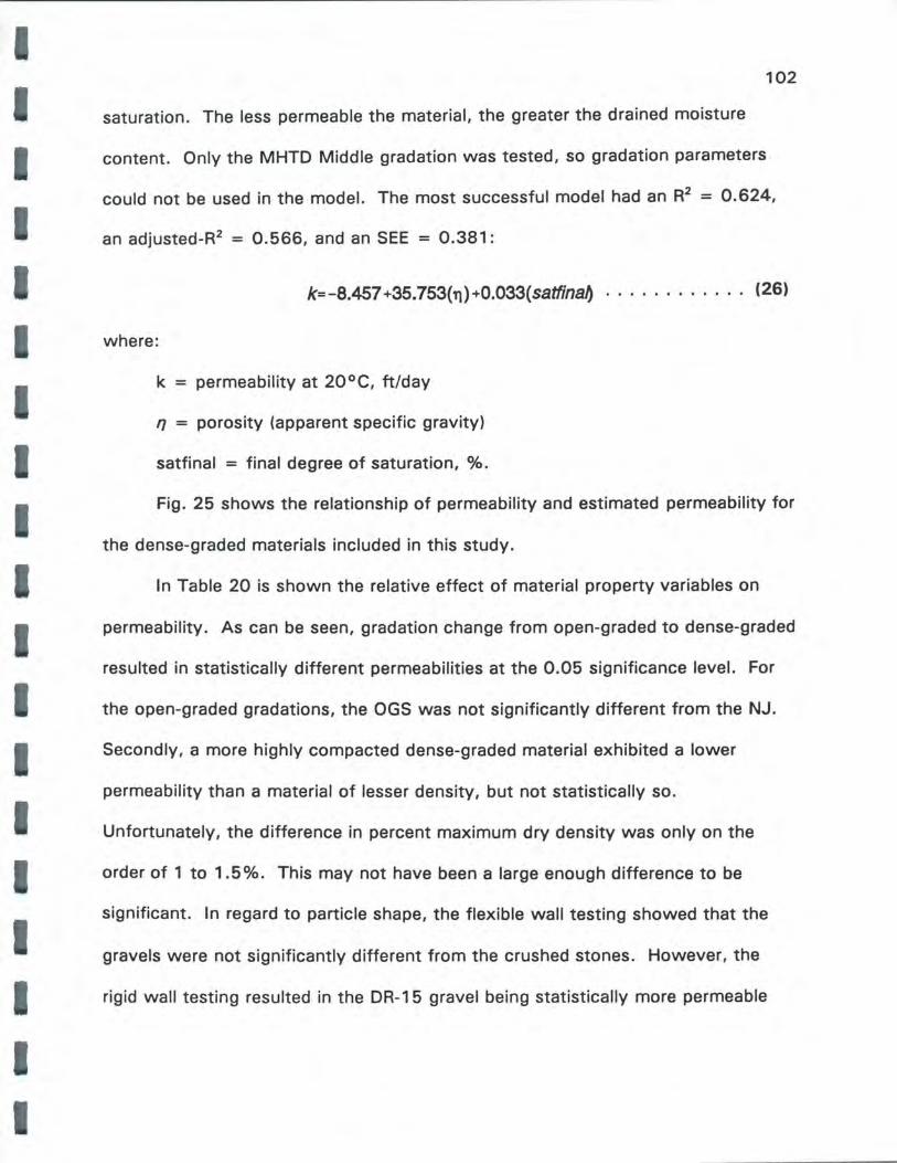
I I I
I
102
saturation. The less permeable the material, the greater the drained moisture
content. Only the MHTD Middle gradation was tested, so gradation parameters
could not be used in the model. The most successful model had an R2 = 0.624,
an adjusted-R2 = 0.566, and an SEE = 0.381:
k=-8.457 +35.753(11)+0.033(satfin~ ........ . ... (26)
where:
k = permeability at 20°C, ft/day
fl = porosity (apparent specific gravity)
I satfinal = final degree of saturation, % .
I I I
Fig. 25 shows the relationship of permeability and estimated permeability for
the dense-graded materials included in this study.
In Table 20 is shown the relative effect of material property variables on
permeability. As can be seen, gradation change from open-graded to dense-graded
resulted in statistically different permeabilities at the 0.05 significance level. For
the open-graded gradations, the OGS was not significantly different from the NJ.
Secondly, a more highly compacted dense-graded material exhibited a lower
permeability than a material of lesser density, but not statistically so.
Unfortunately, the difference in percent maximum dry density was only on the
order of 1 to 1.5%. This may not have been a large enough difference to be
significant. In regard to particle shape, the flexible wall testing showed that the
gravels were not significantly different from the crushed stones. However, the
I rigid wall testing resulted in the DR-15 gravel being statistically more permeable
I I
-~ 2.5
C "tJ 2.0
' -,.;. -..c C I)
E ...
1.5
~ 1.0
"tJ I)
> ... I)
IJ ..c 0
0.5
• • • • 0.0
0.0 0.5 1.0 1.5 2.0
Estimated Permeability (ft/day)
Fig.25. Relationship of Observed Permeability and Estimated Permeability for Dense-Graded Materials.
103
I
I I
104
than both stones. But, it was also shown to be more permeable than the other
gravel, despite the fact that their particle shapes were not much different. Thus,
the effect of particle shape on permeability did not seem to be a factor for the four
aggregates tested. It should be noted that these aggregates did not exhibit a wide
range of shapes.
Table 20. Effect of Material Variables on Permeability.
Permeability (ft/day)
Condition Maximum Minimum Difference Significance
All Data at 0.05 level
Gradation OGS (avg) to 1158 0.925 1157 yes Middle (avg)
Open-Graded
Gradation OGS (avg) to 1158 820 338 no NJ (avg)
Particle Gravel to 1782 812 970 yes shape stone
Dense-Graded
Particle Gravel to 1.286 0.697 0.589 no shape Stone
% MADD Low CE (avg) 0.927 0 .750 0. 177 no to High CE
(avg)
Note: % MADD = % maximum achieveable density CE = Compactive effort

•
I I
105
ESTIMATION OF PERMEABILITY
It is sometimes useful to estimate permeability from readily available
information about a material rather than perform the permeability testing. As
previously mentioned, Moulton (9) has produced a widely-used algorithm based on
data from the literature ( 12-17). For the most part, these tests were of the rigid
wall low head variety, using either constant head or falling head procedures. There
was no provision for prevention of water short circuiting along the permeameter
walls. "Saturation" was usually achieved either by mere submergence of the
specimen or by applying a vacuum to the specimen and permeameter in a tub of
water. Thus, it is doubtful that saturation even approached 100% for the more
densely-graded materials. Additionally, manometer ports were missing in many of
the studies' permeameters.
Moulton's equation is based on porosity, effective aggregate size (010), and
the percent passing the #200 sieve. Three of the six references cited for the data
base lacked porosity data or the means to calculate porosity (specific gravity).
However, because compacted density data was available, apparently specific
gravity values were assumed. As previously shown, this can lead to a wide range
of calculated porosities.
In the present study, a regression equation was developed using data from
the literature and data from this study. Initially, the material parameters of interest
were gradation, porosity (or specific gravity and compacted density), and test
temperature (so that all data could be put on a common temperature basis). Very
few studies in the literature met these criteria. The acceptable data set is shown
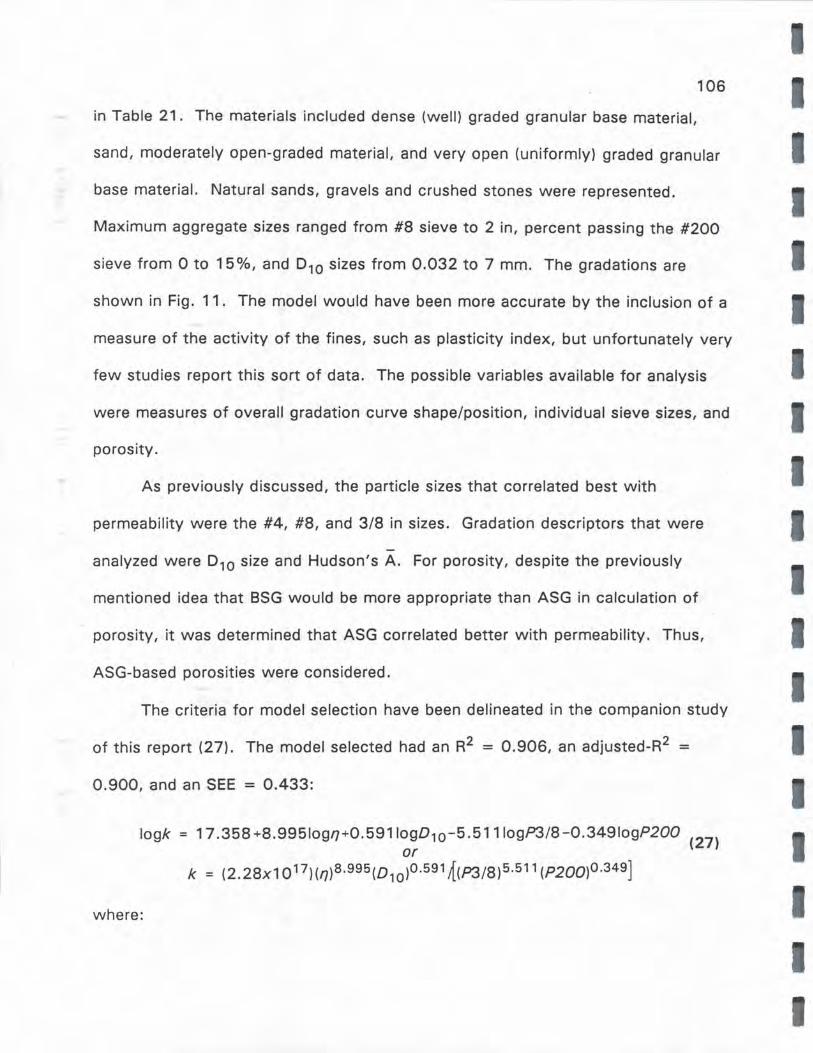
106
in Table 21. The materials included dense (well) graded granular base material,
sand, moderately open-graded material, and very open (uniformly) graded granular
base material. Natural sands, gravels and crushed stones were represented.
Maximum aggregate sizes ranged from #8 sieve to 2 in, percent passing the #200
sieve from Oto 15%, and 0 10 sizes from 0.032 to 7 mm. The gradations are
shown in Fig. 11. The model would have been more accurate by the inclusion of a
measure of the activity of the fines, such as plasticity index, but unfortunately very
few studies report this sort of data. The possible variables available for analysis
were measures of overall gradation curve shape/position, individual sieve sizes, and
porosity.
As previously discussed, the particle sizes that correlated best with
permeability were the #4, #8, and 3/8 in sizes. Gradation descriptors that were
-analyzed were D10 size and Hudson's A. For porosity, despite the previously
mentioned idea that BSG would be more appropriate than ASG in calculation of
porosity, it was determined that ASG correlated better with permeability. Thus,
ASG-based porosities were considered.
The criteria for model selection have been delineated in the companion study
of this report (27). The model selected had an R2 = 0.906, an adjusted-R2 =
0.900, and an SEE = 0.433:
logk = 17 .358 +8.9951ogl]+0.5911ogD10-5.5111ogP3/8-0.3491ogP200 (27
) or
k = (2.28x10¹⁷){1J)8.995(D,o)0.591 ~(P3/8)5.511 (P200)0.349]
where:

- -- -
- -- -
Ta
ble
21
.Da
ta U
sed
in
th
e P
erm
ea
bili
ty P
red
icti
ve E
qu
ati
on
.
RE
F.
MA
TE
RIA
L
PE
RC
EN
T P
AS
SIN
G
1.5
3
/4
3/8
#
4
#8
#
16
#
30
17
C
LS
1
00
6
3
33
2
3
16
11
8
CL
S
10
0
63
3
3
23
1
6
11
8
CL
S
10
0
63
3
3
23
16
11
8
CL
S
10
0
63
3
3
23
16
11
8
CL
S
10
0
63
3
3
23
1
6
11
8
CL
S
10
0
63
3
3
23
1
6
11
8
CL
S
10
0
63
3
3
23
1
6
11
8
CL
S
10
0
63
3
3
23
1
6
11
8
CL
S
10
0
63
3
3
23
1
6
11
8
CL
S
10
0
63
3
3
23
1
6
11
8
CL
S
10
0
63
3
3
23
16
11
8
CL
S
10
0
63
3
3
23
1
6
11
8
CL
S
10
0
63
3
3
23
1
6
11
8
CG
1
00
1
00
4
9
36
2
8
22
1
7
CG
1
00
1
00
4
9
36
2
8
22
1
7
CG
1
00
1
00
4
9
36
2
8
22
1
7
CG
1
00
1
00
4
9
36
2
8
22
1
7
CG
1
00
1
00
4
9
36
2
8
22
1
7
CG
1
00
1
00
4
9
36
2
8
22
1
7
CG
1
00
, 1
00
4
9
36
2
8
22
1
7
CG
1
00
1
00
4
9
36
2
8
22
17
CG
1
00
1
00
4
9
36
2
8
22
1
7
CG
1
00
1
00
4
9
36
2
8
22
1
7
15
S
AN
D
10
0
10
0
10
0
10
0
10
0
99
9
5
SA
ND
1
00
1
00
1
00
1
00
1
00
9
9
95
SA
ND
1
00
1
00
1
00
1
00
1
00
9
9
95
SA
~'"
1
00
1
00
. 1
00
1
00
1
00
9
9
95
SA
~
10
0
10
0
10
0
10
0
10
0
99
9
5
SA
i\ 1
00
1
00
1
00
1
00
1
00
9
9
95
SA
N:J
1
00
1
00
1
00
1
00
1
00
9
7
80
SA
NO
1
00
1
00
1
00
1
00
1
00
9
7
80
SA
ND
1
00
1
00
1
00
1
00
1
00
9
7
80
SA
ND
1
00
1
00
1
00
1
00
1
00
9
7
80
SA
ND
1
00
1
00
1
00
1
00
1
00
9
9
98
SA
ND
1
00
1
00
1
00
1
00
1
00
9
9
98
SA
ND
1
00
1
00
1
00
1
00
1
00
9
9
98
SA
ND
1
00
1
00
1
00
1
00
1
00
9
9
98
41
S&
G
10
0
67
1
9
4 2
0 0
S&
G
98
7
2
32
1
2
8 7
6
S&
G
98
7
7
54
3
7
28
2
5
23
-- -
-0
10
A
#5
0
#1
00
#
20
0
mm
5 3
0 0
.94
2
.62
5 3
0 0
.94
2
.62
5 3
0 0
.94
2
.62
5 3
0 0
.94
2
.62
5 3
0 0
.94
2
.62
5 3
0 0
.94
2
.62
5 3
0 0
.94
2
.62
5 3
0 0
.94
2
.62
5 3
0 0
.94
2
.62
5 3
0 0
.94
2
.62
5 3
0 0
.94
2
.62
5 3
0 0
.94
2
.62
5 3
0 0
.94
2
.62
12
8
5 0
.2
3.7
7
12
8
5 0
.2
3.7
7
12
8
5 0
.2
3.7
7
12
8
5 0
.2
3.7
7
12
8
5 0
.2
3.7
7
12
8
5 0
.2
3.7
7
12
8
5 0
.2
3.7
7
12
8
5 0
.2
3.7
7
12
8
5 0
.2
3.7
7
12
8
5 0
.2
3.7
7
75
3
2
12
0
.06
2
8.1
3
75
3
2
12
0
.06
2
8.1
3
75
3
2
12
0
.06
2
8.1
3
55
2
0
15
0
.03
2
7.8
4
55
2
0
15
0
.03
2
7.8
4
55
2
0
15
0
.03
2
7.8
4
20
3
1 0
.25
7.0
1
20
3
1 0
.25
7
.01
20
3
1 0
.25
7
.01
20
3
1 0
.25
7
.01
70
1
5
6 0
.12
7
.88
70
1
5
6 0
.12
7.8
8
70
15
6
0.1
2
7.8
8
70
1
5
6 0
.12
7
.88
0 0
0 7
1.9
2
5 4
3.5
3
.9
2.4
75
18
8
4 0
.16
3
.72
- n
0.2
61
76
0.2
61
76
0.2
34
06
9
0.2
31
71
2
0.2
10
50
2
0.2
08
73
4
0.1
91
64
8
0.1
89
88
0.1
89
88
0.1
75
15
1
0.1
73
97
2
0.1
46
28
1
0.1
46
0.2
75
54
5
0.2
77
94
6
0.2
48
53
5
0.2
16
12
4
0.2
15
52
4
0.2
11
92
3
0.2
10
12
2
0.2
04
12
0.2
05
32
0.2
01
11
9
0.3
96
0.3
66
0.3
45
0.3
56
0.3
15
0.2
78
0.3
81
0.3
75
0.3
55
0.3
4
0.4
2
0. 4
08
0.3
83
0.3
57
0.3
7
0.3
2
0.2
3
-k fp
d
26
67
23
14
15
99
21
50
911
12
77
73
0
65
7
10
40
29
2
21
6
52
44
12
99
10
14
73
4
181
16
8
13
4
88
50
34
22
39
.5
24
.5
18
.4
6.9
2.4
1.4
25
8.5
23
7.5
19
9.4
17
5.4
77
.1
66
.3
54
.5
34.1
21
54
6
18
14
4
1.2
.... 0 ....
J
-
K)G
S
GR
AV
EL
10
0
91
48
3
0
16
7
6 4
3 2
1.5
3
.07
0
.25
7
93
8
GR
AV
EL
10
0
91
48
3
0
16
7
6 4
3 2
1.5
3
.07
0
.26
5
94
8
GR
AV
EL
10
0
91
48
3
0
16
7
6 4
3 2
1.5
3
. 07
0
.32
9
16
13
GR
AV
EL
10
0
91
48
3
0
16
7
6 4
3 2
1.5
3
.07
0
.30
8
12
92
GR
AV
EL
10
0
91
48
3
0
16
7
6 4
3 2
1.5
3
.07
0
.31
8
27
46
CL
S
10
0
91
48
3
0
16
7
6 4
3 2
1.5
3
.07
0
.28
6
10
27
CL
S
10
0
91
48
3
0
16
7
6 4
3 2
1.5
3
.07
0
.291
1
04
8
CL
S
10
0
91
48
3
0
16
7
6 4
3 2
1.5
3
.07
0
.24
7
83
CL
S
10
0
91
48
3
0
16
7
6 4
3 2
1.5
3
.07
0
.24
9
55
2
NJ
GR
AV
EL
10
0
95
5
8
47
2
0
5 4
2.5
2
.5
2 1
.7
3.3
6
0.2
68
2
28
GR
AV
EL
10
0
95
5
8
47
2
0
5 4
2.5
2
.5
2 1
.7
3.3
6
0.2
6
88
9
GR
AV
EL
10
0
95
5
8
47
2
0
5 4
2.5
2
.5
2 1
.7
3.3
6
0.3
17
1
73
0
GR
AV
EL
10
0
95
5
8
47
2
0
5 4
2.5
2
.5
2 1
.7
3.3
6
0.3
18
9
55
CLS
1
00
9
5
58
4
7
20
5
4 2
.5
2.5
2
1.7
3
.36
0
.29
45
4
02
CL
S
10
0
95
5
8
47
2
0
5 4
2.5
2
.5
2 1
.7
3.3
6
0.2
86
7
73
CLS
1
00
9
5
58
4
7
20
5
4 2.
5 2
.5
2 1
.7
3.3
6
0.2
91
40
2
CL
S
10
0
95
5
8
47
2
0
5 4
2.5
2
.5
2 1
.7
3.3
6
0.2
8
11
78
MID
DLE
C
LS
10
0
95
6
3
50
4
0
33
2
8
22
1
6
8 0
.09
2
4.5
5
0.1
92
0
.16
54
CLS
1
00
9
5
63
5
0
40
3
3
28
22
1
6
8 0
.09
2
4.5
5
0.1
82
0
.28
95
CLS
1
00
9
5
63
5
0
40
3
3
28
2
2
16
8
0.0
92
4
.55
0
.17
8
0.1
52
5
CLS
1
00
9
5
63
5
0
40
3
3
28
22
1
6
8 0
.09
2
4.5
5
0.1
72
5
0.5
94
8
CLS
1
00
9
5
63
5
0
40
3
3
28
22
1
6
8 0
.09
2
4.5
5
0.2
1 1
.19
62
CLS
1
00
9
5
63
5
0
40
3
3
28
22
1
6
8 0
.09
2
4.5
5
0.2
03
2
.07
25
CL
S
10
0
95
6
3
50
4
0
33
2
8
22
1
6
8 0
.09
2
4.5
5
0.1
98
0
.43
2
CL
S
10
0
95
6
3
50
4
0
33
2
8
22
1
6
8 0
.09
2
4.5
5
0.1
94
1
.44
25
GR
AV
EL
10
0
95
6
3
50
4
0
33
2
8
22
1
6
8 0
.09
2
4.5
5
0.2
07
1
.36
58
GR
AV
EL
10
0
95
6
3
50
4
0
33
2
8
22
1
6
8 0
.09
2
4.5
5
0.1
9
0.7
80
2
GR
AV
EL
10
0
95
6
3
50
4
0
33
2
8
22
1
6
8 0
.09
2
4.5
5
0.1
9
1.0
04
GR
AV
EL
10
0
95
6
3
50
4
0
33
2
8
22
16
8
0.0
92
4
.55
0.
181
1.1
36
9
GR
AV
EL
10
0
95
6
3
50
4
0
33
2
8
22
1
6
8 0
.09
2
4.5
5
0.2
05
1
.46
27
GR
AV
EL
10
0
95
6
3
50
4
0
33
2
8
22
1
6
8 0
.09
2
4.5
5
0.1
86
0
.08
47
GR
AV
EL
10
0
95
6
3
50
4
0
33
2
8
22
16
8
0. 0
92
4
.55
0
.18
9
0.8
37
9
GR
AV
EL
10
0
95
6
3
50
4
0
33
2
8
22
16
8
0. 0
92
4
.55
0
.17
4
0.4
03
2
No
te:
CLS
= c
rush
ed
lim
est
on
e
CG
, ~
rush
ed g
rave
l
S&C
sa
nd a
nd g
rave
l

I
I
I
I I I I I
I I
109
k = coefficient of permeability at 20°C, ft/day
fJ = porosity = 1 - (density, pcf/(apparent sp. grav. * 62.4))
D10 = size that represents 10% passing, mm
P 3/8 = percent passing 3/8 in sieve
P200 = percent passing #200 sieve.
The relationship of observed permeability with estimated permeability is shown in
Fig. 26.
As mentioned previously, the Moulton equation underpredicts observed
permeability by almost an order of magnitude. This is shown in Fig. 27; the wide
scatter should be noted. It is postulated that the above inaccuracies are
associated with the manner in which the permeability testing was performed
(complete saturation unlikely) and inaccuracies in porosity determination. The
algorithm developed in the present study is relatively accurate up to permeabilities
of around 1000 ft/day. Beyond that, the model overpredicts permeability
significantly. This is shown in Fig. 28 (arithmetic-scale version of Fig. 26).
Despite all efforts of arriving at good estimates of field permeability, it must
be remembered that there are several factors that will render field permeabilities
different from laboratory derived values. First, it is unlikely that the pavement base
layer will be close to 100% saturated--even in the laboratory, this is very difficult
to achieve under conditions of vacuum. Entrapped air can lower the expected
permeability significantly. Additionally, in pavement sections, the permeant
temperature will be higher or lower than the standard 20°C -- thus raising or
lowering actual permeability. And, the aggregate can become segregated and the

110
density may be off-target, all resulting in a permeability different than expected.
So, the question becomes, which predictive equation should be used if
actual laboratory permeability testing is not possible 7 The equation developed in
this study appears to be a truer representation of permeability in the range of 0. 1
to 1000 ft/day. The Moulton equation underpredicts permeability at all levels.
However, in the field, several factors are at work which result in achieved
permeabilities lower than that which are expected. In this regard, a conservative
estimate may be in order, and the use of the Moulton equation may be justified.
This decision falls in the area of design judgement.
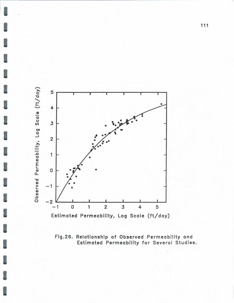
1, I I I I I I I I I I I I
I I I I I
->. C
"tJ
' .... -.._,, CD -C u
(/l
Cl 0
_J
->. .... .c C CIJ
E L. a,
a.. "O a, > L. CIJ rn .c 0
5
4
J •
2 ••
1
0 •
-i •
-2 -1 0 1 2 J 4 5
Estimated Permeability, Log Sec le (ft/dcy)
Fig.26. Relationship of Observed Permeability end Estimated Permeability for Several Studies.
1 1 1
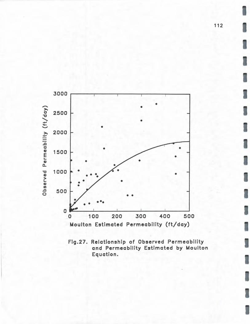
->,
~ 2500
' -.... ->. 2000 .... .c C ID
E ... cu
a.. 'lJ
CD > ... CD rn .c 0
1500
1000
500
0
• •
• •
• • •
• • • • • • •
• • • • •••
0 100 200 300 400 500
Moulton Estimated Permeability {ft/day)
Fig.27. Relationship of Observed Permeability and Permeability Estimated by Moulton Equation.
112

I I
I I
,.... ~ C
"'C
' ~ --~ ~
.a C G
E t.... G a.. "C I)
> t.... G ., .a 0
3000
• • 2500
2000
1500
1000
500
o-------------...... ---------0 2500 5000 7500 10000 12500
Estimated Permeability (ft/day)
Fig.28. Relationship of Observed Permeability and Permeability Estimated by UMR Equation.
113

I
I
I
I
I I
I I I I
I I I I I I
RESULTS OF MODELS EVALUATION
TTI INTEGRATED MODEL
114
This model does not appear suitable for use in the determination of drainage
coefficients. First, it does not have drainage coefficient determination as a goal of
the model, and consequently does not generate drainage coefficients or have
drainage coefficients as an output of the program. However, since some of the
output from the program included the modulus of the pavement layers, a scheme
was devised to use the base course modulus generated by the TTI program in the
calculation of drainage coefficients. Unfortunately, this proved to be impossible
because of limitations in the TTI model output as discussed below.
Review of the program documentation (7) leads one to believe that base and
subbase modulus vs time is an output of the CMS model module. This is shown in
Fig . 1 on page 3 of the documentation. Also, on page 75 of the documentation
under the discussion of the CMS model module, the following statement is made,
"A subroutine to compute accompanying changes in material moduli is
incorporated in the model." After several unsussessfull attempts to obtain base
modulus output that differed from the initial input, the following comment was
discovered on page 82 of the documentation: "The CMS Model, therefore, ignores
the effect of moisture on the resilient modulus of these granular materials when
they are unfrozen." This in fact is correct. The output parrots the input base
course modulus for the frozen and unfrozen condition. This is a fatal flaw in any
program that purports to model the environmental effects on pavement behavior.
This rendered the program unusable for purposes of m-coefficient determination.
115
Other considerations of the TTI model include the sensitivity of results to
changes in inputs. The authors identified the following inputs as highly sensitive:
length of elements used by the CMS program to model the soil pavement column,
temperature at which the soil is considered frozen, the liquid limit for fine grained
soils, material type, plastic limit of the non-asphalt layers, stiffness relationship of
the asphalt bitumen and temperature, saturated water content, water table depth,
maximum daily air temperature, minimum daily air temperature, temperatures for
the bitumen stiffness-temperature relationship, coefficient of variation for
unsaturated permeability, temperature at the upper boundary, modifier of
unsaturated permeability in the frozen zone per layer, saturated permeability of the
soil per layer, exponent of pore pressure for Gardner's unsaturated permeability
function per layer, base course hydraulic permeability, index of base course
material, and rainfall occurrences. According to the authors, the model displayed
low sensitivity to the following inputs {a partial list only): base depth, porosity of
the subgrade, amount of sand and gravel in the base course, and linear length of
cracks and joints and cracks. In the opinion of this reviewer, these low sensitivity
items should be important players in a model that is dealing with drainage of base
courses. Further, it was discovered by trial and error that the prediction of
temperatures in the pavement layers was driven by the input selected for thermal
capacity and resistance to heat flow in each layer. The results generally obtained
were counter-intuitive and did not agree with those obtained by other methods.
An attempt was made to determine if FHWA had evaluated the Integrated
Program separately from the Texas evaluation. ·Persons contacted included Byron

I I
I
I
I I
I
116
Lord, Roger Larson, Jim Sherwood, and Bill Dearasaugh of FHWA in July, 1992.
These gentlemen had not used the program and did not know of any serious users.
Mr. Larson relayed that he had the understanding that the program was
cumbersome and did not handle moisture well. Mr. Larson suggested that Dr.
Barry Dempsey of the University of Illinois might have had an opinion on the
program. Contact with Dr. Dempsey revealed that he thought the program was
not sensitive to moisture.
The TTI program is cumbersome, requires a great deal of input, and outputs
the frozen and unfrozen base course modulus that is input by the users regardless
of the other input variables. For the user interested in base course moduli adjusted
for climatic conditions, this program is not useful.
DAMP
The parts of DAMP that are based upon the work of Moulton as published in
the FHWA Highway Subdrainage Design Manual seem well founded in verifiable
research efforts published in the literature. The parts of DAMP added to the
original to extend the work to drainage coefficient determination are less well
supported.
The percent time the pavement structure is saturated is determined using a
method based upon Thornthwaite's classification of climatic regions. This method
is rational on a regional basis. The leap from Thornthwaites's determination of
monthly water surplus conditions to percent of time saturated is discussed earlier
in this paper. Here, Carpenter simply states that some part of a month the base
course shall be considered saturated because of some conditions being met. For

117
instance, "Surplus following a recharge which does not follow a frozen period
here one-fourth of the months in the surplus period should contribute to the
saturation time." No rationale or references are available to determine the basis for
the allocation of time saturated. Also, the relationship between general soil
moisture content and base course moisture content is assumed to be equal.
Another problem with DAMP is the calculated percent time of saturation.
DAMP was used to analyze data for several sites per each of the six AASHTO
climate zones . First, DAMP classified all six zones into the 5-25 percent saturation
time catagory. Worse yet, when counting months as frozen, thawed, wet, and
dry, problems arose in distinguishing zones. For instance, the Road Test area,
normally thought of as being a moist area, became very similar to Phoenix. One
explanation may be as follows. It was noted that in all the dry (west of the
Mississippi River) states, DAMP puts a 10 cm storage (maximum) in January, no
matter what the rainfall and PET were in previous months. It takes until about July
for this large amount of storage to be diminished to a level that is more in keeping
with the percent-of-time-of-saturation rules stated in DAMP. Included in the output
of DAMP is the Thornthwaite Moisture Index:
TM/ = (100 S-600,/PET . . . . . . . . . . . . . . . (28)
where:
TMI = Thornthwaite Moisture Index,
S = surplus of moisture during the year,
D = deficit of moisture during the year,
I I I
I I I I I I I I I I I I I I
118
PET = potential evapotranpiration during the year.
It appears that when a threshold value of TMI between 5.8 and 18 is calculated,
10 cm storage is automatically invoked in January. If the TMI is greater than the
threshold, the output of DAMP storage seems to follow the stated rules.
The Quality of Drainage determination presented by Carpenter (Table 2) is
entered with information on the subgrade drainability and the base drainability.
These values are determined in a rational manner and are logical. The matrix of the
table is filled in with descriptive terms for the Quality of Drainage such as
Excellent, Good, Fair, Poor, and Very Poor. No rational or documentation is
presented for the position of these descriptors in the table. Cursory review reveals
a base that drains in less than five hours that is placed on a typical low
permeability subgrade earns the Quality of Drainage description of Fair. This
"Fair", when used in the Drainage Coefficient selection (Table 1) for typical
Missouri times of saturation yields an m-coefficient of, say, 0.80. If this is tied
back to the AASHO road test, the base that drains in less than five hours is less
desirable than the AASHO base that had difficulty in draining below 85%
saturation during spring periods. This does not make sense and does not correlate
well with the general assumption in the pavement design community that well
drained bases are more desirable.
A sensitivity analysis was conducted on DAMP by establishing the most
likely value for each variable, a high value and a low value. Several runs were
made with each successive run changing one variable from low to median to high
while holding all other variables constant at the median value. Base drainability
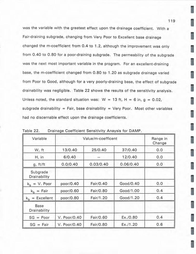
119
was the variable with the greatest effect upon the drainage coefficient. With a
Fair-draining subgrade, changing from Very Poor to Excellent base drainage
changed the m-coefficient from 0.4 to 1.2, although the improvement was only
from 0.40 to 0.80 for a poor-draining subgrade. The permeability of the subgrade
was the next most important variable in the program. For an excellent-draining
base, the m-coefficient changed from 0.80 to 1.20 as subgrade drainage varied
from Poor to Good, although for a very poorly-draining base, the effect of subgrade
drainability was negligible. Table 22 shows the results of the sensitivity analysis.
Unless noted, the standard situation was: W = 13 ft, H = 6 in, g = 0.02,
subgrade drainability = Fair, base drainability = Very Poor. Most other variables
had no discernable effect upon the drainage coefficients.
Table 22. Drainage Coefficient Sensitivity Anaysis for DAMP.
Variable Value/m-coefficent Range in Change
W, ft 13/0.40 25/0.40 37/0.40 0.0
H, in 6/0.40 -- 12/0.40 0.0
g, ft/ft 0.0/0.40 0.03/0.40 0 .06/0.40 0.0
Subgrade Drainability
kh = V. Poor poor/0.40 Fair/0.40 Good/0.40 0.0
kh = Fair poor/0.60 Fair/0.80 Good/1.00 0 .4
kh = Excellent poor/0.80 Fair/1.20 Good/1.20 0.4
Base Drainability
SG = Poor V. Poor/0.40 Fair/0.60 Ex./0.80 0.4
SG = Fair V. Poor/0.40 Fair/0.80 Ex./1.20 0.6

I I I I I I I I I I I I I I I I I I I
120
CONTRAST BETWEEN THE INTEGRATED PROGRAM AND DAMP
Infiltration of surface water into the base course is modeled using
Ridgeway's or Carpenter's methods in DAMP and Ridgeway or Dempsey-Robnett's
methods in the TTI program. There is a choice in each program.
Meltwater contribution to the base course is modeled in the DAMP program
using Moulton's approach of heave rate based upon Unified Soil Classification
system correlations. The TTI program does not add melt water to the water
contained in the base course for saturation purposes.
DAMP provides routines for groundwater and artesian inflow estimation.
TTl's program does not offer this feature .
DAMP calculates time for drainage using Moulton's regression equation for
permeability and Casagrande-Shannon's relationships for time-to-drain. The TTI
model uses a model by Liu fil .fil. that assumes a parabolic phreatic surface and
permeable subgrade for time-to-drain. At a degree of drainage of 0.5, the
Casagrande model better agrees with tests conducted by Casagrande. Liu's model
better predicts at degrees of drainage at either end of the scale. In general, the
region of interest for base course is around 0.5 degree of drainage. The TTI
method uses permeability and porosity inputs for the drainage time calculations
and further modifies those by use of the PD table presented earlier. Thus, if the
input permeabilities are based upon data from material that included plastic fines,
the TTI program will adjust for this fact a second time in the PD calculation .
Saturation exposure has been discussed earlier. DAMP uses the
Thornthwaite method to estimate the saturation exposure. TTI uses the

121
probabilities of wet and dry base course on a monthly basis.
Subgrade drainage is included by DAMP using the NOi concept discussed
earlier. TTI includes this in the drainage analysis when calculating time to drain.
The quality of drainage determination in DAMP is based upon the
combination of time-to-drain and the subgrade drainage. In TTI, both time-to-drain
and subgrade permeability are considered in the infiltration and drainage model to
produce a satisfactory or unsatisfactory drainage categorization. The DAMP
descripton of "excellent" generally corresponds to TTl's "satisfactory".
DAMP has a procedure to select drainage coefficients. TTI does not select
drainage coefficients.
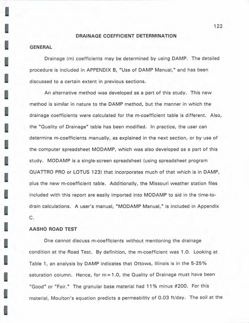
I I I I I I I I I I I I.
I I I I I I I
GENERAL
122
DRAINAGE COEFFICIENT DETERMINATION
Drainage (m) coefficients may be determined by using DAMP. The detailed
procedure is included in APPENDIX 8, "Use of DAMP Manual," and has been
discussed to a certain extent in previous sections.
An alternative method was developed as a part of this study. This new
method is similar in nature to the DAMP method, but the manner in which the
drainage coefficients were calculated for the m-coefficient table is different. Also,
the "Quality of Drainage" table has been modified. In practice, the user can
determine m-coefficients manually, as explained in the next section, or by use of ·
the computer spreadsheet MODAMP, which was also developed as a part of this
study. MODAMP is a single-screen spreadsheet (using spreadsheet program
QUATIRO PRO or LOTUS 123) that incorporates much of that which is in DAMP,
plus the new m-coefficient table. Additionally, the Missouri weather station files
incl.uded with this report are easily imported into MO DAMP to aid · in the time-to
drain calculations. A user's manual, "MO DAMP Manual," is included in Appendix
C.
AASHO ROAD TEST
One cannot discuss m-coefficients without mentioning the drainage
condition at the Road Test. By definition, the m-coefficient was 1 .0. Looking at
Table 1, an analysis by DAMP indicates that Ottawa, Illinois is in the 5-25%
saturation column. Hence, for m = 1 .0, the Quality of Drainage must have been
"Good" or "Fair." The granular base material had 11 % minus #200. For this
material, Moulton's equation predicts a permeability of 0.03 ft/day. The soil at the

123
site was an A-6. This combination of base and subgrade does not appear to be of
a good drainage quality. Indeed, Carpenter's Table 2 rates the drainage as very
poor, thus Table 1 would indicate m = 0.40 to 0. 75.
In setting up Table 1, the authors of Appendix DD in the AASHTO Guide
based a "Good" rating on a base modulus of 30,000 psi, which is the value that
was assigned to the Road Test material. However, in the same document, the
permeability of the base was put at 0.1 ft/day which renders time-to-drain as 1 O
days, which in turn was rated as between "Fair" and "Poor" drainage. The
discrepancy of drainability description was not reconciled. However, in a study by
Haynes and Yoder (53), permeability test results on Road Test crushed stone
granular material were reported as 7.5 ft/day. Furthermore, the laboratory
specimens were so permeable that a uniform moisture content could not be
achieved because the water kept draining down to the bottom portion of the
specimen, indicating a well draining material. Additionally, trench studies at the
Road Test indicated that at the times that the base was tested, the degrees of
saturation were 45 to 60%. Only during the short spring breakup period was
saturation higher. And, the Road Test cross section featured the granular base and
subbase layers extending to the ditches. The ditch bottoms were well below the
grade, and the topography was relatively level. Considering all this, perhaps the
subgrade did behave in a "Fair" manner (not contributing water) and perhaps the
base did manage to be (barely) rated as Fair because it apparently drained in less
than a month (720 hr), which would put the permeability at about 1 ft/day. And,
if one does not count the frozen months as saturated months, then the time of
I I I I
I I I I I I I I I I

I I I I I I I I I I I I I I I I I I I
124
saturation would compute close to 25%. So, if the site was in the 5 to 25%
column, it is conceivable that the table could be reconciled to an m = 1.0.
Certainly, it is conceivable that some subgrade drainage situations could be
considerably worse, and some bases could be significantly less permeable than 1
ft/day . So, a "Fair" rating is reasonable in this context. Finally, it makes sense
that if the Road Test conditions are to be considered as a baseline to which all
other conditions are compared, than a middle value or "Fair" rating is sensible.
DETERMINATION OF AASHTO DRAINAGE COEFFICIENTS-UMR METHOD
Perhaps the best way to describe the manner in which the m-coefficients
were developed in this study is to look at how the designer will use the design
tables, then discuss how the tables were developed.
General Methodology
The AASHTO Guide provides the framework for choosing an m-coefficient
through use of a table (Table 1 ). This has been replaced by Table 23. Two sorts
of information are required: · 1) "Climate Condition" which deals with the climate in
which the project site is located, and 2) "Quality of Drainage" which relates to
how well the pavement structure sheds the water that enters it and the amount of
water supplied by the various components of the highway cross-section. Included
in the following sections is a method to determine the Climate Condition (column
choice in Table 23) and a method to determine the Quality of Drainage (row
choice). The Quality of Drainage is found by use of Table 24 by knowing: 1) the
Granular Layer Quality of Drainage (Base or Subbase), and 2) the Quality of
Subgrade Drainage. The purpose of this section is to provide information to assist

I 125 I
the Missouri designer in determining the above three inputs.
Table 23.
Quality of
Drainage
Excellent
Good
Fair
Poor
Very Poor
Table 24.
Quality of Subgrade Drainage
Good
Fair
Poor
Very Poor
Recommended Drainage Coefficients for Flexible Pavements for Untreated Base and Subbase Materials.
Climate Condition
A B C D E F
1.25- 1.25- 1.25- 1.25- 1.20- 1.20-1.20 1.20 1.20 1.20 1.15 1.15
1.25- 1.20- 1.20- 1.20- 1.20- 1.20-1.20 1.15 1.15 1.15 1.15 1.15
1.20- 1.15- 1.05- 1.05- 1.05- 1.15-1.15 1.05 0.85 0.85 0.85 1.05
1.15- 1.15- 1.05- 1.05- 1.05- 0.85-1.05 1.05 0.85 0.85 0.85 0.70
1.05- 1.05- 0.85- 0.70- 0.85- 0.70-0.85 0.85 0.70 0.60 0.70 0.60
MODAMP Quality of Drainage.
Granular Layer Quality of Drainage (Base or Subbase)
Excellent Good Fair Poor Very Poor < 2 hr* 2 to 24 hr 24 to 168 hr 168 to 720 hr > 720 hr
Excellent Good Fair Fair Fair-Poor
Good Good-Fair Fair Fair Poor
Fair Fair Fair Poor Very Poor
Poor Very Poor Very Poor Very Poor Very Poor
* drainage time to 85% saturation
One problem with the original AASHTO Table (Table 1) is the method of choice of
column. The choice is dependent on the percent of time that the soil in the general
area of the project site is close to saturation. This does not deal well with a soil
I I I I I I I
I I I I I I I I

I I I I I I I I I I I I I I I I I I I
126
that undergoes a seasonal change in resilient modulus as shown in Fig. 29, nor
with the conditions of drainage within the pavement structure. To address this
issue, it is necessary to determine the number of months in the year that the
subgrade is frozen, thawed, wet (recovering from thaw condition) and "dry"
(relative to wet). One way to do this is to import site-specific weather station data
into MODAMP and delineate the number of dry and wet months. From local
experience and MODAMP output, the number of months frozen can be estimated.
With this information, the user should enter Table 25 to find the Climate Condition
description closest to that of the project site. With the Climate Condition defined,
the column choice in Table 23 can be made. It is recommended that for sites in
Zones fl and V, a minimum interval of 0.5 month for frozen and thawed periods
should be used to account for freeze-thaw periods. This will help distinguish
between zones with some of this kind of activity from zones with none. The
season lengths were based on the results of an analysis of weather data by use of
MODAMP for several sites from each of the six AASHTO climate zones. The basic
methods for calculation of water surplus and deficit are identical to those of
DAMP. However, the rules for identifying a particular month as to its providing a
certain saturated pavement time interval were modified to render a better
differentiation between climate zones. In essence, the only rule that was changed
was that if the subgrade was storing the maximum amount of water possible ( 10
cm) and there was a surplus, then the full month was considered to be in a
saturated state. Under certain conditions, DAMP would have considered this as a
one-fourth month saturated interval, namely if there was not a previous frozen
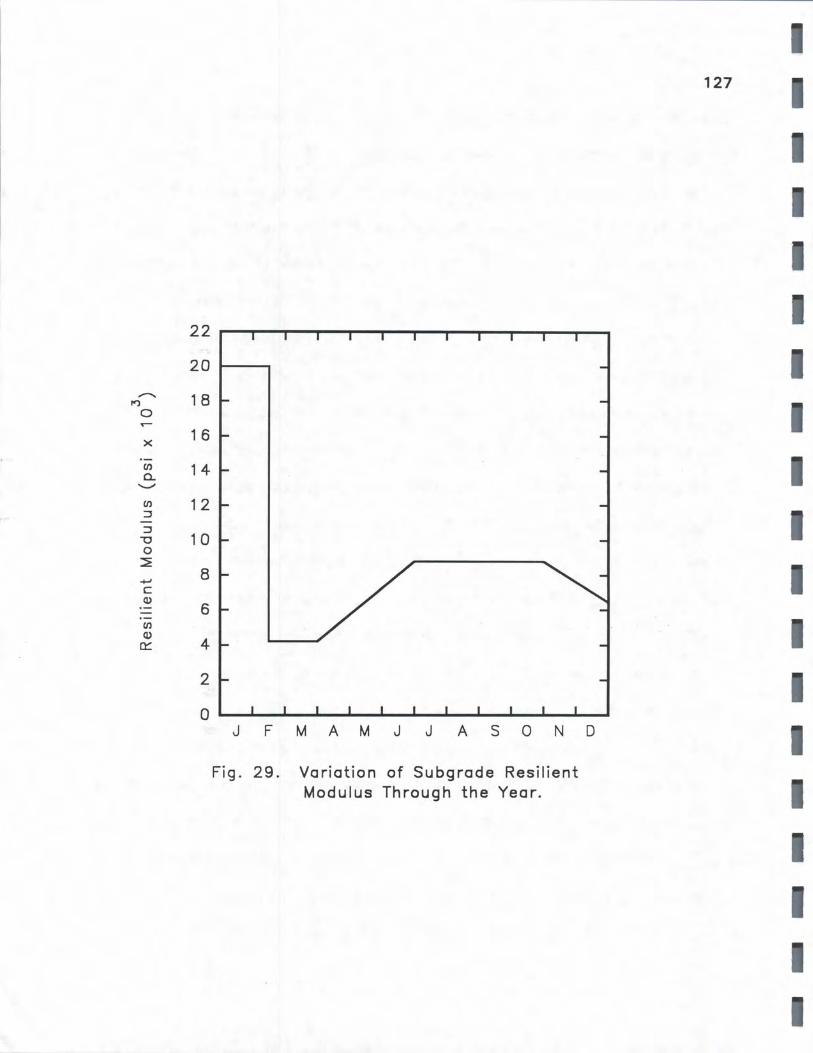
X
(/)
Cl.
(/)
::::,
::::, "'O 0 ~
(/)
Cl> 0::::
22
20
1 8
1 6
1 4
1 2
1 0
8
6
4
2
0 J F M A M J J A s 0 N
Fig. 29. Variation of Subgrade Resilient Modulus Through the Year.
127
D
I I I I I I I I
I I I I I I
I I
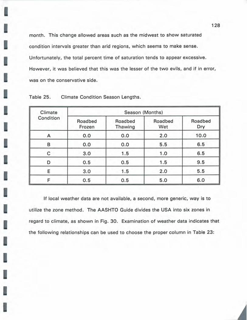
I I I I I I I I I
I I I I I I I I I
128
month. This change allowed areas such as the mid west to show saturated
condition intervals greater than arid regions, which seems to make sense.
Unfortunately, the total percent time of saturation tends to appear excessive.
However, it was believed that this was the lesser of the two evils, and if in error,
was on the conservative side.
Table 25. Climate Condition Season Lengths.
Climate Season (Months) Condition
Roadbed Roadbed Roadbed Roadbed Frozen Thawing Wet Dry
A 0.0 0.0 2.0 10.0
B 0.0 0.0 5.5 6.5
C 3.0 1.5 1.0 6.5
D 0.5 0.5 1.5 9.5
E 3.0 1.5 2.0 5.5
F 0.5 0.5 5.0 6.0
If local weather data are not available, a second, more generic, way is to
utilize the zone method. The AASHTO Guide divides the USA into six zones in
regard to climate, as shown in Fig. 30. Examination of weather data indicates that
the following relationships can be used to choose the proper column in Table 23:
I
REGION CHARACTERISTICS
I . Wet, no freeze
JI Wet, freeze - thaw cycling m Wet, hard-freeze, spring thaw .nz: Dry, no freeze Jz: Dry, freeze - thaw cycling E: Dry, hard freeze , spring thaw
Fig.JO. Six Ciimate Zones in the United States (after 1986
AASHTO Guide for Design of Pavement Structures).
129
I I I I I I I I I I I I I I I I I I I
130
Table 26. Zone - Climate Condition Relationships.
ZONE Table 23 Column
I 8
II F
111 E
IV A
V D
VI C
Note that even though Zone V is quite dry, it is recommended that the designer
consider downgrading the column choice from "less than 1 % to the "5 to 25%"
column if freeze/thaw conditions exist at the particular project site. Choice of row
will be presented next.
It should be noted that for Zones I, II, and Ill (high TMI areas), the storage
calculated by DAMP and MODAMP are essentially identical. Below some TMI
threshold value (somewhere between 5.8 and 18), usually in Zones IV, V, and VI,
DAMP appears to automatically place a 10 cm (maximum) storage in January,
MODAMP does not. In Zones IV through VI output, DAMP and MODAMP output
agree from July through December. It is believed that MODAMP is functioning
correctly because the output agrees well with the various examples in
Thornthwaite's paper (19).
Several Missouri sites were examined. By looking at: 1) Appendix D
weather files for temperature, 2) the output of MODAMP for number of months
saturated (but not frozen or thawing), and 3) Table 25 for Climate Condition
131
(tempered with the suggested number of months thawed), the proper Climate
Condition was found and is shown in Table 27. The Climate Condition was
compared to the corresponding AASHTO Zone by use of Table 26. The two types
of descriptions were found to agree well.
Table 27. Determination of Climate Condition for Several Missouri Sites.
Location Season (Months) Climate Condit-
Roadbed Roadbed Roadbed Roadbed ion Frozen Thawing Wet Dry
Amity 3 1.5 3.5 4.0 E
Rolla 1 0.5 5.5 5.0 F
Springfield 1 0.5 6.5 4.0 F
Sikeston 0.5 0.5 7.0 5.0 F
Obviously, the months that the subgrade is frozen and thawing is only
approximate. Local experience will give a much more realistic estimate.
Quality of Base Drainage
AASHTO Zone
Ill
II
II
II
The Quality of Base Drainage is a function of the time to drain to 85%
saturation. For any pavement cross section and granular material permeability,
MODAMP quickly computes the drainage time. Built into MODAMP is the Moulton
equation for prediction of permeability. MODAMP allows the designer to adjust the
material gradation and dry density to achieve the drainage time that is sought.
Once the time of drainage is determined, the Quality of Base Drainage is
determined in accordance with Table 27. The Quality of Base Drainage criteria
and approximate permeabilities required to meet the criteria are shown in the table.
I
I
I 132
These were determined by making numerous runs of MODAMP with various
I material characteristics. Note that the criteria are in accordance with the AASHTO
I
I I I
I I
Guide, as opposed to those of Carpenter.
The reason that the Appendix DD criteria were adopted rather than those of
Carpenter (DAMP) is that the less stringent criteria of Appendix DD fit better into
the concept that the Road Test drainage condition should be rated as fair. If one
looks at Carpenter's criteria in Table 2, it is seen that the Quality of Drainage at
the Road Test would be rated "Very Poor," and by use of Table 1 the combined
drainage condition plus environment would be considered close to the worst in the
country. This is not reasonable. Plus, the resulting "m" would be 0.4 to 0. 75,
and that cannot be. As discussed previously, use of Appendix DD drainage criteria
leads to a more reasonable assessment of "m" at the Road Test.
Table 28. Required Permeabilities for Quality of Drainage Levels.
Quality of Base or Time to Drain (hr) Required Permeability* Subbase Drainage (ft/day)
Excellent < 2 > 700
Good 2-24 40-699
Fair 24-168 5-39 ~
Poor 168-720 1-4
Very Poor >720 <1
* Based on drainage path = two 12 ft lanes plus 6 ft shoulder; 4 in. thick layer; cross slope = 0.0156, grade = 2%.
From Table 28, it can be seen that most of the open-graded materials tested in this
study would fall into the "Excellent" category when using actual permeability
values or "Good" when using Moulton estimates. Conversely, the MHTD Middle

133
gradation with 8% minus #200 sieve (0.1 ft/day per Moulton or 1 ft/day per test)
would be regarded as "Very Poor" (via Moulton) or "Poor" (via test). These
outcomes fit well with the experience gained from observing these materials both
in the laboratory and in the field.
Typically, an open-graded base will be underlain by a dense-graded subbase,
which serves to protect the base from soil intrusion. Thus, the base Quality of
Drainage may be "Excellent" while the subbase may be "Very Poor".
To assist the designer in achieving a given level of drainage by adjustment of
gradation, a regression equation has been developed to estimate compacted dry
density from gradation and specific gravity data. The adjusted-R2 = 0. 729 with a
S.E.E. = 5.22:
-DryDensity = -87.146+9.522A+66.785ASG · · · · · ·,, (29)
where:
Dry Density = 100 + ·% of T-99 maximum dry density, pcf (the data base of
the equation had only materials tested at 100% T-99 or
greater)
-A = sum of percent passing of sieve series: 1.5 in, 3/4, 3/8, #4, 8, 16,
30, 50, 100, 200, divided by 100
ASG = apparent specific gravity.
Thus, for a given gradation and specific gravity, the dry density can be found.
Then, in MODAMP, knowing the dry density, specific gravity, D10, and percent
minus #200 sieve material, the permeability can be estimated. Finally, by use of
I I
I I I
I I
I
134
Table 28, the Quality of Base Drainage can be found for use in determination of
the Pavement Quality of Drainage.
Subgrade Quality of Drainage
To use the Pavement Quality of Drainage table (Table 24), the Subgrade
Quality of Drainage is required in addition to the Granular Layer Quality of
Drainage. This is found by assessing the subgrade's contribution to the pavement
drainage: 1) a positive drainage of the pavement is "Good", 2) neither draining nor
supplying moisture is "Fair"; and 3) actually supplying water to the pavement is
"Poor" or "Very Poor". Use of Table 29 is recommended for determination of
Quality of Subgrade Drainage.
Pavement Structure Quality of Drainage
By knowledge of both the Granular Layer and Subgrade Quality of Drainage,
the overall Pavement Quality of Drainage can be determined from Table 24.
For instance, an open-graded base on a well-drained subgrade ought to be
rated considerably better than the Road Test, and thus is rated "Excellent." A
pavement whose base has a permeability of about 1 ft/day on a subgrade that
does not help drainage but is not a source of water should be rated about the same
as the Road Test ("Fair"). And, a base that traps water in a worse manner than
that at the Road Test should have a lesser rating ("Poor", "Very Poor") no matter
what the subgrade is doing.
More specifically, a moderately drained soil not in a wet-weather spring
situation combined with an MHTD middle gradation with fines adjusted 3.5%
(k = 13) would have a "Fair" Quality of Drainage. Using this example,

135 I Table 29. Quality of Subgrade Drainage.
Rating Soil Drainage Additional Moisture Contribution
Good • Relatively high permeability Low Moisture Contribution: (predominantly granular • deep water table soils) • absence of wet-weather
springs
• at-grade or on fill
• flooding potential: none or rare
Fair • moderate permeability (fine Moderate to none: to moderately fine soil • deep water table texture) • absence of wet-weather
• may have layer that springs impedes downward • at-grade or on fill drainage • flooding potential: none to
occasional
Poor • low permeability (fill: silty Positive moisture contribution: clays) • shallow water table
• may have layer that • absence of wet-weather impedes downward springs drainage • at-grade or in fill
• flooding potential: occasional to frequent
Very • very low permeability Positive moisture contribution: Poor (heavy clays) • shallow water table
• contains layer that impedes • in area of wet-weather drainage springs
• sidehill cut or cut section
• flooding potential: frequent or common
• marshy area
entering Table 23 finding m-coeffient on the "Fair" row and in the Condition F
column would result in an m of about 1. 1. Thus, a pavement in this situation
would be expected to perform somewhat better in regard to drainage than the
Road Test pavement.

I I I I I I I I I I I I I I I
I I
136
At this point, the user can adjust within the range given based on 1) the
goodness of match between the number of months per season at the project site
and the Climate Catagory chosen, 2) presence or absence of edge drains, 3)
presence or absence of any type of outlet for the draining water, and 4) quality of
the filter/separator. For instance, if the project site's number of wet months is
actually somewhat less than the value shown for the Climate Condition, then the
designer could increase the m-value towards its upper limit (still staying within the
cell). If a drainable base is provided, but the layer is extended under the shoulder
and daylighted at the ditch rather than incorporating edge drains, then the m-value
should be downgraded. If no outlet whatsoever is provided, then the m-value
should be less than 1.0. And, if a drained base is provided, but the filter/separator
layer gradation is not designed to be compatible with both the subgrade and
drainage layer gradations, the m-value should be downgraded. These are examples
of some considerations in the choice of m-coefficient. Edge drains must be
provided in order for a base layer to be catagorized as "Excellent."
DEVELOPMENT OF M-COEFFICIENT TABLE
In the following paragraphs, the development of the drainage coefficient
table will be explained. It will be shown that the m-coefficients are a function of
granular material resilient moduli, and these moduli were calculated from numerous
runs of KEN LA YER for different moisture and temperature conditions.
Drainage coefficients are in essence modifiers of layer coefficients that
adjust for conditions of drainage of a given project relative to the conditions of
drainage at the Road Test. Each drainage coefficient developed in the present
st udy is basically a ratio of the layer coefficient of Road Test granular material
adjusted for specific site conditions to the layer coefficient of the Road Test
material for Road Test conditions:
137
a site m = ---- .................. . (30)
aRoadTest
The determination of each layer coefficient is as outlined in the companion
study of this report (29). The layer coefficient for bases and subbases are
functions of resilient moduli (Egl, and can be calculated by use of the equations
given in the AASHTO Guide:
a2 = 0.249 log Eg - 0.977 . . . . . . . . . . . . . . (31)
a3 = 0 .227 log Eg - 0.839 . . . . . . . . . . . . . . (32)
In this portion of the study, the moduli of the Road Test base and subbase
were determined by use of the program KENLAYER. The average Road Test
pavement cross-section was used for each condition, as shown in Fig. 31. ·
The moduli of any granular base and subbase are functions of the stress
state of the material, represented by the bulk stress (8), and of material
characteristics, represented by k1 and k2 , as shown in Fig. 14. The bulk stress is
a function of the asphalt layer thickness, asphalt layer resilient modulus, granular
layer thickness, and subgrade resilient modulus.
The effect of drainage on the support capacity of a granular layer can be
determined by 1) ascertaining the effect on base modulus by changing subgrade
modulus (as a consequence of it getting wetter or staying wet longer) and 2)

I I
DI
D 2
D 3
= 4 .00
5 .39
= 8.75
138
4500 Lbf 4500 Lbf
p 70 ps1
In u = 0.40 I
In u 0 .35 2
1n u = 0.35 3
u - 0 .45 4
Fig. 31. Average AASHO Road Test Cross-Section .
139
determining the effect of the degree of saturation on the granular material
constants k1 and k2 .
Numerous runs of KENLAYER were required to give a range of modulus
values covering the spectrum of moisture and temperature conditions across the
country. The values for the KEN LAYER input are listed in Table 30. The value
reported by Traylor for the base material k1 ,wet was thought to be excessive. This
necessitated the estimation of k1 ,wet· In order to estimate a more reasonable value
for k1 ,wet' a k 1 reduction factor was required which would allow for a decrease in
k1 as the moisture content changed from a moist state to a wet state. The
reduction factor was determined by examining data from several sources (57, 59)
as well as the data generated in this study. This analysis led to the use of a value
of 20% reduction, which resu lted in a k1 ,wet = 8300 psi.
The subgrade Emin• Emax• and K1 values for various moisture states were
determined as follows. Emin and Emax refer to the minimum and maximum values
that the subgrade resilient modulus is expected to reach throughout the year. K1
is the modulus at a deviator stress of 6.2 psi, and is at the knee of the E59-ad
curve. This is shown in Fig . 32. A more thorough explanation of the derivation
and use of this type of curve is found in reference 29. Briefly, for the moist
condition, K1 moist was calculated by use of the Robnett-Thompson equation (61 ),
while Emin,moist and Emax,moist were found by knowing the slopes of the curves.
K1,thawed was estimated as 55% of K1moist · This value is recommended by
Witczak (56) for the Road Test conditions. The value of 55% was verified by the
Robnett-Thompson K 1-correction relationship for changes in moisture content.
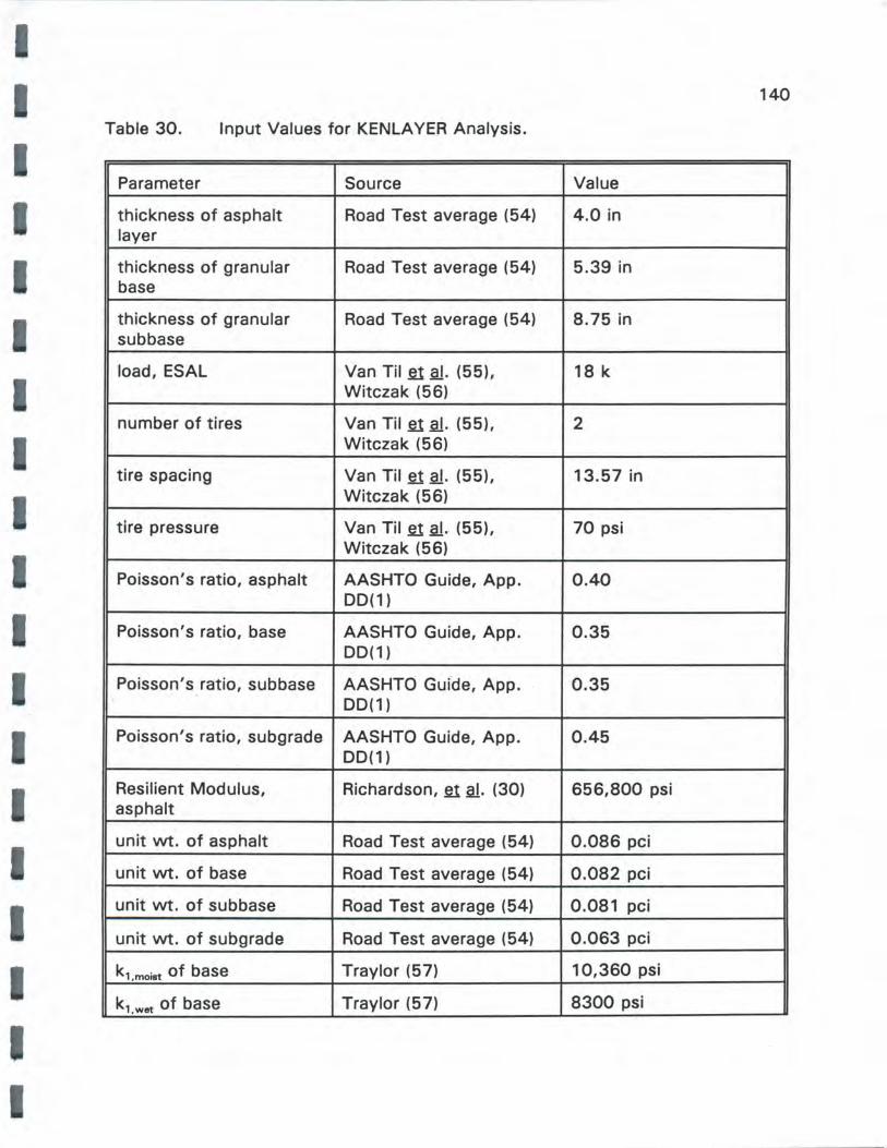
I
I
I I
Table 30. Input Values for KENLAYER Analysis.
Parameter Source
thickness of asphalt Road Test average (54) layer
thickness of granular Road Test average (54) base
thickness of granular Road Test average (54) subbase
load, ESAL Van Til fil gf. (55), Witczak (56)
number of tires Van Tit fil gf. (55), Witczak (56)
tire spacing Van Til fil gf. (55), Witczak (56)
tire pressure Van Til fil gf. (55), Witczak (56)
Poisson's ratio, asphalt AASHTO Guide, App. 00(1)
Poisson's ratio, base AASHTO Guide, App. 00(1)
Poisson's ratio, subbase AASHTO Guide, App. 00(1)
Poisson's ratio, subgrade AASHTO Guide, App. 00(1)
Resilient Modulus, Richardson, fil gf. (30) asphalt
unit wt. of asphalt Road Test average (54)
unit wt. of base Road Test average (54)
unit wt. of subbase Road Test average (54)
unit wt. of subgrade Road Test average (54)
k, ,moist of base Traylor (57)
kl.wet of base Traylor (57)
140
Value
4.0 in
5.39 in
8.75 in
18 k
2
13.57 in
70 psi
0.40
0.35
0;35
0.45
656,800 psi
0.086 pci
0.082 pci
0.081 pci
0.063 pci
10,360 psi
8300 psi

141
k, ,thawed of base Traylor (57) 2850 psi
k, ,moiat of subbase Traylor (57) 6840 psi
k,,wet of subbase Traylor (57) 6270 psi
k, ,thawed of sub base Traylor (57) 4075 psi
k2,moist of base Traylor (57) 0.35
k2,wet of base Traylor (57) 0.34
k2,thawed of base Traylor (57) 0.62
k2,moiat of subbase Traylor (57) 0.32
k2,wet of subbase Traylor (57) 0.30
k2,thawed of subbase Traylor (57) 0.40
k0 of base and subbase Huang (58) 0.6
ko of subgrade Huang (58) 0.8
K2 of subgrade, moist Huang 6.2 psi
K3 of subgrade, moist Huang 1110 psi
K4 of subgrade, moist Huang 178 psi
Emin of subgrade, moist from Fig. 32 5389 psi
Emax of subgrade, moist from Fig. 32 13,420 psi
K, of subgrade, moist Richardson, fil al. (29) 8759 psi
Emin of subgrade, wet from Fig. 32 3515 psi
EmllX of subgrade, wet from Fig. 32 10,402 psi
K, of subgrade, wet calculated 5740 psi
Emin of subgrade, thawed from Fig. 32 1705 psi
Emax of subgrade, thawed from Fig. 32 7382 psi
K, of subgrade, thawed calculated 2720 psi
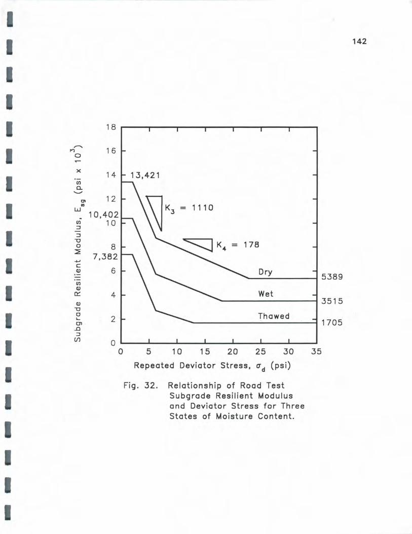
I I I
I I
I I
I
I I
.,.-,,. l'1
0 ,--
X
Cl)
a. '-"
Cl ID
w -Cl)
:J
:J -0 0 ~
-1--'
C Q.)
Cl) Q.)
n::: Q.)
-0 0 "-C)'l '
..c :J
(/)
1 8
1 6
14
12
10,402 1 0
8 7,382
6
4
2
0 0
142
13,421
- 111 0
Dry 5389
Wet 3515
Thawed 1705
5 10 15 20 25 30 35
Repeated Deviator Stress, CT d (psi)
Fig. 32. Relationship of Road Test Subgrade Resilient Modulus and Deviator Stress for Three States of Moisture Content.

143
Again, Emin,thawed and Emax,thawed were determined using geometry. Finally, K 1 wet
was calculated as midway between K1moist and K1thawed because the wet
recovery period E59-time curve is assumed to be a straight line (see Fig. 31 ). And,
Emin,wet and Emax,wet were again calculated by geometric means.
The analysis standard year was divided into 24 one-half month periods, and
the k1 (base), k 1 (subbase), and K1, Emin' Emax (subgrade) were varied for each
period, depending on prevailing environmental conditions. The environmental
conditions were varied according to the particular zone of interest. The six zones
in the U.S. are shown in Fig. 30. Table 25 is adapted from the AASHTO Guide
and tabulates the number of months a subgrade can be expected to be frozen,
thawing, wet, or "dry". These season lengths were modified depending on the
drainage conditions of the subgrade and the base course as shown below.
KENLAYER does not allow a variation in k2 (granular) values, so an average k2 was
input which was weighted for the number of months moist, wet, and thawed for
the particular case being analyzed.
As discussed earlier, soil drainage was considered to be good, fair, poor, or
very poor. These conditions are described in Table 29. Base drainability is tied to
permeability, and is described as excellent, good, fair, poor, and very poor -- these
states are shown in Table 28.
The manner in which the benefit or lack of drainage asserted itself was
taken care of by varying incrementally the season length. For a plot of E59 vs.
time, the dry period was divided into four parts and the thawed period was divided
into five parts. Although quite arbitrary, this was done as an expedient to allow
I
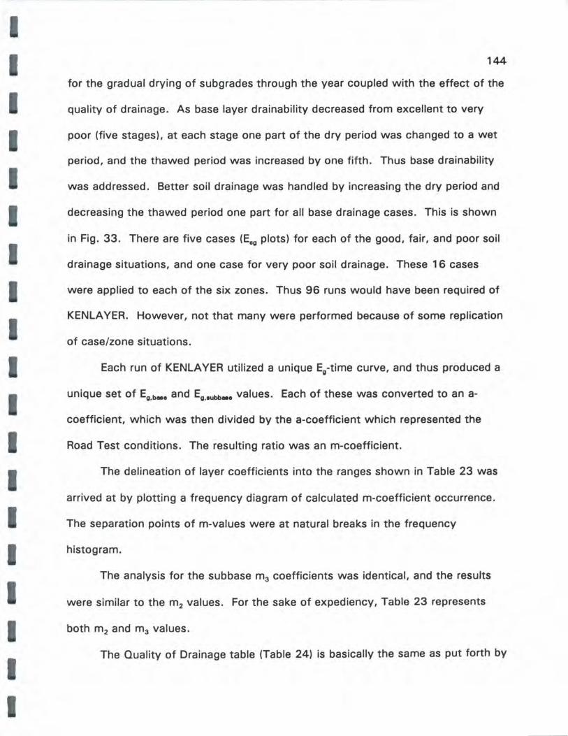
144
for the gradual drying of subgrades through the year coupled with the effect of the
quality of drainage. As base layer drainability decreased from excellent to very
poor (five stages), at each stage one part of the dry period was changed to a wet
period, and the thawed period was increased by one fifth. Thus base drainability
was addressed. Better soil drainage was handled by increasing the dry period and
I decreasing the thawed period one part for all base drainage cases. This is shown
in Fig. 33. There are five cases (E.g plots) for each of the good, fair, and poor soil
drainage situations, and one case for very poor soil drainage. These 16 cases
were applied to each of the six zones. Thus 96 runs would have been required of
KENLAYER. However, not that many were performed because of some replication
of case/zone situations.
I
Each run of KENLAYER utilized a unique Eg-time curve, and thus produced a
unique set of Eg,b•• and Eg,aubb•• values. Each of these was converted to an a
coefficient, which was then divided by the a-coefficient which represented the
Road Test conditions. The resulting ratio was an m-coefficient.
The delineation of layer coefficients into the ranges shown in Table 23 was
arrived at by plotting a frequency diagram of calculated m-coefficient occurrence.
The separation points of m-values were at natural breaks in the frequency
I histogram.
I I
The analysis for the subbase m3 coefficients was identical, and the results
were similar to the m2 values. For the sake of expediency, Table 23 represents
both m2 and m3 values.
The Quality of Drainage table (Table 24) is basically the same as put forth by
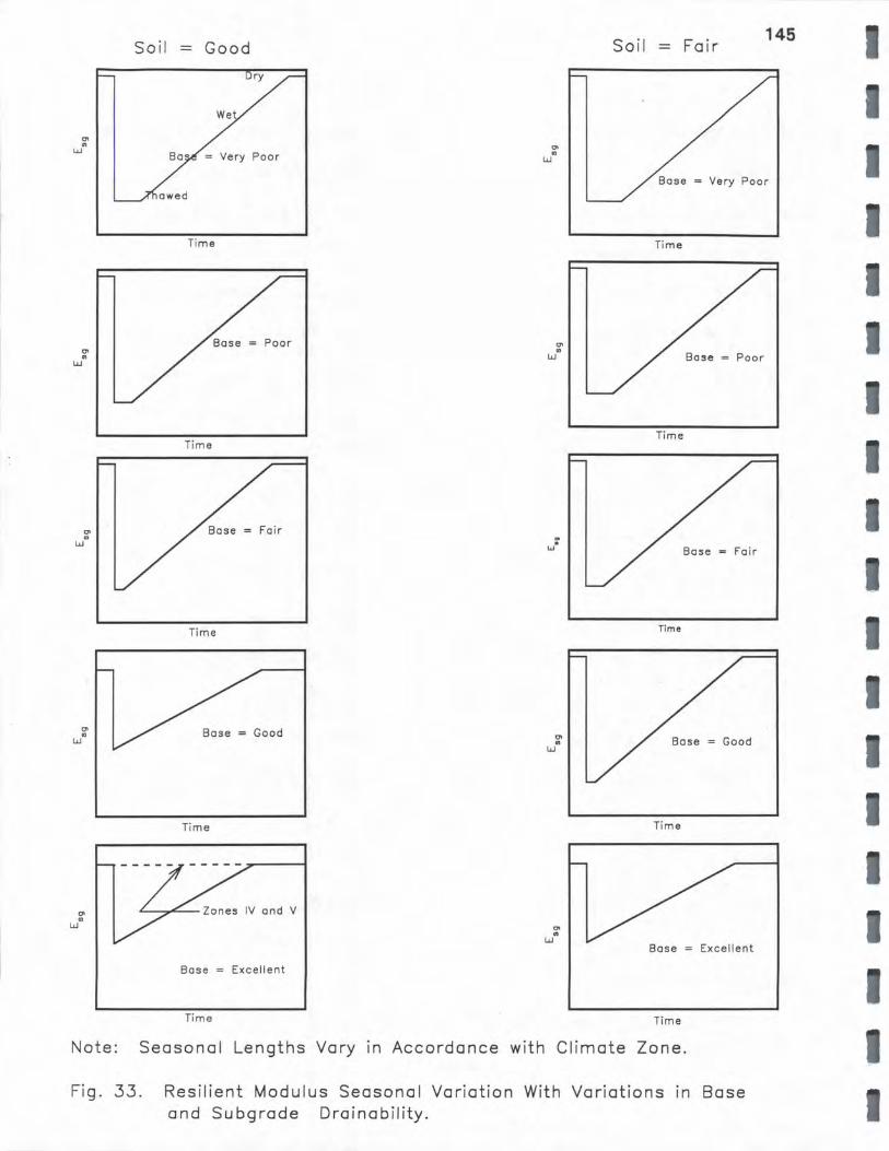
"' " w
Soil - Good
Very Poor "' " w
Soil Fair 145
Base = Very Poor
"' " w
"' " w
"' " w
"' " w
Time
Time
Time
Base Excellent
w "' "
~ . w
"' ., w
"' " w
Time
Time
Time
Base Excellent
Time Time
Note: Seasonal Lengths Vary in Accordance with Climate Zone.
Fig. 33. Resilient Modulus Seasonal Variation With Variations in Base and Subgrade Drainability.
I
I
I I I I
I I I I I I I I I
w
w
'" ..
'" "
'" w
.,
'" ., w
'" .. w
Soil Poor
Bose Very Poor
'" " w
Soil = Very Poor
Very Poor
Time Ti me
Time
Time
Time
Time
Note: Seasonal Lengths Vary in Accord a nee With C Ii mate Zone. Fig. 33. Continued.

Carpenter, although it was adjusted to match the outcome of the m-coefficient
frequency plot.
Reasonableness
147
In comparison of Missouri sites to the Road Test site, in a regional sense
actual data indicates that most of Missouri is in a climatic zone that is rated as
having a greater time of saturation, so a given pavement in Missouri should fare
worse (from moisture-related problems) and therefore should have m-coefficients
less than 1.0, unless something is done to improve the pavement drainage.
Conversely, for a situation where any water that enters the base is quickly
removed laterally and where the soil drains well and does not supply water from
the surrounding soil or side hill wet weather springs and so forth, then an
expectation of a 10 to 20% improvement in pavement performance would be
reasonable. For a somewhat lesser quality of subgrade drainage with a highly
drainable base, a 10% credit may be more realistic. And, going with the belt-and
suspenders approach, there is the option of supplying a drainable section with no
reduction in pavement thickness, a conservative approach to be sure, but not
w ithout merit for as the above discussion reveals, there is an element of conjecture
in this whole business.

II
I I
MODAMP SENSITIVITY ANALYSIS
A sensitivity analysis was performed to observe the effect of the major
drainage variables on design. This information should be helpful for future or
routine work when one is trying to decide which variable can be estimated and
148
I which must be tested. Also, at any time during an actual project, from pavement
I
I I
I
I
design and material selection to construction and inspection, it can be very useful
to have insight into which deviations from certain criteria will significantly affect
the performance of the pavement.
The analysis was divided into two parts: 1) an m-coefficient analysis, and 2)
a pavement thickness analysis.
M-Coefficient Analysis
Drainage coefficients are a function of : 1) pavement drainability, and 2)
climate. Within a given climate, pavement drainability is a function of : 1) width,
2) longitudinal grade 3) subgrade drainability, 4) base thickness, and 5) base
permeability. Cross-slope is usually not a variable that can be changed by the
highway designer. The sensitivity analysis was conducted by establishing three
values for each variable: the most likely value for each variable, a high value, and a
low value. Several runs with MODAMP were made with each successive run
changing one variable from low to median to high while holding all other variables
constant at the median value. Base drainability was the variable with the greatest
effect upon the drainage coefficient. With a Fair-draining subgrade, changing from
Very Poor to Excellent base drainage changed the m-coefficient by 0.30 to 0.45.
The permeability of the subgrade was also an important variable in the program.
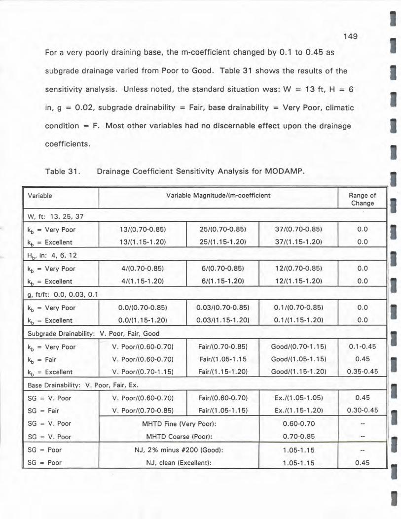
149
For a very poorly draining base, the m-coefficient changed by 0.1 to 0.45 as
subgrade drainage varied from Poor to Good. Table 31 shows the results of the
sensitivity analysis. Unless noted, the standard situation was: W = 13 ft, H = 6
in, g = 0.02, subgrade drainability = Fair, base drainability = Very Poor, climatic
condition = F. Most other variables had no discernable effect upon the drainage
coefficients.
Table 31. Drainage Coefficient Sensitivity Analysis for MODAMP.
Variable Variable Magnitude/(m-coefficient Range of Change
W, ft: 13,25,37
kb = Very Poor 13/(0. 70-0.85) 25/(0. 70-0.85) 37 /(0. 70-0.85) 0.0
kb = Excellent 13/(1.15-1.20) 25/(1.15-1.20) 37/(1.15-1.20) 0.0
Hb, in: 4, 6, 12
kb = Very Poor 4/(0.70-0.85) 6/(0. 70-0.85) 12/(0.70-0.85) 0.0
kb = Excellent 4/(1.15-1.20) 6/(1.15-1.20) 12/(1.15-1.20) 0.0
g, ft/ft: 0.0, 0.03, 0.1
kb = Very Poor 0.0/(0. 70-0.85) 0.03/(0. 70-0.85) 0.1 /(0.70-0.85) 0.0
~ = Excellent 0.0/(1.15-1.20) 0.03/( 1 .1 5-1 .20) 0.1 /(1.15-1.20) 0.0
Subgrade Drainability: V. Poor, Fair, Good
kb = Very Poor V. Poor/(0.60-0.70) Fair/(0. 70-0.85) Good/(0.70-1.15) 0.1-0.45
kb = Fair V. Poor/(0.60-0.70) Fair/(1.05-1.15 Good/(1.05-1.15) 0.45
kb = Excellent V. Poor/(0.70-1.151 Fair/(1.15-1.201 Good/(1.15-1.20) 0.35-0.45
Base Drainability: V. Poor, Fair, Ex.
SG = V. Poor V. Poor/(0.60-0.70) Fair/(0.60-0. 701 Ex./(1.05-1.051 0.45
SG = Fair V. Poor/(0.70-0.85) Fair/(1.05-1.151 Ex./(1.15-1.201 0.30-0.45
SG = V. Poor MHTD Fine (Very Poor): 0.60-0.70 --SG = V. Poor MHTD Coarse (Poor): 0.70-0.85 --
SG = Poor NJ, 2% minus #200 (Good): 1.05-1.15 --SG = Poor NJ, clean (Excellent): 1.05-1.15 0.45
I I I
I
I I
I I
I I
Hb and P200 : 2 in and P200 = 0 or 2%
SG = Fair Hb = 2 in; NJ, clean (Excellent): 1.15-1 .20 0.0
SG = Fair Hb = 2 in; NJ, 2% minus #200 (Good): 1.05-1 .15 0.05-0.10
The gradation of the base material had a pronounced effect on m-coefficient.
A gradation at the fine side of the Type 1 limit with 15 % fines is rated Very Poor
and consequently has low m-values. A Type 1 on the coarse side of the limits
with 2% fines is an improvement, but still a poorly-draining material. A NJ
gradation, somewhat dirty, and a clean NJ render m-values greater than 1.0.
Table 32. Thickness Sensitivity Analysis for MODAMP.
Variable m2 m~ D2, in
Climate:
Worst (Zone F) 1.10 0.78 12.0
Best (Zone A) 1.18 1.10 10.2
(Base, Subbase, and Subgrade all = Fair)
Drainability:
Base: Very Poor
Subgrade: Very Poor 0.65 0.65 21.0
Base: Very Poor
Subgrade: Good 0.95 0.95 13.2
Base: Excellent
Subgrade: Very Poor 0 .78 0.65 17.5
Base: Excellent
Subgrade: Good 1.18 0.95 10.7
All cases o, = 4 in , E1 = 450,000 psi, a1 = 0.44, 82 = 0.10, 83 = 0.09, D3 = 4 in, SN = 3.36
Finally, the effect of accidentally pinching the base layer down to 1 in and
fouling the NJ gradation lowers the m-values somewhat.
150
151
The second portion of the analysis involved an examination of how the major
variables affected base thickness design. Using an asphalt layer thickness (D 1 ) of
4 in and E1 = 450,000 psi; a base layer thickness (D2 ) of 12 in, a subbase layer
thickness (D3 ) of 4 in, and a somewhat soft subgrade (K 1 = 6000 psi), the elastic
layer analysis program KENLAYER was used to calculate the moduli in the base
and subbase layers. These were converted to layer (a2, a3) coefficients by the use
of the AASHTO nomograph equations (see Ref. 5 for further discussion). By use
of Eq. 1, the SN was calculated, and was considered constant for the rest of the
analysis.
First, the effect of climate was considered. Using the above parameters, for
a constant pavement drainability rating, there was a difference in D2 (base
thickness) of 15 % between the best environmental zone and the worst. Second,
for constant base drainability, the required D2 decreased about 38% when the
subgrade drainability improved from Very Poor to Good. Finally, looking at the
variable over which the designer has some control, by improving base drainability,
the required base thickness decreased by about 18%, depending on subgrade
conditions.
I

I I
I I I
I
I I I I I
I I I
152
SUMMARY AND CONCLUSIONS
The purpose of this study was to determine the drainage (m) coefficients of
granular bases and subbases for use in the 1986 AASHTO Guide pavement design
method for flexible pavements. The project entailed a review and compilation of
published literature, laboratory testing, analysis of results, and preparation of this
report.
One existing method with which to determine drainage coefficients was
examined, and two potential strategies for development into a new method were
explored.
1. Seeds and Hicks developed the basic method for determination of drainage
coefficients, which is presented in the 1986 AASHTO Guide. The method
necessitates the determination of: 1) the Percent Time of Saturation of the
pavement structure, and 2) the Quality of Drainage of the base and subbase.
With these, the m-coefficients are found from a table. Unfortunately, little
direction was given in regard to the determination of the necessary input
data that is required for using the m-coefficient table.
2. Carpenter developed a method for determining m-coefficients which can be
easily implemented by use of software called DAMP. DAMP is based on the
method given in the 1986 AASHTO Guide. Carpenter's main contribution
was to provide a method with which to determine the Percent Time of
Saturation for the pavement structure, and the Quality of Drainage of the
combined base and subgrade. Required input for DAMP includes base
material permeability, or dry density and gradation information, certain
weather data, base layer thickness and density, and subgrade drainability

153
based on soil characteristics. DAMP calculates time-to-drain to 85%
saturation, and rates the Quality of Base Drainage. With this, and the
Quality of Subgrade Drainage, the overall Pavement Quality of Drainage is
found. At this point, the AASHTO Guide m-coefficient table is used for
determination of m-coefficients.
3 . A sensitivity analysis was performed using DAMP. Base drainability had the
greatest effect on the magnitude of the coefficients, with subgrade
drainability the second most important. All other variables had a minor or
negligible effect.
4. The major concerns with DAMP were:
a. DAMP's Table 2 (Quality of Drainage) does not lead to reasonable results
if one subscribes to the theory that the Road Test pavement drainage
was "Fair." The whole idea of the use of m-coefficients is to rate any
pavement's drainage relative to that at the Road Test. Better drainage
should be "Good" or "Excellent," worse drainage should be "Poor" or
"Very Poor."
b. The effect of freeze-thaw cycles and frost heave is not addressed well.
The thaw/melt period will typically result in a worse condition than
merely getting the soil wet. This effect is lost in the Time of Saturation
calculations, and the result is that AASHTO Zones I, II, and Ill are usually
lumped together, which could lead to erroneous results.
c. DAMP appears to arbitrarily increase the January storage to the
maximum for Thornthwaite Moisture Indices below a certain threshold
I I I I I I I I I I I I
I I I I
11
I
5.
154
value, regardless of previous month's history of moisture changes.
d. The extrapolation of the Thornthwaite method of regional moisture
available to the conditions in the pavement structure is of concern.
Also, the manner in which the time of saturation for various
environmental conditions is calculated is arbitrary. However, it is
recognized that at the present time there are no practical working
solutions to this dilemna, and that the time of saturation procedure in
DAMP is a significant step forward, and should be used until a more
fundamentally sound, user-friendly method can be developed.
The TTI Integrated Model of the Climatic Effects on Pavements was
evaluated with the idea that it could determine environmental effects on
granular base/subbase materials, which would lead to the calculation of m
coefficients. The TTI model consists of four independent models linked
together: the Precipitation Model, the Infiltration/Drainage Model, the
Climatic-Materials-Structural Model, and the CRREL Frost Heave-Settlement
Model. The Integrated Model examines many variables and processes in
very fundamental terms and thus has the potential for rather detailed and
accurate analysis.
Unfortunately, the scheme was unsuccessful because of limitations in
the TTI model. First, the model requires a minimum of 100 input variables.
Many of these are not easily obtained and must be assumed. Model output
is sensitive to the magnitude of some of these input values. Secondly, the
model has a low sensitivity to variables that are thought to be important to

155
the derivation of m-coefficients. Third, the program is cumbersome. And
most importantly, the output parrots the input base course modulus. This is
a fatal flaw and rendered the program unusable for purposes of drainage
coefficient determination as envisioned in this study.
6 . The materials under study included two sources of crushed stone and two
. gravels. All materials were selected, sampled, and delivered to UMR by
MHTD personnel. The primary tests performed were: 1) resilient modulus
testing at a low and high degree of saturation to assess the moisture
sensitivity of the materials, and 2) permeability and effective porosity to
assess the drainage characteristics of the materials.
7. Two gradations of granular material were used in the resilient modulus
testing: one followed the midpoint of the MHTD Type 1 gradation (MHTD
Middle) acceptance band, and the other was the so-called New Jersey (NJ)
open-graded gradation. An additional gradation (OGS) was used in the
permeability portion of the study, along with the MHTD Middle and the NJ.
8. The aggregates were separated into the appropriate size fractions,
recombined, and tested for specific gravity, plasticity index (Pl) moisture
density relationships, and relative density. Standard and modified proctor
type tests (T-99, T-180) were performed for the dense gradation, while
vibratory table densification was used for the open-graded material. The
specific gravity information was required for calculation of porosity, effective
porosity, and permeability estimation. The Pl data were useful in evaluation
of permeability and effective porosity results. The finer fraction of all four
I I I I
I I I I I I I I I I I I I
9.
156
aggregate types was found to be non-plastic. The density results were
needed in order to determine the compaction target densities and moisture
contents for the resilient modulus and permeability specimens.
Nine different methods were used to characterize the gradation curve shapes
and positions. These methods were fineness modulus, coefficient of
-. uniformity, coefficient of skew, Hudson's A, surface fineness (SF), specific
surface factor (SSF), SF/SSF, slopes-of-gradation curve, and percent passing
or retained on individual sieves. None of the single parameters were superior
in the prediction of k1 or E9 . The percent passing the 3/8 in, #4, #8, ano
#200 sieves proved to be useful in prediction of permeability.
10. Particle shape/surface texture tests were performed on the four aggregates.
The ( +) #4 sieve material was tested in accordance with ASTM D3398,
while the (-) #8 to ( +) #100 fraction was tested using the NAA method.
The measured angularities of the two stones were about the same, and were
more angular than the two gravels, which were about equal. The difference
in angularity/texture was not great between the crushed stones and the
gravels.
11 . Resilient modulus test results were required for use in the TTI method and in
the new method developed in this study. The tests were run on all four
aggregates using two gradations, two compactive efforts, and two degrees
of saturation, with replications. Fourteen combinations of confining pressure
and cyclic applied deviator stress were used for each specimen in the test
sequence. Effective confining pressures ranged from 2 to 20 psi and cyclic
157
deviator stress ranged from 2 to 40 psi. Thirty-two specimens were
fabricated. The total number of tests run was 896.
The results of the testing indicated the Eg increases with a lower degree
of saturation. The average percent loss in k1 due to increased saturation
was 31 %. This information was used in the development of the m
coefficients.
12. An analysis of the interaction of gradation and degree of saturation indicated
that dense-graded material suffered less loss of modulus than open-graded
material. However, in practice the open-graded material would not be in a
saturated state nearly as much (if ever) as a dense-graded state. The data
showed that the drained open-graded moduli were greater than the
undrained dense-graded moduli.
13. A statistical analysis was performed to determine the significance of the
variables. Paired-t tests indicated that change in degree of saturation gave
significantly different results at the 0.05 level. In comparing saturated
dense-graded material with drained open-graded material, there was a
significant (0.088 level) increase in Eg with superior drainage.
An increase in degree of saturation acts to lower k1 and raise k2 of the
granular material, and to lower subgrade support, all of which act to lower
the Eg of the granular material.
14. Permeability of base material is required input for DAMP, TTI Integrated
model, and MODAMP. It is necessary in order to calculate the time-to-drain
for base layers. The rigid wall constant head test procedure was used for
I I I I I I I I I I I I I I I
I I I
158
the NJ and OGS open-graded materials, while the dense-graded MHTD
Middle specimens were tested in a triaxial compression chamber following
the resil ient modulus testing.
15. Measured permeability values have been shown to be sensitive to: 1) air
blockage, 2) specimen sergregation, 3) relative density, 4) gradient, and 5)
short-circuiting. Considerable effort was exerted to eliminate or at least
minimize the above problems, either through the development of the test
procedure or the design of the equipment.
16. The open-graded specimens were tested at a minimum of five gradients with
five repetitions. The permeability coefficients were calculated as the
average of the values which were obtained at or less than the expected field
gradient (approximately 0.1 ). The testing variables included four aggreate
sources and two gradations (NJ and OGS). Duplicate specimens were
tested, for a total of 400 tests; this represented data from 16 total
specimens.
17. The dense-graded specimens were tested at the recommended gradient of
five with five repetitions . Two compactive efforts were used on the four
aggregate sources. Duplicate specimens were used. This resulted in a total
of 80 tests, representing data from 16 specimens.
18. The testing program results for the open-graded materials revealed the
following :
a. Permeabilities estimated from the Moulton equation significantly
underestimated the observed values by an order of magnitude or more in
159
most cases. A review of the data on which the Moulton equation is
based reveals potential problems with air blockage, effect of end
conditions, and possibly incorrect use of specific gravity data, all of
which would lead to falsely low values.
b. The OGS gradation appeared to be more permeable than the NJ, but was
not so at the 0.05 significance level.
c . The #16 sieve size was important to the predicition of permeability of
the open-graded materials.
d. The DR-15 gravel was more permeable in a statistical sense than both of
the crushed stones, but was also more permeable than the DR-14 gravel.
Because their particle shapes were about the same, a strong statement
cannot be made as to the effect of particle shape.
e. A regression equation was developed for the open-graded materials . It
had an adjusted-R2 = 0. 779:
k = -40,962 + 15,284 (/Jett) + 205.89 (P16) + 380. 70 (PDENS)
where:
/Jett = effective porosity
P16 = percent passing #16 sieve
PDENS = percent of maximum achievable density.
f. The average effective porosity was about 68% of the average porosity.
19. The results of the dense-graded permeability testing were:
a. Again , permeabilities estimated with the Moulton equation were
significantly lower than observed values.

I I I I I I I I I I I I I I I I I I I
160
b. Gravels exhibited slightly greater permeabilities than crushed stones, but
not statistically so at the. 0.05 level.
c. A regression equation was fit to the data which resulted in an adjusted
R2 = 0.624:
k = -8.457 + 35.753 (17) + 0.033 (satfinal)
where:
17 = porosity (calculated with apparent specific gravities)
satfinal = final degree of saturation, %.
d. On the average, the effective porosities were about 27% of the total
porosities. This is considerably smaller than the open-graded value,
which is to be expected because of the finer pore sizes in the dense
graded material.
e. Overall, the permeabilities of the dense-graded materials were
significantly lower by several orders of magnitude than those of the
open-graded materials (average of 0.8 ~ 1014 ft/day).
20. A regression equation to estimate permeability was developed by combining
the results from several studies found in the literature with the results of this
study. The equation had an adjusted-R2 = 0.900:
k = (2.28 x 10¹⁷)(l7)8.995 (D,o)0.591 /[(P3/8)5.511 (P200)0.349]
where:
fJ = porosity (calculated with apparent specific gravity data)
D10 = size that represents 10% passing, mm
P3/8 = percent passing 3/8 in sieve
161
P200 = percent passing #200 sieve.
The equation is considered accurate in the range of 0.1 to 1000 ft/day.
21. Although the Moulton equation significantly underpredicts permeability, it
may be the equation of choice because field conditions may render the base
layer less permeable than what would be predicted with good quality
laboratory testing.
22. A new method of calculation of drainage coefficients was developed. In
essence, m-coefficients were calculated as a ratio of the layer coefficient of
Road Test granular base material under a given drainage and climate
condition to the layer coefficient under Road Test site conditions. The layer
coefficients were calculated from resilient moduli. The resilient moduli were
calculated with KENLAYER under varying conditions. By changing subgrade
and base moisture conditions for a given time of year, the moduli were
varied. The base material moisture sensitivity (effect on k1 and k2) was
determined in part by the resilient modulus laboratory testing of granular
materials.
23. The result of the above analysis was the creation of a Quality of Base
Drainability table (based on time-to-drain to 85% saturation), a Quality of
Subgrade Drainability table (based on subgrade permeability, position of
water table, flooding potential, presence of impermeable layers, potential for
water seepage, and so forth), a Quality of Pavement Drainage table(based
on the previous two tables), a Climate Condition table (based on estimated
season lengths), and finally, an m-coefficient table (based on Quality of
I
I
I
I
I
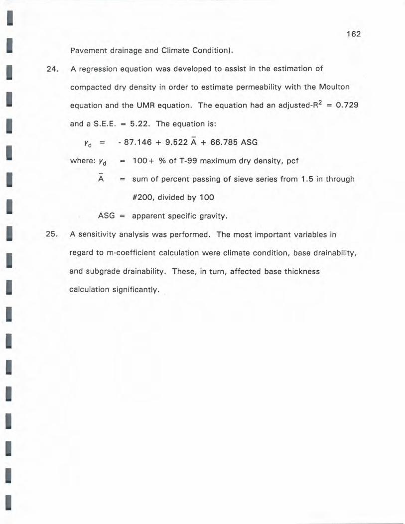
I I I I I
I I I I I I I I I I I I I
24.
25.
162
Pavement drainage and Climate Condition).
A regression equation was developed to assist in the estimation of
compacted dry density in order to estimate permeability with the Moulton
equation and the UMR equation. The equation had an adjusted-R2 = 0. 729
and a S.E.E. = 5.22. The equation is:
yd = - 87.146 + 9.522 A + 66.785 ASG
where: yd
A
= 100+ % of T-99 maximum dry density, pcf
= sum of percent passing of sieve series from 1. 5 in through
#200, divided by 100
ASG = apparent specific gravity.
A sensitivity analysis was performed. The most important variables in
regard to m-coefficient calculation were climate condition, base drainability,
and subgrade drainability. These, in turn, affected base thickness
calculation significantly.

I
I I I I I I I I I
I
I

I I I I
I I I I I I I I I I I I I
1 .
2 .
3.
163
RECOMMENDATIONS
A choice is presented as to the procedure for estimation of permeability.
Moulton's equation underpredicts permeability significantly. The UMR
equation is more accurate. However, due to uncertainties of the impact of
field construction practices, permeabilities estimated by the Moulton method
would err on the conservative side. It is recommended that field
permeabilities should be run to determine which equation should be used .
Until this is done, the Moulton equation is recommended.
In regard to determination of drainage coefficients, it is recommended that
for a given project site, the time-of-saturation should be calculated by
MODAMP to assist in choosing the proper column to use in the m-table.
Local experience should be used to estimate the season length of the project
site. The Climate Condition can then be estimated from season lengths.
Knowing site conditions, Table 28 can be used to assess the Quality of
Subgrade Drainage . Next, using MODAMP, the base time-to-drain can be
calculated. Using the proper table, MODAMP renders the Quality of Base
Drainage, the Quality of Pavement Drainage, and initial value for the m
oefficient. The designer should then adjust the m-value to account for
specific site conditions.
It is recommended that the drainage coefficients developed in this study
should be evaluated for reasonableness by MHTD personnel experienced
with pavement drainability and performance.

I I
I
I I I
I

I
I
I
I I I
I I I
I I I I I
1.
2 .
164
FUTURE RESEARCH NEEDS
One of the major weaknesses of DAMP and MODAMP is the determination
of the time of pavement saturation. As it is now, this value is tied to
monthly precipitation data. Even the TTI method is limited to daily data.
Since drainage times are discussed in terms of hours, a method needs to be
. developed, if possible, that is tied to hourly precipitation.
In order to decide which permeability predictive equation to use (Moulton ~.
UMR), field permeability tests should be performed and correlated with
laboratory test data.

I
I I
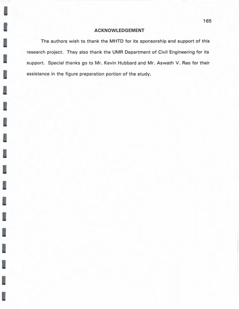
I I I I I
I I I
I I I I
I I I I
165
ACKNOWLEDGEMENT
The authors wish to thank the MHTD for its sponsorship and support of this
research project. They also thank the UMR Department of Civil Engineering for its
support. Special thanks go to Mr. Kevin Hubbard and Mr. Aswath V. Rao for their
assistance in the figure preparation portion of the study.

------------------------------------ - --

I
I I
I I
I
I
I I I I
1.
2.
REFERENCES
AASHTO 1986 Guide for Design of Pavement Structures, AASHTO,
Washington, D.C., 1986.
166
Seeds, S.B. and R.G. Hicks, "Development of Drainage Coefficients for the
1986 AASHTO Guide for Design of Pavement Structures," TRB 68th Annual
Meeting, Washington, D.C., 36 p.
3. Mathis, D.M., "Permeable Base Design and Construction," Stone Review,
Vol. 5, No. 4, 1989, pp. 12-14.
4.
5.
6.
7.
8.
9.
Mann, W.D., "Behind the Shift to Permeable Bases," Hwy. and Heavy
Construction, Vol. , No. , 1990, pp. 38-41.
Richardson, D.N. and P.A. Kremer, "Determination of AASHTO Layer
Coefficients, Vol. II: Unbound Granular Bases and Cement Treated Bases,"
MCHRP Report, Study 90-5, University of Missouri-Rolla, Rolla, Missouri,
1994, 169 p.
Carpenter, S.H., "Selecting AASHTO Drainage Coefficients," TRB 68th
Annual Meeting, Washington, D.C., 1989, 28p.
Lytton, R.L., D.E. Pufahl, C.H. Michalak, H.S. Liang and B. Dempsey, An
Integrated Model of the Climatic Effects on Pavements, Rpt. No. FHWA-RD-
90-033, Fed . Hwy. Admin., McLean, Virginia, 1989, 289 p.
Carpenter, S.H., M.I. Darter, B.J. Dempsey, and S. Herrin, A Pavement
Moisture Accelerated Distress (MAD) Identification System - Volume 1. Rpt.
No. FHWA-RD-81-079, Fed. Hwy. Admin., McLean, Virginia, 1981, 136 p.
Moulton, L.K., Highway Subdrainage Design Manual, Rpt. No. FHWA-TS-80-
167
224, Fed. Hwy. Admin., Mclean, Virginia, 1980, 162 p.
10. Kopperman, S., G. Tiller, and M. Tseng, "ELSYM5, Interactive
Microcomputer Version," FHWA Rot. No. FHWA-TS-8-206, 1986, 33 p.
11. Carpenter, S.H., Highway Subdrainage Design by Microcomputer: DAMP,
Rpt. No. FHWA-IP-90-012, Fed. Hwy. Admin., McLean, Virginia, 1990, 118
p.
12. Lane, K.S., and D.E. Washburn, "Capillarity Tests by Capillarimeter and by
Soil Filled Tubes,"~. Hwy. Res. Bd., 1946, pp. 460-473.
13. Barber, E.S. and C.L. Sawyer, "Highway Subdrainage," fm.c..., Hwy. Res.
Bd., 1952, pp. 643-666.
14. Yemington, E.G., "A Low-Head Permeameter for Testing Granular Materials,"
Permeability of Soils, ASTM Spec. Tech. Pub. No. 163, American Society
for Testing Materials, Philadelphia, Penn., 1955, pp. 37-42.
15. Chu T.Y., D.T. Davidson,. and A.E. Wickstrom, "Permeability Tests for
Sands," Permeability of Soils, ASTM Spec. Tech. Pub. No. 163, American
Society for Testing Materials, Philadelphia, Penn., 1955, pp. 43-55.
16. Smith, T.W., H.R. Cedergren, and C.A. Reyner, "Permeable Materials for
Highway Drainage," Hwy. Res. Rec. No. 68, Hwy. Res. Bd., Washington,
D.C., 1964, pp. 1-16.
17. Strohm, W .E., E.H. Nettles and C.C. Calhoun, "Study of Drainage
Characteristics of Base Course Materials," Hwy. Res. Rec. No. 203. Hwy.
Res. Bd., Washington, D.C., 1967, pp. 8-28
18. Casagrande, A., and W.L. Shannon, "Base Course Drainage for Airport
I 168
Pavements," Proc. of the American Society of Civil Engineers, Vol. 77, June
1951, pp. 792-820.
19. Thornthwaite, C.W. "An Approach Toward a Rational Classification of
Climate," Geographical Review, Vol. 38, 1, 1948, pp. 55-74.
20. Soil Survey Manual, Handbook No. 18, Soil Conservation Service, U.S. Dept.
Ag., 1951, -p.
21. Hole, F.D., "Suggested Terminology for Describing Soils as Three
I Dimensional Bodies," Soil Science Proceedings, Vol. 17(2), 1953, pp. 131-
135.
22. Liang H.S. and R.L. Lytton, "Rainfall Estimation for Pavement Analysis and
I Design," TRB 68th Annual Meeting, Washington, D.C., 19 p.
I
23. Lytton, R.L. and S.J. Liu, Environmental Effects on Pavements - Drainage,
Rpt. No. FHWA/RD-84/116, Fed. Hwy. Admin., McLean, Virginia, 1983,
174 p.
24. Liu, S.J., J.K. Jeyapalan, and R.L. Lytton, "Characteristics of Base and
Subgrade Drainage of Pavements," Trans. Res. Rec. 945, Trans. Res. Bd.,
19-, pp. 1-9.
25. Dempsey, B.J., W.A. Herlache, and A.J. Patel, Environmental Effects on
Pavements - Theory Manual, Rpt. No. FHWA/RD-84/115, Fed. Hwy. Admin.,
McLean, Virginia, 1983, 134 p.
26. Berg, R.L., G.L. Guymon, and T.C. Johnson, Mathematical Model of Frost
Heave and Thaw Settlement in Pavements, Rpt. of the U.S. Army Material
Command, Cold Regions Research and Engineering Laboratory, Hanover,
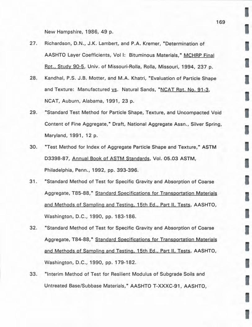
169
New Hampshire, 1986, 49 p.
27. Richardson, D.N., J.K. Lambert, and P.A. Kremer, "Determination of
AASHTO Layer Coefficients, Vol I: Bituminous Materials," MCHRP Final
Rpt., Study 90-5, Univ. of Missouri-Rolla, Rolla, Missouri, 1994, 237 p.
28. Kandhal, P.S. J.B. Motter, and M.A. Khatri, "Evaluation of Particle Shape
and Texture: Manufactured ~. Natural Sands, "NCAT Rpt. No. 91-3,
NCAT, Auburn, Alabama, 1991, 23 p.
29. "Standard Test Method for Particle Shape, Texture, and Uncompacted Void
Content of Fine Aggregate," Draft, National Aggregate Assn., Silver Spring,
Maryland, 1991, 12 p.
30. "Test Method for Index of Aggregate Particle Shape and Texture," ASTM
03398-87, Annual Book of ASTM Standards, Vol. 05.03 ASTM,
Philadelphia, Penn., 1992, pp. 393-396.
31. "Standard Method of Test for Specific Gravity and Absorption of Coarse
Aggregate, T85-88," Standard Specifications for Transportation Materials
and Methods of Sampling and Testing, 15th Ed., Part II, Tests, AASHTO,
Washington, D.C., 1990, pp. 183-186.
32. "Standard Method of Test for Specific Gravity and Absorption of Coarse
Aggregate, T84-88," Standard Specifications for Transportation Materials
and Methods of Sampling and Testing, 15th Ed., Part 11, Tests, AASHTO,
Washington, D.C., 1990, pp. 179-182.
33. "Interim Method of Test for Resilient Modulus of Subgrade Soils and
Untreated Base/Subbase Materials," AASHTO T-XXXC-91, AASHTO, I
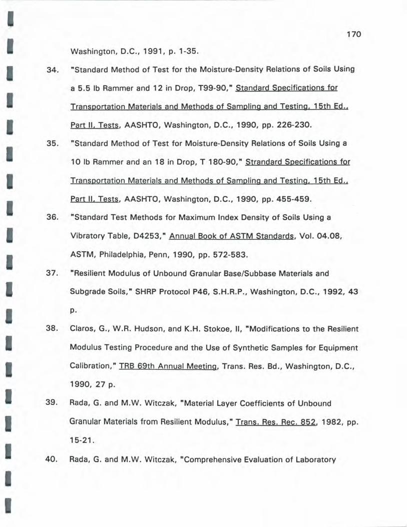
I
I
I
I
34.
170
Washington, D.C., 1991, p. 1-35.
"Standard Method of Test for the Moisture-Density Relations of Soils Using
a 5.5 lb Rammer and 12 in Drop, T99-90," Standard Specifications for
Transportation Materials and Methods of Sampling and Testing, 15th Ed.,
Part II, Tests, AASHTO, Washington, D.C., 1990, pp. 226-230.
35. "Standard Method of Test for Moisture-Density Relations of Soils Using a
1 O lb Rammer and an 18 in Drop, T 180-90," Strandard Specifications for
Transportation Materials and Methods of Sampling and Testing, 15th Ed.,
Part II, Tests, AASHTO, Washington, D.C., 1990, pp. 455-459.
36. "Standard Test Methods for Maximum Index Density of Soils Using a
Vibratory Table, 04253," Annual Book of ASTM Standards, Vol. 04.08,
ASTM, Philadelphia, Penn, 1990, pp. 572-583.
37. "Resilient Modulus of Unbound Granular Base/Subbase Materials and
Subgrade Soils," SHRP Protocol P46, S.H.R.P., Washington, D.C., 1992, 43
p.
38. Claros, G., W.R. Hudson, and K.H. Stokoe, II, "Modifications to the Resilient
Modulus Testing Procedure and the Use of Synthetic Samples for Equipment
Calibration," TRB 69th Annual Meeting, Trans. Res. Bd., Washington, D.C.,
1990, 27 p.
39. Rada, G. and M.W. Witczak, "Material Layer Coefficients of Unbound
Granular Materials from Resilient Modulus," Trans. Res. Rec. 852. 1982. pp.
15-21.
40. Rada. G. and M.W. Witczak. "Comprehensive Evaluation of Laboratory
171
Resilient Moduli Results for Granular Material," Trans. Res . Rec. 81 O. Trans.
Res. Bd., 1981, pp. 23-33.
41. Highlands, K.L. and G.L. Hoffman, "Subbase Permeability and Pavement
Performance," Trans. Res. Rec. 1159. Trans. Res. Bd., 1988, pp. 7-20.
42. "Standard Test Method for Measurement of Hydraulic Conductivity of
Saturated Porous Materials Using a Flexible Wall Permeameter," ASTM
05084-90 Annual Book of ASTM Standards, Vol. 04.08, ASTM,
Philadelphia, Penn, 1990, pp. 1070-1077.
43. "Standard Method of Test for Permeability of Granular Soils (Constant
Head),_ T 215-90," Standard Specifications for Transportation Materials and
Methods of Sampling and Testing, 15th Ed .• Part II, Tests, AASHTO,
Washington, D.C., 1990, pp. 554-558.
44. Moynahan, Jr., T.J. and Y. Sternberg, "Effects on Highway Subdrainage of
Gradation and Direction of Flow within a Densely Graded Base Course
Material," pp. 50-59.
45. Sherard, J.L., L.P. Dunningan, and J.R. Talbot, "Basic Properties of Standard
Gravel Filters," ASCE Geotech. J., Vol. 110, No. 6, 1984, pp. 684-700.
46. Jones, C.W., "The Permeability and Settlement of Laboratory Specimens of
Sand and Sand-Gravel Mixtures," Symp. on Permeability of Soils, ASTM
Special Tech. Pub. No. 163, 1955, pp. 68-79.
47. Karlsdotter, J., "Optimization of Coarse Particles in a Filter Soil," .M....S....
Thesis, University of Missouri-Rolla, Rolla, Missouri, 1991, 96 p.
48. Allen, W .L., Subsurface Drainage of Pavement Structures: Current Corps of
I
I
172
Engineers and Industry Practice, DOT/FAA/RD-91 /24, US DOT, FAA,
Springfield, Virginia, 1991, 31 p.
49. OUATTROPRO, Borland International, Inc.
50. Haynes, J.H. and E.J. Yoder, "Effects of Repeated Loading on Gravel and
Crushed Stone Base Course Materials Used in the AASHO Road Test," ~
Res. Rec. 39, Hwy. Res. Bd., Washington, D.C., pp. 82-96.
51. "The AASHO Road Test, Rpt. 2-Materials and Construction" Hwy. Res. Bd.
Spec. Rot. 61 B, Hwy. Res. Bd., 1962, 173 p.
52. Van Til, C.J., B.F. McCullough, B.A. Vallerga, and R.G. Hicks, "Evaluation of
AASHO Interim Guides for Design of Pavement Structures, "NCHRP Rot.
~ Hwy. Res. Bd., Washington, DC, 1972, 111 p.
53. Witczak, M.W., Development of Regression Model for Asphalt Concrete
Modulus for Use in MS-1 Study, Asphalt Institute, 1978, 39 p.
54. Traylor, M.L., "Characterization of Flexible Pavements by Non-Destructive
Testing," PhD Dissertation, Univ. of Illinois-Urbana-Champaign, Illinois,
1978, 213 p.
55. Huang, Y.H., Pavement Analysis and Design, Prentice Hall, Englewood
Cliffs, NJ, 1993, 805 p.
56. Hicks, R.G., and F.N. Finn, "Prediction of Pavement Performance from
Calculated Stresses and Strains at the San Diego Test Road," Proc. of Assn.
of Asphalt Paving Tech., Vol. 43, 1974, pp. 1-40.
57. Woolstrum, G., "Dynamic Testing of Nebraska Soils and Aggregates," TRB
69th Annual Meeting, Washington, D.C., 1990, 24 p.
173
58. Thompson, M.R. and O.L. Robnett, "Resilient Properties of Subgrade Soils,"
ASCE Trans. Journal, TE1, 1979, pp. 71-89.

I
I
I
I
I
I I
174
APPENDICES

I 175
APPENDIX A
REQUIRED INPUT FOR TTI MODEL
I
I

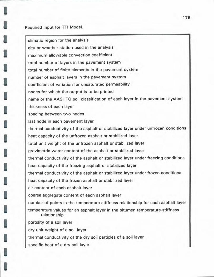
I
I
I
I
I I
Required Input for TTI Model.
climatic region for the analysis
city or weather station used in the analysis
maximum allowable convection coefficient
total number of layers in the pavement system
total number of finite elements in the pavement system
number of asphalt layers in the pavement system
coefficient of variation for unsaturated permeability
nodes for which the output is to be printed
name or the AASHTO soil classification of each layer in the pavement system
thickness of each layer
spacing between two nodes
last node in each pavement layer
176
thermal conductivity of the asphalt or stabilized layer under unfrozen conditions
heat capacity of the unfrozen asphalt or stabilized layer
total unit weight of the unfrozen asphalt or stabilized layer
gravimetric water content of the asphalt or stabilized layer
thermal conductivity of the asphalt or stabilized layer under freezing conditions
heat capacity of the freezing asphalt or stabilized layer
thermal conductivity of the asphalt or stabilized layer under frozen conditions
heat capacity of the frozen asphalt or stabilized layer
air content of each asphalt layer
coarse aggregate content of each asphalt layer
number of points in the temperature-stiffness relationship for each asphalt layer
temperature values for an asphalt layer in the bitumen temperature-stiffness relationship
porosity of a soil layer
dry unit weight of a soil layer
thermal conductivity of the dry soil particles of a soil layer
specific heat of a dry soil layer
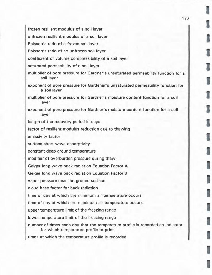
frozen resilient modulus of a soil layer
unfrozen resilient modulus of a soil layer
Poisson's ratio of a frozen soil layer
Poisson's ratio of an unfrozen soil layer
coefficient of volume compressibility of a soil layer
saturated permeability of a soil layer
177
multiplier of pore pressure for Gardner's unsaturated permeability function for a soil layer
exponent of pore pressure for Gardener's unsaturated permeability function for a soil layer
multiplier of pore pressure for Gardner's moisture content function for a soil layer
exponent of pore pressure for Gardner's moisture content function for a soil layer
length of the recovery period in days
factor of resilient modulus reduction due to thawing
emissivity factor
surface short wave absorptivity
constant deep ground temperature
modifier of overburden pressure during thaw
Geiger long wave back radiation Equation Factor A
Geiger long wave back radiation Equation Factor 8
vapor pressure near the ground surface
cloud base factor for back radiation
time of day at which the minimum air temperature occurs
time of day at which the maximum air temperature occurs
upper temperature limit of the freezing range
lower temperature limit of the freezing range
number of times each day that the temperature profile is recorded an indicator for which temperature profile to print
times at which the temperature profile is recorded

I
I I
I I
year in which the first consideration period is started
starting date of a given consideration period
number of days in the consideration period
initial soil temperature profile
initial soil pore pressure profile
coefficient of pore pressure transfer
number of the day for the minimum and maximum temperature
daily minimum temperature
daily maximum temperature
average monthly wind speed
average monthly sunshine percentage
standard deviation of the monthly sunshine percentage
time at which the sun rises each day on a 24 hour clock
time at which the sun sets each day on a 24 hour clock
daily extraterrestrial radiation
the number of lower boundary points for pore pressure; pore pressure at the low boundary
time to begin with the corresponding low boundary pore pressure value
one side width of base
slope ratio or value of tangent alpha of the base
indicator for lower boundary condition
indicator for type of fines added
indicator for amount of fines added
percentage of gravel in the sample
percentage of sand in the sample
pavement type
linear length of cracks and joints of one side of the pavement
total length surveyed for cracks and joints
recurrence period for rainfall
constant K for the intensity-duration-recurrence equation
178
power for the recurrence interval term
power for the rainfall duration term
constant due to the curve shape of the rainfall intensity vs. rainfall period
number of years of rainfall data
monthly rainfall amount
number of wet days in the month
number of thunderstorms in the month
average monthly air temperature
confidence interval to use for the rainfall calculations
179

I
I
I I I
180
APPENDIX B
USE OF DAMP


I
I
I I I I
GENERAL
181
USE OF DAMP MANUAL
The DAMP Manual is self explanatory and can be relied upon by the first
time user of the program. The DAMP version tested at UMR was not able to print
the output reports mentioned in the manual. This may have been due to some
hardware or software problem with our systems that we were not able to detect.
In any case, output was produced by using the printscreen feature of DOS. If you
have not yet installed DAMP on your machine, do so at this time following the
procedures in the DAMP Manual. It must be remembered that the m-coefficients
obtained from DAMP are not in agreement with the recommendations of this
report.
USE OF DAMP DATA FILES
The DAMP data notebook (Appendix D) and accompanying floppy disks
contain the weather data necessary to use the DAMP program for all areas of
Missouri. The user need only copy the weather data files to the DAMP directory.
These files are in the format, "TOWN NAME" .dat. Once the data files are on the
DAMP directory, they can be read while in the DAMP program from the "Main
Selection Menu" by selecting "#4. Read Input Data from Disk File". This loads the
data into the DAMP program for the user to edit as desired. From this point on the
DAMP program can be used as described in the DAMP Manual.
The data files were created at UMR using historical climatological data
published by the National Climatic Data Center.

182
INTERACTIVE DAMP INPUT SELECTION
The DAMP Manual and program are well documented. The user will be able
to proceed through the program provided the subgrade soil type is known or can
be estimated, the gradation of the base/subbase is known, the geometry of the
sections is known.
SUMMARY REQUIREMENTS FOR DAMP INPUT
This section briefly summarizes the data that should be assembled by the
designer before starting either program. The requirements are very simple and fall
into these general categories: pavement geometry, layer thicknesses, layer
densities, base course gradation/specific gravity, and subgrade
drainability/permeability.
Pavement Geometry
This includes the pavement grade (gGrade), the cross slope (Sc), the width
of the drainable base (W), and the number of longitudinal joints in the pavement
surface that water flows over (Ne). Include the joint at the crown if present. The
length of the transverse cracks or joints in the pavement is (We). In the length
measurement, include the portion of the cracks or joints that extend through the
shoulders. The average spacing of these transverse cracks is (Cs).
A typical two lane highway with 12 foot wide lanes that had transverse
cracks every 25 ft would have the following numerical values for input: W = 12
ft, Ne = 3 (one at the crown and one at each shoulder), W c = 12 ft (assume no
cracking in the shoulder), c. = 25 ft. Only W is used for determination of
drainage coefficient. The other parameters are for calculation of crack infiltration,
if so desired.
Layer Thicknesses
183
This is the thickness of the combined asphalt pavement layers above the
base course, the thickness of the base course, and the thickness of the subbase.
If there is no subbase, enter zero. Only the thickness of the base is used for
calculation of m-coefficients.
Layer Densities
This is the expected in-place density of the combined asphalt pavement
layers, the basecourse layer, and the subbase layer. Typical values might be 150
(pcf) for asphalt pavement, 138 (pcf) for base course, and 138 (pcf) for subbase.
I If there is no subbase layer, enter zero. Only the density of the base is used for
calculation of m-coefficient.
I
Base Course Gradation and Specific Gravity
The apparent specific gravity (Gs) of the base course aggregate is needed.
The gradation of the base course aggregate needs to be plotted so the effective
size (010) in millimeters can be delineated. This is the grain size that 10 percent of
the aggregate passes. Also the P200 is required. This is the percent of the base
course aggregate that passes the #200 sieve. Typical numbers for an open
gradation might be 0 10 = 2mm and P200 = 2 percent.
Subgrade Drainability/Permeability
Knowledge of the subgrade soil type will allow approximation of the
subgrade permeability (km) with sufficient accuracy to use these programs. The
soil drainability from the general Missouri Soil Survey is used to enter the SG
184
Drainage input into the programs.
The frost heave rate of the subgrade (h2) in mm/day is a required input. An
acceptable number can be determined from the FHWA Highway Subdrainage
Design Manual (9), Table 4, page 72 or the DAMP Manual, Table 1, page 64 ( 11).
The necessary information to complete this input to DAMP can be found in
the County Soil Survey or in the Missouri General Soil Survey's soil drainage
classification. DAMP asks for either "Good", "Fair", or "Poor" as an input. The
following table summarizes the drainage classifications and the proper relation to
DAMP input.
Table B1. Subgrade Drainability Input Information.
Damp Input Soil Survey Drainability Natural Drainage Index
1. Good Excessively Drained -10 to -2 Somewhat Excessively Drained
2. Fair Well Drained -2 to 2.5 Moderately Well Drained
3. Poor Somewhat Poorly Drained > 2.5 Poorly Drained Very Poorly Drained
This Good, Fair, or Poor rating is all that is used in the m-coefficient determination.
Other Input Variables
The permeability of the surface of the pavement layer (kp) can be input by
the user. It is recommended, however, that the value of zero be used unless
unusual circumstances are present.
The crack infiltration rate is a user input, but the value of 2.4 cfd/linear foot
is the number provided as a default. The originator of the crack infiltration method

I I
I
I
185
determined 2.4 cfd/lft experimentally by testing a small number of pavements.
These variables are not used for calculation of m-coefficients.
DRAINAGE COEFFICIENT OUTPUT SCREEN
In execution of DAMP the screen that comes up immediately after the
subgrade drainability input discussed above is the final summary of the program's
efforts. If a hard copy of the results of the analysis is desired, it is best to
'printscreen' before entering any other keystrokes.

I
I I
I I
I I
I I
I I I
186
APPENDIX C
MODAMP MANUAL

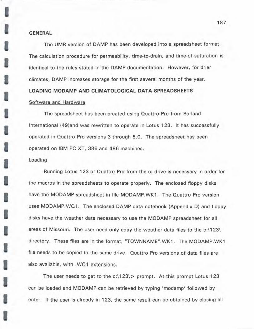
I I I
I I I I
I I
I
I I I I
187
GENERAL
The UMR version of DAMP has been developed into a spreadsheet format.
The calculation procedure for permeability, time-to-drain, and time-of-saturation is
identical to the rules stated in the DAMP documentation. However, for drier
climates, DAMP increases storage for the first several months of the year.
LOADING MODAMP AND CLIMATOLOGICAL DATA SPREADSHEETS
Software and Hardware
The spreadsheet has been created using Quattro Pro from Borland
International (49)and was rewritten to operate in Lotus 123. It has successfully
operated in Quattro Pro versions 3 through 5.0. The spreadsheet has been
operated on IBM PC XT, 386 and 486 machines.
Loading
Running Lotus 123 or Quattro Pro from the c: drive is necessary in order for
the macros in the spreadsheets to operate properly. The enclosed floppy disks
have the MODAMP spreadsheet in file MODAMP.WK1. The Quattro Pro version
uses MODAMP.WQ1. The enclosed DAMP data notebook (Appendix D) and floppy
disks have the weather data necessary to use the MODAMP spreadsheet for all
areas of Missouri. The user need only copy the weather data files to the c:\ 123\
directory. These files are in the format, "TOWNNAME".WK1. The MODAMP.WK1
file needs to be copied to the same drive. Quattro Pro versions of data files are
also available, with .WQ1 extensions.
The user needs to get to the c:\ 123\ > prompt. At this prompt Lotus 123
can be loaded and MODAMP can be retrieved by typing 'modamp' followed by
enter. If the user is already in 123, the same result can be obtained by closing all

188
open spreadsheets and retrieving the MODAMP.WK1 spreadsheet. Once the user
is in the MODAMP spreadsheet, the climatic conditions for the location of interest
can be automatically entered in the proper place in MODAMP by use of a macro.
This macro asks the user what weather file to use. Upon receiving the requested
input, the macro opens the specified file, loads the required weather data into
MODAMP and closes the weather file. The specific keystrokes for the macro are
as follows: "Alt-w" followed by "enter."
The user will be prompted for the name of the weather file to use. Refer to
the first few pages of the DAMP Data Notebook for the proper filename. In
general, the file names are simply the city name or the first eight letters of the city
name where the weather station is located. At the prompt, type in the filename
followed by "enter." The word "macro" will appear in the bottom right corner of
the screen. Wait until the word "macro" disappears from the screen. The end of
the macro will be signalled by a beep. If a file name is entered that is not in the
directory, an error message will be displayed. Simply hit the escape key and rerun
the macro entering the proper filename when prompted.
MODAMP DISPLAY
The display that appears should look like the sample shown in Fig. C1 if the
Quattro Pro version is used. The Lotus version will not show the desktop settings.
The name of the data file that you have imported will appear in the cell next
to the cell labeled "Location."
Permeability of the Drainage Layer
The fourth row in the table solves Moulton's relationship for permeability
(kd) of the drainage layer (base course) material (Eq. 2). The dry density of the

I 189
drainage layer material (dd), apparent specific gravity (G.L drainage layer material
I effective size (D10), and percent drainage layer material passing the #200 sieve
(P200 ) are material properties the user needs to input on line five. Eq. 29 can be
used to estimate "dd" from gradation data. The gradation of the basecourse
I aggregate needs to be plotted so the effective size (D10) in millimeters can be
picked off. This is the grain size that 10 percent of the aggregate passes. Also
the P 200 is required. This is the percent of the base course aggregate that passes
I the #200 sieve. Typical numbers for an open gradation might be D10 = 2mm and
P200 = 2 percent. A nomograph of Moulton's relationship can be found in the
FHWA Highway Subdrainage Design Manual (9), Fig. 28, page 51. Permeability
I (kd), porosity (n) and estimated effective porosity (n.) are calculated and displayed.
The kd and n. values are used in the time-to-drain calculations.
Slope Factor
I The calculations for the slope (slope) and length (L) of the drainage path are
I I I I
I I
based upon the user's input of longitudinal grade (gGrade), cross slope (Sc) and
width of drainage layer drainin_g to the collector (w). Both gGrade and Sc are
expressed in foot/foot or inch/inch, not percent. These inputs are used to calculate
a time-to-drain using the Casagrande-Shannon method as described in this paper.
Thickness of Base
The thickness of the layer in question is input assist in the time-to-drain
calculations.
Subgrade Drainability
This user input is entered in the block just below the label "SG Drainage."
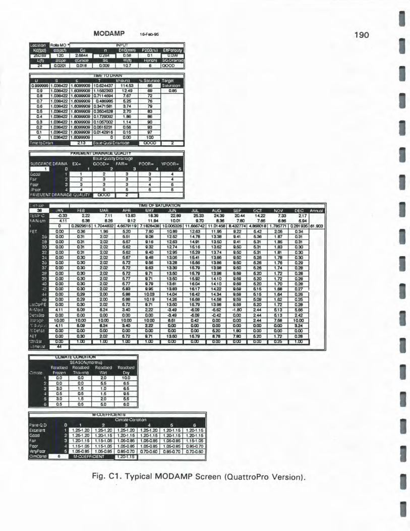
MODAMP 16-fet>-915 190
" . 120 26844 0.1
0.0201 0.018 6
0.11999119 1.038422 1.6099909 10.624437 114.53 0.11 1.038422 1.6099909 1.1682393 1249 0.8 1.038422 1 . IIOIIIIIIOII 0.711481M .67 0.7 1.038422 1.eo99909 0.4869115 6.25 76 0.6 1.038422 1.l!OIIIIIIOII 0.3471681 a14 7'11
1.038422 1.IIO!IIIIIOII 0.2604628 270 83 0.4 1.038422 1.IIOIIIIIIOII 0.172II092 1.116 116 0.3 1.038422 1.l!Clll9SIOII 0.1067002 1.14 IIO 0.2 1.IXJIM22 1.809990II 0.0515231 0.66 113 0.1 1.038422 1.l!08IIII09 0.01421116 0.16 117 0 1.038422 1.6099909 0 0.00 100
8::a . eQu::.aiDrctn:im.:11
222 7.11 1a83 18.311 22.111 26.33 24.311 20.44 14.22 7.33 217 6.38 8.215 11.12 11 .IM 10.01 11.70 8.315 7.lll 7.116 11.88 6.IM
0.21129616 1.7044832 4.667111111 .11128438 10.006326 11 .666742 11 .014511 8.432774 4.868018 1.786771 0.281936 61.903 0.36 1.96 6.20 7.90 10.89 1263 11 .915 11.22 6.42 205 0.34 0.31 202 6.61 11.08 1262 14.78 1a311 11.41 6.36 1.87 0.31 0.31 202 6.67 11.16 1263 14.111 1a60 11.41 6.31 1.116 0.31 0.31 202 6.62 11.32 1274 16.16 1a62 11.60 6.31 1.83 0.30
202 6.62 11.40 12915 16.251 13.74 11.60 6.31 1.81 0.30 202 6.67 11.48 1a0& 16.41 1a86 11.60 6.215 1.78 0.30 202 6.72 11.66 13.28 16.66 1a86 11.50 6.26 1.76 0.251 202 11.63 1a311 1 1 118 11.60 6.215 1. 4 0.28 202 6.72 11.71 1a60 16.7'11 1all8 II.fill 6.20 1.72 0.28 202 6.n 11.71 13.60 16.112 14.10 II.fill 6.20 1.72 0.28 202 6.n 11.7'11 13.61 111.04 14.10 II.fill 6.20 1.70 0.28 202 6.83 11.915 1a83 111.1 14.22 II.fill 16 1.f 18 0.27 200 6.118 10.03 14.04 111.42 14.34 II.fill 6.16 UM 0.215 2.00 6.118 10.111 14.215 16.68 14.68 11.69 6.0II 1.62 0.25 202 6.72 11.71 1a60 16.7'11 13.118 11.69 6.20 1.72 0.28 11.24 a.co 222 -3.49 ~OIi ~62 -1.lll 244 6.66 0.00 0.00 ~OIi -0.42 242
10.00 10.00 0.42 0.00 10.00 tl.24 2.22 0.00 0.00 3.24 0.00 0.00 0.00 6.20 00 2.02 16.7'11 1.78 0.28
1.05-0.85 0.85-0. 70 0.85-0. 70 0. 70-0.60
Fig. C1. Typical MODAMP Screen (OuattroPro Version).

I
I I I I
I I I
I
I I I I I I
191
The program is looking for inputs of "Good", "Fair", "Poor" or "V. Poor".
Guidance for selection can be found in Table C1. Knowledge of the subgrade soil
type will allow approximation of the subgrade drainability with sufficient accuracy
to use these programs. The soil drainability from the general Missouri Soil Survey
(20) is used to enter the SG Drainage input into the programs.
Table C1. Quality of Subgrade Drainage.
Rating Soil Drainage Additional Moisture Contribution
Good • Relatively high permeability Low Moisture Contribution: (predominantly granular • deep water table soils) • absence of wet-weather springs
• at-grade or on fill
• flooding potential: none or rare
Fair • moderate permeability (fine Moderate to none: to moderately fine soil • deep water table texture) • absence of wet-weather springs
• may have layer that • at-grade or on fill impedes downward • flooding potential: none to occasional drainage
Poor • low permeability (.eg: silty Positive moisture contribution: clays) • shallow water table
• may have layer that • absence of wet-weather springs impedes downward • at-grade or in fill drainage • flooding potential: occasional to frequent
Very • very low permeability Positive moisture contribution: Poor (heavy clays) • shallow water table
• contains layer that impedes • in area of wet-weather springs drainage • sidehill cut or cut section
• flooding potential: frequent or common
• marshy area
Time-to-Drain/Quality of Base Drainage
The second large box displays the results of the time-to-drain calculations.
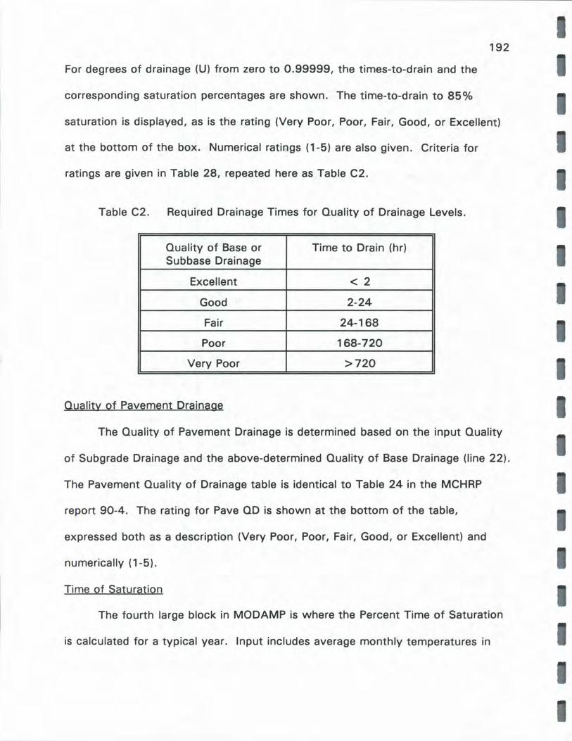
192
For degrees of drainage (U) from zero to 0.99999, the times-to-drain and the
corresponding saturation percentages are shown. The time-to-drain to 85%
saturation is displayed, as is the rating (Very Poor, Poor, Fair, Good, or Excellent)
at the bottom of the box. Numerical ratings (1-5) are also given. Criteria for
ratings are given in Table 28, repeated here as Table C2.
Table C2. Required Drainage Times for Quality of Drainage Levels.
Quality of Base or Time to Dra in (hr) Subbase Drainage
Excellent < 2
Good 2-24
Fair 24-168
Poor 168-720
Very Poor >720
Quality of Pavement Drainage
The Quality of Pavement Drainage is determined based on the input Quality
of Subgrade Drainage and the above-determined Quality of Base Drainage (line 22).
The Pavement Quality of Drainage table is identical to Table 24 in the MCHRP
report 90-4. The rating for Pave OD is shown at the bottom of the table,
expressed both as a description (Very Poor, Poor, Fair, Good, or Excellent) and
numerically (1-5).
Time of Saturation
The fourth large block in MODAMP is where the Percent Time of Saturation
is calculated for a typical year. Input includes average monthly temperatures in

I I I I I I I I I
I I I I I I I I I
193
degrees Celsius and average monthly precipitation in cm. At the bottom of the
block is displayed the saturation condition of each month: 11 1.0 11 if saturated the
entire time, 11 0.25 11 if part of the month is considered saturated.
Climate Condition
The Climate Condition block is identical to Table 25 in the MCHRP report,
except zones are delineated as 1 through 6 instead of A through F. Here the user
chooses the Climate Condition ( 1-6) that is most similar to the project site
condition based on the monthly time of saturation and frozen conditions from the
previous block. The choice is input by the user at the bottom of the next block on
line 73 for "ClimCond. 11
Drainage Coefficients
The last block displays m-coefficients. Input is the Climate Condition (1-6)
based on the information from the previous block, and Pavement Quality of
Drainage which MODAMP brings down from line 31. The resulting m-value is
displayed at the bottom of the block.

I I I
I
I
I I I I I I I I I I I I I I I I I
APPENDIX D
MISSOURI CLIMATOLOGICAL DAT A
(Bound Separately)
194

I
I