Author's personal copy Multi-Gaussian fitting for pulse waveform using Weighted Least Squares and multi-criteria decision making method

This article appeared in a journal published by Elsevier. The attachedcopy is furnished to the author for internal non-commercial researchand education use, including for instruction at the authors institution

and sharing with colleagues.

Other uses, including reproduction and distribution, or selling orlicensing copies, or posting to personal, institutional or third party

websites are prohibited.

In most cases authors are permitted to post their version of thearticle (e.g. in Word or Tex form) to their personal website orinstitutional repository. Authors requiring further information

regarding Elsevier’s archiving and manuscript policies areencouraged to visit:

http://www.elsevier.com/authorsrights

http://www.elsevier.com/authorsrights

Author's personal copy

Multi-Gaussian fitting for pulse waveform using Weighted LeastSquares and multi-criteria decision making method

Lu Wang a, Lisheng Xu b,c,n, Shuting Feng b, Max Q.-H. Meng d, Kuanquan Wang e

a College of Information Science and Engineering, Northeastern University, Shenyang City, Liaoning Province, 110819, Chinab Sino-Dutch Biomedical and Information Engineering School, Northeastern University, Shenyang City, Liaoning Province, 110819, Chinac Key Laboratory of Medical Image Computing (Northeastern University), Ministry of Education, Chinad Department of Electronic Engineering, Chinese University of Hong Kong, Hong Kong, Chinae School of Computer Science and Technology, Harbin Institute of Technology, Harbin 150001, China

a r t i c l e i n f o

Article history:Received 15 November 2012Accepted 11 August 2013

Keywords:Pulse waveformPhotoplethysmographyPulse decomposition analysisMulti-Gaussian modelMulti-criteria decision making

a b s t r a c t

Analysis of pulse waveform is a low cost, non-invasive method for obtaining vital information related tothe conditions of the cardiovascular system. In recent years, different Pulse Decomposition Analysis(PDA) methods have been applied to disclose the pathological mechanisms of the pulse waveform. Allthese methods decompose single-period pulse waveform into a constant number (such as 3, 4 or 5) ofindividual waves. Furthermore, those methods do not pay much attention to the estimation error of thekey points in the pulse waveform. The estimation of human vascular conditions depends on the keypoints' positions of pulse wave. In this paper, we propose a Multi-Gaussian (MG) model to fit real pulsewaveforms using an adaptive number (4 or 5 in our study) of Gaussian waves. The unknown parametersin the MG model are estimated by the Weighted Least Squares (WLS) method and the optimized weightvalues corresponding to different sampling points are selected by using the Multi-Criteria DecisionMaking (MCDM) method. Performance of the MG model and the WLS method has been evaluatedby fitting 150 real pulse waveforms of five different types. The resulting Normalized Root Mean SquareError (NRMSE) was less than 2.0% and the estimation accuracy for the key points was satisfactory,demonstrating that our proposed method is effective in compressing, synthesizing and analyzing pulsewaveforms.

& 2013 Elsevier Ltd. All rights reserved.

1. Introduction

The arterial pulse waves in all their forms, pressure, volume orflow, contain the information about the cardiovascular systemsuch as heart rate, pulsatile pressure and arterial distensibility;therefore, they are often used by clinicians in the assessment ofhealth and the early prediction of cardiovascular diseases. Thearterial pulse wave is generated by the heart and propagatedthrough the arterial tree. The increase in blood volume in theartery causes a transient increase in pressure which depends onthe property of the arterial wall as well as the resistance of theperipheral vessels and tissues. Sphygmograph, an instrument forgraphically recording the form, strength, and variations of thearterial pulse, was developed in 1854 by the German physiologistKarl von Vierordt (1818–1884). Currently, it has been employed asan external, noninvasive device to record the pressure pulse wave

and to estimate the blood pressure. Photoplethysmograph (PPG), anoptical, non-invasive, and easy-to-obtain technique, has been usedfor capturing Digital Volume Pulse (DVP) signals from peripheralpulse sites (e.g. fingers, earlobes, toes etc) [1–3]. Despite the factthat the morphologies of pulse waveforms acquired by differentkinds of sensors at different sites vary greatly, they all containsimilar information of peripheral pulse waves [3] and can provideimportant clinical information related to the conditions of thecardiovascular system [4–7].

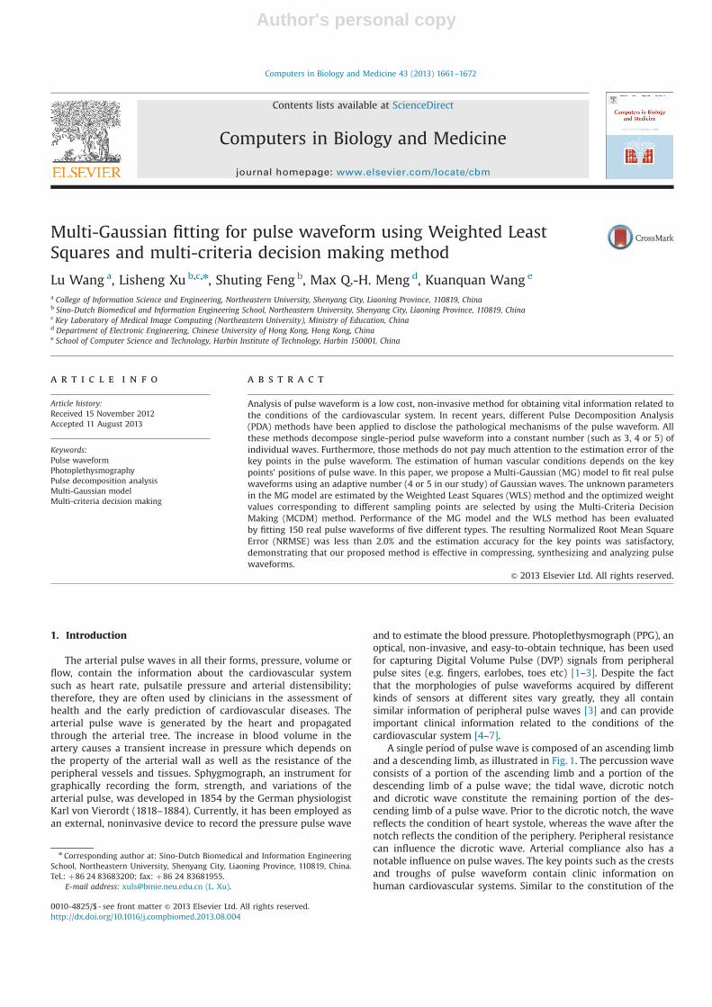
A single period of pulse wave is composed of an ascending limband a descending limb, as illustrated in Fig. 1. The percussion waveconsists of a portion of the ascending limb and a portion of thedescending limb of a pulse wave; the tidal wave, dicrotic notchand dicrotic wave constitute the remaining portion of the des-cending limb of a pulse wave. Prior to the dicrotic notch, the wavereflects the condition of heart systole, whereas the wave after thenotch reflects the condition of the periphery. Peripheral resistancecan influence the dicrotic wave. Arterial compliance also has anotable influence on pulse waves. The key points such as the crestsand troughs of pulse waveform contain clinic information onhuman cardiovascular systems. Similar to the constitution of the

Contents lists available at ScienceDirect

journal homepage: www.elsevier.com/locate/cbm

Computers in Biology and Medicine

0010-4825/$ - see front matter & 2013 Elsevier Ltd. All rights reserved.http://dx.doi.org/10.1016/j.compbiomed.2013.08.004

n Corresponding author at: Sino-Dutch Biomedical and Information EngineeringSchool, Northeastern University, Shenyang City, Liaoning Province, 110819, China.Tel.: þ86 24 83683200; fax: þ86 24 83681955.

E-mail address: [email protected] (L. Xu).

Computers in Biology and Medicine 43 (2013) 1661–1672


peripheral pressure pulse wave, a DVP waveform comprises a systoliccomponent arising from pressure waves propagated from the aorticroot to the finger and a diastolic component arising from pressurewaves reflected backward from peripheral arteries mainly in thelower body, which then propagate to the finger. The reflected wavesproduce an inflection point or second crest in the DVP [8,21–23].

Commonly used parameters of DVP are pulse duration, Aug-mentation Index (AI), Reflection Index (RI), Pulse Transit Time(PTT), Pulse Wave Velocity (PWV) and so on [8]. There are otherways to assess some of these parameters, such as CT, MRI, andultrasound techniques [4,9]. However, these methods are moreexpensive and less convenient than the measurement and analysisof peripheral pulse waveforms. Therefore, many methods for pulseparameter estimation based on peripheral pulse waveforms havebeen proposed [10–18].

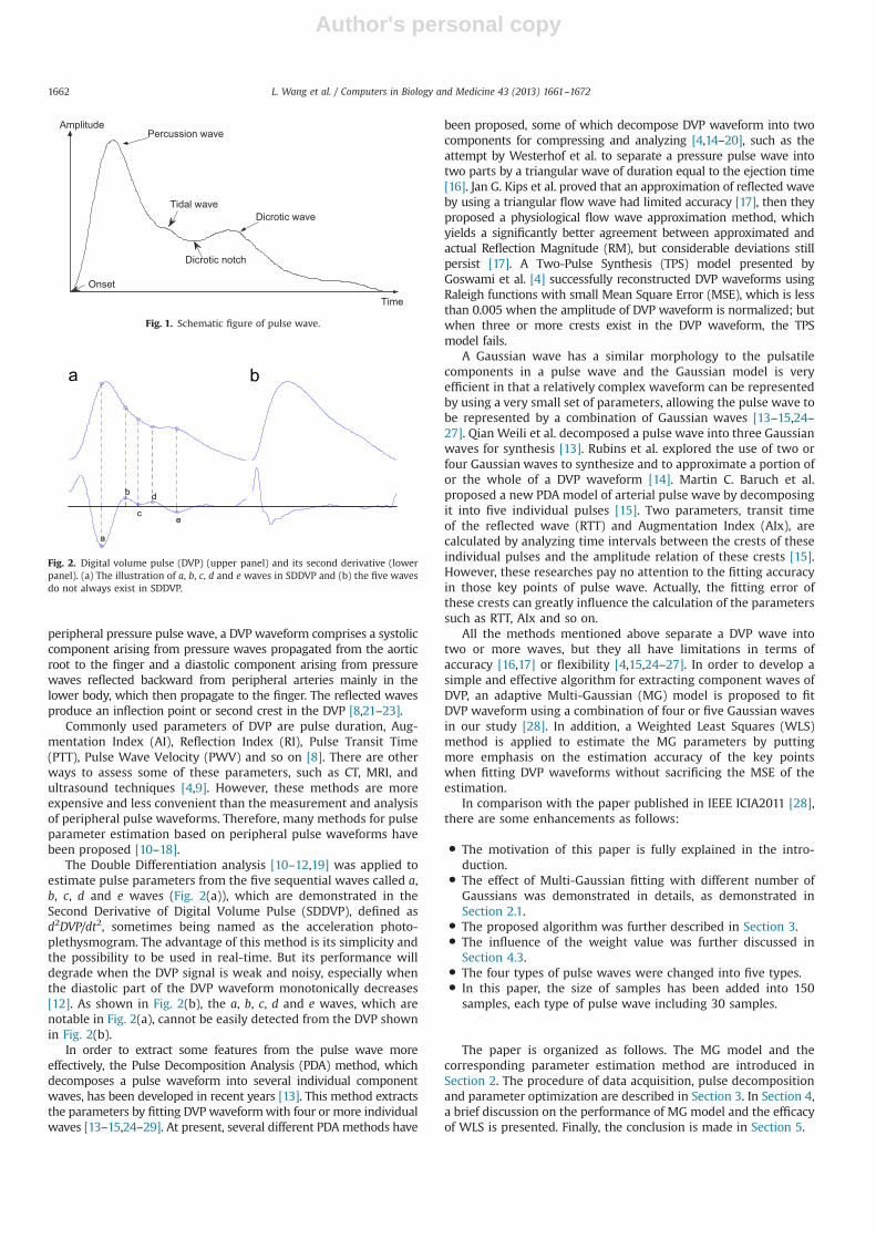
The Double Differentiation analysis [10–12,19] was applied toestimate pulse parameters from the five sequential waves called a,b, c, d and e waves (Fig. 2(a)), which are demonstrated in theSecond Derivative of Digital Volume Pulse (SDDVP), defined asd2DVP/dt2, sometimes being named as the acceleration photo-plethysmogram. The advantage of this method is its simplicity andthe possibility to be used in real-time. But its performance willdegrade when the DVP signal is weak and noisy, especially whenthe diastolic part of the DVP waveform monotonically decreases[12]. As shown in Fig. 2(b), the a, b, c, d and e waves, which arenotable in Fig. 2(a), cannot be easily detected from the DVP shownin Fig. 2(b).

In order to extract some features from the pulse wave moreeffectively, the Pulse Decomposition Analysis (PDA) method, whichdecomposes a pulse waveform into several individual componentwaves, has been developed in recent years [13]. This method extractsthe parameters by fitting DVP waveformwith four or more individualwaves [13–15,24–29]. At present, several different PDA methods have

been proposed, some of which decompose DVP waveform into twocomponents for compressing and analyzing [4,14–20], such as theattempt by Westerhof et al. to separate a pressure pulse wave intotwo parts by a triangular wave of duration equal to the ejection time[16]. Jan G. Kips et al. proved that an approximation of reflected waveby using a triangular flow wave had limited accuracy [17], then theyproposed a physiological flow wave approximation method, whichyields a significantly better agreement between approximated andactual Reflection Magnitude (RM), but considerable deviations stillpersist [17]. A Two-Pulse Synthesis (TPS) model presented byGoswami et al. [4] successfully reconstructed DVP waveforms usingRaleigh functions with small Mean Square Error (MSE), which is lessthan 0.005 when the amplitude of DVP waveform is normalized; butwhen three or more crests exist in the DVP waveform, the TPSmodel fails.

A Gaussian wave has a similar morphology to the pulsatilecomponents in a pulse wave and the Gaussian model is veryefficient in that a relatively complex waveform can be representedby using a very small set of parameters, allowing the pulse wave tobe represented by a combination of Gaussian waves [13–15,24–27]. Qian Weili et al. decomposed a pulse wave into three Gaussianwaves for synthesis [13]. Rubins et al. explored the use of two orfour Gaussian waves to synthesize and to approximate a portion ofor the whole of a DVP waveform [14]. Martin C. Baruch et al.proposed a new PDA model of arterial pulse wave by decomposingit into five individual pulses [15]. Two parameters, transit timeof the reflected wave (RTT) and Augmentation Index (AIx), arecalculated by analyzing time intervals between the crests of theseindividual pulses and the amplitude relation of these crests [15].However, these researches pay no attention to the fitting accuracyin those key points of pulse wave. Actually, the fitting error ofthese crests can greatly influence the calculation of the parameterssuch as RTT, AIx and so on.

All the methods mentioned above separate a DVP wave intotwo or more waves, but they all have limitations in terms ofaccuracy [16,17] or flexibility [4,15,24–27]. In order to develop asimple and effective algorithm for extracting component waves ofDVP, an adaptive Multi-Gaussian (MG) model is proposed to fitDVP waveform using a combination of four or five Gaussian wavesin our study [28]. In addition, a Weighted Least Squares (WLS)method is applied to estimate the MG parameters by puttingmore emphasis on the estimation accuracy of the key pointswhen fitting DVP waveforms without sacrificing the MSE of theestimation.

In comparison with the paper published in IEEE ICIA2011 [28],there are some enhancements as follows:

� The motivation of this paper is fully explained in the intro-duction.

� The effect of Multi-Gaussian fitting with different number ofGaussians was demonstrated in details, as demonstrated inSection 2.1.

� The proposed algorithm was further described in Section 3.� The influence of the weight value was further discussed in

Section 4.3.� The four types of pulse waves were changed into five types.� In this paper, the size of samples has been added into 150

samples, each type of pulse wave including 30 samples.

The paper is organized as follows. The MG model and thecorresponding parameter estimation method are introduced inSection 2. The procedure of data acquisition, pulse decompositionand parameter optimization are described in Section 3. In Section 4,a brief discussion on the performance of MG model and the efficacyof WLS is presented. Finally, the conclusion is made in Section 5.

Time

Amplitude

Onset

Percussion wave

Dicrotic notch

Dicrotic wave Tidal wave

Fig. 1. Schematic figure of pulse wave.

a

b

c

d

e

Fig. 2. Digital volume pulse (DVP) (upper panel) and its second derivative (lowerpanel). (a) The illustration of a, b, c, d and e waves in SDDVP and (b) the five wavesdo not always exist in SDDVP.

L. Wang et al. / Computers in Biology and Medicine 43 (2013) 1661–16721662


2. Methods

2.1. Multi-Gaussian model

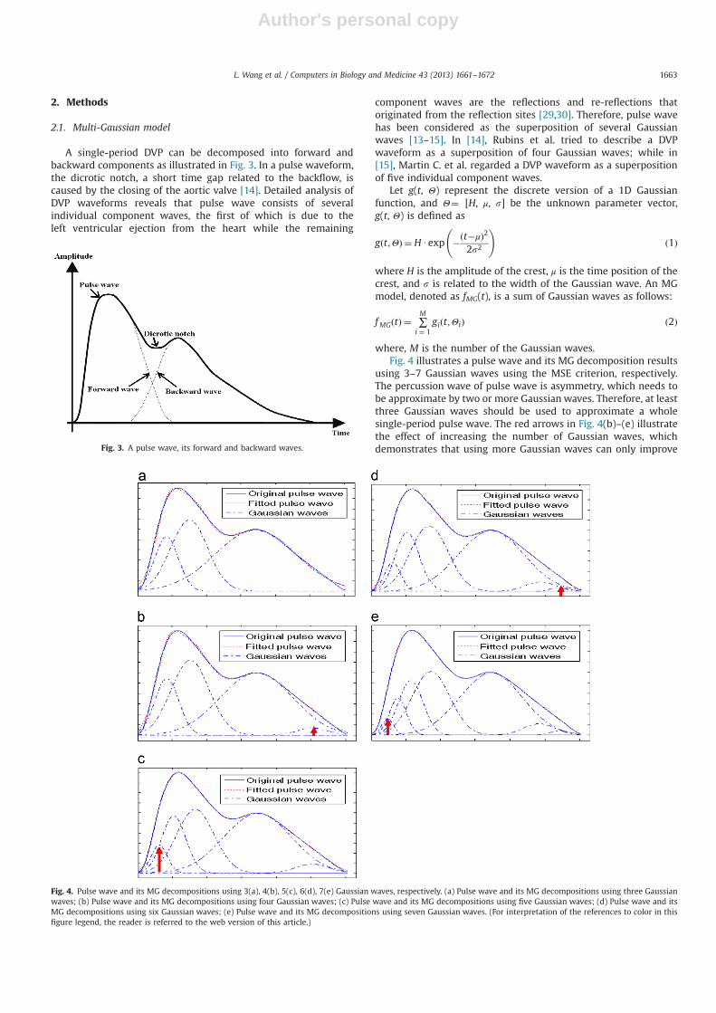
A single-period DVP can be decomposed into forward andbackward components as illustrated in Fig. 3. In a pulse waveform,the dicrotic notch, a short time gap related to the backflow, iscaused by the closing of the aortic valve [14]. Detailed analysis ofDVP waveforms reveals that pulse wave consists of severalindividual component waves, the first of which is due to theleft ventricular ejection from the heart while the remaining

component waves are the reflections and re-reflections thatoriginated from the reflection sites [29,30]. Therefore, pulse wavehas been considered as the superposition of several Gaussianwaves [13–15]. In [14], Rubins et al. tried to describe a DVPwaveform as a superposition of four Gaussian waves; while in[15], Martin C. et al. regarded a DVP waveform as a superpositionof five individual component waves.

Let g(t, Θ) represent the discrete version of a 1D Gaussianfunction, and Θ¼ [H, μ, s] be the unknown parameter vector,g(t, Θ) is defined as

gðt;ΘÞ ¼HUexp �ðt�μÞ22s2

!ð1Þ

where H is the amplitude of the crest, μ is the time position of thecrest, and s is related to the width of the Gaussian wave. An MGmodel, denoted as fMG(t), is a sum of Gaussian waves as follows:

f MGðtÞ ¼ ∑M

i ¼ 1giðt;ΘiÞ ð2Þ

where, M is the number of the Gaussian waves.Fig. 4 illustrates a pulse wave and its MG decomposition results

using 3–7 Gaussian waves using the MSE criterion, respectively.The percussion wave of pulse wave is asymmetry, which needs tobe approximate by two or more Gaussian waves. Therefore, at leastthree Gaussian waves should be used to approximate a wholesingle-period pulse wave. The red arrows in Fig. 4(b)–(e) illustratethe effect of increasing the number of Gaussian waves, whichdemonstrates that using more Gaussian waves can only improveFig. 3. A pulse wave, its forward and backward waves.

Fig. 4. Pulse wave and its MG decompositions using 3(a), 4(b), 5(c), 6(d), 7(e) Gaussian waves, respectively. (a) Pulse wave and its MG decompositions using three Gaussianwaves; (b) Pulse wave and its MG decompositions using four Gaussian waves; (c) Pulse wave and its MG decompositions using five Gaussian waves; (d) Pulse wave and itsMG decompositions using six Gaussian waves; (e) Pulse wave and its MG decompositions using seven Gaussian waves. (For interpretation of the references to color in thisfigure legend, the reader is referred to the web version of this article.)

L. Wang et al. / Computers in Biology and Medicine 43 (2013) 1661–1672 1663


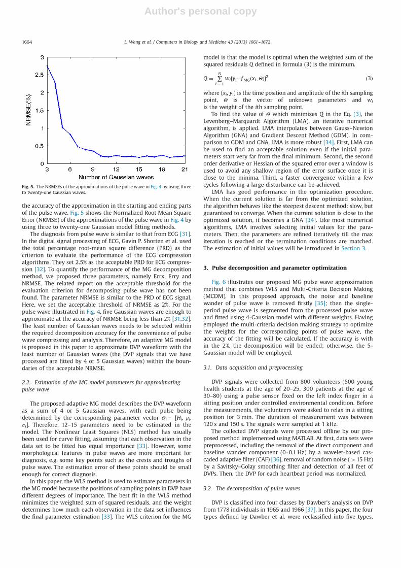
the accuracy of the approximation in the starting and ending partsof the pulse wave. Fig. 5 shows the Normalized Root Mean SquareError (NRMSE) of the approximations of the pulse wave in Fig. 4 byusing three to twenty-one Gaussian model fitting methods.

The diagnosis from pulse wave is similar to that from ECG [31].In the digital signal processing of ECG, Gavin P. Shorten et al. usedthe total percentage root-mean square difference (PRD) as thecriterion to evaluate the performance of the ECG compressionalgorithms. They set 2.5% as the acceptable PRD for ECG compres-sion [32]. To quantify the performance of the MG decompositionmethod, we proposed three parameters, namely Errx, Erry andNRMSE. The related report on the acceptable threshold for theevaluation criterion for decomposing pulse wave has not beenfound. The parameter NRMSE is similar to the PRD of ECG signal.Here, we set the acceptable threshold of NRMSE as 2%. For thepulse wave illustrated in Fig. 4, five Gaussian waves are enough toapproximate at the accuracy of NRMSE being less than 2% [31,32].The least number of Gaussian waves needs to be selected withinthe required decomposition accuracy for the convenience of pulsewave compressing and analysis. Therefore, an adaptive MG modelis proposed in this paper to approximate DVP waveform with theleast number of Gaussian waves (the DVP signals that we haveprocessed are fitted by 4 or 5 Gaussian waves) within the boun-daries of the acceptable NRMSE.

2.2. Estimation of the MG model parameters for approximatingpulse wave

The proposed adaptive MG model describes the DVP waveformas a sum of 4 or 5 Gaussian waves, with each pulse beingdetermined by the corresponding parameter vector Θi¼ [Hi, μi,si]. Therefore, 12–15 parameters need to be estimated in themodel. The Nonlinear Least Squares (NLS) method has usuallybeen used for curve fitting, assuming that each observation in thedata set to be fitted has equal importance [33]. However, somemorphological features in pulse waves are more important fordiagnosis, e.g. some key points such as the crests and troughs ofpulse wave. The estimation error of these points should be smallenough for correct diagnosis.

In this paper, the WLS method is used to estimate parameters inthe MGmodel because the positions of sampling points in DVP havedifferent degrees of importance. The best fit in the WLS methodminimizes the weighted sum of squared residuals, and the weightdetermines how much each observation in the data set influencesthe final parameter estimation [33]. The WLS criterion for the MG

model is that the model is optimal when the weighted sum of thesquared residuals Q defined in formula (3) is the minimum.

Q ¼ ∑N

i ¼ 1wi½yi�f MGðxi;ΘÞ�2 ð3Þ

where (xi, yi) is the time position and amplitude of the ith samplingpoint, Θ is the vector of unknown parameters and wi

is the weight of the ith sampling point.To find the value of Θ which minimizes Q in the Eq. (3), the

Levenberg–Marquardt Algorithm (LMA), an iterative numericalalgorithm, is applied. LMA interpolates between Gauss–NewtonAlgorithm (GNA) and Gradient Descent Method (GDM). In com-parison to GDM and GNA, LMA is more robust [34]. First, LMA canbe used to find an acceptable solution even if the initial para-meters start very far from the final minimum. Second, the secondorder derivative or Hessian of the squared error over a window isused to avoid any shallow region of the error surface once it isclose to the minima. Third, a faster convergence within a fewcycles following a large disturbance can be achieved.

LMA has good performance in the optimization procedure.When the current solution is far from the optimized solution,the algorithm behaves like the steepest descent method: slow, butguaranteed to converge. When the current solution is close to theoptimized solution, it becomes a GNA [34]. Like most numericalalgorithms, LMA involves selecting initial values for the para-meters. Then, the parameters are refined iteratively till the maxiteration is reached or the termination conditions are matched.The estimation of initial values will be introduced in Section 3.

3. Pulse decomposition and parameter optimization

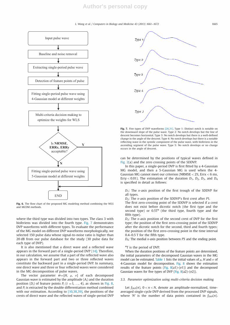
Fig. 6 illustrates our proposed MG pulse wave approximationmethod that combines WLS and Multi-Criteria Decision Making(MCDM). In this proposed approach, the noise and baselinewander of pulse wave is removed firstly [35]; then the single-period pulse wave is segmented from the processed pulse waveand fitted using 4-Gaussian model with different weights. Havingemployed the multi-criteria decision making strategy to optimizethe weights for the corresponding points of pulse wave, theaccuracy of the fitting will be calculated. If the accuracy is within the 2%, the decomposition will be ended; otherwise, the 5-Gaussian model will be employed.

3.1. Data acquisition and preprocessing

DVP signals were collected from 800 volunteers (500 younghealth students at the age of 20–25, 300 patients at the age of30–80) using a pulse sensor fixed on the left index finger in asitting position under controlled environmental condition. Beforethe measurements, the volunteers were asked to relax in a sittingposition for 3 min. The duration of measurement was between120 s and 150 s. The signals were sampled at 1 kHz.

The collected DVP signals were processed offline by our pro-posed method implemented using MATLAB. At first, data sets werepreprocessed, including the removal of the direct component andbaseline wander component (0–0.1 Hz) by a wavelet-based cas-caded adaptive filter (CAF) [36], removal of random noise (415 Hz)by a Savitsky–Golay smoothing filter and detection of all feet ofDVPs. Then, the DVP for each heartbeat period was normalized.

3.2. The decomposition of pulse waves

DVP is classified into four classes by Dawber's analysis on DVPfrom 1778 individuals in 1965 and 1966 [37]. In this paper, the fourtypes defined by Dawber et al. were reclassified into five types,

Fig. 5. The NRMSEs of the approximations of the pulse wave in Fig. 4 by using threeto twenty-one Gaussian waves.



where the third type was divided into two types. The class 3 withbisferiens was divided into the fourth type. Fig. 7 demonstratesDVP waveforms with different types. To evaluate the performanceof the MG model on different DVP waveforms morphologically, weselected 150 pulse data whose signal-to-noise ratio is higher than20 dB from our pulse database for the study (30 pulse data foreach type of DVP).

It is also mentioned that a direct wave and a reflected waveappears in the forward part of a single-period DVP [14]. Therefore,in our calculation, we assume that a part of the reflected wave alsoappears in the forward part and two or three reflected wavesconstitute the backward part in a single-period DVP. In summary,one direct wave and three or four reflected waves were consideredin the MG decomposition of pulse waves.

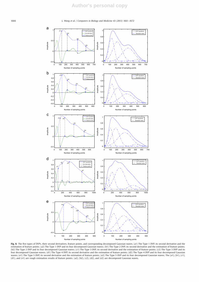
The vector parameter Θ¼[H, μ, s] of each decomposedGaussian wave is estimated by the amplitude (Ai) and the durationposition (Di) of feature points Pi (i ¼1, …, 4), as shown in Fig. 8,and Pi is extracted by the double differentiation method combinedwith our estimation. According to [10,38,39], the positions of thecrests of direct wave and the reflected waves of single-period DVP

can be determined by the positions of typical waves defined inFig. 2(a) and the zero crossing points of the SDDVP.

In this paper, a single-period DVP is first fitted by a 4-GaussianMG model, and then a 5-Gaussian MG is used when the 4-Gaussian MG cannot meet our criterion (NRMSEo2%, Errxo6 ms,Erryo0.01). The estimation of the duration D1, D2, D3, and D4

is specified in detail as follows:

D1: The x-axis position of the first trough of the SDDVP forall types.D2: The x-axis position of the SDDVP's first crest after P1.The first zero-crossing point of the SDDVP is selected if a crestdoes not exist before dicrotic notch (the first type and thesecond type) or 0.5Tn (the third type, fourth type and thefifth type).D3: The x-axis position of the second crest of DVP for the firsttype; the position of the first zero-crossing point of the SDDVPafter the dicrotic notch for the second, third and fourth types;the position of the first zero-crossing point in the time interval0.4–0.5 T for the fifth type.D4: The medial x-axis position between P3 and the ending point.

nT is the period of DVP.When the duration positions of the feature points are determined,

the initial parameters of the decomposed Gaussian waves in the MGmodel can be estimated. Table 1 lists the initial values of μ, H and s of4-Gaussian model for decomposition. Fig. 8 shows the estimationresults of the feature points (Fig. 8(a1)–(e1)) and the decomposedGaussian waves for five types of DVP (Fig. 8(a2)–(e2)).

3.3. Parameter optimization using multi-criteria decision making

Let fDVP(n), 0onoN, denote an amplitude-normalized, time-averaged single-cycle DVP derived from the processed DVP signals,where ‘N’ is the number of data points contained in fDVP(n).

Fig. 7. Five types of DVP waveforms [26,31]. Type 1: Distinct notch is notable onthe downward slope of the pulse wave. Type 2: No notch develops but the line ofdescent becomes horizontal. Type 3: No notch develops but there is a well-definedchange in the angle of the descent. Type 4: No notch develops but there is a notablereflecting wave in the systolic component of the pulse wave, with bisferiens in theascending segment of the pulse wave. Type 5: No notch develops or no changeoccurs in the angle of descent.

Input pulse wave

Baseline and noise removal

Extracting single-period pulse wave

Detection of feature points of pulse

Multi-criteria decision making to optimize the weights for WLS

Fitting single-period pulse wave using 4-Gaussian model at different weights

Is NRMSE, ERRx, ERRy

acceptable?

Fitting single-period pulse wave using 5-Gaussian model at different weights

N

Y

END

Fig. 6. The flow chart of the proposed MG modeling method combining the WLSand MCDM methods.



Fig. 8. The five types of DVPs, their second derivatives, feature points, and corresponding decomposed Gaussian waves. (a1) The Type 1 DVP, its second derivative and theestimation of feature points; (a2) The Type 1 DVP and its four decomposed Gaussian waves; (b1) The Type 2 DVP, its second derivative and the estimation of feature points;(b2) The Type 2 DVP and its four decomposed Gaussian waves; (c1) The Type 3 DVP, its second derivative and the estimation of feature points; (c2) The Type 3 DVP and itsfour decomposed Gaussian waves; (d1) The Type 4 DVP, its second derivative and the estimation of feature points; (d2) The Type 4 DVP and its four decomposed Gaussianwaves; (e1) The Type 5 DVP, its second derivative and the estimation of feature points; (e2) The Type 5 DVP and its four decomposed Gaussian waves; The (a1), (b1), (c1),(d1), and (e1) are rough estimation results of feature points; (a2), (b2), (c2), (d2), and (e2) are decomposed Gaussian waves.



According to WLS, the parameters of the MG model are evaluatedby minimizing the following sum:

MSE¼ 1N

∑N

n ¼ 1

wn

W½f DVPðnÞ�f MGðn;ΘÞ�2; W ¼ ∑

N

n ¼ 1wn ð4Þ

In this paper, NRMSE is calculated to evaluate the accuracy ofthe MG model and is used to compare the fitted results with theoriginal ones.

% NRMSE¼

ffiffiffiffiffiffiffiffiffiffiffiffiffiffiffiffiffiffiffiffiffiffiffiffiffiffiffiffiffiffiffiffiffiffiffiffiffiffiffiffiffiffiffiffiffiffiffiffiffiffiffiffiffiffiffiffiffiffiffiffiffiffi∑N

n ¼ 1wn½f DVPðnÞ�f MGðn;ΘÞ�2∑N

n ¼ 1wnf DVPðnÞ2

vuut � 100% ð5Þ

where, fDVP(n) is fitted by fMG(n,Θ) through solving formula (4), wn

is the weight corresponding to the nth point, W is the sum of theweight vector. The unknown parameter vector Θ in fMG(n,Θ) aredetermined by minimizing the MSE in formula (4) using LMA.Initial values of the unknown parameters in LMA are providedby the estimation in Table 1.

Table 1Initial estimation of μ, H and s.

Parameter Hi μi si

DVP type 1 2 3 4 5 1–5 1 2 3 4 5

i¼1 0.8A1 0.7A1 0.7A1 0.7A1 D1 D1/3i¼2 0.8A2 0.8A2 0.7A2 0.7A2 D2 (D2�D1)/3 D2/3i¼3 0.8A3 0.8A3 0.8A3 0.7A3 D3 min((T�D3),D3)/3i¼4 0.3A4 0.3A4 0.3A4 0.5A4 D4 (T�D4)/3

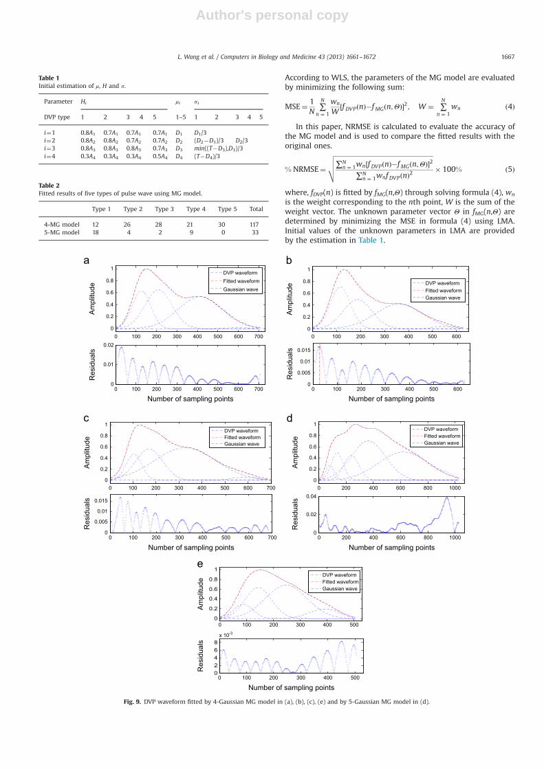
Table 2Fitted results of five types of pulse wave using MG model.

Type 1 Type 2 Type 3 Type 4 Type 5 Total

4-MG model 12 26 28 21 30 1175-MG model 18 4 2 9 0 33

0 100 200 300 400 500 600 7000

0.01

0.02

Number of sampling points

Res

idua

ls

0 100 200 300 400 500 600 7000

0.2

0.4

0.6

0.8

1

Am

plitu

de

DVP waveformFitted waveformGaussian wave

0 100 200 300 400 500 6000

0.005

0.01

0.015


Res

idua

ls

0 100 200 300 400 500 6000

0.2

0.4

0.6

0.8

1

Am

plitu

deDVP waveformFitted waveformGaussian wave

0 100 200 300 400 500 600 7000

0.005

0.01

0.015


Res

idua

ls

0 100 200 300 400 500 600 7000

0.2

0.4

0.6

0.8

1

Am

plitu

de


0 200 400 600 800 10000

0.02

0.04


Res

idua

ls

0 200 400 600 800 10000

0.2

0.4

0.6

0.8

1

Am

plitu

de


0 100 200 300 400 50002468

x 10-3


Res

idua

ls

0 100 200 300 400 5000

0.2

0.4

0.6

0.8

1

Am

plitu

de


Fig. 9. DVP waveform fitted by 4-Gaussian MG model in (a), (b), (c), (e) and by 5-Gaussian MG model in (d).



In order to find the best weight values to minimize theabsolute-error of key points selected in Section 2 with a limitationof MSE, a group of 100 different w was tested. In this group,w corresponding to important points changes from one to onehundred by step one, while the w corresponding to the otherpoints maintains a value of one. Furthermore, a hundred fittedresults corresponding to different weight values will be evaluatedby criteria Errx, Erry, and NRMSE.

Errx—sum of absolute errors of x-axis positions between crestsand troughs in fMG(n,Θ) and fDVP(n).Erry—sum of absolute errors of amplitudes between crests andtroughs in fMG(n,Θ) and fDVP(n).

As criteria NRMSE, Errx, and Erry may conflict with each other,finding the best weight vector can be regarded as a MCDMproblem. The preferences in the MCDM theory may be formulatedand expressed in a cardinal vector of normalized criterion pre-ference weights. Consider Errx, Erry, NRMSE as a.1, a.2, a.3 and thefitted results as set F¼{f1, f2, …, fi, …, f100} (fi represents result

corresponding to the ith weight vector) [40]. The optimal weightis decided according to the decision making theory [41] by thefollowing steps:

Step 1: Setting up a decision matrix.There are 100 results to be assessed for each of the threecriteria, a.1, a.2, a.3. Therefore, the decision matrix is a 100�3matrix with each element rij (1r ir100, 1r jr3) correspond-ing to the jth criteria value of the ith fitting result. As a.1, a.2, a.3are cost criteria, rij is calculated by the following formula [34]:

rij ¼maxða U jÞ�aij

maxða U jÞ�minða U jÞ; ð6Þ

where, max(a.j) and min(a.j) are the maximum and minimumvalue of a.j, respectively.Criteria a.1, a.2, a.3 are normalized by this formula to make sure0rrijr1.Step 2: Setting relative weight value uj for criterion a.j.Relative weight value is normalized (u1þu2þu3¼1 and0rujr1) and decided by the relative importance of criteria.

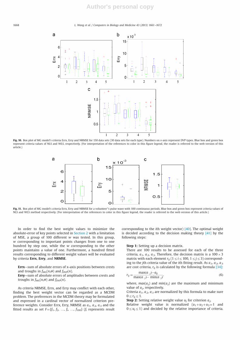
Fig. 10. Box plot of MG model's criteria Errx, Erry and NRMSE for 150 data sets (30 data sets for each type). Numbers on x-axis represent DVP types. Blue box and green boxrepresent criteria values of NLS and WLS, respectively. (For interpretation of the references to color in this figure legend, the reader is referred to the web version of thisarticle.)

Fig. 11. Box plot of MG model's criteria Errx, Erry and NRMSE for a volunteer’'s pulse wave with 100 continuous periods. Blue box and green box represent criteria values ofNLS and WLS method respectively. (For interpretation of the references to color in this figure legend, the reader is referred to the web version of this article.)



To minimize Errx and Erry with the limitation of NRMSE, we setu1¼u2¼0.35, u3¼0.3 according to trials and errors.Step 3: Calculating the fitness value ci for each fi in set F.In this step, an extreme optimal solution E and an extreme badsolution B are defined as: E¼(e1, e2, e3), B¼(b1, b2, b3), whereej¼max(r.j), bj¼ min(r.j) [42]. It is obvious in this case that E¼(1, 1, 1), B¼(0, 0, 0). E is an ideal solution that is nonexistentunder general conditions in the MCDM problem. In this paper,the best solution is obtained by calculating the fitness value cifor each fi as follows:

ci ¼1

1þ ∑3j ¼ 1½ujðej�rijÞ�2=∑3

j ¼ 1½ujðbj�rijÞ�2� � ð7Þ

A fitness value set C¼{c1, c2, …, ci, …, c100} is obtained for F¼{f1, f2, …, fi, …, f100}.Step 4: Finding the best solution.The result fi that corresponds to the maximum fitness value ciis taken as the best solution.

4. Results and discussions

4.1. Performance of MG modeling

A total of 150 DVP signals were processed and fitted by the MGModel, 117 and 33 of which are fitted by 4-Gaussian MG and5-Gaussian MG, respectively. Table 2 shows that 5-Gaussian MG isused more frequently in the first type than in other types of DVPwaveforms; 4-Gaussian MG can be applied to approximate all thefifth type DVP waveforms in this study.

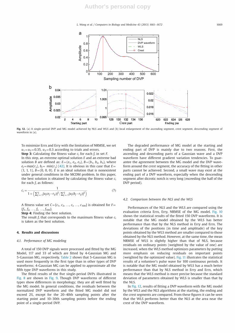
The fitted results of the five single-period DVPs illustrated inFig. 8 are shown in Fig. 9. Though DVP waveforms of differenttypes show differences in morphology; they are all well fitted bythe MG model. In general conditions, the residuals between thenormalized DVP waveform and the fitted MG model did notexceed 2%, except for the 20–40th sampling points after thestarting point and 10–30th sampling points before the endingpoint of a single-period DVP.

The degraded performance of MG model at the starting andending part of DVP is mainly due to two reasons. First, theascending and descending parts of a Gaussian wave and a DVPwaveform have different gradient variation tendencies. To guar-antee the agreement between the MG model and the DVP wave-form around the crest segment, the accuracy of the fitting in otherparts cannot be achieved. Second, a small wave may exist at theending part of a DVP waveform, especially when the descendingsegment after dicrotic notch is very long (exceeding the half of theDVP period).

4.2. Comparison between the NLS and the WLS

Performances of the NLS and the WLS are compared using theevaluation criteria Errx, Erry, NRMSE of the MG model. Fig. 10shows the statistical results of the fitted 150 DVP waveforms. It isnotable that the MG model obtained by the WLS has betterperformance than that by the NLS method in Erry and Errx. Thedeviations of the positions (in time and amplitude) of the keypoints obtained by the WLS method are smaller compared to thoseobtained by the NLS method. However, at the same time, the meanNRMSE of WLS is slightly higher than that of NLS, becauseresiduals on ordinary points (weighted by the value of one) areincreased, when the WLS method optimizes parameters by puttingmore emphasis on reducing residuals on important points(weighted by the optimized value). Fig. 11 illustrates the statisticalresults of a volunteer’s pulse wave for 100 continuous periods. Itis notable that the MG model obtained by WLS has a much betterperformance than that by NLS method in Erry and Errx, whichmeans that the WLS method is more precise because the standarddeviation of parameters obtained by WLS is smaller than that bythe NLS.

In Fig. 12, results of fitting a DVP waveform with the MG modelby the WLS and the NLS algorithms at the starting, the ending andthe crest segments are compared. From these figures it can be seenthat the WLS performs better than the NLS at the area near thecrest of the DVP waveform.

0 100 200 300 400 500 6000

0.2

0.4

0.6

0.8

1

Sampling number of DVPA

mpl

itude

NLSDVP waveformWLSCrest

Fig. 12. (a) A single-period DVP and MG model achieved by NLS and WLS and (b) local enlargement of the ascending segment, crest segment, descending segment ofwaveform in (a).



4.3. Influences of the weight value

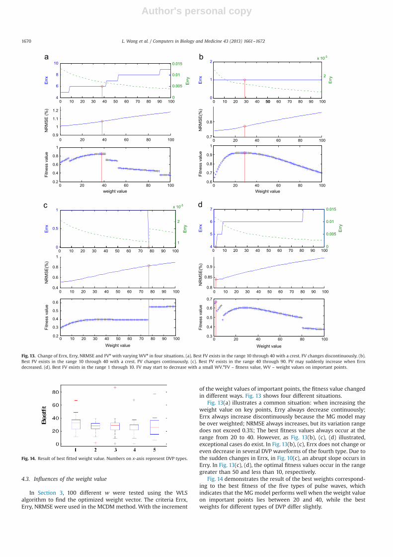
In Section 3, 100 different w were tested using the WLSalgorithm to find the optimized weight vector. The criteria Errx,Erry, NRMSE were used in the MCDM method. With the increment

of the weight values of important points, the fitness value changedin different ways. Fig. 13 shows four different situations.

Fig. 13(a) illustrates a common situation: when increasing theweight value on key points, Erry always decrease continuously;Errx always increase discontinuously because the MG model maybe over weighted; NRMSE always increases, but its variation rangedoes not exceed 0.3%; The best fitness values always occur at therange from 20 to 40. However, as Fig. 13(b), (c), (d) illustrated,exceptional cases do exist. In Fig. 13(b), (c), Errx does not change oreven decrease in several DVP waveforms of the fourth type. Due tothe sudden changes in Errx, in Fig. 10(c), an abrupt slope occurs inErry. In Fig. 13(c), (d), the optimal fitness values occur in the rangegreater than 50 and less than 10, respectively.

Fig. 14 demonstrates the result of the best weights correspond-ing to the best fitness of the five types of pulse waves, whichindicates that the MG model performs well when the weight valueon important points lies between 20 and 40, while the bestweights for different types of DVP differ slightly.

0 10 20 30 40 50 60 70 80 904

6

8

10

Err

x

1000

0.005

0.01

0.015

Err

y

0 20 40 60 80 1000.9

1

1.1

1.2

NR

MS

E (%

)

0 20 40 60 80 1000.2

0.4

0.6

0.8

1

weight value

Fitn

ess

valu

e

0 10 20 30 40 50 60 70 80 90 1000

1

2

Err

x

50

2

x 10-3

Err

y

0 20 40 60 80 1000.7

0.8

NR

MS

E(%

)

0 20 40 60 80 1000.6

0.7

0.8

0.9

1

Weight value

Fitn

ess

valu

e

0 10 20 30 40 50 60 70 80 90 1000

0.5

1

Err

x

1

2

x 10-3

Err

y

0 10 20 30 40 50 60 70 80 90 1000.4

0.6

0.8

1

NR

MS

E(%

)

0 10 20 30 40 50 60 70 80 90 1000.2

0.3

0.4

0.5

0.6

Weight value

Fitn

ess

valu

e

0 10 20 30 40 50 60 70 80 90 1004

5

6

7

Err

x

0

0.005

0.01

0.015

Err

y

0 10 20 30 40 50 60 70 80 90 1000.8

0.85

0.9

NR

MS

E(%

)

0 20 40 60 80 1000.3

0.4

0.5

0.6

0.7

Weight value

Fitn

ess

valu

e

Fig. 13. Change of Errx, Erry, NRMSE and FVn with varying WVn in four situations. (a). Best FV exists in the range 10 through 40 with a crest. FV changes discontinuously. (b).Best FV exists in the range 10 through 40 with a crest. FV changes continuously. (c). Best FV exists in the range 40 through 90. FV may suddenly increase when Errxdecreased. (d). Best FV exists in the range 1 through 10. FV may start to decrease with a small WV.nFV – fitness value, WV – weight values on important points.

Fig. 14. Result of best fitted weight value. Numbers on x-axis represent DVP types.



5. Conclusions

The decomposition analysis method is effective in compressing,synthesizing and analyzing physiological signals. There are somereported researches that decompose physiological signals usingmultiple Gaussian models. However, the number of Gaussian waveis constant. Actually, the number of Gaussian waves depends on themorphology of physiological signals. Furthermore, those methodsdo not pay much attention to the estimation error of the key pointsin physiological signals. In fact, the positions of these key points areimportant for diagnosis.

To analyze component waves in five types of DVP waveforms, anadaptive MG model is introduced in this paper. The model closelyapproximates a single-period DVP by decomposing it into four or fiveGaussian waves. When applying the MG model to 150 DVP wave-forms of five different types, it performed well (NRMSEo2%,Errxo6 ms, Erryo0.01). It should be noted that the choice between4-MG and 5-MG model is determined by the morphology of the DVPwaveform.

The parameters of the MG model are estimated by the DoubleDifferentiation method first and then optimized by WLS. Due to thecrests and troughs of DVP waveforms contain clinical information,the fitted residual error of those points' amplitudes and positionsare required to be smaller by means of assigning the larger weightsto them in WLS. In Section 4, the analysis demonstrated that WLS issuperior to NLS, because the agreement of the MG model achievedby WLS is better than that by NLS at the crests and troughs of DVPwaveforms.

In order to find the set of weight values in the WLS method thatcan obtain the best fitting performance of MG model to DVPwaveform, a group of 100 different weight vectors were tested inSection 3. The MCDM method was applied to choose the bestweight vector by three criteria, namely NRMSE, Errx and Erry.Experimental results show that the MG model always performswell when the weight value for key points lies between 20 and 40.

Component waves of the MG model may relate to the forwardand reflected waves in a single-period DVP. As information of theforward and reflected waves are useful in arterial parameterestimation, further research on amplitude and position estimationof the component Gaussian waves are possibly of great signifi-cance to the advancement in arterial parameter estimation. Thisproposed approach also can be applied to decompose the otherrelated physiological signals.

Conflict of interest statement

We declare that we have no financial and personal relation-ships with other people or organizations that can inappropriatelyinfluence our work, there is no professional or other personalinterest of any nature or kind in any product, service and/orcompany that could be construed as influencing the positionpresented in, or the review of, the manuscript entitled, “Multi-Gaussian Fitting for Pulse Waveform Using Weighted LeastSquares and Multi-Criteria Decision Making Method”.

Acknowledgments

This work is supported by the National Natural Science Foun-dation of China (No. 61374015), the Ph.D. Programs Foundation ofMinistry of Education of China (No. 20110042120037), the Liaon-ing Provincial Natural Science Foundation of China (No.201102067) and the Fundamental Research Funds for the CentralUniversities (No. N110219001). This work is also supported in part

by the Hong Kong Research Grants Council (RGC) General ResearchFund (No. 415709).

References

[1] J. Spigulis, Optical non-invasive monitoring of skin blood pulsations, Appl. Opt.44 (10) (2005) 1850–1857.

[2] J. Allen, A. Murray, Age-related changes in the characteristics of the photo-plethysmographic pulse shape at various body sites, Physiol. Meas. 24 (2)(2003) 297–307.

[3] J. Allen, Photoplethysmography and its application in clinical physiologicalmeasurement, Physiol. Meas. 28 (2007) R1–R39.

[4] D. Goswami, K. Chaudhuri, J. Mukherjee, A new two-pulse synthesis model fordigital volume pulse signal analysis, Cardiovasc. Eng. 10 (3) (2010) 109–117.

[5] Bing Nan Li, Bin Bin Fu, Ming Chui Dong, Development of a mobile pulsewaveform analyzer for cardiovascular health monitoring, Comput. Biol. Med.38 (4) (2008) 438–445.

[6] Yu-Feng Chung, Chung-Shing Hu, Cheng-Chang Yeh, Ching-Hsing Luo, How tostandardize the pulse-taking method of traditional Chinese medicine pulsediagnosis, Comput. Biol. Med. 43 (4) (2013) 342–349.

[7] Ching-Chuan Wei, Chin-Ming Huang, Yin-Tzu Liao, The exponential decaycharacteristic of the spectral distribution of blood pressure wave in radialartery, Comput. Biol. Med. 39 (5) (2009) 453–459.

[8] Wilmer W. Nichols, Michael F. O’Rourke, Charalambos Vlachopoulos, McDo-nald's Blood Flow in Arteries: Theoretical, Experimental and Clinical Princi-ples, 6th Edition, CRC Press, 2011.

[9] H.B. Grotenhuis, J.M. Westenberg, P. Steendijk, R.J. Van der Geest, et al.,Validation and reproducibility of aortic pulse wave velocity as assessed withvelocity-encoded MRI, J. Magn. Reson. Imaging. 30 (3) (2009) 521–526.

[10] K. Takazawa, N Tanaka, M. Fujita, et al., Assessment of vascoactive agents andvascular aging by the second derivative of photoplethysmogram waveform,Hypertension 32 (2) (1998) 365–370.

[11] I. Imanaga, H. Hara, S. Koyanagi, et al., Correlation between wave componentsof the second derivative of the plethysmogram and arterial distensibility, Jpn.Heart J. 39 (6) (1998) 775–784.

[12] L.A. Bortolotto, J. Blacher, T. Kondo, et al., Assessment of vascular aging andatherosclerosis in hypertensive subjects: second derivative of photoplethys-mogram versus pulse wave velocity, Am. J. Hypertension 13 (2) (2000)165–171.

[13] Weili Qian, Lanyi Xu, Fuyu Chen, Rongliang Zheng, Acquiring characteristics ofpulse wave by Gaussian function separation, Chin. J. Biomed. Eng. 13 (1) (1994) 1–7.

[14] Uldis Rubins, Finger and ear photoplethysmogram waveform analysis byfitting with Gaussians, Med. Biol. Eng. Comput. 46 (12) (2008) 1271–1276.

[15] M.C. Baruch, D.ER Warburton, S.SD Bredin, et al., Pulse decomposition analysisof the digital arterial pulse during hemorrhage simulation, Nonlinear Biomed.Phys. 5 (1) (2011).

[16] Berend E. Westerhof, Ilja Guelen, et al., Quantification of wave reflection in thehuman aorta from pressure alone: a proof of principle, Hypertension 48 (4)(2006) 595–601.

[17] C. Gillebert, L.M.V. Bortel, S. Patrick, et al., Evaluation of noninvasive methodsto assess wave reflection and pulse transit time from the pressure waveformalone, Hypertension 53 (2009) 142–149.

[18] R. Couceiro, P. Carvalho, R.P. Paiva, J. Henriques, M. Antunes, I. Quintal,J. Muehlsteff, Multi-Gaussian fitting for the assessment of left ventricularejection time from the photoplethysmogram, in: Proceedings of the Interna-tional Conference of the IEEE Engineering in Medicine and Biology Society,EMBC 2012, San Diego, USA.

[19] S. Mohanalakshmi, A. Sivasubramanian, A review on the non-invasive assess-ment of atherosclerosis and other cardiovascular risk factors through thesecond derivative of the photoplethysmogram (SDPPG), Int. J. Syst., Algor.Appl. 2 (ICRASE12) (2012) 166–170.

[20] Yinghui Chen, Lei Zhang, David Zhang, Dongyu Zhang, Wrist pulse signaldiagnosis using modified Gaussian models and Fuzzy C-Means classification,Med. Eng. Phys. (2009) 1283–1289.

[21] P.J. Chowienczyk, R.P. Kelly, Helen MacCallum, et al., Photoplethysmographicassessment of pulse wave reflection, J. Am. Coll. Cardiol. 34 (7) (1999)2007–2014.

[22] S.C. Millasseau, F.G. Guigui, R.P. Kelly, et al., Non-invasive assessment of thedigital volume pulse: comparison with the peripheral pressure pulse, Hyper-tension 36 (2000) 952–956.

[23] Bernhard Hametnera, Siegfried Wassertheurer, Johannes Kropf, Christopher Mayer,Andreas Holzinger, Bernd Eber, Thomas Weber, Wave reflection quantificationbased on pressure waveforms alone-methods, comparison, and clinical covariates,Comput. Methods Programs Biomed. 109 (2013) 250–259.

[24] Matti Huotari, Antti Vehkaoja, Kari Määttä, Juha Kostamovaara, Photoplethys-mography and its detailed pulse waveform analysis for arterial stiffness,J. Struct. Mech. 44 (4) (2011) 345–362.

[25] Matti Huotari, Antti Vehkaoja, Kari Määttä, Juha Kostamovaaraa, Pulse wave-forms are an indicator of the condition of vascular system, IFMBE Proceedingsof the World Congress on Medical Physics and Biomedical Engineering 39(2013) 526–529.

[26] Chengyu Liu, Dingchang Zheng, Alan Murray, Changchun Liu, Modelingcarotid and radial artery pulse pressure waveforms by curve fitting withGaussian functions, Biomed. Signal. Process Control (2013) 449–454.



[27] Y. Zhao, W.H. Kullmann, Applanation tonometry for determining arterialstiffness, Biomed. Tech. 57 (Suppl.1) (2012) 669–672.

[28] Lisheng Xu, Shuting Feng, Yue Zhong, Cong Feng, Max Q.-H. Meng, HuaichengYan, Multi-Gaussian fitting for digital volume pulse using weighted leastsquares method,” in: Proceedings of IEEE International Conference on Informa-tion and Automation (ICIA2011), Shenzhen China, June 6–8, 2011, pp. 544–549.

[29] S.C. Millaseau, R.P. Kelly, J.M. Ritter, et al., Determination of age-relatedincreases in large artery stiffness by digital pulse contour analysis, Clin. Sci.103 (4) (2002) 371–377.

[30] S.C. Millaseau, J.M. Ritter, K. Takazawa, Contour analysis of the photoplethysmo-graphic pulse measured at the finger, J. Hypertension 24 (8) (2006) 1449–1456.

[31] Gang Zheng, Qingjun Huang, Guodong Yan, Min Dai, Pulse waveform key pointrecognition by wavelet transform for central aortic blood pressure estimation,J. Inf. Comput. Sci. 9 (1) (2012) 25–33.

[32] Gavin P. Shorten, Martin J. Burke, The application of dynamic time warping tomeasure the accuracy of ECG compression, Int. J. Circuits, Syst. Signal Process.5 (3) (2011) 305–313.

[33] N. Cressie, Fitting variogram models by weighted least squares, Math. Geol. 17(5) (1985) 563–585.

[34] M.T. Hagan, H.B. Demuth, M.H. Beale, Neural Network Design, PWS Pub,Boston, London, 1996.

[35] Jung Kim Hyonyoung Han, Artifacts in wearable photoplethysmographsduring daily life motions and their reduction with least mean square basedactive noise cancellation method, Comput. Biol. Med. 42 (4) (2012) 387–393.

[36] Lisheng Xu, David Zhang, Kuanquan Wang, et al., Baseline wander correctionin pulse waveforms using wavelet-based cascaded adaptive filter, Comput.Biol. Med. 37 (5) (2007) 716–731.

[37] T.R. Dawber, H.E. Thomas, P.M. McNamara, et al., Characteristics of the dicroticnotch of the arterial pulse wave in coronary heart disease, Angiology 24 (4)(1973) 244–255.

[38] K. Mustafa, A system for analysis of arterial blood pressure waveforms inhumans, Comput. Biomed. Res. 30 (1997) 244–255.

[39] S.C. Millasseau, R.P. Kelly, J.M. Ritter, et al., Determination of age-relatedincreases in large artery stiffness by digital pulse contour analysis, Clin. Sci.103 (2002) 371–377.

[40] P. Jankowski, Integrating geographical information systems and multiplecriteria decision-making methods, J. Geogr. Inf. Syst. 9 (3) (1995) 251–273.

[41] Dengfeng Li, Multiattribute decision making models and methods usingintuitionistic fuzzy sets, . Syst. Sci. 70 (2005) 73–85.

[42] J.P. Brans, P.H. Vincke, A preference ranking organisation method: (thepromethee method for multiple criteria decision-making), Manage. Sci. 31(2) (1985) 647–656.


Documents

Author's personal copy Multi-Gaussian fitting for pulse waveform using Weighted Least Squares and multi-criteria decision making method