Nonlinear waveform and delay time analysis of triplicated core phases

Nonlinear waveform and delay time analysis

of triplicated core phases

R. GarciaDepartement de Geophysique Spatiale et Planetaire, Institut de Physique duGlobe de Paris, CNRS UMR7096, St. Maur des Fosses, France

S. ChevrotLaboratoire de Dynamique Terrestre et Planetaire, CNRS UMR5562, Toulouse, France

M. WeberGeoForschungsZentrum, Potsdam, Germany

Received 4 February 2003; revised 14 August 2003; accepted 29 August 2003; published 24 January 2004.

[1] We introduce a new method to measure differential travel times and attenuation ofseismic body waves. The problem is formulated as a nonlinear inverse problem, which issolved by simulated annealing. Using this technique, we have analyzed triplicated PKPwaves recorded by the temporary Eifel array in central Europe. These examplesdemonstrate the potential of the technique, which is able to determine differential traveltimes and waveforms of the core phases, even when they interfere on the seismograms orwhen additional depth phases are present. The PKP differential travel times reveal thepresence of large-amplitude and small-scale heterogeneities along the PKP(AB) raypaths and favor a local radial inner core model with �0.9% velocity perturbation in its top150 km and small velocity perturbations below. The quality factor in the top 300 km ofthis inner core region is estimated from PKP differential attenuation. Its preferred value is330 with a lower bound of 75. INDEX TERMS: 0935 Exploration Geophysics: Seismic methods

(3025); 3260 Mathematical Geophysics: Inverse theory; 7203 Seismology: Body wave propagation; 7207

Seismology: Core and mantle; 8180 Tectonophysics: Tomography; KEYWORDS: Earth’s core, simulated

annealing, network data

Citation: Garcia, R., S. Chevrot, and M. Weber (2004), Nonlinear waveform and delay time analysis of triplicated core phases,

J. Geophys. Res., 109, B01306, doi:10.1029/2003JB002429.

1. Introduction

[2] The arrival times of body waves are the primarysource of information exploited in the seismologicalrecords. Large data sets have been created [Engdahl et al.,1998] which allowed tomographic studies at both regionaland global scales [Van der Hilst et al., 1997; Bijwaard et al.,1998]. The growth of data recorded by seismic networksduring the past decade has motivated the search for newmethods to routinely measure body wave arrival times.Classically, these methods are based on cross correlationsbetween the different records of a network [VanDecar andCrosson, 1990]. Previously, Chevrot [2002] described anonlinear algorithm that permits the estimation of theaverage waveform recorded by the stations of a seismolog-ical network and its time delays at each station. While theanalysis of seismograms containing a single prominentseismic phase is relatively simple, seismologists often facecomplex records when different seismic phases interfere. Todemonstrate that the same approach can also be used onsuch records, we have generalized the algorithm to the case

of interfering waves. We focus on the analysis of seismo-grams in the distance range of the PKP triplication. Onthese kinds of records, interference is particularly strong.We invert for the reference PKP(BC) waveform recorded byall the stations, and describe the other body waves asfunctionals of this reference waveform. This approachtherefore incorporates some a priori information in theinversion process.[3] The paper is organized as follows. Section 2 presents

the model parameterization, the a priori information and thesimulated annealing algorithm. Section 3 shows examplesof applications on triplicated core phases recorded by theEifel experiment. These examples are chosen in order todemonstrate the potential of the method. The differentialtravel times and attenuations are analyzed to infer the corestructure in section 4. Finally, we discuss the advantagesand shortcomings of this approach, and present severalpossible applications.

2. Method

2.1. A Priori Information and Model Parameterization

[4] The triplication of PKP, the P phase propagatinginside the core, occurs in the epicentral distance range

JOURNAL OF GEOPHYSICAL RESEARCH, VOL. 109, B01306, doi:10.1029/2003JB002429, 2004

Copyright 2004 by the American Geophysical Union.0148-0227/04/2003JB002429$09.00

B01306 1 of 16

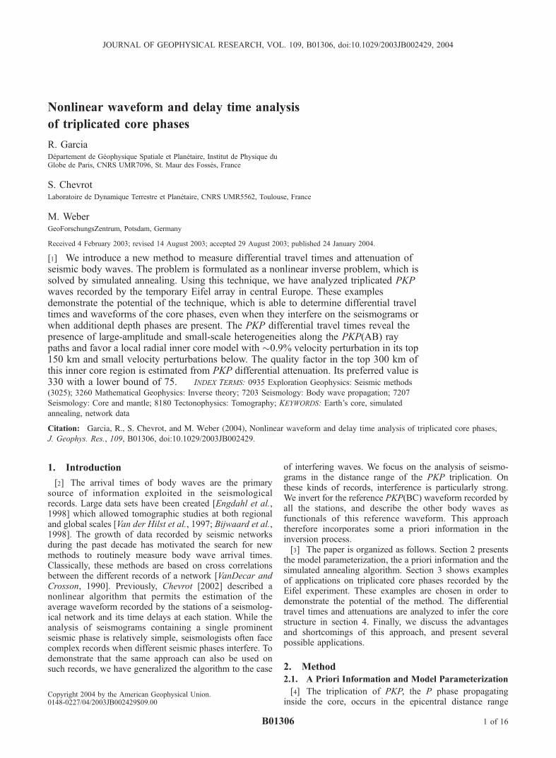
146�–153�. Three core phases interfere: PKP(DF) whichhas its turning point inside the strongly attenuating innercore, PKP(BC) which turns at the base of the liquid core,and PKP(AB) which turns in the middle of the liquid core,and is proportional to the Hilbert transform of PKP(BC)[Choy and Richards, 1976; Creager, 1992; Song, 1997;Garcia and Souriau, 2000]. The ray paths of the three corephases are shown on Figure 1. The inner core reflectedPKiKP phase and the whispering gallery phases (PKIIKP,PK3IKP. . .) could be neglected in this epicentral distancerange due to their small amplitudes compared to the PKPphases. Under this hypothesis, the seismic records of thePKP triplication can be modeled as a sum of three seismicphases:

SiðtÞ ¼ RDFGDFi Aðt*i Þ*W ðt þ tDF

i Þþ GBC

i W ðt þ tBCi Þ

þ RABGABi H*W ðt þ tAB

i Þ ð1Þ

where Si(t) is the seismogram recorded by station number i;W(t) is the waveform of the PKP(BC) phase taken as areference; A(t*i ) is a differential attenuation operator; H isthe Hilbert transform operator; Gi

DF, GiBC, and Gi

AB are thegeometrical spreading amplitude corrections computed inthe reference Earth’s model; RDF and RAB are realparameters standing for relative amplitude corrections;and tDFi , tBCi and tABi are the time shifts of the PKP(DF),PKP(BC) and PKP(AB) phases, respectively, relative to thebeginning of the record. The attenuation operator is definedby A(t*) = F[exp(�pft*)exp(2if ln ( f/f0)t*)], where F isthe Fourier transform operator, f is the frequency, and f0 =0.5 Hz is the reference frequency of PKP(DF). Thisdescription contains our prior knowledge of the seismicrecords in the triplication distance range. The model space isthus described by the time samples of the referencewaveform W(t), the relative amplitude corrections RDF andRAB, and the different times t*i, t

DFi , tBCi and tABi related to

each record i.[5] In the formulation of the problem, we make the

implicit assumptions that the source time function is notaffected by directivity effects, and that the waveforms arenot strongly distorted by mantle heterogeneities. Addition-ally, we assume that PKP(AB) is the Hilbert transform ofthe PKP(BC) phase, and that the PKP(DF) phase has thesame waveform as the PKP(BC) phase, but attenuated. The

PKP(DF) phase passing through the inner core is moreattenuated than the PKP(BC) phase which travels only inthe outer core where attenuation is low [Doornbos, 1983;Souriau and Roudil, 1995; Cormier et al., 1998]. BecausePKP(BC) and PKP(DF) phases follow approximately thesame ray paths in the crust and the mantle, only shortwavelength heterogeneities in the D" layer can distort theirrelative waveforms [Breger et al., 1999]. However,PKP(AB) and PKP(BC) phases follow slightly differentray paths in the mantle, resulting in a larger sensitivity tolateral variations in seismic velocities, particularly in the D"layer [Breger et al., 2000; Tkalcic et al., 2002]. The networksize must not be too large in order to avoid strong waveformvariations over the network owing to crustal heterogeneitiesand directivity effects at the source.[6] A priori information is also introduced by imposing

conditions on the relative time shifts between the differentseismic phases. Admissible variations of the differentialtravel time residuals (BC-DF) and (AB-BC) relative to thereference Earth model AK135 [Kennett et al., 1995] areimposed to lie in the intervals:

�2:0 < ðtBCi � tDFi Þ � ðtBCi � tDFi Þ < 2:0 ð2Þ

�2:0 < ðtABi � tBCi Þ � ðtABi � tBCi Þ < 2:0 ð3Þ

where tiDF, ti

BC, and tiAB are the theoretical travel times of the

three core phases. This a priori information is used tocompute the maximum and minimum values of theparameters ti

DF and tiAB at each step of the algorithm.

The attenuation parameters ti* are allowed to vary between0.0 and 2.2 s. The parameters RDF and RAB correct forrelative amplitude differences between the three PKPphases, owing to source radiation and transmissioncoefficients that produce only smooth amplitude variationswithin the small epicentral distance range investigated here.No a priori information has been introduced on these twoparameters.

2.2. Optimization Algorithm

[7] The inversion is performed by minimizing the fol-lowing L1 norm misfit (analogous to an energy):

E ¼Xi

ZjDiðtÞ � SiðtÞjdt ð4Þ

where Di(t) and Si(t) are the observed and syntheticseismograms, and the sums are over the seismograms iand time. The L1 norm is chosen because of its stabilitywith respect to outliers induced by microseismic and highfrequency noise, which is critical for a fully nonlinearinversion. The waveform inversion is performed following asimulated annealing (SA) algorithm close to the algorithmdescribed by Chevrot [2002]. SA optimization algorithmshave been widely applied in geophysics [Sen and Stoffa,1995; Sharma and Kaikkonen, 1998] and more recently toteleseismic data [Kolar, 2000; Chevrot, 2002]. Thesimulated annealing algorithm is a Monte Carlo MarkovChain algorithm with the probability of uphill investigationof the misfit function decreasing along the cooling schedule.The reader is referred to the references cited above for a fulldescription of the simulated annealing algorithm. Thesimulated annealing algorithm is optimal for the inversion

Figure 1. Ray paths of the three PKP branches in theEarth: PKP(DF) (solid line), PKP(BC) (dashed line) andPKP(AB) (dotted line). The event (black star) and the D"layer at the base of the mantle are also indicated.

B01306 GARCIA ET AL.: NONLINEAR ANALYSIS OF CORE PHASES

2 of 16

B01306

of the waveform W(t) [Kuperman et al., 1990; Chevrot,2002] because energy computations are restricted to thecomputation of energy differences at each time step of thewaveform W(t).[8] The algorithm used in our study is a variation of the

very fast simulated annealing (VFSA) [Sen and Stoffa,1995]. An exponential cooling schedule [Salamon andBerry, 1983; Nulton and Salamon, 1988; Andresen andGordon, 1994] of the form T(k) = g

kT(0) is implementedwith g = 0.98 and N = 1500 iterations. The startingtemperature T(0) is fixed at three times the value of theinitial misfit in order to start well above the criticaltemperature of the system, and T(1500) � 10�14T(0). Ateach temperature step, 5 random perturbations are imple-mented for each parameter Pj, and selection is done accord-ing to Boltzmann statistics. Each perturbation consists inperturbing the waveform parameters W(t) and the amplitudeparameters RDF and RAB by ±�W, with j�Wj = 0.01jWjmax,following the scheme described by Chevrot [2002]. Theother model parameters Pj are randomly perturbed at eachstep l according to the rule

Plþ1j ¼ Pl

j þ yjðPmaxj � Pmin

j Þ ¼ Plj þ yj�Pj ð5Þ

where the random number yj follows a Cauchy distributionparameterized by temperature Tj [Sen and Stoffa, 1995]:

yj ¼ sign uj �1

2

� �Tj 1þ 1

Tj

� �j2uj�1j� 1

" #ð6Þ

where uj is a real number selected randomly in the interval[0, 1]. The main difference to the VFSA algorithm is thatthe temperature Tj is related to the energy E(k) and not to thetemperature T(k) of the system. The temperature describingthe Cauchy probability of yj is defined by

Tj ¼EðkÞEð0Þ

� �2

ð7Þ

where E(k) is the energy of the system. As the energy of thesystem decreases, the temperature Tj decreases and reducesthe area explored in the parameter space. This procedure ischosen in order to adapt the random variations of theparameters to the convergence level of the system, and notto an arbitrary cooling schedule.[9] In order to solve cycle skipping ambiguity on noisy

traces, an additional modification of the SA algorithm isintroduced. Once the system has reached a good conver-gence level, the parameters ti

DF, tiBC and ti

AB are reinitial-ized to the median value of their residuals relative to thePKP(BC) phase at all the stations, and admissible variationsof the differential travel time residuals are limited to ±1 s.This procedure introduces additional a priori information onthe time shifts, which allows to obtain coherent results evenfor noisy records.[10] The a posteriori covariance matrix is estimated

following a method described by Sharma and Kaikkonen[1998]. Twenty runs of the SA algorithm are performedwith different random number seeds, and the covariancematrix is estimated from the results obtained for the twentyinversions. This statistical method allows to compute errorseven for model parameters for which error bars are difficult

to estimate, such as the ti* parameters. An average model isalso computed, and the model presenting the lowest energyover the twenty runs is kept as the best model.[11] The running time of the SA algorithm depends on the

number of seismograms, the time window length, and thesampling rate. For 150 seismograms, sampled at 20 Hz,with a time window of 35 s, the SA algorithm runs in 100CPU minutes on a linux PC Pentium IV at 1.7 GHz.However, the CPU running time could be divided by afactor of 5 by increasing the cooling speed of the algorithm.In this case, the differential travel times are properlyresolved, but the differential attenuations are unstable.[12] The power of the nonlinear waveform inversion with

SA is illustrated in section 3 with a few examples takenfrom the Eifel experiment [Ritter et al., 2000]. Theseexamples are chosen to demonstrate the ability of themethod to investigate interfering PKP branches as well astheir interference with depth phases.

3. Examples

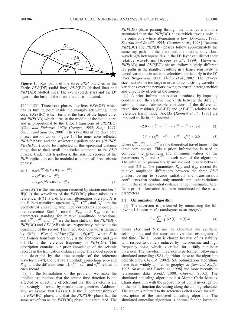
[13] To illustrate the potential of the method, we presentthree examples showing increasing degrees of complexity.The data set consists of core phases recorded by thetemporary Eifel experiment in the 146�–153� epicentraldistance range, and includes waveforms from about 150broadband and short period stations installed in centralEurope in the Eifel plume region [Ritter et al., 2000]. Thisdense temporary network covered an area of 3� by 3�(Figure 2). the instrument responses are deconvolved fromthe data, which are filtered by a band-pass butterworth filterwith corner frequencies at 0.3 Hz and 1.5 Hz. The data set iscomposed of the records of eight earthquakes that occurredin the Fiji-Tonga subduction zone (Table 1), three of whichare presented in details in the next sections.

3.1. A Simple Case: Three Core PhasesThat Are Well Separated in Time

[14] The 152 stations of the Eifel network have recordedthe three core phases generated by earthquake 8 (Table 1).The data, filtered between 0.3 and 1.5 Hz and aligned on thetheoretical arrival time of the PKP(BC), are presented onFigure 3a. The three PKP phases are clearly separated inthis distance range, and the noise level is low. The PKP(DF)phase is characterized by a lower frequency content and asmaller amplitude than the PKP(BC) phase owing to innercore attenuation [Souriau and Roudil, 1995; Cormier et al.,1998]. Figure 3b shows the comparison between data andthe synthetic waveforms for the best model once all theseismograms are aligned on the PKP(BC) arrival time. Thefit is very good for PKP(DF) and PKP(BC) phases, andquite good for the PKP(AB) phase. The energy and variancereductions for the whole data set are 34% and 52%,respectively. The unexplained energy and variance reflectsthe noise level and the parts of the seismograms that are notfitted by the PKP synthetic phases. Figure 3c presents thedifferential time shifts ti

DF � tiBC and ti

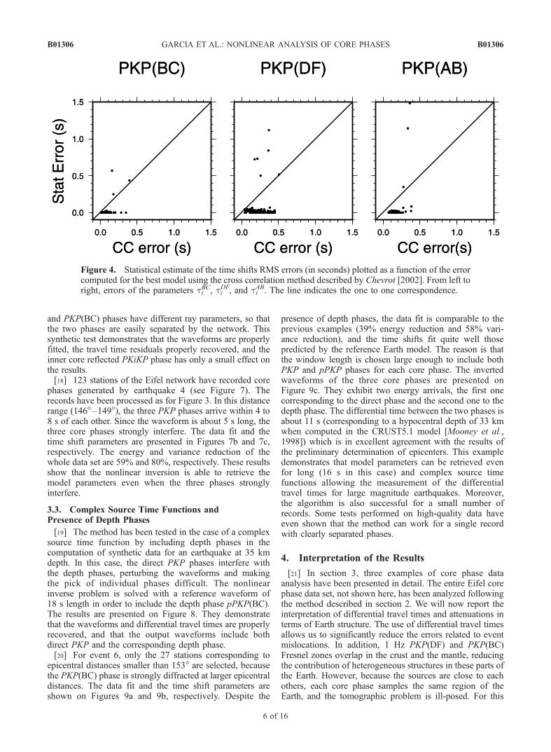
AB � tiBC. The smallamount of scattering of the measurements is indicative oftheir accuracy. Measurement error bars are generally lowerthan 0.5, 0.2, and 0.4 s for PKP(DF), PKP(BC), andPKP(AB) phases, respectively.[15] Figure 4 presents a comparison between the RMS

error estimated by a statistical analysis of the 20 inversion


3 of 16

B01306

results, and the error computed from the waveforms givenby the best model using a cross-correlation method[Chevrot, 2002]. The error estimated by cross correlationis always smaller than 0.5 s. The statistical study of themodels after inversion separates the records in two groups.The records properly fitted present time shifts with a verylow statistical error, indicating that the 20 inversions givethe same results for these parameters. On the other hand, asmall number of noisy records present time shifts withstatistical errors larger than the errors estimated by crosscorrelation owing to cycle skipping ambiguity, which gen-erates multiple local minima in the misfit function, and sodifferent results are obtained for the same parameter overthe 20 inversions. Therefore the statistical error estimategives information on the shape of the misfit function and onthe cycle skipping ambiguity that is not accessible throughthe cross-correlation method.[16] Figure 5 presents typical evolutions of the different

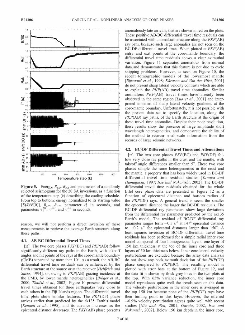
parameters during the cooling schedule for the 20 inversionsperformed. The energy shows a strong decrease close to thetemperature step k = 750, corresponding to the criticaltemperature, and is approximately flat from steps 800 to1500. At this stage, the time shifts are artificially modifiedin order to overcome possible cycle skipping problems, asdescribed above. This perturbation introduces a step likeenergy increase, from which the system quickly recovers.Amplitude correction parameters RDF and RAB are converg-ing once the critical temperature is attained, but the finalvalues for RDF are scattered owing to a trade-off betweenRDF and attenuation parameters ti*. In this example, RDF =1.34 ± 0.04 and RAB = 0.39 ± 0.004, and the standarddeviations of these parameters are lower than 0.06 for all theother earthquakes analyzed in this study. The other plotsshow the evolution of the inverted parameters for a ran-domly chosen seismogram. These parameters present largevariations before the critical temperature, beyond which

they quickly converge to their final value. This value isslightly perturbed by the procedure at step k = 750, butconvergence is achieved at the end of the algorithm. Theconvergence time is the longest for the ti* parameter,because a preliminary alignment of the PKP(DF) waveformis necessary, which simply results from the fact that energyvariations due to ti* are small compared to the ones relatedto the other parameters. The set of final values for t*generally shows the largest scatter, which indicates that itis the most poorly resolved. The different runs show that t*converges to different values suggesting the existence oflocal minima for the misfit function.

3.2. Interference of the Three Core Phases

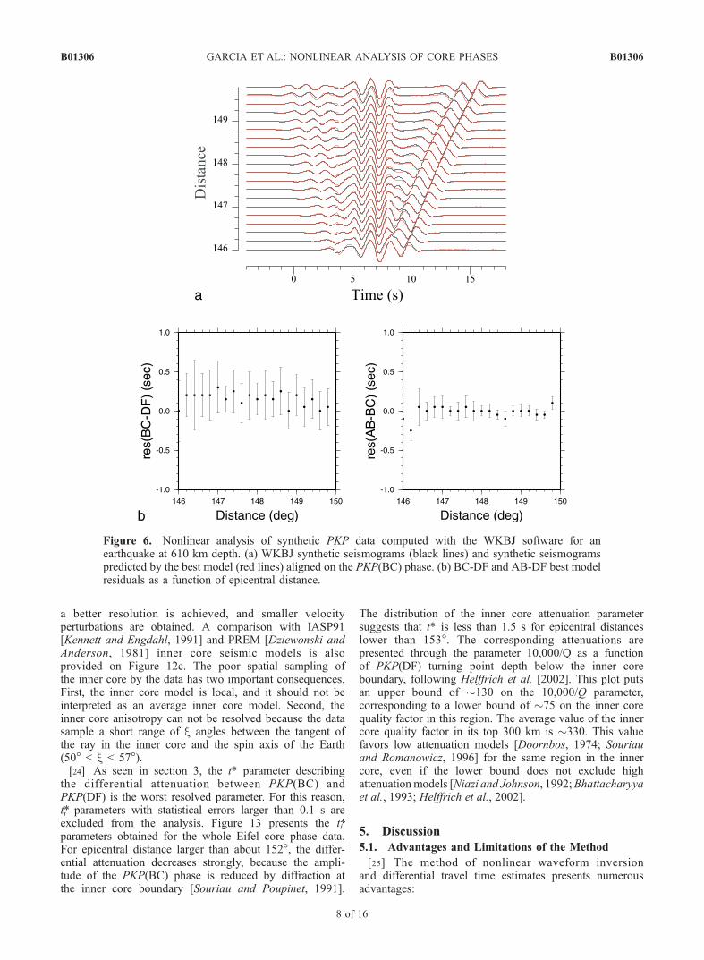
[17] The method has been tested in the case of interferingcore phases with synthetic data computed with the WKBJsoftware [Chapman, 1978] including attenuation in the innercore and additional small amplitude core phases (PKiKP,PKIIKP. . .). As seen on Figure 6a, the inner core reflectedPKiKP phase has a small effect on the data fit just after thePKP(BC) phase for epicentral distances in between 147 and148�. However, it does not change significantly the retrievedreference waveform and output parameters because PKiKP

Figure 2. On the left, stations (solid triangles) and events (open squares) locations with typical greatcircle paths (solid lines). On the right, zoom of the (top) receiver and (bottom) source regions.

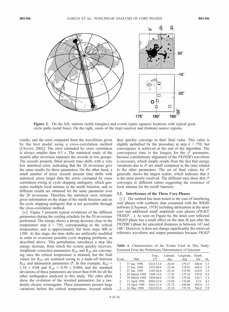
Table 1. Characteristics of the Events Used in This Study,

Extracted From the Preliminary Determination of Epicenter

Event DateTime,UT

Latitude,deg

Longitude,deg

Depth,km Mw

1 27 Jan. 1998 0214:13.0 �20.68 �179.27 646.0 5.32 27 Jan. 1998 1955:00.0 �22.46 178.93 608.8 5.43 27 Jan. 1998 2105:44.0 �22.34 178.90 610.0 5.54 29 March 1998 1948:16.0 �17.42 �179.24 539.0 6.45 29 March 1998 2038:40.0 �17.49 �179.26 526.7 5.46 11 April 1998 0044:35.0 �23.60 �176.08 33.0 4.37 14 April 1998 0341:21.0 �23.73 �180.00 494.4 5.38 16 May 1998 0222:03.0 �22.14 �179.70 586.0 5.9


4 of 16

B01306

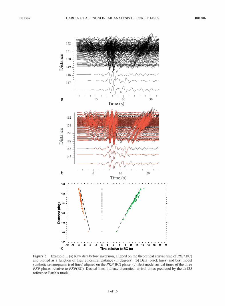
Figure 3. Example 1. (a) Raw data before inversion, aligned on the theoretical arrival time of PKP(BC)and plotted as a function of their epicentral distance (in degrees). (b) Data (black lines) and best modelsynthetic seismograms (red lines) aligned on the PKP(BC) phase. (c) Best model arrival times of the threePKP phases relative to PKP(BC). Dashed lines indicate theoretical arrival times predicted by the ak135reference Earth’s model.


5 of 16

B01306

and PKP(BC) phases have different ray parameters, so thatthe two phases are easily separated by the network. Thissynthetic test demonstrates that the waveforms are properlyfitted, the travel time residuals properly recovered, and theinner core reflected PKiKP phase has only a small effect onthe results.[18] 123 stations of the Eifel network have recorded core

phases generated by earthquake 4 (see Figure 7). Therecords have been processed as for Figure 3. In this distancerange (146�–149�), the three PKP phases arrive within 4 to8 s of each other. Since the waveform is about 5 s long, thethree core phases strongly interfere. The data fit and thetime shift parameters are presented in Figures 7b and 7c,respectively. The energy and variance reduction of thewhole data set are 59% and 80%, respectively. These resultsshow that the nonlinear inversion is able to retrieve themodel parameters even when the three phases stronglyinterfere.

3.3. Complex Source Time Functions andPresence of Depth Phases

[19] The method has been tested in the case of a complexsource time function by including depth phases in thecomputation of synthetic data for an earthquake at 35 kmdepth. In this case, the direct PKP phases interfere withthe depth phases, perturbing the waveforms and makingthe pick of individual phases difficult. The nonlinearinverse problem is solved with a reference waveform of18 s length in order to include the depth phase pPKP(BC).The results are presented on Figure 8. They demonstratethat the waveforms and differential travel times are properlyrecovered, and that the output waveforms include bothdirect PKP and the corresponding depth phase.[20] For event 6, only the 27 stations corresponding to

epicentral distances smaller than 153� are selected, becausethe PKP(BC) phase is strongly diffracted at larger epicentraldistances. The data fit and the time shift parameters areshown on Figures 9a and 9b, respectively. Despite the

presence of depth phases, the data fit is comparable to theprevious examples (39% energy reduction and 58% vari-ance reduction), and the time shifts fit quite well thosepredicted by the reference Earth model. The reason is thatthe window length is chosen large enough to include bothPKP and pPKP phases for each core phase. The invertedwaveforms of the three core phases are presented onFigure 9c. They exhibit two energy arrivals, the first onecorresponding to the direct phase and the second one to thedepth phase. The differential time between the two phases isabout 11 s (corresponding to a hypocentral depth of 33 kmwhen computed in the CRUST5.1 model [Mooney et al.,1998]) which is in excellent agreement with the results ofthe preliminary determination of epicenters. This exampledemonstrates that model parameters can be retrieved evenfor long (16 s in this case) and complex source timefunctions allowing the measurement of the differentialtravel times for large magnitude earthquakes. Moreover,the algorithm is also successful for a small number ofrecords. Some tests performed on high-quality data haveeven shown that the method can work for a single recordwith clearly separated phases.

4. Interpretation of the Results

[21] In section 3, three examples of core phase dataanalysis have been presented in detail. The entire Eifel corephase data set, not shown here, has been analyzed followingthe method described in section 2. We will now report theinterpretation of differential travel times and attenuations interms of Earth structure. The use of differential travel timesallows us to significantly reduce the errors related to eventmislocations. In addition, 1 Hz PKP(DF) and PKP(BC)Fresnel zones overlap in the crust and the mantle, reducingthe contribution of heterogeneous structures in these parts ofthe Earth. However, because the sources are close to eachothers, each core phase samples the same region of theEarth, and the tomographic problem is ill-posed. For this

Figure 4. Statistical estimate of the time shifts RMS errors (in seconds) plotted as a function of the errorcomputed for the best model using the cross correlation method described by Chevrot [2002]. From left toright, errors of the parameters tiBC, ti

DF, and tiAB. The line indicates the one to one correspondence.


6 of 16

B01306

reason, we will not perform a direct inversion of thesemeasurements to retrieve the average Earth structure alongthese paths.

4.1. AB-BC Differential Travel Times

[22] The two core phases PKP(BC) and PKP(AB) followsignificantly different ray paths in the Earth, with takeoffangles and hit points of the rays at the core-mantle boundary(CMB) separated by more than 10�. As a result, the AB-BCdifferential travel time residuals can be influenced by theEarth structure at the source or at the receiver [Helffrich andSacks, 1994], or, owing to PKP(AB) grazing incidence atthe CMB, by lower mantle heterogeneities [Breger et al.,2000; Tkalcic et al., 2002]. Figure 10 presents differentialtravel times obtained for three earthquakes very close toeach others in the Fiji Islands region. The differential traveltime plots show similar features. The PKP(DF) phasearrives earlier than predicted by the ak135 Earth’s model[Kennett et al., 1995], and its advance increases as theepicentral distance decreases. The PKP(AB) phase presents

anomalously late arrivals, that are shown in red on the plots.These positive AB-BC differential travel time residuals canbe associated with anomalous structure along the PKP(AB)ray path, because such large anomalies are not seen on theBC-DF differential travel times. When plotted at PKP(AB)entry and exit points at the core-mantle boundary, thedifferential travel time residuals shows a clear azimuthalvariation. Figure 11 separates anomalous from normaldata and demonstrates that this feature is not due to cycleskipping problems. However, as seen on Figure 10, therecent tomographic models of the lowermost mantle[Bijwaard et al., 1998; Karason and Van der Hilst, 2001]do not present sharp lateral velocity contrasts which are ableto explain the PKP(AB) travel time anomalies. Similaranomalous PKP(AB) travel times have already beenobserved in the same region [Luo et al., 2001] and inter-preted in terms of sharp lateral velocity gradients at thecore-mantle boundary. Unfortunately, it is not possible withthe present data set to specify the location, along thePKP(AB) ray paths, of the Earth structure at the origin ofthese travel time anomalies. Despite their poor resolution,these results show the presence of large amplitude shortwavelength heterogeneities, and demonstrate the ability ofthe method to recover small-scale information from therecords of large seismic networks.

4.2. BC-DF Differential Travel Times and Attenuations

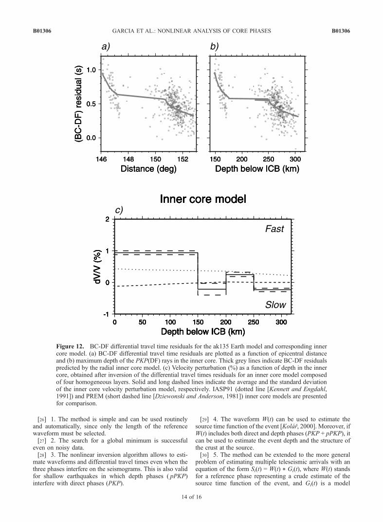
[23] The two core phases PKP(BC) and PKP(DF) fol-low very close ray paths in the crust and the mantle, withtakeoff angle differences smaller than 5�. These two corephases sample the same heterogeneities in the crust andthe mantle, a property that has been widely used in BC-DFdifferential travel time residual studies [Tanaka andHamaguchi, 1997; Isse and Nakanishi, 2002]. The BC-DFdifferential travel time residuals obtained for the wholeEifel core phase data are presented in Figure 12 as afunction of epicentral distance and bottom radius ofthe PKP(DF) rays. A general trend is seen: the smallerthe epicentral distance the larger the BC-DF residuals. TheBC-DF differential ray parameters show large deviationsfrom the differential ray parameter predicted by the ak135Earth’s model. The residual of BC-DF differential rayparameter ranges form �0.5 s/� at 147� epicentral distanceto �0.2 s/� for epicentral distances larger than 150�. Aleast squares inversion of BC-DF differential travel timeresiduals has been performed for a simple radial inner coremodel composed of four homogeneous layers: one layer of150 km thickness at the top of the inner core and threelayers of 50 km thickness below. Inner core lateral velocityperturbations are excluded because the array data analysisdo not show any back azimuth deviation of the PKP(DF)phase compared to PKP(BC). The resulting model isplotted with error bars at the bottom of Figure 12, andthe data fit is shown by thick grey lines in the two plots atthe top. With 65% variance reduction, the inner coremodel reproduces quite well the trends seen on the data.The velocity perturbation in the inner core is averaged inthe top 150 km because none of the PKP(DF) rays havetheir turning point in this layer. However, the inferred�0.9% velocity perturbation agrees quite well with recentstudies [Niu and Wen, 2001; Garcia, 2002; Isse andNakanishi, 2002]. Below 150 km depth in the inner core,

Figure 5. Energy, RDF, RAB and parameters of a randomlyselected seismogram for the 20 SA inversions, as a functionof the temperature step (k) describing the cooling schedule.From top to bottom: energy normalized to its starting value[E(k)/E(0)], RDF, RAB, parameter t1* in seconds, andparameters t1

DF, t1BC, and t1

AB in seconds.


7 of 16

B01306

a better resolution is achieved, and smaller velocityperturbations are obtained. A comparison with IASP91[Kennett and Engdahl, 1991] and PREM [Dziewonski andAnderson, 1981] inner core seismic models is alsoprovided on Figure 12c. The poor spatial sampling ofthe inner core by the data has two important consequences.First, the inner core model is local, and it should not beinterpreted as an average inner core model. Second, theinner core anisotropy can not be resolved because the datasample a short range of x angles between the tangent ofthe ray in the inner core and the spin axis of the Earth(50� < x < 57�).[24] As seen in section 3, the t* parameter describing

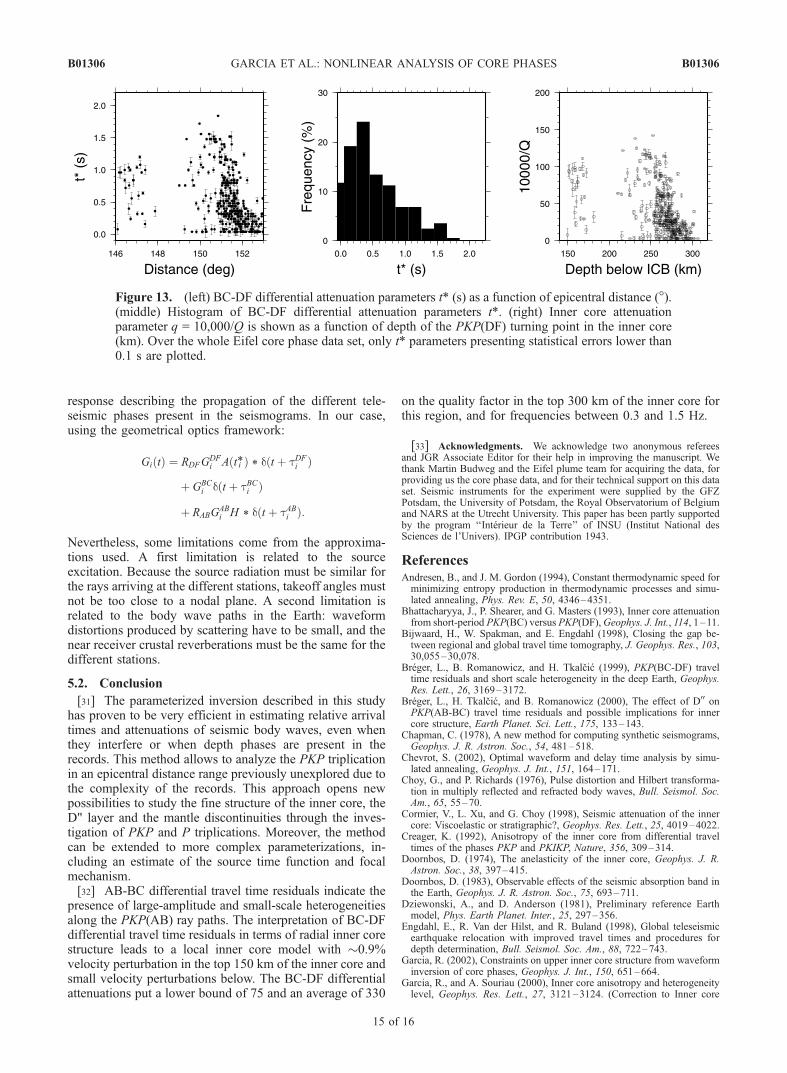
the differential attenuation between PKP(BC) andPKP(DF) is the worst resolved parameter. For this reason,t*i parameters with statistical errors larger than 0.1 s areexcluded from the analysis. Figure 13 presents the t*iparameters obtained for the whole Eifel core phase data.For epicentral distance larger than about 152�, the differ-ential attenuation decreases strongly, because the ampli-tude of the PKP(BC) phase is reduced by diffraction atthe inner core boundary [Souriau and Poupinet, 1991].

The distribution of the inner core attenuation parametersuggests that t* is less than 1.5 s for epicentral distanceslower than 153�. The corresponding attenuations arepresented through the parameter 10,000/Q as a functionof PKP(DF) turning point depth below the inner coreboundary, following Helffrich et al. [2002]. This plot putsan upper bound of �130 on the 10,000/Q parameter,corresponding to a lower bound of �75 on the inner corequality factor in this region. The average value of the innercore quality factor in its top 300 km is �330. This valuefavors low attenuation models [Doornbos, 1974; Souriauand Romanowicz, 1996] for the same region in the innercore, even if the lower bound does not exclude highattenuationmodels [Niazi and Johnson, 1992;Bhattacharyyaet al., 1993; Helffrich et al., 2002].

5. Discussion

5.1. Advantages and Limitations of the Method

[25] The method of nonlinear waveform inversionand differential travel time estimates presents numerousadvantages:

Figure 6. Nonlinear analysis of synthetic PKP data computed with the WKBJ software for anearthquake at 610 km depth. (a) WKBJ synthetic seismograms (black lines) and synthetic seismogramspredicted by the best model (red lines) aligned on the PKP(BC) phase. (b) BC-DF and AB-DF best modelresiduals as a function of epicentral distance.


8 of 16

B01306

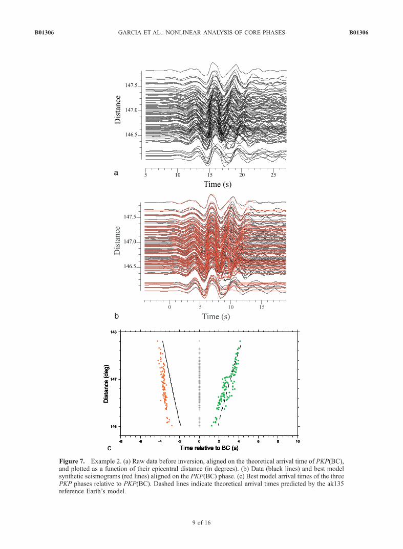
Figure 7. Example 2. (a) Raw data before inversion, aligned on the theoretical arrival time of PKP(BC),and plotted as a function of their epicentral distance (in degrees). (b) Data (black lines) and best modelsynthetic seismograms (red lines) aligned on the PKP(BC) phase. (c) Best model arrival times of the threePKP phases relative to PKP(BC). Dashed lines indicate theoretical arrival times predicted by the ak135reference Earth’s model.


9 of 16

B01306

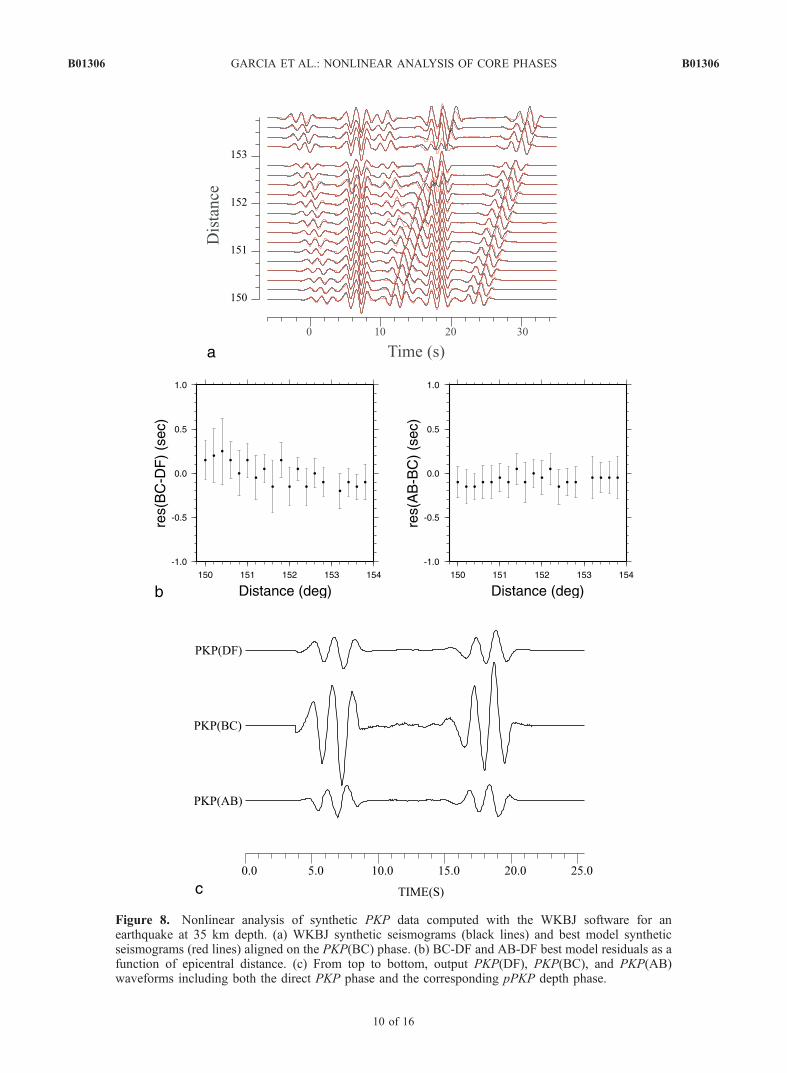
Figure 8. Nonlinear analysis of synthetic PKP data computed with the WKBJ software for anearthquake at 35 km depth. (a) WKBJ synthetic seismograms (black lines) and best model syntheticseismograms (red lines) aligned on the PKP(BC) phase. (b) BC-DF and AB-DF best model residuals as afunction of epicentral distance. (c) From top to bottom, output PKP(DF), PKP(BC), and PKP(AB)waveforms including both the direct PKP phase and the corresponding pPKP depth phase.


10 of 16

B01306

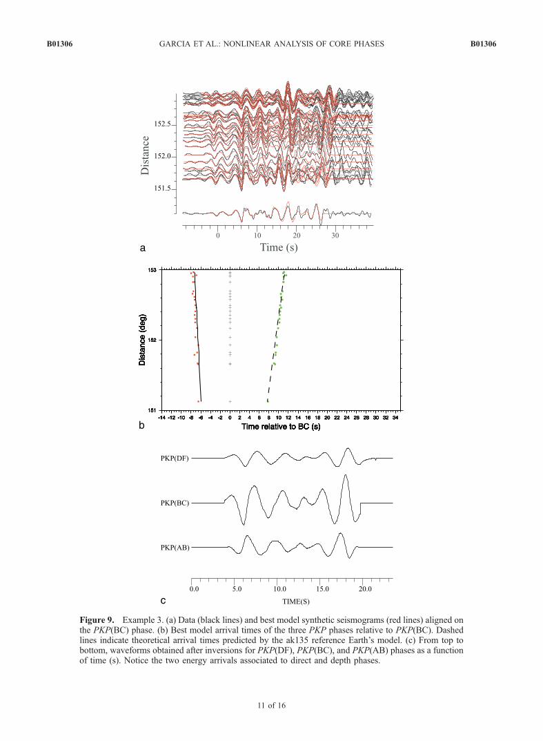
Figure 9. Example 3. (a) Data (black lines) and best model synthetic seismograms (red lines) aligned onthe PKP(BC) phase. (b) Best model arrival times of the three PKP phases relative to PKP(BC). Dashedlines indicate theoretical arrival times predicted by the ak135 reference Earth’s model. (c) From top tobottom, waveforms obtained after inversions for PKP(DF), PKP(BC), and PKP(AB) phases as a functionof time (s). Notice the two energy arrivals associated to direct and depth phases.


11 of 16

B01306

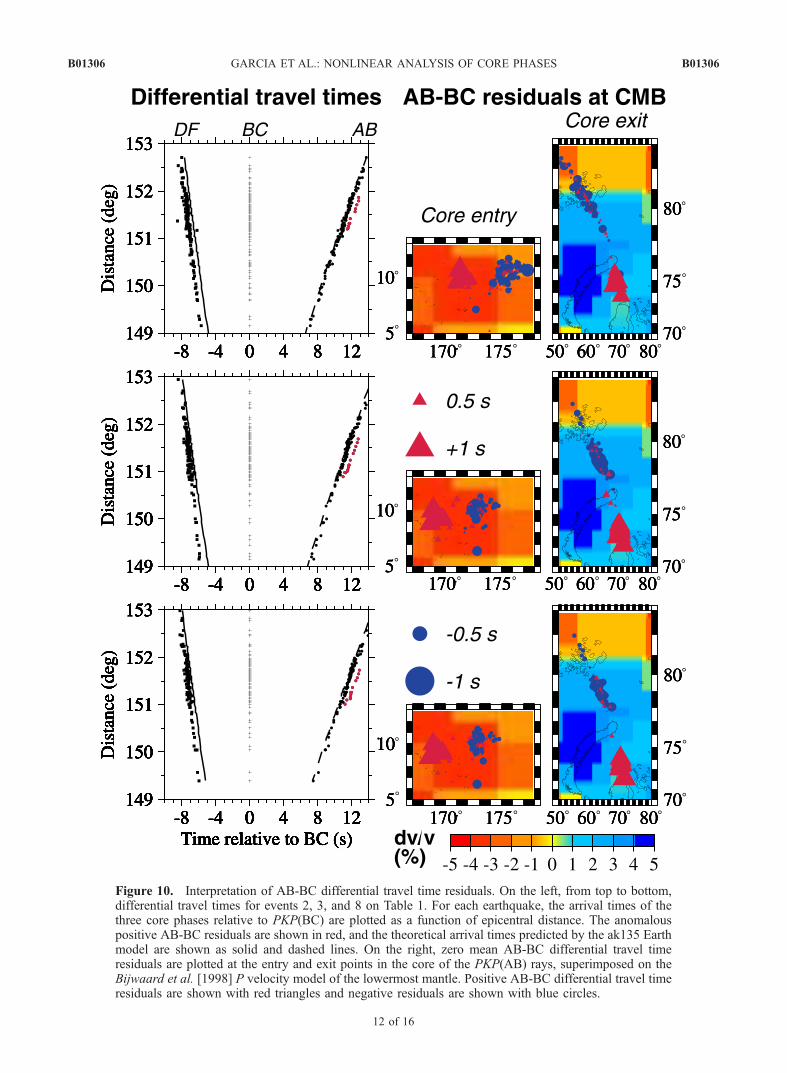
Figure 10. Interpretation of AB-BC differential travel time residuals. On the left, from top to bottom,differential travel times for events 2, 3, and 8 on Table 1. For each earthquake, the arrival times of thethree core phases relative to PKP(BC) are plotted as a function of epicentral distance. The anomalouspositive AB-BC residuals are shown in red, and the theoretical arrival times predicted by the ak135 Earthmodel are shown as solid and dashed lines. On the right, zero mean AB-BC differential travel timeresiduals are plotted at the entry and exit points in the core of the PKP(AB) rays, superimposed on theBijwaard et al. [1998] P velocity model of the lowermost mantle. Positive AB-BC differential travel timeresiduals are shown with red triangles and negative residuals are shown with blue circles.


12 of 16

B01306

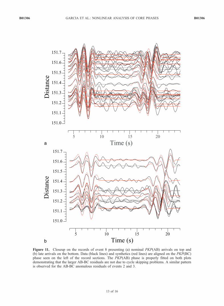
Figure 11. Closeup on the records of event 8 presenting (a) nominal PKP(AB) arrivals on top and(b) late arrivals on the bottom. Data (black lines) and synthetics (red lines) are aligned on the PKP(BC)phase seen on the left of the record sections. The PKP(AB) phase is properly fitted on both plotsdemonstrating that the larger AB-BC residuals are not due to cycle skipping problems. A similar patternis observed for the AB-BC anomalous residuals of events 2 and 3.


13 of 16

B01306

[26] 1. The method is simple and can be used routinelyand automatically, since only the length of the referencewaveform must be selected.[27] 2. The search for a global minimum is successful

even on noisy data.[28] 3. The nonlinear inversion algorithm allows to esti-

mate waveforms and differential travel times even when thethree phases interfere on the seismograms. This is also validfor shallow earthquakes in which depth phases ( pPKP)interfere with direct phases (PKP).

[29] 4. The waveform W(t) can be used to estimate thesource time function of the event [Kolar, 2000]. Moreover, ifW(t) includes both direct and depth phases (PKP + pPKP), itcan be used to estimate the event depth and the structure ofthe crust at the source.[30] 5. The method can be extended to the more general

problem of estimating multiple teleseismic arrivals with anequation of the form Si(t) = W(t) * Gi(t), where W(t) standsfor a reference phase representing a crude estimate of thesource time function of the event, and Gi(t) is a model

Figure 12. BC-DF differential travel time residuals for the ak135 Earth model and corresponding innercore model. (a) BC-DF differential travel time residuals are plotted as a function of epicentral distanceand (b) maximum depth of the PKP(DF) rays in the inner core. Thick grey lines indicate BC-DF residualspredicted by the radial inner core model. (c) Velocity perturbation (%) as a function of depth in the innercore, obtained after inversion of the differential travel times residuals for an inner core model composedof four homogeneous layers. Solid and long dashed lines indicate the average and the standard deviationof the inner core velocity perturbation model, respectively. IASP91 (dotted line [Kennett and Engdahl,1991]) and PREM (short dashed line [Dziewonski and Anderson, 1981]) inner core models are presentedfor comparison.


14 of 16

B01306

response describing the propagation of the different tele-seismic phases present in the seismograms. In our case,using the geometrical optics framework:

GiðtÞ ¼ RDFGDFi Aðt*i Þ * dðt þ tDFi Þ

þ GBCi dðt þ tBCi Þ

þ RABGABi H * dðt þ tABi Þ:

Nevertheless, some limitations come from the approxima-tions used. A first limitation is related to the sourceexcitation. Because the source radiation must be similar forthe rays arriving at the different stations, takeoff angles mustnot be too close to a nodal plane. A second limitation isrelated to the body wave paths in the Earth: waveformdistortions produced by scattering have to be small, and thenear receiver crustal reverberations must be the same for thedifferent stations.

5.2. Conclusion

[31] The parameterized inversion described in this studyhas proven to be very efficient in estimating relative arrivaltimes and attenuations of seismic body waves, even whenthey interfere or when depth phases are present in therecords. This method allows to analyze the PKP triplicationin an epicentral distance range previously unexplored due tothe complexity of the records. This approach opens newpossibilities to study the fine structure of the inner core, theD" layer and the mantle discontinuities through the inves-tigation of PKP and P triplications. Moreover, the methodcan be extended to more complex parameterizations, in-cluding an estimate of the source time function and focalmechanism.[32] AB-BC differential travel time residuals indicate the

presence of large-amplitude and small-scale heterogeneitiesalong the PKP(AB) ray paths. The interpretation of BC-DFdifferential travel time residuals in terms of radial inner corestructure leads to a local inner core model with �0.9%velocity perturbation in the top 150 km of the inner core andsmall velocity perturbations below. The BC-DF differentialattenuations put a lower bound of 75 and an average of 330

on the quality factor in the top 300 km of the inner core forthis region, and for frequencies between 0.3 and 1.5 Hz.

[33] Acknowledgments. We acknowledge two anonymous refereesand JGR Associate Editor for their help in improving the manuscript. Wethank Martin Budweg and the Eifel plume team for acquiring the data, forproviding us the core phase data, and for their technical support on this dataset. Seismic instruments for the experiment were supplied by the GFZPotsdam, the University of Potsdam, the Royal Observatorium of Belgiumand NARS at the Utrecht University. This paper has been partly supportedby the program ‘‘Interieur de la Terre’’ of INSU (Institut National desSciences de l’Univers). IPGP contribution 1943.

ReferencesAndresen, B., and J. M. Gordon (1994), Constant thermodynamic speed forminimizing entropy production in thermodynamic processes and simu-lated annealing, Phys. Rev. E, 50, 4346–4351.

Bhattacharyya, J., P. Shearer, and G. Masters (1993), Inner core attenuationfrom short-period PKP(BC) versus PKP(DF),Geophys. J. Int., 114, 1–11.

Bijwaard, H., W. Spakman, and E. Engdahl (1998), Closing the gap be-tween regional and global travel time tomography, J. Geophys. Res., 103,30,055–30,078.

Breger, L., B. Romanowicz, and H. Tkalcic (1999), PKP(BC-DF) traveltime residuals and short scale heterogeneity in the deep Earth, Geophys.Res. Lett., 26, 3169–3172.

Breger, L., H. Tkalcic, and B. Romanowicz (2000), The effect of D00 onPKP(AB-BC) travel time residuals and possible implications for innercore structure, Earth Planet. Sci. Lett., 175, 133–143.

Chapman, C. (1978), A new method for computing synthetic seismograms,Geophys. J. R. Astron. Soc., 54, 481–518.

Chevrot, S. (2002), Optimal waveform and delay time analysis by simu-lated annealing, Geophys. J. Int., 151, 164–171.

Choy, G., and P. Richards (1976), Pulse distortion and Hilbert transforma-tion in multiply reflected and refracted body waves, Bull. Seismol. Soc.Am., 65, 55–70.

Cormier, V., L. Xu, and G. Choy (1998), Seismic attenuation of the innercore: Viscoelastic or stratigraphic?, Geophys. Res. Lett., 25, 4019–4022.

Creager, K. (1992), Anisotropy of the inner core from differential traveltimes of the phases PKP and PKIKP, Nature, 356, 309–314.

Doornbos, D. (1974), The anelasticity of the inner core, Geophys. J. R.Astron. Soc., 38, 397–415.

Doornbos, D. (1983), Observable effects of the seismic absorption band inthe Earth, Geophys. J. R. Astron. Soc., 75, 693–711.

Dziewonski, A., and D. Anderson (1981), Preliminary reference Earthmodel, Phys. Earth Planet. Inter., 25, 297–356.

Engdahl, E., R. Van der Hilst, and R. Buland (1998), Global teleseismicearthquake relocation with improved travel times and procedures fordepth determination, Bull. Seismol. Soc. Am., 88, 722–743.

Garcia, R. (2002), Constraints on upper inner core structure from waveforminversion of core phases, Geophys. J. Int., 150, 651–664.

Garcia, R., and A. Souriau (2000), Inner core anisotropy and heterogeneitylevel, Geophys. Res. Lett., 27, 3121–3124. (Correction to Inner core

Figure 13. (left) BC-DF differential attenuation parameters t* (s) as a function of epicentral distance (�).(middle) Histogram of BC-DF differential attenuation parameters t*. (right) Inner core attenuationparameter q = 10,000/Q is shown as a function of depth of the PKP(DF) turning point in the inner core(km). Over the whole Eifel core phase data set, only t* parameters presenting statistical errors lower than0.1 s are plotted.


15 of 16

B01306

anisotropy and heterogeneity level, Geophys. Res. Lett., 28, 85–86,2001.)

Helffrich, G., and S. Sacks (1994), Scatter and bias in differential PKPtravel times and implications for mantle and core phenomena, Geophys.Res. Lett., 21, 2167–2170.

Helffrich, G., S. Kaneshima, and J.-M. Kendall (2002), A local, crossingpath study of attenuation and anisotropy of the inner core, Geophys. Res.Lett., 29(12), 1568, doi:10.1029/2001GL014059.

Isse, T., and I. Nakanishi (2002), Inner-core anisotropy beneath Australiaand differential rotation, Geophys. J. Int., 151, 255–263.

Karason, H., and R. Van der Hilst (2001), Tomographic imaging of thelowermost mantle with differential times of refracted and diffracted corephases (PKP, Pdiff), J. Geophys. Res., 106, 6569–6587.

Kennett, B., and E. Engdahl (1991), Traveltimes for global earthquakelocation and phase identification, Geophys. J. Int., 105, 429–465.

Kennett, B., E. Engdahl, and R. Buland (1995), Constraints on seismicvelocities in the Earth from traveltimes, Geophys. J. Int., 122, 108–124.

Kolar, P. (2000), Two attempts of study of seismic source from teleseismicdata by simulated annealing non-linear inversion, J. Seismol., 4, 197–213.

Kuperman, W., M. Collins, J. Perkins, and N. Davis (1990), Optimal time-domain beamforming with simulated annealing including application of apriori information, J. Acoust. Soc. Am., 88, 1802–1810.

Luo, S.-N., S. Ni, and H. D. V. (2001), Evidence for a sharp lateral variationof velocity at the core-mantle boundary from multipathed PKPab, EarthPlanet. Sci. Lett., 189, 155–164.

Mooney, W., G. Laske, and G. Masters (1998), CRUST5.1: A global modelat 5� 5�, J. Geophys. Res., 103, 727–747.

Niazi, M., and L. Johnson (1992), Q in the inner core, Phys. Earth Planet.Inter., 74, 55–62.

Niu, F., and L. Wen (2001), Hemispherical variations in seismic velocity atthe top of the Earth’s inner core, Nature, 410, 1081–1084.

Nulton, J., and P. Salamon (1988), Statistical mechanics of combinatorialoptimization, Phys. Rev. A, 37, 1351–1356.

Ritter, J., U. Achauer, U. Christensen, and Eifel Plume Team (2000), Theteleseismic tomography experiment in the Eifel region, Central Europe:Design and first results, Seismol. Res. Lett., 71, 437–443.

Salamon, P., and R. Berry (1983), Thermodynamic length and dissipatedavailability, Phys. Rev. Lett., 51, 1127–1130.

Sen, M., and P. Stoffa (1995), Global Optimization Methods in GeophysicalInversion, Elsevier Sci., New York.

Sharma, S., and P. Kaikkonen (1998), Two-dimensional non-linear inver-sion of VLF-R data using simulated annealing, Geophys. J. Int., 133,649–668.

Song, X. (1997), Anisotropy of the Earth’s inner core, Rev. Geophys., 35,297–313.

Souriau, A., and G. Poupinet (1991), The velocity profile at the base of theliquid core from PKP(BC+Cdiff) data: An argument in favour of radialinhomogeneity, Geophys. Res. Lett., 18, 2023–2026.

Souriau, A., and B. Romanowicz (1996), Anisotropy in inner core attenua-tion: A new type of data to constrain the nature of the solid core,Geophys. Res. Lett., 23, 1–4.

Souriau, A., and P. Roudil (1995), Attenuation in the uppermost inner corefrom broad-band GEOSCOPE PKP data, Geophys. J. Int., 123, 572–587.

Tanaka, S., and H. Hamaguchi (1997), Degree one heterogeneity and hemi-spherical variation of anisotropy in the inner core from PKP(BC)-PKP(DF) times, J. Geophys. Res., 102, 2925–2938.

Tkalcic, H., B. Romanowicz, and N. Houy (2002), Constraints on D"structure using PKP(AB-DF), PKP(BC-DF), and PcP-P traveltime datafrom broad-band records, Geophys. J. Int., 148, 599–616.

VanDecar, J., and R. Crosson (1990), Determination of teleseismic relativephase arrival times using multi-channel cross-correlation and leastsquares, Bull. Seismol. Soc. Am., 80, 150–169.

Van der Hilst, R., S. Widiyantoro, and E. Engdahl (1997), Evidence fordeep mantle circulation from global tomography, Nature, 386, 578–584.

��S. Chevrot, Laboratoire de Dynamique Terrestre et Planetaire, CNRS

UMR5562, F-31400 Toulouse, France.R. Garcia, Departement de Geophysique Spatiale et Planetaire, IPGP,

CNRS UMR7096, 4, Ave de Neptune, F-94107 Saint Maur Cedex, France.([email protected])M. Weber, GeoForschungsZentrum, D-14473 Potsdam, Germany.


16 of 16

B01306

Documents

Nonlinear waveform and delay time analysis of triplicated core phases