Embed Size (px)
Citation preview
Geophysical Journal InternationalGeophys. J. Int. (2018) 213, 1934–1968 doi: 10.1093/gji/ggy087Advance Access publication 2018 March 6GJI Marine geosciences and applied geophysics
Elastic full-waveform inversion and parametrization analysis appliedto walk-away vertical seismic profile data for unconventional (heavyoil) reservoir characterization
Wenyong Pan,∗,† Kristopher A. Innanen and Yu GengDepartment of Geoscience, University of Calgary, AB T2N 1N4, Canada. E-mail: [email protected]
Accepted 2018 March 1. Received 2018 February 6; in original form 2017 November 20
S U M M A R YSeismic full-waveform inversion (FWI) methods hold strong potential to recover multiple sub-surface elastic properties for hydrocarbon reservoir characterization. Simultaneously updatingmultiple physical parameters introduces the problem of interparameter trade-off, arising fromthe simultaneous variations of different physical parameters, which increase the nonlinearityand uncertainty of multiparameter FWI. The coupling effects of different physical parame-ters are significantly influenced by model parametrization and acquisition arrangement. Anappropriate choice of model parametrization is important to successful field data applicationsof multiparameter FWI. The objective of this paper is to examine the performance of variousmodel parametrizations in isotropic-elastic FWI with walk-away vertical seismic profile (W-VSP) data for unconventional heavy oil reservoir characterization. Six model parametrizationsare considered: velocity–density (α, β and ρ ′), modulus–density (κ , μ and ρ), Lame–density(λ, μ′ and ρ ′′′), impedance–density (IP, IS and ρ ′′), velocity–impedance-I (α′, β ′ and I ′
P )and velocity–impedance-II (α′′, β ′′ and I ′
S). We begin analysing the interparameter trade-offby making use of scattering radiation patterns, which is a common strategy for qualitativeparameter resolution analysis. We discuss the advantages and limitations of the scatteringradiation patterns and recommend that interparameter trade-offs be evaluated using interpa-rameter contamination kernels, which provide quantitative, second-order measurements ofthe interparameter contaminations and can be constructed efficiently with an adjoint-stateapproach. Synthetic W-VSP isotropic-elastic FWI experiments in the time domain verify ourconclusions about interparameter trade-offs for various model parametrizations. Density pro-files are most strongly influenced by the interparameter contaminations; depending on modelparametrization, the inverted density profile can be overestimated, underestimated or spatiallydistorted. Among the six cases, only the velocity–density parametrization provides stable andinformative density features not included in the starting model. Field data applications ofmulticomponent W-VSP isotropic-elastic FWI in the time domain were also carried out. Theheavy oil reservoir target zone, characterized by low α-to-β ratios and low Poisson’s ratios,can be identified clearly with the inverted isotropic-elastic parameters.
Key words: Inverse theory; Numerical modelling; Waveform inversion.
1 I N T RO D U C T I O N
Seismic full-waveform inversion (FWI) is being increasingly applied at both exploration and global scales for the determination of high-resolution subsurface models (Lailly 1983; Tarantola 1984; Pratt et al. 1998; Virieux & Operto 2009; Warner et al. 2013; Yuan et al. 2016;Bozdag et al. 2016). However, several key challenges remain, and when field data applications of FWI methods fail, the failure is often
∗ Pacific Region Office, GJI.†Now at: Los Alamos National Laboratory, Geophysics Group, MS D452, Los Alamos, NM 87545, USA
1934 C© The Author(s) 2018. Published by Oxford University Press on behalf of The Royal Astronomical Society.
Dow
nloaded from https://academ
ic.oup.com/gji/article/213/3/1934/4923054 by guest on 01 February 2022
W-VSP isotropic-elastic FWI 1935
traceable to one of these now quite well-defined obstacles. For instance, because the seismic data-model relationship is strongly nonlinear,FWI model updates are often trapped in local minima, which are caused by the lack of low frequencies and inaccurate initial models, aproblem referred to as cycle-skipping (Leeuwen & Herrmann 2013; Wu et al. 2014; Brossier et al. 2015; Metivier et al. 2016).
Multiparameter isotropic-elastic FWI is concerned with the simultaneous determination of two or more subsurface elastic properties(e.g. P-wave velocity, S-wave velocity and density). This adds a further set of serious challenges to practical FWI application. However, thepotential for multiparameter isotropic-elastic FWI to be an enabling technology for lithological characterization and reservoir monitoring,narrowing the gap between seismic imaging and hydrocarbon reservoir characterization, is a strong motivator. Isotropic-elastic FWI appliedto surface seismic reflection survey data has been widely investigated (Brossier et al. 2009; Kohn et al. 2012; Yuan & Simons 2014; Yuanet al. 2015; Lin & Huang 2015; Borisov & Singh 2015; Raknes & Arntsen 2015; Raknes et al. 2015; Modrak et al. 2016; Lin & Huang2017). However, relatively few isotropic-elastic FWI studies have focused on inverting from vertical seismic profile (VSP) data (Roberts et al.2008; Owusu et al. 2015; Egorov et al. 2017; Podgornova et al. 2017). VSP data have several features making them attractive for analysingthe potential of isotropic-elastic FWI and optimizing parametrization. In comparison with reflection data, VSP data tend to have a highersignal-to-noise ratio, and to be free of surface waves, and to have experienced less energy loss from propagation through weathering layers(Owusu et al. 2015). Also, sensor placement and the predominance of transmitted wave modes permits higher resolution model building andmodel estimates that are less prone to cycle-skipping (Egorov et al. 2017).
Possibly the most significant challenge facing practical multiparameter isotropic-elastic FWI arises from the complex manner in whichmultiple subsurface elastic properties co-determine seismic waveforms. Interparameter trade-off (or parameter cross-talk) occurs when errorsin one subsurface property (e.g. P-wave velocity) are mapped into the updates of another (e.g. density) (Tarantola 1986; Kohn et al. 2012;Kamei & Pratt 2013; Innanen 2013; Operto et al. 2013; Alkhalifah & Plessix 2014; Innanen 2014a,b; Podgornova et al. 2015; Pan et al. 2016).This unwanted ‘interparameter contamination’ increases the nonlinearity and uncertainty of the multiparameter inverse problem. Variousapproaches have been proposed to reduce the interparameter contaminations. Newton-based optimization methods, which incorporate themultiparameter inverse Hessian, and which can therefore alter the update in any one parameter to accommodate the variational properties ofall others (Metivier et al. 2015; Liu et al. 2015; Pan et al. 2016; Wang et al. 2016; Yang et al. 2016; Keating & Innanen 2017; Pan et al. 2017b;Yang et al. 2017), are key to this effort. Alternatively, subspace optimization methods, by scaling different physical parameters (Kennett et al.1988; Bernauer et al. 2014), and also mode-decomposition methods, by separating wave data into components (Wang & Cheng 2017), areboth in principle capable of mitigating interparameter contaminations. Determining optimal parametrization, in which the classes of unknownelastic properties are as uncorrelated as possible, is also crucial to the success of an FWI application.
Tarantola (1986) examined the resolving abilities of various model parametrizations for isotropic-elastic FWI based on scatteringradiation patterns. His analysis suggested that the velocity–density parametrization is more appropriate for inversion with large-offset data,while impedance–density parametrization is more suitable for near-offset data. Fichtner & Trampert (2011a) quantified parameter resolutionand uncertainty with full Hessian kernels calculated by the second-order adjoint-state approach. Kohn et al. (2012) studied the interparametertrade-offs in various model parametrizations with synthetic experiments and summarized that the density property suffers from largestambiguity in different model parametrizations. Prieux et al. (2013) showed with both synthetic and field data examples that a velocity–density parametrization is more suitable than a velocity–impedance parametrization given wide-aperture data. Modrak et al. (2016) comparedisotropic-elastic FWI outcomes varying model parametrizations and misfit functions.
The purpose of this paper is to design and carry out a comprehensive full-waveform parameter trade-off analysis for isotropic-elastic FWIwith various model parametrizations, applied to walk-away VSP (W-VSP) data taken over a producing unconventional heavy oil reservoir.We have designed six different isotropic-elastic FWI model parametrizations: velocity–density (D-V) (α, β and ρ ′), modulus–density (D-M)(κ , μ and ρ), Lame–density (D-L) (λ, μ′ and ρ ′′′), impedance–density (D-IP) (IP, IS and ρ ′′), velocity–impedance-I (V-IP-I) (α′, β ′ and I ′
P )and velocity–impedance-II (V-IP-II) (α′′, β ′′ and I ′
S). The coupling effects of these different physical parameters within W-VSP isotropic-elastic FWI are expected to be different from those observed in reflection seismic surveys, because of their differences in source–receiverillumination. Most current parameter resolution studies are qualitative and based upon scattering radiation patterns. In this paper, we also derivethe scattering patterns of different physical parameters for analysis. Furthermore, we recommend to evaluate the interparameter trade-offsthrough interparameter contamination kernels, which provide quantitative, second-order measurements of the interparameter contaminations(Pan 2017; Pan et al. 2017a, 2018). We have also shown that these interparameter contamination kernels can be computed efficiently byapplying multiparameter Hessian off-diagonal blocks to the model perturbation vectors with the adjoint-state approach.
Density, a strong indicator of, e.g. rock porosity within reservoir fluid prediction, is key rock physics property for reservoir charac-terization. Unfortunately subsurface density structures are generally poorly constrained by seismic data, which may be caused by the weaksensitivity of traveltime to density variations (Plonka et al. 2016; Blom et al. 2017) or the interparameter trade-offs. Our analysis of syntheticW-VSP isotropic-elastic FWI examples based upon interparameter contamination kernels is in agreement with these basic remarks. We haveobserved that density updates experience the strongest interparameter contaminations. Furthermore, in D-M, D-L and D-IP parametrizations,contamination from other parameters to density updates mainly occur in low wavenumber components. However, in D-V parametrization,the density update suffers from strong high wavenumber contamination from P-wave velocity. These observations concerning interparametertrade-offs cannot be inferred from the scattering radiation patterns. In our inversion experiments, all model parametrizations listed aboveprovide reliable estimates of P-wave and S-wave velocities. However, the inverted density structures can be underestimated, overestimatedor distorted. The invert density structures may also mimic the structures of other model parameters negatively. In comparison with other
Dow
nloaded from https://academ
ic.oup.com/gji/article/213/3/1934/4923054 by guest on 01 February 2022
1936 W. Pan, K.A. Innanen and Y. Geng
model parametrizations, the D-V parametrization appears to recover relatively reliable density distributions (though not free of interparametercontaminations). We have found that these observations are consistent with the conclusions about the interparameter trade-offs obtained fromexamination of the interparameter contamination kernels.
We assess the ability of isotropic-elastic FWI, applied to multicomponent W-VSP data, to characterize a producing unconventional (heavyoil) reservoir in Western Canada. Various model parametrizations are used in the assessment; these are compared amongst themselves andagainst independent (i.e. blind) well-log data. As with the synthetic inversion experiments, we observe that most of the model parametrizationsfor W-VSP isotropic-elastic FWI are able to provide reliable P-wave velocity structures. However, some model parametrizations (i.e. D-M)do not produce reliable S-wave velocity estimations, possibly because of weak S-wave information in the recorded data. The inverted densitymodels parameterized in the D-M, D-L, D-IP, and V-IP-I configurations deviate significantly from the well-log data. The inverted densitymodel in the V-IP-II parametrization in contrast more closely matches parts of the well-log data to some extent, but the density modelas a whole is distorted. In the D-V parametrization, the density update is also contaminated by energy most likely leaking from P-wavevelocity variations. However, interparameter contamination in the D-V parametrization appears to be suppressed more effectively than inother parametrizations as the FWI iterations proceed, and the final inverted density model compares most favourably to the well-log data.We are pleased to observe that within the inverted isotropic-elastic parameter models, reservoir zones with lower α-to-β ratios and lowerPoisson’s ratios, are identified clearly.
The paper is organized as follows. First, the basic principles of isotropic-elastic FWI are reviewed, and the sensitivity kernels inthe six different model parametrizations are presented. Scattering radiation patterns for these various model parametrizations are derivedas the starting point for interparameter trade-off analysis, and both the benefits and limitations of these quantities are reviewed. We introducethe definition of interparameter contamination kernels to complete the toolkit for quantifying the interparameter contaminations. The adjoint-state approach is also introduced to calculate these interparameter contamination kernels efficiently. In the numerical modelling section, theinterparameter contamination kernels are first calculated to analyse the interparameter trade-offs in various model parametrizations based ona synthetic isotropic-elastic model. With inversion experiments we examine the performance of various model parametrizations for W-VSPisotropic-elastic FWI. Finally, W-VSP isotropic-elastic FWI is carried out with field data set, which provides the isotropic-elastic propertiesfor heavy oil reservoir description.
2 M E T H O D O L O G Y
2.1 Isotropic-elastic FWI
In seismic FWI methods, the subsurface elastic properties are estimated iteratively by minimizing the differences between the seismicobservations dobs and synthetic seismograms dsyn, which gives the common waveform difference misfit function (Tarantola 1984; Tromp et al.2005; Fichtner et al. 2006; Virieux & Operto 2009):
� (m) = 1
2
∑xr
∫ t ′
0‖dsyn (xr , t ; m) − dobs (xr , t) ‖2dt, (1)
where m represents the model vector, ‖ · ‖ means l-2 norm, xr denotes the receiver location, and t′ indicates the maximum recording time.The synthetic seismic data dsyn = Ru is obtained by sampling the displacement wavefield u with the receiver sampling operator R. Becausethe misfit function �(m) is minimized subject to the wave equation, FWI can be formulated as a PDE-constrained inverse problem with theadjoint-state method, involving the augmented Lagrangian functional (Liu & Tromp 2006; Metivier et al. 2013):
χ (m, u, �, fs) = � (m) −∫ t ′
0
∫x∈
� (x, t) · [ρ (x) ∂2
t u (x, t) − ∇ · (c (x) : ∇u (x, t)) − f (xs, t)]
dxdt, (2)
where ρ and c are density and elastic constant tensor, is the whole volume containing all subsurface locations x, the symbol: denotes thescalar product of two tensors, f is the source term at location xs and � is the Lagrangian multiplier to be determined. Achieving the minimumof the misfit function χ requires that its differential form �χ is zero with respect to its ingredients. Here, we consider the perturbations ofthe variables ρ, c and u, in which case the variation of the Lagrangian functional χ becomes
�χ =∫ t ′
0
∫x∈
∑xr
R† [Ru (xr , t ; m) − dobs (xr , t)] · �u (x, t) dxdt
−∫ t ′
0
∫x∈
� (x, t) · [�ρ (x) ∂2
t u (x, t) − ∇ · (�c (x) : ∇u (x, t)) − f (xs, t)]
dxdt
−∫ t ′
0
∫x∈
� (x, t) · {ρ (x) ∂2
t �u (x, t) − ∇ · [c (x) : ∇ (�u (x, t))]}
dxdt, (3)
Dow
nloaded from https://academ
ic.oup.com/gji/article/213/3/1934/4923054 by guest on 01 February 2022
W-VSP isotropic-elastic FWI 1937
where the symbol ‘†’ denotes the matrix transpose. Applying integration by parts and the divergence theorem, eq. (3) can be reduced to:
�χ =∫ t ′
0
∫x∈
∑xr
R† [Ru (xr , t ; m) − dobs (xr , t)] · �u (x, t) dxdt
−∫ t ′
0
∫x∈
[ρ (x) ∂2
t � (x, t) − ∇ · (c (x) : ∇� (xr , t))] · �u (x, t) dxdt
−∫ t ′
0
∫x∈
[�ρ (x) � (x, t) · ∂2
t u (x, t) + ∇� (x, t) : �c (x) : ∇u (x, t)]
dxdt. (4)
For the integration by parts, we have considered the initial conditions: u(x, 0) = 0, ∂ tu(x, 0) = 0 and the boundary condition: n · (c : ∇u) = 0on the volume surface ∂, where n denotes the unit vector normal to the volume surface. Temporally ignoring the variations of the modelparameters, setting the coefficient of wavefield perturbation �u to zero gives the adjoint-state equation:
ρ (x) ∂2t � (x, t) − ∇ · [c (x) : ∇� (x, t)] =
∑xr
R† [Ru (xr , t ; m) − dobs (xr , t)] , (5)
where the Lagrange multiplier wavefield satisfies the boundary condition: n · (c : ∇�) = 0 on ∂ and the end conditions: �(x, t′) = 0, ∂ t�(x,t′) = 0. The adjoint wavefield u is defined as the time reversed Lagrange multiplier wavefield. Thus, the variation quantity �χ is furtherreduced to:
�χ = −∫ t ′
0
∫x∈
[�ρ (x) � (x, t) · ∂2
t u (x, t) + ∇� (x, t) : �c (x) : ∇u (x, t)]
dxdt. (6)
When considering isotropic-elastic media with D-M parametrization (bulk modulus κ , shear modulus μ and density ρ), perturbation of themisfit function can be expressed as:
�χ =∫
x∈
[Kκ (x) aκ (x) + Kμ (x) aμ (x) + Kρ (x) aρ (x)]dx, (7)
where Kκ , Kμ and Kρ represent the sensitivity kernels with respect to bulk modulus κ , shear modulus μ and density ρ, aκ = �κ/κ ,aμ = �μ/μ and aρ = �ρ/ρ are relative model perturbations. The sensitivity kernels can be constructed by cross-correlating the forwardmodelled wavefields with the backpropagated data residual wavefields (Tromp et al. 2005; Plessix 2006; Fichtner et al. 2006; Modrak &Tromp 2016):
Kκ (x) = −∫ t ′
0κ (x) [∇ · u
(x, t ′ − t
)][∇ · u (x, t)]dt, (8)
Kμ (x) = −∫ t ′
02μ (x) D
(x, t ′ − t
): D (x, t) dt, (9)
and
Kρ (x) = −∫ t ′
0ρ (x) u
(x, t ′ − t
) · ∂2t u (x, t) dt, (10)
where D = 1/2(∇u + ∇u†) − 1/3(∇ · u)I is the traceless strain deviator and D is its adjoint (Tromp et al. 2005; Zhu et al. 2009; Luo et al.2013). To solve the nonlinear inverse problem, at each iteration, the model is updated by
mk+1 = mk + μ�m, (11)
where k is the iteration index, μ is the step length, which can be obtained with line search methods (Nocedal & Wright 2006). In exact Newtonoptimization methods, the search direction �m in eq. (11) can be obtained by preconditioning the gradient with the inverse Hessian (Prattet al. 1998; Pan et al. 2016):
�mk = −H−1k ∇m�k, (12)
where ∇m� and H are the gradient and Hessian, representing the first and second derivatives of the misfit function respectively. In the caseof multiparameter FWI, the gradient updates mix the parameters of different characters and physical dimensionalities (Kennett et al. 1988)and are contaminated by parameter cross-talk artefacts. The multiparameter inverse Hessian is able to suppress the certain important typesof interparameter contamination (Operto et al. 2013; Innanen 2014a,b; Pan et al. 2016; Wang et al. 2016; Wang & Cheng 2017). However,for large-scale inverse problems, explicit calculating, storing and inverting the whole Hessian matrix is considered to be computationallyunaffordable. In truncated-Newton methods, the search direction is obtained by solving the Newton linear system Hk�mk = −∇m�k iterativelywith the (preconditioned) linear conjugate-gradient algorithm (Metivier et al. 2014; Pan et al. 2017b). In l-BFGS method, the search directionis obtained with a low-rank approximation of the Hessian (Nocedal & Wright 2006). In this study, a standard nonlinear conjugate-gradientmethod is adopted to update the model, wherein the search direction is a linear combination of the gradient with previous search direction:
�mk = −∇m�k + βk�mk−1, (13)
Dow
nloaded from https://academ
ic.oup.com/gji/article/213/3/1934/4923054 by guest on 01 February 2022
1938 W. Pan, K.A. Innanen and Y. Geng
where βk is a scalar selected such that �mk and �mk − 1 are conjugate. In this paper, βk is determined following ‘Fletcher-Reeves (FR)’method (Nocedal & Wright 2006). Because limited inverse Hessian information is incorporated into the search direction of nonlinearconjugate-gradient method, it is expected that the inverted models also experience significant interparameter trade-offs.
2.2 Sensitivity kernels in various model parametrizations
Isotropic-elastic media are commonly parameterized in terms of P-wave velocity α, S-wave velocity β and density ρ ′, which we refer to asthe D-V parametrization. The corresponding sensitivity kernels can be written as:
Kα (x) = −2∫ t ′
0ρ ′ (x) α2 (x)
[∇ · u(x, t ′ − t
)][∇ · u (x, t)] dt, (14a)
Kβ (x) =∫ t ′
0
8
3ρ ′ (x) β2 (x)
[∇ · u(x, t ′ − t
)][∇ · u (x, t)] dt
−∫ t ′
04ρ ′ (x) β2 (x) D
(x, t ′ − t
): D (x, t) dt, (14b)
Kρ′ (x) = −∫ t ′
0ρ ′ (x) α2 (x)
[∇ · u(x, t ′ − t
)][∇ · u (x, t)] dt
−∫ t ′
02ρ ′ (x) β2 (x) D
(x, t ′ − t
): D (x, t) dt
+∫ t ′
0
4
3ρ ′ (x) β2 (x)
[∇ · u(x, t ′ − t
)][∇ · u (x, t)] dt
−∫ t ′
0ρ ′ (x) u
(x, t ′ − t
) · ∂2t u (x, t) dt. (14c)
In the D-L parametrization, the corresponding sensitivity kernels for Lame constants λ and μ′ and density ρ ′′′ are given by
Kλ (x) = −∫ t ′
0λ (x) [∇ · u
(x, t ′ − t
)][∇ · u (x, t)]dt, (15a)
Kμ′ (x) = −∫ t ′
02μ′ (x) D
(x, t ′ − t
): D (x, t) dt
−∫ t ′
0
2
3μ′ (x)
[∇ · u(x, t ′ − t
)][∇ · u (x, t)] dt, (15b)
Kρ′′′ (x) = −∫ t ′
0ρ ′′′ (x) u
(x, t ′ − t
) · ∂2t u (x, t) dt. (15c)
Particularly for near-offset data which primarily involve pre-critical reflections, impedance is normally reconstructed rather than densityor velocity independently, because at small angles these parameters can be combined in many ways to produce largely the same dataamplitudes (Mora 1987; Forgues & Lambare 1997). Thus, we also examined the D-IP parametrization, within which the isotropic-elasticmedia are described by P-wave impedance IP = αρ ′′, S-wave impedance IS = βρ ′′ and density ρ ′′. The corresponding sensitivity kernels aregiven by
KIP (x) = −2∫ t ′
0ρ ′′ (x) IP (x) [∇ · u
(x, t ′ − t
)][∇ · u (x, t)]dt, (16a)
KIS (x) =∫ t ′
0
8
3ρ ′′ (x) IS (x) ∇ · u
(x, t ′ − t
)∇ · u (x, t) dt
−∫ t ′
04ρ ′′ (x) IS (x) D
(x, t ′ − t
): D (x, t) dt, (16b)
Kρ′′ (x) =∫ t ′
0ρ ′′ (x) IP (x)
[∇ · u(x, t ′ − t
)][∇ · u (x, t)] dt
−∫ t ′
0
4
3ρ ′′ (x) IS (x)
[∇ · u(x, t ′ − t
)][∇ · u (x, t)] dt
Dow
nloaded from https://academ
ic.oup.com/gji/article/213/3/1934/4923054 by guest on 01 February 2022
W-VSP isotropic-elastic FWI 1939
+∫ t ′
02ρ ′′ (x) IS (x) D
(x, t ′ − t
): D (x, t) dt
−∫ t ′
0ρ ′′ (x) u
(x, t ′ − t
) · ∂2t u (x, t) dt. (16c)
Two velocity–impedance parametrizations are also investigated. In V-IP-I parametrization, the sensitivity kernels for parameters α′, β ′
and P-wave impedance I ′P are given by
Kα′ (x) = −∫ t ′
0I ′
P (x) α′ (x)[∇ · u
(x, t ′ − t
)][∇ · u (x, t)] dt
+∫ t ′
02
I ′P (x)
α′ (x)
(β ′ (x)
)2D
(x, t ′ − t
): D (x, t) dt
−∫ t ′
0
4
3
I ′P (x)
α′ (x)
(β ′ (x)
)2 [∇ · u(x, t ′ − t
)][∇ · u (x, t)] dt
+∫ t ′
0
I ′P (x)
α′ (x)u
(x, t ′ − t
) · ∂2t u (x, t) dt, (17a)
Kβ ′ (x) =∫ t ′
0
8
3
I ′P (x)
α′ (x)
(β ′ (x)
)2 [∇ · u(x, t ′ − t
)][∇ · u (x, t)] dt
−∫ t ′
04
I ′P (x)
α′ (x)
(β ′ (x)
)2D
(x, t ′ − t
): D (x, t) dt, (17b)
KI ′P
(x) = −∫ t ′
0I ′
P (x) α′ (x)[∇ · u
(x, t ′ − t
)][∇ · u (x, t)] dt
−∫ t ′
02
I ′P (x)
α′ (x)
(β ′ (x)
)2D
(x, t ′ − t
): D (x, t) dt
+∫ t ′
0
4
3
I ′P (x)
α′ (x)
(β ′ (x)
)2 [∇ · u(x, t ′ − t
)][∇ · u (x, t)] dt
−∫ t ′
0
I ′P (x)
α′ (x)u
(x, t ′ − t
) · ∂2t u (x, t) dt. (17c)
In V-IP-II parametrization, we describe the isotropic-elastic media with parameters α′′, β ′′ and S-wave impedance I ′S . Explicit expressions
of the sensitivity kernels are given by
Kα′′ (x) = −2∫ t ′
0
I ′S (x)
β ′′ (x)
(α′′ (x)
)2 [∇ · u(x, t ′ − t
)][∇ · u (x, t)] dt, (18a)
Kβ ′′ (x) =∫ t ′
0
I ′S (x)
β ′′ (x)
(α′′ (x)
)2 [∇ · u(x, t ′ − t
)][∇ · u (x, t)] dt
−∫ t ′
02I ′
S (x) β ′′ (x) D(x, t ′ − t
): D (x, t) dt
+∫ t ′
0
4
3I ′
S (x) β ′′ (x)[∇ · u
(x, t ′ − t
)][∇ · u (x, t)] dt
+∫ t ′
0
I ′S (x)
β ′′ (x)u
(x, t ′ − t
) · ∂2t u (x, t) dt, (18b)
KI ′S
(x) = −∫ t ′
0
I ′S (x)
β ′′ (x)
(α′′ (x)
)2 [∇ · u(x, t ′ − t
)][∇ · u (x, t)] dt
−∫ t ′
02I ′
S (x) β ′′ (x) D(x, t ′ − t
): D (x, t) dt
+∫ t ′
0
4
3I ′
S (x) β ′′ (x)[∇ · u
(x, t ′ − t
)][∇ · u (x, t)] dt
−∫ t ′
0
I ′S (x)
β ′′ (x)u
(x, t ′ − t
) · ∂2t u (x, t) dt. (18c)
Dow
nloaded from https://academ
ic.oup.com/gji/article/213/3/1934/4923054 by guest on 01 February 2022
1940 W. Pan, K.A. Innanen and Y. Geng
These sensitivity kernel expressions can be derived starting with the sensitivity kernels in the D-M parametrization and applying chainrule operations. Interrelationships of these sensitivity kernels are given in Appendix A.
3 I N V E R S I O N S E N S I T I V I T Y A NA LY S I S
Inversion sensitivity studies play a crucial role in analysing trade-offs between parameters, choosing the optimal parametrization and designingappropriate acquisition geometry for multiparameter FWI.
3.1 The role of scattering patterns
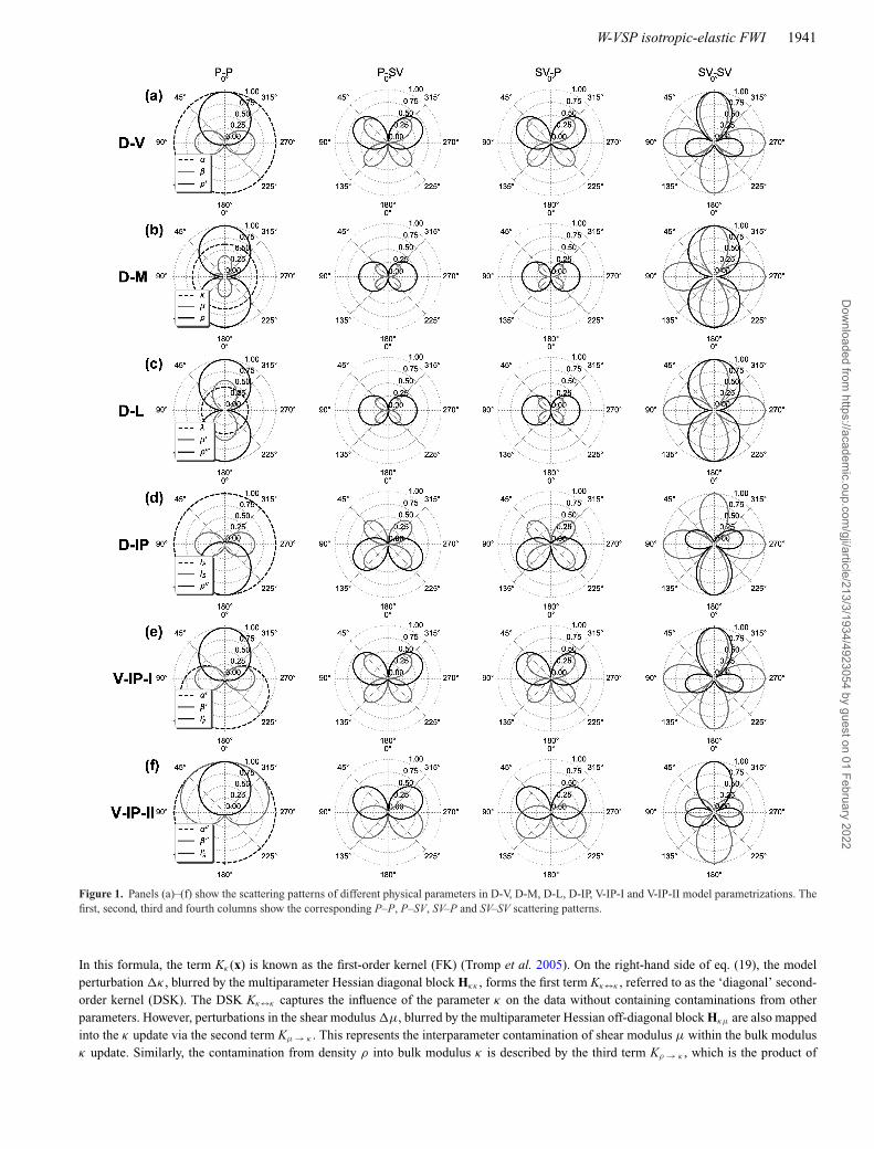
Most current parameter resolution studies follow the work of Tarantola (1986), by making using of scattering radiation patterns, whichare proportional to the amplitude variations with opening angle of the scattered wavefields caused by point heterogeneities (or horizontalreflectors) (Tarantola 1986; Operto et al. 2013; Gholami et al. 2013b; Alkhalifah & Plessix 2014; Kamath & Tsvankin 2014; Moradi & Innanen2015; Pan et al. 2016; Oh & Alkhalifah 2016; Rusmanugroho et al. 2017). The coupling effects between different physical parameters atdifferent scattering angles (or azimuthal angles for 3-D) with different wave modes can be qualitatively inferred from their scattering patterns.Furthermore, strong forward-scattered energy associated with a particular model perturbation will contribute to updating long wavelength ofthat model parameter. Strong backward-scattered waves will contribute to updating short wavelength of the model parameter. In this paper,we derive the scattering patterns for our six different model parametrizations, using the framework of Stolt & Weglein (2012). The explicitderivation process and expressions for these scattering patterns can be found in Appendix B.
Setting the background model properties P-wave velocity, S-wave velocity and density as 3 km s−1, 1.5 km s−1 and 1.6 g cm−3, wecalculate the scattering patterns of different physical parameters in various model parametrizations, as illustrated in Fig. 1. Because theW-VSP data set is dominated by first arrivals and transmitted waves, we focus on the coupling effects between different physical parametersat large scattering angles (135o–225o). In the D-V parametrization (Fig. 1a), for transmitted P–P waves, α and ρ ′ will evidently be morerobustly distinguished than they would in a reflection survey. This is because P–P wave energy radiating from density variations mostlyscatters backward. When the source and receiver are on opposite sides of the unknown medium, as they are in a W-VSP configuration, thecontamination of density ρ ′ into P-wave velocity α and S-wave velocity β is expected to be small. In the D-M parametrization, the P-Pscattering patterns associated with κ , μ and ρ overlap significantly, as shown in Fig. 1(b). This is suggestive that the parameters κ , μ and ρ
correlate with each other strongly in their influence on the transmitted P–P waveforms. Within the P–SV, SV–P and SV–SV waves, it is alsoevidently difficult to decouple parameters μ and ρ. The scattering patterns in the D-L parametrization also overlap significantly, similarly tothe D-M parametrization, as shown in Fig. 1(c). This is suggestive that the D-L parametrization also has poor parameter resolution. In theD-IP parametrization (Fig. 1d), the P-wave impedance IP and density ρ ′ are predicted to have strong, and similar, influences on the transmittedP-P wave amplitudes, and thus should be expected to be difficult to separately determine. In the V-IP-I parametrization, we observe thatthe P-P waves radiating from a perturbation in the P-wave velocity α′ mainly scatter forwards, while those radiating from a perturbationof the P-wave impedance I ′
P mainly scatter backwards. This means that the coupling between α′ and I ′P in a W-VSP survey will be weak.
The V-IP-II parametrization is expected to have a higher parameter resolution than the other model parametrizations, because the scatteringpatterns (especially P–SV, SV–P and SV–SV) of different physical parameters are cleanly separated, as shown in Fig. 1(f).
Scattering radiation patterns provide an efficient means to evaluate the interparameter trade-offs between different physical parameters asthey are simultaneously determined using different wave modes. However, because the scattering patterns only measure the amplitude variationsof the Frechet derivative wavefields, the parameter correlations they illuminate are those associated with an asymptotic multiparameter Gauss-Newton Hessian (Operto et al. 2013; Alkhalifah & Plessix 2014). Perturbations of model properties in reality also result in changes of thetraveltime and phase of the full wavefield, and so scattering patterns do not characterize interparameter trade-offs completely. For example,perturbations in the P-wave velocity result in the changes of amplitude and traveltime of the wavefield. However, traveltime is almostinsensitive to density variations (Plonka et al. 2016). Because the traveltime information plays a dominant role when inverting W-VSP data,scattering patterns cannot completely characterize interparameter trade-offs within this type of isotropic-elastic FWI application.
3.2 Interparameter contamination kernels
In this section, we demonstrate that unwanted parameter cross-talk artefacts are described by interparameter contamination kernels, whichcan be calculated efficiently by applying multiparameter Hessian off-diagonal blocks to the model perturbation vectors with the adjoint-state approach. Compared to the scattering patterns, the interparameter contamination kernels provide a more wave-theoretically completemeasurement of interparameter trade-offs.
Within the Newton linear system in multiparameter isotropic-elastic FWI, the sensitivity kernel Kκ for bulk modulus κ can be writtenas an integral form (Fichtner & van Leeuwen 2015) as
Kκ (x) = −a−1κ
∫x′∈
[Hκκ
(x, x′)�κ
(x′) + Hκμ
(x, x′) �μ
(x′) + Hκρ
(x, x′) �ρ
(x′)] dx′
= Kκ↔κ (x) + Kμ→κ (x) + Kρ→κ (x) . (19)
Dow
nloaded from https://academ
ic.oup.com/gji/article/213/3/1934/4923054 by guest on 01 February 2022
W-VSP isotropic-elastic FWI 1941
Figure 1. Panels (a)–(f) show the scattering patterns of different physical parameters in D-V, D-M, D-L, D-IP, V-IP-I and V-IP-II model parametrizations. Thefirst, second, third and fourth columns show the corresponding P–P, P–SV, SV–P and SV–SV scattering patterns.
In this formula, the term Kκ (x) is known as the first-order kernel (FK) (Tromp et al. 2005). On the right-hand side of eq. (19), the modelperturbation �κ , blurred by the multiparameter Hessian diagonal block Hκκ , forms the first term Kκ↔κ , referred to as the ‘diagonal’ second-order kernel (DSK). The DSK Kκ↔κ captures the influence of the parameter κ on the data without containing contaminations from otherparameters. However, perturbations in the shear modulus �μ, blurred by the multiparameter Hessian off-diagonal block Hκμ are also mappedinto the κ update via the second term Kμ → κ . This represents the interparameter contamination of shear modulus μ within the bulk modulusκ update. Similarly, the contamination from density ρ into bulk modulus κ is described by the third term Kρ → κ , which is the product of
Dow
nloaded from https://academ
ic.oup.com/gji/article/213/3/1934/4923054 by guest on 01 February 2022
1942 W. Pan, K.A. Innanen and Y. Geng
the multiparameter Hessian off-diagonal block Hκρ with the model perturbation �ρ. In contrast to DSK Kκ↔κ , Kμ → κ and Kρ → κ are the‘off-diagonal’ second-order kernels and in this paper they are referred to as ‘interparameter contamination’ kernels (ICKs). The FKs Kμ andKρ for shear modulus μ and density ρ respectively also involve interparameter contaminations:
Kμ (x) = −a−1μ
∫x′∈
[Hμκ
(x, x′) �κ
(x′) + Hμμ
(x, x′) �μ
(x′) + Hμρ
(x, x′) �ρ
(x′)] dx′
= Kκ→μ (x) + Kμ↔μ (x) + Kρ→μ (x) , (20)
Kρ (x) = −a−1ρ
∫x′∈
[Hρκ
(x, x′) �κ
(x′) + Hρμ
(x, x′)�μ
(x′) + Hρρ
(x, x′)�ρ
(x′)] dx′
= Kκ→ρ (x) + Kμ→ρ (x) + Kρ↔ρ (x) . (21)
Here Kμ↔μ and Kρ↔ρ are the DSKs for shear modulus μ and density ρ without containing contaminations from other parameters. Kκ → μ,Kρ → μ, Kκ → μ and Kμ → ρ are the corresponding ICKs. Similar expressions can be obtained for any desired parametrization using eqs (19),(20) and (21).
Interparameter contamination, as defined above, are determined by both the off-diagonal multiparameter Hessian blocks and the modelperturbation vectors. The ICKs measure interparameter contaminations taking amplitude, traveltime, phase, acquisition geometry, etc., intoconsideration. Examining the relative strengths and characteristics of the FKs, DSKs and ICKs provides a direct means to understand howthe interparameter trade-offs affect model updates in the inversion process. If the magnitudes of ICKs (i.e. Kκ → ρ) within some regions ofthe model are stronger than the magnitudes of DSKs (i.e. Kρ↔ρ), the FKs (i.e. Kρ) will be dominated by the contamination, meaning stronginterparameter trade-offs. If the magnitudes of ICKs are much smaller than the magnitudes of the DSKs, interparameter trade-offs can beexpected to be weak, and can be ignored. The multiparameter Hessian off-diagonal blocks may furthermore transform the model perturbationvectors into polarity-conserved or polarity-reversed interparameter contamination. This permits a prediction of whether the inverted modelswill be underestimated, overestimated or distorted.
The product of the Hessian with an arbitrary vector can be efficiently calculated with the adjoint-state approach, which has been a criticalpart of the practical implementation of truncated-Newton optimization methods (Metivier et al. 2013, 2014) and uncertainty quantification(Fichtner & Trampert 2011a,b; Fichtner & van Leeuwen 2015; Zhu et al. 2016). In analysing the Hessian in this study, we neglect thesecond-order term in the full Hessian and calculate the product of the multiparameter Gauss–Newton Hessian with model perturbation vectorsusing the first-order adjoint-state approach. Following Metivier et al. (2013), we consider minimizing the following Lagrangian function:
χ(m, u, �, fs) = uνR
−∫ t ′
0
∫x∈
� (x, t) · [ρ (x) ∂2
t u (x, t) − ∇ · (c (x) : ∇u (x, t)) − f (xs, t)]
dxdt, (22)
where ν can be any vector and � is the new Lagrangian multiplier. Following the first-order adjoint-state method given from eq. (2) toeq. (6), the variation of the new Lagrangian function χ due to the perturbation of wavefield u and model parameters can be written as:
�χ =∫ t ′
0
∫x∈
{νR − [
ρ (x) ∂2t � (x, t) − ∇ · (
c (x) : ∇� (x, t))]} · �u (x, t) dxdt
−∫ t ′
0
∫x∈
[�ρ (x) � (x, t) · ∂2
t u (x, t) + ∇� (x, t) : �c (x) : ∇u (x, t)]
dxdt. (23)
Similarly setting the coefficient of wavefield perturbation to zero gives the following adjoint-state equation:
ρ (x) ∂2t � (x, t) − ∇ · [
c (x) : ∇� (x, t)] = νR, (24)
where νR serves as the adjoint source and Lagrangian multiplier wavefield � can be obtained by solving eq. (24):
� (x, t) =∫ t
0νRG
(x, t − t ′′) dt ′′, (25)
where G is the Green’s tensor and the Lagrangian multiplier wavefield satisfies the boundary condition: n · (c : ∇�
) = 0 on ∂ and the endconditions: � (x, t ′) = 0, ∂t� (x, t ′) = 0. Thus, the variation of the Lagrangian functional is simplified to:
�χ = −∫ t ′
0
∫x∈
[�ρ (x) � (x, t) · ∂2
t u (x, t) + ∇� (x, t) : �c (x) : ∇u (x, t)]
dxdt. (26)
Because the Gauss–Newton Hessian is given by: H = ∇mu†R†R∇mu, to calculate the multiparameter Gauss–Newton Hessian-vector product,we consider the transpose of the gradient of the misfit function χ with respect to density ρ and elastic tensor c:
∇ρ χ† = ∇ρu†R†ν† = −
∫ t ′
0
∫x∈
∂2t u† (
x, t ′′) · G† (x, t ′ − t ′′) R†ν†dxdt ′′, (27)
Dow
nloaded from https://academ
ic.oup.com/gji/article/213/3/1934/4923054 by guest on 01 February 2022
W-VSP isotropic-elastic FWI 1943
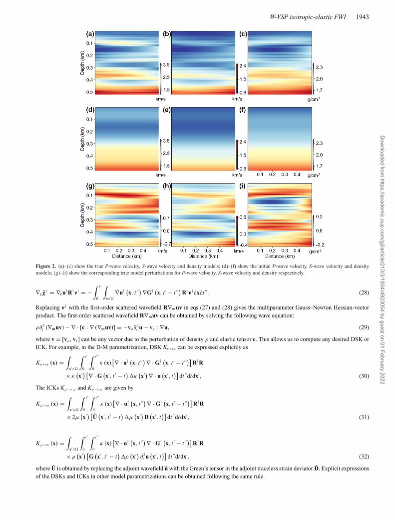
Figure 2. (a)–(c) show the true P-wave velocity, S-wave velocity and density models; (d)–(f) show the initial P-wave velocity, S-wave velocity and densitymodels; (g)–(i) show the corresponding true model perturbations for P-wave velocity, S-wave velocity and density respectively.
∇cχ† = ∇cu
†R†ν† = −∫ t ′
0
∫x∈
∇u† (x, t ′′) ∇G† (
x, t ′ − t ′′) R†ν†dxdt ′′. (28)
Replacing ν† with the first-order scattered wavefield R∇muv in eqs (27) and (28) gives the multiparameter Gauss–Newton Hessian-vectorproduct. The first-order scattered wavefield R∇muv can be obtained by solving the following wave equation:
ρ∂2t (∇muv) − ∇ · [c : ∇ (∇muv)] = −vρ∂
2t u − vc : ∇u, (29)
where v = [vρ , vc] can be any vector due to the perturbation of density ρ and elastic tensor c. This allows us to compute any desired DSK orICK. For example, in the D-M parametrization, DSK Kκ↔κ can be expressed explicitly as
Kκ↔κ (x) =∫
x′∈
∫ t ′
0
∫ t ′′
0κ (x)
[∇ · u† (x, t ′′)∇ · G† (
x, t ′ − t ′′)] R†R
× κ(x′) [∇ · G
(x′, t ′ − t
)�κ
(x′) ∇ · u
(x′, t
)]dt ′′dtdx′, (30)
The ICKs Kμ → κ and Kρ → κ are given by
Kμ→κ (x) =∫
x′∈
∫ t ′
0
∫ t ′′
0κ (x)
[∇ · u† (x, t ′′)∇ · G† (
x, t ′ − t ′′)] R†R
× 2μ(x′) [
U(x′, t ′ − t
)�μ
(x′) D
(x′, t
)]dt ′′dtdx′, (31)
Kρ→κ (x) =∫
x′∈
∫ t ′
0
∫ t ′′
0κ (x)
[∇ · u† (x, t ′′)∇ · G† (
x, t ′ − t ′′)] R†R
× ρ(x′) [
G(x′, t ′ − t
)�ρ
(x′) ∂2
t u(x′, t
)]dt ′′dtdx′, (32)
where U is obtained by replacing the adjoint wavefield u with the Green’s tensor in the adjoint traceless strain deviator D. Explicit expressionsof the DSKs and ICKs in other model parametrizations can be obtained following the same rule.
Dow
nloaded from https://academ
ic.oup.com/gji/article/213/3/1934/4923054 by guest on 01 February 2022
1944 W. Pan, K.A. Innanen and Y. Geng
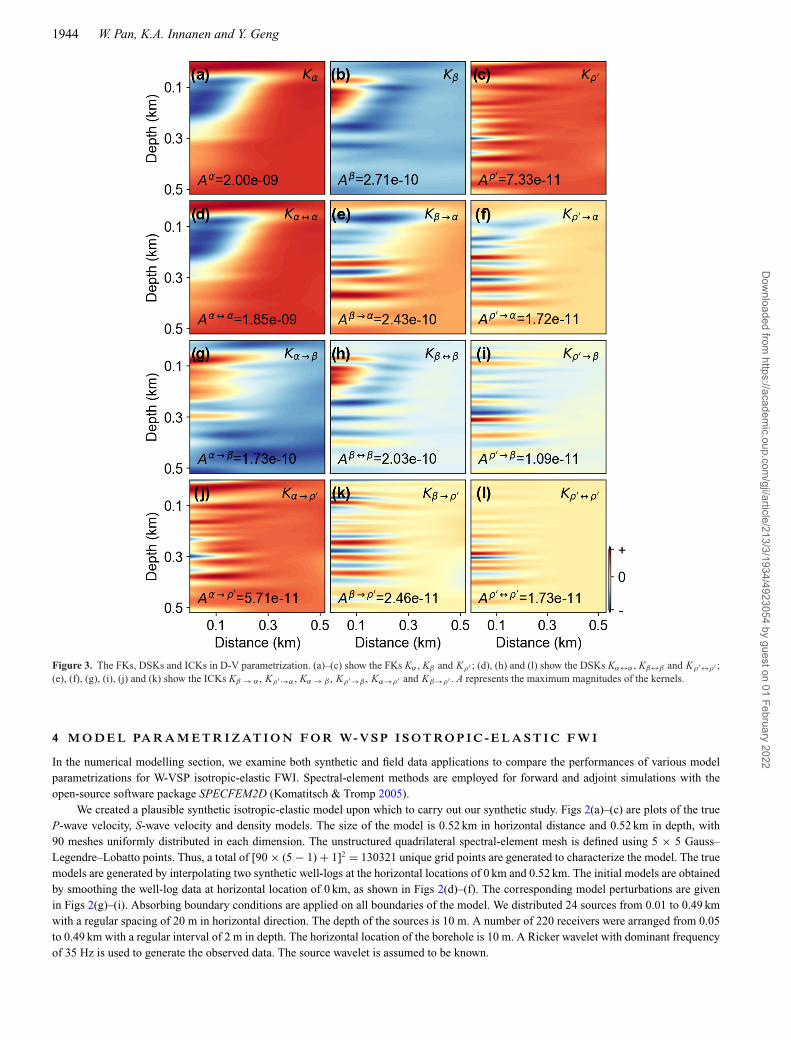
Figure 3. The FKs, DSKs and ICKs in D-V parametrization. (a)–(c) show the FKs Kα , Kβ and Kρ′ ; (d), (h) and (l) show the DSKs Kα↔α , Kβ↔β and Kρ′↔ρ′ ;(e), (f), (g), (i), (j) and (k) show the ICKs Kβ → α , Kρ′→α , Kα → β , Kρ′→β , Kα→ρ′ and Kβ→ρ′ . A represents the maximum magnitudes of the kernels.
4 M O D E L PA R A M E T R I Z AT I O N F O R W- V S P I S O T RO P I C - E L A S T I C F W I
In the numerical modelling section, we examine both synthetic and field data applications to compare the performances of various modelparametrizations for W-VSP isotropic-elastic FWI. Spectral-element methods are employed for forward and adjoint simulations with theopen-source software package SPECFEM2D (Komatitsch & Tromp 2005).
We created a plausible synthetic isotropic-elastic model upon which to carry out our synthetic study. Figs 2(a)–(c) are plots of the trueP-wave velocity, S-wave velocity and density models. The size of the model is 0.52 km in horizontal distance and 0.52 km in depth, with90 meshes uniformly distributed in each dimension. The unstructured quadrilateral spectral-element mesh is defined using 5 × 5 Gauss–Legendre–Lobatto points. Thus, a total of [90 × (5 − 1) + 1]2 = 130321 unique grid points are generated to characterize the model. The truemodels are generated by interpolating two synthetic well-logs at the horizontal locations of 0 km and 0.52 km. The initial models are obtainedby smoothing the well-log data at horizontal location of 0 km, as shown in Figs 2(d)–(f). The corresponding model perturbations are givenin Figs 2(g)–(i). Absorbing boundary conditions are applied on all boundaries of the model. We distributed 24 sources from 0.01 to 0.49 kmwith a regular spacing of 20 m in horizontal direction. The depth of the sources is 10 m. A number of 220 receivers were arranged from 0.05to 0.49 km with a regular interval of 2 m in depth. The horizontal location of the borehole is 10 m. A Ricker wavelet with dominant frequencyof 35 Hz is used to generate the observed data. The source wavelet is assumed to be known.
Dow
nloaded from https://academ
ic.oup.com/gji/article/213/3/1934/4923054 by guest on 01 February 2022
W-VSP isotropic-elastic FWI 1945
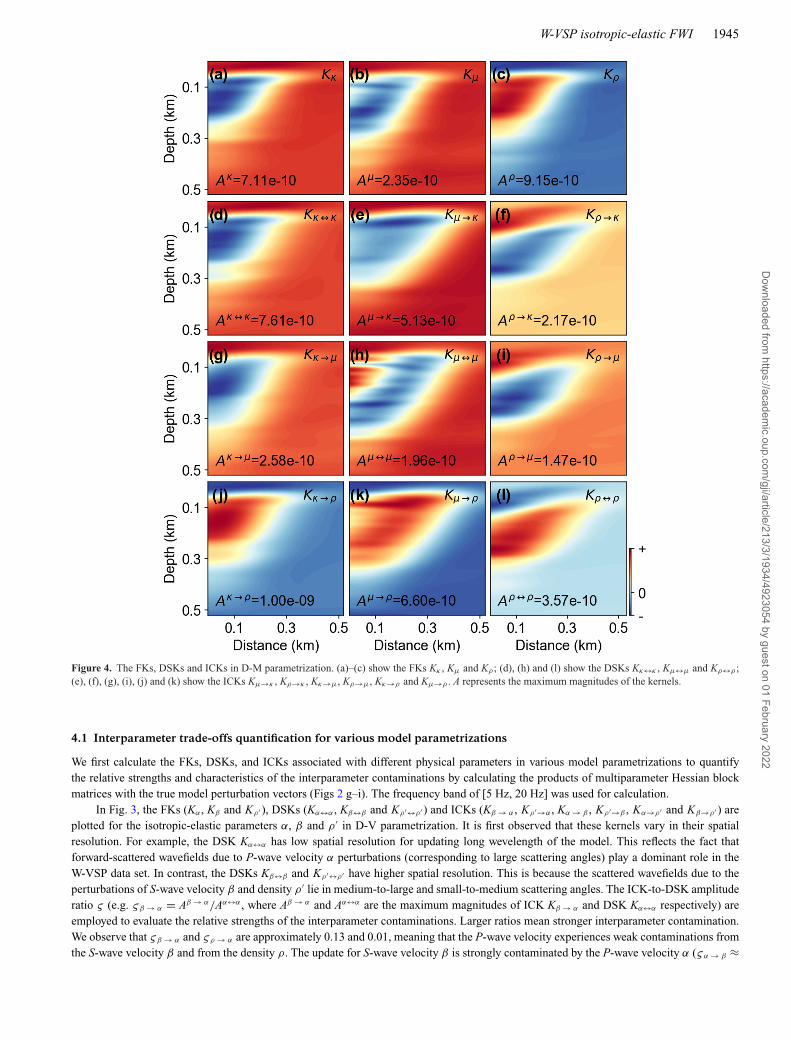
Figure 4. The FKs, DSKs and ICKs in D-M parametrization. (a)–(c) show the FKs Kκ , Kμ and Kρ ; (d), (h) and (l) show the DSKs Kκ↔κ , Kμ↔μ and Kρ↔ρ ;(e), (f), (g), (i), (j) and (k) show the ICKs Kμ→κ , Kρ→κ , Kκ→μ, Kρ→μ, Kκ→ρ and Kμ→ρ . A represents the maximum magnitudes of the kernels.
4.1 Interparameter trade-offs quantification for various model parametrizations
We first calculate the FKs, DSKs, and ICKs associated with different physical parameters in various model parametrizations to quantifythe relative strengths and characteristics of the interparameter contaminations by calculating the products of multiparameter Hessian blockmatrices with the true model perturbation vectors (Figs 2 g–i). The frequency band of [5 Hz, 20 Hz] was used for calculation.
In Fig. 3, the FKs (Kα , Kβ and Kρ′ ), DSKs (Kα↔α , Kβ↔β and Kρ′↔ρ′ ) and ICKs (Kβ → α , Kρ′→α , Kα → β , Kρ′→β , Kα→ρ′ and Kβ→ρ′ ) areplotted for the isotropic-elastic parameters α, β and ρ ′ in D-V parametrization. It is first observed that these kernels vary in their spatialresolution. For example, the DSK Kα↔α has low spatial resolution for updating long wevelength of the model. This reflects the fact thatforward-scattered wavefields due to P-wave velocity α perturbations (corresponding to large scattering angles) play a dominant role in theW-VSP data set. In contrast, the DSKs Kβ↔β and Kρ′↔ρ′ have higher spatial resolution. This is because the scattered wavefields due to theperturbations of S-wave velocity β and density ρ ′ lie in medium-to-large and small-to-medium scattering angles. The ICK-to-DSK amplituderatio ς (e.g. ςβ → α = Aβ → α/Aα↔α , where Aβ → α and Aα↔α are the maximum magnitudes of ICK Kβ → α and DSK Kα↔α respectively) areemployed to evaluate the relative strengths of the interparameter contaminations. Larger ratios mean stronger interparameter contamination.We observe that ςβ → α and ςρ → α are approximately 0.13 and 0.01, meaning that the P-wave velocity experiences weak contaminations fromthe S-wave velocity β and from the density ρ. The update for S-wave velocity β is strongly contaminated by the P-wave velocity α (ςα → β ≈
Dow
nloaded from https://academ
ic.oup.com/gji/article/213/3/1934/4923054 by guest on 01 February 2022
1946 W. Pan, K.A. Innanen and Y. Geng
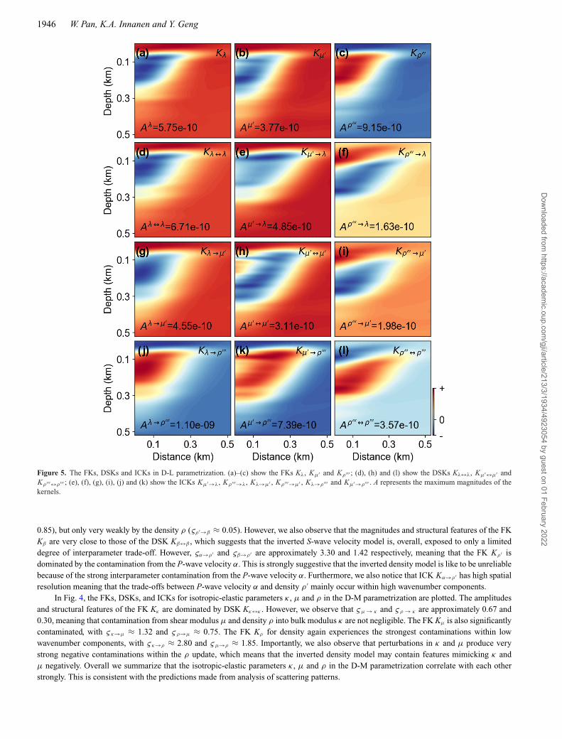
Figure 5. The FKs, DSKs and ICKs in D-L parametrization. (a)–(c) show the FKs Kλ, Kμ′ and Kρ′′′ ; (d), (h) and (l) show the DSKs Kλ↔λ, Kμ′↔μ′ andKρ′′′↔ρ′′′ ; (e), (f), (g), (i), (j) and (k) show the ICKs Kμ′→λ, Kρ′′′→λ, Kλ→μ′ , Kρ′′′→μ′ , Kλ→ρ′′′ and Kμ′→ρ′′′ . A represents the maximum magnitudes of thekernels.
0.85), but only very weakly by the density ρ (ςρ′→β ≈ 0.05). However, we also observe that the magnitudes and structural features of the FKKβ are very close to those of the DSK Kβ↔β , which suggests that the inverted S-wave velocity model is, overall, exposed to only a limiteddegree of interparameter trade-off. However, ςα→ρ′ and ςβ→ρ′ are approximately 3.30 and 1.42 respectively, meaning that the FK Kρ′ isdominated by the contamination from the P-wave velocity α. This is strongly suggestive that the inverted density model is like to be unreliablebecause of the strong interparameter contamination from the P-wave velocity α. Furthermore, we also notice that ICK Kα→ρ′ has high spatialresolution meaning that the trade-offs between P-wave velocity α and density ρ ′ mainly occur within high wavenumber components.
In Fig. 4, the FKs, DSKs, and ICKs for isotropic-elastic parameters κ , μ and ρ in the D-M parametrization are plotted. The amplitudesand structural features of the FK Kκ are dominated by DSK Kκ↔κ . However, we observe that ςμ → κ and ςρ → κ are approximately 0.67 and0.30, meaning that contamination from shear modulus μ and density ρ into bulk modulus κ are not negligible. The FK Kμ is also significantlycontaminated, with ςκ→μ ≈ 1.32 and ςρ→μ ≈ 0.75. The FK Kρ for density again experiences the strongest contaminations within lowwavenumber components, with ςκ→ρ ≈ 2.80 and ςμ→ρ ≈ 1.85. Importantly, we also observe that perturbations in κ and μ produce verystrong negative contaminations within the ρ update, which means that the inverted density model may contain features mimicking κ andμ negatively. Overall we summarize that the isotropic-elastic parameters κ , μ and ρ in the D-M parametrization correlate with each otherstrongly. This is consistent with the predictions made from analysis of scattering patterns.
Dow
nloaded from https://academ
ic.oup.com/gji/article/213/3/1934/4923054 by guest on 01 February 2022
W-VSP isotropic-elastic FWI 1947
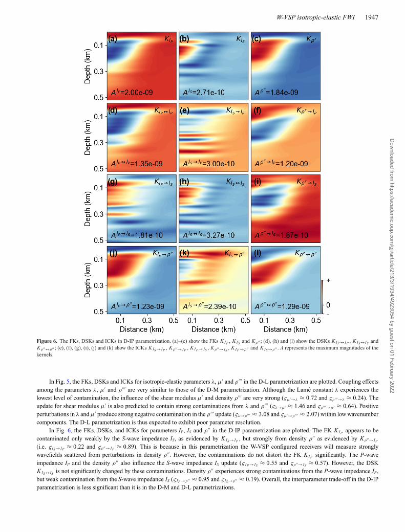
Figure 6. The FKs, DSKs and ICKs in D-IP parametrization. (a)–(c) show the FKs KIP , K IS and Kρ′′ ; (d), (h) and (l) show the DSKs KIP ↔IP , K IS↔IS andKρ′′↔ρ′′ ; (e), (f), (g), (i), (j) and (k) show the ICKs KIS→IP , Kρ′′→IP , K IP →IS , Kρ′′→IS , K IP →ρ′′ and K IS→ρ′′ . A represents the maximum magnitudes of thekernels.
In Fig. 5, the FKs, DSKs and ICKs for isotropic-elastic parameters λ, μ′ and ρ ′′′ in the D-L parametrization are plotted. Coupling effectsamong the parameters λ, μ′ and ρ ′′′ are very similar to those of the D-M parametrization. Although the Lame constant λ experiences thelowest level of contamination, the influence of the shear modulus μ′ and density ρ ′′′ are very strong (ςμ′→λ ≈ 0.72 and ςρ′′′→λ ≈ 0.24). Theupdate for shear modulus μ′ is also predicted to contain strong contaminations from λ and ρ ′′′ (ςλ→μ′ ≈ 1.46 and ςρ′′′→μ′ ≈ 0.64). Positiveperturbations in λ and μ′ produce strong negative contamination in the ρ ′′′ update (ςλ→ρ′′′ ≈ 3.08 and ςμ′→ρ′′′ ≈ 2.07) within low wavenumbercomponents. The D-L parametrization is thus expected to exhibit poor parameter resolution.
In Fig. 6, the FKs, DSKs, and ICKs for parameters IP, IS and ρ ′′ in the D-IP parametrization are plotted. The FK KIP appears to becontaminated only weakly by the S-wave impedance IS, as evidenced by KIS→IP , but strongly from density ρ ′′ as evidenced by Kρ′′→IP
(i.e. ςIS→IP ≈ 0.22 and ςρ′′→IP ≈ 0.89). This is because in this parametrization the W-VSP configured receivers will measure stronglywavefields scattered from perturbations in density ρ ′′. However, the contaminations do not distort the FK KIP significantly. The P-waveimpedance IP and the density ρ ′′ also influence the S-wave impedance IS update (ςIP →IS ≈ 0.55 and ςρ′′→IS ≈ 0.57). However, the DSKKIS↔IS is not significantly changed by these contaminations. Density ρ ′′ experiences strong contaminations from the P-wave impedance IP,but weak contamination from the S-wave impedance IS (ςIP →ρ′′ ≈ 0.95 and ςIS→ρ′′ ≈ 0.19). Overall, the interparameter trade-off in the D-IPparametrization is less significant than it is in the D-M and D-L parametrizations.
Dow
nloaded from https://academ
ic.oup.com/gji/article/213/3/1934/4923054 by guest on 01 February 2022
1948 W. Pan, K.A. Innanen and Y. Geng
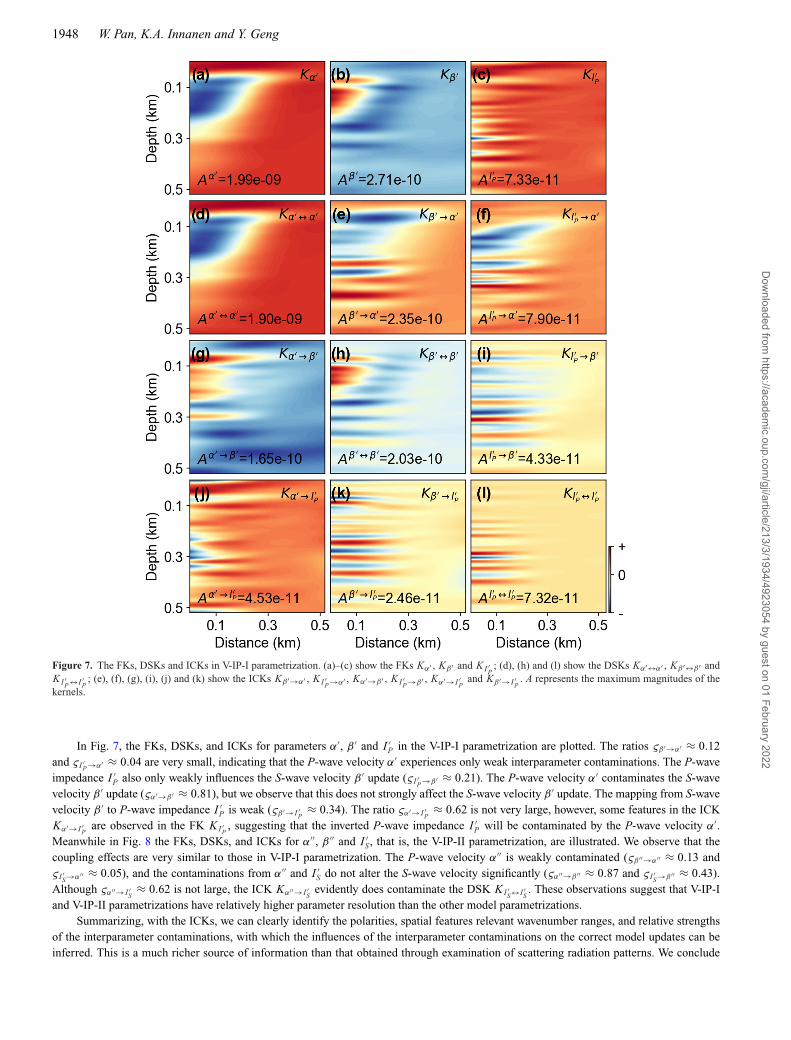
Figure 7. The FKs, DSKs and ICKs in V-IP-I parametrization. (a)–(c) show the FKs Kα′ , Kβ ′ and K I ′P
; (d), (h) and (l) show the DSKs Kα′↔α′ , Kβ ′↔β ′ andK I ′
P ↔I ′P
; (e), (f), (g), (i), (j) and (k) show the ICKs Kβ ′→α′ , K I ′P →α′ , Kα′→β ′ , K I ′
P →β ′ , Kα′→I ′P
and Kβ ′→I ′P
. A represents the maximum magnitudes of thekernels.
In Fig. 7, the FKs, DSKs, and ICKs for parameters α′, β ′ and I ′P in the V-IP-I parametrization are plotted. The ratios ςβ ′→α′ ≈ 0.12
and ςI ′P →α′ ≈ 0.04 are very small, indicating that the P-wave velocity α′ experiences only weak interparameter contaminations. The P-wave
impedance I ′P also only weakly influences the S-wave velocity β ′ update (ςI ′
P →β ′ ≈ 0.21). The P-wave velocity α′ contaminates the S-wavevelocity β ′ update (ςα′→β ′ ≈ 0.81), but we observe that this does not strongly affect the S-wave velocity β ′ update. The mapping from S-wavevelocity β ′ to P-wave impedance I ′
P is weak (ςβ ′→I ′P
≈ 0.34). The ratio ςα′→I ′P
≈ 0.62 is not very large, however, some features in the ICKKα′→I ′
Pare observed in the FK KI ′
P, suggesting that the inverted P-wave impedance I ′
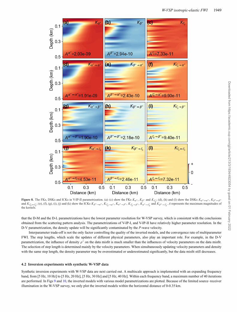
P will be contaminated by the P-wave velocity α′.Meanwhile in Fig. 8 the FKs, DSKs, and ICKs for α′′, β ′′ and I ′
S , that is, the V-IP-II parametrization, are illustrated. We observe that thecoupling effects are very similar to those in V-IP-I parametrization. The P-wave velocity α′′ is weakly contaminated (ςβ ′′→α′′ ≈ 0.13 andςI ′
S→α′′ ≈ 0.05), and the contaminations from α′′ and I ′S do not alter the S-wave velocity significantly (ςα′′→β ′′ ≈ 0.87 and ςI ′
S→β ′′ ≈ 0.43).Although ςα′′→I ′
S≈ 0.62 is not large, the ICK Kα′′→I ′
Sevidently does contaminate the DSK KI ′
S↔I ′S. These observations suggest that V-IP-I
and V-IP-II parametrizations have relatively higher parameter resolution than the other model parametrizations.Summarizing, with the ICKs, we can clearly identify the polarities, spatial features relevant wavenumber ranges, and relative strengths
of the interparameter contaminations, with which the influences of the interparameter contaminations on the correct model updates can beinferred. This is a much richer source of information than that obtained through examination of scattering radiation patterns. We conclude
Dow
nloaded from https://academ
ic.oup.com/gji/article/213/3/1934/4923054 by guest on 01 February 2022
W-VSP isotropic-elastic FWI 1949
Figure 8. The FKs, DSKs and ICKs in V-IP-II parametrization. (a)–(c) show the FKs Kα′′ , Kβ ′′ and K I ′S; (d), (h) and (l) show the DSKs Kα′′↔α′′ , Kβ ′′↔β ′′
and K I ′S↔I ′
S; (e), (f), (g), (i), (j) and (k) show the ICKs Kβ ′′→α′′ , K I ′
S→α′′ , Kα′′→β ′′ , K I ′S→β ′′ , Kα′′→I ′
Sand Kβ ′′→I ′
S. A represents the maximum magnitudes of
the kernels.
that the D-M and the D-L parametrizations have the lowest parameter resolution for W-VSP survey, which is consistent with the conclusionsobtained from the scattering pattern analysis. The parametrizations of V-IP-I, and V-IP-II have relatively higher parameter resolution. In theD-V parametrization, the density update will be significantly contaminated by the P-wave velocity.
Interparameter trade-off is not the only factor controlling the quality of the inverted models, and the convergence rate of multiparameterFWI. The step lengths, which scale the updates of different physical parameters, also play an important role. For example, in the D-Vparametrization, the influence of density ρ ′′ on the data misfit is much smaller than the influences of velocity parameters on the data misfit.The selection of step length is determined mainly by the velocity parameters. When simultaneously updating velocity parameters and densitywith the same step length, the density parameter may be overestimated or underestimated significantly, but the data misfit still decreases.
4.2 Inversion experiments with synthetic W-VSP data
Synthetic inversion experiments with W-VSP data are next carried out. A multiscale approach is implemented with an expanding frequencyband, from [5 Hz, 10 Hz] to [5 Hz, 20 Hz], [5 Hz, 30 Hz] and [5 Hz, 40 Hz]. Within each frequency band, a maximum number of 40 iterationsare performed. In Figs 9 and 10, the inverted models with various model parametrizations are plotted. Because of the limited source–receiverillumination in the W-VSP survey, we only plot the inverted models within the horizontal distance of 0-0.35 km.
Dow
nloaded from https://academ
ic.oup.com/gji/article/213/3/1934/4923054 by guest on 01 February 2022
1950 W. Pan, K.A. Innanen and Y. Geng
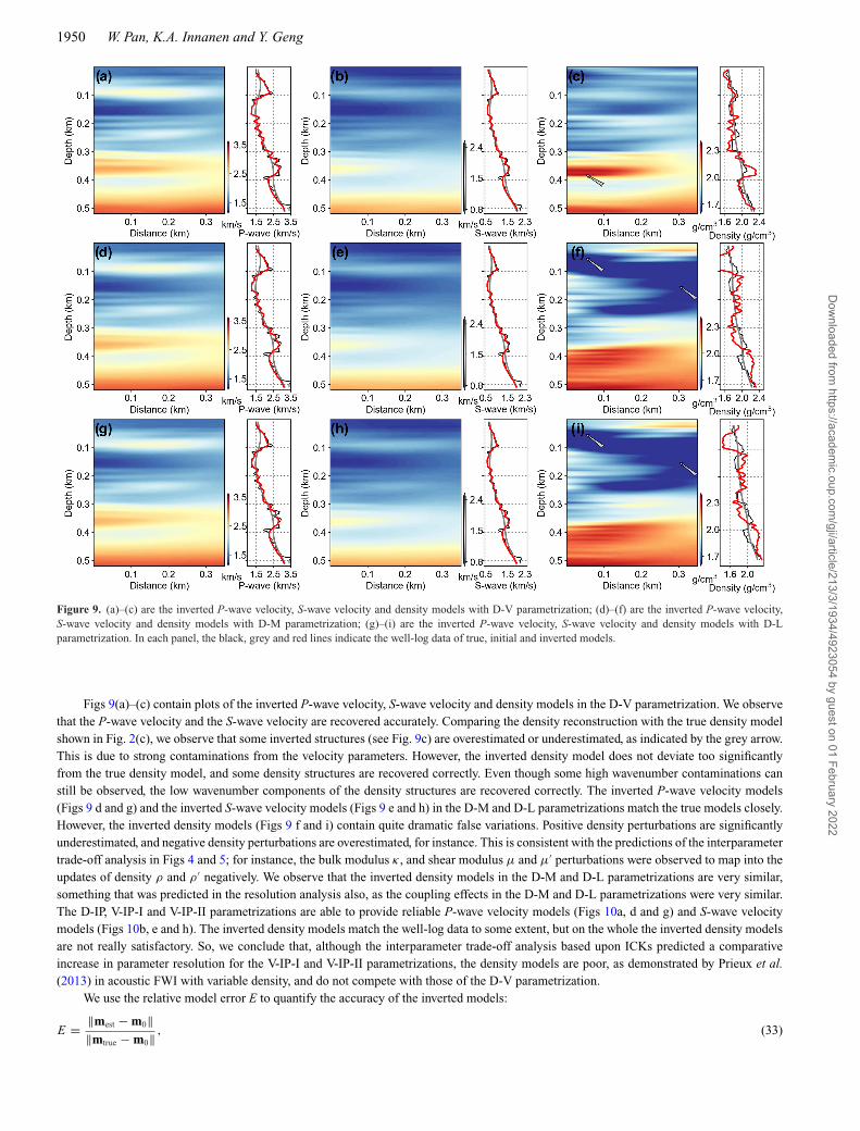
Figure 9. (a)–(c) are the inverted P-wave velocity, S-wave velocity and density models with D-V parametrization; (d)–(f) are the inverted P-wave velocity,S-wave velocity and density models with D-M parametrization; (g)–(i) are the inverted P-wave velocity, S-wave velocity and density models with D-Lparametrization. In each panel, the black, grey and red lines indicate the well-log data of true, initial and inverted models.
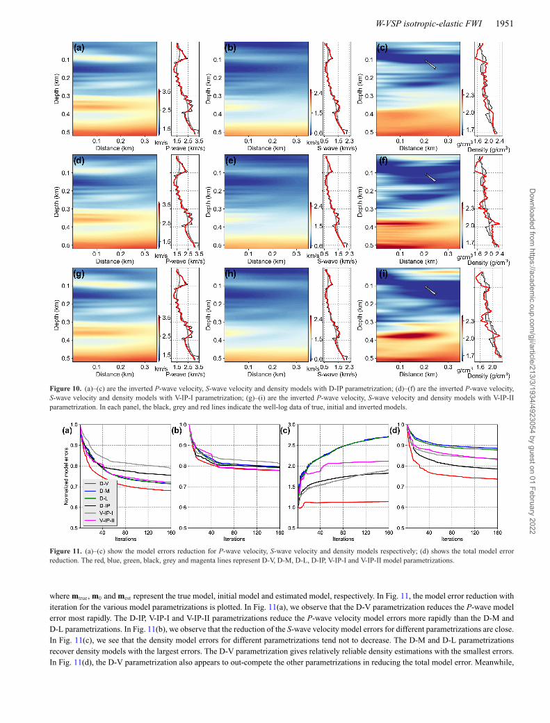
Figs 9(a)–(c) contain plots of the inverted P-wave velocity, S-wave velocity and density models in the D-V parametrization. We observethat the P-wave velocity and the S-wave velocity are recovered accurately. Comparing the density reconstruction with the true density modelshown in Fig. 2(c), we observe that some inverted structures (see Fig. 9c) are overestimated or underestimated, as indicated by the grey arrow.This is due to strong contaminations from the velocity parameters. However, the inverted density model does not deviate too significantlyfrom the true density model, and some density structures are recovered correctly. Even though some high wavenumber contaminations canstill be observed, the low wavenumber components of the density structures are recovered correctly. The inverted P-wave velocity models(Figs 9 d and g) and the inverted S-wave velocity models (Figs 9 e and h) in the D-M and D-L parametrizations match the true models closely.However, the inverted density models (Figs 9 f and i) contain quite dramatic false variations. Positive density perturbations are significantlyunderestimated, and negative density perturbations are overestimated, for instance. This is consistent with the predictions of the interparametertrade-off analysis in Figs 4 and 5; for instance, the bulk modulus κ , and shear modulus μ and μ′ perturbations were observed to map into theupdates of density ρ and ρ ′ negatively. We observe that the inverted density models in the D-M and D-L parametrizations are very similar,something that was predicted in the resolution analysis also, as the coupling effects in the D-M and D-L parametrizations were very similar.The D-IP, V-IP-I and V-IP-II parametrizations are able to provide reliable P-wave velocity models (Figs 10a, d and g) and S-wave velocitymodels (Figs 10b, e and h). The inverted density models match the well-log data to some extent, but on the whole the inverted density modelsare not really satisfactory. So, we conclude that, although the interparameter trade-off analysis based upon ICKs predicted a comparativeincrease in parameter resolution for the V-IP-I and V-IP-II parametrizations, the density models are poor, as demonstrated by Prieux et al.(2013) in acoustic FWI with variable density, and do not compete with those of the D-V parametrization.
We use the relative model error E to quantify the accuracy of the inverted models:
E = ‖mest − m0‖‖mtrue − m0‖ , (33)
Dow
nloaded from https://academ
ic.oup.com/gji/article/213/3/1934/4923054 by guest on 01 February 2022
W-VSP isotropic-elastic FWI 1951
Figure 10. (a)–(c) are the inverted P-wave velocity, S-wave velocity and density models with D-IP parametrization; (d)–(f) are the inverted P-wave velocity,S-wave velocity and density models with V-IP-I parametrization; (g)–(i) are the inverted P-wave velocity, S-wave velocity and density models with V-IP-IIparametrization. In each panel, the black, grey and red lines indicate the well-log data of true, initial and inverted models.
Figure 11. (a)–(c) show the model errors reduction for P-wave velocity, S-wave velocity and density models respectively; (d) shows the total model errorreduction. The red, blue, green, black, grey and magenta lines represent D-V, D-M, D-L, D-IP, V-IP-I and V-IP-II model parametrizations.
where mtrue, m0 and mest represent the true model, initial model and estimated model, respectively. In Fig. 11, the model error reduction withiteration for the various model parametrizations is plotted. In Fig. 11(a), we observe that the D-V parametrization reduces the P-wave modelerror most rapidly. The D-IP, V-IP-I and V-IP-II parametrizations reduce the P-wave velocity model errors more rapidly than the D-M andD-L parametrizations. In Fig. 11(b), we observe that the reduction of the S-wave velocity model errors for different parametrizations are close.In Fig. 11(c), we see that the density model errors for different parametrizations tend not to decrease. The D-M and D-L parametrizationsrecover density models with the largest errors. The D-V parametrization gives relatively reliable density estimations with the smallest errors.In Fig. 11(d), the D-V parametrization also appears to out-compete the other parametrizations in reducing the total model error. Meanwhile,
Dow
nloaded from https://academ
ic.oup.com/gji/article/213/3/1934/4923054 by guest on 01 February 2022
1952 W. Pan, K.A. Innanen and Y. Geng
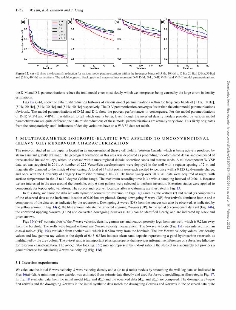
Figure 12. (a)–(d) show the data misfit reduction for various model parametrizations within the frequency bands of [5 Hz, 10 Hz] to [5 Hz, 20 Hz], [5 Hz, 30 Hz]and [5 Hz, 40 Hz] respectively. The red, blue, green, black, grey and magenta lines represent D-V, D-M, D-L, D-IP, V-IP-I and V-IP-II model parametrizations.
the D-M and D-L parametrizations reduce the total model error most slowly, which we interpret as being caused by the large errors in densityestimations.
Figs 12(a)–(d) show the data misfit reduction histories of various model parametrizations within the frequency bands of [5 Hz, 10 Hz],[5 Hz, 20 Hz], [5 Hz, 30 Hz] and [5 Hz, 40 Hz] respectively. The D-V parametrization converges faster than the other model parametrizationsobviously. The model parametrizations of D-M and D-L show the poorest performances in convergence. For the model parametrizationsof D-IP, V-IP-I and V-IP-II, it is difficult to tell which one is better. Even though the inverted density models provided by various modelparametrizations are quite different, the data misfit reductions of these model parametrizations are actually very close. This likely originatesfrom the comparatively small influences of density variations have on a W-VSP data set misfit.
5 M U LT I PA R A M E T E R I S O T RO P I C - E L A S T I C F W I A P P L I E D T O U N C O N V E N T I O NA L( H E AV Y O I L ) R E S E RV O I R C H A R A C T E R I Z AT I O N
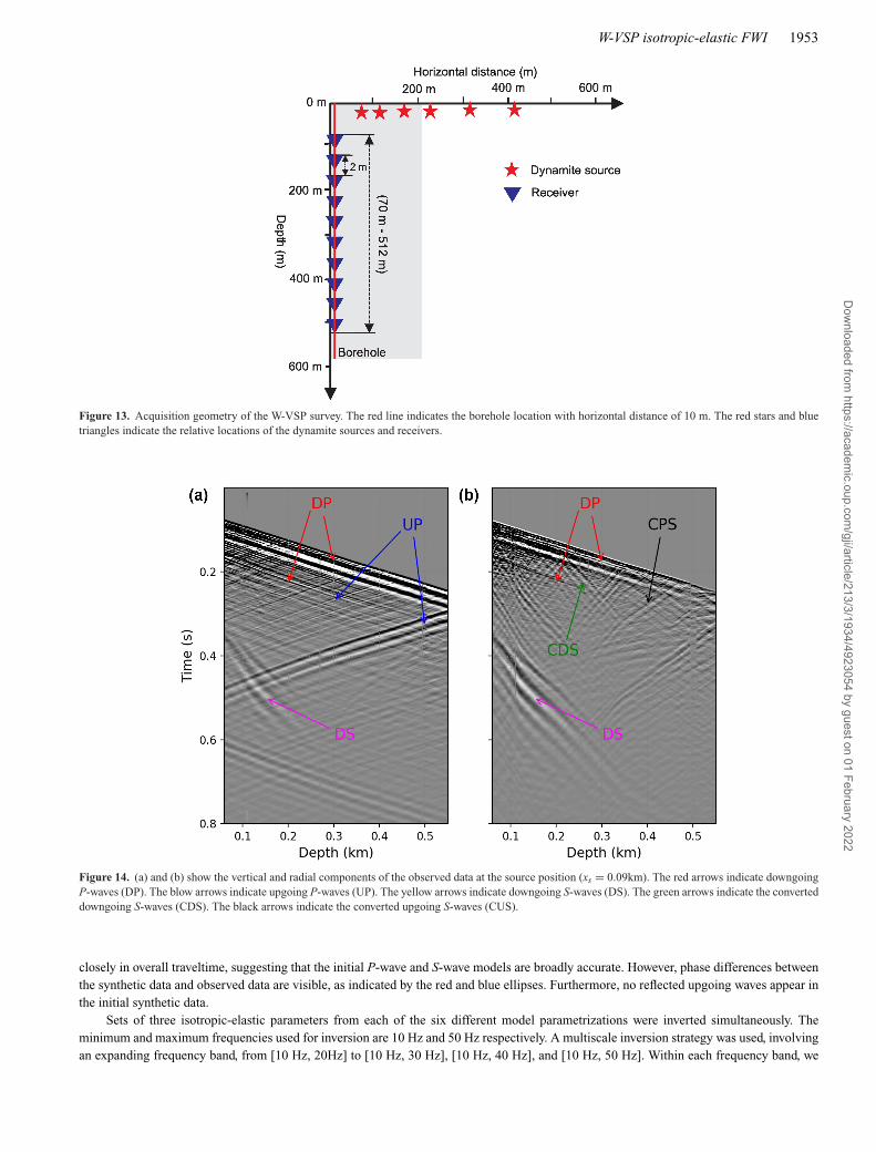
The reservoir studied in this paper is located in an unconventional (heavy oil) field in Western Canada, which is being actively produced bysteam assistant gravity drainage. The geological formation in this area was deposited as prograding tide-dominated deltas and composed ofthree stacked incised valleys, which lie encased within more regional deltaic, shoreface sands and marine sands. A multicomponent W-VSPdata set was acquired in 2011. A number of 222 VectorSeis accelerometers were deployed in the well with a regular spacing of 2 m andmagnetically clamped to the inside of steel casing. A total of 14 shot points were each excited twice, once with a 0.125 kg dynamite charge,and once with the University of Calgary EnviroVibe running a 10–300 Hz linear sweep over 20 s. All data were acquired at night, withsurface temperatures in the -5 to 10 degree Celsius range. The maximum recording time is 3 s with a sampling interval of 0.001 s. Becausewe are interested in the area around the borehole, only 6 shot gathers were selected to perform inversion. Elevation statics were applied tocompensate for topographic variations. The source and receiver locations after re-datuming are illustrated in Fig. 13.
In this study, we chose the data set with dynamite sources for inversion. In Figs 14(a) and (b), the vertical (z) and radial (x) componentsof the observed data at the horizontal location of 0.09 km are plotted. Strong downgoing P-wave (DP) first arrivals dominate both z and xcomponents of the data set, as indicated by the red arrows. Downgoing S-waves (DS) from the sources can also be observed, as indicated bythe yellow arrows. In Fig. 14(a), the blue arrows indicate the reflected upgoing P-waves (UP). In the radial (x) component data set (Fig. 14b),the converted upgoing S-waves (CUS) and converted downgoing S-waves (CDS) can be identified clearly, and are indicated by black andgreen arrows.
Figs 15(a)–(d) contain plots of the P-wave velocity, density, gamma ray and neutron porosity logs from one well, which is 0.2 km awayfrom the borehole. The wells were logged without any S-wave velocity measurement. The S-wave velocity (Fig. 15f) was inferred from anα-to-β ratio σ (Fig. 15e) available from another well, which is 0.5 km away from the borehole. The low P-wave velocity values, low densityvalues and low gamma ray values at the depth of 0.45–0.5 km indicate clean sand deposits representing a good hydrocarbon reservoir, ashighlighted by the grey colour. The α-to-β ratio is an important physical property that provides informative inferences on subsurface lithologyfor reservoir characterization. The α-to-β ratio log (Fig. 15c) may not represent the α-to-β ratio in the studied area accurately but provides agood reference for calculating S-wave velocity log (Fig. 15d).
5.1 Inversion experiments
We calculate the initial P-wave velocity, S-wave velocity, density and σ (α-to-β ratio) models by smoothing the well-log data, as indicated inFigs 16(a)–(d). A minimum phase wavelet was estimated from seismic data directly and used for forward modelling, as illustrated in Fig. 17.In Fig. 18 synthetic data from the initial model (dz
init and dxinit) and the observed data (dz
obs and dxobs) are compared. The downgoing P-wave
first arrivals and the downgoing S-waves in the initial synthetic data match the downgoing P-waves and S-waves in the observed data quite
Dow
nloaded from https://academ
ic.oup.com/gji/article/213/3/1934/4923054 by guest on 01 February 2022
W-VSP isotropic-elastic FWI 1953
Figure 13. Acquisition geometry of the W-VSP survey. The red line indicates the borehole location with horizontal distance of 10 m. The red stars and bluetriangles indicate the relative locations of the dynamite sources and receivers.
Figure 14. (a) and (b) show the vertical and radial components of the observed data at the source position (xs = 0.09km). The red arrows indicate downgoingP-waves (DP). The blow arrows indicate upgoing P-waves (UP). The yellow arrows indicate downgoing S-waves (DS). The green arrows indicate the converteddowngoing S-waves (CDS). The black arrows indicate the converted upgoing S-waves (CUS).
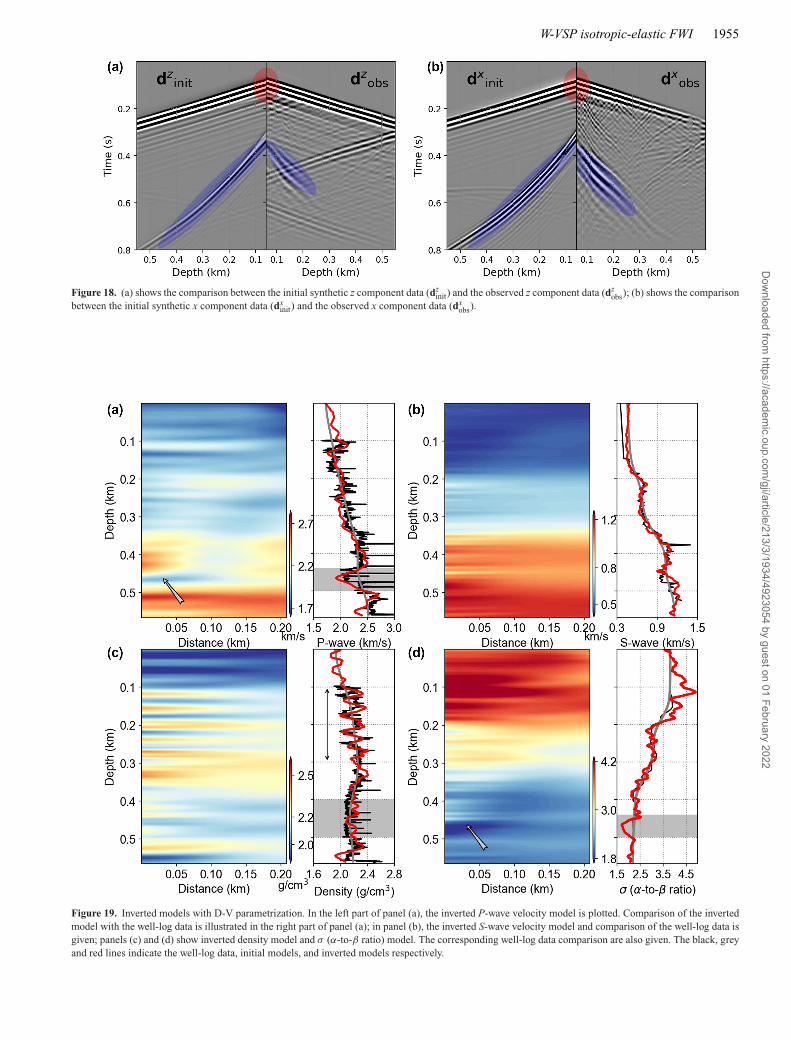
closely in overall traveltime, suggesting that the initial P-wave and S-wave models are broadly accurate. However, phase differences betweenthe synthetic data and observed data are visible, as indicated by the red and blue ellipses. Furthermore, no reflected upgoing waves appear inthe initial synthetic data.
Sets of three isotropic-elastic parameters from each of the six different model parametrizations were inverted simultaneously. Theminimum and maximum frequencies used for inversion are 10 Hz and 50 Hz respectively. A multiscale inversion strategy was used, involvingan expanding frequency band, from [10 Hz, 20Hz] to [10 Hz, 30 Hz], [10 Hz, 40 Hz], and [10 Hz, 50 Hz]. Within each frequency band, we
Dow
nloaded from https://academ
ic.oup.com/gji/article/213/3/1934/4923054 by guest on 01 February 2022
1954 W. Pan, K.A. Innanen and Y. Geng
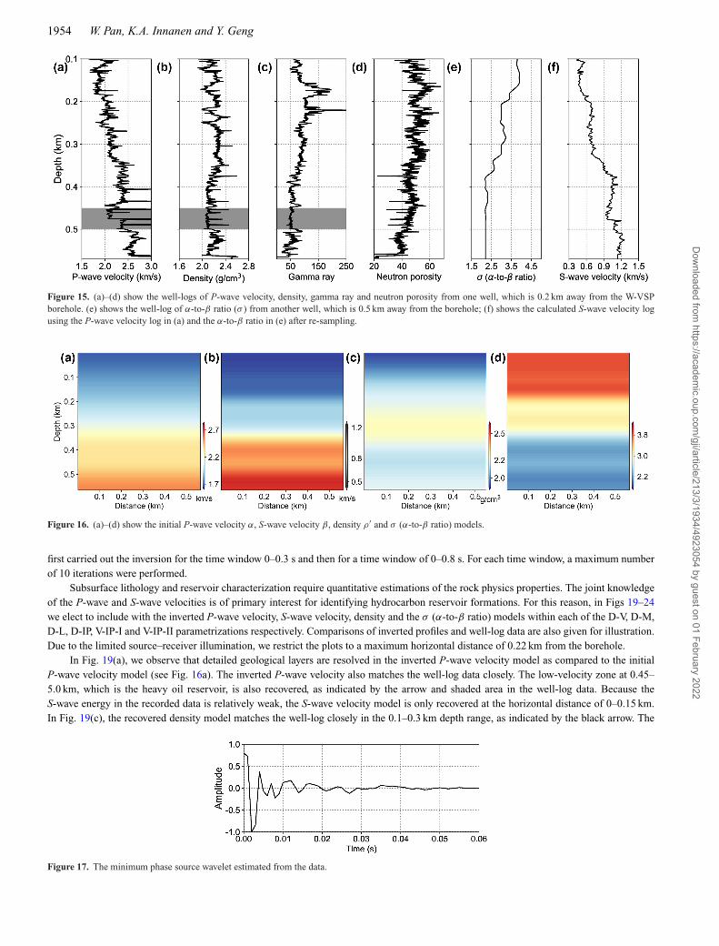
Figure 15. (a)–(d) show the well-logs of P-wave velocity, density, gamma ray and neutron porosity from one well, which is 0.2 km away from the W-VSPborehole. (e) shows the well-log of α-to-β ratio (σ ) from another well, which is 0.5 km away from the borehole; (f) shows the calculated S-wave velocity logusing the P-wave velocity log in (a) and the α-to-β ratio in (e) after re-sampling.
Figure 16. (a)–(d) show the initial P-wave velocity α, S-wave velocity β, density ρ′ and σ (α-to-β ratio) models.
first carried out the inversion for the time window 0–0.3 s and then for a time window of 0–0.8 s. For each time window, a maximum numberof 10 iterations were performed.
Subsurface lithology and reservoir characterization require quantitative estimations of the rock physics properties. The joint knowledgeof the P-wave and S-wave velocities is of primary interest for identifying hydrocarbon reservoir formations. For this reason, in Figs 19–24we elect to include with the inverted P-wave velocity, S-wave velocity, density and the σ (α-to-β ratio) models within each of the D-V, D-M,D-L, D-IP, V-IP-I and V-IP-II parametrizations respectively. Comparisons of inverted profiles and well-log data are also given for illustration.Due to the limited source–receiver illumination, we restrict the plots to a maximum horizontal distance of 0.22 km from the borehole.
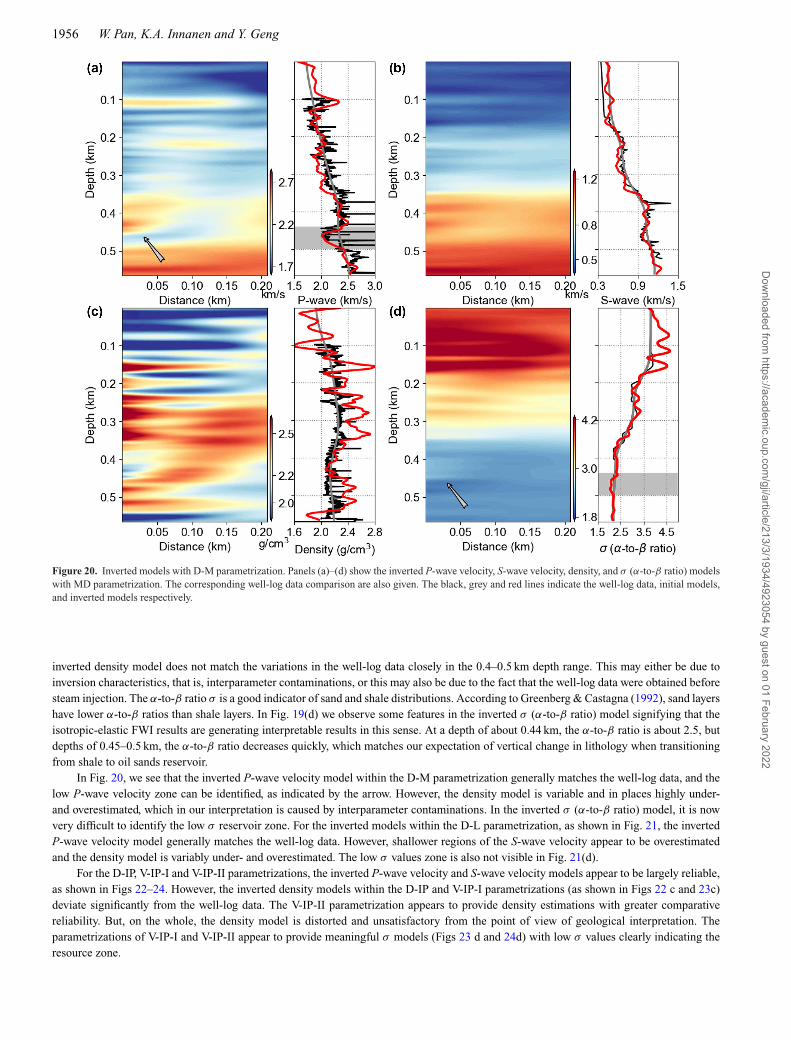
In Fig. 19(a), we observe that detailed geological layers are resolved in the inverted P-wave velocity model as compared to the initialP-wave velocity model (see Fig. 16a). The inverted P-wave velocity also matches the well-log data closely. The low-velocity zone at 0.45–5.0 km, which is the heavy oil reservoir, is also recovered, as indicated by the arrow and shaded area in the well-log data. Because theS-wave energy in the recorded data is relatively weak, the S-wave velocity model is only recovered at the horizontal distance of 0–0.15 km.In Fig. 19(c), the recovered density model matches the well-log closely in the 0.1–0.3 km depth range, as indicated by the black arrow. The
Figure 17. The minimum phase source wavelet estimated from the data.
Dow
nloaded from https://academ
ic.oup.com/gji/article/213/3/1934/4923054 by guest on 01 February 2022
W-VSP isotropic-elastic FWI 1955
Figure 18. (a) shows the comparison between the initial synthetic z component data (dzinit) and the observed z component data (dz
obs); (b) shows the comparisonbetween the initial synthetic x component data (dx
init) and the observed x component data (dxobs).
Figure 19. Inverted models with D-V parametrization. In the left part of panel (a), the inverted P-wave velocity model is plotted. Comparison of the invertedmodel with the well-log data is illustrated in the right part of panel (a); in panel (b), the inverted S-wave velocity model and comparison of the well-log data isgiven; panels (c) and (d) show inverted density model and σ (α-to-β ratio) model. The corresponding well-log data comparison are also given. The black, greyand red lines indicate the well-log data, initial models, and inverted models respectively.
Dow
nloaded from https://academ
ic.oup.com/gji/article/213/3/1934/4923054 by guest on 01 February 2022
1956 W. Pan, K.A. Innanen and Y. Geng
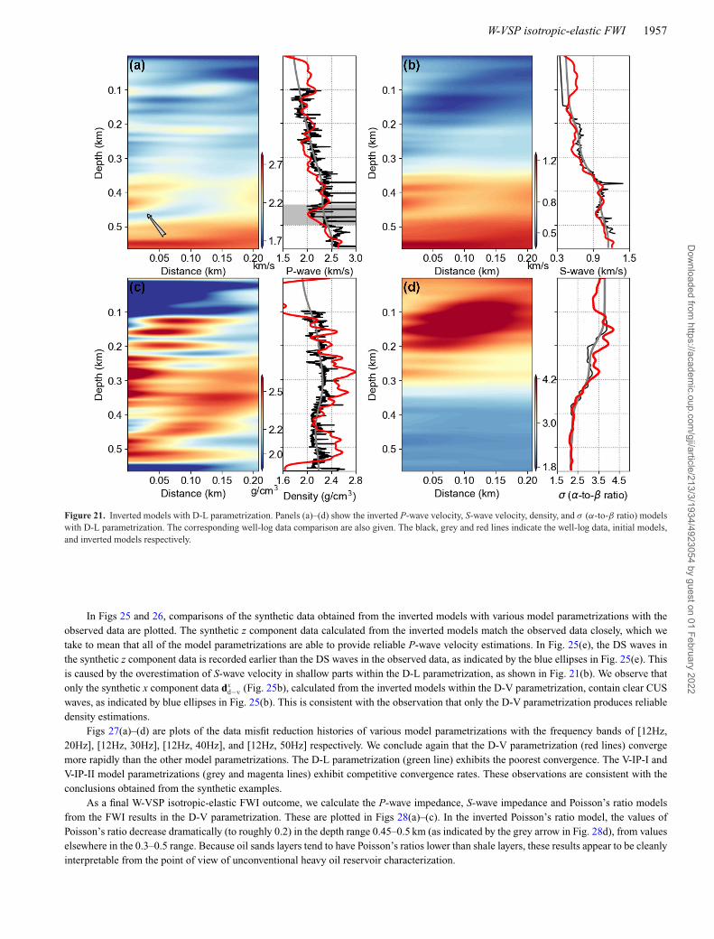
Figure 20. Inverted models with D-M parametrization. Panels (a)–(d) show the inverted P-wave velocity, S-wave velocity, density, and σ (α-to-β ratio) modelswith MD parametrization. The corresponding well-log data comparison are also given. The black, grey and red lines indicate the well-log data, initial models,and inverted models respectively.
inverted density model does not match the variations in the well-log data closely in the 0.4–0.5 km depth range. This may either be due toinversion characteristics, that is, interparameter contaminations, or this may also be due to the fact that the well-log data were obtained beforesteam injection. The α-to-β ratio σ is a good indicator of sand and shale distributions. According to Greenberg & Castagna (1992), sand layershave lower α-to-β ratios than shale layers. In Fig. 19(d) we observe some features in the inverted σ (α-to-β ratio) model signifying that theisotropic-elastic FWI results are generating interpretable results in this sense. At a depth of about 0.44 km, the α-to-β ratio is about 2.5, butdepths of 0.45–0.5 km, the α-to-β ratio decreases quickly, which matches our expectation of vertical change in lithology when transitioningfrom shale to oil sands reservoir.
In Fig. 20, we see that the inverted P-wave velocity model within the D-M parametrization generally matches the well-log data, and thelow P-wave velocity zone can be identified, as indicated by the arrow. However, the density model is variable and in places highly under-and overestimated, which in our interpretation is caused by interparameter contaminations. In the inverted σ (α-to-β ratio) model, it is nowvery difficult to identify the low σ reservoir zone. For the inverted models within the D-L parametrization, as shown in Fig. 21, the invertedP-wave velocity model generally matches the well-log data. However, shallower regions of the S-wave velocity appear to be overestimatedand the density model is variably under- and overestimated. The low σ values zone is also not visible in Fig. 21(d).
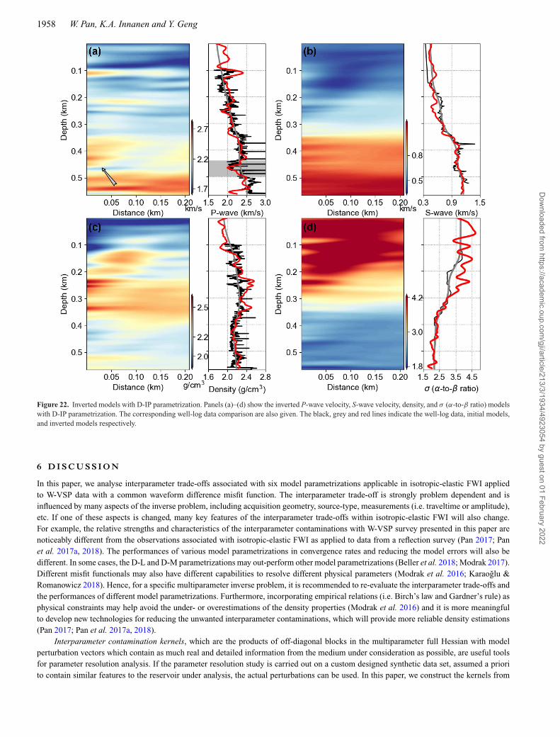
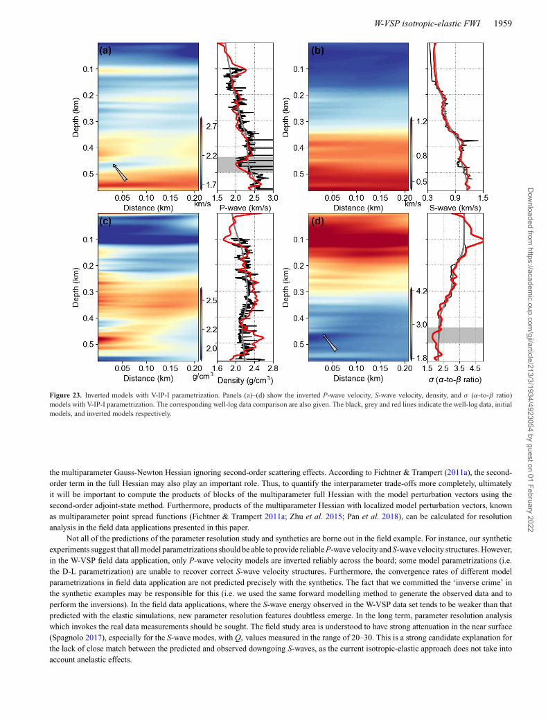
For the D-IP, V-IP-I and V-IP-II parametrizations, the inverted P-wave velocity and S-wave velocity models appear to be largely reliable,as shown in Figs 22–24. However, the inverted density models within the D-IP and V-IP-I parametrizations (as shown in Figs 22 c and 23c)deviate significantly from the well-log data. The V-IP-II parametrization appears to provide density estimations with greater comparativereliability. But, on the whole, the density model is distorted and unsatisfactory from the point of view of geological interpretation. Theparametrizations of V-IP-I and V-IP-II appear to provide meaningful σ models (Figs 23 d and 24d) with low σ values clearly indicating theresource zone.
Dow
nloaded from https://academ
ic.oup.com/gji/article/213/3/1934/4923054 by guest on 01 February 2022
W-VSP isotropic-elastic FWI 1957
Figure 21. Inverted models with D-L parametrization. Panels (a)–(d) show the inverted P-wave velocity, S-wave velocity, density, and σ (α-to-β ratio) modelswith D-L parametrization. The corresponding well-log data comparison are also given. The black, grey and red lines indicate the well-log data, initial models,and inverted models respectively.
In Figs 25 and 26, comparisons of the synthetic data obtained from the inverted models with various model parametrizations with theobserved data are plotted. The synthetic z component data calculated from the inverted models match the observed data closely, which wetake to mean that all of the model parametrizations are able to provide reliable P-wave velocity estimations. In Fig. 25(e), the DS waves inthe synthetic z component data is recorded earlier than the DS waves in the observed data, as indicated by the blue ellipses in Fig. 25(e). Thisis caused by the overestimation of S-wave velocity in shallow parts within the D-L parametrization, as shown in Fig. 21(b). We observe thatonly the synthetic x component data dx
d−v (Fig. 25b), calculated from the inverted models within the D-V parametrization, contain clear CUSwaves, as indicated by blue ellipses in Fig. 25(b). This is consistent with the observation that only the D-V parametrization produces reliabledensity estimations.
Figs 27(a)–(d) are plots of the data misfit reduction histories of various model parametrizations with the frequency bands of [12Hz,20Hz], [12Hz, 30Hz], [12Hz, 40Hz], and [12Hz, 50Hz] respectively. We conclude again that the D-V parametrization (red lines) convergemore rapidly than the other model parametrizations. The D-L parametrization (green line) exhibits the poorest convergence. The V-IP-I andV-IP-II model parametrizations (grey and magenta lines) exhibit competitive convergence rates. These observations are consistent with theconclusions obtained from the synthetic examples.
As a final W-VSP isotropic-elastic FWI outcome, we calculate the P-wave impedance, S-wave impedance and Poisson’s ratio modelsfrom the FWI results in the D-V parametrization. These are plotted in Figs 28(a)–(c). In the inverted Poisson’s ratio model, the values ofPoisson’s ratio decrease dramatically (to roughly 0.2) in the depth range 0.45–0.5 km (as indicated by the grey arrow in Fig. 28d), from valueselsewhere in the 0.3–0.5 range. Because oil sands layers tend to have Poisson’s ratios lower than shale layers, these results appear to be cleanlyinterpretable from the point of view of unconventional heavy oil reservoir characterization.
Dow
nloaded from https://academ
ic.oup.com/gji/article/213/3/1934/4923054 by guest on 01 February 2022
1958 W. Pan, K.A. Innanen and Y. Geng
Figure 22. Inverted models with D-IP parametrization. Panels (a)–(d) show the inverted P-wave velocity, S-wave velocity, density, and σ (α-to-β ratio) modelswith D-IP parametrization. The corresponding well-log data comparison are also given. The black, grey and red lines indicate the well-log data, initial models,and inverted models respectively.
6 D I S C U S S I O N
In this paper, we analyse interparameter trade-offs associated with six model parametrizations applicable in isotropic-elastic FWI appliedto W-VSP data with a common waveform difference misfit function. The interparameter trade-off is strongly problem dependent and isinfluenced by many aspects of the inverse problem, including acquisition geometry, source-type, measurements (i.e. traveltime or amplitude),etc. If one of these aspects is changed, many key features of the interparameter trade-offs within isotropic-elastic FWI will also change.For example, the relative strengths and characteristics of the interparameter contaminations with W-VSP survey presented in this paper arenoticeably different from the observations associated with isotropic-elastic FWI as applied to data from a reflection survey (Pan 2017; Panet al. 2017a, 2018). The performances of various model parametrizations in convergence rates and reducing the model errors will also bedifferent. In some cases, the D-L and D-M parametrizations may out-perform other model parametrizations (Beller et al. 2018; Modrak 2017).Different misfit functionals may also have different capabilities to resolve different physical parameters (Modrak et al. 2016; Karaoglu &Romanowicz 2018). Hence, for a specific multiparameter inverse problem, it is recommended to re-evaluate the interparameter trade-offs andthe performances of different model parametrizations. Furthermore, incorporating empirical relations (i.e. Birch’s law and Gardner’s rule) asphysical constraints may help avoid the under- or overestimations of the density properties (Modrak et al. 2016) and it is more meaningfulto develop new technologies for reducing the unwanted interparameter contaminations, which will provide more reliable density estimations(Pan 2017; Pan et al. 2017a, 2018).
Interparameter contamination kernels, which are the products of off-diagonal blocks in the multiparameter full Hessian with modelperturbation vectors which contain as much real and detailed information from the medium under consideration as possible, are useful toolsfor parameter resolution analysis. If the parameter resolution study is carried out on a custom designed synthetic data set, assumed a priorito contain similar features to the reservoir under analysis, the actual perturbations can be used. In this paper, we construct the kernels from
Dow
nloaded from https://academ
ic.oup.com/gji/article/213/3/1934/4923054 by guest on 01 February 2022
W-VSP isotropic-elastic FWI 1959
Figure 23. Inverted models with V-IP-I parametrization. Panels (a)–(d) show the inverted P-wave velocity, S-wave velocity, density, and σ (α-to-β ratio)models with V-IP-I parametrization. The corresponding well-log data comparison are also given. The black, grey and red lines indicate the well-log data, initialmodels, and inverted models respectively.
the multiparameter Gauss-Newton Hessian ignoring second-order scattering effects. According to Fichtner & Trampert (2011a), the second-order term in the full Hessian may also play an important role. Thus, to quantify the interparameter trade-offs more completely, ultimatelyit will be important to compute the products of blocks of the multiparameter full Hessian with the model perturbation vectors using thesecond-order adjoint-state method. Furthermore, products of the multiparameter Hessian with localized model perturbation vectors, knownas multiparameter point spread functions (Fichtner & Trampert 2011a; Zhu et al. 2015; Pan et al. 2018), can be calculated for resolutionanalysis in the field data applications presented in this paper.
Not all of the predictions of the parameter resolution study and synthetics are borne out in the field example. For instance, our syntheticexperiments suggest that all model parametrizations should be able to provide reliable P-wave velocity and S-wave velocity structures. However,in the W-VSP field data application, only P-wave velocity models are inverted reliably across the board; some model parametrizations (i.e.the D-L parametrization) are unable to recover correct S-wave velocity structures. Furthermore, the convergence rates of different modelparametrizations in field data application are not predicted precisely with the synthetics. The fact that we committed the ‘inverse crime’ inthe synthetic examples may be responsible for this (i.e. we used the same forward modelling method to generate the observed data and toperform the inversions). In the field data applications, where the S-wave energy observed in the W-VSP data set tends to be weaker than thatpredicted with the elastic simulations, new parameter resolution features doubtless emerge. In the long term, parameter resolution analysiswhich invokes the real data measurements should be sought. The field study area is understood to have strong attenuation in the near surface(Spagnolo 2017), especially for the S-wave modes, with Qs values measured in the range of 20–30. This is a strong candidate explanation forthe lack of close match between the predicted and observed downgoing S-waves, as the current isotropic-elastic approach does not take intoaccount anelastic effects.
Dow
nloaded from https://academ
ic.oup.com/gji/article/213/3/1934/4923054 by guest on 01 February 2022
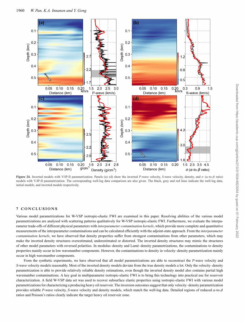
1960 W. Pan, K.A. Innanen and Y. Geng
Figure 24. Inverted models with V-IP-II parametrization. Panels (a)–(d) show the inverted P-wave velocity, S-wave velocity, density, and σ (α-to-β ratio)models with V-IP-II parametrization. The corresponding well-log data comparison are also given. The black, grey and red lines indicate the well-log data,initial models, and inverted models respectively.
7 C O N C LU S I O N S
Various model parametrizations for W-VSP isotropic-elastic FWI are examined in this paper. Resolving abilities of the various modelparametrizations are analysed with scattering patterns qualitatively for W-VSP isotropic-elastic FWI. Furthermore, we evaluate the interpa-rameter trade-offs of different physical parameters with interparameter contamination kernels, which provide more complete and quantitativemeasurements of the interparameter contaminations and can be calculated efficiently with the adjoint-state approach. From the interparametercontamination kernels, we have observed that density properties suffer from strongest contaminations from other parameters, which maymake the inverted density structures overestimated, underestimated or distorted. The inverted density structures may mimic the structuresof other model parameters with reversed polarities. In modulus–density and Lame–density parametrizations, the contaminations to densityproperties mainly occur in low wavenumber components. However, the contaminations to density in velocity–density parametrization mainlyoccur in high wavenumber components.
From the synthetic experiments, we have observed that all model parametrizations are able to reconstruct the P-wave velocity andS-wave velocity models reasonably. Most of the inverted density models deviate from the true density models a lot. Only the velocity–densityparametrization is able to provide relatively reliable density estimations, even though the inverted density model also contains partial highwavenumber contaminations. A key goal in multiparameter isotropic-elastic FWI is to bring this technology into practical use for reservoircharacterization. A field W-VSP data set was used to recover subsurface elastic properties using isotropic-elastic FWI with various modelparametrizations for characterizing a producing heavy oil reservoir. The inversion outcomes suggest that only velocity–density parametrizationprovides reliable P-wave velocity, S-wave velocity and density models, which match the well-log data. Detailed regions of reduced α-to-βratios and Poisson’s ratios clearly indicate the target heavy oil reservoir zone.
Dow
nloaded from https://academ
ic.oup.com/gji/article/213/3/1934/4923054 by guest on 01 February 2022
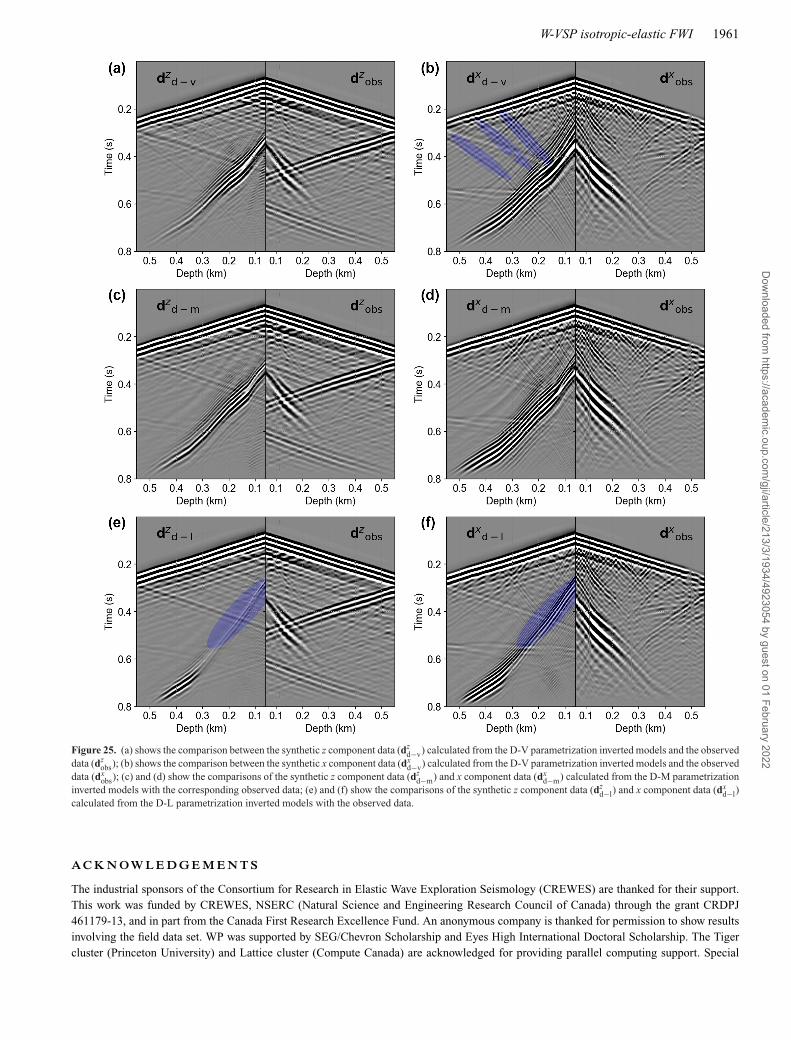
W-VSP isotropic-elastic FWI 1961
Figure 25. (a) shows the comparison between the synthetic z component data (dzd−v) calculated from the D-V parametrization inverted models and the observed
data (dzobs); (b) shows the comparison between the synthetic x component data (dx
d−v) calculated from the D-V parametrization inverted models and the observeddata (dx
obs); (c) and (d) show the comparisons of the synthetic z component data (dzd−m) and x component data (dx
d−m) calculated from the D-M parametrizationinverted models with the corresponding observed data; (e) and (f) show the comparisons of the synthetic z component data (dz
d−l) and x component data (dxd−l)
calculated from the D-L parametrization inverted models with the observed data.
A C K N OW L E D G E M E N T S
The industrial sponsors of the Consortium for Research in Elastic Wave Exploration Seismology (CREWES) are thanked for their support.This work was funded by CREWES, NSERC (Natural Science and Engineering Research Council of Canada) through the grant CRDPJ461179-13, and in part from the Canada First Research Excellence Fund. An anonymous company is thanked for permission to show resultsinvolving the field data set. WP was supported by SEG/Chevron Scholarship and Eyes High International Doctoral Scholarship. The Tigercluster (Princeton University) and Lattice cluster (Compute Canada) are acknowledged for providing parallel computing support. Special
Dow
nloaded from https://academ
ic.oup.com/gji/article/213/3/1934/4923054 by guest on 01 February 2022
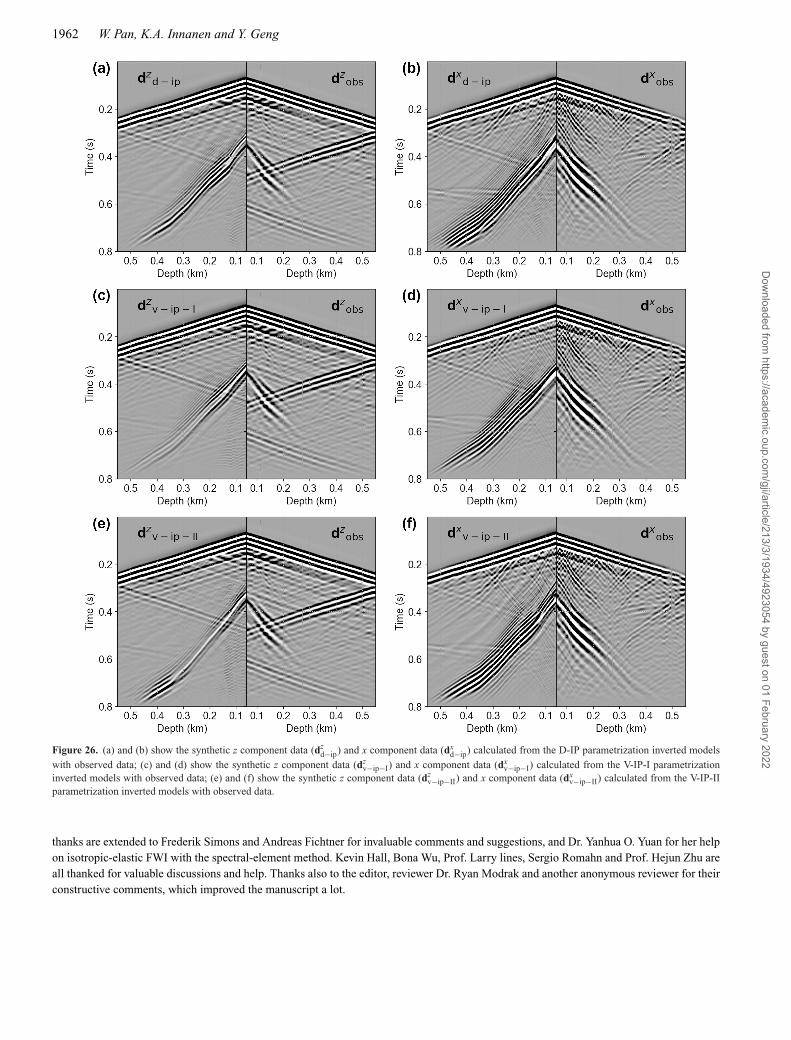
1962 W. Pan, K.A. Innanen and Y. Geng
Figure 26. (a) and (b) show the synthetic z component data (dzd−ip) and x component data (dx
d−ip) calculated from the D-IP parametrization inverted models
with observed data; (c) and (d) show the synthetic z component data (dzv−ip−I) and x component data (dx
v−ip−I) calculated from the V-IP-I parametrizationinverted models with observed data; (e) and (f) show the synthetic z component data (dz
v−ip−II) and x component data (dxv−ip−II) calculated from the V-IP-II
parametrization inverted models with observed data.
thanks are extended to Frederik Simons and Andreas Fichtner for invaluable comments and suggestions, and Dr. Yanhua O. Yuan for her helpon isotropic-elastic FWI with the spectral-element method. Kevin Hall, Bona Wu, Prof. Larry lines, Sergio Romahn and Prof. Hejun Zhu areall thanked for valuable discussions and help. Thanks also to the editor, reviewer Dr. Ryan Modrak and another anonymous reviewer for theirconstructive comments, which improved the manuscript a lot.
Dow
nloaded from https://academ
ic.oup.com/gji/article/213/3/1934/4923054 by guest on 01 February 2022
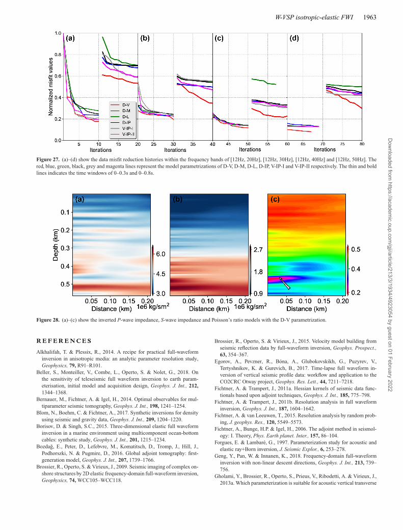
W-VSP isotropic-elastic FWI 1963
Figure 27. (a)–(d) show the data misfit reduction histories within the frequency bands of [12Hz, 20Hz], [12Hz, 30Hz], [12Hz, 40Hz] and [12Hz, 50Hz]. Thered, blue, green, black, grey and magenta lines represent the model parametrizations of D-V, D-M, D-L, D-IP, V-IP-I and V-IP-II respectively. The thin and boldlines indicates the time windows of 0–0.3s and 0–0.8s.
Figure 28. (a)–(c) show the inverted P-wave impedance, S-wave impedance and Poisson’s ratio models with the D-V parametrization.
R E F E R E N C E S
Alkhalifah, T. & Plessix, R., 2014. A recipe for practical full-waveforminversion in anisotropic media: an analytic parameter resolution study,Geophysics, 79, R91–R101.
Beller, S., Monteiller, V., Combe, L., Operto, S. & Nolet, G., 2018. Onthe sensitivity of teleseismic full waveform inversion to earth param-eterisation, initial model and acquisition design, Geophys. J. Int., 212,1344–1368.
Bernauer, M., Fichtner, A. & Igel, H., 2014. Optimal observables for mul-tiparameter seismic tomography, Geophys. J. Int., 198, 1241–1254.
Blom, N., Boehm, C. & Fichtner, A., 2017. Synthetic inversions for densityusing seismic and gravity data, Geophys. J. Int., 209, 1204–1220.
Borisov, D. & Singh, S.C., 2015. Three-dimensional elastic full waveforminversion in a marine environment using multicomponent ocean-bottomcables: synthetic study, Geophys. J. Int., 201, 1215–1234.
Bozdag, E., Peter, D., Lefebvre, M., Komatitsch, D., Tromp, J., Hill, J.,Podhorszki, N. & Pugmire, D., 2016. Global adjoint tomography: first-generation model, Geophys. J. Int., 207, 1739–1766.
Brossier, R., Operto, S. & Virieux, J., 2009. Seismic imaging of complex on-shore structures by 2D elastic frequency-domain full-waveform inversion,Geophysics, 74, WCC105–WCC118.
Brossier, R., Operto, S. & Virieux, J., 2015. Velocity model building fromseismic reflection data by full-waveform inversion, Geophys. Prospect.,63, 354–367.
Egorov, A., Pevzner, R., Bona, A., Glubokovskikh, G., Puzyrev, V.,Tertyshnikov, K. & Gurevich, B., 2017. Time-lapse full waveform in-version of vertical seismic profile data: workflow and application to theCO2CRC Otway project, Geophys. Res. Lett., 44, 7211–7218.
Fichtner, A. & Trampert, J., 2011a. Hessian kernels of seismic data func-tionals based upon adjoint techniques, Geophys. J. Int., 185, 775–798.
Fichtner, A. & Trampert, J., 2011b. Resolution analysis in full waveforminversion, Geophys. J. Int., 187, 1604–1642.
Fichtner, A. & van Leeuwen, T., 2015. Resolution analysis by random prob-ing, J. geophys. Res., 120, 5549–5573.
Fichtner, A., Bunge, H.P. & Igel, H., 2006. The adjoint method in seismol-ogy: I. Theory, Phys. Earth planet. Inter., 157, 86–104.
Forgues, E. & Lambare, G., 1997. Parameterization study for acoustic andelastic ray+Born inversion, J. Seismic Explor., 6, 253–278.
Geng, Y., Pan, W. & Innanen, K., 2018. Frequency-domain full-waveforminversion with non-linear descent directions, Geophys. J. Int., 213, 739–756.
Gholami, Y., Brossier, R., Operto, S., Prieus, V., Ribodetti, A. & Virieux, J.,2013a. Which parameterization is suitable for acoustic vertical transverse
Dow
nloaded from https://academ
ic.oup.com/gji/article/213/3/1934/4923054 by guest on 01 February 2022
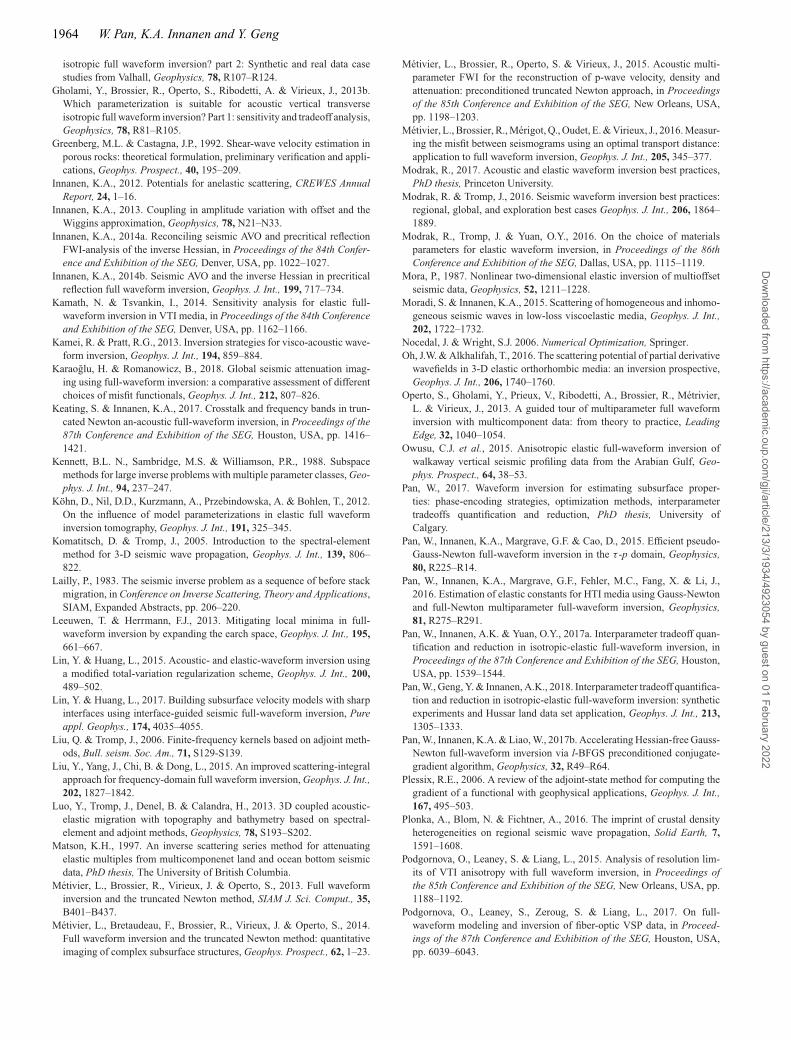
1964 W. Pan, K.A. Innanen and Y. Geng
isotropic full waveform inversion? part 2: Synthetic and real data casestudies from Valhall, Geophysics, 78, R107–R124.
Gholami, Y., Brossier, R., Operto, S., Ribodetti, A. & Virieux, J., 2013b.Which parameterization is suitable for acoustic vertical transverseisotropic full waveform inversion? Part 1: sensitivity and tradeoff analysis,Geophysics, 78, R81–R105.
Greenberg, M.L. & Castagna, J.P., 1992. Shear-wave velocity estimation inporous rocks: theoretical formulation, preliminary verification and appli-cations, Geophys. Prospect., 40, 195–209.
Innanen, K.A., 2012. Potentials for anelastic scattering, CREWES AnnualReport, 24, 1–16.
Innanen, K.A., 2013. Coupling in amplitude variation with offset and theWiggins approximation, Geophysics, 78, N21–N33.
Innanen, K.A., 2014a. Reconciling seismic AVO and precritical reflectionFWI-analysis of the inverse Hessian, in Proceedings of the 84th Confer-ence and Exhibition of the SEG, Denver, USA, pp. 1022–1027.
Innanen, K.A., 2014b. Seismic AVO and the inverse Hessian in precriticalreflection full waveform inversion, Geophys. J. Int., 199, 717–734.
Kamath, N. & Tsvankin, I., 2014. Sensitivity analysis for elastic full-waveform inversion in VTI media, in Proceedings of the 84th Conferenceand Exhibition of the SEG, Denver, USA, pp. 1162–1166.
Kamei, R. & Pratt, R.G., 2013. Inversion strategies for visco-acoustic wave-form inversion, Geophys. J. Int., 194, 859–884.
Karaoglu, H. & Romanowicz, B., 2018. Global seismic attenuation imag-ing using full-waveform inversion: a comparative assessment of differentchoices of misfit functionals, Geophys. J. Int., 212, 807–826.
Keating, S. & Innanen, K.A., 2017. Crosstalk and frequency bands in trun-cated Newton an-acoustic full-waveform inversion, in Proceedings of the87th Conference and Exhibition of the SEG, Houston, USA, pp. 1416–1421.
Kennett, B.L. N., Sambridge, M.S. & Williamson, P.R., 1988. Subspacemethods for large inverse problems with multiple parameter classes, Geo-phys. J. Int., 94, 237–247.
Kohn, D., Nil, D.D., Kurzmann, A., Przebindowska, A. & Bohlen, T., 2012.On the influence of model parameterizations in elastic full waveforminversion tomography, Geophys. J. Int., 191, 325–345.
Komatitsch, D. & Tromp, J., 2005. Introduction to the spectral-elementmethod for 3-D seismic wave propagation, Geophys. J. Int., 139, 806–822.
Lailly, P., 1983. The seismic inverse problem as a sequence of before stackmigration, in Conference on Inverse Scattering, Theory and Applications,SIAM, Expanded Abstracts, pp. 206–220.
Leeuwen, T. & Herrmann, F.J., 2013. Mitigating local minima in full-waveform inversion by expanding the earch space, Geophys. J. Int., 195,661–667.
Lin, Y. & Huang, L., 2015. Acoustic- and elastic-waveform inversion usinga modified total-variation regularization scheme, Geophys. J. Int., 200,489–502.
Lin, Y. & Huang, L., 2017. Building subsurface velocity models with sharpinterfaces using interface-guided seismic full-waveform inversion, Pureappl. Geophys., 174, 4035–4055.
Liu, Q. & Tromp, J., 2006. Finite-frequency kernels based on adjoint meth-ods, Bull. seism. Soc. Am., 71, S129-S139.
Liu, Y., Yang, J., Chi, B. & Dong, L., 2015. An improved scattering-integralapproach for frequency-domain full waveform inversion, Geophys. J. Int.,202, 1827–1842.
Luo, Y., Tromp, J., Denel, B. & Calandra, H., 2013. 3D coupled acoustic-elastic migration with topography and bathymetry based on spectral-element and adjoint methods, Geophysics, 78, S193–S202.
Matson, K.H., 1997. An inverse scattering series method for attenuatingelastic multiples from multicomponenet land and ocean bottom seismicdata, PhD thesis, The University of British Columbia.
Metivier, L., Brossier, R., Virieux, J. & Operto, S., 2013. Full waveforminversion and the truncated Newton method, SIAM J. Sci. Comput., 35,B401–B437.
Metivier, L., Bretaudeau, F., Brossier, R., Virieux, J. & Operto, S., 2014.Full waveform inversion and the truncated Newton method: quantitativeimaging of complex subsurface structures, Geophys. Prospect., 62, 1–23.
Metivier, L., Brossier, R., Operto, S. & Virieux, J., 2015. Acoustic multi-parameter FWI for the reconstruction of p-wave velocity, density andattenuation: preconditioned truncated Newton approach, in Proceedingsof the 85th Conference and Exhibition of the SEG, New Orleans, USA,pp. 1198–1203.
Metivier, L., Brossier, R., Merigot, Q., Oudet, E. & Virieux, J., 2016. Measur-ing the misfit between seismograms using an optimal transport distance:application to full waveform inversion, Geophys. J. Int., 205, 345–377.
Modrak, R., 2017. Acoustic and elastic waveform inversion best practices,PhD thesis, Princeton University.
Modrak, R. & Tromp, J., 2016. Seismic waveform inversion best practices:regional, global, and exploration best cases Geophys. J. Int., 206, 1864–1889.
Modrak, R., Tromp, J. & Yuan, O.Y., 2016. On the choice of materialsparameters for elastic waveform inversion, in Proceedings of the 86thConference and Exhibition of the SEG, Dallas, USA, pp. 1115–1119.
Mora, P., 1987. Nonlinear two-dimensional elastic inversion of multioffsetseismic data, Geophysics, 52, 1211–1228.
Moradi, S. & Innanen, K.A., 2015. Scattering of homogeneous and inhomo-geneous seismic waves in low-loss viscoelastic media, Geophys. J. Int.,202, 1722–1732.
Nocedal, J. & Wright, S.J. 2006. Numerical Optimization, Springer.Oh, J.W. & Alkhalifah, T., 2016. The scattering potential of partial derivative
wavefields in 3-D elastic orthorhombic media: an inversion prospective,Geophys. J. Int., 206, 1740–1760.
Operto, S., Gholami, Y., Prieux, V., Ribodetti, A., Brossier, R., Metrivier,L. & Virieux, J., 2013. A guided tour of multiparameter full waveforminversion with multicomponent data: from theory to practice, LeadingEdge, 32, 1040–1054.
Owusu, C.J. et al., 2015. Anisotropic elastic full-waveform inversion ofwalkaway vertical seismic profiling data from the Arabian Gulf, Geo-phys. Prospect., 64, 38–53.
Pan, W., 2017. Waveform inversion for estimating subsurface proper-ties: phase-encoding strategies, optimization methods, interparametertradeoffs quantification and reduction, PhD thesis, University ofCalgary.
Pan, W., Innanen, K.A., Margrave, G.F. & Cao, D., 2015. Efficient pseudo-Gauss-Newton full-waveform inversion in the τ -p domain, Geophysics,80, R225–R14.
Pan, W., Innanen, K.A., Margrave, G.F., Fehler, M.C., Fang, X. & Li, J.,2016. Estimation of elastic constants for HTI media using Gauss-Newtonand full-Newton multiparameter full-waveform inversion, Geophysics,81, R275–R291.
Pan, W., Innanen, A.K. & Yuan, O.Y., 2017a. Interparameter tradeoff quan-tification and reduction in isotropic-elastic full-waveform inversion, inProceedings of the 87th Conference and Exhibition of the SEG, Houston,USA, pp. 1539–1544.
Pan, W., Geng, Y. & Innanen, A.K., 2018. Interparameter tradeoff quantifica-tion and reduction in isotropic-elastic full-waveform inversion: syntheticexperiments and Hussar land data set application, Geophys. J. Int., 213,1305–1333.
Pan, W., Innanen, K.A. & Liao, W., 2017b. Accelerating Hessian-free Gauss-Newton full-waveform inversion via l-BFGS preconditioned conjugate-gradient algorithm, Geophysics, 32, R49–R64.
Plessix, R.E., 2006. A review of the adjoint-state method for computing thegradient of a functional with geophysical applications, Geophys. J. Int.,167, 495–503.
Plonka, A., Blom, N. & Fichtner, A., 2016. The imprint of crustal densityheterogeneities on regional seismic wave propagation, Solid Earth, 7,1591–1608.
Podgornova, O., Leaney, S. & Liang, L., 2015. Analysis of resolution lim-its of VTI anisotropy with full waveform inversion, in Proceedings ofthe 85th Conference and Exhibition of the SEG, New Orleans, USA, pp.1188–1192.
Podgornova, O., Leaney, S., Zeroug, S. & Liang, L., 2017. On full-waveform modeling and inversion of fiber-optic VSP data, in Proceed-ings of the 87th Conference and Exhibition of the SEG, Houston, USA,pp. 6039–6043.
Dow
nloaded from https://academ
ic.oup.com/gji/article/213/3/1934/4923054 by guest on 01 February 2022
W-VSP isotropic-elastic FWI 1965
Prieux, V., Brossier, R., Operto, S. & Virieux, J., 2013. Multiparameter fullwaveform inversion of multicomponent ocean-bottom-cable data fromthe Valhall field. Part 1: imaging compressional wave speed, density andattenuation, Geophys. J. Int., 194, 1640–1664.
Roberts, M.A., Singh, S. & Hornby, B.E., 2008. Investigation into the use of2D elastic waveform inversion from look-ahead walk-away VSP surveys,Geophys. Prospect., 56, 883–895.
Pratt, R.G., Shin, C. & Hicks, G.J., 1998. Gauss-Newton and full Newtonmethods in frequency-space seismic waveform inversion, Geophys. J. Int.,133, 341–362.
Raknes, E.B. & Arntsen, B., 2015. A numerical study of 3D elastic time-lapse full-waveform inversion using multicomponent seismic data, Geo-physics, 80, R303–R315.
Raknes, E.B., Arntsen, B. & Weibull, W., 2015. Three-dimensional elas-tic full waveform inversion using seismic data from the Sleipner area,Geophys. J. Int., 202, 1877–1894.
Rusmanugroho, H., Modrak, R. & Tromp, J., 2017. Anisotropicfull-waveform inversion with tilt-angle recovery, Geophysics, 82,R135–R151.
Spagnolo, C.M., 2017. Seismic attenuation measurements from multicom-ponent vertical seismic profile data, Master thesis, University of Calgary.
Stolt, R.H. & Weglein, A.B., 2012. Seismic Imaging and Inversion: Appli-cation of Linear Inverse Theory, Cambridge Univ. Express.
Tarantola, A., 1984. Inversion of seismic reflection data in the acousticapproximation, Geophysics, 49, 1259–1266.
Tarantola, A., 1986. A strategy for nonlinear elastic inversion of seismicreflection data, Geophysics, 51, 1893–1903.
Tarantola, A., 2005. Inverse Problem Theory and Methods for Model Pa-rameter Estimation, Society of Industrial and Applied Mathematics.
Tromp, J., Tape, C. & Liu, Q., 2005. Seismic tomography, adjoint meth-ods, time reversal, and banana-doughnut kernels, Geophys. J. Int., 160,195–216.
Virieux, J. & Operto, S., 2009. An overview of full-waveform inversion inexploration geophysics, Geophysics, 74, WCC1–WCC26.
Wang, T. & Cheng, J.B., 2017. Elastic full-waveform inversion based on
mode decomposition: the approach and mechanism, Geophys. J. Int.,209, 606–622.
Wang, Y., Dong, L., Liu, Y. & Yang, J., 2016. 2D frequency-domain elasticfull-waveform inversion using the block-diagonal pseudo-Hessian ap-proximation, Geophysics, 81, R247–R259.
Warner, M. et al., 2013. Anisotropic 3D full-waveform inversion, Geo-physics, 78, R59–R80.
Wu, B., 2016. A Multicomponent Walkaway Vertical Seismic Profile Ex-periment in a heavy oil Reservoir, Master thesis, University of Calgary.
Wu, R., Luo, J. & Wu, B., 2014. Seismic envelope inversion and modulationsignal model, Geophysics, 79, WA13–WA24.
Yang, J., Liu, Y. & Dong, L., 2016. Simultaneous estimation of velocityand density in acoustic multiparameter full-waveform inversion using animproved scattering-integral approach, Geophysics, 81, R399–R415.
Yang, P., Brossier, R., Virieux, J. & Wei, Z., 2017. A Second-order Ad-joint Truncated Newton Approach to Time-domain Multiparameter FullWaveform Inversion in Viscoacoustic Medium, in Proceedings of the 79thConference and Exhibition of the EAGE, Paris, France, p. Tu A3 14.
Yuan, O.Y. & Simons, F.J., 2014. Multiscale adjoint waveform-differencetomography using wavelets, Geophysics, 79, WA79–WA95.
Yuan, O.Y., Simons, F.J. & Bozdag, E., 2015. Multiscale adjoint waveformtomography for surface and body waves, Geophysics, 80, R281–R302.
Yuan, O.Y., Simons, F.J. & Tromp, J., 2016. Double-difference adjoint seis-mic tomography, Geophys. J. Int., 206, 1599–1618.
Zhu, H. & Fomel, S., 2016. Building good starting models for full-waveforminversion using adaptive matching filtering misfit, Geophysics, 81, U61–U72.
Zhu, H., Bozdag, E. & Tromp, J., 2015. Seismic structure of the Europeanupper mantle based on adjoint tomography, Geophys.J. Int., 201, 18–52.
Zhu, H., Luo, Y., Nissen-Meyer, T., Morency, C. & Tromp, J., 2009. Elasticimaging and time-lapse migration based on adjoint methods, Geophysics,74, WCA167–WCA177.
Zhu, H., Li, S., Fomel, S., Stadler, G. & Ghattas, O., 2016. A Bayesian ap-proach to estimate uncertainty for full-waveform inversion using a priorinformation from depth migration, Geophysics, 81, R307–R323.
A P P E N D I X A : R E L AT I O N S O F T H E S E N S I T I V I T Y K E R N E L S I N VA R I O U S M O D E LPA R A M E T E R I Z AT I O N S
The sensitivity kernels for the isotropic-elastic parameters P-wave velocity α, S-wave velocity β and density ρ ′ in D-V parametrization canbe expressed in terms of the sensitivity kernels in D-M parametrization (Tromp et al. 2005):
Kα = 2
(1 + 4
3
μ
κ
)Kκ , (A1a)
Kβ =(
Kμ − 4
3
μ
κKκ
), (A1b)
Kρ′ = Kρ + Kκ + Kμ. (A1c)
Based on the sensitivity kernels in D-M and D-V parametrizations, we derived the sensitivity kernels for parameters Lame constants λ,μ′ and density ρ ′′′ in D-M parametrization following the chain rule:
Kλ =(
1 − 2
3
μ
κ
)Kκ = λ
2 (λ + 2μ′)Kα, (A2a)
Kμ′ = Kμ + 2
3
μ
κKκ = μ′
λ + 2μ′ Kα + Kβ
2, (A2b)
Kρ′′′ = Kρ = − Kα
2− Kβ
2+ Kρ′ . (A2c)
Dow
nloaded from https://academ
ic.oup.com/gji/article/213/3/1934/4923054 by guest on 01 February 2022
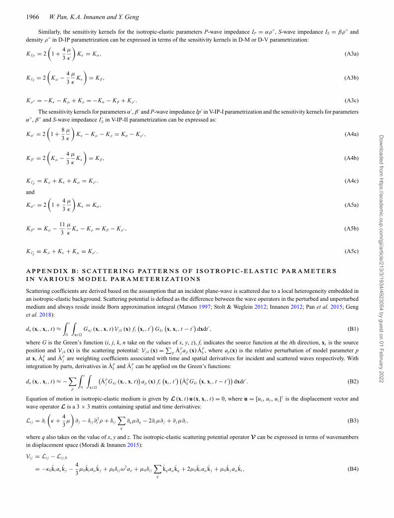
1966 W. Pan, K.A. Innanen and Y. Geng
Similarly, the sensitivity kernels for the isotropic-elastic parameters P-wave impedance IP = αρ ′′, S-wave impedance IS = βρ ′′ anddensity ρ ′′ in D-IP parametrization can be expressed in terms of the sensitivity kernels in D-M or D-V parametrization:
KIP = 2
(1 + 4
3
μ
κ
)Kκ = Kα, (A3a)
KIS = 2
(Kμ − 4
3
μ
κKκ
)= Kβ, (A3b)
Kρ′′ = −Kκ − Kμ + Kρ = −Kα − Kβ + Kρ′ . (A3c)
The sensitivity kernels for parameters α′, β ′ and P-wave impedance Ip′ in V-IP-I parametrization and the sensitivity kernels for parametersα′′, β ′′ and S-wave impedance I ′
S in V-IP-II parametrization can be expressed as:
Kα′ = 2
(1 + 8
3
μ
κ
)Kκ − Kμ − Kρ = Kα − Kρ′ , (A4a)
Kβ ′ = 2
(Kμ − 4
3
μ
κKκ
)= Kβ, (A4b)
KI ′P
= Kρ + Kκ + Kμ = Kρ′ . (A4c)
and
Kα′′ = 2
(1 + 4
3
μ
κ
)Kκ = Kα, (A5a)
Kβ ′′ = Kμ − 11
3
μ
κKκ − Kρ = Kβ − Kρ′ , (A5b)
KI ′S
= Kρ + Kκ + Kμ = Kρ′ . (A5c)
A P P E N D I X B : S C AT T E R I N G PAT T E R N S O F I S O T RO P I C - E L A S T I C PA R A M E T E R SI N VA R I O U S M O D E L PA R A M E T E R I Z AT I O N S
Scattering coefficients are derived based on the assumption that an incident plane-wave is scattered due to a local heterogeneity embedded inan isotropic-elastic background. Scattering potential is defined as the difference between the wave operators in the perturbed and unperturbedmedium and always reside inside Born approximation integral (Matson 1997; Stolt & Weglein 2012; Innanen 2012; Pan et al. 2015; Genget al. 2018):
dn (xr , xs, t) ≈∫ t
0
∫x∈
Gnj (xr , x, t)V jk (x) fi
(xs, t ′) Gki
(x, xs, t − t ′) dxdt ′, (B1)
where G is the Green’s function (i, j, k, n take on the values of x, y, z), fi indicates the source function at the ith direction, xs is the sourceposition and V jk (x) is the scattering potential: V jk (x) = ∑
p Apj ap (x) Ap
k , where ap(x) is the relative perturbation of model parameter pat x, Ap
k and Apj are weighting coefficients associated with time and spatial derivatives for incident and scattered waves respectively. With
integration by parts, derivatives in Apk and Ap
j can be applied on the Green’s functions:
dn (xr , xs, t) ≈ −∑
p
∫ t
0
∫x∈
(Ap
j Gnj (xr , x, t))
ap (x) fi
(xs, t ′) (
Apk Gki
(x, xs, t − t ′)) dxdt ′. (B2)
Equation of motion in isotropic-elastic medium is given by L (x, t) u (x, xs, t) = 0, where u = [ux, uy, uz]† is the displacement vector andwave operator L is a 3 × 3 matrix containing spatial and time derivatives:
Li j = ∂i
(κ + 4
3μ
)∂ j − δi j∂
2t ρ + δi j
∑q
∂qμ∂q − 2∂iμ∂ j + ∂ jμ∂i , (B3)
where q also takes on the value of x, y and z. The isotropic-elastic scattering potential operator V can be expressed in terms of wavenumbersin displacement space (Moradi & Innanen 2015):
Vi j = Li j − Li j,0
= −κ0ki aκ k j − 4
3μ0ki aμk j + ρ0δi jω
2aρ + μ0δi j
∑q
kqaμkq + 2μ0ki aμk j + μ0k j aμki , (B4)
Dow
nloaded from https://academ
ic.oup.com/gji/article/213/3/1934/4923054 by guest on 01 February 2022
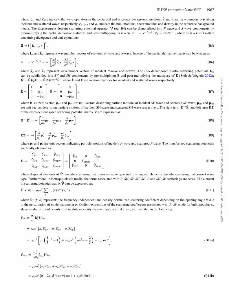
W-VSP isotropic-elastic FWI 1967
where Li j and Li j,0 indicate the wave operators in the perturbed and reference background medium, k and k are wavenumbers describingincident and scattered waves respectively. κ0, μ0 and ρ0 indicate the bulk modulus, shear modulus and density in the reference backgroundmedia. The displacement domain scattering potential operator V (eq. B4) can be diagonalized into P-wave and S-wave components bypre-multiplying the partial derivative matrix � and post-multiplying its inverse �−1 = ∇−2�†: VE = �V�−1, where � is a 4 × 3 matrixcontaining divergence and curl operations:
� = i[
kα·kβ×]†
, (B5)
where kα and kβ represent wavenumber vectors of scattered P-wave and S-wave. Inverse of the partial derivative matrix can be written as
�−1 = ∇−2�† = −i
[α2
0
ω2k†
α·β2
0
ω2k†
β×]
, (B6)
where kα and kβ represent wavenumber vectors of incident P-wave and S-wave. The P–S decomposed elastic scattering potentials VE
can be subdivided into SV and SH components by pre-multiplying E and post-multiplying the transpose of E (Stolt & Weglein 2012):V = EVEE† = E�V�−1E†, where E and E are rotation matrices for incident and scattered waves respectively:
E =
⎡⎢⎣
1 00 pSV
0 −pSH
⎤⎥⎦ , E =
⎡⎢⎣
1 00 pSV
0 −pSH
⎤⎥⎦ , (B7)
where 0 is a zero vector, pSV and pSV are unit vectors describing particle motions of incident SV-wave and scattered SV-wave, pSH and pSH
are unit vectors describing particle motions of incident SH-wave and scattered SH-wave respectively. The right term �−1E† and left term E�
of the displacement space scattering potential matrix V are expressed as:
�−1E† = −i
[ω
α0pP
ω
β0pSH
ω
β0pSV
], (B8)
E� = −i
[ω
α0p†
P
ω
β0p†
SH
ω
β0p†
SV
]†, (B9)
where pP and pP are unit vectors indicating particle motions of incident P-wave and scattered P-wave. The transformed scattering potentialsare finally obtained as:
V =
⎡⎢⎢⎣
VPP VPSH VPSV
VSHP VSHSH VSHSV
VSVP VSVSH VSVSV
⎤⎥⎥⎦ =
⎡⎢⎣
VPP 0 VPSV
0 VSHSH 0VSVP 0 VSVSV
⎤⎥⎦ , (B10)
where diagonal elements of V describe scattering that preserves wave type and off-diagonal elements describe scattering that convert wavetype. Furthermore, in isotropic-elastic media, the terms associated with P–SH, SV–SH, SH–P and SH–SV scatterings are zeros. The elementin scattering potential matrix V can be expressed as:
V (x, θ ) = ρ0ω2∑
p
ap (x) Rp (x, θ ) , (B11)
where Rp (x, θ ) represents the frequency-independent and density-normalized scattering coefficient depending on the opening angle θ due
to the perturbation of model parameter p. Explicit expressions of the scattering coefficeints associated with P–SV mode for bulk modulus κ ,shear modulus μ and density ρ in modulus–density parametrization are derived, as illustrated in the following:
VPP = α20
ω2k†
αV kα
= ρ0ω2[aκR
κPP + aμR
μ
PP + aρRρ
PP
]
= ρ0ω2
[aκ
(4
3σ 2 − 1
)+ 2aμσ 2
(sin2 θ − 2
3
)− aρ cos θ
], (B12a)
VPSV = α20
ωβ0p†
SVV kα
= ρ0ω2(aκR
κPSV + aμR
μ
PSV + aρRρ
PSV
)
= ρ0ω2(0 + 2aμσ 2| sin θ | cos θ + aρ σ | sin θ |) , (B12b)
Dow
nloaded from https://academ
ic.oup.com/gji/article/213/3/1934/4923054 by guest on 01 February 2022
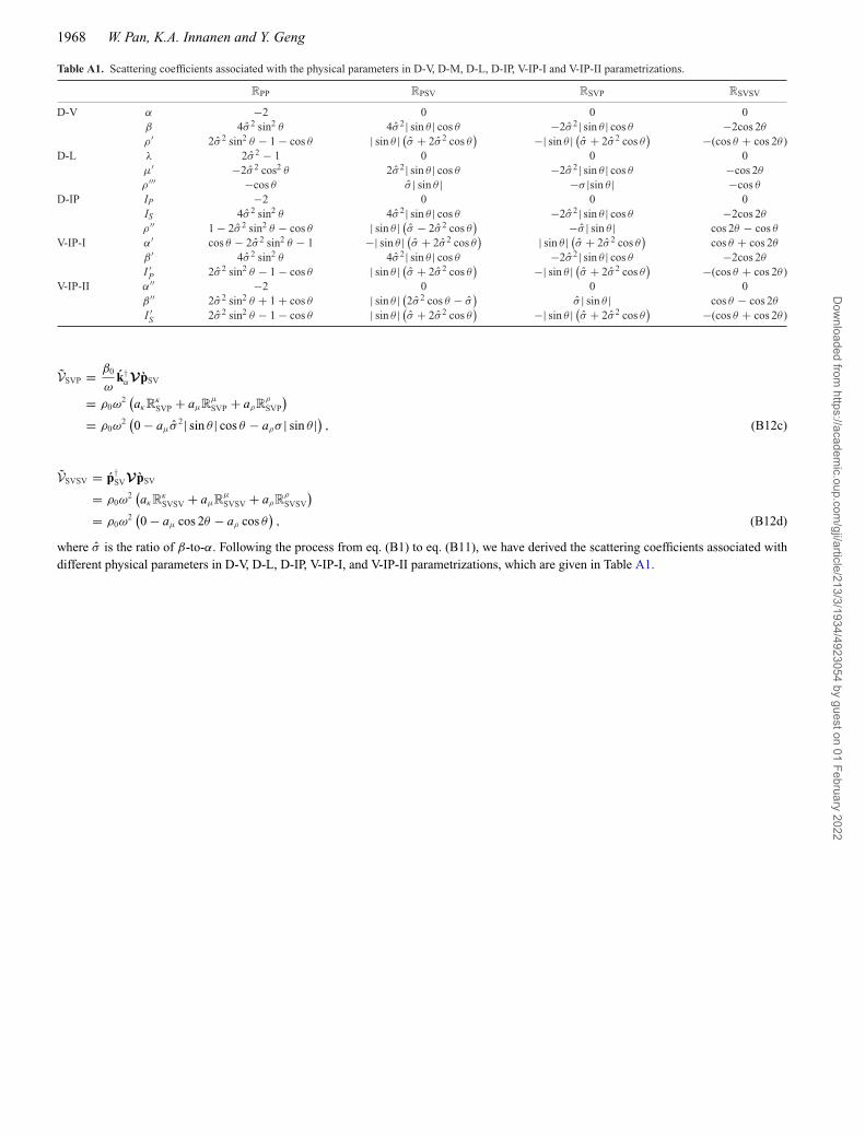
1968 W. Pan, K.A. Innanen and Y. Geng
Table A1. Scattering coefficients associated with the physical parameters in D-V, D-M, D-L, D-IP, V-IP-I and V-IP-II parametrizations.
RPP RPSV RSVP RSVSV
D-V α −2 0 0 0β 4σ 2 sin2 θ 4σ 2| sin θ | cos θ −2σ 2| sin θ | cos θ −2cos 2θ
ρ′ 2σ 2 sin2 θ − 1 − cos θ | sin θ | (σ + 2σ 2 cos θ) −| sin θ | (σ + 2σ 2 cos θ
) −(cos θ + cos 2θ )D-L λ 2σ 2 − 1 0 0 0
μ′ −2σ 2 cos2 θ 2σ 2| sin θ | cos θ −2σ 2| sin θ | cos θ −cos 2θ
ρ′′′ −cos θ σ | sin θ | −σ |sin θ | −cos θ
D-IP IP −2 0 0 0IS 4σ 2 sin2 θ 4σ 2| sin θ | cos θ −2σ 2| sin θ | cos θ −2cos 2θ
ρ′′ 1 − 2σ 2 sin2 θ − cos θ | sin θ | (σ − 2σ 2 cos θ) −σ | sin θ | cos 2θ − cos θ
V-IP-I α′ cos θ − 2σ 2 sin2 θ − 1 −| sin θ | (σ + 2σ 2 cos θ) | sin θ | (σ + 2σ 2 cos θ
)cos θ + cos 2θ
β ′ 4σ 2 sin2 θ 4σ 2| sin θ | cos θ −2σ 2| sin θ | cos θ −2cos 2θ
I ′P 2σ 2 sin2 θ − 1 − cos θ | sin θ | (σ + 2σ 2 cos θ
) −| sin θ | (σ + 2σ 2 cos θ) −(cos θ + cos 2θ )
V-IP-II α′′ −2 0 0 0β ′′ 2σ 2 sin2 θ + 1 + cos θ | sin θ | (2σ 2 cos θ − σ
)σ | sin θ | cos θ − cos 2θ
I ′S 2σ 2 sin2 θ − 1 − cos θ | sin θ | (σ + 2σ 2 cos θ
) −| sin θ | (σ + 2σ 2 cos θ) −(cos θ + cos 2θ )
VSVP = β0
ωk†
αV pSV
= ρ0ω2(aκR
κSVP + aμR
μ
SVP + aρRρ
SVP
)= ρ0ω
2(0 − aμσ 2| sin θ | cos θ − aρσ | sin θ |) , (B12c)
VSVSV = p†SVV pSV
= ρ0ω2(aκR
κSVSV + aμR
μ
SVSV + aρRρ
SVSV
)= ρ0ω
2(0 − aμ cos 2θ − aρ cos θ
), (B12d)
where σ is the ratio of β-to-α. Following the process from eq. (B1) to eq. (B11), we have derived the scattering coefficients associated withdifferent physical parameters in D-V, D-L, D-IP, V-IP-I, and V-IP-II parametrizations, which are given in Table A1.
Dow
nloaded from https://academ
ic.oup.com/gji/article/213/3/1934/4923054 by guest on 01 February 2022


![Rule inversion [1972]](https://img.dokumen.tips/doc/110x75/631b669ea906b217b90671ab/rule-inversion-1972.jpg)


