On the influence of model parametrization in elastic full waveform tomography

Geophysical Journal InternationalGeophys. J. Int. (2012) 191, 325–345 doi: 10.1111/j.1365-246X.2012.05633.x

GJI

Sei

smol

ogy

On the influence of model parametrization in elastic full waveformtomography

D. Kohn,1 D. De Nil,1 A. Kurzmann,2 A. Przebindowska2 and T. Bohlen2

1Institut fur Geowissenschaften (Abteilung Geophysik), Universitat Kiel, Otto-Hahn-Platz 1, 24118 Kiel, Germany. E-mail: [email protected] Institut (GPI), Karlsruher Institut fur Technologie, Hertzstrasse 16, 76187 Karlsruhe, Germany

Accepted 2012 July 26. Received 2012 July 26; in original form 2011 December 27

S U M M A R YElastic Full Waveform Tomography (FWT) aims to reduce the misfit between recorded andmodelled data, to deduce a very detailed model of elastic material parameters in the under-ground. The choice of the elastic model parameters to be inverted affects the convergenceand quality of the reconstructed subsurface model. Using the Cross-Triangle-Squares (CTS)model three elastic parametrizations, Lame parameters m1 = [λ, μ, ρ], seismic velocitiesm2 = [V p, V s, ρ] and seismic impedances m3 = [Ip, Is, ρ] for far-offset reflection seismicacquisition geometries with explosive point sources and free-surface condition are studied. Ineach CTS model the three elastic parameters are assigned to three different geometrical objectsthat are spatially separated. The results of the CTS model study reveal a strong requirementof a sequential frequency inversion from low to high frequencies to reconstruct the densitymodel. Using only high-frequency data, cross-talk artefacts have an influence on the quantita-tive reconstruction of the material parameters, while for a sequential frequency inversion onlystructural artefacts, representing the boundaries of different model parameters, are present.During the inversion, the Lame parameters, seismic velocities and impedances could be recon-structed well. However, using the Lame parametrization μ-artefacts are present in the λ model,while similar artefacts are suppressed when using seismic velocities or impedances. The den-sity inversion shows the largest ambiguity for all parametrizations. However, the artefacts areagain more dominant, when using the Lame parameters and suppressed for seismic velocityand impedance parametrization. The afore mentioned results are confirmed for a geologicallymore realistic modified Marmousi-II model. Using a conventional streamer acquisition ge-ometry the P-velocity, S-velocity and density models of the subsurface were reconstructedsuccessfully and are compared with the results of the Lame parameter inversion.

Key words: Inverse theory; Numerical approximations and analysis; Seismic tomography;Computational seismology; Wave propagation.

1 I N T RO D U C T I O N

Only few studies have investigated the influence of different model parametrizations in isotropic elastic full waveform tomography (FWT).In Tarantola (1986), Tarantola et al. (1985) the response of a point diffractor in a homogenous full space is investigated to find an optimummodel parametrization for an reflection seismic acquisition geometry. Similar investigations are presented by Mora (1987). Both authorsconcluded, that for near-offset data (short wavelengths) the parametrization with seismic impedances and for far-offset data (long wavelengths)the seismic velocities shows the least ambiguity in the elastic multiparameter inversion for a reflection seismic acquisition geometry witha P-wave dominant source, while the parametrization with Lame parameters is not very suitable. Crase et al. (1990) applied the elasticseismic impedance FWT strategy in combination with different objective functions to synthetic and field data. A wide range of studies fordifferent acquistion geometries have been performed by numerous authors. Sears et al. (2008, 2010) studied elastic waveform tomographyfor multicomponent OBC data, while Roberts et al. (2008) investigated the influence of the model parametrization for VSP surveys. Brossier(2011) conducted a simple parameter study for viscoelastic media in the frequency domain and applied the elastic FWT to complex syntheticreflection seismic data (Brossier et al. 2009a, 2010) as well as to OBC data (Brossier et al. 2009b). Choi et al. (2008) presented a FWT studyfor acoustic–elastic coupled media for different reflection seismic acquistion geometries with hydrophones, single- and multicomponent data.On the continental scale Fichtner (2011) and Fichtner & Trampert (2011) applied the elastic FWT to surface waves and long period bodywaves to image crustal and upper-mantle structures. All these studies use seismic velocities for the model parametrization. Recently Zhu et al.

C© 2012 The Authors 325Geophysical Journal International C© 2012 RAS

326 D. Kohn et al.

(2009) compared the resolution and ambiguity of adjoint kernels for different parametrizations (seismic velocities, seismic impedances andelastic moduli). Jeonq et al. (2012) investigated a full waveform inversion strategy for density in the frequency domain using the modifiedMarmousi-II and SEG/EAGE salt model, which combines a two step inversion scheme. Step 1 consists of a Lame parametrization and a fixeddensity model, while step 2 aims at the inversion of seismic velocities and density.

In this study we build the Cross-Triangle-Squares (CTS) model for a new parametrization study. While the analysis of the amplitudediffraction pattern of a point diffractor allows to give some conclusions on the spatial resolution and coupling between different parameters,the CTS model proposed here is a more complex model which includes free-surface and multiple-diffraction effects, but simple enough to givesimple conclusions. With the CTS model the influence of the model parametrization on resolution and ambiguity of the inversion results isinvestigated in detail using Lame parameters, seismic velocities and seismic impedance with a special focus on a far-offset reflection seismicgeometry. Additionally, the influence of a sequential frequency inversion on the quality of the inversion result is tested, especially the impacton the density inversion result. Afterwards the results of this study are applied to the elastic inversion of a modified Marmousi-II model.

2 T H E O R E T I C A L B A C KG RO U N D

The aim of FWT is to minimize the data residuals δu = umod − uobs between the modelled data umod and the field data uobs to deduce thedistribution of the material parameters m in the underground. The misfit can be measured by the objective function (Mora 1987; Tarantola2005):

E = 1

2δuTδu (1)

The term δuTδu represents the residual energy, which is the seismic energy not explained by the actual model m. The objective functioncan be minimized by updating the model parameters mn at iteration step n using a steepest-descent gradient method

mn+1 = mn − μn

(∂ E

∂m

)n

, (2)

where (∂ E/∂m)n denotes the gradient direction of the objective function with respect to the material parameters and μn the step length.According to Tarantola (1986), Mora (1987) and Kohn (2011), the gradients can be expressed in time domain by a zero-lag correlation ofdisplacement wavefields

∂ E

∂λ= −

∑sources

∫dt

(∂ux

∂x+ ∂uz

∂z

)(∂�x

∂x+ ∂�z

∂z

),

∂ E

∂μ= −

∑sources

∫dt

(∂ux

∂z+ ∂uz

∂x

)(∂�x

∂z+ ∂�z

∂x

)+ 2

(∂ux

∂x

∂�x

∂x+ ∂uz

∂z

∂�z

∂z

),

∂ E

∂ρ= −

∑sources

∫dt

(∂2ux

∂t2�x + ∂2uz

∂t2�z

). (3)

While u denotes the forward modelled wavefield for the actual model parameters, the wavefield � is generated by propagating the residualdata δu from the receiver positions backwards in time in the elastic medium. The elastic forward problem and backpropagation of the dataresiduals are solved by using a 2-D time domain stress-velocity P–SV finite-difference (FD) code (Virieux 1986; Levander 1988). Therefore,the displacements in eq. (3) have to be replaced by stresses and particle velocities (Shipp & Singh 2002)

∂ E

∂λ= −

∑sources

∫dt

[(σxx + σzz)(�xx + �zz)

4(λ + μ)2

]

∂ E

∂μ= −

∑sources

∫dt

[σxz�xz

μ2+ 1

4

((σxx + σzz)(�xx + �zz)

(λ + μ)2+ (σxx − σzz)(�xx − �zz)

μ2

)]

∂ E

∂ρ= −

∑sources

∫dt

[∂vx

∂t�x + ∂vz

∂t�z

],

(4)

where σ ij and �ij are the stresses of the forward and backpropagated wavefield, respectively. The displacements � i in the density gradient arecalculated from the particle velocities by numerical integration, while the time derivatives of the particle velocities v are estimated during theupdate of the momentum equation. To increase the convergence speed an appropriate preconditioning operator P is applied to the gradient∂ E/∂m(

∂ E

∂m

)p

n

= Pn

(∂ E

∂m

)n

. (5)

The preconditioning operator used for a reflection seismic acquisition geometry is described in Section 4. To further increase the convergencespeed in small valleys of the objective function, the conjugate gradient direction for iteration steps n ≥ 2 (Nocedal & Wright 2006) iscalculated(

∂ E

∂m

)c

n

=(

∂ E

∂m

)p

n

+ β

(∂ E

∂m

)c

n−1

, with

(∂ E

∂m

)c

1

=(

∂ E

∂m

)p

1

(6)

C© 2012 The Authors, GJI, 191, 325–345

Geophysical Journal International C© 2012 RAS

On the influence of model parametrization 327

where the weighting factor

β P R =

(∂ E∂m

)p

n·[(

∂ E∂m

)p

n−

(∂ E∂m

)p

n−1

](

∂ E∂m

)p

n−1·(

∂ E∂m

)p

n−1

(7)

by Polak-Ribiere is used. The convergence of the Polak-Ribiere method is guaranteed by applying a gradient reset, if the following conditionis satisfied β = max [βPR, 0], so if subsequent search directions lose conjugacy only the gradient information of the current iteration is used(Nocedal & Wright 2006). Similar to Brossier (2011) for the L-BFGS method we normalize the material parameters and the gradients beforethe step length calculation. The optimum step length μn is estimated by a line search algorithm (Kurzmann et al. 2008; Sourbier et al. 2009;Kohn 2011).

3 T H E G R A D I E N T F O R D I F F E R E N T M O D E L PA R A M E T R I Z AT I O N S

The gradients in terms of other material parameters mnew can be calculated by applying the chain rule on the Frechet kernel in the adjointproblem (Mora 1987; Kohn 2011)(

∂ E

∂m

)new

=∑

sources

∫dt

∑receivers

[∂u

∂m

∂m

∂mnew

]∗δu. (8)

Using the relationships between P-wave velocity V p, S-wave velocity V s, the Lame parameters λ, μ and density ρ

Vp =√

λ + 2μ

ρ, Vs =

√μ

ρ(9)

or

λ = ρV 2p − 2ρV 2

s , μ = ρV 2s . (10)

The gradient for V p can be written as(∂ E

∂Vp

)=

∑sources

∫dt

∑receivers

[∂u

∂λ

∂λ

∂Vp+ ∂u

∂μ

∂μ

∂Vp+ ∂u

∂ρ

∂ρ

∂Vp

]∗δui ,

=∑

sources

∫dt

∑receivers

[∂u

∂λ2ρVp

]∗δui ,

= 2ρVp

∑sources

∫dt

∑receivers

[∂u

∂λ

]∗δui ,

= 2ρVp

(∂ E

∂λ

).

(11)

The gradients for V s and ρ are calculated in a similar way, so the gradients in terms of seismic velocities can be written as(∂ E

∂Vp

)= 2ρVp

(∂ E

∂λ

),

(∂ E

∂Vs

)= −4ρVs

(∂ E

∂λ

)+ 2ρVs

(∂ E

∂μ

),

(∂ E

∂ρvel

)= (

V 2p − 2V 2

s

) (∂ E

∂λ

)+ V 2

s

(∂ E

∂μ

)+

(∂ E

∂ρ

). (12)

With the relationships between the Lame parameters and seismic P-impedance Ip, S-impedance Is

λ = 1

ρ

(I 2

p − 2I 2s

), μ = 1

ρI 2

s , (13)

the gradients with respect to Ip, Is and ρ are(∂ E

∂ Ip

)= 2Vp

(∂ E

∂λ

),

(∂ E

∂ Is

)= −4Vs

(∂ E

∂λ

)+ 2Vs

(∂ E

∂μ

),

(∂ E

∂ρimp

)= (

2V 2s − V 2

p

) (∂ E

∂λ

)− V 2

s

(∂ E

∂μ

)+

(∂ E

∂ρ

). (14)

C© 2012 The Authors, GJI, 191, 325–345


328 D. Kohn et al.

4 T H E C T S T E S T P RO B L E M

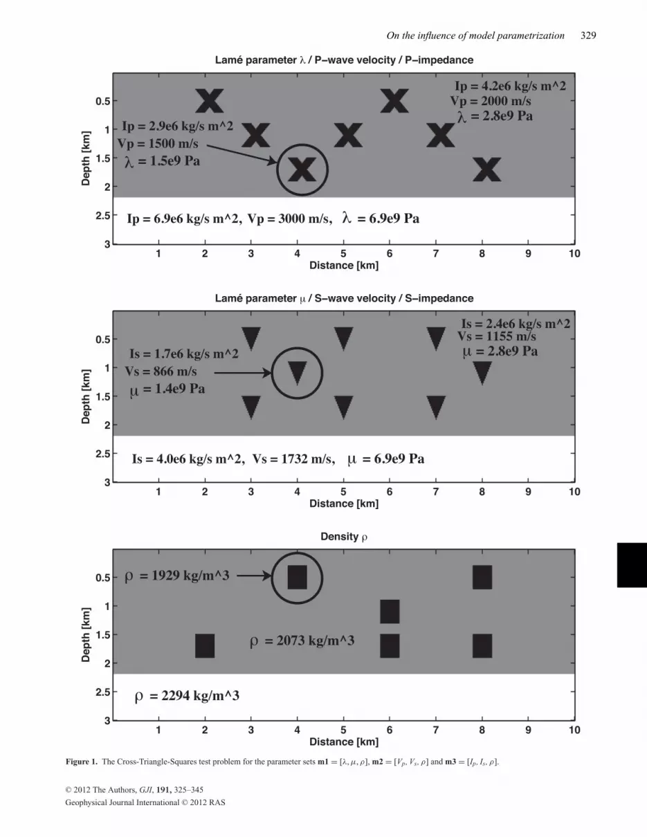
To investigate the influence of different model parametrizations using the gradients eqs (4), (12) and (14) we constructed a simple elastic testproblem (Fig. 1).

4.1 The CTS model

The model consists of an elastic layer over a half-space. PMLs are applied to the boundaries, except for a free surface boundary conditionon top of the model. Seismic waves are travelling from the sources located at the surface and are reflected back at the interface between thelayer and half-space. Embedded in the layer are different geometrical bodies, which are disturbing the wavefield of the reflected waves. Thesegeometrical bodies consist of:

(i) seven crosses indicating perturbations of the Lame parameter λ, P-wave velocity V p or seismic P-impedance Ip.(ii) eight triangles indicating perturbations of the Lame parameter μ, S-wave velocity V s or seismic S-impedance Is.(iii) six squares indicating perturbations of the density ρ.

Due to the different geometrical structures, we call this model CTS model. The geometrical bodies are located at different non-overlappingplaces. This does not represent a realistic geological structure, but it is an effective way to demonstrate the resolution and ambiguity of theFWT results when using different elastic model parametrizations. The models are not exactly comparable, because a simple recalculation ofone parametrization to another would result in mixing of the different geometrical bodies. This might increase the nonlinearity of the inverseproblem for the different parametrizations, which would lead to results which are difficult to interpret. Therefore, we think that our approachis the best compromise between comparability and complexity.

4.2 Acquisition geometry and FD model

The acquisition geometry consists of 100 explosive sources located 40 m below the free surface. The source signature is a Ricker waveletwith a centre frequency of 5 Hz and a maximum frequency of 10 Hz. The elastic wavefield is recorded by 400 two-component receivers in40 m depth. Using an eighth-order spatial FD operator for the forward modelling and backpropagation of the residual wavefield the modelcan be discretized with 500 × 150 gridpoints in x- and z-direction with a spatial gridpoint distance of 20.0 m. The time is discretized usingDT = 2.7 ms, thus, for a recording time of T = 6.0 s 2222 time steps are required.

4.3 FWT of the CTS model

Synthetic multicomponent data sets are calculated for the CTS model using the different model parametrizations and inverted using a startingmodel with the correct elastic material parameters for the layer and the half space but without the geometrical structures. The source waveletis assumed to be known and therefore not estimated during the inversion. The application of a preconditioning operator is vital to suppresslarge gradient values near the source and receiver positions. Additionally, there are strong artefacts present near the free surface which area few orders of magnitude larger than the gradient of the material parameters. To suppress these effects a spatial preconditioning operator,which scales the gradient with depth z, is applied to the gradient (Mora 1987)

P =

⎧⎪⎪⎪⎪⎪⎪⎨⎪⎪⎪⎪⎪⎪⎩

0 if z0 = 0.0 m ≤ z ≤ zgradt1

exp

(−1

2

(a

z − zgradt1 − l

l/2

)2)

if zgradt1 ≤ z ≤ zgradt2

z

zgradt2if zgradt2 < z

(15)

with a = 3.0, l = 200.0 m, zgradt1 = 100.0 m and zgradt2 = 300.0 m.The preconditioning operator sets the gradient near the free surface and the sources/receivers to zero. In a transition zone between 100

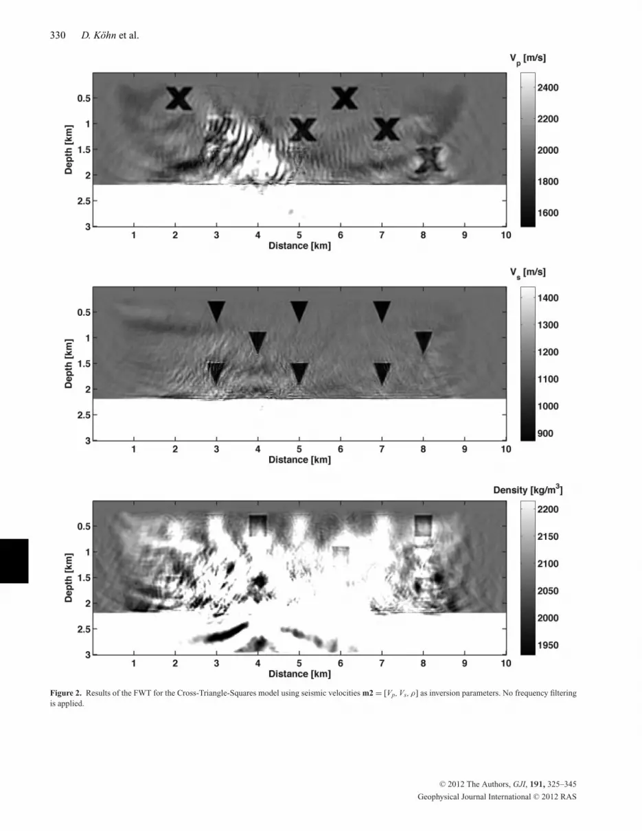
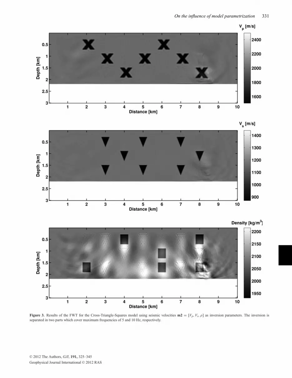
and 300 m depth a Gaussian taper is applied. Beyond a depth of 300 m the operator scales the gradient linearly with depth. This is a verysimple but effective correction for the amplitude loss in larger depths due to geometrical spreading and reflections in the upper parts of themodel. However, it does not fully compensate the effects of the geometrical spreading like a quasi-Newton approach (Brossier 2011). Toreduce the nonlinearity of the inverse problem sequential frequencies (Sirgue & Pratt 2004), or frequency bands (Bunks et al. 1995) areprogressively inverted from low to high frequencies. As noted by Brossier et al. (2009a) the surface waves introduce a strong nonlinearityto the FWT problem. In case of the CTS model the penetration depth of the Rayleigh waves is not large enough to be influenced by thegeometrical bodies. Figs 2–4 illustrate the FWT result for the CTS model using the velocity parametrization and different inverted frequencybands. When the whole frequency content of the data up to 10 Hz is inverted, the P-wave velocity model and even more the density model aredominated by artefacts with unrealistically high values. The triangles of the S-wave velocity model could be reconstructed quite clearly. Whenseparating the inversion into two parts which cover maximum frequencies of 5 and 10 Hz, respectively (Fig. 3), the P- and S-wave velocitymodels are reconstructed with only small artefacts in regions with low ray coverage. The squares of the density model are also recovered,

C© 2012 The Authors, GJI, 191, 325–345



Figure 1. The Cross-Triangle-Squares test problem for the parameter sets m1 = [λ, μ, ρ], m2 = [Vp, Vs, ρ] and m3 = [Ip, Is, ρ].

C© 2012 The Authors, GJI, 191, 325–345


330 D. Kohn et al.

Figure 2. Results of the FWT for the Cross-Triangle-Squares model using seismic velocities m2 = [Vp, Vs, ρ] as inversion parameters. No frequency filteringis applied.

C© 2012 The Authors, GJI, 191, 325–345



Figure 3. Results of the FWT for the Cross-Triangle-Squares model using seismic velocities m2 = [Vp, Vs, ρ] as inversion parameters. The inversion isseparated in two parts which cover maximum frequencies of 5 and 10 Hz, respectively.

C© 2012 The Authors, GJI, 191, 325–345


332 D. Kohn et al.

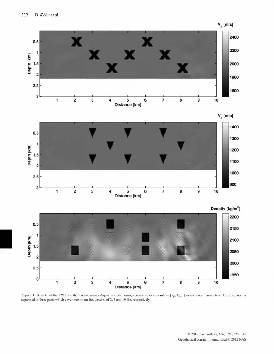
Figure 4. Results of the FWT for the Cross-Triangle-Squares model using seismic velocities m2 = [Vp, Vs, ρ] as inversion parameters. The inversion isseparated in three parts which cover maximum frequencies of 2, 5 and 10 Hz, respectively.

C© 2012 The Authors, GJI, 191, 325–345



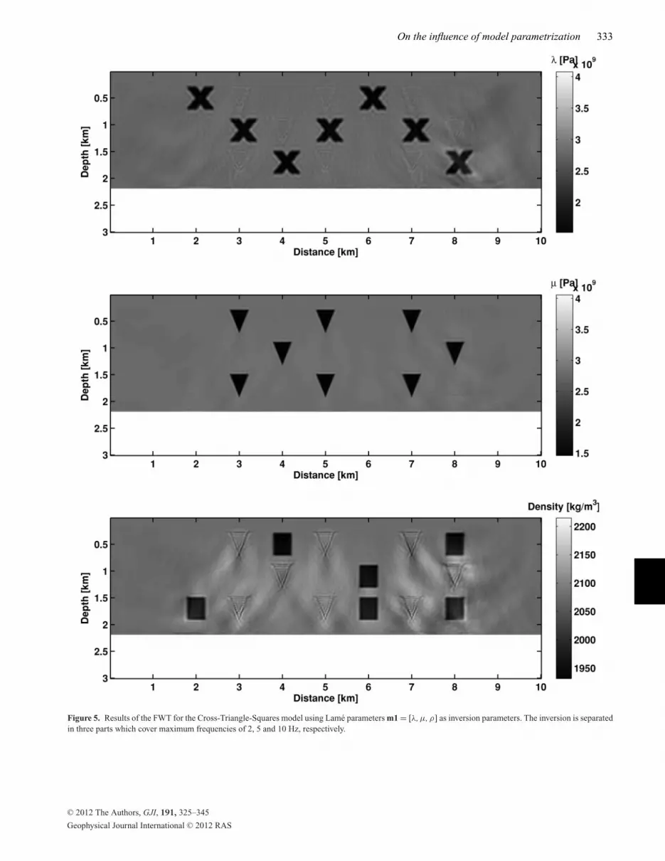
Figure 5. Results of the FWT for the Cross-Triangle-Squares model using Lame parameters m1 = [λ, μ, ρ] as inversion parameters. The inversion is separatedin three parts which cover maximum frequencies of 2, 5 and 10 Hz, respectively.

C© 2012 The Authors, GJI, 191, 325–345


334 D. Kohn et al.

Figure 6. Results of the FWT for the Cross-Triangle-Squares model using seismic impedances m3 = [Ip, Is, ρ] as inversion parameters. The inversion isseparated in three parts which cover maximum frequencies of 2, 5 and 10 Hz, respectively.

C© 2012 The Authors, GJI, 191, 325–345



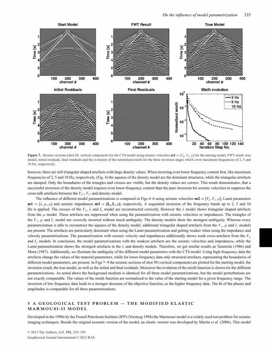
Figure 7. Seismic sections (shot 50, vertical component) for the CTS model using seismic velocities m2 = [Vp, Vs, ρ] for the starting model, FWT result, truemodel, initial residuals, final residuals and the evolution of the normalized misfit for the three inversion stages which cover maximum frequencies of 2, 5 and10 Hz, respectively.

however, there are still triangular shaped artefacts with large density values. When inverting even lower frequency content first, like maximumfrequencies of 2, 5 and 10 Hz, respectively, (Fig. 4) the squares of the density model are the dominant structures, while the triangular artefactsare damped. Only the boundaries of the triangles and crosses are visible, but the density values are correct. This result demonstrates, that asuccessful inversion of the density model requires even lower-frequency content than the pure inversion for seismic velocities to suppress thecross-talk artefacts between the Vp-, Vs- and density-model.

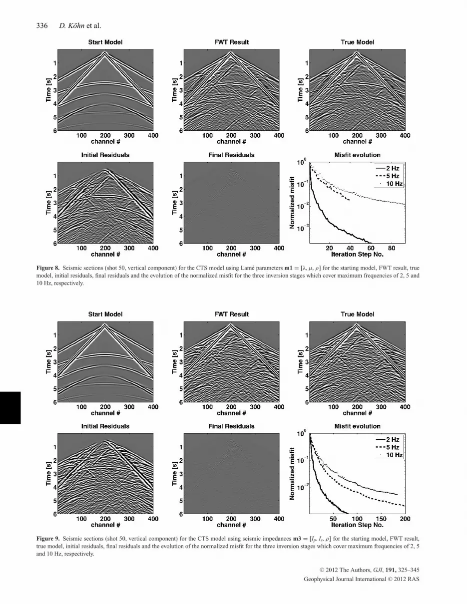
The influence of different model parametrizations is compared in Figs 4–6 using seismic velocities m2 = [Vp, Vs, ρ], Lame parametersm1 = [λ, μ, ρ] and seismic impedances m3 = [Ip, Is, ρ], respectively. A sequential inversion of the frequency bands up to 2, 5 and 10Hz is applied. The crosses of the V p, λ and Ip model are reconstructed correctly. However the λ model shows triangular shaped artefactsfrom the μ model. These artefacts are suppressed when using the parametrization with seismic velocities or impedances. The triangles ofthe V s, μ and Is model are correctly inverted without much ambiguity. The density models show the strongest ambiguity. Whereas everyparametrization is able to reconstruct the squares of the density model, additional triangular shaped artefacts from the V s, μ and Is modelsare present. The artefacts are particularly dominant when using the Lame-parametrization and getting weaker when using the impedance andvelocity parametrizations. The parametrization with seismic velocity and impedances additionally shows weak cross-artefacts from the V p

and Ip models. In conclusion, the model parametrizations with the weakest artefacts are the seismic velocities and impedances, while theLame-parametrization shows the strongest artefacts in the λ and density models. Therefore, we get similar results as Tarantola (1986) andMora (1987). Additionally, we illustrate the ambiguity of the different model parameters with the CTS model. Using high-frequency data theartefacts change the values of the material parameters, while for lower-frequency data only structural artefacts, representing the boundaries ofdifferent model parameters, are present. In Figs 7–9 the seismic sections of shot 50 (vertical component) are plotted for the starting model, theinversion result, the true model, as well as the initial and final residuals. Moreover the evolution of the misfit function is shown for the differentparametrizations. As noted above the background medium is identical for all three model parametrizations, but the model perturbations arenot exactly comparable. The values of the misfit function are normalized to the value of the starting model for a given frequency range. Theinversion of low frequency data leads to a stronger decrease of the objective function, as the higher frequency data. The fit of the phases andamplitudes is comparable for all three parametrizations.

5 A G E O L O G I C A L T E S T P RO B L E M — T H E M O D I F I E D E L A S T I CM A R M O U S I - I I M O D E L

Developed in the 1990s by the French Petroleum Institute (IFP) (Versteeg 1994) the Marmousi model is a widely used test problem for seismicimaging techniques. Beside the original acoustic version of the model, an elastic version was developed by Martin et al. (2006). This model

C© 2012 The Authors, GJI, 191, 325–345


336 D. Kohn et al.

Figure 8. Seismic sections (shot 50, vertical component) for the CTS model using Lame parameters m1 = [λ, μ, ρ] for the starting model, FWT result, truemodel, initial residuals, final residuals and the evolution of the normalized misfit for the three inversion stages which cover maximum frequencies of 2, 5 and10 Hz, respectively.

Figure 9. Seismic sections (shot 50, vertical component) for the CTS model using seismic impedances m3 = [Ip, Is, ρ] for the starting model, FWT result,true model, initial residuals, final residuals and the evolution of the normalized misfit for the three inversion stages which cover maximum frequencies of 2, 5and 10 Hz, respectively.

C© 2012 The Authors, GJI, 191, 325–345



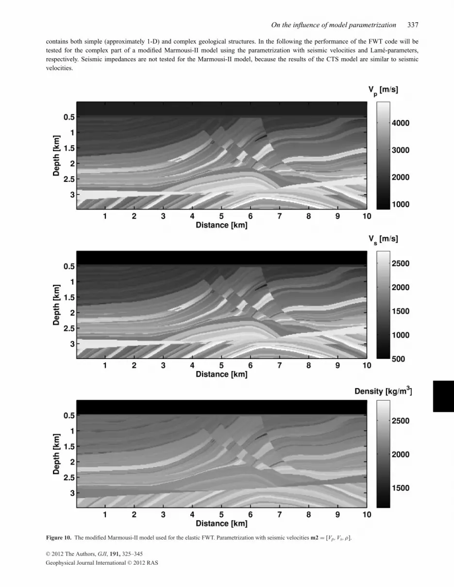
contains both simple (approximately 1-D) and complex geological structures. In the following the performance of the FWT code will betested for the complex part of a modified Marmousi-II model using the parametrization with seismic velocities and Lame-parameters,respectively. Seismic impedances are not tested for the Marmousi-II model, because the results of the CTS model are similar to seismicvelocities.

Figure 10. The modified Marmousi-II model used for the elastic FWT. Parametrization with seismic velocities m2 = [Vp, Vs, ρ].

C© 2012 The Authors, GJI, 191, 325–345


338 D. Kohn et al.

5.1 The complex Marmousi-II model

The Marmousi-II model (Fig. 10) consists of a 500 m thick water layer above an elastic subseafloor model. The sediment model is very simplenear the left and right boundaries but rather complex in the centre. At both sides, the subseafloor is approximately horizontally layered, whilesteep thrust faults are disturbing the layers in the centre of the model. Embedded in the thrust fault system and layers are small hydrocarbon

Figure 11. Starting models for the Marmousi-II model. Parametrization with seismic velocities m2 = [Vp, Vs, ρ].

C© 2012 The Authors, GJI, 191, 325–345



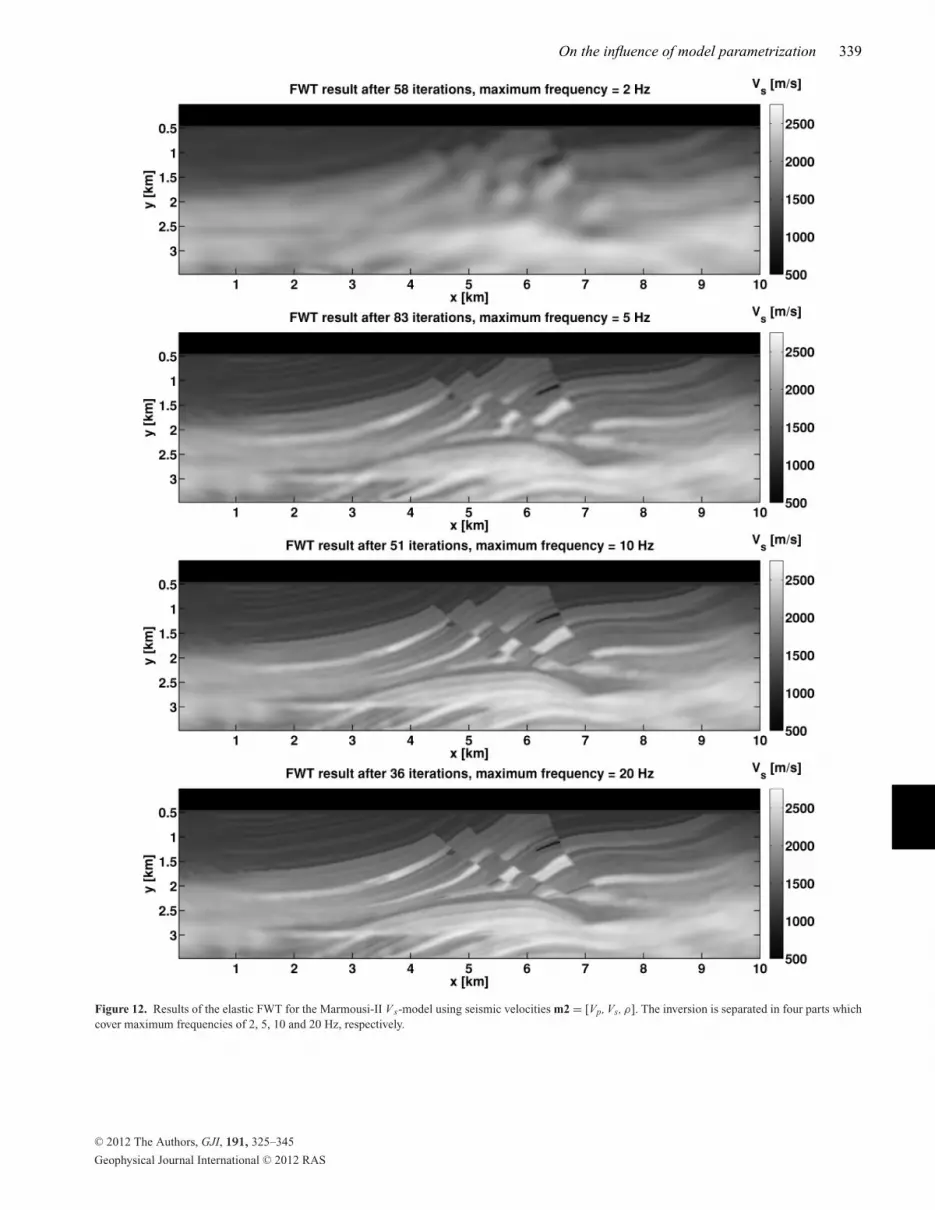
Figure 12. Results of the elastic FWT for the Marmousi-II Vs-model using seismic velocities m2 = [Vp, Vs, ρ]. The inversion is separated in four parts whichcover maximum frequencies of 2, 5, 10 and 20 Hz, respectively.

C© 2012 The Authors, GJI, 191, 325–345


340 D. Kohn et al.

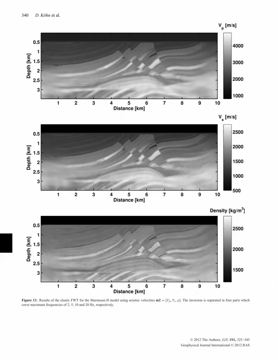
Figure 13. Results of the elastic FWT for the Marmousi-II model using seismic velocities m2 = [Vp, Vs, ρ]. The inversion is separated in four parts whichcover maximum frequencies of 2, 5, 10 and 20 Hz, respectively.

C© 2012 The Authors, GJI, 191, 325–345



reservoirs (Martin et al. 2006). The deeper parts of the model consist of salt and reef structures. The thrust fault system and the reef structuresare not easy to resolve by conventional first arrival tomography, so it is an ideal test model for the FWT. Due to computational restrictionsthe original Marmousi-II model could not be used, because the very low S-wave velocities in the sediments would require a too small spatialsampling of the model. Therefore new S-wave velocities are calculated so that the Poisson ratio is not larger than 0.25, so the soft-seabed isreplaced by a hard-seabed. Sears et al. (2008) and Brossier et al. (2009b) have shown the difficulties associated with soft-seabed environmentsfor elastic FWT. Additionally the size of the Marmousi-II model is reduced from 17 × 3.5 to 10 × 3.48 km.

5.2 Acquisition geometry and FD model

The acquisition geometry consists of a fixed streamer located 40 m below the free surface in the water layer. The streamer contains 400 twocomponent geophones with a spatial spacing of 20 m recording the particle velocities vi. This is somehow unusual, but as shown by Choiet al. (2008) the inversion results of the modified Marmousi-II model do not change very much, when using hydrophone, two-component orone-component data. For the synthetic data set 100 airgun shots are excited. The sources are located at the same depth as the receivers. Thesource signature is a Ricker wavelet with 10 Hz centre frequency. The model has the dimensions 10 × 3.48 km. Using an eight-order spatialFD operator the model can be discretized with 500 × 174 gridpoints in x- and z-direction with a spatial gridpoint distance of 20.0 m. Thetime is discretized using DT = 2.7 ms, thus for a recording time of T = 6.0 s 2222 time steps are needed.

5.3 FWT of the complex Marmousi-II model

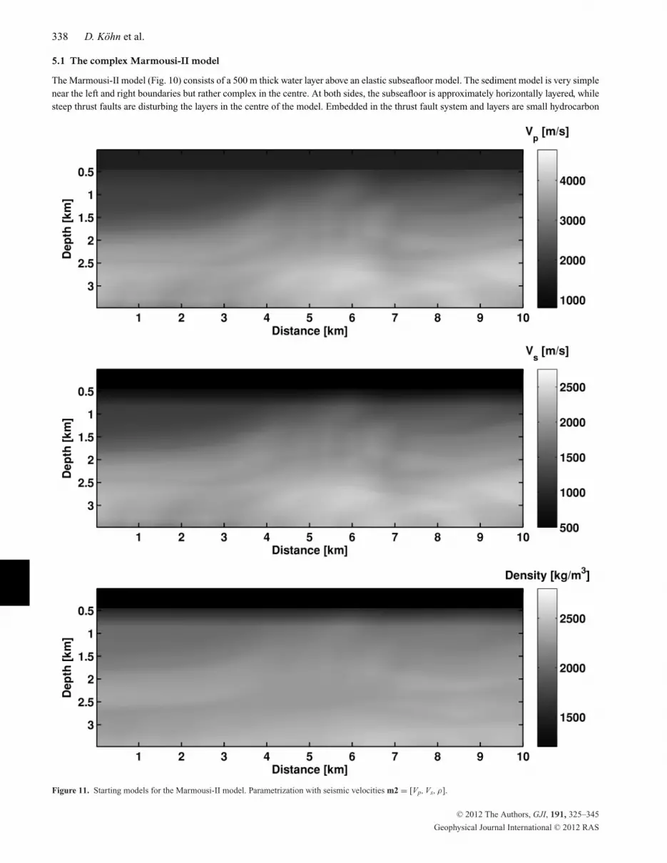
Considering the results of the last section, we chose seismic velocities and Lame-parameters as model parameters for the inversion. To generatea starting model which accurately describes the long wavelength part of the material parameters, the true models m2 = [Vp, Vs, ρ] and m1 =[λ, μ, ρ] are filtered using a spatial 2-D-Gaussian filter with a correlation length λc = 800.0 m. As a result all the small scale structures vanishand only the large scale structures are present (Fig. 11). This starting model is comparable with the resolution of a Laplace-domain waveforminversion (Shin & Ha 2008). Because the Marmousi-II model is more complicated than the CTS problem, an additional constraint is appliedduring the inversion. To stabilize the inversion possible density values are restricted between 1000 and 3000 kg m−3 using hard constraints.Otherwise geophysically unrealistic density values might occur in the model, especially when using the Lame-parametrizations. The same

Figure 14. Depth profiles at xp1 = 3.5 km (top panel) and xp2 = 6.4 km (bottom panel) of the starting model and FWT result using seismic velocities m2 =[Vp, Vs, ρ] are compared with the true model for the Marmousi-II model: P-wave velocity (left-hand side), S-wave velocity (centre) and density (right-handside).

C© 2012 The Authors, GJI, 191, 325–345


342 D. Kohn et al.

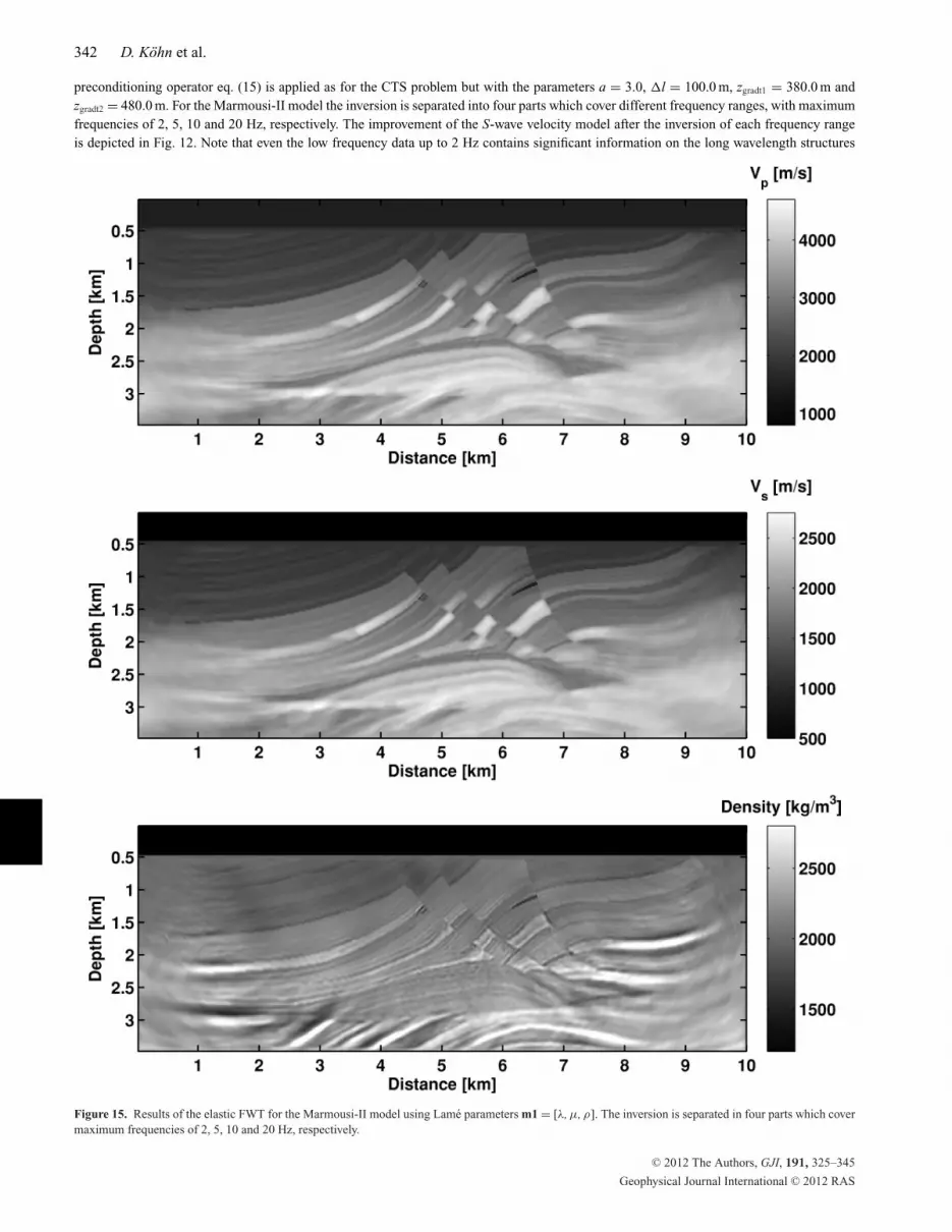
preconditioning operator eq. (15) is applied as for the CTS problem but with the parameters a = 3.0, l = 100.0 m, zgradt1 = 380.0 m andzgradt2 = 480.0 m. For the Marmousi-II model the inversion is separated into four parts which cover different frequency ranges, with maximumfrequencies of 2, 5, 10 and 20 Hz, respectively. The improvement of the S-wave velocity model after the inversion of each frequency rangeis depicted in Fig. 12. Note that even the low frequency data up to 2 Hz contains significant information on the long wavelength structures

Figure 15. Results of the elastic FWT for the Marmousi-II model using Lame parameters m1 = [λ, μ, ρ]. The inversion is separated in four parts which covermaximum frequencies of 2, 5, 10 and 20 Hz, respectively.

C© 2012 The Authors, GJI, 191, 325–345



Figure 16. Depth profiles at xp1 = 3.5 km (top panel) and xp2 = 6.4 km (bottom panel) of the starting model and FWT result using Lame parameters m1 =[λ, μ, ρ] are compared with the true model for the Marmousi-II model: Lame parameter λ (left-hand side), μ (centre) and density (right-hand side).

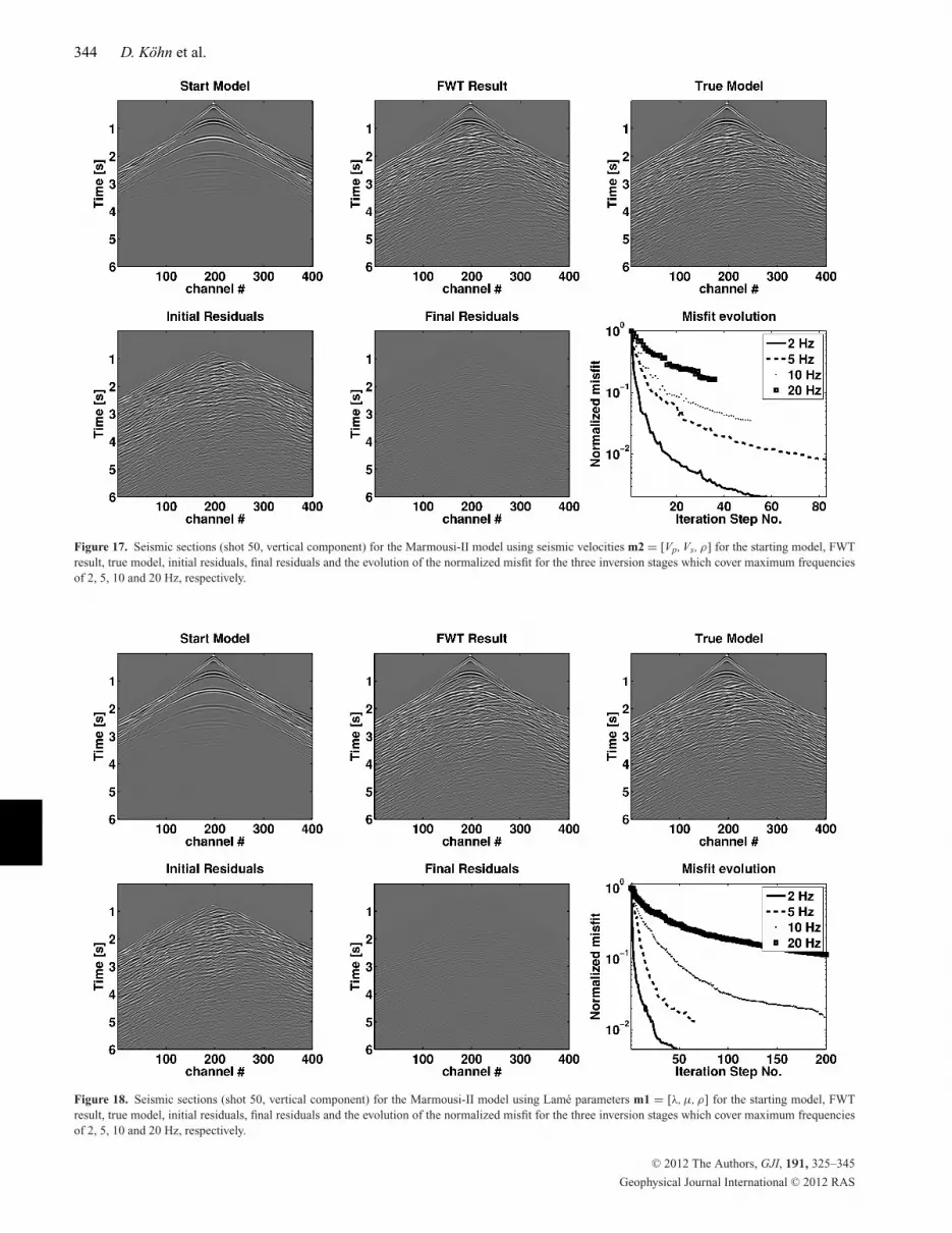
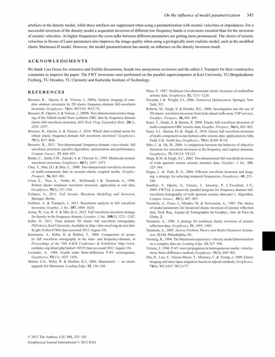
compared to the smooth starting model. The final inversion results after 285 iterations for the velocity parametrization are shown in Fig. 13.Additionally, depth profiles at xp1 = 3.5 km and xp2 = 6.4 km of the starting model and inversion result are compared with the true model inFig. 14. The results contain a lot of small details. All fine layers which are completely absent in the starting model are resolved. The thrustfaults and reef structures in the deeper part of the model are imaged also very well. All hydrocarbon reservoirs can be identified and evenstructures at the scale of the FD grid are resolved. The shear wave velocity model could also be reconstructed, even though only streamerdata and therefore only P-wave information is used. This can be explained by the replacement of the soft-seabed in the original Marmousi-IImodel by the hard-seabed used in this study, which leads to significant P–S conversions and S–P conversions at the seafloor. Therefore thehard-seabed produces a significant footprint in the shear wave velocity model. Even the density, a parameter which can be hardly estimatedfrom seismic data, could be recovered from the seismic wavefield. Keep in mind though, that the density image is based not only on thedensity information, but contains also structural V p and V s information due to the ambiguity investigated by the CTS test problem (Section 4).The inversion results for the Lame parametrization are shown in Figs 15 and 16. For a direct comparison of the results, the models for theLame parameters are converted to seismic velocities.The resolution of the seismic velocities for both parametrizations is comparable. Onlythe density model for the Lame parametrization is less resolved and shows high-frequency artefacts at the layer boundaries.Possible reasonsare the stronger μ-artefacts in the density model as observed in the CTS model study (triangular-shaped artefacts in Fig. 5). The quality ofthe inversion results is also evident in the seismic sections of shot 50 (vertical component) plotted in Figs 17 and 18 for the two differentparametrizations, respectively. Note the direct wave, the reflection from the ocean bottom, a few multiples and the dominant reflection fromthe interface between low-velocity and high-velocity sediments, but the lack of other events beyond the first arrivals in the seismic sectionof the starting model. The initial data residuals show no direct wave anymore, so it is fitted perfectly. The residuals only contain events fromsmall scale model features. The seismic sections of the FWT result and the true model are nearly identical, so the final data residuals for bothparametrizations are very small. All reflection events are fitted perfectly. The normalized misfit function for the different frequency bandsdecreases very fast and smooth, similar to the behaviour for the CTS model.

6 C O N C LU S I O N S

In this paper, we have shown the potential of elastic FWT for imaging structures which are on the same scale or smaller than the seismicwavelength using far-offset reflection seismic data with a P-wave dominant point source. The success of FWT depends on the choice of modelparameters. This was demonstrated using the CTS model for different model parametrizations. The choice of Lame parameters can lead to

C© 2012 The Authors, GJI, 191, 325–345


344 D. Kohn et al.

Figure 17. Seismic sections (shot 50, vertical component) for the Marmousi-II model using seismic velocities m2 = [Vp, Vs, ρ] for the starting model, FWTresult, true model, initial residuals, final residuals and the evolution of the normalized misfit for the three inversion stages which cover maximum frequenciesof 2, 5, 10 and 20 Hz, respectively.

Figure 18. Seismic sections (shot 50, vertical component) for the Marmousi-II model using Lame parameters m1 = [λ, μ, ρ] for the starting model, FWTresult, true model, initial residuals, final residuals and the evolution of the normalized misfit for the three inversion stages which cover maximum frequenciesof 2, 5, 10 and 20 Hz, respectively.

C© 2012 The Authors, GJI, 191, 325–345



artefacts in the density model, while these artefacts are suppressed when using a parametrization with seismic velocities or impedances. For asuccessful inversion of the density model a sequential inversion of different low frequency bands is even more essential than for the inversionof seismic velocities. At higher frequencies the cross-talks between different parameters are getting more pronounced. The choice of seismicvelocities in favour of Lame parameters also improves the image quality when using a geologically more realistic model, such as the modifiedelastic Marmousi-II model. However, the model parametrization has mainly an influence on the density inversion result.

A C K N OW L E D G M E N T S

We thank Lisa Groos for extensive and fruitful discussions, beside two anonymous reviewers and the editor J. Trampert for their constructivecomments to improve the paper. The FWT inversions were performed on the parallel supercomputers at Kiel University, TU-BergakademieFreiberg, TU Dresden, TU Chemnitz and Karlsruhe Institute of Technology.

R E F E R E N C E S

Brossier, R., Operto, S. & Virieux, J., 2009a. Seismic imaging of com-plex onshore structures by 2D elastic frequency-domain full-waveforminversion, Geophysics, 74(6), WCC63–WCC76.

Brossier, R., Operto, S. & Virieux, J., 2009b. Two-dimensional seismic imag-ing of the Valhall model from synthetic OBC data by frequency-domainelastic full-waveform inversion, SEG Tech. Prog. Expanded Abstr., 28(1),2293–2297.

Brossier, R., Operto, S. & Virieux, J., 2010. Which data residual norm forrobust elastic frequency-domain full waveform inversion? Geophysics,75(3), R37–R46.

Brossier, R., 2011. Two-dimensional frequency-domain visco-elastic fullwaveform inversion: parallel algorithms, optimization and performance,Comput. Geosci., 37, 444–455.

Bunks, C., Salek, F.M., Zaleski, S. & Chavent, G., 1995. Multiscale seismicwaveform inversion, Geophysics, 60(5), 1457–1473.

Choi, Y., Min, D.J. & Shin, C., 2008. Two-dimensional waveform inversionof multi-component data in acoustic-elastic coupled media, Geophys.Prospect., 56, 863–881.

Crase, E., Pica, A., Noble, M., McDonald, J. & Tarantola, A., 1990.Robust elastic nonlinear waveform inversion: application to real data,Geophysics, 55(5), 527–538.

Fichtner, A., 2011. Full Seismic Waveform Modelling and Inversion,Springer, Berlin.

Fichtner, A. & Trampert, J., 2011. Resolution analysis in full waveforminversion, Geophys. J. Int., 187, 1604–1624.

Jeonq, W., Lee, H.-Y. & Min, D.-J., 2012. Full waveform inversion strategyfor density in the frequency domain, Geophys. J. Int., 188(3), 1221–1242.

Kohn, D., 2011. Time domain 2D elastic full waveform tomography,PhD thesis, Kiel University. Available at: http://nbn-resolving.de/urn:nbn:de:gbv:8-diss-67866 (last accessed 2012 August 18).

Kurzmann, A., Kohn, D. & Bohlen, T., 2008. Comparison of acous-tic full waveform tomography in the time- and frequency-domain, inProceedings of the 70th EAGE Conference & Exhibition, http://www.earthdoc.org/detail.php?pubid=10539 (last accessed 2012 August 18).

Levander, A., 1988. Fourth order finite-difference P-SV seismograms,Geophysics, 53(11), 1425–1436.

Martin, G.S., Wiley, R. & Marfurt, K.J., 2006. Marmousi2 — an elasticupgrade for Marmousi, Leading Edge, 25, 156–166.

Mora, P., 1987. Nonlinear two-dimensional elastic inversion of multioffsetseismic data, Geophysics, 52, 1211–1228.

Nocedal, J. & Wright, S.J., 2006. Numerical Optimization, Springer, NewYork, NY.

Roberts, M., Singh, S. & Hornby, B.E., 2008. Investigation into the use of2D elastic waveform inversion from look-ahead walk-away VSP surveys,Geophys. Prospect., 56, 883–895.

Sears, T., Singh, S. & Barton, P., 2008. Elastic full waveform inversion ofmulti-component OBC seismic data, Geophys. Prospect., 56(6), 843–862.

Sears, T.J., Barton, P.J. & Singh, S., 2010. Elastic full waveform inversionof multi-component ocean-bottom cable seismic data: application to AlbaField, U.K. North Sea, Geophysics, 75(6), R109–R119.

Shin, C. & Ha, W., 2008. A comparison between the behavior of objectivefunctions for waveform inversion in the frequency and Laplace domains,Geophysics, 73, VE119–VE133.

Shipp, R.M. & Singh, S.C., 2002. Two-dimensional full wavefield inversionof wide aperture marine seismic streamer data, Geophys. J. Int., 151,325–344.

Sirgue, L. & Pratt, R. G., 2004. Efficient waveform inversion and imag-ing: a strategy for selecting temporal frequencies, Geophysics, 69, 231–248.

Sourbier, F., Operto, S., Virieux, J., Amestoy, P., L’Excellent, J.-Y.,2009. FWT2d, A massively parallel program for frequency-domain full-waveform tomography of wide aperture seismic data-part 1: Algorithm,Comput. Geosci., 35(3), 487–495.

Tarantola, A., Fosse, I., Mendes, M. & Nercessian, A., 1985. The choiceof model parameters for linearized elastic inversion of seismic reflectiondata, Tech. Rep., Equipe de Tomographie du Geophys., Inst. de Paris duGlobe, 2.

Tarantola, A., 1986. A strategy for nonlinear elastic inversion of seismicreflection data, Geophysics, 51, 1893–1903.

Tarantola, A., 2005. Inverse Problem Theory and Model Parameter Estima-tion, SIAM, Philadelphia, PA.

Versteeg, R., 1994. The Marmousi experience: velocity model determinationon a complex data set, Leading Edge, 13, 927–936.

Virieux, J., 1986. P-SV wave propagation in heterogeneous media: velocity-stress finite-difference method, Geophysics, 51(4), 889–901.

Zhu, H., Luo, Y., Nissen-Meyer, T., Morency, C. & Tromp, J., 2009. Elasticimaging and time-lapse migration based on adjoint methods, Geophysics,74(6), WCA167–WCA177.

C© 2012 The Authors, GJI, 191, 325–345


Documents

On the influence of model parametrization in elastic full waveform tomography