Geophysical Prospecting, 1996, 44, 427 -455

Linearized elastic parameter sectionsl

Bjorn Ursin,2 Biorn Olav Ekren3 and Egi l Tj i i land2

Abstract

Contrasts in elastic parameters can be estimated directly from seismic data using

offset-dependent information in the PP reflection coefficient. A linear approximation

to the PP reflection coefficient including three coefficients is fitted to the data, and

relative contrasts in various elastic parameters are obtained from linear combinations

of the estimated coefficients. Linearized elastic parameter sections for the contrasts in

P-wave impedance, P-wave velocity, density, plane-wave modulus, and the change in

bulk modulus and shear modulus normalized with the plane-wave modulus are

estimated. If the average P- to S-wave velocity ratio is known, linearized parameter

sections including the contrast in the average P- to S-wave velocity ratio and a fluid

factor section can be computed. Applied to synthetic data, visual comparison of the

estimated and true elastic parameter sections agree qualitatively, and the results are

confirmed by an analysis of the standard deviation of the estimated parameters. The

parameter sections obtained by inversion of a shallow seismic anomaly in the Barents

Sea are promising, but the reliability is uncertain because neither well data nor

regional trends are available.

ln t roduct ion

Amplitude-versus-offset (AVO) analysis is based on offset- or angle-dependent

reflection coefficients, and is successfully used as a qualitative tool for lithology and

fluid prediction in many regions.

AVO inversion, which is still in an early stage, is quantitative and estimates the

elastic parameters in the subsurface. AVO inversion assumes that all offset-

dependent amplitude effects, other than the reflection coefficient, are corrected for.

In this case, at least theoretically, contrasts in elastic parameters can be estimated

from seismic data.AVO inversion methods based on a linear approximation to the PP reflection

coefficient result in weighted stacking schemes (Smith and Gidlow 1987; Ursin and

Dahl 1990; Gidlow, Smith and Vail 1992).In general, AVO inversion is non-unique

I Received January 1994, revision accepted June 1995.2 University of Trondheim, The Norwegian Institute of Technology, Department of Petroleum

Engineering and Applied Geophysics, S.P. Andersens vei 15,A., N-7034 Trondheim NTH, Norway3 Statoil Research Center, Postuttak, N-7005 Trondheim, Norway. Formeriy at'.

O 1996 European Association of Geoscientists & Engineers 427

428 B. Ursin, B.O. Ekren and E. Tir)land

and is not able to find the correct solution. Drufuca and Mazzotti (1995) showed thatthe ambiguity of the AVo inversion result depends on the maximum angle ofincidence and the noise level in the data. Several authors (e.g. Stolt and \Teglein1985; de Nicolao, Drufuca and Rocca 1993; Ursin and Tj6land 1993) have alsopointed out that it is difficult to estimate more than two parameters from thelinearized reflection coefficient.

Smith and Gidlow (1987) eliminated the density contrast in the linearapproximation to the PP reflection coefficient by a hard constraint and this reducesthe ambiguity of the inversion (provided that the imposed hard constraint is correct).They devised the fluid factor section which may pin-point gas-sarurated zones. Theirassumption is that deviations from the mudrock trend (Castagna, Batzle andEastwood 1985) can be used as a gas indicator in some regions. Designing l inearcombinations of the estimated elastic parameter contrasts which are able to detectdeviations from a background trend is a promising application of AVo inversion.

Prestack migration before AVo inversion will improve the results (Beydoun,Hanitzsch and Jin 1993; Ekren and Ursin 1995) because prestack migration improvesthe signal-to-noise (S[.tr) ratio. The prestack migration algorithm should beamplitude preserving, like the technique described by Tygel, Schleicher andHubral (1992).

A major drawback of AVo inversion of NMo-corrected cMp gathers (Smith andGidlow 1987; Ursin and Dahl 1990; Gidlow et al. 1992) is the sensitivity of thesolution to residual moveout errors and NMO stretch. $7e have reduced this problemby using an improved method for AVo estimation (Ursin and Ekren 1995).

The seismic amplitudes are approximated by polynomials in the horizontalslowness variable. By direct comparison with a Taylor expansion of the weak contrastapproximation of the PP reflection coefficient, the coefficients in the slownesspolynomial can be related to contrasts in the elastic parameters. A similar procedurewas used by Balogh, Snyder and Barney (19s6) to compute seismic sections forcontrasts in P-wave velocity, density and the P- to S-wave velocity ratio.

Linearized elastic parameter sections are estimated from marine data from thesouthern Barents Sea, containing a shallow seismic anomaly. In the processing,prestack time migration (as described by Ekren and Ursin 1995) was performed toenhance the data quality before the AVo inversion. The results are promising, butthe reliability of the estimated parameter sections is uncertain, because no well dataor regional trends are available.

The PP ref lect ion coef f ic ient

A weak contrast approximation to the PP reflection coefficient is (chapman 1976)

. ) ^ l A n , ^ , ^s rn - d + AQn 'q .

z oRpp = :^+-il* -^(:)'+) ( 1 )

O 1996EuropeanAssociat ionofGeoscient is ts&Engineers, GeophysicalProspect ing,44,42T-455

Linearized elastic parameter sections 429

Ursin and T jAland (1992) used a Taylor expansion of ( 1 ) to obtain the weak-contrast

small-offset approximation

^ 1 LZp /1 L,oR p p = t 4 + ( 2 " - 2 A u \ , 1 A o

t t ) t " P s ' | 2 n ( a P \ ' (2 )

In (1) and (2), the average elastic properties across the interface are Zp, pt, M and a,where Zp denotes P-wave impedance, p denotes shear modulus, M denotes theplane-wave modulus (: aZp) and a denotes P-wave velocity. The changes in elastic

properties (assumed to be small) are L,Zp, Ap and Aa. The local angle of incidence is

0, and p - sin?f a is the slowness. Note that the average P- to S-wave velocity ratio

@ : ^ I l.D does not appear in (2) because the relationship

has been used. Equation (2) can be written as a polynomial in slowness or olTset as

follows:

Rpp t as -f a1@p)t + az@p)a

! so I t r g t + t 2g t , (4)

by Ursin and Ekren (1995),

where ro:1.0 from the definit ion used by Ursin and Ekren (1995). The vectors

a: (ao,ar ,az)T and s: (ss,s1 ,s2)T are re lated by the l inear t ransformat ion (Taner

and Koehler 1969; Balogh et al. 1986; Ursin and Dahl1992)

(6)

primary reflected P-wave, the velocity

where z denotes vertical depth (positive downwards) and z. is reflector depth. For a

homogeneous medium (; : ez: (22,)".

() 1996 European Association of Geoscientists & Engineers, Geol>hysical Prospecting, 44, 427-455

Lpt l tJ \ tL t 'M: \ a ) ,

(3 )

where the vector s: (so,sr,sz)T is the vector r grvenscaled by the zero-offset amplitude p(t,), i.e.

[ " ] [ " ]. - l r ' l : z t , , ) r : a ( t . ) l r r l .Ls: I L rz )

(7)

I t o o l [ s r ' l. - r s : l o ( , o l l ' , 1 ,

t . | ' lLo (z (i. l Lsz.l

where e, - blltt and (2 : bftzloa. For amoments b7 are defined as

b , : I a t z ) 2 j ' d r - 2 [ ^ o t " t 2 ' - ' a r .J r a v , t v

t \ l

430 B. Ursin, B.O. Ekren and E. Tjdland

Parameter sect ions using the P-wave veloci ty

The explicit relationship between the vector a in (6) and the elastic parameters in (2)is

I LZ'ft - l

l ' r l 1 2 0 0 lr n l * l - l r - t j l . ( s )

I M I l ^ : ll l " l L o o 2 )L ; . 1

Linear combinations of the elements in rn give other elastic parameters independentof q : cr/p. Although linear combinations contain no extra information, they can beeasier to interpret than the individual elements in rn (Lcirtzer and Berkhout 1993).From Zp * pa and M: aZp: K + 4pf 3, where K is the bulk modulus) we get

L t t _ � L Z p _ 4 9 : r , . _ \7 - 4

- ; - ' \ u o - u 2 t '

LM LZ,, Arr

M : t * - : 2 ( a o + o z )

and

i5 : ^4 -!+ : 2@o -r \a1 + !a)M M 3 M

The results are summarized by the model vector rno, given by

LZPIZP

L,af a

Lp/p

LMIMLplMLKIM

that is, m.r : MoTs.Once the coefficients in the offset reflectivity polynomial in (4) have been estimated,the elastic parameters above can be computed. The coefficients (1 and (2 depend onthe P-wave velocity profile which is found from the stacking velocities.

Parameter sect ions us ing the P- and S-wave veloc i t ies

In the previous section, the change in shear modulus and bulk modulus werenormalized by the plane-wave modulus to make the parameters independent of S-wave velocities. However, when the average P- to S-wave velocity ratio (q : al0 isassumed to be known, a new set of elastic parameter sections can be computed.

e 1996 European Association of Geoscientists & Engineers, Geophysical Prospecting,44,427-455

m . : (e)fi '?,;]

t';]2 0 0

0 0 2

2 0 - 2

2 0 2n - l 1" 2 2

1 2 41 a

Linearized elastic parameter sections 431

The difference between the contrast in P-wave impedance and the contrast in

S-wave impedance, Rpp(0) - Rss(0) can be a good hydrocarbon indicator in some

regions (Castagna and Smith 1994) and is related to the ratio Lqlqbv

Rpp(o) - Rss(o) ::(+ "+) ::+, ( 1 0 )

where LZslZs is the S-wave impedance contrast.Another useful hydrocarbon indicator is the fluid factor AF (Smith and Gidlow

1987), which is designed to highlight deviations from the

A o : k A g ( 1 1 )

mudrock trend (Castagna et al. 1985). Equation (11) gives

A , r , L p A o , B L AQ . ( \ A A p

k , ,: ; o r * t u k q a l + ( , - r - i k q ) o r .

( 1 2 )

which will be zero for wet siliclastic rocks, i.e. where the mudrock equation is valid.

In gas-saturated intervals, the mudrock equation breaks down and AF will have large

values. Although a typical value for ft is 1.16 (Castagna et al. 1985), well logs or

regional trends should be used to determine the value of A in each area.

A serious problem in the estimation of the parameters above is that the background

P- to S-wave velocity ratio trend has to be known. Some authors have tackled this

problem by assuming a constant average P- to S-wave velocity ratio. \7iggins, Kenny

and McClure (1983) and Castagna and Smith (1994) showed that for alP :2, (10)

can be written as

Rpr, (O) - Rss(0) : ) (as + a1) . (13)

A scaled version of (13) was proposed by Soroka and Reil ly (1992)' i.e.

L,qao ] : as (as I a1 ) . ( 14 )

q

A popular hydrocarbon indicator is the produ ct asal in (4), which equals the product

sgsl, obtained from the estimated values of s0 and s1 in (4), scaled by (r(> 0), and is

given by

a o d r : ( r s o s r : Q P I , ) 2 r t

_ ! L Z , ( ! L " _ r A p \ ' s r: t 4 \ t ; - " M )

\ r J l

Positive values of sssl (i.e. 11 positive) are often found for reflections at the top and

base of gas-sand reservoirs. Negative values of sssl are typical for reflection

coefficients found at lithological boundaries. Castagna and Smith (1994) showed that

(() 1996 European Association of Geoscientists & Engineers, Geophysical Prospecting,44' 427-455

432 B. Ursin, B.O. Ekren and E. T-idland

the product s6s1 is only reliable as a hydrocarbon indicator for low impedance gassands encased in high impedance rocks, i.e. for Class 3 gas sands in the classificationsystem of Rutherford and \X/illiams (1989).

The set of elastic parameters which can be computed when the average P- toS-wave velocity ratio is known are summarized by the model vector rnn, given by

- \q ' iq ' - r- I n ' t + \ u 2- 5q' !r '2qt 4qt

3 q t - 4 3 q 2 - 4t ^ 24 q | - i q t

8 q - 4 k - k q 2

filq :

LZslZsLt3lpLplttLK lK

Lq/q

AF

4qi nq

1- t

0. 2oq

-3 q " - +

1

Lq

lr''1 ( 1 6 )

that is, mq : MqTs.

Synthet ic data

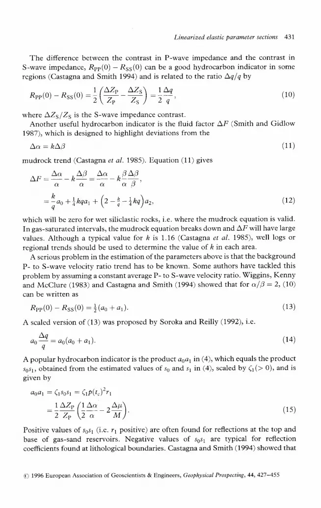
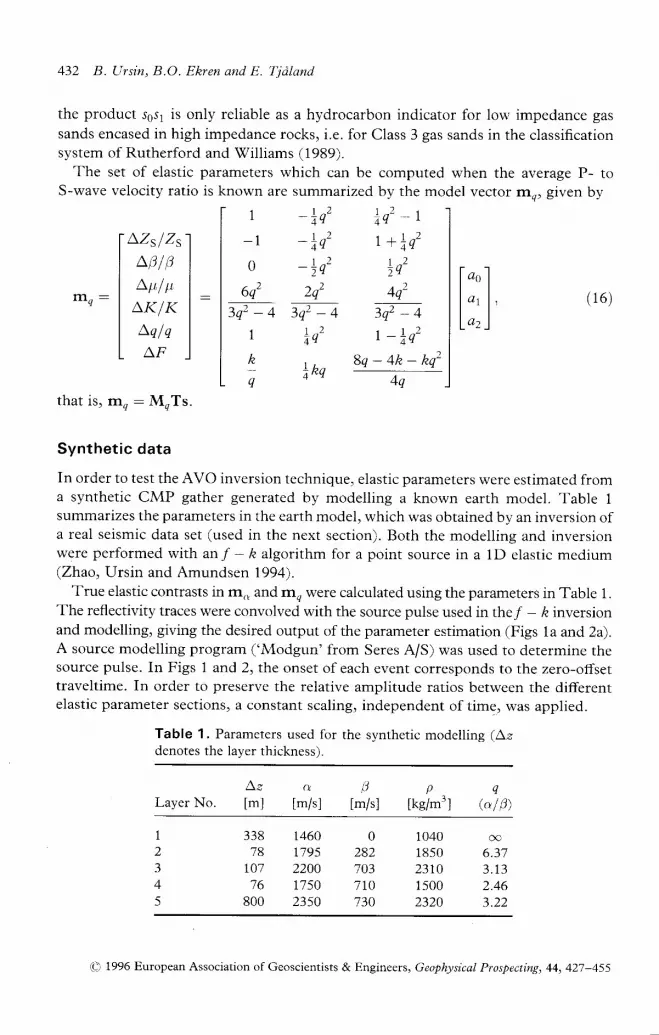
In order to test the AVO inversion technique, elastic parameters were estimated froma synthetic CMP gather generated by modelling a known earth model. Table Isummarizes the parameters in the earth model, which was obtained by an inversion ofa real seismic data set (used in the next section). Both the modelling and inversionwere performed with anf - ft algorithm for a point source in a lD elastic medium(Zhao, Ursin and Amundsen 1994).

True elastic contrasts in m,. and mq were calculated using the parameters in Table 1.The reflectivity traces were convolved with the source pulse used in the/ - A inversionand modelling, giving the desired output of the parameter estimation (Figs la and 2a).A source modelling program ('Modgun' from Seres A/S) was used to determine thesource pulse. In Figs 1 and 2, the onset of each event corresponds to the zero-offsettraveltime. In order to preserve the relative amplitude ratios between the differentelastic parameter sections, a constant scaling, independent of time, was applied.

Table 1. Paramerers used for the synthetic modelling (A:denotes the laver thickness).

L,z aLayer No. [m] [m/s]

i . ) p qtm/sl tkg/m3l (a I 13)

I

2-l

45

02827037 t o730

33878

t0776

800

t460t795220017502350

1040 oo1850 6.372310 3.131500 2.462320 3.22

() L996 European Association of Geoscientists & Engineers, Geophysical Prospecting, 44, 427 -455

Linearized elastic Darameter sections 433

Figure 1. Elastic parameter contrasts in rn,,- (a) Computed from Table 1 and convolved withsource pulse. (b) Estimated parameter contrasts from the synthetic CMl'-gather.

AVO analysis of the synthetic data was performed using the technique describedby Ursin and Ekren (1995). Picked stacking velocities from a standard velocityanalysis were interpolated linearly to obtain a stacking velocity at each time sample.Interval P-wave velocities were computed using the Dix formula (Dix 1955). TheP- to S-wave velocity ratios in Table I (constant in each layer) were used in theestimation of the parameters in rn{.

Figure 1b shows the parameters in rn,, estimated from the elements of the vector a.The sidelobes of the pulse in the estimated traces (Fig. 1b) are caused by artifacts inthe modelling of the CMP gather. A comparison of F'igs la and b shows that thecontrast in P-wave impedance (LZp lZp) is well determined. The contrast in P-wave

ftl 1996 European Association of Geoscientists & Engineers, Geophysical Prospecting, 44,427-455

ooEtr

LZo Ao L ,o LM Lu LK- T " n M M M

U'

o.EF

434 B. Ursin, B.O. Ekren and E. Tjdland

a)

b)

LZ"ZS

Figure 2. Elastic parameter contrasts in mn. (a) Computed from Table 1 and convolved withthe source pulse. (b) Estimated parameter contrasts from the synthetic CMP gather usingP- and S-wave velocity ratios from Table l. Note that the waterbottom contrast is not includedin the figures.

velocity (A,a/a) is less well determined. Both amplitudes and pulse shapes differfrom the true model, but the polarities are correct. A poorly determined contrast inP-wave velocity is consistent with the conclusions reached by Ursin and TjAland(1993). The contrast in density (Lpl D is the difference between the contrast in P-waveimpedance and the contrast in P-wave velocity. Because the contrast in P-wavevelocity is rather small for this synthetic example, the contrast in density resemblesthe contrast in P-wave impedance. The contrast in the plane-wave modulus(LM/M) is the sum of the contrast in P-wave impedance and the contrast in P-wave

A 1996 European Association of Geoscientists & Engineers, Geophysical Prospecting, 44, 427-455

ooEtr

A_S_q af'Mp

AKK

4pu

o

P 0.6E

tr

0.8

Linearized elastic parameter sections 435

velocity, and is also nearly similar to the P-wave impedance. Minor differences in

amplitudes are caused by the poorly determined contrast in P-wave velocity. Thenormalized change in shear modulus (LplM) shows significant differences between

the estimated and the true models for the top reflector. The normalized change in

bulk modulus (LKIM) shows a good match with the true data. Although the

estimation of the parameters in m. is not perfect, the results in Fig. 1 are promising.

Parameter estimation was also performed for the elements in mn. Figure 2 shows

the parameter contrasts estimated from the synthetic CMP gather. All parameter

contrasts in rnn (except for A,KIK and AF) are very large for the waterbottom

reflection(interfacebetweenlayersl and2).ThecontrastsLpl13,L'p.lptandLZslZsare all2.0 at the waterbottomr which is much larger than the assumed contrasts in the

weak contrast approximation. \7e have therefore muted the waterbottom in Figs 2a

and b.Figure 2b shows that the contrast in shear modulus (Lplp') and the contrast in

S-wave velocity (LP I O are the most poorly determined parameters, since there are

differences in both amplitude and pulse shape. The contrast in bulk modulus(LK I K) is, on the other hand, very well determined. This is because LK I K is equal

to the well-determined parameter A'Kf M scaled by a factor involving q". The

contrast in S-wave impedance (LZslZ) is better determined, although the

amplitude of the uppermost reflector (below the waterbottom) is too low compared

to the true data. The contrast in the average P- to S-wave velocity rutio (L'q lQ shows

a relatively good match for the two deepest reflectors, but is significantly different for

the upper-most reflection. In the estimation of the fluid factor (AF), we have used

the mudrock equation (Castagna et al. 1985), using A : 1.16 in (11). The polarit ies of

AF for the two deepest reflectors are correct) although the amplitude of the lowest

reflector is too small compared to the true model. A weak uppermost reflector can be

seen in the estimated data, but not in the true model.Estimations were also performed for other trends of the average P- to S-wave

velocity ratios, giving similar results. This means that the paralneter estimation is

rather insensitive to small errors in the background velocities. In order to compare

the variability of the different sections, we analyse the standard deviation of the

estimated parameters. Note, however, that small standard deviations cannot be

used uniquely as an indication of a reliable parameter estimation, but only as a

diagnostic of the goodness of fit. In the Appendix the covariance matrix of theestimated parameters has been computed assuming independent and normally

distributed data errors with zero mean and variance o!. We have computed thestandard deviations of the estimated parameters for the reflection between layers 3

and 4 in the synthet ic data example, where ( r :1.054, Cz:1.072' q:2.46 and

-yr,:0.995km. As expected, the variance of the parameter L'Zpf Zp is the smallest,

and (A7) gives

1 4var{L,ZplZp} =i"?, (r7)

O 1996 European Association of Geoscientists & Engineers, Geophysical Prospecting,44,427-455

436 B. Ursin, B.O. Ekren and E. Tidland

Table 2. Standard deviations o,, and ao of the modelparameters m,, and mo respectively, estimated fromthe synthetic data.

L,p LM A,p,

P M M2 . 7 2 . 5 1 . 9

AKM1 . 5

LZsZS5 .6

Lp,

lrI 1 . 8

AF

2 .0

where the number of traces N is 40 in this case. In order to compare the results, allstandard deviations are normalized with the standard deviation of L,Zp I Zp and arelisted in Table 2. The best-determined parameter is L,Zp lZp followed by LK lM and4.KIK. As predicted by Ursin and Tji land (1993), LplM is better determined thanLala. Many of the parameters in mn are poorly determined (LZslZs, Lp10, Llt l l tand L,qlq), whereas the fluid factor AF is quite well determined.

The inversion is based on a weak contrast approximation to the PP reflectioncoefficient. This is not fulfilled for some of the contrasts in the model, and this mayexplain why the inversion gives rather poor estimates of some of the parameters inm^ and rno. The most difficult contrasts are those for the S-wave velocity at thesecond interface in Table I where LPIp:0.85, and for the density at thewaterbottom and at the two deepest interfaces, where Lplp:0.6 and LpJp:0.+,respectively. Some of the estimation errors in Figs 1b and 2b canalso be explained bythe relatively large maximum angles of incidence (between 40' and 55") in thesynthetic data which violates the small-offset assumption in the technique.

Rea l da ta examp le

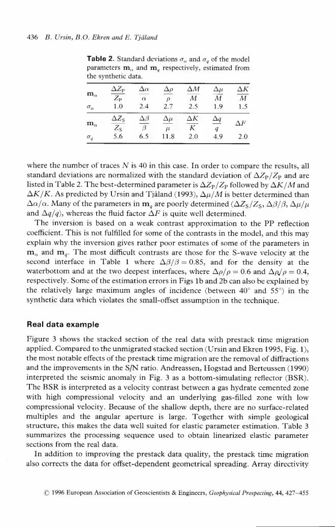
Figure 3 shows the stacked section of the real data with prestack time migrationapplied. Compared to the unmigrated stacked section (Ursin and Ekren 1995, Fig. 1),the most notable effects of the prestack time migration are the removal of diffractionsand the improvements in the S[.J ratio. Andreassen, Hogstad and Berteussen (1990)interpreted the seismic anomaly in Fig. 3 as a bortom-simulating reflector (BSR).The BSR is interpreted as a velocity contrast between a gas hydrate cemented zonewith high compressional velocity and an underlying gas-filled zone with lowcompressional velocity. Because of the shallow depth, there are no surface-relatedmultiples and the angular aperture is large. Together with simple geologicalstructure, this makes the data well suited for elastic parameter estimation. Table 3summarizes the processing sequence used to obtain linearized elastic parametersections from the real data.

In addition to improving the prestack data quality, the prestack time migrationalso corrects the data for offset-dependent geometrical spreading. Array directivity

O 1996 European Association of Geoscientists & Engineers, Geophysical Prospecting,44,427-455

LZp Aam . r h ;

o , , 1 .0 2 .4

AK L,q

K q2.0 4 .9

Lt)76 .5

rnll

oq

Linearized elastic paratneter sections 437

@

C\i

'r=

h0

tr

p

'r4U

ko

E

d

z

j

a Ao q

.=15o

6

d

.FUI

v

C€

d

(-)

o c"t- i O

iI

(() 1996 European Association of Geoscientists & Engineers, Geophysical Prospecting,44,427-455

438 B. Ursin, B.O. Ehren and E. Tjdland

Table 3. Processing sequence.

1 .2 .- 1 .

4 .5 .

Bandpass f i l ter ing (15-100 Hz)Prestack time migration (Ekren and Ursin 1995)Horizon velocity analysisAVO analysis (Ursin and Ekren 1995)Linearized elastic parameter estimation, Eqs (9) and (10)

effects, which may have a large influence on reflections before approximately 1.0s,are corrected for in the AVO analysis (Ursin and Ekren 1995). The key assumption inthe estimation of the elastic parameters) is that the applied processing sequence is ableto isolate and estimate the relative offset-dependent reflection coefficient adequately.

Figure 4 shows the zero-offset two-way traveltime for the main reflectors in theuppermost 0.8 s of the section picked by the horizon velocity analysis, together withtypical interval P-wave velocities for the layers. The waterbottom is situated at0.47 s,the top of the Tertiary unconformity at around 0.56 s, and the top and the bottom ofthe anomaly at about 0.66s and 0.75s, respectively. Figure 4 has been used as anoverlay when interpreting the estimated elastic parameter sections.

Interval P-wave velocities needed in the computation of the linearized elasticparameter sections were estimated from the Dix formula using linearly interpolatedstacking velocities from the horizon velocity analysis. Estimates of the P- to S-wavevelocity ratios, needed to estimate parameters in mo, were taken from Table I andkept constant in each layer.

a = 1460 m/s

a = 1800 m/s

a = 2300 m/s

a = 24OO m/s

1 960

Shotpoint

Figure 4. Zero-offset two-way traveltimes to the main reflectors in Fig. 3, with typical P-wavevelocities in each layer.

6

E

.EF

O 1996 European Association of Geoscientists & Engineers, Geophysical Prospecting,44,427-455

Q N

n a

Linearized elastic parameter sections 439

0 19% European Association of Geosciatists & Engllieers, Geophysicai Roqmting, 44, 427-455

44O B. Ursin, B.O. Ekren and E. Tidlantl

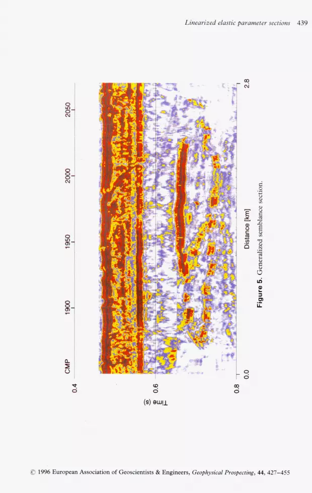
In the AVO analysis, the value of the generalized semblance quantifies the

meaningfulness of the AVO estimates. Values close to one indicate a good model fit,

while values close to zero suggest that the estimates are of no value. The generalized

semblance section (Fig. 5) shows high (brown and red) generalized semblance values

for the main reflectors, indicating that the AVO analysis was successful. Note that the

AVO results seem to be more reliable for the top anomaly reflection than for thereflection defining the bottom of the anomaly.

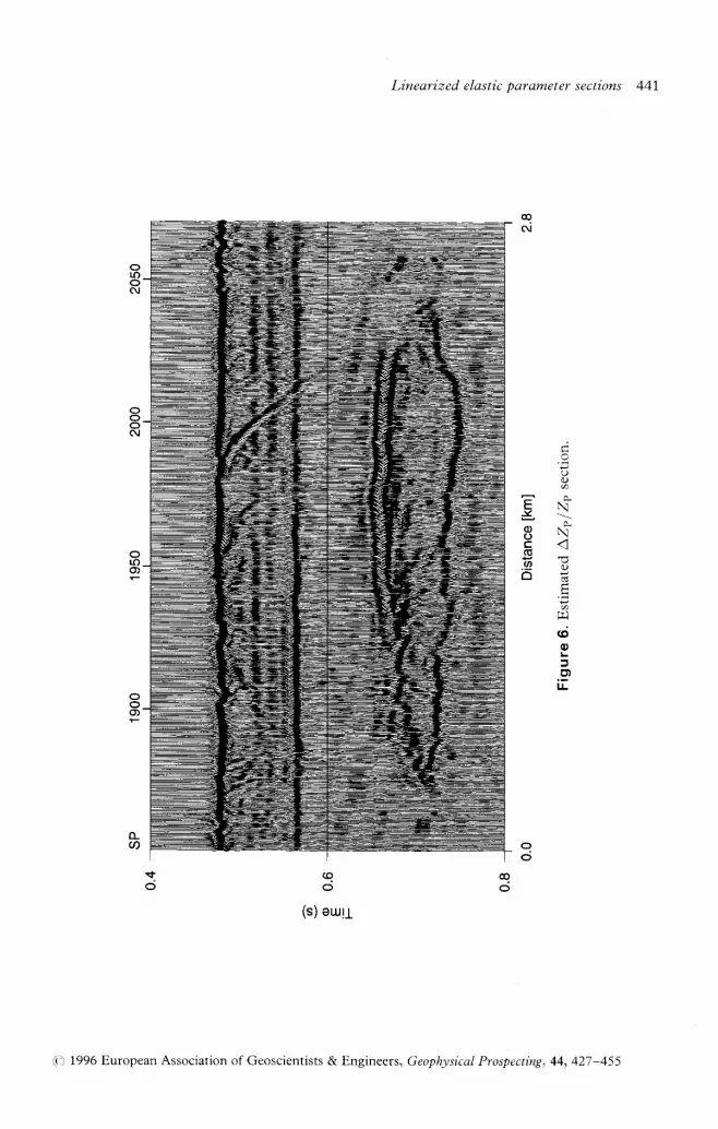
Figure 6 shows the contrast in P-wave impedance (LZplZi. Apart from agenerally lower amplitude level, this section is very similar to the stacked section in

trig. 3. However, differences can be seen, particularly at the bottom of the anomaly,

near shotpoint 2000. In the P-wave impedance section, both the waterbottom and the

base of the anomaly have positive polarity, whereas the top of the anomaly is

negative. At the unconformity the pulse shape is different from the pulse shape at the

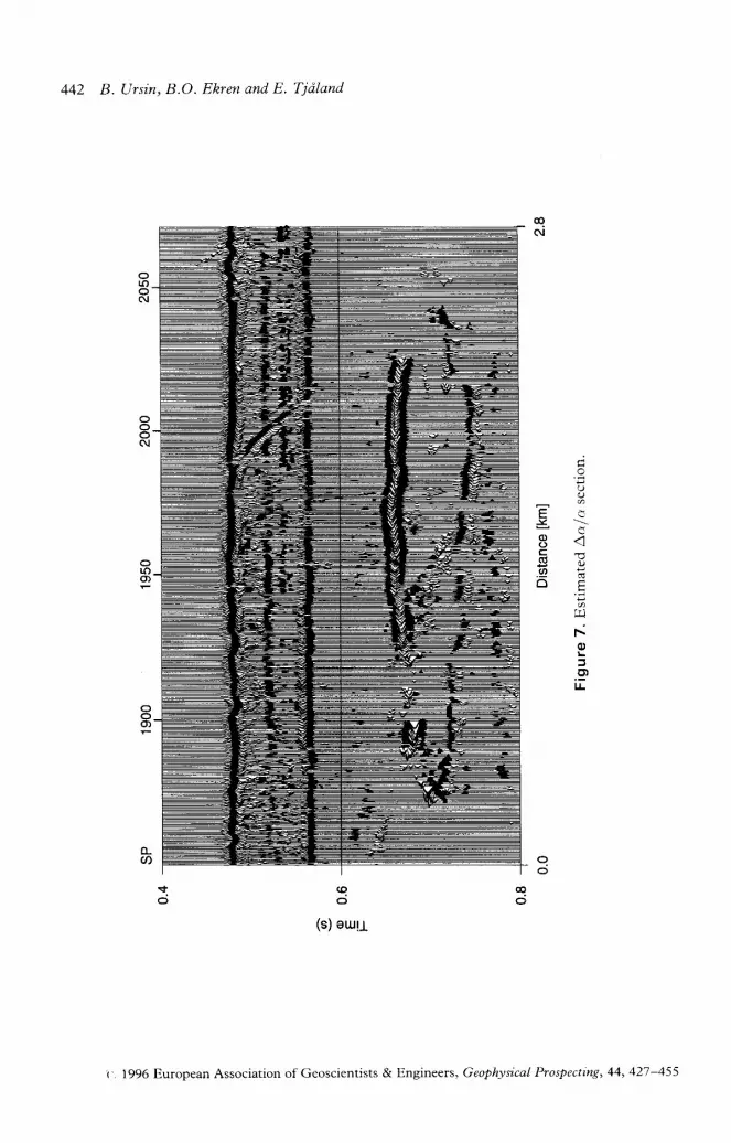
waterbottom, which may be caused by interference between many thin layers abovethe unconformity. Figure 7 shows the contrast in P-wave velocity (L'alrr), which ispositive at the water bottom, negative at the top of the anomaly and weakly positive atthe bottom of the anomaly. It is interesting to note that the amplitude level for thecontrast in P-wave velocity seems to be much higher for the real data than for the

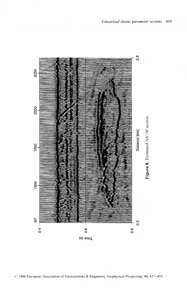
synthetic data in Fig. 1a.Figure 8 shows the normalized change in the bulk modulus (LK I M), which has a

positive polarity at the waterbottom and a large negative polarity at the top of the

anomaly. A negative polarity at the top of the anomaly is consistent with an interfacebetween a gas-filled rock and a tight gas hydrate. At the bottom of the anomaly thecontrast is positive, being consistent with a gas-water contact.

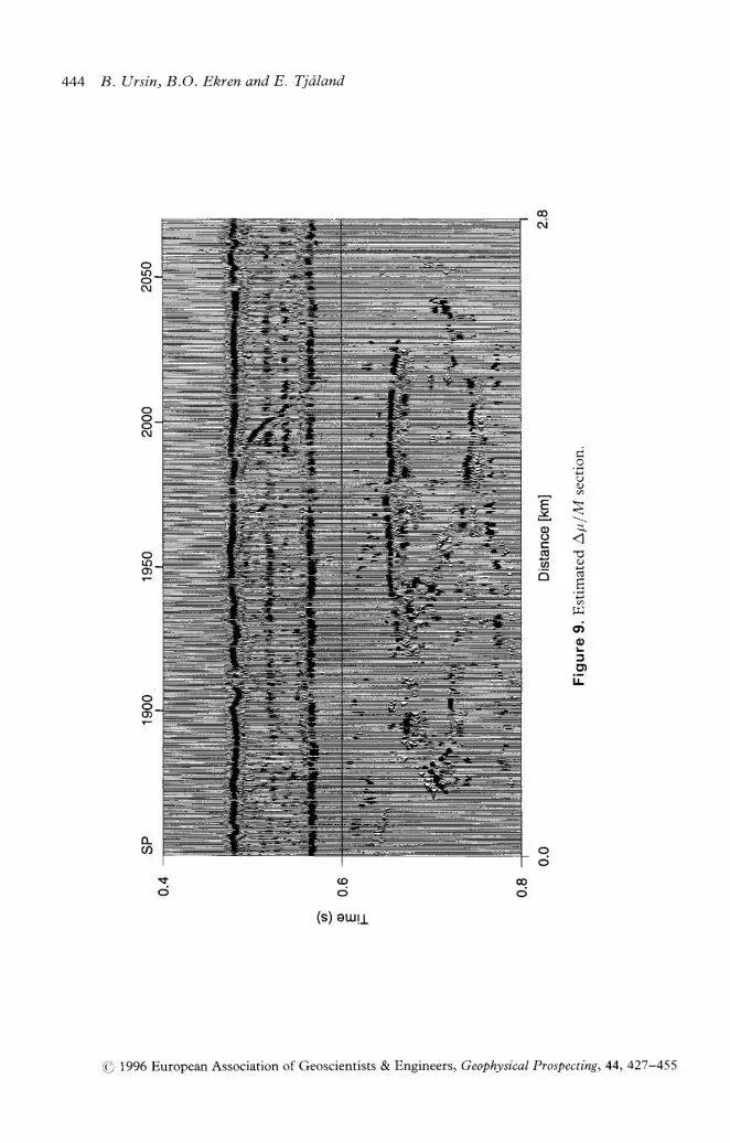
F'igure 9 shows the normalized change in shear modulus (LplM), showing weakpositive amplitudes at the waterbottom, weak negative amplitudes at the top of theanomaly and irregular amplitudes with varying polarities at the base of the anomaly.Note the large difference in amplitudes of LK lM in trig. 8 and of Lpl M in Fig. 9,indicating that the normalized changes in bulk modulus are much larger than thenormalized changes in shear modulus. This is as expected for a gas anomaly encasedin non-gaseous lormat ions.

Figure l0 shows the contrast in density (LplD, which is fairly discontinuouscompared with the other sections, except for the top anomaly reflection which ispositive. Because the waterbottom shows alternating positive and negative polarities,

this parameter must be regarded as very questionable.

The parameter sections mn depending on the background P- to S-wave velocity

ratio q were also estimated. The waterbottom reflector was not estimated because of

the very high parameter contrasts at this interface.Figure 11 shows the contrast in S-wave impedance (LZslZJ, obtained from

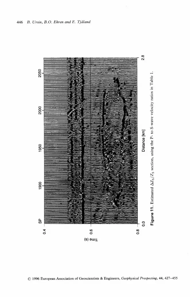
(16). The amplitudes are much more 'spiky' than in the previous figures. Theanomaly is not as clearly defined, but close inspection of the top of the anomaly showsa negative polarity, whereas the base of the anomaly shows both positive and negativepolarit ies.

('r 1996 European Association of Geoscientists & Engineers, Geophysical Prospccring,44,427-455

Linearized elastic parameter sections 441

i

oU

E N)2. --

o . tP )

. a do H

d

r r l

do

iI

(:) 1996 European Association of Geoscientists & Engineers, Geophysical Prospecting,44,427-455

442 B. (Jrsin, B.O. Ekren and E. Tjdland

Yd

@ Ao \C m

o - *

F

F

o

lJ-

qo

( s ) e u g

1'. 1996 European Association of Geoscientists & Engineers, Geophysical Prospecting, 44' 427-455

Linearized elastic Darameter sections 443

I

E <Y \

. . vU <c

A E

r r l

crio)

lJ-

1', 1996 European Association of Geoscientists & Engineers, Geophysical Prospect'ing, 44, 427-455

444 B. Ursin, B.O. Ekren and E. Tjdland

I

t r \ r_vOr i-o < 1c *

6 YN

rr l

o;o

(oo

(s) auitl

(a) 1996 European Association of Geoscientists & Engineers, Geophysical Prospecting, 44, 427-455

Linectrized elastic parameter sections 445

O

_vo <c r o( U 0( / ) c di 5 E

r r l

d

o)

iI

(s) eurl

| 1996 European Association of Geoscientists & Engincers, Geophysical Prospecting, 44,427-155

446 B. Ursin, B.O. Ekren and E. Tjdland

.j

-ol4

o

I

at r o.Yq Ao . ,c F

-u, bon t r

d

N

N4

O

d

o

g'

: l !

O 1996 European Association of Geoscientists & Engineers, Geophysical Prospecting' 44' 427-455

Linearized elastic parameter sections 447

-o()

q6!

I

l < 9

g d .

a ,

i5 bo

d

O

11

€O6

rr l

nirq)

o

lat-) 1996 European Association of Geoscientists & Engineers, Geophysical Prospecting,44' 427-455

448 B. Ursin, B.O. Ekren and E. Tjdland

-ot1

d.

!

q

d

g , )o

oo r

( , - c

M

o

f i

/1

!0

r r l

dt

o

lJ-

qo

(c,) 1996 European Association of Geoscientists & Engineers, Geophysical Prospecting, 44, 127-455

Linearized elastic parameter sections 449

Figure l2 shows the contrast in the average P- to S-wave velocity ratio (Aq/q). The

base of the anomaly shows positive and negative polarities, whereas the top of the

anomaly shows negative polarities.

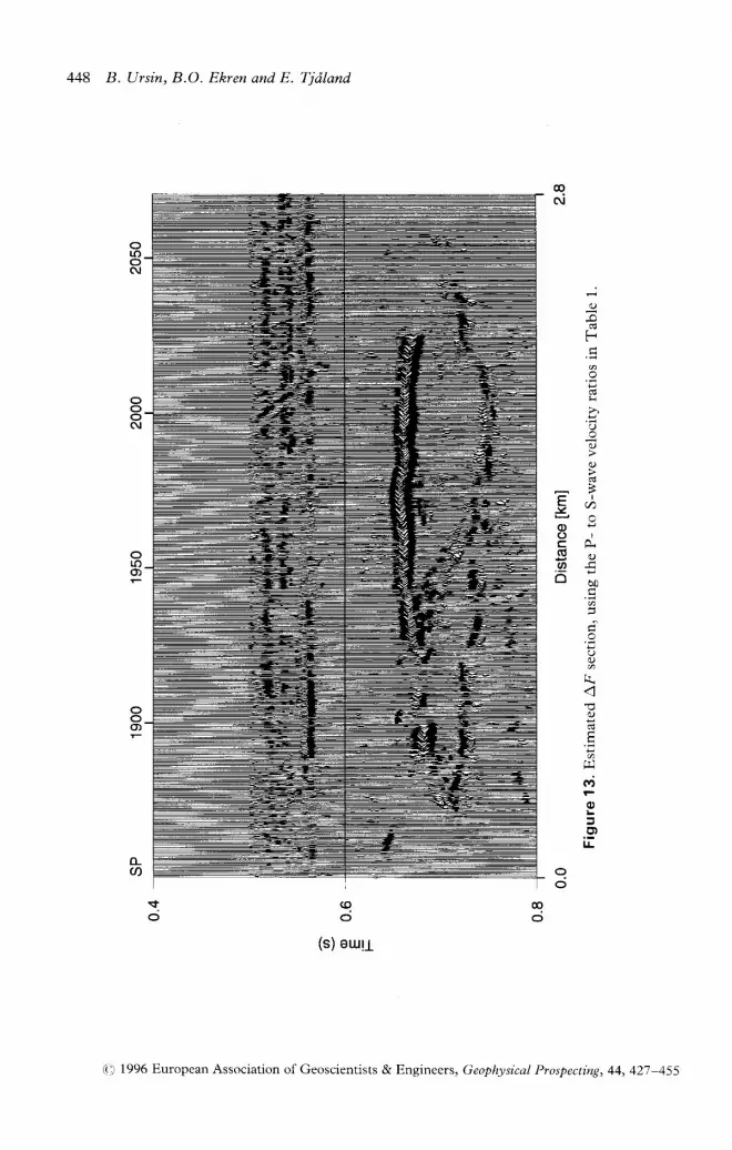
Figure 13 shows the fluid factor (AF), where the mudrock equation is similar to

that used in the synthetic data example. AF shows significant amplitudes only at the

top and the bottom of the anomaly. This supports the interpretation that the anomaly

a)

b)

AF

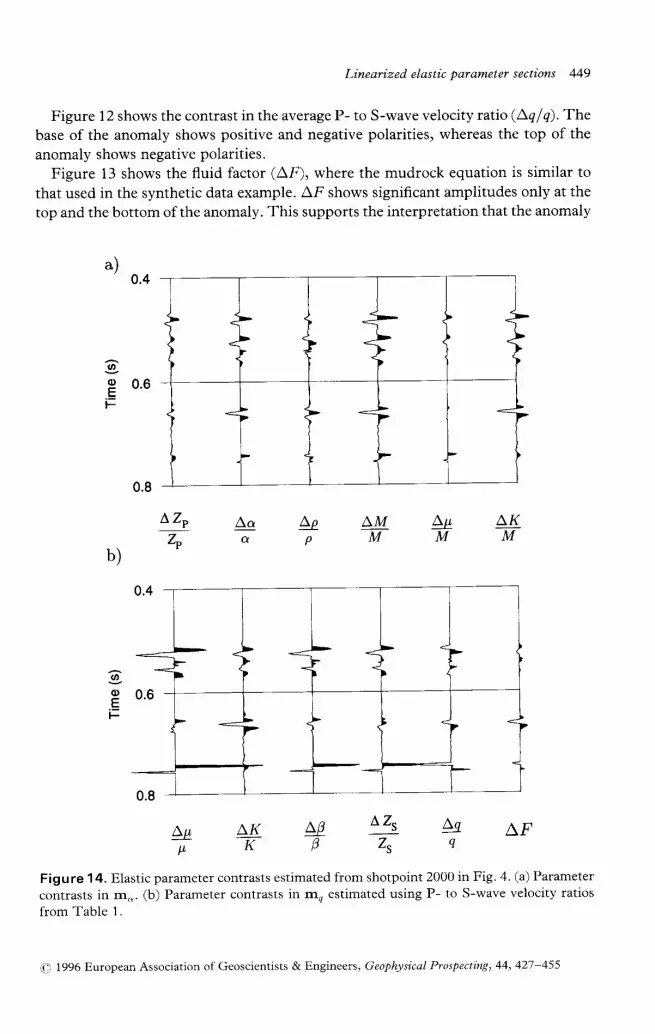
Figure 14. Elastic parameter contrasts estimated from shotpoint 2000 in Fig. 4. (a) Parameter

contrasts in rn.,. (b) Parameter contrasts in rnn estimated using P- to S-wave velocity ratios

from Table 1.

O 1996 European Association of Geoscientists & Engineers, Geophysical Prospecting,44' 427-455

o

I 0.6Etr

AKM

4pM

LZ, Ao Lp LM

4 d P M

aoEtr

Lu LK N LZs LJ

i - K 0 z s q

450 B. Ursin, B.O. Ekren and E. Tjdland

Table 4. Typical polarities for estimated parametercontrasts in rn^ from the real seismic data.

Lzp/Zp, l'K/M Lplp Lp/MA.ala

l7aterbottomUnconformityTop anomalyBase anomaly

+?

.T

+-?l-

zero

+?

weak -)

contains material which deviates from the mudrock equation. The top of the anomalyshows negative polarities and the bottom of the anomaly shows mainly positivepolarities. In order to obtain more details from the parameter estimation, estimatedparameter contrasts at shotpoint 2000 for the model vectors rn,. and mq are plotted inFigs 14a and b, respectively. More reflectors can be seen in Fig. l4a than in thesynthetic data in Fig. 1b, because the synthetic CMP gather in Fig. 1b was modelledfrom a simplified 5-layer earth model, obtained by inverting prestack data aroundshotpoint 2000 in Fig. 3. Tables 4 and 5 show typical polarities of the variousparameter contrasts in rn,, and mn, respectively.

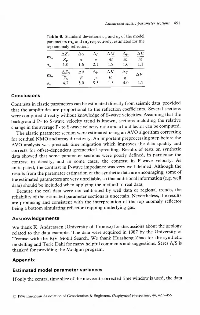
Standard deviations of the model parameters were calculated for the top anomalyreflection at shotpoint 2000 using the method described in the Appendix. Parametervalues in the calculation were (r : 0.882, ez : 0.765, a :2.46 and y.n". : 0.995 km.Table 6 shows the estimated standard deviations normalized as in (17). In general,the standard deviations are lower for the real data than for the synthetic data, but theordering of the best and the most poorly determined parameters is almost similar.One of the reasons for the large discrepancy between the synthetic and the real dataestimation is that the weak contrast approximation breaks down for the simplifiedsynthetic model in Table 1. Because of the larger number of layers in the real data,one should expect less changes in the parameters across the boundaries. Thereforethe assumptions made in the approximations of the reflection coefficients are betterfulfilled. Another difference between the synthetic and the real data is that the f - kmodelling algorithm is based on a lD geometry, whereas the real data show morecomplicated structure.

Table 5. Typical polarities of some estimatedparameter contrasts in rn, from the real seismicdata.

L,Zs/Zs, L,q/q AF

UnconformityTop anomalyBase anomaly

?

T -

zero

weak +-

e' 1996 European Association of Geoscientists & Engineers, Geophgsical Prospecting,44,427-455

Linearized elastic Darameter sections 451

Table 6. Standard deviations oo and an of the modelparameters rno and m, respectively, estimated for the

top anomaly reflection.

L,p LM Ltt

P M M2 . t 1 . 8 1 . 6

AKM1 . 1

LZsZSA A

Lt3n

5 .0

AKv

1 . 5

lL1.

t . 7

Conc lus ions

Contrasts in elastic parameters can be estimated directly from seismic data, provided

that the amplitudes are proportional to the reflection coefficients. Several sections

were computed directly without knowledge of S-wave velocities. Assuming that the

background P- to S-wave velocity trend is known, sections including the relative

change in the average P- to S-wave velocity ratio and a fluid factor can be computed.

The elastic parameter section were estimated using an AVO algorithm correcting

for residual NMO and array directivity. An important preprocessing step before the

AVO analysis was prestack time migration which improves the data quality and

corrects for offset-dependent geometrical spreading. Results of tests on synthetic

data showed that some parameter sections were poorly defined, in particular the

contrast in density, and in some cases) the contrast in P-wave velocity. As

anticipated, the contrast in P-wave impedance was very well defined. Although the

results from the parameter estimation of the synthetic data are encouraging, some of

the estimated parameters are very unreliable, so that additional information (e.g. well

data) should be included when applying the method to real data'

Because the real data were not calibrated by well data or regional trends' the

reliability of the estimated parameter sections is uncertain. Nevertheless' the results

are promising and consistent with the interpretation of the top anomaly reflector

being a bottom simulating reflector trapping underlying gas.

Acknowledgements

We thank K. Andreassen (University of Tromso) for discussions about the geology

related to the data example. The data were acquired in 1987 by the University of

Tromso with the Rfr' Mobil Search. \7e thank Huasheng Zhao fot the synthetic

modelling and Terje Dahl for many helpful comments and suggestions. Seres A/S is

thanked for providing the Modgun program.

Appendix

Est imated model parameter var iances

If only the central time slice of the moveout-corrected time window is used, the data

O 1996 European Association of Geoscientists & Engineers, Geophysical Prospecting,44' 427-455

LZt, Aarn.r

Z" ;o a 1 . 0 1 . 6

Lqq

4.0

L,p,

tr9 .5

rnn

oq

452 B. Ursin, B.O. Ekren and E. Tjdland

can be modelled as

d : F s * w , ( A 1 )

where d is the measured amplitude along the time slice, w denotes noise andmodelling errors) F is the offset matrix, given by

f r v? ut ' lt - ' - ' l" : l ' : : l ' ( ^ 2 )I t v2N v! r )

where y is offset and y1,, is the maximum offset, and s is the coefficient vector, givenby

The least-squares solution

6 : ( F r c ; l F ; - 1 r r c ; 1 d

has the covariance matrix

C , : ( F r C ; t F ) t ,

where Ca is the covariance matrix of the measurement errors. The inverse covariancematrix CJ1 is often called the curvature matrix since it is the second derivative of theobjective function in the least-squares problem. In the case where the errors of themeasured amplitudes are independent and all of equal variance o2,, the covariance

0.2 0.4 0.8 0.9 1.0

OfFset [km]

Figure 15. Eigenvalues of the curvature matrix C. I.

O 1996 European Association of Geoscientists & Engineers, Geophysical Prospecting, 44, 427-455

(A3)': fi;] :'t"r" :"'l)')

0.5 logro );

0.6 0 .s 1 .0

Offset [km]

a

Linearized elastic parameter sections 453

Offset [km]

b

0.4

0 .6 0 .8 1 .0

Offset [km]

c

Figure 16. Eigenvectors ofthe eigenvalues in Fig. 15 corresponding to (a) the largest

eigenvalue, (b) the intermediate eigenvalue, (c) the smallest eigenvalue.

matrix of the errors is

Ca: o?1 ,

and

6 : (F rF ) lF rd ,

giving

c. : ol lrrr;-1. (A4)

Note that C. is only dependent on the geometry of the seismic experiment and the

O 1996EuropeanAssociationofGeoscientists&Engineers, GeophysicalProspecting,44'427-455

454 B. Ursin, B.O. Ekren and E. Tjdland

measurement errors) not the actual seismic amplitude values. Note also that C"assumes that the model in (A1) is correct.

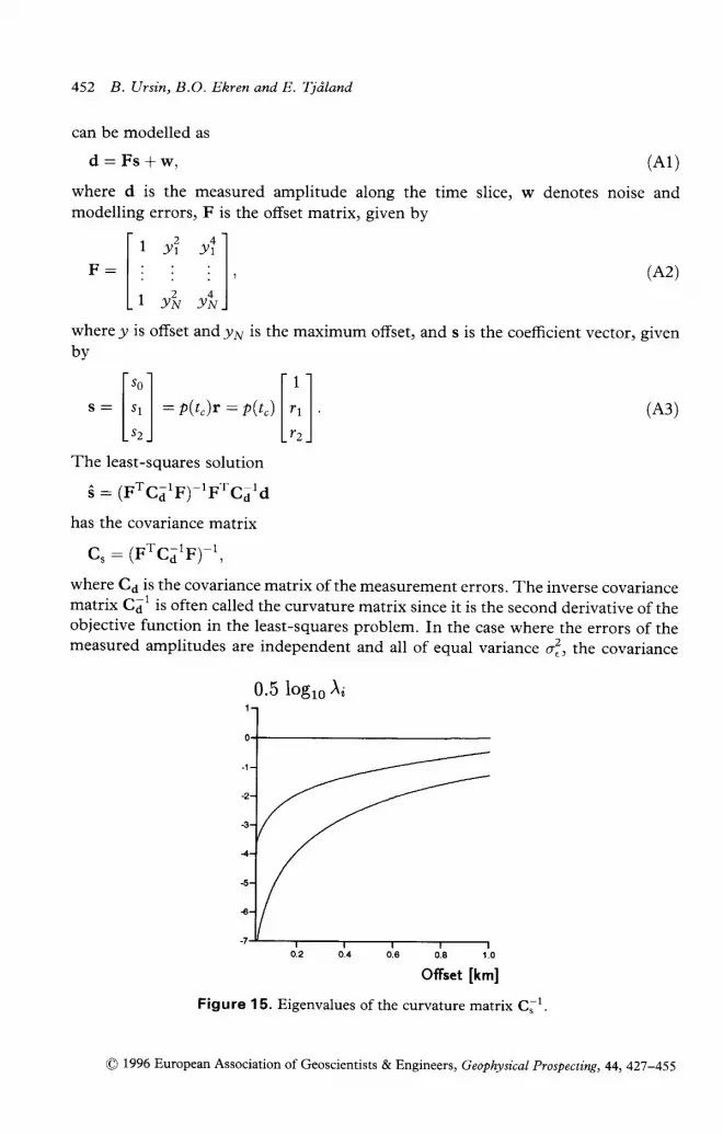
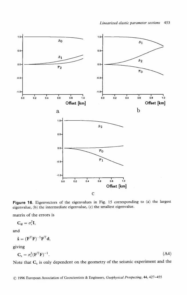
The uncertainty in the estimated coefficients in the reflectivity polynomial se, s1and s2 can be found by performing an eigenvalue analysis of the inverse covariancematrix C, 1. Figure 15 shows the three eigenvalues of C, 1 as a function of maximumoffsetyl', and Fig. 16 shows the corresponding eigenvectors. (The maximum offsetfor the top anomaly reflection at shotpoint 2000 in the real data is 0.995 km). Figure16b shows that the second best-determined parameter (corresponding to theintermediate eigenvalue of C, 1 in Figure 15 is the sum of s1 and s2; and that theworst-determined parameter (corresponding to the smallest eigenvalue of C, i; is thedifference between s2 and s1 . These results are consistent with the generalizedsemblance plot in Fig. 2 of Ursin and Ekren (1995). The model parameter vector rnand the matrix M are defined as

[ m ^ ' l t M ^ Im : l l a n d M - l

' 1 .

LMO. I L MO J

where mo and Mo are defined by (9) and mo and M" by (16). Then

rn : MTs, (A5)

and the covariance matrix of rn is

c* : MTC,tTtMt. ( .46)

The variance of each model parameter mi is then given by

ok, : lC^l,o (A7)

References

Andreassen K., Hogstad K. and Berteussen K.A. 1990. Gas hydrate in the southern BarentsSea indicated by a shallow seismic anomaly. First Break 8,235-245.

Balogh D., Snyder G. and Barney w. 1986. Examples of a new approach to offset amplitudeanalysis. 56th SEG meeting, Houston, USA, Expanded Abstracts, 350-351.

Beydoun \7., Hanitzsch C. and Jin S. 1993. \Why migrate before AVO? A simple example. 55thEAEG meeting, Stavanger, Norway, Expanded Abstracts, paper 8044.

Castagna J.P., Batzle M.L. and Eastwood R.L. 1985. Relationship between compressionalwave and shear wave velocities in clastic silicate rocks. Geophysics 50,551-570.

Castagna J.P. and Smith S.\7. 1994. Comparison of AVO indicators: A modeling study.Geophgsics 59, 1849-1855.

Chapman C.H. 1976. Exact and approximate generalized ray theory in vertically inhomoge-neous media. Geophysical Journal of the Royal Astronomical Society 46,201-233.

de Nicolao A., Drufuca G. and Rocca F. 1993. Eigenvectors and eigenvalues of linearizedelastic inversion. Geophysics 58, 670-679.

Dix C.H. 1955. Seismic velocities from surface measurements. Geophysics 20,68-86.Drufuca G. and Mazzotti A. 1995. Ambiguities in AVO inversion of reflections from a gas-

sand. Geophyszcs 60, 134-141.

O 1996 European Association of Geoscientists & Engineers, Geophysical Prospecting,44,427-455

Linearized elastic parameter sections 455

Ekren B.O. and Ursin B. 1995, Frequency-wavenumber constant-offset migration and AVO.

65th SEG meeting, Houston, USA, Expanded Abstracts, 1377-1380.

Gidlow P.M., Smith G.C. and Vail P.J. 1992. Hydrocarbon detection using f luid factor traces:

A case history. Joint SEG/EAEG summer research workshop "How useful is amplitude-

versus-offset (AVO) analysis?" Big Sky, Montana, USA, Expanded Abstracts, 78-89.

Lcirtzer G.J.M and Berkhout A.J. 1993. Linearized AVO inversion of multi-component

seismic data. In: Offset-dependent Refiectiaity: Theory and Practice of AVO Analysis (eds.

J.P. Castagna and M. Backus), Society of Explorat ion Geophysicists.

Rutherford S.R. and Wil l iams R.H. 1989. Ampli tude-versus-offset variat ions in gas sands.

G eop hy sics 54, 680-688.Smith G.C. and Gidlow P.M. 1987. \Weighted stacking for rock property estimation and

detection of gas. GeophStsical Prospecting 35,993-1014.

Soroka W.L. and Rei1ly J.M. 1992. Interactive AVO quali ty control: A key element for

successful AVO analysis, Joint SEG/EAEG summer research workshop "How useful is

amplitude-versus-offset (AVO) analysis?", Big Sky, Montana, USA' Expanded Abstracts,

237-238.

Stolt R.H. and \Weglein A.B. 1985. Migration and inversion of seismic data. Geophysics 50,

2458-2472.

Taner M.T. and Koehler F. 1969. Velocity spectra - digital computer derivation and

applications of velocity functions. Geophysics 34, 859-881.T1'gel M., Schleicher J. and Hubral P. 1992. Geometrical spreading corrections of offset

reflections in a laterally inhomogeneous earth. Geophysical Prospecting 40, 483-512.

Ursin B. and Dahl T. 1990. Least-squares estimation of ref lect ivi ty polynomials. 60th SEG

meeting, Expanded Abstracts, 1069-107l.

Ursin B. and Dahl T. 1992. Seismic reflection amplitudes. Geophysical Prospecting 40,483-572.

Ursin B. and Ekren B.O. 1995. Robust AVO analysis. Geophysics 60' 317-326.

Ursin B. and Ti i land E. 1992. Seismic ampli tude analysis. 2nd SEGJ/SEG International

Symposium of Geotomography, Tokyo, Japan, Proceedings, 4l-56.

Ursin B. and Tjiland E. 1993. The accuracy of linearized elastic parameter estimation Journalo;f Seismic Exploration 2, 349-363.

Wiggins R., Kenny G.S. and McClure C.D. 1983. A method for determining and displaying the

shear-velocity reflectivities of a geological formation. European Patent Application 0113944.

Zhao H., Ursin B. and Amundsen L. 1994. Frequency-wavenumber elastic inversion of

marine seismic data. Geophysics 59, 1868-1881.

(O 1996 European Association of Geoscientists & Engineers, Geophgsical Prospecting, 44, 427-455