Appendix A: List of Author's Related Publications

107© Springer International Publishing AG 2018 L.F. Abdulrazak, Coexistence of IMT-Advanced Systems for Spectrum Sharing with FSS Receivers in C-Band and Extended C-Band, https://doi.org/10.1007/978-3-319-70588-0

Appendix A: List of Author’s Related Publications

Chapters in Books

1. Lway Faisal Abdulrazak., Kusay Faisal Al-Tabatabaie., and Tharek Abd. Rahman. Utilize 3300–3400 MHz Band for Fixed Wireless Access. In “Advanced Technologies” book. INTECH publications. ISBN 978–953–307–017–9. pp.291–301.

2. Zaid A. Shamsan, Lway F. and Tharek Abd Rahman, Co-sited and Non Co-sited Coexistence Analysis between IMT-Advanced and FWA Systems in Adjacent Frequency Band. In New Aspects Of Telecommunications And Informatics, Published by WSEAS Press 2008, pp. 44–48. ISBN: 978–960–6766–64–0, ISSN: 1790–5117.

3. Zaid A. Shamsan, Lway Faisal and Tharek Abd. Rahman. Transmit Spectrum Mask for Coexistence between Future WiMAX and Existing FWA Systems. In Recent Advances In Systems Engineering And Applied Mathematics, Published by WSEAS Press 2008, pp. 76–83. ISBN: 978–960–6766–91–6, ISSN 1790–2769.

International Journals

1. Lway Faisal Abdulrazak, Zaid A. Shamsan and Tharek Abd. Rahman. Potential Penalty Distance between FSS Receiver and FWA for Malaysia. International Journal Publication in WSEAS Transactions on COMMUNICATIONS, ISSN: 1109–2742, Issue 6, Volume 7, June 2008, pp. 637–646.

2. Lway Faisal Abdulrazak and Tharek Abd. Rahman. Introduce the FWA in the band 3300–3400 MHz. Proceedings of World Academy of Science, Journal of Engineering and Technology (PWASET), Volume 46–32, December 2008 ISSN 2070–3740. pp. 176–179.

3. Zaid A. Shamasn, Lway Faisal and Tharek Abd. Rahman. On Coexistence and Spectrum Sharing between IMT-Advanced and Existing Fixed Systems.

https://doi.org/10.1007/978-3-319-70588-0

108

International Journal Publication in WSEAS TRANSACTIONS on COMMUNICATIONS, Issue 5, Volume 7, May 2008, pp. 505–515.

4. Zaid A. Shamasn, Lway Faisal, S. K. S.Yusof, Tharek A. Rahman. Spectrum Emission Mask for Coexistence between Future WiMAX and Existing Fixed Wireless Access Systems. International Journal Publication in WSEAS Transactions on COMMUNICATIONS, Vol. 7, Issue 6, June 2008, pp. 627–636.

5. Lway Faisal Abdulrazak, Arshed A. O. Tractable Technique to Evaluate the Terrestrial to Satellite Interference in the C-Band Range. International Journal of Theoretical and Applied Information Technology, Vol. 65, No.3, pp. 762–769. 2014.

6. Lway Faisal Abdulrazak and Arshed A. O. Interference Mitigation Technique through Shielding and Antenna Discrimination. International Journal of Multimedia and Ubiquitous Engineering. Vol. 10, No. 3 (2015), pp. 343–352.

7. Lway Faisal Abdulrazak, Kusay F. Al-Tabatabaie. Broad-Spectrum Model for Sharing Analysis between IMT-Advanced Systems and FSS Receiver. Journal of Electronics and Communication Engineering (IOSR-JECE),Volume 12, Issue 1, Ver. III (Jan.-Feb. 2017), pp. 52–56.

8. Lway Faisal Abdulrazak, Kusay F. Al-Tabatabaie. Preliminary design of iraqi spectrum management software (ISMS), International Journal of Advanced Research. Vol.5(issue2), pp. 2560–2568.

Conference Papers

1. Lway Faisal Abdulrazak, Tharek Abd Rahman. Review Ongoing Research of Several Countries on the Interference between FSS and BWA. International Conference on Communication Systems and Applications (ICCSA’08), 2008 Hong Kong China.

2. Lway Faisal Abdulrazak and Tharek Abd. Rahman. Novel Computation of Expecting Interference between FSS and IMT-Advanced for Malaysia. 2008 IEEE International RF and Microwave Conference (RFM08), Malaysia 2–4th December 2008.

3. Lway Faisal Abdulrazak, S.K.Abdul Rahim, and Tharek Abd. Rahman. New Algorithm to Improve the Coexistence between IMT-Advanced Mobile Users and Fixed Satellite Service. Proceedings of 2009 International IACSIT Conference on Machine Learning and Computing (IACSIT ICMLC 2009) Perth, Australia, July 10–12, 2009.

4. Lway Faisal Abdulrazak, Zaid A. Hamid, Zaid A. Shamsan, Razali Bin Nagah and Tharek Abd. Rahman. The Co-Existence of IMT-Advanced And Fixed Satellite Service Networks In The 3400–3600 MHz. Proceeding of MCMC col-loquium 2008. 18-19December 2008. ISBN: 978–983–42,563–2–6. pp. 77–82.

5. Lway F. Abdulrazak, Zaid A. Shamsan and Tharek Abd. Rahman. Potentiality of Interference Correction between FSS and FWA for Malaysia. Selected Paper from the World Scientific and Engineering Academy and Society Conferences in Istanbul, Turkey, May 2008, pp. 84–89.


109

6. Lway Faisal Abdulrazak, Tharek Abd. Rahman, and S.K.Abdul Rahim. IMT- Advanced and FSS Interference Area Ratio Methodology. Proceeding of the 8th international conference on circuits, systems, electronics, control & signal processing (CSECS’09). December 14–16,2009. ISBN: 978–960–474–139–7, ISSN:1790–5117.

7. Zaid A. Shamsan, Lway Faisal, and Tharek Abd Rahman. Co-sited and Non Co-sited Coexistence Analysis between IMT-Advanced and FWA Systems in Adjacent Frequency band. in Proceedings of the International Conference on Telecommunications and Informatics (TELE-INFO ‘08). pp. 44–48, Istanbul, Turkey, May 27–30, 2008.

8. Zaid A. Shamsan, Lway Faisal and Tharek Abd. Rahman. Transmit Spectrum Mask for Coexistence between Future WiMAX and Existing FWA Systems. Selected Paper from the World Scientific and Engineering Academy and Society Conferences in Istanbul, Turkey, May 2008, pp. 76–83.

9. Zaid A. Shamsan, Lway F. Abdulrazak, Tharek Abd. Rahman. On the Impact of Channel Bandwidths and Deployment Areas Clutter Loss on Spectrum Sharing of Next Wireless Systems. International Conference on Electronic Design (ICED08), Malaysia 1–3 December 2008.

10. Shamsan Zaid A., Faisal L. and Rahman Tharek A. (2008). Compatibility and Coexistence between IMT-Advanced and Fixed Systems, in Proceedings of the 4th International Conference and Information Technology and Multimedia at UNITEN (ICIMU’ 2008), 17–19 November, Malaysia.

11. Shamsan Zaid A., Abdulrazak Lway F., and Rahman Tharek A. (2008). Co- channel and Adjacent Channel Interference Evaluation for IMT-Advanced Coexistence with Existing Fixed System, in Proceedings of IEEE International RF and Microwave Conference (RFM 2008), pp. 65–69, 2–4 December, Malaysia.



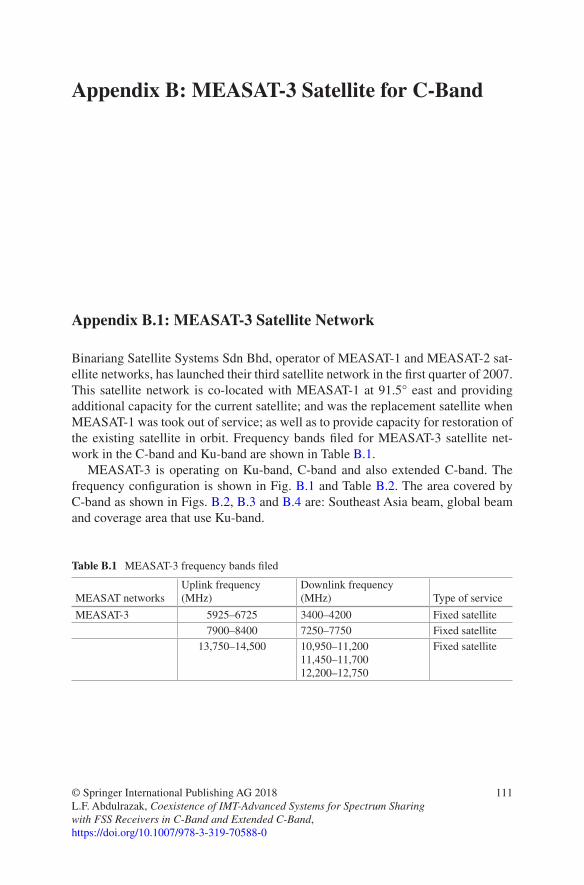
Table B.1 MEASAT-3 frequency bands filed

MEASAT networksUplink frequency (MHz)

Downlink frequency (MHz) Type of service

MEASAT-3 5925–6725 3400–4200 Fixed satellite7900–8400 7250–7750 Fixed satellite

13,750–14,500 10,950–11,20011,450–11,70012,200–12,750

Fixed satellite

Appendix B: MEASAT-3 Satellite for C-Band

Appendix B.1: MEASAT-3 Satellite Network

Binariang Satellite Systems Sdn Bhd, operator of MEASAT-1 and MEASAT-2 sat-ellite networks, has launched their third satellite network in the first quarter of 2007. This satellite network is co-located with MEASAT-1 at 91.5° east and providing additional capacity for the current satellite; and was the replacement satellite when MEASAT-1 was took out of service; as well as to provide capacity for restoration of the existing satellite in orbit. Frequency bands filed for MEASAT-3 satellite net-work in the C-band and Ku-band are shown in Table B.1.

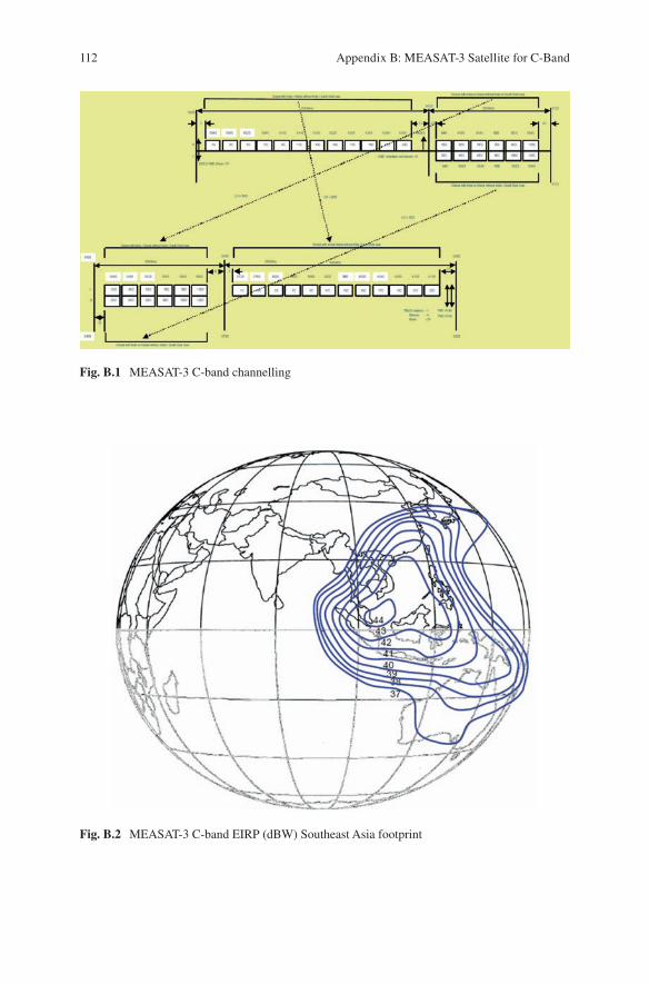
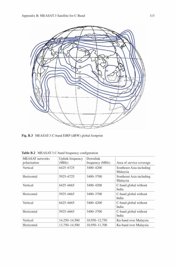
MEASAT-3 is operating on Ku-band, C-band and also extended C-band. The frequency configuration is shown in Fig. B.1 and Table B.2. The area covered by C-band as shown in Figs. B.2, B.3 and B.4 are: Southeast Asia beam, global beam and coverage area that use Ku-band.

https://doi.org/10.1007/978-3-319-70588-0

112

Fig. B.1 MEASAT-3 C-band channelling

Fig. B.2 MEASAT-3 C-band EIRP (dBW) Southeast Asia footprint


113

Fig. B.3 MEASAT-3 C-band EIRP (dBW) global footprint

Table B.2 MEASAT-3 C-band frequency configuration

MEASAT networks polarization

Uplink frequency (MHz)

Downlink frequency (MHz) Area of service coverage

Vertical 6425–6725 3400–4200 Southeast Asia including Malaysia

Horizontal 5925–6725 3400–3700 Southeast Asia including Malaysia

Vertical 6425–6665 3400–4200 C-band global without India

Horizontal 5925–6665 3400–3700 C-band global without India

Vertical 6425–6665 3400–4200 C-band global without India

Horizontal 5925–6665 3400–3700 C-band global without India

Vertical 14,250–14,500 10,950–12,750 Ku-band over MalaysiaHorizontal 13,750–14,500 10,950–11,700 Ku-band over Malaysia


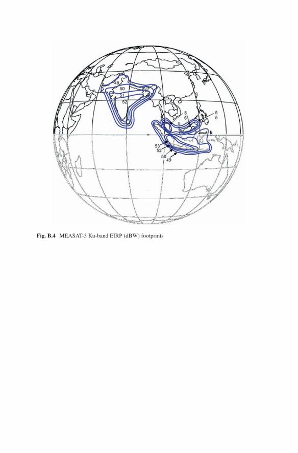
Fig. B.4 MEASAT-3 Ku-band EIRP (dBW) footprints


Appendix C: Mathematical Equations

Appendix C.1: The Eigen-Decomposition: Eigenvalues and Eigenvectors

Eigenvectors and eigenvalues are numbers and vectors associated to square matri-ces, and together they provide the eigen-decomposition of a matrix which analyses the structure of this matrix. Even though the eigen-decomposition does not exist for all square matrices, it has a particularly simple expression for a class of matrices often used in multivariate analysis such as correlation, covariance or cross-product matrices. The eigen-decomposition of this type of matrices is important in statistics because it is used to find the maximum (or minimum) of functions involving these matrices. For example, principal component analysis is obtained from the eigen- decomposition of a covariance matrix and gives the least square estimate of the original data matrix. Eigenvectors and eigenvalues are also referred to as character-istic vectors and latent roots or characteristic equation (in German, “eigen” means “specific of” or “characteristic of”). The set of eigenvalues of a matrix is also called its spectrum.

There are several ways to define eigenvectors and eigenvalues; the most common approach defines an eigenvector of the matrix A as a vector u that satisfies the fol-lowing equation:

Au u= λ

When rewritten, the equation becomes:

A I u−( ) =λ 0

where λ is a scalar called the eigenvalue associated to the eigenvector. In a similar manner, we can also say that a vector u is an eigenvector of a matrix A if the length of the vector (but not its direction) is changed when it is multiplied by A.

https://doi.org/10.1007/978-3-319-70588-0

116

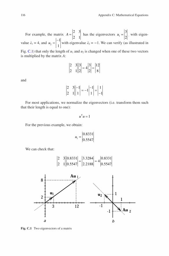
For example, the matrix A =2 3

2 1 has the eigenvectors u1

3

2= , with eigen-

value λ1 = 4, and u2

1

1=−

with eigenvalue λ2 = −1. We can verify (as illustrated in

Fig. C.1) that only the length of u1 and u2 is changed when one of these two vectors is multiplied by the matrix A:

2 3

2 1

3

243

2

12

8= =

and

Fig. C.1 Two eigenvectors of a matrix

2 3

2 1

1

11

1

1

1

1

−= −

−=−

For most applications, we normalize the eigenvectors (i.e. transform them such that their length is equal to one):

u uT = 1

For the previous example, we obtain:

u1

0.8331

0.5547=

We can check that:

2 3

2 1

0.8331

0.5547

3.3284

2.218840.8331

0.5547= =


117

and

2 3

2 1

0.7071

0.7071

0.7071

0.70711

0.7071

0.7071

−=−

= −−

Traditionally, we put together the set of eigenvectors of A in a matrix denoted U. Each column of U is an eigenvector of A. The eigenvalues are stored in a diagonal matrix (denoted Λ), where the diagonal elements give the eigenvalues (and all the other values are zeros). We can rewrite the first equation as:

AU U= Λ

or also as:

A U U= −Λ 1

For the previous example, we obtain:

A U U=

=−

− −=

−Λ 1

3 1

2 1

4 0

0 1

2 2

4 6

2 3

2 1

It is important to note that not all matrices have eigenvalues. For example, the

matrix 0 1

0 0does not have eigenvalues. Even when a matrix has eigenvalues and

eigenvectors, the computation of the eigenvectors and eigenvalues of a matrix requires a large number of computations and is therefore better performed by computers.

Appendix C.2: Conjugate Matrix

A conjugate matrix is a matrix A* obtained from a given matrix A by taking the complex conjugate of each element of A:

a aij ij( ) = ( )

The notation A* is sometimes also used, which can lead to confusion since this symbol is also used to denote the conjugate transpose.


118

Appendix C.3: Conjugate Transpose

The conjugate transpose of a m × n matrix A is the n × m matrix defined by:

A AH T≡

where AT denotes the transpose of matrix A and A denotes the conjugate matrix. In all common space, the conjugate and transpose operations commute, so:

A A AH T T≡ =

Appendix C.4: Frobenius Norm

The Frobenius norm, sometimes also called the Euclidean norm (which may cause confusion with the vector L2 norm also sometimes known as the Euclidean norm), is a matrix norm of a m × n matrix A defined as the square root of the sum of the absolute squares of its elements:

A ai

m

j

n

ijF ≡= =∑∑

1 1

2

Appendix C.5: Root Mean Square Error (RMSE)

The RMSE is the square root of the variance of the residuals. It indicates the abso-lute fit of the model to the data – how close the observed data points are to the model’s predicted values. Whereas R-squared is a relative measure of fit, RMSE is an absolute measure of fit. As the square root of a variance, RMSE can be inter-preted as the standard deviation of the unexplained variance and has the useful property of being in the same units as the response variable. Lower values of RMSE indicate better fit. RMSE is a good measure of how accurately the model predicts the response and is the most important criterion for fit if the main purpose of the model is prediction:

RMSE = −[ ]E x x

2

where E is the expectation, x is the mean and x is the variable element.


119

Appendix C.6: The Expectation

It is an arithmetic average, just one calculated from probabilities instead of being calculated from samples. So, for example, if P(k) is the probability that we find K A1 alleles in our sample, the expected number of A1 alleles in our sample is just:

E k kP np( ) = ∑ =

Appendix C.7: The Standard Deviation σ 2

It is the square root of the variance, where the variance is the average of the squared differences from the mean. So the variance is same like the expectation, and the standard deviation is equal to the RMSE.

Appendix C.8: The Autocorrelation

Autocorrelation is the cross-correlation of a signal with itself. Informally, it is the similarity between observations as a function of the time separation between them. It is a mathematical tool for finding repeating patterns, such as the presence of a periodic signal which has been buried under noise, or identifying the missing fun-damental frequency in a signal implied by its harmonic frequencies. It is often used in signal processing for analysing functions or series of values, such as time-domain signals:

R s t

E x xt t s s

t s

,( ) =−( ) −( )[ µ µσ σ



Appendix D: Null Synthesized Algorithm for Minimum Separation Distance

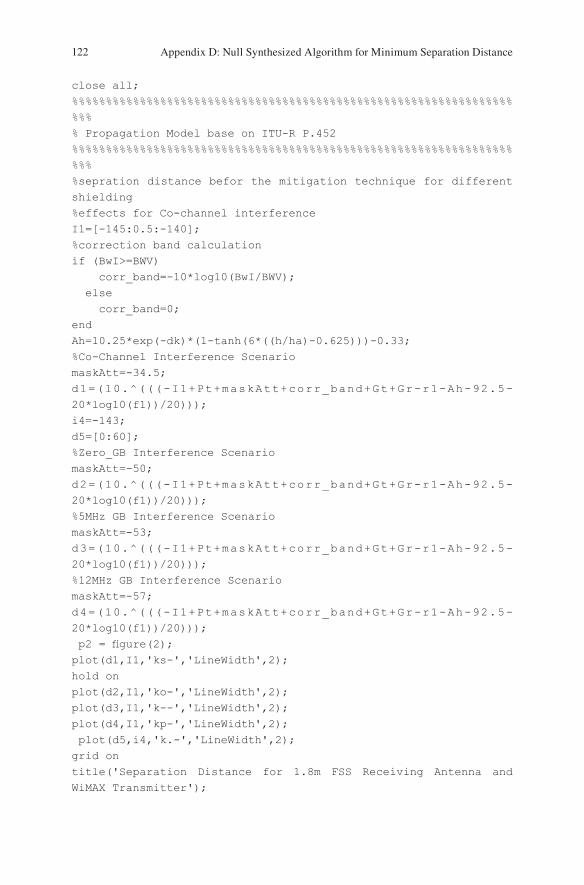
Appendix D.1: Interference Assessment Methodology Code Without Mitigation Technique

The following code is for rural area with a 180 dish diameter 0 shielding attenuation and 36 MHz channel bandwidth. In order to change the environment or dish param-eters, the parameters in the code should be adjusted.

% IMT-Advanced parametersf1=4.040; % frequencey carrier in GHzGt=18; % antenna gain before mitigation technique in dBm for IMT-AdvancedPt=43; %transmitted power of interferer IMT-Advanced in dBmGr=-10; %gain of receiver(victim)in dBiI1=-143; %Interference threshold in dBw/230kHz worst case%%%%%%%%%%%%%%%%%%%%%%%%%%%%%%%%%%%%%%%%%%%%%%%%%%%%%%%%%%%%%%%%%%%%%isolation from site shieldingr1=0; % in dB no shieldingr2=20;r3=40;%%%%%%%%%%%%%%%%%%%%%%%%%%%%%%%%%%%%%%%%%%%%%%%%%%%%%%%%%%%%%%%%%%%%% clutter loss parameters%%%%%%%%%%%%%%%%%%%%%%%%%%%%%%%%%%%%%%%%%%%%%%%%%%%%%%%%%%%%%%%%%%%%dk=0.02;ha=25;h=1.8;BwI=20;%bandwidth of WiMAX (interferer)BWV=36;%bandwidth of victim FSS receiver

https://doi.org/10.1007/978-3-319-70588-0

122

close all;%%%%%%%%%%%%%%%%%%%%%%%%%%%%%%%%%%%%%%%%%%%%%%%%%%%%%%%%%%%%%%%%%%%%% Propagation Model base on ITU-R P.452%%%%%%%%%%%%%%%%%%%%%%%%%%%%%%%%%%%%%%%%%%%%%%%%%%%%%%%%%%%%%%%%%%%%%sepration distance befor the mitigation technique for different shielding%effects for Co-channel interferenceI1=[-145:0.5:-140];%correction band calculationif (BwI>=BWV) corr_band=-10*log10(BwI/BWV); else corr_band=0;endAh=10.25*exp(-dk)*(1-tanh(6*((h/ha)-0.625)))-0.33;%Co-Channel Interference ScenariomaskAtt=-34.5;d1=(10.^(((-I1+Pt+maskAtt+corr_band+Gt+Gr-r1-Ah-92.5- 20*log10(f1))/20)));i4=-143;d5=[0:60];%Zero_GB Interference ScenariomaskAtt=-50;d2=(10.^(((-I1+Pt+maskAtt+corr_band+Gt+Gr-r1-Ah-92.5- 20*log10(f1))/20)));%5MHz GB Interference ScenariomaskAtt=-53;d3=(10.^(((-I1+Pt+maskAtt+corr_band+Gt+Gr-r1-Ah-92.5- 20*log10(f1))/20)));%12MHz GB Interference ScenariomaskAtt=-57;d4=(10.^(((-I1+Pt+maskAtt+corr_band+Gt+Gr-r1-Ah-92.5- 20*log10(f1))/20))); p2 = figure(2);plot(d1,I1,'ks-','LineWidth',2);hold onplot(d2,I1,'ko-','LineWidth',2);plot(d3,I1,'k--','LineWidth',2);plot(d4,I1,'kp-','LineWidth',2); plot(d5,i4,'k.-','LineWidth',2);grid ontitle('Separation Distance for 1.8m FSS Receiving Antenna and WiMAX Transmitter');


123

xlabel('Distance from FSS(Km)'); ylabel('Interference Power [dBW/230KHz)');legend('Co-Channel Interference Scenario', 'Zero-GB Interference Scenario', '5MHz GB Interference Scenario', '12MHz GB Interference Scenario', 'I threshold');

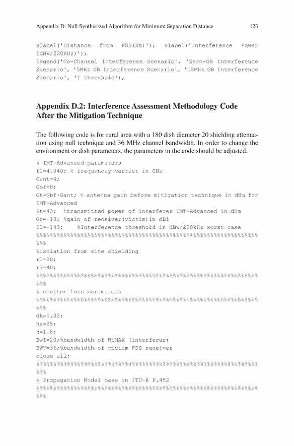
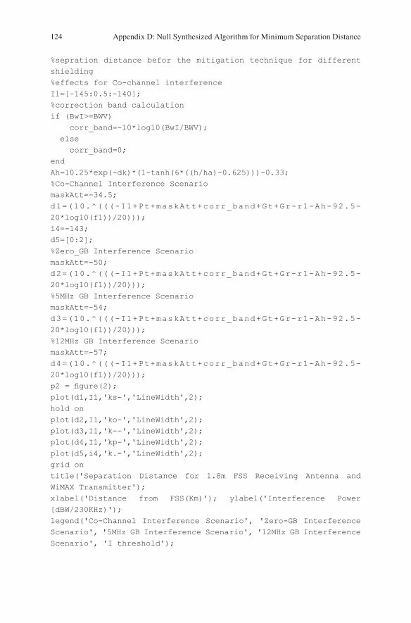
Appendix D.2: Interference Assessment Methodology Code After the Mitigation Technique

The following code is for rural area with a 180 dish diameter 20 shielding attenua-tion using null technique and 36 MHz channel bandwidth. In order to change the environment or dish parameters, the parameters in the code should be adjusted.

% IMT-Advanced parametersf1=4.040; % frequencey carrier in GHzGant=4;Gbf=0;Gt=Gbf+Gant; % antenna gain before mitigation technique in dBm for IMT-AdvancedPt=43; %transmitted power of interferer IMT-Advanced in dBmGr=-10; %gain of receiver(victim)in dBiI1=-143; %Interference threshold in dBw/230kHz worst case%%%%%%%%%%%%%%%%%%%%%%%%%%%%%%%%%%%%%%%%%%%%%%%%%%%%%%%%%%%%%%%%%%%%%isolation from site shieldingr1=20;r3=40;%%%%%%%%%%%%%%%%%%%%%%%%%%%%%%%%%%%%%%%%%%%%%%%%%%%%%%%%%%%%%%%%%%%%% clutter loss parameters%%%%%%%%%%%%%%%%%%%%%%%%%%%%%%%%%%%%%%%%%%%%%%%%%%%%%%%%%%%%%%%%%%%%dk=0.02;ha=25;h=1.8;BwI=20;%bandwidth of WiMAX (interferer)BWV=36;%bandwidth of victim FSS receiverclose all;%%%%%%%%%%%%%%%%%%%%%%%%%%%%%%%%%%%%%%%%%%%%%%%%%%%%%%%%%%%%%%%%%%%%% Propagation Model base on ITU-R P.452%%%%%%%%%%%%%%%%%%%%%%%%%%%%%%%%%%%%%%%%%%%%%%%%%%%%%%%%%%%%%%%%%%%%


124

%sepration distance befor the mitigation technique for different shielding%effects for Co-channel interferenceI1=[-145:0.5:-140];%correction band calculationif (BwI>=BWV) corr_band=-10*log10(BwI/BWV); else corr_band=0;endAh=10.25*exp(-dk)*(1-tanh(6*((h/ha)-0.625)))-0.33;%Co-Channel Interference ScenariomaskAtt=-34.5; d1=(10.^(((-I1+Pt+maskAtt+corr_band+Gt+Gr-r1-Ah-92.5- 20*log10(f1))/20)));i4=-143;d5=[0:2];%Zero_GB Interference ScenariomaskAtt=-50;d2=(10.^(((-I1+Pt+maskAtt+corr_band+Gt+Gr-r1-Ah-92.5- 20*log10(f1))/20)));%5MHz GB Interference ScenariomaskAtt=-54;d3=(10.^(((-I1+Pt+maskAtt+corr_band+Gt+Gr-r1-Ah-92.5- 20*log10(f1))/20)));%12MHz GB Interference ScenariomaskAtt=-57;d4=(10.^(((-I1+Pt+maskAtt+corr_band+Gt+Gr-r1-Ah-92.5- 20*log10(f1))/20)));p2 = figure(2);plot(d1,I1,'ks-','LineWidth',2);hold onplot(d2,I1,'ko-','LineWidth',2);plot(d3,I1,'k--','LineWidth',2);plot(d4,I1,'kp-','LineWidth',2);plot(d5,i4,'k.-','LineWidth',2);grid ontitle('Separation Distance for 1.8m FSS Receiving Antenna and WiMAX Transmitter');xlabel('Distance from FSS(Km)'); ylabel('Interference Power [dBW/230KHz)');legend('Co-Channel Interference Scenario', 'Zero-GB Interference Scenario', '5MHz GB Interference Scenario', '12MHz GB Interference Scenario', 'I threshold');


125

-801

2

3

4

5

6

7

-60 -40 -20 0

Angle in degrees

MUSIC Spectrum

beam forming with mitigation technique

Det

ecte

d P

ower

(dB

m)

20 40 60 80

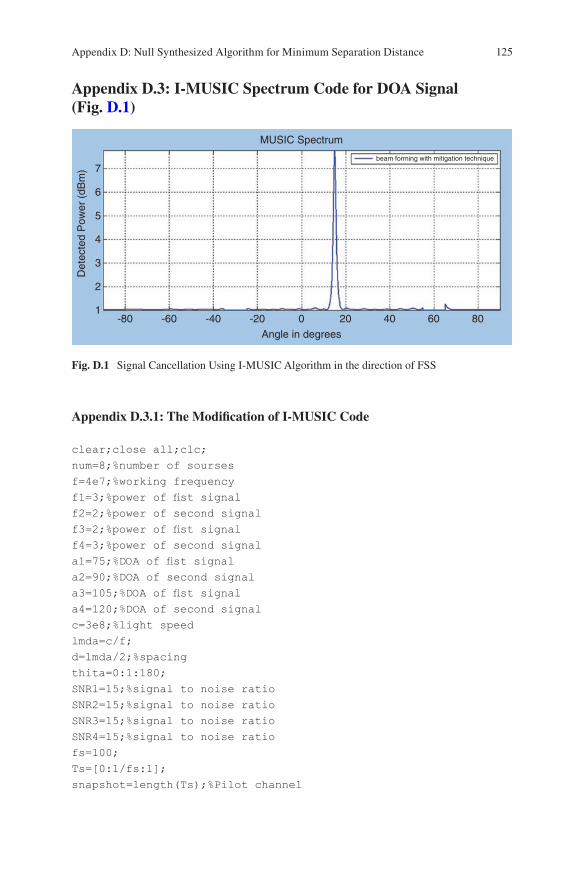
Fig. D.1 Signal Cancellation Using I-MUSIC Algorithm in the direction of FSS

Appendix D.3: I-MUSIC Spectrum Code for DOA Signal (Fig. D.1)

Appendix D.3.1: The Modification of I-MUSIC Code

clear;close all;clc;num=8;%number of soursesf=4e7;%working frequencyf1=3;%power of fist signalf2=2;%power of second signalf3=2;%power of fist signalf4=3;%power of second signala1=75;%DOA of fist signala2=90;%DOA of second signala3=105;%DOA of fist signala4=120;%DOA of second signalc=3e8;%light speedlmda=c/f;d=lmda/2;%spacingthita=0:1:180;SNR1=15;%signal to noise ratioSNR2=15;%signal to noise ratioSNR3=15;%signal to noise ratioSNR4=15;%signal to noise ratiofs=100;Ts=[0:1/fs:1];snapshot=length(Ts);%Pilot channel


126

s1=10^(SNR1/20)*sin(2*pi*f1*Ts);%1st signal waves2=10^(SNR2/20)*sin(2*pi*f2*Ts);%2nd signal waves3=10^(SNR3/20)*sin(2*pi*f1*Ts);%1st signal waves4=10^(SNR4/20)*sin(2*pi*f2*Ts);%2nd signal waveathita1=exp(j*2*pi*d/lmda*cos(a1*pi/180)*[0:num-1]).';%steering vector of first signalathita2=exp(j*2*pi*d/lmda*cos(a2*pi/180)*[0:num-1]).';%steering vector of secod signalathita3=exp(j*2*pi*d/lmda*cos(a3*pi/180)*[0:num-1]).';%steering vector of first signalathita4=exp(j*2*pi*d/lmda*cos(a4*pi/180)*[0:num-1]).';%steering vector of secod signalx=athita1*s1+athita2*s2+sqrt(0.5)+athita3*s3+athita4*s4+sqrt(0.5)*(randn(num,snapshot)+j*randn(num,snapshot));%x=s*a+nR=x*x'/snapshot;[V,D]=eig(R);P=V(:,1:4)*V(:,1:4)';e1=[1,zeros(1,num-1)].';for i=1:length(thita) A=exp(j*2*pi*d/lmda*cos(thita(i)*pi/180)*[0:num-1]).'; S(i)=1/(A'*P*A); S1(i)=1/(A'*P*e1);endfigure(1)% plot(thita,10*log10(abs(S)/(max(abs(S)))));grid on;hold on;plot(thita,10*log10(abs(S1)/(max(abs(S)))),'r--');% title('I-MUSICspectrum')xlabel('DOA Degree')ylabel('Power Amplitude in dB')% legend('commom-Music','Modified-Music')legend('I-MUSICspectrum')

Appendix D.3.2: The Modification of I-MUSIC Code with the Null Introduction

function edit10_Callback(hObject, eventdata, handles)N= str2double(get(hObject,'String'));handles.N = N;guidata(hObject,handles)

function edit10_CreateFcn(hObject, eventdata, handles)if ispc && isequal(get(hObject,'BackgroundColor'), get(0,'defaultUicontrolBackgroundColor'))


127

set(hObject,'BackgroundColor','white');end% --- Executes on button press in pushbutton1function pushbutton1_Callback(hObject, eventdata, handles)

doas=[handles.th1 handles.th2 handles.th3]*pi/180;P=[handles.p1 handles.p2 handles.p3];r=length(doas);% Steering vector matrix. Columns will contain the steering

vectors% of the r signalsA=exp(-i*2*pi*handles.d*(0:handles.N-1)'*sin(doas));% Signal and noise generationsig=round(rand(r,handles.K))*2-1;% Generate random BPSK symbols for each of the% r signalsn o i s e = s q r t ( h a n d l e s . n o i s e _var/2)*(randn(handles.N,handles.K)+i*randn(handles.N,handles.K));%Uncorrelated noiseX=A*diag(sqrt(P))*sig+noise;%Generate data matrixR=X*X'/handles.K;%Spatial covariance matrix[Q ,D]=eig(R);%Compute eigendecomposition of covariance matrix[D,I]=sort(diag(D),1,'descend'); %Find r largest eigenvaluesQ=Q (:,I);%Sort the eigenvectors to put signal eigenvectors first% Qs=Q (:,1:r);%Get the signal eigenvectorsQn=Q(:,r+1:handles.N);%Get the noise eigenvectors% MUSIC algorithm% Define angles at which MUSIC “spectrum” will be computedangles=(-90:0.1:90);%Compute steering vectors corresponding values in anglesa1=exp(-i*2*pi*handles.d*(0:handles.N-1)'*sin(angles*pi/180));for k=1:length(angles) %Compute I-MUSIC “spectrum”e1=[1,zeros(1,D-1)].';

music_spectrum(k)=1/(a1(:,k)'*Qn*Qn'*e1(:,k));end

exceptions=[-30 60];for exception_time=1:length(exceptions) for ee=1:length(music_spectrum) if angles(ee)==exceptions(exception_time) music_spectrum(ee-5:ee+5)=0; end


128

endend

% for e=-90:0.1:90% angle=e*pi/180% endplot(angles,abs(music_spectrum),'LineWidth',2.0)grid on;legend('beam forming with mitigation technique');

title('MUSIC Spectrum'); ylabel('Normalized power') ; xlabel('Angle in degrees'); axis tight;

Appendix D.4: Beam Forming (Smart)

%***********************************************************************% Beamforming_linear.m%***********************************************************************% It is a MATLAB function that simulates beamforming for linear arrays.%**********************************************************************% Start timertic;% Start recordingif (save_in_file=='y') out_file = sprintf('%s.txt',file_string); diary(out_file);end% User input[N,d,sig,noise,type,nn,NN,AF_thresh,Mu,E_pattern] = linear_data_entry;

% Parameters initializationFIG = 'figure(1)'; % Figure to recordSKIP_STEP = 40; % Plot every SKIP_STEP iterationsw = zeros(N,1); % iteration initialization% Generate signals[dd, X, fm] = linear_sig_gen(N,d,nn,NN,type,sig,noise,E_pattern);


129

for i = 1 : length(dd) w0 = w; [w, err(i)] = LMS(w,Mu,X(:,i),dd(i)); mse(i) = sum(abs(err(i))^2); w_err(i) = norm(w0 - w); if i>1 array_factor = linear_AF(N,d,w,sig(1:size(sig,1),2),E_pattern); if (abs(w_err(i) - w_err(i-1)) < eps) | (array_factor <= AF_thresh) linear_plot_pattern(sig,w,N,d,E_pattern,AF_thresh,'half',4,'-'); break; end; end; if rem(i,SKIP_STEP) == 0 % Plot every SKIP_STEP iterations linear_plot_pattern(sig,w,N,d,E_pattern,AF_thresh,'half',4,'-'); if i == SKIP_STEP FIG_HANDLE = eval(FIG); if (isunix) pause; end; end; end;end;% Final weights and betasW = abs(w);beta = angle(w);iterationnumber=i;%-------------------------------------------------------------------function [N,d,sig,noise,type,nn,NN,AF_thresh,Mu,E_pattern] = linear_data_entry

%%%%%%%%%%%%%%%%%%% Default Values %%%%%%%%%%%%%%%%%%def_N = 8;def_d = 0.5;def_SOI = 1;def_q = 1;def_SNOI = 1;def_noise_mean = 0;def_noise_var = 0.1;def_type_n = 2;def_AF_thresh = -60;


130

def_Mu = 0.001;def_nn = 500;def_E_pattern_file = 'linear_isotropic.e';%%%%%%%%%%%%% Strings initialization %%%%%%%%%%%%%%%%N_string = sprintf('Enter number of elements in linear smart antenna [%d]: ',def_N);d_string = sprintf('Enter the spacing d (in lambda) between adjacent elements [%2.1f]: ',def_d);SOI_string = sprintf('Enter the Pilot signal (SOI) ampli-tude [%d]: ',def_SOI);SOId_string = sprintf('Enter the Pilot signal (SOI) direc-tion (degrees between -90 and 90): ');q_string = sprintf('Enter number of interfering signals (SNOI) [%d]: ',def_q);noise_mean_string = sprintf('Enter the mean of the noise [%d]: ',def_noise_mean);noise_var_string = sprintf('Enter the variance of noise [%2.1f]: ',def_noise_var);type = sprintf('Type of signal:\n\t[1] sinusoid\n\t[2] BPSK\nEnter number [%d]: ',def_type_n);nn_string = sprintf('Enter the number of data samples [%d]: ',def_nn);AF_thresh_string = sprintf('Enter AF threshold (dB) [%d]: ',def_AF_thresh);Mu_string = sprintf('Enter a value for Mu of LMS algorithm (0 < Mu < 1) [%5.4f]: ',def_Mu);E_pattern_string = sprintf('Enter element pattern filename (*.e) [%s]: ',def_E_pattern_file);%---------------------------------------------------% %%%%%%%%%%%%%%%%% Error Messages %%%%%%%%%%%%%%%%%%%%err_1 = sprintf('\nSignal type not supported...');%---------------------------------------------------%%%%%%%%%%%%%%%%%%%% User Inputs %%%%%%%%%%%%%%%%%%%%%% ------------ Number of elements? ------------- %N = input(N_string);if isempty(N) N = def_N;end;% ------------ Inter-element spacing? ---------- %d = input(d_string);if isempty(d) d = def_d;end;% -------------- SOI amplitude? ---------------- %SOI = input(SOI_string);


131

if isempty(SOI) SOI = def_SOI;end;% -------------- SOI direction? ---------------- %SOId = [];while isempty(SOId) SOId = input(SOId_string);end;% ------ SNOIs amplitudes and directions? ------ %q = input(q_string);if isempty(q) q = def_q;end;sig = [SOI SOId];for k = 1 : q, SNOI_k_string = sprintf('Enter the amplitude of No. %d Interference signal (SNOI_%d) [%d]: ',k,k,def_SNOI); SNOId_k_string = sprintf('Enter the direction of No. %d Interference signal (SNOI_%d) (degrees between 0 and 90): ',k,k); SNOI_k = input(SNOI_k_string); if isempty(SNOI_k) SNOI_k = def_SNOI; end; SNOId_k = []; while isempty(SNOId_k) SNOId_k = input(SNOId_k_string); end; sig = [sig; SNOI_k SNOId_k];end;% ----------------- Noise data? ---------------- %noise_string = input('Insert noise? ([y]/n):','s');if (isempty(noise_string) | noise_string == 'y') noise_mean = input(noise_mean_string); if isempty(noise_mean) noise_mean = def_noise_mean; end; noise_var = input(noise_var_string); if isempty(noise_var) noise_var = def_noise_var; end; noise = [noise_mean noise_var];else fprintf('------------No noise is inserted.-----------\n'); noise = [];end;


132

% ----------------- Signal type? --------------- %type_n = [];if isempty(type_n) type_n = def_type_n;end;switch type_ncase 1 type = 'sinusoid'; def_NN = 100;

case 2 type = 'bpsk'; def_NN = 1;otherwise error(err_1);end;% ------------ Number of data samples? --------- %nn = input(nn_string);if isempty(nn) nn = def_nn;end;% ------- Number of samples per symbol? -------- %NN = [];if isempty(NN) NN = def_NN;end;% ---------------- Mu for LMS? ----------------- %Mu = input(Mu_string);if isempty(Mu) Mu = def_Mu;end;% ---------------- Nulls depth? ---------------- %if q==0 AF_thresh = def_AF_thresh;else AF_thresh = input(AF_thresh_string); if isempty(AF_thresh) AF_thresh = def_AF_thresh; end;end;% -------------- Element pattern? -------------- %E_pattern_file = [];if isempty(E_pattern_file) E_pattern_file = def_E_pattern_file;end;


133

E_pattern = load(E_pattern_file)';warning off;f u n c t i o n l i n e a r _ p l o t _ p a t t e r n ( s i g , w , N , d , E _ p a t t e r n , A F _limit,TYPE,rticks,line_style)k0 = 2*pi;%%%%%%%%%%%%%%% Parameters initialization %%%%%%%%%%%%%%%%---- default values ----%def_d = .5;def_E_pattern = 1;def_AF_limit = -40;def_TYPE = 'half';def_rticks = 4;def_line_style = '-';H_FIG = 1;%------------------------%switch nargincase 2 d = def_d; E_pattern = def_E_pattern; AF_limit = def_AF_limit; T Y P E = def_TYPE; rticks = def_rticks; line_style = def_line_style;case 3 E_pattern = def_E_pattern; AF_limit = def_AF_limit; T Y P E = def_TYPE; rticks = def_rticks; line_style = def_line_style;case 4 AF_limit = def_AF_limit; T Y P E = def_TYPE; rticks = def_rticks; line_style = def_line_style;case 5 T Y P E = def_TYPE; rticks = def_rticks; line_style = def_line_style;case 6 rticks = def_rticks; line_style = def_line_style;case 7 line_style = def_line_style;end

m = linspace(0,N-1,N);switch TYPE


134

case 'half' theta_1 = -pi/2; theta_2 = pi/2; theta = linspace(-pi/2,pi/2,181);case 'full' theta_1 = -pi; theta_2 = pi; theta = linspace(-pi,pi,361);otherwise disp('ERROR => Only two options are allowed for TYPE: half or full'); returnend%%%%%%%%%%%%%% Total Pattern [Element * AF] %%%%%%%%%%%%%AF = E_pattern .* sum(diag(w)*exp(i*(k0*d*m'*sin(theta))));AF = 20*log10(abs(AF)./max(abs(AF)));%%%%%%%%%%%%%%%%%%%%%%%% Polar Plot %%%%%%%%%%%%%%%%%%%%%figure(H_FIG);switch TYPEcase 'half' linear_semipolar_dB(theta*180/pi,AF,AF_limit,0,rticks,line_style);case 'full' linear_polar_dB(theta*180/pi,AF,AF_limit,0,rticks,line_style);end

%-------------------------------------------------------%%%%%%%%%%%%%%%%%%%%%%% Thermal Noise %%%%%%%%%%%%%%%%%%%%if ~isempty(noise) for k = 1 : N STATE3 = sum(rand(1)*100*clock); randn('state',STATE3); noise_data_real = noise(1,1) + sqrt(noise(1,2)/2)*randn(1,size(s,2)); STATE4 = sum(rand(1)*100*clock); randn('state',STATE4); noise_data_imag = noise(1,1) + sqrt(noise(1,2)/2)*randn(1,size(s,2)); noise_data = complex(noise_data_real,noise_data_imag); s(k,:) = s(k,:) + noise_data; end;end;%-------------------------------------------------------%function [w, error] = LMS(w,Mu,x,d)error = d - w' * x;w = w + 2 * Mu * x * conj(error);



Appendix E: Visualyse Professional

Appendix E.1: Introduction

Visualyse products are well known by its high computation performance for techni-cal excellence in their support for radio spectrum management, in particular inter-ference analysis. Visualyse Professional has used an underlying model that is based on real-world objects; this means that the structure of a simulation is familiar to an engineer the first time he looks at the software. Building new complex analyses is also made easier by use of mobile system Windows interface components which are also familiar to many people.

Ease of use is not the start and end of usability, nor will a simple software pack-age necessarily enhance the productivity. Usable, productive software must do what you want it to do – it must be effective and provide the functionality that is in need.

This last requirement – utility – is the central goal of Visualyse Professional. The object-based design means that it can be adapted to all types of system; the ongoing software development and cross-fertilization from consultancy work mean the new fea-tures and enhancements to existing features. Ease of use remains high on agenda –aim is to make using Visualyse a rewarding experience which is both satisfying and enjoy-able. Visualyse finds a balance between ease of use and utility that really can boost the productivity (Fig. E.1).

Visualyse is, at heart, an engine for calculating carrier levels, interference levels and noise levels in radio links. It produces C/I, C/N, C/N + I, pfd, EPFD and I/N numbers and statistics for almost any spectrum sharing or interference analysis sce-nario it can think of?

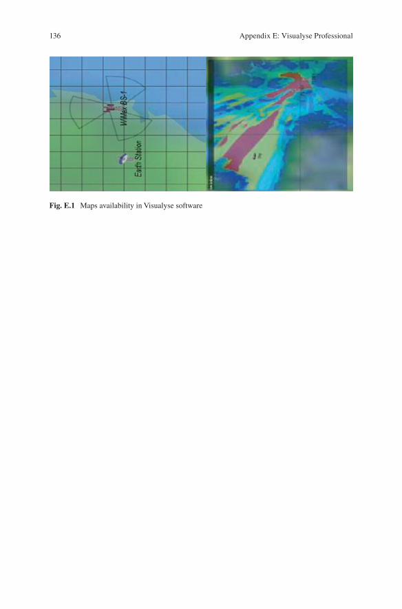
It allows to define geometry, dynamics and RF characteristics in a 3D environ-ment that includes the earth as a central gravitational body and can also include terrain spot heights, geo-climatic factors and local clutter data. However, this does not adequately capture the full capability of the software.

https://doi.org/10.1007/978-3-319-70588-0

136

Fig. E.1 Maps availability in Visualyse software

Appendix E: Visualyse Professional


Appendix F: Experiment Setup and Minimum Separation Distance Simulation Results

Appendix F.1: FSS Aspects and Installation

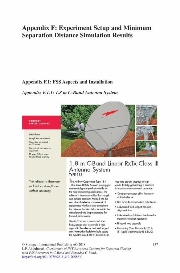
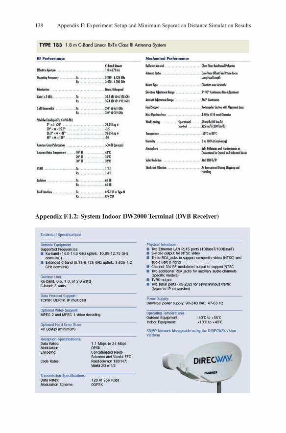
Appendix F.1.1: 1.8 m C-Band Antenna System

https://doi.org/10.1007/978-3-319-70588-0

138

Appendix F.1.2: System Indoor DW2000 Terminal (DVB Receiver)


139

Appendix F.1.3: FSS Unit Installation in Wireless Communication Centre at Universiti Teknologi Malaysia

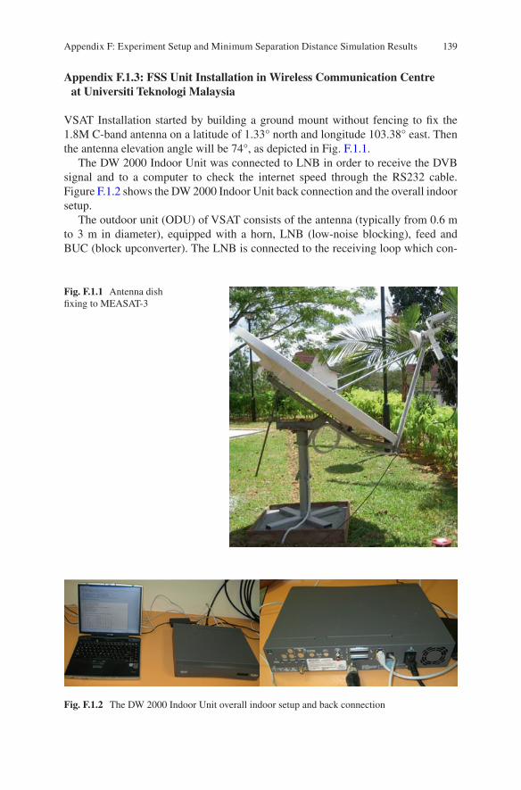
VSAT Installation started by building a ground mount without fencing to fix the 1.8M C-band antenna on a latitude of 1.33° north and longitude 103.38° east. Then the antenna elevation angle will be 74°, as depicted in Fig. F.1.1.

The DW 2000 Indoor Unit was connected to LNB in order to receive the DVB signal and to a computer to check the internet speed through the RS232 cable. Figure F.1.2 shows the DW 2000 Indoor Unit back connection and the overall indoor setup.

The outdoor unit (ODU) of VSAT consists of the antenna (typically from 0.6 m to 3 m in diameter), equipped with a horn, LNB (low-noise blocking), feed and BUC (block upconverter). The LNB is connected to the receiving loop which con-

Fig. F.1.1 Antenna dish fixing to MEASAT-3

Fig. F.1.2 The DW 2000 Indoor Unit overall indoor setup and back connection


140

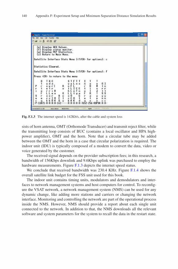
Fig. F.1.3 The internet speed is 142Kb/s, after the cable and system loss

sists of horn antenna, OMT (Orthomode Transducer) and transmit reject filter, while the transmitting loop consists of BUC (contains a local oscillator and HPA high-power amplifier), OMT and the horn. Note that a circular tube may be added between the OMT and the horn in a case that circular polarization is required. The indoor unit (IDU) is typically composed of a modem to convert the data, video or voice generated by the customer.

The received signal depends on the provider subscription fees; in this research, a bandwidth of 156Kbps downlink and 9.6Kbps uplink was purchased to employ the hardware measurements. Figure F.1.3 depicts the internet speed status.

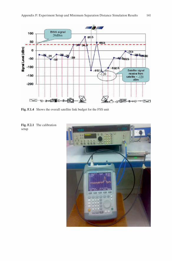
We conclude that received bandwidth was 230.4 KHz. Figure F.1.4 shows the overall satellite link budget for the FSS unit used for this book.

The indoor unit contains timing units, modulators and demodulators and inter-faces to network management systems and host computers for control. To reconfig-ure the VSAT network, a network management system (NMS) can be used for any dynamic change, like adding more stations and carriers or changing the network interface. Monitoring and controlling the network are part of the operational process inside the NMS. However, NMS should provide a report about each single unit connected to the network. In addition to that, the NMS downloads all the relevant software and system parameters for the system to recall the data in the restart state.


141

Fig. F.1.4 Shows the overall satellite link budget for the FSS unit

Fig. F.2.1 The calibration setup


142

Appendix F.2: Signal Generator Calibration

Signal generator calibration was done using a handheld portable spectrum analyser and signal attenuator to check the frequency shift and cable loss as well as power level correction. Figure F.2.1 depicts the calibration setup.

Appendix F.3: Antenna Radiation Pattern and Return Loss Measurement

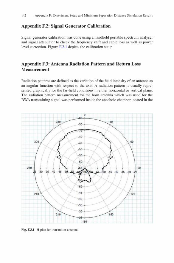
Radiation patterns are defined as the variation of the field intensity of an antenna as an angular function with respect to the axis. A radiation pattern is usually repre-sented graphically for the far-field conditions in either horizontal or vertical plane. The radiation pattern measurement for the horn antenna which was used for the BWA transmitting signal was performed inside the anechoic chamber located in the

Fig. F.3.1 H-plan for transmitter antenna


143

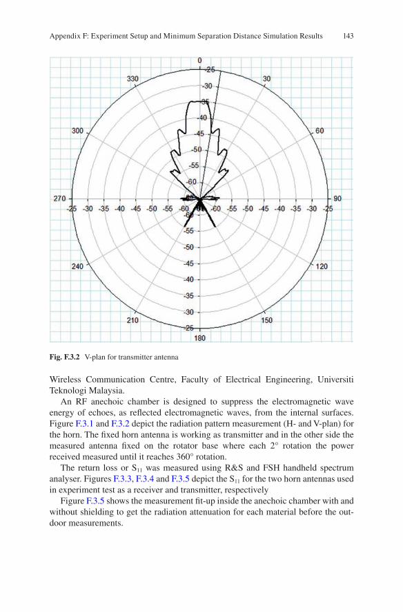
Fig. F.3.2 V-plan for transmitter antenna

Wireless Communication Centre, Faculty of Electrical Engineering, Universiti Teknologi Malaysia.

An RF anechoic chamber is designed to suppress the electromagnetic wave energy of echoes, as reflected electromagnetic waves, from the internal surfaces. Figure F.3.1 and F.3.2 depict the radiation pattern measurement (H- and V-plan) for the horn. The fixed horn antenna is working as transmitter and in the other side the measured antenna fixed on the rotator base where each 2° rotation the power received measured until it reaches 360° rotation.

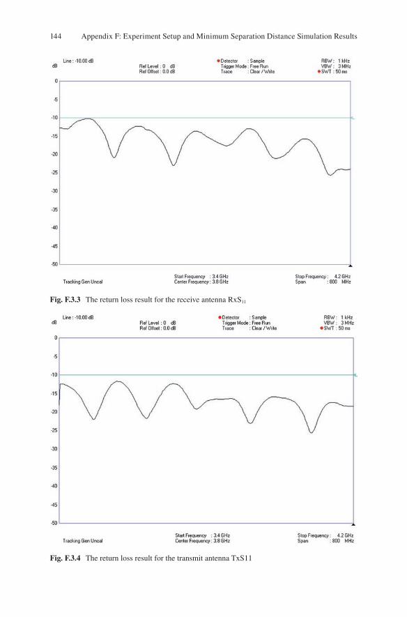
The return loss or S11 was measured using R&S and FSH handheld spectrum analyser. Figures F.3.3, F.3.4 and F.3.5 depict the S11 for the two horn antennas used in experiment test as a receiver and transmitter, respectively

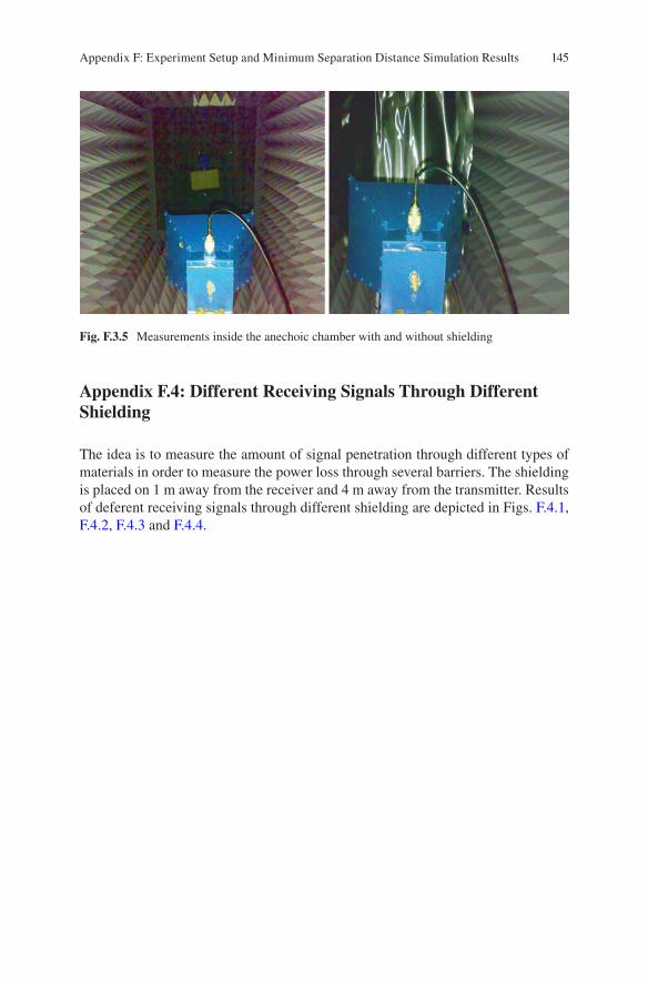
Figure F.3.5 shows the measurement fit-up inside the anechoic chamber with and without shielding to get the radiation attenuation for each material before the out-door measurements.


144

Fig. F.3.3 The return loss result for the receive antenna RxS11

Fig. F.3.4 The return loss result for the transmit antenna TxS11


145

Fig. F.3.5 Measurements inside the anechoic chamber with and without shielding

Appendix F.4: Different Receiving Signals Through Different Shielding

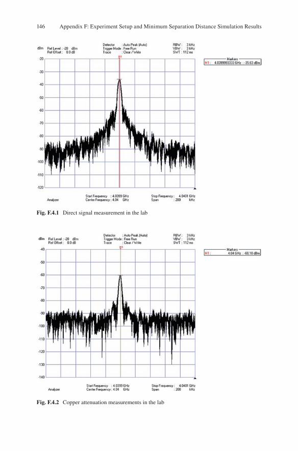
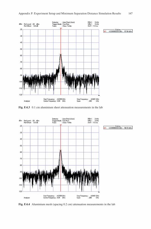
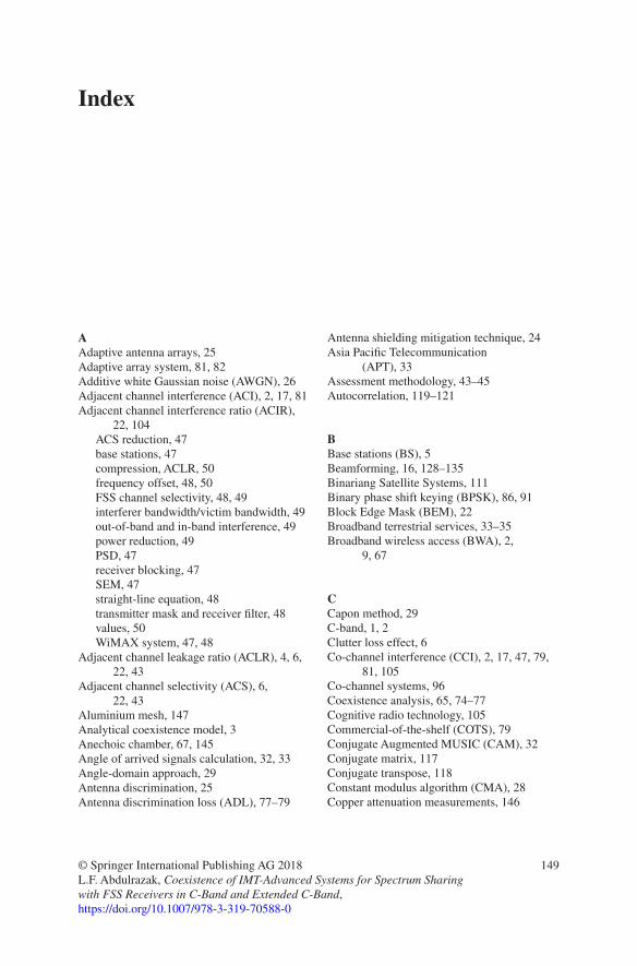
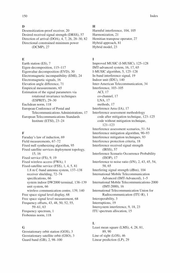
The idea is to measure the amount of signal penetration through different types of materials in order to measure the power loss through several barriers. The shielding is placed on 1 m away from the receiver and 4 m away from the transmitter. Results of deferent receiving signals through different shielding are depicted in Figs. F.4.1, F.4.2, F.4.3 and F.4.4.


146

Fig. F.4.2 Copper attenuation measurements in the lab

Fig. F.4.1 Direct signal measurement in the lab


147

Fig. F.4.4 Aluminium mesh (spacing 0.2 cm) attenuation measurements in the lab

Fig. F.4.3 0.1 cm aluminium sheet attenuation measurements in the lab



AAdaptive antenna arrays, 25Adaptive array system, 81, 82Additive white Gaussian noise (AWGN), 26Adjacent channel interference (ACI), 2, 17, 81Adjacent channel interference ratio (ACIR),

22, 104ACS reduction, 47base stations, 47compression, ACLR, 50frequency offset, 48, 50FSS channel selectivity, 48, 49interferer bandwidth/victim bandwidth, 49out-of-band and in-band interference, 49power reduction, 49PSD, 47receiver blocking, 47SEM, 47straight-line equation, 48transmitter mask and receiver filter, 48values, 50WiMAX system, 47, 48

Adjacent channel leakage ratio (ACLR), 4, 6, 22, 43

Adjacent channel selectivity (ACS), 6, 22, 43

Aluminium mesh, 147Analytical coexistence model, 3Anechoic chamber, 67, 145Angle of arrived signals calculation, 32, 33Angle-domain approach, 29Antenna discrimination, 25Antenna discrimination loss (ADL), 77–79

Antenna shielding mitigation technique, 24Asia Pacific Telecommunication

(APT), 33Assessment methodology, 43–45Autocorrelation, 119–121

BBase stations (BS), 5Beamforming, 16, 128–135Binariang Satellite Systems, 111Binary phase shift keying (BPSK), 86, 91Block Edge Mask (BEM), 22Broadband terrestrial services, 33–35Broadband wireless access (BWA), 2,

9, 67

CCapon method, 29C-band, 1, 2Clutter loss effect, 6Co-channel interference (CCI), 2, 17, 47, 79,

81, 105Co-channel systems, 96Coexistence analysis, 65, 74–77Cognitive radio technology, 105Commercial-of-the-shelf (COTS), 79Conjugate Augmented MUSIC (CAM), 32Conjugate matrix, 117Conjugate transpose, 118Constant modulus algorithm (CMA), 28Copper attenuation measurements, 146

Index

https://doi.org/10.1007/978-3-319-70588-0

150

DDesensitization-proof receiver, 20Desired received signal strength (DRSS), 57Direction of arrival (DOA), 4, 7, 26, 28–30, 82Directional constrained minimum power

(DCMP), 27

EEarth station (ES), 7Eigen-decomposition, 115–117Eigenvalue decomposition (EVD), 30Electromagnetic incompatibility (EMI), 24Electromagnetic signals, 16Elevation angle difference, 71Empirical measurements, 65Estimation of the signal parameters via

rotational invariance techniques (ESPRIT), 29–30

Euclidean norm, 118European Conference of Postal and

Telecommunications Administrations, 17European Telecommunications Standards

Institute (ETSI), 23–24

FFaraday’s law of induction, 69Field measurements, 67–72Fixed null synthesizing algorithm, 95Fixed satellite services deployment topology,

15, 16Fixed service (FS), 9, 19Fixed wireless access (FWA), 1Fixed-satellite service (FSS), 1, 4, 5, 81

1.8 m C-band antenna system, 137–138receiver shielding, 72–74specifications, 66system indoor DW2000 terminal, 138–139unit system, 66wireless communication centre, 139, 140

Free space signal level display, 68Free space signal level measurement, 68Frequency offsets, 43, 48, 50, 52, 55,

59–61, 63Frequency spectrum, 1Frobenius norm, 118

GGeostationary orbit station (GOS), 3Geostationary satellite orbit (GSO), 3Guard band (GB), 2, 98–100

HHarmful interference, 104, 105Harmonization, 21Hemitian transpose operator, 27Hybrid approach, 81Hybrid model, 23

IImproved MUSIC (I-MUSIC), 125–128IMT-advanced system, 16, 17, 65I-MUSIC algorithm, 5, 125–128In-band interference signal, 19Indoor unit (IDU), 140Inter-American Telecommunication, 34Interference, 103–105

ACI, 17co-channel, 17LNA, 17methods, 17

Interference Area (IA), 17Interference assessment methodology

code after mitigation technique, 123–125code without mitigation technique,

121–123Interference assessment scenarios, 51–54Interference mitigation algorithm, 90–93Interference mitigation techniques, 93Interference protection criteria, 18Interference received signal strength

(IRSS), 57Interference Scenario Occurrence Probability

(ISOP), 17Interference to noise ratio (I/N), 2, 43, 45, 54,

58, 65Interfering signal strength (dBm), 104International Mobile Telecommunication

Advanced (IMT-Advanced), 1–5International Mobile Telecommunications-2000

(IMT-2000), 16International Telecommunication Union for

Radiocommunication (ITU-R), 1Interoperability, 3Interruptions, 19Intersystem interference, 9, 18, 23ITU spectrum allocation, 15

LLeast mean square (LMS), 4, 28, 81,

89, 90Line of sight (LOS), 46Linear prediction (LP), 29

Index

151

Linearly constrained minimum variance filter (LCMV), 27

Line-of-sight (LOS), 10, 11

MMatlab code, 6MATLAB code, 43Maximizing signal-to-noise ratio (MSN), 27MEASAT downlink transponders, 95MEASAT-3 satellite network, 111–115Minimizing mean square error (MMSE), 27Minimum coupling loss (MCL), 2Minimum separation distance simulation

area analysis, 57, 58exclusion zone, 56fixed-satellite service specifications, 54protection ratio methodology, 55–57simulated parameters, 55WiMAX 802.16 systems, 54WiMAX and FSS, 0.23 MHz, 60–62WiMAX and FSS, 36 MHz, 58–60

Minimum separation distances, 96, 97Minimum square error (MSE), 83Min-Norm method, 29Mitigation technique, 3, 103Monte Carlo (MC) method, 18Monte Carlo (MC) simulation, 2Multi-carrier modulation technique, 2Multi-invariance MUSIC (MI-MUSIC), 32Multiple input-multiple output (MIMO),

16, 35Multiple signal classification (MUSIC),

29–31adaptive breamforming, 81DOA, 85eigenvalue decomposition, 84minimum variance solution, 85signal subspace, 85spectrum function, 84steering vector, 83–85

NNetwork management system (NMS), 140Non-line-of-sight (NLOS), 10

OOffice of the Telecommunications Authority

(OFTA), 34Orthogonal frequency division multiplexing

(OFDM), 2

Orthomode Transducer (OMT), 140Outdoor unit (ODU), 139Out of band (OOB), 51

PPisarenko method, 29Planar wave model, 26Power flux density (PFD), 22, 23Power spectral density (PSD), 47Propagation model parameters, 45–47

RRadiation patterns, 142Radio propagation, 2, 6

analytical predication algorithm, 12CEPT and ITU organizations, 13clutter losses, 13, 14frequency dependence, 10, 11nominal clutter heights and distances, 13path loss equation, 10–12penetrating obstacles, 10radio coverage, 10single-/multi-transmitters, 11–12spectrum allocation widths, 10wireless communications, 9

Radio wave propagation, 4Receiver sensitivity, 19Research objectives, 3RF anechoic chamber, 143Root mean squared error (RMSE), 5, 45, 118Root-MUSIC method, 29

SSatellite receivers, 5Separation distance, 100, 101, 103–105Sharing studies, 9, 34, 36Shielding, 6, 21, 103, 145Shielding experiment, 65–67Signal generator, 65–67, 69Signal generator calibration, 141, 142Signal of interest (SOI), 82Signal to noise ratio (SNR), 3Signal-to-interference-plus-noise ratio

(SINR), 25Smart antenna receiver configuration, 26Smart antenna technologies, 25–28Special Division Multiple Access (SDMA), 35Spectral emission mask, 20Spectrum allocation, 21Spectrum analyser, 69

Index

152

Spectrum coexistence, 14Spectrum emission mask (SEM), 23, 24, 47Spectrum sharing, 14Standard deviation, 119Subscriber Station (SS), 18Subspace-based method, 30Switched-beam arrays, 25Switched-beam system, 82System design, 15, 16System designers, 103

TTelevision receives-only (TVRO), 34Transfinite Visualyse Pro™, 43, 58

UUniform linear array (ULA), 4, 31, 32Unitary transformation method, 30

VVector expression, 27Very small aperture terminal (VSAT), 15,

65–67, 72, 103Visualyse professionals, 57, 135, 136

WWiener-Hopf equation, 27WiMAX specifications, 75WiMAX system parameters, 94Wireless communication

systems, 13Wireless local loop (WLL), 15Worldwide Interoperability for Microwave

Access (WiMAX), 3, 34

ZZinc sheet material, 69

Index

Documents

Appendix A: List of Author's Related Publications