Embed Size (px)
Citation preview

Appendix
1. Matrix Algebra
1.1 Matrices
Matrix
A matrix of order (n x p) is a rectangular array of elements consisting of n rows and p columns. A matrix is denoted by a bold face letter say A where
The elements are denoted by aij, i = 1,2, ... , nj j = 1,2, ... ,p, where the first subscript i refers to the row location, and the second subscript j refers to the column location of the element. The matrix is also sometimes denoted by (( aij ) ).
Example of a Matrix
The matrix B = [! ~ -;] has 2 rows and 3 columns and hence is a
(2 x 3) matrix, while the matrix C = [-~ -~l has 3 rows and 2 columns -3 8
and hence is a (3 x 2) matrix.
Transpose of a Matrix
The transpose of the matrix A (n x p) is the matrix B (p x n) obtained by interchanging rows and column so that
bij = aji i = 1,2, ... ,pj j = 1,2, ... ,n.
The transpose of A is usually denoted by B = A'. Some additional properties of a matrix transpose are

546 Appendix
1. A' = B' if and only if A = B
2. (A')' = A.
Example of a Matrix Transpose
The transpose of the matrices B and C defined in the above example are given by
B' = [ ~ :] -2 3
C' [-6 4 -3] and = 2 -5 8·
Exercise - Matrix Transpose
Using the matrices Band C defined above verify that (B/)' (C/)' = C.
Row Vector and Column Vector
Band
A row vector is a matrix with only one row and is denoted by a lower case letter with bold face type
A column vector is a matrix with only one column and is also denoted by a lower case bold face letter
Example of Rowand Column Vectors
The (4 xl) mat"x d = [~i 1 in column veet"' while the (1 x 5) matdx
f = [3 5 -7 4 -2] is a row vector.

1. Matrix Algebra 547
Square Matrix
A matrix is square if the number of rows n is equal to the number of columns p (n = p). A square matrix with m rows and columns is said to have order m.
Symmetric Matrix
A square matrix A of order m is symmetric, if the transpose of A is equal to A.
A = A' if A symmetric.
Diagonal Elements
The elements aii, i = 1,2, ... , m are called the diagonal elements of the square matrix A with elements aij, i = 1,2, ... , m; j = 1,2, ... , m.
Trace of a Matrix
The sum of the diagonal elements of A is called the trace of A and is denoted m
by tr(A). The trace of the (m x m) matrix is given by tr(A) = L aii. i=l
Example - Square, Symmetric, Diagonal Elements, Trace
The matrix H = [~ ~ =i] is a (3 x 3) or square matrix of order 3. -4 -1 7
The matrix is symmetric since H' = H. The diagonal elements of Hare the elements 8,2 and 7. The trace of H = trH = 17 which is the sum of the diagonal elements.
Exercise - Symmetric Matrix, Trace
Verify that the matrix A = [ a~ :b fCe ] is symmetric and that tr (A) =
(a+d+f).

548 Appendix
Null or Zero Matrix
The null or zero matrix denoted by 0 is the matrix whose elements are all zero.
Identity Matrix
The identity matrix of order m is the square matrix whose diagonal elements are all unity, and whose off-diagonal elements are all zero. The identity matrix of order m is usually denoted by 1m and is given by
1 0 0 0 0 1 0 0
Im= 0 0 1
0 0 0 0 1
Diagonal Matrix
A diagonal matrix is a matrix whose off-diagonal elements are all zero. The identity matrix is a special case of a diagonal matrix.
Submatrix
A submatrix of a matrix A is a matrix obtained from A by deleting some rows and columns of A.
Example of Submatrix
The (2 x 2) matrix C* = [~ ~4] is a submatrix of the matrix C =
[ ~ =~ ~]. C* is obtained from C by deleting the first row and the 2 1 -5
third column.

1. Matrix Algebra 549
1.2 Matrix Operations
Equality of Matrices
Two matrices A and B are equal, if and only if each element of A is equal to the corresponding element of B: aij = bij , i = 1,2, ... ,ni j = 1,2, ... ,p.
Addition of Matrices
The addition of two matrices A and B is carried out by adding together corresponding elements. The two matrices must have the same order. The sum is given by C where
C=A+B
and where Cij = aij + bij , i = 1,2, ... ,ni j = 1,2, ... ,p.
Additive Inverse
A matrix B is the additive inverse of a matrix A, if the matrices sum to the null matrix 0
B+A=O,
where bij + aij = 0 or bij = -aij, i = 1,2, ... , ni j = 1,2, ... ,po This additive inverse is denoted by B = -A. If C = A + B then C' = A' + B'.
Example
The sum of the matrices A and B given below is denoted by C.
A= H B= H =~] = H -~] [
4+2 3-5] C = -6-2 9- 2
2 +4 -4+6
[-4 -3] The matrix D = 6-9
-2 4 is the additive inverse of the matrix A
ffince A+D = [~ n

550 Appendix
Exercise
Verify that C' = A' + B' using the matrices A, B and C in the previous example.
Scalar Multiplication of a Matrix
The scalar multiplication of a matrix A by a scalar k is carried out by multiplying each element of A by k. This scalar product is denoted by k A and the elements by kaij, i = 1,2, ... , n; j = 1,2, ... ,po
Product of Two Matrices
The product of two matrices A (n x p) = (aij) and B (p x m) = (bjk ) is denoted by C = AB, if the number of columns (P) of A is equal to the number of rows (P) of B, and if the elements of C = (C;,j) are given by
P
C;,k = L aijbjk . j=l
The order of the product matrix Cis (n x m).
Example
The matrix A = [-: ~l when multiplied by the scalar 3 yields the 2 -4
matrix 3A = [-!~ 2~l. 6 -12
The product of the two matrices A and B where A is given above and
B [ 0 6 2]. . b = 1 -2 3 IS given y
[ (4)(0) + (3)(1) (4)(6) + (3)(-2) (4)(2) + (3)(3) 1
C = AB = (-6)(0) + (9)(1) (-6)(6) + (9)(-2) (-6)(2) + (9)(3) (2)(0) + (-4)(1) (2)(6) + (-4)(-2) (2)(2) + (-4)(3)
= [ ~ -~~ !~l· -4 20-8
Some additional properties are:

1. Matrix Algebra 551
1. A+B=B+A
2. (A + B) + C = A + (B + C)
3. a(A + B) = aA + aB
4. (a+b)A=aA+bA
5. (AB)C = A(BC)
6. (A+B)C = AC+BC
7. In general AB =f. BA even if the dimensions conform for multiplication.
8. For square matrices A and B
tr(A + B) = trA + trB and tr(AB) = tr(BA).
Exercise
Given A = [~ -~], B = [i _~] and C [-1 2] o 3 verify the
properties 1 through 8 given above.
Multiplicative Inverse
The multiplicative inverse of the square matrix A (m x m) is the matrix B (m x m) satisfying the equation AB = BA = 1m, where 1m is the identity matrix of order m. The multiplicative inverse of A is usually denoted by B = A-I. If A has an inverse it is unique.
Some additional properties are:
1. If C = AB then C-1 = B-1 A-I
2. (A,)-1 = (A -1)'
3. If C = AB then C' = B'A'.
4. (kA)-1 = (l/k)A -1.
Example
The inverse of the matrix A = [_~ -~] is given by A-I = U~~ 1{2]
sinceAA-1 = [_~ -~] [~~~ 1{2] = [~ n.

552 Appendix
A Useful Result
Given a symmetric nonsingular matrix A (p x p) and matrices Band C of order (p x q), the inverse of the matrix [A + BC'] is given by
An important special case of this result is when Band Care (p x 1) vectors say band c. The inverse of the matrix [A + be'] is given by
Exercise
[A + be']-l = A -1 _ A -lbe' A-1
1+e'A-1b
(a) Verify the above two results by using matrix multiplication.
(b) The equi-correlation matrix has the form B = (1- p)1 + pii' where p is a constant correlation coefficient and i (n x 1) is a vector of unities. Show by using the above result that the matrix B-1 is given by
B-1 = __ 1_ 1 _ pii' (1- p) (1 - p)2 + p(1 - p)n
Idempotent Matrix
An idempotent matrix A is a matrix which has the property AA = A. If A is idempotent and has full rank then A is an identity matrix.
Example
The matrix B [01 -01] is idempotent since
[1 -1] o O·
Exercise
Show that the mean centering matrix [I - ftii'] is idempotent where 1 is an (n x n) identity matrix and i (n x 1) is a vector of unities.

1. Matrix Algebra 553
Kronecker Product
If A(n X m) and B(p x q), the Kronecker product of A and B is denoted by A ® B and is given by the matrix
anB a12B almB
a21B a22B a2mB
Example
Given A = [~ -!] B = [~] then
A0B~ [: [~] -1 [!]] ~ [I~ -3] -5 and
[~] [~] 1~ 12
4 20
B0h [: [~ -!]] [ I: -3] 12
=
[~ -!] -5 15 20
Some properties of Kronecker products are
1. (A ® B) ® C = A ® (B ® C)
2. (A + B) ® C = (A ® C) + (B ® C)
3. (A®B)(C®D) =AC®BD
4. (A ® B)' = A' ® B'
5. tr(A ® B) = tr(A)tr(B)
6. For vectors a and b
a' ®b = b®a' = ba'
7. In general A ® B =f. B ® A as demonstrated in the above example.

554 Appendix
Exercise
(a) Use the matrices A and B defined in the example above to show that (A ® B)' = (A' ® B /).
(b) Use the matrices A = [;
tr(A ® B) = tr(A)tr(B).
-1] [-1 2] 2 and B = 5 3 to verify that
1.3 Determinants and Rank
Determinant
The determinant of a square matrix A is a scalar quantity denoted by IAI and is given by
n!
" '(k) IAI = L)-I)3 all(k)a22(k)·· .ann(k)·
k=l
The determinant represents the sum of n! terms each term consisting of the product of n elements of A. For each term of the summation, the first subscripts are the integers 1 to n in their natural order, and the second subscripts represent a particular permutation of the integers 1 to n. The power j(k) is 1 or 2 depending on whether the second subscripts represent an odd or an even number of interchanges with the integers in their natural order.
For the 2 x 2 matrix
the determinant is given by
IAI = alla22 a12a 21 (0 interchanges) (1 interchange)
For the 3 x 3 matrix
the determinant is given by
IBI = bllb22b33 - bllb23b32 + b12b23b31 (0 interchanges) (1 interchange) (2 interchanges)
- b12b21b33 + b13b21b32 - b13~2b31 . (1 interchange) (2 interchanges) (1 interchange)
NOTE: n! = 3! = 6 terms.

1. Matrix Algebra 555
Nonsingular
If IAI ¥- 0 then A is said to be nonsingular. The detenninant of the matrix A (n x n) can be evaluated in terms
of the determinants of submatrices of A. The determinant of the submatrix of A obtained after deleting the j-th row and k-th column of A is called the minor of ajk and is denoted by IAjkl. The cofactor of ajk is the quantity (-l)j+kIAjk l. The determinant of A can be expressed by
n IAI = L: ajk(-l)j+kIAjk l for any k and is called the cofactor expansion
j=l
ofA.
Example
The determinant of the matrix B = [ 41 35 -21]
-3 -4 7 by expanding about the first row obtaining
Equivalently expanding about the third column
can be determined
-2(-1)41 4 51+ 1(_1)51 1 31+ 7(_1)61 1 53 1=-52. -3 -4 -3 -4 4
Exercise
Verify the value of the determinant in the example by expanding about the second row.
Some useful properties of the determinant are:
1. IAI = IAI'
2. If each element of a row (or column) of A is multiplied by the scalar k then the detenninant of the new matrix is kiAI.
3. IkAI = IAlkP if A is (p x p)
4. If each element of a row (or column) of A is zero then IAI = o. 5. If two rows (or columns) of A are identical then IAI = o. 6. The determinant of a matrix remains unchanged if the elements of one
row (or column) are multipled by a scalar k and the results added to a second row (or column).

556 Appendix
7. The determinant of the product AB of the square matrices A and B is given by IABI = IAIIBI.
8. If A -1 exists then IA -11 = IAI-1.
9. A -1 exists if and only if IAI =F O.
10. IA ® BI = IAlnlBlm where A(n x n) and B(m x m).
11. (A ® B)-1 = A-1 X B-1
12. If A(P x p) is non-singular, B(P x m) and C(m x p) then IA + BCI = IAI-1IIp+A -1BCI = IA -11IIm+CA -1BI where Ip(pxp) and Im(mx m) are identity matrices.
Relation Between Inverse and Determinant
The inverse of the matrix A is given by A -1 = *' A *, where A * is the
transpose of the matrix of cofactors of A. The matrix A * is called the adjoint of A.
Example
For the (2 x 2) matrix A = [_~ -~] the determinant is given by 54-8 =
46. The matrix of cofactors is given by [~ ~] and hence the adjoint
matrix is A * = [~ ~]. The inverse of A is therefore given by A -1 =
i6[~ ~].
Exercise
(a) Verify that IA -11 = IAI-1 using the matrix A in the previous example.
(b) Verify the inverse of the matrix A in the example above using the adjoint and determinant of A -1 to get A.
(c) Use the properties above to show that the determinant of the equicorrelation matrix is given by IpI+(I-p)ii'l = (l-p)n-1[I+p(n-l)], where i (n xI) is a vector of unities.

1. Matrix Algebra 557
Rank of a Matrix
The rank of a matrix A, rank (A), is the order of the largest nonsingular submatrix of A. If A is nonsingular then A is said to have full rank.
Example
Given the matrix B = [ ~ ~l the rank is the order of the largest non--1 4
singular submatrix of B. Since B is (3 x 2) the rank cannot exceed 2 since a (2 x 2) matrix is the largest square submatrix of B. The three possible submatrices are
The first of these submatrices has determinant zero and hence is singular. The remaining two submatrices are nonsingular. The rank of the matrix B is therefore 2.
Exercise
(a) Verify that the rank of the matrix A given by A = is [621 1431 -4~1 2 and determine all (2 x 2) matrices that have rank 2.
(b) Using the matrix B in the above example and A in (a) verify that rank (BA) = 2.
The following properties are useful. 1. If A and Bare nonsingular matrices with the appropriate dimensions
and if C is arbitrary of appropriate dimension then:
(a) rank (AB) ::; min [rank (A), rank (B)]
(b) rank (AC) = rank (C)
(c) rank (CA) = rank (C)
(d) rank (ACB) = rank (C).
2. The rank of an idempotent matrix is equal to its trace.

558 Appendix
1.4 Quadratic Forms and Positive Definite Matrices
Quadratic Form
Given a symmetric matrix A (n x n) and an (n xl) vector x a quadratic form is the scalar obtained from the product
n n
x'Ax = L LaijXiXj. i=1 j=1
The matrix A must be square, but need not be symmetric, since for any square matrix B the quadratic form x'Bx can be written equivalently in terms of a symmetric matrix A. Thus
x'Ax= x'Bx.
There is no loss of generality therefore, in assuming the matrix A in a quadratic form is symmetric.
Exercise
Given x ~ [ -~:] and A ~ [~ j -!] detennine the .ruue of r Ax
and solve for a in the equation x' Ax = 10.
Congruent Matrix
A square matrix B is congruent to a square matrix A, if there exists a nonsingular matrix P such that A = P'BP. By defining the linear transformation y = Px the quadratic form y'By is equivalent to x' Ax. If A is of rank r, there exists a nonsingular matrix P such that the congruent matrix B is diagonal. In this case B has r nonzero diagonal elements and
r the remaining (n - r) diagonal elements zero, therefore y'By = ~ buY;.
i=1
Positive Definite
A real symmetric matrix A (n x n) is positive definite if the quadratic form x' Ax is positive for all (n xl) vectors x. If A is positive definite and nonsingular, then A is congruent to an identity matrix in that there exists a nonsingular matrix P such that
x'Ax = y'y where y = Px.

1. Matrix Algebra 559
Positive Semidefinite, Negative Definite, Nonnegative Definite
The matrix A is positive semidefinite if x' Ax ~ 0 for all x, and x, Ax = 0 for at least one x. It is negative definite if x, Ax < 0 for all x, and negative semidefinite if x' Ax ::; 0 for all x and x' Ax = 0 for at least one x. The matrix A is nonnegative definite if it is not negative definite.
Exercise
Suppose that A definite if a =f. O.
aa' where a(p xl) and show that x' Ax is positive
Some additional results are:
1. The determinant of a positive definite matrix IAI is positive.
2. If A is positive definite (semidefinite) then for any nonsingular matrix P, pI AP is positive definite (semidefinite).
3. A is positive definite if and only if there exists a nonsingular matrix V such that A = V/V.
4. If A is (n x p) of rank p then A' A is positive definite and AA' is positive semidefinite.
5. If A is positive definite then A -1 is positive definite.
1.5 Partitioned Matrices
A matrix A can be partitioned into submatrices by drawing horizontal and vertical lines between rows and columns of the matrix. Each element of the original matrix is contained in one and only one submatrix. A partitioned matrix is usually called a block matrix.
[
an a21
A= a31
a41

560 Appendix
Product of Partitioned Matrices
The product of two block matrices can be determined if the column partitions of the first matrix correspond to the row partitions of the second matrix. As usual the total number of columns of the first matrix must be
Inverse of a Partitioned Matrix
AllB12 + A12B22 + A13B32].
A21B12 + A22B22 + A23B32
Let the (n xp) matrix A be partitioned into four submatrices All (nl x pd, A 12 (nl x (p - pd), A21((n - nl) x PI) and A22((n - nl) x (p - PI)) and
hence A = [!~~ !~~]. If B = A-I exists then B = [:~~ :~~] can
be related to A by the following 1. Bll = [All - A12Ail A 21]-1 = [Ail + All A12B22A21Ail]
2. B12 = -Ail AdA22 - A21Ail Ad-1 = -Ail A12B22
3. B21 = -AilA21[All-A12AilA21]-1 = -AilA21Bll
4. B22 = [A22 - A21Ail A 12]-1 = [Ai21 + Ail A21BllA12Ain
Exercise
1. (a) Verify the above expressions for B = A-I by multiplication to show that AB = I. (b) Verify the above expressions for B = A-I by solving for the four submatrices in B in the equation AB = I.
2. ~:ee ~::r:r:u:e [for! th~ in~rl" b: ::::::::a::: i~ve::~: -7 1 8
[5 -3] 1 8·

1. Matrix Algebra 561
Determinant of a Partitioned Matrix
The determinant of IAI can be expressed as
1. IAI = IAdlAu - A12A;-l A221 = IAullA22 - A21All Ad
2. IAI = IAd/IBul = IAul/IB221, where Bll and B22 are defined above with the inverse of a partitioned matrix.
If A21 = A12 = 0 then
1. A-I = [AJl A~l] . 2. IAI = IAu11A221·
Exercise
(a) Use the expression for IAI in (1) above to determine IAI in the previous exercise.
(b) Show that IAI = IAllIIA221 using the matrix A in the previous exercise.
1.6 Expectations of Random Matrices
An (n xp) random matrix X is a matrix whose elements Xij i = 1,2, ... , n; j = 1,2, ... ,p are random variables. The expected value of the random matrix X denoted by E[X] is the matrix of constants E[Xij] i = 1,2, ... ,n; j = 1,2, ... ,p if these expectations exist.
Let Y (n x p) and X (n x p) denote random matrices whose expectations E[Y] and E[X] exist. Let A (m xn) and B (px k) be matrices of constants. The following properties hold:
1. E[AXB] = AE[X]B-
2. E[X + Y] = E[X] + E[Y].
Let z (n xl) be a random vector and let A (n x n) be a matrix of constants. The expected value of the quadratic form Zl Az is given by
n n E[Z' Az] = 2:: 2:: aijE[ziZj] where A has elements aij and z has ele
i=l j=l
ments Zi.

562 Appendix
Exercise
(a) Show that E[(X + A)'(X + A)] = E + A'II + II' A + A' A where X is a random matrix E[X] = II and E[X'X] = E.
p p p p
(b) Show that E[x' Ax] = :E :E aijO"ij +:E :E aijl-'il-'j where E[(Xi -i=l j=l i=l j=l
l-'i)(Xj - I-'j)] = O"ij, i,j = 1,2, ... ,po
1. 7 Derivatives of Matrix Expressions
If the elements of the matrix A are functions of a random variable x then the derivative of A with respect to x is the matrix whose elements are the
derivatives of the elements of A. For A = (aij) , ~ = (tt;~j). If x is a (p x 1) vector, the derivative of any function of x, say f(x), is
the (p x 1) vector of elements (3.£) j = 1,2, ... ,po
Given a vector x (p x 1) and a vector a (p x 1), the vector derivative
of the scalar x'a with respect to the vector x is denoted by aC:Xa) = a, which is equivalent to the vector
a~x'a) Xl
a~x'a) X2
a~x'a) Xp
Given a vector x (p x 1) and a matrix A (p x p), the vector derivative of Ax is given by 8Aj8x = A' or 8Aj8x' = A.
Given a vector x (p x 1) and a matrix A (p x p), the vector derivative of the quadratic form x' Ax with respect to the vector x is denoted by
8(~~x) = 2Ax, which is equivalent to the vector
8(~Ax) Xl
8(x'Ax) 8X2
8(x' Ax) 8xp

2. Linear Algebra 563
Given a matrix X (nxm) then the derivative of a function of X, say f(X), with respect to the elements of X is the (n x m) matrix of partial derivatives
(l£j ). Some useful properties of the matrix derivative involving the trace
operator are given by
1. &tr(X) = I
2. &tr(AX) = A'
3. &tr(X' AX) = (A + A')X.
The derivative of a determinant IXI of a matrix X, with respect to the
elements of the matrix, is given by 8Jil = (X')* = adjoint of X'.
Exercise
(a) Show that if f = (a - Bx)'(a - Bx) where a (n xI), B (n x p) and
x (p x 1) then ~ = [2B'Bx - 2B'a].
(b) Show that if f = tr(A - BX)'(A - BX) where A (n x p), B (n x r)
and X (r x p) then M = [2B'BX - 2B'A].
2. Linear Algebra
2.1 Geometric Representation for Vectors
A vector x' = (Xl, X2, ... , Xn) can be represented geometrically in an n-dimensional space, as a directed line segment from the origin to the point with coordinates (Xl, X2, ... , xn). The n-dimensional vector space is formed by n mutually perpendicular axes X!, X 2 , ... , X n . The coordinates (Xl, X2, ... , xn) are values of Xl, X2, ... , Xn respectively. Figure A.l shows the vectors xi = (Xll,X2l,X3l) and x~ = (X12,X22,X32) in a three-dimensional space. The addition of the two vectors xi + x~ = (Xll + X12, X2l + X22, X3l + X32) is also shown in Figure A.1. Figure A.2 shows scalar multiplication by a scalar k for a two-dimensional vector x' = (Xll,X2l), where kx' = (kXll, kX2l).
The length of the vector x' = (Xl, X2, . .. , xn) is given by the Euclidean distance between the origin and the point (Xl, X2, ... , Xn) and is denoted by
n 1/2 IIxll = J(XI - 0)2 + (X2 - 0)2 + ... + (Xn - 0)2 = [LX;] .
i=l

564 Appendix
k----------X2
Figure A.I. Addition of Two Vectors
kx
x
Figure A.2. Scalar Multiplication
(kxl1 • kX21 )
I I I I I I I I
The angle () between the vector Xl = (xn, X21, ... , Xnl) and the vector X2 = (XI2, X22, ... , X n 2) is given by

X 21
X 22 --
o
1
1 1 1 (X12 • X22 )
---1------1 1
1 1
X2
2. Linear Algebra 565
~--------L---------L----------Xl
Figure A.3. Angle Between Two Vectors
The matrix product of the (n xl) vectors Xl and X2 is given by x~ X2 = X~XI
and hence Cos () = x~x2/(x~xd/2(x;X2)1/2.
In Figure A.3 the angle () between x~ = (Xl1' X2t) and x~ = (X12' X22) is given by Cos () = [Xl1XI2+X2IX22l/[X~1 +x~lll/2[X~2+X~2ll/2. If Cos () = ±1 the vectors Xl and X2 are said to be orthogonal.
The distance from the vector point x~ = (Xl1' X21, ... , Xnl) to the vector point x~ =:= (XI2' X22,' .. ,Xn 2) is the Euclidean distance between the two points
The projection of the vector X2 on the vector Xl is a vector which is a scalar multiple of Xl given by
where () is the angle between X2 and Xl, and k is the scalar given by
II~~II COS ().

566 Appendix
Exercise
(a) Given Xl = [~] and X2 = [~] plot the vectors Xl and X2 in the
two-dimensional space formed by the axes Xl and X 2 •
(b) Plot the vector (Xl + X2) and the vector 2Xl in the two-dimensional space in (a).
(c) Determine the length of the vectors Xl, X2 and (Xl + X2).
(d) Determine the angle () between the vectors Xl and X2.
(e) Determine the distance between the tips of the vectors Xl and X2.
(f) Determine the projection X2 of the vector X2 on Xl and determine the vector X2 = X2 - X2. Show that X2 and x 2 are orthogonal.
2.2 Linear Dependence & Linear Transformations
Linearly Dependent Vectors
If one vector X in n-dimensional space can be written as a linear combination of other vectors in n-dimensional space, then X is said to be linearly dependent on the other vectors. If
then X is linearly dependent on Vl, ••. , vp-The set of (p + 1) vectors (x, Vl, ••• , vp ) is also a linearly dependent set,
if anyone of the vectors can be written as a linear combination of the remaining vectors in the set.
Linearly Independent Vectors
A set of vectors is linearly independent, if it is not possible to express one vector as a linear combination of the remaining vectors in the set. In an n-dimensional space the maximum number of linearly independent vectors is n. Thus given any set of n linearly independent vectors, all other vectors in the n-dimensional space can be expressed as a linear combination of the linearly independent set.

2. Linear Algebra 567
Basis for an n-Dimensional Space
The set of n linearly independent vectors is said to generate a basis for the n-dimensional space.
In two-dimensional space linearly dependent vectors are co-linear or lie along the same line. In three-dimensional space linearly dependent vectors are in the same two-dimensional plane and may be co-linear. If the set of linearly independent vectors are mutually orthogonal then the basis is said to be orthogonal.
Generation of a Vector Space and Rank of a Matrix
IT the matrix A (n x p) has rank r, then the vectors formed by the p columns of A generate an r-dimensional vector space. Similarly the rows of A generate an r-dimensional vector space. In other words, the rank of a matrix is the maximum number of linearly independent columns, and equivalently the maximum number of linearly independent rows.
Exercise
Ca) Given the vectom X, ~ H]' XF m and x. ~ m show that
they are linearly independent by showing that each cannot be written as a linear combination of the remaining two.
(b) Let A = [XbX2,X3J and determine IAI for the values of Xl,X2,X3
given in (a).
Linear Transformation
Given a p-dimensional vector x, a linear transformation of x, is given by the matrix product
y=Ax,
where A (n x p) is called a transformation matrix. The matrix A maps the n-dimensional vector x into a p-dimensional vector y. IT A is a square nonsingular matrix, the transformation is one to one, in that x = A -ly and hence each point in x corresponds to exactly one and only one point in y.

568 Appendix
Orthogonal Transformation, Rotation, Orthogonal Matrix
If A is a square matrix and A has the property that A' = A-I, then the equation y = Ax is an orthogonal transformation or rotation. The matrix A in this case is called an orthogonal matrix. If A is orthogonal, A also has the property that IAI = ±1. The transformation is orthogonal because it can be viewed as a rotation of the coordinate axes through some angle (J. The angle (J between any pair of vectors remains the same after the transformation.
Example
In Figure A.4, the point M has coordinates (Xl, X2) with respect to the Xl - X 2 axes and has coordinates (Zl' Z2) with respect to the Zl - Z2 axes. The angle ¢ between Xl and Zl is the angle of rotation required to rotate the Xl - X 2 axes into the Zl - Z2 axes. The coordinates (ZI, Z2) of the point M in Zl - Z2 space can be described in terms of the coordinates (Xl, X2) of M in Xl - X 2 space using the equations
Zl = Xl cos¢ + X2 sin¢
Z2 = -Xl sin¢ + X2 cos ¢.
In matrix notation the linear transformation to [~~] from [:~] can be
expressed as [Zl] = [ C?S ~ sin ~] [Xl]. The transformation matrix Z2 - SIll '" cos'" X2
A = [ C?S ~ sin ~] has the property that -SIll", cos",
and hence the transformation is orthogonal as required.
Exercise
[./2/2 -./2/2] .. (a) Let A = ./2/2 ./2/2 denote a transformatlOn matrlX. Show
that A-I = A' and hence that A is an orthogonal transformation matrix.
(b) Use the results of the above example to show that the angle of rotation in (a) is 45°.
(c) Give the transformation matrix corresponding to ¢ = 60° .

X 2
Figure A.4. Rotation of Axes
M -----~
// 1\ .// I \
./ I \ / I
I Zl
2.3 Systems of Equations
2. Linear Algebra 569
Let XI, x2, X3 denote the unknowns in a system of 3 equations
The system of equations can be represented by a matrix equation
Ax=b
where
Solution Vector for a System of Equations
The solution vector x is given by
x= A-lb.

570 Appendix
Exercise
1. Given thethree lineady independent veeton> x, ~ [ - ~ ] , x, ~ [ -!] and '" ~ [~]. If Y ~ [~] is contained in the ,pore genecated
by Xl, X2 and X3 then there exist coefficients a, band c such that y = aXl + bX2 + CX3. Show that the equation for y can be written as
y ~ Af wh",e f ~ [:] and ",I"" fo, f.
2. Solve the system of equations
3Xl + X2 - 4X3 = 3
2Xl + 5X2 + X3 = 10
Xl - 4X2 + 3X3 = -6
for Xl, X2 and X3 using the expression x = A -ly.
Homogeneous Equations - Trivial and Nontrivial Solutions
If the vector b in the system Ax = b is the null vector 0, the system is said to be a system of homogeneous equations. The obvious solution X = 0 is said to be a trivial solution. If A is (n x p) of rank r, where x and bare (p xl), then the system of n homogeneous equations in p unknowns given by Ax = b has (p - r) linearly independent solutions in addition to the trivial solution x = O. In other words, a nontrivial solution exists if and only if the rank of A is less than p. If A is a square matrix a nontrivial solution exists if and only if IAI = o.
2.4 Column Spaces, Projection Operators and Least Squares
Column Space
Given an (n x p) matrix X, the columns of X denoted by the p vectors Xl, X2, ... , xp span a vector space called the column space of X. The set of all vectors y (n x 1), defined by y = Xb for all vectors b (p xl), b i=- 0, is the vector space generated by the columns of X.

2. Linear Algebra 571
Orthogonal Complement
The set of all vectors z (p x 1) such that Xz = 0 generates the orthogonal complement to the column space of X.
Projection
Given a vector y (n x 1) and a p-dimensional column space defined by the matrix X (n x p), p ~ n, the vector y (n x 1) is a projection of y onto the column space of X, if there exists a (p x 1) vector b such that y = Xb, and a vector e (n x 1) such that e is in the orthogonal complement to the column space of X. If Y is the projection of y then y = y + e, and the vector e is the part of y that is orthogonal to the column space of X.
Ordinary Least Squares Solution Vector
Given an (n x p) matrix X of rank p, and a vector y (n x 1), n ~ p, the projection of y onto the column space of X is given by the ordinary least squares solution vector
y = X(X'X)-lX'y where b = (X'X)-lX'y.
I dempotent Matrix - Projection Operator
The matrix X(X'X)-l X' is an idempotent matrix and is called the projection operator for the column space of X. The vector e = (y - y) = (I - X(X'X)-l X')y is orthogonal to the column space of X. The idempotent matrix (I - X(X'X)-l X') is called the projection operator for the vector space orthogonal to the column space of X.
Exercise
1. Given X (n x p) and y (n x 1) demonstrate the following (a) X(X'X)-l X' is idempotent.
(b) (I - X(X'X)-lX') is idempotent.
(c) [I - X(X'X)-lX'][X(X'X)-lX'j =0.
(d) y'(y - y) = 0 where y = X(X'X)-lX'y.

572 Appendix
2. m= h [t ~l y ~ m dm&mIDe b ~ (X'X)-'X'y, Y ~ X(X'X)-l X'y and (y - y).
3. Eigenvalue Structure and Singular Value Decomposition
3.1 Eigenvalue Structure for Square Matrices
Eigenvalues and Eigenvectors
Given a square matrix A of order n, the values of the scalars A and (n xI) vectors v, v =I- 0, which satisfy the equation
AV=AV, (A.l)
are called the eigenvalues and eigenvectors of the matrix A. The problem of finding A and v in (A.l) is commonly referred to as the eigenvalue problem. From (A.l) it can be seen that if v is a solution then kv is also a solution where k is an arbitrary scalar. The eigenvectors are therefore unique up to a multiplicative constant. It is common to impose the additional constraint that v'v = 1, and hence that the eigenvector be normalized to have a length of 1.
Characteristic Polynomial, Characteristic Roots, Latent Roots, Eigenvalues
Rewriting the equation (A.l) as
(A - AI)v =0
we obtain a system of homogeneous equations. A nontrivial solution v =I- 0 requires that
lA-AIl =0.
This equation yields a polynomial in A of degree n and is commonly called the characteristic polynomial. The solutions of the equation are the roots of the polynomial, and are sometimes referred to as characteristic roots or latent roots, although the most common term used in statistics is eigenvalues.

3. Eigenvalue Structure and Singular Value Decomposition 573
The characteristic polynomial has n roots or eigenvalues some of which may be equal. For each eigenvalue >. there is a corresponding eigenvector v satisfying (A.l). The matrix A is singular if and only if at least one eigenvalue is zero.
Some additional properties of eigenvalues and eigenvectors are: 1. The eigenvalues of a diagonal matrix are the diagonal elements;
2. The matrices A and A' have the same eigenvalues but not necessarily the same eigenvectors;
3. If >. is an eigenvalue of A then 1/>. is an eigenvalue of A -1.
4. If >. is an eigenvalue of A and v the corresponding eigenvector then for the matrix A k, >. k is an eigenvalue with corresponding eigenvector v.
5. If the eigenvalues of A are denoted by >'1, >'2, ... , >'n then
n
trA = L>'; and ;=1
n
IAI = II >'j. ;=1
Eigenvalues and Eigenvectors for Real Symmetric Matrices and Some Properties
In statistics the matrix A will usually have real elements and be symmetric. In this case the eigenvalues and eigenvectors have additional properties:
1. If the rank of A is r then (n - r) of the eigenvalues are zero;
2. If k of the eigenvalues are equal the eigenvalue is said to have multiplicity k. In this case there will be k orthogonal eigenvectors corresponding to the common eigenvalue;
3. If two eigenvalues are distinct then the corresponding eigenvectors are orthogonal;
4. An n-th order symmetric matrix produces a set of n orthogonal eigenvectors.
5. For idempotent matrices the eigenvalues are zero or one.
6. The maximum value of the quadratic form v' Av subject to v/v = 1 is given by >'1 = viAv1, where >'1 is the largest eigenvalue of A and V1 is the corresponding eigenvector. Similarly the second largest eigenvalue >'2 = v~A V2 of A is the maximum value of v' A v subject to v~ V1 = 0 and V~V2 = 1, where V2 is the eigenvector corresponding to >'2. The k-th largest eigenvalue >'k = V~AVk of A is the maximum value of v' Av subject to V~V1 = V~V2 = ... = V~V(k-1) = 0 and V~Vk = 1, where Vk is the eigenvector corresponding to >'k.

574 Appendix
The above properties are essentially summarized by the following statement. If A is real symmetric of order n there exists an orthogonal matrix V such that
V'AV=A or A=VAV' where A is a diagonal matrix of eigenvalues of A with diagonal elements >'1, >'2, ... , >'n; and V is the matrix whose columns are the corresponding eigenvectors Vb V2, •.. , V n . The orthogonal matrix V diagonalizes the matrix A.
7. If A is non-singular and symmetric then An = VAnV' where A = VAV'.
8. If A = VAV' then the quadratic form x' Ax can be written as y' Ay where y = Vx.
Example
Given the matrix 6 I¥ 0
A= I¥ 4 I! 0 I! 2
the eigenvalues are obtained by solving the determinantal equation IA ->'11 = 0 which in this case is given by
(6- >.) I¥ o
I¥ (4->') I! = O.
o I! (2- >.)
The resulting characteristic polynomial is given by 3 15
(6 - >.)(4 - >')(2 - >.) - "2(6 - >.) - 2(2 - >.) = O.
The characteristic roots or eigenvalues determined from this polynomial are >. = 1, 3 and 8.
The corresponding eigenvectors are obtained by solving the equation (A - >.I)v = 0 for each of the eigenvalues>. determined above. Corresponding to >. = 3 the equation becomes
3 I¥ 0
1¥11! o I! -1

3. Eigenvalue Structure and Singular Value Decomposition 575
Adding the condition that vr + v~ + v~ = 1 yields the eigenvector
'[1 v = -2
the remaining two eigenvectors are given by
[-a vl -v1[J and [vl vi J1bJ corresponding to >. = 1 and >. = 8 respectively. The complete matrix of eigenvectors is given by
V=
corresponding to >. = 1, 3 and 8 respectively. The reader should verify that V/V = I.
Exercise
(a) Show that the eigenvalues of the matrix A = [ 2i 211 211] are given
by 1, 1 and 4.
(b) Show that v'
>. = 4.
( ~, ~, ~) is an eigenvector corresponding to
(c) Show that the remaining two eigenvectors corresponding to the double root >. = 1 are
and ( 2 1 1) - y'6' y'6' y'6 .
(d) Show that the 3 x 3 matrix of eigenvectors
1 0 2 J3 -y'6
V= 1 1 1 J3 v'2 y'6
1 1 1 J3 -v'2 y'6
satisfies V'V = I.

576 Appendix
Spectral Decomposition
The equation A = VA V' can be written
where AI, A2,"" An are the eigenvalues of A and VI, V2,"" Vn are the corresponding eigenvectors. This equation gives the spectral decomposition of A.
Matrix Approximation
Let Z (n x p) be a matrix such that A = Z'Z and let A(£) denote the first £
£ terms of the spectral decomposition A(£) = L AjVjvj, £ < n. This j=l
n p
expression minimizes tr(Z - X)(Z - X)' = L L (aij - Xij)2 amongst i=l j=l
all (n x p) matrices X of rank £. Thus the first few terms of the spectral decomposition of A = Z'Z can be used to provide a matrix approximation to A.
Example
For the matrix A of the previous example the matrix of eigenvalues can be approximated in decimal form by
[-0.327 -0.500 0.802]
V = 0.598 0.547 0.586 . -0.732 0.671 0.120
The spectral decomposition for A is given by
[ (0.327)2
A = 1 -(0.327)(0.598) (0.327)(0.732)
-(0.327)(0.598) (0.598)2
-(0.598)(0.732)
(0.327)(0.732) ] -(0.598)(0.732)
(0.732)2
[ (0.500)2 -(0.500)(0.547) -(0.500)(0.671)]
+ 3 -(0.500)(0.547) (0.547)2 (0.547)(0.671) -(0.500)(0.671) (0.547)(0.671) (0.671)2
[ (0.802)2 (0.802)(0.586) (0.802)(0.120)]
+ 8 (0.802)(0.586) (0.586)2 (0.586)(0.120). (0.802)(0.120) (0.586)(0.120) (0.120)2

3. Eigenvalue Structure and Singular Value Decomposition 577
This simplifies to
[ 0.107
A = -0.196 0.239
-0.196 0.239] [0.750 0.358 -0.438 + -0.821
-0.438 0.536 -1.007
[5.146 3.760 0.770]
+ 3.760 2.747 0.563 . 0.770 0.563 0.115
-0.821 0.898 1.101
-1.007] 1.101 1.351
Except for inaccuracies due to rounding this matrix should be equivalent to the decimal form of
[6.000 2.739 0.000]
A = 2.739 4.000 1.225 . 0.000 1.225 1.000
As a matrix approximation the term of the spectral decomposition corresponding to A = 8, say AI, can be viewed as a first approximation to A. The difference between the two matrices A - Al is given by
[ 0.857 1.017 -0.768] 1.017 1.256 0.663.
-0.768 0.663 1.887
If two terms (A = 8 and A = 3) are used, we obtain A2 with the difference given by (A - A2 ) which is approximately the matrix term corresponding to A = 1 in the spectral decomposition. It would appear that the variation in the magnitudes of the errors is quite small compared to the variation in the magnitudes in the original matrix. In other words the spectral decomposition approximation seems to be weighted towards the larger elements ofA.
Exercise
Determine the spectral decomposition for the matrix given in the eigenvalue exercise above and comment on the quality of the approximation based on the largest eigenvalue.
Eigenvalues for Nonnegative Definite Matrices
If the real symmetric matrix A is positive definite then the eigenvalues are all positive. If the matrix is positive semidefinite then the eigenvalues are nonnegative with the number of positive eigenvalues equal to the rank of A.

578 Appendix
3.2 Singular Value Decomposition
A real (n x p) matrix A ofrank k can be expressed as the product of three matrices which have a useful interpretation. This decomposition of A is referred to as a singular value decomposition and is given by
A=UDV',
where 1. D (k x k) is a diagonal matrix with positive diagonal elements at, a2,
... , ak which are called the singular values of A; (without loss of generality we assume that the aj, j = 1,2, ... , k are arranged in descending order).
2. The k columns of U (n x k), Ul, U2,"" Uk are called the left singular vectors of A and the k columns of V (p x k), VI, V2,"" Vk are called the right singular vectors of A;
3. The matrix A can be written as the sum of k matrices, each with k
rank 1, A = I: ajujvj. The subtraction of anyone of these terms j=1
from the sum results in a singular matrix for the remainder of the sum.
4. The matrices U (n x k) and V (p x k) have the property that U'U = V'V = I; hence the columns of U form an orthonormal basis for the columns of A in n-dimensional space while the columns of V form an orthonormal basis for the rows of A in p-dimensional space.
5. Let A(e) denote the first e terms of the singular value decomposition I-
for A; hence A(C) = I: ajujvj. This expression minimizes tr[(Aj=1
n p
X)(A - X)'] = I: I: (aij - Xij)2 amongst all (n x p) matrices X of i=1 j=1
rank C. Thus the singular value decomposition can be used to provide a matrix approximation to A.
Complete Singular Value Decomposition
A complete singular value decomposition can be obtained for A by adding (n - k) orthonormal vectors Uk+l, ... , Un to the existing set Ul, ... , Uk.
Similarly the orthonormal vectors Vk+l, ... ,Vp are added to the set VI, V2,
... , vp. Denoting the n column vectors Uj, j = 1,2, ... , n by U* and the p column vectors by V* then U*'U = I and V*'V* = I and A = U*D*V*
is the complete singular value decomposition where D* = [~ ~ ] .

3. Eigenvalue Structure and Singular Value Decomposition 579
Genemlized Singular Value Decomposition
A genemlized singular value decomposition permits the left and right singular vectors to be orthonormalized with respect to given diagonal matrices I) (n x n) and + (p x p) where
N'nN = M'+M = I.
The generalized singular value decomposition of A C n x p) is given by
k
A = NDM' = LQ;jnjmj j=l
where CXj, j 1,2, ... , k are the diagonal elements of D; Dj, j = 1,2, ... , n are the columns of N and mj, j = 1,2, ... ,p are the columns of M. The columns of N and M are referred to as the genemlized left and right singular vectors of A respectively. The diagonal elements of D are called the genemlized singular values.
Let AC£) denote the first £ terms of the generalized singular value del
composition for A hence AC£) = E Q;jnjmj. This expression for AC£) j=l
p n minimizes E E C aij - Xij )2cp jWi amongst all matrices X of rank at most £
j=li=l where the cp j and Wi are the diagonal elements of + and I) respectively. The generalized singular value decomposition can be used to provide a matrix approximation to A.
The generalized singular value decomposition of A given by NDM' where N'nN = I and M'+M = I can be related to the singular value decomposition by writing
where U = 1)1/2N and V = +1/2M and U'U = V'V = I.
Relationship to Spectml Decomposition and Eigenvalues
If the matrix A is symmetric, the singular value decomposition is equivalent to the spectral decomposition
A = UDV' = VAV'.
In this case the left and right singular vectors are equal to the eigenvectors and the singular values are equal to the eigenvalues.

580 Appendix
The singular value decomposition of the (n x p) matrix A can also be related to the spectral decomposition for the symmetric matrices AA' and A' A. For the singular value decomposition
A=UDY'
the eigenvalues of AA' and A' A are the squares of the singular values of A. The eigenvectors of AA' are the columns of U and the eigenvectors of A' A are the columns of Y. Since covariance matrices and correlation matrices can be written in the form A' A, the eigenvalues and eigenvectors are often determined using the singular value decomposition.

Data Appendix for Volume I
Introduction
This data appendix contains nine data tables which will be used in the chapter exercises throughout Volume 1. The data sets summarized by these tables are similar to some of the data sets used to provide examples in the text. In all cases the data tables were derived from additional observations from the same data sets used for the examples. Outlines to the nine data sets followed by the data tables constitute the remainder of the Data Appendix.
Data Set Dl Air Pollution Data
This data set consists of an additional fifty observations from the population of cities used to generate the air pollution data given in Table 4.9 in Chapter 4. The twelve variables in this data set are also defined in Table 4.9 in Chapter 4.
Data Set D2 Financial Accounting Data
This data set consists of an additional forty observations from the population of financial accounting data introduced at the beginning of Chapter 4 in Tables 4.1 and 4.2. The thirteen variables in this data set are defined in Table 4.1.
Data Set D3 Bank Employee Salary Data
This data set consists of 100 observations selected from a larger data set consisting of salary data for bank employees. This data set has been used by SPSSX to provide examples for the SPSSX User's Guide. The variables in this data set are listed below.
LCURRENT - In (current salary)
LSTART - In (starting salary)
SEX
JOBCAT -
male = 0, female = 1
1 = clerical, 2 = office trainee, 3 = security officer,
4 = college trainee, 5 = MBA trainee

582 Data Appendix for Volume I
RACE
SENIOR
AGE
EXPER-
white = 0, nonwhite = 1
seniority with the bank in months
age in years
relevant job experience in years
Additional observations from this data set were used to provide the data in Figure 3.10 and Table 4.54.
Data Set D4 Automobile Fuel Consumption Data
This data set consists of 99 observations taken from a larger data set of automobile fuel consumption data published by Transport Canada in 1985. Additional observations from this data set were introduced in Table 4.41 in Chapter 4.
Data Set D5 Canadian Financial Market Data
This data set consists of 60 observations from the Canadian Financial Market Data set introduced in Table 3.16 and Table 4.22. The five variables in the data set are defined in Chapter 4 immediately prior to Table 4.22.
Data Set D6 Test Marketing Data
This data set was derived by adding a normal random error term to the Test Marketing Data in Table 5.1 of Chapter 5. The means for various cells have also been changed by adding constants.
Data Set D7 Fitness Data
This data set was derived by adding a normal random term to the Fitness Data in Table 5.35 of Chapter 5.
Data Set DB Police Officer Stress Data
This data set consists of an additional fifty observations from the same police officer stress data introduced in Table 5.54 of Chapter 5.

Tab
le D
1.
Air
Po
llu
tio
n D
ata
CIT
Y
TM
R
SM
IN
SM
EA
N
SM
AX
P
MIN
P
ME
AN
P
MA
X
PM
2
GE
65
PE
RW
H
NO
NP
OO
R
LP
OP
Pro
vide
nce
Jack
son
Joh
nst
ow
n
Jers
ey C
ity
H
un
tin
gto
n
Des
Moi
nes
Den
ver
Rea
din
g
Tol
edo
Fre
sno
Mem
phis
Y
ork
Mil
wau
kee
1096
78
9 10
72
1199
96
7 95
0 84
1 11
13
1031
84
5 87
3 95
7 92
1 S
avan
nah
99
0 O
mah
a 92
2 T
opek
a 90
4 C
olu
mb
us
877
Bea
um
on
t 72
8 W
inst
on
80
2 D
etro
it
817
El
Pas
o
618
Mac
on
869
Roc
kfor
d 84
2 Ja
ckso
n 92
8 F
all
Riv
er
1157
30
29
88
155 60
31
2 50
67
18
35
120
65
49
20
19
94
27
28
52
47
18
33
41
62
163 70
123
229 70
88
61
94
86
34
48
162
134 71
74
37
161 71
58
128 87
27
66
52
79
349
161
245
340
137
188
188
186
309
198 69
48
8 23
6 12
0 14
8 91
276
144
128
260
207
128
210
138
136
56
27
70
63
56
61
54
34
52
45
46
28
49
46
39
52
74
32
72
59
49
22
36
39
18
119 74
16
6 14
7 12
2 18
3 12
6 12
0 10
4 11
9 10
2 14
7 15
0 82
10
7 10
1 11
9 76
147
146
150
122 86
77
10
2
223
124
116.
1 21
.3
452
15.8
25
3 13
57.2
21
9 18
.1
329
44.8
22
9 25
.4
242
31.9
19
3 13
3.2
304
6.1
201
83.5
40
8 26
.2
299
150.
2 19
2 42
.7
198
29.9
15
8 25
.9
190
127.
2 19
0 23
.5
306
44.7
23
5 19
1.5
373
29.8
75
4 28
.6
143
40.3
12
4 18
.7
254
71.7
109 64
10
3 10
3 93
97
82
112 98
81
73
97
88
65
90
99
79
58
62
72
45
62
85
90
11
6
97.9
60
.0
98.7
93
.1
97.0
95
.9
95.8
98
.2
90.5
92
.5
63.6
97
.7
94.4
65
.9
94.0
92
.7
88.1
79
.3
75.8
84
.9
96.7
69
.0
95.8
94
.3
98.7
83.9
69
.1
73.3
87
.3
73.2
87
.1
86.9
86
.1
86.1
78
.5
72.5
84
.8
90.4
72
.0
86.4
84
.1
86.3
79
.9
79.9
86
.5
77.9
73
.7
88.2
86
.5
82.9
5.85
5.
27
5.44
5.
78
5.40
5.
42
5.96
5.
43
5.65
5.
56
5.79
5.
37
6.07
5.
27
5.66
5.
15
5.83
5.
48
5.27
6.
57
5.49
5.
25
5.32
5.
12
5.60
t;;39
:f-3
O"'
§flt
::
rr@~
Con =
~
• o-
t-o-
t-Co
n ...
. ~
:0 (
1)
00
oq
(1)
_.
o-t-
o C"
l
= 0
~=
00
...."
-.
....
00
o o-
t-
S ~
o-t-
......
~~
o...~
~
0...
o-t
-o..
. ~
_. o-t-
00
_.
(1)
0 o
-t-=
-. ~
=
...... o-
t->
-' ....
0
o 0
0...
0 >=
0"'
~ ~
0...
....
-. <
= ~
0-·
~o
~ 1i
l '0
__
__
o-t-~
~
Con
Co
n::
r -
0 r:n
S
(1)
(1)
~ ~
-.
C"l
o ~
= 0
Con
......
iXJ8
' -~
~
t:::l
!;:> .... !;:> f{l .... t:::l
~ ;p :;::
c:;.
Cr.i ~
(b .... <c:
e t:::l
!;:> .... !;:>
tJ
~
III ? 'Cj co ::l
0.- x' 0'
.., ~ [ ......
<:11
00
w

01
0
0 .,.
Tab
le D
1.
Air
Po
llu
tio
n D
ata
(con
tinu
ed)
t:J
CIT
Y
TM
R
SM
IN
SM
EA
N
SM
AX
P
MIN
P
ME
AN
P
MA
X
PM
2
GE
65
P
ER
WH
N
ON
PO
OR
L
PO
P
~
I»
Bo
sto
n
1112
42
16
3 33
7 55
14
1 25
2 17
4.5
109
97.3
88
.5
6.49
)-
Day
ton
84
7 18
10
6 24
1 50
13
2 32
7 53
.9
74
89.8
87
.1
5.84
:g
Ch
arlo
tte
791
43
81
147
62
124
234
50.2
57
75
.4
79.5
5.
43
~ M
iam
i 89
7 44
57
68
33
54
12
4 45
.5
100
85.1
77
.2
5.97
B
rid
gep
ort
93
8 13
7 20
5 30
8 32
91
18
2 10
3.3
94
94.7
90
.7
5.81
S'
S
ioux
Fal
ls
795
18
55
121
25
108
358
10.6
92
99
.3
82.4
4.
93
... C
hica
go
1000
75
16
6 32
8 88
18
2 29
6 16
7.5
86
85.2
89
.4
6.79
"§
S
ou
th B
end
88
8 73
77
26
1 28
90
16
4 51
.1
84
94.0
88
.4
5.37
r N
orfo
lk
803
49
112
198
39
89
242
86.7
53
73
.6
73.1
5.
76
Cle
vela
nd
969
69
160
282
86
174
336
261.
1 89
85
.5
88.6
6.
25
.....
Au
stin
68
9 40
46
58
10
78
15
7 20
.9
76
87.2
75
.2
5.32
K
noxv
ille
82
5 56
77
15
7 28
13
5 30
2 25
.8
74
92.5
72
.5
5.56
In
dia
nap
oli
s 96
9 50
13
9 26
9 92
17
8 27
5 17
3.5
85
85.6
87
.2
5.84
N
ashv
ille
91
9 54
16
0 36
2 45
13
0 31
0 75
.1
79
80.8
76
.5
5.60
S
eatt
le
938
1 47
17
9 32
69
14
1 26
.2
96
95.2
88
.8
6.04
D
alla
s 75
7 31
69
14
8 22
96
23
0 29
.7
71
85.4
81
.4
6.03
M
obil
e 82
3 47
6
7
248
29
129
284
25.3
57
67
.7
74.6
5.
49
Ph
oen
ix
758
15
86
266
98
247
573
7.2
72
94.5
80
.9
5.82
A
ug
ust
a 82
3 31
46
15
8 28
66
14
2 15
.2
60
70.2
67
.8
5.33
Y
oung
stow
n 91
5 75
14
5 26
3 58
14
8 37
1 49
.0
89
90.8
87
.1
5.70
C
hat
tan
oo
ga
940
10
105
191
69
186
361
27.7
77
82
.4
74.0
5.
45
Gal
ves
ton
87
3 62
72
86
23
55
12
5 32
.7
64
78.6
76
.8
5.14
F
ort
Wo
rth
78
9 9
32
73
28
79
152
35.8
73
89
.3
80.7
5.
75
Fli
nt
747
64
80
229
49
124
468
58.2
62
90
.1
87.8
5.
57
Ch
arle
sto
n
780
15
283
940
55
225
958
27.9
70
94
.2
78.6
5.
40

Data Appendix for Volume I 585
Table D2. Financial Accounting Data
OBS RETCAP WCFTCL WCFTDT LOGSALE LOGASST GEARRAT
1 0.19 0.16 0.16 5.22 4.83 0.15 2 0.22 0.26 0.16 4.14 4.34 0.54 ;3 0.17 0.26 0.20 5.38 4.88 0.49 4 0.12 0.08 0.08 4.12 3.93 0.39 5 0.21 0.34 0.34 4.77 4.58 0.11 6 0.12 0.25 0.25 4.15 3.90 0.19 7 0.15 0.25 0.16 5.69 5.55 0.35 8 0.10 0.12 0.09 4.41 4.21 0.39 9 0.08 0.04 0.04 4.71 4.51 0.50
10 0.31 0.12 0.11 4.46 4.19 0.41 11 0.21 0.36 0.33 4.38 4.23 0.08 12 0.22 0.37 0.37 4.02 3.83 0.16 13 0.20 0.48 0.48 3.85 3.87 0.13 14 0.11 0.18 0.15 3.90 3.86 0.23 15 0.38 0.25 0.20 5.16 4.66 0.27 16 0.23 0.24 0.24 5.71 4.97 0.00 17 0.32 0.09 0.09 4.71 4.31 0.11 18 0.13 0.06 0.05 4.67 4.49 0.55 19 0.29 0.60 0.60 4.52 4.87 0.00 20 0.09 0.10 0.09 4.98 4.40 0.28 21 -0.50 -1.28 -1.28 4.05 3.54 1.78 22 0.17 0.12 0.11 4.28 3.96 0.28 23 -0.04 -0.04 -0.04 4.76 4.31 0.46 24 0.26 0.23 0.23 4.24 3.87 0.00 25 0.21 0.40 0.30 4.41 4.38 0.20 26 0.15 0.30 0.21 4.39 4.36 0.66 27 0.23 0.07 0.07 4.83 4.43 0.11 28 0.20 0.33 0.28 4.20 4.03 0.33 29 0.19 0.16 0.14 4.31 4.17 0.30 30 0.08 0.18 0.10 4.95 4.86 0.35 31 0.19 0.15 0.14 5.57 5.44 0.19 32 0.20 0.63 0.35 4.77 4.86 0.21 33 0.14 0.27 0.20 4.99 4.82 0.30 34 0.04 0.07 0.07 4.17 3.91 0.18 35 0.10 0.15 0.12 5.76 5.78 0.13 36 -0.09 -0.46 -0.22 3.96 4.08 0.68 37 0.10 0.18 0.14 5.68 5.63 0.23 38 0.20 0.13 0.12 4.79 4.42 0.05 39 0.13 0.17 0.13 5.48 5.35 0.22 40 0.08 0.14 0.14 4.08 3.87 0.19

586 Data Appendix for Volume I
Table D2. Financial Accounting Data (continued)
OBS CAPINT NFATAST FAT- INVTAST PAY- QUIK- CURRAT
1 2 3 4 5 6 7 8 9
10 11 12 13 14 15 16 17 18 19 20 21 22 23 24 25 26 27 28 29 30 31 32 33 34 35 36 37 38 39 40
2.47 0.64 3.18 1.55 1.56 1.74 1.39 1.60 1.58 1.88 1.43 1.55 0.96 1.09 3.13 5.44 2.51 1.51 0.45 3.82 3.21 2.07 2.79 2.34 1.07 1.08 2.46 1.47 1.38 1.21 1.36 0.81 1.48 1.83 0.96 0.77 1.14 2.35 1.37 1.64
TOT OUT RAT
0.28 0.36 0.13 0.16 0.43 0.74 0.23 0.50 0.30 0.50 0.34 0.38 0.48 0.62 0.26 0.42 0.25 0.33 0.17 0.25 0.40 0.71 0.42 0.62 0.68 0.97 0.40 0.64 0.21 0.32 0.27 0.38 0.09 0.13 0.24 0.40 0.57 0.58 0.34 0.50 0.16 0.30 0.26 0.32 0.19 0.32 0.21 0.26 0.24 0.36 0.70 1.07 0.17 0.22 0.53 1.16 0.25 0.33 0.31 0.51 0.22 0.36 0.21 0.34 0.72 0.74 0.28 0.54 0.12 0.21 0.62 0.71 0.33 0.52 0.04 0.07 0.26 0.52 0.17 0.27
0.42 0.31 0.04 0.45 0.13 0.50 0.37 0.65 0.20 0.25 0.31 0.80 0.22 0.46 0.30 1.03 0.31 0.00 0.31 0.25 0.17 0.61 0.17 0.25 0.13 0.60 0.15 0.80 0.38 0.39 0.50 0.36 0.31 0.53 0.42 0.00 0.01 0.21 0.46 1.52 0.37 0.00 0.37 0.22 0.28 0.00 0.27 0.53 0.24 0.42 0.15 0.00 0.00 0.67 0.07 0.21 0.42 0.52 0.27 1.08 0.22 0.40 0.26 0.51 0.09 0.53 0.23 4.21 0.28 0.43 0.19 0.00 0.23 0.12 0.37 0.33 0.41 0.53 0.34 0.91
0.54 0.83 0.84 0.50 1.10 1.00 0.73 0.94 0.74 0.66 1.06 0.97 0.61 0.92 0.33 0.24 0.86 0.44 1.18 0.34 0.50 0.67 0.72 1.20 1.77 0.29 0.88 0.77 0.49 1.44 0.96 2.63 0.26 1.08 0.57 0.60 0.83 0.80 0.75 0.74
1.33 0.93 1.09 1.09 1.74 1.89 1.38 1.57 1.28 1.10 1.49 1.38 1.00 1.23 1.39 1.29 1.34 1.14 1.21 1.28 1.06 1.36 1.11 1.83 2.72 0.58 0.88 0.91 1.28 2.36 1.35 3.98 0.54 1.57 1.40 1.45 1.56 1.42 1.73 1.57

Data Appendix for Volume I 587
Table D3. Bank Employee Salary Data
LCURRENT LSTART SEX JOB- RACE EDUC SENIOR AGE EXPER CAT
10.63 9.99 9.86
10.21 9.41 9.99 9.85
10.00 10.22 10.24 9.99
10.20 10.35 9.99
10.28 9.41 9.96 9.41
10.10 10.18 10.34 10.07 10.06 10.16 9.41 9.87 9.82
10.16 9.94 9.93
10.56 9.51 9.53 9.54 9.02 9.16 9.19 9.33 9.07 9.37 9.16 9.37 9.19 9.65 9.26 9.18 8.92 9.60 9.61 9.18
10.08 9.23 9.07 9.47 8.74 9.25 9.48 9.51 9.30 9.07 9.54 9.54 9.30 9.47 9.48 8.74 9.03 8.69 9.48 9.85 9.39 9.39 9.07 9.41 8.74 9.08 9.04 9.45 9.30 9.58 9.54 8.69 8.48 8.66 8.47 8.59 8.29 8.53 8.51 8.71 8.41 8.64 8.59 8.69 8.59 8.57 8.34 8.88 8.74 8.47
o o o o o o o o o o o o o o o o o o o o o o o o o o o o o o o o 1 1 1 1 1 1 1 1 1 1 1 1 1 1 1 1 1 1
5 5 4 4 3 4 5 4 4 4 5 5 4 5 4 3 4 3 5 5 4 5 4 4 3 4 4 4 5 5 5 3 2 1 1
1 2 1 2 2 2 2 1 2 1 1 2 1 2
o o o o o o o o o o o o o o o o o o o o o o o o o o o o o o o o o o o o o o o o o o o o o o o o o o
16 15 16 18 12 17 19 19 17 16 19 17 18 18 19
8 16
8 19 16 19 20 16 17 12 16 16 19 19 18 19 12 12 16
8 12 12 15 8
12 12 12 12 16 15 12 15 15 12 12
73 40.33 83 31.08 93 31.17 80 29.50 77 52.92 93 32.33 64 31.92 81 30.75 89 34.17 65 28.00 65 39.75 83 30.17 91 30.17 75 41.17 78 32.92 78 63.75 93 30.67 84 63.42 68 29.50 86 42.42 93 31.67 89 35.58 84 30.25 78 29.75 80 61.67 76 32.67 93 29.75 69 28.83 80 45.67 78 39.42 91 34.33 83 50.25 77 24.33 93 31.50 79 50.17 98 47.33 92 44.00 81 27.17 74 59.83 72 25.75 83 25.83 63 25.08 78 27.17 97 30.58 94 29.50 88 54.42 90 58.00 75 28.75 73 54.08 79 24.33
12.50 4.08 1.83 2.42
26.42 2.67 2.25 5.17 3.17 1.58
10.75 0.75 3.92
10.42 3.75
35.75 4.00
31.67 0.75
12.50 0.58 0.50 1.08 2.17
38.33 5.08 2.92 6.17
18.42 12.42 5.67
23.67 0.33 0.67 5.83
20.33 3.67 1.58
26.50 2.50 1.33 0.75 3.92 1.42 0.25 8.92 4.50 0.42
11.00 0.67

588 Data Appendix for Volume I
Table D3. Bank Employee Salary Data (continued)
LCURRENT LSTART SEX JOB- RACE EDUC SENIOR AGE EXPER CAT
9.34 9.20 9.47 9.92 9.11 9.64 9.16 9.02 8.89 8.79 9.40 9.51 9.23 9.32 9.18 9.35 9.25 9.11 8.80 9.02 9.21 9.04 8.83 9.13 9.27 9.36 9.49 8.96 9.25 9.32 9.07 9.10 9.28 9.27 9.30 9.09 9.45 9.27 9.43 9.41 9.55 0.31 9.41 8.84 9.29 8.78 8.82 9.25 8.96 8.90
8.34 8.38 8.59 8.88 8.41 8.79 8.53 8.47 8.38 8.31 8.79 8.47 8.64 8.59 8.38 8.62 8.38 8.41 8.26 8.41 8.62 8.47 8.31 8.41 8.59 8.59 8.85 8.53 8.76 8.79 8.53 8.69 8.88 8.69 8.69 8.69 8.74 8.74 8.69 8.69 8.74 8.64 8.69 8.31 8.74 8.31 8.31 8.59 8.62 8.31
1 1 1 1 1 1 1 1 1 1 1 1 1 1 1 1 1 1 1 1 1 1 1 1 o o o o o o o o o o o o o o o o o o o 1 1 1
2 2 2 1 2 2 2 1 2 1 2 1 1 2 1 2 2 1 1 2 2 2 1 2 1 1 1 1 1 1 1 1 1 2 2 1 2 2 2 3 3 2 3 1 1 1 1 1 1 1
o o o o o o o o o o o o o o o o o o o o o o o o 1 1 1 1 1 1 1 1 1 1 1 1 1 1 1 1 1 1 1
1 1 1 1 1
12 12 15 16 12 16 12 12 12 12 16 12 15 12 12 12 12 12
8 12 15 8
12 12 12 12 16 12
8 15 12 15 17 16 12 12 15 12 15 12 12 15 12 12 15 12 12 12 12 12
92 25.50 79 24.67 90 28.75 93 32.50 68 23.42 90 30.42 69 24.42 87 53.92 80 25.00 84 62.42 98 43.92 82 28.17 82 30.17 73 27.33 93 25.25 72 27.33 89 25.83 69 23.67 88 62.50 69 23.67 64 29.08 73 60.50 82 53.92 81 24.08 88 29.92 96 39.50 67 41.67 84 44.58 67 51.42 66 30.75 97 53.08 82 59.75 70 47.33 78 33.83 90 37.50 80 57.17 67 29.33 76 28.33 96 31.92 91 45.50 78 55.33 98 33.67 90 43.67 72 46.50 84 55.17 66 60.50 72 51.50 72 50.33 69 50.00 85 51.00
0.50 0.42 1.83 1.83 0.17 0.00 1.67
13.58 0.00
24.00 11.92
0.92 4.25 2.67 0.42 1.50 0.00 0.00
34.33 0.17 4.75
13.25 29.83
1.08 3.17 9.42
10.00 15.00
8.08 7.00
26.25 30.92 16.00
8.75 14.42 22.67
4.83 1.50 4.08
20.00 23.42
2.83 17.42
9.67 19.25 13.58 22.58 14.08 11.08 19.00

Tab
le D
4.
Aut
omob
ile
Fue
l C
onsu
mpt
ion
Dat
a
TY
PE
C
OM
B-
WE
IGH
T
CY
LIN
D
FO
R
TY
PE
C
OM
B-
WE
IGH
T
CY
LIN
D
FO
R
RA
TE
R
AT
E
Mer
cede
s 50
0SE
L
138
4000
8
1 S
ub
aru
GL
HB
80
25
00
4 1
Ch
ev M
onte
Car
lo
131
3500
8
0 C
hev
Cit
atio
n
76
2750
4
0 S
ub
aru
GL
-lO
82
25
00
4 1
Vol
vo D
LG
L
90
3000
4
1 C
hev
Cel
ebri
ty
79
3000
4
0 S
ub
aru
GL
XT
81
25
00
4 1
Pon
tiac
Fie
ro
97
3000
6
0 M
ercu
ry G
ran
d M
arqu
is
128
4000
8
0 B
uick
Som
erse
t 75
27
50
4 0
Ren
ault
All
ianc
e 80
22
50
4 1
Bui
ck E
lect
ra
109
3500
6
0 D
odge
Om
ni
79
2500
4
0 P
euge
ot T
hrb
o
99
3000
4
1 N
issa
n 30
0ZX
97
35
00
6 1
Mer
kur
XR
4T
I 10
1 30
00
4 0
Hon
da A
ccor
d 78
25
00
4 1
Ch
ev C
itat
ion
73
27
50
4 0
Dod
ge O
mn
i 87
25
00
4 0
Ho
nd
a C
ivic
65
20
00
4 1
Mer
cury
Gra
nd
Mar
quis
13
2 40
00
8 0
Old
s C
utla
ss
79
3000
4
0 P
lym
ou
th C
arav
elle
89
30
00
4 0
Ply
mo
uth
Rel
iant
90
30
00
4 0
Bui
ck S
kyla
rk
91
3000
6
0 t::J
H
on
da
Acc
ord
68
2500
4
1 C
hev
Cor
vett
e 10
9 35
00
8 0
~
Dod
ge C
harg
er
83
2750
4
0 P
onti
ac S
unbi
rd
85
2750
4
0 ~ >
Bui
ck S
kyla
rk
100
3000
6
0 P
onti
ac 6
000
88
3000
6
0 :g
Nis
san
300Z
X
116
3500
6
1 H
on
da
Pre
lude
78
25
00
4 1
CD
Ch
ev C
amar
o
97
3500
6
0 F
ord
Mu
stan
g
107
3500
8
0 8-
Lad
a S
igne
t 88
25
00
4 1
Bui
ck S
kyla
rk
85
2750
4
0 ><.
Dod
ge C
olt
68
2250
4
0 B
uick
Sky
lark
90
30
00
6 0
0'
.... D
odge
600
89
30
00
4 0
Old
s C
utla
ss
90
3000
6
0 ~
Pon
tiac
Bon
nevi
lle
109
3500
8
0 O
lds
Cut
lass
97
35
00
6 0
Nis
san
300Z
X
108
3500
6
1 D
odge
Col
t 68
22
50
4 0
~ V
olvo
760
GL
E
96
3000
6
1 M
azd
a 62
6 71
25
00
4 1
-D
odge
Ari
es
81
2750
4
0 V
W J
etta
83
25
00
4 1
C1
00
co

Tab
le D
4.
Aut
omob
ile
Fue
l C
onsu
mpt
ion
Dat
a (c
onti
nued
) 0
1
OJ:>
TY
PE
C
OM
B-
WE
IGH
T
CY
LIN
D
FO
R
TY
PE
C
OM
B-
WE
IGH
T
CY
LIN
D
FO
R
0
RA
TE
R
AT
E
Old
s F
iere
nza
102
2750
6
0 S
ub
aru
Tu
rbo
XT
74
27
50
4 1
0 ~ F
ord
Esc
ort
68
2500
4
0 C
adil
lac
Cim
arro
n 10
0 30
00
6 0
.,...
~
Nis
san
Mic
ra
55
1750
4
1 T
oyot
a C
orol
la S
po
rt
68
2500
4
1 >
B
MW
635
CS
IA
101
3500
6
1 R
enau
lt A
llia
nce
54
2250
4
1 '0
'0
C
hev
Cap
rice
10
9 40
00
8 0
Mer
cury
Cou
gar
107
3500
8
0 (!
) ::I
Rol
ls-R
oyce
Cor
nich
e 21
4 55
00
8 1
BM
W 3
25E
A
87
3000
6
1 ~
Toy
ota
Cor
olla
61
22
50
4 1
Max
da
GL
C
71
2250
4
1 8'
M
azda
GL
C
62
2250
4
1 B
MW
535
1 11
0 35
00
6 1
.., C
hrys
ler
Leb
aron
89
30
00
4 0
BM
W 5
28E
A
91
3000
6
1 ~
Su
bar
u G
L-l
O
74
2500
4
1 C
hrys
ler
Las
er
77
2750
4
0 ~
S B
uick
Les
abre
10
7 40
00
8 0
Bui
ck S
kyla
rk
72
2750
4
0 (!
)
Pon
tiac
600
0 90
30
00
6 0
BM
W 7
351A
10
4 35
00
6 1
......
Chr
ysle
r D
ayto
na
84
3000
4
0 M
ercu
ry M
arqu
is
107
3500
8
0 L
ada
Sig
net
79
2500
4
1 P
euge
ot 5
05 T
urb
o
99
3500
4
1 C
hrys
ler
Leb
aron
76
30
00
4 0
Dod
ge C
harg
er
82
2750
4
0 N
issa
n P
ulsa
r 73
22
50
4 1
Pon
tiac
600
0 79
30
00
4 0
Ply
mo
uth
Rel
iant
71
27
50
4 0
Bui
ck S
omer
set
90
3000
6
0 O
lds
Cut
lass
99
30
00
6 0
For
d M
usta
ng
87
3000
4
0 P
onti
ac G
ran
d P
rix
11
3 35
00
8 0
Ply
mo
uth
Tur
ism
o 83
27
50
4 0
Ren
ault
Fue
go
78
2750
4
1 P
onti
ac A
cadi
an
62
2250
4
0 M
ercu
ry C
ouga
r 10
4 35
00
4 0
Hon
da P
relu
de
71
2500
4
1 N
issa
n 20
0SX
85
27
50
4 1
BM
W 3
25E
84
30
00
6 1
Hyu
ndai
Pon
y 76
25
00
4 1
Pon
tiac
Su
nb
urs
t 60
22
50
4 0
Pon
tiac
Bon
nevi
lle
113
3500
8
0 M
ercu
ry M
arqu
is
87
3000
4
0 V
olvo
DL
GL
80
35
00
4 1

Tab
le D
5.
Can
adia
n F
inan
cial
Mar
ket
Dat
a
BA
NK
CA
N
TR
SB
ILL
cp
r U
SS
PO
T
US
FO
RW
B
AN
K C
AN
T
RS
BIL
L cp
r U
SS
PO
T
US
FO
RW
1040
0 8.
59
61.2
1.
01
1.01
13
541
8.43
75
.0
1.12
1.
12
1031
7 8.
70
41.5
0.
99
1.00
13
380
8.77
75
.1
1.13
1.
13
1058
0 9.
04
61.7
0.
98
0.99
14
464
9.02
74
.9
1.15
1.
15
1055
9 8.
97
62.0
0.
98
0.98
16
200
9.52
75
.7
1.18
1.
18
1050
4 8.
94
62.5
0.
98
0.98
13
889
10.2
9 76
.3
1.16
1.
16
1094
6 8.
99
62.9
0.
97
0.98
15
106
10.4
3 76
.5
1.16
1.
16
1099
5 9.
02
63.0
0.
96
0.97
14
012
10.8
0 77
.1
1.18
1.
18
1080
6 9.
12
63.3
0.
97
0.98
14
291
10.7
8 77
.8
1.20
1.
20
1083
0 8.
97
63.6
0.
97
0.97
14
992
10.9
0 78
.8
1.18
1.
18
1100
2 9.
07
64.0
0.
97
0.97
14
841
10.8
4 79
.3
1.15
1.
15
1175
9 8.
88
64.2
0.
97
0.97
14
513
10.8
4 80
.1
1.14
1.
14
1184
3 8.
41
64.5
1.
03
1.03
15
338
10.8
2 80
.5
1.16
1.
16
1136
2 8.
08
65.0
1.
00
1.01
14
989
10.9
1 81
.1
1.16
1.
16
1117
6 7.
67
65.6
1.
02
1.02
15
636
11.3
2 81
.4
1.17
1.
17
1168
7 7.
61
66.3
1.
04
1.05
16
381
11.5
7 82
.1
1.16
1.
16
1204
9 7.
55
66.7
1.
05
1.05
15
133
12.8
6 82
.7
1.16
1.
15
t::l
1183
0 7.
26
67.2
1.
04
1.04
15
566
13.6
1 83
.5
1.18
1.
18
~
1213
2 7.
07
67.7
1.
05
1.05
15
746
13.6
3 84
.0
1.16
1.
16
~ >
1234
8 7.
12
68.3
1.
05
1.05
14
821
13.5
4 84
.5
1.16
1.
16
'0
1202
4 7.
16
68.6
1.
07
1.07
15
010
13.5
6 85
.2
1.15
1.
15
'0
CIl
1210
7 7.
09
69.0
1.
07
1.07
17
245
14.3
5 86
.1
1.14
1.
14
::l c..
1250
3 7.
19
69.6
1.
07
1.07
15
705
15.6
4 86
.6
1.19
1.
19
><'
1230
3 7.
25
70.1
1.
10
1.10
16
516
12.5
4 87
.6
1.18
1.
19
S'
.... 13
416
7.18
70
.6
1.10
1.
10
1595
6 11
.15
88.6
1.
15
1.16
~
1247
1 7.
14
70.8
1.
09
1.09
16
035
10.1
0 89
.3
1.14
1.
15
a"
1294
8 7.
24
71.3
1.
10
1.10
17
476
10.2
1 90
.1
1.15
1.
15
S 13
439
7.62
72
.1
1.11
1.
11
1609
1 10
.63
90.9
1.
15
1.15
CI
l .....
1378
3 8.
18
72.3
1.
13
1.13
17
044
11.5
7 91
.7
1.17
1.
16
1311
9 8.
13
73.3
1.
12
1.12
17
791
12.8
7 92
.9
1.17
1.
17
1380
4 8.
24
73.9
1.
11
1.11
17
313
16.3
1 93
.4
1.19
1.
18
CJ1
<:C .......

Tab
le D
6.
Tes
t M
arke
ting
Dat
a 0
1
AD
#1
A
D#
2
AD
#3
A
D#
4
cc
to,j
EX
PE
N
RE
GIO
N
SIZ
E
EX
PE
N
RE
GIO
N
SIZ
E
EX
PE
N
RE
GIO
N
SIZ
E
EX
PE
N
RE
GIO
N
SIZ
E
20.0
2 1
1 25
.89
1 1
15.0
1 1
1 24
.45
1 1
tJ
25.0
7 1
2 47
.45
1 2
24.1
2 1
2 27
.99
1 2
~
II'
38.2
5 1
3 54
.13
1 3
29.7
3 1
3 45
.16
1 3
>
48.6
2 1
4 70
.97
1 4
33.7
8 1
4 53
.79
1 4
"C
"C
54.8
8 1
5 78
.20
1 5
44.7
5 1
5 63
.71
1 5
CD
i:l
60.1
8 1
6 83
.72
1 6
54.4
8 1
6 89
.31
1 6
e: :-: 36
.38
2 1
19.8
9 2
1 23
.39
2 1
32.7
7 2
1 S'
45
.73
2 2
25.1
1 2
2 30
.70
2 2
55.8
0 2
2 ...
59.2
9 2
3 45
.55
2 3
38.1
3 2
3 52
.71
2 3
~ 66
.70
2 4
50.4
0 2
4 53
.93
2 4
65.2
7 2
4 =
75.5
4 2
5 63
.68
2 5
55.8
0 2
5 84
.92
2 5
i3 CD
78.7
8 2
6 74
.03
2 6
76.8
7 2
6 10
0.37
2
6 .....
.
26.6
3 3
1 9.
21
3 1
3.57
3
1 14
.50
3 1
28.3
6 3
2 4.
64
3 2
24.7
7 3
2 29
.37
3 2
50.3
3 3
3 33
.11
3 3
24.8
8 3
3 31
.73
3 3
57.8
9 3
4 32
.18
3 4
33.0
0 3
4 39
.91
3 4
75.7
5 3
5 41
.00
3 5
37.6
4 3
5 54
.46
3 5
81.6
8 3
6 48
.74
3 6
53.4
3 3
6 68
.43
3 6
15.6
7 4
1 27
.61
4 1
8.62
4
1 26
.41
4 1
21.5
9 4
2 39
.18
4 2
23.6
5 4
2 48
.24
4 2
24.9
9 4
3 55
.17
4 3
28.6
7 4
3 64
.27
4 3
34.3
5 4
4 69
.29
4 4
34.8
2 4
4 82
.17
4 4
53.9
4 4
5 71
.61
4 5
43.4
0 4
5 10
0.17
4
5 52
.39
4 6
91.7
3 4
6 61
.85
4 6
101.
24
4 6
32.3
4 5
1 22
.18
5 1
22.9
5 5
1 24
.40
5 1
30.6
0 5
2 32
.01
5 2
34.7
3 5
2 34
.46
5 2
45.7
8 5
3 45
.13
5 3
52.4
4 5
3 47
.61
5 3
53.5
3 5
4 55
.07
5 4
63.3
7 5
4 49
.01
5 4
54.6
6 5
5 59
.30
5 5
75.5
8 5
5 67
.59
5 5
70.0
1 5
6 68
.90
5 6
79.1
1 5
6 81
.53
5 6

Data Appendix for Volume I 593
Table D7. Fitness Data
Score Smoke Race Sex Rep
54.95 1 1 1 1 46.05 0 1 1 1 45.95 1 1 0 1 22.16 0 1 0 1 46.37 1 0 1 1 17.85 0 0 1 1 4.37 1 0 0 1
24.68 0 0 0 1 51.64 1 1 1 2 39.71 0 1 1 2 38.41 1 1 0 2 20.70 0 1 0 2 51.59 1 0 1 2 23.24 0 0 1 2
6.48 1 0 0 2 19.09 0 0 0 2 56.00 1 1 1 3 47.05 0 1 1 3 42.17 1 1 0 3 16.79 0 1 0 3 55.89 1 0 1 3 16.94 0 0 1 3
2.11 1 0 0 3 26.12 0 0 0 3

594 Data Appendix for Volume I
Table D8. Police Officer Stress Data
2 3 2 2 2 2 3 2 1 123 1 132 1 2 3 5 245 1 2 2 1 3 3 4 3 3 1 3 2 3 4 4 3 3 1 2 2 3 4 3 3 3 2 3 2 4 4 3 4 3 3 1 1 323 3 1 2 1 1 444 3 4 2 1 2 3 2 545 2 1 3 2 222 1 2 1 2 3 5 542 4 3 4 3 433 3 3 3 4 3 4 4 3 2 2 3 3 3 2 3 2 2 2 3 5 444 5 2 1 3 3 2 4 4 1 4 2 2 333 2 4 1 123 1 1 1 1 344 2 3 5 3 4 3 2 1 3 2 2 2 3 1 133 1 5 1 2 1 243 3 3 3 4 3 3 2 4 4 3 4 4 3 4 5 445 5 4
133 432 212 222 423 512 432 123 222 321 432 233 332 132 334 115 533 332
1 1 322 323 333 III 221 113
3 3 2 4 2 34454 3 2 132 3 3 332 34232 3 4 3 4 2 34534 2 2 3 2 2 312 2 2 2 1 2 1 3 244 1 4 3 342 44333 3 2 3 3 1 3 2 143 33331 34454 31212 55454 3 2 242 3 3 3 3 3 4 4 345 22413 33431 4 4 234

Table D9. Public Safety Data
1 1 1 1 1 1 1 1 1 1 1 1 1 1 1 1 1 1 1 1 1 1 1 2 2 2 2 2 2 2 2 2 2 2 2 2 2 2 2 2 2 2 2 2 2 2 2 2 2 2
2 1 1 2 1 2 4 1 3 4 3 4 3 2 2 4 2 4 2 1 1 2 1 2 1 1 1 2 1 2 4 4 3 6 3 6 4 2 1 4 1 5 221 224 5 6 2 4 4 5 2 1 1 1 1 2 2 1 1 224 2 324 2 5 3 1 2 5 2 5 4 2 2 4 2 4 2 1 1 2 1 3 2 2 2 434 2 1 1 2 1 3 11111 1 1 1 1 2 1 2 11111 1 4 2 2 3 2 3 2 2 2 2 2 3 2 1 1 223 2 2 2 2 2 2 1 1 1 2 1 3 2 2 142 4 2 2 1 2 1 2 1 1 1 2 1 2 2 2 1 2 1 2 2 2 2 2 2 2 2 2 2 2 1 2 1 1 1 1 1 1 1 1 2 2 2 2 1 2 1 1 1 2 1 1 1 1 1 1 1 1 1 1 1 1 2 2 1 2 1 2 1 1 1 1 1 1 11111 1 211 1 1 2 2 1 1 2 1 2 111 1 1 2 2 1 1 2 1 2 1 1 1 1 1 2 1 1 1 1 1 1 1 1 1 111 1 1 1 111 2 2 1 2 1 2 1 1 1 2 1 2 1 1 1 2 1 2
Data Appendix for Volume I 595
3 3 3 3 3 3 3 3 3 3 3 3 3 3 3 3 3 3 3 3 3 3 3 3 3 4 4 4 4 4 4 4 4 4 4 4 4 4 4 4 4 4 4 4 4 4 4 4 4 4
2 1 1 2 1 2 2 1 1 2 1 2 2 1 1 2 1 2 2 1 1 2 1 2 6 5 3 6 4 6 1 1 1 1 1 1 4 3 3 434 221 2 1 2 2 1 1 2 1 2 2 1 1 124 2 1 1 2 1 2 2 2 1 223 2 2 1 3 1 5 3 2 2 4 2 3 522 5 2 6 1 1 1 1 1 1 321 122 3 2 1 223 211 1 1 4 1 1 1 1 1 1 2 2 2 2 2 3 4 2 2 4 2 3 2 1 2 3 2 3 2 2 1 4 1 4 2 112 1 4 111 1 1 1 2 2 2 2 2 2 2 2 1 2 1 2 1 1 1 1 1 1 1 1 1 1 1 1 1 1 1 2 1 2 1 1 1 1 1 1 2 1 1 1 1 1 2 1 1 2 1 4 2 1 1 2 1 4 1 1 1 1 1 2 1 1 1 1 1 1 3 135 2 5 111 111 2 1 1 2 1 2 4 2 242 5 111 1 1 1 2 2 1 2 1 2 221 1 1 2 1 1 1 1 1 2 1 1 1 1 1 1 1 1 121 2 1 1 1 122 222 2 2 2 2 2 1 2 1 2

Table Appendix
Tables 1-4 in this appendix are reprinted from Statistical Tables and Formulae by Stephen Kokoska and Christopher Nevision, Springer-Verlag, 1989, with permission. Table 5 is reprinted from Harter, H. Leon (1960), "Tables of Range And Studentized Range," Annals of Mathematical Statistics, 31, 1122-1147, with permission.

Table Appendix 597
Table 1. Cumulative Distribution Function for the Standard Normal Random Variable
This table contains values of the cumulative distribution
function for the standard normal random variable ( ) fZ 1 _z2/2dz
<I> z = P(Z :'S: z) = -<Xl V2,re .
z .00 .01 .02 .03 .04 .05 .06 .07 .08 .09 -3.4 .0003 .0003 .0003 .0003 .0003 .0003 .0003 .0003 .0003 .0002 -3.3 .0005 .0005 .0005 .0004 .0004 .0004 .0004 .0004 .0004 .0003 -3.2 .0007 .0007 .0006 .0006 .0006 .0006 .0006 .0005 .0005 .0005 -3.1 .0010 .0009 .0009 .0009 .0008 .0008 .0008 .0008 .0007 .0007 -3.0 .0013 .0013 .0013 .0012 .0012 .0011 .0011 .0011 .0010 .0010
-2.9 .0019 .0018 .0018 .0017 .0016 .0016 .0015 .0015 .0014 .0014 -2.8 .0026 .0025 .0024 .0023 .0023 .0022 .0021 .0021 .0020 .0019 -2.7 .0035 .0034 .0033 .0032 .0031 .0030 .0029 .0028 .0027 .0026 -2.6 .0047 .0045 .0044 .0043 .0041 .0040 .0039 .0038 .0037 0036 -2.5 .0062 .0060 .0059 .0057 .0055 .0054 .0052 .0051 .0049 .0048
-2.4 .0082 .0080 .0078 .0075 .0073 .0071 .0069 .0068 .0066 .0064 -2.3 .0107 .0104 .0102 .0099 .0096 .0094 .0091 .0089 .0087 .0084 -2.2 .0139 .0136 .0132 .0129 .0125 .0122 .0119 .0116 .0113 .0110 -2.1 .0179 .0174 .0170 .0166 .0162 .0158 .0154 .0150 .0146 .0143 -2.0 .0228 .0222 .0217 .0212 .0207 .0202 .0197 .0192 .0188 .0183
-1.9 .0287 .0281 .0274 .0268 .0262 .0256 .0250 .0244 .0239 .0233 -1.8 .0359 .0351 .0344 .0336 .0329 .0322 .0314 .0307 .0301 .0294 -1.7 .0446 .0436 .0427 .0418 .0409 .0401 .0392 .0384 .0375 .0367 -1.6 .0548 .0537 .0526 .0516 .0505 .0495 .0485 .0475 .0465 .0455 -1.5 .0668 .0655 .0643 .0630 .0618 .0606 .0594 .0582 .0571 .0559
-1.4 .0808 .0793 .0778 .0764 .0749 .0735 .0721 .0708 .0694 .0681 -1.3 .0968 .0951 .0934 .0918 .0901 .0885 .0869 .0853 .0838 .0823 -1.2 .1151 .1131 .1112 .1093 .1075 .1056 .1038 .1020 .1003 .0985 -1.1 .1357 .1335 .1314 .1292 .1271 .1251 .1230 .1210 .1190 .1170 -1.0 .1587 .1562 .1539 .1515 .1492 .1469 .1446 .1423 .1401 .1379
-0.9 .1841 .1841 1788 .1762 .1736 .1711 .1685 .1660 .1635 .1611 -0.8 .2119 .2090 .2061 .2033 .2005 .1977 .1949 .1922 .1894 .1867 -0.7 .2420 .2389 .2358 .2327 .2296 .2266 .2236 .2206 .2177 .2148 -0.6 .2743 .2709 .2676 .2643 .2611 .2578 .2546 .2514 .2483 .2451 -0.5 .3805 .3050 .3015 .2981 .2946 .2912 2877 .2843 .2810 .2776
-0.4 .3446 .3409 .3372 .3336 .3300 .3264 .3228 3192 .3156 .3121 -0.3 .3821 .3783 .3745 .3707 .3669 .3632 .3594 .3557 .3520 .3483 -0.2 .4207 .4168 .4129 .4090 .4052 .4013 .3974 .3936 .3897 3859 -0.1 4602 .4562 .4522 .4483 .4443 .4404 .4364 .4325 .4286 .4247 -0.0 .5000 .4960 .4920 .4880 4840 .4801 .4761 .4721 .4681 .4641

598 Table Appendix
Table 1. (cont.) Cumulative Distribution Function for the Standard Normal
Random Variable
z .00 .01 .02 .03 .04 .05 .06 .07 .08 .09 0.0 .5000 .5040 .5080 .5120 .5160 .5199 .5239 .5279 .5319 .5359 0.1 .5398 .5438 .5478 .5517 .5557 .5596 .5636 .5675 .5714 .5753 0.2 .5793 .5832 .5871 .5910 .5948 .5987 .6026 .6064 .6103 .6141 0.3 .6179 .6217 .6255 .6293 .6331 .6368 .6406 .6443 .6480 .6517 0.4 .6554 .6591 .6628 .6664 .6700 .6736 .6772 .6808 .6844 .6879
0.5 .6915 .6950 .6985 .7019 .7054 .7088 .7123 .7157 .7190 .7224 0.6 .7257 .7291 .7324 .7357 .7389 .7422 .7454 .7486 .7517 .7549 0.7 .7580 .7611 .7642 .7673 .7704 .7734 .7764 .7794 .7823 .7852 0.8 .7881 .7910 .7339 7967 .7995 .8023 .8051 .8078 .8106 .8133 0.9 .8159 .8186 .8212 .8238 .8264 .8289 .8315 .8340 .8365 .8389
1.0 .8413 .8438 .8461 .8485 .8508 .8531 .8554 .8577 .8599 .8621 1.1 .8643 .8665 .8686 .8708 .8729 .8749 .8770 .8790 .8810 .8830 1.2 .8849 .8869 .8888 .8907 .8925 .8944 .8962 .8980 .8997 .9015 1.3 .9032 .9049 .9066 .9082 .9099 .9115 .9131 .9147 .9162 .9177 1.4 .9192 .9207 .9222 .9236 .9251 .9265 .9279 .9292 .9306 .9319
1.5 .9332 .9345 .9357 .9370 .9382 .9394 .9406 .9418 .9429 .9441 1.6 .9452 .9463 .9474 .9484 .9495 .9505 .9515 .9525 .9535 .9545 1.7 .9554 .9564 .9573 .9582 .9591 .9599 .9608 .9616 .9625 .9633 1.8 .9641 .9649 .9656 .9664 .9671 .9678 .9686 .9693 .9699 .9706 1.9 .9713 .9719 .9726 .9732 .9738 .9744 .9750 .9756 .9761 .9767
2.0 .9772 .9778 .9783 .9788 .9793 .9798 .9803 .9808 9812 .9817 2.1 .9821 .9826 .9830 .9834 .9838 .9842 .9846 .9850 .9854 .9857 2.2 .9861 .9864 .9868 .9871 .9875 .9878 .9881 .9884 .9887 .9890 2.3 .9893 .9896 .9898 .9901 .9904 .9906 .9909 .9911 .9913 .9916 2.4 .9918 .9920 9922 .9925 .9927 .9929 .9931 .9932 .9934 .9936
2.5 .9938 .9940 .9941 .9943 .9945 .9946 .9948 .9949 .9951 .9952 2.6 .9953 .9955 .9956 .9957 .9959 .9960 .9961 .9962 .9963 .9964 2.7 .9965 .9966 .9967 .9968 .9969 .9970 .9971 .9972 .9973 .9974 2.8 .9974 .9975 .9976 .9977 .9977 .9978 .9979 .9979 .9980 .9981 2.9 .9981 .9982 .9982 .9983 .9984 .9984 .9985 .9985 .9986 .9986
3.0 .9987 .9987 .9987 .9988 .9988 .9989 .9989 .9989 .9990 .9990 3.1 .9990 .9991 .9991 .9991 .9992 .9992 .9992 .9992 .9993 .9993 3.2 .9993 .9993 .9994 .9994 .9994 .9994 .9994 .9995 .9995 .9995 3.3 .9995 .9995 .9995 .9996 .9996 .9996 .9996 .9996 .9996 .9997 3.4 .9997 .9997 .9997 .9997 .9997 .9997 .9997 .9997 .9997 .9998
Critical Values, P(Z ::::: za) = a
a .10 .05 .025 .01 .005 .001 .0005 .0001 Za 1.2816 1.6449 1.9600 2.3263 2.5758 3.0902 3.2905 3.7190
a .00009 .00008 .00007 .00006 .00005 .00004 .0003 .00002 .00001 Za 3.7455 3.7750 3.8082 3.8461 3.8906 3.9444 4.0128 4.1075 4.2649

Table Appendix 599
Table 2. Critical Values for the t Distribution
This table contains critical values ta,v for the
~ t distribution defined by P(T :::: ta,v) = a.
0 ta,v
a
v .20 .10 .05 .025 .01 .005 .001 .0005 .0001 1.3764 3.0777 6.3138 12.7062 31.8205 63.6567 318.3088 636.6192 3183.9388
2 1.0607 1.8856 2.9200 4.3027 6.9646 9.9248 22.3271 31.5991 70.7001 3 .9785 1.6377 2.3534 3.1824 4.5407 5.8409 10.2145 12.9240 22.2037 4 .9410 1.5332 2.1318 2.7764 3.7469 4.6041 7.1732 8.6103 13.0337 5 .9195 1.4759 2.0150 2.5706 3.3649 4.0321 5.8934 6.8688 9.6776 6 .9057 1.4398 1.9432 2.4469 3.1427 3.7074 5.2076 5.9588 8.0248 7 .8960 1.4149 1.8946 2.3646 2.9980 3.4995 4.7853 5.4079 7.0634 8 .8889 1.3968 1.8595 2.3060 2.8965 3.3554 4.5008 5.0413 6.4420 9 .8834 1.3830 1.8331 2.2622 2.8214 3.2498 4.2968 4.7809 6.0101
10 .8791 1.3722 1.8125 2.2281 2.7638 3.1693 4.1437 4.5869 5.6938 11 .8755 1.3634 1.7959 2.2010 2.7181 3.1058 4.0247 4.4370 5.4528 12 .8726 1.3562 1.7823 2.1788 2.6810 3.0545 3.9296 4.3178 5.2633 13 .8702 1.3502 1.7709 2.1604 2.6503 3.0123 3.8520 4.2208 5.1106 14 .8681 1.3450 1.7613 2.1448 2.6245 2.9768 3.7874 4.1405 4.9850 15 .8662 1.3406 1.7531 2.1314 2.6025 2.9467 3.7328 4.0728 4.8800 16 .8647 1.3368 1.7459 2.1199 2.5835 2.9208 3.6862 4.0150 4.7909 17 .8633 1.3334 1.7396 2.1098 2.5669 2.8982 3.6458 3.9651 4.7144 18 .8620 1.3304 1.7341 2.1009 2.5524 2.8784 3.6105 3.9216 4.6480 19 .8610 1.3277 1.7291 2.0930 2.5395 2.8609 3.5794 3.8834 4.5899 20 .8600 1.3253 1.7247 2.0860 2.5280 2.8453 3.5518 3.8495 4.5385 21 .8591 1.3232 1.7207 2.0796 2.5176 2.8314 3.5271 3.8192 4.4929 22 .8583 1.3212 1.7171 2.0739 2.5083 2.8187 3.5050 3.7921 4.4520 23 .8575 1.3195 1.7139 2.0687 2.4999 2.8073 3.4850 3.7676 4.4152 24 .8569 1.3178 1.7109 2.0639 2.4922 2.7969 3.4668 3.7454 4.3819 25 .8562 1.3163 1.7081 2.0595 2.4851 2.7874 3.4502 3.7251 4.3517 26 .8557 1.3150 1.7056 2.0555 2.4786 2.7787 3.4350 3.7066 4.3240 27 .8551 1.3137 1.7033 2.0518 2.4727 2.7707 3.4210 3.6896 4.2987 28 .8546 1.3125 1.7011 2.0484 2.4671 2.7633 3.4081 3.6739 4.2754 29 .8542 1.3114 1.6991 2.0452 2.4620 2.7564 3.3962 3.6594 4.2539 30 .8538 1.3104 1.6973 2.0423 2.4573 2.7500 3.3852 3.6460 4.2340 40 .8507 1.3031 1.6839 2.0211 2.4233 2.7045 3.3069 3.5510 4.0942 50 .8489 1.2987 1.6759 2.0086 2.4033 2.6778 3.2614 3.4960 4.0140 60 .8477 1.2958 1.6706 2.0003 2.3901 2.6603 3.2317 3.4602 3.9621
120 .8446 1.2886 1.6577 1.9799 2.3578 2.6174 3.1595 3.3735 3.8372 00 .8416 1.2816 1.6449 1.9600 2.3263 2.5758 3.0902 3.2905 3.7190

600 Table Appendix
Table 3. Critical Values for the Chi-Square Distribution
This table contains critical values Y;,I/ for the Chi-Square distribution defined by
P(X2 :::: X;,I/) = a.
a
1/ .9999 .9995 .999 .995 .99 .975 .95 .90 .0 157 .0393 .0 175 .04393 .0002 .0010 .0039 .0158
2 .0002 .0010 .0020 .0100 .0201 .0506 .1026 .2107 3 .0052 .0153 .0243 .0717 .1148 .2158 .3518 .5844 4 .0284 .0639 .0908 .2070 .2971 .4844 .7107 1.0636 5 .0822 .1581 .2102 .4117 .5543 .8312 1.1455 1.6103 6 .1724 .2994 .3811 .6757 .8721 1.2373 1.6354 2.2041 7 .3000 .4849 .5985 .9893 1.2390 1.6899 2.1673 2.8331 8 .4636 .7104 .8571 1.3444 1.6465 2.1797 2.7326 3.4895 9 .6608 .9717 1.1519 1.7349 2.0879 2.7004 3.3251 4.1682
10 .8889 1.2650 1.4787 2.1559 2.5582 3.2470 3.9403 4.8652 11 1.1453 1.5868 1.8339 2.6032 3.0535 3.8157 4.5748 5.5778 12 1.4275 1.9344 2.2142 3.0738 3.5706 4.4038 5.2260 6.3038 13 1.7333 2.3051 2.6172 3.5650 4.1069 5.0088 5.8919 7.0415 14 2.0608 2.6967 3.0407 4.0747 4.6604 5.6287 6.5706 7.7895 15 2.4082 3.1075 3.4827 4.6009 5.2293 6.2621 7.2609 8.5468 16 2.7739 3.5358 3.9416 5.1422 5.8122 6.9077 7.9616 9.3122 17 3.1567 3.9802 4.4161 5.6972 6.4078 7.5642 8.6718 10.0852 18 3.5552 4.4394 4.9048 6.2648 7.0149 8.2307 9.3905 10.8649 19 3.9683 4.9123 5.4068 6.8440 7.6327 8.9065 10.1170 11.6509 20 4.3952 5.3981 5.9210 7.4338 8.2604 9.5908 10.8508 12.4426 21 4.8348 5.8957 6.4467 8.0337 8.8972 10.2829 11.5913 13.2396 22 5.2865 6.4045 6.9830 8.6427 9.5425 10.9823 12.3380 14.0415 23 5.7494 6.9237 7.5292 9.2604 10.1957 11.6886 13.0905 14.8480 24 6.2230 7.4527 8.0849 9.8862 10.8564 12.4012 13.8484 15.6587 25 6.7066 7.9910 8.6493 10.5197 11.5240 13.1197 14.6114 16.4734 26 7.1998 8.5379 9.2221 11.1602 12.1981 13.8439 15.3792 17.2919 27 7.7019 9.0932 9.8028 11.8076 12.8785 14.5734 16.1514 18.1139 28 8.2126 9.6563 10.3909 12.4613 13.5647 15.3079 16.9279 18.9392 29 8.7315 10.2268 10.9861 13.1211 14.2565 16.0471 17.7084 19.7677 30 9.2581 10.8044 11.5880 13.7867 14.9535 16.7908 18.4927 20.5992 31 9.7921 11.3887 12.1963 14.4578 15.6555 17.5387 19.2806 21.4336 32 10.3331 11.9794 12.8107 15.1340 16.3622 18.2908 20.0719 22.2706 33 10.8810 12.5763 13.4309 15.8153 17.0735 19.0467 20.8665 23.1102 34 11.4352 13.1791 14.0567 16.5013 17.7891 19.8063 21.6643 23.9253 35 11.9957 13.7875 14.6878 17.1918 18.5089 20.5694 22.4650 24.7967 36 12.5622 14.4012 15.3241 17.8867 19.2327 21.3359 23.2686 25.6433 37 13.1343 15.0202 15.9653 18.5858 19.9602 22.1056 24.0749 26.4921 38 13.7120 15.6441 16.6112 19.2889 20.6914 22.8785 24.8839 27.3430 39 14.2950 16.2729 17.2616 19.9959 21.4262 23.6543 25.6954 281958 40 14.8831 16.9062 17.9164 20.7065 22.1643 24.4330 26.5093 29.0505 50 21.0093 23.4610 24.6739 27.9907 29.7067 32.3574 34.7643 37.6886 60 27.4969 30.3405 31.7383 35.5345 37.4849 40.4817 43.1880 46.4589 70 34.2607 37.4674 39.0364 43.2752 45.4417 48.7576 51.7393 55.3289 80 41.2445 44.7910 46.5199 51.1719 53.5401 57.1532 60.3915 64.2778 90 48.4087 52.2758 54.1552 59.1963 61.7541 65.6466 69.1260 73.2911
100 55.7246 59.8957 61.9179 67.3276 70.0649 74.2219 77.9295 82.3581

Table Appendix 601
Table 3. (cont.) Critical Values for the Chi-Square Distribution
Q
v .10 .05 .025 .01 .005 .001 .0005 .0001 1 .27055 3.8415 5.0239 6.6349 7.8794 10.2876 12.1157 15.1367 2 4.6052 5.9915 7.3778 9.2103 10.5966 13.8155 15.2018 18.4207 3 6.2514 7.8147 9.3484 11.3449 12.8382 16.2662 17.7300 21.1075 4 7.7794 9.4877 11.1433 13.2767 14.8603 18.4668 19.9974 23.5127 5 9.2364 11.0705 12.8325 15.0863 16.7496 20.5150 22.1053 25.7448 6 10.6446 12.5916 14.4494 16.8119 18.5476 22.4577 24.1028 27.8563 7 12.0170 14.0671 16.0128 18.4753 20.2777 24.3219 26.0178 29.8775 8 13.3616 15.5073 17.5345 20.0902 21.9550 26.1245 27.8680 31.8276 9 14.6837 16.9190 19.0228 21.6660 23.5894 27.8772 29.6658 33.7199
10 15.9872 18.3070 20.4832 23.2093 25.1882 29.5883 31.4198 35.5640 11 17.2750 19.6751 21.9200 24.7250 26.7568 31.2641 33.1366 37.3670 12 18.5493 21.0261 23.3367 26.2170 28.2995 32.9095 34.8213 39.1344 13 19.8119 22.3620 24.7356 27.6882 29.8195 34.5282 36.4778 40.8707 14 21.0641 23.6848 26.1189 29.1412 31.3193 36.1233 38.1094 42.5793 15 22.3071 24.9958 27.4884 30.5779 32.8013 37.6973 39.7188 44.2632 16 23.5418 26.2962 28.8454 31.9999 34.2672 39.2524 41.3081 45.9249 17 24.7690 27.5871 30.1910 33.4087 35.7185 40.7902 42.8792 47.5664 18 25.9894 28.8693 31.5264 34.8053 37.1565 42.3124 44.4338 49.1894 19 27.2036 30.1435 32.8523 36.1909 38.5823 43.8202 45.9731 50.7955 20 28.4120 31.4104 34.1696 37.5662 39.9968 45.3147 47.4985 52.3860 21 29.6151 32.6706 35.4789 38.9322 41.4011 46.7970 49.0108 53.9620 22 30.8133 33.9244 36.7807 40.2894 42.7957 48.2679 50.5111 55.5246 23 32.0069 35.1725 38.0756 41.6384 44.1813 49.7282 52.0002 57.0746 24 33.1962 36.4150 39.3641 42.9798 45.5585 51.1786 53.4788 58.6130 25 34.3816 37.6525 40.6465 44.3141 46.9279 52.6197 54.9475 60.1403 26 35.5632 38.8851 41.9232 45.6417 48.2899 54.0520 56.4069 61.6573 27 36.7412 40.1133 43.1945 46.9629 49.6449 55.4760 57.8576 63.1645 28 37.9159 41.3371 44.4608 48.2782 50.9934 56.8923 59.3000 64.6624 29 39.0875 42.5570 45.7223 49.5879 52.3356 58.3012 60.7346 66.1517 30 40.2560 43.7730 46.9792 50.8922 53.6720 59.7031 62.1619 67.6326 31 41.4217 44.9853 48.2319 52.1914 55.0027 61.0983 63.5820 69.1057 32 42.5847 46.1943 49.4804 53.4858 56.3281 62.4872 64.9955 70.5712 33 43.7452 47.3999 50.7251 54.7755 57.6484 63.8701 66.4025 72.0296 34 44.9032 48.6024 51.9660 56.0609 58.9636 65.2472 67.8035 73.4812 35 46.0588 49.8018 53.2033 57.3421 60.2748 66.6188 69.1986 74.9262 36 47.2122 50.9985 54.4373 58.6192 61.5812 67.9858 70.5881 76.3650 37 48.3634 52.1923 55.6680 59.8925 62.8833 69.3465 71.9722 77.7977 38 49.5126 53.3835 56.8955 61.1621 64.1814 70.7029 73.3512 79.2247 39 50.6598 54.5722 58.1201 62.4281 65.4756 72.0547 74.7253 80.6462 40 51.8051 55.7585 59.3417 63.6907 66.7660 73.4020 76.0946 82.0623 50 63.1671 67.5048 71.4202 76.1539 79.4900 86.6608 89.5605 95.9687 60 74.3970 79.0819 83.2977 83.3794 91.9517 99.6072 102.6948 109.5029 70 85.5270 90.5312 95.0232 100.4252 104.2149 112.3169 115.5776 122.7547 80 96.5782 101.8795 106.6286 112.3288 116.3211 124.8392 128.2613 135.7825
- 90 107.5650 113.1453 118.1359 124.1163 128.2989 137.2084 140.7823 148.6273 100 118.4980 124.3421 129.5612 135.8067 140.1695 149.4493 153.1670 161.3187
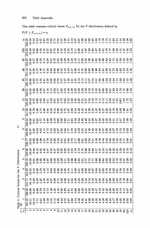
Tab
le 4
. C
riti
cal
Val
ues
for
the
F D
istr
ibut
ion
VI
Q=
.05
V2
1 2
3 4
5 6
7 8
9 10
15
20
30
40
60
12
0 0
0
"t!
"'c3
0)
0
1 16
1.45
19
9.50
21
5.71
22
4.58
23
0.16
23
3.99
23
6.77
23
8.88
24
0.54
24
1.88
24
5.95
24
8.01
25
0.10
25
1.14
25
2.20
25
3.25
25
4.25
0;
; a:
~
'" 2
18.5
1 19
.00
19.1
6 19
.25
19.3
0 19
.33
19.3
5 19
.37
19.3
8 19
.40
19.4
3 19
.45
19.4
6 19
.47
19.4
8 19
.49
19.5
0 IV
"" ~
3 10
.13
9.55
9.
28
9.12
9.
01
8.94
8.
89
8.85
8.
81
8.79
8.
70
8.66
8.
62
8.59
8.
57
8.55
8.
53 ~
CD
~
4 7.
71
6.94
6.
59
6.39
6.
26
6.16
6.
09
6.04
6.
00
5.96
5.
86
5.80
5.
75
5.72
5.
69
5.66
5.
63
$ ("
) r::
J' ;s:
0 CD
5
6.61
5.
79
5.41
5.
19
5.05
4.
95
4.88
4.
82
4.77
4.
74
4.62
4.
56
4.50
4.
46
4.43
4.
40
4.37
~
>
6 5.
99
5.14
4.
76
4.53
4.
39
4.28
4.
21
4.15
4.
10
4.06
3.
94
3.87
3.
81
3.77
3.
74
3.70
3.
67
~. '0
'0
7
5.59
4.
74
4.35
4.
12
3.97
3.
87
3.79
3.
73
3.68
3.
64
3.51
3.
44
3.38
3.
34
3.30
3.
27
3.23
R
en
("
) t:l
8 5.
32
4.46
4.
07
3.84
3.
69
3.58
3.
50
3.44
3.
39
3.35
3.
22
3.15
3.
08
3.04
3.
01
2.97
2.
93
~
p,.
,,' )<
'
9 5.
12
4.26
3.
86
3.63
3.
48
3.37
3.
29
3.23
3.
18
3.14
3.
01
2.94
2.
86
2.83
2.
79
2.75
2.
71
e.. 10
4.
96
4.10
3.
71
3.48
3.
33
3.22
3.
14
3.07
3.
02
2.98
2.
85
2.77
2.
70
2.66
2.
62
2.58
2.
54
f 11
4.
84
3.98
3.
59
3.36
3.
20
3.09
3.
01
2.95
2.
90
2.85
2.
72
2.65
2.
57
2.53
2.
49
2.45
2.
41
en 12
4.
75
3.89
3.
49
3.26
3.
11
3.00
2.
91
2.85
2.
80
2.75
2.
62
2.54
2.
47
2.43
2.
38
2.34
2.
30
'" 13
4.
67
3.81
3.
41
3.18
3.
03
2.92
2.
83
2.77
2.
71
2.67
2.
53
2.46
2.
38
2.34
2.
30
2.25
2.
21
~
14
4.60
3.
74
3.34
3.
11
2.96
2.
85
2.76
2.
70
2.65
2.
60
2.46
2.
39
2.31
2.
27
2.22
2.
18
2.13
$
15
4.54
3.
68
3.29
3.
06
,2.9
0 2.
79
2.71
2.
64
2.59
2.
54
2.40
2.
33
2.25
2.
20
2.16
2.
11
2.07
;s: 8
' 16
4.
49
3.63
3.
24
3.01
2.
85
2.74
2.
66
2.59
2.
54
2.49
2.
35
2.28
2.
19
2.15
2.
11
2.06
2.
01
.... 17
4.
45
3.59
3.
20
2.96
2.
81
2.70
2.
61
2.55
2.
49
2.45
2.
31
2.23
2.
15
2.10
2.
06
2.01
1.
96
"'" r::J' en
18
4.41
3.
55
3.16
2.
93
2.77
2.
66
2.58
2.
51
2.46
2.
41
2.27
2.
19
2.11
2.
06
2.02
1.
97
1.92
":t
j 19
4.
38
3.52
3.
13
2.90
2.
74
2.63
2.
54
2.48
2.
42
2.38
2.
23
2.16
2.
07
2.03
1.
98
1.93
1.
88
~ 20
4.
35
3.49
3.
10
2.87
2.
71
2.60
2.
51
2.45
2.
39
2.35
2.
20
2.12
2.
04
1.99
1.
95
1.90
1.
85
"" ::!. 21
4.
32
3.47
3.
07
2.84
2.
68
2.57
2.
49
2.42
2.
37
2.32
2.
18
2.10
2.
01
1.96
1.
92
1.87
1.
82
r::J' .,:
22
4.30
3.
44
3.05
2.
82
2.66
2.
55
2.46
2.
40
2.34
2.
30
2.15
2.
07
1.98
1.
94
1.89
1.
84
1.79
"'" o·
23
4.28
3.
42
3.03
2.
80
2.64
2.
53
2.44
2.
37
2.32
2.
27
2.13
2.
05
1.96
1.
91
1.86
1.
81
1.76
t:l
24
4.26
3.
40
3.01
2.
78
2.62
2.
51
2.42
2.
36
2.30
2.
25
2.11
2.
03
1.94
1.
89
1.84
1.
79
1.74
p,
. en ~
25
4.24
3.
39
2.99
2.
76
2.60
2.
49
2.40
2.
34
2.28
2.
24
2.09
2.
01
1.92
1.
87
1.82
1.
77
1.71
t:l
en 30
4.
17
3.32
2.
92
2.69
2.
53
2.42
2.
33
2.27
2.
21
2.16
2.
01
1.93
1.
84
1.79
1.
74
1.68
1.
63
p,.
40
4.08
3.
23
2.84
2.
61
2.45
2.
34
2.25
2.
18
2.12
2.
08
1.92
1.
84
1.74
1.
69
1.64
1.
58
1.51
~
50
4.03
3.
18
2.79
2.
56
2.40
2.
29
2.20
2.
13
2.07
2.
03
1387
1.
78
1.69
1.
63
1.58
1.
51
1.44
60
4.
00
3.15
2.
76
2.53
2.
37
2.25
2.
17
2.10
2.
04
1.99
1.
84
1.75
1.
65
1.59
1.
53
1.47
1.
39
120
3.92
3.
07
2.68
2.
45
2.29
2.
18
2.09
2.
02
1.96
1.
91
1.75
1.
66
1.55
1.
50
1.43
1.
35
1.26
0
0
3.85
3.
00
2.61
2.
38
2.22
2.
10
2.01
1.
94
1.88
1.
84
1.67
1.
58
1.46
1.
40
1.32
1.
23
1.00

a =
.01
V
l
V2
1
2 3
4 5
6 7
8 9
10
15
20
30
40
60
120
00
2 98
.50
99.0
0 99
.17
99.2
5 99
.30
99.3
3 99
.36
99.3
7 99
.39
99.4
0 99
.43
99.4
5 99
.47
99.4
7 99
.48
99.4
9 99
.50
3 34
.12
30.8
2 29
.46
28.7
1 28
.24
27.9
1 27
.67
27.4
9 27
.35
27.2
3 26
.87
26.6
9 26
.50
26.4
1 26
.32
26.2
2 26
.13
4 21
.20
18.0
0 16
.69
15.9
8 15
.52
15.2
1 14
.98
14.8
0 14
.66
14.5
5 14
.20
14.0
2 13
.84
13.7
5 13
.65
13.5
6 13
.47
5 16
.26
13.2
7 12
.06
11.3
9 10
.97
10.6
7 10
.46
10.2
9 10
.16
10.0
5 9.
72
9.55
9.
38
9.29
9.
20
9.11
9.
03
6 13
.75
10.9
2 9.
78
9.15
8.
75
8.47
8.
26
8.10
7.
98
7.87
7.
56
7.40
7.
23
7.14
7.
06
6.97
6.
89
~
7 12
.25
9.55
8.
45
7.85
7.
46
7.19
6.
99
6.84
6.
72
6.62
6.
31
6.16
5.
99
5.91
5.
82
5.74
5.
65
~ 8
11.2
6 8.
65
7.59
7.
01
6.63
6.
37
6.18
6.
03
5.91
5.
81
5.52
5.
36
5.20
5.
12
5.03
4.
95
4.86
9
10.5
6 8.
02
6.99
6.
42
6.06
5.
80
5.61
5.
47
5.35
5.
26
4.96
4.
81
4.65
4.
57
4.48
4.
40
4.32
tI"- ----
10
10.0
4 7.
56
6.55
5.
99
5.64
5.
39
5.20
5.
06
4.94
4.
85
4.56
4.
41
4.25
4.
17
4.08
4.
00
3.91
("
) 0
11
9.65
7.
21
6.22
5.
67
5.32
5.
07
4.89
4.
74
4.63
4.
54
4.25
4.
10
3.94
3.
86
3.78
3.
36
3.61
~ ~
12
9.33
6.
93
5.95
5.
41
5.06
4.
82
4.64
4.
50
4.39
4.
30
4.01
3.
86
3.70
3.
62
3.54
3.
45
3.37
C
l 13
9.
07
6.70
5.
74
5.21
4.
86
4.62
4.
44
4.30
4.
19
4.10
3.
82
3.66
3.
51
3.43
3.
34
3.25
3.
17
'"' ;:;: 14
8.
86
6.51
5.
56
5.04
4.
69
4.46
4.
28
4.14
4.
03
3.94
3.
66
3.51
3.
35
3.27
3.
18
3.09
3.
01
,,' ~ 15
8.
68
6.36
5.
42
4.89
4.
56
4.32
4.
14
4.00
3.
89
3.80
3.
52
3.37
3.
21
3.13
3.
05
2.96
2.
87
~
16
8.53
6.
23
5.29
4.
77
4.44
4.
20
4.03
3.
89
3.78
3.
69
3.41
3.
26
3.10
3.
02
2.93
2.
84
2.76
8"
17
8.
40
6.11
5.
19
4.67
4.
34
4.10
3.
93
3.79
3.
68
3.59
3.
31
3.16
3.
00
2.92
2.
83
2.75
2.
66
'" [Jl
18
8.29
6.
01
5.09
4.
58
4.25
4.
01
3.84
3.
71
3.60
3.
51
3.23
3.
08
2.92
2.
84
2.75
2.
66
2.57
8'
'"' 19
8.
18
5.93
5.
01
4.50
4.
17
3.94
3.
77
3.63
3.
52
3.43
3.
15
3.00
2.
84
2.76
2.
67
2.58
2.
50
o-t-
20
8.10
5.
85
4.94
4.
43
4.10
3.
87
3.70
3.
56
3.46
3.
37
3.09
2.
94
2.78
2.
69
2.61
2.
52
2.43
::r
'" 21
8.
02
5.78
4.
87
4.37
4.
04
3.81
3.
64
3.51
3.
40
3.31
3.
03
2.88
2.
72
2.64
2.
55
2.46
2.
37
"':l
22
7.95
5.
72
4.82
4.
31
3.99
3.
76
3.59
3.
45
3.35
3.
26
2.98
2.
83
2.67
2.
58
2.50
2.
40
2.31
t::
l E
ij'
23
7.88
5.
66
4.76
4.
26
3.94
3.
71
3.54
3.
41
3.30
3.
21
2.93
2.
78
2.62
2.
54
2.45
2.
35
2.26
'"'
'"' 24
7.
82
5.61
4.
72
4.22
3.
90
3.67
3.
50
3.36
3.
26
3.17
2.
89
2.74
2.
58
2.49
2.
40
2.31
2.
22
5'
~
>= '"' ~
25
7.77
5.
57
4.68
4.
18
3.85
3.
63
3.46
3.
32
3.22
3.
13
2.85
2.
70
2.54
2.
45
2.36
2.
27
2.18
c'
30
7.56
5.
39
4.51
4.
02
3.70
3.
47
3.30
3.
17
3.07
2.
98
2.70
2.
55
2.39
2.
30
2.21
2.
11
2.01
:::
>
'0
40
7.31
5.
18
4.31
3.
83
3.51
3.
29
2.12
2.
99
2.89
2.
80
2.52
2.
37
2.20
2.
11
2.02
1.
92
1.81
'0
'" 50
7.
17
5.06
4.
20
3.72
3.
41
3.19
3.
02
2.89
2.
78
2.70
2.
42
2.27
2.
10
2.01
1.
91
1.80
1.
69
::: Cl.
60
7.08
4.
98
4.13
3.
65
3.34
3.
12
2.95
2.
82
2.72
2.
63
2.35
2.
20
2.03
1.
94
1.84
1.
73
1.61
x'
120
6.85
4.
79
3.95
3.
48
3.17
2.
96
2.79
2.
66
2.56
2.
47
2.19
2.
03
1.86
1.
76
1.66
1.
53
1.39
0
0
6.65
4.
62
3.79
3.
33
3.03
2.
81
2.65
2.
52
2.42
2.
33
2.05
1.
89
1.71
1.
60
1.48
1.
34
1.00
O
l 0 ""

Q
=
.001
V
I 0
>
0 V2
1
2 3
4 5
6 7
8 9
10
15
20
30
40
60
120
00
~
2 99
8.50
99
9.00
99
9.17
99
9.25
99
9.30
99
9.33
99
9.36
99
9.37
99
9.39
99
9.40
99
9.42
99
9.45
99
9.47
99
9.47
99
9.48
99
9.49
99
9.50
3
167.
03
148.
50
141.
11
137.
10
134.
58
132.
85
131.
58
130.
62
129.
86
129.
25
127.
37 1
26.4
2 12
5.45
12
4.96
12
4.47
12
3.97
12
3.50
~
4 74
.14
61.2
5 56
.18
53.4
4 51
.71
50.5
3 49
.66
49.0
0 48
.47
48.0
5 46
.76
46.1
0 45
.43
45.0
9 44
.75
44.4
0 44
.07
5 47
.18
37.1
2 33
.20
31.0
9 29
.75
28.8
3 28
.16
27.6
5 27
.24
26.9
2 25
.91
25.3
9 24
.87
24.6
0 24
.33
24.0
6 23
.80
g: '"
6 35
.51
27.0
0 23
.70
21.9
2 20
.80
20.0
3 19
.46
19.0
3 18
.69
18.4
1 17
.56
17.1
2 16
.67
16.4
4 16
.21
15.9
8 15
.76
~
>
'1:1
7 29
.25
21.6
9 18
.77
17.2
0 16
.21
15.5
2 15
.02
14.6
3 14
.33
14.0
8 13
.32
12.9
3 12
.53
12.3
3 12
.12
11.9
1 11
.71
C"
'1:1
(D
'" 8
25.4
1 18
.49
15.8
3 14
.39
13.4
8 12
.86
12.4
0 12
.05
11.7
7 11
.54
10.8
4 10
.48
10.1
1 9.
92
9.73
9.
53
9.35
=
~
p.
9 22
.86
16.3
9 13
.90
12.5
6 11
.71
11.1
3 10
.70
10.3
7 10
.11
9.89
9.
24
8.90
8.
55
8.37
8.
19
8.00
7.
82
........
x· 7.
12
6.94
6.
77
<"l
10
21.0
4 14
.91
12.5
5 11
.28
10.4
8 9.
93
9.52
9.
20
8.96
8.
75
8.13
7.
80
7.47
7.
30
0
11
19.6
9 13
.81
11.5
6 10
.35
9.58
9.
05
8.66
8.
35
8.12
7.
92
7.32
7.
01
6.68
6.
52
6.35
6.
18
6.01
t
12
18.6
4 12
.97
10.8
0 9.
63
8.89
8.
38
8.00
7.
71
7.48
7.
29
6.71
6.
40
6.09
5.
93
5.76
5.
59
5.43
0
13
17.8
2 12
.31
10.2
1 9.
07
8.35
7.
86
7.49
7.
21
6.98
6.
80
6.23
5.
93
5.63
5.
47
5.30
5.
14
4.98
~
14
17.1
4 11
.78
9.73
8.
62
7.92
7.
44
7.08
6.
80
6.58
6.
40
5.85
5.
56
5.25
5.
10
4.94
4.
77
4.61
r;.
e:. 15
16
.59
11.3
4 9.
34
8.25
7.
57
7.09
6.
74
6.47
6.
26
6.08
5.
54
5.25
4.
95
4.80
4.
64
4.47
4.
32
~ 16
16
.12
10.9
7 90
.1
7.94
7.
27
6.80
6.
46
6.19
5.
98
5.81
5.
27
4.99
4.
70
4.54
4.
39
4.23
4.
07
16 17
15
.72
10.6
6 8.
73
7.68
7.
02
6.56
6.
22
5.96
5.
75
5.58
5.
05
4.78
4.
48
4.33
4.
18
4.02
3.
86
'" 18
15
.38
10.3
9 8.
49
7.46
6.
81
6.35
6.
02
5.76
5.
56
5.39
4.
87
4.59
4.
30
4.15
4.
00
3.84
3.
68
8'
.., 19
15
.08
10.1
6 8.
28
7.27
6.
62
6.18
5.
85
5.59
5.
39
5.22
4.
70
4.43
4.
14
3.99
3.
84
3.68
3.
52
"'" ::r 20
14
.82
9.95
8.
10
7.10
6.
46
6.02
5.
69
5.44
5.
24
5.08
4.
56
4.29
4.
00
3.86
3.
70
3.54
3.
39
'" 21
14
.59
9.77
7.
94
6.95
6.
32
5.88
5.
56
5.31
5.
11
4.95
4.
44
4.17
3.
88
3.74
3.
58
3.42
3.
27
'>j
tl
22
14.3
8 9.
61
7.80
6.
81
6.19
5.
76
5.44
5.
19
4.99
4.
83
4.33
4.
06
3.78
3.
63
3.48
3.
32
3.16
00
· "'" 23
14
.20
9.47
7.
67
6.70
6.
08
5.65
5.
33
5.09
4.
89
4.73
4.
23
3.96
3.
68
3.53
3.
38
3.22
3.
07
.., s-: 24
14
.03
9.34
7.
55
6.59
5.
98
5.55
5.
23
4.99
4.
80
4.64
4.
14
3.87
3.
59
3.45
3.
29
3.14
2.
98
~ "'"
25
13.8
8 9.
22
7.45
6.
49
5.89
5.
46
5.15
4.
91
4.71
4.
56
4.06
3.
79
3.52
3.
37
3.22
3.
06
2.90
g.
30
13.2
9 8.
77
7.05
6.
12
5.53
5.
12
4.82
4.
58
4.39
4.
24
3.75
3.
49
3.22
3.
07
2.92
2.
76
2.60
40
12
.61
8.25
6.
59
5.70
5.
13
4.73
4.
44
4.21
4.
02
3.87
3.
40
3.14
2.
87
2.73
2.
57
2.41
2.
24
50
12.2
2 7.
96
6.34
5.
46
4.90
4.
51
4.22
4.
00
3.82
3.
67
3.20
2.
95
2.68
2.
53
2.38
2.
21
2.04
60
11
.97
7.77
6.
17
5.31
4.
76
4.37
4.
09
3.86
3.
69
3.54
3.
08
2.83
2.
55
2.41
2.
25
2.08
1.
90
120
11.3
8 7.
32
5.78
4.
95
4.42
4.
04
3.77
3.
55
3.38
3.
24
2.78
2.
53
2.26
2.
11
1.95
1.
77
1.56
0
0
10.8
6 6.
93
5.44
4.
64
4.12
3.
76
3.49
3.
28
3.11
2.
97
2.53
2.
28
2.01
1.
85
1.68
1.
47
1.00

Tab
le 5
. C
riti
cal
Val
ues
for
the
Stu
dent
ized
Ran
ge D
istr
ibut
ion
S ~ ~
S
~.
0"
'tl
::
<1l~
\l>
a=
.05
k ..,
.Q
0"
g, I
V
iD
2 3
4 5
6 7
8 9
10
11
12
13
14
15
16
17
18
19
20
~La
8 1
/ ~p
a 1
17.9
7 26
.98
38.8
2 37
.08
40.4
1 43
.12
45.4
0 47
.36
49.0
7 50
.59
51.9
6 53
.20
54.3
3 55
.36
56.3
2 57
.22
58.0
4 58
.83
59.5
6 S!
"" e.
2 6.
085
8.33
1 9.
798
10.8
8 11
.74
12.4
4 13
.03
13.5
4 13
.99
14.3
9 14
.75
15.0
8 15
.38
15.6
5 15
.91
16.1
4 16
.37
16.5
7 16
.77
CD ~
;
a II
(") 3
4.50
1 5.
910
6.82
5 7.
502
8.03
7 8.
478
8.85
3 9.
177
9.46
2 9.
717
9.94
6 10
.15
10.3
5 10
.53
10.6
9 10
.84
10.9
8 11
.11
11.2
4 ~
Q ~
4 3.
927
5.04
0 5.
757
6.28
7 6.
707
7.05
3 7.
347
7.60
2 7.
826
8.02
7 8.
208
8.37
3 8.
525
8.66
4 8.
794
8.91
4 9.
028
9.13
4 9.
233
o -
~.
.,:
;>s-
(")
5 3.
635
4.60
2 5.
218
5.67
3 6.
033
6.33
0 6.
582
6.80
2 6.
995
7.16
8 7.
324
7.46
6 7.
596
7.71
7 7.
828
7.93
2 8.
030
8.12
2 8.
208
'0
~.
e. 6
3.46
1 4.
339
4.89
6 5.
305
5.62
8 5.
895
6.12
2 6.
319
6.49
3 6.
649
6.78
9 6.
917
7.03
4 7.
143
7.24
4 7.
338
7.42
6 7.
508
7.58
7 ~:e.
7 3.
344
4.16
5 4.
681
5.06
0 5.
359
5.60
6 5.
815
5.99
8 6.
158
6.30
2 6.
431
6.55
0 6.
658
6.75
9 6.
852
6.93
9 7.
020
7.09
7 7.
170
~ 15
~ 0.
. i:
j '"
8 3.
261
4.04
1 4.
529
4.88
6 5.
167
5.39
9 5.
597
5.76
7 5.
918
6.05
4 6.
175
6.28
7 6.
389
6.48
3 6.
571
6.65
3 6.
729
6.80
2 6.
870
:. § ~
9 3.
199
3.94
9 4.
415
4.75
6 5.
024
5.24
4 5.
432
5.95
9 5.
739
5.86
7 5.
983
6.08
9 6.
186
6.27
6 6.
359
6.43
7 6.
510
6.57
9 6.
644
'"
0"
-C"
1-C'D
~'1
r
10
3.15
1 3.
877
4.32
7 4.
654
4.91
2 5.
124
5.30
5 5.
461
5.59
9 5.
722
5.83
3 5.
935
6.02
8 6.
114
6.19
4 6.
269
6.39
9 6.
405
6.46
7 p
-..,
<
<1
l 0
""
11
3.11
3 3.
820
4.25
6 4.
574
4.82
3 5.
028
5.20
2 5.
353
5.48
7 5.
605
5.71
3 5.
811
5.90
1 5.
984
6.06
2 6.
134
6.20
2 6.
265
6.32
6 i:
j ...
.. 0
.,:
0..
....
12
3.08
2 3.
773
4.19
9 4.
508
4.75
1 4.
950
5.11
9 5.
265
5.39
5 5.
511
5.61
5 5.
710
5.79
8 5.
878
5.95
3 6.
023
6.08
9 6.
151
6.20
9 S
<1l
....
0
" ~
p-
13
3.05
5 3.
735
4.15
1 4.
453
4.69
0 4.
885
5.04
9 5.
192
5.31
8 5.
431
5.53
3 5.
625
5.71
1 5.
789
5.86
2 5.
931
5.99
5 6.
055
6.11
2 <1
l (1)
..,
~
00
14
3.03
3 3.
702
4.11
1 4.
407
4.63
9 4.
829
4.99
0 5.
131
5.25
4 5.
364
5.46
3 5.
554
5.63
7 5.
714
5.78
6 5.
852
5.91
5 5.
974
6.02
9 '"
.... ~.
.,:
15
3.01
4 3.
674
4.07
6 4.
367
4.59
5 4.
782
4.94
0 5.
077
5.19
8 5.
306
5.40
4 5.
493
5.57
4 5.
649
5.72
0 5.
785
5.84
6 5.
904
5.95
8 ~
g,
g. 16
2.
998
3.64
9 4.
046
4.33
3 4.
557
4.74
1 4.
897
5.03
1 5.
150
5.25
6 5.
352
5.43
9 5.
520
5.59
3 5.
662
5.72
7 5.
786
5.84
3 5.
897
g-;r
~
0..
(1)
17
2.98
4 3.
628
4.02
0 4.
303
4.52
4 4.
705
4.85
8 4.
991
5.10
8 5.
212
5.30
7 5.
392
5.47
1 5.
544
5.61
2 5.
675
5.73
4 5.
790
5.84
2 (1)
0.
. (1)
i:
j 0
0..
18
2.97
1 3.
609
3.99
7 4.
277
4.49
5 4.
673
4.82
4 4.
956
5.07
1 5.
174
5.26
7 5.
352
5.42
9 5.
501
5.56
8 5.
630
5.68
8 5.
743
5.79
4 o
S ~
S?
19
2.96
0 3.
593
3.97
7 4.
253
4.46
9 4.
645
4.79
4 4.
924
5.03
8 5.
140
5.23
1 5.
315
5.39
1 5.
462
5.52
8 5.
589
5.64
7 5.
701
5.75
2 §.
s· ~
20
2.95
0 3.
578
3.95
8 4.
232
4.44
5 4.
620
4.76
8 4.
896
5.00
8 5.
108
5.19
9 5.
282
5.35
7 5.
427
5.49
3 5.
553
5.61
0 5.
663
5.71
4 ~ ;
. ~
2.91
9 3.
532
3.90
1 4.
166
4.37
3 4.
541
4.68
4 4.
807
4.91
5 5.
012
5.09
9 5.
179
5.25
1 5.
319
5.38
1 5.
439
5.49
4 5.
545
5.59
4 o
(1)
0..
> 24
..,
~.
:g 30
2.
888
3.48
6 3.
845
4.10
2 4.
302
4.46
4 4.
602
4.72
0 4.
824
4.91
7 5.
001
5.07
7 5.
147
5.21
1 5.
271
5.32
7 5.
379
5.42
9 5.
475 ~ E
~
(1)
.., s
~.
i:j
40
2.85
8 3.
442
3.79
1 4.
039
4.23
2 4.
389
4.52
1 4.
635
4.73
5 4.
824
4.90
4 4.
977
5.04
4 5.
106
5.16
3 5.
216
5.26
6 5.
313
5.35
8 ';-
~
g-o..
60
2.82
9 3.
399
3.73
7 3.
977
4.16
3 4.
314
4.44
1 4.
550
4.64
6 4.
732
4.80
8 4.
878
4.94
2 5.
001
5.05
6 5.
107
5.15
4 5.
199
5.24
1 ~ ~
~.
o 0
120
2.80
0 3.
356
3.68
5 3.
917
4.09
6 4.
241
4.36
3 4.
468
4.56
0 4.
641
4.71
4 4.
781
4.84
2 4.
898
4.95
0 4.
998
5.04
4 5.
086
5.12
6 ..
, i:
j
~
0..
2.77
2 3.
314
3.63
3 3.
858
4.03
0 4.
170
4.28
6 4.
387
4.47
4 4.
552
4.62
2 4.
685
4.74
3 4.
796
4.84
5 4.
891
4.93
4 4.
974
5.01
2 ...
. (1)
a>
0
0
P-t:!>
0
<1l
i:j
c;"
(1)
0..

0>
T
able
5.
(con
t.)
Cri
tica
l V
alue
s fo
r th
e S
tude
ntiz
ed R
ange
Dis
trib
utio
n 0 0
>
a =
.0
1 k
~
v 2
3 4
5 6
7 8
9 10
11
12
13
14
15
16
17
18
19
20
~
1 90
.03
135.
0 16
4.3
185.
6 20
2.2
215.
8 22
7.2
237.
0 24
5.6
253.
2 26
0.0
266.
2 27
1.8
277.
0 28
1.8
286.
3 29
0.4
294.
3 29
8.0
>
2 14
.04
19.0
2 22
.29
24.7
2 26
.63
28.2
0 29
.53
30.6
8 31
.69
32.5
9 33
.40
34.1
3 34
.81
35.4
3 36
.00
36.5
3 37
.03
37.5
0 37
.95
'"C:I
'"C:I C!l
3 8.
261
10.6
2 12
.17
13.3
3 14
.24
15.0
0 15
.64
16.2
0 16
.69
17.1
3 17
.53
17.8
9 18
.22
18.5
2 18
.81
19.0
7 19
.32
19.5
5 19
.77
l:j p..
4 6.
512
8.12
0 9.
173
9.95
8 10
.58
11.1
0 11
.55
11.9
3 12
.27
12.5
7 12
.84
13.0
9 13
.32
13.5
3 13
.73
13.9
1 14
.08
14.2
4 14
.40
:::i.
5 5.
702
6.97
6 7.
804
8.42
1 8.
913
9.32
1 9.
669
9.97
2 10
.24
10.4
8 10
.70
10.8
9 l1
.08
11.2
4 11
.40
11.5
5 11
.68
11.8
1 11
.93
6 5.
243
6.33
1 7.
033
7.55
6 7.
973
8.31
8 8.
613
8.86
9 9.
097
9.30
1 9.
485
9.65
3 9.
808
9.95
1 10
.08
10.2
1 10
.32
10.4
3 10
.54
7 4.
949
5.91
9 6.
543
7.00
5 7.
373
7.67
9 7.
939
8.16
6 8.
368
8.54
8 8.
711
8.86
0 8.
997
9.12
4 9.
242
9.35
3 9.
456
9.55
4 9.
646
8 4.
746
5.63
5 6.
204
6.62
5 6.
960
7.23
7 7.
474
7.68
1 7.
863
8.02
7 8.
176
8.31
2 8.
436
8.55
2 8.
659
8.76
0 8.
854
8.94
3 9.
027
9 4.
596
5.42
8 5.
957
6.34
8 6.
658
6.91
5 7.
134
7.32
5 7.
495
7.64
7 7.
784
7.91
0 8.
025
8.13
2 8.
232
8.32
5 8.
412
8.49
5 8.
573
10
4.48
2 5.
270
5.76
9 6.
136
6.42
8 6.
669
6.87
5 7.
055
7.21
3 7.
356
7.48
5 7.
603
7.71
2 7.
812
7.90
6 7.
993
8.07
6 8.
153
8.22
6 11
4.
392
5.14
6 5.
621
5.97
0 6.
247
6.47
6 6.
672
6.84
2 6.
992
7.12
8 7.
250
7.36
2 7.
465
7.56
0 7.
649
7.73
2 7.
809
7.88
3 7.
952
12
4.32
0 5.
046
5.50
2 5.
836
6.10
1 6.
321
6.50
7 6.
670
6.81
4 6.
943
7.06
0 7.
167
7.26
5 7.
356
7.44
1 7.
520
7.59
4 7.
665
7.73
1 13
4.
260
4.96
4 5.
404
5.72
7 5.
981
6.19
2 6.
372
6.52
8 6.
667
6.79
1 6.
903
7.00
6 7.
101
7.18
8 7.
269
7.34
5 7.
417
7.48
5 7.
548
14
4.21
0 4.
895
5.32
2 5.
634
5.88
1 6.
085
6.25
8 6.
409
6.54
3 6.
664
6.77
2 6.
871
6.96
2 7.
047
7.12
6 7.
199
7.26
8 7.
333
7.39
5 15
4.
168
4.83
6 5.
252
5.55
6 5.
796
5.99
4 6.
162
6.30
9 6.
439
6.55
5 6.
660
6.75
7 6.
845
6.92
7 7.
003
7.07
4 7.
142
7.20
4 7.
264
16
4.13
1 4.
786
5.19
2 5.
489
5.72
2 5.
195
6.07
9 6.
222
6.34
9 6.
462
6.56
4 6.
658
6.74
4 6.
823
6.89
8 6.
967
7.03
2 7.
093
7.15
2 17
4.
099
4.74
2 5.
140
5.43
0 5.
659
5.84
7 6.
007
6.14
7 6.
270
6.38
1 6.
480
6.57
2 6.
656
6.73
4 6.
806
6.87
3 6.
937
6.99
7 7.
053
18
4.07
1 4.
703
5.09
4 5.
379
5.60
3 5.
788
5.94
4 6.
081
6.20
1 6.
310
6.40
7 6.
497
6.57
9 6.
655
6.72
5 6.
792
6.85
4 6.
912
6.96
8 19
4.
046
4.67
0 5.
054
5.33
4 5.
554
5.73
5 5.
889
6.02
2 6.
141
6.24
7 6.
342
6.43
0 6.
510
6.58
5 6.
654
6.71
9 6.
780
6.83
7 6.
891
20
4.02
4 4.
639
5.01
8 5.
294
5.51
0 5.
688
5.83
9 5.
970
6.08
7 6.
191
6.28
5 6.
371
6.45
0 6.
523
6.59
1 6.
654
6.71
4 6.
771
6.82
3 24
3.
956
4.54
6 4.
907
5.16
8 5.
374
5.54
2 5.
685
5.80
9 5.
919
6.01
7 6.
106
6.18
6 6.
261
6.33
0 6.
394
6.45
3 6.
510
6.56
3 6.
612
30
3.88
9 4.
455
4.79
9 5.
048
5.24
2 5.
401
5.53
6 5.
653
5.75
6 5.
849
5.93
2 6.
008
6.07
8 6.
143
6.20
3 6.
259
6.31
1 6.
361
6.40
7 40
3.
825
4.36
7 4.
696
4.93
1 5.
114
5.26
5 5.
392
5.50
2 5.
599
5.68
6 5.
764
5.83
5 5.
900
5.96
1 6.
017
6.06
9 6.
119
6.16
5 6.
209
60
3.76
2 4.
282
4.59
5 4.
818
4.99
1 5.
133
5.25
3 5.
356
5.44
7 5.
528
5.60
1 5.
667
5.72
8 5.
785
5.83
7 5.
886
5.93
1 5.
974
6.01
5 12
0 3.
702
4.20
0 4.
497
4.70
9 4.
872
5.00
5 5.
118
5.21
4 5.
299
5.37
5 5.
443
5.50
5 5.
562
5.61
4 5.
662
5.70
8 5.
750
5.79
0 5.
827
00
3.
643
4.12
0 4.
403
4.60
3 4.
757
4.88
2 4.
987
5.07
8 5.
157
5.22
7 5.
290
5.34
8 5.
400
5.44
8 5.
493
5.53
5 5.
574
5.61
1 5.
645

Tab
le 5
. (c
ont.
) C
riti
cal
Val
ues
for
the
Stu
dent
ized
Ran
ge D
istr
ibut
ion
a =
.0
01
k
v 2
3 4
5 6
7 8
9 10
11
12
13
14
15
16
17
18
19
20
1
900.
3 13
51.
1643
. 18
56.
2022
. 21
58.
2272
. 27
30.
2455
. 25
32.
2600
. 26
62.
2718
. 27
70.
2818
. 28
63.
2904
. 29
43.
2980
. 2
44.6
9 60
.42
70.7
7 78
.43
84.4
9 89
.46
93.6
7 97
.30
100.
5 10
3.3
105.
9 10
8.2
110.
4 11
2.3
114.
2 11
5.9
117.
4 11
8.9
120.
3 3
18.2
8 23
.32
26.6
5 29
.13
31.1
1 32
.74
34.1
2 35
.33
36.3
9 37
.34
38.2
0 38
.98
39.6
9 40
.35
40.9
7 41
.54
42.0
7 42
.58
43.0
5 4
12.1
8 14
.99
16.8
4 18
.23
19.3
4 20
.26
21.0
4 21
.73
22.3
3 22
.87
23.3
6 23
.81
24.2
1 24
.59
24.9
4 25
.27
25.5
8 25
.87
26.1
4 5
9.71
4 11
.67
12.9
6 13
.93
14.7
1 15
.35
15.9
0 16
.38
16.8
1 17
.18
17.5
3 17
.85
18.1
3 18
.41
18.6
6 18
.89
19.1
0 19
.31
19.5
1 6
8.42
7 9.
960
10.9
7 11
.72
12.3
2 12
.83
13.2
6 13
.63
13.9
7 14
.27
14.5
4 14
.79
15.0
1 15
.22
15.4
2 15
.60
15.7
8 15
.94
16.0
9 7
7.64
8 8.
930
9.76
8 10
.40
10.9
0 11
.32
11.6
8 11
.99
12.2
7 12
.52
12.7
4 12
.95
13.1
4 13
.32
13.4
8 13
.64
13.7
8 13
.92
14.0
4 8
7.13
0 8.
250
8.97
8 9.
522
9.95
8 10
.32
10.6
4 10
.91
11.1
5 11
.36
11.5
6 11
.74
11.9
1 12
.06
12.2
1 12
.34
12.4
7 12
.59
12.7
0 9
6.76
2 7.
768
8.41
9 8.
906
9.29
5 9.
619
9.89
7 10
.14
10.3
6 10
.55
10.7
3 10
.89
11.0
3 11
.18
11.3
0 11
.42
11.5
4 11
.64
11.7
5 10
6.
487
7.41
1 8.
006
8.45
0 8.
804
9.09
9 9.
352
9.57
3 9.
769
9.94
6 10
.11
10.2
5 10
.39
10.5
2 10
.64
10.7
5 10
.85
10.9
5 11
.03
11
6.27
5 7.
136
7.68
7 8.
098
8.42
6 8.
699
8.93
3 9.
138
9.31
9 9.
482
9.63
0 9.
766
9.89
2 10
.01
10.1
2 10
.22
10.3
1 10
.41
10.4
9 12
6.
106
6.91
7 7.
436
7.82
1 8.
127
8.38
3 8.
601
8.79
3 8.
962
9.11
5 9.
254
9.38
1 9.
498
9.60
6 9.
707
9.80
2 9.
891
9.97
5 10
.06
13
5.97
0 6.
740
7.23
1 7.
595
7.88
5 8.
126
8.33
3 8.
513
8.67
3 8.
817
8.94
8 9.
068
9.17
8 9.
281
9.37
6 9.
466
9.55
0 9.
629
9.70
4 14
5.
856
6.59
4 7.
062
7.40
9 7.
685
7.91
5 8.
110
8.28
2 8.
434
8.57
1 8.
696
8.80
9 8.
914
9.01
2 9.
103
9.18
8 9.
267
9.34
3 9.
414
15
5.76
0 6.
470
6.92
0 7.
252
7.51
7 7.
736
7.92
5 8.
088
8.23
4 8.
365
8.48
3 8.
592
8.69
3 8.
786
8.87
2 8.
954
9.03
0 9.
102
9.17
0 16
5.
678
6.36
5 6.
799
7.11
9 7.
374
7.58
5 7.
766
7.92
3 8.
063
8.18
9 8.
303
8.40
7 8.
504
8.59
3 8.
676
8.75
5 8.
828
8.89
7 8.
963
17
5.60
8 6.
275
6.69
5 7.
005
7.25
0 7.
454
7.62
9 7.
781
7.91
6 8.
037
8.14
8 8.
248
8.34
2 8.
427
8.50
8 8.
583
8.65
4 7.
720
8.78
4 18
5.
546
6.19
6 6.
604
6.90
5 7.
143
7.34
1 7.
510
7.65
7 7.
788
7.90
6 8.
012
8.11
0 8.
199
8.28
3 8.
361
8.43
4 8.
502
8.56
7 8.
628
19
5.49
2 6.
127
6.52
5 6.
817
7.04
9 7.
242
7.40
5 7.
549
7.67
6 7.
790
7.89
3 7.
988
8.07
5 8.
156
8.23
2 8.
303
8.36
9 8.
432
8.49
1 ~
20
5.44
4 6.
065
6.45
4 6.
740
6.96
6 7.
154
7.31
3 7.
453
7.57
7 7.
688
7.77
8 7.
880
7.96
6 8.
044
8.11
8 8.
186
8.25
1 8.
312
8.37
0 0
" ro 24
5.
297
5.87
7 6.
238
6.50
3 6.
712
6.88
4 7.
031
7.15
9 7.
272
7.37
4 7.
467
7.55
1 7.
629
7.70
1 7.
768
7.83
1 7.
890
7.94
6 7.
999
> 30
5.
156
5.69
8 6.
033
6.27
8 6.
470
6.62
8 6.
763
6.88
0 6.
984
7.07
7 7.
162
7.23
9 7.
310
7.37
5 7.
437
7.49
4 7.
548
7.59
9 7.
647
'0
'0
40
5.02
2 5.
528
5.83
8 6.
063
6.24
0 6.
386
6.50
9 6.
616
6.71
1 6.
796
6.87
2 6.
942
7.00
7 7.
067
7.12
2 7.
174
7.22
3 7.
269
7.31
2 (l
) ::;
60
4.89
4 5.
365
5.65
3 5.
860
6.02
2 6.
155
6.26
8 6.
366
6.45
1 6.
528
6.59
8 6.
661
6.72
0 6.
774
6.82
4 6.
871
6.91
4 6.
956
6.99
5 ~
120
4.77
1 5.
211
5.47
6 5.
667
5.81
5 5.
937
6.03
9 6.
128
6.20
6 6.
276
6.33
9 6.
396
6.44
8 6.
496
6.54
2 6.
583
6.62
3 6.
600
6.69
5 0
0
4.65
4 5.
063
5.30
9 5.
484
5.61
9 5.
730
5.82
3 5.
903
5.97
3 6.
036
6.09
2 6.
144
6.19
1 6.
234
6.27
4 6.
312
6.34
7 6.
380
6.41
1 ~
0 -'I

Author Index
A Anderson, V.L. 524,531 Andrews, D.F. 295, 301, 382 Atkinson, A.C. 382
B Barnett, V. 56, 57, 80 Battese, G.E. 379, 380, 382 Beck, G. 58, 80 Beckman, RJ. 154, 205 Belsey, D.A. 159, 205, 282, 294, 382 Berk, K.N. 282, 382 Box, G.E.P. 369, 382 Breusch, T. 376, 382 Brown, M.B. 428, 531
C Chatterjee, S. 382 Cochran, W.G. 502-504,505,531 Conover, W.J. 120, 205, 429, 531 Conerly, M.D. 306, 383 Cook, RD. 159, 205, 295, 382 Cox, G.M. 502, 503, 504, 505, 531
D Davenport, J.M. 437, 531 Dixon, W.J. 36, 58, 59, 80 Draper, N.R 75, 80, 295, 382
E Edwards, A.L. 520, 527, 531 Einot, 1. 413, 531 Emerson, J.D. 164,205
F Feldt, L.S. 519, 531 Filliben, J.J. 63, 80 Fomby, T.B. 175,205,376,381,382 Forsyth, A.B. 428, 531 Freedman, D.A. 274, 275,382 Fuller, W.A. 179, 205, 368, 375, 379,
380, 382, 383 Furnival, G.M. 274,382
G Gabriel, K.R. 413, 531 Gallant, A.R. 368, 382 Gasko, Miriam 60, 80 Geisser, S. 519, 531 Gibbons, Dianne 235, 238, 240, 383 Goldfield, S.M. 377, 383 Gray, J.B. 301, 383 Graybill, F.A. 383 Greenhouse, S.W. 519, 531 Griffiths, W.E. 175, 205, 381, 383 Grubbs, F.E. 58, 80 Gunst, RF. 235, 238, 240, 383
H Hadi, A.S. 382 Hartley, H.P. 427, 428, 532 Hill, R.C. 175, 205, 376, 382, 383 Hinkley, D.V. 72, 74, 80 Hoaglin, D.C. 57, 67, 80, 164, 205 Hochberg, Y. 412, 414, 531 Hocking, RR 274, 383 Hogg, R. 80, 85 Hunter, J.S. 369, 382 Hunter, W.G. 369, 382 Huynh, H. 519, 531
I Iglewicz, B. 57, 80 Iman, R1. 437, 531
J Jobson, J.D. 375, 383 John, J.A. 75, 80, 295, 383 Johnson, D.E. 493, 494, 512, 513,
520, 524, 527, 532 Johnson, RA. 63, 80 Johnson,S.R.175,205,376,381,382 Judge, G.G. 175, 205, 381, 383
K Kempthorne, O. 409, 503-505, 531 Kerlinger, F.N. 383 Kirk, R.E. 512, 520, 527, 532

610 Author Index
Kmenta, J. 179, 205 Kronmal 36, 80 Kuh, E. 159, 205, 294, 382 Kutner, M.H. 141,205,384,512,532
L Lee, T. 175, 205, 381, 383 Levene, H. 428, 429, 532 Lewis, T. 56, 57, 80 Lilliefors, H.W. 61, 80 Lin, C. 67, 80 Ling, RF. 301, 383 Lovell, M.C. 275, 383 Lund, R.E. 154, 205 Liitkepohl, H. 175, 205, 381, 383
M McDonald, G.C. 235, 238, 240, 383 McLean, RA. 524, 531 Mallows, C.L. 268, 306, 383 Mansfield, E.R. 306, 383 Marasingle, M.G. 304, 383 Mardia, K.V. 67, 80 Mason, RL. 383 Miller, R.G. 55, 56, 80, 429, 532 Milliken, G.A. 493, 494, 512, 513,
520, 524, 527, 532 Montgomery, D.C. 369, 383, 505, 532 Moore, R.H. 154, 205 Moors, J.A. 52, 54, 80 Mosteller, F. 67, 80 Mudhulkar, G.S. 67, 80 Mulaik, S.A. 188, 205 Myers, RH. 369, 383
N Neter, J. 141, 205, 384, 512, 532
p Pagan, A. 376, 382 Pearson, E.S. 427, 428, 532 Peck, E.A. 383 Pedhauzer, E.J. 383 Petersen, R 505, 532
Pregibon, D. 295, 301, 382 Prescott, P. 154, 205
Q Quandt, RE. 377, 383
R Rawlings, J.O. 384 Rosenberger, J.L. 60, 80 Ryan, T.A. 413, 532
S Scheffe, H. 411, 414, 532 Searle, S.R. 494, 514, 532 Shiffler, RE. 58, 81 Sidak, Z. 411, 414, 532 Smith, P.L. 368, 384 Spjotvoll, E. 412, 532 Stephans, M.A. 62, 81 Stoline, M.R. 412, 532 Sturges, H.A. 35, 36, 81
T Theil, H. 384 Thompson, M.L. 274, 384 Tietjen, G.L. 154, 205 Tukey, J.W. 57, 67, 80, 412, 414, 435,
533
U Ury, H.K. 412, 532
V Velleman, P.F. 36, 81
W Wasserman, W. 141, 205, 384, 512,
532 Weisberg, S. 159, 205, 295, 383, 384 Welsch, RE. 159, 205, 294, 382, 384,
413,533 Wichern, D.W. 63, 80 Wilson, RB. 274, 382 Winer, B.J. 520, 533

Subject Index
A added variable plot, 197, 305 addition of matrices, 549 addition of vectors, 563 additive inverse, 549 adjusted R2, 227 aliases, aliased, 500 alternative hypothesis, 17 analysis of covariance,
model and assumptions, 467 multiple regression approach, 468 unbalanced design, 469
analysis of variance, balanced two-way model, 443 confounding, 503 experimental design, 399, 408,
493 fractional replication, 500 homogeneity of variance, 426 incomplete blocks, 504 Latin square design, 473 multifactor factorials, 495 multiple comparisons, 409 multiple regression approach, 416,
443, 458, 468, 475, 481 nonparametric analysis of vari-
ance, 425 one-way analysis, 401 random effects model, 505 randomized block design, 431 repeated measures design, 515,
526 split plot design, 521, 526 three-way analysis, 471 three-way factorial, 475 two-factor factorial, 438 two-way analysis, 430 two-way nested design, 465 2P design, 496 unbalanced three-way analysis,
481 unbalanced two-way analysis, 458 variance components, 512
Andrews-Pregibon statistic, 295 angle between two vectors, 564 attribute, 24 augmented residual, 306 autocorrelation, 168, 380 average rate, 44
B backward elimination, 257 balanced incomplete block design, 504 balanced lattice design, 505 balanced two-way layout, 438 balanced two-way model, 438 bar chart, 36 Bartlett's test, 427 base cell model, 407 basis for n-dimensional space, 567 best linear unbiased, 226 bias, biased, 15 biased regression,
latent root regression, 290 principal component regression,
287 ridge regression, 285
bivariate analysis, bivariate normal, 94 comparison of marginal distri
butions, 118 correlation, 90, 94, 110, 117 discrete bivariate distributions,
87 elliptical contours, 96, 115 scatterplot, 96 simple linear regression, 102, 121
bivariate density, 88 bivariate distributions, discrete,
conditional densities, 92 correlation, 90 covariance, 89 independence, 92 joint density, 88 joint probability table, 88 linear combinations, 91 marginal density, 88
612 Subject Index
moments, 89 moments for conditional distri
butions, 93 bivariate normal distribution,
alternative linear relationship, 106
conditional density, 102 definition and properties, 94 elliptical contours, 96 goodness of fit, 115 Mahalanobis distance, 100 regression function, 102 scatterplot, 96
block matrix, 559 Bonferroni, 128, 410 boundaries, 35 Box-Cox transformation, 68
C categorical data, 7 cell means model, 403, 492 cell parameter coding, 336 census, 9 central limit theorem, 24 central tendency, 41 characteristic polynomial, 572 characteristic roots, 572 chi-square distribution, 19 class frequency, 36 classes, 36 cluster analysis, 301 cluster sampling, 9 Cochrane-Orcutt procedure, 174 Cochran's test, 428 coding qualitative variables, 314 coefficient of determination, 103 coefficient of multiple correlation, 228 coefficient of multiple determination,
227 coefficient of skewness, 46 collinearity diagnostic, 281 column space, 570 completely crossed, 438 completely randomized design, 408 compound symmetry, 518 concordant, 114 conditional density, 92 conditional distribution, 93 conditional mean, 93
conditional probability, 92 conditional variance, 93 confidence band, 134 confidence ellipsoid, 233 confidence interval, 17 confidence region, 126 confirmatory analysis, 9 congruent matrix, 558 confounding, confounded, 495 consistent, consistency, 16 continuous, 7 control, 256 control variable, 106 Cook's D statistic, 158, 293 coordinates, 563 corrected sums of squares and cross
products matrix, 246 correlation coefficient, sample,
concordance and discordance, 114 Kendall's correlation, 114 Pearson correlation, 110 robust estimation, 117 Spearman correlation, 113
correlation matrix, 247 covariance, 89 covariance matrix, 90, 246 covariate, 466 COVRATIO, 161, 294 cross validation, 9 cross validation in regression,
Chow test, 307 double cross validation, 312 PRESS statistic, 313 validation by prediction, 311
cumulative frequency, 38 curvilinear models, 363 curvilinear regression,
D
grafted quadratics, 364 polynomial models, 363 response surface models, 368
data analysis, 10 data analysis for univariate samples,
Box-Cox transformation, 68 box plot, 45 frequency distribution, 36 K-S test for normality, 61 measures of kurtosis, 50

measures of location, 42 measures of shape, 46 measures of skewness, 46 measures of spread, 44 outliers, 56 Q-Q plot, 63 robust estimation, 60 stem and leaf display, 35 transformations, 67
data matrix, 1 data reduction, 10 defining contrast, 500 deleted residual, 152 density function, 12 dependent variable, 121 derivatives of matrix expressions, 562 description using regression, 256 design matrix, 417 design structure, 494 determinant of a matrix, 554 determinant of a partitioned matrix,
561 DFBETA, 159, 294 DFFITS, 159, 294 diagonal elements of a matrix, 547 diagonal matrix, 548 directed line segment, 563 discordant, 57 discrete variable, 7, 12 discrete bivariate distribution, 88 dispersion, 41 distribution function, 12 double cross validation, 312 dummy variable, 314 Duncan's procedure, 413 Durbin-Watson test, 173
E effect coding, 334 efficiency, 15, 434 eigenvalue, 281, 572, 577 eigenvalue problem, 572 eigenvector, 281, 572 elliptical contour, 98, 99 empirical distribution function, 61 empirical vs. structural relationship,
201 equality of matrices, 549 equality of means, 402
Subject Index 613
equi-correlation structure, 518 error component models, 378 error sums of squares, 129 error term, 123 estimator, 14 Euclidean distance, 101, 563 exact functional relation, 106 examples, Chapter 1,
bus driver accidents, 27 distribution of blood groups, 26 public opinion poll, 24 waiting times for bank customers,
23 weights of boxes of breakfast ce
real, 23 examples, Chapter 2,
crude oil production, 69-74 T.V. set data, 34-67 world balance of trade, 76-78
examples, Chapter 3, apartment data, 121-134, 151-
163 CPI, treasury bills, 174-176 CPI, treasury bills and stock
market index, 194-197 family expenditure marketing data,
137-139 financial portfolios, 88-94 garbage disposal data, 110-117,143-
148, 163-167, 186 police officer stress and crime
level data, 107-108, 179-180 real estate data, 169-172, 185-
186, 191, 195, 197-200 salary data, 118-121
examples, Chapter 4, air pollution data, 235-242, 250-
251 automobile fuel consumption data,
343-354, 357-362 bank employee salary data, 369-
372 Canadian financial market data,
276-284, 287-289 financial accounting data, 219-
222,225-226,228-232,235-236,245,249,253,258-265, 270-273, 295-299, 307-314
garbage disposal data, 364

614 Subject Index
net income rank data, 365-368 real estate data, 321-339 salary-sex-occupation, 339-342,
354-356, 359 seasonal supply function, 315-
321 examples, Chapter 5,
automobile fuel consumption data, 459-464, 469-470
CEO change data, 481-493 family expenditure marketing data,
400-406,414-415, 418-428, 432-435,442-444,447-459, 467-469,473,507,510-511, 525
police officer stress data, 520-522, police service survey data, 528-
530 salary-sex-occupation, 445-446,
449-451 senior citizen fitness data, 477-
480, 498 expectation, 13 expected mean square error of pre
diction, 269 expected mean squares, 405, 433, 442,
506,508,514,517,524,527 expected value of a matrix, 561 expected value of a quadratic form,
561 experimental design,
definition, 399 design structure, 494 randomization, 408 treatment structure, 494
experimental units, 408 explained variance, 129 explanatory variable, 121, 220 exploratory analysis, 9, 33 externally studentized residual, 155,
293
F F -distribution, 20 factor in analysis of variance, 400 factorial arrangement, 494 factorial design, 438 feasible generalized,
least squares estimator, 374 finite population, 14 finite population correction factor,
15 Fisher transformation, 113 fitted values in regression, 125 forward selection, 257 four-way interaction, 499 fractional factorial, 494, 502 fractional replication,
aliasing, 500 definition, 500 24 design, 500 35 factorial, 502
frequency distribution, 33 Friedman's two-way analysis ofvari
ance,437 full model in regression, 231
G Gabriel method, 413 general linear model, 363 generalized least squares,
autocorrelation, 380 definition, 371 error components model, 378 estimation, 373 feasible generalized least squares,
374 heteroscedasticity, 374
g'9neralized randomized block design, 437
geometric mean, 43 goodness of fit, 9, 230 grafted quadratic, 364 graphical displays for univariate sam-
ples, box plot, 45 cumulative frequency, 38 frequency distribution, 36 histogram, 36 optimum number of intervals,
35 quantile plots, 38 quantile plot for a normal dis
tribution, 40 relative frequency, 36 stem and leaf display, 35
group effects model, 406

grouping for a robust linear fit, 164 grouping method for estimation with
measurement error, 180 GT2 method, 412
H haphazard sample, 9 Hartley's test, 427 hat matrix, 149 heteroscedasticity, 168, 374 hierarchical treatment design, 465 higher order partial correlation, 248 histogram, 36 homogeneity of variance,
Bartlett's test, 427 Cochran's test, 428 Hartley's test, 427 jackknife method, 429 Levene's method, 428 using ranks, 429
homogeneous population, outliers, 57
homogeneous equations, 570 Huynh-Feldt condition, 519 hypergeometric distribution, 26 hypothesis testing, 17
I idempotent matrix, 552 identity matrix, 548 incomplete block design, 494, 504 independent and identically distributed,
14 index of kurtosis, 50 index of skewness, 47 indicator variable, 314 indivisible scale, 7 infinite population, 14 infinitely divisible scale, 7 influence, 157, 293 influence diagnostics,
Andrews-Pregibon, 295, 301 Cook's D, 158, 293, 300 COVRATIO, 161, 294 DFBETA, 159, 294 DFFITS, 159,294 leverage, 149, 291 PRESS, 153, 293
influential subsets, 300
Subject Index 615
interaction, 317, 340, 440, 478, 497 internally studentized residual, 155 interquartile distance, range, 45 interval scale, 7 intervals, optimum number, 35 intraclass correlation, 509 intrinsically continuous, 7 intrinsically linear, 145 inverse of a matrix, 551, 556 inverse of a partitioned matrix, 560 inverse triangular distribution, 54 irrelevant variables in regression, 255
J jackknife procedure, 56, 429 joint density, 87 joint probability, 87
K Kendall's tau, 114 Kolmogorov-Smirnov test, 61 Kronecker product, 553 Kruskal-Wallis test, 425 kurtosis, 50
L lack of fit sum of squares, 137 latent root regression, 285 latent roots, 572 Latin square design, 473 least squares estimation, 124, 223 leptokurtic, 52 levels, analysis of variance, 400 Levene's method, 428 leverage, 149, 291 likelihood function, 16 likelihood ratio test, 18 linear transformation, 68, 567 linearly dependent, 566 linearly independent, 225, 566 location measures, 42 logistic distribution, 52 lurking variable, 181, 202
M Mahalanobis distance, 100 Mallow's Cp statistic, 268 marginal density, 88 marginal distributions,

616 Subject Index
comparison, 118 masking, 303 matrix,545 matrix approximation, 576 maximum likelihood estimation, 16 maximum R2 method, 270 mean centered data, 282 mean corrected linear model, 247 mean corrected prediction vector, 139 mean corrected value, 244 mean shift model, 302 mean square error, 15, 254, 267 measurement error, 176 measurement scales, 7 median absolute deviation,
MAD,45 method of moments, 16,512 minimum variance unbiased
estimator, 15, 124, 226 minimum R2 method, 271 missing variable plots, 197, 304 mixed model, 505 mixture of distributions, 57 mode, 43 model validation, 290 modified power transformation, 75 monotonicity, 114 multicollinearity,
condition number, 281 diagnostics, 280 effects, 275 eigenvalue structure, 281 existence, 225, 275 geometry, 276 remedies, 285
multinomial distribution, 25 multiphase sampling, 9 multiple comparison procedures,
Bonferroni, 410 Duncan, 413 experimentwise error, 410 Fisher's LSD, 410 Gabriel, 413 GT2,412 LSD,409 per comparison error, 410 REGW, 413 S-N-K,413 Scheffe, 411
Sidak,411 Tukey, 412
multiple correlation, 181 multiple linear regression,
adjusted R2, 227 autocorrelation, 380 biased estimation, 285 cell parameter coding, 336, 339 Chow test, 307 coefficient of multiple correla
tion, 228 coefficient of multiple determi-
nation, 227 cross validation, 307 curvilinear regression, 363 dummy variables, 314, 354 effect coding, 334, 355 error components models, 378 feasible generalized least squares, 374 generalized least squares, 371 geometric representation, 255 goodness of fit, F-test, R2, 230 heteroscedasticity, 374 incorrect specification, 252 inference, 229 inference for linear functions, 233,
242 inference for reduced models, 231 influence diagnostics, 293 influential subsets, 300 interaction, 339 interaction variables, 317, 339 irrelevant variables, 252 latent root regression, 290 least squares estimation, 223 leverage, 291 missing variable plots, 304 multicollinearity, 275 multicollinearity diagnostics, 280 omitted variables, 252 outliers, 302, 343 partial correlation, 248 partial F-test, 231 polynomial models, 363 population parameters, 228 prediction, 234 principal component regression,
287

properties of least squares esti-mators, 226
R 2 ,227 residuals, 293 response surface models, 368 ridge regression, 285 slope shifters, 317 standardized coefficients and vari-
ables, 243 stepwise regression, 257 theory and assumptions, 220, 229 variable selection, 255 variance inflation factor, 279
multiple outliers, 303 multivariate random variable, 228
N n-dimensional space, 137, 563, 565 negative definite matrix, 559 negative semi-definite matrix, 559 nested design, 465, 513 nominal scale, 7 nonlinear transformation, 68 nonnegative definite matrix, 559 non-probability sample, 9 nonsingular matrix, 555 nontrivial solution, 570 normal distribution, 12, 17, 18 normal equations, 124, 224 normal goodness of fit,
empirical distribution function (EDF),61
K-S test, 61 p-p plot, 62 Q-Q plot, 63 Wilk-Shapiro, 67
null hypothesis, 17 null (zero) matrix, 548
o omitted variable bias, 254 omitted variables in regression, 252 one-way analysis of variance,
ANOVA table, 405 base cell model, 407 cell means model, 424 dummy variables, 416 effect coding, 419 expected mean squares, 405
Subject Index 617
group effects model, 406 homogeneity of variance, 426 model and assumptions, 403 multiple comparisons, 409 multiple regression approach, 416 orthogonal coding, 421 nonparametric approach, 425 sums of squares, 404
order statistics, 38 ordinal scale, 7 ordinary least squares solution vec-
tor (OLS), 571 orthogonal coding, 422 orthogonal complement, 571 orthogonal design, 454 orthogonal explanatory variables, 252 orthogonal matrix, 568 orthogonal transformation, 568 orthogonal vectors, 565 outliers,
p
detection using indices of skewness and kurtosis, 59
detection using order statistics, 58
multiple outliers in multiple re-gression, 303
multiple regression, 302 simple linear regression, 150 univariate analysis, 57
p-dimensional plane, subspace, 255 p-p plot, 62 p-value, 17 paired comparison test, 120 parallel profiles, 440 parameter, 10 parres plot, 198 partial coefficient of determination,
195 partial correlation,
definition, first order, 182 higher order, 248 inference, 184, 248 multiple correlation, 192 multiple regression, 248 partial coefficient of determina
tion, 195 relation to regression, 189, 248

618 Subject Index
suppressor variables, 187, 193 variance inflation, 196
partial F-statistic, 231 partial plot, 197 partial regression coefficient, 189 partial residual plot, 199, 306 partitioned matrix, 559 peakedness, kurtosis, 48 Pearson correlation coefficient, 110 Pearson X2 test for goodness of fit,
25 percentile, 39 planned experiment, 408 platykurtic distribution, 52 Poisson distribution, 13 Poisson process, 27 polynomial model, 363 population, 9 population parameters in multiple re-
gression, 228 positive definite matrix, 558 positive semidefinite matrix, 559 power of a test, 18 power transformation, 68 Prais-Winsten method, 174 predicted values in regression, 125,
145 prediction in regression, 130, 234, 256
PRESS statistic, 153, 269 principal component regression, 285 probability distribution, theory, density function, 12
discrete distribution, 12 distribution function, 12 expectation, 13 parameters, 14 random variable, 12
probability distributions, types, Chi square, 19,23,25 F,20 hypergeometric, 26 multinomial, 25 normal,12 Poisson, 13, 27 standard normal, 22 t, 20, 22
probability sample, 9 product of partitioned matrices, 560 product of two matrices, 550
projection, vector spaces, 571 projection operator, 571 proportion, 24 pure error in regression, 136
Q Q-Q plot, 62 quadratic form, 511, 558 quadratic model, 363 qualitative variable, 4 qualitative explanatory variables,
bias, 320 cell parameter coding, 336, 359 dummy variables, 314, 339, 343,
354 effect coding, 334, 355 interaction, 339, 349, 355, 357,
359 outliers, 343 slope shifters, 317, 339, 343
quantile plot, 33 quantile value, 38 quantiles, 38 quantitative variable, 4 quartile deviation, 45 quota sample, 9
R random coefficient model, 375 random effects, 408, 506 random effects model,
definition, 505 intraclass correlation, 509, 511 mixed model, 510 nested designs, 513 one-way, 506 two-way, 508 variance components, 513
random matrix, 561 random models, 512 random variable, 12 randomized block design,
ANOVA table, 433 base cell model, 436 cell means model, 435 efficiency, 434 expected mean squares, 433 model and assumptions, 431 nonparametric approach, 437

sums of squares, 433 range, dispersion, 45 range test, 413 rank of a matrix, 557 ratio scale, 7 reduced model in regression, 231 REGW method, 413 regression function, 102 regression sum of squares, 129, 227 relative cumulative frequency, 38 relative frequency, 36 reliability, 8 reliability ratio, 177 repeated measures design,
compound symmetry, 519 correlation structure, 518 definition, 515 Geisser-Greenhouse procedure,
519 Huyhn-Feldt condition, 519, 520 single factor model, 516 split plot design, 527 type H covariance matrix, 519
repeated observations in regression, 135
repeated observations in experimental design, 409, 515
replications in experimental design, 437, 499
representative sample, 9 residuals in regression, 125, 153,227,
293 residual plots, 167 residual variation, 125 response surface model, 368 ridge regression, 285 robust estimation, 60 robust linear fit, 164 rotation of a vector, 568 rotation of axes, 568
S S-N-K method, 413 sample, 12 sample covariance, 110 sample mean, 15 sample standard deviation and vari
ance, 44
Subject Index 619
sampling, 9, 14 sampling distributions,
Chi square, 19 definition, 15 F,20 normal,17 t,20
sampling distribution for r, 111 sampling fraction, 14 scalar mUltiplication of a matrix, 550 scalar multiplication of a vector, 563 scatterplot, 96, 141 Scheffe method, 411 second order interaction, 477 selection criteria, variable selection,
266 Sidak method, 411 shape, measures in distributions, 46 simple linear regression,
autocorrelation, 172 Box-Cox transformation, 147 confidence regions for coefficients,
125 geometric interpretation, 137 goodness of fit, R2, 129 heteroscedasticity, 168 inference, 125 influence diagnostics, 158 intrinsically linear functions, 145 least squares estimation, 124 leverage, 149 measurement error, 176 model and assumptions, 121 moving average, 143 outliers, 149 prediction intervals, 130 repeated observations, 135 residual plots, 167 residuals, 152 robust linear fit, 164 scatterplots, 141 smoothing, 141 test for linearity, 136 transformations, 144
simple random sample, 9 single factor analysis of variance, 400 singular value decomposition, 578 singular values, 578 singular vector, 578

620 Subject Index
skewness, 46 slippage, 57 slope shifter, 317· smoothed value, 141 smoothing, 141 solution of systems of equations, 569 Spearman's rank correlation, 113 spectral decomposition, 576 spline functions, 368 split plot design,
model and analysis, 523 two-way design, 521 with repeated measures, 526
spread, dispersion, 44 square matrix, 547 standard deviation, 16 standard normal, 17 standardized regression coefficients,
244 standardized residuals, 154 standardized values, 244 standardized variables, 243 statistic, 14 statistical inference for,
univariate samples, applications, 22 theory, 14
statistically independent, 92 stem and leaf plot, 35 stepwise methods, regression, 257 stepwise procedure, 264 stratified sampling, 9 structural vs empirical relationship,
198 studentized maximum modulus, 412 studentized mean deviation
(SMD),58 studentized range, 412 studentized residuals, 155, 293 submatrix, 548 subplot, 515 sums of squares among groups, 404 sums of squares and cross
products matrix, 225 sums of squares, regression, 129, 227 suppressor variable, 187 surrogate variable, 8 survey sampling, 8 swamping, 303
symmetric distribution, 46 symmetric matrix, 547 system of equations, 569 systematic sampling, 9
T t-distribution, 20 tails of a distribution, 52 third moment, 47 three factor factorial, 475 three-way analysis of variance,
cell means analysis, 481 cell means model, 492 dummy variables, 488 effect coding, 491 Latin square design, 473 second order interaction, 477 three-way factorial, 475 three-way interaction, 477 two-way factorial in a random-
ized block, 471 three-way interaction, 477 total sum of squares regression, 129,
227 total sum of squares, analysis of vari
ance, 404, 433, 441, 472, 474, 514, 524
total variance, regression, 129 total variation, analysis of variance,
404 total within group sum of
squares, 404 transformations,
univariate distributions, 68 regression, 144 Trans
port Canada, 343, 384 transpose of a matrix, 545 treatment structure, 494 treatments, analysis of variance, 431,
438,471,473,494,506,515 trivial solution, systems of equations,
570 Tukey method, 412 2P factorial design, 499 two-dimensional space, 137 two-factor factorial,
ANOVA table, 441 cell means model, 452 dummy coding, 445, 458

effect coding, 449, 462 expected mean squares, 442 inference, 443 model and assumptions, 438 multiple regression approach, 443 orthogonal coding, 454 sums of squares, 441
two-way analysis of variance, balanced two-way model, 438 cell means model, 452, 462 dummy variables, 445, 458 effect coding, 449, 462 generalized randomized block de-
sign, 437 interaction, 439, 446, 447, 450,
452, 457 interaction and nonlinearity, 440 multiple regression approach, 443 nested design, 465 nonparametric approach, 437 orthogonal coding, 454 randomized block design, 431 two-factor factorial, 438 unbalanced two-way analysis, 458
two-way nested design, 465 two-way split plot design, 521 type H covariance matrix, 519 type I error, 18 type I I error 18
U unbiased, 15 unbalanced design, 445 unbalanced three-way analysis of vari
ance, 481
Subject Index 621
unbalanced two-way analysis of variance, 458
unimodal, 43
v van der Waerden test, 426 variable selection in regression,
adjusted R2 criterion, 267 all possible regressions, 274 application, 256 backward elimination, 262 error of prediction, 269 forward selection, 258 Mallow's Cp statistic, 268 maximum R2, 270 mean square error, 268 minimum R2, 271 PRESS statistic, 269 R2 criterion, 267 stepwise method, 257 variable selection caution, 274
variance, 13, 14, 16 variance around a regression line, 103 variance components, 505 variance explained, regression, 103 variance inflation factor, 196, 279 variation among group means, 404 vector, row and column, 546 vector space, 563 Venn diagram, 128, 129
W whole plot, 515 Wilcoxon signed-rank statistic, 120 Wilk-Shapiro, 67

Springer Texts in Statistics (continued/rom page ii)
Noether: Introduction to Statistics: The Nonparametric Way Peters: Counting for Something: Statistical Principles and Personalities Pfeiffer: Probability for Applications Pitman: Probability Rawlings, Pantula and Dickey: Applied Regression Analysis Robert: The Bayesian Choice: A Decision-Theoretic Motivation Santner and Duffy: The Statistical Analysis of Discrete Data Saville and Wood: Statistical Methods: The Geometric Approach Sen and Srivastava: Regression Analysis: Theory, Methods, and
Applications Whittle: Probability via Expectation, Third Edition Zacks: Introduction to Reliability Analysis: Probability Models and Statistical
Methods


