An Offline Bidirectional Tracking Scheme

Tom Caljon, Valentin Enescu, Peter Schelkens, and Hichem Sahli

Vrije Universiteit Brussel - Interdisciplinary Institute for Broadband Technology,Department of Electronics and Informatics (ETRO),

Brussels, Belgiumtcaljon@vub.ac.be

Abstract. A generic bi-directional scheme is proposed that robustifiesthe estimation of the maximum-a-posteriori (MAP) sequence of statesof a visual object. It enables creative, non-technical users to obtain thepath of interesting objects in offline available video material, which canthen be used to create interactive movies. To robustify against trackerfailure the proposed scheme merges the filtering distributions of a for-ward tracking particle filter and a backward tracking particle filter atsome timesteps, using a reliability-based voting scheme such as in demo-cratic integration. The MAP state sequence is obtained using the Viterbialgorithm on reduced state sets per timestep derived from the mergeddistributions and is interpolated linearly where tracking failure is sus-pected. The presented scheme is generic, simple and efficient and showsgood results for a color-based particle filter.

1 Introduction

One component in our offline video content analysis application needs to trackobjects within shots of all kinds of videos, possibly containing challenges suchas occlusion, lighting changes, moving cameras and cluttered backgrounds. Theidea is that prior to tracking, an operator selects the interesting objects in oneor more frames, called seeds, and can correct at any time during tracking, givingrise to retracking in parts of the sequence using additional seeds. In specific cases(such as face tracking) we envision to drop the necessity for human interactionin favor of a slow but accurate detection algorithm every n frames. Furthermore,we do not want to equate offline processing to ’much slower than realtime’: speedstill matters to remain usable. Intended use cases are the addition of interactivityto video sequences (e.g. clicking on a soccer player to get his resume) and regionof interest coding.

Most trackers in literature are concerned with sequentially obtaining an es-timate xk of the real object state xk at timestep k, or the filtering distributionp(xk|z1:k), given the newly arrived measurement (frame) zk. Often dependentmodules exist that require such an estimate at each timestep, for example tomaneuver a robot or control a pan/tilt camera. Our application has no suchneeds, and the quantity of interest is the state sequence (path) x1:T of the object.Particle filters can be used to sequentially estimate p(x1:k|z1:k) ∀k ∈ {1, . . . , T},

J. Blanc-Talon et al. (Eds.): ACIVS 2005, LNCS 3708, pp. 587–594, 2005.c© Springer-Verlag Berlin Heidelberg 2005

588 T. Caljon et al.

at the real risk of early discarding the future best paths during resampling steps.Another approach is to randomly generate paths from the smoothing densities{p(xk|z1:T )}T

k=1 obtained using a smoothing particle filter[2]. Since the final re-sult is supposed to be one state sequence, the technique presented in [3] is moreappropriate: the object state space at each timestep k is discretized to the Mmost promising states, which correspond to the particles of the filtering densityobtained by a particle filter. Next the O(TM2) Viterbi algorithm is run to findthe maximum-a-posteriori state sequences.

The weakness of the latter technique is the employed particle filter: failureof this filter due to occlusion, clutter or illumination changes often means noparticles are near the real object state at some timesteps, a deficiency that theViterbi step can not correct for. A viable solution is to enhance the particle filterso that it will fail less, and this will likely come at the cost of less generic, care-fully tuned models and increased complexity. Instead, the next sections show ageneric complementary solution that makes use of additional seeds, also at theexpense of extra processing. The main assumptions are that failure-prone inter-vals in the sequence occur only from time to time and that tracking before andafter such intervals is feasible. We show good results for the proposed schemein section 4, for experiments with a color-based particle filter on both syntheticand real world videos.

2 Particle Filters and the Viterbi Algorithm

Given a time-evolving system that is described by an unknown state vectorxk at timestep k, particle filters[1] offer a sequential Monte Carlo style so-lution to finding the filtering distribution p(xk|z1:k), the distribution of thestate given past noisy observations z1:k = {z1, . . . , zk}. This distribution is ap-proximated by a cloud of samples (particles) {x(i)

k }Ni=1 with associated weights

{π(i)k }N

i=1: p(xk|z1:k) =∑N

i=1 π(i)k δ(xk − x

(i)k ). One way to recursively maintain

a weighted samples approximation is by selecting the most succesful particlesat timestep k and propagating them to timestep k + 1 according to the statetransition prior p(xk+1|xk). In this case (sampling-importance-resampling fil-tering) the new weights are the likelihood of the observation given the state:π

(i)k+1 = p(zk+1|x(i)

k+1).Independent of the scheme presented next, we performed experiments with

a color-based particle filter with state vector [x, y, w, h, x, y, w, h] that definesthe bounding box around the tracked object, together with a change in eachparameter. The state transition prior is a constant speed model, the likelihoodp(zk|xk) is the Bhattacharrya distance between the model histogram and thehistogram of pixels inside xk.

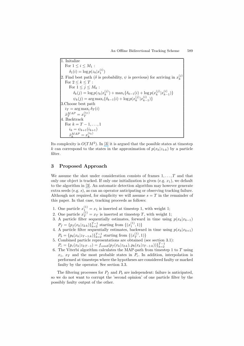
For more information, the reader is referred to [1] and [4].The Viterbi algorithm is used to get the MAP state sequence xMAP

1:T i.e. thesequence for which p(x1)p(z1|x1)ΠT

k=2p(xk|xk−1)p(zk|xk) is maximized, givenMpossible states {x(i)

k }Mi=1 at timestep k:

An Offline Bidirectional Tracking Scheme 589

1. InitalizeFor 1 ≤ i ≤M1 :δ1(i) = log p(zk|x(i)

1 )2. Find best path (δ is probability, ψ is previous) for arriving in x(j)

k

For 2 ≤ k ≤ T :For 1 ≤ j ≤Mk :δk(j) = log p(zk|x(j)

k ) + maxi{δk−1(i) + log p(x(j)k |x(i)

k−1)}ψk(j) = argmaxi{δk−1(i) + log p(x(j)

k |x(i)k−1)}

3.Choose best pathiT = arg maxi δT (i)xMAP

T = x(iT )T

4. BacktrackFor k = T − 1, . . . , 1ik = ψk+1(ik+1)xMAP

k = x(ik)k

Its complexity is O(TM2). In [3] it is argued that the possible states at timestepk can correspond to the states in the approximation of p(xk|z1:k) by a particlefilter.

3 Proposed Approach

We assume the shot under consideration consists of frames 1, . . . , T and thatonly one object is tracked. If only one initialization is given (e.g. x1), we defaultto the algorithm in [3]. An automatic detection algorithm may however generateextra seeds (e.g. s), as can an operator anticipating or observing tracking failure.Although not required, for simplicity we will assume s = T in the remainder ofthis paper. In that case, tracking proceeds as follows:

1. One particle x(1)1 = x1 is inserted at timestep 1, with weight 1;

2. One particle x(1)T = xT is inserted at timestep T , with weight 1;

3. A particle filter sequentially estimates, forward in time using p(xk|xk−1)Pf = {pf(xk|z2:k)}T−1

k=2 starting from {(x(1)1 , 1)}

4. A particle filter sequentially estimates, backward in time using p(xk|xk+1)Pb = {pb(xk|zT−1:k)}T−1

k=2 starting from {(x(1)T , 1)}

5. Combined particle representations are obtained (see section 3.1):Pc = {pc(xk|z2:T−1) = fcomb(pf (xk|z2:k), pb(xk|zT−1:k))}T−1

k=2

6. The Viterbi algorithm calculates the MAP-path from timestep 1 to T usingx1, xT and the most probable states in Pc. In addition, interpolation isperformed at timesteps where the hypotheses are considered faulty or markedfaulty by the operator. See section 3.3.

The filtering processes for Pf and Pb are independent: failure is anticipated,so we do not want to corrupt the ’second opinion’ of one particle filter by thepossibly faulty output of the other.

590 T. Caljon et al.

3.1 Obtaining Pc

Inspired by the integration of cues in multiple-cue trackers, each pf and pb willbe merged into the new probability density function pc according to a measureof reliability.

A popular integration approach by Triesch and von der Malsburg is demo-cratic integration[6]. This scheme is originally used to unidirectionally track facesusing a motion detection cue, a color cue, a prediction cue, a shape cue and acontrast cue. At each timestep k, each cue i votes for each possible state. Thevote weight depends on the similarity with a prototype for that cue and on anadaptive reliability measure for that cue. Spengler and Schiele integrate particlefilters (Condensation) with democratic integration in [5]. Their technique boilsdown to particle filtering where the weight of each particle is a non-adaptivelinear combination of the likelihoods of different cues.

Our integration method is based on a similar voting scheme i.e. after obtain-ing Pf and Pb, we require that each

pc(xk|z2:T−1) = rf (k)pf (xk|z2:k) + rb(k)pb(xk|zT−1:k)

where rf (k) and rb(k) denote the reliability or confidence in pf (xk|z2:k) andpb(xk|zT−1:k) respectively. In our case, these reliabilities will bias the selectionof particles from either pf or pb in section 3.2. A weighted sample representationof pc(xk|z2:T−1) is {(x(i)

c,k, π(i)c,k)}2N

i=1 =

{(x(1)f,k, rf (k)π(1)

f,k), . . . , (x(N)f,k , rf (k)π(N)

f,k ), (x(1)b,k, rb(k)π

(1)b,k), . . . , (x(N)

b,k , rb(k)π(N)b,k )}

as

pc(xk|z2:T−1) =N∑

i=1

(rf (k)π(i)f,k)δ(xk − x

(i)f,k) +

N∑

i=1

(rb(k)π(i)b,k)δ(xk − x

(i)b,k)

In contrast to a scheme that multiplies pf and pb, the anticipated disagreementbetween pf and pb does not leave us with a (near) zero pc or, after normalization,with a pc having unrealistic modes (e.g. when pf and pb are Gaussians).

A straightforward choice for the reliabilities is rb(k) = rf (k) = 0.5. However,since the particle weights {π(i)

f,k} and {π(i)b,k} have been separately normalized

to sum to 1 by the particle filter, only the relative success between particlesof the same particle set is retained. The relative success between particles ofpb(xk|zT−1:k) and pf (xk|z2:k) is lost e.g. the particles of pb could all be spot onthe real object state (all high likelihood) and the particles of pf could all havelost track (all low likelihood), without this being deducible from the normalizedparticle weights. Therefor, the definition of reliability as the sum of the likeli-hoods within a particle set solves this problem: if the non-normalized reliabilitiesare r′f (k) =

∑Ni=1 p(zk|x(i)

f,k) and r′b(k) =∑N

i=1 p(zk|x(i)b,k) then the weights for pc

become

rf (k)π(·)f,k =

r′f (k)r′f (k) + r′b(k)

p(zk|x(·)f,k)

r′f (k)=

p(zk|x(·)f,k)

r′f (k) + r′b(k)

An Offline Bidirectional Tracking Scheme 591

and rb(k)π(·)b,k =

p(zk|x(·)b,k)

r′f (k)+r′

b(k) i.e. each of pc’s particles is now properly weightedrelative to the total likelihood of all particles.

With these definitions, rf (k) and rb(k) respond to occlusion and loss of trackin the expected way. However, another common cause of tracking failure, inabil-ity of a filter’s likelihood function p(z|x) to distinguish between the real objectand distractors, will not cause the ideal response in the corresponding reliability.This weakness is often by design e.g. because a more accurate likelihood func-tion would be too complex or hard to model. We try to compensate for suchgenerically undetectable failures by assuming the odds of encountering them isproportional to the number of frames tracked. At the same time introducing dy-namics for the reliabilities to manage their rate of change, the final reliabilitiesare calculated as follows: ∀k ∈ {2, . . . , T − 1}:

rf (k) = min(max(rf (k − 1) + d(k) − p(k), 0), 1) (1)rb(k) = 1 − rf (k) (2)

where:

d(k) =qf (k) − rf (k − 1)

τ(3)

qf (k) =q′f (k)

q′f (k) + q′b(k)(4)

q′f (k) =N∑

i=1

p(zk|x(i)f,k), q′b(k) =

N∑

i=1

p(zk|x(i)b,k) (5)

As in [6], τ should be configured to filter out high-frequency noise but still allowquick enough adaptation. p(k) is penalty that should work in favor of rf (k) whenk is close to 1, and in favor of rb(k) when k is close to s. In our experiments,p(k) defaults to increasing linearly between p(1) = −0.2 and p(T ) = 0.2.

3.2 Selecting a Reduced State Set

Given the O(TM2) complexity of the Viterbi algorithm, for each timestep k ∈{1, . . . , T} we wish to retain only the M < N distinct most promising states.The main concern is offering enough valid choice to Viterbi. The object states attimestep k that are selected for the Viterbi algorithm are the M distinct statesfrom {x(i)

c,k}2Ni=1 that have the largest probability according to pc(x

(i)c,k|z2:T−1).

3.3 Interpolated Maximum-a-Posteriori Path

We now have a drastically reduced set of possible object states {x(i)k }Mk

i=1 ateach timestep k, that has either been assigned by a user or a detection algo-rithm (Mk = 1), obtained using a particle filter (Mk = M) or obtained usingboth a forward particle filter and a backward particle filter as described above

592 T. Caljon et al.

(Mk = M). Hence the MAP-sequence can be calculated using the Viterbi algo-rithm as described in section 2. The required likelihoods of these states for theViterbi algorithm have already been calculated during filtering.

When loss of track (e.g. due to occlusion) occurs, often no possible objectstates are near the real object state. Many of these situations can be detectedby inspecting maxi{p(zk|x(i)

k )}: if below a certain threshold (e.g. 0.1), loss oftrack at timestep k is assumed. Additionally, the user can select intervals inwhich results are not acceptable. The Viterbi algorithm can easily be extendedto then discard the available hypotheses at these timesteps and interpolate (e.g.linearly): given the current position of the algorithm is timestep k and k−(n+1)is the last timestep that had valid possible object states:

1. Find probability for linearly interpolated pathsFor 1 ≤ j ≤Mk :

For 1 ≤ i ≤Mk−(n+1):Let y1

i,j , . . . , yni,j be the n linearly interpolated states

between x(i)k−(n+1) and x(j)

k

δk(i, j) = log p(zk|x(j)k ) + δk−(n+1)(i) + log p(y1

i,j |x(i)k−(n+1))

+ log p(y2i,j |y1

i,j) + . . .+ log p(x(j)k |yn

i,j)2. For 1 ≤ j ≤Mk :im = arg maxi δk(i, j)δk(j) = δk(im, j)Insert {y1

im,j, . . . , ynim,j} between x(im)

k−(n+1) and x(j)k using ψ

4 Experiments

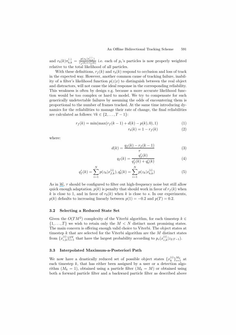
Experiments were performed with the color based particle filter introduced insection 2. The first test sequence consists of 89 frames of a duck disappearingbehind a tree early in the sequence, reappearing 20 frames later. Initializationswere given in the first and last frame. τ is set to 1. Figure 1 shows the 200particles of pf and pb and the reduced particle set for Viterbi (100 states) of pc

at different timesteps. Both the forward and backward particle filter lose trackat the time of disappearance, and rf behaves accordingly. The right states areselected for pc. The occlusion is detected and no states are retained for thecorresponding timesteps. Figure 1 shows that the MAP state sequences usingstates from either Pf or Pb are outperformed by the MAP path obtained usingstates from the combined probability density functions. The resulting path isinterpolated at timesteps where the occlusion takes place.

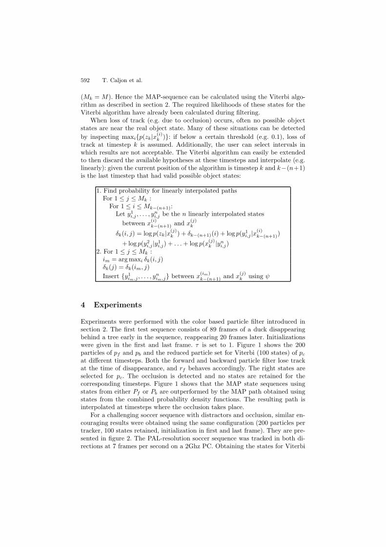
For a challenging soccer sequence with distractors and occlusion, similar en-couraging results were obtained using the same configuration (200 particles pertracker, 100 states retained, initialization in first and last frame). They are pre-sented in figure 2. The PAL-resolution soccer sequence was tracked in both di-rections at 7 frames per second on a 2Ghz PC. Obtaining the states for Viterbi

An Offline Bidirectional Tracking Scheme 593

Fig. 1. Duck sequence. Top,red: forward tracker states. Top,green: backward tracker

states. Top,white: retained states for Viterbi. Top,thick blue: true state. Bottom left:

rf . Bottom middle: MAP state sequences (same color assignments). Bottom right: state

sequence distance to ground truth.

Fig. 2. Soccer sequence. Top,red: forward tracker states. Top,green: backward tracker

states. Top,white: retained states for Viterbi. Top,thick blue: true state. Bottom left:

rf . Bottom right: state sequence distance to ground truth.

594 T. Caljon et al.

takes less than one second, the Viterbi algorithm itself 10 seconds. Simplifyingthe employed state transition prior p(xk|xk−1) for the Viterbi algorithm fromthe tracker’s constant velocity model to a normal distribution over the distancebetween the centers of xk and xk−1 reduces this time to 1 second, while stillproducing good results.

5 Conclusion

The presented scheme per timestep successfully selects a limited amount of statesfrom the filtering distributions of a forward tracking particle filter and a back-ward tracking particle filter using a reliability-based voting scheme. This has thedesirable effect of both speeding up the estimation of the maximum-a-posterioristate sequence so that it becomes interactively usable, and robustifying it byoffering a second opinion, which is indispensable when the forward tracker fails.The Viterbi algorithm is well suited for this application, as it naturally allows toguide paths through states indicated by users. Further enhancements at the userinterface level are possible, for example correction of the MAP-path by simplemouse clicks, preferably without retracking.

Acknowledgments

This work is a result of the Advanced Media project, a joint collaboration be-tween the Vrije Universiteit Brussel, VRT and IBBT. Peter Schelkens holds apost-doctoral fund with the Fund for Scientific Research Flanders (FWO).

References

1. M. Arulampalam, S. Maskell, N. Gordon, and T. Clapp. A tutorial on particle filtersfor online nonlinear/non-gaussian bayesian tracking. IEEE Transactions on SignalProcessing, 50(2):173–188, 2002.

2. A. Doucet, S. Godsill, and M. West. Monte carlo filtering and smoothing withapplication to time-varying spectral estimation. In IEEE International Conferenceon Acoustics, Speech and Signal Processing, volume II, pages 701–704, 2000.

3. S. Godsill, A. Doucet, and M. West. Maximum a posteriori sequence estimationusing monte carlo particle filters. Ann. Inst. Statist. Math., 52, 2001.

4. P. Perez, C. Hue, J. Vermaak, and M. Gangnet. Color-based probabilistic tracking.In ECCV, pages 661–675, 2002.

5. M. Spengler and B. Schiele. Towards robust multi-cue integration for visual tracking.Mach. Vis. Appl., 14(1):50–58, 2003.

6. J. Triesch and C. von der Malsburg. Self-organized integration of visual cues forface tracking. In Proceedings of the Fourth International Conference on AutomaticFace and Gesture Recognition, pages 102–107, 28–30 2000.