Embed Size (px)
Citation preview
Published as a conference paper at ICLR 2022
OFFLINE NEURAL CONTEXTUAL BANDITS:PESSIMISM, OPTIMIZATION AND GENERALIZATION
Thanh Nguyen-Tang ∗
Applied AI InstituteDeakin University
Sunil GuptaApplied AI InstituteDeakin University
A. Tuan NguyenDepartment of Engineering ScienceUniversity of Oxford
Svetha VenkateshApplied AI InstituteDeakin University
ABSTRACT
Offline policy learning (OPL) leverages existing data collected a priori for policyoptimization without any active exploration. Despite the prevalence and recentinterest in this problem, its theoretical and algorithmic foundations in functionapproximation settings remain under-developed. In this paper, we consider thisproblem on the axes of distributional shift, optimization, and generalization inoffline contextual bandits with neural networks. In particular, we propose a prov-ably efficient offline contextual bandit with neural network function approxima-tion that does not require any functional assumption on the reward. We show thatour method provably generalizes over unseen contexts under a milder conditionfor distributional shift than the existing OPL works. Notably, unlike any otherOPL method, our method learns from the offline data in an online manner usingstochastic gradient descent, allowing us to leverage the benefits of online learninginto an offline setting. Moreover, we show that our method is more computa-tionally efficient and has a better dependence on the effective dimension of theneural network than an online counterpart. Finally, we demonstrate the empiricaleffectiveness of our method in a range of synthetic and real-world OPL problems.
1 INTRODUCTION
We consider the problem of offline policy learning (OPL) (Lange et al., 2012; Levine et al., 2020)where a learner infers an optimal policy given only access to a fixed dataset collected a priori byunknown behaviour policies, without any active exploration. There has been growing interest in thisproblem recently, as it reflects a practical paradigm where logged experiences are abundant but aninteraction with the environment is often limited, with important applications in practical settingssuch as healthcare (Gottesman et al., 2019; Nie et al., 2021), recommendation systems (Strehl et al.,2010; Thomas et al., 2017), and econometrics (Kitagawa & Tetenov, 2018; Athey & Wager, 2021).
Despite the importance of OPL, theoretical and algorithmic progress on this problem has been ratherlimited. Specifically, most existing works are restricted to a strong parametric assumption of envi-ronments such as tabular representation (Yin & Wang, 2020; Buckman et al., 2020; Yin et al., 2021;Yin & Wang, 2021; Rashidinejad et al., 2021; Xiao et al., 2021) and more generally as linear models(Duan & Wang, 2020; Jin et al., 2020; Tran-The et al., 2021). However, while the linearity assump-tion does not hold for many problems in practice, no work has provided a theoretical guarantee anda practical algorithm for OPL with neural network function approximation.
In OPL with neural network function approximation, three fundamental challenges arise:
Distributional shift. As OPL is provided with only a fixed dataset without any active exploration,there is often a mismatch between the distribution of the data generated by a target policy and that ofthe offline data. This distributional mismatch can cause erroneous value overestimation and render
∗Email: [email protected].
1
Published as a conference paper at ICLR 2022
many standard online policy learning methods unsuccessful (Fujimoto et al., 2019). To guaranteean efficient learning under distributional shift, common analyses rely on a sort of uniform data cov-erage assumptions (Munos & Szepesvari, 2008; Chen & Jiang, 2019; Brandfonbrener et al., 2021;Nguyen-Tang et al., 2021) that require the offline policy to be already sufficiently explorative overthe entire state space and action space. To mitigate this strong assumption, a pessimism principlethat constructs a lower confidence bound of the reward functions for decision-making (Rashidinejadet al., 2021) can reduce the requirement to a single-policy concentration condition that requires thecoverage of the offline policy only on the target policy. However, Rashidinejad et al. (2021) onlyuses this condition for tabular representation and it is unclear whether complex environments such asones that require neural network function approximation can benefit from this condition. Moreover,the single-policy concentration condition still requires the offline policy to be stationary (e.g., theactions in the offline data are independent and depend only on current state). However, this mightnot hold for many practical scenarios, e.g., when the offline data was collected by an active learner(e.g., by an Q-learning algorithm). Thus, it remains unclear what is a minimal structural assumptionon the distributional shift that allows a provably efficient OPL algorithm.
Optimization. Solving OPL often involves in fitting a model into the offline data via optimization.Unlike in simple function approximations such as tabular representation and linear models whereclosed-form solutions are available, OPL with neural network function approximation poses an addi-tional challenge that involves a non-convex, non-analytical optimization problem. However, existingworks of OPL with function approximation ignore such optimization problems by assuming free ac-cess to an optimization oracle that can return a global minimizer (Brandfonbrener et al., 2021; Duanet al., 2021; Nguyen-Tang et al., 2021) or an empirical risk minimizer with a pointwise convergencebound at an exponential rate (Hu et al., 2021). This is largely not the case in practice, especially inOPL with neural network function approximation where a model is trained by gradient-based meth-ods such as stochastic gradient descents (SGD). Thus, to understand OPL in more practical settings,it is crucial to consider optimization in design and analysis. To our knowledge, such optimizationproblem has not been studied in the context of OPL with neural network function approximation.
Generalization. In OPL, generalization is the ability to generalize beyond the states (or contexts asin the specific case of stochastic contextual bandits) observed in the offline data. In other words, anoffline policy learner with good generalization should obtain high rewards not only in the observedstates but also in the entire (unknown) state distribution. The challenge of generalization in OPLis that as we learn from the fixed offline data, the learned policy has highly correlated structureswhere we cannot directly use the standard concentration inequalities (e.g. Hoeffding’s inequality,Bernstein inequality) to derive a generalization bound. The typical approaches to overcome thisdifficulty are data splitting and uniform convergence. While data splitting splits the offline datainto disjoint folds to break the correlated structures (Yin & Wang, 2020), uniform convergenceestablishes generalization uniformly over a class of policies learnable by a certain model (Yin et al.,2021). However, in the setting where the offline data itself can have correlated structures (e.g., anoffline action can depend on the previous offline data) and the model used is sufficiently large thatrenders a uniform convergence bound vacuous, neither the data splitting technique in (Yin & Wang,2020) nor the uniform convergence argument in (Yin et al., 2021) yield a good generalization. Thus,it is highly non-trivial to guarantee a strong generalization in OPL with neural network functionapproximation from highly correlated offline data.
In this paper, we consider the problem of OPL with neural network function approximation on theaxes of distributional shift, optimization and generalization via studying the setting of stochasticcontextual bandits with overparameterized neural networks. Specifically, we make three contribu-tions toward enabling OPL in more practical settings:
• First, we propose an algorithm that uses a neural network to model any bounded rewardfunction without assuming any functional form (e.g., linear models) and uses a pessimisticformulation to deal with distributional shifts. Notably, unlike any standard offline learningmethods, our algorithm learns from the offline data in an online-like manner, allowing usto leverage the advantages of online learning into offline setting.
• Second, our theoretical contribution lies in making the generalization bound of OPL morerealistic by taking into account the optimization aspects and requiring only a milder con-dition for distributional shifts. In particular, our algorithm uses stochastic gradient descentand updates the network completely online, instead of retraining it from scratch for every
2
Published as a conference paper at ICLR 2022
iteration. Moreover, the distributional shift condition in our analysis, unlike in the exist-ing works, does not require the offline policy to be uniformly explorative or stationary.Specifically, we prove that, under mild conditions with practical considerations above, ouralgorithm learns the optimal policy with an expected error of O(κd1/2n−1/2), where n
is the number of offline samples, κ measures the distributional shift, and d is an effectivedimension of the neural network that is much smaller than the network capacity (e.g., thenetwork’s VC dimension and Rademacher complexity).
• Third, we evaluate our algorithm in a number of synthetic and real-world OPL benchmarkproblems, verifying its empirical effectiveness against the representative methods of OPL.
Notation. We use lower case, bold lower case, and bold upper case to represent scalars, vectorsand matrices, respectively. For a vector v = [v1, . . . , vd]
T ∈ Rd and p > 1, denote ∥v∥p =
(∑d
i=1 vpi )
1/p and let [v]j be the jth element of v. For a matrix A = (Ai,j)m×n, denote ∥A∥F =√∑i,j A
2i,j , ∥A∥p = maxv:∥v∥p=1 ∥Av∥p, ∥A∥∞ = maxi,j |Ai,j | and let vec(A) ∈ Rmn be
the vectorized representation of A. For a square matrix A, a vector v, and a matrix X , denote∥v∥A =
√vTAv and ∥X∥A = ∥ vec(X)∥A. For a collection of matrices W = (W1, . . . ,WL)
and a square matrix A, denote ∥W ∥F =√∑L
l=1 ∥Wl∥2F , and ∥W ∥A =√∑L
l=1 ∥Wl∥2A. For a
collection of matrices W (0) = (W(0)1 , . . . ,W
(0)L ), denote B(W (0), R) = W = (W1, . . . ,WL) :
∥Wl −W(0)l ∥F ≤ R. Denote [n] = 1, 2, . . . , n, and a ∨ b = maxa, b. We write O(·) to hide
logarithmic factors in the standard Big-Oh notation, and write m ≥ Θ(f(·)) to indicate that there isan absolute constant C > 0 that is independent of any problem parameters (·) such that m ≥ Cf(·).
2 BACKGROUND
In this section, we provide essential background on offline stochastic contextual bandits and overpa-rameterized neural networks.
2.1 STOCHASTIC CONTEXTUAL BANDITS
We consider a stochastic K-armed contextual bandit where at each round t, an online learner ob-serves a full context xt := xt,a ∈ Rd : a ∈ [K] sampled from a context distribution ρ, takesan action at ∈ [K], and receives a reward rt ∼ P (·|xt,at
). A policy π maps a full context (andpossibly other past information) to a distribution over the action space [K]. For each full contextx := xa ∈ Rd : a ∈ [K], we define vπ(x) = Ea∼π(·|x),r∼P (·|xa)[r] and v∗(x) = maxπ v
π(x),which is attainable due to the finite action space.
In the offline contextual bandit setting, the goal is to learn an optimal policy only from an offlinedata Dn = (xt, at, rt)nt=1 collected a priori by a behaviour policy µ. The goodness of a learnedpolicy π is measured by the (expected) sub-optimality the policy achieves in the entire (unknown)context distribution ρ:
SubOpt(π) := Ex∼ρ[SubOpt(π;x)], where SubOpt(π;x) := v∗(x)− vπ(x).
In this work, we make the following assumption about reward generation: For each t, rt =h(xt,at)+ξt, where h : Rd → [0, 1] is an unknown reward function, and ξt is a R-subgaussian noiseconditioned on (Dt−1,xt, at) where we denote Dt = (xτ , aτ , rτ )1≤τ≤t,∀t. The R-subgaussiannoise assumption is standard in stochastic bandit literature (Abbasi-Yadkori et al., 2011; Zhou et al.,2020; Xiao et al., 2021) and is satisfied e.g. for any bounded noise.
2.2 OVERPARAMETERIZED NEURAL NETWORKS
To learn the unknown reward function without any prior knowledge about its parametric form, weapproximate it by a neural network. In this section, we define the class of overparameterized neuralnetworks that will be used throughout this paper. We consider fully connected neural networks withdepth L ≥ 2 defined on Rd as
fW (u) =√mWLσ (WL−1σ (. . . σ(W1u) . . .)) ,∀u ∈ Rd, (1)
3
Published as a conference paper at ICLR 2022
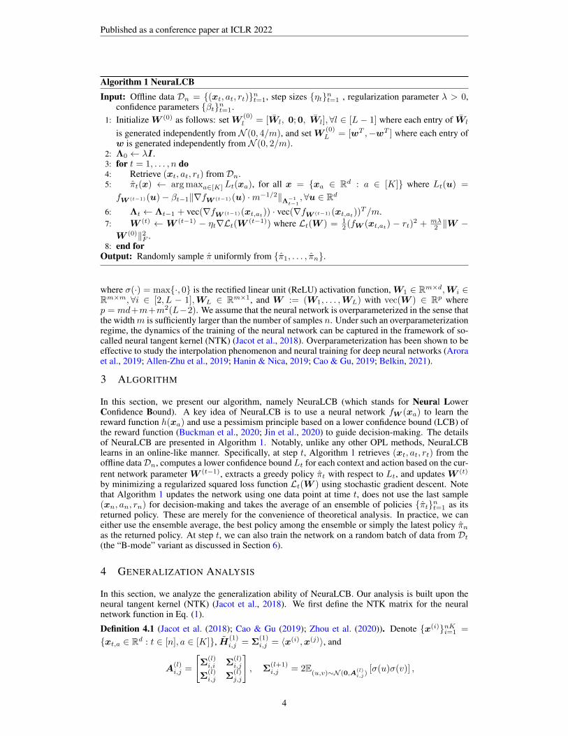
Algorithm 1 NeuraLCBInput: Offline data Dn = (xt, at, rt)nt=1, step sizes ηtnt=1 , regularization parameter λ > 0,
confidence parameters βtnt=1.1: Initialize W (0) as follows: set W (0)
l = [Wl, 0;0, Wl],∀l ∈ [L− 1] where each entry of Wl
is generated independently from N (0, 4/m), and set W (0)L = [wT ,−wT ] where each entry of
w is generated independently from N (0, 2/m).2: Λ0 ← λI .3: for t = 1, . . . , n do4: Retrieve (xt, at, rt) from Dn.5: πt(x) ← argmaxa∈[K] Lt(xa), for all x = xa ∈ Rd : a ∈ [K] where Lt(u) =
fW (t−1)(u)− βt−1∥∇fW (t−1)(u) ·m−1/2∥Λ−1t−1
,∀u ∈ Rd
6: Λt ← Λt−1 + vec(∇fW (t−1)(xt,at)) · vec(∇fW (t−1)(xt,at
))T /m.7: W (t) ← W (t−1) − ηt∇Lt(W
(t−1)) where Lt(W ) = 12 (fW (xt,at
) − rt)2 + mλ
2 ∥W −W (0)∥2F .
8: end forOutput: Randomly sample π uniformly from π1, . . . , πn.
where σ(·) = max·, 0 is the rectified linear unit (ReLU) activation function, W1 ∈ Rm×d,Wi ∈Rm×m,∀i ∈ [2, L − 1],WL ∈ Rm×1, and W := (W1, . . . ,WL) with vec(W ) ∈ Rp wherep = md+m+m2(L−2). We assume that the neural network is overparameterized in the sense thatthe width m is sufficiently larger than the number of samples n. Under such an overparameterizationregime, the dynamics of the training of the neural network can be captured in the framework of so-called neural tangent kernel (NTK) (Jacot et al., 2018). Overparameterization has been shown to beeffective to study the interpolation phenomenon and neural training for deep neural networks (Aroraet al., 2019; Allen-Zhu et al., 2019; Hanin & Nica, 2019; Cao & Gu, 2019; Belkin, 2021).
3 ALGORITHM
In this section, we present our algorithm, namely NeuraLCB (which stands for Neural LowerConfidence Bound). A key idea of NeuraLCB is to use a neural network fW (xa) to learn thereward function h(xa) and use a pessimism principle based on a lower confidence bound (LCB) ofthe reward function (Buckman et al., 2020; Jin et al., 2020) to guide decision-making. The detailsof NeuraLCB are presented in Algorithm 1. Notably, unlike any other OPL methods, NeuraLCBlearns in an online-like manner. Specifically, at step t, Algorithm 1 retrieves (xt, at, rt) from theoffline dataDn, computes a lower confidence bound Lt for each context and action based on the cur-rent network parameter W (t−1), extracts a greedy policy πt with respect to Lt, and updates W (t)
by minimizing a regularized squared loss function Lt(W ) using stochastic gradient descent. Notethat Algorithm 1 updates the network using one data point at time t, does not use the last sample(xn, an, rn) for decision-making and takes the average of an ensemble of policies πtnt=1 as itsreturned policy. These are merely for the convenience of theoretical analysis. In practice, we caneither use the ensemble average, the best policy among the ensemble or simply the latest policy πn
as the returned policy. At step t, we can also train the network on a random batch of data from Dt
(the “B-mode” variant as discussed in Section 6).
4 GENERALIZATION ANALYSIS
In this section, we analyze the generalization ability of NeuraLCB. Our analysis is built upon theneural tangent kernel (NTK) (Jacot et al., 2018). We first define the NTK matrix for the neuralnetwork function in Eq. (1).
Definition 4.1 (Jacot et al. (2018); Cao & Gu (2019); Zhou et al. (2020)). Denote x(i)nKi=1 =
xt,a ∈ Rd : t ∈ [n], a ∈ [K], H(1)i,j = Σ
(1)i,j = ⟨x(i),x(j)⟩, and
A(l)i,j =
[Σ
(l)i,i Σ
(l)i,j
Σ(l)i,j Σ
(l)j,j
], Σ
(l+1)i,j = 2E
(u,v)∼N (0,A(l)i,j)
[σ(u)σ(v)] ,
4
Published as a conference paper at ICLR 2022
H(l+1)i,j = 2H
(l)i,jE(u,v)∼N (0,A
(l)i,j)
[σ′(u)σ′(v)] +Σ(l+1)i,j .
The neural tangent kernel (NTK) matrix is then defined as H = (H(L) +Σ(L))/2.
Here, the Gram matrix H is defined recursively from the first to the last layer of the neural networkusing Gaussian distributions for the observed contexts x(i)nKi=1. Next, we introduce the assump-tions for our analysis. First, we make an assumption about the NTK matrix H and the input data.Assumption 4.1. ∃λ0 > 0,H ⪰ λ0I , and ∀i ∈ [nK], ∥x(i)∥2 = 1. Moreover, [x(i)]j =
[x(i)]j+d/2,∀i ∈ [nK], j ∈ [d/2].
The first part of Assumption 4.1 assures that H is non-singular and that the input data lies in the unitsphere Sd−1. Such assumption is commonly made in overparameterized neural network literature(Arora et al., 2019; Du et al., 2019b;a; Cao & Gu, 2019). The non-singularity is satisfied when e.g.any two contexts in x(i) are not parallel (Zhou et al., 2020), and our analysis holds regardless ofwhether λ0 depends on n. The unit sphere condition is merely for the sake of analysis and can berelaxed to the case that the input data is bounded in 2-norm. As for any input data point x such that∥x∥2 = 1 we can always construct a new input x′ = 1√
2[x,x]T , the second part of Assumption
4.1 is mild and used merely for the theoretical analysis (Zhou et al., 2020). In particular, underAssumption 4.1 and the initialization scheme in Algorithm 1, we have fW (0)(x(i)) = 0,∀i ∈ [nK].
Next, we make an assumption on the data generation.
Assumption 4.2. ∀t,xt is independent of Dt−1, and ∃κ ∈ (0,∞),∥∥∥ π∗(·|xt)µ(·|Dt−1,xt)
∥∥∥∞≤ κ,∀t ∈ [n].
The first part of Assumption 4.2 says that the full contexts are generated by a process independent ofany policy. This is minimal and standard in stochastic contextual bandits (Lattimore & Szepesvari,2020; Rashidinejad et al., 2021; Papini et al., 2021), e.g., when xtnt=1
i.i.d.∼ ρ. The second partof Assumption 4.2, namely empirical single-policy concentration (eSPC) condition, requires thatthe behaviour policy µ has sufficient coverage over only the optimal policy π∗ in the observed con-texts. Our data coverage condition is significantly milder than the common uniform data coverageassumptions in the OPL literature (Munos & Szepesvari, 2008; Chen & Jiang, 2019; Brandfonbreneret al., 2021; Jin et al., 2020; Nguyen-Tang et al., 2021) that requires the offline data to be sufficientlyexplorative in all contexts and all actions. Moreover, our data coverage condition can be consideredas an extension of the single-policy concentration condition in (Rashidinejad et al., 2021) whereboth require coverage over the optimal policy. However, the remarkable difference is that, unlike(Rashidinejad et al., 2021), the behaviour policy µ in our condition needs not to be stationary and theconcentration is only defined on the observed contexts; that is, at can be dependent on both xt andDt−1. This is more practical as it is natural that the offline data was collected by an active learnersuch as a Q-learning agent (Mnih et al., 2015).
Next, we define the effective dimension of the NTK matrix on the observed data as d =log det(I+H/λ)log(1+nK/λ) . This notion of effective dimension was used in (Zhou et al., 2020) for online neural
contextual bandits while a similar notion was introduced in (Valko et al., 2013) for online kernelizedcontextual bandits, and was also used in (Yang & Wang, 2020; Yang et al., 2020) for online kernel-ized reinforcement learning. Although being in offline policy learning setting, the online-like natureof NeuraLCB allows us to leverage the usefulness of the effective dimension. Intuitively, d measureshow quickly the eigenvalues of H decays. For example, d only depends on n logarithmically whenthe eigenvalues of H have a finite spectrum (in this case d is smaller than the number of spectrumwhich is the dimension of the feature space) or are exponentially decaying (Yang et al., 2020). Weare now ready to present the main result about the sub-optimality bound of NeuraLCB.Theorem 4.1. For any δ ∈ (0, 1), under Assumption 4.1 and 4.2, if the network width m, the regu-larization parameter λ, the confidence parameters βt and the learning rates ηt in Algorithm 1satisfym ≥ poly(n,L,K, λ−1, λ−1
0 , log(1/δ)), λ ≥ max1,Θ(L),
βt =√
λ+ C23 tL · (t1/2λ−1/2 + (nK)1/2λ
−1/20 ) ·m−1/2 for some absolute constant C3,
ηt =ι√t, where ι−1 = Ω(n2/3m5/6λ−1/6L17/6 log1/2 m) ∨ Ω(mλ1/2 log1/2(nKL2(10n+ 4)/δ)),
5
Published as a conference paper at ICLR 2022
then with probability at least 1 − δ over the randomness of W (0) and Dn, the sub-optimality of πreturned by Algorithm 1 is bounded as
n · E [SubOpt(π)] ≤ κ√n
√d log(1 + nK/λ) + 2 + κ
√n+ 2 +
√2n log((10n+ 4)/δ),
where d is the effective dimension of the NTK matrix, and κ is the empirical single-policy concen-tration (eSPC) coefficient in Assumption 4.2.
Our bound can be further simplified as E[SubOpt(π)] = O(κ ·max√
d, 1 · n−1/2). A detailedproof for Theorem 4.1 is omitted to Section A. We make several notable remarks about our re-sult. First, our bound does not scale linearly with p or
√p as it would if the classical analyses
(Abbasi-Yadkori et al., 2011; Jin et al., 2020) had been applied. Such a classical bound is vacu-ous for overparameterized neural networks where p is significantly larger than n. Specifically, theonline-like nature of NeuraLCB allows us to leverage a matrix determinant lemma and the notion ofeffective dimension in online learning (Abbasi-Yadkori et al., 2011; Zhou et al., 2020) which avoidsthe dependence on the dimension p of the feature space as in the existing OPL methods such as (Jinet al., 2020). Second, as our bound scales linearly with
√d where d scales only logarithmically with
n in common cases (Yang et al., 2020), our bound is sublinear in such cases and presents a provablyefficient generalization. Third, our bound scales linearly with κ which does not depend on the cov-erage of the offline data on other actions rather than the optimal ones. This eliminates the need for astrong uniform data coverage assumption that is commonly used in the offline policy learning liter-ature (Munos & Szepesvari, 2008; Chen & Jiang, 2019; Brandfonbrener et al., 2021; Nguyen-Tanget al., 2021). Moreover, the online-like nature of our algorithm does not necessitate the stationar-ity of the offline policy, allowing an offline policy with correlated structures as in many practicalscenarios. Note that Zhan et al. (2021) have also recently addressed the problem of off-policy eval-uation with such offline adaptive data but used doubly robust estimators instead of direct methodsas in our paper. Fourth, compared to the regret bound for online learning setting in (Zhou et al.,2020), we achieve an improvement by a factor of
√d while reducing the computational complexity
from O(n2) to O(n). On a more technical note, a key idea to achieve such an improvement is todirectly regress toward the optimal parameter of the neural network instead of toward the empiricalrisk minimizer as in (Zhou et al., 2020).
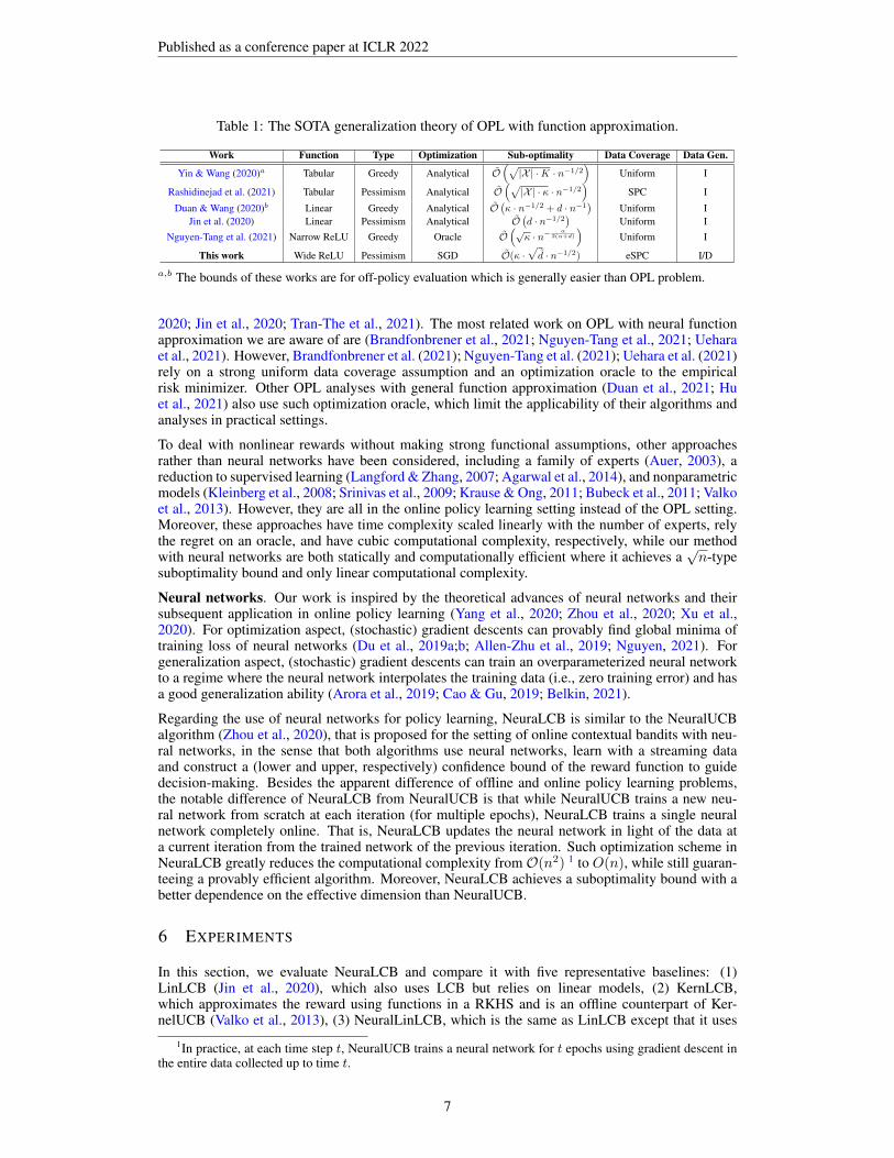
Finally, to further emphasize the significance of our theoretical result, we summarize and compareit with the state-of-the-art (SOTA) sub-optimality bounds for OPL with function approximation inTable 1. From the leftmost to the rightmost column, the table describes: the related works – thefunction approximation – the types of algorithms where Pessimism means a pessimism principlebased on a lower confidence bound of the reward function while Greedy indicates being uncertainty-agnostic (i.e., an algorithm takes an action with the highest predicted score in a given context) –the optimization problems in OPL where Analytical means optimization has an analytical solution,Oracle means the algorithm relies on an oracle to obtain the global minimizer, and SGD meansthe optimization is solved by stochastic gradient descent – the sub-optimality bounds – the datacoverage assumptions where Uniform indicates sufficiently explorative data over the context andaction spaces, SPC is the single-policy concentration condition, and eSPC is the empirical SPC– the nature of data generation required for the respective guarantees where I (Independent) meansthat the offline actions must be sampled independently while D (Dependent) indicates that the offlineactions can be dependent on the past data. It can be seen that our result has a stronger generalizationunder the most practical settings as compared to the existing SOTA generalization theory for OPL.We also remark that the optimization design and guarantee in NeuraLCB (single data point SGD)are of independent interest that do not only apply to the offline setting but also to the original onlinesetting in (Zhou et al., 2020) to improve their regret and optimization complexity.
5 RELATED WORK
OPL with function approximation. Most OPL works, in both bandit and reinforcement learningsettings, use tabular representation (Yin & Wang, 2020; Buckman et al., 2020; Yin et al., 2021;Yin & Wang, 2021; Rashidinejad et al., 2021; Xiao et al., 2021) and linear models (Duan & Wang,
6
Published as a conference paper at ICLR 2022
Table 1: The SOTA generalization theory of OPL with function approximation.
Work Function Type Optimization Sub-optimality Data Coverage Data Gen.
Yin & Wang (2020)a Tabular Greedy Analytical O(√|X | ·K · n−1/2
)Uniform I
Rashidinejad et al. (2021) Tabular Pessimism Analytical O(√|X | · κ · n−1/2
)SPC I
Duan & Wang (2020)b Linear Greedy Analytical O(κ · n−1/2 + d · n−1
)Uniform I
Jin et al. (2020) Linear Pessimism Analytical O(d · n−1/2
)Uniform I
Nguyen-Tang et al. (2021) Narrow ReLU Greedy Oracle O(√
κ · n− α2(α+d)
)Uniform I
This work Wide ReLU Pessimism SGD O(κ ·√
d · n−1/2) eSPC I/D
a,b The bounds of these works are for off-policy evaluation which is generally easier than OPL problem.
2020; Jin et al., 2020; Tran-The et al., 2021). The most related work on OPL with neural functionapproximation we are aware of are (Brandfonbrener et al., 2021; Nguyen-Tang et al., 2021; Ueharaet al., 2021). However, Brandfonbrener et al. (2021); Nguyen-Tang et al. (2021); Uehara et al. (2021)rely on a strong uniform data coverage assumption and an optimization oracle to the empiricalrisk minimizer. Other OPL analyses with general function approximation (Duan et al., 2021; Huet al., 2021) also use such optimization oracle, which limit the applicability of their algorithms andanalyses in practical settings.
To deal with nonlinear rewards without making strong functional assumptions, other approachesrather than neural networks have been considered, including a family of experts (Auer, 2003), areduction to supervised learning (Langford & Zhang, 2007; Agarwal et al., 2014), and nonparametricmodels (Kleinberg et al., 2008; Srinivas et al., 2009; Krause & Ong, 2011; Bubeck et al., 2011; Valkoet al., 2013). However, they are all in the online policy learning setting instead of the OPL setting.Moreover, these approaches have time complexity scaled linearly with the number of experts, relythe regret on an oracle, and have cubic computational complexity, respectively, while our methodwith neural networks are both statically and computationally efficient where it achieves a
√n-type
suboptimality bound and only linear computational complexity.
Neural networks. Our work is inspired by the theoretical advances of neural networks and theirsubsequent application in online policy learning (Yang et al., 2020; Zhou et al., 2020; Xu et al.,2020). For optimization aspect, (stochastic) gradient descents can provably find global minima oftraining loss of neural networks (Du et al., 2019a;b; Allen-Zhu et al., 2019; Nguyen, 2021). Forgeneralization aspect, (stochastic) gradient descents can train an overparameterized neural networkto a regime where the neural network interpolates the training data (i.e., zero training error) and hasa good generalization ability (Arora et al., 2019; Cao & Gu, 2019; Belkin, 2021).
Regarding the use of neural networks for policy learning, NeuraLCB is similar to the NeuralUCBalgorithm (Zhou et al., 2020), that is proposed for the setting of online contextual bandits with neu-ral networks, in the sense that both algorithms use neural networks, learn with a streaming dataand construct a (lower and upper, respectively) confidence bound of the reward function to guidedecision-making. Besides the apparent difference of offline and online policy learning problems,the notable difference of NeuraLCB from NeuralUCB is that while NeuralUCB trains a new neu-ral network from scratch at each iteration (for multiple epochs), NeuraLCB trains a single neuralnetwork completely online. That is, NeuraLCB updates the neural network in light of the data ata current iteration from the trained network of the previous iteration. Such optimization scheme inNeuraLCB greatly reduces the computational complexity from O(n2) 1 to O(n), while still guaran-teeing a provably efficient algorithm. Moreover, NeuraLCB achieves a suboptimality bound with abetter dependence on the effective dimension than NeuralUCB.
6 EXPERIMENTS
In this section, we evaluate NeuraLCB and compare it with five representative baselines: (1)LinLCB (Jin et al., 2020), which also uses LCB but relies on linear models, (2) KernLCB,which approximates the reward using functions in a RKHS and is an offline counterpart of Ker-nelUCB (Valko et al., 2013), (3) NeuralLinLCB, which is the same as LinLCB except that it uses
1In practice, at each time step t, NeuralUCB trains a neural network for t epochs using gradient descent inthe entire data collected up to time t.
7
Published as a conference paper at ICLR 2022
0 2000 4000 6000 8000Number of samples
0.0
0.5
1.0
1.5
2.0
Sub-
optim
ality NeuraLCB
NeuralGreedyLinLCBNeuralLinLCBNeuralLinGreedyKernLCB
(a) h(u) = 10(aTu)2
0 2000 4000 6000 8000Number of samples
4
6
8
10
12
14
16
Sub-
optim
ality
NeuraLCBNeuralGreedyLinLCBNeuralLinLCBNeuralLinGreedyKernLCB
(b) h(u) = uTATAu
0 2000 4000 6000 8000Number of samples
0.05
0.10
0.15
0.20
0.25
Sub-
optim
ality
NeuraLCBNeuralGreedyLinLCBNeuralLinLCBNeuralLinGreedyKernLCB
(c) h(u) = cos(3aTu)
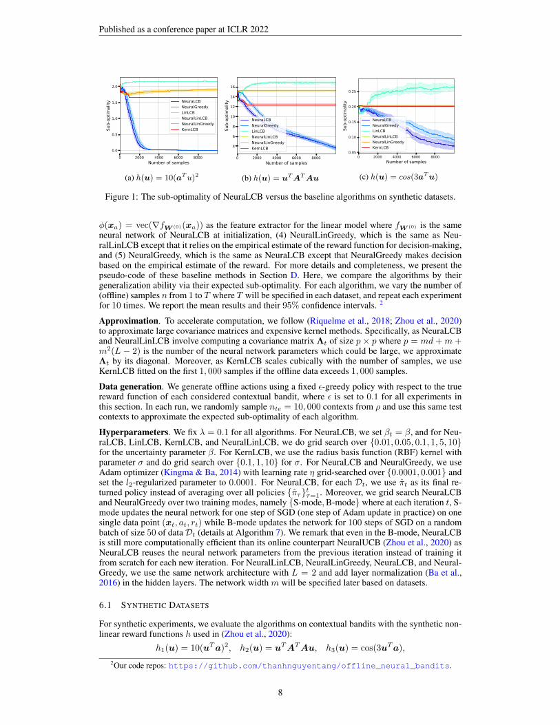
Figure 1: The sub-optimality of NeuraLCB versus the baseline algorithms on synthetic datasets.
ϕ(xa) = vec(∇fW (0)(xa)) as the feature extractor for the linear model where fW (0) is the sameneural network of NeuraLCB at initialization, (4) NeuralLinGreedy, which is the same as Neu-ralLinLCB except that it relies on the empirical estimate of the reward function for decision-making,and (5) NeuralGreedy, which is the same as NeuraLCB except that NeuralGreedy makes decisionbased on the empirical estimate of the reward. For more details and completeness, we present thepseudo-code of these baseline methods in Section D. Here, we compare the algorithms by theirgeneralization ability via their expected sub-optimality. For each algorithm, we vary the number of(offline) samples n from 1 to T where T will be specified in each dataset, and repeat each experimentfor 10 times. We report the mean results and their 95% confidence intervals. 2
Approximation. To accelerate computation, we follow (Riquelme et al., 2018; Zhou et al., 2020)to approximate large covariance matrices and expensive kernel methods. Specifically, as NeuraLCBand NeuralLinLCB involve computing a covariance matrix Λt of size p× p where p = md+m+m2(L − 2) is the number of the neural network parameters which could be large, we approximateΛt by its diagonal. Moreover, as KernLCB scales cubically with the number of samples, we useKernLCB fitted on the first 1, 000 samples if the offline data exceeds 1, 000 samples.
Data generation. We generate offline actions using a fixed ϵ-greedy policy with respect to the truereward function of each considered contextual bandit, where ϵ is set to 0.1 for all experiments inthis section. In each run, we randomly sample nte = 10, 000 contexts from ρ and use this same testcontexts to approximate the expected sub-optimality of each algorithm.
Hyperparameters. We fix λ = 0.1 for all algorithms. For NeuraLCB, we set βt = β, and for Neu-raLCB, LinLCB, KernLCB, and NeuralLinLCB, we do grid search over 0.01, 0.05, 0.1, 1, 5, 10for the uncertainty parameter β. For KernLCB, we use the radius basis function (RBF) kernel withparameter σ and do grid search over 0.1, 1, 10 for σ. For NeuraLCB and NeuralGreedy, we useAdam optimizer (Kingma & Ba, 2014) with learning rate η grid-searched over 0.0001, 0.001 andset the l2-regularized parameter to 0.0001. For NeuraLCB, for each Dt, we use πt as its final re-turned policy instead of averaging over all policies πτtτ=1. Moreover, we grid search NeuraLCBand NeuralGreedy over two training modes, namely S-mode,B-mode where at each iteration t, S-mode updates the neural network for one step of SGD (one step of Adam update in practice) on onesingle data point (xt, at, rt) while B-mode updates the network for 100 steps of SGD on a randombatch of size 50 of data Dt (details at Algorithm 7). We remark that even in the B-mode, NeuraLCBis still more computationally efficient than its online counterpart NeuralUCB (Zhou et al., 2020) asNeuraLCB reuses the neural network parameters from the previous iteration instead of training itfrom scratch for each new iteration. For NeuralLinLCB, NeuralLinGreedy, NeuraLCB, and Neural-Greedy, we use the same network architecture with L = 2 and add layer normalization (Ba et al.,2016) in the hidden layers. The network width m will be specified later based on datasets.
6.1 SYNTHETIC DATASETS
For synthetic experiments, we evaluate the algorithms on contextual bandits with the synthetic non-linear reward functions h used in (Zhou et al., 2020):
h1(u) = 10(uTa)2, h2(u) = uTATAu, h3(u) = cos(3uTa),
2Our code repos: https://github.com/thanhnguyentang/offline_neural_bandits.
8
Published as a conference paper at ICLR 2022
0 2000 4000 6000 8000 10000 12000 14000Number of samples
0
1
2
3
4
5
6
7
Sub-
optim
ality NeuraLCB
NeuralGreedyLinLCBNeuralLinLCBNeuralLinGreedyKernLCB
(a) Mushroom
0 2000 4000 6000 8000 10000 12000 14000Number of samples
0.2
0.3
0.4
0.5
0.6
0.7
0.8
0.9
Sub-
optim
ality
NeuraLCBNeuralGreedyLinLCBNeuralLinLCBNeuralLinGreedyKernLCB
(b) Statlog
0 2000 4000 6000 8000 10000 12000 14000Number of samples
0.70
0.75
0.80
0.85
0.90
0.95
Sub-
optim
ality
NeuraLCBNeuralGreedyLinLCBNeuralLinLCBNeuralLinGreedyKernLCB
(c) Adult
0 2000 4000 6000 8000 10000 12000 14000Number of samples
0.2
0.4
0.6
0.8
Sub-
optim
ality NeuraLCB
NeuralGreedyLinLCBNeuralLinLCBNeuralLinGreedyKernLCB
(d) MNIST
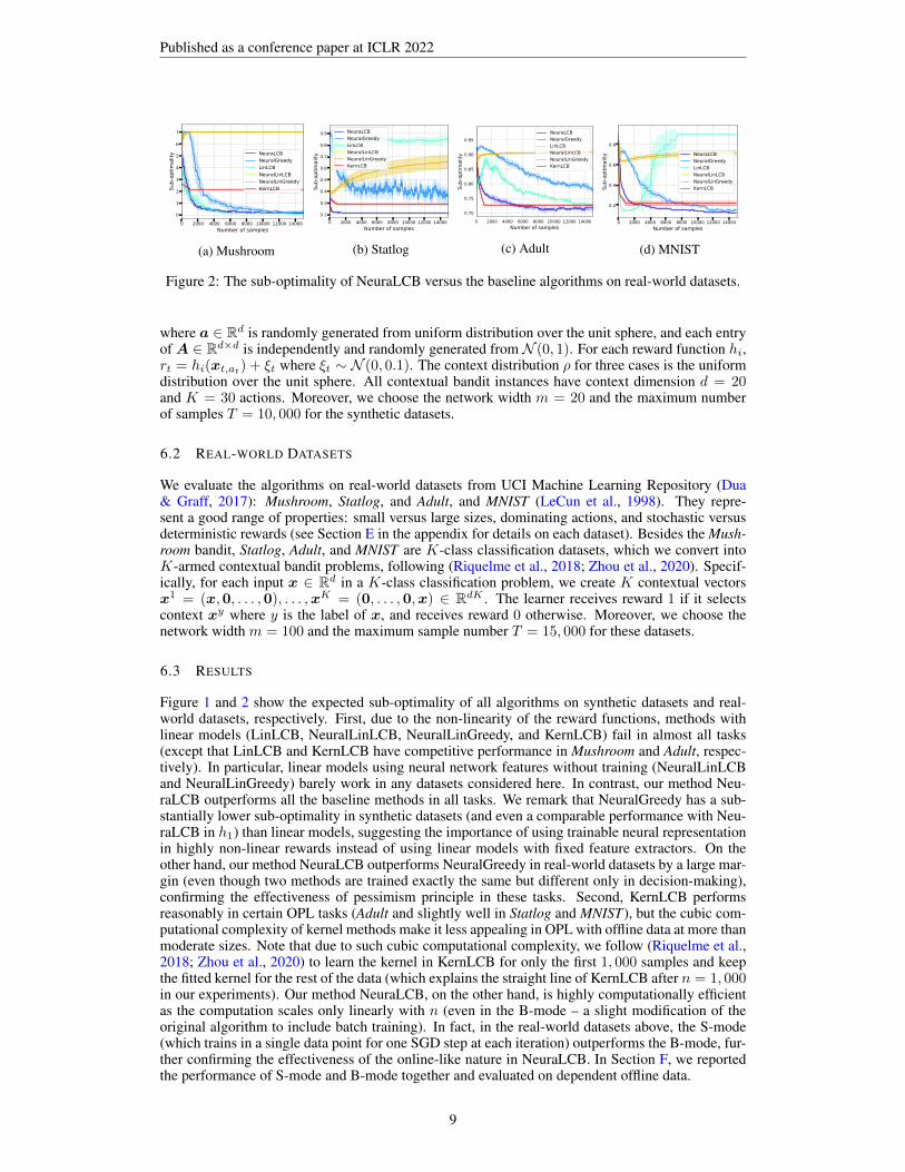
Figure 2: The sub-optimality of NeuraLCB versus the baseline algorithms on real-world datasets.
where a ∈ Rd is randomly generated from uniform distribution over the unit sphere, and each entryof A ∈ Rd×d is independently and randomly generated from N (0, 1). For each reward function hi,rt = hi(xt,at
) + ξt where ξt ∼ N (0, 0.1). The context distribution ρ for three cases is the uniformdistribution over the unit sphere. All contextual bandit instances have context dimension d = 20and K = 30 actions. Moreover, we choose the network width m = 20 and the maximum numberof samples T = 10, 000 for the synthetic datasets.
6.2 REAL-WORLD DATASETS
We evaluate the algorithms on real-world datasets from UCI Machine Learning Repository (Dua& Graff, 2017): Mushroom, Statlog, and Adult, and MNIST (LeCun et al., 1998). They repre-sent a good range of properties: small versus large sizes, dominating actions, and stochastic versusdeterministic rewards (see Section E in the appendix for details on each dataset). Besides the Mush-room bandit, Statlog, Adult, and MNIST are K-class classification datasets, which we convert intoK-armed contextual bandit problems, following (Riquelme et al., 2018; Zhou et al., 2020). Specif-ically, for each input x ∈ Rd in a K-class classification problem, we create K contextual vectorsx1 = (x,0, . . . ,0), . . . ,xK = (0, . . . ,0,x) ∈ RdK . The learner receives reward 1 if it selectscontext xy where y is the label of x, and receives reward 0 otherwise. Moreover, we choose thenetwork width m = 100 and the maximum sample number T = 15, 000 for these datasets.
6.3 RESULTS
Figure 1 and 2 show the expected sub-optimality of all algorithms on synthetic datasets and real-world datasets, respectively. First, due to the non-linearity of the reward functions, methods withlinear models (LinLCB, NeuralLinLCB, NeuralLinGreedy, and KernLCB) fail in almost all tasks(except that LinLCB and KernLCB have competitive performance in Mushroom and Adult, respec-tively). In particular, linear models using neural network features without training (NeuralLinLCBand NeuralLinGreedy) barely work in any datasets considered here. In contrast, our method Neu-raLCB outperforms all the baseline methods in all tasks. We remark that NeuralGreedy has a sub-stantially lower sub-optimality in synthetic datasets (and even a comparable performance with Neu-raLCB in h1) than linear models, suggesting the importance of using trainable neural representationin highly non-linear rewards instead of using linear models with fixed feature extractors. On theother hand, our method NeuraLCB outperforms NeuralGreedy in real-world datasets by a large mar-gin (even though two methods are trained exactly the same but different only in decision-making),confirming the effectiveness of pessimism principle in these tasks. Second, KernLCB performsreasonably in certain OPL tasks (Adult and slightly well in Statlog and MNIST), but the cubic com-putational complexity of kernel methods make it less appealing in OPL with offline data at more thanmoderate sizes. Note that due to such cubic computational complexity, we follow (Riquelme et al.,2018; Zhou et al., 2020) to learn the kernel in KernLCB for only the first 1, 000 samples and keepthe fitted kernel for the rest of the data (which explains the straight line of KernLCB after n = 1, 000in our experiments). Our method NeuraLCB, on the other hand, is highly computationally efficientas the computation scales only linearly with n (even in the B-mode – a slight modification of theoriginal algorithm to include batch training). In fact, in the real-world datasets above, the S-mode(which trains in a single data point for one SGD step at each iteration) outperforms the B-mode, fur-ther confirming the effectiveness of the online-like nature in NeuraLCB. In Section F, we reportedthe performance of S-mode and B-mode together and evaluated on dependent offline data.
9
Published as a conference paper at ICLR 2022
7 ACKNOWLEDGEMENT
This research was partially funded by the Australian Government through the Australian Re-search Council (ARC). Prof. Venkatesh is the recipient of an ARC Australian Laureate Fellowship(FL170100006).
REFERENCES
Yasin Abbasi-Yadkori, David Pal, and Csaba Szepesvari. Improved algorithms for lin-ear stochastic bandits. In John Shawe-Taylor, Richard S. Zemel, Peter L. Bartlett, Fer-nando C. N. Pereira, and Kilian Q. Weinberger (eds.), Advances in Neural InformationProcessing Systems 24: 25th Annual Conference on Neural Information Processing Sys-tems 2011. Proceedings of a meeting held 12-14 December 2011, Granada, Spain, pp.2312–2320, 2011. URL https://proceedings.neurips.cc/paper/2011/hash/e1d5be1c7f2f456670de3d53c7b54f4a-Abstract.html.
Alekh Agarwal, Daniel Hsu, Satyen Kale, John Langford, Lihong Li, and Robert Schapire. Tamingthe monster: A fast and simple algorithm for contextual bandits. In International Conference onMachine Learning, pp. 1638–1646. PMLR, 2014.
Zeyuan Allen-Zhu, Yuanzhi Li, and Zhao Song. A convergence theory for deep learning via over-parameterization. In International Conference on Machine Learning, pp. 242–252. PMLR, 2019.
Sanjeev Arora, Simon S Du, Wei Hu, Zhiyuan Li, Ruslan Salakhutdinov, and Ruosong Wang. Onexact computation with an infinitely wide neural net. arXiv preprint arXiv:1904.11955, 2019.
Susan Athey and Stefan Wager. Policy learning with observational data. Econometrica, 89(1):133–161, 2021.
Peter Auer. Using confidence bounds for exploitation-exploration trade-offs. J. Mach. Learn. Res.,3(null):397–422, March 2003. ISSN 1532-4435.
Jimmy Lei Ba, Jamie Ryan Kiros, and Geoffrey E Hinton. Layer normalization. arXiv preprintarXiv:1607.06450, 2016.
Mikhail Belkin. Fit without fear: remarkable mathematical phenomena of deep learning through theprism of interpolation. arXiv preprint arXiv:2105.14368, 2021.
David Brandfonbrener, William Whitney, Rajesh Ranganath, and Joan Bruna. Offline contextualbandits with overparameterized models. In International Conference on Machine Learning, pp.1049–1058. PMLR, 2021.
Sebastien Bubeck, Remi Munos, Gilles Stoltz, and Csaba Szepesvari. X-armed bandits. Journal ofMachine Learning Research, 12(5), 2011.
Jacob Buckman, Carles Gelada, and Marc G Bellemare. The importance of pessimism in fixed-dataset policy optimization. arXiv preprint arXiv:2009.06799, 2020.
Yuan Cao and Quanquan Gu. Generalization bounds of stochastic gradient descent for wide anddeep neural networks. Advances in Neural Information Processing Systems, 32:10836–10846,2019.
Nicolo Cesa-Bianchi, Alex Conconi, and Claudio Gentile. On the generalization ability of on-linelearning algorithms. IEEE Trans. Inf. Theory, 50(9):2050–2057, 2004. doi: 10.1109/TIT.2004.833339. URL https://doi.org/10.1109/TIT.2004.833339.
Jinglin Chen and Nan Jiang. Information-theoretic considerations in batch reinforcement learning.In ICML, volume 97 of Proceedings of Machine Learning Research, pp. 1042–1051. PMLR,2019.
Simon S. Du, Jason D. Lee, Haochuan Li, Liwei Wang, and Xiyu Zhai. Gradient descent findsglobal minima of deep neural networks. In ICML, volume 97 of Proceedings of Machine LearningResearch, pp. 1675–1685. PMLR, 2019a.
10
Published as a conference paper at ICLR 2022
Simon S. Du, Xiyu Zhai, Barnabas Poczos, and Aarti Singh. Gradient descent provably optimizesover-parameterized neural networks. In ICLR (Poster). OpenReview.net, 2019b.
Dheeru Dua and Casey Graff. UCI machine learning repository, 2017. URL http://archive.ics.uci.edu/ml.
Yaqi Duan and Mengdi Wang. Minimax-optimal off-policy evaluation with linear function approx-imation. CoRR, abs/2002.09516, 2020.
Yaqi Duan, Chi Jin, and Zhiyuan Li. Risk bounds and rademacher complexity in batch reinforcementlearning. arXiv preprint arXiv:2103.13883, 2021.
Scott Fujimoto, David Meger, and Doina Precup. Off-policy deep reinforcement learning withoutexploration. In International Conference on Machine Learning, pp. 2052–2062. PMLR, 2019.
Omer Gottesman, Fredrik Johansson, Matthieu Komorowski, Aldo Faisal, David Sontag, FinaleDoshi-Velez, and Leo Anthony Celi. Guidelines for reinforcement learning in healthcare. Naturemedicine, 25(1):16–18, 2019.
Boris Hanin and Mihai Nica. Finite depth and width corrections to the neural tangent kernel. arXivpreprint arXiv:1909.05989, 2019.
Yichun Hu, Nathan Kallus, and Masatoshi Uehara. Fast rates for the regret of offline reinforcementlearning. In COLT, volume 134 of Proceedings of Machine Learning Research, pp. 2462. PMLR,2021.
Arthur Jacot, Franck Gabriel, and Clement Hongler. Neural tangent kernel: Convergence and gen-eralization in neural networks. arXiv preprint arXiv:1806.07572, 2018.
Ying Jin, Zhuoran Yang, and Zhaoran Wang. Is pessimism provably efficient for offline rl? CoRR,abs/2012.15085, 2020. URL https://arxiv.org/abs/2012.15085.
Diederik P Kingma and Jimmy Ba. Adam: A method for stochastic optimization. arXiv preprintarXiv:1412.6980, 2014.
Toru Kitagawa and Aleksey Tetenov. Who should be treated? empirical welfare maximiza-tion methods for treatment choice. Econometrica, 86(2):591–616, 2018. doi: https://doi.org/10.3982/ECTA13288. URL https://onlinelibrary.wiley.com/doi/abs/10.3982/ECTA13288.
Robert Kleinberg, Aleksandrs Slivkins, and Eli Upfal. Multi-armed bandits in metric spaces. InProceedings of the fortieth annual ACM symposium on Theory of computing, pp. 681–690, 2008.
Andreas Krause and Cheng Soon Ong. Contextual gaussian process bandit optimization. In Nips,pp. 2447–2455, 2011.
Sascha Lange, Thomas Gabel, and Martin Riedmiller. Batch reinforcement learning. In Reinforce-ment learning, pp. 45–73. Springer, 2012.
John Langford and Tong Zhang. The epoch-greedy algorithm for contextual multi-armed bandits.Advances in neural information processing systems, 20(1):96–1, 2007.
Tor Lattimore and Csaba Szepesvari. Bandit Algorithms. Cambridge University Press, 2020. doi:10.1017/9781108571401.
Yann LeCun, Leon Bottou, Yoshua Bengio, and Patrick Haffner. Gradient-based learning applied todocument recognition. Proceedings of the IEEE, 86(11):2278–2324, 1998.
Sergey Levine, Aviral Kumar, George Tucker, and Justin Fu. Offline reinforcement learning: Tuto-rial, review, and perspectives on open problems. arXiv preprint arXiv:2005.01643, 2020.
Volodymyr Mnih, Koray Kavukcuoglu, David Silver, Andrei A Rusu, Joel Veness, Marc G Belle-mare, Alex Graves, Martin Riedmiller, Andreas K Fidjeland, Georg Ostrovski, et al. Human-levelcontrol through deep reinforcement learning. nature, 518(7540):529–533, 2015.
11
Published as a conference paper at ICLR 2022
Remi Munos and Csaba Szepesvari. Finite-time bounds for fitted value iteration. J. Mach. Learn.Res., 9:815–857, 2008.
Quynh Nguyen. On the proof of global convergence of gradient descent for deep relu networks withlinear widths. arXiv preprint arXiv:2101.09612, 2021.
Thanh Nguyen-Tang, Sunil Gupta, Hung Tran-The, and Svetha Venkatesh. Sample complexity ofoffline reinforcement learning with deep relu networks, 2021.
Xinkun Nie, Emma Brunskill, and Stefan Wager. Learning when-to-treat policies. Journal of theAmerican Statistical Association, 116(533):392–409, 2021.
Matteo Papini, Andrea Tirinzoni, Marcello Restelli, Alessandro Lazaric, and Matteo Pirotta. Lever-aging good representations in linear contextual bandits. arXiv preprint arXiv:2104.03781, 2021.
Paria Rashidinejad, Banghua Zhu, Cong Ma, Jiantao Jiao, and Stuart Russell. Bridging offline rein-forcement learning and imitation learning: A tale of pessimism. arXiv preprint arXiv:2103.12021,2021.
Carlos Riquelme, George Tucker, and Jasper Snoek. Deep bayesian bandits showdown: Anempirical comparison of bayesian deep networks for thompson sampling. arXiv preprintarXiv:1802.09127, 2018.
Niranjan Srinivas, Andreas Krause, Sham M Kakade, and Matthias Seeger. Gaussian pro-cess optimization in the bandit setting: No regret and experimental design. arXiv preprintarXiv:0912.3995, 2009.
Alex Strehl, John Langford, Sham Kakade, and Lihong Li. Learning from logged implicit explo-ration data. arXiv preprint arXiv:1003.0120, 2010.
Philip S. Thomas, Georgios Theocharous, Mohammad Ghavamzadeh, Ishan Durugkar, and EmmaBrunskill. Predictive off-policy policy evaluation for nonstationary decision problems, with ap-plications to digital marketing. In Proceedings of the Thirty-First AAAI Conference on ArtificialIntelligence, AAAI’17, pp. 4740–4745. AAAI Press, 2017.
Hung Tran-The, Sunil Gupta, Thanh Nguyen-Tang, Santu Rana, and Svetha Venkatesh. Combiningonline learning and offline learning for contextual bandits with deficient support. arXiv preprintarXiv:2107.11533, 2021.
Masatoshi Uehara, Masaaki Imaizumi, Nan Jiang, Nathan Kallus, Wen Sun, and Tengyang Xie.Finite sample analysis of minimax offline reinforcement learning: Completeness, fast rates andfirst-order efficiency. arXiv preprint arXiv:2102.02981, 2021.
Michal Valko, Nathaniel Korda, Remi Munos, Ilias Flaounas, and Nelo Cristianini. Finite-timeanalysis of kernelised contextual bandits. arXiv preprint arXiv:1309.6869, 2013.
Chenjun Xiao, Yifan Wu, Jincheng Mei, Bo Dai, Tor Lattimore, Lihong Li, Csaba Szepesvari, andDale Schuurmans. On the optimality of batch policy optimization algorithms. In InternationalConference on Machine Learning, pp. 11362–11371. PMLR, 2021.
Pan Xu, Zheng Wen, Handong Zhao, and Quanquan Gu. Neural contextual bandits with deeprepresentation and shallow exploration. arXiv preprint arXiv:2012.01780, 2020.
Lin Yang and Mengdi Wang. Reinforcement learning in feature space: Matrix bandit, kernels, andregret bound. In International Conference on Machine Learning, pp. 10746–10756. PMLR, 2020.
Zhuoran Yang, Chi Jin, Zhaoran Wang, Mengdi Wang, and Michael I Jordan. On function approx-imation in reinforcement learning: Optimism in the face of large state spaces. arXiv preprintarXiv:2011.04622, 2020.
Ming Yin and Yu-Xiang Wang. Asymptotically efficient off-policy evaluation for tabular reinforce-ment learning. In AISTATS, volume 108 of Proceedings of Machine Learning Research, pp.3948–3958. PMLR, 2020.
12
Published as a conference paper at ICLR 2022
Ming Yin and Yu-Xiang Wang. Characterizing uniform convergence in offline policy evaluation viamodel-based approach: Offline learning, task-agnostic and reward-free, 2021.
Ming Yin, Yu Bai, and Yu-Xiang Wang. Near-optimal provable uniform convergence in offlinepolicy evaluation for reinforcement learning. In Arindam Banerjee and Kenji Fukumizu (eds.),The 24th International Conference on Artificial Intelligence and Statistics, AISTATS 2021, April13-15, 2021, Virtual Event, volume 130 of Proceedings of Machine Learning Research, pp. 1567–1575. PMLR, 2021. URL http://proceedings.mlr.press/v130/yin21a.html.
Ruohan Zhan, Vitor Hadad, David A Hirshberg, and Susan Athey. Off-policy evaluation via adap-tive weighting with data from contextual bandits. In Proceedings of the 27th ACM SIGKDDConference on Knowledge Discovery & Data Mining, pp. 2125–2135, 2021.
Dongruo Zhou, Lihong Li, and Quanquan Gu. Neural contextual bandits with ucb-based exploration.In International Conference on Machine Learning, pp. 11492–11502. PMLR, 2020.
13
Published as a conference paper at ICLR 2022
A PROOF OF THEOREM 4.1
In this section, we provide the proof of Theorem 4.1.
Let Dt = (xτ , aτ , rτ )1≤τ≤t. Note that πt returned by Algorithm 1 is Dt−1-measurable. DenoteEt[·] = E[·|Dt−1,xt]. Let the step sizes ηt defined as in Theorem 4.1 and the confidence trade-offparameters βt defined as in Algorithm 1, we present main lemmas below which will culminateinto the proof of the main theorem.Lemma A.1. There exists absolute constants C1, C2 > 0 such that for any δ ∈ (0, 1), if m satisfies
m ≥ max
Θ(nλ−1L11 log6 m),Θ(L6n4K4λ−4
0 log(KL(5n+ 1)/δ))
Θ(L−1λ1/2(log3/2(nKL2(5n+ 1)/δ) ∨ log−3/2 m))
,
then with probability at least 1− δ, it holds uniformly over all t ∈ [n] that
SubOpt(πt;xt) ≤ 2βt−1Ea∗t∼π∗(·|xt)
[∥∇fW (t−1)(xt,a∗
t) ·m−1/2∥Λ−1
t−1|Dt−1,xt
]+ 2C1t
2/3m−1/6 log1/2 mL7/3λ−1/2 + 2√2C2
√nKλ
−1/20 m−11/6 log1/2 mt1/6L10/3λ−1/6.
Lemma A.1 gives an upper bound on the sub-optimality of the returned step-dependent policy πt onthe observed context xt for each t ∈ [n]. We remark that the upper bound depends on the rate atwhich the confidence width of the NTK feature vectors shrink along the direction of only the optimalactions, rather than any other actions. This is an advantage of pessimism where it does not requirethe offline data to be informative about any sub-optimal actions. However, the upper bound dependson the unknown optimal policy π∗ while the offline data has been generated a priori by a differentunknown behaviour policy. This distribution mismatch is handled in the next lemma.Lemma A.2. There exists an absolute constant C3 > 0 such that for any δ ∈ (0, 1), if m and λsatisfy
λ ≥ max1,Θ(L), m ≥ max
Θ(nλ−1L11 log6 m),Θ(L6n4K4λ−4
0 log(nKL(5n+ 2)/δ))
Θ(L−1λ1/2(log3/2(nKL2(5n+ 2)/δ) ∨ log−3/2 m))
,
then with probability at least 1− δ, we have
1
n
n∑t=1
βt−1Ea∗t∼π∗(·|xt)
[∥∇fW (t−1)(xt,a∗
t) ·m−1/2∥Λ−1
t−1|Dt−1,xt
]≤√2βnκ√n
√d log(1 + nK/λ) + 1 + 2C2C2
3n3/2m−1/6(logm)1/2L23/6λ−1/6
+ βnκ(C3/√2)L1/2λ
−1/20 log1/2((5n+ 2)/δ),
where C2 is from Lemma A.1.
We also remark that the upper bound in Lemma A.2 scales linearly with√d instead of with
√p if a
standard analysis were applied. This avoids a vacuous bound as p is large with respect to n.
The upper bounds in Lemma A.1 and Lemma A.2 are established for the observed contexts only.The next lemma generalizes these bounds to the entire context distribution, thanks to the online-like nature of Algorithm 1 and an online-to-batch argument. In particular, a key technical propertyof Algorithm 1 that makes this generalization possible without a uniform convergence is that πt isDt−1-measurable and independent of (xt, at, rt).Lemma A.3. For any δ ∈ (0, 1), with probability at least 1−δ over the randomness ofDn, we have
E [SubOpt(π)] ≤ 1n
∑nt=1 SubOpt(πt;xt) +
√2n log(1/δ).
14
Published as a conference paper at ICLR 2022
We are now ready to prove the main theorem.
Proof of Theorem 4.1. Combining Lemma A.1, Lemma A.2, and Lemma A.3 via the union bound,we have
n · E[SubOpt(π)] ≤ κ√nΓ1
√d log(1 + nK/λ) + Γ2 + κ
√nΓ3 + Γ4 + Γ5 +
√2n log((10n+ 4)/δ),
≤ κ√n
√d log(1 + nK/λ) + 2 + κ
√n+ 2 +
√2n log(10n+ 4)/δ)
where m is chosen to be sufficiently large as a polynomial of (n,L,K, λ−1, λ−10 , log(1/δ)) such
that
Γ1 := 2√2√λ+ C2
3nL(n1/2λ1/2 + (nK)1/2λ
−1/20 ) ·m−1/2 ≤ 1
Γ2 := 1 + 2C2C23n
3/2m−1/6(logm)1/2L23/6λ−1/6 ≤ 2
Γ3 := Γ1
√n(C3/
√2)L1/2λ
−1/20 log1/2((10n+ 4)/δ) ≤ 1
Γ4 := 2C1n5/3m−1/6(logm)1/2L7/3λ−1/2 ≤ 1
Γ5 := 2√2C2(nK)1/2λ
−1/20 m−11/6(logm)1/2n7/6L10/3λ−1/6 ≤ 1.
B PROOF OF LEMMAS IN SECTION A
B.1 PROOF OF LEMMA A.1
We start with the following lemmas whose proofs are deferred to Appendix B.
Lemma B.1. Let h = [h(x(1)), . . . , h(x(nK))]T ∈ RnK . There exists W ∗ ∈ W such that forany δ ∈ (0, 1), if m ≥ Θ(L6n4K4λ−4
0 log(nKL/δ)), with probability at least 1 − δ over therandomness of W (0), it holds uniformly for all i ∈ [nK] that
∥W ∗ −W (0)∥F ≤√2m−1/2∥h∥H−1 ,
⟨∇fW (0)(x(i)),W ∗ −W (0)⟩ = h(x(i)).
Remark B.1. Lemma B.1 shows that for a sufficiently wide network, there is a linear model that usesthe gradient of the neural network at initialization as a feature vector and interpolates the rewardfunction in the training inputs. Moreover, the weights W ∗ of the linear model is in a neighborhoodof the initialization W (0). Note that we also have
S := ∥h∥H−1 ≤ ∥h∥2√∥H−1∥2 ≤
√nKλ
−1/20 ,
where the second inequality is by Assumption 4.1 and Cauchy-Schwartz inequality with h(x) ∈[0, 1],∀x.Lemma B.2. For any δ ∈ (0, 1), if m satisfies
m ≥ Θ(nλ−1L11 log6 m) ∨Θ(L−1λ1/2 log3/2(3n2KL2/δ)),
and the step sizes satisfy
ηt =ι√t
where ι−1 = Ω(n2/3m5/6λ−1/6L17/6 log1/2 m) ∨ Ω(Rmλ1/2 log1/2(n/δ))
then with probability at least 1 − δ over the randomness of W (0) and D, it holds uniformly for allt ∈ [n], l ∈ [L] that
∥W (t)l −W
(0)l ∥F ≤
√t
mλL, and ∥Λt∥2 ≤ λ+ C2
3 tL,
where C3 > 0 is an absolute constant from Lemma C.2.
15
Published as a conference paper at ICLR 2022
Remark B.2. Lemma B.2 controls the growth dynamics of the learned weights Wt around its ini-tialization and bounds the spectral norm of the empirical covariance matrix Λt when the model istrained by SGD.Lemma B.3 (Allen-Zhu et al. (2019, Theorem 5), Cao & Gu (2019, Lemma B.5)). There exist anabsolute constant C2 > 0 such that for any δ ∈ (0, 1), if ω satisfies
Θ(m−3/2L−3/2(log3/2(nK/δ)) ∨ log−3/2 m) ≤ ω ≤ Θ(L−9/2 log−3 m),
with probability at least 1 − δ over the randomness of W (0), it holds uniformly for all W ∈B(W (0);ω) and i ∈ [nK] that
∥∇fW (x(i))−∇fW (0)(x(i))∥F ≤ C2
√logmω1/3L3∥∇fW (0)(x(i))∥F .
Remark B.3. Lemma B.3 shows that the gradient in a neighborhood of the initialization differs fromthe gradient at the initialization by an amount that can be explicitly controlled by the radius of theneighborhood and the norm of the gradient at initialization.Lemma B.4 (Cao & Gu (2019, Lemma 4.1)). There exist an absolute constant C1 > 0 such that forany δ ∈ (0, 1) over the randomness of W (0), if ω satisfies
Θ(m−3/2L−3/2 log3/2(nKL2/δ)) ≤ ω ≤ Θ(L−6 log−3/2 m),
with probability at least 1− δ, it holds uniformly for all W ,W ′ ∈ B(W (0);ω) and i ∈ [nK] that
|fW ′(x(i))− fW (x(i))− ⟨∇fW (x(i)),W ′ −W ⟩| ≤ C1 · ω4/3L3√
m logm.
Remark B.4. Lemma B.4 shows that near initialization the neural network function is almost linearin terms of its weights in the training inputs.
Proof of Lemma A.1. For all t ∈ [n],u ∈ Rd, we define
Ut(u) = fW (t−1)(u) + βt−1∥∇fW (t−1)(u) ·m−1/2∥Λ−1t−1
Lt(u) = fW (t−1)(u)− βt−1∥∇fW (t−1)(u) ·m−1/2∥Λ−1t−1
Ut(u) = ⟨∇fW (t−1)(u),W (t−1) −W (0)⟩+ βt−1∥∇fW (t−1)(u) ·m−1/2∥Λ−1t−1
Lt(u) = ⟨∇fW (t−1)(u),W (t−1) −W (0)⟩ − βt−1∥∇fW (t−1)(u) ·m−1/2∥Λ−1t−1
Ct = W ∈ W : ∥W −W (t−1)∥Λt−1≤ βt−1.
Let E be the event in which Lemma B.1, Lemma B.3, Lemma B.3 for all ω ∈√i
mλL : 1 ≤ i ≤ n
, and Lemma B.4 for all ω ∈√
imλL : 1 ≤ i ≤ n
hold simultaneously.
Under event E , for all t ∈ [n], we have
∥W ∗ −W (t)∥Λt≤ ∥W ∗ −W (t)∥F
√∥Λt∥2
≤ (∥W ∗ −W (0)∥F + ∥W (t) −W (0)∥F )√∥Λt∥2
≤ (√2m−1/2S + t1/2λ−1/2m−1/2)
√λ+ C2
3 tL = βt,
where the second inequality is by the triangle inequality, and the third inequality is by Lemma B.1and Lemma B.2. Thus, W ∗ ∈ Ct,∀t ∈ [n].
Denoting a∗t ∼ π∗(·|xt) and at ∼ πt(·|xt) , under event E , we have
SubOpt(πt;xt) = Et[h(xt,a∗t)]− Et[h(xt,at
)]
(a)= Et
[⟨∇fW (0)(xt,a∗
t),W ∗ −W (0)⟩
]− Et
[⟨∇fW (0)(xt,at
),W ∗ −W (0)⟩]
(b)
≤ Et
[⟨∇fW (t−1)(xt,a∗
t),W ∗ −W (0)⟩
]− Et
[⟨∇fW (t−1)(xt,at
),W ∗ −W (0)⟩]
16
Published as a conference paper at ICLR 2022
+ ∥W ∗ −W (0)∥F · Et
[∥∇fW (t−1)(xt,a∗
t)−∇fW (0)(xt,a∗
t)∥F
+ ∥∇fW (t−1)(xt,at)−∇fW (0)(xt,at
)∥F]
(c)
≤ Et
[⟨∇fW (t−1)(xt,a∗
t),W ∗ −W (0)⟩
]− Et
[⟨∇fW (t−1)(xt,at
),W ∗ −W (0)⟩]
+ 2√2C2Sm
−11/6 log1/2 mt1/6L10/3λ−1/6
(d)
≤ Et
[Ut(xt,a∗
t)]− Et
[Lt(xt,at)
]+ 2√2C2Sm
−11/6 log1/2 mt1/6L10/3λ−1/6
= Et
[Ut(xt,a∗
t)]− Et [Lt(xt,at
)]
+ Et
[⟨∇fW (t−1)(xt,a∗
t),W (t−1) −W (0)⟩ − fW (t−1)(xt,a∗
t) + fW (0)(xt,a∗
t)]
+ Et
[fW (t−1)(xt,at
)− fW (0)(xt,at)− ⟨∇fW (t−1)(xt,at
),W (t−1) −W (0)⟩]
−Et
[fW (0)(xt,a∗
t)]+ Et [fW (0)(xt,at
)]︸ ︷︷ ︸=0 by symmetry at initialization
+2√2C2Sm
−11/6 log1/2 mt1/6L10/3λ−1/6
(e)
≤ Et
[Ut(xt,a∗
t)]− Et
[Lt(xt,a∗
t)]+
(Et
[Lt(xt,a∗
t)]− Et [Lt(xt,at
)])︸ ︷︷ ︸
≤0 by pessimism
+ 2C1t2/3m−1/6 log1/2 mL7/3λ−1/2 + 2
√2C2Sm
−11/6 log1/2 mt1/6L10/3λ−1/6
(f)
≤ Et
[Ut(xt,a∗
t)]− Et
[Lt(xt,a∗
t)]
+ 2C1t2/3m−1/6 log1/2 mL7/3λ−1/2 + 2
√2C2Sm
−11/6 log1/2 mt1/6L10/3λ−1/6
= 2βt−1Et
[∥∇fW (t−1)(xt,a∗
t) ·m−1/2∥Λ−1
t−1
]+ 2C1t
2/3m−1/6 log1/2 mL7/3λ−1/2 + 2√2C2Sm
−11/6 log1/2 mt1/6L10/3λ−1/6
where (a) is by Lemma B.1, (b) is by the triangle inequality, (c) is by Lemma B.1, Lemma B.2, andLemma B.3, (d) is by W ∗ ∈ Ct, and by that maxu:∥u−b∥A≤γ⟨a,u−b0⟩ = ⟨a, b−b0⟩+γ∥a∥A−1 ,and minu:∥u−b∥A≤γ⟨a,u − b0⟩ = ⟨a, b − b0⟩ − γ∥a∥A−1 , (e) is by Lemma B.4 and by thatfW (0)(x(i)) = 0,∀i ∈ [nK], and (f) is by that at is sampled from the policy πt which is greedywith respect to Lt.
By the union bound and the choice of m, we conclude our proof.
B.2 PROOF OF LEMMA A.2
We first present the following lemma.Lemma B.5. For any δ ∈ (0, 1), if m satisfies
m ≥ max
Θ(nλ−1L11 log6 m),Θ(L−1λ1/2(log3/2(nKL2(n+ 2)/δ) ∨ log−3/2 m)),
Θ(L6(nK)4 log(L(n+ 2)/δ))
,
and λ ≥ maxC23L, 1, then with probability at least 1− δ, it holds simultaneously that
t∑i=1
∥∇fW (i−1)(xi,ai) ·m−1/2∥2
Λ−1i−1
≤ 2 logdet(Λt)
det(λI),∀t ∈ [n],∣∣∣∣ log det(Λt)
det(λI)− log
det(Λt)
det(λI)
∣∣∣∣ ≤ 2C2C23 t
3/2m−1/6(logm)1/2L23/6λ−1/6,∀t ∈ [n],
logdet(Λn)
det(λI)≤ d log(1 + nK/λ) + 1,
17
Published as a conference paper at ICLR 2022
where Λt := λI +∑t
i=1 vec(∇fW (0)(xi,ai)) · vec(∇fW (0)(xi,ai
))T /m, and C2, C3 > 0 areabsolute constants from Lemma B.3 and Lemma B.2, respectively.
We are now ready to prove Lemma A.2.
Proof of Lemma A.2. First note that ∥Λt−1∥2 ≥ λ, ∀t. Let E be the event in which Lemma B.2,
Lemma C.2 for all ω ∈√
imλL : 1 ≤ i ≤ n
, and Lemma B.5 simultaneously hold. Thus, under
event E , we have
∥∇fW (t−1)(xt,at) ·m−1/2∥Λ−1
t−1≤ ∥∇fW (t−1)(xt,at
) ·m−1/2∥F√∥Λ−1
t−1∥2 ≤ C3L1/2λ−1/2,
where the second inequality is by Lemma B.2 and Lemma C.2.
Thus, by Assumption 4.2, Hoeffding’s inequality, and the union bound, with probability at least1− δ, it holds simultaneously for all t ∈ [n] that
2βt−1Ea∗t∼π∗(·|xt)
[∥∇fW (t−1)(xt,a∗
t) ·m−1/2∥Λ−1
t−1|Dt−1,xt
]≤ 2βt−1κEa∼µ(·|Dt−1,xt)
[∥∇fW (t−1)(xt,a) ·m−1/2∥Λ−1
t−1|Dt−1,xt
]≤ 2βt−1κ∥∇fW (t−1)(xt,at
) ·m−1/2∥Λ−1t−1
+ βt−1κ√2C3L
1/2λ−1/2 log1/2((5n+ 2)/δ).
Hence, for the choice of m in Lemma A.2, with probability at least 1− δ, we have
1
n
n∑t=1
βt−1Ea∗t∼π∗(·|xt)
[∥∇fW (t−1)(xt,a∗
t) ·m−1/2∥Λ−1
t−1|Dt−1,xt
]≤ βnκ
n
n∑t=1
∥∇fW (t−1)(xt,at) ·m−1/2∥Λ−1t−1
+C3√2βnκL
1/2λ−1/20 log1/2((5n+ 2)/δ)
≤ βnκ
n
√n
√√√√ n∑t=1
∥∇fW (t−1)(xt,at) ·m−1/2∥2
Λ−1t−1
+C3√2βnκL
1/2λ−1/20 log1/2((5n+ 2)/δ)
≤√2βnκ√n
√log
det(Λn)
det(λI)+
C3√2βnκL
1/2λ−1/20 log1/2((5n+ 2)/δ)
≤√2βnκ√n
√log
det(Λn)
det(λI)+ 2C2C2
3n3/2m−1/6(logm)1/2L23/6λ−1/6 +
C3√2βnκL
1/2λ−1/20 log1/2((5n+ 2)/δ)
≤√2βnκ√n
√d log(1 + nK/λ) + 1 + 2C2C2
3n3/2m−1/6(logm)1/2L23/6λ−1/6
+C3√2βnκL
1/2λ−1/20 log1/2((5n+ 2)/δ),
where the first inequality is by βt ≤ βn,∀t ∈ [n], the second inequality is by Cauchy-Schwartzinequality, the second inequality and the third inequality are by Lemma B.5.
B.3 PROOF OF LEMMA A.3
Proof of Lemma A.3. We follow the same online-to-batch conversion argument in (Cesa-Bianchiet al., 2004). For each t ∈ [n], define
Zt = SubOpt(πt)− SubOpt(πt;xt).
Since πt is Dt−1-measurable and is independent of xt, and xt are independent of Dt−1 (by As-sumption 4.2), we have E [Zt|Dt−1] = 0,∀t ∈ [n]. Note that −1 ≤ Zt ≤ 1. Thus, by theHoeffding-Azuma inequality, with probability at least 1− δ, we have
E[SubOpt(π)] =1
n
n∑t=1
SubOpt(πt) =1
n
n∑t=1
SubOpt(πt;xt) +1
n
n∑t=1
Zt
18
Published as a conference paper at ICLR 2022
≤ 1
n
n∑t=1
SubOpt(πt;xt) +
√2
nlog(1/δ).
C PROOF OF LEMMAS IN SECTION B
C.1 PROOF OF LEMMA B.1
We first restate the following lemma.Lemma C.1 (Arora et al. (2019)). There exists an absolute constant c1 > 0 such that for anyϵ > 0, δ ∈ (0, 1), if m ≥ c1L
6ϵ−4 log(L/δ), for any i, j ∈ [nK], with probability at least 1 − δover the randomness of W (0), we have
|⟨∇fW (0)(x(i)),∇fW (0)(x(j))⟩/m−Hi,j | ≤ ϵ.
Lemma C.1 gives an estimation error between the kernel constructed by the gradient at initializationas a feature map and the NTK kernel. Unlike Jacot et al. (2018), Lemma C.1 quantifies an exactnon-asymptotic bound for m.
Proof of Lemma B.1. Let G = m−1/2 ·[vec(∇fW (0)(x(1))), . . . , vec(∇fW (0)(x(nK)))] ∈ Rp×nK .For any ϵ > 0, δ ∈ (0, 1), it follows from Lemma C.1 and union bound, if m ≥Θ(L6ϵ−4 log(nKL/δ)), with probability at least 1− δ, we have
∥GTG−H∥F ≤ nK∥GTG−H∥∞ = nKmaxi,j|m−1⟨∇fW (0)(x(i)),∇fW (0)(x(j))⟩ −Hi,j |
≤ nKϵ.
Under the event that the inequality above holds, by setting ϵ = λ0
2nK , we have
H −GTG ⪯ ∥H −GTG∥2I ⪯ ∥H −GTG∥F I ⪯λ0
2I ⪯ 1
2H. (2)
Let G = PΛQT be the singular value decomposition of G where P ∈ Rp×nK ,Q ∈ RnK×nK
have orthogonal columns, and Λ ∈ RnK×nK is a diagonal matrix. Since GTG ⪰ 12H ⪰ λ0
2 I
is positive definite, Λ is invertible. Let W ∗ ∈ W such that vec(W ∗) = vec(W (0)) + m−1/2 ·PΛ−1QTh, we have
m1/2 ·GT (vec(W ∗)− vec(W (0))) = QΛP TPΛ−1QTh = h.
Moreover, we have
m∥W ∗ −W (0)∥2F = m∥ vec(W ∗)− vec(W (0))∥22 = hTQΛ−1P TPΛ−1QTh
= hTQΛ−2QTh = hT (GTG)−1h ≤ 2hTH−1h,
where the inequality is by Equation (2).
C.2 PROOF OF LEMMA B.2
We present the following lemma that will be used in this proof.Lemma C.2 (Cao & Gu (2019, Lemma B.3)). There exist an absolute constant C3 > 0 such thatfor any δ ∈ (0, 1) over the randomness of W (0), if ω satisfies
Θ(m−3/2L−3/2 log3/2(nKL2/δ)) ≤ ω ≤ Θ(L−6 log−3 m),
with probability at least 1− δ, it holds uniformly for all W ∈ B(W (0);ω), i ∈ [nK], l ∈ [L] that
∥∇lfW (x(i))∥F ≤ C3 ·√m.
19
Published as a conference paper at ICLR 2022
Proof of Lemma B.2. Let δ ∈ (0, 1). Let Lt(W ) = 12 (fW (xt,at
) − rt)2 + mλ
2 ∥W −W (0)∥2F bethe regularized squared loss function on the data point (xt,at
, rt). Recall that W (t) = W (t−1) −ηt∇Lt(W
(t−1)). By Hoelfding’s inequality and that rt is R-subgaussian, for any t ∈ [n], withprobability at least 1− δ, we have
|rt| ≤ |Et[rt]|+R√
2 log(2/δ) = |E [E[rt|Dt−1,xt, at]] |+R√2 log(2/δ)
= E [h(xt,at)|Dt−1,xt, at] +R
√2 log(2/δ) ≤ 1 +R
√2 log(2/δ). (3)
By union bound and (3), for any sequence ωtt∈[n] such thatΘ(m−3/2L−3/2 log3/2(3n2KL2/δ)) ≤ ωt ≤ Θ(L−6 log−3 m) ∧ Θ(L−6 log−3/2 m),∀t ∈ [n],with probability at least 1− δ, it holds uniformly for all W ∈ B(W (0);ωt), l ∈ [L], t ∈ [n] that
∥∇lLt(W )∥F = ∥∇lfW (xt,at)(fW (xt,at
)− rt) +mλ(Wl −W(0)l )∥F
= ∥∇lfW (xt,at)(fW (xt,at)− fW (0)(xt,at)− ⟨∇fW (0)(xt,at),W −W (0)⟩)+∇lfW (xt,at
)fW (0)(xt,at) +∇lfW (xt,at
)⟨∇fW (0)(xt,at),W −W (0)⟩
− rt∇lfW (xt,at) +mλ(Wl −W(0)l )∥F
≤ ∥∇lfW (xt,at)(fW (xt,at
)− fW (0)(xt,at)− ⟨∇fW (0)(xt,at
),W −W (0)⟩)∥F+ ∥∇lfW (xt,at
)fW (0)(xt,at)∥F︸ ︷︷ ︸
=0
+∥∇lfW (xt,at)⟨∇fW (0)(xt,at
),W −W (0)⟩∥F
+ |rt|∥∇lfW (xt,at)∥F +mλ∥Wl −W(0)l ∥F
≤ C1C3ω4/3t L3m log1/2 m+ C3m
1/2(1 +R√2 log(6n/δ)) + C2
3Lmω +mλωt,(4)
where the first inequality is triangle’s inequality, and the second inequality is by Lemma B.4, LemmaC.2 and (3).
We now prove by induction that under the same event that (4) with ωt =√
tmλL holds, W (t) ∈
B(W (0);√
tmλL ),∀t ∈ [n]. It trivially holds for t = 0. Assume W (i) ∈ B(W (0);
√i
mλL ),∀i ∈
[t − 1], we will prove that W (t) ∈ B(W (0);√
tmλL ). Indeed, it is easy to verify that there ex-
ist absolute constants Ci2i=1 > 0 such that if m satisfies the inequalities in Lemma B.2, then
Θ(m−3/2L−3/2 log3/2(3n2KL2/δ)) ≤√
imλL ≤ Θ(L−6 log−3 m) ∧ Θ(L−6 log−3/2 m),∀i ∈
[n]. Thus, under the same event that (4) holds, we have
∥W (t)l −W
(0)l ∥F ≤
t∑i=1
∥W (i)l −W
(i−1)l ∥F =
t∑i=1
ηi∥∇lLi(W(i−1))∥F
≤ ιtC1C3m1/3λ−2/3L7/3n1/6 log1/2 m+ ιtm−1/2λ−1/2L−1/2(C2
3L+ λ)
+ 2C3ι√tm1/2(1 +R
√2 log1/2(6n/δ))
≤ 1
2
√t
mλL+
1
2
√t
mλL=
√t
mλL,
where the first inequality is by triangle’s inequality, the first equation is by the SGD update for eachW (i), the second inequality is by (4) and the last inequality is due to ι be chosen asι−1 ≥ 4C3mλ1/2L1/2
(1 +R
√2 log1/2(6n/δ)
)ι−1 ≥ 2n1/2m1/2λ1/2L1/2
(C1C3m
1/3λ−2/3L7/3n1/6 log1/2 m+m−1/2λ−1/2L−1/2(C23L+ λ)
),
which is satisfied for ι−1 = Ω(n2/3m5/6λ−1/6L17/6 log1/2 m) ∨ Ω(Rmλ1/2 log1/2(n/δ)).
For the second part of the lemma, we have
∥Λt∥2 = ∥λI +
t∑i=1
vec(∇fW (i−1)(xi,ai)) · vec(∇fW (i−1)(xi,ai
))T /m∥2
20
Published as a conference paper at ICLR 2022
≤ λ+
t∑i=1
∥∇fW (i−1)(xi,ai)∥2F /m ≤ λ+ C23 tL,
where the first inequality is by triangle’s inequality and the second inequality is by ∥W (i) −W (0)∥F ≤
√i
mλ ,∀i ∈ [n] and Lemma C.2.
C.3 PROOF OF LEMMA B.5
Proof of Lemma B.5. Let E(δ) be the event in which the following (n + 2) events hold simultane-
ously: the events in which Lemma B.3 for each ω ∈√
imλL : 1 ≤ i ≤ n
holds, the event in
which Lemma C.1 for ϵ = (nK)−1 holds, and the event in which Lemma C.2 holds.
Under event E(δ), we have
∥∇fW (t−1)(xt,at) ·m−1/2∥F ≤ C3L
1/2,∀t ∈ [n].
Thus, by (Abbasi-Yadkori et al., 2011, Lemma 11), if we choose λ ≥ max1, c26L, we have
t∑i=1
∥∇fW (i−1)(xi,ai) ·m−1/2∥2
Λ−1i−1
≤ 2 logdet(Λt)
det(λI).
For the second part of Lemma B.5, for any t ∈ [n], we define
Mt = m−1/2 · [vec(∇fW (0)(x1,a1)), . . . , vec(∇fW (0)(xt,at
))] ∈ Rp×t,
Mt = m−1/2 · [vec(∇fW (t−1)(x1,a1)), . . . , vec(∇fW (t−1)(xt,at))] ∈ Rp×t.
We have Λt = λI + MtMTt and Λt = λI +MtM
Tt , and∣∣∣∣ log det(Λt)
det(λI)− log
det(Λt)
det(λI)
∣∣∣∣ = | log det(I +MtMTt /λ)− log det(I + MtM
Tt /λ)|
= | log det(I +MTt Mt/λ)− log det(I + MT
t Mt/λ)|≤ max∥⟨(I +MT
t Mt/λ)−1,MT
t Mt − MTt Mt⟩∥, ∥⟨(I + MT
t Mt/λ)−1,MT
t Mt − MTt Mt⟩∥
= ∥⟨(I +MTt Mt/λ)
−1,MTt Mt − MT
t Mt⟩∥≤ ∥(I +MT
t Mt/λ)−1∥F · ∥MT
t Mt − MTt Mt∥F
≤√t∥(I +MT
t Mt/λ)−1∥2 · ∥MT
t Mt − MTt Mt∥F
≤√t∥MT
t Mt − MTt Mt∥F
≤√tt max
1≤i,j≤tm−1 ·
∣∣∣∣⟨∇fW (t−1)(xi,ai),∇fW (t−1)(xj,aj
)⟩ − ⟨∇fW (0)(xi,ai),∇fW (0)(xj,aj
)⟩∣∣∣∣
≤ t3/2m−1 max1≤i,j≤t
(∣∣∣∣⟨∇fW (t−1)(xi,ai)−∇fW (0)(xi,ai
),∇fW (t−1)(xj,aj)⟩∣∣∣∣
+
∣∣∣∣⟨∇fW (t−1)(xj,aj )−∇fW (0)(xj,aj ),∇fW (t−1)(xi,ai)⟩∣∣∣∣)
≤ 2t3/2m−1 maxi∥∇fW (t−1)(xi,ai
)−∇fW (0)(xi,ai)∥F ·max
i∥∇fW (t−1)(xi,ai
)∥F
≤ 2C2C23 t
3/2m−1/6(logm)1/2L23/6λ−1/6
where the second equality is by det(I + AAT ) = det(I + ATA), the first inequality is by thatlog det is concave, the third equality is assumed without loss of generality, the second inequality isby that ⟨A,B⟩ ≤ ∥A∥F ∥B∥F , the third inequality is by that ∥A∥F ≤
√t∥A∥2 for A ∈ Rt×t, the
fourth inequality is by that I +MTt Mt/λ ⪰ I , the fifth inequality is by that ∥A∥F ≤ t∥A∥∞ for
A ∈ Rt×t, the sixth inequality is by the triangle inequality, and the last inequality is by Lemma B.3,and Lemma C.2.
21
Published as a conference paper at ICLR 2022
The third part of Lemma B.5 directly follows the argument in (?, (B.18)) and uses Lemma C.1 forϵ = (nK)−1.
Finally, it is easy to verify that the condition of m in Lemma B.5 satisfies the condition of m forE(δ/(n+ 2)), and union bound we have P(E(δ/(n+ 2))) ≥ 1− δ.
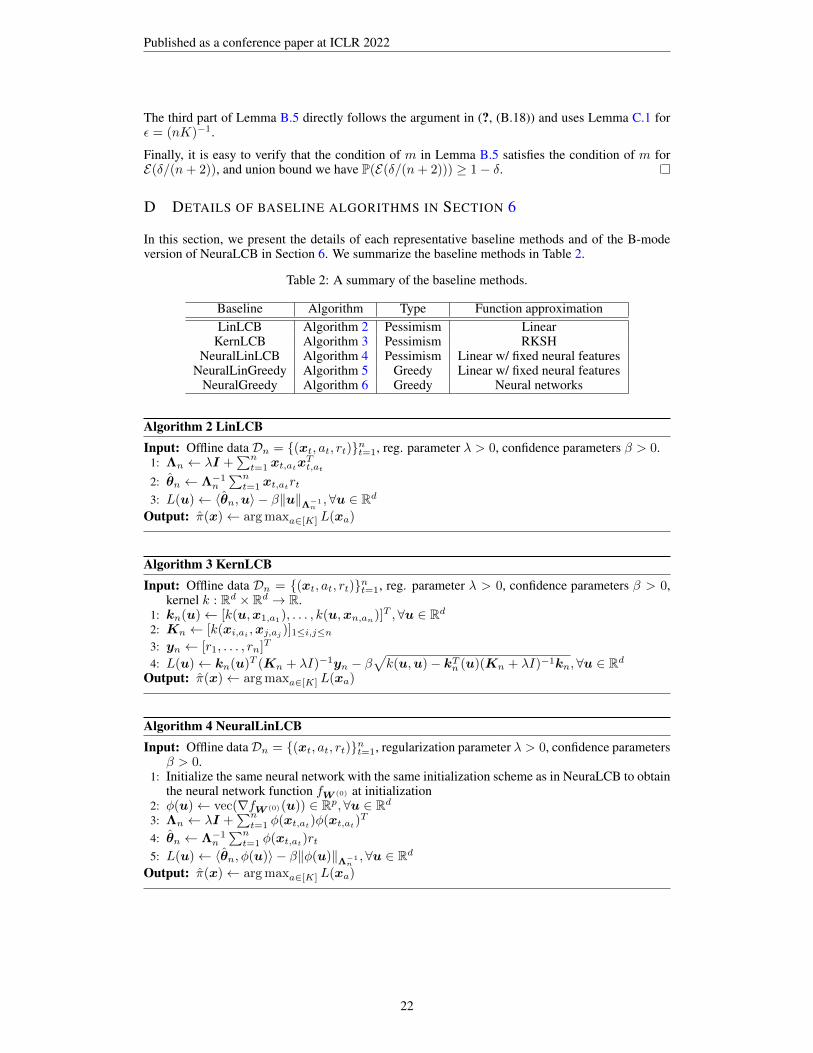
D DETAILS OF BASELINE ALGORITHMS IN SECTION 6
In this section, we present the details of each representative baseline methods and of the B-modeversion of NeuraLCB in Section 6. We summarize the baseline methods in Table 2.
Table 2: A summary of the baseline methods.
Baseline Algorithm Type Function approximationLinLCB Algorithm 2 Pessimism Linear
KernLCB Algorithm 3 Pessimism RKSHNeuralLinLCB Algorithm 4 Pessimism Linear w/ fixed neural features
NeuralLinGreedy Algorithm 5 Greedy Linear w/ fixed neural featuresNeuralGreedy Algorithm 6 Greedy Neural networks
Algorithm 2 LinLCBInput: Offline data Dn = (xt, at, rt)nt=1, reg. parameter λ > 0, confidence parameters β > 0.
1: Λn ← λI +∑n
t=1 xt,atxTt,at
2: θn ← Λ−1n
∑nt=1 xt,at
rt3: L(u)← ⟨θn,u⟩ − β∥u∥Λ−1
n,∀u ∈ Rd
Output: π(x)← argmaxa∈[K] L(xa)
Algorithm 3 KernLCBInput: Offline data Dn = (xt, at, rt)nt=1, reg. parameter λ > 0, confidence parameters β > 0,
kernel k : Rd × Rd → R.1: kn(u)← [k(u,x1,a1
), . . . , k(u,xn,an)]T ,∀u ∈ Rd
2: Kn ← [k(xi,ai,xj,aj
)]1≤i,j≤n
3: yn ← [r1, . . . , rn]T
4: L(u)← kn(u)T (Kn + λI)−1yn − β
√k(u,u)− kT
n (u)(Kn + λI)−1kn,∀u ∈ Rd
Output: π(x)← argmaxa∈[K] L(xa)
Algorithm 4 NeuralLinLCBInput: Offline dataDn = (xt, at, rt)nt=1, regularization parameter λ > 0, confidence parameters
β > 0.1: Initialize the same neural network with the same initialization scheme as in NeuraLCB to obtain
the neural network function fW (0) at initialization2: ϕ(u)← vec(∇fW (0)(u)) ∈ Rp,∀u ∈ Rd
3: Λn ← λI +∑n
t=1 ϕ(xt,at)ϕ(xt,at)T
4: θn ← Λ−1n
∑nt=1 ϕ(xt,at
)rt5: L(u)← ⟨θn, ϕ(u)⟩ − β∥ϕ(u)∥Λ−1
n,∀u ∈ Rd
Output: π(x)← argmaxa∈[K] L(xa)
22
Published as a conference paper at ICLR 2022
Algorithm 5 NeuralLinGreedyInput: Offline data Dn = (xt, at, rt)nt=1, regularization parameter λ > 0.
1: Initialize the same neural network with the same initialization scheme as in NeuraLCB to obtainthe neural network function fW (0) at initialization
2: ϕ(u)← vec(∇fW (0)(u)) ∈ Rp,∀u ∈ Rd
3: θn ← Λ−1n
∑nt=1 ϕ(xt,at
)rt4: L(u)← ⟨θn, ϕ(u)⟩,∀u ∈ Rd
Output: π(x)← argmaxa∈[K] L(xa)
Algorithm 6 NeuralGreedyInput: Offline data Dn = (xt, at, rt)nt=1, step sizes ηtnt=1 , regularization parameter λ > 0.
1: Initialize W (0) as follows: set W (0)l = [Wl, 0;0, Wl],∀l ∈ [L− 1] where each entry of Wl
is generated independently from N (0, 4/m), and set W (0)L = [wT ,−wT ] where each entry of
w is generated independently from N (0, 2/m).2: for t = 1, . . . , n do3: Retrieve (xt, at, rt) from Dn.4: πt(x)← argmaxa∈[K] fW (t−1)(xa),∀x.5: W (t) ← W (t−1) − ηt∇Lt(W
(t−1)) where Lt(W ) = 12 (fW (xt,at
) − rt)2 + mλ
2 ∥W −W (0)∥2F .
6: end forOutput: Randomly sample π uniformly from π1, . . . , πn.
Algorithm 7 NeuraLCB (B-mode)Input: Offline data Dn = (xt, at, rt)nt=1, step sizes ηtnt=1 , regularization parameter λ > 0,
confidence parameters βtnt=1, batch size B > 0, epoch number J > 0.1: Initialize W (0) as follows: set W (0)
l = [Wl, 0;0, Wl],∀l ∈ [L− 1] where each entry of Wl
is generated independently from N (0, 4/m), and set W (0)L = [wT ,−wT ] where each entry of
w is generated independently from N (0, 2/m).2: Λ0 ← λI .3: for t = 1, . . . , n do4: Retrieve (xt, at, rt) from Dn.5: Lt(u)← fW (t−1)(u)− βt−1∥∇fW (t−1)(u) ·m−1/2∥Λ−1
t−1,∀u ∈ Rd
6: πt(x)← argmaxa∈[K] Lt(xa), for all x = xa ∈ Rd : a ∈ [K].7: Λt ← Λt−1 + vec(∇fW (t−1)(xt,at
)) · vec(∇fW (t−1)(xt,at))T /m.
8: W (0) ←W (t−1)
9: for j = 1, . . . , J do10: Sample a batch of data Bt = xtq,atq
, rtqBq=1 from Dt
11: L(j)t (W )←
∑Bq=1
12B (fW (xtq,atq
)− rtq )2 + mλ
2 ∥W −W (0)∥2F12: W (j) ← W (j−1) − ηt∇L(j)
t (W (j−1))13: end for14: W (t) ← W (J)
15: end forOutput: Randomly sample π uniformly from π1, . . . , πn.
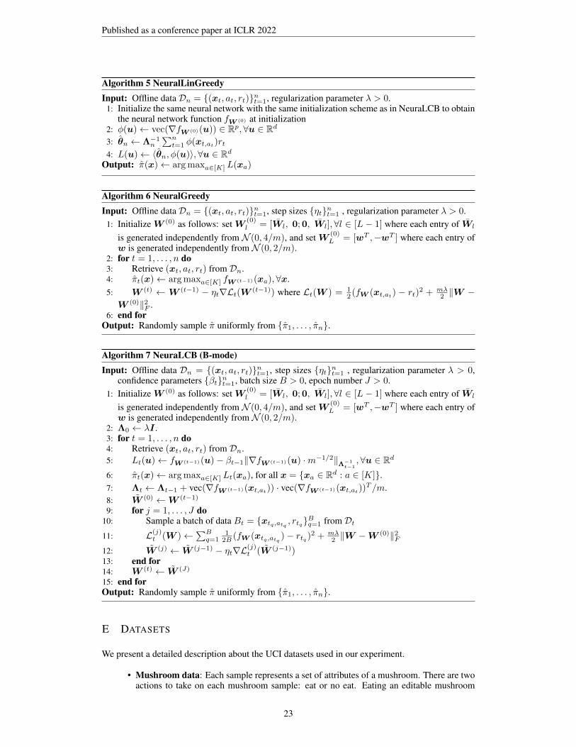
E DATASETS
We present a detailed description about the UCI datasets used in our experiment.
• Mushroom data: Each sample represents a set of attributes of a mushroom. There are twoactions to take on each mushroom sample: eat or no eat. Eating an editable mushroom
23
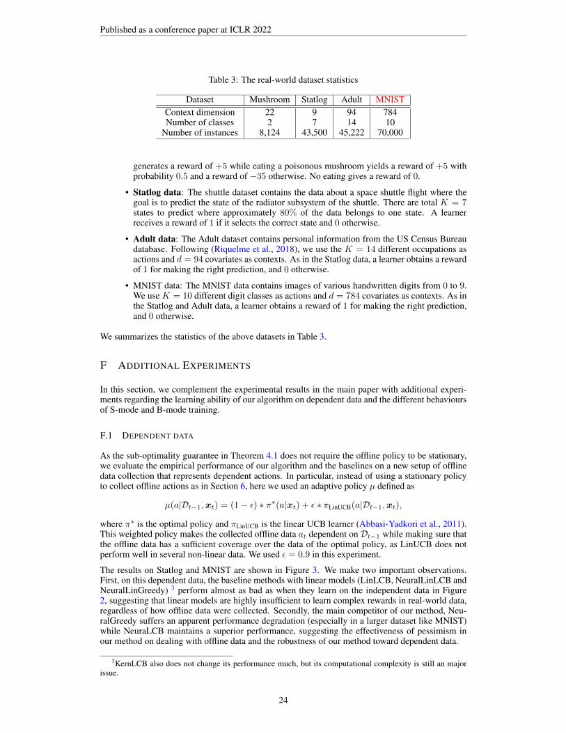
Published as a conference paper at ICLR 2022
Table 3: The real-world dataset statistics
Dataset Mushroom Statlog Adult MNISTContext dimension 22 9 94 784Number of classes 2 7 14 10
Number of instances 8,124 43,500 45,222 70,000
generates a reward of +5 while eating a poisonous mushroom yields a reward of +5 withprobability 0.5 and a reward of −35 otherwise. No eating gives a reward of 0.
• Statlog data: The shuttle dataset contains the data about a space shuttle flight where thegoal is to predict the state of the radiator subsystem of the shuttle. There are total K = 7states to predict where approximately 80% of the data belongs to one state. A learnerreceives a reward of 1 if it selects the correct state and 0 otherwise.
• Adult data: The Adult dataset contains personal information from the US Census Bureaudatabase. Following (Riquelme et al., 2018), we use the K = 14 different occupations asactions and d = 94 covariates as contexts. As in the Statlog data, a learner obtains a rewardof 1 for making the right prediction, and 0 otherwise.
• MNIST data: The MNIST data contains images of various handwritten digits from 0 to 9.We use K = 10 different digit classes as actions and d = 784 covariates as contexts. As inthe Statlog and Adult data, a learner obtains a reward of 1 for making the right prediction,and 0 otherwise.
We summarizes the statistics of the above datasets in Table 3.
F ADDITIONAL EXPERIMENTS
In this section, we complement the experimental results in the main paper with additional experi-ments regarding the learning ability of our algorithm on dependent data and the different behavioursof S-mode and B-mode training.
F.1 DEPENDENT DATA
As the sub-optimality guarantee in Theorem 4.1 does not require the offline policy to be stationary,we evaluate the empirical performance of our algorithm and the baselines on a new setup of offlinedata collection that represents dependent actions. In particular, instead of using a stationary policyto collect offline actions as in Section 6, here we used an adaptive policy µ defined as
µ(a|Dt−1,xt) = (1− ϵ) ∗ π∗(a|xt) + ϵ ∗ πLinUCB(a|Dt−1,xt),
where π∗ is the optimal policy and πLinUCB is the linear UCB learner (Abbasi-Yadkori et al., 2011).This weighted policy makes the collected offline data at dependent on Dt−1 while making sure thatthe offline data has a sufficient coverage over the data of the optimal policy, as LinUCB does notperform well in several non-linear data. We used ϵ = 0.9 in this experiment.
The results on Statlog and MNIST are shown in Figure 3. We make two important observations.First, on this dependent data, the baseline methods with linear models (LinLCB, NeuralLinLCB andNeuralLinGreedy) 3 perform almost as bad as when they learn on the independent data in Figure2, suggesting that linear models are highly insufficient to learn complex rewards in real-world data,regardless of how offline data were collected. Secondly, the main competitor of our method, Neu-ralGreedy suffers an apparent performance degradation (especially in a larger dataset like MNIST)while NeuraLCB maintains a superior performance, suggesting the effectiveness of pessimism inour method on dealing with offline data and the robustness of our method toward dependent data.
3KernLCB also does not change its performance much, but its computational complexity is still an majorissue.
24

Published as a conference paper at ICLR 2022
0 2000 4000 6000 8000 10000 12000 14000Number of samples
0.2
0.3
0.4
0.5
0.6
0.7
0.8
0.9
Sub-
optim
ality
NeuraLCBNeuralGreedyLinLCBNeuralLinLCBNeuralLinGreedyKernLCB
(a) Statlog
0 2000 4000 6000 8000 10000 12000 14000Number of samples
0.2
0.3
0.4
0.5
0.6
0.7
0.8
0.9
Sub-
optim
ality
NeuraLCBNeuralGreedyLinLCBNeuralLinLCBNeuralLinGreedyKernLCB
(b) MNIST
Figure 3: The sub-optimality of NeuraLCB versus the baseline algorithms on real-world datasetswith correlated structures.
F.2 S-MODE VERSUS B-MODE TRAINING
As in Section 6 we implemented two different training modes: S-mode (Algorithm 1) and B-mode(Algorithm 7). We compare the empirical performances of S-mode and B-mode on various datasets.As this variant is only applicable to NeuralGreedy and NeuraLCB, we only depict the performancesof these algorithms. The results on Cosine (synthetic dataset), Statlog, Adult and MNIST are shownin Figure 4.
We make the following observations, which are consistent with the conclusion in the main paperwhile giving more insights. While the B-mode outperforms the S-mode on Cosine, the S-modesignificantly outperforms the B-mode in all the tested real-world datasets. Moreover, the B-mode ofNeuraLCB outperforms or at least is compatible to the S-mode of NeuralGreedy in the real-worlddatasets. First, these observations suggest the superiority of our method on the real-world datasets.Second, to explain the performance difference of S-mode and B-mode on synthetic and real-worlddatasets in our experiment, we speculate that the online-like nature of our algorithm tends to reducethe need of B-mode in practical datasets because B-mode in the streaming data might cause over-fitting (as there could be some data points in the past streaming that has been fitted for multipletimes). In synthetic and simple data such as Cosine, over-fitting tends to associate with strongprediction of the underlying reward function as the simple synthetic reward function such as Cosineis sufficiently smooth, unlike practical reward functions in the real-world datasets.
0 2000 4000 6000 8000Number of samples
0.08
0.10
0.12
0.14
0.16
0.18
0.20
Sub-
optim
ality
NeuraLCB(S-mode)NeuraLCB(B-mode)NeuralGreedy(S-mode)NeuralGreedy(B-mode)
(a) Cosine
0 2000 4000 6000 8000 10000 12000 14000Number of samples
0.2
0.3
0.4
0.5
0.6
0.7
0.8
0.9
1.0
Sub-
optim
ality
NeuraLCB(S-mode)NeuraLCB(B-mode)NeuralGreedy(S-mode)NeuralGreedy(B-mode)
(b) Statlog
0 2000 4000 6000 8000 10000 12000 14000Number of samples
0.70
0.75
0.80
0.85
0.90
0.95
Sub-
optim
ality
NeuraLCB(S-mode)NeuraLCB(B-mode)NeuralGreedy(S-mode)NeuralGreedy(B-mode)
(c) Adult
0 2000 4000 6000 8000 10000 12000 14000Number of samples
0.2
0.4
0.6
0.8
1.0
Sub-
optim
ality
NeuraLCB(S-mode)NeuraLCB(B-mode)NeuralGreedy(S-mode)NeuralGreedy(B-mode)
(d) MNIST
Figure 4: Comparison of S-mode and B-mode training.
25


